Under consideration for publication in J. Fluid Mech. 1

A generalised vortex ring model

By FELIX KAPLANSKI1, SERGEI S SAZHIN2†,YASUHIDE FUKUMOTO3, STEVEN BEGG2,

MORGAN HEIKAL2

1Laboratory of Multiphase Physics, Tallinn University of Technology, Tallinn 19086, Estonia2School of Environment and Technology, Faculty of Science and Engineering,

The University of Brighton, Brighton BN2 4GJ, UK3 Graduate School of Mathematics and Mathematical Research Centre for Industrial

Technology, Kyushu University 33, Fukuoka 812-8581, Japan

(Received ?? and in revised form ??)

28 October 2008

A conventional laminar vortex ring model is generalised by assuming that the timedependence of the vortex ring thickness ` is given by the relation ` = a tb, where a is apositive number, and 1/4 6 b 6 1/2. In the case when a =

√2ν, where ν is the laminar

kinematic viscosity, and b = 1/2, the predictions of the generalised model are identicalwith the predictions of the conventional laminar model. In the case of b = 1/4 some ofits predictions are similar to the turbulent vortex ring models, assuming that the timedependent effective turbulent viscosity ν∗ is equal to ``

′

. This generalisation is performedboth in the case of a fixed vortex ring radius, R0, and increasing vortex ring radius. Inthe latter case, the so called second Saffman’s formula is modified. In the case of fixedR0, the predicted vorticity distribution for short times shows a close agreement with aGaussian form for all b and compares favorably with available experimental data. Thetime evolution of the location of the region of maximal vorticity and the region wherethe velocity of the fluid in the frame of reference moving with the vortex ring centroid isequal to zero, is analysed. It is noted that the locations of both regions depend upon b;the latter region being always further away from the vortex axis than the first one. It isshown that the axial velocities of the fluid in the first region are always greater than theaxial velocities in the second region. Both velocities depend strongly upon b. Althoughthe radial component of velocity in both of these regions is equal to zero, the locationof both of these regions changes with time. This leads to the introduction of an effectiveradial velocity component; the latter case depends upon b. The predictions of the modelare compared with the results of experimental measurements of vortex ring parametersreported in the literature.

† Corresponding author

2 Felix Kaplanski, Sergei Sazhin, Yasuhida Fukumoto, Steven Begg, Morgan Heikal

1. Introduction

Vortex rings have been widely observed as persistent slowly decaying structures (Saffman(1992)). These structures provide a relatively simple flow field, accessible to experimen-tal, numerical and theoretical studies. The importance of vortex rings was emphasised bySaffman (1992) who wrote: ‘This commonly known phenomenon exemplifies the wholerange of problems of vortex motion’. The properties of the vortex rings have been stud-ied for over a century both theoretically and experimentally (Helmholtz (1858), Lamb(1932), Phillips (1956), Norbury (1973), Kambe & Oshima (1975), Saffman (1992), Shar-iff & Leonard (1992), Lim & Nickels (1995)). Recent developments on the modellingside include Stanaway, Cantwell & Spalart (1988), Rott & Cantwell (1993a), Rott &Cantwell (1993b), Mohseni & Gharib (1998), Kaplanski & Rudi (1999), Kaplanski & Rudi(2005), Shusser & Gharib (2000), Fukumoto & Moffatt (2000), Mohseni (2001), Mohseni(2006), Linden & Turner (2001), Fukumoto & Kaplanski (2008).

Classical vortex rings are generated by a moving piston, pushing a liquid column oflength L through an orifice or nozzle of diameter D. The flow separates at the edge ofthe orifice and a cylindrical vortex sheet forms and rolls up into a vortex ring structure.This structure can be laminar or turbulent depending upon the method of generationand the ambient conditions. Also, the mushroom-like patterns resembling classical vortexring motion are often observed in nature and industry, including gasoline engines. Suchstructures can be formed in a fluid when localised forces are applied to the fluid duringa short period of time (e.g in the injection of gasoline in modern engines). In this case,jets with vortex ring structures at the spray periphery can be produced. There is some

similarity between the mathematical tools used to describe these structures and those ofclassical vortex rings.

Saffman (1970) derived an explicit formula for the translational velocity (axial velocityof the centroid as discussed later) of thin-cored laminar vortex rings of radius R0 in theform:

Vx =Γ0

4πR0

[

ln

(

8R0√4νt

)

− 0.558 + O

(√2νt

R0ln

(

2νt

R20

)

)]

, (1.1)

where ν is the fluid kinematic viscosity, Γ0 is the initial circulation of the vortex ringwhich is conserved. The vorticity distribution inside this ring corresponds to the Lamb-Oseen vortex filament (Lamb (1932)). This formula is valid at the initial stage of thevortex ring development.

The description of the final stage of the laminar viscous vortex ring decay can be basedon the Phillips (1956) self-similar solution for vorticity distribution and the correspondingstreamfunction. In this case Rott & Cantwell (1993a) showed that in the limit of largetimes the translational velocity of vortex rings can be described by the following equation:

Vx =M

4π2R30

[

7√πR3

0

30(2νt)3/2

]

, (1.2)

where M is the momentum of vorticity per unit density.An approximate, linear first-order solution of the Navier-Stokes equation for the axi-

symmetric geometry and arbitrary time was reported by Kaltaev (1982), Berezovski& Kaplanski (1995), Kaplanski & Rudi (1999). Based on this solution, Kaplanski &Rudi (2005) derived an expression for the translational velocity of the vortex ring forarbitrary times. In the limit of small and large times this expression reduces to thosedescribed by Equations (1.1) and (1.2) respectively (Kaplanski & Rudi (1999), Fukumoto& Kaplanski (2008)). For the initial stage of vortex ring development, its predictions showgood agreement with the results of numerical simulations reported by Stanaway, Cantwell

A generalised vortex ring model 3

& Spalart (1988) for Reynolds numbers (defined by the ratio of the circulation to thekinematic viscosity) up to 400 (Fukumoto & Kaplanski (2008)). The effects of thesenumbers upon the numerical results was shown to be minimal.

The main limitation of the models mentioned above is that they are based upon theassumption that the vortex ring radius R0 remains constant. Saffman (1970) attemptedto relax this assumption and using simple dimensional analysis, derived an alternativeformula for Vx of the form:

Vx =M

k (R0 + k′

νt)3/2

, (1.3)

where k and k′

are fitting constants. Weigand & Gharib (1997) have shown that anappropriate choice of these constants led to a close match to Equation (1.3) with theiroriginal experimental data and the results of rigorous numerical analysis by Stanaway,Cantwell & Spalart (1988). Both experimental data reported by Weigand & Gharib(1997) and the model by Kaplanski & Rudi (2005) predict the Gaussian distribution ofthe vorticity in the vortex ring. Also, it was shown that the formulae obtained in the limitof small vortex ring Reynolds numbers can be applicable for the description of vortexrings with realistic values of these numbers (see Fukumoto & Kaplanski (2008)).

In contrast to the aforementioned laminar vortex ring models, the theory of turbulentvortex rings is far less developed. To the best of the authors’ knowledge, the first attemptto investigate turbulent vortex ring flow structures was made by Lugovtsov (1970) whobased his analysis on the introduction of the time dependent, turbulent (eddy) viscosity:

ν∗ ∝ ``′

, (1.4)

where ` is the diffusivity scale of the ring core (cf. Lavrentiev & Shabat (1973), Ko-vasznay, Fujita & Lee (1974)). In our paper we assume that ` =

√2νt in the case of

laminar vortex rings. This definition of ` is different from the definitions used by someother authors. For example, Saffman (1970) defined ` =

√4νt. Equation (1.4) made it

possible to describe vortex rings as self-similar structures. However, the comparison ofthis model with experimental observations proved inconclusive (Maxworthy (1972), Max-worthy (1974), Maxworthy (1977), Glezer & Coles (1990), Sazhin, Kaplanski, Feng et al(2001), Cantwell (2002)). Using Equation (1.4), Lugovtsov (1970) and Lugovtsov (1976)developed a turbulent vortex ring model with turbulent viscosity ν∗ and ` ∝ t1/4. Furthersupport of this model was provided by Sazhin, Kaplanski, Feng et al (2001) who appliedit to modelling of turbulent vortex ring structures observed in gasoline engines. At thesame time the model suggested by Lugovtsov was based upon a number of restrictiveassumptions; the applicability of which to realistic physical conditions was not evident.The link between this model and the models described by Kaplanski & Rudi (1999) andKaplanski & Rudi (2005) was not clear. The integral properties of the turbulent vortexrings, such as circulation, kinetic energy and translational velocity were not derived. Asa result, the applicability of the model to realistic physical conditions was not at firstevident. This was therefore the main driving force behind this paper where an attemptis made to generalise the laminar and turbulent vortex ring models by assuming that` ∝ tb, where 1/4 6 b 6 1/2. This model is expected to incorporate both the laminarand turbulent vortex ring models described earlier for the limiting values of b.

The basic equations and approximations of the new model are described in Section2. The analytical solutions of the equations, describing this model, are presented anddiscussed in Section 3. In Section 4 the limiting cases of the solutions of these equationsfor long and short times are discussed. The solutions are validated against experimental

4 Felix Kaplanski, Sergei Sazhin, Yasuhida Fukumoto, Steven Begg, Morgan Heikal

data, available in the literature, where possible. The results are presented in Section 5.The main results of the paper are summarised in Section 6.

2. Basic equations and approximations

The general vorticity equation for incompressible flows follows from the Navier-Stokesequation and can be presented in the form (e.g. Panton (1996)):

Dζ

Dt= ζ · ∇v + ν∇2ζ, (2.1)

where ζ = ∇× v is the vorticity, ν is the kinematic viscosity.Assuming that the flow is axi-symmetric, when the vector ζ has only one azimuthal

component ζ, Equation (2.1) can be simplified to (Batchelor (1967)):

∂ζ

∂t+∂(vxζ)

∂x+∂(vrζ)

∂r= ν

[

∂2ζ

∂x2+∂2ζ

∂r2+

1

r

∂ζ

∂r− ζ

r2

]

, (2.2)

where the meaning of r and x axes is shown in Fig. 1.The streamfunction Ψ is introduced as:

vx =1

r

∂Ψ

∂r+ Vx, vr = −1

r

∂Ψ

∂x, (2.3)

where Vx is the velocity of the centroid at r = 0 and

x = x0 =

∫∞

0

∫∞

−∞2πrxζdxdr

∫∞

0

∫∞

−∞2πrζdxdr

,

Vx = dx0(t)/dt. From the definition of ζ follows the equation:

∂2Ψ

∂x2+∂2Ψ

∂r2− 1

r

∂Ψ

∂r= −rζ. (2.4)

Equations (2.2)-(2.4) describe any axi-symmetric flow, including vortex rings. In thelatter case, physically meaningful solutions of these equations should satisfy the followingboundary conditions: both ζ and Ψ are equal to zero at r = 0 and approach to zero when√x2 + r2 → ∞.Following Berezovski & Kaplanski (1995), we introduce the following dimensionless

variables and parameters:

σ =r

`, η =

x− x0(t)

`, θ =

R0

`, Φ =

Ψ

ζ0`3, ω =

ζ

ζ0, ζ0 = At−λ,

where R0 is the free parameter of the model which is usually identified with the initialradius of the vortex ring (the value of r at which the axial velocity in the frame ofreference moving with Vx reaches its local minimum at η = 0)), the length ` can beidentified with the thickness of the vortex ring as shown in Fig. 1, the parameter A canbe identified with the initial vorticity at an a priori chosen location. As mentioned inthe Introduction, in the case of a laminar vortex ring it was assumed that ` =

√2νt

(Berezovski & Kaplanski (1995)). In our case, a more general assumption is made, suchthat

` = atb. (2.5)

In the case when a =√

2ν and b = 1/2, the value of ` defined by Equation (2.5) reducesto the one considered by Berezovski & Kaplanski (1995). In the case of b = 1/4 and thelong time limit, the model essentially reduces to the one described by Lugovtsov (1976)

A generalised vortex ring model 5

for the turbulent rings. One can expect that for real life vortex ring-like structures, thevalues of b lie in the range of 1/4 6 b 6 1/2. Hence, the analysis of the model will focuson this range of b.

Also, we will assume that ν is not constant, but changes with time (although it remainshomogeneous in space). For this case we can formally replace ν in Equation (2.2) withan effective viscosity ν∗. It is expected that this generalisation of the vortex ring modelcan incorporate the effects of turbulence.

The assumption of spatially homogeneous but time dependent effective viscosity ν∗ issimilar to that made by Lugovtsov (1976) for turbulent viscosity. In practice this viscosityis expected to decrease from its maximal value near the maximal vorticity region to zeroat long distances from the vortex ring. This effect, however, is not important for theanalysis of the vortex ring dynamics since the most important effect of viscosity comesfrom the region when it is maximal (Lugovtsov (1976)).

Remembering the definitions of the above mentioned dimensionless variables and pa-rameters and `, and replacing ν by ν∗ in Equation (2.2), the latter equation can berewritten in the following form:

−b`2

ν∗t

[

λ

bω + θ

∂ω

∂θ+ σ

∂ω

∂σ+ η

∂ω

∂η

]

+ Re

[

− ∂

∂σ

[

ω

σ

∂Φ

∂η

]

+∂

∂η

[

ω

σ

∂Φ

∂σ

]]

=∂2ω

∂σ2+∂2ω

∂η2+

1

σ

∂ω

∂σ− ω

σ2, (2.6)

where the vortex ring Reynolds number is defined as Re = ζ0`2/ν∗.

It should be noted that Re introduced in our paper is time dependent.Further development of this model requires the specification of ν∗(t). Following Lu-

govtsov (1976), one can make a formal dimensionally correct assumption that ν∗ = ``′

,where `

′

= d`/dt (cf. Section 1). Remembering Equation (2.5), this assumption leads tothe following relation:

ν∗ = ``′

= a2bt2b−1. (2.7)

In most realistic physical conditions we expect that the viscosity does not increase withtime and the thickness of the vortex ring does not decrease with time. This imposes thefollowing restriction on the values of b:

0 6 b 6 1/2. (2.8)

As shown later (see Equation (3.3)), the vortex ring Reynolds number is conserved forb = 1/4, decreases with time for 1/4 < b 6 1/2 and increases with time for 0 6 b < 1/4.The latter process has no physical grounds and Condition (2.8) is restricted to:

1/4 6 b 6 1/2. (2.9)

The values of b in the range (2.9) and a can be considered as free parameters. Theirvalues will be estimated based upon the comparison of the predictions of the model withexperimental data.

Using Equations (2.5) and (2.7), it can be shown that

b`2

ν∗t= 1.

Using this result, one can see that for b = 1/2, Equation (2.6) is identical to Equation(8) of Kaplanski & Rudi (1999) if one remembers that a2b = ν when a =

√2ν.

6 Felix Kaplanski, Sergei Sazhin, Yasuhida Fukumoto, Steven Begg, Morgan Heikal

To simplify Equation (2.6) further, the term proportional to Re can be rewritten as:

R ≡ Re

[

− ∂

∂σ

[

ω

σ

∂

∂η

]

+∂

∂η

[

ω

σ

∂

∂σ

]]

Ψ =Re

`2

[ω

σdiv (v) + v∇ω

σ

]

. (2.10)

At the initial stage of vortex ring development, the core is thin and the streamlinesare practically circular and fluid velocities are almost perpendicular to the gradient ofvorticity. This allows one to assume that the term proportional to v∇ω

σis small at

this point. Since div (v) = 0 for incompressible flows, one can ignore the contributionof R in Equation (2.10) in this case. In the final stage of vortex ring development, thecontribution of this term can be ignored, as Re approaches zero. The estimate of R in theintermediate stage is more difficult to determine. Assuming that the term proportionalto Re (R) is close to zero, Equation (2.6) is simplified to

−λbω − θ

∂ω

∂θ− σ

∂ω

∂σ− η

∂ω

∂η=∂2ω

∂σ2+∂2ω

∂η2+

1

σ

∂ω

∂σ− ω

σ2. (2.11)

The range of applicability of Equation (2.11) will be investigated more rigorously laterbased on the comparison of its predictions with available experimental data for non-zerovalues of Re.

Although the values of ω predicted by Equation (2.11) vary in time and space, thespecific momentum of the vortex ring defined by the expression

M = π

∫ ∞

0

∫ ∞

−∞

r2ζdxdr (2.12)

is conserved even in the turbulent case (Lugovtsov (1976)).

3. Analytical solutions

The linearised form of Equation (2.2) (dimensional form of Eq. (2.11) ) was solvedsubject to the initial condition (Fukumoto & Kaplanski (2008)):

ζ0 = Γ0 δ(x) δ(r −R0),

where Γ0 is the initial circulation. The dimensionless form of this solution for λ = 4b canbe presented as:

ω =σ

2exp

[

−1

2

(

σ2 + η2 + θ2)

]

[I0(σ θ) − I2(σ θ)] , (3.1)

where I0 and I2 are modified Bessel functions.Note that Equation (3.1) coincides with the solution of the original system of Equations

(2.2)-(2.4) subject to the same initial condition, valid for arbitrary Re, in the limit of shortand long times. This is an expected result, since for long times Re→ 0 and for short timesthe multiple of Re in Equation (2.6) tends to zero, as follows from the earlier presentedqualitative analysis. Note that in the limit of short times, Equation (3.1) reduces to theOseen solution for the decaying line vortex (see Panton (1996)).

From the conservation of M (see Equation (2.12)) it follows that:

ζ0 =M

π√

2πa−4t−4b =

M

π√

2a−4t−λ. (3.2)

This yields

Re =ζ0`

2

ν∗=

M

π√

2πba−4t1−4b =

M

π√

2πba−4t1−λ. (3.3)

A generalised vortex ring model 7

As follows from Equation (3.3), the Reynolds number is conserved for b = 1/4. Thisproperty of Re turned out to be convenient for the analysis of developed turbulent vortexring flows (Cantwell (2002)). For 1/4 < b 6 1/2 (cf. Condition (2.9)) the Reynolds numberdecreases with time following the power law. For 0 < b < 1/4, Re would increase withtime. This is not consistent with the physical background of the phenomenon.

Although Solution (3.1) was derived based upon the assumption that the non-linearterms proportional to Re in Equation (2.6) are negligible, it is thought that it can beapplied to the analysis of real-life laminar and turbulent vortex ring flows (see Section2).

Remembering that

I1(x) =x (I0(x) − I2(x))

2, (3.4)

Equation (3.1) can be re-written as

ω = exp

[

−1

2

(

σ2 + η2 + θ2)

]

I1(σ θ), (3.5)

where

ω = ζ/ζ0,

ζ0 = ζ0/θ =M

π√

2πR0

a−3t−3b =M

π√

2πR0

a−3t−λ. (3.6)

Note that λ in this case is equal to 3b, due to the different choice of the normalisingparameter ζ0. Equation (3.5) is identical to the one used by Kaplanski & Rudi (1999).

Following earlier approaches to the analysis of this problem (see Kaplanski & Rudi(1999), Kaplanski & Rudi (2005)), the focus is directed to Equations (3.5) and (3.6).The tilde sign ˜ will be omitted to simplify the notation. Note, dimensional forms of thesolutions of Equations (3.1) and (3.5) are identical.

Once the value of vorticity has been found, the dimensionless streamfunction Φ canbe calculated in exactly the same manner as Kaplanski & Rudi (1999). This is given bythe following equation, which follows from Equation (2.4):

Φ =Mσ

4πR0ζ0`3

∫ ∞

0

F (µ, η)J1(θµ)J1(σµ)dµ =σ√

2π

4

∫ ∞

0

F (µ, η)J1(θµ)J1(σµ)dµ,

(3.7)where

F (µ, η) = exp(ηµ)erfc

(

µ + η√2

)

+ exp(−ηµ)erfc

(

µ− η√2

)

,

erfc(x) =2√π

∫ ∞

x

exp(−t2)dt = 1 − erf(x) = 1 − 2√π

∫ x

0

exp(−t2)dt,

J0 and J1 are Bessel functions; when deriving Equation (3.7), Equation (3.6) was takeninto account.

Once the value of Φ has been found, the components of velocity can be calculatedfrom Equations (2.3). At this stage, the dimensionless velocities need to be defined.Following Saffman (1970), our analysis is based upon the following normalisations: ux ≡(vx − Vx)/vn and ur ≡ vr/vn, where:

vn =M

4 π2R30

=Γ0

4 π R0,

Γ0 = M/(π R20) is the initial circulation of the vortex ring (Kaplanski & Rudi (2005)).

8 Felix Kaplanski, Sergei Sazhin, Yasuhida Fukumoto, Steven Begg, Morgan Heikal

Remembering this definition of vn and Equations (2.3) and (3.7), the following expressionshave been obtained:

ux = π θ2∫ ∞

0

µF (µ, η)J1(θµ)J0(σµ)dµ, (3.8)

ur = −π θ2∫ ∞

0

µF (µ, η)J1(θµ)J1(σµ)dµ, (3.9)

where

F (µ, η) = exp(ηµ)erfc

(

µ + η√2

)

− exp(−ηµ)erfc

(

µ− η√2

)

.

Once the values of the vorticity and streamfunction for the vortex ring have beenobtained, then the dimensional energy, E, of the vortex ring can be calculated using thefollowing equation (Batchelor (1967)):

E = π ρ

∫ ∞

0

dr

∫ +∞

−∞

ζΨdx. (3.10)

As in the case of velocities, there are several ways to normalise E. In our analysis,following Saffman (1992), E will be normalised by E0 = ρΓ2

0R0/2 = ρM2/(2π2R30).

Using Equations (2.4), (3.5) and (3.10), we obtain, following the approach developedby Kaplanski & Rudi (2005):

E =E

E0=

√πθ3

122F2

[

3

2,3

2;5

2, 3;−θ2

]

, (3.11)

where

2F2 [a1, a2; b1, b2; x] =

∞∑

k=0

(a1)k (a2)k xk

(b1)k (b2)k k!(3.12)

is the generalised hypergeometric function with the coefficients defined as

(α)0 = 1; (α)1 = α; (α)k = α (α+ 1) .... (α+ k − 1) (k > 2).

The plot of E versus θ as predicted by Equation (3.11) is shown in Fig. 2. As follows fromthis figure, E monotonically increases with increasing θ, which indicates the dissipation ofvortex ring energy with time. In the same figure, the plots obtained under the assumptionsof small and large θ are shown. These will be discussed later in Section 5.

The form of Equation (3.11) is exactly the same as in the case of conventional laminarvortex rings. However, the explicit time dependence of E predicted by this equation isobviously different from that predicted by the conventional model due to the differentfunctions `(t). To illustrate this effect, let us assume that at a certain moment in timet0: θ(t0) ≡ θ0 ≡ R0/(a t

b0) = 1. Hence, at an arbitrary t: θ = θ0(t/t0)

−b = t−b, wheret = t/t0. The plots of E versus t for b = 1/2 and 1/4 in the range 0 6 t 6 5 are shownin Fig. 3. As can be seen from Fig. 3, the rate of energy decrease appears to be rathersensitive to the value of b. For b = 1/2 (laminar case) this rate is the maximal one, whilefor b = 1/4 this rate is the minimal one in the vicinity of t = 1. At t = 1 the plots for allb coincide as expected.

Although the energy is an important parameter for vortex ring characteristics, it isdifficult to measure it in practical applications. A more practically important character-istic of vortex rings is the translational velocity, introduced earlier (see Equation (2.3)).Following Saffman (1970), this velocity is described in terms of the velocity of the vor-tex ring centroid Vx, calculated based upon the following general equation (Helmholtz

A generalised vortex ring model 9

(1858), Lamb (1932)):

Vx =

∫∞

0

∫∞

−∞(Ψ − 6x r vr) ζdxdr

∫∞

0

∫∞

−∞r2ζdxdr

. (3.13)

As in the case of velocities ux and ur, this velocity will be normalised by vn.Using Equations (2.4), (3.5) and (3.13), we obtain, following the approach developed

by Kaplanski & Rudi (2005):

Ux =Vx

vn=

√πθ

3 exp

(

−θ2

2

)

I1

(

θ2

2

)

+θ2

122F2

[

3

2,3

2;5

2, 3;−θ2

]

−3θ2

52F2

[

3

2,5

2; 2,

7

2;−θ2

]

, (3.14)

where the generalised hypergeometric function 2F2 [a1, a2; b1, b2; x] was defined earlier(see Equation (3.12).

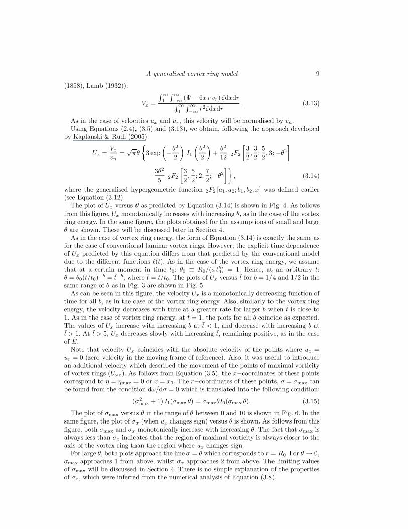
The plot of Ux versus θ as predicted by Equation (3.14) is shown in Fig. 4. As followsfrom this figure, Ux monotonically increases with increasing θ, as in the case of the vortexring energy. In the same figure, the plots obtained for the assumptions of small and largeθ are shown. These will be discussed later in Section 4.

As in the case of vortex ring energy, the form of Equation (3.14) is exactly the same asfor the case of conventional laminar vortex rings. However, the explicit time dependenceof Ux predicted by this equation differs from that predicted by the conventional modeldue to the different functions `(t). As in the case of the vortex ring energy, we assumethat at a certain moment in time t0: θ0 ≡ R0/(a t

b0) = 1. Hence, at an arbitrary t:

θ = θ0(t/t0)−b = t−b, where t = t/t0. The plots of Ux versus t for b = 1/4 and 1/2 in the

same range of θ as in Fig. 3 are shown in Fig. 5.As can be seen in this figure, the velocity Ux is a monotonically decreasing function of

time for all b, as in the case of the vortex ring energy. Also, similarly to the vortex ringenergy, the velocity decreases with time at a greater rate for larger b when t is close to1. As in the case of vortex ring energy, at t = 1, the plots for all b coincide as expected.The values of Ux increase with increasing b at t < 1, and decrease with increasing b att > 1. At t > 5, Ux decreases slowly with increasing t, remaining positive, as in the caseof E.

Note that velocity Ux coincides with the absolute velocity of the points where ux =ur = 0 (zero velocity in the moving frame of reference). Also, it was useful to introducean additional velocity which described the movement of the points of maximal vorticityof vortex rings (Uωx). As follows from Equation (3.5), the x−coordinates of these pointscorrespond to η = ηmax = 0 or x = x0. The r−coordinates of these points, σ = σmax canbe found from the condition dω/dσ = 0 which is translated into the following condition:

(σ2max + 1) I1(σmax θ) = σmaxθI0(σmax θ). (3.15)

The plot of σmax versus θ in the range of θ between 0 and 10 is shown in Fig. 6. In thesame figure, the plot of σx (when ux changes sign) versus θ is shown. As follows from thisfigure, both σmax and σx monotonically increase with increasing θ. The fact that σmax isalways less than σx indicates that the region of maximal vorticity is always closer to theaxis of the vortex ring than the region where ux changes sign.

For large θ, both plots approach the line σ = θ which corresponds to r = R0. For θ → 0,σmax approaches 1 from above, whilst σx approaches 2 from above. The limiting valuesof σmax will be discussed in Section 4. There is no simple explanation of the propertiesof σx, which were inferred from the numerical analysis of Equation (3.8).

10 Felix Kaplanski, Sergei Sazhin, Yasuhida Fukumoto, Steven Begg, Morgan Heikal

As in the case of Figs. 3 and 5, we assume that θ0 ≡ R0/(a tb0) = 1 which implies that

θ = t−b. The plots of rmax/R0 = σmax/θ and rx/R0 = σx/θ versus t for b = 1/2 and 1/4in the range 0 6 t 6 5 are shown in Fig. 7. As follows from this figure, rmax is close toR0 for all b and t 6 1. For t > 1, rmax increases with increasing t and increasing b. Inagreement with Fig. 6, rx is always greater than rmax.

Remembering Equation (3.8) we obtain the expression for the normalised axial velocityof fluid in the region of maximal vorticity in the form:

Uωx ≡ Vωx/vn = Ux + 2πθ2∫ ∞

0

µ erfc

(

µ√2

)

J1(θµ)J0(σmaxµ)dµ, (3.16)

where θ = θmax satisfies Equation (3.15).The plots of Uωx and Ux versus θ in the range of θ between 0 and 10 are shown in Fig.

8. As can be seen from this figure, both Uωx and Ux increase with increasing θ. Uωx isalways substantially greater than Ux, especially at θ > 1. In the same figure, the plots ofUωx and Ux versus θ obtained under the assumptions that θ 1 and θ 1 are shown.These are discussed later in Section 4.

As in the case of Figs. 3, 4 and 7, it is assumed that θ0 ≡ R0/(a tb0) = 1 which implies

that θ = t−b. The plots of Uωx and Ux versus t for b = 1/2 and 1/4 in the range 0 6 t 6 5are shown in Fig. 9. Both Uωx and Ux decrease with increasing time; the values of Uωx

being always greater than the values of Ux, in agreement with Fig. 8. At t = 1, both Uωx

and Ux do not depend on b as in the cases shown in Figs. 3, 5 and 7.From Equation (3.9) it can be seen that the predicted radial component of velocity

at the points of maximal vorticity of vortex rings (η = 0) is equal to zero. This is anexpected result as the streamlines at η = 0 are always perpendicular to plane η = 0.However, this zero fluid velocity in the r−direction by no means prohibits the movementof the point corresponding to the maximal vorticity (ηmax, σmax) in this direction. Thedimensionless effective radial velocity of this point can be found from Equation (3.15)such that:

Ueff(r) =1

vn

drmax

dt, (3.17)

where rmax = `σmax.Note that in contrast to the previously calculated velocities, the expression for Ueff(r)

contains an additional parameter M , via vn. This makes it difficult to compare directlythe values of Uωx predicted by Equation (3.16) and the values of Ueff(r) predicted byEquation (3.17).

As in the case of Figs. 3, 4, 7 and 9, it is assumed that θ(t0) = θ0 = 1. In this case,

θ =(

tt0

)−b

= t−b. Also, we assume that vn = 1 m/s and a = 1 m·s−b. The plots of Ueff(r)

versus t are shown in Fig. 10. As can be seen from this figure, at short times (t < 1)the time dependence of Ueff(r) is complex and highly dependents upon the value of b.This will be discussed in more details in Section 4. However, at long times (starting fromapproximately t = 1) Ueff(r) is a very slowly decreasing function of time. The values ofUeff(r) at these times decrease with decreasing b.

One of the important limitations of the model described so far is that it is basedupon the assumption that R0 =const. The approach suggested by Saffman (1970) andfurther developed by Weigand & Gharib (1997) for laminar vortex rings, can be used togeneralise our model to the case of non-constant R0, which will be referred to as R. Westart with the dimensionally correct equation:

Vx =M

kR3, (3.18)

A generalised vortex ring model 11

where k is a proportionality constant. The decay of circulation can be described by thesecond dimensionally correct equation:

d (VxR)

dt= −k′ ν∗ Vx

R, (3.19)

where k′

is another proportionality constant. The viscosity ν∗ is defined by Equation(2.7). In contrast to the case considered by Saffman (1970) and Weigand & Gharib(1997), ν∗ depends on time. Having substituted Equation (3.18) into Equation (3.19)and integrating the latter equation from t = t0 = 0 to t, one obtains:

R2 −R20 =

k′

a2

2t2b. (3.20)

For b = 1/2 and a =√

2ν, Equation (3.20) reduces to the one derived by Saffman (1970)and Weigand & Gharib (1997). Substituting Equation (3.20) into Equation (3.18) gives:

Vx =M

k (R20 + k

′

a2

2 t2b)3/2. (3.21)

For b = 1/2 and a =√

2 ν, Equations (3.20) and (3.21) reduce to the correspondingequations derived by Saffman (1970) and Weigand & Gharib (1997). In the dimensionlessform, Equation (3.21) can be rewritten as:

Ux =4π2

k(

1 + k′

2θ2

)3/2. (3.22)

The form of Equation (3.22) depends neither upon a nor upon b. As in the previouscases, it is assumed that θ(t0) = θ0 = 1. In this case, θ = t−b and Equation (3.22) canbe rewritten as follows:

Ux =4π2

k(

1 + k′ t2b

2

)3/2. (3.23)

Equations (3.20) – (3.23) can be considered as the generalisation of the so called Saffman’ssecond formula (see Equation (1.3)) for the vortex ring velocity for arbitrary a and b.

The values of k and k′

could be obtained based upon the best fit with the experimentaldata of Weigand & Gharib (1997). Alternatively they can be obtained based on theminimal deviation of Ux predicted by Equations (3.23) and (3.14) in the limit of long t.As the criterion of this minimal deviation, one can use the coincidence of the first twoterms of the asymptotic expansions of these equations in the limit of long times. Thisleads to the following values:

k =1320

2401

√11π3/2 ≈ 10.153200, k

′

=98

11≈ 8.9090909.

The plots of Ux versus θ based on Equations (3.14) and (3.23) for these values of k and k′

are shown in Fig. 11. A reasonable agreement between the values of Ux predicted by theseequations is observed over the whole range of θ. At θ < 2 these values approximatelycoincide as expected.

Let us now introduce another dimensionless time defined as:

t∗ =a2t2b

32R20

=1

32θ2. (3.24)

In the laminar case, when a =√

2ν and b = 1/2, t∗ reduces to the one introduced by

12 Felix Kaplanski, Sergei Sazhin, Yasuhida Fukumoto, Steven Begg, Morgan Heikal

Weigand & Gharib (1997). Remembering (3.24), Equation (3.22) can be rewritten as:

Ux =4π2

k (1 + 16k′

t∗)3/2

. (3.25)

This equation will be investigated in Section 5.

4. Limiting cases

In this section the limiting cases of the solutions presented in Section 3, referring tolong and short times, will be discussed.

4.1. Long times

In the long time limit θ 1, Equations (3.5) and (3.6) can be simplified to:

ω =σ θ

2exp

[

−1

2

(

σ2 + η2)

]

, (4.1)

Φ =σ√

2πθ

16

∫ ∞

0

µF (µ, η)J1(σµ)dµ.

Unfortunately, the latter integral cannot be presented in an analytical form. An alter-native calculation of Φ can be based on substitution of Expression (4.1) into Equation(2.4). The solution of the latter equation gives (Phillips (1956)):

Φ =θ√π

2√

2

σ2

(σ2 + η2)3/2

[

erf (s∗) −2 s∗√π

exp (−s2∗)]

, (4.2)

where

s∗ =

√

σ2 + η2

2.

Note that although ω predicted by Equation (4.1) depends upon θ, the correspondingformula for the dimensional vorticity does not contain R0. This leads to a self-similarsolution when the vorticity depends upon only one parameter, the vortex ring momentumM (cf. Lugovtsov (1970), Lugovtsov (1976)).

The combination of this equation and Equations (2.3) leads to the following expressionsfor the velocity components:

ux =

√2π θ3

2 (σ2 + η2)5/2exp

(

−σ2 + η2

2

)

[

2√

σ2 + η2(

σ4 − 2η2 + σ2(1 + η2))

−√

2π exp

(

σ2 + η2

2

)

(

σ2 − 2η2)

erf

(

√

σ2 + η2

√2

)]

, (4.3)

ur = −√

2π σηθ3

2

2 exp(

−σ2+η2

2

)

(

3 + σ2 + η2)

(σ2 + η2)2−

3√

2π erf

(√σ2+η2

√2

)

(σ2 + η2)5/2

. (4.4)

Keeping only the zeroth term in Series (3.12), Equations (3.11) and (3.14) are simplifiedto:

E =

√π θ3

12, (4.5)

A generalised vortex ring model 13

Ux =7√π θ3

30. (4.6)

This dimensionless velocity corresponds to

Vx =7

120 π√π

M

a3t−3b ≈ 0.0105

M

a3t−3b. (4.7)

The plot of E versus θ, based on Equation (4.5), is shown in Fig. 2. As follows from thisfigure, at θ < 1/2 the values of E predicted by Equation (4.5) show very close agreementwith those predicted by Equation (3.11).

The plot of Ux versus θ, based on Equation (4.6), is shown in Fig. 4. As follows fromthis figure, at θ < 1/2, the values of Ux predicted by Equation (4.6) are again almostindistinguishable from those predicted by Equation (3.14), as in the case of the vortexring energy.

For a =√

2ν and b = 1/2, Equation (4.7) is identical to the one obtained by Rott& Cantwell (1993a) (see Equation (1.2)). For b = 1/4 the time dependence of Vx isidentical to the one reported earlier by Lugovtsov (1976), Glezer & Coles (1990), Cantwell(2002), Afanasyev & Korabel (2004).

The location of the point of the maximal vorticity in the limit of small θ (ηmax =0, σmax = 1) follows from Equation (3.15) (the latter condition corresponds to r = `). Inthis case, Equation (3.16) is simplified to:

Uωx =7√π θ3

30+ 2 π θ2

∫ ∞

0

µ erfc

(

µ√2

)

J1(θµ)J0(µ)dµ. (4.8)

When deriving Equation (4.8) it is important to note that in the limit θ 1, Ux is givenby Equation (4.6).

The plots of Uωx versus θ based on Equation (4.8) are shown in Fig. 8. For θ < 1, thevalues of Uωx predicted by Equation (4.8) are very close to those predicted by Equation(3.16), as in the case of Ux (see Fig. 4).

As in the case of Figs. 3, 4, 7 and 9, it is assumed once again that θ0 ≡ R0/(a tb0) = 1

which implies that θ = t−b. The plots of Uωx versus t for b = 1/2 and 1/4, predicted byEquations (3.16) and (4.8) in the range 2 6 t 6 5 are shown in Fig. 12. The values ofUωx predicted by Equations (3.16) and (4.8) are reasonably close for all b in the wholerange of t under consideration, although the closeness of the curves deteriorates withdecreasing b.

As already mentioned, in a long time limit (θ 1), the solution of Equation (3.15) canbe presented as σmax = 1 which corresponds to rmax = `. In this case, the dimensionlesseffective radial velocity of this point can be found from Equation (3.15) in the form:

Ueff(r) =1

vn

drmax

dt=

1

vn

d`

dt=a b tb−1

vn. (4.9)

Assuming that θ0 ≡ R0/(a tb0) = 1, then θ = t−b. The plots of Ueff(r) versus t for

b = 1/2 and 1/4, predicted by Equations (4.9) (for vn = 1 m/s and a = 1 m/sb) areshown in Fig. 10, alongside the corresponding curves predicted by Equation (3.17). Asfollows from this figure, the values of Ueff(r) predicted by Equations (3.17) and (4.9) are

reasonably close for all b and t > 1.

Note that in the case of θ → 0 we have ` R0. In this case the vortex ring looses itsconventional torus form, and it might be ambiguous to call it as a cohesive ring.

14 Felix Kaplanski, Sergei Sazhin, Yasuhida Fukumoto, Steven Begg, Morgan Heikal

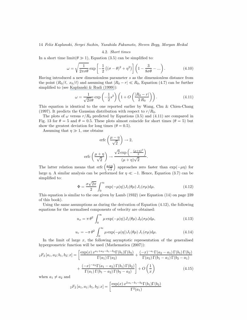
4.2. Short times

In a short time limit(θ 1), Equation (3.5) can be simplified to:

ω =

√

1

2πσθexp

[

−1

2

(

(σ − θ)2 + η2)

](

1 − 3

8σθ− ...

)

. (4.10)

Having introduced a new dimensionless parameter s as the dimensionless distance fromthe point (R0/`, x0/`) and assuming that |R0 − r| R0, Equation (4.7) can be furthersimplified to (see Kaplanski & Rudi (1999)):

ω =1√2πθ

exp

(

−1

2s2)(

1 + O

( |R0 − r|2R0

))

. (4.11)

This equation is identical to the one reported earlier by Wang, Chu & Chien-Chang(1997). It predicts the Gaussian distribution with respect to r/R0.

The plots of ω versus r/R0 predicted by Equations (3.5) and (4.11) are compared inFig. 13 for θ = 5 and θ = 0.5. These plots almost coincide for short times (θ = 5) butshow the greatest deviation for long times (θ = 0.5).

Assuming that η 1, one obtains

erfc

(

µ− η√2

)

→ 2,

erfc

(

µ+ η√2

)

→

√2 exp

(

− (µ+η)2

2

)

(µ + η)√

2.

The latter relation means that erfc(

µ+η√2

)

approaches zero faster than exp(−µη) for

large η. A similar analysis can be performed for η −1. Hence, Equation (3.7) can besimplified to:

Φ =σ√

2π

2

∫ ∞

0

exp(−µ|η|)J1(θµ)J1(σµ)dµ. (4.12)

This equation is similar to the one given by Lamb (1932) (see Equation (14) on page 239of this book).

Using the same assumptions as during the derivation of Equation (4.12), the followingequations for the normalised components of velocity are obtained:

ux = π θ2∫ ∞

0

µ exp(−µ|η|)J1(θµ)J0(σµ)dµ, (4.13)

ur = −π θ2∫ ∞

0

µ exp(−µ|η|)J1(θµ)J1(σµ)dµ. (4.14)

In the limit of large x, the following asymptotic representation of the generalisedhypergeometric function will be used (Mathematica (2007)):

2F2 [a1, a2; b1, b2; x] =

[

exp(x)xa1+a2−b1−b2Γ(b1)Γ(b2)

Γ(a1) Γ(a2)+

(−x)−a1Γ(a2 − a1) Γ(b1) Γ(b2)

Γ(a2) Γ(b1 − a1) Γ(b2 − a1)

+(−x)−a2Γ(a1 − a2) Γ(b1) Γ(b2)

Γ(a1) Γ(b1 − a2) Γ(b2 − a2)

]

+ O

(

1

x

)

(4.15)

when a1 6= a2 and

2F2 [a1, a1; b1, b2; x] =

[

exp(x)x2 a1−b1−b2Γ(b1)Γ(b2)

Γ2(a1)

A generalised vortex ring model 15

+(−x)−a1Γ(b1) Γ(b2) [−2 γ + log(−x) − ψ(a1) − ψ(b1 − a1) − ψ(b2 − a1)]

Γ(a1) Γ(b1 − a1) Γ(b2 − a1)

]

+O

(

1

x

)

(4.16)where γ ≈ 0.57721566 is the Euler constant, Γ(x) is the Gamma function, ψ(x) is thedi-gamma function defined as:

ψ(x) =d log Γ (x)

dx. (4.17)

Having substituted Equation (4.17) into Equation (3.11) we obtain:

E = ln (θ) − γ/2 − ψ(3/2). (4.18)

When deriving Equation (4.18) the contribution of the imaginary term in Equation(4.16) is ignored and the expression for 2F2 is rewritten for the required values of param-eters as:

2F2

[

3

2,3

2;5

2, 3;−θ2

]

=12 θ−3

√π

[

ln θ − γ

2− ψ

(

3

2

)]

. (4.19)

Note than ψ(1) = γ.Remembering that

γ

2+ ψ(3/2) ≈ 1

2+ 2.058− ln 8,

Equation (4.18) is identical to the one derived by Saffman (1992).The plot of E versus θ, based on Equation (4.18), is shown in Fig. 2. As follows from

this figure, at θ > 5 the values of E predicted by Equation (4.18) almost coincide withthose predicted by Equation (3.11).

Having substituted Equations (4.15) and (4.16) into Equation (3.14) one obtains:

Ux = ln θ +3 − γ

2− ψ(3/2) +O(

1

θ). (4.20)

When deriving Equation (4.20), Equation (4.15) was rewritten for the required valuesof parameters as:

2F2

[

3

2,5

2;5

2, 3;−θ2

]

=5 θ−3

2√π

(4.21)

and it was taken into account that

3 exp

(

−θ2

2

)

I1

(

θ2

2

)

=3√π θ

.

In the case when ` =√

2νt, Equation (4.20) reduces to the one obtained by Saffman(1970) (see Equation (1.1)).

The plot of Ux versus θ, based on Equation (4.20), is shown in Fig. 4. As follows fromthis figure, at θ > 5 the values of Ux predicted by Equation (4.20) show good agreementwith those predicted by Equation (3.14); the difference between the values of Ux predictedby these equations is clearly visible over the whole range of θ under consideration.

The location of the point of the maximal vorticity (ηmax = 0, σmax = θ) follows fromEquation (3.15) (the latter condition corresponds to r = R0). In this case, Equation(3.16) is simplified to:

Uωx = ln θ+3 − γ

2− ψ(3/2) + 2 π θ2

∫ ∞

0

µ erfc

(

µ√2

)

J1(θµ)J0(θµ)dµ. (4.22)

When deriving Equation (4.22) it was considered that in the limit θ 1, Ux is given byEquation (4.20).

16 Felix Kaplanski, Sergei Sazhin, Yasuhida Fukumoto, Steven Begg, Morgan Heikal

The plots of Uωx versus θ based on Equation (4.22) are shown in Fig. 8. As follows fromthis figure, for θ > 1 the values of Uωx predicted by Equation (4.22) are reasonably closeto the ones predicted by Equation (3.16), although the closeness of the correspondingcurves is worse than in the case of Ux (see Fig. 4).

As in the case of Figs. 3, 4, 7, 9 and 12, it is assumed that θ0 ≡ R0/(a tb0) = 1 which

implies that θ = t−b. The plots of Uωx versus t for b = 1/2 and 1/4, predicted byEquations (3.16) and (4.22) for t 6 1 are shown in Fig. 14. The values of Uωx predictedby Equations (3.16) and (4.22) are reasonably close for all b for sufficiently small t. Notethat the range of closeness of the curves shown in Fig. 14, is outside the range shown inFig. 8.

In a short time limit (θ 1), Equation (3.15) can be simplified to

(σ2max + 1)

(

1 − 3

8σmaxθ

)

= σmaxθ

(

1 − 1

8σmaxθ

)

.

This is an algebraic equation with respect to θ. Its physically meaningful solution can bepresented as

θ = σmax +3

4σmax

In the dimensional form this solution can be presented as:

rmax = R0 −3`2

4rmax. (4.23)

This equation shows that for sufficiently small, but non-zero t, rmax < R0. In the limitt→ 0, rmax = R0. These properties of rmax are consistent with the plots shown in Fig. 7,although the resolution of the curves in the immediate vicinity of t = 0 is not sufficientto clearly demonstrate the convergence of rmax to R0.

Equation (4.23) can be considered as a quadratic equation in rmax. Its solution in thelimit of short times can be presented as:

rmax = R0

(

1 − 3`2

4R20

)

= R0

(

1 − 3a2t2b

4R20

)

. (4.24)

Having substituted this equation into Equation (3.17) we obtain:

Ueff(r) = − 3a2b

2R0vnt2b−1. (4.25)

As follows from Equation (4.25), for sufficiently small times, Ueff(r) is always negative.

This is consistent with our earlier observation that for sufficiently small, but non-zero t,rmax < R0, while in the limit t → 0, rmax = R0. For b = 1/2, Ueff(r) remains finite at

t → 0, while for 1/4 < b < 1/2, Ueff(r) → −∞ at t → 0. These predictions of Equation(4.25) are consistent with the trends of the curves shown in Fig. 10 for small times.

5. Theory versus experiments

The results of experimental studies of vortex rings in various controlled and un-controlled conditions have been reported in numerous papers (e.g. Shariff & Leonard(1992), Lim & Nickels (1995)). In the case of classical vortex rings generated in liquids(e.g. water) their basic properties have been explained in terms of the conventional mod-els of laminar rings (Saffman (1970), Saffman (1992), Rott & Cantwell (1993a), Rott &Cantwell (1993b), Fukumoto & Moffatt (2000), Wang, Chu & Chien-Chang (1997)). In

A generalised vortex ring model 17

what follows, some of the theoretical results described so far are compared with publishedexperimental data.

The values of Ux, predicted by Equations (3.14) and (3.25) for b = 1/2, Saffman’sformula (1.1) and the upper and lower bounds of the experimental results reported byWeigand & Gharib (1997) are compared in Fig. 15. As shown by Weigand & Gharib(1997), their experimental data in the range of Reynolds numbers between 830 and 1650lie between the lower and upper boundary curves described by Equation (3.23) with(k = 14.5; k

′

= 10.6) and (k = 13.6; k′

= 7.5) respectively. The best curve fit forexperimental data was achieved for (k = 14.4; k

′

= 7.8). As can be seen from Fig. 15,both plots predicted by Equations (3.14) and (3.23) for b = 1/2 are reasonably close tothe experimental results by Weigand & Gharib (1997) in the range 830 6 Re 6 1650.This was expected, as the results presented by Weigand & Gharib (1997) referred tothe laminar case. The result predicted by Equation (1.1) do not depend on a or b. Att∗ > 0.01 the plots based on Equations (3.14) and (3.23) are approximately coincidentin agreement with Fig. 11.

The experimental data obtained by Weigand & Gharib (1997) refer to real life vortexrings, produced in the laboratory. At the initial time, these rings did not have delta-function-like structures of the vorticity distribution, which was assumed in Solution (3.1).Hence, a noticeable deviation of the experimental plots from the predictions of the modelare observed at short times. Note that there is no contradiction between this result andTable 1 of Weigand & Gharib (1997), predicting an almost linear increase in the vortexring translational velocity with increasing Re. This is related to the fact that the velocityin Table 1 of Weigand & Gharib (1997) is dimensional, while the velocity shown in Fig.15 is dimensionless and proportional to Vx/Γ0 ∼ Vx/Re.

Also, an attempt was made to compare the velocities predicted by Equation (3.14) withexperimental data reported by Dabiri & Gharib (2004). The latter authors performedexperimental studies of isolated vortex rings in water in the range of Re between 2000 –4000 based on the initial circulations (when vortex rings were first observed). As in thepreviously described experiments by Weigand & Gharib (1997), the vortex rings weregenerated by a piston motion and they were observed to start approximately 2 s afterthe piston was first set to motion. Two values of the ratio of L (stroke) to D (diameter)were considered: 4 and 2. In the case of L/D = 4, the observed velocities of the vortexrings were approximated as:

Vx = 5 t−0.34. (5.1)

where Vx is in cm/s, and t is in s. Normalising Vx by Vx(tinit = 1 s) and t by tinit = 1 s,Equation (5.1) can be rewritten as:

Ux =Ux

Ux(tinit)=

Vx

Vx(tinit)=

(

t

tinit

)−0.34

= (t)−0.34. (5.2)

The values of Ux versus t predicted by Equation (5.2) are shown in Fig. 16 as a dashedcurve.

To compare the prediction of Equation (5.2) with Equation (3.14) the values of θinit =θ(tinit) and b need to be specified. As follows from the analysis by Kaplanski & Rudi(2005), the values of θinit predicted by the slug-flow model are controlled by L/D. Asfollows from Fig. 2 of Kaplanski & Rudi (2005), for L/D = 4, θinit is expected to bein the range from 4 to 1 (the thickest vortex ring, the shape of which can be clearlyidentified). The model, described earlier in this section, is valid for 1/4 6 b 6 1/2. Theplots of Ux versus t, predicted by Equation (3.14), for b = 1/4, 1/2 and θinit = 1, 4and 2.5 (averaged between 1 and 4), are shown in Fig. 16. As follows from this figure,

18 Felix Kaplanski, Sergei Sazhin, Yasuhida Fukumoto, Steven Begg, Morgan Heikal

in the case of b = 1/4 the predicted values of Ux are the closest to the experimentallyobserved values of Ux when θinit = 2.5. When θinit = 1 the observed values of Ux areexpected to match the predicted ones for b between 1/4 and 1/2. There is no matchbetween the experimentally observed and predicted values of Ux for θinit = 4. The casefor L/D = 4 is particularly important for our comparison, as in this case the momentumof vorticity of the observed vortex rings was conserved in the experiment described byDabiri & Gharib (2004). The derivation of Equation (3.14) was essentially based uponthe assumption that this momentum was conserved.

In the case of L/D = 2, the values of θinit are expected to be in the range between1 and 26 with the average value equal to 13.5. The agreement between theoretical andexperimental results turned out to be the best for b = 1/4 and θinit = 13.5 (the plots arenot shown).

In Fig. 17 the results predicted by Eqs. (5.2), (3.14) and (3.25) are compared forθinit = 2.5. The results predicted by Eq. (3.14) are shown for b = 1/4, while the resultspredicted by Eq. (3.25) are shown for b = 1/4 and b = 1/2. As can be seen from thisfigure, the results predicted by both Eqs. (3.14) and (3.25) for b = 1/4 are reasonablyclose to the results predicted by Eq. (5.2). At the same time the results predicted by Eq.(3.25) for b = 1/2 are noticeably different from those predicted by Eq. (5.2), in agreementwith Fig. 16.

Note that the experimental results predicted by Maxworthy (1972) in the same rangeof Re were approximated as (see Dabiri & Gharib (2004)):

Ux = (t)−1. (5.3)

The reliability of these results was questioned by Dabiri & Gharib (2004). They were notused in our analysis.

6. Conclusions

A conventional laminar vortex ring model has been generalised by assuming that thetime dependence of the vortex ring thickness ` is given by the relation ` = a tb, where a isa positive number, and 1/4 6 b 6 1/2. In the case when a =

√2ν, where ν is the laminar

kinematic viscosity, and b = 1/2, the predictions of the generalised model are identicalwith the predictions of the conventional model. The time dependent effective viscosity ν∗is presented as ` `

′

. In the case when a =√

2ν and b = 1/2, ν∗ = ν . This generalisationwas performed both in the case of fixed vortex ring radius R0, and increasing vortex ringradius. In the latter case, the so called second Saffman’s formula (see Saffman (1970)) hasbeen generalised. The general solutions for vortex ring vorticity, streamfunction, energy,and velocities have been shown to reduce to the previously reported solutions in the casesof long and short times. It has been shown that both vortex ring energy and translationalvelocity depend strongly on the value of the parameter b.

The time evolutions of the locations of the region of maximal vorticity and the region,where the velocity of fluid is equal to zero, in the frame of reference moving with thevortex ring centroid, are found. It is pointed out that the location of both regions dependson b; the second region being always further away from the vortex axis than the first one.It is shown that the axial velocities of the fluid in the first region are always larger thanthe axial velocities in the second region. Both velocities depend strongly on b. Althoughthe radial component of velocity in both these regions is equal to zero, the location of boththese regions changes with time. This leads to the effective radial velocity component,and the latter depends on b.

Theoretical results have been validated against experimental data reported by Weigand

A generalised vortex ring model 19

& Gharib (1997) and Dabiri & Gharib (2004) in a wide range of Reynolds numbers (basedon local circulation).

Acknowledgments

The authors are grateful to the EPSRC (Grant EP/E047912/1) (UK) and EstonianScience Foundation (Grant ETF 6832) for the financial support of this project.

20 Felix Kaplanski, Sergei Sazhin, Yasuhida Fukumoto, Steven Begg, Morgan Heikal

REFERENCES

Afanasyev, Y.D. & Korabel, V.N. 2004 Starting vortex dipoles in a viscous fluid: asymptotictheory, numerical simulation, and laboratory experiments. Physics of Fluids 16(11), 3850-3858.

Batchelor, G.K. (1967) An Introduction to Fluid Dynamics, Cambridge University Press.Berezovski, A. & Kaplanski, F. 1995 Vorticity distributions for thick and thin vortex pairs

and rings. Arch. Mech. 47(6), 1015-1026.Cantwell, B. 2002 Introduction to Symmetry Analysis, Cambridge University Press.Dabiri, J.O.. & Gharib, M. 2004 Fluid entrainment by isolated vortex rings. J. Fluid Mech.

511, 311-331.Fukumoto, Y. & Kaplanski, F. 2008 Global time evolution of an axisymmetric vortex ring

at low Reynolds numbers. Physics of Fluids 20, 053103.

Fukumoto, Y. & Moffatt, H.K. 2000 Motion and expansion of a viscous vortex ring. Part1. A higher-order asymptotic formula for the velocity. J. Fluid Mech. 417, 1-45.

Glezer, A. & Coles, D. 1990 An experimental study of a turbulent vortex ring J. FluidMechanics 211, 243-283.

Helmholtz, H. 1858 On integrals of the hydrodynamical equations which express vortex-motion. Crelle’s J. 55, 485-512.

Kaltaev, A. 1982 Investigation of dynamic characteristics of a vortex ring of viscous fluidContinuum Dynamics 63, Kazah State University, Alma-Ata (in Russian).

Kambe, T. & Oshima, Y. 1975 Generation and decay of viscous vortex rings J. Phys. Soc.Japan 38, 271-280.

Kaplanski, F. & Rudi, U. 1999 Dynamics of a viscous vortex ring. Int. J. Fluid Mech. Res.26, 618-630.

Kaplanski, F. & Rudi, Y. 2005 A model for the formation of ‘optimal’ vortex rings takinginto account viscosity. Phys. Fluids 17, 087101-087107.

Kovasznay, L.S.G., Fujita, H. & Lee, R.L. 1974 Unsteady turbulent puffs. Adv. Geophys.18B, 253-263.

Lamb, H. 1932 Hydrodynamics, 6th edition, Dover, New York, USA.

Lavrentiev, M.A. & Shabat, B.V. 1973 Problems of Hydrodynamics and Mathematical Mod-els, Nauka Publishing House, Moscow (in Russian).

Lim, T. & Nickels, T. 1995 Vortex rings. in Fluid Vortices (ed. S. I. Green) Kluwer, Dordrecht.

Linden, P.E. & Turner, J.S. 2001 The formation of ‘optimal’ vortex rings, and the efficiencyof propulsion devices. J. Fluid Mech. 427, 61-72.

Lugovtsov, B.A. 1970 On the motion of a turbulent vortex ring and its role in the transport ofpassive contaminant. In Some Problems of Mathematics and Mechanics (dedicated to the70th anniversary of M.A. Lavrentiev), Nauka Publishing House, Leningrad (in Russian).

Lugovtsov, B.A. 1976 On the motion of a turbulent vortex ring Archives of Mechanics 28,759-766.

MATHEMATICA Book (2007) version 6.0.0, http://functions.wolfram.com Wolfram ResearchInc.

Maxworthy, T. 1972 The structure and stability of virtex rings. J. Fluid Mech. 51, 15-32.Maxworthy, T. 1974 Turbulent vortex rings (with an appendix on an extended theory of

laminar vortex rings). J. Fluid Mech. 64, 227-239.Maxworthy, T. 1977 Some experimental studies of vortex rings. J. Fluid Mech. 81, 465-495.Mohseni, K. 2001 Statistical equilibrium theory of axisymmetric flows: Kelvin’s variational

principle and an explanation for the vortex ring pinch-off process. Phys. Fluids 13, 1924-1931.

Mohseni, K. 2006 A formulation for calculating the translational velocity of a vortex ring orpair. Bioinspiration & Biommetics 1, S57-S64.

Mohseni, K. & Gharib, M. 1998 A model for universal time scale of vortex ring formation.Phys. Fluids 10, 2436-2438.

Norbury, J. 1973 A family of steady vortex rings. J. Fluid Mech. 57, 417-431.Panton, R.L. 1996 Incompressible Flow, John Wiley & Sons.Phillips, O.M. 1956 The final period of decay of non-homogeneous turbulence. Proc. Camb.

Phil. Society 252, 135-151.

A generalised vortex ring model 21

Rott, N. & Cantwell, B. 1993a Vortex drift. I: Dynamic interpretation Phys. Fluids A 5,1443-1450.

Rott, N. & Cantwell, B. 1993b Vortex drift. II: The flow potential surrounding a driftingvortical region. Phys. Fluids A 5, 1451-1455.

Saffman, P.G. 1970 The velocity of viscous vortex rings. Stud. Appl. Math. 49, 371-380.Saffman, P.G. 1992 Vortex Dynamics, Cambridge University Press.Sazhin, S.S., Kaplanski, F., Feng, G., Heikal, M.R. & Bowen, P.J. 2001 A fuel spray

induced vortex ring. Fuel 80, 1871-1883.Shariff, K. & Leonard, A. 1992 Vortex rings. Annual Review of Fluid Mechanics 24, 235-279.Shusser, M. & Gharib, M. 2000 Energy and velocity of a forming vortex ring. Phys. Fluids

12, 618-621.Stanaway, S., Cantwell, B.J. & Spalart, P.R. 1988 A numerical study of viscous vortex

rings using a spectral method, NASA Technical Memorandum 101041.Wang, C.-T, Chu, C.-C. & Chien-Chang 1994 Initial motion of a vortex ring. Proc. R. Soc.

London A446, 589-599.Weigand, A. & Gharib, M. 1997 On the evolution of laminar vortex rings. Exps. Fluids 22,

447-457.

22 Felix Kaplanski, Sergei Sazhin, Yasuhida Fukumoto, Steven Begg, Morgan Heikal

Figure Captions

Fig. 1

A schematic presentation of the vortex ring with ` = atb.

Fig. 2

The plots of E versus θ as predicted by Equations (3.11) (arbitrary θ), (4.5) (θ 1),and (4.18) (θ 1).

Fig. 3

The plots of E versus t = t/t0 as predicted by Equation (3.11) for b = 1/2 and 1/4.

Fig. 4

The plots of Ux versus θ as predicted by Equations (3.14) (arbitrary θ), (4.6) (θ 1),and (4.20) (θ 1).

Fig. 5

The plots of Ux versus t = t/t0 as predicted by Equation (3.14) for b = 1/2 and 1/4.

Fig. 6

The plots of σmax (location of the point of maximal vorticity) and σx (location of thepoint where ux = ur = 0) versus θ.

Fig. 7

The plots of rx/R0 (location of the point where ux = ur = 0) versus t = t/t0 forb = 1/2 (curve 1) and b = 1/4 (curve 2); the plots rmax/R0 (location of the point ofmaximal vorticity) versus t = t/t0 for b = 1/2 (curve 3) and b = 1/4 (curve 4).

Fig. 8

The plots of Ux versus θ as predicted by Equation (3.14) (long dashed curve), Uωx

versus θ as predicted by Equation (3.16) for arbitrary θ (solid curve), Equation (4.8) forsmall θ (dashed-dotted curve) and Equation (4.22) for large θ (short dashed curve).

Fig. 9

The plots of Uωx (predicted by Equation (3.16)) (curves 1) and Ux (predicted by Equa-tion (3.14)) (curves 2) versus t for b = 1/2 (solid curves) and 1/4 (dashed curves).

Fig. 10

The plots of Ueff(r) versus t predicted by Equation (3.17) (arbitrary t) (solid curves)

and Equation (4.9) (large t) (dashed curves) for b = 1/2 and 1/4 (numbers near thecurves).

Fig. 11

The plots of Ux versus θ based on Equations (3.14) (solid curve) and (3.23) (dashedcurve) for k = 10.153200 and k

′

= 8.9090909.

Fig. 12

The plots of Uωx versus t as predicted by the general Equation (3.16) (solid curves)and by the simplified Equation (4.8) (dashed curves) for b = 1/2 and 1/4 (numbers near

A generalised vortex ring model 23

the curves).

Fig. 13

The plots of ω versus r/R0 as predicted by Equations (3.5) (dashed curves) and (4.11)(solid curves) for θ = 5 and θ = 0.5 (numbers near the curves).

Fig. 14

The plots of Uωx versus t as predicted by the general Equation (3.16) (solid curves)and by the simplified Equation (4.22) (dashed curves) for b = 1/2 and 1/4 (numbers nearthe curves).

Fig. 15

The plots of Ux versus log t∗ = log[

1/(32θ2)]

based on Equations (3.14) (thick solid

curve), (3.23) (dashed curve) for k = 10.153200 and k′

= 8.9090909, and (1.1) (dashed-dotted curve); lower and upper bounds for experimental results by Weigand & Gharib(1997) correspond to the lower and upper boundaries of the shaded area.

Fig. 16

The plots of Ux = Ux(t)/Ux(t = tinit = 1 s) versus t = t/tinit as predicted by exper-imental results by Dabiri & Gharib (2004) for L/D = 4: Ux = (t)−0.34 (dashed curve)and the model (Equation (3.14)) for b = 1/4 (solid curves) and for b = 1/2 (dashed-dotted curves). Thin solid and dashed-dotted curves refer to θinit = 1 (upper curves) andθinit = 4 (lower curves). Thick solid and dashed-dotted curves refer to θinit = 2.5.

Fig. 17

The plots of Ux = Ux(t)/Ux(t = tinit = 1 s) versus t = t/tinit as predicted by ex-perimental results by Dabiri & Gharib (2004) for L/D = 4: Ux = (t)−0.34 (Equation(5.2)) and the model (Equation (3.14) for b = 1/4 and Equation (3.25) for b = 1/4 andb = 1/2). All theoretical curves refer to θinit = 2.5.

x

r2R0

l

Figure 1

A generalised vortex ring model 25

[tbp]

Eq. H3.11L

Eq. H4.18L HΘ>>1L

Eq. H4.5L HΘ<<1L

0 2 4 6 8 10Θ

1

2E

Figure 2.

26 Felix Kaplanski, Sergei Sazhin, Yasuhida Fukumoto, Steven Begg, Morgan Heikal

[tbp]

b=12

b=14

0 1 2 3 4 5t

0.1

0.2

0.3E

Figure 3.

A generalised vortex ring model 27

[tbp]

Eq. H3.14LEq. H4.20L HΘ>>1LEq. H4.6L HΘ<<1L

0 2 4 6 8 10Θ

1

2

3

4

5Ux

Figure 4.

28 Felix Kaplanski, Sergei Sazhin, Yasuhida Fukumoto, Steven Begg, Morgan Heikal

[tbp]

b=12

b=14

0 1 2 3 4 5t

0.1

0.2

0.3

0.4

0.5Ux

Figure 5.

A generalised vortex ring model 29

[tbp]

Σmax

Σx

0 2 4 6 8 10Θ

2

4

6

8

10

Figure 6.

30 Felix Kaplanski, Sergei Sazhin, Yasuhida Fukumoto, Steven Begg, Morgan Heikal

[tbp]

rmaxR0

rxR0

1

2

3

4

0 1 2 3 4 5t

1

2

3

4

5

Figure 7.

A generalised vortex ring model 31

[tbp]

Eq. H3.16LEq. H4.22L HΘ>>1LEq. H4.8L HΘ<<1L

Eq. H3.14L

0 2 4 6 8 10Θ

2

4

6

UΩx, Ux

Figure 8.

32 Felix Kaplanski, Sergei Sazhin, Yasuhida Fukumoto, Steven Begg, Morgan Heikal

[tbp]

1

2

0 1 2 3 4 5t

1

2

3

4

UΩx, Ux

Figure 9.

A generalised vortex ring model 33

[tbp]

12

14

0.4 0.7 1. 1.3 1.6 1.9t

-0.6

-0.3

0.3

0.6Ueff HrL

Figure 10.

34 Felix Kaplanski, Sergei Sazhin, Yasuhida Fukumoto, Steven Begg, Morgan Heikal

[tbp]

0 2 4 6 8 10Θ

1

2

3

4Ux

Figure 11.

A generalised vortex ring model 35

[tbp]

14

12

2 3 4 5t

0.2

0.4

0.6

0.8UΩx

Figure 12.

36 Felix Kaplanski, Sergei Sazhin, Yasuhida Fukumoto, Steven Begg, Morgan Heikal

[tbp]

Θ=5.0

Θ=0.5

0. 0.5 1. 1.5 2.rR0

0.5

1.

Ω

Figure 13.

A generalised vortex ring model 37

[tbp]

12

14

0. 0.2 0.4 0.6 0.8 1.t

0.5

2.5

4.5UΩx

Figure 14.

38 Felix Kaplanski, Sergei Sazhin, Yasuhida Fukumoto, Steven Begg, Morgan Heikal

[tbp]

Eq. H3.14LSaffman formula HEq. H1.1LLEq. H3.23L with k=10.15, k’=8.9

-4 -3 -2 -1logHt*L

1

2

3

4

5Ux

Figure 15.

A generalised vortex ring model 39

[tbp]

1 3 5 7 9t

-

0.2

0.4

0.6

0.8

1Ux

-

Figure 16.

40 Felix Kaplanski, Sergei Sazhin, Yasuhida Fukumoto, Steven Begg, Morgan Heikal

[tbp]

Eq. H3.15L

Eq. H5.2L

Eq. H3.26L for b=14

Eq. H3.26L for b=12

1 3 5 7 9t

-

0.2

0.4

0.6

0.8

Ux

-

Figure 17.