DESIGNING RENEWABLE DOMINATED RESOURCE PLANS ...

DESIGNING RENEWABLE DOMINATED

RESOURCE PLANS FOR FUTURE UTILITIES

– Current Practices of Resource Planning and International Best Practices

October 09, 2020; Time: 03:30 – 05:30 pm

USAID PACE-D 2.0 RE Program

Agenda

Time Session

03:30 – 03:35 pm Welcome Address by Mr. Sumedh Agarwal, Strategic Energy Planning Lead, USAID

PACE-D 2.0 RE Program

03:35 – 04:00 pm Presentation on Methodology for Integrated Resource Planning by Ms. Ammi

Toppo, Director, Central Electricity Authority (CEA)

04:00 – 04:05 pm Quiz and Discussion

04:05 – 05:20 pm Presentation on International Best Practices, Dr. Rafael Kelman, Executive

Director, and Dr. Mario Pereira, Chief Innovation Officer, PSR Consulting

05:20 – 05:25 pm Quiz and Discussion

05:25 – 05:30 pm Concluding Remarks

Ms. Ammi Toppo

❖ 20 years of rich & diverse experience in power sector

❖ Primes formulation of National Electricity Plan (NEP)

❖ B.E. from Govt. Engineering College, Jabalpur and M.B.A from IIT Delhi

❖ Areas of interest include generation, planning studies, demand supply

justification, allocation of power from Central Generating Stations, policy

formulation.

Faculty - Ms. Ammi Ruhama Toppo, Director, Central Electricity Authority, India

Methodology for Integrated Resource Planning

Module ll

Ammi Ruhama Toppo

Director(IRP)

Central Electricity Authority

DESIGNING RENEWABLE DOMINATED

RESOURCE PLANS FOR FUTURE UTILITIES

06-08-2020 IRP Division(Central Electricity Authority)

Legislative framework for National Electricity Plan

Preparation of National Electricity Plan is a statutory responsibility entrusted to CEA under Electricity Act,2003

Electricity Act. 2003 , Section 3(4) stipulates that

– The Authority shall prepare a National Electricity Plan in accordance with the National Electricity Policy and notify such plan once in five years

– Provided that the Authority in preparing the National Electricity Plan shall publish the draft National Electricity Plan and invite suggestions and objections thereon from licensees, generating companies and the public within such time as may be prescribed:

– Provided further that the Authority shall - (a) notify the plan after obtaining the approval of the

Central Government; (b) revise the plan incorporating therein the directions, if any, given by the Central

Government while granting approval under clause (a). (5) The Authority may review or revise the National

Electricity Plan in accordance with the National Electricity Policy. “

National Electricity Policy section 3.2

– Accordingly, the CEA shall prepare short-term and perspective plan. The National Electricity Plan would be for a short-term framework of five years while giving a 15 year perspective plan.

National Electricity Plan


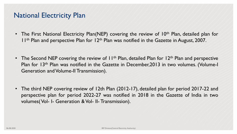
• The First National Electricity Plan(NEP) covering the review of 10th Plan, detailed plan for

11th Plan and perspective Plan for 12th Plan was notified in the Gazette in August, 2007.

• The Second NEP covering the review of 11th Plan, detailed Plan for 12th Plan and perspective

Plan for 13th Plan was notified in the Gazette in December,2013 in two volumes. (Volume-I

Generation andVolume-II Transmission).

• The third NEP covering review of 12th Plan (2012-17), detailed plan for period 2017-22 and

perspective plan for period 2022-27 was notified in 2018 in the Gazette of India in two

volumes(Vol- I- Generation &Vol- II- Transmission).


National Electricity Plan

The NEP includes :

1. Short term and long term demand forecast

2. Proposed capacity addition in generation including Renewables and its integration thereof,

3. Fuel choices based on economy, energy security and environmental considerations.

4. Key inputs viz. infrastructure requirement, fuel requirement, human resource and investment requirement etc.

5. Transmission system planning

The National Electricity Plan is used by prospective generating companies, transmission utilities and transmission /distribution licenses as reference document for future planning

Steps for long term Integrated Resource Plan

Sequential approach of first defining the generation mix, then the optimal transmission capacity for that mix.

Forecasting future load

Existing Resources & Identify Future Resources

Determining Optimal Mix

Uncertainty Analysis

Comments from Stakeholders

Defining the Objective

Supply Demand Reserve

Defining the Objective

Minimizing:

• Operation Cost of the existing and committed generating stations.

• CAPEX of new generating stations

• Financial implications arising out of startup cost, fuel transportation cost etc.

Constraints such as:

• Fuel availability constraints.

• Technical operational constraints viz. minimum technical load of thermal units, ramp rates,

startup and shut down time etc.

• Intermittency associated with renewable energy generation.

Reliability Criteria

10

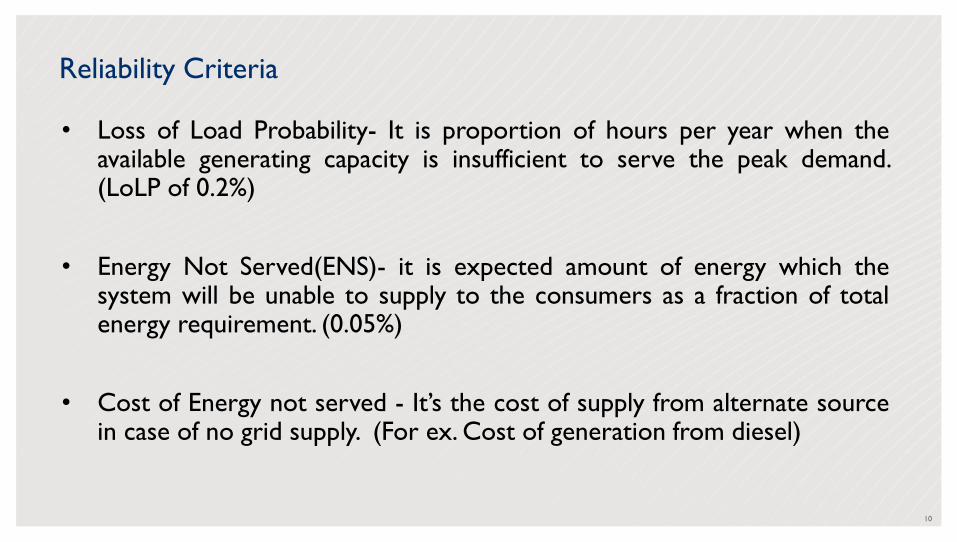
• Loss of Load Probability- It is proportion of hours per year when theavailable generating capacity is insufficient to serve the peak demand.(LoLP of 0.2%)

• Energy Not Served(ENS)- it is expected amount of energy which thesystem will be unable to supply to the consumers as a fraction of totalenergy requirement. (0.05%)

• Cost of Energy not served - It’s the cost of supply from alternate sourcein case of no grid supply. (For ex. Cost of generation from diesel)

Forecasting Future Load

• Long term Peak and Electrical Energy

Requirement are considered as per the

Electric Power Survey Projections.

• Estimating Hourly demand projection for

the study year.

• Long-term models with endogenous

investments are computationally expensive,

especially when optimizing investment

decisions for multiple years simultaneously.

• To reduce the computational burden and

to Capture changes in seasonal, weekly and

daily demand patterns as well as wind and

solar availability , 8760 hours are divided

into time blocks(or time slice)

Wind Generation Patterns

Preparation of time block

With the increase in VRE, models need to capture the variability of the supply options.

1488 1416 2184 1488 2184

0 1000 2000 3000 4000 5000 6000 7000 8000

Seasons Winter Spring Summer Mansoon Autum

1056 432

0 200 400 600 800 1000 1200 1400

Week Day & Week End WeekDay WeekEnd

1 2 3 4 5 6 7 8 9 10 11 12 13 14 14 16 17 18 19 20 21 22 23 24

Day

Validation of time block

020000400006000080000100000120000140000

0

50000

100000

150000

0%

5%

10%

14%

19%

24%

29%

33%

38%

43%

48%

53%

57%

62%

67%

72%

76%

81%

86%

91%

95%

Blo

ck W

ise A

vera

ge W

ind

Geen

rati

on

in

MW

Ho

ur

Wis

e

Win

d g

en

era

tio

n in

MW

Time(%)

COMPARISON BETWEEN BLOCK

WISE & HOUR WISE WIND

GENERATION

Wind Generation Block Wise Average of Wind Generration

0

50000

100000

150000

200000

250000

0

50000

100000

150000

200000

250000

0%

6%

11%

17%

22%

28%

33%

39%

44%

50%

56%

61%

67%

72%

78%

83%

89%

95%

Blo

ck W

ise A

VG

SO

LA

R

GE

NE

RA

TIO

N in

MW

Ho

ur

wis

e S

ola

r ge

ne

rati

on

IN

MW

C O MPA R I S O N B E T W E E N B L O C K

W I S E & H O U R W I S E S O L A R

GE N E RA T I O N

Solar Generation Block Wise Avg Solar Generation

50% 20% 61% 56% 34% 9% 16% 25% 41% 45% 77% 73% 80% 63% 67% 97% 94% 100% 84% 90%

0

50000

100000

150000

200000

250000

300000

-100000.00

0.00

100000.00

200000.00

300000.00

400000.00

0%

3%

5%

8%

10%

13%

15%

18%

20%

23%

25%

28%

30%

33%

35%

38%

40%

43%

45%

48%

50%

53%

55%

58%

60%

63%

65%

68%

70%

73%

75%

78%

80%

83%

85%

88%

90%

93%

95%

98%

Blo

ck W

ise A

VG

SO

LA

R

GE

NE

RA

TIO

N in

MW

Ho

ur

wis

e S

ola

r

gen

era

tio

n I

N M

W

COMPARISON BETWEEN BLOCK WISE & HOUR

WISE RESIDUAL LOAD

Solar Generation Block Wise Avg Solar Generation

Data required from Existing /Committed Resources

• Unit wise characteristics

– Installed capacity, commissioning year, fuel type, heat rate, outage rate, maintenance

duration, fuel cost, fixed O&M cost,

– Flexible Characteristic- start up/down time and cost, ramp rates, minimum technical

load, peak contribution,

– The deterioration in operational efficiency with part loading of units of thermal

plants.

– Annual as well as Seasonal availability of fuel

– In case of hydro- hydro storage related data, Hydro seasonal energy etc.

– Hourly Solar and Wind Profile –data collected from the RE rich States.

– Planned retirements

Identifying potential resource options(Candidate)

Conventional Technologies Renewable Technologies Storage technologies

Coal Solar Pumped Storage

Gas Wind Battery Energy Storage

Nuclear (LWR *PHWR) Biomass

Large Hydro Small Hydro

Resource choices cannot be made simply on the basis of costs (or prices).

The lower-cost resource is not always the most valuable resource.

▪ The generation fleet is represented by a number of different technology types, each with their own unit-

wise, techno-economic parameters including the cost trends of capital cost.

▪ The investment constraints limit, investments based on resource, policy, or technical criteria.

▪ All technologies are constrained to prevent unrealistic rates of capacity growth in any particular year

▪ In case of hydro power projects, only those projects concurred by CEA are considered as investment

option

▪ The Nuclear projects are considered as furnished by Department of Atomic Energy.

Cost Curve of Technology Considered

Projected reduction in capital costs over time for the RE technologies and the Battery

Energy Storage system

0.000

2.000

4.000

6.000

8.000

Battery PV Wind

Rs

Cro

re

Firm Capacity/ Capacity Credit- It is the capacity that can serve that load all time specially

during the peak time

Spinning Reserve- Spinning reserve of 5% as per the National Electricity Policy

Firm Capacity & Reserve

ORDENA (Generation expansion planning software) Optimisation constraints

Plant availability, start up and dynamic characteristics, Ramp rates, fuel constraints etc.

Existing resources data

Unit capacity, auxiliary consumption, fuel type & cost, heat rate, outage rate, availability profile, O&M cost , Hourly Solar and Wind generation profile, etc.

Optimized resource plan

Long Term Planning:-Total system cost, annual system capacity requirement fuel wise.

Short term planning:-Hourly economic dispatch to meet the hourly demand

Input data assumptions

Demand and energy forecast , Load profile, retirements, etc.

New resources data

Capital cost, fixed O&M cost, year of availability, availability profile, fuel type & cost, heat rate, etc.

About the Model

18

Validating flexibility balance with production cost models

Long term generation expansion

models (Capacity Mix)

Production cost models (Short

Term Model)

Result

Conver

ge

Yes

Final Capacity

MIX

No

Scenario

Peak Day / Max Energy demand day

Maximum Variable RE (Wind+Solar) generation day

Maximum Solar generation day

Minimum Solar generation day

Minimum energy demand day

Minimum Variable RE (Wind+Solar) generation day

Maximum variation in demand day

Short Term scenarios considered for Critical days

20

Peak Demand/ Maximum Net Demand

21

Peak

Demand Demand

Curve

Peak Demand – 340 GW, Energy Req- 7.21 BU

Sensitivity studies

Criteria

• Demand Variation

• Variation in Capital Cost

• Reduction in VRE Generation

• Reduction in Hydro Generation

10% reduced variable RE generation & 6% reduced Hydro generation

23

Availability of coal based power plants has to be increased by only 1.5% to fulfill the

demand

DEMAND

Peak-225.7 GW

Energy-1566BU

HYDRO-6823 MW

Nuclear-3300 MW

Gas – 406 GW

RETIREMENTS 22,617

RES IC by 2022

175 GW

BASE CASE(2017-22) ASSUMPTIONS

Additional Coal

based capacity

Requirement

during 2017-22

(MW)*

Coal Based

Generation

(Gross) (GWh)

Expected

PLF% during

2021-22

6445(Coal Based Capacity Under

Construction-47855 MW

)

1072 56.5%

BASE CASE(2017-22) RESULT

Coal+L

ignite

217,30

2 …

Gas

25,736

5%

Hydro

51,301

11%

Nuclea

r

10,080

2%

Renew

ables

175,00

0 …

Hydro

155,742.

0

9.16%

Coal+Lig

nite

1,071,80

1.0

63.05%

Gas+Die

sel

82,626.0

4.86%

Nuclear

62,643.0

3.69%

RES

327,000.

0

19.24%

PROJECTED INSTALLED CAPACITY& GENERATION (MARCH, 2022)

TOTAL 16,99,812

GWh

TOTAL 4,79,419

MW

DEMAND

Peak-298.8 GW

Energy-2047BU

HYDRO-12000 MW

Nuclear-6800 MW

Gas – 0 GW

RETIREMENTS 25,572 MW

RES IC by

2027

275 GW

BASE CASE(2022-27) ASSUMPTIONS

Additional Coal

based capacity

Requirement

during 2022-27

(MW)

Coal Based

Generation

(Gross) (GWh)

Expected

PLF% during

2026-27

46,420 1259 60.5%

BASE CASE(2022-27) RESULT

PROJECTED INSTALLED CAPACITY& GENERATION (MARCH, 2027)

TOTAL 16,99,812

GWh

Coal+Ligni

te

238,150

39%

Gas25,735

4%Hydro63,301

10%

Nuclear16,880

3%

Renewables

275,000

44%

TOTAL 6,19,066 MW

Hydro268,859.0

12.10%Coal+Lignite1,238,906.0

55.74%

Gas+Diesel86,182.0

3.88%

Nuclear110,696.0

4.98%

RES518,000.0

23.31%

https://cea.nic.in/reports/others/planning/ir

p/Optimal_mix_report_2029-

30_FINAL.pdf

https://cea.nic.in/reports/com

mittee/nep/nep_jan_2018.pdf

10/9/2020

Quiz

27

❖ BSc in Civil Engineering, MSc, and PhD in System Optimization from

COPPE/UFRJ.

❖ Dr. Kelman coordinates studies in power sector, such as the integration of

renewable energy, market studies and water-energy nexus. He also

participates in the development of models ranging from long-term planning

to short-term scheduling of power systems.

Faculty - Dr. Rafael Kelman, Executive Director, PSR Consulting

Dr. Rafael Kelman

Ado

be S

tock

CURRENT PRACTICES OF RESOURCE

PLANNING AND INTERNATIONAL

BEST PRACTICES

Summary

• Background

• Integrated Resource Planning

• Models

• International experience

• The Brazil Case

• DER Cost x Benefit analysis

• DER endogenous modeling

• DER Selected cases

• References

10/9/2020 FOOTER GOES HERE 30

This brings the renewable integration challenge

31

► What makes variable renewable energy (VRE) or renewable energy sources (RES) different?

► These six properties drive all relevant techno-economic system integration effects

Risk profileLocation-based effectsTime-based effects

Variable

?

Uncertain

g

g g

g

Non-synchronousModular

A B

Location

constrained

CAPEX

OPEX

Capital

intensive

Flexibility is the tool for handling system integration

32

Flexibility describes all characteristics of a power system that facilitate the reliable and cost-effective

management of variability and uncertainty in supply/demand on all time and geographic scales.

Properties of VRE Power system flexibility

Technical flexibility

› Power plants that can start quickly, have a

wide output range & provide many services

› Grids to connect distant and distributed

VRE plants, smooth variability & pool

flexibility

› Demand shaped to better match VRE

availability (structurally & dynamically) and

provides system services

› Storage that provides system services,

reduces need for other flexibility and

balances remaining surplus/deficit

Flexible markets, policy & regulation

› Rules that deliver fast system operations

based on economic dispatch

› New modelling needs

› Balancing demand/supply across large

geographic areas

› Level playing field for new technologies incl. for

providing system services

Flexible institutions

› Processes and institutional culture to ‘keep up’

in a rapidly changing environment

Six phases of system integration

Where countries stand

• VRE share in annual electricity generation and system integration phase, 2017

► Typical country-level integration issues determine national phase. Regions within a country can be at

a different phase

Phase

1

0%

10%

20%

30%

40%

50%

60%% VRE generation

2

3

4

Source: IEA (2018) Renewable 2018 - Analysis and Forecasts to 2023

Integrated planning with state-of-the-art tools is crucial

Generation (incl. optimal location and mix of VRE)

Energy efficiency

Electrification of heating

and transport,

new loads in industry

Transmission grid

Distribution grid

Demand side response

Storage

Modern power

system planning

State-of-the-art (probabilistic)

modeling tools are indispensible

for successful VRE integration

• Need to combine long-term view on

expansion with short-term view of

operation

– (sub) Hourly time steps

– Unit commitment decisions

– Ramping constraints

– Hydraulic constraints in river

basins

– Variability of renewables, inflows

& demand (uncertainties)

– Energy, capacity and reserve

requirements

Energy planning is becoming important once again…

36

G&T Expansion planning: (PSR approach)


Activity A - Modeling of renewable resources

• Identify candidate projects for wind and solar generation.

– As with hydropower projects, which require historical inflow records, each renewable candidate requires historic energy production with hourly resolution.

– This is usually done with global databases, such as MERRA-2, which contain ~40 years of hourly wind speed and solar radiation data for the entire planet.

• Data for each candidate site is refined/calibrated based on the measured wind / solar records (usually 2-3 years) from existing neighboring plants.

• Finally, the calibrated wind speed and the solar records are transformed into 40 years of hourly energy production using the parameters of the candidate project (type of wind turbine, hub height, solar trackers, etc.).


Activity A - Modeling of renewable resources

• Generation scenarios for existing and candidate renewable sources, including hydro. The methodological challenges are:

– Significant spatial correlation between wind energy and inflows in some regions.

– Generation of scenarios must be integrated (wind, solar, and inflows to hydro plants) and with multiple time scales (hourly for wind & solar, monthly/weekly for inflows).

– Integrated/multiscale scenarios produced by a Bayesian network, a statistical model with variables and their conditional dependencies represented through a graph


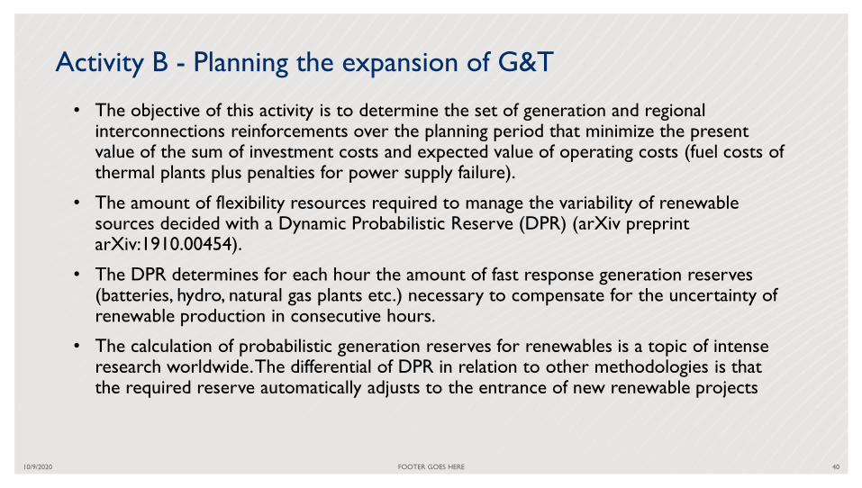
Activity B - Planning the expansion of G&T

• The objective of this activity is to determine the set of generation and regional interconnections reinforcements over the planning period that minimize the present value of the sum of investment costs and expected value of operating costs (fuel costs of thermal plants plus penalties for power supply failure).

• The amount of flexibility resources required to manage the variability of renewable sources decided with a Dynamic Probabilistic Reserve (DPR) (arXiv preprint arXiv:1910.00454).

• The DPR determines for each hour the amount of fast response generation reserves (batteries, hydro, natural gas plants etc.) necessary to compensate for the uncertainty of renewable production in consecutive hours.

• The calculation of probabilistic generation reserves for renewables is a topic of intense research worldwide. The differential of DPR in relation to other methodologies is that the required reserve automatically adjusts to the entrance of new renewable projects


Activity B - Planning the expansion of G&T

• The optimal plan results from the iterative solution of 3 modules:

– decision to invest in new capacity (candidate plan X);

– calculation of DPR requirements R(X) for plan X;

– stochastic system operation for plan X and reserve R(X).

• The iterative process produces the optimal plan X* that minimizes investment costs I(X*) + operation O(X* ).


Activity C - Transmission planning under uncertainty

• Variability of hydro, wind and solar power leads

to diverse power flow patterns in the grid.

• Renewable sources often built in places with no

foreseeable power injections.

• Reinforcement of transmission grid to

accommodate multiple generation patterns is

required to avoid dispatch of more expensive

generators to alleviate overloads or avoid load

shedding.

• Robust transmission plan must be feasible (i.e. with

no overloads) for each of the multiple conditions

that result from the probabilistic operation from

the expansion plan of Activity B


Adding flexibility to transmission

• Power injection at selected nodes to alleviate overloads either with dispatchable generation or batteries / pumped-hydro-storage projects

• By modifying the circuit reactance, redistributing power flows according to Kirchhoff's law

– FACTS (Flexible AC Transmission Systems) technologies allow the control of power flow and voltage, in addition to acting on power quality issues such as voltage compensation and current harmonics in the grid. They fit into a wide range of applications, as they are modular, reusable and have short delivery times.

– Many of these devices provide sensors that enable real-time monitoring of operating conditions, such as power flow limits in transmission lines adjusted for temperature and wind conditions (dynamic line rating).

• Change in grid topology by (dis)connecting one or more circuits (circuit switching)

• Non-Wires Transmission: the effect of transferring X MW from point A to point B is emulated through a combination of demand response and distributed generation. Non-Wire Alternatives (NWA) have attracted attention in the United States.


• Support IRP activities with objective of reducing cost of achieving policy goals, such as GHG reductions by mapping available resources and then selecting the portfolio of project and actions that minimize total costs while maintaining system reliability.

– Importance of mapping resources well

– Importance of forecasting load well for adequate planning

• Various objective, such as: Load forecasting, Capacity expansion, Production costing, Security Constrained Unit Commitment and so on. Usually more than one model is used.

• Key aspects must be addressed before deciding which computational tools to use:

– Features and limitations (e.g. deterministic vs. probabilistic approach, full grid x sing-bus model, etc.)

– Ability of the development team to customize the models according to client needs (flexibility),

– If tool is user-friendly and user-support is adequate

– If the tool can be easily integrated with other tools

– Licensing cost and others

44

Computational models

45

Systematic mapping of power

system models, JRC 2017Software-related features: about 2/3 of the models require

3rd software such as commercial optimization solvers or off-

the-shelf software. Only 14% of the models are open source.

Modelling-related features: models are mostly defined as

optimization problems (78%), simulation (33%) or equilibrium

problems (13%). 71% of the models solve a deterministic

problem while 41% solve probabilistic or stochastic problems.

Modelled power system problems: the economic dispatch

problem is the most modelled problem with a share of

approximately 70%, followed by generation expansion planning,

unit commitment, and transmission expansion planning, with

around 40‒43% each. Most of the models (57%) have non-

public input data while 31% of models use open input data.

Modelled technologies: hydro, wind, thermal, storage and

nuclear technologies are widely considered.



• Key input data for all models according to the survey

46

Source: systematic mapping of power system models, JRC 2017

United States

• Utilities follow different methodologies in Integrated Resource Planning.

• Example from CPUC 2019-2020 Proposed Reference System Plan:

– The value proposition of integrated resource planning is to reduce the cost of achieving

GHG reductions and other policy goals by looking across individual LSE boundaries and

resource types to identify solutions to reliability, cost, or other concerns that might not

otherwise be found.

• IRP from CPUC

– Tools: capacity expansion model (RESOLVE) and production cost model (SERVM).

– Demand forecasting and generation adequacy studies covering a period of 10 years.

– Utilities prepare the plan based on the studies and submit the findings and plans to

the public service commission: system needs, local needs and flexibility needs.

– If needed and approved by CPUC, utilities solicit offers for capacity, energy, DSM and

energy efficiency.

10/9/2020 47

United States

• Example 1: 2012 LTPP authorized procurement for reliability in two transmission

constrained zones of Southern California: the Western LA Basin and Venture-Big Creek

local reliability areas. The decision authorized 1400-1800 MW capacity in the West Los

Angeles subarea, including 1000-1200 MW of conventional gas-fired resources, 50 MW of

energy storage, and 150-600 MW of preferred resources.

• Example II: Retirement of San Onofre Nuclear Generation Stations


Europe (general)

• ENTSO-E, the European Network of Transmission System Operators for Electricity,

represents 43 electricity Transmission System Operators (TSOs) from 36 countries across

Europe.

• ENTSO-E performs the Mid-term Adequacy Forecast (MAF) every year up to 10 years ahead.

MAF evaluates power system resource adequacy with a sequential Monte Carlo probabilistic

methodology using market-modeling tools.

• The Regulation further establishes that this outlook shall build on national generation

adequacy outlooks prepared by each individual TSO, which implicitly is constraining the

approach to bottom-up scenarios.

• The methodology for adequacy assessment is implemented in five different market modeling

tools, namely, ANTARES, BID3, GRARE, PLEXOS and PowrSym.


United Kingdom

• The Electricity Capacity Report (ECR) summarizes the modeling analysis of the National Grid, the system operator in UK, to support Government decision on the amount of capacity to secure through Capacity Market auctions for delivery in future.

• The Government requires National Grid to provide a recommendation for each year studied based on the analysis of several scenarios.

• Demand forecasting includes energy (TWh/year) demand and electricity peak demand (GW).The drivers considered across sectors include Demand Response, Distributed Generation, Storage, Thermal efficient building, EV uptake and Energy Efficiency.

• Several scenarios are studied for supply adequacy. It is noticed that the system requires greater generation flexibility as VRE share increases. Total eligible de-rated capacity needs to be secured to achieve a reliability standard of 3 hours LOLE.


1. Brazil IRP case: candidate projects

• Candidate project preparation per technology resulted

from discussions between Consultants and EPE based on

market references (mainly auctions)

• Coal, open cycle and combined cycle natural gas, nuclear,

biomass, wind, solar PV, storage devices, no hydropower

after 2026.

• Technical parameters (such as ramps, startup costs and

possible dispatch models)

• Economic parameters, such as CAPEX and OPEX (fixed

and variable) and fuel prices

• Expected technological advances considered (e.g. increase

in turbine size, decrease of costs for solar, wind and

storage)

• Utility scale optimized; exogenous DG scenario used.

51

Wind candidates

• Candidate projects from energy auctions (~800 wind projects and 400 solar projects totaling or 22 GW)

• Known data: bus connection and capacity

• Investment cost, fixed O&M cost and lifetime based on market values

• Wind velocity / solar irradiation time series taken from reanalysis data (MERRA2 / NASA)

• Classification attributes: intraday and seasonal wind velocities using a minimum spanning tree algorithm resulted in 22 wind regions and 9 solar regions

• Calibration of simulated (model-based) production based on historical production

52

Solar PV regions

Wind regions

Solar PV project preparation

53

Hydro, wind and solar complementatities need to be captured

54

North-Northeast

Hydro Inflow Energy

North-Northeast

Renewable Energy

(Wind + Solar PV)

W110 W175 W124 W136 W282 W426 W458

W110 1.00

W175 0.93 1.00

W124 1.00 0.95 1.00

W136 0.98 0.97 0.99 1.00

W282 0.41 0.26 0.39 0.35 1.00

W426 0.25 0.17 0.24 0.24 0.54 1.00

W458 0.17 0.20 0.18 0.19 0.35 0.65 1.00

Wind-wind correlation matrix Wind-hydro correlation matrix

Wind-hydro seasonal complementarity Wind-solar daily complementarity Wind parks location

Weekly operation at end-of-horizon (August)

0

20

40

60

80

100

120

140

160

180

1 25 49 73 97 121 145

GW

Thermal Biomass Wind Solar Hydro Batteries

55

IRP Resulted in large penetration of wind and solar power

Transmission reinforcements

56

System Number of

circuits

Total length

[km]

Investment

[billion US$]

NE 140 14397 3.14

SE 41 2063 0.64

N 33 1748 1.79

CW 8 242 0.05

S 7 112 0.26

HVAC Tie Line 4 1100 1.39

HVDC Tie Line 1 bi-pole 3600 2.18

SIN 234 23262 9.45

Mr. Mario Pereira

❖ Mr. Pereira was Principal Presidential Advisor in designing new power market

rules in 2004 and a lead formulator of the country’s energy contracting

auctions (more than 100 GW of new capacity contracted since 2005).

❖ His stochastic dual dynamic programming (SDDP) algorithm is a worldwide

reference and applied in dozens of countries. He also developed novel methods

for optimal expansion planning and supply reliability evaluation.

❖ Author and co-author of four books and about 200 papers in refereed journals.

❖ An electrical engineer and has MSc and PhD degrees in optimization.

Faculty - Mr. Mario Pereira, Chief Innovation Officer, PSR Consulting

DER Benefits

FlexibilityVoltage

control

Frequenc

y control

Operatin

g reserve

Black-

StartReliability /

Resilience

Emissions

Reduction

Loss

reduction

Demand

Response

Distributed

Generation

Distributed

Storage

Electric

Vehicle


How to measure costs and benefits?

• There is no consensus on the best way to assess the costs and benefits of DER

• Methodologies that explicitly calculate costs C (investment + O&M) and benefits B (avoided costs) of DER and eliminates if B < C. Several evaluations can be made.

– Participant Cost Test (do DER users have savings?)

– Ratepayer Impact Measure (are there added costs to non-users of DER?)

– Utility Cost (are benefits of DER higher than their costs?),

– Total Resource Cost (are benefits of DER for utility and consumers higher than their costs)

– Societal Cost (broader than previous, as it includes tradeoffs to Society)

• Alternative approach: methodologies that implicitly develop a cost x benefit analysis by incorporating REDs in IRP modeling.


Evaluation of costs & benefits of DER in planning and operation

• EPRI: bottom-up methodology for evaluating impacts of different DER scenarios

in planning and operation, followed by cost-benefit analysis.


PremisesMarket

Conditions

Scenarios

ConsideredGeneration and

Transmission

SuitabilityTransmission

Performance*

Transmission

ExpansionFlexibility

Operation and Simulation

Advantages / Costs

Net Costs to

the System

Costs / Social

Benefits

Costs / Benefits

for consumers

and participants

Benefits for the

system

Distribution System

Hosting

CapacityEnergy

ReliabilityThermal

Capacity

1 4

3

2 5

6

Impacts to

the

Distribution

System

Net Investment

Net Cost of O&M

Impacts to

the G and T

Systems

Net Investment

Net Cost of O&M and

fuel

Impacts to

the

Consumers

Resilience Improvements

Reliability Improvements

Equipment costs for

consumers

Social

Impacts

Emissions

decrease/increase

General economic effects

Monetization

Monetization

Evaluation in the

costs of companies

Direct Benefits

to Consumers

Social Benefits

Net Social

Benefits

Approaches to model DER insertion endogenously

► Endogenous methodologies to forecast

DER diffusion

– Generation

– Transmission

– Distribution

► Approaches for DER modeling

61

Challenges for DER

representation in the

resource planning model

Model

Exogenous

Variables

Endogenous

Variables

Input Output

Hybrid Model

62

ReEDS

dSolar

Centralized

GenerationDistributed Generation

- Rooftop Solar -

①

②

①

ReEDS Configurations dSolar Configurations dSolar Configurations

Low PV Cost

High Rooftop PV No curtailment

Mid Rooftop PV Net curtailment

No New Rooftop PV Full curtailment

SunShot Cost




Low Natural Gas Cost




Low Wind Cost




②

“centralized” solar (T & D)

PV DG - rooftop

Scenarios

Case studiesAssess interaction between:

dSolar – 2014

Rooftop PV Adoption

ReEDS - 2014

Bulk Power System

dSolar – 2016

Rooftop PV Adoption

ReEDS - 2016

Bulk Power System

dSolar – 2050

Rooftop PV Adoption

ReEDS - 2050

Bulk Power System

1 2 3

4

1 2 3

4

1 2 3

1

2

3

4

Rooftop PV capacity per region

Capacity factor by time slice

Retail electricity prices of adopters

Rooftop PV marginal curtailment rate

Hybrid Model Results

► Impact of rooftop PV installation on the

centralized generation expansion

► Impact of centralized generation expansion

on rooftop PV installation

63

Low PV Cost

Rooftop PV

Installation

The total solar

generation is not

influenced by the

instaled capacity of

PV rooftop

Hybrid Model Asssessment

► Main Conclusions

– Model allows the integration of

“centralized” solar expansion (T & D) with

rooftop PV.

– Shows that rooftop PV is competitive with

utility-scale solar generation (T & D).

► Assessment

64

- Detailed representação of rooftop

PV

- Captures dynamical (time-varying)

system expansion

- No explicit representation of PV

generation uncertainty

- No feedback loop between DER

and centralized solar decisions in

the same year

Gen X Model

• Minimizes investment and operation costs (considering DERs) for one

year.

• The model was extended in a PhD thesis (Jesse Jenkins) to allow assessment of DER

services to the system.

• Depending on the system, detailed representation of the transmission and distribution

networks may not be feasible.

65

Hourly Operation Unit Commitment Transmission network, Distribution, Losses

HV network and DistCo Mid-voltage network not represented explicitly

These networks are represented implicitly as constraints and equations obtained from preprocessing

Distribution losses Operational Reserve Reinforcements

Gen X Model Pre-Processing

66

Transmission and Distribution Network

Distribution network reinforcements

Losses in the distribution network

1. Run power flows for the distribution network forrandomly sampled generation/load configurations;

2. For each sampled configuration add the load andgeneration values for mid- and low-voltage levels.

3. Obtain a scatter gram of load and generation points(mid- and low-voltage) versus losses for the scenarios.

4. Adjust a quadratic expression of losses as a function ofthe load and generation points.

5. Build a piecewise linear approximation of thequadratic expression.

Operational Constraints

Analytical Expressions

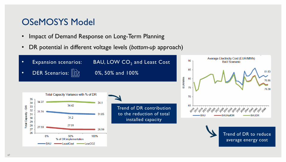
OSeMOSYS Model

• Impact of Demand Response on Long-Term Planning

• DR potential in different voltage levels (bottom-up approach)

67

• Expansion scenarios: BAU, LOW CO2 and Least Cost

• DER Scenarios: 0%, 50% and 100%

Trend of DR contribution

to the reduction of total

installed capacity

Trend of DR to reduce

average energy cost

OSeMOSYS Assessment

► Main Conclusions

– Flexible loads are important for the

system.

– The study did not consider costs related

to demand response.

► Assessment

68

- Dynamical system expansion

- Demand Response with detailed

modeling of flexible loads

- No representation of the

transmission network

- No representation of the

stochastic aspects of intermittent

sources.

Expansion planning of Distribution: EV, Batteries and PV

• Optimal investment in DERs, considering uncertainties in long-term peak load, amount of electric

vehicles, energy purchase/sale prices at the HV voltage level.

69

• Scenarios: Limit on energy purchase

o Unlimited energy purchase (UEP)

o Limited energy purchase (LEP)

#Recharge

stations

Solar capacity

(kW)

Storage

capacity

(kW)

Load

curtailment

(kW)

Total cost ($)

UEP LEP UEP LEP UEP L.EP UEP L.EP UEP L.EP

ΛG =

ΛL =

ΛEV = 0

91 81 0 90 0 790 0 0.332 427.398 484.761

ΛG #Recharge

stations

Solar capacity

(kW)

Storage

capacity

(kW)

Load

curtailment

(kW)

Total cost ($)

UEP LEP. UEP LEP UEP LEP UEP LEP UEP LEP

1 80 24 0 1750 0 800 0 96.43 678.415 1.064.651

Deterministic

With uncertainties on demand, recharging stations and energy prices

Robust expansion planning of the Distribution - Assessment

• Assessment of methodology

70

- Long-term uncertainties in planning

- Does not represent uncertainty in renewable generation.

- Does not assess investments in G + T + D

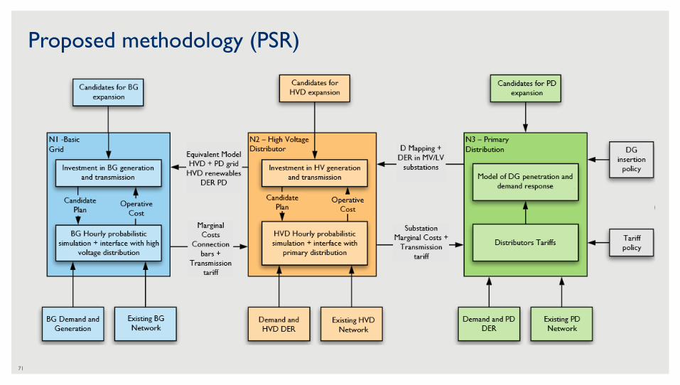
Proposed methodology (PSR)

71

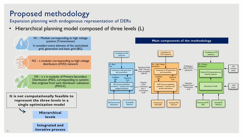
Proposed methodology Expansion planning with endogenous representation of DERs

• Hierarchical planning model composed of three levels (L)

72

It is not computationally feasible to

represent the three levels in a

single optimization model

Hierarchical

levels

Integrated and

iterative process

Main components of the methodologyN1 – Module corresponding to high voltage

systems (Transmission)

It considers every element of the centralized grid, generation and basic grid (BG)

N2 – n modules corresponding to high voltage distributors (HVD) network

N3 – n x m modules of Primary-Secondary Distribution (PSD), corresponding to systems that originate from each distributor substation

(MV/LV).

Candidates for BG

expansion

N1 -Basic

Grid

Investment in BG generation

and transmission

Candidate

PlanOperative

Cost

HVD Hourly probabilistic

simulation + interface with

primary distribution

BG Demand and

Generation

Existing BG

Network

Investment in HV generation

and transmission

Candidate

PlanOperative

Cost

N2 – High Voltage

Distributor

Candidates for

HVD expansionCandidates for PD

expansion

Demand and

HVD DER

Existing HVD

Network

N3 – Primary

Distribution

BG Hourly probabilistic

simulation + interface with high

voltage distribution

Distributors Tariffs

Model of DG penetration and

demand response

DG

insertion

policy

Tariff

policy

Demand and PD

DER

Existing PD

Network

Substation

Marginal Costs +

Transmission

tariff

D Mapping +

DER in MV/LV

substations

Marginal

Costs

Connection

bars +

Transmission

tariff

Equivalent Model

HVD + PD grid

HVD renewables

DER PD

Expansion planning: L1

► Centralized system: detailed G, T, storage (S)

► Simplified distribution system (n network

equivalents of the distribution networks)

► Economic signals from L1 to L2

73

Obj.F.: Min [Inv Cost G+T+S + E (Operation cost) ]

Hourly injection scenarios

N equivalent

networksSt

ep I Given optimum G&T expansion plan

Step 2 Simulate system

hourly operation, many scenarios of inflows & VRE power using a detailed transmission network

Step 3 Obtain

marginal costs from frontier busbars between HV and n systems.

Step 4 Add a term to

the marginal cost related to the location economic signal (wire tariff).

Step 5 Start

planning L2

Expansion planning L2

► Planning of “HV” level of the Distribution grid

(HVDdist):

► Economic signals from L2 to L3

74

Obj.F: Min [Investment costs in G+T+S at HVDDist

+ operation costs of local resources +

costs of acquiring services from L1 ]

Purchase energy and peak capacity

from L1

Invest and/or operate the

distribution system

Dummy generators at

the buses connecting

L1 to L2

Step1 Given

optimum expansion plan N2

Step 2 Retrieve

marginal costs for high voltage distribution system for all simulated hours.

Step 3 Add to

marginal cost term related to transmission / distribution locational tariff TUST/TUSD

Step 4 Start planning

L3

Tradeoff

Expansion planning: L3

• Decision to install DERs is taken by consumer based on:

– Supply tariff and RED cost

75

Decentralized vision

Step

1 Emulate consumer decision making. It can insert GD, batteries or change its demand curve.

Step

2 With the result of step 1, expand the distribution system St

ep

3 Within the expansion process, simulate the distribution system using OpenDss, a three-phase distribution power flow model.

Economic DER

optimization

from consumer

standpoint

New DER,

impact system

requirements

and planning

OBS.:

Centralized vision

Obj.F: Min [Investment costs in distribution +

operation costs of local resources + costs of

acquiring services from L2]

Verify whether the economic signals to

consumers induce maximum benefits

Optimization model like L2, considering

rooftop solar panel candidates.

Feedback (L3 → L2 and L2 → L1)

76

- Output data -

Investment in solar generation, DR,

batteries etc.

- Input data -

New demand and generation

injections mapped to the substations

L2 Expansion

- Output data -

New set of generations and

reinforcements in L2

- Input data -

New network equivalent

L1 Expansion

Detail of 1st feedback

L3 – Primary distribution L2 – “HV” Distribution L1 – HV network

Texas

• A 2019 study presents a method to quantify the benefit of deferred investment in T&D in Texas with a methodology based on approximate cost and directly monetized benefit.

• How can DER reduce T&D cost? It reduces investments related to the supply of peak demand

• How much of T&D cost relates to load growth that can be avoided? 10%-30% of T&D costs

• For how long can DER defer T&D investments? Load growth compared with DER growth data

• What is the value of postponing investments on T&D? Wire costs are for the next 10 years are compared in cases with or without DER (20% penetration)

• Results: (US$ 2019 million).

– Present value without postponement: $1,045

– Present value with postponement due do DER: $700

– Annual savings (DER Benefit): $345

– Saved over next 10 years: $2,452


Texas

• The study also provides a method to quantify short-term price reductions in the Texas market

• The study considers that DER reduces peak demand

• Methodology based on Market Price Appreciation, which requires simulation

– Adds DER if applicable in given hour in the supply stack curve

– Updates prices of electricity

– Reduces the new price from the original price (higher)

– Multiplies this difference by the load to compute total savings

• Results indicate savings of US$3.35 billion over 10 years for 1000 MW of DER.

• The methodology can also compute the incremental benefit of DER, based on it use in peak hours during summer (15h-19h from Jun. to Sep.) and winter (7h-10h,, from Dec. to Mar)

• The unitary yearly savings are roughly: US$ 500/kW for DER <100 MW, US$ 400/kW for DER<1000 MW and reduce sharply for DER penetration > 1000 MW.


10/9/2020

Quiz

79

Ado

be S

tock

Module llThanks!

Models

Software Capability Methods Input Parameters Output Countries

AleaDemand Energy forecasting

Genetic Algorithms,

Neural, Networks and

Statistics

Explanatory variables include

calendar days, weather,

temperature thresholds,

socioeconomic indicators,

climatology and seasons.

Belgium, France,

Italy, Germany,

Netherlands,

Poland, Spain and

UK

Alyuda Energy Forecasting

Logistic regression,

Decision trees, Decision

rules, Neural Networks

GDP, Population density, Prices of

fossil energy carriers, consumer

sector sales expectations

Energy demand forecast and other key

factors that condition profits, increase

in efficiency of combination of

cogeneration & district heating and

ensure availability of

power.

Australia, Chile,

France, Germany

and USA

ANTARESGeneration

Adequacy

Monte Carlo Simulations,

Stochastic models

Technical and meteorological

parametersLOLP, LOLE, LOEE / EENS

Germany,

Luxembourg, The

Netherlands,

Belgium and France

AURORA

Energy Forecast,

Resource Valuation

and Net Power

Costs

Resource capacity or

generation, zone demand,

net flows, fuel usage

LP and MIP North America


Models


BID3Power

Procurement

Stochastic Dynamic

Programming, Detailed

modeling of intermittent

RE generation

Fuel prices and operational

constraints, Detailed and

consistent historical wind speed

and solar radiation.

Simulation of all the major power

market metrics on an hourly basis -

electricity prices, dispatch of power

plants and flows across interconnectors

China, Europe and

North America

EGEASGeneration

Adequacy

Dynamic Program (DP),

Generalized Bender‟s

Decomposition, Screening

Curve Option, Pre-

specified Pathway Option

Planning Reserve Margin, emission

constraint, Resource availability,

Demand and energy forecast, Fuel

forecasts, Retirements, CO2

costs, RPS requirements, Heat

rate,

Outage rate, Emissions rate, Fuel

and O&M costs, For new

resources - Capital cost,

Construction cash flow, Fixed

charge data, Years of availability

20-year resource expansion forecast,

Amount, type and timing of new

resources, Total system Net Present

Value (NPV) of costs, Annual

production costs for system, Annual

fixed charges for new units, Annual

tonnage for each emissions type,

Annual energy generated by fuel type,

Annual system capacity reserves and

generation system reliability

Australia and USA

GRAREGeneration

Adequacy

Time series, Statistical

sampling, Probabilistic

Monte Carlo analysis

RES forecast, and possible aggregation

of area and fixed percentage of load, RE

production, operational reserve level

evaluation, Residual load distribution,

Reservoir and pumping hydro

optimization, ENS, LOLE, LOLP

Europe


Models


OPTGEN &

SDDP

Power

Procurement and

Operation Planning

Benders Decomposition

and Mixed Integer

Programming (MIP)

Energy balance constraints,

Operation reserve constraints,

Generator and contract

constraints: unit commitment,

detailed hydro modeliong,

capacity & energy limits,

transmission modeling, fuel

contraints, grid security

constraints and emission limits

More than 200 results including

operational variables, economic

variables (marginal costs) and others

~60 countries of all

continents

PLEXOS

Energy Forecasting,

Power

Procurement

Advanced Mixed Integer

Programming (MIP)

Energy balance constraints,

Operation reserve constraints,

Generator and contract

constraints: ramp, min capacity,

energy limits, Transmission limits,

Fuel limits and Emission limits

Optimal planning solution in the

medium term. Short-term unit

commitment and economic dispatch.

Hourly electricity spot prices

Europe, Middle East

and Australia

PowrSymGeneration

Adequacy

Cost data and system

operating parameters,

hourly load data and

maintenance data

Monte Carlo Scenarios and

Climate Dependent Time series

Capacity factor, Emissions, Fuel burn,

Electric energy generated , Costs (fuel;

operation and maintenance, O&M; start

up; emissions; total), Number of unit

starts, Operating hour

Japan, South Korea,

Europe and North

America


References

[1] Rogers E., 1962. “Diffusion of Innovations”. New York: Free Press of Glencoe (1st ed). OCLC 254636

[2] Vernon R., 1966. “International Investment and International Trade in the Product Cycle”. International Business Strategy (pp. 35-46). Routledge.

[3] Gartner Inc, 2001. “The Gartner Glossary of Information Technology Acronyms and Terms”.

[4] Dedehayir O., Steinert M., 2016. “The hype cycle model: A review and future directions”. Technological Forecasting and Social Change 108 (2016): 28-41.

[5] Moore, G. A., 1999. “Crossing the chasm: Marketing and Selling Technology Products to Mainstream Consumers”. Collins Business Essentials, 290p.

[6] International Energy Agency (IEA) – Tracking Energy Integration – Disponível em: https://www.iea.org/reports/tracking-energy-integration/energy-storage

(Acessado em 28 de Maio de 2020)

[7] Bass F., 1969. “A New Product Growth Model for Consumer Durables”. Management Science 15, p 215-227

[8] Bass F., Krishnan T., Jain D., 1994. “Why the Bass model fits without decision variables”. Marketing Science 3, volume 13, p 203-223

[9] Meade N., Islam T., 2006. “Modelling and forecasting the diffusion of innovation – A 25-year review”. International Journal of Forecasting 22 (2006) 519– 545

[10] Sigrin B., Gleason M. et al, 2016. “The Distributed Generation Market Demand Model (dGen): Documentation”. Technical Report NREL/TP-6A20-65231

[11] Sigrin B., Drury E., 2014. “Diffusion into New Markets: Economic Returns Required by Households to Adopt Rooftop Photovoltaics”. Energy Market Prediction:

Papers from the 2014 AAAI Fall Symposium.

[12] Konzen G., 2014. “Difusão de sistemas fotovoltaicos residenciais conectados à rede no Brasil: Uma simulação via modelo de Bass”. Dissertação de Mestrado –

Instituto de Energia e Ambiente da Universidade de São Paulo.

[13] EPE, 2019. “Modelo de Mercado da Micro e Minigeração Distribuída (4MD): Metodologia – Versão PDE 2029”. Nota Técnica DEA 016/2019

[14] Dong C., Sigrin B., Brinkman G., 2017. “Forecasting residential solar photovoltaic deployment in California”. Technological Forecasting & Social Change 117

(2017) 251–265

[15] Kurdgelashvili L., Shih C. et al, 2019. “An empirical analysis of county-level residential PV adoption in California”. Technological Forecasting & Social Change 139

(2019) 321–333

[16] Trachuk A., Linde N., 2019. “Dissemination of Distributed Energy Technologies”. DOI: 10.5772/intechopen.88604

[17] Assunção J., Schutze A., 2017. “Developing Brazil’s Market for Distributed Solar Generation”. Núcleo de Avaliação de Políticas Climáticas – PUC-Rio

[18] Prießner, Alfons & Sposato, Robert & Hampl, Nina. (2018). Predictors of Electric Vehicle Adoption: An Analysis of Potential Electric Vehicle Drivers in Austria.

Energy Policy. 122. 701-714. 10.1016/j.enpol.2018.07.058.

84

References

[19] McDermott, Ethan G., "Examining the effects of policy interventions on increasing electric vehicle adoption in California" (2017). Master's Projects and

Capstones. 567.

[20] Danielis, Romeo & Scorrano, Mariangela & Giansoldati, Marco & Rotaris, Lucia, 2019. "A meta-analysis of the importance of the driving range in consumers’

preference studies for battery electric vehicles," Working Papers 19_2, SIET Società Italiana di Economia dei Trasporti e della Logistica.

[21] Srivastava, A., Van Passel, S., & Laes, E. (2018). Assessing the success of electricity demand response programs: A meta-analysis. Energy Research & Social

Science, 40, 110–117. doi:10.1016/j.erss.2017.12.005

[22] Van Dam, Michiel. 2017, “Adoption of battery storage by household consumers Using agent based modeling to improve electricity distribution network

models”. TU Delft

[23] Milis, K., Peremans, H., & Van Passel, S. (2018). Steering the adoption of battery storage through electricity tariff design. Renewable and Sustainable Energy

Reviews, 98, 125–139.

[24] Ito K., Ida T., Tanaka M., 2018. “Moral Suasion and Economic Incentives: Field Experimental Evidence from Energy Demand”. American Economic Journal:

Economic Policy 2018, 10(1): 240–267

[25] Dutra J. (Coordenadora), 2019. “Metodologia de Elaboração da Função de Custo do Déficit”. P&D Estratégico ANEEL PD-0642-002/2015. Colaboradores FGV

CERI, Thymos.

[26] Berry S., Levinsohn J., Pakes A., 1995. “Automobile Prices in Market Equilibrium”. Econometrica, Vol. 63, No. 4 (Jul., 1995), pp. 841-890.

[27] IEA, 2019. “Global EV Outlook 2019”. Acessado em https://www.iea.org/reports/global-ev-outlook-2019

[28] Berlotti M.L., Brunner J., Modanese G., 2016. The Bass diffusion model on networks with correlations and inhomogeneous advertising”. Chaos, Solitons and

Fractals, 90 (2015) pp. 55-63. arXiv:1605.06308 [physics.soc-ph]

[29] Nevo A., 2000. “A Practitioner’s Guide to Estimation of Random-Coefficients Logit Models of Demand”. Journal of Economics & Management Strategy, Volume

9, Number 4, Winter 2000, 513–548

[30] Meade R., 2019. “Measuring Prosumer Welfare: Modelling Household Demand for Distributed Energy Resources and Residual Electricity Supply”. Presentation

at the EPOC Winter Workshop 2019, University of Auckland.

[31] Zhang Y., Zhong M., Geng N., Jiang Y., 2017. “Forecasting electric vehicles sales with univariate and multivariate time series models: The case of China”. PLoS

ONE 12(5): e0176729. https:// doi.org/10.1371/journal.pone.0176729

85

References

[32] Srinivasran V., Mason C. H., 1986. “Technical Note—Nonlinear Least Squares Estimation of New Product Diffusion Models”. Marketing Science 5(2):169-178.

https://doi.org/10.1287/mksc.5.2.169

[33] Bemmaor A.C., 1994. “Modeling the diffusion of new durable goods: Word-of-mouth effect versus consumer heterogeneity”. Research Traditions in Marketing

(Kluwer Academic Publishers, Boston), 221–229.

[34] Boswijk H.P.,Franses P.H., 2005. “On the Econometrics of the Bass Diffusion Model”, Journal of Business and Economic Statistics, 25, 255–268.

[35] Sterman J. D., 2001. “Systems dynamics modeling: tools for learning in a complex world”, California management review, Vol 43 no 1, Summer 2001

[36] Coelho M.D.P., Saraiva J.T., Konzen G., Araujo M.C., Pereira A.J.C., 2019. “Modelling the Growth of DG Market and the Impact of Incentives on its

Deployment: Comparing Fixed Adoption and System Dynamics Methods in Brazil”. 2019 IEEE Milan PowerTech conference. DOI: 10.1109/PTC.2019.8810994

[37] ANEEL, 2020. Base de dados de unidades de geração distribuída. Acessado em http://www2.aneel.gov.br/scg/gd/VerGD.asp, março de 2020.

[38] Department Of Energy, 2018. “Global Energy Storage Database”. Office of Electricity Delivery & Energy Reliability. Acessado em

https://www.energystorageexchange.org/, junho de 2018.

[39] Jackson, M., 2008. “Social and Economic Networks”. Princeton University Press.

[40] Van der Bulte, C., Stremersch, S., 2004. “Social Contagion and Income Heterogeneity in New Product Diffusion: A Meta-Analytic Test”. Marketing Science Vol.

23, No. 4, Fall 2004, pp. 530–544

[41] Kiesling, E., Guenther, M., Stummer, C., Wakolbinger, L.M., 2012. “Agent-based simulation of innovation diffusion: a review”. Central European Journal of

Operations Research 20.2 (2012): 183-230.

86

DESIGNING RENEWABLE DOMINATED RESOURCE PLANS ...

Documents

Transcript of DESIGNING RENEWABLE DOMINATED RESOURCE PLANS ...