1  

Distributed Solar Renewable Generation: Option Contracts with Renewable Energy Credit Uncertainty

Yaxiong Zeng1, Diego Klabjan2, Jorge Arinez3

Abstract

Solar energy is rapidly emerging thanks to the decreasing installation cost of solar panels and the renewable portfolio standard imposed by state governments, which gave birth to the Renewable Energy Credit (REC) and the Alternative Compliance Payment (ACP). To make profits from the REC market in addition to reduced energy costs, more and more home and business owners choose to install solar panels. Recently, third-party financing has become a common practice in solar panel investments. We discuss optimal timing for the host to potentially buy back the solar panels after being installed for a period of time and how to incorporate the optimal timing into a power purchase agreement between the host and the third-party developer. Because the REC price is a major source of uncertainty and also due to the ACP capping the REC price, we first propose a REC price forecasting model that specifically considers the ACP values. Then by a modified real option structure, we model the buyback contract as a real option and solve it with an approximate dynamic program based Monte Carlo simulation method. We find that as the ACP value increases, the value of the buyback option also increases under optimal timing. The method used does not only apply to solar projects but also to other distributed renewable projects that are third-party financed, such as wind generations. Keywords: Real option; Renewable Energy; Solar generation; REC market

1. Introduction In recent years, global warming has been increasingly acknowledged as a threat to long-term human survival. Many countries have thus set up targets concerning emission limitations or reductions of greenhouse gases: the European Union aims at a 20% reduction below the 1990 baseline by 2020 (UNFCCC, 2008) and the United States offers a goal of a 17% reduction below the 2005 level by 2020 (US Department of Energy, 2009). To attain these goals, renewable energy technologies are being widely adopted to reduce the reliance of energy on fossil fuels. In the United States, in 2011 renewable energy accounted for 9% of total primary energy consumption, with hydroelectric (35%), wood (22%), biofuels (21%) and wind power (13%) as major renewable sources (EIA, 2012). The solar market is now rapidly expanding as a result of historically high

                                                                                                               1 PhD Candidate, Industrial Engineering and Management Sciences, Northwestern University E-mail: yaxiongzeng2015@u.northwestern.edu 2 Professor, Industrial Engineering and Management Sciences; Director, MS in Analytics, Northwestern University E-mail: d-klabjan@northwestern.edu 3 Manager, Sustainable Manufacturing System, General Motors E-mail: jorge.arinez@gm.com

  2  

photovoltaic prices and by the financial incentives from the federal government, states and utilities. From the 2012 U.S Solar Market Insight report, photovoltaic installations totaled 3,313 MW, up 76% from 2011 with an estimated market value of $11.5 billion (SEIA/GTM Research, 2013). One important aspect in the solar market is the Renewable Energy Credit (REC). As of 2013, the Renewable Portfolio Standard (RPS) is implemented in 30 U.S. states (including District of Columbia). Under such a policy, local utilities and load-serving entities are obligated to procure a specified fraction of their electricity as renewable energy. As a market response to RPS, the REC trading programs are initiated in most of the 30 states. Eligible renewable power producers receive a REC for each MWh of renewable energy generated. When electricity providers cannot meet the mandatory requirement from their own power facilities, they can in turn purchase RECs from renewable generators to comply with the RPS. The unit of REC price is $/MWh. Specifically, 17 out of the 30 states adopted detailed RPS targets to ensure solar power comprises a minimum fraction of the renewable mix, resulting in the creation and trading of the Solar Renewable Energy Credit (SREC). If the power supplier fails to obtain adequate credits, i.e. fails to meet the RPS, it is then subject to a penalty called the Alternative Compliance Payment (ACP) per MWh. In the solar case, the supplier is subject to the Solar Alternative Compliance Payment (SACP). Generally, SACP caps the SREC price. Otherwise, the obligated entity would prefer to pay the penalty, which is the mechanism of last resort to achieve compliance with the RPS. As the solar market continues to grow, the SREC trading program provides a driving incentive for home and business owners to install photovoltaic panels to satisfy their own electricity needs and financially benefit from selling SRECs. In residential or commercial sites, direct ownership of solar panels is not a common practice. Instead, third party financing is taking off across the U.S. For instance, the 2012 U.S. Solar Insight Report pinpoints the ongoing third-party solar revolution. Specifically, over 50% of all new residential installations in most major residential markets are from third-party-owned systems. The report also forecasts that the momentum will last. Usually, a third-party developer designs, installs, owns, operates and maintains solar panels on the user’s roof and the user or host procures electricity from developer-owned solar panels. The user pays the developer according to a lease or Power Purchase Agreement (PPA). In the lease contract, home or business owners pay a monthly flat fee to the third-party developer. In the PPA, the host pays based on its electricity usage and according to a fixed rate or a rate with a fixed annual escalating factor. In both settings, the host does not pay for the panel installation or maintenance while it is the developer who incurs these costs. We particularly study the PPA setting, where the host buys all the electricity generated from the panels as negotiated in the contract. Although the contract based on third-party financing can bring electricity with low and predictable costs, it prevents the host from making profits by selling RECs since they are owned by the third-party entity because they own the installation. The customer can buy back the panels at a later time (see NREL, 2009). However, when to buy back the panels has not yet been studied. Thus in this paper, we discuss optimal timing of the buyback option by the host, in which the host buys the third-party owned solar

  3  

panels at a particular time and price, and the REC ownership transfers from the developer to the host after panel buyback. The timing decision from our analysis is valuable to both the third-party developer and host. Grounded on the analysis, the two parties can develop the PPA and integrate the best timing decision into the contract. Ultimately, the buyback problem is a real option because it focuses on the exercise opportunity during a predetermined period. Uncertainties involved in the buyback option result from fluctuations of REC prices, the electricity price, electricity demand by the user, and the value of the solar panels. As the REC markets continue to grow in the United States and worldwide, changing REC prices will have an increasing effect on the optimal investment timing decision. In this paper, we first introduce a new financial model to forecast REC prices, which have a lower bound of zero and upper bound of the ACP value. Results show that our model outperforms the existing Geometric Brownian Motion (GBM) forecasting model. Forecasted REC prices are then incorporated in the cost-profit analysis of the solar investment. After the buyback option is exercised, the pattern of the cash flow changes due to REC sales. We thus model the investment timing problem as a real option by proposing a new option structure. We solve the model using a Monte Carlo simulation method based on approximate dynamic programming (ADP). In essence, our real option structure does not rely on sophisticated financial mathematics due to inherent complexity and can provide decision insights under different combinations of uncertainties. In this paper, we consider the host to be a non-power generating company. We only discuss solar projects, but the methodology can be adapted to other distributed renewable generations. For example, on-site wind generation is also applicable to our analytical framework, since it has an equivalent REC market and a similar third-party financing structure. The main contributions of this paper are as follows.

1. A new REC forecasting method that specifically takes ACP values into account. 2. A new real option framework that can handle different patterns of cash flows before and after the

option is exercised. 3. A developer-host contract that explicitly considers optimal buyback timing, the first of its kind in

distributed renewable generation. 4. A case study that solves a problem of a real-world company.

The structure of this paper is as follows. Section 2 provides a literature review. Section 3 introduces the new REC forecasting model and compares it with existing models. Section 4 exhibits the model of the investment timing problem as a real option and it provides the solution methodology by means of the least square ADP algorithm. Section 5 discusses the results from the Monte Carlo simulation with three case studies. Section 6 draws conclusions and suggests relevant future work.

2. Literature Review An important model in our work is the discounted cash flow (DCF) model. When assessing an investment project, the DCF model is chosen traditionally. The model discounts the cash flows of the

  4  

project to present time. If the obtained net present value (NPV) is positive, the project is economically viable. Due to its simplicity, it leads to rigid managerial decisions. It assumes the future cash flows have no variability, and the decision is simply to invest now or abandon the investment. These two drawbacks contradict the current investment styles characterized by uncertainties and dynamic decisions. As a remedy, the concept of real option has been proposed, which has been researched in a variety of disciplines during the last three decades. Essentially, it serves as an extension to the DCF model. Several textbooks have been published to comprehensively introduce the concepts, theories and methods in real option studies (Dixit and Pindyck, 1994; Trigeorgis, 1996; Amram and Kulatilaka, 1999; Mun, 2002). Before year 2000, in the energy sector, most of the real option literature applies to the oil industry. Because of the deregulation of the electricity market in the mid 1990s, real option principles began to be widely adopted in the analysis of electricity relevant topics such as electricity markets and power system investments. However, it is not until the last decade that the real option theory has been applied to the renewable energy field. The first paper by Venetsanos et al. (2002) presents a framework to assess renewable energy projects by real options and illustrates the possible uncertainties under deregulated energy markets. The paper models a Greek wind energy project as a real option and evaluates it by the Black-Scholes model, different from our ADP approach. There are two popular methods in renewable real option analyses: the partial differential equation (PDE) method and the dynamic programming (DP) method. Usually, the PDE method requires an advanced understanding of stochastic models and financial mathematics. It is also not easy to analyze a real option that allows an early exercise using PDE, similar to an American call option. As another method, DP follows a recursive pattern to optimize decisions that influence future cash flows. Unlike PDE, the DP approach makes intermediate values and decisions readily available (Fernandes et al., 2011). In DP applications, a full stochastic DP is sometimes used, but the simplest and most frequently used model is the lattice model. By calculating risk neutral probabilities and up and down factors, it is possible to almost always identify the basic structure from any real option and construct a corresponding lattice model (Mun, 2002). For example, Munoz et al. (2009) use a trinomial lattice model to evaluate the option to invest in a wind power generation project and demonstrate the probabilities of “invest now,” “wait,” and “abandon,” while we only consider one option over the entire time horizon – in which year should we invest. The main problem with the lattice model is the difficulty to deal with multiple uncertainties. It needs multiple variables to represent different uncertainties, and thus the number of nodes grows exponentially with the dimension of uncertainties. Furthermore, to approximate the stochastic process accurately, it requires a high-dimension tree or infinitesimal time intervals. These two factors make it computationally expensive in the attempt to model complex problems with several uncertainties and to retain a satisfactory level of approximations of endogenous stochastic processes. As a result, we adopt a Monte Carlo simulation and optimization method to solve our model. Unlike the PDE method, it requires less mathematical sophistication and can easily handle early exercise situations. In contrast to the lattice model, it better copes with stochastic processes, regardless of the dimension of

  5  

uncertainties. In this study, we integrate Monte Carlo simulation with ADP. It differs from the lattice model mainly in the fact that ADP can cope with a large number of decisions and complex stochastic processes. Overall, Monte Carlo simulation is widely used in real option, but less so in renewable energy. Martínez-Cesena and Mutale (2011) propose an advanced real option methodology for renewable energy generation project planning using a simulation approach for a hydropower case study. In comparison, we focus on the flexibility of the investment decision because the exercise year is to be decided, rather than the flexibility of a project design. In financial theory, Longstaff and Schwartz (2001) propose a simple least-square approach to value American options. The key contribution is their estimation of continuation values, i.e. the conditional expectation of payoff if the option is held. In each time period, the option holder compares the value of exercising the option and expected payoff when holding the option. If the exercise value surpasses the holding value, the holder exercises; otherwise, the option is held and exercised later. The holding value is based on a conditional expectation function that is generated from the regression of ex post realized payoffs from continuation as functions of the values of the state variables. The proposed algorithm falls in the category of ADP and is called least square Monte Carlo (LSM). Applications of LSM in real options have been studied in Rodrigues and Armada (2006). However, such a method has not yet been used in renewable real options. In this paper, we focus on the Monte Carlo simulation and we specifically incorporate LSM in finding the optimal exercise time. Solar-related literature is the scarcest among renewable applications of real options (Fernandes et al., 2011). Four papers relate to our work in terms of the solar investment timing. The most relevant is Ashuri et al. (2011), who study the best timing to invest in photovoltaic panels on solar ready buildings. Ashuri et al. and our work both focus on the timing decision to install solar panels of a stakeholder such as a company or homeowner. They assume the price of solar panels decreases over time according to the experience curve, while we make a different assumption that the price decreases according to market fair values. Ashuri et al. focus on savings from solar panels while we concentrate on the minimization of the total NPV over the entire time horizon. The uncertainty in their model is the electricity price, by which they calculate the savings from solar panels against procuring electricity from a utility, while our uncertainty is predominantly the REC price. They assume no cash flow before exercising the option, making it possible to use the lattice model. But cash flow is captured throughout the future horizon in our model, and has different patterns before and after the option exercise. They use a binomial lattice to forecast electricity prices and by means of decision trees they determine the optimal installation time, while we use a Monte Carlo simulation method combined with ADP. In summary, our model is more general and realistic under current market conditions. Beliën et al. (2013) also consider the optimal timing for a solar panel investment and follow a similar method to Ashuri et al. (2011) to construct the model, and only differ in that they consider more cost and revenue factors, and solve the problem using the future value analysis. Sarkis and Tamarkin (2008) also consider savings as profit, not from electricity, but from green house gas emissions. They also adopt the

  6  

lattice model to solve the timing problem. Martinez-Cesena et al. (2013) from a savings point of view discuss about optimal timing using the economics concept of an indifference curve. These four papers have a similar cash flow structures and similar uncertainties. They differ mainly in the calculations of savings and the methods that solve the models. Unlike these studies, we propose a different real option structure, we combine multiple uncertainties with the focus on REC price volatility and solve the model with a different method. An important building block of this paper is REC price forecasting. To the best of our knowledge, only one paper, Tang et al. (2012), discusses a forecasting method. The paper provides three stochastic models for price processes: Geometric Brownian Motion (GBM), Jump Diffusion and NGARCH processes. By a statistical comparison they choose GBM as the appropriate model. When forecasted prices exceed the ACP value, they simply cap the price by the ACP. This can be problematic because it is possible for GBM to exceed the ACP for a long time; and thus during that period, REC prices are constants (equal to ACP), which obviously deviates from the market trend. In this paper, we provide a forecasting model that in particular accounts for the ACP value.

3. REC Forecasting Model REC is a market response to RPS. It helps electricity providers to meet the RPS by purchasing certificates from the REC market. As a provider of RECs, a company equipped with solar panels should forecast the REC prices and incorporate them in its cash flow (REC sales) calculation. Forecasting of REC prices is needed in our real option model explained in Section 4, but it also has value as a standalone model in NPV analyses. REC prices should have the ACP as the upper bound and zero as a natural lower bound. The ACP value, functioning as the penalty payment that the utility incurs when it fails to meet the RPS, varies across states. For example, New Jersey has a mature SREC market and has designed its 20-year SACP plan so that by 2028 it would have 4.1% of its electricity from the solar power. However, California just initiated a tradable REC market in 2011, with a promotional REC price cap of $50 that will expire at the end of 2013. We base our study on the NJ SREC market and use its available monthly-basis data from 2004 to the present. 81 historical monthly average prices from April 2004 to May 2011 are used to calibrate parameters of forecasting models, while the remaining 20 prices from June 2011 to January 2013 are used to perform out-of-sample tests. The ACP value decreases over time from $711 in 2009 to $239 in 2028. For years before 2004 and after 2028, we assume the ACP is the same as in 2009 and 2028, $711 and $239 correspondingly. To feature the variations of ACP values overtime, we introduce the artificial prices by dividing the actual REC prices by the ACP value at that time. It is the artificial prices on which we base our parameter estimation and price forecasting. To further obtain the forecasted REC prices, we simply multiply the artificial prices by corresponding ACP values.

  7  

We first introduce the GBM model that has been used to forecast REC prices in Tang et al. (2012). The process St , t ≥ 0{ }defined by

St = S0eµt+σBt , t ≥ 0 (1)

is called a Geometric Brownian Motion with driftµ and volatilityσ . The standard Brownian Motion Btis characterized by the independent normal distributions with mean 0 and variance t, t ≥ 0 . In finance,Stis considered as the asset price with S0 being the initial price. It can be also expressed by the stochastic differential equation (SDE):

dSt = St µdt +σdBt( ), t ≥ 0 . (2) In the SDE formulation, dSt is the price increment, dt is the time increment anddBt is the increment for standard Brownian Motion. In particular, dBt also follows a normal distribution with mean 0 and variancedt . By Ito’s formula, (1) and (2) are equivalent. To simulate the GBM process, we need to discretize the time horizon. Suppose we want to simulate a sample path of an asset price from [0,T]. We first divide the time interval into N equal time steps with

the interval lengthΔt = TN

and simulate a sample path Sti , i = 0,1,...,N{ }with ti = iΔt and a starting price

S0 :

Si+1 = Sieµ−1

2σ 2⎛

⎝⎜⎞⎠⎟Δt+σεi+1 Δt

, i = 0,1,...,N −1, whereε i ’s are i.i.d. random variables generated from the standard normal distribution with mean 0 and

variance 1. In each step, we basically simulate the return process Si+1Si

, and multiply it by the previous

asset price Si . To obtain parametersµ andσ , we apply the widely used maximum likelihood estimation method, based on historical prices. A drawback of the GBM model is that even if the parameters are estimated accurately, prices generated by this model can often exceed the ACP upper bound. To confirm this, we performed the following experiment. We first simulated 110 sample paths (with 100 prices in one sample path) generated by the GBM model with fitted parameters µ = 0.2424, σ = 0.4972 using historical REC prices in New Jersey since 2004. If the generated artificial price is greater than 1, then it is considered to exceed the ACP value. Figure 1 illustrates the number of sample paths in which the sample paths exceed the ACP different times. From the plot, we observe that most sample paths exceed the ACP value more than once, which is not acceptable as it contradicts the market fundamentals. Even worse, some sample paths show more than 80% of the prices over the ACP! There are only 17% of sample paths with no or only one exceeded value. This occurs because the GBM model does not have an upper bound that should be fundamental to a REC forecasting model.

  8  

Figure  1:  Histogram  of  the  frequency  of  exceeding  the  ACP  value  

Next we propose a new forecasting model that is borrowed from financial engineering – Jacobi Diffusion (JD). Its stochastic differential equation is:

dst = −b st − β( )dt +σ st 1− st( )dBt , whereb > 0, σ > 0, 0 < β <1 . Quantityb is the mean reverting parameter,β is the mean of the process, andσ is the volatility. Again,dst is the price increment,dt is the time increment and dBt is the increment of standard Brownian Motion. In particular, st generated by this model lie between 0 and 1. To further obtain forecasted REC prices St , we simply multiply st by the ACP value. As the ACP vary year by year, forecasted REC prices display different upper bounds (see Figure 2, whose details are discussed later).

Figure  2:  Simulated  REC  prices  from  the  JD  model  

  9  

In simulation, discretization of the JD process is also needed. We follow the same structure introduced

in the GBM part: Δt = TN

and we simulate a sample path Sti , i = 0,1,...,N{ }with ti = iΔt and starting price

S0 ( s0 = S0 / ACP0 ):

si+1 = si − b si − β( )Δt +σ si 1− si( )Δtε i+1, i = 0,1,...,N −1, (3)

Si+1 = ACPi+1 ⋅ si+1, i = 0,1,...,N −1. (4) In essence, during each step we simulate the difference of the prices. Then we add the difference to the previous price and perform the multiplication to get the forecast. However, due to the discretization of the time, in a few cases si can be greater than 1 or less than 0, making it impossible to produce the next price. To prevent this, we force si to be 0.99 or 0.01 in respective cases. Finally, we follow the approximated maximum likelihood estimation method introduced in Gouriéroux and Valéry (2004) to estimate the parameters in the JD model. The fitted parameters are b = 0.11, β = 0.9085, c = 0.0808 by using the same historical data in New Jersey as in the GBM case. Unlike the GBM sample paths exceeding the ACP multiple times, the JD sample paths exceed the ACP at most once in all 100 sample paths due to the time discretization. To further assess the GBM and JD forecasts, we present the Quantile-Quantile (QQ) plot. The QQ plot is used to test how well the sample data fits a distribution. In Figure 3, the x-axis plots the quantiles of historical REC returns in NJ, and the y-axis plots the quantiles of the log returns of simulated data from GBM and JD processes. We use log returns to normalize the data and consequently we can compare the data over different time periods. From the QQ plots we observe that the points from the JD process lie closer to the straight line, indicating that the JD process fits the historical REC prices better. As another piece of evidence, in an out-of-sample test, we find that the JD sample path behaves better than the GBM sample path. Out of the 101 historical NJ REC prices, we use the first 81 points to estimate parameters for the GBM and JD processes. Then we generate 20 prices separately from the two models and compare them with the remaining 20 historical prices. Because the price before the 81st month are near the ACP value, there is little room for the actual prices to go up and it is very likely that the price should exhibit a downward trend. The JD process captures this feature very well and shows a sharp contrast to the GBM model, which allows the prices to go up (Figures 5 and 6). All of the three comparisons show our forecasting method outperforms the GBM model.

  10  

Figures  3:  QQ  plots  of  the  JD  and  GBM  models  

Figure  4:  Out-­‐of-­‐sample  test  for  the  JD  model  

 

 Figure  5:  Out-­‐of-­‐sample  test  for  the  GBM  model  

  11  

4. Option Contract Modeling As described in the introduction, we consider a host to be an industrial non-power generating company, considering a third-party developer to install, maintain and operate the panels on its property due to the high up-front investment cost of solar panels. In return, the company pays the charge based on the amount of electricity generated from the solar panels according to the PPA. If the panels cannot satisfy the company’s power demand, it has to buy extra electricity from a utility. The third-party developer has a good reason to engage in such a contract: besides the regular profit by selling electricity to the company, the developer can also benefit from selling the RECs from the solar electricity and the tax incentives from the government. However, as time goes by, the value of solar panels declines. To minimize the company’s overall cost, the company has an option to purchase the panels from the developer at a specified time in the future. We model this option as an investment contract. In the contract, the company has the option to buy the solar panels from the third-party developer for a predetermined price based on a buyback time. After the purchase, the company then owns the panels and associated RECs, and thus benefits from the REC market. The buyback option is analogous to the American call option. First, they both have a limited time horizon. The call option has an expiration date, while the buyback can only happen during the panels’ lifespan. Second, they both emphasize the exercise opportunity. The call option exercises at a particular price prior to expiration while the company buys the panels at a given price before the panels turn obsolete. So the questions for the company are: (a) Should the panels be bought? (b) When should they purchase the panels in order to minimize the net cost NPV during the entire time horizon? To answer these questions, we model the buyback contract as a real option. In a buyback contract for solar panels, the cash flows have different patterns before and after the purchase of panels. Before the purchase, the company has to incur the electricity cost from panels paid to the developer and to the utility for the remaining power. While after the purchase, the company only needs to pay the electricity cost to the utility, potentially pay the maintenance cost to the developer and receive profits by selling RECs and potential sales of redundant solar electricity. Specifically, we calculate all costs on a monthly basis, i.e. the time period is a month. We use the following notation

T - life span of solar panels (month) Gm – electricity energy generated from solar panels in month m (kWh) Dm – electricity energy demand in month m (kWh) Pm – price of electricity from solar panels in month m ($/kWh) Um – price of electricity from utility in month m ($/kWh)

Rm – REC price in month m ($/MWh) Wm – one-time purchase price of solar panels in month m ($) Mm – maintenance cost of solar panels in month m ($) Usually, invertors of solar panels need to be replaced at the half of solar panels’ life span and the replacement cost represents 10% of related investment cost. In our model, we incorporate the replacement cost into monthly maintenance cost with

  12  

Mm =Mm , if m ≠ T

2⎢⎣ ⎥⎦

Mm +MINV , if m = T2⎢⎣ ⎥⎦

⎧⎨⎪

⎩⎪,

whereMm is the regular maintenance cost andMINV is the invertor replacement cost. We make the following assumptions:

1. The life span T of solar panels is finite. 2. The amount Gm of electricity generated from the solar panels decreases on a yearly basis and we

do not take into account any panel failures or variability of weather conditions that cause generation variability.

3. The price of solar electricity Pm escalates at a fixed rate per year. 4. The price of utility electricity Um escalates at a fixed rate per year. 5. Panel purchase price Wm decreases according to the net profit the third-party developer expects

to incur from the solar panels after the company’s purchase, not according to experience curves. 6. The company is obligated to purchase all the generated electricity before owning the solar

panels. If the generated electricity Gm exceeds the company’s demand Dm, the current owner will sell it back to the grid at the current utility price Um.

7. The ACP values are known in advance and thus deterministic. 8. After the buyback the company pays the developer to maintain the solar panels with maintenance

cost Mm per month. 9. The company applies the buyback contract to mature factories or buildings so the electricity

demand is deterministic over years (including peak demand). 10. The discount rate is constant. We use different discount rates when calculating NPVs for the

company and the developer since they have dissimilar capital structures and thus different discount rates.

Note that Gm, Pm and Um change on a yearly basis. For example, Gm decreases yearly based on fixed degradation rate a. It means that the value of Gm changes only for m representing January and in that month it decreases by 1 – a% over the value in the previous year. Under these assumptions, we next present the cost analysis. Before exercising the option, the company has to incur the following cost in month m:

Cm = GmPm + Dm −Gm( )+Um . After exercising the option, the company has to incur the following cost during each month:

Bm Rm( ) = Dm −Gm( )Um −GmRm +Mm . At any time, the panel purchase price Wm is the NPV of the developer’s future profit from selling RECs and sales of electricity to the company. Future maintenance costs after the purchase are subtracted from the purchase price in accordance with assumption 8, i.e.

  13  

Wm R!"m( ) = E γ d

n−m Rn + Pn( )Gn −Mn( )n=m+1

T

∑ Fm⎡⎣⎢

⎤⎦⎥

, (5)

where R!"m = Rm+1,Rm+2,...,RT( ), γ d

k = e−rdk is the continuous discount factor and rd is the developer’s discount rate. Note that rd is used only here for the calculation of panel purchase price and the company discount rate is used elsewhere. By (5), the resulting optimal month can balance the profits of the developer and company. Accordingly, the exercise value of the option in month m is

Vm

e R!"m( ) = γ nCn Fm( )

n=1

m

∑ + γ mWm R!"m( ) + E γ nBn Rn( ) Fm( )

n=m+1

T

∑⎡⎣⎢

⎤⎦⎥

,

whereγ k = e−rk is the continuous discount factor, r is the company discount rate, Rk isFk measurable,

i.e. Fk =σ Ru ,u ≤ k( ) and Fk contains the information up to time k. If Rm is a martingale, then the

expectation can be computed by substituting the Rn ’s by Rm and thus Vm

e R!"m( ) =Vme Rm( ) . Note that the

value in month m is function of only R!"m , as we assume other variables can be computed without

uncertainty. Let Vm

h R!"m( ) be the optimal cost if the optimal exercise time happens after month m. This

implies that in month m the option is not exercised and thus this is the holding cost in month m. There does not exist a closed form expression forVm

h . The optimization problem that minimizes the overall cost is to find the latest month mj

* for which

Vmj*−1h R!"mj*−1

j( ) ≤Vmj*e R!"mj*

j( )

for a realization R!"mj*−1

j of REC prices. The selected final time is the average time of allmj* over all

realizations j.

For such a cash flow form, it is difficult to apply traditional approaches of real options that treat cash flows in a consistent pattern. We propose a new option framework that addresses this difficulty. We first define two artificial variables: the artificial strike price and the artificial stock price.

• Artificial Strike Price Km: - (total cost that has incurred before month m + panel purchase price in month m)

• Artificial Stock Price Sm: + (total cost expected to incur after current month m) The artificial strike price is known given the current month m while the artificial stock price is still undetermined. This resembles the structure of an American call option with fixed strike prices and volatile stock prices. In an American call option the option allows option holders to exercise the option,

  14  

i.e. buy an agreed quantity of a particular stock from the seller at a predetermined price K at any time prior to and including its expiration date T. The value of exercising an American option is

S − K( )+ = max 0,S − K( ) = 0, S < KS − K , S ≥ K

⎧⎨⎩

.

The artificial value of our option is thus simply • (total cost expected to incur after current month m + total cost that has incurred before month m

+ panel purchase price in month m) = Total cost during the entire time horizon. To summarize these concepts, we draw a comparison between the American Call option and our solar option in Table 1.

American Option Solar Option Maturity time T Life span of the solar panel T Stock price Sm at time m Total cost the company expects to incur after month m Strike price Km at time m Total cost the company has incurred before and in month m Early exercising time m (<T) Month to buy back the solar panels m (<T) Option price if exercising at time m =max 0,S − K( )

Value of the project (the total cost during T) in month m =Vm

e Rm( )

Table  1:  Comparison  of  the  American  call  option  and  the  solar  option    

Solving this model in traditional ways, such as by a PDE or the lattice model is not easy due to the inconsistent cash flow form. We thereby propose an ADP based Monte Carlo simulation method. The basic idea has been introduced in Longstaff and Schwartz (2001). The algorithm first simulates a series of realizations of sample paths and calculates relevant cash flows. Although exercise values can be easily computed, holding values in each month are difficult to obtain. The algorithm thus approximates holding values by least square regression and then performs DP backward recursion. The algorithm returns an optimal exercise time for each realization. Instead of pricing financial options, we fit it to our proposed solar option framework. Let us first modify the exercise value by changing its discount rates. Then the value becomes

Vm

e R!"m( ) = γ m−nCn Fm( )

n=1

m

∑ +Wm R!"m( ) + E γ n−mBn Rn( ) Fm( )

n=m+1

T

∑⎡⎣⎢

⎤⎦⎥

.

In this form, we consider the value to be the NPV in month m instead of at time zero. By our definition, the artificial strike price

Km

j R!"mj( ) =Wm

j R!"mj( ) + γ m−nCn

j Fm( )n=1

m

∑ , (6)

and the artificial stock price

Smj R!"mj( ) = E γ n−mBn

j Rnj( ) Fm( )

n=m+1

T

∑⎡⎣⎢

⎤⎦⎥

, (7)

  15  

where superscript represents the jth realization of REC prices. To be specific, each realization uses a distinct REC price sample path. We also assume artificial strike prices are positive for ease of computation. As opposed to the simplicity of obtaining the exercise values in each month, it is relatively difficult to calibrate the holding value

Vm

h R!"m( )without knowing when to exercise the option. One remedy is to

approximate the holding values. When implementing the LSM method proposed by Longstaff and Schwartz (2001), we use the following approximation formula,

ε j + c + a1Rmj + a2 Rm

j( )2=

e−r j

e*−m( )ΔmVj

e*

j ,e R!"

je*

j( ), if je* ≤ T ;

0, if je* = T +1.

⎧⎨⎪

⎩⎪ (8)

where je* is the optimal exercise time of realization j after current month m, ε j is the corresponding

regression error, andΔm is the time increment. In (8), the right-hand side is first computed and then

approximated byε j + c + a1Rmj + a2 Rm

j( )2 by means of regression. For each j, there is one regression

observation, which yields coefficientsa1 , a2 and constant c obtained based on the current optimal exercise values in all realizations. The method follows the classic idea of a backward algorithm with the starting month to be the last time period T. Next by substituting coefficientsa1 , a2 and constant c in the left hand side of (8) without the

regression errorε j , we have the approximated holding values

Vmh Rm( ) = c + a1Rm + a2 Rm( )2 .

If the holding value is less than the exercise value, in other words, the cost is less if the option is held, then we go backward to the previous month and keep the current optimal exercise time je* and valueVj

e*

j ,e .

Otherwise, we update the optimal exercise time to the current month m and change the corresponding exercise value toVme . We continue this procedure until we reach the first month. Essentially, in each month, the method compares the value of exercising now with the approximated optimal value of posterior exercising, i.e. the holding value. The algorithm is presented in Algorithm 1. Initialization:

a. Generate N sets of REC price sample paths indexed by j.

b. Calculate artificial strike price Km

j R!"mj( )

and artificial stock price Smj R!"mj( ) for all j, m.

c. Calculate the cash flows Vm

j ,e R!"mj( ) = Km

j R!"mj( ) + Smj R

!"mj( ) for all j, m.

d. SetVTj ,h =VT

j ,e , je* = T for all j.

  16  

For m=T-1 to 1 e. Apply the least square regression based on N realizations and find values a1 , a2 and c by solving

ε i + c + a1Rmi + a2 Rm

i( )2 = e−r ie*−m( )Vie*

i,e for all i=1,…,N.

For j=1 to N f. Set

Vmh Rm( ) = c + a1Rm + a2 Rm( )2 and thusVm

j ,h = c + a1Rmj + a2 Rm

j( )2 .

g. CompareVmj ,h andVm

j ,e :

IfVmj ,h ≤Vm

j ,e , update je* = m andVj

e*

j ,e =Vmj ,e .

End End

Algorithm  1:  The  modified  least  square  ADP  algorithm The algorithm returns the optimal exercise time je* for each realization. The average optimal exercise

month and other statistics can be obtained from these.

5. Case Studies In this section, we present three case studies. We first study the optimal exercise timing and the savings by buying back the panels at the optimal timing by considering only the REC prices as uncertainty. This strictly mimics the setting of our industrial partner. The second case study adds additional uncertainties to the model and the corresponding results are discussed. The third case study presents the sensitivity analysis using different parameter values. These case studies are based on data from a large US company where a project recently conducted is based on a fixed contract. The company assumed a fixed REC price given in advance and stationary during the planning horizon and optimally derived year 21 out of 30 years to buy back its solar panels. By using stochastic REC prices and computing the difference of the total cost with exercise year 21, or the 252th month, and the total cost with the optimal exercise month, we obtain the savings for incorporating the optimal timing. Note that we are using the same simulated REC prices to calculate the total costs of these two cases. We define this saving to be the value of our buyback option, which differs from the previously defined artificial option value, the total cost. Next we introduce the setting of our case studies. The project is in California. Because its REC market just started without adequate data for statistical inference, we use historical REC prices from the New Jersey market instead to calibrate the parameters of the Jacobi process and forecast REC prices. Note that we should first convert the historical REC prices into artificial prices by dividing the REC price by

  17  

the corresponding ACP value in that year since our inference is based on the artificial prices ranging from 0 to 1. Then by approximated maximum likelihood estimation, we obtain the fitted parametersb = 0.11, β = 0.9085,c = 0.0808 for equation (3). To simulate the REC prices in California, we set the ACP value over the 30-year horizon to be constant at $25 since the state does not have a clear plan for ACP. Then by using (3) and (4), 5000 sample paths of REC prices are simulated. The solar project input consists of solar panel generation output, electricity energy and demand and utility electricity rates based on 3-tier periods: on-peak, mid-peak and off-peak periods. The utility rate has three main parts: delivery, demand and energy. A monthly peak-demand cost from the utility is also included and is determined by the largest daily peak demand during mid- and on-peak periods. Besides, there are over 20 other parameters in the model. For example, the annual degradation rate of the solar panel generation output, the annual escalation rate of the solar electricity price, the starting price of solar electricity and many other tax exemption parameters. These parameters were given by the partner company. Invertor replacement cost is not considered in the case study since almost all sample paths have exercise time after year 15, which implies that inventor cost is occurred by the third party. By omitting it we also mimic our industrial partner’s contractual settings. Our methodology has been implemented in MATLAB on a Mac computer with 3.4 GHz Intel Core i7-2600 processor and 8 GB 1333 MHz DDR3 RAM. We first assume that REC prices are the only source of uncertainty. Under a single source of uncertainty, i.e. the REC price, the total cost expected to incur after current month, i.e. the artificial stock price (7) first increases and then decreases (Figure 7), while the total cost that has been incurred, i.e. the artificial strike price (6) increases exponentially (Figure 6). The panel purchase price (8), decreases over time and reaches zero at year 27.5, or the 330th month, out of the 30-year lifespan (Figure 8), which suggests the optimal timing should definitely be prior to this time as the panels can be bought for free and thus utilizing the potential panel benefits over the remaining periods. These costs comprise the basic values in determining the optimal timing. With the ACP value being equal to $25 over the entire time horizon, the average optimal exercise time is year 22.2, or the 266th month. Figure 9 shows the histogram of the optimal exercise year.

  18  

Figure  6:  The  artificial  strike  prices                                                                Figure  7:  The  artificial  stock  prices  

Figure  8:  The  panel  purchase  prices  

Figure  9:  The  histogram  of  optimal  exercise  year  

We next discuss the impact of different ACP choices. We let the ACP values increase from a baseline of $20 to a maximum of $500. It turns out that the optimal year increases with the ACP but tends to stabilize when the ACP is close to or over $300 (Figure 10). Figure 11 shows that the value of the buyback option increases linearly. It should also be noted that the rate of savings, calculated by dividing the savings with the total cost in the fixed contract, increase from 2.55% when ACP value is $20 to a

  19  

level of 10.76% when the value reaches $500 (Figure 12). Since the New Jersey market has a long history of high REC prices (over $500), the savings rate would be over 10% in the NJ case.

Figure  10:  The  optimal  exercise  years  

           Figure  11:  The  values  of  the  solar  options                                  Figure  12:  The  percentages  of  money  saved    

 So far we have only considered one uncertainty. Since electricity demand, utility electricity price and maintenance cost are not deterministic in reality, we next further assume that the electricity demand and maintenance cost in every time period follows a normal distribution centered at the fixed value used thus far with 10% volatility. We also assume that the escalation rate of the utility electricity price follows a uniform distribution between 1% and 2% every year. To handle this situation, we have to augment the state space. Hence (6) changes to

Km

j R!"mj ,D!"

mj ,M! "!

mj ,U!"

mj( ) =Wm R

!"mj ,D!"

mj ,M! "!

mj ,U!"

mj( ) + γ m−nCn

j Fm( )n=1

m

∑ ,

and (7) changes to

Smj R!"mj ,D!"

mj ,M! "!

mj ,U!"

mj( ) = E γ n−mBn

j Rnj ,Dn

j ,Mnj ,Un

j( ) Fm( )n=m+1

T

∑⎡⎣⎢

⎤⎦⎥

,

  20  

where D!"

m = Dm+1,Dm+2,...,DT( ), M! "!

m = Mm+1,Mm+2,...,MT( ), U!"

m = Um+1,Um+2,...,UT( ). Meanwhile, the regression equation in our algorithm also has to be modified. In particular, step e changes to

ε i + c + a1Rmi + a2 Rm

i( )2 + x1Dmi + x2 Dm

i( )2 + y1Mmi + y2 Mm

i( )2 + z1Umi + z2 Um

i( )2 = e−r ie*−m( )Vie*

i,e

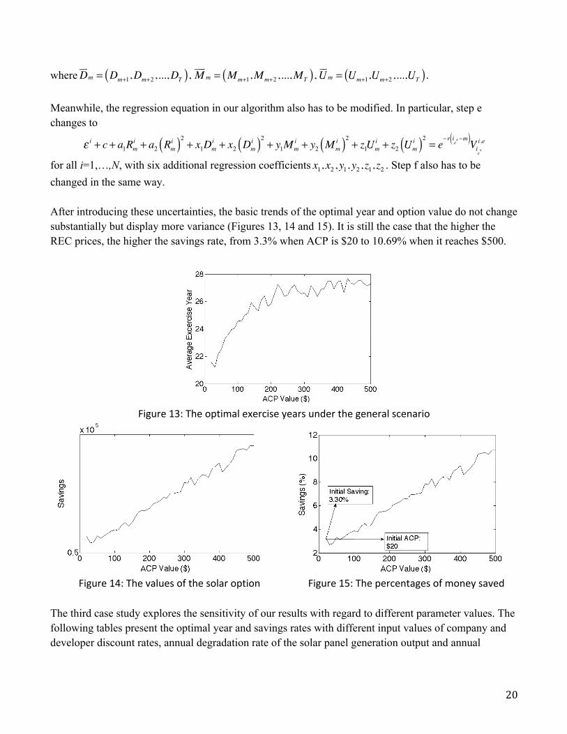
for all i=1,…,N, with six additional regression coefficients x1, x2, y1, y2, z1, z2 . Step f also has to be changed in the same way. After introducing these uncertainties, the basic trends of the optimal year and option value do not change substantially but display more variance (Figures 13, 14 and 15). It is still the case that the higher the REC prices, the higher the savings rate, from 3.3% when ACP is $20 to 10.69% when it reaches $500.

Figure  13:  The  optimal  exercise  years  under  the  general  scenario  

           Figure  14:  The  values  of  the  solar  option                                      Figure  15:  The  percentages  of  money  saved    

The third case study explores the sensitivity of our results with regard to different parameter values. The following tables present the optimal year and savings rates with different input values of company and developer discount rates, annual degradation rate of the solar panel generation output and annual

  21  

escalation rate of the solar electricity price. The savings rate is the percentage change in cost with respect to the baseline case. The results are obtained from the model with REC uncertainty.

 Optimal Exercise Year

  Company Discount Rate

Developer Discount

Rate

  -2% -1% ±0% +1% +2% -2% 23.8 24.3 24.5 24.8 25.2 -1% 22.3 23.1 23.6 24.2 24.4 ±0% 19.9 21.3 22.2 23.0 23.4 +1% 14.2 17.7 19.9 21.2 22.1 +2% 1.2 9.2 14.7 17.7 19.9

Table  2:  Optimal  exercise  years  with  different  discount  rates    

Savings Rate

  Company Discount Rate

Developer Discount

Rate

  -2% -1% ±0% +1% +2% -2% 3.45% 3.18% 2.96% 2.77% 2.59% -1% 3.23% 2.98% 2.78% 2.59% 2.44% ±0% 3.11% 2.83% 2.62% 2.46% 2.30% +1% 3.13% 2.78% 2.54% 2.34% 2.20% +2% 5.71% 3.13% 2.57% 2.31% 2.14%

Table  3:  Savings  rates  with  different  discount  rates

Solar Electricity Price Escalation Rate Optimal Exercise Year Savings Rate 1% 19.3 2.10% 2% 22.2 2.62% 3% 24.4 3.30% 4% 25.7 4.11% 5% 26.9 5.05%

Table  4:  Optimal  exercise  years  and  savings  rates  with  different  solar  electricity  price  escalation  rates

Solar Panel Output Degradation Rate Optimal Exercise Year Savings Rate 0.5% 23.6 2.90% 1.0% 22.2 2.62% 1.5% 20.6 2.41% 2.0% 18.5 2.25% 2.5% 16.0 2.18%

Table  5:  Optimal  exercise  years  and  savings  rates  with  different  solar  panel  output  degradation  rates  

  22  

Tables 2 and 3 exhibit the results when discount rates are perturbed by 1% or 2%. The optimal exercise year increases with increasing company discount rates while it decreases with increasing developer discount rates. The savings rate decreases with increasing company discount rates. With an exception of the +1% case (with a company discount rate perturbed by -2%) and the +2% case (with a company discount rate perturbed by less than or equal to 0%), it decreases with increasing developer discount rates. This exception is reasonable since +2% developer discount rate leads to more volatile exercise years and thus a larger range of savings rates. Generally, the results are more sensitive with low company discount rates and high developer discount rates. Table 4 demonstrates the positive relationships between the solar electricity price escalation rate and our two target metrics. Table 5 reveals that the optimal exercise year and savings rate are negatively correlated with the solar panel output degradation rate.

6. Conclusion and Future Work In this paper we present a developer-host contract that specifies the panel buyback year in which the host buys back the solar panels installed on its property. We model the cash flows of the host as an option framework and solve the minimum cost problem using Monte Carlo simulation based on ADP to obtain a good buyback timing. The modified framework can manage the inconsistent cash flows before and after the option exercise. By considering the panel purchase price to be the expected profit of the developer, the exercise year from the algorithm can balance the benefits of both the developer and host. In addition, we propose a new REC forecasting model, which can be applied to a market with specific RPS and ACP values. The structure we introduced can fit a broader set of projects, such as wind generation. Such projects should have two common characteristics: only one exercise decision is made during the entire time horizon and cash flows differ before and after the exercise. Future work should extend the assumptions of our model. For example, we assume that the utility price increases year by year based on a fixed contract. However, a forward contract between the host and the utility can be employed. For the REC forecasting method, how market and policy factors influence the REC price should also be examined.    Acknowledgment This research was supported by the NSF grant CMII-1201151. We are also acknowledging General Motors for their financial supplement.        

  23  

References Amram, M., Kulatilaka, N., 1999. Real options: Managing strategic investment in an uncertain world. Harvard Business School Press, Boston, Mass. Ashuri, B., Kashani, H., Lu, J., 2011. A real options approach to evaluating investment in solar ready buildings, Management and Innovation for a Sustainable Built Environment, Amsterdam, The Netherlands. Belien, J., De Boeck, L., Colpaert, J., Cooman, G., 2013. The best time to invest in photovoltaic panels in Flanders. Renewable Energy 50, 348-358. Dixit, A.K., Pindyck, R.S., 1994. Investment under uncertainty. Princeton University Press, Princeton, N.J. Energy Information Administration, 2012. Annual Energy Review 2011, www.eia.gov/totalenergy/data/annual/pdf/aer.pdf. Fernandes, B., Cunha, J., Ferreira, P., 2011. The use of real options approach in energy sector investments. Renewable Sustainable Energy Review 15, 4491-4497. Gouriéroux, C., Valéry, P., 2004. Estimation of a Jacobi process. Preprint, http://citeseerx.ist.psu.edu/viewdoc/download?doi=10.1.1.90.196&rep=rep1&type=pdf. Hoff, T.E., Margolis, R., Herig, C., 2003. A simple method for consumers to address uncertainty when purchasing photovoltaics, http://www.cleanpower.com/Research. Longstaff, F.A., Schwartz, E.S., 2001. Valuing American options by simulation: A simple least-squares approach. Review of Financial Studies 14, 113-147. Martinez-Cesena, E.A., Azzopardi, B., Mutale, J., 2013. Assessment of domestic photovoltaic systems based on real options theory. Progress in Photovoltaics 21, 250-262. Martinez-Cesena, E.A., Mutale, J., 2011. Application of an advanced real options approach for renewable energy generation projects planning. Renewable Sustainable Energy Review 15, 2087-2094. Mun, J., 2002. Real options analysis: Tools and techniques for valuing strategic investments and decisions. John Wiley & Sons, Hoboken, N.J. Munoz, J.I., Contreras, J., Caamano, J., Correia, P.F., 2009. Risk assessment of wind power generation project investments based on real options. 2009 IEEE Bucharest Powertech, Vols 1-5, 2346-2353. National Renewable Energy Laboratory, 2009. Power purchase agreement checklist for state and local governments, www.nrel.gov/docs/fy10osti/46668.pdf.

  24  

National Renewable Energy Laboratory, 2011. Solar renewable energy certificate (SREC) markets: Status and trends, http://apps3.eere.energy.gov/greenpower/pdfs/52868.pdf. Rodrigues, A., Armada, M.J.R., 2006. The valuation of real options with the least squares Monte Carlo simulation method, http://ssrn.com/abstract=887953 or http://dx.doi.org/10.2139/ssrn.887953. Sarkis, J., Tamarkin, M., 2008. Real options analysis for renewable energy technologies in a GHG emissions trading environment, Emissions Trading. Springer, New York, pp. 103-119. SEIA/GTM Research, 2013. U.S. Solar Market Insight 2012 Year in Review. Tang, A., Chiara, N., Taylor, J.E., 2012. Financing renewable energy infrastructure: Formulation, pricing and impact of a carbon revenue bond. Energy Policy 45, 691-703. Trigeorgis, L., 1996. Real options: Managerial flexibility and strategy in resource allocation. MIT Press, Cambridge, Mass. United Nations Framework Convention on Climate Change, 2008. Kyoto Protocol Reference Manual, http://unfccc.int/resource/docs/publications/08_unfccc_kp_ref_manual.pdf. U.S. Department of Energy, 2009. President Obama sets a target for cutting U.S. greenhouse gas emissions, http://apps1.eere.energy.gov/news/news_detail.cfm/news_id=15650. Venetsanos, K., Angelopoulou, P., Tsoutsos, T., 2002. Renewable energy sources project appraisal under uncertainty: The case of wind energy exploitation within a changing energy market environment. Energy Policy 30, 293-307.