High order numerical methods for the space non-homogeneous Boltzmann equation

High order numerical methods for the space non-homogeneousBoltzmann equation

Francis Filbet a, Giovanni Russo b,*

a IRMA – Universit�ee Louis Pasteur, 7 rue Ren�ee Descartes, 67084 Strasbourg, Franceb Universit�aa di Catania, Viale Andrea Doria 6, 95125 Catania, Italy

Received 10 September 2002; received in revised form 29 January 2003; accepted 30 January 2003

Abstract

In this paper we present accurate methods for the numerical solution of the Boltzmann equation of rarefied gas. The

methods are based on a time splitting technique. The transport is solved by a third order accurate (in space) positive and

flux conservative (PFC) method. The collision step is treated by a Fourier approximation of the collision integral, which

guarantees spectral accuracy in velocity, coupled with several high order integrators in time. Strang splitting is used to

achieve second order accuracy in space and time. Several numerical tests illustrate the properties of the methods.

� 2003 Elsevier Science B.V. All rights reserved.

Keywords: Boltzmann equation; Rarefied gas dynamics; Spectral methods; Splitting algorithms

1. Introduction

In a microscopic description of rarefied neutral gas, the gas particles move by a constant velocity untilthey undergo binary collisions. In a kinetic picture, the properties of the gas are described by a density

function in phase space, f ðt; x; vÞ, called the distribution function, which gives the number of particles per

unit volume in phase space at time t. The distribution function satisfies the Boltzmann equation, an integro-

differential equation, which describes the effect of the free flow and binary collisions between the particles.

The numerical solution of the Boltzmann equation represents a real challenge for numerical methods.

This is essentially due to the nonlinearity, to the large number of variables (t for the time, two 3D vectors xfor space and v for velocity) and to the fivefold integral that defines the collision operator. Furthermore,

this integration has to be handled carefully since it is at the basis of the macroscopic properties of theBoltzmann equation.

Among the different approaches for the approximation of the Boltzmann equation, we may distinguish

between deterministic and Monte-Carlo methods. The first usually provide accurate oscillations-free

Journal of Computational Physics 186 (2003) 457–480

www.elsevier.com/locate/jcp

*Corresponding author. Tel.: +39-09-533-0533; fax: +39-09-533-0094.

E-mail addresses: [email protected] (F. Filbet), [email protected] (G. Russo).

0021-9991/03/$ - see front matter � 2003 Elsevier Science B.V. All rights reserved.

doi:10.1016/S0021-9991(03)00065-2

mail to: [email protected]

solutions, but they are much more expensive than Monte-Carlo methods with the same number of discrete

degrees of freedom. For example, if we denote by n the number of parameters which characterize the

density with respect to the velocity variables in a space homogeneous calculation, the computational cost of

a conventional deterministic method for the evaluation of the collisional integral is much larger than n2. Asa consequence most numerical computations are based on probabilistic Monte-Carlo techniques at different

levels. Examples are the direct simulation Monte-Carlo method (DSMC) by Bird [2] and the modified Monte

Carlo method by Babovsky and Nanbu [1,13]. For a detailed description of such methods we refer to [2,6].

Probabilistic particle methods present different advantages. First, the computational cost for advancingby a typical collision time Dt is strongly reduced and approximately can be considered of the order of the

number of points n. Second, these methods do not need any artificial boundary in the velocity space. In

fact, particles can have any velocity and thus the discretization points are always well defined independently

of the physical problem. Finally, particle methods make a much more efficient use of computer memory,

since the particles concentrate where the function is not small, and memory is not wasted representing a

function which is virtually zero in most phase space. For this reason, particle methods have no competitor

for situations very far from thermodynamical equilibrium.

At variance, in addition to the computational complexity, a major problem associated with deter-ministic methods that use a fixed discretization in the velocity domain is that the velocity space is ap-

proximated by a finite region. Hence, a large region with a huge number of discretization points is required

in problems with very high Mach numbers, which greatly increase the computing effort. In spite of these

difficulties, deterministic methods can be much more accurate, and can be competitive with Monte-Carlo

methods for problems in which the solution is not very far from thermodynamical equilibrium, and high

accuracy is required. In the framework of deterministic approximations, the most popular class of methods

is based on the so called discrete velocity models (DVM) of the Boltzmann equation. All these methods

[4,10,11,20] make use of regular discretizations on hypercubes in the velocity field and construct a discretecollision mechanics on the nodes of the hypercube in order to preserve the main physical properties.

Although the numerical results have shown that these schemes are able to avoid fluctuations, their

computational cost is high (in general Oðnan2Þ, where na is the number of parameters used for the angular

integration, typically in such methods na � Oðn1=3Þ) and, due to the particular choice of the integration

points imposed by the conservation properties, the order of accuracy is lower than that of a standard

quadrature formula applied directly to the collision operator. Hence we observe that the requirement of

maintaining at a discrete level the main physical properties of the continuous equation makes it extremely

difficult to obtain high order accuracy. On the other hand, even if conservation properties are not imposedfrom the beginning, an accurate scheme would provide an accurate approximation of the conserved

quantities.

In [16], Pareschi and Perthame developed a discretization of the collision operator based on expanding in

Fourier series the distribution function with respect to the velocity variable. The resulting spectral ap-

proximation can be evaluated with a computational cost of Oðn2Þ which is lower than that of previous

deterministic methods. Bobylev and Rjasanow [3] used a Fourier transform approximation of the distri-

bution function, and they were able to obtain exact conservation by a suitable modification of the evolution

equations for the Fourier coefficients. In [18], Pareschi and Russo developed a scheme based on the ap-proximation of the distribution function by a periodic function in phase space, and by its discretization by

Fourier series. Evolution equations for the Fourier modes are explicitly derived for the variable hard sphere

(VHS) model. The method provides spectral accuracy in the velocity domain, which is the highest accuracy

achieved by a numerical method for the Boltzmann equation, and the computational complexity of the

collisional operator is Oðn2Þ. The method preserves mass, and approximates with spectral accuracy mo-

mentum and energy.

In this paper we construct a fractional step deterministic scheme for the time dependent Boltzmann

equation, which is based on five main ingredients:

458 F. Filbet, G. Russo / Journal of Computational Physics 186 (2003) 457–480

Fractional step in time allows to treat separately the transport and the collision. This approach has the

advantage of simplifying the problem, and allows a parallel implementation of the method. As we shall

see, the space cells are independent in the collision step, and velocity grid points are independent in the

free transport. The use of Strang splitting allows second order accuracy in time. Also, the collision andtransport time step can be treated independently, and the latter can be chosen to be smaller than the

former.

Fourier-spectral method for the evolution of the collision step allows a very accurate discretization in

velocity domain, at a reasonable computational cost [18].

Positive and flux conservative (PFC) finite volume method for the free transport [9] provides a third order

(in space) accurate scheme for the evolution of distribution function during the transport step. The scheme

is conservative, and it preserves the positivity of the function. It is much less dissipative than ENO and

WENO schemes usually used for hyperbolic systems of conservation laws [21,22].Positive time discretization. A suitable time discretization of the collisional equation is used, which allows a

large stability time step, even for problems with considerably small Knudsen number. The time discreti-

zation method for the collision step is based on a modified time relaxed scheme [19]. For small Knudsen

number, the relaxed time will be chosen in such a way that positivity of the function is essentially pre-

served.

Multiple resolution. A different resolution will be used in velocity space in the transport and in the collision

step. Considering that the collision step is more expensive, and more accurate than the transport step, it is

convenient to use more points in velocity space during the transport step. This effect is taken into accountin order to optimize the scheme in terms of accuracy and efficiency.

The plan of the paper is the following. In the next section we recall the main properties of the Boltzmann

equation. In Section 3, after a general setup, we describe in detail the PFC method for the free transport

and the spectral method for the evolution of the collision step. Several numerical issues are discussed at theend of the section. Section 4 is devoted to numerical tests for the space homogeneous BE and for 1D and

2D, time dependent and stationary problems. Finally, in the last section we draw conclusions.

2. The governing equation

In absence of external forces the time evolution of a single component mono atomic gas is governed by

the Boltzmann equation (cf. [5])

ofot

þ v � rxf ¼ 1

�Qðf ; f Þ; x; v 2 R3; ð1Þ

where f ¼ f ðt; x; vÞ is a non-negative function describing the distribution of particles which move with

velocity v in the position x at time t > 0. The number � > 0 is called Knudsen number and is proportional to

the mean free path between collisions. In the right-hand side, Qðf ; f Þ is the so-called collision operator givenby

Qðf ; f ÞðvÞ ¼ Qþðf ; f Þ L½f �f ð2Þ

with

Qþðf ; f Þ ¼ZR3

ZS2

Bðjv v1j; hÞf ðv0Þf ðv01Þdxdv1; ð3Þ

L½f � ¼ZR3

ZS2

Bðjv v1j; hÞf ðv1Þdxdv1: ð4Þ

F. Filbet, G. Russo / Journal of Computational Physics 186 (2003) 457–480 459

In the above integrals, v and v1 are the velocities after the collision of two particles which had the velocities

v0 and v01 before the encounter. The deflection angle h is the angle between v v1 and v0 v01.Here the pre-collision velocities are parameterized by

v0 ¼ 1

2ðv þ v1 þ jv v1jxÞ; v01 ¼

1

2ðv þ v1 jv v1 j xÞ; ð5Þ

where x is a unit vector of the sphere S2,

S2 ¼ fx 2 R3; jxj2 ¼ 1g: ð6Þ

The quantities Qþðf ; f Þ and L½f �f are the gain and loss term, respectively. The precise form of the kernel B,which characterizes the details of the binary interactions, depends on the physical properties of the gas. In

the case of inverse kth power forces between particles, the kernel has the form

Bðjv v1j; hÞ ¼ baðhÞjv v1ja; ð7Þ

where a ¼ ðk 5Þ=ðk 1Þ. In particular, we will consider the variable hard sphere(VHS) model [2], i.e.,

baðhÞ ¼ Ca where Ca is a positive constant. The case a ¼ 0 is referred to as Maxwellian gas whereas the case

a ¼ 1 yields the hard sphere gas. Note that in the case of Maxwellian gas the coefficient of the loss term,

L½f �, does not depend on v. Boltzmann�s collision operator has the fundamental properties of conservingmass, momentum and energy

ZR3

Qðf ; f Þ1

vjvj2

0@

1Adv ¼ 0; ð8Þ

and satisfies the well-known Boltzmann�s H -theoremZR3

Qðf ; f Þ logðf Þdv6 0: ð9Þ

Boltzmann H -theorem implies that any equilibrium distribution function, i.e., any function f for which

Qðf ; f Þ ¼ 0, has the form of a locally Maxwellian distribution

Mðq; u; T ÞðvÞ ¼ q

ð2pT Þ3=2exp

ju vj2

2T

!; ð10Þ

where q; u; T are the density, mean velocity and temperature of the gas

q ¼ZR3

f ðvÞdv; u ¼ 1

q

ZR3

vf ðvÞdv; T ¼ 1

3q

ZR3

ju vj2f ðvÞdv: ð11Þ

3. The general framework

Let us consider the initial-boundary value problem for the Boltzmann transport equation

ofot

þ v � rxf þ Eðt; xÞ � rvf ¼ 1

�Qðf ; f Þ; ð12Þ

f ð0; x; vÞ ¼ f0ðx; vÞ;


where x 2 X � Rm, v 2 R3, t 2 ½0; T �. Boundary conditions will be specified in the section on numerical

results. Here Eðt; xÞ represents an external drift field acting on the particles. The approach presented in this

section can be used for a more general kinetic equation, but in this paper we shall apply it only to the

Boltzmann equation of rarefied gas dynamics, where E � 0. We discretize time into discrete values tn, andwe denote by f nðx; vÞ an approximation of the distribution function f ðtn; x; vÞ. As it is usually done for a

kinetic equation like (12), a simple first order time splitting is obtained considering, in a small time interval

Dt ¼ ½tn; tnþ1�, the numerical solution of the transport step

of �

otþ v � rxf � þ Eðt; xÞ � rvf � ¼ 0;

f �ð0; x; vÞ ¼ f nðx; vÞ;ð13Þ

and the space homogeneous collision step

of ��

ot¼ 1

�Qðf ��; f ��Þ;

f ��ð0; x; vÞ ¼ f �ðDt; x; vÞ:ð14Þ

We shall denote by S1ðDtÞ and S2ðDtÞ the solution operators corresponding respectively to the transport andcollision step, i.e., we can write

f �ðDt; x; vÞ ¼ S1ðDtÞf nðx; vÞ;

f ��ðDt; x; vÞ ¼ S2ðDtÞf �ðDt; x; vÞ:

The approximated value at time tnþ1 is then given by

f nþ1ðx; vÞ ¼ f ��ðDt; x; vÞ ¼ S2ðDtÞS1ðDtÞf nðx; vÞ: ð15Þ

We assume that S1 and S2 represent either exact or at least second order evolution operators in time of

transport and collision step, respectively.

A second order scheme for non-stiff problems can be easily derived simply by symmetrizing the firstorder scheme [24]

f nþ1 ¼ S1ðDt=2ÞS2ðDtÞS1ðDt=2Þf n; ð16Þ

provided every step is solved with a method at least second order accurate in time. Recently, second order

splitting algorithms for Boltzmann like equations were also presented in [15]. Although higher ordersplitting strategies are available, in practice they are seldom used because of stability problems. We remind

that second order accuracy for such complex problems is considered ‘‘high order’’ in this field.

In the following two sections we discuss transport and collision steps. As we shall see, the grid step size in

time, space and velocity are not directly related by strict stability requirements, and therefore one can

benefit from high order accuracy whenever possible. Our final scheme will be overall second order in time,

third order in space, and spectrally accurate in velocity.

3.1. The transport step

In this section, we discuss the numerical resolution of the Vlasov equation which characterizes the

transport step. To this aim we use an Eulerian method which consists in discretizing the distribution

function f on a phase space grid [9].


Let us consider the Vlasov equation written in the form

ofot

þ divxðv f Þ ¼ 0: ð17Þ

For simplicity, let us restrict ourselves to the following 1D transport equation for f ðt; xÞ, even if the PFC

reconstruction can be easily generalized to higher dimension using tensor product

otf þ oxðu f Þ ¼ 0 8ðt; xÞ 2 Rþ � R; ð18Þ

where u is a constant velocity. Then, the solution of the transport equation at time tnþ1 reads

f ðtnþ1; xÞ ¼ f ðtn; x uDtÞ 8x 2 R:

Now, let us introduce a finite set of mesh points fxiþ1=2gi2I on the computational domain. We will use the

notations Dx ¼ xiþ1=2 xi1=2 (the grid is uniform), xi ¼ ðxiþ1=2 þ xi1=2Þ=2 and Ci ¼ ½xiþ1=2 xi1=2�. Assumethe values of the distribution function are known at time tn ¼ nDt, we compute the new values at time tnþ1

by integration of the distribution function on each sub-interval. Thus, using the explicit expression of the

solution, we haveZ xiþ1=2

xi1=2

f ðtnþ1; xÞdx ¼Z xiþ1=2uDt

xi1=2uDtf ðtn; xÞdx;

then, setting

Uiþ1=2ðtnÞ ¼Z xiþ1=2

xiþ1=2uDtf ðtn; xÞdx;

we obtain the conservative formZ xiþ1=2

xi1=2

f ðtnþ1; xÞdx ¼Z xiþ1=2

xi1=2

f ðtn; xÞdx þ Ui1=2ðtnÞ Uiþ1=2ðtnÞ: ð19Þ

The evaluation of the average of the solution over ½xi1=2; xiþ1=2� allows to ignore fine details of the exact

solution which may be costly to compute. The main step is now to choose an efficient method to reconstructthe distribution function from the cell average on each cell Ci. In [8], the author used simple linear inter-

polation. Unfortunately this approach does not give a positive scheme and does not control spurious os-

cillations. Here, we will consider a reconstruction via primitive function preserving positivity and maximum

values of f . Let F ðtn; xÞ be a primitive of the distribution function f ðtn; xÞ, if we denote by

f ni ¼ 1

Dx

Z xiþ1=2

xi1=2

f ðtn; xÞdx;

then F ðtn; xiþ1=2Þ F ðtn; xi1=2Þ ¼ Dxf ni and

F ðtn; xiþ1=2Þ ¼ DxXi

k¼0f nk ¼ wn

i :

In the sequel, the time variable tn only acts as a parameter and will be omitted. A reconstruction method

allowing to preserve positivity and maximum principle can be obtained using slope correctors. First we

build an approximation of the primitive on the interval ½xi1=2; xiþ1=2� using the stencil fxi3=2; xi1=2; xiþ1=2;xiþ3=2gi2I ,


~FFhðxÞ ¼ wi1 þ ðx xi1=2Þfi þ1

2Dxðx xi1=2Þðx xiþ1=2Þ½fiþ1 fi�

þ 1

6Dx2ðx xi1=2Þðx xiþ1=2Þðx xiþ3=2Þ½fiþ1 2fi þ fi1�;

where we used the relation wi wi1 ¼ Dxfi. Thus, by differentiation, we obtain a third order accurate

approximation of the distribution function on the interval ½xi1=2; xiþ1=2�,

~ffhðxÞ ¼d ~FFh

dxðxÞ

¼ fi þ1

6Dx22ðx

xiÞðx xi3=2Þ þ ðx xi1=2Þðx xiþ1=2Þðfiþ1 fiÞ

1

6Dx22ðx

xiÞðx xiþ3=2Þ

þ ðx xi1=2Þðx xiþ1=2Þðfi fi1Þ:

In order to satisfy a maximum principle and to avoid spurious oscillations we introduce the slope correctors

fhðxÞ ¼ fi þ�þi6Dx2

2ðx

xiÞðx xi3=2Þ þ ðx xi1=2Þðx xiþ1=2Þðfiþ1 fiÞ

�i6Dx2

2ðx

xiÞðx xiþ3=2Þ þ ðx xi1=2Þðx xiþ1=2Þðfi fi1Þ ð20Þ

with

��i ¼min 1; 2fi=ðfi�1 fiÞð Þ if fi�1 fi > 0;

min 1;2ðf1 fiÞ=ðfi�1 fiÞð Þ if fi�1 fi < 0;

(ð21Þ

where f1 ¼ maxj2Iffjg.It is easy to check that the approximation of the distribution function fhðtn; xÞ previously constructed

satisfies (see [9] for the proof)

• conservation of the average: for all i 2 I ,R xiþ1=2xi1=2

fhðtn; xÞdx ¼ Dxf ni ,

• maximum principle: for all x 2 ðxmin; xmaxÞ; 06 fhðtn; xÞ6 f1• consistency:Z

R

jfhðtn; xÞ ~ffhðtn; xÞjdx6CDx;

where ~ffhðtn; xÞ is the third order approximation previously defined.

3.2. Spectral approximation of the collision operator

We consider now the space homogeneous Boltzmann equation in each cell

ofot

¼ Qþðf ; f Þ L½f �f ; ð22Þ

with Qþ and L given by Eqs. (3) and (4). To keep notation simple, we have fixed � ¼ 1. A simple change of

variables permits to write

Qþðf ; f Þ ¼ZRd

ZSd1

Bðjgj; hÞf ðv0Þf ðv01Þdxdg; ð23Þ


Lðf Þ ¼ZRd

ZSd1

Bðjgj; hÞf ðv gÞdxdg; ð24Þ

where g ¼ v v1 and then

v0 ¼ v 1

2ðg jgjxÞ; v01 ¼ v 1

2ðg þ jgjxÞ: ð25Þ

The dimension of velocity space is d ¼ 3. However we consider the case of d ¼ 2, i.e., the Boltzmann

equation with 2D in velocity, because the realistic case of 3D in velocity requires a more efficient imple-

mentation and a more powerful computer than the one available.

The Fourier approximation is based on the observation that if a distribution function f is well ap-

proximated by a function with compact support in velocity space (say a ball centered at the origin with

radius R), then it can be approximated by a periodic function in velocity space, whose period 2V is pro-

portional to the size of the support: V ¼ ð3þffiffiffi2

pÞR=2 (see Fig. 1 and [18] for details).

To simplify the notation we assume that the half period is V ¼ p and hence R ¼ kp with k ¼ 2=ð3þffiffiffi2

pÞ.

Hereafter, we used just one index to denote the 3D sums with respect to the vector k ¼ ðk1; k2; k3Þ 2 Z3,

hence we set

XNk¼N

¼XN

k1;k2;k3¼N

:

The approximate function fN is represented as the truncated Fourier series

fN ðvÞ ¼XNk¼N

f̂fkeik�v; ð26Þ

f̂fk ¼1

ð2pÞ3Z½p;p�3

f ðvÞeik�vdv:

By inserting Eq. (26) into Eq. (22) and imposing orthogonality of the residual with all trigonometric

polynomials of degree 6N , one obtains the following evolution equations:

of̂fk

ot¼

XminðN ;kþNÞ

m¼maxðN ;kNÞf̂fkmf̂fmðB̂Bðk m;mÞ B̂Bðm;mÞÞ ð27Þ

Fig. 1. Space homogeneous case: time evolution of the value lðtÞ.


with the initial condition

f̂fkð0Þ ¼1

ð2pÞ3Z½p;p�3

f0ðvÞeik�v dv; ð28Þ

where the kernel modes B̂Bðl;mÞ are given by

B̂Bðl;mÞ ¼ZBð0;2kpÞ

ZS2

Bðjgj; hÞ exp� ig � ðl þ mÞ

2 ijgjx � ðm lÞ

2

�dxdg: ð29Þ

The evaluation of the right-hand side of Eq. (27) requires exactly OðN 6Þ operations. We emphasize that the

usual cost for a method based on N 3 parameters for f in the velocity space is OðN 6MÞ where na is the

number of angle discretizations. The loss term on the right hand side is a convolution sum and thus

transform methods allow this term to be evaluated only in OðN 3 logNÞ operations. Hence the most ex-

pensive part of the computation is represented by the gain term.

Explicit expression for the kernel modes for Variable Hard Spheres in 3D can be obtained [18].

For the 2D VHS model one has

B̂Bðl;mÞ ¼ Ca4p2ð2pkÞ2þaFaðn; gÞ

with

Faðn; gÞ ¼Z 1

0

r1þaJ0ðnrÞJ0ðgrÞdr; ð30Þ

where n ¼ jl þ mjkp, g ¼ jl mjkp, r ¼ jgj=2kp, and J0 is the Bessel function of order 0. Note that each

kernel mode can be computed as a 1D integral and stored in an array.

The spectral approximation provides a consistent description of the space homogeneous Boltzmann

equation, which preserves mass, but not energy and momentum. The scheme is spectrally accurate for

smooth solutions, thus providing spectral accuracy in the conservation of momentum and energy as well.

The properties of the scheme are analyzed in detail in [18].

3.3. Time discretization

The time discretization of the transport step has been described in Section 3.1. Here we focus on the timeevolution of the collision step. Let Dt denote the time step of the transport phase. Our goal is to solve, in

each cell, the space homogeneous Boltzmann equation

of �

ot¼ 1

�Qðf �; f �Þ;

f �ð0; vÞ ¼ f nðvÞ;

where, for simplicity, we drop the space dependence. One could use any second order time discretization,such as a Runge–Kutta method, with the same time step, Dt, used for the convection step, for the ordinary

differential system of the Fourier modes, (27). If the time step is too large (for accuracy or stability reasons),

then a smaller time step, Dtc < Dt, can be used during this phase. Since each cell is independent, Dtc maydepend on the cell. If Dtc � Dt, then a multi-step scheme can be used to improve efficiency and accuracy.

With standard methods such as Runge–Kutta or multi-step, it is difficult to control positivity of the so-

lution. Here we propose a time discretization which provides essential positivity of the distribution func-

tion, and allows the use of rather large time step, even in regimes in which the Knudsen number is quite


small. The schemes that we use are based on a variation of time relaxed (TR) schemes [19], which have been

effectively used in the development of Monte-Carlo methods suitable for a very wide range of Knudsen

number. We briefly recall here the idea behind the TR schemes.

Let us consider an equation of the form

ofot

¼ 1

�P ðf ; f Þ½ lf �; f ð0; vÞ ¼ f0ðvÞ; ð31Þ

where l 6¼ 0 is a constant and P a positive bilinear operator. The Boltzmann equation for Maxwell mol-

ecules has the above form, with Qþðf ; f Þ ¼ P ðf ; f Þ, and L½f � ¼ l.A formal representation of the solution of the Cauchy problem (31) is given by the so called Wild sum

expansion (see [19] and [26]),

f ðt; vÞ ¼X1k¼0

ð1 sÞskfkðvÞ; ð32Þ

where s ¼ ð1 elt=�Þ is the reduced time. The functions fk, given by the recurrence formula

fk¼0ðvÞ ¼ f0ðvÞ; fkþ1ðvÞ ¼1

k þ 1

Xk

h¼0

1

lP ðfh; fkhÞ; k ¼ 0; 1; . . . ; ð33Þ

satisfy the property

limk!1

fkðvÞ ¼ MðvÞ; ð34Þ

where MðvÞ is the Maxwellian, satisfying QðM ;MÞ ¼ 0.

Representation (32) and property (34) suggest the use of a truncation of series (32) as a numerical scheme

for time discretization, or, better, of a generalization of such a truncated series, of the form

f nþ1 ¼Xmk¼0

Akfk þ Amþ1M ; ð35Þ

where the coefficients fk are given by Eq. (33) using f0 ¼ f nðvÞ. The weights Ak ¼ AkðsÞ are non-negativefunctions that satisfy some consistency and conservation conditions. Further conditions on the coefficients

will ensure asymptotic preservation (AP), i.e., in the limit of vanishing �, the distribution function is pro-

jected by the scheme into the Maxwellian MðvÞ (see [19] for details). A choice of functions which satisfies the

previous requirements is, for example,

Ak ¼ ð1 sÞsk; k ¼ 0; . . . ;m 1; Am ¼ 1Xm1

k¼0Ak Amþ1; Amþ1 ¼ smþ2; ð36Þ

which corresponds to take fmþ1 ¼ fm, fk ¼ M , k Pm þ 2 in (32). However, other choices are possible and it

is an open problem the determination of the optimal set of functions Ak that satisfies the previous re-

quirements and guarantees the most accurate approximation.

The Boltzmann equation for Maxwell molecules has the form (31), with P ðf ; f Þ ¼ Qþðf ; f Þ. In order to

apply the same discretization to a more general BE, we can proceed as follows. We write the Boltzmann

equation in the form (31), with

P ðf ; gÞ ¼ Qþðf ; gÞ þ 1

2lðfð þ gÞ L½f �g L½g�f Þ;

where the operator P is written in a symmetric form. If we choose


lP L½f �ðvÞ 8v 2 R3; ð37Þ

then Pðf ; f Þ is a positive symmetric operator. However, in general LðvÞ is an unbounded function, and

therefore a constant l satisfying (37) does not exist. Even if we consider that the discrete velocities lie in a

bounded domain Xv ¼ ½V ; V �3, a choice of l satisfying Eq. (37) may lead to excessive numerical viscosity,

as is evident from standard truncation analysis.

Ideally, one should choose the smallest value of l that guarantees positivity of operator P . This shouldbe obtained, for a given function f ðvÞ, by imposing that

minv2Xv

½QþðvÞ þ ðl LðvÞÞf ðvÞ� ¼ 0: ð38Þ

A first order (non-AP) TR scheme has the structure

f nþ1ðvÞ ¼ A0ðsÞf nðvÞ þ A1ðsÞf1ðvÞ

with f1 ¼ Pðf n; f nÞ=l. Because of positivity of the coefficients A0ðsÞ and A1ðsÞ, if P ðf ; f Þ is positive, then thescheme is positive.

Condition (38) is not practical, since the region of phase space Xv near the edge is not physically rep-resentative, because of the approximation of the distribution function by a periodic function in velocity. A

better choice is obtained by computing a critical constant lc as

lc ¼ maxv2Xc

LðvÞ�

Qþ

f

�; ð39Þ

where Xc � Xv is a smaller region, for example, Xc ¼ ½V =2; V =2�3. Then the constant l is computed as

l ¼ Clc, where C is a safety factor of order one. In all our calculations we used the value C ¼ 3=2, whichwe found a good compromise between numerical positivity and numerical viscosity.

These practical criteria deserve further analysis. We have to keep in mind that the spectral scheme itself

does not preserve positivity rigorously [18]. However, the lack of positivity is very small, and can be ne-

glected for all practical purposes. Even if positive spectral schemes can be obtained, as shown in [18] and

[17], they are not practical, because of the lack of accuracy and excessive smoothing.

Accuracy requires a small value of lDt=�. If l is kept constant, independently of �, then the time stepbecomes exceedingly small for small values of �, and the method becomes inefficient. The approach that weoutlined above allows rather large time steps, even for small values of �. The reason for this is that when � issmall, then gain and loss terms balance each other, and therefore the quantity l computed as above be-

comes small. It can be shown in fact that for small values of �, l scales with �, and the ratio l=� remainsbounded.

With these considerations in mind, we maintain the same criterion for the evaluation of the optimal l,even for higher order TR schemes.

A second order (non-AP) TR scheme has the structure

f nþ1ðvÞ ¼ A0ðsÞf mðvÞ þ A1ðsÞf1ðvÞ þ A2ðsÞf2ðvÞ;

with f2ðvÞ ¼ P ðf n; f1Þ. The constant l is computed as above, l ¼ 3=2lc, with lc given by (39). For all

practical purpose the scheme can be considered positive, although it is not rigorously positive.

3.3.1. Parallelization algorithm

Let us denote by f n (resp. f �) the matrix ðf ni;jÞ (resp. ðf �

i;jÞ) corresponding to the values of the discrete

distribution function at time tn (resp. S1ðDtÞf n), where i represents the index of the physical space mesh and


j the index of the velocity space. We note that the big amount of work is performed during steps (13) and

(14). Therefore, we will focus on the parallelization of these computations. To do this we observe that the

operator S1ðDtÞ (resp. S2ðDtÞ) only acts on rows of ðf ni;jÞ (resp. on columns of ðf �

i;jÞ). Thus, for the step S1ðDtÞif we assume that data are distributed by row on each processor, no communications are required and

similarly, for the other step S2ðDtÞ a storage by column does not involve any communication at all. The linkbetween the two steps is done through a transposition of f �.

Following this idea, we present a simple parallel algorithm [7], starting with 1D band distribution f n

along v-direction.

Algorithm 1. For each time step Dt:(a) Compute the matrix f � using S1ðDtÞ from values f n. The storage by rows avoids local communications

for this step.(b) Distribute the matrix f � into the matrix transposed f �T

in order to get a 1D band distribution along x-direction.

(c) Apply S2ðDtÞ to f �Tfor solving Eq. (14) over a time step of Dt. The storage by columns avoids local

communications for this step.

(d) Redistribute matrices f nþ1Tinto matrix f nþ1 in order to get a 1D band distribution along v-direction.

End.

In this case, we notice that with our parallel algorithm, communications only occur during the two data

redistributions phases. In other words, the algorithm falls into phases of computations without any

communication and phases of communications without any computation.

3.3.2. Multi-resolution algorithm

It is easy to check that the computational cost of the transport step (13) is of order OðNxNvÞ, where Nx

(resp. Nv) is the number of points in x-direction (resp. v-direction), whereas the numerical approximation ofthe integral collision operator (14) requires an amount of work of order OðNxN 2

modesÞ, where Nmodes repre-

sents the total number of modes in velocity. Then, this last step is much more time consuming than the first

one. However, the Fourier approximation gives an accurate approximation due to the spectral accuracy

[16], whereas the transport part is only third order. In this section, we then propose a simple algorithm to

reduce the computational time keeping good accuracy. It is based on multilevel resolution: the transport

equation is solved on a fine grid Nx � Nv, whereas the collision operator is treated using a smaller number of

modes. The link between the two grids is achieved through trigonometric interpolation, which preserves the

good accuracy of the spectral method.

Algorithm 2. For each time step Dt:1. Compute the first approximation f � by S1ðDtÞ using f n on the fine grid with a cost OðNxNvÞ.2. Compute a Fourier approximation of f � using FFT with a cost OðNxNv logðNvÞÞ3. Neglect highest frequencies of ðf̂f �

k Þk, keeping only Nmodes terms, and compute f̂f �� the approximated

solution of S2ðDtÞf � in the Fourier space, with a cost OðNxN 2modesÞ, where Nmodes � Nv.

4. Use a trigonometric interpolation to get f nþ1 on the fine grid with a cost of order OðNxNv logðNvÞÞ.End.

4. Numerical tests

In this section, we present a large variety of test cases showing the effectiveness of our method to get an

accurate solution of the Boltzmann equation. We first give a classical example, which illustrates the


property of the time relaxed scheme. Then, we give several results to compare our scheme with the well

known Monte-Carlo method for the Boltzmann equation. Finally, we present an interesting result in the

2þ 2-dimensional phase space proving the high accuracy of our method, which is able to reproduce small

effects (ghost effects). In our space dependent tests we used a 2D model of the Boltzmann equation in

velocity space. Realistic simulations with a full 3D model in velocity space require more powerful computer

and faster algorithms for storage and retrieval of the Fourier modes of the collision kernel.

4.1. Space homogeneous problems

This test is used to find the good strategy for the time discretization. Let us consider the space homo-

geneous 2D-Boltzmann equation for hard sphere molecules. The initial data are chosen as the sum of two

Maxwellian functions

f0ðvÞ ¼1

2

5

ð2pv2thÞexp

" jv v1j2

2v2th

!þ exp

jv v2j2

2v2th

!#; v 2 R2;

with v1 ¼ ð2; 1Þ, v2 ¼ ð2;1Þ and the thermal velocity is vth ¼ 1. The final time of the simulation is

Tend ¼ 5, which is very closed to the stationary state. We first compute an accurate solution by the spectral

method using 642 modes and a fourth order Runge–Kutta scheme for the time discretization. In Fig. 1, werepresent the time evolution of the constant lðtÞ, which allows us to rewrite the Boltzmann operator as the

sum of a positive operator and a loss term

lðtÞ ¼ 3

2maxv2Xc

LðvÞ�

Qþ

f

�:

The solution is computed from time tn to time tnþ1 ¼ tn þ Dt using a first order time-relaxed scheme pre-

serving asymptotic behavior

f nþ1ðvÞ ¼ A0ðsÞf nðvÞ þ A1ðsÞf1ðvÞ þ A2ðsÞMðvÞ

with f1 ¼ Qþðf n; f nÞ=l, whereas A0, A1 and A2 are given by (36).The distribution function is initially far from the equilibrium and the value of l is large. Then, the time

going on, the solution is closer to the Maxwellian corresponding to the stationary state, i.e., Qðf ; f Þ ¼ 0

and the value of lðtÞ goes to zero.

Finally, we compute a numerical solution with an adaptive time step Dt ¼ s=lðtÞ when s is fixed. The

results are reported in Table 1. This solution is compared with one computed with a fixed time step

Dt ¼ T=nTot, where T is the final time and nTot the total number of iterations. Then, the value eð1Þ representsthe numerical error with a fixed time step

eð1Þ ¼ maxt2ð0;T Þ

fkfDtðtÞ fexaðtÞkL1 ; Dt ¼ T=nTg;

we also report the numerical error eð2Þ given by

eð2Þ ¼ maxt2ð0;T Þ

fkfDtðtÞ fexaðtÞkL1 ; Dt ¼ s=lðtÞg:

We first observe that the solution obtained by the second algorithm when s is fixed is more accurate

compared to the solution obtained with a fixed time step using the same number of iterations. Moreover,

in view of Table 1, the numerical error eð2Þ highly depends on the value of s ¼ lðtÞDt. Indeed, when s is

close to zero, the second order time relaxed scheme computes an accurate solution and eð2Þ is small, andwhen s is close to the final time T corresponding to the stationary state, the time relaxed scheme com-


putes a projection of the distribution function on the corresponding Maxwellian, then the value of eð2Þ isalso small.

In conclusion the time step Dt has to be computed with respect to lðtÞ avoiding intermediate values of s:from time tn to time tnþ1 ¼ tn þ Dt, the time step is computed as follows:

if s ¼ DtlðtnÞ 62 ½smin; smax�, then the time step Dtn is set to s=lðtnÞ,else a smaller time step is computed Dtn ¼ smin=lðtnÞ.

For practical calculation, we have fixed smin ¼ 1=10 and smax ¼ 5, which is a good compromise between

accuracy and reasonable computational cost.

4.2. Approximation of smooth solutions

This test is used to evaluate the order of accuracy of the algorithm. Let us consider a smooth initial data

f0ðx; vÞ ¼ ð1þ b cosðk0xÞÞ expðv2=2Þ; ðx; vÞ 2 ½0; L� � R2;

with b ¼ 0:1, k0 ¼ 1=2, L ¼ 4p and assume periodic boundary conditions in x. Numerical solutions arecomputed from different phase space meshes (see Table 2) and an estimation of the relative error in L1 norm

is given by

e2h ¼ maxt2ð0;T Þ

ðkfhðtÞ f2hðtÞk1Þ=kf0k1;

where fh represents the approximation computed from a grid of order h. The numerical scheme is said to bepth order if

e2h 6Cðf Þhp; 0 < h � 1:

Table 1

Space homogeneous case: error with respect to the time discretization

s ¼ lðtÞDt nTot Numerical error eð1Þ with a fixed Dt ¼ T=nTot Numerical error eð2Þ with Dt ¼ s=lðtÞ

0.010 50 0.0036 0.002

0.025 20 0.0080 0.007

0.050 11 0.0160 0.014

0.100 08 0.0300 0.025

0.200 07 0.0520 0.045

0.500 05 0.2000 0.090

1.000 03 XXXX 0.150

3.000 02 XXXX 0.040

5.000 01 XXXX 0.006

The first colum represents the values of s ¼ lDt, the second one represents the number of time step nTot corresponding to s, the thirdone is the error eð1Þ computed from a fixed time step Dt ¼ T=nTot and the fourth one is the error eð2Þ with a time step Dt ¼ s=lðtÞ (s isfixed).

Table 2

Approximation of smooth solutions: discrete relative error norm for different grid sizes

Numerical parameters Relative l1 error norm e2h=eh

nx ¼ 032, nvx ¼ nvy ¼ 08, Dt ¼ 0:100 e4h ¼ 0:3835 5.20

nx ¼ 064, nvx ¼ nvy ¼ 16, Dt ¼ 0:050 e2h ¼ 0:0738 4.35

nx ¼ 128, nvx ¼ nvy ¼ 32, Dt ¼ 0:025 eh ¼ 0:0169 X


The convergence rate estimate is in good agreement with one expected by the theory since the scheme is

second order; even if the collision operator approximation is given by spectral accuracy in v and the

transport step is third order accurate in x, the time splitting scheme is only second order. Note that the

approximation obtained with the coarse grid in velocity nvx ¼ nvy ¼ 8 is poorly accurate, which gives a large

rate �4h=�2h ¼ 5:2 because the error induced by the collision operator approximation is dominant. But with

a refined grid we get the good rate of convergence.

4.3. Riemann problem: time dependent solutions

This test deals with the numerical solution of the non-homogeneous 1D� 2D Boltzmann equation for

hard sphere molecules (a ¼ 1). We present some results for 1D Riemann problem and compare them with

the numerical solution obtained by the Monte-Carlo scheme. The Monte-Carlo results are obtained bysecond order AP TRMC scheme (see [19]).

Let us note that the accuracy of the Monte-Carlo solution is improved by performing averages of the

solution itself by repeating the calculation several times with different seeds in the random number gen-

erator, and averaging the solution over the different runs. Then, we have computed an approximation for

different Knudsen numbers, from rarefied regime up to the fluid limit. The solution in the hydrodynamic

limit is also compared with the numerical solution of Euler system, which is obtained by Nessyahu–Tadmor

scheme [14] using a large number of points (nx ¼ 1600). The initial data are given by

ðql; ul; TlÞ ¼ ð1; 0; 1Þ if 06 x6 0:5;

ðqr; ur; TrÞ ¼ ð0:125; 0; 0:25Þ if 0:5 < x6 1:

In Figs. 2 and 3 we plot the results obtained in the rarefied regime (� ¼ 101, 102) using the S-PFC scheme

and the time relaxed Monte-Carlo (TRMC) method. The TRMC method is used with 100 cells in x con-taining 100 particles per cell (in the cells at the right of the discontinuity in the initial condition) whereas the

S-PFC scheme is used with 64 points in x and the size of the velocity grid is 64� 64 points for the transport

and the total number of modes 32� 32. We observe that the two solutions are in this case very comparable

even if small oscillations, due to the statistical noise, persist. Concerning the computational time on one

processor, the S-PFC scheme is more efficient than Monte-Carlo in this situation because the averaging

highly increases the computational time (see Table 3). Let us note that in the two cases (Monte-Carlo and

spectral methods), the Time Relaxed scheme allows to use a large variety of Knudsen number (� ¼ 101,

102) without increasing the computational cost. Finally, the computational time of the S-PFC scheme canbe highly reduced using the parallel algorithm presented before.

We remark here that the solution to the Riemann problem for the equation with a given value of � can beobtained by scaling space and time by � and setting � ¼ 1, therefore the change in � is a convenient way toperform a change in time and space grid. Here the purpose is to show that accurate results can be obtained

with our scheme with an under resolved grid, i.e., with a grid that resolves macroscopic variations but not

the mean free path.

We also give the result of the computations close to the Euler limit (� ¼ 104) using 128 space cells for the

S-PFC method. In this case, a smaller time step (Dt ¼ 0:001) is needed to keep good accuracy, which in-creases the computational time, while a small time step for the TRMC method does not influence the

numerical solution due to the low order (in space) of the Monte-Carlo scheme (see Table 3). For this reason

a large time step is used, which explains the best computational cost of the TRMC scheme.

Finally, the profiles obtained with TRMC and S-PFC methods are reported in Fig. 4. The use of first

order scheme (in space) for the transport for the TRMC scheme is clearly not sufficient to give accurate

results. On the opposite, using a small time step (Dt ¼ 0:001), an accurate solution is obtained by the S-PFCmethod, which is much less diffusive.


4.4. Shock profile: stationary solutions

Now we present numerical results for 1D stationary shock-profiles for different Knudsen number and

compare the solution with one obtained by the Monte-Carlo method (second order TRMC). We use the

same numerical configuration as for the previous test, except that for the Monte-Carlo solution we use 200

cells, and 200 particles per cell at the right of the discontinuity in the initial condition.

Fig. 2. Riemann problem (� ¼ 101): evolution of (1) the density q, (2) mean velocity u and (3) temperature T at time t ¼ 0:05, 0.15,

0.20.


The gas is initially at the upstream equilibrium state in the left half-space and in the downstream

equilibrium state in the right-half space. The upstream state are determined from downstream state

using the Rankine–Hugoniot relations [25]. In the present calculations, the downstream state is char-

acterized by

qr ¼ 1; T r ¼ 1; M ¼ 3;

Fig. 3. Riemann problem (� ¼ 102): evolution of (1) the density q, (2) mean velocity u and (3) temperature T at time t ¼ 0:05, 0.15,

0.20.


where M is the Mach number of the shock. The downstream mean velocity is then given by

ðurx; u

ryÞ ¼ ðM

ffiffiffiffiffifficT

p; 0Þ

with c ¼ 2 since we have considered a 2D monoatomic gas in velocity space.

The results of the computation are shown in Figs. 5 and 6. On the one hand, we compute a solution using

the S-PFC scheme (128 cells in space and 32� 32 modes in velocity) up to time t ¼ 0:2, so that the profile ispractically stationary. On the other hand, Monte-Carlo calculations (TRMC) are performed by time-av-

eraging the numerical solution after large enough time (t ¼ 0:2). We observe that there is a good agreement

between the TRMC and S-PFC method. In particular, both schemes are able to compute sharp shocks for

very small values of �.

Fig. 4. Riemann problem (� ¼ 104): (1) the density q, (2) mean velocity u and (3) temperature T at time t ¼ 0:20 obtained by the

central scheme for Euler equations (up) and by S-PFC and TRMC methods for Boltzmann equations.

Table 3

Riemann problem: the first column represents the value of Knudsen numbers �, the second one is the computational time obtained for

the TRMC scheme and the third one is the computational time for the third order PFC scheme coupled with the spectral method for

the collision operator

TRMC S-PFC

� ¼ 101 17mn 25 s 10mn 50 s

� ¼ 102 17mn 25 s 10mn 50 s

� ¼ 104 17mn 25 s 44mn 20 s


As in the case of the Riemann problem, a small � here means that the shock is under resolved. Our

scheme is able to capture the shock even in this case.

4.5. Four ð2þ 2Þ-dimensional Boltzmann equation: the ghost effect

Consider a gas between two plates at rest in a finite domain. In this situation, the stationary state at a

uniform pressure (the velocity is equal to zero and the pressure is constant) is an obvious solution of the

Navier–Stokes equations; the temperature field is determined by the heat conduction equation [23]

u ¼ 0; qT ¼ C; rx � ðT 1=2rxT Þ ¼ 0:

According to the Hilbert expansion with respect to the Knudsen number Kn, the density and temperature

fields in the continuum limit are affected by the velocity field, which is of order one with respect to Kn.Finally, the heat conduction equation, although extracted from the incompressible Navier–Stokes system,

is not appropriate in a whole class of situations, in particular when isothermal surfaces are not parallel,

thereby giving rise to ‘‘ghost effects’’.

In this section, we will show that the numerical solution agrees with one obtained by the asymptotic

theory and not with the one obtained from the heat conduction equation; this result is a confirmation of the

validity of the asymptotic theory. This problem has been already studied from the numerical point of view

Fig. 5. Shock profiles (� ¼ 101): (1) the density q, (2) mean velocity u and (3) temperature T obtained by the S-PFC method (up) and

by the TRMC method (bottom).


for the time independent BGK operator, but not for the full time dependent Boltzmann equation for hard

sphere molecules.

Consider a rarefied gas between two parallel plane walls at y ¼ 0 and y ¼ 1. Both walls have a common

periodic temperature distribution Tw,

TwðxÞ ¼ 1 0:5 cosð2pxÞ 8x 2 ð0; 1Þ;

and a common small mean velocity uw of order Kn in its plane

uwðxÞ ¼ ðKn; 0Þ:

On the basis of kinetic theory, we numerically investigate the behavior of the gas, especially the temperature

field, for various small Knudsen numbers Kn. Then, we will assume:

• The behavior of the gas is described by the Boltzmann equation for hard sphere molecules.

• The gas molecules make diffuse reflection on the walls (complete accommodation).

• The solution is 1-periodic with respect to x. Then, the average of pressure gradient in the x-direction is

zero.

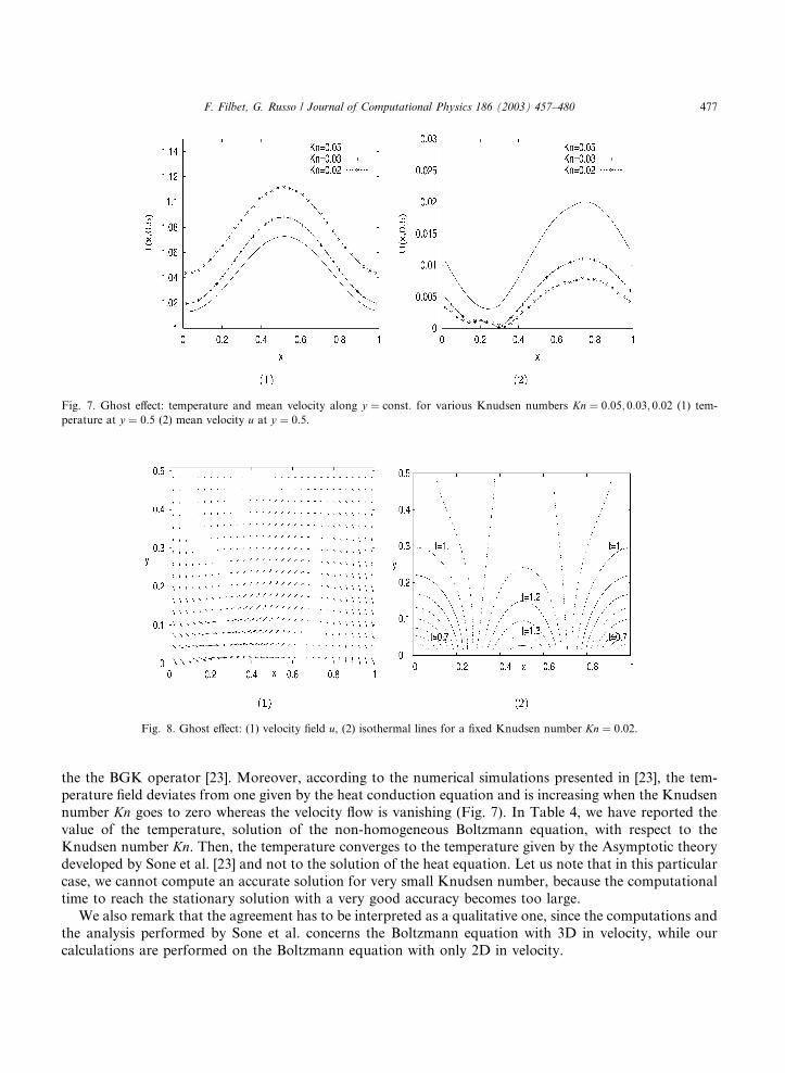
In this example, the walls are moving with a speed of order Kn. The isothermal lines and the velocity field

for Kn ¼ 0:05 are shown in Fig. 8. These results are in good agreement with those obtained by discretizing

Fig. 6. Shock profiles (� ¼ 102): (1) the density q, (2) mean velocity u and (3) temperature T obtained by the S-PFC method (up) and

by the TRMC method (bottom).


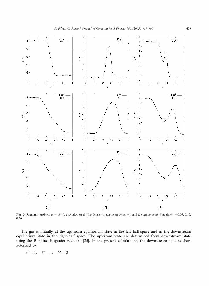
the the BGK operator [23]. Moreover, according to the numerical simulations presented in [23], the tem-

perature field deviates from one given by the heat conduction equation and is increasing when the Knudsen

number Kn goes to zero whereas the velocity flow is vanishing (Fig. 7). In Table 4, we have reported the

value of the temperature, solution of the non-homogeneous Boltzmann equation, with respect to theKnudsen number Kn. Then, the temperature converges to the temperature given by the Asymptotic theory

developed by Sone et al. [23] and not to the solution of the heat equation. Let us note that in this particular

case, we cannot compute an accurate solution for very small Knudsen number, because the computational

time to reach the stationary solution with a very good accuracy becomes too large.

We also remark that the agreement has to be interpreted as a qualitative one, since the computations and

the analysis performed by Sone et al. concerns the Boltzmann equation with 3D in velocity, while our

calculations are performed on the Boltzmann equation with only 2D in velocity.

Fig. 8. Ghost effect: (1) velocity field u, (2) isothermal lines for a fixed Knudsen number Kn ¼ 0:02.

Fig. 7. Ghost effect: temperature and mean velocity along y ¼ const: for various Knudsen numbers Kn ¼ 0:05; 0:03; 0:02 (1) tem-

perature at y ¼ 0:5 (2) mean velocity u at y ¼ 0:5.


5. Conclusions

In this paper we present an accurate deterministic method for the numerical approximation of the space

non-homogeneous, time dependent Boltzmann equation. The method, based on a fractional step approach,

couples a positive and flux conservative scheme for the treatment of the transport step with a Fourier

spectral method for the collision step.

It possesses a high order of accuracy for this kind of problems. In fact it is second order accurate in time,third order accurate in space, and spectrally accurate in velocity. The high accuracy is evident from the

quality of the numerical results that can be obtained with a relatively small number of grid points in velocity

domain.

An effective time discretization allows the treatment of problems with a considerable range of mean free

path, and the decoupling between the transport and the collision step makes it possible the use of parallel

algorithms, which become competitive with state-of-the-art numerical methods for the Boltzmann equation.

The numerical results, and the comparison with other techniques, show the effectiveness of the present

method for a wide class of problems. There are, however, some limitations of the method in its presentform, and several improvements are possible in different directions.

The first limitation is that, because of the Oðn2Þ complexity, the method is presently very expensive for

realistic Boltzmann equation with 3D in velocity. Some research is needed in order to reduce the complexity

in the computation of the collision operator in Fourier space. As a first step in this direction, a fast, low

storage technique can be used for the table look up of the Fourier coefficient of the collisional operator [12].

We plan to use this storage algorithm and fast, parallel machines for space non-homogeneous 3D calcu-

lations with 323 modes per cell.

Another drawback of the method is that, in the present form, it is not able to deal with distributionfunctions that are not well approximated by a periodic function with a reasonable number of Fourier

modes. For the above reason, the method can be successfully used only for systems not very far from local

equilibrium.

A second serious problem arises with space non-homogeneous problems, and concerns the use of an

optimal grid in velocity space. In the present paper we assume that the grid in velocity space is the same for

each space cell of the computational domain.

This is certainly a serious limitation if large variations in the mean velocity and/or in the temperature are

present in the flow, since a grid that is suitable in a given cell might be inadequate in a different space cell.Two possible strategies are under consideration to overcome this problem. One is based on a variable

grid method, in which different points in space have a different grid in velocity. The passage from one grid

to another is performed by weighting and interpolation, as is done in multigrid methods.

A second strategy consists in scaling the velocity variable as

v ¼ u þffiffiffiffiffiffi2T

pn:

Table 4

Ghost effect: temperature at ðx; yÞ ¼ ð0; 1=2Þ with respect to the Knudsen number Kn and temperature given by the asymptotic theory

(Sone et al.) and by the solution of the heat-conduction equation

Temperature Mean velocity

Kn ¼ 0:05 1.0129 0.0107

Kn ¼ 0:03 1.0228 0.0049

Kn ¼ 0:02 1.0436 0.0033

Asymptotic theory 1.045

Heat-conduction equation 1.018

The last column corresponds to the mean velocity at ðx; yÞ ¼ ð0; 1=2Þ.


The function f will be expressed as f ðt; x; vÞ ¼ f ðt; x; u þffiffiffiffiffiffi2T

pnÞ ¼ ~ff ðt; x; nÞ. The evolution equation for ~ff

will be coupled with the evolution equations for u and T . Such approach, although very attractive, presentsseveral numerical difficulties, and is presently under investigation.

Acknowledgements

Part of the research has been performed while one of the authors (Filbet) was visiting University ofCatania in 2001, with a grant of the TMR-Network, contract number ERB FMRX CT97 0157.

References

[1] H. Babovsky, On a simulation scheme for the Boltzmann equation, Math. Methods Appl. Sci. 8 (1986) 223–233.

[2] G.A. Bird, Molecular gas dynamics, Clarendon Press, Oxford, 1994.

[3] A.V. Bobylev, S. Rjasanow, Difference scheme for the Boltzmann equation based on the fast Fourier transform, Eur. J. Mech. B/

Fluids 16 (1997) 293–306.

[4] C. Buet, A discrete velocity scheme for the Boltzmann operator of rarefied gas dynamics, Transport Theory Statist. Phys. 25

(1996) 33–60.

[5] C. Cercignani, The Boltzmann equation and its applications, Springer, Berlin, 1988.

[6] C. Cercignani, R. Illner, M. Pulvirenti, The mathematical theory of dilute gases, Springer, New York, 1995.

[7] O. Coulaud, E. Sonnendr€uucker, E. Dillon, P. Bertrand, A. Ghizzo, Parallelization of semi-Lagrangian Vlasov Codes, J. Plasma

Phys. 61 (1999) 435–448.

[8] E. Fijalkow, A numerical solution to the Vlasov equation, Comput. Phys. Commun. 116 (1999) 319–328.

[9] F. Filbet, E. Sonnendr€uucker, P. Bertrand, Conservative numerical schemes for the Vlasov equation, J. Comput. Phys. 172 (2001)166–187.

[10] D. Goldstein, B. Sturtevant, J.E. Broadwell, Investigation of the motion of discrete velocity gases, Rar. Gas. Dynam., Progr.

Astronautics e Aeronautics, 118, AIAA, Washington, 1989.

[11] T. Inamuro, B. Sturtevant, Numerical study of discrete velocity gases, Phys. Fluids A 12 (1990) 2196–2203.

[12] R. Kirsch, private communication.

[13] K. Nanbu, Direct simulation scheme derived from the Boltzmann equation. I. Monocomponent gases, J. Phys. Soc. Jpn. 52 (1983)

2042–2049.

[14] H. Nessyahu, E. Tadmor, Nonoscillatory central differencing for hyperbolic conservation laws, J. Comput. Phys. 87 (1990) 408–

463.

[15] T. Ohwada, Higher order approximation methods for the Boltzmann equation, J. Comput. Phys. 139 (1998) 1–14.

[16] L. Pareschi, B. Perthame, A Fourier spectral method for homogeneous Boltzmann equations, Transport Theory Statist. Phys. 25

(1996) 369–383.

[17] L. Pareschi, G. Russo, On the stability of spectral methods for the homogeneous Boltzmann equation, in: Proceedings of the Fifth

International Workshop on Mathematical Aspects of Fluid and Plasma Dynamics (Maui, HI, 1998), Transport Theory Statist.

Phys. 29 (2000) 431–447.

[18] L. Pareschi, G. Russo, Numerical solution of the Boltzmann equation. I. Spectrally accurate approximation of the collision

operator, SIAM J. Numer. Anal. 37 (2000) 1217–1245.

[19] L. Pareschi, G. Russo, Time Relaxed Monte Carlo methods for the Boltzmann equation, SIAM J. Sci. Comput. 23 (2001) 1253–

1273.

[20] F. Rogier, J. Schneider, A direct method for solving the Boltzmann equation, Transport Theory Statist. Phys. 23 (1994) 313–

338.

[21] C.-W. Shu, Essentially non-oscillatory and weighted essentially non-oscillatory schemes for hyperbolic conservation laws, in: B.

Cockburn, C. Johnson, C.-W. Shu, E. Tadmor (Eds.), Advanced Numerical Approximation of Nonlinear Hyperbolic Equations,

in: A. Quarteroni (Ed.), Lecture Notes in Mathematics, 1697, Springer, Berlin, 1998, pp. 325–432.

[22] J.A. Carrillo, I.M. Gamba, A. Majorana, C.-W. Shu, A WENO-solver for the transients of Boltzmann–Poisson system

for semiconductor devices, A Performance and comparisons with Monte Carlo methods, J. Comput. Phys. 184 (2003) 498–

525.

[23] Y. Sone, K. Aoki, S. Takata, H. Sugimoto, A.V. Bobylev, Inappropriateness of the heat-conduction equation for description of a

temperature field of a stationary gas in the continuum limit: examination by asymptotic analysis and numerical computation of the

Boltzmann equation, Phys. Fluids 8 (1996) 628–638.


[24] G. Strang, On the construction and comparison of difference schemes, SIAM J. Numer. Anal. 5 (1968) 506–517.

[25] G.B. Whitham, Linear and nonlinear waves, Wiley/Interscience, New York, 1974.

[26] E. Wild, On Boltzmann�s equation in the kinetic theory of gases, Proc. Cambridge Philos. Soc. 47 (1951) 602–609.


High order numerical methods for the space non-homogeneous Boltzmann equation

Documents

Transcript of High order numerical methods for the space non-homogeneous Boltzmann equation