Reliable computation of binary homogeneous azeotropes of multi-component mixtures at higher...

Chemical Engineering Science 59 (2004) 599–609www.elsevier.com/locate/ces

Reliable computation of binary homogeneous azeotropes ofmulti-component mixtures at higher pressures through equation of states

Naveed Aslam, Aydin K. Sunol∗

Department of Chemical Engineering, University of South Florida, 4202 E. Fowler Avenue, Tampa, FL 33620, USA

Received 17 March 2003; received in revised form 20 October 2003; accepted 4 November 2003

Abstract

A method to compute binary homogeneous azeotropes in multi-component mixtures at elevated pressures through the equation of stateapproach is developed. The method is capable of predicting the homogeneous azeotropes and is in close agreement with experimentaldata. At higher pressures, vapor and liquid phase non-idealities are incorporated using vapor and liquid phase fugacity coe4cients fromPeng–Robinson–Stryjek–Vera equation of state with Wong–Sandler mixing rules. The method is also capable of predicting the exactvalue of bifurcation pressure where homogeneous azeotropes may appear or disappear. The method can predict the azeotropes at elevatedpressures and is independent of equation of state and mixing rules. The method is also capable of predicting the double azeotropy in binarymixtures. The method is tested with Ethanol-Water, Isopropanol-Water, Carbon dioxide-Ethane-Ethylene and Ammonia-R-125 systems.The highly non-linear system of equations is solved by homotopy continuation approach.? 2003 Published by Elsevier Ltd.

1. Introduction

The reliable prediction of azeotropes is vital for success-ful design and operation of non-ideal separation sequences.Doherty and colleagues developed and applied residue curvemaps as conceptual design tool for the synthesis and opera-tion of non-ideal separation sequences. Their work is incor-porated well into a text by Malone and Doherty (2001).In order to construct residue curvemaps, all the azeotropes

in a multi-component mixture should be known and char-acterized as stable nodes, unstable nodes, or saddles. Thisclassi=cation gives rise to distillation boundaries. The suc-cess of residue curves as a conceptual design tool dependson the reliability of the algorithm that permits prediction ofall the azeotropes for a multi-component mixture.Most of the initial work in this area was with the sys-

tems operating at lower pressures. Later, Knapp and Do-herty (1992) presented number of heat integrated separationsequences aiming at the separation of non-ideal mixtures,where distillation boundaries arising from the non-ideal be-havior could be crossed through pressure variation in a

∗ Corresponding author. Tel.: +1-813-974-3566; fax: +1-813-974-3651.

E-mail address: [email protected] (A.K. Sunol).

separation sequence. The pressure diBerential can also beutilized to heat integrate a non-ideal separation sequence.They presented a number of heat-integrated schemes fornon-ideal separations. Another area of application fornon-ideal high-pressure distillation is the separation oforganics from the aqueous mixtures through dense gasextraction. De Filippi and Vivian (1982) presented a Dow-sheet for the separation of ethanol from an aqueous mixturethrough dense carbon dioxide extraction. The ethanol isextracted at about 20◦C, and 55:2 bar with the liquid car-bon dioxide. The carbon dioxide extract stream is then fedto a high-pressure distillation column that separates car-bon dioxide from ethanol. The pressure in the column is48:3 bar. They also heat integrated their Dowsheet.Diaz et al. (2000) also described number of separation

sequences for dense gas extraction of organics from aque-ous mixture. Almost all of these sequences are characterizedwith high-pressure non-ideal distillation columns. The suc-cessful design and reliable operation of high-pressure dis-tillation columns requires an e4cient and reliable algorithmfor the prediction of azeotropes at higher pressures, prefer-ably through the same partition coe4cient model that as-sures consistency.Teja and Rowlinson (1973) computed binary azeotropes

using principle of corresponding states. Their method is a

0009-2509/$ - see front matter ? 2003 Published by Elsevier Ltd.doi:10.1016/j.ces.2003.11.010

mailto:[email protected]

600 N. Aslam, A.K. Sunol / Chemical Engineering Science 59 (2004) 599–609

local method and does not guarantee that all the azeotropes ina given mixture can be computed. Wang andWhiting (1986)used an equation of state (EOS) to predict the azeotropes.Furthermore, their method only satis=es the necessary con-ditions of azeotropy and requires a stability test. Seguraet al. (1999) presented a robust algorithm for the predictionof binary azeotropes through an EOS.Fidkowski et al. (1993) described an approach to com-

pute all the homogeneous azeotropes in a multi-componentmixture. He used the homotopy continuation method tosolve the necessary conditions for azeotropy. As the homo-topy parameter is varied from zero to one, the equilibriumvaries from ideal equilibrium (�i = 1:0) to non-ideal equi-librium (�i �= 1:0) in the necessary condition of azeotropy.They used an activity coe4cient model to model the liq-uid phase non-idealities and neglected the vapor phasenon-idealities.Tolsma and Barton (2000a,b) extended Fidkowski’s

approach to compute heterogeneous azeotropes and pre-sented the necessary proofs regarding the computation ofall the homogeneous and heterogeneous azeotropes formulti-component mixtures. They further analysed the vari-ation of phase equilibrium structure with pressure. Theyused the activity coe4cients to model the liquid phase andassumed that vapor phase is ideal.Both Fidkowski’s and Tolsma’s approaches are quite ef-

fective in predicting the azeotropes at atmospheric pressureand possibly up to 5–10 atm. However, if we wish to ex-tend the range to higher pressures, the predicted azeotropiccompositions are not likely to be close to the experimentalvalues probably because these approaches neglect the vaporphase non-idealities and require regression of activity co-e4cient model parameters from higher-pressure data. Fur-thermore, at higher pressures, the vapor phase non-idealitiesbecome quite signi=cant.Our approach is based on Tolsma and Barton’s work and

extends it to higher pressures through an EOS incorporatingvapor phase non-idealities as well. We obtained fugacity co-e4cients from Peng–Robinson–Stryjek–Vera (PRSV) equa-tion of state with Wong–Sandler mixing rules and mappedthe vapor and liquid phase non-idealities. Coupled with thehomotopy continuation based methodology, our approach iscapable to reliably predict the azeotropes at elevated pres-sures. We analyzed Ethanol-Water, IPA-Water and CarbonDioxide-Ethane-Ethylene system through our approach. Wealso modeled the double azeotropy of Ammonia-R-125 sys-tem through our approach. Our results are in close agree-ment with experimental data of David and Dodge (1959),Chaikao et al. (1997) and Clark and Stead (1988). Ourmethod is also capable of predicting the Bifurcation Pres-sures, i.e., the pressures where azeotropes may appear ordisappear. Our approach can also be reliably used to predictthe double azeotropy in binary mixtures. At elevated pres-sures, the bifurcation points of pure component branchesare predicted by using in=nite dilution K-values obtainedfrom EOS.

2. Model formulation

Fidkowski et al. (1993) solved the necessary conditionsof azeotropy (xi = yi) using homotopy continuation. Thehomotopy map is given as follows:

hi(x; ) ≡ (xi − yReali ) + (1− )(xi − yIdeali ); (2.1)

where is a homotopy parameter, which varies from 0 to1 and xi is the liquid composition. The yIdeali is the vaporcomposition for an ideal gas and ideal solution and yReali isfor a real gas and non-ideal solution. For =0, the xi=yIdealiand for = 1, the xi = yReali :

yIdeali = K Ideali xi: (2.2)

yReali = KReali xi: (2.3)

The K Ideali is the ideal solution equilibrium constant and is

derived from Raoult’s law while KReali is a non-ideal equi-

librium constant which maps the liquid phase non-idealitieswith activity coe4cients. The vapor phase is still assumedideal with Fidkowski’s formulation.We based our approach on Fidkowski’s formulation, but

used K values from EOS to account for both the liquid andthe vapor phase non-idealities:

K Ideali =

Psati

P(2.4)

and

KReali =

�̂Li (xi; xj; T; P)

�̂Vi (yi; yj; T; P): (2.5)

Tolsma and Barton (2000a,b) further enhanced theFidkowski’s approach for isobaric conditions. They de-veloped the following formulation shown in Eqs. (2.6)–(2.9), using activity coe4cients to map the liquid phasenon-idealities and assuming ideal vapor phase:

F(x; y; T; ) =

x1 − y1...

xn − yny1 − K0

1 x1

...

yn − K0n xn

n∑i=1

xi − 1

: (2.6)

K0i is the pseudo-equilibrium constant:

K0i = [KReal

i + (1− )K Ideali ]: (2.7)

N. Aslam, A.K. Sunol / Chemical Engineering Science 59 (2004) 599–609 601

They removed the perturbed vapor composition fromEq. (2.6), obtaining the following relation:

F(x; T; ) =

x1 − K01 x1

...

xn − K0n xn

n∑i=1

xi − 1

: (2.8)

As we set F(x; T; ) = 0, we have de=ned a solution spacein x; T; for a =xed pressure. The mapped solution of abovefunction is called the homogeneous homotopy path.The Jacobian matrix of Eq. (2.6) is given as

∇F(x; T; ) =

�1 − x1K1;1 −x1K1;2 : : : −x1K1; n −x1�1 −x1’1

−x2K2;1 �2 − x2K2;2 : : : −x2K2; n −x2�2 −x2’2

......

. . ....

......

−xnKn;1 −xnKn;2 : : : �n − xnKn;n −xn�n −xn’n1 1 1 0 0

; (2.9)

where, one can start incorporating the equation of state basedreformulation

�j = 1−[(

(�̂Lj (xi; xj; T; P)

�̂Vj (yi; yj; T; P)

)+ (1− )

(Psatj

P

))];

(2.10)

�j =

(@(�̂Lj (xi; xj; T; P)=�̂

Vj (yi; yj; T; P))

@T

)x;y;P

+(1− )dPsat

j =dT

P; (2.11)

’j =�̂Lj (xi; xj; T; P)

�̂Vj (yi; yj; T; P)− Psat

j

P; (2.12)

Ki;j =(@Ki@xj

)xi[ j] ;y;T;P

: (2.13)

Without loss of generality, a k-ary branch of a n-componentmixture satis=es the following:

xj �= 0 ∀j ≡ 1; : : : ; k; (2.14)

�j = 0 ∀j ≡ 1; : : : ; k; (2.15)

xj = 0 ∀j ≡ k + 1; : : : ; n; (2.16)

�j �= 0 ∀j ≡ k + 1; : : : ; n: (2.17)

Constraints (2.14) and (2.17) may be simultaneously vio-lated at isolated points along the homotopy branch. If we let

c(s)∈F−1(0) that represents a continuation branch where“s” is arc length and we are following a k-ary branch, thenon c(s) the following relation will hold.

�j = 0 for all j = 1; : : : ; k:

Thus,

∇F(c(s)) =

−x1K1;1 −x1K1;2 : : : −x1K1; k+1 : : : −x1K1; n −x1�1 −x1’1

......

. . ....

. . ....

......

−xkKk;1 −xkKk;2 : : : −xkKk;k+1 : : : −xkKk;n −xk�k −xk’k0 0 : : : �k+1 : : : 0 0 0

......

. . ....

. . ....

......

0 0 : : : 0 : : : �n 0 0

1 1 : : : 1 : : : 1 0 0

: (2.18)

Lemma 1. A necessary condition for a trans-critical bifur-cation from a k-ary branch on to a (k + 1)-ary branch ata point c(s) is

�j(s) = 0 for some j∈{k + 1; : : : ; n}: (2.19)

A necessary condition for trans-critical bifurcation from a(k + 1)-ary branch to a k-ary branch at a point c(s) is

xj(s) = 0 for some j∈{1; : : : ; k + 1}: (2.20)


Condition (2.20) becomes necessary and su4cient for thebifurcation from a (k + 1)-ary branch on to a k-ary branchby adding the following:

(1) dxj=ds|s=s− �= 0,(2) rank∇F(s) = N − 1 where N = n+ 1, and(3) @F=@xj|s=s− ∈R(∇[ j]F(s)) where ∇[ j] denotes partial

derivatives with respect to all variables except xj.

2.1. Prediction of bifurcation points on pure componentbranches

The system of equations for a binary azeotropic mixturecan be extracted from Eq. (2.8):

F(x; T; ) =

x1 − K01 x1

x2 − K02 x2

n=2∑i=1

xi − 1

: (2.21)

As → 0, the pure components will be the solution of abovesystem of equations provided that the pure components havedistinct boiling points. In order to start the continuation,we have all the pure component branches extending from=0 and moving towards =1:0. On these pure componentbranches, there will be a point where the binary branch isgoing to intersect. This point of intersection between a purecomponent and binary branch needs to be properly identi-=ed for ensuring the successful branch tracking. Fortunately,these points can be calculated without any branch tracking.From Eq. (2.21), we get the following equality:

x1(1− K01 ) = 0

which reduces to

(1− K01 ) = 0 (2.22)

using the value of pseudo-equilibrium constant K01 from

Eq. (2.7) in Eq. (2.22), we get

K0i = [KReal

i + (1− )K Ideali ] = 1:0 (2.23)

and solving (2.23) for one obtains

=(

1− K Ideali

KReali − K Ideal

i

): (2.24)

For a binary mixture of component i and j, Eq. (2.24)becomes

ij =

(1− Psat

j (Tbi )=P

Kj − Psatj (Tbi )=P

): (2.25)

For low to moderate pressures, Kj is usually expressed asa function of in=nite dilution activity coe4cient, �∞j . Sincewe are exploring elevated pressure systems, in=nite dilutionK values computed from EOS will be more appropriate asshown below:

Kj = K∞ij =

�̂L∞j (xi; xj; T; P)

�̂V∞j (xi; xj; T; P); (2.26)

where �̂L∞j and �̂V∞j are the in=nite dilution liquid andvapor fugacity coe4cients for component j when xi = 1:0and xj = 0:0.Eq. (2.25) results in a bifurcation point on the pure com-

ponent branch i. The bifurcation point is actually the pointof intersection of pure component branch i and a binarybranch ij. These bifurcation points act as starting points ofbinary branches. Only the binary branches which are inter-secting with pure component branches between the values of06 i; j6 1 will lead to physically meaningful solutions at=1:0. For a binary mixture, a minimum boiling azeotropebifurcates from lower boiling component and a maximumboiling azeotrope bifurcates from higher boiling component.

3. Branch tracking

The highly non-linear system of Eq. (2.21) requires avery robust solver, as the Newton like procedures may notprovide reliable solutions. The non-linear nature of system ofEq. (2.21) lead to multiple solutions and a major limitationof Newton like methods is that they converge to one localsolution. We used a homotopy continuation based techniqueto solve the equation in (2.21). The homotopy continuationis selected due to the following reasons:

• Continuation algorithms enhance the convergencedomain.

• They systematically search and =nd all the possible solu-tions of non-linear systems of equations.

• Homotopy methods have the ability to easily determinethe solution characteristics of a problem as a function ofone of its variables.

We developed a matlab-based code for solving the nec-essary condition of azeotropy through homotopy contin-uation. As indicated in Eq. (2.21), for a binary system,we have three equations and four variables x1; x2; T and for a =xed pressure. We solved the above system of equa-tions with pseudo-arc-length continuation. All the vari-ables become the function of arc-length parameter “s” i.e.,x1(s); x2(s); T (s); (s). The important characteristic of thearc-length parameter “s” is that it can turn back to itself andnever goes negative, thus solution branches can be followedaround the singular or turning points. In order to makeEq. (2.21) a completely de=ned system, the pseudo-arc-length relation shown below is added:

�((x1 − x1s) dx1ds

+ (x2 − x2s) dx2ds+ (T − Ts) dTds

)

+(1− �)(− s) dds −Ps= 0: (3.1)

Eq. (3.1) with system of Eq. (2.21) provides a fully de-termined system, i.e., four equations with four unknowns.Eq. (2.25) provides a starting point on pure componentbranches which is utilized to initialize the combined system


of equations (2.21) and (3.1). The indicated system of equa-tions is coded in matlab and solved with predictor-correctortype of algorithms with self-adapting step-length algorithmas described in Allgower and Georg (1990) and Speight(1999).

4. Results and discussion

Experimental data for binary homogeneous azeotropes inmulticomponent mixtures at high pressure is very limited.Only very few binary homogeneous azeotropes has beenexperimentally evaluated throughout a large pressure range.One of the major features of our work is that it will provide arobust and e4cient method for predicting the high-pressureazeotropes from azeotropic information at lower pressures.The prediction of high-pressure azeotropes will minimize,if not eliminate, the need of conducting the experimentaldetermination of binary homogeneous azeotropes throughthe entire pressure range. The following three homogeneoussystems are used to evaluate the potential of the approach.

• Ethanol-Water system.• Carbon dioxide-Ethane-Ethylene system.• Isopropanol-Water system.• Ammonia-R125 system.

We selected the =rst three systems mainly because of theavailability of high-pressure azeotropic data for these sys-tems (David and Dodge, 1959; Clark and Stead, 1988).Another consideration in selecting above systems is the pos-sible application of high-pressure azeotropes in the devel-opment of conceptual design tools for supercritical systems.The conceptual design tools for supercritical systems willform a solid basis for green processing separation systems.The fourth and last system in above list (Ammonia-R-125)is selected because it has a double azeotropy behavior athigher pressures (Chaikao et al., 1997).

4.1. Identi3cation of a bifurcation point on a purecomponent branch

As → 0 in Eq. (2.8), the solution becomes (x; T; ) =(xk ; T sk ; 0), where k = 1; : : : ; n, and, xk denotes pure compo-nent k with boiling point Tk at a speci=ed pressure. Thus,we start with the solution of Eq. (2.8) for pure componentbranches. For some of these pure component branches, a bi-furcation point (ij) will exist depending on the boiling na-ture of azeotrope. If a component i forms an azeotrope witha component j a bifurcation point will exist on the pure com-ponent branch i. Tolsma and Barton (2000a,b) pointed outthat for a maximum boiling azeotrope, i will be the higherboiling specie and for a minimum boiling azeotrope, i willbe a lower boiling specie. These bifurcation points are thepoints of intersection of a pure component branch i with abinary branch ij. As indicated in Section 2.0, the branches

0.6 0.65 0.7 0.75 0.8 0.850

10

20

30

40

50

60

PR

ES

SU

RE

[AT

M]

Based On Infinite Dilution Activity CoefficientBased On Infinite Dilution K values from EOS

Bifurcation Point [λij]

Fig. 1. Variation of bifurcation point with pressure for Ethanol-WaterSystem (NRTL and PRSV with Wong-Sandler Mixing Rules are used).

starting from the bifurcation points between zero and onecan lead to solution at =1 and satisfy the necessary condi-tion for azeotropy at = 1. These bifurcation points can bepredicted through Eq. (2.25) prior to any branch tracking.We are using in=nite dilutionK values,K∞

i; j , in Eq. (2.25),as opposed to in=nite dilution activity coe4cient, �∞ij . Thein=nite dilution K values will account for both vapor and liq-uid phase non-idealities at higher pressure. Fig. 1 shows thevariation of Bifurcation Point with pressure, based on an ac-tivity coe4cient model and an EOS for Ethanol-Water sys-tem. As can be seen, the bifurcation point based on in=nitedilutionK-values from EOS =rst decreases with pressure andthen it starts to increase. However, the activity coe4cientmodel shows a decreasing trend for Bifurcation Point as weincrease the pressure. This might be due to the incorpora-tion of vapor phase non-idealities. Furthermore, the in=nitedilution K value provides a better scaling in Eq. (2.25). Athigher pressures, neglecting the vapor phase non-idealitiesmay not be a realistic.Fig. 2 depicts bifurcation point variation with pressure

for Carbon Dioxide-Ethane system. For pressures, lessthan 10 atm, the ij is zero indicating that there will be noazeotrope at lower pressures. As we increase the pressure,the Bifurcation Point (ij) exponentially increases around,60:0 atm the Bifurcation Point approaches unity and furtherincreases as we increase the pressure. This is indicating thatsub-critical Carbon-Dioxide-Ethane azeotrope is disappear-ing into critical locus of the mixture also indicated by theexperimental data of Clark and Stead (1988). Figs. 3 and 4represents the bifurcation point variation with pressurefor Carbon Dioxide-Ethylene and Ethane-Ethylene bina-ries in Carbon Dioxide-Ethane-Ethylene system. Knappand Doherty (1992) de=ned the bifurcation pressure as thepressure where a new azeotrope may appear from a purecomponent branch or it may disappear into critical line. ForCarbon Dioxide-Ethane system at 12:0 atm, an azeotrope isborn and around 60:0 atm it disappears into critical line of


-0.2 0 0.2 0.4 0.6 0.8 1 1.20

10

20

30

40

50

60

70

PR

ES

SU

RE

[ A

TM

]

Based On Infinite Dilution K values from EOS


Fig. 2. Variation of bifurcation point with pressure for Carbondioxide-Ethane System (PRSV with Wong-Sandler Mixing Rules is used).

Fig. 3. Variation of bifurcation point with pressure for Carbondioxide-Ethylene Pair (PRSV with Wong-Sandler Mixing Rules is used).

the mixture. Our approach is also capable of predicting thebifurcation pressures more reliably as we are using a robustthermodynamic model.Fig. 5 represents Isopropanol-Water system. The bifurca-

tion point based on in=nite dilution K-values from PRSVwith Wong Sandler mixing rules, =rst decreases and thenincreases as we increase the pressure.The exact location of these bifurcation points is very im-

portant for successful tracking of binary branches which willlead to =nal azeotropic compositions at ij = 1:0. If thesepoints are not correctly calculated, the binary branches maylead to diBerent solutions or may not converge at all.Fig. 6 shows the variation of bifurcation point with

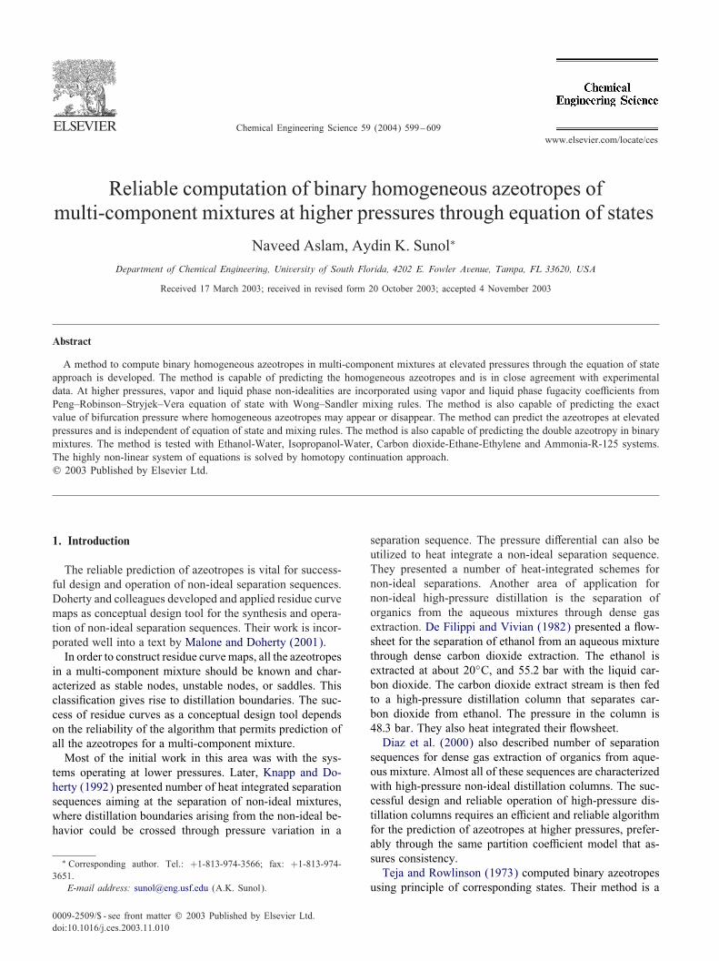
pressure for Ammonia-R-125 binary system. This systemexhibits a double azeotropy behavior (Chaikao et al., 1997).Bifurcation point at both the pure component branches(Ammonia and R-125) is computed using the in=nite dilu-tion activity coe4cient and in=nite dilution K-values from

Fig. 4. Variation of bifurcation point with pressure for Ethane-EthylenePair (PRSV with Wong-Sandler Mixing Rules is used).

0.45 0.5 0.55 0.6 0.65 0.7 0.75 0.8 0.85 0.90

5

10

15

20

25

30

35

40

45

Based On Infinite Dilution Activity CoefficientBased On Infinite Dilution K values from EOS P

RE

SS

UR

E [

AT

M]


Fig. 5. Variation of bifurcation point with pressure for Isopropanol-WaterSystem (NRTL and PRSV with Wong-Sandler Mixing Rules are used).

EOS. Fig. 6 indicates that with activity coe4cient only oneazeotrope is possible as only the bifurcation point appear-ing at pure component R-125 branch is attaining a valuebetween 0 and 1, while the bifurcation point appearing atpure component Ammonia never attains a value between0 and 1 for the entire pressure range. Fig. 6 also depictsthat with the EOS based approach it is possible to com-pute both the azeotropes for this binary system. As it canbe noted from Fig. 6 that bifurcation point appearing onboth the pure component branches (Ammonia and R-125)attain the values between 0 and 1. For pure R-125 branchthe homotopy parameter at bifurcation point is 0.089 atatmospheric pressure while the bifurcation point appear-ing on pure ammonia branch becomes unity at around8:0 atm and then remains in between the range of 0 and1 as pressure is increased. Thus Fig. 6 indicates the pos-sibility of double azeotropy in this system from 8.0 to34:0 atm as homtopy parameter at bifurcation point appear-


Fig. 6. Variation of bifurcation point with pressure for Ammonia-R-125 System (NRTL and PRSV with Wong-Sandler Mixing Rules are used).

0.6 0.65 0.7 0.75 0.8 0.85 0.9 0.95 10.7

0.75

0.8

0.85

0.9

0.95

1

Based On EOS Based On Activity Coefficient

*

*

Experimental Data by David and Dodge [1959]

Homotopy Parameter

Eth

anol

Mol

e F

ract

ion

Fig. 7. Binary homotopy branches for Ethanol-Water System at 55 atm(based on NRTL and PRSV with Wong-Sandler Mixing Rules).

ing on both the pure component branches lies in the rangeof 0 to 1.

4.2. Ethanol-water azeotrope at higher pressures

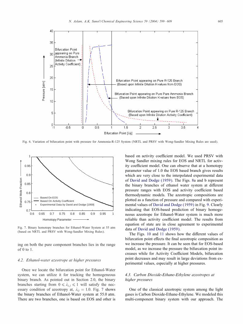
Once we locate the bifurcation point for Ethanol-Watersystem, we can utilize it for tracking the homogeneousbinary branch. As pointed out in Section 2.0, the binarybranches starting from 06 i; j6 1 will satisfy the nec-essary condition of azeotropy at, ij = 1:0. Fig. 7 showsthe binary branches of Ethanol-Water system at 55:0 atm.There are two branches, one is based on EOS and other is

based on activity coe4cient model. We used PRSV withWong Sandler mixing rules for EOS and NRTL for activ-ity coe4cient model. One can observe that at a homotopyparameter value of 1.0 the EOS based branch gives resultswhich are very close to the interpolated experimental dataof David and Dodge (1959). The Figs. 8a and b representthe binary branches of ethanol water system at diBerentpressure ranges with EOS and activity coe4cient basedthermodynamic models. The azeotropic compositions areplotted as a function of pressure and compared with experi-mental values of David and Dodge (1959) in Fig. 9. Clearlyindicating that EOS-based prediction of binary homoge-neous azeotrope for Ethanol-Water system is much morereliable than activity coe4cient model. The results fromequation of state are in close agreement to experimentaldata of David and Dodge (1959).The Figs. 10 and 11 shows how the diBerent values of

bifurcation point eBects the =nal azeotropic composition aswe increase the pressure. It can be seen that for EOS-basedmodel, as we increase the pressure the bifurcation point in-creases while for Activity Coe4cient Models, bifurcationpoint decreases and may result in large deviations from ex-perimental values, especially at higher pressures.

4.3. Carbon Dioxide-Ethane-Ethylene azeotropes athigher pressures

One of the classical azeotropic system among the lightgases is Carbon Dioxide-Ethane-Ethylene. We modeled thismulti-component binary system with our approach. The


0.6 0.65 0.7 0.75 0.8 0.85 0.9 0.95 10.84

0.86

0.88

0.9

0.92

0.94

0.96

0.98

1

P = 5.0ATM

P = 13.0ATM

P = 25.0ATM

P = 55.0ATMP = 50.0ATMP = 37.0ATM

Eth

anol

Mol

e F

ract

ion

Homotopy Parameter(a)

0.6 0.65 0.7 0.75 0.8 0.85 0.9 0.95 10.7

0.75

0.8

0.85

0.9

0.95

1

P = 5.0ATM

P = 13.0ATM

P = 25.0ATM

P = 55.0ATM

P = 50.0ATM

P = 37.0ATM

Eth

anol

Mol

e F

ract

ion

Homotopy Parameter(b)

Fig. 8. (a) Homotopy branches for Ethanol-Water System for diBerentpressures. (PRSV with Wong-Sandler Mixing Rules is used). (b) Homo-topy branches for Ethanol-Water System for diBerent pressures. (ActivityCoe4cient Model (NRTL) is used).

5 10 15 20 25 30 35 40 45 50 550.72

0.74

0.76

0.78

0.8

0.82

0.84

0.86

0.88

0.9

Eth

anol

Mol

e F

ract

ion

*

Based On EOSBased On Activity Coefficient

Experimental Data Of David and Dodge [1959]

PRESSURE [ATM]

Fig. 9. Variation of Ethanol-Water Azeotropic Composition [xi=yi] withPressure. (Activity Coe4cient Model (NRTL) and Equation Of State(PRSV with Wong-Sandler Mixing Rules are used).

system has three binary azeotropes but no ternary azeotropeis detected. The binary branches for Carbon Dioxide-Ethanepair at diBerent pressures are shown in Fig. 12 and were

0 10 20 30 40 50 600.65

0.7

0.75

0.8

0.85

0.9 0.9

0.85

0.8

0.75

0.7

0.65

Pressure [ATM]

Eth

anol

Mol

e F

ract

ion

[xi =

yi]

λ ij

Fig. 10. Variation of azeotropic composition and bifurcation point withPressure for Ethanol-Water System (PRSV with Wong-Sandler MixingRules is used).

0 10 20 30 40 50 600.6

0.65

0.7

0.75

0.8

0.85 0.9

0.85

0.8

0.75

0.7

0.65

Pressure [ATM]

Eth

anol

Mol

e F

ract

ion

[xi =

yi]

λ ij

Fig. 11. Variation of azeotropic composition and bifurcation point withpressure for Ethanol-Water System (NRTL is used).

0 0.1 0.2 0.3 0.4 0.5 0.6 0.7 0.8 0.9 10.6

0.65

0.7

0.75

0.8

0.85

0.9

0.95

1P = 34.5 ATM

P = 19.8 ATM P = 24 ATM

P = 29.6 ATM

Car

bon

Dio

xide

Mol

e F

ract

ion

Homotopy Parameter

P = 39.5 ATM

P = 44.4 ATM

P = 49.3 ATM P = 54.2 ATM

Fig. 12. Homotopy branches for Carbon Dioxide-Ethane System at dif-ferent pressure (Based on PRSV with Wong-Sandler Mixing Rules).

based on PRSV with Wong-Sandler mixing rules. Theseresults are further explored in Fig. 13 where the azeotropiccomposition as a function of pressure is plotted and com-


10 15 20 25 30 35 40 45 50 550.6

0.65

0.7

0.75

0.8

0.85

Car

bon

Dio

xide

Mol

e F

ract

ion

PRESSURE [ATM]

* Based On EOSExperimental Azeotropic Data of Clark and Stead (1988)

Fig. 13. Variation of Carbon Dioxide-Ethane azeotrope composition withPressure. (PRSV with Wong-Sandler Mixing Rules is used).

10 15 20 25 30 35 40 45 50 550

0.1

0.2

0.3

0.4

0.5

0.6

0.7

0.8

0.9 0.9

0.85

0.8

0.75

0.7

0.65

Pressure [ATM]

λ ij

Car

bon

Dio

xide

Mol

eF

ract

ion

[xi =

yi]

Fig. 14. Variation of azeotropic composition and bifurcation point withpressure for Carbon Dioxide-Ethane System (PRSV with Wong-SandlerMixing Rules is used).

pared with experimental data of Clark and Stead (1988).The results from our approach are quite close to theirexperimental values. Fig. 14 presents the dependence ofazeotropic composition on the starting point of a binaryazeotropic branch or bifurcation parameter. As we increasethe pressure, the bifurcation parameter increases whileazeotropic composition =rst decreases then increases withincreasing pressure for Carbon dioxide-Ethane pair. TheFig. 15 shows the binary homotopy branches for Carbondioxide-Ethylene pair at 20 atm. Fig. 16 represents thebinary homotopy branches for Ethane-Ethylene pair at36:85 atm. We calculated the azeotropic composition of0.436 Ethane, which is very close to experimental value of0.45 reported by Gmehling et al. (1994).

4.4. Isopropanol-water azeotrope at higher pressures

The Isopropanol water system is modeled at 27:55 atm asshown in Fig. 17. The result from our approach gives theazeotropic composition of 0.65 Isopropanol that matches theexperimental value of 0.6435 from David and Dodge (1959)within experimental error range.

Fig. 15. Homotopy branches for Carbon Dioxide-Ethylene pair at 20:0 atm(based on PRSV with Wong-Sandler Mixing Rules).

Fig. 16. Homotopy branches for Ethylene-Ethane pair at 36:85 atm (basedon PRSV with Wong-Sandler Mixing Rules).

0.5 0.55 0.6 0.65 0.7 0.75 0.8 0.85 0.95 10.5

0.55

0.6

0.65

0.7

0.75

0.8

0.85

0.9

0.95

1

Based On EOS Based On Activity Coefficient

* Experimental Data by David and Dodge [1959]

Iso

Pro

pano

l Mol

e F

ract

ion

Homotopy Parameter

*

0.9

Fig. 17. Homotopy branches of IsoPropanol (IPA)-Water system at27:55 atm (PRSV with Wong-Sandler Mixing Rules and NRTL modelare used).


Fig. 18. Bifurcation diagram for Ammonia-R-125 system at 15:0 atm (PRSV with Wong-Sandler Mixing Rules are used).

Fig. 19. Bifurcation diagram for Ammonia-R-125 system at 20:0 atm (PRSV with Wong-Sandler Mixing Rules are used).

4.5. Ammonia-R-125 azeotrope at higher pressures

Fig. 18 contains a Bifurcation Diagram for Ammonia-R-125binary system at 15:0 atm. The computed results are based

upon EOS approach. Fig. 18 depicts that Ammonia-R-125system has a maximum boiling and a minimum boilingazeotrope. Fig. 19 contains the Bifurcation Diagram forAmmonia-R-125 binary system at 20:0 atm again two


azeotropes is computed at this pressure. The computedresults are in close agreement with experimental data of(Chaikao et al., 1997).The activity coe4cient model parameters (NRTL) and co-

e4cients of extended Antoine’s equation for above indicatedsystems are obtained from Tolsma and Barton (2000a,b).The pure component parameters for PRSV are obtained fromOrbey and Sandler (1998). The binary interaction parame-ters for Wong Sandler mixing rules are extracted from highpressure data of (David and Dodge, 1959; Clark and Stead,1988; Chaikao et al., 1997; Horstmann et al., 2000).

5. Conclusion

This paper presents a methodology for reliably comput-ing the high-pressure azeotropes through equation of state.The approach is extending Tolsma and Barton’s (2000a,b)work for computing homogeneous and heterogeneousazeotropes to high pressures and employs equation of states.Both the liquid and vapor phase non-idealities are incorpo-rated through liquid and vapor phase fugacity coe4cientsbased on equation of state (PRSV with Wong Sandler mix-ing rules). At higher pressures, the phase equilibrium modelis deformed from an ideal equilibrium (based on Raoultslaw) to highly non-ideal equilibrium (based on equation ofstate) with homotopy parameter varying from 0 to 1. Allthe binary homogeneous azeotropes are computed for threesystems at higher pressures. The approach is also capable ofreliably computing the double azeotropy in binary systemsat elevated pressures. The model results are in good agree-ment to experimental values of azeotropes at higher pres-sures unlike activity coe4cient based models. The approachis also capable of predicting the Bifurcation Pressure. Thereliable and e4cient method of predicting azeotropes athigher pressure in multi-component mixtures will reduce therequirements of experimental data for azeotropes at higherpressures while utilizing the low-pressure information toreliably predict the azeotropes at higher pressures.

Notation

[F] matrix for the necessary condition of azeotropyKij derivative of equilibrium constant with respect to

component jK Ideali equilibrium constant for ideal solutionK∞ij in=nite dilution equilibrium constantK0i pseudo-equilibrium constantKReali equilibrium constant for non-ideal solution

[∇F] Jacobian matrix of FP total pressure of the systemPsati vapor pressure of component is arc lengthT temperaturexi mole fraction of the component i in the liquid phaseyIdeali mole fraction of the component i in the vapor phase

for an ideal gas and ideal solution

yReali mole fraction of the component i in the vapor phasefor a real gas and non-ideal solution

Greek letters

homotopy parameterij bifurcation point�̂Lj fugacity coe4cient of component j in liquid phase�̂L∞j fugacity coe4cient of component j in liquid phase

at in=nite dilution�̂Vj fugacity coe4cient of component j in vapor phase�V∞j fugacity coe4cient of component j in vapor phase

at in=nite dilution

References

Allgower, E.L., Georg, K., 1990. Numerical Continuation Methods: AnIntroduction. Springer, Berlin.

Chaikao, C.P., Paulaitis, M.E., Yokozeki, A., 1997. Double azeotropy inbinary mixture of NH3 and CHF2CF3. Fluid Phase Equilibria 127,191–203.

Clark, A.Q., Stead, K., 1988. (Vapour+liquid) phase equilibria of binary,ternary, quaternary mixtures of CH4, C2H6, C3H8, C4H10, and CO2.Journal of Chemical Thermodynamics 20, 413–428.

David, F.B., Dodge, B.F., 1959. Vapor–liquid equilibrium at highpressures. Journal of Chemical and Engineering Data 4, 107–121.

De Filippi, R.P., Vivian, J.E., 1982. Process for separating liquid solutesfrom their solvent mixtures. U.S. Patent 4,349,415.

Diaz, S., Gros, H., Brignole, E.A., 2000. Thermodynamic modeling,synthesis and optimization of extraction-dehydration processes.Computers and Chemical Engineering 24, 2069–2080.

Fidkowski, Z.T., Malone, M.F., Doherty, M.F., 1993. Computingazeotropes in multi-component mixtures. Computers and ChemicalEngineering 17, 1141–1155.

Gmehling, J., Menke, J., Krafczyk, J., Fischer, K., 1994. Azeotropic Data.VCH, New York.

Horstmann, S., Fischer, K., Gmehling, J., Kolar, P., 2000. Experimentaldetermination of the critical line for (carbon dioxide+ethane) andcalculation of various thermodynamic properties for (carbon dioxide+n-alkane) using the PSRK model. Journal of Chemical Thermo-dynamics 32, 451–464.

Knapp, J.P., Doherty, M.F., 1992. A new pressure swing distillationprocess for separating homogeneous azeotropic mixtures. IndustrialEngineering and Chemical Research 31, 346–357.

Malone, M.F., Doherty, M.F., 2001. Conceptual design of distillationsystems. McGraw Hill, New York.

Orbey, H., Sandler, S.I., 1998. Modeling Vapor-Liquid Equilibria: CubicEquation of State and Their Mixing Rules. Cambridge.

Segura, H., Wisniak, J., Toledo, P.G., Mejia, A., 1999. Prediction ofazetropic behavior using equation of state. Fluid Phase Equilibria 166,141–162.

Speight, A., 1999. Using homotopy methods to solve non smoothequations. M.S. Thesis University of Colorado, Denver.

Teja, A.S., Rowlinson, J.S., 1973. The prediction of thermodynamicproperties of Duids and liquid mixtures: IV. Critical and azeotropicstates. Chemical Engineering Science 28, 529–538.

Tolsma, J.E., Barton, P.I., 2000a. Computation of heteroazeotropes, PartI: Theory. Chemical Engineering Science 55, 3817–3834.

Tolsma, J.E., Barton, P.I., 2000b. Computation of heteroazeotropes,Part II: E4cient calculation of changes in phase equilibrium structure.Chemical Engineering Science 55, 3835–3853.

Wang, J.C., Whiting, W.B., 1986. New algorithm for calculation ofazeotropes from equation of state. Industrial and Engineering ChemistryProcess Design and Development 25, 547–551.

Reliable computation of binary homogeneous azeotropes of multi-component mixtures at higher...

Documents

Transcript of Reliable computation of binary homogeneous azeotropes of multi-component mixtures at higher...