The Simple Distillation of Homogeneous Reactive Mixtures

Chemical Engineering Scrence, Vol. 43. No. 3. pp. 541-550. 1988 OOOS-2509/88 E3.00 +O.OO Prmted in Great Bntam 0 1988 Pergamon Journals Ltd

THE SIMPLE DISTILLATION OF HOMOGENEOUS REACTIVE MIXTURES

DOMINGOS BARBOSA+ and MICHAEL F. DOHERTY Department of Chemical Engineering, Goessmann Laboratory, University of Massachusetts, Amherst,

MA 01003, U.S.A.

(Received 1 December 1986; accepted 12 June 1987)

Abstract-The equations describing the simple distillation of homogeneous reactive mixtures are derived, and residue curve maps are computed for ideal and non-ideal systems. These maps show that, by allowing the components of a liquid mixture to react, we can either create or eliminate distillation boundaries. It is also shown that not all non-reactive azeotropes appear as products of the distiliation process. Knowledge of these features is fundamental for the design and synthesis of sequences of reactive distillation columns.

INTRODUCTION

In recent years, increasing attention has been directed towards reactive distillation processes as an alternative to conventional processes (Grosser et al., 1986; Mommessin and Holland, 1983; Smith and Jones, 1984; Terrill er a[., 1985). This has led to the develop- ment of a variety of techniques for simulating reactive distillation columns (Komatsu, 1977; Komatsu and Holland, 1977; Murthy, 1984; Nelson, 1971; Sawistowski and Pilavakis, 1979; Suzuki et al., 1971; Tierney and Riquelme, 1982). However, the problem of design and synthesis of reactive distillation processes has not yet been addressed.

Most of the distillation synthesis studies to date have been concerned with multicomponent ideal mixtures. Only recently has a technique been devised for the synthesis of distillation processes for non-ideal mixtures (Doherty, 1985; Doherty and Caldarola, 1985; Knight, 1986; Pham and Doherty, 1986). This technique is based on the analysis of residue curve maps, which are obtained from the study of simple distillation processes. These residue curve maps ex- plicitly show the existence of distillation boundaries, a concept that is important not only for the synthesis of distillation columns but also for the design of single columns; since these distillation boundaries limit the range of feasible column specifications. Therefore, a means of calculating residue curve maps for reactive mixtures must be developed before any attempt is made at the design and synthesis of reactive distillation columns.

in this article, we begin by deriving a set of autonomous ordinary differential equations that describe the dynamics of homogeneous, reactive simple distillation. These equations are then used to compute residue curve maps for ideal and non-ideal mixtures. The resulting maps show the remarkable effects that reactions can have on the distillation of multicomponent mixtures.

+Present address: Departamento de Engenharia Quimica, Faculdade de Engenharia, Universidade do Porto, 4099 Porto Codex, Portugal.

UERIVATION OF THE EQUATIONS

In a simple distillation process a liquid is vaporized and the vapor is removed from contact with the liquid as it is formed. Each differential mass of vapor is in equilibrium with the remaining liquid. The composition of the liquid will change with time, since in general the vapor formed is richer in the more volatile components. The locus of the liquid compdsitions remaining from a simple distillation process defines a residue curve. These residue curves are closely related to the composition profiles in continuous distillation processes, which is one of the main reasons for studying simple distillation.

Consider a simple distillation unit, as shown in Fig. 1. If we assume that only one chemical reaction occurs in the liquid phase, we can write the material balance for component i as

d(Hxi) -= dt

i=l,...,c (1)

where H represents the molar liquid holdup in the still, Y the molar flow rate of the escaping vapor, vi the stoichiometric coefficient for component i, and E the extent of reaction. The overall material balance is

dH -= dt

- Y+“r$

t v. Y -

Fig. 1. Schematic representation of the simple distillation process.

541

542 DOMINGOS BARBOSA and MICHAELF.DOHERTY

where

vr= i: vi. (3) (11)

i=I which leads to the following set of c - 2 linearly Since eqs (1) and eq. (2) are linearly dependent, the independent, autonomous, ordinary differential equa-

simple distillation of reactive mixtures can be de- tions to describe the dynamics of simple distillation scribed by using eq. (2) and c - 1 of eqs (1). To solve processes for homogeneous reactive mixtures: this set of differential equations it is convenient to eliminate the common term dsjdt. This can be done by

dXi __ = Xi--Y,

i=l,...,c-1 (12)

writing the material balance for component k as dr j Z k.

Before proceeding with our analysis, some com- (4) ments should be made about the variables in eqs (12).

Even though it is not necessary, it is convenient to ensure that the new time variable (r) changes in the same direction as r. Since Vand H are never negative, t will change in the same direction as t if (v~ - vryL)/ (v~ _

vrxk) is positive. We can guarantee this by a suitable

i=l,...,c-1 (5a)

choice of component k, thus

i#k (i) if vr > 0 choose k as a reactant

or (ii) if v, -C 0 choose k as a product

- (iii) if vr = 0 k can be any of the components.

If component k is chosen using these criteria, it can i=l,...,c-1

(5b) be proved that r is a strictly monotonically increasing

i # k. function of time that takes values between zero and

Using eq. (4) to eliminate ds/dt from the overall infinity as t changes between zero and c,,.,~~ (i.e. the time

material balance gives at which the still pot becomes dry) (see the Appendix). This makes r a more convenient independent variable

s= -~(~~~~:~)+~v~~~=x,~. (6) to use in our set of differential equations.

We should also note that the c - 1 variables Xi and Y, are not all independent, since they must obey the

Equations (6) and (5b) can now be combined to give following relationships:

(13)

(14) i= l,...,c-1

i # k. (7)

With these relations in mind, it is reassuring to note This set of equations can be written in a more that the model presented in eqs (12) requires only c - 2

compact form if we define two new variables: differential equations.

Xi=(~-~j/(v~-rr~~) (8) SINGULAR POINTS

The singular points of eqs (12) are given by the

and solution of

(9) (15)

With these new variables, eq. (7) becomes

z= -(;)(;:_:;;:) (K-Xxi)

Using the definitions of Xi and Yi we can rewrite eqs (15) as

Yk - Xk = Yt--xi i= 1,. . ,c-1 (16)

vk-vTxh I’, - v T xi i # k. i= 1,. . ,c-1

i # k. (10) These are the conditions derived by Barbosa and

Doherty (1987) for the formation of reactive- To obtain the final set of differential equations we azeotropes in two-phase systems in which the com-

define a new time variable, thus ponents undergo an equilibrium chemical reaction.

Simple distillation of homogeneous reactive mixtures 543

Therefore, we conclude that the singular points of the simple distillation eqs (12) correspond to reactive- azeotropes, or pure components and non-reactive azeotropes [i.e. points where yi = xi (i = 1, . . . , c - 1) including component k]. However, as we will soon see, not all azeotropic and pure component points belong to the composition space defined by the trajectories of the simple distillation equations.

COMPUTATION OF RESIDUE CURVE MAPS

In this article we restrict our attention to systems in which the liquid-phase reaction is reversible and always in thermodynamic equilibrium. This means that each differential amount of vapor formed during the course of the distillation is in chemical equilibrium (i.e. simultaneous phase and chemical reaction equilibrium) with the liquid remaining in the still. This implies that reaction equilibrium is attained instantaneously.

The residue curve maps can be obtained by integrating eqs (12) for different sets of initial conditions. However, we have to be more specific about what we mean by an initial condition. Even though we are free to specify any composition for the mixture charged to the still, this composition will not necessarily correspond to the liquid composition in the still when the simple distillation process begins (i.e. the initial condition). This is due to the assumption that reaction equilibrium is attained instantaneously, and therefore, the mixture charged to the still will react (e.g. because of the presence of a catalyst) to give a mixture whose composition satisfies the reaction equilibrium condition. It is the composition of this mixture that must be used as the initial condition for the integration of eqs (12). However, even though the composition of the mixture charged to the still may be different from the composition of the mixture in the still when the simple distillation starts, the value of the variable Xi is the same for both mixtures. This is another reason why the new variable is so convenient for the description of reactive simple distillation processes.

Let us now prove that the variable Xi has the same value for a liquid mixture before and after reaction equilibrium is attained. The initial value of Xi (X0) is given by

x0 = ($~)/(v~-V,xZ). (17)

Once the components begin to react, the composition at each instant of time is given by

N, x;=-= N ~~~~~s j=l,...,c (18)

or, at equilibrium

x; +v,y XT= l+v,<' j= 1,. .,c (19)

where 5’ = se/No. Solving eq. (19) for x0 and x,“, and substituting the result into eq. (17), we obtain

xp=(+$) (vr - VT x/y) = xp. (20)

Therefore, eq. (20) shows that the variable Xi has the same value for a liquid mixture before and after the reaction equilibrium is attained.

Once we have specified the composition of the mixture charged to the still (i.e. X0 = Xp), we can calculate the composition of the equilibrium vapor using an algorithm similar to the one described by Barbosa and Doherty (1988) for the computation of reactive-phase diagrams. Knowing the composition of the vapor, we can calculate Y,, and proceed with the integration of eqs (12) until a singular point (steady state) is reached.

We will now present some residue curve maps for ternary and quaternary, ideal and non-ideal mixtures. In all the examples it is assumed that the simple distillation process takes place at a constant pressure of 101.325 kPa. The physicochemical data for these systems, and the equations used to compute the chemical equilibrium, are given in a previous work (Barbosa and Doherty, 1988). However, in order to identify the ideal systems under consideration, we will report the average values of the relative volatilities of the components in each mixture, and the standard Gibbs free energy change of reaction used to calculate the reaction equilibrium constant, i.e.

,=exp(--g). (21)

TERNARY MTXTURES

We begin by studying the simple distillation of ternary mixtures that undergo an equilibrium liquid- phase reaction of the type

A+BeC. (22)

Consider the ideal system described by Barbosa and Doherty (1988) for which the average value of the volatilities of reactants A and B relative to the product C are 4 and 2, respectively, and AC” = -0.8314 kJ/mol (K z 1.3). To compute the residue curve map for this mixture we need to integrate only one of the differential eqs (12). For this integration we chose the product of reaction (C) as component k.

The new variable (Xi) can be used to represent the change of the liquid composition during the simple distillation of ternary mixtures (i.e. the residue curve map}. However, the phase space is simply a line. Thus, it is more convenient to represent the residue curve maps of ternary mixtures in the space of mole fractions, which is two-dimensional. Figure 2 shows the residue curve map for this system, which is composed of only one residue curve (continuous line). Since the simple distillation process is carried out at constant pressure, and the liquid in the still is in chemical equilibrium with the vapor formed at each instant of time, this residue curve coincides with the isobaric bubble-point line calculated for this system by Barbosa

DOMINGOS BARBOSA and MICHAEL F. DOHERTY

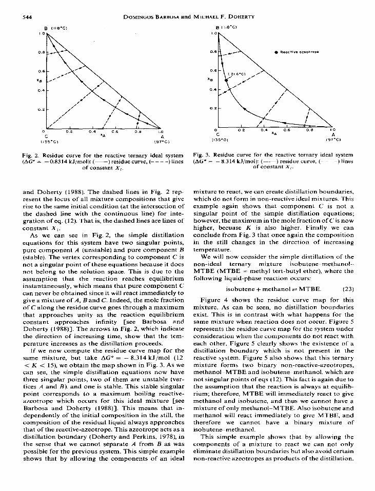
Fig. 2. Residue curve for the reactive ternary ideal system Fig. 3. Residue curve for the reactive ternary ideal system (AG“ = - 0.8314 kJ/mol): (+- ) residue curve, (- - - -) lines (AG” = -X.314 kJ/mol): (-- ) residue curve, (- - - -) lines

of constant Xi. of constant X,.

and Doherty (1988). The dashed lines in Fig. 2 represent the locus of all mixture compositions that give rise to the same initial condition (at the intersection of the dashed line with the continuous line) for integration of eq. (12). That is, the dashed lines are lines of constant Xi.

As we can see in Fig. 2, the simple distillation equations for this system have two singular points, pure component A (unstable) and pure component B (stable). The vertex corresponding to component C is not a singular point of these equations because it does not belong to the solution space. This is due to the assumption that the reaction reaches equilibrium instantaneously, which means that pure compbnent C can never be obtained since it will react immediately to give a mixture of A, Band C. Indeed, the mole fraction of C along the residue curve goes through a maximum that approaches unity as the reaction equilibrium constant approaches infinity [see Barbosa and Doherty (1988)]. The arrows in Fig. 2, which indicate the direction of increasing time, show that the temperature increases as the distillation proceeds.

If we now compute the residue curve map for the same mixture, but take AG” = -8.314 kJ/mol (12 < K -c 15), we obtain the map shown in Fig. 3. As we can see, the simple distillation equations now have three singular points, two of them are unstable (vertices A and B). and one is stable. This stable singular point corresponds to a maximum boiling reactive- azeotrope which occurs for this ideal mixture [see Barbosa and Doherty (1988)]. This means that in- dependently of the initial composition in the still, the composition of the residual liquid always approaches that of the reactive-azeotrope. This azeotrope acts as a distillation boundary (Doherty and Perkins, 1978), in the sense that we cannot separate A from B as was possible for the previous system. This simple example shows that by allowing the components of an ideal

mixture to react, we can create distillation boundaries, which do not form in non-reactive ideal mixtures. This example again shows that component C is not a singular point of the simple distillation equations; however, the maximum in the mole fraction of C is now higher, becuase K is also higher. Finally we can conclude from Fig. 3 that once again the composition in the still changes in the direction of increasing temperature.

We will now consider the simple distillation of the non-ideal ternary mixture isobutene-methanol- MTBE (MTBE = methyl tert-butyl ether), where the following liquid-phase reaction occurs:

isobutene + methanol * MTBE. (23)

Figure 4 shows the residue curve map for this mixture. As can be seen, no distillation boundaries exist. This is in contrast with what happens for the same mixture when reaction does not occur. Figure 5 represents the residue curve map for the system under consideration when the components do not react with each other. Figure 5 clearly shows the existence of a distillation boundary which is not present in the reactive system. Figure 5 also shows that this ternary mixture forms two binary non-reactive-azeotropes, methanol-MTBE and isobutene-methanol, which are not singular points of eqs (12). This fact is again due to the assumption that the reaction is always at equilibrium; therefore, MTBE will immediately react to give methanol and isobutene, and thus we cannot have a mixture of only methanol-MTBE. Also isobutene and methanol will react immediately to give MTBE, and therefore we cannot have a binary mixture of isobutene-methanol.

This simple exampIe shows that by allowing the components of a mixture to react we can not only eliminate distillation boundaries but also avoid certain non-reactive azeotropes as products of the distillation.


METHANOL i64.7'C)

MTBE x* JSOBUTENE

(55 I’CI C-6 9-c)

Fig. 4. Residue curve for the reactive system isobutene-methanol-MTBE: (- ) residue curve, (- - - -) lines

of constant Xi.

METHANOL (64.7OCl

‘.“h

0.2 -

I 0 02 no 06 0.8 1.0

M&E --- _.

x1 ISOBUTENE (55. I~C) c-6.9°c1

Fig. 5. Residue curve map for the non-reactive system isobutene-methanol-MTBE.

FOUR-COMPONENT SYSTEMS

We now study the simple distillation of four- component mixtures that undergo a liquid-phase reaction of the type

A+B-_,C+D. (24)

Consider the ideal system described by Barbosa and Doherty (1988) for which the average value of the volatilities of reactant Band products C and D relative to reactant A are 3.9,4.2 and 1.7 respectively, and AG” = - 8.314 kJ/mol (12 <K < 18). To compute the residue curve map for this mixture we must integrate two of the differential eqs (12). In this integration we again chose the product of reaction, C, as component k, to calculate the transformed variables (Xi, Y,).

Figure 6 represents the X,-X, phase plane for this system. Each trajectory in this phase plane corresponds to a residue curve, i.e. it shows how X, and X, change with time. Since each vertex of the square corresponds to a pure component, we can see that the singular points of the simple distillation equations, for this mixture, are the four pure component vertices. The vertex corresponding to pure component A (the heaviest component) is a stable node, while the vertex corresponding to pure component C (the lightest component) is an unstable node. The remaining vertices corresponding to pure B and D are both saddle points. As happened for the ternary-mixture examples, this residue curve map shows that temperature increases with time.

If we now choose the components in such a way that the average volatilities of reactant B and products C and D relative to reactant A are 1.7, 3.9 and 4.2 respectively, and AG” = 0.8314 kJ/mol (K z 0.76). we will obtain the residue curve map represented in Fig. 7. Figure 7 clearly shows the existence of four distillation boundaries for this system, i.e. the lines connecting the four pure-component vertices to the saddle. These distillation boundaries appear because of the formation of a quaternary saddle reactive-azeotrope for this mixture [see Barbosa and Doherty (1988)]. Figure 7 shows that for this system the simple distillation equations have five singular points, two stable nodes (pure A and B), two unstable nodes (pure C and D),

and a saddle point (the quaternary reactive-azeotrope). Once again we see that by allowing the components of the mixture to react we can create distillation boundaries in systems that otherwise would not have them.

Finally we will study the simple distillation of the non-ideal quaternary system acetic acid-ethanol+thyl acetate-water, when the following liquid-phase esterification reaction occurs:

acetic acid + ethanol e ethyl acetate + water. (25)

(78’C) 177-c) B C

Fig. 6. Residue curve map for the reactive quaternary ideal system, when the volatilities of the reactants and products of

reaction are intermixed.

546 DOMINGOSBARBOSA and MKHAELF.DOHERTY

0 *aactivs az*.¶trop.

(IOO’CI (78’C)

B c -1.0

these components will react to give a mixture of the four components. However, mixtures of ethanol-ethyl acetate and ethanol-water do not react, even in the presence of the catalyst, and, therefore, they can be obtained as products of the simple distillation.

Fig. 7. Residue curve map for the reactive quaternary ideal system, when both reactants are heavier than the products of

reaction.

If we integrate the differential equations that describe the simple distillation, using ethyl acetate as component k, we will obtain the phase plane presented in Fig. 8. As we can see, the singular points are the four pure-component vertices and two binary non-reactive azeotropes (i.e. ethanol-ethyl acetate and ethanol-water). However, this system forms two other non-reactive azeotropes, ethyl acetate-water and ethanol-thy1 acetate-water, that are not singular points of the simple distillation equations. The expla- nation for this fact is once again the assumption of instantaneous reaction equilibrium, which means that once we have a mixture of ethyl acetate and water,

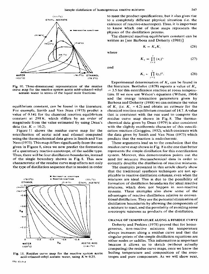
This result is better understood if we see what happens to the residue curve map of the non-reactive system acetic acid+thanolLethyl acetate-water, once we allow these components to react. Figure 9 shows the residue curve map for this quaternary mixture when the components do not react. In Fig. 9 only a selection of the residue curves, that would otherwise fill the entire volume of the tetrahedron, are shown. As expected, all the four pure-component vertices and all the four azeotropes are singular points of the non- reactive simple distillation equations. Once we allow the components to react (e.g. adding the catalyst), we lose one degree of freedom, and the residue curves, instead of occupying the entire volume of the tetrahedron will, instead, lie on a surface inside the tetrahedron, as shown in Fig. 10. This surface is the projection of the bubble-point surface in the reactive T-x phase diagram onto the supporting composition space (as was the case in ternary mixtures). It is clear from Fig. 10 that the ethyl acetate-water and ethyl acetate-water-than01 azeotropes do not lie on this surface, and therefore are not solutions of the reactive simple distillation equations. Note that the transformed variables have the remarkable property of representing these complex reactive bubble-point surfaces by a square.

Once again these results show that by allowing the components in a mixture to react, we can avoid the formation of some non-reactive azeotropes that would otherwise appear as products of the distillation.

To compute the chemical reaction equilibrium constant for this esrerification system we used the thermochemical data given by Dean (1979). However, other sets of thermochemical data for this same system, which give rise to different values for the esterification

. Nonraocrlva 0Zeo,r(JV*

I78 3°C) (77 IPCI ETHANOL 171 BI’C, ETHYL ACETATE

/ (77.I’Cl

ETHYL ACETATE

A I/h\

. N.mr.octl”* Oz.O+lOP.

Cl -0 z -0.4 - 0.6 -0.8 XA

-1.0

WATER ACETIC ACID

(!OO’C~ U48 I OC)

Fig. 9. Three-dimensional representation of the residue curve map for the non-reactive system acetic acid- Fig. 8. Residue curve map for the reactive system acetic

acid-ethanol+thyl acetate-water, using 7.1 -C K -c 8.2. ethanol+thyl acetate--water.


(77 I’CI

ETHYL ACETATE

Fig. 10. Three-dimensional representation of the residue curve map for the reactive system acetic acid-ethanol+thyl

acetate-water in terms of the liquid mole fractions.

equilibrium constant, can be found in the literature. For example, Smith and Van Ness (1975) predict a value of 0.141 for the chemical reaction equilibrium constant at 298 K, which differs by an order of magnitude from the value estimated by using Dean’s data (i.e. K = 10.2).

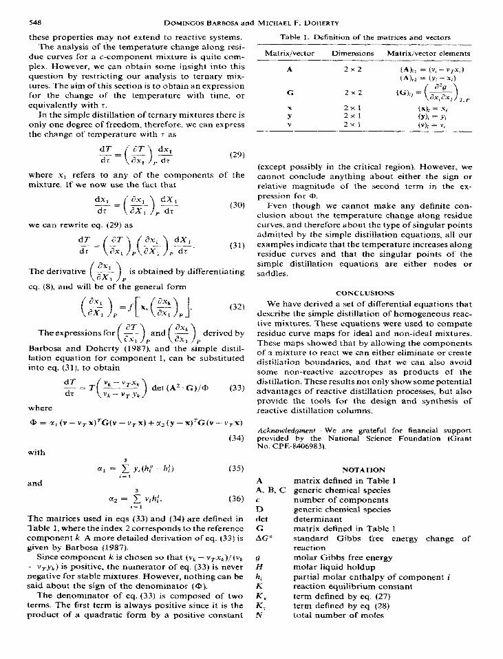
Figure 11 shows the residue curve map for the esterification of acetic acid and ethanol computed using the thermochemical data given in Smith and Van Ness (1975). This map differs significantly from the one given in Figure 8, since we now predict the formation of a quaternary reactive-azeotrope, of the saddle type. Thus, there will be four distillation boundaries, instead of the single boundary shown in Fig. 8. This new characteristic of the residue curve map affects not only the type of distillation sequence that is needed in order

Fig. 11. Residue curve map for the reactive system acetic acid%thanol-ethyl acetate-water, using K a 0.25.

to meet the product specifications, but it also gives rise to a completely different physical situation (i.e. the existence of reactive-azeotropes). Thus, it is important to know which one of these maps represents the physics of the distillation process.

The chemical reaction equilibrium constant can be written as [see Barbosa and Doherty (1988)]

where

K = K,K, (26)

K, = fi (Xi),, (27) i=l

and

K, = lj (Yi)“‘_ (28) i=r

Experimental determination of K, can be found in the literature. Berthelot (1878) reports a value of K, = 3.5 for this esterification reaction at room temperature. If we now use Wilson’s equation (Wilson, 1964) and the energy interaction parameters given by Barbosa and Doherty (1988) we can estimate the value of Kj. (i.e. K, = 4.2) and obtain an estimate for the chemical reaction equilibrium constant of 14.7. A value that is consistent with the one used to compute the residue curve map shown in Fig. 8. The thermochemical data given by Dean (1979) is also consistent with the slightly exothermic character of this esterification reaction (Groggins, 19X2), which contrasts with the data given by Smith and Van Ness (1975) which predicts that the reaction is endothermic.

These arguments lead us to the conclusion that the residue curve map shown in Fig. 8 is the one that better represents the simple distillation for this esterification system. Morever, this demonstration points out the need for accurate thermochemical data in order to correctly describe the distillation of reactive mixtures.

The examples presented in this article clearly show that the traditional synthesis techniques are not ap- plicable to reactive distillation columns, even when the mixtures are ideal. This is due to the possibility of formation of distillation boundaries for ideal reactive mixtures, which does not happen in non-reactive systems. These examples also show some of the advantages of reactive distillation relative to conventional distillation. They are the potential elimination of distillation boundaries by allowing the components of a mixture to react, and the possibility of avoiding some azeotropic mixtures as products of the distillation.

CHANGE OF TEMPERATURE ALONG A RESIDUE CURVE

Doherty and Perkins (1978) proved that for homogeneous, non-reactive mixtures the temperature always increases along a residue curve and that the singular points of the simple distillation equations are either nodes or saddles. This information is important because it allows us to sketch (without actually computing) the residue curve maps, once we know the boiling temperature and composition of the azeotropes and pure components. As we will show next,

548 DUMINGOS BARBOSA and MICHAEL F. DOHERTY

these properties may not extend to reactive systems. The analysis of ihe temperature change along resi-

due curves for a c-component mixture is quite complex. However, we can obtain some insight into this question by restricting our analysis to ternary mixtures. The aim of this section is to obtain an expression for the change of the temperature with time, or equivalently with T.

In the simple distillation of ternary mixtures there is only one degree of freedom, therefore, we can express the change of temperature with T as

(29)

where xi refers to any of the components of the mixture. If we now use the fact that

we can rewrite eq. (29) as

(31)

. The derivative p is obtained by differentiating

eq. (8), and will be of the general form

(32)

The expressions for (g ) and (2) derived by

Barbosa and Doherty (1987: and the’ si&ple distillation equation for component I, can be substituted into eq. (311, to obtain

z = T( $zE) det (A’.G)/ft,

where

@ =~,(~--Y7~)TG(v-vY7~)+a,(y-x)T~(v

with

and

(33)

VTX)

(34)

(35)

(36)

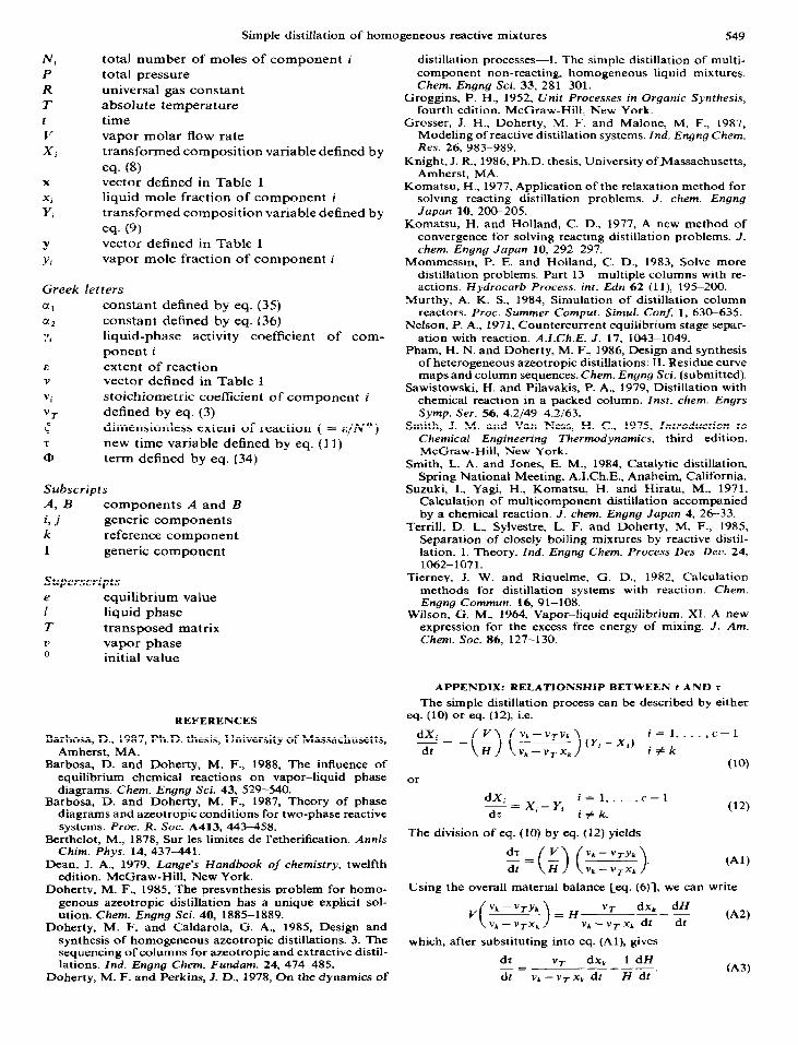
The matrices used in eqs (33) and (34) are defined in Table 1, where the index 2 corresponds to the reference component k. A more detailed derivation of eq. (33) is given by Barbosa (1987).

Since component k is chosen so that (vL - vrxk)/(vn - vryk) is positive, the numerator of eq. (33) is never negative for stable mixtures. However, nothing can be said about the sign of the denominator (Q).

The denominator of eq. (33) is composed of two terms. The firs& term is always positive since it is the product of a quadratic form by a positive constant

Table 1. Definition of the matrices and vectors

Matrix/vector Dimensions Matrix/vector elements

A 2x2 (A):, = (v, - I’~x’<) (A),, = (Y; - xi)

G 2x2 7.P

x 2X1 fX)i = xi Y 2x1 (Y)i = Yi v 2x1 (v); = Y,

(except possibly in the critical region). However, we cannot conclude anything about either the sign or relative magnitude of the second term in the expression for a.

Even though we cannot make any definite conclusion about the temperature change along residue curves, and therefore about the type of singular points admitted by the simpIe distillation equations, all our examples indicate that the temperature increases along residue curves and that the singular points of the simple distillation equations are either nodes or saddles.

CONCLUSIONS

We have derived a set of differential equations that describe the simple distillation of homogeneous reactive mixtures. These equations were used to compute. residue curve maps for ideal and non-ideal mixtures. These maps showed that by allowing the components of a mixture to react we can either eliminate or create distihation boundaries, and that we can also avoid

some non-reactive azeotropes as products of the distillation. These results not only show some potential advantages of reactive distillation processes, but also provide the tools for the design and synthesis of reactive distillation columns.

Acknowledgment--We are grateful for financial support provided by the National Science Foundation (Grant No. CPE-8406983).

A A, 6 C

fi, det G AG”

NOTATION

matrix defined in Table 1 generic chemical species number of components generic chemical species determinant matrix defined in Table 1 standard Gibbs free energy change of reaction molar Gibbs free energy molar liquid holdup partial molar enthalpy of component i reaction equilibrium constant term defined by eq. (27) term defined by eq. (28) total number of moles


N; total number of moles of component i

P total pressure

R universal gas constant T absolute temperature

t time V vapor molar flow rate

Xi transformed composition variable defined by

eq. (8) x vector defined in Table 1

Xi liquid mole fraction of component i Yi transformed composition variable defined by

eq. (9)

Y vector defined in Table 1

Yi vapor mole fraction of component i

Greek letters

a1 constant defined by eq. (35)

a2 constant defined by eq. (36)

Yi liquid-phase activity coefficient of com-

ponent i E extent of reaction Y vector defined in Table 1

vi stoichiometric coefficient of component i

VT defined by eq. (3)

5 dimensionless extent of reaction ( = E/NO) r new time variable defined by eq. (11) CD term defined by eq. (34)

Subscripts

A, B components A and B

i, .i generic components k reference component

1 generic component

Superscripts e equilibrium value 1 liquid phase

T transposed matrix ” vapor phase 0 initial value

REFERENCES

Barbosa, D., 1987, Ph.D. thesis, University of Massachusetts, Amherst, MA.

Barbosa, D. and Doherty, M. F., 1988, The influence of equilibrium chemical reactions on vapor-liquid phase diagrams. Chem. Engng Sci. 43, 529-540.

Barbosa, D. and Doherty, M. F., 1987, Theory of phase diagrams and azeotropic conditions for two-phase reactive systems. Proc. R. Sot. A413, 443458.

Berthelot, M., 1878, Sur les limites de l’etherification. Annls Chim. Phys. 14, 437-441.

Dean, J. A., 1979, Lange’s Handbook of chemistry, twelfth edition. McGraw-Hill, New York.

Doherty, M. F., 1985, The presynthesis problem for homo- genous azeotropic distillation has a unique explicit solution. Chem. Engng Sci. 40, 1885-1889.

Doherty, M. F. and Caldarola, G. A., 1985, Design and synthesis of homogeneous azeotropic distillations. 3. The sequencing of columns for azeotropic and extractive distillations. Ind. Engng Chem. Fundam. 24,474-485.

Doherty, M. F. and Perkins, J. D., 1978, On the dynamics of

distillation processes--l. The simple distillation of multicomponent non-reacting, homogeneous liquid mixtures. Chem. Engng Sci. 33, 281-301.

Groggins, P. H., 1952, Unit Processes in Organic Synthesis, fourth edition. McGraw-Hill, New York.

Grosser, J. H., Doherty, M. F. and Malone,_ M. F., 1987, Modeling of reactive distillation systems. Ind. Engng Chem. Res. 26, 983-989.

Knight, J. R., 1986, Ph.D. thesis, University OfMassachusetts, Amherst, MA.

Komatsu, H., 1977, Application of the relaxation method for solving reacting distillation problems. J. them. Engng Japan 10, 20&205.

Komatsu, H. and Holland, C. D., 1977, A new method of convergence for solving reacting distillation problems. J. them. Engng Japan JO, 292-297.

Mommessin, P. E. and Holland, C. D., 1983, Solve more distillation problems, Part 13-multiple columns with reactions. Hydrocarb Process. int. Edn 62 (ll), 195200.

Murthy, A. K. S., 1984, Simulation of distillation column reactors. Proc. Summer Comput. Simul. ConJ 1, 63&635.

Nelson, P. A., 1971, Countercurrent equilibrium stage separation with reaction. A.1.Ch.E. .I. 17, 1043-1049.

Pham, H. N. and Doherty, M. F., 1986, Design and synthesis of heterogeneous azeotropic distillations: 11. Residue curve maps and column sequences. Chem. Engng Sci. (submitted).

Sawistowski, H. and Pilavakis, P. A., 1979, Distillation with chemical reaction in a packed column. Insr. them. Engrs Symp. Ser. 56, 4.2/494.2/63.

Smith, J. M. and Van Ness, H. C., 1975, Introducrion to Chemical Engineering Thermodynamics, third edition. McGraw-Hill, New York.

Smith, L. A. and Jones, E. M., 1984, Catalytic distillation, Spring National Meeting, A.I.Ch.E., Anaheim, California.

Suzuki, I., Yagi, H., Komatsu, H. and Hirata, M., 1971, Calculation of multicomponent distillation accompanied by a chemical reaction. J. them. Engng Japan 4, 26-33.

Terrill, D. L., Sylvestre, L. F. and Doherty, M. F., 1985, Separation of closely boiling mixtures by reactive distillation. 1. Theory. Ind. Engng Chem. Process Des. Deu. 24, 1062-1071.

Tierney, J. W. and Riquelme, G. D., 1982, Calculation methods for distillation systems with reaction. Chem. Engng Commun. 16, 91-108.

Wilson, G. M., 1964, Vapor-liquid equilibrium. XI. A new expression for the excess free energy of mixing. J. Am. Chem. Sot. 86, 127-130.

APPENDIX: RELATIONSHIP BETWEEN t AND r

The simple distillation process can be described by either eq. (10) or eq. (12) i.e.

or

dX. L=X;_y(

i=l,....c--l

ds i # k.

The division of eq. (10) by eq. (12) yields

$(Ic) (s).

(12)

(Al)

Using the overall material balance [eq. (6)], we can write

v(s) = H,,_‘:,,,%-g (A2)

which, after substituting into eq. (Al), gives

dr “T dx, 1 dH

dt= _-___

v,-vTxk dr H dt c.43)

550 DOMINGOS BARBOSA and MKHAEL F. DOHERTY

If we define 5, so that

r=O att=O

then we obtain a relationship between T and t by integrating eq. (A3), i.e.

7 = In H (0) Cvt - v T xlr (011 H(~)Cvk--vTXk@~l

(A4)

where H (0) and x,(O) are the initial liquid holdup and initial liquid mole fraction of component k, respectively. Since component k is chosen so that v* - v+~(t) is never zero, we obtain the limiting values of r, as t varies between 0 and tmax,

thus

and

r=O att=O

T = + 03 at t = t_.Ji.e. H(t,,,) = 01.

Noting that Vand Hare never negative, and (v,, - vryr) /(vlr - vTxr) is always positive (because of the convenient choice of component k), eq. (Al) guarantees

dr - > 0. dt

Thus, we conclude that r(t) is a strictly monotonically increasing function of time defined between 0 and + co.

The Simple Distillation of Homogeneous Reactive Mixtures

Documents

Transcript of The Simple Distillation of Homogeneous Reactive Mixtures