Abstract— This paper presents a novel procedure to classify data from mixtures of independent component analyzers. The procedure includes two stages: learning the parameters of the mixtures (basis vectors and bias terms) and clustering the ICA mixtures following a bottom-up agglomerative scheme to construct a hierarchy for classification. The approach for the estimation of the source probability density function is non-parametric and the minimum kullback-Leibler distance is used as a criterion for merging clusters at each level of the hierarchy. Validation of the proposed method is presented from several simulations including ICA mixtures with uniform and Laplacian source distributions and processing real data from impact-echo testing experiments.

I. INTRODUCTION

ATTERN analysis and recognition are processes familiar to many human activities. They imply to

separate data into self-similar areas and analyzing each of these clusters under some application framework. Intelligent signal processing algorithms provide an important tool to support automatic pattern recognition, gain insight into problem solving, and complement expert decision making [1-4]. Usually those algorithms make assumptions about data generating process, for instance, modeling the data as a mixture of data generators or analyzers, considering that each generator produces a particular group of data. The most used data mixture model is the well known Gaussian Mixture Model that assumes each generator is a Gaussian density. The field of GMM applications is wide but many clustering problems do not fit the assumption of Gaussian density or the problem high feature dimensionality makes no suitable to use GMM [1,5,6].

Recently has emerged the mixture of Independent Component Analyzers [7,8] as a flexible model to generate arbitrary data densities using mixtures of different distributions for the components [9,10]. In order to span more applications, new versions of ICA mixtures algorithms have loosened up assumptions about component distributions and propose calculating the components in a non-parametric manner [11]. In addition, more general approaches for the procedure to find the cluster structure of ICA analyzers, relaxing the independence hypothesis of ICA in order to analyze more complex problems, and trying to derive physical interpretations, has been proposed [12-14].

This work has been supported by Spanish Administration under grant

TEC 2005-01820. A. Salazar, J. Igual, L. Vergara, and A. Serrano are with Universidad

Politécnica de Valencia, Departamento de Comunicaciones, Camino de Vera s/n, 46022, Valencia, Spain. (e-mails: asalazar@dcom.upv.es, jigual@dcom.upv.es, lvergara@dcom.upv.es, arsercar@upvnet.upv.es).

The contribution of the present paper is a new procedure to classify data from mixtures of independent component analyzers. This method does not consider any assumption on the probability density function of the sources and apply a non-parametric approach to estimate the parameters of the ICA mixture (basis vectors and bias terms). A clustering algorithm is applied on the estimated parameters and the data to merge the ICA mixtures in a bottom-up agglomerative scheme. The symmetric Kullback-Leibler distance [15] is used to select the grouping of the clusters.

We validate the procedure with several simulations, varying the number and kind of distributions of the sources, the number of ICA mixtures and using different supervision ratios in the learning stage of the parameters. In addition, we demonstrate real application of the proposed method to automatic classification of specimens tested by non-destructive impact-echo testing [16]. There are few references of applying ICA in impact-echo signals [17].

The underlying problem of the experiments was to obtain automatically a suitable hierarchical classification of parallelepiped-shape specimens of aluminum alloy with different defective conditions. The pieces were one-defect and multiple-defects, and the defects consisted in holes and cracks with different spatial orientations.

The following sections contain the detailed algorithms and computations of the procedure, results, and conclusions.

II. LEARNING MIXTURES OF INDEPENDENT COMPONENT

ANALYZERS

Normally in mixture of ICAs, the observation vectors kx

corresponding to a given class )1(, KkCk are modeled

as the result of applying a linear transformation kA to a

vector ks (sources), whose elements are independent

random variables, plus a bias vector kb , i.e.

Kkkkkk ...1 bsAx (1)

Optimum classification of a given feature vector x of

unknown class, consists in selecting the class kC having

maximum conditional probability x/kCp . Applying Bayes

theorem we obtain:

K

kkk

kkkkk

CpCp

CpCp

p

CPCpCp

1'''/

///

x

x

x

xx

(2)

If x is a feature vector corresponding to class

kC , then

Learning Hierarchies from ICA Mixtures

Addisson Salazar, Jorge Igual, Luis Vergara, Arturo Serrano

P

kkk pCp sAx 1det/

(3)

where kkk bxAs 1 . Considering equations (3) and (2),

we may write

K

kkk

kk

k

p

pCp

1''

1

1

'det

det/

sA

sAx

(4)

Thus, given a feature vector x , we have to compute the

corresponding source vectors )1(, Kkk s , from

kkk bxAs 1 , to finally select the class having the

maximum computed value kk p sA 1det (note that the

denominator in (4) is not depending on k , so that it does not influence the maximization of x/kCp .

To make the above computation, we need knowledge of 1

kA , kb (to compute

ks from x ) and of the multidimensional

pdf of the source vectors for every class (to compute kp s ).

Two assumptions will be considered to solve this problem. First, that the elements of

ks , are independent random

variables (ICA assumption), so that the multidimensional pdf can be factored into the corresponding marginal pdf’s of every vector element. The second assumption is that there is available a set of independent feature vectors (learning vectors) represented by matrix NxxX ...1 . We consider

a hybrid situation where some of the learning vectors have known class (supervised learning), meanwhile others are of unknown class (unsupervised learning). Actually, we are going to consider a more general case in which knowledge of n

kCp x/ could be available for some a subset of nk

pairs (supervised learning) and unknown for the rest (unsupervised learning).

If we assume a non-parametric model for ),1(, Kkp k s , we can estimate the source pdf’s from a

set of training samples obtained from the original set NxxX ...1 , by applying k

nk

nk bxAs 1

),1 ,,1( KkNn . Hence we can concentrate in the

optimum estimation of 1kA ,

kb ),1( Kk . Let us define 1 kk AW to ease the notation.

We need a cost function definition to obtain optima estimates of the unknowns. In a probability context it is usual to maximize the log-likelihood of the data, i.e., to select those unknowns maximizing the probability of the training set conditioned to the unknowns. As we have assumed independent feature vectors in the training set, we may write the log-likelihood in the form:

N

n

nppL1

/log/log/ ΨxΨXΨX (5)

where Ψ is a compact notation for all the unknown

parameters kW ,

kb for all the classes. In a mixture model,

the probability of every available feature vector can be separated into the contributions due to every class.

The general algorithm (including non-parametric source pdf estimation, supervised-unsupervised learning, and possibility of selecting a particular ICA algorithm) is

0 Initialize 0i , 0,0 kk bW .

1 Compute NnKkiii k

nk

nk ...1..1 bxWs

2 Directly use ΨxΨx ,/,/ nk

nk CpiCp

for those nk pairs with knowledge about Ψx ,/ n

kCp .Compute

Kk

ipi

ipiiCp

K

k

nkk

nkkn

k ...1

det

.det,/

1'''

sW

sWΨx

for the rest of nk pairs.

Use

KkMmeaspnn

h

ss

nkm

nkm

nkm

...1...1'

2

2

1'

to

estimate the marginals ip nks .

3 Use the selected ICA algorithm to compute the increments ik

n

ICAW corresponding to the

observation Nnn ,1, x , that would be applied in ikW , in an “isolated” learning of

class kC . Compute the total increment by

iCpii nk

N

nk

nk ICA

ΨxWW ,/1

.

Update Kkiii kkk ...11 WWW .

4 Compute ikb using

N

n

nkkm

nkk iCpidiagi

1

,/ Ψxwsfb .

Use

nkm

nn

h

ss

nn

h

ss

nkm

nkm s

e

es

hsf

nkm

nkm

nkm

nkm

'

2

2

1

'

2

2

1

'

2 '

'

1 to

estimate nksf .

Actualize

Kkiii kkk ...11 bbb , or

simply re-estimate

Kk

iCp

iCp

iN

n

nk

N

n

nk

n

k ...1

,/

,/

1

1

1

Ψx

Ψxx

b

5 Go back to step 1, with the new values 1,1 ii kk bW and 1 ii

III. HIERARCHICAL ICA MIXTURES

This section describes the procedure to cluster the ICA mixtures obtained for the non-parametric algorithm explained in the previous section. The procedure follows a bottom-up agglomerative scheme for merging the mixtures.

The conditional probability density of x for cluster , 1, 2,..., 1h

kC k K h in layer 1, 2,...,h K is ( / )hkp Cx .

At the first level, 1h , it is modelled by the K-ICA

mixtures, i.e., 1( / )kp Cx is:

1 1( / ) detk k kp C px A s , kkk bxAs 1 (6)

At each consecutive level, two clusters are merged

according to some minimum distance measure until we reach at level h K only one cluster.

As distance measure we use the symmetric Kullback-Leibler divergence between the ICA mixtures. It is defined for the clusters ,u v by:

( / )( , ) ( / ) log

( / )

( / )( / ) log .

( / )

hh h h u

KL u v u hv

hh vv h

u

p CD C C p C d

p C

p Cp C d

p C

xx x

x

xx x

x

(7)

For layer 1j , from (7), we can obtain (we write

1( ) ( / )u up p Cx x x and omit the superscript 1h for

brevity):

( , ) ( ( ) // ( ))

( ) ( )( ) log ( ) log .

( ) ( )

u v

u v

u v

v u

KL u v KLD C C D p p

p pp d p d

p p

x x

x xx x

x x

x x

x xx x x x

x x

(8)

where, imposing the independence hypothesis and

supposing that both clusters have the same number of sources M for simplicity:

11

1 1

( )( ) ,

det

( )( ) ,

det

u ii

u i i i

v jj

v j j j

M

s ui

u u uu

M

s vj

v v vv

p sp s

p sp s

x

x

x A x bA

x A x bA

(9)

The pdf of the sources is approximated by a non-parametric kernel-based density for both clusters:

22 ( )( ) 1122

1 1

( ) , ( )

v vj ju ui i

u i v ji j

s s ns s nN N

hh

s u s vn n

p s ae p s ae

(10)

where again for simplicity we have assumed the same kernel function with the parameters ,a h for all the sources and the same number of samples N for each one. Note that this corresponds to a mixture of Gaussians model where the number of Gaussians is maximum (one for every observation) and the parameters are equal. Reducing to standard mixture of Gaussians with different number of

components and priors for every source does not help in order to compute the Kullback-Leibler distance because there is not analytical solution to it. Therefore, we prefer to maintain the non parametric approximation of the pdf in order to model more complex distributions than a mixture of a small finite number of Gaussians, such as three or four.

The symmetric Kullback-Leibler distance between the clusters ,u v can be expressed such as:

( ( ) // ( )) ( ) ( )

( ) log ( ) ( ) log ( ) .

u v

u v v u

KL u vD p p H H

p p d p p d

x x

x x x x

x x x x

x x x x x x (11)

where ( )H x is the entropy, defined as

( ) log ( )H E p xx x . To obtain the distance, we have to

calculate the entropy for both clusters and the cross-entropy

terms log ( ) , log ( )v u u v

E p E p x x x xx x .

The entropy for the cluster u can be calculated through the entropy of the sources of that cluster considering the linear transformation of the random variables and their independence (9):

1

( ) ( ) log deti

M

u u ui

H H s

x A (12)

The entropy of the sources can not be analytically

calculated. Instead, we can obtain a sample estimate of it, ˆ ( )

iuH s , using the training data. Denote the i-th source

obtained for the cluster u by (1), (2), , ( )i i iu u u is s s Q . The

entropy can be approximated as follows:

2

1

( ) ( )1

2

1

1ˆ ˆ( ) log ( ) log ( ( ))

, ( ( )) .

i

i u i u ii i

u ui i

u ii

Q

u s u s uni

s n s lN

h

s ul

H s E p s p s nQ

p s n ae

(13)

The entropy of ( )vH x is obtained analogously:

2

1

1

1

( ) ( )1

2

1

( ) ( ) log det

ˆ ( ) log det .

1ˆ ( ) log ( ( ))

, ( ( )) .

i

i

i

i v ii

v vi i

v ii

M

v v vi

M

v vi

Q

v s vni

s n s lN

h

s vl

H H s

H s

H s p s nQ

p s n ae

x A

A

(14)

with ˆ ( )ivH s defined analogously to (13).

Once the entropy is computed, we have to obtain the cross-entropy terms. After some operations and considering the relationships ,u u u v v v x A s b x A s b and

1v v u u u v

s A A s b b , the independence of the sources,

and that the samples for clusters ,u v follow the

corresponding distribution (1), (2), , ( )i i iu u us s s Q ,

1,...,i M , (1), (2), , ( )j j jv v vs s s Q , 1,...,j M the

following computation is obtained:

2

1 1

1 1

1

( ) ( )1

2

1

1

ˆ ˆ( ( ) // ( )) ( ) ( )

ˆ ˆ( , ) ( , ).

1ˆ ( ) log ( ( )),

where ( ( )) .

1ˆ ( ) log ( ( ))

u v i j

i j

i u ii

u ui i

u ii

j v jj

M M

KL u vi j

M M

v u u vi j

Q

u s un

s n s lN

hs u

l

v s vn

D p p H s H s

H s H s

H s p s nQ

p s n ae

H s p s nQ

x xx x

s s

2

21

1

1

( ) ( )1

2

1

( )1

2

1 1 1

( )1

2

,

where ( ( )) .

1ˆ ( , )

... log .

1ˆ ( , )

... log

v vj j

v jj

i

u v v v u uii

v vM

j

v u u u v v jj

Q

s n s lN

h

s vl

v u M

s n

Q Q N h

s s n

u v M

s n

h

p s n ae

H sQ

ae

H sQ

ae

A A s b b

A A s b b

s

s

2

11 1 1

.u uM

Q Q N

s s n

(15)

As we can observe, the similarity between clusters depends on not only the similarity between the bias term, but the similarity between the distributions and the mixing matrices.

Once the distances are obtained for all the clusters, the two clusters with minimum distance are merged in level

2h . This is repeated in every step of the hierarchy until we reach one cluster in the level h K . To merge cluster in level h we can calculate the distances from the distances of level 1h . Suppose that from level 1h to h the clusters

1 1,h hu vC C are merged in cluster h

wC . Then, the density for

the merged cluster at level h is:

1 1 1 11 1 1 1

1 11 1

( / )

( ) ( / ) ( ) ( / ).

( ) ( )

hh w

h h h hh u h u h v h v

h hh u h v

p C

p C p C p C p C

p C p C

x

x x (16)

where 1 11 1( ), ( )h h

h u h vp C p C are the priors or proportions

of the clusters ,u v at level 1h . The rest of terms are the

same in the mixture model at level h that at level 1h . The only difference from one level to the next one in the hierarchy is that there is one cluster less and the prior for the new cluster is the sum of the priors of its components and the density the weighted average of the densities that are merged to form it. Therefore, the estimation of the distance at level h can be done easily starting from the distances at level 1h and so on until level 1h . Consequently, we can

calculate the distances at level h from a cluster hzC to a

merged cluster hwC obtained by the agglomeration of clusters

1 1,h hu vC C at level 1h as the distance to its components

weighted by the mixing proportions:

1 1 11 1 1 1

1 11 1

1 1 11 1 1 1

1 11 1

( ( / ) // ( / ))

( ) ( ( / ) // ( / ))

( ) ( )

( ) ( ( / ) // ( / )).

( ) ( )

h hh h w h z

h h hh u h h u h z

h hh u h v

h h hh v h h v h z

h hh u h v

D p C p C

p C D p C p C

p C p C

p C D p C p C

p C p C

x x

x x

x x

(17)

IV. RESULTS

A. Simulations

Fig. 1 shows ten different ICA mixtures, each generated by two independent variables and bias terms. The independent distributions are Laplacians and uniforms. The figure shows an example of how first the algorithm learned the basis vectors and bias terms for each class (Fig. 1a) at level 1, and then uses these estimations in order to create a hierarchical tree of the clusters. The second plot shows the merged clusters at level 5, where 6 clusters remain. The closest clusters are merged. In the third plot there are only 2 clusters remaining. Here we can see how not only the relative bias between clusters is used to merge them, but also similar distributions are merged together. Fig. 1d shows the resulting dendrogram with the distances at which the clusters have been merged.

In order to obtain a good performance of the agglomerative clustering, the bandwidth parameter (h in equation 15) has to be adjusted to avoid the distances are thresholded to one value. There is a compromise between the resolution of the distances and the range of them. Thus we chose a high bandwidth.

To determine a quality criterion that allows knowing the optimum hierarchical level, the partition and entropy coefficient were estimated [17]. Fig. 3 shows the evolution of those coefficients through the levels of clustering of Fig 1. The best number of clusters is at h=5 (6 clusters, Fig. 1b).

The partition coefficient and the partition entropy both tend towards monotone behaviour depending on the number of clusters. So as to find the "best" number of clusters one chooses the number where the entropy value lies below the rising trend and the value for the partition coefficient lies above the falling trend. On viewing the curve of all the

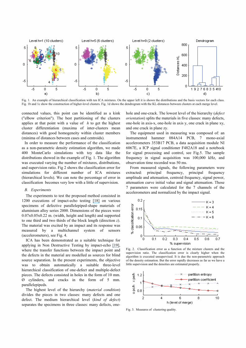
Fig. 1. An example of hierarchical classification with ten ICA mixtures. On the upper left it is shown the distributions and the basis vectors for each class. Fig. 1b and 1c show the construction of higher-level clusters. Fig. 1d shows the dendrogram with the KL-distances between clusters at each merge level.

connected values, this point can be identified as a kink ("elbow criterion"). The best partitioning of the clusters applies at that point with a value of h to get the highest cluster differentiation (maxima of inter-clusters mean distances) with good homogeneity within cluster members (minima of distances between cases and centroids).

In order to measure the performance of the classification as a non-parametric density estimation algorithm, we made 400 MonteCarlo simulations with toy data like the distributions showed in the example of Fig. 1. The algorithm was executed varying the number of mixtures, distributions, and supervision ratio. Fig 2 shows the classification error for simulations for different number of ICA mixtures (hierarchical levels). We can note the percentage of error in classification becomes very low with a little of supervision.

B. Experiments

The experiments to test the proposed method consisted in 1200 executions of impact-echo testing [18] on various specimens of defective parallelepiped-shape materials of aluminium alloy series 2000. Dimensions of the pieces were 0.07x0.05x0.22 m. (width, height and length) and supported to one third and two thirds of the block length (direction z). The material was excited by an impact and its response was measured by a multichannel system of sensors (accelerometers), see Fig. 4.

ICA has been demonstrated as a suitable technique for applying in Non Destructive Testing by impact-echo [19], where the transfer functions between the impact point and the defects in the material are modelled as sources for blind source separation. In the present experiments, the objective was to obtain automatically a suitable three-level hierarchical classification of one-defect and multiple-defect pieces. The defects consisted in holes in the form of 10 mm. Ø cylinders, and cracks in the form of 5 mm. parallelepipeds.

The highest level of the hierarchy (material condition) divides the pieces in two classes: many defects and one defect. The medium hierarchical level (kind of defect) separates the specimens in three classes: many defects, one-

hole and one-crack. The lowest level of the hierarchy (defect orientation) splits the materials in five classes: many defects, one-hole in axis-x, one-hole in axis y, one crack in plane xy, and one crack in plane zy.

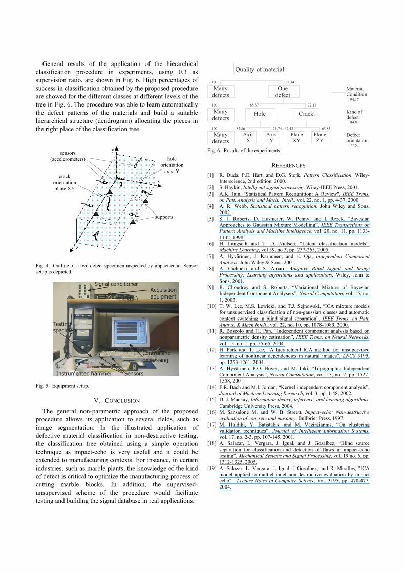
The equipment used in measuring was composed of: an instrumented hammer 084A14 PCB, 7 mono-axial accelerometers 353B17 PCB, a data acquisition module NI 6067E, a ICP signal conditioner F482A18 and a notebook for signal processing and control, see Fig.5. The sample frequency in signal acquisition was 100,000 kHz, and observation time recorded was 50 ms.

From measured signals, the following parameters were extracted: principal frequency, principal frequency amplitude and attenuation, centroid frequency, signal power, attenuation curve initial value and signal attenuation. Those 7 parameters were calculated for the 7 channels of the accelerometers and normalized by the impact signal.

Fig. 2. Classification error as a function of the mixture clusters and the supervision ratio. The classification error is clearly higher when the algorithm is executed unsupervised. It is due the non-parametric approach of the density estimation. But the error rapidly decreases as far as we have a little supervision and the densities are estimated properly.

Fig. 3. Measures of clustering quality.

General results of the application of the hierarchical classification procedure in experiments, using 0.3 as supervision ratio, are shown in Fig. 6. High percentages of success in classification obtained by the proposed procedure are showed for the different classes at different levels of the tree in Fig. 6. The procedure was able to learn automatically the defect patterns of the materials and build a suitable hierarchical structure (dendrogram) allocating the pieces in the right place of the classification tree.

Fig. 4. Outline of a two defect specimen inspected by impact-echo. Sensor setup is depicted.

Fig. 5. Equipment setup.

V. CONCLUSION

The general non-parametric approach of the proposed procedure allows its application to several fields, such as image segmentation. In the illustrated application of defective material classification in non-destructive testing, the classification tree obtained using a simple operation technique as impact-echo is very useful and it could be extended to manufacturing contexts. For instance, in certain industries, such as marble plants, the knowledge of the kind of defect is critical to optimize the manufacturing process of cutting marble blocks. In addition, the supervised-unsupervised scheme of the procedure would facilitate testing and building the signal database in real applications.

Fig. 6. Results of the experiments.

REFERENCES [1] R. Duda, P.E. Hart, and D.G. Stork, Pattern Classification. Wiley-

Interscience, 2nd edition, 2000. [2] S. Haykin, Intelligent signal processing. Wiley-IEEE Press, 2001. [3] A.K. Jain, "Statistical Pattern Recognition: A Review", IEEE Trans.

on Patt. Analysis and Mach. Intell., vol. 22, no. 1, pp. 4-37, 2000. [4] A. R. Webb, Statistical pattern recognition. John Wiley and Sons,

2002. [5] S. J. Roberts, D. Husmeier, W. Penny, and I. Rezek. “Bayesian

Approaches to Gaussian Mixture Modelling”, IEEE Transactions on Pattern Analysis and Machine Intelligence, vol. 20, no. 11, pp. 1133-1142, 1998.

[6] H. Langseth and T. D. Nielsen, “Latent classification models”, Machine Learning, vol 59, no 3, pp. 237-265, 2005.

[7] A. Hyvärinen, J. Karhunen, and E. Oja, Independent Component Analysis. John Wiley & Sons, 2001.

[8] A. Cichocki and S. Amari, Adaptive Blind Signal and Image Processing: Learning algorithms and applications. Wiley, John & Sons, 2001.

[9] R. Choudrey and S. Roberts, “Variational Mixture of Bayesian Independent Component Analysers”, Neural Computation, vol. 15, no. 1, 2003.

[10] T. W. Lee, M.S. Lewicki, and T.J. Sejnowski, “ICA mixture models for unsupervised classification of non-gaussian classes and automatic context switching in blind signal separation”, IEEE Trans. on Patt. Analys. & Mach.Intell., vol. 22, no. 10, pp. 1078-1089, 2000.

[11] R. Boscolo and H. Pan, “Independent component analysis based on nonparametric density estimation”, IEEE Trans. on Neural Networks, vol. 15, no. 1, pp. 55-65, 2004.

[12] H. Park and T. Lee, “A hierarchical ICA method for unsupervised learning of nonlinear dependencies in natural images”, LNCS 3195, pp. 1253-1261, 2004.

[13] A. Hyvärinen, P.O. Hoyer, and M. Inki, “Topographic Independent Component Analysis”, Neural Computation, vol. 13, no. 7, pp. 1527-1558, 2001.

[14] F.R. Bach and M.I. Jordan, “Kernel independent component analysis”, Journal of Machine Learning Research, vol. 3, pp. 1-48, 2002.

[15] D. J. Mackay, Information theory, inference, and learning algorithms. Cambridge University Press, 2004.

[16] M. Sansalone M. and W. B. Streett, Impact-echo: Non-destructive evaluation of concrete and masonry. Bullbrier Press, 1997.

[17] M. Haldiki, Y. Batistakis, and M. Vazirgiannis, “On clustering validation techniques”, Journal of Intelligent Information Systems, vol. 17, no. 2-3, pp. 107-145, 2001.

[18] A. Salazar, L. Vergara, J. Igual, and J. Gosalbez, “Blind source separation for classification and detection of flaws in impact-echo testing”, Mechanical Systems and Signal Processing, vol. 19 no. 6, pp. 1312-1325, 2005.

[19] A. Salazar, L. Vergara, J. Igual, J Gosalbez, and R. Miralles, "ICA model applied to multichannel non-destructive evaluation by impact echo", Lecture Notes in Computer Science, vol. 3195, pp. 470-477, 2004.

y

z

xcrack

orientation plane XY

hole orientation

axis Y

sensors (accelerometers)

supports

Quality of material

Manydefects

Onedefect

Hole Crack

AxisX

AxisY

PlaneXY

PlaneZY

MaterialCondition

Kind ofdefect

Defectorientation

Manydefects

Manydefects

88.34100

100

100

88.37 72.11

82.86 71.74 67.42 65.83

94.17

84.83

77.57

SensorsInstrumented hammer

Signal conditionerAcquisitionequipment

Testingspecimen

Control andprocessing