Commun. Comput. Phys.doi: 10.4208/cicp.2009.09.018

Vol. 7, No. 3, pp. 423-444March 2010

Improved Lattice Boltzmann Without Parasitic

Currents for Rayleigh-Taylor Instability

Daniele Chiappini1,∗, Gino Bella1, Sauro Succi2, Federico Toschi2,3

and Stefano Ubertini4

1 University of Rome Tor Vergata, Via del Politecnico 1, I-00133, Rome, Italy.2 IAC-CNR, Viale del Policlinico 137, I-00161, Rome, Italy.3 Department of Physics and Department of Mathematics and Computer Science,Eindhoven University of Technology, 5600 MB Eindhoven, The Netherlands.4 University of Naples Parthenope, Isola C4 - Centro Direzionale, I-80143, Naples,Italy.

Received 13 January 2009; Accepted (in revised version) 3 June 2009

Communicated by Shiyi Chen

Available online 1 September 2009

Abstract. Over the last decade the Lattice Boltzmann Method (LBM) has gained sig-nificant interest as a numerical solver for multiphase flows. However most of the LBvariants proposed to date are still faced with discreteness artifacts in the form of spuri-ous currents around fluid-fluid interfaces. In the recent past, Lee et al. have proposeda new LB scheme, based on a higher order differencing of the non-ideal forces, whichappears to virtually free of spurious currents for a number of representative situations.In this paper, we analyze the Lee method and show that, although strictly speaking, itlacks exact mass conservation, in actual simulations, the mass-breaking terms exhibita self-stabilizing dynamics which leads to their disappearance in the long-term evo-lution. This property is specifically demonstrated for the case of a moving droplet atlow-Weber number, and contrasted with the behaviour of the Shan-Chen model. Fur-thermore, the Lee scheme is for the first time applied to the problem of gravity-drivenRayleigh-Taylor instability. Direct comparison with literature data for different val-ues of the Reynolds number, shows again satisfactory agreement. A grid-sensitivitystudy shows that, while large grids are required to converge the fine-scale details, thelarge-scale features of the flow settle-down at relatively low resolution. We concludethat the Lee method provides a viable technique for the simulation of Rayleigh-Taylorinstabilities on a significant parameter range of Reynolds and Weber numbers.

AMS subject classifications: 76T02, 68U02

Key words: Lattice-Boltzmann, multiphase, parasitic currents, Rayleigh-Taylor Instability.

∗Corresponding author. Email addresses: chiappini@ing.uniroma2.it (D. Chiappini), bella@

uniroma2.it (G. Bella), succi@iac.cnr.it (S. Succi), toschi@iac.cnr.it (F. Toschi), stefano.ubertini@uniparthenope.it (S. Ubertini)

http://www.global-sci.com/ 423 c©2010 Global-Science Press

424 D. Chiappini et al. / Commun. Comput. Phys., 7 (2010), pp. 423-444

1 Introduction

Multiphase flows are ubiquitous in industrial processes (i.e. chemical, pharmaceutical,electronic, and power-generation industries) and natural phenomena alike [1]. Conse-quently, numerical methods for the investigation of their complex behaviour is in con-stant demand. However, the task of simulating the behavior of multi-phase flows is verychallenging, due to the inherent complexity of the involved phenomena (emergence ofmoving interfaces with complex topology, droplet collision and break-up), and repre-sents one of the leading edges of computational physics [2, 8]. As a matter of fact, ageneral computational approach encompassing the full spectrum of complexity exposedby multiphase flows is still not available.

The numerical methods based on the traditional continuum approach (i.e. Navier-Stokes with closure relationships) are usually based on rather complex correlations andoften require transient solution algorithms with very small time steps. In the last twodecades, a new class of mesoscopic methods, based on minimal lattice formulation ofBoltzmann kinetic equation, have gained significant interest as an efficient alternative tocontinuum methods based on the discretization of the NS equations for non ideal fluids[16].

Since its early days, the Lattice Boltzmann shed promises of becoming a tool forthe modeling of multiphase flows. The earliest Lattice Boltzmann simulations of multi-component flows have been performed by Gunstensen et al. [14, 15] and Grunau et al.[16], based on the pioneering Rothman-Keller lattice gas multi-phase model [13]. Eversince, many models have been proposed in order to simulate multiphase flows withthe LBM, most of them aiming at incorporating the physics of phase-segregation andinterface dynamics, typically hard to model with traditional methods, through simplemesoscopic interaction laws. In particular, the pseudo-potential LBM, due to Shan andChen [18], has gained increasing popularity on account of its conceptual simplicity andcomputational efficiency. In the Shan-Chen (SC) method, potential energy interactionsare represented through a density-dependent, mean-field, pseudo-potential and phaseseparation is achieved by imposing a short-range attraction between the light and densephases. This method allows to track and maintain diffuse interfaces with no need of anyspecial treatment of the interface. However, it is known to present unphysical features(i.e spurious velocities), namely the presence of non-zero velocities even for fluids at rest,with a steady density profile. These spurious currents are disturbing for practical appli-cations, and they may cast doubts on the quantitative accuracy of the simulations meth-ods [28]. The spurious currents have been recently addressed by many authors [3, 4, 17].He et al. [17] proposed a multi-phase LBM scheme with improved numerical stability. Itstill incorporates molecular interactions, but unphysical features are alleviated by intro-ducing a pressure distribution function instead of the single-particle density distributionfunction. A particularly remarkable option has been suggested by Lee et al. [3–6], whoproposed a higher order finite difference treatment of the kinetic forces arising from non-ideal interactions (potential energy). In this model, spurious currents are allegedly tamed

D. Chiappini et al. / Commun. Comput. Phys., 7 (2010), pp. 423-444 425

by a judicious resort to higher-order finite difference treatment of the non-ideal interac-tions.

This model is further investigated in the present paper. More specifically, we analysethe conservation properties of the method proposed by Lee et al. [4, 5] and show thatthe spurious currents in the SC model, for the case of a moving droplet at low Weber,result in a distortion of the flow pattern, which is not seen in the simulation with the Leemodel. Finally we demonstrate the validity of the scheme for a gravity-driven Rayleigh-Taylor (RT) instability, one of the basic and most demanding problems in the numericalsimulation of multiphase flows.

The paper is organized as follows. In Section 2 we briefly review the LB modelscompared in the present paper. Section 3 presents our numerical results. A side by sidecomparison between the Lee and the Shan-Chen methods is presented for the case ofa static and dynamic droplet. Numerical simulations of the two-dimensional Rayleigh-Taylor instability are then presented and compared with previous numerical results atdifferent Reynolds numbers. Finally in Section 4 conclusions and outlooks are drawn.

2 The models

In this section we present a brief survey of the Lee et al. model [4, 5]. As the Shan-Chen [18] has been described at length in many papers, here we only sketch its basicelements.

2.1 The Lee model

The model introduced in [4] starts with a Cahn-Hilliard mixing energy density for-mulation for an isothermal system [26]. In terms of the composition C, this reads as

Emix(C,∇C)=E0(C)+ κ2 |∇C|2, where C is the composition of one component and κ is the

gradient parameter. The bulk energy can be rewritten as E0(C)≈βC2(C−1)2 where β is aconstant fixing the free-energy barrier between the pure states C=0 and C=1. The sameparameter fixes the non-ideal bulk pressure through the (Legendre’s) relation:

p0 =C∂E0

∂C−E0. (2.1)

The two free parameters β and κ provide separate control of the surface tension andinterface thickness, respectively:

σ=

√

2κβ

6, D=

√

8κ

β. (2.2)

The external force representing the non-ideal gas effects can be expressed as:

F=∇ρc2s −∇p0+ρκ∇∇2ρ. (2.3)

426 D. Chiappini et al. / Commun. Comput. Phys., 7 (2010), pp. 423-444

The total pressure in the momentum equation can be obtained by summing to thehydrodynamic pressure p1, defined later in Eq. (2.15), the thermodynamic pressure p0

and the curvature term as follows:

P= p0+p1−κC∇2C+1

2κ |∇C|2 . (2.4)

The Lee model evolves the pressure instead of the density, and consequently, the discretedistribution is defined as follows:

gα = fαc2s +(

p1−ρc2s

)

Γα(0) , (2.5)

where fα is the usual discrete particle distribution, as defined in the classic LBE theory,and Γα(u) = f

eqα /ρ, and α runs over the set of discrete speeds. In this case the model is

written for a two dimensional, nine velocities (D2Q9) LBE.The total derivative, Dt =∂t+cα ·∇, of this variable reads as follows:

∂gα

∂t+cα ·∇gα =−

1

τ

(

gα−geqα

)

+(cα−u)·[

∇ρc2s (Γα−Γα(0))−C∇µΓα

]

, (2.6)

with the following expression for the equilibrium distribution:

geqα =wα

[

p1+ρc2s

(

cα ·u

c2s

+(cα ·u)2

2c4s

−(u·u)

2c2s

)]

. (2.7)

The LBE is obtained by discretizing Eq. (2.6) along the characteristics over a timestep δt.Considering the following non-linear transformation [20]:

gα = gα+1

2τ

(

gα−geqα

)

−δt

2(cα−u)·

[

∇ρc2s (Γα−Γα(0))−C∇µΓα

]

, (2.8)

geqα = g

eqα −

δt

2(cα−u)·

[

∇ρc2s (Γα−Γα(0))−C∇µΓα

]

(2.9)

second-order integration in time (Crank-Nicolson), finally leads to the following LBE forpressure field:

gα (x+cαδt,t+δt)− gα (x,t)

=−1

τ+0.5

(

gα− geqα

)

(x,t)+δt(cα−u)·[

∇ρc2s (Γα−Γα(0))−C∇µΓα

]

(x,t). (2.10)

The same procedure can be applied to the concentration C, by introducing a second dis-tribution hα =(C/ρ) fα, h

eqα =(C/ρ) f

eqα , which can be shown to obey the following LBE:

hα (x+cαδt,t+δt)− hα (x,t)=−1

τ+0.5

(

hα− heqα

)

(x,t)

+δt(cα−u) ·

[

∇C−C

ρc2s

(∇p1+C∇µ)

]

Γα|(x,t)+δt∇·(M∇µ)Γα|(x,t), (2.11)

D. Chiappini et al. / Commun. Comput. Phys., 7 (2010), pp. 423-444 427

where the modified equilibrium distribution hα and its equilibrium are calculated as in(2.8) and (2.9), namely:

heqα =h

eqα −

δt

2(cα−u)·

[

∇C−C

ρc2s

(∇p1+C∇µ)

]

Γα|(x,t)

−δt

2∇·(M∇µ)Γα|(x,t). (2.12)

In the above M is the mobility, a chemical factor which rules the velocity of the conver-gence to the equilibrium. In Lee’s work [4] it is shown that spurious currents decreaserapidly as M is increased.

The composition, the hydrodynamic pressure and the momentum are calculated bytaking the zeroth and the first moments of the modified particle distribution function:

C=∑α

hα+δt

2∇·(M∇µ), (2.13)

ρc2s u=∑

α

cα gα−δt

2C∇µ, (2.14)

p1 =∑α

gα+δt

2u·∇ρc2

s . (2.15)

Eq. (2.13) is non linear, because the equilibrium chemical potential µ is a function of thecomposition C. This means that, in principle, µ should be obtained by solving the nonlin-ear equation µ=µ(C) by iteration at each lattice site. However, due to the slow variationof the chemical potential on the time-scale of a single time-step, in our implementation, Cat time t is updated with the value of µ at the previous time-step t−δt, as suggested in [6].The density and the relaxation time are calculated as local functions of the composition

ρ(C)=Cρ1+(1−C)ρ2,

τ(C)=Cτ1+(1−C)τ2.(2.16)

The additional terms proportional to δt in Eqs. (2.13), (2.14) and (2.15), are introduced inorder to cancel the contribution of the forces to the mass conservation.

2.2 The discretization of the Lee model

Crucial to the successful implementation of the Lee model is the proper discretization ofthe forcing terms:

F(g)α =(cα−u) ·

[

∇ρc2s (Γα−Γα(0))−C∇µΓα

]

(x,t),

Fα(h) =(cα−u)·

[

∇C−C

ρc2s

(∇p1+C∇µ)

]

Γα|(x,t)+∇·(M∇µ)Γα|(x,t).(2.17)

428 D. Chiappini et al. / Commun. Comput. Phys., 7 (2010), pp. 423-444

Both terms are prefactored by the peculiar velocities cα−u, which, once summed uponover all discrete speeds, automatically cancel, as it is appropriate for a mass-conservingterm. However, this property is broken by the Lee discretization. To appreciate this point, let usrewrite both forces as the sum of separate pieces, moving along the molecular and fluidspeed directions, respectively

F(g)α =cα ·∇AΓα−u·∇AΓα,

F(h)α =cα ·∇BΓα−u·∇BΓα+∇·(M∇µ)Γα.

(2.18)

In the above, A and B represent generic space-time dependent quantities to be dis-cretized.

The term corresponding to the microscopic velocity is discretized along the charac-teristics, instead the other one, corresponding to the macroscopic velocity, is discretizedusing standard gradients ( [4] and Lee private communication).

The gradient along the characteristics which approximates cα ·∇A can be expandedto the first and second order, respectively, as follows:

cα ·∇A|(x,t) =A(x+cαδt)−A(x−cαδt)

2, (2.19)

cα ·∇A|(x,t) =5A(x+cαδt)−3A(x)−A(x+2cαδt)−A(x−cαδt)

4. (2.20)

The same approximation is used for the other forcing term cα ·∇CΓα.It should be noticed that each different direction leads to a separate discretization

stencil, i.e. it is a Lagrangian discretization along the characteristics defined by the dis-crete velocities.

The standard (non-Lagrangian) discretization consists of two different gradients, thefirst-order centered and the second-order biased, respectively:

∇C A|(x) = ∑α 6=0

wαcα [A(x+cαδt)−A(x−cαδt)]

2c2s δt

,

∇B A|(x) = ∑α 6=0

wαcα [−A(x+2cαδt)+4A(x+cαδt)−3A(x)]

2c22δt

.

(2.21)

The use of a second order is necessary to ensure the stability to the method. In the differ-ent phases of the simulation, the first order approximation is used for the forcing term ofthe equilibrium distributions defined in Eqs. (2.9) and (2.12), the second order is used forthe force applied to the collision operators of Eqs. (2.10) and (2.11).

By writing the discretized forcing terms for each population and summing up all con-tributions, it is possible to demonstrate that this method is numerically non-conservative.In fact, using only a first order approximation, the method is completely conservative,but in the collision phase there appears a spurious contribution due to the imbalance be-tween the finite differencing over the characteristics and the local fluid direction. The

D. Chiappini et al. / Commun. Comput. Phys., 7 (2010), pp. 423-444 429

main problem is that the coefficients in the second order discretization are different be-tween the flow gradient and the one evaluated along the characteristics. In fact, if thesecoefficients were equal, the local contribution of this ”hybrid” discretization would bezero.

For example, assuming the forcing term written as in Eq. (2.18), the spurious non-conservative contribution of the global forcing is obtained by summing the correctionterms over all the populations:

∑α

F(h)α =−

3

4B(i, j)

8

∑α=1

Γα

+B(i+1, j)

[

5

4Γ1−

1

4Γ3−

2uw1

c2s

]

+B(i−1, j)

[

5

4Γ3−

1

4Γ1+

2uw3

c2s

]

+B(i+2, j)

[

−1

4Γ1+

uw1

2c2s

]

+B(i−2, j)

[

−1

4Γ3−

uw3

2c2s

]

+B(i, j+1)

[

5

4Γ2−

1

4Γ4−

2vw2

c2s

]

+B(i, j−1)

[

5

4Γ4−

1

4Γ2+

2vw4

c2s

]

+B(i, j+2)

[

−1

4Γ2+

vw2

2c2s

]

+B(i, j−2)

[

−1

4Γ4−

vw4

2c2s

]

+B(i+1, j+1)

[

5

4Γ5−

1

4Γ7−

2(u+v)w5

c2s

]

+B(i−1, j−1)

[

5

4Γ7−

1

4Γ5+

2(u+v)w7

c2s

]

+B(i+2, j+2)

[

−1

4Γ5−

(u+v)w5

2c2s

]

+B(i−2, j−2)

[

−1

4Γ7+

(u+v)w7

2c2s

]

+B(i−1, j+1)

[

5

4Γ6−

1

4Γ8+

2(u−v)w6

c2s

]

+B(i+1, j−1)

[

5

4Γ8−

1

4Γ6−

2(u−v)w8

c2s

]

+B(i−2, j+2)

[

−1

4Γ6+

(u−v)w6

2c2s

]

+B(i+2, j−2)

[

−1

4Γ8−

(u−v)w8

2c2s

]

+∇(M ·∇µ) . (2.22)

We notice that the last term, with the second order derivative is not expanded because itcancels out in the Eq. (2.13). It is important to underline that this discretization is non-conservative, as some terms in the local force are different from zero. In particular, the

430 D. Chiappini et al. / Commun. Comput. Phys., 7 (2010), pp. 423-444

discretization is conservative for the case of no-flow (u=v=0.0) and/or A and B are triv-ially constant. Nevertheless, simulation practice shows that the non-conservative term,although non-zero at each lattice site, particularly near the interface, does not apprecia-bly perturb the actual solution. Moreover the total mass (sum over all lattice sites) isconserved. Similar considerations apply to the fluid momentum, whose lack of conser-vation might have implications on the Galilean invariance of the model. This remains asa standing issue for future investigations of the properties of the Lee’s model.

2.3 The Shan Chen Model

The Shan-Chen model [18] is based on the following expression for the non-ideal force:

F(x,t)=−G0ψ(x,t)Npop

∑α

ψ(x+cα∆t,t)cαwα, (2.23)

where Npop is the number of possible directions in every lattice site (9 in this approach)and ψ(x,t) is a local functional of a density:

ψ(x,t)=ρ0

[

1−exp

(

−ρ(x,t)

ρ0

)]

. (2.24)

In this application the reference density ρ0 is set to ρ0 = 1 and G0 is the basic parameterwhich rules the inter-particle interaction. In this model, G0 is the only free parameter fix-ing both density ratio and the surface tension of the model. The possibility of modifyingthese values is limited to a short range of values near the equilibrium ones.

Starting from Eq. (2.23) the component of the interaction potential along each direc-tion can be evaluated. This force is used for shifting the velocities prior to evaluating theequilibrium distribution functions, according to:

u′(x,t)=u(x,t)+

F(x,t)τ

ρ(x,t). (2.25)

The Equation of State of the system is influenced by this contribution, and takes the fol-lowing form:

P= p0+c2

s G0

2ψ2 =ρc2

s +c2

s G0

2ψ2. (2.26)

As evident from the previous equations, the Shan-Chen is significantly simpler than Lee’smodel. Spurious currents, and a relatively narrow range of liquid/gas density ratios arethe price of this simplicity.

Modern variants [21–23] considerably extend the scope of the SC model, but in thesequel we shall refer to the standard version.

D. Chiappini et al. / Commun. Comput. Phys., 7 (2010), pp. 423-444 431

3 Results

3.1 The static drop

As the first test case, a two dimensional static drop is chosen, in order to highlight thedrastic reduction of spurious currents achieved by the Lee versus SC model.

A drop of liquid with radius R=25 is initialized in the centre of a fully periodic box,being the interface thickness D equal to 4 lattice sites. The density ratio between liquidand vapor phases ρsat

l /ρsatv is set to 1000. The simulation is stopped when the kinetic

energy, defined as

KE= ∑domain

(

u2+v2)

2,

becomes practically constant.Fig. 1 shows that KE is constantly decreasing until its minimum value, reached af-

ter about 4×105 iterations, and then remains nearly constant for the following 6×105

iterations.

0 1 2 3 4 5 6 7 8 9 10x 10

5

10−30

10−25

10−20

10−15

10−10

10−5

Iteration Number

Kin

etic

En

erg

y

Kinetic Energy Conservation

Figure 1: Time evolution of the kinetic energy for the case of a static drop. After 4×105 the kinetic energyreaches value near the round-off precision of the machine and remains practically constant. The main parametersare: R=25, ρsat

l /ρsatv =1000.0,τv/τl =10.0. The grid resolution is 100×100.

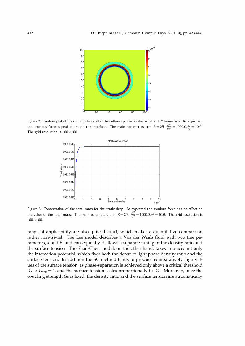
The non-conservative effect of the discretization is apparent from Fig. 2, which showsthe distribution of the local force, summed over all the populations (Eq. (2.11)). However,the non-conservative term of the forcing, still present in the lattice sites of the interfacezone (black line in Fig. 2), has negligible effects on the total mass variation, as shown inFig. 3.

3.2 The dynamic drop – A comparison with the Shan-Chen model

In this section a comparison between the Lee model and the Shan-Chen model is per-formed. These two models differ considerably from each other and, consequently, their

432 D. Chiappini et al. / Commun. Comput. Phys., 7 (2010), pp. 423-444

0 20 40 60 80 1000

10

20

30

40

50

60

70

80

90

100

−4

−3

−2

−1

0

1

2

3x 10

−3

Figure 2: Contour plot of the spurious force after the collision phase, evaluated after 106 time-steps. As expected,

the spurious force is peaked around the interface. The main parameters are: R = 25,ρsat

l

ρsatv

= 1000.0, τvτl

= 10.0.

The grid resolution is 100×100.

0 1 2 3 4 5 6 7 8 9 10x 10

5

1982.0542

1982.0543

1982.0544

1982.0545

1982.0546

1982.0547

1982.0548

1982.0549

Iteration Number

To

tal M

ass

Total Mass Variation

Figure 3: Conservation of the total mass for the static drop. As expected the spurious force has no effect on

the value of the total mass. The main parameters are: R = 25,ρsat

l

ρsatv

= 1000.0, τvτl

= 10.0. The grid resolution is

100×100.

range of applicability are also quite distinct, which makes a quantitative comparisonrather non-trivial. The Lee model describes a Van der Waals fluid with two free pa-rameters, κ and β, and consequently it allows a separate tuning of the density ratio andthe surface tension. The Shan-Chen model, on the other hand, takes into account onlythe interaction potential, which fixes both the dense to light phase density ratio and thesurface tension. In addition the SC method tends to produce comparatively high val-ues of the surface tension, as phase-separation is achieved only above a critical threshold|G|> Gcrit = 4, and the surface tension scales proportionally to |G|. Moreover, once thecoupling strength G0 is fixed, the density ratio and the surface tension are automatically

D. Chiappini et al. / Commun. Comput. Phys., 7 (2010), pp. 423-444 433

imposed. More specifically, with concern to the surface tension, the standard SC schemeoperates in a regime of σ∼0.01−0.1 (lattice units). Smaller values would entail very smalldensity ratios because, as mentioned above, the same parameter G controls both surfacetension and the non-ideal pressure. Larger values, on the other hand, run against prob-lems of numerical stability triggered by strong interface forces. In the Lee’s model, thesurface tension is generally about one order of magnitude below the SC value. Indeed,values of σ > 0.01 are typically found to generate numerical instabilities due to large in-terface forces. The factor ten between the two methods is likely to be due to the majordifference in the discretization of the non-ideal interactions, which requires second-oderneighbors in the Lee’s method and only first-order neighbors in the standard SC method(the situation would be different for multi-range SC methods, which allow considerablysmaller values of σ), [22–25]. The main advantage of achieving low surface tensions isthe possibility to simulate higher Weber numbers at a given grid resolution. As to thedensity ratio, the standard SC model is usually limited to values O(100), whereas theLee’s model can easily reach up to O(1000). This is again due to the fact that in the latter,the density ratio is independent of the surface tension. Thus, the Lee’s method appearsmore suited to applications involving large density ratios between the dense and lightfluid (say water/air mixtures). Finally, as to the kinematic viscosity, ν, although the twoschemes are based on a different time-marching procedure, leading to ν= c2

s (τ−1/2) forSC and ν = c2

s τ for Lee, generally they are both operated in a moderately high-viscousregime, ν∼0.1 (lattice units), which is adequate for a large variety of multiphase flows atmoderate Reynolds numbers. Clearly, the broader applicability of the Lee’s method, hasto be weighted against a higher complexity and computational demand as compared tothe SC method. The above considerations clarify the limitations in identifying an over-lapping region between the models. However, after a series of preliminary tests, it wasfound that a comparison can be established for G0=−4.3, which is close to the separationlimit. The resulting density ratio and the surface tension are:

ρliquid =1.29;

ρgas =0.33;

σ=0.0104.

(3.1)

To calibrate the Lee model in order to obtain the same σ and density ratio, the pa-rameter β has been tuned in Eq. (2.2), by imposing a constant interface thickness D = 4.Starting from Eq. (2.2), the parameter β is evaluated as:

β=12σ

D=0.0312. (3.2)

Droplet deformation by aerodynamic forces is a complex flow phenomenon in whichthe non-homogeneous pressure distribution on the surface of the bubble leads to shapedeformation and then to droplet breakup. Deformation and breakup of a liquid dropletby aerodynamic forces is usually classified through the dimensionless Weber number,

434 D. Chiappini et al. / Commun. Comput. Phys., 7 (2010), pp. 423-444

(a) Lee (b) ShanChen

Figure 4: Comparison between Shan-Chen and Lee models. Density contours at the beginning and at the endof the simulation. The main differences are the distance covered by the two drops and the interface thickness,which remains constant in the Lee model. Parameters of the simulation are We0 =3, σ=0.0104, R=20.

(a) Lee - Vector

(b) Shan Chen- Vector

(c) Shan Chen -Relative Velocity(see text)

Figure 5: Comparison between Shan-Chen and Lee models. Vector and asymptotic velocity at the end of thesimulation (time-step 10000). The main parameters of the simulation are We0 =3, σ=0.0104, R=20. On topof panel 5(c), shown is the blow-up of the velocity field near the interface. The lower panel shows the relativevelocity (see text).

which defines the ratio between the inertia and the surface tension forces:

We=ρgasU

2DC

σ, (3.3)

where DC is the characteristic length of the system (i.e. the droplet diameter).A rectangular box with 100 lattice sites in the x-direction and 300 in the y-direction is

used as computational domain and a two dimensional circular liquid drop with R = 20

D. Chiappini et al. / Commun. Comput. Phys., 7 (2010), pp. 423-444 435

is initialized, with its center located 50 lattice sites from the inlet in the y-dimension andin the center of the other dimension. The initial droplet velocity is set to 0.0486 latticeunits, which corresponds to We0 =3, sufficiently small to avoid drop deformation duringthe simulation. Fig. 4 shows a comparison of the density contours calculated by thetwo models at the beginning and after 10,000 iterations. Two main differences can beidentified. First in the SC case the droplet lies ahead. This is due to a different behaviourin the initial stage of evolution, although the asymptotic speed is the same. Second, theinterface thickness, constantly equal to four lattice units in the Lee model, increases up tosix grid-points with the SC model.

The velocity vectors after 10,000 iterations shown in Figs. 5(a) and 5(b) highlight thatthe Lee model yields a perfectly uniform and aligned velocity field, as it should be atsteady-state, while in the SC model, a flow rate across the interface (i.e. spurious currents)is observed. The parasitic currents are also evident in Fig. 5(c), which shows the relativevelocity Vrel =V−v∞, where v∞ is the flow velocity far from the interface.

The relative velocity for the Lee model is not reported because the value of Vrel isuniform and almost zero all over the domain (two orders of magnitude below the Vrel

calculated with the SC). A quantitative comparison between the two methods is non-trivial due to the basic differences between the two formulations of the intermolecularinteractions. For instance, we have observed that the Lee interaction takes longer to settleto a steady-state configuration. Apart from these differences, it is clear that in the long-term, the Lee model correctly reproduces a situation where the droplet moves at the samevelocity as the surrounding fluid. This confirms that spurious terms are under a bettercontrol as compared with the Shan-Chen model.

3.3 The Rayleigh-Taylor instability

Next, we test the Lee model against a gravity-driven Rayleigh-Taylor (RT) instability,one of the most fundamental forms of interfacial instability between fluids of differentdensities, which has been extensively studied both numerically and experimentally [27].

The computational domain is a channel of width W =100 and a height H =4W. Sym-metric boundary conditions are applied on the top and bottom wall and periodic bound-ary conditions are imposed at the side walls. The heavier fluid, initially placed abovethe lighter one, falls down under the effect of the gravity field when the interface is per-turbed. Subsequently, as the heavy fluid moves downwards, a wave-like disturbanceappears at the interface. Downward-moving ’spikes’ and upward-moving ’bubbles’ areobserved. The initial perturbation of the interface is a sinusoidal function, with ampli-tude A = 0.1W and wavelength λ = 2π/W. Being g the gravity acceleration in latticeunits, the characteristic velocity of the system is U =

√

W ·g, which has been set to 0.04for all the simulations. The Lee model has been tested under different operating condi-tions, given in terms of non-dimensional parameters. The Reynolds number is definedas: Re =

√

WgW/ν where ν is the fluid viscosity. The density ratio is measured in termsof the Atwood number, defined as: At =

(

ρl−ρg

)

/ρl +ρg with ρl and ρg being the den-

436 D. Chiappini et al. / Commun. Comput. Phys., 7 (2010), pp. 423-444

Figure 6: A sequence of density contours for the RT instability at different times, as presented in the reference[12]. The main parameters are: grid-size 256x1024, Re = 2048, At = 0.5 and

√

W ·g=0.04.

sities of the light and heavy fluids, respectively. The natural time-scale of the system isgiven by T =

√

W/g.

In order to assess the validity of the model, the present numerical results are com-pared with those obtained by He et al. [12]. The comparison has been performed for twodifferent cases: a 256x1024 grid, with Re = 2048 and At = 0.5; a 128x512 grid, with Re=256and At=0.5.

Figs. 6 and 7 show the evolution of the fluid interface from He et al. [12] and from theLee model, respectively, at a Re =2048. The agreement with literature results is satisfac-tory. The flow field is qualitatively consistent with the typical RT instability dynamics,experimentally and numerically observed by various authors [7, 29–33]: the initial expo-

D. Chiappini et al. / Commun. Comput. Phys., 7 (2010), pp. 423-444 437

(a) t = 0.0 (b) t = 1.0 (c) t = 1.5 (d) t = 2.0 (e) t = 2.5

(f) t = 3.0 (g) t = 3.5 (h) t = 4.0 (i) t = 4.5 (j) t = 5.0

Figure 7: A sequence of density contours for the RT instability at different times, as computed with the Lee’smodel. The main parameters are: grid-size 256x1024, Re = 2048, At = 0.5 and

√

W ·g=0.04.

nential growth, the rise bubble of the light fluid and the spikes of denser fluid movingin the opposite direction as well as the superficial wave breaking at a later stage of thesimulation, are well visible.

A better insight is obtained by monitoring the evolution of the interface at low andhigh Re, shown in Fig. 8, which reveals significant differences at t=3T. These are mainlyrelated to the dense jet breakup: at high Re, more and smaller dense fluid elements sep-arate from the main jet. A quantitative comparison with the literature data in terms ofthe spike and bubble leading front positions is given in Fig. 9. Again, satisfactory agree-

438 D. Chiappini et al. / Commun. Comput. Phys., 7 (2010), pp. 423-444

(a) t=1.0T (b) t=2.0T (c) t=3.0T (d) t=4.0T (e) t=5.0T

(f) t=1.0T (g) t=2.0T (h) t=3.0T (i) t=4.0T (j) t=5.0T

Figure 8: A sequence of density contours at different times as computed with the Lee’s model - Two differentRe are examined: 1)Re = 256 figure 8(a) to 8(e); 2)Re = 2048 figs 8(f) to 8(j). Other parameters are: Grid

size = 128 x 512, At = 0.5,√

W ·g = 0.04.

ment between our results and literature data is observed. Fig. 9 reveals that the evolutionof the global parameters is only marginally affected by the Reynolds number, as smalldifferences are observed only at a later stage of the simulations.

3.4 Lack of mass conservation

Inspection of mass-conservation for the RT instability (see Fig. 10), shows indeed a dete-rioration with respect to the case of a static droplet shown previously in this work. From

D. Chiappini et al. / Commun. Comput. Phys., 7 (2010), pp. 423-444 439

0 1 2 3 4 5−2

−1

0

1

2

Time

Pos

ition

Spike − Re256Spike − Re2048Spike − Re256 Literature Ref. [9]Spike − Re2048 Literature Ref. [9]Bubble − Re256Bubble − Re2048Bubble − Re256 Literature Ref. [9]Bubble − Re2048 Literature Ref. [9]

Figure 9: Position of the spike and bubble as a function of time. Comparison between the Lee’s model and theliterature data [12] for two different Re numbers. The main parameters are: grid size = 128 x 512, At = 0.5,√

W ·g = 0.04. The examined Re number are 256 and 2048.

0 4,000 8,000 12,000 16,000 20,000 24,000 28,000 32,000−2

0

2

4

6

8

10x 10−5

Conservation of the mass in the case of Rayleigh−Taylor instability

Timestep

Var

iatio

n of

the

mas

s (m

− m

0)/m

0

Figure 10: Conservation of the total mass for the Rayleigh-Taylor Instability. The variation of the mass respectto the initial condition is reported. The parameters of the simulation are Re=2048, grid size = 256 x 1024, At= 0.5,

√

W ·g = 0.04.

Fig. 10), it is seen that the relative mass non-conservation reaches up to 10−4 after 32,000timesteps, with a linear growth rate of about 10−8 per time step. Besides unsteadiness,which is inherent to the RT instability, this error growth could be related also to the effectof symmetric boundary conditions on the north/south walls. The development of op-timal boundary conditions for the Lee model is an open research topic, which deservesa full study on its own. Nevertheless, we notice that for the test cases presented in thiswork, the error due to mass non-conservation appears to be sufficiently low to preservethe essential physics of the problem.

440 D. Chiappini et al. / Commun. Comput. Phys., 7 (2010), pp. 423-444

(a) t=1.0T (b) t=2.0T (c) t=3.0T (d) t=4.0T (e) t=5.0T

(f) t=1.0T (g) t=2.0T (h) t=3.0T (i) t=4.0T (j) t=5.0T

(k) t=1.0T (l) t=2.0T (m) t=3.0T (n) t=4.0T (o) t=5.0T

Figure 11: Grid Size effects. A sequence of density contours of RT instability at different times, as computedwith the Lee’s model with different grids - Three different grids are examined: 1) 64x256 panels 11(a) to 11(e);2) 128x512 panels 11(f) to 11(j); 3) 256x1024 panels 11(k) to 11(o). Other parameters are: Re = 2048, At =

0.5,√

W ·g = 0.04.

D. Chiappini et al. / Commun. Comput. Phys., 7 (2010), pp. 423-444 441

0 1 2 3 4 5−2

−1.5

−1

−0.5

0

0.5

1

1.5

2

Time

Pos

ition

Spike − 64x256Spike − 128x512Spike − 256x1024Bubble − 64x256Bubble − 128x512Bubble − 256x1024

Figure 12: Grid Size effects on the evolution of the penetration of the bubble and the spike. No apparentdifferences can be appreciated for these ”global” quantities. The main differences are shown in the previousfigure, which shows the density contours at different times. Parameters: Re = 2048, At = 0.5 and

√

W ·g=0.04.- Three different grids are examined: 64×256, 128×512 and 256×1024.

3.5 Effect of the grid-size

The gravity-driven RT instability has been simulated at three different resolutions: 64×256; 128×512 and 256×1024. The Reynolds and Atwood numbers have been set to 2048and 0.5, respectively. As can be observed in Fig. 11, which compares the fluid interfaceevolution with the different grids, the grid-resolution significantly affects the interfacedynamics. The difference between the finest and the coarsest grids is evident at anystage of the RT instability growth, as the interface shape and the spike penetration areclearly different already at t=2T.

The effectiveness of the grid refinement, from 128×512 to 256×1024, becomes moreapparent as the fluid interpenetration becomes turbulent and the scale of the wave distur-bances becomes smaller. Since a coarser grid inevitably implies a larger interface thick-ness, liquid breakup is brought forward by the coarser grids, as well as the separatedstructures are smaller with the finest grid. Passing from the 128×512 to the 256×1024grids, the differences in the jet shape become apparent only after 5T, a time at which therelevant scales of the flow have become smaller.

The differences are much less evident at the level of the main penetration parameters.The time evolutions of the falling spike and the rear bubble position are almost the samefor the three grids, as shown in Fig. 11.

4 Conclusions

In this paper we have presented an investigation of the model proposed by Lee et al. [4,5],which tames spurious currents by a higher order finite-differencing treatment of non-

442 D. Chiappini et al. / Commun. Comput. Phys., 7 (2010), pp. 423-444

ideal forces. The comparison with the SC model for a moving low Weber droplet showsthat the Lee model is free of numerical artifacts, such as spurious currents arising in thewake of the droplet. The simulations also highlight that with the Lee model the interfacethickness keeps the same value all along the simulation, while in the SC a slow increasein time is observed (i.e. from four to six lattice units).

The method has been quantitatively validated against previous numerical results ontwo-dimensional Rayleigh-Taylor instabilities at different Reynolds numbers and gridresolutions. The computed flow field is qualitatively consistent with the complex RTinstability dynamics previously observed in experimental studies, and the agreementbetween our results and literature data is very satisfactory in terms of spike and bubbleleading front positions. It is also shown that the Reynolds number, in the range 256-2048,has significant effects only at a late stage, when jet breakup occurs. Finally, we showthat the lattice spacing plays a significant role on the interface dynamics. The differencesbetween the coarse and the fine grids (64×256 vs 256×1024) become more evident as thefluid interpenetration proceeds towards the generation of small scale disturbances.

In this study we also analytically demonstrate that the Lee model is in principle nonconservative, due to the different discretization of the streaming operator along the direc-tion of molecular versus fluid motion. However, numerical practice shows that this lackof conservation produces negligible effects, at least for the cases shown in this paper. Thisproperty, so far un-noticed to the best of our knowledge, is key to the practical success ofthe method.

Acknowledgments

We would like to thank Taheun Lee from City College of City University of New York forthe precious help in the first phases of work and for a very useful mail exchange whichallowed us to better understand the model presented.

References

[1] M. Ishii and T. Hibiki, Thermo-Fluid Dynamics of Two-Phase flow, Springer, 2007.[2] A. Prosperetti and G. Tryggvason, Computational Methods for Multiphase Flow, Cam-

bridge University Press, 2005.[3] T. Lee and C.-L. Lin, A stable discretization of the lattice Boltzmann equation for simulation

of incompressible two-phase flows at high density ratio, Journal of Computational Physics206 (2005) 16-47.

[4] T. Lee and P. F. Fischer, Eliminating parasitic currents in the lattice Boltzmann equationmethod for nonideal gasses, Phys. Rev. E 74 (2006) 046709.

[5] T. Lee, Effects of incompressibility on the elimination of parasitic currents in the lattice Boltz-mann equation method for binary fluids, Computers and Mathematics with Applications(2009), doi:10.1016/j.camwa.2009.02.017

[6] T. Lee and L. Liu, Wall boundary condition in the lattice Boltzmann equation method fornonideal gasses, Phys. Rev. E 78 (2008) 017702.

D. Chiappini et al. / Commun. Comput. Phys., 7 (2010), pp. 423-444 443

[7] R. R. Nourgaliev, T. N. Dinh and T. G. Theofanous, A pseudocompressibility method forthe numerical simulation of incompressible multifluid flows, International Journal of Multi-phase Flow 30 (2004) 901-937.

[8] S. Zaleski, J. Li and S. Succi, Two-dimensional Navier-Stokes simulation of deformation andbreakup of liquid patches, Phys. Rev. Lett. 75 (1995) 244-247.

[9] B. J. Daly, Numerical study of two fluid Rayleigh-Taylor instability, Phys. Fluids 10 (1967)297-307.

[10] D. L. Youngs, Numerical simulation of turbulent mixing by Rayleigh-Taylor instability,Physica D 12 (1984) 32-44.

[11] G. Tryggvason, Numerical simulation of the Rayleigh-Taylor instability, Journal of Compu-tational Physics 75 (1988) 235-282.

[12] X. He, S. Chen and R. Zhang, A Lattice Boltzmann scheme for incompressible multiphaseflow and its application in simulation of Rayleigh-Taylor instability, Journal of Computa-tional Physics 152 (1999) 642-663.

[13] D. H. Rothman and J. M. Keller, Immiscible cellular-automaton fluids, J. Stat. Phys. 52 (1988)1119-1127.

[14] A. K. Gunstensen, D. H. Rothman, S. Zaleski and G. Zanetti, Lattice Boltzmann model ofimmiscible fluids, Phys. Rev. A 43 (1991) 4320-4327.

[15] A. K. Gunstensen and D. H. Rothman, Microscopic modeling of immiscible fluids in threedimensions by a lattice Boltzmann method, Europhys. Lett. 18 (1992) 157-161.

[16] D. Grunau, S. Chen and K. Eggert, A lattice Boltzmann model for multiphase fluid flows,Phys. Fluids A 5 (1993) 2557.

[17] X. He, X. Shan and G. D. Doolen, A discrete Boltzmann equation model for non-ideal gases,Phys. Rev. E 57 (1998) R13.

[18] H. Chen, Discrete Boltzmann systems and fluid flows, Computer in Physics, 7(6) (1993) 632-637.

[19] R. Benzi, S. Succi and M. Vergassola, The lattice Boltzmann equation: theory and applica-tions, Phys. Rep. 222 (1992) 145-197.

[20] S. Chen and G. D. Doolen, Lattice Boltzmann method for fluid flows, Annu. Rev. Fluid Mech.30 (1998) 329-364.

[21] R. Zhang, X. Shan and H. Chen, Efficient kinetic method for fluid simulation beyond theNavier-Stokes equation, Phys. Rev. E 74 (2006) 046703.

[22] M. Sbragaglia, R. Benzi, L. Biferale, S. Succi, K. Sugiyama and F. Toschi, Generalized latticeBoltzmann method with multirange pseudopotential, Phys. Rev. E 75 (2007) 026702.

[23] G. Falcucci, G. Bella, G. Chiatti, S. Chibbaro, M. Sbragaglia and S. Succi, Lattice Bolzmannmodels with mid-range interactions, Commun. Comput. Phys. 2 (2007) 1071-1084.

[24] R. Benzi, S. Chibbaro and S. Succi, Mesoscopic lattice-Boltzmann modeling of flowing softsystem, Phys. Rev. Lett. 102 (2009) 026002.

[25] G. Falcucci, S. Chibbaro, S. Succi et al., Lattice Boltzmann spray-like fluids, Europhys. Lett.82 (2008) 24005.

[26] D. Jacqmin, Calculation of two-phase Navier-Stokes flows using phase-field modeling, Jour-nal of Computational Physics 155 (1999) 96-127.

[27] D. H. Sharp, An overview of Rayleigh-Taylor instability, Physica D 12 (1984) 3.[28] L. S. Luo and S. S. Girimaji, Theory of the lattice Boltzmann method: Two-fluid model for

binary mixtures, Phys. Rev. E 67 (2003) 036302.[29] W. H. Cabot and A. W. Cook, Reynolds number effects on Rayleigh-Taylor instability with

possible implications for type-Ia supernovae, Nature Physics 2 (2006) 562-568.

444 D. Chiappini et al. / Commun. Comput. Phys., 7 (2010), pp. 423-444

[30] B. Cabot, A. Cook and P. Miller, Direct Numerical Simulation of Rayleigh-Taylor Instability,IWPCTM10, Paris July 2006.

[31] J. P. Wilkinson and J. W. Jacobs, Experimental study of the single-mode three-dimensionalRayleigh-Taylor instability, Phys. Fluids 19 (2007) 124102.

[32] M. Chertkov, I. Kolokolov and V. Lebedev, Effects of surface tension on immiscible Rayleigh-Taylor turbulence, Phys. Rev. E 71 (2005) 055301(R).

[33] Z. Huang, A. De Luca, T. J. Atherton, M. Bird and C. Rosenblatt, Rayleigh-Taylor instabilityexperiments with precise and arbitrary control of the initial interface shape, Phys. Rev. Lett.99 (2007) 204502.