Lattice Boltzmann simulation of dispersion in two-dimensional tidal flows
23
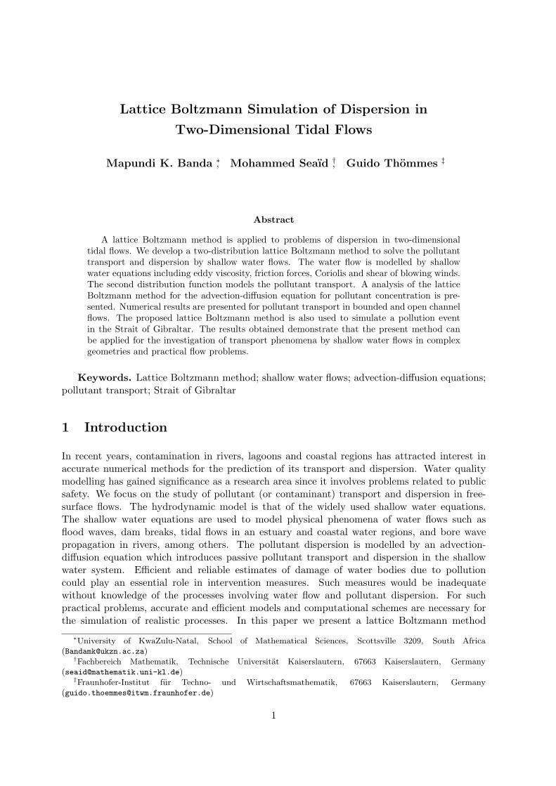
Lattice Boltzmann Simulation of Dispersion in Two-Dimensional Tidal Flows Mapundi K. Banda * , Mohammed Sea¨ ıd † , GuidoTh¨ommes ‡ Abstract A lattice Boltzmann method is applied to problems of dispersion in two-dimensional tidal flows. We develop a two-distribution lattice Boltzmann method to solve the pollutant transport and dispersion by shallow water flows. The water flow is modelled by shallow water equations including eddy viscosity, friction forces, Coriolis and shear of blowing winds. The second distribution function models the pollutant transport. A analysis of the lattice Boltzmann method for the advection-diffusion equation for pollutant concentration is pre- sented. Numerical results are presented for pollutant transport in bounded and open channel flows. The proposed lattice Boltzmann method is also used to simulate a pollution event in the Strait of Gibraltar. The results obtained demonstrate that the present method can be applied for the investigation of transport phenomena by shallow water flows in complex geometries and practical flow problems. Keywords. Lattice Boltzmann method; shallow water flows; advection-diffusion equations; pollutant transport; Strait of Gibraltar 1 Introduction In recent years, contamination in rivers, lagoons and coastal regions has attracted interest in accurate numerical methods for the prediction of its transport and dispersion. Water quality modelling has gained significance as a research area since it involves problems related to public safety. We focus on the study of pollutant (or contaminant) transport and dispersion in free- surface flows. The hydrodynamic model is that of the widely used shallow water equations. The shallow water equations are used to model physical phenomena of water flows such as flood waves, dam breaks, tidal flows in an estuary and coastal water regions, and bore wave propagation in rivers, among others. The pollutant dispersion is modelled by an advection- diffusion equation which introduces passive pollutant transport and dispersion in the shallow water system. Efficient and reliable estimates of damage of water bodies due to pollution could play an essential role in intervention measures. Such measures would be inadequate without knowledge of the processes involving water flow and pollutant dispersion. For such practical problems, accurate and efficient models and computational schemes are necessary for the simulation of realistic processes. In this paper we present a lattice Boltzmann method * University of KwaZulu-Natal, School of Mathematical Sciences, Scottsville 3209, South Africa ([email protected]) † Fachbereich Mathematik, Technische Universit¨ at Kaiserslautern, 67663 Kaiserslautern, Germany ([email protected]) ‡ Fraunhofer-Institut f¨ ur Techno- und Wirtschaftsmathematik, 67663 Kaiserslautern, Germany ([email protected]) 1
-
Upload
wwwgrupolpa -
Category
Documents
-
view
0 -
download
0
Transcript of Lattice Boltzmann simulation of dispersion in two-dimensional tidal flows
Lattice Boltzmann Simulation of Dispersion in
Two-Dimensional Tidal Flows
Mapundi K. Banda ∗, Mohammed Seaıd †, Guido Thommes ‡
Abstract
A lattice Boltzmann method is applied to problems of dispersion in two-dimensionaltidal flows. We develop a two-distribution lattice Boltzmann method to solve the pollutanttransport and dispersion by shallow water flows. The water flow is modelled by shallowwater equations including eddy viscosity, friction forces, Coriolis and shear of blowing winds.The second distribution function models the pollutant transport. A analysis of the latticeBoltzmann method for the advection-diffusion equation for pollutant concentration is pre-sented. Numerical results are presented for pollutant transport in bounded and open channelflows. The proposed lattice Boltzmann method is also used to simulate a pollution eventin the Strait of Gibraltar. The results obtained demonstrate that the present method canbe applied for the investigation of transport phenomena by shallow water flows in complexgeometries and practical flow problems.
Keywords. Lattice Boltzmann method; shallow water flows; advection-diffusion equations;pollutant transport; Strait of Gibraltar
1 Introduction
In recent years, contamination in rivers, lagoons and coastal regions has attracted interest inaccurate numerical methods for the prediction of its transport and dispersion. Water qualitymodelling has gained significance as a research area since it involves problems related to publicsafety. We focus on the study of pollutant (or contaminant) transport and dispersion in free-surface flows. The hydrodynamic model is that of the widely used shallow water equations.The shallow water equations are used to model physical phenomena of water flows such asflood waves, dam breaks, tidal flows in an estuary and coastal water regions, and bore wavepropagation in rivers, among others. The pollutant dispersion is modelled by an advection-diffusion equation which introduces passive pollutant transport and dispersion in the shallowwater system. Efficient and reliable estimates of damage of water bodies due to pollutioncould play an essential role in intervention measures. Such measures would be inadequatewithout knowledge of the processes involving water flow and pollutant dispersion. For suchpractical problems, accurate and efficient models and computational schemes are necessary forthe simulation of realistic processes. In this paper we present a lattice Boltzmann method
∗University of KwaZulu-Natal, School of Mathematical Sciences, Scottsville 3209, South Africa([email protected])
†Fachbereich Mathematik, Technische Universitat Kaiserslautern, 67663 Kaiserslautern, Germany([email protected])
‡Fraunhofer-Institut fur Techno- und Wirtschaftsmathematik, 67663 Kaiserslautern, Germany([email protected])
1

that gives accurate results based on a simple kinetic approach for shallow water equations andadvection-diffusion problems.
The lattice Boltzmann (LB) method, also popularly referred to as LBM, is an alternativenumerical scheme for simulating fluid flows [6]. The method is based on statistical physics andmodels the fluid flow by tracking the evolution of distribution functions of the fluid particlesin discrete phase space.The LBM recovers the macroscopic fluid flow from the microscopic flowbehaviour of the particle movement or the mesoscopic evolution of particle distributions. Thebasic idea is to replace the nonlinear differential equations of macroscopic fluid dynamics bya simplified description modeled on the kinetic theory of gases. Furthermore, the LB methodoffers several desirable properties such as linear convection terms and nearest-neighbor stencils.Secondly, diffusion is not represented by second order spatial derivatives as shown in section 3.On a structured mesh, the LB method can be implemented in a two-stage procedure namely, acollision operator evaluation which involves only local operations, and an advection operationwhere values are transported to adjacent lattice points without performing any computations.In the present work, the dynamics of the two different but dependent models namely, (i) ahydrodynamic model defining the flow, and (ii) a concentration model defining the transport ofthe pollutant are solved by a LB model with two distribution functions modelling the dynamicsof the hydrodynamic flow and the pollutant concentration, respectively. Similar techniques canbe found in the literature especially to derive LB approaches for thermal flows [13, 12] andmultiphase flow computations [26].
To obtain the hydrodynamic flow, a Chapman-Enskog analysis, which exploits a small meanfree path approximation to describe slowly varying solutions of the underlying kinetic equations,is performed. The LB method has been shown to be effective for simulating flows in complicatedgeometries, and to be particularly suited to implementations on parallel computer architectures[14]. It has found a wide range of applications in a variety of fields including the simulationof shallow water equations [28]. The LB method has been successfully applied to shallow wa-ter equations which describe wind-driven ocean circulation [21, 34], to model three-dimensionalplanetary geostrophic equations [22], and to study atmospheric circulation of the northern hemi-sphere [9]. In addition, under the influence of gravity, many free surface flows can be modelledby the shallow water equations under the assumption that the vertical scale is much smallerthan any typical horizontal scale. These equations can be derived from the depth-averaged in-compressible Navier-Stokes equations and usually include continuity and momentum equations.Hence, the applications of shallow water equations include a wide spectrum of phenomena otherthan water waves. Simulation of such real-world flow problems is not trivial since the geometrycan be complex and the topography irregular. Appealing features of the LB method include sim-plicity in programming, and straightforward incorporation of complex geometry and irregulartopography.
Other computational approaches such as the finite difference, the finite volume or the finiteelement methods have been applied to simulate the shallow water equations, see references[4, 36, 25, 23, 29, 17] among others. For most of these approaches, the treatment of bed slopesand friction forces often causes numerical difficulties in obtaining accurate solutions, see forexample [17, 4, 30]. As an alternative, the LB method for shallow water equations has beenstudied in [8, 35, 21, 28]. In this paper, we mainly present a practical study of the LB methodfor pollutant dispersion by tidal flow problems in complex geometry and irregular bathymetry.The bathymetry is given either by an analytical function or by data points in a two-dimensionaldomain. The aim of this paper is to test the accuracy and efficiency of the LB approach for sucha practical situation. The behaviour of the pollutant is investigated especially in connectionwith a non-flat topography and the surface stress originated by the shear of blowing winds. Toverify this approach, the problem of pollutant transport by tidal flows in the Strait of Gibraltar
2

has been used as a test example. Our findings can be applied when the LB method is used as analternative numerical scheme for solving pollutant transport problems modelled by a couplingof the shallow water equations for the flow and an advection-diffusion equation for the pollutanttransport.
In section 2 we give a brief description of the mathematical model, the two-dimensional shal-low water equations for tidal flows and an advection-diffusion equation describing the transportand dispersion of the pollutant. Next, we formulate the LB method for solving the governingequations in section 3. In section 4 numerical results are presented for various test examplesincluding a pollution event in the Strait of Gibraltar. For this latter example the Coriolis forcesand the wind effects are also incorporated into the model. It is one of the goals of this studyto investigate how the LB method performs under these conditions. A summary and someconcluding remarks are presented in section 5.
2 Equations for Dispersion by Tidal Flows
The two-dimensional shallow water equations including friction and Coriolis forces are consid-ered. The model for pollutant dispersion is an advection-diffusion equation for the concentrationof the pollutant. Hence, the water depth h and depth-averaged water velocity u = (u1, u2)T areobtained from solving the shallow water equations
∂th + ∂x(hu1) + ∂y(hu2) = 0,
∂t(hu1) + ∂x
(hu2
1 +12gh2
)+ ∂y (hu1u2) = −gh∂xZ +∇ · (hν∇u1) +
1ρ0
(Twx − Tbx
)− Ωhu2, (2.1)
∂t(hu2) + ∂x (hu1u2) + ∂y
(hu2
2 +12gh2
)= −gh∂yZ +∇ · (hν∇u2) +
1ρ0
(Twy − Tby
)+ Ωhu1,
where u1(x, y, t) and u2(x, y, t) are the depth-averaged water velocity in x- and y-direction, ρ0 thewater density, g the gravitational acceleration, Z the bottom topography, ν the horizontal kine-matic viscosity, Ω the Coriolis parameter defined by Ω = 2ω sinφ (where ω = 0.000073 rad s−1
is the angular velocity of the earth and φ the geographic latitude), and ∇ = (∂x, ∂y)T is thegradient operator. In (2.1), Tbx and Tby are the bed shear stresses in the x- and y-direction,respectively, defined by the depth-averaged velocities as
Tbx = ρ0Cbu1
√u2
1 + u22, Tby = ρ0Cbu2
√u2
1 + u22, (2.2)
where Cb is the bed friction coefficient, which may be either constant or estimated as Cb = g/C2z .
In the latter case Cz = h1/6/nb is the Chezy constant, with nb denoting the Manning roughnesscoefficient at the flow bed. The additional stresses Twx and Twy in (2.1) are created by the shearof the blowing wind and are expressed as a quadratic function of the wind velocity,
Twx = ρ0Cww1
√w2
1 + w22, Twy = ρ0Cww2
√w2
1 + w22, (2.3)
where Cw is the coefficient of wind friction and w = (w1, w2)T is the velocity of wind at 10 mabove water surface. It is usually defined by [4]
Cw = ρa
(0.75 + 0.067
√w2
1 + w22
)× 10−3,
3

where ρa is the air density. Note that other coefficients of wind friction in (2.3) can also beapplied. It is well known that the shallow water equations (2.1) can be derived from the depth-averaged incompressible Navier-Stokes equations under the assumption that the vertical scale ismuch smaller than any typical horizontal scale and the pressure is hydrostatic, see for example[32].
The transport and dispersion of a pollutant is modelled by a standard advection-diffusionequation in the form
∂t(hC) + ∂x (h(u1 + w1)C) + ∂y (h(u2 + w2)C) = ∇ · (hD∇C) + hQ, (2.4)
where C(x, y, t) is the depth-averaged pollution concentration, Q is the depth-averaged pollutantsource, and D the diffusion coefficient. In practical situations the diffusion coefficients dependon water depth, flow velocity, bottom roughness, wind and vertical turbulence, compare [18] formore details. For the purpose of the present work, the problem of variable diffusion coefficientsis not considered. The shallow water equations (2.1) and the pollutant dispersion equations (2.4)have to be equipped with appropriate boundary and initial conditions along with a prescribedbottom topography Z in (2.1) and a given pollutant source Q in (2.4). All of these conditions areproblem dependent and their discussion is postponed until section 4 where numerical examplesare presented.
In the next section we present both the lattice Boltzmann equations for shallow water flowswell as for pollutant dispersion. We also discuss the derivation of the macroscopic equations.
3 Lattice Boltzmann Method
3.1 Discrete-velocity Boltzmann equation for tidal flows
We consider the two-dimensional kinetic equation
∂f
∂t+ v · ∇f = J(f) + F, (3.1)
which describes the evolution of a particle density f(x,v, t) with x = (x, y) ∈ R2 and v =(v1, v2) ∈ R2. In (3.1), v is the microscopic velocity, J is the collision term, and F includes theeffect of external forces.
For discrete models in two space dimensions, we assume
v ∈ c0, c1, . . . , cN−1,with ci ∈ R2. Here, we consider a D2Q9 square lattice model [20], as sketched in Figure 1, withvelocity vectors of particles defined by
c0 =
(00
), c1 =
(10
), c2 =
(01
), c3 =
(−10
), c4 =
(0−1
),
c5 =
(11
), c6 =
(−11
), c7 =
(−1−1
), c8 =
(1−1
).
In the discrete case, the v-dependence of the particle distribution f(x,v, t) is determinedthrough N functions
fi(x, t) = f(x, ci, t), i = 0, 1, . . . , N − 1.
4

c c
cc
c
c cc
c0
1
8
2
3
7
56
4
Figure 1: Links in the D2Q9 lattice Boltzmann method.
The physical variables, the water depth h and the velocity u, are defined in terms of the distri-bution functions as
h(x, t) =∑
i
fi(x, t), h(x, t)u(x, t) =∑
i
cifi(x, t). (3.2)
In our approach to the lattice Boltzmann method, the collision operator J(f) in (3.1) is ofBGK-type [5]
J(f) = − 1τh
(f − feq), (3.3)
where the parameter τh > 0 is called relaxation time and feq is the equilibrium distribution. Inthe shallow water case, feq depends on f through the parameters h and u which are calculatedaccording to (3.2). For the standard D2Q9-model with nine velocities, we have [8, 21]
feqi =
h− f∗0 h
(152
gh− 32u2
), i = 0,
f∗i h
(32gh + 3ci · u +
92(ci · u)2 − 3
2u2
), i = 1, . . . , 8,
(3.4)
with the D2Q9 weight factors
f∗i =
49, i = 0,
19, i = 1, 2, 3, 4,
136
, i = 5, 6, 7, 8.
(3.5)
The local equilibrium function satisfies the following conditions
∑
i
feqi = h,
∑
i
cifeqi = hu,
∑
i
ci ⊗ cifeqi =
12gh2I + hu⊗ u, (3.6)
such that the lattice Boltzmann equation approaches the solution of the two-dimensional shallowwater equations. In (3.6), I denotes the 2× 2 identity matrix.
To obtain the macroscopic equations from equation (3.1), the Chapman-Enskog analysis,a multiscale expansion technique for solving the Boltzmann equation in kinetic theory, can be
5

employed. The LB equation (3.1) with equilibrium function (3.4) and collision term (3.3) resultsin the solution of the shallow water equations (2.1) with a force term F as required. Thus, theexternal force terms such as wind stress, Coriolis force, and bottom friction are easily included inthe model by introducing them into the force term F. For details on this multi-scale expansion,we refer to [21, 34, 8].
Hence, using a special discretization of the above BGK approximation [21, 35], we obtainthe following fully discrete lattice Boltzmann equation
fi(x + ci∆t, t + ∆t)− fi(x, t) = −∆t
τh(fi − feq
i ) + 3∆tf∗i ci · F(x, t), (3.7)
where ∆t is the time scale, F is the force term and ci the velocity vector of a particle in the linki. We use the diffusion scaling ∆t = ∆x2, which relates ∆t to the grid size ∆x. In the LBMmodel for (2.1) we set the force
F(x, t) =
−gh∂xZ +
1ρ0
(Twx − Tbx)− Ωhu2
−gh∂yZ + 1ρ0
(Twy − Tby) + Ωhu1
. (3.8)
By applying a Taylor expansion and the Chapman-Enskog procedure to equation (3.7), it canbe shown that the solution of the discrete lattice Boltzmann equation (3.7) with the equilibriumfunction (3.4) results in the solution of the shallow water equations (2.1) with a lattice Boltzmannviscosity ν defined as
ν =16
(2τh − 1
), (3.9)
where τh = τh/∆t is the scaled relaxation time. This viscosity is related to the physical viscosityin (2.1) by the relation
ν
ν= c2∆t, (3.10)
where c = ∆x/∆t denotes the velocity along a unit link [28].
3.2 Lattice Boltzmann Equation for the Pollutant Transport
In this section we present a derivation of the dispersion equation based on a lattice-Boltzmannformulation. We consider the case in which the pollution is passively advected by shallow waterflow and obeys a simple scalar advection-diffusion equation.
First we rewrite (2.4) by introducing a new variable Θ = hC as
∂tΘ + ∂x ((u1 + w1)Θ) + ∂y ((u2 + w2)Θ) = ∇ · (D∇Θ) + hQ, (3.11)
where C = Θ/h denotes the depth-averaged pollution concentration as above. We choose adistribution function for Θ denoted by qi for i = 0, 1, . . . , N − 1 [7]. This choice needs to satisfythe following conditions for the equilibrium distribution qeq
i
∑
i
qi =∑
i
qeqi = Θ,
∑
i
ciqi =∑
i
ciqeqi = (u + w)Θ, (3.12)
and in this case u + w = (u1 + w1, u2 + w2) is the total velocity vector. The equation of thepollutant distribution function with a source term can be written in the form
∂tq + v · ∇q = − 1τC
(q − qeq
)+Q, (3.13)
6

where τC > 0 is the relaxation time and Q accounts for the effects of the macroscopic sourceterm. The details will be presented below for the discrete case.
The discrete lattice BGK equation for (3.11) and (3.13) is given by
qi(x + ci∆t, t + ∆t)− qi(x, t) = −∆t
τC(qi − qeq
i ) + ∆tQi, (3.14)
where qeqi is the equilibrium distribution given by
qeqi = q∗i Θ
[1 + 3ci · (u + w)
], (3.15)
with the lattice weights defined as
q∗i =
49 , i = 0,
19 , i = 1, 2, 3, 4,
136 , i = 5, 6, 7, 8,
(3.16)
which has a similar form as the linear equilibrium distribution for the incompressible Navier-Stokes equations [20]. The source term in this case has been defined using
Qi = q∗i hQ. (3.17)
A similar approach has also been applied in [7] for reaction-diffusion equations.
It can be shown that equation (3.11) can be derived from the lattice BGK equation (3.14)with equation (3.15) through the Chapman-Enskog procedure. To demonstrate this, firstly, anasymptotic expansion for qi is defined as
qi = q(0)i + εq
(1)i + ε2q
(2)i + . . . , (3.18)
where q(0)i = qeq
i and ε is a small parameter proportional to the Knudsen number. In the long-wave-length and low-frequency limit, the lattice spacing ∆x and the time increment ∆t can beregarded as small parameters of the same order as ε. In equation (3.18)
qneqi = εq
(1)i + ε2q
(2)i + . . . ,
represents the nonequilibrium part of the distribution function qi with the following constraints∑
i
q(m)i = 0, m = 1, 2, . . . . (3.19)
To derive the macroscopic equation for advection-diffusion equation, we introduce two macro-scopic time scales t1 = εt and t2 = ε2t and a macroscopic length scale x1 = εx, thus
∂
∂t= ε
∂
∂t1+ ε2
∂
∂t2, ∇ = ε∇1, Q = ε2Q(2). (3.20)
Through a Taylor expansion in time and space, the lattice BGK equation (3.14) can be writtenin continuous form as
Diqi +∆t
2D2
i qi +O(∆t2) = − 1τC
(qi − q
(0)i
)+Qi, (3.21)
7

where Di =∂
∂t+ ci · ∇ is the total derivative operator. Hence,
Di = ε∂
∂t1+ ε2
∂
∂t2+ εci · ∇ = εD1i + ε2
∂
∂t2, D1i =
∂
∂t1+ ci · ∇1.
Substituting equation (3.18) and (3.20) into equation (3.21), and collecting terms of order ε andε2, we obtain
D1iq(0)i = −q
(1)i
τC, (3.22)
and∂q
(0)i
∂t2+ D1iq
(1)i +
∆t
2D2
1iq(0)i = −q
(2)i
τC+Q(2)
i , (3.23)
respectively. Using equation (3.22), the equation (3.23) can be rewritten in the form
∂q(0)i
∂t2+
(1− ∆t
2τC
)D1iq
(1)i = −q
(2)i
τC+Q(2)
i . (3.24)
Taking the sum of equations (3.22) and (3.24) over index i we can obtain the macroscopicequations on the t1 and t2 time scales in the form
∂Θ∂t1
+∇1 ·((u + w)Θ
)= 0,
(3.25)∂Θ∂t2
+(1− ∆t
2τC
)∇1 ·Π(1) = hQ,
where Π(1) =∑
i
ciq(1)i . To complete the derivation, the term Π(1) needs to be estimated. To
achieve this, we multiply equation (3.22) by the discrete velocity ci and take velocity moments(sum) to obtain
∂
∂t1
((u + w)Θ
)+
13∇1 · (ΘI) = − 1
τCΠ(1), (3.26)
where ∑
i
ci ⊗ ciqeqi =
13c2
ΘI, (3.27)
has been applied and c = ∆x/∆t. Equation (3.26) is substituted into equation (3.25) to give
∂Θ∂t2
− τC
3
(1− ∆t
2τC
)∇2
1Θ = hQ +O(M2), (3.28)
where M is defined based on the characteristic velocity which defines u + w which is small inshallow water flows on which the LB formulation is applied. Combining equations (3.25) and(3.28) we obtain the following equation
∂Θ∂t
+∇ · ((u + w)Θ) = ∇ · (D∇Θ) + hQ, (3.29)
where the diffusion coefficient D is determined by
D =c2
6
(2τC −∆t
). (3.30)
Again, the lattice diffusion is related to the physical diffusion in (2.4) by the relation
D
D= c2∆t, (3.31)
It should be stressed that equations (3.9) and (3.30) give the relation between the lattice diffusionand the time step to be used in the simulations.
8

3.3 Boundary Conditions
Boundary conditions play an important role in the LB method since they can influence theaccuracy and stability of the LB method, compare [37, 10] for more discussions. When no-slip boundary conditions for the flow velocities are imposed at walls, the bounce-back rule isusually used in the lattice Boltzmann algorithm. At a boundary point xb, populations fi oflinks ci which intersect the boundary and point out of the fluid domain are simply reflected(bounce-back) since they cannot participate in the normal propagation step
fi∗(xb, t + ∆t) = fi(xb, t), ci∗ = −ci.
Dirichlet boundary conditions for the prescribed concentration Θ0 can be imposed by the equi-librium for the unknown populations
qi = qeqi (Θ0, u1 + w1, u2 + w2) , i = 0, 1 . . . , 8.
Neumann boundary conditions are also frequently used in advection-diffusion problems. Theyare implemented in the LBM framework in a similar way by prescribing the concentration ofthe neighbour node Θn at the boundary
qi = qeqi (Θn, u1 + w1, u2 + w2) , i = 0, 1 . . . , 8.
In the test example of the Strait of Gibraltar we have flow boundary condition for the waterheight and a Neumann boundary condition for the velocity. These boundary conditions areimplemented by imposing the equilibrium distribution corresponding to the prescribed height,h0, and the velocity of the nearest neighbor in the direction of the normal, (u1n, u2n)
fi = feqi (h0, u1n, u2n) , i = 0, 1 . . . , 8.
For the advection-diffusion LB equation in the test example of the Strait of Gibraltar, wealso need boundary conditions at the coastlines and the open sea boundaries. We impose zeroconcentration Dirichlet boundary conditions at the coastlines and Neumann boundary conditionsfor the concentration at the western and eastern ends of the Strait of Gibraltar.
3.4 Coupled Lattice Boltzmann Algorithm
Discretizing the computational domain using a square lattice using the D2Q9-lattice with 9velocities as shown in Figure 1, the procedure to advance the solution from the time tn to thenext time tn+1 can be carried out in the following steps:
Step 1. Equilibrium functions:
Step 1.a. Using the water depth and velocity at time tn, compute from (3.4) theequilibrium function feq
i , i = 0, 1, . . . , 8.Step 1.b. Using the concentration (and velocity from shallow water equations) at
time tn, compute from (3.15) the equilibrium function qeqi , i = 0, 1, . . . , 8.
Step 2. Distribution functions:
Step 2.a. Calculate the distribution function fi, i = 0, 1, . . . , 8, using the latticeBoltzmann equation (3.7) with an appropriate relaxation time τh and impose thecorresponding boundary conditions.
9
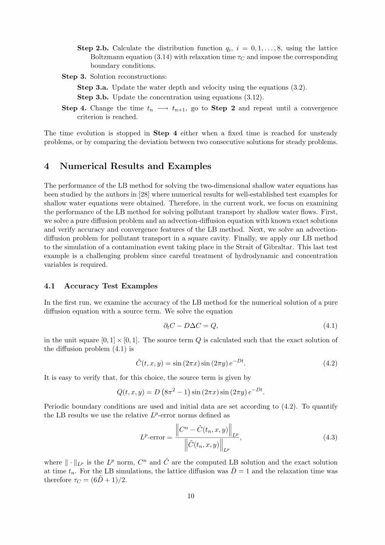
Step 2.b. Calculate the distribution function qi, i = 0, 1, . . . , 8, using the latticeBoltzmann equation (3.14) with relaxation time τC and impose the correspondingboundary conditions.
Step 3. Solution reconstructions:
Step 3.a. Update the water depth and velocity using the equations (3.2).Step 3.b. Update the concentration using equations (3.12).
Step 4. Change the time tn −→ tn+1, go to Step 2 and repeat until a convergencecriterion is reached.
The time evolution is stopped in Step 4 either when a fixed time is reached for unsteadyproblems, or by comparing the deviation between two consecutive solutions for steady problems.
4 Numerical Results and Examples
The performance of the LB method for solving the two-dimensional shallow water equations hasbeen studied by the authors in [28] where numerical results for well-established test examples forshallow water equations were obtained. Therefore, in the current work, we focus on examiningthe performance of the LB method for solving pollutant transport by shallow water flows. First,we solve a pure diffusion problem and an advection-diffusion equation with known exact solutionsand verify accuracy and convergence features of the LB method. Next, we solve an advection-diffusion problem for pollutant transport in a square cavity. Finally, we apply our LB methodto the simulation of a contamination event taking place in the Strait of Gibraltar. This last testexample is a challenging problem since careful treatment of hydrodynamic and concentrationvariables is required.
4.1 Accuracy Test Examples
In the first run, we examine the accuracy of the LB method for the numerical solution of a purediffusion equation with a source term. We solve the equation
∂tC −D∆C = Q, (4.1)
in the unit square [0, 1]× [0, 1]. The source term Q is calculated such that the exact solution ofthe diffusion problem (4.1) is
C(t, x, y) = sin (2πx) sin (2πy) e−Dt. (4.2)
It is easy to verify that, for this choice, the source term is given by
Q(t, x, y) = D(8π2 − 1
)sin (2πx) sin (2πy) e−Dt.
Periodic boundary conditions are used and initial data are set according to (4.2). To quantifythe LB results we use the relative Lp-error norms defined as
Lp-error =
∥∥∥Cn − C(tn, x, y)∥∥∥
Lp∥∥∥C(tn, x, y)∥∥∥
Lp
, (4.3)
where ‖ · ‖Lp is the Lp norm, Cn and C are the computed LB solution and the exact solutionat time tn. For the LB simulations, the lattice diffusion was D = 1 and the relaxation time wastherefore τC = (6D + 1)/2.
10

Table 1: Error-norms for the pure diffusion problem (4.1) at time t = 1.
N L∞-error Rate L1-error Rate L2-error Rate
20 2.527E-02 —— 2.523E-02 —— 2.521E-02 ——
40 6.236E-03 2.0187 6.242E-03 2.0150 6.233E-03 2.0159
80 1.554E-03 2.0046 1.557E-03 2.0032 1.554E-03 2.0039
160 3.883E-04 2.0007 3.889E-04 2.0012 3.883E-04 2.0074
320 9.705E-05 2.0003 9.721E-05 2.0002 9.704E-05 2.0052
In Table 1 we display the relative L∞-, L1- and L2-error norms at time t = 1 for different gridsizes using a diffusion coefficient D = 2. It reveals that increasing the number of lattice points inthe computational domain results in a decay of all error norms. Our LB method exhibits goodconvergence behaviour for this pure diffusion problem. As can be seen from the convergencerates presented in Table 1, second-order accuracy is achieved for this test example in terms ofall considered Lp-error norms.
Next, we assess the accuracy of the LB method for solving an advection-diffusion equationwith a prescribed advection velocity. We consider the test problem of the diffusion of a Gaussianpulse in a uniform rotating flow field [24]. The problem statement consists of solving the equation
∂tC + u1∂xC + u2∂yC −D∆C = 0, (4.4)
in a squared 3200 km× 3200 km domain subject to the initial condition
C(x, y, 0) = 100 exp(−(x− x0)2 + (y − y0)2
2σ2
), (4.5)
where u1 = −ωy and u2 = ωx, with ω = 10−5 /s being the angular velocity. It is easy to verifythat the problem (4.4)-(4.5) has an exact solution given by
C(x, y, t) =100
1 + 2Dtσ2
exp(− x2 + y2
2(σ2 + 2Dt)
), (4.6)
with x = x − x0 cosωt + y0 sinωt, y = y − x0 sinωt − y0 cosωt, and (x0, y0) = (−800 km, 0) isthe centre of the initial Gaussian. The parameters of this test example are σ = 2 × 10⁴ km2
and the diffusion coefficient D is allowed to take the values 104 m2/s and 2 × 10⁴ m2/s. Sincethe analytical solution of this problem is available, relative errors can be computed using theLp-error norms defined in (4.3). Homogeneous Neumann boundary conditions were imposed onall domain boundaries, and we used D = 0.01.
The calculated errors are listed in Table 2 for the selected diffusion coefficients after a com-plete rotation of the Gaussian pulse. As in the previous test example a decay behaviour isobserved for each increase of the number of lattice points. A slower decay is seen for com-putations with D = 2 × 10³ m2/s than those computed with D = 103 m2/s. This fact canbe attributed to the large physical diffusion in the advection-diffusion problem such that theGaussian spreads strongly and the solution is significantly different from zero at the boundariesand outside of the domain. It is evident, however, that our LB method converges to the correctsolution also for this advection-diffusion problem.
11

Table 2: Error-norms for the advection-diffusion problem (4.4).
D = 103 m2/s D = 2× 10³ m2/s
N L∞-error L1-error L2-error L∞-error L1-error L2-error
40 3.733E-02 2.338E-02 2.416E-02 2.435E-03 2.293E-02 1.856E-02
80 9.650E-03 5.811E-03 6.093E-03 2.435E-03 7.170E-03 5.944E-03
160 2.935E-03 1.456E-03 1.527E-03 4.940E-03 3.218E-03 3.658E-03
320 6.098E-04 3.679E-04 3.821E-04 3.907E-03 2.067E-03 2.277E-03
4.2 Pollutant Transport in a squared cavity
We solve an advection-diffusion equation of a pollutant transport in a 9000 m× 9000 m squarecavity with bottom slopes given by
∂xZ = ∂yZ = −0.001.
The Manning resistance coefficient is set to nb = 0.025 s/m1/3. As in [15], we impose uniformflow velocities u1 = u2 = 0.5 m/s and the uniform flow water depth (h + Z) as initial condition.The initial condition for the pollutant concentration is given by the superposition of two Gaussianpulses centered respectively, at (x1 = 1400 m, y1 = 1400 m) and (x2 = 2400 m, y2 = 2400 m),
C(0, x, y) = C1 exp(−(x− x1)2 + (y − y1)2
σ21
)+ C2 exp
(−(x− x2)2 + (y − y2)2
σ22
),
where C1 = 10, C2 = 6.5 and σ1 = σ2 = 264. For this example, the pollutant concentrationmoves along the diagonal cross-section x = y with the constant speed u1 = u2 = 0.5 m/s. Asimilar test example has been studied in the literature, see [15, 1] among others. Here, the windeffects are neglected (w1 = w2 = 0) in the hydrodynamic equations, no source (Q = 0) is consid-ered in the pollutant transport equation. The viscosity ν = 104 m/s2 was chosen and a diffusioncoefficient D = 100 m/s2 was used. In all our LB simulations the gravitational accelerationwas g = 9.81 m/s2. The lattice diffusion coefficient was set to D = 0.01. Neumann boundaryconditions were used for both, the hydrodynamic variables and the pollutant concentration atall walls of the cavity. Simulations were stopped when the pollutant concentration reached theend corner of the cavity.
Figure 2 shows the initial concentration and the numerical result using a uniform mesh withlattice size ∆x = ∆y = 50 m. The corresponding contour plots are presented in Figure 3. Thefigures demonstrate that the proposed LB method accurately reproduces the wave fronts. Itis also clear that the LB method preserves the expected transport trajectory and captures thecorrect dynamics. We remark that, due to the diffusion present in the equation of pollutanttransport, the two initial pulses merge into one concentration pulse during the time interval.In addition, the obtained solutions are completely free of spurious oscillations and the movingfronts are well resolved by the LB method. It should be stressed that the performance of ourLB method is very attractive since the computed hydrodynamic and pollutant solutions remainstable and highly accurate without solving linear systems of algebraic equations or requiringspecial treatment of the source terms or sophisticated upwind discretizations of the gradientfluxes as described in [4, 33, 31, 17] among others.
To check grid convergence of the LB method for this test example, we present in Figure 4cross sections of the pollutant concentration along the main diagonal (x = y) at the end time.
12

Figure 2: Initial concentration distribution (left) and final result at t = 4600 s (right).
We considered four meshes with ∆x = ∆y = 200 m, 100 m, 50 m and 25 m. For the selectedpollutant conditions, a large difference in the concentration profile is detected for the coarsemesh with ∆x = ∆y = 200 m compared with finer meshes. This difference becomes smalleras the mesh is refined. For instance, the discrepancy in the pollutant concentration on mesheswith ∆x = ∆y = 50 m and ∆x = ∆y = 25 m is less than 1%. A similar trend was observed inthe hydrodynamic variables. Therefore, bearing in mind the slight change in the results froma mesh with ∆x = ∆y = 50 m and ∆x = ∆y = 25 m at the expense of rather significantincrease in computation time, the mesh ∆x = ∆y = 50 m is believed to be adequate to obtaincomputational results (shown in Figure 2 and Figure 3) free of grid effects for the consideredpollutant transport problem.
4.3 Pollutant Transport in the Strait of Gibraltar
The Strait of Gibraltar connects the Atlantic Ocean and the Mediterranean Sea and has beena subject of many hydrodynamic and tidal circulation studies, see for instance [2, 11, 16, 27]and further references therein. Since it is the only connection between the Atlantic and theMediterranean, the Strait of Gibraltar is heavily used for shipping traffic and oil cargos. As aconsequence, the strait is considered as one of the most chronically contaminated regions, seefor instance [3]. In this test example we apply our LB method to the numerical simulation of acontamination event in the Strait of Gibraltar accounting for all the hydrodynamic effects suchas friction sources, wind stresses, Coriolis forces and horizontal eddy viscosity.
A schematic map of the Strait of Gibraltar is depicted in Figure 5 along with the mainlocations and ports. In geographical coordinates, the Strait is 35o45′ to 36o15′ N latitude and5o15′ to 6o05′ W longitude. Here, the computational domain is limited by the Tangier-Barbate
13

0 1000 2000 3000 4000 5000 6000 7000 8000 90000
1000
2000
3000
4000
5000
6000
7000
8000
9000
0 1000 2000 3000 4000 5000 6000 7000 8000 90000
1000
2000
3000
4000
5000
6000
7000
8000
9000
Figure 3: Contours for initial concentration (left) and final result at t = 4600 s (right).
0 1000 2000 3000 4000 5000 6000 7000 8000 9000
0
0.2
0.4
0.6
0.8
1
1.2
1.4
1.6
Position
Con
cent
ratio
n
∆ x=200∆ x=100∆ x=50∆ x=25
Figure 4: Cross sections of the pollutant concentration for different meshes.
14

Morocco•Tangier
•Ceuta
Spain
•Tarifa
•Algeciras
•Barbate
•Gibraltar
•Sidi Kankouch
6ο05‘ 5ο55‘ 5ο45‘ 5ο35‘ 5ο25‘ 5ο15‘35ο45‘
35ο55‘
36ο05‘
36ο15‘
0 10Km5
Figure 5: The Strait of Gibraltar map in geographical coordinates along with the main locations.The considered computational domain is marked by dashed lines.
axis from the Atlantic Ocean and the Ceuta-Algeciras axis from the Mediterranean sea. Thisrestricted domain has also been considered in [11, 16, 27] among others, and it is chosen fornumerical simulations mainly because measured data is usually provided by stations located atthe above-mentioned cities. The coastal boundaries and the bed topography in the Strait ofGibraltar are very irregular and several regions of varying depth exist. In our simulations weused a bathymetry reconstructed from published data in [11] and illustrated in Figure 6. Ourobjective in this numerical example is to test the ability of the LB method to handle complexgeometry and irregular topography.
The governing shallow water and pollutant transport equations (2.1)-(2.4) are solved in abounded domain limited by Tangier-Barbate and Ceuta-Algeciras using the bathymetry shown inFigure 6. No-slip boundary conditions are used for the velocity field at the coastal boundaries. Atthe open boundaries, Neumann boundary conditions are imposed for the velocity and the waterelevation is prescribed as a periodic function of time using the main semidiurnal and diurnaltides. The tidal constants at the open boundary lattice nodes were calculated by interpolationfrom those measured at the coastal stations Tangier and Barbate on the western end, and thecoastal stations Ceuta and Algeciras on the eastern end of the strait. The main astronomicaltidal constituents in the Strait of Gibraltar are the semidiurnal M2, S2 and N2 tides, and thediurnal K1 tide. Thus, in our computational study, the boundary conditions on open boundariesare prescribed as
h = h0 + AM2 cos (ωM2t + ϕM2) + AS2 cos (ωS2t + ϕS2) +AN2 cos (ωN2t + ϕN2) + AK1 cos (ωK1t + ϕK1) , (4.7)
where Ak is the wave amplitude, ωk the angular frequency and ϕk the tide phase for the tidek, with k = M2, S2, N2 or K1. The measured data for these parameters are provided for thecities defining the computational domain in Figure 6 and, for the convenience of the reader, aresummarized in Table 3. To obtain boundary values for the lattice nodes at the western andeastern open boundaries, we use a linear interpolation from the data listed in Table 3. Initially,the flow is assumed to be at rest and no pollutant is present i.e.,
u = v = 0, h = h0 and C = 0. (4.8)
15

6ο05‘ 5ο55‘ 5ο45‘ 5ο35‘ 5ο25‘ 5ο15‘35ο45‘
35ο55‘
36ο05‘
36ο15‘
•Tangier
•Ceuta
•Barbate
• Algeciras
100
200
300
400
500
600
700
800
900
1000
Figure 6: Bathymetry contours for the domain under study in the Strait of Gibraltar. The waterdepth is given in meters.
Table 3: Parameters of tidal waves for the stations considered in the present study.
Station Tide k Ak [m] ωk [rad/s] ϕk []Tangier M2 0.680 1.4052× 10⁻⁴ −67.00
S2 0.250 1.4544× 10⁻⁴ −90.00N2 0.130 1.3788× 10⁻⁴ −56.00K1 0.060 7.2921× 10⁻⁵ −80.00
Barbate M2 0.762 1.4052× 10⁻⁴ −53.50S2 0.279 1.4544× 10⁻⁴ −77.00N2 0.160 1.3788× 10⁻⁴ −37.00K1 0.027 7.2921× 10⁻⁵ −59.00
Ceuta M2 0.288 1.4052× 10⁻⁴ −55.02S2 0.105 1.4544× 10⁻⁴ −76.13N2 0.071 1.3788× 10⁻⁴ −37.38K1 0.038 7.2921× 10⁻⁵ −147.72
Algeciras M2 0.323 1.4052× 10⁻⁴ −34.80S2 0.121 1.4544× 10⁻⁴ −65.76N2 0.075 1.3788× 10⁻⁴ −34.96K1 0.025 7.2921× 10⁻⁵ −129.72
16

In (4.7) and (4.8), h0 is a given averaged water elevation set to 3 m in our simulations. Wealso used a constant Manning coefficient of nb = 0.012 s/m1/3, a Coriolis parameter of Ω =8.55 × 10⁻⁵ 1/s, and a horizontal eddy viscosity of ν = 100 m2/s, see for example [11, 27]. Adiffusion coefficient of D = 100 m2/s is used for the pollutant transport and the lattice viscosityis ν = 0.01. The contaminant source is implemented as an indicator function of the form
Q(t, x, y) =
1, if (x, y) ∈ Drelease and t ≤ trelease,
0, otherwise,
where trelease is the release time and Drelease is the release region to be located in the Straitof Gibraltar. In the current work, we consider both continuous and instantaneous releases ofthe contaminant. For the continuous release, trelease corresponds to the final simulation timewhile for the instantaneous release, trelease is set to 3 hours. In this sense, the simulations areschematic, since the number, the arrangement, and the capacities of pollution sources in theStrait of Gibraltar only partially correspond to the real situation.
In order to ensure that the initial conditions of the water flow and pollutant transport areconsistent we proceed as follows. The shallow water equations (2.1) are solved without pollutantrelease for two weeks of real time to obtain a well-developed flow. The obtained results aretaken as the real initial conditions and the pollutant is injected at this stage of computation.Depending on the wind direction, three cases are simulated namely, calm situation, eastern windand western wind. At the end of the simulation time the velocity fields and concentration ofpollutant are displayed after 1, 3 and 6 hours from the injection of pollutant. A mesh withlattice size ∆x = ∆y = 250 m is used for all the results presented in this section. This meshstructure has been selected after a grid independence study assessed by comparing numericalresults obtained using different meshes, compare [28] for more details. A Neumann boundarycondition is used for the pollutant concentration at the open boundaries and zero concentrationis imposed at the coastlines of the Strait.
First we solve a calm situation corresponding to setting w1 = w2 = 0 m/s in the shallowwater equations (2.1) and the transport equation (2.4). The pollutant is injected in the middleof the Strait of Gibraltar and located at (5o37′W, 35o54′N). The simulated results are presentedin Figure 7 at three separated instants from the injection of pollutant. In this figure we show theevolution in time of a velocity field and pollutant concentration for the continuous and instan-taneous releases. A simple inspection of this figure reveals that the velocity field changes thedirection during the time interval according to the period of the considered tides. The decreaseand increase of the strengths of velocities with time can also be seen in the figure. Obviously,the spread of the contaminant patch on the water free-surface is very slow for both continuousand instantaneous releases. This fact can be attributed to the small velocities generated by thetidal waves and also to the periodic character of these tides.
Next, we consider a pollutant transport subject to blowing wind from the east with w1 =−1 m/s and w2 = 0 m/s. Here, the pollutant is injected in the exit of the Strait of Gibraltarat (5o28′W, 35o57′N). In contrast to the previous test example, the present pollutant transportis solved with an extra velocity field. As a consequence, the spread of pollution in this latterexample is expected to be fast and follows the wind direction. The results of the simulationfor the continuous release as well as those obtained for the instantaneous release are shown inFigure 8. It is clear that the pollutant transport is significantly influenced by the action ofthe wind. The figure shows that the proposed LB method accurately reproduces concentrationfronts. Moreover, the steep gradient in the shallow water flow and the high concentration inthe advection-diffusion equation highlights the good stability and capability of the LB model toresolve pollutant transport by tidal flows on an irregular domain and complex bathymetry as
17

After 1 hour After 3 hours After 6 hours
Figure 7: Flow field (first row), concentration contours for continuous release (second row) andfor instantaneous release (third row) using calm conditions at three times after the release.
18

After 1 hour After 3 hours After 6 hours
Figure 8: Flow field (first row), concentration contours for continuous release (second row) andfor instantaneous release (third row) using eastern wind at three different times after the release.
the one considered in the current example.
Finally, the same simulations presented in Figure 8 are repeated but with wind blowing fromthe west with w1 = 1 m/s and w2 = 0 m/s. In this test case, the pollutant is injected inthe entry of the Strait of Gibraltar at (5o46′W, 35o57′N). Figure 9 shows the computed resultsat three different times after the pollutant injection. At an earlier time of the simulation, theconcentration front entering the strait starts to develop and is advected later on by the flow atthe far exit of the strait. It can be clearly seen that the location and time of the concentrationfront is well captured by the LB method. This figure shows also that the numerical solution isstable and the pollutant front is well resolved. From the computed results we can observe that,for the considered tidal conditions characterizing this test problem, the spread of a contaminantpatch strongly depends on the wind state when the release occurs and on the release nature. Insummary, the pollutant transport is captured accurately, the flow field is resolved reasonablywell, and the concentration front is shape preserving. All these features illustrate the robustnessof the LB method.
19

After 1 hour After 3 hours After 6 hours
Figure 9: Flow field (first row), concentration contours for continuous release (second row) andfor instantaneous release (third row) using western wind at three different times after the release.
20

5 Concluding Remarks
A lattice Boltzmann method has been successfully implemented in [28] for solving practicalapplications in shallow water flows. In this work, the lattice Boltzmann method has beenextended and tested for pollutant dispersion by shallow water flows. The mass, momentum andtransport equations are obtained from the nine-velocity distributions of hydrodynamic flow andpollutant concentration variables. Distribution functions of different type have been developedfor the hydrodynamic variables and pollutant concentration, respectively. The emphasis hasbeen on the construction of a stable numerical method such that (i) Riemann solvers, (ii) well-balanced discretization of gradient terms and source terms in the shallow water equations,(iii) iterative solvers required for advection-diffusion problems, and (iv) special treatment ofirregular domain and complex bathymetry, are completely avoided in its implementation. Theseproperties have been achieved in our approach by exploiting techniques offered by the latticeBoltzmann method. For instance, the explicit nature of the Boltzmann equation avoids linearsolvers for systems of algebraic equations, while the linear character of the operator in the latticeBoltzmann equations eliminates the computation of Jacobian matrices and Riemann problems.
The performance of the proposed lattice Boltzmann method has been assessed in diffusionand advection-diffusion problems with known analytical solutions to examine the convergence ofthe method. The method has also been used to solve a pollutant transport problem combinedwith shallow water flow in a squared cavity. Finally, we have applied the lattice Boltzmannmethod to simulate a pollution event in the Strait of Gibraltar. This latter test problem repre-sents a realistic practical test for lattice Boltzmann shallow water flow for two major reasons.Firstly, the computational domain in the Strait of Gibraltar is a large-scale domain includinghigh gradients of the bathymetry and well-defined shelf regions. Secondly, the strait containscomplex fully two-dimensional tidal flow structures, eddy viscosity, Coriolis forces and windshear stresses, which present a challenge for most numerical methods used for the shallow watermodelling. The results of these test problems demonstrate the accuracy of the employed latticeBoltzmann method and its capability to simulate tidal flows and pollutant transport in thehydrodynamic regimes considered.
Although lattice Boltzmann methods are very promising, they are still in the early stage ofdevelopment and validation. More investigations are needed to explore the capability of latticeBoltzmann methods for more practical engineering applications in environmental fluid flows andspecies transport. For instance, extension of the current solver to complex geometries involvingturbulent effects can also be of interest both for hydrodynamics and pollutant transport.
Acknowledgement
This work has been partly supported by the German Research Foundation (DFG) under theGrant No. KL-1105/9.
References
[1] Ahmad, Z., Kothyari, U.C., Time-line cubic spline interpolation scheme for solution of ad-vection equation, Computers & Fluids 2001; 30:737–752.
[2] Almazan, J.I., Bryden, H., Kinder, T., Parrilla, G. eds, ”Seminario Sobre la OceanografıaFısica del Estrecho de Gibraltar”, SECEG, Madrid, (1988).
21

[3] Gomez, F. The Role of the Exchanges through the Starit of Gibraltar on the Budget ofElements in Western Mediterranean Sea: Consequences of Humain-Induced Modifications.Marine Pollution Bulletin, 46:685–694, 2003.
[4] Bermudez, A., Vazquez, M.E., Upwind methods for hyperbolic conservation laws with sourceterms. Computers & Fluids 1994; 23:1049–1071.
[5] Bhatnagar, P., Gross, E., Krook, M., A model for collision process in gases. Phys. Rev. Lett.1954; 94:511–525.
[6] Chen, S., Doolen, G.D., Lattice Boltzmann method for fluid flows. Annual Rev. of FluidMech. 1998; 30:329–364.
[7] Dawson, S.P., Chen, S., Doolen, G.D., Lattice Boltzmann computations for reaction-diffusionequations. J. Chem. Phys. 1993; 98:1514–1523.
[8] Dellar, P.J., Non-hydrodynamic modes and a priori construction of shallow water latticeBoltzmann equations. Phys. Rev. E (Stat. Nonlin. Soft Matter Phys.) 2002; 65:036309 (12Pages).
[9] Feng, S., Zhao, Y., Tsutahara, M., Ji, Z., Lattice Boltzmann model in rotational flow field.Chinese J. of Geophys. 2002; 45:170–175.
[10] Gallivan, M.A., Noble, D.R., Georgiads, J.G. Buckius, R.O., An evaluation of the bounce-back boundary condition for lattice Boltzmann simulations. Int. J. Num. Meth. Fluids. 1997;25:249–263.
[11] Gonzalez, M., Sanchez-Arcilla, A., Un Modelo Numerico en Elementos Finitos para laCorriente Inducida por la Marea. Aplicaciones al Estrecho de Gibraltar. Revista Internacionalde Metodos Numericos para Calculo y Diseno en Ingenierıa. 1995; 11:383–400.
[12] Guo, Z., Shi, B., Zheng, C., A coupled lattice BGK model for the Boussinesq equations.Int. J. Numer. Meth. Fluids 2002; 39:325–342.
[13] He, X., Chen, S., Doolen, G. D., A novel thermal model for the lattice Boltzmann methodin incompressible limit. J. Comp. Phys. 1998; 146:282–300.
[14] Kandhai, D., Koponen, A., Hoekstra, A.G., Kataja, M., Timonen, J., Sloot, P.M.A., LatticeBoltzmann hydrodynamics on parallel systems. Comput. Phys. Commun. 1998; 111:14–26.
[15] Komatsu, T., Ogushi, K., Asai, K., Refined numerical scheme for advective transport indiffusion simulation”, J. Hydraulic Eng. 1997; 123:41–50.
[16] Lafuente, J.G., Almazan, J.L., Catillejo, F., Khribeche, A., Hakimi, A., Sea level in thestrait of Gibraltar: Tides. Int. Hydrogr. Rev. LXVII. 1990; 1:111–130.
[17] LeVeque, R.J., Balancing source terms and the flux gradients in high-resolution Godunovmethods: the quasi-steady wave-propagation algorithm. J. Comput. Phys. 1998; 146:346–365.
[18] Lin, B., Falconer, R.A., Tidal flow and transport modeling using ultimate quickest scheme.J. Hydraulic Eng. 1997; 123:303–314.
[19] Perthame, B., Simeoni, C., A Kinetic Scheme for the Saint-Venant System with a SourceTerm. CALCOLO. 2001; 38:201–231.
22

[20] Qian, Y.H., d’Humieres, D., Lallemand, P., Lattice BGK Models for the Navier-Stokesequation, Europhys. Letters. 1992; 17:479–484.
[21] Salmon, R., The Lattice Boltzmann method as a basis for ocean circulation modeling. J.Mar. Res. 1999; 57:503–535.
[22] Salmon, R., The Lattice Boltzmann solutions of the three-dimensional planetary geostrophicequations. J. Mar. Res. 1999; 57:847–884.
[23] Seaıd, M., Non-oscillatory Relaxation Methods for the Shallow Water Equations in Oneand Two Space Dimensions. Int. J. Num. Meth. Fluids. 2004; 46:457–484.
[24] Staniforth, A., Cote J., Semi-Lagrangian Integration Schemes for the Atmospheric Models:A Review We. Rev. 1991; 119:2206–2223.
[25] Stansby, P.K., Zhou, J.G., Shallow water flow solver with non-hydrostatic pressure: 2Dvertical plane problems. Int. J. Numer. Meth. Fluids 1998; 28:541–563.
[26] Swift, M.R., Orlandini, E., Osborn, W.R., Yeomans, J.M., Lattice Boltzmann simulationsof liquid-gas and binary fluid systems. Physical Rev. E 1996; 54:5041–5052.
[27] Tejedor, L., Izquierdo, A., Kagan, B.A., Sein, D.V., Simulation of the semidiurnal tides inthe Strait of Gibraltar. J. Geophysical Research. 1999; 104:13541–13557.
[28] Thommes, G., Seaıd, M., Banda, M. K., Lattice Boltzmann methods for shallow water flowapplications. Int. J. Num. Meth. Fluids. 2007; in press.
[29] Toro, E.F., Riemann problems and the WAF method for solving two-dimensional shallowwater equations. Phil. Trans. Roy. Soc. Lond. A 1992; 338:43–68.
[30] Vazquez-Cendon, M. E., Improved treatment of source terms in upwind schemes for shallowwater equations in channels with irregular geometry. J. Comput. Phys. 1999; 148:497–526.
[31] Vukovic, S., Sopta, L., ENO and WENO schemes with the exact conservation property forone-dimensional shallow-water equations. J. Comp. Physics. 2002; 179:593–621.
[32] Wood, W.L., ”Introduction to Numerical Methods for Water Resources”, Clarendon Press,Oxford, (1993).
[33] Xing, Y., Shu, C., High Order Well-Balanced Finite Volume WENO Schemes and Discon-tinuous Galerkin Methods for a Class of Hyperbolic Systems with Source Terms. J. Comp.Physics. 2006; 214:567–598.
[34] Zhong, L., Feng, S., Gao, S., Wind-driven ocean circulation in shallow water Lattice Boltz-mann Model. Adv. in Atmospheric Sci. 2005; 22:349–358.
[35] Zhou, J.G., A lattice Boltzmann model for the shallow water equations. Computer methodsin applied mechanics and engineering 2002; 191:3527–3539.
[36] Zhou, J.G., Velocity-depth coupling in shallow water flows. J. Hydr. Engrg., ASCE 1995;10:717–724.
[37] Zou, Q., He, X., On pressure and velocity boundary condition for the lattice BoltzmannBGK model. Phys. Fluids 2002; 9 (6):1591–1598.
23