Pseudo-divergence-free element free Galerkin

method for incompressible fluid flow ?

Antonio HUERTA a,1, Yolanda VIDAL a and Pierre VILLON b

aLaboratori de Calcul Numeric, Universitat Politecnica de Catalunya, JordiGirona 1, E-08034 Barcelona, Spain.

bLaboratoire de Mecanique Roberval, UMR UTC-CNRS Universite de Technologiede Compiegne, BP 20529, 60205 Compiegne cedex, France.

Abstract

Incompressible modelling in finite elements has been a major concern since its earlydevelopments and has been extensively studied. However, incompressibility in mesh-free methods is still an open topic. Thus, instabilities or locking can preclude the useof mesh-free approximations in such problems. Here, a novel mesh-free formulationis proposed for incompressible flow. It is based on defining a pseudo-divergence-freeinterpolation space. That is, the finite dimensional interpolation space approaches adivergence-free space when the discretization is refined. Note that such an interpola-tion does not include any overhead in the computations. The numerical evaluationsare performed using the inf-sup numerical test and two well-known benchmark ex-amples for Stokes flow.

Key words: Locking, Element Free Galerkin, Diffuse derivatives, Moving LeastSquares, Incompressible flow, LBB condition

1 Introduction

Accurate and efficient modeling of incompressible flows is an important issuein finite elements. The continuity equation for an incompressible fluid takes

? Research supported by Ministerio de Ciencia y Tecnologıa under grants DPI2001-2204 and REN2001-0925-C03-01

Email address: antonio.huerta@upc.es (Antonio HUERTA).URL: www-lacan.upc.es (Antonio HUERTA).

1 Correspondence to: Antonio Huerta, Departament de Matematica Aplicada III,E.T.S. de Ingenieros de Caminos, Canales y Puertos, Universitat Politecnica deCatalunya, Jordi Girona 1, E-08034 Barcelona, SPAIN.

Preprint submitted to Comput. Methods Appl. Mech. Eng. 4 September 2003

the peculiar form. It consists of a constraint on the velocity field that mustbe divergence free. Then, the pressure has to be considered as a variable notrelated to any constitutive equation. Its presence in the momentum equationhas the purpose of introducing an additional degree of freedom needed tosatisfy the incompressibility constraint. The role of the pressure variable is thusto adjust itself instantaneously in order to satisfy the condition of divergence-free velocity. That is, the pressure is acting as a Lagrangian multiplier of theincompressibility constraint and thus there is a coupling between the velocityand the pressure unknowns.

Various formulations have been proposed in the literature to deal with incom-pressible flow problems [1–8]. Mixed finite elements present numerical diffi-culties caused by the saddle-point nature of the resulting variational problem.Solvability of the problem depends on a proper choice of finite element spacesfor velocity and pressure. They must satisfy a compatibility condition, the so-called LBB (or inf-sup) condition. If this is not the case, alternative formula-tions (usually depending on a numerical parameter) are devised to circumventthe LBB condition and enable the use of velocity–pressure pairs that are un-stable in the standard Galerkin formulation. Finally, note that it is not trivialto verify analytically the LBB condition for a given interpolation of velocityand pressure, and this has spurred the use of numerical inf-sup testing [9–12].

Incompressibility in mesh-free methods is still an open topic. Even recently,it was claimed [13] that meshless methods do not exhibit volumetric locking.Now it is clear that this is not true. For instance, an analysis of the elementfree Galerkin (EFG) method using the numerical inf-sup condition can befound in [14]. Moreover, several authors claim that increasing the dilationparameter locking phenomena in mesh-free methods can be suppressed, orat least attenuated. Their argument is based on numerical examples [15,14]or on the heuristic constraint ratio [16] proposed in [17]. In a recent paper[18] this issue is clarified determining the influence of the dilation parameteron the locking behavior of EFG near the incompressible limit. This is doneperforming a modal analysis: studying the fundamental modes (base of thesolution space) and their corresponding energy (eigenvalue). In particular EFGbehavior is compared with standard finite elements. The major conclusion isthat an increase of the dilation parameter attenuates, but never suppressesthe volumetric locking and that, as in standard finite elements, an increase inthe order of reproducibility reduces the relative number of locking modes at alower rate than finite elements.

Until now remedies proposed in the literature are extensions of methods de-veloped for finite elements. For instance, in [14] a new EFG formulation is pro-posed using selective reduced integration and in [16] an improved ReproducingKernel Particle Method based on a pressure projection method is suggested.

2

Here a novel approach is explored: the pseudo-divergence-free (PDF) EFGmethod. It consists in using interpolation functions that verify approximatelythe divergence-free constraint for a given discretization, and asymptoticallybecome divergence-free as the discretization is refined. This method is basedon diffuse derivatives [19], which, as proven in [20], converge to the derivativesof the exact solution when the radius of the support goes to zero (for a fixeddilation parameter). One of the key advantages of this approach is that thepseudo-divergence-free (PDF) interpolation functions are computed a priori.That is, prior to determining the specific particle distribution. Thus, there isno extra computational cost.

Preliminary results (modal analysis) in incompressible elasticity were encour-aging [21,22]. In this paper convergence of the approximation in incompressibleflows is studied. In particular, it is shown that the PDF EFG method passesthe numerical inf-sup test. And two well-known examples of Stokes flow areused to compare different mixed formulations.

2 Diffuse derivatives

2.1 Preliminaries of the EFG method

This section will not be devoted to develop or discuss mesh-free methods indetail or their relation with moving least squares (MLS) interpolants. Thereare well known references with excellent presentations of mesh-free methods.See, for instance, the papers in the special issue [23]. Here some basic notionswill be recalled in order to introduce the notation and the approach employedin following sections.

The moving least squares approach is based on the local approximation (i.e.,at any point z in the neighborhood of x) of the unknown scalar function u(z)by uρ as

u(z) ' uρ(x, z) = PT(z) a(x) for z near x, (1)

where the coefficients a(x) = a0(x), a1(x), . . . , al(x)T are not constant, theydepend on point x, and P(z) = p0(z), p1(z), . . . , pl(z)T includes a completebasis of the subspace of polynomials of degree m. In one dimension, it isusual that pi(x) coincides with the monomials xi, and, in this particular case,l = m. The coefficients a are obtained by minimization of the functional Jx(a)centered in x and defined by

Jx(a) =∑

i∈Ix

φ(x, xi)[u(xi)−PT(xi) a(x)

]2, (2)

where φ(x, xi) is a weighting function (positive, even and with compact sup-port) that characterizes the mesh-free method. For instance, if φ(x,xi) is con-

3

tinuous together with its first k derivatives, the interpolation is also continuoustogether with its first k derivatives. The particles cover the computational do-main Ω, Ω ⊂ Rnsd , and, in particular, a number of particles xii∈Ix belongto the support of φ(x,xi). The minimization of Jx(a) induces the standardnormal equations in a weighted least-squares problem

M(x) a(x) =∑

i∈Ix

φ(x,xi) P(xi) u(xi) (3)

where, as usual, the Gram matrix M(x) is the scalar product of the interpo-lation polynomials:

M(x) =∑

i∈Ix

φ(x,xi) P(xi) PT(xi).

That is,〈u, v〉x =

∑

i∈Ix

φ(x,xi) u(xi) v(xi) (4)

must define a discrete scalar product. Thus, several conditions on the particledistribution are implicitly assumed, see for instance [24,25].

Once the normal equations, Eqs (3), are solved the coefficients a are substi-tuted in (1). Since the weighting function φ usually favors the central point x,it seems reasonable to assume that such an approximation is more accurateprecisely at z = x and thus the approximation (1) is particularized at x, thatis,

u(x) ' uρ(x) = PT(x) a(x) = PT(x) M−1(x)∑

i∈Ix

φ(x,xi) P(xi) u(xi). (5)

This expression can also be written in a standard interpolation form

uρ(x) =∑

i∈Ix

Nρi (x) u(xi) =

∑

i∈Ix

[φ(x,xi) PT(x) M−1(x) P(xi)

]

︸ ︷︷ ︸Nρ

i (x)

u(xi). (6)

2.2 The diffuse derivative

The approximation of the derivative of u in each spatial direction is the cor-responding derivative of uρ. This requires to derive (5), that is

∂u

∂x' ∂uρ

∂x=

∂PT

∂xa + PT ∂a

∂x. (7)

On one hand, the second term on the r.h.s. is not trivial. Derivatives of thecoefficients a require the resolution of a linear system of equations with the

4

same matrix M. As noted in [26] this is not an expensive task. However, itrequires the knowledge of the cloud of particles surrounding each point x, and,thus, it depends on the point where derivatives are evaluated.

On the other hand, the first term is easily evaluated. The derivative of thepolynomials in P is trivial and can be evaluated a priori, without knowledgeof the cloud of particles surrounding each point x.

The concept of diffuse derivative proposed in [20,19] consist in approximatingthe derivative only with the first term on the r.h.s. of (7), namely

δuρ

δx=

∂uρ

∂z

∣∣∣∣∣z=x

=∂PT

∂z

∣∣∣∣∣z=x

a(x) =∂PT

∂xa(x).

From a computational cost point of view, this is an interesting alternativeto (7). Moreover, in [20] it is shown that the diffuse derivative converges atoptimal rate to the derivative of u, here the proof is developed in severalspatial dimensions.

Proposition 1 If uρ is an approximation to u with an order of consistencym (i.e., P includes a complete basis of the subspace of polynomials of degreem) and ρ/h is constant, then

∥∥∥∥∥∂|k|u∂xk

− δ|k|uρ

δxk

∥∥∥∥∥∞≤ C(x)

ρm+1−|k|

(m + 1)!∀|k| = 0, . . . , m. (8)

where k is a multi-index, k = (k1, k2, . . . , knsd) and |k| = k1 + k2 + · · ·+ knsd.

Proof. Lets assume u ∈ Cm+1(Ω) where Cm+1 is the space of (m + 1) timescontinuously differentiable functions. Recall that Taylor’s formula of order mcan be written as:

u(x + h) =m∑

|ααα|=0

1

ααα!hααα ∂|ααα|u

∂xααα(x) + R?

m+1(x + θh), (9)

where θ ∈]0, 1[, R?m+1(x + θh) is the error term and ααα is a multi-index such

that,

hααα := hα11 hα2

2 · · ·hαnsdnsd

; ααα! := α1!α2! · · ·αnsd !; |ααα| = α1 + α2 + · · ·+ αnsd .

Without loss of generality, the definitions z := x + h and

Rm+1(x,z) := R?m+1

(x + θ(z − x)

)(10)

5

allow us to rewrite equation (9) as

u(z) =m∑

|ααα|=0

1

ααα!

(z − x

ρ

)ααα

ρααα ∂|ααα|u∂xααα

(x) + Rm+1(x, z),

where, as usual, the dependence of θ in x and z is not explicitly stated. Thus,Taylor’s formula can also be written as:

u(z) = PT(

z − x

ρ

)U(x) + Rm+1(x, z), (11)

where each component of P and U is defined, respectively, by

Pααα(ξξξ) =ξξξααα

ααα!and Uααα(x) = ρααα ∂|ααα|u

∂xαααfor |ααα| = 0, . . . , m. (12)

Observe that U(x) depends on the exact derivatives of u.

The MLS approach is based on the local approximation of the unknown scalarfunction u by uρ, see equation (1). Since in equation (11) polynomials P(ξξξ)are centered and scaled, the MLS interpolant is also centered and scaled,

u(z) ' uρ(x,z) = PT(

z − x

ρ

)a(x) for z near x.

Then the MLS approach requires the resolution of the normal equations givenby (3); here u(xi) is substituted using (11) and the scalar product defined in(4) is employed to simplify the notation,

M(x) a(x) =⟨P

(z − x

ρ

),PT

(z − x

ρ

)U(x) + Rm+1(x, z)

⟩

x.

This equation can be rearranged as

M(x)[a(x)−U(x)] =∑

j∈Ix

φ(

xj − x

ρ

)P

(xj − x

ρ

)Rm+1(x,xj) =: b. (13)

Now, lets rewrite the r.h.s. of (13) in a more convenient way. The error termof Taylor’s formula has the form

Rm+1(x,xj) =∑

|ααα|=m+1

(xj − x)ααα

(m + 1)!

∂m+1u

∂xααα(x,xj), (14)

where, as in equation (10), the intermediate point θ is not explicitly statedbut its dependence on x and xj is reflected. Substituting (14) in the definitionof vector b, see (13), produces

b =∑

j∈Ix

φ(

xj − x

ρ

)P

(xj − x

ρ

) ∑

|ααα|=m+1

(xj − x)ααα

(m + 1)!

∂m+1u

∂xααα(x,xj).

6

Each component of the previously defined vector b is associated to the cor-responding component of P, namely the polynomial of degree |k| = 0, . . . , mdefined as

ξξξk/k! =(ξk11 ξk2

2 · · · ξknsdnsd

)/(k1!k2! · · · knsd !

).

Under these circumstances, each component of b can be written as

bk =∑

j∈Ix

φ(

xj − x

ρ

)(xj − x)k

ρ|k|1

|k|!∑

|ααα|=m+1

(xj − x)ααα

(m + 1)!

∂m+1u

∂xααα(x,xj)

=ρm+1

(m + 1)!

1

|k|!∑

j∈Ix

φ(

xj − x

ρ

) ∑

|ααα|=m+1

(xj − x

ρ

)k+ααα ∂m+1u

∂xααα(x,xj)

︸ ︷︷ ︸rk(x)

=ρm+1

(m + 1)!rk(x).

(15)

Thus, the r.h.s. of (13) becomes

b =ρm+1

(m + 1)!r(x). (16)

Substituting (16) into equation (13) and assuming that M is regular [24,25],

a(x)−U(x) =ρm+1

(m + 1)!M−1(x) r(x).

On one hand, rk is bounded for all |k| = 0, . . . ,m. This can be seen from thedefinition of rk, see (15). Note that for a fixed x, if ρ/h is constant, rk is thesum of products of continuous functions in Ω. Thus, it is a continuous functionin Ω. Moreover, in every product, there is the weighting function φ, which hascompact support. Since rk is a continuous function with compact support itis bounded by a constant that only depends on x.

On the other hand, matrix M is also bounded [27,25]. Then, if both, M andrk, are bounded, a constant C(x) can be defined as the bound of M−1(x)r(x)and consequently

|a(x)−U(x)| ≤ ρm+1

(m + 1)!C(x)

The previous expression can be divided by ρ|k|. Then, for each component,

∣∣∣∣∣ak(x)

ρ|k|− Uk(x)

ρ|k|

∣∣∣∣∣ ≤ρm+1−|k|

(m + 1)!C(x) ∀ |k| = 0, . . . , m, (17)

where ak and Uk are the components of a and U, respectively. Recall thateach component of U(x) depends on the corresponding exact derivatives ofu, see (12). Now, observe that each component of a(x) shall depend on the

7

corresponding pseudo-derivatives; that is, for |k| = 0, ..., m

δ|k|uρ

δxk:=

δ|k|uρ

δxk11 · · · δxknsdnsd

:=∂|k|uρ

∂zk11 · · · ∂z

knsdnsd

∣∣∣∣∣z=x

=ak(x)

ρk1 · · · ρknsd . (18)

Finally, replacing the definition of U(x) and a(x) given by (12) and (18) in(17), one gets the final expression, which completes the proof,

∥∥∥∥∥∂|k|u∂xk

− δ|k|uρ

δxk

∥∥∥∥∥∞≤ C(x)

ρm+1−|k|

(m + 1)!∀|k| = 0, . . . , m. 2

3 A pseudo-divergence-free field

3.1 Diffuse divergence

In the previous section the diffuse derivative was introduced and its conver-gence to the actual derivative as ρ → 0 was proven. Incompressible computa-tions require a divergence-free approximating field. That is, the solution u(x),now a vector u : Rnsd→ Rnsd , verifies ∇ · u = 0, and the approximation uρ(x)should also be divergence-free. This condition however depends on the inter-polation space. Here, instead of imposing a divergence-free interpolation, thediffuse divergence of the approximation, uρ, is imposed equal to zero. That is,given an interpolation defined as

uρ =

uρ1

...

uρnsd

=

PTa1

...

PTansd

=(p0(x) Insd · · · pl(x) Insd

)

c0(x)...

cl(x)

= QT c

impose

∇δ · uρ :=nsd∑

i=1

δuρ

δxi

=nsd∑

i=1

∂PT

∂xi

ai(x) =(∇ ·QT(x)

)c(x) = 0. (19)

Note that Insd is the identity matrix of order nsd and the coefficients have beenrearranged as

cT =(a0,1 · · · a0,nsd︸ ︷︷ ︸

cT0(x)

a1,1 · · · a1,nsd︸ ︷︷ ︸cT1(x)

· · · al,1 · · · al,nsd︸ ︷︷ ︸cT

l(x)

).

Equation (19) must hold at each point x and for any approximation. Thusappropriate interpolation functions, Q, must be defined in order to verify(19) and thus ensure asymptotically a divergence-free interpolation (i.e., thedivergence-free condition is fulfilled as ρ → 0).

8

3.2 A 2D pseudo-divergence-free interpolation

The previous concepts are particularized in a 2D case to clearly define pseudo-divergence-free (PDF) interpolation functions. Suppose for instance that con-sistency of order two is desired, then PT = 1, x1, x2, x

21/2, x1x2, x

22/2, thus

QT(x) =

1 0 x1 0 x2 0 x21/2 0 x1x2 0 x2

2/2 0

0 1 0 x1 0 x2 0 x21/2 0 x1x2 0 x2

2/2

(20)

and

cT =(a0,1 a0,2 a1,1 a1,2 a2,1 a2,2 a3,1 a3,2 a4,1 a4,2 a5,1 a5,2

). (21)

The PDF condition defined by (19) is, in this case, written as

∇δ · uρ =∂PT

∂x1

a1 +∂PT

∂x2

a2 = 0,

which implies: (a1,1+a2,2)+x1(a3,1+a4,2)+x2(a4,1+a5,2) = 0, and consequently,

a1,1 + a2,2 = 0, a3,1 + a4,2 = 0, and a4,1 + a5,2 = 0.

The influence of these three restrictions in the interpolation functions (20) canbe viewed as follows

1 0 x1 0 x2 0 x21/2 0 x1x2 0 x2

2/2 0

0 1 −x2 x1 0 0 −x1x2 x21/2 −x2

2/2 0 0 0

, (22)

where one should note that the coefficients in the x1 and x2 directions are nowcoupled and that the total number of degrees of freedom has decreased.

3.3 The pseudo-divergence-free EFG method

Using (22), let Qδ be the new interpolation matrix (where obviously the un-necessary columns have been removed). The interpolation is then defined as

u(z) ' uρ(x,z) =

uρ1(x,z)

uρ2(x,z)

= QT

δ(z) c(x). (23)

The MLS approximation requires to solve at each point x the normal equa-tions, see (3),

M(x) c(x) =∑

i∈Ix

φ(x,xi) Qδ(xi) u(xi),

9

where

M(x) :=∑

i∈Ix

φ(x,xi) Qδ(xi) QTδ(xi).

As previously, the coefficients c are substituted in (23) and the approximationis particularized at z = x. Then, equation (5) becomes

u(x) ' uρ(x) = QTδ(x) c(x) = QT

δ(x) M−1(x)∑

i∈Ix

φ(x,xi) Qδ(xi) u(xi),

and a final expression similar to (6) can be found:

uρ(x) =∑

i∈Ix

Nρi (x) u(xi) =

∑

i∈Ix

[φ(x,xi) QT

δ(x) M−1(x) Qδ(xi)]u(xi).

It is important to note that the matrix of interpolation functions Nρi is now

a full matrix, not a diagonal one as standard EFG would induce in this nonscalar problem. This is due to the fact that the two components of the solutionare linked by the incompressibility restriction.

4 Stationary Stokes problem

The model problem, steady Stokes flow, is used to analyze the performanceof the PDF EFG formulation. It is well-known that continuous and discretespaces for Stokes equations must verify an inf-sup condition [1]. This stabilityrequirement is evidenced in practical computations by the existence of spuriouspressure modes. The pseudo-divergence-free velocity field and the pressurefield employed should comply asymptotically with the LBB condition.

4.1 Statement of the problem

Let Ω denote an open bounded region of R2 with boundary ∂Ω. The 2D Stokesproblem in Ω seeks a velocity field u = (u1, u2) and a pressure field p suchthat:

−ν∆u +∇p = f in Ω,

∇ · u = 0 in Ω,

u = g on ∂Ω,

(24)

where ν is the viscosity of the fluid and f is the body force.

10

4.2 Weak form

Taking g = 0, the weak form of the Stokes problem defined in (24) is: find(u, p) ∈ V ×Q, where V := [H1(Ω)]2 and Q := L2(Ω), such that

a(u,v) + b(v, p) + b(u, q) = (f ,v) ∀(v, q) ∈ V ×Q

and u = g on ∂Ω, where the bilinear forms a(·, ·) and b(·, ·) are defined as

a(u,v) :=∫

Ω∇v : ν∇u dΩ = ν(∇u,∇v), and

b(v, p) := −∫

Ωp∇ · v dΩ = −(p,∇ · v).

Note that (·, ·) denotes the standard L2(Ω)-scalar product.

In order to impose the Dirichlet boundary conditions Nitsche’s method [28–32]is used because it produces reasonable results in mesh-free methods and it ismore stable than Lagrange multipliers or penalty methods without introducinganother discretization on the boundary, see [32] in this same volume for adiscussion on imposing Dirichlet boundary conditions in mesh-free methods.Under this circumstances, the weak form becomes

a(u,v) + b(v, p) + b(u, q)

− (ν∂nu− pn,v)∂Ω − (u, ν∂nv − q n)∂Ω + νγ(u,v)∂Ω

= (f , v)− (g, ν∂nv − q n)∂Ω + νγ(g, v)∂Ω, (25)

where γ is not a penalty parameter, but must be large enough to ensurestability. In fact, it is an “arbitrary” (for the convergence analysis point ofview) positive value.

We now turn to the consideration of an approximate discrete solution of theproblem. Let Vρ and Qρ denote finite dimensional subspaces of V and Q re-spectively. The index ρ refers to a characteristic measure of the support of theinterpolation functions. It is related to the characteristic measure between par-ticles, h (recall, ρ/h is assumed constant). The discrete version of the problemreads: find uρ ∈ Vρ and pρ ∈ Qρ such that, ∀(vρ, qρ) ∈ Vρ ×Qρ,

a(uρ,vρ) + b(vρ, pρ) + b(uρ, qρ)

− (ν∂nuρ − pρn, vρ)∂Ω − (uρ, ν∂nvρ − qρn)∂Ω + νγ

ρ(uρ,vρ)∂Ω

= (f ,vρ)− (g, ν∂nvρ − qρn)∂Ω + νγ

ρ(g,vρ)∂Ω.

Now, (·, ·)∂Ω denotes the L2(∂Ω)-scalar product. Note that the scalar γ isreplaced by γ = γ/ρ because the threshold of this parameter is inversely

11

proportional to ρ. To guarantee that γ is large enough an eigenvalue problemis solved, see [33].

5 The PDF formulation and the inf-sup compatibility condition

5.1 The inf-sup condition

The previous problem, see (25), can be written in the following form: find(u, p) ∈ V ×Q such that

A(u, v) + B(v, p) = F (v) ∀v ∈ V ,

B(u, q) = G(q) ∀q ∈ Q,(26)

where the new forms are defined as

A(u,v) := a(u,v)− (ν∂nu,v)∂Ω − (u, ν∂nv)∂Ω + νγ(u,v)∂Ω,

B(v, p) := b(v, p) + (p n,v)∂Ω,

F (v) := (f , v)− (g, ν∂nv)∂Ω + νγ(g,v)∂Ω,

G(q) := (g, q n)∂Ω.

The variational problem defined by (26) is well-posed if the following condi-tions are verified [10]:

i) A(·, ·) and B(·, ·) are continuous, i.e.,

∃M1 such that ∀u ∈ V , ∀v ∈ V A(u,v) ≤ M1‖u‖‖v‖,∃M2 such that ∀u ∈ V , ∀q ∈ Q B(v, q) ≤ M2‖v‖‖q‖.

ii) A(·, ·) is coercive, i.e.,

∃α such that ∀v ∈ V A(v,v) ≥ α‖v‖2.

iii) B(·, ·) satisfies:

infq∈Q

supv∈V

B(v, q)

‖v‖ ‖q‖ ≥ β > 0.

Here consideration is given to the discrete problem arising when (26) is dis-cretized using Vρ and Qρ finite dimensional subspaces of V and Q, respec-tively. The index ρ refers to a characteristic measure of the support of theinterpolation functions and it is related to the characteristic measure betweenparticles, h, because, as usual, we assume ρ/h constant. Conditions i) and ii)carry over to the discrete model and condition iii) becomes:

infqρ∈Qρ

supvρ∈Vρ

B(vρ, qρ)

‖vρ‖ ‖qρ‖ =: kρ > 0. (27)

12

The stability condition needed for the convergence of the discrete model is:

limρ→0

kρ ≥ β > 0.

To verify analytically (27) for a given pair (Qρ,Vρ) is not trivial. For thisreason the numerical inf-sup test allows, with relatively little effort, to indicatewhether the inf-sup condition is passed or not.

5.2 The numerical inf-sup test

First, in order to introduce the matrix notation, the discretized problem isrecalled: find uρ ∈ Vρ and pρ ∈ Qρ such that

A(uρ,vρ) + B(vρ, pρ) = F (vρ) ∀vρ ∈ Vρ,

B(uρ, qρ) = G(qρ) ∀qρ ∈ Qρ.

After discretization, the matrix form is obtained,

A BT

B 0

u

p

=

F

G

where A and B are the matrices associated to the bilinear forms A(·, ·) andB(·, ·) respectively.

The numerical inf-sup test is based in the next theorem.

Proposition 2 Let Mv and Mq be the mass matrices associated to the scalarproducts of Vρ and Qρ respectively and let µmin be the smallest non zeroeigenvalue defined by the following eigenproblem:

BTM−1q Bv = µ2Mvv

then the value of kρ is simply µmin.

The proof can be found in [9] or [10]. The numerical test proposed in [11]consists in testing a particular formulation by calculating kρ using meshes ofincreasing refinement. On the basis of three or four results it can be predictedwhether the inf-sup value is probably bounded from underneath or, on thecontrary, goes down to zero when the mesh is refined. The good behavior of thistest is demonstrated on several examples of elements for the incompressibleelasticity problem in [11]. In the following section this test is used to checkthe behavior of the proposed PDF EFG method.

13

5.3 Numerical test of the PDF EFG method

In order to perform the numerical inf-sup test a sequence of four successiverefined meshes is considered (uniform distributions of 11 × 11, 21 × 21, . . . ,81× 81 particles). The objective is to monitor the inf-sup values, kρ, when hdecreases. Remember that the dilation parameter, ρ/h, is kept constant, andthus, if h decreases ρ also decreases.

If a steady decrease in log(kρ) is observed when h goes to zero, the element ispredicted to violate the inf-sup condition and said to fail the numerical test.But, if the log(kρ) stabilizes as the number of particles (or elements) increases,the test is passed.

Figure 1 shows numerical tests comparing the finite element method (FEM),the standard element free Galerkin method (EFG) and the pseudo-divergence-free (PDF) EFG method. For each case different mixed interpolations havebeen employed and compared. Note that some curves present rate of decreaseclose 1 in the log/log graph, clearly indicating that the numerical inf-supcondition fails. As expected, the finite element interpolations indicate thatQ1P0, Q1Q1 and Q2Q2 elements do not verify the inf-sup condition and theQ2Q1 element (biquadratic interpolation for velocity and bilinear for pressure)is LBB compliant. Standard EFG method does not improve the finite elementresults, in fact, the Q2Q1 also fails to pass the inf-sup condition. Finally, forthe PDF EFG method log(kρ) appears to be bounded in every case.

6 Numerical examples

6.1 Analytical test

In order to illustrate the behavior of the PDF EFG interpolation in the solutionof stationary Stokes flow we consider a two-dimensional problem in the squaredomain Ω = ]0, 1[×]0, 1[, which possesses a closed-form analytical solution [34].The problem consists of determining the velocity field u = (u1, u2) and thepressure p such that

−ν∆u +∇p = f in Ω,

∇ · u = 0 in Ω,

u = 0 on ∂Ω,

14

−4.5 −4 −3.5 −3 −2.5

−5

−4.5

−4

−3.5

−3

−2.5

−2

−1.5

−1

−0.5

0

log(h)

log(

k ρ)

FEM Q1P0EFG Q1P0PDF Q1P0

−4.5 −4 −3.5 −3 −2.5

−5

−4.5

−4

−3.5

−3

−2.5

−2

−1.5

−1

−0.5

0

log(h)

log(

k ρ)

FEM Q1Q1EFG Q1Q1PDF Q1Q1

−4.5 −4 −3.5 −3 −2.5

−5

−4.5

−4

−3.5

−3

−2.5

−2

−1.5

−1

−0.5

0

log(h)

log(

k ρ)

FEM Q2Q1EFG Q2Q1PDF Q2Q1

−4.5 −4 −3.5 −3 −2.5

−5

−4.5

−4

−3.5

−3

−2.5

−2

−1.5

−1

−0.5

0

log(h)

log(

k ρ)

FEM Q2Q2EFG Q2Q2PDF Q2Q2

Fig. 1. Inf-sup results: comparing FEM, EFG and the PDF EFG method.

where the fluid viscosity is taken as ν = 1. The components of the body forcef are prescribed as

f1 = (12− 24 y) x4 + (−24 + 48 y) x3 + (−48 y + 72 y2 − 48 y3 + 12) x2

+ (−2 + 24 y − 72 y2 + 48 y3) x + 1− 4 y + 12 y2 − 8 y3,

f2 = (8− 48 y + 48 y2) x3 + (−12 + 72 y − 72 y2) x2

+ (4− 24 y + 48 y2 − 48 y3 + 24 y4) x− 12 y2 + 24 y3 − 12 y4,

where, for simplicity, we have used in this 2D problem the notation (x, y) :=(x1, x2). With this prescribed body force, the exact solution is

u1(x, y) = x2 (1− x)2 (2 y − 6 y2 + 4 y3),

u2(x, y) = −y2 (1− y)2 (2 x− 6 x2 + 4 x3),

p(x, y) = x (1− x).

This problem is solved with the standard EFG and the PDF EFG methodusing ρ/h = 1.2 with an equal bilinear interpolation base for velocity andpressure, the results are shown in Figures 2 and 3. Note that, on one hand,standard EFG produces, as expected, unstable pressure results (and a reason-able velocity field). On the other hand, the PDF EFG results are stable andno spurious global oscillations are observed on the pressure field.

15

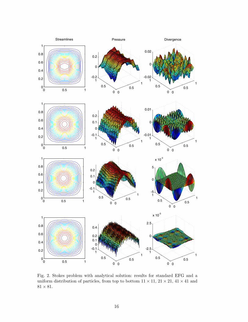
Fig. 2. Stokes problem with analytical solution: results for standard EFG and auniform distribution of particles, from top to bottom 11× 11, 21× 21, 41× 41 and81× 81.

16

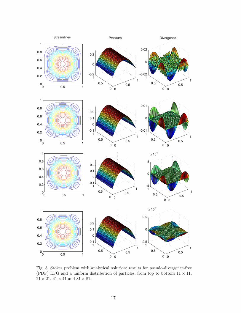
Fig. 3. Stokes problem with analytical solution: results for pseudo-divergence-free(PDF) EFG and a uniform distribution of particles, from top to bottom 11 × 11,21× 21, 41× 41 and 81× 81.

17

0 0.05 0.1−7

−6

−5

−4

−3

−2

h

log(

rela

tive

velo

city

err

or)

0 0.05 0.1−7

−6

−5

−4

−3

−2

h

log(

rela

tive

pres

sure

err

or)

0 0.05 0.1−7

−6

−5

−4

h

log(

dive

rgen

ce)

EFGDiv. Free

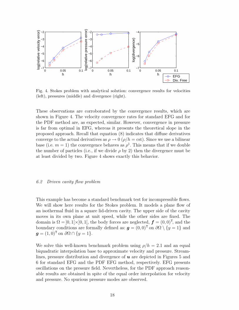
Fig. 4. Stokes problem with analytical solution: convergence results for velocities(left), pressures (middle) and divergence (right).

These observations are corroborated by the convergence results, which areshown in Figure 4. The velocity convergence rates for standard EFG and forthe PDF method are, as expected, similar. However, convergence in pressureis far from optimal in EFG, whereas it presents the theoretical slope in theproposed approach. Recall that equation (8) indicates that diffuse derivativesconverge to the actual derivatives as ρ → 0 (ρ/h = cst). Since we use a bilinearbase (i.e. m = 1) the convergence behaves as ρ1. This means that if we doublethe number of particles (i.e., if we divide ρ by 2) then the divergence must beat least divided by two. Figure 4 shows exactly this behavior.

6.2 Driven cavity flow problem

This example has become a standard benchmark test for incompressible flows.We will show here results for the Stokes problem. It models a plane flow ofan isothermal fluid in a square lid-driven cavity. The upper side of the cavitymoves in its own plane at unit speed, while the other sides are fixed. Thedomain is Ω = ]0, 1[×]0, 1[, the body forces are neglected, f = (0, 0)T, and theboundary conditions are formally defined as: g = (0, 0)T on ∂Ω \ y = 1 andg = (1, 0)T on ∂Ω ∩ y = 1.

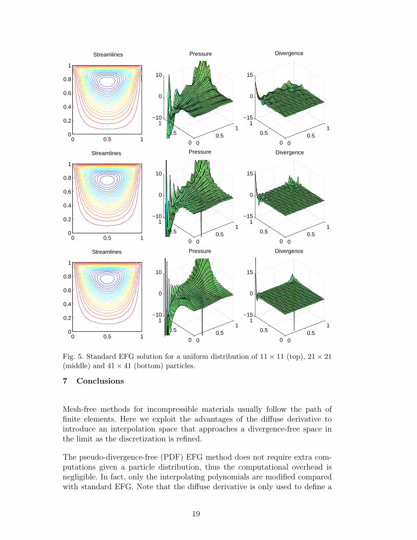
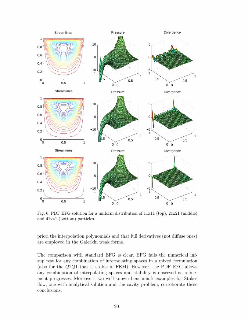
We solve this well-known benchmark problem using ρ/h = 2.1 and an equalbiquadratic interpolation base to approximate velocity and pressure. Stream-lines, pressure distribution and divergence of u are depicted in Figures 5 and6 for standard EFG and the PDF EFG method, respectively. EFG presentsoscillations on the pressure field. Nevertheless, for the PDF approach reason-able results are obtained in spite of the equal order interpolation for velocityand pressure. No spurious pressure modes are observed.

18

0 0.5 10

0.2

0.4

0.6

0.8

1

Streamlines

00.5

1

0

0.5

1−10

0

10

00.5

1

0

0.5

1−15

0

15

Pressure Divergence

0 0.5 10

0.2

0.4

0.6

0.8

1

Streamlines

00.5

1

0

0.5

1−10

0

10

00.5

1

0

0.5

1−15

0

15

Pressure Divergence

0 0.5 10

0.2

0.4

0.6

0.8

1

Streamlines

00.5

1

0

0.5

1−10

0

10

00.5

1

0

0.5

1−15

0

15

Pressure Divergence

Fig. 5. Standard EFG solution for a uniform distribution of 11× 11 (top), 21× 21(middle) and 41× 41 (bottom) particles.

7 Conclusions

Mesh-free methods for incompressible materials usually follow the path offinite elements. Here we exploit the advantages of the diffuse derivative tointroduce an interpolation space that approaches a divergence-free space inthe limit as the discretization is refined.

The pseudo-divergence-free (PDF) EFG method does not require extra com-putations given a particle distribution, thus the computational overhead isnegligible. In fact, only the interpolating polynomials are modified comparedwith standard EFG. Note that the diffuse derivative is only used to define a

19

0 0.5 10

0.2

0.4

0.6

0.8

1

Streamlines

00.5

1

0

0.5

1−10

0

10

Pressure

00.5

1

0

0.5

1−5

0

5

Divergence

0 0.5 10

0.2

0.4

0.6

0.8

1

Streamlines

00.5

1

0

0.5

1−10

0

10

Pressure

00.5

1

0

0.5

1−5

0

5

Divergence

0 0.5 10

0.2

0.4

0.6

0.8

1

Streamlines

00.5

1

0

0.5

1−10

0

10

Pressure

00.5

1

0

0.5

1−5

0

5

Divergence

Fig. 6. PDF EFG solution for a uniform distribution of 11x11 (top), 21x21 (middle)and 41x41 (bottom) particles.

priori the interpolation polynomials and that full derivatives (not diffuse ones)are employed in the Galerkin weak forms.

The comparison with standard EFG is clear. EFG fails the numerical inf-sup test for any combination of interpolating spaces in a mixed formulation(also for the Q2Q1 that is stable in FEM). However, the PDF EFG allowsany combination of interpolating spaces and stability is observed as refine-ment progresses. Moreover, two well-known benchmark examples for Stokesflow, one with analytical solution and the cavity problem, corroborate theseconclusions.

20

References

[1] V. Girault, P.-A. Raviart, Finite element methods for Navier-Stokes equations.Theory and algorithms, Springer-Verlag, Berlin, 1986.

[2] P. M. Gresho, R. L. Sani, Incompressible flow and the finite element method.Vol. 1: Advection diffusion. Vol. 2: Isothermal laminar flow, John Wiley & Sons,Chichester, 2000.

[3] M. D. Gunzburger, Finite element methods for viscous incompressible flows. Aguide to theory, practice, and algorithms, Academic Press, Boston, MA, 1989.

[4] O. Pironneau, Finite element methods for fluids, John Wiley & Sons, Chichester,1989.

[5] L. Quartapelle, Numerical solution of the incompressible Navier-Stokesequations, Vol. 113 of International Series of Numerical Mathematics,Birkhauser-Verlag, Basel, 1993.

[6] A. Quarteroni, A. Valli, Numerical Approximation of Partial DifferentialEquations, Vol. 23 of Springer Series in Computational Mathematics, Springer-Verlag, Berlin, 1994.

[7] R. Temam, Navier-Stokes equations. Theory and numerical analysis, AMSChelsea Publishing, Providence, RI, 2001, corrected reprint of the 1984 edition[North-Holland, Amsterdam, 1984].

[8] J. Donea, A. Huerta, Finite element methods for flow problems, John Wiley &Sons, Chichester, 2003.

[9] D. S. Malkus, Eigenproblems associated with the discrete LBB condition forincompressible finite elements, Int. J. Eng. Sci. 19 (10) (1981) 1299–1310.

[10] F. Brezzi, M. Fortin, Mixed and hybrid finite element methods, Vol. 15 ofSpringer Series in Computational Mathematics, Springer-Verlag, New York,1991.

[11] D. Chapelle, K.-J. Bathe, The inf-sup test, Comput. Struct. 47 (4–5) (1993)537–545.

[12] K.-J. Bathe, D. Hendriana, F. Brezzi, G. Sangalli, Inf-sup testing of upwindmethods, Int. J. Numer. Methods Eng. 48 (5) (2000) 745–760.

[13] T. Zhu, S. N. Atluri, A modified collocation method and a penalty formulationfor enforcing the essential boundary conditions in the element free Galerkinmethod, Comput. Mech. 21 (3) (1998) 211–222.

[14] J. Dolbow, T. Belytschko, Volumetric locking in the element free Galerkinmethod, Int. J. Numer. Methods Eng. 46 (6) (1999) 925–942.

[15] H. Askes, R. de Borst, O. Heeres, Conditions for locking-free elasto-plasticanalyses in the element-free galerkin method, Comput. Methods Appl. Mech.Eng. 173 (1–2) (1999) 99–109.

21

[16] J. S. Chen, S. Yoon, H. Wang, W. K. Liu, An improved reproducing kernelparticle method for nearly incompressible finite elasticity, Comput. MethodsAppl. Mech. Eng. 181 (1–3) (2000) 117–145.

[17] T. J. R. Hughes, The finite element method: linear static and dynamic finiteelement analysis, Dover Publications Inc., New York, 2000, corrected reprint ofthe 1987 original [Prentice-Hall Inc., Englewood Cliffs, N.J.].

[18] A. Huerta, S. Fernandez-Mendez, Locking in the incompressible limit for theelement free galerkin method, Int. J. Numer. Methods Eng. 51 (11) (2001)1361–1383.

[19] B. Nayroles, G. Touzot, P. Villon, Generating the finite element method: diffuseapproximation and diffuse elements, Comput. Mech. 10 (5) (1992) 307–318.

[20] P. Villon, Contribution a l’optimisation, These presentee pour l’obtention dugrade de docteur d’etat, Universite de Technologie de Compiegne, Compiegne,France (1991).

[21] Y. Vidal, P. Villon, A. Huerta, Locking in the incompressible limit: pseudo-divergence-free element-free galerkin, Revue europeene des elements finis11 (7/8) (2002) 869–892.

[22] Y. Vidal, P. Villon, A. Huerta, Locking in the incompressible limit: pseudo-divergence-free element-free galerkin, Commun. Numer. Methods Eng. 19 (9)(2003) 725–735.

[23] W. K. Liu, T. Belytschko, J. T. Oden, editors, Meshless methods, Comput.Methods Appl. Mech. Eng. 139 (1–4) (1996) 1–440.

[24] S. Fernandez-Mendez, A. Huerta, Coupling finite elements and particles foradaptivity: An application to consistently stabilized convection-diffusion, in:M. Griebel, M. A. Schweitzer (Eds.), Meshfree methods for partial differentialequations, Vol. 26 of Lecture Notes in Computational Science and Engineering,Springer-Verlag, Berlin, 2002, pp. 117–129, papers from the Internationalworkshop, Universitat Bonn, Germany, September 11-14, 2001.

[25] S. Fernandez-Mendez, P. Dıez, A. Huerta, Convergence of finite elementsenriched with meshless methods, Numer. Math. DOI 10.1007/s00211-003-0465-x.

[26] T. Belytschko, Y. Krongauz, M. Fleming, D. Organ, W. K. Liu, Smoothingand accelerated computations in the element free Galerkin method, J. Comput.Appl. Math. 74 (1–2) (1996) 111–126.

[27] A. Huerta, S. Fernandez-Mendez, P. Dıez, Enrichissement des interpolations d´elements finis en utilisant des methodes de particules, ESAIM-Math. Model.Numer. Anal. 36 (6) (2002) 1027–1042.

[28] R. Stenberg, On some techniques for approximating boundary conditions in thefinite element method, J. Comput. Appl. Math. 63 (1-3) (1995) 139–148.

22

[29] D. N. Arnold, F. Brezzi, B. Cockburn, L. D. Marini, Unified analysis ofdiscontinuous Galerkin methods for elliptic problems, SIAM J. Numer. Anal.39 (5) (2001/02) 1749–1779.

[30] I. Babuska, U. Banerjee, J. E. Osborn, Meshless and generalized finite elementmethods: A survey of some major results, in: M. Griebel, M. A. Schweitzer(Eds.), Meshfree methods for partial differential equations, Vol. 26 of LectureNotes in Computational Science and Engineering, Springer-Verlag, Berlin, 2002,pp. 1–20, papers from the International workshop, Universitat Bonn, Germany,September 11-14, 2001.

[31] R. Becker, Mesh adaptation for dirichlet flow control via nitsche’s method,Commun. Numer. Methods Eng. 18 (9) (2002) 669–680.

[32] S. Fernandez-Mendez, A. Huerta, Imposing essential boundary conditionsin mesh-free methods, Comput. Methods Appl. Mech. Eng. Accepted forpublication.

[33] M. Griebel, M. A. Schweitzer, A particle-partition of unity method. Part V:Boundary conditions, in: S. Hildebrandt, H. Karcher (Eds.), Geometric Analysisand Nonlinear Partial Differential Equations, Springer, Berlin, 2002, pp. 517–540.

[34] J. T. Oden, O.-P. Jacquotte, Stability of some mixed finite element methods forStokesian flows, Comput. Methods Appl. Mech. Eng. 43 (2) (1984) 231–247.

23