ICES REPORT 12-22

June 2012

The DPG Method for the Stokes Problem.by

N. Roberts, T. Bui-Thanh, and L. Demkowicz

The Institute for Computational Engineering and SciencesThe University of Texas at AustinAustin, Texas 78712

Reference: N. Roberts, T. Bui-Thanh, and L. Demkowicz, The DPG Method for the Stokes Problem., ICESREPORT 12-22, The Institute for Computational Engineering and Sciences, The University of Texas at Austin,June 2012.

THE DPG METHODFOR THE STOKES PROBLEM

N. Roberts, T. Bui-Thanh and L. Demkowicz

Institute for Computational Engineering and SciencesThe University of Texas at Austin, Austin, TX 78712, USA

Abstract

We discuss well-posedness and convergence theory for the DPG method applied to a general systemof linear Partial Differential Equations (PDEs) and specialize the results to the classical Stokes problem.The Stokes problem is an iconic troublemaker for standard Bubnov Galerkin methods; if discretizationsare not carefully designed, they may exhibit non-convergence or locking. By contrast, DPG does notrequire us to treat the Stokes problem in any special manner. We illustrate and confirm our theoreticalconvergence estimates with numerical experiments.

Key words: Discontinuous Petrov Galerkin, Stokes problem

AMS subject classification: 65N30, 35L15

Acknowledgment

Roberts and Demkowicz were supported by the Department of Energy [National Nuclear Security Adminis-tration] under Award Number [DE-FC52-08NA28615]. We also thank Pavel Bochev and Denis Ridzalfor hosting and collaborating with Roberts in the summers of 2010 and 2011, when he was supported byinternships at Sandia National Laboratories (Albuquerque).

1 Introduction

In this paper, we apply the Discontinuous Petrov-Galerkin (DPG) with optimal test functions methodologyrecently developed by Demkowicz and Gopalakrishnan [14, 15] to the Stokes problem, and analyze itswell-posedness. Our analysis is corroborated by numerical experiments.

The Discontinuous Petrov-Galerkin Method with Optimal Test Functions. We begin with a short his-torical review of the method. By a discontinuous Galerkin (DG) method, we mean one that allows testand/or trial functions that are not globally conforming; by a Petrov-Galerkin method, we mean one that

1

allows the test and trial spaces to differ. In 2002, Bottasso et al. introduced a method [3, 4], also calledDPG. Like our DPG method, theirs used an “ultra-weak” variational formulation (moving all derivativesto test functions) and replaced the numerical fluxes used in DG methods to “glue” the elements togetherwith new independent unknowns defined on element interfaces. The idea of optimal testing was introducedby Demkowicz and Gopalakrishnan in 2009 [14], which is distinguished by an on-the-fly computation ofan approximation to a set of test functions that are optimal in the sense that they guarantee minimizationof the residual in the dual norm. In 2009-2010, a flurry of numerical experimentation followed, includingapplications to convection-dominated diffusion [15], wave propagation [34], elasticity [6], thin-body (beamand shell) problems [29], and the Stokes problem [32]. The wave propagation paper also introduced theconcept of an optimal test norm, whose selection makes the energy norm identical to the norm of intereston the trial space. In 2010, Demkowicz and Gopalakrishnan proved the convergence of the method for theLaplace equation [16], and Demkowicz and Heuer developed a systematic approach to the selection of atest space norm for singularly perturbed problems [18]. In 2011, Bui-Thanh et al. [8] developed a unifiedanalysis of DPG problems by means of Friedrichs’ systems, upon which we rely for our present analysis ofthe Stokes problem.

Some work has been done on nonlinear problems as well. Very early on, Chan, Demkowicz, and Robertssolved the 1D Burgers and compressible Navier-Stokes equations by applying DPG to the linearized problem[10]. More recently, Moro et al. have applied their related HDPG method to the 2D Burgers equation; a keydifference in their work is that they apply DPG to the nonlinear problem, using optimization techniques tominimize the DPG residual.

Most DPG analysis assumes that the optimal test functions are computed exactly, but in practice we mustapproximate them. Gopalakrishnan and Qiu have shown that for the Laplace equation and linear elasticity,for sufficiently high-order approximations1 of the test space, optimal convergence rates are maintained [23].

We will now briefly derive DPG, motivating it as a minimum residual method. Suppose that U is thetrial space, and V the test space (both Hilbert) for a well-posed variational problem b(u, v) = l(v). Writingthis in the operator form Bu = l, where B : U → V ′, we seek to minimize the residual for the discretespace Uh ⊂ U :

uh = arg minuh∈Uh

1

2‖Buh − l‖2V ′ .

Now, the dual space V ′ is not especially easy to work with; we would prefer to work with V itself. Recallingthat the Riesz operator RV : V → V ′ defined by

〈RV v, δv〉 = (v, δv)V , ∀δv ∈ V,

where 〈·, ·〉 denotes the duality pairing between V ′ and V , is an isometry—that is, ‖RV v‖V ′ = ‖v‖V —we

1ktest = ktrial + N , where N is the number of space dimensions, and by ktest we mean the polynomial order of the basisfunctions for the test space, and by ktrial we mean the order for the L2 bases in the trial space.

2

can rewrite the term we want to minimize as a norm in V :

1

2‖Buh − l‖2V ′ =

1

2

∥∥R−1V (Buh − l)

∥∥2

V=

1

2

(R−1V (Buh − l) , R−1

V (Buh − l))V. (1.1)

The first-order optimality condition requires that the Gateaux derivative of (1.1) be equal to zero for mini-mizer uh; we have (

R−1V (Buh − l) , R−1

V Bδuh)V

= 0, ∀δuh ∈ Uh.

By the definition of RV , the preceding equation is equivalent to

〈Buh − l, R−1V Bδuh〉 = 0 ∀δuh ∈ Uh. (1.2)

Now, if we identify vδuh = R−1V Bδuh as a test function, we can rewrite (1.2) as

b(uh, vδuh) = l(vδuh).

Note that the last equation is exactly the original variational form, tested with a special function vδuh thatcorresponds to δuh ∈ Uh; we call vδuh an optimal test function. The DPG method is then to solve theproblem b(uh, vδuh) = l(vδuh) with optimal test functions vδuh ∈ V that solve the problem

(vδuh , δv)V = 〈RV vδuh , δv〉 = 〈Bδuh, δv〉 = b(δuh, δv), ∀δv ∈ V. (1.3)

In standard conforming methods, test functions are continuous over the entire domain, which would meanthat solving (1.3) would require computations on the global mesh, making the method impractical. In DPG,we use test functions that are discontinuous across elements, so that (1.3) becomes a local problem—thatis, it can be solved element-by-element. Of course, (1.3) still requires inversion of the infinite-dimensionalRiesz map, and we approximate this by using an “enriched” test space Vh of polynomial order higher thanthat of the trial space Uh. Note that the test functions vδuh immediately give rise to a hermitian positivedefinite stiffness matrix; if ei is a basis for Uh, we have:

b(ei, vej ) = (vei , vej )V = (vej , vei)V = b(ej , vei).

It should be pointed out that we have not made any assumptions about the inner product on V . Animportant point is that by an appropriate choice of test space inner product, the induced energy norm on thetrial space can be made to coincide with the norm of interest [34]; DPG then delivers the best approximationerror in that norm. In practice this optimal test space inner product is approximated by a “localizable” innerproduct, and DPG delivers the best approximation error up to a mesh-independent constant. That is,

‖u− uh‖U ≤M

γDPGinf

wh∈Uh

‖u− wh‖U ,

where M = O(1) and γDPG is mesh-independent, and γDPG is of the order of inf-sup constants for thestrong operator and its adjoint (see Section 2.3). We therefore say that DPG is automatically stable, moduloany error in solving for the test functions vδuh .

3

DPG also provides a precise measurement of the error in the dual norm:

‖Buh − l‖V ′ =∥∥R−1

V (Buh − l)∥∥V.

If we then define an error representation function e = R−1V (Buh − l) ∈ V , we can solve

(e, δv)V = b(uh, δv)− l(δv), ∀δv ∈ V,

locally for e. We use ‖eK‖V = ‖Buh − l‖V ′(K) on each element K to drive adaptive mesh refinements.

It is a relatively simple matter, when desired, to enforce local conservation—that is, an element-wiseproperty that corresponds to a (mass) conservation law—by means of Lagrange multipliers. This was firstnoted by Moro et al. [28]. This is often useful in the context of practical fluid problems, but falls outside thescope of our present analysis. In the context of the numerical examples presented here, local conservationappears to have negligible effect.

The Stokes problem. The classical strong form of the Stokes problem in Ω ⊂ R2 is given by

−µ∆u+∇p = f in Ω, (1.4a)

∇ · u = g in Ω, (1.4b)

u = uD on ∂Ω, (1.4c)

where µ is viscosity, p pressure, u velocity, and f a vector forcing function. The first equation correspondsto conservation of momentum, and the second to conservation of mass. While the analysis will treat the casewhere mass can be added or removed from the system (g 6= 0), in practice generally (and in our numericalexperiments) g = 0. Since by appropriate non-dimensionalization we can eliminate the constant µ, we takeµ = 1 throughout.

In order to apply the DPG method, we need to cast the system (1.4a)–(1.4c) as a first-order system. Weintroduce σ = ∇u:

−∇ · σ +∇p = f inΩ, (1.5a)

∇ · u = g in Ω, (1.5b)

σ −∇u = 0 in Ω, (1.5c)

u = uD on∂Ω. (1.5d)

Clearly, the first-order formulation is by no means unique; we have chosen this one for convenience ofmathematical analysis and simplicity of presentation. Previously, we have experimented with other formu-lations; the velocity-stress-pressure (VSP) and the velocity-vorticity-pressure (VVP) formulations [32, 31].Note also that σ in this formulation is not the physical stress (the physical stress does enter the VSP formu-lation).

4

The Stokes equations model incompressible viscous (“creeping”) flow; they can be derived by neglect-ing the convective term in the incompressible Navier-Stokes equations. Naive discretizations for the Stokesproblem can lead to non-convergence or locking [2]. Of crucial importance for Bubnov-Galerkin formula-tions of the Stokes equations—and more generally, of saddle point problems—is the satisfaction of the twoso-called Brezzi inf-sup conditions [7]. For the Stokes equations, the first of these, the “inf-sup in the ker-nel” condition, is satisfied automatically. If the discrete spaces for velocity u and pressure p are V h ⊂H1

and Qh ⊂ L2, respectively, the second Brezzi condition for Stokes is then

infq∈Qh

supv∈Vh

(q,∇ · v)

‖q‖L20‖v‖H1

≥ γh ≥ γ0 > 0.

In the context of Stokes, this condition is often called the Ladyzhenskaya-Babuska-Brezzi (LBB) condition,because Ladyzhenskaya first proved the continuous analog of the condition for the Stokes equations [25];much of the challenge in solving Stokes lies in the selection of discrete spaces that satisfy this condition.

In [2], Boffi, Brezzi, and Fortin survey some choices for finite element discretizations to satisfy the LBBcondition for the Stokes problem, among which are the MINI element, Crouzeix-Raviart element, and theclass of Qk − Pk−1 elements. Generalized Hood-Taylor elements can be shown to satisfy the conditionunder certain regularity constraints on the mesh. (Each of these elements generalizes to three-dimensionalspaces as well.) It is worth noting that each of these elements uses a polynomial approximation for pressureof one order lower than that used for velocity, so that the theoretical optimal convergence rate is lower forthe pressure than it is for the velocity.

Cockburn et al. have applied the local discontinuous Galerkin (LDG) method [9] to the Stokes prob-lem [11]; LDG derives its name from the local elimination of some variables (in the case of Stokes, thestresses)—by comparison with standard DG methods, the global solve in LDG involves only about half asmany unknowns, a significant savings. By means of carefully chosen numerical fluxes, the LDG methodcan enforce conservation laws weakly element by element, in a locally conservative way. The method alsoallows one to choose spaces for the pressure and velocity independently, so that they can use equal-orderapproximations, but they show that the convergence rate for pressure and stress will be of order one less thanthat for velocity. They numerically compare the efficiency of using lower-order approximations for pressureand stress with that of equal-order approximations, and conclude that in most cases the equal-order ap-proximations are more efficient: although both choices yield the same rate of convergence, the lower-orderapproximation requires more degrees of freedom to achieve the same accuracy.

It is also worth emphasizing that finding these good spaces for the Stokes problem is difficult—this hasbeen an area of ongoing research for decades. In this paper, we demonstrate that DPG allows solution ofthe Stokes problem without any special effort—that is, the Stokes problem is approached and analyzed withexactly the same DPG-theoretical tools that we use for other linear problems, and we can use the samediscrete spaces for velocity and pressure. In particular, we use equal-order spaces for velocity and pressure,and both pressure and velocity converge at the same rate, a contrast with LDG [11]. Indeed, one of ournumerical experiments demonstrates not only that the method delivers the optimal convergence rate, but

5

also that the method provides a solution close to the L2 projection of the exact solution.

Our Stokes work began in collaboration with Pavel Bochev and Denis Ridzal in the summer of 2010[32], when Roberts did an internship at Sandia. Bochev astutely suggested the Stokes problem as a goodexample problem for DPG. That summer, we were puzzled by the poor performance of DPG using what weherein refer to as the naive test space norm; the present analysis serves (among other things) to explain whythe naive norm fails to achieve optimal convergence rates, in contrast to the choice to which our analysisleads us, which we here call the adjoint graph norm.

The structure of this paper is as follows. In Section 2, we present the general theory for the DPGmethod, and apply it to the Stokes problem. In Section 3 we detail some numerical experiments involving amanufactured solution and the lid-driven cavity flow problem. Section 4 concludes the paper, followed by anappendix in which we show that the operator for the first-order Stokes system with homogeneous boundaryconditions is bounded below.

2 Analysis

The purpose of this section is to present a general theory for the DPG method for linear PDEs and imme-diately specialize it to the Stokes problem. The presented theory summarizes results obtained in [16, 5, 17]for particular boundary-value problems and specializes the general theory for Friedrichs systems, presentedin [8], for cases in which the traces of the graph spaces are available. As most of the technical results hereare classical, we have chosen a colloquial format of presentation.

2.1 Notation and Definitions

Let Ω denote a bounded Lipschitz domain in IRn, n = 2, 3, with boundary Γ = ∂Ω. We shall use thefollowing standard energy spaces:

H1(Ω) := u ∈ L2(Ω) : ∇u ∈ L2(Ω),

H(div,Ω) := σ ∈ L2(Ω) : divσ ∈ L2(Ω),

with the corresponding trace spaces on Γ:

H1/2(Γ) := u =u|Γ, u ∈ H1(Ω),

H−1/2(Γ) := σn = (σ · n)|Γ, σ ∈H(div,Ω),

where n denotes the outward normal unit vector to the boundary Γ. The definition of trace space H1/2(Γ)

is classical but far from trivial, see e.g. [26, pp. 96]. The assumption on the regularity of the domain(being Lipschitz) is essential; domains with “cracks” require a special and non-classical treatment. Whennecessary, we will formalize the use of the trace operator by identifying it with a separate symbol,

tr : H1(Ω) 3 u→ tr u = u =u|Γ ∈ H1/2(Γ).

6

The space H−1/2(Γ) is the topological dual of H1/2(Γ) and a second trace operator corresponding to it,

tr : H(div,Ω) 3 σ → tr σ = σn = (σ · n)|Γ ∈ H−1/2(Γ),

is usually defined by the generalized Green Formula; see e.g. [33, pp. 61] or [30, pp. 530]. Note that,unless otherwise stated, in this paper we use the same trace notation “tr” for functions in both H1(Ω) andH(div,Ω).

We shall also use group variables consisting of multiple copies of functions from H1(Ω),H(div,Ω),and H1/2(Γ) or distributions from H−1/2(Γ). We will then switch to boldface notation:

H1(Ω) = H1(Ω)× . . .×H1(Ω),

H1/2(Γ) = H1/2(Γ)× . . .×H1/2(Γ),

H−1/2(Γ) = H−1/2(Γ)× . . .×H−1/2(Γ),

etc. In the case of tensors, the definitions will be applied row-wise:

σ = (σij) ∈H(div,Ω) ⇐⇒ (σi1, . . . , σin) ∈H(div,Ω), i = 1, . . . , n.

Broken energy spaces. Let Ω be partitioned into finite elements K such that

Ω =⋃K

K, K open,

with corresponding skeleton Γh and interior skeleton Γ0h,

Γh :=⋃K

∂K Γ0h := Γh − Γ.

The usual regularity assumptions for the elements can essentially be relaxed. The elements may be generalpolygons in 2D, or polyhedra2 in 3D (with triangular and quadrilateral faces). Meshes may be irregular,i.e. with hanging nodes (see e.g. [13, pp. 211]). Also, at this point, we do not make any shape regularityassumptions. By broken energy spaces we simply mean standard energy spaces defined element-wise:

H1(Ωh) :=∏K H

1(K),

H(div,Ωh) :=∏KH(div,K).

With broken energy spaces, integration by parts is performed element-wise. For σ ∈ H(div,Ωh) andv ∈ H1(Ω), we have

(divhσ, v)Ωh:=

∑K

(divσ, v)K

=∑K

(−(σ,∇v)K + 〈σn, v〉∂K)

= −(σ,∇v) +∑K

〈σn, v〉∂K︸ ︷︷ ︸=:〈σn,v〉Γh

.

2Possibly curvilinear polyhedra.

7

Here (·, ·) and (·, ·)K denote the L2-product over the whole domain and elementK, resp., and 〈·, ·〉∂K standsfor the duality pairing between H−1/2(∂K) and H1/2(∂K).

Integration by parts leads naturally to the concept of the trace space over the skeleton Γh,

H1/2(Γh) :=

v = vK ∈

∏K

H1/2(∂K) : ∃v ∈ H1(Ω) : v|∂K = vK

.

This is not a trivial definition. First of all, to be more precise, by v|∂K we mean the trace (for element K)

of the restriction of v to K. Secondly, H1/2(Γh) is a closed subspace of∏K H

1/2(∂K), as we shall showmomentarily. For convenience, we assume that all trace spaces are endowed with minimum-energy extensionnorms, i.e.,

‖u‖H1/2(∂K) := infEu∈H1(K)Eu|∂K=u

‖Eu‖H1(K),

etc. Let un = unK be a sequence of functions in H1/2(Γh) converging in the product space to a limitu = uK. For each element K, unK is the trace of restriction un|K for some un ∈ H1(Ω). By thedefinition of norms, un|K

n→∞−→ uK in H1(K), for each element K. The delicate question is whetherwe can claim that the union u of uK is in H1(Ω). But this follows from the definition of distributionalderivatives. Indeed, given a test function φ ∈ D(Ω), we have for each n,∫

Ωun

∂φ

∂xi= −

∫Ω

∂un

∂xiφ

or ∑K

∫Kun

∂φ

∂xi= −

∑K

∫K

∂un

∂xiφ.

Passing to the limit with n→∞, we get∫Ωu∂φ

∂xi= −

∑K

∫K

∂uK∂xi

φ,

which proves that the union of element-wise derivatives ∂uK∂xi

, a function in L2(Ω), is the distributionalderivative of u. Consequently, u ∈ H1(Ω).

Notice that we have not attempted to extend the classical definition of the trace space H1/2(Γ) forLipschitz boundary Γ to a non-Lipschitz skeleton Γh.3 This is not impossible but much more technical (likefor domains with cracks).

3The definition of a Lipschitz domain includes the assumption that the domain is on one side of its boundary, see [26, pp. 89].

8

A similar construction holds for globally conforming σ ∈H(div,Ω) but broken v ∈ H1(Ωh):

(σ,∇hv)Ωh:=∑K

(σ,∇v)K

=∑K

(−(divσ, v)K + 〈σn, v〉∂K)

= −(divσ, v) +∑K

〈σn, v〉∂K︸ ︷︷ ︸=:〈σn,v〉Γh

.

In this case, we are led to the definition of the trace space H−1/2(Γh):

H−1/2(Γh) :=

σn = σKn ∈

∏K

H−1/2(∂K) : ∃σ ∈H(div,Ω) : σKn = (σ · n)|∂K

.

We equip both trace spaces over the mesh skeleton with minimum energy extension norms

‖v‖H1/2(Γh) := infu∈H1(Ω)u|Γh

=u

‖u‖H1(Ω) and

‖σn‖H−1/2(Γh) := inf σ∈H(div,Ω)(σ·n)|Γh

=σn

‖σ‖H(div,Ω).

We will also need the space of traces on the internal skeleton

H1/2(Γh) :=

v = vK ∈

∏K

H1/2(∂K) : ∃v ∈ H10 (Ω) : v|∂K = vK

,

which we likewise equip with the minimum energy extension norm.

To summarize, we have defined the term 〈σn, v〉Γhwhen one of the variables is a trace over the whole

skeleton and the other is the trace of a function from the broken energy space. Also notice that, for suf-ficiently regular functions, 〈σn, v〉Γh

represents either the L2(Γh)-product of trace of a conforming σ andinter-element jumps of v, or the product of jumps in σn and the trace of a globally conforming v. This canbe seen by switching from the summation over elements to the summation over element faces (edges in 2D).

2.2 Strong and Ultra-Weak Formulations

Integration by parts. Let u now represent a group variable consisting of functions defined on the domainΩ, and A be a linear differential operator corresponding to a system of first order PDEs. We start with anabstract integration by parts formula,

(Au, v) = (u,A∗v) + 〈Cu, v〉. (2.6)

Here (·, ·) denotes the L2(Ω)-inner product, A∗ is the formal adjoint operator, C is a boundary operator andat this point 〈·, ·〉 stands for just the L2(Γ)-inner product on boundary Γ = ∂Ω. Obviously, the formula

9

holds under appropriate regularity assumptions, e.g. u, v ∈ C1(Ω), if all derivatives are understood in theclassical sense.

If we assume u, v ∈ L2(Ω) and interpret the derivatives in a distributional sense, we arrive naturally atthe graph energy spaces

HA(Ω) := u ∈ L2(Ω) : Au ∈ L2(Ω) and

HA∗(Ω) := u ∈ L2(Ω) : A∗u ∈ L2(Ω).

Assumption 1: We take operators A and A∗ to be surjections; i.e. given f ∈ L2(Ω), we can always findu ∈ HA(Ω) and v ∈ HA∗(Ω) such that Au = f or A∗v = f . Roughly speaking, this corresponds to anassumption that neither A nor A∗ are, in a sense, degenerate.4

With u and v coming from the energy spaces, the domain integrals (Au, v) and (u,A∗v) are well-defined. We now assume that the graph spaces admit trace operators

trA : HA(Ω) HA(Γ) and

trA∗ : HA∗(Ω) HA∗(Γ).

The double arrowheads indicate that the trace operators are surjective. We equip the trace spaces with theminimum energy extension norms

‖u‖HA(Γ) = infu∈HA(Ω)

trAu=u

‖u‖HA(Ω) and ‖v‖HA∗ (Γ) = infv∈HA∗ (Ω)

trA∗v=v

‖v‖HA∗ (Ω).

We now generalize the classical integration by parts formula (2.6) to a more general, distributional case:

(Au, v) = (u,A∗v) + c(trAu, trA∗v),

with u ∈ HA(Ω), v ∈ HA∗(Ω), and

c(u, v), u ∈ HA(Γ), v ∈ HA∗(Γ)

being a duality pairing,5 i.e. a definite continuous bilinear (sesquilinear) form. Recall that form c(u, v) isdefinite if

(c(u, v) = 0 ∀v) =⇒ u = 0 and

(c(u, v) = 0 ∀u) =⇒ v = 0.

Equivalently, the corresponding boundary operator

C : HA(Γ)→ (HA∗(Γ))′, 〈Cu, v〉 = c(u, v)

and its adjoint C ′ are injective and therefore both C and C ′ are isomorphisms.6 Above and in what follows,〈·, ·〉 denotes the usual duality pairing between a space and its dual.

4Ivo Babuska, private communication.5This notion extends the definition of the “usual” duality pairing between a space and its dual.6R(A) = N (C′)⊥.

10

Integration by parts for the Stokes problem. We verify (and illustrate) our general assumptions forthe Stokes problem. Multiplying equations (1.4a-1.4c) with test functions v, q, τ , integrating by parts andsumming up the equations, we obtain

(−div(σ − pI),v) + (divu, q) + (σ −∇u, τ ) = (σ − pI,∇v) + 〈(−σ + pI)n,v〉

+ (u,−∇q) + 〈u · n, q〉

+ (σ, τ ) + (u,divτ ) + 〈u,−τn〉

= (u,div(τ − qI)) + (p,−divv) + (σ, τ +∇v)

+ 〈(−σ + pI)n,v〉+ 〈u, (−τ + qI)n〉.

Thus, comparing with the abstract theory, we have

u = (u, p,σ),

v = (v, q, τ ),

Au = (−div(σ − pI), divu,σ −∇u),

A∗v = (div(τ − qI),−divv, τ +∇v).

The operator is not (formally) self-adjoint but the corresponding energy graph spaces are identical,HA(Ω) =

HA∗(Ω), whereHA(Ω) = (u, p,σ) : σ − pI ∈H(div,Ω),u ∈H1(Ω).

The traces are also the same; that is, trA = trA∗ , where

trA : HA(Ω) 3 (u, p,σ)→ ((−σ + pI)n,u) ∈H−1/2(Γ)×H1/2(Γ).

The boundary term, being the sum of standard duality pairings for respective components of the traces, isdefinite.

Remark 1 The Stokes problem can be framed into a general abstract case discussed in [30, Section 6.6].The boundary term is identified as a concominant of the corresponding traces. Moreover, the Stokes equationcan be cast into a Friedrichs’ system [19], and hence can be studied using the unified DPG framework [8]which uses boundary operator and graph spaces. Here, inspired by our previous work [8], we develop anabstract DPG theory using the trace operators and graph spaces, assuming the existence of traces, and studythe Stokes equation using this framework.

Strong formulation with homogeneous BC. We return now to our abstract setting and assume that theboundary operator C can be split into two operators C1 and C2 such that

〈Cu, v〉 = 〈C1u, v〉+ 〈C2u, v〉= 〈C1u, v〉+ 〈u,C ′2v〉;

11

we also take C1 and C2 to be “reasonable” in the sense that both have closed range. It should be pointed outthat this is analogous to boundary operator splitting due to Friedrichs [22, 20].

We are interested in solving a non-homogeneous boundary-value problemAu = f in Ω,C1u = fD on Γ,

(2.7)

with f ∈ L2(Ω) and fD ∈ R(C1).

We begin with the homogeneous BC case:Au = f in Ω,C1u = 0 on Γ.

(2.8)

Introducing the spacesU := u ∈ HA(Ω) : C1 trAu = 0 and

V := v ∈ HA∗(Ω) : C ′2 trA∗v = 0,we see that, if we restrict operators A and A∗ to U and V , the boundary term vanishes. However, for A andA∗ to be L2-adjoint, we have to make an additional technical assumption.7

Assumption 2: (〈u,C ′2v〉 = 0 ∀u : C1u = 0

)=⇒ C ′2v = 0. (2.9)

We now need to do some elementary algebra.

Lemma 1Assume that C : X → Y is an isomorphism from Hilbert space X onto a Hilbert space Y . Assume Chas been split into C1 and C2 that satisfy condition (2.9). Each of following conditions is then equivalentto (2.9).

N (C1)⊥ ∩R(C ′2) = 0,

N (C1)⊥ ∩N (C2)⊥ = 0,

N (C2) ∩N (C1) = 0,

X = N (C2)⊕N (C1).

Proof: Elementary with an application of the Closed Range Theorem that we recall below.

Condition (2.9) thus decomposes the trace space HA(Γ) into the direct sum of the nullspaces of operatorsC1 and C2;

HA(Γ) = H1A(Γ)⊕ H2

A(Γ), (2.10)7The domain of the adjoint operator has to be maximal in the sense that it includes all v for which the boundary term vanishes.

12

where H1A(Γ) = N (C2) and H2

A(Γ) = N (C1). In other words, for each u ∈ HA(Γ), there exist uniqueu1 ∈ H1

A(Γ) and u2 ∈ H2A(Γ) such that

u = u1 + u2,

which is analogous to the condition introduced by Friedrichs [22] on his boundary operatorM , subsequentlygeneralized in [20], and first used in the DPG context in [8].

Having reduced the problem with homogeneous BC to the classical theory of L2-adjoint operators, wenow recall the Banach Closed Range Theorem. Let T : X → Y be a linear, continuous operator from aHilbert space X into a Hilbert space Y . Let T be the corresponding operator defined on the quotient spaceX/N (T ) or, equivalently, the restriction of T to the X-orthogonal complement of null space of operator T ,N (T )⊥ ⊂ X . Let T ∗ denote the analogous operator for the adjoint T ∗. The following conditions are thenequivalent to each other.

T has a closed range ,

T ∗ has a closed range ,

T is bounded below, i.e. ‖Tu‖ ≥ γ‖u‖ ∀u ∈ N (T )⊥,

T ∗ is bounded below, i.e. ‖T ∗v‖ ≥ γ‖v‖ ∀v ∈ N (T ∗)⊥.

Note that the (maximal) constant γ is the same for T and T ∗.

Assumption 3: The operator A|U , restricted to the L2- orthogonal complement N (A)⊥, is boundedbelow.

The homogeneous problem (2.8) and its adjoint counterpart are thus well-posed. More precisely, foreach data function f which is L2-orthogonal to the null space of the adjoint operator, a solution exists, isunique in the orthogonal complement of the null space of the operator (equivalently, in the quotient space),and depends continuously on f . The inverse of the maximal constant γ is precisely the norm of the inverseoperator from R(A) into N (A)⊥ (which is equal to the norm of the solution operator from R(A∗) intoN (A∗)⊥).

Strong formulation with homogeneous BC for the Stokes problem. We have

C1u = C1(u, p,σ) = tr u and C ′2v = C ′2(v, q, τ ) = tr v.

Condition (2.9) is easily satisfied. We have U = V , where

U = (u, p,σ) ∈ (L2(Ω)× L2(Ω)×L2(Ω)) : σ − pI ∈H(div,Ω),u ∈H10(Ω).

Both A and A∗ have non-trivial null space consisting of constant pressures. To ensure uniqueness, we haveto restrict ourselves to pressures p and q with zero average;

p, q ∈ L20 :=

q ∈ L2(Ω) :

∫Ωq = 0

.

13

The proof that A and A∗ are bounded below involves the Ladyzenskaya inf-sup condition; for the reader’sconvenience we reproduce the classical reasoning in Appendix A.

Strong formulation with non-homogeneous BC. We are now ready to tackle the case with a non-homogeneous boundary condition. We have

(Au, v)− 〈C1u, v〉 = (u,A∗v) + 〈u,C ′2v〉 u ∈ HA(Ω), v ∈ HA∗(Ω).

We are interested in the operators

HA(Ω) 3 u→ (Au,C1u) ∈ L2(Ω)× (HA∗(Γ))′ and

HA∗(Ω) 3 v → (A∗v, C ′2v) ∈ L2(Ω)× (HA(Γ))′.

We have the following classical result.

THEOREM 1Assume that data f ∈ L2(Ω) and fD ∈ R(C1) satisfy the compatibility condition

(f, v)− 〈fD, v〉 = 0 ∀v : A∗v = 0, C ′2v = 0.

Problem (2.7) has a unique solution u in N (A)⊥ that depends continuously upon the data; i.e. there existsa constant γ > 0, independent of the data, such that

γ‖u‖HA(Ω) ≤(‖f‖2 + ‖fD‖2

)1/2.

The analogous result holds for the adjoint operator (A∗, C ′2).

Proof: Let C1 denote the restriction of C1 to H1A(Γ). Since C1 is then injective and has closed range, it

admits a continuous inverse:

‖u1‖HA(Γ) =∥∥C−1

1 fD∥∥HA(γ)

≤ 1

δ‖fD‖(HA∗ (Γ))′ .

Let u = (u1, 0) and let ˜u be the minimum-energy extension of u in HA(Ω). We seek a solution u in theform

u = u0 + ˜u,where u0 ∈ N (A|U )⊥ solves the homogeneous BVP (2.8) with the modified right-hand side f − A˜u. Theload f −A˜u satisfies the compatibility condition for the homogeneous case. Indeed,

(f −A˜u, v) = (f, v)− (A˜u, v)

= (f, v)−(

(˜u,A∗v)− 〈fD, v〉 − 〈˜u,C ′2v〉)= (f, v)− 〈fD, v〉 = 0,

14

for each v such that A∗v = 0 and C ′2v = 0.

We now have‖u‖2HA

= ‖u0 + ˜u‖2HA

≤ 2(‖u0‖2HA

+ ‖˜u‖2HA

).

Now, observe that

‖˜u‖HA(Ω) = ‖u‖HA(Γ) ≤1

δ‖fD‖(HA∗ (Γ))′

and that‖u0‖2HA

= ‖u0‖2 + ‖Au0‖2

≤(

1

γ2+ 1

)‖Au0‖2

≤ 2

(1

γ2+ 1

)[‖f‖2 +

1

δ2‖fD‖2

].

Combining these results ends the proof with

1

γ≤ 2 max

√1

γ2+ 1,

1

δ

√1

γ2+

3

2

.

Strong formulation with non-homogeneous BC for the Stokes problem. The ranges of operators C1

and C ′2 coincide exactly with H1/2(Γ). The strong formulation for the non-homogeneous Stokes problemis well-posed, provided the data g and uD satisfy the compatibility condition∫

Ωg =

∫ΓuD · n.

The analogous conclusion holds for the adjoint operator.

Ultra-weak (variational) formulation. We are now ready to formulate the ultra-weak variational formu-lation for problem (2.7). The steps are as follows.

1. Integrate by parts:(u,A∗v) + 〈CtrAu, v〉 = (f, v).

2. Split the boundary operator C into C1 and C2 according to the decomposition in (2.10):

(u,A∗v) + 〈C1(trAu)1, v〉+ 〈C2(trAu)2, v〉 = (f, v).

3. Apply the BC, moving the known term C1(trAu)1 = fD to the right-hand side:

(u,A∗v) + 〈(trAu)2, C′2v〉 = (f, v)− 〈fD, v〉.

15

4. Declare u2 = (trAu)2 to be an independent unknown. The problem then becomesFind u ∈ L2(Ω), u2 ∈ H2

A(Γ) such that

(u,A∗v) + 〈u2, C′2v〉 = (f, v)− 〈fD, v〉 ∀v ∈ HA∗(Ω).

(2.11)

The bilinear formb((u, u2), v) := (u,A∗v) + 〈u2, C

′2v〉 = (u,A∗v) + c(u2, v) (2.12)

generates two associated operators B and B′, where

b((u, u2), v) = 〈B(u, u2), v〉 = 〈(u, u2), B′v〉.

Operator B′ corresponds to the strong setting for the adjoint A∗ with non-homogeneous BC;

B′v = (A∗v, C ′2v) ∈ L2(Ω)× (HA(Γ))′.

In order to determine the null-space of operator B, assume that

b((u, u2), v) = 0 ∀v ∈ HA∗(Ω).

Testing first with v ∈ D(Ω), we deduce that Au = 0. Integrating the first term by parts, and testing witharbitrary v, we learn that u2 = u on Γ and C1u = 0.

THEOREM 2Problem (2.12) is well-posed. In particular, for each f and fD which satisfy the compatibility condition

(f, v)− 〈fD, v〉 = 0 ∀v ∈ N (A∗|V ), (2.13)

a solution of (2.12) exists which is unique up to u ∈ N (A|U ) and corresponding u2 ∈ H2A(Γ) such that

u2 − u2 ∈ N (C1) where u2 is the corresponding component of trace of u in H2A(Γ).

The inf-sup constant for bilinear form (2.13) is equal to the inf-sup constant of the adjoint operator(A∗, C ′2) from Theorem 1.

Proof: We observe that the conjugate B′ of operator B corresponding to the bilinear form (2.13) co-incides with the strong form of operator (A∗, C ′2). The result is then a direct consequence of Theorem 1.

Ultra-weak formulation for the Stokes problem. The Stokes formulation is now just a matter of inter-pretation. The solution consists of u = (u, p,σ) and unknown traction

t = (−σ + pI)n

16

Remember that only for sufficiently regular8 solution u will t coincide with the trace (−σ + pI)n. In theultra-weak formulation, the traction t appears as an independent unknown. With homogeneous incompress-ibility constraint, the variational problem reads as follows.

Find u ∈ L2(Ω), p ∈ L2(Ω),σ ∈ L2(Ω), t ∈ H−1/2(Γ) such that

(u,div(τ − qI)) + (p,−divq) + (σ, τ +∇v) + 〈t,v〉 = (f ,v)− 〈uD, (−τ + qI)n〉

∀(v, q, τ ) such that τ − qI ∈H(div,Ω),v ∈H1(Ω).

The load is specified by a body force f ∈ L2(Ω) and a velocity uD ∈ H1/2(Γ) on the boundary withvanishing normal component: ∫

ΓuD · n = 0.

The solution is determined up to a constant pressure p0 and corresponding constant traction t0 = p0n.

Notice that there are no boundary conditions imposed on the test functions. This is important from apractical point of view.

Remark 2 Strong versus weak imposition of boundary conditions. In classical variational formulationsfor second order PDEs, we distinguish between strong (Dirichlet) BCs and weak (Neumann) BCs. DirichletBCs are accounted for by coming up with a finite-energy lift of the BC data, and looking for a solution tothe problem with homogeneous BCs and a modified “load vector” that includes the action of the bilinearform on the lift [13, p. 34]. In practice, the Dirichlet data is first projected (interpolated) into the trace ofFE space and then lifted with FE shape functions. By contrast to the Dirichlet BC case, Neumann BCs onlycontribute to the load vector. The terms “strong” and “weak” refer to the fact that, with Dirichlet data in theFE space, Dirichlet BCs are enforced pointwise, whereas Neumann BCs, in general, are satisfied only in thelimit.

In an ultra-weak variational formulation, each BC may be specified either in a “strong” or “weak” way.The formulation discussed above corresponds to a weak imposition of the BC. Data fD contributes to theload vector and is accounted for on the element level, in the integration for the load vector. An alternate,strong imposition of the same BC, starts with finding a trace lift u0 of the BC,

C1u0 = fD.

Notice that the lift may have a non-zero H2A-component but the final trace will be equal to the sum of the

lift and an unknown component u2 ∈ H2A,

u = u0 + u2.

The term 〈fD, v〉 on the right-hand side of (2.13) is simply replaced with c(u0, v). The rest of the formula-tion remains unchanged. The difference between the two formulations becomes more visible in context ofdiscontinuous test functions discussed next.

8That is, u ∈ HA(Ω).

17

2.3 DPG formulation

The essence of the DPG formulation lies in extending the concept of the ultra-weak variational formulationto broken test spaces. We begin by partitioning domain Ω into finite elements K and integrating by parts oneach element:

(Au, v)K = (u,A∗v)K + c∂K(u, v) u ∈ HA(K), v ∈ HA∗(K).

Next, we sum over all elements to obtain∑K

(Au, v)K︸ ︷︷ ︸=(Au,v)

=∑K

(u,A∗v)K︸ ︷︷ ︸=:(u,A∗hv)h

+∑K

c∂K(u, v)︸ ︷︷ ︸=:ch(u,v)

u ∈ HA(Ω), v ∈ HA∗(Ωh).

Here we take u to be globally conforming but allow v to come from the broken graph space

HA∗(Ωh) :=v ∈ L2(Ω) : A∗v|K ∈ L2(K) ∀K

.

The index h on the domain indicates that the formal adjoint operator is to be understood element-wise. Theboundary term now extends to the whole skeleton Γh = ∪K∂K. For the internal skeleton Γ0

h = Γh − Γ,this term represents the action of traces u on the jumps of traces v. As with H1/2(Γh) and H−1/2(Γh), weintroduce a general, abstract space of traces on the skeleton,

HA(Γh) :=

u = uK ∈

∏K

HA(∂K) : ∃u ∈ HA(Ω) : trAu|K = uK

,

and the corresponding subspace of traces that vanish on Γ = ∂Ω,

ˆHA(Γh) :=

u = uK ∈

∏K

HA(∂K) : ∃u ∈ HA(Ω) : trAu|K = uK

,

whereHA(Ω) = u ∈ HA(Ω) : tr u = 0 on Γ .

As usual, we equip the trace space with the minimum energy extension norm.

Any function u ∈ HA(Ω) can be decomposed into an extension of its trace to Γ and a component thatvanishes on Γ:

u = E(tr u) + u, u ∈ HA(Ω).

If the extension E(tr u) is the minimum-energy extension, the decomposition above is HA-orthogonal. Thisimplies a corresponding decomposition for traces u ∈ HA(Γh):

u = Eu0 + ˆu, ˆu ∈ ˆHA(Γh).

Here u0 ∈ HA(Γ) is the restriction of u to Γ and Eu0 ∈ HA(Γh) is any extension of u0 back to the wholeskeleton Γh. Again, if we use the minimum-energy extension, the decomposition is HA(Γh)-orthogonal.We have

HA(Γh) = EHA(Γ)⊕ ˆHA(Γh). (2.14)

18

By construction, we have a generalization of the trace operator to the whole skeleton,

tr : HA(Ω) HA(Γh).

The skeleton term ch(u, v) is well-defined for u ∈ HA(Γh) and v = vK ∈∏K HA∗(∂K). We also have

the condition ((ch(u, v) = 0 ∀u ∈ ˆ

HA(Γh))⇐⇒ v ∈ HA∗(Ω).

Indeed, if we restrict ourselves to a globally conforming test function, the skeleton term reduces to a termthat involves only the domain boundary Γ, where the trace u vanishes. The converse follows from thedefinition of distributional derivatives. Indeed, for any test function φ ∈ D(Ω), we have

ch(trφ, v) = (Aφ, v)− (φ,A∗hv)h = 0,

which proves that the union of element-wise values A∗hv (which lives in L2(Ω)) is equal to A∗v in the senseof distributions.

We now use the decomposition of traces (2.15) to set up the boundary operators. Recall that con-dition (2.9) decomposed the trace space HA(Γ) into the direct sum of the nullspaces of operators C2 andC1:

HA(Γ) = H1A(Γ)⊕ H2

A(Γ), u = u1 + u2.

The first term is known from the boundary condition; the second remains as an additional unknown. Wehave

ch(u, v) = ch(Eu0, v) + ch(ˆu, v)

= ch(Eu10, v) + ch(Eu2

0, v) + ch(ˆu, v).(2.15)

For conforming test functions v ∈ HA∗(Γh), the bilinear form on the skeleton reduces to the bilinear formon the domain boundary,

ch(u, v) = c(u, v) = c(u10, v) + c(u2

0, v) = 〈fD, v〉+ c(u20, v).

In particular, this is independent of the choice of lift E. To impose the BC strongly, we need to find a tracelift of the BC data fD,

C1u0 = fD,

move the term with the lift to the right-hand side, and look for the unknown component u2 of the trace onΓ. The final formulation reads as follows. u ∈ L2(Ω), u ∈ EH2

A(Γ)⊕ ˆHA(Γh)

(u,A∗hv)h + ch(u, v) = (f, v)− ch(Eu0, v) ∀v ∈ HA∗(Ωh)

However, if we decide to enforce the BC in a weak way, we need to replace the first term on the right-handside of (2.16) with an extension of known BC data 〈f, v〉 to discontinuous test functions. This is alwayspossible as the term ch(Eu0, v) provides an example of such an extension.

19

The final abstract DPG formulation9 is then u ∈ L2(Ω), u ∈ EH2A(Γ)⊕ ˆ

HA(Γh)

(u,A∗hv)h + ch(u, v) = (f, v)− 〈fD, v〉Γh∀v ∈ HA∗(Ωh).

(2.16)

The bilinear10 form corresponding to the formulation

b((u, u), v) := (u,A∗hv)h + ch(u, v)

generates operators B and B′, where

b((u, u), v) = 〈B(u, u), v〉 = 〈(u, u), B′v〉.

The null space of conjugate operator B′ coincides with the null space of A∗|V . Indeed, let

b((u, u), v) = 0 ∀(u, u).

Taking arbitrary u ∈ ˆHA(Γh), we conclude that v must be globally conforming, so the bilinear form in (2.3)

reduces to the bilinear form (2.13).

The null space of DPG operator B consists of all (u, u) such that

b((u, u), v) = 0 ∀v ∈ HA∗(Ωh).

As with the ultra-weak variational formulation, we first test with v ∈ D(Ω) to conclude that Au = 0.Integrating the first term by parts and testing with arbitrary v, we conclude that u = u on Γh. In particular,as u|Γ ∈ H2

A(Γ), this implies that C1u = 0 on Γ.

We are in the position to state our main abstract result.

THEOREM 3Problem (2.17) is well-posed. More precisely, for any data f and fD that satisfy the compatibility condi-tion (2.14), the problem has a solution (u, u) such that (u, u|Γ) coincides with the solution of (2.12). Thebilinear form satisfies the inf sup condition

supv∈HA∗ (Ωh)

|(u,A∗hv)h + ch(u, v)|‖v‖HA∗ (Ωh)

≥ γDPG(‖u‖2L2(Ω) + ‖u‖2

HA(Γh)

)1/2

for all u ∈ EH2A(Γ)⊕ ˆ

HA(Γh), and u ∈ L2(Ω) orthogonal to the null space:

(u, u) : u ∈ N (A|U ) and u = u on Γh9That is, the ultra-weak variational formulation with broken test functions.

10Sesquilinear for complex-valued problems.

20

The inf-sup constant γDPG is mesh-independent and γDPG =O(γ) andO(γ) for the adjoint operator.

Proof: We will switch the order of spaces in the inf-sup condition and prove that

supu∈L2(Ω)

u∈EH2A(Γ)⊕ ˆ

HA(Γh)

|(u,A∗hv)h + ch(u, v)|(‖u‖2

L2(Ω)+ ‖u‖2

HA(Γh)

)1/2≥ γDPG‖v‖HA∗ (Ωh) (2.17)

for all v L2-orthogonal to N (A∗|V ).

Step 1: Consider first a special case when A∗hv = 0. Consider a conforming u ∈ (N (A|U ))⊥ ⊂ U suchthat Au = v. Since v ∈ (N (A∗|V ))⊥, such a u exists. We then have

‖v‖2 = (Au, v) = (u,A∗hv)︸ ︷︷ ︸=0

+ch(tr u, v)

≤ |ch(tr u, v)|‖tr u‖

‖tr u‖

≤ supu

|ch(u, v)|‖u‖

‖u‖HA(Ω)

≤ 1

γsupu

|ch(u, v)|‖u‖

‖v‖.

Dividing both sides by ‖v‖, we get the required inequality.

Step 2: Now let v be arbitrary. Consider a conforming v ∈ HA∗(Ω) such that A∗v = A∗hv. ByAssumption 1, such a function always exists and can be interpreted as a solution to the strong adjointproblem with non-homogeneous BC data fD = C ′2v:

A∗v = A∗hv

C ′2v = fD.

To ensure uniqueness and boundedness in the L2-norm, we assume that v is L2-orthogonal to the null spaceN (A∗|V ).

Now, by construction, Ah(v − v) = 0 and v − v ∈ (N (A∗|V ))⊥ so, by the Step 1 result, the differencev − v is bounded in both L2 and HA∗ norms by the supremum in (2.18). We thus need only demonstratethat we can control the norm of the conforming v. But, if we restrict ourselves in (2.18) to conforming testfunctions, the bilinear form collapses to (2.13).

This finishes the proof.

2.4 DPG formulation for the Stokes problem

We begin by emphasizing the global character of decomposition of traces in (2.15). Velocity trace u ∈H1/2(Γh) can be decomposed into an extension of the velocity trace on the boundary Γ and the trace on the

21

internal skeleton Γ0h:

u = Eu0 + ˆu

In FE computations, traces are approximated with functions that are globally continuous on the skeletonΓh. The trace u0, which is known from the boundary condition, has to be lifted to the whole skeleton. Incomputations, we use FE shape functions and lift u0 only into the layer of elements neighboring Γ. The

unknown part of velocity trace ˆu ∈ H1/2

(Γ0h) lives on the internal skeleton only.

The unknown traction trace t ∈ H−1/2(Γh) lives on the whole skeleton. On the continuous level, the

decomposition of traction into a lift of its restriction to Γ and the remaining component ˆt ∈ H−1/2

(Γ) thatlives on the internal skeleton Γ0

h is also global. In 2D for instance, for t from a standard boundary spaceH−1/2(Γ), the corresponding restriction to an edge e of an element K adjacent to boundary Γ lives onlyin H−1/2(e) and cannot just be extended by zero to a functional in H−1/2(∂K). However, the conformitypresent in the definition of space H−1/2(Γh) is so weak that it does not translate into any global continuityconditions for the approximating polynomial spaces that are discontinuous from edge to edge.

For the Stokes problem, the boundary operators represent exactly the velocity and traction componentsof the solution trace;

C1(t, u) = u, C2(t, u) = t.

The difference between the strong and weak imposition of BCs is, in our case, insignificant. The abstract〈fD, v〉 term corresponds to 〈uD, r〉Γ, where r is the traction component of the test function. Its extension todiscontinuous test functions v is constructed by lifting Dirichlet data uD to the whole skeleton. The strongimposition of the BCs is essentially the same. The abstract lift u0 of uD can be selected to be (uD,0)

(zero traction) and, if we use the same extension of uD to the whole skeleton, the two formulations willbe identical. A subtle difference lies in the way we treat those lifts in FE computations. Assume, e.g., thatwe approximate traces with quadratics. Assume that we have a non-polynomial data uD. With the strongimposition of BCs, we first interpolate the data with quadratics and use quadratic shape functions to lift it tothe whole skeleton. The contributions to the load vector will be computed by integrating the quadratic liftsagainst test functions. With the weak imposition of the BCs, the non-polynomial uD on Γ will be integrateddirectly against the test functions and, in general, will yield different values. Additionally, even if we lift thenon-polynomial uD to the whole skeleton with the same quadratic shape functions, the lifts will differ onthe internal skeleton and, consequently, the resulting approximate traces will differ. In the limit, of course,the difference will disappear.

The null space of conjugate operator B′ coincides with the null space of adjoint A∗ with homogeneousBC v = 0 on Γ and consists of constant pressures

(0, c,0) : c ∈ IR.

The null space of operatorB is the same as that for the operator corresponding to the ultra-weak formulation,

((u, p,σ), t) : u = 0, p = c,σ = 0, t = cn where c ∈ IR.

22

The non-trivial null spaces imply the compatibility condition for the load and non-uniqueness of the solution.The compatibility condition for the load involves the right-hand side g of the divergence equation11 and thevelocity trace BC data uD, and takes the form∫

Ωg =

∫ΓuD · n.

This well-known condition can be obtained immediately by integrating the divergence equation and usingthe boundary condition on u: ∫

Ωg =

∫Ω

div u =

∫Γu · n =

∫ΓuD · n.

Assumption 1 thus reduces to the condition that the divergence operator is surjective, a well-known fact.

With data satisfying the compatibility condition, the solution (pressure and tractions) is determined up toa constant. In computations, the constant can be fixed by implementing an additional scaling condition. Wecan enforce, for instance, zero average pressure in one particular element, or zero average normal tractionon a particular edge. The scaling will affect the ultimate values for pressure and tractions, but has no effecton the velocity or on its gradient and trace.

2.5 A summary

We have presented a general theory on well-posedness for DPG variational formulation for an arbitrary sys-tem of differential operators represented by an abstract operatorA. We have made a number of assumptions,which we now summarize.

• Operator A and its formal adjoint A∗ are surjective (Assumption 1).

• Both energy graph spacesHA(Ω) andHA∗(Ω) admit corresponding trace spaces HA(∂Ω), HA∗(∂Ω).

• The boundary bilinear term c(u, v) resulting from integration by parts is definite.

• Boundary operator C1 has been selected in such a way that Assumption 2 is satisfied.

• With homogeneous boundary condition C1u = 0 in place, operator A is bounded below in the L2-orthogonal complement of its null space (Assumption 3).

With these conditions satisfied, the DPG formulation is well-posed. The corresponding inf-sup constantis mesh independent. Sweeping technical details under the carpet, this is the main take-home message:boundedness below of the strong operator with homogeneous BC implies the inf-sup condition for the DPGformulation with a mesh-independent constant.

11g = 0 in practice.

23

The general theory is guiding us how to select unknown traces on the skeleton. The energy settinginvolves graph norms for both operator A and its formal adjoint A∗. The graph norm in the test space isequivalent to the optimal test norm [34] with mesh-independent equivalence constants. The graph norm forA implies the energy setting for unknown traces and the minimum energy extension norm.

All these conditions are satisfied for the Stokes problem.

3 Numerical Experiments

To illustrate the theoretical results, we perform three numerical experiments. In the first two we use bound-ary conditions and forcing function corresponding to a manufactured solution; first showing optimal con-vergence using the graph norm arising from the analysis as the test space norm, then showing sub-optimalconvergence when a naive norm is selected instead. Finally, we examine the classic lid-driven cavity flowproblem.

We implemented the experiments described below using Camellia, a toolbox for DPG developed byRoberts starting at Sandia in summer 2011, in collaboration with Denis Ridzal and Pavel Bochev [31].Camellia supports 2D meshes of triangles and quads of variable polynomial order, provides mechanismsfor easy specification of DPG variational forms, supports h- and p- refinements, and supports distributedcomputation of the stiffness matrix, among other features.

Recall that the pressure p in the Stokes problem is only determined up to a constant. Following a methoddescribed by Bochev and Lehoucq [1], we add a constraint on the pressure that enforces∫

Ωp = 0,

thereby determining the solution uniquely. This constraint is also satisfied by the manufactured solutionused in our experiments.

Before turning to the experiments themselves, we briefly note the expected convergence properties andgive a few implementation details. When implementing DPG, we have several choices: what polynomial or-ders to use for the approximation of fields, traces, and fluxes; how to approximate the optimal test functions,and what norm to use on the test space. We discuss each of these in turn.

3.1 Convergence and orders of polynomial approximation

For a DPG solution (uh, uh) and exact solution (u, u), the analysis in Section 2 gives us(‖u− uh‖2 + ‖u− uh‖2HA(Γh)

)1/2≤ M

γDPGinf

(wh,wh)

(‖u− wh‖2 + ‖u− wh‖2HA(Γh)

)1/2, (3.18)

where M = O(1) and γDPG = O(γ) (and for the Stokes problem, γ = O(1)), the salient point forconvergence being that these are mesh-independent constants: for the graph norm presented in the analysis,

24

the method is automatically stable.12

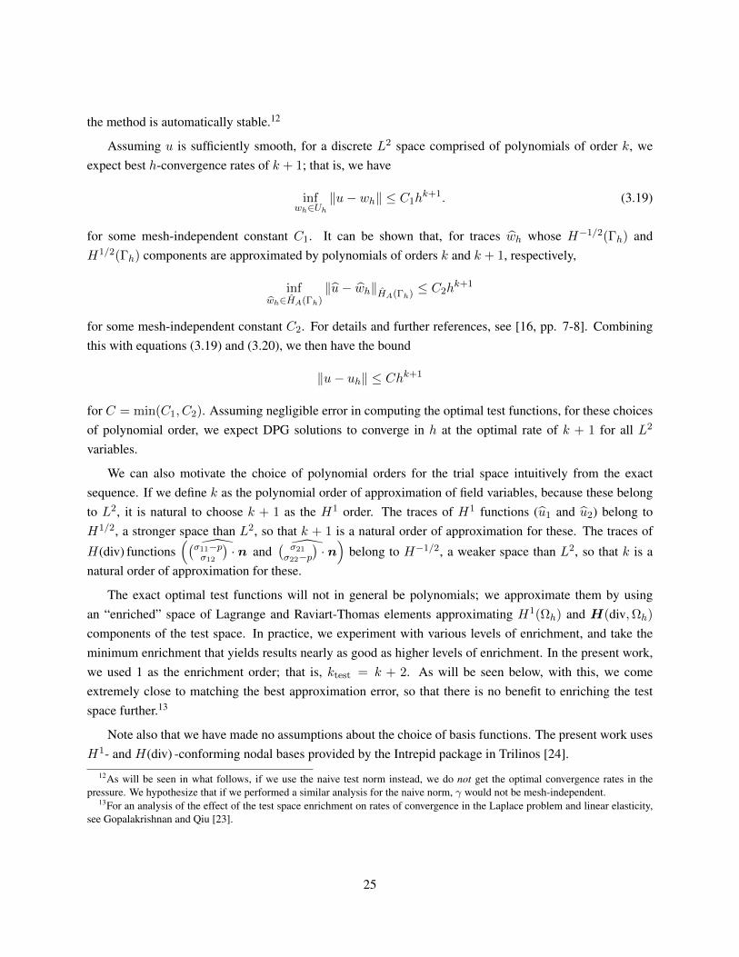
Assuming u is sufficiently smooth, for a discrete L2 space comprised of polynomials of order k, weexpect best h-convergence rates of k + 1; that is, we have

infwh∈Uh

‖u− wh‖ ≤ C1hk+1. (3.19)

for some mesh-independent constant C1. It can be shown that, for traces wh whose H−1/2(Γh) andH1/2(Γh) components are approximated by polynomials of orders k and k + 1, respectively,

infwh∈HA(Γh)

‖u− wh‖HA(Γh) ≤ C2hk+1

for some mesh-independent constant C2. For details and further references, see [16, pp. 7-8]. Combiningthis with equations (3.19) and (3.20), we then have the bound

‖u− uh‖ ≤ Chk+1

for C = min(C1, C2). Assuming negligible error in computing the optimal test functions, for these choicesof polynomial order, we expect DPG solutions to converge in h at the optimal rate of k + 1 for all L2

variables.

We can also motivate the choice of polynomial orders for the trial space intuitively from the exactsequence. If we define k as the polynomial order of approximation of field variables, because these belongto L2, it is natural to choose k + 1 as the H1 order. The traces of H1 functions (u1 and u2) belong toH1/2, a stronger space than L2, so that k + 1 is a natural order of approximation for these. The traces of

H(div) functions(

(σ11−pσ12

)· n and ( σ21

σ22−p)· n)

belong to H−1/2, a weaker space than L2, so that k is anatural order of approximation for these.

The exact optimal test functions will not in general be polynomials; we approximate them by usingan “enriched” space of Lagrange and Raviart-Thomas elements approximating H1(Ωh) and H(div,Ωh)

components of the test space. In practice, we experiment with various levels of enrichment, and take theminimum enrichment that yields results nearly as good as higher levels of enrichment. In the present work,we used 1 as the enrichment order; that is, ktest = k + 2. As will be seen below, with this, we comeextremely close to matching the best approximation error, so that there is no benefit to enriching the testspace further.13

Note also that we have made no assumptions about the choice of basis functions. The present work usesH1- and H(div) -conforming nodal bases provided by the Intrepid package in Trilinos [24].

12As will be seen in what follows, if we use the naive test norm instead, we do not get the optimal convergence rates in thepressure. We hypothesize that if we performed a similar analysis for the naive norm, γ would not be mesh-independent.

13For an analysis of the effect of the test space enrichment on rates of convergence in the Laplace problem and linear elasticity,see Gopalakrishnan and Qiu [23].

25

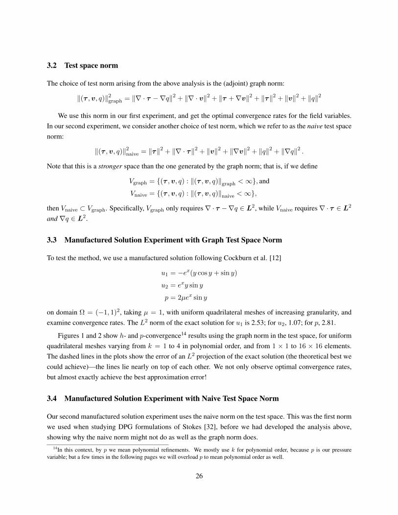
3.2 Test space norm

The choice of test norm arising from the above analysis is the (adjoint) graph norm:

‖(τ ,v, q)‖2graph = ‖∇ · τ −∇q‖2 + ‖∇ · v‖2 + ‖τ +∇v‖2 + ‖τ‖2 + ‖v‖2 + ‖q‖2

We use this norm in our first experiment, and get the optimal convergence rates for the field variables.In our second experiment, we consider another choice of test norm, which we refer to as the naive test spacenorm:

‖(τ ,v, q)‖2naive = ‖τ‖2 + ‖∇ · τ‖2 + ‖v‖2 + ‖∇v‖2 + ‖q‖2 + ‖∇q‖2 .

Note that this is a stronger space than the one generated by the graph norm; that is, if we define

Vgraph = (τ ,v, q) : ‖(τ ,v, q)‖graph <∞, and

Vnaive = (τ ,v, q) : ‖(τ ,v, q)‖naive <∞,

then Vnaive ⊂ Vgraph. Specifically, Vgraph only requires∇ · τ −∇q ∈ L2, while Vnaive requires∇ · τ ∈ L2

and ∇q ∈ L2.

3.3 Manufactured Solution Experiment with Graph Test Space Norm

To test the method, we use a manufactured solution following Cockburn et al. [12]

u1 = −ex(y cos y + sin y)

u2 = exy sin y

p = 2µex sin y

on domain Ω = (−1, 1)2, taking µ = 1, with uniform quadrilateral meshes of increasing granularity, andexamine convergence rates. The L2 norm of the exact solution for u1 is 2.53; for u2, 1.07; for p, 2.81.

Figures 1 and 2 show h- and p-convergence14 results using the graph norm in the test space, for uniformquadrilateral meshes varying from k = 1 to 4 in polynomial order, and from 1 × 1 to 16 × 16 elements.The dashed lines in the plots show the error of an L2 projection of the exact solution (the theoretical best wecould achieve)—the lines lie nearly on top of each other. We not only observe optimal convergence rates,but almost exactly achieve the best approximation error!

3.4 Manufactured Solution Experiment with Naive Test Space Norm

Our second manufactured solution experiment uses the naive norm on the test space. This was the first normwe used when studying DPG formulations of Stokes [32], before we had developed the analysis above,showing why the naive norm might not do as well as the graph norm does.

14In this context, by p we mean polynomial refinements. We mostly use k for polynomial order, because p is our pressurevariable; but a few times in the following pages we will overload p to mean polynomial order as well.

26

10−1

100

10−10

10−8

10−6

10−4

10−2

100

k =1

2

1

k =2

3

1

k =3

4

1

k =4

5

1

h

err

or

in L

2−

no

rm

actual

best

(a) u1

10−1

100

10−10

10−8

10−6

10−4

10−2

100

k =1

2

1

k =2

3

1

k =3

4

1

k =4

5

1

h

err

or

in L

2−

no

rm

actual

best

(b) u2

10−1

100

10−10

10−8

10−6

10−4

10−2

100

102

k =1

2.171

k =2

3.12

1

k =3

4.13

1

k =4

5.12

1

h

err

or

in L

2−

no

rm

actual

best

(c) p

Figure 1: h-convergence of u1, u2 and p when using the graph norm for the test space. We observe optimalconvergence rates, and nearly match the L2-projection of the exact solution.

27

1 2 3 410

−10

10−8

10−6

10−4

10−2

100

h =1

h =0.5

h =0.25

h =0.12

h =0.062

k

err

or

in L

2−

no

rm

actual

best

(a) u1

1 2 3 410

−10

10−8

10−6

10−4

10−2

100

h =1

h =0.5

h =0.25

h =0.12

h =0.062

k

err

or

in L

2−

no

rm

actual

best

(b) u2

1 2 3 410

−10

10−8

10−6

10−4

10−2

100

102

h =1

h =0.5

h =0.25

h =0.12

h =0.062

k

err

or

in L

2−

no

rm

actual

best

(c) p

Figure 2: p-convergence of u1, u2 and p when using the graph norm for the test space. We observe expo-nential convergence for the finer meshes, and nearly match the L2-projection of the exact solution.

28

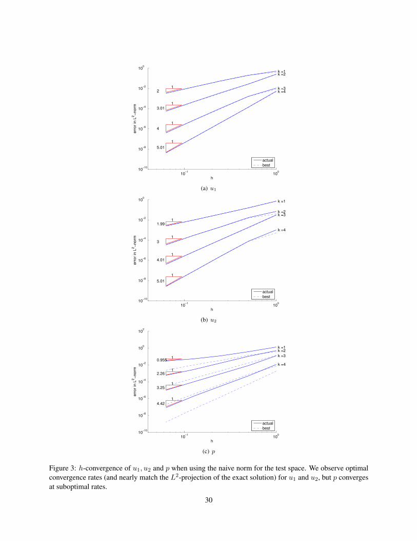
Figures 3 and 4 show h- and p-convergence results using the naive norm in the test space, for uniformquadrilateral meshes varying from k = 1 to 4 in polynomial order, and from 1 × 1 to 16 × 16 elements;we have again plotted for comparison the error in the L2 projection of the exact solution. As with the graphnorm, here we observe optimal convergence rates and almost exactly achieve the best approximation errorin velocities u1 and u2, but in the pressure p we are sub-optimal by up to two orders of magnitude.

Why do we not see optimal convergence for the naive norm? Recall that this is a stronger norm than thegraph norm used in our analysis; thus the test functions that we seek—namely, the ones that will minimizethe residual—may not reside within the continuous space represented by the naive norm. By using the naivenorm, we are searching for these test functions inside a smaller space, and we may not find them there.

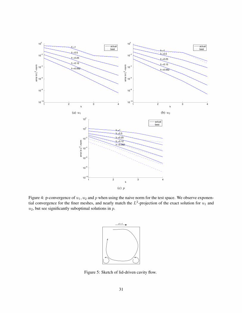
3.5 Lid-Driven Cavity Flow

A classic test case for Stokes flow is the lid-driven cavity flow problem. Consider a square cavity with anincompressible, viscous fluid, with a lid that moves at a constant rate. The resulting flow will be vorticular;as sketched in Figure 5, there will also be so-called Moffat eddies at the corners; in fact, the exact solutionwill have an infinite number of such eddies, visible at progressively finer scales [27]. Note that the problemas described will have a discontinuity in the fluid velocity at the top corners, and hence its solution willnot conform to the spaces we used in our analysis; for this reason, in our experiment we approximate theproblem by introducing a thin ramp in the boundary conditions—we have chosen a ramp of width 1

64 . Thismakes the boundary conditions continuous,15 so that the solution conforms to the spaces used in the analysis.

As described in the introduction, DPG gives us a mechanism for measuring the residual error in the dualnorm (the very error we seek to minimize) precisely, and we use this to drive adaptivity, by measuring theerror ‖eK‖V for each element K. Both the method and our code allow refinements in h or p or in somecombination of h and p. However, we do not yet have a general mechanism for deciding which refinementto apply (h or p), once we have decided that a given element should be refined. We run two experiments,one with h-adaptivity and one using an ad hoc hp-adaptive strategy, described below.

Although it is not required by the code, we enforce 1-irregularity throughout—that is, before an elementcan be refined twice along an edge, its neighbor along that edge must be refined once. In limited comparisonsrunning the same experiments without enforcing 1-irregularity, this did not appear to make much practicaldifference.

3.5.1 h-refinement strategy

For h-refinements, our strategy is very simple:

1. Loop through the elements, determining the maximum element error ‖eKmax‖V .15It is worth noting that these boundary conditions are not exactly representable by many of the coarser meshes used in our

experiments. We interpolate the boundary conditions in the discrete space.

29

10−1

100

10−10

10−8

10−6

10−4

10−2

100

k =1

2

1

k =2

3.01

1

k =3

4

1

k =4

5.01

1

h

err

or

in L

2−

no

rm

actual

best

(a) u1

10−1

100

10−10

10−8

10−6

10−4

10−2

100

k =1

1.99

1

k =2

3

1

k =3

4.01

1

k =4

5.01

1

h

err

or

in L

2−

no

rm

actual

best

(b) u2

10−1

100

10−10

10−8

10−6

10−4

10−2

100

102

k =1

0.9551

k =2

2.261

k =3

3.25

1

k =4

4.42

1

h

err

or

in L

2−

no

rm

actual

best

(c) p

Figure 3: h-convergence of u1, u2 and p when using the naive norm for the test space. We observe optimalconvergence rates (and nearly match the L2-projection of the exact solution) for u1 and u2, but p convergesat suboptimal rates.

30

1 2 3 410

−10

10−8

10−6

10−4

10−2

100

h =1

h =0.5

h =0.25

h =0.12

h =0.062

k

err

or

in L

2−

no

rm

actual

best

(a) u1

1 2 3 410

−10

10−8

10−6

10−4

10−2

100

h =1

h =0.5

h =0.25

h =0.12

h =0.062

k

err

or

in L

2−

no

rm

actual

best

(b) u2

1 2 3 410

−10

10−8

10−6

10−4

10−2

100

102

h =1

h =0.5

h =0.25

h =0.12

h =0.062

k

err

or

in L

2−

no

rm

actual

best

(c) p

Figure 4: p-convergence of u1, u2 and p when using the naive norm for the test space. We observe exponen-tial convergence for the finer meshes, and nearly match the L2-projection of the exact solution for u1 andu2, but see significantly suboptimal solutions in p.

u1 = 1

Figure 5: Sketch of lid-driven cavity flow.

31

2. Refine all elements with error at least 20% of the maximum ‖eKmax‖V .

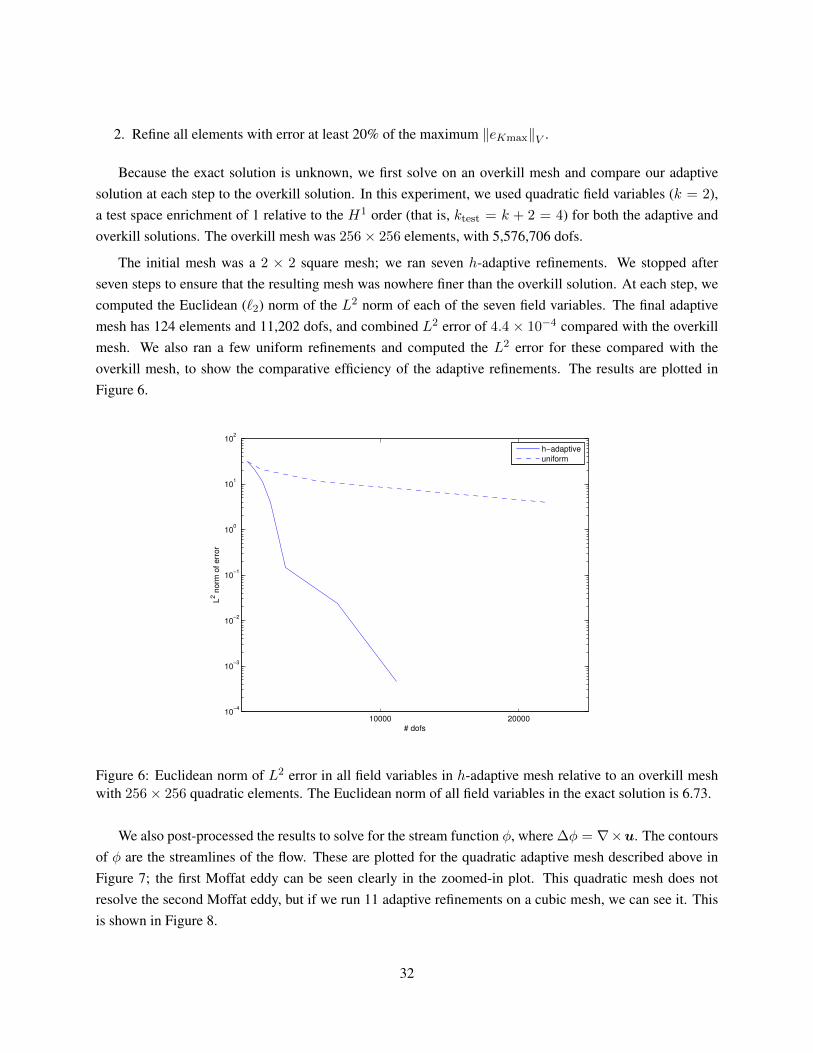
Because the exact solution is unknown, we first solve on an overkill mesh and compare our adaptivesolution at each step to the overkill solution. In this experiment, we used quadratic field variables (k = 2),a test space enrichment of 1 relative to the H1 order (that is, ktest = k + 2 = 4) for both the adaptive andoverkill solutions. The overkill mesh was 256× 256 elements, with 5,576,706 dofs.

The initial mesh was a 2 × 2 square mesh; we ran seven h-adaptive refinements. We stopped afterseven steps to ensure that the resulting mesh was nowhere finer than the overkill solution. At each step, wecomputed the Euclidean (`2) norm of the L2 norm of each of the seven field variables. The final adaptivemesh has 124 elements and 11,202 dofs, and combined L2 error of 4.4 × 10−4 compared with the overkillmesh. We also ran a few uniform refinements and computed the L2 error for these compared with theoverkill mesh, to show the comparative efficiency of the adaptive refinements. The results are plotted inFigure 6.

10000 2000010

−4

10−3

10−2

10−1

100

101

102

L2 n

orm

of err

or

# dofs

h−adaptive

uniform

Figure 6: Euclidean norm of L2 error in all field variables in h-adaptive mesh relative to an overkill meshwith 256× 256 quadratic elements. The Euclidean norm of all field variables in the exact solution is 6.73.

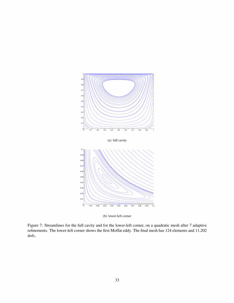
We also post-processed the results to solve for the stream function φ, where ∆φ = ∇×u. The contoursof φ are the streamlines of the flow. These are plotted for the quadratic adaptive mesh described above inFigure 7; the first Moffat eddy can be seen clearly in the zoomed-in plot. This quadratic mesh does notresolve the second Moffat eddy, but if we run 11 adaptive refinements on a cubic mesh, we can see it. Thisis shown in Figure 8.

32

0 0.1 0.2 0.3 0.4 0.5 0.6 0.7 0.8 0.9 10

0.1

0.2

0.3

0.4

0.5

0.6

0.7

0.8

0.9

1

(a) full cavity

0 0.01 0.02 0.03 0.04 0.05 0.06 0.07 0.08 0.09 0.10

0.01

0.02

0.03

0.04

0.05

0.06

0.07

0.08

0.09

0.1

(b) lower-left corner

Figure 7: Streamlines for the full cavity and for the lower-left corner, on a quadratic mesh after 7 adaptiverefinements. The lower-left corner shows the first Moffat eddy. The final mesh has 124 elements and 11,202dofs.

33

3.5.2 Ad hoc hp-refinement strategy

For the hp experiment, we adopt a similar strategy; this time, our overkill mesh contains 64 × 64 quinticelements, and our initial mesh has 2× 2 linear elements. We know a priori that we should refine in h at thetop corners—if only to fully resolve the boundary condition. The strategy is again:

1. Loop through the elements, determining the maximum element error ‖eKmax‖V .

2. Refine all elements with error at least 20% of the maximum ‖eKmax‖V .

However, this time we must decide whether to refine in h or p. The basic constraints we would like to followare:

• the adaptive mesh must be nowhere finer than the overkill mesh (in h or p), and

• prefer h-refinements at all corners (top and bottom).

So, once the corner elements are as small as the overkill mesh, then they refine in p, and all other elementsrefine in p until they are quintic, after which they may refine in h.

The primary purpose of this experiment is to demonstrate that the method allows arbitrary meshes ofarbitrary, variable polynomial order. The strategy described above clearly depends on a priori knowledgeof the particular problem we are solving; we have yet to determine a good general strategy for decidingbetween h- and p-refinements.

We ran 9 refinement steps. The final mesh has 46 elements and 5,986 dofs, compared with 1,223,682dofs in the overkill mesh. The L2 error of the adaptive solution compared with the overkill is 8.0 × 10−4.

0 0.001 0.002 0.003 0.004 0.005 0.006 0.007 0.008 0.009 0.010

0.001

0.002

0.003

0.004

0.005

0.006

0.007

0.008

0.009

0.01

Figure 8: Streamlines for the lower-left corner on a cubic mesh after 11 adaptive refinements: the secondMoffat eddy. The final mesh has 298 elements and 44,206 dofs.

34

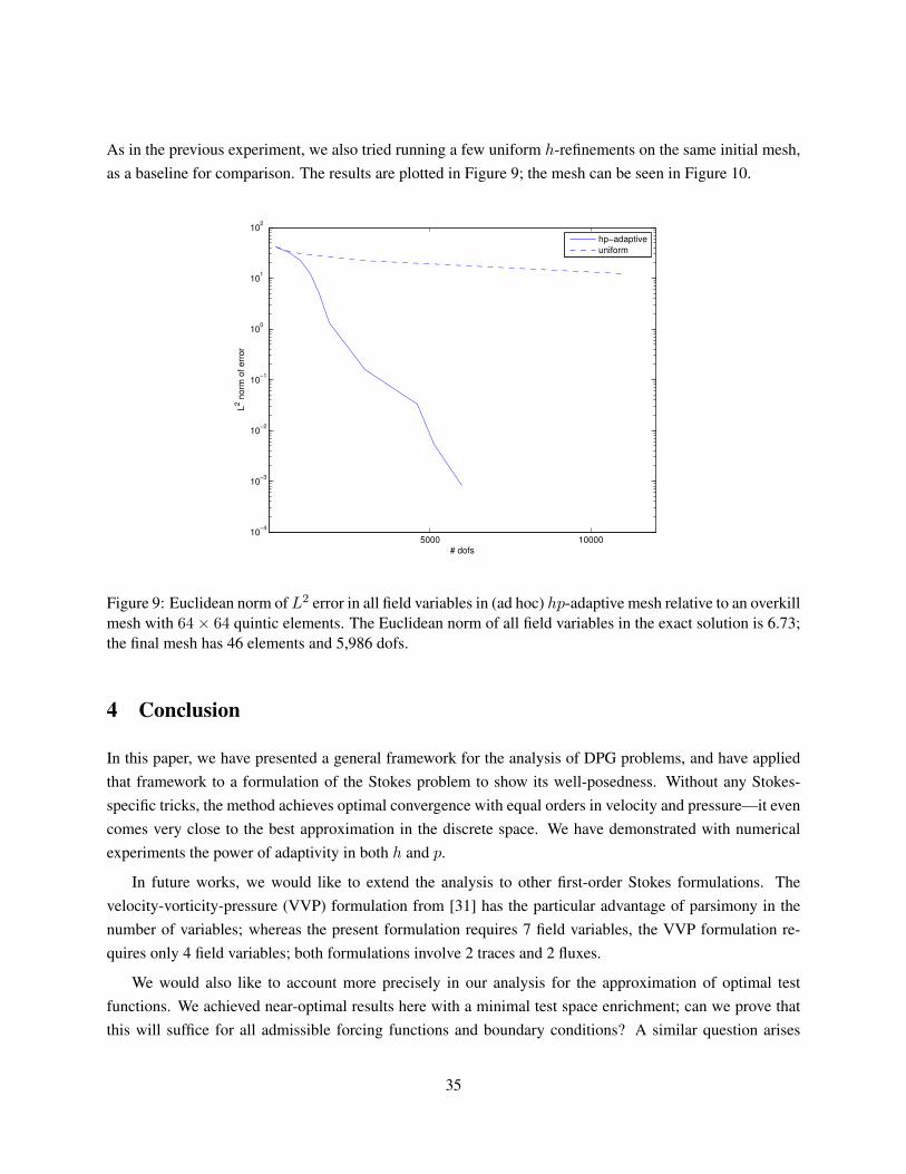
As in the previous experiment, we also tried running a few uniform h-refinements on the same initial mesh,as a baseline for comparison. The results are plotted in Figure 9; the mesh can be seen in Figure 10.

5000 1000010

−4

10−3

10−2

10−1

100

101

102

L2 n

orm

of err

or

# dofs

hp−adaptive

uniform

Figure 9: Euclidean norm ofL2 error in all field variables in (ad hoc) hp-adaptive mesh relative to an overkillmesh with 64× 64 quintic elements. The Euclidean norm of all field variables in the exact solution is 6.73;the final mesh has 46 elements and 5,986 dofs.

4 Conclusion

In this paper, we have presented a general framework for the analysis of DPG problems, and have appliedthat framework to a formulation of the Stokes problem to show its well-posedness. Without any Stokes-specific tricks, the method achieves optimal convergence with equal orders in velocity and pressure—it evencomes very close to the best approximation in the discrete space. We have demonstrated with numericalexperiments the power of adaptivity in both h and p.

In future works, we would like to extend the analysis to other first-order Stokes formulations. Thevelocity-vorticity-pressure (VVP) formulation from [31] has the particular advantage of parsimony in thenumber of variables; whereas the present formulation requires 7 field variables, the VVP formulation re-quires only 4 field variables; both formulations involve 2 traces and 2 fluxes.

We would also like to account more precisely in our analysis for the approximation of optimal testfunctions. We achieved near-optimal results here with a minimal test space enrichment; can we prove thatthis will suffice for all admissible forcing functions and boundary conditions? A similar question arises

35

with respect to the asymptotic convergence: it appears from our numerical experiments that the solutionsconverge to the best approximations, with a scaling constant of 1. If this is true, we would like to prove it.

We would like to extend the present work to related problems. In particular, we plan to investigate theOseen equations and the incompressible Navier-Stokes equations in the near future. For the Oseen equations,which involve a linear approximation to the nonlinear convection term in Navier-Stokes, we expect that anearly identical approach to the one that we have taken for Stokes will work well. For the Navier-Stokesequations, we hope to apply the minimum-residual approach directly to the nonlinear problem, perhaps in asimilar fashion to the work by Moro et al. [28].

References

[1] Pavel Bochev and R. B. Lehoucq. On the finite element solution of the pure Neumann problem. SIAMReview, 47(1):55–66, March 2005.

[2] D. Boffi, F. Brezzi, and M. Fortin. Finite elements for the Stokes problem. In Lecture Notes inMathematics, volume 1939, pages 45–100. Springer, 2008.

[3] C.L. Bottasso, S. Micheletti, and R. Sacco. The discontinuous Petrov-Galerkin method for ellipticproblems. Comput. Methods Appl. Mech. Engrg., 191:3391–3409, 2002.

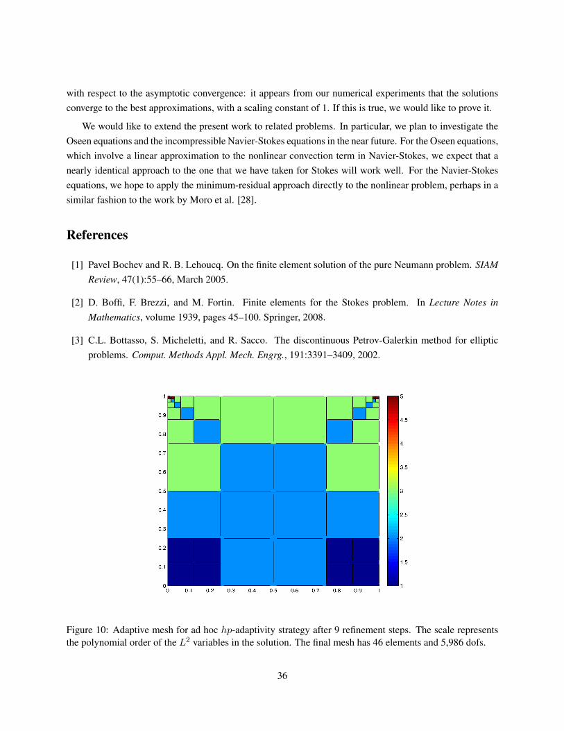
Figure 10: Adaptive mesh for ad hoc hp-adaptivity strategy after 9 refinement steps. The scale representsthe polynomial order of the L2 variables in the solution. The final mesh has 46 elements and 5,986 dofs.

36

[4] C.L. Bottasso, S. Micheletti, and R. Sacco. A multiscale formulation of the discontinuous Petrov-Galerkin method for advective-diffusive problems. Comput. Methods Appl. Mech. Engrg., 194:2819–2838, 2005.

[5] J. Bramwell, L. Demkowicz, J. Gopalakrishnan, and W. Qiu. A locking-free hp DPG method for linearelasticity with symmetric stresses. Num. Math., 2012. accepted.

[6] J. Bramwell, L. Demkowicz, and W. Qiu. Solution of dual-mixed elasticity Equations using Arnold-Falk-Winther Element and discontinuous Petrov-Galerkin method, a comparison. (2010-23), 2010.

[7] F. Brezzi. On the existence, uniqueness, and approximation of saddle point problems arising fromLagrangian multipliers. R.A.I.R.O., Anal. Numer., 2:129–151, 1974.

[8] Tan Bui-Thanh, Leszek Demkowicz, and Omar Ghattas. A unified discontinuous Petrov-Galerkinmethod and its analysis for Friedrichs’ systems. Submitted to SIAM J. Numer. Anal., 2011. Also ICESreport ICES-11-34, November 2011.

[9] P. Castillo, B. Cockburn, I. Perugia, and D. Schotzau. An a priori error analysis of the local discontin-uous Galerkin method for elliptic problems. SIAM J. Numer. Anal., 38:1676–1706., 2000.

[10] J. Chan, L. Demkowicz, R. Moser, and N. Roberts. A class of Discontinuous Petrov–Galerkin meth-ods. Part V: Solution of 1D Burgers and Navier–Stokes equations. Technical Report 25, ICES, 2010.submitted to J. Comp. Phys.

[11] B. Cockburn, G. Kanschat, D. Schotzau, and Ch. Schwab. Local Discontinuous Galerkin methods forthe Stokes system. SIAM J. on Num. Anal., 40:319–343, 2003.

[12] Bernardo Cockburn, Guido Kanschat, Dominik Schotzau, and Christoph Schwab. Local discontinuousGalerkin methods for the Stokes system. SIAM Journal on Numerical Analysis, 40(1):319–343, 2003.

[13] L. Demkowicz. Computing with hp Finite Elements. I.One- and Two-Dimensional Elliptic andMaxwell Problems. Chapman & Hall/CRC Press, Taylor and Francis, October 2006.

[14] L. Demkowicz and J. Gopalakrishnan. A class of discontinuous Petrov-Galerkin methods. Part I: Thetransport equation. Comput. Methods Appl. Mech. Engrg., 2009. accepted, see also ICES Report2009-12.

[15] L. Demkowicz and J. Gopalakrishnan. A class of discontinuous Petrov-Galerkin methods. Part II:Optimal test functions. Numer. Meth. Part. D. E., 2010. in print.

[16] L. Demkowicz and J. Gopalakrishnan. Analysis of the DPG method for the Poisson problem. SIAM J.Num. Anal., 49(5):1788–1809, 2011.

37

[17] L. Demkowicz, J. Gopalakrishnan, I. Muga, and J. Zitelli. Wavenumber explicit analysis for a DPGmethod for the multidimensional Helmholtz equation. Comput. Methods Appl. Mech. Engrg., 213-216:126–138, 2012.

[18] L. Demkowicz and N. Heuer. Robust DPG method for convection-dominated diffusion problems.Technical Report 33, ICES, 2011.

[19] Alexandre Ern and Jean-Luc Guermond. Discontinuous Galerkin methods for Friedrichs’ systems.Part III. Multifield theories with partial coercivity. SIAM J. Numer. Anal., 46(2):776–804, 2008.

[20] Alexandre Ern, Jean-Luc Guermond, and Gilbert Caplain. An intrinsic criterion for the bijectivityof Hilbert operators related to Friedrichs’ systems. Communications in partial differential equations,32(2):317–341, 2007.

[21] G.B. Folland. Introduction to Partial Differential Equations. Princeton, 1976.

[22] Kurt O. Friedrichs. Symmetric positive linear differential equations. Communications on pure andapplied mathematics, XI:333–418, 1958.

[23] Jay Gopalakrishnan and Weifeng Qiu. An analysis of the practical DPG method. Technical ReportarXiv:1107.4293, July 2011.

[24] Michael A. Heroux, Roscoe A. Bartlett, Vicki E. Howle, Robert J. Hoekstra, Jonathan J. Hu, Tamara G.Kolda, Richard B. Lehoucq, Kevin R. Long, Roger P. Pawlowski, Eric T. Phipps, Andrew G. Salinger,Heidi K. Thornquist, Ray S. Tuminaro, James M. Willenbring, Alan Williams, and Kendall S. Stanley.An overview of the Trilinos project. ACM Trans. Math. Softw., 31(3):397–423, 2005.

[25] O.A. Ladyzhenskaya. The Mathematical Theory of Viscous Incompressible Flows. Gordon and Breach,London, 1969.

[26] W. McLean. Strongly Elliptic Systems and Boundary Integral Equations. Cambridge University Press,2000.

[27] H.K. Moffat. Viscous and resistive eddies near a sharp corner. Journal of Fluid Mechanics, 18(1):1–18,1964.

[28] D. Moro, N.C. Nguyen, and J. Peraire. A hybridized discontinuous Petrov-Galerkin scheme for scalarconservation laws. Int.J. Num. Meth. Eng., 2011. in print.

[29] A.H. Niemi, J.A. Bramwell, and L.F. Demkowicz. Discontinuous Petrov–Galerkin method with opti-mal test functions for thin-body problems in solid mechanics. Computer Methods in Applied Mechan-ics and Engineering, 200(9-12):1291–1300, Feb 2011.

[30] J.T. Oden and L.F. Demkowicz. Applied Functional Analysis for Science and Engineering. Chapman& Hall/CRC Press, Boca Raton, 2010. Second edition.

38

[31] Nathan V. Roberts, Denis Ridzal, Pavel B. Bochev, and Leszek D. Demkowicz. A Toolbox for aClass of Discontinuous Petrov-Galerkin Methods Using Trilinos. Technical Report SAND2011-6678,Sandia National Laboratories, 2011.

[32] N.V. Roberts, D. Ridzal, P.N. Bochev, L. Demkowicz, K.J. Peterson, and Siefert Ch. M. Application ofa discontinuous Petrov-Galerkin method to the Stokes equations. In CSRI Summer Proceedings 2010.2010.

[33] R. E. Showalter. Hilbert Space Methods for Partial Differential Equations. Pitman Publishing Limited,London, 1977.

[34] J. Zitelli, I. Muga, L. Demkowicz, J. Gopalakrishnan, D. Pardo, and V. Calo. A class of discontinuousPetrov-Galerkin methods. Part IV: Wave propagation problems. J. Comp. Phys., 230:2406–2432, 2011.

39

Appendix

A Boundedness Below of the First-Order Stokes Operator with Homoge-neous BCs

In this appendix, we show that the operator corresponding to our first-order Stokes problem with homoge-neous BCs is bounded below. While in the body of the paper we have taken µ = 1, here we consider themore general case of constant µ > 0.

Recall the classical strong form of the Stokes problem:

−µ∆u+∇p = f in Ω, (A.20)

∇ · u = 0 in Ω, (A.21)

u = uD on ∂Ω. (A.22)

Recall also our first-order system for the Stokes equations:

−∇ · σ +∇p = f in Ω, (A.23a)

∇ · u = 0 in Ω, (A.23b)1

µσ −∇u = 0 in Ω, (A.23c)

u = uD on ∂Ω. (A.23d)

If we introduce A : HA → L2 (Ω) with group variable u = (u, p,σ), the Stokes equation in first orderform (A.24), ignoring the boundary conditions, can be written succinctly as

Audef=

−∇ · σ +∇p∇ · u

1µσ −∇u

=

f00

. (A.24)

Considering linear operator A as defined in equation (A.25) operating on group variable u = (u, p,σ),we seek to show that ||Au||L2 ≥ γ||u||HA

.

A.0.3 ||Au||Ω ≥ γ||u||HA

Adding right-hand sides g and h

40

−∇ · σ +∇p = f in Ω, (A.25)

∇ · u = g in Ω, (A.26)1

µσ −∇u = h in Ω, (A.27)

u = 0 on ∂Ω, (A.28)

we have that Au = (f , g,h). If we can establish bounds for the L2 norms of each of the solution variablesin terms of L2 norms on f , g, and h, then we will have the required lower bound ||Au||Ω ≥ γ||u||HA

, where||u||HA

def=(||Au||2Ω + ||u||2Ω

)1/2.

Note that, by linearity of A, it suffices to consider cases in which only one of f , g, and h is non-zero.We consider each of these cases in the following three subsections.

A.0.4 f 6= 0, g = 0,h = 0

In this case, we have exactly the system (A.24a)-(A.24d), which reduces (in a distributional sense) to (A.21)-(A.23). Testing the first equation with the velocity u ∈H1

0(Ω), we have

−(µ∆u,u)Ω + (∇p,u)Ω = (f ,u)Ω.

Integrating by parts, we obtain:

(µ∇u,∇u)Ω − 〈µ∇u · n,u〉∂Ω − (p,∇ · u)Ω + 〈p,u · n〉∂Ω = (f ,u)Ω.

Noting that u = 0 on ∂Ω and that ∇ · u = 0 in Ω, this reduces to:

µ(∇u,∇u)Ω = µ||∇u||2Ω = µ||σ||2Ω = (f ,u)Ω

≤ ||f ||Ω||u||Ω≤ CP ||f ||Ω||∇u||Ω,

where CP is the Poincare constant. Thus ||σ||Ω ≤ CPµ ||f ||Ω, and ||u|| ≤ C2

Pµ ||f ||Ω.

To bound the pressure p, we require a result by Ladyzhenskaya [25] for p ∈ L20

def= w ∈ L2(Ω) :∫

Ωw = 0:

supv∈H1(Ω)

(p,∇ · v)Ω

‖v‖H1(Ω)

≥ β ‖p‖Ω

41

for some constant β > 0. Testing equation (A.21) with v ∈H10(Ω), we have

(∇p,v)Ω = (f ,v)Ω + (µ∆u,v)Ω.

Integrating by parts, dividing by ‖v‖H1(Ω) and taking the supremum:

sup−(p,∇ · v)

‖v‖H1(Ω)

= sup

(f ,v)

‖v‖H1(Ω)

− µ(∇u,∇v)

‖v‖H1(Ω)

≤‖f‖ ‖v‖L2

‖v‖H1(Ω)

+ µ ‖∇u‖ ≤ ‖f‖+ µCPµ‖f‖ = (1 + CP ) ‖f‖ .

By the Ladyzhenskaya result, we then have ‖p‖ ≤ 1+CPβ ‖f‖, bounding p, as required.

A.0.5 f = 0, g 6= 0,h = 0

In this case, we have

−∇ · σ +∇p = 0 in Ω, (A.29)

∇ · u = g in Ω, (A.30)1

µσ −∇u = 0 in Ω, (A.31)

u = 0 on ∂Ω. (A.32)

We must also assume compatibility between g and the boundary condition on u; that is, that g has zeroaverage on Ω: ∫

Ωg =

∫∂Ωu · n = 0.

Now, by surjectivity of ∇· : H(div) → L2, there exists u0 such that ∇ · u0 = g. By the Lax-Milgramtheorem, we have ∃!φ ∈ H1

0 : u0 = ∇φ, so that ∆φ = g and, assuming that Ω is convex, then by theElliptic Regularity theorem (see [21, p. 214] for a proof), φ ∈ H2 and:

‖φ‖H2 ≤ C ‖g‖

=⇒ ‖∇φ‖H1 ≤ C ‖g‖ ,

for some C > 0 independent of g and φ. That is, in fact u0 ∈ H1 and ‖u0‖H1 ≤ C ‖g‖.

Settingw = u−u0, we have∇·w = 0, andw = 0 on ∂Ω. Note that we can recover−µ∆u+∇p = 0

42

by substituting (A.32) into (A.30). Testing this with w and integrating by parts, we obtain:

µ(∇u,∇w)Ω = 0

µ(∇w +∇u0,∇w)Ω = 0

=⇒ ‖∇w‖2 = −(∇u0,∇w)

≤ ‖∇u0‖ ‖∇w‖

≤ C ‖g‖ ‖∇w‖ ,

so that ‖∇w‖ ≤ C ‖g‖, and therefore as before we obtain a bound on ‖σ‖ = ‖∇u‖ ≤ 2C ‖g‖, and againby means of the Poincare inequality we may bound ‖u‖ ≤ CP ‖∇u‖ ≤ 2CCP ‖g‖ as well.

The bound on p is established exactly as before, except that now f = 0, so that we obtain the bound‖p‖ ≤ µ

β ‖∇u‖ ≤2µCCP

β ‖g‖.

A.0.6 f = 0, g = 0,h 6= 0

In this case, we have

−∇ · σ +∇p = 0 in Ω, (A.33)

∇ · u = 0 in Ω, (A.34)1

µσ −∇u = h in Ω, (A.35)

u = 0 on ∂Ω. (A.36)

Then, σ = µ(∇u+ h), and we have:

−∇ · σ +∇p = −µ∆u− µ∇ · h+∇p = 0,

so that

−µ∆u+∇p = −µ∇ · h

in a distributional sense. Testing with u, and integrating the left hand side by parts, again the pressure termvanishes because∇ · u = 0, so that much as before, we obtain:

µ(∇u,∇u)Ω = µ(∇ · h,u)Ω

= −µ(h,∇u)Ω ≤ µ ‖h‖L2(Ω) ‖∇u‖L2(Ω) .

So ‖∇u‖ ≤ ‖h‖, and the bounds ‖u‖ ≤ CP ‖h‖ and ‖p‖ ≤ µβ (‖∇u‖+ ‖h‖) ≤ 2µ

β ||h|| can be establishedin a similar fashion as above.

43