Journal of Computational and Applied Mathematics 214 (2008) 457–479www.elsevier.com/locate/cam

An adaptive stabilized finite element methodfor the generalized Stokes problem

Rodolfo Araya∗,1, Gabriel R. Barrenechea2, Abner Poza1

Departamento de Ingeniería Matemática, Universidad de Concepción, Casilla 160-C, Concepción, Chile

Received 24 August 2006; received in revised form 23 February 2007

Abstract

In this work we present an adaptive strategy (based on an a posteriori error estimator) for a stabilized finite element method for theStokes problem, with and without a reaction term. The hierarchical type estimator is based on the solution of local problems posedon appropriate finite dimensional spaces of bubble-like functions. An equivalence result between the norm of the finite element errorand the estimator is given, where the dependence of the constants on the physics of the problem is explicited. Several numericalresults confirming both the theoretical results and the good performance of the estimator are given.© 2007 Elsevier B.V. All rights reserved.

MSC: 65N15; 65N30; 65N50

Keywords: Stokes equation; A posteriori error estimator; Bubble function; Stabilized finite element method; Adapted mesh

1. Introduction

A posteriori error analysis and adaptive finite element methods for problems in fluid dynamics has been a very activesubject of research in the last few decades. For instance, for the advective–diffusive model we can quote the works[22,17,5,6], among others. Now, for the Stokes problem, the works by Verfürth [20,21] and Bank and Welfert [7],laid the basic foundation for the mathematical analysis of practical methods (see also [11] for error estimators in thenonconforming case). More recently, in [2,3,12], a posteriori error estimators rigorously bounding the discretizationerrors have been addressed. All previous references deal with stable (in the sense of the discrete inf-sup condition [9])discretizations for the Stokes problem. In [18,4], an a posteriori error analysis of stabilized formulations for the Stokesproblem was performed, but the analysis was restricted to the pure Stokes case (i.e., without a reaction term).

In this paper we introduce and analyze from theoretical and experimental points of view an adaptive scheme toefficiently solve the generalized Stokes problem. The scheme is based on the unusual stabilized finite element methodintroduced in [8], combined with an error estimator which is based on an idea from [3], building an auxiliary problem,whose solution is equivalent with the norm of the finite element error. Since this auxiliary problem is posed on aninfinite dimensional setting, we build a hierarchical estimation for the solution of this problem, which turns out to

∗ Corresponding author.E-mail addresses: raraya@ing-mat.udec.cl (R. Araya), gbarrene@ing-mat.udec.cl (G.R. Barrenechea), abner@ing-mat.udec.cl (A. Poza).

1 Partially supported by CONICYT through FONDECYT Project 1040595 (Chile).2 Partially supported by CONICYT through FONDECYT Project 1061032 and by FONDAP Program in Applied Mathematics (Chile).

0377-0427/$ - see front matter © 2007 Elsevier B.V. All rights reserved.doi:10.1016/j.cam.2007.03.011

458 R. Araya et al. / Journal of Computational and Applied Mathematics 214 (2008) 457–479

be equivalent with the norm of its solution, and hence the resulting finite element approximation is equivalent to theoriginal finite element error.

An outline of the paper is as follows. The model problem is stated in Section 2, and the bases of the discreteapproximation are settled in Section 3. Next, in Section 4 we propose the auxiliary problem and prove that we candefine a norm based on the solution of this auxiliary problem, which is equivalent to the norm of the error. This auxiliaryproblem is applied to the solution of the residual equation and hence we state, at the end of Section 4.1, a first equivalenceresult between the norm of the error and the solution of the auxiliary problem (with the residual as right-hand side).As we told before, the auxiliary problem is posed on an infinite dimensional space, and hence in Section 5 we define afinite dimensional approximation (based on a hierarchical idea) of its solution. Finally, in Section 6 we present severalnumerical results confirming the theoretical results and showing the good performance of our estimator, and in Section7 we give some conclusions.

2. The model problem

Let � ⊆ R2 be a bounded open set with polygonal boundary �. We denote by Hm(�) the usual Sobolev spaceof order m�0, with norm ‖ · ‖m,� and seminorm | · |m,�, respectively (with the convention H 0(�) = L2(�) and| · |0,� = ‖ · ‖0,�). Then, given f ∈ L2(�)2, ��0 and � ∈ R+, our generalized Stokes problem reads: Find a velocity uand the pressure field p such that

(P )

{�u − ��u + ∇p = f in �,

div u = 0 in �,

u = 0 on �.

Let then H := H 10 (�)2 and Q := L2

0(�) := {q ∈ L2(�) : (q, 1)� = 0}, where (·, ·)D stands for the inner productin L2(D) (or in L2(D)2, L2(D)2×2, if necessary) be the functional spaces to be used. The weak formulation of theproblem (P ) reads: Find (u, p) ∈ H × Q such that

a(u, v) + b(v, p) + b(u, q) = (f, v)�, ∀(v, q) ∈ H × Q, (2.1)

where

a(u, v) := �(u, v)� + �(∇u, ∇v)�, (2.2)

b(v, q) := −(q, div v)�. (2.3)

Furthermore, let c : Q × Q → R be the symmetric bilinear form defined by

c(p, q) := 1

�(p, q)�.

Using bilinear forms a and c we define the following norms:

‖v‖a := a(v, v)1/2, ∀v ∈ H,

‖q‖c := c(q, q)1/2, ∀q ∈ Q

and the following norm on the product space H × Q:

‖(v, q)‖ := {‖v‖2a + ‖q‖2

c}1/2 ∀(v, q) ∈ H × Q. (2.4)

The following result states the main properties of these bilinear forms.

Lemma 1. Let a and b be the bilinear forms given by (2.2) and (2.3), respectively. Then

|a(v, w)|�‖v‖a‖w‖a, ∀v, w ∈ H, (2.5)

R. Araya et al. / Journal of Computational and Applied Mathematics 214 (2008) 457–479 459

|b(v, q)|�√2‖v‖a‖q‖c, ∀(v, q) ∈ H × Q, (2.6)

supv∈H

b(v, q)

‖v‖a

��b

√�

� + �‖q‖c, ∀q ∈ Q, (2.7)

where �b > 0 is a constant depending only on �.

Proof. The proof follows from the norms definition and the well-known properties of these bilinear forms (see [15,Theorem 4.1]). �

Then, using the classical theory of Babuska–Brezzi (cf. [15]), we can state the following result.

Lemma 2. The weak problem (2.1) has a unique solution (u, p) ∈ H × Q.

3. Notations and preliminary results

Let {Th}h>0 be a regular family of triangulations of � and let us denote by Eh the set of all sides of Th with theusual splitting Eh =E� ∪E�, where E� stands for the sides lying on the interior of �. Also, for T ∈ Th, we denote byN(T ) the set of nodes of T and by E(T ) the set of sides of T. Also, for T ∈ Th and F ∈ Eh we define the followingneighborhoods:

�T :=⋃

E(T )∩E(T ′) =∅T ′, �T :=

⋃N(T )∩N(T ′) =∅

T ′,

�F :=⋃

F∈E(T ′)T ′, �F :=

⋃N(F )∩N(T ′) =∅

T ′.

Next, for T ∈ Th and F ∈ E�, let hT be the diameter of T, hF := |F |, and let us define the following mesh-dependentconstants:

�T :={

�−1/2hT , � = 0,

�−1/2 min{hT �1/2�−1/2, 1}, � > 0,

�F :={

�−1/2h1/2F , � = 0,

�−1/4�−1/4 min{hF �1/2�−1/2, 1}1/2, � > 0.

In the rest of the paper we will use the notation

a�b ⇐⇒ a�Kb,

a � b ⇐⇒ a�b and b�a,

where the positive constant K is independent of h, � and �.Finally, let k, l ∈ N, and let us define the following finite element spaces:

Hh := {� ∈ C(�)2 : �|T ∈ Pk(T )2, ∀T ∈ Th} ∩ H 10 (�)2,

Qh := { ∈ C(�) : |T ∈ Pl (T ), ∀T ∈ Th} ∩ L20(�).

Lemma 3. The following estimates hold for all vh ∈ Hh and ��0:

‖∇vh‖0,T �h−1T �T ‖vh‖a,T , (3.1)

‖�vh‖0,T �h−2T �T ‖vh‖a,T . (3.2)

Proof. If � = 0 the proof follows from the inverse inequality

‖∇vh‖0,T �h−1T ‖vh‖0,T , ∀vh ∈ Hh (3.3)

460 R. Araya et al. / Journal of Computational and Applied Mathematics 214 (2008) 457–479

(see Lemma 1.138 in [14]) and the definition of �T . For � > 0, from the definition of ‖ · ‖a,T we see that

‖∇vh‖0,T ��−1/2‖vh‖a,T . (3.4)

On the other hand, using the inverse inequality (3.3) we obtain

‖∇vh‖0,T �h−1T ‖vh‖0,T �h−1

T �−1/2‖vh‖a,T . (3.5)

Then (3.1) arises using (3.4)–(3.5). For the second estimate (3.3) and (3.1) lead to

‖�vh‖0,T �h−1T ‖∇vh‖0,T �h−2

T �T ‖vh‖a,T

and the result follows. �

Let now Ih : H −→ Hh denote the Clément interpolation operator (cf. [10,15]). For all T ∈ Th and all F ∈ E(T )

this operator satisfies

|v − Ihv|m,T �hn−mT |v|n,�T

, (3.6)

‖v − Ihv‖0,F �hn−1/2F |v|n,�F

, (3.7)

for all v ∈ Hn(�)2, and all 0�m�1, 1�n�k + 1. The following result holds for the Clément interpolation operator:

Lemma 4. For all T ∈ Th, F ∈ E(T ), v ∈ H 1(�)2, there holds

‖v − Ihv‖0,T ��T ‖v‖a,�T, (3.8)

‖v − Ihv‖0,F ��F ‖v‖a,�F, (3.9)

‖Ihv‖a,T �‖v‖a,�T. (3.10)

Proof. First and third estimates arise using (3.6)–(3.7), the previous lemma and the mesh regularity. In order to provethe second one, from [22], Lemma 3.1, we obtain

‖v − Ihv‖0,F �h−1/2T ‖v − Ihv‖0,T + ‖v − Ihv‖1/2

0,T |v − Ihv|1/21,T . (3.11)

Then, using (3.11) and (3.8) we arrive at

‖v − Ihv‖0,F �h−1/2T �T ‖v‖a,�T

+ �−1/4�1/2T ‖v‖a,�T

� [h−1/2T �T + �−1/4�1/2

T ]‖v‖a,�T.

Finally, since the mesh is regular

h−1/2T �T + �−1/4�1/2

T = �−1/4�−1/4 min{hT �−1/2�1/2, 1}1/2[1 + min{1, h−1T �1/2�−1/2}1/2]

� �F

and the second estimate follows. �

Corollary 5. For all � ∈ H, the following estimates hold:∑T ∈Th

�−2T ‖� − Ih�‖2

0,T �a(�, �),

∑F∈E�

�−2F ‖� − Ih�‖2

0,F �a(�, �).

R. Araya et al. / Journal of Computational and Applied Mathematics 214 (2008) 457–479 461

Proof. First, from (3.8) and the mesh regularity we obtain∑T ∈Th

�−2T ‖� − Ih�‖2

0,T �∑

T ∈Th

�−2T �2

T ‖�‖2a,�T

�a(�, �).

Next, from (3.9) and the mesh regularity we obtain the second estimate. �

4. The auxiliary problem

Let (e, E) ∈ H × Q, and let us define (�, ) ∈ H × Q as the solution of the weak problem:

a(�, v) + c(, q) = a(e, v) + b(v, E) + b(e, q), ∀(v, q) ∈ H × Q. (4.1)

The well-posedeness of this problem arises from the fact that a and c are elliptic bilinear forms on H and Q, respectively.Let?·?: H × Q → R be the mapping defined by

(e, E) �−→ ?(e, E)?:= {‖�‖2a + ‖‖2

c}1/2, (4.2)

where (�, ) is the solution of (4.1).

Lemma 6. The mapping (4.2) defines a norm on H × Q.

Proof. Since ‖ · ‖a and ‖ · ‖c are norms on H and Q, respectively, we only have to prove that ?(e, E)?= 0 implies(e, E) = 0. If?(e, E)?= 0, then

a(e, v) + b(v, E) + b(e, q) = 0, ∀(v, q) ∈ H × Q. (4.3)

If we consider v = 0 in (4.3), then e ∈ Ker(div ). Next, if q = 0 and v = e, then b(e, E) = 0 and hence a(e, e) = 0,which implies e = 0. Finally, since e = 0, we have

(E, div v)� = 0, ∀v ∈ H

and, since div : H −→ Q is a surjective operator, there exists v ∈ H, such that div v = E. Hence E = 0. �

The next result shows the equivalence between ?·?and (2.4).

Theorem 7. There exists a positive constant K2, independent of � and �, such that

1

4?(e, E)?2 �‖e‖2

a + ‖E‖2c �K2

(� + �

�

)2

?(e, E)?2

for all (e, E) ∈ H × Q.

Proof. Upper bound: Using (2.7), q = 0 in (4.1), Cauchy–Schwarz’s inequality and (2.5), we have

�b

√�

� + �‖E‖c � sup

v∈H

|b(v, E)|‖v‖a

= supv∈H

|a(�, v) − a(e, v)|‖v‖a

�‖�‖a + ‖e‖a ,

and then

‖E‖c ��−1b

√� + �

�{‖�‖a + ‖e‖a}. (4.4)

462 R. Araya et al. / Journal of Computational and Applied Mathematics 214 (2008) 457–479

Now, considering q = −E, v = e in (4.1), using (2.5), Cauchy–Schwarz’s inequality and (4.4), we obtain

‖e‖2a = a(e, e)

= a(�, e) − c(, E)

�‖�‖a‖e‖a + ‖‖c‖E‖c

�{

‖�‖a + �−1b

√� + �

�‖‖c

}‖e‖a + �−1

b

√� + �

�‖‖c‖�‖a

� 1

2

{‖�‖a + �−1

b

√� + �

�‖‖c

}2

+ 1

2‖e‖2

a + 1

2

� + �

�2b�

‖�‖2a + 1

2‖‖2

c

�‖�‖2a + � + �

�2b�

‖‖2c + 1

2‖e‖2

a + 1

2

� + �

�2b�

‖�‖2a + 1

2‖‖2

c

�C� + �

�{‖�‖2

a + ‖‖2c} + 1

2‖e‖2

a ,

which leads to

‖e‖2a �C

� + �

�{‖�‖2

a + ‖‖2c}. (4.5)

Hence, from (4.4) and (4.5), we have

‖e‖2a + ‖E‖2

c �K2

(� + �

�

)2

?(e, E)?2.

Lower bound: Taking v = �, q = 0 in (4.1) and using (2.6), we obtain

‖�‖2a = a(�, �) = a(e, �) + b(�, E)�‖e‖a‖�‖a + √

2‖�‖a‖E‖c,

and then, dividing by ‖�‖a we obtain

‖�‖a �‖e‖a + √2‖E‖c. (4.6)

Next, taking v = 0, q = in (4.1) and using (2.6), we obtain

‖‖2c = c(, ) = b(e, )�

√2‖e‖a‖‖c �‖e‖2

a + 12 ‖‖2

c ,

which leads to

‖‖2c �2‖e‖2

a . (4.7)

Hence, from (4.6) and (4.7), we finally obtain

?(e, E)?2 �4{‖e‖2a + ‖E‖2

c}and the result follows. �

Remark 8. It is worth remarking that if we are dealing with a “pure” Stokes problem, i.e., if � = 0, then the previousresult gives an equivalence result with constants independent of � (of course, � is present in the definition of ‖ · ‖a and‖ · ‖c).

4.1. Application to the residual equation

The finite element method to be considered in this paper is the following stabilized finite element method for (2.1)(cf. [8]): Find (uh, ph) ∈ Hh × Qh such that:

A�((uh, ph), (vh, qh)) = F�(vh, qh), ∀(vh, qh) ∈ Hh × Qh, (4.8)

R. Araya et al. / Journal of Computational and Applied Mathematics 214 (2008) 457–479 463

where

A�((uh, ph), (vh, qh)) := a(uh, vh) + b(vh, ph) + b(uh, qh)

−∑

T ∈Th

�T (�uh − ��uh + ∇ph, �vh − ��vh + ∇qh)T ,

and

F�(vh, qh) := (f, vh)� −∑

T ∈Th

�T (f, �vh − ��vh + ∇qh)T .

If � > 0, the stabilization parameter �T is given by:

�T := h2T

�h2T max{�T , 1} + 4�/mk

, (4.9)

where

�T := 4�

mk�h2T

,

mk := min{ 13 , Kk} (4.10)

and Kk is the positive constant appearing in the inverse inequality

Kkh2T ‖�vh‖2

0,T �‖∇vh‖20,T , ∀vh ∈ Hh,

which depends only on k and the mesh regularity. If � = 0, we recover the GLS method [16] with �T = h2T mk/8�.

Remark 9. The choice of a continuous finite element space for the pressure is made only for simplicity of the presen-tation. Discontinuous spaces for the pressure may also be considered, but in that case appropriate jump terms on theinterelement boundaries should be added (see [13] for a discussion on the subject and [4] for a residual a posteriorierror analysis for a stabilized method using discontinuous pressures).

Next, let e and E be the errors in approximating the velocity and pressure, respectively, i.e.,

e := u − uh,

E := p − ph.

Then, with this choice for (e, E), the variational problem (4.1) reads

a(�, v) + c(, q) = (f, v)� − a(uh, v) − b(v, ph) − b(uh, q), (4.11)

for all (v, q) in H × Q, or, written in another way

a(�, v) + c(, q) = Rh(v, q), ∀(v, q) ∈ H × Q, (4.12)

where Rh : H × Q −→ R stands for the residual functional given by

Rh(v, q) := (f, v)� − a(uh, v) − b(v, ph) − b(uh, q).

This auxiliary problem is clearly uncoupled. Indeed, defining the linear bounded operators A : H → H′, Au(v) :=a(u, v), and C : Q → Q′, Cp(q) := c(p, q), then (4.12) may be rewritten as[

A 00 C

] [�

]=[R1

h

R2h

], (4.13)

where R1h ∈ H′ and R2

h ∈ Q′ are given by

R1h(v) := (f, v)� − a(uh, v) − b(v, ph),

464 R. Araya et al. / Journal of Computational and Applied Mathematics 214 (2008) 457–479

R2h(q) := −b(uh, q).

Remark 10. Considering v = 0 in (4.11), we have∫�(�−1 − div uh)q dx = 0, ∀q ∈ Q,

and hence, since �−1 − div uh ∈ Q, we can see that

= � div uh,

and then we know the explicit solution for .

Now, from the previous remark, in (4.13) we only need to solve

A� = R1h,

which is equivalent to the following variational equation:

a(�, v) = R1h(v), ∀v ∈ H. (4.14)

In order to give a more precise (and useful in what follows) expression for R1h, denoting �h := �∇uh − phI (where I

stands for the R2×2 identity matrix), integration by parts leads to

R1h(v) =

∑T ∈Th

(RT , v)T +∑

F∈E�

(RF , v)F , (4.15)

where RT ∈ L2(T )2 and RF ∈ L2(F )2 are given by

RT := (f − �uh + ��uh − ∇ph)|T ,

and

RF := −��h · n�F ,

�v�F being the jump of v across F. Note that in our caseph is a continuous function, and then RF reduces to −��∇uh·n�F .Finally, we remark that if (�, ) is the solution of (4.12), then = � div uh, and hence, applying Theorem 7 we see

that

‖�‖2a + �‖div uh‖2

0,��‖e‖2a + ‖E‖2

c�(

� + �

�

)2

[‖�‖2a + �‖div uh‖2

0,�].

Based on this remark in the next section we will build an a posteriori error estimator for �.

5. The hierarchical error estimator

Let Wh be a finite element space such that Hh ⊆ Wh ⊆ H. Let us suppose that there exist M subspaces Hi of Wh

such that

Wh = H0 +M∑i=1

Hi ,

where H0 := Hh. Associated with each subspace Hi there exists a projection operator Pi : H −→ Hi given by thesolution of the local problem

a(Piv, wi ) = a(v, wi ), ∀wi ∈ Hi , Piv ∈ Hi .

R. Araya et al. / Journal of Computational and Applied Mathematics 214 (2008) 457–479 465

Using these notations we define our hierarchical a posteriori error estimator H by

H :={

M∑i=1

a(Pi�, Pi�)

}1/2

,

where � is the solution of (4.14). Let us recall that Pi� is the solution of the local problem: Find Pi� ∈ Hi such that

a(Pi�, vi ) = R1h(vi ), ∀vi ∈ Hi .

We remark that, if Hi is local enough and of small dimension, then the computation of Pi� is easy and cheap. In whichfollows, we will define a space Hi associated to each element T ∈ Th and each side F ∈ E�. In this way, our aposteriori error estimator H reduces to

H =⎧⎨⎩ ∑

T ∈Th

a(PT �, PT �) +∑

F∈E�

a(PF �, PF �)

⎫⎬⎭1/2

. (5.1)

These finite element spaces Hi may be spanned by appropriate bubble functions. Let us define the finite dimensionalspaces Hb, called bubble function spaces, by

Hb ={

HbT for each T ∈ Th,

HbF for each F ∈ E�,

with the restriction HbT ⊂ H 1

0 (T )2 and HbF ⊂ H 1

0 (�F )2. Moreover, we will suppose that these bubble spaces areaffine-equivalent to fixed finite dimensional spaces on a reference configuration, so that the following estimate holds:

‖b‖20,T �h2

T |b|21,T , (5.2)

for all b ∈ Hb, and all T ∈ Th.Finally, we will suppose that these bubble function spaces satisfy the following inf-sup condition (LBB): There exists

� > 0, independent of h, � and �, such that

supBT ∈Hb

T

(BT , RT )T

aT (BT ,BT )1/2 ���T ‖RT ‖0,T , ∀T ∈ Th,

supBF ∈Hb

F

(BF , RF )F

a�F(BF ,BF )1/2 ���F ‖RF ‖0,F , ∀F ∈ E�,

where aD(·, ·) stands for integration over D ⊆ R2.

Remark 11. Later, in Appendix B, we will give a concrete example of bubble function spaces satisfying (LBB).

Lemma 12. If (LBB) holds, then

R1h(v)�

∑T ∈Th

a(PT �, PT �)1/2�−1T ‖v‖0,T +

∑F∈E�

⎡⎣a(PF �, PF �)1/2 +∑

T ′⊂�F

a(PT ′�, PT ′�)1/2

⎤⎦ �−1F ‖v‖0,F

for all v in H.

Proof. We first note that from (4.15) and Cauchy–Schwarz’s inequality we arrive at

R1h(v)�

∑T ∈Th

‖RT ‖0,T ‖v‖0,T +∑

F∈E�

‖RF ‖0,F ‖v‖0,F .

466 R. Araya et al. / Journal of Computational and Applied Mathematics 214 (2008) 457–479

Next, using Cauchy–Schwarz’s inequality, (LBB) condition and the definition of PT � we obtain

�T ‖RT ‖0,T � 1

�sup

BT ∈HbT

(BT , RT )T

aT (BT ,BT )1/2

= 1

�sup

BT ∈HbT

R1h(BT )

aT (BT ,BT )1/2

= 1

�sup

BT ∈HbT

a(PT �,BT )

a(BT ,BT )1/2

� 1

�a(PT �, PT �)1/2. (5.3)

Moreover, for each F ∈ E� we have

�F ‖RF ‖0,F � 1

�sup

BF ∈HbF

(BF , RF )F

a(BF ,BF )1/2

= 1

�sup

BF ∈HbF

R1h(BF ) −∑T ′⊂�F

(RT ′ ,BF )T ′

a(BF ,BF )1/2

� 1

�sup

BF ∈HbF

a(PF �,BF )

a(BF ,BF )1/2 + 1

�sup

BF ∈HbF

∑T ′⊂�F

‖RT ′ ‖0,T ′ ‖BF ‖0,T ′

a(BF ,BF )1/2

� a(PF �, PF �)1/2 +∑

T ′⊂�F

�T ′ ‖RT ′ ‖0,T ′ ,

since, on each T ′ ⊂ �F there holds

‖BF ‖20,T ′

aT ′(BF ,BF )��2

T ′ .

In fact, if � > 0, applying (5.2) and the definition of �T yields to

‖BF ‖20,T ′

aT ′(BF ,BF )=

∫T ′ BF · BF

�∫T ′ BF · BF + �

∫T ′ ∇BF : ∇BF

�∫T ′ BF · BF

�∫T ′ BF · BF + �h−2

T ′∫T ′ BF · BF

� 1

� + �h−2T ′

� �−1

max{1, ��−1h−2T ′ }

� �−1 min{1, �−1�h2T ′ }

� �2T ′ .

The result for � = 0 follows in an analogous way. �

Up to now we have not used any particular feature of the stabilized finite element method (4.8). The followingtechnical result, whose proof may be found in Appendix A, will be useful in the proof of the reliability of our errorestimator (5.1) (see Lemma 14 below).

R. Araya et al. / Journal of Computational and Applied Mathematics 214 (2008) 457–479 467

Lemma 13. For all vh ∈ Hh there holds

R1h(vh)�

∑T ∈Th

�T ‖RT ‖0,T ‖vh‖a,T .

Lemma 14. Let � be the solution of (4.14). Then, if (LBB) holds, then

a(�, �)� 2H .

Proof. From Lemma 12 applied to v = � − Ih�, Cauchy–Schwarz’s inequality and Corollary 5 we obtain

R1h(� − Ih�)�

∑T ∈Th

a(PT �, PT �)1/2�−1T ‖� − Ih�‖0,T

+∑

F∈E�

⎡⎣a(PF �, PF �)1/2 +∑

T ′⊂�F

a(PT ′�, PT ′�)1/2

⎤⎦ �−1F ‖� − Ih�‖0,F

�

⎧⎨⎩ ∑T ∈Th

a(PT �, PT �) +∑

F∈E�

a(PF �, PF �)

⎫⎬⎭1/2

×⎧⎨⎩ ∑

T ∈Th

�−2T ‖� − Ih�‖2

0,T +∑

F∈E�

�−2F ‖� − Ih�‖2

0,F

⎫⎬⎭1/2

�

⎧⎨⎩ ∑T ∈Th

a(PT �, PT �) +∑

F∈E�

a(PF �, PF �)

⎫⎬⎭1/2

‖�‖a .

Hence, from Lemmas 12, 13, (5.3), (3.10) and Cauchy–Schwarz’s inequality we obtain

a(�, �) = R1h(�)

=R1h(� − Ih�) + R1

h(Ih�)

�

⎧⎨⎩ ∑T ∈Th

a(PT �, PT �) +∑

F∈E�

a(PF �, PF �)

⎫⎬⎭1/2

‖�‖a +∑

T ∈Th

�T ‖RT ‖0,T ‖Ih�‖a,T

�

⎧⎨⎩ ∑T ∈Th

a(PT �, PT �) +∑

F∈E�

a(PF �, PF �)

⎫⎬⎭1/2

‖�‖a +∑

T ∈Th

a(PT �, PT �)1/2‖�‖a,�T

�

⎧⎨⎩ ∑T ∈Th

a(PT �, PT �) +∑

F∈E�

a(PF �, PF �)

⎫⎬⎭1/2

‖�‖a

and the result follows from the definition of ‖ · ‖a . �

Using the previous results we can state the following equivalence theorem:

Theorem 15. Let � be the solution of (4.14). If (LBB) holds, then

a(�, �) � 2H ,

where H is given by (5.1) and the equivalence constants are independent of h, � and �.

468 R. Araya et al. / Journal of Computational and Applied Mathematics 214 (2008) 457–479

Proof. The upper bound has already been stated in Lemma 14. For the lower bound, for simplicity let us write

∑T ∈Th

a(PT �, PT �) +∑

F∈E�

a(PF �, PF �) =M∑i=1

a(Pi�, Pi�)

for some positive integer M. From the definition of Pi� and Cauchy–Schwarz’s inequality we have[M∑i=1

a(Pi�, Pi�)

]2

=[

M∑i=1

a(�, Pi�)

]2

=[a

(�,

M∑i=1

Pi�

)]2

�a(�, �)a

(M∑i=1

Pi�,

M∑i=1

Pi�

). (5.4)

Using Cauchy–Schwarz’s inequality once more we arrive at

a

(M∑i=1

Pi�,

M∑i=1

Pi�

)=

M∑i=1

∑j∈Ii

a(Pi�, Pj�)

�M∑i=1

∑j∈Ii

{1

2a(Pi�, Pi�) + 1

2a(Pj�, Pj�)

}

�Kmax

M∑i=1

a(Pi�, Pi�), (5.5)

where Ii denotes the set of spaces Hj which are neighbors of Hi , i.e.,

Ii := {j : ∃vj ∈ Hj and vi ∈ Hisuch that a(vi , vj ) = 0}and where Kmax is the maximum number of neighbors, i.e.,

Kmax := max{card(Il) : 1� l�M},which is uniformly bounded from the mesh regularity. Hence, from (5.4) and (5.5) we obtain

M∑i=1

a(Pi�, Pi�)�Kmaxa(�, �)

and the result follows. �

Finally, from the discussion at the end of the last section and Theorem 15, we can prove the following main result.

Theorem 16. Let (u, p), (uh, ph) and � be the solutions of (2.1), (4.8) and (4.14), respectively. If (LBB) holds, thenthe following equivalence holds:∑

T ∈Th

2H,T �‖u − uh‖2

a + ‖p − ph‖2c�(

� + �

�

)2 ∑T ∈Th

2H,T ,

where

H,T :=⎧⎨⎩a(PT �, PT �) + 1

2

∑F∈E(T )∩E�

a(PF �, PF �) + �‖div uh‖20,T

⎫⎬⎭1/2

.

R. Araya et al. / Journal of Computational and Applied Mathematics 214 (2008) 457–479 469

Remark 17. It is worth remarking that the above results hold supposing only the (LBB) condition, which is simplerto verify than the saturation assumption. In fact, Appendix B is devoted to show a concrete example of bubble functionspaces satisfying the (LBB) condition.

6. Numerical results

In this section we report some results obtained for the standard Stokes problem (i.e. � = 0), and the generalized one(� = 0). In both cases we show the ability of the adaptive scheme based on our a posteriori error estimator to generateadapted meshes and to improve the discrete solution without using a highly refined uniform mesh. We first test thetheoretical results concerning the reliability and efficiency of the a posteriori error estimator given by (5.1) using ananalytical solution as reference and comparing the exact finite element error and the estimated error. Afterward, wetest the adaptive finite element scheme in test cases for which we do not know the exact solution, but we have some apriori information about the location of singularities and/or boundary layers. All the numerical results of this sectionhave been obtained using equal-order [P1]2 × P1 elements, and from now on d.o.f. will denote the degrees of freedomassociated with a particular mesh.

The adaptive procedure consists of solving problem (4.8) on a sequence of meshes up to finally attain a solutionwith an estimated error within a prescribed tolerance. To attain this purpose, we initiate the process with a quasi-uniform mesh and, at each step, a new mesh better adapted to the solution of problem (2.1) is created. This is doneby computing the local error estimators H,T for all T in the “old” mesh Th, and refining those elements T with H,T �� max{ H,T : T ∈ Th}, where � ∈ (0, 1) is a prescribed parameter. In all our experiments we have chosen� = 1

2 .We have used the mesh generator Triangle. This generator allows us to create successively refined meshes based

on a hybrid Delaunay refinement algorithm. This process provides a sequence of refined meshes that form a hierarchyof nodes, but not a hierarchy of elements (for details, see [19]).

6.1. The Stokes problem (� = 0)

6.1.1. An analytical solutionFor this test case, the domain is taken as the square � = (0, 1) × (0, 1), � = 1, and f is set such as the exact solution

of our Stokes problem given by

u1(x, y) = −256x2(x − 1)2y(y − 1)(2y − 1),

u2(x, y) = −u1(y, x),

p(x, y) = 150(x − 0.5)(y − 0.5).

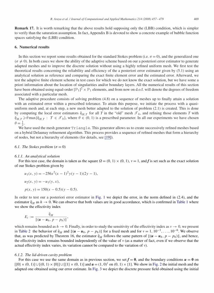
In order to test our a posteriori error estimator in Fig. 1 we depict the error, in the norm defined in (2.4), and theestimator H as h → 0. We can observe that both values are in good accordance, which is confirmed in Table 1 wherewe show the effectivity index

Ei := H

‖(u − uh, p − ph)‖ ,

which remains bounded as h → 0. Finally, in order to study the sensitivity of the effectivity index as � → 0, we presentin Table 2 the behavior of H and ‖(u − uh, p − ph)‖ for a fixed mesh and for � = 1, 10−1, . . . , 10−6. We observethat, as was predicted by Theorem 16, the estimator H follows the same pattern of ‖(u − uh, p − ph)‖, and hence,the effectivity index remains bounded independently of the value of � (as a matter of fact, even if we observe that theactual effectivity index varies, its variation cannot be compared to the variation of �).

6.1.2. The lid-driven cavity problemFor this case we use the same domain as in previous section, we set f = 0, and the boundary conditions u = 0 on

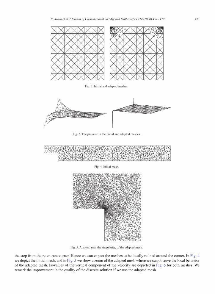
[{0}× (0, 1)] ∪ [(0, 1)×{0}] ∪ [{1}× (0, 1)] and u = (1, 0)t on (0, 1)×{1}. We show in Fig. 2 the initial mesh and theadapted one obtained using our error estimate. In Fig. 3 we depict the discrete pressure field obtained using the initial

470 R. Araya et al. / Journal of Computational and Applied Mathematics 214 (2008) 457–479

err

or

10000010000100010010

10

1

0.1

0.01

d.o.f

||(u−uh, p−ph)||

Fig. 1. Exact error and the a posteriori error estimate.

Table 1Exact error, a posteriori error estimator and effectivity index

d.o.f ‖(u − uh, p − ph)‖ H Ei

39 6.641955 5.216376 0.785367123 3.292848 2.873238 0.872569435 1.671618 1.523188 0.9112051635 0.838908 0.775193 0.9240506339 0.419710 0.392412 0.93496024 963 0.209854 0.197351 0.94042299 075 0.104919 9.900770e − 02 0.943655

Table 2Sensitivity of the estimator to �

� ‖(u − uh, p − ph)‖ H Ei

1 0.209854 0.197351 0.9404221e − 01 6.643132e − 02 6.244997e − 02 0.9400681e − 02 2.309899e − 02 2.105384e − 02 0.9114611e − 03 3.123896e − 02 2.392909e − 02 0.7660011e − 04 9.655438e − 02 7.305909e − 02 0.7566621e − 05 0.305260 0.227342 0.7447501e − 06 0.965315 0.645566 0.668762

and adapted meshes where we note the improvement in the quality of the computed solution since the singular natureof the pressure is better captured in the adapted mesh.

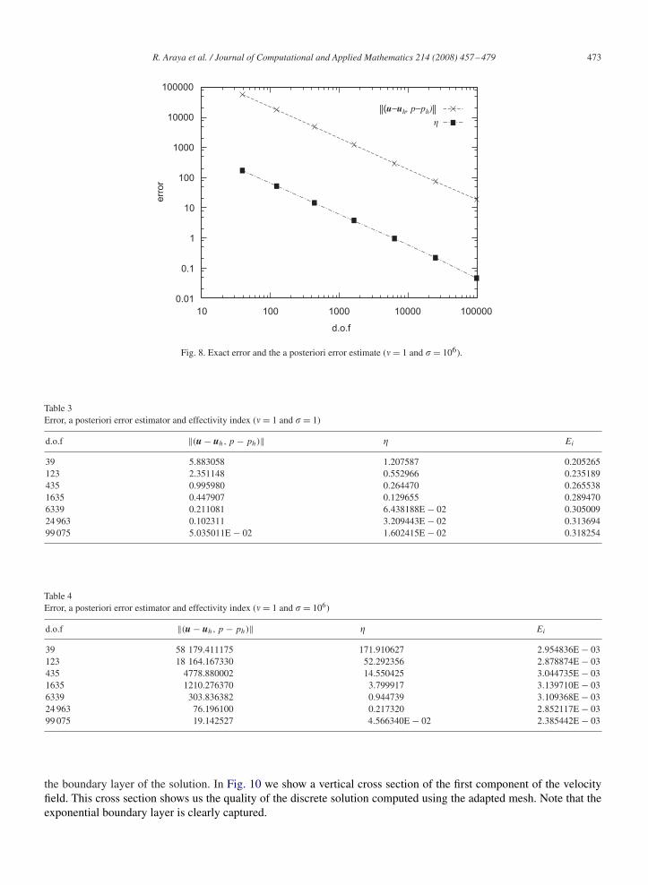
6.1.3. The backward facing step problemThis test case is posed on the backward facing step configuration. The step is located at (x, y) = (2.5, 0), the entry

of the channel is at x = 0 and the exit of the channel is at x = 22. The channel width is 1 at entry and 2 at exit. Theboundary conditions are inflow parabolic profiles and free outflow. We assume f = 0. In this case a singularity arises at

R. Araya et al. / Journal of Computational and Applied Mathematics 214 (2008) 457–479 471

Fig. 2. Initial and adapted meshes.

Fig. 3. The pressure in the initial and adapted meshes.

Fig. 4. Initial mesh.

Fig. 5. A zoom, near the singularity, of the adapted mesh.

the step from the re-entrant corner. Hence we can expect the meshes to be locally refined around the corner. In Fig. 4we depict the initial mesh, and in Fig. 5 we show a zoom of the adapted mesh where we can observe the local behaviorof the adapted mesh. Isovalues of the vertical component of the velocity are depicted in Fig. 6 for both meshes. Weremark the improvement in the quality of the discrete solution if we use the adapted mesh.

472 R. Araya et al. / Journal of Computational and Applied Mathematics 214 (2008) 457–479

Fig. 6. A zoom, near the singularity, of the vertical velocity in the initial and the adapted meshes.

err

or

10000010000100010010

10

1

0.01

0.1

d.o.f

||(u−uh, p−ph)||

Fig. 7. Exact error and the a posteriori error estimate (� = 1 and � = 1).

6.2. The generalized problem (� = 0)

6.2.1. An analytical solutionFor this test case we consider � = (0, 1) × (0, 1), and with the aim of testing our approach using nonpolynomial

solutions, we set f such that the exact solution of our generalized Stokes problem is given by

u1(x, y) = sin(�x) sin(�y),

u2(x, y) = cos(�x) cos(�y),

p(x, y) = 150(x − 0.5)(y − 0.5).

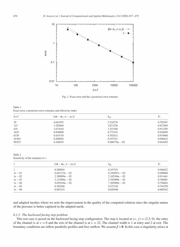
In Figs. 7 and 8 we present the behavior, when � = 1 and � = 1, 106, of the true error and the error estimate when hgoes to 0. In Tables 3 and 4 we show the same kind of information plus the effectivity index. Note that this case is notcovered by our theoretical results since condition (F) is not satisfied. Nevertheless, the exact error follows the samepattern of our a posteriori error estimator.

6.2.2. The lid-driven cavity problemAgain, we consider the problem described in Section 6.1.2, but in this case we assume � = 1 and � = 106. In Fig. 9

we depict the initial and final adapted meshes. We note that our a posteriori error estimate is able to detect correctly

R. Araya et al. / Journal of Computational and Applied Mathematics 214 (2008) 457–479 473

err

or

10000010000100010010

100000

10000

1000

100

10

1

0.01

||(u−uh, p−ph)||

0.1

d.o.f

Fig. 8. Exact error and the a posteriori error estimate (� = 1 and � = 106).

Table 3Error, a posteriori error estimator and effectivity index (� = 1 and � = 1)

d.o.f ‖(u − uh, p − ph)‖ Ei

39 5.883058 1.207587 0.205265123 2.351148 0.552966 0.235189435 0.995980 0.264470 0.2655381635 0.447907 0.129655 0.2894706339 0.211081 6.438188E − 02 0.30500924 963 0.102311 3.209443E − 02 0.31369499 075 5.035011E − 02 1.602415E − 02 0.318254

Table 4Error, a posteriori error estimator and effectivity index (� = 1 and � = 106)

d.o.f ‖(u − uh, p − ph)‖ Ei

39 58 179.411175 171.910627 2.954836E − 03123 18 164.167330 52.292356 2.878874E − 03435 4778.880002 14.550425 3.044735E − 031635 1210.276370 3.799917 3.139710E − 036339 303.836382 0.944739 3.109368E − 0324 963 76.196100 0.217320 2.852117E − 0399 075 19.142527 4.566340E − 02 2.385442E − 03

the boundary layer of the solution. In Fig. 10 we show a vertical cross section of the first component of the velocityfield. This cross section shows us the quality of the discrete solution computed using the adapted mesh. Note that theexponential boundary layer is clearly captured.

474 R. Araya et al. / Journal of Computational and Applied Mathematics 214 (2008) 457–479

Fig. 9. Initial and final adapted meshes.

0 0.1 0.2 0.3 0.4 0.5 0.6 0.7 0.8 0.9 1

-0.1

0

0.1

0.2

0.3

0.4

0.5

0.6

0.7

0.8

0.9

1

Fig. 10. A cross section of the tangential velocity at x = 12 .

7. Concluding remarks

An adaptive finite element scheme for the generalized Stokes equation has been introduced and analyzed. This schemeis based on a stabilized finite element method combined with an a posteriori error estimator. This error estimator is cheapand easy to calculate once we have chosen the bubble function spaces to be used. The equivalence between the estimatorand the finite element error has been proved using a general hypothesis on the auxiliary bubble function spaces, thusavoiding the use of a saturation assumption, and we have provided a concrete pair of bubble spaces satisfying thisrequirement.

Even if the theoretical results concerning the estimator include constants depending on the physics of the problem,we remark that, for the pure Stokes problem, they provide equivalence constants which are independent of the viscosity.We also note that this dependence arises from the auxiliary problem posed on the continuous setting, and not from thehierarchical approach.

Finally, it is worth remarking that, even if the basic idea is closely related to the idea from [2] (see also [18]), ourpresentation is more general and the actual error estimator is quite different, and easier to compute. The extension ofthis idea to the Oseen and to the fully nonlinear Navier–Stokes equations will be the subject of future research.

R. Araya et al. / Journal of Computational and Applied Mathematics 214 (2008) 457–479 475

Appendix A. The proof of Lemma 13

First, we give the following result concerning the stabilization parameter �T .

Lemma 18. Let T ∈ Th and let �T be given by (4.9). Then, the following estimates hold:

��T � 112h2

T , (A.1)

��T � min{hT �−1/2�1/2, 1}. (A.2)

Proof. In order to prove the first estimate we use (4.9) and (4.10) to obtain

�T �h2

T

4�/mk

� 1

12�−1h2

T

estimate which is valid independently of the value of �. Second estimate is obvious if � = 0, hence we will supposefrom now on that � > 0. First, we use (4.9) to get

��T � 1

max{�T , 1} �1. (A.3)

On the other hand, we know from (A.1) that �T � 112�−1h2

T , and then

��T � 112h2

T �−1�. (A.4)

Taking then the geometric mean of (A.3) and (A.4), we have

��T � 1√12

hT �−1/2�1/2. (A.5)

Finally, from (A.3) and (A.5), we obtain (A.2). �

Now, we are ready to prove Lemma 13. We will prove the result only for the case � > 0, the other one being completelyanalogous. From the definition of R1

h, using (4.8) with qh = 0, we have

R1h(vh) =

∫�

f · vh − a(uh, vh) − b(vh, ph) =∑

T ∈Th

∫T

�T RT (�vh − ��vh).

Next, from Cauchy–Schwarz’s inequality, (3.2) and (A.1), we obtain

��T

∫T

RT �vh ���T

∫T

|RT ||�vh|

�h2

T

12‖RT ‖0,T ‖�vh‖0,T

� �T ‖RT ‖0,T ‖vh‖a,T .

On the other hand, using (A.2), Cauchy–Schwarz’s inequality and the definition of �T we obtain

��T

∫T

RT vh � min{�−1/2�1/2hT , 1}‖RT ‖0,T ‖vh‖0,T

��T ‖RT ‖0,T ‖vh‖a,T

and the result follows.

476 R. Araya et al. / Journal of Computational and Applied Mathematics 214 (2008) 457–479

Appendix B. Bubble function spaces satisfying (LBB) condition

For each element T ∈ Th we define the element bubble function bT by

bT := 27∏

x∈N(T )

�x , (B.1)

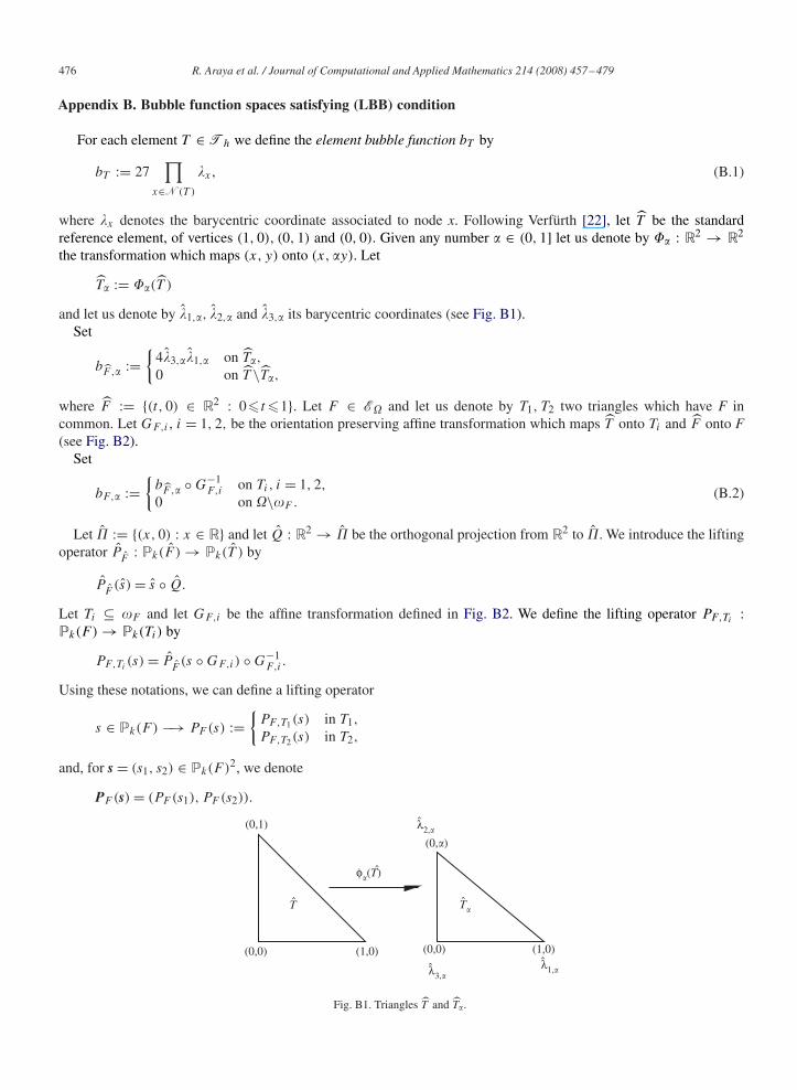
where �x denotes the barycentric coordinate associated to node x. Following Verfürth [22], let T be the standardreference element, of vertices (1, 0), (0, 1) and (0, 0). Given any number � ∈ (0, 1] let us denote by �� : R2 → R2

the transformation which maps (x, y) onto (x, �y). Let

T� := ��(T )

and let us denote by �1,�, �2,� and �3,� its barycentric coordinates (see Fig. B1).Set

bF ,� :={

4�3,��1,� on T�,

0 on T \T�,

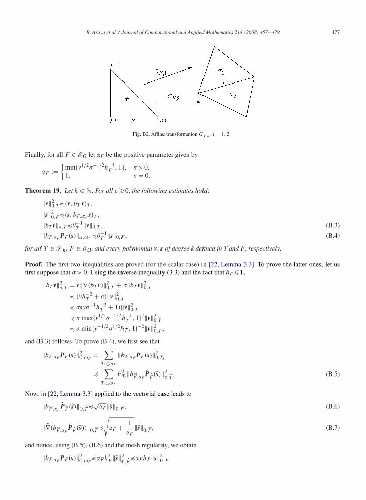
where F := {(t, 0) ∈ R2 : 0� t �1}. Let F ∈ E� and let us denote by T1, T2 two triangles which have F incommon. Let GF,i , i = 1, 2, be the orientation preserving affine transformation which maps T onto Ti and F onto F(see Fig. B2).

Set

bF,� :={

bF ,� ◦ G−1F,i on Ti, i = 1, 2,

0 on �\�F .(B.2)

Let � := {(x, 0) : x ∈ R} and let Q : R2 → � be the orthogonal projection from R2 to �. We introduce the liftingoperator P

F: Pk(F ) → Pk(T ) by

PF(s) = s ◦ Q.

Let Ti ⊆ �F and let GF,i be the affine transformation defined in Fig. B2. We define the lifting operator PF,Ti:

Pk(F ) → Pk(Ti) by

PF,Ti(s) = P

F(s ◦ GF,i) ◦ G−1

F,i .

Using these notations, we can define a lifting operator

s ∈ Pk(F ) −→ PF (s) :={

PF,T1(s) in T1,

PF,T2(s) in T2,

and, for s = (s1, s2) ∈ Pk(F )2, we denote

PF (s) = (PF (s1), PF (s2)).

(0,0) (1,0)

T

(0,1)

(1,0)

(0,�)

(0,0)

T�

φ�(T)

λ2,�ˆ

λ3,�ˆ λ1,�

ˆ

Fig. B1. Triangles T and T�.

R. Araya et al. / Journal of Computational and Applied Mathematics 214 (2008) 457–479 477

Fig. B2. Affine transformation GF,i , i = 1, 2.

Finally, for all F ∈ E� let �F be the positive parameter given by

�F :={

min{�1/2�−1/2h−1F , 1}, � > 0,

1, � = 0.

Theorem 19. Let k ∈ N. For all ��0, the following estimates hold:

‖v‖20,T �(v, bT v)T ,

‖s‖20,F �(s, bF,�F

s)F ,

‖bT v‖a,T ��−1T ‖v‖0,T , (B.3)

‖bF,�FPF (s)‖a,�F

��−1F ‖s‖0,F , (B.4)

for all T ∈ Th, F ∈ E�, and every polynomial v, s of degree k defined in T and F, respectively.

Proof. The first two inequalities are proved (for the scalar case) in [22, Lemma 3.3]. To prove the latter ones, let usfirst suppose that � > 0. Using the inverse inequality (3.3) and the fact that bT �1,

‖bT v‖2a,T = �‖∇(bT v)‖2

0,T + �‖bT v‖20,T

� (�h−2T + �)‖v‖2

0,T

� �(��−1h−2T + 1)‖v‖2

0,T

� � max{�1/2�−1/2h−1T , 1}2‖v‖2

0,T

� � min{�−1/2�1/2hT , 1}−2‖v‖20,T ,

and (B.3) follows. To prove (B.4), we first see that

‖bF,�FPF (s)‖2

0,�F=

∑Ti⊂�F

‖bF,�FPF (s)‖2

0,Ti

�∑

Ti⊂�F

h2Ti

‖bF ,�FP

F(s)‖2

0,T. (B.5)

Now, in [22, Lemma 3.3] applied to the vectorial case leads to

‖bF ,�FP

F(s)‖0,T �√

�F ‖s‖0,F , (B.6)

‖∇(bF ,�FP

F(s))‖0,T �

√�F + 1

�F

‖s‖0,F , (B.7)

and hence, using (B.5), (B.6) and the mesh regularity, we obtain

‖bF,�FPF (s)‖2

0,�F��F h2

F ‖s‖20,F

��F hF ‖s‖20,F .

478 R. Araya et al. / Journal of Computational and Applied Mathematics 214 (2008) 457–479

Moreover

�hF �F = �1/2�1/2 min{1, �−1/2�1/2hF }��1/2�1/2 min{1, �−1/2�1/2hF }−1 = �−2

F

and then

�‖bF,�FPF (s)‖2

0,�F��−2

F ‖s‖20,F . (B.8)

On the other hand, from (B.7) and �F �1, it holds

‖∇(bF,�FPF (s))‖2

0,�F=

∑Ti⊂�F

‖∇(bF,�FPF (s))‖2

0,Ti

� ‖∇(bF,�FP

F(s))‖2

0,T

� �−1F ‖s‖2

0,F

� h−1F �−1

F ‖s‖20,F

and using that �h−1F �−1

F = �−2F , we obtain

�‖∇(bF,�FPF (s))‖2

0,�F��−2

F ‖s‖20,F . (B.9)

Hence, the result for � > 0 follows from (B.8) and (B.9). The proof for � = 0 follows in an analogous way. �

In order to satisfy the (LBB) condition we need to impose the following condition on f:(F) f is a piecewise polynomial function, i.e., there exists a positive integer t such that

f ∈ {g ∈ L2(�)2 : g|T ∈ Pt (T )2, ∀T ∈ Th}.

Remark 20. One possibility to overcome condition (F) above is to split the error between the error due to dataapproximation and the error due to the numerical method, as it has been done, for instance, in [1]. In any case, weremark that, since the degree t of the polynomial from condition (F) is not upper bounded, the error between f and itslocal projection onto the piecewise polynomial space may be seen as a higher order term.

Next, we define the following bubble function spaces:

HbT := 〈{bT RT }〉, ∀T ∈ Th,

HbF := 〈{bF,�F

PF (RF )}〉, ∀F ∈ E�,

where bT and bF,�Fare the bubble functions given by (B.1) and (B.2), respectively.

Remark 21. We remark that this definition of bubble functions allows us use any polynomial order to approximatethe velocity and the pressure. In fact, for every k, l�1 the bubble function bT RT belongs to Pmax{t,k,l−1}+3(T ) andbF,�F

PF (RF ) belongs to Pk+1(T ). Hence, HbT and Hb

F are not subspaces of Hh.

Since bT RT ∈ HbT , using Theorem 19 we arrive at

supBT ∈Hb

T

(RT ,BT )T

�T ‖RT ‖0,T aT (BT ,BT )1/2 � (RT , bT RT )T

�T ‖RT ‖0,T aT (bT RT , bT RT )1/2

�‖RT ‖2

0,T

�T ‖RT ‖0,T �−1T ‖RT ‖0,T

��.

R. Araya et al. / Journal of Computational and Applied Mathematics 214 (2008) 457–479 479

The same analysis may be carried out for every F ∈ E�. In fact, we have

supBF ∈Hb

F

(RF ,BF )F

�F ‖RF ‖0,F a�F(BF ,BF )1/2 � (RF , bF,�F

RF )F

�F ‖RF ‖0,F a�F(bF,�F

PF (RF ), bF,�FPF (RF ))1/2

�‖RF ‖2

0,F

�F ‖RF ‖0,F �−1F ‖RF ‖0,F

� �.

References

[1] M. Ainsworth, A posteriori error estimation for lowest order Raviart-Thomas mixed finite elements. Technical Report 23, University ofStrathclyde, Department of Mathematics, 2006.

[2] M. Ainsworth, J.T. Oden, A posteriori error estimators for the Stokes and Oseen equations, SIAM J. Numer. Anal. 34 (1997) 228–245.[3] M. Ainsworth, J.T. Oden, A Posteriori Error Estimation in Finite Element Analysis, Wiley, New York, 2000.[4] R. Araya, G.R. Barrenechea, F. Valentin, A stabilized finite-element method for the Stokes problem including element and edge residuals, IMA

J. Numer. Anal. 27 (1) (2007) 172–197.[5] R. Araya, E. Behrens, R. Rodríguez, An adaptive stabilized finite element scheme for the advection–reaction–diffusion equation, Appl. Numer.

Math. 54 (2005) 491–503.[6] R. Araya, A. Poza, E.P. Stephan, A hierarchical a posteriori error estimate for an advection–diffusion–reaction problem, Math. Models Methods

Appl. Sci. 15 (7) (2005) 1119–1139.[7] R.E. Bank, B.D. Welfert, A posteriori error estimators for the Stokes problem, SIAM J. Numer. Anal. 28 (1991) 591–623.[8] G. Barrenechea, F. Valentin, An unusual stabilized finite element method for a generalized Stokes problem, Numer. Math. 92 (4) (2002)

653–677.[9] F. Brezzi, M. Fortin, Mixed and Hybrid Finite Element Methods, Springer, New York, 1991.

[10] P. Clément, Approximation by finite element functions using local regularization, R.A.I.R.O. Anal. Numer. 9 (1975) 77–84.[11] E. Dari, R. Durán, C. Padra, Error estimators for nonconforming finite element approximations of the Stokes problem, Math. Comp. 64 (1995)

1017–1033.[12] W. Dörfler, M. Ainsworth, Reliable a posteriori error control for nonconformal finite element approximation of Stokes flow, Math. Comp. 54

(252) (2005) 1599–1619.[13] H. Elman, D. Silvester, A. Wathen, Finite elements and fast iterative solvers: with applications in incompressible fluid dynamics, Oxford

University Press, New York, 2005.[14] A. Ern, J.-L. Guermond, Theory and Practice of Finite Elements, Springer, New York, 2004.[15] V. Girault, P.A. Raviart, Finite Element Methods for the Navier–Stokes Equations, Springer, Berlin, 1986.[16] T.J.R. Hughes, L.P. Franca, A new finite element formulation for computational fluid dynamics: VII. The Stokes problem with various well-

posed boundary conditions: symmetric formulations that converge for all velocity/pressure spaces, Comput. Methods Appl. Mech. Eng. 65 (1)(1987) 85–96.

[17] V. John, A numerical study of a posteriori error estimators for convection–diffusion problems, Comput. Methods Appl. Mech. Eng. 190 (2000)757–781.

[18] D. Kay, D. Silvester, A posteriori error estimation for stabilized mixed approximations of the Stokes equations, SIAM J. Sci. Comput. 21 (1999)1321–1336.

[19] J.R. Shewchuk, Delaunay refinement algorithms for triangular mesh generation, Comput. Geom. Theory Appl. 22 (1–3) (2002) 21–74.[20] R. Verfürth, A posteriori error estimators for the Stokes problem, Numer. Math. 55 (1989) 309–325.[21] R. Verfürth, A posteriori error estimators for the Stokes problem II. Non-conforming discretizations, Numer. Math. 60 (1991) 235–249.[22] R. Verfürth, A posteriori error estimators for convection–diffusion equations, Numer. Math. 80 (1998) 641–663.