FCNN: Five-point stencil CNN for solvingreaction-diffusion equations

Yongho Kima, Yongho Choib,∗

aFaculty of Mathematics, Otto-von-Guericke-Universitat Magdeburg, Universitatsplatz 2,39106, Magdeburg, Germany

bDepartment of Mathematics and Big Data, Daegu University, Gyeongsan-si,Gyeongsangbuk-do 38453, Republic of Korea

Abstract

In this paper, we propose Five-point stencil CNN (FCNN) containing a five-

point stencil kernel and a trainable approximation function. We consider reaction-

diffusion type equations including heat, Fisher’s, Allen–Cahn equations, and

reaction-diffusion equations with trigonometric functions. Our proposed FCNN

is trained well using few data and then can predict reaction-diffusion evolutions

with unseen initial conditions. Also, our FCNN is trained well in the case of

using noisy train data. We present various simulation results to demonstrate

that our proposed FCNN is working well.

Keywords: convolutional neural network, reaction-diffusion type equations,

data-driven model

1. Introduction

To express diverse natural phenomena such as sound, heat, electrostatics,

elasticity, thermodynamics, fluid dynamics, and quantum mechanics mathe-

matically, various partial differential equations (PDEs) have been derived and

numerical methods can be applied to solve these PDEs. Representative numer-

ical methods for solving PDEs are the finite difference method, finite element

∗Corresponding authorEmail addresses: ykim@mpi-magdeburg.mpg.de (Yongho Kim),

yongho_choi@daegu.ac.kr (Yongho Choi)URL: https://sites.google.com/view/yh-choi (Yongho Choi)

Preprint submitted to - January 7, 2022

arX

iv:2

201.

0185

4v1

[cs

.LG

] 4

Jan

202

2

method, finite volume method, spectral method, etc. We focus on the finite dif-

ference method (FDM) which is to divide a given domain into finite grids and

find an approximate solution using derivatives with finite differences [1]. This

method uses each and its neighbor points to predict the corresponding point

at the next time step. Likewise, in convolutional neural networks (CNNs) [20],

convolution operators extract each pixel of an output by using the correspond-

ing pixel and its neighbor pixels of an input. Also, the convolution operator

is basically immutable. Hence, well-structured convolutional neural networks

have a potential to solve partial differential equations numerically. Therefore,

we propose Five-point stencil CNN (FCNN) containing a five-point stencil ker-

nel and a trainable approximation function to obtain numerical solutions of

the PDEs. Among the various PDEs representing natural phenomena, we deal

with reaction-diffusion type equations. The reaction-diffusion model has been

applied and used in various fields such as biology [3, 4, 5], chemistry [6, 7, 8],

image segmentation [9, 10, 11], image inpainting [12, 13, 14], medical [15, 16, 17],

and so on. In this paper, we use second order reaction-diffusion type equations:

heat, Fisher’s, Allen–Cahn (AC) equation, and reaction-diffusion equations with

trigonometric functions terms.

In recent years, neural networks have been widely applied to solve PDEs.

Physics-informed neural networks (PINNs) [22] based on multi-layer perceptron

(MLP) models approximate solutions by the optimization of a loss function

consisting of given physics laws. The biggest benefit of PINNs is that solutions

can be inferred without any iterative process such as a recurrence equation with

respect to time. Furthermore, it is used for diverse applications such as Hidden

Fluid Mechanics [25] that extracts hidden variables of a given equation using

a PINN and observations. However, it is hard to optimize model parameters

when we deal with complicated PDEs and their coefficients. In order to improve

the training ability, combinations of PINNs and numerical methods have been

developed, or other neural networks such as CNNs are selected. M. Raissi et

al. [22] added Runge-Kutta methods to a PINN model for solving AC equation.

Aditi et al. [23] proposed transfer learning and curriculum regularization which

2

start training PINNs on a specific safe domain and then transfer to a target

domain. Hao Ma et al. [24] proposed a U-shape CNN so-called U-net [27] and

they showed that the usage of target data in a loss function significantly improves

optimization. Elie Bretin et al. [26] used convolutional neural networks derived

from a semi-implicit approach to learn phase field mean curvature flows of the

AC equation.

We propose data-driven models that approximate the solution of explicit

finite difference scheme to solve second order reaction-diffusion type equations

numerically. Our contributions are as follows:

1. We propose a five-point stencil convolution operator to solve reaction-

diffusion type equations.

2. Our proposed model is trained using two consecutive snapshots to solve a

given equation.

3. We demonstrate the robustness of our method using five reaction-diffusion

type equations and noisy data.

The remainder of this paper is organized as follows. In Section 2, we present

how to create training data using explicit FDM, explain the FCNN concept,

training process, and numerical solutions. In Section 3, we compare the predic-

tion results using our proposed FCNN and the evolution of PDEs results using

the FDM method and show the robustness of our FCNN. Finally conclusions

are drawn in Section 4.

2. Methods and numerical solutions

FDM is to divide a given domain into finite grids and find an approximate

solution using derivatives with finite differences [1]. We use explicit FDM to

create training data with random initial conditions. We use only two consecutive

FDM results, the initial and next time step results, as training data for each

equation. To create training data, a computational domain is defined using a

uniform grid of size h = 1/Nx = 1/Ny and Ωh = (xi, yj) = (a+ (i− 1.5)h, c+

(j− 1.5)h) for 1 ≤ i ≤ Nx + 2 and 1 ≤ j ≤ Ny + 2. Here, Nx and Ny are mesh

3

sizes on the computational domain (a, b) × (c, d). Let φnij be approximations

of φ(xi, yj , n∆t) and ∆t is temporal step size. The boundary condition is zero

Neumann boundary condition. Laplacian of a function φ is calculated using a

five-point stencil method, the Laplacian 4φ can be approximated as follows:

4φ ≈ φ(x+ h, y) + φ(x− h, y)− 4φ(x, y) + φ(x, y + h) + φ(x, y − h)

h2. (1)

In this way, the first and second derivatives of φ at each point (xi, yj) (e.g.,

φx, φy, φxx and φyy) can be approximated within the 3 × 3 local area centered

(xi, yj). This concept can be equivalent to 3 × 3 convolution kernels. The 3 ×

3 kernels K following properties:

1. k1 ⊕ k2 ∈ K for any k1, k2 ∈ K (element-wise summation)

2. k1 k2 ∈ K for any k1, k2 ∈ K (element-wise multiplication)

3. k−1 ∈ K for any k ∈ K (element-wise division)

4. ak ∈ K for any k ∈ K and any real numbers a

The second-order PDEs can be solved numerically using combinations of 3

× 3 kernels. Therefore, if we build a proper CNN as the form of recurrence Eq.

(4), we can solve a PDE (2) numerically. A previous study about AC equation

[19] shows that FDM can be expressed as CNN.

∂φ

∂t= g(φ(x, y, t)), (2)

φn+1 − φn

∆t= g(φn), (3)

φn+1 = φn + ∆tg(φn). (4)

To solve second order reaction-diffusion type equations

φt = α4 φ+ βf(φ), (5)

where α is a diffusion coefficient, β is a reaction coefficient, and f is a smooth

function to present reaction effect, we propose FCNN as a recurrence relation:

φn+1 = φn + ∆tα4 φn + ∆tβf(φn). (6)

As a CNN, F (φn) containing a 5-point stencil filter and a pad satisfying given

boundary conditions solves ∆tα4 φn. In order to approximate φn + ∆tβf(φn)

4

Figure 1: Computational graph of FCNN for second order reaction-diffusion type equations

terms, we define a trainable polynomial function ε(φn) as follows:

ε(φn) = a0 +

N∑k=1

ai(φn − b)k, (7)

with model parameters ai for any i ∈ 0, 1, · · · , N and a real value b. Let

M(φn) = F (φn) + ε(φn) be a FCNN. Then, the inference is as follows:

φn+1 = Mθ(φn), (8)

where θ is a set of model parameters. Figure 1 shows the computational

graph of our explicit model FCNN containing model parameters wi for any

i ∈ 0, 1, 2, 3, 4 in a filter. Furthermore, F represents the diffusion term on the

uniform grid of x and y axises, so we set up w1 = w3 and w0 = w4 to cut down

on training time. When the five-point stencil filter is used and ε is a p-th order

polynomial function, the number of model parameters is only p+ 4. Thus, the

set-up enables to learn physical patterns from few data. In Algorithm 1, an

initial image φ0(= u0) and the prediction φ1 at the next time ∆t are used with

train data u0 and u1 to train a model Mθ. The objective function L(φ1, u1) is

the mean square error function as follows:

L(φ1, u1) =1

N

N∑i=1

(φ1i − u1i )2 (9)

5

Algorithm 1 Training Procedure

Set an initial value φ0 = u0, a small constant δ > 0

Initialize Mθ(φ0) = F (φ0) + ε(φ0) with model parameters θ

while ` > δ do

φ1 ←Mθ(φ0)

Compute loss ` = L(φ1, u1)

Update θ

end while

where N , φ1 and u1 are the number of pixels in an output image, a prediction

and its target respectively.

2.1. Reaction-diffusion type equations

To demonstrate the robustness of FCNN, we consider reaction-diffusion

type equations: heat, Fisher’s, AC equation, reaction-diffusion equations with

trigonometric functions. The reaction and diffusion coefficients used in each

formula are arranged in Table 1. For the AC equation, β = 1/ρ2 where ρ is

Table 1: Diffusion (α) and reaction (β) coefficients for the simulations.

Heat Fisher’s AC Sine Tanh

α 1 1 1 0.1 0.5

β 0 20 6944 40 10

the thickness of the transition layer and which value is ρ5 ≈ 0.012 [19]. For the

other equations, we select arbitrary coefficients. For all the following equations,

the continuous equations and the discretized equations are described in turn,

and the zero Neumann boundary condition is used.

6

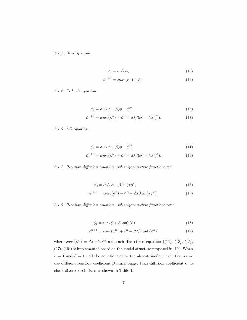
2.1.1. Heat equation

φt = α4 φ, (10)

φn+1 = conv(φn) + φn. (11)

2.1.2. Fisher’s equation

φt = α4 φ+ β(φ− φ2), (12)

φn+1 = conv(φn) + φn + ∆tβ(φn − (φn)2). (13)

2.1.3. AC equation

φt = α4 φ+ β(φ− φ3), (14)

φn+1 = conv(φn) + φn + ∆tβ(φn − (φn)3). (15)

2.1.4. Reaction-diffusion equation with trigonometric function: sin

φt = α4 φ+ β sin(πφ), (16)

φn+1 = conv(φn) + φn + ∆tβ sin(πφn). (17)

2.1.5. Reaction-diffusion equation with trigonometric function: tanh

φt = α4 φ+ β tanh(φ), (18)

φn+1 = conv(φn) + φn + ∆tβ tanh(φn). (19)

where conv(φn) = ∆tα 4 φn and each discretized equation ((11), (13), (15),

(17), (19)) is implemented based on the model structure proposed in [19]. When

α = 1 and β = 1 , all the equations show the almost similary evolution so we

use different reaction coefficient β much bigger than diffusion coefficient α to

check diverse evolutions as shown in Table 1.

7

3. Simulation results

Assume that we observe a reaction-diffusion pattern and investigate the pat-

tern rule under the constraint meaning that the observations and predictions

follow the same PDE. Our proposed FCNN is trained using only two consecutive

data which are the initial and next time step results for each equation. Then,

we evaluate the model using diverse unseen initial values.

In the simulations, we use random initial value data with 100 × 100 mesh

so that the size of the input data is 102× 102 containing a pad as a boundary

condition. Also, N = 3 (Heat, Fisher’s, AC) or 9 (Sine, Tanh) for ε(φn) is

fixed depending on given equations and a 3× 3 convolutional filter is used with

the stride of 1 in Eq. (7). Hence, the filter has 10,000 (= ((100 + 2 − 3)/1 +

1)2) chances to learn the evolution of results images, so training a model using

only two consecutive images are enough to optimize nine or thirteen model

parameters (w0, · · · , w4, a0, · · · , a3). As an optimizer, ADAM [21] is used with

a learning rate of 0.01 and without any regularization. Instead, we apply early

stopping [28] based on a validation data to avoid overfitting. To demonstrate

the approximation ε(φn) for non-polynomial functions f(φn), we additionally

consider sine and tanh functions besides heat, Fisher’s, and AC equations.

For the evaluation, we implement FCNN and FDM respectively and then

measure the averaged relative L2 error with 95% confidence interval over 100

novel random initial values as shown in Table 2.

Table 2: Relative L2 error between FCNN and FDM. The ± shows 95% confidence intervals

over 100 different random initial values.

Equations Relative L2 error

Heat 8.4× 10−5 ± 4× 10−6

Fisher’s 4.0× 10−5 ± 2× 10−6

AC 1.3× 10−6 ± 8× 10−7

Sine 7.0× 10−5 ± 5× 10−6

Tanh 1.9× 10−4 ± 4× 10−6

8

Furthermore, we validate the errors using different types of initial values for

each equation as shown in Table 3. The initial conditions are described in the

Appendix Section.

Table 3: Relative L2 error between FCNN and FDM with diverse initial values.

Initial shapes: circle star circles torus maze

Heat 3.4× 10−5 4.4× 10−5 1.1× 10−5 1.1× 10−4 4.9× 10−5

Fisher’s 8.7× 10−4 7.2× 10−4 1.9× 10−4 1.3× 10−4 3.7× 10−5

AC 2.6× 10−7 2.7× 10−7 2.3× 10−7 2.0× 10−7 1.9× 10−7

Sine 3.7× 10−4 2.2× 10−4 9.5× 10−5 7.5× 10−5 4.1× 10−5

Tanh 1.8× 10−3 1.4× 10−3 6.3× 10−4 2.5× 10−5 2.9× 10−5

Figures 2-6 show the time evolution results when unseen initial shapes (cir-

cle, star, three circles, torus, and maze) are given after learning with two train-

ing data (random initial condition and next time step result with FDM). We

compare the predicted results from pretrained models to the FDM results.

Table 4: Relative L2 error with noise. The ± shows 95% confidence intervals over 100 different

random initial values.

σ Relative L2 Error

0 1.3× 10−6 ± 8× 10−7

10−6 9.1× 10−5 ± 6× 10−4

10−4 3.3× 10−4 ± 2× 10−4

10−2 1.4× 10−1 ± 3× 10−2

Data-driven models are sensitive to data noise. To investigate the noise

effect, we inject Gaussian random noise η ∼ N(0, σ2) to u1 and then the model

is trained using u0 and u1 + η for the AC equation. Table 4 shows that the

model can be trained under the noise condition. Figure 7 displays the results of

the inference using contaminated models.

9

(a)

(b)

(c)

(d)

(e)

Figure 2: Time evolution of a circle shape of (a) Heat, (b) Fisher’s, (c) AC, (d) Sine, and (e)

Tanh equations.

10

(a)

(b)

(c)

(d)

(e)

Figure 3: Time evolution of a star shape of (a) Heat, (b) Fisher’s, (c) AC, (d) Sine, and (e)

Tanh equations.

11

(a)

(b)

(c)

(d)

(e)

Figure 4: Time evolution of three circles of (a) Heat, (b) Fisher’s, (c) AC, (d) Sine, and (e)

Tanh equations.

12

(a)

(b)

(c)

(d)

(e)

Figure 5: Time evolution of a torus shape of (a) Heat, (b) Fisher’s, (c) AC, (d) Sine, and (e)

Tanh equations.

13

(a)

(b)

(c)

(d)

(e)

Figure 6: Time evolution of a maze shape of (a) Heat, (b) Fisher’s, (c) AC, (d) Sine, and (e)

Tanh equations.

14

Figure 7: Inference using a contaminated model with noise rates (γ = 0, 5, and 30%)

4. Conclusions

In this paper, we proposed Five-point stencil CNN (FCNN) containing a

five-point stencil kernel and a trainable approximation function. We considered

reaction-diffusion type equations including heat, Fisher’s, Allen–Cahn equa-

tions, and reaction-diffusion equations with trigonometric functions. We showed

that our proposed FCNN can be trained well using few data (used only two

consecutive data) and then can predict reaction-diffusion evolution with unseen

diverse initial conditions. Also, we demonstrated the robustness of our FCNN

under the noise condition.

15

Acknowledgments

The corresponding author Y. Choi was supported by the National Research

Foundation of Korea (NRF) grant funded by the Korea government (NRF-

2020R1C1C1A0101153712).

Appendix

In this appendix session, we describe the initial conditions used in the sim-

ulation results session 3. A detailed description of these initial conditions can

be found in our previous research paper [19].

(1) The initial condition of a circle shape

φ(x, y, 0) = tanh

(R0 −

√(x− 0.5)2 + (y − 0.5)2√

2ε

), (20)

where R0 is the initial radius of a circle.

(2) The initial condition of a star shape

φ(x, y, 0) = tanh

(0.25 + 0.1 cos(6θ)−

√(x− 0.5)2 + (y − 0.5)2√2ε

), (21)

where

θ =

tan−1(y−0.5x−0.5

), if (x > 0.5)

π + tan−1(y−0.5x−0.5

), otherwise.

(3) The initial condition of a torus shape

φ(x, y, 0) = −1 + tanh

(R1 −

√XY√

2ε

)− tanh

(R2 −

√XY√

2ε

), (22)

where R1 and R2 are the radius of major (outside) and minor (inside) circles,

respectively. And, for simplicity of expression, XY = (x− 0.5)2 + (y − 0.5)2.

(4) The initial condition of a maze shape

16

The initial condition of a maze shape is complicated to describe its equa-

tion, so refer to the codes which are available from the first author’s GitHub

web page (https://github.com/kimy-de) and the corresponding author’s web

page (https://sites.google.com/view/yh-choi/code).

(5) The initial condition of a random shape

φ(x, y, 0) = rand(x, y), (23)

here the function rand(x, y) has a random value between −1 and 1.

References

[1] P. Zhou, Numerical analysis of electromagnetic fields. Springer Science &

Business Media, 2012.

[2] S Kondo, T Miura, ”Reaction-diffusion model as a framework for un-

derstanding biological pattern formation.” science 329.5999 (2010): 1616-

1620.

[3] NF Britton, Reaction-diffusion equations and their applications to biology.

Academic Press, 1986.

[4] P Broadbridge, BH Bradshaw-Hajek, ”Exact solutions for logistic reac-

tion–diffusion equations in biology.” Zeitschrift fur angewandte Mathe-

matik und Physik 67.4 (2016): 1-13.

[5] D Jeong, Y Li, Y Choi, M Yoo, D Kang, J Park, J Choi, J Kim ”Numerical

simulation of the zebra pattern formation on a three-dimensional model.”

Physica A: Statistical Mechanics and its Applications 475 (2017): 106-116.

[6] BA Grzybowski, Chemistry in motion: reaction-diffusion systems for

micro-and nanotechnology. John Wiley & Sons, 2009.

[7] I Sgura, B Bozzini, D Lacitignola, ”Numerical approximation of oscillating

Turing patterns in a reaction-diffusion model for electrochemical material

17

growth.” AIP Conference Proceedings. Vol. 1493. No. 1. American Insti-

tute of Physics, 2012.

[8] G Hariharan, R Rajaraman, ”A new coupled wavelet-based method ap-

plied to the nonlinear reaction–diffusion equation arising in mathematical

chemistry.” Journal of Mathematical Chemistry 51.9 (2013): 2386-2400.

[9] H Tek, BB Kimia, ”Image segmentation by reaction-diffusion bubbles.”

Proceedings of IEEE International Conference on Computer Vision. IEEE,

1995.

[10] S Esedog, YHR Tsai, ”Threshold dynamics for the piecewise constant

Mumford–Shah functional.” Journal of Computational Physics 211.1

(2006): 367-384.

[11] Z Zhang, YM Xie, Q Li, S Zhou, ”A reaction–diffusion based level set

method for image segmentation in three dimensions.” Engineering Appli-

cations of Artificial Intelligence 96 (2020): 103998.

[12] M Bertalmio et al. ”Image inpainting.” Proceedings of the 27th annual

conference on Computer graphics and interactive techniques. 2000.

[13] Y Li, D Jeong, J Choi, S Lee, J Kim, ”Fast local image inpainting based

on the Allen–Cahn model.” Digital Signal Processing 37 (2015): 65-74.

[14] J Yu, J Ye, S Zhou, ”Reaction-diffusion system with additional source

term applied to image restoration.” International Journal of Computer

Applications 975 (2016): 8887.

[15] E Ozugurlu, ”A note on the numerical approach for the reaction–diffusion

problem to model the density of the tumor growth dynamics.” Computers

& Mathematics with Applications 69.12 (2015): 1504-1517.

[16] HG Lee, Y Kim, J Kim, ”Mathematical model and its fast numerical

method for the tumor growth.” Mathematical Biosciences & Engineering

12.6 (2015): 1173.

18

[17] M Yousefnezhad, CY Kao, SA Mohammadi, ”Optimal Chemotherapy for

Brain Tumor Growth in a Reaction-Diffusion Model.” SIAM Journal on

Applied Mathematics 81.3 (2021): 1077-1097.

[18] S.M. Allen, J.W. Cahn, “A microscopic theory for antiphase boundary

motion and its application to antiphase domain coarsening.” Acta metal-

lurgica 27.6 (1979): 1085–1095.

[19] Yongho Kim, Gilnam Ryu, and Yongho Choi (2021) Fast and Accu-

rate Numerical Solution of Allen-Cahn Equation, Mathematical Prob-

lems in Engineering, vol. 2021, Article ID 5263989, 12 pages, 2021.

https://doi.org/10.1155/2021/5263989

[20] LeCun, Yann and Boser, Bernhard and Denker, John and Henderson,

Donnie and Howard, R. and Hubbard, Wayne and Jackel, Lawrence,

(1990), Handwritten Digit Recognition with a Back-Propagation Network,

Advances in Neural Information Processing Systems, Vol 2.

[21] Diederik P. Kingma and Jimmy Ba, (2017). Adam: A Method for Stochas-

tic Optimization, arXiv:1412.6980.

[22] Maziar Raissi, Paris Perdikaris, and George Em Karniadakis, (2018).

Physics-informed neural networks: A deep learning framework for solv-

ing forward and inverse problems involving nonlinear partial differential

equations, Journal of Computational Physics 378 (2019): 686-707.

[23] Aditi S. Krishnapriyan, Amir Gholami, Shandian Zhe, Robert M. Kirby,

and Michael W. Mahoney, (2021). Characterizing Possible Failure Modes

in Physics-Informed Neural Networks, Neural Information Processing Sys-

tems (NeurIPS) 2021, arXiv:2109.01050.

[24] Hao Ma, Yuxuan Zhang, Nils Thuerey, Xiangyu Hu, Oskar J. Haidn,

(2021). Physics-driven Learning of the Steady Navier-Stokes Equations

using Deep Convolutional Neural Networks, arXiv:2106.09301.

19

[25] Maziar Raissi, Alireza Yazdani, and George Em Karniadakis. (2020) Hid-

den fluid mechanics: Learning velocity and pressure fields from flow visu-

alizations, Science 367.6481 (2020): 1026-1030.

[26] Elie Bretin, Roland Denis, Simon Masnou, and Garry Terii, (2021).

Learning Phase Field Mean Curvature Flows With Neural Networks,

arXiv:2112.07343.

[27] Olaf Ronneberger, Philipp Fischer and Thomas Brox, (2015). U-Net: Con-

volutional Networks for Biomedical Image Segmentation, Medical Image

Computing and Computer-Assisted Intervention (MICCAI) 2015, Lecture

Notes in Computer Science, vol 9351. Springer, Cham.

[28] Lutz Prechelt, (1998). Early Stopping - but when?, In: Orr G.B., Muller

KR. (eds) Neural Networks: Tricks of the Trade. Lecture Notes in Com-

puter Science, vol 1524.

20