1 INTRODUCTION

Nowadays panel methods represent a standard for propeller flow analysis and, especially at de-sign advance coefficients, the results obtained from this approach can be considered enough ac-curate to be employed for propeller design and optimization. Unfortunately off-design condi-tions are a more challenging task for a potential flow approach, that needs special treatments or viscous corrections, such as the vortex wake alignment (Gaggero and Brizzolara, 2007), proper definition of the geometry at tip (Lee C.S, 2004) and ultimately a strong coupling with a bound-ary layer solver in order to allow for separated flow. Hence, with the increase of computational power, a RANSE solver, though still requiring higher computational times (in the range of one order of magnitude), could be a valid approach to solve for these uncertainties and to have a complete description of the steady flow around the propeller. But only in the recent years these methods have been applied for complex geometries, thus it is quite difficult to find extensive validation studies for these kind of engineering problems. After an initial series of studies per-formed by different authors on DTMB 4119 propeller for the 22nd ITTC conference (Gindroz B., 1999), other presented works known to the authors are those of Rhee and Joshi (2005) on a more modern highly skewed propeller which shows interesting local flow characteristics as pre-dicted by the CFD code and demonstrates a certain inaccuracies in the prediction of the torque. Other interesting articles regards the studies made by several institutes, such as that of Qin (2006) and Becchi et al. (2005) in the framework of the leading edge project, unfortunately on unpublished propeller geometries. Interesting recent application is that of Sileo et al. (2007) which shows CFD results obtained for a small ROV propeller in the complete four quadrant range of operation.

A systematic comparison between RANS and Panel Methods for Propeller Analysis

S. Brizzolara, D. Villa & S. Gaggero Marine CFD Group, University of Genova Department of Naval Architecture and Marine Engineering, Genova, Italy

ABSTRACT: An extensive validation study about the quality of the results of two different CFD methods currently used for marine propeller design and analysis is going on at the Marine CFD Group of the University of Genova. The intention being that to find the optimal character-istics of mesh generation and problem definition for each code, as well as their relative limits of application in solving the isolated propeller problem. The paper presents a series of results ob-tained in the case of five standard test propellers, all simulated into a uniform onset flow (axis-symmetric problem) over a wide range of advance coefficient. The hydrodynamic results are compared not only in terms of global characteristics, such as pressure and frictional component of thrust and torque, but also in terms of local variables, such as pressure distributions on the blade sections and limiting streamlines, in many cases compared also with experimental data. The main theoretical and numerical details of the panel method and RANSE solver used are also resumed.

More recently, novel CFD studies on the old DTMB 4119 propeller (Kulczyk et al., 2007) highlight the high risk of results variability obtainable with RANSE codes on propellers and the effects of a good mesh quality and of the turbulence model on the quality of the results. The re-cent frontier of the CFD research for propellers seems to be devoted to the application of the methods for the prediction of cavitation, even in difficult (Bulten, 2006) also in unsteady work-ing conditions (Kawamura et al., 2006).

The present paper presents a systematic application of CFD codes (a in house developed panel method and a commercial RANSE solver) on a broad range of propeller geometries, used in the past for validation of lifting surface codes at MIT (Kerwin, 1978 and Greeley, 1982) for which a wide database of experimental results is available: the 4119 and the 4381-4 highly skewed propeller family. The intent is to give a picture of what is today achievable with two state of the art methods for propeller analysis, and the relative difference between the two meth-ods, both applied with the best experience and with definite intellectual independence by the same research group. Emphasis is given to the comparison of pressure distribution, velocities induced in the wake and characteristics strictly related to viscous effects, such as frictional components of thrust and torque, friction coefficients on the blade and streamline paths on the blade surface. In the next two paragraphs a short overview of the two methods is given together with the geo-metric and physical particulars of the CFD models created to obtain the presented results. Then prior to the presentation of the numerical results, a paragraph is dedicated to the description of the geometries of the simulated propellers to enhance the validation of codes on the same cases among the scientific community.

2 PANEL METHOD AND NUMERICAL MODEL

With the assumption of an inviscid, irrotational and incompressible fluid, the flow around an ar-bitrary body can be written in terms of a scalar function, the perturbation potential φ , in a way such that the total velocity on each point of the flow field can be written, in a propeller fixed reference coordinate system, as the sum of the undisturbed inflow plus the gradient of the per-turbation potential:

inf( , , ) ( , , ) ( , , )t x y z x y z x y zφ= + × +∇q U rω (1)

The perturbation potential φ also satisfies a partial differential equation: mixing the continu-ity equation with equation (1) a Laplace’s equation arises and by applying adequate boundary conditions and Green’s second theorem it is possible to write the differential problem as a Fredholm equation of second kind for the potential at each point p laying on the body surface.

( )1 1 12 ( ) ( ) ( )

( ) ( ) ( )B B W

qp q qS S S

q pq q pq q pq

tt t dS dS t dS

r t r t r tφ

πφ φ φ⎡ ⎤∂∂ ∂⎡ ⎤= − + Δ⎢ ⎥⎣ ⎦ ∂ ∂ ∂⎢ ⎥⎣ ⎦

∫ ∫ ∫n n n (2)

Equation (2) expresses the potential on the propeller blade as a superposition of the potential induced by a continuous distribution of sources on the blade and hub surfaces and a continuous distribution of dipoles on the blade, hub and wake surfaces that can be calculated, directly, via kinematic boundary condition, or, indirectly, inverting equation (2). Via the non-permeability conditions on the body surface the source strength is known and equal to:

inf ( , , , )pq q q q

q

x y z tφ∂

= − ⋅∂

U nn (3)

while the dipoles strength, unknown, is equal to the perturbation potential on the solid boundaries (blade and hub) and to the potential jump in the wake via the Kutta condition (fol-lowing Morino approach or a pressure iterative approach as in Gaggero & Brizzolara (2007) and Lee (1988)). This surface must satisfy a kinematic boundary condition and a dynamic boundary condition: the kinematic boundary condition requires that the wake surface is a stream surface of the flow, while the dynamic boundary condition requires that the wake surface is a force free surface, so the pressure jump between the upper and lower wake surface must be zero. After

discretization of body surfaces and singularity intensities as constant distribution over each quadrilateral patch, equation (2) can be written as a linear system of algebraic equations, whose solution is the dipoles intensity over each panel, equal to the perturbation potential. By numeri-cal differentiation it is possible, by applying equation (1), to calculate the total velocity on each point of the blade and to compute the local pressure coefficient using Bernoulli’s theorem:

( )inf

2

221 t

Pq

C = −⎡ ⎤+ ×⎣ ⎦U rω (4)

In order to calculate forces on the propeller the pressure has to be integrated over the blades surface and a viscous correction needs to be adopted to include frictional effect not taken into account with the potential approach. In particular the viscous correction employed for each i section along the radius is based on a frictional coefficient dependents by the local sectional ra-tio between maximum thickness and chord and a chord based Reynold’s number:

( )1 ( )D Nchord itC k a i Rc

α⎛ ⎞= + ⋅⎜ ⎟⎝ ⎠ (5)

where k, a and α are adequate coefficients. After the convergence study, the simulations with panel methods were made using a mesh with about 20 panels strips along the radius and about 50 panels along blade profiles, for a total number of about 1200 for one propeller with relative hub portion.

3 RANSE SOLVER AND NUMERICAL MODEL

Aside the panel method, developed in house, a state of the art RANS solver has been applied to the same propellers to capture viscous phenomena and to highlight main deficiencies of the po-tential flow approach. The software suite (CD-Adapco, 2008) has the capability to solve the tur-bulent viscous flow around a moving body in stationary or non stationary conditions.

The solver is applied to the following group of equations which express the mass and mo-mentum balance with a Eulerian approach and Reynolds time-Average approach with the par-ticular boundary conditions valid for the devised CFD model. The RANS equations can be ex-pressed, in our case, for an incompressible flow:

⎩⎨⎧

+⋅∇+Δ⋅+−∇=

=⋅∇

MP STUUU

Re

0μρ (6)

where U is the average velocity vector field, P is the average pressure field, μ is the dynamic viscosity, TRe is the tensor of Reynolds stresses and SM is the vector of momentum sources.

The component of TRe are computed in agreement with the k-ε turbulence model selected for this application:

( ) ( )

( ) ( )⎪⎪⎪⎪

⎩

⎪⎪⎪⎪

⎨

⎧

−⋅+⎟⎟⎠

⎞⎜⎜⎝

⎛=+

∂∂

⋅+−⎟⎟⎠

⎞⎜⎜⎝

⎛=+

∂∂

−=−⎟⎟⎠

⎞⎜⎜⎝

⎛

∂

∂+

∂∂

=

kCDD

kCgraddivdiv

t

DDkgraddivkdivtk

kDDkx

UxU

ijijtt

ijijk

t

ijijtijiji

j

j

itij

2

21

Re

2

2

322

32

ερμεεσμ

ρερε

μρεσμ

ρρ

δρμδρμτ

εεε

U

U

(7)

in which μτ is the turbulent viscosity, k is the turbulent kinetic energy and ε is the dissipation term of turbulent kinetic energy.

The RANS solver is based on a Finite-Volume method to discretise the physical domain. The equation for an incompressible single-phase fluid has been used in the simulation, in combina-tion with the implicit solver to find the stationary field of all hydrodynamic unknown quantities. The software uses a SIMPLE method to conjugate pressure field and velocity field, and a AMG (Algebraic Multi-Grid) solver to accelerate the convergence of the solution. The calculation was

distributed on 6 processors, obtaining a quasi-linear optimal speed-up: this has permitted to reach reasonable computational time of about 2 hours for each advance coefficient. The stan-dard k-ε turbulence model was selected to close the hydrodynamic problem together with a two layer wall function.

The peculiar unstructured polyhedral mesh (with trimmed type of cells) was created by using the internal mesher, paying special attention to keep the y+ value on the blade well below a maximum value of 100 (y+=20 on the major part of the surface), in order to resolve with a suf-ficient accuracy the flow in the turbulent boundary layer region. The moving reference system for the solution of the RANSE is used to impose the blade speed of rotation when immersed into the onset flow.

In order to solve the viscous flow problem in the particular case of the propeller it is neces-sary to define a set of proper boundary conditions. A constant velocity-inlet condition was set at a distance of about one diameter upstream of the propeller disc: distant enough from the blade so that the suction generated by the propeller effect does not affect the constant pressure profile at the inlet section.

To optimize the computational time, exploitation is made of the aximsymmetric nature of the flow: so only a single blade is modelled together with its support domain (a prismatic sector) and a periodic boundary at the interface between two adjacent sectors is used. Hence the geo-metric domain considered for the problem becomes like that of figure 1, for example.

Moreover around the blade, far enough from it (4 / 5 diameters) a pressure-outlet condition is imposed, assuming the atmospheric pressure on this boundary; in the cells wherein the com-puted velocity is predicted inflow, a pressure equal to the stagnation theory is imposed. A longi-tudinal section of the generated mesh is given in figure 1 (right): it consists in an un-structured mesh most part of which is carthesian, i.e. cubic cells with progressive refinement coming closer to the body (in order to improve the quality of the solution avoiding a large number of cells) The rest of the mesh elements, in a closer proximity of the body, is made of polyhedral elements (trimmed cubes) in the region of transition between the Cartesian mesh. Near the blade surface, where the boundary layer need to be accurately solved, a three layers of prismatic cells extruded from the surface has been create (i.e. the blade and hub surface meshes have been ex-truded in a direction orthogonal to the surface). Figure 1 presents a longitudinal section of a typical mesh used for the calculations in this study. The number and type of refinement of the mesh have been standardized after convergence studies on several propellers. In the average a total number of about 8·105 cells has been used for the simulations presented.

Figure 1. Domain and trimmed mesh used for the propeller CFD model.

4 PROPELLERS ADOPTED FOR VALIDATION

The validation study presented in the following section is focused on five propellers, developed at David Taylor Model Basin: the standard DTMB 4119, a three blades propeller still widely used for numerical code validation (Gindroz, 1999; Kulczyk J., 2007 ), and the DTMB 438x family (DTMB 4381, 4382, 4383 and 4384), obtained systematically from DTMB 4381, a five blades propeller, keeping the same chord and thickness distributions while progressively in-creasing the skew distribution and correcting the pitch and maximum camber with the a lifting surface method, to obtain always the optimum circulation along the radius. All the propellers, as

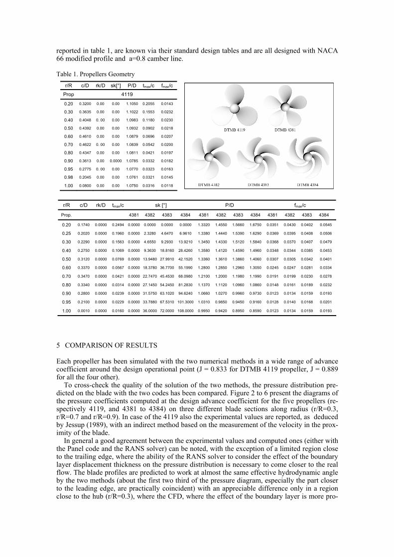
reported in table 1, are known via their standard design tables and are all designed with NACA 66 modified profile and a=0.8 camber line.

Table 1. Propellers Geometry

r/R c/D rk/D sk[°] P/D tmax/c fmax/c

Prop 4119

0.20 0.3200 0.00 0.00 1.1050 0.2055 0.0143

0.30 0.3635 0.00 0.00 1.1022 0.1553 0.0232

0.40 0.4048 0. 00 0.00 1.0983 0.1180 0.0230

0.50 0.4392 0.00 0.00 1.0932 0.0902 0.0218

0.60 0.4610 0.00 0.00 1.0879 0.0696 0.0207

0.70 0.4622 0. 00 0.00 1.0839 0.0542 0.0200

0.80 0.4347 0.00 0.00 1.0811 0.0421 0.0197

0.90 0.3613 0.00 0.0000 1.0785 0.0332 0.0182

0.95 0.2775 0. 00 0.00 1.0770 0.0323 0.0163

0.98 0.2045 0.00 0.00 1.0761 0.0321 0.0145

1.00 0.0800 0.00 0.00 1.0750 0.0316 0.0118 r/R c/D rk/D tmax/c sk [°] P/D fmax/c

Prop. 4381 4382 4383 4384 4381 4382 4383 4384 4381 4382 4383 4384

0.20 0.1740 0.0000 0.2494 0.0000 0.0000 0.0000 0.0000 1.3320 1.4550 1.5660 1.6750 0.0351 0.0430 0.0402 0.0545

0.25 0.2020 0.0000 0.1960 0.0000 2.3280 4.6470 6.9610 1.3380 1.4440 1.5390 1.6290 0.0369 0.0395 0.0408 0.0506

0.30 0.2290 0.0000 0.1563 0.0000 4.6550 9.2930 13.9210 1.3450 1.4330 1.5120 1.5840 0.0368 0.0370 0.0407 0.0479

0.40 0.2750 0.0000 0.1069 0.0000 9.3630 18.8160 28.4260 1.3580 1.4120 1.4590 1.4960 0.0348 0.0344 0.0385 0.0453

0.50 0.3120 0.0000 0.0769 0.0000 13.9480 27.9910 42.1520 1.3360 1.3610 1.3860 1.4060 0.0307 0.0305 0.0342 0.0401

0.60 0.3370 0.0000 0.0567 0.0000 18.3780 36.7700 55.1990 1.2800 1.2850 1.2960 1.3050 0.0245 0.0247 0.0281 0.0334

0.70 0.3470 0.0000 0.0421 0.0000 22.7470 45.4530 68.0980 1.2100 1.2000 1.1980 1.1990 0.0191 0.0199 0.0230 0.0278

0.80 0.3340 0.0000 0.0314 0.0000 27.1450 54.2450 81.2830 1.1370 1.1120 1.0960 1.0860 0.0148 0.0161 0.0189 0.0232

0.90 0.2800 0.0000 0.0239 0.0000 31.5750 63.1020 94.6240 1.0660 1.0270 0.9960 0.9730 0.0123 0.0134 0.0159 0.0193

0.95 0.2100 0.0000 0.0229 0.0000 33.7880 67.5310 101.3000 1.0310 0.9850 0.9450 0.9160 0.0128 0.0140 0.0168 0.0201

1.00 0.0010 0.0000 0.0160 0.0000 36.0000 72.0000 108.0000 0.9950 0.9420 0.8950 0.8590 0.0123 0.0134 0.0159 0.0193

5 COMPARISON OF RESULTS

Each propeller has been simulated with the two numerical methods in a wide range of advance coefficient around the design operational point (J = 0.833 for DTMB 4119 propeller, J = 0.889 for all the four other).

To cross-check the quality of the solution of the two methods, the pressure distribution pre-dicted on the blade with the two codes has been compared. Figure 2 to 6 present the diagrams of the pressure coefficients computed at the design advance coefficient for the five propellers (re-spectively 4119, and 4381 to 4384) on three different blade sections along radius (r/R=0.3, r/R=0.7 and r/R=0.9). In case of the 4119 also the experimental values are reported, as deduced by Jessup (1989), with an indirect method based on the measurement of the velocity in the prox-imity of the blade.

In general a good agreement between the experimental values and computed ones (either with the Panel code and the RANS solver) can be noted, with the exception of a limited region close to the trailing edge, where the ability of the RANS solver to consider the effect of the boundary layer displacement thickness on the pressure distribution is necessary to come closer to the real flow. The blade profiles are predicted to work at almost the same effective hydrodynamic angle by the two methods (about the first two third of the pressure diagram, especially the part closer to the leading edge, are practically coincident) with an appreciable difference only in a region close to the hub (r/R=0.3), where the CFD, where the effect of the boundary layer is more pro-

nounced (due to the profiles higher thickness)and the different prediction of cross-flow can also play a role.

The series of graphs of figures 2 to 6 is completed with the comparison of the computed thrust and torque curves predicted by the two codes in a wide range of advance ratio against ex-perimental values measured at cavitation tunnel of David Taylor Model Basin and that of M.I.T. (where available). In general, again, computed values fit very well to the experimental ones, also for what regards the torque which not always confirmed by other researchers using other methods. While both the panel method and the RANS solver are able to predict exactly the thrust and torque in proximity of the design advance coefficients, the RANS solver shows better accuracies al lower advance coefficients values, i.e. for highly loaded conditions, quite off-design. In this operating region, the viscous effects and possibly flow separation at the leading edge start to play a relative importance also on the global values and the current version of the panel method (already improved with respect to standard panel method as outlined in the previ-ous sections, but still not coupled with a thin boundary layer solver) is inherently incapable to take into account these phenomena.

Figure 2. Pressure distribution and Thrust and Torque Coefficients – Propeller DTMB 4119

Figure 3. Pressure distributions (r/R=0.3, 0.7, 0.9 respectively) and Thrust and Torque Coefficients – Pro-peller DTMB 4381

Figure 4. CP on blade profiles (at r/R=0.3, 0.7, 0.9 respectively), KT, KQ: Propeller DTMB 4382

Figure 5. CP on blade profiles (at r/R=0.3, 0.7, 0.9 respectively), KT, KQ: Propeller DTMB 4383

Figure 6. CP on blade profiles (at r/R=0.3, 0.7, 0.9 respectively), KT, KQ: Propeller DTMB 4382

For the 4119 propeller, experimental measurements of velocities in the wake flow field of the propeller were performed by Jessup (1989) and they are compared with those predicted by the two codes. The comparison of figure 7 relates to a circular arc in a transverse section about one third of diameter aft of the propeller, at a radius r/R=0.7 and with an angular development equal to 2π/z (z is the blade number) in order to span from the vortical wake surface shed by one blade to that of the consecutive one. Radial, tangential and axial components of the velocity field are compared. In general a sufficiently good agreement is found on the trends between the experi-mental value and the numerical obtained by both codes (with a better conformity of the RANS model), except for the region close to the core of the helical vortex line (at the examined radial position), where the experiments show a much sharper reduction in the axial induced component and an increase of the tangential component, consistent with the vortex theory. It is believed that the RANSE model was not sufficiently refined in the region of the wake to capture this local-ized viscous phenomena, hence dissipating the vortical energy too much; while it is strange that the panel method, based on potential flow so on a conservative formulation, shows results more similar to the (viscous) RANS model than to the experiments, in this case.

Table 2. Comparison of the prediction of thrust and torque, due to pressure and tangential components, with Panel Method and RANS solver. DTMB 4119 – J = 0.833 Visc. Corr. No Visc. ΔPan Press+Shear Press. Only ΔRANS KT 0.1463 0.1508 0.0045 0.1384 0.1436 0.0052 10KQ 0.2831 0.2518 0.0313 0.2819 0.2488 0.0331 DTMB 4383 – J = 0.889 Visc. Corr. No Visc. ΔPan Press+Shear Press. Only ΔRANS KT 0.2218 0.2289 0.0071 0.2082 0.2149 0.0067 10KQ 0.4670 0.4260 0.0410 0.4444 0.3995 0.0449 DTMB 4383 – J = 0.400 Visc. Corr. No Visc. ΔPan Press+Shear Press. Only ΔRANS KT 0.4577 0.4629 0.0052 0.4608 0.4650 0.0042 10KQ 0.6900 0.6531 0.0369 0.7686 0.7351 0.0335

40 60 80 100 120 140−0.2

0

0.2

0.4

0.6

0.8

1

1.2

1.4

θ

VX/V

, V T

V,

V R/V

VX/V exp.

VT/V exp.

VR

/V exp.

VX/V Rans

VT/V Rans

VR

/V Rans

VX/V Pan.

VR

/V Pan

VT/V Pan

Figure 7. Comparison between axial, radial and tangential induced velocities computed and measured downstream, x/D = 0.328, r/R = 0.7

The predictions of induced velocities on the blade surface is better rendered by plotting the

streamlines predicted, as in the example of figures 8 and 9 for the face an back side of DTMB-4119 and figures 10 and 11 for the DTMB 4383, both simulated at their respective design ad-vance ratios. Main difference between the two numerical methods are found in the region close to the hub mainly at the trailing edge of the blade, where the RANS method shows large radial outward velocity components, that the panel method shows in much minor entity only on the back of 4119, while on the face it shows the opposite trend. Similar picture in the case of the

4383 DTMB propeller, with a more extended blade area in which the RANS code predict these strong outward cross flow velocities. These effects could be due to boundary layer abrupt thick-ening at the trailing edge of the blade which force the attached flow to curve and avoid this low energy region. This phenomenon, capture by the RANS method, is clarified and confirmed by the behaviour of the friction coefficient on the blade, as represented in figures 12 and 13, which shows in the same region an almost null tangential force on the blade.

In terms of global results, though, the difference between the two methods is almost disap-pear. Table 2, in fact, shows the thrust and torque coefficients computed by the two methods, with and without the friction forces: for the panel method this correspond to the viscous correc-tion of equation (5), and for RANS the calculation of the forces have been done with the only pressure components or including the shear stresses on the blade and hub surface. It is clear that, while there is a small discrepancy between the two methods, in particular regarding thrust, the empirical formula used in the panel method to allow for viscous effects is substantially able to capture the global result of the above mentioned phenomena. In fact, the relative differences (viscous computation minus potential computation and pressure computation minus pressure plus shear stress computation) are almost equal between the two methods. This finding is true also in off design conditions the viscous correction applied to the panel method seems to predict well the relative difference between pressure and shear stress calculations, while a substantial difference remains (especially in the torque computation) with respect to RANS calculation. This difference, then, has to be imputed to the viscous-pressure effects, evidently not adequately modelled by the simple formula (5) and not to shear stress components.

Figure 8. Streamlines on DTMB 4119 (Back). Panel method left, RANS right

Figure 9: Streamlines on DTMB 4119 (Face). Panel method left, RANS right

Figure 10: Streamlines on DTMB 4383 (Back). Panel method left, RANS right

Figure 11: Streamlines on DTMB 4383 (Face). Panel method left, RANS right

Figure 12: Local friction coefficient Cf on DTMB 4119, at J=0.833. Face (left), Back (right)

Figure 13: Local friction coefficient Cf on DTMB 4383 at J=0.889. Face (left), Back (right)

6 CONCLUSION AND FURTHER PERSPECTIVES

A systematic application of state of a state of the art panel method (developed by the same ma-rine CFD group at DINAV) and a RANSE solver has been performed on a series of propellers for which the experimental measurements obtained in cavitation tunnel are available.

From the analysis of the local and global parameters the following conclusions can be drawn: both methods are able to predict with a sufficient accuracy for design purposes (within 2-3%) the thrust and torque curves in a wide range of advance coefficients. In fact, pressure distribu-tions predicted by both methods along the blade at design advance coefficient are very similar (except for a limited region at the trailing edge) and in also congruent with the experimental measurements.

The RANSE solver, as expected, demonstrates a better accuracy at low advance ratios, i.e. is better suited for representing highly loaded propeller, or in off-design conditions, where impor-tant viscous effects boundary layer thickness (and eventually separation) at the trailing edge and at blade root and the generation of a strong secondary cross flows along the blade, start to condi-tion heavily the potential flow solution. These effects are currently not adequately represented by the actual too simplified empirical viscous corrections that are applied to the potential flow method and confirm the possibility of improving the panel methods through a strong coupling with a boundary element method, allowing for limited flow separated regions. This can improve also the prediction of radial components of the velocities especially on the back of the blade sur-face, close to the trailing edge, at root. In this respect, systematic applications of RANS code as those presented in this paper can be useful for studying deriving alternative more general em-pirical corrections, for instance based on the deviation of the operating advance ratio from the design value. An semi-empirical treatment for modeling these dead flow regions on the blade could be sufficient as a first approximation and is currently under investigation.

For what regards the predictions of induced velocities in the wake, both methods agree rather well with experiments, but both are not able to adequately capture the increase of tangential ve-locities and decrease of axial velocities close to the position of the helical vortex line shed from the blade in the wake. However, the main hydrodynamic effects that may be necessary to study the hydrodynamic action of a propeller on body immersed in its wake (like a rudder or another propeller in the case of contra-rotating system) are sufficiently well captured by both methods for engineering purposes. Future activities will be directed to the coupling of a thin boundary layer theory to the panel method and to the application of such investigations as those presented in this study to the case of sheet cavitating propeller. In fact, both the in house panel method and the RANS solver are able to consider (with different theoretical models) these phenomena.

7 REFERENCES

Becchi P., Pittaluga C. (2005), “Comparison between RANSE calculation and Panel Method Results for the Hydrodynamic Analysis of Marine Propeller” , RINA Marine CFD, Royal Institution of Naval Ar-chitects

Bulten N., Oprea I. (2006), “Evaluation of McCormick’s rule for propeller tip vortex cavitation inception based on CFD results”, Proceedings of CAV 2006 International Symposium on Propeller Cavitation, Wageningen (NL)

Gaggero S., Brizzolara S. (2007), “Exact Modelling of Trailing Vorticity in Panel Method for Marine Propeller”, Proceedings of ICMRT 2007, Ischia (IT)

Gindroz B. (1999), “ Final report and recommendations to the 22nd ITTC” Propulsion Committee, Venice (IT).

Greeley D. S., Kerwin J.E. (1982), “Numerical Methods for Propeller Design and Analysis in Steady Flow” SNAME Transaction, Vol. 90, pp. 415-453

Jessup S. (1989), “An Experimental Investigation of Viscous Effects of Propeller Blade Flow”, PhD The-sis, The Catholic University of America

Kawamura T., Takekoshi Y., Minowa T., Maeda M., Yamaguchi H., Fujii A., Kimura K., Taketani T. (2006), “Simulation of Unsteady Cavitating Flow around Marine Propeller using a RANS CFD code”, Proceedings of CAV 2006 International Symposium on Propeller Cavitation, Wageningen (NL)

Kerwin J.E., Lee C.S. (1978), “Prediction of Steady and Unsteady Marine Propeller Performances by Numerical Lifting Surface Theory”, SNAME Transaction, Vol. 88, pp. 218-253

Kulczyk J., Skraburski L., Zawislak M. (2007), “Analysis of screw propeller 4119 using the Fluent sys-tem”, Archives of Civil and Mechanical Engineering, Vol. VII 2007 No. 4

Lee C.S., Kim G.D., Kerwin J.E. (2004), “ A B-Spline Based High Order Panel Method for the Analysis of Steady Flow around Marine Propeller”, 25th Symposium on Naval Hydrodynamics, St. John’s, Newfoundland.

Lee J.T. (1988), “ A Potential Based Panel Method for the Analysis of Marine Propeller in Steady Flow”, PhD. Thesis, M.I.T. Department of Ocean Engineering

Rhee S.H., Joshi S. (2005), “ Computational Validation for Flow around Marine Propeller using Unstruc-ture Mesh Based Navier-Stokes Solver”, JSME International Journal Series B, Vol. 48 (2005), pp.562-570.

Sanchez-Caja A. (1998), “DTRC Propeller 4119 Calculations at VTT”, Proceedings of the 22nd ITTC Propulsion Committee Propeller RANS/Panel Method Workshop, Grenoble, France.

Sileo L., Bonfiglioli A., Magi V., (2007), ”RANSEs Simulation of the Flow past a Marine Propeller under Design and Off-design Conditions”, Proceedings of ICMRT 2007, Ischia (IT)

CD-Adapco (2008), StarCCM+, v. 2.10 Users manual.