Optimizing Visual Vocabularies UsingSoft Assignment Entropies

Yubin Kuang, Kalle Astrom, Lars Kopp,Magnus Oskarsson and Martin Byrod

Centre for Mathematical SciencesLund University, Sweden

Abstract. The state of the art for large database object retrieval inimages is based on quantizing descriptors of interest points into visualwords. High similarity between matching image representations (as bagsof words) is based upon the assumption that matched points in the twoimages end up in similar words in hard assignment or in similar rep-resentations in soft assignment techniques. In this paper we study howground truth correspondences can be used to generate better visual vo-cabularies. Matching of image patches can be done e.g. using deformablemodels or from estimating 3D geometry. For optimization of the vocab-ulary, we propose minimizing the entropies of soft assignment of points.We base our clustering on hierarchical k-splits. The results from ourentropy based clustering are compared with hierarchical k-means. Thevocabularies have been tested on real data with decreased entropy andincreased true positive rate, as well as better retrieval performance.

1 Introduction

One of the general problems in computer vision is to automate the recognitionprocess using computer algorithms. For problems such as object recognitionand image retrieval from large databases, the state of the art is based on thebags of words (BOW) framework [18, 20, 21, 23]. Firstly a set of interest pointsare extracted in each of the images using interest point detectors[6, 11, 14, 13]or dense sampling. Then feature descriptors e.g. SIFT or SURF [11, 2, 15] arecomputed at each interest point. To enable fast matching, feature descriptorsare quantized into visual words as a vocabulary, where the descriptors assignedwith the same word are regarded as matched. Finally, the co-occurrence of visualwords between a query image and those in the database is then used to generatehypotheses of matched images. The matching is often based on the histograms ofvisual words and the L1 norm or L2 norm of differences between two histograms(or the intersection of two histograms) after normalization.

A good vocabulary in the quantization step of the BOW pipeline is crucial forthe recognition and retrieval system. Traditional approaches [23, 18, 21, 9] con-struct vocabulary by clustering descriptor vectors derived from training imagesin an unsupervised way, i.e. without ground truth information on which corre-spondence class a specific feature belongs to. These approaches either suffer from

2

quantization errors or have difficulties in matching wide variety of appearancesof objects in images, due to large differences in view points, lighting conditionsand background clutter as well as the large intra-class variations of the ob-jects themselves. One way to resolve this is through learning, with the presenceof large amount of correspondence ground truth data. While obtaining groundtruth data from raw images can be expensive, incorporating such informationwith proper schemes can enable efficient and accurate recognition performance.

Efforts have been made on learning vocabulary with ground truth informa-tion. Winn et al. [26] quantized features with k-means after which the resultingwords were merged to obtain intra-class compactness and inter-class discrimina-tion. On the other hand, Moosman et al. used random forests as the quantizersuch that at each split an entropy measure based on the class labels is maxi-mized [17]. In [19] Perronnin et al. used class-level labels and proposed to trainclass-specific vocabularies modeled by GMMs and combine them with a univer-sal vocabulary. The most related work to ours in technical aspects, is the workby Lazebnik et al. in [10], where they simultaneously optimize the quantizer inEuclidean feature space and the posterior class distribution. All these previousworks imposed the supervision such that each word in the vocabulary has adiscriminative representation of the different object classes. However, they havemainly focused on object categorization and the number of class labels is rel-atively small (≈ 20) except for the the work in [7] introduced hidden Markovrandom fields for semantic embedding of local patch features with relatively largenumber of class labels ( ≈ 3600). Our approach is designed for image retrievaland uses very large scale (≈ 80K − 250K) partially labeled patch correspon-dences to quantize feature space in a hierarchical manner.

For object recognition, the learned vocabulary has to be more specific regard-ing matching features. Each word in the vocabulary should contain only smallnumber of features such that each word might encode the appearance variationsof a single physical point. In [16], Mikulik et al. start with an unsupervised vo-cabulary and apply a supervised soft-assignment afterwards, where words areconnected based on the statistics of matched feature points from a huge datasetwith ground truth correspondences. Another line of work [22, 24], is to incorpo-rate the supervision into the feature metric learning before quantization suchthat the matched pairs of features have small distances than non-matched pairsin the new mapping. Both methods achieves substantial improvement in the re-trieval tasks. Our approach works on the original feature space and encodes theground truth correspondences in the process of vocabulary generation.

In this paper, we focus on vocabulary for recognition and would like to ad-dress systematically the following questions: (i) How large should the vocabularybe? In the current literature the sizes range from less than a thousand to millionsof words in the vocabulary. This could of course be highly application dependent.(ii) How can we evaluate the quality of the vocabulary? (iii) What is the optimaldivision of the feature space into words and How do we avoid splitting matchingfeatures into different words? To address the first two questions, we first studiedstatistically how true positive rates and false positive rates in matching features

3

of a vocabulary affect the retrieval performance. We then present a frameworkfor supervised vocabulary training using partial or full ground truth informationon correspondences. In such a way, we obtain a vocabulary that encodes theintra-class variation of each correspondence class leading to improved retrievalperformance.

The rest of the paper is organized as follows. Section 2 contains brief discus-sion on methods for obtaining the ground truth correspondences. In Section 3 wepresent the modelling of mAP from vocabulary matching statistics. In Section 4we describe our optimization method for training the vocabulary using groundtruth data. The method is then tested on real image data in Section 5.

2 Ground Truth Correspondence Data

In order to obtain a good visual vocabulary for object recognition in images, wepropose to learn the vocabulary using ground truth information on correspondingpoints. The motivation is that we believe that this strengthens the vocabularyas opposed to just doing unsupervised clustering and we expect the gain to beworthwhile since the the more expensive training with ground truth is a off-lineprocess in the retrieval pipeline.

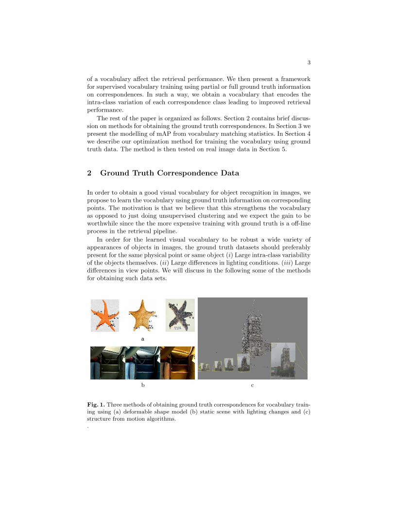
In order for the learned visual vocabulary to be robust a wide variety ofappearances of objects in images, the ground truth datasets should preferablypresent for the same physical point or same object (i) Large intra-class variabilityof the objects themselves. (ii) Large differences in lighting conditions. (iii) Largedifferences in view points. We will discuss in the following some of the methodsfor obtaining such data sets.

a

b c

Fig. 1. Three methods of obtaining ground truth correspondences for vocabulary train-ing using (a) deformable shape model (b) static scene with lighting changes and (c)structure from motion algorithms..

4

For object categorization, intra-class variability that is present for most ob-ject categories that are interesting for recognition. Deformable models can beused here to generate correspondences. Training these models can be cumber-some, but we believe that this will benefit the training process of the visualvocabulary enabling a very fast but accurate bottom up search process, that isbased on learned high level features. In Figure 1(a) a deformable shape modelestimated from image data is shown, where the correspondences are based onoptimizing the minimum description length according to [8]. The images arefrom the starfish category of the Caltech-256 object category dataset [4].

The lighting variabilities could be achieved by having images of static scenestaken under substantially changing lighting conditions. Images taken by a cameramounted at the entrance of a moving bus are shown in Figure 1(b). View pointsvariabilities could be obtained by estimating the geometry of objects from imagestaken at different view points using a RANSAC framework in combination withepipolar geometry estimation such as in e.g. [5, 1]. In Figure 1(c) the typicalresult from the geometry estimation is shown. From the corresponding points inthe images, feature descriptors can then be extracted from the images. In [16],Mikulik et al. present an efficient way of generating large scale ground truthdataset from collections of images by image matching graph. An alternativein [24], Strecha et al. also utilize geo-tags in their 3D-reconstruction pipelineto obtain geometrically consistent patches. In the experimental section of thispaper the visual vocabularies are trained on partial ground truth data obtainedfrom the UBC Patch Data [25].

3 Modelling Mean Average Precision from VocabularyStatistics

One key argument made in this paper is that good retrieval systems, e.g. asmeasured by mean Average Precision (mAP) can be obtained by studying theproperties of the vocabulary on the statistics of descriptor distribution both forrandom (not necessarily matching) descriptor pairs and for matching descriptorpairs. By matching descriptor pairs we do not mean descriptors that end up inthe same word in the vocabulary, but rather descriptors of matching interestregions, i.e. regions which are matching in a ground truth sense.

We can evaluate a vocabulary with two simple characteristics, (i) the falsepositive rate pfp or FPR, which is the probability that two random descriptorsend up in the same word and (ii) the true positive rate ptp or TPR, which is theprobability that two matching descriptors end up in the same word.

We argue that the mapping from true positive and false positive rates to meanaverage precision can be modelled and analyzed. High mean average precision isobtained using vocabularies with low false positive rates and high true positiverates.

The mapping depends on many characteristics of the test, such as the numberof features in each image, the number of images in the database, the proportionof positive vs negative answers to a image retrieval query etc. In this model we

5

have for simplicity assumed that histograms are measured with the normed L1

distance, but other distance metrics could be used. In fact the modelling couldcome to good use in determining which metrics to use.

Modelling the L1-distance Distribution for Two Random ImagesAssuming that the distribution of features in different visual words is known,

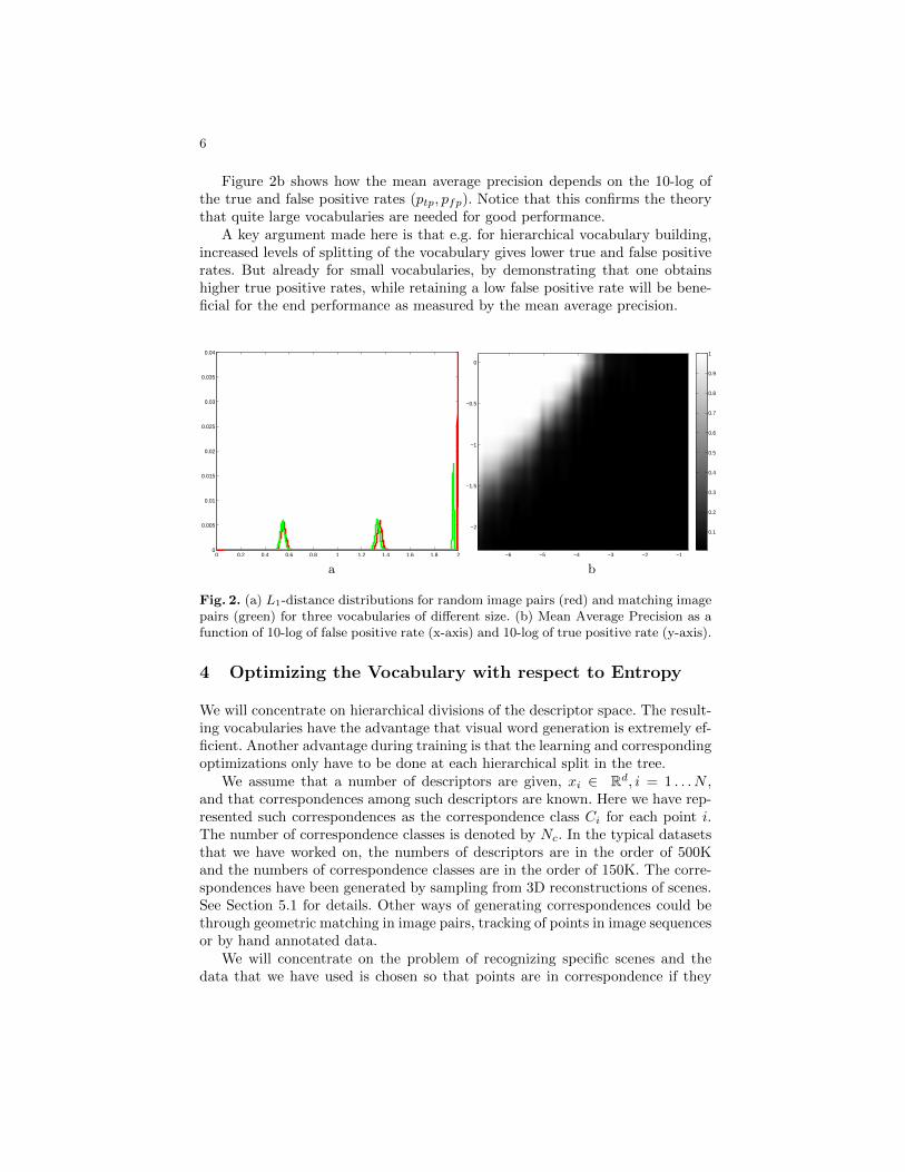
and assuming that features in two random images are independent, it is possibleto simulate and model the distribution of L1 distances. In Figure 2a three suchdistributions are shown for small, medium and large vocabularies.

For large vocabularies the histograms are sparse. A reasonable approximationhere is that the distance is d = (2n−2o)/n, where n is the number of features inthe images and o is the number of common features. The number of overlappingfeatures o can be approximated reasonably using binomial distributions using nsamples with probability p = n/Nw, where Nw is the size of the vocabulary. Forincreasing vocabulary size this distribution is pushed towards the right end ofthe spectrum.

Modelling the L1-distance Distribution for Two Matching ImagesFor two matching images we assume that there are a number of matching

features. For each matching feature pair there is a certain probability pt that theyend up in the same word. For the remaining features we assume that they end upin random words according to the distribution above. The resulting distributionof L1-distance is similar to that of two random features, but pushed slightly tothe left. In Figure 2a three such distributions are shown, again for small, mediumand large vocabularies.

Modelling Precision, Recall and Mean Average PrecisionFor each vocabulary as characterized by its true and false positive rates

(ptp, pfp), we can estimate the probability distribution of matched image L1-distance, pm, and the probability distribution of two random image L1-distance,pr.

Assuming that in a random query there are Ninlier matching images andNoutlier non-matching images. For each threshold D of L1-distances we obtaina query result with recall

R =Ninlier

∫D

0pm(x)dx

Ninlier

∫ 2

0pm(x)dx

=

∫ D

0

pm(x)dx

and precision

P =Ninlier

∫D

0pm(x)dx

Ninlier

∫D

0pm(x)dx+Noutlier

∫D

0pr(x)dx

=

∫D

0pm(x)dx∫D

0pm(x)dx+K

∫D

0pr(x)dx

, where K = Noutlier

Ninlieris the ratio of outliers to inliers in a typical query.

Note that the domain of the normalized L1 distance is between [0,2]. There-fore, in the equation for recall, we have used 2 as the integration limit in de-nominator. It follows that the integral in the denominator is 1. From these twocurves it is straightforward to estimate the mean average precision.

6

Figure 2b shows how the mean average precision depends on the 10-log ofthe true and false positive rates (ptp, pfp). Notice that this confirms the theorythat quite large vocabularies are needed for good performance.

A key argument made here is that e.g. for hierarchical vocabulary building,increased levels of splitting of the vocabulary gives lower true and false positiverates. But already for small vocabularies, by demonstrating that one obtainshigher true positive rates, while retaining a low false positive rate will be bene-ficial for the end performance as measured by the mean average precision.

0 0.2 0.4 0.6 0.8 1 1.2 1.4 1.6 1.8 20

0.005

0.01

0.015

0.02

0.025

0.03

0.035

0.04

−6 −5 −4 −3 −2 −1

−2

−1.5

−1

−0.5

0

0.1

0.2

0.3

0.4

0.5

0.6

0.7

0.8

0.9

1

a b

Fig. 2. (a) L1-distance distributions for random image pairs (red) and matching imagepairs (green) for three vocabularies of different size. (b) Mean Average Precision as afunction of 10-log of false positive rate (x-axis) and 10-log of true positive rate (y-axis).

4 Optimizing the Vocabulary with respect to Entropy

We will concentrate on hierarchical divisions of the descriptor space. The result-ing vocabularies have the advantage that visual word generation is extremely ef-ficient. Another advantage during training is that the learning and correspondingoptimizations only have to be done at each hierarchical split in the tree.

We assume that a number of descriptors are given, xi ∈ Rd, i = 1 . . . N ,and that correspondences among such descriptors are known. Here we have rep-resented such correspondences as the correspondence class Ci for each point i.The number of correspondence classes is denoted by Nc. In the typical datasetsthat we have worked on, the numbers of descriptors are in the order of 500Kand the numbers of correspondence classes are in the order of 150K. The corre-spondences have been generated by sampling from 3D reconstructions of scenes.See Section 5.1 for details. Other ways of generating correspondences could bethrough geometric matching in image pairs, tracking of points in image sequencesor by hand annotated data.

We will concentrate on the problem of recognizing specific scenes and thedata that we have used is chosen so that points are in correspondence if they

7

denote the same physical point in the scene. That descriptors are in differentcorrespondence classes does not necessarily mean that they are not in corre-spondence. On the contrary, we expect there to be many descriptors in differentcorrespondence classes that actually correspond quite well. However for pointsthat are in correspondence we would like the corresponding descriptors to endup in the same word in the final vocabulary.

Our hierarchical division will be based on k splits in the descriptor space Dat each step. Each such split is represented by k center points c1, . . . , ck and ascalar m that can be interpreted as a margin. Low values of m represent sharpercuts and high values represent softer classification.

We study both hard assignment and soft assignment in the following sense.For hard assignment a descriptor is put in the bin i corresponding to the closestcenter ci. For soft assignment we put each point x in the k bins in proportion tothe weight wi according to

wi =exp( ||x−ci||2m )∑kj=1 exp(

||x−cj ||2m )

. (1)

where ||.||2 is the L2 norm. Contrary to [10] we use exponential distributions,which give smoothing that only depends on the differance of distances to thecluster center. Descriptors for which the distance to the closest centers is similarfall into several bins to a fair degree, whereas descriptors for distance differencebetween the two closest centers is much larger than m fall essentially only intoone part of the tree.

4.1 Entropy Model

To optimize the division parameters z = (c1, . . . , ck) for hard assignment andz = (c1, . . . , ck,m) for soft assignment, we use entropy as a criterion. Entropytakes into account both that the split is balanced, i.e. that approximately equalnumber of descriptors fall into each bin, and that the correspondence classes aresplit as cleanly as possible. The entropy for a random variable X with N possiblestates is defined as E = −

∑Ni=1 p(i) log2(p(i)) , where p is the probability density

function of X. Here we use the 2-log as it is more intuitive and easier to interpret.Entropy is fairly easy to use in the sense that it is straightforward to define

for both hard and soft assignment. The probability density function is calculatedin the following manner. In each split we calculate the (weighted) histogram ofdescriptors in each correspondence class htot = (h(1), . . . , h(Nc)) before the split.Each descriptor falls partly in the k different parts of the tree, thus contributingin part to both the k-weighted histogram h1, . . . hk.

By normalizing the histograms with the sum, we obtain correspondence class

probabilities, i.e. ptot(i) = htot(i)∑Nci=1 htot(i)

, for the distribution of descriptors among

the correspondence classes before the split and similarly for p1, . . . , pk. The en-tropy before the split is defined as Etot =

∑Nc

i=1−ptot(i) log2(ptot(i)) , and simi-

larly for the k branches, Ej =∑Nc

i=1−pj(i) log2(pj(i)) . For the split as a whole

8

we define the entropy as Esplit =∑k

j=1nj

ntotEj . Here nj =

∑Nc

i=1 hj(i). Ideallyeach split, which uses log2(k) extra bits of information, should lower the entropywith log2(k) bits, i.e. we expect Esplit to be approximately log2(k) less than Etot.In practice it is difficult to split all examples in the descriptor space as cleanlyas this.

4.2 Optimizing Entropy

For training data (x1, . . . , xN ), (C1, . . . , CN ) with possible weights (y1, . . . , yN ),it is thus possible to define the split entropy Esplit as a function of the divi-sion parameters z. For hard assignment, using z = (c1, . . . , ck), this function isnot smooth. The entropy is typically constant as the decision boundaries areperturbed as long as they do not pass through any of the points xi. For softassignment, however, entropy is a smooth function of the division parametersz = (c1, . . . , ck,m).

In our experiments we have tried a few different approaches for optimizing Ewith respect to z. We did not optimize E with respect to the margin m in thispaper.

In the main approach we initialize using k-means iterations with a coupleof different starting points. The best initial estimate is then used as an initialestimate to a non-linear optimization of z. Here we have calculated the analyticalderivatives dE

dz , which are then used in a non linear optimization.

The entropy for the split can be written as Esplit =∑k

j=1nj

ntotEj . which

since njpj(i) = hj(i) gives Esplit =∑k

j=11

ntot

∑Nc

i=1(−hj(i) log2(pj(i))) . Thederivative of Esplit is thus

dEsplit

dz=−1

ntot

k∑j=1

Nc∑i=1

(dhj(i)

dzlog2(pj(i)) +

njln(2)

dpj(i)

dz) (2)

Here the sum of the second term over all i is zero, since the sum of the proba-bilities is constant. Thus

dEsplit

dz=

1

ntot

k∑j=1

Nc∑i=1

(−dhj(i)dz

log2(pj(i))) . (3)

The derivatives of the histogram bins aredhj(i)dz =

∑l,Cl=i

dωj(l)dz . Finally the

derivatives of the weights are

dωj(l)

dz=

dej(l)dz∑k

j=1 ej(l)− ej(l)

∑kj=1

dej(l)dz

(∑k

j=1 ej(l))2, (4)

where ej(l) =exp(||xl−cj ||2)

m and

dej(l)

dz= ej(l)(

(xl − cj)m||xl − cj ||2

dcjdz− ||xl − cj ||2

m2

dm

dz) . (5)

9

The value E and the gradient dEdz are utilized in a non-linear optimization

update with the limited-memory Broyden-Fletcher-Goldfarb-Shanno method, [3,12]. In the implementation we have limited the maximum number of iterations ofthe optimization to 20 iterations for the first levels, but increased to 30 iterationsfor the subsequent levels to avoid over-fitting. This scheme is general for differentvalues of k.

5 Experimental Validation

We have tested our method on vocabulary construction with real image data.The dataset is described in details in Section 5.1. The resulting vocabularies areevaluated in Section 5.2.

5.1 Dataset and Evaluation

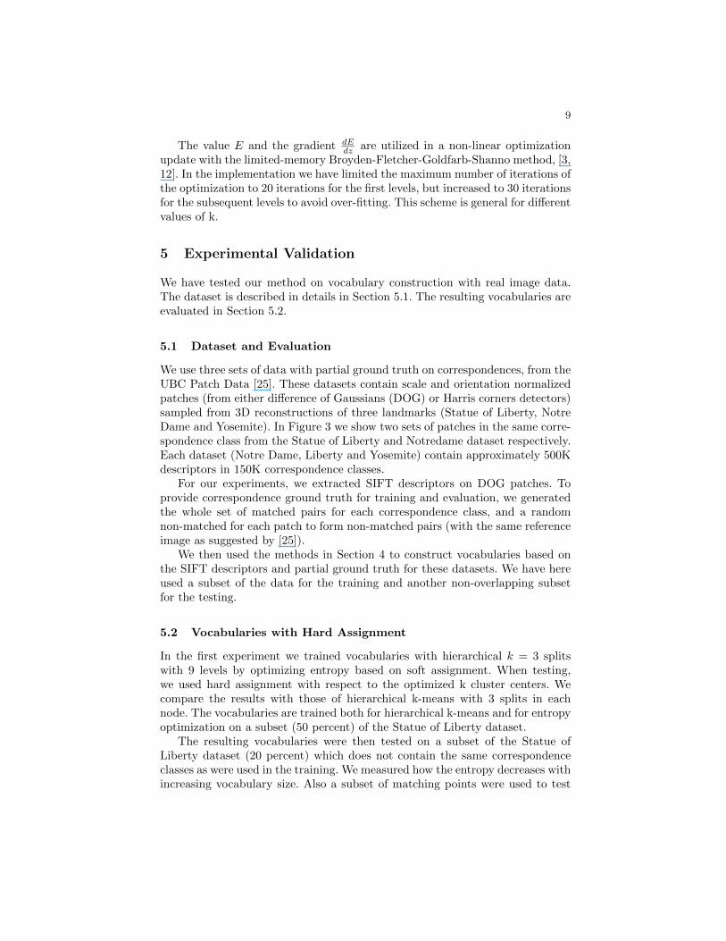
We use three sets of data with partial ground truth on correspondences, from theUBC Patch Data [25]. These datasets contain scale and orientation normalizedpatches (from either difference of Gaussians (DOG) or Harris corners detectors)sampled from 3D reconstructions of three landmarks (Statue of Liberty, NotreDame and Yosemite). In Figure 3 we show two sets of patches in the same corre-spondence class from the Statue of Liberty and Notredame dataset respectively.Each dataset (Notre Dame, Liberty and Yosemite) contain approximately 500Kdescriptors in 150K correspondence classes.

For our experiments, we extracted SIFT descriptors on DOG patches. Toprovide correspondence ground truth for training and evaluation, we generatedthe whole set of matched pairs for each correspondence class, and a randomnon-matched for each patch to form non-matched pairs (with the same referenceimage as suggested by [25]).

We then used the methods in Section 4 to construct vocabularies based onthe SIFT descriptors and partial ground truth for these datasets. We have hereused a subset of the data for the training and another non-overlapping subsetfor the testing.

5.2 Vocabularies with Hard Assignment

In the first experiment we trained vocabularies with hierarchical k = 3 splitswith 9 levels by optimizing entropy based on soft assignment. When testing,we used hard assignment with respect to the optimized k cluster centers. Wecompare the results with those of hierarchical k-means with 3 splits in eachnode. The vocabularies are trained both for hierarchical k-means and for entropyoptimization on a subset (50 percent) of the Statue of Liberty dataset.

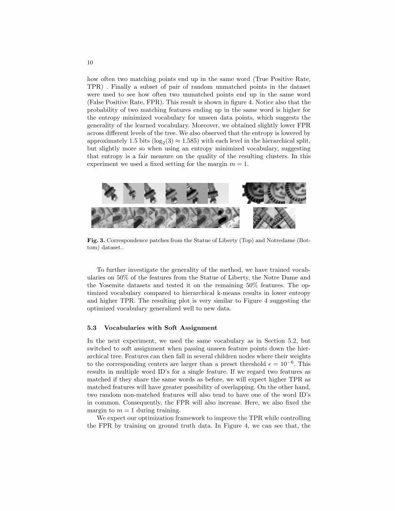
The resulting vocabularies were then tested on a subset of the Statue ofLiberty dataset (20 percent) which does not contain the same correspondenceclasses as were used in the training. We measured how the entropy decreases withincreasing vocabulary size. Also a subset of matching points were used to test

10

how often two matching points end up in the same word (True Positive Rate,TPR) . Finally a subset of pair of random unmatched points in the datasetwere used to see how often two unmatched points end up in the same word(False Positive Rate, FPR). This result is shown in figure 4. Notice also that theprobability of two matching features ending up in the same word is higher forthe entropy minimized vocabulary for unseen data points, which suggests thegenerality of the learned vocabulary. Moreover, we obtained slightly lower FPRacross different levels of the tree. We also observed that the entropy is lowered byapproximately 1.5 bits (log2(3) ≈ 1.585) with each level in the hierarchical split,but slightly more so when using an entropy minimized vocabulary, suggestingthat entropy is a fair measure on the quality of the resulting clusters. In thisexperiment we used a fixed setting for the margin m = 1.

Fig. 3. Correspondence patches from the Statue of Liberty (Top) and Notredame (Bot-tom) dataset..

To further investigate the generality of the method, we have trained vocab-ularies on 50% of the features from the Statue of Liberty, the Notre Dame andthe Yosemite datasets and tested it on the remaining 50% features. The op-timized vocabulary compared to hierarchical k-means results in lower entropyand higher TPR. The resulting plot is very similar to Figure 4 suggesting theoptimized vocabulary generalized well to new data.

5.3 Vocabularies with Soft Assignment

In the next experiment, we used the same vocabulary as in Section 5.2, butswitched to soft assignment when passing unseen feature points down the hier-archical tree. Features can then fall in several children nodes where their weightsto the corresponding centers are larger than a preset threshold ε = 10−6. Thisresults in multiple word ID’s for a single feature. If we regard two features asmatched if they share the same words as before, we will expect higher TPR asmatched features will have greater possibility of overlapping. On the other hand,two random non-matched features will also tend to have one of the word ID’sin common. Consequently, the FPR will also increase. Here, we also fixed themargin to m = 1 during training.

We expect our optimization framework to improve the TPR while controllingthe FPR by training on ground truth data. In Figure 4, we can see that, the

11

proposed method is marginally better than the hierarchical k-means with respectto the TPR and FPR curve. Only achieving marginal optimality might be dueto the fact that we have not used enough data for training. On the other hand,we noted that both soft assignment vocabularies have better matching propertythan hard assignment vocabularies. For instance if we aim for 5% false positiverate, soft assignment achieves approximately 60% true positive rate while hardassignment obtains only 45%.

2 4 6 8 100

0.1

0.2

0.3

0.4

0.5

0.6

0.7

0.8

Level of tree

Pro

babi

lity

TPR OursTPR HKMFPR OursFPR HKM

0 2 4 6 82

4

6

8

10

12

14

Level of tree

Ent

ropy

(bi

ts)

Entropy OursEntropy HKM

Fig. 4. Evaluation on Liberty data. (50% for training and 20% for testing with k = 3.Left: Estimated probability of two corresponding (TPR) and two random descriptors(FPR) ending up in the same word as a function of tree depth. Middle : Entropy as afunction of tree depth. Notice that with each depth entropy is lowered close to 1.5 bit.

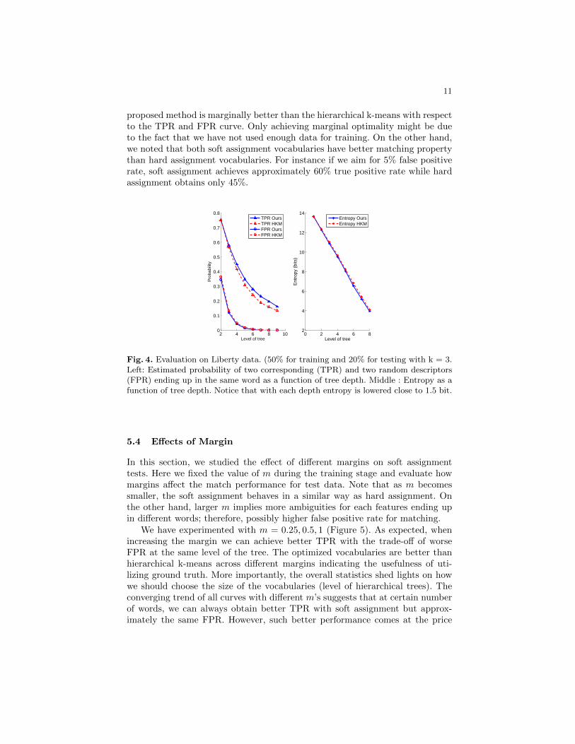
5.4 Effects of Margin

In this section, we studied the effect of different margins on soft assignmenttests. Here we fixed the value of m during the training stage and evaluate howmargins affect the match performance for test data. Note that as m becomessmaller, the soft assignment behaves in a similar way as hard assignment. Onthe other hand, larger m implies more ambiguities for each features ending upin different words; therefore, possibly higher false positive rate for matching.

We have experimented with m = 0.25, 0.5, 1 (Figure 5). As expected, whenincreasing the margin we can achieve better TPR with the trade-off of worseFPR at the same level of the tree. The optimized vocabularies are better thanhierarchical k-means across different margins indicating the usefulness of uti-lizing ground truth. More importantly, the overall statistics shed lights on howwe should choose the size of the vocabularies (level of hierarchical trees). Theconverging trend of all curves with different m’s suggests that at certain numberof words, we can always obtain better TPR with soft assignment but approx-imately the same FPR. However, such better performance comes at the price

12

of heavier computation when assigning features to multiple leaf nodes. If m istoo large, features will end up in many words at the leaf node. Therefore, theefficiency of vocabulary representation of features is overwhelmed by computingthe intersections in the space of word ID’s.

10−4

10−3

10−2

10−1

100

10−0.9

10−0.7

10−0.5

10−0.3

10−0.1

FPR

TP

R

Ours Hard AssignmentHKM Hard AssignmentOurs m = 0.25HKM m = 0.25Ours m = 0.5HKM m = 0.5Ours m = 1HKM m = 1

Fig. 5. The effects of different margins on soft assignment with respect to TPR andFPR. m = 0.25, 0.5, 1 and hard assignment, where k = 3

5.5 Image Retrieval

In this section, we verify the usefulness of optimized vocabulary in the recogni-tion pipeline on the Oxford 5K dataset [20, 21]. The task is to retrieve similarimages to the 55 query images (5 for each of the 11 landmarks in Oxford) in thedataset of 5062 images. The performance is then evaluate with mean AveragePrecision (mAP) score. Higher mAP indicates that the underlying system onaverage retrieves the similar corresponding images at the top of the ranked list.

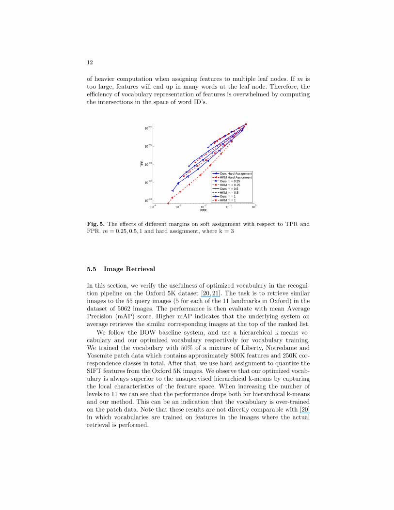
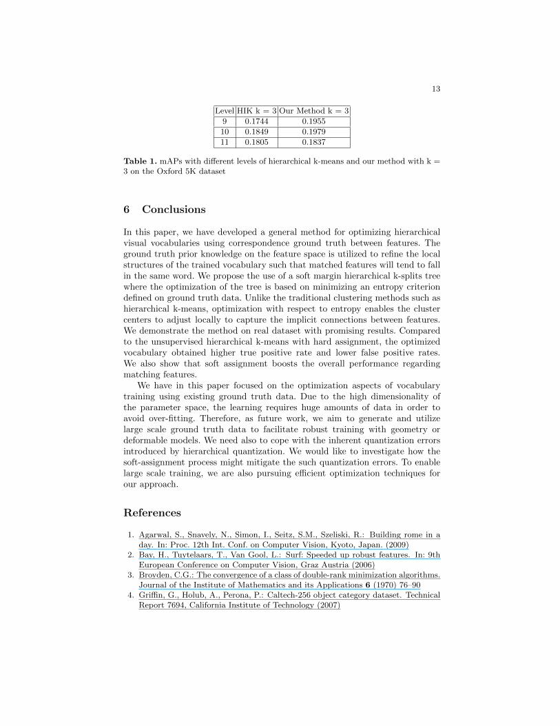
We follow the BOW baseline system, and use a hierarchical k-means vo-cabulary and our optimized vocabulary respectively for vocabulary training.We trained the vocabulary with 50% of a mixture of Liberty, Notredame andYosemite patch data which contains approximately 800K features and 250K cor-respondence classes in total. After that, we use hard assignment to quantize theSIFT features from the Oxford 5K images. We observe that our optimized vocab-ulary is always superior to the unsupervised hierarchical k-means by capturingthe local characteristics of the feature space. When increasing the number oflevels to 11 we can see that the performance drops both for hierarchical k-meansand our method. This can be an indication that the vocabulary is over-trainedon the patch data. Note that these results are not directly comparable with [20]in which vocabularies are trained on features in the images where the actualretrieval is performed.

13

Level HIK k = 3 Our Method k = 3

9 0.1744 0.1955

10 0.1849 0.1979

11 0.1805 0.1837

Table 1. mAPs with different levels of hierarchical k-means and our method with k =3 on the Oxford 5K dataset

6 Conclusions

In this paper, we have developed a general method for optimizing hierarchicalvisual vocabularies using correspondence ground truth between features. Theground truth prior knowledge on the feature space is utilized to refine the localstructures of the trained vocabulary such that matched features will tend to fallin the same word. We propose the use of a soft margin hierarchical k-splits treewhere the optimization of the tree is based on minimizing an entropy criteriondefined on ground truth data. Unlike the traditional clustering methods such ashierarchical k-means, optimization with respect to entropy enables the clustercenters to adjust locally to capture the implicit connections between features.We demonstrate the method on real dataset with promising results. Comparedto the unsupervised hierarchical k-means with hard assignment, the optimizedvocabulary obtained higher true positive rate and lower false positive rates.We also show that soft assignment boosts the overall performance regardingmatching features.

We have in this paper focused on the optimization aspects of vocabularytraining using existing ground truth data. Due to the high dimensionality ofthe parameter space, the learning requires huge amounts of data in order toavoid over-fitting. Therefore, as future work, we aim to generate and utilizelarge scale ground truth data to facilitate robust training with geometry ordeformable models. We need also to cope with the inherent quantization errorsintroduced by hierarchical quantization. We would like to investigate how thesoft-assignment process might mitigate the such quantization errors. To enablelarge scale training, we are also pursuing efficient optimization techniques forour approach.

References

1. Agarwal, S., Snavely, N., Simon, I., Seitz, S.M., Szeliski, R.: Building rome in aday. In: Proc. 12th Int. Conf. on Computer Vision, Kyoto, Japan. (2009)

2. Bay, H., Tuytelaars, T., Van Gool, L.: Surf: Speeded up robust features. In: 9thEuropean Conference on Computer Vision, Graz Austria (2006)

3. Broyden, C.G.: The convergence of a class of double-rank minimization algorithms.Journal of the Institute of Mathematics and its Applications 6 (1970) 76–90

4. Griffin, G., Holub, A., Perona, P.: Caltech-256 object category dataset. TechnicalReport 7694, California Institute of Technology (2007)

14

5. Hartley, R.I., Zisserman, A.: Multiple View Geometry in Computer Vision. Cam-bridge University Press (2004) Second Edition.

6. Harris, C., Stephens, M.: A combined corner and edge detector. In: Proc. of the4th Alvey Vision Conference. (1988) 147–151

7. Ji, R., Yao, H., Sun, X., Zhong, B., Gao, W.: Towards semantic embedding invisual vocabulary. In: Proc. Conf. Computer Vision and Pattern Recognition, SanFrancisco, California, USA. (2010)

8. Karlsson, J., Astrom, K.: MDL patch correspondences on unlabeled data. In: Proc.International Conference on Pattern Recognition, Tampa, USA. (2008)

9. Lamrous, S., Taileb, M.: Divisive hierarchical k-means. CIMCA-IAWTIC’06,IEEEComputer Society (2006)

10. Lazebnik, S., Raginsky, M.: Supervised learning of quantizer codebooks by infor-mation loss minimization. IEEE Trans. Pattern Analysis and Machine Intelligence31 (2009) 1294 – 1309

11. Lowe, D.G.: Distinctive image features from scale-invariant keypoints. Int. Journalof Computer Vision 60 (2004) 91–110

12. Luenberger, D.G.: Linear and Nonlinear Programming. Addison-Wesley (1984)13. Matas, J., Chum, O., Urban, M., Pajdla, T.: Robust wide-baseline stereo from

maximally stable extremal regions. Image Vision Computing 22 (2004) 761–76714. Mikolajczyk, K., Schmid, C.: An affine invariant interest point detector. In: Eu-

ropean Conference on Computer Vision, Springer (2002) 128–142 Copenhagen.15. Mikolajczyk, K., Schmid, C.: A performance evaluation of local descriptors. In:

Proc. Conf. Computer Vision and Pattern Recognition. (2003)16. Mikulik, A., Perdoch, M., Chum, O., Matas, J.: Learning a fine vocabulary. In:

Proc. 11th European Conf. on Computer Vision, Crete, Greece. (2010)17. Moosmann, F., Triggs, B., Jurie, F.: Randomized clustering forests for building

fast and discriminative visual vocabularies. In: Twentieth Annual Conference onNeural Information Processing Systems, Vancouver, Canada. (2006)

18. Nister, D., Stewenius, H.: Scalable recognition with a vocabulary tree. In: IEEEConference on Computer Vision and Pattern Recognition. (2006) 2161–2168

19. Perronnin, F.: Universal and adapted vocabularies for generic visual categorization.IEEE Trans. Pattern Analysis and Machine Intelligence 30 (2008) 1243–1256

20. Philbin, J., Chum, O., Isard, M., Sivic, J., Zisserman, A.: Object retrieval with largevocabularies and fast spatial matching. In: Proceedings of the IEEE Conferenceon Computer Vision and Pattern Recognition. (2007)

21. Philbin, J., Chum, O., Isard, M., Sivic, J., Zisserman, A.: Lost in quantization: Im-proving particular object retrieval in large scale image databases. In: Proceedingsof the IEEE Conference on Computer Vision and Pattern Recognition. (2008)

22. Philbin, J., Isard, M., Sivic, J., Zisserman, A.: Descriptor learning for efficientretrieval. In: Proc. 11th European Conf. on Computer Vision, Crete, Greece.(2010)

23. Sivic, J., Zisserman, A.: Video Google: A text retrieval approach to object matchingin videos. In: Proceedings of the International Conference on Computer Vision.(2003)

24. Strecha, C., Bronstein, A., Bronstein, M., Fua, P.: LDAhash: Improved matchingwith smaller descriptors. Technical report, CVlab, EPFL Switzerland,Tel-AvivUniversity and Israel Institute of Technology, Israel (2010)

25. Winder, S., Hua, G., Brown, M.: Picking the best daisy. In: Proceedings of theInternational Conference on Computer Vision and Pattern Recognition (CVPR09),Miami (2009)

15

26. Winn, J., Criminisi, T., Minka, T.: Object categorization by learned visual dictio-nary. In: Proc. 10th Int. Conf. on Computer Vision, Bejing, China. (2005)