
Optimizing defensive naval minefields through network ...
92
Aalto University School of Science Master’s Programme in Mathematics and Operations Research Tuomas Suominen Optimizing defensive naval minefields through network interdiction modeling Master’s Thesis Espoo, May 4, 2021 Supervisor: Professor Kai Virtanen Advisor: Markku Kujala, M.Sc. (Tech.) The document can be stored and made available to the public on the open internet pages of Aalto University. All other rights are reserved.
-
Upload
khangminh22 -
Category
Documents
-
view
0 -
download
0
Transcript of Optimizing defensive naval minefields through network ...

Aalto University
School of Science
Master’s Programme in Mathematics and Operations Research
Tuomas Suominen
Optimizing defensive naval minefieldsthrough network interdiction modeling
Master’s ThesisEspoo, May 4, 2021
Supervisor: Professor Kai VirtanenAdvisor: Markku Kujala, M.Sc. (Tech.)
The document can be stored and made available to the public on the openinternet pages of Aalto University. All other rights are reserved.
Aalto UniversitySchool of ScienceMaster’s Programme in Mathematics and Operations Research
ABSTRACT OFMASTER’S THESIS
Author: Tuomas Suominen
Title: Optimizing defensive naval minefields through networkinterdiction modeling
Date: May 4, 2021 Pages: vii + 85
Major: Systems and Operations Research Code: SCI3055
Supervisor: Professor Kai Virtanen
Advisor: Markku Kujala, M.Sc. (Tech.)
Naval mine warfare has been an important feature in military operations sincethe 16th century. Deploying mines to a contested area has the capability todirect and channel the movement of enemy forces and potentially to prevent theuse of some key areas entirely. As such, mining is a force multiplier providing asmaller naval force with an advantage. Mines are, however, limited in numberdespite their generally good availability. Thus, placing mines into an area ofoperations such that their effectiveness is optimized is key. Finding this optimalplacement is the defensive minefield planning problem.
Minefield planning is typically conducted by experienced officers manuallyor using simulation for decision support. The main contribution of this thesisis the representation of an area of operations as a network and consequentlyusing optimization and a network interdiction framework and models to solvethe defensive minefield planning problem. These models are given as mixedinteger programs. Furthermore, a novel approach for measuring the effectivenessof any planned minefield, using quantifiable network properties is introduced.Contrary to existing literature where the probability of hitting deployed mines ismeasured, this thesis presents novel measurements that quantify the operationalobjectives of a minefield: how well is access through an area prevented and howmuch of an area becomes restricted.
The test results presented in this thesis demonstrate that network inter-diction models provide optimal solutions to the defensive minefield planningproblem and that network interdiction is a valid theoretical framework forminefield planning and associated decision support. Results also imply that thenovel measurements of effectiveness quantify the quality of obtained solutionswell while simultaneously measuring several different objectives. Overall, theemployed network interdiction models and the measurements of effectivenessprovide improved alternatives to the planning models and quality measurementsfound in existing literature.
Keywords: naval mine warfare, network optimization, network interdic-tion, decision support, mixed integer programming
Language: English
ii
Aalto-yliopistoPerustieteiden korkeakouluMatematiikan ja operaatiotutkimuksen maisteriohjelma
DIPLOMITYONTIIVISTELMA
Tekija: Tuomas Suominen
Tyon nimi: Merimiinoitteiden optimointi verkko-optimoinnin keinoin
Paivays: 4. toukokuuta 2021 Sivumaara: vii + 85
Paaaine: Systeemi- ja operaatiotutkimus Koodi: SCI3055
Valvoja: Professori Kai Virtanen
Ohjaaja: DI Markku Kujala
Merimiinoittaminen on ollut merkittava osa merisodankayntia jo 1500-luvultaalkaen. Miinojen kaytolla vihollisen liiketta voidaan ohjata puolustajan kan-nalta edullisille alueille tai alueiden kaytto voidaan estaa. Merimiinat antavatsaatavuuteensa ja edullisuutensa ansiosta selkean edun erityisesti pienille sota-voimille. Edullisuudestaan huolimatta kayttoon saatavien miinojen maara onrajallinen. Taman takia niiden sijoittelulla on kyettava vastaamaan miinoitteelleasetettuihin operatiivisiin tavoitteisiin mahdollisimman hyvin. Taman sijoittelunmaarittaminen on tassa tyossa kasitelty merimiinoittamisen suunnitteluongelma.
Miinoitteiden suunnittelu tehdaan tyypillisesti asiantuntijatyona. Tassa tyossaesitetaan uusi lahestymistapa miinoitussuunnitelman laatimiseksi sekalukuopti-moinnilla. Lahestymistavassa toiminta-aluetta kasitellaan verkkona, jonka kayttoestetaan optimoimalla sijoituspaikat rajatulle maaralle miinoja. Lisaksi tyossamuodostetaan verkon ominaisuuksiin perustuvat operatiiviset mittarit miinoit-teen laadulle. Olemassa olevassa kirjallisuudessa miinoitteen laatua mitataanmiinaan ajamisen todennakoisyytena, mutta tassa tyossa mittareita laajenne-taan mittaamaan miinoitteen operatiivisen tavoitteen saavuttamista. Mittareitavoidaan myos hyodyntaa milla tahansa muulla suunnittelumenetelmalla tehdynmiinoitteen arviointiin.
Tassa tyossa esitelty lahestymistapa seka menetelmat ja mittarit ovat uusiaeika niille loydy vastinetta olemassa olevasta kirjallisuudesta. Tyon yhteydessatoteutettujen testien perusteella kaytetyt optimointimenetelmat osoittautui-vat toimiviksi miinoitteiden suunnitteluun. Verkon kayton estamisen (networkinterdiction) eri malleja ja menetelmia ei ole aiemmin hyodynnetty merimiinoit-tamisen kontekstissa, mutta taman tyon tuloksena verkon kayton estaminenhavaittiin hyvin soveltuvaksi lahestymistavaksi miinoitteiden suunnitteluun.Myos laaditut mittarit osoittautuivat toimiviksi.
Asiasanat: merimiinoitus, verkko-optimointi, verkon kayton estaminen,paatoksenteon tuki, sekalukuoptimointi
Kieli: Englanti
iii

Preface
An old joke about the evolution of an academic research project states thatthere are four phases to any project: initial excitement, the moment realismkicks in, enduring desperation and final panic. From a personal perspectiveI can confirm that this joke is alarmingly close to reality. Completing thisthesis while simultaneously handling the responsibilities of work and familylife has been a difficult task during which all four phases of the joke did in-deed take place.
I would like to thank all of my friends and fellow students for bearing withme during the first phase of initial excitement. I am truly grateful for yourpatience in listening to an endless tirade of ideas and interesting papers thatI found and all of the valuable feedback and ideas received in turn. For thesecond phase, when the realism of the project kicked in, I would like to offermy sincerest gratitude to my advisor Markku and to Prof Kai Virtanen forkeeping me grounded and helping me focus on a proportionally sized chunkof the topic. Without their guidance I would still be lost in a jungle ofinteresting papers and possible approaches. The third phase was the mostdifficult one for me. Desperation to complete the project was amplified byself doubt and the appearance of yet more unexplored angles. It was duringthese moments that I really began to understand what true friends are for.Thank you Markku and Juhani for helping me and most importantly for be-lieving in me when I myself did not. I can’t express how much that meansto me and how much you helped me during this process either knowingly orwithout being aware of doing so. Thank you. For the final phase I wouldlike to express my gratitude, once again, to Prof Kai Virtanen, my advisorMarkku Kujala and my friend Ellie for their invaluable feedback and help inproofreading and finalizing this work.
I want to thank my family for their patience with me and finally, and mostimportantly, I want to thank my darling wife Marketta for being nothing
iv

short of perfect. Thank you for holding the fort when I needed the spaceto write and think. Thank you for supporting and encouraging me when Ineeded it the most. I love you.
Espoo, May 4, 2021
Tuomas Suominen
v
Contents
1 Introduction 1
1.1 Background and motivation . . . . . . . . . . . . . . . . . . . 2
1.2 A network interdiction framework for solving the defensiveminefield planning problem . . . . . . . . . . . . . . . . . . . . 4
1.3 Structure of the thesis . . . . . . . . . . . . . . . . . . . . . . 5
2 Mine warfare and the network interdiction problem 6
2.1 Naval mine warfare . . . . . . . . . . . . . . . . . . . . . . . . 6
2.2 Defensive minefield planning problem . . . . . . . . . . . . . . 8
2.2.1 Operational objectives . . . . . . . . . . . . . . . . . . 9
2.3 Literature review . . . . . . . . . . . . . . . . . . . . . . . . . 12
2.4 Network interdiction and related literature . . . . . . . . . . . 16
3 Models for the defensive minefield planning problem 21
3.1 Constructing the model network . . . . . . . . . . . . . . . . . 21
3.2 Shortest path network interdiction . . . . . . . . . . . . . . . . 23
3.2.1 Extended bilevel max-min shortest path problem . . . 29
3.3 Area denial interdiction . . . . . . . . . . . . . . . . . . . . . . 34
3.3.1 Weighted area denial interdiction problem . . . . . . . 36
3.4 The most relevant nodes of a graph . . . . . . . . . . . . . . . 37
4 Measurements of effectiveness 40
4.1 Quantifying operational objectives . . . . . . . . . . . . . . . . 40
vi

4.2 Anti-access . . . . . . . . . . . . . . . . . . . . . . . . . . . . 42
4.3 Area denial . . . . . . . . . . . . . . . . . . . . . . . . . . . . 44
4.4 Resilience . . . . . . . . . . . . . . . . . . . . . . . . . . . . . 46
5 Implementation and test instance creation 49
6 Test results and analysis 54
6.1 Performance tests . . . . . . . . . . . . . . . . . . . . . . . . . 55
6.1.1 Computation time as a function of instance size andmine count . . . . . . . . . . . . . . . . . . . . . . . . 55
6.1.2 Effect of landmass on computation time . . . . . . . . 59
6.2 Solution quality tests . . . . . . . . . . . . . . . . . . . . . . . 62
6.2.1 MOE results from model tests . . . . . . . . . . . . . . 65
6.2.2 Effect of landmass . . . . . . . . . . . . . . . . . . . . 72
6.3 Conclusions from the analysis . . . . . . . . . . . . . . . . . . 74
7 Summary and future research themes 77
vii

Chapter 1
Introduction
The naval mine is a formidable weapon of maritime warfare that has seenuse from as early as the 16th century and is still in use today. Naval mine isa weapon system that is deployed to a fixed location where it remains wait-ing until a sufficient threshold for detonation is reached. Examples of thesethresholds vary from manual control signals to combinations of emissions inthe electromagnetic spectrum. Sea mines do not have to move once they aredeployed, which makes manufacturing them relatively cheap compared to themore advanced self propelled and guided naval weaponry such as missiles ortorpedoes. Yet, the destructive effectiveness of naval mines over their moreexpensive alternatives is significant as has been demonstrated across mar-itime conflicts [1] [2].
Naval mine warfare is likely to remain an affordable yet powerful tool fornavies with limited defense budgets mainly due to the low cost of procuringand using commercially available mines. The relatively low price and avail-ability of naval mines means that they can be deployed in larger quantitiesthan other more advanced weapons systems [3]. The general availability ofsea mines provides smaller navies with the means to gain a potential advan-tage over their better equipped adversaries and the naval mine is likely toremain an important part of maritime warfare also well into the future. De-spite the relatively low price of naval mines, they are not, however, unlimitedin number. The amount of mines that may be deployed into one theater orarea of operations is limited and the placement of a limited number of minesmust be carefully taken into consideration.
1
CHAPTER 1. INTRODUCTION 2
1.1 Background and motivation
Planning the deployment of mines into an area of operation is typically doneby experienced planning officers. However, the overall effectiveness of theplanned minefields are difficult to quantify and finding the optimal place-ment for the deployed mines is also difficult to achieve without computa-tional decision support. This difficulty is the motivation behind this thesis.Optimizing the placement of a limited number of mines such that the opera-tional objectives for their deployment are achieved is the defensive minefieldplanning problem discussed from now on. In this thesis, various optimizationmodels are formulated and used to solve the planning problem. Additionally,and in order to find optimal solutions to the defensive planning problem, ametric for how well the operational objectives of a deployed minefield areachieved must also be defined. The number of operational objectives is notlimited, however, and it is possible that more than one objective may bedesired simultaneously. Thus, it may not be possible to formulate the oper-ational objectives as objective functions in the optimization sense. Instead,they need to be defined in a way that allows measuring the quality of anysolution, regardless of how it is obtained, independently. The aim of thisthesis is thus twofold. Firstly, optimization models that provide an answerto the defensive minefield planning problem are to be developed. Secondly,independent measurements for the operational quality of any obtained solu-tion are to be developed.
While maritime mine warfare, including the use of naval mines and the pre-vention of their effects, is a topic of continuous research in navies aroundthe world, the typical models being reported are mostly only concerned withmine avoidance and mine countermeasures (MCM) (see, e.g., [4] and [5]). Atpresent, there are no publicly available models that are looking to maximizethe utility of the minefields while remaining resource conservative, i.e., usingas few mines as possible to reach desired operational outcomes. Further-more, there are at present no publicly available reports or research papersthat explicitly consider the spatial placement of the mines to achieve a spe-cific operational objective.
A common approach used in many publicly available MCM related papers(see, e.g., [6], [7], [4] and [5]), is to take advantage of a network (graph)model to represent the mined area. A graph representation of a geographicalarea enables the use of established methods, approaches and correspondingresearch from the fields of graph theory and network optimization to solve

CHAPTER 1. INTRODUCTION 3
the MCM problems. Therefore, in this thesis a similar approach is adoptedfor addressing the defensive minefield planning problem as well. Namely, therepresentation of an eligible mining area as a network. This allows usingthe models and algorithms discussed in the context of network interdictionto solve the problem [8] [9]. Network interdiction problems consider suchproblems where an interdictor attempts to influence the optimal use of a net-work, such as maximum flow or finding the shortest path, through attackingnodes and/or arcs in that network using limited resources. Assuming thatan area of operations considered for mining is represented as a network, net-work interdiction provides a promising theoretical framework for answeringthe defensive minefield planning problem. Any network optimization prob-lem may be transformed into a network interdiction problem by reversingthe problem objective from maximization to minimization or vice versa, andintroducing constraints for the interdictor. Due to this flexibility, networkinterdiction should be seen as a framework of models and approaches. Theword framework is used here to highlight that instead of using only individ-ual interdiction models, the concepts introduced in network interdiction maybe employed to effect any type of real world network optimization problems.Indeed, following the approach adopted from the MCM models found in lit-erature and representing an area of operations as a network, allows usingthe network interdiction framework to solve the defensive minefield planningproblem. Yet, this approach has never been used for defensive minefieldplanning as far as the author is aware. Thus, in this thesis various networkinterdiction models are used to obtain optimal spatial locations for minesin a given minefield such that the operational objectives for the mining ef-fort are achieved. The models are divided to two broad categories based ontheir desired operational effects: Anti-access models attempt to maximizethe length of the shortest path through a network while area denial modelsattempt to restrict the free use of a network as much as possible. In relationto the anti-access and area denial models, the eligibility of network interdic-tion as an overall framework for solving specific minefield planning problemsis discussed.

CHAPTER 1. INTRODUCTION 4
1.2 A network interdiction framework for solv-
ing the defensive minefield planning prob-
lem
Based on existing literature, there are currently no applicable models forsolving the defensive minefield planning problem. Using network interdic-tion approaches for solving military planning problems is a commonly usedapproach, but it has not been used in the context of naval minefield plan-ning. Thus, the aim of this thesis is to adapt and modify the existing networkinterdiction models and approaches in a way that enables addressing the de-fensive minefield planning problem.
Initially, a formal network representation of the area of operations is con-structed. Then, the best applicable network interdiction models found inliterature are modified in order to solve the operational defensive minefieldproblem. Network interdiction models that are used for interdicting networkshortest paths are first explored. The shortest path interdiction model at-tempts to maximize the anti-access objective of a given minefield. In thisthesis, the nodewise shortest path interdiction problem is formulated follow-ing the approach originally presented by Fulkerson and Harding [10] and laterused by, e.g., Israeli and Wood [11] but modified to enable the interdictionof nodes instead of edges. Furthermore, the solution methods presented byFulkerson and Harding [10] and Israeli and Wood [11] are used, but theyare modified to enable node interdiction. The reformulation of a bilevel op-timization problem into a unilevel mixed integer linear program (MILP) tomake the problem easier to solve is adopted from [10].
The area denial problem is not strictly a network interdiction problem buta standard maximum coverage problem instead (for a general formulation ofthe maximum coverage problem, see, e.g., [12]). However, an optimal solu-tion to the maximum coverage problem effectively contributes to the areadenial objective of a minefield. Thus, the maximum coverage problem for-mulations are used in this thesis as area denial interdiction models. In thecontext of maximum coverage, both the integer programming formulationand common greedy heuristics are considered [13].
In order to improve the applicability of the anti-access and area denial mod-els over large real world networks, the definitions, approaches and algorithmsof both Corley and Sha [14] and Ball et al. [15] are used for reducing the
CHAPTER 1. INTRODUCTION 5
size of the problem network. This is conducted through identification of themost relevant nodes and edges. In particular, the algorithm AMRAP [15]that identifies the most relevant edges in a network is used.
Finally, general concepts related to network theory such as percolation, com-ponents, connectivity and general network characteristics are used to deriveways for measuring the effectiveness of the generated interdiction solutions.
1.3 Structure of the thesis
The rest of this thesis is structured as follows. Chapter 2 provides an overviewof the general features and objectives of naval mine warfare, a description ofthe defensive minefield planning problem together with the basic concepts ofnetwork interdiction and discussion on relevant literature. Chapter 5 detailsthe adopted and modified network interdiction models that are used to solvethe defensive minefield planning problem. Chapter 4 details the networkproperty based metrics that are used to evaluate the effectiveness of solu-tions to the defensive minefield planning problem. Chapter 5 describes howthe models described in Chapter 3 have been implemented and changed asa result of implementation observations. Details on the creation of randomtest instances that are used to test and validate the models and to comparetheir performance are also presented. Chapter 6 contains the computationalresults of tests conducted with the implemented models and a statisticalanalysis on model performance. Finally, Chapter 7 contains the conclusionsobtained from the validation and performance tests as well as implied recom-mendations with regard to the defensive minefield planning problem. Certainopen topics and proposals for areas of future research are also discussed.
Chapter 2
Mine warfare and the networkinterdiction problem
This chapter discusses the background for the defensive minefield planningproblem and the use of network interdiction to solve similar problems. Fur-thermore, the operational objectives for minefield planning are discussed andliterature on defensive minefield planning and network interdiction is pre-sented and reviewed.
2.1 Naval mine warfare
History of naval and maritime conflicts from the American Civil War toWorld War II and beyond is filled with documented incidents where a fewcheap, even crude, naval mines have been able to significantly change thepower balance of the warring parties [1]. This is true for all major navalconflicts during the last two centuries and is likely to retain its importance.As a numerical example, the United States Navy have lost 14 warships tonaval mines compared to only two ships to missiles or torpedoes since WorldWar II [1]. Or as an operational example consider this quote from AdmiralArthur, former commander of US Navy Central Command, on Iraq’s use ofmines during the Gulf War:
“Iraq successfully delayed and might have prevented an amphibious assault onKuwait’s assailable flank, protected a large part of its force from the effectsof naval gunfire and severely hampered surface operations in the northernArabian Gulf, all through the use of naval mines.” [16]
6
CHAPTER 2. MINE WARFARE AND NETWORK INTERDICTION 7
As these anecdotes attempt to demonstrate, naval mines are and have beenpowerful assets in naval warfare. They are a cost-efficient, yet powerful tool,capable of directing movement and positioning of forces of a numericallylarger adversary. This power is further amplified in a suitably constrictedmaritime topography. It should be noted that naval mine warfare is consid-ered to be a branch of increasing research interest in the navies around theworld [17].
A mine consists of an explosive charge of sufficient size to be effective againsta target vehicle, such as a ship, and a detonator that activates the explosiveonce a given actuation signal is received. Actuation means that the mine re-ceives some sort of confirmation that a target vehicle is inside the explosiveradius of the mine. In some mines, the actuation requires physical contactbetween the target vehicle and the mine, whereas other mine types monitorthe emitted electromagnetic signals of the target vehicle. Mines that requirephysical contact for actuation are called contact mines, whereas mines thatemploy some form of emission detection for actuation are called influencemines. Influence mines are further subdivided to different types based ontheir actuation mechanism to, e.g., magnetic mines, acoustic mines, or gen-erally just influence mines that employ more than one actuation mechanism[3].
One more division of mine types that is based on some property is theirarea of deployment. Since contact mines require physical contact with agiven target, they must be deployed close to the surface yet hidden beneathit, in order to make locating them more difficult. This is usually achievedby making a contact mine float and then anchoring it on the seabed with ananchoring wire or cable. Naturally, the cable must be shorter than the waterdepth to allow the mine to float out of sight just beneath the surface. Forthis reason contact mines are often called anchored mines interchangeably [3].
However, it has been shown that an underwater explosion is most effectivewhen it takes place underneath the target and not in direct contact with it(see, e.g., [18], [19]). This has lead to the development of influence mines,which are often deployed on the seabed and are designed to monitor thesurrounding environment for actuation signals and then designed to explodeat the optimal spot underneath a traversing target vessel. These influencemines are often referred to also as bottom mines. The explosive energy ofa bottom mine uses the sea bed to direct most of the energy towards thesurface, causing a larger amount of potential energy to be directed against

CHAPTER 2. MINE WARFARE AND NETWORK INTERDICTION 8
the target vehicle on the surface. Thus, bottom mines have advantages overmoored contact mines in their potential effectiveness but they are more ex-pensive to manufacture. Furthermore, bottom mines are sensitive to waterdepth and consequently may not be used in waters that are too shallow ortoo deep [3].
Other novel types of sea mines have also been or are being developed. Ex-amples of these new more modern mine types are torpedo mines and homingmines. Torpedo mines are in fact not actual mines but “dormant” homingtorpedoes. They rest inside the hull of a bottom mine and are launchedat their target once a relevant actuation signal has been received. Homingmines, on the other hand, are “torpedo like” influence mines that are capableof being self propelled and thus move over short distances to more advanta-geous positions autonomously. Both of these mine types are very expensiveand thus unlikely to be deployed in greater numbers [3].
2.2 Defensive minefield planning problem
Due to their affordable price and general characteristics, naval mines are apowerful and affordable tool. Deploying mines has the capability to denypassage through restricted waters, to shape naval battle space and the pos-sibly critical sea lanes that it contains. Naval mining can be used to slowor stop movement to and through narrow straits or disembarking zones andbeaches. An enemy stopped or slowed down by properly placed minefieldswill often become more vulnerable to other types of attacks. Using mines toforce an enemy into an area that is more suited for the defender and theirpossibly more expensive and more sophisticated weapon systems, offers aclear advantage. Thus, the use of mines can be regarded as an operational“force multiplier” employable by a numerically smaller naval force to protectkey areas, to divide enemy forces and remove their numerical advantages.Naturally, naval mines also have the potential for causing casualties to theadversary naval force [20].
Regardless of price and their general availability, naval mines are still alimited resource and their deployment must be planned accordingly. Tra-ditionally, the planning of where to deploy mines and how many and of whattype of mine should be employed, has been the domain of expert evaluation.Additionally, the bottom contours of the sea bed should also be considered.

CHAPTER 2. MINE WARFARE AND NETWORK INTERDICTION 9
This means that the planning of the various minefields takes place in threedimensions. This adds an element of complexity to the planning and theresulting planning effort. Yet, computational tools for decision support arenot widely available and even the few publicly available sources are basedon finding good solutions only through Monte Carlo simulation. For exam-ples, see [21] and [3]. Thus, the obtained minefield plans may or may notbe “optimal” in a general sense and evaluating their efficiency objectively isalso difficult. Furthermore, the manual planning effort included in the expertplanning approach is time consuming.
When a minefield is planned, there is an operational reason, or sometimesseveral reasons, for using naval mines instead of some other naval weaponsystems. Taking all of these reasons into consideration is, yet again, timeconsuming and often based on assumptions of the adversary’s planned ac-tions. However, when a mine is deployed, excluding homing mines, it willremain fixed in place and is consequently independent from adversary ac-tion. This means that deterministic optimized solutions to the placementand the number of mines being deployed should be considered. Furthermore,the solutions should be able to address all or at least most of the operationalreasons for deploying mines. Thus, the aim of this thesis is to explore deci-sion support methods that help the minefield planners to solve the defensiveminefield planning problem defined as follows: Given a limited number ofmines that may be deployed in an area, find their optimal placement suchthat the operational objectives of the minefield are achieved.
2.2.1 Operational objectives
From an operational perspective, and paraphrasing the official definition bythe United States of America Department of Defense, “naval mine warfareis divided into two basic subdivisions: the laying of mines to degrade theenemy’s capabilities to wage [. . .] maritime warfare and the countering ofenemy-laid mines to permit friendly maneuver or use of selected [. . .] sea ar-eas” [22]. In the context of this thesis these two elements are further divided,based on the desired effects for the mine warfare actions being taken.
For mining, the act of laying mines in the water in a given area, the desiredeffects can roughly be divided into three different effects. Some minefields aredesigned to cause maximal damage to vehicles entering the mined sea area.This effect is called attrition. Other minefields are intended to prevent theuse of a given area from vehicles all together through the creation of a mine

CHAPTER 2. MINE WARFARE AND NETWORK INTERDICTION 10
threat in the area. Because of the mine threat, the area becomes contestedsuch that freedom of movement for an adversary cannot be guaranteed with-out expending notable effort to remove the threat. In other words, the freeuse of the area has been denied from the adversary. Therefore, this desiredeffect from mine deployment is known as area denial. Then there are mine-fields that are designed to prevent vehicles from passing through a designatedimportant area such as a narrow strait or access to a port. The desired effectis one where access through the mined area has been successfully cut off fromthe adversary and is called anti-access.
For the countering of enemy-laid mines (or mine countermeasures, MCM),the desired operational effects are the removal of a mine threat in a givenoperational area by eliminating mines that have been deployed (mine sweep-ing), avoiding the mine threat through pinpointing the locations of minesin the area (mine hunting) and channelization. Navigation routes or chan-nels that are known to be free of mine threat, up to a specified level of risk,may be exploited to avoid the mine threat; an approach called channelization.
The basic division of naval mine warfare is presented in Figure 2.1.
Figure 2.1: Naval Mine Warfare is divided to mining and mine countermea-sures and their operational objectives.
An emerging trend of warfare during the last decade, in particular to thewestern military forces, is anti-access and area denial or A2AD. The basicconcept of A2AD is the deployment of weapon systems that have the ability

CHAPTER 2. MINE WARFARE AND NETWORK INTERDICTION 11
to impact military operations by affecting movements to a theater or areaof operations (anti-access) and affecting maneuver within a theater or desig-nated area of operations (area denial) [23]. Naval mines are a weapon capableof creating the A2AD effect on a smaller or local scale. Indeed, the desiredoperational effects of using naval mines correspond well to the concept ofA2AD. Yet, this concept is rarely discussed in combination with naval minewarfare. Despite the A2AD capability and the potential of using naval minesto force a numerically superior adversary to operate in a disadvantageousarea, the effectiveness of naval mines is often only considered in relation tothe number of ships that have been damaged or destroyed by the mines. Forexample the Naval Studies Board of the National Research Council of theUnited States states in their paper Naval Mine Warfare state that “whileascertaining the missions to be accomplished by minefields, considerationshould be put to defining the primary application against either subsurfacethreats, surface threats or both and what degree of lethality is desired” [17].There is no mention about the other operational objectives of naval mine-fields such as denying access to certain areas or preventing the use of certainwaters. Methods and approaches for measuring the operational effectivenessof a minefield are needed.
In this thesis, the main focus is on mine deployment and thus only the op-erational effects related to mining are considered. MCM and its associatedoperational effects are excluded from consideration. Furthermore, attrition isexcluded from the thesis scope. Excluding attrition is done deliberately dueto the observation that lethality has been a focus area in previous researchrelated to mine warfare models (for an overview, see [3]), while the other ef-fects have not received attention. However, from an operational perspective,the utility of a minefield extends beyond its lethality into the operationalreasons for deploying the mines as part of a larger operation. Thus, the mainemphasis for the rest of this thesis are models and measurements that ap-ply to the two remaining operational objectives of anti-access and area denial.
Finally, the effect of mine field resilience should be considered when theeffectiveness of minefields is being discussed. It is only natural that the ef-fectiveness of any minefield that has been deployed will decline. Reasonsfor this decline are many and include natural breaking down of mechanicalor electrical parts, detonations of the mines through countermeasures, etc.Therefore, the resilience in itself is not a measurement of how well a mine-field is able to achieve its operational objective, but rather how long. Thus,resilience should be quantified as a multiplier that reduces the effectivenessof a minefield as a function of the number of degraded mines regardless of

CHAPTER 2. MINE WARFARE AND NETWORK INTERDICTION 12
the reason for their decline.
2.3 Literature review
Publicly available models or papers regarding the deployment of naval minesare very few. In his notes on mine warfare models, Alan Washburn [3] in-troduces several models employed by the United States Navy for both wargaming and planning purposes. All of the reported models in [3] are based oncalculating or estimating probabilities together with the other few availablepapers regarding mine warfare such as [21]. Thus, probability based mod-els are the most commonly used approach to minefield planning at present.Probability based models are also a common approach to counter mining op-erations as well (see, e.g., [6], [7] and [4]). This is understandable because ofthe implicit uncertainty present in all operational use of naval mines. Thus,the effectiveness of mines is often evaluated in relation to how well this un-certainty is addressed. Therefore it quite naturally follows, that the modelsfor mining, and in particular mine countermeasures, are probability based.
The most simple model found in [3] is one that has been implemented inthe US Navy Enhanced Naval Warfare Gaming System (ENWGS). ENWGSonly assumes that a minefield has been deployed and that it contains somefixed number of randomly distributed mines. It should be noted that theENWGS model is only designed to represent that a mined area causes a hin-drance to the movement of forces through Monte Carlo simulation. Thus, theactual composition of the minefield has been purposefully excluded to keepthe model as simple as possible. Instead, the key parameter for the model isthe number of mines in the minefield. The number of mines is set to decreaseover time due to natural decline, detonations caused by hitting mines andmine clearance operations. In the ENWGS Monte Carlo simulation, the like-lihood of a target vehicle hitting some mine in the area is simply a functionof the number of mines deployed and the length of a path the target vehicletraverses within the area. Thus, the reducing number of mines will also nat-urally decrease the probability of hitting a mine as a result. The ENWGSis simplistic and assessed to be unrealistic. Furthermore, it does not provideany means for optimization since the effectiveness of the minefield may onlybe increased by increasing the number of mines being deployed. The onlyrealistic component of the model is the gradual decline of the minefield. Thisdecline is an attempt at representing the resiliency or “staying power” of the

CHAPTER 2. MINE WARFARE AND NETWORK INTERDICTION 13
minefield in quantifiable terms.
The next model presented by Washburn [3] is the uncountered minefieldplanning model (UMPM). UMPM is more realistic than ENWGS, but isonly concerned with ship-mine interactions. Thus, only the damage causingpotential of the minefield is considered and other operational objectives areconsequently omitted. In the UMPM, each mine (or mine type) is given aprobability distribution for actuation. The probability of actuation dependson the distance between a target vehicle and the mine. The model also as-sumes that ships do not traverse in a straight line and thus, a stochasticnavigation error is included in the model. Additionally, each mine is alsogiven a probability distribution for how likely it is that a vehicle is damagedby the mine’s detonation. This probability is also a function of distance be-tween the mine and a target vehicle. The combined probability of actuation,damage and navigation error is given as the probability of a single vehiclebeing hit by a mine.
While the UMPM assumes that no mine counter measures are taken byan adversary, it does include an implicit assumption of channelization. Thisis logical and representative of real life in the sense that channelization is asimple yet effective passive counter measure for reducing the probability ofhitting a mine. If a minefield consists of mines that have not been equippedwith some form of counter-counter measures and if a ship traverses a routewithout hitting a mine it is very likely that another ship traversing the exactsame trajectory will not hit a mine either. Furthermore, if a channel insidethe same minefield is cleared of mines by use of effective mine countermea-sures, it is very unlikely that a ship transiting through that channel will behit. Thus, channelization is an effective tool for reducing the effectiveness ofminefields. In any given minefield, however, there may potentially be a largenumber of these channels present and thus the planner’s problem becomesone of reducing their number. Historically minefields are often planned intoareas where their topography naturally reduces the number of potential chan-nels such as straits or port entrances. This is a logical consequence of thebenefit obtained through channelization. The operational objective of areadenial is an attempt at reducing the number of available channels in a moreopen topography. The UMPM, however, fails to support the achievementof this objective. Instead, the mine hit probability is calculated with theexpectation of channeling taking place.
The UMPM model may be extended to calculate the probabilities for theith vehicle of n ships in a convoy hitting a mine given an individual naviga-
CHAPTER 2. MINE WARFARE AND NETWORK INTERDICTION 14
tion error for each vehicle. Alternatively, casualty distributions where k outof n ships are hit (or survive the transit) may be calculated, among othersimilar distributions [3]. As with the ENWGS, the UMPM does not provideuseful tools for optimizing the placement of the mines but provides a meansof calculating the expected number of mines that are needed to hit one ormore vehicles. This expectation naturally holds only under the assumptionthat realistic probability distributions for actuation and damage are available.
One attempt at optimization, which is based on the underlying UMPMmodel, is the MINAPLAN presented by Carlos Game in his thesis [21]. MI-NAPLAN is a computer program that simulates the passage of one or morevehicles through a mined area using Monte Carlo and consequently providesrecommendations on the optimal placement of mines. Thus, it is not anoptimization model as such, but instead a simulation based decision sup-port tool. As with ENWGS and UMPM, the aim of MINAPLAN is also themaximization of the probability of being hit by a mine. Other operationalobjectives are not included in the evaluation of the simulated results or therecommendations derived from them.
All other models presented in [3] are concerned with calculating the probabil-ity of a vehicle being hit when mine counter measures are expected. Again,these models are concerned with the ship-mine interactions without takinginto account the other objectives of naval mine deployment. Thus, we do notcover those models here.
All of the models found in [3] that have been discussed earlier use the proba-bility of hitting a mine (for one or more vehicles) as the measure of effective-ness of a modeled minefield. As has been stated earlier, this is insufficient asit only addresses the single operational objective of causing damage withoutmeasuring any of the other objectives and alternative models are required toaddress the defensive minefield planning problem.
While publicly available models and research papers regarding operationalmodels for minefield planning are very few in number, the problem of countermining (mine countermeasures, MCM) has received much more attention inpublic literature. An interesting observation in the master’s thesis of R.Swallow states that mine counter measures models could be used “in re-verse” for minefield planning [24]. In particular, the MCM models could beparametrized using the estimated adversary MCM capability as input, anda worst case scenario for the adversary could then be calculated. This ap-proach may indeed provide computational and optimized results for planning
CHAPTER 2. MINE WARFARE AND NETWORK INTERDICTION 15
against adversary countermeasures, but it does not address the problem ofoptimizing minefields to meet the defenders designated operational objec-tives. The idea is intriguing nevertheless.
A common approach used in many publicly available papers on mine coun-termeasures (see [6], [7] and [4]), is taking advantage of a network (graph)model to represent the mined area. As an example, Richards, et al. [5]show how a mapped minefield, a minefield where the location of each mineis known, may be transformed into a graph. Furthermore, in his bachelor’sthesis Olander [25] presents a method for constructing graphs from navi-gational charts. In Richards et al. [5] the authors define risk measures asmodified costs of traversing certain arcs and use that definition to formulatean optimization problem. The objective of the optimization problem is tofind the minimal cost (minimum-risk) path through the transformed networkmodel. It is worth noting that the model and the resulting minimum-riskpath assume a two dimensional topology.
The “networking the sea” approach is an appealing choice for mine coun-termeasures models. A graph representation of an area enables the use ofestablished and readily available methods, approaches and corresponding re-search from the fields of graph theory and network optimization to solve theMCM problems. A similar approach may be adopted for minefield optimiza-tion as well.
Recall that the UMPM model assumes counter measures in the form of chan-nelization by the adversary as discussed earlier. This is likely to result in theminefield planner employing more advanced mines that allow ships to passover them without being detonated in order to mislead the attacker. Whensuccessful, these advanced mines have the potential to reduce the benefits ofchannelization [3]. The adversary, however, is also equally likely to assumethat the minefield planner is assuming channelization and he is thus preparinghis own countermeasures to counter the countermeasures. This line of think-ing results in the defensive minefield planning problem becoming a sequentialzero-sum game of two players. This in turn suggests exploring alternativeapproaches to the planner’s problem from game theory and optimization ap-proaches designed for various zero-sum game problem formulations. Indeed,the game theoretical approach in combination with a network (graph) model,is the main research focus in the field of network interdiction.

CHAPTER 2. MINE WARFARE AND NETWORK INTERDICTION 16
2.4 Network interdiction and related litera-
ture
Network interdiction concerns a family of mathematical programming prob-lems where one player attempts to optimize their objective function oversome network, while another opposing player alters the network in order tonegatively affect the first players’ objective. For example, consider a situ-ation where a military force is using some transportation network as theirlogistics supply chain: The problem of their enemy, the interdictor, is to findwhich parts of the network they should target in order to maximally disruptthe flow of supply. This problem was considered by, e.g., MacMasters andMustin [26], and is an example of how network interdiction has its roots in anational defense context. Despite the military origins, network interdictionproblems have received increased attention in other areas as well from home-land security [27], counter-terrorism [28] [29] and drug enforcement [30] tohospital infection control [31], cyber security [32] and even business compe-tition [8]. Network interdiction problems still do remain a research area formilitary applications as well (for some examples see [33] and [34]).
At their core, network interdiction problems are types of Stackelberg games[35] with one player designated as the leader and one or more players calledfollowers. While Stackelberg games do not need to be zero-sum games, thenetwork interdiction problems do assume that the players have opposing ob-jectives and thus, the resulting problems are either max-min or min-maxzero-sum games. A typical Stackelberg game is sequential, meaning that theleader will make their decision first and the follower(s) attempt to optimizetheir own objective in response to the leader’s decision and often only a singleround is being played [9]. This results in an equilibrium solution in whichneither player is able to improve their own objective value further.
While network interdiction has received wide attention with regard to supplychains and capacitated flow networks as well as with communications net-works, the standard principles are widely applicable to any kind of network.Thus, the prevention of the spread of disinformation or infections in socialnetworks or indeed deliberate targeting of key individuals in a known socialnetwork such as in [28], are just a few examples of how network interdic-tion may be applied to a variety of problems over various types of networks.Indeed, a wide variety of network interdiction problems have been reportedin literature and novel contemporary approaches are being constantly devel-

CHAPTER 2. MINE WARFARE AND NETWORK INTERDICTION 17
oped. For a thorough overview of the latest research, see the survey by Smithand Song [9].
Earliest works that relate to network interdiction concern the study of net-work flows as noted by Smith and Song [9]. In particular, the max-flowmin-cut theorem presented by Elias et al. [36] and Fulkerson and Ford [37],provides the first fundamentals of network interdiction. The theorem statesthat in a flow network, the maximum amount of flow through a networkfrom some source node to some sink node is exactly the sum of weights inthe network’s minimum cut. Interestingly, Dantzig and Fulkerson [38] showthat when the maximum flow problem is expressed as a linear program thenthe dual of that program is the linear programming formulation of the min-imum cut problem. Consequently, this means that under the assumptionthat a cost of removing some arc equals the capacity of that edge, then theproblem of disconnecting the source and sink entirely is simply a minimumcut problem as demonstrated by Harris in [39]. Indeed, this duality relation-ship, and duality in general, are key in many network interdiction problemformulations and the techniques devised to solve them. See Fulkerson andHarding [10] or Golden [40] as examples.
In addition to using duality to solve the interdiction problem, the papersby Fulkerson and Harding [10] and Golden [40] introduce another variantof the interdiction problem involving shortest paths. The idea is that thefollower is attempting to traverse a network through a minimum cost pathwhile the leader uses a constrained amount of resources to interdict networklinks with the purpose of making the minimum cost path as expensive aspossible. The model presented by Fulkerson and Harding requires the in-terdiction effort to be continuous, i.e., the cost of each interdicted link isincreased linearly with the amount of resources used in the interdiction. Is-raeli and Wood [11] generalize this formulation to allow binary interdiction(link removal) in addition to the continuous interdiction as well as using dif-ferent types of resources to carry out the interdiction.
This is in contrast to a related problem called the “k most vital links” prob-lem and studied, among others, by Corley and Sha [14], Ball et al. [15] andMalik et al. [41]. Corley and Sha [14] define that “the k most vital links (ornodes) in a weighted network are those k links (nodes) whose removal fromthe network results in the greatest increase in shortest distance between twospecified nodes” ([14], p. 157). Their approach is thus one early example ofshortest path interdiction problems. A similar definition was also presentedby Ball, Golden and Vohra [15]. In this problem the leader operates under a

CHAPTER 2. MINE WARFARE AND NETWORK INTERDICTION 18
budget constraint that limits the number of links that may be removed froma network to k. The purpose of the link removal is to maximize (minimize)the follower’s shortest path (maximum flow). Unfortunately, the problem offinding the most vital nodes in a network is NP-hard in complexity (see, e.g.,[30] and [42]). In an attempt to work around the complexity of the problem,Ball et al. [15] provide an alternative weaker definition for the “most relevantarcs” and an algorithm for finding them in polynomial time.
One more related problem, namely that of finding the single most vital link ina shortest path has been studied by Nardelli et al. [43]. This paper providesefficient ways of calculating the single most important link in a shortest pathin relation to determining which components in a communication networkare the most critical. It is tempting to think that solving the (link removal)shortest path interdiction problem is possible to do iteratively by first solv-ing for a shortest path through a network, finding the most important linkand interdicting that and repeating this process until the budget has beenspent. This, however, does not guarantee an optimal solution as shown in[15] although the idea is intriguing.
While Stackelberg games in the network interdiction context are ones con-taining a single round of play, the idea of iteratively solving for optimalleader-follower action-response pairs until an equilibrium is reached has beenstudied in relation to decomposition techniques. For example Israeli [33]and Israeli and Wood [11] exploit the convexity of the follower’s problemand develop a variant of Bender’s decomposition to solve the shortest pathinterdiction problem. Indeed, Bender’s decomposition, in addition to otherdecomposition techniques, is a widely used approach to solving network inter-diction problems due to the innate master problem - sub problem structure[9].
The flow interdiction and shortest path interdiction problems discussed thusfar make certain assumptions in their formulations. Firstly, the problemsassume that both players have full knowledge of the other player’s objectivesand in the follower’s case also of the leader’s optimal solution. Consequently,the problems also assume that the leader has complete knowledge on the ef-fect his interdiction plan will have on the follower. This makes the flow inter-diction and shortest path interdiction problems deterministic in nature. Thisis, however, often not the case in a real life application. Thus, a few more re-cent areas of interest in network interdiction problems involve stochasticity inthe form of so called network interdiction under asymmetric information andnetwork interdiction under incomplete information problems. These prob-

CHAPTER 2. MINE WARFARE AND NETWORK INTERDICTION 19
lems have linked network interdiction to the field of robust optimization inaddition to the “traditional” optimization approaches in order to deal withthe stochastic elements of the applications [9]. Other modern areas of re-search include dynamic network interdiction and simultaneous play networkinterdiction.
For the scope of this thesis however, we limit our approaches to deterministicnetwork interdiction problems and techniques for solving them. Therefore,these more modern approaches are not discussed further.
In network interdiction the area of operations is represented as a networkwhich allows the use of other concepts related to network theory. In particu-lar, the concepts of network connectivity and measurable network character-istics may be used in formulating objective functions for network interdictionor for solution evaluation. In an article by Li et al. [44] the authors introducea way to estimate communication network reliability using percolation as de-fined by Paul Erdos and Alfred Renyi [45] when they introduced the materialphysics theory of percolation into the context of random graphs. Assumingthat there is a fixed probability for an edge to exists in a randomly formedgraph, they show that there is a critical point for this probability after whichthe network becomes connected. Conrrespondingly, below this percolationthreshold the network connectivity breaks. Being connected or unconnectedis achieved through the formation or breaking down of a giant connectedcomponent respectively [45] [46]. In a more recent article, Joos et al. [47]show that the size of the giant connected component may be numericallyapproximated with high probability which is also interesting for developingapproximated bounds for optimization. In the paper by Li et al. [44], thenetwork reliability is measured as a probability of maintaining network con-nectivity after some nodes are deteriorating and eventually fail. This is con-ceptually identical to node removal and thus also network interdiction, withthe sole exception that node removal through interdiction does not happenrandomly. However, it is possible that some mines become removed from thearea due to mine clearance measures or natural decline. If mines are removeddue to counter measures or detonations, the “failing nodes” may be consid-ered to be selected randomly. Naturally, the decline of the deployed minesis also a random phenomenon and thus similar in behaviour to the failingcommunication nodes discussed by Li et al [44]. A random removal of anymine from the interdiction solution corresponds to adding a new node andits incident edges back into the network when interdiction is represented asnodes being removed from the original network. Consequently, this “invertedpercolation” phenomenon may be used to estimate the resilience of interdic-

CHAPTER 2. MINE WARFARE AND NETWORK INTERDICTION 20
tion solutions. This suggests, that also other network based measurementsmay be utilized for evaluating interdiction solutions as well.

Chapter 3
Models for the defensive mine-field planning problem
All of the models in this chapter are related to the overarching operationaldefensive minefield planning problem of finding the optimal placement of a fi-nite set of mines, such that the defender’s operational objectives of anti-accessand area denial are addressed. Network interdiction problems are used as abasis for constructing the models presented in this chapter. Each presentedmodel is designed to approach the defensive minefield planning problem froma different perspective, based on the prioritized objective. Namely, each ofthe following network interdiction models is used to focus on either the anti-access or area denial objective. Therefore, the models are also roughly di-vided into these two general categories, respectively. All of the followingmodels share a common property: The solution to the defensive minefieldplanning problem is obtained through network interdiction optimization overa discrete representation of the real world area of operations. The represen-tation of the discretized area is a graph.
3.1 Constructing the model network
In this thesis, an area of operation for a minefield is represented as a directedk-regular lattice network in either two or three dimensions. Let this networkbe denoted as G = (N,E) where N is the set of network nodes and E is theset of network edges (links) in G. |N | and |E| are used to denote the numberof nodes and edges respectively. In the following notation, the tuple (i, j) isused to describe an edge between nodes i and j.
21

CHAPTER 3. THE MODELS 22
Note that the models discussed in this thesis do not require the underly-ing network to be a lattice or otherwise regular. However, since geographicaldata is typically available as rasterized maps that form a grid of coordinates,the choice of using a lattice as a representative model for the geographicalarea is a convenient one. The process of transforming a set of geographicaldata to a network is not included in the scope of this thesis. Instead, a pre-constructed network given as an input to each problem instance is assumed tobe available. For one example of a useful way to transform geographical datainto a network, see [25]. There are, however, requirements that are neededfor a network to be used as input for the interdiction models described inthis chapter. These requirements may either be considered directly and beincluded as parts of the input data, or alternatively an input network thatdoes not meet these requirements should be modified to satisfy these require-ments prior to optimization.
It is also worth noting that the interdiction models considered here are “di-mensionless”. This means that as long as some edge in the network existsbetween any two nodes that are on different (discretized) planes, that edgemay be used for traversal exactly as if the two nodes it connects were on thesame plane. Thus, using the third dimension will only increase the size ofthe network without otherwise affecting the network interdiction models. Forthe remainder of this thesis, all examples are presented in two dimensions forease of visualization.
The horizontal distance between two adjacent nodes in the plane is fixed,but the distance itself may be freely chosen as an input parameter. Sim-ilarly, the vertical distance between two planes may be arbitrarily chosendepending on the requirements of the planning problem. However, what isalways required, is that each node on any given plane shares the same pla-nar coordinates as the corresponding node on all other planes to ensure thelattice structure is properly retained.
Let cij denote the non-negative weight of each edge (i, j) ∈ E. Further-more let cij be defined as the euclidean distance between its end nodes i andj, i.e., cij is the length of edge (i, j). The borders of the area of operationare restricted by not allowing periodic boundary conditions in the networkand limiting the connectivity of nodes located at the boundaries or “sides”.This limitation is done by removing those edges that lead away from the net-work “center”. Once the bounded network topology has been defined, twoartificial “dummy nodes”, s and t, are added to the graph such that s has

CHAPTER 3. THE MODELS 23
an incident edge with each node that the area of operations can be enteredfrom. Similarly, node t has an incident edge with each node that the area ofoperations can be exited from. The weight (length) of each of these edges isfixed to zero. This allows any path through the area of operation, from anyentry node to any exit node, to be given as a path between the two artificialnodes s and t irrespective of where the actual entry and exit points. Thepossible entry and exit nodes are assumed to be given as input to the networkinterdiction problems described in the following sections. Furthermore, anadditional list of reference nodes (locations) is assumed to be given as inputto the minefield planning problem. These reference points depict points ofinterest that are manually selected and prioritized to be of importance bythe minefield planner. Figure 3.1 shows an example of a network model intwo dimensions.
Figure 3.1: An example of an area of operations as a two-dimensional lattice,including artificial nodes s and t.
3.2 Shortest path network interdiction
The first type of network interdiction problem to be investigated is a specialcase variant of the “maximizing the shortest path” problem originally pre-sented by Israeli and Wood [11]. In the following variation of the problem,

CHAPTER 3. THE MODELS 24
nodes in the target network are interdicted in their entirety. This means thatall access through them is prevented. Furthermore, only a single resource isneeded to interdict one node whereas Israeli and Wood present a more gen-eral model where edges may be interdicted either partly or completely byexpending a continuous amount of resources on each edge. Thus, the vari-ation presented here is a special case to the original problem presented in [11].
Firstly, an actor called an adversary (or follower) is assumed to attemptto traverse an area from one end to the other via the shortest possible path.The rationale for this assumption is twofold: the adversary is likely to ex-pect that the defender is taking measures to prevent the free use of the areaof operations and thus wishes to minimize the likelihood of encountering adefensive device by using the shortest possible route. Furthermore, usingthe shortest possible route will also minimize the time that the adversaryis exposed to surveillance systems or other, e.g., airborne defensive systemsdeployed in the area. Consequently, the adversary’s problem is thus to findthe shortest path through the area they are traversing.
The assumption that the follower is attempting to find the shortest paththrough an area leads to the corresponding network interdiction problem of“maximizing the shortest path”. The problem is a deterministic, sequentialbi-level optimization problem where the follower attempts to find an opti-mal path through a defined area of operations, while a defender (leader) isattempting to block that path using a limited amount of mines to obstructnodes and/or edges in an optimal way. Hence, a network representation ofthe area of operations is assumed. The “maximizing the shortest path” prob-lem is a version of an adversarial Stackelberg game, where it is assumed thatboth the adversary and defender are opposed to one another while still beingcompletely and equally informed of each others’ optimal solution [35]. Thisassumption of equally informed players removes the element of “I think thatyou think what I think” guesswork from the problem and allows a determin-istic equilibrium to be obtained. Consequently, the leader is assumed to beaware of the follower’s objective and therefore plan their response accord-ingly. The “maximing the shortest path” is the leader’s problem. In reallife however, the defender’s plan for obstructing the area of operations wouldlikely be unknown to the adversary. Hence, by the assumption of equallyinformed players, the final outcome of the paired solutions of both players isinterpreted to be at an optimal equilibrium. The shortest path the adver-sary chooses with full knowledge of the defender’s interdiction plan cannotbe made shorter than any other alternative path by definition. Selecting anyother path is therefore not optimal. Similarly, and given restricted resources,

CHAPTER 3. THE MODELS 25
the defender can only interdict a limited set of nodes and/or edges in thenetwork. Thus, the optimal post-interdiction shortest path cannot be madeany longer with the available number of interdiction resources. Adopting theapproach of equally and completely informed players may thus be justifiedas a pessimistic approach for the “maximizing the shortest path” problem.
Let N denote a set of network nodes and E denote the set containing theirincident edges. Given some weighted network G = (N,E) and two artificialnodes s and t, representing the source and sink respectively, the follower’s(inner) problem is to find a path P from s to t, such that the sum of edgeweights that belong in P are minimized. Let yij∀(i, j) ∈ E be binary vari-ables denoting an edge between nodes i and j ∈ N . Given a path P , yi,j isdefined as
yij =
{1, if (i, j) ∈ P0, otherwise
(3.1)
Thus, the follower’s problem may be written as the following optimizationproblem:
miny
∑(i,j)∈E
cijyij
s.t.∑
{j|(i,j)∈E}
yij −∑
{j|(i,j)∈E}
yji =
1, if i = s
0, if i ∈ N − {s, t}−1, if i = t
yij ∈ {0, 1} , ∀(i, j) ∈ E,
(3.2)
following the common linear programming formulation for finding the short-est path in a network (see, e.g., [48] p. 94). The first set of constraints inthe follower’s problem (3.2) are the flow balance constraints which ensurethat all flow entering a node must also leave that node. Flow balance is zerofor all nodes except the sending node s, which has a positive outflow, andthe receiving node t that has a positive inflow. Interpreted in this way, theshortest path problem attempts to send a single unit of flow from the sourcenode to the target, using a path with minimal cost. The edge costs cij inthe above formulation represent the euclidean distance between nodes i andj, ∀(i, j) ∈ E.
The leader, i.e., the defensive minefield planner, wishes to stop the fol-lower from using the shortest path as their counter move. This prevention

CHAPTER 3. THE MODELS 26
is achieved by interdicting some nodes that belong to G and ensuring thatinterdicted nodes, or any edges incident to them, may not be traversed by thefollower. Recall that the objective function of the follower’s problem in (3.2)minimizes the length of the shortest path through the network. Thus, theobjective of the leader becomes one of maximizing the follower’s objectiveby node (or edge) interdiction. This in turn extends the shortest path tobe as long as possible. Thus, a bilevel optimization problem is introduced.In this problem the leader’s (outer) problem is the master problem and thefollower’s problem is introduced as a constraint to the master problem.
Let θi ∀i ∈ N be binary variables such that
θi =
{1, if node i is interdicted
0, otherwise(3.3)
Node interdiction is represented by introducing two additional switching con-straints to the follower’s optimization problem (3.2). Thus, the followingconstraints apply for each edge (yi,j):
yij ≤ (1− θi) ∀(i, j) ∈ E, ∀i ∈ N (3.4)
yji ≤ (1− θi) ∀(i, j) ∈ E, ∀i ∈ N. (3.5)
This ensures that if either end of an edge is interdicted, the edge cannot betraversed by the follower.
Let the number of nodes that the leader is able to interdict be limited.Furthermore, let m be an integer that defines the maximum number of in-terdiction resources the leader has available, i.e., at most m nodes may beinterdicted in any given solution. This creates one more constraint∑
i∈N
θi ≤ m, (3.6)
to be included to the master problem in order to obtain the full “nodewise

CHAPTER 3. THE MODELS 27
shortest path interdiction” formulation:
maxθ
miny
∑(i,j)∈E
cijyij
s.t.∑
{j|(i,j)∈E}
yij −∑
{j|(i,j)∈E}
yji =
1, if i = s
0, if i ∈ N − {s, t}−1, if i = t
yij ≤ (1− θi), ∀(i, j) ∈ E, ∀i ∈ Nyji ≤ (1− θi), ∀(i, j) ∈ E, ∀i ∈ N∑i∈N
θi ≤ m
yij ∈ {0, 1} , ∀(i, j) ∈ Eθi ∈ {0, 1} , ∀i ∈ N.
(3.7)
In order to make the bilevel “nodewise shortest path interdiction” optimiza-tion problem easier to solve, it is first transformed to a single level mixedinteger linear program (MILP) following the approach originally presentedby Fulkerson and Harding [10]. First, the master problem’s decision variableθ is fixed. The follower’s inner problem may now consider θ as constant.Next, the follower’s inner problem is transformed into its dual formulation.
Each flow balance constraint in (3.7), one for each node, has a correspondingdual variable πi ∀i ∈ N that is unrestricted in sign in the dual solution.Interpreted as the shadow costs for the primal shortest path problem, eachdual variable πi may be considered to contain the shortest distance betweenthe source node and node i in a given solution. This implies that πs = 0because the shortest path from a node to itself is zero. This means that thedual would have a single redundant flow balance constraint (which is indeedtrue for every network flow model).
Each edge (i, j) ∈ E also has two additional dual variables pk, k ∈ {1, 2}corresponding to the switching constraints (3.4). The signs of the dual arechanged compared to common convention following the approach of Israeliand Wood [11] for ease of interpretation. The inner shortest path minimiza-

CHAPTER 3. THE MODELS 28
tion problem may now be equivalently written in its dual form as
maxπ,p
πt − πs−∑
(i,j)∈E
(1− θi)p1ij −
∑(i,j)∈E
(1− θi)p2ji
s.t. πj − πi ≤ cij, ∀(i, j) ∈ Eπs = 0
p1ij ≥ cij, ∀(i, j) ∈ Ep2ij ≥ cij, ∀(i, j) ∈ Ep1ij, p
2ij,≥ 0, ∀(i, j) ∈ E.
(3.8)
Notice that the resource constraint (3.6) that limits the number of nodes thatmay be interdicted, is only relevant to the (leader’s) master problem and isconsequently not included in the dual of the inner problem.
If the follower’s inner problem in the original bilevel “nodewise shortest pathformulation” is next transformed into its dual, and θ is consequently released,the following single level MILP follows as a resulting model formulation:
maxθ,π,p
πt − πs−∑
(i,j)∈E
(1− θi)p1ij −
∑(i,j)∈E
(1− θi)p2ji
s.t. πj − πi ≤ cij, ∀(i, j) ∈ Eπs = 0
p1ij ≥ cij, ∀(i, j) ∈ Ep2ij ≥ cij, ∀(i, j) ∈ Ep1ij, p
2ij,≥ 0, ∀(i, j) ∈ E∑
i∈N
θi ≤ m
θi ∈ {0, 1} , ∀i ∈ N.
(3.9)
Notice that releasing θ has made (the last two terms of) the objective functionnon-linear. Thus, the objective function needs to be linearized in order toretain the linearity of the model. For each edge in the network, two newbinary variables, γkij, k ∈ {1, 2}, are introduced with each k correspondingto one of the two non-linear terms in the objective function. Thus, the finalsingle level MILP model, which is called “shortest path interdiction MILP”

CHAPTER 3. THE MODELS 29
for the rest of this thesis, becomes
maxθ,π,p
πt − πs−∑
(i,j)∈E
γ1ij −
∑(i,j)∈E
γ2ij
s.t. πj − πi ≤ cij, ∀(i, j) ∈ Eπs = 0
p1ij ≥ cij, ∀(i, j) ∈ Ep2ij ≥ cij, ∀(i, j) ∈ Ep1ij, p
2ij,≥ 0, ∀(i, j) ∈ E
γ1ij ≤ A(1− θi), ∀(i, j) ∈ Eγ1ij ≤ p1
ij, ∀(i, j) ∈ Eγ1ij,≥ p1
ij − θiA, ∀(i, j) ∈ Eγ2ij ≤ A(1− θi), ∀(i, j) ∈ Eγ2ij ≤ p2
ij, ∀(i, j) ∈ Eγ2ij,≥ p2
ij − θiA, ∀(i, j) ∈ Eγ1ij, γ
2ij ≥ 0∑
i∈N
θi ≤ m
γ1ij, γ
2ij ∈ {0, 1} , ∀(i, j) ∈ E
θi ∈ {0, 1} , ∀i ∈ N,
(3.10)
where A is a sufficiently large constant.
3.2.1 Extended bilevel max-min shortest path problem
An optimal solution to the shortest path interdiction MILP problem (3.10)provides the leader with an optimal interdiction plan. The objective valuegiven by the optimal solution corresponds to the length of the remainingpost-interdiction shortest path. The optimal interdiction plan contains atmost m nodes to be interdicted, due to the assumption that interdicting asingle node uses exactly one unit of resources. This, however, is not alwaysthe case. Some mines have an area of influence. This means that it is possibleto interdict more than one node using a single mine. The opposite, however,is not true and using more than one mine to interdict a single node is notrequired or allowed.

CHAPTER 3. THE MODELS 30
In order to represent the area of influence in the model, the previous ba-sic shortest path interdiction problem formulation in (3.7) is extended. Forsimplicity, exactly two types of mines are assumed: contact mines with anarea of influence containing a single node and influence mines with an areaof influence containing the node where the mine is located together with allof its neighboring nodes. Given a node i ∈ N , the neighbors of i are a set N ′iof nodes that share an incident edge with node i, i.e., {j ∈ N ′i , ∀(i, j) ∈ E}.Figure 3.2 shows an example of the area of influence of a contact mine andand influence mine.
Figure 3.2: An example of the areas of influence for a contact mine and aninfluence mine.
Firstly, the definition of the leader’s decision variables must be extended suchthat
θi =
{1, if node is in the area of influence of an interdicted node
0, otherwise.(3.11)
Furthermore, an additional set of decision variables is introduced for eachmine type. Let xi, ∀i ∈ N be binary variables that have a value of one ifa contact mine has been placed in node i and zero otherwise. Similarly, letwi, ∀i ∈ N be binary variables that have value of one when an influence

CHAPTER 3. THE MODELS 31
mine is place in node i and zero otherwise.
The relationship between decision variables θ and x is straightforward andcan be expressed as a simple linear constraint
θi ≥ xi, ∀i ∈ N. (3.12)
The constraint may be simply interpreted to mean that if node i is interdictedwith a contact mine, then θi = 1 must hold and if node i is not interdictedthen θi = 0 or θi = 1. The latter may happen in cases where node i is insidethe area of influence of some other node j 6= i and when an influence minehas been assigned to node j.
For the influence mines, two conditions have to be enforced. Firstly, theinterdicted node itself must be affected by the interdiction similar to contactmines. Secondly, all neighbours of the interdicted node must be affected aswell. These two conditions are included in (leader’s) master problem as thefollowing linear constraints:
θi ≥ wi, ∀i ∈ Nθj ≥ wi, ∀(i, j) ∈ E.
(3.13)
Also, we do not wish to interdict a single node using both a contact mineand an influence mine, so the constraint
xi ≤ (1− wi), ∀i ∈ N, (3.14)
is included. Finally, the number of affected nodes, represented by the vari-ables θ, should not be limited by resource constraints. However, the numberof available mines is limited. Thus, the resource constraint (3.6) is replacedwith the following two new constraints:∑
i∈N
xi ≤ m∑i∈N
wi ≤ µ,(3.15)
where m is the number of available contact mines and µ is the number ofavailable influence mines.
The resulting full model for the “extended bilevel max-min shortest path

CHAPTER 3. THE MODELS 32
problem” is thus
maxθ,x,w
miny
∑(i,j)∈E
cijyij
s.t.∑
{j|(i,j)∈E}
yij −∑
{j|(i,j)∈E}
yji =
1, if i = s
0, if i ∈ N − {s, t}−1, if i = t
yij ≤ (1− θi) ∀(i, j) ∈ E, ∀i ∈ Nyji ≤ (1− θi) ∀(i, j) ∈ E, ∀i ∈ Nθi ≥ xi, ∀i ∈ Nθi ≥ wi, ∀i ∈ Nθj ≥ wi, ∀(i, j) ∈ Exi ≤ (1− wi), ∀i ∈ N∑i∈N
xi ≤ m∑i∈N
wi ≤ µ
yij ∈ {0, 1} , ∀(i, j) ∈ Eθi, xi, wi ∈ {0, 1} , ∀i ∈ N.
(3.16)
In order to solve the “extended bilevel shortest path interdiction” problemthe same techniques as before are employed. The inner minimization prob-lem, or follower’s problem, is again transformed to its maximization dual andthe emerging non-linear terms in the objective function are linearized. Theresulting model is a unilevel MILP formulation of the “extended shortestpath interdiction” problem (3.16). Note that the constraints defining the re-lationships between θ and x and between θ and w together with the resourceconstraints, are not part of the inner minimization and thus only included aspart of the master problem. Hence, the dual of the inner minimization prob-lem is exactly the same as the one used in (3.8). The full single level extended

CHAPTER 3. THE MODELS 33
nodewise shortest path interdiction problem may therefore be formulated as
maxθ,π,p
πt − πs−∑
(i,j)∈E
γ1ij −
∑(i,j)∈E
γ2ij
s.t. πj − πi ≤ cij, ∀(i, j) ∈ Eπs = 0
p1ij ≥ cij, ∀(i, j) ∈ Ep2ij ≥ cij, ∀(i, j) ∈ Ep1ij, p
2ij,≥ 0, ∀(i, j) ∈ E
γ1ij ≤ A(1− θi), ∀(i, j) ∈ Eγ1ij ≤ p1
ij, ∀(i, j) ∈ Eγ1ij,≥ p1
ij − θiA, ∀(i, j) ∈ Eγ2ij ≤ A(1− θi), ∀(i, j) ∈ Eγ2ij ≤ p2
ij, ∀(i, j) ∈ Eγ2ij,≥ p2
ij − θiA, ∀(i, j) ∈ Eγ1ij, γ
2ij ≥ 0
θi ≥ xi, ∀i ∈ Nθi ≥ wi, ∀i ∈ Nθj ≥ wi, ∀(i, j) ∈ Exi ≤ (1− wi), ∀i ∈ N∑i∈N
xi ≤ m∑i∈N
wi ≤ µ
yij ∈ {0, 1} , ∀(i, j) ∈ Eγ1ij, γ
2ij ∈ {0, 1} , ∀(i, j) ∈ E
θi, xi, wi ∈ {0, 1} , ∀i ∈ N,
(3.17)
where A is a sufficiently large constant.

CHAPTER 3. THE MODELS 34
3.3 Area denial interdiction
Thus far, the models that have been discussed were concerned with maximiz-ing the adversary’s shortest path through some area of operations. The oper-ational objective under focus has thus been the prevention of access througha designated area or the anti-access objective. A complementary, yet dif-ferent, objective for mine laying is an attempt to block off an entire areainstead of only focusing on the shortest paths. In this area denial setting,the defender’s objective is to minimize the available “free space” throughnode interdiction instead of cutting or extending shortest paths. The term“free space” is vague and thus needs to be formalized. The exact definitionand objective for the “area denial interdiction problem” are defined as follows.
Given a directed network G = (N,E), find the optimal placement for m+ µcontact and influence mines respectively, such that the number of interdictednodes vi ∈ N is maximized.
Formulated in this way, the area denial interdiction problem is a standardmaximum coverage problem (for a generic formulation, see [12] or [13]).Let N denote the set of all nodes in G such that each element vi ∈ Ncorresponds to a single node. Furthermore, let S be a collection of setsSk, S
Il ⊂ S, k, l = [1, 2, . . . , |N |]. Each set Sk contains only a singleton node
vi ∈ N . Each set SIl contains a node vi ∈ N and all of its neighboring nodes.Furthermore, let |Sk| denote the cardinality or number of elements containedin Sk (similarly also for
∣∣SIl ∣∣, |S|, etc.). The sets in S represent possible lo-cations in the network where mines may be placed, irrespective of their type.The interdiction problem thus becomes one of finding a combination of setsS∗ ⊆ S such that, the number of elements in the their union is maximizedwhen the total number of selectable sets Sk and SIl is bounded by m and µrespectively, i.e.,
maxv
∣∣∣∣∣ ⋃vi∈S∗
∣∣∣∣∣s.t. |Sk| ≤ m∣∣SIl ∣∣ ≤ µ.
(3.18)
Let ui ∀i ∈ N, ∀Sk, SIl ∈ S be a binary indicator variable that is 1 if and onlyif a corresponding node vi is part of a given set Sk or SIl and zero otherwise.This means that for any Sk ∈ S, the sum of all elements
∑ui∈Sk
ui = 1.
Similarly for any SIl the sum of all elements contained in the set must equalthe degree of the corresponding node plus one.

CHAPTER 3. THE MODELS 35
Let xk and wl be binary decision variables defined as follows
xk =
{1, if set Sk is selected
0, otherwise
wl =
{1, if set SIl is selected
0, otherwise.
(3.19)
Furthermore, let yi ∀i ∈ N be binary decision variables that are 1 if a cor-responding node vi is covered in some solution to the maximum coverageproblem and 0 otherwise.
A corresponding integer programming formulation for equation (3.18), namedas “area denial interdiction problem” from now on, is then formulated as
maxy
∑yi∈N
yi
s.t.∑ui∈Sk
uixk ≥ yi, ∀i ∈ N, ∀Sk ∈ S∑ui∈SI
l
uiwl ≥ yi, ∀i ∈ N, ∀SIl ∈ S∑Sk∈S
Sk ≤ m∑SIl ∈S
SIl ≤ µ
yi = {0, 1} , ∀i ∈ Nxk = {0, 1} , ∀Sk ∈ Swl = {0, 1} , ∀SIl ∈ S.
(3.20)
The first two constraints ensure that an element vi, represented by the respec-tive indicator variable ui is not selected unless the set xk (or wl) containingthe element is also chosen. Note that element vi may still be chosen throughselecting some other set xk 6=k (or wl 6=l) that contains the element. The nexttwo constraints limit the maximum number of contact and influence minesthat may be employed and the final three constraints are used to define thedomains of the decision variables.
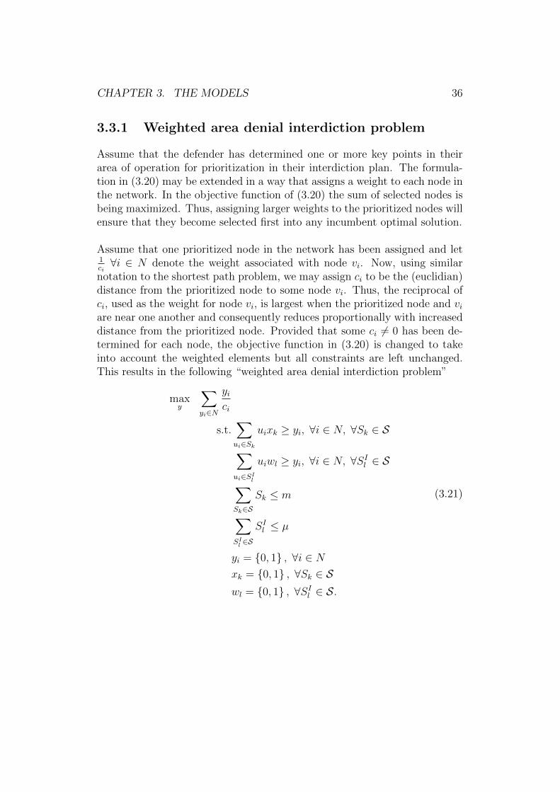
CHAPTER 3. THE MODELS 36
3.3.1 Weighted area denial interdiction problem
Assume that the defender has determined one or more key points in theirarea of operation for prioritization in their interdiction plan. The formula-tion in (3.20) may be extended in a way that assigns a weight to each node inthe network. In the objective function of (3.20) the sum of selected nodes isbeing maximized. Thus, assigning larger weights to the prioritized nodes willensure that they become selected first into any incumbent optimal solution.
Assume that one prioritized node in the network has been assigned and let1ci∀i ∈ N denote the weight associated with node vi. Now, using similar
notation to the shortest path problem, we may assign ci to be the (euclidian)distance from the prioritized node to some node vi. Thus, the reciprocal ofci, used as the weight for node vi, is largest when the prioritized node and viare near one another and consequently reduces proportionally with increaseddistance from the prioritized node. Provided that some ci 6= 0 has been de-termined for each node, the objective function in (3.20) is changed to takeinto account the weighted elements but all constraints are left unchanged.This results in the following “weighted area denial interdiction problem”
maxy
∑yi∈N
yici
s.t.∑ui∈Sk
uixk ≥ yi, ∀i ∈ N, ∀Sk ∈ S∑ui∈SI
l
uiwl ≥ yi, ∀i ∈ N, ∀SIl ∈ S∑Sk∈S
Sk ≤ m∑SIl ∈S
SIl ≤ µ
yi = {0, 1} , ∀i ∈ Nxk = {0, 1} , ∀Sk ∈ Swl = {0, 1} , ∀SIl ∈ S.
(3.21)

CHAPTER 3. THE MODELS 37
3.4 The most relevant nodes of a graph
“Maximizing the shortest path” and “area denial problem” are NP-hardproblems in their computational complexity (see, e.g., [11] and [49] respec-tively for proof). This will naturally become an issue as the size of theoptimized network grows. Finding ways to reduce the size of the underlyingnetwork without compromising the optimality of an obtained solution is thusimportant for the overall efficiency of the interdiction optimization models.
Recall that the availability of the leader’s resources is assumed to be lim-ited in all of the discussed models so far. This means that instead of allnodes in a given network, in most cases only some subset of nodes N canbe interdicted. Thus, identifying nodes that cannot belong to any optimalsolution and removing them from the network prior to the actual optimiza-tion, allows reducing the size of the network such that the optimal solutionis retained. Thus, a variant of the algorithm AMRAP by Ball et al. [15] forfinding the most relevant arcs in a network, is used as a pre-processing stepfor the “shortest path interdiction” and “area denial interdiction” models.This algorithm, however, is slightly modified to accommodate finding themost relevant nodes as follows.
It is well known that several shortest path algorithms, such as A* for ex-ample, are able to calculate the shortest paths and their respective lengthsfrom a source node to all other nodes with no more computational effortthan calculating the shortest path between the source and any other individ-ual node. Taking advantage of this fact, the A* algorithm is first executedusing the artificial source node s as the root node to obtain the (forward)lengths `F (v1) of the shortest paths between nodes s and vi for each node viin the network. Obtaining the forward lengths is then followed by a secondA* run that uses node t as the root node. Let the backward lengths obtainedfrom the second run be defined as `B(vi), ∀i ∈ N . Next if a path vs− vi− vtexists, the shortest s− t path distance through node vi for all nodes is
`(vi) = `F (vi) + `B(vi). (3.22)
If, however, for some node vi only the forward or backward distance, but notboth, has been calculated it means that a path does not exist between eithervs − vi or vt − vi. In this case, the shortest path distance is `(vi) =∞.
All unique values found in all of the different `(vi)’s are then sorted in in-creasing order. Let these unique values be denoted by l(1), l(2), . . . , l(k)

CHAPTER 3. THE MODELS 38
where k is the number of unique values found. The next step is to createcuts corresponding to each of the unique values l(k), such that for each cutCk the condition `(vi) ≤ l(k), ∀vi ∈ N holds. Now, the number of nodescontained in each Ck is the upper limit on the number of nodes that need tobe interdicted in order to force the follower to follow a path that is longerthan l(k).
Suppose now that the leader is able to interdict at most M nodes irrespectiveof the types of mines being employed. Starting with the smallest k, for anycut Ck there are now two cases to consider:
1) If the number of nodes |Ck| ≥ M , the optimal solution must includea subset of these most relevant nodes found in Ck+1 (see remark be-low) and a reduced network G′ containing the nodes in Ck+1 and theirincident edges is constructed.
2) If the number of nodes |Ck| < M , the next cuts Ck+1, Ck+2, . . . areevaluated one at a time until case 1) takes place.
Remark. The removal of every node in Ck is not required to make a replace-ment shortest path longer. Some shortest paths may contain more than onenode in Ck and the removal of one of these nodes may indeed disconnect theremaining nodes of such a path from the network as a consequence. There-fore, it is not required to interdict every node in Ck in which case some minesare left unused. Thus, the cut Ck+1 is selected to be included into the reducednetwork in order to ensure that shortest paths with length > k are not leftuninterdicted while there are any “leftover” mines remaining.
Since each contact mine is only able to interdict the node in which it is placed,the number of nodes the leader is able to interdict with contact mines equalsthe number of available mines, m. Influence mines on the other hand interdictall nodes within their area of influence. Since a fixed area of influence thatencompasses all incident neighbors of a node is used, the number of nodesthat a single influence mine is able to interdict equals the degree of the minednode plus the node itself. Thus, in order to obtain the maximum number ofnodes that may be interdicted, the average degree of the network, roundedup to the nearest integer, is calculated. One is added to the average degreeto account for the interdicted node itself, and then the appended averagedegree is multiplied with the number of available influence mines, µ. Thus,the maximum number of nodes that the leader may interdict, M , that is

CHAPTER 3. THE MODELS 39
needed for the above comparisons is obtained simply as
M = m+ µ
(⌈|E||N |
⌉+ 1
). (3.23)
Once the reduced network G′ of most relevant nodes has been formed, itmay then be used in place of the original network for optimization in orderto improve performance.

Chapter 4
Measurements of effectiveness
This section discusses the the three operational objectives that a planneris attempting to achieve through mine deployment. These operational ob-jectives are quantified using network properties that are measured beforeand after a network interdiction action has taken place and using their re-spective ratios. Each of the interdiction models presented in Chapter 3 hasa specific objective function that is independent from the measurements ofthe operational objectives in this chapter. Consequently, the measurementspresented here are formulated in a way that allows the comparison of anysolution regardless of the method for obtaining it in an objective and in-dependent manner. All of these properties measure the connectivity of thenetwork and the changes to it. The anti-access objective measures how wellfree passage through the mined area has been restricted whereas area denialmeasures how much “free space”, or area that is usable by an adversary,has been reduced. Resilience, or the ability of the minefield to maintain itsefficiency even though mines are being removed from it, is also discussedand introduced as a third measurement for the operational effectiveness of aminefield.
4.1 Quantifying operational objectives
All of the few publicly available models in, e.g., [3] are probability based.Furthermore, they are only able to represent and calculate ship-mine inter-actions with accuracy. As a result, the perceived operational effect of anymining operation is only quantified as the likelihood of a ship or ships hittinga mine. This in turn may be used to derive how likely the minefield is to
40

CHAPTER 4. MEASUREMENTS OF EFFECTIVENESS 41
cause damage to an adversary’s force. This approach is therefore suited forsimulating and, in some cases, also for optimizing those mining and countermining operations whose objective is inflicting as much damage as possible orconversely avoiding as much damage as possible. Thus, a common approachfor measuring the performance of a mining operation is the maximizationof the amount of damage caused to the adversary. Alternatively from theperspective of counter mining operations, the objective is minimizing theprobability that a given number of ships will hit a mine. This objective, how-ever, mostly concerns optimizing mine quantities or mine properties, such astheir operational reliability, instead of their placement. Spatial distributionand placement or other approaches or measurements are not evaluated aspart of the “probabilistic” models. While measuring lethality as the met-ric for the effectiveness of the minefield is certainly easy, it is not able toproperly describe the desired operational effects. Instead, lethality may beperceived as a component that is able to contribute to the other operationalobjectives, but cannot be used as the sole measurement of a minefields op-erational usefulness. In general, the quality of a given minefield should beseen as a combination of several operational effects that depict how well themine field performs against any action made by an adversary. Thus, newmore comprehensive measurements of effectiveness for different mine layingoperational objectives need to be defined.
In the solutions generated using the models presented in Chapter 3, determin-istic interdiction plans are produced and thus, deterministic measurementsof effectiveness (MOE) are also desired. It is important to note that theseMOE’s are designed to be independent of the objective functions given inthe various model formulations for the defensive minefield planning problem.While the objective of the minefield planner is indeed to maximize the valueof these MOE’s, they are not maximized in the optimization sense. Instead,they are formulated to measure the qualities of different solutions to the de-fensive minefield planning problem irrespective of the optimization model orobjective function that was used to obtain them. Thus, the purpose of theMOE’s are only to provide a means for comparing the solutions given by thedifferent optimization models against the different operational requirementssimultaneously. In essence, the MOE’s are designed to provide the meansfor comparing the operational “goodness” of two different optimal solutionsbased on operational prioritization.
In their general sense, network interdiction problems concern the connec-tivity of networks. In a typical network interdiction setting the interdictor,the actor who attempts to disrupt the network in some way, is effectively at-

CHAPTER 4. MEASUREMENTS OF EFFECTIVENESS 42
tempting to reduce the connectivity of the network operated by the follower.Thus, it is natural to examine the effectiveness of our defensive minefieldoptimization problem using concepts related to general connectivity of net-works and, in particular, how the obtained interdiction solutions are effectingthe connectivity of the original uninterdicted network.
4.2 Anti-access
Earlier, the two principal objectives for the defensive minefield planning prob-lem have been defined to be the prevention of an adversary’s passage to, orthrough, a designated key area and to prevent the unrestricted use of thatarea as well as possible. These two complementary objectives were definedas anti-access and area denial, respectively. Attrition as an objective is easyto measure using the ship-mine interactions and is excluded from this thesis.
A clear representation of the anti-access objective relates to the shortestpath(s) through a network. In order for an adversary to pass through anetwork, they must enter the network through some node and then exit thenetwork through some other node at the opposite end. This requires thata continuous path between the entry point and exit points must exist. Inthis context, a path is defined as a sequence of nodes that are traversed fromone incident edge to another through the network. When this path is short,the time it takes to pass through the newtwork is also small. A quick pas-sage through the area makes the adversary less susceptible to other possibledefensive measures or systems that have been deployed. Thus, we assumethat the adversary attempts to pass the area using the shortest (quickest)possible route. The logical countermove for the leader is thus, to attemptto maximize the shortest possible path of access through the network or toeven completely disconnect the start and end nodes from one another in thebest possible case. Let us borrow the terminology used in [11] and call thiscountermove “maximizing the shortest path”.
For the anti-access objective, the obvious choice for a metric is the lengthof the shortest path and how it is being affected due to interdiction. Inother words, we would like to measure how much the interdictor has beenable to extend the shortest path through their interdiction effort. This sug-gests using a simple comparison or ratio of the pre- and post-interdictionpath lengths. Let this ratio be denoted as
¯
`where ` is the pre-interdiction

CHAPTER 4. MEASUREMENTS OF EFFECTIVENESS 43
shortest path length and ¯ is the post-interdiction shortest path length. In atypical scenario, however, the area of operation for the mining activity hasmany parallel shortest paths of equal length and thus a simple comparisonis inadequate as a measurement. Consider an area of open sea as a concreteexample. In this type of geography it is likely that there are many shortests-t paths of equal length and the number of available mines is insufficient tocover all of these paths. This being the case, the difference between the pre-and post-interdiction shortest path length would be zero indicating that theeffectiveness of the interdiction plan is also zero which clearly is not the case.Consider, as an example, that there are more than one shortest paths in somenetwork and some of them have been interdicted. Furthermore, assume thatan adversary will randomly select which one of these shortest paths theywill use based on some probability distribution and selecting any one of theshortest paths has a probability greater than zero. It then follows that theeffectiveness of any interdiction plan, while perhaps infinitesimally close tozero, cannot equal zero. Thus, the simple comparison of path lengths cannotbe used as the sole measurement.
Suppose next that path P is an s− t shortest path of length ` in a networkG. Suppose also that there are n paths of length ` including P . Assume nextthat some interdiction plan has been carried out and some nodes or edgesin G have been removed as a result but the source and target nodes havenot been disconnected from each other. Thus, at least one path betweenthe nodes s and t must still exist. The next step is to examine all possi-ble paths between the source and target nodes and calculate the number ofpaths with length ` (note that this is the original shortest path length beforeinterdiction). Let n denote the number of post-interdiction paths of length`. Now the inverse ratio 1 − n
nmay be used as the measurement for the
fulfilment of the anti-access objective. Thus, what is now measured is thenumber of shortest paths that the interdictor was able to effectively removefrom the network, instead of only comparing the increase in the length ofone shortest path. Using the above inverted ratio is straightforward whensome, but not all, of the original shortest path have been interdicted. Ifthere are no shortest paths of length ` remaining, however, then the rationn
= 0n
= 0 =⇒ 1 − nn
= 1. This would mean that the interdiction isperfectly successful, which is not the case. Recall that the best case scenariofor any interdiction operation is to disconnect node s from node t in whichcase the length of any shortest s − t path would be infinite. Thus, if anyfinite length s− t path exists in the network it then implies that 1− n
n< 1
because the best case scenario is not reached. Using just the ratio of thenumber of pre- and post-interdiction shortest paths fails to capture the dif-

CHAPTER 4. MEASUREMENTS OF EFFECTIVENESS 44
ference between reducing the number of shortest paths and disconnecting thenetwork entirely. This in turn implies that neither the shortest path lengthnor the number of remaining shortest paths may be individually used as ameasurement for anti-access quality. Instead a combination of the differentnetwork measures is required in order to properly represent the quality ofany obtained solution. Thus, the anti-access MOE is formulated as
Ψ1 =
1 if ¯=∞
1−(
( `¯)+( n
n)2
)if ¯ is finite.
(4.1)
Note that now the value of the anti-access MOE Ψ1 is zero only if there isno difference between the shortest path length and the number of shortestpaths after interdiction, i.e., the interdiction effort had no effect. Further-more, since 0 < `
¯ ≤ 1 when ` is finite, this means that Ψ1 = 1 if and onlyif the solution has completely prevented access through the designated area.This only holds when all s− t paths are disconnected meaning that ¯=∞.
4.3 Area denial
Evaluating the effectiveness of network interdiction solutions is also closelyrelated to the concept of network components since network components arealso defined through paths: For any undirected graph G = (N,E), an in-duced subgraph H = (N∗, E∗) of G is a graph that contains a set of nodesN∗ ⊂ N together with all edges incident to any vi∀i ∈ N∗. If there ex-ists a path between all pairs of nodes in N∗ ⊂ N , then H is a connectedcomponent of G (note that by the definition given by Erdos and Renyi in[45] single nodes are not connected components unless there is a link from anode to itself). If all pairs of nodes are connected by a path in a directed net-work, H is called a strongly connected component instead. For simplicity, letboth (direct graph) strongly connected components and (undirected graph)connected components be called components from now on regardless of thedirectness of the underlying graph. In order for a shortest path between asource node s and a destination node t to exist in a graph G, both of thesenodes must belong to the same component based on the above definition ofa component. Equivalently, there is an implicit assumption that there mustbe at least one component in the network, and that this component mustcontain both end nodes s and t for any shortest s− t path to exist. The in-terdiction problem becomes trivial if this assumption does not hold and thus
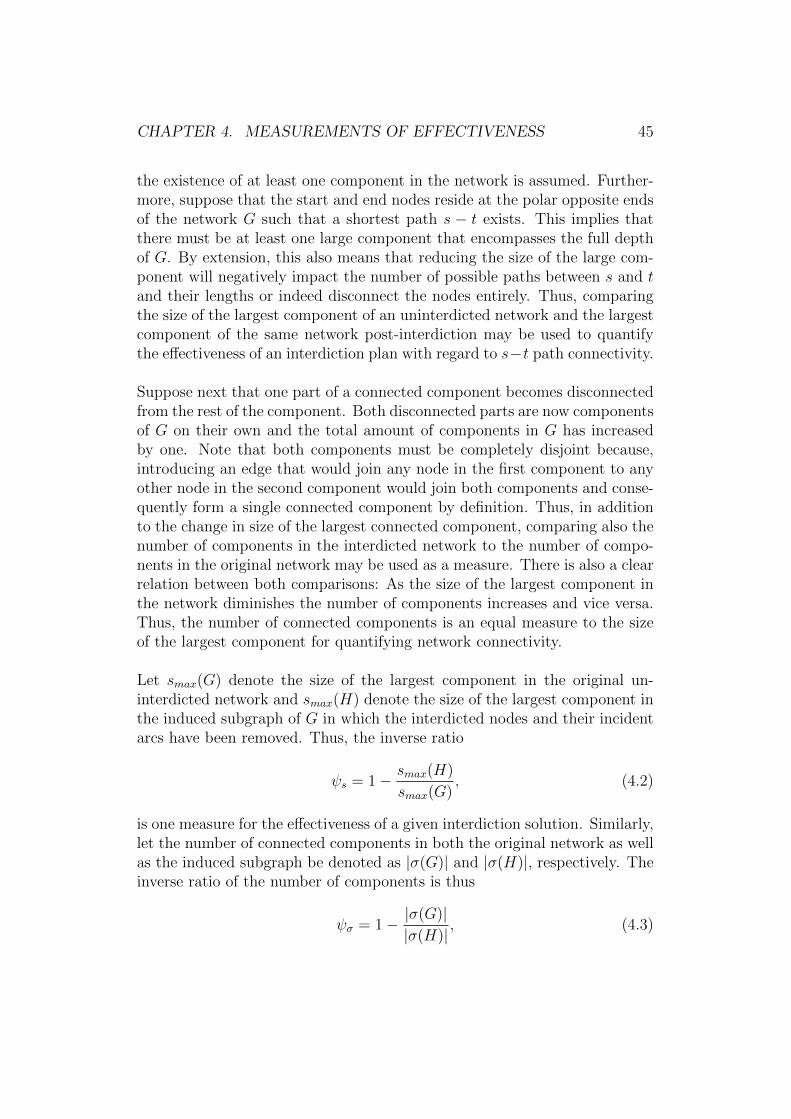
CHAPTER 4. MEASUREMENTS OF EFFECTIVENESS 45
the existence of at least one component in the network is assumed. Further-more, suppose that the start and end nodes reside at the polar opposite endsof the network G such that a shortest path s − t exists. This implies thatthere must be at least one large component that encompasses the full depthof G. By extension, this also means that reducing the size of the large com-ponent will negatively impact the number of possible paths between s and tand their lengths or indeed disconnect the nodes entirely. Thus, comparingthe size of the largest component of an uninterdicted network and the largestcomponent of the same network post-interdiction may be used to quantifythe effectiveness of an interdiction plan with regard to s−t path connectivity.
Suppose next that one part of a connected component becomes disconnectedfrom the rest of the component. Both disconnected parts are now componentsof G on their own and the total amount of components in G has increasedby one. Note that both components must be completely disjoint because,introducing an edge that would join any node in the first component to anyother node in the second component would join both components and conse-quently form a single connected component by definition. Thus, in additionto the change in size of the largest connected component, comparing also thenumber of components in the interdicted network to the number of compo-nents in the original network may be used as a measure. There is also a clearrelation between both comparisons: As the size of the largest component inthe network diminishes the number of components increases and vice versa.Thus, the number of connected components is an equal measure to the sizeof the largest component for quantifying network connectivity.
Let smax(G) denote the size of the largest component in the original un-interdicted network and smax(H) denote the size of the largest component inthe induced subgraph of G in which the interdicted nodes and their incidentarcs have been removed. Thus, the inverse ratio
ψs = 1− smax(H)
smax(G), (4.2)
is one measure for the effectiveness of a given interdiction solution. Similarly,let the number of connected components in both the original network as wellas the induced subgraph be denoted as |σ(G)| and |σ(H)|, respectively. Theinverse ratio of the number of components is thus
ψσ = 1− |σ(G)||σ(H)|
, (4.3)

CHAPTER 4. MEASUREMENTS OF EFFECTIVENESS 46
which may be regarded as another quantifiable metric for the effectiveness ofthe interdiction plan.
Similar metrics have previously been used by Shen, Smith and Goli [50]regarding maximizing network disconnectivity through node deletions whichis closely related to our interdiction problem. Both metrics related to graphcomponents are able to quantify how well a particular interdiction solutionsucceeds in preventing access through the network as well as how well thesolution is able to “deny” the available free space in our network but withdifferent emphasis. In a disjointly partitioned graph, the amount of “freespace” that may be freely exploited by the network operator is effectivelyminimized. The existence of many small components indicates that connec-tivity between any arbitrarily chosen pair of nodes is limited. This equatesto the definition of area denial. Thus, the average of ψs and ψσ is used asthe metric for area denial denoted as Ψ2. The reduction in size of the largestcomponent, however, is also a good indicator of how much the number ofpossible shortest paths decreases provided that the component remains con-nected and the source and target nodes belong in the connected component.Thus, the size of the giant connected component may be regarded as an ap-proximation of anti-access quality as well.
4.4 Resilience
Since both the anti-access and area denial metrics have been normalized, theaverage of these two metrics may be used as a single Measure of Effectiveness(MOE) to describe the “goodness” of interdiction solutions with one value ifnecessary. Both metrics, however, will be tracked separately when analyzingthe obtained solutions. This is done in order to gain better understanding tothe differences between solutions and interdiction plans with regard to thetwo interdiction objectives.
The decline of a minefield’s efficiency was briefly discussed in the contextof the ENWGS model earlier. This phenomenon requires further attentionsince in addition to a natural decline due to time, the adversary very oftenattempts to remove mines through mine sweeping. This decline will also nat-urally happen through mine detonations when ships hit any of the deployedmines. Regardless of the cause, each minefield’s capability to perform its taskdeteriorates over time. Thus, some sort of measurement to quantify or ap-

CHAPTER 4. MEASUREMENTS OF EFFECTIVENESS 47
proximate the resiliency or staying power of a mine field is needed. Note thatwe may think of resiliency as either an individual measure, or as a multiplierthat reduces the other MOE’s for anti-access and area denial as a functionof deteriorated mines.
Consider a network of N nodes and E edges such that all nodes are present inthe network at all times, but each edge has a fixed, yet individual, probabilityPr of existing. Or phrased differently, each edge has a probability 1− Pr ofnot being a part of the network. Consequently, the number of edges presentin the network for any given value of Pr is Pr · E. Now, for very smallvalues of Pr the number of edges is also small. This means that many of thenetwork nodes are unconnected simply because there are not enough edgesto connect them. Those nodes that are connected, are still likely to be onlyconnected with a few other nodes at most. This type of a scenario is alsothe attempted outcome of a network interdiction plan in the area denial sense.
Suppose that the value of Pr is increased and the number of available edgesin the network is thus also increased. Recall also that the probability Prwas assumed to be independent for every single link. Thus, as the num-ber of edges increases, the nodes that are already connected are more likelyto gain more connected nodes because they have more available interfacinglinks. This causes the formation of larger, yet still relatively small, connectedcomponents. As Pr increases the likelihood of these larger components con-necting with other connected components also increases.
Eventually, since for large values of Pr the number of edges is also large,most nodes are connected via some path. What this means in terms of con-nectivity, is that the majority of nodes now belong to a single very largecomponent and the number of smaller components or isolated nodes is min-imal. Note, how this situation corresponds quite well to an uninterdictednetwork. Examining the behaviour of the network as Pr changes and theresulting differences between the number of components and the size of thelargest component suggests that there must be some value of Pr for whichthe largest component breaks apart to form a collection of the smaller com-ponents.
The random network and its behavior described above is an example of anErdos-Renyi random graph model. Erdos-Renyi showed that there exists a“critical point”, PrC , for the probability Pr such that when Pr exceeds thiscritical point a giant connected component is formed. On the other hand,when Pr remains below this critical point the network consists only of small

CHAPTER 4. MEASUREMENTS OF EFFECTIVENESS 48
components and isolated nodes [45], [46]. The critical point may be cal-culated numerically with high probability (see [47]). Using this calculatedcritical point and comparing that to the estimated Pr of an interdiction so-lution, allows estimating the number of mines that may be removed until thegiant component forms again.
Assume that network interdiction is attempted through node removal, wherea deployed contact mine effectively only removes one node from the network.Also, assume that an influence or bottom mine is able to remove n nodesfrom the network including the node where the device is placed. Let m andµ denote the number of contact and influence mines, respectively. Thus, themaximum number of nodes that may be removed by an interdiction solutionis m + nµ. Following the definition by Erdos and Renyi of the percolationcritical point this results in the equality
m+ nµ = 1− Pr =⇒ Pr = 1− (m+ nµ). (4.4)
Now there are two cases to consider:
1) If 1 − (m + nµ) > Pr′C then a giant component exists also after theinterdiction effect and we conclude that we cannot make further as-sumptions on the resiliency of the minefield.
2) If 1−(m+nµ) ≤ Pr′C it means that the giant connected component hasbeen disconnected to parts and removing one or more of the deployedmines will cause the giant connected component to reappear.
For the first case, an analytical resilience approximation cannot be made andthus the approximation for the effect of mine removal should be evaluatedthrough, for example, simulation.
For the second case, the average number of nodes that are being removed bya single mine is known to be
ψ′ =m+ nµ
m+ µ. (4.5)
Thus, evaluating how many mines on average need to be removed until thegiant connected component reappears, the solution to the following equationmay be interpreted as an estimate of the interdiction solution resiliency.
Ψ3(ψ′x) = 1−(m+ nµ+
∑m+µx=1 ψ′i
m+ µ
)> Pr′C . (4.6)
Chapter 5
Implementation and test instancecreation
The adaptations and modifications that were done during the implementa-tion of the models from Chapter 3 are discussed next.
All models were implemented using Python 3.1 together with the NetworkX2.5 package. NetworkX is a Python tool designed for network analysis andresearch, and offers efficient pre-implemented tools for the most commonnetwork related algorithms, e.g., Dijkstra, A*, Bellman-Ford and Floyd-Warshall. In addition, the PyMip (Python Mixed integer programming)package and Gurobi solver were used for constructing and solving mixed in-teger problem instances using Python.
The basic bilevel max-min shortest path problem was implemented in PyMipas a single level MILP using the dual of the inner minimization as formu-lated in (3.10). The extended bilevel max-min shortest path problem (withmines having an area of effect) was similarly transformed to single level asformulated in (3.17) and implemented directly to PyMip.
Another variant of the extended bilevel max-min shortest path problem wasalso implemented. In this second implementation, the problem is solved us-ing two different solving approaches in succession. Initially for each availableinfluence mine, the number of nodes that may be interdicted is multipliedby 9 corresponding to the degree found in the majority of nodes. This mul-tiplied number of nodes that may be affected is then used in place of m (thenumber of contact mines in the basic bilevel max-min shortest path prob-lem) and solved using the basic min-max single level shortest path MILP
49
CHAPTER 5. IMPLEMENTATION 50
implementation (3.10). The solution, a list of 9 · µ interdicted nodes, ob-tained through this first step is then used to create a subgraph that containsonly the interdicted nodes and the source and sink nodes s and t, respec-tively. The second step of this variant implementation is to find the optimalplacement for the µ influence mines as given in the original problem. Themaximum coverage heuristic is used to do that but the heuristic is executedover the subgraph obtained during the first phase. The resulting solution isan interdiction plan that approximates the optimal solution of the extendedmax-min shortest path problem (3.17) when the original problem cannot besolved exactly.
An attempt at improving the performance of the MILP model (3.10) andthe other models was made through identification of the most relevant nodesof the network. The process for finding the most relevant nodes of the net-work as described in Section 3.4 was implemented using the single sourceA* algorithm in the NetworkX 2.5 package in order to take full advantageof the efficient implementation available. The implementation for “findingthe most relevant nodes” was created as a separate Python script in orderto keep it fully optional and easy to apply as a pre-processing step to allother models. The A* algorithm has a known worst case time complexity ofO(E) after which each node is evaluated once to determine if it is retainedor removed. Thus, the resulting worst case time complexity for creating thereduced network is O(E +N).
In addition to the most relevant nodes, the pairwise distances between allpairs of nodes in the network need to be calculated. The Floyd-Warshall al-gorithm, as it is implemented in the NetworkX 2.5 package, is used for find-ing these all-pairs distances. Floyd-Warshall algorithm has a known timecomplexity of O(N3). The obtained pairwise node distances are used forconstructing the sets that are required for the maximum coverage heuristicmodel. For contact mines, each node is considered as one set for the problemformulation. Furthermore, another set for each node in the network is createdsuch that this set contains the node itself and all other nodes that are withinsome distance of the original node. This distance is defined by the area ofeffect of an influence mine type. Finding the nodes that are within somearbitrary distance of the origin node may be done by traversing the pairwisedistances obtained from running the most relevant nodes process. For eachnode in the network, we find all other nodes that are within a given distance.This takes at worst N − 1 look-ups for each node. Thus, the creation of twosets for each node in the network has a worst case time complexity of O(N2).In the implementation the inter-node distance is set to one, and thus each of

CHAPTER 5. IMPLEMENTATION 51
the “contact mine sets” consists simply of a single node, and the “influencemine sets” consists of a node and all of its neighbours.
The distance information obtained through the creation of the sets may alsobe used for constructing the weight vector needed in the weighted area de-nial problem implementation. Reference points that are given as an input tothe “defensive minefield problem” are assumed to be available. However, ifno other reference points are given, the node that is considered to be geo-graphically in the center of the network is determined and given as the onlyreference point to be used. Using the pairwise distances between nodes, itis now possible to simply select the closest reference point to each node andthen use the reciprocal of the distance between that node and their closestreference point as the weight for both the “contact mine set” and the “influ-ence mine set” corresponding to that node. Since each node needs only tobe evaluated once for both sets, the time complexity of assigning the weightsfor sets is O(N). Thus, finding the all pairs shortest path lengths serves twopurposes simultaneously: To construct the “influence mine sets” as well asto obtain the weight vector required for the weighted area denial problem.Combined together, the procedures for reducing the network size and con-struction of the required sets together with constructing the weight vectorhave a worst case time complexity of O(N3).
For the area denial interdiction problems, an exact integer program for themaximum coverage and weighted maximum coverage problems was not im-plemented. Instead, and in order to reduce computation times at the expenseof optimality, the maximum coverage and weighted maximum coverage prob-lems are solved by implementing a greedy approximation heuristic for bothproblems. The decision rule used in the maximum coverage heuristic is toselect the unassigned set that contains the largest number of nodes thathave not yet been covered during previous iterations of the algorithm untilthe maximum allowed number of sets have been selected. Similarly, for theweighted maximum coverage problem the decision rule for the heuristic is toselect the unassigned set that has the largest weight and contains the largestamount of nodes that have not yet been covered. It is known that the greedyalgorithm used in the implementation has a polynomial time complexity withan approximation ratio of 1− 1
exp[51].
Finally, a script for calculating the measures of effectiveness (MOE) is imple-mented using the available functions in NetworkX. Three key characteristicsof the network are calculated before and after the interdiction, namely: thenumber of shortest paths, the number of connected components and the size

CHAPTER 5. IMPLEMENTATION 52
of the largest connected component. The pre- and post-interdiction resultsare then compared to calculate the final normalized measures of effectivenessfor anti-access, area denial and resilience operational objectives separately,as discussed in Chapter 4.
The implemented optimization and approximation models were tested using(pseudo) randomly generated test instances. The instance generator thatwas used in testing was also implemented using Python. Each test instanceconsists of a two-dimensional 8-regular square lattice such that the nodes onthe “edges” of the graph have only a degree of 5, as described in Chapter3. Both planar dimensions of the lattice are of the same size n. Thus, eachgenerated instance has initially n2 nodes.
The next step of the instance creation process is to remove some nodes ofthe graph in order to create an artificial “landmass”. Thus, nodes representareas of open water that may be traversed by an adversary vehicle and themissing nodes represent islands or other land features in the area of opera-tions. A number of islands between 0 and some upper limit defined by a useris (pseudo) randomly generated. For each of these islands both a (pseudo)random center node and a (pseudo) random number r are generated. Thenumber r is the radius of the island measured in number of edges from theassigned center node. Thus, each island is a collection of nodes centered onsome node and containing all nodes that are within distance r from the cen-ter. Each of these collections of nodes, or islands, are then removed from theoriginal lattice. If the number of removed nodes is high the resulting latticerepresents a cluttered sea area such as some archipelago. Conversely if thenumber of removed nodes is very small then the resulting area represents anopen sea scenario. The landmass proportion, or the ratio of removed nodesand original number of nodes is calculated and recorded for each test instanceto understand the effect the area topography has on the obtained results.
Reference points used in the creation of the weight vector for the maximumcoverage algorithm are generated automatically for each test instance. Thisis done to proxy the list of reference points a user is expected to provide forthe models. To obtain these reference points pairwise shortest paths betweenall island centers are calculated. Then for each of these paths, a center nodeis identified and added to a list of tentative reference points. If the numberof nodes in a given path is odd, then the center node is the ith node wherei is the number of nodes in the path divided by two and rounded up. If thenumber of nodes is even, then the center node is the ith node where i is thenumber of nodes in the path divided by two. After the landmass or islands

CHAPTER 5. IMPLEMENTATION 53
has been removed from the generated lattice network, each tentative refer-ence point is checked against the remaining nodes of the lattice network. If atentative reference point does not exist in the lattice, it is also removed fromthe tentative reference points list. The remaining points are then used asthe input reference points a user would provide. Finally, the artificial sourcenode s and sink node t are added to the network together with their inci-dent edges to provide a complete single test instance. Edges that originatein the source node s are connected to nodes on one “side” of the lattice andthe edges leading to the sink node t are set to originate from nodes on theopposite “side” (see Figure 5.1).
Figure 5.1: An example of a generated lattice with n = 10. Source node s isnode number 101 and sink node t is node number 102.

Chapter 6
Test results and analysis
All tests described in this section were conducted on a laptop computer witha 64 bit Windows 10 operating system, an Intel Core i3-8130U processor (2.20GHz) and 4 GB of RAM memory. Initial testing was performed to tune theparameters of the test instance creator. After that, the tests were conductedto evaluate the computational performance and the solution quality of thedifferent models. Some statistical analyses were done on the obtained testresults and their results are presented in this section. This section concludeswith insights derived from the testing.
Initial testing of the Python code showed that having the maximum numberof islands set to 15 and the maximum radius r set to 3, produced the mostdiverse selection of instances in both landmass as well as the positioning ofthe generated islands regardless of the lattice size when n > 20. Thus, for alltests that were conducted the maximum number of islands was set to 15 and0 ≤ r ≤ 3. The same parameters were also applied even for instances wheren < 20 such that the few emerging empty graphs or completely disconnectedgraphs were regenerated as soon as they were observed.
In addition to these findings, the initial tests on the extended single levelshortest path problem with influence mines (formulation (3.17)) showed thatthe PyMip implementation of the model did not work as intended. Theresults given by the implementation using the Gurobi solver, produced solu-tions that were identical to those of the basic max-min shortest path problem(3.10). In practice, the desired effect of mines having an area of influence wasnot achieved and the mine placement was exactly the same as if the mineswere contact mines. For this reason, the two phase approximation schemedescribed in Section 5 was selected to be used. This two phase approach is
54

CHAPTER 6. TEST RESULTS AND ANALYSIS 55
called the “shortest path heuristic” for the rest of this document to clearlyindicate that it is significantly different in application than the “exact” MILPshortest path interdiction model (3.10), and to highlight that the obtainedsolutions are approximations. Finally, the initial tests showed that the max-imum coverage greedy heuristic clearly prioritizes nodes that have a smallindex number in the programmed application. This is very likely caused bythe way nodes are numbered when a network is created in NetworkX andin the way Python iterates over lists and arrays. Thus, the non-weightedvariant of the maximum algorithm was excluded from further testing. Con-sequentially, the second phase of the shortest path heuristic was also replacedwith the weighted maximum coverage greedy heuristic.
Thus, the final four variants of the implemented models that were testedare:
i) the basic shortest path interdiction MILP model using contact mines(shortest path MILP),
ii) the extended shortest path heuristic using influence mines (shortestpath heuristic),
iii) the weighted maximum coverage greedy heuristic using contact mines(max coverage heuristic (contact)); and
iv) the weighted maximum coverage greedy heuristic using influence mines(max coverage heuristic (influence)).
Additionally, each of the above variants was tested both with and withoutthe pre-processing procedure for creating a reduced problem network thatonly consists of the most relevant nodes.
6.1 Performance tests
6.1.1 Computation time as a function of instance sizeand mine count
The first series of tests were conducted to evaluate the computation timesof the implemented models as a function of instance size. For each test, arandom instance was generated and solved using both the shortest path and

CHAPTER 6. TEST RESULTS AND ANALYSIS 56
the maximum coverage models for both mine types, and their respective exe-cution times were recorded. This was done in order to analyze the differencein execution times between the implemented models. For the shortest pathMILP, the commercially available Gurobi solver was used to obtain a solu-tion and for the other models the solution implementation was programmed.Recall that for influence mines the shortest path heuristic algorithm usedto solve the shortest path problem is essentially the same as the maximumcoverage greedy heuristic and is thus likely to show similar characteristics.Each conducted test execution for the first test set used a fixed amount ofavailable contact mines that was set to 10. A fixed number of mines wasused in order to ensure that the only parameter that could have an effecton execution times is the instance size. Each test was repeated a total of 30times for a set of different network sizes, defined through the parameter n,and the median computation times from the solutions were computed.
Figure 6.1: Median computation times of the shortest path MILP and max-imum coverage heuristic (contact) as a function of instance size n, when foreach value of n the test was executed 30 times. Number of mines was fixedto 10 in each test execution.
Figure 6.1 shows the observed computation times required to obtain a solu-tion for contact mines using the shortest path MILP and maximum coverage

CHAPTER 6. TEST RESULTS AND ANALYSIS 57
heuristic respectively.
Figure 6.2: Median computation times of the shortest path heuristic andmaximum coverage heuristic (influence) as a function of instance size n. Foreach value of parameter n the test was executed 30 times. A fixed numberof 10 mines was used in every test execution.
The same setting of running 30 test executions for each parameter combi-nation was also conducted for the influence mine models. As before, themedian computation times were recorded. A fixed number of 10 mines foreach value of test instance size parameter n was used. The results from thetesting of influence mine models are shown in Figure 6.2. The executiontimes of both the shortest path heuristic and the maximum coverage heuris-tic using influence mines increases quadratically. This is expected behaviourconsidering the quadratic increase in the size of the test instances, and dueto both models effectively using the same greedy heuristic. Interestinglyhowever, the data from the influence mine tests suggests that the shortestpath heuristic is much more efficient. This is surprising, since the shortestpath heuristic actually solves two problems in sequence while the maximumcoverage heuristic (influence) only has to solve one problem. Recall that inthe first phase of the shortest path heuristic (influence), the original instanceis reduced using a solution obtained through the MILP model and then thesame greedy heuristic is run on the remaining reduced network.

CHAPTER 6. TEST RESULTS AND ANALYSIS 58
Consider once more the computation times of the contact mine models inFigure 6.1. It seems that the efficiency of the commercial Gurobi solver,which is optimized for performance, is capable of outperforming the greedyheuristic with the way the models are currently implemented. However, thegreedy heuristic used in both model implementations is known to find a solu-tion in polynomial time as discussed in Section 2.3. Hence, the difference inefficiency suggests that the main cause for the increased computation time,is the creation of the sets that the greedy heuristic uses. The time requiredfor set construction, obviously, is directly related to instance size. Test re-sults suggest that the greedy algorithm is indeed fast and efficient, but thetime required to initialize the heuristic, i.e., constructing the sets, exceedsthe combined running time of the shortest path MILP and the maximumcoverage heuristic executed over the remaining much smaller network. Amore efficient way to construct the required sets for the maximum coverageheuristic is likely to improve the algorithm performance compared to theresults presented here. Note however, that all analyzed test instances wererelatively small. Large problem instances were not tested due to memoryrestrictions on the laptop used in the testing. Thus, these results cannot begeneralized and further testing over large test instances should be conducted.
The next set of tests were conducted in order to investigate the effect thenumber of mines have on the execution times of the implemented models. Theonly parameter that was changed during these tests was the number of mines.The network size selected for the tests was 2500 nodes (n = 50). Again, 30independent runs were conducted for each number of available mines and themedian execution time of each of these test runs was calculated. The testruns were conducted separately for both contact and influence mines, andtheir respective models. Figure 6.3 presents the results of testing for modelsemploying contact mines. The observations plotted in the figure suggest thatthe effect of the number of mines is minimal. An interesting finding, how-ever, is that there seems to be a negative relation between mine count andexecution time for both models. This suggests that an increase in mine countresults in a decrease in the number of possible node combinations that theimplemented models are required to iterate to obtain a solution. Thus, largenumbers of contact mines that are available to be planned are also beneficialfor the execution performance of both implemented models.
Based on the test results for influence mine algorithms the number of minesdoes not appear to have a similar effect on execution efficiency. Figure 6.4is a plot of the median execution times of the influence mine models thatillustrates this finding.

CHAPTER 6. TEST RESULTS AND ANALYSIS 59
Figure 6.3: Computation times of the shortest path heuristic and maximumcoverage heuristic (influence) as a function of the number of mines used.
6.1.2 Effect of landmass on computation time
Notable variances in execution times were observed during testing. Further-more, the differences in computation times and landmass proportion seemedto be correlated. Therefore, a separate test was conducted for investigatingthis phenomenon in a structured fashion. 30 test instances were generatedand solved using the shortest path MILP and maximum coverage heuristic(contact). For each individual test, the landmass proportion was recordedtogether with the execution time required to find a solution. The size ofeach instance was set to n = 50 and the number of contact mines was fixedto m = 15. Furthermore, a similar set of 30 instances was also generatedand solved using the influence mine shortest path and maximum coverage(influence) heuristics.
The independent 30 pairs of landmass proportion and computation time pairsfor each of the four models were used to calculate correlations between execu-
CHAPTER 6. TEST RESULTS AND ANALYSIS 60
Figure 6.4: Computation times of the shortest path heuristic and maximumcoverage heuristic (influence) as a function of the number of mines used.
tion times and landmass. Table 6.1 shows the Pearson correlation coefficientstogether with their respective p-values. Note that the calculated correlationsare all statistically significant.It is interesting to note, that there is a near perfect negative correlation be-tween the proportion of landmass and algorithm execution times for all fourmodels. What this means in practice, is that execution times get shorteras the landmass proportion is increased and consequently the number of re-maining nodes decreases. This observation is an expected one and alignsperfectly with the results obtained from the earlier tests showing that thereis a clear relation between model time performance and instance size. A no-table difference in execution performance, however, could not be found whenthe “finding the most relevant nodes” procedure was used as a pre-processingstep. The effect of the pre-processing was analyzed individually through an-other set of tests.
For these tests, the test setting was changed, such that “finding the mostrelevant nodes” procedure was executed immediately after an instance wascreated and the models that were tested were consequently used on the re-
CHAPTER 6. TEST RESULTS AND ANALYSIS 61
Landmass correlationsN Correlation p-value
Shortest path MILP 30 -0.99 < 6.5 · 10−23
Max cover (contact) 30 -0.98 < 1.04 · 10−20
Shortest path heuristic 30 -0.99 < 2.1 · 10−25
Max cover (influence) 30 -0.99 < 6.4 · 10−27
Table 6.1: Pearson correlations and p-values between the proportion of land-mass and computation times. Size of the test instances were n = 50 and atotal of m = 15 mines were used.
sulting reduced network. The network size was again fixed to n = 50 andthe number of mines available was 15. As before, 30 independent executionruns were conducted and a pairwise t-test with a significance level of 95%was used to determine if the reduced size of the network has an effect onthe execution times of the models. The p-values p < 0.22 and p < 0.17obtained from the t-tests for the shortest path MILP and the maximumcoverage heuristic respectively, clearly exceed the significance level. Thus,using using the “finding the most relevant nodes” procedure does not havea statistically significant effect on computation times. This suggests that inall of the analyzed test instances, the reduced network created during the“finding the most relevant nodes” process had to be of similar size to theoriginal network. This means that the majority of nodes in the network, ifnot all of them, were assessed to be relevant. This is very likely a conse-quence of the lattice structure in the networks and the limited availability ofmines that may be deployed. A lattice structure means that the number ofshortest paths found in the network is large and thus, given the number ofavailable mines, there simply are not enough nodes that could be classifiedas non-relevant. Note that there is also a computation time cost involved inrunning the “most relevant nodes” procedure as well. Since this cost must betaken into consideration when evaluating the time efficiency of the differentmodels it is likely that using the “finding the mist relevant nodes” proce-dure will only slow them down instead of improving efficiency. However,the theoretical gains obtained from identifying the most relevant nodes areintuitively evident with real world topographies. Thus, testing the effect ofpre-processing on real world networks should be investigated further.
CHAPTER 6. TEST RESULTS AND ANALYSIS 62
6.2 Solution quality tests
Quality of solutions obtained through the implemented models was alsotested. The first tests were conducted with the purpose of visually evalu-ating the obtained solutions. Networks of size n = 10 were used in thesetests. The number of available mines was set to m = 9 and µ = 3 for con-tact and influence mines respectively. This was done in order to prevent thetrivial solutions of entirely disconnecting the network by interdicting the 10nodes that are incident to the source node s. In addition to the visual evalua-tion, the anti-access and area denial MOE’s were calculated for the solutions.An example instance with both of its corresponding solutions using contactmines is in Figure 6.5.
Figure 6.5: Solutions of the MILP and max cover heuristic algorithms for aninstance with n = 10 and m = 9. There are 64 + 2 nodes remaining in thenetwork meaning a 36% proportion of landmass.
CHAPTER 6. TEST RESULTS AND ANALYSIS 63
An optimal solution to the shortest path interdiction MILP model was foundaccording to the solver. Furthermore, and with a landmass proportion of36%, the resulting anti-access (A2) MOE was 0.57 for the shortest pathMILP and 1.0 for the max cover heuristic. The area denial (AD) MOE’swere 0.095 and 0.27 respectively. Recall that the MILP optimization modelattempts to maximize the length of the shortest path. Thus, disconnectingthe graph entirely is the desired optimal solution, since then the length of theshortest path becomes infinite. Yet from a visual examination, it is clear thatthis is not the case with the solution. The network may be disconnected byinterdicting only three nodes, namely nodes 5, 45 and 64. In the given solu-tion, these nodes are unaffected and the network remains connected. Whenthe optimization model is examined using the obtained solution, however, thelength of the remaining shortest path is infinite meaning that the optimizerconsiders the network to be disconnected indeed. This mismatch betweenthe solutions is alarming and a definite explanation cannot be determined bythe author. One possible explanation is that the subproblem of the shortestpath interdiction formulation attempts to find the edgewise shortest path,while problem (3.10) considers the interdiction of nodes. This means thatthe solver appears to consider both ends of an edge to be interdicted if eitherend node has a mine placed on it. By extending the solution on the left inFigure 6.5 to also include nodes that are incident to the interdicted nodes, oneobserves that the network does indeed become disconnected. Furthermore,this extended solution covers a larger area than the three nodes required todisconnect the network. This in turn provides a better area denial MOE tothe solution. Thus, theoretically the MILP model is able to provide optimalsolutions relatively efficiently. However, the implementation artefacts shouldbe removed in order to further improve the applicability of the model to reallife problems.
Unlike the shortest path MILP model, the maximum coverage heuristic doesnot attempt to disconnect the network. Instead, the maximum coveragemodel attempts to cover as much area as possible, centered around the givenreference points. Recall that the reference points in the test instances areautomatically calculated to be the center points between landmass areas. Inparticular, for the example in Figure 6.5 the reference points include at leastnodes 45 and 65. This is clearly represented in the way the interdicted nodesin the solution are concentrated around them. The fact that the solution iscentered around the reference points suggests that the implemented modelfunctions exactly as intended, but also highlights the drawbacks of usinga heuristic solutions instead of an exact optimum. Consider node 76 as a

CHAPTER 6. TEST RESULTS AND ANALYSIS 64
clear example: Interdicting node 76 is redundant since the possible pathsthat would use the node as their elements have already been cut off by in-terdicting nodes 65 and 67. Despite the observed sub-optimality of the maxcoverage heuristic solution it achieves both operational objectives quite wellbased on the two MOE values.
The results of the MOEs are also interesting. The original number of shortestpaths that are of equal length was 46 paths. For the shortest path MILPmodel, the number of remaining post-interdiction shortest paths that are ofequal length to the original shortest path is 22. This ratio is naturally alsoreflected in the anti-access MOE. The remaining number of shortest paths isa direct consequence of the mismatch in how the solver interprets the edgesincident to interdicted nodes. Note that if the solution is extended to alsoinclude the additional “edge nodes”, then the network becomes disconnectedand the number of remaining shortest paths would be zero with a corre-sponding MOE value of 1. However, for the maximum coverage heuristic theanti-access(A2) MOE is indeed 1.0, yet the network remains connected. Thismeans that all shortest paths with a length that equals that of the originalpath have been removed, and any remaining path must thus be longer bydefinition. It is important to note that due to the way the A2 MOE has beendefined, it cannot be used to evaluate whether a network is disconnectedwithout also considering the actual post-interdiction shortest path lengthsas this example demonstrates. This is not a problem however, since addi-tional measures of quality are easy to calculate by comparing the pre- andpost-interdiction shortest path lengths as discussed in Section 4.2.
Unfortunately, the area denial (AD) MOE for the shortest path MILP modelis likely to also suffer from the mismatch in the solver interpretation butverifying this is difficult to do manually. An attempt to mitigate this prob-lem was made by extending the solution given by the MILP model to alsoinclude the additional “edge nodes” but this resulted in an increased minecount and thus an infeasible solution. The infeasibility issue was also at-tempted to be mitigated through a heuristic. In this heuristic the extendedsolution was used as a subgraph of the original network and the max coverheuristic with the original mine count was then executed on the subgraph.While this ensures that the solution becomes feasible again, it does not im-prove the original solution unfortunately. In the result obtained after thediscussed mitigation methods were implemented, only a fraction of the “edgenodes” became considered and the original network still remained connected.Furthermore, no notable increase in either MOE value was observed. Themitigation procedures were thus excluded from further testing. Because of
CHAPTER 6. TEST RESULTS AND ANALYSIS 65
the mismatch in the MILP model implementation, the shortest path MILPmodel and the other heuristic models cannot be compared to one anotherobjectively. Instead, the statistical comparisons and tests are conducted onthe models separately in order to analyze the effect that changing parametershave on the relevant measurements of effectiveness.
6.2.1 MOE results from model tests
Resilience MOE, as discussed in Section 4.4 was also calculated for every con-ducted test run, but the critical percolation point was never reached. Thismeans that a giant connected component was present in the network in ev-ery executed test, both before and after the interdiction actions. As a result,the resilience MOE was zero in every test. This means that the results willbegin to degrade immediately with the removal of any single mine from thesolution, given the mine count and instance size combinations used in thetesting. Thus, no further inferences regarding the resilience of the solutionscould be made.
The anti-access (A2) and area denial (AD) MOE tests were conducted ina similar fashion to the tests performed to evaluate computation times. Foreach test, only one parameter was varied at a time and a total of 30 indepen-dent test runs were executed for each parameter combination. Recall that thetest instances are randomly generated and therefore the MOE medians of thetest runs were used in the analysis, in order to derive meaningful inferenceson algorithm performance. The number of test executions was selected to be30 in order to enhance the significance of the statistical estimators derivedfrom the recorded test data.
The first set of test executions was conducted using a fixed mine count forboth contact and influence mine models, while the test instance size wasvaried. Results for test instance sizes between n = 10 to n = 50 with 5 unitincrements were recorded and the median MOE for each individual value ofn was calculated from the data. For influence mines, a mine count of µ = 5was used in the tests in order to minimize the likelihood of obtaining trivialresults.
Figure 6.6 shows the anti-access and area denial measures of effectiveness asa function of instance size when using influence mines. The figure shows anexponential decline in MOE as the instance size increases for both the short-

CHAPTER 6. TEST RESULTS AND ANALYSIS 66
(a) Shortest path heuristic
(b) Max coverage heuristic
Figure 6.6: Anti-access and area denial MOE as a function of instance sizen. Number of mines used in the testing testing was fixed to µ = 5.

CHAPTER 6. TEST RESULTS AND ANALYSIS 67
est path and maximum coverage heuristic (influence) solutions. Recall thatboth implemented influence mine models employ the same greedy heuristic,and thus the actual values for the MOE are omitted from the analysis dueto their similarity. The results also clearly indicate that the most effectiveway to increase the effectiveness of a minefield, is to increase the amount ofmines being deployed. This is however against the constraints given for theplanning problem, and thus this observation is considered to be trivial. Amore interesting observation however, is that the median area denial MOEseems to be consistently better than the anti-access MOE when using influ-ence mines. This is likely a consequence of the larger footprint provided bythe area effect of the influence mine in combination with network topology.Recall, how the area denial MOE initially compares the size of the largestconnected component before and after interdiction. For each influence minedeployed within the largest component, the component size is reduced by theamount of nodes included within the footprint. The lattice structure used inthe test instances gives an average footprint of 8 nodes per mine and the re-sults are observable in the median MOE values. Furthermore, the area denialMOE considers the number of disjoint connected components found in thenetwork before and after interdiction. The median landmass proportion forthe tests in Figure 6.6 is 29.6% suggesting that bottlenecks, or constrainednarrow areas in the network, exist. This means that the network topologyis likely to include many shortest paths together with few bottlenecks ornarrows between areas of landmass. Placing influence mines into these bot-tlenecks seems to cause small connected components to separate from thelargest component reducing its size, and thus contributing to an increase inthe AD MOE. Based on the results, the number of shortest paths remainingin the network does not seem to decrease similarly, however. This is indi-cated in the overall lower values for the A2 MOE.
The next set of tests were conducted using a fixed instance size of n = 50but varying the number of influence mines used in generating the solution.As before, 30 test runs were executed for each parameter combination.
Figure 6.7 shows the resulting median MOE values for anti-access and areadenial. Based on the calculated median MOE values the relationship betweenthe measurements of effectiveness and the number of used mines is linear,regardless of the MOE or solution method being used. This observation,together with the exponential relationship in instance size, suggests that anoptimal proportion between mines and instance size could be obtained suchthat the MOE are maximized. This would however change the original prob-lem objective to MOE maximization, whereas the current purpose of the

CHAPTER 6. TEST RESULTS AND ANALYSIS 68
(a) Shortest path heuristic
(b) Max coverage heuristic
Figure 6.7: Anti-access (A2) and area denial (AD) measurements of effective-ness as a function of the number of used influence mines. Used test instancesize is n = 50.

CHAPTER 6. TEST RESULTS AND ANALYSIS 69
MOE is only to provide an independent metric for measuring any obtainedsolution regardless of the objective function being used in solution genera-tion. For that reason, further study of the optimal mine count to instancesize configuration is omitted from this thesis. Using the MOE as the objec-tive value for optimization, however, is an approach that could be studiedfurther in the future.
Similarly to the tests conducted for evaluating MOE values as a functionof instance size, the area denial objective seems to provide a better MOEcompared to the anti-access MOE in the test results where mine count wasaltered. Since the median landmass proportion in all of the test instancesdepicted in Figure 6.7 is 0.289% and influence mines are being used, it seemslikely that the previous analysis on the reasons for the relative differencesbetween the two MOE values would also apply.
The next set of tests was conducted to obtain solutions employing contactmines and using the instance size as a changing parameter. Each solution wasobtained using a fixed number of mines M = 15. As before, each parametercombination was tested 30 times and the median values for MOE values werecalculated. The test results are shown in Figure 6.8. An exponential declinein MOE values as instance size is increased was observed earlier. This declineis even more pronounced in the test results obtained from using contact minemodels. Due to the parameter n, the instance size increases quadratically.Thus, the observed exponential decline in MOE is expected behaviour andsuggests that the implemented models work.
Figure 6.9 shows how the MOE for both anti-access and area denial changesas a function of the number of contact mines used in the solutions. An in-stance size of n = 50 was used for each of the 30 test runs executed permine count value. As with the prior tests regarding influence mines, bothMOE values exhibit a linear relationship with the number of mines beingused. This, in turn, suggests that mine count is the most important factorin maximizing the effectiveness of the solutions. Yet, since we assume theavailable number of mines is limited, this observation is trivial for the defen-sive minefield planning problem discussed in this thesis.
An interesting result seen in both Figure 6.8 and Figure 6.9 is that the anti-access MOE provides a higher score than the area denial MOE when usingthe shortest path MILP model. This finding differs from all other test resultsobtained thus far. Recall that the formulation for the shortest path MILPmodel was only properly implemented for contact mines and the extended

CHAPTER 6. TEST RESULTS AND ANALYSIS 70
(a) Shortest path heuristic
(b) Max coverage heuristic
Figure 6.8: Anti-access (A2) and area denial (AD) measurements of effec-tiveness as a function of instance size using contact mines. Number of minesused is M = 15.

CHAPTER 6. TEST RESULTS AND ANALYSIS 71
(a) Shortest path heuristic
(b) Max coverage heuristic
Figure 6.9: Anti-access (A2) and area denial (AD) measurements of effec-tiveness as a function of the number of contact mines. The used instancesize is n = 50.
CHAPTER 6. TEST RESULTS AND ANALYSIS 72
model employing influence mines in a MILP model could not be implementedsuccessfully. Thus, all of the influence mine models of the solution methodsuse the maximum coverage heuristic during solution generation. This in turnsuggests that the shortest path MILP, when implemented correctly, is ableto generate solutions that provide better anti-access quality compared tothe other implemented models. Conversely, the maximum coverage heuristicseems to provide solutions that address the area denial objective better. Thisseems logical because the objective that the shortest path MILP is designedto address, is maximizing the anti-access effect. Even though a direct com-parison between the performances of the MILP and heuristic models cannotbe made due to the implementation artefacts discovered earlier, the relativedifference between the results shown is indeed notable.
6.2.2 Effect of landmass
Landmass proportion and the MOE of the resulting solutions were calcu-lated and stored during each of the computational performance test runsusing contact mines. A Pearson correlation coefficient and its correspondingp-value were calculated to measure the correlation between landmass pro-portion and the MOE values for the test runs. Each individual test runconsisted of 30 independent test case executions, such that in each execu-tion, both contact mine models were run over the same network topology.This allows measuring the correlation between landmass and solution qualitybetween both models in a comparable way. There were 14 · 2 · 2 = 56 datapoints in total to analyze, since two MOE values were calculated for bothmodels: the shortest path MILP and the max coverage heuristic (contact).Out of these 56 calculated Pearson correlation coefficients, a total of 6 valueswere omitted from the analysis due to their p-value exceeding the signifi-cance level of 0.05. The average, standard deviation and a 95% confidenceinterval for the correlation coefficients were calculated to estimate the effectthat landmass has on solution quality. The results are presented in Table 6.2.
From Table 6.2 it is clear that there is a notable positive correlation be-tween landmass and both types of MOE values. This observation is alsointuitively logical, since a large proportion of landmass often indicates theexistence of narrow areas or bottlenecks that are easier to interdict usingfewer resources. Exploiting these areas contributes positively to the anti-access MOE by forcing the post-interdiction shortest paths to circumventthe bottlenecks using longer paths. Furthermore, area denial MOE is also

CHAPTER 6. TEST RESULTS AND ANALYSIS 73
Landmass correlationsmin.(95%) Mean max.(95%) σ
A2 - Shortest path MILP 0.63 0.68 0.74 0.09AD - Shortest path MILP 0.69 0.76 0.83 0.12A2 - Max cover heuristic (contact) 0.58 0.65 0.72 0.10AD - Max cover heuristic (contact) 0.7 0.77 0.83 0.10
Table 6.2: Mean Pearson correlation coefficients between landmass and dif-ferent MOE values for MILP and maximum coverage algorithms. Standarddeviation, σ, and 95% confidence interval are also presented.
improved because interdicting the bottlenecks decomposes the network toseveral smaller components while reducing the size of the largest componentin the process. Thus, there is a positive effect on both MOE values whenthe landmass proportion is increased. This intuitive logic is verified in thecorresponding correlation values.
Figure 6.10: Anti-access (A2) MOE plotted as a function of landmass pro-portion for different problem instance size parameters, n.
When the individual test runs used to calculate the correlation coefficientswere analyzed further, other interesting observations emerged. Firstly, therelationship between landmass proportion and the area denial MOE was

CHAPTER 6. TEST RESULTS AND ANALYSIS 74
observed to be mostly linear based on visual examination of plotted data.However, plotting the anti-access MOE as a function of landmass shows apeak in the MOE when a certain proportion of landmass is reached as pre-sented in Figure 6.10. Furthermore, the peak gets flatter and shifts towardsthe positive end of the x-axis as the instance size n increases. This suggeststhat there exists an optimal configuration for the ratio between instance sizeand mine count, after which adding more resources will not improve the so-lution further. This observation is also intuitive. When a certain proportionof landmass in the network topology is reached, the anti-access MOE cannotbe improved further since all of the original shortest paths have been inter-dicted. However, adding more mines into the solution will still contribute tothe reduction in the size of the greatest component and possibly also in anincrease to the number of connected components in the remaining network.Thus, the area denial MOE will continue to increase (approximately) linearlywhile the anti-access MOE will reach a peak after which it cannot improvefurther. This suggests that for a given ratio between landmass and instancesize, there exists an “optimal” number of mines that should be employed toreach a hypothetical upper bound on the the anti-access MOE value. Thisfinding is however currently speculative and inconclusive, and should be re-searched in more detail in the future. Furthermore, the peak is only notablewhen the shortest path MILP is used and cannot be generalized to apply toany of the other models.
6.3 Conclusions from the analysis
The shortest path MILP model is able to generate solutions to the anti-accessminefield planning problem and is an applicable and novel way to solve thedefensive minefield planning problem. However, due to the currently per-sisting errors and artefacts in the implementation, the generated solutionsare not optimal. However, a manual post-processing of the solutions showthat the model works correctly except that it omits nodes that are not offull rank and that have an interdicted adjacent node. Thus, the measuredresults cannot be used to objectively quantify the quality of the optimizationmodel. However, the quality of the generated result is still quantifiable andcomparable to other solutions using other generation methods. Computationtimes using the MILP model are considered to be acceptable for practical ap-plications.
The maximum coverage heuristic solution method for the minefield plan-

CHAPTER 6. TEST RESULTS AND ANALYSIS 75
ning problem was intended to speed up calculations at the expense of so-lution optimality. The solution optimality in comparison to an obtainedexact solution could not be properly evaluated due to the implementationartifacts discovered in testing. However, the test results clearly show thatthe objective of speeding up calculations was not entirely achieved. Theinitialization phase of the implemented model, the set creation, was discov-ered to cause the greatest computational bottleneck. The model is howeverable to produce useful and applicable approximate solutions to the defen-sive minefield planning problem. Furthermore, the computational efficiencyof the max coverage heuristic may be improved when more efficient meth-ods for constructing the sets is developed and implemented. In the currentimplementation, the maximum coverage heuristic requires significantly morecomputation time than the shortest path MILP model. This may be a re-sult of the efficiency of the off-the-shelf Gurobi solver compared to the codeimplemented by the author which has not been optimized for efficiency. Themaximum coverage algorithm seems to provide solutions with better areadenial quality than anti-access quality. The converse is also true in that theshortest path MILP provides better anti-access solutions. These observa-tions imply that the objective functions defined for the shortest path MILP(3.10 and weighted maximum coverage heuristic (3.18) are able to accuratelyrepresent and emphasize the designed operational effects of anti-access andarea denial respectively. The optimality or approximability bounds of thegenerated solutions could not be verified from the test results because anoptimal reference solution could not be obtained for the test cases.
Pre-processing approaches did not show statistical improvements to modelperformance. A statistically significant positive or negative difference inmodel performance could not be determined for any of the implementedmodels when the network size was reduced using pre-processing.
The main factor affecting both the computation time and solution qual-ity is network topology and its representative landmass proportion value. Amore “broken” topology is likely to provide a better quality solution withless computational effort than an unobstructed topology. The shortest pathMILP model is recommended to be used when the network topology is unevenand when the principal objective of the mine laying operation is anti-access.Conversely, all other implemented models that are based on the maximumcoverage heuristic, are recommended to be used when the principal objectiveis area denial irrespective of topology.
The measurements of effectiveness for the anti-access and area denial ob-

CHAPTER 6. TEST RESULTS AND ANALYSIS 76
jectives, as they are defined, reflect the desired objectives of the defensiveminefield planning problem well and are a useful quantifiable value of so-lution quality. The resilience MOE is theoretically useful, but this couldnot be verified during testing. The A2 and AD MOE definitions provide away that enables the independent comparison of solutions that are generatedusing different models and approaches - even manually created ones. Thiswas demonstrated in the way that the MOE values were able to catch theimplementation artefact errors given by the MILP model.

Chapter 7
Summary and future research themes
This thesis presents novel models for solving the defensive minefield plan-ning problem. Furthermore, a framework for defensive minefield optimiza-tion using network interdiction is demonstrated and discussed. In general,the adopted network interdiction models discussed are applicable and use-ful for minefield planning optimization. As long as an area of operations isrepresented as a network, the objective functions for both the network oper-ator (follower) as well as the interdictor may be defined freely to representthe real world application and operational purpose. Thus, network inter-diction should be regarded as a framework of various models that may bemodifed on a case-by-case basis. Due to the network structure being used,this framework is also equally applicable for 2- and 3-dimensional probleminstances provided that the problem is defined as a network optimizationproblem. The choice of dimensionality is made during the initialization ofthe network model used to represent the real life area of operations, andconsequently the methods and approaches covered in this thesis may be usedwithout modification regardless of the selected dimensionality. Initially, thearea of operations for the defensive minefield planning problem is discretizedinto a network of nodes and edges allowing the use of network optimizationfor solving the problem. The modeling assumptions used in this work assumethat an adversary is attempting to minimize the length, or the aggregatedsum of edge weights, of a path they are traversing through the discretizednetwork. Thus, the objective function for the adversary is to find the shortestpath through the network while the defender’s objective is the maximizationof the adversary’s objective function. This results in a two player zero-sumStackelberg game that may be expressed as a bi-level optimization problemwith a shared objective function with opposing objectives, i.e., max-min ormin-max, for optimization. Any opposing objective functions may be used
77

CHAPTER 7. SUMMARY 78
to solve the defender’s problem, but this thesis only concerns the shortestpath interdiction and maximum coverage problems because they representthe real life constraints of the defensive minefield planning problem in a suit-ably realistic manner.
The shortest path network interdiction model is able to solve the defensiveminefield planning problem well and is well suited as a solution method to theproblem. Furthermore, using shortest path interdiction as the means to solvethe defensive minefield planning problem demonstrates the usability of net-work interdiction models in doing so. The application created for this thesishowever, requires further study in order to improve the usability of the pre-sented models in practical applications. In particular, the observed behaviorwhere the solver omits nodes that are incident to both “blank” nodes andat least one interdicted node in the implementation requires further investi-gation. The tests that were conducted on the current implementation showthat the used shortest path interdiction models provide good, yet currentlynon-optimal solutions to the defender’s problem. If the implementation arte-facts are addressed properly, an optimal solution may be generated throughthe models and their adaptations that are used in this thesis. While an ex-perienced analyst with in-depth knowledge of the implementation is able tobypass the observed issues to obtain optimal solutions, a non-expert userwould not be able to do so and thus, the implementation should be improvedin the future. However, the observed pitfalls in the implementation do notdisprove the applicability of the shortest path interdiction models presentedin this thesis for solving the defensive minefield planning problem. In gen-eral, improvements to the implementation of the models covered in this thesisshould be considered as an important area for future work, both in the re-moval of solver artefacts as well as programming the area effect of influencemines to be included in the single level MILP optimization model. Further-more due to the model structure and how it can be decomposed, it is alsopossible that solution efficiency could be improved through parallelization.This is one additional consideration for future research on the topic.
Other truly novel contributions to the defensive minefield planning prob-lem presented in this thesis are the measurements of effectiveness and theirdefinitions. An adversary’s ability to utilize the network that representsthe area of operations is quantified through measurements of network con-nectivity. This allows the defender to also measure the effect their actionshave on the adversary, through similar connectivity measures independentlyof any objective function or method for generating the defender’s solution.In particular, this allows the defender to quantify the operational effect of

CHAPTER 7. SUMMARY 79
their solution in terms of anti-access and area denial objectives taking intoaccount the topology of the network and the spatial locations of the minesbeing deployed. Thus, any generated solution, regardless of the generationmethod used, may be measured using these definitions. This provides the de-fender the means to quantify the achievement of their operational objectivesinstead of only estimating mine hit probabilities. This also suggests usingnetwork connectivity measures as alternative objective functions for the de-fensive minefield planning problem and corresponding network interdictionmodels.
While the shortest path interdiction models presented in this thesis pro-vide means for optimizing the defensive minefields against the anti-accessoperational objective, an interesting topic for future research is the creationof an area denial interdiction model that separates the given area of oper-ations to its maximum number of disjoint connected components using alimited amount of mines. Furthermore, the parametrization of the objectiveconfiguration of mine count against the size of the area of operations andthe landmass proportion should be analyzed in the context of the anti-accessobjective.
Currently, the models presented in this thesis assume that the defender andadversary are completely and equally informed and both actors will optimizetheir objectives during a single game round. Thus, other potential areas offuture research concern the inclusion of stochastic elements and asymmetricinformation into the problem setting. Two interesting research topics thatemerge from these additions are the evaluation of the shortest path interdic-tion solutions through simulation and the robust interdiction optimizationmodel of uninformed actors that allows less restrictive assumptions. Theformer topic is of particular interest also for this thesis. It is a case of asym-metric information between the two players where an adversary will assumethat the defender has deployed mines in the area and will attempt to se-lect their trajectories through the area of operations accordingly. Simulatingthe adversary’s various “mine avoidance” trajectories against the solutionsgenerated using the methods from this thesis and comparing the simulationresults against the theoretical MOE values would provide further insight intothe validity of the shortest path interdiction approaches and the respectivemeasurements of effectiveness.
Despite the shortcomings in the final implementation of the methods pre-sented in this thesis, network interdiction methods are an effective approachfor optimizing defensive minefields based on the theoretical analysis as well as

CHAPTER 7. SUMMARY 80
the tests conducted on the various solution methods for the defensive mine-field planning problem. Furthermore, it should be noted that quantifiablecharacteristics of the networks used by the actors may be used to objec-tively measure the effectiveness of any interdiction solutions regardless ofthe objective functions used in optimization. Network interdiction optimiza-tion may be used in relation to any network optimization objective functionthat an adversary employs over some network. This provides the variousnetwork interdiction models with a flexibility that allows the defender to op-timize their solution against their desired operational objectives, dependingon the requirements of their situation and operational context. Thus, net-work interdiction should be considered a framework for defensive minefieldplanning and the models contained therein are a research area that shouldbe researched further in the context of defensive minefield planning.

Bibliography
[1] T. M. Melia, Damn the torpedoes: a short history of US naval minecountermeasures, 1777-1991. No. 4, Naval Historical Center, 1991.
[2] D. Wettern, “Coping with the hidden threat,” Sea Power, vol. 34, no. 3,pp. 36–40, 1991.
[3] A. Washburn, “Mine warfare models.” https://core.ac.uk/download/
pdf/36730792.pdf, 2007. Accessed: 2020-09-08.
[4] L. Babel and T. Zimmermann, “Planning safe navigation routes throughmined waters,” European Journal of Operational Research, vol. 241,no. 1, pp. 99–108, 2015.
[5] C. Richards, C. Odom, D. Morton, and A. Newman, “Minimum-riskrouting through a mapped minefield,” Networks, vol. 73, no. 3, pp. 358–376, 2019.
[6] J. Bekker and J. Schmid, “Planning the safe transit of a ship through amapped minefield,” ORiON, vol. 22, no. 1, pp. 1–18, 2006.
[7] P.-C. Li, “Planning the optimal transit for a ship through a mappedminefield,” tech. rep., Naval Postgraduate School, Monterey CA, De-partment of Operations Research, 2009.
[8] C. J. Smith, M. Prince, and J. Geunes, “Modern network interdictionproblems and algorithms,” in Handbook of combinatorial optimization,pp. 1949–1987, Springer New York, 2013.
[9] J. C. Smith and Y. Song, “A survey of network interdiction models andalgorithms,” European Journal of Operational Research, vol. 283, no. 3,pp. 797–811, 2020.
81

BIBLIOGRAPHY 82
[10] D. R. Fulkerson and G. C. Harding, “Maximizing the minimum source-sink path subject to a budget constraint,” Mathematical Programming,vol. 13, no. 1, pp. 116–118, 1977.
[11] E. Israeli and K. R. Wood, “Shortest-path network interdiction,” Net-works: An International Journal, vol. 40, no. 2, pp. 97–111, 2002.
[12] G. L. Nemhauser, L. A. Wolsey, and M. L. Fisher, “An analysis of ap-proximations for maximizing submodular set functions,” Mathematicalprogramming, vol. 14, no. 1, pp. 265–294, 1978.
[13] D. S. Hochbaum and A. Pathria, “Analysis of the greedy approach inproblems of maximum k-coverage,” Naval Research Logistics, vol. 45,no. 6, pp. 615–627, 1998.
[14] H. W. Corley and D. Y. Sha, “Most vital links and nodes in weightednetworks,” Operations Research Letters, vol. 1, no. 4, pp. 157–160, 1982.
[15] M. O. Ball, B. L. Golden, and R. V. Vohra, “Finding the most vitalarcs in a network,” Operations Research Letters, vol. 8, no. 2, pp. 73–76,1989.
[16] E. J. Marolda and R. J. Schneller, Shield and Sword: The United StatesNavy and the Persian Gulf War. US Government Printing Office, 1998.
[17] N. S. Board, N. R. Council, et al., Naval mine warfare: operational andtechnical challenges for naval forces. National Academies Press, 2001.
[18] A. B. Hwee and H. M. Jeremy, “Managing shock requirements of ship-board equipment,” Gas, vol. 1, p. T2, 2013.
[19] B. Szturomski, “The effect of an underwater explosion on a ship,”Zeszyty Naukowe Akademii Marynarki Wojennej, vol. 56, no. 2 (201),pp. 57–73, 2015.
[20] J. J. Rios, “Naval mines in the 21st century: Can nato navies meet thechallenge?,” tech. rep., Naval Postgraduate School, Monterey CA, 2005.
[21] C. V. Game, “Defensive minefield planning,” tech. rep., Naval Postgrad-uate School, Monterey CA, 1989.
[22] US DoD, “Mine warfare (us dod definition).” https://www.
militaryfactory.com/dictionary/military-terms-defined.asp?
term_id=3437, 2021. Accessed: 2021-14-01.
BIBLIOGRAPHY 83
[23] B. P. Walsh, “Access denied: Future military operations in an anti-access environment,” tech. rep., Naval War College, Newport RI, JointMilitary Operations Department, 2011.
[24] R. C. Swallow, “Optimizing minefield planning and clearance,” tech.rep., Naval Postgraduate School, Monterey CA, 1993.
[25] L. Olander, “Generating a navigation graph for coastal waters,” tech.rep., Aalto University, 2019.
[26] A. W. McMasters and T. M. Mustin, “Optimal interdiction of a supplynetwork,” Naval Research Logistics Quarterly, vol. 17, no. 3, pp. 261–268, 1970.
[27] J. Yates and K. Lakshmanan, “A constrained binary knapsack approxi-mation for shortest path network interdiction,” Computers & IndustrialEngineering, vol. 61, no. 4, pp. 981–992, 2011.
[28] A. Aichele, “Social network interdiction: reducing the capabilities of aterrorist network,” tech. rep., Naval Academy, Annapolis MD, 2010.
[29] J. Salmeron, K. R. Wood, and R. Baldick, “Analysis of electric gridsecurity under terrorist threat,” IEEE Transactions on power systems,vol. 19, no. 2, pp. 905–912, 2004.
[30] K. R. Wood, “Deterministic network interdiction,” Mathematical andComputer Modelling, vol. 17, no. 2, pp. 1–18, 1993.
[31] N. Assimakopoulos, “A network interdiction model for hospital infectioncontrol,” Computers in biology and medicine, vol. 17, no. 6, pp. 413–422,1987.
[32] A. Gutfraind, “New models of interdiction in networked systems,” Pha-lanx, vol. 44, no. 2, pp. 25–27, 2011.
[33] E. Israeli, “System interdiction and defense.,” tech. rep., Naval Post-graduate School, Monterey CA, 1999.
[34] P. S. B. Whiteman, “Improving single strike effectiveness for networkinterdiction,” Military Operations Research, pp. 15–30, 1999.
[35] H. von Stackelberg et al., “Theory of the market economy,” 1952.
[36] P. Elias, A. Feinstein, and C. Shannon, “A note on the maximum flowthrough a network,” IRE Transactions on Information Theory, vol. 2,no. 4, pp. 117–119, 1956.

BIBLIOGRAPHY 84
[37] L. R. Ford and D. R. Fulkerson, “Maximal flow through a network,”Canadian journal of Mathematics, vol. 8, pp. 399–404, 1956.
[38] G. Dantzig and D. R. Fulkerson, “On the max flow min cut theorem ofnetworks,” Linear inequalities and related systems, vol. 38, pp. 225–231,2003.
[39] T. Harris and F. Ross, “Fundamentals of a method for evaluating railnet capacities,” tech. rep., RAND Corp. Santa Monica CA, 1955.
[40] B. Golden, “A problem in network interdiction,” Naval Research Logis-tics Quarterly, vol. 25, no. 4, pp. 711–713, 1978.
[41] K. Malik, A. K. Mittal, and S. K. Gupta, “The k most vital arcs inthe shortest path problem,” Operations Research Letters, vol. 8, no. 4,pp. 223–227, 1989.
[42] A. Bar-Noy, S. Khuller, and B. Schieber, “The complexity of findingmost vital arcs and nodes,” tech. rep., 1998.
[43] E. Nardelli, G. Proietti, and P. Widmayer, “Finding the most vitalnode of a shortest path,” Theoretical computer science, vol. 296, no. 1,pp. 167–177, 2003.
[44] D. Li, Q. Zhang, E. Zio, S. Havlin, and R. Kang, “Network reliabilityanalysis based on percolation theory,” Reliability Engineering & SystemSafety, vol. 142, pp. 556–562, 2015.
[45] P. Erdos and A. Renyi, “On the evolution of random graphs,” Publ.Math. Inst. Hung. Acad. Sci, vol. 5, no. 1, pp. 17–60, 1960.
[46] B. Bollobas and B. Bela, Random graphs. No. 73, Cambridge universitypress, 2001.
[47] F. Joos and G. Perarnau, “Critical percolation on random regulargraphs,” Proceedings of the American Mathematical Society, vol. 146,no. 8, pp. 3321–3332, 2018.
[48] R. K. Ahuja, T. L. Magnanti, and J. B. Orlin, Network Flows: Theory,Algorithms, and Applications. Prentice hall, 1993.
[49] B. H. Korte and J. Vygen, Combinatorial optimization, vol. 1. Springer,2011.

BIBLIOGRAPHY 85
[50] S. Shen, J. C. Smith, and R. Goli, “Exact interdiction models and al-gorithms for disconnecting networks via node deletions,” Discrete Opti-mization, vol. 9, no. 3, pp. 172–188, 2012.
[51] D. S. Hochbaum, “Approximating covering and packing problems: setcover, vertex cover, independent set, and related problems,” in Approx-imation algorithms for NP-hard problems, pp. 94–143, 1996.