
NAVAL POSTGRADUATE SCHOOL - DTIC
286
AD-A264 880 NPSEC-93-009 NAVAL POSTGRADUATE SCHOOL Monterey, California L EL GT S IMAY 2 6 1993 0 i AD Predicting Radiation Characteristics from Antenna Physical Dimensions by Daniel S. Dietrich R. Clark Robertson December 1992 Approved for public release; distribution unlimited. 93-11574
-
Upload
khangminh22 -
Category
Documents
-
view
0 -
download
0
Transcript of NAVAL POSTGRADUATE SCHOOL - DTIC

AD-A264 880
NPSEC-93-009
NAVAL POSTGRADUATE SCHOOLMonterey, California
L EL GTS IMAY 2 6 1993
0
i
AD
Predicting Radiation Characteristics from
Antenna Physical Dimensions
by
Daniel S. Dietrich
R. Clark Robertson
December 1992
Approved for public release; distribution unlimited.
93-11574

Naval Postgraduate SchoolMonterey, California 93943-5000
Rear Admiral T. A. Mercer H. SchullSuperintendent Provost
This report was prepared and funded by NAVMARINTCEN.
Reproduction of all or part of this report is authorized.
This report was prepared by:
R. CLARK ROBERTSONAssociate Professor ofElectrical andComputer Engineering
Reviewed by: Released by:
MICHAEL A. MORGAN >ATJ MARTOChairman, Dean ofResearchDepartment of Electrical andComputer Engineering

UNCLASSIFIEDSECURITY CLASSiFICATiON OF 'HIS PAGE
FomApproved'
REPORT DOCUMENTATION PAGE OF=No r 70-01oed
la REPORT SECURITY CLASSIFICATION lb RESTRICTIVE 'MARKiNGS
Unclassi fied
2a SECURITY CLASSIFICATION AUTHORITY 3 DISTRIBUTION/AVAILABILITY OF REPORTApproved for public release;
2b DECLASSIFICATIONi DOWNGRADING SCHEDULE di st r i but ion is unl imi ted.
4 PERFORMING ORGANIZATION REPORT NUMBER(S) S MONITORING ORGANIZATION REPORT NUMBIER(S)
NPSEC-0096a. NAME OF PERFORMING ORGANIZATION 6b OFFICE SYMBOL 7a. NAME OF MONITORING ORGANIZATION
(if apoplicable) NAVMAR INTCEN
Naval Postgraduate School 31
6c. ADDRESS (City, State, and ZIP Code) 7b ADDRESS (City, State, and ZIP Code)
Monterey, CA 93943-5000 014334301 Suitland
,Washinaton DC 203CIS-S20_8a. NAME OF FUNOING/SPONSORING j8b. OFFICE SYMBOL 9 PROCUREMENT INSTRUMENT iDENTIFiCATION NUMBER
ORGANIZATION f; 14 33 (If applicable)
NAVMAR I NTCEN I8c. ADDRESS (City, State, and ZIP Code) 10 SOURCE OF FUNDING NUMBERS
D1433 PROGRAM I PROJECT TASK WORK UNIT
4301 Suitland ELEMENT NO NO NO ACCESSION NO
We'shincgton DC 20395-5C2011 TITLE (Include SecurIty Classification)
Predicting Radiation Characteristics from Antenna Physical Dimensions
12 PERSONAL AUITHOR(S)
Daniel S. Dietrich and R. Clark Robertson13a. TYPE OF REPORT 13b TIME COVERED 14 DATE OF REPORT (Year, Month, Day) 15 PAGE COUNT
FROM 3/q2 o1 2 /92 11992 December 10 287'16 SUPP)LEM'ENTARY NOTATION The views in this report are those of the author and do not reflect
the official policy or position of the Department of Defense or the U.S. Government.
I7 COSA: CODES 18 SUBJECT TERMS (Continue on reverse if necessary and identify by block number)
FIELD GROUP SUB-GROUP Radiation pattern, average radiated power, radiationresistance, directivity, effective area/length, spacewave, surface wave, surface wive attenuation factnr
19 ABSTRACT (Conrinue on reverse if necessary a identify by block number) This report explains tFe fundamentaltheory and equations used in writing a set of software applications which predict antennaradiation parameters. Each application predicts the radiation characteristics of aparticular type of antenna over a planar surface which serves as a model of either earthor seawater. The radiation parameter predictions are based solely on an antenna'sphysical dimensiors, the properties of the underlying surface, and electromagnetic theory.Existing electric field equations provide the basis for radiation parameter predictions,and the accuracy of tt-e predicted radiation parameters is totally dependent upon theextent to which the electric field equations used realistically model the actualradiated electromagnetic fields of the antennas.
In addition to a review of applicable electromagnetic field theory, this report isalso intended to be a user's guide for the corresponding computer applications. Theappendices contain computer hardcopies of sample calculations for several antenna typesand remarks regarding the conformity of predicted radiation parameters to expectations.Radiation parameters computed thus far are consistent with expectations based on othercomputational programs and empirictl rmeasur•lnt .. ..... ..
20 DISTRIBUTION/AVAILABILITY OF ABSTRACT 21 ABSTRACT SECURITY CLASSIFICATION
O1UNCLASSIFIED(UNLIMITED _] SAME AS RPT 0 DTIC USERS Unclassified22a NAME OF RESPONSIBLE INDIVIDUAL . 22b TELEPHONE (include Area Code) 22c OFFICE SYMBOL
R. Clark Robertson (.tlnR •r fA-rR7I EC/Rc
DO Form 1473, JUN 86 Previous editions are obso'ete, SECURITY CLASSIFICATION OF TIS PAGE
S/N 0102-LF-014-6603 UNCLASSIFIED

ABSTRACT
This report explains the fundamental theory and equations
used in writing a set of software applications which predict
antenna radiation parameters. Each application predicts the
radiation characteristics of a particular type of antenna over
a planar surface which serves as a model of either earth or
seawater. The radiation parameter predictions are based
solely on an antenna's physical dimensions, the properties of
the underlying surface, and electromagnetic theory. Existing
electric field equations provide the basis for radiation
parameter predictions, and the accuracy of the predicted
radiation parameters is totally dependent upon the extent to
which the electric field equations used realistically model
the actual radiated electromagnetic fields of the antennas.
In addition to a review of applicable electromagnetic
field theory, this report is also intended to be a user's
guide for the corresponding computer applications. The
appendices contain computer hardcopies of sample calculations
for several antenna types and remarks regarding the conformity
of predicted radiation parameters to expectations. Radiation
parameters computed thus far are consistent with expectations
based on other computational programs and empirical
measurements.
iii

TABLE OF CONTENTS
I. BACKGROUND AND PURPOSE ................................ 1
II. INTRODUCTION .......................................... 2
III. FUNDAMENTAL ELECTROMAGNETIC THEORY .................... 3
A. MAXWELL' S EQUATIONS AND HFT.MHOLTZ' S EQUATIONS ..... 3
B. ELECTROMAGNETIC FIELD REGIONS ..................... 5
C. RADIATION PATTERNS ................................ 6
D. POWER DENSITY, POYNTING VECTOR ANDRADIATION RESISTANCE .............................. 9
E. DIRECTIONAL GAIN, DIRECTIVITY AND POWER GAIN ..... 11
F. HALF- POWER BEAMWIDTH .............................. 13
G. POLARIZATION AND BANDWIDTH ....................... 14
H. EFFECTIVE LENGTH AND EFFECTIVE AREA ............... 15
IV. THE VERTICAL DIPOLE ANTENNA .......................... 18
A. THE ELEMENTAL DIPOLE ............................. 18
B. THE ELECTRICALLY SHORT DIPOLE .................... 22
C. THE FINITE LENGTH DIPOLE ......................... 24
D. GROUND PLANE EFFECTS ON THE RADIATED SPACE WAVE . 28
E. THE SURFACE WAVE ................................. 32
V. THE ELEVATED VERTICAL DIPOLE ......................... 39
VI. THE VERTICAL MONOPOLE ................................ 44
VII. THE HORIZONTAL DIPOLE ................................ 49
VIII. THE ARBITRARILY ORIENTED DIPOLE ...................... 56
IX. THE INVERTED L ANTENNA ............................... 61
X. THE SLOPING LONG-WIRE ANTENNA ........................ 67
XI. THE TERMINATED SLOPING V ANTENNA ...................... 72
XII. THE SIDE- LOADED VERTICAL HALF- RHOMBIC ANTENNA ........ 79
XIII. THE TERMINATED SLOPING ORHORIZONTAL RHOMBIC ANTENNA ............................ 85
XIV. THE TERMINATED SLOPING DOUBLE RHOMBOID ANTENNA ....... 93
XV. THE VERTICALLY POLARIZEDLOG-PERIODIC DIPOLE ARRAY ............................ 103
XVI. THE HORIZONTALLY POLARIZEDLOG-PERIODIC DIPOLE ARRAY ............................ 122
iv
XVII. THE HORIZONTAL YAGI-UDA ARRAY ....................... 137
XVIII. REMARKS AND CONCLUSION ............................... 150
APPENDIX A (VERTICAL DIPOLE COMPUTER OUTPUT) ............... 153
APPENDIX B (VERTICAL MONOPOLE COMPUTER OUTPUT) ............. 166
APPENDIX C (HORIZONTAL DIPOLE COMPUTER OUTPUT) ............. 179
APPENDIX D (VERTICAL LOG-PERIODIC DIPOLEARRAY COMPUTER OUTPUT) .......................... 214
APPENDIX E (HORIZONTAL LOG-PERIODIC DIPOLEARRAY COMPUTER OUTPUT) ......................... 235
APPENDIX F (HORIZONTAL YAGI-UDA ARRAY) ..................... 256
REFERENCES ................................................. 279
INITIAL DISTRIBUTION LIST .................................. 280
SI
V

I. BACKGROU9D AND PURPOSE
This report and associated computer software applications
are submitted in fulfillment of the thesis requirements for
the degree of Master of Science, Aeronautical Engineering from
the Naval Postgraduate School in Monterey, CA. The thesis
text explains the fundamental theory and equations used in
writing a set of software applications which predict an
antenna's radiat. on parameters. Each application predicts the
radiation characteristics of a given type of antenna over a
planar surface which serves as a model of either earth or
seawater. The thesis requirement was generated by a request
from the Naval Maritime Intelligence Center (NAVMARINTCEN).
At the request of NAVMARINTCEN, Mathcad mathematical software,
DOS version 3.1, was used to write the applications. The
NAVMARINTCEN request was extensive enough to be tasked as two
separate thesis topics. This thesis fulfills the first half
of the NAVMARINTCEN requirements. Mathcad applications are
complete for the following types of antennas:
1. Vertical Monopole Antenna2. Elevated Vertical Dipole Antenna3. Elevated Horizontal Dipole Antenna4. Arbitrarily Oriented Dipole Antenna5. Inverted L Antenna6. Long-Wire Antenna7. Terminated Sloping V Antenna8. Side-Loaded Vertical Half Rhombic Antenna9. Terminated Sloping or Horizontal Rhombic Antenna
10. Sloping Double Rhomboid Antenna11. Vertically Polarized Log-Periodic Dipole Array12. Horizontally Polarized Log-Periodic Dipole Array13. Horizontal Yagi-Uda Array
1

II. INTRODUCTION
New American Heritage Dictionary defines antenna as 'an
apparatus for sending and receiving electromagnetic waves'.
An electromagnetic wave is a time-varying, self-propagating,
interrelated combination of electric and magnetic fields.
Antennas radiate electromagnetic fields as a function of their
time-varying surface charge density and surface current
density distributions. There are many different types of
antennas, each with its own set of radiation characteristics
or radiation parameters. These radiation characteristics are
related to an antenna's radiated electromagnetic field
distribution, and they determine the useful applications for
a particular antenna design.
Current personal computers with high-speed processors can
quickly and accurately predict antenna radiation parameters
from electromagnetic theory. The Mathcad routines described
in this report predict an antenna's radiation parameters based
solely on its physical dimensions and electromagnetic theory.
Accurately :redicted radiation characteristics provide
intelligence analysts with a reliable estimate of an antenna's
capabilities, limitations, and vulnerabilities. Chapters III
and IV are a review of applicable electromagnetic theory, and
the remaining chapters describe the calculations of the
associated Mathcad computer code, and are intended to be a
user's guide for the associated Mathcad applications.
2

III. FUNDAHNRTAL ELECTROMAGNETIC THEORY
A. MAXWELL'S EQUATIONS AND HELMHOLTZ'S EQUATIONS
Maxwell's equations are the basis for electromagnetic
field calculations. Their differential form is given by [Ref
1: pp. 321-325]
aHVX = - (3.1a) V•E9= P (3.1c)at e
VXH=J+e. (3.2b) V -H = 0 (3.1d)at
Equation 3.1a is Faraday's Law, 3.1b is Ampere's Circuital
Law, 3.1c is Gauss's Law, and 3.1d postulates the inexistence
of magnetic charge.
Maxwell's equations dictate the relationship between the
electric and magnetic field intensities (E and H) and the
charge/current density source distributions (p and J) (i.e.,
the antenna). Maxwell's equations are often applied in a
source-free, current-free region, and an e" time dependence
is assumed. The time-harmonic, free space Maxwell's equations
are [Ref 1: p. 340)
V X E = -jwi 0o (3.2a) V•E = 0 (3.2c)
V XH = joeoE (3.2b) V • = 0 (3.2d)
where
C. =free space permittivity= •l 10-9 Faradsm36n meter)/
No=free space permeability= 4n 1 0- Henryslmeter)
3

Rather than solve Maxwell's equations directly, the
method of vector potentials is often used where the scalar
potential (V) and magnetic vector potential (A) can be
obtained from the nonhomogeneous Helmholtz equations
V72V + 02V P -• (3.3) V2A + 02 A = -p0J (3.4)
where H=(l/1 0 ) (V X A) (Ref 1: pp. 338-340).
The solutions to Helmholtz's equations are the retarded
scalar potential and the retarded vector potential. The value
of V and A at some distance (R) from the source depends on the
source's charge/current density at an earlier time (t-R/c),
where c=I/VT0e0 is equal to the speeu of light in free space.
The delay (R/c) is the time required for electromagnetic waves
to propagate through a distance, R, in free space from source
to observation point. The solutions to the nonhomogeneous
Helmholtz equations are [Ref 1: pp.338-340]
V(R) P -dv' (3.5)4 e o f V I k - l I
A (R) -to- JeJPIf-fIdv/ (3.6)4u I F
where the wavenumber (f) is IT in free space, R is the
observaticn vector, and R' is the source vector. The wave-
number is most often expressed as w/c = 2w/X, where X is the
wavelength. The Mathcad applications use the expression 2r/X
to calculate j.
4

The Mathcad applications described herein assume that the
antenna under analysis is radiating in free space above a
defined ground pl--e. The free space Maxwell's equations and
nonhomogeneous Helmholtz equations (using the free space
wavenurrber) provide the theoretical basis for deriving the
ec'.itions for an antenna's radiated electromagnetic fields.
The radiated E and H fields can be calculated directly from
their source's charge and current densities using Maxwell's
equations. However, as previously mentioned, it is often
simpler to find the magnetic vector potential using
Helmholtz's equations. Once the vector potential is
determined, the electric and magnetic fields are calculated
from H=(I/p 0 ) (V X A) and E=(I/jwE0 ) (V X R) [Ref 1: pp. 338-
341]. Existing theoretical equations for the radiated
electric fields of many antenna types have been derived in
this manner. These equations are used in the Mathcad
applications to predict an antenna's radiated electric field
distribution. Other radiation parameters are then calculated
on the basis of the predicted electric field distribution.
B. ELECTROMAGNETIC FIELD REGIONS
The space surrounding an antenna is divided into three
regions: the reactive near-field, radiating near-field, and
far-field (Ref 2: pp. 22-24). The reactive near-field
occupies the space immediately surrounding the antenna out to
a radius of about 0.62-(D 3/X) , where X is the wavelength and
D is the maximum dimension of the antenna. Reactive
5

electromagnetic fields dominate in this region. The radiating
near-field occupies the space from the boundary of the
reactive field out to a radius of about 2-(D 2/X). Radiation
fields dominate in this region, and radiation patterns are
often a function of both radial and angular coordinates. The
far-field region occupies all space outside the radiating
near-field which meets two additional far-field requirements:
2rR/X >> 1 and R > 5D. Radiation fields also dominate in the
far-field, but field components are primarily transverse, and
radiation patterns are normally a function of directional
variables only. The Mathcad antenna applications are valid
only in the far-field region of a given antenna.
C. RADIATION PATTERNS
A radiation pattern is a three-dimensional representation
of an antenna's radiated electromagnetic field distribution or
power distribution at a fixed distance from the antenna.
Because it is difficult to depict three-dimensional images,
the patterns are most often plotted in a defined vertical or
horizontal plane. The Mathcad antenna applications plot two-
dimensional radiation patterns in polar coordinates depicting
the far-field electric field distribution. Patterns are
plotted in the 0=0 and O=r/2 vertical planes, and also in a
horizontal plane at an elevation angle set by an index from
the applicable 'Elevation Angle Index Table' (Table 3.1 or
3.2). Field magnitudes are normalized with respect to the
maximum radiated electric field intensity. The magnitude to
which each pattern is normalized is displayed below its plot.
6

TABLE 3,1ELEVATION ANGLE INDEX TA&.E FOR NON-ARRAY ANTENAS
ELEVATION INDEX ELEVATION INDEX
0.2850 630 460 470
20 624 480 463
40 617 500 456
60 610 520 449
80 603 540 442
100 596 560 435
120 589 580 428
140 582 600 421
160 575 620 414
180 568 640 407
200 561 660 400
220 554 680 393
240 547 700 386
260 540 720 379
280 533 740 372
300 526 760 365
320 519 780 358
340 512 800 351
360 505 820 344
390 498 840 337
400 491 860 331)
420 484 880 323
440 477 88.8570 316
7

TMLW 3,2ELEVATION ANGLE INDEX TABLE
FOR LOG-PERIODIC AND YAGI-UDA ARRAYS
ELEVATION INDEX ELEVATION INDEX
0.570 314 45.710 235
2.280 311 48.000 231
4.570 307 50.280 227
6.860 303 52.570 223
9.140 299 54.860 219
11.430 295 57.140 215
13.710 291 59.430 211
16.000 287 61.710 207
18.280 283 64.000 203
20.570 279 66.290 199
22.860 275 68.570 195
25.140 271 70.860 191
27.430 267 73.140 187
29.710 263 75.430 183
32.000 259 77.710 179
34.290 255 80.000 175
3r).570 251 82.290 171
38.860 247 84.570 167
41.140 243 86.860 163
43.430 239 89.140 159
8
The Mathcad applications plot the far-field radiation
patterns for an antenna's space wave, surface wave, and total
radiated electric field. The space wave is comprised of the
electromagnetic waves which propagate directly from antenna to
the field point and electromagnetic waves reflected from the
surface below the antenna. The surface wave is composed of
electromagnetic waves ducted along the surface, much like
waveguide propagation. The total field is composed of the
space wave and surface wave combined.
Space wave patterns typically vary with directional
spherical coordinates, 0 and 4, but they are predominately
invariant with distance from the antenna. The surface wave
attenuates exponentially with distance, and far-field surface
wave patterns are a function of distance from the antenna.
Total field patterns are still predominately invariant with
distance, because the maximum surface wave intensity is
usually many orders of magnitude less than the maximum space
wave intensity. Even at distances which just meet far-field
requirements, the surface wave contribution to the total field
is barely significant for parameter values of interest.
D. POWER DENSITY, POYNTING VECTOR AND RADIATION RESISTANCE
The instantaneous real power flux density of an electro-
magnetic wave is called the Poynting vector (60),
P (x.y.z) = EXH= OeE(x,y,z) ei} X ReH(x,y,z) ej't) (3.7)
- x&eE XH} + 1a{ X Ixe2i(t2 2
9

The time invariant term on the right hand side of equation 3.7
is the time average power flux density or average Poynting
vector. Far-field E and H fields are related by the simple
expression 1E1= (i/i 0) • IHI, where 10=$ E,0 /e 0 .12ON is the
intrinsic impedance of free space. The average Poynting
vector solely in terms of the radiated electric field
intensity is given by [Ref 1: pp. 382-385).
P. (x~y,z)=~1.e(ZXH})=1&eIFXA _I= I jr 1 (3.8)2 2 el 11o1=2 i~
The total power flux density is composed of both the
Poynting vector and the imaginary part of X- (E X H') which
represents the reactive power of the radiated electromagnetic
fields. Far-field power flux density is predominately real
and is approximately equal to the average Poynting vector. An
antenna's total average radiated power is calculated by
integrating the poynting vector over a Gaussian surface which
surrounds the antenna in the far-field (Ref 1: pp. 382-386).
Prad7! P., v= f Pvg ds = 1s"eZX W)" do (3.9)
The Mathcad applications use equations 3.8 and 3.9 for power
calculations by integrating over the hemisphere which encloses
the antenna with the ground plane as the lower boundary.
Radiation resistance relates an antenna's total average
radiated power to its peak input current. If a DC current
equal to the rms input current were applied to a resistance
equal to the radiation resistance, the dissipated power would
10

equal the antenna's total average radiated power [Ref 3: pp.
47-48]. For the Mathcad antenna applications, the radiation
resistance is defined in terms of the total average radiated
power and input current by
Rrad• 2rad or Prad- inRrad (3.10)Ilinl 2 2
A sinusoidal input current (or voltage response across the
input terminals for Yagi-Uda Arrays) with a maximum of unity
is assumed in the Mathcad applications.
E. DIRECTIONAL GAIN, DIRECTIVITY AND POWER GAIN
An isotropic radiator is a hypothetical antenna which
radiates electromagnetic energy equally in all directions.
Its radiation pattern in any plane passing through the source
is a circle. All real antennas are directional radiators
which radiate or receive electromagnetic energy more
effectively in some directions compared to others. Some
antennas radiate an omnidirectional pattern which is
directional in elevation, but non-directional in azimuth.
Directive gain (D,) is the ratio of an antenna's Poynting
vector in a given direction, divided by the power flux density
of an isotropic source with equal total average radiated
power. Directivity (DO) is the maximum value of the directive
gain, and it is the primary measure of an antenna's
directional properties. The power flux density of an
isotropic radiator is equal to the total average radiated
power divided by the surface area of a sphere at a given
11
distance from the antenna (4wR 2 ). The expression for
directive gain is (Ref 2: pp. 29-31]
Dg(0 4) = 6(6,) _41R 25(0, ) (3.11)
The Mathcad applications calculate only directivity using
D9 (e,,, 0)n) R (0', (3.12)Pi so Prad
Power gain accounts for an antenna's radiation efficiency
in addition to its directional properties. Power gain (Gd) is
defined as 41rR2 times the ratio of the Poynting vector
magnitude in a given direction to the total inpu power to the
antenna. Total input power includes losses due to ohmic power
dissipation and impedance mismatches between transmission line
and antenna. The ratio of total average radiated power to the
total input power is the radiation efficiency, p.,. The
relationship between power gain, directive gain, and radiation
efficiency is given by [Ref 2: pp. 42-45]
Peff- Pin
Gd(, ) = PffDg (0, (3.14)
G0 =Gd. (e, 0) = p0fD,,.D (0, i) =p9 f2 D0 (3.15)
Since radiation efficiency and power gain account for
ohmic losses and impedance mismatches, these parameters are
difficult to predict based on antenna dimensions alone. For
these reasons, the Mathcad applications do not predict power
12
gain and radiation efficiency. Gain calculations are limited
to directivity since it depends only on total average radiated
power and the radiated electromagnetic field distribution.
The maximum Effective Isotropic Radiated Power (EIRP) is also
calculated from EIRP=P,4-D0 [Ref 3: p. 621.
F. HALF-POWER BEAMWIDTH
Radiation lobes are portions of the radiation pattern
where a local maximum field intensity is bounded on either
side by relative minimum intensities. The major lobe, or
main beam, is the lobe in the direction of maximum radiated
power flux density. Split beam antennas have more than one
main beam. A minor lobe is any lobe except the main beam.
Beamwidth refers to the half-power beamwidth of an antenna's
main beam (or beams), and it can be measured in the vertical
or horizontal. For antennas with a defined beamwidth, the
power intensity drops off on either side of the point of
maximum radiated average power density until it is one half of
the maximum value. The angle between the radials which
intersect the half power points is defined as the half-power
beamwidth. Main beams are not necessarily symmetrical since
the radial which intersects the point of maximum power density
does not necessarily bisect the half-power radials.
The Mathcad applications do not calculate half-power
beamwidth directly, but radiation patterns provide a good
estimate. Since the radiation patterns depict the electric
field distribution normalized to unity, a magnitude of
13

approximately 0.7 represents the half power-points of the
pattern. If two radials are drawn from the origin through the
half-power points, the angle subtended by the two radials is
the antenna's half-power beamwidth.
G. POLARIZATION AND BANDWIDTH
Polarization describes the time varying properties of an
antenna's radiated electric field at a set spatial coordinate
as electromagnetic waves propagate outward from the antenna.
Signals are usually transmitted with linear, elliptical, or
circular polarization. Linear polarization is where the field
vector at the spatial coordinate is directed along a fixed
linear path. An elliptically polarized signal is one in which
the tip of the electric field vector traces an ellipse acound
the fixed coordinate as the wave propagates outward. Circular
polarization is a special case of elliptical polarization
where the magnitude of the electric field remains constant as
it rotates about the spatial coordinate. Clockwise rotation
of the electric field vector is right-hand polarization, and
counter-clockwise rotation is left-hand polarization. The
Mathcad applications do not quantitatively predict the
polarization at a selected spatial coordinate because of the
computational intensity of such a calculation. Only the
predominant type of polarization expected is addressed briefly
in the introductory remarks of each application.
The bandwidth of an antenna is the range of frequencies
over which its radiation characteristics meet or exceed a
14

specified acceptable performance standard. Because radiation
characteristics of dissimilar antennas vary differently with
frequency, there are no set rules or guidelines which define
bandwidth for all antennas in general. Bandwidth standards
vary depending on antenna design and intended application.
Therefore, the Mathcad applications do not predict operational
bandwidth. Instead, multiple frequencies can be input for a
given configuration to determine the bandwidth for whatever
standards are used to define acceptable performance.
H. EFFECTIVE LENGTH AND EFFECTIVE AREA
The effective area, or effective aperture, gives the
power delivered to the antenna load when multiplied by the
inc 4eent average power flux density. It is defined by [Ref 2:
pp 59-63]
Prec=Aeff Pinc (3.16)
The maximum effective area is related to directivity for all
antennas by [Ref 4: pp. 46-47]
)I2D° 3 0AmaxD (3.17)
This is a theoretical maximum effective area since directivity
does not account for radiation efficiency. Like directive
gain and power gain, actual effective area and theoretical
effective area are related by radiation efficiency
)L2G.a
Aeoff- 4 a -PefAmax (3.18)
15

The maximum theoretical effective area is a good approximation
of actual effects -e area for frequencies within the bandwidth
of a well designed antenna with a high radiation efficiency.
Effective length is defined as the ratio of the voltage
induced across the antenna terminals by the incident electric
field and is given by [Ref 4: pp. 40-421
- V.l1Of -= (3.19)
Effective length is related to effective area by
1M=2 RradA!o (3.20)
Substituting equation 3.17 into equation 3.20, we get the
maximum theoretical effective length in terms of wavelength,
directivity, radiation resistance and intrinsic impedance of
free space as
1iax=2 Rrad)2DO (3.21)
Finally, the actual effective length is related to the
theoretical effective length by
1 eff=Peffmax (3.22)
Effective area and effective length are actually a
function of directional coordinates with respect to the
source. The equations given here are for maximum values of
effective area and effective length along the radial of
16

maximum directive gain (directivity). While effective area is
a parameter more generally applied to all antennas, the
Mathcad applications use equations 3.17 and 3.21 to calculate
both a theoretical maximum effective area and effective
length. If an antenna's radiation efficiency for a given
frequency is known, the actual effective area and length can
be calculated by multiplying the theoretical values by the
radiation efficiency.
The next chapter on the dipole antenna explains in detail
the derivation of the r diated electric field equations for a
vertical dipole antenna. The elevated vertical dipole Mathcad
application uses this equation to obtain the electric field
distribution and total average radiated power (Pmd) based on
an assumed sinusoidal current distribution on the antenna with
a maximum of unity. Total average radiated power is then used
to predict the radiation parameters discussed in the preceding
paragraphs. In follow-on chapters, only the final electric
field equations are presented because the derivation is
similar for all types of antennas. They are primarily summary
chapters which describe the calculations of each individual
application, but any new or important concepts not presented
in previous chapters will be discussed as required.
17

IV. THE VERTICAL DzPOLEANTENNA
A. THE ELEMENTAL DIPOLE
The current element, or elemental dipole, is the
building block for calculating antenna radiation parameters.
The elemental dipole is a hypothetical differential length
thin-wire antenna with a sinusoidally oscillating surface
current. The antenna length (1) is many orders of magnitude
smaller than the wavelength (X), so the instantaneous current
is considered uniform over the length of the dipole. Figure
4.1 depicts the elemental dipole oriented along the z axis in
a rectangular coordinate system with its center at the origin.
Z
R
1/2 L
X
FIGURE 4.1: Elemental dipole spatial orientation.
18

The surface current is given by
i.(t) =1 cos (wt) =:e{leil t} (4.1)
and the magnetic vector potential, A, is found from equation
3.6 to be
P J, dlO e-JlRl
A=-_ [ Je0Rdl- p ( i'=a.- R (4.2)4Z7ric 'R 7 R 4)
Primed coordinates refer to source points, R is the distance
from the origin to the field point, =/•0T is the free space
wavenumber, and the magnitude of the current density (J) is
given by I [Ref 2: pp. 100-102]. The magnetic vector
potential in spherical coordinates is
AR=AZ POIdltcos (0)eiR (4.3a)
e= -Azs in (0)= 11d R sn(O) (4.3b)
A4=0 (4.3c)
The magnetic field intensity, H, is found from
1X Ano [- (RA) - (4.4)
H4= Idl 2 sin(0) 1 1 (45)4njR (jPR) J
19

and the electric field intensity, E, is found from Ampere's
Law by
Rs x a [Hsin (0 ) ]1 a (RHO) (4.6)[= . 1 l X (RH)3WC0 j~e1Rsin (e) ae -R 8
.Idl 0p 2cos ( J)) 1 + ]e jPR (4.7a)271- ý- (jPR) 2 ÷(JOR) 3_1
Eo=- Id---! 32sin (e) 1 1 + 1) 2 + R 3 je-j (4 .7b)4n (jPRa) (j OR) (jm DR
HR=H =E,4O (4.7c)
At far-field distances, the only significant components are
the first terms inside the parenthesis on the right hand side
of equations 4.5 and 4.7b. The far-field E and H fields are
functions of a single angular coordinate (0) for a vertically
orientated element [Ref 1: pp. 602-6071.
Retaining only those terms that vary as 1/R, we get the
far-field electric and magnetic field intensities for the
current element as
H,= ,Idl ( e-jR) (4.8)
E.-jJL( e-,R)qpsin(e) (4.9)
Note that the far-field relationship IJl-=-ojl holds true for
the elemental dipole's radiated fields in the far-field
region.
The elemental dipole's radiated average Poynting vector
(power density) is (Ref 1: 607-612]
20

P a= e{= xH'}=a I IE I1H.12= 111 ) .. Rsn2 e) (4.10)avg "22 32 ( 2 2R .2 .. (
The Poynting vector integrated over a Gaussian surface in the
far-field yields the total average radiated power
Prad=f•PAvg dS= (Idl) 2 -f2'f:fIosin2()jSin()d64 (4.11)fs32n2 0 o]osn()si()d 4.1
2(Idl)2 nO COS' _COS (e) I =21i (Id )2 ry0P2(•4
a 87t (Idl)2 2 (Id1)27P 23 32n2 d12n
The directive gain and directivity are found from the
power density and total radiated power as
D (0 ) = 4R2 Pavy, 4nsin (6) =3 sin2 (0) (4.12)Prad 8n 23
Do=Dg,_8,4•)=D•2,•)=1.5 or 10 log1 0 1.5=1.76 dB (4.13)
Radiation resistance is found directly from P,, and equation
2.10 as [Ref 1: pp. 607-6121.
-1 R .(Idl ) 2Pra.d=-12Rrad= Il)2• n°P2 (4.14)
_T2ý_!jj 2 (.,t 21=:!8o72( dP 1= 2 r 6 nr 1 2 0 7 2 )~2]
Rp I80z[2( ddl 2
2(4.15)
21

B. THE ELECTRICALLY SHORT DIPOLE
The derivation of the electric field for an electrically
short dipole is the next step in deriving the field equations
for a practical finite length dipole. The electrically short
dipole is a center fed thin-wire antenna oriented as in Figure
4.1 with length greater than 0.02X, but less than 0.10X. The
current distribution is estimated as triangular where
1,I _I - 2 (4.16)lý.
I(x,',y'z') = I(z') = . 1z)'o
where I, is the current maximum at the center feed.
The dotted line in Figure
4.2 is a more exact
representation of the
-.Im actual current distri-
Z II bution, but the triangular
estimate is a reasonable
approximation for short
FIGURE 4.2: Current distribution dipoles.for an electrically short dipole. The electrically
short dipole has a magnetic vector potential given by
V oIe I e ] ole-jARA(xyz)=a,0 1+-z' dz+I(l-2z) dz (4.17)
z 4n 4IfR -82RR
22

Because dipole length is small in comparison to the far-field
distance, R is considered constant throughout the integration
over the length of the dipole. Note that the magnitude of the
magnetic vector potential for the electrically short dipole is
half that of the elemental dipole for the same current input.
The equations for the radiated electromagnetic fields are
derived in the same way as for the elemental dipole, and the
final expressions for the electric and magnetic field
distributions of the electrically short dipole are given by
Ee =J o 0I.1e -JPR8jr1 R sin(8) (4.18)
Imle -jPRH=j 87rR sin(8) (4.19)
Directive gain and directivity for the electrically short
dipole are the same as those of the elemental dipole.The
magnitudes of the radiated power density, total radiated
power, and radiation resistance for the short dipole are given
by [Ref 2: pp. 109-112]
Pa, 9 - (Idl)2 -noP2sin'(0) (4.20)
Pzad (Id (4.21)
Rrad=20n 2 (_1)2 (4.22)
23

C. THE FINITE LENGTH DIPOLE
Finite length dipoles are center fed thin'wire antennas
with negligible diameter (diameter << X and radius << length).
Dipoles with a length greater than 0.10X can no longer use the
assumption of triangular current distribution with acceptable
accuracy. The finite length dipole must account for the
sinusoidal current variation along the length of the antenna.
The sinusoidal surface current distribution for a finite
length dipole oriented as depicted in Figure 4.1 is
a&Io sin•i(h-z)], 0•z'• 1
I(x',y', zl) = i(z/) = 2 (4.23)
&JO0 sin[P(h+zj], 2 !zs
where Io is the peak current input and h=2
Considering the finite length dipole as an aggregate of
elemental dipoles, we get the expression for the electric far-
field from equation 4.7b as [Ref 2: pp. 118-120]
Eef dEei =j1 0P sin (0) 1 L(X' y' z'/) e iP'dzI (4.24)4inR L-h
For purposes of the radiated electric field's phase
angle, the radial field distance (R) cannot be considered
constant while integrating over the length of the dipole. The
variable r (which stands for IR-R'I) in the exponential
(phase) terr. is approximated as [R-z'cos(0)], where R is the
distance from the origin to the field point, and z' is the
source coordinate of the vertical dipole along the z axis
24

[Ref 2: pp. 112-114). The
approximation is depicted
h in Figure 4.3, and is
Z_ accurate in the far-field
zCos () for r > 21 2 /X. For
h Far Field Approximation purposes of calculatingr-R-z'cos(e) electric field magnitude,
FIGURE 4.3: Phase approximation the variation of r overfor distance variable, r. the length of the dipole
is negligible, and the distance from the origin to the field
point (spherical coordinate R) is used in the denominator of
equation 4.24. Substituting equation 4.23 for I(x',y',z')
into equation 4.24 and [R-z'cos(O)) for r in the exponential
term of equation 4.24 and integrating, we get
Ee= %P°e-JOR Vf 0EO3 R sin(6 ) fosinp (h+z) ]e jOz'c.s(e) dz/ (4.25)
+ fohiS~p (b-z')] eij~z'cO8(e) dzi
-j 4•e-R sin(e).
[fTsin[p (h+z') ][cos [Pz'cos (e) ] +jsin [ 3z'cos (0) ]dz'Ih
+fho (h-z') [cos [Pz'cos(0)] +jsin [pz'cos (0)] ]dz'1
Since the current distribution is an even function, the
odd term of j.sin(z-z'cos(O)) integrates to zero over the
interval from -h to h. Since the cos(O-z'-cos(f)) term is
even, the integral can be written as
25

E=j I R sin (0)fhsir•p (h-z')]cos [Pz'cos (0) dz' (4.26)
After integrating, the final expressions for radiated electric
and magnetic field distributions of a finite vertical dipole
are given by [Ref 2: pp. 118-120]
I6= -TxLiPR[cosIPhcos(O)j - cos(Ph)Ee=J7 2•75 _R sin (0) ...](4 .27)
Ee =j cos[Phcos (0)f-cosf] (428)7o 27rR I sin (0)1
The coefficient outside the brackets is called the element
factor, and the expression inside the brackets is the space
factor.
The electric field radiation pattern is a function of
elevation (0) and wavelength (W). For a fixed wavelength, the
radiation pattern for any vertical plane through the antenna
axis is obtained by plotting the magnitude of equation 4.27 in
polar coordinates as 0 varies from zero to 2w. The pattern is
normalized by multiplying the electric field magnitude by a
factor such that the maximum result is one. Since electric
field distribution is independent of 0, the pattern for -ws050
is symmetrical with that for 0s~sw. Figure 4.4 depicts the
normalized radiation patterns of four finite dipoles with
successive lengths of X/4, X/2, 3X/4, and X. These lengths
simplify calculation of the electric field patterns since fh
is w/4, i/2, 3w/4, and w for each successive dipole. If
dipole length is greater than one wave-length, the patterns
26

"become more complex and the
number of lobes increases.
..... *The radiated power
, ----- --.... . density and total radiated
power are found just as
~ they were for the elemental
. ..dipole and the electrically. ..........................................
short dipole. The final
expressions for radiated
FIGUE 4.4: Vertical plane power density and total
patterns for dipoles of length radiated power are [Ref 2:l=X/4 ....... , 1=/2i=3X/4 .... , and l .-------- pp. 120-124]
2__ =tE X ¶-}=&, 1IO 0 cos [Phcos (O) 1 -cos (ph) j2
avg 2 87-2R2 sin(O) (4.29)
Prad40 f 09agR sin () dd (4.30)
- OoZ f I [cosfphcos (9) 1-cos (ph) 2d
-4- a sin(0)
The Mathcad applications evaluate equation 4.30 to obtain
total radiated power for a sinusoidal input current with a
maximum of unity. An expression for radiation resistance is
also derived by Balanis [Ref 2: p. 124]. However, the Mathcad
applications calculate radiation resistance from total average
radiated power and equation 2.10.
When the dipole is elevated above the origin along the z
axis, an additional phase shift term of exp[-jI3H0cos (0) ] must
27

be included in equations 4.27 and 4.28, where H0 is the
elevation of the feed at the center of the dipole; hence,
e -jfl (R-HCOS[()Phcsphc{os8)] ) cos(ph)] (31EO=9 2 7R sin M8 (431
E6_ __ _ _ . .e-o(-OCS()1fc s hcos (0) 1-oshlH#= - = [7c2[R sin (0) j (4.32)710
D. GROUND PLANE EFFECTS ON THE RADIATED SPACE WAVE
The electric field equations derived in Chapters 3A-3C
are free space equations which do not consider the presence of
a ground plane. Since antenna orientation is described with
respect to the ground plane, orientation descriptions are not
really valid until a ground plane is introduced. The free
space electric field distribution for a dipole oriented along
the x axis or y axis is identical to the distribution for the
same dipole along the z axis. The radiation pattern is
displaced to correspond to the new position of the dipole, but
the radiated electric field distribution relative to the
antenna is unaffected.
The free space electric field equations no longer provide
an accurate description of an antennas radiated electric
field distribution above a ground plane. The free space
equations only provide the direct wave component of the space
wave which propagates directly from the antenna to the field
points above ground (-w/2 < 0 < w/2). They are not valid for
101 > w/2 (points below the ground plane).
28

A complete description of the space wave above a ground
plane must include the reflected wave component. The
reflected component consists of electromagnetic waves radiated
at elevation angles corresponding to 101 > w/2 in the free
space equations. These waves strike the ground plane and are
absorbed, partially reflected, or completely reflected before
reaching a field point above the ground plane. The total
space wave is obtained by adding the direct wave and reflected
wave components for field points defined by -w/2 < 0 < w/2.
The distribution of the reflected waves vary relative to the
antenna as its spatial orientation changes, so the electric
field distribution (radiation pattern) is also affected when
the antenna is repositioned with respect to the ground.
The reflected wave component is determined using
reflection coefficients and image theory. Reflection
coefficients determine how much of an incident electric field
is reflected by a given ground plane, and they are a function
of 0 and the complex index of refraction. The complex index
of refraction (n) in terms of frequency, conductivity (a), and
relative dielectric constant (E,) of the ground plane is
n •° 18000f (4.33)
The vertical reflection coefficient (F)
rv= n 2cos (or) -fn 2 -sin2 (e') (4.34)
n 2cos (0.) + n 2-sin2 (e.)
29

is used to find the reflected wave contribution to the 0
component of the space wave. The horizontal reflection
coeffi ci en t (Tb)
rFh- cos (e,) -•n2-sin2 d8r (4.35)
Cos (or) + n 2 -sin2 (0s)
is used to find the reflected wave contribution to the
component of the space wave [Ref 5: pp. 629-633).
Antenna image theory accounts for phase differences
between the direct and reflected wave components. Phase
differences are caused by the different distances travelled by
the two components to a given field point. The image is a
'mirror image' located below the ground plane at a distance
equal to the antenna height above ground. The distance from
the image to a given field point is the distance travelled by
the reflected wave to that field point. This distance is
approximated by R+H0cos(0), similar in derivation to the
approximation illustrated in Figure 4.4 for the direct wave
distance of R-Hocos(0). The distances travelled by the two
components differ by 2H0cos(0), but the direct wave expression
already includes the term exp[+j#Hocos(0)], so the reflected
wave expression includes the term exp[-j H0cos(0)] to account
for any resulting phase differences.
In equations 4.34 and 4.35, the variable O, is the angle
between the z axis and the radial from antenna image to field
point. If the height of the antenna is small in comparison to
the far-field distance, 0, is approximated as 0 (the angle
30

between the z axis and the radial from origin to field point).
The Mathcad applications use this approximation to find the
reflection coefficients for 632 discrete values of 6 (316 for
the array applications) in the interval -w/2 < 0 < w/2 at a
specified distance (R) from the antenna.
The direct wave component of the space wave is calculated
for discrete values of 0 with the free space electric field
equation and the phase terms derived from the antenna height.
The reflected wave components are then calculated for each 0
by multiplying the direct wave components by their
corresponding reflection coefficients and applicable phase
terms. The reflected wave components are then added to the
direct wave components to obtain the total radiated space wave
at each 0. The discrete results for the space wave are
normalized with respect to the value with maximum magnitude,
and the space wave radiation pattern is depicted by plotting
the normalized field magnitudes for -w/2 < 0 < w/2.
The Mathcad applications plot radiation patterns assuming
a planar surface below the antenna. The planar earth model
provides accurate results for (1) antenna heights within
several wavelengths of the surface and (2) wavelengths much
smaller than the radius of the earth. The antennas addressed
in this report are usually mounted well within several
wavelengths of the ground, so the planar assumption in not a
problem for the majority of calculations. If a configuration
is encountered where the antenna is more than four or five
31

wavelengths above the ground, the Mathcad applications still
provide a fair estimate of the radiation parameters. However,
if highly accurate results are required, a computer program
which accounts for the curvature of the earth should be used.
The final expression for the radiated space wave of a
vertical dipole antenna is (Ref 6: p. 166]
F•=j i ~Iae -jPR [cos[Phcos(O)i - cos(Ph) (4.36)-- -r [sin(e) I(.6
[e JPNcos (e) +rve-JPHocose)]
=j6OI0 eiP[ cos [Phcos (0)]-cos (ph) ]
[e jiPcos (0) +Fro -jHOCOS (8)]
This is the equation used in the Elevated Vertical Dipole
application to calculate the space wave radiation pattern and
radiated electric field distribution.
E. TME SURFACE WAVE
The radiated electric field of an antenna above a ground
plane includes a surface wave component in addition to the
space wave. The surface wave radiation pattern is a function
of the distance from the antenna and the relative dieieccric
constant and conductivity of the ground plane. Since the
surface wave attenuates exponentially with increasing range,
the surface wave radiation pattern varies with distance from
the antenna. While the space wave can be calculated at
different distances from the antenna, its radiation pattern is
predominately invariant with distance from the antenna.
32
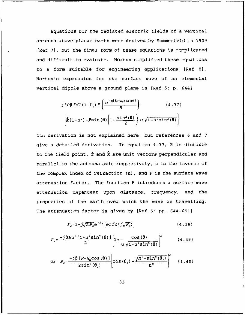
Equations for the radiated electric fields of a vertical
antenna above planar earth were derived by Sommerfeld in 1909
[Ref 7], but the final form of these equations is complicated
and difficult to evaluate. Norton simplified these equations
to a form suitable for engineering applications [Ref 81.
Norton's expression for the surface wave of an elemental
vertical dipole above a ground plane is [Ref 5: p. 644)
j 3 00 Idl (1 -r_) F ( e-j [R'-HcOs()1 (4.37)
['(l-u25 +2sin(O) l+ sin 2(e) U vl-u-sinl(W)2
Its derivation is not explained here, but references 6 and 7
give a detailed derivation. In equation 4.37, R is distance
to the field point, k and k are unit vectors perpendicular and
parallel to the antenna axis respectively, u is the inverse of
the complex index of refraction (n), and F is the surface wave
attenuation factor. The function F introduces a surface wave
attenuation dependent upon distance, frequency, and the
properties of the earth over which the wave is travelling.
The attenuation factor is given by [Ref 5: pp. 644-6511
Fe =] -j /eP@[erfc jfP)J (4.38)
P= -jPRu 2 [1)l-u 2 siu 2,s1+ cos(5) 2 (4.39)
2 U v1U 2 sin 2 (e)
or P= -jP [R+Hcos()] cos (Or) + 2n2 (4.40)2sin2 ()n3
33

where P, is the complex numerical distance for vertical
polarization and the erfc term is the complementary error
function defined by
erfc ( ) = -Lfe X22dx (4.41)
Mathcad is incapable of evaluating the complementary error
function for complex numbers, so an asymptotic expansion and
infinite series approximation [Ref 9] was written into the
Mathcad code to evaluate the erfc terms.
When the magnitude of j -V5 is less than 2.18, the
Mathcad applications use
e-X2erf(x+jy)=elf(x)++ -22x [(1-cos(2xy)) + j sin(2xy) (4.42)
,2+2 e ~ ~e tf,(XY) + J "(X +e(X, Y) where
7C n-1 4
fn (x, y) =2x-2x cosh (ny) cos (2xy) +n sinh (ny) sin (2xy)
g_ (x, y) =2x cosh (ny) sin (2xy) +n sinh (ny) cos (2xy)
le(x,y) I = 10-16 Ierf(x+jy) I
an infinite series approximation which evaluates erf(jV'-),
where 'erf' is the standard error function. [Ref 9 p. 2991.
The solution to erfc(jv',) is then found by
erfc(x+jy) =1-erf(x+jy) (4.43)
34

When the magnitude of j-V' is greater than 2.18, the
Mlathcad code uses
,/i"zez 2erfc(z) =1+ (1)mI3-5 ..... (2m-1l) (4.44)r-.i (2z 2 )M
or j iPe-Peerfc(jV/e)=1+£ (-i)' 1.3"5 .... (2m-1)m.i1 (2Pe) M
an asymptotic expansion which solves for j.V7-erfc(jV•7)
[Ref 9 p. 298]. Either of these solutions can be substituted
directly into equation 4.38 to find the surface wave
attenuation factor.
A magnitude of 2.18 is used as the transition point in the
Mathcad applications because it provides the smoothest
transition in both magnitude and phase between the series
approximation and asymptotic expansion results.
For antennas which radiate an electric field with a
component, the surface wave attenuation factor for horizontal
polarization (Fm) must be found using
Fm=l -jV e -P'erfc (jV) (4.45)
and P =-jp (R+H~cos(e))2and M"- 20+cs (0) [cos (Or) +n2 +-sin2 (0,)] 2 (4.46)
where P. is the complex numerical distance for horizontal
polarization. The variable 0, in equations 4.40 and 4.46 for
P, and P,, respectively is approximated as 0 (just as it was
for the reflection coefficients in equations 4.34 and 4.35).
35

The numerical distances (P, and P.) and the surface wave
attenuation factors (F. and F,) are evaluated for 0°s~s9O° to
determine surface wave radiation patterns. Their value is of
most interest, however, directly at the surface (0=900) where
the magnitude of F is called the ground wave attenuation
factor. Numerical distance is proportional to distance from
the antenna and the square of the frequency, while it is
approximately inversely proportional to ground conductivity.
When the magnitude of the numerical distance is less than
about 4.5, empirical formulas show that the ground wave
attenuation factor varies exponentially with numerical
distance. For numerical distance magnitudes greater than 4.5,
empirical formulas show that the ground w: ;e attenuation
factor is inversely proportional to the numerical distance.
Numerical distance magnitudes are typically much greater than
4.5 in the far-field. This implies that the ground wave
(0=900) field strength varies inversely with the square of the
distance from the antenna since numerical distance is directly
proportional to distance from the antenna and equation 4.37
shows an explicit I/R dependence in addition to the
attenuation factor.
The Mathcad applications determine the complex numerical
distances for the same discrete values of 0 described in
Chapter 4.D. After determining the complementary error
function for each numerical distance result, the surface wave
attenuation factor is calculated for each discrete 0. The
36

surface wave is evaluated for each 0 using the equations for
the electric field distribution, and the discrete results of
the surface wave are normalized with respect to the value with
maximum magnitude. The surface wave pattern is depicted by
plotting the normalized magnitudes for -r/2 < 8 < r/2. The
numerical distances (P, and P.) at the surface (0=900) are also
listed with the predicted radiation parameters.
With all of the terms defined, equation 4.37 is
integrated over the length of a generic finite length vertical
dipole to obtain the radiated surface wave distribution of an
elevated vertical dipole [Ref 6 p.166]
Ee=j6oI0 e-JPER+Hcs (0)l [cos[Phcos(@)]-cos(Ph)s ()]. (4.47)
(1-r,) F, [sin() 2 22n -inl 2(0) cos(6)j
The total radiated far-field electric field distribution
of an elevated vertical dipole above a planar earth can now be
expressed by combining equations 4.36 and 4.37 to write
E,=j60I° e'_P[Re-HOcs()]r cos[(h cos(6)]-cos(ph) (4.48)
F e sin ~n (( cs )
1 +Pve -j2Pcs(0)+ (1 -rFv) Fe ej2 cs(8)sin2()-_n2-sin2(()cos(e)
The first two teLms inside the brackets represent the space
wave and the third term represents the surface wave.
Chapter IV has defined the necessary terms and provided
a detailed derivation of the total electric field distribution
37

for an elevated vertical dipole antenna. The result is a
radiated electric field distribution with a 8 component only.
Most antenna types radiate an electric field with both 0 and
(P components. While a detailed derivation of an electric
field 4 component was not presented here, the necessary
horizontal polarization terms associated with deriving 0
components were discussed. When these horizontal terms are
substituted for their vertical counterparts, the method used
to derive the electric field equation for the 4 component of
a radiated space wave or surface wave is identical to that
used in deriving the 0 component for the elevated vertical
dipole.
The remaining chapters of this thesis explain the antenna
configuration and the calculations of each individual Mathcad
application. Only the final expressions for the radiated far-
field electric field distributions are provided since the
derivation of each follows the same procedure as explained in
this chapter. There is a lot of text repetition among the
remaining chapters because each is written as a stand alone
users guide for its associated Mathcad application. Any
important concepts not presented in previous chapters are
discussed as required.
38

V. THE ELEVATED VERTICAL DIPOLE
The orientation of the elevated vertical dipole is
depicted in Figure 5.1, where I is the length of the dipole,
Ho is the height of the feed above ground, R is the radial
coordinate, 0 is the elevation coordinate, and 0 is the
azimuth coordinate.
Z axis
o*FIELD POINT(R, 0,4))
Ho
y/ axi-1s
/.... x axi s
Vertical Dipole Orien-;ation
FIGURE 5.1: Spatial orientation of the elevated verticaldipole antenna for its corresponding Mathcad application.
39

The Mathcad application for the elevated vertical dipole
requires the following inputs:
1 ........ length of the dipole (meters)f5 ....... operational frequency (Hertz)H0 . . . . . . . antenna feed height above ground plane (meters)R ........ distance from antenna (meters)E• ....... relative dielectric constant of ground planea ........ conductivity of ground plane
The length of the dipole is used to determine the frequencies
which correspond to a X/4, X/2, 3A/4, or X length dipole. The
user inputs the frequency and the radiation parameters
discussed in Chapter 3 are calculated. Feed height (H0 ) must
be at least equal to the half-length of the dipole (h=1/2),
and the distance from the antenna (R) must meet the far-field
requirements of Chapter 3.C.
The equation for the radiated electric field distribution
of the elevated vertical dipole was derived in Chapter 4 as
E. =j 6010 ' J (R-HOcoO (e) I cos [p~h cos (0) 1-cos (ph) /(5.1)R ~sin (0)
jpocos (e)62HO e)_____ 0____ cos'9
{1+rve~r + (1 -i',) Fee i2~cs6sin2 e - V_E -Sin____
The first two terms inside the brackets represent the space
wave and the third term represents the surface wave. 10 is
one since a sinusoidal current input with a maximum of unity
is assumed.
The requested inputs are used to calculate variables at
the top of page 41 for 632 discrete values of 8 which are
equally incremented from -7/2 to r/2.
40

h ........ half-length of the dipole (meters)X5 ....... wavelength of the operational frequency (meters)
S........ free space wavenumber for operational frequencyRd ....... distance from antenna to field point (meters)R ....... distance from antenna image to field point (meters)n ........ index of refractionP ........ complex numerical distance (vertical polarization)1 ........ vertical reflection coefficientF. ....... vertical surface ;.ave attenuation factor
The calculated variables are used to evaluate the
radiated far-field space wave and surface wave for each
discrete 0. The space wave and surface wave results are
combined for corresponding values of 0 to obtain the total
radiated electric field distribution. The space wave, surface
wave, and total electric field results are then normalized
with respect to the maximum field intensity of each, and the
normalized magnitudes are plotted for each value of 0 to
depict the radiation patterns. The patterns are valid for any
vertical plane containing the antenna axis, because the
radiated electric field does not vary with changes in 0.
Equations 3.8 and 3.9 are used to integrate equation 5.1
over the hemispherical Gaussian surface above the ground plane
at a fixed radius (R) from the antenna to find total average
radiated power (Pd). With the discrete values of the electric
field and total average radiated power determined, the Mathcad
application predicts the following radiation characteristics
from the equations in Chapter 3:
Rd ..... radiation resistance (Ohms)Do ...... directivityEIRP ..... effective radiated isotropic power (Watts)A . ..... maximum theoretical effective area (square meters)1ima, ..... maximum theoretical effective length (meters)P. ...... numerical distance (vertical polarization, 0=900)Anglem .elevation angle of maximum directive gain (degrees)
41

As an example, the Mathcad vertical dipole application
was executed with the following inputs:
dipole length 3 metersfrequency 100-106 Hertzheight of antenna feed 1.5 metersdistance from the antenna 3000 metersrelative dielectric constant 15ground conductivity 5-104
Figures 5.2 and 5.3 depict the radiation patterns for the
space wave and surface wave for this example.
\ I i , . . ' " . . . i
V,"~ I
• -
. .... '1- .- I . .. . /
• , 1.... / I "\ . /
FIGURE 5.2: Vertical dipole FIGURE 5.3: Vertical dipolespace wave radiation pattern. surface wave pattern.
The following radiation parameters were predicted by the
Mathcad application for a sinusoidal current input of one Amp:
Total power radiated 31.233 WattsRadiation resistance 62.467 OhmsDirectivity 6.034Effective isotropic radiated power 188.470 WattsMaximum theoretical effective area 4.322 sq metersMaximum theoretical effective length 1.692 metersNumerical distance (vertical) 195.178Elevation of directivity 12.266 degrees
42

These results are consistent with expectations for this
particular configuration. Appendix A .ontains computer
hardcopies of additional example calculations for the vertical
dipole and compares predicted radiation parameters to those
expected based on previous calculations.
43

VI. THE VERTICAL MONOPOLE
The orientation of the vertical monopole is depicted in
Figure 6.1, where h is the length of the monopole, the antenna
feed is at around level. R is the radial coordinate, 0 is the
elevation coordinate, and 0 is the azimuth coordinate.
/z axis
A oFIELD POINT
(R,6, )
h R
y axis
X axis
Vertical Monopole Orientation
FIGURE 6.1: Spatial orientation of the vertical monopoleantenna for its corresponding Mathcad application.
44

The Mathcad application for the vertical monopole
requires the following inputs:
h ........ length of the monopole (meters)f3 ....... operational frequency (Hertz)R ........ distance from antenna (meters)E•........ relative dielectric constant of ground plane
S........ conductivity of ground plane
The length of the monopole is used to determine frequencies
which correspond to a X/8, X/4, 3A/8, or X/2 long monopole.
The user inputs the frequency for which the radiation
parameters discussed in Chapter 3 are calculated. Distance
from the antenna (R) must meet the far-field requirements of
Chapter 3.C.
The monopole's electric field distribution is derived in
the same way as the vertical dipole equation was derived in
Chapter 4 and is given by (Ref 6: p.152]
Eg=j30I eR A+jB + rV A-jB (6.1)R sin (O) sin(0)
+ -,)F.A-jB (sin 2(0)_- n 2-sin 2(a) cos(e))
sin(B) o2
(n n-i 2 (0 n 2 -sin2 (0)1
A=cos [Ph cos (0) ] -cos (Ph)
B=sin [h cos()) ]-cos(O)sin(Ph)
The first two terms inside the brackets represent the space
wave and the second two terms represent the surface wave. The
vertical monopole's far-field electric field has a 0 component
only , just as the vertical dipole. 10 is one since a
sinusoidal current input with a maximum of unity is assumed.
45

The requested inputs are used to calculate the following
variables for 632 discrete values of 0 which are equally
incremented from -w/2 to w/2:
X5 ....... wavelength of the operational frequency (meters)S........ free space wavenumber for operational frequency
n ........ index of refractionP ....... complex numerical distance (vertical polarization)
S.vertical reflection coefficientF ........ vertical surface wave attenuation factor
The calculated variables are used to evaluate the
radiated far-field space wave and surface wave for each
discrete 0. The space wave and surface wave results are
combined for corresponding values of 0 to obtain the total
radiated electric field distribution. The space wave, surface
wave, and total electric field results are then normalized
with respect to the maximum field intensity of each, and the
normalized magnitudes are plotted for each value of 0 to
depict the radiation patterns. The patterns are valid for any
vertical plane containing the antenna axis, because the
radiated electric field does not vary with changes in 0.
Equations 3.8 and 3.9 are used to integrate equation 6.1
over the hemispherical Gaussian surface above the ground plane
at a fixed radius (R) from the antenna to find the total
average radiated power (PA). With the discrete values of the
electric field and total average radiated power determined,
the Mathcad application predicts the radiation characteristics
listed at the top of the next page from the equations in
Chapter 3.
46

Radiation characteristics determined by the vertical
monopole application are:
RA ..... radiation resistance (Ohms)Do ...... directivityEIRP.....effective radiated isotropic power (Watts)A. ..... maximum theoretical effective area (square meters)in ..... maximum theoretical effective length (meters)P ....... numerical distance (vertical polarization, 8-900)Angle_..elevation angle of maximum directive gain (degrees)
As an example, the Mathcad monopole application wasexecuted with the following inputs:
monopole length 0.5 metersfrequency 150-106 Hertzdistance from the antenna 3000 metersrelative dielectric constant 15ground conductivity 5•10-1
Figures 6.2 and 6.3 depict the radiation patterns for the
space wave and surface wave for this example.
r4L> --t'-.,, ", .-k
," / .. . .\\ . ..
?IGURE 6.2: Monopole space FIGURE 6.3= Monopole surface
wave radiation pattern, wave radiation pattern.
The following radiation parameters were predicted by the
Mathcad application for a sinusoidal current input of one Amp:
47

Total power radiated 5.607 WattsRadiation resistance 11.215 OhmsDirectivity 3.246Effective isotropic radiated power 18.203 WattsMaximum theoretical effective area 1.033 sq metersMaximum theoretical effective length 0.351 metersNumerical distance (vertical) 293.016Elevation of directivity 26.815 degrees
These results are consistent with expectations for this
particular configuration. Appendix B contains computer
hardcopies of additional example calculations for the vertical
monopole and compares predicted radiation parameters to those
expected based on previous calculations.
48

VII. THE HORIZONTAL DIPOLE
The orientation of the horizontal dipole is depicted in
Figure 7.1, where 1 is length of the dipole, Ho is the height
of the feed above ground, R is the radial coordinate, 0 is the
elevation coordinate, and 0 is the azimuth coordinate.
iz axis
9FIELD POINT
/J
RK'
- I-
HI/ I
H0
y axis
xaxi s
Horizontal Dipole_ Orientation
FIGURE 7.1: Spatial orientation of the horizontal dipoleantenna for its corresponding Mathc d application.
49

The Mathcad application for the horizontal dipole requires
the following inputs:
1 ........ length of the dipole (meters)H0 ....... antenna feed height above ground plane (meters)f5 ....... operational frequency (Hertz)R ........ distance from antenna (meters)E ........ relative dielectric constant of ground planea ........ conductivity of ground planed ........ elevation angle index (from Table 3.1)
The length of the dipole is used to determine frequencies
which correspond to a X/4, X/2, 3X/4, or X length dipole. The
user inputs the frequency for which the radiation parameters
discussed in Chapter 3 are computed. Feed height, HO, must be
greater than or equal to zero, and distance from the antenna
(R) must meet the far-field requirements of Chapter 3.C. The
elevation angle index (d) sets the elevation coordinate, 0,
for which a horizontal radiation pattern is determined. Table
3.1 lists possible indices and their corresponding elevation
angles from .2850 to 88.8570 in increments of about 20.
Indices between those listed can be used to interpolate a
better approximation of a desired elevation.
The horizontal dipole's radiated electric field is a
combination of R and $ components. In addition, unlike the
vertical dipole, its radiation pattern varies with changes in
4. The total radiated electric field is the vector sum of the
Sand $ components. The electric field for the horizontal
dipole is obtained in a manner analogous to that used for the
vertical dipole discussed in Chapter 4. The horizontal
dipole's ý and ý field components are given by [Ref 6: p. 144]
5o

co(CO)I h sin (0) cos (4))1 -cos (ph). (7.1)e-Sin 2 ()COS (0) . )
) [cos (0) ( -Fve -j2P11coS (0)R I
+(-I'v) Fe-j2PHocOs() (n2-sin2(W) sin - 2 (0) cos (0)e n 2
E,=j6IOIsin ()( cos [Ph sin (0) cos (g) -cos (7.2)1-sin2 (6) cos[ ((0)
e _j [,RHOCO [(0 +Ph -j2PHOCOS (0) + (1 -r. Fe -i2PHoCO3 (0)1R h
The first two terms inside the brackets of each equation are
the space wave components and the third terms are the surface
wave components. 10 is taken to be one, since a sinusoidal
current input with a maximum of unity is assumed.
The requested inputs are used to calculate the following
variables using a constant 0 of =0 and O=w/2 for 632 discrete
values of 0 which are equally incremented from -r/2 to ir/2:
h ....... half-length of the dipole (meters)X5 ...... wavelength of the operational frequency (meters)S....... free space wavenumber for operational frequencyRd ...... distance from antenna to field point (meters)R ....... distance from antenna image to field point (meters)n ....... index of reiractionP ...... complex numerical distance (vertical polarization)Pm ..... complex numerical distance (horizontal polarization).r ...... vertical reflection coefficientr, ...... horizontal reflection coefficientF ....... vertical surface wave attenuation factorFm ..... horizontal surface wave attenuation factor
The calculated variables are used to evaluate the far-
field space wave and surface wave for the discrete values of
0 for 0=0 and O=r/2. The total space wave and surface wave
distributions are determined from vector addition of
51

corresponding ý and ý components. The space wave and surface
wave results aLe then combined for corresponding discrete
values of 0 to obtain the total radiated electric field
distribution for the 0=0 and O=w/2 vertical planes. The space
wave, surface wave, and total electric field results are then
normalized with respect to the maximum field intensity of
each, and the normalized magnitudes are plotted for each
discrete 0 to depict the radiation patterns. The Mathcad
horizontal dipole application computes the space wave, surface
wave, and total electric field radiation patterns and
radiation parameters in the 0=0 and O=i/2 vertical planes.
The variables corresponding to the selected elevation
angle index (d) are used to evaluate the radiated electric
field components for the space wave and surface wave at the
fixed elevation angle (0 .) as 4 varies from 0 to 2w in 632
equal increments. The horizontal radiation patterns are then
plotted for the space wave, surface wave, and total radiated
electric field just as those for the vertical planes.
To find the contributions of the b and ý electric field
components to the total average radiated power (Pd), equations
3.8 and 3.9 are used to integrate equations 7.1 and 7.2 over
the hemispherical Gaussian surface above the ground plane at
a fixed radius (R) from the antenna. With the discrete values
of the electric field and total average radiated power, the
Mathcad application predicts the following radiation
characteristics from the equations in Chapter 3:
52

R,,d ..... radiation resistance (Ohms)Do ....... directivityEIRP ..... effective radiated isotropic power MWatts)Am,, . . . . . . maximum theoretical effective area (square meters)lma, ..... maximum theoretical effective length (meters)P ...... numerical distance (vertical polarization, 0-900)Pm ...... numerical distance (horizontal polarization, 0=900)Angle, . elevation angle of maximum directive gain (degrees)
The directivity (DO), effective isotropic radiated power
(EIRP), maximum theoretical effective area (A.,), maximum
theoretical effective length (l.), and the elevation angle of
maximum directive gain (Angle,,) are all determined for both
the 0=0 and O=r/2 vertical planes.
As an example, the Mathcad horizontal dipole application
was executed with the following inputs:
dipole length 1.0 meterfrequency 150.106 Hertzheight of antenna feed 1.0 meterdistance from the antenna 3000 metersrelative dielectric constant 15ground conductivity 10.2elevation angle index 535 (-270)
The following radiation parameters were predicted by the
Mathcad application for a sinusoidal current input of one Amp:
Total power radiated (Watts) 26.116Radiation resistance (Ohms) 52.233Numerical distance (vertical) 292.419Numerical distance (horizontal) 66215.4
't=0 !=ir/2
Directivity 1.310 7.215EIRP (Watts) 34.221 188.435Max eff area (sq meters) 0.417 2.297Max eff length (meters) 0.481 1.128Anglemax (degrees) 45.071 28.241
Figures 7.2 through 7.7 are the space wave and surface
wave radiation patterns in the 0=0 and 0=w/2 vertical planes
and the designated horizontal plane for this example.
53

--
Il'l
FIGURE 7.2: Horizontal FIGURE 7.3: Horizontaldipole space wave radiation dipole surface wave radiationpattern for 4) 0 vertical pattern for 4)=0 verticalplane. plane.
IL: 1...~~. .- .X ........--
plne plne
54

", ~ ~ ~ ~~~~.. ....... " i... .... :/ . .. .'" " "\ I " I ' " •' •'
-- 4 . .---- -
-AxS...i
t ...
"FIGURE 7.6- Horizontal FIGURE 7.7: Horizontaldipole space wave radiation dipole surface wave radiationpattern for horizontal plane. pattern for horizontal plane.
These results are consistent with expectations for this
particular configuration. Appendix C contains computer
hardcopies of additional example calculations for the
horizontal dipole and compares predicted radiation parameters
to those expected based on previous calculations.
55

VIII. THE ARBITRARILY ORIENTED DIPOLE
The orientation of the arbitrarily oriented dipole is
depicted in Figure 8.1, where 1 is length of the dipole, H0 is
the feed height above ground, a is the angle of the dipole
axis with the horizontal, R is the radial coordinate, 0 is the
elevation coordinate, and 0 is the azimuth coordinate.
z axis
/
FIELD POINT* (R, O, )
/ i;y axis
,/
///
//
/'x axis
Arbitrarily Oriented Dipole Orientation
FIGURE 8.1: Spatial orientation of the arbitrarilyoriented dipole antenna for its Mathcad application.
56

The Mathcad application for the arbitrarily oriented
dipole requires the following inputs:
1 ........ length of the dipole (meters)H0 . . . . . . . antenna feed height above ground plane (meters)S........ angle of antenna axis with the horizontal (degrees)f5 ....... operational frequency (Hertz)R ........ distance from antenna (meters)Cr ....... relative dielectric constant of ground planeS........ conductivity of ground planed ........ elevation angle index (from Table 3.1)
The length of the dipole is used to determine frequencies
which correspond to a X/4, X/2, 3A/4, or X length dipole. The
user inputs the frequency for which the radiation parameters
discussed in Chapter 3 are computed. Feed height, H0 , must be
greater than or equal to (i/2).sin(u), and the distance from
the antenna (P) must meet the far-field requirements of
Chapter 3.C. The elevation angle index (d) sets the elevation
coordinate, 9, for which a horizontal radiation pattern is
determined. Table 3.1 lists possible indices and their
corresponding elevation angles from .2850 to 88.8570 in
increments of about 20. Indices between those listed can be
used to interpolate a better approximation of a desired
elevation.
The radiated electric field for the arbitrarily oriented
dipole is a combination of 0 and ý components, and its
radiation pattern varies with changes in 0. The total
electric field is the vector sum of the 0 and ý components.
The arbitrarily oriented dipole's radiated electric field is
obtained in a manner analogous to that used for the vertical
dipole discussed in Chapter 4, and is given by
57

E9-6O~ e-PRJPe pzcosge} (8.1)F,9-j60Xo R POCSO
R
{lA -(cos (a) sin (4) cos (8) -sin (a) sin ())1-cos2(4r)
-rv A2 (cos(a)sin(•)cos(0)+sin(a)sin(0) )e-j2co9(8)-(cos2 (W0)
+( -rv) Fee-J2PHOCOs(0'2 (sin2 (9) - Vn 2-sin2 (0) cos (0))l-sin2 (*I) n 2
n 2 -sin 2(e)
E,=j6O1I0 &- eJPHOCOZ ( cos(a)cos(O) (8.2)
l A _+ A2 -i 2 OCOS e(e)(fh+ (1-rh) F,)1-coS 2 (*k) 1-_COS 2 (4)hij
where A1=cos [ph cos (4)]-cos (ph)
cos (w) =cos (0) sin (a) +sin (0) cos (a) sin (1)
A2=cos [Ph cos (4')] -cos (ph)
cos (Wi) =sin (0) cos (a) sin (4) -cos (0) sin(a)
Equation 8.1 is the • component (vertically polarized), and
equation 8.2 is the • (horizontally polarized) component [Ref
6: p. 174-175]. The first two terms inside the brackets of
each equation represent the space wave components and the
third terms represent the surface wave components. 10 is
taken to be one, since a sinusoidal current input with a
maximum of unity is assumed.
58

The requested inputs are used to calculate the following
variables using a constant 0 of 0=0 and O=w/2 for 632 discrete
values of 0 which are equally incremented from -7/2 to 7/2:
h ....... half-length of the dipole (meters)X5 ...... wavelength of the operational frequency (meters)0 ....... free space wavenumber for operational frequencyRd ...... distance from antenna to field point (meters)Rr ...... distance from antenna image to field point (meters)n ....... index of refractionP ...... complex numerical distance (vertical polarization)Pm ..... complex numerical distance (horizontal polarization)r ...... vertical reflection coefficientrh ...... horizontal reflection coefficientF ...... vertical surface wave attenuation factorFM ..... horizontal surface wave attenuation factor
The calculated variables are used to evaluate the far-
field space wave and surface wave for the discrete values of
0 for 0=0 and O=w/2. The total space wave and surface wave
distributions are determined from vector addition of
corresponding ý and $ components. The space wave and surface
wave results are then combined for corresponding discrete
values of 0 to obtain the total radiated electric field
distribution for the 0=0 and O=w/2 vertical planes. The space
wave, surface wave, and total electric field results are then
normalized with respect to the maximum field intensity of
each, and the normalized magnitudes are plotted for each
discrete 0 to depict the radiation patterns. The arbitrarily
oriented dipole Mathcad application computes the space wave,
surface wave, and total electric field radiation patterns and
radiation parameters in the 0=0 and O=a/2 vertical planes.
The variables corresponding to the selected elevation
angle index (d) are used to evaluate the radiated electric
59

field components for the space wave and surface wave at the
fixed elevation angle (0d) as 0 varies from 0 to 2w in 632
equal increments. The horizontal radiation patterns are then
plotted for the space wave, surface wave, and total radiated
electric field just as those in the vertical planes.
To find the contributions of the ; and $ electric field
components to the total average radiated power, P,,, equations
3.8 and 3.9 are used to integrate equations 8.1 and 8.2 over
the hemispherical Gaussian surface above the ground plane at
a fixed radius (R) from the antenna. The sum of the two
integrals is the antenna's P,. With the discrete values of
the electric field and total average radiated power
determined, the Mathcad application predicts the following
radiation characteristics from the equations in Chapter 3:
R... ..... radiation resistance (Ohms)Do ....... directivityEIRP ..... effective radiated isotropic power (Watts)A,, ..... maximum theoretical effective area (square meters)lnx ..... maximum theoretical effective length (meters)P ........ numerical distance (vertical polarization, 0=900)Pm ...... numerical distance (horizontal polarization, 6=900)Angle,, .elevation angle of maximum directive gain (degrees)
The directivity (DO), effective isotropic radiated power
(EIRP), maximum theoretical effective area (A,.), maximum
theoretical effective length (I.), and the elevation angle of
maximum directive gain (Angle.) are all determined for both
the 0=0 and O=w/2 vertical planes.
60

IX. INVERTED L ANTENNA
The orientation of the inverted L antenna is depicted in
Figure 9. 1, where H is length of the vertical antenna segment,
1 is the length of the horizontal antenna segment, the feed is
at ground level, R is the radial coordinate, 0 is the
elevation coordinate, and 0 is the azimuth coordinate.
/z axis1
AS FIELD POINT
(R, 0,.)
RH
y axis
x axis
Inverted L Antenna Orientation
FIGURE 9.1: Spatial orientation of the inverted L antennafor its corresponding Mathcad application.
61

The Mathcad application for the inverted L antenna
requires the following inputs:
H ........ length of vertical antenna segment (meters)1 ........ length of horizontal antenna segment (meters)f5 ....... operational frequency (Hertz)R ........ distance from antenna (meters)e. ........ relative dielectric constant of ground plane
S........ conductivity of ground planed ........ elevation angle index (from Table 3.1)
The combined length of the vertical and horizontal antenna
segments (H+l) is used to determine frequencies which
correspond to a X/8, X/4, 3A/8, or X/2 long inverted L
antenna. The user inputs the frequency for which the
radiation parameters discussed in Chapter 3 are computed.
Distance from the antenna (R) must meet the far-field
requirements of Chapter 3.C. The elevation angle index (d)
sets the elevation coordinate, 0, for which a horizontal
radiation pattern is determined. Table 3.1 lists possible
indices and their corresponding elevation angles from .2850 to
88.8570 in increments of about 20. Indices between those
listed can be used to interpolate a better approximation of a
desired elevation.
The inverted L's radiated electric field is a varying
combination of i and $ components; and its radiation pattern
varies with changes in 0. The total radiated electric field
is the vector sum of the G and $ components. The radiated
electric field for the inverted L antenna is obtained in a
manner analogous to that used for the vertical dipole
discussed in Chapter 4. The radiated fields of each antenna
62

segment are considered separately, and superposition is us-d
to determine the total radiated elec ric field. The vertical
segment radiates only a 0 field component, but the horizontal
segment radiates both ý and ý components. The electric field
equations for the inverted L are [Ref 6: p. 169-170]
3 etP[ A,+jBv r Av-jB(3 sin(0) vsin(0)
+ si--,n(F.Av- jBV[ (Sin n 2- sinn2 (6) cos (8)+ (l-rv) Fe nsiis (0)
-[sin [ (HI1) ] -sin (P1) cos (PH cos (8)]
+jsin(Pi) sin [PH cos (0) ]]j2F,(sin2 (0) n2-sin2"') cos(0e) )n 2 -sin2s(0) (e)
cos02) n 2si~n(O))
where Av=cos [pHcos(0)]cos(fi)-cosf[l3(H+1)3
-sin[PH cos (O)]cos (', sin(f31)
By=sin [pHcos(8)]cos(fi)-cos(0)sin[f (H+I)]
+coS ([PH cos (8) ] cos (8) sin (P2)
-jOR tan'Bhsin (1) cos (0) eJ a
1 -sin2 (0) sin2 (4)) R e ,.+B
{l-ve-J22AcOS(e)+ (sin2 (0) - n 2 'sin 2 (0) cos(8))
L -r.) F~eij2pHcos(e) Vn 2-sin2 (0)1n2
E h=j 3 0/0 cos (4) e-jPR tnAh B,2+ (9.3)E h j o o e 7 11 A 2 ,h+ Z h (
l-sin 2 (8) sin2 (4t) R
fi +rhe .j2DHcos(e) + ( I -rh) F.,e -j20Hcos (0)
where Ah=cos [PI sin (0) sir. (4))] -cos (PI)
Bh=sin[T[l sin(0)sin(4))]-sin(0)sin(4))sin(p2)
63
Equation 9.1 is the a component for the vertical segment,
equation 9.2 is the 0 (vertically polarized) component for the
horizontal segment, and equation 9.3 is the ý (horizontally
polarized) component for the horizontal segmeýnt. The first
two terms inside the brackets of each equation are the space
wave components and any additional terms are the surface wave
components. 10 is taken to bc one, since a sinusoidal current
input with maximum of unity is assumed.
The requested inputs are used to calculate the following
variables using a constant 0 of 0=0 and O=w/2 for 632 discrete
values of 0 which are equally incremented from -ir/2 to g/2:
h ....... half-length of the dipole (meters)X5 ...... wavelength of the operational frequency (meters)S....... free space wavenumber for operational frequencyRd ...... distance from antenna to field point (meters)R ....... distance from antenna image to field point (meters)n ....... index of refractionP ....... complex numerical distance (vertical polarization)Pm ...... complex numerical distance (horizontal polarization)r ...... vertical reflection coefficientr. ...... horizontal reflection coefficientF. ...... vertical surface wave attenuation factorFm. ..... horizontal surface wave attenuation factor
The calculated variables are used to evaluate the far-
field space wave and surface wave for the discrete values of
0 for 0=0 and O=g/2. The total space wave and surface wave
distributions are determined from vector addition of
corresponding ý and ý components. The space wave and surface
wave results are then combined for corresponding discrete
values of 0 to obtain the total radiated electric field
distribution for the 0=0 and 0=7/2 vertical planes. The space
wave, surface wave, and total electric field results are then
64

normalized with respect to the maximum field intensity of
each, and the normalized magnitudes are plotted for each
discrete 0 to depict the radiation patteu.ns. The inverted L
Mathcad application computes the space wave, surface wave, and
total electric field radiation patterns and radiation
parameters in the 0=0 and 0=r/2 vertical planes.
The variables corresponding to the selected elevation
angle index (d) are used to evaluate the radiated electric
field components for the space wave and surface wave at the
fixed elevation angle ( 0 d) as 0 varies from 0 to 2w in 632
equal increments. The horizontal radiation patterns are then
plotted for the space wave, surface wave, and total radiated
electric field just as those for the vertical planes.
To find the contributions of the 0 and $ electric field
components to the total average radiated power, P,.d, equations
3.8 and 3.9 are used to integrate equations 9.1, 9.2, and 9.3
over the hemispherical Gaussian surface above the ground plane
at a fixed radius (R) from the antenna. The sum of the
integrals is the antenna's Pd. With the discrete values of
the electric field and total average radiated power
determined, the Mathcad application predicts the following
radiation parameters using the equations from Chapter 3:
Rr..d ..... radiation resistance (Ohms)Do . . . . . . . directivityEIRP ..... effective isotropic radiated power (Watts)Ama.. ..... maximum theoretical effective area (square meters)Imax ..... maximum theoretical effective length (meters)Pý ....... numerical distance (vertical polarization, 0=900)P. ...... numerical distance (horizontal polarization, 0=900)Angle., .elevation angle of maximum directive gain (degrees)
65

The directivity (DO), effective isotropic radiated power
(EIRP), maximum theoretical effective area (A.), maximum
theoretical effective length (l.), and the elevation angle of
maximum directive gain (Angle,) are all determined for both
the =0 and O=r/2 vertical planes.
66

X. THE SLOPING LONG-WIRE ANTENNA
The orientation of the sloping long-wire antenna is
depicted in Figure 10.1, where 1 is length of the antenna, the
feed is at ground level, a is the angle of the antenna with
the horizontal, R is the radial coordinate, 0 is the elevation
coordinate, and 0 is the azimuth coordinate.
z axis
. FIELD POINT(R,,4ý)
"" iax
//
/
ix axis
Sloping Long-Wire Orientation
FIGURE 10.1: Spatial orientation of the sloping long-wireantenna for its corresponding Mathcad application.
67

The Mathcad application for the sloping long-wire antenna
requires the following inputs:
1 ........ length of the antenna (meters)S........ angle of antenna with horizontal (degrees)f5 ....... operational frequency (Hertz)R ........ distance from antenna (meters)E ........ relative dielectric constant of ground plane
S........ conductivity of ground planed ........ elevation angle index (from Table 3.1)
The user inputs the frequency (f.) for which the radiation
parameters discussed in Chapter 3 are computed. The distance
from the antenna (R) must meet the far-field requirements of
Chapter 3.C. The elevation angle index (d) sets the elevation
coordinate, 0, for which a horizontal radiation pattern is
determined. Table 3.1 lists possible indices and their
corresponding elevation angles from .2850 to 88.8570 in
increments of about 20. Indices between those listed can be
used to interpolate a better estimate of a desired elevation.
The electric field equations for the sloping long-wire
are given by [Ref 6: p. 180-1811
E.=-j 3010 R
AI+jB 1 [cos (a) sin (40 cos (0) -sin (a) sin ((0) 1 i .i
l-cos2 )- A2+jB 2 [cos(&)sin(ý)cos(O) +sin(a)sin(6)]
1-cos2 (h)
A2 +JB 2 (sin2(e) n 2 -sin 2 (6)+ (i-r,) icos2 _ cos" (
cos(a)sin() n 2- sin2( -sin(a) sin(0)n6
68

E#=j3 0 e--cos(a)cos(4ý) (10.2)R
A 1 +jBBI A 2+jB 2 A2 +jB 2 1{ l-cos 2 () ÷h I-COS,(W)+ (l-oh) F.(*I)
where A1=cos[P31 cos(4)]-cos(j3i)
B,=sin [P1 Cos (40 ] -sin (Pi) cos()
cos () =COS () sin (a) +sin (e)cos(a) sin (i)
A2 =cos [P1 cos (4)6 -cos (Pi)
B2=sin[PI cos (*I)]I-sin (Pl) cos)
cos (V') =sin (0) cos (a) sin (() -cos (0) sin (a)
The radiated electric field for the sloping long-wire is 22
obtained in a manner analogous to the vertical dipole equation
discussed in Chapter 4. The long-wire's radiated electric
field is a varying combination of i and • components, and its
radiation patterns vary with changes in •. The total radiated
electric field is the vector sum of the 0 and ý components.
The first two terms inside the brackets of each equation are
the space wave components and the additional terms are the
surface wave components. I0 is taken to be one since a
sinusoidal current input with a maximum of unity is assumed.
Requested inputs are used to compute the variables on the
next page using a constant 0 of 0=0 and O=r/2 for 632 discrete
values of 0 which are equally incremented from -w/2 to w/2.
X5 ...... wavelength of the operational frequency (meters)S....... free space wavenumber for operational frequencyn ....... index of refractionP .complex numerical distance (vertical polarization)P. ..... complex numerical distance (horizontal polarization)r ....... vertical reflection coefficientrh ...... horizontal reflection coefficientF. ...... vertical surface wave attenuation factorFm ..... horizontal surface wave attenuation factor
69

The calculated variables are used to evaluate the far-
field space wave and surface wave for the discrete values of
0 for 0=0 and O=n/2. The total space wave and surface wave
distributions are determined from vector addition of
corresponding 6 and ý components. The space wave and surface
wave results are then combined for corresponding discrete
values of 0 to obtain the total radiated electric field
distribution for the 0=0 and O=r/2 vertical planes. The space
wave, surface wave, and total electric field results are then
normalized with respect to the maximum field intensity of
each, and the normalized magnitudes are plotted for each
discrete 0 to depict the radiation patterns. The sloping
long-wire Mathcad application computes the space wave, surface
wave, and total electric field radiation patterns and
radiation parameters in the 0=0 and O=r/2 vertical planes.
The variables corresponding to the selected elevation
angle index (d) are used to evaluate the radiated electric
field components for the space wave and surface wave at the
fixed elevation angle (08) as 0 varies from 0 to 27 in 632
equal increments. The horizontal radiation patterns are then
plotted for the space wave, surface wave, and total radiated
electric field just as those for the vertical planes.
To find the contributions of the 9 and ý electric field
components to the total average radiated power, P,, equations
3.8 and 3.9 are used to integrate equations 10.1 and 10.2 over
the hemispherical Gaussian surface above the ground plane at
70

a fixed radius (R) from the antenna. The sum of the integrals
is the antenna's Pram- With the discrete values of the electric
field and total average radiated power determined, the Mathcad
application predicts the following radiation parameters using
the equations from Chapter 3:
Rrad ..... radiation resistance (Ohms)Do . . . . . . . directivityEIRP.....effective isotropic radiated power (Watts)A,. ..... maximum theoretical effective area (square meters)Imax ..... maximum theoretical effective length (meters)Pý ....... numerical distance (vertical polarization, 6=90")P. ...... numerical distance (horizontal polarization, 0=900)Angle,, .elevation angle of maximum directive gain (degrees)
The directivity (DO), effective isotropic radiated power
(EIRP), maximum theoretical effective area (A,.), maximum
theoretical effective length (l,), and the elevation angle of
maximum directive gain (Angle,) are all determined for both
the 0=0 and O=w/2 vertical planes.
71

XI. THE TERMINATED SLOPING V ANTENNA
The orientation of the terminated sloping V antenna is
depicted on the next page in Figure 11.1, where 1 is length of
the antenna wires (numbered 1 and 2), H0 is the feed height
above ground, H, is the height of the termination points above
ground, 7 is the angle subtended by the wires, n is the angle
between the x axis and the projection of the antenna legs in
the x-y plane, a is the angle between the plane which contains
the antenna and the x-y plane, R is the radial coordinate, 0
is the elevation coordinate, and 0 is the azimuth coordinate.
The Mathcad application for the sloping V antenna requires
the following inputs:
1 ........ length of the antenna legs(meters)H0 . . . . . . . feed height above ground (meters)H, ....... height of termination points above ground (meters)y ........ angle subtended by the antenna legs (degrees)f5 ....... operational frequency (Hertz)R ........ distance from antenna (meters)E.......... relative dielectric constant of ground planeS........ conductivity of ground planed ........ elevation angle index (from Table 3.1)
The user inputs the frequency (f.) for which the radiation
parameters discussed in Chapter 3 are computed. The feed
height (H0) and termination height (HI) can be any value
greater than zero. The angle a is found from HO, H,, wire
length (1), and the half-angle between the wires (7/ 2 ) by
a=sin-11 HI-HOCos(11.1)
72

FIELD POINT
yaxis
A x axls
Terminated Sloping V Antenna OrientationFIGUR 11.1: Spatial orientation of the terminatedsloping V antenna for :its corresponding Mathcadapplication.
The angle n is then found from a and 7/2 by
S cos(a)
Distance from the antenna (R) must meet the far-field
requirements of Chapter 3.C. The elevation angle index (d)sets the 0 coordinate for which a horizontal radiation pattern
is determined. Table 3.1 lists possible indices and their
corresponding elevation angles from .285( to 88.8570 in
73

increments of about 20. Indices between those listed can be
used to interpolate a better estimate of a desired elevation.
The radiated electric field for the sloping V antenna is
obtained in a manner analogous to that used for the vertical
dipole discussed in Chapter 4. The sloping V electric field
equations are given by [Ref 6: p. 185-1861
EO.i=301o e jRCos (cc) Cos (0) Cos (40-7) l-e-jolu, 113E6 ,301 (11.3)
_v -e -jp1U 3 -j2PCos (0) 1- e -jpLU3 e-j2PHOcos(8)e+(I-rv) F6
-sin2 n(O)[ -sJIn Ur, -j(8 o8 2 iU 11
+ (I-r,) Fe 1-O-JPeUU e-J2PHOcos(8)(sin2 (0) - •n 2 sin(2 cos(0)]}
E#,I=01° -JPR[
E#.,=3 I -ýcos(a)sin(4o-,) l-e-Jpiul 114R u, 114
-r+ (i-rh) F, l-e -jPIU3 e-j2PH0 COS (e)1
+ _____3_ e s(0) + 1 )U 3
where U1=l-cos (9F) U3=i-cos (T 3 )
cos (TO) =cos (0) sin(a) +sin (0) cos (a) cos (4-0)
cos (T3) =sin (0) cos (a) cos (4-)) -cos (0) sin(a)
74

OIejAR 1l-e -Jolu,E."=301. -Cos (a) cos (6) Cos (40)[ 1-e (11.5)
e~oRI U2
-rv l-e-jolu4 -j20H0 COS (e) + (I -rv) F 1- e -j•lU4 e -j2AHOCOS (0)e e ,
k n2-cos( ) n 2 cos (a)
+sn()si (8 -e-JolU, l-e-jplUl -j2P~fCOS(0)+sn(a)snU2 r U[
+(e-v) F. I-e-j' 1 -e2PHOCO(sin2 n• 2 -sin 2 (0) cos(0U4 n 2
E,, 1=-301Z7o eiPcos(c)sin(+,) 1-e-jPlU2 (11.6)
+ rh l-e-jplz74 e -j2AH VOcS(0) + (I-rh) F , 1-e-P e(U4 -J2PHOCOS(0)
where U2=1-cos (T 2 ) U4 =1-cos (I 4 )
cos (T 2 ) =cos (0) sin (a) +sin (0) cos (a) cos (4o-q)
cos(T 4)=sin(O)cos(a)cos($+q)-cos(8)sin(a)
The sloping V's radiated electric field is a varying
combination of D and ý components, and its radiation pattern
varies with changes in 0. The total radiated electric field
is the vector sum of the D and ý components. The fields of
each antenna leg are considered separately, and superposition
is used to determine the total electric field. Equations 11.3
and 11.4 are the radiated 0 and $ components, respectively for
75

number one, and equations 11.5 and 11.6 are the 0 and
components, respectively for wire number two. The first two
terms inside each set of brackets represent the space wave
components and any additional terms represent the surface wave
components. 10 is taken to be one, since a sinusoidal current
input with a maximum of unity is assumed.
The requested inputs are used to calculate the following
variables using a constant 0 of 0=0 and O=w/2 for 632 discrete
values of 0 which are equally incremented from -i1/2 to 7r/2:
X5 ...... wavelength of the operational frequency (meters)S....... free space wavenumber for operational frequency
n ....... index of refractionP ....... complex numerical distance (vertical polarization)Pm ..... complex numerical distance (horizontal polarization)S...... vertical reflection coefficientr. ...... horizontal reflection coefficientF ...... vertical surface wave attenuation factorF. ..... horizontal surface wave attenuation factor
The calculated variables are used to evaluate the far-
field space wave and surface wave for the discrete values of
0 for 0=0 and O=r/2. The total space wave and surface wave
distributions are determined from vector addition of
corresponding b and ý components. The space wave and surface
wave results are then combined for corresponding discrete
values of 0 to obtain the total radiated electric field
distribution for the 0=0 and O=w/2 vertical planes. The space
wave, surface wave, and total electric field results are then
normalized with respect to the maximum field intensity of
each, and the normalized magnitudes are plotted for each
discrete 8 to depict the radiation patterns. The sloping V
76

Mathcad application computes the space wave, surface wave, and
total electric field radiation patterns and radiation
parameters in the 0=0 and 0=7T/2 vertical planes.
The variables corresponding to the selected elevation
angle index (d) are used to evaluate the radiated electric
field components for the space wave and surface wave at the
fixed elevation angle (0d) as 0 varies from 0 to 27 in 632
equal increments. The horizontal radiation patterns are then
plotted for the space wave, surface wave, and total radiated
electric field just as those for the vertical planes.
To find the contributions of the 0 and ý electric field
components to the total average radiated power, P,.d, equations
3.8 and 3.9 are used to integrate equations 11.3, 11.4, 11.7,
and 11.6 over the hemispherical Gaussian surface above the
ground plane at a fixed radius (R) from the antenna. The sum
of the integrals is the antenna's P,d- With the discrete
values of the electric field and total average radiated power
determined, the Mathcad application predicts the following
radiation parameters using the equations from Chapter 3:
R,.. ..... radiation resistance (Ohms)D( . . . . . . . directivityEIRP ..... effective isotropic radiated power (Watts)PM; .. .. .maximurn theoretical effective area (square meters)1iý ..... maximum theoretical effective length (meters)Pc ....... numerical distance (vertical polarization, 0=900)P. numF ical distance (horizontal nolarization, 0=900)Angle,, .elevation angle of maximum directive gain (degrees)
The directivity (DO), effective isotropic radiated power
(EIPP), maximum theoretical effective area (A,), maximum
77

theoretical effective length (1i), and the elevation angle of
maximum directive gain (Angle,) are all determined for both
the 0=0 and O=r/2 vertical planes-
78

XII. THE SIDE-LOADED VERTICAL HALF RHOMBIC ANTENNA
The orientation of the side-loaded vertical half rhombic
antenna is depicted in Figure 12.1, where 1 is length of the
antenna wires (numbered 1 and 2), the feed is at ground level,
a is the angle between the antenna wires and the horizontal
plane, R is the radial coordinate, 6 is the elevation
coordinate, and • is the azimuth coordinate.
FIELD POINT
(R,,)' ;z axis
S0~
S1:
--•y axis
x axis
Side-Loaded Vertical Half-Rhombic Orientation
FIGURE 12.1: Spatial orientation of the side-loadedvertical half rhombic antenna for its Mathcad application.
79

The Mathcad application for the vertical half rhombic
antenna requires the following inputs:
1 ........ length of the antenna legs(meters)S........ angle of antenna wires with horizontal (degrees)f5 ....... operational frequency (Hertz)R ........ distance from antenna (meters)E ,......... relative dielectric constant of ground planea......... conductivity of ground planed ........ elevation angle index (from Table 3.1)
The user inputs the frequency (f 5 ) for which the radiation
parameters discussed in Chapter 3 are computed. Distance from
the antenna (R) must meet the far-field requirements of
Chapter 3.C. The elevation angle index (d) sets the 0
coordinate for which a horizontal radiation pattern is
determined. Table 3.1 lists possible indices and their
corresponding elevation angles from .2850 to 88.8570 in
increments of about 20. Indices between those listed can be
used to interpolate a better approximation of a desired
elevation.
The vertical half rhombic's radiated electric field is a
combination of 0 and s components, and its radiation pattern
varies with changes in 0. The total radiated electric field
is the vector sum of the b and ý components. The radiated
electric field for the vertical half rhombic antenna is
obtained in a manner analogous to that used for the vertical
dipole discussed in Chapter 4. The radiated fields of each
antenna leg are considered separately, and superposition is
used to determine the total electric field. The electric
field equations for the half rhombic are [Ref 6: p. 198-200]
80

E8,=301 e jRCos (a) Cos (0) Cos(40)fI-e-o. (12.1),0 -R I[IU,
U2____ a.elU2
sin 2 ()- Vn2-sin2 (0WO ()) 2-si 2 (0-)
+(1 TvFe ~e~l 2 C s(e) ýr¶~ n2I Icsi(n
+sina~sU 2 O +1-,eTh)1Fe jpu
U, U2
e21i()o()+ (1-r, ,1-To(sn2( ) -F 6 1-sn2e )., Co2~sin~cs
E#,,=-3010 R ePcos(d)sin(lo){1e UeiP (12.4)
rhIe-jP'U2 + (1-r,,) F. l-e-1UU2 U2~
Ee2=30,-ýý-jlu cs~o(OCOOP 1e-~l28123

where U, and U2 are given by
U1=l-cos (h)) U2=1-cos (T 2)
COS (IF) =COS (e) sin(a) +sin(e) cos (a) cos()
cos (T2) =sin(8) cos (a) cos (4) -cos (e) sin (a)
Equations 12.1 and 12.2 are the b (vertically polarized) and
$ (horizontally polarized) components, respectively for leg
number one, and equations 12.3 and 12.4 are the 0 and ý
components, respectively for leg number two. The first two
terms inside each set of brackets are the space wave
components and any additional terms are the surface wave
components. 10 is taken to be one, since a sinusoidal current
input with a maximum of unity is assumed. The requested
inputs are used to calculate the following variables using a
constant 0 of 0=0 and 0=r/2 for 632 discrete values of 0 which
are equally incremented from -w/2 to w/2:
X5 ...... wavelength of the operational frequency (meters)S....... free space wavenumber for operational frequencyn ....... index of refractionP, ...... complex numerical distance (vertical polarization)P, ..... complex nu~cicrical distance (horizontal polarization)r ...... vertical reflection coefficientrh ...... horizontal reflection coefficientF ....... vertical surface wave attenuation factorFm ..... horizontal surface wave attenuation factor
The calculated variables are used to evaluate the far-
field space wave and surface wave for the discrete values of
0 for 0=0 and O=w/2. The total space wave and surface wave
distributions are determined from vector addition of
corresponding b and $ components. The space wave and surface
82

wave results are then combined for corresponding discrete
values of 0 to obtain the total radiated electric field
distribution for the 0=0 and O=r/2 vertical planes. The space
wave, surface wave, and total electric field results are then
normalized with respect to the maximum field intensity of
each, and the normalized magnitudes are plotted for each
discrete 0 to depict the radiation patterr- The vertical
half rhombic Mathcad application computes the space wave,
surface wave, and total electric field radiation patterns and
radiation parameters in the 0=0 and O=w/2 vertical planes.
The variables corresponding to the selected elevation
angle index (d) are used to evaluate the radiated electric
field components for the space wave and surface wave at the
fixed elevation angle ( 0 d) as 0 varies from 0 to 2w in 632
equal increments. The horizontal radiation patterns are then
plotted for the space wave, surface wave, and total radiated
electric field just as those for the vertical planes.
To find the contributions of the 0 and ý electric field
components to the total average radiated power, Pd, equations
3.8 and 3.9 are used to integrate equations 12.1, 12.2, 12.3,
and 12.4 over the hemispherical Gaussian surface above the
ground plane at a fixed radius (R) from the antenna. The sum
of the integrals is the antenna's P.. With the discrete
values of the electric field and total average radiated power
determined, the Mathcad application predicts the following
radiation parameters using the equations from Chapter 3:
83

R~d ..... radiation resistance (Ohms)Do ....... directivityEIRP ..... effective isotropic radiated power (Watts)A.X ..... maximum theoretical effective area (square meters)1i. ..... maximum theoretical effective length (meters)Pý ....... numerical distance (vertical polarization, 0=90)P. ...... numerical distance (horizontal polarization, 0=900)Angle., .elevation angle of maximum directive gain (degrees)
The directivity (DO), effective isotropic radiated power
(EIRP), maximum theoretical effective area (A.•), maximum
theoretical effective length (i.w), and the elevation angle of
maximum directive gain (Angle.) are all determined for both
the 0=0 and 0=7/2 vertical planes.
84

XIII. THE TERMINATED S•OPING OR HORIZONTAL RHOMBIC ANTENNA
The orientation of the terminated sloping or horizontal
rhombic antenna is depicted on the next page in Figure 13.1,
where 1 is the length of the antenna wires (numbered 1 to 4),
H0 is the feed height above ground, H2 is the height of the
termination point above ground, 7 is the angle subtended by
the feed wires (I and 2), n is the angle between the x axis
and the projection of the feed wires in the x-y plane, a is
the angle between the plane which contains the antenna and the
x-y plane, R is the radial coordinate, 0 is the elevation
coordinate, and 0 is the azimuth coordinate.
The Mathcad application for the rhombic antenna requires
the following inputs:
1 ........ length of the antenna legs(meters)H0 . . . . . . . feed height above ground (meters)H2 . . . . . . . height of termination point above ground (meters)-y ........ angle subtended by the antenna legs (degrees)f5 ....... operational frequency (Hertz)R ........ distance from antenna (meters)E ........ relative dielectric constant of ground planeS.......... conductivity of ground planed ........ elevation angle index (from Table 3.1)
The feed height (H0 ) and termination height (H2) can be any
value greater than zero. The angle a is found from H0 , H2,
wire length (1), and the half -angle between the wires (y/2) by
a=sin-1 2"cs( 8 (13.1)
85

z axis FIELD POINT
,(4) axis
'114)
2 HOiT
"x axis
Terminated Rhombic Antenna OientationFIGURE 13.1: Spatial orientation of the terminated slopingor horizontal rhombic antenna for its Mathcad application.
The angle n is then found from a and y/2 by
Tj =tan[1Co ()j (13.2)
The user inputs the frequency (f5) for which the radiation
parameters discussed in Chapter 3 are computed. Distance from
the antenna (R) must meet the far-field requirements of
Chapter 3.C. The elevation angle index (d) sets the 0
86

coordinate for which a horizontal radiation pattern is
determined. Table 3.1 lists possible indices and their
corresponding elevation angles from .2850 to 88.8570 in
increments of about 20. Indices between those listed can be
us--d to interpolate a better estimate of a desired elevation.
The radiated electric field for the rhombic antenna is
obtained in a manner analogous to that for the vertical dipole
discussed in Chapter 4. The radiated field of each wire is
considered separately, and superposition is used to determine
the total electric field. The rhombic's electric field
equations are [Ref 6: p. 183-191]
--3O RC cos (a) cos (0) cos (- U2 (133)
i jlU *01 ul (rV l-e- ~e -j2PRMcas(6) + (I-rv) F. 1-e- e -j2Hccs(e)
U3 U3
{sin2 (0) -J2sini cos(0)) n2-sin2(n)
-sin(a)sin(O) 1-e- +rolu +rV -e-jA1U. -j2PHoro6)
+ ( F - -jIU3e -j 4 pfoCOs (0) sin2 (0) - Vn2-sin 2 cos(0)OS-V e U 3 n 2
E.,,e=30 --2-- -cos (a) sin 0-n)[ (13.4)RL U ,
+, Ih - e-j3-] 3 i e -j2PR0COS (e) + ( Fh .F 1 1- eu -jo lu e -J2plfoeos (e)]
3 U3
87

Eo, =3 Ro ejo -Cos (00Cos (f))Cos 4+1l/[ I- j~ (13.5)
-r 1eij~lQ4 e i2PROCOS (6) + (1-r,) F.le~ e -j2pHocos (0)U4 U4
sin 2 ýflsif 2(e) Cos (0)'L)'VII2I- (0) 1n. 2 n 2 cos (0)
+sin (cc) sin (0)[1-e-jl2+I,1-e-pu4 . -j2PHocos (0)
+ (1-,,) F I-e-plule j2PHOCoS (0)(sin2 (0) - Vn 2sin Cos~(0
E.O,,=-30O.T0 eJcos (a) sin (O.+l)[l-ejPU (13 .6)
+rh 1~-ejplu4 e -j2AOCOSe(0 + (1-rh) Fm -- pu jPOOU4 U
EO, 3 =3010 fýe-'A'U2j -Cos (a) Cos(0) Cos(40-11)[U1-jpu (13.7)
__________U3 -j2p11 cosM +( 1-r, F.. 1 -e 'jp u3 -j2P ICOS (0)
U3 .U 3
n- 2 - n -2 C~os (8)
-jpU U33 / 1'+(-,F1-e-jU e j2ficos (0)sin'(e ýn 2 --sin2 (0 (o )
U3 n~i 0 2 co J
E4, 3 =- 30. 0 1, 9--eiejo1uzcos (a sin 1-[e (13.8)
rh1-eJP3 e-j2pHco(0+ 1r)F 1--j~U e -j2plflCoS (0)
88

E8 4 =301 0 Rej lu (a) Cos( ()GOS ()COS(•+) leU2 (13.9)eJR
_v !- e-JP1U4 e-J2PH1cos W + (l -rI ) F 1 -e jplU4 e -j2PHICOS (8)
isin2 (0)-A2-sin2 ()cos(0) )n -sin2 (0)nn2cosnk n 2 cos (0)
-sin (a)sin (0 ) l -e J_ l-e-j_ lu_ -e ___¢°C (
U2U4U
+(1-rv) Fe - -e-jplu C e -J2HOs(e(sin2 (8) -2-sin• (e) Cos
E ,4=3010e jP e-_Jolulcos (a) sin 00+,n) l-e-j41U2 (13.1i0)
R U
r - e _j14e -32AH1 COS O + (1-rh)1U FmjPCO e
where U1, U2 , U3 , and U4 are given by
U1=1-cos (V1 ) U2=1-cos (T 2)
U3 =--cos (O3) U4=1-cos (T4)
where
cos (TO) =cos (0) sin (a) +sin (0) cos (a) cos (i-i)
cos ('2) =cos (0) sin (a) +sin (0) cos (a) cos (O-Y)
cos(T 3) =sin(0) cos (a) cos (1-1) -cos (0) sin (a)
cos (T 4 ) =sin (0) cos (a) cos (0+1) -cos (0) sin (a)
The rhombic's radiated electric field is a varying combination
of ý and ý components, and its radiation pattern varies with
changes in 4. The total radiated electric field is the vector
sum of the • and ý components. Equations 13.3 and 13.4 are
the b (vertically polarized) and $ (horizontally polarized)
89

components, respectively for wire one, and equations 13.5 and
13.6 are the R and ý components, respectively for wire number
two. Equations 13.7 and 13.8 are the analogous equations for
wire three, and 13.9 and 13.10 are those for wire four. The
first two terms inside each set of brackets represent are the
space wave components, and any additional terms represent the
surface wave components. Ia is taken to be one, since a
sinusoidal current input with a maximum of unity is assumed.
The requested inputs are used to calculate the following
variables using a constant 0 of 0=0 and O=w/2 for 632 discrete
values of 6 which are equally incremented from -w/2 to w/2:
X5 ...... wavelength of the operational frequency (meters)S ....... free space wavenumber for operational frequencyn ....... index of refractionP ...... complex numerical distance (vertical polarization)P. ..... complex numerical distance (horizontal polarization)rv ...... vertical reflection coefficientrh ...... horizontal reflection coefficientF. ...... vertical surface wave attenuation factorFm ...... horizontal surface wave attenuation factor
The calculated variables are used to evaluate the far-
field space wave and surface wave for :he discrete values of
0 for 0=0 and O=w/2. The total space wave and surface wave
distributions are determined from vector addition of
corresponding R and ý components. The space wave and surface
wave results are then combined for corresponding discrete
values of 0 to obtain the total radiated electric field
distribution for the 0=0 and O=w/2 vertical planes. The space
wave, surface wave, and total electric field results are then
90

normalized with respect to the maximum field intensity of
each, and the normalized magnitudes are plotted for each
discrete 0 to depict the radiation patterns. The rhombic
antenna Mathcad application computes the space wave, surface
wave, and total electric field radiation patterns and
radiation parameters in the *=0 and O=w/2 vertical planes.
The variables corresponding to the selected elevation
angle index (d) are used to evaluate the radiated electric
field components for the space wave and surface wave at the
selected elevation angle (0 d) as 0 varies from 0 to 2w in 632
equal increments. The horizontal radiation patterns are then
plotted for the space wave, surface wave, and total radiated
electric field just as those for the vertical planes.
To find the contributions of the ý and ý electric field
components to the total average radiated power, P,,d equations
3.8 and 3.9 are used to integrate equations 13.3 to 13.10 cver
the hemispherical Gaussian surface above the ground plane at
a fixed radius (R) from the antenna. The sum of the integrals
is the antenna's Pd. With the discrete values of the electric
field and total average radiated power determined, the Mathcad
application predicts the following radiation parameters using
the equations from Chapter 3:
Rrad ..... radiation resistance (Ohms)Do ....... directivityEIRP ..... effective isotropic radiated power (Watts)A. ..... maximum theoretical effective area (square meters)1MX ..... maximum theoretical effective length (meters)Pe ....... numerical distance (vertical polarization, 0=90")PM ...... numerical distance (horizontal polarization, 0=900)Angle. .elevation angle of maximum directive gain (degrees)
91

The directivity (DO), effective isotropic radiated power
(EIRP), maximum theoretical effective area (A -), maximum
theoretical effective length (1.), and the elevation angle of
maximum directive gain (Angle.) are all determined for both
the 0=0 and O=w/2 vertical planes.
92

XIV. THE TERMINATED SLOPING DOUBLE RHOMBOID ANTENNA
The orientation of the terminated sloping double rhomboid
antenna is depicted on the next page in Figure 14.1, where 1,
is the length of the four short antenna wires (A, D, E, and
H), 12 is the length of the four long antenna wires (B, C, F,
and G), 13 is the length of the radials which connect the feed
to the two termination points, H0 is the feed height above
ground, H3 is the height of the termination points above
ground, -y is the aigle between by the radials which connect
the feed to the termination points, 6 is the angle between the
termination radials and the short feed wires, n is the angle
between the termination radials and the long feed wires, a is
the angle between the plane which contains the antenna and the
x-y plane, R is the radial coordinate, 0 is the elevation
coordinate, and 0 is the azimuth coordinate.
The Mathcad application for the double rhomboid antenna
requires the following inputs:
11 ....... length of the short antenna wires (meters)12 ....... length of the long antenna wires (meters)13 ....... length of the termination radials (meters)H0 . . . . . . . feed height above ground (meters)H3 . . . . . . .* height of termination points above ground (meters)-y ........ angle subtended by termination radials (degrees)f5 ....... operational frequency (Hertz)R ........ distance from antenna (meters)E•,....... relative dielectric constant of ground planea......... conductivity of ground planed ........ elevation angle index (from Table 3.1)
The feed height (HO) and termination height (H3) can be any
value greater than zero. The length of the radials to the
93

TOP VIEW 1 B 13 E
12 E
122
x axisa
133
x/_ _ _ y axis\
Sloping Double Rhomboid Orientation
FIGURE 14.1: Spatial orientation of the terminated slopingdouble rhomboid antenna for its Mathcad application.
94

termination points must be less than the combined lengths of
a long and short antenna wire (13 < 11+12). The angle 71 is
found from the law of sines and cosines by
¶1=sin-1•-•sin cos- (14.1)21 11 3
The angle 6 is also found from the law of cosines by
C={os-f (11)2+(13)2-(12)21 (14.2)21113 -y(42
The angle a is then found from H0 , H3, 1l, 12, and the half-
angle between the wires (7/ 2 ) by
)=sini[ 3+0 (14.3)
The user inputs the frequency (fs) for which the radiation
parameters discussed in Chapter 3 are computed. Distance from
the antenna (R) must meet the far-field requirements of
Chapter 3.C, and the elevation angle index (d) sets the 0
coordinate for which a horizontal radiation pattern is
determined. Table 3.1 lists possible indices and their
corresponding elevation angles from .2850 to 88.8570 in
increments of about 20. Indices between those listed can be
used to interpolate a better estimate of a desired elevation.
The radiated electric field for the double rhomboid is
obtained in a manner analogous to that used for the vertical
dipole discussed in Chapter 4. The electric field equations
for the double rhomboid are given by [Ref 6: p. 235-2441
95

e jRcos (a) cosM()sin (40-1 )(44
r 1- e -ip11t4 -i2pHiocos (e) + (1 -r.,) F. 1 e -jp11 (4 e -j2PROCOS (6)
U5 US
s n2(e) n2i-siE M9K Co (0) /n n2 cos(O)
-sin(a) sin(e)[ 1.e-j~lu1 +r 1 - e-ioIU e -j2PH~con(0)
+ (i rv)..e' j1lus e-j2PHOCO8(O(si 2 (e) ýn 2 -sin 2 ( 0) Cos('1
E=-30.I e _______ (14.5)
rh1ejlus e-J20HOCOS () + (i-rh) F..m -ejlus e 2 PlfOCO (0)]
E9, B=30O q -j-- cos (a) cos (0) sin (4o y-l) -- OI (46
1r Ie JA!2f6 e -20Hcos(8) + (1-r ") Fe. l~JlU5 e -20 HOCOS(0)
(sin2 (0) -J -in -cs Nr si 1ý6
COSW2 n2 Cos (0)
-sin(U)sin(O)[1e-O22+vieJO26e-~mcl 0
+(1vFe 1-e -012U e -i20HOCOS(6)(sin 2 (9) n n 2-sin2 (e) Cos()]}
E,=3 0 10-t~f c Os (a) cos 4 - 1I.-ri)U (14.7)R ~2 U
+r IeiPJO2U6 e-j 2 AHOCOS + (1-r.) Fm 1e -1 -~~csU6 Us6)6
96

-r,30, 1-eA e -j2PH~ccs(O)si (4 F ,j 1-e -jP2UHc(14.)R 1 - 2-rU
Si2 n 2 -sin2 (0) cos (0)n 2 -sin 2 (0) 1n. 2 n 2 Cos(O0)
+sin (a) sin (0) [ U3JP2 +r> iU7'~e~P~o(
-jPl. -j2PHOCOS(e) 5 2 () 12 -Sf 2 co (0eir)F le -ýi (0)- sinJJs
E+, ;=3 0 0 -!R-cos (a) Cos (0+I+11) e-lu (14.9)R2 [U3
+r 1e-~lU7e -j*PHfcos(0) + (1l-r.) Fm 1-e-jlU e 0~~cos (e)U7 U7
Ee,=310R Cos(a)Cos 6cost#~+Y+b 1eJl4(4.0
1- 2 J . U4t7
U8v e--oiu -j2pHocos ()+ (3. -rvs) F. 1 e-jlU e-j2AH~cos Ce)U8 U8
{sin' 0) -1Zsin2 cos(0) ) 22n sin2 (8)1n22 ) 12 2 c (0)
+sn~a~~n UJ1 4 Us
+ (1-r,) F e )jJu jPoo(O(i 0 n2-sn2()Cs(
E*,=300 eiIRcOs (a) Cos(40+1+6 ) r1-e-Al1 (4"1R 2 [ 1411
+r, 1-eijoluse ej2011ocos (0)+ (1-rh F--ou i e -j2piocs 0me e)F U8s(
97

e--JAR eip12U2J cos(a)cos(O)sifl(ý+1X+8) (14.12)Eo =31 R e2
______1-e-j~u -r - -plte j2PHCO (_)_+_(______
,e-~~o 0 in V n 2 -Si 2 (0) COS (9) '18)
*e i (a) sin' (0) 1-e plu r 1e - Jp l n~2PHCOs(8)
+ 1-v)F.1--A11.9e j2H 2cOS(0)( sn(0-In 2 _-sin 2 COS (~II
E+, E=-30 I eA _0 12U2COS (a) COS ((0+ -1+ 8 {1-e pl4 (14.13)
+r 1-e *e -japli 2 cos (e) F 1- e-jl e -3 2pHzcOS (8)4h U8 e(1-rh)F UI
R2
__ _ __ _ pi - e -j o12 U . ei2P HiC osOS (e) ~ F0 e - 0132U 61-e U2 2U _ __ __ _
_____e____-rv F U
n/ n 2-CSin (8)
.Sjol~u 122 '') n 2-sn (8
+ (1 -I') Fe uL - ek-2P'sfl (e - 2 COS
R 2 [U 2
1r Ie U 2 4e i2APlcOS (e) + (i-L'h) F. - jpfo 0
98

E0,G= 3OI 0 e -jPR e _~I o a o a o 1.6
R 2CSaCSuCSw4+1 1.6
r -~ P'U l-eiPl2U7 ,jpfc.SeI e piu
l~JIU3 ______ e7 +J~Hc~() -r, U7 (6
_j2PjcoS(8) in 2 2 (6) vn 2 -sin 2 J
(6)- n c0)nCos (0)
-sin (a) sin (0) _______,+r 1-e-jlU e- fHlcos (e)
U3 U7
+(1-r ) F Le jlU7 e i2 ~ffcos (0)Sin2 (f6) - n 2 -sin 2 e ()_ o
E#G= -3 0 Ie j!L e i1olulcos (a) Cos 4 + -1+11) 1-e- p 1.7*. O R 2 L U 3 ~ 41
lr 1e~jP12E e -j2pHlcos (e) + (1 -Ph) F, le -j~2U7 e - j2AHICOS (6)]
ES H 3010e JR eo u-Cos (a) Cos (6) sin (40--1-8) (118I- l-eplu1 _rv 1-e ijol~u!e j2pH~cos (e)+ (-, .IejlU1 US U
-j2PH2cos()sn (0) 2(o -)n (e) (0 n-sn(6
+S2 Lf(G)Sfl(0rle r~lejlU ei2PH2coS (e)
U, U5
+ (1-rv) F. e _jlu j2pH.cos (e) sin 2 (6) - cos(6J1}Co
Eo t=30Io-ýeJP -jlU UCos (a) COE;1-e)[le u (14.19)R 2 "' U1
1- e -j2pH2cos (0) 1-e lu J2Ho (eer + (1--r.) F, e2~ao~
99
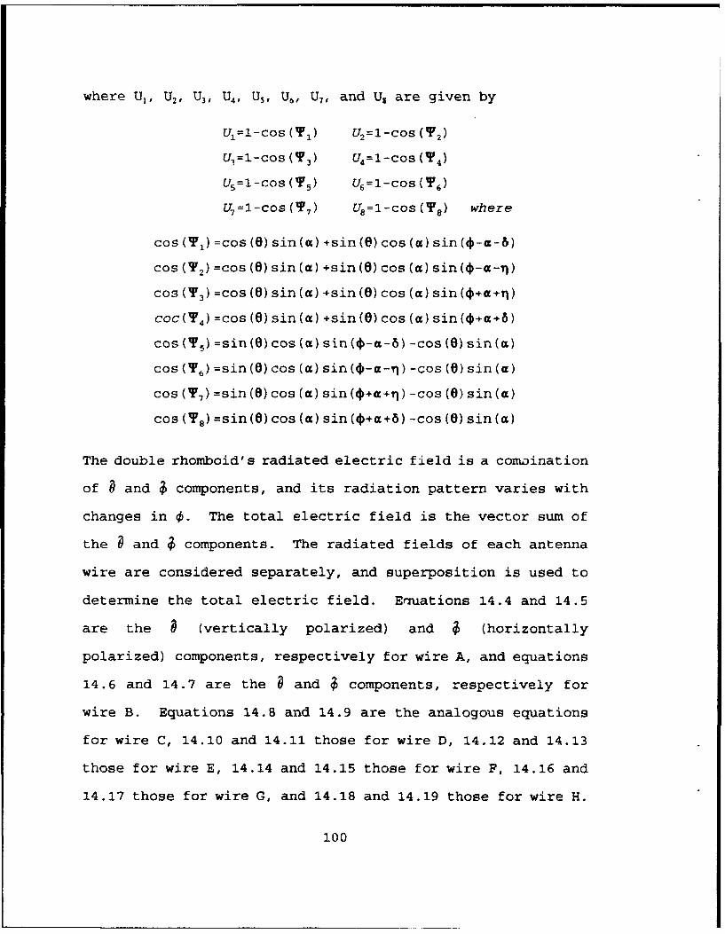
where U,, U2, U3, U4, U5, U6, U7 , and U. are given by
U1 =I-cos ('1 ) U2 =1-cos (T 2 )
U3=l-cos (' 3 ) U4=I-cos (T 4 )
U5=1-cos (T5 ) U6=1-cos (T6 )
U7 ='-cos (T7 ) U,=1-cos (T.) where
cos (TO) =cos (0) sin(a) +sin(0) cos (a) sin(4-a-b)
cos (T 2 ) =cos (0) sin(a) +sin(0) cos (a) sin (*-a-yi)
cos (T,) =cos (0) sin (a) +sin (0) cos (a) sin (i+a-+ij)
coc(F4 ) =cos (0) sin(a) +sin(0) cos (a) sin(0+a+6)
cos ('5) =sin (e) cos (a) sin (o-a-8) -cos (0) sin (a)
cos (TF) =sin (0) cos (a) sin (0-a-i) -cos (0) sin (a)
cos ( 77) =sin (e) cos (a) sin (+a++) -cos (0) sin (a)
cos (T.) =sin (M) cos (a) sin (0+a+6) -cos (6) sin (a)
The double rhomboid's radiated electric field is a comoination
of 9 and $ components, and its radiation pattern varies with
changes in 0. The total electric field is the vector sum of
the b and ý components. The radiated fields of each antenna
wire are considered separately, and superposition is used to
determine the total electric field. Eruations 14.4 and 14.5
are the 6 (vertically polarized) and $ (horizontally
polarized) components, respectively for wire A, and equations
14.6 and 14.7 are the 3 and ý components, respectively for
wire B. Equations 14.8 and 14.9 are the analogous equations
for wire C, 14.10 and 14.11 those for wire D, 14.12 and 14.13
those for wire E, 14.14 and 14.15 those for wire F, 14.16 and
14.17 those for wire G, and 14.18 and 14.19 those for wire H.
100

The first two terms inside each set of brackets represent the
space wave components and any additional terms represent the
surface wave components. I0 is taken to be one since a
sinusoidal current input with a maximum of unity is assumed.
The requested inputs are used to calculate the following
variables using a constant 0 of 0=0 and O=i/2 for 632 discrete
values of 0 which are equally incremented from -ir/2 to 7/2:
...... wavelength of the operational frequency (meters)....... free space wavenumber for operational frequency
n ....... index of refractionP ....... complex numerical distance (vertical polarization)P. ..... complex numerical distanc• (horizontal poiarization)r ...... vertical reflecti.n coefficientr. ...... horizontal reflection coefficientF ...... vertical surface wave attenuation factorF, ..... horizontal surface wave attenuation factor
The calculated variables are used to evaluate the far-
field space wave and surface wave for the discrete values of
0 with 0=0 and O=w/2. The total space wave and surface wave
distributions are determined from vector addition of
corresponding 0 and $ components. The space wave and surface
wave results are then combined for corresponding discrete
values of 0 to obtain the total radiated electric field
distribution for the 0=0 and 0=w/2 vertical planes. The space
wave, surface wave, and total electric field results are then
normalized with respect to the maximum field intensity of
each, and the normalized nagnitudes are plotted for each
discrete 0 to depict the radiation patterns. The Mathcad
double rhomboid antenna application computes the space wave,
surface wave, and total electric field radiation pj.tterns and
radiation parameters in the 0=0 and O=fr/2 vertical planes.
101

The variables correspondin9 to the selected elevation
angle index (d) are used to evaluate the radiated electric
field components for the space wave and surface wave at the
fixed elevation angle (0d) as 0 varies from 0 to 2r in 632
equal increments. The horizontal radiation patterns are then
plotted for the space wave, surface wave, and total radiated
electric field just as those for the vertical planes.
To find the contributions of the b and ý electric field
components to the total average radiated power, P2d, equations
3.8 and 3.9 are used to integrate equations 14.4 to 14.19 over
the hemispherical Gaussian surface above the ground plane at
a fixed radius (R) from the antenna. The sum of the integrals
is the antenna's Pd. With the discrete values of the electric
field and total average radiated power determined, the Mathcad
application predicts the following radiation parameters using
the equations from Chapter 3:
Rj ..... radiation resistance (Ohms)Do . . . . . . . directivityEIRP ..... effective isotropic radiated power (Watts)A.X ..... maximum theoretical effective area (square meters)im ..... maximum theoretical effective length (meters)S....... numerical distance (vertical polarization, 0=900)P. ...... numerical distance (horizontal polarization, 0=900)Anglen1 .elevation angle of maximum directive gain (degrees)
The directivity (D.), effective isotropic radiated power
(EIRP), maximum theoretical effective area (A,,), maximum
theoretical effective length (iw), and the elevation angle of
maximum directive gain (Angle,,) are all determined for both
the 0=0 and O=r/2 vertical planes.
102

XV, THE VERTICALLY POLARIZED LOG-PERIODIC DIPOLE j Y
The orientation of the vertically polarized log-periodic
dipole array is depicted in Figure 15.1, where N is the number
of dipoles, n is an index equal to 0,1,2..N-1, 1, is the
length of the n'+l dipole, d. is the distance between the n +l
and nh+2 dipole elements, HO is the height of the antenna feed
above ground, H, is the height of the n'+1 dipole center, * is
the angle between the vertical axis and the array's center
axis, ct is the angle between the center axis and the line
which connects the upper tips of the elements, U 2 is the angle
between the center axis and the line which connects the lower
tips of the elements, U 3 is the angle between the horizontal
and the line connecting the lower tips of the elements, R is
the radial coordinate, 0 is thc. elevation coordinate, and 0 is
the azimuth coordinate.
The Mathcad application for the vertically polarized log-
periodic array requires the following inputs:
N ........ number of dipole elements10 ....... length of the shortest dipole (meters)11 ....... length of the second shortest dipole (meters)do ....... distance between first two elements (meters)rad0 . . . . . radius of the shortest dipole (meters)H0 . . . . . . . feed height above ground plane (meters)* ......... ngle from vertical axis to array axis (degrees)fs ....... operational frequency (Hertz)R ........ distance from array (meters)E ......... relative dielectric constant of ground planea ........ conductivity of ground planew ........ elevation angle index (from Table 3.2)ADM ...... transmission line characteristic admittanceTIMP ..... termination impedance connected to longest dipole
103

-H
", • 0
z\ I-H
-.-,
---------
........... I .I - --
ý10
-H
-HH
rdI 0'1
104)

The user inputs the frequency for which the radiation
parameters discussed in Chapter 3 are computed. The lengths
of the first two elements (1i and 11) are used to calculate the
log-periodic relationship (T) given by [Ref 10: p. 3171
in,=-- (n=0,1,2 .... N-2,N-1) (15.1)in+1
The remaining element lengths (12 to i.1I) are then found from
12÷+= (15.2)
As noted in equation 15.1, indices start at zero instead of 1,
so an index simply refers to the index-plus-one position in
terms of successive values for a given parameter. This is to
maintain continuity with Mathcad which also indexes from zero.
The radius of the first element (rado) is used to find the
remaining radii by substituting rad. and rad÷+, for 1, and 1,,,
in equation 15.2. The angle between the vertical axis and the
array axis (1) can be between 00 and 900. The angles a2 and
%3 are found by substituting
C2 +a 3=- 7C (15.3)2
into
d , _l- T (15.4)44÷ sin(a 2 +a 3)-tan(a3 )cos(a 2 +aO)
which yields
hn+dnsi-2-'Q)-hn) l
13 =tanj d 2
105

The angle a, is then found from [Ref 10: pp. 351-3541
sin(a1 ) -sin(a 2 ) (15.5)cos(91+a 2÷a 3 ) cos(a 3 )
or
ai=tan_[1 sin (a 2 ) cos (a 2 ÷ 3 )
SCos (a 3 ) +sin(a) sin(u2 +a,)J
The remaining separations (d, to dN_2 ) are then found from
equation 15.4. The dipole half-lengths (h,) are found from
l./2, the feed height (H0 ) must be at least equal to the half-
length of the longest dipole (hN.1), and distance from the
array (R) must meet the far-field requirements of Chapter 3.C.
The elevation angle index (w) sets the 0 coordinate for which
a horizontal radiation pattern is determined. Table 3.2 lists
possible indices and their corresponding elevation angles from
.570 to 89.10 in increments of about 2.30. Indices between
those listed can be used to interpolate a better approximation
of a desired elevation. The termination impedance (TIMP) is
assumed to be connected to the array's center axis opposite
the feed at a distance of hN./2 from the longest element.
Typical termination impedances are the transmission line's
matched impedance (complex conjugate) or a short circuit
(zero). The characteristic admittance (ADM) is simply the
inverse of the transmission line's characteristic impedance.
If computed lengths, separations and radii are not
desired, they can be entered manually as described on the page
two of the application. Consult a Mathcad manual to be
certain the entries are made correctly.
106

The open circuit impedance matrices must be calculated to
determine the current distribution among the dipole elements.
The matrix of open circuit mutual impedances between the
dipole elements is represented as
Zo.0 Zo. Zo.2 . . . . ,-1
Z, 0 1 Z11 ,2 . . . ZI, N-1)
[z = Z2,0 Z2 , 1 Z2"2 . . . Z2, (N-1) (15.6)
Z (N-i).0 Z ( N- i), i Z (N- 1),2 . . . (N -_1),(N -_1) .
Each main diagonal term (Zi,3 ) is the self-impedance of the i1+ 1
dipole. The off-diagonal terms (Zik) are the mutual impedances
between the i6+1 and ke+1 elements. Subscripts i and k are
matrix indices from 0,1,2 .... N-1.
The matrix of open circuit mutual impedances between the
actual dipoles and their images is represented as
ZIo' 0 ZIo. ZIo. . . . . (N1ZI1.o 0 Z i I. ZII, 2 . . . .- ZI 1, (N-1)
[ZI = Z12,0 Z12 , 1) Z' 2, 2 .. .. Z12 . (N-1 ) (15.7)
Zf(N*-),o ZI0(N- ,1 ZIT (N-1) .2 . . . )(Ni)
The main diagonal terms (ZIj) are the mutual impedances
between the i1+l element and its image, and the off-diagonal
terms (ZI,k) are the mutual impedances between the i1+l element
and the image of the k'+l element.
107

The main diagonal self-impedance terms of equation 15.6
(Zi,,) are found from [Ref 6: pp. 205-2061
Zi~i= 60 -r,,-j2ph 1 Q(O U)(58
where Q(x)=Ci(x)-jSi(x)=fCos (Y) dy-jifsin y) dy (15.9)- 0
U,= [ý2radiý+4h4-2h1 ] [1=,2Pa V0,=p [ 2radj'+4hj2+2h1 ]
ul=P [ 2r ad.j.h2-.hj] V,.= P [ý _2r a d i2+hi2+ h
For *~=900, the off-diagonal mutual impedance terms of
equation 15.6 (Z1,1) are given by [Ref 1l]
Zi~kZk~i 60(15.10)
+2Q (PDjk) (cos (P (hi-hk) I +cos( (hl+hk)])
where Q(x) =C'I (x) -j-Si (x) =f Cos Y) dy - i~f sin y) dyY 0
u0= [D,(hh)2(hi+hklI V0 [ D _12 (h, +hk) + (h +hký)]
U2 = [FDjk+2-hk] V2 [FDj2 2h+hk]
108

For *I less than 900, the dipoles are in echelon. The
expression f or the mutual impedance terms of 'equation 15.6
(Zi,k) for an echelon configuration is given by [Ref 12]
+ij=5e jO(hi-SDI~k) [Q(Ua) -Q( U 2)]+e jO (hI-SDI~,k) Q( V')-~ 0(15.11
" e-jP (h 1 2hjt SD1 ,* [Q 1(U4) -Q (U2 ) ]+ eiP(hj+2hk+SDi.k) [Q( 1/) -Q( V2 )
+2cos (phi) e-SI"jfQ(W2) -Q(Wi)]+2cos(ph,) ejP5D'I1 Q(Y 2 ) -Q(Y 1 )l
+2 cos (ph.) leiP ksik[( 2 ) _Q(W,) +ejl( 2 hk+SDI.k)[Q( y 2 ) _Q(y 3 )]
x x
where Q(X) =C~i (X) -ji(Si Wx f Cos (v) dyi.jf sin (Y) dy
U.= 0 [ D.ik+(SDi k-hj) 2+(SDik ,hi)1'r.=f3[D,+(D & 1 -(SDi,k-hi)1
U10(=SD 1 k-s-hi)D 2 (SDl,k~hi)]
V' 0 -P[ D~k D ~ + ( SDI, k~ hi)
Ul=jP [Vi2 ( SD1 k-hi+hk )2+ (SDik-hi+hk)]
r1p[~~k (DkhIh) 2.(SD1 khi+hk) IV1= P [yiL,k+ (SD1 k-h+hI--k)2 (SD.khIh
I~u ~ ~ +hl+hk)2 4(Dk+hl+hk~
V2WP IVDi.k+ ( SDj k-hl+2hk)2 (SDIk-hi+2hk)]
U3 =0 V~~k ( SD1 k-h~k 2.+ (SDj )(hi+2hk)
U4 =0 [Vil ( SD1 k+hi+2 hk) . (SDi~k+hi+2hk]
109

V4= ~DI~,k+ (SDi, k h+ 2 k) '+ (SDi, kh+h+hi +2h,)]
W1=P [VD J]k+SDkSDjkj
Y1=13 I Dik+SD~,k+SDi~kI2 2W2 =1 P D-+(Si ~k (SDi k+hk)]
Y2 =1 Dk( SD k+h) (SDjk~ihk)]
W = P [ DIk (Dlik 2 h) (SDik + 2hk
Y3=P [r(Df,.+ (SD,.k+2hk) 2+ (SD,.k+ 2 hk) ]
The Div, terms in equations 15.10 and 15.11 are the perpen-
dicular distances between the i*+l and k1+1 elements given by
k-1
Dik=Dk.i=E d,, sin(Y) (15.12)n-i
The SDk terms for equation 15.11 are the vertical distance
from the center of the ih+l dipole to the z coordinate of the
nearest end of the k1+1 dipole and are given by
k-1
SD Dk,I=E d,"cos (T) -h- (15.13)n-I
For ground planes with high conductivities relative to
the operating frequency, it is necessary to compute equation
15.7, [ZI] , for the mutual impedances between the elements and
their images. The main diagonal terms (ZI 1 ) are the mutual
impedances between the id'+1 dipole and its own image. These
Z,,i terms are calculated from the mutual impedance equation for
a collinear configuration given by (Ref 12)
110

zi =l~eij(h-h1i.I) [Q(Uo) -Q(U,) ]+ejl (hr-hijI) 1n hi1 ,1 (15.14)Zr. =15 L q hi1 , 1-hi I
+ejf~h~hj~) QV'') -Q(V2) ]e3p(hI~hi'i.)1 hi1 1+2h14 hi1 1+h1
Veph-j~ ) V +i(h+i~)p hii+2h[Q (3) Q W I e hi. .+3hi
+i2cos (h)e JPhii.I[Q (Y 2 ) -Q0(Y1)J+ 2co s(p~hi) e-oi hii1 i
(13h) e~hIIlr{hi1 ,1+h1 ]
+2 cos (ph,) eip (2hj~h±ij ) [Q( y) -Q(y 3 )1
where Q(x)=C!(x)-frSi(x)=fCos (Z) dy jfsin (y) dyy 0
ul=p [FD'k ( hij. k-hi +h)2 (hii~khi~h)
v1= [V J. k+ hi~k-hi h) 2- (hiilk-hih)]
72O=1 [rD , k+ (hij, k+ hlh) 2.( hi1i k+hIjh)
V2 =13[FD ,k ;( hi khih) 2+( hij k+hi~h)
U:3 = [ Din J. (hijk-hl+2hk )2_ (hil,k-hi+2hk)I
U2=03 [VDi2,k+ ( hi k-hi+2hk )2- (hi ilk-hi +hk)I
= p 211 2

U4=P týik (ij +h1 +2 hk )(hij I+hi +2hx)]
v~= [~.~ (i~,~h +2k)2+(hi hik2 +212k)]
W2 =P [VDi,k+ (hii,k+hk) 2_2 (hij,k+hk)
D12= P 1 1 ,k 1 k + (hi jk+ hk)
W3 =P [VDj,k+ (hiiok+2 hk) 2- (hi ,k+2hk)]
Y3= [rIwj, +(h 1k+ 2 h )+ (h i + 2 h
The symbol hij,j in equation 15.14 is the height of the ith• 1
dipole above the nearest end of its own image, and with i=k is
obtained from
hiiok=Hi+Hk-hk (15.15)
The off-diagonal mutual impedances between the dipoles and the
images (ZIj,) are found using equation 15.13, except the Q(x)
arguments are those given for equation 15.14, but with SD,,k
replaced by hijA from equation 15.15.
The function Q(x) given by equation 15.9 is defined in
terms of sine [Si(x)] and cosine (Ci(x)] integrals. Mathcad
is incapable of evaluating Si(x) and Ci(x) directly, so a
series expansion and polynomial approximation are written into
the Mathcad code for both the sine and cosine integrals to
evaluate the functions Q(x). The arguments for Q(x) are
always real, so it is unnecessary to find Si(x) and Ci(x)
expressions valid for complex numbers. For arguments less
than one, Si(x) and Ci(x) are evaluated by series expansions
given by [Ref 9: p. 232]
112

n-0 (2n+1) (2n+1)
Ci (x) =Y+in xW +F (-2) ( X1 (15.17)
n-1 (2n)(2n)
where y=0. 5772156649
For arguments greater than one, Si(x) and Ci(x) are
defined in terms of two auxiliary functions, f(x) and g(x)
given by [Ref 9: p. 233]
f(x)=! 8aIX a2x a3x 2+a 4+e (15.18)x (X+blxfi+b2x4+b~x2+b4)
where le(x) I < 5-10-7
a 1=38. 027264 b1 =40.021433
a 2 =265.187033 b 2 =322.624911
a 3 =335.677320 b 3=570.236280
a4 =38. 102495 b 4 =157 .105423
_ I(x 8 +aix +a2 x4+a 3x 2 +a4 +e(x) (15.19)
x2-+b x 6+b2x 4 +b3x 2 +b4 )
where le(x) I < 3"10-7
a,=42.242855 b1 =48.196927
a 2=302.757865 b 2 =482.485984
a3 =352. 018498 b3=1114.978885
a 4=21.821899 b 4 =449.690326
The sine and cosine integral functions are then defined in
terms of these auxiliary functions by [Ref 9: p. 2321
Si (x) =--f (x)cos (x) -g(x)sin (x) (15.20)2
Ci(x)=f(x)sin(x)-g(x)cos(x) (15.21)
113

In addition to the matual impedance matrices, it is
necessary to calculate the short circuit admittance matrix to
determine the elemental current distribution. The short
circuit admittance matrix is given by [Ref 10: p. 3211
YO, 0 YO, 1 0 0 0 0
Y1, 0 Y1, 1 Y1, 2 0 0 0
0 Y2, 1 Y2, 2 Y2, 3 0
[y] 0 0 Y3, 2 Y3, 3 Y3, 4 (15.22)
0 0 0 Y(N-2), (N-3) Y(N-2), (N-2) Y(N-2), (N-1)
0 0 0 0 Y(N- 1) , (9- 2) Y(N_ 1) (N- 1)
where the diagonal terms are given by
YO, O= -i Yocot (P do) and Y(Nj),(N-,)=Y'T-jYOcot(Pdvj)
and for 0 < n < N-1:
Yn, n.... YOV-2), (N-2) =-jY, (cot (Pdn-1) +cos (Pdn)
and the off diagonal terms are given by
Y(n-1),n= Y., =-jYQcsc(Pdn-1)
The term Y. is the characteristic admittance of the trans-
mission line given by the input (ADM), and Y'T is given by
cos(P hN_+jYOZTs,+ hv-,)Y/ T -o 2 2 (15.23)
YO ZTC 0 S(P 2 2
where ZT is the termination impedance input (TIMP)
The ground conductivity relative to the operating
frequency (a,,,) is then computed by [Ref 6: p. 6401
a el 0 = 18000 a (15.24)Wereo fýM' er
114

to determine which equation to use for the array's current
distribution. A surface with a relative conductivity greater
than 20 is considered to be highly conductive relative to the
transmitted frequency and the current distribution is given by
[Ref 10: p. 342]
[IB] ={[I + [Y] [Z] +Y] [ZI]}-I [IREF] (15.25)
where [U] is the N X N identity matrix. The entries of the
[IB] matrix are the base currents of the dipole elements. The
matrix [IREF] represents the input current to which the [IBI
distribution is referenced. Since the current input is only
to the feed at the center of the first element, and since the
input current is sinusoidal with a maximum of unity, [IREF] is
a 1 X N matrix with a one as the first entry and N-I zeroes in
the remaining positions.
For surfaces with a relative conductivity of less than
20, the mutual impedances due to the images are neglected and
the current distribution is given by
[IBI =1 [ + [11 [Z]}-p [IREF] (15.26)
The electric field equations are referenced to the
current maxima values for the dipole elements, [I] , which are
obtained from the [IB] matrix using [Ref 6: p. 209]
¾ IB( (15.27)Ssin (ph,)
115

The mutual impedance calculations are not valid when any
element length is an exact integer multiple of the wavelength.
When this occurs, there is a singularity error in the mutual
impedance calculations, and it is necessary to vary the
frequency such that no element is an exact integer multiple of
the wavelength. The change required is only one or two
percent, and the predicted radiation parameters are still a
good estimate of those for the original frequency.
The electric field for the vertical log-periodic array is
obtained for each individual dipole in a manner analogous to
that used for the vertical dipole discussed in Chapter 4. The
equations for the individual elements are combined into a
single expression for the array's total electric field by the
array factor. The array factor for the vertical log-periodic
array is [Ref 6 p. 2221
N-iA+jB=: IiejPHICOSe() [cos [ Phicos (0) ] -cos (ph)] (15.28)
i=0
1 + e-J2PHIC)+- Fe (sin2 (6) - (n)2-sin2 )cos()
eJPYI•eC(42&,) [cos (8) sin (a,÷a,) +sin (8) cos (aa,) sin(*)]
where Yj is the y coordinate of the ih+l dipole given by
Y d. sin(7) (15.29)1n-0
116

The first two terms inside the brackets of equation 15.28
represent the space wave, the third term represents the
surface wave, and Ii is the current term for each element based
on a sinusoidal current input with a maximum of unity. The
array factor is combined with the element factor to find the
expression for the total radiated electric field given by
Ee_ j60e-jP" A+jB (15-30)
R sin(O)
The requested inputs are used to calculate the tollowing
variables using a constant 0 of 4=0 and O=n/2 for 312 discrete
values of 0 which are equally incremented from -r/2 to n/2:
h ....... half-length of the i'b+l dipole (meters)Hi ...... height of the id'+l dipole (meters)Y. ...... y coordinate of the it+l dipoleIi ...... current for the i'+l dipoleX5 ...... wavelength of the operational frequency (meters)S....... free space wavenumber for operational frequencyn ....... index of refractionP ....... complex numerical distance for vertical polarizationr ...... vertical reflection coefficientF,..... vertical surface wave attenuation factor
The calculated variables are used to evaluate the far-
field space wave and surface wave for the discrete values of
0 with 0=0 and O=w/2. The space wave and surface wave results
are combined for corresponding values of 0 to obtain the total
radiated electric field distribution for the 4=0 and 4P=ir/2
vertical planes. The space wave, surface wave, and total
electric field results are then normalized with respect to the
maximum field intensity of each, and the normalized magnitudes
are plotted for each discrete 0 to depict the radiation
patterns. The Mathcad vertical log-periodic dipole array
117

application computes the space wave, surface wave, and total
electric field radiation patterns and radiationparameters in
the 0=0 and O=w/2 vertical planes.
The variables corresponding to the selected elevation
angle index (w) are used to evaluate the radiated electric
field components for the space wave and surface wave at the
fixed elevation angle (0,) as 0 varies from 0 tc 2r in 312
equal increments. The horizontal radiation patterns are then
plotted for the space wave, surface wave, and total radiated
electric field just as those for the vertical planes.
Equations 3.8 and 3.9 are used to integrate equation
15.30 over the hemispherical Gaussian surface above the ground
plane at a fixed radius (R) from the array to find total
average radiated power (P.). With the discrete values of the
electric field and total average radiated power determined,
the Mathcad application predicts the following radiation
characteristics from the equations in Chapter 3.
R,, ..... radiation resistance (Ohms)Do . . . . . . . directivityEIRP ..... effective radiated isotropic power (Watts)Am. ..... maximum theoretical effective area (square meters)i= ..... maximum theoretical effective length (meters)P ....... numerical distance (vertical polarization, 0=900)P ....... numerical distance (horizontal polarization, 0=90D)Angle. .elevation angle of maximum directive gain (degrees)
The directivity (DO), effective isotropic radiated power
(EIRP), maximum theoretical effective area (A.), maximum
theoretical effective length (1.), and the elevation angle of
maximum directive gain (Angle.) are all determined for both
the 0-0 and O=w/2 vertical planes.
118

As an example, the Mathcad vertical log-periodic array
application was executed with the following inputs:
number of elements 12length of first dipole 3.246 meterslength of second dipole 3.732 metersfirst separation distance 1.096 metersradius of first element 0.00325 metersheight of antenna feed 8.0 metersfrequency 10-106 Hertzdistance from the antenna 3000 metersrelative dielectric constant 4ground conductivity 1.I0characteristic admittance 1/450 Mhostermination impedance 0 Ohmsangle from vertical to array axis 900elevation angle index 285 (-170)
Figures 15.2 through 15.7 are the space wave and surface wave
radiation patterns in the 0-0 and 0-w/2 vertical planes, and
the designated horizontal plane for this example.
". .. \. .. :.. T .
- /
.. .........
S... - I**-L•...' .i -... ;* ...... .- ~
FIGURE 15.2: Vertical log- FIG.. 15..3: Vertical log-periodic space wave radiation periodic surface wavepattern for 0.0 vertical radiation pattern for 0-0plane. vertical plane.
119

-T1
FIGURE 15.4: Vertical log- FIGURE 15.5; Vertical log-periodic space wave radiation periodic surface wavepattern for 0.7r/2 vertical radiation pattern f or 0=7r/2plane. vertical plane.
.... ...t , -. I I I~
... .... A
71
FIGUE 15 6: vertcallog- FIGUE 1. 7: Vericallog
periodic~. spc aerdain peidc srae wv
patr f or hoiotlpae-aito atr ohoiona plne
.(.................................................

The following radiation parameters were predicted by the
Mathcad application for a sinusoidal current input of one Amp.
Total power radiated (Watts) 37.967Radiation resistance (Ohms) 75.934Numerical distance (vertical) 57.126
Directivity 3.415 12.176EIRP (Watts) 129.656 462.272Max eff area (sq meters) 244.578 872.012Max eff length (meters) 14.038 26.506Angle, (degrees) 21.71 21.14
These results are consistent with expectations for this
particular configuration. Appendix D contains computer
hardcopies of additional example calculations for the vertical
log-periodic dipole array and compares predicted radiation
parameters to those expected based on previous calculations.
121

XVI. THE HORIZONTALLY POLARIZED LOG-PERIODIC DIPOLE ARRAY
The orientation of the horizontally polarized log-
periodic dipole array is depicted in Figure 16.1, where N is
the number of dipoles, n is an index equal to 0,1,2..N-1, i,
is the length of the n'+1 dipole, d,, is the distance between
the n"h+1 and n±+2 dipole elements, H0 is the height of the
antenna feed above ground, H, is the height of the n•h+l dipole,
* is the angle between the vertical axis and the array's
center axis, a is the angle between the array's center axis
and the lines which connect the tips of the elements, R is the
radial coordinate, 0 is the elevation coordinate, and 0 is the
azimuth coordinate.
The Mathcad application for the horizontally polarized
log-periodic array requires the following inputs:
N ........ number of dipole elements10 ....... length of the shortest dipole (meters)11 ....... length of the second shortest dipole (meters)do ....... distance between first two elements (meters)rad0 . . . . . radius of the shortest dipole (meters)H0 . . . . . . . feed height above ground plane (meters)S........ angle from vertical axis to array axis (degrees)f5 ....... operational frequency (Hertz)R ........ distance from array (meters)e. ........ relative dielectric constant of ground planea ........ conductivity of ground planew ........ elevation angle index (from Table 3.2)ADM ...... transmission line characteristic admittanceTIMP ..... termination impedance connected to longest dipole
The user inputs the frequency for which the radiation
parameters discussed in Chapter 3 are computed. The lengths
122

Top View
.dod d 2 d 3S.... E,,:-,• ..... N.... .2 1 N1
-~N-1
113
z/Side View
.. H........
x!
Horizontal Log-Periodic Orientation
FIGURE 16.1: Spatial orientation of the horizontallypolarized log-periodic dipole array for its correspondingMathcad application.
123

of the first two elements (10 and 1,) are used to calculate the
log-periodic relationship (r) given by [Ref 10: p. 317)
T = - (n=0,1,2 .... N-2,N-I) (16.1)1n+1
The remaining element lengths (12 to IN-1) are then found from
I n:L= in (16.2)
As noted in equation 16.1, indices start at zero instead of 1,
so the index simply refers to the index-plus-one position in
terms of successive values for a given parameter. This is to
maintain continuity with Mathcad which also indexes from zero.
The dipole half-lengths (h,) are found from 1,/2. The radius
of the first element (rad4) is used to find remaining radii by
substituting rad, and rad,+1 for 1, and 1,,, into equation 16.2.
The angle between the vertical axis and array axis (*) can be
between 00 and 900, and a is found from [Ref 10: p. 319J
d_ = (i-0) cot (a) (16.3)
which can be written as
a =tan-[(-) (,1 6.411 dn I 164
The remaining separations (d, to dN.2 ) are found from equation
16.3. Feed height (H0 ) can be greater than or equal to zero.
Distance from the array (R) must meet the far-field require-
ments of Chapter 3.C. The elevation angle index (w) sets the
0 coordinate for which a horizontal radiation pattern is
124

determined. Table 3.2 lists possible indices and their cor-
responding elevation angles from .570 to 89.10 .in increments
of about 2.30. Indices between those listed can be used to
interpolate a better estimate of a desired elevation. The
termination impedance (TIMP) is assumed to be connected to the
array's center axis opposite the feed at a distance of hN,-/2
from the last element. Typical termination impedances are the
transmission line's matched impedance (complex conjugate) or
a short circuit (zero). The characteristic admittance (ADM)
is just the inverse of the transmission line's characteristic
impedance. If computed lengths, separations and radii are not
desired, they can be entered manually on page two of the
application. Consult a Mathcad manual to be certain the
entries are made correctly.
The open circuit impedance matrices are calculated to
determine the current distribution among the dipole elements.
The matrix of mutual impedances between dipole elements is
represented as
Z o, Z(N1 I Z(N1 .2 . . .ZO (-1)[z] ... .. (16.5)
Z (AV ), 0 Z (N- 1), I Z (N- 1),2 . . . (N -_ 1),1( WI )
Each main diagonal term (Z13) is the self- impedance of the
i'+l dipole. The off-diagonal terms (Zik) are the mutual
impedances between the ih+1 and k'+l elements. Subscripts i
and k are matrix indices (0,1,2 .... N-l).
125

The matrix of open circuit mutual impedances between the
actual dipoles and their images is represented'as
ZIo. 0 Z1 0o i ZIo. 2 . ... ZI. (N-1)
Z1I.0 ZI1,I ZI1,2 .... ZI, (N-1)
[ZI]= .... . .. (16.6)
Z/(N-1 ).O ZI(N-1 ),l ZI(N-1),2 • . . I (N1).
The main diagonal terms (ZIj,j) are the mutual impedances
between the i*+l element and its image, and the off-diagonal
terms (ZIjk) are the mutual impedances between the i*+l element
and the image of the k6+1 element.
The main diagonal self-impedance terms of equation 16.5
are found from [Ref 6: pp. 205-2061
1 60 [-2 [Q U() -2Q (U•] (16.7)Z1i -cos (2 ph.,)
+ei•2 oP [Q(Vo) -2Q(Vl) ]+2[Q(U'o) -Q(U 1 ) -Q(V 1 ) ]+2Q(U'o)[lcos (23h1 ) ]X X
where Q(x)=Ci(x)-j'Si(x)=fcOs(y) dy-j'fsin(y) dy (16.8)y y
Uo=13 [ 2rad2+4h1 -2hj] U' 0=v',prad1 VO= [P 2rad +4h>2h1 ]
Ul=p [•2radj.+h.-h 1 j V1-, [j/2radj2+h2+hj]
The off-diagonal mutual impedance terms of equation 16.5
are given by [Ref i1]60
Zik= Zk, [1hh=[p60 (16.9)Zi'=Zki=cos [ (hi -hk) I -cos [•(hj+hk) ]I169
[e-•J (hi,÷•) [Q (UO) -•Q(U) -Q(U2)]+e jp (h'*ht) [Q (Vo) -Q(Vl) -Q( V2)]
+2Q(PDik)(cos [P (hI-hk) ] +cos [( (hj+hk)])]
126

x x
wheze Q(x) =CCi (x) -j'Si (x) f cos (y) dy - j'f sin (y) dyY Y
uO= [ý J~,k+ (hi+hk )2- (hi+hk)] V.=P [ FDi,k..(hi+hk) 2+ (hj+h,)}U = VDi2?k+ (hi-hk) 2-(hl-hk)I V.0 f [jDj-,k+ý(h j-h k) 2 +(h -h k)]
U,.= P [ Dj2,khjf-hI] V1=p [rDi-2k;h-2+hl1U2 = P [FDj2 h2-hk] V2=P [VDl2 kh+hk1
The Dik terms are the distances between the i-1 and k'+l
dipole elements and are given by
k-i
D••k=Dki=Ed, (16.10)n=j
For ground planes with high conductivities relative to
the operating frequency, it is necessary to compute equation
16.6, [ZI] , for the mutual impedances between the elements and
their images. The mutual impedance terms (ZIjk) are given by
equation 16.9 with the Q(x) arguments
Uo=p [P -,. +hi-hk)2(hl+hk)I vo=P [Vd-.i•, (hj+hýgj+(hj-h.)]
U/'0= P [Vdi ý k+(hj-hk )2- (hl-hk)I V'0=f [d~ k (Ih) ( hk)1
UjP [iV'T. *+hi-h] VI= P [Fdw 7,k+hi2+hi]
u--p [ d ý,k2-hk] V-=- [VWdi, khk+hkI
The diik entries are the distance from the i1+l dipole to the
image of the k'+l dipole and are given by
diik=2 (Hi+Hk) 2+ (Di, sin (T)) 2 (lb.11)
127

The function Q(x) given by equation 16.8 is defined in
terms of sine [Si(x)] and cosine [Ci(x)] integrals. Mathcad
is incapable of evaluating Si(x) and Ci(x) directly, so a
series expansion and polynomial approximation are written into
the Mathcad code for both the sine and cosine integrals to
evaluate the functions Q(x) . The arguments for Q(x) are
always real, so it is unnecessary to find Si(x) and Ci(x)
expressions valid for complex numbers.
For arguments greater than one, two auxiliary functions,
f(x) and g(x) are determined by [Ref 9: p. 233]
If(X) I x +a1x6+a 2x 4+a 3 x2+a 4 +, (X) (16.12)XI x8+bix 6+b2X4+b 2X
2 +b4 )
where Ie (x) I < 5"10-7
a 1 =38.027264 b 1=40.021433
a 2=265. 187033 b2 =322.624911
a 3=335.677320 b3 =570.236280
a4 =38. 102495 b4 =157. 105423
g(x) =( x:+alxi+a 2x:+a 3x 2 +a, +e(x) (16.13)x) xe+b x6+b 2x4+b 3x2+b4)
where Ie (x) I < 31-0-7
a 1=42.242855 b 1=48. 196927
a 2=302.757865 b 2 =482.485984
a3 =352. 018498 b 3=1114.978885
a 4=21. 821899 1,4=449.690326
128

and Si(x) and Ci(x) are defined in terms of these auxiliary
functions by [Ref 9: p. 232]
Si (x) =-7C -f(x) cos (x) -g(x) Sin (x) (16.14)2
Ci (x) =f(x) sin (x) -g(x) cos (x) (16 .15)
For arguments less than one, Si (x) and Ci (x) are
evaluated by series expansions given by [Ref 9: p. 232]
Si W)= E (_-1)n x2n÷1(1.6n-0 (2n+l) (2n+l) ! (16.16)
Ci(x)= n(x)+ -)x 2 (16.17)nx) (2n) (2n) 1
where y=0.5772156649
It is also necessary to calculate the short circuit
admittance matrix to find the elemental current distribution.
The admittance matrix is given by [Ref 10: p. 321]
Y, 0o Yo, 1 0 0 0 . 0
Y1.0 Y1, 1 Y1,2 0 0 0
0 Y2,1 Y2,2 12,3 0
[Y]= 0 0 Y3,2 Y3, 3 Y3 , 4 (16.18)
0 0 0 Y(N-2), (N-3) Y(N-2), (N-2) Y(N-2)o (N-1)
0 0 0 •0 Y(N-1)I (N-2) Y(N-1) (N-i)
where the diagonal terms are given by
Yoo=-jYocot (Pd 0 ) and Y(N-1). (N-1)=YT.-jYocot (pd.,-)
and for 0 < n < N-1:
Yn-n.n... Y(N-2). (N-2) =-jYO (cot (Pd,_-) +cos (pd,)
and the off diagonal terms are given by
v(n-1),' n=V, (n-1)2=-J9 oCSC(Pdn-)
129

The term Y0 is the transmission line's characteristic admit-
tance obtained from the input (ADM), and Y'T is given by
YoC os(P h~v,) j o~ i Pl( h v-)(1 . 9
The ground conductivity relative to the operating
frequency (a,,) is then computed by [Ref 6: p. 640]
a 18000 a (16.20)e er 0 fm. ez
A surface with a relative conductivity greater than 20 is
considered to be highly conductive relative to the frequency
and the current distribution is given by [Ref 10: p. 342]
EIB]-{ [U]I.[Y] [Z]+[Y] [ZI] 1" [IREFJ (16.21)
where [U] is the N X N identity matrix. The entries of the
(IB] matrix are the base currents of the dipole elements. The
matrix [IREF] represents the input current to which the JIB]
distribution is referenced. Since the current is input only
to the feed at the center of the first element, and since the
input current is sinusoidal with a maximum of unity, [IREF] is
a 1 X N matrix with a one as the first entry and N-i zeroes in
the remaining positions.
For surfaces with a relative conductivity of less than
20, the mutual impedances due to the image elements are
neglected and the current distribution is given by
[IB] -{ U][I] + Z]} [IRE•] (16.22)
130

The electric field equations are referenced to the
current maxima values for the dipole elements, [I], which are
obtained from the [IB] matrix using [Ref 6 p.2093
1 .= IBh (16.23)I-sin (ph,)
The mutual impedance calculations are not valid when any
element length is an exact integer multiple of the wavelength.
When this occurs, there is a singularity error in the mutual
impedance calculations, and it is necessary to vary the
frequency such that no element is exactly an integer multiple
of the wavelength. The change required is only a percent or
two, and the predicted radiation parameters are still a good
estimate of those for the original frequency.
The electric field for the horizontal log-periodic array
is obtained for each individual dipole in a manner analogous
to that for the vertical dipole discussed in Chapter 4. The
equations for the individual elements are combined into a
single expression for the array's total electric field by the
array factors. The array factors for the horizontal log-
periodic array are [Ref 6: p. 214]
N- .
Se=E Ii[cos[PhI(cos (e) cos (v) +sin (0) sin (7) sin (4))]-cos (ph,)]i=0
+rveJ2PHjcos () + (l-r,) F e -J20HCos (e) •n sn(0) (16.24)n 2cos(0)
(sin2 (0)- n7-sin2 (0)cos(e))e p Ycsc(T)[cos (0 cs(T)*sin () in(T)sin
131

N-1
S*=• IX[cos[Phi(cos (e) cos (Y) +sin (0) sin (T) sin (O))]-cos (ph,)]
[l+rhe-i2PNMCO0•8) + (1-rh) F. e-i 2Pj°cos (]. (16.25)
ejP Ylcsc (Y) [cos (0) cos (T) *sin (0) sin () ein () ]
where Y, is the y coordinate of the i,+1 dipole given by
Yi(i-iE d.Isin (T) (16.26)
The first two terms inside the brackets of equations
16.24 and 16.25 represent the space wave, the third term
represents the surface wave, and Ii is the current term for
each element based on a sinusoidal current input with r
maximum of unity. The array factors are combined with the
element factors to find the total radiated electric field
equation, and the expression for the radiated electric field
distribution of the horizontal log-periodic dipole array is
given by [Ref 6: p. 213)
Eo_-j60e-JPR cos (4) cos (0) So (16.27)R l-sin 2 (e) cos 2 (4)
j60e-jPR sin(l) (16.28)R 1-sin2 (f) cos 2 (e)
The requested inputs are used to calculate the following
variables using a constant 0 of 0=0 and O=-/2 for 312 discrete
values of 0 which are equally incremented from -r/2 to w/2:
132

hi ...... half-length of the i"+1 dipole (meters)Hi . . . . . . height of the ih+l dipole (meters)Yi ...... y coordinate of the it+l dipoleIi ...... current for the i"+l dipoleX5 ...... wavelength of the operational frequency (meters)
S....... free space wavenumber for operational frequencyn ....... index of refractionP, ...... complex numerical riistance (vertical polarization)PM ..... complex numerical distance (horizontal polarization)r ...... vertical reflection coefficientr. ...... horizontal reflection coefficientF. ...... vertical surface wave attenuation factorF. ..... horizontal surface wave attenuation factor
The calculated variables are used to evaluate the
radiated far-field space wave and surface wave for the
discrete values of 0 with 0=0 and O=w/2. The space wave and
surface wave results are combined for corresponding values of
0 to obtain the total radiated electric field distribution for
the 0=0 and 0=7r/2 vertical planes. The space wave, surface
wave, and total electric field results are then normalized
with respect to the maximum field intensity of each, and the
normalized magnitudes are plotted for each discrete 0 to
depict the radiation patterns. The Mathcad horizontal log-
periodic dipole array application computes the space wave,
surface wave, and total electric field radiation patterns and
radiation parameters in the 0=0 and O=r/2 vertical planes.
The variables corresponding to the selected elevation
angle index (w) are used to evaluate the radiated electric
field components for the space wave and surface wave at the
fixed elevation angle (0.) as 0 varies from 0 to 2w in 312
equal increments. The horizontal radiation patterns are then
plotted for the space wave, surface wave, and total radiated
electric field just as those for the vertical planes.
133

Equations 3.8 and 3.9 are used to integrate equations
16.27 and 16.28 over the hemispherical Gaussian surface above
the ground plane at a fixed radius (R) from the array to find
total average radiated power Pd). With the discrete values
of the electric field and total average radiated power
determined, the Mathcad application predicts the following
radiation characteristics from the equations in Chapter 3:
Rw ..... radiation resistance (Ohms)Do . . . . . . . directivityEIRP ..... effective radiated isotropic power (Watts)A . ..... maximum theoretical effective area (square meters)im ..... maximum theoretical effective length (meters)P, ....... numerical distance (vertical polarization, 0=900)P. ...... numerical distance (horizontal polarization, 0=900)Anglem .elevation angle of maximum directive gain (degrees)
The directivity (DO), effective isotropic radiated power
(EIRP), maximum theoretical effective area (A.), maximum
theoretical effective length (im), and elevation angle of the
directivity (Angle.) are determined for both vertical planes.
As an example, the Mathcad horizontal log-periodic array
application was executed with the following inputs:
number of elements 12length of first dipole 3.246 meterslength of second dipole 3.732 metersfirst separation distance 1.096 metersradius of first element 0.00325 metersheight of antenna feed 8.0 metersfrequency 20-106 Hertzdistance from the antenna 3000 metersrelative dielectric constant 4ground conductivity 5-103characteristic admittance 1/450termination impedance 0 Ohmsangle from vertical to array axis 900elevation angle index 285 (-170)
134

Figures 16.2 through 16.7 are the space wave and surface wave
radiation patterns in the *-0 and 6-ir12 vertical planes, and
the designated horizontal plane for this example.
- A.,
.4
~A
FIGURE 16.2: Horizontal log- FIGURE163 Hointlog
periodic space wave radiation periodic surface wavepattern for (A-0 vertical radiation pattern for 0.0plane. vertical plane.
L..... .
ti
FIGREoi 16.ce Hoiznalatog-13 FIGURE 16.5:. Horizontal log-perodi spcewaveraito pe odc sfce wv
pattern for (A-ir/2 vertical radiation pattern for O-7r/2plane. vertical plane.

I .., .. -,"'1 " -" 1
7-- 7
:.~ ~ ~ ~ ~ ~~ ~ ~~~~~~. ....". -..i ,. "...- . .'v- -". .. ".. ..
"' . .. +. , I : .. _-, U
"FGR 16..: "I ":.. .6 Hoiona log-. FIUR 1.... Hor" " izna log-... "".."".... space- w, ....... .. y wave
FIGURE ~ ~ ~ ~ hoiona p6laorznanlge.UE1 Hrzntllg
The following radiation parameters were predicted by
the Mathcad application for a sinusoidal current input of one
Amp. The predicted radiation parameters are:
Total power radiated (Watts) 75.546Radiation resistance (Ohms) 151.092Numerical distance (vertical) 93.742Numerical distance (horizontal) 3398.15
Directivity 0.838 18.384EIRP (Watts) 63.301 1388.82Max eff area (sq meters) 15.003 329.159Max eff length (meters) 4.904 22.971Angle..., (degrees) 89.7 24.0
These re'qults are consistent with expectations for this
particular configuration. Appendix E contains computer
hardcopies of additional example calculations for the
horizontal log-periodic dipole array and compares predicted
radiation parameters to those expected based on previous
calculations.
136

XVII. THE HORIZONTAL YAGI- UDAARRAY
The orientation of the horizontal Yagi-Uda array is
depicted in Figure 17.1, where 1. is the length of the
current driven element, NR is the number of parasitic
reflector elements, ND is the number of parasitic director
elements, n is an index equal to 0,1,2..NR+ND, and 1, is the
length of the n"+l element starting with the outermost
reflector and counting consecutively toward the opposite end.
The d, terms are the separation distances between the nlh+l and
n'+2 elements, H0 is the height of all antenna elements above
ground, R is the radial coordinate, 0 is the elevation
coordinate, and 4 is the azimuth coordinate.
The Mathcad application for the horizontal Yagi-Uda array
requires the following inputs:
NR ....... number of reflector elementsND ....... number of director elementsi...... length of the n6+l element (meters)S....... distance between ný+l and nth+2 elements (meters)rad . . . . . radius of the nd+1 element (meters)HO ....... antenna height above ground plane (meters)fs ....... operational frequency (Hertz)R ........ distance from array (meters)E ....... relative dielectric constant of ground planea ........ conductivity of ground planew ........ elevation angle index (from Table 3.2)
Unlike the log-periodic applications, all element
lengths, radii, and separation distances must be input
manually on page two of the application. Consult a Mathcad
manual to be certain the entries are made correctly. The user
137

044 -+H
4-) H
4-) F_ +
r,'- Z ,• H *H HZ 0
+11
-Hr-r-]
-H H0- H
7;0i
* m
r--ICD
H r
G od
0>6 -
0 T_____ __ _ __
FIGURE 17.1: Spatial orientation of the horizontal Yagi-Udaarray for its corresponding Mathcad application.
138

inputs the frequency for which the radiation parameters
discussed in Chapter 3 are calculated. As noted in the first
paragraph, indices start at zero instead of 1, so the index
simply refers to the index-plus-one position in terms of
successive values for a given parameter. This is to maintain
continuity with Mathcad which also indexes from zero. The
dipole half-lengths (k) are found from 1,/2. Antenna height
(H0 ) can be any value greater than or equal to zero, and the
distance from the array (R) must meet the far-field
requirements of Chapter 3.C. The elevation angle index (w)
sets the 0 coordinate for which a horizontal radiation pattern
is determined. Table 3.2 lists possible indices and their
corresponding elevation angles from .570 to 89.10 in
increments of about 2.30. Indices between those listed can be
used to interpolate a better approximation of a desired
elevation.
The open circuit impedance matrices are calculated to
determine the current distribution among the dipole elements.
The matrix of mutual impedances between the dipole elements is
represented as
Zoo 0 2 . . . .. . (M-1
Z 0 Z i %Z, 2 . . . .
Z 2 , 0 Z 2 , 1 Z, 2 . . . . Z2071[Z] = ... .(17.1I)
Z(N- 1 ),O Z(N- 1 ).l Z(N-1 ), 2 . . . . Z
139

Each main diagonal term (Z1u) is the self impedance of the i I+l
element. The off-diagonal terms (Zjk) are the mutual
impedances between the i*+1 and k1+l elements. Subscripts i
and k are matrix indices (0,1,2 .... NR+ND).
The matrix of open circuit mutual impedances between the
actual elements and their images is represented as
Zl0, 0 ZIooI ZIo, 2 . . .. ZlO, -i)
ZI1o 0 ZI, I ~ i,2 .... Z,, 2(-1)
(ZI] Z = ZII2, 1 Z1 2, 2 . 2, (N-1) (17.2)
ZI(N-1) ZI (N-1),i ZI(N-I),2 • ZI(N-1)(N_)
The main diagonal terms (ZI3u) are the mutual impedances
between the i1+l element and its image, and the off-diagonal
terms (ZI1,) are the mutual impedances between the i*+I element
and the image of the k6+1 element.
The main diagonal self-impedance terms of equation 17.1
are found from [Ref 6: pp. 205-2061
Zii= 60c[s( h e-ie2h[ [Q(UO)-2Q(U1 )I (17 .3)1•i 1-cos (2 Phi)
+epl [ (Vo) -2 Q(v,) ]+2[Q (&o) - (Uj) -Q (Vj)]+2Q0('o)[1.cos (2Ph,) ]]X X
where Q(x)=Ci(x)-j.Si(x)=f cos(y) dy-jfsin(y) dy (17.4)y y- 0
Uo=P [/2rad.2+4hj2-2h,] Ul'=v_2prad1 VO=1 [i2rad1 .. 4h•+2h i
U1 =P [ 2rad+h2-h1 ] V.-P [2.radh+h14
140

The off-diagonal mutual impedance terms of equation 17.1
are given by [Ref 11]
Z_ kZ 60 (17.5).i=k' cos[P(hi-hk) ]-cos[P (hi+hk) (
[e-_jO(hi+hk) [Q(U[O) -Q( UI) -Q( U2)]+e JA(hi÷h,) [Q( Vo) -Q ( VY) -Q( V2)]
+e -jP (hl-hk)[O(U'G-Q(U(V) -Q(U2)]+ejP (hj-hk)[Q (VIo) - Q (U) -Q (V2)
+2 2(PD.,,•)(cos [ P (hi-hk) I *cos [p(hi~hk) ])]
X X4 cos (y) _ _._sin(y
where Q(x) =Ci (x) -j.Si (x) dy -jf s (Y)dy0
U0~ D;k(hi+hk) 2- hihk)I V~p[ k+ (hi+h,) 2+ (hi+hk)]
U'0=P [ID~,2,;(12j-k) 2- (hi-hk)I VO = P [ID~,2k+ý(hi-h,) 2+ (hi-h,)I
u,.=p [1Dj2k+hj2-hI] v1=P [ D2fhk+h.'hj
U2 = P [rD 2 ;h 2-h.] V2=P [ FIDjfýýk2+hk]
The Di.k terms are the distances between the i,+l and k,+l
dipole elements and are given by
k-1
DI.k=DkI=E dn (17.6)n-i
The mutual impedances between the actual elements and
their images must also be computed to determine the elemental
current distribution. The mutual impedance terms of equation
17.2 (ZIi) are given by equation 17.5, except the Di,k terms in
141

the Q(x) arguments are replaced by diik terms which represent
the distance from the i*+l element to the image of the k*+l
element and are given by (Ref 6: pp. 205-208]
dii,k=VH(o +D .k (17.7)
The function Q(x) given by equations 17.4 is defined in
terms of sine [Si(x)] and cosine [Ci(x)] integrals. Mathcad
is incapable of evaluating Si(x) and Ci(x) directly, so a
series expansion and polynomial approximation are written into
the Mathcad code for both the sine and cosine integrals to
evaluate the functions Q(x). The arguments for Q(x) are
always real, so it is unnecessary to find Si(x) and Ci(x)
expressions valid for complex numbers.
For arguments less than one, Si (x) and Ci (x) are
evaluated by series expansions given by [Ref 9: p. 2321
Si (x) =f ( -n.,) n(2n+1) (17 .8)n=O (2n+1) (2++1) !
(-1 n X2n
n-1 (2n) (2n) 7
where y=0.5 7 7215664 9
For arguments greater than one, Si(x) and Ci(x) are
expressed in terms of auxiliary functions, f(x) and g(x),
given by Ref 9: p.2323
Si (x) = 7c -f(x) cos (x) -g(x) sin(x) (17 .10)2
Ci (x) =f(x) sin (x) -g(x) cos (x) (17 .11)
142

The auxiliary functions f(x) and g(x) are evaluated by the
polynomial approximations [Ref 9: p. 233]
f(x)=1i xa+a x 6 +a2x 4 +a 3 x 2+a4 (17.12)
X x 8 +b x 6 +b2x 4 +b2x 2 +b4 )
where le (x) I < 5"10-7
a 1 =38. 027264 b1=40.021433
a2 =265. 187033 b2=322.624911
a 3=335.677320 b 3=570.236280
a4 =38. 102495 b4=157.105423Sxa+al x6+ax x4+ax x2+a
g W) --L x 4 )+e(x) (17.13)x) 2- x8 +blx6 +b2x 4+b3x 2.+b4 )
where le(x) I < 3.10-7
a1 =42.242855 b1=48.196927
a 2 =302.757865 b2 =482.485984
a 3 =352. 018498 b3=1114.978885
a4 =21. 821899 b 4=449.690326
When the mutual impedances are found, the array's base
current distribution is computed from [Ref 10 p. 258-259]
[IB] ={ [Z] +rh,, [ZI] }-' [VREF] (17.14)
where I-n
I+n
and n is the complex index of refraction. The entries of the
[IB] matrix are the base currents of the dipole elements, and
[VREF] is the voltage matrix to which the [IB] distribution is
referenced. Since the Yagi-Uda has only one driven element
(corresponding to the NRUI index), and since a sinusoidal
voltage response with a maximum of unity is assumed across the
143

input terminals, [VREF] is a 1 X NR+ND matrix with a 1 as the
NR• entry and NR+ND-l zeroes in the remaining positions. The
electric field equations are referenced to the current maxima
values for the dipole elements, [I] , which are determined from
the [IB] matrix using [Ref 6 p. 2091
lB11 Ih (17.15)I- sin (ph,)
The mutual impedance calculations are not valid when any
element length is an exact integer multiple of the wavelength.
When this occurs, there is a singularity error in the mutual
impedance calculations, and it is necessary to vary the
frequency such that no element is exactly an integer multiple
of the wavelength. The change required is only a percent or
two, and the predicted radiation parameters are still a good
estimate of those for the original frequency.
The electric field for the horizontal Yagi-Uda array is
obtained for each element in a manner analogous to that used
for the vertical dipole in Chapter 4. The equations for the
individual elements are simplified into two expressions for
the array's electric field components by the array factor.
The Yagi-Uda's array factor is given by [Ref 6: p. 204]
NR.ND- 1
S Ii(cos[phi(sin (0) sin (()))J-cos (ph.)] ejAYisin(i)sin() (17.16
where Y, is the y coordinate for the i th+l element given by
i-IYj=F d, (17.17)
n-O
144

The array factor is multiplied by the element factors to
find the equations for the total radiated electric field
distribution of the horizontal Yagi-Uda array,
,=-j60 e-JO R Cos (H) e jP•c'(S (aS) (17.18)R l-sin 2 (0) cos 2 (W)
[Cos (0) (i -ve -j2PHCOS (e) )+ (i -rv) Fee -ý2pH•cos (e).
n 2 -sin 2 (0 )(sinf2(()-Vn 2 -sin 2 (0) cos(e))l
.rn 2 n12
E*=j60 e sin (g) ej"Ocos(8) (S) • (17.19)R I-sin2 (0) cos 2 (0)
[1 +Phe-j2H °cos (0) + ( 1 -rh) Fre -j2pR 0COS (0)]
The first two terms inside the brackets of each equation are
the space wave, the third terms are the surface wave, and Ii
is the current term for each element based on a sinusoidal
voltage across the input terminals with a maximum of unity.
The requested inputs are used to calculate the following
variables using a constant 0 of 4=0 and O=w/2 for 312 discrete
values of 0 which are equally incremented from -7r/2 to r/2:
h ...... half-length of the i1+l element (meters)Y ....... y coordinate of the ih+l elementI ....... current for the ih+l elementX5 ...... wavelength of the operational frequency (meters)0 ....... free space wavenumber for operational frequencyn ....... index of refractionP ....... complex numerical distance (vertical polarization)Pm ..... complex numerical distance (horizontal polarization)
...... vertical reflection coefficientrh ...... horizontal reflection coefficientF ...... vertical surface wave attenuation factorFm ..... horizontal surface wave attenuation factor
145

The calculated variables are used to evaluate the far-
field space wave and surface wave for the discrete values of
0 with 0=0 and O=w/2. The space wave and surface wave results
are combined for corresponding values of 0 to obtain the total
radiated electric field distribution for the 0=0 and O=w/2
vertical planes. The space wave, surface wave, and total
electric field results are then normalized with respect to the
maximum field intensity of each, and the normalized magnitudes
are plotted for each discrete 0 to depict the radiation
patterns. The Mathcad horizontal Yagi-Uda array application
computes the space wave, surface wave, and total electric
field radiation patterns and radiation parameters in the 0=0
and O=w/2 vertical planes.
The variables corresponding to the selected elevation
angle index (w) are used to evaluate the radiated electric
field components for the space wave and surface wave at the
fixed elevation angle (0,) as 0 varies from 0 to 2r in 312
equal increments. The horizontal radiation patterns are then
plotted for the space wave, surface wave, and total radiated
electric field just as those for the vertical planes.
Equations 3.8 and 3.9 are used to integrate equations
17.18 and 17.19 over the hemispherical Gaussian surface above
the ground plane at a fixed radius (R) from the array to find
total average radiated power (Pd). Since the Yagi-Uda current
distribution is referenced to a sinusoidal voltage input with
a maximum of unity, the radiation resistance can not be
146

calculated from equation 3.10 as in previous applications.
Instead, radiation resistance must be found with respect to
the unity voltage input usingSIVI2 Va2p
Pz.==V2 or Rrad= i (17.20)2Rrad 2 Prad"
With the discrete values of the electric field and total
average radiated power, the Mathcad application predicts the
following radiation characteristics from Chapter 3:
R. ..... radiation resistance (Ohms)Do ....... directivityEIRP.....effective radiated isotropic power (Watts)A . ..... maximum theoretical effective area (square meters)inux ..... maximum theoretical effective length (meters)P ....... numerical distance (vertical polarization, 0=900)PM ...... numerical distance (horizontal polarization, 0=900)Angle,. elevation angle of maximum directive gain (degrees)
The directivity (DO), effective isotropic radiated power
(EIRP), maximum theoretical effective area (A,.), maximum
theoretical effective length (Iw), and elevation angle of the
directivity (Angle,,) are determined for both vertical planes.
As an example, the Mathcad horizontal Yagi-Uda array
application was executed with the following inputs:
number of reflectors 1number of directors 1element lengths 15.6, 15, and 14 meterselement separations 7.5 and 6.5 meterselement radii 0.001, 0.001, and 0.001 metersheight of antenna 8.0 metersfrequency 10.106 Hertzdistance from the antenna 3000 metersrelative dielectric constant 72ground conductivity 4elevation angle index 285 (-17')
147

Figures 17.2 through 17.7 are the space wave and surface wave
radiation patterns in the 0=0 ana O=wI2 vertical planes, and
the designated horizontal plane for this example.
..... ..... 1
71
~PV
FIGURE 17.2: Horizontal FIGURE 17.3: HorizontalYagi-Uda space wave radiation Yagi -Uda surface wavepattern for 0=0 vertical radiation pattern for 0.0plane. vertical plane.
S ~ I
plne vetia plane
F1; I .-148

S... ... . , . .. ... . ..... ---.- - .... ....
).i ..... ' \•.. -" '"'
FIGURE 17.6: Horizontal FIGURE 17.7: HorizontalYagi-Uda space wave radiation Yagi -Uda surface wavepattern f or horizontal plane. radiation pattern for
horizontal plane.
The predicted radiation parameters based on a one volt
response across the input terminals are:
Total power radiated (Watts) 0.00482Radiation resistance (Ohms) 103.760Numerical distance (vertical) 0.04363Numerical distance (horizontal) 2.26-106
Directivity 1.679 14.631EIRP (Watts) 0.0081 0.0705Max eff area (sq meters) 120.26 1047.9Max eff length (meters) 11.506 33.966Angle., (degrees) 89.7 41.714
These results are consistent with expectations for this
particular configuration. Appendix F contains computer
hardcopies of additional example calculations for the
horizontal Yagi-Uda array and compares predicted radiation
parameters to those expected based on previous calculations.
149

XVIII, REMARKS AND CONCLUSION
This thesis is the culmination of nine months of research
and computer programming. No new electric field equations
were derived exclusively for this project. It was directed by
NAVMARINTCEN prior to commencing that existing electric field
equations would provide the basis for the radiation parameter
predictions. The expressions used in this thesis are all
previously derived by pioneers in antenna radiation theory
such as Sommerfeld, Norton, Cox, King, Ma, and Walters. The
equations are compiled here solely for the purpose of
crediting the source references and to describe how the
Mathcad code was assembled.
The accuracy of the predicted radiation characteristics
is totally dependent upon the extent to which the equations
used realistically model the actual radiated electric fields
of the antennas. It is near impossible to obtain analytic
results which accurately model an antenna's radiation
characteristics in all cases. There are too many operational
and environmental variables to obtain one general, all-purpose
expression. Even if all possible variables could be accounted
for in a single expression, computer processing times would be
unacceptably long. The equations used herein are simple
enough to be evaluated by Mathcad in a reasonable length of
time, but the radiation parameter predictions are accurate
enough to be useful for antenna analysis.
150

As addressed in appendices A-F, the equations presented
in previous chapters and evaluated by the Mathcad applications
provide radiation parameters consistent with expectations for
the inputs which have been executed to date. All antenna
configurations which have been computed exhibit radiation
characteristics consistent with other computational programs
and empirically obtained patterns and parameters. There is no
way to test the accuracy of the Mathcad predictions other than
empirical measurements for each antenna configuration, clearly
a task beyond the scope and purpose of this report. However,
adequate analysis of the Mathcad results has been provided to
demonstrate that the applications provide very good estimates
of antenna radiation parameters as a base level analysis tool.
Most of the applications have computations times under
ten minutes. However, even with the simplified equations used
by Mathcad, some of the applications can take upwards of two
hours to compute on a 33 MHz 80386 PC. The applications for
the rhombic, double rhomboid, and array (with more than four
to five elements) antennas can take an exorbitantly long time
for power calculations. For this reason, the applications
should be run on the fastest PC available; a 50 MHz 80486 is
preferable. Computation times can also be reduced by
computing only the radiation patterns until it is determined
which frequencies are of greatest interest. Then the average
power calculations for those frequencies can be executed.
151

The Mathcad applications were written for NAVMARINTCEN to
provide antenna analysts with the capability to predict
radiation parameters based solely on antenna physical
dimensions and ground properties. The Mathcad results
computed thus far are consistent with expectations and are
most likely providing accurate predictions of actual antenna
radiation characteristics. Only extended use of the
applications and empirical confirmation of results will prove
out the accuracy of the Mathcad code. Results obtained thus
far certainly justify continued use of the Mathcad code as an
antenna analysis tool.
152

APPENDIX A:
VERTICAL DIPOLE ARRAY COMPUTER OUTPUT
This appendix contains computer hardcopies from the Mathcad
vertical dipole application which show the input values and
predicted radiation characteristics for two sample calculations.
The configuration is a half-wave dipole at one quarter wavelength
above soil (E,=10 and a=102) for the first example and the same
configuration above seawater (er=7 2 and a=4) for the second.
Reference 6 [p. 91] provides the radiation patterns and gain
predictions from several sources for the configuration in the
first example.
The elevation of maximum directive gain is slightly higher
for the Mathcad output than for those given in reference 6, but
the overall radiation patterns are very similar. The 4.17 (6.2
dB) value of directivity for Mathcad is quite a bit higher than
the maximum gain values of about zero dB in reference 6.
However, since a half-wave dipole has a free-space directivity of
1.64 (2.21 dB), one would expect the actual directivity to be
closer to the Mathcad prediction because of the effect of the
reflected wave (constructive and destructive interference) on the
space wave, and the lower total average radiated power resulting
from ground plane losses. The seawater example yields results
consistent with expectations. With respect to the soil example,
the seawater example's directivity is slightly higher due to a
stronger reflected wave, and the surface wave is stronger at
grazing angles (0-900) due to higher conductivicy.
153

VERTICAL DIPOLE
This application calculates far field radiation patterns and parameters associatedwith vertical thin-wire dipole antennas (diameter << wavelength). The antenna ismounted vertically along the z-axis in a rectangular coordinate system with the feedat the antenna's center at a set height above the surface. Required inputs are theantenna length, feed height above the surface, transmitted frequency, distance fromthe antenna, the conductivity and dielectric constant of the surface below theantenna. The planar earth model is assumed in predicting radiation patterns.Predicted operating frequencies assume that the antenna is a quarter- wavelength,half-wavelength, three-quarter-wavelength, or full-wavelength dipole. A sinusoidalcurrent input with a maximum of unity is assumed. All radiation patterns arenormalized with respect to the maximum electric field intensity transmitted by theantenna. Plotted radiation patterns are valid for any vertical plane passing throughthe antenna axis. The electric field magnitudes to which the Radiation Patterns arenormalized are displayed below their respective plots. Polarization is vertical for allvertical dipoles.Input the Dipole I := 5 hlength in meters 2
Wavelengths and Frequencies
41 214.1X1 := 4-1 A2 ;= 2'1 X3 4-1 A 4
c c c cf 1. ~ f ..- f f3 . -f=
X1 X2 x3 A4
Possible Operating Frequencies (Hertz)
SDipole: fi =.5.107 X Dipole: f2 = 3 107
3 Dipole: f3 = 4.5. 107 Dipole: f4 6 107
Input the operating f5 3106 Input the DistanceFrequency (Hertz) from the Antenna R 3000
(meters)
Input the ground 10 Input the ground o0 2Dielectric Constant Conductivity
Input the Height of H0 .= 2.5the Antenna Feed(meters) 154

Radiation Patterns valid for any Vertical Plane passing through tde Antenna
Space Wave Radiation Pattern
1 1 A.
-155

Surface Wave Radiation Pattern
.........
~1L
Wtq -0ýMaxmu Sufc av.lcri.il
Intesit /Vk e ee)mx(aE)26r-1
05156

Combined Space and Surface Wave Radiation Pattern
... ......
-0.5 ' 5
-t -0.5 0 01
Maximum Radiated Electric FieldIntensity (Volts per meter) max (MagE3) =0.01732
157

2 -JJ3/.(- ,,oo.s(• ] J~.(
power 30 . 2 cos(#.,; cos(C)) - co '.(P.h) e . e•
sin(•) R - 110 .cos(3) R - H0o
.10
E3 ( I E311) 2 4.__-R2_mx____sq 2.(120 ) Directivity 4R 2 "max(sqE3)2.( 12. X )power
Radres = 2.power
Total Power Radiated (Watts) power = 10.79029
Radiation Resistance (Ohms) Radres - 21.58059
Directivity (maximum Power Gainassuming 100% Antenna efficiency) Directivity = 4.16784
Effective Isotropic RadiatedPower (EIRP) Watds) Directivity*p-wer = 44.97225
Maximum Effective Area (X) 2(Along Radial of Directivity) 33 4 Direcivity
(square meters) 4-
Maximum Effective Length IRadres. (X5) Directivity(Along Radial of Directivity) 2"1 2.75579
(meters) 480- x 2
158

Numerical Distance for 74.95924Vertical Polarization e
Elevation Angle of Maximum A4 4le3 [19.39778)~Power Gain (Degrees) 19.39778 /
159

VERTICAL DIPOLE
This application calculates far field radiation patterns and parameters associatedwith vertical thin-wire dipole antennas (diameter << wavelength). The antenna ismounted vertically along the z-axis in a rectangular coordinate system with the feedat the antenna's center at a set height above the surface. Required inputs an theantenna length. feed height above the surface, transmitted frequency. distance fromthe antenna, the conductivity and dielectric constant of the surface below theantenna. The planar earth model is assumed in predicting radiation patterns.Predicted operating frequencies assume that the antenna is a quarter- wavelength,half-wavelength, three-quarter-wavelength, or full-wavelength dipole. A sinusoidalcurrent input with a maximum of unity is assumed. All radiation vatterns arenormalized with respect to the maximum electric field intensity trinsmitted by theantenna. Plotted radiatioA patterns are valkd for any vertical plane passing throughthe antenna axis. The electric field magnitudes to which the Radiation Patterns arenormalized are displayed below their respective plots. Polarization is vertical for allvertical dipoles.
Input the Dipole I := 5 h Ilength in meters 2
Wavelengths and Frequencies
4-1~X•1 -:4-1 X2 := 2.1 X' 4=-1- A'
c c c cfl f2 = ~- 1` ` = C
X1 A2 A3 X
Possible Operating Frequencies (Hertz)
Dipole: f1 - 1.5 .107 Dipole: f2 = 3. 1072
3.___ Dipole: f3 = 4.5-107 X Dipole: f 4 - t07
Input the operating f 30.106 Input the Distance
Frequency (Hertz) 5 from the Antenna R = 3000(meters)
Input the ground 72 Input the ground 4Dielectric Constant Conductivity
Input the Height of Ho - 2.5the Antenna Feed(meters)
160

Radiation Potterns valid for any Vertical Plane passing through the Antenna
Space Waive Radiation Pattern
-1* -0. .* 0.5-*-= 1
1' II
0aiu.5ceWv lcti il
Inenit (Vh4e ee)mxMgl .39
/ 161-I

Surface Wave Radiation Pattern
ii
0.- X
% % 3.
tI
-O' - m
162

Combined Space and Swtface Wave Radiation Pattern
¶ 1 ~ -.4...........
l -
A.
.. .. . ...... . ....
/4 .
- 050 0.5
Maximum Radiated Electric FieldIntensity (Vohts per meter) nax( MagE3) 0.03398
163

r!power :-- 30 2 cos(f.h-cos(r)) - cos(e.h) e 0 e
p sin() R - H0.cos(C) R + Ho.
sqE3 E3 12 Directivity 4..-R2 .max(sqE3)s~1E31 -power
2-( 120-x)poe
Radres := 2.power
Total Power Radiated (Watts) power - 37.64371
Radiation Resistance (Ohms) Radres - 75.28741
Directivity (maximum Power Gainassuming 100% Antenna efficiency) Directivity = 4.59967
Effective Isotropic RadiatedPower (EIRP) (Watts) Directivity. power = 173.14876
Maximum Effective Area(Along Radial of Directivity) () 2 Directiviy 60304
(square meters) 4.
Maximum Effective Length Radres. (XS) 2. Directivity(Along Radial of Directivity) 2.. 5.40735
(meters)2 480. x
164

Numerical Distance for 0.39252Vertical Polarization Pto
Elevation Angle of Maximum Angle3 = (8.55784)Power Gain (Degrees) 8.55784/
165

APPENDIX B:
VERTICAL MONOPOLE ARRAY COKPUTER OUTPUT
This appendix contains computer hardcopies from the Mathcad
vertical monopole application which show the input values and
predicted radiation characteristics for two sample calculations.
The configuration is a quarter-wave monopole above soil (E,=10 and
u=10 2 ) for the first example and the same configuration above
seawater (e,=72 and a=4) for the second. Reference 6 [p. 89]
provides the radiation patterns and gain predictions from several
sources for the configuration in the first example.
The elevation of maximum directive gain is slightly higher
for the Mathcad output than for those given in reference 6, but
the overall radiation patterns are very similar. The 3.24 (5.1
dB) value of directivity for Mathcad is quite a bit higher than
the maximum gain values of about zero dB in reference 6.
However, since a half-wave dipole has a free-'pace directivity of
1.64 (2.1 dB), the actual directivity of a quarter-wave monopole
above a ground plane should be closer to the Mathcad prediction
because of the effect of the reflected wave (constructive and
destructive interference) on the space wave and the lower total
average radiated power resulting from ground plane losses. The
seawater example yields results consistent with expectations.
With respect to the soil example, the seawater example's
directivity is slightly higher due to a stronger reflected wave,
and the surface wave is stronger at grazing angles (8-900) due to
higher conductivity.
166

VERTICAL MONOPOLE
This application calculates far field radiation patterns and parameters associatedwith vertical thin-wire monopole antennas (diameter << wavelength). The antennais mounted vertically along the z-axis in a rectangular coordinate system with thefeed at the origin. Required inputs are the antenna length, transmitted frequency,distance from the antenna, the conductivity and dielectric constant of the surfacebelow the antenna. The planar earth model is assumed in predicting radiationpatterns. Predicted operating frequencies assume that the antenna is an eighth-wavelength, quarter-wavelength, three-eighths-wavelength, or half-wavelengthmonopole. A sinusoidal current input with a maximum of unity is assumed. Allradiation patterns are normalized with respect to the maximum electic field intensitytransmitted by the antenna. The electric field magnitudes to which the patterns arenormalized ae displayed below their respective plots. Radiation patterns are validfor any vertical plane passing through the z-axis, because the radiation pattern issymmetrical with respect to phi. Polarization is vertical for all vertical monopoles.
Input the Monopole h - 7.5 1 :- 2. hlength in meters
Wavelengths and Frequencies4.1
X1 4'1 X2 .21 X3 4-1 X4 :
c c c f c
Possible Operating Frequencies (Hertz)
X Monopole: f 5-105 X Monopole: f2 = I.1078 4
3-8_X Monopole: f3 = 1.5- 107 Monopole: f4 = 2"107
Input the operating f5 - 10. 105 Input the Distance from R 3000Frequency (Hertz) the Antenna (meters)
Input the ground e = 10 Input the ground = 10- 2Dielectric Constant Conductivity:
167

Radiation Patterns valid for any Vetlical Plans passing drugh the Antenna
Space Wave Radiation Pattern
0.5 -....
0 ... ... .... ..
-0.5 "
-1 -0. 0 1
1681

Surface Wave Pattern
.. .......
ID
---------
05 -0.5. 0. 1~.
Nwk Hal'
N1 6

Combined Space and Surface Wave Pattern
... ......... I
-0.5
wok . *..
Maxium Rdiatd ElctrkFiel
Intensity.. (Vh pe ee)/xMg3 .11
~ I, 170

I
2 cos(,6.h-cos(U)) - cos(f-h) ...i+ j., sin(#.h.cos(0')) ...
"power R.5 [+ (-(cos(ý).sin(P.h)))s cos(O-h.cos(')) - cos(f.h) ...
s,2 2 [: ~.[5 ldn(#.h.cos(t)) ..4*
+ 2cos(t) - - sin( .) , L +(-(cos(ý).sin(.m .h))
. .cos(c) + in 2 sin(C) 2
J0
sqE3 2(120.x) Directivity 4"%'R 2 "max(sqE3)2-(10-x)power
Radres = 2.power
Total Power Radiated (Watts) power = 5.74454
Radiation Resistance (Ohms) Radres = 11.48908
Directivity (maximum Power Gainassuming 100% Antenna Efficiency) Directivity = 3.2389
Effective Isotropic RadiatedPower (EIRP) (Watts) Directivity.power = 18.60648
Maximum Effective Area(Along Radial of Directivity) S) 2. Directiviy= 231.97519
(square meters) 4.%
171

Maximum Effective Length Radres-. 2) -Directivity(Along Radial of Directivity) 2 5.31775
(motors) 409
Numerical Distance for P i4.91116Vertical Polarization P I
Elevation Angle of Maximum Ang(e3 = 25.67351)Power Gain (Degrees) (25.67353/
172

VERTICAL MONOPOLE
This application calculates far field radiation patterns and parameters associatedwith vertical thin-wire monopole antennas (diameter << wavelength). The antennais mounted vertically along the z-axis in a rectangular coordinate system with thefeed at the origin. Required inputs are the antenna length, transmitted frequency,distance from the antenna, the conductivity and dielectric constant of the surfacebelow the antenna. The planar earth model is assumed in predicting radiationpatterns. Predicted operating frequencies assume that the antenna is an eighth-wavelength, quarter-wavelength, three-eighths-wavelength, or half-wavelengthmonopole. A sinusoidal current input with a maximum of unity is assumed. Allradiation patterns are normalized with respect to the maximum electic field intensitytransmitted by the antenna. The electric field magnitudes to which the patterns arenormalized are displayed below their respective plots. Radiation patterns are validfor any vertical plane passing through the z-axis, because the radiation pattern issymmetrical with respect to phi. Polarization is vertical for all vertical monopoles.
Input the Monopole h - 7.5 I ýý 2. h
length in meters
Wavelengths and Frequencies
4.1~X'1 :-4.1 X 2 2-1 X"I•3 4- X•4 '-
C C c Cf , f2 f3 f 4
Possible Operating Frequencies (Hertz)
SMonopole: f, = 5.10 - Monopole: f2 = I -1078 4
3-_ Monopole: f3 1.5- 10 7 X Monopole: f4 = 2. 107
8 2
Input the operating f5 1t- 10- I Input the Distance from R 3000Frequency (Hertz) the Antenna (meters)
Input the ground er = 72 Input the ground 4
Dielectric Constant Conductivity:
173

Radiation Patterns valid for any Vertical Plane passing through the Antenna
Space Wave Radiation Pattern
A.-.
0.5
Maxmu Space WaeElcrcil
Intnsty(Votspe mter mx(ag~) .085
174

Surface Wave Pattern
0. A
I Til
-0.5
\\ I %
-2r\-0.5.0\ 0.5( 7 \tok . 1
Maxium tufae Wve FeldIntesit(Volt pe/ee)mxMg2 .17
-~ 'V.I\175

Combined Space and Studace Wave Pattern
i ....... ............
/*/
.................
0- f
J1 ....-0.5 -
wok. "3
Maximum Radiated Electric FieldIntensity (Volts per meter) maz( MagE3) =0.01976
176

z
2 cos( h-_cos() - cos(S.h) ...+ j'. sin(O.h-cos(t)) ... ]
7.w + (-(cos(ý)*sn(f-h)))power R-12 sin(•)icos(".h.cos(C)) - cos(f.h)
+ n .cos(C) - •n - si()2. t[ + (-(cos(ý).sim(i.h))
n 2.cos() + n 2_ sin(C)2 sin(O)0
sqE31 (I E31 1)-2 Directivity 4"x'R2"max(sqE3)2-(1t20-x) power
Radres := 2.power
Total Power Radiated (Watts) power = 16.19454
Radiation Resistance (Ohms) Radres = 32.38909
Directivity (maximum Power Gainassuming 100% Antenna Efficiency) Directivity = 3.61503
Effective Isotropic RadiatedPower (EIRP) (Watts) Directivity. power = 58.54372
Maximum Effective Area(Along Radial of Directivity) 2 Directivy 258.9073
(square meters) 4. x
177

Maximum Effective Length JRadres- (11) '.Directivity(Along Radial of Directivity) 2. 02 = 9.4327
(meters)
Numerical Distance for 0.04363Vertical Polarization PeoI
Elevation Angle of Maximum AngIe3Power Gain (Degrees)
178

APPENDIX C:
HORIZONTAL DIPOLE ARRAY COMPUTER OUTPUT
This appendix contains computer hardcopies from the Mathcad
horizontal dipole application which show the input values and
predicted radiation characteristics for four sample calculations.
The configuration is a half-wave dipole at one- quarter, one-half,
and three-quarters wavelengths above soil (Er=10 and u=10 2 ) for the
first three examples, respectively, and a half-wave dipole at one-
quarter wavelength above seawater (e,=72 and u=4) for the fourth.
Reference 6 [pp. 86-88] provides the radiation patterns and gain
predictions from several sources for the configurations in the
first three examples.
The radiation patterns and maximum directive gain computed by
the first three Mathcad examples are almost identical to the those
given in reference 6. The directivity predictions are slightly
higher for Mathcad, but the overall similarity between the
predicted radiation characteristics is noteworthy. The seawater
example also yields results consistent with expectations. With
respect to the soil example, the seawater example's directivity is
slightly higher due to a stronger reflected wave, and the surface
wave is slightly stronger at grazing angles (0-900) due to higher
conductivity. For horizontal polarization, the higher conductivity
surface below the antenna does not result in a greatly enhanced
surface wave and increased directivity as it does for vertical
polarization.
179

HORIZONTAL DIPOLE
This application calculates far field radiation patterns and parameters associated withhorizontal thin-wire dipole antennas (diameter << wavelength). The antenna ismounted above and parallel to the x-axis in a rectangular coordinate system. Thefeed is at the center of the antenna at a set height directly above the origin.Required inputs awe the antenna length, feed height above the suwfece, transmittedfrequency, distance from the antenna, the conductivity and dielectric constant of thesurface below the antenna. The planar earth model is assumed in predictingradiation patterns. Predicted operating frequencies assume that the antenna is aquarter-wavelength, half-wavelength. three-quarter-wavelength, or full wave-length dipole. A sinusoidal current input with a maximum of unity is assumed. Allradiation patterns are normalized with respect to the maximum electric fieldintensity transmitted by the antenna in the plane of interest. The electric fieldmagnitudes to which the patterns are normalized are displayed below theirrespective plots. The radiation patterns are plotted for the phi=O and phi=pi/2vertical planes parallel and perpendicular to the x-axis respectively. A horizontalradiation pattern is plotted at an elevalion selected by the index from the elevationangle index table. Polarization is a combination of vertical and horizontaldepending upon spatial orientation relative to the dipole.
Input the dipole I 15 h Ilength in meters 2
Input the index of the elevation angle forwhich to calculate the horizontal radiation d 535pattern (from the angle index table)
Wavelengths and Frequencies
X1 4-1 A2 2-1 X3 4 3 1
C C C cI X= - f2 X= 2 X3• = X- f 4
Possible Operating Frequencies (Hertz)
- Dipole: f1l 5.1 - Dipole: f2 =.1.107
4 2
3. x Dipole: f 1.5.10? X Dipole: f4 = 210 74 f
180

Input the operating 10- 10c 2. xFrequency (Hertz) -' 5
Input the Heighto7 Input teground 30AnenaFed(reer) Ho := 7.6 30u hegon
Antenna Feed (meters) Dielectric Constant
Input the Distance R := 3000 Input the ground o 3.10- 2from Antenna (meters) Conductivity:
Index of Refraction
Rd, R - H0 .cos(6,) 180
Rr R + H:o- cos()'. 10- 6
2
Complex Numerical Distance Pei 1#.jr 60j + in sn- 0for Vertical Polarization 2.msin(6j)" koS(I) 2 )2
Complex Numerical Distance pm I PlrI ICos(e1 + n 2 -(sin ' 1 '"2) 12
for Horizontal Polarization 2.smin (s1) 2
Vertical Reflection Coefficient -v . (12.cos()) - (in 2 s -(01,)2)
( 2.cos(6,)) + (n 2 sin(,)2)
Horizontal Reflection Coefficient h7cos() - (i 2 s
C)S() + (i ~2 si- 0)2
181

Radiation Patterns in Pl&hi-- Plane (Perpendicular to Dipole)
Space Wave Radiation Pattern (Phi-PiI2)
x,
-1
-0 -0. 0 05
-wal W IHip I
Max E-Field Intensity (Vohts per meter) max(MagEIP) =0.03632
Surface Wave Radiation Pattern (Phi--pit2)
II
y182

Combined Space and Surface Wave Radiation Pattern (Phiipit2)
0. .%o.
I. / ".
IT0 --,, -.... . . ..... ------
/ ..... .
we 0.5- - .
0 i .\i:•.. '1;- "
1 -0... 0 0. , .-
- .. ",,• . I-" -.\ ,
0 "- . , . ,
, " "" •."" '%
,.~
.... , . - ,
I3P ...___ ______/I •-_ __---_._ _... 'r_.... ...
Max E-Field Intensity (Volts per meter) max( MagE3P) 0.03632
183

Radiation Patterns in Phi=O Plane (Parallel to Dipole)
Space Wave Radiation Patmr (Phi=O)
0.5 x~
Iqý ' I / -
I.
-1 05.5I 411 0
Max E-Field Intensity (Votts per meter) inux(MagE2O) =0.043594 -
Sufae ae adaio Pt1r84hiO

Combined Space and Surface Wave Radiation Pattern (Phi=O)
1..1 I.............. ..
4 1 .../.
-0.5 /
weft H \0
Max ~ ~ ~ ' 1/Fel Inest Vh e eera aE0 .39
185

Radiation Patterns in Horizontal Plane
Space Wave Radiation Pattern
0.5 >(
4--..--
-0. -0 'I.5 .i 0.5 1
/ 3.
4'4
-1 0.5 0 0.51
Max E-Field Intensity (Volts per meter) max( MagE211) =2.62147 10-'6
186

Combined Space and Surface Wave Radiation Pattern (Horizontal Plane)
/"! \ *\.. ........ ,..i
0 . ..... 7'
"".1-. 7 .....I.... f"wok. ON. - / .h" O
-,a"..,
N
Max E-Feld Intensity (Vols per meter) max(.MagE3H) 0.02634
187

Total Power Radiated (Watts) power = 37.80286
Radiation Resistance (versus Radres = 75.60572Maximum Antenna Current)(Ohms)
Directivity (or Maximum Power Gain assuming 100% Antenna Efficiency)
Phi pi2 Plane Phi = 0 Plane
DirectivityP = 5.23417 DirectivityO = 5.12535
Effective Isotropic Radiated Power (EIRP) (Watts)
Phi = p Plane Phi = 0 Plane
DirectivityP. power = 197.86674 Directivity0. power = 193.75275
Maximum Effective Area (Along Radial of Directivity)(square meters)
Phi = pV2 Plane Phi = 0 Pane
(X5) 2. DirectivityP (X5) 2. DirectivityO
4 - 374.87006 = 367.07586
188
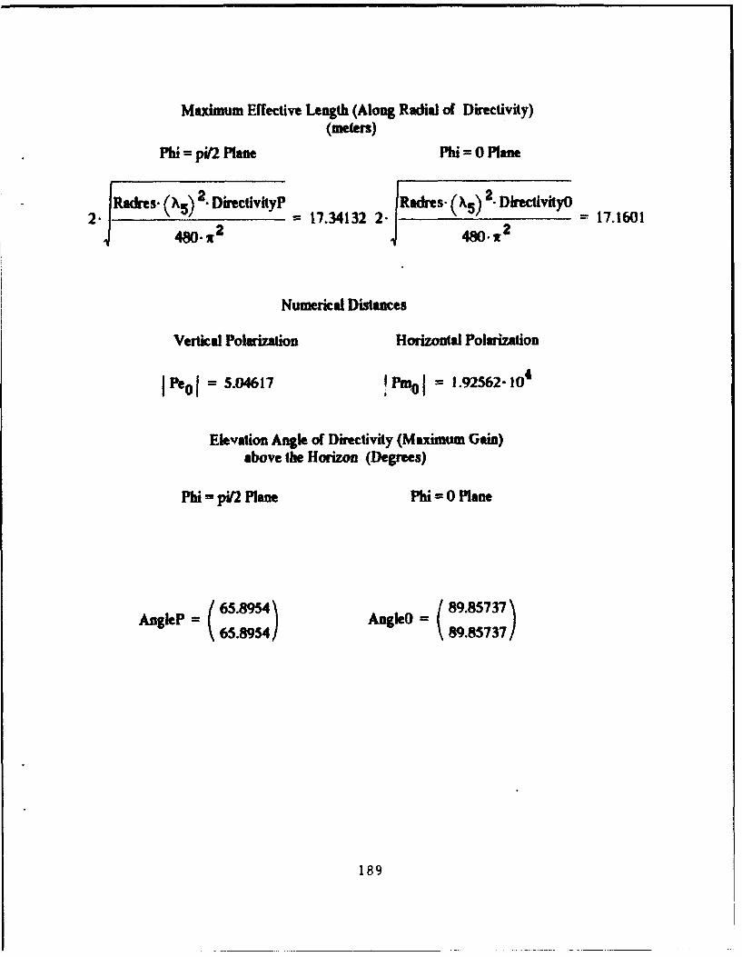
Maximum Effective Length (Along Radial of Directivity)(meters)
Phi = pV2 Plane Phi = 0 Plane
jRadres" (X5) 2" DirectlvityP jRadres- (XS) 2" Dreclvit70yO2 ...- 17/.34132 2 .. ..- 17.1601
,480. x2 480.%2
Numerical Distances
Vertical Polarization Horizontal Polarization
Pe0o " 5.04617 I Pmol I =.92562-104
Elevation Angle of Direclivity (Maximum Gain)above the Horizon (Degrees)
Phi = pi/2 Plane Phi = 0 Plane
= (le 65.8954) AngkeO = 9877(65.8954 (89.85t71/
189

HORIZONTAL DIPOLE
This application calculates far field radiation patterns and parameters associated withhorizontal thin-wire dipole antennas (diameter << wavelength). The antenna ismounted above and parallel to the x-axis in a rectangular coordinate system. Thefeed is at the center of the antenna at a set height directly above the origin.Required inputs are the antenna length, feed height above the surface, transmittedfrequency, distance from the antenna, the conductivity and dielectric constant of thesurface below the antenna. The planar earth model is assumed in predictingradiation patterns. Predicted operating frequencies assume that the antenna is aquarter-wavelength. half-wavelength, three-quarter-wavelength, or full wave-length dipole. A sinusoidal current input with a maximum of unity is assumed. Allradiation patterns are normalized with respect to the maximum electric fieldintensity transmitted by the antenna in the plane of interest. The electric fieldmagnitudes to which the patterns are normalized are displayed below theirrespective plots. The radiation patterns are plotted for the phi=O and phi=pi/2vertical planes parallel and perpendicular to the x-axis respectively. A horizontalradiation pattern is plotted at an elevation selected by the index from the elevationangle index table. Polarization is a combination of vertical and horizontaldepending upon spatial orientation relative to the dipole.
Input the dipole I 7.5 h :- Ilength in meters 2
Input the index of the elevation angle forwhich to calculate the horizontal radiation d 535pattern (from the angle index table)
Wavelengths and Frequencies
21 4.1X - 4-1 2 2- 3 -X= CI4
c1 f2;cc f4:c
Possible Operating Frequencies (Hertz)
X Dipole: f 1.10- Dipole: f = 2. 104 [11 22
3 4 Dipole: f3 - 3. 107 Dipole: f4 - 4. 10
190

Input the operating f5 := 20. 106 X5 = c 2-xFrequency (Hertz) f3 X5
Input the Height of HO 7.6 Input the ground 30Antenna Feed (meters) Dielectric Constant
Input the Distance R 3000 Input te ground 3.10- 2from Antenna (meters) Conductivity:
Index of Refraction
Rd, R - HD-cos(O 1) 18000.0n erRrf R + Ho.cos(6 1) t(f.o )
Complex Numerical Distance Pm -1 cos(2- + 2 (sin(01)21
for Horizontal Polarization 2. sin (o,)2 \ +0
Vertical Reflection Coefficient rv (: Z.Cos(8g)) _ (02 sin(6))
(n2.cos(8,)) + ( 2 - s~in(01))
Horizontal Reflection Coefficient Cos(,I) - s( 2r o, *0 = -Cos1(1 ) + ( 2 s
191

Radiation Patterns in Phi=PiI2 Plane (Perpendicular to Dipole)
Space Wave Radiation Pattern (Phl=Pi2)
YI
\0. \
-05 '0. *'0
/ t I HP
Max E-Field Intensity (Volts per meter) max( MagEIP) =0.03737
Surface Wave Radiation Pattern (Phi~pil)
0 ... ... . . . ..... /...
- 05 0 0.5 1wk.L HUI1
Max E-Field Intensity (Vohts per meter) max (MagIE2P) =8.03309- 10-
192

Radiation Patterns in Phi0O Plane (Parallel to Dipole)
Space Wave Radiation Pattern (Phi--O)
viol
...... ...........
-j -0.5 00.51
Max E-Field Intensity (Volts per meter) max( MagElO) = 0,01561
Swface Wave Radiation Pattern (Pbi=O)
0
i.. 'A ,.....I
- 0.5 0 .
Hff,Ok I R201
Max E-Field Intensity (Volts per meter) max (MagE2O) = 154902 IOý4
193

Radiation Patterns in Horizontal Plaue
Space Wave Radiation Pattern
--
wo .mu
-0.5A-1,
-1 ~ -0. 0 0. -
I~k- v--'
Max~~~~ E-il nestIVh e et)mxMg2)16061-
S194

Total Power Radiated (Watts) power = 27.68975
Radiation Resistance (versus Radres : 55.3795Maximum Antenna Current)(Ohms)
Directivity (or Maximum Power Gain assuming 100% Antenna Efficiency)
Phi = pit2 Plane Phi = 0 Plane
DirectivityP = 7.56408 DirectivityO = 1.32021
Effective Isotropic Radiated Power (EIRP) (Wats)
Phi = pi2 Plane Phi = 0 Plane
DirectivityP. power = 209.44744 Directivity0. power = 36.55637
Maximum Effective Area (Along Radial of Directivity)(squae meters)
Phi= p/2 Plane Phi= 0 Plane
2. DirectivityP (X=) 2. DirectivitvO--______ 135.43431 = 23.63833
4.1 4.1
195

Maximum Effective Length (Along Radial of Directivity)(metes)
Phi = pit2 Plane Phi = 0 Plane
2.Radres. 0)2. DrectvityP 8.920792.Rakes- 0\5) DirectlvityO2.j.y = 8.92079 21"4 - 3.7269
480. X2 480. X2
Numerical Distances
Vertical Polarization Horizontal Polarization
I eol = 15.283 IPmoI = 2.4896-104
Elevation Angle of Directivity (Maximum Gain)above the Horimzon (Degrees)
Phi = pi/2 Plane Phi = 0 Plane
(2:.24089/ (41.64818
196

HORIZONTAL DIPOLE
This application calculates far field radiation patterns and parameters associated withhorizontal thin-wire dipole antennas (diameter << wavelength). The antenna ismounted elve and parallel to the x-axis in a rectangular coordinate system. Thefeed is r ,ne center of the antenna at a set height directly above the origin.Req,..,ed inputs are the antenna length, feed height above the surface, transmittedfrequency, distance from the antenna, the co3nductivity and dielectric constant of thesurface below the antenna. The planar earth model is assumed in predictingradiation patterns. Predicted operating frequencies assume that the antenna is aquarter-wavelength, half-wavelength, three-quarter-wavelength, or full wave-length dipole. A sinusoidal current Input with a maximum of unity is assumed. Allradiation patterns are normalized with respect to the maximum electric fieldintensity transmitted by the antenna in the plane of interest. The electric fieldmagnitudes to which the patterns are normalized are displayed below theirrespective plots. The radiation patterns are plotted for the phi--O and phi=pi/2vertical planes parallel and perpendicular to the x-axis respectively. A horizontalradiation pattern is plotted at an elevation selected by the index from the elevationangle index table. Polarization is a combination of vertical and horizontaldepending upon spatial orientation relative to the dipole.
Input the dipole I = 5 h = Ilength in meters 2
Input the index of the elevation angle forwhich to calculate the horizontal radiation d 535pattern (from the angle index table)
Wavelengths and Frequencies
4-1Al1 4.1 A = 2.1 X3 4 3 A4 =
c c c C
Possible Operating Frequencies (Hertz)
X Dipole: f1 1.5. 107 A Dipole: 12 3 104 2
3.4 ADipole: 13 4.5. I07 A Dipole: 14= 6. I0 7
4
197

Input the operating 6 c 2wFrequency (Hertz) :3 f- X 5
Input the Height of H = 7.6 Inputthe groundAntenna Feed (meters) Dielectric Constant
Input the Distance R := 3000 Input the ground o 3-10- 2from Antenna (meters) Conductivity:
Index of Refraction
Rd, R - H0-cos(O,) 18000.a
Rr, R + H-o,(,) - iC(OS.)o-
Complex Numerical Distance Pe1 R- T sin (01for Vertical Polarization 2.sin " s0 + n2
Complex Numerical Distance __ - ' Cos() +Jo (+(,) 2)
for Horizontal Polarization 2. si (01) 2 L 1
2.• o(). Qn sin(-,.<o))Veltical Reflection Coefficient rv1 (n Cos( ))- n -sn( ))
(ncos(8)) (+n( - sin(o,)2)
Horizontal Reflection Coefficient UhI :=os(,,) - ( n (0 1)2)
Cos(98) + ( 2 sin(Oj)2)
198

Radiation Patterns in Phi-Pi/2 Plane (Perpendicular to Dipole)
Space Wave Radiation Pattern (Phi=Pit2)
VIP,
I V "I
05 -0. 0 1' 5
yIP IP
Max E-Field Intensity (Vots per meter) max( MagEIP) =0.03799
Surface Wave Radiation Pattern (Phi=pVt2)
i
-05
-0.
-1 0.5 0 053w~fhIL m2P,
M-x E-Field Intensity (Volts per meter) max( MagE2P) = 6.21706-1607
199

Radiation Patterns in PhI'0 Plane (Parllel to Dipole)
Space Wave Radiation Patters (Phi=0)
0.5 .
Y'I~A
-10..5.0.
w4.- -H.- I
Max E-Field Intensity (Volts per meter) max( MagElO) - 0.03422
Stwface Wave Radiation Patter (Plii=O)
0.
Max E-Fiekll ntensity (Vohts per mewe) max(MagE20) - 9.39091-16-5
200

Radiation Patterns in Horizontal Plane
Space Wave Radiation Pattern
0.5.
0 A -0. 0 1 *.
-0.t 0.
000
Max E-Fiekl Intensity (Volta per meter) max ( MagEl H) 0.0244972 1
Sw ae ae adato Pttr (orzotl0lae

Total Power Radiated (Waits) power 31.69054
Radiation Resistance (versus Radres = 63.38107Maximum Antenna Cutrent)(Ohms)
Directiviy (or Maximum Power Gain assuming 100% Antenna Efficiency)
Phi = pit2 Plane Phi = o Plane
DirectivityP = 6.8304 DirectivityO = 5.54301
Effective Isotropic Radiated Power (EIRP) (Waits)
Phi = pil2 Plane Phi = 0 Plane
DirectiviyP. power = 216.45893 DirectivtyO- power = 175.66087
Maximum Effective Area (Along Radial of Directivity)(square meters)
Phi = pi2 Plane Phi = 0 Pane
(X5) 2. DirectivityP 4 X5) 2. DirectivityO________= 54.35457 = 44.10985
4.x 4-z
202

Maximum Effective Length (Along Radial of Directivity)(meters)
Phi = pi/2 Plane Phi - 0 Plane
2 IRades. (?,5) 2- DlrectivityP 6.04592 2Rdres. (X) . DictiviyO 5.44643480.*2 4480.x2
Numerical Distances
Vertical Polarization Horizontal Polarization
I =o l 26.28165 IPmD I = 3.21687•-0'
Elevation Angle of Directivity (Maximum Gain)above the Horizon (Degrees)
Phi = pi/2 Plane Phi = 0 Plane
AngleP =(18.542) AngleO = 89.85737)(18.542/ (89285737
203

HORIZONTAL DIPOLE
This application calculates far field radiation patterns and pmrmeters associated withhorizontal thin-wire dipole antennas (diameter << wavelength). The antenna ismounted above and parallel to the x-axis in a rectangular coordinate system. Thefeed is at the center of the antenna at a set height directly above the origin.Required inputs are the antenna length. feed height above the surface, transmittedfrequency, distance from the antenna. the conductivity and dielectric constant of thesurface below the antenna. The planar earth model is assumed in predictingradiation patterns. Predicted operating frequencies assume that the antenna is aquarter-wavelength, half-wavelength, three-quarter-wavelength, or full wave-length dipole. A sinusoidal current input with a maximum of unity is assumed. Alradiation patterns are normalized with respect to the maximum electric fieldintensity transmitted by the antenna in the plane of interest. The electric fieldmagnitudes to which the patterns are normalized are displayed below theirrespective plots. The radiation patterns are plotted for the phi-O and phi=pi/2vertical planes parallel and perpendicular to the x-axis respectively. A hori7,6ntalradiation pattern is plotted at an elevation selected by the index from the elevationangle index table. Polarization is a combination of vertical and horizontaldepending upon spatial orientation relative to the dipole.
Input the dipole I :- 3 h - Ilength in meters 2
Input the index of the elevation angle forwhich to calculate the horizontal radiation d 535pattern (from the angle index table)
Wavelengths and Frequencies
4-1\ 1 4-1 1\2 2-1 A -X-- X = I
c C c cIt Al r2 A 2 [3 A 4=AA•4
Possible Operating Frequencies (Hertz)
SDipole: f1 2.5. 10 X Dipole: f2 5.10
3-X Dipole: f3 7.5 10? A Dipole: 14 = 1. 108
204

Input the operating 6 so0 106 c 2.1Frequency (Hertz) .X5
Input the Height of H0 := 1.5 Input the ground r : 72Antenna Feed (reeters) Dielectric Constant
Input the Distance R := 3000 Input the ground 4from Antenna (meters) Conductivity:
Index of Refraction
Rd1 = R - H0.cos(60 Ia 0o
Rri R + Ho.cos(6l) nf=3. 10-6O )
Complex Numerical Distance Pe i in 2 s(in )
for Vertical Polarization 2. sin 1)( n 2 I
Complex Numerical Distance pm, - -'0Rr, I cos(6,)+ Jn 2 _ (sin 12for Horizontal Polarization .2.sin (61) 2
(.,.o,(,)) (o, ,,2,,Vertical Reflection Coefficient l "I W .,.1 ,(0,)1 (i 2 _-n (0,)2)
(n20co(e)) + ( n2 _ sin(0 1)2)
Iforizontol Rteflection Coefficient Cos) n si0
Cos (6,) + Ti- sin(01) 2)
205

Radiation Patterox in Ptai=Pi/2 Plane (Perpndicular to Dipole)
Space Wave Radiation Pattern (Phi--Pif2)
..... ....
05 ~ ~ ~ .X.. ...
-0.5 .. X.
-1 -0.5 0 0.51
Max E-Field Intensity (Volts per meter) max( MagEIP) =0.03926
Surface Wave Radiation Pattern (Fhi pit)
0.!5' I -Y.
-1 0.5 0D 0.3"wek - a
Max E-Field Intensity (Volts per meter) max( MagE2P) =8.83121-16O9
206

Combined Space and Surface Wave Radiation Pattern (Phi--pi/2)
I A
t . ......
-I 'IJ' I +
I~. 1- I-
\(lt H;!.1
Max~~~~~~ E-Fel Inest-Vlsprmte) mx sEP .32
0 ~ i ~L.-.207

Radiation Patterns in Phi=O Plane (Parallel to D~ipole)
Space Wave Radation Pattern (Phi~o)
I A--
It A
-05 -0* 0/.
wersl. RIC I
Max E-Field Intensity (Volts per meter) max ( MagE 10) 0 0.3925
Surface Wave Radiation Pattern (Phi=O)
-2 01
-1 -0.5 0 0.51
Max E-Field Intensity (Volts per meter) max( MagE2O) = 3.2224- 16-4
208

Combined Space and Swface Wave Radiation Pattern (PhlO)
.I ........
0.5-
y 0 - ...... I
~.........
-0.5
I ... ... .
0I 1
W4 -. "3 1
Max E-Field uinensity (Volts per meter) max (MagI330) =0.03925
209

Radation Patterns in Horizontal Plane
Space Wave Radiation Pattern
0 ....... \ 'h=
-0.5 17-
*< k / I I .*
I -*
-1 -05 0 .
923-. .......
X
Max E-Field Intensity (Volts per meter) max ( MgE211) =4.07737-16-
210

Combined Space and Surface Wave Radiation Pattern (Horizontal Plane)
..-.. ......
.... ... . .. ....
Y I ......
I ..... .....
we. OR-..
2111

Total Power Radiated (Watts) power = 41.98012
Radiation Resistance (versus Radres = 83.96025Maximum Antenna Current)(Ohms)
Directivity (or Maximum Power Gain assuming 100% Antenna Efficiency)
Phi = pil2 Plane Phi = 0 Plane
DirectiviiyP = 5.50819 Directi!ityO = 5.50321
Effective Isotropic Radiated Power (EIRP) (Watts)
Phi = pi/2 Plane Phi = 0 Plane
DirectivityP. power = 231.23457 DirectivilyO. power = 231.02563
Maximum Effective Area (,long Radial of Directivity)(square meters)
Phi = pi2 Plane Phi = 0 Plane
2XS) 2. DirectivyP (X5 ) 2. Directivit yO
4-s 15.77981 4- 15.765554- 4.-21
212

Maximum Effective Length (Along Radial of Directivity)(meters)
Phi = pi Plmne Phi = 0 Plane
2R (A5) 2. - 3.74932 (.iRadres. (X,5) 2 DirectivityO 3.74762480.x2 480.x2
Numerical Distances
Vertical Polarization Horizontal Polarization
I Peol = 1.08943 PmoI = 2.26469-o10
Elevation Angle of Directivity (Maximum Gain)above the Horizon (Degrees)
Phi = piY2 Plane Phi =0 Plane
AngleP 78.7317) =nlO 8.5378.73217/ (89.825737
213

APPEMNIX V:VERTICAL LOG-PERIODIC DIPOLE ARRAY COMPUTER OUTPUT
This appendix contains computer hardcopies from the
Mathcad vertical log-periodic dipole array application which
show the input values and predicted radiation characteristics
for two sample calculations. The configuration is a given by
the inputs on the first two pages of each printout. The first
antenna is mounted above soil (E,=10 and a=10-3) and the second
above seawater (e,=72 and a=4). Reference 6 [p. 114) provides
the radiation patterns and gain predictions from several
sources for the configuration in the first example.
The radiation patterns and maximum directive gain
computed by the first Mathcad example are almost identical to
the those given in reference 6. The directivity prediction is
slightly higher for Mathcad, and the elevation of the maximum
directive gain is also slightly higher, but the overall
similarity between the predicted radiation characteristics is
still quite good. The seawater example also yields results
consistent with expectations. With respect to the soil
example, the seawater example's directivity is higher due to
a stronger reflected wave, and the surface wave is stronger at
grazing angles (0-900) due to higher conductivity.
214

VERTICAL LOG PERIODIC DIPOLE ARRAY
This application calculates far field radiation patterns and parameters associated withvertical log periodic dipole arruys. The antenna is oriented such that the projectionof its center axis lies on the positive y-axis of a rectangular coordinate system. Theantenna axis can be oriented with respect to the vertical at any angle between zeroand ninety degrees. The feed is at the center of the shortest element directly abovethe origin. The dipole elements are bisected by the antenna axis and are parallel tothe z-axis. Required inputs are the number of dipole elements, shortest and secondshortest element lengths. separation between the shortest and second shortestelements, radius of the shortest element, height of the feed above the surface,angle of the antenna axis with the vertical, characteristic admittance of the linefeeding the antenna, termination impedance of the antenna, transmitted frequency,distance from the antenna, the conductivity and dielectric constant of the surfacebelow the antenna. The planar earth model is assumed in predicting radiationpatterns. A sinusoidal current input with a maximum of unity is assumed. Allradiation patterns are normalized with respect to the maximum electric fieldintensity transmitted by the antenna in the plane of interest. The electric fieldmagnitudes to which the patterns are normalized are displayed below theirrespective plots. Radiation patterns are plotted for the phi--0 and phi=pi/2 verticalplanes perpendicular and parallel to the y-axis respectively. A horizontal radiationpattern is plotted at an elevation selected by the index from the elevation angleindex table. Polarization is vertical for all vertical log-periodic antennas.
Input the number N 12 Input the shortest red : .00918of elements element's Radius 0
(meters)
Input the length Input the lengthof the shortest 0 3.673 of the second 11 4.373element (meters) shortest element
(meters)
Input the distance Input the height offrom shortest to do 1.0766 the shortest element H0o 6.87second shortest above the surfaceelement (meters) (meters)
Input the operating f 6 Input the Distance R 3000Frequency (Hertz) from the Antenna
(meters)
Input the ground 0 1. to- 3 Input the ground er 10Conductivity Dielectric Constant
Input the Characteristic I Input the TerminationAdmittance of the Line ADM - Impedance connected TIMP = 450Feeding the Antenna to longest element(Ohms) (Ohms)
215

Input the angle between Input the elevation indexthe vertical (z axis) and • 78 for which to calculate the w 285the antenna axis (degrees) horizontal radiation pattern
(from angle index table)
NOTE: The Vertical Log-Periodic Dipole mutual impedance calculations are notvalid if there is an antenna element whose length is an exact integer multiple of thewavelength. If this occurs, there will be a singularity error in the mutual impedancecalculations. If this problem arises, it will be necessary to vary the operating frequencysuch that no element is exactly an integer multiple of the wavelength.
If the log-periodic calculations of element length and spacing do not represent thedesired antenna configuration, you can enter the values directly by selecting thevariables I and d, using the define key (shift, colon), and entering the lengths andspacings by separating each successive entry by a comma.
Calculated distanceCalculated length between successive Calculated radiiof elements from elements-shortest of elements fromshortest to longest to longest shortest to longest
d radV
3.673 1.0766 0.009184.373 1.28178 0.010935.20641 1.52606 0.013016.19864 1.8169 0.015497.37998 2.16316 0.018448.78645 2.57541 0.0219610.46098 3.06624 0.0261512.45463 3.6506 0.0311314.82823 4.34633 0.0370617.65419 5.17465 0.0441221.01873 6.16084 0.0525325.02447 0.06254
216

Radiation Patterns in Phi--Wi2 Plane(Perpendicular to X -Axis)
Space Wave Radiation Pattern (Phi=PVf2)
* ,... t I
..........J
-05 -05 0.
MaxE-FeldIntensity (Volts per meter) niax( MagEIP) 0.59
Surface Wave Radiation Pattern (Phi~pi(2)
I -4
0. ........ T ..~ .
y2P1 .r..
-0.5 7.\
Al -0.5 0 0.5wo~k - 2PI
Max E-Field Intensity (Volhs per meter) max( MagE2P) =0.00124
217

Combined Space and Surface Wave Radiation Pattern (Phi~piI2)
.. .. .. .. .. ... ....
. .. . ..... ....
V3; r ..~ .....
-0.5
218~

Radiation Patterns in Phi=O Plane
(Perpendicular to Phi-pitl Plane)
Space Wave Radiation Pattern (Phi4))
I. r
0.5
-1 0.5 0 0.5we% Ro
Max E-Field Intensity (Volts per meter) max( MagEl) 0 0.03221
Surface Wave Radiation Pattern (PlW!O)
1.. ......
0 ............... :,:........ ..........I
7, *.......
-- 00. 0 0~i4 .5 1Ieý . .*
1 219

Combined Space and Surface Wave Radiation Pattern (PhiO))
.. ..... .. ... .... I
.5. 4 1
.. __ .. I ,...
30 I' ..........
"" X
-0.5
7. %
-05 0 0.51
Max E-Field Intensity (Volts per meter) max( MagE3O) 0.032 1
220

Radiation Patterns in Horizontal Plane(Parallel to Ground)
Space Wave Radiation Pattern (Horizontal)
-0.5
-1 -0.5 0 0.5 1Wtk Hil
Max E-Field Intensity (Volts per meter) max (MagE I11 H 0.05438
Surface Wave Radiation Pattern (Horizontal)
J'I
00
Max E-Field Intensity (Vohts per meter) nmax( MagE2H) = 1.09861- 10O
221

Combined Space and Surface Wave Radiation Pattern (Horizontal)
..................
0o ....... ... Phi=O
......... .
-0.5 0 0. 1** . -
wok ... OI
Max~~~~~~~~~~7. E-il Itnit Vh prmte)mx Mg3)..52
222

2 2po e e 30 a-E IT eJ '0-' Y .-see(a2 + ( 3)-( ¢os(ý) .sin(a2 -1 0 ) ,sin(rl)
- 02
power - powerO Radres := 2 -power
qE3P 2 M E3P-( 120) DirectivityP 4-.R2. max(sqE3P)power
Sq3,:-(I MagE3Ol) 2 _________
sqE30 1 ( 2.(120-.) DirectivityO 4.-wR2.max(sqE30)2 % power
Total Power Radiated (Watts) power - 34.29572
Radiation Resistance (versus Radres = 68.59144Maximum Input Current)(Ohms)
Directivity (or Maximum Power Gain assuming 100% Antenna Efficiency)
Phi = pi/2 Plane Phi = 0 Plane
DirectivityP = 13.63346 DirectivityO = 4.50794
Effective Isotropic Radiated Power (EIRP) (Watts)
Phi = pi2 Plane Phi - 0 Plane
DirectivityP- power = 467.56917 DirectivityO. power = 154.6031
223

Maximum Effective Area (Along Radial of Directivity)
(square meters)
Phi = pI Plane Phi = 0 Plane
5) 2 -D irectivityP 30 . 6 5 ,5 . D irectivityO = 9 . 4 3_______= 301.36553 = 99.647394.s 4.w
Maximum Effective Length (Along Radial of Directivity)(meters)
Phi = pi/2 Plane Phi = 0 Plane
iRadres' (\3) 2. DirectivityP = Radres. (\) 2. DirecivityO 8.5159448).x2 480.%2
Numerical Distance for Vertical Polarization
IPeoI =50.7
Elevation Angle of Directivity (Maximum Gain)above the Horizon (Degrees)
Phi = pi/2 Plane Phi= 0 Plane
AngleP = 14.28571 AngleO = (13.71429)
224

VERTICAL LOG PERIODIC DIPOLE ARRAY
"This application calculates far field radiation patterns and parameters associated withvertical log periodic dipole arrays. The antenna is oriented such that the projectionof its center axis lies on the positive y-axis of a rectangular coordinate system. Theantenna axis can be oriented with respect to the vertical at any angle between zeroand ninety degrees. The feed is at the center of the shortest element directly abovethe origin. The dipole elements are bisected by the antenna axis and are parallel tothe z-axis. Required inputs are the number of dipole elements, shortest and secondshortest element lengths. separation between the shortest and second shortestelements, radius of the shortest element, height of the feed above the surface,angle of the antenna axis with the vertical, characteristic admittance of the linefeeding the antenna, termination impedance of the antenna, transmitted frequency,distance from the antenna, the conductivity and dielectric constant of the surfacebelow the antenna. The planar earth model is assumed in predicting radiationpatterns. A sinusoidal current input with a maximum of unity is assumed. Allradiation patterns are normalized with respect to the maximum electric fieldintensity transmitted by the anteana in the plane of interest. The electric fieldmagnitudes to which the patterns are normalized are displayed below theirrespective plots. Radiation patterns are plotted for the phi=0 and phi=piI2 verticalplanes perpendicular and parallel to the y-axis respectively. A horizontal radiationpattern is plotted at an elevation selected by the index from the elevation angleindex table. Polarization is vertical for all vertical log-periodic anteanas.
Input the number N = 12 Input the shortest rad0 .00918of elements element's Radius
(meters)
Input the length Input the lengthof the shortest 1 0 3.673 of the second !1 ý= 4.373element (meters) shortest element
(meters)
Input the distance Input the height offrom shortest to do = 1.0766 tue shortest element Ho 6.87second shortest above the surfaceelement (meters) (meters)
Input the operating f5 18.06 ~ Input the Distance R 3000Frequency (Hertz) from the Antenna
(meters)
Input the ground 4 Input the ground fr 72Conductivity Dielectric Constant
Input the Characteristic I Input the TerminationAdmittance of the Line ADM - 450 Impedance connected TIMP = 450Feeding the Antenna to longest element(Ohms) (Ohms)
225

Input the angle between Input the elevation indexthe vertical (z axis) and 78 for which to calculate the w = 285the antenna axis (degrees) horizontal radiation pattern
(from angle index table)
NOTE: The Vertical Log-Periodic Dipole mutual impedance calculations are notvalid if there is an antenna element whose length is an exact inleger multiple of thewavelength. If this occurs, there will be a singularity error in the mutual impedancecalculations. If this problem arises, it will be necessary to vary the operating frequencysuch that no element is exactly an integer multiple of the wavelength.
If the log-periodic calculations of element length and spacing do not represent thedesired antenna configuration, you can enter the values directly by selecting thevariables I and d, using the define key (shift, colon), and entering the lengths andspacings by separating each successive entry by a comma.
Calculated distanceCalculated length between successive Calculated radiiof elements from elements-shortest of elements fromshortest to longest to longest shortest to longest
I d radY ~ V
3.673 1.0766 0.009184.373 1.28178 0.010935.20641 1.52606 0.013016.19864 1.8169 0.015497.37998 2.16316 0.018448.78645 2.57541 0.0219610.46098 3.06624 0.0261512.454631 3.6506 0.0311314.82823 4.34633 0.0370617.65419 5.17465 0.0441221.01873 6.16084 0.0525325.02447 0.06254
2?6

Radiation Patterns in Phi--Pi/2 Plane(Perpendicular to X -Axis)
Space Wave Radiation Pattern (Phi=Pi/2).
05'~
YI1L
-0.5/
1 -05 0 0.5WOV HIP,1
Max E-Field Intensity (Volts per meter) max( MagEl P) =0.10756
Surface Wave Radiation Pattern (Phi~pi2)
..........
0.5 .. .....
y2F1P.
-1 -05 0 0.51woL,1 142P I
Max E-Fiekl Intensity (Volts per meter) inax( MagE2P) = 0.12392
227

Combined Space and Stuface, Wave Radiation Patterni 'Phi~pU2)
\f ~ 1
wel. I :'
Ma /-ik nest Vlspr ee) mx aEP 0 2"
2281

Radiation Patterns in Phi=0 Plane
(Perpendicular to Phi~pi2 Plane)
Space Wave Radiation Pattern (Phi=O)
Ij
-0.5 7, T
-1 -0.5 0 0.51wok, 1 0*
Max E-Field Intensity (Volts per meter) max(MagEO 10 0.06687
Swface Wave Radiation Pattern (PhiO))
~. \, i....I
I'. -- A
-1-0.5 0 05
Max E-Fiekl Intensity (Volts per meter) max (MagE20) = 0.07827
229

Combined Space and Swfac~e Wave Radiation Pattern (Phi=O)
Y,30~
4
. . .. .....
-0. .0.5 0 0.1 1
-1 05t 0 05
Max E-Field Intensity (Volts per meter) max ( MagE3O) 0.07827
230

Radiation Patterns in Horizontal Plane(Parallel to Ground)
Space Wave Radiation Pattern (Horizontal)
AA
0.3 '4
---
S 0.5 0 0.5 1
Max E-Field Intensity (Volts per meter) max (MagE III H 0.06821
Surface Wave Radiation Pattern (Horizontal)
I ...........
.:* ... .I . ...
0 .T . .... 111=0
S 0.5 0 053 1weik. m2E1i
Max E-Fiekt Intensity (Volts per meter) max( MagE2H) = 4.93203-1IO5
231

Combined Space and Surface Wave Radiation Pattern (Horizontal)
...... ...
.... ... .....
Y32 ......
.......................
-t-0.5 0 0.5
Max E-Field Intensity (Volts per meter) max( MagE311) =0.0682
232

power 30 2J'i.P Y Y.sec(a2 + a3)(.oo5(ý1J* t(ca2 + a3) + s•(ý|
2
power := powerV Radres ý= 2-power
sqE3P, (I MagE3Pi 1) 2 DirectivityP 4-x'R2"max(sqE3P)S2.(120.%) power
sqE30 ('MagE3O ) 1 ) DirectivityO 4"x'R 2.max(sqE30)
2-q( 120-x)_2 power
Total Power Radiated (Watts) power = 99.48703
Radiation Resistance (versus Radres = 198.97405Maximum Input Current)(Ohms)
Directivity (or Maximum Power Gain assuming 100% Antenna Efficiency)
Phi = pi/2 Plane Phi = 0 Plane
DirectivityP = 23.15454 DirectivityO = 9.2.377
Effective Isotropic Radiated Power (EIRP) (Watts)
Phi = pi/2 Plane Phi = 0 Plane
DirectivityP. power = 2.30358. 103 Directivity0. power = 919.03096
233

Maximum Effective Area (Along Radial of Directivity)
(square meters)
Phi = pi/2 Plane Phi = 0 Plane
(X5) 2. DirectivityP (x5) 2- DirectivltyO =_______= 511.82763 = 204.19793
4. r 4. w
Maximum Effective Length (Along Radial of Directivity)(meters)
Phi = pi/2 Plane Phi = 0 Plane
Radres. (X5) 2. DirectivityP Radres. (X5) 2. DirectivityO2- 48..w2 32.87188 2... = 80% 20.76291
48O-*2•480-o
Numerical Distance for Vertical Polarization
I Pe0 I = 0.14135
Elevation Angle of Directivity (Maximum Gain)above the Horizon (Degrees)
Phi = pi2 Plane Phi = 0 Plane
AngleP = 0 AngleO= 0
234

"APPENDIX E:
HORIZONTAL LOG-PERIODIC DIPOLE ARRAY COMPUTER OUTPUT
This appendix contains computer hardcopies from the
Mathcad horizontal log-periodic dipole array application which
show the input values and predicted radiation characteristics
for two sample calculations. The configuration is a given by
the inputs on the first two pages of each printout. The first
antenna is mounted above soil (e,=4 and a=10-3) and the second
above seawater (E,=72 and a=4). Reference 6 [p. 1081 provides
the radiation patterns and gain predictions from several
sources for the configuration in the first example.
The radiation patterns and maximum directive gain
computed by the first Mathcad example are almost identical to
the those given in reference 6. The directivity prediction is
slightly higher for Mathcad, but the overall similarity among
the predicted radiation patterns is remarkably good. The
seawater example has results very much like the soil example.
For horizontal polarization, the higher conductivity surface
below the antenna does not result in a greatly enhanced
surface wave and increased directivity as it does for vertical
polarization.
235

HORIZONTAL LOG PERIODIC DIPOLE ARRAY
This application calculates far field radiation patterns and parameters associated withhorizontal log periodic dipole arrays. The antenna is oriented such that theprojection of its center axis lies on the positive y-axis of a rectangular coordinatesystem. The antenna axis can be oriented with respect to the vertical at any anglebetween zero and ninety degrees. The feed is at the center of the shortest elementdirectly above the origin. The dipole elements are bisected by the antenna axis andare parallel to the x-axis. Required inputs are the number of dipole elements,shortest and second shortest element l,'ngthi, separation between the shortest andsecond shortest elements, radius of the shortest element, height of the feed abovethe surface, angle of the antenna axis with the vertical, characteristic admittance ofthe line feeding the antenna, termination impedance of the antenna, transmittedfrequency, distance from the antenna, the conductivity and dielectric constant of thesurface below the antenna. The planar earth model is assumed in predictingradiation patterns. A sinusoidal current input with a maximum of unity is assumed.All radiation patterns are normalized with respect to the maximum electric fieldintensity transmitted by the antenna in the plane of interest. The electric fieldmagnitudes to which the patterns are normalized awe displayed below theirrespective plots. Radiation patterns are plotted for the phi=pi12 and phi--O verticalplanes parallel and perpendicular to the y-axis respectively. A horizontal radiationpattern is plotted at an elevation selected by the index from the elevation angleindex table. Polarization is a varying combination of horizontal and verticaldepending on spatial orientation with respect to the antenna.
Input the number N 12 Input the shortestof elements N 12 element's Radius rad 0 .00144
(meters)
Input the length Input the lengthof the shortest lo 7.219 of the second 11 '= 8.297element (meters) shortest element
(meters)
Input the distance Input the height offrom shortest to do 1.659 the shortest element H0 9.4second shortest above the surfaceelement (meters) (meters)
Input the operating 12.106 Input the Distance
Frequency (Hertz) from the Antenna R 3000(meters)
Input the ground 1.0- 3 Input the ground 4r 4Conductivity Dielectric Constant
Input the Characteristic Input the TerminationAdmittance of the Line 1 Impedance connected flMPFeeding the Antenna ADM 3 to longest element(Ohms) (Ohms)
236

Input the angle between Elevation index for whichthe vertical (z axis) and ' 90 to calculate horizontal pattern w 285the antenna axis (degrees) (from angle index table)
NOTE: The Horizontal Log-Periodic Dipole mutual impedance calculations are notvalid if there is an antenna element whose length is an exact integer multiple of thewavelength. If this occurs, there will be a singularity error in the mutual impedancecalculations. If this problem arises, it will be necessary to vary the operating frequencysuch that no element is exactly an integer multiple of the wavelength.
If the log-periodic calculations of element length and spacing do not represent thedesired antenna configuration. you can enter the values directly by selecting thevariables I and d, using the define key (shift, colon), and entering the successivelengths and spacings by separating each successive entry by a comma.
Calculated distanceCalculated length between successive Calculated radfiof elements from elements-shortest of elements fromshortest to longest to longest shortest to longest
d radV
7.219 1.659 0.001448.297 1.90674 0.001669.53598 2.19146 0.001910.95997 2.51871 0.0021912.5966 2.89483 0.0025114.47762 3.32711 0.0028916.63954 3.82394 0.3033219.12429 4.39496 0.0038121.98009 5.05125 0.0043825.26233 5.80554 0.0050429.03471 6.67247 0.0057933.37041 0.00666
237

Radiation Patterns in Phi--PiI2 Plane(Perpendicular to X-Axis and Dipol. Elements)
Space Wave Radiation Pattern (Pbi=Pit2)
74'
Y f
IL , - 'P
Max E-Field Intensity (Volts per meter) max( MagEIP) =0.08512
Surface Wave Radiation Pattern (Phi pi/2)
I 1
0.5 7.
- ~ ~ ~ ~ y ..*. .- jj.
a P
II
-*05 .4.. .. ........
Max E-Field Intensity (Volts per meter) max( MagE2P) 4.54242-1-
238

Combined Space and Surface Wave Radiation Pattern (Phi~pi/2)
1-.. \ .....
..............................
0.
y P . ....
e~ . 3r,
-0. .1:
-0.5. 0 ~ 0. 1~//*1'i"/ e' **.3.***
Max E-Field Intensity (Volts per meter) max( MagE3P) =0.08511
239

Radiation Patterns in Phi=0 Plane(Perpendicular to Phi~pi/2 Plane)
Space Wave Radiation Pattern (Phi=O)
0.Oi. 4.'
I=A
-1 -05 0 0.51
M ax E-Field Intensity (Volts per meter) max( MagE 10) 0.03495
Surface Wave Radiation Pattern (Phi=O)
0.51
y201 v. ....
Max E-Field Intensity (Volts per meter) max( MagE2O) =1.45261- 0-
240

Combined Space and Surface Wave Radiation Pattern (Phi=O)
0 .5 - .....
03 ......... ......
-0.5 01
Ke,~ "30i
Max E-Field Intensity (Volts per meter) max ( MagE3O) 0.03495
24 1
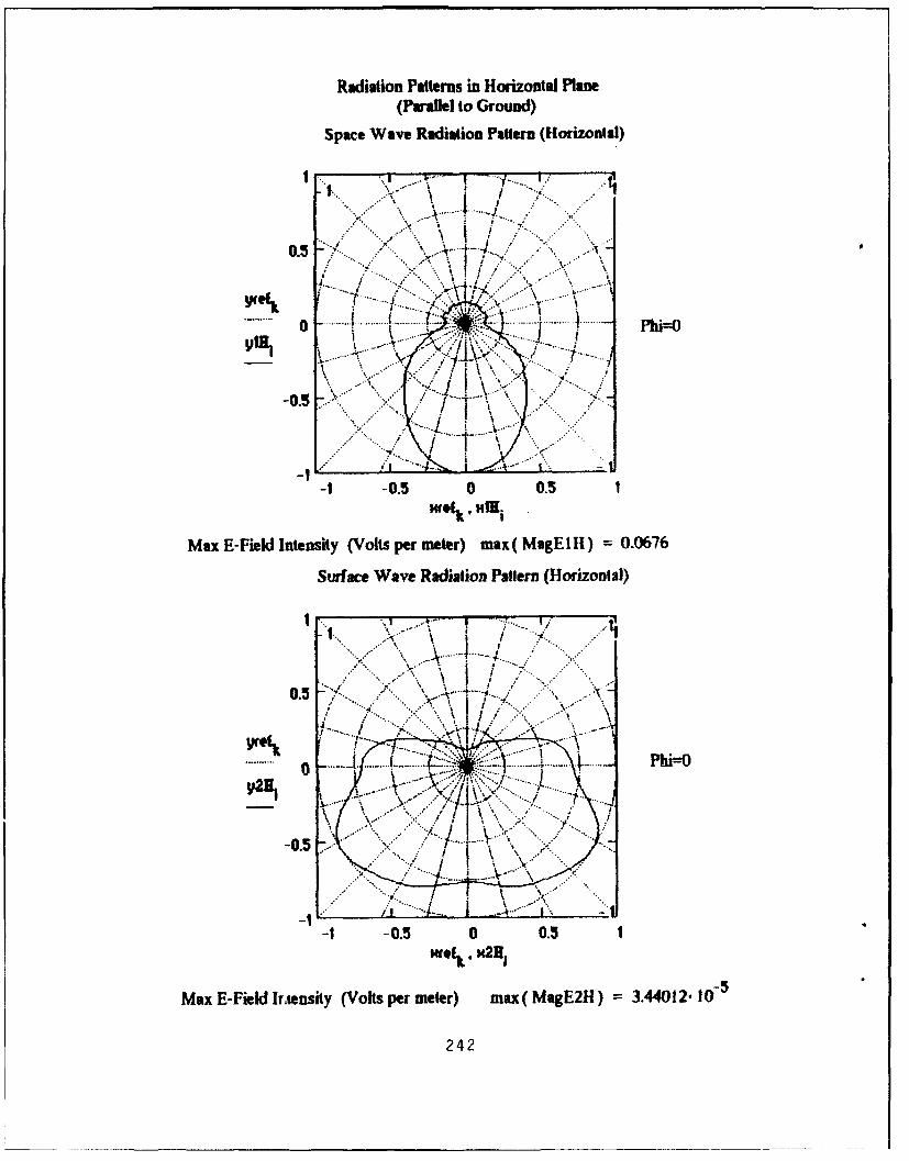
Radiation Patterns in Horizontal Plane(Parallel to Ground)
Space Wave Radiation Pattern (Horizontal)
.. .' ... 1...
..........
0.5
...... -. --- P h -
yIN 1
A -A
-1 -0.5 0 0.5 1
Max E-Field Ifntensity (Vohts per meter) max (MagE2 311) 4001276 6
SufaeWaeRaitinPatr2(orzn2l

Combined Space and Surface Wave Radiation Pattern (Horizontal)
...... ..
. .....
y3E ....
........
-1-0.5 0 0.51w*' OR 311
Max E-Field Intensity (Volts per meter) max (MagE3H) 0.06758
243

r1.57073 1.570763
power - fR30 1cos( ).cos(U).I j. .Y *csoc'•xR 2 J-I(sin(•).cos(•))2"
-- 1.5707963-0
poer _-_3 .sin(.•)-l j'p'Y .csc(wp -1 os{( }.co.(q
powero 2* i ei-R 2 1- (sin(').cos(E))
power powerO + powero Radres - 2-power
sqE3P MagE3P 2 DirectivityP 4a; R2 max(sqE3P)
2.( 120.•i) power
sqE301 (I MagE30i 1)2 Directivityo - 4"7rR 2 .max(sqE30)2.( 120-%) power
Total Power Radiated (Watts) power = 83.98604
Radiation Resistance (versus Radres = 167.97209Maximum Input Current)(Ohms)
Directivity (or Maximum Power Gain assuming 100% Antenna Efficiency)
Phi = pit2 Plane Phi = 0 Plane
DirectivityP = 12.93749 DirectivityO = 2.18175
244

Effective Isotropic Radiated Power (EIRP) (Watts)
Phi = pi/2 Plane Phi = 0 Plane
DirectivityP- power = 1.08657" 103 DirectivityO- power = 183,23657
Maximum Effective Area (Along Radial of Directivity)(square meters)
Phi = piI2 Plane Phi = 0 Plane
()1) 2. DirectivityP = 6 9) 2. Directivity0________= 643.45795 = 108.51135
4.x 4- i
Maximum Effective Length (Along Radial of Directivity)(meters)
Phi = pi/2 Plane Phi = 0 Plane
1 Radres" (X 5) 2"DirectivityP 2 "jRadres (1k.5) 2.Directivi(y42- __________ 33.86438 =- 13.90659
4,901 1480.12
Numerical Distances
Vertical Polarization Horizontal Polarization
IPeo 69.285M4 IPmoI = 1.26447 -103
Elevation Angle of Directivity (Maximum Gain)above the Horizon (Degrees)
Phi = pi/2 Plane Phi = 0 Plane
AngleP = 31.42857 AngleO 89,71429)
(89.71429/
245

HORIZONTAL LOG PERIODIC DIPOLE ARRAY
This application calculates far field radiation patterns and parameters associated withhorizontal log periodic dipole arrays. The antenna is oriented such that theprojection of its center axis lies on the positive y-axis of a rectangular coordinatesystem. The antenna axis can be oriented with respect to the vertical at any anglebetween zero and ninety degrees. The feed is at the center of the shortest elementdirectly above the origin. The dipole elements are bisected by the antenna axis andae parallel to the x-axis. Required inputs are the number of dipole elements,shortest and second shortest element lengths, separation between the shortest andsecond shortest elements, radius of the shortest element, height of the feed abovethe surface, angle of the antenna axis with the vertical, characteristic admittance ofthe line feeding the antenna, termination impedance of the antenna, transmittedfrequency, distance from the antenna, the conductivity and dielectric constant of thesurface below the antenna. The planar earth model is assumed in predictingradiation patterns. A sinusoidal current input with a maximum of unity is assumed.AU radiation patterns are normalized with respect to the maximum electric fieldintensity transmitted by the antenna in the plane of interest. The electric fieldmagnitudes to which the patterns are normalized are displayed below theirrespective plots. Radiation patterns are plotted for the phi-pi/2 and phi=0 verticalplanes parallel and perpendicular to the y-axis respectively. A horizontal radiationpattern is plotted at an elevation selected by the index from the elevation angleindex table. Polarization is a varying combination of horizontal and verticaldepending on spatial orientation with respect to the antenna.
Input the number NInput the shortestof ehents N 12 element's Radius rad0 = .00144
Selements (meters)
Input the length Input the lengthoftheshortest 10 7.219 of the second ]I := 8.297
element (meters) shortest element(meters)
Input the distance Input the height offrom shortest to do 1.659 the shortest element H0 - 9.4second shortest above the surfaceelement (meters) (meters)
Input the operating 121 Input the Distance
Frequency (Hertz) f5 from the Antenna R = 3000(meters)
Input the ground = 4 Input the ground a- 72Conductivity Dielectric Constant
Input the Characteristic Input the TerminationAdmittance of the Line I Impedance connected lIMP = 300Feeding the Antenna ADM to longest element(Ohms) (Ohms)
246

Input the angle between Elevation index for whichthe vertical (z axis) and ' = 90 to calculate horizontal pattern w := 285
the antenna axis (degrees) (from angle index table)
NOTE: The Horizontal Log-Periodic Dipole mutual impedance calculations are notvalid if there is an antenna element whose length is an exact integer multiple of thewavelength. If this occurs, there will be a singularity error in the mutual impedancecalculations. If this problem arises, it will be necessary to vary the operating frequencysuch that no element is exactly an integer multiple of the wavelength.
If the log-periodic calculations of element length and spacing do not represent thedesired antenna configuration. you can enter the values directly by selecting thevariables I and d, using the define key (shift, colon), and entering the successivelengths and spacings by separating each successive entry by a comma.
Calculated distanceCalculated length between successive Calculated radiiof elements from elements-shortest of elements fromshortest to longest to longest shortest to longest
I d radY v ..7.219 1.659 0.001448.297 1.90674 0.001669.53598 2.19146 0.001910.95997 2.51871 0.0021912.5966 2.89483 0.0025114.47762 3.32711 0.0028916.63954 3.82394 0.0033219.12429 4.39496 0.0038121.98009 5.05125 0.0043825.26233 5.80554 0.0050429.03471 6.67247 0.0057933.37041 0.00666
247

Radiation Patterns in Pfi=NY2 Plane(Perpendicular to X-Axis and Dipole Elements)
Space Wave Radiation Pattern (Phi=-, ?)
%I
-i V,~
-1 0.5 0 0.5WOVk HIP,
Max E-Pield Intensity (Volts per meter) max (MagE IP) =0.13724
Surface Wave Radiation Pattern (Plii=pit2)
0S..
-0.5.J '.
V /I
Max E-Field Intensity (Volts per meter) ,max( MagE2P) =3.19958-18
248

Combined Space and Surface Wave Radiation Pattern (Phi~pi2)
........ .. ----
0-3
.. .......
.............
- ............
-050 05
Max E-Field Intensity (Volts per meter) max (MagE3P) 0.13724
249

Radiation Patterns in P1,1=0 Plane(Perpendicular to Pi-pV Plane)
Space Wave Radiation Pattern (Phi=0)
0.5 -
0 ... .. .. .*YU1L~... ......*. *
-0.5 I
qA
-0.5 0 0.5HfOk MIDI 10
Max E-Field Intensity (Volts per meter) max( MagE 10) =0.05843
Suorface Wave Radiation Pattern (Phii=0)
.. ........
Y20 ..\ ....... .
0.5
1 0. 0 0.51
Max E-Field Intensity (Volts per meter) max (MagE2O) = 4.46943-10O4
250

Combined Space and Surf ace Wave Radiation Pattern (TPhi=O)
0 .5 - *
-~ I.
.I ..........
-0.5
..- . ........ ....
-0. -050.wet "30
Max -Fied Inensiy (Vhs er mter) max(......0.584
2.................

Radiation Patterns in Horizontal Plane(Parallel to Ground)
Space Wave Radiation Pattern (Horizontal)
YIN* j\ .. .... .i .....
-IN -05 0 .-~wo - " Vj is
1 7.
-1 -. 5 00.
I. .... .> ..... I ~ *'*
-0.57
S 0.5 0 0.5 1
Max E-Field Intensity (Volts per meter) max( MagE2H) =5.57296- 10-7
252

Combined Space and Surf ace Wave Radiation Pattern (Horizontal)
. ......... ..... 'i....
...................
-0.5
..... ........ .......
253.

[1.5707963 [1.5707%63
power - -30 2 cos(0)*cos(0),I j* JpY Y •CS('f
x.R 2 - (Sin(D).cos(O))2
--1.5707963 -,-
power€ =.30 2sin( 1) '2 j1 eJ "-YY -'¢so( 41 ).cos( C 'os( 4xpR2 1 - (sin(ý).cos(f))
power powerO + power€ Radres - 2-power
(t MagE3P1 1)2 4.z.R2.nmax(sqE3P)
sqE 2.( 120. x) DirectivityP = power
2(I MagE3O1 2 DirectivityO 4-x-R 2 .max(sqE30)2( 120.a) power
Total Power Radiated (Watts) power = 261.928
Radiation Resistance (versus Radres 523.856Maximum Input Current)(Ohms)
Directivity (or Maximum Power Gain assuming 100% Antenna Efficiency)
Phi = pi/2 Plane Phi = 0 Plane
DirectivityP = 10.78579 DirectivityO = 1.95488
254

Effective Isotropic Radiated Pc wer (EIRP) (Watts)
Phi = pit2 Plane Phi = 0 Plane
DirectiviHyP power = 2.8251. -10 DirectivityO. power = 512.03765
Maximum Effective Area (Along Radial of Directivity)(square meters)
Phi = pi2 Plane Phi = 0 Plane
(X5) 2. Direcivitym (X5) 2. DirectivityOe= 536.4412 97.227724.-% 4. r
Maximum Effective Length (Along Radial of Directivity)(meters)
Phi = pi/2 Plane Phi = 0 Plane
Radres" (XS) 2" DirectivityP Radres" 05) 2" DirectivilyO
2. d-- 54.60488 2. 23.24692
480.2 2 480.%2
Numerical Distances
Vertical Polarization Iforizontal Polerization
I Peoj -0.06283 IPmoI = 2.26211-10 6
Elevation Angle of Directivity (Maximum Gain)above the Horizon (Degrees)
Phi = pi/2 Plane Phi =0 Plane
/5657143AngleP 34.85714 AngheO = 56.57143
255

APPENDIX F:HORIZONTAL yAGI -DA ARRAY COKPUTER OUTPUT
This appendix contains computer hardcopies from the
Mathcad horizontal Yagi-Uda array application which show the
input values and predicted radiation characteristics for two
sample calculations. The configuration is a given by the
inputs on the first three pages of each printout. The first
antenna is mounted above soil (E,=4 and a=10 3 ) and the second
above seawater (E,=72 and a=4). Reference 6 [p. 107] provides
the radiation patterns and gain predictions from several
sources for the configuration in the first example.
The radiation patterns and maximum directive gain
computed by the first Mathcad example are almost identical to
the those given in reference 6. The directivity prediction is
slightly higher for Mathcad, but the overall similarity among
the predicted radiation patterns is very good. The seawater
example has results very much like the soil example. For
horizontal polarization, the higher conductivity surface below
the antenna does not result in a greatly enhanced surface wave
and increased directivity as it does for vertical
polarization.
256

HORIZONTAL YAGI-UDA ARRAY
This application calculates far field radiation patterns and parameters associated withhorizontal Yagi-Uda arrays. The antenna is oriented such (hat the projection of itscenter axis lies on the positive y-axis of a rectangular coordinate system. The feedis at the center of a single driven element between a set number of longer parasiticreflector elements and shorter parasitic director elements. Antenna elements arebisected by the antenna axis and are parallel to the x-axis. The center of the firstreflector is directly above the origin at a set height on the z-axis. Required inputsare the number of reflector and director elements, individual element lengths,individual element radii, separation between adjacent elements, height of the feedabove the surface, transmitted frequency, distance from the antenna, conductivityand dielectric constant of the surface below the antenna. The planar earth model isassumed in predicting radiation patterns. A sinusoidal voltage with a one voltmaximum across the input terminals is assumed. AD radiation patterns arenormalized with respect to the maximum electric field intensity transmitted by theantenna in the plane of interest. The electric field magnitudes to which the patternsare normalized are displayed below their respective plots. Radiation patterns areplotted for the phi=pit2 and phi--O vertical planes parallel and perpendicular to they-axis respectively. A horizontal radiation pattern is plotted at an elevationselected by the index from the elevation angle index table. Polarization is avarying combination of horizontal and vertical depending on spatial orientation withrespect to the antenna.
NOTE: The Yagi-Uda mutual impedance calculations are not valid if there is anantenna element whose length is an exact integer multiple of the wavelength. Ifthis occurs, there will be a singularity error in the mutual impedance calculations.This should not be a problem since Yagi-Uda Antennas are designed to operate atfrequencies such that the driven element is approximately one-half-wavelength long,the reflectors are slightly longer, and the directors are slightly shorter. If the problemdoes arise, it will be necessary to vary the operating frequency such that no elementis exactly an integer multiple of the wavelength.
Input the number of NR := I Input the number of ND -=reflector elements director elements
y = O..(NR + ND) a - O..(NR + ND - 1)
257

This entire page is alloted for these entries to allow for as many elements as necessary.
Input the lengths and radii of the Yagi Input the distances betweenelements, starting with the outermost successiv elements in the samereflector and proceeding inward to the order as the length and radiusdriven element. After entering the driven inputs. There should be one lesselement length and radius, enter those of entry in the separation distancethe director elements, starting with the array than there is in the lengthdirector next to the driven element and and radius array.proceeding outward to the final element.
I -- rad d7 7
15 .001
258

Input the operating f5 10 101 Input the height of Ho 7.5Frequency (Hertz) the array above the
surface (meters)
Input the ground o 1. 10- 3 Input the ground er 4Conductivity Dielectric Constant
Input the Distance R 3000 Index of Refractionfrom the Antenna(meters)- 18000-0
Input the index of the elevation w 8" 10-angle for which to calculate the w 285horizontal radiation pattern(from the angle index table)
Complex Numerical Distance for Vertical Polarization )2-j.-.(R + 11.o.O()0) n2 - sin(, 1) 2
2. sin(O1) 2 (Cos(60 n2
Complex Numerical Distance for Horizontal Polarization
Pm1 -j-$.(R + Hocos'(O1)).1 cos(ei) + JIM-2(sin(oj2) 12
21, (sin,(o,) 2)
(° -.cos(,e)) (o"2 -_ sn(of,2)Vertical Reflection Coefficient rv, ( . ))+ (: =2)
Horizontal Reflection Coefficient h Cos(0 1) - ( n2 _ sin ()2)
Cos(0 1) + (n' - sin8(o,)2)
259

Radiation Patterns in Phi=Pi/2 Plane(Perpendicular to X-Axis and Dipole Elements)
Space Wave Radiation Pattern (Phi=P112)
I. ... ....
0.51
- 1 0. 0 0.. . .
0.5.
.O5 ..I .......
-1 0.5 0 0.5woE1 , x2W1
Max E-Fiekl Intensity (Volts per meter) max ( MagE2PI) = 4.857-13247
~~260

Combined Space and Surface Wave Radiation Pattern (Phi~pi/2)
..........
05
-3P -0.5 ' 0 0.5we, I OF
Max~~~~~~~ E-il Inest (Vlsprmtr a(Mg3)51121-
261S

Radiation Patterns in Phi=O Plane(Perpendicular to Phi--pi/2 Plane)
Space Wave Radiation Pattern (Phi=O)
... .... ..
..........
yfeý. ...... .....,
-1 I
-1 -0.5 0 0.51Hwef,, 400
Max E-Field Intensity (Volts per meter) max( MagElO) = 1-35264- 1O-4
Surface Wave Radiation Pattern (Phi=-O)
0.5j.
-0.7 "-* ...
.........
-0. * 07< 05
Max E-Field Intensity (Volts per meter) max( MagE2O) = 5.32341-10O7
262

Combined Space and Surface Wave Radiation Pattern (Pbi=-O)
... ~ ..........
........ I
....-....... ..... -%...
-0..500.WV H30
Max~~~~~~~~~~~~ E-il nest Vlsprmte) mx aE0 .56-1-
263

Radiation Patterns in Horizontal Plane(Parallel to Ground)
Space Wave Radiation Pattern (Horizontal)
0.5
.- .... 0 ...... ....... f.. .~..... ..... .. .
' Phi=O
-0.5 3
-1 -0.5 0 0.5Nlk,14N
Max E-Field Intensity (Voltsper meter) max( MagE 11) =3.79643- 104
Surface Wave Radiation Pattern (Horizontal)
-0.5 7A
-1-0.5 0' 0.
Max E-Field Intensity (Volts per meter) max( MagE211) = 2.73697- 1-264

Combined Space and Surface Wave Radiation Pattern (Horizontal)
i 7.
0.5 - ... ......
i Iý0 / .. ..... ......... ....L.. ....... t....P f =
... .....
Y7 ......
-0.5 .........
-1 -0.3 00.51
MxE-Field Intensity (Volts per meter) max( MagE311) 3.7942- l0
265

[1.5707963 1.5707%3
power 30 s )2 J 1e5707-63
%.R2 0- (sin(17).cos(0))2.e • 1os(s.
power •;powerO •- power0 Radres - (VREFqR) 2
2. power(2 MagE3P j)2 4.xRma_(sE3P
sqE3P1 - 2.( 120. ) DirectivityP 4*x: pow~ser P
powrpowerCo
(I ! M a E O 1 I_________________
([MagE30j1 ) 2 4. x.R2. max (sqE30 )
sqE301 1 )2 DirectivityO a=xpower2.(120.%) power
Total Power Radiated (Watts) power = 0.00266
Radiation Resistance (versus Radres - 187.94973Maximum Input Current)(Ohms)
Directivity (or Maximum Power Gain assuming 100% Antenna Efficiency)
Phi = pi/2 Plane Phi = 0 Plane
DirectivityP = 14.84639 DirectivityO = 1.03163
266

Effective Isotropic Radiated Power (EIRP) (Watts)
Phi = pi/2 Plane Phi = 0 Plane
DirectivityP. power = 0.0395 DirectivilyO. power = 0.00274
Maximum Effective Area (Along Radial of Directivity)(square meters)
Phi = pit2 Plane Phi = 0 Plane
Os) 2. DirectivityP 3 (X5) 2. Directivity0 ==_______ 1.06329.103 =_ 73.88536
4.-w 4.1
Maximum Effective Length (Along Radial of Directivity)(meters)
Phi = pii2 Plane Phi = 0 Plane
2'IRadres" (115) 2. DirectivityP = 46.04814 2( .Radres. (115) 2. Directivityo 12.13848
480 z2 480-x
Numerical Distances
Vertical Polarization Horizontal Polarization
SPe0 f = 57.12622 PmorI = 1.09911.103
Elevation Angle of Directivity (Maximum Gain)above the Horizon (Degrees)
Phi = pi/2 Plane Phi = 0 Plane
89.71429)AngleP =36 Angle = (9.7
267

HORIZONTAL YAGI-UDA ARRAY
This application calculates far field radiation patterns and parameters associated withhorizontal Yagi-Uda arrays. The antenna is oriented such that the projection of itscenter axis lies on the positive y-axis of a rectangular coordinate system. The feedis at the center of a single driven element between a set number of longer parasiticreflector elements and shorter parasitic director elements. Antenna elements arebisected by the antenna axis and are parallel to the x-axis. The center of the firstreflector is directly above the origin at a set height on the z-axis. Required inputsare the number of reflector and director elements, individual element lengths,individual element radii, separation between adjacent elements, height of the feedabove the surface, transmitted frequency, distance from the antenna, conductivityand dielectric constant of the surface below the antenna. The planar earth model isassumed in predicting radiation patterns. A sinusoidal voltage with a one voltmaximum across the input terminals is assumed. All radiation patterns arenormalized with respect to the maximum electric field intensity transmitted by theantenna in the plane of interest. The electric field magnitudes to which the patternsare normalized are displayed below their respective plots. Radiation patterns areplotted for the phi=pi/2 and phi--O vertical planes parallel and perpendicular to they-axis respectively. A horizontal radiation pattern is plotted at an elevationselected by the index from the elevation angle index table. Polarization is avarying combination of horizontal and vertical depending on spatial orientation withrespect to the antenna.
NOTE: The Yagi-Uda mutual impedance calculations are not valid if there is anantenna element whose length is an exact integer multiple of the wavelength. Ifthis occurs, there will be a singularity error in the mutual impedance calculations.This should not be a problem since Yagi-Uda Antennas are designed to operate atfrequencies such that the driven element is approximately one-half-wavelength long.the reflectors are slightly longer, and the directors are slightly shorter. If the problemdoes arise, it will be necessary to vary the operating frequency such that no elementis exactly an integer multiple of the wavelength.
Input the number of NR :- I Input the number of ND - Ireflector elements director elements
0 - O..(NR + ND) a : O..(NR + ND 1)
268

This entire page is alioted for these entries to allow for as many elements as necessary.
Input the lengths and radii of the Yagi Input the distances betweenelements, starting with the outermost successiv elements in the samereflector and proceeding inward to the order as the length and radiusdriven element. After entering the driven inputs. There should be one lesselement length and radius, enter those of entry in the separation distancethe director elements, starting with the array than there is in the lengthdirector next to the driven element and and radius array.proceeding outward to the final element.
I = rad= dY 26
269

Input the operating f5 := 10. 106 Input the height of H0 - 7.5Frequency (Hertz) the array above the
surface (meters)
Input the ground a 4 Input the ground er 72Conductivity Dielectric Constant
Input the Distance R 3000 Index of Refractionfrom the Antenna(meters) lo
Input the index of the elevation (f. 10angle for which to calculate the w 285horizontal radiation pattern(from the angle index table)
Complex Numerical Distance for Vertical Polarization
- j ' '(R - H o 'c sO , (0 In( - sin ( ) z)2
Pc1 -: .. ( H0 °s((j))) _______2.-sin(o) 2
) /
Complex Numerical Distance for Horizontal Polarization
-j'#.(R + HO.cos(O,)) 2 (Pm(sin (6) +
(nZ.co(,,,)).- ( n,,- S,.(0,)2)Vertical Reflection Coefficient Fvi J (.2 -sin(0 1)2)n, .,+S(,,,) + (In sin ý,•1,
Horizontal Reflection Coefficient Fhi cos(6) - ( n2 -
COS(0 1) 4 -( In(2)
270

Radiation Patterns in Phi=Pit2 Plane(Perpendicular to X-Axis and Dipole Elements)
Space Wave Radiation Pattern (Phi=Pit2)
0.5
YIP
-0.5 05
Max E-Field Intensity (Volts per meter) max( MS&EIP) 6.85595- 1CF4
Surface Wave Radiation Pattern (Phi=pi/2)
05,' -K \ 2 I
y271

Combined Space and Surface Wave Radiation Pattern (Phi~pi/2)
0.5 ....
-...........
y3P. f
-0.5 Y j .
.. . . . .1 .. ... .. . .n
. . . ....... --/----
-1 0.5 0 0.5mf*ý P
Max E-Field Intensity (Volts per meter) max( MagE3P) 6.85595 -1-
272

Radiation Patterns in Phi=O Plane(Perpendicular to Phi~pi/2 Plane)
Space Wave Radiation Pattern (Phit=O)
... .... ...
I. .... ....' ... ....
- . *.... . .......
-0.5
-1 0.5 0 0.3HreEx. H10 I
Max E-Field Intensity (Voltsper meter) max( MagE 10) =2.32256-10-4
Surf ace Wave Radiation Pattern (Phi=O)
0.5.
.........
92 I- .. ....
-1 *0.5 0i920w#ý H20.. I
Ma -FedItniy(osprmtr ma(Mg2)=989510
b273

Combined Space and Surface Wave Radiation Pattern (Phi4-))
0.5 I
P.
y3 ........ ... . ...
1- -0. 0 0.
Hfolk 1*'3*.1
274

Radiation Patterns in Horizontal Plane(Parallel to Ground)
Space Wave Radiation Pattern (Horizontal)
11 ... .....
050.
.. .. .. .. ~ . .. . ....
-1N -050 .
027

Combined Space and Surface WVave Radiation Pafttern (Horizontal)
.I . . .... ...
y3 ....
0 ( .... .. .......... 4
-0.5I I
-1 -,D. . D.. 5 .
Max E-Field Intensity (Volts per meter) max( MagE3H) 4.25018- 10-
276

pow r0 30 Cos ( • cos ( •). - p . ,snpo --r 2" Z ep r R2
I - (sin(ý).cos(()) 2
S1.5707963 0
p o er :- 30 sin( E) .l jp O s ( ) s.power" 'e
power = powerO + powero Radres (VREFNR)2
2" power
s(f3P, MagE3i 1 ) 2 4-x. R2 .max(sqE3P)sqE 1 2- ( 120- x) DirectivityP power
S 0 .(I MagE3o,I) 2________
2.( _10.) 2 Directiviy0_ 4"x'R2.max(sqE30)
2-( 120-%) power
Total Power Radiated (Watts) power = 0.00482
Radiation Resistance (versus Radres 103.76004Maximum Input Current)(Ohms)
Directivity (or Maximum Power Gain assuming 100% Antenna Efficiency)
Phi = piI2 Plane Phi = 0 Plane
DirectiviyP = 14.63143 DirectivityO = 1.67913
277

Effective Isotropic Radiated Power (EIRP) (Waits)
Phi = pi/2 Plane Phi = 0 Plane
DirectiviyP. power = 0.07051 DirectivityO. power = 0.00809
"laximum Effective Area (Along Radial of Directivity)(square meters)
Phi = pi/2 Plane Phi = 0 Plane(•'5)2. DrectiilyP(A-'i2.DireclivitvyO
DirectiviyP = 1.0479-1 3 = 120.25911
4-.a 4.%
Maximum Effective Length (Along Radial of Directivity)(meters)
Phi = pit2 Plane Phi = 0 Plane
2 IRadres. (?\) 2- DirectivityP e 336559 2- Radres. (\S) 2. DirectivityO 11.50637
48~O x2 1 8-2
Numerical Distances
Vertical Polarization Horizontal Polarization
P0I = 0.04363 Pmo I = 2.26206-* 0'
Elevation Angle of Directivity (Maximum Gain)above the Horizon (Degrees)
Phi = pii2 Plane Phi = 0 Plane
AngleP = 41.71429 AngleO 89=71429)89.71429/
278

References
1. Cheng, David k., Field and Wave Electromagnetics, Addison-Wesley Publishing Company, 1989.
2. Balanis, Constantine A., Antenna Theory Analysis andDesign, John Wiley & Sons, Inc., 1982.
3. Stutzman, Warren L. and Thiele, Gary A., Antenna Theoryand Design, John Wiley & Sons, Inc., 1981.
4. Kraus, John D., Antennas, McGraw-Hill Book Company, 1988.
5. Jordan, Edward C. and Balmain, Keith G., ElectromagneticWaves and Radiating Systems, Prentice-Hall, Inc., 1968.
6. Cheng, Sooyoung and Maddocks, Hugh C., The AccessibleAntenna Package Combined Antenna and Propagation Model,ITT Research Institute, Technical Report ESD-TR-80-102,July 1981.
7. Sommerfeld, A., The Propagation of Radio Waves in WirelessTelegraphy, p. 665, Ann. Physik, Volume 28, 1909.
8. Norton, K. A., The Propagation of .,cdio Waves over theSurface of the Earth and in the Upper Atmosphere, p. 1367,Proc. IRE, Volume 24, 1936; p. 1203, Proc. IRE, Volume 25,1937; p. 1192, Proc. IRE, Volume 25, 1937.
9. Abramowitz, M. and Stegun, I. A., Handbook of MathematicalFunctions, National Bureau of Standards AppliedMathematics Series, Volume 55, December 1972.
10. Ma, M. T., Theory and Application of Antenna Arrays, JohnWiley & Sons, Inc., 1974.
11. Cox, C. R., Mutual Impedance Between Vertical Antennas ofUnequal Heights, p. 1367, Proc IRE, Volume 35, November1947.
12. King, H. E., Mutual Impedance of Unequal Length Antennasin Echelon, p. 306, IRE Trans. Antennas and PropaQation,Volume AP-5, No. 3, 1957.
279
Initial Distribution List
1. Defense Technical Information Center 2Cameron StationAlexandria, VA 22304-6145
2. Library, Code 52 2Naval Postgraduate SchoolMonterey, CA 93943-5000
3. Chairman, Code AE 1Department of Aeronautical and Astronautical EngineeringNaval Postgraduate SchoolMonterey, CA 93943-5000
4. Chairman, Code EC 1Department of Electrical and Computer EngineeringNaval Postgraduate SchoolMonterey, CA 93943-5000
5. Professor R. C. Robertson, Code EC/Rc 3Department of Electrical and Computer EngineeringNaval Postgraduate SchoolMonterey, CA 93943-5000
6. Professor Richard W. Adler, Code EC/Ab 1Department of Electrical and Computer EngineeringNaval Postgraduate SchoolMonterey, CA 93943-5000
7. LT Daniel S. Dietrich 14387 Atwater ArchVirginia Beach, VA 23456
8. NAVMARINTCEN 4ATTN: Mr. Ron UllomD14334301 SuitlandWashington, DC 20395-5020
280