1

Diagnosing Chaos in the Logistic Family of Discrete Market Dynamical Models

Jixiu Jiang and D. Brynn Hibbert School of Chemistry, The University of New South Wales

Sydney, NSW 2052, Australia

Ian F. Wilkinson School of Marketing, The University of New South Wales

Sydney, NSW 2052, Australia

2

Diagnosing Chaos in the Logistic Family of Discrete Market Dynamical Models

Abstract

We describe and illustrate a method for detecting chaotic behaviour in marketing time

series data, and for estimating the value of parameters in underlying driving equations.

The procedure is based on trajectory predictions and innovation sequence tests using the

local overall model test (LOMT) method in the standard Kalman filter. The

effectiveness of the detection method is tested using artificial time series data generated

from a logistic model of market dynamics that is known to produce chaotic behaviour

under certain conditions to which various degrees of random noise is added. The results

show that the technique can convincingly detect chaotic behaviour in the generated time

series data and future developments are discussed.

3

1 Introduction

The existence of chaotic behavior in microeconomic and macroeconomic systems has been extensively

demonstrated [Dechert 1996; Lorenz 1993; Rosser 1991; Frank and Stengos 1988]. Chaos theory

concepts clearly have the potential to enhance our understanding of apparently irregular patterns of

market time series data such as that evident in financial markets and scanner data.

The detection of chaotic dynamics in apparently unstable or irregular behaviour is important because it

effects the ability of both managers and policymakers to predict and control market behaviour. Two

sources of market instability may be identified. The first types is called here exogenous instability and

is irregular market behaviour over time that arises as a result of the constant buffeting of a market

system by various types of external shocks. This type of instability has motivated considerable

research on market stabilization policy and the management of uncertainty [Newbery and Stiglitz

1981]. The second type is called endogenous instability, and arises from the nonlinear nature of market

systems themselves, irrespective of external conditions. By nonlinear we mean that effects are not

proportional to cause (Sternman 2000). The behaviour of a market system arises from complex

interactions and feedbacks taking place among its components in such a way that the resulting

behaviour is not a simple sum of the behaviour of the parts. Such behavior is the hallmark of chaotic

dynamics (Hibbert and Wilkinson 1994) and has led to a reexamination of many nonlinear marketing

models to detect the presence of chaos.

For purely exogenous market instability, market prediction can be performed by modeling techniques

and time series analysis. Models often used in modeling marketing systems include: the autoregressive

moving average (ARMA) model [Harvey 1989 p. 12-13]; the autoregressive integrated moving average

(ARIMA) model [Box and Jenkins 1976]; the autoregressive conditional heteroscedasticity (MRCH)

model [Engle 1982]; and the generalized autoregressive conditional heteroscedasticity (GMRCH)

model [Bollerslev 1986]. If there are only random shocks in a marketing system, classical statistical

4

techniques can filter out the random signals interrupted by the shocks so that the models can

effectively, even in the long-term, forecast a marketing system.

For purely endogenous market instability, it is impossible to make accurate long-term predictions of

market behavior and only possible to make short-term predictions. Classical statistical techniques not

only do not explain chaotic behavior, but also confuse chaotic patterns with purely random phenomena

(Hibbert and Wilkinson 1994).

In almost all market systems there may well be not only random shocks but also random-looking

chaotic behaviour. In such situations, traditional linear statistical techniques, such as time series

regression, are not able to distinguish between exogenous random shocks and endogenous chaos. For a

firm's forecasting and planning behaviour, it is important to distinguish chaotic behavior from purely

random behavior and the impact of exogenous factors. This is necessary in order to develop

stabilisation and response strategies appropriate to the driving causal mechanisms. Endogenous market

instability may call for changes in response patterns and collective action among market participants,

whereas random shocks and external perturbations lead to other strategic responses such environmental

scanning mechanisms and buffer systems such as safety margins and safety stocks.

The main problem addressed in this paper is the detection of chaotic behavior in market dynamics.

We make use of some recently developed methods by Jiang and Hibbert [1999], which are based on

Kalman filtering techniques [Kalman 1960] using trajectory predictions and innovation tests. These

procedures can filter out random noise, estimate the parameters of an underlying model and

simultaneously detect chaotic behavior.

The procedures described represent an advance over previous methods such as those described by

Hibbert and Wilkinson [1994] because they make fewer demands on the data series required to

estimate key parameters. The parameters in such methods as the correlation dimension and the

5

Lyapunov exponent are quite difficult to estimate, even when a long and accurate series of observation

is available [Serio 1994].

To demonstrate the effectiveness of the procedures we use them to analyse artificially developed time

series data that has an embedded chaotic signal as well as random noise and compare this with the

results from analyzing time series data containing other complex behaviour as well as random noise.

Specifically we seek answers to the following questions:

(a) Can the procedures detect underlying chaotic behaviour in the presence of random noise when

we know the underlying model is chaotic?

(b) Can the procedures distinguish between chaotic and other complex behaviour regimes in an

underlying model in the presence of random noise?

(c) Do the procedures provide accurate estimates of key parameters of the underlying model in

chaotic regimes in the presence of random noise?

To derive the chaotic behaviour component of the time series data, as well as other types of dynamics,

we use the logistic family of models. This is done for three reasons. First, because, as we will show,

they have been used frequently by researchers to model the dynamics of marketing, economic and

business systems, as well as other phenomena. Therefore they may be expected to represent the kind of

underlying mechanism generating the observed behaviour over time in real market systems, even

though this underlying mechanism is hard to detect because of the presence of chaotic regimes that

cannot be handled by traditional estimation techniques as well as random noise and the buffeting of

various environmental factors. Second, the logistic family of models is quite flexible and involves a

variety of functional forms that may be used to model both simple dynamic mechanisms depending on

only one or two parameters as well as more complex ones depending on a number of parameters.

Third, the logistic family of models has been extensively studied in relation to chaotic dynamics and

6

hence we know that the logistic model exhibits chaotic behaviour with certain parameter values as well

as other complex patterns of behaviour. Future work involves testing the procedures using other kinds

of underlying models capable of producing chaotic behaviour and examining how sensitive the

procedures are to different types of underlying models.

The structure of the paper is as follows. First, in section 2, we briefly review examples of the use of the

logistic family of models to model market dynamics. The techniques we propose to detect chaos, i.e.,

the discrete Kalman filter, trajectory predictions and innovation tests, are introduced in section 3. The

procedures for diagnosing chaos will be outlined in section 4. In section 5 two numerical examples of

diagnosing chaos in a market will be presented. Conclusions are drawn in section 6.

2 The Logistic Family of Models in Market Dynamics

A variety of functional forms related to the logistic family of discrete dynamics have been used to

model adoption, diffusion, evolution, growth and competition in marketing systems [Jensen and Robin

1984, Lambkin and Day 1989, Mahajan et al 1990, Putsis 1998, Rosser 1991] and macroeconomic

systems [Dixon 1994]. Although the logistic family comprises relatively simple nonlinear equations,

with changes of the control parameters of the equations they show very complex dynamic behavior,

such as periodic, period doubling and chaotic behavior that looks random [May 1976]. For example,

Hibbert and Wilkinson [1994] have used this functional form to model brand competition in a market

with feedback effects and they show how, under plausible conditions, the market may exhibit complex

dynamics including chaos.

Logistic type models have been used by many researchers to model aspects of market dynamics in

terms of discrete time processes [Rosser 1991 p.2-3]. Hibbert and Wilkinson [1994] reviewed a number

of such models developed to explain new product diffusion [Granovetter and Soong 1986, Mahajan,

Muller, and Bass 1990] and market evolution [Lambkin and Day 1989]. Dixon [1994] reviews five

discrete logistic models developed in economics. These types of models are commonly used in the

7

study of adoption, diffusion, evolution, growth and competition in economic and marketing systems,

and they can exhibit chaos in certain conditions. Below we summarise some of the more frequently

used types.

An early model is the ‘Roos’ [1934] logistic or modified stock-adjustment model, which may be

expressed as follows:

211

111

)1(

)(

��

���

���

���

trtr

ttrtt

YbYKb

YKYbYY (1)

where Yt and Yt-1 are the values observed in the market of interest at period t and t-1, respectively, br and

K are constants. Equilibrium Ye in this model occurs when either Yt-1 = 0 or Yt-1 = K. Chaotic behaviour

occurs when br K > 2.57 with br > 0. Roos suggested that the probability of purchase would depend

upon the cumulative value of past sales. Thus, the rate ( Yt-Yt-1/Yt-1) of adjustment or growth is not fixed,

but is made proportional to the extent br of the ‘disequilibrium’ ( K-Yt-1) in any period.

This type of model is equivalent to that used by Hibbert and Wilkinson [1994] in the case of a single

brand market with feedback effects between brand marketing effort and sales response. They explain

the implications of the constants and show how complex dynamics including periodic, period doubling

and chaotic regimes can emerge.

Mansfield [1961] suggested the following dynamic model of technical change, the so called

‘Mansfield’ logistic model:

211

111

)1(

11

��

���

���

��

���

���

tm

tm

ttmtt

YKb

Yb

YK

YbYY (2)

8

where bm and K are constants. Equilibrium Ye is obtained when either Yt-1 = 0 or Yt-1 = K. Chaos occurs

when bm > 2.57 with bm/K > 0. Mansfield has given a theoretical justification of Eq. (2) in modeling

economic dynamics and especially diffusion processes.

The population growth logistic model has been widely used to describe the growth of biological

populations [May 1976] and the evolution of economic dynamics [Creedy and Martin 1994]. Although

this model is very simple, it is important historically in the development of chaos theory [Hilborn

1994]. It exhibits very complex behavior with changes of the control parameter. This model, so called

Verhulst-May logistic, is

21111

2111

)1(

)1(

����

���

����

����

tttt

tttt

AYAYYAY

AYYAYY (3)

where A is a control parameter. Y is in equilibrium Ye when Yt-1 = 0 or Yt-1 = A – 1/A. If A > 3.57, chaos

occurs. Almost all textbooks on chaos introduce this model and its dynamic properties. The model of

market evolution described by Lambkin and Day [1989] is an example of the way this model has been

used in a marketing context.

Approximating the Logistic Family of Models in terms of a Polynomial Model

In this section we show how a generalised form of the logistic family of models may be developed,

which forms the basis of subsequent analysis. In order to do this we start with a more complex logistic

model derived by Hibbert and Wilkinson [1994] from their more general dynamic model of brand

competition. The essential logic of the model is depicted in Figure 1. Brand market shares depend on

their relative attractiveness and attractiveness is a function of marketing effort (measured in terms of

dollar expenditure) and an intrinsic brand specific attractiveness factor. Changes in marketing effort

each period depend on current marketing effort and the net revenue or ‘profit’ made in the previous

period i.e. the difference between total revenue (share of total market expenditure) and total costs of

9

marketing effort. Several parameters drive the dynamics of the market including, the responsiveness of

marketing effort to changes in net revenue, the elasticity of response of sales to changes in marketing

effort, the total size of the market, and the degree of heterogeneity among brands in the market

including their starting shares and brand specific attractiveness. Further details are provided in Hibbert

and Wilkinson [1994].

Insert Figure1 about here. Here we focus on the situation of a brand with a very small market share of a large market, such that

changes in the levels of marketing effort do not noticeably affect market shares of other brands in the

market and hence they do not respond to any changes in the marketing effort of the small brand. This is

termed the ‘small fish’ model and it approximates a perfectly competitive market situation comprising

numerous very small players. The equation for this model is

10 ,1111 ����

���

��

����

���

ttttt YYS

aBYYY (4)

where � indicates the degree of response of marketing effort per period, S is the market share of brand j

in period t, Yt is the total marketing effort for brand j in period t, a is a brand specific attractiveness

factor (or a brand specific marketing effectiveness factor), B is the total consumer market expenditure

in period t, � is a parameter reflecting the response of sales to changes in marketing effort ( 0<� <1).

The dynamic behaviour of this model is more complicated than other logistic models as demonstrated

by Hibbert and Wilkinson [1994]. Eq. (4) can be generalised in the following way.

10 ,21

111 �����

�

�

����

��

tttt YYSaBYY (5)

where Y is a nonlinear function with exponent � <1, which can be expanded using Taylor

approximation. To the expansion we add a random term �

�

1�t

t , which models random shocks that lead to

exogenous instability of the market of interest.

10

t

n

i

nti

ntnttt YbYbYbYbbY �������� �

�

����

011

212110 � (6)

All of the logistic family models (Eqs. 1 – 5) can be described by polynomials like Eq. 6. The

parameters bi, so called control parameters, have different meanings corresponding to different models

of the logistic family although they are mathematically the same. Expansion to a polynomial of degree

3 therefore gives:

ttttt YbYbYbbY ���������

313

212110 (7)

The polynomial form is an enormously powerful tool, which opens the way to handling a wide range of

observation series. The polynomial model (Eq. 7) can express well almost all of the logistic family,

despite their different theoretical meanings, because Eqs. (1 – 5) and (6 – 7) are all mathematically

reconcilable. The Kalman filter also opens the way to maximum likelihood estimation of the unknown

parameters in a polynomial model. Using optimally estimated parameters we can predict the trajectory

{Yi} of the model and test the innovations generated from the Kalman filtering. The main techniques

used [Jiang and Hibbert 1999], i.e., the discrete Kalman filter, trajectory predictions and innovation

tests, are briefly described in the following sections.

3 The Kalman Filter

The Kalman filter is a model employing recursive regression. In a traditional mathematical model of a

system all the data is collected and then the model parameters estimated, usually by least squares

regression. In the Kalman filter, the model evolves as the data is collected, allowing for changes in the

variables with time and continuous updating of the values of the model parameters. The discrete

Kalman filter has been widely used in many areas of industrial and government applications such as

video and laser tracking systems, satellite navigation, aircraft guidance systems, ballistic missile

trajectory estimation, radar, fire control and stock price forecasting systems [Catlin 1989; Chui and

11

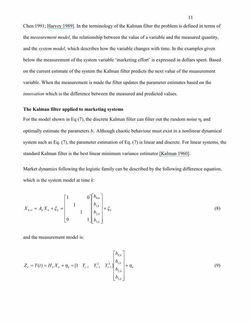
Chen 1991; Harvey 1989]. In the terminology of the Kalman filter the problem is defined in terms of

the measurement model, the relationship between the value of a variable and the measured quantity,

and the system model, which describes how the variable changes with time. In the examples given

below the measurement of the system variable ‘marketing effort’ is expressed in dollars spent. Based

on the current estimate of the system the Kalman filter predicts the next value of the measurement

variable. When the measurement is made the filter updates the parameter estimates based on the

innovation which is the difference between the measured and predicted values.

The Kalman filter applied to marketing systems

For the model shown in Eq (7), the discrete Kalman filter can filter out the random noise �t and

optimally estimate the parameters bi. Although chaotic behaviour must exist in a nonlinear dynamical

system such as Eq. (7), the parameter estimation of Eq. (7) is linear and discrete. For linear systems, the

standard Kalman filter is the best linear minimum variance estimator [Kalman 1960].

Market dynamics following the logistic family can be described by the following difference equation,

which is the system model at time k:

k

k

k

k

k

kkkk

bbbb

XAX �� �

�����

�

�

�����

�

�

����

�

�

����

�

�

����

101

101

,3

,2

,1

,0

1 (8)

and the measurement model is:

k

k

k

k

k

tttkkkk

bbbb

YYYXHtYZ �� �

�����

�

�

�����

�

�

�������

,3

,2

,1

,0

31

211 ]1[ )( (9)

12

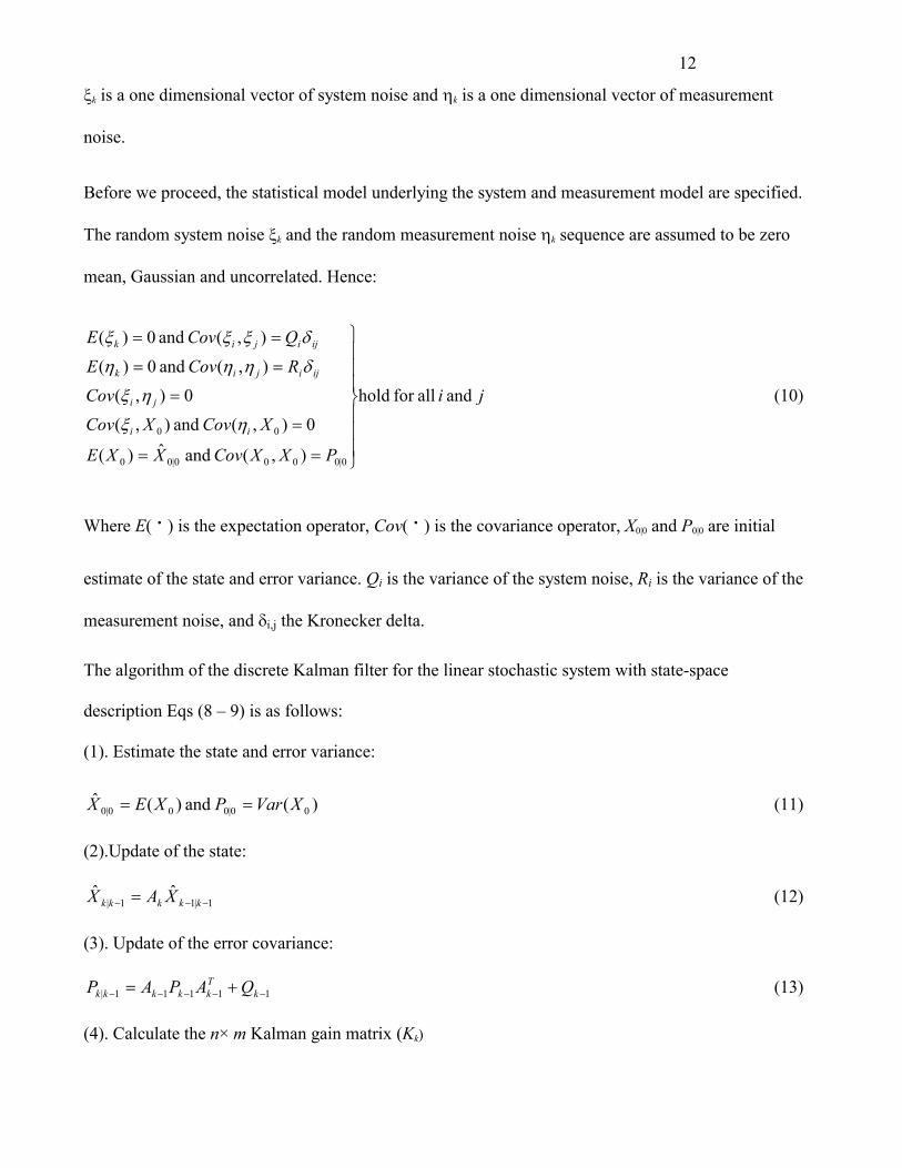
�k is a one dimensional vector of system noise and �k is a one dimensional vector of measurement

noise.

Before we proceed, the statistical model underlying the system and measurement model are specified.

The random system noise �k and the random measurement noise �k sequence are assumed to be zero

mean, Gaussian and uncorrelated. Hence:

ji

PXXCovXXE

XCovXCovCov

RCovE

QCovE

ii

ji

ijijik

ijijik

and allfor hold

),( and ˆ)(

0),( and ),(0),(

),( and 0)(

),( and 0)(

0|0000|00

00

���

�

���

�

�

��

�

�

��

��

��

��

����

����

(10)

Where E( · ) is the expectation operator, Cov( · ) is the covariance operator, X0|0 and P0|0 are initial

estimate of the state and error variance. Qi is the variance of the system noise, Ri is the variance of the

measurement noise, and �i,j the Kronecker delta.�

The algorithm of the discrete Kalman filter for the linear stochastic system with state-space

description Eqs (8 – 9) is as follows:

(1). Estimate the state and error variance:

)( and )(ˆ00|000|0 XVarPXEX �� (11)

(2).Update of the state:

1|11|ˆˆ

���

� kkkkk XAX (12)

(3). Update of the error covariance:

11111| �����

�� kTkkkkk QAPAP (13)

(4). Calculate the n× m Kalman gain matrix (Kk)

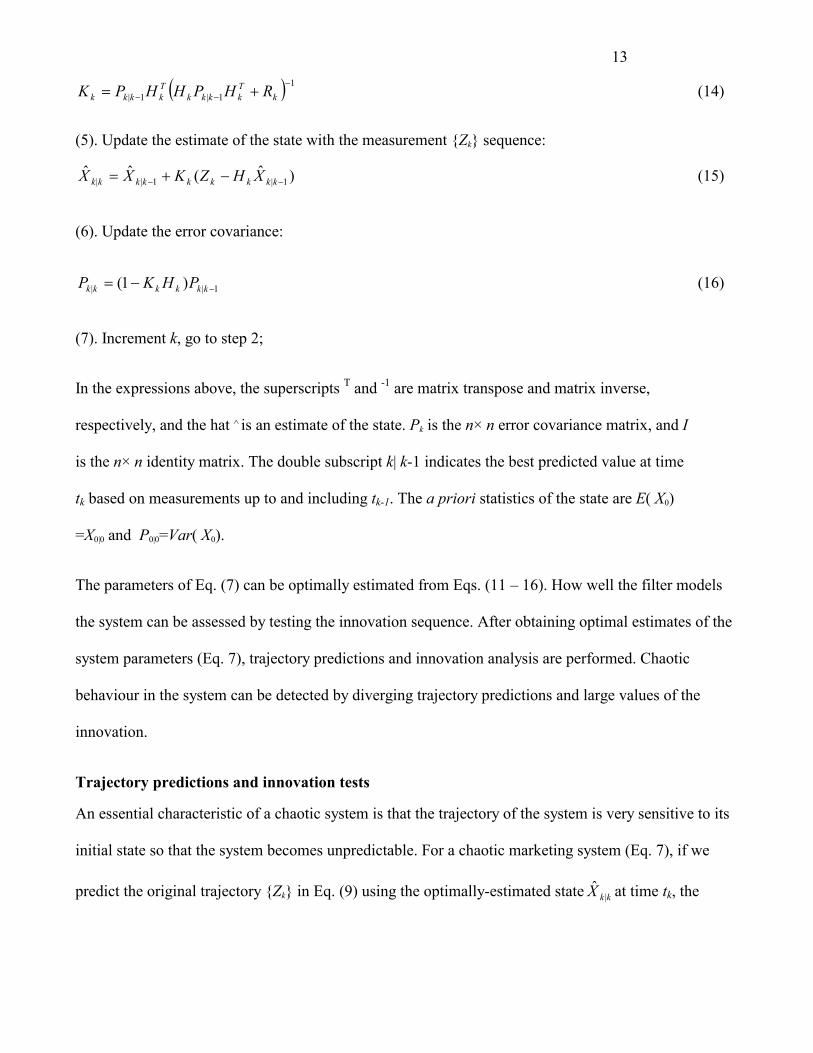
13

� � 11|1|

�

��

�� kTkkkk

Tkkkk RHPHHPK (14)

(5). Update the estimate of the state with the measurement {Zk} sequence:

)ˆ(ˆˆ1|1|| ��

��� kkkkkkkkk XHZKXX (15)

(6). Update the error covariance:

1|| )1(�

�� kkkkkk PHKP (16)

(7). Increment k, go to step 2;

In the expressions above, the superscripts T and -1 are matrix transpose and matrix inverse,

respectively, and the hat � is an estimate of the state. Pk is the n× n error covariance matrix, and I

is the n× n identity matrix. The double subscript k| k-1 indicates the best predicted value at time

tk based on measurements up to and including tk-1. The a priori statistics of the state are E( X0)

=X0|0 and P0|0=Var( X0).

The parameters of Eq. (7) can be optimally estimated from Eqs. (11 – 16). How well the filter models

the system can be assessed by testing the innovation sequence. After obtaining optimal estimates of the

system parameters (Eq. 7), trajectory predictions and innovation analysis are performed. Chaotic

behaviour in the system can be detected by diverging trajectory predictions and large values of the

innovation.

Trajectory predictions and innovation tests

An essential characteristic of a chaotic system is that the trajectory of the system is very sensitive to its

initial state so that the system becomes unpredictable. For a chaotic marketing system (Eq. 7), if we

predict the original trajectory {Zk} in Eq. (9) using the optimally-estimated state at time tkkX |ˆ k, the

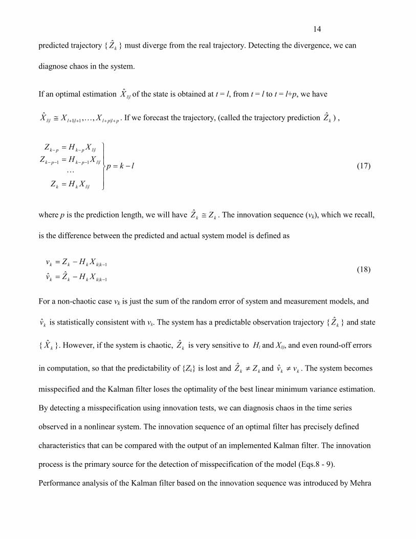
14

predicted trajectory { } must diverge from the real trajectory. Detecting the divergence, we can

diagnose chaos in the system.

kZ

plp �|

p �

If an optimal estimation of the state is obtained at t = l, from t = l to t = l+p, we have

. If we forecast the trajectory, (called the trajectory prediction ) ,

llX |ˆ

lllll XXX���

� 1|1| ,,ˆ� kZ

lk

XHZ

XHZXHZ

llkk

llpkpk

llpkpk

�

��

�

��

�

�

�

�

�

����

��

|

|11

|

�

(17)

where p is the prediction length, we will have . The innovation sequence (vkk ZZ �ˆ k), which we recall,

is the difference between the predicted and actual system model is defined as

1|

1|

ˆˆ�

�

��

��

kkkkk

kkkkk

XHZv

XHZv (18)

For a non-chaotic case vk is just the sum of the random error of system and measurement models, and

is statistically consistent with vkv

X

k. The system has a predictable observation trajectory { } and state

{ }. However, if the system is chaotic, is very sensitive to H

kZ

k kZ l and Xl|l, and even round-off errors

in computation, so that the predictability of {Zk} is lost and and . The system becomes

misspecified and the Kalman filter loses the optimality of the best linear minimum variance estimation.

By detecting a misspecification using innovation tests, we can diagnosis chaos in the time series

observed in a nonlinear system. The innovation sequence of an optimal filter has precisely defined

characteristics that can be compared with the output of an implemented Kalman filter. The innovation

process is the primary source for the detection of misspecification of the model (Eqs.8 - 9).

Performance analysis of the Kalman filter based on the innovation sequence was introduced by Mehra

kk ZZ �ˆ

kk vv �ˆ

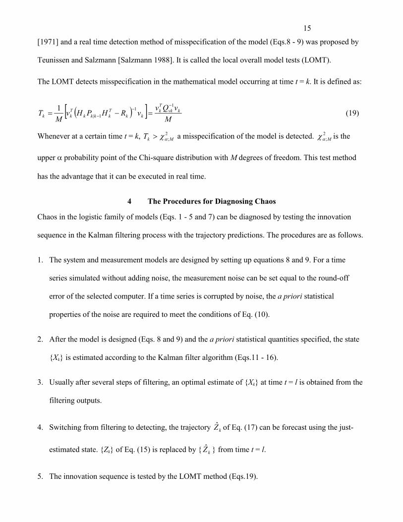
15

[1971] and a real time detection method of misspecification of the model (Eqs.8 - 9) was proposed by

Teunissen and Salzmann [Salzmann 1988]. It is called the local overall model tests (LOMT).

The LOMT detects misspecification in the mathematical model occurring at time t = k. It is defined as:

� �� �M

vQvvRHPHv

MT kvk

Tk

kkTkkkk

Tkk

11

1|1 �

�

���� (19)

Whenever at a certain time t = k, a misspecification of the model is detected. is the

upper � probability point of the Chi-square distribution with M degrees of freedom. This test method

has the advantage that it can be executed in real time.

2;MkT

���

2;M�

�

4 The Procedures for Diagnosing Chaos

Chaos in the logistic family of models (Eqs. 1 - 5 and 7) can be diagnosed by testing the innovation

sequence in the Kalman filtering process with the trajectory predictions. The procedures are as follows.

1. The system and measurement models are designed by setting up equations 8 and 9. For a time

series simulated without adding noise, the measurement noise can be set equal to the round-off

error of the selected computer. If a time series is corrupted by noise, the a priori statistical

properties of the noise are required to meet the conditions of Eq. (10).

2. After the model is designed (Eqs. 8 and 9) and the a priori statistical quantities specified, the state

{Xk} is estimated according to the Kalman filter algorithm (Eqs.11 - 16).

3. Usually after several steps of filtering, an optimal estimate of {Xk} at time t = l is obtained from the

filtering outputs.

4. Switching from filtering to detecting, the trajectory of Eq. (17) can be forecast using the just-

estimated state. {Z

kZ

k} of Eq. (15) is replaced by { } from time t = l. kZ

5. The innovation sequence is tested by the LOMT method (Eqs.19).

16

6. The filtering for k = k+1 is repeated, the state estimate and the test results are output. If Tk > � 0.01; M2

in the filtering process, the innovation tests have detected a misspecification which indicates

chaotic behaviour in the system of interest.

If a given system is known to be chaotic in a certain range of the parameters in Eq.(7), the chaos can be

directly diagnosed from the Kalman filter output of the state estimate (Eq.15).

5 Detecting Chaos in Market Competition Dynamics

In this section we demonstrate the power of the techniques described in detecting chaos. As already

noted the dynamic behaviour of the small fish model of brand competition (Eq 4) is a complex one in

the logistic family of models. Therefore we chose it as the basis for the numerical example. First we

discuss the dynamic properties of the model. The model can be written as

21 ,2111 ��������

���

tttt YAYYY (20)

where ���

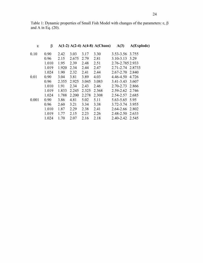
��� 1 ,SaBA . Hibbert and Wilkinson [1994] show that Eq. (20) results in complex

dynamics. Some of the key features are shown in Table 1. This shows the dynamics of the system when

� =0.1, 0.01 and 0.001 and � =0.90, 0.96, 1.010, 1.019 and 1.024. The values of the parameter A at

bifurcation, chaos beginning (A( Chaos) ) , 3-period windows and when it explodes (A( Explode) ) are

presented. The bifurcation from period 1 to period 2 is denoted as A(1-2) , from period 2 to period 4 as

A(2-4) , and so on. The ranges of the 3-period windows are denoted as A(3). A 3-dimensional portrait

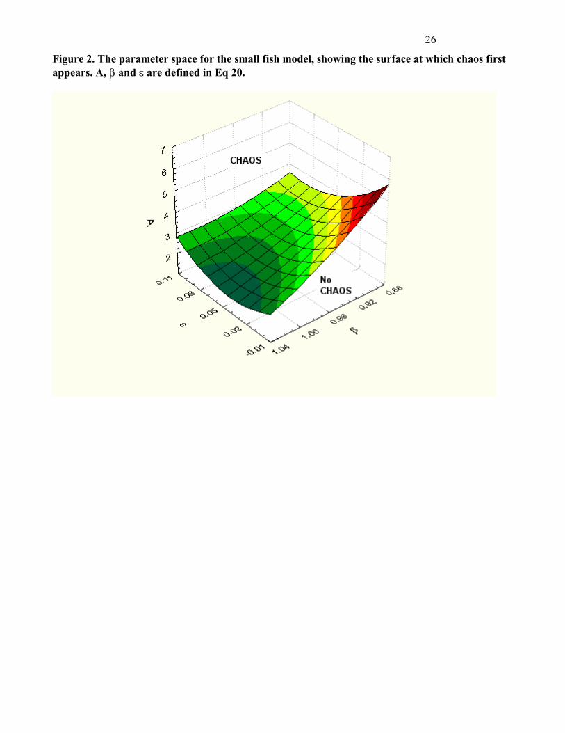
of the parameter space {A, �, �} of this model is given in Figure 2, with the surface cutting the regions

of chaos and non-chaos.

Insert Table 1 and Figure 2 about here.

17

The procedures in section 4 can detect chaotic behaviour if the system (Eq. 20) is chaotic, and can

detect the absence of chaos if the system is non-chaotic when the system is fitted to the polynomial

model (Eq.7).

Non-chaotic case of the small fish model

When the trajectory of the system (Eq. 20) is period doubling, 4-periodic, or window-3-periodic, the

system is non-chaotic. Two artificial data series, with 1000 points in each series, were generated. One

is in the period doubling regime with A=2.20, � =1.019 and � =0.01 in Eq. 20. Another is in the 3-

periodic window with A=2.60, � =1.019 and � =0.01. The two data series were fitted to the polynomial

model (Eq.7) by the standard Kalman filter (Eqs.11 - 16) with observation error variance Rk = 10-10 and

dynamic error variance Qk = 10-10 which approximate round-off errors in the computer simulation. The

initial state of the model can be estimated as X0|0=0, and P0|0=I4× 4 (I is an identity matrix).

For the period doubling case, the Kalman filter estimates the parameters of the polynomial at time

t=500:

ttttt YYYY �����������

�

�

�

�

�� 31

521

31

1415 1018.21079.91057.11019.1 (21)

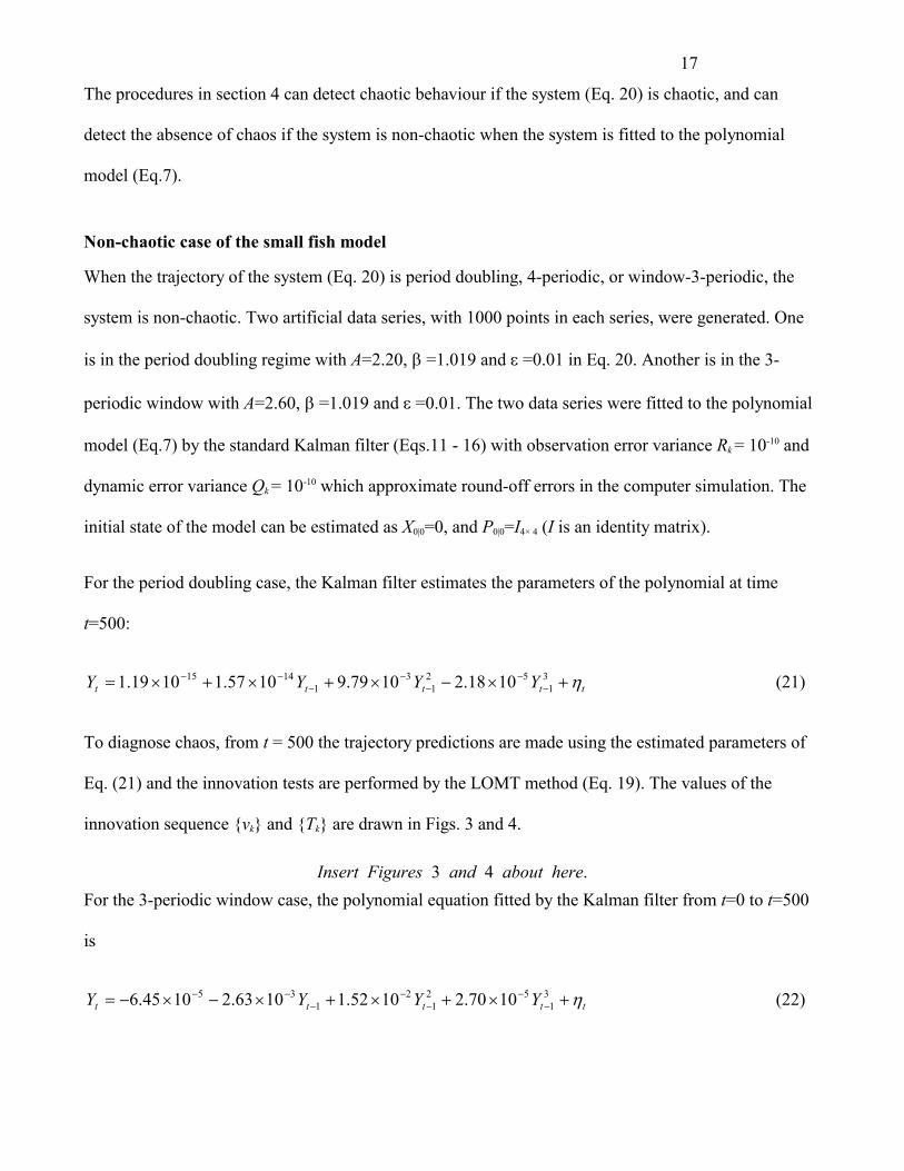
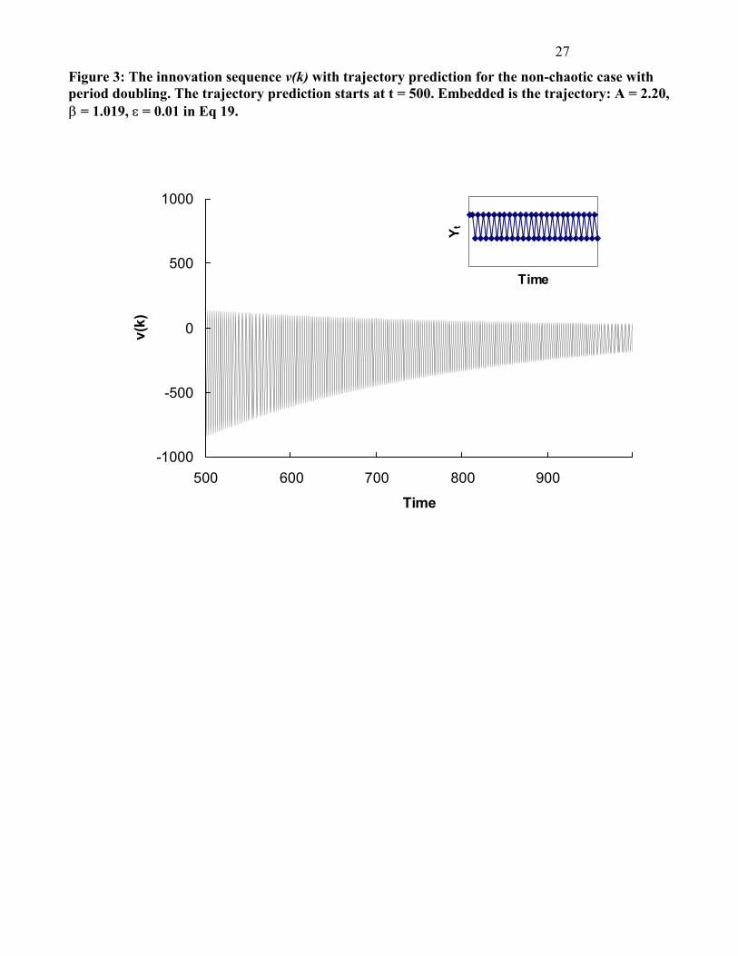
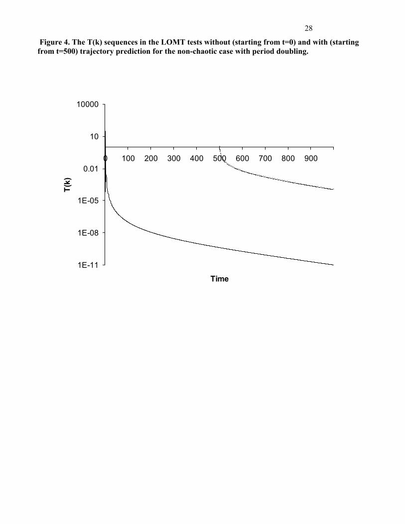
To diagnose chaos, from t = 500 the trajectory predictions are made using the estimated parameters of

Eq. (21) and the innovation tests are performed by the LOMT method (Eq. 19). The values of the

innovation sequence {vk} and {Tk} are drawn in Figs. 3 and 4.

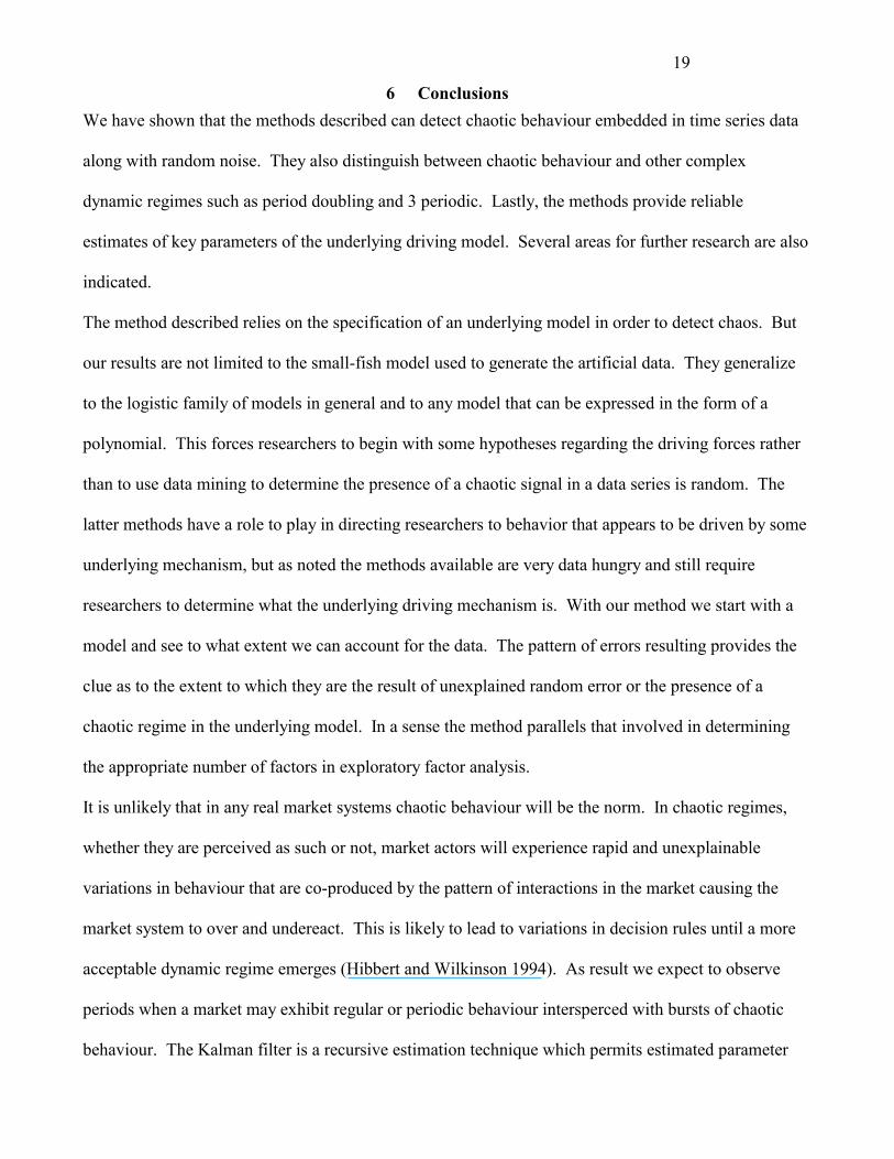
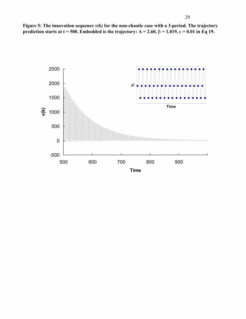
Insert Figures 3 and 4 about here. For the 3-periodic window case, the polynomial equation fitted by the Kalman filter from t=0 to t=500

is

ttttt YYYY ������������

�

�

�

�

�� 31

521

21

35 1070.21052.11063.21045.6 (22)

18

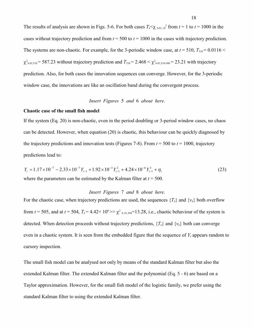
The results of analysis are shown in Figs. 5-6. For both cases Tk<� 0.01; M2 from t = 1 to t = 1000 in the

cases without trajectory prediction and from t = 500 to t = 1000 in the cases with trajectory prediction.

The systems are non-chaotic. For example, for the 3-periodic window case, at t = 510, T510 = 0.0116 <

�20.01;510

= 587.23 without trajectory prediction and T510 = 2.468 < �20.01;510-500 = 23.21 with trajectory

prediction. Also, for both cases the innovation sequences can converge. However, for the 3-periodic

window case, the innovations are like an oscillation band during the convergent process.

Insert Figures 5 and 6 about here.

Chaotic case of the small fish model

If the system (Eq. 20) is non-chaotic, even in the period doubling or 3-period window cases, no chaos

can be detected. However, when equation (20) is chaotic, this behaviour can be quickly diagnosed by

the trajectory predictions and innovation tests (Figures 7-8). From t = 500 to t = 1000, trajectory

predictions lead to:

ttttt YYYY �����������

�

�

�

�

�� 31

621

31

77 1024.41092.11033.21017.1 (23)

where the parameters can be estimated by the Kalman filter at t = 500.

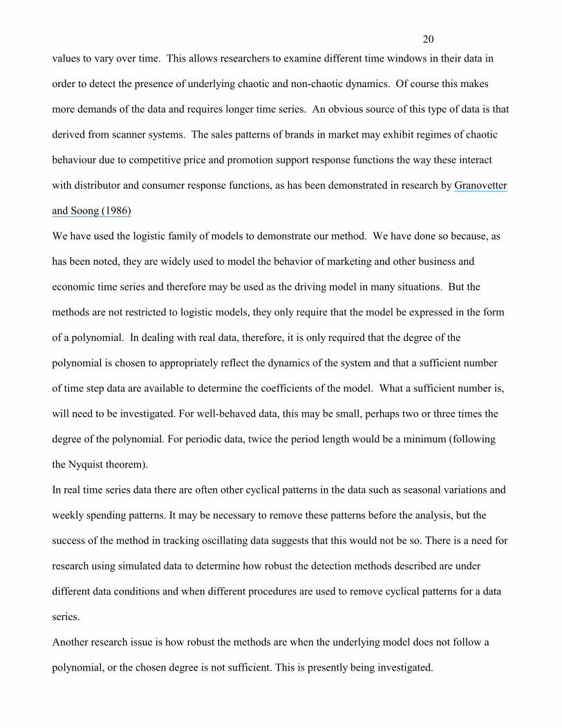
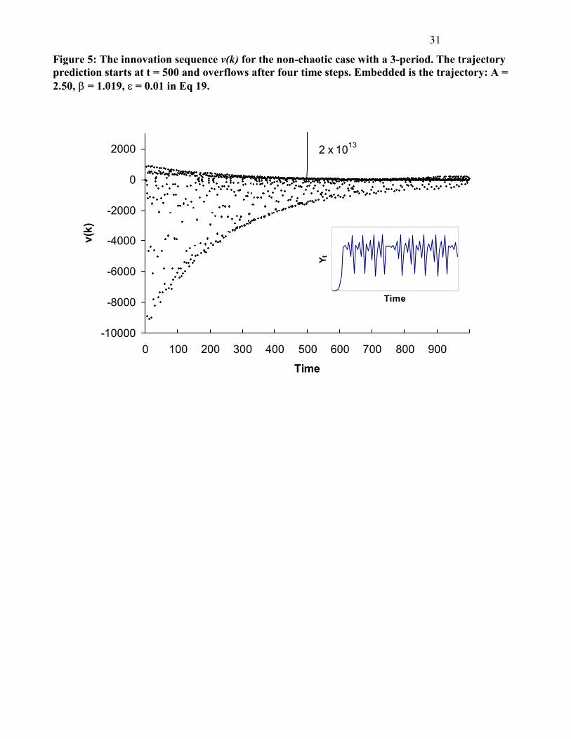
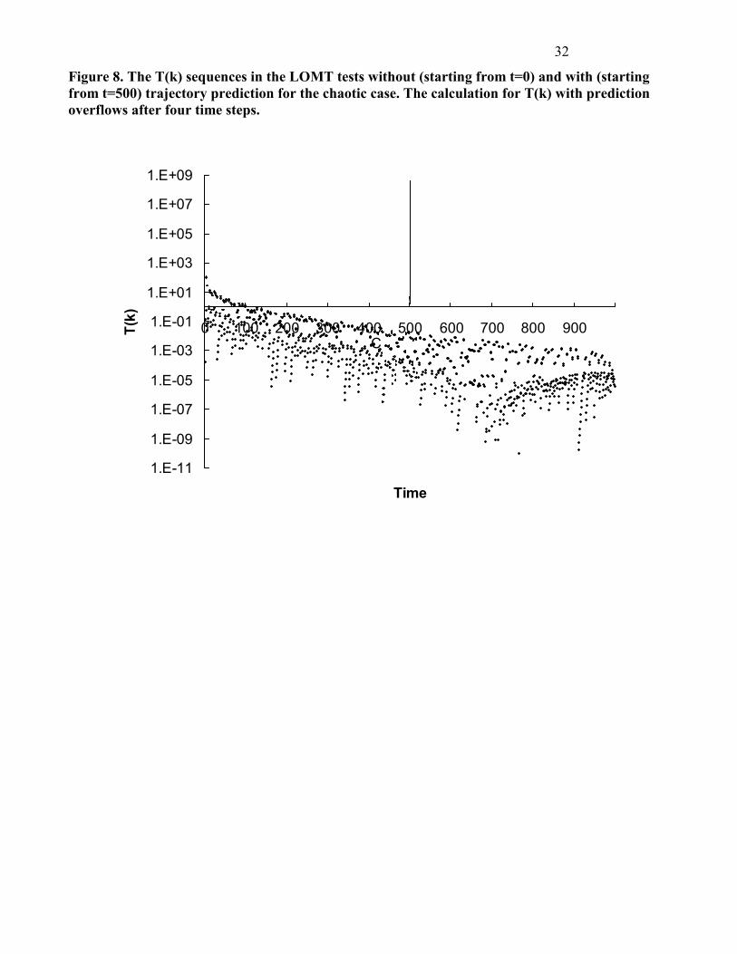
Insert Figures 7 and 8 about here. For the chaotic case, when trajectory predictions are used, the sequences {Tk} and {vk} both overflow

from t = 505, and at t = 504, Tk = 4.42× 108 >> �2 0..01,504=13.28, i.e., chaotic behaviour of the system is

detected. When detection proceeds without trajectory predictions, {Tk} and {vk} both can converge

even in a chaotic system. It is seen from the embedded figure that the sequence of Yt appears random to

cursory inspection.

The small fish model can be analysed not only by means of the standard Kalman filter but also the

extended Kalman filter. The extended Kalman filter and the polynomial (Eq. 5 - 6) are based on a

Taylor approximation. However, for the small fish model of the logistic family, we prefer using the

standard Kalman filter to using the extended Kalman filter.

19

6 Conclusions We have shown that the methods described can detect chaotic behaviour embedded in time series data

along with random noise. They also distinguish between chaotic behaviour and other complex

dynamic regimes such as period doubling and 3 periodic. Lastly, the methods provide reliable

estimates of key parameters of the underlying driving model. Several areas for further research are also

indicated.

The method described relies on the specification of an underlying model in order to detect chaos. But

our results are not limited to the small-fish model used to generate the artificial data. They generalize

to the logistic family of models in general and to any model that can be expressed in the form of a

polynomial. This forces researchers to begin with some hypotheses regarding the driving forces rather

than to use data mining to determine the presence of a chaotic signal in a data series is random. The

latter methods have a role to play in directing researchers to behavior that appears to be driven by some

underlying mechanism, but as noted the methods available are very data hungry and still require

researchers to determine what the underlying driving mechanism is. With our method we start with a

model and see to what extent we can account for the data. The pattern of errors resulting provides the

clue as to the extent to which they are the result of unexplained random error or the presence of a

chaotic regime in the underlying model. In a sense the method parallels that involved in determining

the appropriate number of factors in exploratory factor analysis.

It is unlikely that in any real market systems chaotic behaviour will be the norm. In chaotic regimes,

whether they are perceived as such or not, market actors will experience rapid and unexplainable

variations in behaviour that are co-produced by the pattern of interactions in the market causing the

market system to over and undereact. This is likely to lead to variations in decision rules until a more

acceptable dynamic regime emerges (Hibbert and Wilkinson 1994). As result we expect to observe

periods when a market may exhibit regular or periodic behaviour intersperced with bursts of chaotic

behaviour. The Kalman filter is a recursive estimation technique which permits estimated parameter

20

values to vary over time. This allows researchers to examine different time windows in their data in

order to detect the presence of underlying chaotic and non-chaotic dynamics. Of course this makes

more demands of the data and requires longer time series. An obvious source of this type of data is that

derived from scanner systems. The sales patterns of brands in market may exhibit regimes of chaotic

behaviour due to competitive price and promotion support response functions the way these interact

with distributor and consumer response functions, as has been demonstrated in research by Granovetter

and Soong (1986)

We have used the logistic family of models to demonstrate our method. We have done so because, as

has been noted, they are widely used to model the behavior of marketing and other business and

economic time series and therefore may be used as the driving model in many situations. But the

methods are not restricted to logistic models, they only require that the model be expressed in the form

of a polynomial. In dealing with real data, therefore, it is only required that the degree of the

polynomial is chosen to appropriately reflect the dynamics of the system and that a sufficient number

of time step data are available to determine the coefficients of the model. What a sufficient number is,

will need to be investigated. For well-behaved data, this may be small, perhaps two or three times the

degree of the polynomial. For periodic data, twice the period length would be a minimum (following

the Nyquist theorem).

In real time series data there are often other cyclical patterns in the data such as seasonal variations and

weekly spending patterns. It may be necessary to remove these patterns before the analysis, but the

success of the method in tracking oscillating data suggests that this would not be so. There is a need for

research using simulated data to determine how robust the detection methods described are under

different data conditions and when different procedures are used to remove cyclical patterns for a data

series.

Another research issue is how robust the methods are when the underlying model does not follow a

polynomial, or the chosen degree is not sufficient. This is presently being investigated.

21

22

References

Bollerslev, T. 1986. ''Generalized Autoregressive Conditional Heteroscedasticity.'' Journal of Econometrics 31: 307-327.

Catlin, Donald E. 1989. Estimation, Control, and the Discrete Kalman Filter. New York; Springer-Verlag, 133-163.

Chui, C. K. and G. Chen. 1991. Kalman Filtering with Real-Time Applications. Berlin; Springer-Verlag, 20-96.

Creedy, John, and Vance L. Martin 1994. ''The Strange Attraction of Chaos in Economics.'' In Chaos and Non-linear Models in Economics. Eds. Creedy, John, and Vance L. Martin. England; Edward Elgar, 7-29.

Dechert, W. Davis, Eds. 1996. Chaos Theory in Economics: Methods, Models and Evidence. Cheltenham, UK, Edward Elgar, Part III: 377-590.

Box, G. E. P., and G. M. Jenkins. 1976. Time Series Analysis: Forecasting and Control. revised edn., San Francisco, Holden-Day.

Dixon, R. 1994. ''The Logistic Family of Discrete Dynamic Models.'' In Chaos and Non-linear Models in Economics: Theory and Applications. Eds. Creedy, John, and Vance L. Martin. England; Edward Elgar, 44-69.

Engle, R. F. 1982. ''Autoregressive Conditional Heteroscendasticity with Estimates of the Variance of UK inflation.'' Econometrica 50: 987-1007.

Frank, M., and T. Stengos. 1988. ''Chaotic Dynamics in Economic Time-Series.'' Journal of Economic Surveys 2 (2): 103-133.

Harvey, A. C. 1989. Forecasting, Structural Time Series Models and the Kalman Filter. Cambridge; Cambridge University Press.

Hibbert, D. Brynn, and Ian F. Wilkinson. 1994. ''Chaos Theory and the Dynamics of Marketing Systems.'' Journal of the Academy of Marketing Science 22 (Summer): 218-233.

Hilborn, Robert C. 1994. Chaos and Nonlinear Dynamics: An Introduction for Scientists and Engineers. New York; Oxford University Press, p. 19-28.

Granovetter, Mark and Roland Soong (1986) “Threshold Models of Interpersonal Effects in Consumer Demand” Journal of Economic Behavior and Organization, 7 (March) 83-99

Jenson, R. V., and U. Robin. 1984. ''Chaotic Price Behavior in a Nonlinear Cobweb Model.'' Economics Letters 15: 235-240.

Jiang, J and Hibbert, D.B.1999, “Diagnosing Chaos in Non-Linear Dynamical Systems by Trajectory Predictions and Innovation Tests of the Kalman Filter.” Chemometrics and Intelligent Laboratory Systems 45:353 – 359.

Kailath, T. 1968a. ''An Innovation Approach to Least-squares Estimation, Part I: Linear Filtering in additive White Noise.'' IEEE-Trans. on Automatic Control, IEEE-AC 13 (6): 645-655.

23

Kailath, T. 1968b. ''An Innovation Approach to Least-squares Estimation, Part II: Linear Smoothing in Additive White Noise.'' IEEE-Trans. on Automatic Control, IEEE-AC 13 (6): 655-660.

Kalman, R. E. 1960. ''A New Approach to Linear Filtering and Prediction Problems.'' Journal of Basic Engineering (ASME) 82D (March): 35-45.

Lambkin, Mary and George S. Day. 1989. ''Evolutionary Processes in Competitive Markets: Beyond the Product Life Cycle.'' Journal of Marketing 53 (July): 4-20.

Lorenz, Hans-Walter. 1993. Nonlinear Dynamical Economics and Chaotic Motion. Berlin, Springer-Verlag, 119-200.

Mahajan, Vijay, Eitan Muller and Frank M. Bass. 1990. ''New Product Diffusion Model in Marketing: A Review and Directions for Research.'' Journal of Marketing 54 (January): 1-26.

Mansfield, E. 1961. ''Technical Change and the Rate of Imitation.'' Econometrica 29: 741-66.

May, R. M. 1976. ''Simple Mathematical Models with Very Complicated Dynamics.'' Nature 261: 45-67.

Mehra, R. K. 1971. ''An Innovation Approach to Fault Detection and Diagnosis in Dynamic System.'' Automatica 7: 637-640.

Newbery, D. M. G. and J. E. Stiglitz. 1981. The Theory of Commodity Price Stabilization: A Study in the Economics of Risk. Oxford, Clarendon Press.

Putsis, W.P. 1998 “Parameter Variation and New Product Diffusion” Journal of Forecasting 17(June-July) 231-257

Roos, C. 1934. Dynamic Economics. Yale; Principal Press.

Rosser, J. Barkley 1991. From Catastrophe to Chaos: A General Theory of Economic Discontinuities. Boston, Kluwer Academic Publishers, 37-56, 97-124.

Salzmann, M. A. 1988. Some Aspects of Kalman Filtering, Technical Report No. 140. Canada; University of New Brunswick, 61-74; Ref.: Teunissen, P. J. G. and M. A. Salzmann. 1988. ''Performance of Analysis of Kalman Filter.'' The paper was presented at HYDRO88, Amsterdam, 15-17 November. Serio, C. 1994. ''Detecting Chaos in Time Series.'' In Fractals in the Natural and Applied Science. Eds. Novak, M. M., Netherlands; IFIP, 371-383.

24

Table 1: Dynamic properties of Small Fish Model with changes of the parameters: �, � and A in Eq. (20).

�� � A(1-2) A(2-4) A(4-8) A(Chaos) A(3) A(Explode)

0.10 0.90 2.42 3.03 3.17 3.30 3.53-3.56 3.755 0.96 2.15 2.675 2.79 2.81 3.10-3.13 3.29 1.010 1.95 2.39 2.48 2.51 2.76-2.785 2.933 1.019 1.920 2.34 2.44 2.47 2.71-2.74 2.8733 1.024 1.90 2.32 2.41 2.44 2.67-2.70 2.840 0.01 0.90 3.04 3.81 3.89 4.03 4.46-4.50 4.726 0.96 2.355 2.925 3.045 3.083 3.41-3.43 3.607 1.010 1.91 2.34 2.43 2.46 2.70-2.73 2.866 1.019 1.833 2.245 2.325 2.368 2.59-2.62 2.746 1.024 1.788 2.200 2.278 2.308 2.54-2.57 2.685 0.001 0.90 3.86 4.81 5.02 5.11 5.63-5.65 5.95 0.96 2.60 3.21 3.34 3.38 3.72-3.74 3.955 1.010 1.87 2.29 2.38 2.41 2.64-2.66 2.802 1.019 1.77 2.15 2.23 2.26 2.48-2.50 2.633 1.024 1.70 2.07 2.16 2.18 2.40-2.42 2.545

25

Figure 1 A Dynamic Model of Brand Competition

OTHERS CHANGE IN

MARKETING EFFORT

OTHERS’ COSTS

OTHERS’ NET REVENUE

MARKETING EFFORT

OTHER BRANDS’

X’s CHANGE IN MARKETING

EFFORT

SHARE

X’S COSTS

MARKETING EFFORT BRAND X

X’s NET REVENUE

26

Figure 2. The parameter space for the small fish model, showing the surface at which chaos first appears. A, � and � are defined in Eq 20. �

27

Figure 3: The innovation sequence v(k) with trajectory prediction for the non-chaotic case with period doubling. The trajectory prediction starts at t = 500. Embedded is the trajectory: A = 2.20, ��= 1.019, � = 0.01 in Eq 19.

-1000

-500

0

500

1000

500 600 700 800 900

Time

v(k)

Time

Y t

28

Figure 4. The T(k) sequences in the LOMT tests without (starting from t=0) and with (starting from t=500) trajectory prediction for the non-chaotic case with period doubling.

1E-11

1E-08

1E-05

0.01

10

10000

0 100 200 300 400 500 600 700 800 900

Time

T(k)

29

Figure 5: The innovation sequence v(k) for the non-chaotic case with a 3-period. The trajectory prediction starts at t = 500. Embedded is the trajectory: A = 2.60, ��= 1.019, � = 0.01 in Eq 19. �

�

�

�

�

-500

0

500

1000

1500

2000

2500

500 600 700 800 900

Time

v(k)

Time

Y t

�

�

30

Figure 6. The T(k) sequences in the LOMT tests without (starting from t=0) and with (starting from t=500) trajectory prediction for the non-chaotic case with a 3-period. �

�

�

1.E-09

1.E-06

1.E-03

1.E+00

1.E+03

0 100 200 300 400 500 600 700 800 900

Time

T(k)

�

�

�

31

Figure 5: The innovation sequence v(k) for the non-chaotic case with a 3-period. The trajectory prediction starts at t = 500 and overflows after four time steps. Embedded is the trajectory: A = 2.50, ��= 1.019, � = 0.01 in Eq 19.

-10000

-8000

-6000

-4000

-2000

0

2000

0 100 200 300 400 500 600 700 800 900

Time

v(k)

2 x 1013

Time

Y t

�

32

Figure 8. The T(k) sequences in the LOMT tests without (starting from t=0) and with (starting from t=500) trajectory prediction for the chaotic case. The calculation for T(k) with prediction overflows after four time steps.

1.E-11

1.E-09

1.E-07

1.E-05

1.E-03

1.E-01

1.E+01

1.E+03

1.E+05

1.E+07

1.E+09

0 100 200 300 400 500 600 700 800 900

Time

T(k)

C