Diagnosing Network-Wide Traffic Anomalies

Anukool Lakhina, Mark Crovella, and Christophe Diot �

February 19, 2004

BUCS-TR-2004-008 and RR04-ATL-022666

Abstract

Anomalies are unusual and significant changes in a network’s traffic levels, which can often in-volve multiple links. Diagnosing anomalies is critical for both network operators and end users. It isa difficult problem because one must extract and interpret anomalous patterns from large amounts ofhigh-dimensional, noisy data.

In this paper we propose a general method to diagnose anomalies. This method is based on a sep-aration of the high-dimensional space occupied by a set of network traffic measurements into disjointsubspaces corresponding to normal and anomalous network conditions. We show that this separationcan be performed effectively using Principal Component Analysis.

Using only simple traffic measurements from links, we study volume anomalies and show that themethod can: (1) accurately detect when a volume anomaly is occurring; (2) correctly identify the under-lying origin-destination (OD) flow which is the source of the anomaly; and (3) accurately estimate theamount of traffic involved in the anomalous OD flow.

We evaluate the method’s ability to diagnose (i.e., detect, identify, and quantify) both existing andsynthetically injected volume anomalies in real traffic from two backbone networks. Our method con-sistently diagnoses the largest volume anomalies, and does so with a very low false alarm rate.

�A. Lakhina and M. Crovella are with the Department of Computer Science, Boston University;email: fanukool,crovellag@cs.bu.edu. C. Diot is with Intel Research, Cambridge, UK; email:christophe.diot@intel.com. This work was performed while M. Crovella was at Laboratoire d’Informatique deParis 6 (LIP6), with support from Centre National de la Recherche Scientifique (CNRS) France. Part of this work was done whenA. Lakhina was at Intel Research, Cambridge, UK. Data used in the paper was collected while A. Lakhina was at Sprint Labs. Thiswork was supported in part by a grant from Sprint Labs, and by NSF grants ANI-9986397 and CCR-0325701.

1

1 Introduction

Understanding the nature of traffic anomalies in a network is an important problem. Regardless of whetherthe anomalies in question are malicious or unintentional, it is important to analyze them for two reasons:

� Anomalies can create congestion in the network and stress resource utilization in a router, whichmakes them crucial to detect from an operational standpoint.

� Some anomalies may not necessarily impact the network, but they can have a dramatic impact on acustomer or the end user.

A significant problem when diagnosing anomalies is that their forms and causes can vary considerably: fromDenial of Service (DoS) attacks, to router misconfigurations, to the results of BGP policy modifications.

Despite a large literature on traffic characterization, traffic anomalies remain poorly understood. Thereare a number of reasons for this. First, identifying anomalies requires a sophisticated monitoring infras-tructure. Unfortunately, most ISPs only collect simple traffic measures, e.g., average traffic volumes (usingSNMP). More adventurous ISPs do collect flow counts on edge links, but processing the collected data isa demanding task. A second reason for the lack of understanding of traffic anomalies is that ISPs do nothave tools for processing measurements that are fast enough to detect anomalies in real time. Thus, ISPs aretypically aware of major events (worms or DoS attacks) after the fact, but are generally not able to detectthem while they are in progress. A final reason is that the nature of network-wide traffic is high-dimensionaland noisy, which makes it difficult to extract meaningful information about anomalies from any kind oftraffic statistics.

In this paper we address the problem of efficiently diagnosing traffic anomalies that may span multiplelinks in a network, using link-based statistics. Our approach addresses the anomaly diagnosis problemin three steps: it first uses a general method to detect anomalies in network traffic, then employs distinctmethods to identify and quantify them. We believe that this three step approach is appropriate for addressingthe large variety of network traffic anomalies. This is because the detection step can target different trafficcharacteristics such as volume, number of flows, or routing events, while isolation and quantification arespecific to each type of anomaly.

The goal of this paper is not to explain the cause of network anomalies, but rather to provide a generaltechnique to diagnose traffic anomalies. We believe that a necessary first step to discovering the causes ofanomalies is the correct detection, identification, and quantification of anomalies.

The contributions of this paper are: (i) a general approach to diagnose anomalies in network traffic, (ii)the application of this method on simple link traffic statistics to isolate “volume anomalies,” and (iii) thevalidation of this method using real data collected on two different backbone networks.

Our method is based on a separation of the space of traffic measurements into normal and anomaloussubspaces, by means of Principal Component Analysis. We evaluate the approach using traffic collectedfrom two large backbone networks. We apply the method to both real and synthetically generated anomalies.Our results show that our algorithms are effective at detection (with high detection rate and low false alarmrate); are quite accurate in identifying the underlying OD flow responsible for the anomaly; and are alsoaccurate in estimating the number of bytes in the anomaly.

The paper is organized as follows. In Section 2, we introduce a specific variant of traffic anomalies calledvolume anomalies and explain why they are important. In Section 3, we describe the data used to illustrateand validate this work. In Section 4, we explain our general approach, which is to decompose the networkoperating conditions in two subspaces: normal and anomalous. In Section 5, we show how to diagnose

1

volume anomalies by analyzing the anomalous subspace. In Section 6, we validate our approach in twoways: we exploit access to underlying flow data to extract true anomalies using timeseries methods, againstwhich we evaluate detection and false alarm rates and we systematically inject anomalies across timestepsand flows to thoroughly evaluate the method. In Section 7, we discuss further extensions and generalizationsof our approach to other types of network anomalies. We contrast our approach from exisiting work on trafficanomalies in Section 8 and conclude in Section 9.

2 Volume Anomalies

A typical backbone network is composed of nodes (also called Points of Presence, or PoPs) that are con-nected by links. We define an Origin-Destination (OD) flow as the traffic that enters the backbone at theorigin PoP and exits at the destination PoP. The path followed by each OD flow is determined by the routingtables. Therefore, the traffic observed on each backbone link arises from the superposition of these ODflows.

We will use the term volume anomaly to refer to a sudden change (positive or negative) in an OD flow’straffic. Because such an anomaly originates outside the network, it will propagate from the origin PoP to thedestination PoP and will thus be visible on each link traversed.

One could detect volume anomalies by collecting IP flow-level traffic summaries on all input links at allPoPs, and applying temporal decomposition methods to each OD flow in the manner of [2, 19]. In general,this is impractical, for a number of reasons. First, there can be hundreds of customer links in a network.Monitoring all input links to collect and aggregate flow level data is extremely resource intensive; for manyISPs this cost is prohibitive. Second, each OD flow would need to be processed separately, requiring esti-mation of associated parameters for each of the (potentially hundreds of) temporal decompositions.

Instead, we develop a simpler and more practical technique for diagnosing volume anomalies. Giventhat a volume anomaly propagates through the network, we make use of the fact that we should be able toobserve it on all links it traverses. Thus we identify OD flow based anomalies by observing only link counts.(If more detailed information about IP source and destination of an anomaly is then needed, our method canbe used as a trigger to indicate which routers need IP flow-level data collection initiated on temporary basis.)

In the next section, we illustrate volume anomalies on link time series taken from a backbone network.Then we propose a diagnosis technique in three steps that relies on the link statistics that are already collectedsystematically by network operators.

2.1 An Illustration

The difficulty of the volume anomaly diagnosis problem stems in part from the fact that it only uses link data(such as can be collected via SNMP). From this link data, one must form inferences about unusual eventsoccuring in the underlying OD flows.

We illustrate this difficulty in Figure 1. The top plot on each side of the figure shows an OD flowtimeseries with an associated volume anomaly – this information is not available to our algorithms, but wepresent it to show the nature of the anomalies we are concerned with. The point at which each anomalyoccurs is designated by a circle on the timeline. Below the timeline are plots of link traffic on the four linksthat carry the given OD flow. These four plots represent the data that is available to our algorithm. Diagnosisof the anomaly consists of processing all link data so as to: (1) correctly detect that at the time shown, thenetwork is experiencing an anomaly; (2) correctly isolate the four links shown as those experiencing theanomaly; and (3) correctly estimate the size of the spike in the OD flow.

2

2

4

x 107

5

10x 10

7

0.60.8

11.21.41.6

x 108

22.5

3x 10

8

Wed Thu Fri1.5

22.5

x 108

OD flow b−i

Link f−i

Link d−f

Link c−d

Link b−c

51015

x 106

468

x 107

246

x 107

246

x 107

Fri Sat Sun2

4

6x 10

7

OD flow i−b

Link c−b

Link d−c

Link f−d

Link i−f

(a) Example 1 (b) Example 2

Figure 1: Examples of anomalies at the OD flow level (top row) that we want to diagnose from link traffic.

We make three observations from these examples. First, while the OD flows have pronounced spikes,the corresponding spike in the link traffic is dwarfed, and difficult to detect even from visual inspection. Forinstance, the traffic volume at the spike time on links c-d and b-c in Example 1 is barely distinguishable.Second, the temporal traffic patterns may vary substantially from one link to another. In Example 2, linki-f has a smooth trend, whereas the other links for the OD flow have more noisy traffic. Separating thespike from the noise in the traffic on link c-b is visually more difficult than separating the spike in linki-f. Thus isolating all the links exhibiting an anomaly is challenging. Finally, mean traffic levels varyconsiderably. In Example 1, the mean traffic level on link c-d is more than twice that of link f-i. Thevarying traffic levels makes it difficult to estimate the size of the volume anomaly and hence its operationalimportance.1

2.2 Problem Definition

The problem of diagnosing a volume anomaly in an OD flow can be separated into three steps: detection,identification and quantification.

The detection problem consists of designating those points in time at which the network is experienc-ing an anomaly. An effective algorithm for solving the detection problem should have a high detectionprobability and a low false alarm probability.

The identification problem consists of selecting the true anomaly type from a set of possible candidateanomalies. The method we propose is extensible to a wide variety of anomalies. However, as a first step inthis paper, our candidate anomaly set is the set of all individual OD flows.

Finally, quantification is the problem of estimating the number of additional or missing bytes in theunderlying traffic flows. Quantification is important because it gives a measure of the importance of theanomaly.

For a successful diagnosis of a volume anomaly, one must be able to detect the time of the anomaly,identify the underlying responsible OD flow, and quantify the size of the anomaly within that flow.

1Both these examples were successfully diagnosed by the methods in this paper.

3

nycm

atla

hstn

wash

losa

snva

sttl

dnvr

kscy

chin

ipls

h

e

m

gd

c

ba

lk

f

i

j

(a) Abilene (b) Sprint-Europe

Figure 2: Topology of networks studied.

3 Data

Our technique operates on link traffic data, of the kind obtained by SNMP. For validation purposes we alsouse OD flow data, but this data is not an input to our algorithms. All these data have been collected fromtwo backbone networks, Sprint-Europe and Abilene. Note that our anomaly diagnosis method is not limitedto backbone networks; it can be applied in any network where link counts are available.

Sprint-Europe (henceforth Sprint) is the European backbone of a US tier-1 ISP. This network has 13 PoPsand carries commercial traffic for large customers (companies, local ISPs, etc.). Abilene is the Internet2backbone network. It has 11 PoPs and spans the continental USA. Traffic on Abilene is non-commerical,arising mainly from major universities in the US. The network topologies are shown in Figure 2.

We collected sampled flow data from each router in both networks. For Sprint, we used Cisco’s Net-Flow [6] to collect every 250th packet (periodic sampling). Packets are aggregated into flows at the networkprefix level, and reported in 5 minute bins. On Abilene sampling is random, capturing 1% of all packets.Sampled packets are then aggregated at the 5-tuple level (IP address and port number for both source anddestination, along with protocol type) every minute using Juniper’s Traffic Sampling [28]. We found goodagreement (within 1%-5% accuracy) between sampled flow bytecounts, adjusted for sampling rate, and thecorresponding SNMP bytecounts on links with utlization more than 1 Mbps. Most of the links from bothnetworks fall in this category, and so our sampled flow bytecounts are likely to be reasonably accurate. Weaggregated both the Sprint and Abilene flow traffic counts into bins of 10 minutes to avoid synchronizationissues that could have arisen in the data collection.

Traffic anomalies can last anywhere from milliseconds [25] to hours [3]. Although our method can beused on data with any time granularity, in this paper we work with data binned on 10 minute intervals. Infact, the most prevalent anomalies in our datasets were those that lasted less than 10 minutes and show upas a pronounced spike at a single point in time, as depicted in Figure 1. Thus the anomalies that we detectare those that are significant when traffic is viewed at 10 minute intervals. In Section 7 we will discuss someimplications of the particular timescale we use.

To construct OD flows from the raw flows collected, we identify the ingress and egress PoPs of eachflow. The ingress PoP can be identified because we collect flows from each ingress link in both networks.

4

# PoPs # Links Time Bin PeriodSprint-1 13 49 10 min Jul 07-Jul 13Sprint-2 13 49 10 min Aug 11-Aug 17Abilene 11 41 10 min Apr 07-Apr 13

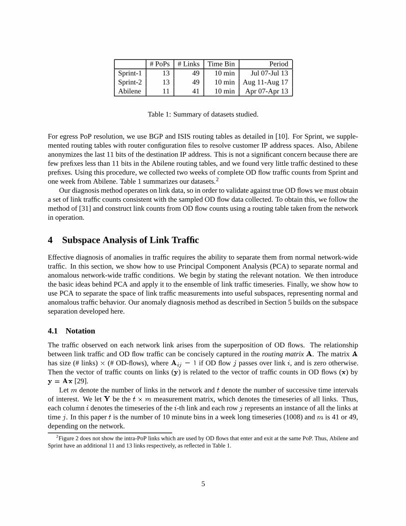
Table 1: Summary of datasets studied.

For egress PoP resolution, we use BGP and ISIS routing tables as detailed in [10]. For Sprint, we supple-mented routing tables with router configuration files to resolve customer IP address spaces. Also, Abileneanonymizes the last 11 bits of the destination IP address. This is not a significant concern because there arefew prefixes less than 11 bits in the Abilene routing tables, and we found very little traffic destined to theseprefixes. Using this procedure, we collected two weeks of complete OD flow traffic counts from Sprint andone week from Abilene. Table 1 summarizes our datasets.2

Our diagnosis method operates on link data, so in order to validate against true OD flows we must obtaina set of link traffic counts consistent with the sampled OD flow data collected. To obtain this, we follow themethod of [31] and construct link counts from OD flow counts using a routing table taken from the networkin operation.

4 Subspace Analysis of Link Traffic

Effective diagnosis of anomalies in traffic requires the ability to separate them from normal network-widetraffic. In this section, we show how to use Principal Component Analysis (PCA) to separate normal andanomalous network-wide traffic conditions. We begin by stating the relevant notation. We then introducethe basic ideas behind PCA and apply it to the ensemble of link traffic timeseries. Finally, we show how touse PCA to separate the space of link traffic measurements into useful subspaces, representing normal andanomalous traffic behavior. Our anomaly diagnosis method as described in Section 5 builds on the subspaceseparation developed here.

4.1 Notation

The traffic observed on each network link arises from the superposition of OD flows. The relationshipbetween link traffic and OD flow traffic can be concisely captured in the routing matrix A. The matrix Ahas size (# links) � (# OD-flows), where Aij = 1 if OD flow j passes over link i, and is zero otherwise.Then the vector of traffic counts on links (y) is related to the vector of traffic counts in OD flows (x) byy = Ax [29].

Let m denote the number of links in the network and t denote the number of successive time intervalsof interest. We let Y be the t �m measurement matrix, which denotes the timeseries of all links. Thus,each column i denotes the timeseries of the i-th link and each row j represents an instance of all the links attime j. In this paper t is the number of 10 minute bins in a week long timeseries (1008) and m is 41 or 49,depending on the network.

2Figure 2 does not show the intra-PoP links which are used by OD flows that enter and exit at the same PoP. Thus, Abilene andSprint have an additional 11 and 13 links respectively, as reflected in Table 1.

5

While Y denotes the set of links measurements over time, we will also frequently work just with y, avector of measurements from a single timestep. Thus y is an arbitrary row of Y, transposed to a columnvector.

We refer to individual columns of a matrix using a single subscript, so the timeseries of measurementsof link i is denoted Yi. All vectors in this paper are column vectors, unless otherwise noted.

Finally, all vectors and matrices will be displayed in boldface; matrices are denoted by upper case lettersand vectors by lower case letters.

4.2 PCA

PCA is a coordinate transformation method that maps a given set of data points onto new axes [15]. Theseaxes are called the principal axes or principal components. When working with zero-mean data, each prin-cipal component has the property that it points in the direction of maximum variance remaining in the data,given the variance already accounted for in the preceding components. As such, the first principal compo-nent captures the variance of the data to the greatest degree possible on a single axis. The next principalcomponents then each capture the maximum variance among the remaining orthogonal directions. Thus, theprincipal axes are ordered by the amount of data variance that they capture.

We will apply PCA on our link data matrixY, treating each row ofY as a point in IRm. However, beforewe can do so it is necessary to adjust Y so that that its columns have zero mean. This ensures that PCAdimensions capture true variance, and thus avoids skewing results due to differences in mean link utilization.For the rest of this paper, Y will denote the mean-centered link traffic data.

Applying PCA to Y yields a set of m principal components, fvigmi=1. The first principal component v1is the vector that points in the direction of maximum variance in Y:

v1 = arg maxkvk=1

kYvk

where kYvk2 is proportional to the variance of the data measured along v. Proceeding iteratively, oncethe first k � 1 principal components have been determined, the k-th principal component corresponds tothe maximum variance of the residual. The residual is the difference between the original data and the datamapped onto the first k � 1 principal axes. Thus, we can write the k-th principal component vk as:

vk = arg maxkvk=1

k(Y �k�1Xi=1

YvivTi )vk:

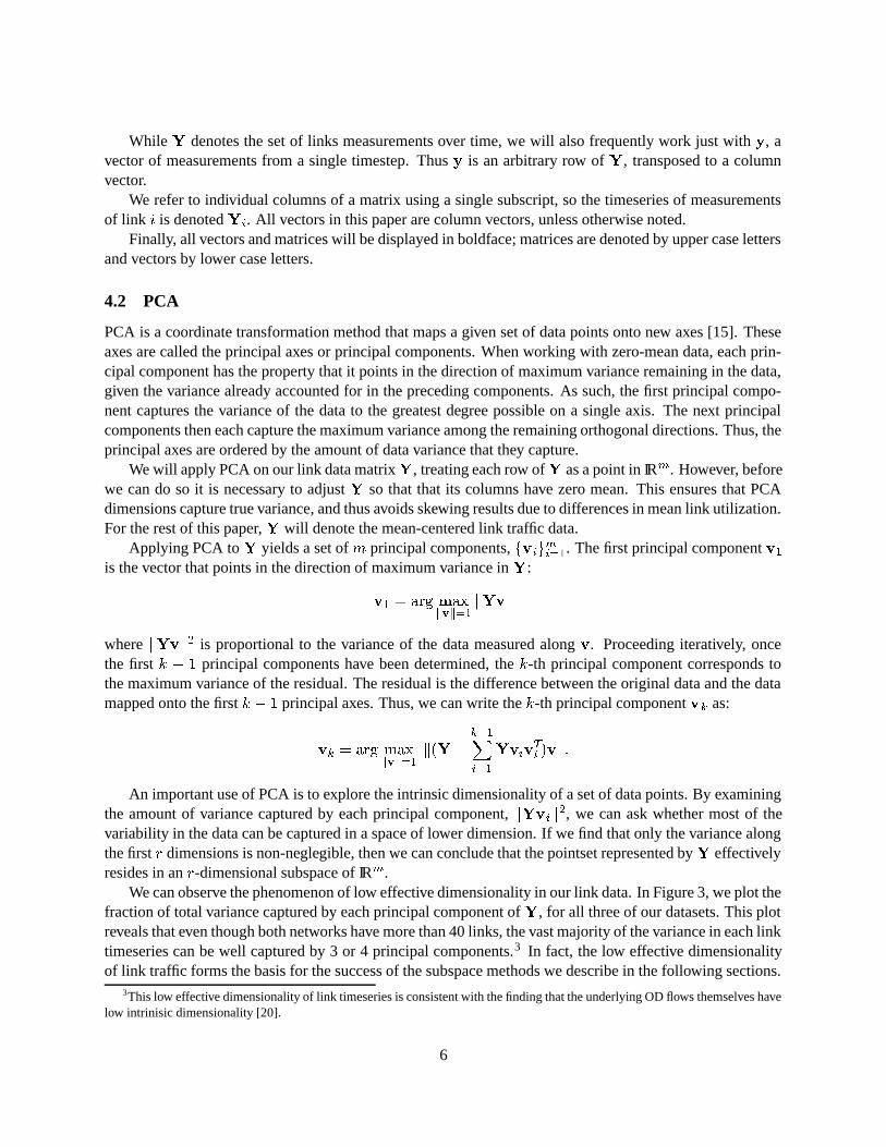
An important use of PCA is to explore the intrinsic dimensionality of a set of data points. By examiningthe amount of variance captured by each principal component, kYvik2, we can ask whether most of thevariability in the data can be captured in a space of lower dimension. If we find that only the variance alongthe first r dimensions is non-neglegible, then we can conclude that the pointset represented by Y effectivelyresides in an r-dimensional subspace of IRm.

We can observe the phenomenon of low effective dimensionality in our link data. In Figure 3, we plot thefraction of total variance captured by each principal component of Y, for all three of our datasets. This plotreveals that even though both networks have more than 40 links, the vast majority of the variance in each linktimeseries can be well captured by 3 or 4 principal components.3 In fact, the low effective dimensionalityof link traffic forms the basis for the success of the subspace methods we describe in the following sections.

3This low effective dimensionality of link timeseries is consistent with the finding that the underlying OD flows themselves havelow intrinisic dimensionality [20].

6

5 10 15 20 25 30 35 40 45

0.1

0.2

0.3

0.4

0.5

0.6

0.7

0.8

Principal Component

Var

ianc

e C

aptu

red

Sprint−1Sprint−2Abilene

1 2 3 4 50

0.02

0.04

0.06

0.08

0.1

Figure 3: Fraction of total link traffic variance captured by each principal component.

4.3 Subspace construction via PCA

Once the principal axes have been determined, the dataset can be mapped onto the new axes. The mappingof the data to principal axis i is given by Yvi. This vector can be normalized to unit length by dividing it bykYvik. Thus, we have for each principal axis i,

ui =Yvi

kYviki = 1; :::;m:

The ui are vectors of size t and are orthogonal by construction. The above equation shows that all thelink counts, when weighted by vi, produce one dimension of the transformed data. Thus vector ui capturesthe temporal variation common to the entire ensemble of link traffic timeseries along principal axis i. Sincethe principal axes are in order of contribution to overall variance, u1 captures the strongest temporal trendcommon to all link traffic, u2 captures the next strongest, and so on. Specifically as Figure 3 shows, theset fuig4i=1 captures most of the variance and hence the most significant temporal trends common to theensemble of all link traffic timeseries.

The subspace method works by separating the principal axes into two sets, corresponding to normal andanomalous variation in traffic. The space spanned by the set of normal axes is the normal subspace S andthe space spanned by the anomalous axes is the anomalous subspace ~S.

Figure 4 illustrates the difference between normal and anomalous traffic variation, as captured in thePCA decomposition. The figure shows sample projections of the Sprint-1 dataset onto selected principalcomponents. On the left, we show projections onto the first two principal components (u1 and u2), whichcapture the most significant variation in the data. These timeseries are periodic and reasonably deterministic,and clearly capture the typical diurnal patterns which are common across traffic on all links. The subspacemethod assigns these traffic variations to the normal subspace.

We also show projections u6 and u8 on the right side of Figure 4. In contrast to u1 and u2, these pro-jections of the data exhibit significant anomalous behavior. These traffic “spikes” indicate unusual networkconditions, possibly induced by a volume anomaly at the OD flow level. The subspace method treats suchprojections of the data as belonging to the anomalous subspace.

7

Mon Tue Wed Thu Fri Sat Sun

−0.05

−0.04

−0.03

−0.02

−0.01

0

0.01

0.02

0.03

0.04

0.05

PC

−1

Pro

ject

ion

Mon Tue Wed Thu Fri Sat Sun

−0.08

−0.06

−0.04

−0.02

0

0.02

0.04

0.06

PC

−2

Pro

ject

ion

Mon Tue Wed Thu Fri Sat Sun

−0.05

0

0.05

0.1

0.15

0.2

0.25

PC

−6

Pro

ject

ion

Mon Tue Wed Thu Fri Sat Sun−0.15

−0.1

−0.05

0

0.05

PC

−8 P

roje

ctio

n

u1 u2 u6 u8(a) Normal Behavior (b) Anomalous Behavior

Figure 4: Projections onto principal components showing normal and anomalous traffic variation.

A variety of procedures can be applied to separate the two types of projections into normal and anoma-lous sets. Based on examining the differences between typical and atypical projections (left and right sidesof Figure 4), we developed a simple threshold-based separation method that we found to work well in prac-tice. Specifically, the separation procedure examines the projection on each principal axis in order; as soonas a projection is found that contains a 3� deviation from the mean, that principal axis and all subsquentaxes are assigned to the anomalous subspace. All previous principal axes then are assigned to the normalsubspace. This procedure resulted in placing the first four principal components in the normal subspace ineach case; as can be seen from Figure 3, this means that all dimensions showing significant variance areassigned to the normal subspace.

Having separated the space of all possible link traffic measurements into the subspaces S and ~S , we canthen decompose the traffic on each link into its normal and anomalous components. We show how to usethis idea to diagnose volume anomalies in the next section.

5 Diagnosing Volume Anomalies

The methods we use for detecting and identifying volume anomalies draw from theory developed forsubspace-based fault detection in multivariate process control [7, 8, 16]. Our notation in the following sub-sections follows [7].

5.1 Detection

Detecting volume anomalies in link traffic relies on the separation of link traffic y at any timestep intonormal and anomalous components. We will refer to these as the modeled and residual parts of y.

The key idea in the subspace-based detection step is that, once S and ~S have been constructed, thisseparation can be effectively performed by forming the projection of link traffic onto these two subspaces.That is, we seek to decompose the set of link measurements at a given point in time y:

y = y + ~y

such that y corresponds to modeled and ~y to residual traffic. We form y by projecting y onto S , and weform ~y by projecting y onto ~S .

To accomplish this, we arrange the set of principal components corresponding to the normal subspace(v1;v2; :::;vr) as columns of a matrix P of size m� r where r denotes the number of normal axes (chosen

8

as described in Section 4.3). We can then write y and ~y as:

y = PPTy = Cy and ~y = (I�PPT)y = ~Cy

where the matrixC = PPT represents the linear operator that performs projection onto the normal subspaceS , and ~C likewise projects onto the anomaly subspace ~S .

Thus, y contains the modeled traffic and ~y the residual traffic. In general, the occurrence of a volumeanomaly will tend to result in a large change to ~y.

A useful statistic for detecting abnormal changes in ~y is the squared prediction error (SPE):

SPE � k~yk2 = k ~Cyk2

and we may consider network traffic to be normal if

SPE � Æ2�

where Æ2� denotes the threshold for the SPE at the 1 � � confidence level. A statistical test for the residualvector known as the Q-statistic was developed by Jackson and Mudholkar and is given in [16] as:

Æ2� = �1

�c�q2�2h20

�1+ 1 +

�2h0(h0 � 1)

�21

� 1

h0

where

h0 = 1�2�1�33�22

; and �i =mX

j=r+1

�ij ; for i = 1; 2; 3

and where �j is the variance captured by projecting the data on the j-th principal component (kYvjk2), and

c� is the 1�� percentile in a standard normal distribution. Jackson and Mudholkar’s result holds regardlessof how many principal components are retained in the normal subspace.

The confidence limit for the Q-statistic is derived under the assumption that the sample vector y followsa multivariate Gaussian distribution. However, Jensen and Solomon point out that the Q-statistic changeslittle even when the underlying distribution of the original data differs substantially from Gaussian [17].While we believe that normal traffic in our datasets is reasonably well described as multivariate Gaussian,we have not closely examined the data for violations of this assumption. However, we find that the Q-statisticgives excellent results in practice, perhaps due to the robustness noted by Jensen and Solomon.

An important property of this approach is that it does not depend on the mean amount of traffic in thenetwork. Thus, one can apply the same test on networks of different sizes and utilization levels.

In Figure 5 we illustrate the effectiveness of subspace separation of y and ~y on two of our datasets. Theupper half of the figures shows timeseries plots of kyk2 over week-long periods. On these plots, we havemarked with circles the locations where volume anomalies are known to occur (based on inspection of theunderlying flows, as will be described in Section 6.2). It is clear that the magnitude of the state vector y isdominated by effects other than the anomalies, and that it is quite difficult to see the effects of anomalies onthe traffic volume as a whole.

In the lower half of each plot we show timeseries plots of the SPE, k~yk2, over the same one-weekperiods. For each dataset, the values of the Q statistic Æ2� at the 1� � = 99.5% and 99.9% confidence levelsare also shown as dotted lines. The lower plots show how the projection of the state vector onto the residualsubspace ~S very effectively captures the anomalous traffic while capturing little normal traffic, and so makesthe statistical detection of anomalies much easier.

9

Mon Tue Wed Thu Fri Sat Sun

5

10

15

x 1015

Sta

te V

ecto

r

Mon Tue Wed Thu Fri Sat Sun

0.5

1

1.5

2

2.5

3

3.5x 10

15

Res

idua

l Vec

tor

Mon Tue Wed Thu Fri Sat Sun

0.5

1

1.5

2

2.5

3x 10

16

Sta

te V

ecto

r

Mon Tue Wed Thu Fri Sat Sun

1

2

3

4

5x 10

15

Res

idua

l Vec

tor

(a) Sprint-1 (b) Sprint-2

Figure 5: Timeseries plots of state vector squared magnitude (kyk2, upper) and residual vector squaredmagnitude (k~yk2, lower) for two weeks of Sprint data.

This figure shows how sharply the subspace method is able to separate anomalous traffic patterns (lowerplots) from the mass of traffic (upper plots). It also gives some insight into why (as we will show in Section 6)the method yields such high detection rates combined with low false alarm rates. As can be seen in the lowerplots, the distinct separation of anomalies from normal traffic means that almost all anomalies result in valuesof k~yk2 greater than Æ2�, while very few of the normal traffic measurements yield k~yk2 greater than Æ2�.

5.2 Identification

In the subspace framework, a volume anomaly represents a displacement of the state vector y away fromS . The particular direction of the dispacement gives information about the nature of the anomaly. Thus ourgeneral approach to anomaly identification is to ask which anomaly out of a set of potential anomalies isbest able to describe the deviation of y from the normal subspace S .

We denote the set of all possible anomalies as fFi; i = 1; :::; Ig. This set should be chosen to be ascomplete as possible, because it defines the set of anomalies that can be identified.

For simplicity of exposition, we will consider only one-dimensional anomalies; that is, anomalies inwhich the additional per-link traffic can be described as a linear function of a single variable. However, inSection 7 we show that it is straightforward to generalize the approach to multi-dimensional anomalies.

Then each anomaly Fi has an associated vector �i which defines the manner in which this anomaly addstraffic to each link in the network. We assume that �i has unit norm, so that in the presence of anomaly Fi,the state vector y is represented by

y = y� + �ifi

where y� represents the sample vector for normal traffic conditions (and which is unknown when theanomaly occurs), and fi represents the magnitude of the anomaly.

Given some hypothesized anomaly Fi, we can form an estimate of y� by eliminating the effect of theanomaly, which corresponds to subtracting some traffic contribution from the links associated with anomalyFi. The best estimate of y� assuming anomaly Fi is found by minimizing the distance to the normalsubspace S in the direction of the anomaly:

fi = argminfi

k~y � ~�ifik

10

where ~y = ~Cy and ~�i = ~C�i. This gives fi = (~�Ti~�i)

�1 ~�Ti ~y. Thus the best estimate of y� assuminganomaly Fi is:

y�i = y � �ifi

= y � �i(~�Ti~�i)

�1 ~�Ti ~y

= (I� �i(~�Ti~�i)

�1 ~�Ti ~C)y (1)

To identify the best hypothesis from our set of potential anomalies, we choose the hypothesis that ex-plains the largest amount of residual traffic. That is, we choose the Fi that minimizes the projection of y�ionto ~S.

Thus, in summary, our identification algorithm consists of:

1. for each hypothesized anomaly Fi, i = 1; :::; I , compute y�i using Equation (1)

2. choose anomaly Fj as j = argmini k ~Cy�i k:

As discussed in Section 2.2, in this paper we consider only the set of anomalies that arise due to unusualtraffic occurring in a single OD flow. Thus the possible anomalies are fFi; i = 1; :::; ng where n is thenumber of OD flows in the network. In this case, each anomaly adds (or subtracts) an equal amount oftraffic to each link it affects. Then �i is defined as column i of the routing matrix A, normalized to unitnorm: �i = Ai=kAik:

5.3 Quantification

Having formed an estimate of the particular volume anomaly, Fi, we now proceed to estimate the numberof bytes the constitute this anomaly.

The estimated amount of anomalous traffic on each link due to the chosen anomaly Fi is given by

y0 = y � y�i :

Then the estimated sum of the additional traffic is proportional to �Ti y0. Since the additional traffic flows

over multiple links, one must normalize by the number of links affected by the anomaly.In the current case, where anomalies are defined by the set of OD flows, our quantification relies on

A. We use �A to denote the routing matrix normalized so that each column of A has unit sum, that is:�Ai =

AiPAi

. Then given identification of anomaly Fi, our quantification estimate is:

�ATi y

0:

5.4 Necessary and Sufficient Conditions for Detectability

Some anomalies may lie completely within the normal subspace S and so cannot be detected by the subspacemethod. Formally, this can occur if ~C�i = 0 for some anomaly Fi. In fact this is very unlikely as it requiresthe anomaly and the normal subspace S to be perfectly aligned. However, the relative relationship betweenthe anomaly �i and the normal subspace can make anomalies of a given size in one direction harder to detectthan in other directions.

11

A sufficient condition for detectability in our context is given in [7]. Specializing their results to the caseof one-dimensional anomalies, we can guarantee detectability of anomaly Fi if:

fi >2�

k ~C�ik

If a single-flow anomaly Fi consists of bi additional or missing bytes, then this threshold becomes

bi >2�

k ~C�ik kAik

This shows that, the larger the projection of the normalized anomaly vector in the residual subspace, thelower the threshold for detectability at a given confidence level.

In practice, the normal subspace S will tend to capture the directions of maximum variability in the data,meaning that it will tend to be more closely aligned with those flows that have the largest variances. Thus,anomalies of a given size will tend to be harder to detect in flows with large variance, as compared to flowswith small variance. We quantitatively explore this effect for our data in Section 6.3.

6 Validation

In this section, we evaluate the subspace anomaly diagnosis method using the datasets introduced in Sec-tion 3.

6.1 Methodology

Our validation approach is centered on answering two questions: (1) how well can the method diagnoseactual anomalies observed in real data? and (2) how does the time and location of the anomaly affectperformance of the method?

To answer the first question, we proceed as follows: using timeseries analysis on OD flow data, we firstisolate a set of “true” anomalies. This allows us to then evaluate the subspace method quantitatively. Inparticular, it allows us to measure both the detection probability and the false alarm probability.

To answer the second question, we injected anomalies of different sizes in OD flows and applied ourprocedure to diagnose these known anomalies from link data. We perform this repeatedly for each timestepand for each anomaly so as to form a complete picture of how diagnosis effectiveness varies with the timeand location of the anomaly.

In each case, we quantify the performance of each step in our diagnosis procedure as follows. Detectionsuccess is measured by two metrics: the detection rate and the false alarm rate. The detection rate is thefraction of true anomalies detected. The false alarm rate is the fraction of normal measurements that triggeran erroneous detection. Identification success is captured in the identification rate, which is the fraction ofdetected anomalies that are correctly identified. Finally, quantification success is measured by computingthe the mean absolute relative error between our estimate and the true size of all the volume anomaliesidentified.

6.2 Actual Volume Anomalies

To identify the set of “true” anomalies in our data (as a precursor to our validation step), we look forunusual deviations from the mean in each OD flow. There are two general classes of techniques to detect

12

such changes in a nonstationary timeseries. The first class of methods identifies anomalies based on grossdeviations from forecasted behavior. Simple instances of such a strategy are the exponential weightedmoving average (EWMA) and Holt-Winters forecasting algorithms, both used in [5,19]; more sophisticatedexamples are ARIMA-based Box-Jenkins forecasting models [19,26]. A second class of methods are basedon signal analysis techniques, such as the wavelet analysis scheme used in [2]. Such schemes model thetimeseries mean by isolating low-frequency components; anomalies are then flagged at those points in timethat deviate significantly from the modeled behavior of the mean.

It should be pointed out that no scheme is ideal for isolating and quantifing spikes in a timeseries, andthat some schemes are sensitive to a suite of configurable parameters and/or modeling assumptions. Thus,to obtain sets of true anomalies, we employed a candidate method from each class of techniques.

From the class of forecasting based techniques, we select EWMA and apply it on each individual ODflow timeseries to isolate anomalies. EWMA (also known as exponential smoothing [4]) is a simple algo-rithm that predicts the next value in a given timeseries based on recent history. Specifically, if z t denotes thetraffic in OD flow at time t, then the EWMA prediction for time t+ 1 is given by zt+1 as:

zt+1 = �zt + (1� �)zt

where 0 � � � 1 is a parameter that controls the relative weight placed on past values. We selected valuesfor � based on applying a multi-grid parameter search (see [19]) performed on sample training data, andfound that values of 0:2 � � � 0:3 isolated the spikes in our data well. Anomalies can then be measuredby taking the difference between the forecasted and the actual value, i.e., jzt � ztj. This difference is theEWMA estimate of the anomaly size.4

From the class of signal analysis techniques, we draw on Fourier analysis to capture the diurnal trendsthat most OD flows exhibit over long timeperiods. Specifically, we approximate the timeseries of eachOD flow as a weighted sum of eight Fourier basis functions. These basis functions correspond to trafficvariations with period 7 days, 5 days, 3 days, 24 hours, 12 hours, 6 hours, 3 hours, and 1.5 hours. The sizeof an anomaly then is the difference between the actual value and the modeled value, jzt � ztj where zt isthe Fourier approximation of the OD flow at time index t.

We confirmed that every OD flow anomaly that we could visually isolate was also discovered by boththese approaches. However, we did find several instances where both schemes mistakenly marked a point intime as an anomaly (e.g., because of shifting phase effects in the underlying OD flow.) We did not removethese erroneous anomalies, so as to avoid introducing any bias in the set of anomalies. As a result there aresome misidentified anomalies in our set of “true” anomalies, and in the text that follows we note where theseaffect our results.

We now present the results of evaluating our method against the set of volume anomalies obtained byapplying the EWMA and Fourier methods. Recall that while both Fourier and EWMA are applied on the

4A problem with using such an EWMA-based approach (and most moving average schemes) to identify single-timestep spikes,is that the scheme often mistakenly marks the time after a spike as an additional spike. To avoid this problem, we ran EWMA inboth directions, estimated the size of the spike in each direction and reported the minimum of the two estimates.

13

5 10 15 20 25 30 35 400

0.5

1

1.5

2

2.5

3

3.5

4

x 107

Tru

e A

nom

aly

Siz

e

Anomaly (rank order)

AllDetected

5 10 15 20 25 30 35 400

0.5

1

1.5

2

2.5

3

3.5

4

x 107

Tru

e A

nom

aly

Siz

e

Anomaly (rank order)

AllIdentified

1 2 3 4 5 6 7 8 90

0.5

1

1.5

2

2.5

3

3.5

4

x 107

Ano

mal

y S

ize

Anomaly (rank order)

True SizeEstimated Size

5 10 15 20 25 30 35 400

0.5

1

1.5

2

2.5

3

3.5

4

4.5

x 107

Tru

e A

nom

aly

Siz

e

Anomaly (rank order)

AllDetected

5 10 15 20 25 30 35 400

0.5

1

1.5

2

2.5

3

3.5

4

4.5

x 107

Tru

e A

nom

aly

Siz

e

Anomaly (rank order)

AllIdentified

1 2 3 4 5 60

0.5

1

1.5

2

2.5

3

3.5

4

4.5

x 107

Ano

mal

y S

ize

Anomaly (rank order)

True SizeEstimated Size

5 10 15 20 25 30 35 400

0.5

1

1.5

2

2.5

x 108

Tru

e A

nom

aly

Siz

e

Anomaly (rank order)

AllDetected

5 10 15 20 25 30 35 400

0.5

1

1.5

2

2.5

x 108

Tru

e A

nom

aly

Siz

e

Anomaly (rank order)

AllIdentified

1 2 3 40

0.5

1

1.5

2

2.5

x 108

Ano

mal

y S

ize

Anomaly (rank order)

True SizeEstimated Size

(a) Detection (b) Identification (c) Quantification

Figure 6: Results of applying our method on link traffic to diagnose volume anomalies found in OD flowsby the Fourier approach. From top to bottom: Sprint-1, Sprint-2, and Abilene.

OD flow level, our diagnosis method operates on the link data.In Figure 6(a) (left hand column) we present the top 40 anomalies isolated by the Fourier scheme for

our three datasets. The first point to note is that in each dataset, there is a sharp knee in the rank-ordered plotof anomaly sizes. This suggests that the largest anomalies are qualitatively different from the large set ofnearly equal anomalies to the right of the knee. In fact, the question of how large a spike should be in orderto be considered an anomaly can be addressed in this way. We choose the anomalies that “stand out” to theleft of the knee as the important set to detect. For the Sprint datasets this means that anomalies of greaterthan 2� 107 bytes are important to detect; for the Abilene dataset, the value is 8� 107 bytes.

14

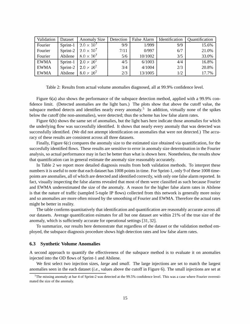
Validation Dataset Anomaly Size Detection False Alarm Identification QuantificationFourier Sprint-1 2:0� 107 9/9 1/999 9/9 15.6%Fourier Sprint-2 2:0� 107 7/11 0/997 6/7 21.0%Fourier Abilene 8:0� 107 5/6 10/1002 3/5 33.0%EWMA Sprint-1 2:0� 107 4/5 6/1003 4/4 16.8%EWMA Sprint-2 2:0� 107 3/4 4/1004 2/3 20.8%EWMA Abilene 8:0� 107 2/3 13/1005 1/2 17.7%

Table 2: Results from actual volume anomalies diagnosed, all at 99.9% confidence level.

Figure 6(a) also shows the performance of the subspace detection method, applied with a 99.9% con-fidence limit. (Detected anomalies are the light bars.) The plots show that above the cutoff value, thesubspace method detects and identifies nearly every anomaly.5 In addition, virtually none of the spikesbelow the cutoff (the non-anomalies), were detected; thus the scheme has low false alarm rates.

Figure 6(b) shows the same set of anomalies, but the light bars here indicate those anomalies for whichthe underlying flow was successfully identified. It shows that nearly every anomaly that was detected wassuccessfully identified. (We did not attempt identification on anomalies that were not detected.) The accu-racy of these results are consistent across all three datasets.

Finally, Figure 6(c) compares the anomaly size to the estimated size obtained via quantification, for thesuccesfully identified flows. These results are sensitive to error in anomaly size determination in the Fourieranalysis, so actual performance may in fact be better than what is shown here. Nonetheless, the results showthat quantification can in general estimate the anomaly size reasonably accurately.

In Table 2 we report more detailed diagnosis results from both validation methods. To interpret thesenumbers it is useful to note that each dataset has 1008 points in time. For Sprint-1, only 9 of these 1008 time-points are anomalies, all of which are detected and identified correctly, with only one false alarm reported. Infact, visually inspecting the false alarms revealed that most of them were classified as such because Fourierand EWMA underestimated the size of the anomaly. A reason for the higher false alarm rates in Abileneis that the nature of traffic (sampled 5-tuple IP flows) collected from this network is generally more noisyand so anomalies are more often missed by the smoothing of Fourier and EWMA. Therefore the actual ratesmight be better in reality.

The table confirms quantitatively that identification and quantification are reasonably accurate across allour datasets. Average quantification esimates for all but one dataset are within 21% of the true size of theanomaly, which is sufficiently accurate for operational settings [31, 32].

To summarize, our results here demonstrate that regardless of the dataset or the validation method em-ployed, the subspace diagnosis procedure shows high detection rates and low false alarm rates.

6.3 Synthetic Volume Anomalies

A second approach to quantify the effectiveness of the subspace method is to evaluate it on anomaliesinjected into the OD flows of Sprint-1 and Abilene.

We first select two injection sizes, large and small. The large injections are set to match the largestanomalies seen in the each dataset (i.e., values above the cutoff in Figure 6). The small injections are set at

5The missing anomaly at bar 4 of Sprint-2 was detected at the 99.5% confidence level. This was a case where Fourier overesti-mated the size of the anomaly.

15

0.1 0.2 0.3 0.4 0.5 0.6 0.7 0.8 0.9 10

20

40

60

80

100

120

Detection Rate

Fre

quen

cy

0.1 0.2 0.3 0.4 0.5 0.6 0.7 0.8 0.90

10

20

30

40

50

60

Detection Rate

Fre

quen

cy

(a) Large Injected Spike (b) Small Injected Spike

Figure 7: Detection rate histograms from injecting synthetic spikes (Sprint-1).

0h 6h 12h 18h 24h0

0.1

0.2

0.3

0.4

0.5

0.6

0.7

0.8

0.9

1

Det

ectio

n R

ate

Time

Figure 8: Timeseries of detection rates on large injections (Sprint-1).

values slightly below the cutoff in Figure 6 and so constitute non-anomalies that we do not want to detect.This allows us to quantify false alarm rates across all timepoints and all OD flows. For Sprint-1, we set largeat 3 � 107 bytes and small at 1:5 � 107 bytes. For Abilene, we set large at 1:2 � 108 bytes and small at5� 107 bytes.

Then, in multiple experiments, we insert a spike of each size in every OD flow and at every point in timeover the period of a day. For each permutation of spike size, timestep and OD flow selected, we generatethe corresponding set of link traffic counts. We then apply our procedure and note whether it successfullydiagnoses the injected anomaly.

Our results from these experiments reveal that the diagnosis procedure works well in general across alllinks and across all times. The first set of these results are presented in Figure 7, which shows the histogramof detection rates (rates are computed over time) for both sized injections for Sprint-1. Figure 7(a) showsthat the method detects the large (and therefore the most important) injections very well. On the other hand,Figure 7(b) shows that the small injected spikes rarely trigger detections, which is as desired. Together,these plots confirm that the subspace method has a high detection and a low false alarm rate.

Evaluation results across time for Sprint-1 are presented in Figure 8. Here we show the mean detection

16

102

104

106

0.1

0.2

0.3

0.4

0.5

0.6

0.7

0.8

0.9

1

Det

ectio

n R

ate

Mean OD Flow Size

Figure 9: Scatter plots of detection rate of large injections and mean OD flow rate (Sprint-1).

Network Injection Size Detection Identification QuantificationSprint Large (3:0� 107) 93% 85% 18%Abilene Large (1:2� 108) 90% 69% 21%Sprint Small (1:5� 107) 15% 14% 11%Abilene Small (5:0� 107) 5% 3% 18%

Table 3: Results on diagnosing synthetic volume anomalies.

rates (rates are computed over OD flows) as a timeseries for the large injections. This plot shows that themethod’s detection rate is fairly constant, regardless of when the anomaly was injected. Thus the diagnosisprocedure works equally well across timepoints, and is not affected by the underlying nonstationarities intraffic.

In Figure 9, we present a scatter plot of mean detection rate (rates are computed over time) against themean OD flow rate for the large injections for Sprint-1. This plot shows that for a fixed size anomaly, themethod tends to detect the injections on the smaller OD flows better than on larger OD flows. There aretwo reasons for this. First, the larger variance OD flows are likely better aligned with S , as explained inSection 5.4. Second, an inserted spike can be canceled out by a large negative spike in the OD flow, an effectmore likely to occur on a high variance OD flow.

Corresponding experiments for Abilene and for identification and quantification yield similar results.Summary results from all these experiments for both Sprint-1 and Abilene are tabulated in Table 3. Thefirst two rows quantify the method’s ability to diagnose large injections, and shows very good detection,identification and quantification rates. The next two rows capture the method’s ability to avoid the smallinjected spikes, representing false anomalies. These results show that regardless of the underlying network,OD flow and the timepoint of the injected spike, the subspace method is able to diagnose the volume anomalywith high accuracy and low false alarm rates.

7 Discussion

In this section we consider issues related to deployment of the subspace method and its potential extensions.

17

7.1 Computational Complexity

Since the subspace method operates on link measurements, it imposes relatively low cost in data collection.We envision that the method may therefore be used as a first-level online monitoring tool, capable of raisingan alarm and directing attention to particular OD flows as the focus of attention. The diagnosis of an anomalymay then trigger sophisticated, fine-scale (but more expensive) measurements to further isolate the cause ofthe anomaly.

To be used in this manner, the method must impose low computational demand. Computing all theprincipal components of link traffic Y is in fact equivalent to solving the symmetric eigenvalue problemfor the covariance matrix, YTY. The standard procedure for this relies on computing the singular valuedecomposition (SVD) of Y [27]. The computation complexity of a complete SVD of a t � m matrix isO(tm2) [11]. However, the computation is typically not expensive for reasonable-sized datasets. For our1008 � 49 matrices the computation requires less than two seconds on a 1.0 GHz Intel-based laptop.

To apply the subspace method online, one processes each arrival of new traffic measurements using thematrix PPT , which is derived from the SVD. Previous work has shown that (for OD flows) this matrix canbe reasonably stable from week to week [20]. Thus one need only compute the SVD occasionally, ratherthan at each timestep.

Finally, it is conceivable that the straightforward SVD procedure could become a bottleneck if applied todata with a larger set of sources and destinations, e.g., IP-level flow data. However, such cases may still bemanageable using one of the methods that exist for updating previously computed decompositions as newdata arrives [12, 13, 24].

7.2 Extensions

There are a number of ways in which the work described in this paper can be extended.The choice made here to identify only single-flow anomalies is in fact somewhat arbitrary. The set

of anomalies that can be potentially identified is a function of the construction of fF ig and the associatedanomaly vectors f�ig. For example, to identify anomalies involving any two flows, one simply extends fFigto include the new anomalies, with associated elements in f�ig constructed from the (normalized) union ofthe two corresponding columns of A.

An important generalization is to the case in which an anomaly involves multiple flows having differenttraffic intensities. This can occur when an anomaly involves multiple OD flows, with it arises from routingchanges, or when it arises from network abuse (e.g, DDoS attacks). To handle this case, we may proceedas follows (see also [7]). We replace �i with a matrix �i having as many columns as there are flows thatparticipate in the anomaly; each column of �i consists of the (normalized) column of A corresponding toa participating flow. We then replace fi with a vector fi which will capture the intensity of the anomaly ineach flow. The identification algorithms remain the same (in particular, Equation (1) is unchanged).

It is also possible to consider applying the subspace method to other metrics on links for which the `2norm is an appropriate measure. For example, we may choose to look at the number of IP flows passing overa link, or the average packet size. We believe that the method we have outlined in this paper is applicable tosuch metrics as well.

7.3 Alternate Basis Sets forY

Seen in a general light, the subspace method constructs an alternate basis set for representing link measure-ments that makes the separation of “normal” and “anomalous” conditions easier. It does so by making

18

Mon Tue Wed Thu Fri Sat Sun

1

2

3

x 1015

Res

idua

l Vec

tor

Mon Tue Wed Thu Fri Sat Sun

1

2

3

x 1015

Fou

rier−

Res

idua

l

Mon Tue Wed Thu Fri Sat Sun0

1

2x 10

15

EW

MA

−R

esid

ual

Figure 10: Comparing squared magnitude of Subspace, Fourier and EWMA residual vectors.

use of spatial correlation (correlation across links) in network measurements.The same general strategy of seeking a useful alternate basis set for data representation lies behind

previous approaches to anomaly detection as well [2,5,19]. However, these previous approaches have madeuse of correlation in the temporal domain – for example, using the wavelet transform, or using exponentialsmoothing. This is natural when working with 1-dimensional timeseries data; in fact, we made use of justsuch methods in extracting “true” anomalies from OD flows in Section 6.2.

However it is reasonable to ask how temporal correlation compares to spatial correlation as a tool forconstructing such alternate basis sets in the multivariate case. This is an especially appropriate questionsince we made use of time-domain methods in constructing our “true” anomalies.

For example, one method we used for constructing “true” anomalies was extracting the periodicityof OD flows (especially daily variation) from each OD flow using frequency-domain filtering via Fourieranalysis. Since each link’s traffic is a linear combination of traffic in all flows, we might consider that thesame frequencies filtered from each link timeseries might yield good results for detecting anomalies in linkdata.

While a detailed exploration of this issue is beyond our scope, we contrast here the results of extracting“normal” link behavior via frequency-domain filtering, exponential smoothing, and subspace separation. Todo this, we apply to each timeseries of link data the same Fourier-based filtering and EWMA smoothingthat we applied to flow data in Section 6.2. In each case, this allows the separation of link measurements yinto modeled and residual components. We then plot the squared norm of the residual vector as a functionof time. These plots are shown in Figure 10. In this figure, the upper plot (showing the subspace methodresults) is the same as the lower plot in Figure 5(a).

The figure shows that the anomaly detection problem is much easier using the subspace method thanusing the EWMA and Fourier-based methods. In the case of the subspace method, it is possible to finda threshold such that all anomalies appear above the threshold, while very few normal data points appearabove the threshold – in other words, achieving high detection probability and low false alarm rate. TheEWMA and Fourier methods are quite different; the anomalous data points do not stand sharply out from

19

the normal data, and there is no threshold having high detection probability that does not also have highfalse alarm rate.

It is also striking that noticeable periodic behavior remains, even when the most significant frequenciesare removed. This shows that periodic behavior in network traffic can be rather complex and difficult tomodel using only a small set of frequencies. The subspace method avoids this difficulty by not beingrestricted to a fixed set or number of frequencies. Quite complex behavior can be captured in the first fewprincipal components, as shown in Figure 4(a).

Finally, it is important to note that temporal and spatial correlation are both valuable sources of pre-dictability in network traffic, and there is room for methods that attempt to exploit both simultaneously. Inparticular, it is possible to use the subspace method across multiple time scales by applying PCA to thewavelet transform of measured data [23]. In principle, such a method can allow the detection of anomaliesat all timescales.

8 Related Work

A number of techniques have been proposed to detect anomalies in traffic volume. Some examples include[1,2,5,9,19]. As discussed in Section 7, all these schemes operate on single-timeseries traffic, measured forexample from a network link, and independent of traffic on other links in a network. Thus, these techniquesexploit temporal patterns within a single traffic timeseries to expose anomalies. In contrast, our schemeexploits correlation properties across links to detect network-wide anomalies.

Another distinguishing feature of our approach is that it does not require detailed modeling assumptionsabout the underlying normal traffic behavior. Previous methods have principally relied on timeseries modelsto approximate normal traffic [5, 14, 19] or have relied on building models of the data during a trainingperiod [30]. In our scheme, normal traffic behavior is captured directly in the data, by extracting the commonfeatures across all links.

Isolating faults in networks (which is a more general problem than traffic anomaly detection) has also at-tracted some attention in the past. A review of research in this area is [21]; noteworthy examples include [14]and [18]. The approach of [14] relies on an autoregressive (AR) model of signals, coupled with Bayes netsfor detecting faults, but no significant validation is given. The methods of [18] rely on an exhaustive analysisof how faults might be detected through a variety of matching algorithms. Once a fault is found, the bestexplanation for it is obtained by relying on heuristics, some of which are unsubstantiated. In contrast, ourapproach is more systematic, relying on statistical tools; it requires no modeling assumptions, and has beensuccessful validated on data from two modern backbone networks.

The problem of identification in our anomaly diagnosis framework bears resemblance to the problemof traffic matrix estimation as formulated in [29]. However, traffic matrix estimation is concerned with theproblem of estimating all underlying OD flow intensities from link data, which is a much harder problem.As a result, most traffic matrix estimation work to date has concentrated on estimating mean values of largeflows [22, 32]. In contrast, our work addresses estimation of anomalous values occurring in any flow.

Finally, as has been noted earlier in the paper, our methodology draws strongly on techniques fromsubspace-based fault diagnosis, such as those used in chemical engineering [7, 8]. Those methods exploitcorrelation patterns among state variables in an industrial process control setting, whereas we focus oncovariance patterns across link traffic timeseries.

20

9 Conclusions

In this paper we have proposed an approach called the subspace method to diagnose network-wide trafficanomalies. The method can detect, identify and quantify traffic anomalies. The subspace method usesPrincipal Component Analysis to separate network traffic into a normal component that is dominated bypredictable traffic, and an anomalous component which is more noisy and contains the significiant trafficspikes.

We evaluate the method on volume anomalies, which are a specific instance of network-wide trafficanomalies resulting from unusual changes in the traffic of an OD flow. We showed how to use our method todiagnose volume anomalies from simple and readily available link measurements. We quantified the efficacyof our approach on OD flow data collected from two backbone networks, and showed that the subspacemethod can successfully diagnose volume anomalies with high detection rate and small false alarm rate.

Although the evaluation in this paper is in terms of volume anomalies, the subspace method is notspecific to them. The strength of the method lies in its use of correlations in timeseries data from multiplelinks. This allows it to treat diagnosis of network-wide traffic anomalies as a spatial problem. Such anapproach can therefore be extended to other types of network-wide data, and thus other types of network-wide anomalies.

Our ongoing work is centered on extending the methodology proposed here to diagnose additionalnetwork-wide anomalies, including routing related anomalies. Once effective mechanisms for diagnosinganomalies are built, we can begin to understand the causes of the anomalies. Finally, we plan to incorpo-rate these algorithms in a toolset that can be used by network operators to better diagnose, understand andultimately prevent network-wide anomalies.

10 Acknowledgements

We are grateful to Rick Summerhill, Mark Fullmer (Internet 2), Matthew Davy (Indiana University) for help-ing us collect and understand the flow measurements from Abilene, and to Bjorn Carlsson, Jeff Loughridge(SprintLink) and Richard Gass (Sprint ATL) for instrumenting and collecting the Sprint NetFlow measure-ments. We also thank Tim Griffin and Gianluca Iannaccone for feedback on early drafts. Finally, we aregrateful to Eric Kolaczyk for many helpful discussions, and for clarifying the issues behind the discussionin Section 7.3.

References

[1] A. Akella, A. Bharambe, M. Reiter, and S. Seshan. Detecting DDoS Attacks on ISP Networks. InACM SIGMOD/PODS Workshop on Management and Processing of Data Streams (MPDS) FCRC,2003.

[2] P. Barford, J. Kline, D. Plonka, and A. Ron. A signal analysis of network traffic anomalies. In InternetMeasurement Workshop, 2002.

[3] P. Barford and D. Plonka. Characteristics of network traffic flow anomalies. In Internet MeasurementWorkshop, 2001.

[4] P. J. Brockwell and R. A. Davis. Introduction to Time Series and Forecasting. Springer, New York,1996.

21

[5] J. Brutlag. Aberrant behavior detection in time series for network monitoring. In USENIX FourteenthSystems Administration Conference (LISA), 2000.

[6] NetFlow. At www.cisco.com/warp/public/732/Tech/netflow/.

[7] R. Dunia and S. J. Qin. Multi-dimensional Fault Diagnosis Using a Subspace Approach. In AmericanControl Conference, 1997.

[8] R. Dunia and S. J. Qin. A subspace approach to multidimensional fault identification and reconstruc-tion. American Institute of Chemical Engineers (AIChE) Journal, pages 1813–1831, 1998.

[9] F. Feather, D. Siewiorek, and R. Maxion. Fault Detection in an Ethernet Network Using AnomalySignature Matching. In ACM SIGCOMM, 1993.

[10] A. Feldmann, A. Greenberg, C. Lund, N. Reingold, J. Rexford, and F. True. Deriving traffic demandsfor operational IP networks: Methodology and experience. In IEEE/ACM Transactions on Neworking,2001.

[11] G. Golub and C. F. V. Loan. Matrix Computations. The Johns Hopkins University Press.

[12] M. Gu and S. C. Eisenstat. Downdating the singular value decomposition. Technical Report TechnicalReport YaleU/DCS/RR-939, Yale University, 1993.

[13] M. Gu and S. C. Eisenstat. A stable and fast algorithm for updating the singular value decomposition.Technical Report Technical Report YaleU/DCS/RR-966, Yale University, 1994.

[14] C. Hood and C. Ji. Proactive Network Fault Detection. In IEEE INFOCOM, 1997.

[15] H. Hotelling. Analysis of a complex of statistical variables into principal components. J. Educ. Psy.,pages 417–441, 1933.

[16] J. E. Jackson and G. S. Mudholkar. Control procedures for residuals associated with Principal Com-ponent Analysis. Technometrics, pages 331–349, 1979.

[17] D. R. Jensen and H. Solomon. A Gaussian Approximation to the Distribution of a Definite QuadraticForm. J. of the American Statistical Association, pages 898–902, 1972.

[18] I. Katzela and M. Schwartz. Fault identification schemes in communication networks. In IEEE/ACMTransactions on Neworking, December 1995.

[19] B. Krishnamurthy, S. Sen, Y. Zhang, and Y. Chen. Sketch-based Change Detection: Methods, Evalua-tion, and Applications. In Internet Measurement Conference, 2003.

[20] A. Lakhina, K. Papagiannaki, M. Crovella, C. Diot, E. D. Kolaczyk, and N. Taft. Structural Analysisof Network Traffic Flows. In ACM SIGMETRICS, 2004.

[21] A. A. Lazar, W. Wang, and R. Deng. Models and algorithms for network fault detection and identifi-cation: A review. In ICC, 1992.

[22] A. Medina, N. Taft, K. Salamatian, S. Bhattacharyya, and C. Diot. Traffic Matrix Estimation: ExistingTechniques and New Directions. In ACM SIGCOMM, 2002.

22

[23] M. Misra, H. H. Yue, S. J. Qin, and C. Ling. Multivariate process monitoring and fault diagnosis bymulti-scale PCA. Computers and Chemical Engineering, pages 1281–1293, 2002.

[24] M. Moonen, P. Dooren, and J. Vandewalle. A singular value decomposition updating algorithm forsubspace tracking. SIAM J. Matrix Anal. Appl., pages 1015–1038, 1992.

[25] K. Papagiannaki, R. Cruz, and C. Diot. Network performance monitoring at small time scales. InInternet Measurement Conference, 2003.

[26] K. Papagiannaki, N. Taft, Z. Zhang, and C. Diot. Long-Term Forecasting of Internet Backbone Traffic:Observations and Initial Models. In IEEE INFOCOM, 2003.

[27] G. Strang. Linear Algebra and its Applications, pages 442–451. Thomson Learning, 1988.

[28] Juniper Traffic Sampling. At www.juniper.net/techpubs/software/junos/junos60/swconfig60-policy/html/%sampling-overview.html.

[29] Y. Vardi. Network Tomography: Estimating Source-Destination Traffic Intensities from Link Data. J.of the American Statistical Association, pages 365–377, 1996.

[30] N. Ye. A Markov Chain Model of Temporal Behavior for Anomaly Detection. In Workshop onInformation Assurance and Security, 2000.

[31] Y. Zhang, M. Roughan, N. Duffield, and A. Greenberg. Fast Accurate Computation of Large-Scale IPTraffic Matrices from Link Loads. In ACM SIGMETRICS, 2003.

[32] Y. Zhang, M. Roughan, C. Lund, and D. Donoho. An Information-Theoretic Approach to TrafficMatrix Estimation. In ACM SIGCOMM, 2003.

23