Diagnosing and Repairing Data Anomaliesin Process Models

Ahmed Awad1, Gero Decker1, and Niels Lohmann2

1 Business Process Technology GroupHasso Plattner Institute at the University of Potsdam{ahmed.awad,gero.decker}@hpi.uni-potsdam.de

2 Institut fur Informatik, Universitat Rostock, Germanyniels.lohmann@uni-rostock.de

Abstract. When using process models for automation, correctness ofthe models is a key requirement. While many approaches concentrate oncontrol flow verification only, correct data flow modeling is of similar im-portance. This paper introduces an approach for detecting and repairingmodeling errors that only occur in the interplay between control flow anddata flow. The approach is based on place/transition nets and detectsanomalies in BPMN models. In addition to the diagnosis of the modelingerrors, a subset of errors can also be repaired automatically.

1 Introduction

Process models reflect the business activities and their relationships in an or-ganization. They can be used for analyzing cost, resource utilization or processperformance. They can also be used for automation. Especially in the latter case,not only the control flow between activities must be specified but also branchingconditions, data flow and preconditions and effects of activities.

The Business Process Modeling Notation (BPMN [1]) is the de-facto standardfor process modeling. It provides support for modeling control flow, data flow andresource allocation. For facilitating the handover of BPMN models to developersor enabling the transformation of BPMN to executable languages such as theBusiness Process Execution Language (BPEL [2]), data flow modeling is anessential aspect. This is mainly done through so called data objects that arewritten or read by activities. On top of that, it can be specified that a dataobject must be in a certain state before an activity can start or that a dataobject will be in another state after it was written by an activity. This allows tostudy the interplay between control flow and data flow in a process.

When using process models for automation, correctness of the process modelsis of key importance. Many different notions of correctness have been reported inthe literature, mostly concentrating on control flow only [3–7]. These techniquesreveal deadlocks, livelocks and other types of unwanted behavior of process mod-els. Although data flow modeling is as important when it comes to automation,only few corresponding verification techniques can be observed [8, 9].

In this context, the contribution of our paper is three-fold. (i) We provide aformalization of basic data object processing in BPMN based on place/transition

nets [10], (ii) we define a correctness notion for the interplay between control flowand data flow that can be computed efficiently, and (iii) we provide a techniquefor automatically repairing some of the modeling errors. While we use BPMNas main target language of our approach, it could easily be applied to otherlanguages as well.

The paper is structured as follows. The next section will provide an examplethat will be used throughout this paper. Section 3 introduces the mapping ofBPMN to place/transition nets. Different types of data anomalies are discussedin Sect. 4. Section 6 reports on related work, before Sect. 7 concludes the paperand points to future work.

2 Motivating Example

Fig. 1 depicts a business process that handles insurance claims. The circles rep-resent the start and end of the process, the rounded rectangles are activitiesand the diamond shapes are gateways for defining the branching structure. Dataobjects are represented by rectangles with dog-ears.

First, the new claim (the data object under study) is registered. It is checkedwhether the claim is fraudulent or not. In case it is fraudulent, an investigationis initiated to reveal this fraud. Otherwise, the claim is evaluated to be eitheraccepted or rejected. Accepted claims are paid to the claimer. In all cases claimsare closed at the end.

Register new

claim

Check for

fraud

Initiate fraud

investigation

Evaluate

claim

Pay

Close

Claim accepted

Claim rejected

Claim

[registered]

Claim

[Fraudulent]

Claim

[NotFraudulent]

Claim

[accepted]

Claim

[rejected]

Settlement

[created]

File and

update history

Settlement

[paid]

Claim

[filed]

Claim

[new]

Fig. 1. A process model regarding data object handling adapted from [11]

From the control flow perspective, the process model is correct according toseveral correctness notions from the literature. This can be proved by translatingthe BPMN model to a place / transition net as described in [12]. The result ofthis transformation is shown in Fig. 2.

P2

Register

claimCheck for

fraud

P3

P4

Initiate fraud

investigation

P5

Evaluate

claim

P6

P7

P8

P9

File and

update

historyP12 P14

Close

P15

Pay

P10

P11 P13

P1t1 t2

t3

t4

t5

t6t7

t8

t9

t10

t11

t12

t13

t14

t15

Fig. 2. Petri net representation of the example (considering the control flow only)

The Petri net is sound [13], implying that the process will terminate properlyin all possible execution scenarios without leaving running activities behind.Therefore, we can conclude that the control flow of the given BPMN model isfine.

On the other hand, the BPMN model also contains information about dataflow. As we did with the control flow aspects, we want to make sure that alsothe data flow is correct.

The use of BPMN data objects with defined states can be interpreted aspreconditions and effects of activities. For instance, a registered claim existsafter activity “register new claim” has completed. Activity “pay” can in turnonly be executed if an accepted claim is present. Also branching conditions canbe specified, as it is the case for distinguishing accepted and rejected claims fordeciding to take the upper or lower branch.

The example contains a number of anomalies that only appear in the in-terplay between control flow and data flow. For instance, “pay” and “file andupdate history” are specified to run concurrently, while executing “file and up-date history” before starting “pay” would lead to a problem: The claim needsto be in state accepted but it was already set to filed. Further discussion aboutdata anomalies is deferred to Sect. 4.

3 Mapping of Data Objects to Petri Nets

The BPMN specification considers data objects as a way to visualize how data isprocessed. The semantics of data objects remain unspecified and even left to theinterpretation of the modeler (see [1] page 93). Therefore, we introduce a partic-ular semantics of BPMN data objects in this paper as a necessary preconditionfor formal verification.

First of all, we assume a single copy of the data object that is handled withinthe process. This single copy is assumed to exist from the moment of processinstantiation. Multiple data object shapes with the same label are considered torefer to the same data object. For instance, all shapes labeled “claim” refer tothe same claim object (cf. Fig. 1). Exactly one claim object is assumed to existfor each instance of that process.

On the other hand, each data object is in a certain state at any time duringthe execution of the process. This state changes through the execution of activi-ties. BPMN offers the possibility to specify allowed states of a data object. Even

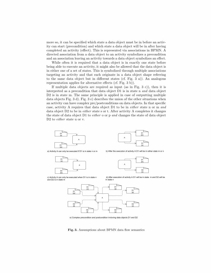
more so, it can be specified which state a data object must be in before an activ-ity can start (precondition) and which state a data object will be in after havingcompleted an activity (effect). This is represented via associations in BPMN. Adirected association from a data object to an activity symbolizes a preconditionand an association leaving an activity towards a data object symbolizes an effect.

While often it is required that a data object is in exactly one state beforebeing able to execute an activity, it might also be allowed that the data object isin either one of a set of states. This is symbolized through multiple associationstargeting an activity and that each originate in a data object shape referringto the same data object but in different states (cf. Fig. 3 a)). An analogousrepresentation applies for alternative effects (cf. Fig. 3 b)).

If multiple data objects are required as input (as in Fig. 3 c)), then it isinterpreted as a precondition that data object D1 is in state n and data objectD2 is in state m. The same principle is applied in case of outputting multipledata objects Fig. 3 d). Fig. 3 e) describes the union of the other situations whenan activity can have complex pre/postconditions on data objects. In that specificcase, activity A requires that data object D1 to be in either state n or m anddata object D2 to be in either state s or t. After activity A completes it changesthe state of data object D1 to either o or p and changes the state of data objectD2 to either state u or v.

a) Activity A can only be executed if D1 is in state n or m

A

D1

[m]

D1

[n]

b) After the execution of activity A D1 will be in either state m or n

A

D1

[n]

D2

[m]

c) Activity A can only be executed when D1 is in state n

and D2 is in state m

A

D1

[m]

D2

[n]

d) After execution of activity A D1 will be in state m and D2 will be

in state n

A

D1

[o]

D2

[u]

D1

[n]

D2

[t]

D1

[m]

D2

[s]D2

[v]

D1

[p]

e) Complex precondition and postcondition invloving data objects D1 and D2

A

D1

[n]

D1

[m]

Fig. 3. Assumptions about BPMN data flow semantics

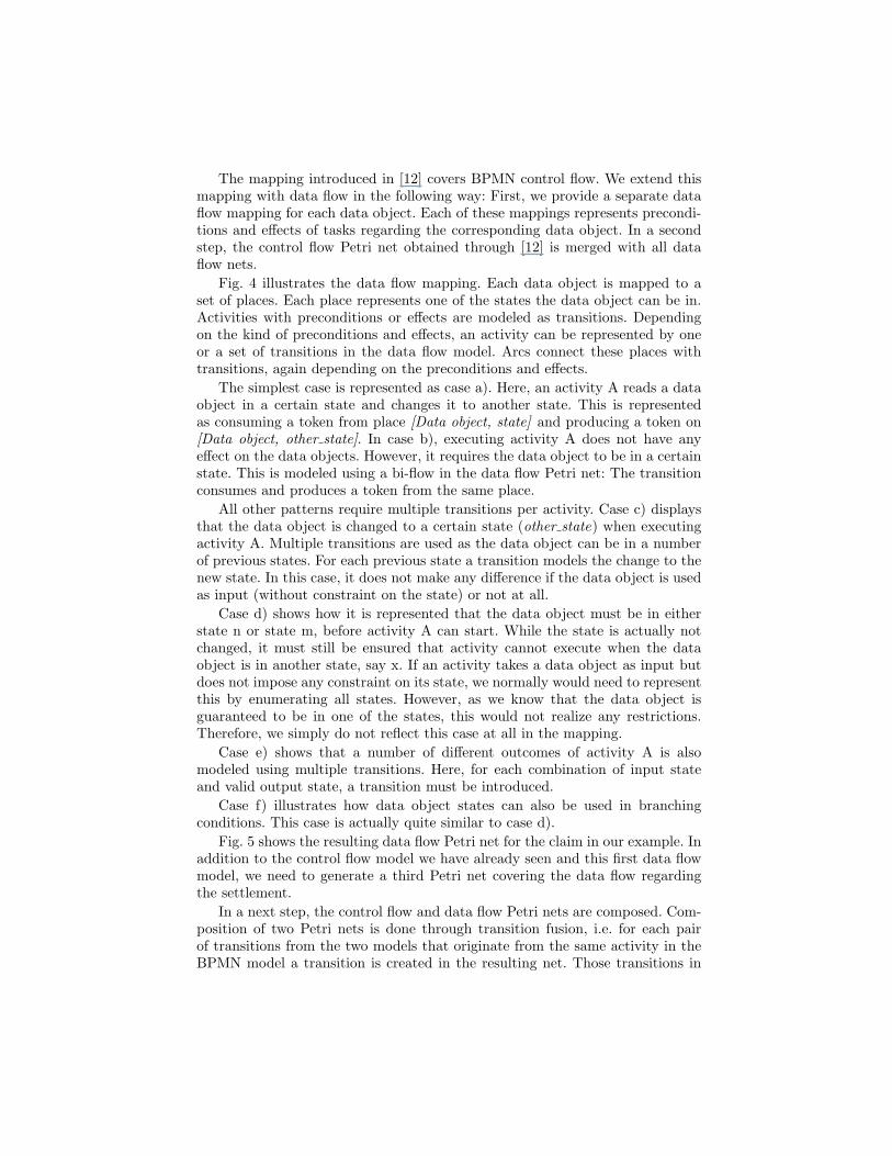
The mapping introduced in [12] covers BPMN control flow. We extend thismapping with data flow in the following way: First, we provide a separate dataflow mapping for each data object. Each of these mappings represents precondi-tions and effects of tasks regarding the corresponding data object. In a secondstep, the control flow Petri net obtained through [12] is merged with all dataflow nets.

Fig. 4 illustrates the data flow mapping. Each data object is mapped to aset of places. Each place represents one of the states the data object can be in.Activities with preconditions or effects are modeled as transitions. Dependingon the kind of preconditions and effects, an activity can be represented by oneor a set of transitions in the data flow model. Arcs connect these places withtransitions, again depending on the preconditions and effects.

The simplest case is represented as case a). Here, an activity A reads a dataobject in a certain state and changes it to another state. This is representedas consuming a token from place [Data object, state] and producing a token on[Data object, other state]. In case b), executing activity A does not have anyeffect on the data objects. However, it requires the data object to be in a certainstate. This is modeled using a bi-flow in the data flow Petri net: The transitionconsumes and produces a token from the same place.

All other patterns require multiple transitions per activity. Case c) displaysthat the data object is changed to a certain state (other state) when executingactivity A. Multiple transitions are used as the data object can be in a numberof previous states. For each previous state a transition models the change to thenew state. In this case, it does not make any difference if the data object is usedas input (without constraint on the state) or not at all.

Case d) shows how it is represented that the data object must be in eitherstate n or state m, before activity A can start. While the state is actually notchanged, it must still be ensured that activity cannot execute when the dataobject is in another state, say x. If an activity takes a data object as input butdoes not impose any constraint on its state, we normally would need to representthis by enumerating all states. However, as we know that the data object isguaranteed to be in one of the states, this would not realize any restrictions.Therefore, we simply do not reflect this case at all in the mapping.

Case e) shows that a number of different outcomes of activity A is alsomodeled using multiple transitions. Here, for each combination of input stateand valid output state, a transition must be introduced.

Case f) illustrates how data object states can also be used in branchingconditions. This case is actually quite similar to case d).

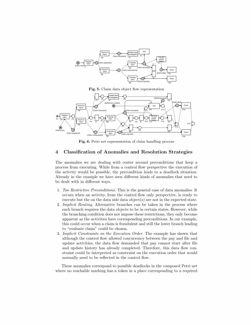
Fig. 5 shows the resulting data flow Petri net for the claim in our example. Inaddition to the control flow model we have already seen and this first data flowmodel, we need to generate a third Petri net covering the data flow regardingthe settlement.

In a next step, the control flow and data flow Petri nets are composed. Com-position of two Petri nets is done through transition fusion, i.e. for each pairof transitions from the two models that originate from the same activity in theBPMN model a transition is created in the resulting net. Those transitions in

BPMN Description Petri Net

a) Read-write with a condition on input state

Activity A has a precondition on the state of the data object at input. After completion, activity A changes the state of the data object.

b) Read-only with a condition on input state

Activity A conditionally reads data object i.e. data object has to be has to be in this specific state

[Data Object, state]

A

Data Object Data Object

[other state]

A

Data Object

[other state]

A

OR

c) Read-write without a condition on input state

Activity A has no specific condition on the state of data object as input. After completion, A will change the state of the data object to other state

[Data Object,other_state]

[Data Object,state1]

[Data Object,state n]

A

A

d) Multiple read-only condition on input state

Activity A accepts data object as input in any of the specified states. The data object can assume only one of these states when A is about of execute.

e) An activity can change a data object state to one of many states

Activity A can produce the data object after completion in only one of the specified states.

A

[Data Object,state m]

[Data Object, state n]

A

f) Explicit XOR arc conditions

Explicit XOR arc conditions based on data object states must be reflected in the resulting Petri net.

Fig. 4. Mapping options for data objects association with activities

any of the two models without partners in the other model are simply copied,as are all places. The arcs are set accordingly and the initial marking is thecomposition of the two initial markings. The result of the composition of twomodels is then again composed with the third model. The result for our threemodels is displayed in Fig. 6.

Register

claim

Check for

fraud

Check for

fraud

Initiate fraud

investigation

Evaluate

claim

Evaluate

claim

File and

update

history

Close

Close

[Claim,fraudulent]

[Claim,notfraudulent]

[Claim,rejected]

[Claim,accepted]

Pay

[Claim,filed]

[Claim,new]

[Claim,registered]

t1

t2a

t2b

t5

t6a

t6b

t10

t7

t8

t11

t15a

t15b

Fig. 5. Claim data object flow representation

P2

Register

claim

Check for

fraud

Check for

fraud P3

P4

Initiate fraud

investigation

P5

Evaluate

claim

Evaluate

claim

P6

P7

P8

P9

File and

update

historyP12

P14

Close

Close

P15

[Claim,registered]

[Claim,fraudulent]

[Claim,notfraudulent][Claim,rejected]

[Claim,accepted]

[Settlement,created]

Pay

P10

[Settlement,paid]

P11

[Claim,filed]

P13

P1

[Claim,new]

t1

t2a

t2b

t3

t4

t5

t6a

t6b

t7

t8

t9

t10

t11

t12

t13

t14

t15a

t15b

Fig. 6. Petri net representation of claim handling process

4 Classification of Anomalies and Resolution Strategies

The anomalies we are dealing with center around preconditions that keep aprocess from executing. While from a control flow perspective the execution ofthe activity would be possible, the precondition leads to a deadlock situation.Already in the example we have seen different kinds of anomalies that need tobe dealt with in different ways.

1. Too Restrictive Preconditions. This is the general case of data anomalies. Itoccurs when an activity, from the control flow only perspective, is ready toexecute but the on the data side data object(s) are not in the expected state.

2. Implicit Routing. Alternative branches can be taken in the process whereeach branch requires the data objects to be in certain states. However, whilethe branching condition does not impose these restrictions, they only becomeapparent as the activities have corresponding preconditions. In our example,this could occur when a claim is fraudulent and still the lower branch leadingto “evaluate claim” could be chosen.

3. Implicit Constraints on the Execution Order. The example has shown thatalthough the control flow allowed concurrency between the pay and file andupdate activities, the data flow demanded that pay cannot start after fileand update history has already completed. Therefore, this data flow con-straint could be interpreted as constraint on the execution order that wouldnormally need to be reflected in the control flow.

These anomalies correspond to possible deadlocks in the composed Petri netwhere no reachable marking has a token in a place corresponding to a required

object state. The problem of Implicit Constraints on the Execution Order occurswhen it comes to firing transitions “Pay” and “File and update history”. Bothtransitions are enabled but a deadlock occurs if the transition “Fire and updatehistory” fires first. If the firing sequence is that “Pay” fires first no deadlockoccurs. The Too Restrictive Preconditions anomaly takes place when a claimis declared to be fraudulent, at this time the transition “Close” is waiting for atoken in place [Claim, filed] or place [Claim, rejected] so this transition deadlocksand that instance is not able to terminate.

While we devote Sect. 5 to provide diagnosis and resolution in a formal way,in the rest of this section we informally list the different anomalies discussedabove and propose a set of resolution strategies for them if there are any.

Too Restrictive Preconditions This problem occurs when an activity in theBPMN model has a precondition on a certain data object state but this stateis not reachable at the time the activity is ready to execute. Solutions to thissituation could be:

– Remove the precondition: this is the naive solution in which the dependencyon this specific object state is removed.

– Loosening the precondition: by looking at what are the available states ofthe data object at the time the activity is ready to execute and add themto the preconditions as alternative acceptable states. The “Close” activityin Fig. 1 is expecting the “Claim” data object to be in either state rejectedor filed while it is possible that when it is activated; the “Claim” is in statefraudulent.

Implicit Routing This could be seen as a special case of the too restrictivepreconditions anomaly where the data precondition is missed for some activitydue to improper selection of the path to go. For instance, in Fig. 1 activity“Check for fraud” could produce the “Claim” is state not fraudulent but stillthe control flow could be routed by the XOR-Split to activity “Initiate fraudinvestigation”. This happened because the branches of the XOR-Split did nothave explicit conditions. The solution for this problem is to avoid this unwantedrouting by discovering the branching conditions of the XOR-Split and updatingthe model with them.

Implicit Constraints on the Execution Order Whenever there are two ac-tivities running in parallel and they have the same precondition(s), the anomalyoccurs when at least one of these activities updates the state of the data object.If there is only one activity that changes the state of the object while the restonly read it, the best solution to the problem could be to force the updatingactivity to execute last after all read only activities have executed. Unfortu-nately, making local changes by forcing sequentialization between these parallelactivities might lead to further anomalies. On the other hand, if more than oneactivity change the state of the object then forcing sequentialization will notsolve the problem. A less than optimal solution is to apply resolution strategies

for the too restrictive preconditions anomaly by loosening the precondition forthe deadlocking activity.

5 Resolution of Data Anomalies

5.1 Notations and Basic Definitions

To formally reason about the behavior of a BPMN model with data objects, weuse classical Petri nets [10] with their standard definitions: A Petri net is a tuple[P, T, F,m0] where P and T are two finite disjoint sets of places and transitions,respectively, F ⊆

((P × T ) ∪ (T × P )

)is a flow relation, and m0 : P → IN is

an initial marking. For a node x ∈ P ∪ T , define •x = {y | [y, x] ∈ F} andx• = {y | [x, y] ∈ F}. A transition t is enabled by a marking m (denoted m t−→) ifm(p) > 0 for all p ∈ •t. An enabled transition can fire in m (denoted m

t−→ m′),resulting in a successor marking m′ with m′(p) = m(p) + 1 for p ∈ t• \ •t,m′(p) = m(p) + 1 for p ∈ •t \ t•, and m′(p) = m(p) otherwise.

Let Nc = [Pc, Tc, Fc,m0c,finalc] be the Petri net translation of the control

flow aspects of the BPMN process under consideration (using the translationfrom [12]). Similarly, let N = [P, T, F,m0,final ] be the Petri net translationincluding control flow and data flow (using the patterns from Fig. 4). We assumethat the set of places P is a disjoint union of control flow places Pc and dataplaces Pd ⊆ D × S; that is, a data place is a pair of a data object and a datastate thereof. Furthermore, there is a surjective labeling function ` : T → Tc thatmaps each transition of N to a transition of Nc. For two transitions t1, t2 ∈ Twe have `(t1) = `(t2) iff t1 and t2 model the same activity, but t1 is connectedto different data places as t2, i.e. •t1 ∩ Pc = •t2 ∩ Pc and t1

• ∩ Pc = t2• ∩ Pc.

We further extend the standard definition of Petri nets by defining a finite setfinal of final markings to distinguish desired final states from unwanted blockingstates. We use the term deadlock for a marking m /∈ final which does not enableany transition.

Example. For the net Nc in Fig. 2, the marking [p15] is the only final marking.When also considering data places for net N in Fig. 6, any marking m with (i)m(p15) = 1, (ii) m(p) = 0 for all other control places p ∈ Pc \ {p15}, and (iii) foreach data object d ∈ D, marks exactly one place [d, s]. For instance, the marking[p15, [Settlement, paid], [Claim, filed]] is a final marking of N .

As a starting point of the analysis, we assume that the control flow model Ncis weakly terminating. That is, from each marking m reachable from the initialmarking m0c

, a final marking mf ∈ finalc is reachable. A control flow model thatis not weakly terminating can deadlock or livelock, which is surely undesired.Such flaws need to be corrected even before considering data aspects and aretherefore out of scope of this paper.

5.2 Resolving Too Restrictive Preconditions

If the model of both the control flow and the data flow deadlocks, such a deadlockm of N marks control flow places that enable transitions in the pure control flowmodel Nc. These transitions can be used to determine which data flow tokensare missing to enable a transition in m.

Definition 1 (Control-flow enabledness). Let m be a deadlock of N andlet mc be a marking of Nc with mc(p) = m(p) for all p ∈ Pc. Define the set ofcontrol-flow-enabled transitions of m as Tcfe(m) = {t′ ∈ T | mc

t−→Nc∧ `(t′) = t}.

As Nc weakly terminates, Tcfe(m) 6= ∅ for all deadlocks of N . We now canexamine the preset of control-flow enable transitions to determine which dataflow tokens are missing.

Definition 2 (Missing data states). Let m be a deadlock of N and t ∈Tcfe(m) a control-flow-enabled transition. Define the missing data states of tin m as Pmdi(t,m) = (•t ∩ Pd) \ {p | m(p) > 0}.

For a control-flow-enabled transition t in m, Pmdi(t,m) consists of those dataplaces that additionally need to be marked to enable t. This information can nowbe used to fix the model as sketched in Sect. 4: (1) to change the model such thatthese tokens are present; (2) to add an additional transition t′ with `(t) = `(t′)that can fire in the current data state.

Example. Consider the deadlock [p14, [Claim, fraudulent], [Settlement, created]] ofnetN in Fig. 6. The transitions t15a and t15b are control flow enabled. The missingdata inputs are [Claim, filed] and [Claim, rejected], respectively. The deadlock canbe resolved by either relaxing a transition’s input condition (e.g. by removingthe edge [[Claim, filed], t15a] or to add a new “Close” transition t15c to the netwith •t15c = {p14, [Claim, fraudulent]} and t15c

• = {p15, [Claim, fraudulent]} (seeFig. 7.

5.3 Resolving Implicit Routing

In this section, we introduce the notion of data equivalence which can be usedto classify occurring deadlocks. The classification then can be used to proposeresolution strategies for these deadlocks.

Definition 3 (Data invariance, data equivalence). A transition t ∈ T isdata invariant, iff (•t ∪ t•) ∩ Pd = ∅. Let m1,m2 be markings of N . m1 and m2

are data equivalent, denoted m1 ∼d m2, iff (i) m1(p) = m2(p) for all p ∈ Pdand (ii) there is a data invariant transition sequence σ such that m1

σ−→ m2 orm2

σ−→ m1. For a marking m of N , define the data equivalence class of m as[[m]] = {m′ | m ∼d m′}.

Obviously, ∼d is an equivalence relation that partitions the set of reachablemarkings of N into data equivalence classes. These equivalence classes can beused to classify deadlocks of N .

Definition 4 (Unsynchronized deadlock). Let m be a deadlock of N . mis an unsynchronized deadlock if there exists a marking m′ ∈ [[m]] such thatm′

∗−→ m′′ with [[m′′]] 6= [[m]] or m′′ ∈ final.

Let m∗ ∈ [[m]] be a marking such that the transition sequence m∗ σ−→ m isminimal and m∗

∗−→ m′′. m∗ enables at least two mutually exclusive transitionst1 and t2. Let t1 be the first transition of σ. To avoid the deadlock m, thistransition must not fire in the data state of [[m]]. Hence, the BPMN model hasto be changed such that the XOR-split modeled by t1 is refined by an appropriatebranching condition.

Example. Consider the deadlock [p5, [Claim, fraudulent], [Settlement, created]] ofthe net of Fig. 6. There exists a data-equivalent marking [p4, [Claim, fraudulent],[Settlement, created]] which activates transition “Initiate fraud investigation”. Toavoid the deadlock, transition t4 must not fire in this data state[Claim, fraudulent]. This can be achieved by adding explicit XOR split branchingconditions.

Branching conditions are realized on the Petri net level using bi-flows, asalready illustrated in Fig. 4. Refining branching conditions means in this contextthat certain combinations of data object states should be excluded. We need todistinguish two cases in this context. Either there is currently no restriction onthe data objects in question or there is one. The latter case is easier as we cansimply delete the corresponding transition from the Petri net. If no transitionis left for the XOR-split we know that we cannot find any branching conditionthat would guarantee proper behavior. In the first case, we need to enumerateall combinations of data object states except for the current combination (seeFig. 7.

5.4 Resolving Implicit Constraints on the Execution Order

The case of “implicit constraints on the execution order” occurs when a deadlockis reached from a point where two or more transitions can run in parallel andthey have common input data places.

Definition 5 (Implicit Constraints on the Execution Order). Let m bea deadlock of N . m is called a data-flow/control-flow conflict iff ∃ m′ wherem′

t1−→ m ∧ m′ t2−→ m′′ ∧ (•t1 ∩ Pc) ∩ (•t2 ∩ Pc) = ∅ ∧ (•t1 ∩ Pd) ∩ (•t2 ∩ Pd) 6=∅ ∧ (•t1 ∩ Pd) ∩ (t2• ∩ Pd) = ∅

Example. The deadlock [p11, p12, [Claim, filed], [Settlement, created]] of net N inFig. 6 occurred because there was a previous marking [p10, p11, [Claim, accepted],[Settlement, created]] where t10 and t11 were enabled. Both t10 and t11 are runningin parallel and share a common data place [Claim, accepted].

Resolving implicit constraints on the execution order requires the modifica-tion of the control flow logic of the process. On a reachability graph level, statetransitions from “good” states to “bad” states need to be removed. “Good”states would be those states from where a valid final state is still reachable and

“bad” states from where no valid final state is reachable. While the problematicstate transitions are identified in the combined model for control flow and dataflow, corresponding state transitions would then be removed from the controlflow model.

While this is feasible on the state transition / reachability graph level, pro-jecting a corresponding change back to Petri nets (and finally back to BPMN) isvery challenging. This is due to the fact that one transition in the Petri net corre-sponds to potentially many state transitions in the reachability graph. Therefore,removing individual state transitions from the reachability graph typically re-sults in heavy modifications of the Petri net structure rather than just removingindividual nodes. There exist techniques for generating Petri nets for a givenautomata [14]. However, this clearly goes beyond the scope of the paper. Pro-jecting the modification of the Petri net back to a modification of the initialBPMN model is then the next challenge that would need to be tackled.

Therefore, our approach simply suggests to the modeler that the executionorder must be altered in order to avoid a certain firing sequence of transitions.It is then up to the modeler to perform modifications that actually lead to aresolved model.

P2

Register

claim

Check for

fraud

Check for

fraud

P3

P4

Initiate fraud

investigation

P5

Evaluate

claim

Evaluate

claim

P6

P7

P8

P9

File and

update

historyP12

P14

Close

Close

P15

[Claim,registered]

[Claim,fraudulent]

[Claim,notfraudulent][Claim,rejected]

[Claim,accepted]

[Settlement,created]

Pay

P10

[Settlement,paid]

P11

[Claim,filed]P13

P1

[Claim,new]

0

t1

t2a

t2b

t3

t4

t5

t6a

t6b

t7

t8

t9

t10

t11

t12

t13

t14

t15a

t15b

Close

t15c

Fig. 7. Modified net with data anomalies corrected

6 Related Work

To the best of our knowledge, there is no research conducted to formalize the dataflow aspects in BPMN. On the other hand, data flow formalization in processmodeling has been recently addressed from different points of view.

The first discussion of the importance of modeling data in process models isin [8]. They identify a set of data anomalies as redundant data, lost data, miss-ing data, mismatched data, inconsistent data, misdirected data, and insufficientdata. However, the paper just signaled these types of anomalies without an ap-proach to detect them. A refinement of the aforementioned set of data anomalieswas given in [9]. In addition, authors provide a formal approach that extendsUML ADs to model data flow aspects and detect anomalies. An earlier work

to formalize data flow semantics in UML ADs was discussed in [15, 16] whereColored Petri Nets CPNs were used as the formal background.

Van Hee et al. [17] present a case study how consistency between modelsof different aspects of a system can be achieved. They model object life cyclesderived from CRUD matrices as workflow nets and later synchronized with thecontrol flow. Their approach is, however, does not present strategies how incon-sistencies between data flow and control flow can be removed.

Verification of data flow aspects in BPEL was discussed in [18]. Authors use amodern compiler technology to discover the data dependency between interact-ing services as a step to enhance control-flow only verification of BPEL processes.Later on, the extracted data dependency enriches the underlying Petri net rep-resenting the control flow with extra places and transitions. The approach mapsonly those messages that affect the value of a data item used in decision points.Model checking data aware message exchange with web services was discussedin [19] where authors have extended Computational Tree Logic CTL with firstorder quantification in order to verify that sequence of messages exchanged willsatisfy certain properties based on data contents of these messages.

Recent data-centric business process modeling approach let data dependencydrive control flow among activities in a process [20]. A business artifact is anabstraction of a document that can be consumed and produced by tasks of theprocess. Nine patterns of processing such business artifacts have been defined.However, the notion of a state of an artifact is defined by means of repositories.The approach to a large extent is similar to ours, however, in their verification,deadlock scenarios and their resolution as we discussed were not addressed. Workin [11, 21] has addressed the consistency between business process models andlifecycle of business objects processed in these models. A more recent approachfor making data dependencies first class citizens is discussed in [22]. [23] comesto formalize the aspects of data-centric business process modeling and developsan algorithm to derive data-centric models from activity-centric ones.

In [24], object life cycles are studied in the context of inter-organizationalbusiness processes implemented as services. The synchronization between controlflow and data flow not only confines the control flow of a service, but also itsinteraction with other services. It is likely that the results of this paper can beadapted to inter-organizational business processes.

Dual Workflow Nets [25] Dual Workflow Nets DWF-net is a new approachthat enables the explicit modeling of data flow along with the control flow.As DWF-net introduces new types of nodes and differentiates between dataand control tokens, specific algorithms for verification of such types of nets isdeveloped. In comparing to our approach, we can model the same situationsDWF-net is designed to model using only P/T nets.

7 Conclusion

An approach to detect and resolve data anomalies in process models was in-troduced. This approach is based on an extension of formalization of BPMNusing Petri nets. Three categories of data anomalies, based on the formalization

we introduced, were identified. Moreover, resolution strategies to some of theseanomalies where discussed.

The proposed resolution of deadlocks coming up from the different dataanomalies by loosening preconditions/discovering routing conditions by intro-ducing/removing a set of transitions and flow relations do not prohibit a back-ward mapping from the modified control and data flow Petri net to a modifiedBPMN model.

The contribution in this paper can be seen as a step forward in verificationof process models. Moreover, automated remedy of anomalies is possible. In casethat the anomaly is not automatically resolvable, the modeler is aware of thepart of the model where the problem is so that corrective actions can take place.

A prototypical implementation of the proposed approach is currently an on-going activity within the context of our open source web based modeling toolOryx [26]

References

1. OMG: Business Process Modeling Notation (BPMN) Specification, Final AdoptedSpecification. Technical report, Object Management Group (OMG) (2006)http://www.bpmn.org/.

2. Fallside, D.C., Walmsley, P.: Web Services Business Process Execu-tion Language Version 2.0. Technical report (2005) http://www.oasis-open.org/apps/org/workgroup/wsbpel/.

3. Aalst, W.v.d.: Verification of Workflow Nets. In: Application and Theory of PetriNets 1997, volume 1248 of LNCS, Berlin, Springer Verlag (1997) 407–426

4. Puhlmann, F., Weske, M.: Investigations on Soundness Regarding Lazy Activities.In: Business Process Management, volume 4102 of LNCS, Berlin, Springer Verlag(2006) 145–160

5. Sadiq, W., Orlowska, M.E.: Applying Graph Reduction Techniques for IdentifyingStructural Conflicts in Process Models. In: CAiSE ’99: Proceedings of the 11thInternational Conference on Advanced Information Systems Engineering, London,UK, Springer-Verlag (1999) 195–209

6. Dongen, B.F.v., Mendling, J., Aalst, W.v.d.: Structural Patterns for Soundnessof Business Process Models. In: EDOC ’06: Proceedings of the 10th IEEE Inter-national Enterprise Distributed Object Computing Conference (EDOC’06), Wash-ington, DC, USA, IEEE Computer Society (2006) 116–128

7. Awad, A., Puhlmann, F.: Structural Detection of Deadlocks in Business ProcessModels. In: BIS. Volume 7 of LNBIP., Springer (2008) 239–250

8. Sadiq, S., Orlowska, M., Sadiq, W., Foulger, C.: Data Flow and Validation inWorkflow Modeling. In: ADC ’04: Proceedings of the 15th Australasian databaseconference, Darlinghurst, Australia, Australia, Australian Computer Society, Inc.(2004) 207–214

9. Sun, S.X., Zhao, J.L., Nunamaker, J.F., Sheng, O.R.L.: Formulating the Data-Flow Perspective for Business Process Management. Info. Sys. Research 17 (2006)374–391

10. Reisig, W.: Petri Nets. EATCS Monographs on Theoretical Computer Science edn.Springer (1985)

11. Ryndina, K., Kuster, J.M., Gall, H.C.: Consistency of Business Process Models andObject Life Cycles. In: Models in Software Engineering. Number 4364 in LNCS,Springer (2007) 80–90

12. Dijkman, R.M., Dumas, M., Ouyang, C.: Semantics and analysis of business processmodels in BPMN. Inf. Softw. Technol. 50 (2008) 1281–1294

13. van der Aalst, W., van Hee, K.: Workflow Management: Models, Methods, andSystems (Cooperative Information Systems). The MIT Press (2002)

14. Cortadella, J., Kishinevsky, M., Kondratyev, A., Lavagno, L., Yakovlev, A., Eng-land, N.R.: Petrify: a Tool for Manipulating Concurrent Specifications and Synthe-sis of Asynchronous Controllers. IEICE Transactions on Information and Systems80 (1997) 315–325

15. Stoerrle, H.: Semantics and Verification of Data Flow in UML 2.0 Activities. In:Workshop on Visual Languages and Formal Methods (VLFM 2004). (2004) 35–52

16. Stroelle, H.: Semantics and Verification of Data Flow in UML 2.0 Activities.Electronic Notes in Theoretical Computer Science 127 (2005) 35–52

17. Hee, K.M.v., Sidorova, N., Somers, L.J., Voorhoeve, M.: Consistency in ModelIntegration. Data Knowl. Eng. 56 (2006) 4–22

18. Moser, S., Martens, A., Gorlach, K., Amme, W., Godlinski, A.: Advanced Ver-ification of Distributed WS-BPEL Business Processes Incorporating CSSA-basedData Flow Analysis. In: IEEE SCC, IEEE Computer Society (2007) 98–105

19. Halle, S., Villemaire, R., Cherkaoui, O., Ghandour, B.: Model Checking Data-Aware Workflow Properties with CTL-FO+. In: EDOC, IEEE Computer Society(2007) 267–278

20. Liu, R., Bhattacharya, K., Wu, F.Y.: Modeling Business Contexture and BehaviorUsing Business Artifacts. In: CAiSE. Volume 4495 of LNCS., Springer (2007)324–339

21. Kuster, J.M., Ryndina, K., Gall, H.: Generation of Business Process Models forObject Life Cycle Compliance. In: BPM. Volume 4714 of LNCS., Springer (2007)165–181

22. Sun, S.X., Zhao, J.L.: Developing a Workflow Design Framework Based onDataflow Analysis. In: HICSS ’08: Proceedings of the 41st Annual Hawaii Inter-national Conference on System Sciences, Washington, DC, USA, IEEE ComputerSociety (2008) 19

23. Kumaran, S., Liu, R., Wu, F.Y.: On the Duality of Information-Centric andActivity-Centric Models of Business Processes. In: CAiSE. Volume 5074 of LNCS.,Springer (2008) 32–47

24. Lohmann, N., Massuthe, P., Wolf, K.: Behavioral Constraints for Services. In:Business Process Management, 5th International Conference, BPM 2007, Brisbane,Australia, September 24–28, 2007, Proceedings. (2007)

25. Fan, S., Dou, W.C., Chen, J.: Dual Workflow Nets: Mixed Control/Data-FlowRepresentation for Workflow Modeling and Verification. In: APWeb/WAIM Work-shops. Volume 4537 of LNCS., Springer (2007) 433–444

26. Decker, G., Overdick, H., Weske, M.: Oryx - An Open Modeling Platform for theBPM Community. In: BPM. Volume 5240 of LNCS., Springer (2008) 382–385