Diagnosing CH4 models using the equivalent length in the ...

Diagnosing CH4 models using the equivalent length in thestratosphereZhiting Wang1, Thorsten Warneke1, Bart Dils2, Justus Notholt1, Marielle Saunois3

(1) Institute of Environmental Physics, University of Bremen, Germany(2) Belgian Institute for Space Aeronomy, BIRA-IASB, Brussels, Belgium(3) Laboratoire des Sciences du Climat et de l'Environnement, LSCE-IPSL (CEA-CNRS-UVSQ),Université Paris-Saclay, 91 191 Gif Sur Yvette, France

Abstract

The equivalent length, a measure for mixing strength in the atmosphere, in meridional direction in thecurrent application, is used here to investigate the causes of the atmospheric chemistry model (TM3,TM5-4DVAR and LMDz-PYVAR) biases in the stratosphere. Compared to measurements, we find thatthe modeled surf zone (a strongly stirred region caused by planetary wave breaking in mid-latitudestratosphere in the winter hemisphere), especially in the southern hemisphere, is not strong enough. Weassume that this is due to an underestimation of the planetary wave breaking magnitude in the models.Consequently, the region with meridional uniform stratospheric CH4 concentrations has smallerlatitudinal coverages in the models than the measurements, especially in the southern hemispherebetween June and September. During the southern winter, a region with both vertically and horizontallywell mixed CH4 concentrations occur between 450 and 850 K (~18 and 30 km) in surf zone latitudes.Such a region is absent in the models, and underestimations of CH4 concentrations within it are visiblein comparisons with measured CH4 profiles. The modeled polar vortex breaks too fast and during thevortex period CH4 concentration differences across its barrier are underestimated compared to themeasurements.

1. Introduction

Methane (CH4) is emitted at the surface and transported into the stratosphere in the tropics. In thestratosphere CH4 is distributed by the residual circulation and mixing processes induced by wavebreaking events, e.g. planetary wave breaking (McIntyre and Palmer, 1983). Chemical oxidationdestructs CH4 mostly in the upper stratosphere and results in a strong decline of CH4 concentrations withaltitudes above the tropopause. One common deficiency of the CTMs, using an Eulerian transportalgorithm, as currently applied in the inverse modeling, is smoothing CH4 gradients across transport

1

5

10

15

20

25

30

Atmos. Chem. Phys. Discuss., doi:10.5194/acp-2017-435, 2017Manuscript under review for journal Atmos. Chem. Phys.Discussion started: 22 May 2017c© Author(s) 2017. CC-BY 3.0 License.

barriers, such as the subtropical barrier (Trepte and Hitchman, 1992; Chen et al., 1994a; Neu et al.,2003) and the polar barrier (Chen et al., 1994b; Steinhorst et al., 2005) in the stratosphere, and thetropopause itself as a barrier for the stratosphere-troposphere exchange. Using a Langrangian transportscheme, the CTMs give much better performances in representing large CH4 gradients across thesetransport barriers in the stratosphere (Stenke et al., 2009; Hoppe et al., 2014).

Inverse modeling technique is widely used to infer CH4 emissions from measured concentrations. Themost frequently used measurements include CH4 mixing ratios at the surface, and the total columnsfrom satellite-based sensors (e.g., SCHIAMACHY and GOSAT). Compared to in-situ surfacemeasurements, satellite-based instruments provide valuable information for CH4 sources due to theirwider spatial coverage. This larger coverage is particularly important for tropical regions where in situmeasurements are not possible or sparse, such as in South America (Pison et al., 2013). However,inaccuracies in the models prevent correct extraction of the information contained within themeasurements. For example inverted surface emissions change when applying different physicalparameterization or different vertical resolutions (Locatelli et al., 2015). Also, model errors in thestratosphere could be aliased into inverted emissions when assimilating total column measurements. Analternative approach to avoid the CTMs deficiencies in the stratosphere is using satellites measurementsthat have small or no sensitivities to the stratosphere. For examples, Payne et al. (2009) describes amethod that extracts the troposphere representative CH4 concentrations with peak sensitivities around500 hPa from the Tropospheric Emission Spectrometer measurements (TES). Crevoisier et al. (2013)retrieves a mid-to-upper tropospheric CH4 concentration from the Infrared Atmospheric SoundingInterferometer (IASI) with atmospheric temperature constrained by the Advanced Microwave SoundingUnit (AMSU). The precision is estimated to be ~0.9%. Xiong et al. (2013) retrieves mid-uppertropospheric CH4 from IASI (its most sensitive layer is between 100-600 hPa in the tropics and 200-750hPa in the extratropics). Worden et al. (2015) also presents lower tropospheric CH4 retrieved throughcombination usage of TES and GOSAT sensors, which is estimated to have an accuracy of 10~30 ppbfor a monthly average.

One of the processes that determine stratospheric tracer transports and distributions is the mixingassociated with filament structures induced by wave breaking. For example, isentropic mixing processescontribute to (1) horizontally uniform tracer distributions in the surf zone, which is a region stronglystirred by planetary wave breaking in the winter stratosphere as defined by McIntyre and Palmer (1983),and (2) strong gradients of tracer concentrations at ends of the surf zone. The filament structure is oneof the processes that induce exchange between air of the tropics, mid-latitudes and the polar vortex(Randel et al., 1993; Chen et al., 1994b, 1994c; Kalicinsky et al., 2013) because it increases interfaces

2

35

40

45

50

55

60


between air masses with different properties. Usually Eulerian models cannot represent filamentstructures as well as Lagrangian models (e.g. Khosrawi et al., 2005). This means that tracer transport inan Eulerian model could be not well resolved because of the important roles played by these mixingprocesses, such as shown by Konopka et al. (2007) and Ploeger et al. (2013). In this study the isentropicmixing in the models are evaluated with a tool called the equivalent length (Le), which is introduced byNakamura (1996) to characterize complexity of tracer distributions. In the 2D case, the equivalentlength is the length of the lines of constant tracer mixing ratios if the gradient of the mixing ratios in thedirection perpendicular to the isolines of the mixing ratios does not change along the isolines. Mixingprocesses disturb tracer contours and increase complexity of the contours and then enlarge Le. The workin this study is partly presented by Wang (2016).

2. Models, measurements and method

Three Eulerian models evaluated here are TM3, TM5-4DVAR and LMDz-PYVAR whose resolutionsare 4°×5°×26 (latitudinal and longitudinal resolution in degree, and number of vertical levels),6°×4°×25 and 1.875°×3.75°×39, respectively. The modeled CH4 4D fields are obtained after inversionbased on in situ surface measurements. The details about the global atmospheric tracer model TM3 canbe found in work of Heimann and Köerner (2003) and inversion method is described by Rödenbeck(2005). TM5-4DVAR is a four-dimensional data assimilation system for inverse modeling ofatmospheric methane emissions (Meirink et al., 2008). The system is based on the TM5 atmospheretransport model (Krol et al., 2005). LMDz-PYVAR is a framework that combines the inversion systemPYVAR (Chevallier et al., 2005; Pison et al., 2009) with the transport model LMDz (Hourdin et al.,2006). The version used here is presented by Locatelli et al. (2015).

The measurements of stratospheric CH4 profiles are those by MIPAS (Michelson Interferometer forPassive Atmospheric Sounding) (Fischer et al., 2008). MIPAS is a Fourier transform infrared (FTIR)spectrometer aboard ENVISAT for the detection of limb emission spectra in the middle and upperatmosphere. It acquires spectra over the range 685 to 2410 cm-1. The primary geophysical parameters ofinterest are vertical profiles of atmospheric pressure, temperatures, and volume mixing ratios of about25 trace constituents. The product used here is operational V6 data processed by ESA. For comparisonwith the models, modeled 3D fields are extracted at each measurement record through spatial andtemporal interpolations.

The definition of the equivalent length, Le, is:

3

65

70

75

80

85

90


,

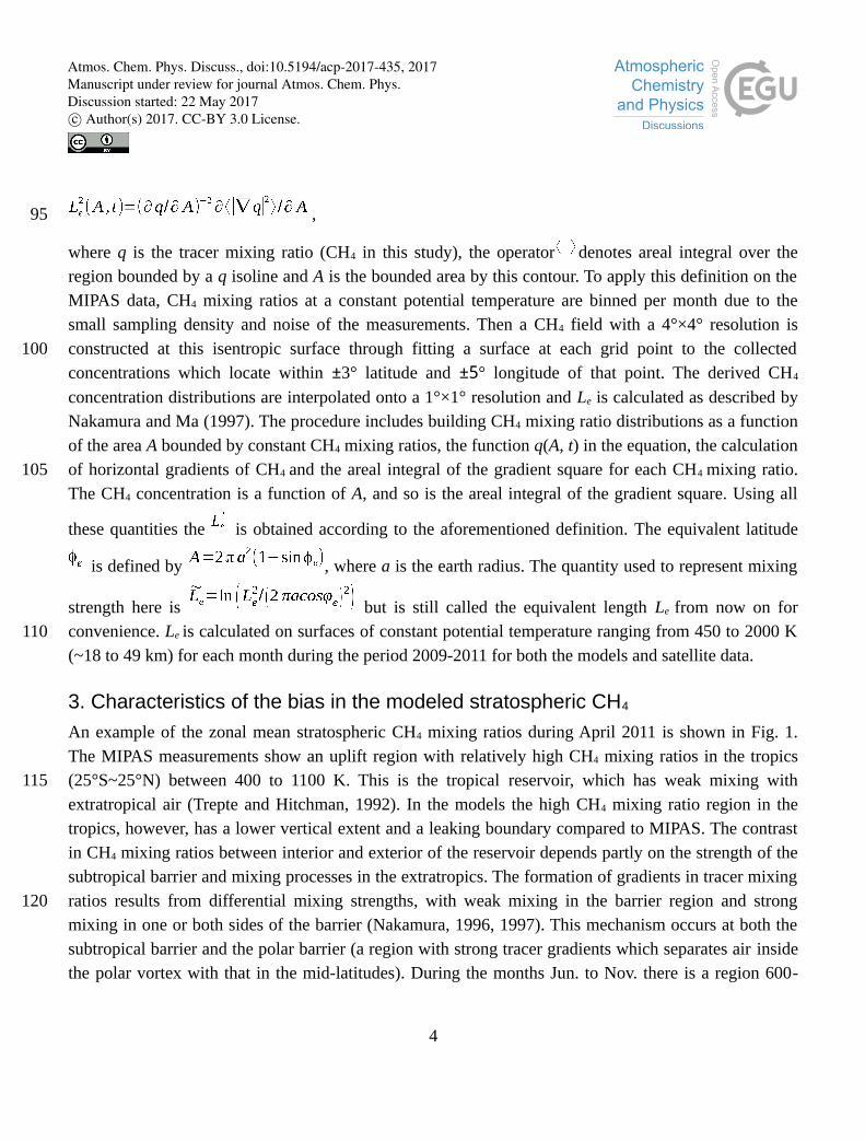
where q is the tracer mixing ratio (CH4 in this study), the operator denotes areal integral over theregion bounded by a q isoline and A is the bounded area by this contour. To apply this definition on theMIPAS data, CH4 mixing ratios at a constant potential temperature are binned per month due to thesmall sampling density and noise of the measurements. Then a CH4 field with a 4°×4° resolution isconstructed at this isentropic surface through fitting a surface at each grid point to the collectedconcentrations which locate within ±3° latitude and ±5° longitude of that point. The derived CH4

concentration distributions are interpolated onto a 1°×1° resolution and Le is calculated as described byNakamura and Ma (1997). The procedure includes building CH4 mixing ratio distributions as a functionof the area A bounded by constant CH4 mixing ratios, the function q(A, t) in the equation, the calculationof horizontal gradients of CH4 and the areal integral of the gradient square for each CH4 mixing ratio.The CH4 concentration is a function of A, and so is the areal integral of the gradient square. Using all

these quantities the is obtained according to the aforementioned definition. The equivalent latitude

is defined by , where a is the earth radius. The quantity used to represent mixing

strength here is but is still called the equivalent length Le from now on forconvenience. Le is calculated on surfaces of constant potential temperature ranging from 450 to 2000 K(~18 to 49 km) for each month during the period 2009-2011 for both the models and satellite data.

3. Characteristics of the bias in the modeled stratospheric CH4

An example of the zonal mean stratospheric CH4 mixing ratios during April 2011 is shown in Fig. 1.The MIPAS measurements show an uplift region with relatively high CH4 mixing ratios in the tropics(25°S~25°N) between 400 to 1100 K. This is the tropical reservoir, which has weak mixing withextratropical air (Trepte and Hitchman, 1992). In the models the high CH4 mixing ratio region in thetropics, however, has a lower vertical extent and a leaking boundary compared to MIPAS. The contrastin CH4 mixing ratios between interior and exterior of the reservoir depends partly on the strength of thesubtropical barrier and mixing processes in the extratropics. The formation of gradients in tracer mixingratios results from differential mixing strengths, with weak mixing in the barrier region and strongmixing in one or both sides of the barrier (Nakamura, 1996, 1997). This mechanism occurs at both thesubtropical barrier and the polar barrier (a region with strong tracer gradients which separates air insidethe polar vortex with that in the mid-latitudes). During the months Jun. to Nov. there is a region 600-

4

95

100

105

110

115

120


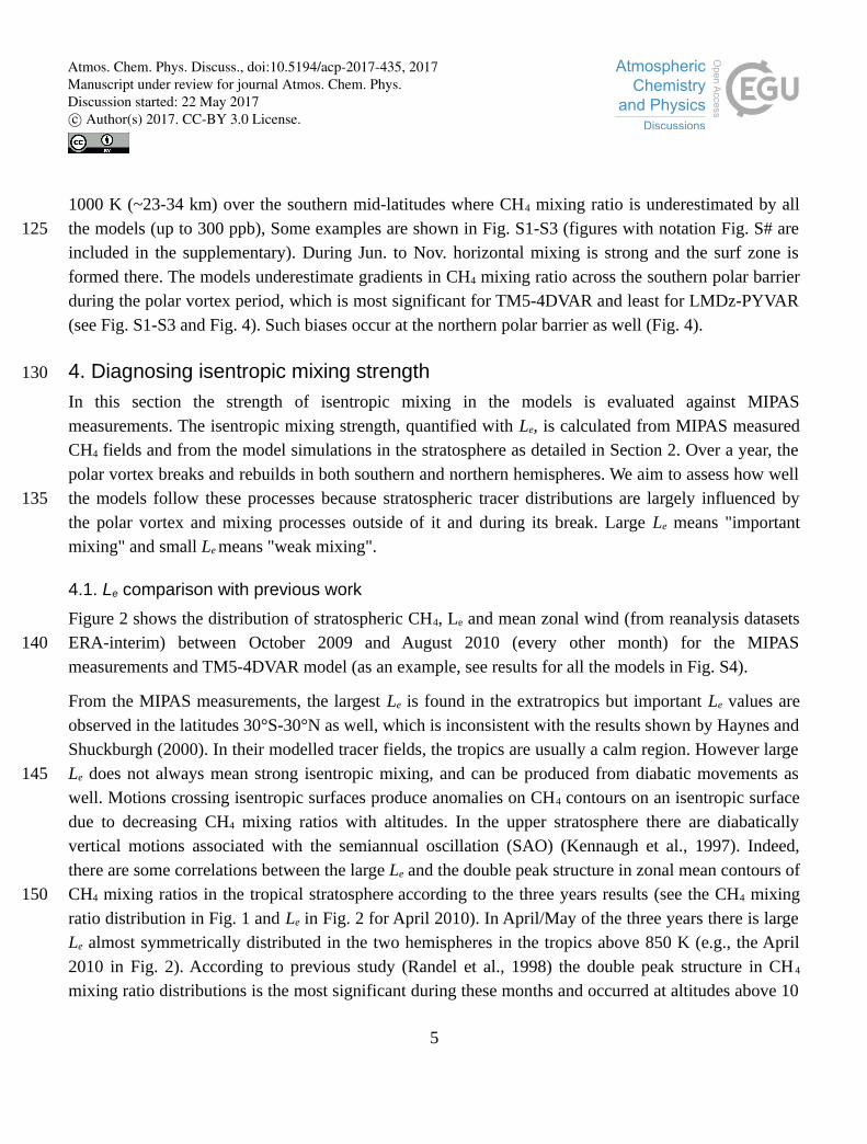
1000 K (~23-34 km) over the southern mid-latitudes where CH4 mixing ratio is underestimated by allthe models (up to 300 ppb), Some examples are shown in Fig. S1-S3 (figures with notation Fig. S# areincluded in the supplementary). During Jun. to Nov. horizontal mixing is strong and the surf zone isformed there. The models underestimate gradients in CH4 mixing ratio across the southern polar barrierduring the polar vortex period, which is most significant for TM5-4DVAR and least for LMDz-PYVAR(see Fig. S1-S3 and Fig. 4). Such biases occur at the northern polar barrier as well (Fig. 4).

4. Diagnosing isentropic mixing strength

In this section the strength of isentropic mixing in the models is evaluated against MIPASmeasurements. The isentropic mixing strength, quantified with Le, is calculated from MIPAS measuredCH4 fields and from the model simulations in the stratosphere as detailed in Section 2. Over a year, thepolar vortex breaks and rebuilds in both southern and northern hemispheres. We aim to assess how wellthe models follow these processes because stratospheric tracer distributions are largely influenced bythe polar vortex and mixing processes outside of it and during its break. Large Le means "importantmixing" and small Le means "weak mixing".

4.1. Le comparison with previous work

Figure 2 shows the distribution of stratospheric CH4, Le and mean zonal wind (from reanalysis datasetsERA-interim) between October 2009 and August 2010 (every other month) for the MIPASmeasurements and TM5-4DVAR model (as an example, see results for all the models in Fig. S4).

From the MIPAS measurements, the largest Le is found in the extratropics but important Le values areobserved in the latitudes 30°S-30°N as well, which is inconsistent with the results shown by Haynes andShuckburgh (2000). In their modelled tracer fields, the tropics are usually a calm region. However largeLe does not always mean strong isentropic mixing, and can be produced from diabatic movements aswell. Motions crossing isentropic surfaces produce anomalies on CH4 contours on an isentropic surfacedue to decreasing CH4 mixing ratios with altitudes. In the upper stratosphere there are diabaticallyvertical motions associated with the semiannual oscillation (SAO) (Kennaugh et al., 1997). Indeed,there are some correlations between the large Le and the double peak structure in zonal mean contours ofCH4 mixing ratios in the tropical stratosphere according to the three years results (see the CH4 mixingratio distribution in Fig. 1 and Le in Fig. 2 for April 2010). In April/May of the three years there is largeLe almost symmetrically distributed in the two hemispheres in the tropics above 850 K (e.g., the April2010 in Fig. 2). According to previous study (Randel et al., 1998) the double peak structure in CH 4

mixing ratio distributions is the most significant during these months and occurred at altitudes above 10

5

125

130

135

140

145

150


hpa (~30 km and 850 K). Except for the diabatic motions, isentropic mixing is possible in the tropicalstratosphere. The vertical motions in SAO result from zonal forces due to wave breaking events.Another example is the 2-day wave (Rojas and Norton, 2007), which peaks in the mesosphere and canpropagate downward to 40 km (~1350 K) and has the maximum meridional perturbation at the equator.Another difference with the results of Haynes and Shuckburgh (2000) is the high Le poleward of70°S/N. In their simulation, mixing in both regions is really weak. According to Chen et al. (1994b)strong stirring could exist inside the polar vortex but the strongest stirring locates in the surf zone.

4.2. Annual cycle in Le between Oct. 2009 and Aug. 2010

As revealed by MIPAS data in Fig. 2, in Oct. 2009 the southern polar vortex is strong and largemeridional CH4 gradients occur around 60°S, but starts to break at levels around 1250 K (~38 km) sinceisolines of CH4 mixing ratios bend toward the pole there. The surf zone, which is formed by wavebreaking of planetary waves propagating upward from the troposphere, is found approximately inlatitudes 60°S-30°S. The planetary wave breaking results into isentropic mixing of tracers, and then ameridional uniform distribution of the tracers. The measured large Le and uniform CH4 mixing ratioswith respect to latitudes in the surf zone is consistent with our knowledge. However, between 450-850K (about 18-30 km) the CH4 mixing ratio in the surf zone is also almost uniform in the verticaldirection. Actually this uniform region occurs earlier than Oct. (in August) and lasts until spring 2010 asshown in Fig. 3. There should be vertical mixing in that region since CH4 mixing ratios generallydecrease with altitudes in the stratosphere. Some gravity-type waves could be the source of the verticaldisturbances instead of planetary waves. In Oct. 2009, the polar barrier appears in the southernhemisphere with small Le between the polar vortex and the surf zone. At about 45°N the northern surfzone starts to develop in this month as indicated by a horizontally narrow and vertically long zone, withslightly larger Le than its surroundings, mostly visible in levels 650-1850K.

Considering model performances, the polar vortex and surf zone are more or less represented in thesouthern hemisphere. The models give a weaker than measured mixing in the surf zone and CH4 mixingratios decrease across the polar barrier is better represented by LMDz-PYVAR (Fig. S4) compared tothe other two models. The region with both horizontally and vertically well-mixed CH4 (within 450-850K and 60°S-30°S) is completely absent in the models (Fig. 2, 3 and S4) during the surf zone period. Thelarger vertical gradients in CH4 mixing ratios in the models compared to the observation are moreclearly shown in Fig. 3 (representing the southern mid latitudes). This absence of the vertically uniformregion is visible as a negative region of the model to the measurements differences during the JJA andSON period (see Fig. S1-S3). The tropical region with large Le is the best represented by TM5-4DVAR

6

155

160

165

170

175

180

185


and LMDz-PYVAR, which capture the double peak structure of CH4 mixing ratio distributions to thelargest extent (not shown).

In December 2009 the southern polar vortex is already broken, and the zonal wind changes to easterlies(Fig. 2). Strong mixing occurs in the whole extratropics, and the polar barrier with small Le disappears.This is consistent with the strengthening of planetary wave breaking during polar vortex breakingbecause of the development of weak zonal winds (Holton, 2004, p. 424-429). However, southern CH 4 isstill not well mixed horizontally at this time below 900 K (~31 km). In the northern hemisphere thepolar vortex, polar barrier and surf zone are well defined in December. The surf zone seems to split intotwo regions above 850 K (~30 km) with smaller Le in the region between them, or is extending towardthe tropics. Similar but less significant compared to the southern hemisphere, a region (about 20°N-60°N and 450-850 K) with small gradients in both vertical and horizontal directions occurs. In themodels southern CH4 is unrealistically uniform in the horizontal direction southward of 30°S, but thenorthern surf zone is represented well. Again TM3 and LMDz-PYVAR better capture the CH4

concentration decrease across the northern polar barrier compared to TM5-4DVAR (see Fig. S4 and Fig.4).

The northern polar vortex breaks above 1050 K (~35 km) in Feb. 2010 and strong stirring occurs as inthe southern hemisphere in December 2009 (Fig. 2). However, the northern polar vortex is reestablishedin April but now less potent (the polar barrier is now located northward of 75°N) and without the polarwesterly jet. During this period only weak easterlies (with a maximum of 10 m/s in February and belowin April) occur northward of 60°N. The surf zone become wider (30°N~70°N) and shows strongerisentropic mixing in April than in February (about 35°N~45°N). The stronger mixing is consistent withweakened westerlies that are suitable for quasi-stationary planetary wave propagation and breaking. Inthe southern hemisphere the situation in February is similar to that in December. But the large Le couldresult from remnants from the southern polar vortex breaking (Hess, 1991) instead of strong stirringsince stationary planetary wave can not propagate in easterlies.

The model simulations show CH4 and Le patterns similar to measurements in February and April of2010. The Le southward of 60°S is underestimated in the models in February. That could reflect a toofast dissipation of polar vortex remnants. The reappearance of the northern polar vortex in April 2010 isrepresented by TM3 and LMDz-PYVAR but the contrast in simulated CH4 concentration betweenoutside and inside is too weak. A narrow and weak mixing region in the two models replaces the wideand strong stirring surf zone. TM5-4DVAR modelled CH4 is completely uniform in the horizontaldirection northward of ~60°N.

7

190

195

200

205

210

215


In June 2010 the polar vortex has disappeared in the northern hemisphere with a strongly stirred regionnorthward of 50°N and easterlies established. In the southern hemisphere the polar vortex and surf zonestart to build. The developing isentropic stirring in the mid-latitudes mixed with the deceasing tropicallarge Le region at that time. The more complete developing process of the surf zone can be seen fromFig. 3. Propagation of the planetary waves starts around 40°S at 450 K level and tilts along isolines ofzonal wind, consistent with the theory that the quasi-stationary planetary wave propagates in westerliesis no stronger than a threshold (Holton, 2004, p. 424). That is reflected in the LMDz-PYVAR well, butwith significant underestimated amplitudes in the other two models.

In August 2010 the polar vortex and surf zone are matured in the southern hemisphere. The modelsroughly capture the meridional distribution of southern CH4. The deficiencies of the models are tooweak isentropic mixing in the surf zone. Large departures in Le occur at the level around 1050 K andbelow 700 K (~26 km) in the mid-latitudes.

4.3. Evolution of CH4 concentration and Le on isentropic surfaces in the southern mid-latitudes

Figure 3 gives the evolution of Le and CH4 mixing ratios in the southern mid-latitudes (35°S-55°S) fromthe MIPAS measurements and the three models. As said before, the models underestimate mixingstrength in the surf zone. But this underestimation differs from year to year, e.g. the models performbetter in 2009 and 2011 than 2010. In the measurement, the surf zone starts in May at 450 K level andhereafter extends upward into the mid- and upper- stratosphere. In the models, the surf zone occurs latercompared to the measurement. The large Le regions (about 450-850 K initially and the vertical extentdecreases with time) extend into next spring in the measurement in contrast to a sudden disappearancein the models after the end of each year. As explained in Sect. 4.2, the large Le could come fromremnants of strong disturbances during polar vortex breaking since easterlies of zonal wind haveestablished in that time. There is a strong mixing region moving downward from the upper stratosphereand finally mixing into the developing surf zone, which is shown in the measurement only. That couldbe associated with the SAO mentioned in Sect. 4.2.

The distribution of CH4 concentrations and the meridional gradients, and Le at 600 K (~24 km) as afunction of latitudes in the period 2009-2011 is given in Fig. 4 to further reveal the model deficienciesin representing the surf zone development and the polar vortex breaking. The surf zone (the mid-latitudes beside the band with strong meridional gradients of CH4 concentrations) mixing is weaker inall the models compared to the observation. In 2010 and 2011, the biases in the modeled mixingstrength in the surf zone are more important than during 2009 in latitudes between about 30°-60°, whenpolar vortexes are well defined in CH4 distributions. Consequently, the region with small meridional

8

220

225

230

235

240

245

250


gradients (<5 ppb/degree) in CH4 mixing ratios has smaller latitudinal and temporal coverage in 2010and 2011. The polar barrier (band with large meridional gradients in CH4 concentrations around 60°) isstronger in the measurements compared to the models, particularly for TM5-4DVAR. Although low CH4

concentrations in the polar vortex result from sink down motion, the tight boundary could have anattribution to mixing processes both inside and outside of the polar vortex. The stronger the mixing atboth sides of a transport barrier is, the tighter the barrier appears in a tracer distribution. The role ofmixing in the barrier formation can be seen in the subtropical barrier (the ~30° latitudes with localmaximum meridional gradients in CH4 mixing ratios), which is meridionally narrower in themeasurements than in the models. The mixing inside the southern polar vortex has similar/largerstrength in the models but covers a smaller latitudinal range as compared to the observation. Strongmeridional shear of zonal wind could be a source of the disturbances inside the polar vortex. It is notclear whether other sources contribute as well.

5. Discussions and conclusions

The region with both vertical and meridional uniform CH4 distributions in southern mid-latitudes islocated just above the subtropical jet at the tropopause. The jet exit region is recognized as a favoredlocation for large-amplitude, subsynoptic gravity waves (Plougonven and Zhang, 2013). Such a jetsystem occurs in the northern hemisphere in winter as well, but there is no, or insignificant, region withuniform CH4 mixing ratios above the jet. The main sources of gravity waves include orography,convection, and jet/front system. The strength of these sources is larger or the same in the northernhemisphere compared to the southern hemisphere. It is not clear what factors contribute to thedifference in CH4 distributions above the winter jet between the two hemispheres. The horizontal scalesof the gravity waves typically range from 10 to 1000 km. The horizontal resolutions of 2°-6° of themodels, which represent waves with wavelength longer than ~600 km only, is not fine enough to resolvegravity waves completely.

Isentropic mixing in the surf zone is too weak in the models compared to the observation. Reasonscould be an underestimation of the planetary wave strength or deficiencies in describing the dissipationprocesses of the wave. In the southern hemisphere convection is an important source for the planetarywave, but orography plays a role in the northern hemisphere as well. Filament structures occur inbreaking processes of planetary waves, the smaller Le in the models than in the observations indicate thefine-scale structure is smeared out partly. The ability of models to preserve fine-scale structure dependson both the resolution and transport scheme. For example the finite-volume scheme (Van Leer, 1977) asapplied in LMDz is originally designed for resolving sharp gradients and discontinuities and is expected

9

255

260

265

270

275

280


to describe the filament structures better than the slope scheme (Russel and Lerner, 1981) used in TM3.Sensitivity tests, such as changing horizontal resolutions, using different advection algorithms andconvection parameterization schemes could be helpful to clarify the dominant factor leading to modelbiases in the surf zone.

The polar barrier is not as tight in the models as in the observation. That could be due to the inability ofthe models to simulate mixing processes both inside and outside of the polar vortex. The contrasts inCH4 mixing ratios inside and outside of the polar vortex are better preserved by LMDz-PYVAR. Thereason could be that LMDz uses a sharp-gradient-preserved transport scheme and a finer resolution. Thelooser barrier could be a reason for faster dissipation of the polar vortex in the model. The polar vortexis frequently forced away from the pole and sometimes to lower latitudes during the dissipation period.Unrecognized remains of the polar vortex in the model could cause problems when assimilating totalcolumn measurements.

Code availability

The model outputs of TM3, TM5-4DVAR and LMDz-PYVAR are provided by other institutes. Thecorresponding PIs (see Data availability section) should be contacted for the availability of the modelcodes.

Data availability

The model outputs are from Marille Saunois (Laboratoire des Sciences du Climat et del'Environnement, France) for LMDz-PYVAR, Ute Karstens (the Max Plank Institute forBiogeochemistry, Jena, Germany) for TM3, and Peter Bergamaschi (European Commission JointResearch Centre) for TM5-4DVAR. One should contact these authors directly considering theavailability the model output. The MIPAS data is operational V6 data processed by ESA, which ispublicly available.

Acknowledgements

We thank Ute Karstens at the Max Plank Institute for Biogeochemistry, Jena, Germany for providingTM3 model data and Peter Bergamaschi at European Commission Joint Research Centre for providingTM5-4DVAR data.

10

285

290

295

300

305


References

Bernath, P. F., McElroy, C. T., Abrams, M. C., et al.: Atmospheric Chemistry Experiment (ACE):Mission overview, Geophys. Res. Lett., 32, L15S01, 2005.

Chen, P., Holton, J. R., O'neill, A. and Swinbank, R.: Isentropic Mass Exchange between the Tropicsand Extratropics in the Stratosphere, J. Atmos. Sci., 51(20), 3006–3018, 1994a.

Chen, P., Holton, J. R., O'neill, A. and Swinbank, R.: Quasi-horizontal transport and mixing in theAntarctic stratosphere, J. Geophys. Res., 99(D8), 16851, doi:10.1029/94jd00784, 1994b.

Chen, P.: The permeability of the Antarctic vortex edge, J. Geophys. Res., 99(D10), 20563,doi:10.1029/94jd01754, 1994c.

Crevoisier, C., Nobileau, D., Armante, R., Crépeau, L., Machida, T., Sawa, Y., Matsueda, H., Schuck, T.,Thonat, T., Pernin, J., Scott, N. A., and Chédin, A.: The 2007–2011 evolution of tropical methane in themid-troposphere as seen from space by MetOp-A/IASI, Atmos. Chem. Phys., 13, 4279-4289,doi:10.5194/acp-13-4279-2013, 2013.

Chevallier, F., Fisher, P., Serrar, S., Bousquet, P., Breon, F.-M., Chedin, A., and Ciais, P.: Inferring CO 2

sources and sinks from satellite observations: Method and application to TOVS data, J. Geophys. Res.,110, D24309, doi:10.1029/2005JD, 2005.

Fischer, H., Birk, M., Blom, C., Carli, B., Carlotti, M., von Clarmann, T., Delbouille, L., Dudhia, A.,Ehhalt, D., Endemann, M., Flaud, J. M., Gessner, R., Kleinert, A., Koopman, R., Langen, J., López-Puertas, M., Mosner, P., Nett, H., Oelhaf, H., Perron, G., Remedios, J., Ridolfi, M., Stiller, G., andZander, R.: MIPAS: an instrument for atmospheric and climate research, Atmos. Chem. Phys., 8, 2151-2188, doi:10.5194/acp-8-2151-2008, 2008.

Hoppe, C. M., Hoffmann, L., Konopka, P., Grooß, J.-U., Ploeger, F., Günther, G., Jöckel, P. and Müller,R.: The implementation of the CLaMS Lagrangian transport core into the chemistry climate modelEMAC 2.40.1: application on age of air and transport of long-lived trace species, Geosci. Model Dev.,7(6), 2639–2651, doi:10.5194/gmd-7-2639-2014, 2014.

Heimann, M., and S. Körner, The Global Atmospheric Tracer Model TM3: Model description and usersmanual release 3.8a, Tech. Rep. 5, Max Planck Inst. for Biogeochem., Jena, Germany, 2003.

Hourdin, F., Musat, I., Bony, S., Braconnot, P., Codron, F., Dufresne, J. L., Fairhead, L., Filiberti, M. A.,Friedlingstein, P., Grandpeix, J. Y., Krinner, G., Li, Z. X., and Lott, F.: The LMDz4 general circulation

11

310

315

320

325

330

335


model: climate performance and sensitivity to parametrized physics with emphasis on tropicalconvection, Climate Dynamics, 27, 787-813, 2006.

Haynes, P. and Shuckburgh, E.: Effective diffusivity as a diagnostic of atmospheric transport: 1.Stratosphere, J. Geophys. Res., 105(D18), 22777–22794, doi:10.1029/2000jd900093, 2000.

Hess, P. G.: Mixing Processes Following the Final Stratospheric Warming, J. Atmos. Sci., 48(14), 1625–1641, 1991.

Holton, J. R.: An Introduction to Dynamic Meteorology, fourth edition, International Geophysics Series,Elsevier Academic Press, 88, 2004.

Kalicinsky, C., Grooß, J.-U., Günther, G., Ungermann, J., Blank, J., Höfer, S., Hoffmann, L., Knieling,P., Olschewski, F., Spang, R., Stroh, F., and Riese, M.: Observations of filamentary structures near thevortex edge in the Arctic winter lower stratosphere, Atmos. Chem. Phys., 13, 10859-10871,doi:10.5194/acp-13-10859-2013, 2013.

Khosrawi, F., Grooß, J.-U., Müller, R., Konopka, P., Kouker, W., Ruhnke, R., Reddmann, T. and Riese,M.: Intercomparison between Lagrangian and Eulerian simulations of the development of mid-latitudestreamers as observed by CRISTA, Atmos. Chem. Phys., 5(1), 85–95, doi:10.5194/acp-5-85-2005,2005.

Konopka, P., Günther, G., Müller, R., dos Santos, F. H. S., Schiller, C., Ravegnani, F., Ulanovsky, A.,Schlager, H., Volk, C. M., Viciani, S., Pan, L. L., McKenna, D.-S., and Riese, M.: Contribution ofmixing to upward transport across the tropical tropopause layer (TTL), Atmos. Chem. Phys., 7, 3285-3308, doi:10.5194/acp-7-3285-2007, 2007.

Krol, M., Houweling, S., Bregman, B., van den Broek, M., Segers, A., van Velthoven, P., Peters, W.,Dentener, F., and Bergamaschi, P.: The two-way nested global chemistry-transport zoom model TM5:algorithm and applications, Atmos. Chem. Phys., 5, 417-432, doi:10.5194/acp-5-417-2005, 2005.

Kennaugh, R., Ruth, S. and Gray, L. J.: Modeling quasi-biennial variability in the semiannual doublepeak, J. Geophys. Res., 102(D13), 16169–16187, doi:10.1029/97jd00867, 1997.

Mcintyre, M. E. and Palmer, T. N.: Breaking planetary waves in the stratosphere, Nature, 305(5935),593–600, doi:10.1038/305593a0, 1983.

Meirink, J. F., Bergamaschi, P., and Krol, M. C.: Four-dimensional variational data assimilation forinverse modelling of atmospheric methane emissions: method and comparison with synthesis inversion,

12

340

345

350

355

360

365


Atmos. Chem. Phys., 8, 6341-6353, doi:10.5194/acp-8-6341-2008, 2008.

Neu, J. L.: Variability of the subtropical “edges” in the stratosphere, J. Geophys. Res., 108(D15),doi:10.1029/2002jd002706, 2003.

Nakamura, N.: Two-Dimensional Mixing, Edge Formation, and Permeability Diagnosed in an AreaCoordinate, J. Atmos. Sci., 53(11), 1524–1537, 1996.

Nakamura, N. and Ma, J.: Modified Lagrangian-mean diagnostics of the stratospheric polar vortices: 2.Nitrous oxide and seasonal barrier migration in the cryogenic limb array etalon spectrometer andSKYHI general circulation model, Journal of Geophysical Research: Atmospheres J. Geophys. Res.,102(D22), 25721–25735, 1997.

Pison, I., Bousquet, P., Chevallier, F., Szopa, S., and Hauglustaine, D.: Multi-species inversion of CH4,CO and H2 emissions from surface measurements, Atmos. Chem. Phys., 9, 5281-5297, doi:10.5194/acp-9-5281-2009, 2009.

Pison, I., Ringeval, B., Bousquet, P., Prigent, C. and Papa, F.: Stable atmospheric methane in the 2000s:key-role of emissions from natural wetlands, Atmos. Chem. Phys., 13(23), 11609–11623,doi:10.5194/acp-13-11609-2013, 2013.

Payne, V. H., Clough, S. A., Shephard, M. W., Nassar, R., and Logan, J. A.: Information-centeredrepresentation of retrievals with limited degrees of freedom for signal: Application to methane from theTropospheric Emission Spectrometer, J. Geophys. Res., 114, D10307, doi:10.1029/2008JD010155,2009.

Ploeger, F., Günther, G., Konopka, P., Fueglistaler, S., Müller, R., Hoppe, C., Kunz, A., Spang, R.,Grooß, J.-U. and Riese, M.: Horizontal water vapor transport in the lower stratosphere from subtropicsto high latitudes during boreal summer, J. Geophys. Res., 118(14), 8111–8127, doi:10.1002/jgrd.50636,2013.

Plougonven, R. and Zhang, F.: Internal gravity waves from atmospheric jets and fronts, Rev. Geophys.,52(1), 33–76, doi:10.1002/2012rg000419, 2014.

Randel, W. J., Gille, J. C., Roche, A. E., Kumer, J. B., Mergenthaler, J. L., Waters, J. W., Fishbein, E. F.and Lahoz, W. A.: Stratospheric transport from the tropics to middle latitudes by planetary-wavemixing, Nature, 365(6446), 533–535, doi:10.1038/365533a0, 1993.

Rödenbeck, C., Estimating CO2 sources and sinks from atmospheric mixing ratio measurements using a

13

370

375

380

385

390

395


global inversion of atmospheric transport, Technical Report 6, Max Planck Institute forBiogeochemistry, Jena, Germany, 2005.

Rojas, M. and Norton, W.: Amplification of the 2-day wave from mutual interaction of global Rossby-gravity and local modes in the summer mesosphere, J. Geophys. Res., 112(D12),doi:10.1029/2006jd008084, 2007.

Randel, W. J., Wu, F., Russell, J. M., Roche, A. and Waters, J. W.: Seasonal Cycles and QBO Variationsin Stratospheric CH4 and H2O Observed in UARS HALOE Data, J. Atmos. Sci., 55(2), 163–185, 1998.

Russell, G. L. and Lerner, J. A.: A New Finite-Differencing Scheme for the Tracer Transport Equation,J. Appl. Meteor., 20(12), 1483–1498, 1981.

Steinhorst, H.-M., Konopka, P., Günther, G. and Müller, R.: How permeable is the edge of the Arcticvortex: Model studies of winter 1999-2000, J. Geophys. Res., 110(D6), doi:10.1029/2004jd005268,2005.

Stenke, A., Dameris, M., Grewe, V. and Garny, H.: Implications of Lagrangian transport for simulationswith a coupled chemistry-climate model, Atmos. Chem. Phys., 9(15), 5489–5504, doi:10.5194/acp-9-5489-2009, 2009.

Trepte, C. R. and Hitchman, M. H.: Tropical stratospheric circulation deduced from satellite aerosoldata, Nature, 355(6361), 626–628, 1992.

Leer, B. V.: Towards the ultimate conservative difference scheme. Part IV: A new approach to numericalconvection, Journal of Computational Physics, 23(3), 276–299, 1977.

Xiong, X., Barnet, C., Maddy, E. S., Gambacorta, A., King, T. S., and Wofsy, S. C.: Mid-uppertropospheric methane retrieval from IASI and its validation, Atmos. Meas. Tech., 6, 2255-2265,doi:10.5194/amt-6-2255-2013, 2013.

Worden, J. R., Turner, A. J., Bloom, A., Kulawik, S. S., Liu, J., Lee, M., Weidner, R., Bowman, K.,Frankenberg, C., Parker, R., and Payne, V. H.: Quantifying lower tropospheric methane concentrationsusing GOSAT near-IR and TES thermal IR measurements, Atmos. Meas. Tech., 8, 3433-3445,doi:10.5194/amt-8-3433-2015, 2015.

Wang, Z.: Remote sensing of tropospheric methane and isotopes of atmospheric carbon dioxide usingFourier Transform Spectrometry, http://elib.suub.uni-bremen.de/edocs/00105597-1.pdf, 2016

14

400

405

410

415

420


Figures

Figure 1. Zonal median CH4 mixing ratios as a function of latitudes and potential temperature in Aprilof 2010 for (from top to bottom) MIPAS, TM3, TM5-4DVAR and LMDz-PYVAR.

15

425

430


16

435


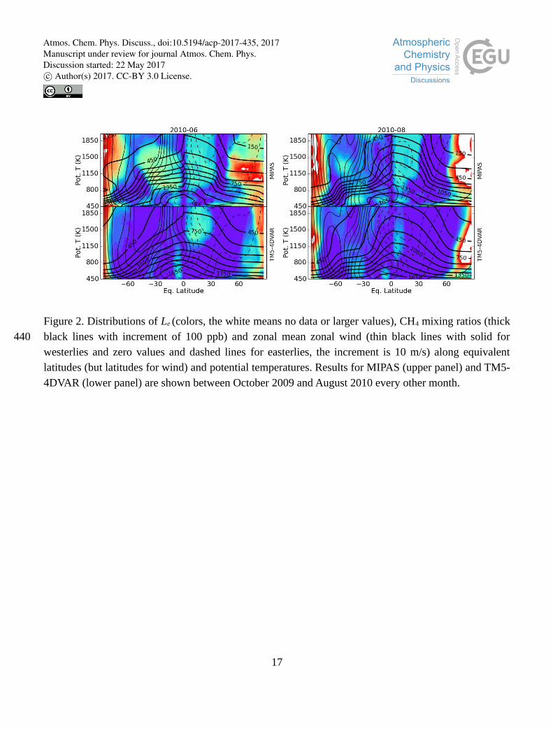
Figure 2. Distributions of Le (colors, the white means no data or larger values), CH4 mixing ratios (thickblack lines with increment of 100 ppb) and zonal mean zonal wind (thin black lines with solid forwesterlies and zero values and dashed lines for easterlies, the increment is 10 m/s) along equivalentlatitudes (but latitudes for wind) and potential temperatures. Results for MIPAS (upper panel) and TM5-4DVAR (lower panel) are shown between October 2009 and August 2010 every other month.

17

440


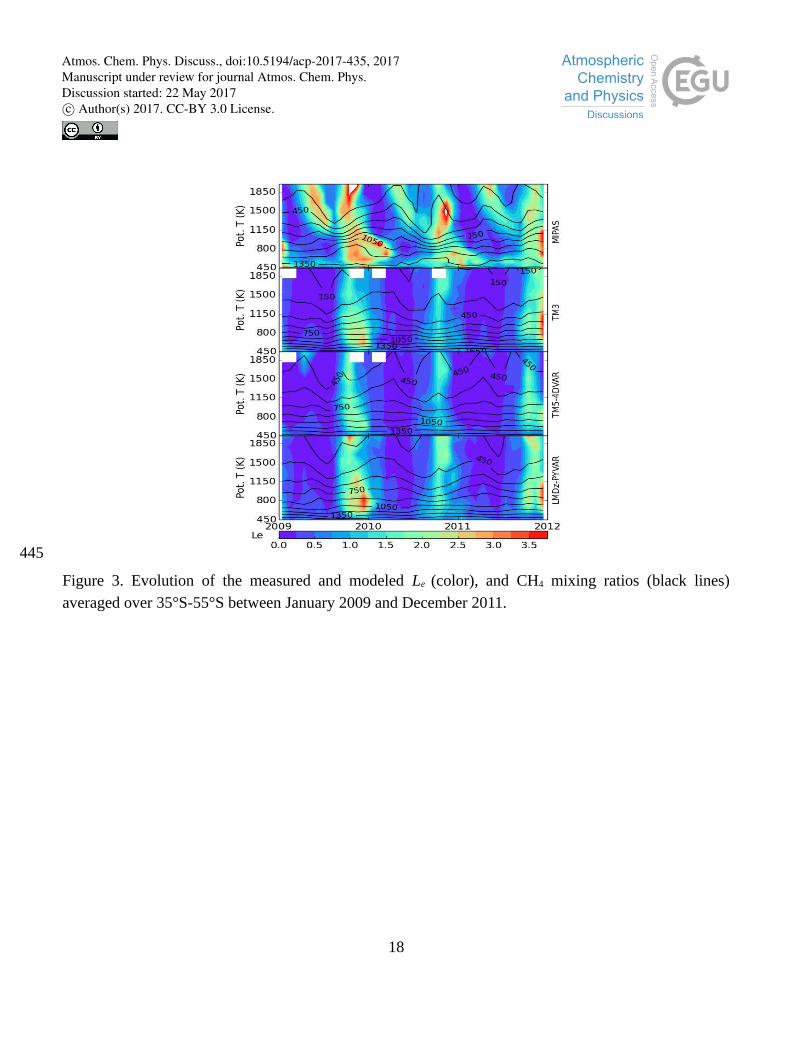
Figure 3. Evolution of the measured and modeled Le (color), and CH4 mixing ratios (black lines)averaged over 35°S-55°S between January 2009 and December 2011.

18

445


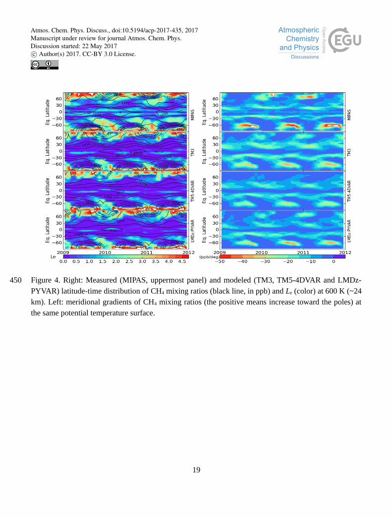
Figure 4. Right: Measured (MIPAS, uppermost panel) and modeled (TM3, TM5-4DVAR and LMDz-PYVAR) latitude-time distribution of CH4 mixing ratios (black line, in ppb) and Le (color) at 600 K (~24km). Left: meridional gradients of CH4 mixing ratios (the positive means increase toward the poles) atthe same potential temperature surface.

19

450


Diagnosing CH4 models using the equivalent length in the ...

Documents

Transcript of Diagnosing CH4 models using the equivalent length in the ...