Constraining Anthropogenic CH4 Emissions in Nanjing and ...

ADVANCES IN ATMOSPHERIC SCIENCES, VOL. 31, NOVEMBER 2014, 1343–1352

Constraining Anthropogenic CH4 Emissions in Nanjing and the Yangtze River

Delta, China, Using Atmospheric CO2 and CH4 Mixing Ratios

SHEN Shuanghe1,2, YANG Dong3, XIAO Wei∗1,2, LIU Shoudong1, and Xuhui LEE1,4

1Yale-NUIST Center on Atmospheric Environment & Collaborative Innovation Center on Forecast and Evaluation of Meteorological

Disasters, Nanjing University of Information Science & Technology, Nanjing 2100442Jiangsu Key Laboratory of Agricultural Meteorology, Nanjing University of Information Science & Technology, Nanjing 210044

3Ningbo Meteorological Observatory, Ningbo 3150124School of Forestry and Environmental Studies, Yale University, New Haven, CT 06511, USA

(Received 27 November 2013; revised 2 March 2014; accepted 3 April 2014)

ABSTRACT

Methane (CH4) emissions estimated with the Intergovernmental Panel on Climate Change (IPCC) inventory method atthe city and regional scale are subject to large uncertainties. In this study, we determined the CH4:CO2 emissions ratio forboth Nanjing and the Yangtze River Delta (YRD), using the atmospheric CH4 and CO2 concentrations measured at a suburbansite in Nanjing in the winter. The atmospheric estimate of the CH4:CO2 emissions ratio was in reasonable agreement withthat calculated using the IPCC method for the YRD (within 20%), but was 200% greater for the municipality of Nanjing. Themost likely reason for the discrepancy is that emissions from unmanaged landfills are omitted from the official statistics ongarbage production.

Key words: methane, IPCC inventory, atmospheric mixing ratio, city, region

Citation: Shen, S. H., D. Yang, W. Xiao, S. D. Liu, and X. H. Lee, 2014: Constraining anthropogenic CH4 emissions inNanjing and the Yangtze River Delta, China, using atmospheric CO2 and CH4 mixing ratios. Adv. Atmos. Sci., 31(6),1343–1352, doi: 10.1007/s00376-014-3231-3.

1. Introduction

Cities are greenhouse gas (GHG) emission hotspots, andare responsible for 70%–80% of global anthropogenic GHGemissions (e.g., O’Meara and Peterson, 1999; Koerner andKlopatek, 2002; Satterthwaite, 2008; Canadell et al., 2009).In many countries, strategies for controlling GHG emissionsare shifting from the national level to the city scale. In orderto verify the effectiveness of these strategies, GHG invento-ries have been established in New York, Tokyo, and London(e.g., Baldasano et al., 1999; Mayor of London, 2007; VandeWeghe and Kennedy, 2007; City of New York, 2012). InChina, cities play a disproportionately large part in the na-tional GHG emission totals: in 2006 they accounted for 75%of the national economy but 84% of the GHG emissions(e.g., Dhakal, 2009). In China’s 12th five-year plan, reducingGHG emissions has become an important goal of sustainabledevelopment (e.g., Geng, 2011). Even though GHG invento-ries are useful indicators of low-carbon city development, weare only aware of a few published studies on emissions in-ventories for municipalities in China (e.g., Geng et al., 2011;

∗ Corresponding author: XIAO WeiE-mail: [email protected]

Liu et al., 2012).In China, CH4 emissions account for 11% to 13% of the

total global warming potential associated with anthropogenicactivities (e.g., Chen and Zhang, 2010; Leggett et al., 2011).At the city scale, this proportion has a tenfold variation: from2% in Shanghai to 19.5% in Chongqing (e.g., Zhu, 2009;Yang et al., 2011, 2012; Zhao et al., 2011). The most com-mon method used to calculate the CH4 emissions inventoryis the Intergovernmental Panel on Climate Change (IPCC)method. This method was originally intended for establish-ing national estimates. At the urban or regional scale, largeuncertainties exist because in many applications local emis-sion factors are not known (e.g., Bun et al., 2010). Moreover,official energy consumption and pollution discharge statisticsoften have large uncertainties. Therefore, it is important thatIPCC-based estimates are verified against other independentmethods.

The goal of this study was to evaluate the inventory CH4emission rates, using measurements of atmospheric CH4 andCO2 concentrations for the city of Nanjing and the YangtzeRiver Delta (YRD; encompassing the provinces of Jiangsu,Zhejiang, Anhui and the city of Shanghai). The YRD isone of the most developed economic regions in China andhas one of the highest concentrations of urbanized land of

© Institute of Atmospheric Physics/Chinese Academy of Sciences, and Science Press and Springer-Verlag Berlin Heidelberg 2014

1344 CONSTRAINING CH4 EMISSIONS USING CO2 AND CH4 CONCENTRATIONS VOLUME 31

any region in the world, with a total land area of 3.5× 105

km2, and an urban fraction of 2.4%. After Shanghai, Nan-jing is the second-largest city in the YRD, with an area of6.6× 103 km2. Specifically, in this study we aimed to com-pare the CH4:CO2 emissions ratio derived from the atmo-spheric method and the emissions ratio determined with theIPCC inventory method.

The atmospheric method assumes that the correlation be-tween the concentrations of two inert and passive scalars inthe atmosphere preserves the source emission signals. Thismethod is frequently used to determine local and regionalemission rates of air pollutants (e.g., Lee et al., 2001; Widoryand Javoy, 2003; Yamada et al., 2005; Tarasova et al., 2006;Greally et al., 2007; Warneke et al., 2007). In recent years,it has been increasingly used in the investigation of GHGcycling in urban airsheds. Hsu et al. (2010) used the cor-relation between CH4 and CO to calculate the CH4 emis-sions in the airshed of Los Angles, USA. Suntharalingam etal. (2004) used the CO2:CO concentrations ratio correlationsin the Asian outflow from the TRACE-P aircraft campaignto improve the quantification of CO2 flux in eastern China.Wang et al. (2010) analyzed the observed CO2:CO concen-trations ratio at a rural site near Beijing, China, and comparedit to the bottom-up CO2:CO emissions ratio to investigate thecombustion efficiency of urban sources. The research pre-sented in this paper is one of the few studies that uses CO2 asa tracer to investigate CH4 emission rates (e.g., Conway andSteele, 1989; Wunch et al., 2009). As shown by Bakwin etal. (1997), Lee et al. (2001), Pataki et al. (2005) and others,the CO2 mixing ratio can be used as a tracer of wintertime at-mospheric transport and mixing at midlatitudes. In this study,the method was refined by dividing the observations into day-time and nighttime periods, before linking them to emissionpatterns on two different spatial scales (the YRD versus Nan-jing).

2. Methods

2.1. CO2 and CH4 observationsWe measured the mixing ratios of CO2 and CH4 con-

tinuously on the campus of Nanjing University of Informa-tion Science and Technology (NUIST; 32◦12’N, 118◦43’E)in Nanjing from June 2010 to April 2011. This is a suburbansite situated 18 km northwest of the city center, surroundedby residential housing. The prevailing wind direction in 2011was southeasterly. Except for vehicles, there were no signifi-cant CO2 or CH4 emission sources within 5 km of the site.

The CO2 and CH4 mixing ratios were measured with aninfrared gas analyzer based on wavelength-scanned cavityring-down spectroscopy (model G1301, Picarro, Inc, Sunny-vale, California). The measurement precision was better than50 ppbv for CO2 and 0.7 ppbv for CH4 (5 min average). Theanalyzer was installed on the ninth floor of an office buildingwith a total of 13 floors. Ambient air was drawn in at a heightof 25 m above the ground into the analyzer for analysis. Atthe end of the experiment, the analyzer was calibrated against

both a CO2 and a CH4 standard (mixing ratios: 390 ppm and3.05 ppm, balance gas: synthetic air), both of which had a1% uncertainty in concentration.

2.2. Inventory estimates

The International Council for Local Environmental Ini-tiatives have classified carbon accounting into three cate-gories (ICLEI, 2008): the first includes direct emissions fromsources within the geographic boundary of investigation; thesecond comprises indirect emissions associated with electric-ity, steam and heating generated outside the boundary; whilethe third category covers other lifecycle emissions excludedfrom the first and second categories. In this paper, only thedirect GHG emissions of the first category are considered.

In both Nanjing and the YRD, the direct sources of CO2include both energy consumption sectors (industry, transport,service and household) and non-energy consumption indus-trial processes. The main sources of CH4 are rice cultivation,landfill, coal mining, wastewater, livestock, and combustionof fossil fuel and biomass. The CH4 emissions from rice cul-tivation were not included in the anthropogenic CH4 emis-sions calculated using the atmospheric method, as the emis-sions in winter are negligible for Nanjing and the YRD. TheCH4 emissions from natural wetland were included. The an-thropogenic emissions of CO2 and CH4 were calculated usingthe IPCC methodology by assigning an emission factor foreach of the source categories. Energy consumption and otherdata were obtained from official sources (Energy StatisticsDivision of the National Bureau of Statistics, 2010; Agricul-tural Social and Economic Survey Office of the State Statis-tics Bureau, 2010; National Bureau of Statistics of China,2010; Nanjing Municipal Bureau of Statistics, 2010).

For the purpose of comparison with the atmosphericmethod, the total CH4 emission was divided by the total CO2emission in Nanjing and in the YRD as molar ratios. Ex-pressing the results as an emissions ratio has the advantageof canceling out some of the errors in the official statistics onenergy consumption.

We used the Monte Carlo method to investigate how er-rors in the emission factors propagated through the inventorycalculations (e.g., Reilly et al., 1987; Winiwarter and Ryp-dal, 2001; Kumar et al., 2004; Brown et al., 2012). Thismethod involved four steps (e.g., Morgan and Henrion, 1990;Bevington and Robinson, 1992). First, a uniform probabil-ity distribution was assigned to each of the emission fac-tors, which were bounded by the limits suggested by theIPCC guidelines. Second, an ensemble of emission estimateswas obtained, with combinations of the emission factor val-ues randomly generated according to the probability distri-bution. Third, a probability distribution function was deter-mined from the ensemble. Fourth, the 2.5% and 97.5% prob-ability values were used as the lower and upper bounds of theestimates of the total CH4 and CO2 emissions and their emis-sions ratio. In the following, the inventory data are reportedas the mean of the ensemble generated by the Monte Carlomethod, with the 2.5%–97.5% uncertainty range noted.

NOVEMBER 2014 SHEN ET AL. 1345

2.3. Atmospheric methodIn this study, we used CO2 as a tracer to constrain the

anthropogenic CH4 emission rate. Because CH4 and CO2have long lifetimes, they can be considered non-reactive pas-sive scalars on the spatial scale of diffusion considered inthis study. Following the method of studies conducted inKrakow, Poland (Zimnoch et al., 2010), the South Coast AirBasin in California, USA (Wunch et al., 2009), and Barrow,Alaska, USA (Conway et al., 1993), the slope of the linearcorrelation of the CH4 mixing ratio against the CO2 mix-ing ratio was taken as being equivalent to their emissions ra-tio. This method is based on the principle that atmospherictransport and diffusion do not discriminate the passive scalarsand therefore the slope of the regression line preserves theirsource information. The geometric linear regression (Ricker,1973) was adopted to derive the correlation slope between theCH4 and CO2 mixing ratios.

The source area of air concentration in the atmosphericboundary layer is variable from day to night because ofchanges in air stability. The measurements were divided intomidday [1000–1700 local standard time (LST)] and midnight(2300–0500 LST) periods. The midday measurements wereassumed to be influenced by anthropogenic emissions in theYRD, while the midnight boundary layer was assumed to besensitive to local sources in the city of Nanjing. The rationalefor this assumption will be discussed in section 3.2.

Even though the measurements were continuous, thecorrelation analysis was restricted mostly to the winter(December–February), when the biological fluxes were negli-gible compared to the anthropogenic fluxes. The main driverof seasonal variation in fuel consumption is residential heat-ing. Unlike in northern China, residents in the YRD generallydo not heat their homes in the winter. Consequently, while atthe national level fuel consumption shows slight variationsbetween the four seasons (winter 29%, spring 25%, summer22%, autumn 24%; Rotty, 1987), the CO2 emissions in Nan-jing and in the YRD region should have negligible seasonalvariations. Therefore, the emission intensity of CO2 was re-garded as a constant all year round.

3. Results and discussion

3.1. Atmospheric CH4 and CO2 mixing ratios

Nearly a year of observations at the NUIST and MaunaLoa monitoring stations were used to analyze the characteris-tics of the atmospheric CO2 and CH4 (Fig. 1). The measure-ments at Mauna Loa were regared as the atmospheric back-ground values. Comparision between the two sites allowedassessment of the impact of anthropogenic sources on the at-mospheric CO2 and CH4 mixing ratios. The annual meanCO2 and CH4 mixing ratios at NUIST were, respectively,11.5 ppm (1 ppm = 1 μmol mol−1) and 0.30 ppm higher thanthe background values. For CO2, the largest difference oc-curred in November (20.99 ppm) and the smallest differencein July (3.77 ppm). In the case of CH4, the largest differenceoccurred in July (0.46 ppm) and the smallest difference inJanuary (0.21 ppm).

The seasonal variations of CO2 and CH4 at NUIST werecontrolled by several factors. Due to the prescence of grow-ing vegetation, low CO2 mixing ratios were observed in thesummer and autumn months. In comparison, higher CO2concentrations were maintained in winter months. The max-imum monthly mean concentration was observed in Novem-ber for both CO2 and CH4, mainly due to field burning ofcrop straw at that time of the year (e.g., Su and Zhu, 2011;Su et al., 2012). Seasonal variation of CH4 concentrations iscontrolled by biological activities and chemical reactions inthe atmosphere (e.g., Robbins et al., 1973; Dlugokencky etal., 1994). Although the primary chemical sink of CH4 has amaximum concentration in the summer, biological emissionsources of CH4 increase too and in fact dominate, resultingin higher concentrations in the summer.

Numerous studies have demonstrated enhanced CO2 con-centration in urban areas. Idso et al. (1998) refer to this phe-nomenon as the urban CO2 dome. They found that the maxi-mum mean winter CO2 mixing ratio at the center of Phoenix,USA, was 619 ppm, or 67% greater than that of the ruralbackground value. George et al. (2007) found that the annualmean difference between the urban and background sites in

Fig. 1. Monthly mean value of the CO2 and CH4 concentrations measured be-tween June 2010 to April 2011 at NUIST and the background Mauna Loa sitein Hawaii, USA. (http://www.esrl.noaa.gov/gmd/dv/data/?site=MLO.)


Baltimore, USA, was 66 ppm. While in Nottingham, UK,Berry and Colls (1990) found the difference between urbanand rural sites was small (5 ppm) during an 8 month study,due to the fact that both sites were close to power stations.

Significant differences have also been observed betweenurban and background atmospheric CH4 mixing ratios. An-thropogenic emissions have been seen to cause higher CH4concentrations (by 0.2 ppm, annual mean) in Moscow, Rus-sia, when compared with the background value (Vinogradovaet al., 2007). Similarly, the annual mean CH4 concentrationin Krakow, Poland, was found to be 0.5 ppm higher thanthe regional background level (Kuc et al., 2003). The an-nual mean CH4 concentration enhancement in Nanjing wascomparable to the values reported in these studies.

3.2. Relationship between the CH4 and CO2 mixing ratioFigure 2 shows the relationship between the CH4 and

CO2 mixing ratios measured in the winter (December–February). In this plot, each data point represents the meanvalue of a midday (1000–1700 LST) or midnight (2300–0500LST) period. Regression analysis was used to determine theCH4:CO2 emissions ratio. The regression slope for midnightperiods is (0.011±0.002) ppm CH4 : 1 ppm CO2, where theerror bound represents the 95% confidence interval of theparameter estimate, and is about twice that of the middayslope of (0.0043± 0.0007) ppm CH4 : 1 ppm CO2. Thesetwo slopes are significantly different at the confidence levelof p < 0.05, according to the Student’s t-test.

The significantly different slope values imply that a largedifference existed in the relative emissions intensity of CH4and CO2 between the Nanjing municipality and the YRD.This interpretation is based on the consideration that thesource area for scalar concentrations in the boundary layeris different during the day and at night. During the mid-day period, the surface measurements are representative ofthe full mixed layer (e.g., Conway and Steele, 1989; Lee etal., 2001), as the atmospheric boundary layer is well mixed.Consequently, scalar concentrations are indicative of regionalscale influences, with a source area size on the order of 100to 1000 km (e.g., Potosnak et al., 1999; Gloor et al., 2001;

Lee et al., 2001; Wunch et al., 2009). To quantify the sourcearea size, we carried out a 2 day backward trajectory anal-ysis following the procedure of Sigler and Lee (2006). Oneair parcel was released every hour from 1000 to 1700 LSTat a height of 500 m above the ground, within the estimatesof the midday boundary layer height in winter for the regionof Nanjing (e.g., Zhang et al., 2009). This result indicatedthat the source area was about 3.94×105 km2 (Fig. 3), withthe area boundary determined using the end-point probabil-ity threshold of 0.1. Of this area, 77% was found to lie onland with the remainder over the oceans. Within the landsource area, 73% was in the YRD and the rest in neighboringprovinces that have similar GHG emission structures. Thelikeliest source region, as measured by the potential sourcecontribution functions PSCF > 0.5, almost overlapped withthe YRD.

Compared to its daytime counterpart, the nighttime tracercorrelation had a much smaller source area. Several otherstudies have agreed with this conclusion. According to themeasurement campaign carried out by Guha and Ghosh(2010) in Bangalore, India, the δ 13C of atmospheric CO2 wasmuch more depleted in the early morning than in the after-noon. This indicated that a greater proportion of the night-time CO2 in the city originated locally from fossil fuel com-bustion whose δ 13C signal was lower than the regional back-ground value. Kelliher et al. (2002) used the nighttime tracermethod to determine the flux of N2O from a pasture land witha size of roughly 9 km2. Pattey et al. (2002) used profile mea-surements in the nocturnal boundary layer to obtain the CO2flux of a boreal forest over several square kilometers. Obristet al. (2006) carried out a 222Rn and Hg0 tracer correlationanalysis in Basel, Switzerland, and found that the source areaof the resulting emissions ratio represented an area of ∼ 80km2. Similarly, Zimnoch et al. (2010) calculated the night-time surface fluxes of CO2 and CH4, using atmospheric con-centrations of CO2 and CH4, and found that the source areawas about 20 km2, roughly the size of the city of Krakow.

The winter CH4:CO2 correlation slope was different fromthose found for the other seasons (Fig. 4). Because CO2is removed by biological activity in the summer, and CH4

Fig. 2. Scatter plots of winter (December–February) CH4 and CO2 concentrations at NUIST.Lines represent the regression equation shown. The 95% confidence bound (numbers in paren-theses), the number of observations (n) and the regression coefficient (R) are also shown.


Fig. 3. The potential source contribution function (PSCF) grid values during winter2010–11. The solid point marks the location of NUIST.

Fig. 4. (a) Midnight and (b) midday correlation slopes (with the 95% confidence interval indi-cated) for the four seasons (Spr: Spring; Sum: Summer; Aut: Autumn; Win: Winter). The valueabove each bar is the linear correlation coefficient.

is emitted by rice paddies, the midday CH4:CO2 correla-tion had a slope value [(0.009 ± 0.002) ppm CH4 : 1 ppmCO2] in the summer (June–August) that was higher than thatin the spring [March–May; (0.0045± 0.0008) ppm CH4 : 1ppm CO2], autumn [September–November; (0.006± 0.001)ppm CH4 : 1 ppm CO2] and winter (December–February;(0.0043 ± 0.0007) ppm CH4 : 1 ppm CO2). The mid-night slope was (0.0098±0.0024), (0.024±0.005), (0.014±0.003) and (0.011 ± 0.002) ppm CH4 : 1 ppm CO2 in thespring, summer, autumn and winter, respectively.

The CH4:CO2 flux ratio for Nanjing, as determined us-ing nighttime measurements in the winter [(0.011 ± 0.002)ppm CH4 : 1 ppm CO2; Fig. 2], appears high comparedto some results in the published literature. This ratio was(0.0028±0.0003) CH4 : 1 ppm CO2 in Florence, Italy, fromlate winter to late spring according to the eddy covariancemeasurements carried out by Gioli et al. (2012). The si-multaneous measurements of CO2 and CH4 concentrations

made by Conway and Steele (1989) revealed a flux ratio of(0.0076±0.0007) ppm CH4 : 1 ppm CO2 for Boulder, USA.Mays et al. (2009) reported a ratio of (0.0089±0.0079) ppmCH4 : 1 ppm CO2 for Indianapolis, USA, based on aircrafteddy covariance measurements in the winter to early spring.The tracer correlation analysis by Wunch et al. (2009) yieldeda flux ratio of (0.0078± 0.0008) ppm CH4 : 1 ppm CO2 forthe Los Angeles air basin, USA. There are two possible rea-sons why the CH4:CO2 flux ratio for Nanjing was found to belarger than those in the European and American cities men-tioned above. First, the proportion of the sources with highCH4:CO2 flux ratios, such as landfill and wastewater, is largerin Nanjing (Table 2). Second, the management standards forlandfills and wastewater in Nanjing are weak in comparisonto those of the cities mentioned above. On the other hand,Zimnoch et al. (2010) reported a flux ratio [(0.011±0.0036)ppm CH4 : 1 ppm CO2] for Krakow, Poland, similar to thisstudy.


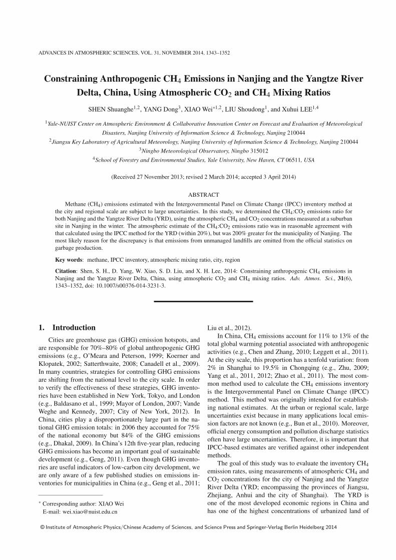
Fig. 5. CH4:CO2 emissions ratio estimated with the two differ-ent methods. Error bars represent the 95% confidence boundon the midday and midnight correlation slopes, the 1% uncer-tainty on the concentration measurement for ΔCH4:ΔCO2, andthe 95% confidence interval calculated with the Monte Carlomethod for the IPCC estimates (uncertainty associated withemission factors).

The CH4:CO2 correlation pattern differed from those re-ported for other chemical species. Wang et al. (2010) foundthat the slope of the CO2:CO correlation measured near Bei-jing, China, was similar in both the summer and the winter,although the slope showed diurnal variations in the summerand remained nearly constant throughout the diurnal cycle inthe winter. Hsu et al. (2010) studied CH4 emissions in south-ern California, USA, and showed that the CH4:CO correla-tion slope was a conserved property independent of time ofthe day or season, suggesting that combustion was the dom-inant emission source for both species. In this study, theCH4:CO2 correlation slope varied seasonally, due to changesin the biological CO2 and CH4 fluxes, and diurnally, due tochanges in the size of source area.

The CH4:CO2 correlation slope can also be comparedwith the concentration enhancement ratio ΔCH4:ΔCO2.Greenberg et al. (1984) and Cofer et al. (1988) have usedthis ratio to approximate the CH4:CO2 emissions ratio ofbiomass burning events. The flux enhancement was calcu-lated in this study as the difference in the winter concentra-tions in Nanjing and Mauna Loa. This method gives a fluxratio of (0.022± 0.009) ppm CH4 : 1 ppm CO2, with the er-ror bound representing a 1% uncertainty on the concentrationmeasurements. The value of ΔCH4:ΔCO2 was much higherthan the CH4:CO2 slope derived from the midday and mid-night measurements and the emissions ratio derived from theinventory estimates (Fig. 5). It appears that this enhancementratio is not suitable for assessing urban GHG emissions.

3.3. CH4 and CO2 emissions based on the IPCC method

Table 1 and table 2 summarize the anthropogenic CO2and CH4 emissions calculated using the IPCC inventorymethod. There were large differences in the relative con-tributions of the source categories of CH4 between Nanjing

and the YRD. Rice cultivation, landfill and wastewater werethe main sources of CH4 in Nanjing, while fugitive emissionsfrom coal mining played the most important role in the YRD.Compared to CH4, there were smaller relative differences ofthe source categories of CO2 between Nanjing and the YRD.The CO2 emissions were mainly from the industrial burningof fossil fuels and other processes both for Nanjing and theYRD. Nanjing has advanced chemical and metal industries,and the CO2 from industrial processes accounted for 42% ofits total anthropogenic CO2 emissions, compared to 21% forthe same category in the YRD.

The inventory estimates presented in this paper are inbroad agreement with those published by other researchers.The estimate of the CO2 emission of Nanjing in 2009 was9% to 14% higher than that in 2007–08 (Bi et al., 2011; Wanget al., 2012), and is approximately equal to the direct emis-sion in 2009 (6.71× 1010 kg) given by Xu (2011). For theYRD region, the emission of CO2 increased by 26% whencompared to that (1.22×1012 kg) in 2007 (Liu et al., 2010).

The CH4 and CO2 emissions of China were also calcu-lated using the same methodology as for Nanjing and theYRD. Excluding rice cultivation, the national CO2 and CH4emissions were 7.41±0.45×1012 kg and 3.29±0.32×1010

kg, respectively. The CO2 emission in 2009 increased by12% to 14%, when compared with the CO2 emissions in2007 (CDIAC, 2010; Chen and Zhang, 2010), and is 8%and 2% higher than that for the year 2009 estimated by IEA(2011) and Guan et al. (2012), respectively. Excluding therice field emissions in the growing season, the CH4 emission(3.12×1010 kg) given by Zhang and Chen (2010) is equal tothe estimate presented here.

3.4. Comparison between the two methodsFigure 5 shows the comparison of the emissions ratio

derived from the atmospheric data with the inventory emis-sion ratios at the three different scales (Nanjing, the YRD,China) calculated with the IPCC methodology. Using theIPCC inventory methodology, there was a gradually increas-ing trend with scale in the CH4:CO2 emissions ratio. Theratio was lowest for Nanjing [(0.0036±0.0011) ppm CH4 : 1ppm CO2], intermediate for the YRD [(0.0051 ± 0.0012)ppm CH4 : 1 ppm CO2] and highest for the whole of China[(0.012± 0.0015) ppm CH4 : 1 ppm CO2]. By comparison,China’s CH4:CO2 emissions ratio was 29% lower than thatof the USA (EPA, 2011), mostly due to a lower proportionof natural gas in China’s fuel mix. The disparity among thethree scales is associated with differences in source type andintensity.

The atmospheric data reveal an opposite trend. The mid-night data, which correspond to a source area size simi-lar to the scale of Nanjing, yielded an emissions ratio of(0.011±0.002) ppm CH4 : 1 ppm CO2, whereas the middaydata, having a source in the order of the size of the YRD, pro-duced an emissions ratio of (0.0043± 0.0007) ppm CH4 : 1ppm CO2. The midday estimate was within 20% of the in-ventory estimate for the YRD, but the midnight estimate was200% greater than the inventory estimate for Nanjing.


Table 1. CO2 emissions estimated with the IPCC inventory method for Nanjing and the Yangtze River Delta in 2009 (units: kg). Theuncertainty range represents the 95% confidence interval.

Nanjing YRD

Emission (×109 kg) Percent of total (%) Emission (×1011 kg) Percent of total (%)

Industrial energy Consumption 30.18 (±7%) 45.4 10.81 (±5%) 70.4Industrial processes 28.01 (±20%) 42.1 3.26 (±16%) 21.2Transportation 7.82 (±2%) 11.8 0.94 (±2%) 6.1Household 0.48 (±3%) 0.9 0.34 (±3%) 2.2Commercial — — — —Total 66.49 (±8%) 100 15.35 (±10%) 100

Table 2. CH4 emissions estimated with the IPCC inventory method for Nanjing and the Yangtze River Delta in 2009 (units: kg). Theuncertainty range represents the 95% confidence interval.

Nanjing YRD

Emission (×107 kg) Percent of total (%) Emission (×108 kg) Percent of total (%)

Landfill 6.16 (±32%) 40.8 5.71 (±31%) 10.8Wastewater 1.40 (±30%) 9.3 1.76 (±30%) 3.3Livestock 0.51 (±29%) 3.4 3.70 (±30%) 7.0Fuel and biomass 0.52 (±33%) 3.4 3.46 (±37%) 6.6Coal mining — — 13.89 (±20%) 26.4Rice cultivation 6.22 (±14%) 41.2 22.20 (±11%) 42.1Natural wetland 0.27 (±25%) 1.9 1.98 (±20%) 3.8Anthropogenic totala 8.59 (±29%) 56.9 28.52 (±22%) 54.1Total 15.08 (±20%) 100 52.70 (±15%) 100

aAnthropogenic total consists of the CH4 emissions from landfill, wastewater, livestock, coal mining, fuel and biomass. CH4 emissions from rice cultivationwere not included in the anthropogenic total as the analysis was limited to wintertime measurements.

Several possible reasons may explain the large differencebetween the top-down atmospheric and the bottom-up inven-tory estimate for Nanjing:

(1) As landfill was the most important CH4 source in Nan-jing, the uncertainties in this source category could have hada large impact on the total emission estimate. There are twosources of uncertainty. First, the default IPCC emission fac-tor may not be appropriate for Nanjing. Toward that end, themodels of Gardner and Probert (1993) and Marticorena et al.(1993) were also used to calculate the landfill CH4 emission.These two models are also dynamic models but, unlike theIPCC method, they either separate the garbage input into dif-ferent age layers or biomass groups of different decay rates.The CH4 emission calculated with the Gardner and Probertmodel (6.22× 107 kg) was nearly equal to the inventory es-timate, and that with the Marticorena model (5.74× 107 kg)was only 7% lower than the inventory estimate. Second, thedata on landfills from official sources may be inaccurate. Us-ing remote sensing image analysis, Dai et al. (2012) foundthat the area actually covered by landfill (6.35× 105 m2) islarger than the area (2.85 × 105 m2) reported to be so bythe government source for Nanjing. This finding was con-firmed through site visits to the predicted landfills. Usingthe area measured by Dai et al. (2012) as a correction fac-tor, the inventory CH4:CO2 emissions ratio would increase to(0.0068±0.002) ppm CH4 : 1 ppm CO2. A further increase ispossible because some unreported landfills may have evaded

remote sensing detection, owing to the fact that they aresmaller than the resolution (30 m) of the Landsat TM im-age used by Dai et al. (2012), and because these unmanagedlandfills may be emitting CH4 at rates much higher than themanaged landfills.

(2) The source area size in the nocturnal boundary layeris another source of uncertainty. Estimating the nocturnalconcentration footprint and source area remains challenging(Sogachev and Leclerc, 2011). In this paper, as an order ofmagnitude estimate, the source area of the nocturnal concen-tration was assumed to be about the size of the city of Nan-jing, and the value of CH4:CO2 was assumed to be influencedby the local sources in Nanjing. However, as the adminis-trative region of Nanjing has a larger north–south than east–west span, the nocturnal concentration source area and thegeographic area of Nanjing may not overlap precisely. As aresult, the CH4:CO2 value may have been influenced by theanthropogenic emissions from the neighboring province, An-hui, which has a CH4:CO2 flux ratio of 0.015 ppm CH4 : 1ppm CO2—significantly higher than that of Nanjing. As theanthropogenic sources of CH4 and CO2 are distributed un-evenly, and because the CH4:CO2 flux ratio may well varysignificantly on a local scale, detailed statistics for the citiesand counties around Nanjing are needed in order to furtherimprove the comparison of the two methodologies.

(3) The atmospheric concentrations of CO2 and CH4 weremeasured in 2010 and 2011, while the statistical data for the


IPCC estimates were for 2009. However, uncertainty arisingfrom this mismatch is negligible, as according to the statisti-cal data for Nanjing, the interannual variations in the sourcesof CO2 and CH4 were very small. For example, the coal con-sumption change from 2005 to 2009 was less than 3%, andthe change in garbage volume during this period was less than2%.

(4) The atmospheric emissions ratio may have been in-flated by the CH4 emissions from natural wetlands (total area:4.4× 102 km2) and rice paddies (total area: 9.7× 102 km2)in the Nanjing municipality. According to Chen et al. (2007),the emissions of CH4 from winter wetlands (1.56×105 kg) isnegligible when compared to anthropogenic emissions (Table2). Using the CH4 flux intensity observed in the rice paddiesin the YRD in the winter (0.18–0.65mg m−2 h−1; Huang etal., 2001; Zhang et al., 2012), it was estimated that the totalemission from the rice paddies in Nanjing was 3.77×105 to1.36×106 kg, which is also negligible when compared to theanthropogenic emissions (Table 2).

(5) CH4 can escape from leaky natural gas distributionnetworks. Kuc et al. (2003) used a carbon isotope tracermethod to assess CH4 sources, and found that network leak-age is an important source of CH4 in Krakow, Poland. Zim-noch et al. (2010) also found a strong source of CH4 inKrakow, Poland, linked to the leakage of natural gas from thecity’s network. In the city center of Florence, the gas networkleakage accounts for 86% of the observed CH4 flux (Gioli etal., 2012). While in the USA, the natural gas system emis-sions accounted for nearly 30% of the total CH4 emission in2009 (EPA, 2011). However, the leakage problem was proba-bly insignificant in Nanjing, because CH4 emission from nat-ural gas consumption was less than 0.1% of the total anthro-pogenic CH4 emission. To put it in another way, if the dispar-ity between the atmospheric and the inventory emissions ratiowere to be attributed solely to distribution line leakage, theamount leaked would be huge (11.5% of the supplied CH4).

4. Conclusions

In this study, the CH4:CO2 emissions ratios calculatedfrom atmospheric concentration measurements and from theIPCC inventory method were compared for the city of Nan-jing and for the YRD. The midday and midnight atmosphericmeasurement data revealed emissions ratios of (0.0043 ±0.0007) and (0.011± 0.002) ppm CH4 : 1 ppm CO2, corre-sponding to source areas comparable to the size of the YRDand the city of Nanjing, respectively. The midday CH4:CO2emissions ratio was approximately 20% smaller than that cal-culated with the IPCC method for the YRD, but the midnightvalue was nearly 200% greater than the inventory estimate forNanjing. The most likely reason for this discrepancy was thata large number of unmanaged landfills were omitted from theofficial statistics. Finally, it is suggested that the atmospherictracer correlation method provides a useful approach to con-strain the CH4 emission rate at the municipality scale wherethe IPCC method is uncertain.

Acknowledgements. This research was supported by the Min-istry of Education of China (Grant PCSIRT), the Priority Aca-demic Program Development of Jiangsu Higher Education Institu-tions (PAPD), the National Natural Science Foundation of China(Grant No. 31100359), the Natural Science Foundation of JiangsuProvince (Grant No. BK2011830), and the Ningbo Planning Projectof Science and Technology (Grant No. 2012C50044).

REFERENCES

Agricultural Social and Economic Survey Office of the StateStatistics Bureau, 2010: China Rural Statistical Yearbook,421 pp. [Available online at http://tongji.cnki.net/kns55/Navi/YearBook.aspx?id=N20 10120027&floor=1.]

Bakwin, P. S., D. F. Hurst, P. P. Tans, and J. W. Elkins, 1997: An-thropogenic sources of halocarbons, sulfur hexafluoride, car-bon monoxide and methane in the southeastern United States.J. Geophys. Res., 102(D13), 15 915–15 925.

Baldasano, J. M., C. Soriano, and L. Boada, 1999: Emission in-ventory for greenhouse gases in the city of Barcelona, 1987–1996. Atmos. Environ., 33(23), 3765–3775.

Berry, R. D., and J. J. Colls, 1990: Atmospheric carbon dioxideand sulphur dioxide on an urban/rural transect-I. Continu-ous measurements at the transect ends. Atmos. Environ., 24,2681–2688.

Bevington, P. R., and D. K. Robinson, 1992: Data Reduction andError Analysis for the Physical Sciences. McGraw-Hill, 328pp.

Bi, J., R. Zhang, H. Wang, M. Liu, and Y. Wu, 2011: Thebenchmarks of carbon emissions and policy implications forChina’s cities: Case of Nanjing. Energy Policy, 39(9), 4785–4794.

Brown, K., and Coauthors, 2012: UK Greenhouse Gas Inven-tory, 1990 to 2010: Annual Report for Submission underthe Framework Convention on Climate Change. Didcot, AEATechnology, 357 pp.

Bun, R., K. Hamal, M. Gusti, and A. Bun, 2010: Spatial GHGinventory at the regional level: Accounting for uncertainty.Climatic Change, 103, 227–224.

Canadell, J. G., P. Ciais, and S. Dhakal, 2009: The human per-turbation of the carbon cycle. UNESCO-SCO-UNEP PolicyBriefs. NO.10, Paris, France, 6 pp. [Available online at http://www.indiaenvironmentportal.org.in/ files/USU-PBCARBONBasseDEF.pdf]

CDIAC (Carbon Dioxide Information Analysis Center), 2010:Global, regional and national annual time series (1751–2006).[Available online at http:// cdiac.ornl.gov/ trends/ emis/methreg.html.]

Chen, G. Q., and B. Zhang, 2010: Greenhouse gas emissions inChina 2007: Inventory and input–output analysis. Energy Pol-icy, 38(10), 6180–6193.

Chen, Y. G., X. H. Bai, X. H. Li, Z. X. Hu, W. L. Liu, and W. P.Hu, 2007: A primary study of the methane flux on the water-air interface of eight lakes in winter, China. Journal of LakeScience, 19(1), 11–17.

City of New York, 2012: Inventory of New York City Green-house Gas Emissions, December 2012, by Jonathan Dichin-son, Jamil Khan, Douglas Price, Steven A. Caputo, Jr. andSergej Mahnovski. Mayor’s Office of Long-Term Planningand Sustainability, New York, 36 pp.

Cofer, W. R. III, J. S. Levine, P. J. Riggan, D. I. Sebacher, E. L.


Winstead, E. F. Jr. Shaw, J. A. Brass, and V. G. Ambrosia,1988: Trace gas emissions from a mid-latitude prescribedchaparral fire. J. Geophys. Res., 93, 1653–1658.

Conway, T. J., and L. P. Steele, 1989: Carbon dioxide and methanein the arctic atmosphere. J. Atmos. Chem., 9, 81–99.

Conway, T. J., L. P. Steele, and P. C. Novelli, 1993: Correlationsamong atmospheric CO2, CH4 and CO in the Arctic, March1989. Atmos. Environ., 27, 2881–2894.

Dai, J. C., Q. Yang, D. M. Lu, and F. Zhang, 2012: Application ofremote sensing to garbage dump recognizing in Nanjing City.Geomatics & Spatial Information Technology, 35(1), 127–135.

Dhakal, S., 2009: Urban energy use and carbon emissions fromcities in China and policy implications. Energy Policy, 37,4208–4219.

Dlugokencky, E. J., L. P. Steele, P. M. Lang, and K. A. Masarie,1994: The growth rate and distribution of atmosphericmethane. J. Geophys. Res., 99(D8), 17 021–17 043.

EPA, 2011: Inventory of U.S. Greenhouse Gas Emissions andSinks: 1990–2009. U.S. Environmental Protection Agency,Washington, DC, EPA 430-R-11-005.

Energy Statistics Division of the National Bureau of Statistics,2010: China Energy Statistical Yearbook. China Statisti-cal Publishing House, Beijing, 286 pp. [Available onlineat http://www. stats.gov.cn/tjsj/nd sj/2010/indexch.htm.] (inChinese)

Gardner, N., and S. D. Probert, 1993: Forecasting landfill gasyields. Appl. Energy, 44(2), 131–163.

Geng, Y., 2011: Eco-indicators: Improve China’s sustainabilitytargets. Nature, 477, 162.

Geng, Y., C. Peng, and M. Tian, 2011: Energy use and CO2 emis-sion inventories in the four municipalities of China. EnergyProcedia, 5, 370–376.

George, K., L. H. Ziska, J. A. Bunce, and B. Quebedeaux, 2007:Elevated atmospheric CO2 concentration and temperatureacross an urban–rural transect. Atmos. Environ., 41, 7654–7665.

Gioli, B., P. Toscano, E. Lugato, A. Matese, F. Miglietta, A. Zaldei,and F. P. Vaccari, 2012: Methane and carbon dioxide fluxesand source partitioning in urban areas: The case study of Flo-rence, Italy. Environ. Pollut., 164, 125–131.

Gloor, M., P. Bakwin, D. Hurst, L. Lock, R. Draxler, and P. Tans,2001: What is the concentration footprint of a tall tower? J.Geophys. Res., 106(D16), 17 831–17 840.

Greally, B. R., and Coauthors, 2007: Observations of 1,1-difluoroethane (HFC-152a) at AGAGE and SOGE monitor-ing stations in 1994–2004 and derived global and regionalemission estimates. J. Geophys. Res., 112, D06308, doi:10.1029/2006JD007527.

Greenberg, J. P., P. R. Zimmerman, L. Heidt, and W. Pollock, 1984:Hydrocarbon and carbon monoxide emissions from biomassburning in Brazil. J. Geophys. Res., 89, 1350–1354.

Guan, D., Liu, Z., Geng, Y., Lindner, S., and Hubacek, K., 2012:The gigatonne gap in China’s carbon dioxide inventories. Nat.Clim. Chang., 2(9), 672–675.

Guha, T., and P. Ghosh, 2010: Diurnal variation of atmosphericCO2 concentration and δ 13C in an urban atmosphere dur-ing winter—Role of the nocturnal boundary layer. J. Atmos.Chem., 65(1), 1–12.

Hsu, Y. K., T. VanCuren, S. Park, C. Jakober, J. Herner, M.FitzGibbon, D. R. Blake, and D. D. Parrish, 2010: Methaneemissions inventory verification in southern California. At-

mos. Environ., 44, 1–7.Huang, Y., J. Jiang, L. Zong, R. Sass, and F. Fisher, 2001: Compar-

ison of field measurements of CH4 emission from rice culti-vation in Nanjing, China and in Texas, USA. Adv. Atmos. Sci.,18(6), 1121–1130.

ICLEI (International Council for Local Environmental Initiatives),2008:. Local government operations protocol for the quan-tification and reporting of greenhouse gas emissions invento-ries. [Available online at http://www.arb.ca.gov/cc/protocols/localgov/archive/final lgo protocol 2008–09–25.pdf.]

Idso, C. D., S. B. Idso, and R. C. Balling Jr., 1998: The urban CO2dome of Phoenix, Arizona. Phys. Geogr., 19, 95–108.

IEA (International Energy Agency), 2011: CO2 Emissions fromFuel Combustion-2011 [EB/OL]. [Available online at http://www.iea.org/co2highlights /co2highlights.pdf.]

Kelliher, F. M., A. R. Reisinger, R. J. Martin, M. J. Harvey, S.J. Price, and R. R. Sherlock, 2002: Measuring nitrous oxideemission rate from grazed pasture using Fourier-transform in-frared spectroscopy in the nocturnal boundary layer. Agric.For. Meteor., 111, 29–38.

Koerner, B., and J. Klopatek, 2002: Anthropogenic and naturalCO2 emission sources in an arid urban environment. Environ.Pollut., 116, S45–S51.

Kuc, T., K. Rozanski, M. Zimnoch, J. M. Necki, and A. Korus,2003: Anthropogenic emissions of CO2 and CH4 in an urbanenvironment. Appl. Energy, 75, 193–203.

Kumar, S., A. N. Mondal, S. A. Gaikwad, S. Devotta, and R. N.Singh, 2004: Qualitative assessment of methane emission in-ventory from municipal solid waste disposal sites: A casestudy. Atmos. Environ., 38, 4921–4929.

Lee, X., O. R. Bullock Jr, and R. J. Andres, 2001: Anthropogenicemission of mercury to the atmosphere in the northeast UnitedStates. Geophys. Res. Lett., 28(7), 1231–1234.

Leggett, J. A., J. Logan, and A. Mackey, 2011: China’s green-house gas emissions and mitigation policies. CongressionalResearch Service R41919, 22 pp.

Liu, L. C., J. N. Wang, G. Wu, and Y. M. Wei, 2010: China’sregional carbon emissions change over 1997–2007. Interna-tional Journal of Energy and Environment, 1(1), 161–176.

Liu, Z., S. Liang, Y. Geng, B. Xue, F. Xi, Y. Pan., T. Zhang,and T. Fujita, 2012: Features, trajectories and driving forcesfor energy-related GHG emissions from Chinese mega cities:The case of Beijing, Tianjin, Shanghai and Chongqing. En-ergy, 37, 245–254.

Marticorena, B., A. Attal, P. Camacho, J. Manem, D. Hesnault,and P. Salmon, 1993: Prediction rules for biogas valorizationin municipal solid waste landfill. Water Sci. Technol., 27(2),235–241.

Mayor of London, 2007: Action Today to Protect Tomorrow: TheMayor’s Climate Change Action Plan. Greater London Au-thority, London, 28 pp.

Mays, K. L., P. B. Shepson, B. H. Stirm, A. Karion, C. Sweeney,and K. R. Gurney, 2009: Aircraft-based measurements of thecarbon footprint of Indianapolis. Environ. Sci. Technol., 43,7816–7823.

Morgan, M. G., and M. Henrion, 1990: Uncertainty: A Guideto Dealing with Uncertainty in Quantitative Risk and PolicyAnalysis. Cambridge University Press, New York, 332 pp.

Nanjing Municipal Bureau of Statistics, 2010: Nanjing Statisti-cal Yearbook. Nanjing Municipal Bureau Statistics, 424 pp.[Available online at http:// tongji.cnki.net/ kns55/ Navi/YearBook.aspx?id=N2011120066&floor=1.]


National Bureau of Statistics of China, 2010: China StatisticalYearbook, 1032 pp. [Available online at http://www.stats.gov.cn/tjsj/ndsj/2010/indexch.htm.]

Obrist, D., F. Conen, R. Vogt, R. Siegwolf, and C. Alewell, 2006:Estimation of Hg0 exchange between ecosystems and the at-mosphere using 222Rn and Hg0 concentration changes in thestable nocturnal boundary layer. Atmos. Environ., 40, 856–866.

O’Meara, M., and J. A. Peterson, 1999: Reinventing Cities for Peo-ple and the Planet. Worldwatch Institute, Washington, 12–31.

Pataki, D. E., B. J. Tyler, R. E. Peterson, A. P. Nair, W. J. Steen-burgh, and E. R. Pardyjak, 2005: Can carbon dioxide be usedas a tracer of urban atmospheric transport? J. Geophys. Res.,110, D15102, doi: 10.1029/2004JD005723.

Pattey, E., I. B. Strachan, R. L. Desjardins, and J. Massheder, 2002:Measuring nighttime CO2 flux over terrestrial ecosystems us-ing eddy covariance and nocturnal boundary layer methods.Agric. For. Meteor., 113, 145–158.

Potosnak, M. J., S. C. Wofsy, A. S. Denning, T. J. Conway, J.W. Munger, and D. H. Barnes, 1999: Influence of bioticexchange and combustion sources on atmospheric CO2 con-centration in New England from observations at a forest fluxtower. J. Geophys. Res., 104, 9561–9569.

Reilly, J., J. Edmonds, R. Gardner, and A. Brenkert, 1987: Montecarlo analysis of the IEA/ORAU energy/carbon emissionsmodel. Energy J., 8(3), 1–29.

Ricker, W. E., 1973: Linear regression in fishery research. Journalof Fishery Research Board Canada., 30(3), 409–434.

Robbins, R. C., L. A. Cavanagh, and L. J. Salas, 1973: Analysis ofancient atmosphere. J. Geophys. Res., 78, 5341–5344.

Rotty, R. M., 1987: Estimates of seasonal variation in fossil fuelCO2 emissions. Tellus, 39, 184–202.

Satterthwaite, D., 2008: Cities’ contribution to global warming:Notes on the allocation of greenhouse gas emissions. Envi-ronment and Urbanization, 20(2), 539–549.

Sigler, J. M., and X. Lee, 2006: Recent trends in anthropogenicmercury emission in the northeast United States. J. Geophys.Res., 111, D14316, doi: 10.1029/2005JD006814.

Sogachev, A., and M. Y. Leclerc, 2011: On concentration foot-prints for a tall tower in the presence of a nocturnal low-leveljet. Agricultural and Forest Meteorology, 151, 755–764.

Su, J., and B. Zhu, 2011: Crop residue burning influence on the airquality over Nanjing and surrounding regions. M. S. thesis,Nanjing University of Information Science and Technology,Nanjing, China, 96 pp. (in Chinese)

Su, J., B. Zhu, T. Zhou, and Y. Ren, 2012: Contrast analysisof two serious air pollution events affecting Nanjing and itssurrounding regions resulting from burning of crop residues.Journal of Ecology and Rural Environment, 28(1), 37–41. (inChinese)

Suntharalingam, P., and Coauthors, 2004: Improved quantifi-cation of Chinese carbon fluxes using CO2/CO correla-tions in Asian outflow. J. Geophys. Res., 109(D18), doi:10.1029/2003JD004362.

Tarasova, O. A., C. A. M. Brenninkmeijer, S. S. Assonovb, N. F.Elanskyc, T. Rockmann, and M. Brassd, 2006: AtmosphericCH4 along the Trans-Siberian railroad (TROICA) and riverOb: Source identification using stable isotope analysis. At-mos. Environ., 40, 5617–5628.

Vande Weghe, J., and C. Kennedy, 2007: A spatial analysis ofresidential greenhouse gas emissions in the Toronto census

metropolitan area. J. Ind. Ecol., 11(2), 133–144.Vinogradova, A. A., E. I. Fedorova, I. B. Belikov, A. S. Ginzburg,

N. F. Elansky, and A. I. Skorokhod, 2007: Temporal varia-tions in carbon dioxide and nethane concentrations under ur-ban conditions. Atmos. Ocean. Phys., 43(5), 599–611.

Wang, H., J. Bi, R. Zhang, and M. Liu, 2012: The carbon emis-sions of Chinese cities. Atmos. Chem. Phys., 12, 6197–6206.

Wang, Y., J. W. Munger, S. Xu, M. B. McElroy, J. Hao, C. P.Nielsen, and H. Ma, 2010: CO2 and its correlation with COat a rural site near Beijing: Complications for combustion ef-ficiency in China. Atmos. Chem. Phys., 10, 8881–8897.

Warneke, C., and Coauthors, 2007: Determination of urbanvolatile organic compound emission ratios and comparisonwith an emissions database. J. Geophys. Res., 112, D10S47,doi: 10.1029/2006JD007930.

Widory, D., and M. Javoy, 2003. The carbon isotope compositionof atmospheric CO2 in Paris. Earth Planet. Sci. Lett., 215,289–298.

Winiwarter, W., and K. Rypdal, 2001: Assessing the uncertaintyassociated with national greenhouse gas emission inventories:A case study for Austria. Atmos. Environ., 35, 5425–5440.

Wunch, D., P. O. Wennberg, G. C. Toon, G. Keppel-Aleks, andY. G. Yavin, 2009: Emissions of greenhouse gases from aNorth American megacity. J. Geophys. Res., 36, L15810, doi:10.1029/2009GL039825.

Xu, S., 2011: Carbon accounting and space distribution for thecities in China—A case of Nanjing city. M. S. thesis, NanjingUniversity, Nanjing, China, 53 pp. (in Chinese)

Yamada, K., N. Yoshida, F. Nakagawa, and G. Inoue, 2005: Sourceevaluation of atmospheric methane over western Siberia usingdouble stable isotopic signatures. Org. Geochem., 36, 717–726.

Yang, J., L. P. Ju, and B. Chen, 2012: Greenhouse gas inventoryand emission accounting of Chongqing. China Population.Resources and Environment, 22(3), 63–69. (in Chinese)

Yang, Y., W. M. Wang, Y. Chen, L. Kang, Z. Li, N. Zhang, andZ. J. Yu, 2011: Greenhouse gas estimation for Tianjin. UrbanEnvironment & Urban Ecology, 24(3), 34–36. (in Chinese)

Zhang, B., and G. Q. Chen, 2010: Methane emissions by Chineseeconomy: Inventory and embodiment analysis. Energy Pol-icy, 38, 4304–4316.

Zhang, L. C., B. Zhu, S. J. Niu, and Z. H. Li, 2009. Con-trastive analysis of atmospheric boundary layer structures infair weather of winter between urban and suburban areas ofNanjing. Journal of Nanjing University of Information Sci-ence and Technology: Natural Science Edition, 1(4), 329–337. (in Chinese)

Zhang, X. Y., G. B. Zhang, Y. Ji, J. Ma, H. Xu, and Z. C. Cai,2012: Temporal variation of CH4 flux and its δ 13C from win-ter flooded rice field. Acta Pedologica Sinica, 49(2), 296–302.

Zhao, Q., Y. Ma, Q. Yu, and Y. Zhang, 2011: Greenhouse gas in-ventory of Shanghai. M. S. thesis, Fudan University, Shang-hai, China, 121 pp. (in Chinese)

Zhu, S. L., 2009: Present situation of greenhouse gas emission inBeijing and the approach to its reduction. China Soft Science,24(9), 93–106. (in Chinese)

Zimnoch, M., J. Godlowska, J. M. Necki, and K. Rozanski, 2010:Assessing surface fluxes of CO2 and CH4 in urban environ-ment: A reconnaissance study in Krakow, Southern Poland.Tellus, 62B, 573–580.

Constraining Anthropogenic CH4 Emissions in Nanjing and ...

Documents

Transcript of Constraining Anthropogenic CH4 Emissions in Nanjing and ...