Effective Field Theory of Cosmic Acceleration:constraining dark energy with CMB data

Marco Raveri1,2, Bin Hu3, Noemi Frusciante1,2, Alessandra Silvestri1,2,4

1 SISSA - International School for Advanced Studies, Via Bonomea 265, 34136, Trieste, Italy2 INFN, Sezione di Trieste, Via Valerio 2, I-34127 Trieste, Italy

3 Institute Lorentz, Leiden University, PO Box 9506, Leiden 2300 RA, The Netherlands4 INAF-Osservatorio Astronomico di Trieste, Via G.B. Tiepolo 11, I-34131 Trieste, Italy

We introduce EFTCAMB/EFTCosmoMC as publicly available patches to the commonly usedCAMB/CosmoMC codes. We briefly describe the structure of the codes, their applicability andmain features. To illustrate the use of these patches, we obtain constraints on parametrized pureEFT and designer f(R) models, both on ΛCDM and wCDM background expansion histories, usingdata from Planck temperature and lensing potential spectra, WMAP low-` polarization spectra(WP), and baryon acoustic oscillation (BAO). Upon inspecting theoretical stability of the modelson the given background, we find non-trivial parameter spaces that we translate into viability priors.We use different combinations of data sets to show their individual effects on cosmological andmodel parameters. Our data analysis results show that, depending on the adopted data sets, in thewCDM background case this viability priors could dominate the marginalized posterior distributions.Interestingly, with Planck+WP+BAO+lensing data, in f(R) gravity models, we get very strongconstraints on the constant dark energy equation of state, w0 ∈ (−1,−0.9997) (95%C.L.).

I. INTRODUCTION

Ongoing and upcoming cosmological surveys will mapmatter and metric perturbations through different epochswith exquisite precision. Combined with geometricprobes, they will provide us with a set of independentmeasurements of cosmological distances and growth ofstructure. In the cosmological standard model, ΛCDM,the rate of linear clustering can be determined from theexpansion rate of the Universe; however this consistencyrelation is generically broken in models of modified grav-ity (MG) and dark energy (DE), even when they predictthe same expansion history as ΛCDM. Therefore mea-surements of the growth of structure, such as weak lens-ing and galaxy clustering, add complementary constrain-ing power to measurements of the expansion history viageometric probes. They can be used to perform consis-tency tests of ΛCDM as well as to constrain the param-eter space of alternative approaches to the phenomenonof cosmic acceleration.

Over the past years there has been a lot of activ-ity in the community to construct frameworks [1–46]that would allow model-independent tests of gravitywith cosmological surveys like Planck [47], SDSS [48],DES [49], LSST [50], Euclid [51], WiggleZ Dark EnergySurvey [52, 53] and CFHTLenS [54–56]. These are gen-erally based on parametrizations of the dynamics of lin-ear scalar perturbations, either at the level of the equa-tions of motion, e.g. [39], of solutions of the equations,e.g. [6, 14, 31], or of the action, e.g. [57–59], with the gen-eral aim of striking a delicate balance among theoreticalconsistency, versatility and feasibility of the parametriza-tion. We shall focus on the latter approach, in particularon the effective field theory (EFT) for cosmic accelerationdeveloped in [57, 58] (see [60–66] for previous work in the

context of inflation, quintessence and large scale struc-ture). This formalism relies on an action written in uni-tary gauge and built out of all the operators that are con-sistent with the unbroken symmetries of the theory, i.e.time-dependent spatial diffeomorphisms, and are orderedaccording to the power of perturbations and derivatives.At each order in perturbations, there is a finite num-ber of such operators that enter the action multiplied bytime-dependent coefficients commonly referred to as EFTfunctions. In particular, the background dynamics is de-termined solely in terms of the three EFT functions mul-tiplying the three background operators, while the gen-eral dynamics of linear scalar perturbations is affected byfurther operators but can still be analyzed in terms of ahandful of time-dependent functions. Despite the model-independent construction, there is a precise mapping thatcan be worked out between the EFT action and the actionof any given single scalar field DE/MG model for whichthere exists a well defined Jordan frame [57, 58, 67, 68].As such, EFT of cosmic acceleration represents an in-sightful parametrization of the general quadratic actionfor single scalar field DE/MG which has the dual qualityof offering a unified language to describe a broad range ofsingle field DE/MG models as well as a versatile frame-work for model independent tests of gravity. For a morein depth description of the EFT formalism we refer thereader to the original papers [57, 58, 69].

In [70] we introduced EFTCAMB, a patch which im-plements the effective field theory formalism of cosmicacceleration into the public Einstein-Boltzmann solverCAMB [71, 72]. As such, the code can be used to inves-tigate the implications of the different EFT operators onlinear perturbations as well as to study perturbations inany specific dark energy or modified gravity model thatcan be cast into the EFT language, once the mapping isworked out. Besides its versatility, an important feature

arX

iv:1

405.

1022

v1 [

astr

o-ph

.CO

] 5

May

201

4

2

of EFTCAMB is that it evolves the full equations with-out relying on any quasi-static approximation and it stillallows for the implementation of specific single field mod-els of DE/MG. Furthermore, as we will briefly review inSection II, our code has a built-in check of stability ofthe theory and allows to safely evolve perturbations inmodels that cross the phantom-divide.

We have now completed a modified version of the stan-dard Markov-Chain Monte-Carlo code CosmoMC [73],that we dubbed EFTCosmoMC. In combination with thecheck for stability of the theory embedded in EFTCAMB,it allows to explore the parameter space of models of cos-mic acceleration under general viability criteria that arewell motivated from the theoretical point of view. Itcomes with built-in likelihoods for several cosmologicaldata sets.

We illustrate the use of these patches obtaining con-straints on different models within the EFT frameworkusing data from Planck temperature and lensing poten-tial spectra, WMAP low-` polarization (WP) spectra aswell as baryon acoustic oscillations (BAO). In particu-lar we consider designer f(R) models and an EFT linearparametrization involving only background operators, onboth a ΛCDM and wCDM bacgkround.

Finally, we are publicly releasing the EFTCAMBand EFTCosmoMC patches at http://www.lorentz.leidenuniv.nl/~hu/codes/. We are completing a setof notes that will guide the reader through the structureof the codes [74].

II. EFTCAMB

In this Section we shall briefly review the main featuresof EFTCAMB. For a more in depth description of theEFT formalism, the equations evolved by the code andthe integration strategy, we refer the reader to [70].

The EFT formalism for cosmic acceleration is based onthe following action written in unitary gauge and Jordanframe

S =

∫d4x√−gm2

0

2(1 + Ω)R+ Λ− a2c δg00

+M4

2

2(a2δg00)2 − M3

1

2a2δg00δKµ

µ −M2

2

2(δKµ

µ )2

−M23

2δKµ

ν δKνµ +

a2M2

2δg00δR(3)

+m22(gµν + nµnν)∂µ(a2g00)∂ν(a2g00) + . . .

+Sm[χi, gµν ], (1)

where we have used conformal time andΩ,Λ, c,M2, M1, M2, M3, M ,m2 are free functionsof time which multiply all the operators that areconsistent with time-dependent spatial diffeomorphisminvariance and are at most quadratic in the perturba-tions. We will refer to these as EFT functions. Thefirst line of (1) displays only operators that contribute

to the evolution of the background. There follow thesecond order operators that affect only the dynamicsof perturbations, in combination with the backgroundoperators. The ellipsis indicate higher order operatorswhich would affect the non-linear dynamics and are notyet included in the code. Finally, Sm is the action for allmatter fields, χi.

A given single scalar field model of DE/MG, for whichthere exists a well defined Jordan frame, can be mappedinto the formalism (1) as illustrated in [57, 58, 67, 68].As such, EFT offers a unified language for most of theviable approaches to cosmic acceleration; among other,we shall mention the Horndeski class [75] which in-cludes quintessence [76], k-essence [77], f(R), covariantGalileon [78], the effective 4D limit of DGP [79] to namea few. Furthermore, action (1) represents a parametrizedframework to test gravity on large scales via the dynamicsof linear cosmological perturbations. To this extent, onecan use a designer approach to fix a priori the backgroundevolution and use the Friedmann equations to determinetwo of the EFT background functions Ω,Λ, c in termsof the third one [57, 58]. It turns out to be convenientto solve for c and Λ in terms of Ω. In the unitary gaugeadopted for action (1), the extra scalar d.o.f. associatedto DE or the modifications of gravity is eaten by the met-ric. While such set up is convenient to construct the ac-tion, in order to analyze the dynamics of perturbations itis convenient to make the scalar d.o.f. explicit. This canbe achieved restoring the time-diffeomorphism invarianceof the action via the Stuckelberg technique, i.e. perform-ing the following infinitesimal time diffeomorphism to theaction

τ → τ + π(xµ), (2)

and Taylor-expanding the resulting action in π. TheStuckelberg field, π, now encodes the departures fromthe standard cosmological model. At the level of lin-ear scalar perturbations, EFTCAMB evolves the stan-dard equations for all matter species, a set of modifiedEinstein-Boltzmann equations and a full Klein-Gordonequation for π as described at length in [70]. We shallrecall that this treatment of the extra dynamics asso-ciated to DE/MG, as opposed to an effective fluid ap-proach [27, 80, 81], it allows us to maintain a bettercontrol of the stability of the theory and to cross thephantom divide.

As described in [70], the multifaceted nature of theEFT formalism is implemented in EFTCAMB, where thebackground dynamics can be approached with either ofthe following procedures:

• pure EFT: in this case one works with a given subsetof the operators in (1), possibly all, treating their co-efficients as free functions. The background is treatedvia the EFT designer approach, i.e. a given expansionhistory is fixed, a viable form for Ω [82] is chosen andthe remaining two background EFT functions are de-termined via the Friedmann equations. The code al-lows for ΛCDM and wCDM expansion histories, as well

3

as for the Chevallier-Polarski-Linder (CPL) [83, 84]parametrization of the dark energy equation of state.In addition it offers a selection of functional forms forΩ(a): the minimal coupling, corresponding to Ω = 0;the linear model, that can be thought of as a first or-der approximation of a Taylor expansion; power law,inspired by f(R), and exponential ones. There is alsothe possibility for the user to choose an arbitrary formof Ω according to any ansatz the user wants to inves-tigate. At the level of perturbations, more operatorscome into play, each with a free function of time infront of it, and one needs to choose some ansatze inorder to fix their functional form. To this extent, weadopted the same scheme as for the background func-tion Ω, still providing the possibility to define and useother forms that might be of interest. Of course thepossibility to set all/some second order EFT functionsto zero is included. The code evolves the full perturbedequations consistently implemented to account for theinclusion of more than one second order operator pertime, ensuring that even more and more complicatedmodels can be studied.

• mapping EFT: in this case a particular DE/MG modelis chosen, the corresponding background equations aresolved and then everything is mapped into the EFT for-malism [57, 58, 67, 68] to evolve the full EFT perturbedequations. Let us stress that in the mapping case, oncethe background equations are solved, all the EFT func-tions are completely fixed by the choice of the model.Built-in to the first code release there are f(R) modelsfor which a designer approach is used for the ΛCDM,wCDM and CPL backgrounds following [85, 86]. Inthe future other theories will be added to graduallycover the wide range of models included in the EFTframework.

In summary, EFTCAMB is a full Einstein-Bolztmanncode which exploits the double nature of the EFT frame-work. As such, it allows to investigate how the differ-ent operators entering (1) affect the dynamics of linearperturbations as well as to study a particular DE/MGmodel, once the mapping to the EFT formalism is de-termined. Let us stress that EFTCAMB evolves the fulldynamical equations on all linear scales both in the pureEFT and mapping mode, ensuring that we do not missout on any potentially interesting dynamics at redshiftsand scales that might be within reach of upcoming, widerand deeper, surveys.

Ultimately, we built a machinery which allows to testgravity and its modifications on large scale in a modelindependent framework which ideally covers most of themodels of cosmological interest by computing cosmologi-cal observables which are the two-point auto- and cross-correlations provided by the combination of galaxy clus-tering, CMB temperature and polarization anisotropyand weak lensing.

III. EFTCOSMOMC: SAMPLING OF THEPARAMETER SPACE UNDER STABILITY

CONDITIONS

To fully exploit the power of EFTCAMB we equippedit with a modified version of the standard Markov-ChainMonte-Carlo code CosmoMC [73] that we dubbed EFT-CosmoMC. The complete code now allows to explorethe parameter space performing comparisons with sev-eral cosmological data sets, and it does so with a built-instability check that we shall discuss in the following.

In the EFT framework, the stability of perturbationsin the dark sector can be determined from the equationfor the perturbation π, which is an inhomogeneous Klein-Gordon equation with coefficients that depend both onthe background expansion history and the EFT func-tions [57, 58, 70]. Following the arguments of [61], in [70]we listed general viability requirements in the form ofconditions to impose on the coefficients of the equationfor π; these include a speed of sound c2s ≤ 1, a positivemass m2

π ≥ 0 and the avoidance of ghost. Furthermorewe required a positive non-minimal coupling function, i.e.1+Ω > 0, to ensure a positive effective Newton constant.

When exploring the parameter space one needs tocheck the stability of the theory at every sampling point.While this feature at first might seem a drawback, how-ever, it is one of the main advantages of the EFT frame-work and a virtue of EFTCAMB/EFTCosmoMC. In-deed, as we outlined in [70], checking the stability ofthe theory ensures not only that the dynamical equa-tions are mathematically consistent and can be reliablynumerically solved, but also, perhaps more importantly,that the underlying physical theory is acceptable. Thisof course is desired when considering specific DE/MGmodels and, even more, when adopting the pure EFTapproach. In the latter case indeed, one makes a some-what arbitrary choice for the functional form of the EFTfunctions and satisfying the stability conditions will en-sure that there is an underlying, theoretically consistentmodel of gravity corresponding to that given choice.

Imposing stability conditions generally results in a par-tition of the parameter space into a stable region andan unstable one. In order not to alter the statisticalproperties of the MCMC sampler [87], like the conver-gence to the target distribution, when dealing with apartitioned parameter space we implement the stabil-ity conditions as priors so that the Monte Carlo step isrejected whenever it would fall in the unstable region.We call these constraints viability priors as they rep-resent the degree of belief in a viable underlying singlescalar field DE/MG theory encoded in the EFT frame-work. We would like to stress that they correspondto specific conditions that are theoretically well moti-vated and, hence, they represent the natural require-ments to impose on a model/parametrization. One ofthe virtues of the EFT framework, and consequently ofEFTCAMB/EFTCosmoMC, is to allow their implemen-tation in a straightforward way. We shall emphasize that

4

our EFTCosmoMC code automatically enforces the via-bility priors for every model considered, both in the pureand mapping EFT approach.

IV. DATA SETS AND RESULTS

In this Section we shall briefly review the data setswe used and discuss the resulting constraints obtainedfor some selected pure and mapping EFT models onboth ΛCDM and wCDM backgrounds. While we willwork with models that involve only background opera-tors, EFTCAMB/EFTCosmoMC are fully equipped tohandle also second order operators; the same procedurethat we shall outline here can be followed when the latterare at play.

A. Data sets

We adopt Planck temperature-temperature powerspectra considering the 9 frequency channels rangingfrom 30 ∼ 353 GHz for low-` modes (2 ≤ ` < 50)andthe 100, 143, and 217 GHz frequency channels for high-`modes (50 ≤ ` ≤ 2500) 1 [88, 89]. In addition we includethe Planck collaboration 2013 data release of the full-skylensing potential map [90], by using the 100, 143, and 217GHz frequency bands with an overall significance greaterthan 25σ. The lensing potential distribution is an indi-cator of the underlying large-scale structure, and as suchit is sensitive to the modified growth of perturbationscontributing significant constraining power for DE/MGmodels.

In order to break the well-known degeneracy betweenthe re-ionization optical depth and the amplitude ofCMB temperature anisotropy, we include WMAP low-` polarization spectra (2 ≤ ` ≤ 32) [91]. Finally, weconsider the external baryon acoustic oscillations mea-surements from the 6dFGS (z = 0.1) [92], SDSS DR7 (ateffective redshift zeff = 0.35) [93, 94], and BOSS DR9(zeff = 0.2 and zeff = 0.35) [95] surveys to get comple-mentary constraining power on cosmological distances.

To explicitly show the effect of individual datasets on the different parameters that we con-strain, we adopt three different combinations ofdata, namely: Planck+WP; Planck+WP+BAO;Planck+WP+BAO+lensing, where with lensing wemean the CMB lensing potential distributions as mea-sured by Planck. In all cases we assume standard flatpriors from CMB on cosmological parameters while weimpose the viability priors discussed in Section III onmodel parameters.

1 http://pla.esac.esa.int/pla/aio/planckProducts.html

B. Linear EFT model

We start our exploration of CMB constraints onDE/MG theories with a pure EFT model. We adoptthe designer approach choosing two different models forthe expansion history, the ΛCDM one and the wCDMone (corresponding to a constant dark energy equationof state). As we reviewed in Section II, after fixing thebackground expansion history one can use the Friedmannequations to solve for two of the three EFT backgroundfunctions in terms of the third one; as it is common, weuse this to eliminate Λ and c. We are then left with Ωas a free background function that will leave an imprintonly on the behaviour of perturbations. We assume thefollowing functional form:

Ω(a) = ΩEFT0 a , (3)

which can be thought of as a first order approximationof a Taylor expansion in the scale factor. We set to zerothe coefficients of all the second order EFT operators. Inthe remaining we refer to this model as the linear EFTmodel.

Before proceeding with parameter estimation, it is in-structive to study the shape of the viable region in theparameter space of the model. As we discussed in Sec-tion III, the check on the stability of any given model isa built-in feature of EFTCAMB/EFTCosmoMC, so thatthe user does not need to separately perform such an in-vestigation prior to implementing the model in the code.Nevertheless, in some cases it might be useful to look atthe outcome of such analysis as one can learn interestingthings about the model/parametrization under consider-ation. Let us briefly discuss the stability of the linearEFT model.

In the case of a ΛCDM expansion history, it is easyto show that all the stability requirements that we listedin [70], and reviewed in Section III, imply the followingviability prior :

ΩEFT0 ≥ 0 . (4)

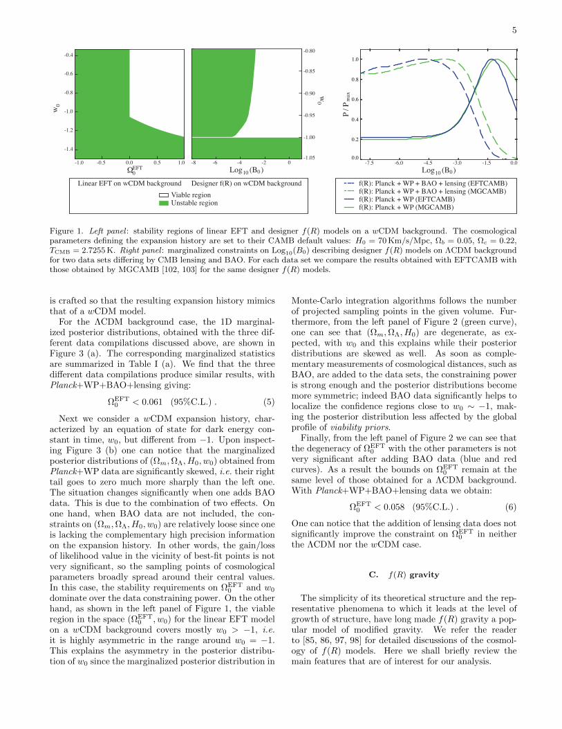
On the other hand, the case of a wCDM expansion his-tory can not be treated analytically so we used our EFT-CAMB code along with a simple sampling algorithm, in-cluded in the code release, to explore the stability of themodel in the parameter space. We varied the parametersdescribing the dark sector physics while keeping fixed allthe other cosmological parameters. The result is shownin Figure 1 and includes interesting information on thebehaviour of this model. First of all, also in this case thestable region correspond to ΩEFT

0 > 0; furthermore it ispossible to have a viable gravity model with w0 < −1,although in this case ΩEFT

0 needs to acquire a bigger andbigger value to stabilize perturbations in the dark sec-tor. Finally, we see that if ΩEFT

0 = 0 we recover theresult, found in the context of quintessence models [96],that w0 > −1. This case corresponds, in fact, to mini-mally coupled quintessence models with a potential that

5

0.0

0.2

0.4

0.6

0.8

1.0

Log10 (B0)-7.5 -6.0 -4.5 -3.0 -1.5 0.0

-0.80

-0.85

-0.90

-0.95

-1.00

-1.05

w0

Log10 (B0)-8 -6 -4 -2 0

-0.4

-0.6

-0.8

-1.0

-1.2

-1.4

w0

-1.0 -0.5 0.0 0.5 1.0ΩEFT

0

P/P

max

f(R): Planck + WP + BAO + lensing (EFTCAMB)Linear EFT on wCDM background Designer f(R) on wCDM backgroundf(R): Planck + WP + BAO + lensing (MGCAMB)f(R): Planck + WP (EFTCAMB)f(R): Planck + WP (MGCAMB)

Viable regionUnstable region

Figure 1. Left panel : stability regions of linear EFT and designer f(R) models on a wCDM background. The cosmologicalparameters defining the expansion history are set to their CAMB default values: H0 = 70 Km/s/Mpc, Ωb = 0.05, Ωc = 0.22,TCMB = 2.7255 K. Right panel : marginalized constraints on Log10(B0) describing designer f(R) models on ΛCDM backgroundfor two data sets differing by CMB lensing and BAO. For each data set we compare the results obtained with EFTCAMB withthose obtained by MGCAMB [102, 103] for the same designer f(R) models.

is crafted so that the resulting expansion history mimicsthat of a wCDM model.

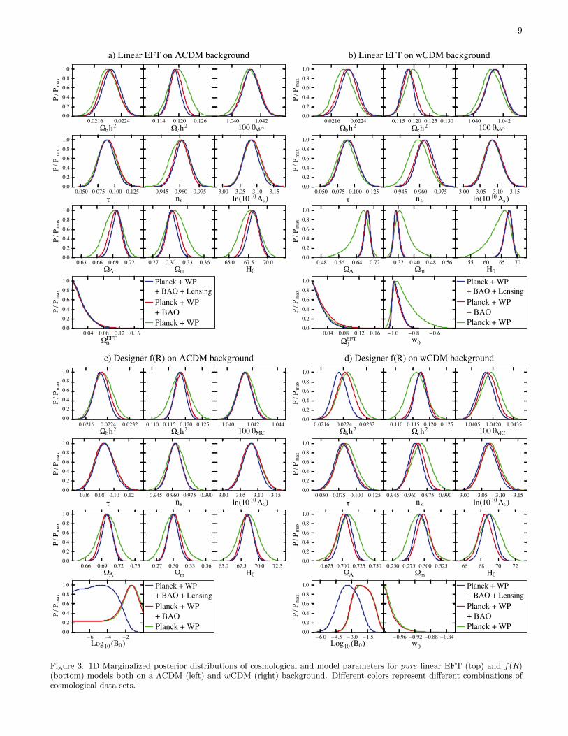
For the ΛCDM background case, the 1D marginal-ized posterior distributions, obtained with the three dif-ferent data compilations discussed above, are shown inFigure 3 (a). The corresponding marginalized statisticsare summarized in Table I (a). We find that the threedifferent data compilations produce similar results, withPlanck+WP+BAO+lensing giving:

ΩEFT0 < 0.061 (95%C.L.) . (5)

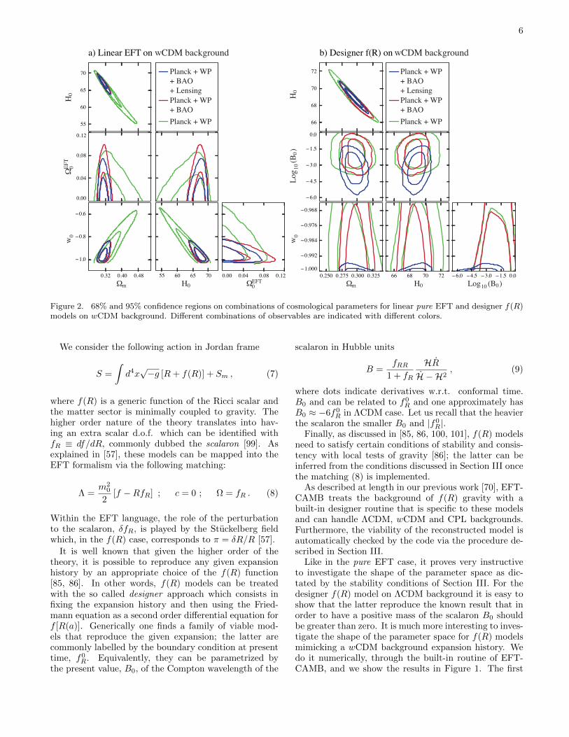
Next we consider a wCDM expansion history, char-acterized by an equation of state for dark energy con-stant in time, w0, but different from −1. Upon inspect-ing Figure 3 (b) one can notice that the marginalizedposterior distributions of (Ωm,ΩΛ, H0, w0) obtained fromPlanck+WP data are significantly skewed, i.e. their righttail goes to zero much more sharply than the left one.The situation changes significantly when one adds BAOdata. This is due to the combination of two effects. Onone hand, when BAO data are not included, the con-straints on (Ωm,ΩΛ, H0, w0) are relatively loose since oneis lacking the complementary high precision informationon the expansion history. In other words, the gain/lossof likelihood value in the vicinity of best-fit points is notvery significant, so the sampling points of cosmologicalparameters broadly spread around their central values.In this case, the stability requirements on ΩEFT

0 and w0

dominate over the data constraining power. On the otherhand, as shown in the left panel of Figure 1, the viableregion in the space (ΩEFT

0 , w0) for the linear EFT modelon a wCDM background covers mostly w0 > −1, i.e.it is highly asymmetric in the range around w0 = −1.This explains the asymmetry in the posterior distribu-tion of w0 since the marginalized posterior distribution in

Monte-Carlo integration algorithms follows the numberof projected sampling points in the given volume. Fur-thermore, from the left panel of Figure 2 (green curve),one can see that (Ωm,ΩΛ, H0) are degenerate, as ex-pected, with w0 and this explains while their posteriordistributions are skewed as well. As soon as comple-mentary measurements of cosmological distances, such asBAO, are added to the data sets, the constraining poweris strong enough and the posterior distributions becomemore symmetric; indeed BAO data significantly helps tolocalize the confidence regions close to w0 ∼ −1, mak-ing the posterior distribution less affected by the globalprofile of viability priors.

Finally, from the left panel of Figure 2 we can see thatthe degeneracy of ΩEFT

0 with the other parameters is notvery significant after adding BAO data (blue and redcurves). As a result the bounds on ΩEFT

0 remain at thesame level of those obtained for a ΛCDM background.With Planck+WP+BAO+lensing data we obtain:

ΩEFT0 < 0.058 (95%C.L.) . (6)

One can notice that the addition of lensing data does notsignificantly improve the constraint on ΩEFT

0 in neitherthe ΛCDM nor the wCDM case.

C. f(R) gravity

The simplicity of its theoretical structure and the rep-resentative phenomena to which it leads at the level ofgrowth of structure, have long made f(R) gravity a pop-ular model of modified gravity. We refer the readerto [85, 86, 97, 98] for detailed discussions of the cosmol-ogy of f(R) models. Here we shall briefly review themain features that are of interest for our analysis.

6

66

68

70

72

−6.0

−4.5

−3.0

−1.5

0.0

0.250 0.275 0.300 0.325−1.000

−0.992

−0.984

−0.976

−0.968

66 68 70 72 −6.0 −4.5 −3.0 −1.5 0.0

w0

Log 1

0(B

0)H

0

Log10 (B0)H0Ωm

b) Designer f(R) on wCDM background

Planck + WP+ BAO+ LensingPlanck + WP+ BAOPlanck + WP55

60

65

70

0.04

0.00

0.08

0.12

0.32 0.40 0.48

−1.0

−0.8

−0.6

55 60 65 70 0.040.00 0.08 0.12

w0

ΩEF

T0

H0

H0Ωm ΩEFT0

a) Linear EFT on wCDM background

Planck + WP+ BAO+ LensingPlanck + WP+ BAOPlanck + WP

Figure 2. 68% and 95% confidence regions on combinations of cosmological parameters for linear pure EFT and designer f(R)models on wCDM background. Different combinations of observables are indicated with different colors.

We consider the following action in Jordan frame

S =

∫d4x√−g [R+ f(R)] + Sm , (7)

where f(R) is a generic function of the Ricci scalar andthe matter sector is minimally coupled to gravity. Thehigher order nature of the theory translates into hav-ing an extra scalar d.o.f. which can be identified withfR ≡ df/dR, commonly dubbed the scalaron [99]. Asexplained in [57], these models can be mapped into theEFT formalism via the following matching:

Λ =m2

0

2[f −RfR] ; c = 0 ; Ω = fR . (8)

Within the EFT language, the role of the perturbationto the scalaron, δfR, is played by the Stuckelberg fieldwhich, in the f(R) case, corresponds to π = δR/R [57].

It is well known that given the higher order of thetheory, it is possible to reproduce any given expansionhistory by an appropriate choice of the f(R) function[85, 86]. In other words, f(R) models can be treatedwith the so called designer approach which consists infixing the expansion history and then using the Fried-mann equation as a second order differential equation forf [R(a)]. Generically one finds a family of viable mod-els that reproduce the given expansion; the latter arecommonly labelled by the boundary condition at presenttime, f0

R. Equivalently, they can be parametrized bythe present value, B0, of the Compton wavelength of the

scalaron in Hubble units

B =fRR

1 + fR

HRH − H2

, (9)

where dots indicate derivatives w.r.t. conformal time.B0 and can be related to f0

R and one approximately hasB0 ≈ −6f0

R in ΛCDM case. Let us recall that the heavierthe scalaron the smaller B0 and |f0

R|.Finally, as discussed in [85, 86, 100, 101], f(R) models

need to satisfy certain conditions of stability and consis-tency with local tests of gravity [86]; the latter can beinferred from the conditions discussed in Section III oncethe matching (8) is implemented.

As described at length in our previous work [70], EFT-CAMB treats the background of f(R) gravity with abuilt-in designer routine that is specific to these modelsand can handle ΛCDM, wCDM and CPL backgrounds.Furthermore, the viability of the reconstructed model isautomatically checked by the code via the procedure de-scribed in Section III.

Like in the pure EFT case, it proves very instructiveto investigate the shape of the parameter space as dic-tated by the stability conditions of Section III. For thedesigner f(R) model on ΛCDM background it is easy toshow that the latter reproduce the known result that inorder to have a positive mass of the scalaron B0 shouldbe greater than zero. It is much more interesting to inves-tigate the shape of the parameter space for f(R) modelsmimicking a wCDM background expansion history. Wedo it numerically, through the built-in routine of EFT-CAMB, and we show the results in Figure 1. The first

7

noticeable feature is that for wCDM models the value ofthe equation of state of dark energy can not go below−1, which is consistent with what was found in [86]. Thesecond one is that the parameter B0 controls the limit toGR of the theory i.e. when B0 gets smaller the expansionhistory is forced to go back to that of the ΛCDM modelin order to preserve a positive mass of the scalaron. Theconverse is not true and this same feature do not appearin pure EFT models where the ΩEFT

0 = 0 branch con-tains viable theories and corresponds to the wide class ofminimally coupled quintessence models.

In what follows, we shall first investigate the con-straints onB0 in models reproducing ΛCDM background,performing also a comparison with analogous results ob-tained using MGCAMB [102, 103]. We will then move tostudy constraints on designer models on a wCDM back-ground, which is a novel aspect of our work.

In the right panel of Figure 1, we compare the 1Dmarginalized posterior distributions of Log10B0 from ourEFTCAMB to those from MGCAMB. Overall there isgood agreement between the two results. Moreover,one can notice that generally the constraints obtainedwith EFTCAMB are a little bit tighter than those ob-tained with MGCAMB. This is because in the latter codef(R) models are treated with the quasi-static approxi-mation which looses out on some of the dynamics of thescalaron [104], which is instead fully captured by our fullEinstein-Boltzmann solver, as discussed already in [70].

The detailed 1D posterior distributions and corre-sponding marginalized statistics are summarized in Fig-ure 3 (c) and Table I (c) and they are consistent withprevious studies employing the quasi-static approxima-tions [105]. The right panel of Figure 1 and Figure 3(c) show that lensing data add a significant consrtainingpower on B0. This is because Planck lensing data arehelpful in breaking the degeneracy between Ωm and B0

which affect the lensing spectrum in different ways. In-deed, in f(R) gravity the growth rate of linear structureis enhanced by the modifications, hence the amplitude ofthe lensing potential spectrum is amplified whenever B0

is different than zero (see our previous work [70]); how-ever, the background angular diameter distance is notaffected by B0, so the position of the lensing potentialspectrum is not shifted horizontally. On the other hand,Ωm affects both the background and linear perturbationso that both the amplitude and position of the peaks ofthe lensing potential are sensitive to it.

Similarly to what happens in the linear EFT model,f(R) gravity shows some novel features in the case ofa wCDM background. Once again we find a non-triviallikelihood profile of Log10B0 (see Figure 3 (d)) for all thethree data compilations, with the shape of the marginal-ized posterior distribution of Log10B0 being dominatedby the shape of the stable region. In the middle panelof Figure 1 one can see indeed that when B0 tends tosmaller values, i.e. the theory tends to GR, the stableregions becomes narrower and narrower, with a tiny tippointing to the GR limit. Since the width of this tip is so

narrow compared with the current capability of parame-ter estimation from Planck data, the gains of likelihoodof the sampling points inside this parameter throat arenot significant, i.e. they are uniformly sampled in thethroat. Hence, even though the full data set has a verygood sensitivity to B0, the marginalized distribution ofLog10B0 is dominated by the volume of the stable regionin the parameter space. One can also notice that thebound on w0 with Planck lensing data is quite stringentcompared to those without lensing, namely:

w0 ∈ (−1,−0.94) (95%C.L.) without lensing,

w0 ∈ (−1,−0.9997) (95%C.L.) with lensing. (10)

We argue that this stringent constraint actually is a con-sequence of the combination of the sensitivity of lens-ing data to B0, that we capture well with our code,and the degeneracy between B0 and w0. As shownin [34] Planck lensing data is very sensitive to MGparameters such as B0; indeed, in our analysis withPlanck+WP+BAO+lensing data we get

Log10B0 = −3.35+1.79−1.77 (95%C.L.) . (11)

Furthermore, from Figure 2 (b), one can see thatthe ellipse in the (Log10B0, w0) space corresponding toPlanck+WP+BAO+lensing data (blue) is orthogonal tothose without lensing (red and green). In other words,when lensing data is included, Log10B0 and w0 displaya degeneracy which propagates the stringent constrainton the scalar Compton wavelength from CMB lensingdata to w0. Besides this, we do not find other remark-able degeneracies between B0 and standard cosmologicalparameters.

V. CONCLUSIONS

Solving the puzzle of cosmic acceleration is one of themajor challenges of modern cosmology. In this respect,cosmological surveys will provide a large amount of highquality data allowing to test gravity on large scales withunprecedented accuracy. The effective field theory frame-work for cosmic acceleration will prove useful in perform-ing model independent tests of gravity as well as in test-ing specific theories as, while being a parametrization ofthe quadratic action, it preserves a direct link to a widerange of DE/MG models. Indeed, any single scalar fieldDE/MG models with a well defined Jordan frame can becast into the EFT language and most of the cosmologicalmodels of interest fall into this class.

In a previous work [70], we presented the implementa-tion of the EFT formalism into the Einstein-Boltzmannsolver CAMB [71], resulting into EFTCAMB. The lattercode has several virtues: it allows for the implementa-tion of the parameterized EFT framework in what wedub the pure EFT approach, and for the implementa-tion of specific DE/MG models in the mapping mode;it does not rely on any quasi-static approximation, but

8

rather it implements the full perturbative equations onall linear scale for both the pure and the mapping caseensuring that no potentially interesting physics is lost;it has a built-in check of the stability conditions of per-turbations in the dark sector in order to guarantee thatthe underlying gravitational theory is viable; it enablesto choose among different expansion histories, namelyΛCDM, wCDM and CPL backgrounds, naturally allow-ing phantom-divide crossings.

In the present work, we equipped EFTCAMB with amodified version of CosmoMC, that we dubbed EFTCos-moMC, creating a bridge between the EFT parametriza-tion of the dynamics of perturbations and observations.EFTCosmoMC allows to practically perform tests ofgravity and get constraints analyzing the cosmologicalparameter space with, in its current version, data sets,such as Planck, WP, BAO and Planck lensing. Furtherdata sets, mainly from large-scale structure surveys, willbe included in the near future.

As discussed in Section III, exploring the parameterspace requires a step by step check of the stability ofthe theory. We implemented the resulting stability con-ditions as viability priors that makes the Monte Carlostep be rejected whenever it would fall in the unstableregion of the parameter space. The latter procedure, inour view, represents a clean and natural way to imposepriors on parameters describing the dark sector.

To illustrate the use of the EFT-CAMB/EFTCosmoMC package, we have derivedconstraints on two different classes of models, namely apure linear EFT model and a mapping designer f(R).We used three different combinations of Planck, WP,BAO and CMB lensing data sets to show their differenteffects on constraining the parameter space. For bothmodels we have adopted the designer approach built-inin EFTCAMB and have considered the case of a ΛCDMas well as of a wCDM background.

For the linear EFT model, we have derived bounds onthe only model parameter, i.e the present value of theconformal coupling functions ΩEFT

0 , as described in Sec-tion IV B. In the case of a ΛCDM background, we havefound that the latter needs to satisfy ΩEFT

0 ≥ 0 as aviability condition and with Planck+WP+BAO+lensingdata we get a bound of ΩEFT

0 < 0.061 (95%C.L.) (thethree different data compilations give similar results).For the wCDM expansion history, the outcome of thestability analysis is shown in Figure 1; specifically, thereis a stable region in parameter space where the darkenergy equation of state can be smaller than −1 aslong as the corresponding value of ΩEFT

0 is high enoughto stabilize perturbations in the dark sector; finally,the value ΩEFT

0 = 0 corresponds to a minimally cou-pled model and requires w0 > −1, like in the caseof quintessence. The combined bound on ΩEFT

0 withPlanck+WP+BAO+lensing data gives ΩEFT

0 < 0.058(95%C.L.).

Finally, we have investigated designer f(R) models onΛCDM/wCDM backgrounds, in terms of constraints on

the model parameter B0, as described in Section IV C.For the ΛCDM case we also compared our results to thosethat we obtained with the quasi-static treatment of thesemodels via MGCAMB [102, 103]. The two treatmentsgive results that are in good agreement, with bounds fromEFTCAMB/EFTCosmoMC being a little tighter thanksto the full treatment of the dynamics of perturbations.On wCDM background we have found a non-trivial likeli-hood profile of Log10B0 (see Figure 3 (d)) for all the threedata compilations and the shape of the marginalized pos-terior distribution in this case strongly reflects that ofthe viable region in parameter space. In the wCDMbackground, with Planck+WP+BAO+lensing data weget Log10B0 = −3.35+1.79

−1.77 (95% C.L.). The bounds onw0 with Planck lensing data (w0 ∈ (−1,−0.9997) (95%C.L.)) are quite stringent compared to those without thisdata set (w0 ∈ (−1,−0.94) (95% C.L.)) due to the strongconstraining power of lensing measurements on B0 andthe degeneracy between w0 and B0.

Within the pure EFT approach, the code we are re-leasing contains already all operators relevant for the dy-namics of linear perturbations. In particular, while inthis work we showed results for a model involving onlybackground operators, we shall stress that the code isfully functional for second order operators too. In thefuture we will add some third order operators to studymildly non-linear scales. As for the mapping mode, thecode currently allows for a full treatment of f(R) mod-els via a specific designer approach that can handle bothΛCDM, wCDM and CPL backgrounds. We will gradu-ally implement the mapping procedure for many othersingle scalar field DE/MG models which are of relevancefor cosmological tests. Finally, more data sets will beadded into EFTCosmoMC allowing to test gravity withthe most recent data releases with a particular empha-sis toward large scale structure observations in view ofsurveys such as Euclid [51].

The complete EFTCAMB/EFTCosmoMC bundleis now publicly available at http://www.lorentz.leidenuniv.nl/~hu/codes/.

ACKNOWLEDGMENTS

We are grateful to Carlo Baccigalupi, Matteo Cal-abrese, Luca Heltai, Matteo Martinelli and Riccardo Val-darnini for useful conversations. AS is grateful to AlirezaHojjati, Levon Pogosian and Gong-Bo Zhao for their pre-vious and ongoing collaboration on related topics. BH issupported by the Dutch Foundation for Fundamental Re-search on Matter (FOM). NF acknowledges partial finan-cial support from the European Research Council underthe European Union’s Seventh Framework Programme(FP7/2007-2013) / ERC Grant Agreement n. 306425“Challenging General Relativity”. AS acknowledges sup-port from a SISSA Excellence Grant. MR and AS ac-knowledge partial support from the INFN-INDARK ini-tiative.

9

0.0216 0.0224 0.0232Ωbh2

0.0

0.2

0.4

0.6

0.8

1.0

P/P

max

0.110 0.115 0.120 0.125Ωch2

1.0405 1.0420 1.0435100 θMC

0.050 0.075 0.100 0.125τ

0.0

0.2

0.4

0.6

0.8

1.0

P/P

max

0.945 0.960 0.975 0.990ns

3.00 3.05 3.10 3.15ln(10 10 As )

0.675 0.700 0.725 0.750ΩΛ

0.0

0.2

0.4

0.6

0.8

1.0

P/P

max

0.250 0.275 0.300 0.325Ωm

66 68 70 72H0

−6.0 −4.5 −3.0 −1.5Log10 (B0)

0.0

0.2

0.4

0.6

0.8

1.0

P/P

max

−0.96 −0.92 −0.88 −0.84w0

d) Designer f(R) on wCDM background

Planck + WP + BAOPlanck + WP

Planck + WP + BAO + Lensing

0.0216 0.0224Ωbh2

0.00.20.40.60.81.0

P/P

max

0.115 0.120 0.125 0.130Ωch2

1.040 1.042100 θMC

0.050 0.075 0.100 0.125τ

0.00.20.40.60.81.0

P/P

max

0.945 0.960 0.975ns

3.00 3.05 3.10 3.15ln(10 10 As )

0.48 0.56 0.64 0.72ΩΛ

0.00.20.40.60.81.0

P/P

max

0.32 0.40 0.48 0.56Ωm

55 60 65 70H0

0.04 0.08 0.12 0.16ΩEFT

0

0.00.20.40.60.81.0

P/P

max

−1.0 −0.8 −0.6w0

b) Linear EFT on wCDM background

Planck + WP + BAOPlanck + WP

Planck + WP + BAO + Lensing

0.0216 0.0224 0.0232Ωbh2

0.0

0.2

0.4

0.6

0.8

1.0

P/P

max

0.110 0.115 0.120 0.125Ωch2

1.040 1.042 1.044100 θMC

0.06 0.08 0.10 0.12τ

0.0

0.2

0.4

0.6

0.8

1.0

P/P

max

0.945 0.960 0.975 0.990ns

3.00 3.05 3.10 3.15ln(10 10 As )

0.66 0.69 0.72 0.75ΩΛ

0.0

0.2

0.4

0.6

0.8

1.0

P/P

max

0.27 0.30 0.33 0.36Ωm

65.0 67.5 70.0 72.5H0

−6 −4 −2Log10 (B0)

0.0

0.2

0.4

0.6

0.8

1.0

P/P

max

c) Designer f(R) on ΛCDM background

Planck + WP + BAOPlanck + WP

Planck + WP + BAO + Lensing

0.0216 0.0224Ωbh2

0.00.20.40.60.81.0

P/P

max

0.114 0.120 0.126Ωch2

1.040 1.042100 θMC

0.050 0.075 0.100 0.125τ

0.00.20.40.60.81.0

P/P

max

0.945 0.960 0.975ns

3.00 3.05 3.10 3.15ln(10 10 As )

0.63 0.66 0.69 0.72ΩΛ

0.00.20.40.60.81.0

P/P

max

0.27 0.30 0.33 0.36Ωm

65.0 67.5 70.0H0

0.04 0.08 0.12 0.16ΩEFT

0

0.00.20.40.60.81.0

P/P

max

a) Linear EFT on ΛCDM background

Planck + WP + BAOPlanck + WP

Planck + WP + BAO + Lensing

Figure 3. 1D Marginalized posterior distributions of cosmological and model parameters for pure linear EFT (top) and f(R)(bottom) models both on a ΛCDM (left) and wCDM (right) background. Different colors represent different combinations ofcosmological data sets.

10

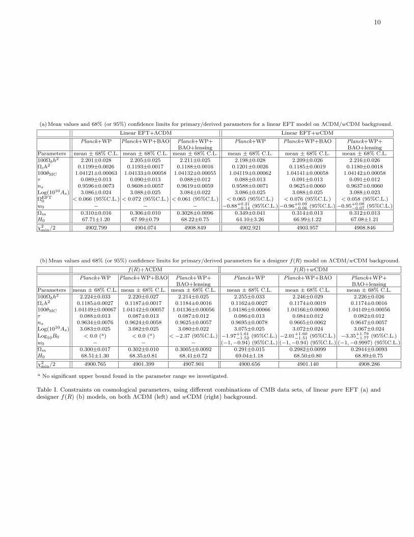
(a) Mean values and 68% (or 95%) confidence limits for primary/derived parameters for a linear EFT model on ΛCDM/wCDM background.

Linear EFT+ΛCDM Linear EFT+wCDM

Planck+WP Planck+WP+BAO Planck+WP+BAO+lensing

Planck+WP Planck+WP+BAO Planck+WP+BAO+lensing

Parameters mean ± 68% C.L. mean ± 68% C.L. mean ± 68% C.L. mean ± 68% C.L. mean ± 68% C.L. mean ± 68% C.L.100Ωbh

2 2.201±0.028 2.205±0.025 2.211±0.025 2.198±0.028 2.209±0.026 2.216±0.026Ωch2 0.1199±0.0026 0.1193±0.0017 0.1188±0.0016 0.1201±0.0026 0.1185±0.0019 0.1180±0.0018100θMC 1.04121±0.00063 1.04133±0.00058 1.04132±0.00055 1.04119±0.00062 1.04141±0.00058 1.04142±0.00058τ 0.089±0.013 0.090±0.013 0.088±0.012 0.088±0.013 0.091±0.013 0.091±0.012ns 0.9596±0.0073 0.9608±0.0057 0.9619±0.0059 0.9588±0.0071 0.9625±0.0060 0.9637±0.0060Log(1010As) 3.086±0.024 3.088±0.025 3.084±0.022 3.086±0.025 3.088±0.025 3.088±0.023ΩEFT

0 < 0.066 (95%C.L.) < 0.072 (95%C.L.) < 0.061 (95%C.L.) < 0.065 (95%C.L.) < 0.076 (95%C.L.) < 0.058 (95%C.L.)

w0 − − − −0.88+0.21−0.14 (95%C.L.) −0.96+0.09

−0.06 (95%C.L.) −0.95+0.08−0.07 (95%C.L.)

Ωm 0.310±0.016 0.306±0.010 0.3028±0.0096 0.349±0.041 0.314±0.013 0.312±0.013H0 67.71±1.20 67.99±0.79 68.22±0.75 64.10±3.26 66.99±1.22 67.08±1.21

χ2min/2 4902.799 4904.074 4908.849 4902.921 4903.957 4908.846

(b) Mean values and 68% (or 95%) confidence limits for primary/derived parameters for a designer f(R) model on ΛCDM/wCDM background.

f(R)+ΛCDM f(R)+wCDM

Planck+WP Planck+WP+BAO Planck+WP+BAO+lensing

Planck+WP Planck+WP+BAO Planck+WP+BAO+lensing

Parameters mean ± 68% C.L. mean ± 68% C.L. mean ± 68% C.L. mean ± 68% C.L. mean ± 68% C.L. mean ± 68% C.L.100Ωbh

2 2.224±0.033 2.220±0.027 2.214±0.025 2.255±0.033 2.246±0.029 2.226±0.026Ωch2 0.1185±0.0027 0.1187±0.0017 0.1184±0.0016 0.1162±0.0027 0.1174±0.0019 0.1174±0.0016100θMC 1.04149±0.00067 1.04142±0.00057 1.04136±0.00056 1.04186±0.00066 1.04166±0.00060 1.04149±0.00056τ 0.088±0.013 0.087±0.013 0.087±0.012 0.086±0.013 0.084±0.012 0.082±0.012ns 0.9634±0.0076 0.9624±0.0058 0.9625±0.0057 0.9695±0.0078 0.9665±0.0062 0.9647±0.0057Log(1010As) 3.083±0.025 3.082±0.025 3.080±0.022 3.075±0.025 3.072±0.024 3.067±0.024

Log10B0 < 0.0 (a) < 0.0 (a) < −2.37 (95%C.L.) −1.97+1.61−1.52 (95%C.L.) −2.01+1.60

−1.51 (95%C.L.) −3.35+1.79−1.77 (95%C.L.)

w0 − − − (−1,−0.94) (95%C.L.) (−1,−0.94) (95%C.L.) (−1,−0.9997) (95%C.L.)Ωm 0.300±0.017 0.302±0.010 0.3005±0.0092 0.291±0.015 0.2982±0.0099 0.2944±0.0093H0 68.51±1.30 68.35±0.81 68.41±0.72 69.04±1.18 68.50±0.80 68.89±0.75

χ2min/2 4900.765 4901.399 4907.901 4900.656 4901.140 4908.286

a No significant upper bound found in the parameter range we investigated.

Table I. Constraints on cosmological parameters, using different combinations of CMB data sets, of linear pure EFT (a) anddesigner f(R) (b) models, on both ΛCDM (left) and wCDM (right) background.

11

[1] E. Bertschinger, Astrophys. J. 648, 797 (2006), [astro-ph/0604485].

[2] E. V. Linder and R. N. Cahn, Astropart. Phys. 28, 481(2007), [astro-ph/0701317].

[3] P. Zhang, M. Liguori, R. Bean and S. Dodelson, Phys.Rev. Lett. 99, 141302 (2007), [arXiv:0704.1932 [astro-ph]].

[4] W. Hu and I. Sawicki, Phys. Rev. D 76, 104043 (2007),[arXiv:0708.1190 [astro-ph]].

[5] L. Amendola, M. Kunz and D. Sapone, JCAP 0804,013 (2008), [arXiv:0704.2421 [astro-ph]].

[6] E. Bertschinger and P. Zukin, Phys. Rev. D 78, 024015(2008) [arXiv:0801.2431 [astro-ph]].

[7] S. F. Daniel, R. R. Caldwell, A. Cooray andA. Melchiorri, Phys. Rev. D 77, 103513 (2008),[arXiv:0802.1068 [astro-ph]].

[8] Y. -S. Song and K. Koyama, JCAP 0901, 048 (2009),[arXiv:0802.3897 [astro-ph]].

[9] C. Skordis, Phys. Rev. D 79, 123527 (2009),[arXiv:0806.1238 [astro-ph]].

[10] Y. -S. Song and O. Dore, JCAP 0903, 025 (2009),[arXiv:0812.0002 [astro-ph]].

[11] G. -B. Zhao et al., Phys. Rev. Lett. 103, 241301 (2009),[arXiv:0905.1326 [astro-ph.CO]].

[12] Y. -S. Song, L. Hollenstein, G. Caldera-Cabral andK. Koyama, JCAP 1004, 018 (2010), [arXiv:1001.0969[astro-ph.CO]].

[13] S. F. Daniel et al., Phys. Rev. D 81, 123508 (2010),[arXiv:1002.1962 [astro-ph.CO]].

[14] L. Pogosian, A. Silvestri, K. Koyama and G. -B. Zhao,Phys. Rev. D 81, 104023 (2010), [arXiv:1002.2382[astro-ph.CO]].

[15] R. Bean and M. Tangmatitham, Phys. Rev. D 81,083534 (2010), [arXiv:1002.4197 [astro-ph.CO]].

[16] G. -B. Zhao et al., Phys. Rev. D 81, 103510 (2010),[arXiv:1003.0001 [astro-ph.CO]].

[17] J. Dossett, M. Ishak, J. Moldenhauer, Y. Gong,A. Wang, Y. Gong and A. Wang, JCAP 1004, 022(2010) [arXiv:1004.3086 [astro-ph.CO]].

[18] S. A. Thomas, S. A. Appleby and J. Weller, JCAP1103, 036 (2011), [arXiv:1101.0295 [astro-ph.CO]].

[19] T. Baker, P. G. Ferreira, C. Skordis and J. Zuntz, Phys.Rev. D 84, 124018 (2011), [arXiv:1107.0491 [astro-ph.CO]].

[20] D. B. Thomas and C. R. Contaldi, JCAP 1112, 013(2011), [arXiv:1107.0727 [astro-ph.CO]].

[21] J. N. Dossett, M. Ishak and J. Moldenhauer, Phys. Rev.D 84, 123001 (2011), [arXiv:1109.4583 [astro-ph.CO]].

[22] G. -B. Zhao et al., Phys. Rev. D 85, 123546 (2012),[arXiv:1109.1846 [astro-ph.CO]].

[23] A. Hojjati et al., Phys. Rev. D 85, 043508 (2012),[arXiv:1111.3960 [astro-ph.CO]].

[24] P. Brax, A. -C. Davis and B. Li, Phys. Lett. B 715, 38(2012), [arXiv:1111.6613 [astro-ph.CO]].

[25] J. Dossett and M. Ishak, Phys. Rev. D 86, 103008(2012) [arXiv:1205.2422 [astro-ph.CO]].

[26] P. Brax, A. -C. Davis, B. Li and H. A. Winther, Phys.Rev. D 86, 044015 (2012), [arXiv:1203.4812 [astro-ph.CO]].

[27] I. Sawicki, I. D. Saltas, L. Amendola and M. Kunz,JCAP 1301, 004 (2013), [arXiv:1208.4855 [astro-

ph.CO]].[28] T. Baker, P. G. Ferreira and C. Skordis, Phys. Rev. D

87, 024015 (2013), [arXiv:1209.2117 [astro-ph.CO]].[29] L. Amendola et al., Phys. Rev. D 87, 023501 (2013),

[arXiv:1210.0439 [astro-ph.CO]].[30] A. Hojjati, JCAP 1301, 009 (2013), [arXiv:1210.3903

[astro-ph.CO]].[31] A. Silvestri, L. Pogosian and R. V. Buniy, Phys. Rev.

D 87, no. 10, 104015 (2013) [arXiv:1302.1193 [astro-ph.CO]].

[32] B. Hu, M. Liguori, N. Bartolo and S. Matarrese, Phys.Rev. D 88, no. 2, 024012 (2013) [arXiv:1211.5032 [astro-ph.CO]].

[33] J. Dossett and M. Ishak, Phys. Rev. D 88, 103008(2013), [arXiv:1311.0726 [astro-ph.CO]].

[34] B. Hu, M. Liguori, N. Bartolo and S. Matarrese, Phys.Rev. D 88, 123514 (2013), [arXiv:1307.5276 [astro-ph.CO]].

[35] M. Motta, I. Sawicki, I. D. Saltas, L. Amendolaand M. Kunz, Phys. Rev. D 88, 124035 (2013),[arXiv:1305.0008 [astro-ph.CO]].

[36] S. Asaba et al., JCAP 1308, 029 (2013),[arXiv:1306.2546 [astro-ph.CO]].

[37] A. Terukina, L. Lombriser, K. Yamamoto, D. Bacon,K. Koyama and R. C. Nichol, arXiv:1312.5083 [astro-ph.CO].

[38] F. Piazza, H. Steigerwald and C. Marinoni,arXiv:1312.6111 [astro-ph.CO].

[39] T. Baker, P. G. Ferreira and C. Skordis, Phys. Rev. D89, 024026 (2014), [arXiv:1310.1086 [astro-ph.CO]].

[40] Las. A.Gergely and S. Tsujikawa, Phys. Rev. D 89,064059 (2014) [arXiv:1402.0553 [hep-th]].

[41] D. Munshi, B. Hu, A. Renzi, A. Heavens and P. Coles,arXiv:1403.0852 [astro-ph.CO].

[42] H. Steigerwald, J. Bel and C. Marinoni, arXiv:1403.0898[astro-ph.CO].

[43] Q. -G. Huang, arXiv:1403.0655 [astro-ph.CO].[44] L. Lombriser, arXiv:1403.4268 [astro-ph.CO].[45] S. Tsujikawa, arXiv:1404.2684 [gr-qc].[46] E. Bellini and I. Sawicki, arXiv:1404.3713 [astro-

ph.CO].[47] http://sci.esa.int/planck .[48] http://www.sdss.org .[49] http://www.darkenergysurvey.org .[50] http://www.lsst.org .[51] http://sci.esa.int/euclid .[52] M. J. Drinkwater, R. J. Jurek, C. Blake, D. Woods,

K. A. Pimbblet, K. Glazebrook, R. Sharp andM. B. Pracy et al., Mon. Not. Roy. Astron. Soc. 401,1429 (2010) [arXiv:0911.4246 [astro-ph.CO]].

[53] D. Parkinson, S. Riemer-Sorensen, C. Blake,G. B. Poole, T. M. Davis, S. Brough, M. Collessand C. Contreras et al., Phys. Rev. D 86, 103518(2012) [arXiv:1210.2130 [astro-ph.CO]].

[54] F. Simpson, C. Heymans, D. Parkinson, C. Blake,M. Kilbinger, J. Benjamin, T. Erben and H. Hilde-brandt et al., arXiv:1212.3339 [astro-ph.CO].

[55] C. Heymans, E. Grocutt, A. Heavens, M. Kilbinger,T. D. Kitching, F. Simpson, J. Benjamin and T. Er-ben et al., arXiv:1303.1808 [astro-ph.CO].

12

[56] L. Fu, M. Kilbinger, T. Erben, C. Heymans, H. Hilde-brandt, H. Hoekstra, T. D. Kitching and Y. Mellier etal., arXiv:1404.5469 [astro-ph.CO].

[57] G. Gubitosi, F. Piazza and F. Vernizzi, JCAP 1302,032 (2013) [arXiv:1210.0201 [hep-th]].

[58] J. K. Bloomfield, E. E. Flanagan, M. Park and S. Wat-son, JCAP 1308, 010 (2013) [arXiv:1211.7054 [astro-ph.CO]].

[59] R. A. Battye and J. A. Pearson, JCAP 1207, 019(2012), [arXiv:1203.0398 [hep-th]].

[60] S. Weinberg, Phys. Rev. D 77, 123541 (2008),[arXiv:0804.4291 [hep-th]].

[61] P. Creminelli, G. D’Amico, J. Norena and F. Vernizzi,JCAP 0902, 018 (2009), [arXiv:0811.0827 [astro-ph]].

[62] M. Park, K. M. Zurek and S. Watson, Phys. Rev. D 81,124008 (2010), [arXiv:1003.1722 [hep-th]].

[63] C. Cheung et al., JHEP 0803, 014 (2008),[arXiv:0709.0293 [hep-th]].

[64] R. Jimenez, P. Talavera and L. Verde, Int. J. Mod. Phys.A 27, 1250174 (2012), [arXiv:1107.2542 [astro-ph.CO]].

[65] J. J. M. Carrasco, M. P. Hertzberg and L. Sena-tore, JHEP 1209, 082 (2012), [arXiv:1206.2926 [astro-ph.CO]].

[66] M. P. Hertzberg, Phys. Rev. D 89, 043521 (2014),[arXiv:1208.0839 [astro-ph.CO]].

[67] J. Gleyzes, D. Langlois, F. Piazza and F. Vernizzi,JCAP 1308, 025 (2013), [arXiv:1304.4840 [hep-th]].

[68] J. Bloomfield, JCAP 12, 044 (2013), [arXiv:1304.6712[astro-ph.CO]].

[69] F. Piazza and F. Vernizzi, Class. Quant. Grav. 30,214007 (2013) [arXiv:1307.4350].

[70] B. Hu, M. Raveri, N. Frusciante and A. Silvestri,arXiv:1312.5742 [astro-ph.CO].

[71] http://camb.info .[72] A. Lewis, A. Challinor and A. Lasenby, Astrophys. J.

538, 473 (2000), [astro-ph/9911177].[73] A. Lewis and S. Bridle, Phys. Rev. D 66, 103511 (2002)

[astro-ph/0205436].[74] M. Raveri, B. Hu, N. Frusciante, A. Silvestri,

“EFTCAMB/EFTCosmoMC: Numerical Notes v1.0’ inpreparation

[75] G. W. Horndeski, Int. J. Theor. Phys. 10, 363 (1974).[76] E. J. Copeland, M. Sami and S. Tsujikawa, Int. J. Mod.

Phys. D 15, 1753 (2006) [hep-th/0603057].[77] C. Armendariz-Picon, T. Damour and V. F. Mukhanov,

Phys. Lett. B 458, 209 (1999) [hep-th/9904075].[78] C. Deffayet, G. Esposito-Farese and A. Vikman, Phys.

Rev. D 79, 084003 (2009) [arXiv:0901.1314 [hep-th]].[79] A. Nicolis, R. Rattazzi and E. Trincherini, Phys. Rev.

D 79, 064036 (2009), [arXiv:0811.2197 [hep-th]].[80] J. Bloomfield and J. Pearson, JCAP 1403, 017 (2014),

[arXiv:1310.6033 [astro-ph.CO]].[81] R. A. Battye and J. A. Pearson, JCAP 1403, 051

(2014), [arXiv:1311.6737 [astro-ph.CO]].[82] N. Frusciante, M. Raveri and A. Silvestri, JCAP 1402,

026 (2014), [arXiv:1310.6026 [astro-ph.CO]].[83] M. Chevallier and D. Polarski, Int. J. Mod. Phys. D 10,

213 (2001), [gr-qc/0009008].

[84] E. V. Linder, Phys. Rev. Lett. 90, 091301 (2003), [astro-ph/0208512].

[85] Y. -S. Song, W. Hu and I. Sawicki, Phys. Rev. D 75,044004 (2007), [astro-ph/0610532].

[86] L. Pogosian and A. Silvestri, Phys. Rev. D 77,023503 (2008), [Erratum-ibid. D 81, 049901 (2010)],[arXiv:0709.0296 [astro-ph]].

[87] W. R. Gilks, “Markov Chain Monte Carlo In Practice”,Chapman and Hall/CRC, (1999), 0412055511.

[88] P. A. R. Ade et al. [Planck Collaboration],arXiv:1303.5075 [astro-ph.CO].

[89] P. A. R. Ade et al. [Planck Collaboration],arXiv:1303.5076 [astro-ph.CO].

[90] P. A. R. Ade et al. [Planck Collaboration],arXiv:1303.5077 [astro-ph.CO].

[91] G. Hinshaw et al. [WMAP Collaboration], Astrophys. J.Suppl. 208, 19 (2013), [arXiv:1212.5226 [astro-ph.CO]].

[92] F. Beutler, C. Blake, M. Colless, D. H. Jones,L. Staveley-Smith, L. Campbell, Q. Parker andW. Saunders et al., Mon. Not. Roy. Astron. Soc. 416,3017 (2011), [arXiv:1106.3366 [astro-ph.CO]].

[93] W. J. Percival et al. [SDSS Collaboration], Mon. Not.Roy. Astron. Soc. 401, 2148 (2010), [arXiv:0907.1660[astro-ph.CO]].

[94] N. Padmanabhan, X. Xu, D. J. Eisenstein, R. Scalzo,A. J. Cuesta, K. T. Mehta and E. Kazin, Mon. Not. Roy.Astron. Soc. 427, no. 3, 2132 (2012), [arXiv:1202.0090[astro-ph.CO]].

[95] L. Anderson, E. Aubourg, S. Bailey, D. Bizyaev,M. Blanton, A. S. Bolton, J. Brinkmann andJ. R. Brownstein et al., Mon. Not. Roy. Astron.Soc. 427, no. 4, 3435 (2013), [arXiv:1203.6594 [astro-ph.CO]].

[96] I. Zlatev, L. -M. Wang and P. J. Steinhardt, Phys. Rev.Lett. 82, 896 (1999) [astro-ph/9807002].

[97] R. Bean, D. Bernat, L. Pogosian, A. Silvestri andM. Trodden, Phys. Rev. D 75, 064020 (2007), [astro-ph/0611321].

[98] A. De Felice and S. Tsujikawa, Living Rev. Rel. 13, 3(2010), [arXiv:1002.4928 [gr-qc]].

[99] A. A. Starobinsky, JETP Lett. 86, 157 (2007),[arXiv:0706.2041 [astro-ph]].

[100] L. Amendola, R. Gannouji, D. Polarski and S. Tsu-jikawa, Phys. Rev. D 75, 083504 (2007) [gr-qc/0612180].

[101] W. Hu and I. Sawicki, Phys. Rev. D 76, 064004 (2007)[arXiv:0705.1158 [astro-ph]].

[102] G. -B. Zhao, L. Pogosian, A. Silvestri and J. Zylberberg,Phys. Rev. D 79, 083513 (2009) [arXiv:0809.3791 [astro-ph]].

[103] A. Hojjati, L. Pogosian and G. -B. Zhao, JCAP 1108,005 (2011) [arXiv:1106.4543 [astro-ph.CO]].

[104] A. Hojjati, L. Pogosian, A. Silvestri and S. Talbot, Phys.Rev. D 86, 123503 (2012), [arXiv:1210.6880 [astro-ph.CO]].

[105] J. Dossett, B. Hu and D. Parkinson, JCAP 1403, 046(2014), [arXiv:1401.3980 [astro-ph.CO]].