Constraining the composition and thermal state of the moon ...

tters 248 (2006) 579–598www.elsevier.com/locate/epsl

Earth and Planetary Science Le

Constraining the composition and thermal state of the moon from aninversion of electromagnetic lunar day-side transfer functions

A. Khan a,⁎, J.A.D. Connolly b, N. Olsen c, K. Mosegaard a

a Niels Bohr Institute, University of Copenhagen, Denmarkb Earth Sciences Department, Swiss Federal Institute of Technology, Zurich, Switzerland

c Danish National Space Centre, Copenhagen, Denmark

Received 17 November 2005; received in revised form 6 March 2006; accepted 6 April 2006Available online 27 June 2006

Editor: V. Courtillot

Abstract

We present a general method to constrain planetary composition and thermal state from an inversion of long-periodelectromagnetic sounding data. As an example of our approach, we reexamine the problem of inverting lunar day-side transferfunctions to constrain the internal structure of the Moon. We go beyond the conventional approach by inverting directly forchemical composition and thermal state, using the model system CaO–FeO–MgO–Al2O3–SiO2, rather than subsurface electricalconductivity structure, which is only an indirect means of estimating the former parameters. Using Gibbs free energy minimisation,we calculate the stable mineral phases, their modes and densities. The mineral modes are combined with laboratory electricalconductivity measurements to estimate the bulk lunar electrical conductivity structure from which transfer functions are calculated.To further constrain the radial density profile in the inversion we also consider lunar mass and moment of inertia. The jointinversion of electromagnetic sounding and gravity data for lunar composition and selenotherm as posited here is found to befeasible, although uncertainties in the forward modeling of bulk conductivity have the potential to significantly influence theinversion results. In order to improve future inferences about lunar composition and thermal state, more electrical conductivitymeasurements are needed especially for minerals appropriate to the Moon, such as pyrope and almandine.© 2006 Elsevier B.V. All rights reserved.

Keywords: planetary composition; thermal state; inverse problems; Moon; thermodynamic modeling

1. Introduction

Constraining the present-day lunar thermal state isimportant as it holds the potential of providing valuableinformation on lunar origin and evolution. Moreover,temperature is a fundamental parameter in understand-ing the dynamic behaviour of the properties mantle in

⁎ Corresponding author. Tel.: +45 35320564.E-mail address: [email protected] (A. Khan).

0012-821X/$ - see front matter © 2006 Elsevier B.V. All rights reserved.doi:10.1016/j.epsl.2006.04.008

that it governs such as viscosity, density, convection,melting and electrical conductivity. However, there arepresently few data available that directly constrain lunarthermal state and most of these provide only indirectconstraints. Several theoretically predicted selenothermshave been disseminated over the years (e.g. [1–5]) andshow considerable scatter. These variations are mainlydue to the different prior assumptions that are aprerequisite of thermal modeling, including differencesin assumptions about the initial thermal state, modelparameters (thermal conductivity), melting conditions

mailto:[email protected]

http://dx.doi.org/10.1016/j.epsl.2006.04.008

580 A. Khan et al. / Earth and Planetary Science Letters 248 (2006) 579–598

and not least the relevance of subsolidus convective heattransport throughout lunar history.

Geophysical data that bear directly on the lunartemperature profile are scanty and include surface heatflow measurements [6], seismic Q-values inferred fromthe Apollo lunar seismic data [7] and maintenance ofmascon anisostasy over a period of 3–4 b.y. [8].

A method that, in principle, can be used to put limitson the present-day lunar temperature profile involvesthe use of electromagnetic sounding data, which, wheninverted provide knowledge on the conductivity profileof the lunar interior (e.g. [9–12]). As mineral conduc-tivity measured in the laboratory has been found todepend inversely on temperature, limits on the sele-notherm can be derived from the inferred bounds on thelunar electrical conductivity profile when combinedwith laboratory measurements of electrical conductivityas a function of temperature. Attempts along these lineshave been undertaken (e.g. [13–17]), but were limitedbecause of, among other things, uncertainty in bulklunar composition and inverted electrical conductivitystructure.

Building upon earlier as well as recent laboratorymeasurements of mineral electrical conductivities (e.g.[18–22]) our intent here is to invert measurements ofthe lunar inductive response to time-varying externalmagnetic fields during intervals when the Moon was inthe solar wind or terrestrial magnetosheath in order toconstrain the lunar thermal state and bulk chemicalcomposition. Given the Moon's temperature profileand composition, equilibrium mineral modes andphysical properties can be calculated by thermody-namic methods. When combined with laboratory elec-trical conductivity measurements and appropriatemixing laws, the bulk electrical conductivity of theMoon can be estimated. From a knowledge of the bulkconductivity the geomagnetic response at the lunarsurface or in space is easily evaluated. Whereasprevious studies assumed both mineralogy, and hencecomposition, and temperature as known a priori, thelatter two parameters constitute our unknowns, deter-mining all other parameters.

The application of this method to the Moon isfacilitated because temperatures and pressures in itsinterior are easily reached in the laboratory, therebyallowing laboratory data to be used directly or withmodest extrapolation. Also, as regards field measure-ments, relatively short magnetometer records(∼days) are required for deep lunar sounding [16].In comparison, periods up to several years areneeded for sounding of the deep terrestrial mantle[23–25].

The inverse problem of estimating composition andthermal state of the Moon from electromagneticsounding data, mass and moment of inertia it isstrongly non-linear. We invoke a Markov chain MonteCarlo (MCMC) sampling algorithm to solve theinverse problem. It is formulated within a Bayesianframework, i.e. through the extensive use of proba-bility density functions (pdf 's) to delineate every itemof information, as laid out by [26] and [27]. Thesolution to the inverse problem is defined as theconjunction of these pdf 's and contained in theposterior pdf (e.g. [28–30]).

The inverse method presented here is general andprovides through the unified description of phaseequilibria a way of constructing planetary modelswhere the radial variation of mineralogy and densitywith pressure and temperature is naturally specified,permitting a direct inversion for chemical compositionand temperature. Given these parameters mineralogy,and bulk physical properties can be calculated.Inversion based on electrical conductivity is particu-larly intriguing, when compared to inversions basedon seismic properties, because variations in conduc-tivity with mineralogy are much stronger than thecorresponding variations in elastic properties. Inprinciple, electrical conductivity therefore offers amore sensitive means of probing planetary composi-tion; unfortunately in practice bulk conductivityestimates are dependent on a mineralogical conduc-tivity data base that is much more uncertain than is thecase for elastic properties. For this reason, thesynthesis presented here is to be viewed as a first-order model. Our purpose in constructing such amodel is to establish whether such an inversion ispossible. The validity of this model may be influencedby a number of factors affecting the electricalconductivity of the lunar mantle which include: poorlyknown effects of mineral chemistry and redox state onconductivity of mantle minerals; and how rock fabricaffects conductivity.

In spite of any such reservations, we would liketo point out that the goal of the present inversion,apart from trying to constrain chemical compositionand selenotherm, serves a deeper purpose, namelythat of integrating widely different geophysical datasets into a joint inversion. This is presentlyexemplified by jointly inverting electromagnetic andgravity data and is achieved by appealing to a set ofparameters which are not only common to alldifferent geophysical fields considered, but alsocharacterises the media studied at a fundamentallevel.

Table 1Apparent resistivities, ρa, calculated from the estimated day-sidetransfer functions tabulated in [34] including error bars (dρa)

Period(s)

ρa(Ω m)

dρa(Ω m)

100,000.00 58.6 2.150,000.00 113.9 4.033,333.33 164.5 5.725,000.00 209.8 7.420,000.00 250.8 9.216,666.67 288.7 11.014,285.71 324.6 12.712,500.00 358.9 13.911,111.11 392.3 14.410,000.00 424.8 14.25000.00 693.5 36.63333.33 921.4 70.52500.00 1099.2 91.92000.00 1212.7 109.61666.67 1283.2 110.81428.57 1350.8 96.81250.00 1471.7 82.31111.11 1542.5 74.51000.00 1674.9 84.3

581A. Khan et al. / Earth and Planetary Science Letters 248 (2006) 579–598

2. Geophysical data and earlier lunar inductionstudies

Several methods have been developed to infer theelectrical conductivity structure of a planet using thenatural electromagnetic variations recorded on itssurface. The magnetic deep sounding method, whichemploys only magnetic and no electric variations, isbased on the assumption that an external (inducing) partinduces currents in the planet creating an internal(induced) field. Using the geomagnetic variationsobtained from the observations, the amplitudes andphases of the ratios of the internal to the external partscan be calculated. The ratios, formally known as transferfunctions, can be used to obtain a spherically symmetricmodel of the planet's interior.

Measurements of the lunar inductive response totime-varying external magnetic fields when the Moonwas in the solar wind or terrestrial magnetosheath havebeen used to infer the lunar conductivity as a function ofdepth. Early analyses (e.g. [9,31–33]) based on magne-tometer data from Explorer 35 while in orbit (definingthe incident magnetic field) and simultaneous Apollo 12surface magnetometer data (defining incident as well asinduced field) were limited to a frequency range of5·10− 4–4·10− 2 Hz. As a consequence only the uppermantle electrical conductivity structure covering thedepth range 150–600 km could be inferred. Due toimproved data analysis, Wiskerehen and Sonett [11]were able to obtain transfer function estimates at lowerfrequencies, covering the range 10− 3–10− 5 Hz, andcould therefore sound much deeper. Considering thesame magnetometer data, Hood et al. [12] was able tofurther minimise error sources, obtaining a revised set oftransfer function estimates for the same frequency rangeas above. The study by Hobbs et al. [34] saw one of thelast attempts at inverting this data set.

Theoretical formulations of these analyses assumed,as is also the case here, perfect confinement of theinduced fields by the solar wind. This model, which isknown as the spherical symmetric plasma (SSP) modelis not rigorously perfect, because of the incompleteconfinement of the solar wind in the cavity downstream[35]. However, as discussed by Hood et al. [12] thevalidity of the SSP approximation increases withdecreasing frequency and is justified for measurementsobtained on the sunward hemisphere at sufficiently lowfrequency. Data analysis is reported in detail in Hood etal. [12] and the theoretical model for the interpretationof the magnetometer measurements is reviewed bySonett [35]. Error may also stem from the assumption ofincomplete external plasma confinement of induced

fields [36]. The transfer functions estimated by Hood etal. [12] and tabulated in Hobbs et al. [34] are used in thepresent study (see Table 1). The obtained conductivitymodels showed that mainly the mantle conductivitystructure was constrained by the electromagneticsounding data and that reasonable agreement betweenthe different electromagnetic sounding studies, withinorder of magnitude was obtained. Results by Dyal et al.[10] were obtained using classical vacuum inductiontheory from an analysis of a large 6-h geomagnetic tailfield transient event. The results of Hood et al. [12] wereobtained by employing a Monte Carlo algorithm torandomly generate a large number of models fromwhich were selected those that provided an adequate fitto data. Generally, the conductivity was found to risefrom 10− 4–10− 3 S/m at a few hundred km depth toroughly 10− 2–10− 1 S/m at about 1100 km depth.

3. Laboratory electrical conductivity measurementsand the lunar thermal profile

Turning planetary conductivity profiles into con-straints on thermal state is principally done by combiningthe conductivity profiles with electrical conductivitymeasurements made on minerals as a function oftemperature. Success hinges on (1) knowledge of theinternal composition of the planet and hence mineralogy,and (2) laboratory measurements of the conductivity ofthese minerals at the appropriate temperature and


pressure regimes. In the ease of the Moon, these issuesare discussed further by Huebner et al. [15].

Electrical conductivity has been found to be a sum ofseveral thermally activated processes whose temperaturedependence is usuallymodeled by anArrhenius equation

r ¼ roe�E=kT ð1Þ

where σo is a constant depending upon the conductionmechanism, E is activation energy, being the sum of theenergy required to produce and to move a charge carrierin the structure, T is temperature and k is Boltzmann'sconstant.

Temperature estimates from early electromagneticsounding studies (limited to depths <600 km) assumed alunar mineralogy consisting essentially of only olivineand orthopyroxene with no minor element impurities[13,14]. The resultant temperature bounds so derivedwere, however, found to be within 100–200 °C of theprobable solidus of Ringwood and Essene [37] atshallow depths (200–400 km) and were irreconcilablewith the high seismic Q-values indicated by the Apollolunar seismic data [7] and mascon maintenance over aperiod of 3–4 b.y. [8]. Aware of the fact that minorconstituents, e.g. alumina, can significantly effectelectrical conductivity, Huebner et al. [15] and Dubaet al. [38] performed additional conductivity measure-ments for orthopyroxenes including small amounts ofalumina (these data are summarised by Hood [36] in hisFig. 6, showing that alumina significantly increases theelectrical conductivity of orthopyroxene). The reasonthat aluminum was singled out as minor constituent isbecause it is assumed to be enriched in the bulk Mooncompared to the chondrites and most probably alsocompared to the Earth. Several lines of evidence supportan alumina rich lunar composition. This is based on thelarge crustal thickness inferred for the Moon fromseismic data and its high alumina content of about(∼28 wt.%) measured from highland regolith samples[39] and inferred from central-peaks of impact craters[40]. The plagioclase-rich crust is supposed to haveoriginated by crystallisation from a molten magmasphere which might have encompassed the entire lunarglobe (e.g. [41]).

To translate the experimentally derived data intobounds on temperature, Huebner et al. [15] chose amodel lunar bulk composition corresponding to thatproposed by Kesson and Ringwood [42], which is basedon petrologic studies of mare basalts. Their modelassumed an outer differentiated zone, from which theplagioclase-rich crust had been extracted, made up ofapproximately 76% olivine, 13% pyroxene, 10%plagioclase and 1% oxides and a primitive lunar interior

consisting of an olivine pyroxenite composition (38%olivine, 50% pyroxene, 10% plagioclase and 2%oxides). However, since conductivity measurementsfor arbitrary inhomogeneous mixtures of mineral phasesof compositions such as these are not available, theeffective conductivity of such mixtures must bedetermined from the data for olivine and aluminousorthopyroxenes using appropriate mixing laws. Theapproach considered by Huebner et al. [15] was tocalculate the bulk conductivity for those minerals thatexceeded 15 vol.% using a set of parallel conductorswhose cross-sectional areas were each proportional tovolume concentration. This formally corresponds to anaveraging scheme where the individual mineral con-ductivities are weighted according to volume concen-tration. In agreement with what had been theoreticallyexpected, the bulk conductivity model thus estimated,resulted in lower temperatures in the mantle, bringingthese into accord with the other geophysical evidence.

In an attempt to further limit lunar internal tempera-tures, Hood et al. [16] employed a Monte Carlo schemeto first generate 18 electrical conductivity profiles thatwere consistent with previously derived lunar transferfunction data. Electrical conductivity data were thenused to convert the conductivity profiles into tempera-ture profiles given a series of radially homogeneousolivine pyroxene mixtures that ranged from 100%olivine (Fo91) to 100% aluminous orthopyroxenecontaining 6.8 wt.% Al2O3. Like Sonett and Duba[13] and Duba et al. [14], they found that thecomposition consisting of 100% olivine yielded tem-perature profiles close to the Ringwood-Essene solidusat depths of 500 km, while the addition of aluminousorthopyroxene in concentrations >15–30 vol.% signif-icantly lowered the selenotherms so that they onlyapproached the solidus at depths >1000 km. Hood et al.[16] found that temperature limits agreed with those ofHuebner et al. [15], but were generally lower by 100–200 °C at any given depth. The location of the deepmoonquakes in the depth range 800–1100 km [43–45]suggests temperatures several hundred degrees belowthe solidus.

4. Mantle mineral electrical conductivitymeasurements

The process of determining electrical conductivity asa function of temperature experimentally is anything butstraight forward, which, early on was reflected in thescatter of measurements obtained by different laborato-ries. This discrepancy was mainly because of a lack ofappreciation of the role played by oxygen fugacity [46].


For olivine (ol) we used the data obtained by Xuet al. [21], who found that within the temperaturerange from 1000 to 1400 °C the data could be fit bya single straight line, that is, with a single activationenergy of E=1.62±0.04 eV and pre-exponentialfactor of log(σo/η)=2.69±0.12 (η is a constant andequals 1 S/m for the remainder of the discussion), inagreement with results obtained by Constable and Duba[47]. Orthopyroxene (opx) and clinopyroxene (cpx)were investigated by Xu and Shankland [20]. For opx,containing 2.89 wt.% Al2O3, they determined anactivation energy of 1.8±0.02 eV and log(σo,/η)=3.72±0.1 over the temperature range 1000–1400 °C. Theactivation enthalpy of 1.8 eV largely resembles the valuedetermined by Duba et al. [48] of 1.54–1.79 eVmeasured between 875–1375 °C, but is higher than thevalue of ∼1.0 eV found by Huebner et al. [15], which ismost probably related to the higher alumina content ofthe pyroxenes, allowing for more ferric iron andtherefore a higher conductivity of the pyroxene[15,38,20]. For cpx, Xu and Shankland [20] foundE=1.87±0.12eV and log(σo/η)=3.25±0.11, between1000–1400 °C, which is somewhat higher than theactivation enthalpy found earlier with values rangingfrom 0.97 to 1.77eV at temperatures of 900–1300 °C[49]. The only measurements for garnet (gt) are those byKavner et al. [19], who investigated high-pressuremajoritic gt at low temperatures. However, pressures atwhich majoritic gt becomes stable are not achieved in theMoon. So, in the absence of measurements on appropriategt compositions, i.e., grossular-pyrope-almandine mix-

Fig. 1. Electrical conductivity as a function of temperature for the mantletemperature. (B) Conductivity of ol and opx as a function of temperature and col conductivities at various xMg, (a) 0.95, (b) 0.9 and (c) 0.8. The dot-dashed0.04. As before η=1 S/m.

tures, we chose to use the values determined by Kavner etal. [19], who found E=0.55±0.1 eVand σo=1±0.5·10

3

S/m over the temperature range 290–370 K. Whenextrapolated to mantle conditions this phase becomeshighly conductive, but given that it is present at onlysmall levels (<15 vol.%) it is of minor importance. This issupported by an inversion where we used a less con-ductive gt phase (E=1.66±0.03 eV and log(σo/η)=3.35±0.18, representative of the il+gt phase measuredby [20]) and found only minor changes in the results.Electrical conductivities are summarised in Fig. 1A.For plagioclase we employed the results compiled byTyburczy and Fisler [49] for synthetic anorthite overthe temperature range 673–1173 K, where anactivation energy of E=0.87 eV and pre-exponentialfactor of log(σo/η)=−0.2 were found. In the case ofspinel we face the same problem as in the case of gtas no measurements exist. However, disregarding thecontribution altogether of spinel is not going toinfluence the results to any significant extent as spinelis present of levels of <1 vol.%.

Concerning compositional effects on conductivity,the compilations of Hood [36] and Tyburczy andFisler [49] have suggested a dependence of theelectrical conductivity of ol on Fe content and of opxon Al content. To incorporate these dependenciesexplicitly into our modeling we used data compiledby Hood [36] (his Fig. 6) and obtained the followingfirst-order dependencies of σo for ol (using conduc-tivity measurements of Fo91 and Fo100) and opx(using conductivity measurements for opx containing

minerals considered here. (A) Conductivity of major minerals versusomposition using the relations described in the main text. Solid lines arelines are opx conductivities at various xAl, (I) 0.01, (II) 0.025 and (III)


1.9 and 6.8 wt.% and Al2O3), respectively, by simpleinterpolation at a temperature of 1000 °C

logðrolo Þ � 14:4dðxMg � xoMgÞ

logðropxo Þ þ 9:74dðxAl � xoAlÞwhere xMg is nMgO/[nFeo+nMgO], xAl is tetrahedral Alcontent (nAl2O3/nAl2O3+nSiO2

]) and xMgo and xAl

o are thecompositions at which the reference value of σo isknown (here 0.91 and 0.029, respectively). We didnot consider the compositional dependence of cpx oneither Fe or Al content as it is a minor phase.Electrical conductivities for ol and opx at various xMg

and xAl are summarised in Fig. 1B.As concerns oxygen fugacity, the recent measure-

ments of ol, opx and cpx described here were allperformed using the Mo–MoO2 buffer which is close tothe iron–wüstite (IW) buffer [22]. The conductivitymeasurements from which we extracted compositionaldependencies for olivine where done using a buffer ofH2+CO2 [50] and is also close to the IW buffer. For theconductivity dependence of opx on Al content,measurements were performed employing a CO–CO2

buffer [38,15]. The oxidation state of the lunar mantle, isthought to be 0.2–1.0 log units below the IW bufferfrom direct measurements of intrinsic oxygen fugacitiesof mare basalts [51]. However, Delano [52] has pointedout that if lunar picritic glasses originated from sourceregions at pressures of 2 GPa in the Moon [53], thepressure dependence of the C–CO–CO2 buffer wouldcause the redox state at those pressures in the Moon tobe ∼1.5 log units fO2, above the IW buffer. Given thisdiscrepancy we shall presently disregard effects ofoxygen fugacity. Furthermore, we will also neglect thecontributions which might arise from the presence ofgrain boundaries, porosity, melt and water as these arethought to represent only a small fraction of the bulkconductivity. Effects of porosity can easily be dis-regarded as these are annealed due pressure and are onlyimportant if the uppermost crust is considered, which isnot the case here. Water is present at levels less than ppb[39] and will thus not give rise to any large contributionto conductivity. Melt might potentially be important,although only for the lowermost mantle where apartially molten state has been tentatively inferred toexist [54]. However, as the electromagnetic soundingdata considered here are not sensitive to such depths,melt contribution to electrical conductivity can effec-tively be disregarded. As contributions from grainboundaries are believed to give rise to only a minorfraction of bulk terrestrial conductivity [22], we will notconsider these in the case of the Moon either. While we

model the temperature variation of electrical conductiv-ity, we neglect effects of pressure. There is evidence thatthis effect is of minor importance. First of all, becausepressure increases in the Moon are very small (thepressure at the center of the Moon is ∼4.7 GPa which isreached at a depth of ∼150 km in the Earth). Second, ina recent study by Xu and Shankland [21] where pressureeffects on the electrical conductivity of mantle olivinewere investigated, mainly positive activation volumeswere found, which led the authors to suggest that for theterrestrial upper mantle (80–200 km depth) neglectingpressure effects on olivine conductivity were justified.

5. Solving the inverse problem—theoreticalpreliminaries

The sequence of steps that are usually employed insolving an inverse problem could be captured asfollows. Parametrisation of the physical system understudy, by which is meant enumerating a set of modelparameters that completely characterise the system, i.e.we define a set of coordinates m={m1, m2, …} in themodel spaceM. Next follows forward modeling, that is,the act of using m to predict a set of measuredparameters d={d1, d2, …} defined in some data spaceD, through the application of physical laws pertinent tothe problem at hand. The final step involves inversemodeling which means making inferences aboutphysical systems (m) from real data (dobs). In presentingthe solution to the inverse problem, we shall follow inthe steps of 26 and 27.

Central to the conjecture is the notion of a state ofinformation over a parameter set, which is describedusing a probability density function (pdf ) over thecorresponding parameter space. This includes theinformation contained in measurements of the observ-able parameters qDðdÞ, the a priori information onmodel parameters qMðmÞ, combined into a joint pdfρ(d,m) and the information on the physical correlationsbetween observable and model parameters, also writtenas a joint pdf, Θ(d, m). Solving the inverse problem,then, shall be formulated as a conjunction of these pdf 's,representing all the information we possess about thesystem and from which we can extract, by suitablemethods, answers to selected queries. The extensive useof pdf 's has the advantage in that the solution to theinverse problem is presented in the most generic way,thereby implicitly incorporating any non-linearities[26]. The solution to the inverse problem is given by

r d;mð Þ ¼ kqðd;mÞHðd;mÞ

lðd;mÞ ð2Þ


where σ(d,m) and μ(d,m) represent the a posteriori andhomogeneous states of information, respectively. Thisform of the solution to the general inverse problem isessentially seen to be defined as a combination of expe-rimental, a priori and theoretical information. Introduc-ing the functions (1) Hðd;mÞ ¼ hðdjmÞlMðmÞ, whichstates that our physical theory can be written in the formof a pdf for d given any possible m, where lMðmÞis the homogeneous pdf over the model space, (2)qðd;mÞ ¼ qDðdÞqMðmÞ, i.e. that prior information onobservable parameters has been gathered independentlyof the prior information on model parameters and (3)lðd;mÞ ¼ lDðdÞlMðmÞ, that in the homogeneous limitof qMðmÞ, the posterior pdf in the model space Mcan be written as

rM mð Þ ¼ kqM mð ÞZD

qDðdÞhðdjmÞlDðdÞ

dd ð3Þwhich is generally summarised as

rMðmÞ ¼ kqMðmÞLðmÞ ð4Þwhere k is a constant and LðmÞ the likelihood function,measuring how well a given model fits the observeddata.

Eq. (2), or equivalently Eq. (4), is defined as the solutionto the general inverse problem [26,27]. Having obtainedrMðmÞ, we can proceed to evaluate any estimator (mean,median, maximum likelihood, uncertainty, etc.) for anygiven model parameter that we might be interested in orsimply consider a sequence or samples from rMðmÞ.

Let us now turn to the problem of actually obtainingrMðmÞ. The basic idea is to design a random walk in themodel space, that, if unmodified, samples some initialprobability distribution. By subsequently applying cer-tain probabilistic rules, we can modify the random walkin such a way that it will sample some target distribution.The Metropolis-Hastings algorithm [55,56], which is aMCMC method, can be shown to be the one that mostefficiently achieves this goal. The MCMC method is sonamed, because it is random (Monte Carlo) and has gotshortest possible memory, that is, each step is onlydependent upon the previous step (Markov chain).

To sample the posterior pdf rMðmÞ ¼ kqMðmÞLðmÞ using the Metropolis algorithm we shall invokethe following sequence of steps, assuming that we areable to sample the prior pdf. Let us start out from somepoint mi in the model space. We now wish to make atransition to another point mj. The acceptance of theproposed transition is governed by the following rule

• if LðmjÞzLðmiÞ, then accept the proposed transitionto mj;

• if LðmjÞ < LðmiÞ, then decide randomly to move tomj or to remain atmi, with transition probability Pi→j

of accepting the move to mj;

PiYj ¼ LðmjÞLðmiÞ

• if the transition i→ j is accepted, then mi+1=mj elsemi+1=mi and repeat the above steps.

This iterative scheme will, if given steps enough,sample the posterior distribution.

It is obvious from the preceding developments that thesolution to the general inverse problem, as presented here,being a pdf, cannot be described by one single realisationlike the mean or the median model or even the maximumlikelihood model, but is best characterised by looking atsamples from the posterior pdf. This approach adheres towhat is advocated by Tarantola [27,p,47], who states:“The common practice of plotting the ‘best image’ or the‘mean image’ should be abandoned, even if it isaccompanied by some analysis of error and resolution”.Of course some situations might nonetheless call for thecalculation of certain moments (mean, covariances, etc.)which, if needed, are easily evaluated using the sampledmodels. As concerns the question of analysis of theposterior pdf, Tarantola [27] strongly advocates the use of,what Mosegaard and Tarantola [28] termed the moviestrategy for inverse problems as the most natural way ofdisplaying the information contained in a pdf. Thisinvolves displaying a set of images, i.e. models, fromthe pdf. A large number of randomly generated modelsfrom the posterior pdf will give us a good understan-ding of the general information contained in it. Also, bydisplaying in the samemanner samples from the prior pdf,not only allows us to verify that prior information is beingadequately sampled and moreover, by comparing priorand posterior images we gain valuable insight into howmuch information is actually provided by data. Finally, wecan also analyse rMðmÞ by simply asking questions of avery general form

PðmaEÞ ¼ZErMðmÞdm ð5Þ

i.e. what is the probability that a model m belongs to agiven region EaM of the model space?

6. Constructing the forward model

To solve a forward problem means to predict error-free values of observable parameters, signified by d andtermed predicted or calculated data, that corresponds to

Table 2Solution notation, formulae and model sources

Symbol Solution Formula Source

crd cordierite [MgxFe1−x]2Al4Si5O18 idealcpx clinopyroxene CaMgxFe1−xSi2O6 [60]gt garnet [Fe Ca Mg ] Al Si O , [60]


a given model m. This statement is usually condensedinto the expression

d ¼ gðmÞ ð6Þwhere g is a (usually non-linear) functional relationgoverning the physical laws that relate model and data,expressing our mathematical model of the physicalsystem under study. Let us break Eq. (6) up into anumber of forward modeling sequences

where m1 is an assumed starting composition andselenotherm, g1 is the forward operator embodying theGibbs free energy minimisation routine, calculatingmineral phase proportions (modal mineralogy) and theirphysical properties, in the form of density, contained in themodel parameter vectors m2 and m4, respectively. g2embodies the combination of modal mineralogies withlaboratory electrical conductivity measurements and anappropriate mixing law,m3 contains the bulk conductivitymodel, g3 is the physical law connecting the electricalconductivity profile to the electromagnetic transfer func-tions (d1), and finally, g4 is the operator that calculatesmass and moment of inertia, contained in the data vectord2. Before taking a closer look at each single forwardoperator, let us briefly delineate our physical model of theMoon.

We assume a spherically symmetric model of theMoon, which is divided into three concentric shells whosethicknesses are variable. The three layers correspond tocrust, mantle and core. The outermost shells are describedby the model parameters: thiekness d, composition c andtemperature T. The physical properties of the core arespecified by the model parameters: size, density andelectrical conductivity. The simplification for the corelayer was made because we lack the thermodynamic datarequired tomodel metallic compositions. The temperatureT is defined at six fixed radial nodes. To determine themineralogical structure and corresponding mass density itis also necessary to specify the pressure profile in additionto composition and temperature.

x y 1−x−y 3 2 3 12

x+y≤1ol olivine [MgxFe1−x]2SiO4 [60]opx orthopyroxene [MgxFe1−x]2−yAl2ySi2−yO6 [60]sp spinel MgxFe1−xAl2O3 ideal

Unless otherwise noted, the compositional variables x and y may varybetween zero and unity and are determined as a function of thecomputational variables by free-energy minimization.

6.1. Solving the forward Problem I—petrologicmodeling

Crust and mantle compositions were allowed to varywithin the system CaO–FeO–MgO–Al2O3–SiO2 (here-

after abbreviated CFMAS). This system was chosen inorder to model the greatest fraction of the likely lunarcompositions while minimising the number of variablesin the inversion. The CFMAS system describes morethan 98% of the lunar bulk composition estimates givenby [57] and the model results presented in the followingsections show that the geophysical observations can bematched using this simple system. Furthermore thethermodynamic properties of the CFMAS system arerelatively well known when compared with systemsincluding additional components, such as NaO2 andTiO2 [57]. Minor components such as Na2O (e.g. [58])and redox state [22] can significantly influence theelectrical conductivity of minerals, but these effects arenot known or too poorly quantified to be incorporatedhere. Other components that are also not considered hereinclude Cr2O3, NiO, MnO and TiO2, because of lack ofexperimental data on the effect of their physicalproperties and phase equilibria. The lunar mineralogyis assumed to be dictated by equilibrium and is computedtogether with mineral densities from thermodynamicdata for a given model pressure, temperature and bulkcomposition by Gibbs free energy minimization [59].These calculations were made taking into considerationthe non-stoichiometric phases summarized in Table 2and the stoichiometric phases and species in thethermodynamic data compilation of [60]. The equilibri-um assumption is dubious at low temperature (e.g. [61]).In recognition of this limitation, if a model required atemperature below 1073 K, then the equilibriummineralogy was calculated at 1073 K. Thermodynamicproperties were then computed for the assemblage soobtained at the temperature of interest at 31 fixed radialpoints (this number was found to provide more thanadequate resolution for the present purposes) startingfrom the surface and continuing down to the CMB. Thethickness of the individual layers was chosen in such away that the highest resolution, i.e. thin layers, were


placed in the crust, with layer thickness increasing at theexpense of resolution as we go down through the mantle.

6.2. Solving the forward Problem II—calculating bulkrock electrical conductivity

As rocks are a natural mixture of minerals and areinhomogeneous due to their mixed mineral content, theeffective conductivity of an aggregate is sensitive to itsmicrostructure. However, in the absence of informationon texture, one can consider conduction models in termsof macroscopic mixture theory which is usuallyorganised into three general categories, including exactresults, bounds and estimates [62]. Xu et al. [22] discussthe various mixture theories as applied to the estimationof bulk electrical conductivity from individual minerals.Given that Xu et al. [22] have shown that the variationsbetween different calculated conductivities are of theorder of 0.1 log unit or less, we employ the geometricmean [18], computed as

rðrÞ ¼ rGM ðrÞ ¼ jirxiðrÞi ðrÞ

where σi(r) is the conductivity of phase i and xi(r) itsvolume fraction as a function of radius r.

6.3. Solving the forward Problem III—estimatingtransfer functions for a spherically symmetric con-ductivity model

Estimating the internal conductivity structure of asphere from transfer functions is a well-expoundedproblem (e.g. [63,64]). Because the Moon lacks aninsulating atmosphere, the boundary conditions in thecase of lunar induction are different to those applied tothe Earth. However, most of the approaches that havebeen derived for the terrestrial case can nonetheless beapplied to the Moon if different definitions of thetransfer functions are used [64].

The transfer function traditionally employed instudying lunar induction, Γ, is defined as (Be+Bi)/Be,i.e. the absolute value of the ratio of total (external+ induced) to external magnetic fields. This transferfunction is related to the C-response often used interrestrial induction studies by means of [34, Eq. (11)]

jCðxÞj ¼ a=2CðxÞ ð7Þwhere a is lunar radius. In deriving this relationship weassumed, as done previously [12,32–35], perfectconfinement of the induced fields by the solar wind(SSP theory) and the presence of a uniform external(inducing) field.

Given a 1D conductivity structure σ(r), that is, aconductivity model which only depends on radius, wesolve the induction equation numerically for the functionG(r, ω)

d2Gdr2

� ixlor rð Þ þ 2r2

� �G ¼ 0 ð8Þ

where μo is vacuum permeability, with the boundaryconditionG(a,ω)=1 for all frequenciesω. OnceG(r,ω) isknown for a given conductivity distribution and at variousfrequencies ω, the lunar transfer function is determinedfrom

C xð Þ ¼��BeðxÞ þ BiðxÞ

BeðxÞ�� ¼

�� a2dGðr;xÞ

dr

��r¼a

�� ð9Þ

[34, Eqs. (3) and (4)]. Rather than using the transferfunction Γ we employ apparent resistivities which arerelated to the admittance or C-response through thefollowing relation

qaðxÞ ¼ xlojCðxÞj2 ð10ÞCombining Eqs. (7) and (10), then, provides the desiredrelationship between apparent resistivity and transferfunction for the lunar case

qa xð Þ ¼ xloa2

4C2ðxÞ ð11Þ

which can be compared to observed apparent resistivities.

6.4. Solving the forward Problem IV—estimating massand moment of inertia

Once the mineral densities as a function of depthhave been calculated we can estimate lunar mass andmoment of inertia using the simple relations

I ¼ 8p3

Zq rð Þr4dr; M ¼ 4p

Zq rð Þr2dr: ð12Þ

The adopted values are M=7.3477±0.0033·1022 kgand I/MR2 =0.3935±0.0002 [65], based on the momentof inertia value of 0.3931 obtained through the analysisof Lunar Prospector [66] and resealed to a mean radius Rof 1737.1 km.

7. Solving the inverse problem

7.1. Parameterization of the Problem

7.1.1. Composition, temperature and layer thicknessOur spherically symmetric model of the Moon is

divided into 3 layers, a crust, a mantle and a core.


Thermodynamic modeling is restricted to the layerscomprising crust and mantle, as metallic Fe is notincluded in the compositional space. Crust and mantlelayers are variable in size, modeled by depth d and areassumed to be uniformly distributed within the follow-ing intervals 30<dcrust <60 km, dcrust<dmantle<dCMB,where dCMB is the depth to the core mantle boundaryand the radius of the Moon is anchored at rmoon=1737 km. The depth to the CMB is determined asdCMB=rmoon−rcore, where rcore is the variable core radius.The core is parametrised in terms of its radius, density(ρcore) and bulk electrical conductivity (σcore). These aredistributed uniformly in the intervals 0<rcore<400 km,ρm<ρcore<ρc, where ρm is the value of ρ at the base of themantle and ρc=7.5 g/cm3 (density of pure γ-Fe at theconditions at the center of theMoon [57]).σcore∈ [σm;σc],where σm is likewise the electrical conductivity at thebase of the mantle and σc is some upper bound, here105 S/m.

Temperature T is parametrised at 6 fixed nodal points,corresponding to depths of 0, 200, 400, 500, 1000 and1700 km. At each of these nodes the logarithm of T isuniformly distributed in the interval Tk∈ [Tk−1; Tk+1],with the added constraint,…Tk−1≤Tk≤Tk+1…, to preventtemperature models from decreasing as a function ofdepth. We have chosen the peridotite solidus of [67] as an

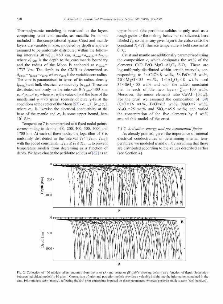
Fig. 2. Collection of 100 models taken randomly from the prior (A) and pbetween individual models is 10 g/cm3. Comparison of prior and posterior mdata. Prior models seem ‘messy’, reflecting the few prior constraints impose

upper bound (the peridotite solidus is only used as arough guide to the melting behaviour of silicates), herelabeled Tp, so that in any given layer k there also exists theconstraint Tk<Tk

p. Surface temperature is held constant at0 °C.

Crust and mantle are additionally parametrised usingthe composition c, which designates the wt.% of theelements CaO–FeO–MgO–Al2O3–SiO2. These arelog-uniformly distributed within certain intervals, cor-responding to 1<CaO<8 wt.%, 5<FeO<15 wt.%,20 <MgO < 55 wt.%, 1 < Al2O3 < 8 wt.% and35<SiO2<55 wt.% and with the added constraintthat in each of the two layers ∑ici=100 wt.%.Moreover, the minor elements ratio Ca/Al∈ [0.5;2].For the crust we assumed the composition of [39](CaO=16 wt.%, FeO=6.5 wt.%, MgO=7 wt.%,Al2O3=25 wt.% and SiO2=45.5 wt.%) and variedthe concentration of the five elements by 5 wt.%around this model of the crust.

7.1.2. Activation energy and pre-exponential factorAs already pointed, given the importance of mineral

electrical conductivities in determining internal tem-peratures, we modeled E and σo, by assuming that theseare distributed according to the values described earlier(see Section 4).

osterior (B) pdf 's showing density as a function of depth. Separationodels provides a valuable insight into the information contained in thed on these parameters, whereas posterior models seem ‘well behaved’.


For the major mineral phases ol, opx, cpx, gt and plg,we assumed the values of E and σo described in Section4 and varied these uniformly by amounts ±ΔE and±Δσo, corresponding to the uncertainty estimates alsoquoted in Section 4. In other words prior information onthese parameters is described by a uniform distributionin the interval [E−ΔE; E+ΔE] and [σo−Δσo; σo

+Δσo].

7.1.3. Mineralogy, density and bulk electricalconductivity

From a knowledge of composition, temperature andpressure we can use free energy minimisation to obtainthe mineral phases that are stable at these conditions aswell as its physical properties, in the form of thedensity and electrical conductivity. These parameterswere evaluated at 31 fixed radial nodes from thesurface down to the CMB using the followingparametrization. Layers 1 and 2 are 5 km thick, layers3–7 are 10 km thick, while the remaining layersthicknesses are 50 km. In sampling density profiles, weintroduced a penalty function to ensure that the

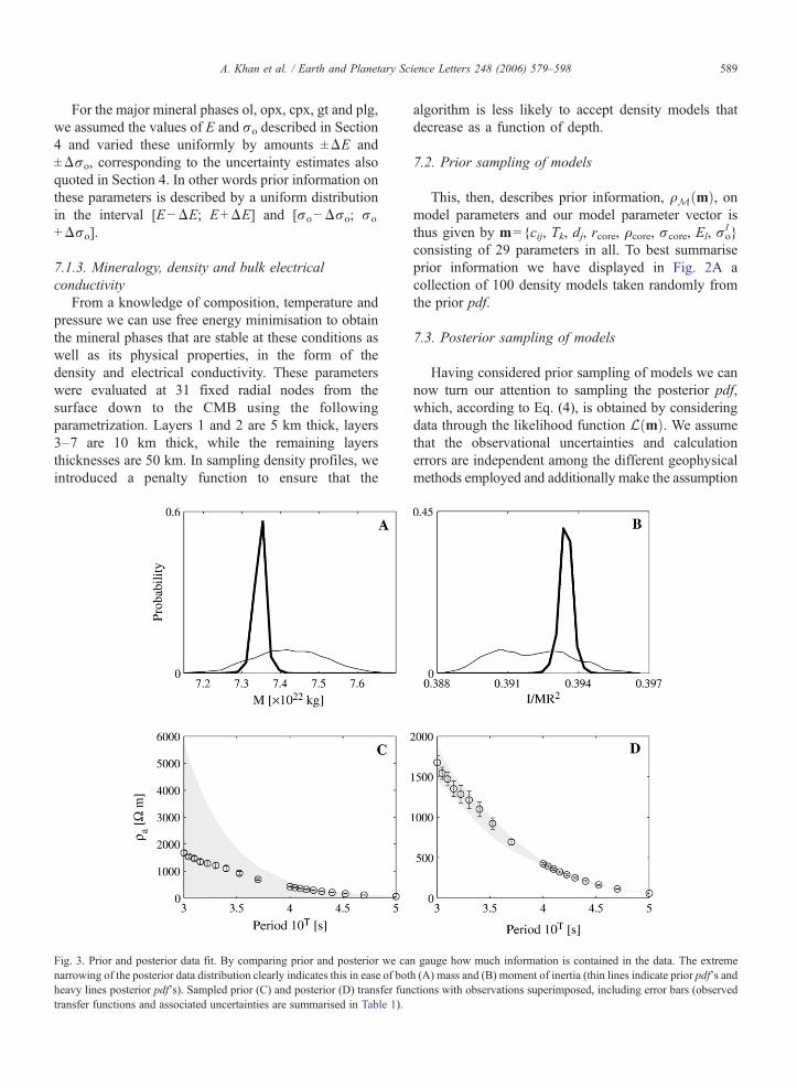
Fig. 3. Prior and posterior data fit. By comparing prior and posterior we canarrowing of the posterior data distribution clearly indicates this in ease of botheavy lines posterior pdf's). Sampled prior (C) and posterior (D) transfer funtransfer functions and associated uncertainties are summarised in Table 1).

algorithm is less likely to accept density models thatdecrease as a function of depth.

7.2. Prior sampling of models

This, then, describes prior information, qMðmÞ, onmodel parameters and our model parameter vector isthus given by m={cij, Tk, dj, rcore, ρcore, σcore, El, σo

l }consisting of 29 parameters in all. To best summariseprior information we have displayed in Fig. 2A acollection of 100 density models taken randomly fromthe prior pdf.

7.3. Posterior sampling of models

Having considered prior sampling of models we cannow turn our attention to sampling the posterior pdf,which, according to Eq. (4), is obtained by consideringdata through the likelihood function LðmÞ. We assumethat the observational uncertainties and calculationerrors are independent among the different geophysicalmethods employed and additionally make the assumption

n gauge how much information is contained in the data. The extremeh (A) mass and (B) moment of inertia (thin lines indicate prior pdf's andctions with observations superimposed, including error bars (observed

Fig. 4. Prior (black) and posterior (white) marginal pdf's for the oxide elements in the CFMAS system (marked to the right of each panel) making upthe mantle composition. Note that as we are not plotting the logarithm of the individual parameters, we do not obtain homogeneous distributions, butones that are skewed.

Fig. 5. Marginal prior (left panel) and posterior (right panel) pdf 's depicting sampled temperature models as a function of depth from the surface to thecore mantle boundary (CMB). At the 6 fixed depth nodes a histogram reflecting the marginal probability distribution of sampled temperatures hasbeen set up. By lining up these marginals, temperature as a function of depth can be envisioned as contours directly relating its probability ofoccurrence. Shades of gray between white and black indicating, respectively, least and most probable outcomes. Solid lines indicate the temperaturebounds obtained by Hood et al. [12] using pyroxenes containing 6.8 wt.% Al2O3 and dashed lines are for pyroxenes with 1.9 wt.% Al2O3.



that data uncertainties can be modeled using a Gaussiandistribution. With this in mind, the likelihood functiontakes the following form

L mð Þ~exp

�Xi

½dqaobs;i � dqacal;iðmÞ�22s2i

� ½dMobs � dMcal ðmÞ�22s2M

� ½dIobs � dIcalðmÞ�22s2I

�ð13Þ

where dobs denotes observed data, dcal(m) is synthetic datacomputed usingmodelmwith superscripts alluding to theparticular geophysical observation and s is the uncertaintyon either of these.

We are now in the position to actually run theMetropolis-Hastings algorithm. Let us assume that weare currently residing at point mi in the model space.From here we wish to make a transition to theneighbouring point mj. This is done in the followingmanner. In a given iteration we start off by choosing ashell at random, that is, either the crust, mantle or core,and then randomly change the parameters describing

Fig. 6. Marginal posterior pdf 's of major minerals, showing the vol.% of emarginals have been constructed in the same manner as in Fig. 5. Shades of

this shell, using the proposal (prior) distribution justdiscussed. The adopted proposal distribution has a burn-in time of about 1000 iterations. Once this point hasbeen reached we retain samples for analysis. In all wesampled 1 million models from which we retained 104.The overall acceptance rate was about 40%.

There are a number of technical issues, concerningthe Metropolis-Hastings algorithm which have not beenmentioned. These include the question of whenconvergence has been reached, how many samples areneeded and the problem of acquiring independentsamples. To ensure convergence of the MCMCalgorithm we monitored the time series of all outputparameters from the algorithm. We also chose differentinitial conditions in the model space (different startingcompositions) and compared the results from thesedifferent runs to verify that the algorithm converged tosimilar likelihood values. Concerning the number ofsamples that are needed to provide a good representationof the posterior pdf, we adopted the criterion that oncethere are no longer any significant changes to the

ach phase as a function of depth from the surface to the CMB. Thegray as in Fig. 5.


characteristics of the posterior pdf we have sampled anadequate number. To ensure near-independent samples,we introduced an ‘elapse time’ between retention ofsamples. By analysing the autocorrelation function ofthe fluctuations of the likelihood function we found anelapse time of 100.

Fig. 2B shows a collection of 100 density modelstaken randomly from the posterior pdf. A directcomparison with the prior models (Fig. 2A) providesus with an indication of those structures in the Moon thatare well resolved and those that are ill resolved. Well-resolved structures are those that tend to appearfrequently, whereas ill-resolved structures tend to appearinfrequently.

8. Results

Our model of the Moon assumes spherical symmetry,obviating the consideration of heterogeneity. Althoughthe Moon is thought to be heterogeneous, especially asconcerns crustal structure [68], this will not seriouslyaffect our results as the contribution of the crust to theelectromagnetic induction signal is almost negligiblegiven the low temperatures in this part of the Moon.Moreover, as remarked by Herbert et al. [69], to furtherconstrain the shallow structure (depths<450 km),additional measurements at higher frequency areneeded.

Fig. 7. Marginal prior (left panel) and posterior (right panel) pdf 's depictinsurface to the CMB. Log signifies base 10 logarithm. Shades of gray as beHood et al. [12].

8.1. Predicted data

Fig. 3 shows prior and posterior distributions ofcalculated data from which we can see that excellentdata fits are obtained.

8.2. Composition and thermal state

Fig. 4 displays composition c for the mantle in theform of 1D prior and posterior marginals, showing that cis being constrained by data (we are presently onlyconcerned with the mantle as crustal stucture is not wellconstrained by the data). Temperature models are shownin Fig. 5 using 1D marginal prior and posterior pdf's.Like c, the posterior marginals for T are also seen to besignificantly narrowed, signaling that inversion of thedata considered here are able to provide information oncomposition and thermal state.

From Fig. 5 we can see that while our thermalprofiles are broadly in agreement with previous work[12,15,17], most probable temperatures in the lowermantle are slightly lower than earlier results. This isprobably due to the higher activation energy of opx asdetermined recently [20] in comparison to previousinvestigations [15,48], which, as discussed in Section 4,is related to the higher alumina content and results in ahigher conductivity of the pyroxenes. The inferredtemperatures are well below the probable solidus

g sampled bulk conductivity profiles as a function of depth from thefore. Solid gray lines indicate the bounds on conductivity derived by

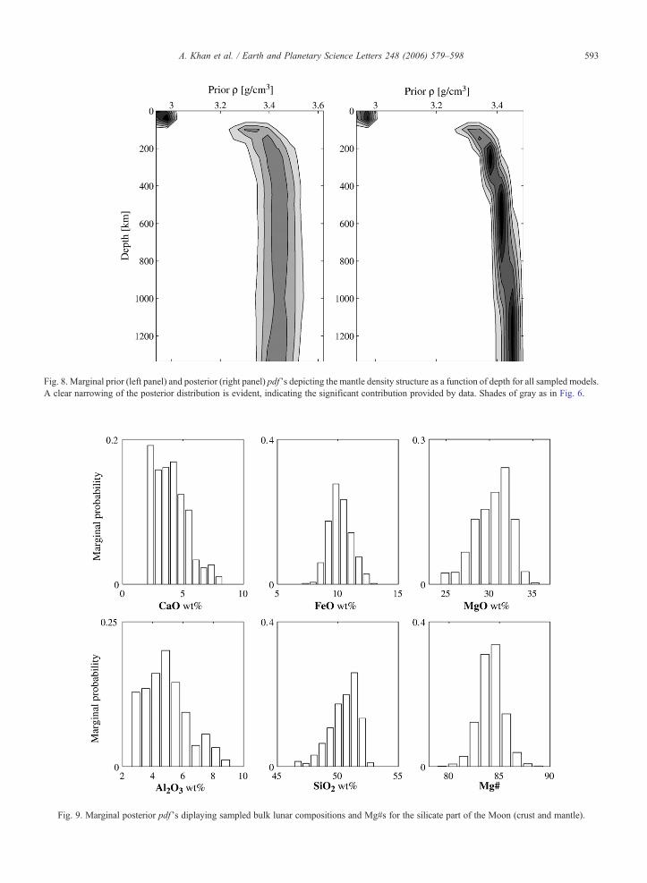
Fig. 9. Marginal posterior pdf 's diplaying sampled bulk lunar compositions and Mg#s for the silicate part of the Moon (crust and mantle).

Fig. 8. Marginal prior (left panel) and posterior (right panel) pdf 's depicting the mantle density structure as a function of depth for all sampled models.A clear narrowing of the posterior distribution is evident, indicating the significant contribution provided by data. Shades of gray as in Fig. 6.



condition at a depth of 1000 km, in accord with seismicevidence for a rigid lunar mantle (for discussions ofthese and other geophysical evidence on mantle thermalevolution and present-day state the reader is referred toe.g. [70,73]).

8.3. Mantle mineralogy and physical properties

Mineral phases and derived bulk physical properties,in the form of density and conductivity profiles areshown in Figs. 6–8. Again, when compared to previousinvestigations of lunar electrical conductivity structure,our results are in overall agreement. As already noted,previous investigations found conductivity to increasefrom 10− 4–10− 3 S/m at a few hundred km depth toroughly 10− 2–10− 1 S/m at about 1100 km depth (e.g.[17]). Lunar density profiles have only been constrainedby indirect means, such as mass and moment of inertiaconsiderations [66] as well as in combination with the

Fig. 10. Marginal posterior pdf 's showing sampled bulk lunar compositions athe Apollo lunar seismic data in combination with mass and moment of inertiawith the results presented here (Fig. 9). Upward and downward pointing arrWarren [75] and Kuskov and Kronrod [72] (model II), respectively, while croMcDonough and Sun [76].

constraints provided by derived seismic P and S-wavevelocity profiles (e.g. [71,72,57]). Although modeldependent Kuskov et al. [57] obtained the followingdensity ranges for the mantle 3.22–3.34 g/cm3 (60–300 km depth), 3.29–3.44 g/cm3 (300–500 km depth)and 3.34–3.52 g/cm3 (500 km-core mantle boundary),which are generally in accordance with the mantledensities obtained here.

8.4. Bulk composition and Mg#

Bulk sampled compositions and Mg#s for the silicatepart of the Moon, i.e. crust and mantle, are displayed inthe histograms in Fig. 9. In support of our results, weobserve that independent inversion of the Apollo lunarseismic data [73] yields bulk lunar compositions (Fig.10) that are largely consistent with those obtained here.

A certain care, of course, has to be exercised whendrawing inferences from this sort of modeling, involving

nd Mg#s for the silicate part of the Moon, obtained from an inversion of[73,74]. The obtained distributions are seen to be in overall agreementows indicate for comparison bulk compositional estimates derived bysses denote bulk composition of the Earth's upper mantle estimated by

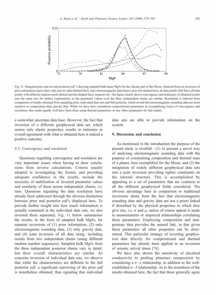
http://dx.doi.org/10.1029/2005JE002608

http://dx.doi.org/10.1029/2005JE002608

Fig. 11. Marginal prior and several posterior pdf 's showing sampled bulk lunar Mg#s for the silicate part of the Moon, obtained from an inversion ofprior information (gray line), only gravity data (dashed line), only electromagnetic data (heavy gray dot-dashed line), all data jointly (full line), all datajointly with different random seeds (dotted and dot-dashed line), respectively. The figure clearly shows convergence and stationary of obtained results(see the main text for further explanation), as the parameter values over the three independent chains are similar. Resolution is inferred fromcomparison of results obtained from sampling prior, individual data sets and full posterior, which reveal that electromagnetic sounding data are moresensitive to composition than gravity data. While we have here considered compositional parameters in exemplifying issues of convergence andresolution, this could equally well have been done using thermal parameters or any other parameters for that matter.


a somewhat uncertain data base. However, the fact thatinversion of a different geophysical data set, whichsenses only elastic properties, results in estimates inoverall agreement with what is obtained here is indeed apositive outcome.

8.5. Convergence and resolution

Questions regarding convergence and resolution arevery important issues when having to draw conclu-sions from inverse calculations. Criteria usuallyadopted in investigating the former, and providingadequate confidence in the results, include thenecessity of stabilisation of inverted parameter valuesand similarity of these across independent chains, i.e.runs. Questions regarding the data resolution havealready been addressed through the obvious distinctionbetween prior and posterior pdf's displayed here. Toprovide further insight into how much information isactually contained in the individual data sets, we alsoinverted these separately. Fig. 11 below summarisesthe results, in the form of sampled bulk Mg#s, forseparate inversions of (1) prior information, (2) onlyelectromagnetic sounding data, (3) only gravity data,and (4) joint inversion of all data using, includingresults from two independent chains (using differentrandom number sequences). Sampled bulk Mg#s fromthe three independent posterior chains vary in detail,but their overall characteristics are similar. Asconcerns inversion of individual data sets, we observethat while the characteristics are different to the fullposterior pdf, a significant narrowing of the prior pdfis nonetheless obtained, thus signaling that individual

data sets are able to provide information on thesystem.

9. Discussion and conclusion

As mentioned in the introduction the purpose of thepresent study is twofold—(1) to present a novel wayof analysing electromagnetic sounding data with thepurpose of constraining composition and thermal stateof a planet, here exemplified for the Moon, and (2) theintegration of widely different geophysical data setsinto a joint inversion providing tighter constraints onthe internal structure. This is accomplished byappealing to a set of parameters that are common toall the different geophysical fields considered. Theobvious advantage here in comparison to traditionalinversions stems from the fact that electromagneticsounding data and gravity data are not a priori linkedif described by the physical properties to which theygive rise, i.e. σ and ρ, unless of course appeal is madeto measurements or empirical relationships correlatingthese parameters. Employing composition and tem-perature thus provides the natural link, in that giventhese parameters all other properties can be deter-mined. This particular strategy of inverting geophys-ical data directly for compositional and thermalparameters has already been applied in an inversionof seismic arrival times [74].

We have also shown the sensitivity of electricalconductivity to probing planetary composition byconsidering a σ–x relationship, in addition to the well-established σ–T relationship. As to the soundness of theresults obtained here, the fact that these generally agree


with electrical conductivity and thermal profiles derivedearlier, provides some confidence in the overallcorrectness of what has been undertaken here. Also, insupport of our results, we observed that independentinversion of the Apollo lunar seismic data [73,74],yields bulk lunar compositions that are largely consis-tent with those presented here. However, as the resultsare directly influenced by the available laboratoryelectrical conductivity data, it has to be stressed, thatwell-constrained laboratory measurements of relevantphases are necessary in order to carefully characterisethe contributions made by individual phases to the bulkelectrical conductivity profile. It is accordingly our hopethat future laboratory electrical conductivity measure-ments will not only include more relevant minerals, suchas pyrope and almandine, but will, given that electricalconductivity varies significantly as a function of thecomposition of individual minerals, also includemeasurements of systematics.

In summary, the approach presented here of jointlyinverting electromagnetic sounding and gravity data toconstrain composition and thermal state is feasible andits advantage consists in confronting compositionaland thermal parameters directly with geophysicalobservations and as such is a step beyond thetraditional geophysical sequence of first performingfield measurements followed by interpretations basedon laboratory results.

Acknowledgements

The authors would like to thank three anonymousreviewers for comments that improved the manuscript.A. Khan gratefully acknowledges financial support fromthe Carlsberg Foundation.

References

[1] M.N. Toksijz, S.C. Solomon, Thermal history and evolution ofthe moon, Moon 7 (1973) 251.

[2] G. Schubert, R.E. Young, P. Cassen, Subsolidus convectionmodels of the lunar internal temperature, Philos. Trans. R. Soc.Lond., A 285 (1977) 523.

[3] M.N. Toksijz, A.T. Hsui, D.H. Johnston, Thermal evolutions ofthe terrestrial planets, Moon Planets 18 (1978) 281.

[4] A.B. Binder, M. Lange, On the thermal history, thermal state, andrelated teetonism of a Moon of fission origin, J. Geophys. Res. 85(1980) 3194.

[5] T. Spohn, W. Konrad, D. Breuer, R. Ziethe, The longevity oflunar volcanism: implications of thermal evolution calculationswith 2D and 3D mantle convection models, Icarus 149 (2000)54.

[6] M.G. Langseth, S.J. Keihm, K. Peters, Revised lunar heat-flowvalues, in: Proc. Lunar Planet. Sci. Conf. 7th, 1976, p. 3143.

[7] Y. Nakamura, J. Koyama, Seismic Q of the lunar upper mantle, J.Geophys. Res. 87 (1982) 4855.

[8] S. Pullan, K. Lambeek, On constraining lunar mantle tempera-tures from gravity data, in: Proc. Lunar Planet. Sci. Conf. 11th,1980, p. 2031.

[9] C.P. Sonett, B.F. Smith, D.S. Colburn, G. Schunbert, K.Schwartz, The induced magnetic field of the moon: conductivityprofiles and inferred temperature, in: Proc. Lunar Planet. Sci.Conf. 3rd, 1972, p. 2309.

[10] P. Dyal, C.W. Parkin, W.D. Daily, Structure of the lunar interiorfrom magnetic field measurements, in: Proc. Lunar Planet. Sci.Conf. 7th, 1976, p. 3077.

[11] M.J. Wiskerchen, C.P. Sonett, A lunar metal core? in: Proc.Lunar. Planet. Sci. Conf. 8th, 1977, p. 515.

[12] L.L. Hood, F. Herbert, C.P. Sonett, The deep lunar electricalconductivity profile: structural and thermal inferences, J.Geophys. Res. 87 (1982) 5311.

[13] C.P. Sonett, A. Duba, Lunar temperature and global heat fluxfrom laboratory electrical conductivity and lunar magnetometerdata, Nature 258 (1975) 118.

[14] A. Duba, H.C. Heard, R.N. Schock, Electrical conductivity oforthopyroxene to 1400 °C and the resulting selenotherm, in:Proc. Lunar. Planet. Sci. Conf. 7th, 1976, p. 3173.

[15] J.S. Huebner, L.B. Wiggins, A. Duba, Electrical conductivity ofpyroxene which contains trivalent cations—laboratory measure-ments and the lunar temperature profile, J. Geophys. Res. 84(1979) 4652.

[16] L.L. Hood, F. Herbert, C.P. Sonett, Further efforts to limit lunarinternal temperatures from electrical conductivity determina-tions, J. Geophys. Res. 87 (1982) A109 (Suppl.).

[17] L.L. Hood, C.P. Sonett, Limits on the lunar temperature profile,Geophys. Res. Lett. 9 (1982) 37.

[18] T.J. Shankland, A. Duba, Standard electrical conductivity ofisotropic, homogeneous olivine in the temperature range 1200–1500 °C, Geophys. J. Int. 103 (1990) 25.

[19] A. Kavner, L. Xiaoyuan, R. Jeanloz, Electrical conductivity of anatural (Mg, Fe)SiO3 majorite garnet, Geophys. Res. Lett. 22(1995) 3103.

[20] Y. Xu, T.J. Shankland, Electrical conductivity of orthopyroxeneand its high pressure phases, Geophys. Res. Lett. 26 (1999) 2645.

[21] Y. Xu, T.J. Shankland, A. Duba, Pressure effect on electricalconductivity of mantle olivine, Phys. Earth Planet. Inter. 118(2000) 149.

[22] Y. Xu, T.J. Shankland, B.T. Poe, Laboratory-based electricalconductivity in the Earth's mantle, J. Geophys. Res. 108 (2000)2314.

[23] J. Ducruix, V. Courtillot, J. Le Mouel, The late 1960's secularvariation impulse, the eleven year magnetic variation, and theelectrical conducitivity of the deep mantle, Geophys. J. R.Astron. Soc. 61 (1980) 73.

[24] S.C. Constable, Constraints on mantle electrical conductivityfrom field and laboratory measurements, J. Geomagn. Geoelectr.45 (1993) 707.

[25] N. Olsen, The electrical conductivity of the mantle beneathEurope derived from C-responses from 3 to 720 hr, Geophys. J.Int. 133 (1998) 298.

[26] A. Tarantola, B. Valette, Inverse problems: quest for information,J. Geophys. 50 (1982) 159.

[27] A. Tarantola, Inverse Problem Theory and Model ParameterEstimation, SIAM, Philadelphia, USA, 2004.

[28] K. Mosegaard, A. Tarantola, Monte Carlo sampling of solutionsto inverse problems, J. Geophys. Res. 100 (1995) 12431.

http://dx.doi.org/10.1029/2005JE002608


[29] K. Mosegaard, Resolution analysis of general inverse problemsthrough inverse Monte Carlo sampling, Inverse Probl. 14 (1998)405.

[30] K. Mosegaard, M. Sambridge, Monte Carlo analysis of inverseproblems, Inverse Probl. 18 (2002) 29.

[31] R.J. Phillips, The lunar conductivity profile and the nonunique-ness of electromagnetic data inversion, Icarus 17 (1972) 88.

[32] B.A. Hobbs, The inverse problem of the moon's electricalconductivity, Earth Planet. Sci. Lett. 17 (1973) 380.

[33] B.A. Hobbs, The electrical conductivity of the moon: anapplication of inverse theory, Geophys. J. R. Astron. Soc. 51(1977) 727.

[34] B.A. Hobbs, L.L. Hood, F. Herbert, C.P. Sonett, An upper boundon the radius of a highly electrically conducting lunar core, J.Geophys. Res. 88 (1983) B97 (Suppl.).

[35] C.P. Sonett, Electromagnetic induction in the moon, Rev.Geophys. Space Phys. 20 (1982) 411.

[36] L.L. Hood, Geophysical constraints on the interior of the Moon,in: W.K. Hartmann, R.J. Phillips, G.J. Taylor (Eds.), Origin of theMoon, LPI, Houston, 1986, p. 361.

[37] A.E. Ringwood, E. Essene, Petrogenesis of the Apollo 11 basalts,internal constitution and origin of the Moon, in: Proc. Apollo 11Lunar Sci. Conf., 1, 1970, p. 769.

[38] A. Duba, M. Dennison, A.J. Irving, C.R. Thornber, J.S. Huebner,Electrical conductivity of aluminous orthopyroxene, LunarPlanet. Sci. X, Abstract, 1979, p. 318.

[39] S.R. Taylor, Planetary Science: A Lunar Perspective, LPI,Houston, 1982.

[40] M.A. Wieczorek, M.T. Zuber, The composition and origin of thelunar crust: constraints from central peaks and crustal thicknessmodeling, Geophys. Res. Lett. 28 (2001) 4023.

[41] P.H. Warren, The magma ocean concept and lunar evolution,Annu. Rev. Earth Planet. Sci. 13 (1985) 201.

[42] S.E. Kesson, A.E. Ringwood, Mare basalt petrogenesis in adynamic moon, Earth Planet. Sci. Lett. 30 (1976) 155.

[43] Y. Nakamura, Farside deep moonquakes and deep interior ofthe Moon, J. Geophys. Res. 110 (E1) (2005), doi:10.1029/2004JE002332.

[44] A. Khan, K. Mosegaard, An inquiry into the lunar interior: a non-linear inversion of the Apollo lunar seismic data, J. Geophys.Res. 107 (E6) (2002), doi:10.1029/2001JE001658.

[45] P. Lognonné, J. Gagnepain-Beyneix, H. Chenet, A new seismicmodel of the Moon: implications for structure, thermal evolutionand formation of the Moon, Earth Planet. Sci. Lett. 211 (2003)27.

[46] A. Duba, Are laboratory electrical conductivity data relevant tothe Earth? Acta Geod. Geophys. Montan. Acad. Sci. Hung.Tomus 11 (1976) 485.

[47] S.C. Constable, A. Duba, The electrical conductivity of olivine, adunite, and the mantle, J. Geophys. Res. 95 (1990) 6967.

[48] A. Duba, J.N. Boland, A.E. Ringwood, The electrical conduc-tivity of pyroxene, J. Geol. 81 (1973) 727.

[49] J.A. Tyburczy, D.K. Fisler, Electrical properties of minerals andmelts, in: T.J. Ahrens (Ed.), Mineral Physics and Crystallogra-phy: A Handbook of Physical Constants, AGU,Washington, DC,1995, p. 185.

[50] A. Duba, H.C. Heard, R.N. Schock, Electrical conductivity ofolivine at high pressure and under controlled oxygen fugacity, J.Geophys. Res. 79 (1974) 1667.

[51] M. Sato, Oxygen fugacity and other thermochemical parametersof Apollo 17 high-Ti basalts, in: Proc. Lunar Planet. Sci. Conf.7th, 1976, p. 1323.

[52] J.W. Delano, Redox state of the Moon's interior, Oxygenin the Terrestrial Planets, Abstract# 3008, LPI, Houston,2004.

[53] L.T. Elkins, V.A. Fernandez, W.W. Delano, T.L. Grove, Originof lunar ultramafic green glasses: constraints from phaseequilibrium studies, Geochim. Cosmochim. Acta 64 (2000)2339.

[54] Y. Nakamura, D. Lammlein, G.V. Latham, M. Ewing, J. Dorman,F. Press, M.N. Toksöz, New seismic data on the state of the deeplunar interior, Science 181 (1973) 49.

[55] N. Metropolis, A.W. Rosenbluth, M.N. Rosenbluth, A.H. Teller,E. Teller, Equation of state calculations by fast computingmachines, J. Chem. Phys. 21 (1995) 1087.

[56] W.K. Hastings, Monte Carlo sampling methods using Markovchains and their applications, Biometrika 57 (1973) 97.

[57] O.L. Kuskov, V.A. Kronrod, L.L. Hood, Geochemical constraintson the seismic properties of the lunar mantle, Phys. Earth Planet.Inter. 134 (2002) 175.

[58] D.P. Dobson, J.P. Brodholt, The electrical conductivity andthermal profile of the Earth's mid-mantle, Geophys. Res. Lett. 27(2000) 2325.

[59] J.A.D. Connolly, Computation of phase equilibria by linearprogramming: a tool for geodynamic modeling and an applica-tion to subduction zone decarbonation, Earth Planet. Sci. Lett.236 (2005) 524.

[60] T.J.B. Holland, R. Powell, An internally consistent thermody-namic data set for phases of petrological interest, J. Metamorph.Geol. 16 (1998) 309.

[61] B.J. Wood, J.R. Holloway, A thermodynamic model forsubsolidus equilibria in the system CaO–MgO–Al2O3–SiO2,Geochim. Cosmochim. Acta 66 (1984) 159.

[62] J.G. Berryman, Mixture theories for rock properties, in: T.J.Ahrens (Ed.), American Geophysical Union Handbook ofPhysical Constants, AGU, Washington, DC, 1995, p. 205.

[63] U. Schmucker, Magnetic and electric fields due to electromag-netic induction by external sources, Landolt-Bornstein, New-Series, 5/2b, Springer-Verlag, Berlin, 1985, p. 100.

[64] W.D. Parkinson, V.R.S. Hutton, The electrical conductivity of theEarth, in: J.A. Jacobs (Ed.), Geomagnetism, vol. 3, AcademicPress, London, 1989, p. 261.

[65] M.A. Wieczorek, B.L. Jolliff, J.J. Gillis, L.L. Hood, K. Righter,A. Khan, M.E. Pritchard, B.P. Weiss, S. Thompkins, J.G.Williams, The constitution and structure of the lunar interior, inNew Views of the Moon, in press.

[66] A. Konopliv, A.B. Binder, L.L. Hood, A.B. Kucinskas, W.L.Sjögren, J.G. Williams, Improved gravity field of the moon fromlunar prospector, Science 281 (1998) 1476.

[67] M. Hirschmann, Mantle solidus: experimental constraints and theeffects of peridotite composition, Geochem. Geophys. Geosyst. 1(2000), doi:10.1029/2000GC000070.

[68] B.L. Jolliff, J.J. Gillis, L.A. Haskin, R.L. Korotev, M.A.Wieczorek, Major crustal terranes: surface expressions andcrust–mantle origins, J. Geophys. Res. 105 (2000) 4197.

[69] F. Herbert, L.D. Smith, L.L. Hood, C.P. Sonett, Waves in theEarth's magnetosheath, the high frequency electromagneticresponse of the Moon and the shallow (150–250 km depth)lunar electrical conductivity profile, Lunar Planet. Sci. XIII(1982) 321.

[70] M.E. Pritchard, D.J. Stevenson, Thermal aspects of a lunarorigin by giant impact, in: R.M. Canup, K. Righter (Eds.),Origin of the Earth and Moon, Arizona University Press,Arizona, 2000, p. 179.

http://dx.doi.org/10.1029/2004JE002332

http://dx.doi.org/10.1029/2004JE002332

http://dx.doi.org/10.1029/2001JE001658

http://dx.doi.org/10.1029/2000GC000070


[71] L.L. Hood, J.H. Jones, Geophysical constraints on lunar bulkcomposition and structure: a reassessment, J. Geophys. Res. 92(1987) 396.

[72] O.L. Kuskov, V.A. Kronrod, Constitution of the Moon: 5.Constraints on density, temperature and radius of a core, Phys.Earth Planet. Inter. 107 (1998) 285.

[73] A. Khan, J. Maclennan, S.R. Taylor, J.A.D. Connolly, Are theEarth and the Moon compositionally alike?-Inferences on lunarcomposition and implications for lunar origin and evolution fromgeophysical modeling, J. Geophys. Res. 111 (2006) EO5005,doi:10.1029/2005JE002608.

[74] A. Khan, J.A.D. Connolly, J. Maclennan, K. Mosegaard, Jointinversion of gravity and seismic data for lunar composition andthermal state, Geophys. J. Int. (in press).

[75] P.H. Warren, “New” lunar meteorites: II. Implications forcomposition of the global lunar surface, lunar crust, and thebulk Moon, Meteorit. Planet. Sci. 40 (2005) 1.

[76] W.F. McDonough, S.S. Sun, The composition of the Earth,Chem. Geol. 120 (3–4) (1995) 223.

Constraining the composition and thermal state of the moon ...

Documents

Transcript of Constraining the composition and thermal state of the moon ...