Citation: Zhang, Z.; Chatterjee, A.;

Ott, L.; Reichle, R.; Feldman, A.F.;

Poulter, B. Effect of Assimilating

SMAP Soil Moisture on CO2 and CH4

Fluxes through Direct Insertion in a

Land Surface Model. Remote Sens.

2022, 14, 2405. https://doi.org/

10.3390/rs14102405

Academic Editor: Gabriel Senay

Received: 17 March 2022

Accepted: 13 May 2022

Published: 17 May 2022

Publisher’s Note: MDPI stays neutral

with regard to jurisdictional claims in

published maps and institutional affil-

iations.

Copyright: © 2022 by the authors.

Licensee MDPI, Basel, Switzerland.

This article is an open access article

distributed under the terms and

conditions of the Creative Commons

Attribution (CC BY) license (https://

creativecommons.org/licenses/by/

4.0/).

remote sensing

Article

Effect of Assimilating SMAP Soil Moisture on CO2 and CH4Fluxes through Direct Insertion in a Land Surface ModelZhen Zhang 1,* , Abhishek Chatterjee 2,3,† , Lesley Ott 2, Rolf Reichle 2 , Andrew F. Feldman 4

and Benjamin Poulter 4

1 Earth System Science Disciplinary Center, University of Maryland, College Park, MD 20740, USA2 Global Modeling and Assimilation Office, NASA Goddard Space Flight Center, Greenbelt, MD 20771, USA;

abhishek.chatterjee@jpl.nasa.gov (A.C.); lesley.e.ott@nasa.gov (L.O.); rolf.reichle@nasa.gov (R.R.)3 Universities Space Research Association, Columbia, MD 20771, USA4 Biospheric Sciences Laboratory, NASA Goddard Space Center, Greenbelt, MD 20771, USA;

andrew.feldman@nasa.gov (A.F.F.); benjamin.poulter@nasa.gov (B.P.)* Correspondence: zzhang88@umd.edu† Current address: NASA Jet Propulsion Laboratory, California Institute of Technology,

Pasadena, CA 91326, USA.

Abstract: Soil moisture impacts the biosphere–atmosphere exchange of CO2 and CH4 and plays animportant role in the terrestrial carbon cycle. A better representation of soil moisture would improvecoupled carbon–water dynamics in terrestrial ecosystem models and could potentially improvemodel estimates of large-scale carbon fluxes and climate feedbacks. Here, we investigate using soilmoisture observations from the Soil Moisture Active Passive (SMAP) satellite mission to informsimulated carbon fluxes in the global terrestrial ecosystem model LPJ-wsl. Results suggest that thedirect insertion of SMAP reduces the bias in simulated soil moisture at in situ measurement sitesby 40%, with a greater improvement at temperate sites. A wavelet analysis between the model andmeasurements from 26 FLUXNET sites suggests that the assimilated run modestly reduces the biasof simulated carbon fluxes for boreal and subtropical sites at 1–2-month time scales. At regionalscales, SMAP soil moisture can improve the estimated responses of CO2 and CH4 fluxes to extremeevents such as the 2018 European drought and the 2019 rainfall event in the Sudd (Southern Sudan)wetlands. The simulated improvements to land–surface carbon fluxes using the direct insertion ofSMAP are shown across a variety of timescales, which suggests the potential of SMAP soil moisturein improving the model representation of carbon–water coupling.

Keywords: data assimilation; land surface model; methane; remote sensing; dynamics global vegetationmodel

1. Introduction

Soil moisture plays a critical role in controlling interactions between the soil, vegetation,and atmosphere, and is one of the major drivers that affects the carbon fluxes of terrestrialecosystems [1]. Because of the coupling between water and carbon fluxes at the leaf level,soil moisture is a major constraint for the assimilation of carbon by vegetation throughphotosynthesis [2]. Soil moisture is the dominant driver of dryness stress on ecosystemproduction across more than 70% of vegetated land areas [3]. The spatial and temporalvariations in soil moisture strongly affect the terrestrial carbon uptake [4]. Meanwhile, soilmoisture serves as a proxy for water table depth, a variable that regulates the soil redox statefor microbes to favor methanogenesis, which is used to determine the time and locationof inundated areas at a regional scale that can significantly affect the estimate of methane(CH4) flux [5]. Therefore, it is essential to understand the spatio-temporal distribution ofsoil moisture and its role in influencing terrestrial carbon fluxes in a warming climate.

Understanding the influence of soil moisture on terrestrial carbon fluxes is challengingbecause of the large uncertainty in the spatio-temporal distributions of soil moisture, which

Remote Sens. 2022, 14, 2405. https://doi.org/10.3390/rs14102405 https://www.mdpi.com/journal/remotesensing

Remote Sens. 2022, 14, 2405 2 of 25

is due to both its high spatial heterogeneity and uncertainty in characterizing surfaceproperties. A common approach to estimate soil moisture is through land surface modelsimulations driven with surface meteorological forcing data from observations or atmo-spheric reanalysis systems. This approach depends on the appropriate parameterization ofhydraulic parameters and soil texture [6], model structure, and external forcings from themeteorological datasets. These models can produce vast differences in soil moisture evenwith the same forcings [7]. Previous studies have explored the impact of soil moisture onpast and future CO2 fluxes using prognostic models [1,4,8–11]. These studies show thatthe influence of soil moisture on carbon fluxes is still affected by bias and remains unclear,given the various sources of uncertainty that prevail in the models [12–14].

Satellite observations of soil moisture have become increasingly available during thepast decade and provide much needed information at the global scale [15–20]. These soilmoisture observations are based on radar (active) or radiometer (passive) measurementsof low-frequency microwave signals. The European Space Agency’s Soil Moisture OceanSalinity (SMOS; [21]) mission and the NASA Soil Moisture Active Passive (SMAP; [22])missions were specifically designed for measuring soil moisture, and both carry L-bandradiometers (1.41 GHz). Compared to C- and X-band data from sensors such as theAdvanced Scatterometer (ASCAT), L-band measurements have the advantage of deeperpenetration through vegetation canopies and into the soil, leading to a higher accuracy ofthe soil moisture signals received [18,23]. A recent comprehensive evaluation of satellite-and model-based soil moisture products suggests that SMAP outperforms other satellite-based datasets when compared to in situ soil moisture measurements [24]. Future satellitemissions, such as NASA Surface Water and Ocean Topography (SWOT) and NASA-ISROSAR (NISAR), will continue to improve the monitoring and understanding of soil moisture.

Assimilating satellite-based observations of soil moisture into terrestrial carbon cyclemodels provides a potential opportunity to reduce the uncertainty of carbon flux estimates.Data assimilation approaches have previously been applied to integrate soil moistureobservations into the models over different climatological and hydrological environments.Past data assimilation studies have primarily focused on improving hydrologic modelingby addressing seasonal dynamics [25–28]. The NASA SMAP Level 4 Carbon product(L4_C Version4, Greenbelt MD, USA) provides estimates of net ecosystem CO2 exchange(NEE) from a simple terrestrial carbon flux model constrained with the SMAP Level 4 soilmoisture data assimilation product [29]. Surprisingly, few studies have investigated thepotential of directly assimilating information from satellite soil moisture observations into aterrestrial ecosystem model with full water–carbon coupling at the global scale to constrainthe simulated CO2 fluxes, and we are not aware of any such studies investigating CH4fluxes. For example, the author of [30] demonstrates that the assimilation of soil moistureobservations from SMOS has a high potential for reducing uncertainty in the gross and netCO2 fluxes, while [31] uses a direct insertion of a remote sensing-based Leaf Area Index toimprove several components of land surface. Recently, Ref. [32] simultaneously optimizedmodel parameters for CO2 concentration and model state for soil moisture by assimilatingSMOS soil moisture observations. These studies show potential to improve the modelingof carbon fluxes in a model–data fusion framework.

The objective of the present paper is to investigate whether modeled CO2 and CH4fluxes can be improved by constraining soil moisture using SMAP observations in theLPJ-wsl terrestrial ecosystem model [33,34]. We present evidence that assimilating SMAPobservations into a terrestrial ecosystem model yields significant benefits for the simulatedCO2 and CH4 fluxes at the global scale. In our feasibility study, we use the Level 3 GlobalDaily 36 km passive soil moisture retrievals from SMAP (L3SMPE Version 6, GreenbeltMD, USA) to adjust the LPJ-wsl model estimates whenever a SMAP observation is avail-able. We carry out a set of model sensitivity tests to evaluate the impact of assimilatingSMAP observations into different representative depths of the model soil moisture. Toevaluate the simulated soil moisture and CO2 fluxes, we use ground observations from theFLUXNET2015 [35] and FLUXNET-CH4 datasets [36]. Wavelet analysis [37,38] is applied

Remote Sens. 2022, 14, 2405 3 of 25

to evaluate the influence of SMAP data assimilation on the performance of modeled CO2and CH4 fluxes for wetland sites in the time–frequency domain. We also select two extremeclimatic events, a drought and a flood event, as examples to explore the implications ofSMAP data assimilation for carbon cycle research.

2. Materials and Methods2.1. LPJ-Wsl Terrestrial Ecosystem Model2.1.1. Hydrology Scheme

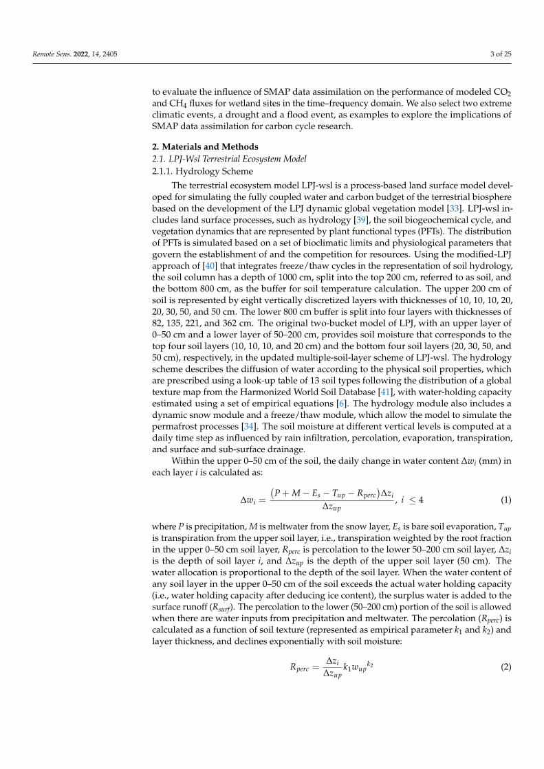
The terrestrial ecosystem model LPJ-wsl is a process-based land surface model devel-oped for simulating the fully coupled water and carbon budget of the terrestrial biospherebased on the development of the LPJ dynamic global vegetation model [33]. LPJ-wsl in-cludes land surface processes, such as hydrology [39], the soil biogeochemical cycle, andvegetation dynamics that are represented by plant functional types (PFTs). The distributionof PFTs is simulated based on a set of bioclimatic limits and physiological parameters thatgovern the establishment of and the competition for resources. Using the modified-LPJapproach of [40] that integrates freeze/thaw cycles in the representation of soil hydrology,the soil column has a depth of 1000 cm, split into the top 200 cm, referred to as soil, andthe bottom 800 cm, as the buffer for soil temperature calculation. The upper 200 cm ofsoil is represented by eight vertically discretized layers with thicknesses of 10, 10, 10, 20,20, 30, 50, and 50 cm. The lower 800 cm buffer is split into four layers with thicknesses of82, 135, 221, and 362 cm. The original two-bucket model of LPJ, with an upper layer of0–50 cm and a lower layer of 50–200 cm, provides soil moisture that corresponds to thetop four soil layers (10, 10, 10, and 20 cm) and the bottom four soil layers (20, 30, 50, and50 cm), respectively, in the updated multiple-soil-layer scheme of LPJ-wsl. The hydrologyscheme describes the diffusion of water according to the physical soil properties, whichare prescribed using a look-up table of 13 soil types following the distribution of a globaltexture map from the Harmonized World Soil Database [41], with water-holding capacityestimated using a set of empirical equations [6]. The hydrology module also includes adynamic snow module and a freeze/thaw module, which allow the model to simulate thepermafrost processes [34]. The soil moisture at different vertical levels is computed at adaily time step as influenced by rain infiltration, percolation, evaporation, transpiration,and surface and sub-surface drainage.

Within the upper 0–50 cm of the soil, the daily change in water content ∆wi (mm) ineach layer i is calculated as:

∆wi =

(P + M − Es − Tup − Rperc

)∆zi

∆zup, i ≤ 4 (1)

where P is precipitation, M is meltwater from the snow layer, Es is bare soil evaporation, Tupis transpiration from the upper soil layer, i.e., transpiration weighted by the root fractionin the upper 0–50 cm soil layer, Rperc is percolation to the lower 50–200 cm soil layer, ∆ziis the depth of soil layer i, and ∆zup is the depth of the upper soil layer (50 cm). Thewater allocation is proportional to the depth of the soil layer. When the water content ofany soil layer in the upper 0–50 cm of the soil exceeds the actual water holding capacity(i.e., water holding capacity after deducing ice content), the surplus water is added to thesurface runoff (Rsurf). The percolation to the lower (50–200 cm) portion of the soil is allowedwhen there are water inputs from precipitation and meltwater. The percolation (Rperc) iscalculated as a function of soil texture (represented as empirical parameter k1 and k2) andlayer thickness, and declines exponentially with soil moisture:

Rperc =∆zi

∆zupk1wup

k2 (2)

Remote Sens. 2022, 14, 2405 4 of 25

where k is soil-type-dependent hydraulic conductivity and wup is the water content of theupper soil layer. The change in water content ∆wi in each of the bottom 4 layers is given by:

∆wi =(

Rperc − Tlow) ∆zi

∆zlow, i > 4 (3)

where Tlow is transpiration from the 50–200 cm layer and ∆zlow is the depth of the lowersoil layers (150 cm). If the water content of any lower soil layers exceeds the actual waterholding capacity, the water is added to subsurface runoff.

The hydrologic processes affect the soil heat capacity and its thermal conductivity,which are related to the volumetric fractions of the soil physical components, such as thewater and ice fractions, as well as whether the soil is mineral or peat. The representationof Hortonian runoff in the LPJ-wsl model considers the effects of a reduction in waterinfiltration capacity in frozen soils [34]. In general, the model includes the effect of soilmoisture on the soil thermal regime and the feedback mechanisms of the soil thermalregime on the water cycle, which means that altering the status of soil moisture can affectthe carbon cycle processes directly (through water availability constraints) and indirectly(through the modulation of soil temperature constraints by soil moisture).

2.1.2. LPJ-Wsl Carbon Processes

The net ecosystem exchange (defined positive for a net CO2 source) in LPJ-wsl iscalculated as the balance between carbon uptake from photosynthesis and the losses fromecosystem respiration and fire, excluding carbon fluxes from land use change.

The CH4 flux calculation is based on a prognostic wetland model as presented in [42],which is a function of the two scaling factors for boreal (FB) and tropical (FT) wetlands,soil temperature in the upper 0–50 cm soil layer, the soil moisture-dependent fraction ofheterotrophic respiration, and inundation extent as:

E(t, x) = A(t, x) Rh(t, x) (σ(x)FT + (1 − σ(x))FB) (4)

where A(t,x) and Rh(t,x) represent wetland extent (Unit: fraction) and ecosystem respi-ration (Unit: g C m−2 mon−1) of grid cell x at time t, respectively. The Q10 factor σ(x)describes the temperature dependence of the ratio of C respired as CH4 and is calculated asexp(T(x) − Tmax)/10, where T(x) is the soil temperature (Unit: K), Tmax is 303.35 K, and FT(0.084) and FB (0.016) are the tropical and boreal scaling factors, respectively, derived fromfitting to match to the estimates from regional inventories for the Hudson Bay lowlands [43]and the Amazon Basin lowland [44].

Inundation is simulated by a TOPMODEL hydrological framework [34], which de-termines the area fraction with soil water saturation from the knowledge of the meanwatershed water table depth and a probability density function of combined topographicand soil properties. LPJ-wsl has been applied in carbon cycle studies [45] and has been eval-uated using global inventory data sets and satellite observations. The simulated dynamicsof wetland area and CH4 emissions have been evaluated against large-scale observations inprevious studies [34,46–48].

2.2. SMAP Soil Moisture

Since 31 March 2015, SMAP has been continuously observing L-band surface bright-ness temperature emission from the Earth with near-global revisit coverage every 2–3 days,repeating the same ground track every eight days, and with a spatial resolution of ~40 km2.Here, we use Version 6 of the SMAP Level 3 daily soil moisture retrievals on the 36 kmEASE grid [49]. The SMAP soil moisture retrieval algorithm derives moisture conditionsin the top 5 cm of the soil from the surface brightness temperature observations aftercorrecting for the effects of vegetations and soil surface roughness and using the Mironovdielectric soil mixing model [50,51]. Soil moisture retrievals for times and locations withvegetation canopy water content in excess of 5 kg m−2 are considered unreliable. Soil mois-

Remote Sens. 2022, 14, 2405 5 of 25

ture retrievals with quality flags indicating dense vegetation, snow, or freezing temperaturewere not used here. We used bilinear interpolation to re-project the daily SMAP data fromthe 36 km EASE grid to the 0.5-degree global grid of our LPJ-wsl simulation.

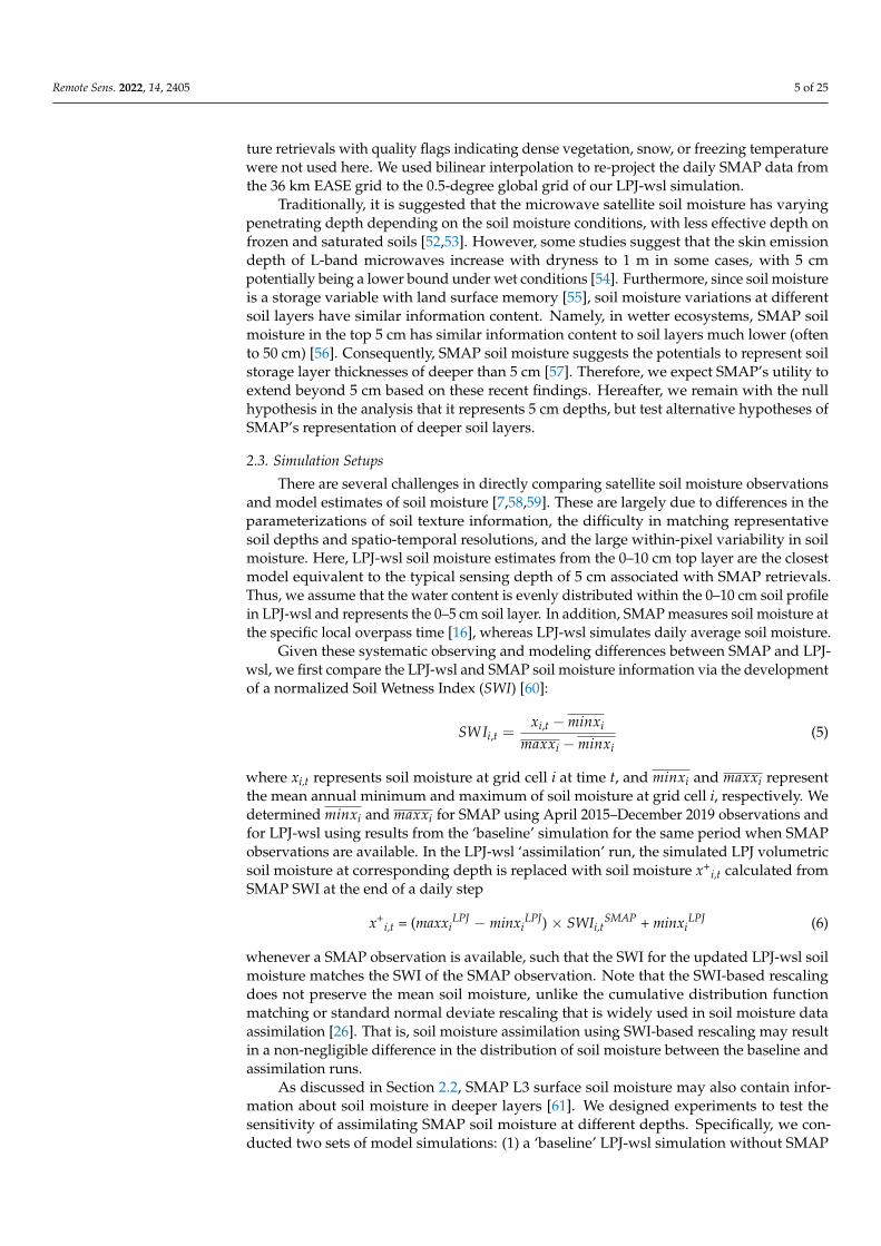
Traditionally, it is suggested that the microwave satellite soil moisture has varyingpenetrating depth depending on the soil moisture conditions, with less effective depth onfrozen and saturated soils [52,53]. However, some studies suggest that the skin emissiondepth of L-band microwaves increase with dryness to 1 m in some cases, with 5 cmpotentially being a lower bound under wet conditions [54]. Furthermore, since soil moistureis a storage variable with land surface memory [55], soil moisture variations at differentsoil layers have similar information content. Namely, in wetter ecosystems, SMAP soilmoisture in the top 5 cm has similar information content to soil layers much lower (oftento 50 cm) [56]. Consequently, SMAP soil moisture suggests the potentials to represent soilstorage layer thicknesses of deeper than 5 cm [57]. Therefore, we expect SMAP’s utility toextend beyond 5 cm based on these recent findings. Hereafter, we remain with the nullhypothesis in the analysis that it represents 5 cm depths, but test alternative hypotheses ofSMAP’s representation of deeper soil layers.

2.3. Simulation Setups

There are several challenges in directly comparing satellite soil moisture observationsand model estimates of soil moisture [7,58,59]. These are largely due to differences in theparameterizations of soil texture information, the difficulty in matching representativesoil depths and spatio-temporal resolutions, and the large within-pixel variability in soilmoisture. Here, LPJ-wsl soil moisture estimates from the 0–10 cm top layer are the closestmodel equivalent to the typical sensing depth of 5 cm associated with SMAP retrievals.Thus, we assume that the water content is evenly distributed within the 0–10 cm soil profilein LPJ-wsl and represents the 0–5 cm soil layer. In addition, SMAP measures soil moisture atthe specific local overpass time [16], whereas LPJ-wsl simulates daily average soil moisture.

Given these systematic observing and modeling differences between SMAP and LPJ-wsl, we first compare the LPJ-wsl and SMAP soil moisture information via the developmentof a normalized Soil Wetness Index (SWI) [60]:

SWIi,t =xi,t − minxi

maxxi − minxi(5)

where xi,t represents soil moisture at grid cell i at time t, and minxi and maxxi representthe mean annual minimum and maximum of soil moisture at grid cell i, respectively. Wedetermined minxi and maxxi for SMAP using April 2015–December 2019 observations andfor LPJ-wsl using results from the ‘baseline’ simulation for the same period when SMAPobservations are available. In the LPJ-wsl ‘assimilation’ run, the simulated LPJ volumetricsoil moisture at corresponding depth is replaced with soil moisture x+

i,t calculated fromSMAP SWI at the end of a daily step

x+i,t = (maxxi

LPJ − minxiLPJ) × SWIi,t

SMAP + minxiLPJ (6)

whenever a SMAP observation is available, such that the SWI for the updated LPJ-wsl soilmoisture matches the SWI of the SMAP observation. Note that the SWI-based rescalingdoes not preserve the mean soil moisture, unlike the cumulative distribution functionmatching or standard normal deviate rescaling that is widely used in soil moisture dataassimilation [26]. That is, soil moisture assimilation using SWI-based rescaling may resultin a non-negligible difference in the distribution of soil moisture between the baseline andassimilation runs.

As discussed in Section 2.2, SMAP L3 surface soil moisture may also contain infor-mation about soil moisture in deeper layers [61]. We designed experiments to test thesensitivity of assimilating SMAP soil moisture at different depths. Specifically, we con-ducted two sets of model simulations: (1) a ‘baseline’ LPJ-wsl simulation without SMAP

Remote Sens. 2022, 14, 2405 6 of 25

assimilation and (2) three “assimilation” schemes that assimilate SMAP soil moisture intoLPJ-wsl for different soil depths in the model: 0–10 cm (topsoil layer, denoted LPJ_10),0–50 cm (top four soil layers, denoted LPJ_50), and 0–200 cm (all 8 soil layers, denotedLPJ_200). The soil moisture values for these soil depths (0–10 cm, 0–50 cm, and 0–200 cm,respectively) were replaced with volumetric soil moisture derived from SMAP SWI usingEquation (5). The performance of the different assimilation schemes was tested against insitu measurements to find the best representative depth.

We used surface meteorological forcing data from the Climate Research Unit (CRUv4.05) [62] to run the LPJ-wsl model in this study. CRU forcing data is a global-scale, in situ-based, monthly spatial-interpolated climate dataset for 1901–2019. A weather generatorin LPJ is used to generate daily precipitation events based on a wet-day frequency inputand a set of linear interpolations with monthly temperature and cloud cover as inputsto calculate daily temperature, photosynthetically active radiation flux, and potentialevapotranspiration. The LPJ-wsl simulations include a spin-up phase, which equilibratesthe prognostic variables, including vegetation state, soil carbon pools, and soil moisturecontent. The spin-up run is a 1000-year simulation that recycles the CRU forcing data from1901–1930 for the spin-up period until the onset of transient simulation in 1901. Duringthe spin-up run, the atmospheric CO2 concentration is held constant at the pre-industriallevel (286.00 ppm). For the transient simulation, the simulation is forced with varyingannual atmospheric CO2 concentrations using data from observations. For the baseline andassimilation runs, the model setup is the same until 31 March 2015 when SMAP is available.

We first compare our baseline to the assimilated version to assess the effect of differentassimilating soil depth on simulated soil moisture values. Because the FLUXNET obser-vations are not available for the study period of 2015–2019, we evaluated the simulatedaverage seasonal cycle from the SMAP assimilation period against the observations. Thedifferent schemes were compared at regional scales to discuss the effect of the soil moistureassimilation on large-scale carbon fluxes.

2.4. Evaluation Strategy and Statistical Analysis2.4.1. Benchmark Datasets

Site-level observations of soil moisture and carbon (i.e., CO2 and CH4) fluxes fromFLUXNET2015 and FLUXNET-CH4 (hereafter, FLUXNET) were used to evaluate thetemporal patterns of simulated results. Given that there are systematic differences betweenthe remotely sensed and ground data due to the spatial representativeness, differentmeasurement depths [63], and uncertainty in the LPJ parameterizations, we evaluated soilmoisture on the basis of SWI. We used the same minimum and maximum soil moisturevalues derived from the baseline run for the SWI calculation of the assimilated runs. TheFLUXNET soil moisture used in this study are measurements for the top soil layer (0–15 cm)listed in Tables 1 and A1 [35,36,64].

Table 1. List of sites used in the soil moisture and carbon flux assessment.

Site ID Site Name Longitude Latitude IGBP Biome Type Duration

US-Prr Poker Flat Research Range Black SpruceForest −147.48 65.12 Evergreen Needleleaf Forests 2010–2014

CA-TP1 Ontario—Turkey Point 2002 PlantationWhite Pine −80.55 42.66 Evergreen Needleleaf Forests 2002–2014

US-ARM ARM Southern Great Plains site- Lamont −97.49 36.61 Croplands 2003–2012

US-MMS Morgan Monroe State Forest −86.41 39.22 Deciduous Broadleaf Forests 1999–2014

US-Oho Oak Openings −83.84 41.55 Deciduous Broadleaf Forests 2004–2013

US-Ton Tonzi Ranch −120.97 38.43 Woody Savannas 2001–2014

US-Whs Walnut Gulch Lucky Hills Shrub −110.05 31.74 Open Shrublands 2007–2014

Remote Sens. 2022, 14, 2405 7 of 25

Regional-level evaluations were also carried out by comparing with one independentsatellite soil moisture product and two gridded carbon flux products that were developedbased on upscaling eddy covariance measurements. We use the European Space Agency’sClimate Change Initiative for Soil Moisture (ESA CCI SM) product, which harmonizesand merges soil moisture retrievals from multiple satellites into a single product at a 0.25◦

regular grid [65]. The version applied in this study was the v4.07 combined product from1 January 2015–31 December 2019 at daily time step. The CO2 flux estimates were basedon a net ecosystem exchange estimate from upscaled FLUXNET observations [66,67].

Figure 1 provides a map of the sites for the evaluation of soil moisture and carbonfluxes. The site selection for soil moisture evaluation followed the criteria to represent landcover spanning from evergreen needleleaf forest (ENF) to grasslands, including croplands;all sites were situated within North America. Therefore, we used 7 sites from FLUXNETfor comparison with the LPJ-wsl simulated soil moisture and CO2 fluxes. Because theupland sites do not have measurements of CH4 fluxes, we used 26 wetland sites fromFLUXNET-CH4 (Table A1; [36,64]) to assess the influence of assimilation on CO2 and CH4fluxes at different time scales for different biome sub-types across the globe.

Remote Sens. 2022, 14, x 7 of 25

Figure 1. Mean annual maximum of SMAP soil moisture for 2015–2019. Symbols show site locations used in the evaluation, with dots surrounded by rectangles representing the upland sites that are used for the comparison of soil moisture and CO2 fluxes. The wetland sites used in the evaluation of CO2 and CH4 fluxes are grouped into four broad categories according to the classifications from Delwiche et al. (2021). White areas have insufficient good-quality SMAP soil moisture retrievals.

2.4.2. Statistical Analysis and Wavelets A variety of metrics are applied in this study for evaluating the model performance, which

include: - Root mean standard difference (RMSD) between two datasets; - Three components of RMSD: squared bias, difference in the magnitude of fluctuation between

simulation and measurements (∆𝜎𝜎)2 , and lack of correlation weighted by the standard deviations (LCS), which are used to evaluate the relative skill in reproducing the observations (see below for details);

- The Pearson product–moment correlation coefficient r to assess the relative agreement of the temporal structures between two datasets. The spatial correlation is also calculated using the same formula but on a single vector of locations at specific time steps;

- Taylor diagrams [68] are used to visually evaluate the relative skill among model-data fits by illustrating the linear correlation coefficient, RMSD, and standard deviation in a polar coordinate plot. The square of RMSD can be decomposed into three informative components related to bias,

the difference in standard deviation between the model and the observations, and the lack of correlation. Specifically, the RMSD can be written as follows [51,60]:

𝑅𝑅𝑀𝑀𝑆𝑆𝑅𝑅2 = 𝐵𝐵𝑖𝑖𝑚𝑚𝐵𝐵2 + 𝑉𝑉𝐴𝐴𝑅𝑅 + 𝐿𝐿𝐿𝐿𝑆𝑆 (7)

where bias is the mean difference between the time series of the model (xi = 1..n) and the observations (yi = 1..n) for a given location i:

𝐵𝐵𝑖𝑖𝑚𝑚𝐵𝐵2 = (𝑥𝑥𝚤𝚤� − 𝑦𝑦𝚤𝚤�)2 (8)

and the square differences of the standard deviations of the model and observations (VAR) are expressed as:

𝑉𝑉𝐴𝐴𝑅𝑅 = (𝜎𝜎𝑥𝑥𝑖𝑖 − 𝜎𝜎𝑦𝑦𝑖𝑖)2 (9)

A large value of VAR indicates that the model fails to simulate the variability. Finally, LCS reflects the lack of correlation (r) between the observations and the model, weighted by the product of the standard deviations:

Figure 1. Mean annual maximum of SMAP soil moisture for 2015–2019. Symbols show site locationsused in the evaluation, with dots surrounded by rectangles representing the upland sites that areused for the comparison of soil moisture and CO2 fluxes. The wetland sites used in the evaluationof CO2 and CH4 fluxes are grouped into four broad categories according to the classifications fromDelwiche et al. (2021). White areas have insufficient good-quality SMAP soil moisture retrievals.

2.4.2. Statistical Analysis and Wavelets

A variety of metrics are applied in this study for evaluating the model performance,which include:

- Root mean standard difference (RMSD) between two datasets;- Three components of RMSD: squared bias, difference in the magnitude of fluctuation

between simulation and measurements (∆σ)2, and lack of correlation weighted by thestandard deviations (LCS), which are used to evaluate the relative skill in reproducingthe observations (see below for details);

- The Pearson product–moment correlation coefficient r to assess the relative agree-ment of the temporal structures between two datasets. The spatial correlation is

Remote Sens. 2022, 14, 2405 8 of 25

also calculated using the same formula but on a single vector of locations at specifictime steps;

- Taylor diagrams [68] are used to visually evaluate the relative skill among model-datafits by illustrating the linear correlation coefficient, RMSD, and standard deviation ina polar coordinate plot.

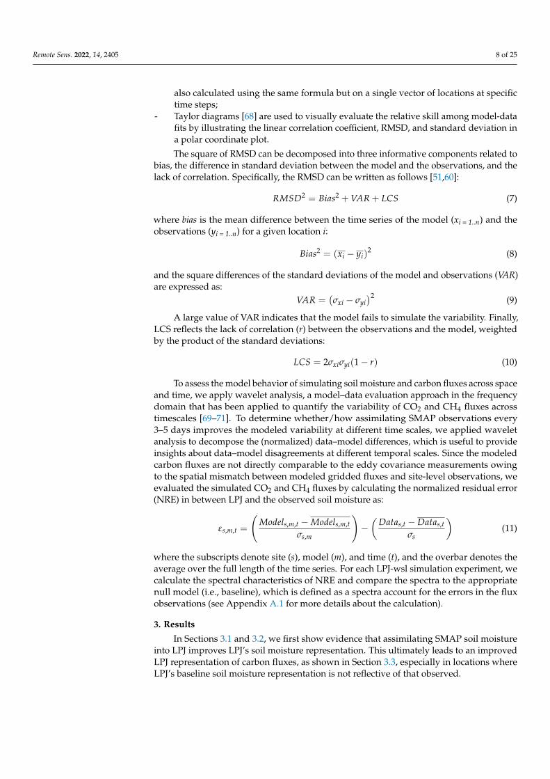
The square of RMSD can be decomposed into three informative components related tobias, the difference in standard deviation between the model and the observations, and thelack of correlation. Specifically, the RMSD can be written as follows [51,60]:

RMSD2 = Bias2 + VAR + LCS (7)

where bias is the mean difference between the time series of the model (xi = 1..n) and theobservations (yi = 1..n) for a given location i:

Bias2 = (xi − yi)2 (8)

and the square differences of the standard deviations of the model and observations (VAR)are expressed as:

VAR =(σxi − σyi

)2 (9)

A large value of VAR indicates that the model fails to simulate the variability. Finally,LCS reflects the lack of correlation (r) between the observations and the model, weightedby the product of the standard deviations:

LCS = 2σxiσyi(1 − r) (10)

To assess the model behavior of simulating soil moisture and carbon fluxes across spaceand time, we apply wavelet analysis, a model–data evaluation approach in the frequencydomain that has been applied to quantify the variability of CO2 and CH4 fluxes acrosstimescales [69–71]. To determine whether/how assimilating SMAP observations every3–5 days improves the modeled variability at different time scales, we applied waveletanalysis to decompose the (normalized) data–model differences, which is useful to provideinsights about data–model disagreements at different temporal scales. Since the modeledcarbon fluxes are not directly comparable to the eddy covariance measurements owingto the spatial mismatch between modeled gridded fluxes and site-level observations, weevaluated the simulated CO2 and CH4 fluxes by calculating the normalized residual error(NRE) in between LPJ and the observed soil moisture as:

εs,m,t =

(Models,m,t − Models,m,t

σs,m

)−(

Datas,t − Datas,t

σs

)(11)

where the subscripts denote site (s), model (m), and time (t), and the overbar denotes theaverage over the full length of the time series. For each LPJ-wsl simulation experiment, wecalculate the spectral characteristics of NRE and compare the spectra to the appropriatenull model (i.e., baseline), which is defined as a spectra account for the errors in the fluxobservations (see Appendix A.1 for more details about the calculation).

3. Results

In Sections 3.1 and 3.2, we first show evidence that assimilating SMAP soil moistureinto LPJ improves LPJ’s soil moisture representation. This ultimately leads to an improvedLPJ representation of carbon fluxes, as shown in Section 3.3, especially in locations whereLPJ’s baseline soil moisture representation is not reflective of that observed.

Remote Sens. 2022, 14, 2405 9 of 25

3.1. An Analysis of Model Depth Selection

The comparison of site-level soil moisture for different assimilation schemes suggeststhat the majority of the assimilation experiments showed improved simulations over thebaseline in comparison to the FLUXNET measurements, with the degree of improvementdepending on the underlying agreement of SMAP with FLUXNET data. The modelgenerally compares closest to FLUXENT when assimilating the SMAP soil moisture forthe soil columns 0–50 cm and 0–200 cm, as indicated in Figure 2. The performance ofthe modeled results also largely depended on the agreement between SMAP and theobservation at the evaluation sites. For the boreal site (US-Prr), which showed higherdiscrepancies between SMAP and FLUXNET, the assimilation runs tended to have little/noimprovement against the in situ observations. The spread in performance within biometypes was broad: two of the seven sites with the best performance were open shrublandand savanna, where the relatively low vegetation density and low soil organic carbontended to have less influence on the accuracy of the SMAP soil moisture.

Figure 3 more comprehensively shows the discrepancies between the assimilationschemes’ soil moisture values (represented as SWI) and those of the in situ FLUXNETsoil moisture values using the decomposed RMSD2 metrics in SWI. It ultimately confirmsthat several components of LPJ_200 soil moisture compare closely to those of the in situmeasurements. In each LPJ-wsl simulation, the bias and LCS with FLUXNET site wereconsiderably reduced after assimilating the SWI from the SMAP soil moisture, whilethe Var (∆σ)2 was only slightly affected by the assimilation. This was mainly due tothe assimilation of normalized observations, which preserves the variability but altersthe seasonality of soil moisture. This indicates that, after the assimilation of SMAP soilmoisture, the biases with site-level observations were removed, and the agreement wasconsiderably improved. However, the ability to improve the performance in simulating thevariability at the level of individual sites was limited. Since assimilating SMAP into thewhole soil column (0–200 cm) in LPJ-wsl had a better performance than the other schemes,we use the LPJ_200 scheme for the remainder of this paper to interpret the effect of soilmoisture assimilation on carbon fluxes.

3.2. Site-Level Comparison of Soil Moisture

The comparison of the simulated daily soil moisture with the FLUXNET in situ andSMAP satellite measurements suggested that, by construction, the assimilated results had abetter agreement with the SMAP observations. The agreement of the density distribution ofSMAP assimilated soil moisture vs. that of FLUXNET strongly depended on the accuracyof the SMAP retrievals in detecting surface soil moisture (Figure 4). At the US-Prr site,the assimilation estimates agreed less well with the in situ measurements than they didwith the baseline estimates, owing to the mismatch between SMAP and the in situ data.This was mainly attributed to the effect of the soil freeze/thaw processes on the SMAPretrievals at high latitudes, as suggested by previous studies [72–74], which causes relativelypoor performance in the validation. Other than US-Prr, for five of the seven sites (CA-TP1, US-MMS, US-Oho, US-Ton, US-Whs), the assimilated results had better agreementthan the LPJ-wsl baseline simulation with FLUXNET in terms of the median value anddistribution. For open shrubland and savanna sites (US-Whs and US-Ton), all simulationswere comparable with each other, given the reduced influence of vegetation canopies onthe SMAP retrievals and the relatively good performance of the LPJ-wsl baseline in dryand temperate regions.

Remote Sens. 2022, 14, 2405 10 of 25Remote Sens. 2022, 14, x 9 of 25

Figure 2. Taylor plots of monthly mean soil moisture in the 0–10 cm layer by assimilation schemes forall 7 sites. The cosine of the angle from the x axis is the correlation coefficient between simulated andobserved soil moisture, which measures how well the simulated soil moisture captures the phasingand timing of the observed soil moisture from in situ sites. The black dots on the x axis representobservations. The radial distance from the origin is the standard deviation. The dotted and dashedgrey lines represent correlation and RMSD normalized by standard deviation, respectively. The starsymbol indicates a perfect model that has a zero RMSD and a correlation of 1.0.

Remote Sens. 2022, 14, 2405 11 of 25

Remote Sens. 2022, 14, x 10 of 25

Figure 2. Taylor plots of monthly mean soil moisture in the 0–10 cm layer by assimilation schemes for all 7 sites. The cosine of the angle from the x axis is the correlation coefficient between simulated and observed soil moisture, which measures how well the simulated soil moisture captures the phasing and timing of the observed soil moisture from in situ sites. The black dots on the x axis represent observations. The radial distance from the origin is the standard deviation. The dotted and dashed grey lines represent correlation and RMSD normalized by standard deviation, respectively. The star symbol indicates a perfect model that has a zero RMSD and a correlation of 1.0.

Figure 3 more comprehensively shows the discrepancies between the assimilation schemes’ soil moisture values (represented as SWI) and those of the in situ FLUXNET soil moisture values using the decomposed RMSD2 metrics in SWI. It ultimately confirms that several components of LPJ_200 soil moisture compare closely to those of the in situ measurements. In each LPJ-wsl simulation, the bias and LCS with FLUXNET site were considerably reduced after assimilating the SWI from the SMAP soil moisture, while the Var (∆𝜎𝜎)2 was only slightly affected by the assimilation. This was mainly due to the assimilation of normalized observations, which preserves the variability but alters the seasonality of soil moisture. This indicates that, after the assimilation of SMAP soil moisture, the biases with site-level observations were removed, and the agreement was considerably improved. However, the ability to improve the performance in simulating the variability at the level of individual sites was limited. Since assimilating SMAP into the whole soil column (0–200 cm) in LPJ-wsl had a better performance than the other schemes, we use the LPJ_200 scheme for the remainder of this paper to interpret the effect of soil moisture assimilation on carbon fluxes.

Figure 3. Boxplots showing the decomposed MSD for simulated monthly SWI from different assimilation schemes against the FLUXNET sites. The dots represent the outliers from the boreal site US-Prr, where SMAP has large discrepancies with the FLUXNET measurements.

3.2. Site-Level Comparison of Soil Moisture The comparison of the simulated daily soil moisture with the FLUXNET in situ and SMAP

satellite measurements suggested that, by construction, the assimilated results had a better agreement with the SMAP observations. The agreement of the density distribution of SMAP assimilated soil moisture vs. that of FLUXNET strongly depended on the accuracy of the SMAP retrievals in detecting surface soil moisture (Figure 4). At the US-Prr site, the assimilation estimates agreed less well with the in situ measurements than they did with the baseline estimates, owing to the mismatch between SMAP and the in situ data. This was mainly attributed to the effect of the soil freeze/thaw processes on the SMAP retrievals at high latitudes, as suggested by previous studies [72–74], which causes relatively poor performance in the validation. Other than US-Prr, for five of the seven sites (CA-TP1, US-MMS, US-Oho, US-Ton, US-Whs), the assimilated results had better agreement than the LPJ-wsl baseline simulation with FLUXNET in terms of the median value and distribution. For open shrubland and savanna sites (US-Whs and US-Ton), all simulations were

Figure 3. Boxplots showing the decomposed MSD for simulated monthly SWI from different assimi-lation schemes against the FLUXNET sites. The dots represent the outliers from the boreal site US-Prr,where SMAP has large discrepancies with the FLUXNET measurements.

Remote Sens. 2022, 14, x 11 of 25

comparable with each other, given the reduced influence of vegetation canopies on the SMAP retrievals and the relatively good performance of the LPJ-wsl baseline in dry and temperate regions.

Figure 4. Distribution of simulated daily soil wetness index from baseline and assimilated run with FLUXNET and SMAP at the seven sites. The upper part and lower part of individual plots show the density distribution and box plot, respectively. The variable width of bars in the box plots corresponds to the sample size, with a wider bar indicating higher sample size.

The evaluation of the mean seasonal cycle of soil wetness in the simulations (versus that of FLUXNET measurements) suggested diverse patterns among sites and better agreement between the assimilation run and FLUXNET than was seen for the baseline (Figure 5). The improvement was more significant for the biomes that were less influenced by the freeze/thaw cycle and dense vegetation canopies. For the high-latitude site (US-Prr), both simulations captured well the onset and termination of the freeze/thaw cycle and produced a lower peak growing season compared to FLUXNET, with the assimilation run producing even lower soil moisture due to the weak seasonality captured by SMAP. For temperate forest sites (CA-TP1, US-MMS, and US-Oho), the assimilation run had a generally better agreement with FLUXNET, capturing the timing fairly well with improved peak and phase compared to the baseline run. The good agreements for US-Ton and US-Whs suggest there was less discrepancy between the model and the observations for the biomes

Figure 4. Distribution of simulated daily soil wetness index from baseline and assimilated run withFLUXNET and SMAP at the seven sites. The upper part and lower part of individual plots show thedensity distribution and box plot, respectively. The variable width of bars in the box plots correspondsto the sample size, with a wider bar indicating higher sample size.

Remote Sens. 2022, 14, 2405 12 of 25

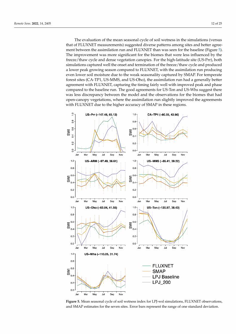
The evaluation of the mean seasonal cycle of soil wetness in the simulations (versusthat of FLUXNET measurements) suggested diverse patterns among sites and better agree-ment between the assimilation run and FLUXNET than was seen for the baseline (Figure 5).The improvement was more significant for the biomes that were less influenced by thefreeze/thaw cycle and dense vegetation canopies. For the high-latitude site (US-Prr), bothsimulations captured well the onset and termination of the freeze/thaw cycle and produceda lower peak growing season compared to FLUXNET, with the assimilation run producingeven lower soil moisture due to the weak seasonality captured by SMAP. For temperateforest sites (CA-TP1, US-MMS, and US-Oho), the assimilation run had a generally betteragreement with FLUXNET, capturing the timing fairly well with improved peak and phasecompared to the baseline run. The good agreements for US-Ton and US-Whs suggest therewas less discrepancy between the model and the observations for the biomes that hadopen-canopy vegetations, where the assimilation run slightly improved the agreementswith FLUXNET due to the higher accuracy of SMAP in these regions.

Remote Sens. 2022, 14, x 12 of 25

that had open-canopy vegetations, where the assimilation run slightly improved the agreements with FLUXNET due to the higher accuracy of SMAP in these regions.

Figure 5. Mean seasonal cycle of soil wetness index for LPJ-wsl simulations, FLUXNET observations, and SMAP estimates for the seven sites. Error bars represent the range of one standard deviation.

3.3. Effect of Assimilation on Carbon Fluxes Generally, for sites that have considerable discrepancies in soil moisture, the SMAP

assimilation improved the agreement of seasonality in the net ecosystem CO2 exchange with the FLUXNET observations (Figure 6). The assimilation of SMAP slightly altered the simulated CO2 flux during the growing season, but had a limited effect on the seasonal pattern, despite significant changes in soil moisture for a few sites (e.g., US-Prr and CA-CP1). For the sites where the probability

Figure 5. Mean seasonal cycle of soil wetness index for LPJ-wsl simulations, FLUXNET observations,and SMAP estimates for the seven sites. Error bars represent the range of one standard deviation.

Remote Sens. 2022, 14, 2405 13 of 25

3.3. Effect of Assimilation on Carbon Fluxes

Generally, for sites that have considerable discrepancies in soil moisture, the SMAPassimilation improved the agreement of seasonality in the net ecosystem CO2 exchangewith the FLUXNET observations (Figure 6). The assimilation of SMAP slightly altered thesimulated CO2 flux during the growing season, but had a limited effect on the seasonalpattern, despite significant changes in soil moisture for a few sites (e.g., US-Prr and CA-CP1). For the sites where the probability density function of modeled soil moisture agreedrelatively well with SMAP (Figure 4; S-Ton and US-Whs), the assimilation resulted in ahigher carbon uptake during the growing season but had a slightly weaker correlation withFLUXNET observations, suggesting that factors other than soil moisture likely control CO2flux during the growing season.

Remote Sens. 2022, 14, x 13 of 25

density function of modeled soil moisture agreed relatively well with SMAP (Figure 4; S-Ton and US-Whs), the assimilation resulted in a higher carbon uptake during the growing season but had a slightly weaker correlation with FLUXNET observations, suggesting that factors other than soil moisture likely control CO2 flux during the growing season.

Figure 6. Mean seasonal cycle of simulated average monthly net ecosystem CO2 exchange (NEE) from LPJ baseline and LPJ_200 in comparison with the FLUXNET sites. Error bar indicates standard deviation for multi-year NEE. The correlation coefficient between simulated NEE and FLUXNET observations are listed (purple: LPJ baseline; blue: LPJ_200).

To assess the effect of the assimilation of soil moisture on carbon fluxes at different time scales, we calculated the wavelet spectral of normalized residual errors between modeled carbon fluxes and FLUXNET measurement on the basis of site year (Figure 7). To improve the representativeness for biomes, 26 FLUXNET sites where SMAP observations were available and assimilated into LPJ-wsl were used to make the comparison. For each site year (2015–2019) from the LPJ-wsl simulation, the mean marginal distribution of the power spectrum showed the variations of model error with time scales. In this context, any time scales for which the model had lower power indicated improvements against the observations. This showed, for example, that the error in CO2 flux in the model was generally lowest at the monthly time scale (30 days) and higher at the shorter and longer time scales. This was reflected partly because of using the monthly climate datasets, as the sub-monthly simulations were based on a weather generator.

Figure 6. Mean seasonal cycle of simulated average monthly net ecosystem CO2 exchange (NEE)from LPJ baseline and LPJ_200 in comparison with the FLUXNET sites. Error bar indicates standarddeviation for multi-year NEE. The correlation coefficient between simulated NEE and FLUXNETobservations are listed (purple: LPJ baseline; blue: LPJ_200).

To assess the effect of the assimilation of soil moisture on carbon fluxes at differenttime scales, we calculated the wavelet spectral of normalized residual errors betweenmodeled carbon fluxes and FLUXNET measurement on the basis of site year (Figure 7). Toimprove the representativeness for biomes, 26 FLUXNET sites where SMAP observationswere available and assimilated into LPJ-wsl were used to make the comparison. For eachsite year (2015–2019) from the LPJ-wsl simulation, the mean marginal distribution of thepower spectrum showed the variations of model error with time scales. In this context,any time scales for which the model had lower power indicated improvements againstthe observations. This showed, for example, that the error in CO2 flux in the model was

Remote Sens. 2022, 14, 2405 14 of 25

generally lowest at the monthly time scale (30 days) and higher at the shorter and longertime scales. This was reflected partly because of using the monthly climate datasets, as thesub-monthly simulations were based on a weather generator.

Remote Sens. 2022, 14, x 14 of 25

Figure 7. Mean marginal distribution of power spectra of the normalized residual error between modeled carbon fluxes and observations from FLUXNET sites. The higher power at specific time scales (period) indicates that the model error has a significantly higher mismatch at certain time scales. Sample sizes of site year for each biome are listed.

The comparison between the baseline and the assimilation run suggested improved agreement at time scales greater than 40 days for the boreal and tropical sites, with little/no improvement for the tundra and temperate sites. However, the assimilation run tended to have higher bias for time scales less than 30 days, which was partly due to the simple assimilation strategy that corrected the soil moisture every 3–5 days given the revisit time of SMAP. This assimilation strategy could possibly introduce unrealistic variability at these time scales, due to misaligned SMAP sampling meteorology with the weather generator in LPJ-wsl. Note that the site observations have large uncertainties in carbon fluxes with high year-to-year variations, especially for CH4 observations, which are sensitive to environmental conditions such as water table depth and microbial composition [36,64,71]. The lack of measurements limits the evaluation for the tropical sites since only two subtropical grassland sites are available while no representation of tropical floodplain is included. In addition, the sites with CH4 flux measurements tend to have high soil organic matter and saturated soil water; thus, the evaluation of assimilated CH4 is affected by the accuracy of SMAP retrieval [73,75].

3.4. Evaluation of the Assimilation at Global Scale To assess the effect of soil moisture assimilation at a global scale, we calculated the correlation

coefficients and RMSD of the simulated daily soil moisture from the baseline and assimilated the run against SMAP and against the satellite-based surface soil moisture retrievals from the ESA CCI SM dataset for 2015–2019 (Figure 8). The results showed that LPJ-wsl baseline produced different temporal patterns than SMAP for the high latitudes and had a higher RMSD for most regions, except semi-arid regions, which is consistent with previous studies [74,76]. This was also the case for the metrics computed versus ESA CCI, which suggested a systematic difference between the satellite and model data, with the highest agreement for semi-arid regions. As expected, the correlation and RMSD were improved (by construction) between the assimilation run and SMAP. The comparison with ESA CCI suggested that the assimilation could significantly increase the correlation coefficient and lower the RMSD for the northern high latitudes. Given that ESA CCI is an independent product,

Figure 7. Mean marginal distribution of power spectra of the normalized residual error betweenmodeled carbon fluxes and observations from FLUXNET sites. The higher power at specific timescales (period) indicates that the model error has a significantly higher mismatch at certain timescales. Sample sizes of site year for each biome are listed.

The comparison between the baseline and the assimilation run suggested improvedagreement at time scales greater than 40 days for the boreal and tropical sites, with little/noimprovement for the tundra and temperate sites. However, the assimilation run tendedto have higher bias for time scales less than 30 days, which was partly due to the simpleassimilation strategy that corrected the soil moisture every 3–5 days given the revisit timeof SMAP. This assimilation strategy could possibly introduce unrealistic variability at thesetime scales, due to misaligned SMAP sampling meteorology with the weather generatorin LPJ-wsl. Note that the site observations have large uncertainties in carbon fluxes withhigh year-to-year variations, especially for CH4 observations, which are sensitive to envi-ronmental conditions such as water table depth and microbial composition [36,64,71]. Thelack of measurements limits the evaluation for the tropical sites since only two subtropicalgrassland sites are available while no representation of tropical floodplain is included. Inaddition, the sites with CH4 flux measurements tend to have high soil organic matter andsaturated soil water; thus, the evaluation of assimilated CH4 is affected by the accuracy ofSMAP retrieval [73,75].

3.4. Evaluation of the Assimilation at Global Scale

To assess the effect of soil moisture assimilation at a global scale, we calculated thecorrelation coefficients and RMSD of the simulated daily soil moisture from the baselineand assimilated the run against SMAP and against the satellite-based surface soil moistureretrievals from the ESA CCI SM dataset for 2015–2019 (Figure 8). The results showed thatLPJ-wsl baseline produced different temporal patterns than SMAP for the high latitudesand had a higher RMSD for most regions, except semi-arid regions, which is consistentwith previous studies [74,76]. This was also the case for the metrics computed versusESA CCI, which suggested a systematic difference between the satellite and model data,

Remote Sens. 2022, 14, 2405 15 of 25

with the highest agreement for semi-arid regions. As expected, the correlation and RMSDwere improved (by construction) between the assimilation run and SMAP. The comparisonwith ESA CCI suggested that the assimilation could significantly increase the correlationcoefficient and lower the RMSD for the northern high latitudes. Given that ESA CCIis an independent product, the reduced RMSD over large regions against the ESA CCIestimate indicates that the behavior of the model soil moisture is largely adjusted to bemore consistent with satellite-based observations.

Remote Sens. 2022, 14, x 15 of 25

the reduced RMSD over large regions against the ESA CCI estimate indicates that the behavior of the model soil moisture is largely adjusted to be more consistent with satellite-based observations.

Figure 8. Difference in correlation coefficient (a,b) and RMSD (c,d) of simulated daily SWI between LPJ_200 and baseline when compared to two satellite soil moisture datasets (SMAP and ESA CCI) for 2015–2019. SMAP data were assimilated into LPJ_200. Blue color suggests improved agreement of LPJ-simulated SWI against the satellite datasets with the darker color representing higher agreements, while the red color represents reduced agreements.

3.5. Implications of Assimilated Results for Carbon Cycle Science Even though, for many regions (e.g., tropical forests, high latitudes), SMAP observations are

unavailable or have a very limited number of samples, it is still feasible to assess the influence of assimilating SMAP soil moisture at a regional scale. Below, we use two examples to demonstrate its potential influences on estimating carbon fluxes.

3.5.1. European Drought in 2018 Europe was stricken by an extreme summer heat wave and drought in 2018, which resulted in

strong reductions in vegetation productivity and increased ecosystem respiration due to soil moisture deficits and, consequently, a reduction in the net CO2 uptake in ecosystems [77]. Previous studies [78–80] have shown that prognostic land surface models tend to underestimate the effect of droughts due to the limited representation of hydrologic processes, which affects the simulated carbon balance through soil moisture deficits, high water vapor pressure, and heat stress.

Figure 9 shows that assimilating SMAP moisture into LPJ-wsl can introduce an improved seasonality in the net carbon uptake. Figure 9a shows that, despite both the baseline and assimilation runs showing good agreement, that there was a minimum in the soil moisture during the growing season, and assimilating SMAP reduced the amplitude of the seasonal cycle, with drier conditions during the non-growing seasons for 2015–2019. It should also be noted that, even though the baseline simulated the extreme drought condition in 2018 reasonably well given the precipitation input from the observation-based climate datasets, SMAP suggested a less distinctive drought feature with higher 2018 summer soil moisture compared to the baseline.

Figure 8. Difference in correlation coefficient (a,b) and RMSD (c,d) of simulated daily SWI betweenLPJ_200 and baseline when compared to two satellite soil moisture datasets (SMAP and ESA CCI) for2015–2019. SMAP data were assimilated into LPJ_200. Blue color suggests improved agreement ofLPJ-simulated SWI against the satellite datasets with the darker color representing higher agreements,while the red color represents reduced agreements.

3.5. Implications of Assimilated Results for Carbon Cycle Science

Even though, for many regions (e.g., tropical forests, high latitudes), SMAP observa-tions are unavailable or have a very limited number of samples, it is still feasible to assessthe influence of assimilating SMAP soil moisture at a regional scale. Below, we use twoexamples to demonstrate its potential influences on estimating carbon fluxes.

3.5.1. European Drought in 2018

Europe was stricken by an extreme summer heat wave and drought in 2018, whichresulted in strong reductions in vegetation productivity and increased ecosystem respirationdue to soil moisture deficits and, consequently, a reduction in the net CO2 uptake inecosystems [77]. Previous studies [78–80] have shown that prognostic land surface modelstend to underestimate the effect of droughts due to the limited representation of hydrologicprocesses, which affects the simulated carbon balance through soil moisture deficits, highwater vapor pressure, and heat stress.

Figure 9 shows that assimilating SMAP moisture into LPJ-wsl can introduce an im-proved seasonality in the net carbon uptake. Figure 9a shows that, despite both the baselineand assimilation runs showing good agreement, that there was a minimum in the soilmoisture during the growing season, and assimilating SMAP reduced the amplitude ofthe seasonal cycle, with drier conditions during the non-growing seasons for 2015–2019.

Remote Sens. 2022, 14, 2405 16 of 25

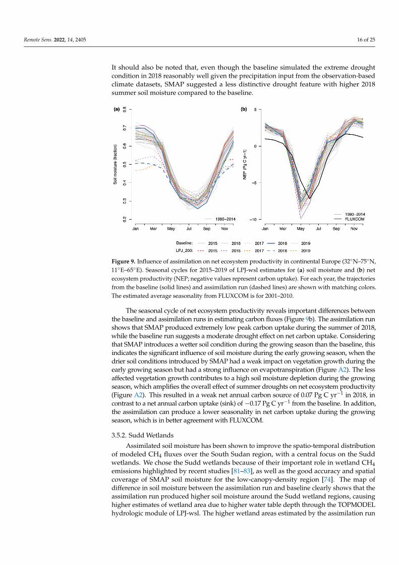
It should also be noted that, even though the baseline simulated the extreme droughtcondition in 2018 reasonably well given the precipitation input from the observation-basedclimate datasets, SMAP suggested a less distinctive drought feature with higher 2018summer soil moisture compared to the baseline.

Remote Sens. 2022, 14, x 16 of 25

Figure 9. Influence of assimilation on net ecosystem productivity in continental Europe (32° N–75° N, 11° E–65° E). Seasonal cycles for 2015–2019 of LPJ-wsl estimates for (a) soil moisture and (b) net ecosystem productivity (NEP; negative values represent carbon uptake). For each year, the trajectories from the baseline (solid lines) and assimilation run (dashed lines) are shown with matching colors. The estimated average seasonality from FLUXCOM is for 2001–2010.

The seasonal cycle of net ecosystem productivity reveals important differences between the baseline and assimilation runs in estimating carbon fluxes (Figure 9b). The assimilation run shows that SMAP produced extremely low peak carbon uptake during the summer of 2018, while the baseline run suggests a moderate drought effect on net carbon uptake. Considering that SMAP introduces a wetter soil condition during the growing season than the baseline, this indicates the significant influence of soil moisture during the early growing season, when the drier soil conditions introduced by SMAP had a weak impact on vegetation growth during the early growing season but had a strong influence on evapotranspiration (Figure A2). The less affected vegetation growth contributes to a high soil moisture depletion during the growing season, which amplifies the overall effect of summer droughts on net ecosystem productivity (Figure A2). This resulted in a weak net annual carbon source of 0.07 Pg C yr−1 in 2018, in contrast to a net annual carbon uptake (sink) of −0.17 Pg C yr−1 from the baseline. In addition, the assimilation can produce a lower seasonality in net carbon uptake during the growing season, which is in better agreement with FLUXCOM.

3.5.2. Sudd Wetlands Assimilated soil moisture has been shown to improve the spatio-temporal distribution of

modeled CH4 fluxes over the South Sudan region, with a central focus on the Sudd wetlands. We chose the Sudd wetlands because of their important role in wetland CH4 emissions highlighted by recent studies [81–83], as well as the good accuracy and spatial coverage of SMAP soil moisture for the low-canopy-density region [74]. The map of difference in soil moisture between the assimilation run and baseline clearly shows that the assimilation run produced higher soil moisture around the Sudd wetland regions, causing higher estimates of wetland area due to higher water table depth through the TOPMODEL hydrologic module of LPJ-wsl. The higher wetland areas estimated by the assimilation run were consistent with the findings from [83], which suggests that wetland models largely underestimate the wetland area of the Sudd region.

The modeled CH4 fluxes over the Sudd wetlands from the assimilation run had better agreement in terms of their seasonal cycle and annual total with posterior estimates from the inversion models [81,83] based on satellite measurements (Figure 10). The assimilation run showed a dual peak of CH4 fluxes in the March–April–May and September–October–November seasons, which is consistent with the seasonality detected by inversion models based on GOSAT and TROPOMI measurements [81,82]. In contrast, the baseline generally produces a lower intra-seasonal variability than the assimilation run, with the highest emissions in the late growing season. In addition, the timing of a record high peak in SON 2019 is consistent with the posterior estimates

Figure 9. Influence of assimilation on net ecosystem productivity in continental Europe (32◦N–75◦N,11◦E–65◦E). Seasonal cycles for 2015–2019 of LPJ-wsl estimates for (a) soil moisture and (b) netecosystem productivity (NEP; negative values represent carbon uptake). For each year, the trajectoriesfrom the baseline (solid lines) and assimilation run (dashed lines) are shown with matching colors.The estimated average seasonality from FLUXCOM is for 2001–2010.

The seasonal cycle of net ecosystem productivity reveals important differences betweenthe baseline and assimilation runs in estimating carbon fluxes (Figure 9b). The assimilation runshows that SMAP produced extremely low peak carbon uptake during the summer of 2018,while the baseline run suggests a moderate drought effect on net carbon uptake. Consideringthat SMAP introduces a wetter soil condition during the growing season than the baseline, thisindicates the significant influence of soil moisture during the early growing season, when thedrier soil conditions introduced by SMAP had a weak impact on vegetation growth during theearly growing season but had a strong influence on evapotranspiration (Figure A2). The lessaffected vegetation growth contributes to a high soil moisture depletion during the growingseason, which amplifies the overall effect of summer droughts on net ecosystem productivity(Figure A2). This resulted in a weak net annual carbon source of 0.07 Pg C yr−1 in 2018, incontrast to a net annual carbon uptake (sink) of −0.17 Pg C yr−1 from the baseline. In addition,the assimilation can produce a lower seasonality in net carbon uptake during the growingseason, which is in better agreement with FLUXCOM.

3.5.2. Sudd Wetlands

Assimilated soil moisture has been shown to improve the spatio-temporal distributionof modeled CH4 fluxes over the South Sudan region, with a central focus on the Suddwetlands. We chose the Sudd wetlands because of their important role in wetland CH4emissions highlighted by recent studies [81–83], as well as the good accuracy and spatialcoverage of SMAP soil moisture for the low-canopy-density region [74]. The map ofdifference in soil moisture between the assimilation run and baseline clearly shows that theassimilation run produced higher soil moisture around the Sudd wetland regions, causinghigher estimates of wetland area due to higher water table depth through the TOPMODELhydrologic module of LPJ-wsl. The higher wetland areas estimated by the assimilation run

Remote Sens. 2022, 14, 2405 17 of 25

were consistent with the findings from [83], which suggests that wetland models largelyunderestimate the wetland area of the Sudd region.

The modeled CH4 fluxes over the Sudd wetlands from the assimilation run hadbetter agreement in terms of their seasonal cycle and annual total with posterior esti-mates from the inversion models [81,83] based on satellite measurements (Figure 10).The assimilation run showed a dual peak of CH4 fluxes in the March–April–May andSeptember–October–November seasons, which is consistent with the seasonality detectedby inversion models based on GOSAT and TROPOMI measurements [81,82]. In contrast,the baseline generally produces a lower intra-seasonal variability than the assimilation run,with the highest emissions in the late growing season. In addition, the timing of a recordhigh peak in SON 2019 is consistent with the posterior estimates based on TROPOMI mea-surements [82], which suggests a strong positive anomaly of CH4 flux due to an exceptionalrainfall event. The average annual total flux for 2015–2019 almost doubled from 2.4 Tg CH4yr−1 at the baseline to 4.4 Tg CH4 yr−1 in the assimilation run, which can be explained by apotential underestimation of the wetland area in the baseline run. The mean annual totalflux in 2018–2019 from the assimilation run was 4.7 Tg CH4 yr−1, which falls into the rangeof 7.3 ± 3.2 Tg yr−1 from [83] based on TROPOMI measurements, but is higher than the3.4 ± 0.3 Tg CH4 yr−1 estimate from [82] based on TROPOMI and GOSAT measurements.

Remote Sens. 2022, 14, x 17 of 25

based on TROPOMI measurements [82], which suggests a strong positive anomaly of CH4 flux due to an exceptional rainfall event. The average annual total flux for 2015–2019 almost doubled from 2.4 Tg CH4 yr−1 at the baseline to 4.4 Tg CH4 yr−1 in the assimilation run, which can be explained by a potential underestimation of the wetland area in the baseline run. The mean annual total flux in 2018–2019 from the assimilation run was 4.7 Tg CH4 yr−1, which falls into the range of 7.3 ± 3.2 Tg yr−1 from [83] based on TROPOMI measurements, but is higher than the 3.4 ± 0.3 Tg CH4 yr−1 estimate from [82] based on TROPOMI and GOSAT measurements.

Figure 10. Influence of assimilation on CH4 fluxes over South Sudan’s wetlands. (a) Spatial distribution of difference of annual mean soil moisture between assimilation and baseline (LPJ_200 minus baseline) over 2015–2019 for the South Sudan region. The area within the blue rectangle (5° N–10° N, 28° E–35° E) is referred to as the Sudd wetland region. (b) Seasonal cycle of wetland CH4 fluxes for the Sudd wetland region.

4. Discussion Throughout this paper, we assessed the potential of the SMAP soil moisture product to be

used to improve the LPJ-wsl simulation of carbon fluxes. Because systematic errors exist in both the SMAP product and the process-based models, the climatological rescaling of soil moisture between SMAP and LPJ-wsl is essential. The SWI conversion approach in this study has been proven to be useful at inducing the seasonality of soil moisture dynamics [84,85]. Given that it is difficult to adjust the model formulation, soil hydraulic characterization, and the degree of wetness relative to the range of moisture over which key processes (drainage, evapotranspiration) occur, the potential bias in the SWI conversion in this study and its effect on assimilation needs further investigation. A better rescaling approach for SMAP is needed to keep both sources relatively consistent, such as the linear cumulative density distribution (CDF) matching or the full CDF matching [26,60]. In addition, because the SMAP descending retrievals at local time (6 a.m.) were applied in this study, a proper conversion of SMAP soil moisture to daily averages may need to be developed to minimize the mismatch with the modeled daily average soil moisture.

The simulation experiments with different representative depths demonstrate the importance of assessing the suitable depth to be considered in the assimilation. Despite the fact that LPJ-wsl is discretized by an eight-layered hydrology scheme, there is no exact corresponding depth to match the thin surface layer detected by the SMAP instrument. In addition, the sensing depth of SMAP is affected by local environmental conditions and vegetation types [75]. Therefore, it is impossible to fully reconcile the discrepancies in modeled soil moisture with remotely sensed measurements, as there is a structural mismatch between satellite-based observations and terrestrial ecosystem models. In this study, we tested altering the soil moisture using a first-order method by replacing the soil moisture with observations for a specific depth. A better approach to improve the issue of representativeness is to use an exponential filter [86–88], which assumes that the soil moisture of deeper layers can be derived from an exponential relationship given the observed soil moisture in the surface layer.

The improvement of the assimilation over different regions largely depended on the agreement of SMAP with the in situ measurements. This is reflected in the comparison between the model and the data, which highlighted that the model behavior with respect to soil moisture after assimilation had high similarity in a spatio-temporal pattern with SMAP, despite the simulated

Figure 10. Influence of assimilation on CH4 fluxes over South Sudan’s wetlands. (a) Spatial distribu-tion of difference of annual mean soil moisture between assimilation and baseline (LPJ_200 minusbaseline) over 2015–2019 for the South Sudan region. The area within the blue rectangle (5◦N–10◦N,28◦E–35◦E) is referred to as the Sudd wetland region. (b) Seasonal cycle of wetland CH4 fluxes forthe Sudd wetland region.

4. Discussion

Throughout this paper, we assessed the potential of the SMAP soil moisture productto be used to improve the LPJ-wsl simulation of carbon fluxes. Because systematic errorsexist in both the SMAP product and the process-based models, the climatological rescalingof soil moisture between SMAP and LPJ-wsl is essential. The SWI conversion approachin this study has been proven to be useful at inducing the seasonality of soil moisturedynamics [84,85]. Given that it is difficult to adjust the model formulation, soil hydrauliccharacterization, and the degree of wetness relative to the range of moisture over which keyprocesses (drainage, evapotranspiration) occur, the potential bias in the SWI conversionin this study and its effect on assimilation needs further investigation. A better rescalingapproach for SMAP is needed to keep both sources relatively consistent, such as the linearcumulative density distribution (CDF) matching or the full CDF matching [26,60]. Inaddition, because the SMAP descending retrievals at local time (6 a.m.) were applied inthis study, a proper conversion of SMAP soil moisture to daily averages may need to bedeveloped to minimize the mismatch with the modeled daily average soil moisture.

The simulation experiments with different representative depths demonstrate theimportance of assessing the suitable depth to be considered in the assimilation. Despitethe fact that LPJ-wsl is discretized by an eight-layered hydrology scheme, there is no exactcorresponding depth to match the thin surface layer detected by the SMAP instrument.

Remote Sens. 2022, 14, 2405 18 of 25

In addition, the sensing depth of SMAP is affected by local environmental conditionsand vegetation types [75]. Therefore, it is impossible to fully reconcile the discrepanciesin modeled soil moisture with remotely sensed measurements, as there is a structuralmismatch between satellite-based observations and terrestrial ecosystem models. In thisstudy, we tested altering the soil moisture using a first-order method by replacing thesoil moisture with observations for a specific depth. A better approach to improve theissue of representativeness is to use an exponential filter [86–88], which assumes that thesoil moisture of deeper layers can be derived from an exponential relationship given theobserved soil moisture in the surface layer.

The improvement of the assimilation over different regions largely depended on theagreement of SMAP with the in situ measurements. This is reflected in the comparisonbetween the model and the data, which highlighted that the model behavior with respectto soil moisture after assimilation had high similarity in a spatio-temporal pattern withSMAP, despite the simulated carbon fluxes that are still subject to the model structure,forcing errors, and parameter errors. This indicates that, globally, the assimilation does notnecessarily yield better agreement with upscaled carbon flux products. This is possiblydue to the limited accuracy of SMAP for regions with dense vegetation or high soil organicmatter, given the influence of vegetation water content on the canopy in terms of theretrieval of soil moisture at the surface [89] and the underrepresentation of soil organicmatter in radiative transfer modeling [90]. It is also worth noting that it is difficult toevaluate the spatial patterns of carbon fluxes with the upscaling products, which are alsoaffected by the spatial distribution of sites, where regions with little/no representativenesstend to have higher bias in carbon fluxes, e.g., in the tropics [67].

Nevertheless, our result, showing that SMAP soil moisture can be used to representdeeper layers than 5 cm, was expected based on previous studies. Namely, under drierconditions, the emission depth of L-band microwaves greatly increases beyond 5 cm. Underwetter conditions, L-band soil moisture has a greater information content of deeper soillayers [56,57]. It is unexpected that SMAP would best represent moisture dynamics in thefull 200 cm LPJ soil column. We speculate that this results from the fact that LPJ’s simplerepresentation of infiltration to deeper soil layers may not capture monthly and seasonaldynamics. SMAP may provide a first-order constraint on the deeper soil layer dynamics.It is possible that the best performance may come from an improved LPJ representationof deeper soil moisture dynamics between 50 and 200 cm, along with SMAP assimilatedinto the top 50 cm layer. Alternatively, future LPJ representations can consider assimilatingGRACE terrestrial water storage dynamics for the deepest soil layers.

The evaluation of simulated carbon fluxes against FLUXNET is inherently limited bythe sparse spatial observations and the nature of high site-to-site variability. Owing to thevery sparse coverage of the FLUXNET sites (n = 26) applied in the wavelet analysis, there isstill large uncertainty and potential bias in the analysis that needs to be further investigated.Because of the purpose of evaluating CO2 and CH4 fluxes simultaneously, the selected sitestended to have high soil moisture and soil organic matter. This influences the accuracyof SMAP retrievals as the dielectric mixing model in SMAP does not explicitly considerorganic matter or the potential bias of SMAP in high soil wetness conditions [75,89]. Inaddition, errors in the surface meteorological forcing may explain the differences betweenthe model estimate and the SMAP product, as most of the variability of soil moisture isdriven by precipitation events [91]. Therefore, the evaluation metrics are affected by theforcing errors, especially since the gridded climate dataset (i.e., CRU) applied in LPJ-wslsimulation is different from the in situ meteorological conditions.

The promising but limited improvements in modeled carbon fluxes after the first-orderassimilation in this study show that more sophisticated assimilation approaches are needed.A thorough examination of the bias in simulated soil moisture would help to isolate the biasinduced by parameterization and unmodeled processes from the total systematic differencebetween the model and observations, which was treated as bias in this study. This is theprerequisite to employ more sophisticated assimilation approaches such as the ensemble Kalman

Remote Sens. 2022, 14, 2405 19 of 25

filter [92]. To improve the simulated carbon fluxes at a sub-monthly scale, a few temporal gap-filling approaches (e.g., SWI smoothing filter) are useful to potentially improve the soil moistureat a sub-monthly scale. Lastly, given that soil moisture can influence multiple components of thecarbon cycle processes in terrestrial ecosystem models, it is better to use multiple independentconstraints in the data assimilation, as proven by previous studies [30,32]. A further principalcomponent analysis is needed to examine the best combination of constraining parameterswith SMAP to determine the multiple-constraint assimilation scheme either by a stepwiseapproach [93] or by a simultaneous approach [30].

The improved estimates of CO2 and CH4 fluxes after assimilation at regional scale suggestimportant implications of assimilating SMAP soil moisture into terrestrial ecosystem models forcarbon cycle research. The assimilation of SMAP can help explain the response of terrestrialecosystems to climate events. As the simulations for the 2018 European extreme droughtsuggested, the assimilated spatio-temporal patterns of soil moisture could result in strongreductions in vegetation productivity during the onset of drought events and cause a stronglegacy effect in the subsequent vegetation mortality, yielding a significant impact on the netcarbon uptake. Assimilating SMAP soil moisture also shows capacity in capturing pulsesof wetland CH4 emissions for regions that do not have reliable direct measurements. Thespatio-temporal distribution of wetland CH4 in Sudd wetlands corroborates the underestimatedwetland CH4 emission in that region detected by the TROPOMI measurements [82], as well as afew recent atmospheric inversion results [81,82]. Note that improving soil moisture has a limitedeffect. An example is that TROPOMI detected high emission in the December–January–February(DJF) season for the Sudd wetland, whereas for both the baseline and assimilation runs theinundated area was lowest. This can be explained by model structure: the model is mainlydriven by precipitation, which is suggested to be lowest in the DJF season, while river height isat a high level. This is a feasible way to incorporate the advantages of SMAP to assess the effectof soil moisture on the terrestrial carbon cycle given its unique role in directly monitoring thesurface condition continuously.

5. Conclusions

Even though there have been many studies evaluating the usefulness of the SMAP datasetfor land surface modeling, this study provides the first experiment at a global scale that evaluatesthe effect of SMAP soil moisture on simulated CO2 and CH4 fluxes. Through a direct insertionmethod, we found that assimilating SMAP can produce a modest improvement in soil moistureagainst site-level observations with altered seasonal dynamics. The assimilated run showeda promising but limited improvement over site-level CO2 and CH4 fluxes at long time scales(>40 days) for boreal and tropical sites, with little/no improvement for the tundra and temperatesites. The assessment of the assimilating run for two climatic events at a regional scale suggestedthat SMAP can help the model to capture the observed seasonality of CO2 and CH4 fluxes.The work presented here confronts how well the model can capture the temporal pattern ofsoil moisture and prompts future analysis to utilize SMAP in simulating coupling between soilmoisture and carbon fluxes.

Author Contributions: Conceptualization, Z.Z., A.C. and B.P.; Data curation, Z.Z.; Formal analysis,Z.Z.; Funding acquisition, A.C. and B.P.; Investigation, L.O., R.R. and A.F.F.; Project administration,L.O.; Writing—original draft, Z.Z.; Writing—review & editing, Z.Z., A.C., L.O., R.R., A.F.F. and B.P.All authors have read and agreed to the published version of the manuscript.

Funding: This research was funded by the NASA SUSMAP grant under Cooperative AgreementNumber NNX16AQ22G. Z. Zhang was supported by the NASA Research Grant and CooperativeAgreement 80NSSC20K0731. R. Reichle was supported by the NASA SMAP mission.

Data Availability Statement: SMAP Level3 soil moisture data are available from the NationalSnow and Ice Data Center following registration. The eddy covariance observations from theFLUXNET and FLUXNET-CH4 dataset can be downloaded at https://fluxnet.fluxdata.org/ (accessedon 12 September 2021) and https://fluxnet.org/data/fluxnet-ch4-community-product (accessed on12 September 2021).

Remote Sens. 2022, 14, 2405 20 of 25

Acknowledgments: We thank Alka Singh for sharing the processed SMAP Level 3 soil mois-ture dataset. We gratefully acknowledge the eddy covariance data acquired and shared by theFLUXNET community.

Conflicts of Interest: The authors declare no conflict of interest.

Appendix A

Appendix A.1. Wavelet Analysis

Figure A1 show an example of how the marginal distribution of power spectra iscalculated. First, we use the time series of model and observation for each site-year tocalculate the normalized residual error. Second, we tested data-model agreement in thefrequency domain for CO2 and CH4 fluxes by calculating the spectral properties of the dailytimes series of normalized residual error in CO2 and CH4 fluxes. At the last we calculatemarginal distribution of spectra of the normalized residual errors grouped by site biomes.

Table A1. List of sites from FLUXNET for carbon fluxes evaluations. Descriptions about the site canbe found via Site ID at https://fluxnet.org/sites/site-summary/ (accessed on 19 February 2021).

Biome Site ID

Boreal FI-LOM; RU-CH2; RU-HE; US-BZB; US-BZS; US-NGC; US-UAF

Tundra RU-COK; RU-SAM; RU-VRK; SE-ST1; SE-STO; US-A03; US-A10; US-ATQ; US-BEO; US-BES; US-BRW; US-EML; US-ICS;US-IVO; US-NGB

Temperate CH-DAV; DE-DGW; DE-ZRK; FR-LGT; IT-CAS; MA-ERC; UK-LBT; US-BI1; US-BI2; US-CRT; US-TW3;

Tropical US-DPW; US-LA1; US-LA2;

Remote Sens. 2022, 14, x 20 of 25

Temperate CH-DAV; DE-DGW; DE-ZRK; FR-LGT; IT-

CAS; MA-ERC; UK-LBT; US-BI1; US-BI2; US-CRT; US-TW3;

Tropical US-DPW; US-LA1; US-LA2;

Figure A1. An example of the processing of wavelet analysis for CH4 fluxes in one site US-DPW v.s. LPJ-wsl.

Figure A2. Seasonal cycles for 2015–2019 of LPJ-wsl estimates for (a) Gross Primary Production (GPP) and (b) mean evapotranspiration (ET). For each year, the trajectories from the baseline (solid lines) and assimilation run (dashed lines) are shown with matching colors.

Figure A1. An example of the processing of wavelet analysis for CH4 fluxes in one site US-DPWv.s. LPJ-wsl.

Remote Sens. 2022, 14, 2405 21 of 25

Remote Sens. 2022, 14, x 20 of 25

Temperate CH-DAV; DE-DGW; DE-ZRK; FR-LGT; IT-

CAS; MA-ERC; UK-LBT; US-BI1; US-BI2; US-CRT; US-TW3;

Tropical US-DPW; US-LA1; US-LA2;

Figure A1. An example of the processing of wavelet analysis for CH4 fluxes in one site US-DPW v.s. LPJ-wsl.

Figure A2. Seasonal cycles for 2015–2019 of LPJ-wsl estimates for (a) Gross Primary Production (GPP) and (b) mean evapotranspiration (ET). For each year, the trajectories from the baseline (solid lines) and assimilation run (dashed lines) are shown with matching colors.

Figure A2. Seasonal cycles for 2015–2019 of LPJ-wsl estimates for (a) Gross Primary Production (GPP)and (b) mean evapotranspiration (ET). For each year, the trajectories from the baseline (solid lines)and assimilation run (dashed lines) are shown with matching colors.

References1. Green, J.K.; Seneviratne, S.I.; Berg, A.M.; Findell, K.L.; Hagemann, S.; Lawrence, D.M.; Gentine, P. Large influence of soil moisture

on long-term terrestrial carbon uptake. Nature 2019, 565, 476–479. [CrossRef] [PubMed]2. Zhao, M.; Running, S.W. Drought-Induced Reduction in Global Terrestrial Net Primary Production from 2000 through 2009.

Science 2010, 329, 940–943. [CrossRef] [PubMed]3. Liu, L.; Gudmundsson, L.; Hauser, M.; Qin, D.; Li, S.; Seneviratne, S.I. Soil moisture dominates dryness stress on ecosystem

production globally. Nat. Commun. 2020, 11, 4892. [CrossRef] [PubMed]4. Humphrey, V.; Zscheischler, J.; Ciais, P.; Gudmundsson, L.; Sitch, S.; Seneviratne, S.I. Sensitivity of atmospheric CO2 growth rate

to observed changes in terrestrial water storage. Nature 2018, 560, 628–631. [CrossRef]5. Fan, Y.; Miguez-Macho, G. A simple hydrologic framework for simulating wetlands in climate and earth system models. Clim.

Dyn. 2011, 37, 253–278. [CrossRef]6. Cosby, B.J.; Hornberger, G.M.; Clapp, R.B.; Ginn, T.R. A Statistical Exploration of the Relationships of Soil Moisture Characteristics

to the Physical Properties of Soils. Water Resour. Res. 1984, 20, 682–690. [CrossRef]7. Koster, R.D.; Guo, Z.; Yang, R.; Dirmeyer, P.A.; Mitchell, K.; Puma, M.J. On the Nature of Soil Moisture in Land Surface Models. J.

Clim. 2009, 22, 4322–4335. [CrossRef]8. Ahlström, A.; Xia, J.; Arneth, A.; Luo, Y.; Smith, B. Importance of vegetation dynamics for future terrestrial carbon cycling.

Environ. Res. Lett. 2015, 10, 054019. [CrossRef]9. Poulter, B.; Frank, D.; Ciais, P.; Myneni, R.B.; Andela, N.; Bi, J.; Broquet, G.; Canadell, J.G.; Chevallier, F.; Liu, Y.Y.; et al.

Contribution of semi-arid ecosystems to interannual variability of the global carbon cycle. Nature 2014, 509, 600–603. [CrossRef]10. Rodell, M.; Famiglietti, J.S.; Wiese, D.N.; Reager, J.T.; Beaudoing, H.K.; Landerer, F.W.; Lo, M.-H. Emerging trends in global

freshwater availability. Nature 2018, 557, 651–659. [CrossRef]11. dos Santos, T.; Keppel-Aleks, G.; De Roo, R.; Steiner, A.L. Can Land Surface Models Capture the Observed Soil Moisture Control

of Water and Carbon Fluxes in Temperate-to-Boreal Forests? J. Geophys. Res. Biogeosci. 2021, 126, e2020JG005999. [CrossRef]12. Booth, E.G.; Loheide, S.P., II. Hydroecological model predictions indicate wetter and more diverse soil water regimes and

vegetation types following floodplain restoration. J. Geophys. Res. Biogeosci. 2012, 117, G02011. [CrossRef]13. Knorr, W.; Heimann, M. Uncertainties in global terrestrial biosphere modeling: 1. A comprehensive sensitivity analysis with a

new photosynthesis and energy balance scheme. Glob. Biogeochem. Cycles 2001, 15, 207–225. [CrossRef]14. Zaehle, S.; Sitch, S.; Smith, B.; Hatterman, F. Effects of parameter uncertainties on the modeling of terrestrial biosphere dynamics:

Parameter-Based Uncertainty of a Dgvm. Glob. Biogeochem. Cycles 2005, 19, GB3020. [CrossRef]15. Babaeian, E.; Sadeghi, M.; Jones, S.B.; Montzka, C.; Vereecken, H.; Tuller, M. Ground, Proximal, and Satellite Remote Sensing of

Soil Moisture. Rev. Geophys. 2019, 57, 530–616. [CrossRef]16. Chan, S.K.; Bindlish, R.; O’Neill, P.E.; Njoku, E.; Jackson, T.; Colliander, A.; Chen, F.; Burgin, M.; Dunbar, S.; Piepmeier, J.; et al.

Assessment of the SMAP Passive Soil Moisture Product. IEEE Trans. Geosci. Remote Sens. 2016, 54, 4994–5007. [CrossRef]

Remote Sens. 2022, 14, 2405 22 of 25

17. Fernandez-Moran, R.; Al-Yaari, A.; Mialon, A.; Mahmoodi, A.; Al Bitar, A.; de Lannoy, G.; Rodriguez-Fernandez, N.; Lopez-Baeza,E.; Kerr, Y.; Wigneron, J.-P. SMOS-IC: An Alternative SMOS Soil Moisture and Vegetation Optical Depth Product. Remote Sens.2017, 9, 457. [CrossRef]

18. Kerr, Y.H.; Al-Yaari, A.; Rodriguez-Fernandez, N.; Parrens, M.; Molero, B.; Leroux, D.; Bircher, S.; Mahmoodi, A.; Mialon, A.;Richaume, P.; et al. Overview of SMOS performance in terms of global soil moisture monitoring after six years in operation.Remote Sens. Environ. 2016, 180, 40–63. [CrossRef]

19. Parinussa, R.M.; Holmes, T.R.H.; Wanders, N.; Dorigo, W.A.; de Jeu, R.A.M. A Preliminary Study toward Consistent Soil Moisturefrom AMSR2. J. Hydrometeorol. 2015, 16, 932–947. [CrossRef]

20. Wagner, W.; Hahn, S.; Kidd, R.; Melzer, T.; Bartalis, Z.; Hasenauer, S.; Figa-Saldaña, J.; de Rosnay, P.; Jann, A.; Schneider, S.; et al.The ASCAT Soil Moisture Product: A Review of its Specifications, Validation Results, and Emerging Applications. Meteorol. Z.2013, 22, 5–33. [CrossRef]

21. Kerr, Y.H.; Waldteufel, P.; Wigneron, J.; Delwart, S.; Cabot, F.; Boutin, J.; Escorihuela, M.; Font, J.; Reul, N.; Gruhier, C.; et al. TheSMOS Mission: New Tool for Monitoring Key Elements ofthe Global Water Cycle. Proc. IEEE 2010, 98, 666–687. [CrossRef]

22. Entekhabi, D.; Njoku, E.G.; O’Neill, P.E.; Kellogg, K.H.; Crow, W.T.; Edelstein, W.N.; Entin, J.K.; Goodman, S.D.; Jackson, T.J.;Johnson, J.; et al. The Soil Moisture Active Passive (SMAP) Mission. Proc. IEEE 2010, 98, 704–716. [CrossRef]

23. Wigneron, J.-P.; Jackson, T.J.; O’Neill, P.; de Lannoy, G.; de Rosnay, P.; Walker, J.P.; Ferrazzoli, P.; Mironov, V.; Bircher, S.;Grant, J.P.; et al. Modelling the passive microwave signature from land surfaces: A review of recent results and application to theL-band SMOS & SMAP soil moisture retrieval algorithms. Remote Sens. Environ. 2017, 192, 238–262. [CrossRef]

24. Beck, H.E.; Pan, M.; Miralles, D.G.; Reichle, R.H.; Dorigo, W.A.; Hahn, S.; Sheffield, J.; Karthikeyan, L.; Balsamo, G.; Parinussa,R.M.; et al. Evaluation of 18 satellite- and model-based soil moisture products using in situ measurements from 826 sensors.Hydrol. Earth Syst. Sci. 2021, 25, 17–40. [CrossRef]

25. Barbu, A.L.; Calvet, J.-C.; Mahfouf, J.-F.; Lafont, S. Integrating ASCAT surface soil moisture and GEOV1 leaf area index intothe SURFEX modelling platform: A land data assimilation application over France. Hydrol. Earth Syst. Sci. 2014, 18, 173–192.[CrossRef]

26. de Lannoy, G.J.M.; Reichle, R.H. Assimilation of SMOS brightness temperatures or soil moisture retrievals into a land surfacemodel. Hydrol. Earth Syst. Sci. 2016, 20, 4895–4911. [CrossRef]

27. Lievens, H.; Reichle, R.H.; Liu, Q.; de Lannoy, G.J.M.; Dunbar, R.S.; Kim, S.B.; Das, N.N.; Cosh, M.; Walker, J.P.; Wagner, W. JointSentinel-1 and SMAP data assimilation to improve soil moisture estimates. Geophys. Res. Lett. 2017, 44, 6145–6153. [CrossRef]

28. de Rosnay, P.; Drusch, M.; Vasiljevic, D.; Balsamo, G.; Albergel, C.; Isaksen, L. A simplified Extended Kalman Filter for the globaloperational soil moisture analysis at ECMWF. Q. J. R. Meteorol. Soc. 2013, 139, 1199–1213. [CrossRef]

29. Jones, L.A.; Kimball, J.S.; Reichle, R.H.; Madani, N.; Glassy, J.; Ardizzone, J.V.; Ardizzone, J.V.; Colliander, A.; Cleverly, J.; Desai,A.R.; et al. The SMAP Level 4 Carbon Product for Monitoring Ecosystem Land–Atmosphere CO2 Exchange. IEEE Trans. Geosci.Remote Sens. 2017, 55, 6517–6532. [CrossRef]

30. Scholze, M.; Kaminski, T.; Knorr, W.; Blessing, S.; Vossbeck, M.; Grant, J.P.; Scipal, K. Simultaneous assimilation of SMOS soilmoisture and atmospheric CO2 in-situ observations to constrain the global terrestrial carbon cycle. Remote Sens. Environ. 2016,180, 334–345. [CrossRef]

31. Rahman, A.; Zhang, X.; Xue, Y.; Houser, P.; Sauer, T.; Kumar, S.; Mocko, D.; Maggioni, V. A synthetic experiment to investigate thepotential of assimilating LAI through direct insertion in a land surface model. J. Hydrol. X 2020, 9, 100063. [CrossRef]

32. Wu, M.; Scholze, M.; Kaminski, T.; Voßbeck, M.; Tagesson, T. Using SMOS soil moisture data combining CO2 flask samples toconstrain carbon fluxes during 2010–2015 within a Carbon Cycle Data Assimilation System (CCDAS). Remote Sens. Environ. 2020,240, 111719. [CrossRef]

33. Sitch, S.; Smith, B.; Prentice, I.C.; Arneth, A.; Bondeau, A.; Cramer, W.; Kaplan, J.O.; Levis, S.; Lucht, W.; Sykes, M.T.; et al.Evaluation of ecosystem dynamics, plant geography and terrestrial carbon cycling in the LPJ dynamic global vegetation model.Glob. Chang. Biol. 2003, 9, 161–185. [CrossRef]

34. Zhang, Z.; Zimmermann, N.E.; Kaplan, J.O.; Poulter, B. Modeling spatiotemporal dynamics of global wetlands: Comprehensiveevaluation of a new sub-grid TOPMODEL parameterization and uncertainties. Biogeosciences 2016, 13, 1387–1408. [CrossRef]

35. Pastorello, G.; Trotta, C.; Canfora, E.; Chu, H.; Christianson, D.; Cheah, Y.-W.; Poindexter, C.; Chen, J.; Elbashandy, A.; Humphrey,M.; et al. The FLUXNET2015 dataset and the ONEFlux processing pipeline for eddy covariance data. Sci. Data 2020, 7, 225.[CrossRef]

36. Delwiche, K.B.; Knox, S.H.; Malhotra, A.; Fluet-Chouinard, E.; McNicol, G.; Feron, S.; Ouyang, Z.; Papale, D.; Trotta, C.; Canfora,E.; et al. FLUXNET-CH4: A global, multi-ecosystem dataset and analysis of methane seasonality from freshwater wetlands. EarthSyst. Sci. Data 2021, 13, 3607–3689. [CrossRef]

37. Katul, G.; Lai, C.-T.; Schäfer, K.; Vidakovic, B.; Albertson, J.; Ellsworth, D.; Oren, R. Multiscale analysis of vegetation surfacefluxes: From seconds to years. Adv. Water Resour. 2001, 24, 1119–1132. [CrossRef]

38. Torrence, C.; Compo, G.P. A Practical Guide to Wavelet Analysis. Bull. Am. Meteorol. Soc. 1998, 79, 61–78. [CrossRef]39. Gerten, D.; Schaphoff, S.; Haberlandt, U.; Lucht, W.; Sitch, S. Terrestrial vegetation and water balance—Hydrological evaluation

of a dynamic global vegetation model. J. Hydrol. 2004, 286, 249–270. [CrossRef]40. Wania, R.; Ross, I.; Prentice, I.C. Integrating peatlands and permafrost into a dynamic global vegetation model: 2. Evaluation and

sensitivity of vegetation and carbon cycle processes. Glob. Biogeochem. Cycles 2009, 23, GB3015. [CrossRef]

Remote Sens. 2022, 14, 2405 23 of 25

41. Fischer, G.; Nachtergaele, F.; Prieler, S.; van Velthuizen, H.T.; Verelst, L.; Wiberg, D. Global Agro-Ecological Zones Assessment forAgriculture (GAEZ 2008); IIASA: Italy, Austria; FAO: Rome, Italy, 2008.

42. Hodson, E.L.; Poulter, B.; Zimmermann, N.E.; Prigent, C.; Kaplan, J.O. The El Niño-Southern Oscillation and wetland methaneinterannual variability. Geophys. Res. Lett. 2011, 38, L08810. [CrossRef]

43. Pickett-Heaps, C.A.; Jacob, D.J.; Wecht, K.J.; Kort, E.A.; Wofsy, S.C.; Diskin, G.S.; Worthy, D.E.J.; Kaplan, J.O.; Bey, I.; Drevet, J.Magnitude and seasonality of wetland methane emissions from the Hudson Bay Lowlands (Canada). Atmos. Chem. Phys. 2011,11, 3773–3779. [CrossRef]

44. Pangala, S.R.; Enrich-Prast, A.; Basso, L.S.; Peixoto, R.B.; Bastviken, D.; Hornibrook, E.R.C.; Gatti, L.V.; Marotta, H.; Calazans,L.S.B.; Sakuragui, C.M.; et al. Large emissions from floodplain trees close the Amazon methane budget. Nature 2017, 552, 230–234.[CrossRef] [PubMed]

45. Poulter, B.; Frank, D.C.; Hodson, E.L.; Zimmermann, N.E. Impacts of land cover and climate data selection on understandingterrestrial carbon dynamics and the CO2 airborne fraction. Biogeosciences 2011, 8, 2027–2036. [CrossRef]

46. Sweeney, C.; Chatterjee, A.; Wolter, S.; McKain, K.; Bogue, R.; Newberger, T.; Hu, L.; Ott, L.; Poulter, B.; Schiferl, L.; et al.Atmospheric carbon cycle dynamics over the ABoVEdomain: An integrated analysis using aircraft observations (Arctic-CAP)and model simulations (GEOS). Atmos. Chem. Phys. Discuss. 2020, 4, 1–30. [CrossRef]

47. Zhang, Z.; Zimmermann, N.E.; Stenke, A.; Li, X.; Hodson, E.L.; Zhu, G.; Huang, C.; Poulter, B. Emerging role of wetland methaneemissions in driving 21st century climate change. Proc. Natl. Acad. Sci. USA 2017, 114, 9647–9652. [CrossRef]

48. Zhang, Z.; Zimmermann, N.E.; Calle, L.; Hurtt, G.; Chatterjee, A.; Poulter, B. Enhanced response of global wetland methaneemissions to the 2015–2016 El Niño-Southern Oscillation event. Environ. Res. Lett. 2018, 13, 074009. [CrossRef]

49. O’Neill, P.E.; Chan, E.G.S.; Jackson, N.T.; Bindlish, R.; Chaubell, J. SMAP L3 Radiometer Global Daily 36 km EASE-Grid Soil Moisture,Version 6; National Snow and Ice Data Center: Boulder, CO, USA, 2019. [CrossRef]

50. Das, N.N.; Entekhabi, D.; Njoku, E.G. An Algorithm for Merging SMAP Radiometer and Radar Data for High-ResolutionSoil-Moisture Retrieval. IEEE Trans. Geosci. Remote Sens. 2011, 49, 1504–1512. [CrossRef]

51. Entekhabi, D.; Reichle, R.H.; Koster, R.D.; Crow, W.T. Performance Metrics for Soil Moisture Retrievals and ApplicationRequirements. J. Hydrometeorol. 2010, 11, 832–840. [CrossRef]

52. Zheng, D.; Li, X.; Wang, X.; Wang, Z.; Wen, J.; van der Velde, R.; Schwank, M.; Su, Z. Sampling depth of L-band radiometermeasurements of soil moisture and freeze-thaw dynamics on the Tibetan Plateau. Remote Sens. Environ. 2019, 226, 16–25.[CrossRef]

53. Escorihuela, M.J.; Chanzy, A.; Wigneron, J.P.; Kerr, Y.H. Effective soil moisture sampling depth of L-band radiometry: A casestudy. Remote Sens. Environ. 2010, 114, 995–1001. [CrossRef]

54. Entekhabi, D.; Yueh, S.; de Lannoy, G. SMAP Handbook; Jet Propulsion Laboratory, California Institute of Technology: Pasadena,CA, USA, 2014.

55. McColl, K.A.; Alemohammad, S.H.; Akbar, R.; Konings, A.G.; Yueh, S.; Entekhabi, D. The global distribution and dynamics ofsurface soil moisture. Nat. Geosci. 2017, 10, 100–104. [CrossRef]

56. Gianotti, D.J.S.; Salvucci, G.D.; Akbar, R.; McColl, K.A.; Cuenca, R.; Entekhabi, D. Landscape Water Storage and SubsurfaceCorrelation From Satellite Surface Soil Moisture and Precipitation Observations. Water Resour. Res. 2019, 55, 9111–9132. [CrossRef]

57. Akbar, R.; Gianotti, D.S.; McColl, K.A.; Haghighi, E.; Salvucci, G.D.; Entekhabi, D. Hydrological Storage Length Scales Representedby Remote Sensing Estimates of Soil Moisture and Precipitation. Water Resour. Res. 2018, 54, 1476–1492. [CrossRef]

58. Gruber, A.; de Lannoy, G.; Albergel, C.; Al-Yaari, A.; Brocca, L.; Calvet, J.-C.; Colliander, A.; Cosh, M.; Crow, W.; Dorigo, W.; et al.Validation practices for satellite soil moisture retrievals: What are (the) errors? Remote Sens. Environ. 2020, 244, 111806. [CrossRef]

59. Reichle, R.H.; Koster, R.D.; Dong, J.; Berg, A.A. Global Soil Moisture from Satellite Observations, Land Surface Models, andGround Data: Implications for Data Assimilation. J. Hydrometeorol. 2004, 5, 430–442. [CrossRef]

60. Raoult, N.; Delorme, B.; Ottlé, C.; Peylin, P.; Bastrikov, V.; Maugis, P.; Polcher, J. Confronting Soil Moisture Dynamics from theORCHIDEE Land Surface Model with the ESA-CCI Product: Perspectives for Data Assimilation. Remote Sens. 2018, 10, 1786.[CrossRef]

61. Qiu, J.; Crow, W.T.; Nearing, G.S. The Impact of Vertical Measurement Depth on the Information Content of Soil Moisture forLatent Heat Flux Estimation. J. Hydrometeorol. 2016, 17, 2419–2430. [CrossRef]

62. Harris, I.; Osborn, T.J.; Jones, P.; Lister, D. Version 4 of the CRU TS monthly high-resolution gridded multivariate climate dataset.Sci. Data 2020, 7, 109. [CrossRef]

63. Crow, W.T.; Berg, A.A.; Cosh, M.H.; Loew, A.; Mohanty, B.P.; Panciera, R.; de Rosnay, P.; Ryu, D.; Walker, J.P. Upscaling sparseground-based soil moisture observations for the validation of coarse-resolution satellite soil moisture products. Rev. Geophys.2012, 50, RG2002. [CrossRef]

64. Knox, S.H.; Jackson, R.B.; Poulter, B.; McNicol, G.; Fluet-Chouinard, E.; Zhang, Z.; Hugelius, G.; Bousquet, P.; Canadell, J.G.;Saunois, M.; et al. FLUXNET-CH4 Synthesis Activity: Objectives, Observations, and Future Directions. Bull. Am. Meteor. Soc.2019, 100, 2607–2632. [CrossRef]

65. Gruber, N.; Clement, D.; Carter, B.R.; Feely, R.A.; van Heuven, S.; Hoppema, M.; Ishii, M.; Key, R.M.; Kozyr, A.; Lauvset, S.K.; et al.The oceanic sink for anthropogenic CO2 from 1994 to 2007. Science 2019, 363, 1193–1199. [CrossRef] [PubMed]

66. Jung, M.; Reichstein, M.; Bondeau, A. Towards global empirical upscaling of FLUXNET eddy covariance observations: Validationof a model tree ensemble approach using a biosphere model. Biogeosciences 2009, 13, 2001–2013. [CrossRef]

Remote Sens. 2022, 14, 2405 24 of 25

67. Jung, M.; Koirala, S.; Weber, U.; Ichii, K.; Gans, F.; Camps-Valls, G.; Papale, D.; Schwalm, C.; Tramontana, G.; Reichstein, M. TheFLUXCOM ensemble of global land-atmosphere energy fluxes. Sci. Data 2019, 6, 74. [CrossRef] [PubMed]

68. Taylor, K.E. Summarizing multiple aspects of model performance in a single diagram. J. Geophys. Res. Atmos. 2001, 106, 7183–7192.[CrossRef]

69. Dietze, M.C.; Vargas, R.; Richardson, A.D.; Stoy, P.C.; Barr, A.G.; Anderson, R.S.; Arain, M.A.; Baker, I.T.; Black, T.A.;Chen, J.M.; et al. Characterizing the performance of ecosystem models across time scales: A spectral analysis of the NorthAmerican Carbon Program site-level synthesis. J. Geophys. Res. Biogeosci. 2011, 116, G04029. [CrossRef]

70. Stoy, P.C.; Dietze, M.C.; Richardson, A.D.; Vargas, R.; Barr, A.G.; Anderson, R.S.; Arain, M.A.; Baker, I.T.; Black, T.A.; Chen,J.M.; et al. Evaluating the agreement between measurements and models of net ecosystem exchange at different times andtimescales using wavelet coherence: An example using data from the North American Carbon Program Site-Level InterimSynthesis. Biogeosciences 2013, 10, 6893–6909. [CrossRef]

71. Vargas, R.; Detto, M.; Baldocchi, D.D.; Allen, M.F. Multiscale analysis of temporal variability of soil CO2 production as influencedby weather and vegetation. Glob. Chang. Biol. 2010, 16, 1589–1605. [CrossRef]

72. Al-Yaari, A.; Wigneron, J.-P.; Ducharne, A.; Kerr, Y.; de Rosnay, P.; de Jeu, R.; Govind, A.; Al Bitar, A.; Albergel, C.; Muñoz-Sabater,J.; et al. Global-scale evaluation of two satellite-based passive microwave soil moisture datasets (SMOS and AMSR-E) withrespect to Land Data Assimilation System estimates. Remote Sens. Environ. 2014, 149, 181–195. [CrossRef]

73. Jin, M.; Zheng, X.; Jiang, T.; Li, X.; Li, X.-J.; Zhao, K. Evaluation and Improvement of SMOS and SMAP Soil Moisture Products forSoils with High Organic Matter over a Forested Area in Northeast China. Remote Sens. 2017, 9, 387. [CrossRef]

74. Zhang, R.; Kim, S.; Sharma, A. A comprehensive validation of the SMAP Enhanced Level-3 Soil Moisture product using groundmeasurements over varied climates and landscapes. Remote Sens. Environ. 2019, 223, 82–94. [CrossRef]

75. O’Neill, P.; Chan, S.; Colliander, A.; Dunbar, S.; Njoku, E.; Bindlish, R.; Chen, F.; Jackson, T.; Burgin, M.; Piepmeier, J.; et al.Evaluation of the validated Soil Moisture product from the SMAP radiometer. In Proceedings of the 2016 IEEE InternationalGeoscience and Remote Sensing Symposium (IGARSS), Beijing, China, 10–15 July 2016; pp. 125–128.

76. Al-Yaari, A.; Wigneron, J.-P.; Kerr, Y.; Rodriguez-Fernandez, N.; O’Neill, P.E.; Jackson, T.J.; de Lannoy, G.J.M.; Al Bitar, A.; Mialon,A.; Richaume, P.; et al. Evaluating soil moisture retrievals from ESA’s SMOS and NASA’s SMAP brightness temperature datasets.Remote Sens. Environ. 2017, 193, 257–273. [CrossRef]

77. Bastos, A.; Ciais, P.; Friedlingstein, P.; Sitch, S.; Pongratz, J.; Fan, L.; Wigneron, J.P.; Weber, U.; Reichstein, M.; Fu, Z.; et al. Directand seasonal legacy effects of the 2018 heat wave and drought on European ecosystem productivity. Sci. Adv. 2020, 6, eaba2724.[CrossRef] [PubMed]

78. De Kauwe, M.G.; Zhou, S.-X.; Medlyn, B.E.; Pitman, A.J.; Wang, Y.-P.; Duursma, R.A.; Prentice, I.C. Do land surface models needto include differential plant species responses to drought? Examining model predictions across a mesic-xeric gradient in Europe.Biogeosciences 2015, 12, 7503–7518. [CrossRef]

79. Le Vine, N.; Butler, A.; McIntyre, N.; Jackson, C. Diagnosing hydrological limitations of a land surface model: Application ofJULES to a deep-groundwater chalk basin. Hydrol. Earth Syst. Sci. 2016, 20, 143–159. [CrossRef]

80. Ukkola, A.M.; Pitman, A.J.; Decker, M.; de Kauwe, M.G.; Abramowitz, G.; Kala, J.; Wang, Y.-P. Modelling evapotranspirationduring precipitation deficits: Identifying critical processes in a land surface model. Hydrol. Earth Syst. Sci. 2016, 20, 2403–2419.[CrossRef]

81. Lunt, M.F.; Palmer, P.I.; Feng, L.; Taylor, C.M.; Boesch, H.; Parker, R.J. An increase in methane emissions from tropical Africabetween 2010 and 2016 inferred from satellite data. Atmos. Chem. Phys. 2019, 19, 14721–14740. [CrossRef]

82. Lunt, M.F.; Palmer, P.I.; Lorente, A.; Borsdorff, T.; Landgraf, J.; Parker, R.J.; Boesch, H. Rain-fed pulses of methane from EastAfrica during 2018–2019 contributed to atmospheric growth rate. Environ. Res. Lett. 2021, 16, 024021. [CrossRef]

83. Pandey, S.; Houweling, S.; Lorente, A.; Borsdorff, T.; Tsivlidou, M.; Bloom, A.A.; Poulter, B.; Zhang, Z.; Aben, I. Using satellitedata to identify the methane emission controls of South Sudan’s wetlands. Biogeosciences 2021, 18, 557–572. [CrossRef]

84. Koster, R.D.; Milly, P.C.D. The Interplay between Transpiration and Runoff Formulations in Land Surface Schemes Used withAtmospheric Models. J. Clim. 1997, 10, 1578–1591. [CrossRef]

85. Saleem, J.A.; Salvucci, G.D. Comparison of Soil Wetness Indices for Inducing Functional Similarity of Hydrologic Response acrossSites in Illinois. J. Hydrometeorol. 2002, 3, 80–91. [CrossRef]

86. Albergel, C.; Rüdiger, C.; Pellarin, T.; Calvet, J.-C.; Fritz, N.; Froissard, F.; Suquia, D.; Petitpa, A.; Piguet, B.; Martin, E. Fromnear-surface to root-zone soil moisture using an exponential filter: An assessment of the method based on in-situ observationsand model simulations. Hydrol. Earth Syst. Sci. 2008, 12, 1323–1337. [CrossRef]

87. Alvarez-Garreton, C.; Ryu, D.; Western, A.W.; Crow, W.T.; Su, C.-H.; Robertson, D.R. Dual assimilation of satellite soil moisture toimprove streamflow prediction in data-scarce catchments. Water Resour. Res. 2016, 52, 5357–5375. [CrossRef]

88. Wagner, W.; Lemoine, G.; Rott, H. A Method for Estimating Soil Moisture from ERS Scatterometer and Soil Data. Remote Sens.Environ. 1999, 70, 191–207. [CrossRef]

89. Colliander, A.; Jackson, T.J.; Bindlish, R.; Chan, S.; Das, N.; Kim, S.B.; Cosh, M.H.; Dunbar, R.S.; Dang, L.; Pashaian, L.; et al.Validation of SMAP surface soil moisture products with core validation sites. Remote Sens. Environ. 2017, 191, 215–231. [CrossRef]

90. Park, C.-H.; Montzka, C.; Jagdhuber, T.; Jonard, F.; Lannoy, G.D.; Hong, J.; Jackson, T.J.; Wulfmeyer, V. A Dielectric Mixing ModelAccounting for Soil Organic Matter. Vadose Zone J. 2019, 18, 190036. [CrossRef]

Remote Sens. 2022, 14, 2405 25 of 25

91. Polcher, J.; Piles, M.; Gelati, E.; Barella-Ortiz, A.; Tello, M. Comparing surface-soil moisture from the SMOS mission and theORCHIDEE land-surface model over the Iberian Peninsula. Remote Sens. Environ. 2016, 174, 69–81. [CrossRef]

92. Reichle, R.H.; McLaughlin, D.B.; Entekhabi, D. Hydrologic Data Assimilation with the Ensemble Kalman Filter. Mon. Weather Rev.2002, 130, 103–114. [CrossRef]

93. Peylin, P.; Bacour, C.; MacBean, N.; Leonard, S.; Rayner, P.; Kuppel, S.; Koffi, E.; Kane, A.; Maignan, F.; Chevallier, F.; et al. A newstepwise carbon cycle data assimilation system using multiple data streams to constrain the simulated land surface carbon cycle.Geosci. Model Dev. 2016, 9, 3321–3346. [CrossRef]