HYDROLOGICAL PROCESSESHydrol. Process. 16, 531–556 (2002)DOI: 10.1002/hyp.352

Tikhonov regularization as a tool for assimilating soilmoisture data in distributed hydrological models

E. E. van Loon1* and P. A. Troch2

1 Erosion and Soil & Water Conservation Group, Wageningen University, Nieuwe Kanaal 11, 6709 PA Wageningen, The Netherlands2 Sub-department of Water Resources, Wageningen University, Nieuwe Kanaal 11, 6709 PA Wageningen, The Netherlands

Abstract:

Discharge, water table depth, and soil moisture content have been observed at a high spatial and temporal resolutionin a 44 ha catchment in Costa Rica over a period of 5 months. On the basis of the observations in the first 3 months(period A), two distinct soil moisture models are identified and calibrated: a linear stochastic time-varying state-spacemodel, and a geo-statistical model. Both models are defined at various spatial and temporal resolutions. For thesubsequent period of 2 months (period B), four different ways to predict the soil moisture dynamics in the catchmentare compared: (1) the application of the dynamic models in open-loop form; (2) a re-calibration of the dynamicmodels with soil moisture data in period B, and subsequent prediction in open-loop form; (3) prediction with the geo-statistical models, using the soil moisture data in period B; (4) prediction by combining the outcomes of (1) and (3)via generalized cross-validation. The last method, which is a form of data assimilation, compares favourably with thethree alternatives. Over a range of resolutions, the predictions by data assimilation have overall uncertainties that areapproximately half that of the other prediction methods and have a favourable error structure (i.e. close to Gaussian)over space as well as time. In addition, data assimilation gives optimal predictions at finer resolutions compared withthe other methods. Compared with prediction with the models in open-loop form, both re-calibration with soil moistureobservations and data assimilation result in enhanced discharge predictions, whereas the prediction of ground waterdepths is not improved. Copyright 2002 John Wiley & Sons, Ltd.

KEY WORDS soil moisture prediction; catchment scale; data assimilation; regularization; generalized cross-validation

INTRODUCTION

The ability to predict soil water storage and movement in a heterogeneous landscape is important to managewater resources. Many studies have addressed spatial variability of soils and soil water by recognizing thestochastic nature of local variability (e.g. Greminger et al., 1985; Yeh et al., 1986; Unlu et al., 1990). Also,systematic components have been identified and linked to topographic characteristics (e.g. Hanna et al., 1982;Moore et al., 1991; Hairston and Grigal, 1991), soil morphological features (e.g. Kreznor et al., 1989), orchemical and physical attributes (Brubaker et al., 1993). The integration of both systematic and stochasticcomponents has partially been achieved by conditioning geo-statistical techniques with secondary data suchas topographic indices via (indicator) co-kriging (e.g. Lehmann et al., 1995; Western et al., 1998, 1999).However, geo-statistical techniques do not explicitly incorporate the knowledge about system dynamics andcannot easily take advantage of additional conditioning information at various scales, such as catchmentdischarge or evapotranspiration from different vegetation patches. Such an integration of observations fromvarious sources with a dynamic model is known as data assimilation. Examples of data assimilation techniquesapplied to soil moisture estimation are found in Callies et al. (1998), Calvet et al. (1998), Galantowiczet al. (1999), Hoeben and Troch (2000), Houser et al. (1998), Katul et al. (1993) and Mahfouf (1991). All

* Correspondence to: E. E. van Loon, Sub-department of Water Resources, Wageningen University, Nieuwe Kanaal 11, 6709 PA Wageningen,The Netherlands. E-mail: vanLoon@users.whh.wau.nl

Received 20 June 2000Copyright 2002 John Wiley & Sons, Ltd. Accepted 16 May 2001

532 E. E. VAN LOON AND P. A. TROCH

these data assimilation studies have in common that they consider one-dimensional soil water movement(i.e. in the vertical direction), while utilizing only rain and remotely sensed soil moisture estimations asobservations.

In summary, we can say that there are two distinct types of soil moisture study: those that focus on thelateral soil moisture distribution and use static models, and those that consider the vertical distribution of soilmoisture while using dynamic models. The first type of study uses mainly field observations of soil moisturein combination with soil and terrain properties, whereas the second type of study almost exclusively usesremote-sensing observations. It is the aim of this study to combine elements from both areas, as a first steptowards an integration of the two approaches. More precisely, in this study a data assimilation technique isapplied to a system where both lateral and vertical soil water movement take place and for which only ground-based observations are available. First a distributed hydrological model (which will be called the d-model)and a geo-statistical soil moisture model (s-model) are developed. Then a data assimilation algorithm (theda-model) is developed to combine the results from both models. The relative efficiency of the da-modelis compared with the alternative methods of state estimation through the straightforward application of thed-model, the re-calibrated distributed hydrological model (the dc-model) or the s-model.

Each model is parameterized for a number of resolutions. The reason for considering different resolutionsis that a priori it is unclear at which resolutions the different methods will perform best. Different modelparameterizations are required at different resolutions because the models for the hydrological system underconsideration can generally not be defined at multiple resolutions (van Loon and Keesman, 2000).

MATERIAL AND METHODS

Description of data

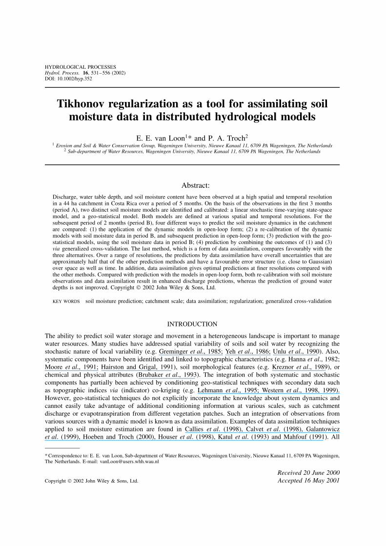
The data for this study have been collected in a 44 ha catchment in north-west Costa Rica. A series oflow-resolution measurements is available from 20 July 1997 till 21 December 1997 and within this period aset of high-resolution measurements is available for 4 October till 21 December. At four locations rain hasbeen measured using tipping buckets. At two locations discharge has been measured at 1 min time instants,using v-crest weirs. Ground water depth has been observed manually in 20 piezometers at hourly instantsduring and just after rain, and daily between rainfall events. During the period 20 July–4 October, volumetricsoil moisture was measured at 40 locations once every 4 days, and during the period 4 October–21 Decemberat 60 locations once every 2 days. For the soil moisture measurements a Trime time domain reflectometry(TDR) system (in plastic tubes) was used, enabling the measurement of soil moisture over 20 cm layers downto 80 cm. The location of the various instruments is shown in Figure 1. Close to the Trime tubes about 150soil moisture measurements were taken within the 0–10 cm topsoil every 10 days, using a TDR system thatwas directly inserted into the ground. These measurements were used to correlate soil moisture observationswith soil and terrain properties and for checking the other measurements.

Terrain and soil were mapped in detail. The terrain was measured using a kinematic GPS technique incombination with a conventional ground-based survey. Soil colour, soil depth, the dimensions of cracks,stability of soil aggregates, organic matter content, and texture were determined at 90 locations, and thehydraulic permeability was determined at 30 of these locations, using a Guelph permeameter (both at 10and 20 cm depths). In addition, the soil colour, the dimension of cracks, the areal density of cracks and thetexture (field-determined) were observed at a regular spacing of 20 ð 20 m2. The purpose of the soil datais either to relate these directly to soil moisture behaviour or group them into a limited number of modelunits.

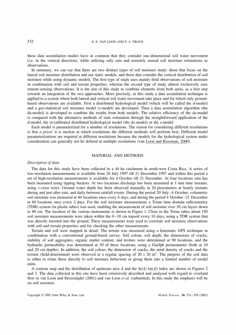
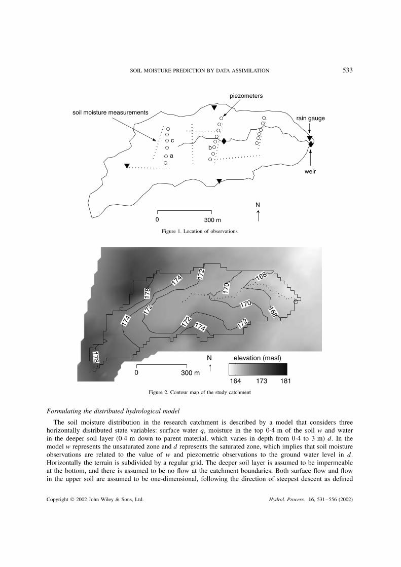
A contour map and the distribution of upstream area A and the ln�A/ tan ˇ� index are shown in Figures 2and 3. The data collected at this site have been extensively described and analysed with regard to overlandflow in van Loon and Stroosnijder (2001) and van Loon et al. (submitted). In this study the emphasis will beon soil moisture.

Copyright 2002 John Wiley & Sons, Ltd. Hydrol. Process. 16, 531–556 (2002)

SOIL MOISTURE PREDICTION BY DATA ASSIMILATION 533

0 300 m

N

soil moisture measurements rain gauge

weir

piezometers

ab

c

Figure 1. Location of observations

164 173 181300 m

N elevation (masl)

0

178

174

172

178

174 17

2

170

170 168

172174172

168

Figure 2. Contour map of the study catchment

Formulating the distributed hydrological model

The soil moisture distribution in the research catchment is described by a model that considers threehorizontally distributed state variables: surface water q, moisture in the top 0Ð4 m of the soil w and waterin the deeper soil layer (0Ð4 m down to parent material, which varies in depth from 0Ð4 to 3 m) d. In themodel w represents the unsaturated zone and d represents the saturated zone, which implies that soil moistureobservations are related to the value of w and piezometric observations to the ground water level in d.Horizontally the terrain is subdivided by a regular grid. The deeper soil layer is assumed to be impermeableat the bottom, and there is assumed to be no flow at the catchment boundaries. Both surface flow and flowin the upper soil are assumed to be one-dimensional, following the direction of steepest descent as defined

Copyright 2002 John Wiley & Sons, Ltd. Hydrol. Process. 16, 531–556 (2002)

534 E. E. VAN LOON AND P. A. TROCH

10

20

30

40

Upstream area (A, ha)

0 300 m

N

5

10

15

Topographic index: ln(A/tanβ)

Figure 3. Topographic features of the study catchment

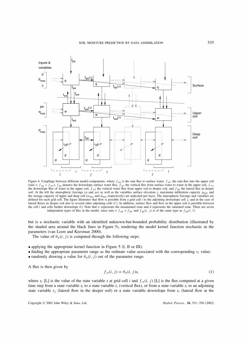
by a D8 algorithm (Marks et al., 1984). Flow in the deeper soil layer is assumed to be driven by watertable differences and is two-dimensional. Atmospheric forcings are rain p and potential evapotranspirationpe. The surface elevation z, the maximum infiltration capacity pmax and the maximum storage capacity ofthe upper soil and deeper soil layers (wmax and dmax respectively) are time-invariant variables in the model.The couplings between the different model-components are schematically drawn in Figure 4.

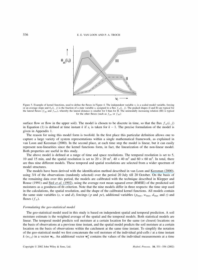
The fluxes indicated in Figure 4 are computed based on the method described fully in van Loon andKeesman (2000). In essence, the fluxes are determined by empirical relationships made up of linear segments(so-called kernel functions). Figure 5 illustrates the form of the kernel functions: the variable at the horizontalaxis vi is a scaled model variable (wi/wmax,i, di/dmax,i), a scaled forcing (pi/pmax,i) or an average slope betweenlocations i and j (zi,j/xi,j), depending on the model state variable to which the kernel function applies. Thevariable on the vertical axis, �st�i, j�, is a transport fraction (0 � �st�i, j� � 1). For transport in the verticaldirection �st�i, j� gives the fraction of transport from the system compartment si to ti (si and ti refer to anytwo state variables with a connection in Figure 4, e.g. qi and wi). For transport in the horizontal direction�st�i, j� gives the fraction of transport from the system compartment si to sj (e.g. from qi to qj in Figure 4).Note that vi is always defined by the state si (not by ti). The value of �st�i, j� is not treated as deterministic,

Copyright 2002 John Wiley & Sons, Ltd. Hydrol. Process. 16, 531–556 (2002)

SOIL MOISTURE PREDICTION BY DATA ASSIMILATION 535

fww(i,j)

fww

fdd

fwd

fpq

fqq(i,j)

fqq

fwe

wmax

dmax

pmax

pe

z

p

fdd

fdd

fpw

ww

w(i,l)

d

d

ii’

jj’

ll’

d

d

soilDeep

Uppersoil

qq

q(i,l)fqwSurface

variables

Inputs &

d

d

Figure 4. Couplings between different model-components, where fpq is the rain flux to surface water, fpw the rain flux into the upper soil(rain D fpq C fpw), fqq denotes the downslope surface water flux, fqw the vertical flux from surface water to water in the upper soil, fwwthe downslope flux of water in the upper soil, fwd the vertical water flux from upper soil to deeper soil, and fdd the lateral flux in deepersoil. At the left the atmospheric forcings (p and pe) as well as the variables surface elevation z, maximum infiltration capacity pmax andthe storage capacity of upper and deep soil (wmax and dmax respectively) are indicated per layer. The atmospheric forcings and variables aredefined for each grid cell. The figure illustrates that flow is possible from a grid cell i to the adjoining downslope cell j, and in the case oflateral fluxes in deeper soil also to several other adjoining cells (i0). In addition, surface flow and flow in the upper soil is possible betweenthe cell i and cells further downslope (l). Note that w represents the unsaturated zone and d represents the saturated zone. There are seven

independent types of flux in the model, since rain D fpq C fqw and fqq�i, j� is of the same type as fqq�i, l�

but is a stochastic variable with an identified unknown-but-bounded probability distribution (illustrated bythe shaded area around the black lines in Figure 5), rendering the model kernel function stochastic in theparameters (van Loon and Keesman 2000).

The value of �st�i, j� is computed through the following steps:

ž applying the appropriate kernel function in Figure 5 (I, II or III);ž finding the appropriate parameter range as the ordinate value associated with the corresponding vi value;ž randomly drawing a value for �st�i, j� out of the parameter range.

A flux is then given byfst�i, j� D �st�i, j�si �1�

where si [L] is the value of the state variable s at grid cell i and fst�i, j� [L] is the flux computed at a giventime step from a state variable si to a state variable ti (vertical flux), or from a state variable si to an adjoiningstate variable sj (lateral flow in the deeper soil) or a state variable downslope from si (lateral flow at the

Copyright 2002 John Wiley & Sons, Ltd. Hydrol. Process. 16, 531–556 (2002)

536 E. E. VAN LOON AND P. A. TROCH

θst

(i,j)

vi

I

II

III

Figure 5. Example of kernel functions, used to define the fluxes in Figure 4. The independent variable vi is a scaled model variable, forcingor an average slope and �st�i, j� is the fraction of a state variable si assigned to a flux fst�i, j�. The peaked shapes (I and II) are typical forthe lateral fluxes (fqq and fww), whereby the lateral distance is smaller for I than for II. The unimodally increasing relation (III) is typical

for the other fluxes (such as fqw or fdd)

surface flow or flow in the upper soil). The model is chosen to be discrete in time, so that the flux fst�i, j�in Equation (1) is defined at time instant k if si is taken for k � 1. The precise formulation of the model isgiven in Appendix 1.

The reason for using this model form is twofold. In the first place this particular definition allows one tocapture a large variety of system representations within a single mathematical framework, as explained invan Loon and Keesman (2000). In the second place, at each time step the model is linear, but it can easilyrepresent non-linearities since the kernel functions form, in fact, the linearization of the non-linear model.Both properties are useful in this study.

The above model is defined at a range of time and space resolutions. The temporal resolution is set to 5,10 and 15 min, and the spatial resolution is set to 20 ð 20 m2, 40 ð 40 m2 and 60 ð 60 m2. In total, thereare thus nine different models. These temporal and spatial resolutions are selected from a wider spectrum ofmodel structures.

The models have been derived with the identification method described in van Loon and Keesman (2000),using 3/4 of the observations (randomly selected) over the period 20 July till 20 October. On the basis ofthe remaining data over this period, the models are calibrated with the technique described in Klepper andRouse (1991) and Stol et al. (1992), using the average root mean squared error (RMSE) of the predicted soilmoistures as a goodness-of-fit criterion. Note that the nine models differ in three respects: the time step usedin the calculations, the spatial resolution, and the shape of the calibrated kernel functions. All models containthe same state variables (s, w and d), forcings (p and pe), additional variables (pmax, wmax, dmax and z) andfluxes (fst).

Formulating the geo-statistical model

The geo-statistical model used in this study is based on independent spatial and temporal prediction. A soilmoisture estimate is the weighted average of the spatial and the temporal models. Both statistical models arelinear. The temporal model predicts soil moisture at a certain location for the same (or closest) locations onthe basis of observations at a previous time instant, and the spatial model predicts the soil moisture at a certainlocation on the basis of observations within the catchment at the same time instant. To simplify the notationof the geo-statistical model we first concatenate the soil moisture of the individual grid-cells i at a time instantk (wi,k) in a vector wk . An additional vector wo

k contains the values of the individual measurements at a time

Copyright 2002 John Wiley & Sons, Ltd. Hydrol. Process. 16, 531–556 (2002)

SOIL MOISTURE PREDICTION BY DATA ASSIMILATION 537

instant k. The soil moisture estimation, which is based on wk�1 and wok , is named wŁ

k . The model can thenbe summarized as follows

wŁk D �1 � ok�Kwk�1 C �ok�Lwo

k �2�

where K and L are cross-correlation matrices for w at a previous time instant and at distant locationsrespectively. ok is a parameter that is set zero for time instants where no observations are available, and hasa fixed value when observations are available. Through L Equation (8) implicitly converts point observationsto averaged grid-cell values. The matrices K and L are fixed for the entire simulation period. The structureof these matrices is determined by trial and error and will be explained in the section ‘Distribution of soilmoisture in space’. The parameter ok is determined (after fixing K and L) on the basis of a calibrationprocedure, using the observations over the period 20 July till 20 October and the average RMSE of thepredicted soil moistures as a goodness-of-fit criterion.

The geo-statistical model is defined at the same resolutions as the distributed hydrological model, i.e.temporal resolutions of 5, 10 and 15 mins, and spatial resolutions of 20 ð 20 m2, 40 ð 40 m2 and 60 ð 60 m2.The temporal resolutions are so small, relative to the sampling intervals of 2 or 4 days, that these do notinfluence the model parameterization. For that reason only three different geo-statistical models are defined(one for each spatial resolution).

Formulating the data assimilation procedure

The distributed hydrological model outlined in the section ‘Formulating the distributed hydrological model’can be formulated as a time-varying linear discrete state-space model of the following form:

xk D Akxk�1 C Bkuk C vk �3�

yk D Hkxk C vŁk �4�

In these equations the vector xk contains the state variables of surface water q, moisture in the top 40 cm ofthe soil w and water in the deeper soil layer (0Ð4 m to parent material, which varies in depth from 0Ð4 to 3 m)d, for each grid cell. The vector uk contains the atmospheric forcings at time instant k, rain p and potentialevapotranspiration pe. The matrices Ak and Bk contain the parameters �st�i, j� (as explained earlier these areknown functions of xk�1 and uk). Ak can be seen as an operator that defines spatial redistribution of soilmoisture in both the lateral and the vertical direction. Bk is an operator that defines the spatial redistributionof rain and evapotranspiration, i.e. movement in the vertical direction only. The vector yk contains theobservations, which are in this study discharge and water table depth. Hk is the observation matrix that relatesthe model state variables to observations. The vector vk contains model errors and vŁ

k observation errors. Inwhat follows we will assume that the distributions of vk and vŁ

k are unknown but bounded, so that xk as wellas yk are characterized by a minimum and a maximum (xk > xk > xk , y

k> y > yk). The initial condition

for this system, x0, is known. Van Loon and Keesman (2000) describe a system to identify models with thestructure of Equation (3). A more elaborate description of Equations (3) and (4) is given in Appendix 1.

The estimation of xk can be achieved by combining Equations (3) and (4) with a Kalman filter. Thedrawback of this approach is that it requires accurate knowledge of the error structure of both the modeland the observations to give a relatively good performance. Moreover, it is not very robust in cases wherean incorrect model is used (Anderson and Moore 1979). In this study the structure of the model error isnon-Gaussian and largely unknown (as will be illustrated later). Moreover, owing to the indeterminacy of theproblem in this study, it is not the optimal weighting of the observations and model predictions (one of theassets of the Kalman filter) but rather the robust weighting that is crucial for good performance. Optimality isnamely not defined for indeterminate problems. For these reasons a different approach was chosen to combinemodel predictions with observations, making use of a technique called Tikhonov regularization (Tikhonov andArsenin, 1977; Johansen, 1997). Recall that Equations (3) and (4) can be used straightforwardly for predictionby supplying the necessary inputs and draw realizations of the stochastic parameter vectors in Equation (3).

Copyright 2002 John Wiley & Sons, Ltd. Hydrol. Process. 16, 531–556 (2002)

538 E. E. VAN LOON AND P. A. TROCH

If there are, in addition, observations (in yk) available, Equation (4) can be inverted in order to derive Oxk . Theweighted average of this result and the state vector estimated by Equation (3) gives the desired state estimate.This problem of state estimation is ill-posed, since the observation matrix Hk (and consequently HkAk aswell as HkBk) is not of full rank. Assumptions have to be made about the variables to be estimated in orderto find a solution to an ill-posed problem. In this context the making of assumptions is called regularization.

Before we will apply regularization, Equation (3) is substituted into Equation (4). Hence

yk � [HkBk]uk D [HkAk]xk�1 C �Hkvk C vŁk � �5�

and for ease of notation we rename this equation to

zk D Dkmk C ek �6�

Now the elements of the vector mk D [xk�1�1� . . . xk�1�n�]T are considered model parameters that have tobe estimated. A regularization technique finds a pseudo-inverse of Dk , by constraining the solution space ofmk . In this study we use the weighted average of prior estimates and additional observations, not includedin yk , as additional constraints (the weighted average is named mŁ

k ). Adding these additional constraints toEquation (6) gives a problem that can be solved in a least-squares sense:[

zkrkmŁ

k

]D

[Dk

rkE

]mk C

[ekeŁk

]�7�

where E is a matrix with ones and zeros to select those elements from mk that correspond to mŁk , rk is a

so-called regularization parameter, which can be established on the basis of various criteria such as entropy,some sort of cross-validation or an l-curve (Tarantola, 1987, Hansen, 1992). Here a technique known asgeneralized cross-validation is used to determine the desired value of rk (Hansen 1998). In this study mŁ

kcontains only soil moisture data, hence mŁ

k D wŁk . We will, however, continue to use mŁ

k to keep Equation (7)general. mŁ

k is defined as the weighted sum of the estimations at a previous time instant (mk�1) and additionalobservations (mo

k D wok), analogous to the geo-statistical model introduced in the section ‘Formulating the

geo-statistical model’:

mŁk D �1 � ok�

[ 0K

0

]mk�1 C �ok�

[ 0L

0

]mo

k �8�

where the cross-correlation matrices K and L and the parameter ok are the same as in Equation (2).Whereas the values of zk , mo

k and mk�1 are loose constraints on the values that mk may take, hard constraintscan be imposed as well. In this study the mass balance at the catchment scale is imposed as a hard constrainton Equation (7). It is given by

L∑lD1

�wk,l � wk�1,l � qk,l � dk,l C pk,l � eak,l� D 0 �9�

where l (1 < l < L) is an index indicating each spatial element in the catchment and eak,l is actualevapotranspiration (eak,l is defined in Appendix 1). The precise mathematical operations involved to solveEquation (7), under the constraint given by Equation (9), are given in Appendix 2.

It should be noted that, in a model with time-variable parameters, state estimation is also possible viaparameter estimation. This can be seen when the substitution of Equation (3) into Equation (4) is expressed as

yk D [HkAk]xk�1 C [HkBk]uk C ek �10�

whereafter the known vectors xk�1 and uk are put into the data matrix Dk , and all the unknown parameters(in Ak and Bk) are put in the parameter vector mk (for details see Appendix 3). This results in an equation

Copyright 2002 John Wiley & Sons, Ltd. Hydrol. Process. 16, 531–556 (2002)

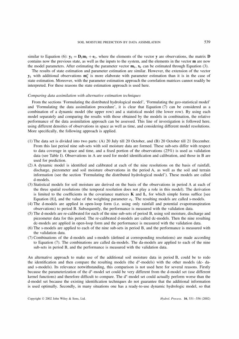
SOIL MOISTURE PREDICTION BY DATA ASSIMILATION 539

similar to Equation (6): yk D Dkmk C ek , where the elements of the vector y are observations, the matrix Dcontains now the previous state, as well as the inputs to the system, and the elements in the vector m are nowthe model parameters. After estimating the parameter vector mk , xk can be estimated through Equation (3).

The results of state estimation and parameter estimation are similar. However, the extension of the vectoryk with additional observations mo

k is more elaborate with parameter estimation than it is in the case ofstate estimation. Moreover, with the parameter estimation approach the correlation matrices cannot readily beinterpreted. For these reasons the state estimation approach is used here.

Comparing data assimilation with alternative estimation techniques

From the sections ‘Formulating the distributed hydrological model’, ‘Formulating the geo-statistical model’and ‘Formulating the data assimilation procedure’, it is clear that Equation (7) can be considered as acombination of a dynamic model (the upper row) and a statistical model (the lower row). By using eachmodel separately and comparing the results with those obtained by the models in combination, the relativeperformance of the data assimilation approach can be assessed. This line of investigation is followed here,using different densities of observations in space as well as time, and considering different model resolutions.More specifically, the following approach is applied.

(1) The data set is divided into two parts: (A) 20 July till 20 October, and (B) 20 October till 21 December.From this last period nine sub-sets with soil moisture data are formed. These sub-sets differ with respectto data coverage in space and time, and a fixed portion of the observations (25%) is used as validationdata (see Table I). Observations in A are used for model identification and calibration, and those in B areused for prediction.

(2) A dynamic model is identified and calibrated at each of the nine resolutions on the basis of rainfall,discharge, piezometer and soil moisture observations in the period A, as well as the soil and terraininformation (see the section ‘Formulating the distributed hydrological model’). These models are calledd-models.

(3) Statistical models for soil moisture are derived on the basis of the observations in period A at each ofthe three spatial resolutions (the temporal resolution does not play a role in this model). The derivationis limited to the coefficients in the covariance matrices K and L, for which simple forms suffice [seeEquation (8)], and the value of the weighting parameter ok . The resulting models are called s-models.

(4) The d-models are applied in open-loop form (i.e. using only rainfall and potential evapotranspirationobservations) to period B. Subsequently, the performance is measured with the validation data.

(5) The d-models are re-calibrated for each of the nine sub-sets of period B, using soil moisture, discharge andpiezometer data for this period. The re-calibrated d-models are called dc-models. Then the nine resultingdc-models are applied in open-loop form and the performance is measured with the validation data.

(6) The s-models are applied to each of the nine sub-sets in period B, and the performance is measured withthe validation data.

(7) Combinations of the d-models and s-models (defined at corresponding resolutions) are made accordingto Equation (7). The combinations are called da-models. The da-models are applied to each of the ninesub-sets in period B, and the performance is measured with the validation data.

An alternative approach to make use of the additional soil moisture data in period B, could be to redothe identification and then compare the resulting models (the dŁ-models) with the other models (dc- da-and s-models). Its relevance notwithstanding, this comparison is not used here for several reasons. Firstlybecause the parameterization of the dŁ-model set could be very different from the d-model set (use differentkernel functions) and therefore difficult to compare. The dŁ-model set could actually perform worse than thed-model set because the existing identification techniques do not guarantee that the additional informationis used optimally. Secondly, in many situations one has a ready-to-use dynamic hydrologic model, so that

Copyright 2002 John Wiley & Sons, Ltd. Hydrol. Process. 16, 531–556 (2002)

540 E. E. VAN LOON AND P. A. TROCH

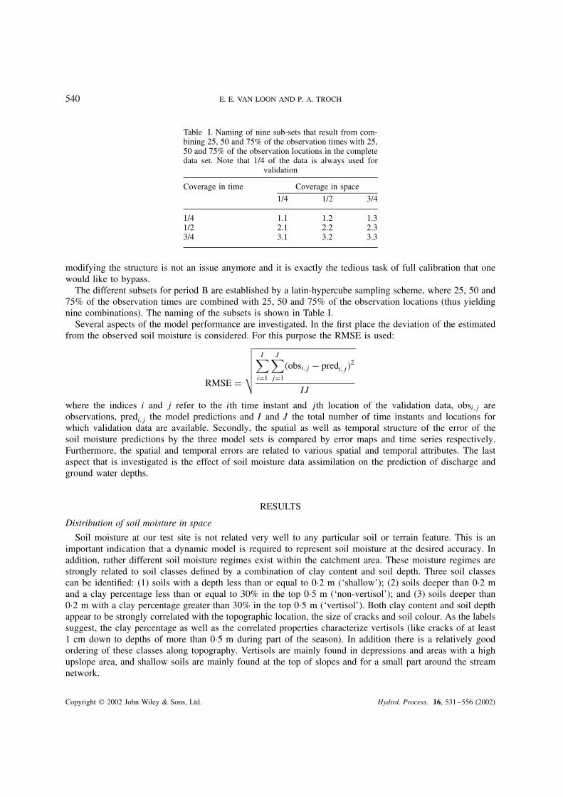
Table I. Naming of nine sub-sets that result from com-bining 25, 50 and 75% of the observation times with 25,50 and 75% of the observation locations in the completedata set. Note that 1/4 of the data is always used for

validation

Coverage in time Coverage in space

1/4 1/2 3/4

1/4 1.1 1.2 1.31/2 2.1 2.2 2.33/4 3.1 3.2 3.3

modifying the structure is not an issue anymore and it is exactly the tedious task of full calibration that onewould like to bypass.

The different subsets for period B are established by a latin-hypercube sampling scheme, where 25, 50 and75% of the observation times are combined with 25, 50 and 75% of the observation locations (thus yieldingnine combinations). The naming of the subsets is shown in Table I.

Several aspects of the model performance are investigated. In the first place the deviation of the estimatedfrom the observed soil moisture is considered. For this purpose the RMSE is used:

RMSE D

√√√√√√I∑

iD1

J∑jD1

�obsi,j � predi,j�2

IJ

where the indices i and j refer to the ith time instant and jth location of the validation data, obsi,j areobservations, predi,j the model predictions and I and J the total number of time instants and locations forwhich validation data are available. Secondly, the spatial as well as temporal structure of the error of thesoil moisture predictions by the three model sets is compared by error maps and time series respectively.Furthermore, the spatial and temporal errors are related to various spatial and temporal attributes. The lastaspect that is investigated is the effect of soil moisture data assimilation on the prediction of discharge andground water depths.

RESULTS

Distribution of soil moisture in space

Soil moisture at our test site is not related very well to any particular soil or terrain feature. This is animportant indication that a dynamic model is required to represent soil moisture at the desired accuracy. Inaddition, rather different soil moisture regimes exist within the catchment area. These moisture regimes arestrongly related to soil classes defined by a combination of clay content and soil depth. Three soil classescan be identified: (1) soils with a depth less than or equal to 0Ð2 m (‘shallow’); (2) soils deeper than 0Ð2 mand a clay percentage less than or equal to 30% in the top 0Ð5 m (‘non-vertisol’); and (3) soils deeper than0Ð2 m with a clay percentage greater than 30% in the top 0Ð5 m (‘vertisol’). Both clay content and soil depthappear to be strongly correlated with the topographic location, the size of cracks and soil colour. As the labelssuggest, the clay percentage as well as the correlated properties characterize vertisols (like cracks of at least1 cm down to depths of more than 0Ð5 m during part of the season). In addition there is a relatively goodordering of these classes along topography. Vertisols are mainly found in depressions and areas with a highupslope area, and shallow soils are mainly found at the top of slopes and for a small part around the streamnetwork.

Copyright 2002 John Wiley & Sons, Ltd. Hydrol. Process. 16, 531–556 (2002)

SOIL MOISTURE PREDICTION BY DATA ASSIMILATION 541

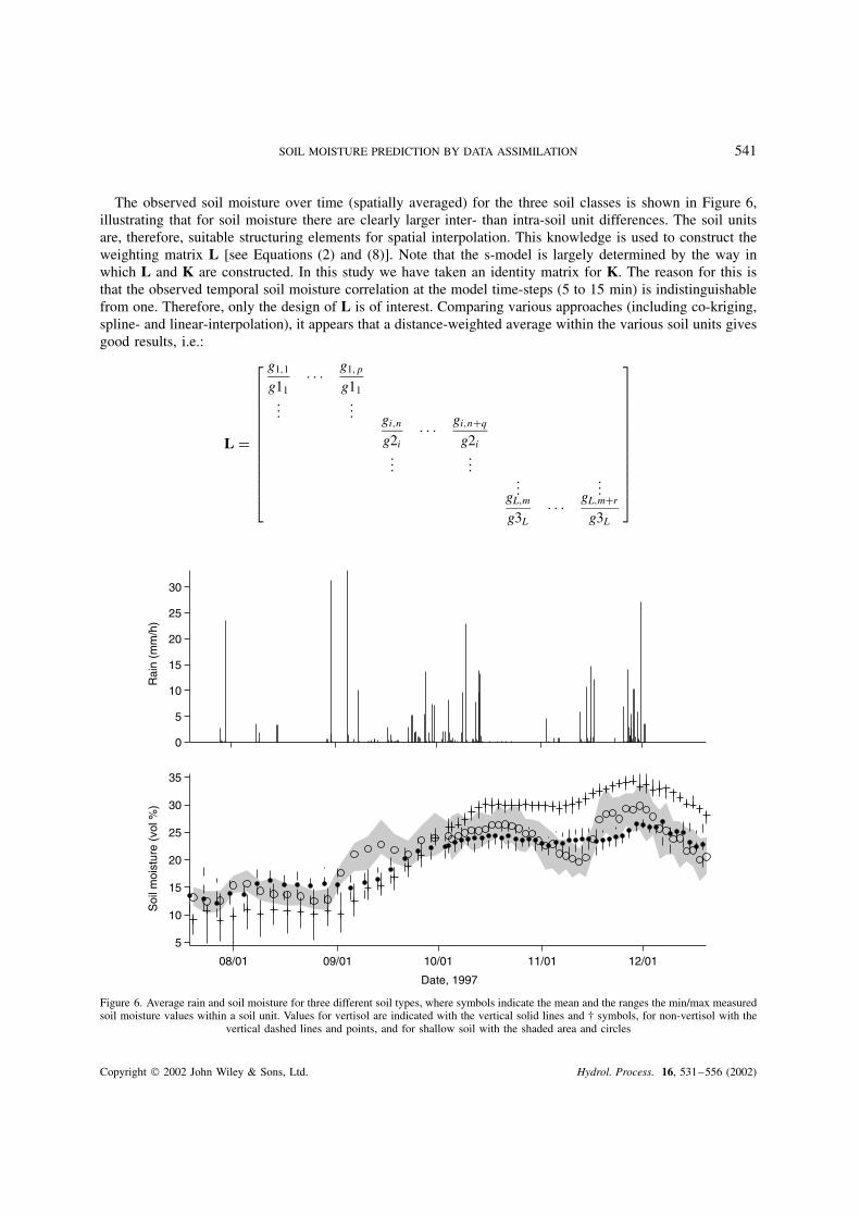
The observed soil moisture over time (spatially averaged) for the three soil classes is shown in Figure 6,illustrating that for soil moisture there are clearly larger inter- than intra-soil unit differences. The soil unitsare, therefore, suitable structuring elements for spatial interpolation. This knowledge is used to construct theweighting matrix L [see Equations (2) and (8)]. Note that the s-model is largely determined by the way inwhich L and K are constructed. In this study we have taken an identity matrix for K. The reason for this isthat the observed temporal soil moisture correlation at the model time-steps (5 to 15 min) is indistinguishablefrom one. Therefore, only the design of L is of interest. Comparing various approaches (including co-kriging,spline- and linear-interpolation), it appears that a distance-weighted average within the various soil units givesgood results, i.e.:

L D

g1,1

g11Ð Ð Ð g1,p

g11...

... gi,ng2i

Ð Ð Ð gi,nCq

g2i...

......

...gL,mg3L

Ð Ð Ð gL,mCr

g3L

0

5

10

15

20

25

30

Rai

n (m

m/h

)

08/01 09/01 10/01 11/01 12/01

5

10

15

20

25

30

35

Date, 1997

Soi

l moi

stur

e (v

ol %

)

Figure 6. Average rain and soil moisture for three different soil types, where symbols indicate the mean and the ranges the min/max measuredsoil moisture values within a soil unit. Values for vertisol are indicated with the vertical solid lines and † symbols, for non-vertisol with the

vertical dashed lines and points, and for shallow soil with the shaded area and circles

Copyright 2002 John Wiley & Sons, Ltd. Hydrol. Process. 16, 531–556 (2002)

542 E. E. VAN LOON AND P. A. TROCH

where gi,q is the distance of observation q to model unit i, gxi the sum of the distances from all the observationswithin soil unit x to model unit i; p, q and r are the total number of observations in the first, second and thirdunit respectively, n�D p C 1� and m�D p C q C 1� are used for a compact notation; and L is the total numberof model units. The parameter values in the L matrix are thus only being based on the terrain observations. Thisimplies that for each spatial resolution (20 ð 20 m2, 40 ð 40 m2, 60 ð 60 m2) a different L matrix is derived.After fixing the values of K and deriving the values of L as described above, the weighting parameter ok[see Equations (2) and (8)] is obtained by optimization (minimizing the RMSE of the predicted soil moisture,using the data from period A). As previously stated, ok is zero for time instants where no observations areavailable and has a fixed value otherwise. Optimal performance is achieved with values for ok between 0Ð86and 0Ð93 (there is not a unique optimum). This optimum appears to be the same for the different spatialresolutions. Based on this result, ok is set to 0Ð9 (at time instants when observations are available and zerootherwise) for all three models.

Characteristics of the various models

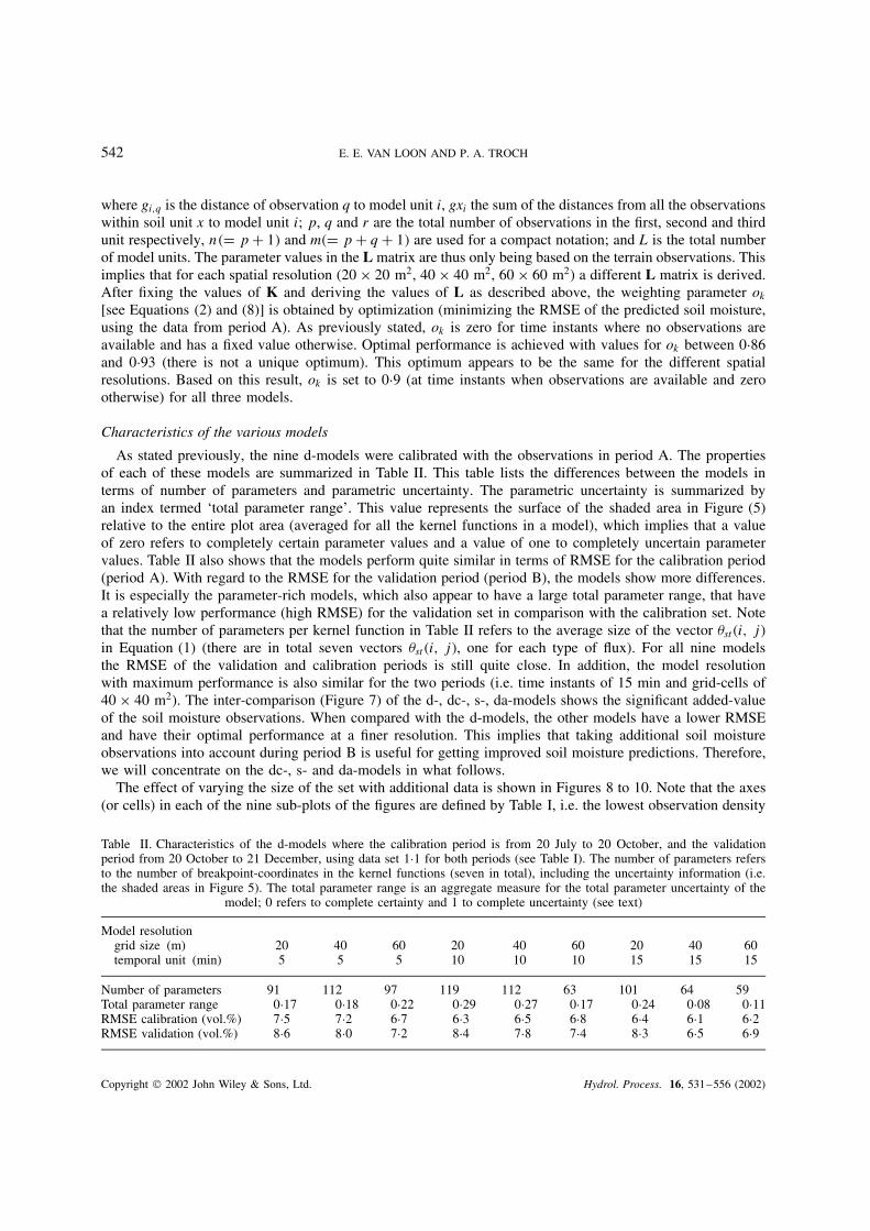
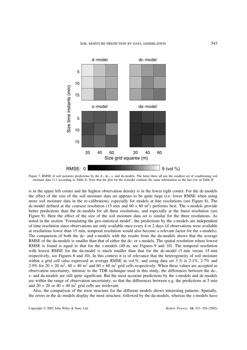
As stated previously, the nine d-models were calibrated with the observations in period A. The propertiesof each of these models are summarized in Table II. This table lists the differences between the models interms of number of parameters and parametric uncertainty. The parametric uncertainty is summarized byan index termed ‘total parameter range’. This value represents the surface of the shaded area in Figure (5)relative to the entire plot area (averaged for all the kernel functions in a model), which implies that a valueof zero refers to completely certain parameter values and a value of one to completely uncertain parametervalues. Table II also shows that the models perform quite similar in terms of RMSE for the calibration period(period A). With regard to the RMSE for the validation period (period B), the models show more differences.It is especially the parameter-rich models, which also appear to have a large total parameter range, that havea relatively low performance (high RMSE) for the validation set in comparison with the calibration set. Notethat the number of parameters per kernel function in Table II refers to the average size of the vector �st�i, j�in Equation (1) (there are in total seven vectors �st�i, j�, one for each type of flux). For all nine modelsthe RMSE of the validation and calibration periods is still quite close. In addition, the model resolutionwith maximum performance is also similar for the two periods (i.e. time instants of 15 min and grid-cells of40 ð 40 m2). The inter-comparison (Figure 7) of the d-, dc-, s-, da-models shows the significant added-valueof the soil moisture observations. When compared with the d-models, the other models have a lower RMSEand have their optimal performance at a finer resolution. This implies that taking additional soil moistureobservations into account during period B is useful for getting improved soil moisture predictions. Therefore,we will concentrate on the dc-, s- and da-models in what follows.

The effect of varying the size of the set with additional data is shown in Figures 8 to 10. Note that the axes(or cells) in each of the nine sub-plots of the figures are defined by Table I, i.e. the lowest observation density

Table II. Characteristics of the d-models where the calibration period is from 20 July to 20 October, and the validationperiod from 20 October to 21 December, using data set 1Ð1 for both periods (see Table I). The number of parameters refersto the number of breakpoint-coordinates in the kernel functions (seven in total), including the uncertainty information (i.e.the shaded areas in Figure 5). The total parameter range is an aggregate measure for the total parameter uncertainty of the

model; 0 refers to complete certainty and 1 to complete uncertainty (see text)

Model resolutiongrid size (m) 20 40 60 20 40 60 20 40 60temporal unit (min) 5 5 5 10 10 10 15 15 15

Number of parameters 91 112 97 119 112 63 101 64 59Total parameter range 0Ð17 0Ð18 0Ð22 0Ð29 0Ð27 0Ð17 0Ð24 0Ð08 0Ð11RMSE calibration (vol.%) 7Ð5 7Ð2 6Ð7 6Ð3 6Ð5 6Ð8 6Ð4 6Ð1 6Ð2RMSE validation (vol.%) 8Ð6 8Ð0 7Ð2 8Ð4 7Ð8 7Ð4 8Ð3 6Ð5 6Ð9

Copyright 2002 John Wiley & Sons, Ltd. Hydrol. Process. 16, 531–556 (2002)

SOIL MOISTURE PREDICTION BY DATA ASSIMILATION 543

d−model dc−model

s−model da−model

5

10

15

20 40 60

5

10

15

20 40 60

Siz

e tim

e in

stan

ts (

min

)

Size grid squares (m)

RMSE: 0 9 (vol %)

Figure 7. RMSE of soil moisture predictions by the d-, dc-, s- and da-models. The latter three all use the smallest set of conditioning soilmoisture data (1Ð1 according to Table I). Note that the plot for the d-model contains the same information as the last row in Table II

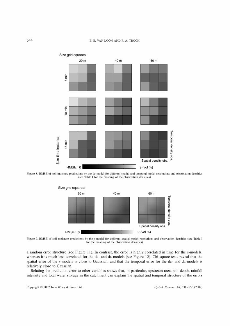
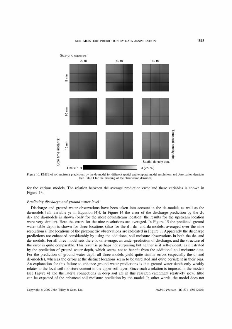
is in the upper left corner and the highest observation density is in the lower right corner. For the dc-modelsthe effect of the size of the soil moisture data set appears to be quite large (i.e. lower RMSE when usingmore soil moisture data in the re-calibration), especially for models at fine resolutions (see Figure 8). Thedc-model defined at the coarsest resolution (15 min and 60 ð 60 m2) performs best. The s-models providebetter predictions than the dc-models for all three resolutions, and especially at the finest resolution (seeFigure 9). Here the effect of the size of the soil moisture data set is similar for the three resolutions. Asnoted in the section ‘Formulating the geo-statistical model’, the predictions by the s-models are independentof time resolution since observations are only available once every 4 or 2 days (if observations were availableat resolutions lower than 15 min, temporal resolution would also become a relevant factor for the s-models).The comparison of both the dc- and s-models with the results from the da-models shows that the averageRMSE of the da-models is smaller than that of either the dc- or s-models. The spatial resolution where lowestRMSE is found is equal to that for the s-models (40 m, see Figures 9 and 10). The temporal resolutionwith lowest RMSE for the da-model is much smaller than that for the dc-model (5 min versus 15 minrespectively, see Figures 8 and 10). In this context it is of relevance that the heterogeneity of soil moisturewithin a grid cell (also expressed as average RMSE in vol.%; and using data set 3Ð3) is 2Ð1%, 2Ð7% and2Ð9% for 20 ð 20 m2, 40 ð 40 m2 and 60 ð 60 m2 grid cells respectively. When these values are accepted asobservation uncertainty, intrinsic to the TDR technique used in this study, the differences between the dc-,s- and da-models are still quite significant. But the most accurate predictions by the s-models and dc-modelsare within the range of observation uncertainty, so that the differences between e.g. the predictions at 5 minand 20 ð 20 or 40 ð 40 m2 grid cells are irrelevant.

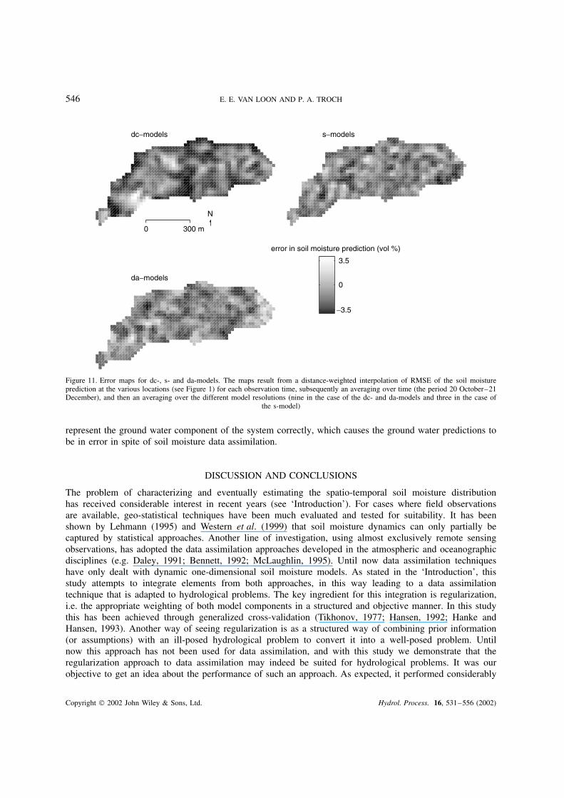
Also, the comparison of the error structure for the different models shows interesting patterns. Spatially,the errors in the dc-models display the most structure, followed by the da-models, whereas the s-models have

Copyright 2002 John Wiley & Sons, Ltd. Hydrol. Process. 16, 531–556 (2002)

544 E. E. VAN LOON AND P. A. TROCH

20 m

5 m

in

40 m 60 m

10 m

in15

min

Spatial density obs.

Tem

poral density obs.S

ize

time

inst

ants

:Size grid squares:

RMSE: 0 9 (vol %)

Figure 8. RMSE of soil moisture predictions by the dc-model for different spatial and temporal model resolutions and observation densities(see Table I for the meaning of the observation densities)

20 m 40 m 60 m

Spatial density obs.

Tem

poral density obs.

Size grid squares:

RMSE: 0 9 (vol %)

Figure 9. RMSE of soil moisture predictions by the s-model for different spatial model resolutions and observation densities (see Table Ifor the meaning of the observation densities)

a random error structure (see Figure 11). In contrast, the error is highly correlated in time for the s-models,whereas it is much less correlated for the dc- and da-models (see Figure 12). Chi-square tests reveal that thespatial error of the s-models is close to Gaussian, and that the temporal error for the dc- and da-models isrelatively close to Gaussian.

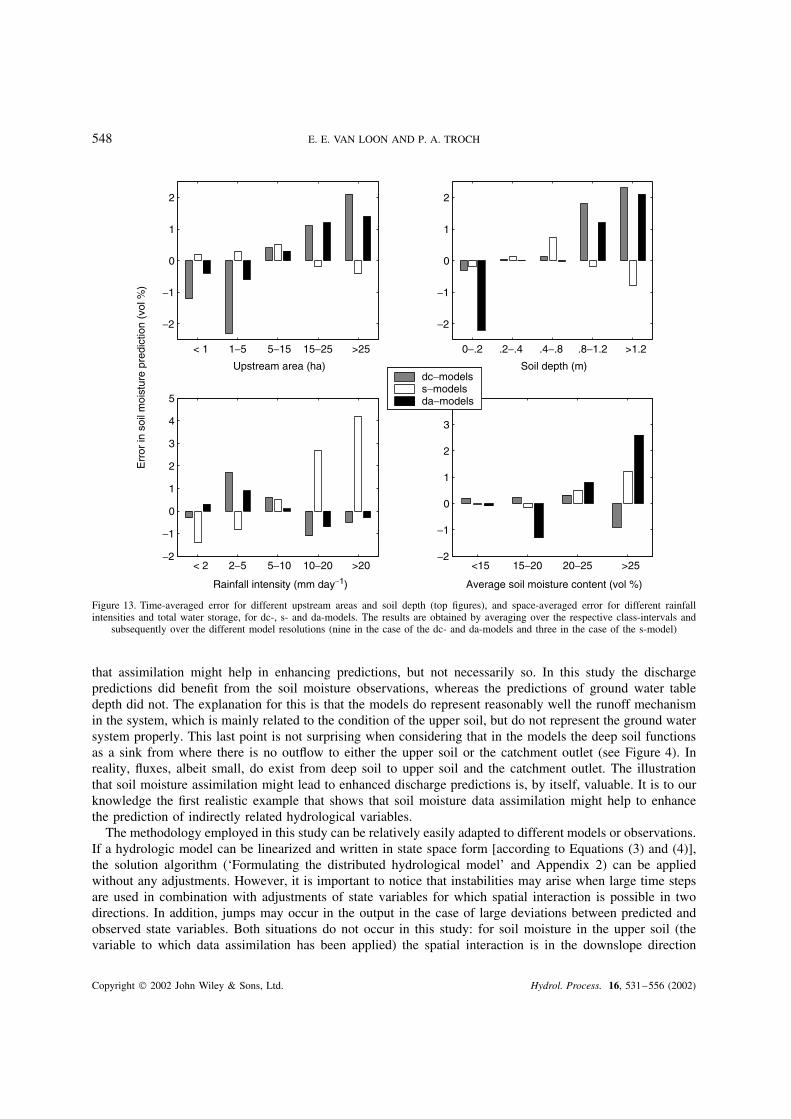
Relating the prediction error to other variables shows that, in particular, upstream area, soil depth, rainfallintensity and total water storage in the catchment can explain the spatial and temporal structure of the errors

Copyright 2002 John Wiley & Sons, Ltd. Hydrol. Process. 16, 531–556 (2002)

SOIL MOISTURE PREDICTION BY DATA ASSIMILATION 545

20 m

5 m

in

40 m 60 m

10 m

in15

min

Spatial density obs.

Tem

poral density obs.S

ize

time

inst

ants

:Size grid squares:

RMSE: 0 9 (vol %)

Figure 10. RMSE of soil moisture predictions by the da-model for different spatial and temporal model resolutions and observation densities(see Table I for the meaning of the observation densities)

for the various models. The relation between the average prediction error and these variables is shown inFigure 13.

Predicting discharge and ground water level

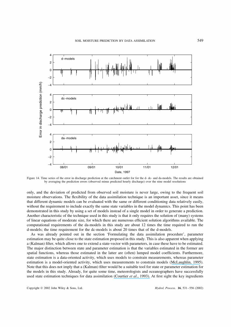
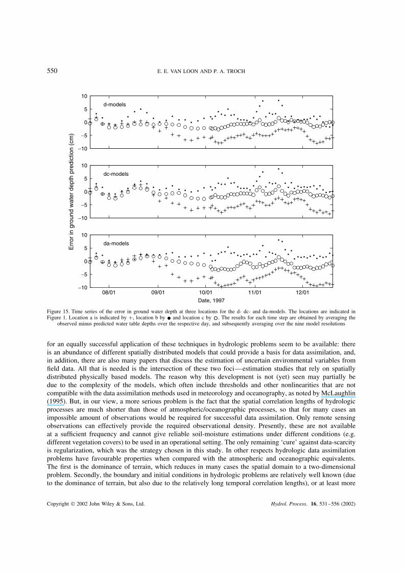
Discharge and ground water observations have been taken into account in the dc-models as well as theda-models [via variable yk in Equation (4)]. In Figure 14 the error of the discharge prediction by the d-,dc- and da-models is shown (only for the most downstream location; the results for the upstream locationwere very similar). Here the errors for the nine resolutions are averaged. In Figure 15 the predicted groundwater table depth is shown for three locations (also for the d-, dc- and da-models, averaged over the nineresolutions). The locations of the piezometric observations are indicated in Figure 1. Apparently the dischargepredictions are enhanced considerably by using the additional soil moisture observations in both the dc- andda- models. For all three model sets there is, on average, an under-prediction of discharge, and the structure ofthe error is quite comparable. This result is perhaps not surprising but neither is it self-evident, as illustratedby the prediction of ground water depth, which seems not to benefit from the additional soil moisture data.For the prediction of ground water depth all three models yield quite similar errors (especially the d- anddc-models), whereas the errors at the distinct locations seem to be unrelated and quite persistent in their bias.An explanation for this failure to enhance ground water predictions is that ground water depth only weaklyrelates to the local soil moisture content in the upper soil layer. Since such a relation is imposed in the models(see Figure 4) and the lateral connections in deep soil are in this research catchment relatively slow, littlecan be expected of the enhanced soil moisture prediction by the model. In other words, the model does not

Copyright 2002 John Wiley & Sons, Ltd. Hydrol. Process. 16, 531–556 (2002)

546 E. E. VAN LOON AND P. A. TROCH

dc−models

0 300 m

N

s−models

da−models

error in soil moisture prediction (vol %)

−3.5

0

3.5

Figure 11. Error maps for dc-, s- and da-models. The maps result from a distance-weighted interpolation of RMSE of the soil moistureprediction at the various locations (see Figure 1) for each observation time, subsequently an averaging over time (the period 20 October–21December), and then an averaging over the different model resolutions (nine in the case of the dc- and da-models and three in the case of

the s-model)

represent the ground water component of the system correctly, which causes the ground water predictions tobe in error in spite of soil moisture data assimilation.

DISCUSSION AND CONCLUSIONS

The problem of characterizing and eventually estimating the spatio-temporal soil moisture distributionhas received considerable interest in recent years (see ‘Introduction’). For cases where field observationsare available, geo-statistical techniques have been much evaluated and tested for suitability. It has beenshown by Lehmann (1995) and Western et al. (1999) that soil moisture dynamics can only partially becaptured by statistical approaches. Another line of investigation, using almost exclusively remote sensingobservations, has adopted the data assimilation approaches developed in the atmospheric and oceanographicdisciplines (e.g. Daley, 1991; Bennett, 1992; McLaughlin, 1995). Until now data assimilation techniqueshave only dealt with dynamic one-dimensional soil moisture models. As stated in the ‘Introduction’, thisstudy attempts to integrate elements from both approaches, in this way leading to a data assimilationtechnique that is adapted to hydrological problems. The key ingredient for this integration is regularization,i.e. the appropriate weighting of both model components in a structured and objective manner. In this studythis has been achieved through generalized cross-validation (Tikhonov, 1977; Hansen, 1992; Hanke andHansen, 1993). Another way of seeing regularization is as a structured way of combining prior information(or assumptions) with an ill-posed hydrological problem to convert it into a well-posed problem. Untilnow this approach has not been used for data assimilation, and with this study we demonstrate that theregularization approach to data assimilation may indeed be suited for hydrological problems. It was ourobjective to get an idea about the performance of such an approach. As expected, it performed considerably

Copyright 2002 John Wiley & Sons, Ltd. Hydrol. Process. 16, 531–556 (2002)

SOIL MOISTURE PREDICTION BY DATA ASSIMILATION 547

−5

0

5 dc−models

−5

0

5 s−models

08/01 09/01 10/01 11/01 12/01

−5

0

5

Date, 1997

da−modelsErr

or in

soi

l moi

stur

e pr

edic

tion

(vol

%)

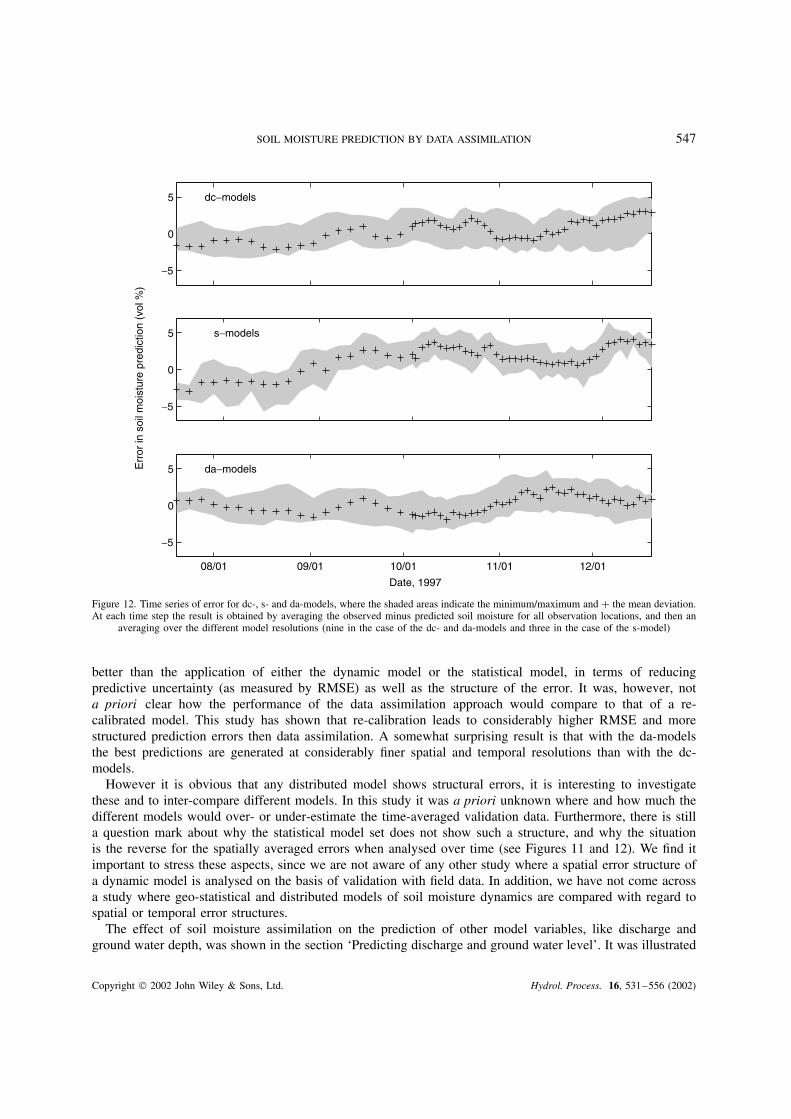
Figure 12. Time series of error for dc-, s- and da-models, where the shaded areas indicate the minimum/maximum and C the mean deviation.At each time step the result is obtained by averaging the observed minus predicted soil moisture for all observation locations, and then an

averaging over the different model resolutions (nine in the case of the dc- and da-models and three in the case of the s-model)

better than the application of either the dynamic model or the statistical model, in terms of reducingpredictive uncertainty (as measured by RMSE) as well as the structure of the error. It was, however, nota priori clear how the performance of the data assimilation approach would compare to that of a re-calibrated model. This study has shown that re-calibration leads to considerably higher RMSE and morestructured prediction errors then data assimilation. A somewhat surprising result is that with the da-modelsthe best predictions are generated at considerably finer spatial and temporal resolutions than with the dc-models.

However it is obvious that any distributed model shows structural errors, it is interesting to investigatethese and to inter-compare different models. In this study it was a priori unknown where and how much thedifferent models would over- or under-estimate the time-averaged validation data. Furthermore, there is stilla question mark about why the statistical model set does not show such a structure, and why the situationis the reverse for the spatially averaged errors when analysed over time (see Figures 11 and 12). We find itimportant to stress these aspects, since we are not aware of any other study where a spatial error structure ofa dynamic model is analysed on the basis of validation with field data. In addition, we have not come acrossa study where geo-statistical and distributed models of soil moisture dynamics are compared with regard tospatial or temporal error structures.

The effect of soil moisture assimilation on the prediction of other model variables, like discharge andground water depth, was shown in the section ‘Predicting discharge and ground water level’. It was illustrated

Copyright 2002 John Wiley & Sons, Ltd. Hydrol. Process. 16, 531–556 (2002)

548 E. E. VAN LOON AND P. A. TROCH

< 1 1−5 5−15 15−25 >25

−2

−1

0

1

2

Upstream area (ha)

0−.2 .2−.4 .4−.8 .8−1.2 >1.2

−2

−1

0

1

2

Soil depth (m)

< 2 2−5 5−10 10−20 >20−2

−1

0

1

2

3

4

5

Rainfall intensity (mm day−1)

<15 15−20 20−25 >25−2

−1

0

1

2

3

4

Average soil moisture content (vol %)

dc−modelss−modelsda−models

Err

or in

soi

l moi

stur

e pr

edic

tion

(vol

%)

Figure 13. Time-averaged error for different upstream areas and soil depth (top figures), and space-averaged error for different rainfallintensities and total water storage, for dc-, s- and da-models. The results are obtained by averaging over the respective class-intervals and

subsequently over the different model resolutions (nine in the case of the dc- and da-models and three in the case of the s-model)

that assimilation might help in enhancing predictions, but not necessarily so. In this study the dischargepredictions did benefit from the soil moisture observations, whereas the predictions of ground water tabledepth did not. The explanation for this is that the models do represent reasonably well the runoff mechanismin the system, which is mainly related to the condition of the upper soil, but do not represent the ground watersystem properly. This last point is not surprising when considering that in the models the deep soil functionsas a sink from where there is no outflow to either the upper soil or the catchment outlet (see Figure 4). Inreality, fluxes, albeit small, do exist from deep soil to upper soil and the catchment outlet. The illustrationthat soil moisture assimilation might lead to enhanced discharge predictions is, by itself, valuable. It is to ourknowledge the first realistic example that shows that soil moisture data assimilation might help to enhancethe prediction of indirectly related hydrological variables.

The methodology employed in this study can be relatively easily adapted to different models or observations.If a hydrologic model can be linearized and written in state space form [according to Equations (3) and (4)],the solution algorithm (‘Formulating the distributed hydrological model’ and Appendix 2) can be appliedwithout any adjustments. However, it is important to notice that instabilities may arise when large time stepsare used in combination with adjustments of state variables for which spatial interaction is possible in twodirections. In addition, jumps may occur in the output in the case of large deviations between predicted andobserved state variables. Both situations do not occur in this study: for soil moisture in the upper soil (thevariable to which data assimilation has been applied) the spatial interaction is in the downslope direction

Copyright 2002 John Wiley & Sons, Ltd. Hydrol. Process. 16, 531–556 (2002)

SOIL MOISTURE PREDICTION BY DATA ASSIMILATION 549

−4

−2

0

2

4d−models

−4

−2

0

2

4dc−models

08/01 09/01 10/01 11/01 12/01−4

−2

0

2

4

Date, 1997

da−modelsErr

or in

dis

char

ge p

redi

ctio

n (m

m/h

)

Figure 14. Time series of the error in discharge prediction at the catchment outlet for for the d- dc- and da-models. The results are obtainedby averaging the prediction errors (observed minus predicted hourly discharge) over the nine model resolutions

only, and the deviation of predicted from observed soil moisture is never large, owing to the frequent soilmoisture observations. The flexibility of the data assimilation technique is an important asset, since it meansthat different dynamic models can be evaluated with the same or different conditioning data relatively easily,without the requirement to include exactly the same state variables in the model dynamics. This point has beendemonstrated in this study by using a set of models instead of a single model in order to generate a prediction.Another characteristic of the technique used in this study is that it only requires the solution of (many) systemsof linear equations of moderate size, for which there are numerous efficient solution algorithms available. Thecomputational requirements of the da-models in this study are about 12 times the time required to run thed-models; the time requirement for the dc-models is about 20 times that of the d-models.

As was already pointed out in the section ‘Formulating the data assimilation procedure’, parameterestimation may be quite close to the state estimation proposed in this study. This is also apparent when applyinga (Kalman) filter, which allows one to extend a state-vector with parameters, in case these have to be estimated.The major distinction between state and parameter estimation is that the variables estimated in the former arespatial functions, whereas those estimated in the latter are (often) lumped model coefficients. Furthermore,state estimation is a data-oriented activity, which uses models to constrain measurements, whereas parameterestimation is a model-oriented activity, which uses measurements to constrain models (McLaughlin, 1995).Note that this does not imply that a (Kalman) filter would be a suitable tool for state or parameter estimation forthe models in this study. Already, for quite some time, meteorologists and oceanographers have successfullyused state estimation techniques for data assimilation (Courtier et al., 1993). At first sight the key ingredients

Copyright 2002 John Wiley & Sons, Ltd. Hydrol. Process. 16, 531–556 (2002)

550 E. E. VAN LOON AND P. A. TROCH

−10

−5

0

5

10

−10

−5

0

5

10

08/01 09/01 10/01 11/01 12/01−10

−5

0

5

10

Date, 1997

Err

or in

gro

und

wat

er d

epth

pre

dict

ion

(cm

)

d-models

dc-models

da-models

Figure 15. Time series of the error in ground water depth at three locations for the d- dc- and da-models. The locations are indicated inFigure 1. Location a is indicated by C, location b by ž and location c by °. The results for each time step are obtained by averaging the

observed minus predicted water table depths over the respective day, and subsequently averaging over the nine model resolutions

for an equally successful application of these techniques in hydrologic problems seem to be available: thereis an abundance of different spatially distributed models that could provide a basis for data assimilation, and,in addition, there are also many papers that discuss the estimation of uncertain environmental variables fromfield data. All that is needed is the intersection of these two foci—estimation studies that rely on spatiallydistributed physically based models. The reason why this development is not (yet) seen may partially bedue to the complexity of the models, which often include thresholds and other nonlinearities that are notcompatible with the data assimilation methods used in meteorology and oceanography, as noted by McLaughlin(1995). But, in our view, a more serious problem is the fact that the spatial correlation lengths of hydrologicprocesses are much shorter than those of atmospheric/oceanographic processes, so that for many cases animpossible amount of observations would be required for successful data assimilation. Only remote sensingobservations can effectively provide the required observational density. Presently, these are not availableat a sufficient frequency and cannot give reliable soil-moisture estimations under different conditions (e.g.different vegetation covers) to be used in an operational setting. The only remaining ‘cure’ against data-scarcityis regularization, which was the strategy chosen in this study. In other respects hydrologic data assimilationproblems have favourable properties when compared with the atmospheric and oceanographic equivalents.The first is the dominance of terrain, which reduces in many cases the spatial domain to a two-dimensionalproblem. Secondly, the boundary and initial conditions in hydrologic problems are relatively well known (dueto the dominance of terrain, but also due to the relatively long temporal correlation lengths), or at least more

Copyright 2002 John Wiley & Sons, Ltd. Hydrol. Process. 16, 531–556 (2002)

SOIL MOISTURE PREDICTION BY DATA ASSIMILATION 551

easily observed than in atmospheric/oceanographic problems. Both properties have been exploited in thisstudy: the three-dimensional problem has been reduced to a number of parallel one-dimensional problems,and by starting the study period from a dry condition the boundary and initial conditions were relativelycertain.

Based on the results of this investigation, the next step will be to develop further the data assimilationtechnique presented by applying it to various other data sets and models, and especially to test its feasibilityin an operational setting with a much lower observational density. Another question is how the approachpresented compares with the Kalman filter and smoother, where regularization can also be applied (Boutayebet al., 1997; Reif et al., 1998).

ACKNOWLEDGEMENTS

This study was funded by the EU 5th Framework Programme, project EVK1-CT1999-00022—‘DAUFIN’.The authors would like to thank Claudio Paniconi and Keith Beven for their careful reading and constructivecomments.

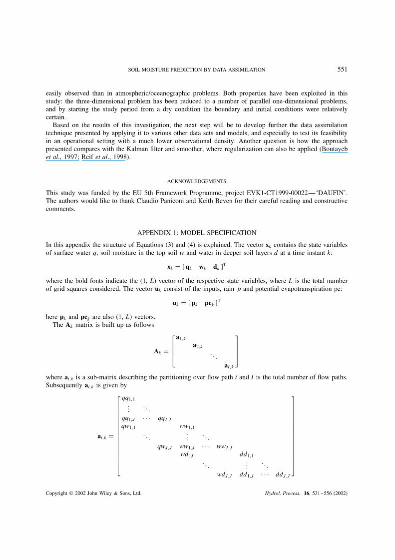
APPENDIX 1: MODEL SPECIFICATION

In this appendix the structure of Equations (3) and (4) is explained. The vector xk contains the state variablesof surface water q, soil moisture in the top soil w and water in deeper soil layers d at a time instant k:

xk D [ qk wk dk ]T

where the bold fonts indicate the (1, L) vector of the respective state variables, where L is the total numberof grid squares considered. The vector uk consist of the inputs, rain p and potential evapotranspiration pe:

uk D [ pk pek ]T

here pk and pek are also (1, L) vectors.The Ak matrix is built up as follows

Ak D

a1,k

a2,k. . .

aI,k

where ai,k is a sub-matrix describing the partitioning over flow path i and I is the total number of flow paths.Subsequently ai,k is given by

ai,k D

qq1,1...

. . .qq1,J Ð Ð Ð qqJ,Jqw1,1 ww1,1

. . ....

. . .qwJ,J ww1,J Ð Ð Ð wwJ,J

wd1J dd1,1. . .

.... . .

wdJ,J dd1,J Ð Ð Ð ddJ,J

Copyright 2002 John Wiley & Sons, Ltd. Hydrol. Process. 16, 531–556 (2002)

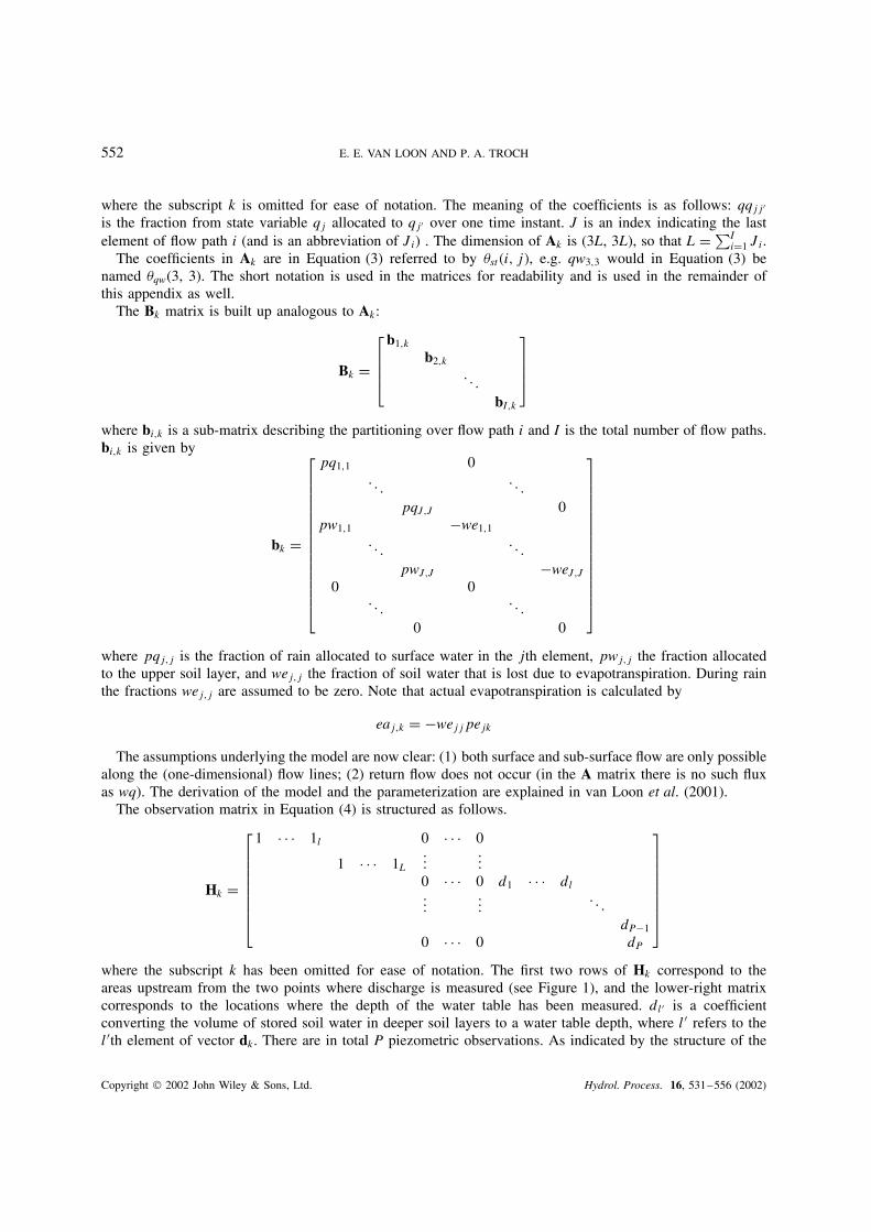
552 E. E. VAN LOON AND P. A. TROCH

where the subscript k is omitted for ease of notation. The meaning of the coefficients is as follows: qqjj0

is the fraction from state variable qj allocated to qj0 over one time instant. J is an index indicating the lastelement of flow path i (and is an abbreviation of Ji) . The dimension of Ak is (3L, 3L), so that L D ∑I

iD1 Ji.The coefficients in Ak are in Equation (3) referred to by �st�i, j�, e.g. qw3,3 would in Equation (3) be

named �qw(3, 3). The short notation is used in the matrices for readability and is used in the remainder ofthis appendix as well.

The Bk matrix is built up analogous to Ak :

Bk D

b1,k

b2,k. . .

bI,k

where bi,k is a sub-matrix describing the partitioning over flow path i and I is the total number of flow paths.bi,k is given by

bk D

pq1,1 0. . .

. . .pqJ,J 0

pw1,1 �we1,1. . .

. . .pwJ,J �weJ,J

0 0. . .

. . .0 0

where pqj,j is the fraction of rain allocated to surface water in the jth element, pwj,j the fraction allocatedto the upper soil layer, and wej,j the fraction of soil water that is lost due to evapotranspiration. During rainthe fractions wej,j are assumed to be zero. Note that actual evapotranspiration is calculated by

eaj,k D �wejjpejk

The assumptions underlying the model are now clear: (1) both surface and sub-surface flow are only possiblealong the (one-dimensional) flow lines; (2) return flow does not occur (in the A matrix there is no such fluxas wq). The derivation of the model and the parameterization are explained in van Loon et al. (2001).

The observation matrix in Equation (4) is structured as follows.

Hk D

1 Ð Ð Ð 1l 0 Ð Ð Ð 0

1 Ð Ð Ð 1L...

...0 Ð Ð Ð 0 d1 Ð Ð Ð dl...

.... . .

dP�1

0 Ð Ð Ð 0 dP

where the subscript k has been omitted for ease of notation. The first two rows of Hk correspond to theareas upstream from the two points where discharge is measured (see Figure 1), and the lower-right matrixcorresponds to the locations where the depth of the water table has been measured. dl0 is a coefficientconverting the volume of stored soil water in deeper soil layers to a water table depth, where l0 refers to thel0th element of vector dk . There are in total P piezometric observations. As indicated by the structure of the

Copyright 2002 John Wiley & Sons, Ltd. Hydrol. Process. 16, 531–556 (2002)

SOIL MOISTURE PREDICTION BY DATA ASSIMILATION 553

lower-right matrix, a single observation for various grid cells as well as multiple observations per grid cellare possible.

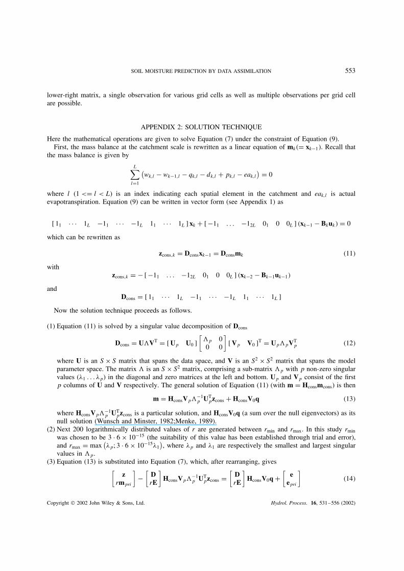
APPENDIX 2: SOLUTION TECHNIQUE

Here the mathematical operations are given to solve Equation (7) under the constraint of Equation (9).First, the mass balance at the catchment scale is rewritten as a linear equation of mk�D xk�1�. Recall that

the mass balance is given by

L∑lD1

(wk,l � wk�1,l � qk,l � dk,l C pk,l � eak,l

) D 0

where l (1 <D l < L) is an index indicating each spatial element in the catchment and eak,l is actualevapotranspiration. Equation (9) can be written in vector form (see Appendix 1) as

[ 11 Ð Ð Ð 1L �11 Ð Ð Ð �1L 11 Ð Ð Ð 1L ] xk C [ �11 . . . �12L 01 0 0L ] �xk�1 � Bkuk� D 0

which can be rewritten as

zcons,k D Dconsxk�1 D Dconsmk �11�

withzcons,k D � [ �11 . . . �12L 01 0 0L ] �xk�2 � Bk�1uk�1�

andDcons D [ 11 Ð Ð Ð 1L �11 Ð Ð Ð �1L 11 Ð Ð Ð 1L ]

Now the solution technique proceeds as follows.

(1) Equation (11) is solved by a singular value decomposition of Dcons

Dcons D UVT D [ Up U0 ][p 00 0

][ Vp V0 ]T D UppVT

p �12�

where U is an S ð S matrix that spans the data space, and V is an S2 ð S2 matrix that spans the modelparameter space. The matrix is an S ð S2 matrix, comprising a sub-matrix p with p non-zero singularvalues (&1 . . . &p) in the diagonal and zero matrices at the left and bottom. Up and Vp consist of the firstp columns of U and V respectively. The general solution of Equation (11) (with m D Hconsmcons) is then

m D HconsVp�1p UT

pzcons C HconsV0q �13�

where HconsVp�1p UT

pzcons is a particular solution, and HconsV0q (a sum over the null eigenvectors) as itsnull solution (Wunsch and Minster, 1982;Menke, 1989).

(2) Next 200 logarithmically distributed values of r are generated between rmin and rmax. In this study rmin

was chosen to be 3 Ð 6 ð 10�15 (the suitability of this value has been established through trial and error),and rmax D max

(&p; 3 Ð 6 ð 10�15&1

), where &p and &1 are respectively the smallest and largest singular

values in p.(3) Equation (13) is substituted into Equation (7), which, after rearranging, gives[

zrmpri

]�

[DrE

]HconsVp

�1p UT

pzcons D[

DrE

]HconsV0q C

[e

epri

]�14�

Copyright 2002 John Wiley & Sons, Ltd. Hydrol. Process. 16, 531–556 (2002)

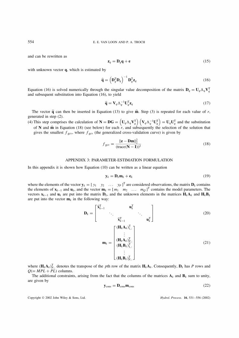
554 E. E. VAN LOON AND P. A. TROCH

and can be rewritten aszq D Dqq C e �15�

with unknown vector q, which is estimated by

q D(

DTqDq

)�1DTqzq �16�

Equation (16) is solved numerically through the singular value decomposition of the matrix Dq D UqqVTq

and subsequent substitution into Equation (16), to yield

q D Vq�1q UT

qzq �17�

The vector q can then be inserted in Equation (13) to give m. Step (3) is repeated for each value of r,generated in step (2).(4) This step comprises the calculation of N D DG D

(UqqVT

q

)(Vq�1

q UTq

)D UqUT

q and the substitutionof N and m in Equation (18) (see below) for each r, and subsequently the selection of the solution thatgives the smallest fgcv, where fgcv (the generalized cross-validation curve) is given by

fgcv D jjz � Dmjj22�trace�N � I��2

�18�

APPENDIX 3: PARAMETER-ESTIMATION FORMULATION

In this appendix it is shown how Equation (10) can be written as a linear equation

yk D Dkmk C ek �19�

where the elements of the vector yk D [ y1 y2 . . . yP ]T are considered observations, the matrix Dk containsthe elements of xk�1 and uk , and the vector mk D [m1 m2 . . . mQ ]T contains the model parameters. Thevectors xk�1 and uk are put into the matrix Dk , and the unknown elements in the matrices HkAk and HkBk

are put into the vector mk in the following way:

Dk D

xTk�1 uT

k. . .

. . .xTk�1 uT

k

�20�

mk D

�HkAk�T1,:

...�HkAk�

TP,:

�HkBk�T1,:

...�HkBk�

TP,:

�21�

where �HkAk�TP,: denotes the transpose of the pth row of the matrix HkAk . Consequently, Dk has P rows and

Q�D MPL C PL� columns.The additional constraints, arising from the fact that the columns of the matrices Ak and Bk sum to unity,

are given byycons D Dconsmcons �22�

Copyright 2002 John Wiley & Sons, Ltd. Hydrol. Process. 16, 531–556 (2002)

SOIL MOISTURE PREDICTION BY DATA ASSIMILATION 555

and, to convert mcons to m,m D Hconsmcons �23�

The matrix forms of the equation’s elements are as follows.

ycons D [ 1 1 Ð Ð Ð 1�MC1�L ]T

Dcons D zT

cons. . .

zTcons

mcons D

�Ak�:,1...

�Ak�:,LM�Bk�:,1

...�Bk�:,L

where Dcons is an S ð S2 matrix (S D ML C L) and �Ak�:,i denotes the ith column of the matrix �Ak�. m canbe obtained by multiplication with an output matrix Hcons, and subsequent reformatting to obtain the rightordering of the coefficients. Hcons is given by

Hcons D �Hk�1

. . .�Hk�S

REFERENCES

Anderson BDO, Moore JB. 1979. Optimal Filtering . Prentice-Hall: Englewood Cliffs, NJ.Bennett AF. 1992. Inverse Methods in Physical Oceanography . Cambridge University Press.Boutayeb M, Rafaralahy H, Darouach M. 1997. Convergence analysis of the extended Kalman filter used as an observer for nonlinear

deterministic discrete-time systems. IEEE Transactions on Automatic Control 42(4): 581–586.Brubaker SC, Jones AJ, Lewis DT, Frank. K. 1993. Soil properties associated with landscape position. Soil Science Society of America

Journal 57: 235–239.Callies U, Rhodin A, Eppel DP. 1998. A case study on variational soil moisture analysis from atmospheric observations. Journal of Hydrology

212–213: 95–108.Calvet JC, Noilhan J, Bessemoulin P. 1998. Retrieving the root-zone soil moisture from surface soil moisture or temperature estimates: a

feasibility study based on field measurements. Journal of Applied Meteorology 37(4): 371–386.Courtier P, Derber J, Errico R, Louis JF, Vukıcevic T. 1993. Important literature on the use of adjoint, variational methods and the Kalman

filter in meteorology. Tellus 45A: 342–357.Daley R. 1991. Atmospheric Data Analysis . Cambridge University Press.Galantowicz JF, Entekhabi D, Njoku EG. 1999. Test of sequential data assimilation for retrieving profile soil moisture and temperature from

observed L-band radiobrightness. IEEE Transactions on Geoscience and Remote Sensing 37(4): 1860–1870.Greminger PD, Sud YK, Nielsen DR. 1985. Spatial variability of field-measured soil-water characteristics. Soil Science Society of America

Journal 49: 1075–1082.Hairston AB, Grigal DF. 1991. Topographic influences on soils and trees within single mapping units on a sandy outwash landscape. Forest

Ecology and Management 43: 35–45.Hanke M, Hansen PC. 1993. Regularization methods for large-scale problems. Surveys on Mathematics in Industry 3: 253–315.Hanna AY, Harlan PW, Lewis DT. 1982. Soil available water as influenced by landscape position and aspect. Agronomy Journal 74:

999–1004.Hansen PC. 1992. Analysis of discrete ill-posed problems by means of the l-curve. SIAM Review 34: 561–580.Hansen PC. 1998. Rank-Deficient and Discrete Ill-Posed Problems: Numerical Aspects of Linear Inversion. SIAM: Philadelphia.Hoeben R, Troch PA. 2000. Assimilation of active microwave observation data for soil moisture profile estimation. Water Resources Research

36(10): 2805–2819.Houser PR, Shuttleworth WJ, Famiglietti JS, Gupta HV, Syed KH, Goodrich DC. 1998. Integration of soil moisture remote sensing and

hydrologic modeling using data assimilation. Water Resources Research 34(12): 3405–3420.

Copyright 2002 John Wiley & Sons, Ltd. Hydrol. Process. 16, 531–556 (2002)

556 E. E. VAN LOON AND P. A. TROCH

Johansen TA. 1997. On Tikhonov regularization, bias and variance in nonlinear system identification. Automatica 33(3): 441–446.Katul GG, Wendroth O, Parlange MB, Puente CE, Folegatti MV, Nielsen DR. 1993. Estimation of in situ hydraulic conductivity function

from nonlinear filtering theory. Water Resources Research 29(4): 1063–1070.Klepper O, Rouse DI. 1991. A procedure to reduce parameter uncertainty for complex models by comparison with a real system output

illustrated on a potato growth model. Agricultural Systems 36: 375–395.Kreznor WR, Olson KR, Banwart WL, Johnson DL. 1989. Soil, landscape and erosion relationships in a northwest Illinois watershed. Soil

Science Society of America Journal 53: 1763–1771.Lehmann W. Anwendung geostatistischer verfahren auf die bodenfeuchte in landlichen einzugsgebieten. PhD thesis, Institut fur Hydrologie

und Wasserwirtschaft, Universitat Karlsruhe, Germany, 1995.Mahfouf JF. 1991. Analysis of soil moisture from near-surface parameters: a feasibility study. Journal of Applied Meteorology 30:

1354–1365.Marks D, Dozier J, Frew J. 1984. Automated basin delineation from digital elevation data. Geo-Processing 2: 299–311.McLaughlin D. 1995. Recent developments in hydrologic data assimilation. U.S. National Report to the IUGG (1991–1994). Reviews in

Geophysics (suppl.): 977–984.Menke W. 1989. Geophysical Data Analysis: Discrete Inverse Theory, vol. 45, revised edn. International Geophysics Series . Academic

Press.Moore ID, Grayson RB, Ladson AR. 1991. Digital terrain modelling: a review of hydrological, geomorphological and biological applications.

Hydrological Processes 5: 3–30.Reif K, Sonnemann F, Unbehauen R. 1998. An EKF-based nonlinear observer with a prescribed degree of stability. Automatica 34(9):

1119–1123.Stol W, Rouse DI, van Kraalingen DWG, Klepper O. 1992. FSEOPT, a Fortran program for calibration and uncertainty analysis of simulation

models. CABO-TT 24, CABO-DLO, Wageningen, the Netherlands.Tarantola A. 1987. Inverse Problem Theory: Methods for Data Fitting and Model Parameter Estimation. Elsevier: Amsterdam.Tikhonov AN, Arsenin VY. 1977. Solutions of Ill-Posed Problems . Winston & Sons: Washington, DC.Unlu K, Nielsen DR, Biggar JW, Moroc F. 1990. Statistical parameters characterizing the spatial variability of selected soil hydraulic

properties. Soil Science Society of America Journal 54: 1537–1547.Van Loon EE, Keesman KJ. 2000. Investigating scale-dependent models: the case of overland flow at the hillslope scale. Water Resources

Research 36(1): 243–255.Van Loon EE, Stroosnijder L. 2001. Overland flow: observations in two tropical catchments. Water Resources Research submitted for

publication.Van Loon EE, Keesman KJ, Stroosnijder L. Submitted. Overland flow: identification and calibration of distributed models. Water Resources

Research.Western AW, Bloschl G, Grayson RB. 1998. Geostatistical characterisation of soil moisture patterns in the Tarrawarra catchment. Journal

of Hydrology 205: 20–37.Western AW, Grayson RB, Bloschl G, Willgoose GR, McMahon TA. 1999. Observed spatial organization of soil moisture and its relation

to terrain indices. Water Resources Research 35(3): 797–810.Wunsch C, Minster JF. 1982. Methods for box models and ocean circulation tracers: mathematical programming and non-linear inverse

theory. Journal of Geophysical Research 87: 5647–5662.Yeh TCJ, Gelhar LW, Wierenga PJ. 1986. Observations of spatial variability of soil water pressure in a field soil. Soil Science 142: 7–12.

Copyright 2002 John Wiley & Sons, Ltd. Hydrol. Process. 16, 531–556 (2002)