RESEARCHPAPER

Diversity anomalies and spatial climateheterogeneityIván Jiménez1* and Robert E. Ricklefs2

1Center for Conservation and Sustainable

Development, Missouri Botanical Garden, PO

17 Box 299, St Louis, MO 63166-0299, USA,2Department of Biology, University of Missouri

at St. Louis, One University Boulevard, St

Louis, MO 63121-4499, USA

ABSTRACT

Aim Diversity anomalies are differences in species richness between areas thatbelong to different regions but have similar environments. Some hypothesesaddressing the origin of well-known anomalies in plant diversity propose thatregions with higher environmental spatial heterogeneity have higher diversitybecause heterogeneity fosters diversification or coexistence. Arguments supportingthese hypotheses emphasize inter-regional comparisons of diversity and assumethat spatial environmental heterogeneity is higher in: (1) eastern Asia (EA) than ineastern North America (ENA), (2) western North America (WNA) than in ENA,and (3) the Cape Floristic Region in southern Africa (CFR) than in the SouthwestAustralian Floristic Region (SWA). Here, we evaluate these assumptions by meas-uring two kinds of environmental heterogeneity – spatially implicit and explicit –each thought to affect diversity via different mechanisms. The former refers toenvironmental variation among sites within a region, regardless of site location.The latter refers to the spatial pattern of environmental variation across a region(e.g., monotonic or undulating).

Location EA, ENA, WNA, CFR and SWA.

Methods Multivariate and univariate analyses of spatially implicit and explicitheterogeneity in 17 climatic variables describing central tendency, variation andextremes of temperature and precipitation.

Results Multivariate (spatially implicit and explicit) climate heterogeneity ishigher in: (1) EA than in ENA, (2) WNA than in ENA, and (3) CFR than in SWA.However, univariate analysis revealed that the regions thought to be most homo-geneous (ENA and SWA) were actually most heterogeneous in three or four cli-matic variables, including precipitation during the driest (ENA) or wettest (SWA)seasons.

Main conclusions The overall inter-regional pattern of spatially implicit andexplicit heterogeneity in climate supports the three assumptions listed in the Aim.However, particular climate variables deviate from this overall pattern, implyingthat hypotheses linking diversity to regional heterogeneity can yield more precisepredictions, and thus can be more stringently tested, than previously recognized.

KeywordsClimate, diversity anomalies, environmental heterogeneity, regional effects,spatial heterogeneity, spatially explicit, spatially implicit.

*Correspondence: Iván Jiménez, Center forConservation and Sustainable Development,Missouri Botanical Garden, PO 17 Box 299, StLouis, MO 63166-0299, USA.E-mail: ivan.jimenez@mobot.org

INTRODUCTION

Explaining the broad-scale geographic variation in species rich-

ness has presented a persistent challenge to ecologists and bio-

geographers (Ricklefs, 2004; Mittelbach et al., 2007). Insights

have come from attempts to understand the origin of relation-

ships between species richness and the physical environment

(Currie et al., 2004; Ricklefs, 2006), as well as regional deviations

from those relationships known as ‘diversity anomalies’

(Ricklefs, 2004). Examples of diversity anomalies are well

bs_bs_banner

Global Ecology and Biogeography, (Global Ecol. Biogeogr.) (2014)

© 2014 John Wiley & Sons Ltd DOI: 10.1111/geb.12181http://wileyonlinelibrary.com/journal/geb 1

known (Schluter & Ricklefs, 1993; Qian & Ricklefs, 2000;

Ricklefs, 2004; Kreft & Jetz, 2007) but their causes remain elusive

(Harrison & Cornell, 2008). Hypotheses invoking ‘regional

effects’ suggest that differences among regions in geographic

configuration and history result in regional differences in rates

of speciation, immigration and extinction that underlie diver-

sity anomalies (Schluter & Ricklefs, 1993; Ricklefs, 2004). Here

we focus on hypotheses about how regional differences in the

geographic configuration of environmental variation may

underlie diversity anomalies. These hypotheses rely on ‘back-

ground assumptions’ (sensu Turner, 2005) about regional differ-

ences in one of two distinct aspects of environmental spatial

heterogeneity, each thought to affect diversity via different

mechanisms.

One such aspect of environmental spatial heterogeneity is

variation among different sampling points within a region,

regardless of the location of those points within the region. This

aspect of environmental spatial heterogeneity is referred to as

‘spatially implicit heterogeneity’ (Wiens, 2000) and can be

operationally defined as the variance in environmental condi-

tions across a region (Fig. 1). Spatially implicit heterogeneity has

been hypothesized to determine the number of species that may

co-occur within a region through ecological sorting (i.e. the

differential success of species in contrasting environments;

Chesson, 2000). It is also thought to partly determine the range

of environmental conditions potentially experienced by a

species within a region (Fig. 1) and, therefore, the selective pres-

sures experienced by different populations across a region and

the potential contribution of ecological speciation to regional

species richness (Schluter, 2000).

The second aspect of environmental spatial heterogeneity is

the geographic distribution of sample points with different

characteristics across a region, referred to as ‘spatially explicit

heterogeneity’ (Wiens, 2000). This is independent of the abso-

lute variation among localities, and can be operationally defined

as the proportion of variance in environmental variables across

a region due to different kinds of spatial structure (sensu

Legendre & Legendre, 2012; Fig. 1). In linear or other monot-

0 5 10 15 20

Spatial dimension

−1.

0−

0.5

0.0

0.5

1.0

Env

ironm

enta

l var

iabl

eS

uita

ble

habi

tat

B

A

0 5 10 15 20

Spatial dimension

−1.

0−

0.5

0.0

0.5

1.0

B

A

0 5 10 15 20

Spatial dimension

−1.

0−

0.5

0.0

0.5

1.0

Env

ironm

enta

l var

iabl

eS

uita

ble

habi

tat

B

A

0 5 10 15 20

Spatial dimension

−1.

0−

0.5

0.0

0.5

1.0

B

A

a b

c d

Figure 1 Spatially implicit environmental heterogeneity (i.e. variation among locations), spatially explicit environmental heterogeneity (i.e.arrangement of locations with different characteristics) and the distribution of species suitable habitat. Each panel shows environmentalvariation along a spatial dimension of an idealized region. Regions (a) and (b) are equal in spatially implicit variation (standarddeviation = 0.71) but differ in spatially explicit variation: a sinusoidal spatial structure dominates (a) and a monotonic structure dominates(b). Regions illustrated in (c) and (d) have lower spatially implicit variation (standard deviation = 0.28) than regions in (a) and (b).Nonetheless, spatially explicit variation does not differ between (a) and (c) nor between (b) and (d). The limits of the niche of species Aand B are shown as black and gray dotted lines, respectively. The niche is defined as the set of environmental conditions in which intrinsicgrowth rate is non-negative. The distribution of suitable habitat for species A and B is shown at the bottom of each panel as black and greylines, respectively. Suitable habitat for a species is defined as the set of areas having environments within the niche of the species.

I. Jiménez and R. E. Ricklefs

Global Ecology and Biogeography, © 2014 John Wiley & Sons Ltd2

onic spatial structures, patches of suitable habitat for particular

species are less isolated than expected by chance (Fig. 1 and

Appendix S1 and Fig. S1 in Supporting Information). In con-

trast, in sinusoidal (undulating) spatial structures patches of

suitable habitat for particular species can be more isolated than

expected by chance (Figs. 1 & S1, Appendix S1). These patterns

of isolation of suitable habitat are thought to determine how

regional species richness is influenced by metacommunity

dynamics (Holyoak et al., 2005) and opportunities for allopatric

speciation (Allmon, 1992; Barraclough, 2006). Based on the

effects of different spatial structures on the isolation of suitable

habitat (Appendix S1, Fig. S1), we consider spatially explicit

heterogeneity to be negatively related to the proportion of envi-

ronmental variance explained by linear or other monotonic

structures, and positively related to the proportion of environ-

mental variance explained by sinusoidal spatial structures

(Fig. 1).

Hypotheses about how regional differences in geographic

configuration may cause diversity anomalies can be scrutinized

by analysing their background assumptions, by separately quan-

tifying regional differences in spatially implicit and explicit het-

erogeneity. To the best of our knowledge, such comparisons have

not been made before. Previous regional comparisons of spatial

heterogeneity as a potential cause of diversity anomalies have

contrasted climate and vegetation maps for different regions

with little input from formal quantitative analyses of environ-

mental spatial variation (e.g. Hobbs et al., 1995; Cowling et al.,

1996; Qian & Ricklefs, 2000), and they have not distinguished

spatially implicit and explicit heterogeneity. Here, we evaluate

the background assumptions of hypotheses proposing mecha-

nisms by which differences in geographic configuration may

have caused well-known diversity anomalies. In particular, we

empirically examine the assumptions that spatially implicit and

explicit environmental heterogeneity are higher in: (1) moist

environments in eastern Asia (EA) than in eastern North

America (ENA), (2) western North America (WNA) than in

eastern North America (ENA), and (3) the Cape Floristic Region

(CFR) in southern Africa than in the Southwest Australian Flo-

ristic Region (SWA).

METHODS

Study system

We focused on salient examples of diversity anomalies. One is

the diversity anomaly between temperate disjunct floras of EA

and ENA (Wen, 1999). Disjunct plant genera occupy similar

moist environments in EA and ENA (Qian & Ricklefs, 2004) and

have, on average, twice as many species in EA as in ENA (Qian &

Ricklefs, 1999). Extinctions during the Neogene period of

cooling climate and glaciation are thought to explain the low

diversity in European moist temperate environments relative to

EA and ENA (Svenning, 2003), but not the contrast between EA

and ENA (Latham & Ricklefs, 1993). Detailed phylogenetic

studies of 10 plant genera indicate that differences in species

numbers are unlikely to be explained by the time available for

diversification on each continent (Xiang et al., 2004). Rather,

diversification rates (the net outcome of speciation and extinc-

tion rates) of clades restricted to EA are thought to be higher

than those of clades restricted to ENA (Qian & Ricklefs, 2000;

Xiang et al., 2004). A hypothesis advanced to explain these pre-

sumed differences in diversification rates suggests that global

temporal variation in climate and sea level during the late Ter-

tiary would have resulted in more opportunities for allopatric

speciation (Qian & Ricklefs, 2000), and also less extinction

(Xiang et al., 2004), in EA than in ENA due to higher physi-

ographic heterogeneity and geographic complexity in EA.

Furthermore, disjunct EA–North American plant genera that

are restricted to ENA within North America tend to have fewer

species than those extending their ranges into WNA, again, pur-

portedly due to differences in diversification rates caused by

regional differences in physiographic heterogeneity between

ENA and WNA (Qian & Ricklefs, 2000).

Another diversity anomaly involves comparisons between the

CFR (Born et al., 2007) and the SWA (Hopper & Gioia, 2004),

both with similar Mediterranean climates (Milewski, 1979) and

well known for their high plant diversity and endemism

(Cowling et al., 1996; Crisp et al., 2001; Goldblatt & Manning,

2002; Linder, 2003) despite reputedly little spatial environmen-

tal heterogeneity (Rosenzweig, 1995). High diversity in CFR and

SWA relative to other Mediterranean-climate regions has been

explained as the result of a combination of key features promot-

ing diversification, including high fire frequency, nutrient-poor

soils and a relatively mild Quaternary climate (Cowling et al.,

1996). In spite of these similarities, CFR has higher species rich-

ness than comparable environments in SWA (Cowling et al.,

1996), largely due to parallel differences in species richness in

several clades (e.g. Restionaceae, Linder et al., 2003; Proteaceae,

Sauquet et al., 2009). This diversity anomaly has been hypoth-

esized to result partly from relatively high physiographic hetero-

geneity in CFR, which might have increased the opportunities

for geographic isolation and ecological speciation and reduced

extinction risk across the region (Goldblatt & Manning, 2002;

Linder, 2003; Linder, 2005; Cowling et al., 2009; van der Niet &

Johnson, 2009; Verboom et al., 2009), perhaps conditional on

rainfall regimes (Cowling & Lombard, 2002; Forest et al., 2007).

Beyond spatial heterogeneity, relatively high fire frequency and

climatic stability during the Pleistocene may have driven high

plant diversity in CFR, in addition to intrinsic factors such as

short dispersal distances and specialized pollination relation-

ships (Cowling & Lombard, 2002; Goldblatt & Manning, 2002;

Linder, 2003, 2005; Barraclough, 2006).

Sampling regional environments

We defined limits of regions of disjunct floras of EA, ENA and

WNA based on the distribution of distinct assemblages of

species (Qian & Ricklefs, 2000; Fig. 2a–c), and those of CFR and

SWA following previous floristic work (Hopper & Gioia, 2004;

Born et al., 2007; Fig. 2e–h). We described environmental het-

erogeneity in terms of 17 climate variables thought to influence

distribution of suitable habitat for plant species. Specifically, we

Diversity anomalies and climate heterogeneity

Global Ecology and Biogeography, © 2014 John Wiley & Sons Ltd 3

used data at a resolution of 30 arcsec available from WorldClim

(Hijmans et al., 2005; http://www.worldclim.org/) on nine tem-

perature and eight precipitation variables describing the central

tendency, variation and extremes of climatic conditions (Fig. 2,

Tables S1 & S2).

We obtained systematic samples of WorldClim maps of each

region by arranging sample points in regular grids of

50 km × 50 km across EA, ENA and WNA, and in regular grids

of 10 km × 10 km across the smaller areas of CFR and SWA.

Although denser grids would be desirable to capture variation at

smaller distances, we used the densest grids that did not exceed

computational limits for estimating spatially explicit measures

of heterogeneity. We relied on systematic sampling because it is

thought to outperform random sampling in terms of statistical

efficiency under realistic assumptions (Haining, 2003). None-

theless, we also conducted analyses of samples obtained by ran-

domly locating sample points across WorldClim maps of each

region. These latter analyses yielded the same conclusions as

those based on systematic samples, so we do not discuss them

further.

Testing regional differences in spatially implicit andexplicit heterogeneity

We first compared regions in terms of spatially implicit climatic

heterogeneity, measured as variance in climate across a region

(Fig. 1). In multivariate space we measured variance as the

determinant of the variance–covariance matrix for the 17

climate variables (i.e. the dispersion matrix), and tested regional

differences using Bartlett’s modified likelihood ratio test statis-

tic, Bm, and critical values based on a bootstrap procedure

appropriate for distributions that depart from multivariate nor-

mality (Zhang & Boos, 1992; Goodnight & Schwartz, 1997;

Fig. 3a). This procedure might potentially perform poorly

Figure 2 Equal-area projection maps ofclimate variables across eastern Asia (EA)(a, c), western North America (WNA)and eastern North Aamerica (ENA) (b,d), the Cape Floristic Region (CFR) (e,g), and south-west Australia (SWA) (f, h).The limits of these regions, shown asthick black lines, are based on thedistribution of distinct assemblages ofspecies (Qian & Ricklefs, 2000; Hopper &Gioia, 2004; Born et al., 2007). Annualmean temperature (a, b, e, f),precipitation of the driest month (c, d),and precipitation of the wettest month(g, h). Panels in the same row share asingle scale, shown in the left panel ofeach row.

I. Jiménez and R. E. Ricklefs

Global Ecology and Biogeography, © 2014 John Wiley & Sons Ltd4

because bootstrap samples do not attempt to preserve spatial

dependence in the data (Davison & Hinkley, 1997), so we used

an additional bootstrap approach that preserved spatial struc-

ture in the data (details in Appendix S2).

Next we compared regions in terms of spatially explicit het-

erogeneity in multivariate climate, measured as the proportion

of variance due to two kinds of spatial structure: linear and

sinusoidal (Fig. 1). We used redundancy analysis (RDA;

Legendre & Legendre, 2012) to regress multivariate climate data

on two kinds of explanatory variables: geographic coordinates

and spatial eigenvector maps (Borcard & Legendre, 2002; Dray

et al., 2006; Fig. 3b). Geographic coordinates accounted for

linear spatial structures in climate, while spatial eigenvector

maps accounted for sinusoidal spatial structures. We obtained

spatial eigenvector maps from a truncated matrix of geographic

distances among sampling sites, with a truncation distance equal

to the maximum distance of the minimum spanning tree across

sampling sites. Higher truncation distances are thought to

decrease the power to detect spatial structures at small scales

(Borcard & Legendre, 2002). When derived from regularly

spaced localities, as in our systematic samples of WorldClim

maps, spatial eigenvector maps are sinusoidal variables whose

wavelengths are associated with the respective eigenvalues

(Borcard et al., 2011; Figs S2 & S3). Because positive spatial

autocorrelation at short distances predominates in climatic vari-

ables, the RDA included only spatial eigenvector maps associ-

ated with positive eigenvalues, which represent positive spatial

autocorrelation at short distances (Dray et al., 2006).

We quantified the proportion of variation in climate due to

linear and sinusoidal spatial structures with the ‘adjusted redun-

dancy statistic’ (Peres-Neto et al., 2006; Fig. 3b) for geographic

coordinates and spatial eigenvector maps, respectively. We

examined regional differences in these proportions using a test

based on bootstrap samples constructed by resampling residuals

of RDA models (Peres-Neto et al., 2006). We did not perform

any forward or backward selection of spatial eigenvector maps,

because inclusion of null predictors in RDA models does not

bias the adjusted redundancy statistic (Peres-Neto et al., 2006).

Spatial dependence in residuals of RDA models, however, might

result in bootstrap samples that do not preserve spatial depend-

ence in the data and, consequently, the test might perform

poorly (Davison & Hinkley, 1997). To determine whether this

was a concern, we tested for spatial dependence in residuals of

RDA models using multivariate Mantel correlograms (Legendre

& Legendre, 2012).

The analyses above addressed regional differences in implicit

and explicit measures of multivariate climate heterogeneity that

might arise from proportional differences in all terms (variances

and covariances) of the dispersion matrices or from non-

proportional differences known as differences in matrix shape.

We examined regional differences in the shape of dispersion

matrices using a bootstrap procedure to test the null hypothesis

that both matrices have the same shape (Goodnight & Schwartz,

1997; Fig. 3c). The null hypothesis in this test is that the Mantel

correlation coefficient, rM, equals 1. To ensure that our conclu-

sions were unaffected by bootstrap samples that do not preserve

spatial dependence, we used an additional approach that pre-

served spatial structure in the data (Appendix S2).

Whenever we found significant regional differences in the

shape of dispersion matrices, we also examined whether single

climate variables showed patterns that were opposite to the

overall multivariate pattern. In particular, we compared regions

in terms of a spatially implicit estimate of univariate climatic

variance using a two-sample F-test statistic and critical values

based on a bootstrap procedure appropriate for non-normal

Raw data A

VCV matrix

A

Raw data B

VCV matrix

B

Bartlett’s modified

test

VCV matrix

A

VCV matrix

B

Manteltest

Raw data A

Explanatory variables

RDA Radj2 linear (± bootstrap CI)

Radj2 sinusoidal (± bootstrap CI)

rM statistic and P-value for the null hypothesis that the shape of VCV matrices does not differ between regions (i.e., H0: rM = 1).

Bm statistic and P-value for the null hypothesis that (multivariate) variance does not differ between regions

Radj2 linear (± bootstrap CI)

Radj2 sinusoidal (± bootstrap CI)

a) Regional differences in spatially implicit heterogeneity

b) Regional differences in spatially explicit heterogeneity

c) Regional differences in the shape of VCV matrices

Raw data B

Explanatory variables

RDA

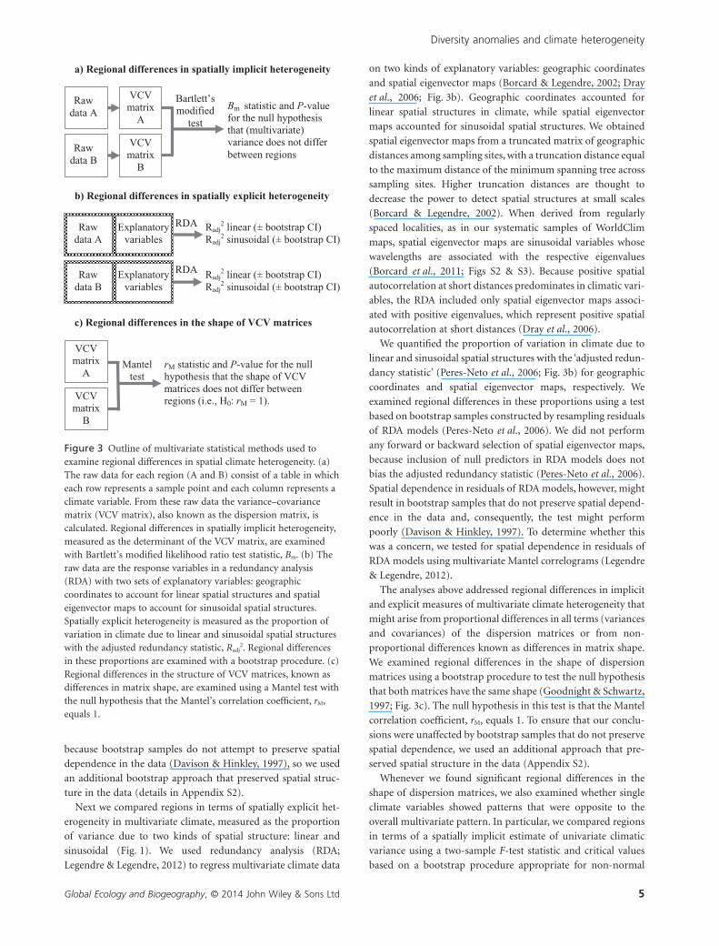
Figure 3 Outline of multivariate statistical methods used toexamine regional differences in spatial climate heterogeneity. (a)The raw data for each region (A and B) consist of a table in whicheach row represents a sample point and each column represents aclimate variable. From these raw data the variance–covariancematrix (VCV matrix), also known as the dispersion matrix, iscalculated. Regional differences in spatially implicit heterogeneity,measured as the determinant of the VCV matrix, are examinedwith Bartlett’s modified likelihood ratio test statistic, Bm. (b) Theraw data are the response variables in a redundancy analysis(RDA) with two sets of explanatory variables: geographiccoordinates to account for linear spatial structures and spatialeigenvector maps to account for sinusoidal spatial structures.Spatially explicit heterogeneity is measured as the proportion ofvariation in climate due to linear and sinusoidal spatial structureswith the adjusted redundancy statistic, Radj

2. Regional differencesin these proportions are examined with a bootstrap procedure. (c)Regional differences in the structure of VCV matrices, known asdifferences in matrix shape, are examined using a Mantel test withthe null hypothesis that the Mantel’s correlation coefficient, rM,equals 1.

Diversity anomalies and climate heterogeneity

Global Ecology and Biogeography, © 2014 John Wiley & Sons Ltd 5

distributions (Boos & Brownie, 1989; Fig. 4a). We used multiple

regression to measure the proportion of variation in univariate

climate explained by linear and sinusoidal spatial structures

(Fig. 4b). Similar to multivariate analysis, we regressed the single

climate variable of interest on geographic coordinates and

spatial eigenvector maps. We compared regions in terms of vari-

ation in single climate variables explained by linear and

sinusoidal spatial structures using a test based on bootstrap

samples constructed by resampling residuals of regression

models (Peres-Neto et al., 2006). To ensure that our conclusions

were not affected by a failure to account for spatial dependence,

we used univariate versions of procedures described above for

multivariate tests (Appendix S2). All statistical procedures were

performed in the R environment (R Development Core Team,

2009).

RESULTS

Spatially implicit and explicit measures of multivariate climate

heterogeneity supported the three postulated contrasts between

regions. Spatially implicit measures showed that ENA was less

heterogeneous than EA (Bm = 10,732, P = 0.001; Fig. 5a) and

WNA (BM = 10,673, P = 0.001, Fig. 5a) and that SWA was less

heterogeneous than CFR (Bm = 29293, P = 0.001, Fig. 6a). Tests

preserving spatial structure in the data yielded the same conclu-

sions (Table S3). Spatially explicit measures showed that a higher

proportion of variation in multivariate climate was due to linear

structures in ENA than in EA and WNA (Fig. 5b) and in SWA

than in CFR (Fig. 6b). Conversely, a lower proportion of vari-

ation in multivariate climate was due to sinusoidal structures in

ENA than in EA and WNA (Fig. 5c) and in SWA than in CFR

(Fig. 6c). Statistically significant autocorrelations in residuals of

RDAs were small in all cases, suggesting a negligible impact on

results (Fig. S4).

Regional differences in multivariate climate heterogeneity did

not arise from proportional differences across components

(variances and covariances) of dispersion matrices. The shape of

the dispersion matrix for climate of ENA differed from that of

EA (rM = 0.57, P = 0.001, Fig. 7a,b) and WNA (rM = 0.65,

P = 0.001, Fig. 5c,d). The shape of the dispersion matrix of SWA

also differed from that of CFR (rM = 0.54, P = 0.001, Fig. 7e,f).

Tests preserving spatial structure in the data yielded the same

conclusions (Table S3). Importantly, these results indicate that

empirical support for the three postulated regional contrasts

might vary depending on the set of climatic variables included

in the analysis.

Indeed, regional differences in univariate implicit measures of

heterogeneity deviated from the respective multivariate pattern

(Figs 5a & 6a). Contrary to the three postulated regional con-

trasts, spatially implicit measures showed that ENA was more

heterogeneous than EA in precipitation for the driest month

(F = 1.58, P = 0.001, Fig. 2c,d), the driest quarter (F = 1.38,

P = 0.001) and the coldest quarter (F = 1.75, P = 0.001). ENA

was also more heterogeneous than WNA in precipitation for the

driest month (F = 2.66, P = 0.001, Fig. 2d) and the driest quarter

(F = 2.33, P = 0.001). Furthermore, SWA was more hetero-

geneous than CFR in mean temperature of the warmest quarter

(F = 1.49, P = 0.001), precipitation for the wettest month

(F = 2.67, P = 0.001, Fig. 2g,h), the wettest quarter (F = 2.20,

P = 0.001) and the coldest quarter (F = 2.01, P = 0.001). Tests

preserving spatial structure in the data yielded the same conclu-

sions (Table S3).

Univariate spatially implicit measures that deviated from the

multivariate pattern of regional differences were mirrored by the

respective univariate spatially explicit measures in only some

cases. In particular, the proportion of variation in precipitation

of the driest month, the driest quarter and the coldest quarter

due to sinusoidal structures was larger in ENA than in EA

(Fig. 5c), and thus deviated from the multivariate pattern of

regional differences in the same way as the univariate implicit

measures. Respective differences in the proportion of variation

due to linear structures were less marked (Fig. 5b), but also

tended to mirror univariate implicit measures. In all other cases,

implicit and explicit measures did not show similar deviations

from the multivariate pattern of regional differences. The pro-

portion of variation in precipitation of the driest month and the

Raw data A

Raw data B

F test

Raw data A

Explanatory variables

OLS Radj2 linear (± bootstrap CI)

Radj2 sinusoidal (± bootstrap CI)

F statistic and p-value for the null hypothesis that (univariate) variance does not differ between regions

Radj2 linear (± bootstrap CI)

Radj2 sinusoidal (± bootstrap CI)

a) Regional differences in spatially implicit heterogeneity

b) Regional differences in spatially explicit heterogeneity

Raw data B

Explanatory variables

OLS

Figure 4 Outline of univariate statistical methods used toexamine regional differences in spatial climate heterogeneity.Whenever regional differences in shape of variance–covariancematrices are significant (Fig. 3c), single climate variables areexamined to determine if they deviated from the overallmultivariate pattern. (a) Regional differences in spatially implicitheterogeneity of single climate variables (one shown as a blackrectangle in the raw data table) are examined using the F-test.(b) To measure spatially explicit heterogeneity, a single climatevariable (shown as a black rectangle in the raw data table) is theresponse variable in ordinary least square regression (OLS) withtwo sets of explanatory variables: geographic coordinates toaccount for linear spatial structures and spatial eigenvector mapsto account for sinusoidal spatial structures. The proportion ofvariation in a climate variable due to linear and sinusoidal spatialstructures is measured as the adjusted redundancy statistic, Radj

2.Regional differences in these proportions are then examined witha bootstrap procedure.

I. Jiménez and R. E. Ricklefs

Global Ecology and Biogeography, © 2014 John Wiley & Sons Ltd6

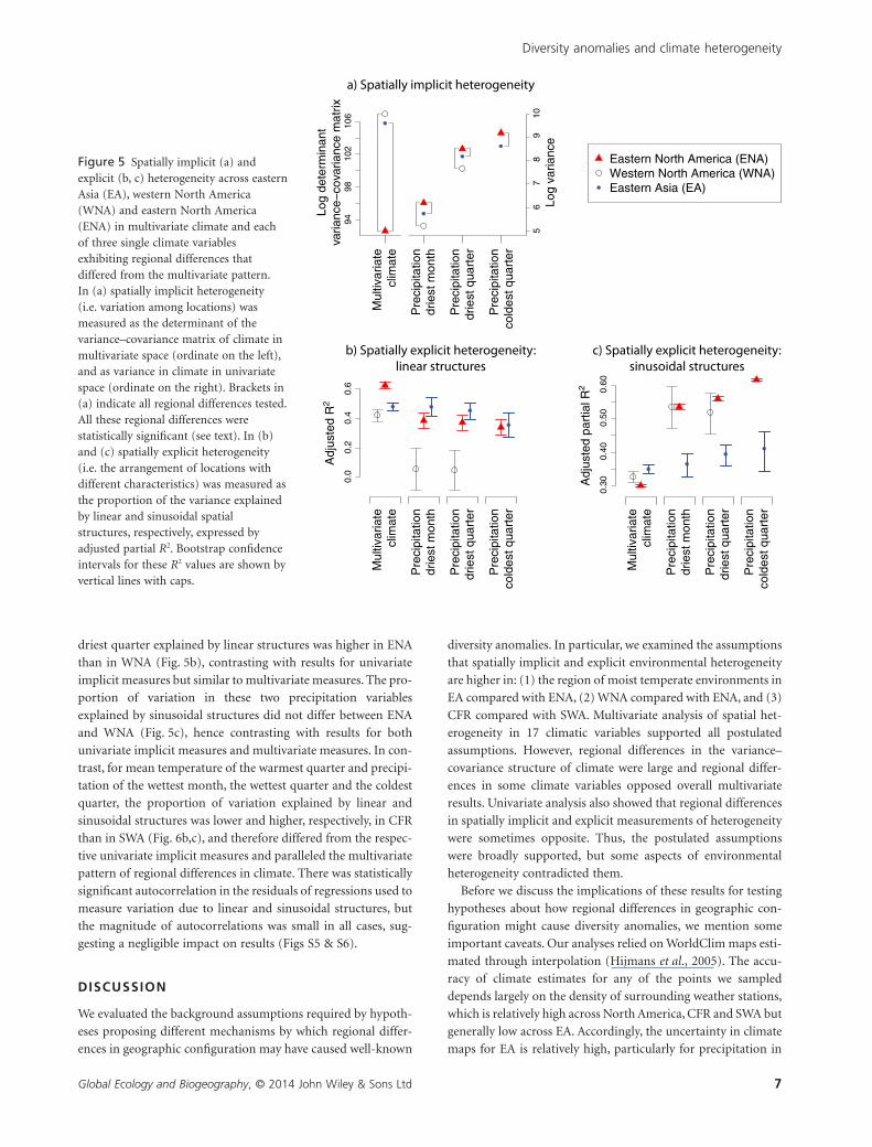
driest quarter explained by linear structures was higher in ENA

than in WNA (Fig. 5b), contrasting with results for univariate

implicit measures but similar to multivariate measures. The pro-

portion of variation in these two precipitation variables

explained by sinusoidal structures did not differ between ENA

and WNA (Fig. 5c), hence contrasting with results for both

univariate implicit measures and multivariate measures. In con-

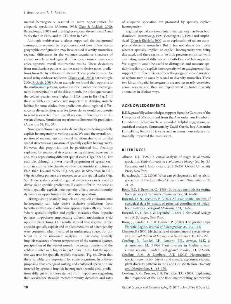
trast, for mean temperature of the warmest quarter and precipi-

tation of the wettest month, the wettest quarter and the coldest

quarter, the proportion of variation explained by linear and

sinusoidal structures was lower and higher, respectively, in CFR

than in SWA (Fig. 6b,c), and therefore differed from the respec-

tive univariate implicit measures and paralleled the multivariate

pattern of regional differences in climate. There was statistically

significant autocorrelation in the residuals of regressions used to

measure variation due to linear and sinusoidal structures, but

the magnitude of autocorrelations was small in all cases, sug-

gesting a negligible impact on results (Figs S5 & S6).

DISCUSSION

We evaluated the background assumptions required by hypoth-

eses proposing different mechanisms by which regional differ-

ences in geographic configuration may have caused well-known

diversity anomalies. In particular, we examined the assumptions

that spatially implicit and explicit environmental heterogeneity

are higher in: (1) the region of moist temperate environments in

EA compared with ENA, (2) WNA compared with ENA, and (3)

CFR compared with SWA. Multivariate analysis of spatial het-

erogeneity in 17 climatic variables supported all postulated

assumptions. However, regional differences in the variance–

covariance structure of climate were large and regional differ-

ences in some climate variables opposed overall multivariate

results. Univariate analysis also showed that regional differences

in spatially implicit and explicit measurements of heterogeneity

were sometimes opposite. Thus, the postulated assumptions

were broadly supported, but some aspects of environmental

heterogeneity contradicted them.

Before we discuss the implications of these results for testing

hypotheses about how regional differences in geographic con-

figuration might cause diversity anomalies, we mention some

important caveats. Our analyses relied on WorldClim maps esti-

mated through interpolation (Hijmans et al., 2005). The accu-

racy of climate estimates for any of the points we sampled

depends largely on the density of surrounding weather stations,

which is relatively high across North America, CFR and SWA but

generally low across EA. Accordingly, the uncertainty in climate

maps for EA is relatively high, particularly for precipitation in

9498

102

106

Log

dete

rmin

ant

varia

nce−

cova

rianc

e m

atrix

56

78

910

Log

varia

nce

0.0

0.2

0.4

0.6

Adj

uste

d R

2

Mul

tivar

iate

clim

ate

Pre

cipi

tatio

ndr

iest

mon

th

Pre

cipi

tatio

ndr

iest

qua

rter

Pre

cipi

tatio

nco

ldes

t qua

rter

Mul

tivar

iate

clim

ate

Pre

cipi

tatio

ndr

iest

mon

th

Pre

cipi

tatio

ndr

iest

qua

rter

Pre

cipi

tatio

nco

ldes

t qua

rter

Mul

tivar

iate

clim

ate

Pre

cipi

tatio

ndr

iest

mon

th

Pre

cipi

tatio

ndr

iest

qua

rter

Pre

cipi

tatio

nco

ldes

t qua

rter

0.30

0.40

0.50

0.60

Adj

uste

d pa

rtia

l R2

Eastern North America (ENA)Western North America (WNA)Eastern Asia (EA)

a) Spatially implicit heterogeneity

b) Spatially explicit heterogeneity:linear structures

c) Spatially explicit heterogeneity:sinusoidal structures

Figure 5 Spatially implicit (a) andexplicit (b, c) heterogeneity across easternAsia (EA), western North America(WNA) and eastern North America(ENA) in multivariate climate and eachof three single climate variablesexhibiting regional differences thatdiffered from the multivariate pattern.In (a) spatially implicit heterogeneity(i.e. variation among locations) wasmeasured as the determinant of thevariance–covariance matrix of climate inmultivariate space (ordinate on the left),and as variance in climate in univariatespace (ordinate on the right). Brackets in(a) indicate all regional differences tested.All these regional differences werestatistically significant (see text). In (b)and (c) spatially explicit heterogeneity(i.e. the arrangement of locations withdifferent characteristics) was measured asthe proportion of the variance explainedby linear and sinusoidal spatialstructures, respectively, expressed byadjusted partial R2. Bootstrap confidenceintervals for these R2 values are shown byvertical lines with caps.

Diversity anomalies and climate heterogeneity

Global Ecology and Biogeography, © 2014 John Wiley & Sons Ltd 7

mountainous areas with local effects such as rain shadows

(Hijmans et al., 2005). Nonetheless, we believe that WorldClim

maps are accurate enough to portray broad-scale spatial hetero-

geneity across each of the five regions. Further analyses would be

useful when improved climate maps become available. We also

stress that our analyses are restricted to climate and do not

address other dimensions of physiography that may be impor-

tant for explaining diversity anomalies (e.g. soil properties).

The scale along which environment is measured would ideally

be meaningful in terms species niches (Fig. 1), but that may be

difficult to accomplish in practice and results may depend on

scales of measurement. For example, on a linear scale, spatially

implicit heterogeneity in precipitation of the driest month and

quarter was higher in ENA than WNA (Fig. 5a). Precipitation of

the driest month and quarter are generally low in WNA and

variable in ENA (Fig. 2c,d, Table ST1). If variation at low values

of precipitation is ecologically more important than variation at

higher values, then a logarithmic scale might be more meaning-

ful than a linear scale. On a logarithmic scale, ENA was not more

heterogeneous than WNA in precipitation of the driest month

(F = 0.34, P = 1) or the driest quarter (F = 0.31, P = 1). These

results emphasize the difficulty in testing hypotheses about envi-

ronmental heterogeneity as a determinant of diversity anomalies

if there is uncertainty regarding the appropriate scales of envi-

ronmental measurement.

The regional differences in climate we describe here are rel-

evant to hypotheses about how regional differences in geo-

graphic configuration may cause diversity anomalies via

processes that may have operated over relatively recent times.

Specifically, our multivariate results support a background

assumption required of the hypothesis that higher spatially

implicit climatic heterogeneity may have allowed more species

to coexist through ecological sorting (Chesson, 2000) in EA and

WNA than in ENA, and in CFR than in SWA. Under this

hypothesis, higher regional diversity is fostered by higher vari-

ance in the physical attributes of a region. Our results also

support a background assumption needed by a different

hypothesis, focused on metacommunity dynamics (Holyoak

et al., 2005), according to which higher spatially explicit climatic

heterogeneity would allow more species to coexist in EA and

WNA than in ENA, and in CFR than in SWA. Under the latter

hypothesis, isolation of patches of similar habitat fosters coex-

istence by moderating the impact of species interactions.

Whether our measurements of regional differences in spatial

heterogeneity are relevant to hypotheses emphasizing processes,

such as allopatric speciation, operating through geological

a) Spatially implicit heterogeneity

b) Spatially explicit heterogeneity:linear structures

c) Spatially explicit heterogeneity:sinusoidal structures

5660

6468

Log

dete

rmin

ant

varia

nce−

cova

rianc

e m

atrix

56

78

910

Log

varia

nce

Mul

tivar

iate

clim

ate

Mea

n te

mp.

war

mes

t qua

rter

Pre

cipi

tatio

nw

ette

st m

onth

Pre

cipi

tatio

nw

ette

st q

uart

er

Pre

cipi

tatio

nco

ldes

t qua

rter

Mul

tivar

iate

clim

ate

Mea

n te

mp.

war

mes

t qua

rter

Pre

cipi

tatio

nw

ette

st m

onth

Pre

cipi

tatio

nw

ette

st q

uart

er

Pre

cipi

tatio

nco

ldes

t qua

rter

Mul

tivar

iate

clim

ate

Mea

n te

mp.

war

mes

t qua

rter

Pre

cipi

tatio

nw

ette

st m

onth

Pre

cipi

tatio

nw

ette

st q

uart

er

Pre

cipi

tatio

nco

ldes

t qua

rter

0.0

0.2

0.4

0.6

0.8

1.0

Adj

uste

d R

2

0.0

0.2

0.4

0.6

0.8

Adj

uste

d pa

rtia

l R2

Southwest Australia (SWA)Cape Floristic Region (CFR)

Figure 6 Spatially implicit (a) andexplicit (b, c) heterogeneity across theCape Floristic Region (CFR) andsouth-west Australia (SWA) inmultivariate climate and each of foursingle climate variables exhibitingregional differences that differed fromthe multivariate pattern. In (a) spatiallyimplicit heterogeneity (i.e. variationamong locations) was measured as thedeterminant of the variance–covariancematrix in multivariate space (ordinate onthe left) and as variance in univariatespace (ordinate on the right). Brackets in(a) indicate all regional differences tested.All these regional differences werestatistically significant (see text). In (b)and (c) spatially explicit heterogeneity(i.e. the arrangement of locations withdifferent characteristics) was measured asthe proportion of the variance explainedby linear and sinusoidal spatialstructures, respectively, expressed byadjusted partial R2. Bootstrap confidenceintervals for these R2 values are shown byvertical lines with caps.

I. Jiménez and R. E. Ricklefs

Global Ecology and Biogeography, © 2014 John Wiley & Sons Ltd8

epochs depends on how the physiography of each region has

changed through time. An approximate reconstruction of the

physiographic heterogeneity of CFR since the Oligocene sug-

gests substantial changes before the end of the Pliocene

(Cowling et al., 2009). In contrast, the physiography of SWA is

thought to have been more stable (Hopper & Gioia, 2004;

Cowling et al., 2009). We note that physiographic change

through geological time need not imply that present-day relative

differences in spatial heterogeneity between regions do not

reflect past relative differences. For example, despite substantial

temporal change, relative differences in physiographic heteroge-

neity between the western and eastern portions of CFR are

estimated to have persisted since at least the late Oligocene

(Cowling et al., 2009). Nonetheless, reconstructions of regional

differences in physiography through geological time might be

hampered by ‘information-destroying’ processes linking the past

and present, so that competing historical hypotheses might be

more likely to be empirically equivalent than non-historical

hypotheses (Turner, 2005).

To the extent that current regional differences in spatial het-

erogeneity reflect past regional differences, our results would be

relevant to hypotheses focused on the impacts of speciation on

regional diversity. Our multivariate results would support a

background assumption needed by the hypothesis that higher

spatially implicit climatic heterogeneity fostered ecological spe-

ciation leading to higher regional diversity in EA and WNA than

in ENA, and in CFR than in SWA. This hypothesis is based on

the notion that variation in the physical attributes of a region

partly determines the number of peaks in the fitness function of

phenotypes of closely related species (Schluter, 2000). Our mul-

tivariate results would also support a background assumption

needed by the hypothesis that higher spatially explicit environ-

−1.

5−

0.5

0.5

1.0

1.5

Temperature

Precipitation

−2.

0−

1.0

0.0

1.0

2.0

−2

−1

01

23

Sta

ndar

dize

d va

rianc

e-co

vara

ince

a) Eastern North America b) Eastern Asia

c) Eastern North America d) Western North America

e) Southwest Australia f) Cape Floristic Region

Figure 7 Regional variance–covariancematrices for 17 climate variables. Eachrow of panels compares matricesstandardized to a single scale (shown inthe left of each row), followingGoodnight & Schwartz (1997; AppendixS3). The longest diagonal of each matrixshows the variances of nine temperaturevariables followed by the variances ofeight precipitation variables. Shorterdiagonals show the respectivecovariances. From bottom to top, climaticvariables along the longest diagonal are:annual mean temperature, mean diurnalrange, temperature seasonality (standarddeviation), maximum temperature of thewarmest month, minimum temperatureof the coldest month, mean temperatureof the wettest quarter, mean temperatureof the driest quarter, mean temperatureof the warmest quarter, meantemperature of the coldest quarter,annual precipitation, precipitation of thewettest month, precipitation of the driestmonth, precipitation seasonality(coefficient of variation), precipitation ofthe wettest quarter, precipitation of thedriest quarter, precipitation of thewarmest quarter and precipitation of thecoldest quarter.

Diversity anomalies and climate heterogeneity

Global Ecology and Biogeography, © 2014 John Wiley & Sons Ltd 9

mental heterogeneity resulted in more opportunities for

allopatric speciation (Allmon, 1992; Qian & Ricklefs, 2000;

Barraclough, 2006) and thus higher regional diversity in EA and

WNA than in ENA, and in CFR than in SWA.

Although multivariate analyses supported the background

assumptions required by hypotheses about how differences in

geographic configuration may have caused diversity anomalies,

regional differences in the variance–covariance structure of

climate were large and regional differences in some climate vari-

ables opposed overall multivariate results. These deviations

from multivariate patterns can be used to derive novel predic-

tions from the hypotheses of interest. Those predictions can be

tested using clades as replicates (Xiang et al., 2004; Barraclough,

2006; Ricklefs, 2006). As an example, we found that, opposite to

the multivariate pattern, spatially implicit and explicit heteroge-

neity in precipitation of the driest month, the driest quarter and

the coldest quarter were higher in ENA than in EA (Fig. 5). If

these variables are particularly important in defining suitable

habitat for some clades, then predictions about regional differ-

ences in diversification rates for those clades would be opposite

to what is expected from overall regional differences in multi-

variate climate. Simulation experiments illustrate this prediction

(Appendix S4, Fig. S7).

Novel predictions may also be derived by considering spatially

explicit heterogeneity at various scales. We used the overall pro-

portion of regional environmental variation due to sinusoidal

spatial structures as a measure of spatially explicit heterogeneity.

However, this proportion can be partitioned into fractions

explained by sinusoidal structures having different wavelengths

and, thus, representing different spatial scales (Figs S2 & S3). For

example, although a lower overall proportion of spatial vari-

ation in multivariate climate was due to sinusoidal structures in

ENA than EA and WNA (Fig. 5c), and in SWA than in CFR

(Fig. 6c), these patterns are reversed at certain spatial scales (Fig.

S8). These scale-dependent regional differences can be used to

derive clade-specific predictions if clades differ in the scale at

which spatially explicit heterogeneity affects metacommunity

dynamics or opportunities for allopatric speciation.

Distinguishing spatially implicit and explicit environmental

heterogeneity can help derive exclusive predictions from

hypotheses that would otherwise appear empirically equivalent.

Where spatially implicit and explicit measures show opposite

patterns, hypotheses emphasizing different mechanisms yield

opposite predictions. Our results showed that regional differ-

ences in spatially explicit and implicit measures of heterogeneity

were consistent when measured in multivariate space, but dif-

ferent in some univariate analyses. In particular, spatially

implicit measures of mean temperature of the warmest quarter,

precipitation of the wettest month, the wettest quarter and the

coldest quarter were higher in SWA than in CFR, but the oppo-

site was true for spatially explicit measures (Fig. 6). Given that

these variables are important for some organisms, hypotheses

proposing that ecological sorting and ecological speciation are

fostered by spatially implicit heterogeneity would yield predic-

tions different from those derived from hypotheses suggesting

that coexistence through metacommunity dynamics and rates

of allopatric speciation are promoted by spatially explicit

heterogeneity.

Regional spatial environmental heterogeneity has been both

dismissed (Rosenzweig, 1995; Cowling et al., 1996) and empha-

sized (Qian & Ricklefs, 2000) as an explanation of salient exam-

ples of diversity anomalies. But it has not always been clear

whether spatially implicit or explicit heterogeneity was being

discussed, and there seems to be little previous empirical work

estimating regional differences in both kinds of heterogeneity.

We suggest it would be useful to distinguish and measure spa-

tially implicit and explicit heterogeneity when gauging empirical

support for different views of how the geographic configuration

of regions may be causally related to diversity anomalies. These

two kinds of spatial heterogeneity are not necessarily correlated

across regions and they are hypothesized to foster diversity

anomalies in distinct ways.

ACKNOWLEDGEMENTS

R.E.R. gratefully acknowledges support from the Curators of the

University of Missouri and from the Alexander von Humboldt

Foundation. Sebastián Tello provided helpful suggestions on

statistical analyses. Comments by David Currie, José Alexandre

Diniz-Filho, Bradford Hawkins and an anonymous referee sub-

stantially improved the manuscript.

REFERENCES

Allmon, D.J. (1992) A causal analysis of stages in allopatric

speciation. Oxford surveys in evolutionary biology (ed. by D.J.

Futuyma and J. Antonovics), pp. 219–257. Oxford University

Press, New York.

Barraclough, T.G. (2006) What can phylogenetics tell us about

speciation in the Cape flora? Diversity and Distributions, 12,

21–26.

Boos, D.D. & Brownie, C. (1989) Bootstrap methods for testing

homogeneity of variances. Technometrics, 31, 69–82.

Borcard, D. & Legendre, P. (2002) All-scale spatial analysis of

ecological data by means of principal coordinates of neigh-

bour matrices. Ecological Modelling, 153, 51–68.

Borcard, D., Gillet, F. & Legendre, P. (2011) Numerical ecology

with R. Springer, New York.

Born, J., Linder, H.P. & Desmet, P. (2007) The greater Cape

Floristic Region. Journal of Biogeography, 34, 147–162.

Chesson, P. (2000) Mechanisms of maintenance of species diver-

sity. Annual Review of Ecology and Systematics, 31, 343–366.

Cowling, R., Rundel, P.H, Lamont, B.B., Arroyo, M.K. &

Arianoutsou, M. (1996) Plant diversity in Mediterranean-

climate regions. Trends in Ecology and Evolution, 11, 362–366.

Cowling, R.M. & Lombard, A.T. (2002) Heterogeneity,

speciation/extinction history and climate: explaining regional

plant diversity patterns in the Cape Floristic Region. Diversity

and Distributions, 8, 163–179.

Cowling, R.M., Proches, S. & Partridge, T.C. (2009) Explaining

the uniqueness of the Cape flora: incorporating geomorphic

I. Jiménez and R. E. Ricklefs

Global Ecology and Biogeography, © 2014 John Wiley & Sons Ltd10

evolution as a factor for explaining its diversification. Molecu-

lar Phylogenetics and Evolution, 51, 64–74.

Crisp, M.D., Laffan, S., Linder, H.P. & Monro, A. (2001)

Endemism in the Australian flora. Journal of Biogeography, 28,

183–198.

Currie, D.J., Mittelbach, G.G., Cornell, H.V., Field, R., Guegan, J.,

Hawkins, B.A., Kaufman, D.M., Kerr, J.T., Oberdorff, T.,

O’Brien, E. & Turner, J.R.G. (2004) Predictions and tests of

climate-based hypotheses of broad-scale variation in taxo-

nomic richness. Ecology Letters, 7, 1121–1134.

Davison, A.C. & Hinkley, D.V. (1997) Bootstrap methods

and their application. Cambridge University Press, New

York.

Dray, S., Legendre, P. & Peres-Neto, P.R. (2006) Spatial model-

ling: a comprehensive framework for principal coordinate

analysis of neighbour matrices (PCNM). Ecological Modelling,

196, 483–493.

Forest, F., Grenyer, R., Rouget, M., Davies, T.J., Cowling, R.M.,

Faith, D.P., Balmford, A., Manning, J.C., Proches, S.,

van der Bank, M., Reeves, G., Hedderson, T.A.J. & Savolainen,

V. (2007) Preserving the evolutionary potential of floras in

biodiversity hotspots. Nature, 445, 757–760.

Goldblatt, P. & Manning, J. (2002) Plant diversity of the cape

region of South Africa. Annals of the Missouri Botanical

Garden, 89, 281–302.

Goodnight, C.J. & Schwartz, J.M. (1997) A bootstrap compari-

son of genetic covariance matrices. Biometrics, 53, 1026–1039.

Haining, R. (2003) Spatial data analysis: theory and practice.

Cambridge University Press, Cambridge.

Harrison, S. & Cornell, H. (2008) Toward a better understanding

of the regional causes of local community richness. Ecology

Letters, 11, 969–979.

Hijmans, R.J., Cameron, S.E., Parra, J.L., Jones, P.G. & Jarvis, A.

(2005) Very high resolution interpolated climate surfaces for

global land areas. International Journal of Climatology, 25,

1965–1978.

Hobbs, R.J., Richardson, D.M. & Davis, G.W. (1995) Mediter-

ranean-type ecosystems: opportunities and constraints for

studying the function of biodiversity. Mediterranean-type eco-

systems: the function of biodiversity (ed. by G.W. Davis and

D.M. Richardson), pp. 1–42. Springer-Verlag, Berlin.

Holyoak, M., Leibold, M.A. & Holt, R.D. (2005)

Metacommunities: spatial dynamics and ecological commu-

nities. University of Chicago Press, Chicago, IL.

Hopper, S.D. & Gioia, P. (2004) The Southwest Australian Flo-

ristic Region: evolution and conservation of a global hot spot

of biodiversity. Annual Review of Ecology, Evolution and Sys-

tematics, 35, 623–650.

Kreft, H. & Jetz, W. (2007) Global patterns and determinants of

vascular plant diversity. Proceedings of the National Academy of

Sciences USA, 104, 5925–5930.

Latham, R.E. & Ricklefs, R.E. (1993) Continental comparisons

of temperate-zone tree species diversity. Species diversity in

ecological communities: historical and geographical perspectives

(ed. by R.E. Ricklefs and D. Schluter), pp. 294–314. University

of Chicago Press, Chicago, IL.

Legendre, P. & Legendre, L. (2012) Numerical ecology, 3rd edn.

Elsevier, Amsterdam.

Linder, H.P. (2003) The radiation of the Cape flora, southern

Africa. Biology Reviews, 78, 597–638.

Linder, H.P. (2005) Evolution of diversity: the Cape flora. Trends

in Plant Science, 10, 536–541.

Linder, H.P., Eldenas, P. & Briggs, B.G. (2003) Contrasting pat-

terns of radiation in African and Australian Restionaceae. Evo-

lution, 57, 2688–2702.

Milewski, A.V. (1979) A climatic basis for the study of conver-

gence of vegetation structure in Mediterranean Australia and

southern Africa. Journal of Biogeography, 6, 293–299.

Mittelbach, G.G., Schemske, D.W., Cornell, H.V. et al. (2007)

Evolution and the latitudinal diversity gradient: speciation,

extinction, and biogeography. Ecology Letters, 10, 315–331.

van der Niet, D. & Johnson, S.D. (2009) Patterns of plant spe-

ciation in the Cape floristic region. Molecular Phylogenetics

and Evolution, 51, 85–93.

Peres-Neto, P.R., Legendre, P., Dray, S. & Borcard, D.

(2006) Variation partitioning of species data matrices:

estimation and comparison of fractions. Ecology, 87, 2614–

2625.

Qian, H. & Ricklefs, R.E. (1999) A comparison of the taxonomic

richness of vascular plants in China and the United States. The

American Naturalist, 154, 160–181.

Qian, H. & Ricklefs, R.E. (2000) Large-scale processes and the

Asian bias in species diversity of temperate plants. Nature,

407, 180–182.

Qian, H. & Ricklefs, R.E. (2004) Geographical distribution and

ecological conservatism of disjunct genera of vascular plants

in eastern Asia and eastern North America. Journal of Ecology,

92, 253–265.

R Development Core Team (2009) R: a language and environ-

ment for statistical computing. R Foundation for Statistical

Computing, Vienna, Austria. Available at: http://www

.R-project.org (accessed July 2009).

Ricklefs, R.E. (2004) A comprehensive framework for global

patterns in biodiversity. Ecology Letters, 7, 1–15.

Ricklefs, R.E. (2006) Evolutionary diversification and the origin

of the diversity–environment relationship. Ecology, 87, 3–13.

Rosenzweig, M.L. (1995) Species diversity in space and time.

Cambridge University Press, Cambridge.

Sauquet, H., Weston, P.H., Anderson, C.L., Barker, N.P., Cantrill,

D.J., Mast, A.R. & Savolainen, V. (2009) Contrasted patterns of

hyperdiversification in Mediterranean hotspots. Proceedings of

the National Academy of Sciences USA, 106, 221–225.

Schluter, D. (2000) The ecology of adaptive radiation. Oxford

University Press, New York.

Schluter, D. & Ricklefs, R.E. (1993) Convergence and the

regional component of species diversity. Species diversity in

ecological communities: historical and geographical perspectives

(ed. by R.E. Ricklefs and D. Schluter), pp. 230–242. University

of Chicago Press, Chicago, IL.

Svenning, J.C. (2003) Deterministic Plio-Pleistocene extinctions

in the European cool-temperate tree flora. Ecology Letters, 6,

646–653.

Diversity anomalies and climate heterogeneity

Global Ecology and Biogeography, © 2014 John Wiley & Sons Ltd 11

Turner, D. (2005) Local underdetermination in historical

science. Philosophy of Science, 72, 209–230.

Verboom, G.A., Archibald, J.K., Bakker, F.T., Bellstedt, D.U.,

Conrad, F., Dreyer, L.L., Forest, F., Galley, C., Goldblatt, P.,

Henning, J.F., Mummenhoff, K., Linder, H.P., Muasya, A.M.,

Oberlander, K.C., Savolainen, V., Snijman, D.A., van der Niet,

T. & Nowell, T.L. (2009) Origin and diversification of the

Greater Cape flora: ancient species repository, hot-bed of

recent radiation, or both? Molecular Phylogenetics and Evolu-

tion, 51, 44–53.

Wen, J. (1999) Evolution of eastern Asian and eastern North

American disjunct distributions on flowering plants. Annual

Review of Ecology and Systematics, 30, 421–455.

Wiens, M.J. (2000) Ecological heterogeneity: an ontogeny of

concepts and approaches. The ecological consequences of envi-

ronmental heterogeneity: the 40th symposium of the British Eco-

logical Society, held at the University of Sussex, 23–25 March

1999 (ed. by M.J. Hutchings, E.A. John & A.J.A. Stewart), pp.

9–31. Cambridge University Press, Cambridge.

Xiang, Q., Zhang, W.H., Ricklefs, R.E., Qian, H., Chen, Z.D.,

Wen, J. & Li, J.H. (2004) Regional differences in rates of plant

speciation and molecular evolution: a comparison between

eastern Asia and eastern North America. Evolution, 58, 2175–

2184.

Zhang, J. & Boos, D.D. (1992) Bootstrap critical values for

testing homogeneity of covariance matrices. Journal of the

American Statistical Association, 87, 425–429.

SUPPORTING INFORMATION

Additional supporting information may be found in the online

version of this article at the publisher’s web-site.

Figure S1 Illustration of computer simulation experiments

testing the effects of linear and sinusoidal spatial structures on

isolation of species suitable habitat.

Figure S2 Examples of spatial eigenvector maps of each region.

Figure S3 Examples of correlograms for spatial eigenvectors

maps of each region.

Figure S4 Mantel correlograms for redundancy analysis

residuals.

Figure S5 Correlograms for regression residuals corresponding

to western North America, eastern North America and eastern

Asia.

Figure S6 Correlograms for regression residuals corresponding

to the Cape Floristic Region and south-west Australia.

Figure S7 Simulation results show contrasting effects of spatial

heterogeneity in precipitation of the driest month and annual

mean precipitation on isolation of species suitable habitat in

eastern North America and eastern Asia.

Figure S8 Proportion of variation in multivariate climate

explained by sinusoidal spatial structures at different spatial

scales across western North America, eastern North America,

eastern Asia, the Cape Floristic Region and south-west Australia.

Table S1 Central tendency and variation in 17 climatic variables

across western North America, eastern North America and

eastern Asia.

Table S2 Central tendency and variation in 17 climatic variables

across the Cape Floristic Region and south-west Australia.

Table S3 Results of tests for differences in climate heterogeneity

that preserve spatial structure.

Appendix S1 Computer simulation experiments testing the

effect of linear and sinusoidal spatial structures on isolation of

species suitable habitat.

Appendix S2 Testing for differences in climate heterogeneity

while preserving spatial structure.

Appendix S3 Standardization of dispersion matrices.

Appendix S4 Computer simulation experiments comparing the

effects of spatial heterogeneity in precipitation of the driest

month and annual mean precipitation on isolation of species

suitable habitat in eastern North America and eastern Asia.

BIOSKETCHES

Iván Jiménez is interested in testing theory that

attempts to explain the spatial patterns of diversity and

the size, structure, and dynamics of geographic ranges

of taxa.

Robert E. Ricklefs researches diversity in ecological

systems at several levels of organization and scales of

time and space; he has a long-standing interest in the

evolutionary diversification of avian life histories and

the historical development of ecological communities

and regional species richness.

Editor: José Alexandre Diniz-Filho

I. Jiménez and R. E. Ricklefs

Global Ecology and Biogeography, © 2014 John Wiley & Sons Ltd12