Some comments on 6D global gauge anomalies

Prog. Theor. Exp. Phys. 2021, 08B103 (29 pages)DOI: 10.1093/ptep/ptab015

Some comments on 6D global gauge anomalies

Yasunori Lee and Yuji Tachikawa∗

Kavli Institute for the Physics and Mathematics of the Universe (WPI), University of Tokyo, Kashiwa, Chiba277-8583, Japan∗E-mail: [email protected]

Received December 1, 2020; Revised February 1, 2021; Accepted February 1, 2021; Published February 10, 2021

... . . . . . . . . . . . . . . . . . . . . . . . . . . . . . . . . . . . . . . . . . . . . . . . . . . . . . . . . . . . . . . . . . . . . . . . . . . . . . . . . . . . . . . . . . . . . . . . . . . . . . . . . . . . . . . . .Global gauge anomalies in six dimensions associated with non-trivial homotopy groups π6(G)

for G = SU (2), SU (3), and G2 have been computed and utilized in the past. From the modernbordism point of view of anomalies, however, they come from the bordism groups �

spin7 (BG),

which are in fact trivial and therefore preclude their existence. Instead, it was noticed that a propertreatment of the 6D Green–Schwarz mechanism reproduces the same anomaly cancellationconditions derived from π6(G). In this paper, we revisit and clarify the relation between thesetwo different approaches... . . . . . . . . . . . . . . . . . . . . . . . . . . . . . . . . . . . . . . . . . . . . . . . . . . . . . . . . . . . . . . . . . . . . . . . . . . . . . . . . . . . . . . . . . . . . . . . . . . . . . . . . . . . . . . . . .

Subject Index B31, B33

Dedicated to the memory of the late Professor Tohru Eguchi.

1. Introduction and summary

Given a gauge theory, its gauge anomaly must be canceled as a whole in order for the theory to beconsistent. This imposes non-trivial constraints on the possible matter content. One notable subtletyhere is that, even if perturbative anomaly cancellation is achieved, the theory may still suffer from aglobal anomaly, coming from a global gauge transformation corresponding to non-trivial elementsof πd(G), where d is the spacetime dimension and G is the gauge group. It was first pointed out inRef. [1] that such a situation indeed arises for 4D SU (2) gauge theory with a Weyl fermion in thedoublet.

In six dimensions the situation is subtler, since the anomaly cancellation often involves chiral2-form fields through the Green–Schwarz mechanism. The cancellation condition can nonethelessbe derived by embedding G in a larger group G whose global anomaly is absent. This approach wasoriginally developed by Elitzur and Nair [2], and the extension to six dimensions with the Green–Schwarz mechanism was done in Refs. [3–5].1 The list of simply connected simple Lie groups withnon-trivial π6(G) is2

1 There are many other works from the late 1980s where the analysis in six dimensions was done without theGreen–Schwarz mechanism. We do not cite them here; interested readers can find them by looking up papersciting Ref. [2] in the INSPIRE-HEP database.

2 Homotopy groups π6(G) for classical groups were computed in Sect. 19 in Ref. [6]. Homotopy groupsπ6(G) for G2 and F4 were considered as known in the review article [7] and were attributed to H. Toda; aderivation can be found in Ref. [8], in which πi(G2) and πi(F4) were completely determined up to i = 21.Homotopy groups π6(G) for E6,7,8 were determined to be trivial in Theorem V in Ref. [9]. π6(G) for G =SU (2) = S3 belongs more properly to the unstable homotopy groups of spheres and has been computed bymany people; see footnote 7 of Sect. 19 in Ref. [6] and the comments on p. 428 of Ref. [7].

© The Author(s) 2021. Published by Oxford University Press on behalf of the Physical Society of Japan.This is an Open Access article distributed under the terms of the Creative Commons Attribution License (http://creativecommons.org/licenses/by/4.0/),which permits unrestricted reuse, distribution, and reproduction in any medium, provided the original work is properly cited.Funded by SCOAP3

Dow

nloaded from https://academ

ic.oup.com/ptep/article/2021/8/08B103/6132355 by guest on 29 M

ay 2022

PTEP 2021, 08B103 Y. Lee and Y. Tachikawa

π6(SU (2)) = Z12,π6(SU (3)) = Z6,π6(G2) = Z3,

(1)

and the references above found a mod-12, mod-6, mod-3 condition for G = SU (2), SU (3), and G2,respectively. In Ref. [4], it was indeed found that the F-theory compactification to six dimensionsonly produces gauge theories that are free from the global gauge anomalies.

From the modern point of view, the anomaly of a theory Q in d spacetime dimensions is describedvia its anomaly theory A(Q) in (d +1) dimensions, which hosts the original theory Q on its boundary.The anomalous phase associated with a gauge transformation g : Sd → G is now reinterpreted asthe partition function

ZA(Q)[Sd+1, Pg] (2)

of the anomaly theory on Sd+1 equipped with the G gauge field Pg obtained by performing gaugetransformation g at the equator Sd ⊂ Sd+1.

More generally, the possible anomalies of a symmetry group G are characterized by Invd+1spin (BG),

the group formed by deformation classes of (d +1)-dimensional invertible phases with G symmetry.This group fits in the following short exact sequence:

0 −→ ExtZ(�spind+1(BG), Z) −→ Invd+1

spin (BG) −→ HomZ(�spind+2(BG), Z) −→ 0 (3)

where �spind (BG) is the bordism group of d-dimensional spin manifolds equipped with a G bundle

[10]. In particular, the information on global anomalies is encoded in the part

ExtZ(�spind+1(BG), Z) = Hom(Tors �

spind+1(BG), U (1)), (4)

while the information on the anomaly polynomial is encoded in the part

HomZ(�spind+2(BG), Z) = HomZ(Free �

spind+2(BG), Z). (5)

For 4D theory with G = SU (2) symmetry, the group �spin5 (BSU (2)) is indeed Z2, and is generated

by (S5, P[g]) where g : S4 → SU (2) belongs to the generator of π4(SU (2)) = Z2. This correspondsto Witten’s original global anomaly.

When we apply this argument to six dimensions, we encounter an immediate puzzle. Namely, forG = SU (2), SU (3), and G2 for which π6(G) is non-trivial, we have

�spin7 (BSU (2)) = 0,

�spin7 (BSU (3)) = 0,

�spin7 (BG2) = 0,

(6)

and in particular the configuration (S7, P[g]) for [g] ∈ π6(G) is null-bordant. Therefore, the partitionfunction of the anomaly theory on this background should be automatically trivial when the anomalypolynomial is canceled, and there should be no global anomalies at all for the gauge groups G =SU (2), SU (3), and G2. But the old computations indeed found non-trivial anomalous phases, so oneis led to wonder whether they were legitimate to start with.

The way out is suggested by another set of observations made more recently, in Sect. 3.1.1 in Ref.[11] and in Refs. [12,13]. Namely, it was observed there that the mod-12, mod-6, mod-3 conditions

2/29

Dow



ay 2022


for G = SU (2), SU (3), G2 theories can be derived by demanding that the factorized anomalypolynomial of the fermions can actually be canceled by a properly constructed Green–Schwarzterm. For example, the non-(purely) gravitational part of the anomaly polynomial3 of n fermions in3 of SU (3) is

Ifermion = n

6· 1

2· c2(F)

(c2(F) + p1(R)

2

)(7)

and it is always factorized, which is a necessary condition for the Green–Schwarz mechanism tobe applicable. But it is not a sufficient condition. The instanton configurations of the G gauge fieldcorrespond to strings charged under 2-form fields, and their self Dirac pairing is given by n/6, whichneeds to be an integer. This shows that n needs to be divisible by 6 (see Sect. 3.1.1 in Ref. [11]).Furthermore, when this is the case, one can actually construct a theory of 2-form fields with thisanomaly, thanks to the series of works by Monnier and his collaborators [12–23].

As we have discussed, there are now two ways to understand the mod-12, mod-6, mod-3 conditionsfor G = SU (2), SU (3), and G2. One is from the absence of global gauge anomalies associated withnon-trivial elements of π6(G), and the other is from the proper consideration of the Green–Schwarzterm canceling the fermion anomaly. The aim of this rather technical paper is to reconcile these twopoints of view.

The rest of the paper is organized as follows: In Sect. 2, we carefully study all possible anomaliesof theories with 0-form symmetry G = SU (2), SU (3), G2, and theories with 2-form U (1) symmetry.This is done by finding the integral basis of the space of anomaly polynomials with these symmetries.This allows us to deduce the necessary and sufficient condition when the anomalies of fermionscharged under G = SU (2), SU (3), G2 can be canceled by the anomalies of 2-form fields. Theanalysis in this section does not use the homotopy groups π6(G) at all.

In Sect. 3, we move on to study how the derivation in Sect. 2 is related to the homotopy groupsπ6(G). We do this by carefully reformulating the approach of Elitzur and Nair [2] in more modernlanguage. The old computations of global anomalies associated with π6(G) can then be reinterpretedin two ways. The first interpretation, which we give in Sect. 3.2, is simply the following: if we assumethat the perturbative anomaly is canceled by the Green–Schwarz mechanism, the Elitzur–Nair methodshows that there is a global anomaly associated with π6(G) = Zk . But there should not be any globalanomaly, since �

spin7 (BG) = 0. This means that it is impossible to cancel the fermion anomaly by the

Green–Schwarz mechanism unless a mod-k condition is satisfied. The second interpretation, whichwe give in Sect. 3.3, is more geometric: we introduce a 3-form field H satisfying dH = c2(F) to thebulk 7D spacetime, mimicking an important half of the Green–Schwarz mechanism. This modifiesthe bordism group to be considered in the classification of anomalies, and then there actually is aglobal gauge anomaly associated with π6(G), which defines a non-trivial element in the modifiedbordism group.

Before proceeding, we pause here to mention that the arguments in Sect. 3 that use πd(G) only givenecessary conditions. The derivation given in Sect. 2, in contrast, gives conditions that are necessaryand sufficient at the same time. In this sense, we consider that the latter is better.

3 In this paper, we denote by I the anomaly polynomial of a theory, and by I the part of the anomalypolynomial not purely formed by the Pontrjagin classes pi(R) of the spacetime.

3/29

Dow



ay 2022


Furthermore, the discussions that we provide in Sect. 2 have already been essentially given inRefs. [12,13], albeit in a slightly different form. Therefore, strictly speaking, our discussions in thispaper do not add anything scientifically new. That said, the authors were very much confused whenthey encountered the apparent contradiction that people discussed global gauge anomalies associatedwith non-trivial π6(G), while �

spin7 (BG) is trivial and therefore there should not be any global gauge

anomalies to start with. The authors wanted to record their understanding of how this contradictionis resolved, for future reference.

We have four appendices. In Appendix A, we summarize basic formulas of fermion anomalies andgroup-theoretical constants. In Appendices B and C, we compute various spin bordism groups ofinterest using the Atiyah–Hirzebruch spectral sequence (AHSS) and the Adams spectral sequence(Adams SS), respectively. Finally, in Appendix D, one of the authors (Yuji Tachikawa) would liketo share some of his recollections of his advisor, the late Professor Tohru Eguchi, to whose memorythis paper is dedicated.

2. Anomalies and their cancellation

In this paper, we are interested in the anomalies of fermionic 6D theories with G symmetry, whereG = SU (2), SU (3), and G2. To cancel them, we are also interested in the anomaly of 2-form fields,which can couple to the background 4-form field strength G, which is the background field fortheir U (1) 2-form symmetry.4 We will study when the fermion anomalies can be canceled by theanomalies of 2-form fields, by carefully studying all possible anomalies under these symmetries.As discussed in Eq. (3), the anomalies are then characterized by the group of 7D invertible phasesInv7

spin(X ), where X = BSU (2), BSU (3), BG2, and K(Z, 4). As πi(BE7) = πi(K(Z, 4)) for i < 12,we can think of BE7 � K(Z, 4) for our purposes. This equivalence is useful for us, as we will seebelow, and has also been used in the past [25–27].

Since �spin7 (X ) = 0 for all four cases, the anomalies are completely specified by the anomaly

polynomials, encoded in HomZ(�spin8 (X ), Z). Below we do not worry about the purely gravitational

part of the anomalies, which means that we are going to study HomZ(�spin8 (X ), Z).

Over rational numbers, the anomaly polynomials are then elements of

HomZ(�spin8 (X ), Z) ⊗ Q � H 8(X × BSO; Q)/H 8(BSO; Q). (8)

As H∗(BSO; Q) = Q[p1, p2, . . . , ] where pi ∈ H 4i(BSO; Z) are the ith Pontrjagin classes of thespacetime, Eq. (8) becomes

H 4(X ; Q) p1 ⊕ H 8(X ; Q). (9)

Our classifying spaces X have a simplifying feature that

H 4(X ; Z) = Z c2, H 8(X ; Z) = Z (c2)2 (10)

where c2 is a generator of H 4(X ; Z) corresponding to the instanton number, whose explicit formsare given in Appendix A. In the rest of this paper, the Pontrjagin classes pi = pi(R) are always for

4 The authors apologize that the same symbol G is used in three distinct ways, for groups in general, for thespecific group G2, and for 4-form background field strengths. Hopefully the context makes it clear which useis intended.

4/29

Dow



ay 2022


the spacetime part and the elements c2 = c2(F) are always for the gauge part. For X = K(Z, 4) orequivalently for X = BE7, we also use the symbol G = c2(F) interchangeably.

The preceding discussions show that the anomaly polynomials (modulo the purely gravitationalpart) are rational linear combinations

I = a · (c2)2 + b · c2 ∧ p1, (11)

which has a nice quadratic form to be canceled by the Green–Schwarz mechanism. This is, however,only a necessary condition, since the Green–Schwarz mechanism cannot cancel anomaly polynomialswith arbitrary rational numbers a, b in Eq. (11). We need to find the basis over Z, not just over Q, ofelements of HomZ(�

spin8 (X ), Z). They are degree-8 differential forms (11) that integrate to integers

on any spin manifold. We will find in Sects. 2.1, 2.2, 2.3, and 2.4 that they are given by

I = n · 1

2kG· c2

(c2 + p1

2

)+ m · (c2)

2, n, m ∈ Z (12)

where kG = 12, 6, 3, 1 for G = SU (2), SU (3), G2, and E7, respectively. We then use this result tofind the anomaly cancellation condition in Sect. 2.7. Note that π6(G) = ZkG , but we do not directlyuse π6(G) in the derivation in this section.

Before proceeding, we also note that the results analogous to Eq. (12) pertaining to the integralityproperties of the coefficients in the anomaly polynomial were derived in previous literature suchas Refs. [5,28] by explicitly computing the anomaly polynomials for free fermionic theories forall possible representations of G. The symplectic Majorana condition was often not consideredsystematically either. As we will see below, our argument utilizes only a single representation of G,thanks to the use of the bordism invariance.

2.1. With U (1) 2-form symmetry

Let us start with the case X = K(Z, 4). We will find the dual bases of HomZ(�spin8 (X ), Z) = Z ⊕ Z

and Free �spin8 (X ) = Z ⊕ Z by writing down two elements from each and explicitly checking that

they do form a set of dual bases.5

First, let us take two elements of HomZ(�spin8 (X ), Z). One is

G ∧ G, (13)

where G is a generator of H 4(K(Z, 4); Z). The other element of HomZ(�spin8 (X ), Z) that we use is

1

2· G

(G + p1

2

). (14)

There are two ways to show that it integrates to an integer on spin manifolds. One method todemonstrate this only uses algebraic topology. Let us first recall that the standard generator λ ofH 4(BSpin; Z) = Z satisfies p1 = 2λ. Now, for any SO bundle, there is a relation

p1 = P(w2) + 2w4 mod 4. (15)

Here, the 2 in front of w4 is a map sending Z2 = {0, 1} to {0, 2} ⊂ Z4. For spin bundles, we havew2 = 0, and therefore 2λ = p1 = 2w4, meaning that

λ = w4 mod 2. (16)

5 We note that HomZ2(�spin10 (K(Z, 4)), Z2) was determined in a similar manner in Sect. 3.2 in Ref. [29].

5/29

Dow



ay 2022


With this relation we can show∫M8

G ∧ p1

2=∫

M8

G ∪ w4 =∫

M8

Sq4G =∫

M8

G ∧ G mod 2, (17)

where we have used the fact that w4 is the Wu class ν4 on a spin manifold. Therefore the expression(14) integrates to an integer.

The other method is differential geometric, or uses a physics input. We consider the non-gravitational part I 1

2 56 of the anomaly polynomial of a fermion in the representation 1256 of E7,

where 12 means that we impose a reality condition using the fact that both 56 of E7 and the Weyl

spinor in six dimensions with Lorentz signature are pseudo-real. In terms of the index theory ineight dimensions, the same 1

2 uses the fact that 56 is pseudo-real and that the Weyl spinor in eightdimensions with Euclidean signature are strictly real, and therefore the index in eight dimensions isa multiple of 2. Using group-theoretical constants tabulated in Appendix A, the anomaly polynomialcan be computed and turns out to be

I 12 56 = 1

2· c2

(c2 + p1

2

). (18)

We next take two elements of �spin8 (X ), following Ref. [30]. One is the quaternionic projective

space HP2. It has a canonical Sp(1) = SU (2) bundle Q, whose c2 generates H 4(HP2; Z) = Z suchthat

∫HP

2(c2)2 = 1. The Pontrjagin classes of the tangent bundle are p1 = −2c2 and p2 = 7(c2)

2.6

The other is CP1 × CP3 equipped with the element c ∧ c′ ∈ H 4(X ; Z) where c, c′ are the standardgenerators of H 2(CP1; Z) and H 2(CP3; Z), respectively.

The pairings between these elements are given by∫(HP

2,Q)

G ∧ G = 1,∫

(HP2,Q)

1

2· G

(G + p1

2

)= 0, (19)∫

(CP1×CP

3,c∧c′)G ∧ G = 0,

∫(CP

1×CP3,c∧c′)

1

2· G

(G + p1

2

)= −1 (20)

and therefore they constitute dual bases. In other words, the classes (HP2, Q) and (CP1 ×CP3, c ∧ c′) generate Free �

spin8 (K(Z, 4)) = Z ⊕ Z, while G ∧ G and 1

2 · G(G + p1

2

)generate

HomZ(�spin8 (K(Z, 4)), Z) = Z ⊕ Z.

2.2. With SU (2) symmetry

Let us next consider the case X = BSU (2). Our approach is the same as the previous case. We firsttake two elements of HomZ(�

spin8 (X ), Z). One is c2 ∧ c2 as before, and the other is this time the

non-gravitational part I 12 2 of the anomaly polynomial for the fermion in the representation 1

22. Usingthe group-theoretical data in Appendix A, we have

I 12 2 = 1

24· c2

(c2 + p1

2

). (21)

This can also be derived from Eq. (18) by splitting 56 as 2⊗12⊕1⊗32 under su(2)× so(12) ⊂ e7,which implies I 1

2 56 = 12 · I 12 2 under SU (2) ⊂ E7; see, e.g., Table A.178 in Ref. [32].

6 The total Pontrjagin class of HPk is (1−c2)2(k+1)

(1−4c2); see, e.g., Ref. [31].

6/29

Dow



ay 2022


We next consider two elements of �spin8 (BSU (2)). One is (HP2, Q) as before. As the other, we take

(S4, I ) × K3, where S4 is equipped with a standard instanton bundle I on it, which has∫

S4 c2 = 1,while K3 has

∫K3 p1 = −48. Note that S4 � HP1 and I is its canonical Sp(1) bundle.

The pairings of these elements are then∫(HP

2,Q)

c2 ∧ c2 = 1,∫

(HP2,Q)

1

24· c2

(c2 + p1

2

)= 0, (22)∫

(S4,I )×K3c2 ∧ c2 = 0,

∫(S4,I )×K3

1

24· c2

(c2 + p1

2

)= −1, (23)

again guaranteeing that they form dual bases. Equivalently, we have now shown that (HP2, Q) and(S4, I ) × K3 generate Free �

spin8 (BSU (2)) = Z ⊕ Z, and similarly c2 ∧ c2 and 1

24 · c2(c2 + p1

2

)generate HomZ(�

spin8 (BSU (2)), Z) = Z ⊕ Z.

2.3. With SU (3) symmetry

Next we consider the case X = BSU (3). Two elements of HomZ(�spin8 (X ), Z) can be chosen as

before. One is c2 ∧ c2 as always, and the other is the non-gravitational part I3 of the anomalypolynomial in the representation 3. Under SU (3) ⊂ E7, we have I 1

2 56 = 6 · I3 and therefore

I3 = 1

12· c2

(c2 + p1

2

). (24)

A dual basis to c2 ∧ c2 can be taken to be (HP2, Q) as always. Unfortunately, we have not founda concrete dual basis to I3 in �

spin8 (X ). Instead we need to proceed indirectly, using the AHSS. As

computed in Appendix B, the entries E2p,8−p of the E2-page for various X are given by

X E24,4 E2

6,2 E27,1 E2

8,0

BSU (2) Z Z

BSU (3) Z Z2 Z

BG2 Z Z2 Z2 Z

K(Z, 4) Z Z2 Z2 Z ⊕ Z3

(25)

where the other E2p,8−p are trivial. From the AHSS, it is clear that E2 = E∞ for X = BSU (2), and

indeed�spin8 (BSU (2)) = Z⊕Z.We also know Free �

spin8 (K(Z, 4)) = Z⊕Z from the explicit analysis

in Sect. 2.1. Comparing the bases in Sects. 2.1 and 2.2, we find that under BSU (2) → K(Z, 4), theimage of �

spin8 (BSU (2)) is 12Z ⊕ Z ⊂ Z ⊕ Z. This means that the extension problem in the AHSS

for K(Z, 4) is solved as follows: we have

0 → E24,4 ⊕ Free E2

8,0︸︷︷︸=Z⊕Z

→ �spin8 (K(Z, 4))︸︷︷︸

=Z⊕Z

→ Z12 → 0 (26)

where Z12 is composed of E26,2 = Z2, E2

7,1 = Z2, and Tors E28,0 = Z3 in the last row of Eq. (25).

Since BSU (3) is sandwiched as in BSU (2) → BSU (3) → K(Z, 4), we conclude that�

spin8 (BSU (3)) = Z ⊕ Z whose image under BSU (3) → K(Z, 4) is 6Z ⊕ Z ⊂ Z ⊕ Z. This

abstract analysis provides a dual basis element to I3 = 16 · I 1

2 56.

7/29

Dow



ay 2022


2.4. With G2 symmetry

The G2 case is completely analogous to the SU (3) case. One basis of HomZ(�spin8 (BG2), Z) = Z⊕Z

is given by c2 ∧ c2 as always and the other is given by

I7 = 1

6· c2

(c2 + p1

2

), (27)

which satisfies I7 = 13 · I 1

2 56 under G2 ⊂ E7. The dual basis to c2 ∧ c2 is given by (HP2, Q). The

existence of the dual basis to I7 can be argued exactly as before, and the image of �spin8 (BG2) = Z⊕Z

under BG2 → K(Z, 4) is 3Z ⊕ Z ⊂ Z ⊕ Z.

2.5. Pure gravitational part

Before proceeding, here we record the dual bases of HomZ(�spin8 (pt), Z) = Z ⊕ Z and �

spin8 (pt) =

Z ⊕ Z. Two generators of the latter were found in, e.g., Ref. [33], which are HP2 and L8, where4L8 is spin bordant to K3 × K3. They have Pontrjagin numbers p2

1(HP2) = 4, p2(HP2) = 7 andp2

1(L8) = 1152, p2(L8) = 576, respectively. As for the generators of the former, we can take theanomaly polynomials Ifermion and Igravitino of the 6D fermion and the gravitino, which can be foundin any textbook:

Ifermion = 7 p21 − 4 p2

5760, Igravitino = 275 p2

1 − 980 p2

5760. (28)

They have the pairing∫HP

2Ifermion = 0,

∫HP

2Igravitino = −1, (29)∫

L8

Ifermion = 1,∫

L8

Igravitino = −43 (30)

and form a pair of dual bases.

2.6. Anomalies of self-dual 2-forms

Now that we have discussed the general structures of anomalies with the symmetries we are interestedin, we would like to study their cancellation. For this, we need to examine the anomalies of self-dualform fields in more detail.

Let us start by recalling the naive analysis often found in older literature. The one-loop anomalypolynomial of a self-dual tensor can be found in, e.g., Ref. [34]. In general dimensions, it is givenby ±L/8, where L is the Hirzebruch genus. In six dimensions this gives7

Itensor,one-loop = 16 p21 − 112 p2

5760. (31)

Furthermore, at the level of differential forms, a self-dual tensor B can be coupled to a background4-form G via dH = G, which contributes to the anomaly polynomial by 1

2 G ∧ G. Then the total

7 Our sign choice here is for −L/8 while the fermion anomaly in Eq. (28) corresponds to +A. They are theanomaly polynomials for the tensor field in the tensor multiplet and for the fermion in the hypermultiplet inN=(1, 0) supersymmetry in six dimensions.

8/29

Dow



ay 2022


anomaly is

Itensor = Itensor,one-loop + 1

2G ∧ G. (32)

Note that this does not integrate to integers on HP2 and L8 when we naively set G = 0. Rather, weneed to set

G = p1

4(33)

for which we find

Itensor = 196 p21 − 112 p2

5760= 28 · Ifermion, (34)

which does integrate to integers on HP2 and L8. We cannot, however, promote G to be a 3-form fieldstrength, since p1

4 is not integrally quantized in general, although p12 is, as we saw above.

A proper formulation was first proposed by Belov and Moore in Ref. [35] using the results ofHopkins and Singer [36], and it requires the use of Wu structure in general (4k + 2) dimensions.This formulation was then developed in detail in a series of papers by Monnier and collaborators[12–23]. For our case of interest in six spacetime dimensions, a spin structure induces a canonicalWu structure, and self-dual form fields can be naturally realized on the boundary of a natural classof 7D topological field theories [27]; an in-depth discussion can also be found in Ref. [37].

In the case of a single self-dual form field of level 1, the bulk theory has the action

S = −∫

M7

(1

2· c(

dc + p1

2

)+ c ∧ G

)(35)

where c is a 3-form gauge field to be path-integrated and G is a background 4-form field strength. Itshould more properly be written using its 8D extension as

S = −∫

M8

(1

2· g(

g + p1

2

)+ g ∧ G

)(36)

where M8 is a spin manifold such that ∂M8 = M7, and g = dc is the field strength of c; we extendg and G to the entire M8. Such extension is guaranteed to exist since �

spin7 (K(Z⊕n, 4)) = 0, and the

action does not depend on the choice of the extension since we know that 12 · g(g + p1

2 ) and g ∧ Gintegrate to integers on spin manifolds, as we saw in Sect. 2.1.

At the level of differential forms, one is tempted to rewrite Eq. (35) as

S = −∫

M7

(1

2· c ∧ dc + c ∧ G

)(37)

where

G = p1

4+ G. (38)

In this sense, a single self-dual 2-form is forced to couple to p14 from its consistency, explaining the

observation (33) above. In this paper, we stick to using the unshifted G that is integrally quantized.

9/29

Dow



ay 2022


In Eq. (36), we can introduce a new variable g = g + G and rewrite it as

S = −∫

M8

1

2· g(

g + p1

2

)+∫

M8

1

2· G

(G + p1

2

). (39)

As g is path-integrated, the first term produces the pure gravitational anomaly of a single self-dualtensor field “properly coupled to 1

4p1”, and the second term is the residual dependence on G, which

we saw in Sect. 2.1 to be a generator of HomZ(�spin8 (K(Z, 4)), Z).

The other generator was G∧G, which can be realized as the standard anomaly of a non-chiral 2-formfield coupled to G both electrically and magnetically. Combining these two pieces of information,we find that every possible anomaly of HomZ(�

spin8 (K(Z, 4)), Z) can be realized by a system of

2-form fields in six dimensions. More generally, if there are n self-dual 2-form fields, the 7D bulkTQFT has the form

S = −∫

M8

(1

2

(Kij · gi ∧ gj + ai · gi ∧ p1

2

)+ gi ∧ Yi

). (40)

Here, i runs from 1 to n, ci are the 3-form fields to be integrated over, gi = dci are their curvatures,Yi are the background fields of U (1) 2-form symmetry, and Kij and ai are integer coefficients. Forthis expression to be well defined, we need to require8

Kii = ai mod 2 (not a sum over i). (41)

To see this, we first note that the expression 12

∑i =j Kij · gi ∧ gj = ∑

i<j Kij · gi ∧ gj clearlyintegrates to an integer. Then, we can separately analyze each i. We finally recall that the generatorsof HomZ(�

spin8 (K(Z, 4)), Z) are G ∧ G and 1

2 · G(G + p12 ), and we are done.

If det K = 1, this theory is not invertible but rather a topological field theory with a multi-dimensional Hilbert space. Correspondingly, the boundary 6D theory is a relative theory in the senseof Ref. [40], which does not have a partition function but rather a partition vector. The system thendepends on the background fields Yi in a complicated manner, and cannot be directly used to cancelthe fermion anomaly. However, suppose that Yi has the form Yi = Kij · Gj + Yi. In this case, shiftinggi to new fields gi = gi + Gi, one can factor out as

S = −∫

M8

(1

2

(Kij · gi ∧ gj + ai · gi ∧ p1

2

)+ gi ∧ Yi

)+∫

M8

(1

2

(Kij · Gi ∧ Gj + ai · Gi ∧ p1

2

)+ Gi ∧ Yi

)(42)

where the second line is invertible since it only depends on the background field Gi. It is this invertiblepart that is used to cancel the fermion anomaly, and the remaining non-invertible part is irrelevantfor our purposes. Setting Gi = ni ·G for a single G and integers ni, we again see that we can producean arbitrary element of HomZ(�

spin8 (K(Z, 4)), Z) as the anomaly of a system of self-dual 2-form

8 This relation can be more invariantly stated as follows. We introduce a lattice � = Zn whose pairing isgiven by Kij. Then the vector (ai) ∈ � is a characteristic vector, i.e., 〈x, x〉 ≡ 〈a, x〉 modulo two. That thecoefficients ai multiplying gi ∧ p1

2 in the anomaly polynomial of the fermionic part of a 6D theory form acharacteristic vector was long conjectured in, e.g., Ref. [23] and finally proved in Refs. [12,13]. We also notethat an analogous constraint in the case of 3D Chern–Simons theory coupled to the spinc connection was firstnoted in Sect. 7 in Ref. [38], which was later utilized to great effect in Sect. 2.3 in Ref. [39].

10/29

Dow



ay 2022


fields. In the examples in M-theory and F-theory treated in Ref. [11], the cancellation was indeeddone in this manner, where Gi were set to c2 of dynamical gauge fields and Yi were set to c2 of theR-symmetry background.

2.7. Cancellation

After all these preparations, the analysis of the cancellation is very simple. Consider a system offermions charged under G = SU (2), SU (3), or G2. From the results of Sects. 2.2, 2.3, and 2.4, itsanomaly is necessarily of the form

Ifermion = n · 1

2kG· c2

(c2 + p1

2

)+ m · c2 ∧ c2 (43)

where n and m are integers and kG = 12, 6, 3 for G = SU (2), SU (3), and G2, respectively.Now, take a number of self-dual 2-form fields and use c2 as their background field G. As we saw in

Sect. 2.6, the form of anomalies that can be produced by a system of 2-form fields has the structure

Itensor = n · 1

2· G

(G + p1

2

)+ m · G ∧ G, (44)

where n and m are again integers. This means that the necessary and sufficient condition for theanomaly of fermions to be cancelable by the anomaly of 2-form fields is

n ≡ 0 mod kG. (45)

Here, π6(G) = ZkG for our G, but we did not use this in the derivation presented in this section.We note that the coefficient n controls the fractional part of the coefficient of c2 ∧ c2, which comes

from the Tr F4 term in the fermion anomaly. For G = SU (2), SU (3), and G2, we have

trrep.F4 = γrep. ·

(trfund.F

2)2, (46)

and we saw in Sects. 2.2, 2.3, and 2.4 that a fermion in the representation 122, 3, and 7 corresponds

to n = 1 in Eq. (43). Therefore, the condition (45) can be expanded more concretely into

SU (2) :∑i+

γrep.(i+)

γ 12 2

−∑i−

γrep.(i−)

γ 12 2

= 0 mod 12,

SU (3) :∑i+

γrep.(i+)

γ3−∑i−

γrep.(i−)

γ3= 0 mod 6,

G2 :∑i+

γrep.(i+)

γ7−∑i−

γrep.(i−)

γ7= 0 mod 3,

(47)

where γ 12 2 = 1/4, γ3 = 1/2, and γ7 = 1/4, and the summation runs over all fermions in the theory

where +/− represents their chiralities. Some values of γrep. are collected in Appendix A.

2.8. Examples: N = (1, 0) supersymmetric cases

Let us provide some concrete examples of the anomaly cancellation. In 6D N = (1, 0) QFT, fermionscharged under the gauge group are gaugini in the adjoint representation and hyperini in the matterrepresentation. They are in opposite chiralities. Let us restrict the representations of hyperini and

11/29

Dow



ay 2022


denote their numbers as follows:

n2 : SU (2) fundamental,n3 : SU (3) fundamental,n6 : symmetric,n7 : G2 fundamental.

(48)

Then, the conditions for the perturbative anomaly cancellation (47) are

SU (2) : 4γadj. − 4γfund. · n2 = 32 − 2 · n2 = 0 mod 12,SU (3) : 2γadj. − 2γfund. · n3 − 2γsym. · n6 = 18 − n3 − 17 · n6 = 0 mod 6,

G2 : 4γadj. − 4γfund. · n7 = 10 − n7 = 0 mod 3,(49)

which exactly coincide with the conditions for the absence of global anomalies appearing in Ref.[4].

3. Relation to π 6(G)

In the last section, we deduced the condition under which the anomaly of a fermion system with Gsymmetry can be canceled by the anomaly of 2-form fields for G = SU (2), SU (3), and G2. Ourexposition used a careful determination of integral generators of the group of anomalies. In the end,we found a mod-12, mod-6, and mod-3 condition, respectively.

Traditionally, the same anomaly cancellation condition was related to the anomaly by a globalgauge transformation associated with π6(G) = Z12, Z6, and Z3 for each G. However, our derivationin the last section did not use π6(G) at all. In this section, we would like to clarify the relationbetween these two approaches.

3.1. The Elitzur–Nair method

Let us first remind ourselves of the method to determine the global gauge anomaly of a systemunder G symmetry, assuming the cancellation of perturbative gauge anomalies, by rewriting it as aperturbative anomaly under a larger group G whose global gauge anomaly is absent. This method isoriginally due to Ref. [2]. In the context of the modern bordism approach to the anomalies, it wasrediscovered in Ref. [41] and further developed more extensively in Ref. [42]. The basic idea is asfollows.

The global G gauge anomaly may arise due to gauge transformations g : Sd → G belonging to non-trivial elements of πd(G) = Zk , which cannot be continuously deformed to the trivial transformation.The first step is then to embed the gauge group G into a larger group G with πd(G) = 0. This meansthat g can be trivialized within G. Further, assume that our G-symmetric system Q is obtained byrestricting the symmetry of a G-symmetric system Q. Using this, one can describe the global Ggauge anomaly of Q in terms of the perturbative G gauge anomaly of Q.

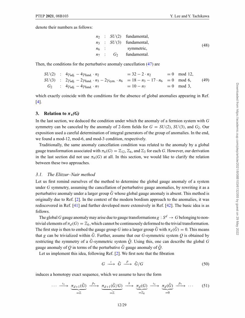
Let us implement this idea, following Ref. [2]. We first note that the fibration

Gι−−→ G

p−−→ G/G (50)

induces a homotopy exact sequence, which we assume to have the form

· · · ι∗−−→ πd+1(G)︸︷︷︸=Z

p∗−−−→ πd+1(G/G)︸︷︷︸=Z

∂−−→ πd(G)︸︷︷︸=Zk

ι∗−−→ πd(G)︸︷︷︸=0

p∗−−−→ · · · (51)

12/29

Dow



ay 2022


so that the generator of πd+1(G) is mapped to a kth power of the generator of Z = πd+1(G/G).Now, to compute the anomaly under g : Sd → G, we consider a G bundle on Sd+1 obtained bygluing two trivial bundles on two hemispheres at the equator Sd ⊂ Sd+1. The resulting G bundleon Sd+1 is classified by an element πd+1(BG), which is naturally isomorphic to πd(G). We denotethe resulting G bundle by P[g] where [g] ∈ πd(G) � πd+1(BG). In the modern understanding, theanomaly is the partition function ZA(Q)[Sd+1, P[g]] of the (d +1)-dimensional anomaly theory A(Q)

evaluated on (Sd+1, P[g]).From the assumption that πd(G) = πd+1(BG) = 0, we can extend this G bundle P[g] on Sd+1

to a G bundle on Dd+2. Such an extension is classified by an element [f ] ∈ πd+1(G/G) such that∂[f ] = [g]. Denoting the corresponding G bundle on Dd+2 by P[f ], the anomaly is exp(2π iJ ([f ]))where

J ([f ]) =∫

(Dd+2,P[f ])IQ (52)

where IQ is the anomaly polynomial of the G-symmetric theory Q. One can check that the expression(52) gives a well defined homomorphism

J : πd+1(G/G) → R, (53)

since IQ is a closed form and its restriction to G bundles is zero by assumption. Let us now take a

generator [f0] ∈ πd+1(G/G) = Z, which maps to a generator [g0] = ∂[f0] ∈ πd+1(BG) = Zk . Thenthe global anomaly that we are after is

ZA(Q)[Sd+1, P[g0]] = exp(

2π iJ ([f0]))

. (54)

To compute it, note that k[f0] ∈ πd+1(G/G) is the image of the generator [g0] ∈ πd+1(G) �πd+2(BG). In this case, we can attach a trivial G bundle over another copy of Dd+2 to the bundle(Dd+2, Pk[f0]) discussed above along the common boundary Sd+1 via gauge transformation in [g0],to form a G bundle P[g0] on Sd+2. Then

J (k[f0]) =∫

(Dd+2,Pk[f0])IQ =

∫(Sd+2,P[g0])

IQ. (55)

This last expression is often computable, resulting in the final formula in which the anomalous phaseassociated with the gauge transformation in [g0] ∈ πd(G) is given by

ZA(Q)[Sd+1, P[g0]] = exp

(2π i

k

∫(Sd+2,P[g0])

IQ

). (56)

This derivation was originally devised by Elitzur and Nair [2] for the 4D analysis, where Witten’soriginal anomaly in the G = SU (2) case was derived by embedding G to G = SU (3). It was alsorediscovered in the context of our recent progress in the understanding of anomalies in the bordismpoint of view by Ref. [41], who embedded SU (2) to U (2) instead.

Let us quickly see how Witten’s anomaly is computed in this framework. The sequence is

· · · ι∗−−→ π5(SU (3))︸︷︷︸=Z

p∗−−−→ π5(SU (3)/SU (2))︸︷︷︸=Z

∂−−→ π4(SU (2))︸︷︷︸=Z2

ι∗−−→ π4(SU (3))︸︷︷︸=0

p∗−−−→ · · · ,

(57)

13/29

Dow



ay 2022


where SU (3)/SU (2) � S5. We take the doublet in SU (2) minus two uncharged Weyl spinors as thetheory Q, and the triplet in SU (3) minus three uncharged Weyl spinors as the theory Q. By restrictingthe symmetry from SU (3) to SU (2), the theory Q reduces to Q, since an uncharged pair of Weylspinors of different chirality can be given a mass and therefore does not contribute to the anomaly.The anomaly polynomial of Q is simply 1

3! Tr( F

2π

)3, which is known to integrate to 1 against the

generator [g0] of π5(SU (3)) = π6(BSU (3)), meaning that J (2[f0]) = 1. Therefore, the anomalousphase under the generator [g0] ∈ π4(SU (2)) is exp(2π iJ ([f0])) = exp(2π i · 1

2) = −1. In this way,we see that the anomaly theory of a 4D fermion in the doublet of SU (2) detects the generator of�

spin5 (BSU (2)) = Z2.

3.2. 6D analysis, take 1

The analysis of Elitzur and Nair was applied and extended to the 6D case in Refs. [3–5]. However, theanalyses there were not quite satisfactory from a more modern point of view, since the contributionfrom the self-dual tensor field was not properly taken into account. The first objection to their analysesis the following: we know that π6(SU (2)) = Z12 → �

spin7 (BSU (2)) = 0 is a zero map. How can

there be a global anomaly? The second objection is the following: we know from Sect. 2.7 that wecannot cancel the perturbative anomaly of a single fermion in 1

22 of SU (2) by that of self-dual tensorfields. How can we apply the Elitzur–Nair method? We can combine these two objections into aconsistent modern reinterpretation of the old analyses, as follows.

Suppose that the perturbative anomaly of n fermions in 122 of SU (2) can be canceled by a com-

bination of 2-form fields, by using c2 of the SU (2) bundle as the background of the U (1) 2-formsymmetry of the 2-form fields. We also assume that the perturbative gravitational anomaly is can-celed by adding some uncharged fields, and take the combined theory as Q. Since the perturbativeanomaly vanishes, it determines a bordism invariant

�spin7 (BSU (2)) → U (1), (58)

but as �spin7 (BSU (2)) = 0, it is trivial. In particular, the anomalous phase associated with (S7, P[g0])

for the generator [g0] ∈ π7(BSU (2)) = Z12 should also be trivial, i.e.,

ZA(Q)[S7, P[g0]] = 1. (59)

We now compute this anomalous phase by the Elitzur–Nair method. Taking G = SU (2) = Sp(1)

and G = Sp(2), the sequence is

· · · ι∗−−→ π7(Sp(2))︸︷︷︸=Z

p∗−−−→ π7(Sp(2)/Sp(1))︸︷︷︸=Z

∂−−→ π6(Sp(1))︸︷︷︸=Z12

ι∗−−→ π6(Sp(2))︸︷︷︸=0

p∗−−−→ · · · ,

(60)where Sp(2)/Sp(1) � S7. As the theory Q, we take n copies of 1

24 of Sp(2), coupled to the samecombination of 2-form fields, by using c2 of the Sp(2) bundle as the background of the U (1)

2-form symmetry. Note that our presentation of the Elitzur–Nair method in Sect. 3.1 applies tothis case. The anomaly polynomial IQ of Q is n times 1

2 · 14! Tr

( F2π

)4modulo multi-trace terms.

Now, it is known that the expression 12 · 1

4! Tr( F

2π

)4integrates to 1 against the generator [g0] of

π7(Sp(2)) = π8(BSp(2)) = Z (see Appendix B.2 in Ref. [5]). This means that for ∂[g0] = 12[f0]

14/29

Dow



ay 2022


we have

J (12[f0]) =∫

(Sd+2,P[g0])IQ = n

∫(Sd+2,P[g0])

1

2· 1

4! Tr(

F

2π

)4

= n. (61)

Therefore the anomalous phase associated with (S7, P[g0]) is

ZA(Q)[S7, P[g0]] = exp(

n · 2π i

12

). (62)

For the results (59) and (62) to be consistent, we conclude that n needs to be divisible by 12. Theanalysis can be extended to arbitrary fermions charged under SU (2), and we can rederive Eq. (47)as a necessary condition. The argument in this subsection, however, does not say that they are alsosufficient. Differently put, the method in this section does not directly show that the fermion anomalycan actually be canceled, without the analysis of Sect. 2.7.

The analysis for G = SU (3) and G2 can be rephrased in a completely similar manner by choosingG to be SU (4) and SU (7) respectively, so will not be repeated.

3.3. 6D analysis, take 2

The argument in the previous subsection can also be phrased in the following manner. Let us start byassuming that the perturbative anomaly of a single fermion in 1

22 can be canceled. Then, we can applythe Elitzur–Nair argument to compute the anomaly under the generator [g0] ∈ π6(SU (2)) = Z12,which is the partition function of the anomaly theory on (S7, P[g0]). The value turns out to be

exp(2π i/12). The configuration (S7, P[g0]) is however null-bordant in �spin7 (BSU (2)), and therefore

the partition function should be 1. This leads to a contradiction, meaning that the initial assumptionis incorrect. We conclude that the perturbative anomaly cannot be canceled for a single fermion in122.

This argument still leaves us wondering whether it is possible to have a setup where the anomalyassociated with [g0] is actually exp(2π i/12). It turns out that it can be achieved by considering aslightly different bordism group as follows. This is essentially the computation done in Refs. [3,4].

So far, we have considered the manifolds in question to be equipped with spin structure and a Ggauge field. Let us equip the manifolds with a classical 3-form field H , which we consider to be a(modified) field strength of the 2-form field B, satisfying

dH = c2. (63)

This relation makes the part of the anomaly polynomial divisible by c2 cohomologically trivial, andeffectively cancels it. Let us see this more concretely. Take G = SU (2) and consider fermions in122. The partition function of its anomaly theory A(Q) is given by the associated eta invariant η 1

2 2,whose variation is controlled by the anomaly polynomial

1

24· c2

(c2 + p1

2

). (64)

With Eq. (63) we can add a local counterterm in seven dimensions, and consider the anomaly theoryto be

ZA(Q)′ = exp(

2π i

(η 1

2 2 −∫

M7

1

24· H

(c2 + p1

2

))). (65)

15/29

Dow



ay 2022


This combination is clearly constant under infinitesimal variations of the background fields, andgives a invariant of the bordism group equipped with spin structure, a G gauge field, and a 3-formfield satisfying Eq. (63).

The G-field configuration P[g0] on S7 has a cohomologically trivial c2, since H 4(S7) vanishes.Therefore we can solve Eq. (63) to find H on S7. The G-field configuration P[f0] on D8 can also beaugmented with a solution to Eq. (63), since H 4(D8) is again trivial. Then the Elitzur–Nair argumentgoes through, and this time we actually conclude that

ZA(Q)′ [S7, P[g0], H ] = exp(

2π i

12

). (66)

The classifying space X of a G gauge field and a 3-form field satisfying Eq. (63) can be describedas a total space of the fibration

K(Z, 3) → X → BG (67)

where the extension is controlled by Eq. (63). Therefore the relevant bordism group for us is �spin7 (X ).

See Appendix B.6 for the details of the calculations; we do find that �spin7 (X ) = Z12, and our

modified anomaly theory A(Q)′ detects its generator. Again the cases G = SU (3) and G2 can betreated similarly, and we will not detail it.

We now see that with 12 copies of the same fermion system, the global anomaly associated withπ6(SU (2)) vanishes, when the manifolds involved are all equipped with a classical 3-form field Hsatisfying Eq. (63). However, this does not directly imply that one can perform the path integral overthe G gauge field and the 2-form field B satisfying Eq. (63). Indeed, the 7D counterterm in Eq. (65)with 12 copies corresponds to the 6D coupling

−1

2· B(

c2 + p1

2

)(68)

but 12(c2 + p1

2 ) is not integrally quantized. As we know from Sect. 2.7, we need to use chiral 2-formfields in six dimensions to cancel the fermion anomaly in this case, and the subtlety of the chiral2-forms is not encoded in the classical equation (63).

Before closing, we note that the spacetime structure analogous to Eq. (63), given by providing a3-form field strength H satisfying

dH = p1

2− c2 (69)

on a spin manifold, is known as the (twisted) string structure in mathematical literature. This capturespart of the original 10D Green–Schwarz mechanism, where the fermion anomalies of the form

I12 =(p1

2− c2

)X8 (70)

are canceled by the anomaly of the B-field. Indeed, analogously to the analysis in this subsection,equipping manifolds with (twisted) string structure automatically cancels the factorized I12. It mustbe noted, however, that vanishing the anomaly with the use of the (twisted) string structure does notguarantee that the part X8 is integrally quantized, again as analogous to the 6D analysis. This needsto be kept in mind whenever we try to use string bordism to study the anomaly cancellation in stringtheory.

16/29

Dow



ay 2022


Acknowledgements

The authors would like to thank the anonymous referees for their detailed comments, which led to an improve-ment in the representation of this paper. Y.L. is partially supported by the Programs for Leading GraduateSchools, MEXT, Japan, via the Leading Graduate Course for Frontiers of Mathematical Sciences and Physicsand also by a Japan Society for the Promotion of Science (JSPS) Research Fellowship for Young Scientists.Y.T. is partially supported by a JSPS KAKENHI Grant-in-Aid (Wakate-A), No. 17H04837, a JSPS KAKENHIGrant-in-Aid (Kiban-S), No. 16H06335, and also by the WPI Initiative, MEXT, Japan at IPMU, the Universityof Tokyo.

Funding

Open Access funding: SCOAP3.

Note added

When this paper was almost completed, the authors learned that there is an upcoming work byDavighi and Lohitsiri [24] that has a large overlap with it.

Appendix A. Fermion anomalies and group-theoretic constants

The perturbative gauge anomaly of a fermion is given by

Ifermion = [A(R) ch(F)

]8

= (trrep.1) · 7 p1(R)2 − 4 p2(R)

5760+ p1(R)

24

[1

2! · trrep.

(F

2π

)2]

+ 1

4! · trrep.

(F

2π

)4

.

(A.1)

In general, the traces have following forms:

trrep.F2 = αrep. · trfund.F2,

trrep.F4 = βrep. · trfund.F4 + γrep. ·(trfund.F2

)2,(A.2)

and in particular βrep. = 0 for SU (2), SU (3), and G2. Explicitly, α and γ for some commonrepresentations are given as follows:

SU (2) SU (3) G2

tradj.F2 4 · trfund.F2 6 · trfund.F2 4 · trfund.F2 αadj.

trsym.F2 – 5 · trfund.F2 – αsym.

trfund.F4 1

2· (trfund.F2

)2 1

2· (trfund.F2

)2 1

4· (trfund.F2

)2γfund.

tradj.F4 8 · (trfund.F2)2 9 · (trfund.F2

)2 5

2· (trfund.F2

)2γadj.

trsym.F4 –17

2· (trfund.F2

)2 – γsym.

. (A.3)

17/29

Dow



ay 2022


Furthermore, the instanton number c2(F) is normalized so that

c2(F) = 1

4· 1

h∨ · tradj.

(F

2π

)2

=

⎧⎪⎪⎪⎪⎪⎪⎪⎪⎨⎪⎪⎪⎪⎪⎪⎪⎪⎩

1

4· 1

2· 4 · trfund.

(F

2π

)2

= 1

2· trfund.

(F

2π

)2

: SU (2),

1

4· 1

3· 6 · trfund.

(F

2π

)2

= 1

2· trfund.

(F

2π

)2

: SU (3),

1

4· 1

4· 4 · trfund.

(F

2π

)2

= 1

4· trfund.

(F

2π

)2

: G2,

(A.4)where h∨ is the dual Coxeter number of each gauge group. As a result, the non-gravitational part ofthe anomaly becomes

Ifermion = 1

24

(αrep. · trfund.

(F

2π

)2

∧ p1(R)

2+ γrep. · trfund.

(F

2π

)2

∧ trfund.

(F

2π

)2)

=

⎧⎪⎪⎪⎪⎪⎪⎨⎪⎪⎪⎪⎪⎪⎩

4γrep. · 1

24· c2(F)

(c2(F) + p1(R)

2

)+ 2αrep. − 4γrep.

24· c2(F) ∧ p1(R)

2: SU (2),

2γrep. · 1

12· c2(F)

(c2(F) + p1(R)

2


24· c2(F) ∧ p1(R)

2: SU (3),

4γrep. · 1

6· c2(F)

(c2(F) + p1(R)

2


24· c2(F) ∧ p1(R)

2: G2.

(A.5)

From our general argument in Sects. 2.2, 2.3, and 2.4, the numerical coefficients before · of the twoterms in each row, such as 4γrep and 1

24(2αrep. − 4γrep.), are guaranteed to be integers.

Appendix B. Bordisms via the Atiyah–Hirzebruch spectral sequence

In this appendix, we compute �spind (X ) for X = K(Z, 4), BSU (2), BSU (3), BG2, and K(Z, 3)-

fibered BSU (2) by using the Atiyah–Hirzebruch spectral sequence (AHSS), associated with thetrivial fibration

pt −→ Xp−→ X . (B.1)

Here we will not give an introduction to AHSS; consult, e.g., Ref. [43] for a detailed introduction toAHSS for �

spin∗ .9

9 We note that the AHSS first appeared in the physics literature in the context of K-theory classification ofD-branes in Refs. [29,44,45]; see Appendix C, Appendix A, and Sect. 3 of respective references.

18/29

Dow



ay 2022


Appendix B.1. K(Z, 4)

The E2-page of the AHSS is as follows:

where the horizontal axis and the vertical axis are for p and q, respectively. The integral homologyof K(Z, 4) is due to Appendix B.2 in Ref. [46]. For Z2 (co)homology, it is known that (see, e.g., Ref.[47])

H∗(K(Z, 4); Z2) = Z2[u4, u6, u7, u10, u11, u13, . . .] (B.3)

where

Sq2u4 = u6,Sq1u6 = u7.

(B.4)

The differentials d2 : E26,0 → E2

4,1 and d2 : E26,1 → E2

4,2 are known to be (mod 2 reduction com-

posed with) the dual of Sq2 [48], and therefore none of the Z2 involved survive to the E∞-page.10 Asa result, one has �

spin7 (K(Z, 4)) = 0. The extension problem for �

spin8 (K(Z, 4)) was solved in Sect.

2.3; see in particular the discussions around Eq. (26). Summarizing, we have the (non-canonical)isomorphism of groups

Inv7spin(K(Z, 4)) = Free �

spin8 (K(Z, 4))︸︷︷︸=Z⊕Z

⊕ Tors �spin7 (K(Z, 4))︸︷︷︸

=0

. (B.5)

10 This indeed agrees with the result in Ref. [49] up to odd torsion.

19/29

Dow



ay 2022


Appendix B.2. BSU (2)


(B.6)

where the relevant (co)homologies are

H∗(BSU (2); Z) = Z[c2],

H∗(BSU (2); Z2) = Z2[c2].

(B.7)

For the range p + q ≤ 7, there are no differentials and all the elements survive to the E∞-page. Asa result, one has

Inv7spin(BSU (2)) = Free �

spin8 (BSU (2))︸︷︷︸=Z⊕Z

⊕ Tors �spin7 (BSU (2))︸︷︷︸

=0

. (B.8)

Since BSU (2) = HP∞, each generator of H4i(BSU (2); Z) = Z is the embedded HP4i. As SU (2) =Sp(1) bundles, they are the canonical bundles Q over HP4i. Therefore, the generator of E2

4,4 = Z

is (HP1, Q) × K3 and the generator of E28,0 = Z is (HP2, Q). They are the generators discussed in

Sect. 2.2.

Appendix B.3. BSU (3)


(B.9)

20/29

Dow



ay 2022



H∗(BSU (3); Z) = Z[c2, c3],

H∗(BSU (3); Z2) = Z2[c2, c3].

(B.10)

Here, c2 and c3 in H∗(BSU (3); Z2)

are related as

Sq2c2 = c3,

and therefore the differentials d2 : E26,0 → E2

4,1 and d2 : E26,1 → E2

4,2 are again non-trivial as in

the X = K(Z, 4) case. As a result, one has

Inv7spin(BSU (3)) = Free �

spin8 (BSU (3))︸︷︷︸=Z⊕Z

⊕ Tors �spin7 (BSU (3))︸︷︷︸

=0

. (B.11)

As discussed in Sect. 2.3, E26,2 = Z2 extends E2

4,4 = Z to form a Z. The generator is a dual basis to

I3 = 16 · 1

2c2(c2 + p12 ). Another factor of Z simply comes from H8(BSU (3); Z) = Z.

Appendix B.4. BSU (n ≥ 4)

In passing, we briefly comment on the case of BSU (n ≥ 4). The (relevant part of the) E2-page ofthe AHSS is almost the same as BSU (3). The only difference is the additional Z in the E2

8,∗ elements

due to c4 ∈ H 8(BSU (n); Z), which also newly shows up in the anomaly polynomial In. As a result,one has

Inv7spin(BSU (n)) = Free �

spin8 (BSU (n))︸︷︷︸

=Z⊕Z⊕Z

⊕ Tors �spin7 (BSU (n))︸︷︷︸

=0

. (B.12)

In comparison with the BSU (3) case, we find that one factor of Z is given by extending E24,4 = Z

by E26,2 = Z2 as before, whose generator is obtained by sending the corresponding one for BSU (3)

by the embedding SU (3) → SU (n). This is a dual basis to In = − c46 + 1

6 · 12c2(c2 + p1

2 ). The othertwo factors of Z simply come from H8(BSU (n); Z) = Z ⊕ Z and are dual to (c2)

2 and c4. Then wesee that a basis of HomZ(�

spin8 (BSU (n)), Z) can be chosen to be In, (c2)

2, and 12c2(c2 + p1

2 ), thelast two of which can be obtained by pulling back from K(Z, 4). Applying the logic of Sect. 2.7, wefind that the anomaly of 2-form fields can cancel the fermion anomaly if and only if the coefficientof c4 in the anomaly polynomial vanishes.

21/29

Dow



ay 2022


Appendix B.5. BG2


(B.13)


H∗(BG2; Zp≥3) = Zp[x4, x12],

H∗(BG2; Z2) = Z2[x4, x6, x7].

(B.14)

For the latter, generators are related as

Sq2x4 = x6,

Sq1x6 = x7,(B.15)

and therefore the differentials d2 : E26,0 → E2

4,1 and d2 : E26,1 → E2

4,2 are again non-trivial as in

the X = K(Z, 4) case. Since the (co)homology of BG2 is p-torsion free for p ≥ 3 (see, e.g., Ref.[47]), one can deduce the integral (co)homology as in the E2-page. As a result, one has

Inv7spin(BG2) = Free �

spin8 (BG2)︸︷︷︸

=Z⊕Z

⊕ Tors �spin7 (BG2)︸︷︷︸=0

. (B.16)

Appendix B.6. K(Z, 3) → X → BSU (2)

Here we compute �spind (X ) for a fibration K(Z, 3) → X → BSU (2) designed to kill the generator

c2 ∈ H 4(BSU (2); Z) = Z via dH = c2, where H ∈ H 3(K(Z, 3); Z) = Z is also the generator.To compute �

spind (X ), let us first calculate the cohomology group of X via the Leray–Serre spectral

sequence (LSSS), and then throw it into the AHSS. The E2-page of the LSSS is given on the left-hand

22/29

Dow



ay 2022


side of the following equation:

(B.17)

where the integral homology of K(Z, 3) is again due to Appendix B.2 in Ref. [46]. The differentials

d4 : E0,32 → E4,0

2 and d4 : E0,92 → E4,6

2 are non-trivial due to dH = c2, and d4 : E4,32 → E8,0

2

is also non-trivial due to

d(H ∧ c2(F)) = (c2(F))2. (B.18)

This results in the cohomology group of X as given on the right-hand side of Eq. (B.17).The knowledge of H∗(X , Z) allows us to compute the AHSS for pt → X → X , whose E2-page

is as follows:

(B.19)

where the relevant homology groups can be obtained from the universal coefficient theorems. As aresult, one has

Inv7spin(X ) = Free �

spin8 (X )︸︷︷︸

=0

⊕ Tors �spin7 (X ) (B.20)

and Tors �spin7 (X ) is a finite group with at most 2 · 2 · 3 = 12 elements. As we saw in Sect. 3.3, there

is a bordism invariant with the value exp(2π i/12), meaning that the AHSS is indeed consistent withthe previous analyses on 6D global anomaly claiming

�spin7 (X ) = Z12. (B.21)

23/29

Dow



ay 2022


Appendix C. Bordisms via the Adams spectral sequence

In this appendix, we compute �spind (BG) for G = SO(n), Spin(n), and G2 by using the Adams

spectral sequence

Es,t2 = Exts,t

A(1)(H∗(X ; Z2), Z2) ⇒ kot−s(X )∧2 (C.1)

where A(1) is the algebra generated by the Steendrod operations Sq1 and Sq2, and ko is the connectiveKO theory. The RHS is known to agree with the reduced spin bordism �

spint−s (X ) for t − s ≤ 7 [50],

allowing us to compute the spin bordism groups of interest to us. Here we will not give an introductionto Adams SS; consult Ref. [51] for the details (to which we refer for the Adams charts of variousmodules below), or see Appendix C in Ref. [52] for a brief description.

Appendix C.1. BSO(n)

Appendix C.1.1. n ≥ 5The module M BSO = H∗(BSO(n); Z2) up to degree 7 is as follows:

(C.2)

where, as is customary, we have used a dot for a basis in a Z2-vector space, and a vertical straightline and a curved line show the action of Sq1 and Sq2. We therefore have

M BSO≤7∼= (

J [2] ⊕ A(1)[4] ⊕ A(1)[6] ⊕ A(1)[6])≤7 (C.3)

in terms of Ref. [51], and the Adams chart is correspondingly given as

where the horizontal axis and the vertical axis are for t − s and s, a dot corresponds to a generator,and the vertical line shows the action of a multiplication by a special element known as h0; a towerof h0 generates the ring Z2 of 2-adic integers. As this E2-page is too sparse for any differentials, one

24/29

Dow



ay 2022


obtains

d 0 1 2 3 4 5 6 7

�spind (BSO(n ≥ 5)) 0 0 Z2 0 Z ⊕ Z2 0 Z⊕2

2 0. (C.4)

Appendix C.1.2. n = 4Removing wi≥5 from the module M BSO, it becomes (J [2] ⊕ Q[4] ⊕ A(1)[6])≤7 as an A(1)-module.Correspondingly, the Adams chart becomes

Again, this E2-page is too sparse for any differentials, and one obtains

d 0 1 2 3 4 5 6 7

�spind (BSO(4)) 0 0 Z2 0 Z⊕2 0 Z2 0

. (C.5)

Appendix C.1.3. n = 3Further removing w4 from the module M BSO, it becomes (J [2] ⊕ A(1)[6])≤7 as an A(1)-module.Correspondingly, the Adams chart becomes

Again, this E2-page is too sparse for any differentials, and one obtains

d 0 1 2 3 4 5 6 7

�spind (BSO(3)) 0 0 Z2 0 Z 0 Z2 0

. (C.6)

25/29

Dow



ay 2022


Appendix C.2. BSpin(n)

For n ≤ 6, one can use the exceptional isomorphisms to deduce �spin7 (BSpin(n)) = 0. Therefore,

let us focus on the remaining n ≥ 7 cases. Since M BSpin = H∗(BSpin(n); Z2) up to degree 7 can beobtained by removing w2, w3, and w5 from M BSO≤7 (see Theorem 6.5 in Ref. [53]),11 it is

(C.7)

which means

M BSpin≤7

∼= Q[4]. (C.8)

Therefore, the Adams chart is

As there is no room for any differentials, one obtains

d 0 1 2 3 4 5 6 7

�spind (BSpin(n ≥ 7)) 0 0 0 0 Z 0 0 0

. (C.9)

Appendix C.3. BG2

Since H∗(BG2; Z2) = Z2[x4, x6, x7] and each element is related as [47]

Sq2x4 = x6,Sq1x6 = x7,

(C.10)

the result is completely the same as the BSpin case, and in particular one has �spin7 (BG2) = 0. This

is also consistent with the AHSS computation (B.13).

11 This happens to be completely the same as K(Z, 4), and the result is indeed consistent with the AHSScomputation (B.1). See also Ref. [30].

26/29

Dow



ay 2022


Appendix D. Recollections of Eguchi-sensei

In this appendix, one of the authors (Yuji Tachikawa) would like to share memories of his late advisorProfessor Tohru Eguchi, who passed away unexpectedly in early 2019. In the rest of the appendix, Iwould like to use the first person, and I would also like to refer to my late advisor as Eguchi-sensei( ) as I often called him.

My first encounter with him should have been when I was reading the August 1994 issue of apopular Japanese mathematics magazine, Suugaku Seminar, in which there was a write-up of hisinterview with Professor Edward Witten. It was interesting for me to reread that article to prepare thisappendix. The interview was dated May 13, 1994, and there was a discussion of the Seiberg–Wittentheory in it, which was not even available as a preprint at that time. I do not think I understoodanything back then, as I was a high school student at that time. But somehow, by a miraculous actionat distance, I became a student of Eguchi-sensei several years later, and started specializing in theSeiberg–Witten theory. It was Eguchi-sensei who advised me to read Nekrasov’s influential instantoncounting paper when it appeared in 2002, which became the basis of my career.

In the last year of graduate school, recommendation letters from him and Hirosi Ooguri allowedme to stay at KITP from August to December 2005 for a long-term workshop. Despite all his dutiesin the university, he also attended the workshop for one month in August. While preparing for myfirst visit to the USA, he suggested that I stay with him in a large apartment already arranged forhim by KITP, since he did not want to live alone. It is a fond memory that I cooked barely ediblebreakfasts for him every day, and we often went to restaurants in Isla Vista together for supper. Healso taught me then what is, according to him, the most delicious and at the same time easiest wayto eat avocado, which is to cut one in half, remove the big stone, and then pour a bit of soy sauceinto the resulting depression. Then all that is left is to scoop the flesh out with a spoon. During mystay there, I worked on the 6D global anomaly cancellation with Suzuki-kun, another student ofEguchi-sensei, across the Pacific Ocean using Skype. As this paper can be considered a direct sequelto that paper [5], I feel it quite appropriate that I dedicate this paper to his memory.

Due to the age difference, Eguchi-sensei was always a father-like figure to me, including thefollowing unfortunate events in his last few years. In 2015, I was a faculty member in the Departmentof Physics at the University of Tokyo, from which he had retired and moved to Rikkyo University. Forvarious reasons, I wanted to move to my current affiliation, and one day I went to Rikkyo Universityto visit him to ask if he could write a recommendation letter for me, as he had done countless timesbefore. I was surprised then that he flatly refused to do so. I think I now understand how he felt atthat time; he had been in the same Department of Physics at the University of Tokyo for decades.Surely he felt strongly attached to the place, which I was suddenly trying to abandon. After that,we met once in a while at workshops and in other places, but I never felt reconciled to him, just asa father and a son would feel when the partner brought home by the son was not acceptable to thefather.

In late 2018, I knew he was sick, but I was never able to make up my mind to visit him in hospital.Then came the sudden news of his passing away on January 30, 2019. I deeply regret that I did notgo to see him at least once before he left this world.

On his passing, I recalled a parable of Zhuang-zi:12

12 For the classical Chinese original and the modern English translation, see https://ctext.org/zhuangzi/perfect-enjoyment#n2831 .

27/29

Dow



ay 2022


Roughly: Zhuang-zi’s wife died, and his friend Hui-zi came to mourn her. Hui-zi finds Zhuang-zidrumming and singing. Hui-zi says: “Not mourning is one thing, but isn’t drumming and singing abit too much!” Zhuang-zi replies: “Not so. Of course I was sad when I first realized that my wifehad died! But after reflecting how life forms from nothingness and then goes back to nothingness, itis no different from the change of the four seasons. She just started sleeping comfortably in a largeroom, and there was no use in me crying loudly, so I decided to stop.”

Eguchi-sensei is no more, but in some sense his existence went back to become one with the world,or the universe, or whatever I should call this entirety, to which I will eventually return, too.

References[1] E. Witten, Phys. Lett. B 117, 324 (1982).[2] S. Elitzur and V. P. Nair, Nucl. Phys. B 243, 205 (1984).[3] Y. Tosa, Phys. Rev. D 40, 1934 (1989).[4] M. Bershadsky and C. Vafa, arXiv:hep-th/9703167 [Search INSPIRE].[5] R. Suzuki and Y. Tachikawa, J. Math. Phys. 47, 062302 (2006) [arXiv:hep-th/0512019] [Search

INSPIRE].[6] A. Borel and J.-P. Serre, Am. J. Math. 75, 409 (1953).[7] A. Borel, Bull. Am. Math. Soc. 61, 397 (1955).[8] M. Mimura, J. Math. Kyoto Univ. 6, 131 (1967).[9] R. Bott and H. Samelson, Am. J. Math. 80, 964 (1958).

[10] D. S. Freed and M. J. Hopkins, arXiv:1604.06527 [hep-th] [Search INSPIRE].[11] K. Ohmori, H. Shimizu, Y. Tachikawa, and K. Yonekura, Prog. Theor. Exp. Phys. 2014, 103B07 (2014)

[arXiv:1408.5572 [hep-th]] [Search INSPIRE].[12] S. Monnier and G. W. Moore, Commun. Math. Phys. 372, 963 (2019) [arXiv:1808.01334 [hep-th]]

[Search INSPIRE].[13] S. Monnier and G. W. Moore, arXiv:1808.01335 [hep-th] [Search INSPIRE].[14] S. Monnier, Commun. Math. Phys. 314, 305 (2012) [arXiv:1011.5890 [hep-th]] [Search INSPIRE].[15] S. Monnier, Commun. Math. Phys. 325, 41 (2014) [arXiv:1109.2904 [hep-th]] [Search INSPIRE].[16] S. Monnier, Commun. Math. Phys. 325, 73 (2014) [arXiv:1110.4639 [hep-th]] [Search INSPIRE].[17] S. Monnier, arXiv:1208.1540 [math.AT] [Search INSPIRE].[18] S. Monnier, Ann. Henri Poincaré 17, 1003 (2016) [arXiv:1309.6642 [hep-th]] [Search INSPIRE].[19] S. Monnier, Adv. Theor. Math. Phys. 19, 701 (2015) [arXiv:1310.2250 [hep-th]] [Search INSPIRE].[20] S. Monnier, J. High Energy Phys. 1409, 088 (2014) [arXiv:1406.4540 [hep-th]] [Search INSPIRE].[21] S. Monnier, Rev. Math. Phys. 29, 1750015 (2017) [arXiv:1607.01396 [math-ph]] [Search INSPIRE].[22] S. Monnier, Adv. Theor. Math. Phys. 22, 2035 (2018) [arXiv:1706.01903 [hep-th]] [Search INSPIRE].[23] S. Monnier, G. W. Moore, and D. S. Park, J. High Energy Phys. 1802, 020 (2018) [arXiv:1711.04777

[hep-th]] [Search INSPIRE].[24] J. Davighi and N. Lohitsiri, arXiv:2012.11693 [hep-th] [Search INSPIRE]. ][25] E. Witten, J. Geom. Phys. 22, 1 (1997) [arXiv:hep-th/9609122] [Search INSPIRE].[26] E. Witten, J. Geom. Phys. 22, 103 (1997) [arXiv:hep-th/9610234] [Search INSPIRE].[27] C.-T. Hsieh, Y. Tachikawa, and K. Yonekura, arXiv:2003.11550 [hep-th] [Search INSPIRE].[28] V. Kumar, D. R. Morrison, and W. Taylor, J. High Energy Phys. 1011, 118 (2010) [arXiv:1008.1062

[hep-th]] [Search INSPIRE].[29] D.-E. Diaconescu, G. Moore, and E. Witten, Adv. Theor. Math. Phys. 6, 1031 (2002)

[arXiv:hep-th/0005090] [Search INSPIRE].

28/29

Dow



ay 2022

http://dx.doi.org/10.1016/0370-2693(82)90728-6

http://dx.doi.org/10.1016/0550-3213(84)90024-5

http://dx.doi.org/10.1103/PhysRevD.40.1934

http://www.arxiv.org/abs/hep-th/9703167

http://www.inspirehep.net/search?p=find+EPRINT+hep-th/9703167


http://dx.doi.org/10.1063/1.2209767




http://dx.doi.org/10.2307/2372495

http://dx.doi.org/10.1090/S0002-9904-1955-09936-1

http://dx.doi.org/10.1215/kjm/1250524375

http://dx.doi.org/10.2307/2372843

http://www.arxiv.org/abs/1604.06527

http://www.inspirehep.net/search?p=find+EPRINT+1604.06527


http://dx.doi.org/10.1093/ptep/ptu140




http://dx.doi.org/10.1007/s00220-019-03341-7







http://dx.doi.org/10.1007/s00220-012-1525-9




http://dx.doi.org/10.1007/s00220-013-1844-5




http://dx.doi.org/10.1007/s00220-013-1845-4







http://dx.doi.org/10.1007/s00023-015-0423-z




http://dx.doi.org/10.4310/ATMP.2015.v19.n3.a5




http://dx.doi.org/10.1007/JHEP09(2014)088




http://dx.doi.org/10.1142/S0129055X17500155




http://dx.doi.org/10.4310/ATMP.2018.v22.n8.a6











https://doi.org/10.1016/S0393-0440(96)00042-3




http://dx.doi.org/10.1016/S0393-0440(97)80160-X







https://doi.org/10.1007/JHEP11(2010)118




https://dx.doi.org/10.4310/ATMP.2002.v6.n6.a2





[30] J. Francis, Integrals on spin manifolds and the K-theory of K(Z, 4), Master’s Thesis, NorthwesternUniversity (available at: https://sites.math.northwestern.edu/∼jnkf/writ/bspin2011.pdf).

[31] D. Crowley and S. Goette, Trans. Am. Math. Soc. 365, 3193 (2013) [arXiv:1012.5237 [math.GT]].[32] R. Feger, T. W. Kephart, and R. J. Saskowski, Comput. Phys. Commun. 257, 107490 (2020)

[arXiv:1912.10969 [hep-th]] [Search INSPIRE].[33] J. Milnor, Enseign. Math. 9, 198 (1963).[34] L. Alvarez-Gaumé and E. Witten, Nucl. Phys. B 234, 269 (1984).[35] D. Belov and G. W. Moore, arXiv:hep-th/0605038 [Search INSPIRE].[36] M. J. Hopkins and I. M. Singer, J. Diff. Geom. 70, 329 (2005) [arXiv:math/0211216 [math.AT]]

[Search INSPIRE].[37] S. Gukov, P.-S. Hsin, and D. Pei, arXiv:2010.15890 [hep-th] [Search INSPIRE].[38] D. Belov and G. W. Moore, arXiv:hep-th/0505235 [Search INSPIRE].[39] N. Seiberg and E. Witten, Prog. Theor. Exp. Phys. 2016, 12C101 (2016) [arXiv:1602.04251

[cond-mat.str-el]] [Search INSPIRE].[40] D. S. Freed and C. Teleman, Commun. Math. Phys. 326, 459 (2014) [arXiv:1212.1692 [hep-th]]

[Search INSPIRE].[41] J. Davighi and N. Lohitsiri, J. High Energy Phys. 2005, 098 (2020) [arXiv:2001.07731 [hep-th]]

[Search INSPIRE].[42] J. Davighi and N. Lohitsiri, arXiv:2011.10102 [hep-th] [Search INSPIRE].[43] I. García-Etxebarria and M. Montero, J. High Energy Phys. 1908, 003 (2019) [arXiv:1808.00009

[hep-th]] [Search INSPIRE].[44] O. Bergman, E. Gimon, and S. Sugimoto, J. High Energy Phys. 0105, 047 (2001)

[arXiv:hep-th/0103183] [Search INSPIRE].[45] J. Maldacena and N. Seiberg, J. High Energy Phys. 0111, 062 (2001) [arXiv:hep-th/0108100] [Search

INSPIRE].[46] L. Breen, R. Mikhailov, and A. Touzé, Geom. Topol. 20, 257 (2016) [arXiv:1312.5676 [math.AT]].[47] M. Mimura and H. Toda, Topology of Lie groups, I and II (American Mathematical Society,

Providence, RI, 1991), Translations of Mathematical Monographs, Vol. 91. Translated from the 1978Japanese edition by the authors.

[48] P. Teichner, Math. Ann. 295, 745 (1993).[49] R. E. Stong, Calculation of �

Spin11 (K(Z, 4)), in Workshop on Unified String Theories (Santa Barbara,

California, 1985) (World Scientific, Singapore, 1986), p. 430.[50] D. W. Anderson, E. H. Brown, Jr, and F. P. Peterson, Ann. Math. 86, 271 (1967).[51] A. Beaudry and J. A. Campbell, arXiv:1801.07530 [math.AT].[52] Y. Lee, K. Ohmori, and Y. Tachikawa, arXiv:2009.00033 [hep-th] [Search INSPIRE].[53] D. Quillen, Math. Ann. 194, 197 (1971).

29/29

Dow



ay 2022

https://sites.math.northwestern.edu/~jnkf/writ/bspin2011.pdf

http://dx.doi.org/10.1090/S0002-9947-2012-05732-1


http://dx.doi.org/10.1016/j.cpc.2020.107490




https://www.e-periodica.ch/digbib/view?pid=ens-001:1963:9::292

https://doi.org/10.1016/0550-3213(84)90066-X




http://dx.doi.org/10.4310/jdg/1143642908

http://www.arxiv.org/abs/math/0211216

http://www.inspirehep.net/search?p=find+EPRINT+math/0211216

http://www.inspirehep.net/search?p=find+EPRINT+math/0211216







http://dx.doi.org/10.1093/ptep/ptw083




http://dx.doi.org/10.1007/s00220-013-1880-1




https://doi.org/10.1007/JHEP05(2020)098











http://dx.doi.org/10.1088/1126-6708/2001/05/047




http://dx.doi.org/10.1088/1126-6708/2001/11/062




http://dx.doi.org/10.2140/gt.2016.20.257


http://dx.doi.org/10.1007/BF01444915

http://dx.doi.org/10.2307/1970690





http://dx.doi.org/10.1007/BF01350050

Some comments on 6D global gauge anomalies

Documents

Transcript of Some comments on 6D global gauge anomalies