Leadership Capacity Building for Manufacturing and Manufacturing ...
Upload
khangminh22Category
view
2download
0
DOT/FAA/AR-10/32 Air Traffic Organization NextGen & Operations Planning Office of Research and Technology Development Washington, DC 20591
Nondestructive Evaluation of Manufacturing-Induced Anomalies April 2011 Final Report This document is available to the U.S. public through the National Technical Information Services (NTIS), Springfield, Virginia 22161. This document is also available from the Federal Aviation Administration William J. Hughes Technical Center at actlibrary.tc.faa.gov.
U.S. Department of Transportation Federal Aviation Administration

NOTICE
This document is disseminated under the sponsorship of the U.S. Department of Transportation in the interest of information exchange. The United States Government assumes no liability for the contents or use thereof. The United States Government does not endorse products or manufacturers. Trade or manufacturer's names appear herein solely because they are considered essential to the objective of this report. The findings and conclusions in this report are those of the author(s) and do not necessarily represent the views of the funding agency. This document does not constitute FAA certification policy. Consult your local FAA aircraft certification office as to its use. This report is available at the Federal Aviation Administration William J. Hughes Technical Center’s Full-Text Technical Reports page: actlibrary.tc.faa.gov in Adobe Acrobat portable document format (PDF).

Technical Report Documentation Page 1. Report No.
DOT/FAA/AR-10/32
2. Government Accession No. 3. Recipient's Catalog No.
4. Title and Subtitle
NONDESTRUCTIVE EVALUATION OF MANUFACTURING-INDUCED ANOMALIES
5. Report Date
April 2011
6. Performing Organization Code
7. Author(s)
Thadd Patton1, Jeff Umbach2, Surendra Singh3, Lisa Brasche4, David Eisenmann4, John Pfeiffer1, Christopher Meyer2, Daniel Ryan3, Frank Margetan4, Terry Jensen4, Chester Lo4, Dave Raulerson2, and Darrel Enyart4
8. Performing Organization Report No.
9. Performing Organization Name and Address 1GE Aviation 3Honeywell Aerospace 10270 St. Rita Lane, MD-Q8 111 S. 34th Street, M/S 503-118 Cincinnati, OH 45215-6301 Phoenix, AZ 85034 2Pratt & Whitney 4Iowa State University P. O. Box 109600, M/S 702-06 Center for Nondestructive Evaluation West Palm Beach, FL 33410-9600 1915 Scholl Road Ames, IA 50011
10. Work Unit No. (TRAIS)
11. Contract or Grant No.
12. Sponsoring Agency Name and Address
U.S. Department of Transportation Federal Aviation Administration Air Traffic Organization NextGen & Operations Planning Office of Research and Technology Development Washington, DC 20591
13. Type of Report and Period Covered
Final Report
14. Sponsoring Agency Code
ANE-180 15. Supplementary Notes
The Federal Aviation Administration Airport and Aircraft Safety R&D Division COTR was Cu Nguyen. 16. Abstract
Anomalous machining events can occur that result in damage and/or anomalies that lead to catastrophic failure of jet engine components. A number of potential anomalous machining-induced damages may result depending on the machining process, the alloy, the condition or parameter that exceeded limits, and the duration that parameters were out of range, among other things. Detection and characterization, i.e., lateral extent and depth of damage, of these anomalies is needed. While a number of nondestructive evaluation methods are available for damage detection, data specific to anomalous machining-induced damage is not available. The purpose of this program was to develop representative anomaly types for hole-drilling, broaching, and turning processes for use in nondestructive evaluation studies. A variety of NDE methods were compared for select anomaly types. 17. Key Words
Engine inspection, Nondestructive evaluation, Nondestructive inspection, Nondestructive testing, Machining, Heat-affected zone, Material damage, Manufacturing anomalies, Probability of detection
18. Distribution Statement
This document is available to the U.S. public through the National Technical Information Service (NTIS), Springfield, Virginia 22161. This document is also available from the Federal Aviation Administration William J. Hughes Technical Center at actlibrary.tc.faa.gov.
19. Security Classif. (of this report)
Unclassified
20. Security Classif. (of this page)
Unclassified
21. No. of Pages
523
22. Price
Form DOT F 1700.7 (8-72) Reproduction of completed page authorized

ACKNOWLEDGEMENTS
The Engine Titanium Consortium team would like to acknowledge the cooperation of members of the Rotor Manufacturing Committee and the Manufacturing to Produce High Integrity Rotating Parts for Modern Gas Turbines program for their insight into manufacturing/machining issues for engine alloys. The team would also like to express their appreciation to Dan Kerman and Cu Nguyen for the guidance and perspective as it relates to regulatory issues and the Federal Aviation Administration’s commitment to safety.
iii/iv

TABLE OF CONTENTS
Page EXECUTIVE SUMMARY xxi 1. INTRODUCTION 1
1.1 Purpose 1 1.2 Program Focus 1 1.3 Objectives 2 1.4 Background 3
1.4.1 The MANHIRP Program Overview 3 1.4.2 The MANHIRP Manufacturing Anomalies 3 1.4.3 Brief Summary of MANHIRP NDE Results 6
1.5 Current Practices Overview 8
1.5.1 Primary Damage Types 9 1.5.2 Visual Inspections 9 1.5.3 Surface Metrology 9 1.5.4 Chemical and/or Anodic Etch Methods 10 1.5.5 Blue Etch Anodizing for Titanium Materials 10
2. TECHNICAL APPROACH 11
2.1 Primary Damage Types 11 2.2 Conventional Inspection Methods 11 2.3 Advanced NDE Methods 12 2.4 Project Objectives 12 2.5 Program Tasks 13
3. RESULTS 14
3.1 Sample Definition and Fabrication 14
3.1.1 The MANHIRP Test Samples 14 3.1.2 The ETC Test Samples—Option A 16 3.1.3 The ETC Test Samples—Option C 18
3.2 Sample Tests and NDE Analysis Planning 36
3.2.1 Literature Survey Summary 36 3.2.2 The NDE Analysis Planning 39 3.2.3 Planning and Coordination of NDE Analysis 44
v

3.3 Preliminary NDE Assessment 47
3.3.1 Baseline Metrology 47
3.3.2 Positron Annihilation 55
3.3.3 Magnetic Remanence Methods 64
3.3.4 Parallel Beam X-Ray Diffraction Using Polycapillary-Collimating Optics 68
3.3.5 Magnetic Carpet Probe 72
3.3.6 Thermoelectric AMR 76
3.3.7 Multifrequency Eddy-Current Methods Using Swept Frequency 79
3.3.8 Multifrequency Eddy-Current Methods, Eddy-Current Phase Analysis 85
3.3.9 Conventional Eddy Current 89
3.3.10 Single-Frequency Eddy-Current Statistical Noise Analysis 94
3.3.11 Single-Frequency Eddy-Current Study of Ti 6-4 and In 718 Samples 102
3.3.12 Surface Wave UT 109
3.3.13 Ultrasonic Microscopy Imaging of Turning Samples 114
3.3.14 High-Energy X-Ray Diffraction Depth Profile 120
3.3.15 Round-Robin Comparisons 126
3.4 Microstructure Correlations 128 3.5 The NDE Evaluation Matrix 143
4. SUMMARY AND CONCLUSIONS 158
4.1 Summary 158
4.1.1 Test Samples 159 4.1.2 The NDE Method Evaluation—Results and Discussion 159 4.1.3 Summary Comments on NDE Methods 161
4.2 Conclusions 163
5. REFERENCES 164
vi
vii
APPENDICES
A—Test Sample Serial Number Identification
B—Literature Survey of Potential Nondestructive Evaluation Methods for the Detection of Anomalous Machining-Induced Damage
C—Option A—Development of Test Sample Fabrication Processes
D—Option C—Manufacture of Test Samples
E—Characterization of Anomalously Machined Samples
F—Positron Annihilation
G—Magnetic Remanence Method
H—Parallel Beam X-Ray Diffraction Using Polycapillary-Collimating Optics
I—Magnetic Carpet Probe
J—Thermoelectric Anisotropic Magneto-Resistive
K—Swept High-Frequency Eddy Current
L—Multifrequency Eddy-Current Analysis
M—Single-Frequency Eddy-Current Analysis
N—Single-Frequency Eddy-Current Statistical Noise Analysis
O—Surface Acoustic Wave Ultrasonics
P—Ultrasonic Microscopy Imaging of Turning Samples
Q—High-Energy X-Ray Diffraction Depth Profiling, Center for Nondestructive Evaluation

LIST OF FIGURES Figure Page 1 Pictorial Representative of Anomaly Severity 19
2 Sample Geometry for NDE Hole-Drilling Samples 20
3 Micrographs of Representative Ti 6-4 Type 1* Anomalies Fabricated by the Hole-Drilling Process 21
4 Micrographs of Representative Ti 6-4 Type 6* Anomalies Fabricated by the Hole-Drilling Process 21
5 Micrographs of In 718 Type 1* Anomaly Fabricated by the Hole-Drilling Process (Hole 4), Showing Damage to a Depth of 2.95 mil 22
6 Result of Postfinished Surface in In 718 Hole-Drilling Samples Fabricated to Contain Type 1* Anomalies 22
7 Surface Photographs of Smeared Hole Material—Type 6* Anomaly 23
8 Micrographs of In 718 Type 6* Anomaly Fabricated by the Hole-Drilling Process Shown in Figure 7 23
9 Example of 1″ by 2″ Segments cut for Flat Turning Samples 24
10 Micrograph of Representative Ti 6-4 Baseline (Clean) Sample Fabricated by the Turning Process 25
11 Micrograph of Representative Ti 6-4 Type 1* Anomaly Fabricated by the Turning Process 25
12 Surface Image of Redeposited Material Prior to Skim Cut Made in Ti 6-4 Material 26
13 Micrograph of Ti 6-4 Type 6* Anomaly Fabricated by the Turning Process— Parallel View to the Machining Direction 26
14 Micrograph of Ti 6-4 Type 6* Anomaly Fabricated by the Turning Process—Perpendicular View to the Machining Direction 27
15 Micrograph of Representative In 718 Baseline (Clean) Sample Fabricated by the Turning Process 27
16 Micrograph of In 718 Type 1* Anomaly Fabricated by the Turning Process 28
17 Micrograph of In 718 Type 6* Anomaly Fabricated by the Turning Process 28
viii

18 Broaching Samples 29
19 Broaching Sample Profiles 29
20 Surface SEM Photograph of Ti 6-4 Baseline (Pristine) Sample 31
21 Micrograph of Ti 6-4 Baseline (Pristine) Sample 31
22 Surface SEM Photograph of Ti 6-4 Type 1* Anomaly 31
23 Micrograph of Ti 6-4 Type 1* Anomaly Fabricated by the Broaching Process Shown in Figure 22 32
24 Surface SEM Photograph of Ti 6-4 Type 6* Anomaly 32
25 Micrograph of Ti 6-4 Type 6* Anomaly Fabricated by the Broaching Process Shown in Figure 24 32
26 Surface SEM Photograph of In 718 Baseline (Pristine) Sample 33
27 Micrograph of In 718 Baseline (Pristine) Sample Fabricated to Nominal Production-Quality Processes 33
28 Surface SEM Photograph of In 718 Type 1* Anomaly 34
29 Micrograph of In 718 Type 1* Anomaly Fabricated by the Broaching Process Shown in Figure 28 34
30 Surface SEM Photograph of In 718 Type 6* Anomaly 35
31 Micrograph of In 718 Type 6* Anomaly Fabricated by the Broaching Process 35
32 Scan Plan for Broaching and Turning Samples 48
33 Width of 50-Point-Wide Line Used for Measurement 48
34 Device Used to Measure the Sides of the Hole-Drilling Samples 49
35 Average Roughness of Broaching Samples for Both Alloys 49
36 Average Waviness of Broaching Samples for Both Alloys 50
37 Typical Roughness Graph for a Broaching Sample 50
38 Typical Waviness Graph for a Broaching Sample 51
39 Roughness of the Turning Samples for Both Alloys 51
40 Average Waviness of Turning Samples for Both Alloys 52
ix

41 Typical Roughness Graph for a Turning Sample 52
42 Typical Waviness Graph for a Turning Sample 53
43 Roughness of the Hole-Drilling Samples for Both Alloys 53
44 Average Waviness of Hole-Drilling Samples for Both Alloys 54
45 Typical Roughness Graph for a Hole-Drilling Sample 54
46 Typical Waviness Graph for a Hole-Drilling Sample 55
47 S-Parameter Measurements Made on Side A of the Ti 6-4 Turning Samples Assumed to Contain Anomalous Machining-Induced Damage 56
48 S-Parameter Measurements Made on Side B of the Ti 6-4 Turning Samples Assumed to be Undamaged and Representative of Nominal Material Conditions 57
49 S-Parameter Measurements Made on Side A of the Ti 6-4 Turning Samples Assumed to Contain Anomalous Machining-Induced Damage 58
50 S-Parameter Measurements Made on Side B of the In 718 Turning Samples Assumed to be Undamaged and Representative of Nominal Material Conditions 58
51 S-Parameter Measurements Made on In 718 Broaching Samples With the Probe Side Facing the Detector 59
52 S-Parameter Measurements Made on In 718 Broaching Samples With the Probe Side Facing Away From the Detector 60
53 S-Parameter Measurements Made on Ti 6-4 Broaching Samples With the Probe Side Facing the Detector 60
54 S-Parameter Measurements Made on Ti 6-4 Hole-Drilling Samples With the Probe Placed Interior to the Axial Length of the Hole 61
55 S-Parameter Measurements Made on In 718 Hole-Drilling Samples With the Probe Placed Interior to the Axial Length of the Hole 62
56 C-Scan of Sample Ti-T-T6-080508 With MRM Signatures at Zones A, B, C, and D 65
57 C-Scan Sample Ti-T-T6A-10-080602 65
58 C-Scan Sample Ti-D-P8-FF3-070806 With MRM Signatures at Zones A, B, and C 66
59 C-Scan Sample Ti-D-T6A-FF3-080508 With MRM Signatures at Zones A and B 67
60 Typical Diffraction Image From a Ti 6-4 Broaching Sample and a Resulting Profile of the Center Segment Obtained From the Image 69
x
61 Comparison of Diffraction Images Obtained From Ti 6-4 Broaching Samples 69
62 Diffraction Peak Profiles for all Ti 6-4 Broaching Samples Tested 70
63 Diffraction Peak Profiles for all In 718 Broaching Samples Tested 70
64 Screen Displays From MCP-SSEC II-M Images Taken on Pristine Ti 6-4 Turning Samples 72
65 Screen Displays From MCP-SSEC II-M Images Taken on an Assumed Type 1* Anomaly Lightly Damaged Ti 6-4 Turning Sample Ti-T-T1-7-080107 73
66 Screen Displays From MCP-SSEC II-M Images Taken on an Assumed Type 1* Anomaly Medium Damaged Ti 6-4 Turning Sample Ti-T-T1A-15-080606-M 73
67 Screen Displays From MCP-SSEC II-M Images Taken on an Assumed Type 6* Anomaly Lightly Damaged Ti 6-4 Turning Sample Ti-T-T6-7-080505 74
68 Screen Displays From MCP-SSEC II-M Images Taken on an Assumed Type 6* Anomaly Heavily Damaged Ti 6-4 Turning Sample Ti-T-T6A-15-080602 74
69 Maximum Amplitude Response Obtained in Ti 6-4 Turning Samples Containing Assumed Machining-Induced Damage From Light to Heavy Severity for Both Type 1* and Type 6* Anomalies 75
70 Maximum Amplitude Response Obtained in In 718 Turning Samples Containing Assumed Machining-Induced Damage From Light to Heavy Severity for Type 1* Anomalies 75
71 Thermoelectric Current Magnetic Field Measurement Data 77
72 Summary of Thermoelectric Current Magnetic Field Measurements on Ti Turning Sample 78
73 The Lift-Off Normalized Vertical Component Eddy-Current Signals vs Frequency for In-T-P-15-080725 (Pristine) and Ti-T-T1-1-080107 (Damaged) 80
74 Diagram of the Layered Sample Used in the Validation Study and Measured Lift-Off Normalized Vertical Component Eddy-Current Signals as a Function of Frequency—103 μm Thick 81
75 Diagram of the Layered Sample Used in the Validation Study and Measured Lift-Off Normalized Vertical Component Eddy-Current Signals as a Function of Frequency—133 m Thick 81
76 The SHFEC Data From Machine-Damaged Coupons 83
77 The SHFEC Data From Pristine Coupons 84
xi
78 Multifrequency Analysis of a Turning Sample Illustrating Localized Indications 86
79 Multifrequency Analysis of a Turning Sample Illustrating Localized Indications Within a Rough Surface 86
80 Example of Multifrequency Analysis of a Pristine Hole-Drilling Sample Illustrating Localized Indications Within a Rough Surface 87
81 Multifrequency Analysis of a Type 6* Smeared Hole-Drilling Sample Illustrating Localized Indications Within a Rough Surface 87
82 The MFPA Results of Hole-Drilling Samples 88
83 The MFPA Results on a Hole Consisting of Two Half-Hole Samples 88
84 The ETC 4 Flat-Plate Sample Scanned With PW Conventional Eddy Current, C-Ti-T-T1D-4-101607 90
85 The ETC 4 Flat-Plate Sample Scanned With PW Conventional Eddy Current, Ti-T-T6-4-080508 91
86 Photomicrographs of C-Ti-T1D-4-101607 91
87 Photomicrographs of Ti-T6-4-080508 92
88 The 6-MHz Maximum Peak-to-Peak Data for all Samples 93
89 Eddy-Current C-Scan Images of the Damaged Side, Undamaged Side of the Round-Robin Sample In-T-T1A-7-081130-M, and the Surface Morphology of the Damaged Side Imaged by Laser Profilometry 95
90 Eddy-Current C-Scan Image of the Damaged Side, Sample In-T-T1-1-070112, and Surface Anomalies in the Surface Morphology Image After Suppressing the Machine Marks by FFT Filtering 95
91 Eddy-Current C-Scan Images of the Undamaged and Damaged Sides of the Ti 6-4 Sample C-Ti-T-T1D-1-101607, and the Surface Morphology Image Obtained by Laser Profilometry 96
92 Eddy-Current C-Scan Image of the Damaged Side of the Ti 6-4 Sample Ti-T-T6A-9-080602, the Dipole Patterns Corresponding to the Surface Anomalies, and the Surface Morphology Image 97
93 An Eddy-Current C-Scan Image of the Damaged Side of the Ti 6-4 Sample Ti-T-T6A-22-081201 Showing Strong Eddy-Current Signal Variations in Regions Where a High Density of Minuscule Anomalies Exists, as Shown in (b) 98
xii

94 The Standard Deviations of the Eddy-Current C-Scan Data for the Round-Robin In 718 Samples 99
95 The Standard Deviations of the Eddy-Current C-Scan Data for the Round-Robin Ti 6-4 Samples 99
96 Eddy-Current C-Scan Images Measured From the two Slots of In 718 Broaching Samples 100
97 Eddy-Current C-Scan Images Measured From the two Slots of Ti 6-4 Broaching Samples 101
98 The Standard Deviations of the Eddy-Current C-Scan Data for In 718 and Ti 6-4 Broaching Samples 101
99 The ETC-2000 Eddy-Current Scanning System 103
100 Inspection Stage and Coupon Scan Setup 103
101 The US-450 Setup Parameters 104
102 Eddy-Current Scan Orientation 104
103 Standard Deviation Data of Titanium Coupons 105
104 Standard Deviation Plot of Titanium Coupons (via Figure 106) 105
105 Standard Deviation Data of In 718 Samples 106
106 Standard Deviation Plot for In 718 Coupons (via Figure 108) 106
107 The EDM Notch C-Scans With PSDisplay and Microsoft Excel Surface Charts 107
108 Microsoft Excel C-Scan and PSDisplay C-Scan of Ti-T-T6A-24-081201 108
109 Microsoft Excel C-Scan and PSDisplay C-Scan of C-Ti-T1D-3-101607 108
110 Setup for Surface Wave Backscatter Measurements and an Angle-X C-Scan of a Pristine Ti 6-4 Sample 109
111 Surface Wave Backscatter Method Applied to the Damaged and Undamaged Surfaces of two Samples 110
112 Transducer Tilt Angles Producing Maximized Backscattered Surface Wave Responses 112
113 Transducer Tilt Angles Producing Maximized Backscattered Surface Wave Responses for Both Sides of Various In 718 Turning Coupons 113
xiii
114 C-Scans for Both 100 and 230 MHz for PE and SW for a 0.020- by 0.010- by 0.002-Inch Notch 115
115 C-Scans for Front Echo and Surface Wave 115
116 A 230-MHz C-Scan Revealing Details as Good as the 100-MHz C-Scan 116
117 C-Scans for Pristine (C-Ti-T-P-1-101607) Samples 117
118 Sample Ti-T-T1-7-080107 Showing Presences of Heterogeneity but With Little Difference in Bulk Properties 118
119 Histogram Showing how Flatness Degrades the Quality of Images and Adversely Affects the C-Scan Data for Sample Ti-T-T1-2-080107b 118
120 Histogram Showing Significant Difference in Bulk Properties and in the Presence of Local Heterogeneity in Sample C-Ti-T-T1-1-101607 119
121 Histogram Showing the Presence of Local Heterogeneity but Little Difference in Bulk Properties for Sample Ti-T-T1-1-080107 119
122 Histogram Showing the Presence of Local Heterogeneity With Little Difference in Bulk Properties for Sample Ti-T-T1A-9-080606-M 119
123 Typical Diffraction -2 Scans for a Ti 6-4 Type 1* Sample 121
124 Typical Diffraction Depth Profile Scans for Sides A and B of a Ti 6-4 Type 1* Sample 122
125 Typical Diffraction -2 Scans of a Ti 6-4 Type 6* Sample 123
126 Example Diffraction -2 Scans for an In 718 Type 1* Sample 124
127 Diffraction Depth Profile Scans for Sides A and B of the In 718 Sample in Figure 126 125
128 Diagram of Sample Orientation for Microstructure Examination 128
129 Microstructural Results for Sample Ti-T-T1-1-080107 130
130 Microstructural Results for Sample C-Ti-T-T1D-1-101607 131
131 Microstructural Results for Sample C-Ti-T-T1D-4-101607 132
132 Microstructural Results for Sample Ti-T-T1-2-080107b 133
133 Microstructural Results for Sample Ti-T-T1A-9-080608 134
134 Microstructural Results for Sample Ti-T-T6-1-080508 135
xiv

xv
135 Microstructural Results for Sample Ti-T-T6-8-080508 136
136 Microstructural Results for Sample In-T-T1A-3-080722-S 137
137 Microstructural Results for Sample In-T-T1A-6-080722-S 138
138 Microstructural Results for Sample In-T-T1A-3-081130-M 139
139 Microstructural Results for Sample In-T-T1A-7-081130-M 140
140 Microstructural Results for Sample In-T-T6A-13-081006 141
141 Microstructural Results for Sample In-T-T6A-14-081006 142
LIST OF TABLES Table Page 1 The MANHIRP-Defined Anomalous Manufacturing Parameters 4
2 Association of MANHIRP Anomalies and Manufacturing Processes 5
3 Brief Summary of MANHIRP NDE Results 6
4 High-Potential MANHIRP Anomalies 15
5 Highest-Priority Anomalies Fabricated Under Option C 18
6 Average Roughness and Waviness Data for Broaching Samples by Surface Condition and Alloy 50
7 Average Roughness and Waviness Data for Turning Samples by Surface Condition and Alloy 52
8 Average Roughness and Waviness Data for Hole-Drilling Samples by Surface Condition and Alloy 54
9 The IPA-S Conclusions for Each Sample Set 64
10 The MRM Conclusions for Each Sample Set 68
11 The XRD Conclusions for Each Sample Set 71
12 The MCP Conclusions for Each Sample Set 76
13 The TEM Conclusions for Each Sample Set 79
14 The Reference and Test Surfaces of the Round-Robin Samples Used in the SHFEC Measurements 82
15 Conclusions of the SHFEC Study for Each Sample Set 85
16 Conclusions for the Swept-Frequency Eddy-Current Method for Each Sample Set 89
17 Conclusions for the Single-Frequency Eddy-Current Method for Each Sample Set 94
18 Conclusions of Single-Frequency Eddy-Current C-Scan Study for Each Sample Set 102
19 Conclusions for Each Surface Wave Backscatter Sample Set 114
20 Samples Evaluated by HW Using UT Methods 116
21 Conclusions for Each Sample Set 126
xvi

xvii
22 Round-Robin In 718 Samples and NDE Methods Performed on Each Sample 127
23 Round-Robin Ti 6-4 Samples and NDE Methods Performed on Each Sample 127
24 Measurement Depths of Microstructural Analysis 129
25 Scoring Definitions Used for NDE Matrix 144
26 Modified Definitions of DoD MRL Used for NDE Matrix 148
27 Modified Definitions of DoD TRL Used for NDE Matrix 150
28 Sensitivity Score—NDE Matrix 153
29 Implementation Score—NDE Matrix 155
30 Total Score—NDE Matrix 158

LIST OF ACRONYMS
2D Two-dimensional 3D Three-dimensional AM Acoustic microscopy AMD Anomalous machining-induced damage or abusive machining damage AMR Anisotropic magneto-resistive ASPW Angular spectrum of plane waves BEA Blue etch anodizing CSA Cambridge Scientific Abstracts CN Calculation number COE Center of Excellence CT Computed tomography DC Direct current DoD Department of Defense EBD Effective beam diameter ECP Electric current perturbation EDM Electro-discharge machining EGB Enlarged grain block ETC Engine Titanium Consortium FAA Federal Aviation Administration FFT Fast Fourier Transform FGM Fluxgate magnetometer FOM Figure-of-Merit FPI Fluorescent penetrant inspection FPM Feet per minute FW Front wall GE General Electric GMR Giant magnetoresistance HAZ Heat-affected zone HEXRD High-energy x-ray diffraction HW Honeywell Aerospace, Inc. IACS International Annealed Copper Standard In 718 Inconel® 718 alloy IPA Induced Position Analysis ISO International Organization for Standardization ISU Iowa State University, Center for NDE keV Kiloelectronvolt LCF Low-cycle fatigue L/D Length to diameter MANHIRP Manufacturing to Produce High Integrity Rotating Parts for Modern Gas
Turbines MCP Magnetic Carpet Probe MPE Materials and Processes Engineering
xviii

MRL Manufacturing Readiness Level MRM Magnetic Remanence Method NDE Nondestructive evaluation NDI Nondestructive inspection NDT Nondestructive test NiCr Nickel chromium Ni Nickel nT Nanotesla OEM Original equipment manufacturer Pa Primary profile PC Personal computer PCB Printed circuit board PE Pulse echo PEC Pulsed eddy current POD Probability of detection PW Pratt & Whitney QAM Quadrature amplitude modulator Ra or RA Roughness profile ROMAN Rotor Manufacturing rpm Revolutions per minute SAM Scanning acoustic microscope SAW Surface acoustic wave SEM Scanning electron microscopy sfm Surface feet per minute SHFEC Swept high-frequency eddy current S/N Signal-to-grain-noise ration SNR Signal-to-noise ratio SQUID Superconducting Quantum Interference Device SW Surface wave TEM Thermoelectric method Ti, Ti 6-4 Titanium, Titanium Ti-6Al-4V alloy TOF Time-of-flight TRL Technology Readiness Level Type 1 Anomaly identification (HAZ) Type 6 Anomaly identification (non-HAZ) UMI Ultrasonic microscopy imaging USAF United States Air Force UT Ultrasonic VTL Vertical turret lathe Wa Waviness WLI White light interferometer XRD X-ray diffraction
xix/xx

EXECUTIVE SUMMARY
Propulsion systems are comprised of critical components that undergo a variety of manufacturing processes to arrive at their final functional form. The performance of components produced from the predominant alloys, titanium and nickel, can be detrimentally affected by deviations from the nominal machining process parameters. Reductions in part life or, in some cases catastrophic failures, can be caused by the defects generated during machining excursions. Studies conducted by the Manufacturing to Produce High Integrity Rotating Parts for Modern Gas Turbines (MANHIRP) program identified and characterized a range of defect types that can have detrimental effects on component performance. Based on the results of the MANHIRP characterization and fatigue studies, the Engine Titanium Consortium developed hole-drilling, broaching, and turning fabrication process parameters capable of producing two of the MANHIRP anomalies (Type 1 and Type 6 defects) in nickel and titanium test samples. A Type 1 defect is defined as a surface-connected parent metal anomaly, while a Type 6 defect is defined as a subsurface parent metal anomaly with no visible or geometric connection to the surface. After developing the machining conditions, defects of varying severity (depth) were produced for use in nondestructive evaluation (NDE) studies. Selection of the individual test samples was based on initial characterization of the defects using optical profilometry and white-light microscopy. NDE methods in the program evaluation included positron annihilation, magnetic resonance, x-ray residual stress, high-energy x-ray diffraction, eddy-current scanning (conventional, multifrequency, swept frequency, and magnetic carpet probe), thermal electric anisotropic magneto-resistive (AMR), and several ultrasonic approaches including surface wave ultrasonics. NDE evaluation matrices were created to rank each method with respect to defect detectability and estimated production implementation potential. The data indicate the defect detectability of Type 1 and Type 6 defects in both nickel and titanium samples were essentially equivalent for all NDE methods. Although the results varied somewhat as a function of the machining process and not all NDE methods were applied to all three processes, a general ranking of the method capabilities is as follows: Detection Capability (highest to lowest) 1. Eddy Current
Single frequency Multiple frequency Swept frequency
2. Positron Annihilation 3. X-Ray Residual Stress
xxi

xxii
4. Ultrasonic (UT) Microscopy Magnetic Carpet Probe 5. Thermal Electric AMR High-Energy X-Ray Backscatter UT Microscopy Production Implementation (easiest to most difficult) 1. Eddy Current
Single frequency Multiple frequency Swept frequency
2. Magnetic Carpet Probe 3. UT Microscopy 4. Backscatter UT Microscopy 5. X-Ray Residual Stress Positron Annihilation Thermal Electric AMR These rankings must be viewed with consideration given to the limited number and types of manufacturing defects evaluated, and are only intended to serve as a guide for identification of the most promising NDE methods for possible future development. It should also be recognized that all NDE methods would require some degree of optimization and refinement before being considered viable for detection of manufacturing defects in a production environment.

1. INTRODUCTION.
Propulsion systems are comprised of components that undergo a variety of manufacturing processes to arrive at the final engineered system. While rare, catastrophic failures have resulted from shortcomings in manufacturing processes, both materials discontinuities and machining/handling anomalies. Significant efforts have been completed to address inspection for material discontinuities for rotor-grade titanium (Ti) and nickel (Ni) alloys as part of the Engine Titanium Consortium (ETC) Phase I and II programs [1-12]. Machining-induced anomalies for both Ti and Ni alloys also present a threat to flight safety, with incidents attributed to their occurrence in 1996 and 1999 [13]. Anomalous machining-induced damage (AMD) can result in “disturbed microstructure,” which can have a detrimental effect on local properties and lead to crack generation. As an example, an “alpha case” can result in Ti alloys when surface temperatures exceed recommended levels. Etchant processes are in place as a quality control check for alpha case and other anomalies in Ti and Ni. However, the need for assessment tools that could provide for corrective actions and damage quantification tools, once the anomalous microstructure has been detected, has been identified. 1.1 PURPOSE.
The purpose of this program was to develop representative anomaly types for hole-drilling, broaching, and turning processes for use in nondestructive evaluation (NDE) studies. A variety of NDE methods were compared for select anomaly types. 1.2 PROGRAM FOCUS.
Manufacturing-induced anomalies in rotating components can limit engine life if not detected before the part is introduced into service. These anomalies may result from issues in the manufacturing process and are usually detected immediately by the machine operator. However, not all anomalies are visually detectable. To address these manufacturing anomalies, it is necessary to use a combination of process controls, process monitoring, and inspection to minimize their occurrence and/or escape and to detect their presence. This program focused on using NDE of the component to detect these anomalies and prevent their inadvertent escape into an engine assembly. Current NDE techniques used include visual, fluorescent penetrant inspection (FPI), or an etching process, but they rely on line-of-sight inspections to detect anomalies. These techniques may be inadequate due to part geometry. The Federal Aviation Administration (FAA) New England Engine and Propeller Directorate initiated discussions with the propulsion industry through the auspices of the Aerospace Industries Association Propulsion Committee to address machining processes and generating related best practices. Conceptualization for this project was based on input from the industry, New England Directorate, and National Transportation Safety Board inquiries. An industry committee, known as ROtor MANufacturing (ROMAN), was established to address machining-related issues. The ROMAN team was established to provide industry guidelines that improve manufacturing, engineering, and quality practices towards eliminating manufacturing-induced anomalies in critical rotating parts [14]. A European Union program known as Manufacturing to Produce High Integrity Rotating Parts for Modern Gas Turbines (MANHIRP) has identified the damage types resulting from various manufacturing event lapses [15]. Eleven anomaly types were
1

identified. ETC members were in contact with ROMAN participants and MANHIRP representatives in performance of this program. Given the need to detect and quantify the occurrence of anomalous machining-induced damage, a four-stage program was proposed consisting of the following: Stage 1—Fabrication and Characterization of Samples: Members of MANHIRP
established fabrication processes to generate anomalies. ETC planned to purchase samples from the MANHIRP members. A contingency plan was put in place to use ETC facilities at the original equipment manufacturer (OEM) partners to generate the samples or subsets of the samples as necessary (identified as “Option A” within this report). Upon delivery, samples were characterized as necessary to document their as-received condition and to provide the necessary input parameters for probability of detection (POD) analysis as defined by the POD subteam.
Stage 2—NDE Preliminary Evaluation: A feasibility comparison was completed for
existing technologies. Through OEM experience, MANHIRP reporting, and literature surveys, the ETC members identified several NDE technologies that have high potential for success. From the identified NDE techniques, a comparative matrix was generated to quantitatively assess the performance of the selected technologies. A set of baseline samples was provided to each technology provider. Based on the results of the baseline data comparison, a subset of technologies will be recommended for further development in Stage 3.
Stage 3—NDE Development: Due to funding limitations, Stage 3 was not completed.
The original plan called for optimization of selected technologies using the baseline set sample to assess sensitivity improvements. After completion of the optimization process, a full sample set was to be provided for evaluation and to generate data for use in POD analysis.
Stage 4—Quantitative Assessment: Due to funding limitations, Stage 4 was not
completed. The original plan called for a typical metric used in assessing inspection performance: the POD. However, the exact nature of the samples, the distribution of their properties, and the disparate nature of their morphologies complicate the use of the traditional POD approach, which is based on low-cycle fatigue (LCF) cracks that are easily characterized. A POD subteam would provide guidance on sample characterization, NDE data acquisition, and data analysis to ensure that POD-related comparisons are available for those technologies that were developed in Stage 3.
Note that only the first two stages were completed as part of this program. 1.3 OBJECTIVES.
The objective of the program was to identify and evaluate advanced NDE techniques that do not rely on visual inspections and that are capable of detecting rotor disk surface and surface-connected, manufacturing-induced material anomalies that result from finish and semi-finish manufacturing processes.
2

1.4 BACKGROUND.
1.4.1 The MANHIRP Program Overview.
The MANHIRP program is a European Union-funded international development program, “Integrating Process Controls with Manufacturing to Produce High Integrity Rotating Parts for Modern Gas Turbines.” The program consists of engine manufacturers and institutes and universities from seven European countries working together to investigate the effects of life-limiting, manufacturing-induced anomalies produced through the hole-drilling, turning, and broaching processes. The objectives of the MANHIRP program included demonstrating the ability to specify process controls to achieve a specified low level of
the risk of burst from machining anomalies. providing a scientific basis on which to control manufacturing process development,
change, and sentencing of nonconforming product in terms of the required surface condition in the materials.
providing a reduction in the probability of burst of a disc from a manufacturing anomaly
by a factor of ten. Within the information placed in the public domain by MANHIRP, the knowledge contained within three program deliverables is particularly important to the current ETC program: A common method for identifying and quantifying manufacturing anomalies.
Quantitative evaluation of current and near-term nondestructive inspection (NDI) (evaluation) and process monitoring techniques for detecting manufacturing anomalies.
Fatigue test results on a range of samples that capture disc-feature geometry and surface conditions and contain a range of manufacturing anomalies produced by thermal, mechanical, or surface damage.
Whenever possible, efforts were made to leverage the deliverables of the MANHIRP program within the ETC program. Fatigue testing and anomaly characterization are two areas where MANHIRP’s experience is substantial; the ETC program concentrated on advancing NDE state of the art rather than spending resources replicating information placed by MANHIRP in the public domain [15]. Discussions of materials, manufacturing processes, and anomalies within this report are purposely designed to reference the same as those within the MANHIRP program. A brief summary of NDE results, as published by MANHIRP, is discussed in section 1.4.3. 1.4.2 The MANHIRP Manufacturing Anomalies.
MANHIRP has identified 11 manufacturing-induced anomalies that are produced in Ti 6-4 and In 718 materials when manufacturing process parameters are allowed to extend beyond normal operating ranges. The 11 anomalies along with a list of manufacturing process parameters that
3

contribute to their production are reproduced from reference 15 in table 1. The original MANHIRP anomaly identification numbering is also included in table 1. The MANHIRP numbering system changed through the course of their research program; however, for consistency, the ETC program uses the original MANHIRP numbering as provided in reference 15.
Table 1. The MANHIRP-Defined Anomalous Manufacturing Parameters [15]
Identification No.
Anomaly Description Possible Cause of Anomaly
Damage Type
1 Change to parent material continuous with surface
Lack of lubricant, high-feed rate, blunt tools, and overheating
2 Discoloration (Overheating)
Lack of lubricant, which causes overheating
3 Contamination Formation of alpha case (Ti) due to oxidation. Diffusion of elements into the machined surface
4 Foreign/nonparent material
Embedding of tool tip in material. Smearing of material from tool or other extraneous source
5 Recast layer Extreme overheating due to lack of lubricant
6 Change to parent material discontinuous with surface
Redepositing of material (swarf or chips) from the machined surface. In some cases, this is visible only after macroetching.
Nongeometric (Material) Anomalies
7 Plucking and flaking Too large a cut depth
8 Laps Plucked material can be folded back into the surface with a subsequent manufacturing process such as boring/reaming. Material from a sharp corner can be folded back in by a process such as shot peening to form an “elephant tail.”
9 Cracks Excessive deformation of surface due to overheating/ high strain
10 Surface roughness Nonoptimized machining parameters. A periodic undulation in insert, fixturing, machine or work piece. A nonperiodic undulation of the surface.
11 Scores and scratches Withdrawal of tool
Geometric Anomalies
For the manufacturing processes of hole-drilling, turning, and broaching, the MANHIRP program has identified anomalies that were produced into test samples within the scope of their program. The combination of anomalies and their manufacturing process associations are listed in table 2.
4

Table 2. Association of MANHIRP Anomalies and Manufacturing Processes [16-18]
Hole-Drilling Turning Broaching No. Anomaly Type Comments Ti 6-4 In 718 Ti 6-4 In 718 Ti 6-4 In 718
1 Change to parent material continuous with surface
Bent grain, white layer, amorphous layer
X X X X X X
2 Discoloration Metallurgical change when a material is overheated, dependant on different influences (access to oxygen, removal of material after cooling)
O X O
3 Contamination Not examined by MANHIRP
4 Foreign/nonparent material
Transfer of tool material, e.g., coating
X
5 Recast layer Not examined by MANHIRP but may have occurred in some limited quantity
O
6 Change to parent material discontinuous with surface
Smearing of chips of parent material which bond back onto surface
X X X O X X
7a Plucking Particularly apparent in broaching
X X
7b Flaking Particularly apparent in broaching
O O
8 Laps Particularly apparent in broaching
O O
9 Cracks Generated under extreme conditions, not uniquely created
X X
10 Surface roughness Mostly orange peel in titanium X
11 Scores and scratches Created by various methods X X X X X X
X = High probability that the anomaly (or the presence of the anomaly contained within the presence of other
anomalies) can be fabricated and reproduced within multiple test samples. O = Fabrication of the anomaly (or the presence of the anomaly contained within the presence of other anomalies) is
possible; however, there is a low probability that the anomalous condition can be reproduced within multiple test samples.
The ETC program has concurred that the generic descriptions of manufacturing-induced anomalies defined by MANHIRP in tables 1 and 2 are representative of the same as concurred by the ETC members. It is important to recognize that the presence of one of more anomalies cannot be uniquely related back to the cause of the anomaly or its impact on fatigue life. The fatigue debit attributed to the presence of an anomaly is caused by metallurgical and geometric changes introduced into the metal during a special-cause event, i.e., anomalous machining-induced damage. Different types of special-cause events can introduce similar metallurgical or geometric changes to the metal that may produce a similar deficit in fatigue strength. It is the intention of the ETC program to use NDE to identify and characterize the presence of the metallurgical and/or
5

geometric changes that are present within base metals produced under nominal manufacturing conditions. It is the opinion of the ETC members that material anomalies are much more difficult to detect and quantify than geometric-based anomalies. Many NDE techniques can be employed to detect geometrical anomalies. The difficulty lies with quantifying the amount of material distortion confounded by the presence of a geometrical anomaly. In the MANHIRP anomaly list, there are a few anomalies for which there is a great wealth of information currently available regarding their detection and characterization, e.g., cracks. Within the literature survey, articles were reviewed with the intent of finding techniques that are applicable to a wide range of machining-induced anomalies without particular interest shown for the detection of cracks. Given the numerous available techniques for crack detection, the ETC did not concentrate on crack detection as this is beyond the scope of this project. 1.4.3 Brief Summary of MANHIRP NDE Results.
As discussed earlier, a significant body of research in the detection and characterization of manufacturing-induced anomalies techniques has been accomplished and documented by the MANHIRP program [16 and 17]. For the purposes of completeness, a brief summary of NDE results from the MANHIRP program is presented in table 3. It is not the intention of the ETC to duplicate the results of the MANHIRP program, but rather to expand the industrial knowledge base whenever possible. Discussions of potential NDE techniques found in subsequent sections of this report will only concentrate on results that expand upon that previously attempted by MANHIRP. Limited summaries of NDE results have been presented by MANHIRP. However, detailed quantitative data and full technical descriptions of the techniques have not yet been placed in the public domain.
Table 3. Brief Summary of MANHIRP NDE Results [17 and 18]
Process/ Material Anomalies Produced NDE Technique Used Assessment
Eddy-current VAC method Feasible Overheating
Blue etch anodizing with optical laser scanning and image processing
Feasible
Eddy-current VAC method Marginal
Optical laser scanning and image processing Feasible
Smearing of parent metal
Eddy-current rotating probe with image Marginal
Eddy-current rotating probe with image Feasible
Hole-drilling Ti
Foreign material (tungsten carbide tool tip)
Multifrequency eddy current Feasible
6
Table 3. Brief Summary of MANHIRP NDE Results [17 and 18] (Continued)
Process/ Material Anomalies Produced NDE Technique Used Assessment
Overheating and oxidation
Eddy-current VAC method Feasible
Overheating Eddy-current rotating probe with image Marginal
Smearing of parent metal
Standard eddy-current rotating probe Not feasible
Hole-drilling Ni
Foreign material (tungsten carbide tool tip)
Eddy-current rotating probe with image Feasible
Standard eddy current Marginal Local overheating
Standard eddy current with image Feasible
Aided visual Feasible
Standard eddy current Marginal
Smearing of parent metal
Blue etch anodizing Feasible
Standard eddy current Marginal
Multifrequency eddy current Feasible
Magnetic powder Feasible
Foreign material (tungsten carbide tool tip)
Magnetic Remanence Method Feasible
Multifrequency eddy current (Meandering Winding Magnetometry)
Feasible
Eddy current with image and signal enhancements Feasible
Turning Ti
Residual deformation and adiabatic shear bands from tool break after rework
Blue etch anodizing Feasible
Turning Ni
Overheating Standard eddy current Marginal
Overheating Blue etch anodizing Feasible
Eddy current with signal analysis Marginal Smearing of parent metal Blue etch anodizing Feasible
Flaking Eddy current with signal analysis Feasible
Cracking Blue etch anodizing and florescent penetrant Marginal
Broaching Ti
Scores, scratches, and cracking
Eddy current with signal analysis Feasible
Smearing of parent metal
Aided visual Feasible
Standard eddy current Feasible
Multifrequency eddy current Feasible
Foreign material (high-speed steel tool tip)
Magnetic powder Feasible
Laps High-resolution eddy current Marginal
Laps Aided visual Feasible
Plucking High-resolution eddy current Marginal
Plucking Aided visual Feasible
Broaching Ni
Cracks Florescent penetrant and standard eddy current Feasible
7

1.5 CURRENT PRACTICES OVERVIEW.
Within the engine manufacturing community, NDE represents a very small portion of a well-defined and regulated process and a quality control system that routinely produces efficient and safe flight-critical hardware. In the most common sense, NDE is often utilized within manufacturing environments as a verification tool to determine whether a condition exists or not. Some of the simplest examples include (1) measurement of thickness to determine whether a dimension is within tolerance and (2) measurement of material uniformity to determine whether a surface is cracked. Like any measurement tool, results can only be provided to within the measurement capability and error of the tool itself. NDE is no different; however, as its name implies, NDE is an inferred measurement process and requires correlations of response to relate physical interactions with the measurable property of interest. These physical interactions provide a basis for a measurement system relating a change in physical characteristics against a measurable physical property requiring correlation and interpretation. As a tool, NDE is probabilistic in nature, limited by the application of interest and the magnitude and resolution of interactions between the physical measurement method and the physical property being measured. The MANHIRP program identified 11 possible anomalous conditions through abusive machining conditions. The ETC agrees that these 11 conditions are important and also contends that all 11 conditions can be detected given appropriate production controls that balance cost and risk management of the probability of anomaly occurrence against the frequency and probabilistic measurement capability of the inspection method applied. Arguments could be made, and specific examples found, where every abusive manufacturing anomaly presented can be found through a visual examination of the surface under appropriate lighting, magnification, and contrast conditions. It is the exceptions to the normal conditions where advanced NDE methods like those presented herein demonstrate value. Examples include: situations where operator access to a surface is not optimum, such as high length-to-
diameter (L/D) hole.
locations where part geometry interferes with the ability of an operator to distinguish anomalous conditions against the nominal background, such as cavities, fillet boundaries and part edges.
anomalous material conditions that are not directly connected to the surface, such as inclusions and shot-peened, closed cracks.
widespread material damage that has been surface finished removing any direct evidence of geometric distortion.
For metallic surface inspections, it is industry practice for all aero-engine OEMs to apply visual inspection, FPI, and different chemical and/or anodic etch methods to inspect 100% of their high-energy rotating parts before offering them into service. Additionally, eddy-current NDE is employed on selected high-risk commercial components, a majority of military rotating hardware, and difficult inspection areas.
8

1.5.1 Primary Damage Types.
With anomalous machining-induced damage in metallic materials, there are two primary physical property characteristics that NDE can exploit to correlate the existence or extent of machining-induced damage; these are geometric distortions and material distortions present against the background of a nominally uniform material property. In fact, if both of these primary damage types simultaneously exist, a common method to employ NDE is to correlate the measurement response against the damage condition that produces the highest signal-to-noise ratio. Larger signal-to-noise ratios, likewise, allow for greater control when process variation is expected to be present. For example, if confirmation is required that a suspect material damage exists and the damage condition itself produces a visually apparent indication, i.e., a shadow or contrast image that can be seen under white light, then the answer should be relatively easy to obtain. Training and visual acuity of an operator should easily distinguish a well-defined and distinct pattern different than a nominally and uniformly distributed background. 1.5.2 Visual Inspections.
The simple visual recognition of material condition difference was clearly identified through the work by Feist [17]. Feist demonstrated that artificially fabricated adiabatic shear bands in Ti 6-4 material produced using a punch tool up to 0.0787 in. in diameter (2 mm) could easily be seen by the naked eye, even when the geometric cavity caused by the punch operation was machined away leaving a flat surface. This is because the human operator can easily recognize distinct patterns that exist within a uniform background. The pattern was distinct because the adiabatic shear band produced high material gradient distortions (large signal-to-noise ratio) over a very small visual range of interest against a background surface that is relatively uniform. If this same simplistic visual recognition process were applied to the same change in material property gradient over an area that is considerably larger (thus a much smaller signal-to-noise ratio), e.g., an circular area approximately 4 inches in diameter (101.6 mm), then the ability of the operator to interpret the difference caused by the adiabatic shear bands against the background material is clearly limited. It could be argued that the change in material condition may not be detected at all by visual means. 1.5.3 Surface Metrology.
Besides direct visual methods, the next commonly used method for detecting an abusive machining condition can be found through examination of existing rough surfaces. Usually, a material distortion is not accompanied by a slight and corresponding surface condition that is geometrically different from its intended structure. Many inexpensive optical, patterned light, and metrology measurement systems can be employed to detect a simple change in surface roughness or structural distortion. Even eliminating the operator influence entirely, the resolution of automated surface metrology measurement systems can be of the same order as the wavelength of the light source used. Since high-energy rotating hardware components typically have surface roughness (Ra) on the order of 60 Ra or better when surface metrology systems are used. The application of advanced NDE will likely be used for special cases or high-risk areas.
9

1.5.4 Chemical and/or Anodic Etch Methods.
Almost without exception, the current start of the art in NDE of material surface microstructural damage, such as grain structure, grain segregation, cracks, micro-shrinkage, or other discontinuities that are open or otherwise connected to the surface, are through metallic etch methods. These methods, both chemical and anodic, combined with a controlled visual examination process, are the most commonly used methods in practice today and, as such, are the basis of comparison with the advanced NDE methods described herein. Metallic etch processes are not entirely nondestructive by the true sense of the definition; however, a typical etch process removes only slight material structures (less than 0.0005 in. (0.01 mm)) and can be applied to amounts sufficient to match the visual acuity and recognition of a trained operator. The material loss due to an etch process is easily controlled and can be easily calculated so as to not adversely impact the final dimensional tolerance of a part. Simple finishing operations can easily be employed to remove any cosmetic blemishes, leaving a very smooth part post etch. The sensitivity of a nominal etch process, as applied to typical aerospace engine alloys, produces an anomalous anomaly resolution of approximately 15-30 mil (0.38-0.76 mm) amidst a uniform and contrasted material background [18]. The human eye of a trained operator can detect and resolve much smaller dimensions; but as described previously, tradeoffs of cost, sensitivity, and signal-to-noise come into play. Etch methods cannot directly measure anomaly depth, but depth is often inferred based upon the contrast pattern itself or the size of the contrasting change produced. In general, etching as an NDE method can be applied at any point during the manufacture and/or in-service use of an applicable part and can be controlled through well-established electro-chemical process control. The application of an etch line is inexpensive and since it is a general-purpose, large-area surface method, the ability of an operator to inspect a part for material distortion greater than the sensitivity level are only limited by human factors. Since the etch process requires human interpretation of a contrast background, the primary limitations of the etch process are connected to the same limitations involved with florescent penetrant NDE; factors such as chemical process control, human interpretation, operator fatigue, direct line-of-sight access, and very small, tight, or complex part shapes. 1.5.5 Blue Etch Anodizing for Titanium Materials.
Blue etch anodizing (BEA) is a highly sensitive NDT technique for titanium alloy materials. It has been employed to detect surface discontinuities such as laps, cracks, material segregations, heat-treating imperfections, and abnormalities caused by machining. Indications from BEA are identified by patterns of different color contrast corresponding to areas of etch-affected microstructure. Heavy, heat-affected material turns grey (silver), which can be mistaken for the normal color grey/blue. Under normal conditions, surface anomalies as small as 0.015 in. (0.38 mm) have been reliably detected within areas of direct operator observation and attention.
10

2. TECHNICAL APPROACH.
Results of the MANHIRP program provided the foundation for this investigation by identifying a total of 11 anomalous conditions that could be produced by abusive machining conditions. While some of these anomalous conditions can be detected using conventional inspection methods under ideal circumstances, the objective of this program was to focus on advanced NDE methods capable of detecting defects that are unlikely to be detected by conventional methods. A few examples of these defect/location conditions include: situations where operator access to a surface is difficult or impossible, such as the inner
diameter surface of a high L/D hole. locations where part geometry interferes with the ability of an operator to distinguish
anomalous conditions from the nominal background, such as cavities, fillet boundaries, and part edges.
anomalous material conditions that are not directly connected to the surface, such as
subsurface inclusions and closed cracks. widespread material damage that has been made undetectable through application of a
surface-finishing process that eliminates all direct visual evidence of geometric distortion.
For metallic surface inspections, it is industry practice for all aero-engine OEMs to apply visual inspection, FPI, and different chemical and/or anodic etch methods to inspect 100% of their high-energy rotating parts before putting them into service. Additionally, single-probe, eddy-current NDE is frequently used on selected high-risk commercial components, most military rotating hardware, and difficult-to-inspect areas. 2.1 PRIMARY DAMAGE TYPES.
There are two primary physical property characteristics that can be exploited by NDE to correlate the existence or extent of machining damage. These anomalous material conditions are (1) geometric and (2) nongeometric material distortions. Of these two, it is the nongeometric distortions that are most difficult to discern using conventional NDE methods, and therefore most likely to require an advanced NDE method to identify. The two defects selected from the MANHIRP program for study in this effort generally are included in the nongeometric defect category. 2.2 CONVENTIONAL INSPECTION METHODS.
Although the standard conventional NDE methods would not be very effective in detecting the two machining defects selected for the study, several were selected for use in characterizing the baseline features of the test samples. These methods were: Visual—aided or unaided white light
11

Surface metrology—manual or automated Chemical and/or anodic etch—combined with visual inspection BEA (for Ti)—combined with visual inspection The inspection capabilities of these methods are limited to detecting surface-connected defects and are all subject to variability due to differences in operator interpretation. 2.3 ADVANCED NDE METHODS.
An extensive literature search was conducted to identify previously evaluated advanced NDE methods with the potential to detect manufacturing anomalies. Based on the results of this search, the following NDE techniques were selected for inclusion in the program: Electromagnetic methods
- Single-probe eddy current - Multiple-frequency/multiple-phase eddy current - Swept-frequency eddy current - Magnetic carpet probe - Magnetic resonance
Ultrasonic methods
- Normal incidence scanning acoustic microscopy - Oblique incidence scanning acoustic microscopy
Radiographic methods
- High-energy x-ray diffraction - Positron annihilation - Wide-area x-ray residual stress
Other methods
- Thermoelectric anisotropic magneto-resistive (AMR) Although it was recognized that none of these advanced NDE methods may be capable of providing a cost-effective inspection for all types of manufacturing anomalies, it was believed that this wide-ranging sample would provide a basis for selecting the most promising methods for continued development. 2.4 PROJECT OBJECTIVES.
In addition to the European Union MANHIRP program, the FAA has sponsored a team of OEM manufacturing experts, designated the ROMAN team, over the past 10+ years to address improving manufacturing process control of critical rotating parts. One aspect of the ROMAN
12

team strategy was the development of NDE techniques that are capable of detecting manufacturing anomalies. NDE is part of a three-tiered manufacturing process improvement effort that also includes the establishment of a manufacturing quality system and machining process controls. This research program was conceived with the goal of supporting the overall ROMAN efforts to reduce the probability of a machining defect escaping into the field. As identified in section 1.2, the objectives of this program, as originally planned, were to identify and evaluate advanced NDE techniques that do not rely on visual inspections
and are capable of detecting rotor disk surface and surface-connected, manufacturing-induced material anomalies that result from abusive finish and semi-finish manufacturing processes.
to refine the inspection process parameters for select techniques. to develop preliminary process specifications and associated POD curves. Due to funding limitations, only the first objective was addressed in this program. The NDE methods included in this program intentionally exclude common visual and routine surface roughness inspections and concentrate on the most challenging damage type, “material distortion” without obvious geometric surface distortion. 2.5 PROGRAM TASKS.
The original program was organized into five main subtask elements. Task 1: Pre-Project Planning Task 2: NDE Technique Evaluation and Selection Task 3: NDE Process Development and Enhancement Task 4: Quantitative Validation of Technique Performance Task 5: Final Report Only Tasks 1, 2, and 5 were completed in this amended program. This report documents the funded work completed in the program. Major activities of the program included the following: Literature Survey: The survey consisted of two aspects. First, the ETC members
established cooperative interactions with MANHIRP and ROMAN to better understand the nature of the defects of concern. The MANHIRP definitions of anomaly types were adopted to facilitate later communication of results. Secondly, ETC surveyed potential NDE methods for detection of anomalous machining conditions. The results of this survey were later used to plan the NDE evaluation.
13

Sample Fabrication: Original plans called for purchase of samples from MANHIRP members. However, logistics and intellectual property difficulties led to the initiation of Option A, which produced test samples fabricated by the program OEMs. After demonstrating the ability to produce nominally similar defects compared to the published results of MANHIRP, the ETC began fabrication of a full suite of samples, known as Option C. Appendix A provides a list of samples produced during the program.
Sample Characterization: A combination of traditional metallurgy and comparison of
machining process parameters were used to sort samples into light, medium, and severe damage. Samples were then sorted into sets containing nominally similar characteristics.
NDE Assessment: Based on recommendations from the literature survey, provided in
appendix B, a number of NDE methods were used to inspect the test samples. A subset of the test samples was used in round-robin fashion to facilitate back-to-back comparisons between methods.
The results of each of these activities are reported below. 3. RESULTS.
3.1 SAMPLE DEFINITION AND FABRICATION.
3.1.1 The MANHIRP Test Samples.
During the planning stages of this FAA-ETC project and through previous conversations with representatives of the manufacturing partners who participated under the MANHIRP program, it was assumed that ETC could obtain access to representative anomalous test samples similar in nature as those produced under the MANHIRP program. The turning, broaching, and hole-drilling samples would be obtained through either in-kind support or through a purchase order from ETC to the manufacturing partner that created the original MANHIRP test samples. It was not the original intent of ETC to recreate activity related to test sample manufacturing, but rather obtain representative anomalous test samples from those most experienced in their creation and then concentrate ETC efforts toward NDE analysis methods. Early in the start of this program, several teleconference calls were held with MANHIRP and ETC participants to define the character of anomalies to be present in the test samples provided by MANHIRP. With the assistance of Rolls Royce Group, PLC, agreement was obtained on the types of anomalies and test samples that could be provided by several of the MANHIRP partners. It was anticipated that the final selection of test samples for ETC would be constrained both in terms of quantity and character by available budget because in-kind test samples were not available. At that time, the primary difference between the test samples requested by the ETC and those that MANHIRP were willing to provide dealt with fabricating severity within the anomalous test samples. According to MANHIRP, it was difficult to fabricate test samples that contain various grades of severity. In general, the test samples could be reliably fabricated to contain anomalies
14

containing low or high severities; however, they could not guarantee a predefined level of anomaly severity between the two extremes. Any anomaly severity grade would be identified through a characterization process defined by ETC after MANHIRP had delivered the test samples to ETC. In response to this information, within the statement of work for fabrication of the test samples, the ETC would provide guidelines of progressively severe manufacturing process conditions and assumed anomalies that may be fabricated as a result; and it would be up to MANHIRP to manufacture anomalies in the test samples to the best of their ability. A comparison of the anomalies commonly fabricated by MANHIRP and the associated ETC priority ranking of importance is provided in table 4.
Table 4. High-Potential MANHIRP Anomalies
Hole-Drilling Turning Broaching No. Anomaly Type Comments Ti 6-4 In 718 Ti 6-4 In 718 Ti 6-4 In 718
1 Change to parent material Continuous with surface
Bent grain, white layer, amorphous layer
X X X X X X
ETC Priority H H H H H H
2 Discoloration Not really examined but may happen in Ti in particular
Z Z
ETC Priority M M M
3 Contamination Not examined
ETC Priority
4 Foreign/nonparent material Transfer of tool material, e.g., coating
X
ETC Priority L
5 Recast layer Not really examined but may have occurred
Z
ETC Priority H
6 Change to parent material discontinuous with surface
Smearing of chips of parent material which bond back onto surface
X X X Z X X
ETC Priority H H H H H H
7 Plucking and flaking Particularly apparent in broaching
X X
ETC Priority M M
8 Laps Particularly apparent in broaching
Z Z
ETC Priority M M
11 Cracks Generated under extreme conditions, not uniquely created
X X
ETC Priority L L
12 Surface roughness Mostly orange peel in Ti X
ETC Priority L
13a Scores and Scratches X X X
ETC Priority L L L
15

Notes for table 4: MANHIRP Identifications: X = High probability that the anomaly (or the presence of the anomaly contained within
the presence of other anomalies) can be fabricated and reproduced within multiple test samples.
Z = Fabrication of the anomaly (or the presence of the anomaly contained within the
presence of other anomalies) is possible; however, there is a low probability that the anomalous condition can be reproduced within multiple test samples.
Rankings of Importance to ETC AMD Program: H = High M = Medium L = Low While numerous teleconference meetings took place between and the ETC and MANHIRP and general technical agreement was reached on the quantity and character of the test samples required by the ETC program, a legal agreement was not reached to allow a purchase order to be placed for the desired test samples. Thus, it became necessary to exercise alternative options for obtaining anomalous test samples identified as Option A. 3.1.2 The ETC Test Samples—Option A.
Option A was an FAA and ETC risk management plan that allowed the program to proceed under a schedule that removed the acquisition of MANHIRP test samples from the critical path. In November 2005, agreement was reached with the FAA to allow the ETC to fabricate a limited set of test samples that were similar in nature to that produced under the MANHIRP program. Under Option A, a minimum set of 120 test samples were fabricated to obtain a similar set of targeted manufacturing anomalies, as identified under the MANHIRP program. To stay within the budget of the program, only the test samples identified as the highest priority (see table 4) by the ETC were considered for fabrication under Option A. Manufacturing details and parameters for fabricating and validating the Option A test samples are provided in appendix C. A summary of the test samples produced under Option A are listed below. 36 Broaching Samples (In 718 and Ti 6-4) fabricated by Honeywell Aerospace, Inc.
(HW)
- Six reference test samples (of each material) representing a nominal fabrication process.
- Six test samples (of each material) representing a Type 1* anomaly.
Change to parent material continuous with the surface (microstructure
damage, bent grain, white layer, amorphous layer, heat damage)
See section 3.2.3.1 for an explanation of the test sample identification number.
16

- Six test samples (of each material) representing a Type 6* anomaly.
Change to parent material discontinuous with the surface (redeposited material, smearing of chips of parent material which bond back onto surface)
36 Turning Samples (In 718 and Ti 6-4) fabricated by Pratt & Whitney (PW)
- Six reference test samples (of each material) representing a nominal fabrication process
- Six test samples (of each material) representing a Type 1* anomaly
Change to parent material continuous with the surface (microstructure
damage, bent grain, white layer, amorphous layer, possible heat damage)
- Six test samples (of each material) representing a Type 6* anomaly
Change to parent material discontinuous with the surface (redeposited material, smearing of chips of parent material which bond back onto surface)
48 Hole-Drilling Samples (In 718 and Ti 6-4) fabricated by General Electric (GE)
- Six test reference test samples (of each material) representing a nominal fabrication process.
- Six test samples (of each material) representing a Type 1* anomaly.
Change to parent material continuous with the surface (microstructure
damage, bent grain, white layer, amorphous layer, heat damage)
- Six test samples (of each material) representing a Type 6* anomaly.
Change to parent material discontinuous with the surface (redeposited material, smearing of chips of parent material which bond back onto surface)
- Six test samples (of each material) fabricated as per Type 1*, but lightly reamed
to remove geometrical distortions, leaving only material distortions present For each set of six identified reference and anomaly sample types, two were retained for NDE and fixturing use by ETC and NDE vendors, two were destructively characterized to compare metallographic microstructure against that published by MANHIRP, and two were destructively fatigue tested to compare life debit correlation to the same published by MANHIRP. The limited
17

quantity of fatigue test samples was only used to illustrate general trends of the data and was not intended to provide a statistically significant sample size of correlation to the MANHIRP results. Details of the Option A destructive metallographic characterization and fatigue testing results are also provided in appendix C. In March 2007, agreement was made between the FAA and the ETC that the Ti 6-4 and In 718 test samples fabricated under Option A were representative of similar test samples fabricated by MANHIRP, and following a budget review by the ETC, fabrication of additional test samples identified as Option C began. 3.1.3 The ETC Test Samples—Option C.
With the constraints imposed by the ETC budget, it was decided to focus Option C test sample fabrication on the highest two types of manufacturing anomalies—those with primarily material deformations with little or no geometric distortions. The Option C anomalies are identified in table 5.
Table 5. Highest-Priority Anomalies Fabricated Under Option C
Type Anomaly Description Possible Cause of Anomaly
Type 1* Change to parent material continuous with the surface (microstructure damage, bent grain, white layer, amorphous layer, heat damage)
Lack of lubricant, high-feed rate, blunt tools, overheating
Type 6* Change to parent material discontinuous with the surface (redeposited material, smearing of chips of parent material which bond back onto surface)
Redepositing of material (swarf or chips) from the machined surface. In some cases, this is visible only after macroetching.
While the ETC members still deemed it important to investigate the ability of NDE techniques to detect and characterize both material and geometric anomalies (and their confounding affects), it was decided that NDE techniques to detect material distortions should be given higher priority over geometric distortions caused by abusive machining processes. This extends itself to a modification of the pictorial representation of the test sample severity scale shown in previous reports to that identified in figure 1. Within this figure, the H, T, and B represents the machining processes hole-drilling, turning, and broaching, respectively; the superscripts 1, 1*, 6, and 6* represent anomalies Type 1, Type 1*, Type 6, and Type 6*, respectively; the subscript A represents the test samples fabricated under Option A; and the white circle represents the planned test sample coverage for fabrication under Option C.
18

B = Broaching, T = Turning, H = Hole-drilling, 6 = Type 6, 1 = Type 1, A = * Note: Within the Option C test samples, the “*” represents surfaces of the test samples containing anomalies that are lightly processed to remove excessive geometrical distortions, leaving primarily material distortions present—the more difficult NDE analysis condition. This is different than samples produced by Option A and also different than that fabricated by MANHIRP.
Figure 1. Pictorial Representative of Anomaly Severity
(Used for ETC test samples fabricated under Option A and Option C.)
Pristine sample
High metallurgical distortionHigh geometrical distortion
High geometrical distortion
High metallurgical distortion
BH
T
B6A
B1AT1
A
H6*A
H1*A
T6A
H6A
H1A
Option CTarget
(>2.0 mil)
(>1.5 mil)
(>2.0 mil)
Pristine sample
High metallurgical distortionHigh geometrical distortion
High geometrical distortion
High metallurgical distortion
BH
T
B6A
B1AT1
A
H6*A
H1*A
T6A
H6A
H1A
Option CTarget
(>2.0 mil)
(>1.5 mil)
(>2.0 mil)
3.1.3.1 Option C—Test Sample Set Descriptions.
Under the Option C plan, seven nominally identical test samples sets were fabricated to obtain a set of targeted manufacturing anomalies with assumed varying severity of material damage. Four sets were identified for use by the ETC member organizations and three sets were targeted for use by third-party NDE vendors. Manufacturing details and parameters for fabricating and validating the Option C test samples are provided within appendix D. Summaries of the test samples produced under Option C are discussed in the following sections. The complete list of all ETC fabricated anomalous turning, broaching, and hole-drilling samples are identified in appendix A. 3.1.3.1.1 Option C—Hole-Drilling Samples.
Under Option C, pristine and anomalous hole-drilling samples of Ti 6-4 and In 718 material and the geometry of figure 2 were fabricated for NDE tests and analysis. Each (material) sample
19

set contains a baseline (reference) hole and three test samples containing anomalies characterized per the following severity scale: Type 1* Hole Anomalies
- Low (<1.0-mil anomaly depth) - Medium (~1.0- to 2.0-mil anomaly depth) - High (~ >2.0-mil anomaly depth) Note: Depth = amorphous layer + bent material grains. The heat-affected zone (HAZ) is assumed to be present.
Type 6* Hole Anomalies
- Medium (~0.5- to 1.5-mil anomaly depth) - High (~ >1.5-mil anomaly depth) Note: Depth = damaged material + bent grains below nominal surface plane. The HAZ is not assumed to be present.
NDE Test Samples The hole centered within a 1.0″ x 1.0″ square area. Interior corners of holes have
Figure 2. Sample Geometry for NDE Hole-Drilling Samples A full set of Option C hole-drilling samples contained approximately 12 samples: Reference baseline material fabricated under OEM nominal production-quality
manufacturing conditions = 2 hole-drilling samples Type 1* - (2 materials) * (3 severity) = 6 hole-drilling samples Type 6* - (2 materials) * (2 severity) = 6 hole-drilling samples
20

An example of a Ti 6-4 Type 1* anomaly sample manufactured using the hole-drilling process is shown in figure 3. The photomicrographs in figure 3 show the hole wall on the left side, exhibiting over a 0.004-inch HAZ.
Figure 3. Micrographs of Representative Ti 6-4 Type 1* Anomalies Fabricated by the Hole-Drilling Process
Type 6* anomalies require the machining operation to produce discontinuous smearing and gouging without substantial thermal damage. An example micrograph (figure 4) shows the remaining microstructure of a Type 6* hole. The Type 6* holes do not receive an abrasive brush operation to round the corners at the edges of the chamfers because this might also remove some of the smeared material from the hole wall. Instead, a thin strip of fine abrasive cloth (shoestring) is manually used to lightly round the chamfer edges.
Figure 4. Micrographs of Representative Ti 6-4 Type 6* Anomalies Fabricated by the Hole-Drilling Process
21

Figure 5 provides an example of the In 718 Type 1* anomaly from the hole-drilling process. The micrograph of figure 5 shows the hole wall on the left side, exhibiting over 0.004-inch HAZ. Excessive material depth is useful at this point to provide a margin for removing material necessary to remove a surface layer from holes with deep Type 1* anomalies. The goal is to yield a surface that does not exhibit visible surface anomalies, but which retains some sufficient subsurface metallurgical damage. An example is shown in figure 6.
Figure 5. Micrographs of In 718 Type 1* Anomaly Fabricated by the Hole-Drilling Process (Hole 4), Showing Damage to a Depth of 2.95 mil
Figure 6. Result of Postfinished Surface in In 718 Hole-Drilling Samples Fabricated to Contain Type 1* Anomalies
A similar strategy employed to make Ti 6-4 Type 6* holes is used for the fabrication of Type 6* holes in In 718 material. Examples are shown in figures 7 and 8.
22
Figure 7. Surface Photographs of Smeared Hole Material—Type 6* Anomaly (Note: The surface has not been fully processed to remove excessive geometrical distortions.)
Figure 8. Micrographs of In 718 Type 6* Anomaly Fabricated by the Hole-Drilling Process Shown in Figure 7
3.1.3.1.2 Option C—Turning Samples.
The turning samples were fabricated from washer-shaped segments cut from scrap disks or forgings. From this disk/forging, blanks were cut to produce a washer shape and from this, a series of 1″ by 2″ segments were cut to produce the flat turning samples. An example is shown in figure 9.
23

Figure 9. Example of 1″ by 2″ Segments cut for Flat Turning Samples
Under Option C, pristine and anomalous turning samples of Ti 6-4 and In 718 material in the geometry of figure 9 were fabricated for NDE test and analysis. Each material sample set contained a baseline reference flat turning sample and three test samples containing anomalies characterized per the following severity scale: Type 1* Turn Anomalies
- Low (<0.5-mil anomaly depth) - Medium (~0.5- to 1.5-mil anomaly depth) - High (~ >1.5-mil anomaly depth)
Note: Depth = bent grains + amorphous layer, amorphous layer is assumed to not exist in the turning samples. The HAZ is not assumed to be present.
Type 6* Turn Anomalies
- Low (<0.5-mil anomaly depth) - Medium (~0.5- to 1.5-mil anomaly depth) - High (~ >1.5-mil anomaly depth)
Note: Depth = damaged material + bent grains below nominal surface plane. The HAZ is not assumed to be present.
A full set of turning samples will contain approximately 14 samples: Reference baseline material fabricated under OEM nominal production-quality
manufacturing conditions = 2 turning samples
Type 1* - (2 materials) * (3 severity) = 6 turning samples
Type 6* - (2 materials) * (3 severity) = 6 turning samples
24
Figure 10 shows the Ti 6-4 reference microstructure for the turning process with typical Type 1* results shown in figure 11 and Type 6* shown in figure 12.
Figure 10. Micrograph of Representative Ti 6-4 Baseline (Clean) Sample Fabricated by the Turning Process
Figure 11. Micrograph of Representative Ti 6-4 Type 1* Anomaly Fabricated by the Turning Process
25

Figure 12. Surface Image of Redeposited Material Prior to Skim Cut Made in Ti 6-4 Material Type 6* anomalies of redeposited material were produced by placing chips on the surface and rolling the surface to embed the material. The technique produced ample amounts of embedded material as shown in figure 12, which is a photograph of the surface prior to making a skim cut to smooth the surface. The microstructure in figure 13 is shown in a view that is parallel to the machining direction, and the embedded material is evident as well as the damaged grains. Figure 14 shows a view transverse of the machining direction from the same region of embedded material.
Figure 13. Micrograph of Ti 6-4 Type 6* Anomaly Fabricated by the Turning Process—Parallel View to the Machining Direction
26

Figure 14. Micrograph of Ti 6-4 Type 6* Anomaly Fabricated by the Turning Process—Perpendicular View to the Machining Direction
Figure 15 shows a reference microstructure for the In 718 turning surface with Type 1*, and the Type 6* microstructures are shown in figures 16 and 17, respectively.
Figure 15. Micrograph of Representative In 718 Baseline (Clean) Sample Fabricated by the Turning Process
27

28
Figure 16. Micrograph of In 718 Type 1* Anomaly Fabricated by the Turning Process (Note: The surface has not been fully processed to remove excessive geometrical distortions.)
0.040″
(a) (b)
Figure 17. Micrograph of In 718 Type 6* Anomaly Fabricated by the Turning Process (a) Surface Image and (b) Microstructure
As with Ti 6-4 turning Type 6* anomalies, Type 6* anomalies in In 718 fabricated in turning consist primarily of re-embedded material due to chips that are not adequately removed during machining.

3.1.3.1.3 Option C—Broaching Samples.
The broaching samples were fabricated from scrap disks or forgings. From the material, a series of 3.4″ by 1.0″ by 0.8″ samples were extracted from the forging using electro-discharge machining (EDM). Surface grinding was used to achieve the critical dimensions (flatness and parallelism) required. An edge break operation was used in the broached gage section to reduce the risk of flaw initiation at the sharp transition between the sample sides and the broached surface. Examples are shown in figures 18 and 19.
(d)
(c) (b) (a)
Figure 18. Broaching Samples (a) Extracted From the Forgings for use in Fabricating the Ti 6-4 Broaching Sample, (b) a Pristine Broaching Sample With the Honeywell Broaching Profile, (c) the Sample Used in the Fatigue Test for the Baseline of the Ti 6-4 Material and for the
Broaching Sample Tests With Anomalies, and (d) a Zoom-In on the Actual Profile Used in the Broaching Process
Pristine Specimen # M4
0.318”
R = 0.505”
”0 .0102R =
0.072R =
R = 0.060”
”
R = 0.133”
(a) (b)
Figure 19. Broaching Sample Profiles (a) Ti 6-4 and (b) In 718
29

Broaching samples of Ti 6-4 and In 718 material and the geometry of figures 18 and 19 were made available for NDE tests and analysis. Each material sample set contained a baseline reference surface and three test samples containing anomalies characterized per the following severity scale: Type 1* Broach Anomalies
- Low (<0.5-mil anomaly depth) - Medium (~0.5- to 1.5-mil anomaly depth) - High (~ >1.5-mil anomaly depth) Note: Depth = bent grains + amorphous layer
Type 6* Broach Anomalies
- Low (<0.5-mil anomaly depth) - Medium (~0.5- to 1.5-mil anomaly depth) - High (~ >1.5-mil anomaly depth) Note: Depth = damaged material + bent grains below nominal surface plane
A full set of broaching samples will contain approximately 14 samples: Reference baseline material fabricated under OEM nominal production-quality
manufacturing conditions = 2 broaching samples Type 1* - (2 materials) * (3 severity) = 6 broaching samples Type 6* - (2 materials) * (3 severity) = 6 broaching samples Figure 20 shows scanning electron microscopy (SEM) results for a pristine Ti 6-4 sample. Figure 21 shows the reference microstructure for the Ti 6-4 broaching process SEM, and microstructure results for the Type 1* anomaly are shown in figures 22 and 23, respectively. Similarly, figures 24 and 25 show SEM and microstructure results for Type 6* anomalies in Ti 6-4.
30

Figure 20. Surface SEM Photograph of Ti 6-4 Baseline (Pristine) Sample Figure 20. Surface SEM Photograph of Ti 6-4 Baseline (Pristine) Sample
Figure 21. Micrograph of Ti 6-4 Baseline (Pristine) Sample Figure 21. Micrograph of Ti 6-4 Baseline (Pristine) Sample
31
Figure 22. Surface SEM Photograph of Ti 6-4 Type 1* Anomaly
31
Figure 23. Micrograph of Ti 6-4 Type 1* Anomaly Fabricated by the Broaching Process Shown in Figure 22
Figure 24. Surface SEM Photograph of Ti 6-4 Type 6* Anomaly
Figure 25. Micrograph of Ti 6-4 Type 6* Anomaly Fabricated by the Broaching Process Shown in Figure 24
32
The SEM results for In 718 reference samples are shown in figure 26, and the microstructure results are shown in figure 27.
Figure 26. Surface SEM Photograph of In 718 Baseline (Pristine) Sample
Figure 27. Micrograph of In 718 Baseline (Pristine) Sample Fabricated to Nominal Production-Quality Processes
A Type 1* amorphous-layer anomaly was consistently produced with the broaching process in the In 718 samples at production-cutting speeds. A dull crown cutter tool and a significant offset of the crown cutter tool in the positive direction were required to make the anomaly. The thickness of the amorphous layer was typically larger closer to the tool entrance, and the damaged layer became thinner towards the tool exit region. Figure 28 shows a typical surface during the broaching of this type of anomaly. Figure 29 shows the resulting microstructure.
33

Figure 28. Surface SEM Photograph of In 718 Type 1* Anomaly
Amorphous / White Layerr
Distorted Grains
Base Material
Figure 29. Micrograph of In 718 Type 1* Anomaly Fabricated by the Broaching Process Shown in Figure 28
The Type 6* anomaly was produced with the broaching process in the In 718 samples at production-cutting speeds by offsetting the carbide insert form cutter in the positive direction. The coolant was turned on to minimize the amount of metallurgical damage to the substrate due to overheating. Figure 30 shows an SEM of an In 718 Type 6* anomaly. The Type 6* anomaly was only observed near the exit region of the broach slot on the pressure angle (i.e., contact surface). Metallurgical sections were taken in the longitudinal direction through the anomaly on the broaching contact surface. Figure 31 is an image of the redeposited material near the tool exit region of the broached slot. It can be observed that the redeposited material appears to be both continuous and discontinuous with the surface, depending upon the location. When evaluated with optical microscopy, the redeposited material is metallurgically similar in appearance to the amorphous layer observed in the Type 1* anomaly samples.
34
Figure 30. Surface SEM Photograph of In 718 Type 6* Anomaly
Figure 31. Micrograph of In 718 Type 6* Anomaly Fabricated by the Broaching Process (A redeposited layer was observed near the tool exit. The cross section was taken
through the pressure angle.) Type 1* anomalies in In 718 material were readily manufactured by offsetting dull tooling and cutting with no coolant flow. An amorphous white layer was formed in the layer nearest to the cutting surface, and distorted grains were formed below the white layer. The machining of the Type 1* anomaly is considered repeatable and relatively controllable. Type 6* anomalies in In 718 material were manufactured by (1) offsetting a dull carbide insert cutter and (2) cutting with coolant flowing. The redeposited material was created on the contact surface of the broaching slot near the tool exit region. There was limited damage to the substrate
35
below the redeposited material. Although multiple samples with Type 6* anomalies were manufactured and the anomaly was subsequently reproduced on the deliverable samples, the mechanism responsible for creating the Type 6* anomaly is not well understood. 3.2 SAMPLE TESTS AND NDE ANALYSIS PLANNING.
With a range of anomaly conditions available, the ETC team considered a variety of NDE methods to evaluate the samples. To downselect the methods for study, a literature survey was conducted, as described in section 3.2.1, with full details in appendix B. A number of vendors were contacted regarding participation, and those that accepted are listed in section 3.2.2.2. In addition, a number of promising methods were applied by the ETC members, as described in section 3.2.2.3. 3.2.1 Literature Survey Summary.
The aim of the literature survey was to identify NDE techniques that have the potential to detect and characterize the types of manufacturing-induced anomalies previously identified within the MANHIRP program [15]. This report was intended to be used as a common framework between the ETC and MANHIRP programs when comparing the NDE results of the two research programs. The survey is not intended to be a comprehensive treatise of all NDE methods and their applicability toward the detection and/or characterization of manufacturing-induced anomalies; but rather a foundation for systematic research aimed at advancing the industrial knowledge of NDE methods that are useful and practical from the perspective of a U.S.-based aero-engine manufacturer. As the purpose of the literature survey is to identify potential NDE techniques, the references cited herein do not represent an exhaustive list of all applicable publications on the topics at hand. The references cited only serve to identify a significant body of work that presents an argument for a technique’s applicability. The results of this ETC literature survey were used to identify techniques for inclusion in an evaluation matrix. The purpose of the evaluation matrix was to prioritize the capabilities of relevant NDE methods/techniques to detect and/or characterize the identified anomalies. The combined information obtained from this literature survey and the data generated within the evaluation matrix were used to prioritize the applicability of available techniques for further development. The results of prioritization of technologies identified during the literature survey are summarized in appendix B. Efforts were made to identify relevant anomalies along with each high-potential NDE techniques/method. Columns 1 and 4, from table 3, are summaries that identify MANHIRP test samples and their NDE results, respectively. In some situations, similar techniques within the same method were combined for reading ease. For example, within appendix B, all ultrasonic surface wave methods are combined as a single technique. Image processing is specifically identified within several of the techniques to denote that it is assumed
36
that a postanalysis processing of an image will be required to achieve desired results. A summary of NDE techniques is provided here with full details in appendix B. Optical Techniques (Baseline Methods)
- Evaluation with white light and charge-coupled device camera has the advantages of a wide field of view, fast data collection, and a history of image analysis techniques to allow automation. Anomalies for this type of inspection include geometric anomalies and metallurgical anomalies that result in surface discoloration or associated change in appearance.
- A technique that incorporates lasers or light patterns for inspection of drilled
holes or broach slots showed high potential to allow full imaging of features that have proven difficult to inspect in the past. Important advancements could be made if quantifiable inspections can replace operator visual interpretation, especially in the challenging geometry of high L/D holes. Anomalies for this type of inspection include geometric anomalies and metallurgical anomalies that result in surface discoloration or associated change in appearance.
- Combined-use optical imaging and image processing with white or patterned
light, with or without the use of BEA contrast enhancements. High-Potential Ultrasonic Techniques
- Conventional Scanning Acoustic Microscopy: This includes high-frequency, normal incidence, pulse-echo scanning at one water path. Display of gated peak response (or some other response attribute) versus surface position to create C-scan images.
- Surface Acoustic Wave Variant 1: Measurement of leaky surface wave speed or
surface wave speed dispersion curve (speed versus frequency). This technique will likely require a two-transducer pitch/catch oblique-incidence inspection geometry in which the two probes are scanned in tandem to create C-scan images of speed versus position. It may also be possible to use a single probe with multiple water paths at each scanning position (i.e., the V(z) method).
- Surface Acoustic Wave Variant 2: Measurement of leaky surface wave
attenuation, possibly as a function of frequency. This technique will likely require a two-transducer pitch/catch oblique-incidence inspection geometry in which the two probes are scanned in tandem to create C-scan images of attenuation (or signal loss) versus position.
- Surface Acoustic Wave Variant 3: Measurement of leaky surface wave
backscattering (i.e., grain noise and noise arising from surface roughness), possibly as a function of frequency. This technique will likely require a single-transducer pulse-echo, oblique-incidence inspection geometry in which the
37

probe is scanned above the sample to create C-scan images of noise amplitude (or some other noise attribute) versus position.
- Scanning Laser Source Ultrasonic Method: A laser-generated ultrasonic signal is
monitored as a laser source (using flexible fiber delivery) is scanned over the surface. This monitoring can be accomplished with a traditional surface wave transducer or a laser interferometer. C-scan images of response amplitude (or some other response attribute) versus fiber position are constructed.
High-Potential Radiographic Techniques
Most of the techniques are not well suited for production measurements. However, a number of the methods may be useful for providing baseline information for qualifying other techniques.
- Inclusions of foreign material, such as broken tool chips, can often be detected
using traditional radiography or computed tomography (CT) methods. - For relatively small samples, it may be possible to use CT imaging to detect
cracks generated by excessive tool heating. - Positron annihilation measurements may be useful for measuring stress
concentration due to tool breakage and micro-cracking due to overheating. - X-ray diffraction may be useful for measuring damage caused by tool breakage or
overheating that will change the lattice parameter. High-Potential Electromagnetic Techniques
- Multifrequency and multiphase analyses (100 kHz to 50 MHz) for small flaw discrimination and detection. Manipulation of the operating frequencies has been a useful tool in material property measurements. The phase angle between vertical and horizontal signals can be used to characterize material condition such as residual stress, HAZ, surface roughness, and other anomalies. The phase angle may be a significant factor in segregating relevant indications versus nonrelevant indications.
- Expand previous method using probes packaged into array sensors for
productivity improvements. - Magnetic remanence is especially suited for detecting ferromagnetic inclusions,
such as those occurring from tool breakage. - Thermoelectric method (TEM) is especially suited for detecting nonferromagnetic
metallic inclusions and materials imperfections.
38

- Typical recent applications that benefited from the sensitive Superconducting Quantum Interference Device (SQUID) technology included:
Detection of ferromagnetic inclusions, overheating zone, microstructural
changes and fatigue damage and segregations in turbine disks made from In 718 using the noncontacting thermoelectric SQUID method.
Distributed ferromagnetic impurities in nonmagnetic material.
High-Potential Thermographic Techniques. Currently, no thermal techniques have a high
potential for detecting machining anomalies. 3.2.2 The NDE Analysis Planning.
Following a successful Option A review, planning was initiated to evaluate the fabricated test samples using representative NDE methods that were identified during the proposal process and the results of the literature survey. Evaluation and characterization of the test samples was completed by the ETC organizations, third-party NDE vendors (external to ETC participants), or both. Prior to NDE evaluation, samples were characterized optically. 3.2.2.1 Baseline Characterization.
For the initial characterization, measurements were made using an optical profilometer capable of scanning with a resolution of up to 800 nm in the z axis at 5x magnification, and up to a resolution of 10 nm in the z axis at 100x magnification, over an extended x-y range of 100 by 76 mm, respectively, at 5x magnification, and 5 by 4 mm, respectively, at 100x magnification. Three types of surface measurements were made for this characterization: the primary profile (Pa), which is the initial condition of the surface of the sample itself, including the peaks and valleys as well as the overall shape of the sample; the roughness profile (Ra), which consists of the peaks and valleys of the sample; and the waviness profile (Wa), which is the general shape of the sample. The calculation of the P parameters (equation 1) is determined over the entire sample length (lp) measured.
1
0
1( ) ( )Pa Z x d x
l (1)
Calculation of the Wa parameters (equation 2) is over a previously specified number of segments, which here is called the calculation number (CN). Current industrial practice uses 5 as the default CN. Currently, the International Organization for Standardization (ISO) does not indicate a default CN.
39
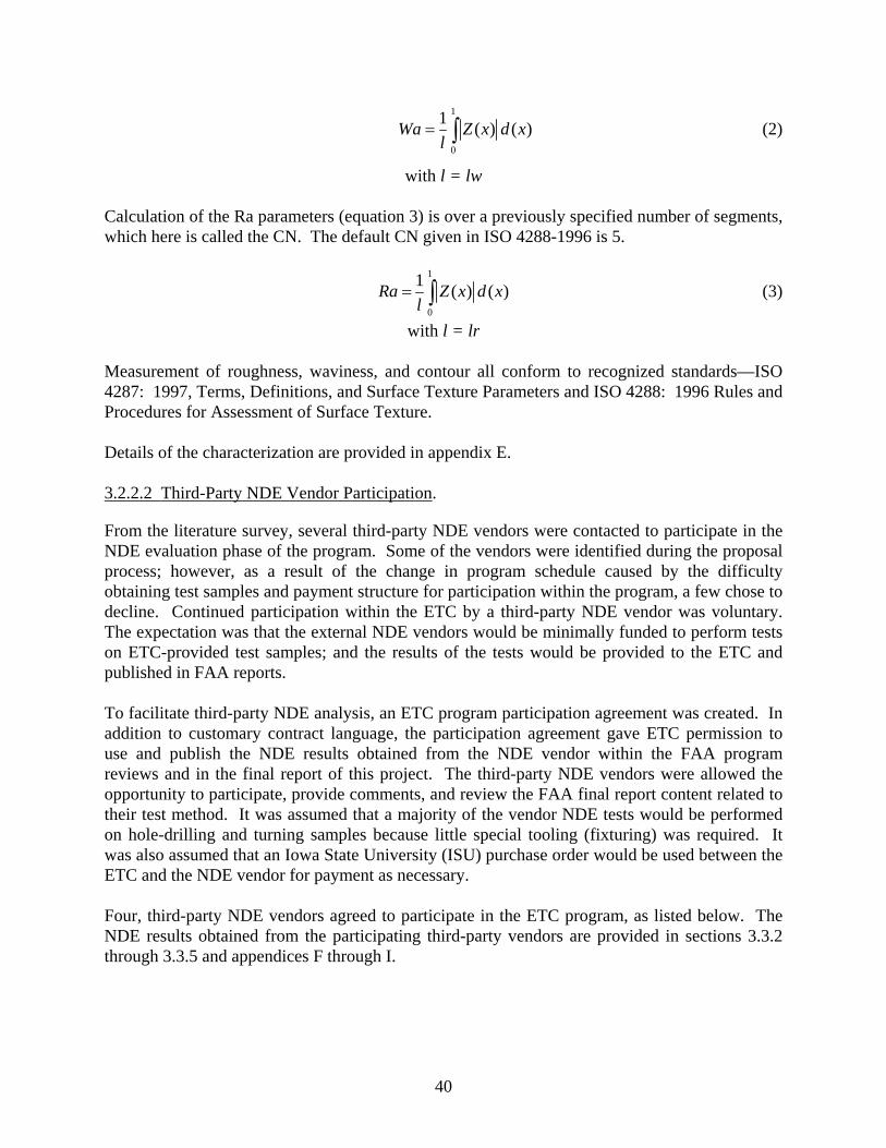
1
0
1( ) ( )Wa Z x d x
l (2)
with l = lw
Calculation of the Ra parameters (equation 3) is over a previously specified number of segments, which here is called the CN. The default CN given in ISO 4288-1996 is 5.
1
0
1( ) ( )Ra Z x d
l x (3)
with l = lr Measurement of roughness, waviness, and contour all conform to recognized standards—ISO 4287: 1997, Terms, Definitions, and Surface Texture Parameters and ISO 4288: 1996 Rules and Procedures for Assessment of Surface Texture. Details of the characterization are provided in appendix E. 3.2.2.2 Third-Party NDE Vendor Participation.
From the literature survey, several third-party NDE vendors were contacted to participate in the NDE evaluation phase of the program. Some of the vendors were identified during the proposal process; however, as a result of the change in program schedule caused by the difficulty obtaining test samples and payment structure for participation within the program, a few chose to decline. Continued participation within the ETC by a third-party NDE vendor was voluntary. The expectation was that the external NDE vendors would be minimally funded to perform tests on ETC-provided test samples; and the results of the tests would be provided to the ETC and published in FAA reports. To facilitate third-party NDE analysis, an ETC program participation agreement was created. In addition to customary contract language, the participation agreement gave ETC permission to use and publish the NDE results obtained from the NDE vendor within the FAA program reviews and in the final report of this project. The third-party NDE vendors were allowed the opportunity to participate, provide comments, and review the FAA final report content related to their test method. It was assumed that a majority of the vendor NDE tests would be performed on hole-drilling and turning samples because little special tooling (fixturing) was required. It was also assumed that an Iowa State University (ISU) purchase order would be used between the ETC and the NDE vendor for payment as necessary. Four, third-party NDE vendors agreed to participate in the ETC program, as listed below. The NDE results obtained from the participating third-party vendors are provided in sections 3.3.2 through 3.3.5 and appendices F through I.
40

1. NDE Method: Positron Annihilation Positron Systems, Inc. 411 S 5th Street Boise, ID, 83702-7626 Telephone: (208) 514-4570 Fax: (208) 338-2659 http://www.positronsystems.com Attention: Steve Yano [email protected]
Evaluation by Induced Positron AnalysisSM has been shown to be sensitive to detection of variations within material microstructures, measured at the atomic scale. The technique is used to measure material condition within a region of material beneath the surface. It has been used for practical NDE applications of metal alloy condition, such as cold working, heat treatment, operational damage, and manufacturing process effects, such as phase changes.
2. NDE Methods: Thermoelectric SQUID and Magnetic Remanence Methods
Hochschule Magdeburg-Stendal (FH) Institut für Elektrotechnik, Breitscheidstrasse 2, D-39114 Magdeburg, Germany Telephone: +49-(0)391-8 86 47 19 Fax: +49-(0)391-8 86 41 26 http://www.hs-magdeburg.de/fachbereiche/f-iwid/ET/Personen/Hinken Attention: Professor Dr.-Ing. Johann H. Hinken [email protected]
The Thermoelectric SQUID Method has been shown to be capable of detecting material crystallography, texture, or inhomogeneities within metals through the Seebeck effect by measuring differences in thermo-voltages generated between different (contacting) metals, given a common boundary at different temperatures. The Magnetic Remanence Method (MRM) has previously shown the ability to detect very small ferromagnetic inclusions in a nonferromagnetic surrounding. It was an NDE method employed in the MANHIRP program and was successful in detecting abusive material damage through the transfer of manufacturing material embedded into the nonmagnetic parent material.
41

3. NDE Method: X-Ray Diffraction Using Polycapillary-Collimating Optics
X-Ray Optical Systems, Inc. 15 Tech Valley Dr. East Greenbush, NY 12061-4134 Telephone: (518) 880-1500 Fax: (518) 880-1510 http://www.xos.com Attention: Matthew Cusack [email protected]
X-ray diffraction is a common method employed in material crystalline structure characterization. It has been used in many different applications to measure sample textures, monitor crystalline phase and structure changes, and to investigate common stress and strain measurements. Polycapillary-collimating x-ray optics are used to overcome many of the drawbacks and constraints of conventional x-ray diffraction systems enabling measurements using low-power x-ray sources, which reduces instrument size, cost, and power requirements.
4. NDE Method: Eddy-Current Static Array (Magnetic Carpet Probe)
Innovative Materials Testing Technologies, Inc. 3141 W. Torreys Peak Dr. Superior, CO 80027 Telephone: 303-554-8000 Fax: 303-554-8001 http://www.imtt-usa.com Attention: Dr. Yushi Sun [email protected] The Magnetic Carpet Probe is an array of pancake eddy-current coils fabricated within a flexible substrate to measure large areas of curved surfaces using absolute static measurements of eddy-current NDE.
3.2.2.3 The ETC Participation.
Within the capability of the ETC organization, the following seven NDE methods were identified for use. Note, there may be multiple approaches within a method. The NDE results obtained from ETC are provided in sections 3.3.6 through 3.3.11 and also in the appendices. The particular test samples generated by this ETC program are purposely fabricated to be nominally uniform in geometric distortions and to contain primarily material distortions. Geometric distortion and discontinuities are commonly found through optical and conventional NDE
42

methods. Actual (real-life) material conditions caused by abusive machining are expected to contain surface conditions characteristic of both geometric and material distortions. 1. NDE Method: Optical and Conventional Metrology
ETC Participants: ISU Each test sample fabricated by the ETC was measured to determine its baseline metrology condition, such as nominal surface roughness in each test sample. Measurements of surface roughness on the anomalous surfaces were made via conventional stylus methods and through optical surface scans. The test sample characterization plan for each of the manufacturing geometries is provided in section 3.3.1.
2. NDE Method: Conventional Single-Frequency Eddy-Current Analysis
ETC Participants: ISU, GE, HW, and PW
Conventional eddy-current NDE is a very common method employed by all engine OEMs for quality control of high-energy rotating hardware, such as turbine disks. However, the use of eddy-current NDE is driven primarily toward the detection of cracking conditions. This method is expected to provide localized anomaly detection and a relatively easy platform for implementation of an analysis method if found to be successful.
3. NDE Method: Multifrequency Eddy-Current Analysis
ETC Participants: ISU and GE
Multifrequency eddy-current NDE has been shown to be useful in separating eddy-current signals as a function of frequency and depth of penetration within the material. It is a very common method employed by many industries, including engine OEMs, in selected applications. This method is expected to provide localized anomaly detection and a relatively easy platform for implementation of an analysis method, if found to be successful.
4. NDE Method: Thermoelectric AMR
ETC Participants: GE
The thermoelectric AMR method has been shown to be capable of detecting material crystallography, texture, or inhomogeneities within metals through the Seebeck effect by measuring differences in thermo-voltages generated between different (contacting) metals, given a common boundary at different temperatures. To generate a temperature gradient in a sample, two air guns with a linear array of holes were used. Self-referencing thermoelectric measurement is conducted in a noncontact way by sensing the weak magnetic field due to the thermoelectric current around various types of imperfections and material variations.
43

5. NDE Method: Surface Wave Ultrasonic Analysis ETC Participants: ISU and HW Since the abusive material damage is confined to a thin surface layer having a depth of a few mil, it is best to similarly confine the ultrasonic examination through surface waves by operating at high frequencies. The bulk of the energy carried by a propagating surface wave is confined within an expected depth of a single wavelength. The bulk property measurements involve examining samples and measuring differences in quantities that arise from the underlying differences in surface wave velocity, attenuation, or backscatter. This method is not expected to be fast enough to use in scanning large components; however, it may be very useful in providing a qualitative measurement comparison for areas that have been flagged as suspect by other techniques.
6. NDE Method: High-Energy X-Ray Diffraction
ETC Participants: ISU
X-ray diffraction is a standard technique for determining lattice spacing of crystalline materials. Traditionally, this has been a surface measurement, but recent developments that use high-energy x-rays have enabled depth profiling (to several hundred microns in titanium). This method is not expected to be fast enough to use in scanning large components; however, it may be very useful in giving a quantitative measure for areas that have been flagged as suspect by other techniques. It may also prove useful as a nondestructive characterization method to provide reference samples for the development of other techniques.
7. Metallographic Analysis for NDE Correlation
ETC Participants: ISU and PW (all OEMs for Option A and C fabrication verification)
Commonly employed metallographic analysis methods are used to examine polished material samples under high optical magnification.
3.2.3 Planning and Coordination of NDE Analysis.
Due to the compressed schedule present under the Option C test sample fabrication activity, the coordination of NDE analysis followed a straightforward path leading up to a round-robin NDE analysis of relevant test samples selected by the participating organizations. A statistical analysis and replication study using multiple NDE methods on multiple test samples was not employed. However, results of the program would be useful to define future efforts. Since the goal of the Option C fabrication activity was to create seven nominally identical test sample sets with each test sample characterized through comparative (baseline), metallographic, and metrology analysis, it was determined that, for the purpose of generating data to evaluate a technique’s capability, application of an NDE method to a single test sample set would be sufficient. It was also decided during the planning stages that any highly suspect NDE data could be replicated using selected test samples or another complete test sample set, if the program schedule allowed.
44

It should also be noted that for the purpose of evaluating of a technique’s ability to discriminate between anomalous material conditions (e.g., those different than fabricated under nominal manufacturing conditions), higher weight was given to the ability to discriminate that a difference exists and less weight was given the ability of particular NDE methods to “grade” the severity of the assumed anomalous condition. The ability to determine severity, e.g., to quantify depth of damage, is viewed as technique optimization and is beyond the scope of this program. The evaluation process employed for the NDE methods are described in greater detail in section 3.4. During the Option C test sample fabrication process, the available Option A test samples were shipped to the identified locations for NDE analysis to allow them to become familiar with the test sample geometry and expected surface conditions. For the Option C test sample, each of the ETC sample sets provided to the ETC and the third-party NDE vendors followed essentially the same schedule. The steps were as follows: 1. Test sample fabrication by OEM organizations
a. Hole-drilling—GE b. Turning—PW c. Broaching—HW
2. Metallographic comparisons by OEM organizations 3. Serialization of test samples by OEM organizations 4. Baseline metrology characterization by ISU 5. Assembly and identification of test sample sets by ISU 6. Shipment of test sample sets coordinated through GE and ISU 7. Review of draft NDE results via draft reports and teleconference discussions 8. Selection of test samples for NDE round-robin analysis In general, the test samples were fabricated per schedule expediency with the simplest fabricated first. At the OEMs, shipment of test samples to ISU occurred as their fabrication and characterization efforts were completed. Not all test samples were assembled and shipped to ISU as a completed sample set. Shipment of a complete test sample set for NDE analysis was directed toward the availability of the test samples and the ability of the participating organization to process the results in a timely manner. When the sample sets were being assembled for shipment, ISU had access to the test samples for NDE analysis. An arrangement was made such that the primary organization that had the ability to make multiple NDE measurements over a wider range of test samples was the primary organization involved in the round-robin tests selected by the team for further NDE comparisons. 3.2.3.1 Test Sample Identifications.
The Option A and Option C test samples are identified per the following sample number markings:
aa-b-c-d-yymmdd (where c can be 1, 2, or 3 letters long)
45

where:
aa = Ti or In (C-Ti*, C-In*) b = T, D, or B for turning, hole drilling, broaching c = P, T1, T1A, T6, T6A for pristine or damage types 1, 1A, 6, 6A d = 1, 2, 3, ... indicating the i-th sample of this type yymmdd = manufacture date in year-month-day format (e.g., 071231 for Dec. 31, 2007) *C = Option C
3.2.3.2 Test Sample Metrology Characterization Plan.
The Option A and Option C test samples were characterized per the following steps. 1. Perform baseline visual inspection of all samples (i.e., screening inspections to identify
that test samples being sent out for NDE are nominally identical and to identify high-suspect locations for detailed NDE and further metrology examinations.)
Optical photographs Surface, area, or line profilometry (metrology) measurements
2. Following baseline characterization, send test samples for NDE analysis. 3. Following return from NDE analysis, perform detailed inspection of areas identified as
special interest using white light interferometer (WLI), or other metrology method, per NDE recommendations or baseline assessments.
4. Report baseline and special inspection data to correlate with NDE findings. Registration
of metrology and NDE was made based on sample number location placed on either the test sample or a special marker specific to the test sample itself.
3.2.3.2.1 Hole-Drilling-Specific Sample Characterization Plan.
With a defined coordinate Z-R-Theta system, the following steps are performed for characterization. 1. Using a video borescope with a manipulated probe/sample rotator, perform a visual
screening to locate and document areas of special interest. 2. Baseline inspection will be five circular profiles at 10%, 30%, 50%, 70%, and 90% depth
or three profiles at 20%, 50%, and 80% depth. 3. Special inspection for scratches and surface roughness will be done using axial surface
finish scans and/or a WLI scan of hole replica. 4. It is assumed that a small percentage of hole-drilling samples will be examined with WLI
(or other method).
46

3.2.3.2.2 Turning-Specific Sample Characterization Plan.
With a defined coordinate X-Y system, the following steps are performed for characterization. 1. Using a stereo microscope or video microscope, perform a visual screening to locate and
document areas of special interest. 2. Baseline inspection will be done using a coordinate measurement machine for flatness
and/or a surface finish probe for roughness. 3. Samples with smeared or redeposited metal will be three-dimensionally (3D) profiled
using a laser sensor. 4. Special 3D anomalies will have their length, width, and height measured with the WLI. 5. It is assumed that a small percentage of turning samples will be examined with WLI (or
another method). 3.3 PRELIMINARY NDE ASSESSMENT.
3.3.1 Baseline Metrology.
Baseline metrology was completed on nearly all AMD samples prior to NDE testing. Samples were analyzed for roughness and waviness using Gaussian filters, as prescribed by both ISO 4287 and ISO 4288. In most cases, the numerical index of roughness increased in value from the pristine to the T1 and T6 samples, which correlated to the increase in anomalous machining. The values for waviness generally increased from pristine to the T1 samples, but then decreased from the T1 to the T6 samples. The scan plan for the broaching and turning samples is shown in figure 32. The length of those scans was approximately 0.58 inch in length and 0.084 inch in width. The actual measurement of roughness and waviness was set at 50 points wide or approximately 0.015 inch wide (see figure 33).
47

Area Examined
Sample
Figure 32. Scan Plan for Broaching and Turning Samples
Figure 33. Width of 50-Point-Wide Line Used for Measurement Measurements on the hole-drilling samples were slightly more difficult to make since the surface to be measured was parallel to the light and the camera view of the optical profilometer. To make accurate measurements, a brass rod was turned down to a diameter slightly less than the diameter of the drilled hole (7 mm or 1/2 inch, depending on the sample), cut at a 45° angle, and polished to a 0.1-micron finish (see figure 34). When the brass rod was inserted into the drilled hole, the focal length needed for measurement was held at a constant value, and the side of the hole’s surface was able to be captured and measured in the same fashion as the broaching and turning samples. The length of the scan was dependent on the depth of the sample or the diameter of the hole, allowing for a 45° plane to bisect the hole, but generally the 7-mm holes had a scan length of 7 mm and the 1/2-inch holes had a scan length of 0.687 inch (17.45 mm). A description of the equipment and the general process of measurement acquisition, as well as a more detailed discussion of roughness and waviness S-parameters, can be found in appendix E.
48

Figure 34. Device Used to Measure the Sides of the Hole-Drilling Samples 3.3.1.1 Metrology Results for Broaching Samples.
The broaching samples showed a general increase in roughness and waviness with an increased machining on the surface of the samples, except for the roughness of the Ti T6 samples and the waviness of the In 718 T6 sample, shown in figures 35 and 36 and table 6. Examples of roughness and waviness graphs are shown in figures 37 and 38, respectively. One interesting feature of the broaching samples’ waviness was that nearly every sample examined showed a slight bump in the middle of the sample, as shown in the waviness graph in figure 38. This feature was not unique to one particular type of sample, but was evident in each type examined.
Broach In 718
Broach Ti 6-4
Figure 35. Average Roughness of Broaching Samples for Both Alloys
49
Broach In 718
Broach Ti 6-4
Figure 36. Average Waviness of Broaching Samples for Both Alloys
Table 6. Average Roughness and Waviness Data for Broaching Samples by
Surface Condition and Alloy
Sample Ra
Average
Ra Standard Deviation
Wa Average
Wa Standard Deviation
Broaching In 718 Pristine 19.08 4.66 44.75 15.42
Broaching In 718 Type 1* 25.06 7.44 112.47 33.86
Broaching In 718 Type 6* 30.25 27.34 134.19 73.46
Broaching Ti 6-4 Pristine 24.36 30.27 151.75 65.73
Broaching Ti 6-4 Type 1* 29.30 45.64 188.65 51.14
Broaching Ti 6-4 Type 6* 21.33 11.73 140.56 70.15
Figure 37. Typical Roughness Graph for a Broaching Sample
50

Figure 38. Typical Waviness Graph for a Broaching Sample 3.3.1.2 Methodology Results for Turning Samples.
The turning samples did not exhibit the same type of correlation for roughness and waviness as the broaching or hole-drilling samples with regard to an increased roughness and waviness with increased surface treatment. For the Ti samples, the trend line shows a general increase in roughness, with the exception of the T1 samples, which appeared to have a slightly smoother finish than the pristine samples. The In 718 samples show an increased roughness from the pristine to the T1 condition, but the T6 samples show a marked decrease in roughness, as evidenced in figure 39 and table 7. The waviness for the turning samples (figure 40) was similar to the broaching samples in that there was an increase in waviness from pristine to T1 samples, but a decrease from the T1 to the T6 samples. Typical roughness and waviness graphs for the turning samples are shown in figures 41 and 42. It is of interest to note that nearly all turning samples exhibited a matched pair of concave and convex shapes, which were nearly equal in the amount of curvature within the sample itself. This is believed to have been the result of how the sample was extracted from the parent material.
Turned In 718
Turned Ti 6-4
Figure 39. Roughness of the Turning Samples for Both Alloys
51
Table 7. Average Roughness and Waviness Data for Turning Samples by Surface Condition and Alloy
Sample Ra
Average
Ra Standard Deviation
Wa Average
Wa Standard Deviation
Turning In 718 Pristine 96.55 16.73 58.35 25.12
Turning In 718 Type 1* 193.33 188.10 201.06 197.60
Turning In 718 Type 6* 71.18 12.41 138.76 91.74
Turning Ti 6-4 Pristine 66.67 12.69 44.25 22.23
Turning Ti 6-4 Type 1* 46.40 22.81 302.67 171.55
Turning Ti 6-4 Type 6* 142.78 54.15 103.91 78.05
Turned In 718
Turned Ti 6-4
Figure 40. Average Waviness of Turning Samples for Both Alloys
Figure 41. Typical Roughness Graph for a Turning Sample
52

Figure 42. Typical Waviness Graph for a Turning Sample 3.3.1.3 Methodology Results for Hole-Drilling Samples.
The hole-drilling samples showed an increase in surface roughness and waviness for both alloys with an increase in surface treatment, as shown in figures 43 and 44 and in table 8. Values of roughness for both alloys were nearly identical for all three types of surface treatment. Although the value for the waviness of the Ti T6 was slightly less than the T1 values, it still represented the general trend of increased waviness values with an increase in surface treatment. Both roughness and waviness, as shown in figures 45 and 46, were typical for all samples examined, with no unique features as observed in the broaching and turning samples.
Drilled In 718
Drilled Ti 6-4
Figure 43. Roughness of the Hole-Drilling Samples for Both Alloys
53

Drilled In 718
Drilled Ti 6-4
Figure 44. Average Waviness of Hole-Drilling Samples for Both Alloys
Table 8. Average Roughness and Waviness Data for Hole-Drilling Samples by Surface
Condition and Alloy
Sample Ra
Average
Ra Standard Deviation
Wa Average
Wa Standard Deviation
Hole-Drilling In 718 Pristine 76.72 31.87 294.06 148.62
Hole-Drilling In718 Type 1* 132.50 10.61 523.00 45.25
Hole-Drilling In 718 Type 6* 170.00 47.18 559.77 192.50
Hole-Drilling Ti 6-4 Pristine 85.43 43.95 370.05 174.12
Hole-Drilling Ti 6-4 Type 1* 149.70 28.84 599.24 151.78
Hole-Drilling Ti 6-4 Type 6* 182.54 42.42 497.21 143.48
Figure 45. Typical Roughness Graph for a Hole-Drilling Sample
54
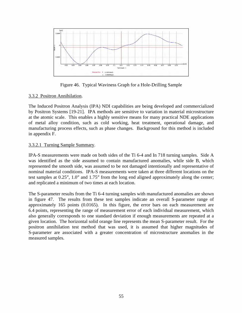
Figure 46. Typical Waviness Graph for a Hole-Drilling Sample 3.3.2 Positron Annihilation.
The Induced Positron Analysis (IPA) NDI capabilities are being developed and commercialized by Positron Systems [19-21]. IPA methods are sensitive to variation in material microstructure at the atomic scale. This enables a highly sensitive means for many practical NDE applications of metal alloy condition, such as cold working, heat treatment, operational damage, and manufacturing process effects, such as phase changes. Background for this method is included in appendix F. 3.3.2.1 Turning Sample Summary.
IPA-S measurements were made on both sides of the Ti 6-4 and In 718 turning samples. Side A was identified as the side assumed to contain manufactured anomalies, while side B, which represented the smooth side, was assumed to be not damaged intentionally and representative of nominal material conditions. IPA-S measurements were taken at three different locations on the test samples at 0.25″, 1.0″ and 1.75″ from the long end aligned approximately along the center; and replicated a minimum of two times at each location. The S-parameter results from the Ti 6-4 turning samples with manufactured anomalies are shown in figure 47. The results from these test samples indicate an overall S-parameter range of approximately 165 points (0.0165). In this figure, the error bars on each measurement are 6.4 points, representing the range of measurement error of each individual measurement, which also generally corresponds to one standard deviation if enough measurements are repeated at a given location. The horizontal solid orange line represents the mean S-parameter result. For the positron annihilation test method that was used, it is assumed that higher magnitudes of S-parameter are associated with a greater concentration of microstructure anomalies in the measured samples.
55

Figure 47. S-Parameter Measurements Made on Side A of the Ti 6-4 Turning Samples Assumed
to Contain Anomalous Machining-Induced Damage The two pristine test samples, Ti-P-8 and Ti-P-15, had a lower S-parameter than the other test samples. This was expected, as these test samples should have the lowest damage, and thus a lesser amount of dislocations. Correspondingly, the damaged Type 1* test samples had an elevated S-parameter in comparison to the pristine samples. Test sample Ti-T1-7, which was identified to contain light deformation, had an intermediate S-parameter value. Test samples Ti-T1A-15 and Ti-T1-2, identified to contain medium and heavy deformation, respectively, had higher S-parameter values. Both of these two heavy deformation test samples had similar S-parameter values, which suggested that either the induced damage on the material or the measurement had reached a saturation point or the material state at the measurement location contained similar damage. The test samples with Type 6* anomaly, both with medium deformation, showed similar S-parameter values that are elevated over the baseline values. Interestingly, these S-parameter values were lower than the Type 1* test samples identified to contain medium deformation. This suggests that IPA-S may not be as sensitive to Type 6* damage as it is to Type 1* damage or that inducing material anomalies from Type 6* damage actually results in lower corresponding material damage for a given level of deformation. A destructive characterization would be necessary to further separate these effects. The S-parameter results from the pristine test samples (Ti-P-8 and Ti-P-15) of figure 47 show good agreement between the abusively machined surfaces (the side with the anomaly, i.e., side A), and this surface. This was expected, and S-parameter values in this range can be assumed to represent the same nominal baseline conditions. Figure 48 shows the S-parameter results from the assumed nondamaged side of the samples, side B. These results, with one exception, show good overall agreement.
56

Figure 48. S-Parameter Measurements Made on Side B of the Ti 6-4 Turning Samples Assumed
to be Undamaged and Representative of Nominal Material Conditions As shown in figure 48, one of the test samples with Type 6* material damage, Ti-T6A-14, shows results with an unexplained trend. The S-parameter values for side A assumed to have the material damage were very similar to the other test samples (figure 47), while the values for the undamaged side B were not. This may indicate that this side B of the test sample was machined in an abusive manner similar to the other test samples. Also of note is that the S-parameter value for side B does not closely correlate with the results for any of the anomaly types measured. Given the dramatic S-parameter change indicated for both Ti 6-4 Type 1* and Type 6* anomalies, there is a legitimate ability to differentiate between damaged and undamaged material conditions in flat-plate sample geometries. In addition, for Type 1* anomalies, the IPA-S method has shown the ability to provide reasonable levels of measurement capability to discern an assumed range of severity from light to heavy material damage. Data from side A of the In 718 samples are shown in figure 49. The orange lines represent the mean S-parameter result. The data for each of the samples show good agreement in relation to the overall variation between sample groups. The two pristine samples have lower S-parameters than the other samples. This was expected, as these samples should have the lowest damage. The anomaly Type 1* samples had an elevated S-parameter compared to the pristine samples. The Type 1* samples were also segregated in relation to the damage level; the light deformation samples had lower S-parameters than the medium deformation samples. The anomaly Type 6* samples, both with light deformation, had S-parameter values that were intermediate between the two levels of damage of the Type 1* samples.
57

Figure 49. S-Parameter Measurements Made on Side A of the Ti 6-4 Turning Samples Assumed to Contain Anomalous Machining-Induced Damage
It is understood that the back of the sample was not manufactured with any intentional anomaly level. Data from IPA-S measurements on the rear (side B) side are shown in figure 50. A number of samples showed S-parameter values similar to the pristine samples on side A. However, some, such as In-T-P-1-080725 and In-T-T6A-7-080916, had measured S-parameters that suggest that they may have been abusively machined.
Figure 50. S-Parameter Measurements Made on Side B of the In 718 Turning Samples Assumed to be Undamaged and Representative of Nominal Material Conditions
58

3.3.2.2 Broaching Sample Summary.
S-parameter measurements were made on the Ti 6-4 and In 718 broaching samples in a similar manner as were made for the turning samples. The positron source was positioned in the broaching slot by locating the probe on the flat section of the broaching interior (slot bottom), along its long axis. It was assumed that for each test sample that contained two broaching slots, both slots contained the same type and severity of manufacturing-induced anomaly. One side was randomly identified as A, the other side was identified as B. Unlike the turning samples, the S-parameter measurements were taken in two different configurations, one with the probe facing the detector and one with the probe on the side facing away from the detector. Results from measurements on the In 718 broaching samples with the probe side facing the detector are shown in figure 51. Similar results are shown in figure 52 with the probe side facing away from the detector. The overall spread of the S-parameter measurements taken from the In 718 broaching samples was approximately 90 points. Like the Ti 6-4 turning samples, the S-parameter measurements observed for the pristine samples were lower than the test samples assumed to contain anomalous material conditions. The measurements taken on the locations with manufactured anomalies showed an elevated S-parameter response that was well beyond the measurement noise compared to the pristine test samples. The measurements taken on side A on test sample In-T1A-15 are the exceptions to this trend. These data points lie significantly lower than the general trend. This may indicate that the material condition at this particular location is less severely damaged than intended. There was no apparent difference, however, between the S-parameter results from different anomaly types or anomaly severity, Type 1* or Type 6*, other than separation from that identified as nominal material conditions.
Figure 51. S-Parameter Measurements Made on In 718 Broaching Samples With the Probe Side
Facing the Detector
59

Figure 52. S-Parameter Measurements Made on In 718 Broaching Samples With the Probe Side Facing Away From the Detector
Figure 53 shows the S-parameter measurements made on Ti 6-4 broaching samples with the probe side facing the detector. The spread of the largest to smallest S-parameter is roughly 45 points for a given measurement orientation. This is significantly lower than what was observed in the In 718 samples. The pristine samples trend generally lower than the samples with anomalies; however, this difference is not beyond the measurement noise. The S-parameter data for test sample Ti-T1A-16 trends lower than the other test samples with similar Type 1* anomalies. The data for this test sample is closer in range to the pristine coupons. S-parameter data from the Ti 6-4 broaching samples with Type 6* anomalies correspond closely to data from test samples containing Type 1*.
Figure 53. S-Parameter Measurements Made on Ti 6-4 Broaching Samples With the Probe Side
Facing the Detector
60

For the In 718 broaching samples, the method demonstrated some ability to differentiate between pristine test samples and test samples containing manufacturing-induced anomalies; however, it was unable to differentiate between the anomaly types or to discern an assumed range of severity from light to heavy material damage in the In 718 broaching sample configuration. For the Ti 6-4 broaching samples, the method showed evidence of trending between the S-parameter measurements of pristine test samples and test samples containing manufacturing-induced anomalies; however, the signal-to-noise ratio (SNR) was not sufficient to quantitatively differentiate between the two material conditions. Given the low SNR, it was likewise unable to differentiate between the anomaly types or discern an assumed range of severity from light to heavy material damage in the Ti 6-4 broaching samples. 3.3.2.3 Hole-Drilling Sample Summary.
S-parameter measurements were made on the Ti 6-4 and In 718 hole-drilling samples in a similar manner to the turning samples. The positron source was positioned in the hole against the surface of the material. Also in a manner similar to the turning and broaching samples, the S-parameter measurements were replicated at various clock positions around the periphery of the hole and in some instances, multiple measurements were made at each clock position. The Ti 6-4 hole-drilling samples, shown in figure 54, have an overall S-parameter spread of about 90 points, which is comparable to the same overall spread found on the Ti 6-4 broaching samples. The pristine Ti 6-4 hole-drilling samples show a wide range of measurements values, which tend to increase with sample number. There were too few anomaly Type 1* samples to make any definitive conclusions, although the data fell within the range of the pristine coupons. S-parameter data from anomaly Type 6* (smearing with no heat damage) were lower than the pristine samples, which was an unexpected result compared to the results obtained from the broaching and turning samples.
Figure 54. S-Parameter Measurements Made on Ti 6-4 Hole-Drilling Samples With the Probe Placed Interior to the Axial Length of the Hole
61

Figure 55 shows the results from the S-parameter measurements taken on the In 718 hole-drilling samples. Some measured samples were not included due to poor measurement quality indicators. The overall range of the In 718 hole-drilling samples was approximately 160 points. This is significantly greater than in the broaching and turning samples. A possible reason for the wide spread in data is the variation in the surface condition of the holes. The data from the pristine In 718 hole-drilling samples showed reasonable agreement. Of interest is how the S-parameter tends to increase as the sample numbering increases. This same S-parameter trend was observed in the Ti 6-4 pristine hole-drilling samples. If the sample numbering reflects the order of manufacture, this could reflect the influence of dulling of the tooling. The In 718 hole-drilling samples with anomaly Type 1* show a wide range of S-parameter values with little agreement and no general trend. This may be due to variations in the surface condition of the interior of the hole, which prevents the probe from making consistent contact with the material surface. The S-parameter data from the In 718 hole-drilling sample with Type 6* anomalies show good general agreement with trending observed from light to heavy damaged material. However, this data corresponds closely to the S-parameter range of the pristine samples. This data also seems to show a trend between sample numbering and S-parameters that mimics what was observed in the pristine In 718 hole-drilling samples.
Figure 55. S-Parameter Measurements Made on In 718 Hole-Drilling Samples With the Probe Placed Interior to the Axial Length of the Hole
For measurement in the hole-drilling samples, the sensitivity could likely be improved with a custom probe design that enabled better surface contact along the inner surface of the hole. Additionally, only one probe isotope was tested due to time constraints. Different isotopes probe at varying depths of material, and this was not explored for this particular study. For the Ti 6-4 hole-drilling samples, the method showed evidence of trending between the S-parameter measurements of pristine test samples and test samples containing manufacturing-induced Type 6* anomalies; however, the SNR was not sufficient to quantitatively differentiate between the two material conditions. Because of the limited number of Type 1* hole-drilling samples examined, no comment on sensitivity is presented.
62

For the In 718 hole-drilling samples, the method shows evidence of trending between the S-parameter measurements of pristine test samples and test samples containing manufacturing-induced Type 6* anomalies; however, the SNR was not sufficient to quantitatively differentiate between the two material conditions. The S-parameter measurements from In 718 hole-drilling samples with Type 1* anomalies presented a wide range of values with little agreement and no general trend. 3.3.2.4 Conclusions and Recommendations.
IPA-S measurements on the turning samples showed the greatest assumed correlations with material damage. Measurements on the Ti 6-4 samples showed the most promising results, although the In 718 showed definite differentiation between the levels of damage. There are several reasons that may explain why the turning samples showed a stronger response than the other sample types. The turning samples might be more damaged than the other sample types. The coupon design was the easiest to measure consistently. The flat surface may also have been the easiest to verify that the manufacturing process had been done according to plan. The broaching samples were somewhat more complicated to measure than the turning samples, which may be reflected in the mixed results. The In 718 results indicate the ability to differentiate between the pristine samples and the samples with manufacturing-induced anomalies; however, it is unable to differentiate between the anomaly types. With the Ti 6-4 samples, there was a small difference in S-parameter response between the pristine samples and samples with anomalies, but the measurement noise made it difficult to differentiate between the two. It may be possible, however, to increase the resolution through process refinement. The hole-drilling samples proved to be difficult to measure consistently. This may be due, in part, to the variations in the internal surface finish of the holes, which could interfere with consistent placement of the positron-emitting probe. Table 9 outlines the conclusions of each sample set. Many optimization methods remain unexplored to improve measurement sensitivity and repeatability. The overall probe design parameters should be refined, including the selection of the positron source, size, and geometry. Additionally, the PS6100 test platform, unavailable when the tests were manually completed, could dramatically increase the number of measurements made and enable profile mapping of surfaces of interest.
63

Table 9. The IPA-S Conclusions for Each Sample Set
Turning
Ti 6-4 Given the dramatic S-parameter change for anomaly Type 1*, there is a legitimate ability to differentiate between samples that have this anomaly and samples that do not, as well as differentiate between light damage and medium to high deformation. Type 6* data also showed this trend, although the difference is not as great.
In 718 The S-parameter measurements from these samples show that IPA-S has the ability to differentiate the level of induced damage between samples.
Broaching
Ti 6-4 There may be a small difference in S-parameter response between the pristine samples and samples with anomalies, but the measurement noise drowns out the ability to differentiate between the two. It may be possible, however, to increase the resolution through process refinement.
In 718 IPA-S shows the ability to differentiate between the pristine samples and the samples with manufacturing-induced anomalies; however, it is unable to differentiate between the anomaly types.
Hole-Drilling
Ti 6-4 It is somewhat possible to differentiate between the pristine and anomaly Type 6*.
In 718 Not possible to differentiate anomaly types in the standard coupon geometry. Large hole coupons show a significant trend.
3.3.3 Magnetic Remanence Methods.
The MRM has previously shown the ability to detect very small ferromagnetic inclusions in a nonferromagnetic surrounding [22-24]. Using a strong magnetic field, any ferromagnetic particles present are magnetized near to saturation. After this step, the magnetic field, which acts on the device under test, is made zero and the ferromagnetic inclusions, if present, act as small permanent magnets with remnant magnetization. The surface of the device under test is then scanned with a magnetometer. Magnetic field signatures then indicate a ferromagnetic inclusion whose size and depth below the surface can be estimated. Details of the background for this method are included in appendix G. 3.3.3.1 Turning Sample Summary.
Figure 56 shows the C-scan image of sample Ti-T-T6-080508 containing Type 6* material damage. The arrangement of the sample is such that the sample number stamp is on the bottom. The indicated zones (A, B, C, and D) show typical MRM signatures. The C-scan images in figure 56 show the right side of the sample on the right-hand side and the left side of the sample on the left. Figure 56 includes a C-scan of the first (figure 56(b)) and the repeated (figure 56(c)) tests. The samples were cleaned using an ultrasonic bath and the measurements were repeated several times, all showing similar results.
64

Figure 56. C-Scan of Sample Ti-T-T6-080508 With MRM Signatures at Zones A, B, C, and D (a) Photograph, (b) First Test, and (c) Repeated Test
Figure 57 shows the C-scan image of sample Ti-T-T6A-10-080602 containing Type 6* material damage. The arrangement of the sample is the same as sample Ti-T-T6-080508 above. The C-scan of the sample shows multiple MRM signatures. These signatures are spread over the sample and are repeatable. Visual inspection shows that the surface of the sample has heavy smearing.
Figure 57. C-Scan Sample Ti-T-T6A-10-080602 (a) Photograph and (b) MRM C-Scan
65
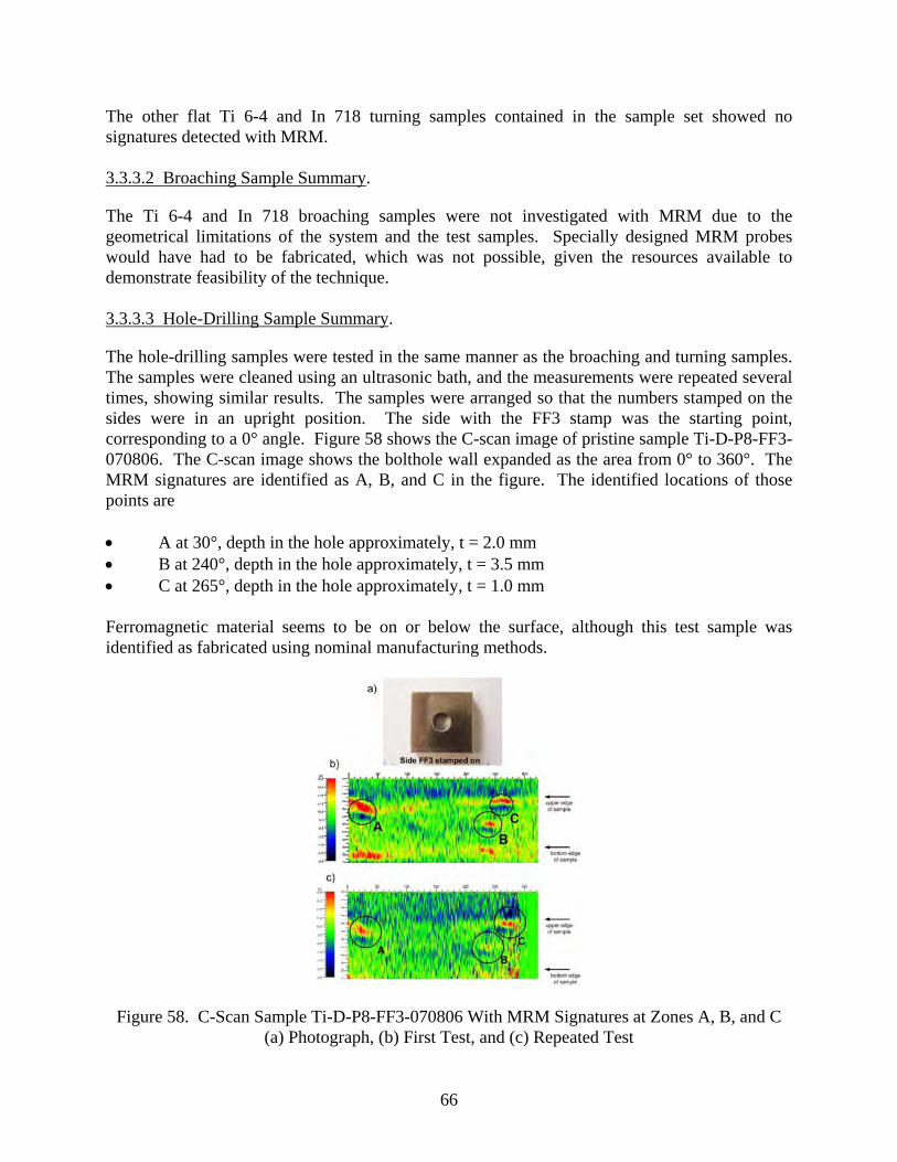
The other flat Ti 6-4 and In 718 turning samples contained in the sample set showed no signatures detected with MRM. 3.3.3.2 Broaching Sample Summary.
The Ti 6-4 and In 718 broaching samples were not investigated with MRM due to the geometrical limitations of the system and the test samples. Specially designed MRM probes would have had to be fabricated, which was not possible, given the resources available to demonstrate feasibility of the technique. 3.3.3.3 Hole-Drilling Sample Summary.
The hole-drilling samples were tested in the same manner as the broaching and turning samples. The samples were cleaned using an ultrasonic bath, and the measurements were repeated several times, showing similar results. The samples were arranged so that the numbers stamped on the sides were in an upright position. The side with the FF3 stamp was the starting point, corresponding to a 0° angle. Figure 58 shows the C-scan image of pristine sample Ti-D-P8-FF3-070806. The C-scan image shows the bolthole wall expanded as the area from 0° to 360°. The MRM signatures are identified as A, B, and C in the figure. The identified locations of those points are A at 30°, depth in the hole approximately, t = 2.0 mm B at 240°, depth in the hole approximately, t = 3.5 mm C at 265°, depth in the hole approximately, t = 1.0 mm Ferromagnetic material seems to be on or below the surface, although this test sample was identified as fabricated using nominal manufacturing methods.
Figure 58. C-Scan Sample Ti-D-P8-FF3-070806 With MRM Signatures at Zones A, B, and C (a) Photograph, (b) First Test, and (c) Repeated Test
66

Figure 59 shows the C-scan of sample Ti-D-T6A-FF3-080508. The side with the FF3 stamp is at the bottom. At points A and B, significant MRM signatures can be detected. The locations of these points are A at 80°, depth in the hole approximately t = 4.0 mm B at 300°, depth in the hole approximately t = 6.0 mm
Figure 59. C-Scan Sample Ti-D-T6A-FF3-080508 With MRM Signatures at Zones A and B (a) Photograph, (b) First Test, and (c) Repeated Test
The other hole-drilling samples contained in the FAA ETC sample set showed no signatures when tested with MRM. 3.3.3.4 Conclusions and Recommendations.
In some samples, ferromagnetic inclusions were detected using MRM. This was surprising since, according to the description of the manufacturing process, no tool abrasions or similar traces should be found. This was unlike the turning samples, which contained abusive and smeared material conditions where tool particles or other contaminations may have been present as a result of tool wear. The presence of an MRM signature on any pristine sample is a surprising result, as it was not anticipated that any magnetic materials would be present within the pristine samples. For the geometry of test samples, nonmagnetic materials, or the anomalous machining conditions used, magnetic indications were not anticipated to exist. Table 10 outlines the conclusions of each sample set.
67
Table 10. The MRM Conclusions for Each Sample Set
Turning
Ti 6-4 A selected Type 6* sample was found to contain indications of magnetic properties within the surface of the sample. This condition was observed to repeat. The cause of magnetic indication is unknown as no tool abrasions or similar traces could be identified within the manufacturing process for the Type 6* condition.
In 718 Not tested due to unavailability.
Broaching
Ti 6-4 Not tested due to geometric and system constraints.
In 718 Not tested due to geometric and system constraints.
Hole-Drilling
Ti 6-4 Same as the turning results above. Condition observed in one of the pristine hole-drilling samples.
In 718 Not tested due to unavailability of In 718 test samples. 3.3.4 Parallel Beam X-Ray Diffraction Using Polycapillary-Collimating Optics.
X-ray diffraction (XRD) relies on the coherent scatterings of x-rays to obtain information about the structure of crystalline materials [25 and 26]. A primary use of the technique is the identification and characterization of compounds based on their diffraction pattern. Scattering of those x-rays from atoms within the target material is the dominant effect that occurs when an incident beam of monochromatic x-rays interacts with a target material. In materials with regular structure (i.e., crystalline), the scattered x-rays undergo constructive and destructive interference. This is the process of diffraction. The diffraction condition of x-rays by crystals is described by Bragg’s Law, nλ = 2d sinθ. The diffractions direction depends on the size and symmetry of the unit cell of the material. Detailed background information [27 and 28] is provided in appendix H. 3.3.4.1 Turning Sample Summary.
The provided Ti 6-4 and In 718 turning samples were used to investigate XRD measurement sensitivity and were not analyzed for anomalous conditions. The results are included in appendix H. 3.3.4.2 Broaching Sample Summary.
Measurements were taken to directly compare the diffraction images instead of measuring the residual stress. The diffraction images were collected for the broaching samples with the same conditions: an x-ray source was run at full 40W power, a Bruker area detector was set at a fixed position with a 60-second exposure time, and the beam incident angle was the same for each sample.
68

A typical diffraction image from a Ti 6-4 broaching sample and a profile of the center segment in this diffraction image is shown in figure 60.
Figure 60. Typical Diffraction Image From a Ti 6-4 Broaching Sample and a Resulting Profile of the Center Segment Obtained From the Image
Significant differences are shown in the profiles presented in figure 61. This is encouraging since there are some physical explanations regarding the sample damage status. For example, the profile difference between 7C and 16A could be due to the difference of crystal grain orientation distribution as might result from bent grain, and the profile difference between 17B and 31B could be due to an amorphous layer. However, it is difficult to make firm conclusions because of two things: first, with the limited independent characterization information, solid relationships cannot be established between these observations and the presence of manufacturing-induced anomalies. Second, the system configuration factors, which also play a significant role, must be taken into account. Figures 62 and 63 illustrate the peak profiles for all remaining Ti 6-4 and In 718 broaching samples examined.
(a) (b)
Figure 61. Comparison of Diffraction Images Obtained From Ti 6-4 Broaching Samples (a) 7C vs 16A Profiles and (b) 17B vs 31B Profiles
69

Figure 62. Diffraction Peak Profiles for all Ti 6-4 Broaching Samples Tested
Figure 63. Diffraction Peak Profiles for all In 718 Broaching Samples Tested For Ti 6-4 broaching samples, notice that the peak position shifts are principally due to sample position displacements, and not only are there significant variations in peak counts but also in two-peak ratios. It can easily be shown that sample 335 and sample P7 have higher peak counts, while samples 612A and 331 have lower peak counts. The peak count variation could indicate a change in crystal quality, while the two-peak ratio variation could be due to the change of grain orientation.
For the In 718 broaching samples XRD peaks, there are about two clusters; samples 49B, 40B, and 31B have lower peak counts, while samples 17B, 37B, 225A, and 225B have similar higher peak counts, with sample 46A between them.
70

For the In 718 and Ti 6-4 broaching samples, the method has shown some ability to differentiate between pristine test samples and test samples containing Type 1* anomalies; however, it is not suitable for the general investigation of Type 6* anomalies because a small beam (1.5 mm) and an area detector were used. Selected analysis of Type 6* anomalies may be possible if the location of the anomaly is known. This approach measures a very thin surface layer of the samples. The penetration depth of the Cu Kα radiation is less than 1 mil (25 μm) for Ti-based alloys and less than 0.5 mil (~10 μm) for Ni-based alloys. Thus, the method is capable of detecting the presence of anomalies, but it cannot discriminate between the severities of anomalies beyond the penetration depth range in these materials. 3.3.4.3 Hole-Drilling Sample Summary.
The Ti 6-4 and In 718 hole-drilling samples were not investigated with the XRD method due to the geometrical limitations of the system and the test samples. 3.3.4.4 Conclusions and Recommendations.
In principal, the approach could be applied to evaluate the Type 1* anomalies but is not suitable for Type 6* anomalies since a small beam (1.5 mm) and an area detector were used. The penetration depth of the Cu Kα radiation is less than 1 mil (25 μm) for Ti-based alloys and less than 0.5 mil (~10 μm) for Ni-based alloys. This XRD approach can be used to detect but not to characterize medium-high anomalies. Table 11 outlines the conclusions of each sample set.
Table 11. The XRD Conclusions for Each Sample Set
Turning
Ti 6-4 Not tested due to schedule/budget constraints and lack of In 718 samples. Available Ti 6-4 and In 718 turning samples were used for measuring theoretical limits of diffraction peaks (deltas) for the two materials under consideration.
In 718 Not tested due to unavailability of In 718 test samples.
Broaching
Ti 6-4 The peak count variation may indicate a change in crystal quality, while the two-peak ratio variation could be due to the change of grain orientation.
In 718 Peak count profile shows some ability to differentiate between the pristine samples and the samples with induced anomalies; however, it is unable to differentiate between the anomaly types.
Hole-Drilling
Ti 6-4 Not tested due to geometric and system constraints.
In 718 Not tested due to geometric and system constraints.
71

3.3.5 Magnetic Carpet Probe.
Recent advances in flexible printed circuit techniques have allowed for building very thin copper traces and spacing in very thin material layers. This has also enabled for building a large number of electromagnetic coils, or coil arrays, within a thin layer structure with reasonable coil size, impedance value, and inspection resolution. Additionally, advances in digital electronic devices have enabled control of complex and high-speed electronic and electromagnetic scans over coil arrays containing large numbers of elements, or coils, using a very limited number of miniature chips. Achievement of these two techniques together has established the capability for creating the Magnetic Carpet Probe (MCP) [29 and 30]. The details are provided in appendix I. 3.3.5.1 Turning Sample Summary.
In figures 64 through 68, the color scale represents the impedance change from the nominal baseline measurement. The blue color represents the higher, or convex, portion of the surface, which has less lift-off to the corresponding coil in the MCP. The red color represents the lower, or concave, portion of the surface, which has greater lift-off to the MCP coil. Rapid change of image color represents unevenness of the surface. Each coil measurement location is identified in the figure as a cell to correlate spatial position of the coil over the turning samples. Baseline measurements were made on the pristine samples and the thresholds were set (color locked) accordingly to capture the range of anomalies of interest. Example MCP images of the pristine conditions taken on Ti 6-4 turning samples are shown in figure 64.
b a
Figure 64. Screen Displays From MCP-SSEC II-M Images Taken on Pristine Ti 6-4 Turning
Samples (a) Ti-T-P-8-060206 and (b) Ti-T-P-15-060206 (Note: the uniformity of color scale across the image at each coil location indicating uniformity of conductivity measurement
of the surface.)
72

As test samples were introduced containing assumed Type 1* anomalous machining-induced damage from light (figure 65) to heavy severity (figure 68), the conductivity images displayed by the MCP system indicate increasing ranges of nonuniformity and color ranges different than the nominal conditions shown in figure 64.
Figure 65. Screen Displays From MCP-SSEC II-M Images Taken on an Assumed Type 1* Anomaly Lightly Damaged Ti 6-4 Turning Sample Ti-T-T1-7-080107
Figure 66. Screen Displays From MCP-SSEC II-M Images Taken on an Assumed Type 1* Anomaly Medium Damaged Ti 6-4 Turning Sample Ti-T-T1A-15-080606-M
73
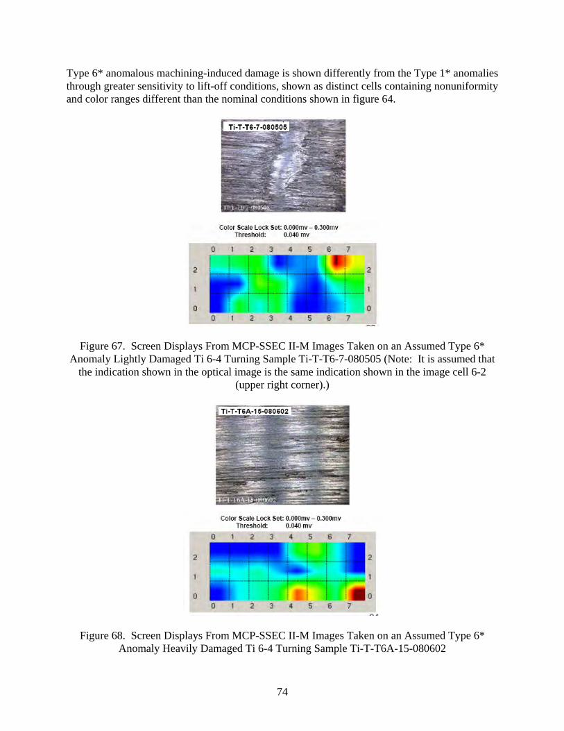
Type 6* anomalous machining-induced damage is shown differently from the Type 1* anomalies through greater sensitivity to lift-off conditions, shown as distinct cells containing nonuniformity and color ranges different than the nominal conditions shown in figure 64.
Figure 67. Screen Displays From MCP-SSEC II-M Images Taken on an Assumed Type 6* Anomaly Lightly Damaged Ti 6-4 Turning Sample Ti-T-T6-7-080505 (Note: It is assumed that
the indication shown in the optical image is the same indication shown in the image cell 6-2 (upper right corner).)
Figure 68. Screen Displays From MCP-SSEC II-M Images Taken on an Assumed Type 6* Anomaly Heavily Damaged Ti 6-4 Turning Sample Ti-T-T6A-15-080602
74

Test results for all Ti 6-4 turning samples examined are presented in figure 69. In this figure, the height of the bar graph represents the maximum signal amplitude obtained throughout the MCP image from at least one eddy-current coil. The display of maximum amplitude by itself is shown to correlate fairly well to the assumed severity of the turning samples for both Type 1* and Type 6* anomalies. Other image correlations could be used; however, for simplicity, only the maximum amplitude is shown here.
Figure 69. Maximum Amplitude Response Obtained in Ti 6-4 Turning Samples Containing Assumed Machining-Induced Damage From Light to Heavy Severity for Both Type 1* and Type
6* Anomalies Similar results were obtained in In 718 Type 1* anomalies and are presented in figure 70. Type 6* anomalies were not available for testing.
Figure 70. Maximum Amplitude Response Obtained in In 718 Turning Samples Containing Assumed Machining-Induced Damage From Light to Heavy Severity for Type 1* Anomalies
75

Given the dramatic eddy-current measurements indicated for both Ti 6-4 and Type 1* and Type 6* anomalies, there is a legitimate ability to differentiate between damaged and undamaged material conditions in flat-plate sample geometries. In addition, for Type 1* anomalies, the MCP technique has shown the ability to provide reasonable levels of measurement capability to discern an assumed range of severity from light to heavy material damage. 3.3.5.2 Broaching Sample Summary.
The Ti 6-4 and In 718 broaching samples were not investigated with the MCP method due to the geometrical limitations of the system and the test samples. Specially designed MCP probes would have had to have been fabricated, which was not possible, given the resources available to demonstrate feasibility of the technique. 3.3.5.3 Hole-Drilling Sample Summary.
The Ti 6-4 and In 718 hole-drilling samples were not investigated with the MCP method due to the geometrical limitations of the system and the test samples. Specially designed MCP probes would have had to have been fabricated, which was not possible using the resources available to demonstrate feasibility of the technique. 3.3.5.4 Conclusions and Recommendations.
Table 12 outlines the conclusions of each sample set.
Table 12. The MCP Conclusions for Each Sample Set
Turning
Ti 6-4 MCP shows the ability to differentiate between the pristine samples and the samples with induced anomalies over a measured surface range.
In 718 MCP shows the ability to differentiate between the pristine samples and the samples with induced anomalies over measured surfaces. Measurement is limited to absolute eddy-current conductivity measurement changes.
Broaching
Ti 6-4 Not tested due to geometric and system constraints.
In 718 Not tested due to geometric and system constraints.
Hole-Drilling
Ti 6-4 Not tested due to geometric and system constraints.
In 718 Not tested due to geometric and system constraints. 3.3.6 Thermoelectric AMR.
A thermoelectric data acquisition system developed at GE Nondestructive Technologies laboratory has been used for data acquisition from FAA-ETC samples. The thermoelectric technique is based on the Seebeck effect [31-39]. Two air guns equipped with nozzles that have
76

a linear array of holes are used to generate a temperature gradient in a sample. Self-referencing thermoelectric measurement is conducted in a noncontact way by sensing the weak magnetic field due to the thermoelectric current around various types of imperfections and material variations. The details of this method are provided in appendix J. 3.3.6.1 Turning Sample Summary.
To estimate the severity of the sample damage, the spread of the envelope was used as an informative parameter. Linear profiles were smoothed with a low-pass filter (figure 71) and the spread of the smoothed line in the direction of the signal trend was defined. Figure 72 shows how this informative parameter loosely corresponds with the intensity of machining abuse. This chart shows a higher level of deformation correlating to higher thermoelectric current magnetic field variations obtained with a linear scan.
No residual stress or HAZ in these specimen
Very likely – some sort of residual stress or HAZ in these specimen
Figure 71. Thermoelectric Current Magnetic Field Measurement Data (BZ fields were measured and is shown in figure J-2 in appendix J. Two samples in the middle column and three samples
at the right clearly indicate presence of stressed/HAZ-damaged regions.)
C-Ti-T-P-5-101607
-40
-20
0
20
40
60
80
100
120
140
0 0.2 0.4 0.6 0.8 1 1.2 1.4 1.6 1.8 2
Scan (in)
B (
nT
)
C-Ti-T-P-5-101607
-40
-20
0
20
40
60
80
100
120
140
0 0.2 0.4 0.6 0.8 1 1.2 1.4 1.6 1.8 2
Scan (in)
B (
nT
)
Ti-T-P-13-060208
-40
-20
0
20
40
60
80
0 0.2 0.4 0.6 0.8 1 1.2 1.4 1.6 1.8 2
Scan (in)
B (
nT
)
Ti-T-P-13-060208
-40
-20
0
20
40
60
80
0 0.2 0.4 0.6 0.8 1 1.2 1.4 1.6 1.8 2
Scan (in)
B (
nT
)
C-Ti-T-T1D-5-101607
0
20
40
60
80
100
120
140
0 0.2 0.4 0.6 0.8 1 1.2 1.4 1.6 1.8 2
Scan (in)
B (
nT
)
C-Ti-T-T1D-5-101607
0
20
40
60
80
100
120
140
0 0.2 0.4 0.6 0.8 1 1.2 1.4 1.6 1.8 2
Scan (in)
B (
nT
)
Ti-T-T1-5-080107
0
10
20
30
40
50
60
70
80
90
100
0 0.2 0.4 0.6 0.8 1 1.2 1.4 1.6 1.8 2
Scan (in)
B (
nT
)
Ti-T-T1-5-080107
0
10
20
30
40
50
60
70
80
90
100
0 0.2 0.4 0.6 0.8 1 1.2 1.4 1.6 1.8 2
Scan (in)
B (
nT
)
Ti-T-T1A-13-080606-MED
0
10
20
30
40
50
60
70
80
90
0 0.2 0.4 0.6 0.8 1 1.2 1.4 1.6 1.8 2
Scan (in)
B (
nT
)
This has clear visual indication on the surface
Ti-T-T1A-13-080606-MED
0
10
20
30
40
50
60
70
80
90
0 0.2 0.4 0.6 0.8 1 1.2 1.4 1.6 1.8 2
Scan (in)
B (
nT
)
Ti-T-T1A-13-080606-MED
0
10
20
30
40
50
60
70
80
90
0 0.2 0.4 0.6 0.8 1 1.2 1.4 1.6 1.8 2
Scan (in)
B (
nT
)
This has clear visual indication on the surface
Ti-T-T6A-13-080602
0
10
20
30
40
50
60
70
80
90
0 0.2 0.4 0.6 0.8 1 1.2 1.4 1.6 1.8 2
Scan (in)
B (
nT
)
Ti-T-T6A-13-080602
0
10
20
30
40
50
60
70
80
90
0 0.2 0.4 0.6 0.8 1 1.2 1.4 1.6 1.8 2
Scan (in)
B (
nT
)
Ti-T-T6-5-080508
0
20
40
60
80
100
120
140
0 0.2 0.4 0.6 0.8 1 1.2 1.4 1.6 1.8 2
Scan (in)
B (
nT
)
Ti-T-T6-5-080508
0
20
40
60
80
100
120
140
0 0.2 0.4 0.6 0.8 1 1.2 1.4 1.6 1.8 2
Scan (in)
B (
nT
)
Not sure – may be some sort of residual stress or HAZ in these specimen?
77

Values TEM
1.2
Ti Nominal
1 N
orm
aliz
ed T
EM
Mag
nit
ud
e
0.8
0.6 Values TEM
0.4
0.2
0 Ti Light Ti Medium Ti High
Figure 72. Summary of Thermoelectric Current Magnetic Field Measurements on
Ti Turning Sample Due to the unavailability of In 718 turning samples at the time of testing, the AMR method was not investigated on In 718 flat anomalous materials; however, it is anticipated that results similar to the Ti 6-4 turning sample results using the AMR method would be obtained. 3.3.6.2 Broaching Sample Summary.
The Ti 6-4 and In 718 broaching samples were not investigated with the AMR method due to the geometrical limitations of the system and the test samples. Specially designed AMR probes would have had to have been fabricated, which was not possible using the resources available to demonstrate feasibility of the technique. 3.3.6.3 Hole-Drilling Sample Summary.
The Ti 6-4 and In 718 hole-drilling samples were not investigated with the AMR method due to the geometrical limitations of the system and the test samples. 3.3.6.4 Conclusions and Recommendations.
Table 13 outlines the conclusions of each sample set.
78

Table 13. The TEM Conclusions for Each Sample Set
Turning
Ti 6-4 Relative gross differences in magnetic field strength B(z) were observed between the pristine and the anomalous Type 1* turning samples. Localized measurements of anomalous conditions on Type 1* and Type 6* turning samples was not clearly evident.
In 718 Turning In 718 samples were not available for tests.
Broaching
Ti 6-4 Not tested due to geometric and system constraints.
In 718 Not tested due to geometric and system constraints.
Hole-Drilling
Ti 6-4 Not tested due to geometric and system constraints.
In 718 Not tested due to geometric and system constraints. 3.3.7 Multifrequency Eddy-Current Methods Using Swept Frequency.
The swept high-frequency eddy-current (SHFEC) methodology is based on the measurements of lift-off normalized vertical component eddy-current signals. The technique was initially developed to characterize surface conditions of aerospace engine materials using proprietary detection coils and laboratory instrumentation operational up to tens of MHz. The technique is primarily aimed at detecting Type 1 anomalies in In 718 and Ti 6-4, such as amorphous layer or bent grains, which may be present even without obvious geometric distortion of the machined surface. The details are provided in appendix K. 3.3.7.1 Turning Sample Summary.
As an example, the lift-off normalized vertical component eddy-current signals measured from a pristine In 718 coupon and a Type 1* Ti 6-4 coupon are shown in figure 73 for comparison. As described in appendix K, the vertical component signal is a measure of the difference in the near surface conductivity profiles between the test and reference surfaces. Therefore, the vertical component signals are zero if the test and reference surfaces have the same conductivity profiles. For the pristine sample In-T-P-15-080725, the vertical component signals were essentially zero within the experimental errors, suggesting that the two sides of the coupon had nominally identical conductivity profiles. For the Type 1* sample Ti-T-T1-1-080107, the vertical component signals were negative throughout the frequency range, indicating that the test surface (the bottom side) had a lower conductivity than the reference surface (the top side). This, in turn, implies that the bottom side was the machine-damaged side, under the assumption that a machine-damaged surface has a lower conductivity than a pristine/undamaged surface. Results of surface wave ultrasonic (UT) and high-energy XRD studies conducted at ISU consistently identify the bottom side as the damaged side for this turning coupon.
79

(a) (b)
Figure 73. The Lift-Off Normalized Vertical Component Eddy-Current Signals vs Frequency for (a) In-T-P-15-080725 (Pristine) and (b) Ti-T-T1-1-080107 (Damaged)
The interpretation that negative vertical component signals correspond to lower conductivity of the test surface than the reference surface has been established in a validation study using two layered samples. The first layered sample consisted of a 103-m-thick In 718 foil placed on a 0.5-inch-thick In 718 block. The second sample was comprised of 133-m-thick nickel chromium (NiCr) foil placed on the 0.5-inch-thick In 718 block. The In 718 block has a conductivity of 1.38% International Annealed Copper Standard (IACS). The conductivities of the In 718 and NiCr foils were measured by a four-point, direct-current potential drop to be 1.34% and 1.526% IACS, respectively. The layered samples mimic the situation where the surface layer had a slightly lower (by 3% for the In 718 foil on the In 718 block), or slightly higher conductivity (by 11% for the NiCr foil on the In 718 block) than the bulk. As shown in figures 74 and 75, the measured lift-off normalized vertical component signals are negative for the In 718-on-In 718 sample, but are positive for the NiCr-on-In 718 sample throughout the frequency range. The measurement results were confirmed by performing model-based calculations [ISU_SFR1] using the known conductivity values of the foils and the In 718 block. The modeled results agreed with the experimental data from figures 74 and 75.
80

(a) (b)
Figure 74. (a) Diagram of the Layered Sample Used in the Validation Study and (b) Measured Lift-Off Normalized Vertical Component Eddy-Current Signals (blue squares) as a Function of Frequency (The layered sample comprises a 103-m-thick In 718 foil ( = 1.34% IACS) placed on an In 718 block ( = 1.38% IACS). The modeled vertical component signals (pink diamonds
and solid line) were found to agree with the experimental data.)
(a) (b)
Figure 75. (a) Diagram of the Layered Sample Used in the Validation Study and (b) Measured Lift-Off Normalized Vertical Component Eddy-Current Signals (blue squares) as a Function of Frequency (The layered sample comprises 133-m-thick NiCr foil ( = 1.56% IACS) placed on an In 718 block ( = 1.38% IACS). The modeled vertical component signals (pink diamonds
and solid lines) were found to agree with the experimental data.) The details of the SHFEC measurements and the results obtained from the round-robin turning samples are summarized in table 14. The table lists which side of each sample was used as the reference surface to obtain the reference and lift-off signals and which side was treated as the test surface. From the SHFEC data, the conductivity of the test surface relative to the reference surface was inferred based on the results of the validation study (i.e., negative vertical component signals indicates a lower conductivity of the test surface than that of the reference surface).
81

Table 14. The Reference and Test Surfaces of the Round-Robin Samples Used in the SHFEC Measurements
Option Sample Identification
Number Reference Surface Condition
Test Surface Condition
Sign of Vertical
Component Eddy-Current
Signal Interpretation1
A Ti-T-P-1-0611XX_ post-anneal
Bottom Pristine Top Pristine Null signal T = B
C C-Ti-T-P-1-101607 Bottom Pristine Top Pristine Null signal T = B
A In-T-P-1-0207XX Bottom Pristine Top Pristine -ve T <B
C In-T-P-1-080725 Bottom Pristine Top Pristine -ve T <B
C Ti-T-T1-1-080107 Top “7” Pristine Bottom Damaged -ve T >B
C Ti-T-T1-7-080107 Bottom “7” Pristine Top Damaged +ve T >B
C Ti-T-T1A-9-080606-M Bottom Pristine Top Damaged -ve T <B
C Ti-T-T1A-15-080606-M Bottom Pristine Top Damaged -ve T <B
C C-Ti-T-T1D-1-101607 Top Pristine Bottom Damaged -ve T >B
C Ti-T-T1-2-080107b Top Pristine Bottom Damaged -ve T >B
C Ti-T-T6-1-080508 Top Pristine Bottom Damaged -ve up to 50 MHz
T >B
C Ti-T-T6-2-080508 Bottom Pristine Top Damaged -ve T <B
C Ti-T-T6-7-080508 Bottom Pristine Top Damaged -ve up to 58.5 MHz
T <B
C Ti-T-T6A-15-080602 Bottom Pristine Top Damaged -ve from 6 to 38 MHz
T <B
C In-T-T1A-1-080722-S Top Pristine Bottom Damaged -ve T >B
C In-T-T1A-7-080722-S Top Pristine Bottom Damaged -ve T >B
C In-T-T1A-1-081130-M Bottom Pristine Top Damaged -ve T <B
C In-T-T1A-7-081130-M Bottom Pristine Top Damaged -ve T <B
C In-T-T6A-7-080916 Top Pristine Bottom Damaged -ve up to 57.5 MHz
T >B
C In-T-T6A-8-080916 Top Pristine Bottom Damaged -ve T >B
C In-T-T6A-14-081006 Top Pristine Bottom Damaged -ve T >B 1Note: T >B means top (T) surface is more conducting than the bottom (B) surface. T <B means top (T) surface is less conducting than the bottom (B) surface. T = B means top (T) surface is equal to the bottom (B) surface -ve = vertical component eddy current Table 14 also shows the signs of the lift-off normalized vertical component signals. For each sample, the relative conductivities of the top and bottom surfaces were compared based on the interpretation of the SHFEC data.
82
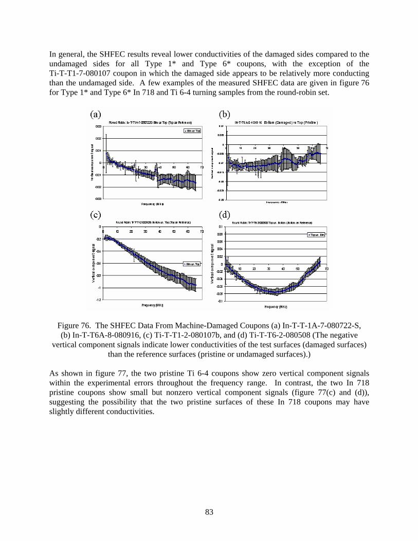
In general, the SHFEC results reveal lower conductivities of the damaged sides compared to the undamaged sides for all Type 1* and Type 6* coupons, with the exception of the Ti-T-T1-7-080107 coupon in which the damaged side appears to be relatively more conducting than the undamaged side. A few examples of the measured SHFEC data are given in figure 76 for Type 1* and Type 6* In 718 and Ti 6-4 turning samples from the round-robin set.
Figure 76. The SHFEC Data From Machine-Damaged Coupons (a) In-T-T-1A-7-080722-S, (b) In-T-T6A-8-080916, (c) Ti-T-T1-2-080107b, and (d) Ti-T-T6-2-080508 (The negative
vertical component signals indicate lower conductivities of the test surfaces (damaged surfaces) than the reference surfaces (pristine or undamaged surfaces).)
As shown in figure 77, the two pristine Ti 6-4 coupons show zero vertical component signals within the experimental errors throughout the frequency range. In contrast, the two In 718 pristine coupons show small but nonzero vertical component signals (figure 77(c) and (d)), suggesting the possibility that the two pristine surfaces of these In 718 coupons may have slightly different conductivities.
83

Figure 77. The SHFEC Data From Pristine Coupons (a) Ti-T-P-0611, (b) C-Ti-T-P-1-101607, (c) In-T-P-1-0207xx, and (d) In-T-P-1-080725 (The nonzero vertical component signals of the
pristine In 718 coupons suggest that the possibility that the two sides of those coupons may have slightly different conductivities. The two curves in (c) are results of two repeated measurements at different times on the same coupons, indicating the repeatability of the measurement results.)
3.3.7.2 Broaching Sample Summary.
The broaching samples were not studied using the SHFEC method due to the geometrical constraints of the samples and the rigid printed circuit board (PCB) coils used, which are only applicable to flat surfaces with circular areas of at least 12 mm in diameter. To demonstrate the technique’s feasibility on the broaching sample, specially designed detection coils with a smaller foot print would have to be fabricated on flexible substrates. This was not possible within the time available. 3.3.7.3 Hole-Drilling Sample Summary.
The hole-drilling samples were not studied using the SHFEC method due to the geometrical constraints of the test samples and the detection PCB coils. To demonstrate the technique’s feasibility, specially designed detection coils would have to be fabricated, which was not possible within the time available.
84

3.3.7.4 Conclusions and Recommendations.
Table 15 summarizes the conclusions of the SHFEC study on each sample set.
Table 15. Conclusions of the SHFEC Study for Each Sample Set
Turning
Ti 6-4 It is possible to detect anomalous machining-induced damages manifested as a surface layer with a lower conductivity than the pristine/undamaged counterpart. Unconventional instrumentation is needed for high-frequency operations. Rigid PCB coils are not applicable to coupons with a large surface curvature. For components with nonplanar geometries, further study is needed to evaluate the feasibility of the technique using PCB coils on flexible substrates.
In 718 It is possible to detect anomalous machining-induced damages manifested as a surface layer with a lower conductivity than the pristine/undamaged counterpart. Unconventional instrumentation is needed for high-frequency operations. Rigid PCB coils are not applicable to coupons with a large surface curvature. For components with nonplanar geometries, further study is needed to evaluate the feasibility of the technique using PCB coils on flexible substrates.
Broaching
Ti 6-4 Not tested due to geometric and system constraints.
In 718 Not tested due to geometric and system constraints.
Hole-Drilling
Ti 6-4 Not tested due to geometric and system constraints.
In 718 Not tested due to geometric and system constraints. 3.3.8 Multifrequency Eddy-Current Methods, Eddy-Current Phase Analysis.
It should be noted that multifrequency phase analysis results vary with how the processing parameters are derived. Best results can be obtained if the anomaly type is known and parameters are fine-tuned with training samples that have known anomalies. The results in figures 76 and 77 were obtained with the intention to suppress the background noise. Details for this method [40-45] are in appendix L. 3.3.8.1 Turning Sample Summary.
For the Ti 6-4 turning samples provided, it was found, experimentally, that a combination of 1 and 2.5 MHz provides the highest eddy-current image quality of the turning sample. Examples of images obtained separately with 1 and 2.5 MHz, as well as with their linear combination, are presented in figures 78 and 79. In these examples, the background noise was completely eliminated in the multifrequency images. This helps to define small area indications, which are present on the single-frequency images, but buried under a stronger background feature pattern. The white speckles in the phase image seem to be correlated with microscopic examination of
85

debris (possibly from tool tip breakage) left on the surface. Suspect localized indications are identified with red circles; whereas general surface roughness is identified by predominant wave patterns. Due to the unavailability of In 718 turning samples at the time of the tests, the MFPA method was not investigated on In 718 flat anomalous materials; however, it was anticipated that results similar to that obtained on Ti 6-4 turning samples using the MFPA method would be obtained.
Multifrequency Eddy Current (2.5 and 1 MHz)
Single- Frequency Eddy Current
2.5 MHz 1 MHz
MFPA Details
Figure 78. Multifrequency Analysis of a Turning Sample Illustrating Localized Indications
2.5 MHz
MFPA
Ti-T- T6A-50080107
Figure 79. Multifrequency Analysis of a Turning Sample Illustrating Localized Indications Within a Rough Surface
86

3.3.8.2 Broaching Sample Summary.
The Ti 6-4 and In 718 broaching samples were not investigated with the MFPA method due to the geometrical limitations of the system and the test samples. Specially designed MFPA probes would have had to have been fabricated, which was not possible using the resources available to demonstrate feasibility of the technique. 3.3.8.3 Hole-Drilling Sample Summary.
Similar results were obtained using hole-drilling samples scanned using the Nortec R600 probe and a computer-controlled turntable with a sample holder. These results are shown in figures 80 and 81. The red circles indicate areas of suspect, localized indications.
Suppressing picked feature
6 MHz and 500
6 MHz
UNI : X ( x1deg) by Y( x 0.001”) by Z (mV / deg)
Ti-D-P-11 FAA hole_SGE627_Z5milR0.5deg
Figure 80. Example of Multifrequency Analysis of a Pristine Hole-Drilling Sample Illustrating Localized Indications Within a Rough Surface
IN-D-6A-S5 hole_SGE627_Z10milR0.5deg
6 MHz
6 MHz and 500 kHz
Figure 81. Multifrequency Analysis of a Type 6* Smeared Hole-Drilling Sample Illustrating
Localized Indications Within a Rough Surface
87

After suppressing some featured noise during the test, figures 82 and 83 show very interesting indications of certain anomalies, which need to be verified. The In-D-6A-S5 and In-D-6A-M5 did not have the “patch” pattern shown on other samples. For the two half-hole samples in figure 83, the Ti-D-P-24-A3 sample looks rougher than the In-D-29-A3 sample.
M5 hole_SGE627_Z10milR0.5deg-6A--DIn
6 MHz and 500
6
Figure 82. The MFPA Results of Hole-Drilling Samples
6 MHz and 500 kHz
6 MHz
Ti - D - P - 24 - A3&In - D-P-29TiIn
-A3 hole_SGE627_Z10milR0.5deg
Figure 83. The MFPA Results on a Hole Consisting of Two Half-Hole Samples The above preliminary results with MFPA are subjective. Without knowing what kinds of anomalies are present, MFPA may not work well. 3.3.8.4 Conclusions and Recommendations.
Table 16 outlines the conclusions of each sample set using swept-frequency eddy-current analysis methods.
88

Table 16. Conclusions for the Swept-Frequency Eddy-Current Method for Each Sample Set
Turning Ti 6-4 It is possible to differentiate between pristine and anomalous machining test
samples using conventional eddy-current analysis. Localized Type 1* and Type 6* anomalous indications can be separated using multifrequency eddy-current phase analysis. Evidence of trending with anomaly severity was observed.
In 718 It is possible to differentiate between pristine and anomalous machining test samples using conventional eddy-current analysis. Localized Type 1* and Type 6* anomalous indications can be separated using multifrequency eddy-current phase analysis. Evidence of trending with anomaly severity was observed.
Broaching Ti 6-4 Not tested due to geometric and system constraints.
In 718 Not tested due to geometric and system constraints.
Hole-Drilling Ti 6-4 It is somewhat possible to differentiate between the pristine and anomaly
Type 6*. In 718 As with turning samples above, it is somewhat possible to differentiate
between the pristine and anomaly Type 6*. 3.3.9 Conventional Eddy Current.
Conventional, single-frequency eddy-current inspection has common application to metal sorting, coating thickness measurement, surface and near-surface flaw detection, and displacement measurement. In all cases, an alteration of the eddy-current probe’s electromagnetic field occurs by some change in the electromagnetic characteristics of the part under test (electrical conductivity, magnetic permeability, and anomaly) and/or physical attributes changing (geometry and orientation). The eddy-current probe is highly sensitive to displacement, which makes it well suited as a displacement measurement device, which also affects the other inspection applications in a negative way. The displacement of the probe from the surface of a part is often referred to as lift-off. Lift-off needs to be controlled to use the eddy-current probe to perform measurements other than displacement. For AMD detection, it follows that the eddy-current inspection could be exposed to deformation of material at the surface (tearing and smearing) and distortion of the microstructure at and near the surface (deformation of grains and electromagnetic property changes due to temperature/pressure). Eddy current is very sensitive to the tearing and smearing conditions that result in a lift-off response, while the microstructural issues behave more like bulk conductivity changes.
89

For bulk-type properties, an absolute probe is a more suitable choice than a differential probe. The differential probe is better suited for discrete anomalies, like cracks, due to its bulk property-canceling effect. Another aspect of eddy-current inspections is the use of filters to help reduce noise effects during the inspection. The noise can be from many sources such as geometry, electrical, and surface roughness. Frequently, a high-pass filter is used to remove or reduce low-frequency effects, such as slight variations in lift-off or local geometric features, which are repeated when scanning an engine rotor. High-pass filters are typically used to remove electrical noise. For the AMD application, the high-pass filter is not used to allow for the detection of bulk property changes. Ultimately, the filter selection should not remove much of the energy associated with the target anomaly and so the filter settings should be selected with some knowledge of the signal bandwidths. The details are provided in appendix M. 3.3.9.1 Turning Sample Summary.
To detect AMD, single-frequency eddy-current data was acquired from the AMD samples and analyzed. The objective of the analysis was to identify a parameter or parameters that provide a method for identifying the presence of AMD. An absolute solenoid and a differential electric current perturbation (ECP) were used to acquire data. An example of the data for Type 1* and Type 6* category samples are provided in figures 84 and 85. Figures 86 and 87 show the photomicrographs for metallography, which were performed on a small piece taken from one end of several samples.
Figure 84. The ETC 4 Flat-Plate Sample Scanned With PW Conventional Eddy Current, C-Ti-T-T1D-4-101607
90

Figure 85. The ETC 4 Flat-Plate Sample Scanned With PW Conventional Eddy Current, Ti-T-T6-4-080508
A = View at 2 magnifications for the direction parallel to the machining direction B = View at 2 magnifications for the direction perpendicular to the machining direction
Figure 86. Photomicrographs of C-Ti-T1D-4-101607
91

A = View at 2 magnifications for the direction parallel to the machining direction B = View at 2 magnifications for the direction perpendicular to the machining direction
Figure 87. Photomicrographs of Ti-T6-4-080508
Compiling the data for two parameters (maximum peak amplitude and standard deviation) showed some trends. Figure 88 shows the maximum peak amplitude value plotted for the groups sorted by material and intended anomaly type. There appears to be a trend with Type 1* where the titanium samples had very low values and the nickel samples had medium to high values. The four Type 1* nickel samples are identified in the plot and the labels that end in “-M” were intended to have medium levels of damage and the other two were intended to have shallow damage. The order of the response does not correlate with the order of intended anomaly level. There were no nickel samples produced with heavy Type 1* damage. For Type 6*, the titanium had high values and the nickel medium values. There was not a means of controlling the level of damage in the Type 6* samples.
92

0
2
4
6
8
10
12
14
16
18
0 1 2 3 4 5 6 7
Specimen Types
Am
plit
ud
e (v
olt
s p
-p)
P-Ti
P-Ni
T1*-Ti
T1*-Ni
T6*-Ti
T6*-Ni
Figure 88. The 6-MHz Maximum Peak-to-Peak Data for all Samples
3.3.9.2 Broaching Sample Summary.
The Ti 6-4 and In 718 broaching samples were not investigated with the single-frequency eddy-current method. 3.3.9.3 Hole-Drilling Sample Summary.
The Ti 6-4 and In 718 hole-drilling samples were not investigated with the single-frequency eddy-current method. 3.3.9.4 Conclusions and Recommendations.
Table 17 outlines the conclusions of each sample set.
93

Table 17. Conclusions for the Single-Frequency Eddy-Current Method for Each Sample Set
Turning
Ti 6-4 The Type 1* samples showed very low values in peak amplitude parameter. All Type 6* samples showed high values in peak amplitude parameter.
In 718 The Type 1* samples showed medium to high values in the peak amplitude parameter. The intended damage levels in these samples did not correspond with the order of the amplitude parameter. All Type 6* samples showed medium-level amplitudes compared to the Ti 6-4.
Broaching
Ti 6-4 Not tested due to geometric and system constraints.
In 718 Not tested due to geometric and system constraints.
Hole-Drilling
Ti 6-4 Not tested.
In 718 Not tested. 3.3.10 Single-Frequency Eddy-Current Statistical Noise Analysis.
Single-frequency eddy-current scans were performed using commercial eddy-current probes and instruments to detect machining-induced surface anomalies, particularly Type 6* damages, in both turning and broaching In 718 and Ti 6-4 samples. The objectives were to evaluate the feasibility of detecting anomalous machine damages by the conventional eddy-current technique, to devise a procedure for analyzing C-scan data, and to identify measurement parameters that could be used to characterize surface damages. To these ends, the C-scan eddy-current images were compared with surface morphology images obtained by laser profilometry to examine the detectability of surface anomalies by eddy current. To aid the comparison between undamaged and damaged samples, the C-scan data were quantified in terms of their standard deviations that characterize the spatial variations of the eddy-current signals. The details of this method are provided in appendix N. 3.3.10.1 Turning Sample Summary.
An example of the eddy-current C-scan images obtained from a round-robin turning sample is shown in figure 89. The C-scan images of the damaged surface show distinctive dipole patterns at various locations, which spatially correlate with the surface anomalies (identified by the numbers) detected by laser profilometry as surface extrusions (figure 89(c)). In contrast, the undamaged surface shows a featureless C-scan image, indicating a more uniform eddy-current signal level on this surface in the absence of surface anomalies.
94

Figure 89. Eddy-Current C-Scan Image of the (a) Damaged Side, (b) Undamaged Side of the Round-Robin Sample In-T-T1a-7-081130-M, and (c) the Surface Morphology of the Damaged Side Imaged by Laser Profilometry (The images were plotted in the same color scale for direct
comparison. The rectangular box in (c) outlines the area covered by the eddy-current C-scan images.)
Machining-induced anomalies in the form of surface indents were also detected in other samples. As shown in figure 90, dipole patterns were observed in the eddy-current C-scan image of the damaged surface of an In 718 sample (In-T-T1-1-070112). These patterns are in good spatial correlation with the surface intrusions (figure 90(c)), which became prominent in the laser profilometer image after the machining marks had been suppressed by Fast Fourier Transform (FFT) filtering. Such dipole patterns were not observed on the C-scan image of the undamaged surface of the sample.
Figure 90. Eddy-Current C-Scan Image of the (a) Damaged Side, (b) Sample In-T-T1-1-070112, and (c) Surface Anomalies in the Surface Morphology Image After Suppressing the Machine
Marks by FFT Filtering (The numbered dipole patterns in the eddy-current C-scan image in (a) correspond to the surface anomalies identified in (c).)
95

The eddy-current C-scan images of the Ti 6-4 samples, in general, exhibit irregular patterns with significant contrast even without any detectable surface anomalies. An example is shown in figure 91(a), which shows the C-scan image of the undamaged side of an option C Ti 6-4 sample (C-Ti-T-T1D-1-101607). The image pattern was found repeatable by rescanning the surface under the same measurement conditions. The exact cause of the signal patterns is yet to be identified. One possibility is that the patterns could be caused by inhomogeneity in conductivity, which is known to exist in hexagonal (α phase) Ti 6-4 (figure 92). The length scale (over which the conductivity varies) could be larger than the grain size if clusters of grains exist with similar orientation. High-resolution acoustic microscopy images obtained from a round-robin Ti 6-4 sample revealed large-scale patterns (millimeter in size), which are suspected to correspond to a clustered grain structure. The C-scan image of the damaged side of the sample shows a relatively stronger contrast (figure 91(b)), indicating larger spatial variations in eddy-current signals attributed to the presence of surface anomalies.
Figure 91. Eddy-Current C-Scan Image of the (a) Undamaged and (b) Damaged Sides of the Ti 6-4 Sample C-Ti-T-T1D-1-101607, and (c) the Surface Morphology Image
Obtained by Laser Profilometry
96

Figure 92. Eddy-Current C-Scan Image of (a) the Damaged Side of the Ti 6-4 Sample Ti-T-T6A-9-080602, (b) the Dipole Patterns Corresponding to the Surface Anomalies, and (c)
the Surface Morphology Image (The arrows point to a deep cut on the coupon surface. The red circles in (b) and (c) highlight examples of surface intrusions, which were not detected in the
C-scan image because of the overwhelming signal caused by the machining marks.) In addition to the typical Type 6* damage, such as redeposited materials, other machining-induced surface damages also give rise to distinctive features in the C-scan images. An example is given in figure 93(a), which shows a band structure in the C-scan image that closely follows the deep machining marks found on the sample surface. In this case, the dipole patterns corresponding to the surface extrusions found near the band become obscured (e.g., anomaly number 4 in figure 93(c)) or overshadowed by the anomaly signal due to the machining marks. For damaged surfaces with a high density of surface anomalies (e.g., figure 93), it becomes difficult and impractical to identify individual anomalies (e.g., redeposited debris) from the C-scan image. In fact, it is more desirable to identify measurement parameters that can be used to characterize the C-scan data quantitatively for comparison among the samples. To this end, statistical analysis was applied to the C-scan images. Specifically, the standard deviations of the C-scan data were calculated as
N
VVV
PositionAll
i
ECMean
ECi
ECStd
2
97

where N is the total number of scan positions, ViEC is the signal voltage at the scan position i, and
VmeanEC is the mean signal level averaged over the entire scan area. This parameter was chosen
to characterize C-scan data, based on the consideration that for a pristine surface, the eddy-current signal is the same everywhere and therefore, VStd
EC would be zero. In contrast, for a machining-induced damaged surface, the eddy-current signals are expected to vary in the proximity of surface damages, thus giving rise to a nonzero standard deviation VStd
EC.
Figure 93. (a) An Eddy-Current C-Scan Image of the Damaged Side of the Ti 6-4 Sample Ti-T-T6A-22-081201 Showing Strong Eddy-Current Signal Variations in Regions Where a High
Density of Minuscule Anomalies Exists, as Shown in (b) (The numbers highlight some of the surface anomalies identified in both the C-scan image and the photograph.)
The standard deviations of the C-scan data are summarized in figures 94 and 95 for the round-robin In 718 and Ti 6-4 samples, respectively. It is evident that the damaged surfaces exhibit larger standard deviations in eddy-current signals than the undamaged surfaces. The differences in VStd
EC between the pristine and damaged surfaces are larger for In 718 than for Ti 6-4. This is attributed to the fact that the pristine Ti 6-4 samples show larger spatial variations in eddy-current signals (i.e., higher eddy-current noise level) than the pristine In 718 samples, possibly due to the presence of conductivity anisotropy in the Ti 6-4 samples.
98

Inconel 718 coupons
0.00
0.05
0.10
0.15
0.20
0.25
0.30
NI-
T-P
-1-0
20
7X
X
IN-T
-P-1
-08
07
25
In-T
-T1
A-1
-08
07
22
-S
In-T
-T1
A-7
-08
07
22
-S
In-T
-T1
A-1
-08
11
30
-M
In-T
-T1
A-7
-08
11
30
-M
IN-T
-T6
A-7
-08
09
16
IN-T
-T6
A-8
-08
09
16
IN-T
-T6
A-1
4-0
81
00
6
Sta
nd
ard
dev
iati
on
s o
f E
C c
-sca
n im
ages
Pristine/Undamaged Surface
Damaged Surface
Pristine Type 1 / Type 6
Figure 94. The Standard Deviations of the Eddy-Current C-Scan Data for the Round-Robin In 718 Samples
Ti 6-4 coupons
0.00
0.10
0.20
0.30
0.40
0.50
0.60
0.70
0.80
TI-
T-P
-1-0
61
1X
X_
po
st-
an
ne
al
C-T
i-T
-P-1
-10
16
07
Ti-
T-T
1-1
-08
01
07
Ti-
T-T
1-7
-08
01
07
Ti-
T-T
1A
-9-0
80
60
6-M
ED
Ti-
T-T
1A
-15
-08
06
06
-ME
D
C-T
i-T
-T1
D-1
-10
16
07
Ti-
T-T
1-2
-08
01
07
b
Ti-
T-T
6-1
-08
05
08
Ti-
T-T
6-2
-08
05
08
Ti-
T-T
6-7
-08
05
08
Ti-
T-T
6A
-15
-08
06
02
Sta
nd
ard
dev
iati
on
s o
f E
C c
-sca
n im
ages
Pristine/Undamaged Surface
Damaged Surface
Pristine Type 1 / Type 6
Figure 95. The Standard Deviations of the Eddy-Current C-Scan Data for the Round-Robin Ti 6-4 Samples (Compared to the In 718 samples, the Ti 6-4 samples, in general, show smaller
differences in the standard deviations between the damaged and undamaged surfaces.)
99
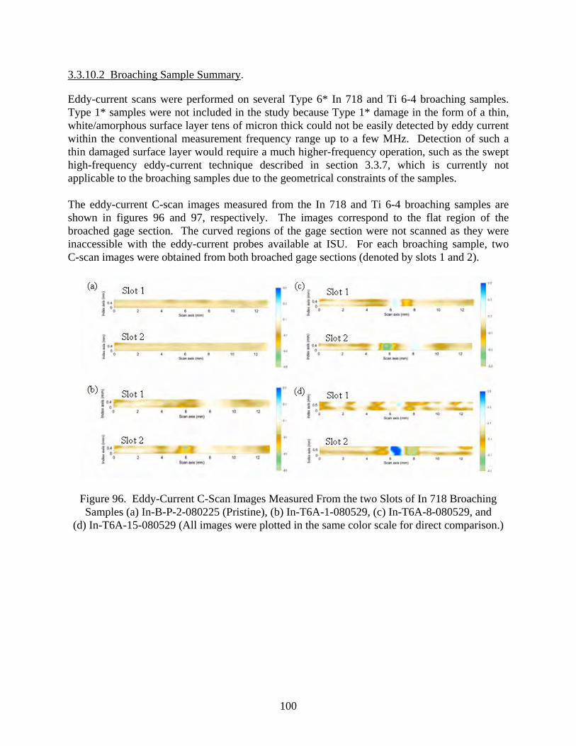
3.3.10.2 Broaching Sample Summary.
Eddy-current scans were performed on several Type 6* In 718 and Ti 6-4 broaching samples. Type 1* samples were not included in the study because Type 1* damage in the form of a thin, white/amorphous surface layer tens of micron thick could not be easily detected by eddy current within the conventional measurement frequency range up to a few MHz. Detection of such a thin damaged surface layer would require a much higher-frequency operation, such as the swept high-frequency eddy-current technique described in section 3.3.7, which is currently not applicable to the broaching samples due to the geometrical constraints of the samples. The eddy-current C-scan images measured from the In 718 and Ti 6-4 broaching samples are shown in figures 96 and 97, respectively. The images correspond to the flat region of the broached gage section. The curved regions of the gage section were not scanned as they were inaccessible with the eddy-current probes available at ISU. For each broaching sample, two C-scan images were obtained from both broached gage sections (denoted by slots 1 and 2).
Figure 96. Eddy-Current C-Scan Images Measured From the two Slots of In 718 Broaching Samples (a) In-B-P-2-080225 (Pristine), (b) In-T6A-1-080529, (c) In-T6A-8-080529, and
(d) In-T6A-15-080529 (All images were plotted in the same color scale for direct comparison.)
100

Figure 97. Eddy-Current C-Scan Images Measured From the two Slots of Ti 6-4 Broaching Samples (a) Ti-B-P-2-080121 (Pristine), (b) Ti-B-T6A-3-080613, (c) Ti-B-T6A-1-080613, and
(d) Ti-B-T6A-8-080613 (All images were plotted in the same color scale for direct comparison.) In general, the C-scan images of the Type 6* samples show a larger spatial variation in the signal level than those of the pristine counterparts. In most cases, the eddy-current signals exhibit the largest change near the midpoint of the gage section. The spatial variations of the eddy-current signals are quantified by calculating the standard deviations of the signals over the scanned area. The results are summarized in figure 98. It is evident that the C-scan data from the Type 6* sample show significantly larger standard deviations than the pristine samples beyond the experimental error, indicating that it is possible to separate Type 6* broaching samples from the pristine samples by statistical analysis of the C-scan data.
Figure 98. The Standard Deviations of the Eddy-Current C-Scan Data for (a) In 718 and (b) Ti 6-4 Broaching Samples (The error bars were determined as the difference in the standard
deviations obtained by repeating eddy-current C-scans on the samples.)
101

3.3.10.3 Hole-Drilling Sample Summary.
The hole-drilling samples were not studied due to the geometrical constraints of the test samples. 3.3.10.4 Conclusions and Recommendations.
Table 18 summarizes the conclusions of the single-frequency eddy-current C-scan study on each sample set.
Table 18. Conclusions of Single-Frequency Eddy-Current C-Scan Study for Each Sample Set
Turning
Ti 6-4 Eddy-current C-scan data from machine-damaged surfaces show spatial variations in signal level with larger standard deviations than those from the undamaged surfaces.
In 718 It is possible to separate damaged surfaces from pristine/undamaged surfaces according to standard deviations of eddy-current C-scan data. In some cases, the C-scan images exhibit characteristic dipole patterns in good spatial correlation with the localized surface anomalies.
Broaching
Ti 6-4 It is possible to separate Type 6* damaged samples from pristine samples in terms of the standard deviations of the C-scan data.
In 718 It is possible to separate Type 6* damaged samples from pristine samples in terms of the standard deviations of the C-scan data.
Hole-Drilling
Ti 6-4 Not tested due to geometric and system constraints.
In 718 Not tested due to geometric and system constraints. 3.3.11 Single-Frequency Eddy-Current Study of Ti 6-4 and In 718 Samples.
Eddy-current inspection has been used extensively to detect cracks and other surface anomalies produced during manufacturing and in service turbine engine components. Eddy current has also been used for inspecting surface and subsurface anomalies in parts and monitoring processes as well. In this study performed at HW, single-frequency eddy-current scanning was evaluated to detect abusive machining in Ti 6-4 and In 718 turning samples. The approach used in this work included studying the relationship between eddy-current response and manufacturing-related anomalies, including surface and subsurface. This was based on the statistical analysis of data related to the small changes in eddy-current response (higher than normal system measurement error and different than conventional noise) due to anomalies in the sample being studied. The UniWest ETC-2000 scanning system, which was developed during the initial phase of the ETC for use in service aircraft turbine engine components (figure 99), was used for this study. The UniWest ETC-2000 was interfaced with US-450 to study 23 samples.
102

Aerospac
$12~35
.7 B
ETC-2000 Controller
ETC-2000Scanner
InspectionStage
M-Axis Extension
M-Axis
Figure 99. The ETC-2000 Eddy-Current Scanning System In the current configuration, the eddy-current probe can be attached directly to the ETC-2000 through the scanner head, which has a signal amplifier/conditioner. However, this study opted to connect the eddy-current probe directly to the US-450 to bypass the amplifier/conditioner and improve system performance. The probe used in this work was a 0.030-inch (0.76-mm) “D” core split core differential eddy-current probe fastened to a spring-loaded probe holder ETC-2298. UniWest ETC-2298 was used to provide constant pressure during scanning. Teflon tape (0.003 inch thick (0.08 mm thick)) was used to produce a constant liftoff of the eddy-current coil during scanning. An extension arm was used to position the eddy-current probe at approximately an 18-inch (457-mm) radius (figure 100). Using the arc-web scanning routine in the ETC-2000 software, an almost straight-line x-y scan was produced.
ETC-2350Eddy Current Probe
ETC-2298Probe Holder
Step DirectionScan Direction
Coupon
Figure 100. Inspection Stage and Coupon Scan Setup
103

Teflon tape was used to create a constant liftoff of the eddy-current probe as well as protecting the eddy-current coil. Teflon tape was first attached the face of the eddy-current probe but was found unsuitable as the damaged coupon caused excessive wear of the tape. Instead, the Teflon tape was placed across the entire inspection surface of the coupon (figure 100). An attempt was made to use a 30-mil-long by 10-mil-deep by 2-mil-wide reference standard EDM notch for studying system repeatability and overall performance. The system measurement error was further improved by using the US-450 setup parameters shown in figure 101.
Frequency 2.0 MHz
Gain 60 dB
Phase angle 145° *
Low-pass filter 500 Hz
High-pass filter 1 Hz
*The phase angle was set so that the eddy-current response from a 0.020″ long x 0.010″ deep x 0.002″ wide EDM notch was at 90º.
Figure 101. The US-450 Setup Parameters
3.3.11.1 Turning Samples.
A dimple on the turned coupons was selected as a criterion for identifying the undamaged side in these coupons. However, HW received several coupons with no dimples. Therefore, HW defined the top and bottom surfaces as shown in figure 102.
NI-T-T6A-17-081006
Scan Start Scan End
StepDirection
Scan Direction
NI-T-T6A-17-081006
Scan Start Scan End
StepDirection
Scan Direction
Top-Scan Orientation Bottom-Scan Orientation
Figure 102. Eddy-Current Scan Orientation
Eddy-current scan data were collected and stored in the ETC-2000 using an IDL PSDisplay program. PSDisplay coverts and displays the eddy-current data in amplitude and phase angle for eddy-current signal evaluation. PSDisplay also stores the raw digital data in a proprietary format that requires a program to convert these data to a format compatible to Microsoft® Excel®. Finally, these converted data in the form of counts were converted back into voltage for statistical analysis, such as standard deviation. Standard deviation results for eddy-current
104

signals for the entire surface in both pristine and damaged samples were used to analyze the statistical difference between any two samples. These data are shown in figures 103 through 106.
Specimen Identification Side Damage Type Vertical Horizontal
C‐Ti‐T‐P‐3‐101607 D Top 0.34 0.15
C‐Ti‐T‐P‐3‐101607 Bottom None 0.15 0.37
Ti‐T‐P‐11‐080602 Top None 0.24 0.25
Ti‐T‐P‐11‐080602 D Bottom 0.26 0.53
C‐Ti‐T‐p‐1‐101607 Top None 0.20 0.10
C‐Ti‐T‐p‐1‐101607 D Bottom 0.20 0.11
Ti‐T‐T1‐3‐080107 Top Type 1* 0.13 0.37
Ti‐T‐T1‐3‐080107 D Bottom 0.31 0.16
Ti‐T‐T1A‐11‐080606‐Med D Top Type 1* 0.94 1.02
Ti‐T‐T1A‐11‐080606‐Med Bottom 0.84 0.35
C‐Ti‐T‐T1D‐3‐101607 D Top 0.95 0.42
C‐Ti‐T‐T1D‐3‐101607 Bottom Type 1* 0.93 0.24
Ti‐T‐T1‐7‐080107 Top Type 1* 0.21 0.12
Ti‐T‐T1‐7‐080107 D Bottom 0.20 0.08
Ti‐T‐T1A‐9‐080606‐Med Top Type 1* 0.80 0.55
Ti‐T‐T1A‐9‐080606‐Med D Bottom 0.84 0.35
C‐Ti‐T‐T1D‐1‐101607 D Top 0.20 0.09
C‐Ti‐T‐T1D‐1‐101607 Bottom Type 1* 0.33 0.10
Ti‐T‐T1‐1‐080107 D Top 0.21 0.11
Ti‐T‐T1‐1‐080107 Bottom Type 1* 0.23 0.10
Ti‐T‐T1‐2‐080107b D Top 0.26 0.11
Ti‐T‐T1‐2‐080107b Bottom Type 1* 0.38 0.11
Ti‐T‐T6‐3‐080508 Top Type 6* 0.97 0.40
Ti‐T‐T6‐3‐080508 D Bottom 0.34 0.26
Ti‐T‐T6A‐11‐080602 Top Type 6* 0.42 0.46
Ti‐T‐T6A‐11‐080602 D Bottom 0.67 1.29
Ti‐T‐T6A‐20‐081201 D Top 0.57 0.87
Ti‐T‐T6A‐20‐081201 Bottom Type 6* 1.35 0.99
Ti‐T‐T6A‐24‐081201 Top Type 6* 1.67 1.10
Ti‐T‐T6A‐24‐081201 D Bottom 1.61 0.93
Round-Robin Samples Note: Serial numbers ending with a D indicate dimpled side of coupon.
Figure 103. Standard Deviation Data of Titanium Coupons
Figure 104. Standard Deviation Plot of Titanium Coupons (via Figure 106)
0.00
0.20
0.40
0.60
0.80
1.00
1.20
1.40
1.60
1.80
Unclassified Damaged
Ti-64 Turning Coupons
Pristine Vertical
Horizontal
105
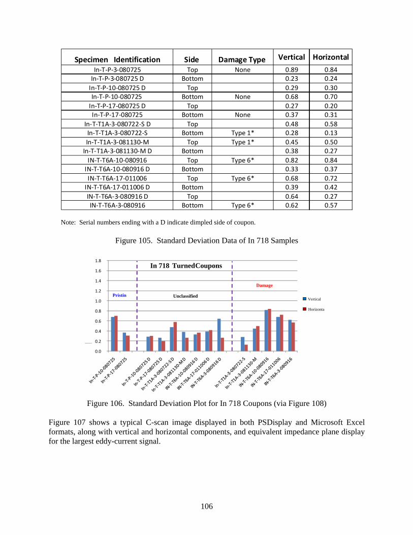
Specimen Identification Side Damage Type Vertical Horizontal
In‐T‐P‐3‐080725 Top None 0.89 0.84In‐T‐P‐3‐080725 D Bottom 0.23 0.24
In‐T‐P‐10‐080725 D Top 0.29 0.30In‐T‐P‐10‐080725 Bottom None 0.68 0.70
In‐T‐P‐17‐080725 D Top 0.27 0.20In‐T‐P‐17‐080725 Bottom None 0.37 0.31
In‐T‐T1A‐3‐080722‐S D Top 0.48 0.58In‐T‐T1A‐3‐080722‐S Bottom Type 1* 0.28 0.13
In‐T‐T1A‐3‐081130‐M Top Type 1* 0.45 0.50In‐T‐T1A‐3‐081130‐M D Bottom 0.38 0.27
IN‐T‐T6A‐10‐080916 Top Type 6* 0.82 0.84IN‐T‐T6A‐10‐080916 D Bottom 0.33 0.37
IN‐T‐T6A‐17‐011006 Top Type 6* 0.68 0.72IN‐T‐T6A‐17‐011006 D Bottom 0.39 0.42
IN‐T‐T6A‐3‐080916 D Top 0.64 0.27IN‐T‐T6A‐3‐080916 Bottom Type 6* 0.62 0.57
Note: Serial numbers ending with a D indicate dimpled side of coupon.
Figure 105. Standard Deviation Data of In 718 Samples
Figure 106. Standard Deviation Plot for In 718 Coupons (via Figure 108)
0.0
0.2
0.4
0.6
0.8
1.0
1.2
1.4
1.6
1.8In 718 Turned Coupons
Standard Deviation of C
Pristin
Damage
UnclassifiedVertical
Horizonta
Figure 107 shows a typical C-scan image displayed in both PSDisplay and Microsoft Excel formats, along with vertical and horizontal components, and equivalent impedance plane display for the largest eddy-current signal.
106
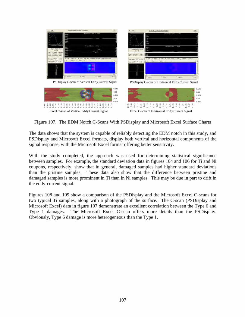
0.005
0.04
0.075
0.11
0.145
0.005
0.035
0.065
0.095
0.125
0.155
0.185
0.215
0.245
0.275
0.305
0.335
0.365
0.395
0.425
0.455
0.485
0.515
0.545
0.575
0.605
0.635
0.665
0.695
0.725
0.005
0.04
0.075
0.11
0.145
0.005
0.04
0.075
0.11
0.145
0.18
0.215
0.25
0.285
0.32
0.355
0.39
0.425
0.46
0.495
0.53
0.565
0.6
0.635
0.67
0.705
PSDisplay C-scan of Vertical Eddy Current Signal PSDisplay C-scan of Horizontal Eddy Current Signal
Excel C-scan of Vertical Eddy Current Signal Excel C-scan of Horizontal Eddy Current Signal
Figure 107. The EDM Notch C-Scans With PSDisplay and Microsoft Excel Surface Charts The data shows that the system is capable of reliably detecting the EDM notch in this study, and PSDisplay and Microsoft Excel formats, display both vertical and horizontal components of the signal response, with the Microsoft Excel format offering better sensitivity. With the study completed, the approach was used for determining statistical significance between samples. For example, the standard deviation data in figures 104 and 106 for Ti and Ni coupons, respectively, show that in general, damaged samples had higher standard deviations than the pristine samples. These data also show that the difference between pristine and damaged samples is more prominent in Ti than in Ni samples. This may be due in part to drift in the eddy-current signal. Figures 108 and 109 show a comparison of the PSDisplay and the Microsoft Excel C-scans for two typical Ti samples, along with a photograph of the surface. The C-scan (PSDisplay and Microsoft Excel) data in figure 107 demonstrate an excellent correlation between the Type 6 and Type 1 damages. The Microsoft Excel C-scan offers more details than the PSDisplay. Obviously, Type 6 damage is more heterogeneous than the Type 1.
107

Horizontal
Vertical
Excel C-scan PSDisplay C-scan
Ti-T-T6A-24-081201
Figure 108. Microsoft Excel C-Scan and PSDisplay C-Scan of Ti-TT6A-24-081201
C-Ti-T1D-3-101607
Horizontal
Vertical
PSDisply C-ScanC-Scan from Excel
Figure 109. Microsoft Excel C-Scan and PSDisplay C-Scan of C-Ti-T1D-3-101607 3.3.11.2 Conclusions.
The single-frequency eddy-current method is capable of characterizing surface and subsurface anomalies in a semi-quantitative manner. The Microsoft Excel C-scan was more sensitive than
108

the PSDisplay C-scan. Microsoft Excel data can be used for more in-depth statistical analysis. Further study is strongly recommended, repeating the single-frequency measurements over a range of frequencies. When fully understood, it may be possible to integrate these findings in a production environment wherein one inspection can be used to characterize anomalies and detect inclusions, flaws, and cracks. 3.3.12 Surface Wave UT.
The use of surface wave UT to detect machining-induced damage was studied at both ISU and HW using different equipment and methods. At both facilities, only turning samples were studied due to geometric constraints. The details of the ISU work can be found in appendix O. 3.3.12.1 Turning Summary.
ISU examined the backscattered grain noise observed when a surface wave propagated along the metal surface. With the sample immersed in water, surface waves were generated using a 25-MHz planar transducer oriented at oblique incidence. As shown in figure 110(a), an Angle-X scan was generated by varying both the probe tilt angle (θ) and the lateral surface coordinate (X). At each (θ, X) location, the backscattered grain noise amplitude was measured and displayed, resulting in the C-scan image shown in figure 110(b).
The surface-acoustic wave (SAW) signal
backscattered by grain boundaries and surface irregularities is studied.
25-MHz, 0.25”-dia, planar transducer25-MHz, 0.25”-dia, planar transducer
Scan in X
Scan in
SAW
Tilt Angle (degrees)
Late
ral P
ositi
on X
(in
ches
)
High Backscatter
Low Backscatter
Side B 56 dB
30.2 o
Ti64 Pristine Specimen C-Ti-T-P-2-101607
(a) (b)
The surface-acoustic wave (SAW) signal
backscattered by grain boundaries and surface irregularities is studied.
25-MHz, 0.25”-dia, planar transducer25-MHz, 0.25”-dia, planar transducer
Scan in X
Scan in
SAW
The surface-acoustic wave (SAW) signal
backscattered by grain boundaries and surface irregularities is studied.
25-MHz, 0.25”-dia, planar transducer25-MHz, 0.25”-dia, planar transducer
Scan in X
Scan in
SAW
25-MHz, 0.25”-dia, planar transducer25-MHz, 0.25”-dia, planar transducer
Scan in X
Scan in
SAW
Tilt Angle (degrees)
Late
ral P
ositi
on X
(in
ches
)
High Backscatter
Low Backscatter
High Backscatter
Low Backscatter
Side B 56 dB
30.2 o
Ti64 Pristine Specimen C-Ti-T-P-2-101607
(a) (b)
Figure 110. (a) Setup for Surface Wave Backscatter Measurements and (b) an Angle-X C-Scan
of a Pristine Ti 6-4 Sample Of chief interest is the angular dependence of the backscattering rather than the absolute backscatter amplitude itself. The angle of peak backscatter (e.g., 30.2° in figure 110(b)) is sensitive to the surface wave speed within a depth region extending about one wavelength below the surface. If surface damage causes an appreciable change in the surface wave speed, then that damage should be readily detectable by observing a change in the peak backscatter angle. The UT surface wave backscatter method was applied to both sides of 53 turning samples. Of these, 34 were Ti 6-4 alloy and 19 were In 718 alloy. For each tested surface, an Angle-X C-scan was obtained, and the probe-tilt angle producing the greatest backscatter was recorded.
109

Measurements were made using both positive and negative tilt angles, which were averaged to correct for any initial alignment errors. The area of the interrogated surface region depended on the scan length X and the lateral size of the beam “foot print” on the surface. This area was typically 0.8″ x 0.3″ for the measurements at ISU. The measured peak backscatter angle serves as the damage indicator for this area as a whole. For the ISU measurements, the interrogated surface of a given sample was specified either by its orientation relative to the serial number (side A versus side B) or by the nature of the surface (damaged versus pristine). Examples of Angle-X C-scans for pristine and damaged surfaces are shown in figure 111. Figure 111(a) shows scans of the damaged and undamaged surfaces of an In 718 sample having Type 6* damage on one surface. Figure 111(b) shows a similar comparison for a Type 1*-damaged Ti 6-4 coupon. An undamaged surface typically displays peak surface wave backscatter at a single, well-defined angle. This was the case for all pristine coupons examined, as well as for the undamaged (opposite) faces of all damaged coupons. For undamaged In 718 surfaces, this probe-tilt angle for peak backscatter is typically near 31.5°, depending slightly on water temperature. For Ti 6-4, it is near 30.2°. Figure 111 shows the damaged In 718 surface has its peak backscatter angle near 32.2°, or about 0.8° above the undamaged surface. A higher peak backscatter angle is expected for situations where the nature of the damage acts to reduce the elastic stiffness of the near-surface layer, for example, by introducing distributed microcracking in the near-surface layer.
- 32.2 o
Side B 57 dB
Tilt Angle (degrees)
Late
ral P
ositi
on X
(in
ches
)
- 31.4 o
Side A 54 dB
Tilt Angle (degrees)
Late
ral P
osi
tion
X (
inch
es)
Undamaged SideDamaged Side
IN718 Specimen In-T-T6A-7-080916
High Backscatter
Low Backscatter
Ti64 Specimen C-Ti-T-T1D-6-101607
Undamaged SideDamaged Side
Late
ral P
osi
tion
X (
inch
es)
Tilt Angle (degrees)
Side A 56 dB
- 30.2 o
Tilt Angle (degrees)
Late
ral P
ositi
on X
(in
ches
)
“Primary”peak
Backscatter from bulk
shear waves
“Secondary”peak
- 29.0 o
Side B 56 dB
- 30.6 o
- 30.6 o
- 32.2 o
Side B 57 dB
Tilt Angle (degrees)
Late
ral P
ositi
on X
(in
ches
)
- 31.4 o
Side A 54 dB
Tilt Angle (degrees)
Late
ral P
osi
tion
X (
inch
es)
- 32.2 o
Side B 57 dB
Tilt Angle (degrees)
Late
ral P
ositi
on X
(in
ches
)
- 31.4 o
Side A 54 dB
Tilt Angle (degrees)
Late
ral P
osi
tion
X (
inch
es)
Undamaged SideDamaged Side
IN718 Specimen In-T-T6A-7-080916
High Backscatter
Low Backscatter
High Backscatter
Low Backscatter
Ti64 Specimen C-Ti-T-T1D-6-101607
Undamaged SideDamaged Side
Late
ral P
osi
tion
X (
inch
es)
Tilt Angle (degrees)
Side A 56 dB
- 30.2 o
Late
ral P
osi
tion
X (
inch
es)
Tilt Angle (degrees)
Side A 56 dB
- 30.2 o
Tilt Angle (degrees)
Late
ral P
ositi
on X
(in
ches
)
“Primary”peak
Backscatter from bulk
shear waves
“Secondary”peak
- 29.0 o
Side B 56 dB
- 30.6 o
- 30.6 o
Tilt Angle (degrees)
Late
ral P
ositi
on X
(in
ches
)
“Primary”peak
Backscatter from bulk
shear waves
“Secondary”peak
- 29.0 o
Side B 56 dB
- 30.6 o
- 30.6 o
(a)
(b) Figure 111. Surface Wave Backscatter Method Applied to the Damaged and Undamaged
Surfaces of two Samples (a) In 718 Turning Sample In-T-T6A-7-080916 (Type 6* Damage) and (b) Ti 6-4 Turning Sample C-Ti-T-T1D-6-101607 (Type 1* Deep Damage)
110
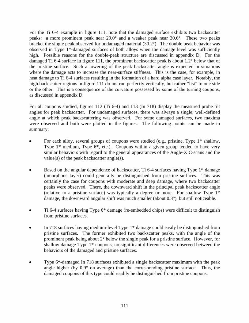
For the Ti 6-4 example in figure 111, note that the damaged surface exhibits two backscatter peaks: a more prominent peak near 29.0° and a weaker peak near 30.6°. These two peaks bracket the single peak observed for undamaged material (30.2°). The double peak behavior was observed in Type 1*-damaged surfaces of both alloys when the damage level was sufficiently high. Possible reasons for the double-peak structure are discussed in appendix D. For the damaged Ti 6-4 surface in figure 111, the prominent backscatter peak is about 1.2° below that of the pristine surface. Such a lowering of the peak backscatter angle is expected in situations where the damage acts to increase the near-surface stiffness. This is the case, for example, in heat damage to Ti 6-4 surfaces resulting in the formation of a hard alpha case layer. Notably, the high backscatter regions in figure 111 do not run perfectly vertically, but rather “list” to one side or the other. This is a consequence of the curvature possessed by some of the turning coupons, as discussed in appendix D. For all coupons studied, figures 112 (Ti 6-4) and 113 (In 718) display the measured probe tilt angles for peak backscatter. For undamaged surfaces, there was always a single, well-defined angle at which peak backscattering was observed. For some damaged surfaces, two maxima were observed and both were plotted in the figures. The following points can be made in summary: For each alloy, several groups of coupons were studied (e.g., pristine, Type 1* shallow,
Type 1* medium, Type 6*, etc.). Coupons within a given group tended to have very similar behaviors with regard to the general appearances of the Angle-X C-scans and the value(s) of the peak backscatter angle(s).
Based on the angular dependence of backscatter, Ti 6-4 surfaces having Type 1* damage
(amorphous layer) could generally be distinguished from pristine surfaces. This was certainly the case for coupons with moderate and deep damage, where two backscatter peaks were observed. There, the downward shift in the principal peak backscatter angle (relative to a pristine surface) was typically a degree or more. For shallow Type 1* damage, the downward angular shift was much smaller (about 0.3°), but still noticeable.
Ti 6-4 surfaces having Type 6* damage (re-embedded chips) were difficult to distinguish
from pristine surfaces. In 718 surfaces having medium-level Type 1* damage could easily be distinguished from
pristine surfaces. The former exhibited two backscatter peaks, with the angle of the prominent peak being about 2° below the single peak for a pristine surface. However, for shallow damage Type 1* coupons, no significant differences were observed between the behaviors of the damaged and pristine surfaces.
Type 6*-damaged In 718 surfaces exhibited a single backscatter maximum with the peak
angle higher (by 0.9° on average) than the corresponding pristine surface. Thus, the damaged coupons of this type could readily be distinguished from pristine coupons.
111

The 25-MHz transducer used at ISU for these measurements was the highest frequency planar transducer that was available. For that transducer, the surface wave penetrated about 120 microns below the surface. That was likely well beyond the damage zone thickness, particularly for all shallow damage coupons. Shifts in the peak backscatter angle due to near-surface damage would likely be larger at higher inspection frequencies, since the surface wave energy would be more concentrated in the damage zone.
The ISU method relies on the angular dependence of surface wave backscatter rather than
on its absolute amplitude. For this reason, the method is believed to be relatively insensitive to surface roughness or to the inspection water path used (probe liftoff).
Peak Backscatter Angle (25 MHz)Ti 6-4 Type-1 "Shallow" Coupons
28.0
28.5
29.0
29.5
30.0
30.5
31.0
31.5
32.0
S1 S2 S3 S4 S5 S6 S7
Specimen Designation
Pe
ak
An
gle
(d
eg
ree
s)
Undamaged
Damaged
Peak Backscatter Angle (25 MHz)Ti 6-4 Pristine Coupons
28.0
28.5
29.0
29.5
30.0
30.5
31.0
31.5
32.0
P1 P2 P3 P4 P5 P6 P9P16 P1A
Specimen Designation
Pe
ak
An
gle
(d
eg
ree
s)
Side B
Side A
Peak Backscatter Angle (25 MHz)Ti 6-4 Type-1 "Deep" Coupons
28.0
28.5
29.0
29.5
30.0
30.5
31.0
31.5
32.0
D1 D2 D3 D4 D5 D6 D2b
Specimen Designation
Pe
ak
An
gle
(d
eg
ree
s)
Undamaged
Damaged (Peak 1)
Damaged (Peak 2)
?
Peak Backscatter Angle (25 MHz)Ti 6-4 Type-1 "Medium" Coupons
28.0
28.5
29.0
29.5
30.0
30.5
31.0
31.5
32.0
M9 M10 M11 M12 M15 M16
Specimen Designation
Pe
ak
An
gle
(d
eg
ree
s)
UndamagedDamaged (Peak 1)Damaged (Peak 2)
Peak Backscatter Angle (25 MHz)Ti 6-4 Type-6 Coupons
28.0
28.5
29.0
29.5
30.0
30.5
31.0
31.5
32.0
T6-1 T6-2 T6-7 T6-15 T6-16
Specimen Designation
Pe
ak
An
gle
(d
eg
ree
s)
Undamaged
Damaged
Various Ti64 pristine and damaged coupons
Angle at which peak backscatter is seen
(Average of values obtained for scans over positive and
negative angles)
A * above a coupon designation denotes a round-robin coupon.
* * * * * *
* * * ** *
Pristine Type-1* “Shallow”
Type-6*
Type-1* “Medium”
Type-1* “Deep”
Peak Backscatter Angle (25 MHz)Ti 6-4 Type-1 "Shallow" Coupons
28.0
28.5
29.0
29.5
30.0
30.5
31.0
31.5
32.0
S1 S2 S3 S4 S5 S6 S7
Specimen Designation
Pe
ak
An
gle
(d
eg
ree
s)
Undamaged
Damaged
Peak Backscatter Angle (25 MHz)Ti 6-4 Pristine Coupons
28.0
28.5
29.0
29.5
30.0
30.5
31.0
31.5
32.0
P1 P2 P3 P4 P5 P6 P9P16 P1A
Specimen Designation
Pe
ak
An
gle
(d
eg
ree
s)
Side B
Side A
Peak Backscatter Angle (25 MHz)Ti 6-4 Type-1 "Deep" Coupons
28.0
28.5
29.0
29.5
30.0
30.5
31.0
31.5
32.0
D1 D2 D3 D4 D5 D6 D2b
Specimen Designation
Pe
ak
An
gle
(d
eg
ree
s)
Undamaged
Damaged (Peak 1)
Damaged (Peak 2)
?
Peak Backscatter Angle (25 MHz)Ti 6-4 Type-1 "Medium" Coupons
28.0
28.5
29.0
29.5
30.0
30.5
31.0
31.5
32.0
M9 M10 M11 M12 M15 M16
Specimen Designation
Pe
ak
An
gle
(d
eg
ree
s)
UndamagedDamaged (Peak 1)Damaged (Peak 2)
Peak Backscatter Angle (25 MHz)Ti 6-4 Type-6 Coupons
28.0
28.5
29.0
29.5
30.0
30.5
31.0
31.5
32.0
T6-1 T6-2 T6-7 T6-15 T6-16
Specimen Designation
Pe
ak
An
gle
(d
eg
ree
s)
Undamaged
Damaged
Various Ti64 pristine and damaged coupons
Angle at which peak backscatter is seen
(Average of values obtained for scans over positive and
negative angles)
A * above a coupon designation denotes a round-robin coupon.
* * * * * *
* * * ** *
Peak Backscatter Angle (25 MHz)Ti 6-4 Type-1 "Shallow" Coupons
28.0
28.5
29.0
29.5
30.0
30.5
31.0
31.5
32.0
S1 S2 S3 S4 S5 S6 S7
Specimen Designation
Pe
ak
An
gle
(d
eg
ree
s)
Undamaged
Damaged
Peak Backscatter Angle (25 MHz)Ti 6-4 Pristine Coupons
28.0
28.5
29.0
29.5
30.0
30.5
31.0
31.5
32.0
P1 P2 P3 P4 P5 P6 P9P16 P1A
Specimen Designation
Pe
ak
An
gle
(d
eg
ree
s)
Side B
Side A
Peak Backscatter Angle (25 MHz)Ti 6-4 Type-1 "Deep" Coupons
28.0
28.5
29.0
29.5
30.0
30.5
31.0
31.5
32.0
D1 D2 D3 D4 D5 D6 D2b
Specimen Designation
Pe
ak
An
gle
(d
eg
ree
s)
Undamaged
Damaged (Peak 1)
Damaged (Peak 2)
?
Peak Backscatter Angle (25 MHz)Ti 6-4 Type-1 "Medium" Coupons
28.0
28.5
29.0
29.5
30.0
30.5
31.0
31.5
32.0
M9 M10 M11 M12 M15 M16
Specimen Designation
Pe
ak
An
gle
(d
eg
ree
s)
UndamagedDamaged (Peak 1)Damaged (Peak 2)
Peak Backscatter Angle (25 MHz)Ti 6-4 Type-6 Coupons
28.0
28.5
29.0
29.5
30.0
30.5
31.0
31.5
32.0
T6-1 T6-2 T6-7 T6-15 T6-16
Specimen Designation
Pe
ak
An
gle
(d
eg
ree
s)
Undamaged
Damaged
Various Ti64 pristine and damaged coupons
Angle at which peak backscatter is seen
(Average of values obtained for scans over positive and
negative angles)
A * above a coupon designation denotes a round-robin coupon.
* * * * * *
* * * ** *
Pristine Type-1* “Shallow”
Type-6*
Type-1* “Medium”
Type-1* “Deep”
Figure 112. Transducer Tilt Angles Producing Maximized Backscattered Surface Wave Responses
112

29
30
31
32
33
34
P1
P6
P7
P1
3
P2
0
P1
A
S1
S6
S7
S8
M1
M2
M3
M7
T6
-1A
T6
-7
T6
-8
T6
-11
T6
-14
Specimen
Pea
k A
ng
le (
deg
rees
)
Side 1, main peak
Side 1, 2nd peak
Side 2 (undamaged)
PristineType 1Shallow
Type 1Medium
Type 6
Here, Side-1 is the damaged side for damaged coupons, and is Side-A for pristine coupons
* * * ** *
* * *
* Denotes a round-robin coupon
* * *
Figure 113. Transducer Tilt Angles Producing Maximized Backscattered Surface Wave Responses for Both Sides of Various In 718 Turning Coupons
3.3.12.2 Broaching Summary.
Broaching samples were not investigated using the surface wave backscatter method due to the geometrical limitations of the scanning system and available transducers. Specially designed transducers would be necessary for similar broaching inspections. 3.3.12.3 Hole-Drilling Summary.
Hole-drilling samples were not investigated using the surface wave backscatter method due to the geometrical limitations of the scanning system and available transducers. Specially designed transducers would be necessary for similar hole-drilling inspections. 3.3.12.4 Conclusions and Recommendations.
For certain damage types and severity levels, the surface wave backscatter method was able to reliably distinguish damaged from pristine surfaces in turning samples. Such discrimination would likely be better at higher inspection frequencies (25 MHz was used here). In principle, it should be possible to estimate the depth of the damage later by studying the frequency dependence of backscattering. This could be done by either (1) making measurements using multiple transducers or (2) using a single broadband transducer and analyzing the frequency content of the backscatter. These topics were largely beyond the scope of the present study, but would be a fruitful field for future research. Table 19 outlines the conclusions of each sample set.
113

Table 19. Conclusions for Each Surface Wave Backscatter Sample Set
Turning
Ti 6-4 25-MHz surface wave backscatter could readily distinguish (from a pristine surface) Type 1* damage having either a medium or deep severity level. Type 1* shallow damage and Type 6* damage were much harder to distinguish from the pristine state, but small systematic differences were observed.
In 718 25-MHz surface wave backscatter could readily distinguish (from a pristine state) either Type 1* medium or Type 6* damage. Type 1* shallow damage could not be distinguished from the pristine state.
Broaching
Ti 6-4 Not tested due to geometric and system constraints.
In 718 Not tested due to geometric and system constraints.
Hole-Drilling
Ti 6-4 Not tested due to geometric and system constraints.
In 718 Not tested due to geometric and system constraints. 3.3.13 Ultrasonic Microscopy Imaging of Turning Samples.
NDT R&D Engineering, Materials & Process Engineering HW Aerospace participated in round-robin studies to evaluate machining-induced damages in Ni and Ti turning samples using both conventional and emerging NDT methods. The broaching and hole-drilling samples were not included in this study due, in part, to the complex geometry and practical difficulties in the evaluation process. The objectives of this portion of the program included detecting and characterizing any machining-induced damages for surface and subsurface regions in turning samples using high-frequency ultrasonic microscopy imaging (UMI). High-frequency UT waves offer an excellent way to evaluate surface and subsurface machining-induced damages because the sampling depth can be controlled by varying frequency. In addition, ultrasound is sensitive to variations in elastic properties and density in materials. In contrast to other physical techniques, such as SEM, TEM, optical microscopy, and laser profile, UMI displays variation (both local heterogeneity and bulk) in elastic properties and density instead of structure [46-48]. In this study, two transducers (100 and 230 MHz) were used, in both pulse-echo (PE) and leaky surface wave (SW) modes, for evaluating the capability of UMI by examining the C-scans from a 0.020- by 0.010- by 0.002-inch notch in an Ni sample. The details are provided in appendix P. The C-scans for direct and surface waves are shown in figure 114. The scanning had 2048 by 2048 pixels extending over a 2″ by 1″ area; indicating the pixel size was close to 0.001 inch or 25 µm.
114

Figure 114. C-Scans for Both 100 and 230 MHz for PE and SW for a 0.020- by 0.010- by 0.002-Inch Notch
A close examination of the C-scans shown in figure 115 indicates that a 100-MHz surface wave provided the best results, based on resolution and noise. Figure 116 further shows that the surface wave provides better resolution than the pulse-echo at 100 MHz when studying the C-scans from a typical sample. In figure 114, the darker colored regions represent less reflected energy due to either grain scattering or a complete match in the acoustic properties and vice versa for the white regions.
(a) (b)
Figure 115. C-Scans for (a) Pulse Echo and (b) Surface Wave
115

Figure 116. A 230-MHz C-Scan Revealing Details as Good as the 100-MHz C-Scan The beam’s spot size can also play a vital role when analyzing the C-scan images from a notch. For example, it is quite possible that the 230-MHz small focal spot size can display images that are equal to or better than 100-MHz images, due to such factors as loss of trigger or even reflection from the bottom of the notch. In some cases, 230 MHz was observed to be equally effective in imaging details in terms of local heterogeneities, but it suffered from excessive noise (figure 115). Therefore, a 100-MHz transducer was used in leaky SW mode. 3.3.13.1 Turning Samples.
A total of 15 samples were evaluated in this study, but for the sake of brevity and clarity, the results for only 6 samples (table 20) were included in the round-robin study. The details for selecting a scanning technique/plan and resolution are described in appendix P.
Table 20. Samples Evaluated by HW Using UT Methods
Round-Robin Sample Assignment Ni or Ti Type
C-Ti-T-P-1-101607 ETC Set 1 Ti 6-4 None
Ti-T-T1-1-080107 ETC Set 1 Ti 6-4 Type 1*
Ti-T-T1-7-080107 Vendor Set 3 Ti 6-4 Type 1*
Ti-T-T1A-9-080606-M ETC Set 1 Ti 6-4 Type 1*
C-Ti-T-T1D-1-101607 ETC Set 1 Ti 6-4 Type 1*
Ti-T-T1-2-080107b Vendor Set 3 Ti 6-4 Type 1*
116

Based on the basic Surface Acoustic Wave theory, the sampling depth should be close to 0.90 27 m or close to 0.001 inch), assuming the peak frequency is close to 90 MHz, as shown in figure P-4 in appendix P. These results serve two purposes: (1) displaying local heterogeneity in terms of variation in elastic properties and density and (2) determining bulk properties in terms of a histogram. The local variations in elastic properties along with histogram for all six round-robin Ti samples are shown in figures 117-122. Similarly, figures 120-122 show C-scans for the remaining three Ti samples from the round-robin study. The histograms in figure 117 show that both sides of the pristine sample have comparable bulk properties. But the C-scans in figure 117 show the presence of enough local heterogeneity with the dark areas having low-amplitude echoes (either due to excessive grain scattering or due to no difference in the acoustic properties, i.e., high transmission) and the white areas representing the opposite scenarios. Under normal circumstances, it is quite possible that local heterogeneity can be mistakenly masked by bulk properties in the absence of the necessary resolution to display local variation in the elastic properties. This is also clear in another case, as shown in figure 118, wherein the histograms from both sides show comparable energy distributions but local heterogeneity appears to vary vastly.
Top side Back side
Figure 117. C-Scans for Pristine (C-Ti-T-P-1-101607) Samples
117

Figure 118. Sample Ti-T-T1-7-080107 Showing Presences of Heterogeneity but With Little Difference in Bulk Properties
The anomalies in figure 118 may be due, in part, to lack of flatness, which may adversely affect the quality of C-scan images and thereby mask any local variation in the elastic properties, as shown in figure 119. The change in water path due to flatness can affect the entry beam circle diameter, which can be erroneously attributed to change in local heterogeneity and bulk properties. Figure 119 further shows that flatness varies as much as 500 ns (equivalent to 0.018 inch in water and 0.0625 inch or 1.5 mm in metal) from 4.50 to 5.00 s when measured across the sample.
Figure 119. Histogram Showing how Flatness Degrades the Quality of Images and Adversely Affects the C-Scan Data for Sample Ti-T-T1-2-080107b
The C-scans in figure 120 show that the side of noninterest (top left corner) is more heterogeneous than the side of interest (top right corner) but the histogram data show contrary results. This reiterates the earlier statements that this may be due in part to flatness of the sample. A similar trend was found in other samples, as shown in figures 121 and 122. The flatness effect is clearly observed in figure 122.
118

Figure 120. Histogram Showing Significant Difference in Bulk Properties and in the Presence of
Local Heterogeneity in Sample C-Ti-T-T1-1-101607
Figure 121. Histogram Showing the Presence of Local Heterogeneity but Little Difference in Bulk Properties for Sample Ti-T-T1-1-080107
Figure 122. Histogram Showing the Presence of Local Heterogeneity With Little Difference in
Bulk Properties for Sample Ti-T-T1A-9-080606-M
119

3.3.13.2 Conclusions.
The following are the conclusions from this study: UMI is capable of displaying variations in both local heterogeneity and bulk elastic
properties simultaneously.
The degradation in C-scans for imaging local heterogeneity, as well as the bulk properties, may be due, in part, to the lack of flatness, which can change the entry beam circle diameter and angle of refraction to a great extent.
It is often possible that significant change in bulk properties due to flatness can mask any
subtle variations in local elastic properties in a sample; especially when the variation due to flatness in not taken into consideration and the system lacks enough resolution.
The largest flatness variation was 500 ns, which is equivalent to 1.56 mm or 0.0625 inch
in metal.
3.3.14 High-Energy X-Ray Diffraction Depth Profile.
Aggressive machining is expected to induce lattice changes similar to what was observed in work-hardening. High-energy x-ray diffraction (HEXRD) uses a 6-keV x-ray beam collimated to an ~140-µm width to measure the diffraction intensity and deduce the lattice parameter as a function of depth in a sample. 3.3.14.1 Turning Summary.
The study concentrated on the samples chosen for round-robin measurements. Initial inconsistencies as to the identity of the damaged side led to making measurements on both sides of the samples. For most samples, measurements were made near the center of the 1″ by 2″ sample. -2 measurements were made both near the surface and as deep as practical (typically ~160 m in Ti 6-4 and ~100 m in In 718). Depth profile measurements of each surface were then made at the deep diffraction angle. Typical diffraction-2 scans for a Ti 6-4 Type 1* sample are shown in figure 123. The side of the sample assumed to be pristine (B) has the same peak diffraction angle at both depths, whereas the damaged side (A) shows a significant shift in the shallow diffraction angle. The green line on each plot indicates the diffraction angle used for the depth profile of the corresponding side. Depth profiles for this same sample are displayed in figure 124. Side B has a typical profile expected for pristine material. On side A, however, the intensity is greatly reduced near the surface due to the shift in diffraction angle. At a depth of ~160 m (0.006 inch), the intensity matches that of side B, indicating the depth of damage. This is considerably greater than the 0.0005-inch deformation depth estimated from the manufacturing process. The samples with medium and high deformation show damage to even greater depths.
120

(a)
(b)
Figure 123. Typical Diffraction -2 Scans for a Ti 6-4 Type 1* Sample (a) Top Side at Two
Depths and (b) Bottom Side at Two Depths
121

Figure 124. Typical Diffraction Depth Profile Scans for Sides A and B of a Ti 6-4 Type 1* Sample
Typical diffraction -2 scans of the Type 6* Ti 6-4 samples all showed behavior similar to that shown in figure 125. In this case, it was possible to position the x-ray beam on a visible, large, embedded chip and compare it to a nearby smooth region. The peak diffraction angle is different for sides A and B, and the -2 distribution near the surface is skewed in opposite directions on sides A and B. This was expected from stress due to bending of the coupon. The -2 distributions both on and off the embedded chip are very similar, indicating that HEXRD is not sensitive to Type 6* damage.
122

(a)
(b)
Figure 125. Typical Diffraction -2 Scans of a Ti 6-4 Type 6* Sample (a) Top at Two Depths and Two Surface Locations and (b) Bottom at Two Depths (The green line indicates the angle
chosen for depth profile scan on the corresponding surface.)
123
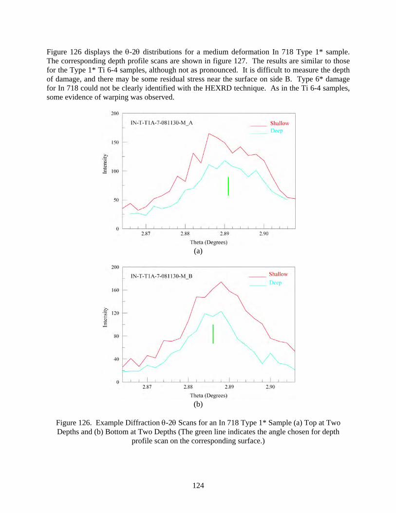
Figure 126 displays the -2 distributions for a medium deformation In 718 Type 1* sample. The corresponding depth profile scans are shown in figure 127. The results are similar to those for the Type 1* Ti 6-4 samples, although not as pronounced. It is difficult to measure the depth of damage, and there may be some residual stress near the surface on side B. Type 6* damage for In 718 could not be clearly identified with the HEXRD technique. As in the Ti 6-4 samples, some evidence of warping was observed.
(a)
(b)
Figure 126. Example Diffraction -2 Scans for an In 718 Type 1* Sample (a) Top at Two Depths and (b) Bottom at Two Depths (The green line indicates the angle chosen for depth
profile scan on the corresponding surface.)
124

Figure 127. Diffraction Depth Profile Scans for Sides A and B of the In 718 Sample in Figure 126
3.3.14.2 Broaching Summary.
The Ti 6-4 and In 718 broaching samples were not investigated with the HEXRD method due to the geometrical limitations of the system and the test samples. 3.3.14.3 Hole-Drilling Summary.
The Ti 6-4 and In 718 hole-drilling samples were not investigated with the HEXRD method due to the geometrical limitations of the system and the test samples. 3.3.14.4 Conclusions and Recommendations.
HEXRD shows good potential for characterizing Type 1* damage, especially in Ti 6-4. However, even with projected improvements in speed and sensitivity, this method is not practical for scanning large areas. It may be very useful for confirming and measuring the depth of damage at specific points indicated by other methods. HEXRD does not show sensitivity to Type 6* damage. Table 21 outlines the conclusions of each sample set.
125

126
Table 21. Conclusions for Each Sample Set
Turning
Ti 6-4 For Type 1* anomalies, six round-robin samples ranging from light to high deformation were inspected. Clear indication of damage was observed for all samples. Differences in damage depth were noted, although the measured depth was greater than that assumed based on manufacturing techniques. Four Type 6* anomaly samples were inspected. All showed signals that could be attributed to coupon warping rather than embedded material. Even some of the pristine samples showed evidence of some near-surface residual stress.
In 718 For Type 1* anomalies, three round-robin samples of medium and light deformation were inspected. Of these, only one medium sample showed a clear indication of damage, though it was difficult to determine the depth of damage. Three Type 6* anomaly samples were inspected. All three produced qualitatively different results that were difficult to interpret. There was an indication that sample warping could have been responsible for some of the discrepancies. Some of the pristine samples showed differences between side A and side B, indicating the presence of some work-hardening or residual stress.
Broaching
Ti 6-4 Not tested due to geometric and system constraints.
In 718 Not tested due to geometric and system constraints.
Hole-Drilling
Ti 6-4 Not tested due to geometric and system constraints.
In 718 Not tested due to geometric and system constraints.
3.3.15 Round-Robin Comparisons.
There were 21 turning samples designated for the round-robin study. Samples were chosen from both In 718 and Ti 6-4 that included each type of damage as well as two samples from each material that were machined to contain no intentional damage. The sample choices were based on current NDE results and the availability of the samples at the location where the studies were to be performed. Table 22 lists all the In 718 samples, and table 23 lists all the Ti 6-4 samples. The “X” indicates which NDE methods were performed with that sample. The results of these studies are listed in the appropriate section for each method.

Table 22. Round-Robin In 718 Samples and the NDE Methods Performed on Each Sample
Sample ID Target
Anomaly ISU—Base
Surface Metrology
ISU—Surface Wave UT Oblique
Incidence
ISU— Multifrequency ET
Swept High Frequency
ISU—Single- Frequency
ET Statistical Noise Analysis
ISU—High- Energy
Radiographic Diffraction
Positron Systems, Inc.—
Positron Annihilation
Innovative Materials— Magnetic
Carpet Probe
In-T-P-1-080725 None X X X X X X
In-T-P-1-0207XX None X X X X X
In-T-T1A-1-080722-S Type 1* X X X X X X
In-T-T1A-1-081130-M Type 1* X X X X X X
In-T-T1A-7-080722-S Type 1* X X X X X X X
In-T-T1A-7-081130-M Type 1* X X X X X X
In-T-T6A-14-011006 Type 6* X X X X X X
In-T-T6A-7-080916 Type 6* X X X X X X X
In-T-T6A-8-080916 Type 6* X X X X X X
In-T-T6A-8-080916 Type 6* X X X X X X
ET = Eddy-current technique
Table 23. Round-Robin Ti 6-4 Samples and NDE Methods Performed on Each Sample
127
Sample ID Target
Anomaly
ISU—Base Surface
Metrology
ISU—Surface Wave UT Oblique
Incidence
ISU— Multifrequency ET Swept High
Frequency
ISU—Single- Frequency
ET Statistical Noise
Analysis
ISU—High- Energy
Radiographic Diffraction
HW—Surface Wave
UT
HW— Multifrequency
ET
Positron Systems, Inc —Positron
Annihilation
Innovative Materials—Magnetic
Carpet Probe
C-Ti-T-P-1-101607 None X X X X X X X
Ti-T-P-1-0611XX None X X X X
Ti-T-T1A-9-080606-M Type 1* X X X X X X X
Ti-T-T1A-15-080606-M Type 1* X X X X X X X
Ti-T-T1-1-080107 Type 1* X X X X X X X
Ti-T-T1-7-080107 Type 1* X X X X X X X X
C-Ti-T-T1D-1-101607 Type 1* X X X X X X X
Ti-T-T1-2-080107b Type 1* X X X X X X X X X
Ti-T-T6-1-080508 Type 6* X X X X X
Ti-T-T6-2-080508 Type 6* X X X X X
Ti-T-T6-7-080508 Type 6* X X X X X X X
Ti-T-T6A-15-080602 Type 6* X X X X X X
ET = Eddy-current technique
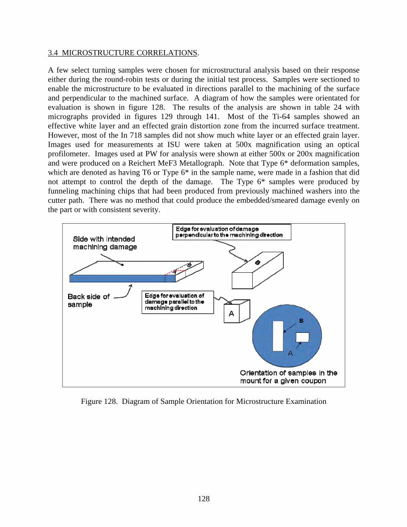
3.4 MICROSTRUCTURE CORRELATIONS.
A few select turning samples were chosen for microstructural analysis based on their response either during the round-robin tests or during the initial test process. Samples were sectioned to enable the microstructure to be evaluated in directions parallel to the machining of the surface and perpendicular to the machined surface. A diagram of how the samples were orientated for evaluation is shown in figure 128. The results of the analysis are shown in table 24 with micrographs provided in figures 129 through 141. Most of the Ti-64 samples showed an effective white layer and an effected grain distortion zone from the incurred surface treatment. However, most of the In 718 samples did not show much white layer or an effected grain layer. Images used for measurements at ISU were taken at 500x magnification using an optical profilometer. Images used at PW for analysis were shown at either 500x or 200x magnification and were produced on a Reichert MeF3 Metallograph. Note that Type 6* deformation samples, which are denoted as having T6 or Type 6* in the sample name, were made in a fashion that did not attempt to control the depth of the damage. The Type 6* samples were produced by funneling machining chips that had been produced from previously machined washers into the cutter path. There was no method that could produce the embedded/smeared damage evenly on the part or with consistent severity.
Figure 128. Diagram of Sample Orientation for Microstructure Examination
128

Table 24. Measurement Depths of Microstructural Analysis
White Layer Depth (in.)
Effected Grain Layer Depth
(in.) Sample A B A B
Ti-T-T1-1-080107 0.000109 0.000236 0.00057 0.000372
C-Ti-T-T1D-1-101607 0.000481 0.000374 0.001764 0.001748
C-Ti-T-T1D-4-101607 0.00039 0.00049 0.00394 0.00197
Ti-T-T1-2-080107b 0.002354 0.001958 0.007599 0.004895
Ti-T-T1A-9-080608 0.00049 0.000909 0.002797 0.001935
Ti-T-T6-1-080508 0.000607 0.000862 0.001562 0.001212
Ti-T-T6-8-080508 0.00039 0.00065 N/A N/A
In-T-T1A-3-080722-S 0.0001259 0.000769 N/A N/A
In-T-T1A-6-080722-S N/A N/A 0.00012 0.00012
In-T-T1A-3-081130-M 0.000816 0.000208 N/A N/A
In-T-T1A-7-081130-M 0.000163 0.000434 N/A N/A
In-T-T6A-13-081006 0.00039 0.00039 0.00059 0.00059
In-T-T6A-14-081006 0.000793 0.000513 0.001259 0.001445 Sample Ti-T-T1-1-080107 showed very little white layer or grain distortion for both the parallel (A) and the perpendicular (B) samples. The amount of deformation is in the range of light deformation, which that was intended for this sample. Light deformation is defined as less than 0.0005″.
129

White Layer Depth
(in.) Effected Grain Layer Depth
(in.) Sample A B A B
Ti-T-T1-1-080107 0.000109 0.000236 0.00057 0.000372
(A)
(B)
Figure 129. Microstructural Results for Sample Ti-T-T1-1-080107 (A) Parallel and
(B) Perpendicular to Machining Direction Sample C-Ti-T-T1D-1-101607 showed a distinctive white layer and grain distortion for both the parallel (A) and the perpendicular (B) samples. The degree of damage matches the intended category of heavy deformation where the damage exceeds 0.0015″ depth.
130

White Layer Depth (in.)
Effected Grain Layer Depth (in.)
Sample A B A B
C-Ti-T-T1D-1-101607 0.000481 0.000374 0.001764 0.001748
(A)
(B)
Figure 130. Microstructural Results for Sample C-Ti-T-T1D-1-101607 (A) Parallel and
(B) Perpendicular to Machining Direction
131

Sample C-Ti-T-T1D-4-101607 showed a distinctive white layer and grain distortion for both the parallel (A) and the perpendicular (B) samples. The degree of deformation fits the category of heavy damage, which was intended for this sample.
White Layer Depth (in.)
Effected Grain Layer Depth (in.)
Sample A B A B
C-T-T1D-4-101607 0.00039 0.00049 0.00394 0.00197
(A)
(B)
Figure 131. Microstructural Results for Sample C-Ti-T-T1D-4-101607 (A) Parallel and
(B) Perpendicular to Machining Direction (200X)
132

Sample Ti-T-T1-2-080107b showed a distinctive white layer and grain distortion for both the parallel (A) and the perpendicular (B) samples. The degree of damage meets the definition of heavy deformation, which was intended for this sample.
White Layer Depth (in.)
Effected Grain Layer Depth (in.)
Sample A B A B
Ti-T-T1-2-080107b 0.002354 0.001958 0.007599 0.004895
(A)
(B)
Figure 132. Microstructural Results for Sample Ti-T-T1-2-080107b (A) Parallel and
(B) Perpendicular to Machining Direction
133
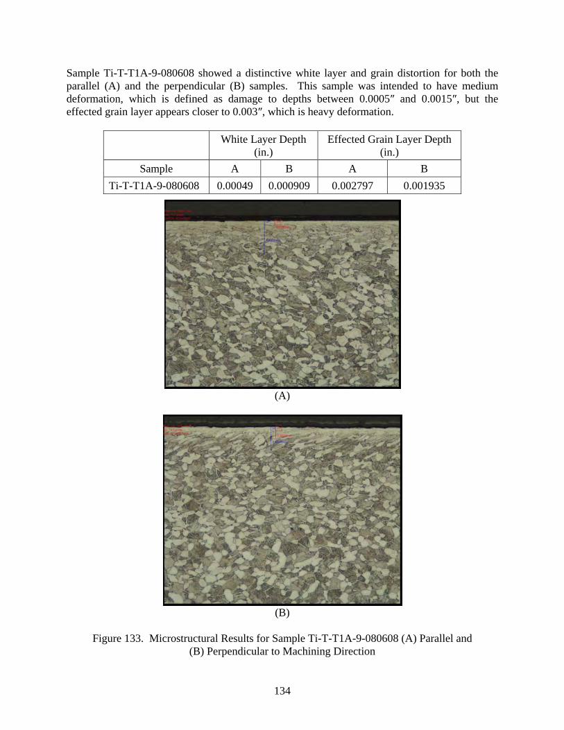
Sample Ti-T-T1A-9-080608 showed a distinctive white layer and grain distortion for both the parallel (A) and the perpendicular (B) samples. This sample was intended to have medium deformation, which is defined as damage to depths between 0.0005″ and 0.0015″, but the effected grain layer appears closer to 0.003″, which is heavy deformation.
White Layer Depth
(in.) Effected Grain Layer Depth
(in.)
Sample A B A B
Ti-T-T1A-9-080608 0.00049 0.000909 0.002797 0.001935
(A)
(B)
Figure 133. Microstructural Results for Sample Ti-T-T1A-9-080608 (A) Parallel and
(B) Perpendicular to Machining Direction
134

Sample Ti-T-T6-1-080508 showed a distinctive white layer and grain distortion for both the parallel (A) and the perpendicular (B) samples. The degree of deformation for this sample can be categorized as heavy since the depth of the damage appears to reach approximately 0.002″. As noted, the damage was not expected to be uniform throughout the sample.
White Layer Depth (in.)
Effected Grain Layer Depth (in.)
Sample A B A B
Ti-T-T6-1-080508 0.000607 0.000862 0.001562 0.001212
(A)
(B)
Figure 134. Microstructural Results for Sample Ti-T-T6-1-080508 (A) Parallel and
(B) Perpendicular to Machining Direction
135

Sample Ti-T-T6-8-080508 showed a distinctive white layer but no measurable grain distortion for both the parallel (A) and the perpendicular (B) samples. The extent of damage fits the description of light damage; however, it should not be expected that the damage is uniform over the sample surface.
White Layer Depth (in.)
Effected Grain Layer Depth (in.)
Sample A B A B
Ti-T-T6-8-080508 0.00039 0.00065 N/A N/A
(A)
(B)
Figure 135. Microstructural Results for Sample Ti-T-T6-8-080508 (A) Parallel and
(B) Perpendicular to Machining Direction (500X)
136

Sample In-T-T1A-3-080722-S shows a white layer in both the parallel (A) and the perpendicular (B) samples, but due to the small grain size, shows no noticeable grain distortion. The damage layer fits the description of light deformation.
White Layer Depth (in.)
Effected Grain Layer Depth (in.)
Sample A B A B
In-T-T1A-3-080722-S 0.0001259 0.000769 N/A N/A
(A)
(B)
Figure 136. Microstructural Results for Sample In-T-T1A-3-080722-S (A) Parallel and
(B) Perpendicular to Machining Direction
137

Sample In-T-T1A-6-080722-S shows only a minimal grain distortion in the parallel (A) and the perpendicular (B) samples. This sample fits the description of light deformation, which was the intended condition.
White Layer Depth (in.)
Effected Grain Layer Depth (in.)
Sample A B A B
In-T-T1A-6-080722-S N/A N/A 0.00012 0.00012
(A)
(B)
Figure 137. Microstructural Results for Sample In-T-T1A-6-080722-S (A) Parallel and
(B) Perpendicular to Machining Direction
138

Sample In-T-T1A-3-081130-M shows a white layer in both the parallel (A) and the perpendicular (B) samples, but due to the small grain size, shows no noticeable grain distortion. The damage layer is in the range of medium deformation.
White Layer Depth (in.)
Effected Grain Layer Depth (in.)
Sample A B A B
In-T-T1A-3-081130-M 0.000816 0.000208 N/A N/A
(A)
(B)
Figure 138. Microstructural Results for Sample In-T-T1A-3-081130-M (A) Parallel and
(B) Perpendicular to Machining Direction
139

Sample In-T-T1A-7-081130-M shows a very small white layer on the parallel sample (A) and a rather rough surface with a few places of white layer on the perpendicular sample (B), but due to the small grain size, shows no noticeable grain distortion. The intended deformation level for this sample was medium, but it appears that light deformation is the appropriate description.
White Layer Depth (in.)
Effected Grain Layer Depth (in.)
Sample A B A B
In-T-T1A-7-081130-M 0.000163 0.000434 N/A N/A
(A)
(B)
Figure 139. Microstructural Results for Sample In-T-T1A-7-081130-M (A) Parallel and
(B) Perpendicular to Machining Direction
140

Sample In-T-T6A-13-081006 shows an effective white layer and a region of grain distortion for both the parallel (A) and the perpendicular (B) samples. The deformation level would be considered medium in the area where the micrograph was taken, but that condition is not necessarily present in other regions of the sample.
White Layer Depth (in.)
Effected Grain Layer Depth (in.)
Sample A B A B
In-T-T6A-13-081006 0.00039 0.00039 0.00059 0.00059
(A)
(B)
Figure 140. Microstructural Results for Sample In-T-T6A-13-081006 (A) Parallel and
(B) Perpendicular to Machining Direction
141

Sample In-T-T6A-14-081006 shows an effective white layer and distorted grains for both the parallel (A) and the perpendicular (B) samples. The damage in this region would be considered heavy deformation, but as noted with all Type-6 samples, the deformation is not necessarily distributed evenly across the surface.
White Layer Depth
(in.) Effected Grain Layer Depth
(in.)
Sample A B A B
In-T-T6A-14-081006 0.000793 0.000513 0.001259 0.001445
(A)
(B)
Figure 141. Microstructural Results for Sample In-T-T6A-14-081006 (A) Parallel and
(B) Perpendicular to Machining Direction
142

3.5 THE NDE EVALUATION MATRIX.
The effort of this subtask was to define an analog comparison metric that represents how well each inspection technology is able to detect the selected flaw types. A generic protocol was developed to compare the various techniques using a weighting scheme, such as low, medium, and high, for identified factors. The evaluation matrix includes consideration of all NDE test results completed to date. The scores are broken into two main categories, Sensitivity and Implementation. The definitions for each NDE technique and scoring method used are provided in tables 25 through 30. Definitions for the Manufacturing Readiness Level (MRL) and Technology Readiness Levels (TRL) are provided in tables 26 and 27, respectively. The definitions were taken from standard Department of Defense (DoD) terminology and modified for ETC use in table 28. Each NDE technique is scored per the evaluation criteria identified above and those results are summarized in tables 28 through 30 as the Sensitivity Score, Implementation Score, and Total Score, respectively. Discussions of the score results are provided in section 4. The Sensitivity Score is a summary of the techniques’ ability to measure and discriminate an anomalous surface condition from a baseline condition. It includes rankings based upon: Signal-to-noise ratio Lateral resolution Depth resolution Edge effect Flexibility to access the location of the anomaly Selectivity to indications The Implementation Score is based upon similar conditions and includes rankings of: Applicability in a production environment Applicability in a depot environment The MRL of technology for use The TRL of technology for itself Return on investment Operator use and training
143

Table 25. Scoring Definitions Used for NDE Matrix
Sensitivity and Ability to Resolve the Anomaly in the Presence of the Background Condition
High Nominal Low None - N/A Criteria
10 9 8 7 6 5 4 3 2 1 0
Signal to noise ratio X GT 3:1 2:1 GE X LE
3:1 X LT 2:1
Not Possible or Applicable
1
Comments Signal-to-noise ratios based upon use of the method over the range of anomaly
damage and types
High Nominal Low None - N/A Criteria
10 9 8 7 6 5 4 3 2 1 0
Lateral resolution X LT 10
mil 10 mil GE X
LE 20 mil X GT 20 mil
Not Possible or Applicable
2
Comments Lateral resolution based upon the ability to measure and characterize the localized
presence of an anomaly on the surface of the feature
High Nominal Low None - N/A Criteria
10 9 8 7 6 5 4 3 2 1 0
Depth resolution X LT 0.5
mil 0.5 mil GE X
LE 1.5 mil X GT 1.5 mil
Not Possible or Applicable
3
Comments Depth resolution based upon the ability to measure and characterize the depth of an
anomaly from the nominal surface of the feature
High Nominal Low None - N/A Criteria
10 9 8 7 6 5 4 3 2 1 0
Edge effect (geometric effect discrimination)
X LT 5 mil 5 mil GE X
LE 20 mil X GT 20 mil
Not Possible or Applicable
4
Comments Ability to measure and characterize the presence of an anomaly at a location of the
part that contains a distinct feature of nonuniform material structure, such as an edge
144

Table 25. Scoring Definitions Used for NDE Matrix (Continued)
Sensitivity and Ability to Resolve the Anomaly in the Presence of the Background Condition
High Nominal Low None - N/A Criteria
10 9 8 7 6 5 4 3 2 1 0
Flexibility to access the location of the anomaly
Can easily access a wide
range of features of
interest within typical part geometries
Has selected ability to access
the feature of interest within
typical part geometries
Has limited ability to access
the feature of interest within
typical part geometries
Not Possible or Applicable
5
Comments Ability to access the feature of interest (i.e., holes, slots, fillets, scallops) within the
typical geometry of engine parts requiring inspection
High Nominal Low None - N/A Criteria
10 9 8 7 6 5 4 3 2 1 0
Selectivity to indications
Can distinguish
between Type 1* and Type 6* anomalies at all anomaly
depths and severity
Has the selected ability to
distinguish between some anomalies and
depths
Can detect, although not distinguish
between Type 1* and Type 6*
anomalies through all
anomaly depths and severities
Not Possible or Applicable
6
Comments Ability to distinguish and characterize both the anomaly type and its severity
Applicability for Practical Implementation in a Relevant Environment
High Nominal Low None - N/A Criteria
10 9 8 7 6 5 4 3 2 1 0
Applicability in a production environment
Speed & productivity
Can easily be applied at 100% with little of no impact to existing
productivity
Requires some modification of existing process to accommodate method at 100%. It's application is noticeable but not
intrusive.
Is difficult to implement on a
100% basis. Expect
resistance to implement
based upon cost-benefit. Would be the target of
elimination during any cost saving efforts.
Not Possible or Applicable
7
Comments Impact to productivity in applying method to existing processes of a production
manufacturing environment
145

Table 25. Scoring Definitions Used for NDE Matrix (Continued)
Applicability for Practical Implementation in a Relevant Environment
High Nominal Low None - N/A Criteria
10 9 8 7 6 5 4 3 2 1 0
Applicability in a depot environment
Speed & productivity
Can easily be applied at 100% with little of no impact to existing
productivity
Requires some modification of existing process to accommodate method at 100%. It's application is noticeable but not
intrusive.
Is difficult to implement on a
100% basis. Expect
resistance to implement
based upon cost-benefit. Would be the target of
elimination during any cost saving efforts.
Not Possible or Applicable
8
Comments Impact to productivity in applying method to existing processes of a depot or in-
service environment
Criteria High Nominal Low None - N/A
The maturity level of technology for use
10 9 8 7 6 5 4 3 2 1 0 9
Comments Readiness for full manufacturing production implementation per DOD MRL
Scoring (See Tab "DOD MRL Dens")
Criteria High Nominal Low None - N/A
The maturity level of technology itself
10 9 8 7 6 5 4 3 2 1 0 10
Comments Readiness and maturity of the technology itself per DOD TRL Scoring
(See Tab "DOD TRL Defns")
High Nominal Low None - N/A Criteria
10 9 8 7 6 5 4 3 2 1 0
Return on Investment X LT 1 year 1 year GE X
LE 3 years X GT 3 years
Not Possible or Applicable
11
Comments Time line required to recover return on the investment to implement the technology
at 100% utilization rate.
146

147
Table 25. Scoring Definitions Used for NDE Matrix (Continued)
Applicability for Practical Implementation in a Relevant Environment
High Nominal Low None - N/A Criteria
10 9 8 7 6 5 4 3 2 1 0
Operator use and training
Can easily be implemented into written procedures
with minimal operator training.
Control of sustained
operations can be monitored
through periodic audits
Requires some specialized training and certification.
Operator control for sustained
operations can be monitored through
combinations of periodic audits and statistical
process control
Requires high levels of
specialized training and redundant
process and statistical control for sustained
operations.
Not Possible or Applicable
12
Comments Human resource specialization and control required to fully utilize the technology in
a safe manner to produce quality results
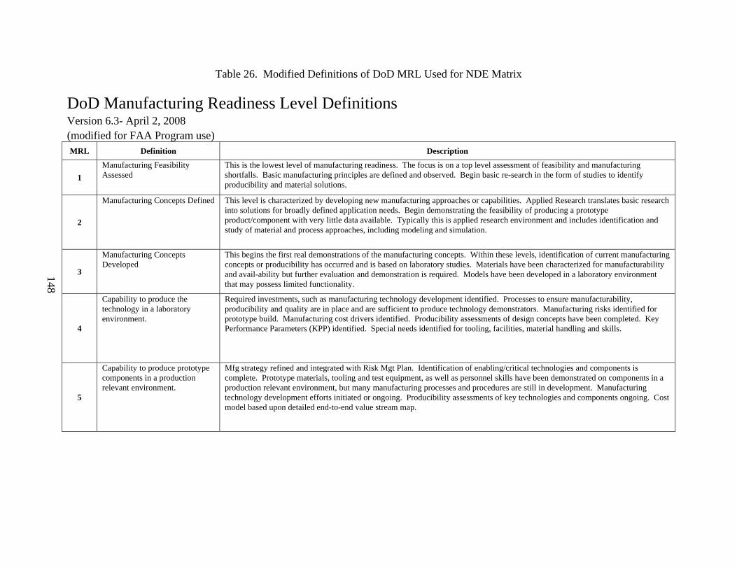
Table 26. Modified Definitions of DoD MRL Used for NDE Matrix
DoD Manufacturing Readiness Level Definitions Version 6.3- April 2, 2008
(modified for FAA Program use)
MRL Definition Description
1
Manufacturing Feasibility Assessed
This is the lowest level of manufacturing readiness. The focus is on a top level assessment of feasibility and manufacturing shortfalls. Basic manufacturing principles are defined and observed. Begin basic re-search in the form of studies to identify producibility and material solutions.
2
Manufacturing Concepts Defined This level is characterized by developing new manufacturing approaches or capabilities. Applied Research translates basic research into solutions for broadly defined application needs. Begin demonstrating the feasibility of producing a prototype product/component with very little data available. Typically this is applied research environment and includes identification and study of material and process approaches, including modeling and simulation.
3
Manufacturing Concepts Developed
This begins the first real demonstrations of the manufacturing concepts. Within these levels, identification of current manufacturing concepts or producibility has occurred and is based on laboratory studies. Materials have been characterized for manufacturability and avail-ability but further evaluation and demonstration is required. Models have been developed in a laboratory environment that may possess limited functionality.
4
Capability to produce the technology in a laboratory environment.
Required investments, such as manufacturing technology development identified. Processes to ensure manufacturability, producibility and quality are in place and are sufficient to produce technology demonstrators. Manufacturing risks identified for prototype build. Manufacturing cost drivers identified. Producibility assessments of design concepts have been completed. Key Performance Parameters (KPP) identified. Special needs identified for tooling, facilities, material handling and skills.
5
Capability to produce prototype components in a production relevant environment.
Mfg strategy refined and integrated with Risk Mgt Plan. Identification of enabling/critical technologies and components is complete. Prototype materials, tooling and test equipment, as well as personnel skills have been demonstrated on components in a production relevant environment, but many manufacturing processes and procedures are still in development. Manufacturing technology development efforts initiated or ongoing. Producibility assessments of key technologies and components ongoing. Cost model based upon detailed end-to-end value stream map.
148

Table 26. Modified Definitions of DoD MRL Used for NDE Matrix (Continued)
MRL Definition Description
6 Capability to produce a prototype system or subsystem in a production relevant environment.
Initial mfg approach developed. Majority of manufacturing processes have been defined and characterized, but there are still significant engineering/design changes. Preliminary design of critical components completed. Producibility assessments of key technologies complete. Prototype materials, tooling and test equipment, as well as personnel skills have been demonstrated on subsystems/ systems in a production relevant environment. Detailed cost analysis include design trades. Cost targets allocated. Producibility considerations shape system development plans. Long lead and key supply chain elements identified.
7 Capability to produce systems, subsystems or components in a production representative environment.
Detailed design is underway. Material specifications are approved. Materials available to meet planned pilot line build schedule. Manufacturing processes and procedures demonstrated in a production representative environment. Detailed producibility trade studies and risk assessments underway. Cost models updated with detailed designs, rolled up to system level and tracked against targets. Unit cost reduction efforts underway. Supply chain and supplier QA assessed. Long lead procurement plans in place. Production tooling and test equipment design & development initiated.
8 Pilot line capability demonstrated. Ready to begin low rate production.
Detailed system design essentially complete and sufficiently stable to enter low rate production. All materials are available to meet planned low rate production schedule. Manufacturing and quality processes and procedures proven in a pilot line environment, under control and ready for low rate production. Known producibility risks pose no significant risk for low rate production. Engineering cost model driven by detailed design and validated. Supply chain established and stable.
9 Low Rate Production demonstrated. Capability in place to begin Full Rate Production.
Major system design features are stable and proven in test and evaluation. Materials are available to meet planned rate production schedules. Manufacturing processes and procedures are established and controlled to three-sigma or some other appropriate quality level to meet design key characteristic tolerances in a low rate production environment. Production risk monitoring ongoing. LRIP cost goals met, learning curve validated. Actual cost model developed for FRP environment, with impact of Continuous improvement.
10 Full Rate Production demonstrated and lean production practices in place.
This is the highest level of production readiness. Engineering/design changes are few and generally limited to quality and cost improvements. System, components or items are in rate production and meet al.l engineering, performance, quality and reliability requirements. All materials, manufacturing processes and procedures, inspection and test equipment are in production and controlled to six-sigma or some other appropriate quality level. FRP unit cost meets goal, funding sufficient for production at required rates. Lean practices well established and continuous process improvements ongoing.
149
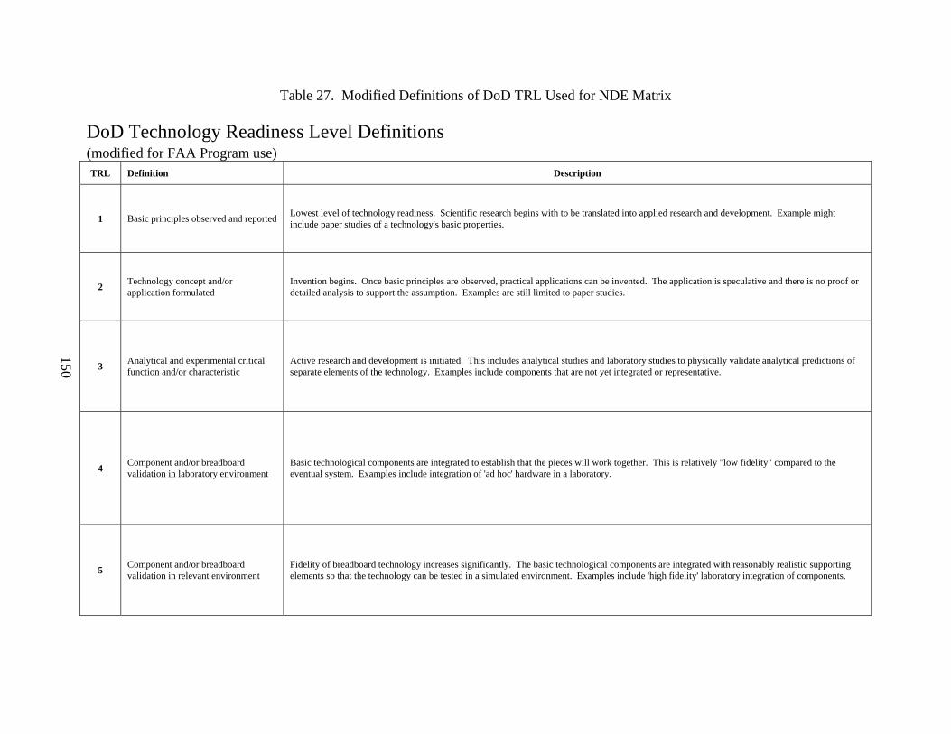
Table 27. Modified Definitions of DoD TRL Used for NDE Matrix
DoD Technology Readiness Level Definitions (modified for FAA Program use) TRL Definition Description
1 Basic principles observed and reported Lowest level of technology readiness. Scientific research begins with to be translated into applied research and development. Example might include paper studies of a technology's basic properties.
2 Technology concept and/or application formulated
Invention begins. Once basic principles are observed, practical applications can be invented. The application is speculative and there is no proof or detailed analysis to support the assumption. Examples are still limited to paper studies.
3 Analytical and experimental critical function and/or characteristic
Active research and development is initiated. This includes analytical studies and laboratory studies to physically validate analytical predictions of separate elements of the technology. Examples include components that are not yet integrated or representative.
4 Component and/or breadboard validation in laboratory environment
Basic technological components are integrated to establish that the pieces will work together. This is relatively "low fidelity" compared to the eventual system. Examples include integration of 'ad hoc' hardware in a laboratory.
5 Component and/or breadboard validation in relevant environment
Fidelity of breadboard technology increases significantly. The basic technological components are integrated with reasonably realistic supporting elements so that the technology can be tested in a simulated environment. Examples include 'high fidelity' laboratory integration of components.
150

151
Table 27. Modified Definitions of DoD TRL Used for NDE Matrix (Continued)
TRL Definition Description
6 System/subsystem model or prototype demonstration in a relevant environment
Representative model or prototype system, which is well beyond the breadboard tested for TRL 5, is tested in a relevant environment. Represents a major step up in a technology's demonstrated readiness. Examples include testing a prototype in a high fidelity laboratory environment or in simulated operational environment.
7 System prototype demonstration in a operational environment
Prototype near or at planned operational system. Represents a major step up from TRL 6, requiring the demonstration of an actual system prototype in an operational environment. Examples include testing the prototype in a test bed production, depot or in-service facility.
8 Actual system completed and 'qualified' through test and demonstration
Technology has been proven to work in its final form and under expected conditions. In almost all cases, this TRL represents the end of true system development. Examples include developmental test and evaluation of the system in its intended system to determine if it meets design specifications.
9 Actual system 'proven' through successful operations
Actual application of the technology in its final form and under nominal conditions, such as those encountered in operational test and evaluation. In almost all cases, this is the end of the last "bug fixing" aspects of true system development. Examples include using the system under operational conditions.
10 Actual system 'used' in normal operations
Nominal application of the technology in its final form and under production, depot or in-service conditions.

The DoD MRL and TRL definitions and terminology are as follows: Production-relevant environment—An environment normally found during MRL 5 and 6
that contains key elements of production realism not normally found in the laboratory environment (e.g., uses production personnel, materials, equipment, tooling, process steps, work instructions, or stated cycle time). May occur in a laboratory or model shop if key elements or production realism are added.
Production representative environment—An environment normally found during MRL 7
(probably on the manufacturing floor) that contains most of the key elements (tooling, equipment, temperature, cleanliness, lighting, personnel skill levels, materials, work instructions, etc.) that will be present in the shop floor production areas where low-rate production will eventually take place.
Pilot line environment—An environment normally found during MRL 8 in a
manufacturing floor production area that incorporates all the key elements (equipment, personnel skill levels, materials, components, work instructions, tooling, etc.) required to produce production configuration items, subsystems or systems that meet design requirements in low-rate production. To the maximum extent practical, the pilot line should use rate production processes.
Manufacturability—The characteristics considered in the design cycle that focus on
process capabilities, machine or facility flexibility, and the overall ability to consistently produce at the required level of cost and quality. Activities can include some or all of the following activities:
- Design for commonality and standardization—fewer parts
- Perform comprehensive Technology Assessment, including commercial industrial
applications and the supplier base
Design for multi- and dual-use applications Design for modularity and plug-compatible interface/integration Design for flexibility, adaptability, and robust design Utilize reliable processes and materials
Producibility—Is the capability of an item to be produced, including some or all of the
following activities:
- Design to specific Cp-CpK process control parameters—six sigma - Perform material characterization analysis - Perform variability reduction analysis—Taguchi, DOE - Develop critical materials and processes before selecting product design - Use pervasive modeling and simulation for product and process design tradeoffs - Design and deployment of closed-loop process control on critical items
152
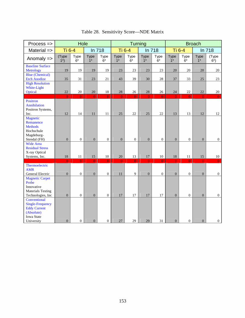
Table 28. Sensitivity Score—NDE Matrix
Process => Hole Turning Broach Material => Ti 6-4 In 718 Ti 6-4 In 718 Ti 6-4 In 718
Anomaly => (Type 1*)
Type 6*
Type 1*
Type 6*
Type 1*
Type 6*
Type 1*
Type 6*
Type 1*
Type 6*
Type 1*
(Type 6*)
Baseline Surface Metrology 19 19 19 19 23 23 23 23 20 20 20 20 Blue (Chemical) Etch Anodize 35 31 23 21 43 39 30 28 37 33 25 23 High Resolution White-Light Optical 22 20 20 18 28 26 28 26 24 22 22 20 0 0 0 0 0 0 0 0 0 0 0 0 Positron Annihilation Positron Systems, Inc. 12 14 11 11 25 22 25 22 13 13 12 12 Magnetic Remanence Methods Hochschule Magdeburg-Stendal (FH) 0 0 0 0 0 0 0 0 0 0 0 0 Wide Area Residual Stress X-ray Optical Systems, Inc. 18 11 15 10 20 13 17 10 18 11 15 10 0 0 0 0 0 0 0 0 0 0 0 0 Thermoelectric AMR General Electric 0 0 0 0 11 9 0 0 0 0 0 0 Magnetic Carpet Probe Innovative Materials Testing Technologies, Inc 0 0 0 0 17 17 17 17 0 0 0 0 Conventional Single-Frequency Eddy Current (Absolute) Iowa State University 0 0 0 0 27 29 29 31 0 0 0 0
153

154
Table 28. Sensitivity Score—NDE Matrix (Continued)
Process => Hole Turning Broach
Material => Ti 6-4 In 718 Ti 6-4 In 718 Ti 6-4 In 718
Anomaly => Type
1* Type
6* Type
1* Type
6* Type
1* Type
6* Type
1* Type
6* Type
1* Type
6* Type
1* Type
6*
Conventional Single-Frequency Eddy Current (Absolute Solenoid Bridge) Pratt and Whitney 0 0 0 0 26 28 28 30 0 0 0 0 Conventional Single-frequency Eddy Current (Differential ECP) Pratt and Whitney 0 0 0 0 0 0 0 0 0 0 0 0 0 0 0 0 0 0 0 0 0 0 0 0 Multiple-Frequency Phase Analysis Eddy Current General Electric 17 17 17 17 24 24 24 24 0 0 0 0 Swept High-Frequency Eddy Current Iowa State University 0 0 0 0 32 6 33 0 0 0 0 0 0 0 0 0 0 0 0 0 0 0 0 0 Normal-incidence Acoustic (Ultrasonic) Microscopy Iowa State University 0 0 0 0 19 20 20 21 0 0 0 0 Oblique-incidence Backscatter (Ultrasonic) Microscopy Iowa State University 0 0 0 0 15 13 14 12 0 0 0 0 0 0 0 0 0 0 0 0 0 0 0 0 High Energy X-Ray Diffraction Iowa State University 0 0 0 0 11 11 11 11 0 0 0 0 Other method 4 0 0 0 0 0 0 0 0 0 0 0 0
Other method 5 0 0 0 0 0 0 0 0 0 0 0 0

Table 29. Implementation Score—NDE Matrix
NDE Technique Total Score Implementation
Applicability in a production environment Speed & productivity
Applicability in a depot environment Speed & productivity
The maturity level of technology for use (MRL)
The maturity level of technology itself (TRL)
Return on Investment
Operator use and training NOTES
Baseline Surface Metrology
60 10 10 10 10 10 10 In common use
Blue (Chemical) Etch Anodize
56 10 9 10 10 7 10 In common use
High Resolution White-Light Optical
48 8 10 7 7 9 7
In common use, not directly applicable to NDE
Positron Annihilation Positron Systems, Inc.
24 2 2 6 7 2 5
Current production system utilized by Boeing Helicopter
Magnetic Remanence Methods Hochschule Magdeburg-Stendal (FH)
28 4 2 5 6 5 6
Magnetic remance methods are not directly applicable to the target anomalies and materials. Score is based on the ability to measure magnetic inclusions imbedded within the target materials through tool wear or contamination
Wide Area Residual Stress X-ray Optical Systems, Inc.
29 2 2 8 7 3 7
Current systems utilized in production, not directly applicable to NDE
155

Table 29. Implementation Score—NDE Matrix (Continued)
NDE Technique Total Score Implementation
Applicability in a production environment Speed & productivity
Applicability in a depot environment Speed & productivity
The maturity level of technology for use (MRL)
The maturity level of technology itself (TRL)
Return on Investment
Operator use and training NOTES
Thermoelectric AMR General Electric
17 2 2 3 3 3 4
Magnetic Carpet Probe Innovative Materials Testing Technologies, Inc
26 5 3 4 4 5 5
Conventional Single-frequency Eddy Current (Absolute) Iowa State University
47 8 6 9 9 8 7
Conventional Single-frequency Eddy Current (Absolute Solenoid Bridge) Pratt and Whitney
47 8 6 9 9 8 7
Conventional Single-frequency Eddy Current (Differential ECP) Pratt and Whitney
47 8 6 9 9 8 7
Multiple-frequency Phase Analysis Eddy Current General Electric
31 7 4 6 4 5 5
Swept High-frequency Eddy Current Iowa State University
28 5 3 6 4 4 6
156

157
Table 29. Implementation Score—NDE Matrix (Continued)
NDE Technique Total Score Implementation
Applicability in a production environment Speed & productivity
Applicability in a depot environment Speed & productivity
The maturity level of technology for use (MRL)
The maturity level of technology itself (TRL)
Return on Investment
Operator use and training NOTES
Normal-incidence Acoustic (Ultrasonic) Microscopy Iowa State University
29 4 3 5 6 4 7
Oblique-incidence Backscatter (Ultrasonic) Microscopy Iowa State University
25 3 3 4 5 4 6
High Energy X-Ray Diffraction Iowa State University
21 3 2 4 6 2 4
Other method 4 0
Other method 5 0

Table 30. Total Score—NDE Matrix
Process =>Material =>
Anomaly =>Type
1*Type
6*Type
1*Type
6*Type
1*Type
6*Type
1*Type
6*Type
1*Type
6*Type
1*Type
6*
Baseline Surface Metrology 136 19 19 19 19 152 23 23 23 23 140 20 20 20 20Blue (Chemical) Etch Anodize 166 35 31 23 21 196 43 39 30 28 174 37 33 25 23High Resolution White-Light Optical
128 22 20 20 18 156 28 26 28 26 136 24 22 22 20
21 21Positron AnnihilationPositron Systems, Inc.
117 15 14 14 14 155 26 22 25 22 110 13 13 12 12
Magnetic Remanence MethodsHochschule Magdeburg-Stendal (FH)
112 14 14 14 14 84 14 14
Polycapillary Collimating X-ray OpticsX-ray Optical Systems, Inc.
106 18 13 15 12
21 21Thermal-Electric AMRGeneral Electric
37 11 9
Magnetic Carpet ProbeInnovative Materials Testing Technologies, Inc
94 17 17 17 17
Conventional Single-frequency Eddy Current (Statistical Noise)Iowa State University
163 27 29 29 31 118 17 18 18 18
Conventional Single-frequency Eddy CurrentPratt and Whitney, Honeywell
109 15 16 15 16
Multiple-frequency Phase Analysis Eddy CurrentGeneral Electric
109 19 20 19 20 80 24 25
Swept High Frequency Eddy CurrentIowa State University
130 28 22 29 22
Normal-incidence Acoustic (Ultrasonic) MicroscopyIowa State University, Honeywell
83 14 12 15 13
Oblique-incidence Backscatter (Ultrasonic) MicroscopyIowa State University
81 15 13 16 12
High Energy X-Ray DiffractionIowa State University
75 16 11 16 11
Not Tested
Not Tested
Not Tested
Not Tested
Not Tested
Not Tested
Not Tested
Not Tested
Not Tested
Used for Sensitivity Analysis
Not Tested
Not Tested
Not Tested
Not Tested
Not Tested
Total Total Total
Not Tested
Not Tested
Not TestedNot Tested
Not Tested
Not Tested
Not Tested
Home
Ti 6-4 In718Ti 6-4 In718 Ti 6-4 In718Hole Turning Broach
4. SUMMARY AND CONCLUSIONS.
4.1 SUMMARY.
The primary objective of this program was to evaluate a number of advanced NDE methods to determine which, if any, have the potential to detect manufacturing (machining) defects that are difficult or impossible to identify using standard inspection techniques. Commonly used methods, such as visual or chemical etch, cannot effectively detect machining defects such as the two types studied in this program. Studies conducted by the MANHIRP program identified and characterized a range of defect types that can have detrimental effects on component performance. Based on the results of the MANHIRP characterization and fatigue studies, the ETC developed hole-drilling, broaching, and turning fabrication process parameters capable of producing two of the MANHIRP anomalies
158

(Type 1 and Type 6 defects) in nickel and titanium test samples. A Type 1 defect is defined as a surface-connected parent metal anomaly, while a Type 6 defect is defined as a subsurface parent metal anomaly with no visible or geometric connection to the surface. After development of the machining conditions, defects of varying severity (depth) were produced for use in NDE studies. Selection of the individual test samples was based on initial characterization of the defects using optical profilometry and white light microscopy. NDE methods in the program evaluation included positron annihilation, magnetic resonance, x-ray residual stress, high-energy XRD, eddy-current scanning (conventional, multifrequency, swept frequency, and magnetic carpet probe), thermoelectric AMR, and several UT approaches including surface wave UTs. 4.1.1 TEST SAMPLES.
Three manufacturing machining processes—hole drilling, broaching, and turning—were applied to nickel and titanium alloy samples using process parameters outside the acceptable machining range to produce material defects. Two types of defects, designated Type 1 and Type 6, were produced. A Type 1 defect is defined as a change to parent material that is continuous with the surface (e.g., microstructure damage, bent grains, white layer, amorphous layer, or heat damage), and is typically a result of lack of lubricant, excessively high feed rates, blunt tools, or material overheating. A Type 6 defect is defined as a change to parent material that is discontinuous with the surface (i.e., redeposited material or smearing of chips of parent material, which bond back onto surface), and is typically a result of redepositing of material (swarf or chips) from the machined surface. The material damage produced on samples ranged in depth from 0.0005 inch to greater than 0.002 inch. The primary depth of interest for material damage is less than 0.001 inch for both defect types. However, the damage range selected for this program was extended beyond 0.001 inch to allow the responses of various NDE methods to be graded on defects characterized from heavily to lightly damaged. The test samples used were purposely manufactured to minimize geometric surface distortion so attention could be focused on detecting material distortions caused by abusive machining conditions. 4.1.2 The NDE Method Evaluation—Results and Discussion.
NDE evaluation matrices were created to rank each method with respect to defect detectability and estimated production implementation potential. The data indicate the defect detectability of Type 1 and Type 6 defects in both nickel and titanium samples were essentially equivalent for all NDE methods. The Sensitivity Score is an estimate of the techniques’ ability to measure and discriminate an anomalous surface condition from a baseline condition. It includes rankings based upon: Signal-to-noise ratio Lateral resolution
159

Depth resolution Edge effect Flexibility to access the location of the defect Selectivity to indications The Implementation Score is based upon similar conditions and includes qualitative estimated rankings of: Applicability in a production environment Applicability in a depot environment The manufacturing readiness level (MRL) of technology for use The technology readiness level (TRL) of technology for itself Return on investment Operator use and training Although the results varied somewhat as a function of the machining process and some NDE methods were applied only to the turning samples due to geometry limitations (note asterisks), a general ranking of the capabilities of the methods is shown below. Detection Capability (highest to lowest)
6. Eddy current a. Single frequency** b. Multiple frequency* c. Swept frequency**
7. Positron annihilation*
8. X-ray residual stress*
9. UT microscopy** Magnetic carpet probe**
10. Thermoelectric AMR** High-energy XRD** Backscatter UT microscopy**
Production Implementation (easiest to most difficult)
1. Eddy Current
a. Single frequency b. Multiple frequency c. Swept frequency
160

2. Magnetic carpet probe 3. UT microscopy 4. Backscatter UT microscopy High-energy XRD 5. X-ray residual stress Positron annihilation Thermoelectric AMR *estimate based on data from turning, hole-drilling, and broaching samples **estimate based on data from turning sample only 4.1.3 Summary Comments on NDE Methods.
4.1.3.1 Eddy Current.
At the start of this program, it was anticipated that eddy-current methods would prove useful in some capacity toward evaluating the Type 1* and Type 6* defects under consideration. Eddy-current inspections are most sensitive at the surface, with exponential decaying sensitivity through the depth of the material. With a given set of nominal material properties, the depth of sensitivity can be tailored through selection of appropriate oscillation frequencies. Multiple interrogation depths can be evaluated using multiple oscillation frequencies and mixing algorithms to minimize undesirable conditions that interfere with the inspection process. 4.1.3.1.1 Single-Frequency Eddy-Current Methods.
An unexpected result of the tests was that the incoherent noise contained within the measurement process may be used as a statistical measure of material damage (as discussed in section 3.3.9). 4.1.3.1.2 Dual-Frequency Eddy-Current Methods.
Dual-frequency eddy current is usually applied to suppress background signals from spurious sources (e.g., geometric features) from interfering or confounding signals from the defects of interest. Once a frequency-mixing algorithm is defined, the data collection process is practically identical to the single-frequency eddy-current method (as demonstrated in section 3.3.9). 4.1.3.1.3 Multifrequency Eddy-Current Methods.
Multifrequency (i.e., greater than two) eddy-current methods are not routinely employed within the aero-engine community due to the added complexity and increased cost of the method. However, these methods have shown the ability to not only identify unacceptable surfaces, but have also shown the capability to grade the severity of anomalous damage (especially for Type 1* defects).
161

Because of the expensive instrumentation required, multifrequency methods, such as those described in section 3.3.7, would require additional development to reduce the number of relevant frequencies involved and decrease the time required per measurement location. 4.1.3.1.4 Magnetic Carpet Probe.
Recent advances in flexible printed circuit techniques coupled with advances in digital electronic devices have enabled development of a new eddy-current array probe, the magnetic carpet probe. Given the excellent detection capabilities demonstrated for both Ti Type 1* and Type 6* defects (see section 3.3.5), there appears to be a legitimate ability to differentiate between damaged and undamaged material conditions in simple, flat-plate samples. However, significant development work will be required to adapt this technology to complex geometries, such as holes or broach slots.
4.1.3.2 Other NDE Methods.
Although several other NDE methods were very successful in detecting Type 1* and Type 6* anomalies, the practical application of most will only be possible after significant additional technical work is completed. The problems that must be addressed before any of these other methods can be considered for production application are varied, since each method is in a different stage of development. The following list outlines the major problem areas.
Significant time required to setup, collect, and analyze data
- Thermoelectric AMR - High-energy XRD
Difficult to adapt to varying geometric features especially those containing edges
- Thermoelectric AMR - Parallel beam XRD - High-energy XRD - Surface wave UT - Normal incidence acoustic microscopy
Anomaly Detection Selectivity and Sensitivity
- Thermoelectric AMR - High-energy XRD - Normal incidence acoustic microscopy - Magnetic resonance (only nonmagnetic anomalies were considered)
162

Bulk property assessment rather than localized property assessment
- Positron annihilation - Thermoelectric AMR - Oblique incidence backscatter UT
4.2 CONCLUSIONS.
Although the primary objective of the program was to evaluate the capability of nondestructive evaluation (NDE) methods to detect manufacturing-induced defects, significant efforts were expended on support activities to successfully address this goal. The following is a brief description of each activity along with the key conclusions drawn from it.
An extensive literature search was completed to provide a background for selection of candidate NDE methods for inclusion in the program.
Conclusions: A significant amount of prior work was conducted to evaluate the effectiveness of various NDE methods to detect manufacturing defects. The highest priority ultrasonic, radiographic, and electromagnetic, and thermographic NDE methods were identified for consideration in the program evaluation.
Test sample fabrication was undertaken after attempts to procure test samples from the
Manufacturing to Produce High Integrity Rotating Parts for Modern Gas Turbines (MANHIRP) participants failed.
Conclusions: Machining parameters capable of producing two key defect types identified in the MANHIRP program were successfully developed for the hole-drilling, turning, and broaching processes. Several test sample sets containing nominally identical machining defects were produced for NDE method evaluation.
Baseline characteristics were determined for the test samples. Conclusions: All samples could be characterized using surface profilometry techniques. The degree of damage in the as-manufactured samples could be separated by surface roughness into light, medium, and severe. This ranking permitted sample separation into test sets that contained nominally equivalent assortments of defect types and surface conditions.
The sample test sets were used to evaluate the most promising NDE methods as
identified in the literature survey. Defect detection capabilities were evaluated by outside suppliers and the original equipment manufacturer laboratory personnel. The results were then ranked by relative ability to detect the machining defects and by the effort needed to transition the methods to a production inspection capability.
163

Conclusions: All the methods evaluated displayed some degree of capability to detect both machining defects. Three different techniques, single-, multi-, and swept-frequency eddy-current methods all showed high promise in detecting both defects. Positron annihilation and x-ray residual stress measurements were the next most promising methods evaluated.
The eddy-current methods were also rated highest in terms of having the least detrimental effect on manufacturing productivity. Slightly behind eddy current were the magnetic carpet probe and surface wave ultrasonic methods. The results of this program suggest that eddy-current techniques generally provided the best sensitivity to the two machining defects studied and are also estimated to have the least detrimental effect on machining productivity when implemented in a production environment. These conclusions, along with the sensitivity and implementation rankings, must be viewed with consideration given to the limited number and types of manufacturing defects evaluated and are only intended to serve as a guide for identification of the most promising NDE methods for possible future development. It should also be recognized that all the NDE methods would require some degree of optimization and refinement before being considered viable for detection of manufacturing defects in a production environment. 5. REFERENCES.
1. Margetan, F.J., Gigliotti, M., Brasche, L., and Leach, W., “Fundamental Studies: Inspection Properties for Engine Titanium Alloys,” FAA report DOT/FAA/AR-02/114, December 2002.
2. Brasche, L., Chiou, T., Thompson, B., Smith, K., Meeker, B., Margetan, F., Panetta, P., Chenail, R., Galli, F., Umbach, J., Raulerson, D., Degtyar, A., Bartos, J., Copley, D., McElligott, B., Howard, P., and Bashyam, M., “Contaminated Billet Study,” FAA report DOT/FAA/AR-05/16, September 2005.
3. Margetan, F.J., Nieters, E., Haldipur, P., Brasche, L., Chiou, T., Keller, M., Degtyar, A., Umbach, J., Hassan, W., Patton, T., and Smith, K., “Fundamental Studies of Nickel Billet Materials—Engine Titanium Consortium Phase II,” FAA report DOT/FAA/AR-05/17, June 2005.
4. Margetan, F., Nieters, E., Brasche, L., Yu, L., Degtyar, A., Wasan, H., Keller, M., and Kinney, A., “Fundamental Studies of Titanium Forging Materials—Engine Titanium Consortium Phase II,” FAA report DOT/FAA/AR-05/22, June 2005.
5. Keller, M., Patton, T., Degtyar, A., Umbach, J., Hassan, W., Kinney, A., Roberts, R., Margetan, F., and Brasche, L., “Inspection Development for Nickel Billet—Engine Titanium Consortium Phase II,” FAA report DOT/FAA/AR-05/29, September 2005.
164

6. Keller, M., Patton, T., Degtyar, A., Umbach, J., Hassan, W., Kinney, A., Roberts, R., Margetan, F., and Brasche, L., “Inspection Development for Titanium Billet—Engine Titanium Consortium Phase II,” FAA report DOT/FAA/AR-05/30, September 2005.
7. Margetan, F., Umbach, J., Roberts, R., Friedl, J., Degtyar, A., Keller, M., Hassan, W., Brasche, L., Klassen, A., Wasan, H., and Kinney, A., “Inspection Development for Titanium Forgings,” FAA report DOT/FAA/AR-05/46, May 2007.
8. Friedl, J., Roberts, R., Margetan, F., Degtyar, A., Hassan, W., Umbach, J., Brasche, L., and Keller, M., “Transducer Variability Study,” FAA report DOT/FAA/AR-07/46, July 2007.
9. Brasche, L., Clements, L., D’Orvilliers, A., Griffiths, K., Griffiths, W., Khandelwal, P., Kessler, T., Kinney, A., Larson, B., Lively, J., Lopez, R., Meeker, W., Stevens, J., Smith, K., and Vandiver, S., “Engineering Studies of Cleaning and Drying Processes in Preparation for Fluorescent Penetrant Inspection,” FAA report DOT/FAA/AR-03/73, January 2004.
10. Brasche, L., Mellors, T., Patton, T., Stephen, R., Smith, K., Kinney, A., Hassan, W., Ohm, J., and Schraan, J., “High-Speed Bolthole Eddy-Current Scanning for In-Service Inspection of Engine Disks,” FAA report DOT/FAA/AR-05/34, September 2005.
11. Keller, M., Degtyar, A., Umbach, J., and Brasche, L., “Inspection Development for Large-Diameter Titanium Billet—Engine Titanium Consortium Phase II,” FAA report DOT/FAA/AR-05/47, May 2007.
12. Thompson, R. B., Meeker, B., Keller, M., Umbach, J., Chiou, T., Wang, Y., Burkel, D., Hassan, W., Smith, K., Patton, T., and Brasche, L., “Update of Default Probability of Detection Curves for the Ultrasonic Detection of Hard Alpha Inclusions in Titanium Alloy Billets,” FAA report DOT/FAA/AR-07/63, February 2008.
13. National Transportation Safety Board website, www.ntsb.gov (last visited 11/17/10)
14. AIA Rotor Manufacturing Project Team, “Guidelines to Minimize Manufacturing-Induced Anomalies in Critical Rotating Parts,” FAA report DOT/FAA/AR-06/3, February 2006.
15. Fox, K.M., “Integrating Process Controls With Manufacturing to Produce High-Integrity Rotating Parts for Modern Gas Turbines,” Report No. MANHIRP-01-000006-WP1-RPT, August 2002.
16. MANHIRP public domain publications website, http://wzl-tf4.wzl.rwth-aachen.de /manhirp/ (last visited 11/17/10)
17. Feist, W.D., “Advances in NDI,” Presentation to FAA-ETC Open Forum IV, Burlington, Massachusetts, September 2005.
165

18. Feist, W.D., Mook, G., Taylor, S., Söderberg, H., Mikic, A., and Stepinski, T., “Non-Destructive Evaluation of Manufacturing Anomalies in Aero-Engine Rotor Disks,” Proceedings of the 16th World Conference in Nondestructive Testing, Montreal, Canada, August 2004.
19. Krause-Rehberg, R. and Leipner, H.S., Positron Annihilation in Semiconductors,
“Chapter 3: Experimental Techniques,” Springer-Verlag, New York, New York, 1999. 20. Holzwarth, U., Barbieri, A., Hansen-Ilzhöfer, S., and Haaks, M., “Positron Annihilation
Studies on the Migration of Deformation-Induced Vacancies in Stainless Steel AISI 316 L,” Applied Physics A: Materials Science & Processing, Vol. 73, No. 4, October 2001.
21. Kawaguchi, Y. and Shirai, Y., “Fatigue Evaluation of Type 316 Stainless Steel Using
Positron Annihilation Lineshape Analysis and β+-γ Coincidence Positron Lifetime Measurement,” Journal of Nuclear Science and Technology, Vol. 39, No. 10, October 2002, pp. 1033-1040
22. Hinken, J.H., Wrobel, H., Mook, G., and Simonin, J., “Detection and Characterization of
Ferromagnetic Inclusions in Non-Ferromagnetic Alloys,” 16th World Conference on Nondestructive Testing, Montreal, Canada, August 30-September 3, 2004. http://www.hs -magdeburg.de/fachbereiche/f-iwid/ET/Personen/Hinken/forschung/n14.html (last visited 11/17/10)
23. Hinken, J.H. and Tavrin, Y., “N6: Basics of the Thermoelectric Effect with Magnetic Readout,” http://www.hs-magdeburg.de/fachbereiche/f-iwid/ET/Personen/Hinken /forschung/N6.htm
24. Tavrin, Y. and Hinken, J.H., “N1: High-Resolution Magnetometry Based on Unshielded
SQUID System,” http://www.hs-magdeburg.de/fachbereiche/f-iwid/ET/Personen/Hinken /forschung/N1.htm
25. Cullity, B.D. and Stock, S.R., Element of X-Ray Diffraction, Addison-Wesley, Reading,
Massachusetts, 2001, Third Edition. 26. Klug, H.P. and Alexander, L.E., X-Ray Diffraction Procedures for Polycrystalline and
Amorphous Materials, Wiley-Interscience, Hoboken, New Jersey, Second Edition. 27. Huang H., Denver X-Ray Conference, “New Development of In Situ, Compact, Low-
Power XRD Systems,” Denver, Colorado, August 7-11, 2006. 28. Industrial Applications of X-ray Diffraction, F.H. Chung and D.K. Smith, eds., Marcel-
Dekker, Inc., New York, New York, 2000.
166

167
29. Sun, Y., et al., “Magnetic Carpet Probe for Large Area Instant Crack/Corrosion Detection and Health Monitoring,” Proceedings of the QNDE 2006 Conference, Portland, Oregon, July 30-August 4, 2006.
30. Sun, Y., et al., “Large Area Instant Crack Detection and Identification Using Magnetic
Carpet Probe,” Proceedings of the 9th Joint FAA/DoD/NASA Conference on Aging Aircraft, Atlanta, Georgia, March 6-9, 2006.
31. Tavrin, Y., Krivoy, J.S., Hinken, J.H., and Lallmeyer, J.P., “A Theoretical Method to
Detect Weak Local Structural Changes and Inclusions in Metal Parts,” Review of Progress in Quantitative Nondestructive Evaluation, Vol. 20, American Institute of Physics, New York, New York, 2001, pp. 1710-1716.
32. Nagy, P.B. and Nayfeh, A.H., “On the Thermoelectric Magnetic Field of Spherical and
Cylindrical Inclusions,” Journal of Applied Physics, Vol. 87, 2000, pp. 7481-7490. 33. Carreon, H., Nagy, P.B., and Nayfeh, A.H., “Thermoelectric Detection of Spherical Tin
Inclusions in Copper by Magnetic Sensing,” Journal of Applied Physics, Vol. 88, 2000, pp. 6495-6500.
34. Nayfeh, A.H. and Faidi, W., “Theoretical Investigations of the Thermoelectric Magnetic
Field in Metal Material Characterizations,” Proceedings of the 7th ASME NDE Topical Conference 20, 2001, The American Society of Mechanical Engineers, New York, New York, pp. 201-207.
35. Nayfeh, A.H. and Faidi, W., “Thermoelectrically Induced Magnetic Field of Elliptical
Cylindrical and Spheroidal Inclusions,” European Physical Journal—Applied Physics, Vol. 19, No. 2, September 2002.
36. Carreon, H., Nagy, P.B., and Blodgett, M.P., “Thermoelectric Nondestructive Evaluation
of Residual Stress in Shot-Peened Metals,” Research in Nondestructive Evaluation, Vol. 14, No. 2, June 2002.
37. Carreon, H., Nagy, P.B., and Blodgett, M.P., “Thermoelectric Nondestructive Evaluation
of Residual Stress in Shot-Peened Metals,” Review of Progress in Quantitative Nondestructive Evaluation, Vol. 21, AIP, Melville, New York, 2002.
38. Carreon, H. and Nagy, P.B., “Characterization of Shot-Peened Surface by a
Noncontacting Thermoelectric Method,” Nondestructive Evaluation and Characterization of Engineering Materials for Reliability and Durability Predictions, Vol. 18, The American Society of Mechanical Engineers, New York, New York, 2000, pp. 31-39.

39. Carreon, H. and Nagy, P.B., “Detection of Surface Imperfections in Metals by a Noncontacting Thermoelectric Method,” Proceedings of the 7th ASME NDE Topical Conference 20, The American Society of Mechanical Engineers, New York, New York, 2001, pp. 209-215.
40. U.S. Patent 7,206,706, Inspection Method and System Using Multifrequency Phase
Analysis. 41. Libby, H.L., Introduction to Electromagnetic Nondestructive Test Methods, Wiley-
Interscience, New York, New York, 1971. 42. Moulder, J.C., Kubovich, M.W., Uzal, E., and Rose, J.H., Review of Progress in QNDE,
Vol. 14B, Thompson D.O. and Chimenti, D.E., eds., Plenum Press, New York, New York, 1995, pp. 2065.
43. Plotnikov, Y.A. and Bantz, W.J., “Subsurface Anomaly Detection in Metals With Pulsed
Eddy Current,” Review of Progress in QNDE, Vol. 24A, Thompson, D.O. and Chimenti, D.E., eds., AIP, Melville, New York, 2005, pp. 447-454.
44. Plotnikov, Y.A., Nath, S.C., and Rose, C.W., “Anomaly Characterization in Multi-
Layered Conductive Components with Pulsed Eddy Current,” Review of Progress in QNDE, Vol. 21A, AIP, Melville, New York, 2002, pp. 1976-1983.
45. Smith, R.A. and Hugo, G.R., “Transient Eddy Current NDE for Aging Aircraft—
Capabilities and Limitations,” Insight, Vol. 43, No. 1, January 2001, pp. 14. 46. Briggs, A., “An Introduction to Scanning Acoustic Microscopy,” Royal Microscopic
Society, Microscopy Handbook 12, 1986, pp. 26-32. 47. Semmens, J. and Canumalla, S., “Application of Highly Focused, High-Frequency
Transducers for Evaluation of Near-Surface Flaws and Thin Packages: Smart Cards, Flip Chip, Flex Circuits, and Thick Films,” Proceedings of Pan Pacific Conference, Hawaii, 1999.
48. Canumalla, S. and Oravecz, M.G., “Nondestructive Elastic Property Characterization of
I’C Encapsulated,” ASME Symposium and Applications of Fracture Mechanics in Electronic Packaging, 1997, pp. 151.
168

APPENDIX A—TEST SAMPLE SERIAL NUMBER IDENTIFICATION
Table A-1. Turning Samples
Sample ID Material
Sample Thickness
(inch)
Sample Dimensions
(inch) Target
Anomaly Manufacturing Description
and Target Anomaly In-T-P-10-080725 In 718 0.2 2.0 x 1.0 None Nominal - Option C In-T-P-1-080725 In 718 0.2 2.0 x 1.0 None Nominal - Option C In-T-P-11-080725 In 718 0.2 2.0 x 1.0 None Nominal - Option C In-T-P-12-080725 In 718 0.2 2.0 x 1.0 None Nominal - Option C In-T-P-13-080725 In 718 0.2 2.0 x 1.0 None Nominal - Option C In-T-P-14-080725 In 718 0.2 2.0 x 1.0 None Nominal - Option C In-T-P-15-080725 In 718 0.2 2.0 x 1.0 None Nominal - Option C In-T-P-16-080725 In 718 0.2 2.0 x 1.0 None Nominal - Option C In-T-P-17-080725 In 718 0.2 2.0 x 1.0 None Nominal - Option C In-T-P-18-080725 In 718 0.2 2.0 x 1.0 None Nominal - Option C In-T-P-19-080725 In 718 0.2 2.0 x 1.0 None Nominal - Option C In-T-P-20-080725 In 718 0.2 2.0 x 1.0 None Nominal - Option C In-T-P-2-080725 In 718 0.2 2.0 x 1.0 None Nominal - Option C In-T-P-21-080725 In 718 0.2 2.0 x 1.0 None Nominal - Option C In-T-P-3-080725 In 718 0.2 2.0 x 1.0 None Nominal - Option C In-T-P-4-080725 In 718 0.2 2.0 x 1.0 None Nominal - Option C In-T-P-5-080725 In 718 0.2 2.0 x 1.0 None Nominal - Option C In-T-P-6-080725 In 718 0.2 2.0 x 1.0 None Nominal - Option C In-T-P-7-080725 In 718 0.2 2.0 x 1.0 None Nominal - Option C In-T-P-8-080725 In 718 0.2 2.0 x 1.0 None Nominal - Option C In-T-P-9-080725 In 718 0.2 2.0 x 1.0 None Nominal - Option C In-T-T1-1-070112 In 718 0.2 1.8 x 1.0 Type 1 Very High Deformation: >0.002 depth In-T-T1A-1-080722-S In 718 ??? ??? Type 1* Light Deformation: <0.0005 depth In-T-T1A-1-081130-M In 718 ??? ??? Type 1* Medium Deformation: 0.0005>
<0.0015 depth In-T-T1A-2-080722-S In 718 ??? ??? Type 1* Light Deformation: <0.0005 depth In-T-T1A-2-081130-M In 718 ??? ??? Type 1* Medium Deformation: 0.0005>
<0.0015 depth In-T-T1A-3-080722-S In 718 ??? ??? Type 1* Light Deformation: <0.0005 depth In-T-T1A-3-081130-M In 718 ??? ??? Type 1* Medium Deformation: 0.0005>
<0.0015 depth In-T-T1A-4-080722-S In 718 ??? ??? Type 1* Light Deformation: <0.0005 depth In-T-T1A-4-081130-M In 718 ??? ??? Type 1* Medium Deformation: 0.0005>
<0.0015 depth In-T-T1A-5-080722-S In 718 ??? ??? Type 1* Light Deformation: <0.0005 depth In-T-T1A-5-081130-M In 718 ??? ??? Type 1* Medium Deformation: 0.0005>
<0.0015 depth In-T-T1A-6-080722-S In 718 ??? ??? Type 1* Light Deformation: <0.0005 depth In-T-T1A-6-081130-M In 718 ??? ??? Type 1* Medium Deformation: 0.0005>
<0.0015 depth In-T-T1A-7-080722-S In 718 ??? ??? Type 1* Light Deformation: <0.0005 depth
A-1
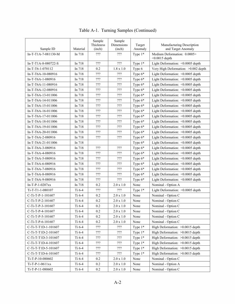
Table A-1. Turning Samples (Continued)
Sample ID Material
Sample Thickness
(inch)
Sample Dimensions
(inch) Target
Anomaly Manufacturing Description
and Target Anomaly In-T-T1A-7-081130-M In 718 ??? ??? Type 1* Medium Deformation: 0.0005>
<0.0015 depth In-T-T1A-8-080722-S In 718 ??? ??? Type 1* Light Deformation: <0.0005 depth In-T-T6-1-070112 In 718 0.2 1.8 x 1.0 Type 6 Very High Deformation: >0.002 depth In-T-T6A-10-080916 In 718 ??? ??? Type 6* Light Deformation: <0.0005 depth In-T-T6A-1-080916 In 718 ??? ??? Type 6* Light Deformation: <0.0005 depth In-T-T6A-11-080916 In 718 ??? ??? Type 6* Light Deformation: <0.0005 depth In-T-T6A-12-080916 In 718 ??? ??? Type 6* Light Deformation: <0.0005 depth In-T-T6A-13-011006 In 718 ??? ??? Type 6* Light Deformation: <0.0005 depth In-T-T6A-14-011006 In 718 ??? ??? Type 6* Light Deformation: <0.0005 depth In-T-T6A-15-011006 In 718 ??? ??? Type 6* Light Deformation: <0.0005 depth In-T-T6A-16-011006 In 718 ??? ??? Type 6* Light Deformation: <0.0005 depth In-T-T6A-17-011006 In 718 ??? ??? Type 6* Light Deformation: <0.0005 depth In-T-T6A-18-011006 In 718 ??? ??? Type 6* Light Deformation: <0.0005 depth In-T-T6A-19-011006 In 718 ??? ??? Type 6* Light Deformation: <0.0005 depth In-T-T6A-20-011006 In 718 ??? ??? Type 6* Light Deformation: <0.0005 depth In-T-T6A-2-080916 In 718 ??? ??? Type 6* Light Deformation: <0.0005 depth In-T-T6A-21-011006 In 718 Type 6* Light Deformation: <0.0005 depth In-T-T6A-3-080916 In 718 ??? ??? Type 6* Light Deformation: <0.0005 depth In-T-T6A-4-080916 In 718 ??? ??? Type 6* Light Deformation: <0.0005 depth In-T-T6A-5-080916 In 718 ??? ??? Type 6* Light Deformation: <0.0005 depth In-T-T6A-6-080916 In 718 ??? ??? Type 6* Light Deformation: <0.0005 depth In-T-T6A-7-080916 In 718 ??? ??? Type 6* Light Deformation: <0.0005 depth In-T-T6A-8-080916 In 718 ??? ??? Type 6* Light Deformation: <0.0005 depth In-T-T6A-9-080916 In 718 ??? ??? Type 6* Light Deformation: <0.0005 depth In-T-P-1-0207xx In 718 0.2 2.0 x 1.0 None Nominal - Option A Ti-T-T1-1-080107 Ti 6-4 ??? ??? Type 1* Light Deformation: <0.0005 depth C-Ti-T-P-1-101607 Ti 6-4 0.2 2.0 x 1.0 None Nominal - Option C C-Ti-T-P-2-101607 Ti 6-4 0.2 2.0 x 1.0 None Nominal - Option C C-Ti-T-P-3-101607 Ti 6-4 0.2 2.0 x 1.0 None Nominal - Option C C-Ti-T-P-4-101607 Ti 6-4 0.2 2.0 x 1.0 None Nominal - Option C C-Ti-T-P-5-101607 Ti 6-4 0.2 2.0 x 1.0 None Nominal - Option C C-Ti-T-P-6-101607 Ti 6-4 0.2 2.0 x 1.0 None Nominal - Option C C-Ti-T-T1D-1-101607 Ti 6-4 ??? ??? Type 1* High Deformation: >0.0015 depth C-Ti-T-T1D-2-101607 Ti 6-4 ??? ??? Type 1* High Deformation: >0.0015 depth C-Ti-T-T1D-3-101607 Ti 6-4 ??? ??? Type 1* High Deformation: >0.0015 depth C-Ti-T-T1D-4-101607 Ti 6-4 ??? ??? Type 1* High Deformation: >0.0015 depth C-Ti-T-T1D-5-101607 Ti 6-4 ??? ??? Type 1* High Deformation: >0.0015 depth C-Ti-T-T1D-6-101607 Ti 6-4 ??? ??? Type 1* High Deformation: >0.0015 depth Ti-T-P-10-080602 Ti 6-4 0.2 2.0 x 1.0 None Nominal - Option C Ti-T-P-1-0611xx Ti 6-4 0.2 2.0 x 1.0 None Nominal - Option A Ti-T-P-11-080602 Ti 6-4 0.2 2.0 x 1.0 None Nominal - Option C
A-2

Table A-1. Turning Samples (Continued)
Sample ID Material
Sample Thickness
(inch)
Sample Dimensions
(inch) Target
Anomaly Manufacturing Description
and Target Anomaly Ti-T-P-12-080602 Ti 6-4 0.2 2.0 x 1.0 None Nominal - Option C Ti-T-P-13-080602 Ti 6-4 0.2 2.0 x 1.0 None Nominal - Option C Ti-T-P-14-080602 Ti 6-4 0.2 2.0 x 1.0 None Nominal - Option C Ti-T-P-15-080602 Ti 6-4 0.2 2.0 x 1.0 None Nominal - Option C Ti-T-P-16-080602 Ti 6-4 0.2 2.0 x 1.0 None Nominal - Option C Ti-T-P-8-080602 Ti 6-4 0.2 2.0 x 1.0 None Nominal - Option C Ti-T-P-9-080602 Ti 6-4 0.2 2.0 x 1.0 None Nominal - Option C Ti-T-T1-1-061031 Ti 6-4 0.2 1.8 x 1.0 Type 1 Very High Deformation: >0.002 depth Ti-T-T1-1-080107a Ti 6-4 ??? ??? Type 1* Light Deformation: <0.0005 depth Ti-T-T1-2-080107 Ti 6-4 ??? ??? Type 1* Light Deformation: <0.0005 depth Ti-T-T1-2-080107b Ti 6-4 ??? ??? Type 1* High Deformation: >0.0015 depth Ti-T-T1-3-080107 Ti 6-4 ??? ??? Type 1* Light Deformation: <0.0005 depth Ti-T-T1-4-080107 Ti 6-4 ??? ??? Type 1* Light Deformation: <0.0005 depth Ti-T-T1-5-080107 Ti 6-4 ??? ??? Type 1* Light Deformation: <0.0005 depth Ti-T-T1-6-080107 Ti 6-4 ??? ??? Type 1* Light Deformation: <0.0005 depth Ti-T-T1-7-080107 Ti 6-4 ??? ??? Type 1* Light Deformation: <0.0005 depth Ti-T-T1A-10-080606-M Ti 6-4 ??? ??? Type 1* Medium Deformation: 0.0005>
<0.0015 depth Ti-T-T1A-11-080606-M Ti 6-4 ??? ??? Type 1* Medium Deformation: 0.0005>
<0.0015 depth Ti-T-T1A-12-080606-M Ti 6-4 ??? ??? Type 1* Medium Deformation: 0.0005>
<0.0015 depth Ti-T-T1A-13-080606-M Ti 6-4 ??? ??? Type 1* Medium Deformation: 0.0005>
<0.0015 depth Ti-T-T1A-14-080606-M Ti 6-4 ??? ??? Type 1* Medium Deformation: 0.0005>
<0.0015 depth Ti-T-T1A-15-080606-M Ti 6-4 ??? ??? Type 1* Medium Deformation: 0.0005>
<0.0015 depth Ti-T-T1A-16-080606-M Ti 6-4 ??? ??? Type 1* Medium Deformation: 0.0005>
<0.0015 depth Ti-T-T1A-9-080606-M Ti 6-4 ??? ??? Type 1* Medium Deformation: 0.0005>
<0.0015 depth Ti-T-T6-1-061031 Ti 6-4 0.2 1.7 x 1.0 Type 6 Very High Deformation: >0.002 depth Ti-T-T6-1-080508 Ti 6-4 ??? ??? Type 6* Medium Deformation: 0.0005>
<0.0015 depth ??? Ti-T-T6-2-080508 Ti 6-4 ??? ??? Type 6* Medium Deformation: 0.0005>
<0.0015 depth ??? Ti-T-T6-3-080508 Ti 6-4 ??? ??? Type 6* Medium Deformation: 0.0005>
<0.0015 depth ??? Ti-T-T6-4-080508 Ti 6-4 ??? ??? Type 6* Medium Deformation: 0.0005>
<0.0015 depth ??? Ti-T-T6-5-080508 Ti 6-4 ??? ??? Type 6* Medium Deformation: 0.0005>
<0.0015 depth ??? Ti-T-T6-6-080508 Ti 6-4 ??? ??? Type 6* Medium Deformation: 0.0005>
<0.0015 depth ???
A-3

Table A-1. Turning Samples (Continued)
Sample ID Material
Sample Thickness
(inch)
Sample Dimensions
(inch) Target
Anomaly Manufacturing Description
and Target Anomaly Ti-T-T6-7-080508 Ti 6-4 ??? ??? Type 6* Medium Deformation: 0.0005>
<0.0015 depth ??? Ti-T-T6-8-080508 Ti 6-4 ??? ??? Type 6* Medium Deformation: 0.0005>
<0.0015 depth ??? Ti-T-T6A-10-080602 Ti 6-4 ??? ??? Type 6* Medium Deformation: 0.0005>
<0.0015 depth ??? Ti-T-T6A-11-080602 Ti 6-4 ??? ??? Type 6* Medium Deformation: 0.0005>
<0.0015 depth ??? Ti-T-T6A-12-080602 Ti 6-4 ??? ??? Type 6* Medium Deformation: 0.0005>
<0.0015 depth ??? Ti-T-T6A-13-080602 Ti 6-4 ??? ??? Type 6* Medium Deformation: 0.0005>
<0.0015 depth ??? Ti-T-T6A-14-080602 Ti 6-4 ??? ??? Type 6* Medium Deformation: 0.0005>
<0.0015 depth ??? Ti-T-T6A-15-080602 Ti 6-4 ??? ??? Type 6* Medium Deformation: 0.0005>
<0.0015 depth ??? Ti-T-T6A-16-080602 Ti 6-4 ??? ??? Type 6* Medium Deformation: 0.0005>
<0.0015 depth ??? Ti-T-T6A-17-081201 Ti 6-4 ??? ??? Type 6* Medium Deformation: 0.0005>
<0.0015 depth ??? Ti-T-T6A-18-081201 Ti 6-4 ??? ??? Type 6* Medium Deformation: 0.0005>
<0.0015 depth ??? Ti-T-T6A-19-081201 Ti 6-4 ??? ??? Type 6* Medium Deformation: 0.0005>
<0.0015 depth ??? Ti-T-T6A-20-081201 Ti 6-4 ??? ??? Type 6* Medium Deformation: 0.0005>
<0.0015 depth ??? Ti-T-T6A-21-081201 Ti 6-4 ??? ??? Type 6* Medium Deformation: 0.0005>
<0.0015 depth ??? Ti-T-T6A-22-081201 Ti 6-4 ??? ??? Type 6* Medium Deformation: 0.0005>
<0.0015 depth ??? Ti-T-T6A-23-081201 Ti 6-4 ??? ??? Type 6* Medium Deformation: 0.0005>
<0.0015 depth ??? Ti-T-T6A-24-081201 Ti 6-4 ??? ??? Type 6* Medium Deformation: 0.0005>
<0.0015 depth ??? Ti-T-T6A-8-080602 Ti 6-4 ??? ??? Type 6* Medium Deformation: 0.0005>
<0.0015 depth ??? Ti-T-T6A-9-080602 Ti 6-4 ??? ??? Type 6* Medium Deformation: 0.0005>
<0.0015 depth ???
A-4

Table A-2. Hole-Drilling Samples
Sample ID Material
Sample Thickness
(inch (mm))
Sample Dimensions
(inch)
Unique Dimension (inch (mm))
Target Anomaly
Manufacturing Description and Target Anomaly
Manufacturing Processes Used
In-D-P-1-061215 In 718 0.34 (8.5) 1.0 x 1.0 0.276 (7.0) None Nominal Option A - GE Specification P11TF12
Drill + Ream + Edgebreak
In-D-P-2-061215 In 718 0.34 (8.5) 1.0 x 1.0 0.276 (7.0) None Nominal Option A - GE Specification P11TF12
Drill + Ream + Edgebreak
In-D-P-3-061215 In 718 0.34 (8.5) 1.0 x 1.0 0.276 (7.0) None Nominal Option A - GE Specification P11TF12
Drill + Ream + Edgebreak
In-D-P-4-061215 In 718 0.34 (8.5) 1.0 x 1.0 0.276 (7.0) None Nominal Option A - GE Specification P11TF12
Drill + Ream + Edgebreak
In-D-P-5-061215 In 718 0.34 (8.5) 1.0 x 1.0 0.276 (7.0) None Nominal Option A - GE Specification P11TF12
Drill + Ream + Edgebreak
In-D-P-6-061215 In 718 0.34 (8.5) 1.0 x 1.0 0.276 (7.0) None Nominal Option A - GE Specification P11TF12
Drill + Ream + Edgebreak
In-D-P-7-070710 In 718 0.34 (8.5) 1.0 x 1.0 0.276 (7.0) None Nominal Option C - GE Specification P11TF12
Drill + Ream + Edgebreak
In-D-P-8-070710 In 718 0.34 (8.5) 1.0 x 1.0 0.276 (7.0) None Nominal Option C - GE Specification P11TF12
Drill + Ream + Edgebreak
In-D-P-9-070710 In 718 0.34 (8.5) 1.0 x 1.0 0.276 (7.0) None Nominal Option C - GE Specification P11TF12
Drill + Ream + Edgebreak
In-D-P-10-70710 In 718 0.34 (8.5) 1.0 x 1.0 0.276 (7.0) None Nominal Option C - GE Specification P11TF12
Drill + Ream + Edgebreak
In-D-P-11-70710 In 718 0.34 (8.5) 1.0 x 1.0 0.276 (7.0) None Nominal Option C - GE Specification P11TF12
Drill + Ream + Edgebreak
In-D-P-12-70710 In 718 0.34 (8.5) 1.0 x 1.0 0.276 (7.0) None Nominal Option C - GE Specification P11TF12
Drill + Ream + Edgebreak
In-D-P-13-070710 In 718 0.34 (8.5) 1.0 x 1.0 0.276 (7.0) None Nominal Option C - GE Specification P11TF12
Drill + Ream + Edgebreak
In-D-P-14-070710 In 718 0.34 (8.5) 1.0 x 1.0 0.276 (7.0) None Nominal Option C - GE Specification P11TF12
Drill + Ream + Edgebreak
In-D-P-15-070710 In 718 0.34 (8.5) 1.0 x 1.0 0.276 (7.0) None Nominal Option C - GE Specification P11TF12
Drill + Ream + Edgebreak
In-D-P-16-070710 In 718 0.34 (8.5) 1.0 x 1.0 0.276 (7.0) None Nominal Option C - GE Specification P11TF12
Drill + Ream + Edgebreak
In-D-P-17-070710 In 718 0.34 (8.5) 1.0 x 1.0 0.276 (7.0) None Nominal Option C - GE Specification P11TF12
Drill + Ream + Edgebreak
In-D-P-18-070710 In 718 0.34 (8.5) 1.0 x 1.0 0.276 (7.0) None Nominal Option C - GE Specification P11TF12
Drill + Ream + Edgebreak
A-5
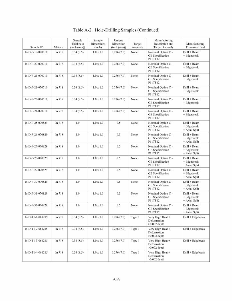
Table A-2. Hole-Drilling Samples (Continued)
Sample ID Material
Sample Thickness
(inch (mm))
Sample Dimensions
(inch)
Unique Dimension (inch (mm))
Target Anomaly
Manufacturing Description and Target Anomaly
Manufacturing Processes Used
In-D-P-19-070710 In 718 0.34 (8.5) 1.0 x 1.0 0.276 (7.0) None Nominal Option C - GE Specification P11TF12
Drill + Ream + Edgebreak
In-D-P-20-070710 In 718 0.34 (8.5) 1.0 x 1.0 0.276 (7.0) None Nominal Option C - GE Specification P11TF12
Drill + Ream + Edgebreak
In-D-P-21-070710 In 718 0.34 (8.5) 1.0 x 1.0 0.276 (7.0) None Nominal Option C - GE Specification P11TF12
Drill + Ream + Edgebreak
In-D-P-21-070710 In 718 0.34 (8.5) 1.0 x 1.0 0.276 (7.0) None Nominal Option C - GE Specification P11TF12
Drill + Ream + Edgebreak
In-D-P-23-070710 In 718 0.34 (8.5) 1.0 x 1.0 0.276 (7.0) None Nominal Option C - GE Specification P11TF12
Drill + Ream + Edgebreak
In-D-P-24-070710 In 718 0.34 (8.5) 1.0 x 1.0 0.276 (7.0) None Nominal Option C - GE Specification P11TF12
Drill + Ream + Edgebreak
In-D-P-25-070829 In 718 1.0 1.0 x 1.0 0.5 None Nominal Option C - GE Specification P11TF12
Drill + Ream + Edgebreak + Axial Split
In-D-P-26-070829 In 718 1.0 1.0 x 1.0 0.5 None Nominal Option C - GE Specification P11TF12
Drill + Ream + Edgebreak + Axial Split
In-D-P-27-070829 In 718 1.0 1.0 x 1.0 0.5 None Nominal Option C - GE Specification P11TF12
Drill + Ream + Edgebreak + Axial Split
In-D-P-28-070829 In 718 1.0 1.0 x 1.0 0.5 None Nominal Option C - GE Specification P11TF12
Drill + Ream + Edgebreak + Axial Split
In-D-P-29-070829 In 718 1.0 1.0 x 1.0 0.5 None Nominal Option C - GE Specification P11TF12
Drill + Ream + Edgebreak + Axial Split
In-D-P-30-070829 In 718 1.0 1.0 x 1.0 0.5 None Nominal Option C - GE Specification P11TF12
Drill + Ream + Edgebreak + Axial Split
In-D-P-31-070829 In 718 1.0 1.0 x 1.0 0.5 None Nominal Option C - GE Specification P11TF12
Drill + Ream + Edgebreak + Axial Split
In-D-P-32-070829 In 718 1.0 1.0 x 1.0 0.5 None Nominal Option C - GE Specification P11TF12
Drill + Ream + Edgebreak + Axial Split
In-D-T1-1-061215 In 718 0.34 (8.5) 1.0 x 1.0 0.276 (7.0) Type 1 Very High Heat + Deformation: >0.002 depth
Drill + Edgebreak
In-D-T1-2-061215 In 718 0.34 (8.5) 1.0 x 1.0 0.276 (7.0) Type 1 Very High Heat + Deformation: >0.002 depth
Drill + Edgebreak
In-D-T1-3-061215 In 718 0.34 (8.5) 1.0 x 1.0 0.276 (7.0) Type 1 Very High Heat + Deformation: >0.002 depth
Drill + Edgebreak
In-D-T1-4-061215 In 718 0.34 (8.5) 1.0 x 1.0 0.276 (7.0) Type 1 Very High Heat + Deformation: >0.002 depth
Drill + Edgebreak
A-6

Table A-2. Hole-Drilling Samples (Continued)
Sample ID Material
Sample Thickness
(inch (mm))
Sample Dimensions
(inch)
Unique Dimension (inch (mm))
Target Anomaly
Manufacturing Description and Target Anomaly
Manufacturing Processes Used
In-D-T1-5-061215 In 718 0.34 (8.5) 1.0 x 1.0 0.276 (7.0) Type 1 Very High Heat + Deformation: >0.002 depth
Drill + Edgebreak
In-D-T1-6-061215 In 718 0.34 (8.5) 1.0 x 1.0 0.276 (7.0) Type 1 Very High Heat + Deformation: >0.002 depth
Drill + Edgebreak
In-D-T1A-1-061215 In 718 0.34 (8.5) 1.0 x 1.0 0.276 (7.0) Type 1* Very High Heat + Deformation: >0.002 depth
Drill + Ream + Edgebreak
In-D-T1A-2-061215 In 718 0.34 (8.5) 1.0 x 1.0 0.276 (7.0) Type 1* Very High Heat + Deformation: >0.002 depth
Drill + Ream + Edgebreak
In-D-T1A-3-061215 In 718 0.34 (8.5) 1.0 x 1.0 0.276 (7.0) Type 1* Very High Heat + Deformation: >0.002 depth
Drill + Ream + Edgebreak
In-D-T1A-4-061215 In 718 0.34 (8.5) 1.0 x 1.0 0.276 (7.0) Type 1* Very High Heat + Deformation: >0.002 depth
Drill + Ream + Edgebreak
In-D-T1A-5-061215 In 718 0.34 (8.5) 1.0 x 1.0 0.276 (7.0) Type 1* Very High Heat + Deformation: >0.002 depth
Drill + Ream + Edgebreak
In-D-T1A-6-061215 In 718 0.34 (8.5) 1.0 x 1.0 0.276 (7.0) Type 1* Very High Heat + Deformation: >0.002 depth
Drill + Ream + Edgebreak
In-D-T1A-U1-080325 In 718 0.34 (8.5) 1.0 x 1.0 0.276 (7.0) Type 1* Used for metallography verification - not shipped
Drill + Ream + Edgebreak
In-D-T1A-U2-080325 In 718 0.34 (8.5) 1.0 x 1.0 0.276 (7.0) Type 1* High Heat + Deformation: >0.002 depth
Drill + Ream + Edgebreak
In-D-T1A-U3-080325 In 718 0.34 (8.5) 1.0 x 1.0 0.276 (7.0) Type 1* High Heat + Deformation: >0.002 depth
Drill + Ream + Edgebreak
In-D-T1A-U4-080325 In 718 0.34 (8.5) 1.0 x 1.0 0.276 (7.0) Type 1* Failed drill Drill + Ream + Edgebreak
In-D-T1A-U5-080325 In 718 0.34 (8.5) 1.0 x 1.0 0.276 (7.0) Type 1* High Heat + Deformation: >0.002 depth
Drill + Ream + Edgebreak
In-D-T1A-U6-080325 In 718 0.34 (8.5) 1.0 x 1.0 0.276 (7.0) Type 1* High Heat + Deformation: >0.002 depth
Drill + Ream + Edgebreak
In-D-T1A-U7-080325 In 718 0.34 (8.5) 1.0 x 1.0 0.276 (7.0) Type 1* Failed drill Drill + Ream + Edgebreak
In-D-T1A-V1-080325 In 718 0.34 (8.5) 1.0 x 1.0 0.276 (7.0) Type 1* High Heat + Deformation: >0.002 depth
Drill + Ream + Edgebreak
In-D-T1A-V2-080325 In 718 0.34 (8.5) 1.0 x 1.0 0.276 (7.0) Type 1* High Heat + Deformation: >0.002 depth
Drill + Ream + Edgebreak
In-D-T1A-V3-080325 In 718 0.34 (8.5) 1.0 x 1.0 0.276 (7.0) Type 1* High Heat + Deformation: >0.002 depth
Drill + Ream + Edgebreak
In-D-T1A-V4-080325 In 718 0.34 (8.5) 1.0 x 1.0 0.276 (7.0) Type 1* Failed drill Drill + Ream + Edgebreak
A-7

Table A-2. Hole-Drilling Samples (Continued)
Sample ID Material
Sample Thickness
(inch (mm))
Sample Dimensions
(inch)
Unique Dimension (inch (mm))
Target Anomaly
Manufacturing Description and Target Anomaly
Manufacturing Processes Used
In-D-T1A-V5-080325 In 718 0.34 (8.5) 1.0 x 1.0 0.276 (7.0) Type 1* High Heat + Deformation: >0.002 depth
Drill + Ream + Edgebreak
In-D-T1A-V6-080325 In 718 0.34 (8.5) 1.0 x 1.0 0.276 (7.0) Type 1* Used for metallography verification - not shipped
Drill + Ream + Edgebreak
In-D-T1A-V7-080325 In 718 0.34 (8.5) 1.0 x 1.0 0.276 (7.0) Type 1* Failed drill Drill + Ream + Edgebreak
In-D-T1A-W1-080414 In 718 0.34 (8.5) 1.0 x 1.0 0.276 (7.0) Type 1* Waiting metallography verification
Drill + Ream + Edgebreak
In-D-T1A-W2-080414 In 718 0.34 (8.5) 1.0 x 1.0 0.276 (7.0) Type 1* Waiting metallography verification
Drill + Ream + Edgebreak
In-D-T1A-W3-080414 In 718 0.34 (8.5) 1.0 x 1.0 0.276 (7.0) Type 1* Failed drill Drill + Ream + Edgebreak
In-D-T1A-W4-080414 In 718 0.34 (8.5) 1.0 x 1.0 0.276 (7.0) Type 1* Waiting metallography verification
Drill + Ream + Edgebreak
In-D-T1A-W5-080414 In 718 0.34 (8.5) 1.0 x 1.0 0.276 (7.0) Type 1* Waiting metallography verification
Drill + Ream + Edgebreak
In-D-T1A-W6-080414 In 718 0.34 (8.5) 1.0 x 1.0 0.276 (7.0) Type 1* Failed drill Drill + Ream + Edgebreak
In-D-T1A-X1-080414 In 718 0.34 (8.5) 1.0 x 1.0 0.276 (7.0) Type 1* Waiting metallography verification
Drill + Ream + Edgebreak
In-D-T1A-X2-080414 In 718 0.34 (8.5) 1.0 x 1.0 0.276 (7.0) Type 1* Waiting metallography verification
Drill + Ream + Edgebreak
In-D-T1A-X3-080414 In 718 0.34 (8.5) 1.0 x 1.0 0.276 (7.0) Type 1* Failed drill Drill + Ream + Edgebreak
In-D-T1A-X4-080414 In 718 0.34 (8.5) 1.0 x 1.0 0.276 (7.0) Type 1* Used for metallography verification
Drill + Ream + Edgebreak
In-D-T1A-X5-080414 In 718 0.34 (8.5) 1.0 x 1.0 0.276 (7.0) Type 1* Waiting metallography verification
Drill + Ream + Edgebreak
In-D-T1A-X6-080414 In 718 0.34 (8.5) 1.0 x 1.0 0.276 (7.0) Type 1* Used for metallography verification
Drill + Ream + Edgebreak
In-D-T1A-X7-080414 In 718 0.34 (8.5) 1.0 x 1.0 0.276 (7.0) Type 1* Failed drill Drill + Ream + Edgebreak
In-D-T1A-Y1-080414 In 718 0.34 (8.5) 1.0 x 1.0 0.276 (7.0) Type 1* Waiting metallography verification
Drill + Ream + Edgebreak
In-D-T1A-Y2-080414 In 718 0.34 (8.5) 1.0 x 1.0 0.276 (7.0) Type 1* Waiting metallography verification
Drill + Ream + Edgebreak
In-D-T1A-Y3-080414 In 718 0.34 (8.5) 1.0 x 1.0 0.276 (7.0) Type 1* Failed drill Drill + Ream + Edgebreak
In-D-T1A-Y4-080414 In 718 0.34 (8.5) 1.0 x 1.0 0.276 (7.0) Type 1* Used for metallography verification
Drill + Ream + Edgebreak
In-D-T1A-Y5-080414 In 718 0.34 (8.5) 1.0 x 1.0 0.276 (7.0) Type 1* Waiting metallography verification
Drill + Ream + Edgebreak
In-D-T1A-Y6-080414 In 718 0.34 (8.5) 1.0 x 1.0 0.276 (7.0) Type 1* Used for metallography verification
Drill + Ream + Edgebreak
In-D-T1A-Y7-080414 In 718 0.34 (8.5) 1.0 x 1.0 0.276 (7.0) Type 1* Waiting metallography verification
Drill + Ream + Edgebreak
In-D-T6-1-061215 In 718 0.34 (8.5) 1.0 x 1.0 0.276 (7.0) Type 6 Very High Deformed/ Smeared: >0.002 depth
Drill + Edgebreak
In-D-T6-2-061215 In 718 0.34 (8.5) 1.0 x 1.0 0.276 (7.0) Type 6 Very High Deformed/ Smeared: >0.002 depth
Drill + Edgebreak
In-D-T6-3-061215 In 718 0.34 (8.5) 1.0 x 1.0 0.276 (7.0) Type 6 Very High Deformed/ Smeared: >0.002 depth
Drill + Edgebreak
A-8

Table A-2. Hole-Drilling Samples (Continued)
Sample ID Material
Sample Thickness
(inch (mm))
Sample Dimensions
(inch)
Unique Dimension (inch (mm))
Target Anomaly
Manufacturing Description and Target Anomaly
Manufacturing Processes Used
In-D-T6-4-061215 In 718 0.34 (8.5) 1.0 x 1.0 0.276 (7.0) Type 6 Very High Deformed/ Smeared: >0.002 depth
Drill + Edgebreak
In-D-T6-5-061215 In 718 0.34 (8.5) 1.0 x 1.0 0.276 (7.0) Type 6 Very High Deformed/ Smeared: >0.002 depth
Drill + Edgebreak
In-D-T6-6-061215 In 718 0.34 (8.5) 1.0 x 1.0 0.276 (7.0) Type 6 Very High Deformed/ Smeared: >0.002 depth
Drill + Edgebreak
In-D-T6A-1-071206 In 718 0.34 (8.5) 1.0 x 1.0 0.276 (7.0) Type 6* Medium Deformed/Smeared: 0.0005 - 0.0015 depth
Drill + Ream + Edgebreak
In-D-T6A-2-071206 In 718 0.34 (8.5) 1.0 x 1.0 0.276 (7.0) Type 6* Medium Deformed/Smeared: 0.0005 - 0.0015 depth
Drill + Ream + Edgebreak
In-D-T6A-3-071206 In 718 0.34 (8.5) 1.0 x 1.0 0.276 (7.0) Type 6* Medium Deformed/Smeared: 0.0005 - 0.0015 depth
Drill + Ream + Edgebreak
In-D-T6A-4-071206 In 718 0.34 (8.5) 1.0 x 1.0 0.276 (7.0) Type 6* Medium Deformed/Smeared: 0.0005 - 0.0015 depth
Drill + Ream + Edgebreak
In-D-T6A-5-071206 In 718 0.34 (8.5) 1.0 x 1.0 0.276 (7.0) Type 6* Medium Deformed/Smeared: 0.0005 - 0.0015 depth
Drill + Ream + Edgebreak
In-D-T6A-6-071206 In 718 0.34 (8.5) 1.0 x 1.0 0.276 (7.0) Type 6* Medium Deformed/Smeared: 0.0005 - 0.0015 depth
Drill + Ream + Edgebreak
In-D-T6A-7-071206 In 718 0.34 (8.5) 1.0 x 1.0 0.276 (7.0) Type 6* Medium Deformed/Smeared: 0.0005 - 0.0015 depth
Drill + Ream + Edgebreak
In-D-T6A-8-071206 In 718 0.34 (8.5) 1.0 x 1.0 0.276 (7.0) Type 6* Medium Deformed/Smeared: 0.0005 - 0.0015 depth
Drill + Ream + Edgebreak
In-D-T6A-9-071206 In 718 0.34 (8.5) 1.0 x 1.0 0.276 (7.0) Type 6* Medium Deformed/Smeared: 0.0005 - 0.0015 depth
Drill + Ream + Edgebreak
In-D-T6A-10-071206 In 718 0.34 (8.5) 1.0 x 1.0 0.276 (7.0) Type 6* Medium Deformed/Smeared: 0.0005 - 0.0015 depth
Drill + Ream + Edgebreak
In-D-T6A-11-071206 In 718 0.34 (8.5) 1.0 x 1.0 0.276 (7.0) Type 6* Medium Deformed/Smeared: 0.0005 - 0.0015 depth
Drill + Ream + Edgebreak
In-D-T6A-12-071206 In 718 0.34 (8.5) 1.0 x 1.0 0.276 (7.0) Type 6* Medium Deformed/Smeared: 0.0005 - 0.0015 depth
Drill + Ream + Edgebreak
In-D-T6A-Z1-080414 In 718 0.34 (8.5) 1.0 x 1.0 0.276 (7.0) Type 6* Used for metallography verification - not shipped
Drill + Ream + Edgebreak
In-D-T6A-Z2-080414 In 718 0.34 (8.5) 1.0 x 1.0 0.276 (7.0) Type 6* Light Deformation: <0.0005 depth
Drill + Ream + Edgebreak
In-D-T6A-Z3-080414 In 718 0.34 (8.5) 1.0 x 1.0 0.276 (7.0) Type 6* Light Deformation: <0.0005 depth
Drill + Ream + Edgebreak
In-D-T6A-Z4-080414 In 718 0.34 (8.5) 1.0 x 1.0 0.276 (7.0) Type 6* Light Deformation: <0.0005 depth
Drill + Ream + Edgebreak
In-D-T6A-Z5-080414 In 718 0.34 (8.5) 1.0 x 1.0 0.276 (7.0) Type 6* Light Deformation: <0.0005 depth
Drill + Ream + Edgebreak
In-D-T6A-Z6-080414 In 718 0.34 (8.5) 1.0 x 1.0 0.276 (7.0) Type 6* Light Deformation: <0.0005 depth
Drill + Ream + Edgebreak
A-9

Table A-2. Hole-Drilling Samples (Continued)
Sample ID Material
Sample Thickness
(inch (mm))
Sample Dimensions
(inch)
Unique Dimension (inch (mm))
Target Anomaly
Manufacturing Description and Target Anomaly
Manufacturing Processes Used
In-D-T6A-Z7-080414 In 718 0.34 (8.5) 1.0 x 1.0 0.276 (7.0) Type 6* Light Deformation: <0.0005 depth
Drill + Ream + Edgebreak
In-D-T6A-AA1-080414 In 718 0.34 (8.5) 1.0 x 1.0 0.276 (7.0) Type 6* Light Deformation: <0.0005 depth
Drill + Ream + Edgebreak
In-D-T6A-AA2-080414 In 718 0.34 (8.5) 1.0 x 1.0 0.276 (7.0) Type 6* Light Deformation: <0.0005 depth
Drill + Ream + Edgebreak
In-D-T6A-AA3-080414 In 718 0.34 (8.5) 1.0 x 1.0 0.276 (7.0) Type 6* Light Deformation: <0.0005 depth
Drill + Ream + Edgebreak
In-D-T6A-AA4-080414 In 718 0.34 (8.5) 1.0 x 1.0 0.276 (7.0) Type 6* Light Deformation: <0.0005 depth
Drill + Ream + Edgebreak
In-D-T6A-AA5-080414 In 718 0.34 (8.5) 1.0 x 1.0 0.276 (7.0) Type 6* Light Deformation: <0.0005 depth
Drill + Ream + Edgebreak
In-D-T6A-AA6-080414 In 718 0.34 (8.5) 1.0 x 1.0 0.276 (7.0) Type 6* Light Deformation: <0.0005 depth
Drill + Ream + Edgebreak
In-D-T6A-AA7-080414 In 718 0.34 (8.5) 1.0 x 1.0 0.276 (7.0) Type 6* Used for metallography verification - not shipped
Drill + Ream + Edgebreak
In-D-T6A-BB1-080414 In 718 0.34 (8.5) 1.0 x 1.0 0.276 (7.0) Type 6* Used for metallography verification - not shipped
Drill + Ream + Edgebreak
In-D-T6A-BB2-080414 In 718 0.34 (8.5) 1.0 x 1.0 0.276 (7.0) Type 6* Medium Deformed/Smeared: 0.0005 - 0.0015 depth
Drill + Ream + Edgebreak
In-D-T6A-BB3-080414 In 718 0.34 (8.5) 1.0 x 1.0 0.276 (7.0) Type 6* Medium Deformed/Smeared: 0.0005 - 0.0015 depth
Drill + Ream + Edgebreak
In-D-T6A-BB4-080414 In 718 0.34 (8.5) 1.0 x 1.0 0.276 (7.0) Type 6* Medium Deformed/Smeared: 0.0005 - 0.0015 depth
Drill + Ream + Edgebreak
In-D-T6A-BB5-080414 In 718 0.34 (8.5) 1.0 x 1.0 0.276 (7.0) Type 6* Medium Deformed/Smeared: 0.0005 - 0.0015 depth
Drill + Ream + Edgebreak
In-D-T6A-BB6-080414 In 718 0.34 (8.5) 1.0 x 1.0 0.276 (7.0) Type 6* Medium Deformed/Smeared: 0.0005 - 0.0015 depth
Drill + Ream + Edgebreak
In-D-T6A-BB7-080414 In 718 0.34 (8.5) 1.0 x 1.0 0.276 (7.0) Type 6* Medium Deformed/Smeared: 0.0005 - 0.0015 depth
Drill + Ream + Edgebreak
In-D-T6A-CC1-080414 In 718 0.34 (8.5) 1.0 x 1.0 0.276 (7.0) Type 6* Medium Deformed/Smeared: 0.0005 - 0.0015 depth
Drill + Ream + Edgebreak
In-D-T6A-CC2-080414 In 718 0.34 (8.5) 1.0 x 1.0 0.276 (7.0) Type 6* Medium Deformed/Smeared: 0.0005 - 0.0015 depth
Drill + Ream + Edgebreak
In-D-T6A-CC3-080414 In 718 0.34 (8.5) 1.0 x 1.0 0.276 (7.0) Type 6* Medium Deformed/Smeared: 0.0005 - 0.0015 depth
Drill + Ream + Edgebreak
In-D-T6A-CC4-080414 In 718 0.34 (8.5) 1.0 x 1.0 0.276 (7.0) Type 6* Medium Deformed/Smeared: 0.0005 - 0.0015 depth
Drill + Ream + Edgebreak
In-D-T6A-CC5-080414 In 718 0.34 (8.5) 1.0 x 1.0 0.276 (7.0) Type 6* Medium Deformed/Smeared: 0.0005 - 0.0015 depth
Drill + Ream + Edgebreak
In-D-T6A-CC6-080414 In 718 0.34 (8.5) 1.0 x 1.0 0.276 (7.0) Type 6* Medium Deformed/Smeared: 0.0005 - 0.0015 depth
Drill + Ream + Edgebreak
A-10

Table A-2. Hole-Drilling Samples (Continued)
Sample ID Material
Sample Thickness
(inch (mm))
Sample Dimensions
(inch)
Unique Dimension (inch (mm))
Target Anomaly
Manufacturing Description and Target Anomaly
Manufacturing Processes Used
In-D-T6A-CC7-080414 In 718 0.34 (8.5) 1.0 x 1.0 0.276 (7.0) Type 6* Used for metallography verification - not shipped
Drill + Ream + Edgebreak
In-D-T6A-M1-080325 In 718 1.0 1.0 x 1.0 0.5 Type 6* Medium Deformed/Smeared: 0.0005 - 0.0015 depth - 1/2 sample, axial split, 2nd half shipped
Drill + Ream + Edgebreak + Axial Split
In-D-T6A-M2-080325 In 718 1.0 1.0 x 1.0 0.5 Type 6* Medium Deformed/Smeared: 0.0005 - 0.0015 depth
Drill + Ream + Edgebreak + Axial Split
In-D-T6A-M3-080325 In 718 1.0 1.0 x 1.0 0.5 Type 6* Medium Deformed/Smeared: 0.0005 - 0.0015 depth - failed drill
Drill + Ream + Edgebreak + Axial Split
In-D-T6A-M4-080325 In 718 1.0 1.0 x 1.0 0.5 Type 6* Medium Deformed/Smeared: 0.0005 - 0.0015 depth - failed drill
Drill + Ream + Edgebreak + Axial Split
In-D-T6A-M5-080325 In 718 1.0 1.0 x 1.0 0.5 Type 6* Medium Deformed/Smeared: 0.0005 - 0.0015 depth
Drill + Ream + Edgebreak + Axial Split
In-D-T6A-M6-080325 In 718 1.0 1.0 x 1.0 0.5 Type 6* Medium Deformed/Smeared: 0.0005 - 0.0015 depth - failed drill
Drill + Ream + Edgebreak + Axial Split
In-D-T6A-M7-080325 In 718 1.0 1.0 x 1.0 0.5 Type 6* Medium Deformed/Smeared: 0.0005 - 0.0015 depth
Drill + Ream + Edgebreak + Axial Split
In-D-T6A-N2-080325 In 718 1.0 1.0 x 1.0 0.5 Type 6* ==> MISSING <== Medium Deformed/Smeared: 0.0005 - 0.0015 depth
Drill + Ream + Edgebreak + Axial Split
In-D-T6A-S1-080325 In 718 1.0 1.0 x 1.0 0.5 Type 6* Medium Deformed/Smeared: 0.0005 - 0.0015 depth
Drill + Ream + Edgebreak + Axial Split
In-D-T6A-S2-080325 In 718 1.0 1.0 x 1.0 0.5 Type 6* Medium Deformed/Smeared: 0.0005 - 0.0015 depth
Drill + Ream + Edgebreak + Axial Split
In-D-T6A-S3-080325 In 718 1.0 1.0 x 1.0 0.5 Type 6* Medium Deformed/Smeared: 0.0005 - 0.0015 depth
Drill + Ream + Edgebreak + Axial Split
In-D-T6A-S4-080325 In 718 1.0 1.0 x 1.0 0.5 Type 6* Medium Deformed/Smeared: 0.0005 - 0.0015 depth
Drill + Ream + Edgebreak + Axial Split
In-D-T6A-S5-080325 In 718 1.0 1.0 x 1.0 0.5 Type 6* Medium Deformed/Smeared: 0.0005 - 0.0015 depth
Drill + Ream + Edgebreak + Axial Split
In-D-T6A-S6-080325 In 718 1.0 1.0 x 1.0 0.5 Type 6* Medium Deformed/Smeared: 0.0005 - 0.0015 depth
Drill + Ream + Edgebreak + Axial Split
In-D-T6A-S7-080325 In 718 1.0 1.0 x 1.0 0.5 Type 6* Medium Deformed/Smeared: 0.0005 - 0.0015 depth
Drill + Ream + Edgebreak + Axial Split
In-D-T6A-T5-080325 In 718 1.0 1.0 x 1.0 0.5 Type 6* Medium Deformed/Smeared: 0.0005 - 0.0015 depth
Drill + Ream + Edgebreak + Axial Split
A-11

Table A-2. Hole-Drilling Samples (Continued)
Sample ID Material
Sample Thickness
(inch (mm))
Sample Dimensions
(inch)
Unique Dimension (inch (mm))
Target Anomaly
Manufacturing Description and Target Anomaly
Manufacturing Processes Used
In-D-T6A-T6-080325 In 718 1.0 1.0 x 1.0 0.5 Type 6* Medium Deformed/Smeared: 0.0005 - 0.0015 depth
Drill + Ream + Edgebreak + Axial Split
In-D-T6A-T7-080325 In 718 1.0 1.0 x 1.0 0.5 Type 6* Used for metallography verification - not shipped
Drill + Ream + Edgebreak + Axial Split
Ti-D-P-1-061215 Ti 6-4 0.34 (8.5) 1.0 x 1.0 0.276 (7.0) None Nominal Option A - GE Specification P11TF12
Drill + Ream + Edgebreak
Ti-D-P-2-061215 Ti 6-4 0.34 (8.5) 1.0 x 1.0 0.276 (7.0) None Nominal Option A - GE Specification P11TF12
Drill + Ream + Edgebreak
Ti-D-P-3-061215 Ti 6-4 0.34 (8.5) 1.0 x 1.0 0.276 (7.0) None Nominal Option A - GE Specification P11TF12
Drill + Ream + Edgebreak
Ti-D-P-4-061215 Ti 6-4 0.34 (8.5) 1.0 x 1.0 0.276 (7.0) None Nominal Option A - GE Specification P11TF12
Drill + Ream + Edgebreak
Ti-D-P-5-061215 Ti 6-4 0.34 (8.5) 1.0 x 1.0 0.276 (7.0) None Nominal Option A - GE Specification P11TF12
Drill + Ream + Edgebreak
Ti-D-P-6-061215 Ti 6-4 0.34 (8.5) 1.0 x 1.0 0.276 (7.0) None Nominal Option A - GE Specification P11TF12
Drill + Ream + Edgebreak
Ti-D-P-7-070806 Ti 6-4 0.34 (8.5) 1.0 x 1.0 0.276 (7.0) None Nominal Option C - GE Specification P11TF12
Drill + Ream + Edgebreak
Ti-D-P-8-070806 Ti 6-4 0.34 (8.5) 1.0 x 1.0 0.276 (7.0) None Nominal Option C - GE Specification P11TF12
Drill + Ream + Edgebreak
Ti-D-P-9-070806 Ti 6-4 0.34 (8.5) 1.0 x 1.0 0.276 (7.0) None Nominal Option C - GE Specification P11TF12
Drill + Ream + Edgebreak
Ti-D-P-10-070806 Ti 6-4 0.34 (8.5) 1.0 x 1.0 0.276 (7.0) None Nominal Option C - GE Specification P11TF12
Drill + Ream + Edgebreak
Ti-D-P-11-070806 Ti 6-4 0.34 (8.5) 1.0 x 1.0 0.276 (7.0) None Nominal Option C - GE Specification P11TF12
Drill + Ream + Edgebreak
Ti-D-P-12-070806 Ti 6-4 0.34 (8.5) 1.0 x 1.0 0.276 (7.0) None Nominal Option C - GE Specification P11TF12
Drill + Ream + Edgebreak
Ti-D-P-13-070806 Ti 6-4 0.34 (8.5) 1.0 x 1.0 0.276 (7.0) None Nominal Option C - GE Specification P11TF12
Drill + Ream + Edgebreak
Ti-D-P-14-070806 Ti 6-4 0.34 (8.5) 1.0 x 1.0 0.276 (7.0) None Nominal Option C - GE Specification P11TF12
Drill + Ream + Edgebreak
Ti-D-P-15-070806 Ti 6-4 0.34 (8.5) 1.0 x 1.0 0.276 (7.0) None Nominal Option C - GE Specification P11TF12
Drill + Ream + Edgebreak
Ti-D-P-16-070806 Ti 6-4 0.34 (8.5) 1.0 x 1.0 0.276 (7.0) None Nominal Option C - GE Specification P11TF12
Drill + Ream + Edgebreak
Ti-D-P-17-070806 Ti 6-4 0.34 (8.5) 1.0 x 1.0 0.276 (7.0) None Nominal Option C - GE Specification P11TF12
Drill + Ream + Edgebreak
Ti-D-P-18-070806 Ti 6-4 0.34 (8.5) 1.0 x 1.0 0.276 (7.0) None Nominal Option C - GE Specification P11TF12
Drill + Ream + Edgebreak
Ti-D-P-19-070806 Ti 6-4 0.34 (8.5) 1.0 x 1.0 0.276 (7.0) None Nominal Option C - GE Specification P11TF12
Drill + Ream + Edgebreak
Ti-D-P-20-070806 Ti 6-4 0.34 (8.5) 1.0 x 1.0 0.276 (7.0) None Nominal Option C - GE Specification P11TF12
Drill + Ream + Edgebreak
Ti-D-P-21-070806 Ti 6-4 0.34 (8.5) 1.0 x 1.0 0.276 (7.0) None Nominal Option C - GE Specification P11TF12
Drill + Ream + Edgebreak
Ti-D-P-22-070829 Ti 6-4 1.0 1.0 x 1.0 0.5 None Nominal Option C - GE Specification P11TF12
Drill + Ream + Edgebreak + Axial Split
Ti-D-P-23-070829 Ti 6-4 1.0 1.0 x 1.0 0.5 None Nominal Option C - GE Specification P11TF12
Drill + Ream + Edgebreak + Axial Split
A-12

Table A-2. Hole-Drilling Samples (Continued)
Sample ID Material
Sample Thickness
(inch (mm))
Sample Dimensions
(inch)
Unique Dimension (inch (mm))
Target Anomaly
Manufacturing Description and Target Anomaly
Manufacturing Processes Used
Ti-D-P-24-070829 Ti 6-4 1.0 1.0 x 1.0 0.5 None Nominal Option C - GE Specification P11TF12
Drill + Ream + Edgebreak + Axial Split
Ti-D-P-25-070829 Ti 6-4 1.0 1.0 x 1.0 0.5 None Nominal Option C - GE Specification P11TF12
Drill + Ream + Edgebreak + Axial Split
Ti-D-P-26-070829 Ti 6-4 1.0 1.0 x 1.0 0.5 None Nominal Option C - GE Specification P11TF12
Drill + Ream + Edgebreak + Axial Split
Ti-D-P-27-070829 Ti 6-4 1.0 1.0 x 1.0 0.5 None Nominal Option C - GE Specification P11TF12
Drill + Ream + Edgebreak + Axial Split
Ti-D-P-28-070829 Ti 6-4 1.0 1.0 x 1.0 0.5 None Nominal Option C - GE Specification P11TF12
Drill + Ream + Edgebreak + Axial Split
Ti-D-P-29-070829 Ti 6-4 1.0 1.0 x 1.0 0.5 None Nominal Option C - GE Specification P11TF12
Drill + Ream + Edgebreak + Axial Split
Ti-D-T1A-1-061215 Ti 6-4 0.34 (8.5) 1.0 x 1.0 0.276 (7.0) Type 1* Very High Heat + Deformation: >0.002 depth
Drill + Ream + Edgebreak
Ti-D-T1A-2-061215 Ti 6-4 0.34 (8.5) 1.0 x 1.0 0.276 (7.0) Type 1* Very High Heat + Deformation: >0.002 depth
Drill + Ream + Edgebreak
Ti-D-T1A-3-061215 Ti 6-4 0.34 (8.5) 1.0 x 1.0 0.276 (7.0) Type 1* Very High Heat + Deformation: >0.002 depth
Drill + Ream + Edgebreak
Ti-D-T1A-O1-080325 Ti 6-4 0.34 (8.5) 1.0 x 1.0 0.276 (7.0) Type 1* Medium Heat + Deformation: 0.001> <0.002 depth
Drill + Ream + Edgebreak
Ti-D-T1A-O2-080325 Ti 6-4 0.34 (8.5) 1.0 x 1.0 0.276 (7.0) Type 1* Failed drill Drill + Ream + Edgebreak
Ti-D-T1A-O3-080325 Ti 6-4 0.34 (8.5) 1.0 x 1.0 0.276 (7.0) Type 1* Used for metallography Verification - 2nd half not shipped
Drill + Ream + Edgebreak
Ti-D-T1A-O4-080325 Ti 6-4 0.34 (8.5) 1.0 x 1.0 0.276 (7.0) Type 1* Medium Heat + Deformation: 0.001 > <0.002 depth
Drill + Ream + Edgebreak
Ti-D-T1A-O5-080325 Ti 6-4 0.34 (8.5) 1.0 x 1.0 0.276 (7.0) Type 1* Medium Heat + Deformation: 0.001> <0.002 depth
Drill + Ream + Edgebreak
Ti-D-T1A-O6-080325 Ti 6-4 0.34 (8.5) 1.0 x 1.0 0.276 (7.0) Type 1* Medium Heat + Deformation: 0.001> <0.002 depth
Drill + Ream + Edgebreak
Ti-D-T1A-O7-080325 Ti 6-4 0.34 (8.5) 1.0 x 1.0 0.276 (7.0) Type 1* Medium Heat + Deformation: 0.001> <0.002 depth
Drill + Ream + Edgebreak
Ti-D-T1A-P1-080325 Ti 6-4 0.34 (8.5) 1.0 x 1.0 0.276 (7.0) Type 1* Medium Heat + Deformation: 0.001> <0.002 depth
Drill + Ream + Edgebreak
Ti-D-T1A-P2-080325 Ti 6-4 0.34 (8.5) 1.0 x 1.0 0.276 (7.0) Type 1* Medium Heat + Deformation: 0.001> <0.002 depth
Drill + Ream + Edgebreak
Ti-D-T1A-P3-080325 Ti 6-4 0.34 (8.5) 1.0 x 1.0 0.276 (7.0) Type 1* Medium Heat + Deformation: 0.001> <0.002 depth
Drill + Ream + Edgebreak
A-13

Table A-2. Hole-Drilling Samples (Continued)
Sample ID Material
Sample Thickness
(inch (mm))
Sample Dimensions
(inch)
Unique Dimension (inch (mm))
Target Anomaly
Manufacturing Description and Target Anomaly
Manufacturing Processes Used
Ti-D-T1A-P4-080325 Ti 6-4 0.34 (8.5) 1.0 x 1.0 0.276 (7.0) Type 1* Medium Heat + Deformation: 0.001> <0.002 depth
Drill + Ream + Edgebreak
Ti-D-T1A-P5-080325 Ti 6-4 0.34 (8.5) 1.0 x 1.0 0.276 (7.0) Type 1* Medium Heat + Deformation: 0.001> <0.002 depth
Drill + Ream + Edgebreak
Ti-D-T1A-P6-080325 Ti 6-4 0.34 (8.5) 1.0 x 1.0 0.276 (7.0) Type 1* Medium Heat + Deformation: 0.001> <0.002 depth
Drill + Ream + Edgebreak
Ti-D-T1A-P7-080325 Ti 6-4 0.34 (8.5) 1.0 x 1.0 0.276 (7.0) Type 1* Medium Heat + Deformation: 0.001> <0.002 depth
Drill + Ream + Edgebreak
Ti-D-T1A-Q1-080325 Ti 6-4 0.34 (8.5) 1.0 x 1.0 0.276 (7.0) Type 1* Medium Heat + Deformation: 0.001> <0.002 depth
Drill + Ream + Edgebreak
Ti-D-T1A-Q2-080325 Ti 6-4 0.34 (8.5) 1.0 x 1.0 0.276 (7.0) Type 1* Waiting metallography verification - 1/2 sample, axial split, 2nd half shipped
Drill + Ream + Edgebreak
Ti-D-T1A-Q3-080325 Ti 6-4 0.34 (8.5) 1.0 x 1.0 0.276 (7.0) Type 1* Failed drill Drill + Ream + Edgebreak
Ti-D-T1A-Q4-080325 Ti 6-4 0.34 (8.5) 1.0 x 1.0 0.276 (7.0) Type 1* Waiting metallography verification - 1/2 sample, axial split, 2nd half shipped
Drill + Ream + Edgebreak
Ti-D-T1A-Q5-080325 Ti 6-4 0.34 (8.5) 1.0 x 1.0 0.276 (7.0) Type 1* High Heat + Deformation: >0.002 depth
Drill + Ream + Edgebreak
Ti-D-T1A-Q6-080325 Ti 6-4 0.34 (8.5) 1.0 x 1.0 0.276 (7.0) Type 1* High Heat + Deformation: >0.002 depth
Drill + Ream + Edgebreak
Ti-D-T1A-Q7-080325 Ti 6-4 0.34 (8.5) 1.0 x 1.0 0.276 (7.0) Type 1* High Heat + Deformation: >0.002 depth
Drill + Ream + Edgebreak
Ti-D-T1A-R1-080325 Ti 6-4 0.34 (8.5) 1.0 x 1.0 0.276 (7.0) Type 1* High Heat + Deformation: >0.002 depth
Drill + Ream + Edgebreak
Ti-D-T1A-R2-080325 Ti 6-4 0.34 (8.5) 1.0 x 1.0 0.276 (7.0) Type 1* High Heat + Deformation: >0.002 depth
Drill + Ream + Edgebreak
Ti-D-T1A-R3-080325 Ti 6-4 0.34 (8.5) 1.0 x 1.0 0.276 (7.0) Type 1* High Heat + Deformation: >0.002 depth
Drill + Ream + Edgebreak
Ti-D-T1A-R4-080325 Ti 6-4 0.34 (8.5) 1.0 x 1.0 0.276 (7.0) Type 1* High Heat + Deformation: >0.002 depth
Drill + Ream + Edgebreak
Ti-D-T1A-R5-080325 Ti 6-4 0.34 (8.5) 1.0 x 1.0 0.276 (7.0) Type 1* High Heat + Deformation: >0.002 depth
Drill + Ream + Edgebreak
Ti-D-T1A-R6-080325 Ti 6-4 0.34 (8.5) 1.0 x 1.0 0.276 (7.0) Type 1* High Heat + Deformation: >0.002 depth
Drill + Ream + Edgebreak
Ti-D-T1A-R7-080325 Ti 6-4 0.34 (8.5) 1.0 x 1.0 0.276 (7.0) Type 1* Waiting metallography verification - 1/2 sample, axial split, 2nd half shipped
Drill + Ream + Edgebreak
A-14

Table A-2. Hole-Drilling Samples (Continued)
Sample ID Material
Sample Thickness
(inch (mm))
Sample Dimensions
(inch)
Unique Dimension (inch (mm))
Target Anomaly
Manufacturing Description and Target Anomaly
Manufacturing Processes Used
Ti-D-T6-1-061215 Ti 6-4 0.34 (8.5) 1.0 x 1.0 0.276 (7.0) Type 6 Very High Deformed/Smeared: >0.002 depth
Drill + Edgebreak
Ti-D-T6-2-061215 Ti 6-4 0.34 (8.5) 1.0 x 1.0 0.276 (7.0) Type 6 Very High Deformed/Smeared: >0.002 depth
Drill + Edgebreak
Ti-D-T6-3-061215 Ti 6-4 0.34 (8.5) 1.0 x 1.0 0.276 (7.0) Type 6 Very High Deformed/Smeared: >0.002 depth
Drill + Edgebreak
Ti-D-T6-4-061215 Ti 6-4 0.34 (8.5) 1.0 x 1.0 0.276 (7.0) Type 6 Very High Deformed/Smeared: >0.002 depth
Drill + Edgebreak
Ti-D-T6-5-061215 Ti 6-4 0.34 (8.5) 1.0 x 1.0 0.276 (7.0) Type 6 Very High Deformed/Smeared: >0.002 depth
Drill + Edgebreak
Ti-D-T6-6-061215 Ti 6-4 0.34 (8.5) 1.0 x 1.0 0.276 (7.0) Type 6 Very High Deformed/Smeared: >0.002 depth
Drill + Edgebreak
Ti-D-T6A-DD1-080508 Ti 6-4 0.34 (8.5) 1.0 x 1.0 0.276 (7.0) Type 6* Used for metallography verification - not shipped
Drill + Ream + Edgebreak
Ti-D-T6A-DD2-080508 Ti 6-4 0.34 (8.5) 1.0 x 1.0 0.276 (7.0) Type 6* Medium Deformed/Smeared: 0.0005 - 0.0015 depth
Drill + Ream + Edgebreak
Ti-D-T6A-DD3-080508 Ti 6-4 0.34 (8.5) 1.0 x 1.0 0.276 (7.0) Type 6* Medium Deformed/Smeared: 0.0005 - 0.0015 depth
Drill + Ream + Edgebreak
Ti-D-T6A-DD4-080508 Ti 6-4 0.34 (8.5) 1.0 x 1.0 0.276 (7.0) Type 6* Medium Deformed/Smeared: 0.0005 - 0.0015 depth
Drill + Ream + Edgebreak
Ti-D-T6A-DD5-080508 Ti 6-4 0.34 (8.5) 1.0 x 1.0 0.276 (7.0) Type 6* Medium Deformed/Smeared: 0.0005 - 0.0015 depth
Drill + Ream + Edgebreak
Ti-D-T6A-DD6-080508 Ti 6-4 0.34 (8.5) 1.0 x 1.0 0.276 (7.0) Type 6* Medium Deformed/Smeared: 0.0005 - 0.0015 depth
Drill + Ream + Edgebreak
Ti-D-T6A-DD7-080508 Ti 6-4 0.34 (8.5) 1.0 x 1.0 0.276 (7.0) Type 6* Medium Deformed/Smeared: 0.0005 - 0.0015 depth
Drill + Ream + Edgebreak
Ti-D-T6A-EE1-080508 Ti 6-4 0.34 (8.5) 1.0 x 1.0 0.276 (7.0) Type 6* Medium Deformed/Smeared: 0.0005 - 0.0015 depth
Drill + Ream + Edgebreak
Ti-D-T6A-EE2-080508 Ti 6-4 0.34 (8.5) 1.0 x 1.0 0.276 (7.0) Type 6* Medium Deformed/Smeared: 0.0005 - 0.0015 depth
Drill + Ream + Edgebreak
Ti-D-T6A-EE3-080508 Ti 6-4 0.34 (8.5) 1.0 x 1.0 0.276 (7.0) Type 6* Medium Deformed/Smeared: 0.0005 - 0.0015 depth
Drill + Ream + Edgebreak
Ti-D-T6A-EE4-080508 Ti 6-4 0.34 (8.5) 1.0 x 1.0 0.276 (7.0) Type 6* Medium Deformed/Smeared: 0.0005 - 0.0015 depth
Drill + Ream + Edgebreak
Ti-D-T6A-EE5-080508 Ti 6-4 0.34 (8.5) 1.0 x 1.0 0.276 (7.0) Type 6* Medium Deformed/Smeared: 0.0005 - 0.0015 depth
Drill + Ream + Edgebreak
A-15
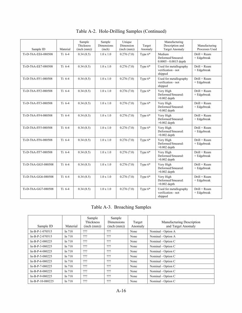
Table A-2. Hole-Drilling Samples (Continued)
Sample ID Material
Sample Thickness
(inch (mm))
Sample Dimensions
(inch)
Unique Dimension (inch (mm))
Target Anomaly
Manufacturing Description and Target Anomaly
Manufacturing Processes Used
Ti-D-T6A-EE6-080508 Ti 6-4 0.34 (8.5) 1.0 x 1.0 0.276 (7.0) Type 6* Medium Deformed/Smeared: 0.0005 - 0.0015 depth
Drill + Ream + Edgebreak
Ti-D-T6A-EE7-080508 Ti 6-4 0.34 (8.5) 1.0 x 1.0 0.276 (7.0) Type 6* Used for metallography verification - not shipped
Drill + Ream + Edgebreak
Ti-D-T6A-FF1-080508 Ti 6-4 0.34 (8.5) 1.0 x 1.0 0.276 (7.0) Type 6* Used for metallography verification - not shipped
Drill + Ream + Edgebreak
Ti-D-T6A-FF2-080508 Ti 6-4 0.34 (8.5) 1.0 x 1.0 0.276 (7.0) Type 6* Very High Deformed/Smeared: >0.002 depth
Drill + Ream + Edgebreak
Ti-D-T6A-FF3-080508 Ti 6-4 0.34 (8.5) 1.0 x 1.0 0.276 (7.0) Type 6* Very High Deformed/Smeared: >0.002 depth
Drill + Ream + Edgebreak
Ti-D-T6A-FF4-080508 Ti 6-4 0.34 (8.5) 1.0 x 1.0 0.276 (7.0) Type 6* Very High Deformed/Smeared: >0.002 depth
Drill + Ream + Edgebreak
Ti-D-T6A-FF5-080508 Ti 6-4 0.34 (8.5) 1.0 x 1.0 0.276 (7.0) Type 6* Very High Deformed/Smeared: >0.002 depth
Drill + Ream + Edgebreak
Ti-D-T6A-FF6-080508 Ti 6-4 0.34 (8.5) 1.0 x 1.0 0.276 (7.0) Type 6* Very High Deformed/Smeared: >0.002 depth
Drill + Ream + Edgebreak
Ti-D-T6A-FF7-080508 Ti 6-4 0.34 (8.5) 1.0 x 1.0 0.276 (7.0) Type 6* Very High Deformed/Smeared: >0.002 depth
Drill + Ream + Edgebreak
Ti-D-T6A-GG5-080508 Ti 6-4 0.34 (8.5) 1.0 x 1.0 0.276 (7.0) Type 6* Very High Deformed/Smeared: >0.002 depth
Drill + Ream + Edgebreak
Ti-D-T6A-GG6-080508 Ti 6-4 0.34 (8.5) 1.0 x 1.0 0.276 (7.0) Type 6* Very High Deformed/Smeared: >0.002 depth
Drill + Ream + Edgebreak
Ti-D-T6A-GG7-080508 Ti 6-4 0.34 (8.5) 1.0 x 1.0 0.276 (7.0) Type 6* Used for metallography verification - not shipped
Drill + Ream + Edgebreak
Table A-3. Broaching Samples
Sample ID Material
Sample Thickness
(inch (mm))
Sample Dimensions (inch (mm))
Target Anomaly
Manufacturing Description and Target Anomaly
In-B-P-1-070515 In 718 ??? ??? None Nominal - Option A In-B-P-2-070515 In 718 ??? ??? None Nominal - Option A In-B-P-2-080225 In 718 ??? ??? None Nominal - Option C In-B-P-3-080225 In 718 ??? ??? None Nominal - Option C In-B-P-4-080225 In 718 ??? ??? None Nominal - Option C In-B-P-5-080225 In 718 ??? ??? None Nominal - Option C In-B-P-6-080225 In 718 ??? ??? None Nominal - Option C In-B-P-7-080225 In 718 ??? ??? None Nominal - Option C In-B-P-8-080225 In 718 ??? ??? None Nominal - Option C In-B-P-9-080225 In 718 ??? ??? None Nominal - Option C In-B-P-10-080225 In 718 ??? ??? None Nominal - Option C
A-16

Table A-3. Broaching Samples (Continued)
Sample ID Material
Sample Thickness
(inch (mm))
Sample Dimensions (inch (mm))
Target Anomaly
Manufacturing Description and Target Anomaly
In-B-P-11-080225 In 718 ??? ??? None Nominal - Option C In-B-P-12-080225 In 718 ??? ??? None Nominal - Option C In-B-P-13-080225 In 718 ??? ??? None Nominal - Option C In-B-P-14-080225 In 718 ??? ??? None Nominal - Option C In-B-P-15-080225 In 718 ??? ??? None Nominal - Option C In-B-P-16-080225 In 718 ??? ??? None Nominal - Option C In-B-T1-1-070515 In 718 ??? ??? Type 1 Very High Deformation: >0.002 depth In-B-T1-2-070515 In 718 ??? ??? Type 1 Very High Deformation: >0.002 depth In-B-T1-3-070515 In 718 ??? ??? Type 1 Very High Deformation: >0.002 depth In-B-T1A-2-080519 In 718 0.75 (19) 3.4 x 1.0 Type 1* Light Deformation: <0.0005 depth In-B-T1A-3-080519 In 718 0.75 (19) 3.4 x 1.0 Type 1* Light Deformation: <0.0005 depth In-B-T1A-4-080519 In 718 0.75 (19) 3.4 x 1.0 Type 1* Light Deformation: <0.0005 depth In-B-T1A-5-080519 In 718 0.75 (19) 3.4 x 1.0 Type 1* Light Deformation: <0.0005 depth In-B-T1A-6-080519 In 718 0.75 (19) 3.4 x 1.0 Type 1* Light Deformation: <0.0005 depth In-B-T1A-7-080519 In 718 0.75 (19) 3.4 x 1.0 Type 1* Light Deformation: <0.0005 depth In-B-T1A-8-080519 In 718 0.75 (19) 3.4 x 1.0 Type 1* Light Deformation: <0.0005 depth In-B-T1A-9-080519 In 718 0.75 (19) 3.4 x 1.0 Type 1* Medium Deformation: 0.0005> <0.0015 depth In-B-T1A-10-080519 In 718 0.75 (19) 3.4 x 1.0 Type 1* Medium Deformation: 0.0005> <0.0015 depth In-B-T1A-11-080519 In 718 0.75 (19) 3.4 x 1.0 Type 1* Medium Deformation: 0.0005> <0.0015 depth In-B-T1A-12-080519 In 718 0.75 (19) 3.4 x 1.0 Type 1* Medium Deformation: 0.0005> <0.0015 depth In-B-T1A-13-080519 In 718 0.75 (19) 3.4 x 1.0 Type 1* Medium Deformation: 0.0005> <0.0015 depth In-B-T1A-14-080519 In 718 0.75 (19) 3.4 x 1.0 Type 1* Medium Deformation: 0.0005> <0.0015 depth In-B-T1A-15-080519 In 718 0.75 (19) 3.4 x 1.0 Type 1* Medium Deformation: 0.0005> <0.0015 depth In-B-T1A-16-080519 In 718 0.75 (19) 3.4 x 1.0 Type 1* High Deformation: >0.0015 depth In-B-T1A-17-080519 In 718 0.75 (19) 3.4 x 1.0 Type 1* High Deformation: >0.0015 depth In-B-T1A-18-080519 In 718 0.75 (19) 3.4 x 1.0 Type 1* High Deformation: >0.0015 depth In-B-T1A-19-080519 In 718 0.75 (19) 3.4 x 1.0 Type 1* High Deformation: >0.0015 depth In-B-T1A-20-080519 In 718 0.75 (19) 3.4 x 1.0 Type 1* High Deformation: >0.0015 depth In-B-T1A-21-080519 In 718 0.75 (19) 3.4 x 1.0 Type 1* High Deformation: >0.0015 depth In-B-T1A-22-080519 In 718 0.75 (19) 3.4 x 1.0 Type 1* High Deformation: >0.0015 depth In-B-T6-1-070515 In 718 ??? ??? Type 6 Very High Deformation: >0.002 depth In-B-T6-2-070515 In 718 ??? ??? Type 6 Very High Deformation: >0.002 depth In-B-T6-3-070515 In 718 ??? ??? Type 6 Very High Deformation: >0.002 depth In-B-T6A-1-080529 In 718 0.75 (19) 3.4 x 1.0 Type 6* Light Deformation: <0.0005 depth In-B-T6A-2-080529 In 718 0.75 (19) 3.4 x 1.0 Type 6* Light Deformation: <0.0005 depth In-B-T6A-3-080529 In 718 0.75 (19) 3.4 x 1.0 Type 6* Light Deformation: <0.0005 depth In-B-T6A-4-080529 In 718 0.75 (19) 3.4 x 1.0 Type 6* Light Deformation: <0.0005 depth In-B-T6A-5-080529 In 718 0.75 (19) 3.4 x 1.0 Type 6* Light Deformation: <0.0005 depth In-B-T6A-6-080529 In 718 0.75 (19) 3.4 x 1.0 Type 6* Light Deformation: <0.0005 depth In-B-T6A-7-080529 In 718 0.75 (19) 3.4 x 1.0 Type 6* Light Deformation: <0.0005 depth In-B-T6A-8-080529 In 718 0.75 (19) 3.4 x 1.0 Type 6* Medium Deformation: 0.0005> <0.0015 depth In-B-T6A-9-080529 In 718 0.75 (19) 3.4 x 1.0 Type 6* Medium Deformation: 0.0005> <0.0015 depth In-B-T6A-10-080529 In 718 0.75 (19) 3.4 x 1.0 Type 6* Medium Deformation: 0.0005> <0.0015 depth In-B-T6A-11-080529 In 718 0.75 (19) 3.4 x 1.0 Type 6* Medium Deformation: 0.0005> <0.0015 depth In-B-T6A-12-080529 In 718 0.75 (19) 3.4 x 1.0 Type 6* Medium Deformation: 0.0005> <0.0015 depth In-B-T6A-13-080529 In 718 0.75 (19) 3.4 x 1.0 Type 6* Medium Deformation: 0.0005> <0.0015 depth
A-17

A-18
Table A-3. Broaching Samples (Continued)
Sample ID Material
Sample Thickness
(inch (mm))
Sample Dimensions (inch (mm))
Target Anomaly
Manufacturing Description and Target Anomaly
In-B-T6A-14-080529 In 718 0.75 (19) 3.4 x 1.0 Type 6* Medium Deformation: 0.0005> <0.0015 depth In-B-T6A-15-080529 In 718 0.75 (19) 3.4 x 1.0 Type 6* High Deformation: >0.0015 depth In-B-T6A-16-080529 In 718 0.75 (19) 3.4 x 1.0 Type 6* High Deformation: >0.0015 depth In-B-T6A-17-080529 In 718 0.75 (19) 3.4 x 1.0 Type 6* High Deformation: >0.0015 depth In-B-T6A-18-080529 In 718 0.75 (19) 3.4 x 1.0 Type 6* High Deformation: >0.0015 depth In-B-T6A-19-080529 In 718 0.75 (19) 3.4 x 1.0 Type 6* High Deformation: >0.0015 depth In-B-T6A-20-080529 In 718 0.75 (19) 3.4 x 1.0 Type 6* High Deformation: >0.0015 depth In-B-T6A-21-080529 In 718 0.75 (19) 3.4 x 1.0 Type 6* High Deformation: >0.0015 depth Ti-B-P-1-070515 Ti 6-4 ??? ??? None Nominal - Option A Ti-B-P-2-080121 Ti 6-4 ??? ??? None Nominal - Option C Ti-B-P-3-080121 Ti 6-4 ??? ??? None Nominal - Option C Ti-B-P-4-080121 Ti 6-4 ??? ??? None Nominal - Option C Ti-B-P-5-080121 Ti 6-4 ??? ??? None Nominal - Option C Ti-B-P-6-080121 Ti 6-4 ??? ??? None Nominal - Option C Ti-B-P-7-080121 Ti 6-4 ??? ??? None Nominal - Option C Ti-B-P-8-080121 Ti 6-4 ??? ??? None Nominal - Option C Ti-B-P-9-080121 Ti 6-4 ??? ??? None Nominal - Option C Ti-B-P-10-080121 Ti 6-4 ??? ??? None Nominal - Option C Ti-B-P-11-080121 Ti 6-4 ??? ??? None Nominal - Option C Ti-B-P-12-080121 Ti 6-4 ??? ??? None Nominal - Option C Ti-B-P-13-080121 Ti 6-4 ??? ??? None Nominal - Option C Ti-B-P-14-080121 Ti 6-4 ??? ??? None Nominal - Option C Ti-B-P-15-080121 Ti 6-4 ??? ??? None Nominal - Option C Ti-B-P-16-080121 Ti 6-4 ??? ??? None Nominal - Option C Ti-B-T1-1-070515 Ti 6-4 ??? ??? Type 1 Very High Deformation: >0.002 depth Ti-B-T1-2-070515 Ti 6-4 ??? ??? Type 1 Very High Deformation: >0.002 depth Ti-B-T1A-3-030331 Ti 6-4 0.75 (19) 3.4 x 1.0 Type 1* Light Deformation: <0.0005 depth Ti-B-T1A-4-080331 Ti 6-4 0.75 (19) 3.4 x 1.0 Type 1* Light Deformation: <0.0005 depth Ti-B-T1A-5-080331 Ti 6-4 0.75 (19) 3.4 x 1.0 Type 1* Light Deformation: <0.0005 depth Ti-B-T1A-6-080331 Ti 6-4 0.75 (19) 3.4 x 1.0 Type 1* Light Deformation: <0.0005 depth Ti-B-T1A-7-080331 Ti 6-4 0.75 (19) 3.4 x 1.0 Type 1* Light Deformation: <0.0005 depth Ti-B-T1A-8-08033d Ti 6-4 0.75 (19) 3.4 x 1.0 Type 1* Light Deformation: <0.0005 depth Ti-B-T1A-9-080331 Ti 6-4 0.75 (19) 3.4 x 1.0 Type 1* Light Deformation: <0.0005 depth Ti-B-T1A-10-080331 Ti 6-4 0.75 (19) 3.4 x 1.0 Type 1* Medium Deformation: 0.0005> <0.0015 depth Ti-B-T1A-11-080331 Ti 6-4 0.75 (19) 3.4 x 1.0 Type 1* Medium Deformation: 0.0005> <0.0015 depth Ti-B-T1A-12-080331 Ti 6-4 0.75 (19) 3.4 x 1.0 Type 1* Medium Deformation: 0.0005> <0.0015 depth Ti-B-T1A-13-080331 Ti 6-4 0.75 (19) 3.4 x 1.0 Type 1* Medium Deformation: 0.0005> <0.0015 depth Ti-B-T1A-14-080331 Ti 6-4 0.75 (19) 3.4 x 1.0 Type 1* Medium Deformation: 0.0005> <0.0015 depth Ti-B-T1A-15-080331 Ti 6-4 0.75 (19) 3.4 x 1.0 Type 1* Medium Deformation: 0.0005> <0.0015 depth Ti-B-T1A-16-080331 Ti 6-4 0.75 (19) 3.4 x 1.0 Type 1* Medium Deformation: 0.0005> <0.0015 depth Ti-B-T1A-17-080331 Ti 6-4 0.75 (19) 3.4 x 1.0 Type 1* High Deformation: >0.0015 depth Ti-B-T1A-18-080331 Ti 6-4 0.75 (19) 3.4 x 1.0 Type 1* High Deformation: >0.0015 depth Ti-B-T1A-19-080331 Ti 6-4 0.75 (19) 3.4 x 1.0 Type 1* High Deformation: >0.0015 depth Ti-B-T1A-20-080331 Ti 6-4 0.75 (19) 3.4 x 1.0 Type 1* High Deformation: >0.0015 depth Ti-B-T1A-21-080331 Ti 6-4 0.75 (19) 3.4 x 1.0 Type 1* High Deformation: >0.0015 depth Ti-B-T1A-22-080331 Ti 6-4 0.75 (19) 3.4 x 1.0 Type 1* High Deformation: >0.0015 depth

Table A-3. Broaching Samples (Continued)
Sample ID Material
Sample Thickness
(inch (mm))
Sample Dimensions (inch (mm))
Target Anomaly
Manufacturing Description and Target Anomaly
Ti-B-T1A-23-080331 Ti 6-4 0.75 (19) 3.4 x 1.0 Type 1* High Deformation: >0.0015 depth Ti-B-T6-1-070515 Ti 6-4 ??? ??? Type 6 Very High Deformation: >0.002 depth Ti-B-T6-2-070515 Ti 6-4 ??? ??? Type 6 Very High Deformation: >0.002 depth Ti-B-T6A-1-080610 Ti 6-4 0.75 (19) 3.4 x 1.0 Type 6* Light Deformation: <0.0005 depth Ti-B-T6A-2-080610 Ti 6-4 0.75 (19) 3.4 x 1.1 Type 6* Light Deformation: <0.0005 depth Ti-B-T6A-3-080610 Ti 6-4 0.75 (19) 3.4 x 1.2 Type 6* Light Deformation: <0.0005 depth Ti-B-T6A-4-080610 Ti 6-4 0.75 (19) 3.4 x 1.3 Type 6* Light Deformation: <0.0005 depth Ti-B-T6A-5-080610 Ti 6-4 0.75 (19) 3.4 x 1.4 Type 6* Light Deformation: <0.0005 depth Ti-B-T6A-6-080610 Ti 6-4 0.75 (19) 3.4 x 1.5 Type 6* Light Deformation: <0.0005 depth Ti-B-T6A-7-080610 Ti 6-4 0.75 (19) 3.4 x 1.6 Type 6* Light Deformation: <0.0005 depth Ti-B-T6A-8-080610 Ti 6-4 0.75 (19) 3.4 x 1.7 Type 6* Medium Deformation: 0.0005> <0.0015 depth Ti-B-T6A-9-080610 Ti 6-4 0.75 (19) 3.4 x 1.8 Type 6* Medium Deformation: 0.0005> <0.0015 depth Ti-B-T6A-10-080610 Ti 6-4 0.75 (19) 3.4 x 1.9 Type 6* Medium Deformation: 0.0005> <0.0015 depth Ti-B-T6A-11-080610 Ti 6-4 0.75 (19) 3.4 x 1.10 Type 6* Medium Deformation: 0.0005> <0.0015 depth Ti-B-T6A-12-080610 Ti 6-4 0.75 (19) 3.4 x 1.11 Type 6* Medium Deformation: 0.0005> <0.0015 depth Ti-B-T6A-13-080610 Ti 6-4 0.75 (19) 3.4 x 1.12 Type 6* Medium Deformation: 0.0005> <0.0015 depth Ti-B-T6A-14-080610 Ti 6-4 0.75 (19) 3.4 x 1.13 Type 6* Medium Deformation: 0.0005> <0.0015 depth Ti-B-T6A-15-080610 Ti 6-4 0.75 (19) 3.4 x 1.14 Type 6* High Deformation: >0.0015 depth Ti-B-T6A-16-080613 Ti 6-4 0.75 (19) 3.4 x 1.15 Type 6* High Deformation: >0.0015 depth Ti-B-T6A-17-080610 Ti 6-4 0.75 (19) 3.4 x 1.16 Type 6* High Deformation: >0.0015 depth Ti-B-T6A-18-080610 Ti 6-4 0.75 (19) 3.4 x 1.17 Type 6* High Deformation: >0.0015 depth Ti-B-T6A-19-080610 Ti 6-4 0.75 (19) 3.4 x 1.18 Type 6* High Deformation: >0.0015 depth Ti-B-T6A-20-080610 Ti 6-4 0.75 (19) 3.4 x 1.19 Type 6* High Deformation: >0.0015 depth Ti-B-T6A-21-080610 Ti 6-4 0.75 (19) 3.4 x 1.20 Type 6* High Deformation: >0.0015 depth
A-19/A-20

APPENDIX B—LITERATURE SURVEY OF POTENTIAL NONDESTRUCTIVE EVALUATION METHODS FOR THE DETECTION OF ANOMALOUS
MACHINING-INDUCED DAMAGE B.1 LITERATURE SURVEY APPROACH. Each Engine Titanium Consortium (ETC) organization was assigned a primary area of responsibility for obtaining and reviewing abstracts and full copies of any identified pertinent literature sources. To minimize the impact of a single reviewer’s opinion and to accommodate the fact that several methods had a significant volume of material to review, there was an overlap in the nondestructive evaluation (NDE) methods selected for the review by each organization. Even though each participant was assigned a primary review responsibility, each was allowed to provide comment on any abstract for any method. B.2 LITERATURE SOURCES. Abstracts were selected from databases searched using a related Boolean word string (identified below). The Boolean search request was first submitted to the Nondestructive Testing Information Analysis Center to search their database of NDE-related articles. After some refinement of the Boolean search string, an additional search was conducted by Iowa State University (ISU) using the same Boolean string with several databases available from the ISU Library. The databases used were found either through the Engineering Village 2 or the Cambridge Scientific Abstracts (CSA) Illumina, which contained the specific databases of CSA Technology Research Database, MicroPatent Materials Patents, and National Technical Information Services. Using similar Boolean strings, General Electric conducted an additional search for articles from the Northeast Regional Advisory Council. For illustration purposes, the Boolean search string presented herein has been modified for publication. The actual syntax of the search string is considerably different, but contains the same content. The content listed between ( - ) represents the Boolean “OR”. ( (aerospace alloy, In 718, In 718, inco, inconel, metal, metallic, metallurgy, nickel alloy, nicked-based, powder alloy, super alloy, ti 64, ti 6-4, ti 6al 4v, Ti 64, ti6al4v, titanium alloy, Ti-based)
OR (bench, bore, broach, drill, finish, grind, hole, hone, lathe, machine, machining, manufacture, manufacturing, mill, ream, slot, tap, thread, turn) )
AND ( (abusive, adiabatic shear, alpha case, anomalies, anomaly, burr, conductivity, crack, creep damage, defect, deformation, degradation, depth profile, discoloration, distorted, distortion, embed, fatigue, flaw, flake, hardness, haz, heat, helical, hone, inclusion, micro-damage, microstructure, overheat, plastic deformation, pluck, porosity, recast, redeposited, residual, rough, score, scratch, serrated, shear, smear, strain, stress)
B-1

AND
(absorption, acoustic, acoustoelastic, algorithms, analysis, anisotropic, anisotropy, eddy-current, diffraction, electromagnetic, emat, evaluation, excitation, fabry-perot, ferromagnetic, flux, guided-wave, harmonic, image, impedance, inductive, induction, infrared, in-situ, inspection, interferometry, laser, magnetic, magnetic-optic, magneto, magnetoacoustic, measurement, microwave, multifrequency, multiparameter, nde, ndt, ndi, neural, noise, nondestructive, nonlinear, optical, paramagnetic, penetration, permeability, photo, photothermal, piezoelectric, probe, profiling, propagation, pulse, radiometry, radiography, rayleigh, recognition, reflection, resonance, saw, scatter, scattering, segmentation, segregation, sensor, shearography, signal, sonic, spectral, spectroscopy, spectrum, squid, superconductor, surface wave, testing, thermal, thermo, thermoelastic, thermoelectric, tomography, ultrasonic, ultrasound, visual, wave, wavelets, x-ray) ) B.1.2 SEARCH RESULTS. As a result of the search process, over 800 abstracts were identified. Using a database setup using mySQL and PHP software, an online database of all identified abstracts was made available to the team members through the use of a security Username/Password. The security was created to comply with international copyright laws that require limited access to only those who have permission to use the data obtained from the various literature sources and databases. As abstracts were entered into the database, ISU performed a check to eliminate duplication of abstracts. In addition to this check, frequent modifications were made to the database to increase the effectiveness of the review process for benefit of the ETC members. B.1.3 REVIEW AND RANKING PROCESS. The database was set up in a manner that allowed an individual to search the abstracts by individual NDE method. To initiate the review process, individuals were asked to review the abstracts found in the literature database that were pertinent to the respective NDE methods. A reviewer rated each abstract on a scale of 1 to 5—1 being “not relevant” and 5 being “highly pertinent.” The reviewer was able to leave short comments about the abstracts usefulness. B.2 LITERATURE REVIEW SUMMARIES. Once the articles were located, reviewed, and ranked, ETC team members prepared a written description of the potential NDE methods following a suggested format. The first few paragraphs for each NDE method would discuss the problems associated
with that method and the detection of the different anomalies, the significance of these problems, along with desired outcomes for them.
The second section would serve as a review of the articles and the results of the methods
reviewed.
B-2

The last portion would serve as a summary of the findings and allow the identification of specific steps for further research to detect anomalies.
It is anticipated that many of the NDE techniques will employ data collection through scanning operations, producing two-dimensional (2D) or three-dimensional (3D) representative images of the surface under concern. Unless the NDE technique uniquely identifies an image-processing method as part of its analysis, it is understood that all data images can be processed to determine whether the technique adequately discriminates between damaged and undamaged surfaces. The general image-processing methods used to extract the data features from the data sources are not discussed herein. NDE methods or techniques that are not applicable to the detection and/or characterization of the identified anomalies in titanium (Ti)- or nickel (Ni)-based materials are not discussed. Also not discussed are material analysis techniques requiring material cut-ups or material analysis methods that employ high magnification of surface features at the submicron scale, as these techniques, though useful for material and anomaly characterization, are not practical for production use. Summaries of the applicable methods are provided below by technique. B.2.1 VISUAL (OPTICAL/LASER) METHODS. Traditionally, visual inspections are used to evaluate machined surfaces to determine if the surface deviates from nominal conditions. It is also used to detect and/or identify anomalies, if present. Metallurgical anomalies usually require visual enhancements as an aid to visual sight. In the case of Ti parts, blue etch anodize (BEA) highlights many features, such as segregation and work hardening. Fluorescent penetrant inspection (FPI) is a method used to enhance crack visibility. Ultimately, the optical evaluations for geometric and metallurgical anomalies require visual line-of-sight inspections whether or not BEA, FPI, or magnification enhances them. Under conditions that are less optimal for viewing, especially drilled holes with length-to-diameter (L/D) ratios of 1 or higher, the quality of the evaluations is expected to diminish. A majority of visual inspections depend on inspector interpretation. Unless detailed reference standards exist for visual comparison, interpretation and lack of quantifiable criteria can be significant sources of variability. Establishing quantifiable measurements is a key characteristic that must be met. The approaches using image capture by optical methods, both white light and laser light, and image evaluation are the subject of this section of the report. For the geometric anomalies of concern, optical methods are applicable to all the geometric anomalies described by Manufacturing to Produce High Integrity Rotating Parts for Modern Gas Turbines (MANHIRP) since there is necessarily a change to the surface of the sample that can be detected and imaged. Sensitivity to metallurgical anomalies with optical methods is possible where discoloration is present. Enhancement with BEA and optical image systems on Ti parts may provide a high probability of detection. The use of automation through optical image analysis could lead to a higher probability of detection although no published data was found.
B-3

Whether optical inspections are geared for aerospace applications, pharmaceuticals, electronics, or any other industrial field, the techniques are generally used to either detect positions of objects or an image, which was produced and processed to determine a particular surface characteristic. To automate visual inspections, the challenge is to make the system mimic the human eye and associated mental processing while removing the variability that accompanies human inspections, e.g., subjective interpretation and inspector fatigue. With visual techniques, one area of particular interest is the detection of anomalies in drilled holes. Since machining anomalies, such as scores and work hardening, are generally detected with visual techniques, there is interest in improving inspection capability in holes with high L/D ratios, i.e., L/D >1. The literature survey identified several articles concerning optical/laser methods, but the bulk of the articles addressed laser ultrasonics (UT) [B-1 through B-6]. Similarly, a paper discussing photo-acoustic and photo-thermal detection is also based on input energy supplied by a laser [B-7]. Laser UTs will not be considered in this section since the technique will be addressed, if appropriate, after the interaction of UT energy with the anomalies of interest is studied. The literature survey provided three other papers on optical techniques, but these were not directed toward detection of machining anomalies. One paper dealt with detection of fatigue damage during cyclic loading [B-8]. The second paper discussed an automated method of detecting turbine blade positions during rotation in an overhauled engine [B-9]. The third paper discussed detection of fretted surfaces in rotors that have been in service [B-10]. Although the three papers described above do not deal with machined surfaces, the techniques incorporate optical methods that are used widely in various industrial applications. For instance, the positions of turbine blade tips can be precisely measured with multiple lasers and fretting can be detected with image comparison techniques. These techniques have been applied to many other industries and may have benefit in detection of anomalous machining conditions. Previous literature surveys have shown that optical measurement systems are widely available and a number of companies offer devices that characterize surfaces. Most systems include a camera and a light source. Machine vision has an extensive development history in both hardware and software components. The hardware available today is fairly consistent; however, the software that extracts features from the collected images is still specialized to particular problems. To date, general machine vision systems that perform to human levels do not exist, and those that do work are applicable only to very limited conditions, where lighting and positioning are carefully controlled. The advantages of automation are easily noted, namely, the reproducibility and speed of the analysis. The types of damage that are of concern to the anomalous machining damage (AMD) program involve surface images; a broken tool tip with remnants lodged in the component is an obvious example. Approaches that have shown promise include an automated feature extraction task. The first approach is the application of a reference image of the surface of interest. Images of good surfaces are readily available. The noise analysis allows a robust test to be done based on the observation that the signal is unlikely to be a result of a noise fluctuation. This test for the
B-4

probability that a noise fluctuation can produce the observed signal can be selected making this a rigorous criteria. The second development that has been recently demonstrated is the automatic feature identification from images—features that are suitable for use in 3D stereographic reconstructions. Recent work by Kobbelt, et al. [B-11], has shown that progress can be made by identifying stationary points in an image. The identification of these stationary points involves an automated set of processing steps—a feature that limits the human involvement component of stereographic reconstructions. The stationary points are based on taking the derivative of the image in several directions and identifying points where the change in the sign of the derivative occurs. These points in the image are very stable as the perspective changes. However, with optical images, the ambient lighting is critical [B-12 and B-13]. The human eye is remarkably adept at normalizing lighting variations both in terms of absolute brightness and color variation. Lighting control is crucial for repeatable results in inspection situations. Investigations concerning the level of lighting control that is required and guidelines for specifying lighting booths for controlling the environmental light are necessary. The effect of variation of ambient lighting is one of the issues that make the performance of algorithms extracting information from images difficult. This effect has been observed in the digitization of images using charge-coupled device cameras, in particular, in digitizing radiographs. An evaluation of the effect of ambient light and the degree of control of the lighting conditions are needed to generate reproducible results. One inspection technique that has already demonstrated feasibility for detection of machining anomalies incorporates lasers and a detector that scans the surface of drilled holes. The technique, developed by Laser Techniques Company, LLC (Bellevue, WA), showed the capability to detect scratches as well as work-hardened regions [B-14]. This technique is particularly interesting in that it was demonstrated on actual holes and does not suffer from image distortions that can occur from using diffuse white light and the application of mirrors or borescopes. The scanned data from laser sources of various wavelengths produces digital images that are processed to highlight features of interest. Such image data could also be a source for image analysis algorithms. B.2.2 THE UT METHODS. For several of the identified anomalies, it should be possible to detect the presence of the anomaly by detecting associated changes in UT wave propagation characteristics. For example, at the boundary between the parent metal and an embedded anomaly, the UT impedance (speed times density) may change abruptly, and this impedance change causes some of the incident UT energy to be reflected by the boundary. In addition to impedance, other UT properties that can be exploited to search for anomalies or to otherwise characterize metals are sound speed, attenuation, and the UT grain noise capacity. The latter property quantifies the scattering severity of an incident sound wave from microstructural boundaries within the metal. Since the damage associated with machining anomalies is confined within a thin near-surface layer, an inspection method is required that is particularly sensitive to near-surface properties.
B-5

This suggests using UT surface-skimming waves (also known as Rayleigh waves) [B-15]. As illustrated in figure B-1, Rayleigh waves propagate parallel to the surface of the sample, and their depth of penetration is dependent upon frequency. Thus by varying the frequency, one can effectively vary the penetration depth. A rough rule-of-thumb is that the majority of the sound energy is confined to within about one UT wavelength of the surface. For representative Ti- and Ni-based jet engine alloys, the table in figure B-1 lists the penetration depth as a function of frequency. Since AMD layers are expected to be quite thin (50 microns), optimal surface wave inspection frequencies may be rather high (50 MHz), typical of those used in acoustic microscopy. As is the case with UT inspections, the use of surface waves involves both the generation and reception of sound waves. For the immersion inspection depicted in figure B-1, a standard UT transducer positioned at the proper angle generates the surface wave. A portion of the energy carried by the propagating surface wave radiates (or leaks) into the water, and this radiated sound can be subsequently detected and analyzed. Lasers can also be used to generate and detect UT surface waves without the need for a couplant layer.
Transducer angled togenerate a strongRayleigh wave
Surface-skimming sound wave
Rayleigh wave speed, attenuation, and scattering from grain boundaries will likely be different for normal and damaged material
Figure B-1. A Simple UT Pulse-Echo Immersion Inspection Using Surface Waves (The accompanying table lists approximate surface wave penetration depths for jet engine
Ti- and Ni-based alloys.) The presence of machining-induced damage will likely affect UT surface wave velocity, attenuation, and/or grain noise. However, these same properties will also vary somewhat within undamaged metal because the microstructure is usually not uniform. Generally, on a
water
metal
Metal microstructure
Freq. (MHz) Ti 6-4 In71810 294 28720 147 14430 98 9640 73 7250 59 5760 49 4880 37 36100 29 29150 20 19200 15 14
Penetration depth (microns)(one wavelength)
Transducer angled togenerate a strongRayleigh wave
Surface-skimming sound wave
Rayleigh wave speed, attenuation, and scattering from grain boundaries will likely be different for normal and damaged material.
water
metal
Metal microstructure
Freq. (MHz) Ti 6-4 In71810 294 28720 147 14430 98 9640 73 7250 59 5760 49 4880 37 36100 29 29150 20 19200 15 14
Penetration depth (microns)(one wavelength)
B-6

macroscopic scale, there are variations of gross microstructure within a forging, e.g., variations in the average size, shape, or preferred orientation of the grains. These microstructural variations will produce variations in wave propagation characteristics. In addition, typical machining grooves fabricated onto component surfaces, while within machining specifications, may influence surface wave propagation. It may be that the acceptable microstructural variations and the presence of machining grooves will make it difficult to reliably discriminate AMD from acceptable metal conditions. Thus, experiments will be required to explore the utility of the recommended UT techniques. UT wave propagation in metals is strongly influenced by metal microstructure and/or damage to that microstructure. The use of UT surface waves to detect relatively large surface-breaking cracks or pits is well established [B-16 and B-17]. However, the literature survey uncovered only a few articles dealing directly with the use of UT surface waves to detect more subtle near-surface damage or microstructural changes in jet engine material. For supposed bulk waves (longitudinal or shear) propagating within the interior of a metal sample, there is a large body of theoretical and experimental data relating UT properties to microstructure, both with and without damage. Although bulk-wave UT inspection is not directly recommended, conclusions from bulk-wave literature may help refine UT inspection choices for AMD detection. Note that from a UT inspection point of view there are three broad categories of machining-induced damage that are potentially detectable using surface wave techniques: 1. Isolated damage (e.g., a single localized crack or an embedded tool head) 2. Distributed non-geometric damage (e.g., a change in the gross metal microstructure,
possibly accompanied by microcracking, from the parent material, which exists over a sizeable lateral area and some finite depth)
3. Periodic geometric damage (e.g., out-of-specification machining groove depth or spacing,
or periodic “plucking”) To better focus the discussion, note the damage examples listed above in parentheses. Additionally, the results of the literature survey are discussed. B.2.2.1 Relationship Between Microstructure and UT Properties. The jet engine alloys of interest often have complicated microstructures [B-18 through B-20]. The alloys are polycrystalline metals consisting of single crystals (metal grains) that may be of one or more crystal symmetry types (phases). The elementary grains may be grouped into larger structures such as the platelets, colonies, or macrograins often observed in engine Ti alloys [B-18 and B-20]. The shapes of the grains or the larger structures may be equiaxed or elongated, and, if elongated, there may be a preferred elongation direction. Other complicating factors can include precipitates along grain boundaries, preferred atomic lattice orientation (texture), residual stress, and the presence of distributed damage (e.g., porosity or microcracking). In addition, the alignment of atomic planes within a given grain may be regular or irregular (e.g., contain
B-7

dislocations). These microstructural features will affect the manner in which sound waves propagate through the metal. The primary sound wave characteristics that influence typical UT inspections (which, in turn, are influenced by microstructure) are wave type, propagation speed, attenuation, and grain noise. Wave speed affects the refraction of sound waves at interfaces and also the rates of focusing or spreading during propagation. Attenuation describes the loss of wave energy with distance and plays a key role in determining the strength of UT responses. UT grain noise is a limiting factor in many inspections since it can act to cover or obscure the responses from bona fide anomalies. Grain noise is often quantified by using the Figure-of-Merit (FOM) for noise severity as a measure of the capacity of the microstructure to reflect or otherwise scatter sound energy. Experimental techniques have been developed to readily measure velocity, attenuation, and noise capacity (as functions of frequency) for UT longitudinal or shear waves [B-18 through B-20]. Much is known from past studies about the manner in which metal microstructure influences UT wave propagation. Most of the literature concerns bulk longitudinal or shear waves traveling in the interior of samples without being influenced by sample boundaries. For simple single-phase materials, at common inspection frequencies where the grain size is smaller that the wavelength, grain noise capacity and attenuation tend to increase systematically with grain size. This is well known, as summarized by Papadakis [B-21] and Goebbels [B-22], and has long been used to estimate grain size ultrasonically. However, the situation is more complicated for the duplex microstructures typically observed in Ti engine alloys. There, macrograin properties, particularly orientation and size, play key roles in the determination of attenuation and grain noise capacity. Fortunately, past studies by the ETC have greatly clarified the relationship between microstructure and UT properties in jet engine alloys and have determined their variability in typical billets and forgings. One component of the ETC studies involved cutting numerous coupons from representative billets and forgings, measuring their UT properties, and then correlating those properties with microstructure. The findings are well documented by a series of detailed reports [B-18 through B-20]. One FAA-sponsored ETC study [B-19] examined UT property variations within 10-inch-diameter billets of Ni-based engine alloys (In 718 and Wasploy). The microstructures of both alloys were characterized by single-phase (cubic), equiaxed, untextured grains. At a given location in a billet, the microstructure was found to be locally uniform, and UT properties were approximately independent of the sound-propagation direction. However, the average grain diameter was found to vary considerably with position (primarily with radial depth in the billet), leading to substantial changes in both attenuation and grain noise capacity. Rectangular coupons were cut from various regions of each billet studied, and attenuation and grain noise FOM were measured as functions of frequency. The measurement methods are discussed in detail in reference B-19. A key conclusion of the Ni alloy billet study was that UT properties were locally isotropic and primarily dictated by the average size of the grains. In the 5- to 15-MHz range, attenuation and noise FOM were strong functions of both frequency and grain size. UT velocity on the other hand, showed little variation with grain size or frequency. Because the average grain diameter varied significantly with position (from 13 to 35 microns in the In 718 billets studied and from 47 to 115 microns in a Waspaloy billet), the local values of attenuation and grain noise FOM varied greatly as well. However, the maximal variations tended to occur
B-8

slowly with position over distances of several inches. Although this particular study was conducted on billet material, similar findings were reported in smaller studies on coupons from In 718 forgings [B-23]. The situation for engine Ti alloys is quite different. In Ti, both small- and large-scale structures are present, with the largest structures commonly referred to as macrograins. The macrograins correspond to regions where large single crystals of cubic (beta) phase material, which existed during an early high-temperature phase of metal processing. As the billet cools, smaller structures (colonies of cubic and hexagonal phase grains) develop within the macrograins. In engine Ti alloys, local UT properties are often strongly dependent on the direction of sound propagation. The macrograins tend to be elongated in billets and forgings, and measured attenuation tends to be largest for propagation parallel to the elongation direction, while backscattered grain noise is largest for propagation perpendicular to the elongation [B-8 and B-20]. For Ti alloys, the directional dependence of UT properties within a localized region can be quite severe. It is not uncommon to find a factor of 5 or higher difference in noise (or attenuation) between the high- and low-noise directions [B-8, B-20, and B-24]. The ETC studies indicate that in Ti alloys, macrograin shape, orientation, and size are all key microstructural parameters, which influence UT properties [B-18 and B-20]. This same point was concluded by Foister, et al. [B-25]. In one noteworthy study [B-20 and B-26], macrograin shape and orientation within a particular Ti 6-4 engine forging were estimated, as functions of position, from simulations of plastic flow during forging (using the commercial software package DEFORM [B-27]). The shape and orientation information were then used as inputs for grain noise model calculations, assuming that the macrograin volume was fairly constant throughout the forging. The model was able to successfully explain the large grain noise amplitude variations observed within coupons cut from the forging. This indicates that macrograin shape and orientation were as important as macrograin size in determining the noise-generation capacity of Ti alloy microstructures. The grain noise models used in that study were based on a weak scattering assumption, i.e., that the bulk of the observed grain noise results from single-scattering events and that multiple scattering may be neglected. Single-scattering noise models, based on the pioneering work of James Rose [B-28], are often used to simulate UT bulk-wave inspections of jet engine alloys. A good introduction to the use of the noise models in Ti alloys is presented by Thompson, et al. [B-29], while the applicability of the models to Ni engine alloys is discussed in references B-19 and B-30. In typical Ti alloy billets or forging materials, microstructure-induced variations in UT velocity are generally small (i.e., typically <1% when measured over distances of a few centimeters or more). The much larger variations in local grain noise and attenuation have significant consequences for UT inspections. For example, in Ti 6-4 billet inspections, microstructure variations can lead to significant differences in anomaly echo amplitude for nominally identical anomalies located at the same depth in the billet [B-31]. Similarly, the presence of microstructural noise in billets and forgings requires inspection strategies for increasing signal-to-grain-noise ratios (S/N). Improvements in S/N are often accomplished by focusing the sound beam in the vicinity of the anomaly [B-32 through B-34]. Although focusing tends to increase
B-9

the absolute level of grain noise, the anomaly signal amplitude rises even faster, producing an overall increase in S/N [B-20 and B-34]. Another way in which the microstructure of jet engine alloys can influence sound propagation is through the generation of beam distortions. If the grains or macrograins are not small compared to the sound wavelength, the amplitude or phase profiles of a propagating sound beam can be significantly distorted compared to those observed for a homogeneous material. For bulk waves in engine Ti alloys, this phenomenon has been demonstrated by Panetta, et al. [B-35], via beam-mapping experiments in which a small receiver is scanned through a sound field produced by a source transducer after passage through the sample. Thus, visualizing distorted sound fields by beam-mapping is another potential tool for interrogating microstructures. Several key points were identified from portions of the reviewed literature dealing with the relationship between microstructure and UT bulk-wave properties of jet engine alloys. These are also expected to apply to surface wave inspections for AMD: UT velocity, attenuation, and backscattered grain noise capacity are influenced by the
metal microstructure, and thus can serve as tools to detect microstructural changes. On a percentage change basis, attenuation and grain noise are much more sensitive to microstructural differences than velocity, and thus may be better candidates for detecting AMD conditions.
When the UT wavelength is larger than the mean grain size, attenuation and scattered grain noise tend to increase with frequency. Thus, these two wave propagation characteristics become better discriminators of microstructural changes at higher frequencies. This is an expected benefit in the case of AMD detection, since the need to confine surface waves to a thin near-surface layer will necessitate the use of higher frequencies.
When the beam spot encompasses at least several grains, focusing the sound beam tends to enhance the absolute grain noise level (without distance amplitude correction) and, hence, enhance the ability to discriminate between different microstructures. Thus, for AMD inspection methods that make use of scattered grain noise, focused sound beams will likely be preferable to unfocused beams.
In jet engine alloys that have acceptable microstructures, attenuation and grain noise capacity can vary significantly over distances of several centimeters. These variations in Ni alloys are generally tied to changes in the mean grain diameter. In Ti alloys, the UT property changes are principally due to changes in the shape, orientation, or size of the macrograins. Because of these acceptable natural variations, a measured change in UT properties does not necessarily mean that a damage condition exists.
AMD damage detection is likely to be simpler in Ni-based engine alloys than in Ti alloys. This is because the UT properties of the Ti alloys are much more direction-dependent, leading to greater attenuation and scattering variability within the range of acceptable microstructures.
B-10

B.2.2.2 Effect of Distributed Damage on UT Wave Propagation. The literature survey uncovered several papers that examine the use of bulk-wave ultrasound to detect or characterize distributed damage within metals. In some cases of practical interest, distributed damage acts to lower both the elastic stiffness modulus of the metal and its local strength. This is the expected case for distributed microcracking, distributed porosity, or damage due to creep. If the damage zone is localized, the inspection problem is approximately equivalent to detecting a low modulus inhomogeneity in an otherwise homogenous elastic solid. In principle, a damaged region of this type can be detected and characterized by insonifying the region with ultrasound and studying the scattered sound waves. A theoretical discussion of this approach is summarized by Achenbach, Sotiropoulos, and Zhuare [B-36]. Several papers describe experimental studies conducted to detect distributed microstructure damage in metals using traditional pulse-echo, bulk-wave ultrasound. In the work of Hirsekorn, et al. [B-37], the samples were thick sections of steel tubing that had been damaged by hydrogen attack. The damaged region, characterized by distributed cracking, extended inward approximately 20 mm from the inner surface of the tube. Standard pulse-echo inspection techniques were used, and velocity, attenuation, and backscattered grain noise were measured using 5- and 10-MHz transducers. The authors found that the difference in UT velocity between damaged and undamaged regions was similar to velocity measurement inaccuracies. However, UT attenuation and backscattering were observed to increase significantly in the damaged region, leading to the conclusion that attenuation and backscattering are good tools for assessing damage due to distributed cracking. A related study was conducted by Tittmann, Abdel-Gawad, and Fertig [B-38] using powder metallurgy samples of the Ni-based powder alloy In-100. The samples contained distributions of small pores and were studied using pulse-echo ultrasound with frequencies ranging from 2 to 20 MHz. At these frequencies, the sound wavelength was much larger than the average diameter of either the grains or pores. The presence of the distributed damage (porosity) again caused UT attenuation and backscattering to increase. The authors concluded that the frequency dependence of UT backscatter can serve as a key indicator of the degree of damage. In addition, the measured frequency dependence of backscattered noise was in good agreement with model predictions, indicating that single-scattering grain noise models can be used to simulate and optimize inspections for distributed porosity. Another Ni-based superalloy, MA6000, which is used in turbine engine blades, was studied by Morissey and Scholz [B-39]. Samples were heated and stressed to induce creep damage. Subsequent metallographic analysis revealed the development of small cavities at grain boundaries that tended to coalesce into larger voids at higher damage levels. UT velocity was measured before and after repeated stressing using standard pulse-echo UT techniques with 10-MHz transducers. It was expected that the sound velocity would decrease with creep damage level, due to the overall decrease in elastic stiffness resulting from the cavities. This expected behavior was observed for one sample but not for another. In addition, the velocity changes for both samples were quite small, never exceeding 2% of the unstressed value. The authors concluded that two effects acted to determine UT velocity in these microstructures: (1) the development of cavities, which act to lower the sound speed, and (2) other microstructural
B-11
changes (e.g., in the shapes and textures of grains). Because of the interplay between these two effects, the sound speed may increase or decrease during creep damage. This study implies that UT velocity measurements may not be a reliable method to detect AMD having distributed near-surface microcracking or pores if other microstructural changes are also present. Shah, et al. [B-40], studied a third Ni-based alloy (Inconel® 625 Alloy), which is widely used in the chemical industry for its strength and corrosion resistance at high temperatures. Samples were subjected to long exposures (5,000-100,000 hours) at elevated temperatures to promote a type of damage, known as age hardening, in which precipitates form along grain boundaries resulting in a decrease in ductility and toughness. UT velocities (shear and longitudinal) and attenuation coefficients (longitudinal only) were measured using 10-MHz transducers operating in pulse-echo mode. As in the other experimental studies described above, the sonic wavelengths were much larger than grain diameters (or precipitate dimensions). It was found that age hardening caused the UT velocities to increase slightly (by up to 2% for longitudinal waves and up to 3.5% for shear waves) and caused the longitudinal wave attenuation (in dB/inch units) to increase by 40%. By suitably annealing the samples, the effects of age hardening could be reversed, and the UT parameters were shown to return to their prehardening (original) values. One of the damage conditions of interest in AMD is the development of a surface layer of increased hardness and reduced grain size caused by excess heating during machining. The characterization of such damage is akin to the characterization of intentionally induced case hardening. In this regard, the work of Morris Good is noteworthy [B-41 through B-43]. For steel samples, Good has demonstrated that the thickness of case hardness layers can be measured by analyzing the backscattered grain noise observed using obliquely incident bulk longitudinal or shear waves. The smaller grains in the induction-hardened layer produce much less scattering than the larger ones in the underlying substrate or in the transition zone between the two microstructures. Thus, the depth dependence (i.e., time dependence) of the noise can be analyzed to deduce the thickness of the hardened layer. This approach is used in a commercial instrument for case hardness measurements marketed by Sonix, Inc. [B-44]. The minimum thickness layer that can be characterized by that instrument is approximately 1 millimeter (1,000 microns), which is considerably larger than the expected maximal damage layers under consideration in AMD. However, the success of Good’s approach in practice suggests that a similar technique using high-frequency surface waves may be useful for detecting related classes of AMD. Regarding bulk wave studies of distributed damage in metals, the following points can be made. Again, these are also expected to apply to surface wave inspections for AMD. Distributed damage to metal microstructure may cause UT velocity to increase or
decrease, depending on the details of the damage. Thus, the use of velocity in AMD may be very damage-specific. In the studies cited, the change in velocity was, at most, a few percent and tended to be larger for shear waves than for longitudinal waves.
Distributed damage to metal microstructure in which either microcracking or porosity was present caused significant increases in both UT attenuation and backscattered microstructural noise in all the cited studies where these parameters were measured.
B-12

The frequency dependence of attenuation or scattering will likely offer a more robust tool for discriminating between damaged and undamaged microstructures than simple amplitude measurements at a single (averaged) frequency. However, such frequency-dependent measurements require more time-consuming data acquisition and analysis methods than amplitude-based measurements.
UT measurement of case hardness depth using backscattered grain noise can be done using a commercially available instrument. A similar inspection approach using surface waves may be viable for certain related categories of AMD.
B.2.2.3 UT Surface Waves and Near-Surface Damage Detection. As noted earlier in the discussion of figure B-1, it is expected that the most viable UT techniques for detecting AMD will employ surface acoustic waves (SAW). This is because the energy carried by SAWs penetrates only about one wavelength beneath the surface, thus providing a good tool for interrogating the near-surface region. SAWs have long been used as one modality for acoustic microscopy. In a scanning acoustic microscope (SAM), a localized but defocused sound beam is scanned across a sample surface and variations in near-surface UT properties lead to variations in measured UT responses, which are then used to image the sample. Gilmore, et al., provides a good introduction to acoustic microscopy and the use of SAWs in UT inspection [B-17]. Common experimental arrangements for generating and detecting SAWs are illustrated in figure B-2. The standard immersion arrangement for pulse-echo SAW microscopy is depicted in figure B-2(a), where a sharply focused sound beam approaches the sample. Although the central ray is shown at normal incidence, other rays approach the surface at the proper angle to excite strong surface waves. These propagate along the sample surface and leak sound energy back into the water as they propagate. This “leaky Rayleigh” wave is received by the transducer and carries information about the sample properties. In its simplest configuration, the water path is fixed and the transducer is scanned laterally in two dimensions across the sample. From the amplitude of the received response (or some other response characteristic), a 2D C-scan image of the near-surface region can be constructed. Alternatively, the V(z) method [B-45] can be used, as depicted in figure B-2(b). There, at each location above the sample, the water path (z) is varied, and the analysis of the response (V) as a function of z and frequency allows more detailed information of surface properties to be deduced. The transducer depicted in figure B-2(a) or (b) is often spherically focused, thus producing SAWs traveling in all directions parallel to the surface within the beam footprint. Alternatively, a cylindrically focused transducer can be used so that the SAWs propagate primarily along a specific line. SAW propagation in a specific direction can also be accomplished by tilting the transducer at the proper angle to excite surface waves, as illustrated in figure B-2(c). This configuration, for example, should be ideal for measuring backscattered SAW grain noise or for detecting a surface-breaking crack whose orientation is known and aligned perpendicular to the SAW propagation direction. As depicted in figure B-2(d) and (e), a pitch/catch measurement can be performed by using separate transducers for generating and receiving the surface waves. The transducers can be scanned together, as in figure B-2(d), or one can be fixed and the other scanned about it, as in figure B-2(e). The former configuration would be useful, for example, in detecting changes in surface wave attenuation
B-13

during scanning, while the latter could be used to map the local surface waves generated by the transmitter.
water
metal
FocusedTransducer Scan
in 2D
D
V(z) method: at each scan position, vary water path (z) to vary the defocusing distance (D)
(b)
water
metal
FocusedTransducer Scan
in 2D
D
V(z) method: at each scan position, vary water path (z) to vary the defocusing distance (D)
(b)
water
metal
FocusedTransducer Scan
in 2D
Scan transducer with water path fixed
(a)
water
metal
FocusedTransducer Scan
in 2D
Scan transducer with water path fixed
(a)
water
metal
Scan in 2D
Scan transducer with water path fixed
(c)
reflected surface wave from crack, microstructure, etc.
water
metal
Scan in 2D
Scan transducer with water path fixed
(c)
reflected surface wave from crack, microstructure, etc.
water
metal
Scan in 2D
Scan transducers in tandem with water path fixed
(d)
water
metal
Scan in 2D
Scan transducers in tandem with water path fixed
(d)
water
metal
Scan in 2D
Scan receiving transducer with transmitter fixed.
(e)
Fixed
water
metal
Scan in 2D
Scan receiving transducer with transmitter fixed.
(e)
Fixed
Figure B-2. Common Experimental Setups for UT Tests Using SAWs (a) Normal-Incidence Pulse Echo, (b) Normal-Incidence Pulse-Echo V(z) Method, (c) Oblique-Incidence Pulse Echo,
(d) Oblique-Incidence Pitch/Catch, and (e) Surface Wave Field Mapping In figure B-2(a-e), the use of UT transducers to generate and receive SAWs is depicted. However lasers can also be used to either generate or receive the waves [B-46]. For example, local heating of the surface by a laser spot (followed by thermal expansion or ablation) can generate a SAW. On the receiving end, laser interferometers (or laser vibrometers) can be used to measure the displacements of a region of the surface as a SAW passes by. The literature survey identified several articles in which SAW techniques were used to detect near-surface damage in metals. Isolated surface-breaking cracks longer than a wavelength are particularly easy to detect using SAWs. If the crack’s lateral size is not small compared to the beam footprint on the surface, the crack can be detected in C-scan images formed using the simple pulse-echo setup in figure B-2(a). There, the crack disrupts some of the SAW ray paths that contribute to the measured response. Alternatively, if the crack’s cross-sectional area is oriented normal to the sound propagation direction, a pulse-echo inspection geometry, as shown in figure B-2(c), can be used. The abrupt impedance change between the crack and host metal causes a portion of the SAW incident on the crack to be reflected, and the echo arising from this reflection is then observed. In pitch/catch mode (e.g., figure B-2(d)), a loss of signal is observed due to the presence of the crack, and the crack orientation need not be perpendicular to the approaching SAW. As discussed by Lame, et al. [B-47], cracks can also be sized using SAWs and time-of-flight methods. One can observe the time delay between the primary reflection from the crack and a later secondary signal generated by sound, which travels down the crack face and reflects from the crack tip. Bykov, et al. [B-48], have studied the UT detection of fatigue cracks
B-14

in Ti alloy engine disks, and reported that cracks with lengths above 0.8 mm are detectable using a 5-MHz transducer in pulse echo. Smaller surface-breaking cracks in jet engine alloys would presumably be detectable using higher sonic frequencies. Several papers dealt specifically with the detection of surface-breaking anomalies using scanned laser beams to generate SAWs. In this category are papers by Kromine, et al. [B-49]; Fomitchov, et al. [B-50]; Wagner [B-51]; Monchalin, et al. [B-52]; and Choi, et al. [B-53]. The latter deals specifically with the detection and characterization of cracks in jet engine materials, namely Ni and Ti alloy turbine blades, using the scanning laser source technique to construct images of fatigue cracks on the blades. The method requires no couplant and is reported to work well on curved as well as flat surfaces. Although crack detection using surface waves is a common research topic, few references were found in which SAWs were used to detect or characterize near-surface distributed damage. One example, involving measurements on Ti 6-4 samples, is provided by the work of Brasche, et al. [B-54]. The goal was to compare UT velocities for oxygen-contaminated hard alpha material and undamaged alloy. A thin layer of hard alpha case (approximately 100 microns thick) was produced on the surface of a test block by heating Ti 6-4 alloy in air for an extended period. Rayleigh wave speeds were then measured using the two inspection geometries shown in figure B-3. In each case, a tightly focused 50-MHz transducer was used. In the first, the water path was shortened to defocus the beam at the sample surface, and the time difference, t0-t1, was measured as a function of water path. The Rayleigh wave speed could then be deduced from the slope of the time shift-versus-defocusing distance curve. In the second method, the transducer was operated at oblique incidence and the arrival time of the surface wave echo from a boundary was recorded versus the scan coordinate. Both methods found that the surface wave speed in hard alpha material was about 8% higher than in undamaged alloy. Thus, Rayleigh wave speed measurements may be a viable technique for detecting an alpha case arising from AMD. A second example of using SAW velocities to detect and characterize near-surface distributed damage can be found in the work of Tardy, et al. [B-45]. Ceramic samples were studied and surface roughness resulting from machining operations was correlated with changes in the Rayleigh wave velocity. As with Brasche, the defocusing distance was varied, allowing surface wave velocity to be determined. However, the analysis was more involved, allowing velocity to be measured as a function of frequency. Brasche and Tardy only used SAW velocity. However, based on the review of the UT bulk-wave literature, attenuation and backscattered noise would seem to be more useful parameters for detecting distributed damage using SAWs. The literature survey uncovered only one paper describing experiments in which SAW attenuation or noise were directly used to examine metal surfaces for nongeometric, distributed microstructural damage. That sole paper was written by Ogi, Minami, Aoki, and Hirao [B-56], who studied cylindrical carbon steel samples exposed to rotating bending fatigue. SAW attenuation (among other parameters) was measured as a function of fatigue and was found to generally increase until fracture occurred. Simultaneously, SAW velocity tended to drop with fatigue, presumably due to the formation of microcracks and the weakening of the elastic modulus.
B-15

(c)
(d)
(e)
(b)
Deformed Layer
(~ 35 microns thick)
Hardness 1.75 times
higher than base
metal
(a) (b)(b)
Deformed Layer
(~ 35 microns thick)
Hardness 1.75 times
higher than base
metal
(a)
(c)
(d)
(e)
(b)
Deformed Layer
(~ 35 microns thick)
Hardness 1.75 times
higher than base
metal
(a) (b)(b)
Deformed Layer
(~ 35 microns thick)
Hardness 1.75 times
higher than base
metal
(a)
Figure B-3. The Measurement of Surface Wave Speed in a Thin Layer of Hard Alpha Case on a Ti 6-4 Sample (a) a MANHIRP [B-55] Sample With a Hardened Surface Layer due to
Abusive Machining; (b) the Ti 6-4 Sample Studied by Brasche, et al., Before Polishing; (c) Setup for the First Method of Measuring Surface Wave Speed; (d) Observed
Time Shift vs Defocusing Distance, Used for Wave Speed Determination; and (e) Second Method of Measuring Surface Wave Speed
B-16

A number of related papers were found in which SAWs were used to inspect and characterize coatings. These include papers by McCarthy [B-57]; Abbate, et al. [B-58]; Lee and Cheng [B-59]; and Coste [B-60 and B-61]. For example, for a homogeneous single-layer coating applied to a metal substrate, Coste has derived approximate formulas relating the velocity and attenuation coefficient of Rayleigh waves to the characteristics of the metal substrate and layer material. The grain structure of the metal is even taken into account in an approximate way. Coste’s equations can be used to back-out properties of the coating and substrate from measured SAW velocity and attenuation as functions of frequency. He demonstrated his method through SAW measurements on samples containing a metallic coating applied (via vacuum plasma spraying) to Ni alloy turbine blades. From the sonic measurements, he was able to estimate the thickness and density of the coating and the Young’s moduli of the coating and substrate. Subsequent destructive measurements found the coat thickness and density estimates accurate to within about 10%. Because a coating has a sharp demarcation with the underlying substrate, Coste’s analysis is not directly applicable to common cases of distributed machining-induced damage where the damaged microstructure slowly transforms into the parent microstructure as one moves deeper into the metal. However, Coste’s analysis does indicate that the attenuation of SAWs (measured as a function of frequency) might play a useful role in the assessment of near-surface damage. Thus, the literature review indicates that SAWs may be useful for detecting certain categories of machining-induced damage. For example, if there is distributed damage to the microstructure, which extends some depth into the component over a sizeable area, the damage may be detectable by monitoring the SAW velocity, attenuation, or scattered noise. Also, isolated damage (e.g., a single crack or an imbedded tool tip) should be detectable using a setup that simply monitors the amplitude of SAW signals, such as echoes produced by reflection from the anomaly. If there is geometric damage to the component’s surface that is periodic in nature, then SAW may also be useful. Examples would include overly deep machining grooves, or systematic plucking within otherwise acceptable grooves. When SAWs propagate perpendicular to the grooves (or other periodic structures), some of the sound energy is reflected from each groove. At particular frequencies, constructive interference can occur between the echoes from adjacent grooves, resulting in abnormally high levels of scattered noise. Thus, in principle, the detection and frequency analysis of SAW noise can be used to characterize periodic surface geometries. The practical use of SAW noise in this manner was demonstrated by Guo, et al. [B-62 and B-63], who modeled the interaction of a finite sound beam with a periodic rough surface and showed that properties of the acoustic noise spectrum are related to the spacing and height of the surface grooves. In related experimental studies on metal samples having periodic roughness, it was demonstrated that the model formalism could accurately predict the time domain noise arising from the roughness. Guo demonstrated that SAW noise will likely be a useful tool for evaluating periodic surface geometry. However, one must consider that acceptable machining grooves will generally be present at some level in finished components and, hence, will be a source of SAW noise. The extent to which this noise will interfere with efforts to detect nongeometric damage can best be determined experimentally.
B-17

In connection with the UT bulk-wave measurements discussed earlier, it was suggested that UT beam mapping (to image beam amplitude and phase distortions) could serve as a tool for interrogating microstructures. Such beam-mapping measurements are also feasible for surface waves, for example, using a setup equivalent to that shown in figure B-3(e). One novel approach to surface wave beam mapping is provided by the Laser UT Camera, developed at the Idaho National Engineering and Environmental Laboratory [B-64]. In this method, the camera uses laser illumination projected first onto the sample surface and subsequently onto a photorefractive material to produce an optical image of the vibrating surface. The net effect is to obtain an optical image of the entire vibrating surface without scanning. The surface wave images are provided by a separate source, such as a traditional UT transducer. The vibration images can have frequencies ranging from a few Hertz to several GHz. As in the bulk wave case, such images should provide information about surface wave speed, attenuation, and grain scattering. The images may prove useful in detecting certain categories of AMD, particularly those involving distributed damage over an extended region. Finally, the literature survey identified a number of unusual techniques in which surface wave ultrasound could play some role. For example, Yan and Nagy [65] describe the use of thermo-optical modulation to improve the UT detection of surface-breaking anomalies. The sample is illuminated with pulsed infrared laser energy to induce heating, thus changing crack openings and the UT signals from cracks without modifying UT signatures of grain noise or surface grooves. When coupled to UT SAW inspection, thermo-optical modulation tends to emphasize crack-like anomalies. Other authors discussed the use of nonlinear ultrasound to detect distributed damage. A noteworthy example is Ogi, et al. [B-56]. In their study of fatigued steel samples, the authors measured a nonlinearity parameter by injecting a surface wave of one frequency and detecting a second wave at twice that frequency. The measured nonlinearity parameter tended to increase as surface microcracking accumulated due to fatigue tests. However, the nonlinearity parameter displayed large swings in value during the tests, perhaps indicating that it is difficult to measure in practice, and that measurement errors are large. The following points serve to summarize the review of the UT SAW literature and the possible use of SAWs for detecting machining-induced damage. The use of SAW in nondestructive tests (NDT) is well established using both UT
transducers and lasers to generate and detect the waves.
Surface-breaking fatigue cracks in jet engine alloys have been detected and sized using surface waves. It is expected that machining-induced damage resulting in isolated near-surface anomalies (e.g., a localized crack or an embedded tool tip) should be readily detected using SAW.
Certain types of near-surface distributed damage in metals have been detected by measuring SAW velocity and/or attenuation. This includes a hard alpha case layer on Ti 6-4 alloy and distributed microcracking in steel. Scattered grain noise observed in SAW inspections may also be a viable tool for detecting near-surface microstructural changes, but no specific examples were found in the literature search.
B-18

The problem of characterizing a metallic coating on a metal substrate is similar in some respects to the characterization of distributed nongeometric near-surface damage. The joint measurement of SAW velocity and attenuation has been successfully used to determine coating properties.
The height and spacing of machining grooves influence the SAW noise generated by resonant scattering from the grooves. Consequently, groove properties can be characterized by analyzing the frequency spectra of SAW noise. This suggests that overly-deep grooves or other types of periodic geometrical damage can be detected by a similar analysis.
B.2.2.4 Summary From the UT Literature Review. A literature review examined the potential use of UT methods to detect AMD in Ti and Ni alloy jet engine components. The overall conclusions from that review are summarized below. SAWs are the preferred UT inspection modality because the sound energy can be
confined to the near-surface region by properly choosing the inspection frequency. Surface wave velocity, attenuation, and scattering may each be affected by surface damage, and hence are potential tools for detecting AMD.
In jet engine alloys having acceptable microstructures, microstructural details (and hence,
attenuation and grain noise capacity) can vary significantly over distances of a few centimeters. Because of these acceptable variations, a measured change in UT surface wave properties does not necessarily mean that a damage condition exists. Thus, experimentation is required to see if particular surface wave techniques can distinguish AMD damage from natural microstructural variations.
Different categories of AMD will affect surface wave properties differently and, hence,
require different SAW measurement setups and analysis techniques. Typical measurement setups that may prove useful are illustrated in figure B-2.
For detecting isolated damage (e.g., an embedded tool head, a single crack, or a lap near a
drilled hole), the simplest measurement setup/analysis may suffice. This involves traditional pulse-echo acoustic microscopy at a fixed water path (figure B-2(a)) and appropriate frequency. This same modality may suffice for other categories of AMD damage and should be explored before other SAW setups are considered.
Measurement of surface wave attenuation changes (figure B-2(d)) or backscattered grain noise changes (figure B-2(c)) may be useful for detecting distributed damage that is nongeometric in nature. In some cases, velocity measurement may also be useful, e.g., if distributed microcracking is present (lowering the wave speed) or alpha phase hardening is present (raising the wave speed).
B-19

Periodic geometric damage, such as overly deep machining grooves or systematic plucking within acceptable grooves, may be detectable by examining resonances in the frequency spectra of backscattered noise (figure B-2(c)). For such measurements, the surface wave should propagate perpendicular to the grooves, if possible, to emphasize the groove noise.
Any machining grooves that are present will likely have some influence on the
propagation of UT surface waves and will affect the various SAW damage detection methods. To investigate the influence of the grooves, it would be best to have access to the component surface in such a way that Rayleigh waves can be propagated (and received) in two directions: parallel to the machining grooves and perpendicular to the grooves. Given the typical size of SAM transducers and lenses, this will be much more difficult inside holes or slots than for turning surfaces. It is recommended that proof-of-concept measurements first be attempted using flat, turning surfaces. This requires that every possible AMD category that can be produced on a flat, turning surface should be so produced and represented in the suite of test samples. UT damage detection techniques, which prove viable for turning surfaces, can later be applied to holes and slots (with some modifications to accommodate the tighter geometric constraints).
Signal analysis methods that yield the frequency dependence of surface wave properties
(e.g., speed, attenuation, scattered noise) are likely to be more robust at detecting AMD than those that rely on broadband, frequency-averaged properties. However, such analyses will require more elaborate data treatment (such as A-scan acquisition and fluorescent penetrant inspection analysis) than those methods that rely on simple amplitude or time-of-flight measurements.
For surface wave inspection geometries where either focused or unfocused sound beams
can be used (e.g., figure B-3(c)), focusing is expected to produce better damage discrimination, although it will generally require longer scanning times. When inspecting for isolated near-surface anomalies, focusing will improve spatial resolution. For AMD inspection methods, which make use of backscattered grain noise, focusing also tends to enhance the absolute grain noise level and, therefore, enhance the ability to discriminate between different microstructures.
SAWs can be generated and detected using either traditional UT transducers or lasers.
With transducers, there is no concern that the inspection itself will damage the surface, and larger amounts of surface wave energy can generally be injected into the part. With lasers, weaker surface waves are generated but scanning operations may be faster. It is recommended that using both transducer- and laser-generated SAWs be investigated in parallel, utilizing appropriate test facilities.
In summary, UT surface wave inspections appear to offer a viable inspection modality for detecting certain categories of AMD. Acceptable machining grooves will be a source of noise in all SAW inspections, as will be the scattering by acceptable metal microstructures. Because of this noise, it may be difficult to discriminate AMD from acceptable metal conditions. Anomaly discrimination may be more difficult in Ti alloys than in Ni alloys because the Ti alloys tend to
B-20

have larger microstructural features and local UT properties, which can vary greatly depending on the beam propagation direction. The utility of SAW techniques for AMD discrimination will have to be investigated experimentally for each damage category, in turn. Based on the UT literature review, seven variants of SAW inspections have been designated as high-potential techniques. The first and simplest technique makes use of traditional pulse-echo acoustic microscopy employing a single UT transducer at a fixed water path, sometimes referred to as SAM. The next three variants involve different measurement setups and/or signal analysis techniques aimed specifically at measuring surface wave velocity, attenuation, and microstructural noise, respectively. It is expected that these first four variants will all use UT transducers to generate and detect the surface waves. The next three variants specifically make use of laser beams for either surface wave generation or detection, or both. One of these, the Laser UT Camera, is a novel technique that may not be practical for detecting AMD. It is anticipated that by scanning operations, each of the seven SAW variants could be used to produce a 2D image of the component surface. Such images could then be used to determine whether the technique adequately discriminates between damaged and undamaged surfaces. B.2.3 RADIOGRAPHIC METHODS. As outlined in the MANHIRP program, material damage due to machining-induced anomalies can be broadly classified as follows: (1) scores or scratches due to erroneous tool motion, (2) plucking or smearing of surface material, (3) distortion or cracks due to overheating caused by incorrect machining parameters, (4) microstructural distortion and local residual stress concentration caused by tool breakage, and (5) inclusions from broken tool material [B-66]. Generally, this damage is confined to the near surface of a component. Penetrating radiation techniques tend to measure bulk properties of samples, indicating that they should not be very successful for detecting the machining anomalies of concern. The following sections will cover the survey results for penetrating radiation methods: x-ray projection, x-ray backscatter, and neutron radiography, computed tomography, x-ray and neutron diffraction, and positron annihilation analysis. A brief summary of the fundamentals of each technique is provided and the potential for applying that method to detecting the types of damage described is discussed. B.2.3.1 X-Ray Projection Radiography. Projection radiography is one of the oldest and the most commonly implemented inspection techniques. The conventional configuration for this inspection is that an x-ray source is located on one side of the target object and an imaging detector is placed on the other side. Historically, the detector of choice for projection radiography is x-ray film. In recent years, there has been a gradual migration to new digital detectors. In projection radiography, the target object attenuates the incident beam through absorption and scattering processes. The modulated beam interacts in the detector to produce an image. In general, the scattered x-rays that strike the detector will degrade the contrast in the final image. In addition, the image may be further degraded by noise driven by quantum fluctuations; electronic noise, if applicable; or film grain noise. When
B-21

projection radiography is implemented for homogenous industrial materials, the detection capability is limited to thickness changes that are on the order of a couple of percent of the total thickness of the object. When the material is not homogenous and/or the inspected object has an irregular geometrical shape, this detectability limit will generally be worse. Some improvement in contrast can be obtained by using a microfocus source to produce magnified images, but this places limitations on sample thickness. For digital detectors, image-processing techniques can also be used to enhance signals. Most of the machining-induced damage described produces only small changes in material thickness or density, and thus will have a low probability of detection using projection radiography. If the tool material has x-ray absorption properties significantly different from the sample, then inclusions from broken tools may be fairly easily detected using projection radiography, but for the other types of damage, this method is impractical. This literature survey did not find any examples of conventional radiography being used to detect machining-induced damage. B.2.3.2 X-Ray Computed Tomography. X-ray computed tomography (CT) can provide detailed information on the internal structure and composition of objects without requiring destruction or modification of the objects. Projection images are acquired at a multitude of directions as a sample is rotated through an x-ray beam. Depending on the geometry of the source and detector, appropriate algorithms are used to reconstruct 2D slices or 3D volume representations of the object [B-67]. Many of the sensitivity issues present for projection radiography carry over to CT imaging. In addition, there is a relation between the size of an object and the spatial resolution achievable. For best results, the full diameter of a sample must remain within the field of view of the detector at all angles. Limitations on detector size and resolution, as well as computational limitations, restrict high-resolution measurements to relatively small samples. For samples a few millimeters in diameter, resolution of a few microns has been demonstrated [B-68]. For machined engine components, one can expect CT resolution in the range of 0.1-5 mm. CT imaging has been used to measure the dimensions of complex objects, especially castings [B-69]. This has an obvious advantage in cases where internal surfaces are not easily accessible. For the machining-induced damage of concern in this program, the surface is generally accessible, so this advantage is lost. CT imaging may be useful in taking some baseline nondestructive measurements on samples used to qualify other techniques. This may be most useful for measuring the size of broken tool inclusions as well as the crack depths created by overheating. Even for these examples, it may be necessary to cut a region of interest to achieve the desired resolution. B.2.3.3 Backscatter Radiography. Backscatter radiography is a technique implemented for one-sided inspection of the target object. In this implementation, both the x-ray source and the detector are on the same side of the target object. Usually, the position and the orientation of the detector relative to the x-ray source are
B-22

fixed, and the image is obtained through a scan rather than a single shot as in projection radiography. The orientation of the x-ray beam and the position and orientation of the detector with respect to the target object surface are important parameters that need to be determined for a successful implementation of backscatter radiography. Results can be affected by attenuation of the x-ray beam as it enters the sample, as well as by attenuation of the scattered x-rays. Irregular sample shapes can create image artifacts that are hard to interpret. Another issue is that the acquisition of backscattered photons is a relatively inefficient process when the target object is a relatively high atomic number material. The reason for this is shown in figure B-4. X-ray attenuation at low energies is predominantly due to the photoelectric process. Backscatter imaging relies primarily on the incoherent (Compton) scattering process. In figure B-4, the rates for these processes in a hydrocarbon material and in Ti are plotted. As observed for Ti, the photoelectric process dominates below 100 kiloelectronvolt (keV). In the hydrocarbon material, Compton scattering dominates down to 15 keV. Basically, heavier materials, such as Ti- and Ni-based alloys, act as a beam stop for backscattering. General descriptions of x-ray backscatter imaging can be found in references B-70 and B-71, but no references were found for using this technique for detecting machining-induced damage.
Figure B-4. Interaction Rates for a Hydrocarbon Material (Left) and Ti (Right) B.2.3.4 Positron Annihilation Analysis. Positron annihilation is a very sensitive probe of the electronic structure of condensed matter. The observed signals are particularly sensitive to microscopic anomalies in materials at concentrations ranging from 10-7 to 10-4. This corresponds to the very early stages of damage due to manufacturing processes or in-service operation of components. As described in Krause-Rehberg and Leipner, a high-energy positron, , emitted by a radioactive source, enters a solid with an initial energy on the order of 100 keV. This is much greater than the thermal energy of diffusion (~0.03 eV). The difference between these energies is dissipated through collisions in the material within the first few picoseconds after positron implantation. This process is called thermalization and its duration is much shorter than the positron lifetimes in metals.
e
B-23

After thermalization, the positron motion is diffusive until the moment of annihilation with an electron. On average, there is only one positron at a time in the sample, residing in a simple low-energy state, whereas, the many electrons present must obey the Pauli exclusion principle, and thus have a wide range of energies. This makes the positron an ideal probe of the electron energy states. The diffusion length of a positron is defined as the mean distance from the point of thermalization to the point of trapping or annihilation and determines the region in the medium that is probed by a single positron during its lifetime. Thermalized positrons in condensed matter behave as waves. Due to their positive charge, the positrons are repelled by the nuclei and have their largest probability density in interstitial regions. Positron annihilation techniques have been used for several decades in fundamental studies of material properties. Several research groups have investigated the application of positron annihilation analysis to NDT of manufactured components, as reviewed recently [B-72]. This review also describes different methods of positron annihilation analysis. Here, only the most commonly applied method of Doppler broadening is described. With Doppler-broadening measurements, the energy of one of the annihilation gammas is measured very accurately. Typically, a germanium detector cooled to liquid nitrogen temperature is used. The signal is amplified, shaped, and digitized with stabilized electronics. The energy resolution of the detector system (~1.5-keV Full Wave Half Max) typically is as large as the observed Doppler-broadening. Statistics of at least 106 counts are required to accurately measure the shape of the energy spectrum. The line width of the 511-keV annihilation gamma rays is broadened due to the momentum of the electrons in the sample. Electrons associated with anomalies have more available energy states, so they have lower momentum on average. This results in a narrower annihilation spectrum for materials with anomalies. Several positron annihilation signal analyses have been done for damaged materials, including Ti [B-73 and B-74]. A significant correlation is found, though sometimes it is difficult to interpret the signal. It is usually necessary to compare the results with known good samples, and the history of the sample, such as annealing, can significantly affect the results. Finally, if the damage is too great, the signal can saturate. Traditionally, positron annihilation techniques have employed a small radioactive source that emits positrons. The penetration depth of these positrons is generally less than 100 microns. Several groups have used high-energy accelerator beams to produce gamma rays that interact throughout the sample to produce positrons [B-75 through B-77]. These methods have a drawback; they require extensive radiation shielding. Hutchings, et al. [B-78], have developed a portable instrument that would be quite amenable to use on jet engine components. This requires several minutes per data point though, so scanning an entire large sample would be impractical. The types of damage that positron annihilation would be best suited to detect are stress concentration due to tool breakage, or microcracking caused by overheating during machining. However, the cautions mentioned above must be considered when interpreting the signals.
B-24

B.2.3.5 Neutron Radiography and Tomography. Neutron radiography and tomography are other methods that are occasionally used to detect anomalies in materials. The general idea for x-rays carries over to neutrons, if the x-ray source is replaced by a neutron source, and the detectors are sensitive to neutrons instead of x-rays. A small reactor is usually required to produce sufficient flux of thermal neutrons to generate a reasonable image. The mechanism for neutron radiography is based on scattering. Unlike x-ray radiography where the x-ray interaction is larger for high atomic number elements, neutron scattering is largest for low atomic number elements. It must be noted that this is a general trend as some specific elements, such as gadolinium, have a very large interaction cross-section. With this point in mind, neutron radiography is generally more sensitive to light elements. A nice demonstration of the complementary nature between x-ray radiography and neutron radiography is the imaging of a cigarette lighter. The metal case is clearly observed in the x-ray radiography, but the fuel in the lighter is difficult to detect. In the neutron radiograph, the fuel, with its high carbon and hydrogen content, is easy to image while the metal case is not. This motivates one of the main uses of neutron radiography in NDT inspections, namely, the detection of water in a structure. The hydrogen makes for an excellent scattering source for the neutrons. Neutron tomography has been used for imaging hydrogen distribution in Ti compressor blades [B-79]. The contrast in a neutron radiograph is controlled by the varying amounts of scattering coming from different materials. In the case of water entrapped in a structure, the hydrogen scatters the neutrons much more than the metal surrounding the water. In the case of machining-induced damage, the compositional change to the damaged material is small. The only altered parameter that might be detected by neutron radiography is a very small change in the material density. However, that density change applies only to the damage zone, a small percentage of the total amount of material in the sample. The combination of the small volume affected and the small change in density creates signals that are very difficult to detect, making neutron radiography an unlikely candidate to detect these small alterations. Probably the only example where neutron imaging would have a chance would be if a neutron-sensitive contrast agent were applied to a surface containing cracks [B-80]. The contrast agent that seeped into the cracks could then be imaged. For routine inspections, even this approach would be impractical due to the cost of a nuclear reactor. B.2.3.6 X-Ray Diffraction. X-ray diffraction is an interference phenomenon that occurs in materials for x-rays with a wavelength ranging from 10Å to 0.005Å (1 keV to 150 keV). As with any interference phenomena involving waves, the scattering from various locations must add constructively at a particular location for the effect to be observed. In the case of light in the x-ray region of the electromagnetic spectrum, this interference phenomenon occurs for typical lattice spacing(s) found in matter [B-81]. In figure B-5, an x-ray incident at an angle on a material with lattice spacing d is shown. For scattering from a point in the material to constructively interfere and so produce a diffraction peak, the path length difference needs to be an integer multiple of the x-ray wavelength.
B-25

d
d
Figure B-5. The Diffraction Geometry for a Lattice Spacing of d and Incident Angle
The Bragg Diffraction Condition (equation B-1) shows the relationship between the diffraction angle and the wavelength of the x-ray photon. The same condition can be rewritten in terms of the photon energy (equation B-2).
2 sinn d (B-1)
sin
2
nhcE
d (B-2)
where E is the photon energy, d is the lattice spacing, h is Planck’s constant, c is the speed of light, is the photon wavelength, and is the incident angle. An x-ray diffraction measurement is sensitive to the lattice spacing. Any phenomenon that produces changes in the lattice parameter is amenable to a diffraction measurement. A standard example is the measurement of residual stress in surfaces. The machining anomalies, such as scratches, local hot spots, and imbedded inclusions that produce a change in the lattice parameter will be those that provide a signature that a diffraction method can detect. There are limitations on the kind of information that can be gleaned from a diffraction measurement. The energy of typical diffraction measurements is low by x-ray radiography standards, typically below 20 keV. This has an immediate consequence of limiting an x-ray diffraction measurement to a surface measurement. This is typical of available commercial systems. The depth of penetration depends on the material and is usually only a few microns deep. A recent United States Air Force (USAF) report on low-energy diffraction measurements summarizes the basic capabilities of residual stress measurements as done by commercial systems [B-82]. There are high-energy methods emerging with the promise of penetrating several inches of materials [B-83 through B-86]. These methods are in the early demonstration stage.
B-26

The basic mechanism probed by x-ray diffraction is a change in the lattice parameter. This measurement is a bulk measurement that integrates over many grains in a sample. This is an important issue in that machining anomalies are largely limited to the surface, perhaps penetrating a few millimeters at most, and more importantly, often involve a small portion of the bonds in a material. If the damage mechanism involves a small percentage of the bonds (for example, cold working that introduces lattice dislocations, or an annealing process that relaxes some of the dislocations or an annealing that reduces residual stress), the x-ray diffraction signal is revealed as a line broadening. This is due to the fact that the sample has two lattice parameters, one for normal material, and one for damaged material, each with a particular angle that supports the constructive interference conditions noted in equation B-1. Mixing these two diffraction signals results in two superimposed, slightly displaced diffraction peaks. To detect these small changes requires careful measurement and good counting statistics. Standard x-ray diffraction systems that are available commercially are useful tools in providing a laboratory measurement of a baseline level of damage in surface types of damage. These systems are limited in their access to surfaces of fairly large areas, typically a few square inches. Used as a means to calibrate other methods, the x-ray diffraction measurements could be an important tool. The relatively slow scanning speed implies that this is not a method to scan large areas. B.2.3.7 Neutron Diffraction. It should be noted that neutron diffraction also has capabilities similar to x-ray diffraction due to the same constructive interference mechanism that produces the diffraction peak. There are two points regarding neutron diffraction. The first is that the penetration into a material using neutrons is much greater than the low-energy x-ray diffraction. Samples of several cubic centimeters are routinely scanned using neutron diffraction. The second point is that the facilities for this type of measurement are expensive and largely limited to major national laboratories with high-flux nuclear reactors. The limited availability restricts the use of the method to laboratory samples. B.2.4 ELECTROMAGNETIC METHODS. As one of the more common NDE methods used for detecting surface anomalies in metallic materials, electromagnetic methods (eddy current) hold great promise. Eddy currents are created through a process called electromagnetic induction that involves changing primary and secondary (induced) magnetic fields within a conductive media and an external conductor coil. For the case presented here, the conductive mediums are Ti and Ni metallic alloys. From basic physics, the sensitivity of the induced current at the surface of the metal is greatest directly under the primary conductor coil and decays in strength exponentially within the depth of the material [B-87]. The sensitivity of electromagnetic measurements are dependent upon the stability of the electrical (bridge) circuitry, the geometry of the primary coil and its changing magnetic field, along with the conductivity and magnetic permeability present within the material under inspection. Since the Ti and Ni alloys used in aero-engine rotors are not magnetic, the magnetic permeability effects can be negated, and it would appear that given a stable measurement process and a well-designed probe coil, a straightforward eddy-current inspection would suffice to detect
B-27

any of the identified manufacturing-induced anomalies. As with the NDE methods discussed previously, the measurement process is dictated by experimental boundary conditions, and thus, the sensitivity becomes one of flaw discrimination in the presence of nominal and acceptable tolerances. The use of eddy current to detect relatively small geometric anomalies in metallic structures, such as laps, cracks, plucking, surface roughness, seams, or even material variations (such as hardness caused by overheating and adiabatic shear banding) is well established [B-88 through B-91]. In fact, the MANHIRP program has achieved great success in detecting a majority of the identified anomalies using one or more variants of eddy-current inspection [B-92]. If this is indeed the case, then what remains as the problem? The existing problem associated with eddy-current NDE for detection and characterization of manufacturing-induced anomalies can be summarized as follows. Anomalies detectable through carefully controlled experimental conditions are still much
larger than that desired.
Detectable flaw signatures are of the same order-of-magnitude as noise signatures produced from nominal machining practices and metal microstructure.
An optimized experimental approach tailored to detect the presence of a specific anomaly
in the presence of a specific set of boundary conditions, generally, will not perform equally well when used to detect other anomalies under a different set of boundary conditions.
The analysis of NDE test results still requires extensive training and careful operator
skill. In short, the detection sensitivity for small anomalies still contains too much variation and takes too long to perform. The summary of the eddy-current literature survey will proceed along three paths. First, a review of Ti and Ni alloy microstructure and its influence on the eddy-current measurement process will be discussed; second, the tradeoff between inspection sensitivity and productivity will be discussed using multifrequency and multisensor methods; third, high sensitivity to flaw discrimination through thermal electric and Superconductive Quantum Interference Device (SQUID) magnetometers will be made. B.2.4.1 Relationship Between Microstructure and Engine Ti Properties. The measurement of compressive residual stress and its depth profile within aero-engine rotating hardware is the subject of great material and financial benefit to the aero-engine manufacturing community. In many respects, the objectives of measuring residual stress mirror those identified for detecting and characterizing manufacturing-induced anomalies. Both are concerned with aero-engine-grade Ti and Ni alloy materials with nonuniform microstructure, both are concerned with detecting and characterizing very small changes present within the very thin top surface of
B-28

the material, and both have yet to successfully achieve their goals in the presence of nominal and acceptable tolerances. There is a demonstrated relationship between near-surface residual stresses and rotor component fatigue life [B-93 and B-94]. For this reason, the USAF has funded, and continues to fund, research programs aimed at providing a measurable linkage between near-surface residual stress and its validation to analytical life predictions [B-94]. The primary barrier to extending the life of rotor hardware and the life calculation process is the accuracy and reliability of NDE measurements made on the same. Research by Blodgett, Nagy, and Yu [B-95 through B-99], based on the electro-elastic effect, i.e., the stress dependence of the electrical conductivity, have shown that a relatively small change in electrical conductivity caused by the presence of compressive residual stresses is often distorted, or even completely overshadowed, by the accompanying conductivity loss caused by cold working and surface roughness effects. They have also shown that because of microstructure, Ni-based alloys exhibit paramagnetic behavior, and when subjected to dynamic loading, the eddy-current response changes accordingly. For a circular probe, the measurement yields an averaged result from all directions, whereas a directional probe measures the stress in only one direction. For example, the results have shown that under conditions of increasing compressive loading, the conductivity increases in both normal and parallel directions. These researchers and others have also indicated that, in Ti-based alloys, the unique relationships measured through eddy-current conductivity do not exist and that the rough surfaces resulting from the shot-peening operation and the material grain noise dominates the analysis [B-98 through B-101]. This does not imply that conductivity measurements made on Ti-based alloys is not practical. On the contrary, average measurements of alpha case for thicknesses representing 0.0003 in. (0.008 mm) are possible using 2-MHz oscillation frequencies [B-102]. The average requirement obtained through these measurements dictated that a relatively large-diameter coil (~0.25 in. (0.6 mm)) be used to perform the experiment. Again, this is a trade-off of sensitivity versus the flaw size for the anomalies of concern. Assuming that material-based anomaly detection is of the same nature as that required for residual stress measurements, and given that typical conductivity values in Ti- and Ni-based alloys are approximately 1% and 1.5%, respectively, a measurement accuracy of 0.1% is required to separate and detect material changes caused by plastic deformation and cold working. For a sufficient depth profile, this represents a requirement for an eddy-current instrument to have an oscillation frequency range from 100 kHz to 50 MHz or higher [B-94]. B.2.4.2 Multifrequency and Multisensor Electromagnetic Methods. For practical use, two functional characteristics of an eddy-current technique are required to produce successful results under this program: (1) multifrequency capability to handle both the expected quantity and variety of anomalies present within any particular machining-induced condition and (2) multisensor capability to handle productivity concerns dictated by the requirement that small-area probe coils are used to obtain sufficient flaw discrimination.
B-29
Multifrequency eddy-current analysis offers the greatest benefit for the variety of identified anomalies. This is not a surprising conclusion, given that a multifrequency analysis offers the benefits of wide penetration depth and flaw discrimination over that possible with conventional eddy current. Multifrequency eddy-current analysis can be used to both suppress noise signatures and vectorially combine flaw signals to greatly enhance signal-to-noise ratios. The problem of signal-to-noise is compounded by the fact that multiple types, shapes, and quantities of anomalies are commonly identified together within the same defective region. Conventional eddy-current analysis generally assumes that a single flaw signature can be separated from its background components. This is a common assumption used to control experimental test conditions. If multiple flaws are present, constructive and destructive interference may dominate and signals produced from the different flaws combine to produce excessive signal noise, thereby minimizing the chance of detecting any one of the flaws. Again, the presence of multiple flaws lessens the flaw discrimination ability. It was surprising to learn that the literature survey did not produce more references to multifrequency or multisensor eddy-current analysis. A consistent source was found referencing the Meandering Winding Magnetometer® array system for the characterization of coatings and fretting damage [B-88 and B-103]. Other sources referenced methods for minimizing boundary conditions caused by geometrical structures and for measuring cracks in the presence of variations in coating thickness [B-104 and B-105]. Pulsed eddy-current methods, while inherently multifrequency in nature, did not produce results from the literature survey beyond that typically used for crack detection in layered structures [B-106 and B-107]. More complex signal and image analysis methods need to be developed for the technique to be useful for the anomalies of concern. B.2.4.3 Thermoelectric Methods. Thermoelectricity is caused by coupled transport of heat and electricity in metals [B-108], therefore thermoelectric measurements are inherently relative in nature. Since the ratio of electrical to thermal conductivity is independent of geometrical boundary conditions (features), thermoelectric inspection is sensitive to intrinsic material variations only—regardless of the size, shape, and surface quality of the sample to be tested. In spite of its obvious advantages over other, more conventional methods in numerous applications requiring high sensitivity to subtle variations in material properties, thermoelectric testing is rarely used in NDE because of the requirement that a metallic contact be established between the sample and the reference electrode. A relatively new, noncontacting thermoelectric technique has been deployed that is based on magnetic detection of local thermoelectric currents around imperfections when a temperature gradient is established throughout the sample. By overcoming one of the most important, if not the most important, limitation of thermoelectric inspection, numerous applications of this method in NDT and materials characterization can be identified, especially in manufacturing-induced anomalies of concern. Most thermoelectric NDE methods are based on the well-known “seebeck” effect that is commonly used in thermocouples to measure temperature at the junction of two different conductors [B-109]. With a common thermoelectric measurement, one of the reference
B-30
electrodes is heated by electrical means to a preset temperature, very much like the tip of a temperature-stabilized soldering iron. The thermoelectric voltage is measured by a sensitive voltmeter with respect to another electrode that is left cold at room temperature. The measurement is done quickly in a few seconds to ensure that (1) the hot reference electrode is not perceivably cooled and (2) the rest of the sample beyond the close vicinity of the contact point is not perceivably warmed. Ideally, regardless of the temperature difference between the junctions, only thermocouples made of different materials or, more precisely, materials of different thermoelectric power, will generate a thermoelectric signal. This unique feature makes the simple thermoelectric tester one of the most sensitive material discriminators used in NDE [B-109]. Unfortunately, the application of a thermoelectric configuration is limited by the requirement for direct metallic contact between the reference electrodes and the part to be inspected. In addition, detection of small variations in the thermo power of the material requires that a reference electrode of very similar material be used so that the inevitable adverse effect of temperature uncertainties could be minimized [B-110]. Both limitations can be eliminated by the noncontacting thermoelectric method. A strong temperature gradient is induced in the sample to be tested by directional heating or cooling. As a result, local thermoelectric currents are generated in the vicinity of material imperfections, which can be detected by scanning the sample with a sensitive magnetometer. Since the intact host material serves as the reference electrode and there is no artificial interface between the host and the imperfect region to be detected, the relative sensitivity to variations in material properties could be very high, assuming that the absolute sensitivity of the magnetometer is high enough to pick up the weak magnetic field generated by the thermoelectric currents in the sample. B.2.4.4 The SQUID Methods. Magnetic field strength is measured using a variety of different technologies. A very good and exhaustive fundamental description of both mechanical and electrical means for sensing magnetic fields can be found in Lion [B-111]. Less detailed but more up-to-date surveys of magnetic sensor technologies can be found in reference B-111. The detection of very weak magnetic fields resulting from very small thermoelectric currents at the interface between the material under inspection and any imperfections within it forms the basis of the detection technique of interest. Scanning the sample with a sensitive magnetometer carries out the detection of imperfections. Clearly, the absolute sensitivity of the technique will crucially depend on the type of magnetic sensor used in building the magnetometer. Fortunately, as a result of recent technological advances in the development of high-sensitivity magnetic sensors such as giant magnetoresistance detectors, fluxgates, and especially, SQUID magnetometers, it has become feasible to achieve very high sensitivity levels that were not attainable before. It is anticipated that the use of SQUID technology for sensing magnetic fields that result from the presence of flaws, inclusions, and anomalies in aero-engine components would be very beneficial in the detection of nongeometric material-type anomalies resulting from abusive machining practices. This includes flaws like changes to parent material—continuous with surface, discoloration (for Ti due to heat), contamination, foreign/nonparent material, recast
B-31

layer, and change to parent material—discontinuous with the surface. A brief discussion of the SQUID-based magnetometer proposed for sensing the weak magnetic fields is presented below. The HMT Magnetometer System is based on SQUIDs made from high-temperature superconductors, which are cooled with liquid nitrogen for operation. The SQUID magnetometers are electronically connected such that they make up a second-order gradiometer. The output of the system is not the magnetic field itself but its second-order gradient. Working similar to an electronic bridge circuit, this second-order gradiometer essentially suppresses environmental noise because the output signal is proportional to 1/R5, where R is the distance of the gradiometer unit to the magnetic field source. The sample is typically placed directly below the HMT (R small), and thus, the signal from the sample is practically unsuppressed. The noise sources, however, are usually far enough (R large) to ensure that the magnetic noise is suppressed considerably. SQUID-based magnetometers are the most sensitive instruments available for measuring magnetic field strength with noise around 01 , almost 30 times less than the fluxgate. 1 2. /pT / Hz New spin-dependent technology promises noise levels very close to that attained by fluxgate magnetometers. It should be noted that the level of sensitivity needed is dependent upon the strength of the external heating or cooling applied to produce the thermoelectric currents to be detected. It should also be noted that the increased level of sensitivity comes with several orders-of-magnitude increases in transducer cost. Other issues of portability, ruggedness, and ease of use should also be considered in the selection of the transducer. For example, SQUID magnetometers are cooled using liquid nitrogen, which makes them rather bulky and nonportable. Fluxgate magnetometers, on the other hand, are physically small and, therefore, portable and potentially practical for use. B.2.5 OTHER METHODS—THERMAL NDE. Thermal techniques, excluding thermal acoustics, generally use a heat source such as flash lamps to apply energy; an infrared camera then evaluates the dissipation of energy into the subject part. This technique works very well for layered materials, such as ceramic composites, whereby a discontinuity between layers does not allow the energy to dissipate easily beyond the barrier. The build-up of heat is detected at the surface with an infrared camera. Other anomalies that may cause anomalous heat transfer are regions of porosity, braze anomalies, or other types of interrupted structure. However, for the AMD program, machining anomalies are studied, which are quite different in nature and would preclude established thermal practices other than crack detection with thermal acoustics. The Thermal Acoustic Studies program is a companion ETC program that addresses thermal acoustic issues so the technique will not be included in this AMD program. The literature survey returned 133 abstracts dealing with the topic of thermal inspections. Almost all of these, however, were either not relevant to inspection of machining anomalies or they overlapped with another inspection technique. For example, several papers dealt with the SQUID technique that is already being evaluated for applicability. Others dealt with thermal stress analysis and production of thermal barrier coatings.
B-32

There were seven papers in the literature survey dealing with flaw detection but none provided new techniques that could be applied to machining-induced anomalies. Four papers provided general reviews of thermal techniques and three papers dealt with detection of coating spallation. Some limited, unpublished work performed at Pratt & Whitney suggests there may be a means of detecting material anomalies with a flash thermal technique that could be applicable to machining anomalies. If regions of metallurgical anomalies prove to have thermal properties different than neighboring parent material, then the anomalies might be detectable with the thermal technique. To have merit as an inspection that could be applied to suspect parts, the technique would likely have to be effective without the application of black paint. B.3 SUMMARY. The prioritization of the technologies identified during the literature survey is summarized in table B-1. Efforts were made to identify relevant anomalies along with each high-potential NDE technique/method. In some situations, similar techniques within the same method are combined for reading ease. For example, within table B-1, all UT surface wave methods are combined as a single technique. Image processing is specifically identified within the following techniques to denote that it is assumed that a postanalysis processing of an image will be required to achieve desired results. High-Potential Optical Techniques
- Evaluation with white light and charge-coupled device camera has the advantages of a wide field of view, fast data collection, and a history of image analysis techniques to allow automation. Anomalies for this type of inspection include geometric anomalies and metallurgical anomalies that result in surface discoloration or associated change in appearance.
- A technique that incorporates lasers or light patterns for inspection of drilled holes
or broach slots showed high potential to allow full imaging of features that have proven difficult to inspect in the past. Important advancements could be made if quantifiable inspections can replace operator visual interpretation, especially in the challenging geometry of high L/D holes. Anomalies for this type of inspection include geometric anomalies and metallurgical anomalies that result in surface discoloration or associated change in appearance.
- This technique uses a combination of optical imaging and image processing with
white or patterned light, with or without the use of BEA contrast enhancements. High-Potential UT Techniques
- Conventional Scanning Acoustic Microscopy: This includes high-frequency, normal incidence, pulse-echo scanning at one water path. Display of gated peak
B-33

response (or some other response attribute) versus surface position to create C-scan images.
- Surface Acoustic Wave Variant 1: Measurement of leaky surface wave speed or
surface wave speed dispersion curve (speed versus frequency). This technique will likely require a two-transducer pitch/catch oblique-incidence inspection geometry in which the two probes are scanned in tandem to create C-scan images of speed versus position. It may also be possible to use a single probe with multiple water paths at each scanning position (i.e., the V(z) method).
- Surface Acoustic Wave Variant 2: Measurement of leaky surface wave
attenuation, possibly as a function of frequency. This technique will likely require a two-transducer pitch/catch oblique-incidence inspection geometry in which the two probes are scanned in tandem to create C-scan images of attenuation (or signal loss) versus position.
- Surface Acoustic Wave Variant 3: Measurement of leaky surface wave
backscattering (i.e., grain noise and noise arising from surface roughness), possibly as a function of frequency. This technique will likely require a single-transducer pulse-echo, oblique-incidence inspection geometry in which the probe is scanned above the sample to create C-scan images of noise amplitude (or some other noise attribute) versus position.
- Scanning Laser Source Ultrasonic Method: A laser-generated ultrasonic signal is
monitored as a laser source (using flexible fiber delivery) and scanned over the surface. This monitoring can be accomplished with a traditional surface wave transducer or a laser interferometer. C-scan images of response amplitude (or some other response attribute) versus fiber position are constructed.
High-Potential Radiographic Techniques
Most of the techniques are not well suited for production measurements. However, a number of the methods may be useful for providing baseline information for qualifying other techniques.
- Inclusions of foreign material, such as broken tool chips, can often be detected
using traditional radiography or CT methods. - For relatively small samples, it may be possible to use CT imaging to detect
cracks generated by excessive tool heating. - Positron annihilation measurements may be useful for measuring stress
concentration due to tool breakage and microcracking due to overheating. - X-ray diffraction may be useful for measuring damage caused by tool breakage or
overheating that will change the lattice parameter.
B-34

B-35
High-Potential Electromagnetic Techniques
- Multifrequency and multiphase analyses (100 kHz to 50 MHz) may be useful for small flaw discrimination and detection. Manipulation of the operating frequencies has been a useful tool in material property measurements. The phase angle between vertical and horizontal signals can be used to characterize material condition such as residual stress, heat-affected zone, surface roughness, and other anomalies. The phase angle may play a significant factor for segregating real indications versus irrelevant indications.
- Expand previous method using probes packaged into array sensors for
productivity improvements. - Magnetic remanence is especially suited to detect ferromagnetic inclusions, such
as that occurring from tool breakage. - The thermoelectric method is especially suited for the detection of
nonferromagnetic metallic inclusions and materials imperfections.
- Typical recent applications that benefited from the sensitive SQUID technology include:
Detection of ferromagnetic inclusions, overheating zone, microstructural
changes, fatigue damage, and segregations in turbine disks made from In 718 using noncontacting thermoelectric SQUID method.
Distributed ferromagnetic impurities in nonmagnetic material.
High-Potential Thermographic Techniques: Currently, no thermal techniques have a high
potential for detection of machining anomalies. A limited study is suggested to test feasibility using available samples.
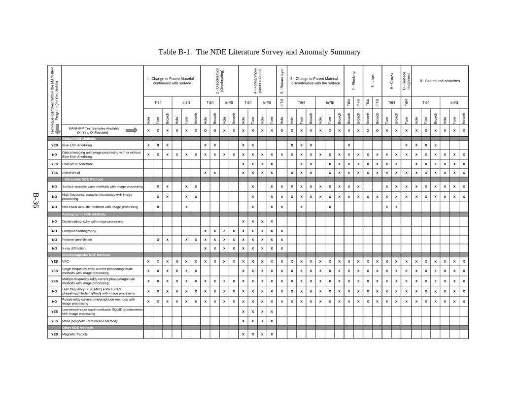
Table B-1. The NDE Literature Survey and Anomaly Summary
5 -
Re
cast
laye
r
l0 -
Su
rfac
e ro
ugh
nes
s
In7
l8
Ti6
4
In7
l8
Ti6
4
In7
l8
Ti6
4
Hol
e
Tur
n
Bro
ach
Hol
e
Tur
n
Bro
ach
Hol
e
Bro
ach
Hol
e
Bro
ach
Hol
e
Tur
n
Hol
e
Tur
n
Hol
e
Hol
e
Tur
n
Bro
ach
Hol
e
Tur
n
Bro
ach
Bro
ach
Bro
ach
Bro
ach
Bro
ach
Tur
n
Bro
ach
Tur
n
Hol
e
Tur
n
Bro
ach
Hol
e
Tur
n
Bro
ach
MANHIRP Test Samples Available (X=Yes, O=Possible)
X X X X X X O O X X X X X X O X X X X O X X X O O X X X X X X X X X
Optical NDE Methods
YES Blue Etch Anodizing X X X X X X X X X X X X X X X
NOOptical imaging and image processing with or without Blue Etch Anodizing
X X X X X X X X X X X X X X X X X X X X X X X X X X X X X X X X X X
YES Florescent penetrant X X X X X X X X X X X X X X X X X X X X
YES Aided visual X X X X X X X X X X X X X X X X X X X X X X X X
Ultrasonic NDE Methods
NO Surface acoustic wave methods with image processing X X X X X X X X X X X X X X X X X X X X X X X X
NOHigh frequency acoustic microscopy with image processing
X X X X X X X X X X X X X X X X X X X X X X X X X X
NO Non-linear acoustic methods with image processing X X X X X X X X X
Radiographic NDE Methods
NO Digital radiography with image processing X X X X
NO Computed tomography X X X X X X X X X
NO Positron annihilation X X X X X X X X X X X X X
NO X-ray diffraction X X X X X X X X X
Electromagnetic NDE Methods
YES VAC X X X X X X X X X X X X X X X X X X X X X X X X X X X X X X X X X X
YESSingle frequency eddy current phase/magnitude methods with image processing
X X X X X X X X X X X X X X X X X X X X X X X X X X X X X X
YESMultiple frequency eddy current phase/magnitude methods with image processing
X X X X X X X X X X X X X X X X X X X X X X X X X X X X X X X X X X
NOHigh frequency (> 20 MHz) eddy current phase/magnitude methods with image processing
X X X X X X X X X X X X X X X X X X X X X X X X X X X X X X X X X X
NOPulsed eddy current time/amplitude methods with image processing
X X X X X X X X X X X X X X X X X X X X X X X X X X X X X X X X X X
YESLow-temperature superconductor SQUID gradiometers with image processing
X X X X
YES MRM (Magnetic Remanence Method) X X X X
Other NDE Methods
YES Magnetic Particle X X X X
6 - Change to Parent Material – discontinuous with the surface
In7l8
l - Change to Parent Material – continuous with surface
In7l8Ti64 In7l8 Ti64 Ti64In7l8Ti64
ll - Scores and scratches
7 -
Plu
ckin
g
8 -
Lap
s
9 -
Cra
cks
Te
chni
que
Ide
ntif
ied
With
in th
e M
AN
HIR
P
Pro
gra
m (
Y=
Yes
, N
=N
o)
In7l8
2 -
Dis
colo
ratio
n (O
verh
eatin
g)
4 -
For
eig
n/n
on-
pare
nt m
ater
ial
Ti64Ti64
B-36

B.4 REFERENCES. B-1. Fomitchov, P., Kromine, A.K., Sohn, Y., Krishnaswamy, S., and Achenbach, J.D.,
“Ultrasonic Imaging of Small Surface-Breaking Defects Using Scanning Laser Source Technique,” Review of Progress in Quantitative Nondestructive Evaluation, Vol. 21A, Thompson, D. and Chimenti, D., eds., 2001.
B-2. Bamberg, J., Gindorf, A., and Steinhauser, L., “Surface Monitoring by Combination of an Optical Sensor and an Ultrasonic Scanning System,” 22nd Symposium on Quantitative Nondestructive Evaluation, Seattle, Washington, 1995.
B-3. Monchalin, J.P., Ochiai, M., Levesque, D., Blouin, A., Talbot, R., and Fukumoto, A., “Characterization of Surface-Breaking Tight Cracks Using Laser-Ultrasonic Shadowing,” Review of Progress in Quantitative Nondestructive Evaluation, Vol. 23B, 2003.
B-4. Choi, S.W., Lee, J.H., Nam, A.J., and Krishnaswamy, S., “Application of Scanning Laser Source Technique for Nondestructive Flaw Detection,” Key Engineering Materials, Vols. 270-279, 2004.
B-5. Kromine, K., Fomitchoev, P.A., Krishnaswamy, S., and Achenbach, J.D., “Scanning Laser Source Technique and its Application to Turbine Disk Inspection,” Review of Progress in Quantitative Nondestructive Evaluation, 1999.
B-6. Abbate, A., Russell, W., Goldman, J., Kotidis, P., and Berndt, C.C., “Nondestructive Determination of Thickness and Elastic Modulus of Plasma Spray Coatings Using Laser Ultrasonics,” Review of Progress in Quantitative Nondestructive Evaluation, Vol. 18, 1999, pp. 373-380.
B-7. Hoshimiya, T., “Nondestructive Evaluation of Surface Defects Under Dry/Wet Environment by the use of Photoacoustic and Photothermal Electrochemical Imaging,” NDT International, Vol. 32, 1999.
B-8. Earthman, J.C., Angeles, J., Markov, V., Trolinger, J., and Moffatt, J.G., “Scattered Light Scanning for Fatigue Damage Precursor Detection on Turbine Components,” Materials Evaluation, Vol. 62, 2004.
B-9. Montague, J., “Laser Sensor Vision System Improves Surface Quality Inspection,” Council Engineering, Vol. 50, 2003.
B-10. Gustafson, S.C., Mehta, J.R., and Frantziskonis, G.N., “Practical Optical Characterization of Fretted Surfaces,” Nondestructive Characterization of Materials in Aging Systems, Crane, R., et al., eds., Materials Research Society, Boston, Massachusetts, 1998.
B-11. Kobbelt, L., Botsch, K., Schwanecke, U., and Seidel, H., “Feature Sensitive Surface Extraction From Volume Data,” Association for Computing Machinery Special Interest Goup on Graphics and Interactive Techniques, 2001, pp. 57-66.
B-37

B-12. Livingston, M., Vision and Art: The Biology of Seeing, Harry N. Abrams, New York, New York, 2002.
B-13. Barten, P., “Contrast Sensitivity of the Human Eye and its Effects on Image Quality,” SPIE Optical Engineering Press, Bellingham, Washington, 1999.
B-14. Doyle, J., “Laser-Based Inspection of High L/D Bores in Titanium Aircraft Engine Components,” Internal MANHIRP Report, Not released for publication, December 2002.
B-15. Auld, B.A., Acoustic Fields and Waves in Solids, Volume II, Robert E. Krieger Publishing Co., Inc., Malibar, Florida, 1990.
B-16. Blitz, J. and Simpson, G., Ultrasonic Methods of Non-Destructive Testing, Chapman and Hall, London, 1996.
B-17. Gilmore, R.S., Tam, K.C., Young, J.D., and Howard, D.R., “Acoustic Microscopy From 10 to 100 MHz for Industrial Applications,” Philosophical Transactions of the Royal Society, Vol. A320, 1986.
B-18. Margetan, F.J., Gigliotti, M., Brasche, L., and Leach, W., “Fundamental Studies: Inspection Properties for Engine Titanium Alloys,” FAA report DOT/FAA/AR-02/114, December 2002.
B-19. Margetan, F.J., Nieters, E., Haldipur, P., Brasche, L., Chiou, T., Keller, M., Degtyar, A., Umbach, J., Hassan, W., Patton, T., and Smith, K., “Fundamental Studies of Nickel Billet Materials—Engine Titanium Consortium II,” FAA report DOT/FAA/AR-05/17, June 2005.
B-20. Margetan, F.J., Nieters, E., Brasche, L., Yu, L., Degtyar, A., Wasan, H., Keller, M., and Kinney, A., “Fundamental Studies of Titanium Forging Materials—Engine Titanium Consortium II,” FAA report DOT/FAA/AR-05/22, June 2005.
B-21. Papadakis, E.P., “Ultrasonic Attenuation Caused by Scattering in Polycrystalline Media,” Physical Acoustics, Vol. IV, Mason, W.P. and Thurston, D., eds., Academic Press, New York, New York, 1968, pp. 269-328.
B-22. Goebbels, K., “Structure Analysis by Scattered Ultrasonic Radiation,” Research Techniques in Nondestructive Testing, Vol. IV, Sharpe, R.S., ed., Academic Press, New York, New York, 1980.
B-23. Wasan, H., “Influence of Microstructure on Ultrasonic Detection of Flaws in Aircraft Engine Alloys,” Masters Thesis, Iowa State University, Ames, Iowa, 2000.
B-24. Panetta, P.D., Thompson, R.B., and Margetan, F.J., “Use of Electron Backscatter Diffraction in Understanding Texture and the Mechanisms of Backscattered Noise Generation in Titanium Alloys,” Review of Progress in QNDE, Vol. 17A, Thompson, D.O. and Chimenti, D.E., eds., Plenum Press, New York, New York, 1998, pp. 89-96.
B-38

B-25. Foister, S.A.M., McKenzie, S.G., and Chivers, R.C., “An Experimental Investigation of Ultrasonic Grain Noise in Titanium-6Al-4V,” Review of Progress in QNDE, Vol. 15, Thompson, D.O. and Chimenti, D.E., eds., Plenum Press, New York, New York, 1996, pp. 1479-1485.
B-26. Linxiao, Y., Thompson, R.B., Margetan, F.J., and Degtyar, A., “Modeling Ultrasonic Grain Noise Within Ti-6Al-4V Forgings,” Review of Progress in QNDE, Vol. 22, Thompson, D.O. and Chimenti, D.E., eds., AIP, Melville, New York, 2003, pp. 1339-1346.
B-27. DEFORM is a commercial software package produced by Scientific Forming Technologies Corporation, Columbus, Ohio.
B-28. Rose, J.H., “Theory of Ultrasonic Backscatter From Multiphase Polycrystalline Solids,” Review of Progress in QNDE, Vol. 12, Thompson, D.O. and Chimenti, D.E., eds., Plenum Press, New York, New York, 1993, pp. 1719-1726.
B-29. Thompson, R.B., Panetta, P., and Margetan, F.J., “Relationship of the Ultrasonic Backscattering Coefficient of Titanium Alloys to Microstructure,” Materials and Processes Affordability: Keys to the Future, Kliger, H.S., Rasmussen, B.J., Pilato, L.A., and Tolle, T.B., eds., SAMPE, Covina, California, 1998, pp. 1448-1457.
B-30. Margetan, F.J., Haldipur, P., and Thompson, R.B., “Looking for Multiple Scattering Effects in Backscattered Ultrasonic Noise From Jet Engine Nickel Alloys,” Review of Progress in QNDE, Vol. 24, Thompson, D.O. and Chimenti, D.E., eds., AIP, Melville, New York, 2005, pp. 75-82.
B-31. Margetan, F.J., Thompson, R.B., Keller, M., and Hassan, W., “Compensating for Attenuation Differences in Ultrasonic Inspections of Titanium-Alloy Billets,” Review of Progress in QNDE, Vol. 23B, Thompson, D.O. and Chimenti, D.E., eds., AIP, Melville, New York, 2004, pp. 1091-1098.
B-32. Friedl, J.H., Gray, T.A., Khandelwal, P., and Dunhill, T., “Ultrasonic Phased Array Inspection of Seeded Titanium Billet,” Review of Progress in QNDE, Vol. 23, Thompson, D.O. and Chimenti, D.E., eds., AIP, Melville, New York, 2004, pp. 809-816.
B-33. Solomon, K., Luttrell, M., and Long, J., “The Use of Focused Array Transducer Techniques for Improved Titanium and Other Billet Inspections,” Review of Progress in QNDE, Vol. 13, Thompson, D.O. and Chimenti, D.E., eds., Plenum Press, New York, 1994, pp. 1069-1074.
B-34. Umbach, J., Roberts, R., Margetan, F.J., et al., “Inspection Development for Titanium Forgings,” FAA report DOT/FAA/AR-05/46, May 2007.
B-35. Panetta, P.D., Margetan, F.J., Yalda, I., and Thompson, R.B., “Ultrasonic Attenuation Measurements in Jet Engine Titanium Alloys,” Review of Progress in QNDE, Vol. 15B, Thompson, D.O. and Chimenti, D.E., eds., Plenum Press, New York, New York, 1996, pp. 1525-1532.
B-39

B-36. Achenbach, J.D., Sotiropoulos, D.A., and Zhu, H., “On the Direct and Inverse Elastic Wave Scattering Problem to Characterize Damage in Materials,” Review of Progress in QNDE, Vol. 6A, Thompson, D.O. and Chimenti, D.E., eds., Plenum Press, New York, New York, 1987, pp. 37-43.
B-37. Hirsekorn, S., Van Andel, P.Q., and Netzelmann, U., “Ultrasonic Methods to Detect and Evaluate Damage in Steel,” Nondestructive Testing and Evaluation, Vol. 15, 2000, pp. 373-391.
B-38. Tittmann, R., Abdel-Gawad, M., and Fertig, K., “Ultrasonic Characterization of Microstructure in Powder Metal Alloy,” Research in Nondestructive Evaluation, Vol. 2, 1990, pp. 119-133.
B-39. Morissey, M. and Scholz, R., “Determination of Creep Damage in the ODS Superalloy MA6000,” Key Engineering Materials, Vol. 99-100, 1995, pp. 135-142.
B-40. Shah, K., Nanekar, P.P., Bandyopadhyay, M., Bandyopadhyay, A.K., Biswas, A.K., and Kulharni, P.G., “Ultrasonic Characterization of Aging Degradation During Long-Term High-Temperature Exposure in Nickel-Base Alloy 625,” 14th World Conference on Nondestructive Testing, Vol. 3, December 1996, pp. 2235-2238.
B-41. Good, M.S., “Effective Case Depth Measurement by an Ultrasonic Backscatter Technique,” Metals/Materials Technology Series, paper No. 8405-003, American Society for Metals, Metals Park, Ohio, 1984.
B-42. Good, M.S. and Rose, J.L., “Measurement of Thin Case Depth in Hardened Steel by Ultrasonic Pulse-Echo Angulation Techniques,” Nondestructive Methods for Material Property Determination, Ruud, C.O. and Green, Jr., R.E., eds., Plenum Press, New York, New York, 1984, pp. 189-203.
B-43. Good, M.S. and Rogers, D.D., “General Motors Corporation and Pacific Northwest Laboratory Staff Exchange: Inspection of Case Hardened Steels and Metal-Matrix Composites,” PNL-8926, Pacific Northwest Laboratory, Richland, Washington, 1993.
B-44. The Ultrasonic Microstructural Analyzer is described at the Sonix Incorporated website (see www.sonix.com/learning/files/UMA_Breakthrough.pdf, last visited 11/22/10.)
B-45. Tardy, F., Noroy, M.H., Paradis, L., and Baboux, J.C., “Material Surface Characterization by a Raleigh Velocity Measurement,” Proceedings of the World Congress on Ultrasonics, Berlin, Germany, September 3-7, 1995, pp. 451-454.
B-46. Scruby, C.B. and Drain, L.E., Laser, Ultrasonics: Techniques and Applications, Taylor & Francis Group, New York, New York, 1990.
B-47. Lamy, C.A., Rebello, J.M.A., Sauer, A., and Chartier, J., “Surface Crack Sizing Related to the Stress State by an Ultrasonic Time-of-Flight Technique,” Insight–Nondestructive Testing and Condition Monitoring, Vol. 40, 1998, pp. 421-429.
B-40

B-48. Bykov, Y.G., Petukhov, A.N., and Cherkasova, S.A., “Cyclic Cracking Resistance of VT3-1 and VT-25 Titanium Alloys,” Soviet Materials Science, Vol. 26, 1990, pp. 288-291.
B-49. Kromine, K., Fomitchov, P.A., Krishnaswamy, S., and Achenbach, J.D., “Scanning Laser Source Technique and its Application to Turbine Disk Inspection,” Review of Progress in QNDE, Vol. 18A, Thompson, D.O. and Chimenti, D.E., eds., Kluwer/Plenum Press, New York, New York, 1999, pp. 381-386.
B-50. Fomitchov, P., Kromine, A.K., Younghoon, S., Krishnaswamy, S., and Achenbach, J.D., “Ultrasonic Imaging of Small Surface-Breaking Defects Using Scanning Laser Source Technique,” Review of Progress in QNDE, Vol. 21A, Thompson, D.O. and Chimenti, D.E., eds., AIP, Melville, New York, 2002, pp. 356-362.
B-51. Wagner, J.S., “Optical Generation and Detection of Ultrasound for Flaw Detection and its Potential for In-Line Process/Quality Control,” NDE of Microstructure for Process Control, Wadley, H.N.G., ed., ASM Publication, 1985, pp. 173-177.
B-52. Monchalin, J.P., Ochiai, M., Levesque, D., Blouin, A., Talbot, R., and Fukumoto, A., “Characterization of Surface-Breaking Tight Cracks Using Laser-Ultrasonic Shadowing,” Review of Progress in QNDE, Vol. 23B, Thompson, D.O. and Chimenti, D.E., eds., AIP, Melville, New York, 2004, pp. 1264-1271.
B-53. Choi, S.W., Lee, J.H., Nam, A.-J., and Krishnaswamy, S., “Application of Scanning Laser Source Technique for Nondestructive Flaw Detection,” Key Engineering Materials, Vol. 270-273, 2004, pp. 787-792.
B-54. Brasche, L.J.H., Margetan, F.J., and Thompson, R.B., “Sample Preparation Techniques and Material Property Measurements of Hard Alpha Titanium Samples,” Review of Progress in QNDE, Vol. 11B, Thompson, D.O. and Chimenti, D.E., eds., Plenum Press, New York, New York, 1992, pp. 1733-1738.
B-55. RISC Meeting—MANHIRP Workshop, “Fatigue and Analysis of Holes Specimen—
Ti 6-4 and In 718—Low Cycle Fatigue,” available online at http://wzl-tf4.wzl.rwth
-aachen.de/manhirp/public/Presentations%20of%20RISC-Meeting%20May_2004_Paris /09a_MANHIRP_Paris_2004.pdf
B-56. Ogi, H., Minami, Y., Aoki, S., and Hirao, M., “Contactless Monitoring of Surface-Wave Attenuation and Nonlinearity for Evaluating Remaining Life of Fatigued Steels,” available online at http://www.ndt.net/article/wcndt00/papers/idn184/idn184.htm (last visited on 11/22/10).
B-57. McCarthy, R., “The Application of Ultrasonic Wave Propagation Models to the Nondestructive Testing of Surface Coatings,” Ph.D. Thesis, Cambridge University, Cambridge, England, 2002.
B-41

B-58. Abbate, A., Russell, W., Goldman, J., Kotidis, P., and Berndt, C.C., “Nondestructive Determination of Thickness and Elastic Modulus of Plasma Spray Coatings Using Laser Ultrasonics,” Review of Progress in QNDE, Vol. 18A, Thompson, D.O. and Chimenti, D.E., eds., Kluwer/Plenum Press, New York, New York, 1999, pp. 373-380.
B-59. Lee, Y.C. and Cheng, S.W., “Measurement of Leaky Lamb Wave Dispersion Curves With Application on Coating Characterization,” Review of Progress in QNDE, Vol. 20A, Thompson, D.O. and Chimenti, D.E., eds., AIP, Melville, New York, 2001, pp. 196-203.
B-60. Coste, J.F., “Approximate Dispersion Formulae for Rayleigh-Like Waves in a Layered Medium,” Ultrasonics, Vol. 35, 1997, pp. 431-440.
B-61. Coste, J.F., “Nondestructive Determination of the Thickness of Plasma Sprayed Coatings by Means of Propagating [Ultrasonic] Surface Waves,” Report EUR-16424. Publ: L-2985 Luxembourg; Commission of the European Communities, 1996, pp. 1-133.
B-62. Guo, Y., Margetan, F.J., and Thompson, R.B., “Effects of Periodic Surface Roughness on Ultrasonic Backscattered Noise,” Review of Progress in QNDE, Vol. 20, Thompson, D.O. and Chimenti, D.E., eds., AIP, Melville, New York, 2001, pp. 1306-1313.
B-63. Thompson, R.B., Guo, Y., and Margetan, F.J., “Advances in Modeling Ultrasonic Noise Induced by Machining Roughness: Development and Validation of Computationally Efficient Approximations,” Review of Progress in QNDE, Vol. 22, Thompson, D.O. and Chimenti, D.E., eds., AIP, Melville, New York, 2003, pp. 125-132.
B-64. The Laser Ultrasonic Camera at the Idaho National Engineering and Environmental Laboratory (INEEL) is described at website http://www.inl.gov/physics/nlo /laserultrasonic.shtml
B-65. Yan, Z. and Nagy, P.B., “Thermo-Optical Modulation for Improved Ultrasonic Fatigue Crack Detection in Ti-6Al-4V,” NDT International, Vol. 33, 2000, pp. 213-223.
B-66. Feist, W.D., et al., “Nondestructive Evaluation of Manufacturing Anomalies in Aero-Engine Rotor Disks,” 16th World Conference on Nondestructive Testing, Montreal, Canada, 2004.
B-67. Hsieh, J., Computed Tomography: Principles, Design, Artifacts, and Recent Advances, SPIE Press, Belingham, Washington, 2003.
B-68. Zhang, J., Chiou, C., Jensen, T., and Gray, J., “Development of a High-Resolution CT System and 3D Data Visualization Tools,” Review of Progress in Quantitative Nondestructive Evaluation, Vol. 24, Thompson, D.O. and Chimenti, D.E., eds., AIP, Melville, New York, 2005, pp. 686-693.
B-69. Georgeson, G. and Bossi, R., “X-Ray CT for Quantitative Casting Material Evaluation,” Review of Progress in Quantitative Nondestructive Evaluation, Vol. 12B, Thompson, D.O. and Chimenti, D.E., eds., Plenum Press, New York, New York, 1993, pp. 1681-1688.
B-42

B-70. Bossi, R.H., Friddell, K.D., and Nelson, J.M., “Backscatter X-Ray Imaging,” Materials Evaluation, Vol. 46, 1988, pp. 1462-1467.
B-71. Harding, G. and Kosanetzky, J., “Scattered X-Ray Beam Nondestructive Testing,” Nuclear Instruments,and Methods in Physics Research, Vol. A280, 1989, pp. 517-528.
B-72. Jensen, T. and Melikhova, O., “A Review of Positron Annihilation as a Nondestructive Testing Tool,” submitted to AFRL for publication as part of contract no. FA8650-04-C5528, July 2005.
B-73. Reno, R.C., Swartsendruber, L.J., and Bennet, L.H., “Positron Annihilation Studies of Defects in Titanium,” NDT International, Vol. 12, 1979, pp. 224-226.
B-74. Coleman, C.F., Hughes, A.E., and Smith, F.A., “Positron Annihilation Measurements of Deformation in an Elastically and Plastically Deformed Ti Alloy,” NDT International, Vol. 12, 1979, pp. 267-269.
B-75. Akers, D.W., “Method for Photon Activation Positron Annihilation Analysis,” United States Patent Application 20030048864, 2003.
B-76. Akers, D.W. and Rideout, C.A., Proceedings of the Conference on Materials Science and Technology, Symposium on Materials Damage Prognosis, New Orleans, Louisiana, September 2004.
B-77. Selim, F.A., Wells, D.P., Harmon, J.F., Scates, W., Kwofie, J., Spaulding, R., Duttagupta, S.P., Jones, J.L., White, J., and Roney, T., “Doppler Broadening Measurements of Positron Annihilation Using Bremsstrahlung Radiation,” Nuclear Instruments and Methods in Physics Research, Section B, Vol. 192, 2002, pp. 197-201.
B-78. Hutchings, M.T., Buttle, D.J., Colbrook, R., Dalzell, W., and Scruby, C.B., Journal de Physique IV, Colloque C1, Vol. 5, pp. C1-111 to C1-117, 1995.
B-79. McFarland, E.W., Leigh, J., and Lanza, R.C., “Detection and Characterization of the Heterogeneous Distribution of Hydrogen in Titanium Compressor Blades by Neutron Computed Tomography,” Journal of Advanced Materials, Vol. 26, 1984, pp. 3-10.
B-80. Poeth II, D.F., Rudd, C.O., and Levine, S.H., “The Experimental Determination of the Neutron Cross Section for Selected Solvents,” Journal of Nondestructive Evaluation, Vol. 15, 1996, pp. 35-42.
B-81. Warren, B.E., X-Ray Diffraction, Addison-Wesley, Reading, Massachusetts, 1969.
B-82. Lamda Research, “Development of Nondestructive Residual Stress Profile Measurement Methods—The Integral Method,” United States Air Force Final Report 674-10717, 2003.
B-43

B-83. Yanase, E., Nisho, K., Kusumi, Y., Arai, K., Susuki, K., Akiniwa, Y., Kimachi, H. and Tanaka, K., “Residual Stress Distribution of Shot-Peened Steel Estimated by High-Energy X-Rays From Synchrotron Radiation Source,” Journal of the Society of Materials Science, Japan, Vol. 51, No. 7, 2002, pp. 756-763.
B-84. Tanaka, K., Akiniwa, Y., Susuki, K., Yanase, E., Nisho, K., Kusumi, Y., and Arai, K., “High-Energy X-Ray Diffraction Synchrotron Radiation Analysis of Residual Stress Distribution of Shot-Peened Steel,” Materials Science Forum, Vols. 404-407, 2002, pp. 341-348.
B-85. Wendt, S., Gray, J., and Beckman, S., “Energy Dispersive Measurements of Anisotropic Diffraction Mottling Effects,” Review of Progress in Quantitative Nondestructive Evaluation, Vol. 20A, Thompson, D.O. and Chimenti, D.E., eds., American Institute of Physics, 2000, pp. 514.
B-86. Al-shorman, M., Gray, J., and Jensen, T., “Developments in Using High Energy X-Ray Diffraction for Measuring Residual Stress,” Review of Progress in Quantitative Nondestructive Evaluation, 2006.
B-87. Harnwell, P., Principles of Electricity and Magnetism, 2nd edition, McGraw-Hill Book Co., New York, New York, 1949.
B-88. Goldfine, N., Schlicker, D., Tsukernik, V., Shay, I., Windoloski, M., Zilberstein, V., Washabaugh, A., Walrath, K., and Carill, S., “High Resolution MWM-Array Imaging of Cracks in Fretting Regions of Engine Disk Slots,” Proceeding of the 6th Joint FAA/DoD/NASA Aging Aircraft Conference, 2002.
B-89. Chernyak, V.Y., Kudrin, A.P., and Kralya, V.A., “Study of ZhS6K Heat-Resistant Alloy for Overheating by the NDT Methods,” Tekhnicheskaya Diagnostika I Nerazrushayushchij Kontrol (Technical Diagnostics and Nondestructive Control), Vol. 2, 1996, pp. 60-62.
B-90. Capobianco, T.E., “Real-Time Eddy Current Monitoring of Fatigue Crack Growth,” Review of Progress in Quantitataive Nondestructive Evaluation, Vol. 11B, 1992.
B-91. Braun, T.J., Keppler, E.E., Price, L.S., Nuxoll, G., Gehlen, M., Lyders, D., Jenderson, J., Stone, R., and Arispe, B., “The Emergence of Extended Field Technology in the Air Force,” Proceedings of the 22nd Symposium on Quantitative Nondestructive, Seattle, Washington, 1996.
B-92. Feist, W.D., Mook, G., Taylor, S., Söderberg, H., Mikic, A., and Stepinski, T., “Non-Destructive Evaluation of Manufacturing Anomalies in Aero-Engine Rotor Disks,” Proceeding of the 16th World Conference in Nondestructive Testing, Montreal, Canada, August 2004.
B-93. Lavrentyev, A. and Veronesi, A.I., “Ultrasonic Characterization of Near-Surface Material Properties in Shot-Peened Waspaloy,” AIP Conference Proceedings, No. 615B, 2002, pp. 1659-1666.
B-44

B-45
B-94. “Development of Residual Stress Depth Profile Measurement Instrument,” Broad Agency Announcement (BAA) NR: 04-01-MLK Annual MCNEAT Open-Ended BAA Activity Update 01 Posted on 14 February 2005.
B-95. Blodgett, M.P. and Nagy, P.B., “Eddy Current Assessment of Near-Surface Residual Stress in Shot-Peened Nickel-Base Superalloys,” Journal of Nondestructive Evaluation, Vol. 23, 2004, pp. 107-123.
B-96. Blodgett, M. and Nagy, P.B., “On the Feasibility of Eddy Current Characterization of the Near-Surface Residual Stress Distribution in Nickel-Base Superalloys,” Review of Progress in QNDE, Vol. 23B, AIP, Melville, New York, 2004, pp. 1216-1223.
B-97. Blodgett, M., Yu, F., and Nagy, P.B., “Eddy Current Nondestructive Residual Stress Assessment in Shot-Peened Nickel-Base Superalloys,” Review of Progress in QNDE, Vol. 24B, AIP, Melville, New York, 2005, pp. 1347-1354.
B-98. Yu, F. and Nagy, P.B., “Piezoresistive Effect for Near-Surface Eddy Current Residual Stress Assessment,” Review of Progress in QNDE, Vol. 24, AIP, Melville, New York, 2005, pp. 1371-1378.
B-99. Yu, F. and Nagy, P.B., “Simple Analytical Approximations for Eddy Current Profiling of the Near-Surface Residual Stress in Shot-Peened Metals,” Journal of Applied Physics, Vol. 96, 2004, pp. 1257-1266.
B-100. Soules, J.A., Schoenig, Jr., F.C., Chang, H., and DiCillo, J.J., “Eddy-Current Measurements of Residual Stresses Induced by Shot Peening in Titanium Ti6A14V,” Materials Evaluation, Vol. 53, No. 1, January 1995.
B-101. Ko, R.T. and Pipenburg, S.J., “Automated Eddy-Current Detection of Flaws in Shot-Peened Titanium Materials,” Review of Progress in Quantitative Nondestructive Evaluation, 1995, Vol. 14A.
B-102. Hagemaier, D.J., “Nondestructive Detection of Hydrides and Alpha-Case in Titanium Alloys,” Proceedings of the 2nd International Conference on Titanium, Cambridge, Massachusetts, Massachusetts Institute of Technology, 1972.
B-103. Zilberstein, V., Shay, I., Lyons, R., Goldfine, N., Malow, T., and Reiche, R., “Validation of Multi-Frequency Eddy Current MWM Sensors and MWM-Arrays for Coating Production Quality and Refurbishment Assessment,” American Society of Mechanical Engineers Turbo Expo, co-located with International Gas Turbine Institute, Atlanta, Georgia, 2003.
B-104. Crowther, P., “Non-Destructive Evaluation of Coatings for Land-Based Gas Turbines Using a Multi-Frequency Eddy-Current Technique,” Insight—Non-Destructive Testing and Condition Monitoring, September 2004.

B-105. Scholz, E., “Characterization of Service-Exposed Blades by Evaluation of the Chromium Content With Eddy-Current Equipment,” Life Assessment & Repair: Technology for Combustion Turbine Hot Section Components, ASM International, 1990.
B-106. Johnson, M.J. and Bowler, J.R., “Pulsed Eddy-Current Measurements for the Characterization of Thin Layers and Surface Treatments,” Proceedings of the 24th Annual Symposium on Quantitative Nondestructive Evaluation, 1997.
B-107. Sophian, G.-Y. Tian, Taylor, D., and Rudlin, D., “A Feature Extraction Technique Based on Principal Component Analysis for Pulsed Eddy Current NDT,” Nondestructive Testing & Evaluation International, Vol. 36, 2003.
B-108. Nye, J.F., Physical Properties of Crystals, Their Representation by Tensors and Matrices, Oxford, Clarendon Press, 1985.
B-109. Morgner, W., “Introduction to Thermoelectric Nondestructive Testing,” Materials Evaluation, Vol. 9, 1991, pp. 1081-1088.
B-110. Hu, J. and Nagy, P.B., “On the Role of Interface Imperfections in Thermoelectric Nondestructive Materials Characterization,” Applied Physics Letters, Vol. 73, 1998, pp. 467-469.
B-111. Lion, K.S., Instrumentation in Scientific Research: Electrical Input Transducers, New York, New York, McGraw Hill, 1959.
B-46

APPENDIX C—OPTION A—DEVELOPMENT OF TEST SAMPLE FABRICATION PROCESSES
C.1 INTRODUCTION. Option A was a risk management plan that allowed the program to proceed under a schedule that removed the acquisition of Manufacturing to Produce High Integrity Rotating Parts for Modern Gas Turbines (MANHIRP) test samples from the critical path. The objectives and samples produced for Option A were not sufficient to complete the requirements of the program. The purpose of Option A was to establish manufacturing practices that would generate comparable anomalies to those produced by the MANHIRP program. Completion of the full program required a sufficient number of test samples fabricated as Option C by the Engine Titanium Consortium (ETC). Under Option A, a minimum set of 120 test samples were fabricated to obtain a set of targeted manufacturing anomalies, as identified in the MANHIRP program. Baseline test samples were manufactured under nominal production quality. The test sample definitions fabricated by ETC are listed below, with details of the process types and quantities listed in table C-1. Type 1: Change to parent material continuous with the surface (microstructure damage,
bent grain, white layer, amorphous layer, and heat damage)
Type 1*: Fabricated as Type 1, but lightly reamed to remove geometrical distortions, leaving material distortions present (Note: Hole-drilling samples only)
Type 6: Change to parent material discontinuous with the surface (redeposited material and smearing of parent material chips, which bond back onto the surface)
Table C-1. The ETC Test Samples Fabrication Plan Under Option A
Material and
Process
Original Equipment
Manufacturer Primary
Anomalies Quality Baseline
Quality for Nondestructive
Testing
Quality Low-Cycle
Fatigue Quality
Metallurgical
Low-Cycle Fatigue Test Method**
Ti 6-4 Hole-Drilling
Type 1 Type 1* Type 6
3 each 2 each 2 each 2 each Axial
In 718 Hole-Drilling
General Electric Aviation
Type 1 Type 1* Type 6
3 each 2 each 2 each 2 each Axial
Ti 6-4 Turning
Type 1 Type 6
3 each 2 each 2 each 2 each Axial
In 718 Turning
Pratt & Whitney
Type 1 Type 6
3 each 2 each 2 each 2 each Axial
Ti 6-4 Broaching
Type 1 Type 6
3 each 2 each 2 each 2 each Axial
In 718 Broaching
Honeywell Aerospace
Type 1 Type 6
3 each 2 each 2 each 2 each Axial
**The limited quantity of low-cycle fatigue (LCF) test samples were only used to illustrate general data trends and do not provide a statistically significant sample size correlation to MANHIRP results.
C-1

Under the Option A plan, each original equipment manufacturer (OEM) was responsible for obtaining its own titanium (Ti) Ti-6A1-4V alloy (Ti 6-4) material for development and final test sample fabrication. Common Inconel 718 alloy (In 718) material with a grain size of 8 or less (finer) was found to be exceptionally difficult to obtain. Obtaining this material was more difficult given that In 718 is not a commonly used production material within the ETC. Several different options for locating In 718 material were explored, such as using scrap Pratt & Whitney (PW)-JT8D engine hardware located at the Federal Aviation Administration (FAA) Airworthiness Assurance Nondestructive Inspection Validation Center, purchasing and heat-treating production DA718 (CFM56 HPT) disks to the required grain size, and finally, purchasing In 718 material from material suppliers. In the third option, scrap and (purchased) billet material was eventually acquired from a billet supplier (Carpenter Technology) and then forged, machined, and heat-treated through a forging supplier (Wyman-Gordon). This arrangement provided the ETC with the best opportunity to obtain a sufficient volume of In 718 material at the required microstructure. The scrap billet end materials were of double-melt quality obtained from 12-inch- (or less) diameter stock. The final disk shape was forged to the same dimensions as those previously used for Turbine Rotor Material Design studies, producing 14.6-inch-diameter, 3-inch-thick pancakes. Each OEM received a single forged disk of In 718 material. The remaining sections of this report outline the progress in fabricating test samples to that identified in table C-1. C.2 THE HOLE-DRILLING SAMPLE APPROACH. Hole-drilling samples were produced in the General Electric (GE) Metalworking Laboratory with Type 1 and Type 6 anomalies using best-practice parameters to produce damage-free baseline samples. Limited details are available of the process conditions used to produce MANHIRP anomalies. The MANHIRP anomaly information is consistent with prior GE experiments showing that the following hole-making process conditions can lead to the production of surface anomalies and a reduction in LCF performance: Poor tool condition, especially extreme wear or work material adhered to cutting edges
and tool margins
Inappropriate tool geometry, especially excessive margins or inadequate clearance angles
Excessive cutting speed
Lack of coolant
Consistent with prior experience, anomalies for the current program were produced using tools in poor condition, extreme cutting parameters, and in some cases, without coolant. For each material and anomaly type, holes were initially machined in scrap material using practices expected to produce the intended levels of damage. Holes that visually met the target criteria were then sectioned axially using wire electro-discharge machining (EDM) to allow closer examination of the hole surface; the holes were then mounted and polished to examine the microstructure.
C-2

Once the process condition was validated by metallography, the process was repeated by machining four to six holes in each of the two samples to yield what would become the metallography and nondestructive evaluation (NDE) samples. Machining four to six holes made it possible to select the two adjacent holes that exhibited the best representation of the target anomalies for metallography and NDE, respectively. One pair of samples (metallography and NDE) was harvested from each of the two bars. Two LCF samples were produced for each condition to validate that the anomalies were significant enough to reduce LCF performance, consistent with the earlier MANHIRP results. Two bars were also produced using the baseline process to provide an LCF reference for undamaged material at the test stress and temperature. Although there are known practices that produce damage in holes, producing specific anomalies typically involves more than a simple process formula. More complex practices require high levels of interaction from the test technician and frequently result in unsuccessful campaigns due to sudden, catastrophic tool failure. Undamaged baseline holes were produced using machining practices typical of those used on production hardware, including sharp tools, flood coolant, and speeds and feeds previously validated for surface integrity. These processes are codified in GE Special Process Specification P11TF12, Processing of Holes in Critical Parts. C.2.1 EQUIPMENT USED. The holes were machined in the GE Metalworking Technology Laboratory on a Monarch VMC-75B 3-axis Vertical Machining Center. This machine, shown in figure C-1, is equipped with a power-monitoring system that produces a millivolt-range signal proportional to spindle power. This signal gives an indication of the health of the cutting process, including tool wear progression and detection of special-cause events.
Figure C-1. Test Bed Machine Used to Make Hole-Drilling Samples at GE
C-3

The machine is equipped with a touch-probe system that is used to locate reference features on the work piece. This allows a work piece to be removed after a roughing operation (e.g., drilling) for examination and then replaced for subsequent finishing operations (e.g., ream or edge break). The machine table is configured with a vice capable of holding a range of work piece sizes and an adjacent fixture sized to hold LCF test bars. As shown in table C-2, other equipment included a Zeiss stereomicroscope with digital image capture used to examine tool geometry, tool condition, and where accessible, the condition of the hole surface. Conventional tooling and equipment used for micrograph analysis were also used. The only characterizations involved with the test samples were a visual comparison between photographs. Metallography was accomplished through 200-500x magnification. The samples were polished and etched with Krolls reagent to show the grain structure and digitally photographed. No further surface characterization was performed.
Table C-2. Equipment Used to Manufacture and Characterize Hole-Drilling Samples
Identification (Name, Model) Purpose Notes
Monarch VMC 75B Hole Manufacturing Multan 50 semi-synthetic metalworking fluid (when used)
Zeiss Axiovision Stereomicroscope
Digital Photography —
C.2.2 MACHINING. Hole samples with no anomalies are machined using P11TF12-compliant cutting parameters, which was previously demonstrated to have no negative impact on LCF properties. Except for variations in cutting speed, the same four-step process described below is typically used for all materials. 1. Holes are rough-drilled using sharp carbide tools, conservative cutting parameters, and
flood coolant. Spindle power is monitored to ensure there are no unnoticed special-cause events.
2. Holes are finish-reamed using sharp carbide tools, conservative cutting parameters, and flood coolant. Spindle power is monitored to ensure there are no unnoticed special-cause events.
3. A chamfer milling operation is typically used to edge break the hole entrance and exit; however, due to the extreme amount of displaced material produced during the heat-damage operations in Ti, a hand-fed plunge countersink operation was used instead. For consistency, this approach was used on all the Ti samples.
C-4

4. An abrasive brush operation is used on LCF samples to break the sharp intersections that remain after the chamfer cut. This brushing operation also slightly improves the surface finish of the hole body. This process was also used to produce the baseline holes supplied for metallographic and NDE.
Samples with targeted anomalies were produced using specific process variations for each alloy. C.2.3 METALLOGRAPHY. The metallographic mounts were examined along the axial surface of the hole at 20-100x magnification. This orientation allows examination of the variation in the machined surface and underlying microstructure as a function of hole depth. Adhered/rebonded material and heat-affected zone (HAZ) depth are readily apparent in this orientation. Grain deformation depth can also be evaluated although the primary direction of grain deformation (the circumferential direction) is perpendicular to the plane of polish. The metallographic results were used to identify whether the target anomalies had been achieved and, for the Type 1* condition, whether the damage was deep enough that it would still be present after reaming. C.2.4 AN LCF TEST DESCRIPTION. LCF tests were performed on an MTS 20-kip servohydraulic system. Other holes for NDE evaluation and the supporting metallography, shown in figures C-2 and C-3 were machined in blanks 1 inch wide by 0.335 inch thick by approximately 7.5 inches long. This length made it possible to machine up to six holes at 1.25-inch-center spacing. The holes that exhibited the best representation of the target anomaly were then cut from the bar into finished 1-inch-square samples.
Figure C-2. Sample Geometry for NDE Hole Samples
C-5

Figure C-3. Hole-Drilling Sample Geometry LCF tests were performed on an MTS 20-kip servohydraulic system, figure C-4, which has MTS 20-kip servohydraulic wedge grips to hold the test articles. Load-controlled LCF tests evaluated the hole-drilling samples using the following test parameters: Triangular wave form R ratio = 0.01 Frequency = 0.5 Hz The Ti 6-4 samples were tested at room temperature and 59-ksi alternating pseudo-stress while the In 718 samples were tested at an elevated temperature of 550°C. These conditions were selected to best match previous MANHIRP test points.
Figure C-4. The LCF Test Machine Used at GE
C-6

The LCF sample design used in this study, figure C-5, has two holes per bar, spaced far enough apart that after the first hole fails, the portion of the bar with the remaining hole can be regripped and tested to failure. Although the program target is only two LCF data points, the second hole in each sample allows for the possibility of another result from each bar if the first hole to fail yields an unexpected result.
Figure C-5. Hole-Drilling Sample Geometry—LCF Samples The LCF blanks are peened CW14 9-14N on all surfaces prior to the hole-making operations. This reduces the risk of unintended initiation sites away from test features and reduces friction-grip failures. C.2.5 FABRICATION OF TYPE 1 ANOMALIES IN Ti 6-4 WITH HOLE-MAKING PROCESSES. C.2.5.1 Process Development. Ti exhibits erratic results when producing anomalous holes. The number of holes generated before anomalous cutting begins varies significantly, even for nominally identical tools. Once the process begins to produce poor holes, the effect may spontaneously clear itself or it may decline rapidly to tool failure. This has been demonstrated in a number of prior hole-making studies at GE. It was relatively easy to fabricate a single extreme anomalous condition; however, as reported by MANHIRP, duplication of moderate characteristics under controlled conditions proved to be challenging. Initial studies in scrap material validated that high-speed dry machining could be used to produce extreme temperatures after several holes. Process parameters were selected from the initial trials that typically produced the desired result within approximately five holes, while minimizing the risk of catastrophic tool failure.
C-7
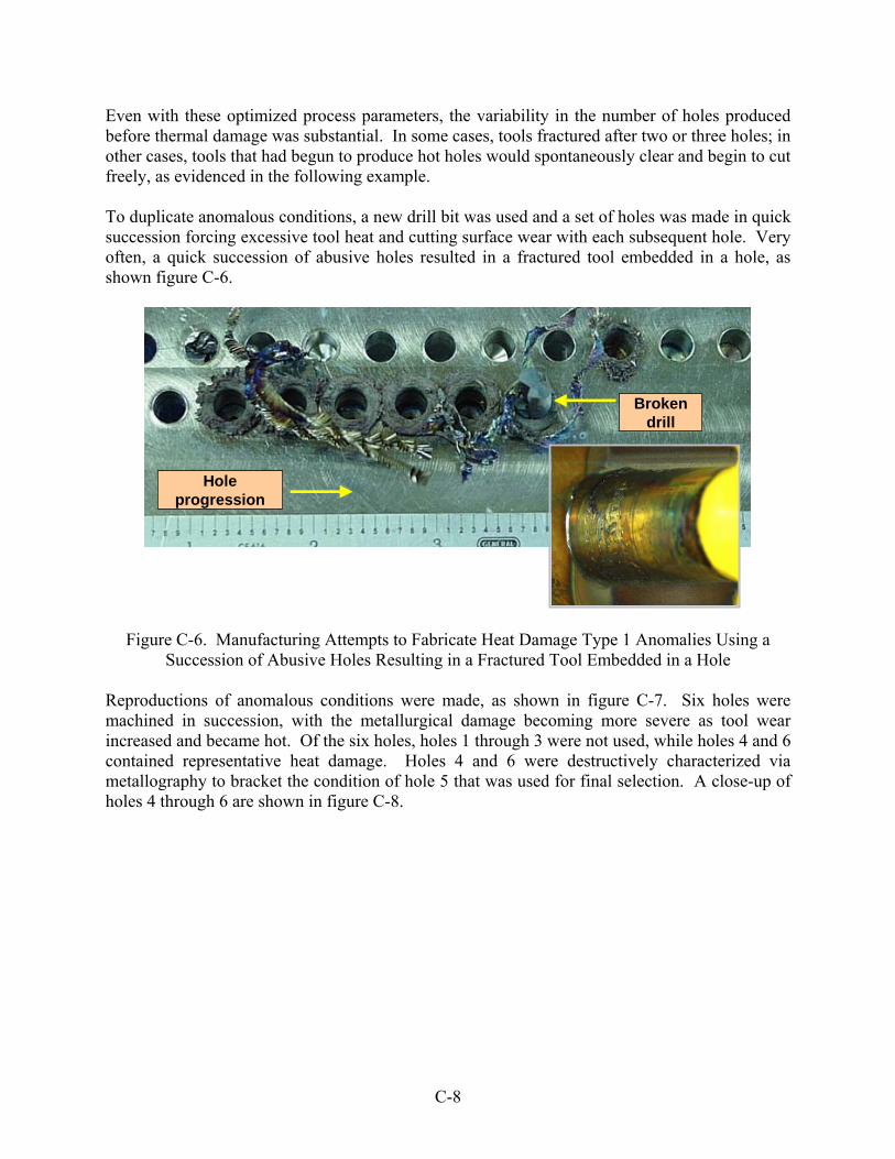
Even with these optimized process parameters, the variability in the number of holes produced before thermal damage was substantial. In some cases, tools fractured after two or three holes; in other cases, tools that had begun to produce hot holes would spontaneously clear and begin to cut freely, as evidenced in the following example. To duplicate anomalous conditions, a new drill bit was used and a set of holes was made in quick succession forcing excessive tool heat and cutting surface wear with each subsequent hole. Very often, a quick succession of abusive holes resulted in a fractured tool embedded in a hole, as shown figure C-6.
Broken drill
Hole progression
Broken drill
Hole progression
Figure C-6. Manufacturing Attempts to Fabricate Heat Damage Type 1 Anomalies Using a Succession of Abusive Holes Resulting in a Fractured Tool Embedded in a Hole
Reproductions of anomalous conditions were made, as shown in figure C-7. Six holes were machined in succession, with the metallurgical damage becoming more severe as tool wear increased and became hot. Of the six holes, holes 1 through 3 were not used, while holes 4 and 6 contained representative heat damage. Holes 4 and 6 were destructively characterized via metallography to bracket the condition of hole 5 that was used for final selection. A close-up of holes 4 through 6 are shown in figure C-8.
C-8

Usedfor NDE
Characterized bymetallography
Characterized bymetallography
Hole1
Hole2
Hole3
Hole4
Hole5
Hole6
Usedfor NDE
Characterized bymetallography
Characterized bymetallography
Hole1
Hole2
Hole3
Hole4
Hole5
Hole6
Figure C-7. Reproductions of Heat Damage Holes Made Through Bracketing Conditions
Hole4
Hole5
Hole6
Hole4
Hole5
Hole6
Figure C-8. Close-Up of Holes 4 Through 6 Figure C-9 shows this effect on scrap wear-in plates. The first hole machined with the given tool is circled in red. Progressing to the right, significant thermal damage was produced on the sixth hole (yellow circle), but the seventh hole was relatively clean. The tool continued to cut into the next row of holes (not all the intervening holes are captured in the photograph) where it again began to produce substantial heat until it ultimately seized in the hole, fracturing the shank. (Note that although some of the holes do not appear to be drilled completely through, this is due to an exit cap hinged to the exit burr visible through the hole in this view.)
C-9

Figure C-9. Successive Progression of Type 1 Hole With Uneven Heat Conditions It was observed that once a tool has produced two to three sequential hot (and high power) holes, it will typically continue to do so until tool failure. A three-hole threshold was employed to indicate that the tool was in a condition to produce Type 1 anomalies. The same condition shown in figure C-10 is also shown in figure C-11 with power-monitoring output displayed, illustrating the holes that contain sufficient heat-induced damage (Type 1).
Hole6
Hole19
Hole6
Hole19
Figure C-10. Successive Progression of Type 1 Hole With Uneven Heat Conditions Using Power-Monitoring Output
Drilling Ti 6-4 (200 sfm, 0.002 ipt dry)
Hole6
Hole19
Drilling Ti 6-4 (200 sfm, 0.002 ipt dry)
Hole6
Hole19
Figure C-11. Power-Monitoring Output of Figure C-10
C-10
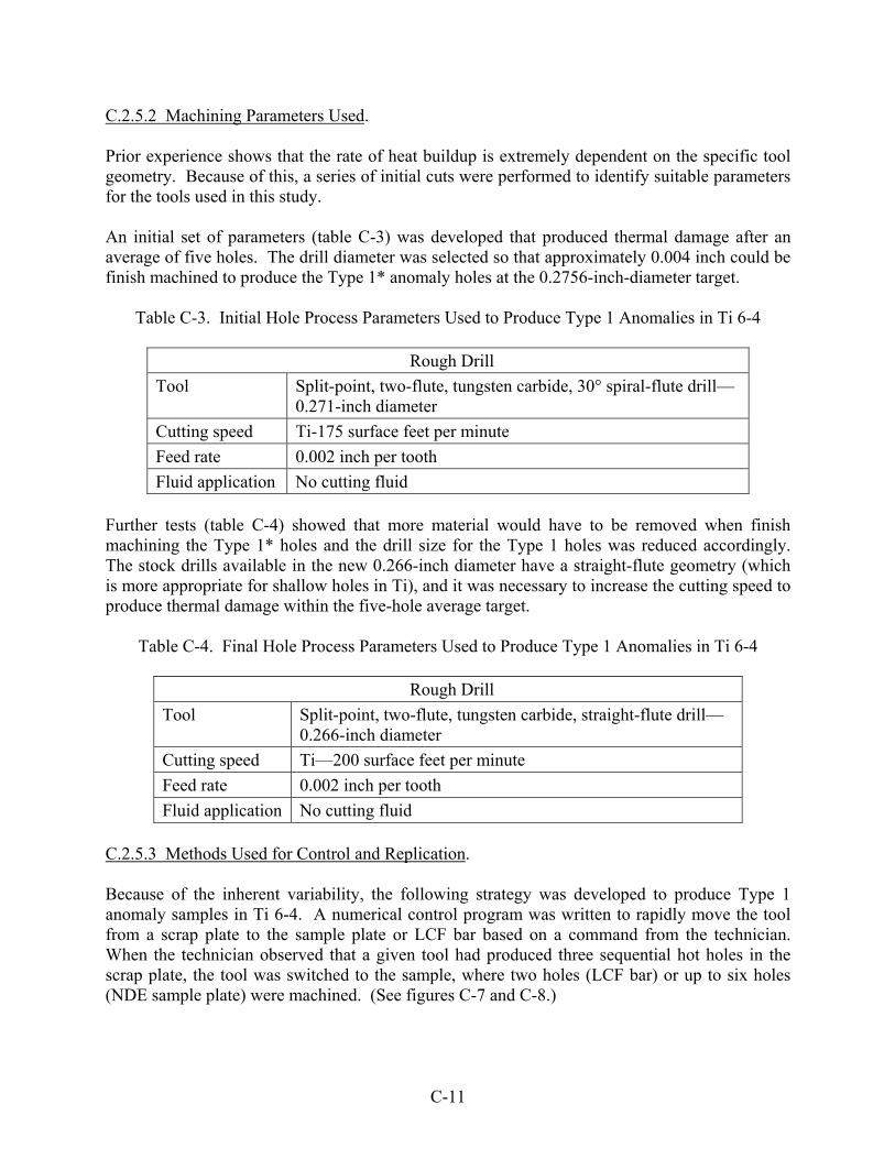
C.2.5.2 Machining Parameters Used. Prior experience shows that the rate of heat buildup is extremely dependent on the specific tool geometry. Because of this, a series of initial cuts were performed to identify suitable parameters for the tools used in this study. An initial set of parameters (table C-3) was developed that produced thermal damage after an average of five holes. The drill diameter was selected so that approximately 0.004 inch could be finish machined to produce the Type 1* anomaly holes at the 0.2756-inch-diameter target.
Table C-3. Initial Hole Process Parameters Used to Produce Type 1 Anomalies in Ti 6-4
Rough Drill
Tool Split-point, two-flute, tungsten carbide, 30° spiral-flute drill—0.271-inch diameter
Cutting speed Ti-175 surface feet per minute
Feed rate 0.002 inch per tooth
Fluid application No cutting fluid Further tests (table C-4) showed that more material would have to be removed when finish machining the Type 1* holes and the drill size for the Type 1 holes was reduced accordingly. The stock drills available in the new 0.266-inch diameter have a straight-flute geometry (which is more appropriate for shallow holes in Ti), and it was necessary to increase the cutting speed to produce thermal damage within the five-hole average target.
Table C-4. Final Hole Process Parameters Used to Produce Type 1 Anomalies in Ti 6-4
Rough Drill
Tool Split-point, two-flute, tungsten carbide, straight-flute drill—0.266-inch diameter
Cutting speed Ti—200 surface feet per minute
Feed rate 0.002 inch per tooth
Fluid application No cutting fluid C.2.5.3 Methods Used for Control and Replication. Because of the inherent variability, the following strategy was developed to produce Type 1 anomaly samples in Ti 6-4. A numerical control program was written to rapidly move the tool from a scrap plate to the sample plate or LCF bar based on a command from the technician. When the technician observed that a given tool had produced three sequential hot holes in the scrap plate, the tool was switched to the sample, where two holes (LCF bar) or up to six holes (NDE sample plate) were machined. (See figures C-7 and C-8.)
C-11

Metallography was performed to verify the nature of the anomalous surface and to quantify the depth of the thermal damage. The latter was necessary to ensure that the Type 1 anomaly depth was large enough that the same process could be used to produce the target Type 1* samples. The photomicrographs of figure C-12 show the hole wall on the left side exhibiting over a 0.004-inch HAZ.
Figure C-12. Micrographs of Ti 6-4 Type 1 Anomaly by Hole Process C.2.5.4 Summary of Ti 6-4 Type 1 Anomalies—Holes. It is difficult to produce consistent hole-making anomalies in Ti because much of the damage is due to work material temporarily adhering to the cutting edge or in the flutes of the tool at high temperatures. The effect can be transient, either causing the tool to begin cutting freely again or accelerating to the point where the forces cause tool fracture. These effects are also very sensitive to the geometry and condition of the specific tool, such that nominally identical tools will perform somewhat differently due to minute differences within their normal grind tolerance. To achieve high temperatures, drilling was performed at excessive cutting speed and without coolant. To overcome the process variability, human intervention was employed to determine when a given tool had entered the regime where the desired anomalies were being produced. C.2.6 FABRICATION OF TYPE 1* ANOMALIES IN Ti 6-4 WITH HOLE-MAKING PROCESSES. Type 1* anomalies were produced by using typical best-practice finish machining processes to remove a surface layer from holes with deep Type 1 anomalies. The goal was to yield a surface that does not exhibit visible surface anomalies, but retains some subsurface metallurgical damage sufficient to negatively impact LCF performance.
C-12

C.2.6.1 Machining Parameters Used. Type 1 holes with significant thermal damage were finish machined to produce a Type 1* hole with a surface visually typical of an undamaged hole. Holes with large “volcano” burrs from the initial hot drilling operation were first manually deburred using a hand-fed plunge countersink operation and/or an abrasive disk. They were then finish machined using the same process used to produce anomaly-free baseline holes. A summary of machining parameters used to fabricate Type 1* holes is listed in table C-5.
Table C-5. Hole Process Parameters Used to Produce Type 1* Anomalies in Ti 6-4
Finish Ream
Tool Six-flute, tungsten carbide, 15º helix reamer—0.2756-inch diameter
Cutting speed Ti—45 surface feet per minute
Feed rate 0.0015 inch per tooth
Fluid application Flood coolant
Edge Break
Tool Ti—100º, tungsten carbide, single-flute plunge countersink
Cutting speed Ti—7.2-surface-feet-per-minute plunge countersink
Feed rate Hand feed 0.001 inch per tooth
Fluid application Flood coolant
Chamfer Corner Rounding
Tool Brush Research Flexhone, SiC, sized for 0.276 hole
Cutting speed Ti—65 surface feet per minute
Feed rate 50 inches per minute
Fluid application Flood coolant C.2.6.2 Methods Used for Control/Replication. GE’s P11TF12 hole-making specification requires at least 0.006-inch radial material removal (0.012 inch on the diameter) using finish-machining operations after rough drilling on most holes. However, to ensure that sufficient thermally damaged material remains in the holes, the reaming amount for this program was reduced initially to ~0.002 inch per side. Metallography was performed on a series of Type 1 holes, and it was determined that the typical damage depth of 0.004-0.005 inch prior to ream would be sufficient for a 0.002-inch ream. However, reaming 0.002 inch per side was insufficient to remove all visible damage to meet the requirements for the Type 1* surface. Some scores and evidence of smearing remained visible on the hole walls, particularly under 10x magnification. To allow removal of more material by reaming while retaining the target 0.2756-inch final hole diameter, the initial drill diameter was decreased to 0.266 inch. As noted earlier, the new drill style performed somewhat better, and the Type 1 process parameters were modified to accelerate the onset of thermal damage. The new tool and
C-13

parameters also provided a deeper thermal damage layer, as indicated by the size of the entrance volcano burr and verified by metallography. A series of holes were produced to determine which finishing practice produced the best visual surface. Semi-finish + finish ream, single ream, and single ream + abrasive brush were evaluated for hole appearance and remaining metallurgical condition. All met the goal for remaining thermal damage, as shown by metallographic analysis. The single ream + abrasive brush process was chosen because of the slightly superior finish and because it closely matched many production processes. Figure C-13 shows the remaining microstructure after a Type 1 hole was reamed and brushed to produce a Type 1* hole. The edge break operation was not performed on this particular sample.
Figure C-13. Micrographs Showing Remaining Microstructure After a Type 1 Hole was Reamed
and Brushed to Produce a Type 1* Hole
C.2.6.3 Summary of Ti 6-4 Type 1* Anomalies—Holes. Production of the Type 1* anomalies confirms that it is possible to produce severe thermal damage in a Ti 6-4 hole, yet finish machine that hole to a condition that would pass visual inspection. The visible damage from a severely overheated hole can extend more than 0.002 inch deep, requiring a finish-machining operation of at least 0.004 inch per side to produce a visually acceptable surface. Type 1* samples are straight forwardly produced from Type 1 holes. C.2.7 FABRICATION OF TYPE 6 ANOMALIES IN Ti 6-4 WITH HOLE-MAKING PROCESSES. Type 6 anomalies require the machining operation to produce discontinuous smearing and gouging without substantial thermal damage. The difficulty from the standpoint of a machining
C-14

practice is that most of the physical cutting conditions that produce the desired smearing also produce heat energy. A strategy was employed using tools modified to induce rubbing, moderately aggressive machining parameters, and flood coolant to limit thermal damage. Similar to the process described for Type 1 anomalies, a series of test holes were run to determine parameters that produce the desired hole condition. Also similar to the Type 1 studies, tool-to-tool performance variation was the most significant challenge. The final process involves running the drill into a scrap plate until it causes severe buildup of adhered material on the cutting edges and also on the margins. The last holes produced in the scrap plate are also examined to ensure they exhibit the desired level of anomalies. The tool is then used to produce holes in a six-hole or LCF sample for Type 1 processing. C.2.7.1 Machining Parameters Used. The Type 6 holes do not receive any finish machining, so the drill is sized at the target final diameter of 0.2756 inch. To increase the rubbing action on the hole walls, the test drills are circle-ground down from a slightly larger nominal diameter to create wide, low-clearance margins and minimum back-taper. The drills are run using the noted parameters (see table C-6) in a scrap plate until significant Ti buildup is noted on the tool.
Table C-6. Hole Process Parameters Used to Produce Type 6 Anomalies in Ti 6-4
Rough Drill
Tool Split-point, two-flute, tungsten carbide, 30° spiral-flute drill—0.271-inch diameter with modified low-clearance margins and low back-taper.
Cutting speed Ti—100 surface feet per minute
Feed rate 0.002 inch per tooth
Fluid application No cutting fluid
Edge Break
Tool Ti—100º, tungsten carbide, single-flute plunge countersink
Cutting speed Ti—7.2-surface-feet-per-minute plunge countersink
Feed rate Hand feed 0.001 inch per tooth
Fluid application Flood coolant The Type 6 holes do not receive an abrasive brush operation to round the corners at the edges of the chamfers because this might also remove some of the smeared material from the hole wall. Instead, a thin strip of fine abrasive cloth (“shoestring”) is manually used to lightly round the chamfer edges. This is especially critical on the LCF samples to prevent early failures initiating from edge break burrs.
C-15

C.2.7.2 Methods Used for Control/Replication. Drills are used to machine holes in a scrap plate without coolant until significant material buildup is noted on the tool. This is indicated by changes in the power signal (see figure C-14) and by evidence of heat building at the hole exit.
Figure C-14. Power-Monitoring Output of Type 6 Anomalies for Hole Process
The tool is then removed and examined for the condition of the cutting edges and margins. If significant adhered material is noted and the last holes in the scrap plate show smearing, the tool is then used to produce sample holes for metallography, NDE, or LCF. An example of a tool with significant adhered material is shown in figure C-15. The adhered material in the flute shows evidence of overheat, but recall that the tool is conditioned without coolant and that the sample holes are then machined with flood coolant to limit thermal effects on the work piece.
Figure C-15. Adhered Material in the Flute Showing Wear and Evidence of Overheat for Type 6 Holes
C-16

Holes from the initial campaign to develop machining process parameters were examined metallographically to confirm the existence of smeared/rebonded material and to verify the absence of thermal damage. These examples (figure C-16) show locations exhibiting a fairly uniform smeared/rebonded layer slightly over 0.001 inch thick and the edge of a similar region overlapping an area of clean hole surface.
Figure C-16. Micrographs of a Ti 6-4 Type 6 Anomaly by Hole Process C.2.7.3 Summary of Ti 6-4 Type 6 Anomalies—Holes.
Similar to the Type 1 thermal damage, the intermittent nature of Type 6 anomalies makes them difficult to produce consistently. Nominally identical tools and processes can produce dramatically different levels of anomalies. Because the effect is largely dependent on built-up material on the tool cutting and clearance surfaces, it can spontaneously clear or rapidly degrade to produce tool fracture. The use of custom suboptimal tool geometry and dry machining to precondition the tool reduces the time necessary to generate a tool condition that produces Type 6 anomalies. Power monitoring can provide a useful real-time indication of whether the desired process conditions have been achieved. C.2.8 THE LCF RESULTS FOR ANOMALIES IN Ti 6-4 WITH HOLE-MAKING PROCESSES.
LCF samples were produced to validate that the damage noted by metallography was of a nature and severity that it would negatively impact LCF performance. The LCF results are shown in figure C-17.
C-17

Figure C-17. Comparison of the LCF Test Results for Hole Samples Containing Baseline, Type 1*, and Type 6 Anomalies
Tests of the baseline (best-practice) holes were suspended after 486,000 cycles without failure. This was considerably higher than the MANHIRP baseline life, but given that complete information on the MANHIRP test parameters was not identified in the public domain, this may be due to some unaccounted differences in the LCF test parameters—particularly the handling of the stress concentration factor Kt associated with the hole geometry in setting the test load. Two Type 1* (thermal damage + finish ream) holes were tested to failure, one failing at 6838 cycles and the other at 9705. The holes were in two separate bars. The Type 6 sample was tested, failing at 17,775 and 19,100 cycles, respectively. Both the Type 1* and Type 6 results were in a range that would typify a severely damaged, machined surface. C.2.9 SUMMARY OF Ti 6-4 HOLE-MAKING PROCESSES. Holes with Type 1, Type 1*, and Type 6 anomalies have been successfully produced in Ti 6-4. The anomaly conditions have been verified in metallographic examination and the impact on material properties has been demonstrated in LCF tests. Damage-free baseline holes have also been produced and verified. Processes have been developed and documented to produce the Type 1, Type 1*, and Type 6 anomalies, as well as damage-free baseline holes. The processes to produce the anomalies are subject to variability and require attentive interaction from the test technician. This is consistent with several prior test campaigns within GE and with observations reported by participants in the MANHIRP program.
C-18
C.2.10 In 718 FORGED MATERIAL. Prior to sample fabrication, ultrasonic analysis was performed to capture C-scan images at 10 MHz using multiple zones and examine the noise variations within individual C-scans and between comparable zones to determine if any depth-dependent variation in noise existed. Using this comparison process, the inspection did not reveal any unusual grain noise variations and the signals from the backscattered echoes were very low, similar to those associated with nominal material noise. For the In 718 disk, several representative C-scan results are illustrated in figure C-18. In these images, note that the rough surface of the forge is evident in Zone 2, representative of both sides A and B. The interior Zones 3 and 4 for both sides A and B are shown to be nearly identical, thus representing material with uniform grain structure.
Zone 3 Side A Zone 4 Side A
Zone 3 Side BZone 4 Side B
Zone 2 Side A
Zone 2 Side B
Zone 3 Side A Zone 4 Side A
Zone 3 Side BZone 4 Side B
Zone 2 Side A
Zone 2 Side B
Figure C-18. Representative Ultrasonic Multizone C-Scan Images of In 718 Forged Material Besides the forged disk described above, a quantity of scrap In 718 rolled material was made available to the ETC from another GE internal program. The 2.0- by 6.0-inch by 0.30-inch-thick In 718 material was mistakenly cut to incorrect dimensions, rendering it scrap to its original purpose; however, it was quite useful to the ETC for development test purposes. This scrap material was used to perform all development tests, thus establishing appropriate machining parameters to produce anomalies in In 718 material. C.2.11 FABRICATION OF TYPE 1 ANOMALIES IN In 718 WITH HOLE-MAKING PROCESSES. Both loss of coolant and excessive cutting speed have been demonstrated in a number of past studies to eventually produce thermal damage in In 718. Relative to the prior work in Ti, the number of holes generated before anomalous cutting begins is relatively consistent in In 718 and the hole-making processes are more repeatable. However in In 718, once significant levels of heat are generated, the tool fails within just a few holes.
C-19

Also unlike Ti, significantly increasing the cutting speed (without coolant) leads to almost immediate drill failure and is not a sufficiently repeatable process. Conversely, heat builds very slowly over a large number of holes when drilling in dry conditions and using only modestly increased cutting speed. Therefore, to minimize the number of holes required to achieve Type 1 anomalies, the feed rate/chip load was significantly reduced. This reduces the volume of the chip and its capacity to carry away heat, and increases the amount of time that the tool spends in the hole. Specially modified drills were also employed. The 0.281-inch-diameter tools were circle-ground down to a 7-mm diameter, producing wide margins without primary clearance and no back-taper. This increases the frictional heat generated by the sides of the tool. The tool material was also found to introduce variability and drills ground from K40UF carbide were used for all tests, the results of which are detailed in table C-7. This strategy produced the desired level of thermal damage after four to seven holes.
Table C-7. Process Parameters Used to Produce Type 1 Hole-Making Anomalies in In 718
Rough Drill
Tool Split-point, two-flute, K40UF tungsten carbide, 30° spiral-flute drill—0.276-inch diameter
Cutting speed In 718—60 surface feet per minute
Feed rate 0.00025 inch per tooth
Fluid application No cutting fluid C.2.11.1 Methods Used for Control and Replication. A numerical control program was written to rapidly move the tool from a scrap plate to the sample plate or LCF bar based on a command from the technician. When the technician observed that a given tool had begun to glow red (typically three to four holes) in the scrap plate, the tool was switched to the sample, where one to three holes were typically produced before tool failure. The power signal also correlates to the tool condition. An example of this progression in a scrap plate is shown in figure C-19 with the corresponding power-monitoring output in figure C-20.
Figure C-19. Successive Progression of Type 1 Hole With Uneven Heat Conditions
C-20
Figure C-20. Power-Monitoring Output of Figure C-19 Holes with thermal damage in the range of 0.03- to 0.005-inch radial depth were consistently produced. The following photomicrographs show damage to the hole wall of the fourth (figure C-21), sixth (figure C-22), and seventh (figure C-23) holes produced by a particular tool. The damage depth can be much larger near the hole exit (figure C-24) as shown for hole 7, although damage of the depth demonstrated on this sample was not common.
Figure C-21. Micrograph of In 718 Type 1 Anomaly by Hole Process (Hole 4), Showing Damage to a Depth of 2.95 mil
C-21

Figure C-22. Micrograph of In 718 Type 1 Anomaly by Hole Process (Hole 6), Showing Damage to a Depth of 3.08 mil
Figure C-23. Micrograph of In 718 Type 1 Anomaly by Hole Process (Hole 7), Showing Damage to a Depth of 4.47 mil
C-22
Figure C-24. Micrograph of In 718 Type 1 Anomaly by Hole Process (Hole 7—Figure C-23), Showing Excessive Damage Depth at the Hole Exit
C.2.11.2 Summary In 718 Type 1 Anomalies—Holes. Producing Type 1 anomalies in In 718 was achieved using a combination of moderately elevated cutting speed, significantly reduced feed rate, and modified tooling run without coolant. The results are more consistent in In 718 than were previously obtained in Ti, but tool failure occurred rapidly at the levels of thermal input required to produce material damage to the target depth.
C.2.12 FABRICATION OF TYPE 1* ANOMALIES IN In 718 WITH HOLE-MAKING PROCESSES.
Type 1* anomalies were produced by using typical best-practice finish-machining processes to remove a surface layer from holes with deep Type 1 anomalies. The goal was to yield a surface that does not exhibit visible surface anomalies, but retains some subsurface metallurgical damage sufficient to negatively impact LCF performance. C.2.12.1 Machining Parameters Used. Type 1 holes with significant thermal damage were finish machined to produce a Type 1* hole with a surface visually typical of an undamaged hole. Holes with large volcano burrs from the initial hot drilling operation were manually deburred using a hand-fed plunge countersink operation and/or an abrasive disk. They were then finish-machined via the same process used to produce anomaly-free baseline holes—reaming followed by edge break and an abrasive brush. A summary of the manufacturing process parameters are provided in table C-8.
C-23

Table C-8. Hole Process Parameters Used to Produce Type 1* Anomalies in In 718
Machining Process Used to Produce Anomaly-Free Holes
Rough Drill
Tool Split-point, two-flute, tungsten carbide, spiral-flute drill— 0.271-inch diameter
Cutting speed In 718—60 surface feet per minute
Feed rate In 718—0.00025 inch per tooth
Fluid application None
Finish Ream
Tool Six-flute, tungsten carbide, 15º helix reamer—7-mm (0.2756-inch) diameter
Cutting speed In 718—35 surface feet per minute
Feed rate In 718—0.001 inch per tooth
Fluid application Flood coolant
Edge Break
Tool 100º, tungsten carbide, single-flute plunge countersink
Cutting speed 7.2-surface-feet-per-minute plunge countersink
Feed rate Hand feed
Fluid application Flood coolant
Chamfer Corner Rounding
Tool Brush research Flexhone, SiC, sized for 0.276 hole
Cutting speed 65 surface feet per minute
Feed rate 50 inches per minute
Fluid application Flood coolant
C.2.12.2 Methods Used for Control and Replication. GE’s P11TF12 hole-making specification requires at least 0.006-inch radial material removal (0.012 inch on the diameter) using finish-machining operations after rough drilling on most holes. However, metallographic examination of early test holes showed that the maximum thermal damage layer would be completely removed by this level of finish machining. To ensure that sufficient thermally damaged material remains in the holes, the reaming amount for this program was reduced to ~0.002 inch per side. Metallography was performed on a series of Type 1 holes, and it was determined that the typical damage depth of approximately 0.004 inch prior to ream would be sufficient for a 0.002-inch ream. Unlike the Ti samples, the 0.002-inch depth-of-cut was sufficient to provide a good visual surface condition (figures C-25 through C-27).
C-24

Figure C-25. Resulting Postfinished Surface In 718 Hole-Drilling Samples for Type 1 Anomalies
Figure C-26. Micrographs of In 718 Type 1* Anomaly by Hole Process, Showing Remaining Material Damage Postfinishing
Exit 100x Near Exit 200x
Near Entrance 100x Near Entrance 100x
Figure C-27. Additional Micrographs of In 718 Type 1* Anomaly by Hole Process, Showing Remaining Damaged Material Structure
C-25

C.2.12.3 Summary In 718 Type 1* Anomalies—Holes. Production of the Type 1* anomalies confirms that it is possible to produce thermal damage in a In 718 hole, yet finish machining that hole to a condition that would pass visual inspection. Type 1* samples are straight forwardly produced from Type 1 holes. C.2.13 FABRICATION OF TYPE 6 ANOMALIES IN In 718 WITH HOLE-MAKING PROCESSES. Type 6 anomalies require the machining operation to produce discontinuous smearing and gouging without substantial thermal damage. The difficulty of the machining practice is that most of the physical cutting conditions that produce the desired smearing also produce heat energy. A strategy was employed using modified tools to induce rubbing, moderately aggressive machining parameters, and flood coolant to limit thermal damage. Holes are machined in a scrap plate in the same manner as for Type 1 anomalies until the tool exhibits severe adhered material/built-up edge on the cutting edges and margins. The process parameters are then reduced, and the last hole produced in the scrap plate is examined to ensure it exhibits the desired level of anomalies. The tool is then used to produce holes in a six-hole or LCF sample for Type 1 processing. Entrance and exit edge break are applied. The NDE and metallographic samples receive a light manual shoestring operation to remove the edge break burr, but the holes are not reamed or finished with an abrasive brush. The LCF bars receive a light abrasive brush operation to remove any chamfer burrs, since these burrs have demonstrated to have a significant impact on LCF results. C.2.13.1 Machining Parameters Used. The Type 6 holes do not receive any finish machining, so the drill is sized at the target final diameter of 0.2756 inch. To increase the rubbing action on the hole walls, the test drills are circle-ground down from 0.281-inch diameter to create wide, low-clearance margins with no back-taper. The drill is preconditioned using the same elevated speed/reduced feed parameters used to produce Type 1 anomalies, but once adhered material is noted on the tool, the parameters are reduced to those noted to produce the required Type 6 anomalies. Running at these less aggressive parameters, the process is stable and will produce six or more Type 6 holes without tool breakage. A summary of the manufacturing process parameters are provided in table C-9.
C-26

Table C-9. Hole Process Parameters Used to Produce Type 6 Anomalies in In 718
Rough Drill
Tool Split-point, two-flute, tungsten carbide, 30º spiral-flute drill—0.276-inch diameter with modified low-clearance margins and low back-taper. Preconditioned to produce visible adhered work material.
Cutting speed In 718—20 surface feet per minute
Feed rate 0.0002 inch per tooth
Fluid application No cutting fluid
Edge Break
Tool 100°, tungsten carbide, single-flute plunge countersink
Cutting speed 7.2-surface-feet-per-minute plunge countersink
Feed rate Hand feed
Fluid application Flood coolant C.2.13.2 Methods Used for Control and Replication. Drills are used to machine holes in a scrap plate without coolant until significant material buildup is noted on the tool. This is indicated by changes in the power signal and by evidence of heat building at the hole exit. The tool is then removed and examined for the condition of the cutting edges and margins. If significant adhered material is noted and the last holes in the scrap plate show smearing, the tool is then used to produce sample holes for metallography, NDE, or LCF. An example of a tool with significant adhered material is shown in figure C-28. Typical surface conditions are shown in figure C-29 with metallographic results shown in figures C-30 and C-31.
Figure C-28. Example of a Tool With Significant Adhered Material Used to Fabricate Type 6 Anomalies in In 718
C-27

Figure C-29. Surface Photographs of Smeared Hole Material—Type 6 Anomaly
Figure C-30. Micrographs of In 718 Type 6 Anomaly by Hole Process of Figure C-29
Near Entrance 200x Midspan 200x
Figure C-31. Additional Micrographs of In 718 Type 6 Anomaly by Hole Process, Showing Remaining Damaged Material Structure From Metal Smearing
C-28

C.2.13.3 Summary of In 718 Type 6 Anomalies—Holes. Using custom suboptimal tool geometry and dry machining to precondition the tool reduces the time necessary to generate a tool condition that produces Type 6 anomalies. Power monitoring can provide a useful real-time indication of whether the desired process conditions have been achieved. Compared to previous work in Ti, Type 6 anomalies in In 718 can be produced consistently once a tool has been properly preconditioned. C.2.14 THE LCF RESULTS FOR ANOMALIES IN In 718 WITH HOLE-MAKING PROCESSES. LCF samples were produced to validate that the damage noted by metallography was of a nature and severity that it would negatively impact LCF performance. The LCF results are shown in figure C-32. Since a fatigue debit was demonstrated to be similar to that obtained by MANHIRP and ETC for the Ti 6-4 hole-drilling samples, a complete baseline test to failure was not accomplished.
Test suspended
Cyc
les
to F
ailu
re x
100
0
Anomaly Type
BaselineBaselineType 6Type 6Type 1*Type 1*0
50 100 150 200 250 300 350 400 450 500
12.611.557.3
86.3
8.27.0
Low-Cycle Fatigue Results
Figure C-32. Comparison of the LCF Test Results for In 718 Hole Samples Containing
Baseline, Type 1*, and Type 6 Anomalies (Note baseline samples were tested to failure.) C.2.15 SUMMARY In 718 HOLE-MAKING PROCESSES. Holes with Type 1, Type 1*, and Type 6 anomalies were successfully produced in In 718. The anomaly conditions were verified by metallographic examination, and the impact on material properties was demonstrated by LCF tests. Damage-free baseline holes were also produced and verified. Processes were developed and documented to produce the Type 1, Type 1*, and Type 6 anomalies, as well as damage-free baseline holes. The processes to produce the anomalies are subject to variability and require attentive interaction from the test technician. This is consistent with several prior test campaigns within GE and with observations reported by participants in the MANHIRP program.
C-29

C.3 TURNING SAMPLE APPROACH. At PW, the turning samples were fabricated from washer-shaped segments cut from a scrap Ti 6-4 disk obtained from Iowa State University. The scrap disk was previously used in the FAA-ETC Phase II program under subtasks that evaluated the sensitivity of #1/2 flat-bottom hole (ultrasonic) zoned inspection. The sonic-shaped sample obtained is shown in figure C-33. From this disk, blanks were cut, producing washer and LCF test sample shapes, as shown in figures C-34 and C-35.
Figure C-33. Sonic-Shaped Sample of Ti 6-4 Material Used for Initial Turning Samples
Figure C-34. Sectioning Plan for Washers to Make Blanks for Initial Ti 6-4 Turning Samples
Figure C-35. Sectioning Plan for Washer A to Make Baseline Clean Turning Samples With no Anomalies
C-30

The initial plan to fabricate the turning samples within PW had to be abandoned since the intended equipment became unavailable. Instead a machining supplier, Budney, Overhall & Repair Ltd. (hereinafter referred to as Budney), was employed to fabricate the required turning samples. This particular supplier had produced similarly shaped samples under previous internal PW programs. All machining was outsourced to Budney because they could turn large-diameter objects on a vertical turret lathe (VTL) machine. Washer shapes were EDM-cut from the sonic shape at the full disk diameter. The first washer with no anomalies added was cut into clean 1″ by 2″ samples for metallography and NDE as well as clean MT30 samples for LCF tests. Previous MANHIRP studies were referenced for machining details; however, very little detail within these reports was available to illustrate how to produce the anomalous conditions. PW and Budney personnel determined all machining parameters used for this program. C.3.1 EQUIPMENT USED. Turning samples were machined on a Bullard 42″ VTL. This type of lathe, shown in figure C-36, was selected due to the large size of the scrap Ti disk; and a VTL is the only tool capable of turning such a large piece.
Figure C-36. The VTL Test Bed Machine Used to Make Turning Samples for PW at Budney
All metallography was performed at the PW Materials and Processes Engineering laboratory in East Hartford, Connecticut. Coupons or washers delivered from Budney were cut into samples using a Buehler® Delta Abrasimet Cutter after which they were mounted in Bakelite™ using a Buehler SimpliMet® 2000. The mounted samples were then ground and polished successively finer using Struers Abraplan and Abrapol polishing tools. Machined samples in the MT30 shape received from Budney were used for the LCF tests. An Instron Model 1331 was used for the LCF tests. Table C-10 lists the equipment used for the turning samples.
C-31

Table C-10. Equipment Used to Manufacture and Characterize Turning Samples
Identification (Name, Model) Purpose
Bullard 42″ VTL Turning sample manufacturing
Instron Model 1331 LCF tests
Buehler Delta Abrasimet Cutter Metallography samples
Buehler SimpliMet 2000 Metallography sample mounting
MeF3 Inverted Microscope High magnification C.3.2 MACHINING. The parameters most likely to produce Type 1 and Type 6 anomalies were identified to be (1) varying the speed and feed rates of the turning process; (2) lacking coolant; and (3) using a dull cutting tool. These parameters were determined through several meetings with PW and Budney personnel, after which Budney machined the washer with several variations of the agreed parameters. The three different parameter sets are shown in table C-11. Clean samples were delivered to PW for metallography and LCF testing. An initial washer with machined anomalies was delivered to PW for preliminary metallography to determine which set of machining parameters produced the desired anomalies.
Table C-11. Machining Parameters Used to Fabricate Anomalous Turning Samples
Parameter Set 1 Set 2 Set 3
Spindle speed (rpm) 59 70 70
Feed rate (in/min) 0.015 0.015 0.015
Cutting speed (surface feet per minute) 200 187 300
Depth of cut (in.) 0.010 0.040 0.010
Corner radius (in.) 0.030 0.030 0.015
Other No coolant and dull tool
No coolant and dull tool
No coolant and dull tool
Feed rate and lack of coolant were used as control parameters. Dull cutting tools, lack of coolant, and cut depth were believed to be the best abusive machining parameters for achieving Type 1 anomalies. Lack of coolant and dull cutting tools were used throughout the experimental machining runs. The corner radius (the radius of the edge of the tool) was 0.030 inch for runs 1 and 2, creating a significantly duller cutting tool than run 3, which had a corner radius of 0.015 inch. Cut depth was significantly increased to 0.040 inch for machining run 2, but it was kept constant at a more reasonable 0.010 inch for runs 1 and 3. Control was a challenge, and with the exception of feed rate and lack of coolant, varied through each machining run. The washer was turned at the full diameter, which uses a substantial amount of material for each experimental machining run. This limited the amount of material available to adjust parameters, hence several parameters were varied for each machining run, in an attempt to get the desired
C-32
anomalies into the first machined washer. If successful, this would allow the remaining two available washers to be machined at the parameters determined to produce the desired anomalies. The original clean samples were sectioned, mounted in Bakelite, and polished at the PW MPE Laboratory in East Hartford, Connecticut. The sample is shown in figure C-37. Micrographs were taken to show the structure of each sample. The machined washer was also delivered to East Hartford. Wedges were cut from the washer, as shown in figure C-38, which were sectioned, mounted, polished, and micrographed (figure C-39).
Figure C-37. Example Turning Sample Used for Metallography
Figure C-38. Sectioned Washer With Initial Anomaly Parameters and Two Mounted Samples
C-33
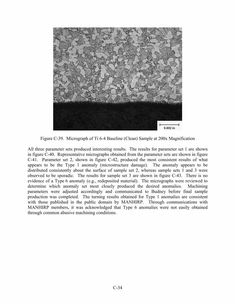
Figure C-39. Micrograph of Ti 6-4 Baseline (Clean) Sample at 200x Magnification
All three parameter sets produced interesting results. The results for parameter set 1 are shown in figure C-40. Representative micrographs obtained from the parameter sets are shown in figure C-41. Parameter set 2, shown in figure C-42, produced the most consistent results of what appears to be the Type 1 anomaly (microstructure damage). The anomaly appears to be distributed consistently about the surface of sample set 2, whereas sample sets 1 and 3 were observed to be sporadic. The results for sample set 3 are shown in figure C-43. There is no evidence of a Type 6 anomaly (e.g., redeposited material). The micrographs were reviewed to determine which anomaly set most closely produced the desired anomalies. Machining parameters were adjusted accordingly and communicated to Budney before final sample production was completed. The turning results obtained for Type 1 anomalies are consistent with those published in the public domain by MANHIRP. Through communications with MANHIRP members, it was acknowledged that Type 6 anomalies were not easily obtained through common abusive machining conditions.
C-34

Figure C-40. Micrograph of Ti 6-4 Turning Parameter Set 1 at 500x Magnification
Figure C-41. Micrograph of Ti 6-4 Turning Parameter Set 2 at 200x Magnification
C-35

Figure C-42. Micrograph of Ti 6-4 Turning Parameter Set 2 at 500x Magnification
Figure C-43. Micrograph of Ti 6-4 Turning Parameter Set 3 at 500x Magnification
C-36

C.3.3 THE LCF RESULTS FOR ANOMALIES IN Ti 6-4 WITH TURN-MAKING PROCESSES. Two smooth MT30 samples were tested using constant-amplitude axial load-controlled fatigue per ASTM Standard E466-96. The sample consists of pin-loaded flat grips, which blend to a rectangular 0.500″ by 0.1875″ by 2.000″ gage section (see figure C-44). Both samples were loaded using a sinusoidal waveform to a maximum stress of 85 ksi and stress ratio of 0.05 at 60 cpm and room temperature. Both samples were cyclically loaded until failure occurred. The results are summarized in table C-12.
Figure C-44. Turning Sample Geometry
Table C-12. Baseline LCF Results for Turning Samples
Temperature (°F)
Maximum Stress (ksi)
Minimum Stress (ksi)
Frequency (cpm)
Cycles to Failure
70 85 4.3 60 57,905
70 85 4.3 60 163,280
C-37

The first sample failed at 57,905 cycles. The second failed at 163,280 cycles. Both failed along the 0.190″ face, 90° from the desired face (see figure C-45). The samples were not peened, which likely led to the failure away from the desired face.
Figure C-45. Ruptured MT30 LCF Test Sample C.3.3.1 Summary of Ti 6-4 Turn-Making Processes. Clean samples machined from Ti 6-4 were produced for metallography and LCF tests. LCF tests produced results, the validity of which is currently in doubt because of failure away from the desired surface. Initial attempts to produce the two anomaly types were made using three different parameter sets. Preliminary analysis after metallography showed that parameter set 2 produced the most consistent results. The turning results obtained for Type 1 anomalies are consistent with those published in the public domain by MANHIRP. C.3.3.2 Fabrication of Type 1 Anomalies in In 718 With Turning Processes.
Turning of In 718 to produce Type 1 and Type 6 anomalies was performed using material that was supplied in pancake form. The pancakes were forged and heat treated to typical rotor-grade microstructure. The pancake was sectioned to produce washer shapes that could be used on the same vertical turning lathe that was used for the Ti 6-4 machining trials. Figure C-46 shows the sectioning layout for the washers and how the LCF and NDE samples were sectioned after trials were completed.
C-38

Figure C-46. Sectioning of In 718 Pancake to Produce Test Samples For Type 1 anomalies, the MANHIRP literature indicated that turning speed was the major factor in producing anomalies with titanium nickel-coated carbide cutting tools. Even so, the distorted layers reported were less than 1 mil and the amorphous layer was not consistent. Similar results were found in the current trials at PW to create Type 1 anomalies. C.3.3.2.1 Machining Parameters Used. Table C-13 shows a summary of the machining conditions used to produce the pristine samples and the variations used to produce anomaly samples. For the washers used in this machining study, the inner diameter was 7″ and the outer diameter was 12.5″, so the mid-diameter was 9.75″. The machinist reported the machine’s rpm and the surface speed is shown for the mid-diameter.
Table C-13. Parameters for Nominal Machining and Trials for Production of Anomaly Type 1
Test Speed (rpm)
Surface Speed Mid-Diameter
Feed Rate (in/min)
Depth of Cut (in.) Coolant
Tool Condition
A (pristine) 16 40.8 ft/min 0.006 0.010 Yes New
B 23 58.7 ft/min 0.006 0.010 Yes Dull
D 6.5 16.6 ft/min 0.012 0.005 No Dull Note: Test C had the same parameters as Test B. The excessive amount of material required for machining trials did not allow for further testing, but success was observed for test washer B. The same parameters were applied to test washer C to produce the LCF and NDE samples, and further metallography was performed on samples from washer C to verify the presence of the disturbed microstructure that denotes Type 1 anomalies. Figure C-47 shows the microstructure of the pristine material from test washer A from which the LCF and NDE baseline samples were made. Figures C-48 and C-49 show the microstructures of test washer B and washer C, respectively. It is apparent that the desired anomaly was produced in both washers.
C-39

Figure C-47. Microstructure of Nominal Material Without Machining Anomalies
Figure C-48. Microstructure of Type 1 Anomalies in Test Washer B
C-40

Figure C-49. Microstructure of Type 1 Anomalies in Washer C Used to Make LCF and NDE Samples
Figure C-50 shows that parameters used for test washer D did not produce the desired amorphous layer and distorted grain structure of Type 1 anomalies.
Figure C-50. Microstructure of Test Washer D
C-41
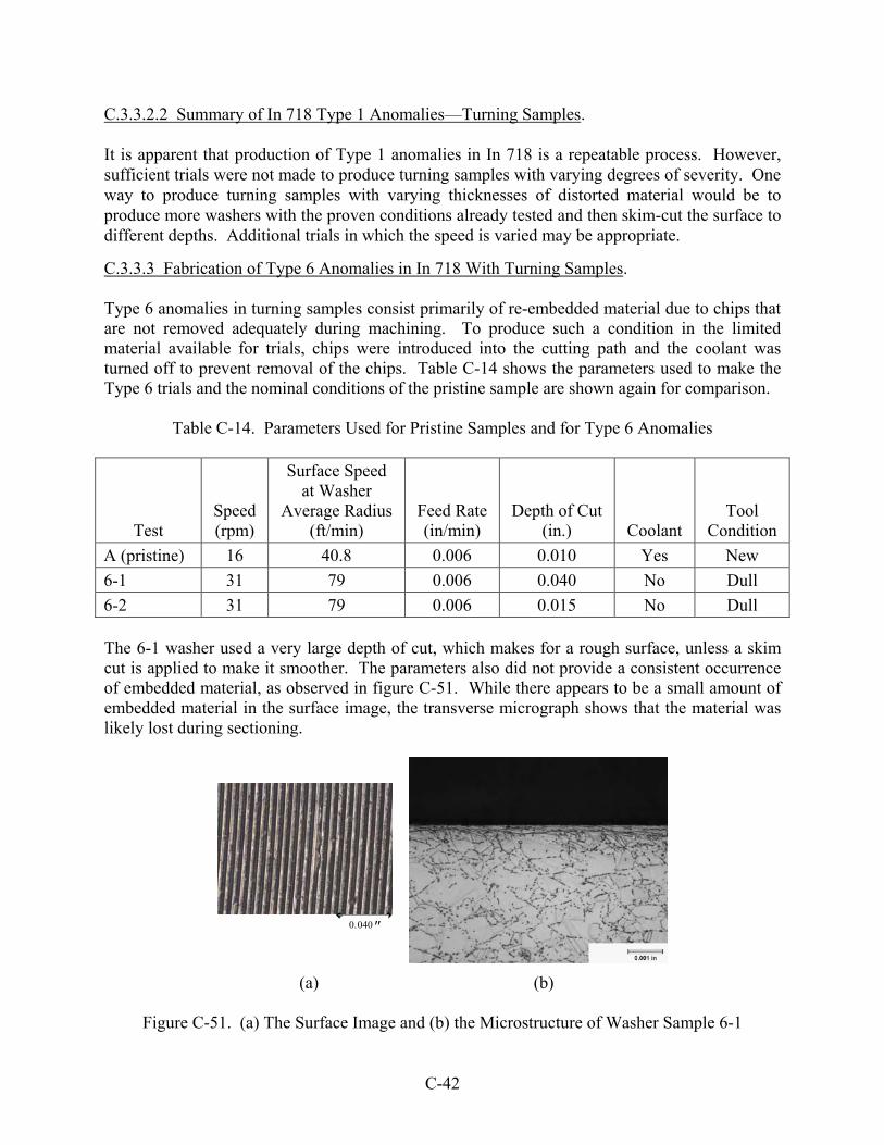
C.3.3.2.2 Summary of In 718 Type 1 Anomalies—Turning Samples. It is apparent that production of Type 1 anomalies in In 718 is a repeatable process. However, sufficient trials were not made to produce turning samples with varying degrees of severity. One way to produce turning samples with varying thicknesses of distorted material would be to produce more washers with the proven conditions already tested and then skim-cut the surface to different depths. Additional trials in which the speed is varied may be appropriate.
C.3.3.3 Fabrication of Type 6 Anomalies in In 718 With Turning Samples. Type 6 anomalies in turning samples consist primarily of re-embedded material due to chips that are not removed adequately during machining. To produce such a condition in the limited material available for trials, chips were introduced into the cutting path and the coolant was turned off to prevent removal of the chips. Table C-14 shows the parameters used to make the Type 6 trials and the nominal conditions of the pristine sample are shown again for comparison.
Table C-14. Parameters Used for Pristine Samples and for Type 6 Anomalies
Test Speed (rpm)
Surface Speed at Washer
Average Radius (ft/min)
Feed Rate (in/min)
Depth of Cut (in.) Coolant
Tool Condition
A (pristine) 16 40.8 0.006 0.010 Yes New
6-1 31 79 0.006 0.040 No Dull
6-2 31 79 0.006 0.015 No Dull The 6-1 washer used a very large depth of cut, which makes for a rough surface, unless a skim cut is applied to make it smoother. The parameters also did not provide a consistent occurrence of embedded material, as observed in figure C-51. While there appears to be a small amount of embedded material in the surface image, the transverse micrograph shows that the material was likely lost during sectioning.
″0400.
(a) (b)
Figure C-51. (a) The Surface Image and (b) the Microstructure of Washer Sample 6-1
C-42
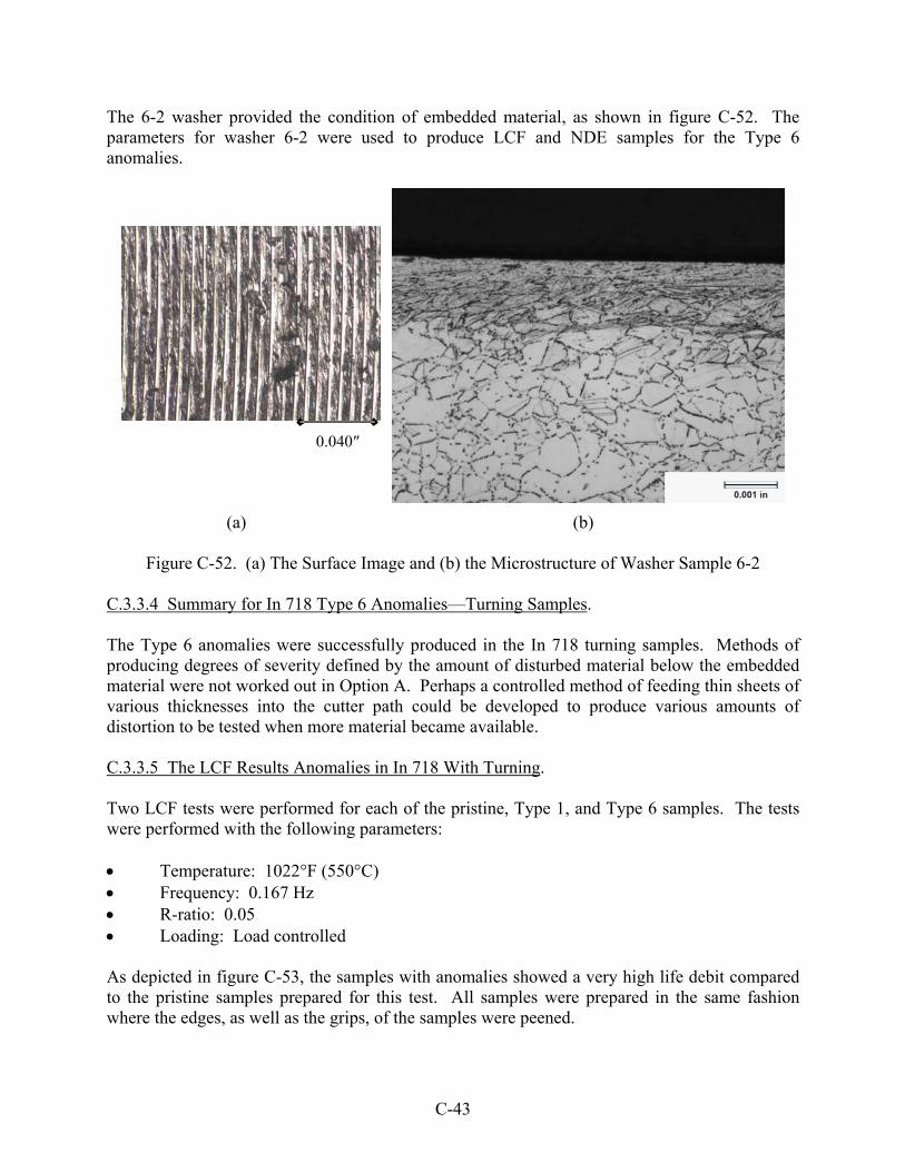
The 6-2 washer provided the condition of embedded material, as shown in figure C-52. The parameters for washer 6-2 were used to produce LCF and NDE samples for the Type 6 anomalies.
0.040″
(a) (b)
Figure C-52. (a) The Surface Image and (b) the Microstructure of Washer Sample 6-2 C.3.3.4 Summary for In 718 Type 6 Anomalies—Turning Samples. The Type 6 anomalies were successfully produced in the In 718 turning samples. Methods of producing degrees of severity defined by the amount of disturbed material below the embedded material were not worked out in Option A. Perhaps a controlled method of feeding thin sheets of various thicknesses into the cutter path could be developed to produce various amounts of distortion to be tested when more material became available. C.3.3.5 The LCF Results Anomalies in In 718 With Turning. Two LCF tests were performed for each of the pristine, Type 1, and Type 6 samples. The tests were performed with the following parameters: Temperature: 1022°F (550°C) Frequency: 0.167 Hz R-ratio: 0.05 Loading: Load controlled As depicted in figure C-53, the samples with anomalies showed a very high life debit compared to the pristine samples prepared for this test. All samples were prepared in the same fashion where the edges, as well as the grips, of the samples were peened.
C-43

0
20000
40000
60000
80000
100000
120000
0 1 2 3 4 5 6 7
baseline
Type-1
Type-693% 95%
Figure C-53. Results of the LCF Tests Performed for In 718 Turning Samples C.3.3.6 Summary of In 718 Turning Process. Parameters were determined that are capable of making both Type 1 and Type 6 anomalies in In 718 samples with a turning process. Due to the difficulty in obtaining the amount of material required to perform turning trials, additional trials that would have allowed accurate definition of controlling factors to produce various degrees of severity could not be performed. At the onset of Option A, it was stated that more severe anomalies would be made, which was accomplished as evidenced by the significant reduction in LCF life for the anomaly samples. For Option C, additional tests are required to produce different severity levels in the In 718 samples. C.3.4 BROACHING SAMPLE APPROACH. Honeywell (HW) Aerospace took on the challenge of manufacturing broaching samples with and without machining anomalies. Two types of anomalies were selected under Option A, which calls for the manufacturing of a limited number of samples with machining anomalies for three different machining operations, namely, hole drilling, turning, and broaching. The two selected anomaly types were Type 1—metallurgical change to parent material continuous with the surface, amorphous layer and Type 6—change to parent material—discontinuous with surface. Figure C-54 shows the HW Ti 6-4 forging that provided the material for the coupons used in manufacturing the broaching samples.
Samples
Cyc
les
C-44

Figure C-54. The HW Ti 6-4 Forging Used in Fabricating the Initial Set of Broaching Samples
Figures C-55 through C-57 show the drawings used in the extraction of the coupons from the forging; figure C-55 outlines the overall dimensions of the forging, and figures C-56 and C-57 show the actual locations of the coupons in the forging. The actual coupons, which were 3.4 inches long, 1.0 inch wide, and 0.8 inch thick, were extracted from the forging using EDM. Figure C-58 shows an example of the extracted coupons for use in fabricating the Ti 6-4 broaching samples, as illustrated in figure C-58(a). Figure C-58(b) shows a pristine broaching sample with the HW broaching profile, which is compared to the MANHIRP profile in figure C-59. Figure C-58(c) shows the sample used in the fatigue test for generating the Ti 6-4 material LCF baseline and for testing broaching samples with anomalies. Figure C-58(d) shows a close-up of the actual profile used in the broaching process.
16.95
6.75
2.99
1.75
8.822
12.70
4.86
6.43
AMD Broaching SamplesLocation and Numbering
Surface Finish 63 rms
112 Total Samples
Samples to be cut in the radial direction is indicated by drawing
Location of each sample most be maintained as indicated
Forging is identified with 0° and 90°
Forward side c-scan starts at 15º
Identification shall be permanently marked on ID side of samples
Forward
AFT
2
1
3
4
5
6
7
16.95
6.75
2.99
1.75
8.822
12.70
4.86
6.43
AMD Broaching SamplesLocation and Numbering
Surface Finish 63 rms
112 Total Samples
Samples to be cut in the radial direction is indicated by drawing
Location of each sample most be maintained as indicated
Forging is identified with 0° and 90°
Forward side c-scan starts at 15º
Identification shall be permanently marked on ID side of samples
Forward
AFT
22
11
33
44
55
66
77
(a) Figure C-55. The HW Ti 6-4 Forging Cross Section and Overall Dimensions
C-45

4
1
3
2
1
2
4
1
3
2
1
2
0º
90º
AA
BB
CC
DD
EE
FF
Sample Dimensions typ.
3.40 0.800
1.00
Section AA
Forward
Forward
AFT
3.40 typ.
0.800 typ.
1.00 typ.
Section AA
Figure C-56. Coupon Dimensions and Map for Ti 6-4 Broaching Samples
4
1
3
2
1
2
4
1
3
2
1
2
0º
90º
A YX
W
C
D
V
U
T
S
R
Q
PO
NML
K
J
I
H
G
F
E
B
Section AA
Section AA
Forward
AFT
AFT
3.40 typ.
1.00 typ.
0.800 typ.
Sample Dimensions typ.
3.40 0.800
1.00
Figure C-57. Coupon Dimensions and Map for Ti 6-4 Broaching Samples Detailed View of Coupon Location
C-46

(a) (b) (c) (d)
Figure C-58. Broaching Forging Coupons (a) the Coupons Extracted From the HW Forgings Used to Fabricate the Ti 6-4 Broaching Sample, (b) a Pristine Broaching Sample With the HW
Broaching Profile, (c) the Sample Used in the Fatigue Tests for Both Baseline of the Ti 6-4 Material and for Testing Broaching Samples With Anomalies, and (d) a Close-Up of the Actual
Profile Used in the Broaching Process
(a) (b)
Figure C-59. The MANHIRP Broaching Sample Profile (a) and HW Broaching Sample Profile Generated Using Tool No. T249263—Part Number 3075326-3/5(b)
C.3.4.1 Pristine and Type 6 (Smeared) Anomaly Samples. All Ti 6-4 samples were broached using a KV5 broaching machine and a HW tool, number T249263. Pristine samples were produced using a feed rate of 20 feet per minute (fpm) (normal rate for broaching Ti) with coolant and a dull tool. Smeared anomaly samples were produced by further dulling the tool to the greatest extent possible and running the broach without coolant at the fastest possible rate for the KV5 machine (without changing the production gear box on the machine), which is 22.5 fpm.
C-47
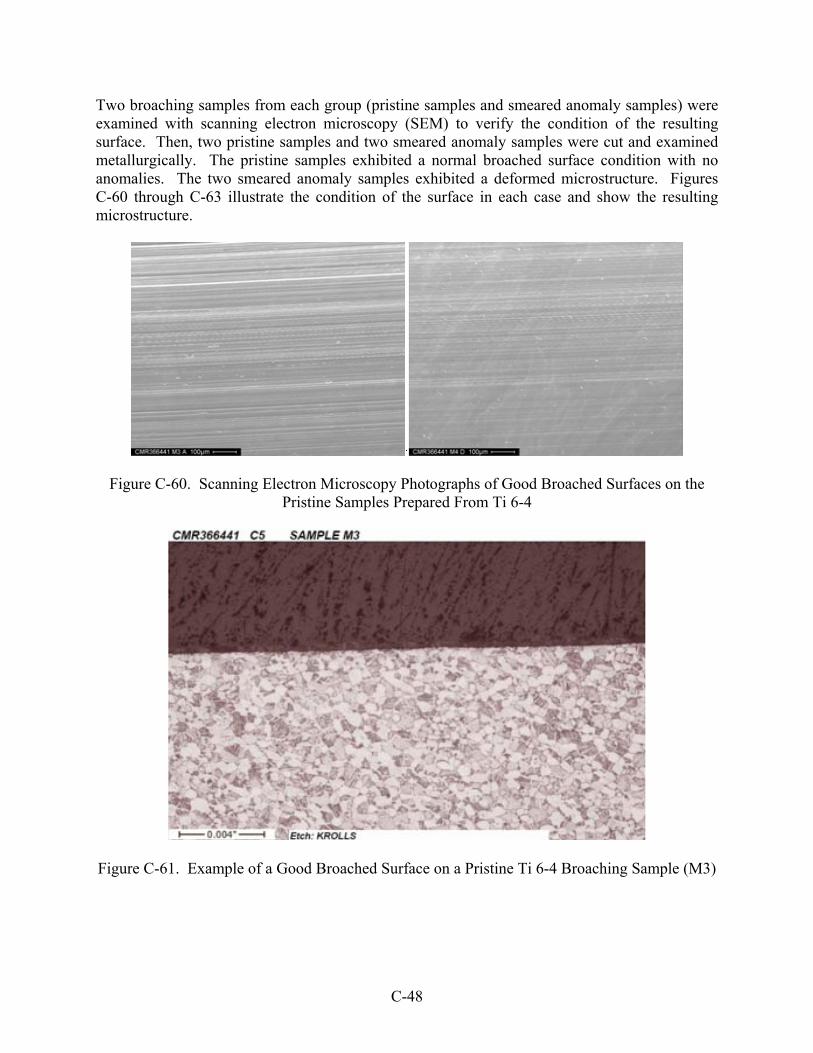
Two broaching samples from each group (pristine samples and smeared anomaly samples) were examined with scanning electron microscopy (SEM) to verify the condition of the resulting surface. Then, two pristine samples and two smeared anomaly samples were cut and examined metallurgically. The pristine samples exhibited a normal broached surface condition with no anomalies. The two smeared anomaly samples exhibited a deformed microstructure. Figures C-60 through C-63 illustrate the condition of the surface in each case and show the resulting microstructure.
Figure C-60. Scanning Electron Microscopy Photographs of Good Broached Surfaces on the Pristine Samples Prepared From Ti 6-4
Figure C-61. Example of a Good Broached Surface on a Pristine Ti 6-4 Broaching Sample (M3)
C-48

Figure C-62. Scanning Electron Microscopy Photographs of Broached Surfaces With Smeared Anomalies in Samples Prepared From Ti 6-4
Figure C-63. Example of Broached Surface With Smeared Anomaly on a Ti 6-4 Broaching Sample (J2) With Anomalies
A total of six samples were produced in each condition (pristine and smeared) in accordance with the original program plan. Two were used for metallurgical and SEM examination of the broached surfaces, two were used for fatigue tests, and the remaining two were used for NDE method development. All six samples for each condition were broached in the same run in sequence without altering setup conditions. This was done to ensure that all six samples were produced under the same conditions to the greatest extent possible. The first and last samples of each run were chosen for metallurgical analysis to verify that the conditions had not changed during the run. The same procedure was used for all conditions.
C-49

Two broaching samples representing each condition were cut up for metallurgical and SEM analysis to verify condition of the resulting surface. The first and last sample in each run group were chosen for cutting to verify that no change in broach setup conditions had occurred during the run of the same group of samples. The pristine samples exhibited a normal broached surface condition with no anomalies. Figure C-60 shows the examples of typical SEM images of the broached pristine surfaces, and figure C-61 shows a cross section of one of the good samples (M3). The two smeared samples (Y2 and J2) reflected the presence of the smeared anomalies. SEM examination of the broached surface revealed the presence of multiple smeared anomalies in each sample, as shown in figures C-62 and C-63. C.3.4.2 Type 1 (Amorphous-Layer) Anomaly Samples. To produce the amorphous-layer anomaly Type 1, broaching had to be performed at a higher speed, which required the gear box to be exchanged on the KV5 broaching machine. The broaching speed required to produce an amorphous-layer anomaly was about 200 fpm, and coolant was not used. These conditions produced parts with severe exit deformation, as shown in figure C-64. Also, the chips removed during the broaching process were fused to the broaching tool. Figure C-65 illustrates some of these severe results. It should be noted that under normal broaching conditions, it is almost impossible to produce this type of anomaly because there is a software limit that prohibits the broaching speed to exceed 22.5 fpm. In addition, coolant is normally used during production broaching operations. In this case, a total of six samples were produced for the amorphous-layer condition in accordance with the original program plan. Two samples were used for metallurgical and SEM examination of the broached surfaces, two were used for fatigue tests, and the remaining two were used for NDE method development. Table C-15 summarizes the different conditions produced in this effort along with the sample identification numbers for each condition.
Figure C-64. Severe Exit Conditions Caused by the Very High Broaching Speed (200 fpm) Used in Producing the Broaching Samples With Type 1, Amorphous-Layer Anomaly
C-50

Figure C-65. Metal Chips Removed From the Ti 6-4 Coupons During the Broaching Process for Producing the Amorphous Layer
Table C-15. Manufacturing Conditions and Sample Identification Numbers for Each Ti 6-4
Broaching Sample Condition
Sample Type Manufacturing
Condition
Metallography and SEM
Identification No.
Fatigue Sample Identification
No.
NDE Sample Identification
No.
Good broach 20 fpm with coolant
M3, M4 J1, K3 H2, H3
Smeared anomaly Type 6
22.5 fpm without coolant
Y2, J2 N2, K2 G3, E2
Amorphous anomaly Type 1
200 fpm without coolant
U3, N3 Y3, V3 W3, T3
All six amorphous-layer anomaly samples were broached in the same run, in sequence, and without the same setup conditions. This was done to ensure that all six samples were produced under the same conditions. The first and last samples of each run were chosen for metallurgical analysis to verify that the conditions had not changed during the run. As mentioned, to generate the amorphous-layer anomaly, the broaching speed had to be increased significantly. This produced an extreme anomaly at the tool exit point. SEM examinations of the surfaces showed anomalies on the broached surfaces, and the metallurgical cross section verified that areas with amorphous anomaly were present, as shown in figures C-66 and C-67.
C-51

Figure C-66. Scanning Electron Microscopy of Broached Surfaces With Amorphous Anomalies in Samples Prepared From Ti 6-4
Figure C-67. Example of Broached Surface With Amorphous-Layer Anomaly in a Ti 6-4 Broaching Sample (N3)
C.3.4.3 The LCF Test Results Ti 6-4 Test Samples.
LCF samples were produced to Honeywell sample drawing MTL3500-2. The design of the LCF sample is shown in figure C-68, the actual sample was shown in figure C-58. Each broaching sample yielded three samples (two outside and one center fatigue sample). The outside samples were used for setup and trials only. Only the center samples were fatigue-tested for baseline and comparison purposes. The decision was made not to use outside fatigue samples to avoid having
C-52
tool entry and exit conditions influencing the fatigue results. All fatigue tests were performed at room temperature. Samples were loaded axially in a stress control with a stress ratio of 0.1 and a stress range of 65 ksi. The test frequency was 200 cpm (3.33 Hz).
Figure C-68. Fatigue Sample Design Used in LCF Testing of Pristine Samples and Samples With Smeared Anomalies
Figure C-69 shows a summary of all the fatigue test results completed on the pristine samples along with an illustration of a resulting fracture surface. Table C-16 summarizes the results from the LCF tests for all conditions. Note that only two samples of each condition were used in generating LCF results. This number of samples was not enough to capture the scatter in LCF results, and therefore, the results should be viewed as very preliminary and more qualitative than quantitative. The results shown in table C-16 are graphically plotted in figure C-70 along with the average fatigue life deficit expected for the two anomaly conditions under consideration.
Table C-16. Summary of the LCF Tests for Pristine Samples and Samples With Machining Anomalies
Sample Condition Sample Cycles to Failure (Nf)
J1-2 44,430 Good sample
K3-2 48,888
K2-2 39,796 Smeared anomaly Type 6 N2-2 26,098
V3-2 37,902 Amorphous anomaly Type 1 Y3-2 31,316
C-53

Figure C-69. Summary of the LCF Test Trails and Results for the Pristine Broaching Samples
Smeared Amorphous26%30%
Pristine
Cyc
les
to F
ailu
re (
in T
hous
snad
s)
Sample Identification
Y3-2 V3-2N2-2K2-2K3-2J1-2
60
50
40
30
20
10
0
Figure C-70. Comparison of the LCF Test Results for Pristine Broaching Samples, Broaching Samples With Smeared Anomaly, and Broaching Samples With Amorphous-Layer Anomaly
From the results shown in table C-16 and figure C-70, it is estimated that, on average, there is about a 30% reduction in the LCF life of the broaching samples due to the smeared anomaly and about a 26% reduction in the LCF life due to the amorphous-layer anomaly. Again, the reader is cautioned not to use these values in any quantitative analysis related to component life assessment but to use these values as a qualitative guide of the effect of such anomalies on the LCF life.
C-54
C.3.4.4 Summary Ti 6-4 Broaching Processes. Honeywell completed the manufacturing of six broaching samples for Ti 6-4 for three machining conditions, i.e., pristine broaching samples with no anomalies, broaching samples with smeared anomaly (Type 6), and broaching samples with amorphous-layer anomaly (Type 1). Two of the six samples were used for metallurgical and SEM examination of the broached surfaces, two were used for fatigue testing, and the remaining two were used for NDE inspection development. All six samples for each condition were broached in the same run, in sequence, without altering setup conditions. This was done to ensure that all six samples were produced under the same conditions to the greatest extent possible. The first and last samples of each run were chosen for metallurgical analysis to verify that the conditions had not changed during the run. SEM and metallographic analysis of the samples verified the presence of the anomalies. Furthermore, LCF tests showed that, on average, there is about a 30% reduction in the LCF life of the broaching samples due to the smeared anomaly and about a 26% reduction in the LCF life due to the amorphous-layer anomaly. No MANHIRP-published results are available for direct comparison with Honeywell results. Such a comparison would be very useful in determining the resemblance of the anomalies produced by Honeywell to those produced by MANHIRP should further public domain releases occur. C.3.4.5 Broaching Samples Approach for In 718. Broaching samples in In 718 material were produced at the HW Rotating Hardware Center of Excellence (COE). The target anomalies were Type 1 and Type 6 of the nongeometric material, i.e., as previously defined by the MANHIRP consortium. Type 1 anomalies are described as a “Change to parent material continuous with surface,” and Type 6 anomalies are described as a “Change to parent material discontinuous with surface.” In addition, samples were manufactured using nominal production manufacturing conditions to create baseline pristine samples. The broaching trials for In 718 were conducted in three phases: Phase 1—manufacturing of baseline pristine samples
Phase 2—Designed experiments to determine the effect of broaching parameters on manufacturing-induced anomalies
Phase 3—Manufacturing of samples with targeted anomalies
After the pristine samples were machined, nondestructive test (NDT), metallographic, and LCF samples were manufactured. An iterative process of broaching samples and evaluation of the broaching samples was employed to study a full range of parameters. The broaching samples were evaluated visually, metallographically, and with SEM. A 6-inch sample length was used for elevated temperature LCF tests, and a 3.4-inch sample length was used for metallographic and NDT samples. The extended length of LCF samples was employed to readily accommodate the heating elements required for the elevated temperature tests. The 3.4-inch length was used for the other samples to maximize the number of samples that could be extracted from the In 718 forging.
C-55

C.3.4.5.1 Equipment Used. All broaching was performed on a production 15-180-HE Detroit Horizontal broach machine in the HW Rotating Hardware COE. This machine is capable of cutting at speeds up to 22 ft/min. The fixture used to hold samples and parts during broaching is equipped with a vibration monitoring system. The system gives an indication of tool wear, coolant flow, and aggressive depth of cuts. A Nikon D1 digital camera was used to document the condition of the dulled/worn cutting tools. Metallographic samples were prepared on standard metallographic equipment and a Reichert Jung optical microscope capable of 16x to 1000x magnification was used to evaluate the samples. A Jeol JSM6460 SEM was used to characterize the surface of the broaching samples. C.3.4.5.2 Machining. The baseline pristine samples were broached using the following typical production conditions and settings: Cutting speed: 5 ft/min Coolant: On Crown cutting tool edge: Sharp Carbide form cutter edge: Sharp Tool offset: None The following manufacturing conditions/settings were evaluated for their effect on the broached surface: Cutting speed (2 ft/min-22 ft/min) Cooling of samples (coolant on-coolant off) Tool sharpness (sharp cutting edge-rounded cutting edge) Crown cutter tool offset (0.000″-0.015″) Carbide form cutter offset (0.000″-0.015″) Once the baseline NDT, metallography, and LCF sample blanks were manufactured, a series of three broaching trials were conducted. The first broaching trial was used to study the effect of cutting speed and coolant flow when broaching with sharp tools. The final form carbide insert was removed to prevent it from “cleaning up” any anomalies created by the final crown cutter tool segment. The second trial was used to study the effect of cutting speed, coolant flow, and tool offset when broaching with a dulled tool. The final form carbide insert was removed for this trial as well. The third trial was conducted to evaluate the effect of cutting speed, coolant flow, and offset of the final carbide insert form cutter. The specific broaching parameters used to create the deliverable samples with anomalies are described in the subsequent sections of this report.
C-56

C.3.4.5.3 Metallography. The broaching samples were sectioned so that the polished surface was parallel to the broaching direction and down the centerline of the slot through the crown. This sectioning orientation allowed evaluation of the variation in microstructural damage as a function of position relative to the broach tool entrance and exit. Amorphous-layer thickness and grain deformation depth were readily evaluated when using this sectioning orientation. Samples were mounted in Bakelite. The polished samples were etched with Kalling’s reagent and evaluated at magnifications between 16x and 500x magnification. C.3.4.5.4 The LCF Test Description. LCF tests were performed on an MTS servohydraulic system with a 10-kip test frame. MTS hydraulic wedge grips (Model 647) were used to hold the test samples. The temperature of the samples was controlled using resistance element heating with a Yokogama controller and Type K thermocouples. The sample alignment and temperature profile were verified prior to the tests. Figure C-71 shows the dimensions of the LCF broaching sample used for In 718. The dimensions are identical to that used for Ti except for the length, which was increased from 3.4 to 5.5 inches minimum to accommodate the heating element for the elevated temperature tests.
Figure C-71. The LCF Sample Configuration
C-57

Load-controlled LCF tests were performed using the following test conditions: Sinusoidal loading cycle Test temperature = 1022°F (550°C) Test frequency = 5 Hz R-ratio = 0.1 Stress range = 100 ksi C.3.4.5.5 Test Blanks. Short sample blanks (60 blanks: 3.4″ by 0.750″ by 1.0″) were extracted from the In 718 forging using the EDM process (see figure C-72). These samples were used for the designed experiments samples, metallographic samples, and NDT samples. Long samples (12 blanks: 6.0″ minimum by 0.750″ by 1.0″) were extracted from the forging to be used as blanks for creating the elevated temperature LCF test samples. The extended length was required to accommodate the heating equipment used for elevated temperature testing. Figure C-73 shows the layout of the extracted sample blanks from the In 718 pancake forging. After broaching the deliverable LCF sample blanks, the EDM process was used to extract the 0.250″ thick LCF samples shown in figure C-71. Surface grinding was used to achieve the critical dimensions (flatness and parallelism) required for LCF samples. An edge break operation was used in the broached gage section to reduce the risk of flaw initiation at the sharp transition between the sample sides and the broached surface.
Figure C-72. The EDM Setup Used for Extracting the In 718 Coupons for the Broaching Samples From the 14-Inch-Diameter, 3.5-Inch-Thick In 718 Pancake
C-58

Figure C-73. The Layout of the Extracted Sample Blanks From the In 718 Pancake Forging C.3.4.5.6 Broaching Geometry and Terminology. Figure C-74 shows the profile of the broached slot. Figure C-75 shows the crown area and the pressure angle area. The pressure angle serves as the contact surface for inserted blades.
Figure C-74. Broaching Profile Dimensions for In 718 Samples
R = 0.133″ R = 0.060″
R =0.072″
R = 0.0102″
R = 0.505″
0.318″
C-59

Figure C-75. Broaching Profile Nomenclature C.3.4.6 Broaching Process. The broach slot is created by a series of tools that have teeth, which remove small amounts of material from the broach slot. A typical broach slot is the result of the cutting action of several hundred individual teeth that are pulled through the sample. Each individual cutting tool is designed to remove material from one area of the slot. The cutting tools work together as a group to create the complete broach slot profile. The first group of tools is typically referred to as roughers, and they remove relatively large amounts of material with each tooth. The final sets of cutting tools take a less aggressive cut and bring the broach slot to the final dimensions. In certain cases, a single carbide insert that contains the complete broach slot profile is used to ensure tight dimensional tolerances. Figure C-76 shows a photograph of a final crown cutting tool, and figure C-77 shows a photograph of the carbide insert form cutter.
C-60
Figure C-76. Typical Crown Cutting Tool
Figure C-77. Carbide Insert Form Cutting Tool The baseline pristine samples were broached using the following typical production conditions and settings: Cutting speed: 5 ft/min Coolant: On Crown cutting tool edge: Sharp Carbide form cutter edge: Sharp Tool offset: None
C-61

Figure C-78 shows a typical surface of a pristine sample broached using the above parameters, and figure C-79 shows the resulting typical microstructure of a pristine sample in In 718.
Figure C-78. A Typical Surface of a Pristine Sample Broached Using Typical Broaching Parameters
Figure C-79. The Resulting Typical Microstructure of a Pristine Broaching Sample in In 718 (500x magnification)
C-62

C.3.4.7 Fabrication of Amorphous-Layer Type 1 Anomaly in In 718 Broaching Samples. The Type 1 amorphous-layer anomaly was consistently produced with the broaching process in the In 718 samples at production cutting speeds. A dull, crown cutting tool and a significant offset of the crown cutting tool in the positive direction were required to make the anomaly. Although the maximum depth of damage was produced with the coolant off, an amorphous layer was also produced with the coolant on and at even lower cutting speeds on development test samples. The thickness of the amorphous layer was typically larger near the tool entrance, and the damaged layer became thinner toward the tool exit region. Figure C-80 shows a typical surface resulting during the broaching of this type of anomaly. The broach conditions used were: Cutting speed: 5 ft/min Coolant: Off Crown cutting tool edge dulled (last of the tools) Crown cutter offset 0.015″ in the positive direction Carbide insert form cutter removed
Figure C-80. A Typical Surface of a Broaching Sample With Type 1 Anomaly (Amorphous Layer, 100x magnification)
Figures C-81 and C-82 show Type 1 damage near the tool entrance. The amorphous layer was measured at ~0.0007″ deep and grain distortion was observed to depths of ~0.0025″. Figure C-83 shows the amorphous layer near the tool exit region of the broach slot. The amorphous layer was measured at ~0.0005″ deep with grain distortion to a shallower depth of ~0.0015″.
C-63
Figure C-81. Amorphous Layer Observed Near the Tool Entrance—Cross Section Through Crown Line (100x magnification, Etch-Kallings)
Figure C-82. Amorphous Layer Observed Near the Tool Entrance—Cross Section Through Crown Line (500x magnification, Etch-Kallings)
Base Material
C-64
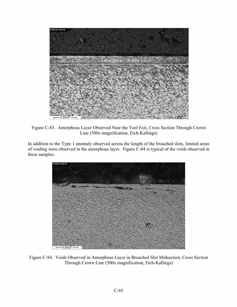
Figure C-83. Amorphous Layer Observed Near the Tool Exit, Cross Section Through Crown Line (500x magnification, Etch-Kallings)
In addition to the Type 1 anomaly observed across the length of the broached slots, limited areas of voiding were observed in the amorphous layer. Figure C-84 is typical of the voids observed in these samples.
Figure C-84. Voids Observed in Amorphous Layer in Broached Slot Midsection, Cross Section Through Crown Line (500x magnification, Etch-Kallings)
C-65
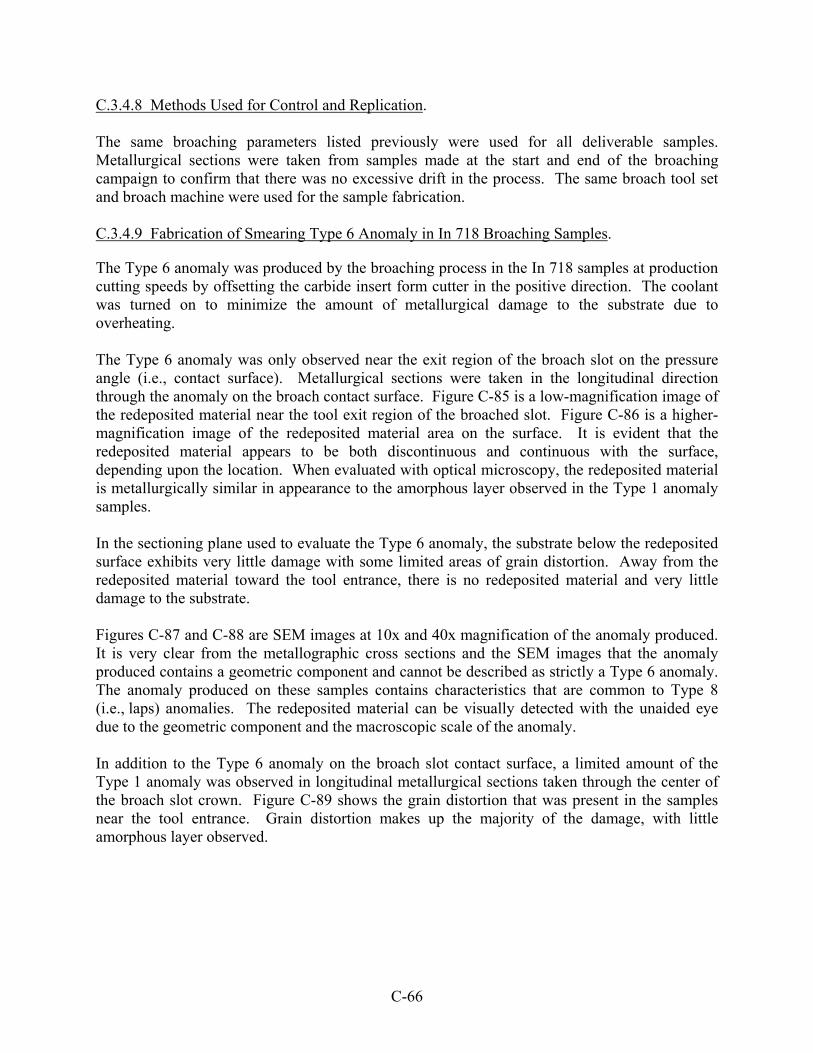
C.3.4.8 Methods Used for Control and Replication. The same broaching parameters listed previously were used for all deliverable samples. Metallurgical sections were taken from samples made at the start and end of the broaching campaign to confirm that there was no excessive drift in the process. The same broach tool set and broach machine were used for the sample fabrication. C.3.4.9 Fabrication of Smearing Type 6 Anomaly in In 718 Broaching Samples.
The Type 6 anomaly was produced by the broaching process in the In 718 samples at production cutting speeds by offsetting the carbide insert form cutter in the positive direction. The coolant was turned on to minimize the amount of metallurgical damage to the substrate due to overheating. The Type 6 anomaly was only observed near the exit region of the broach slot on the pressure angle (i.e., contact surface). Metallurgical sections were taken in the longitudinal direction through the anomaly on the broach contact surface. Figure C-85 is a low-magnification image of the redeposited material near the tool exit region of the broached slot. Figure C-86 is a higher-magnification image of the redeposited material area on the surface. It is evident that the redeposited material appears to be both discontinuous and continuous with the surface, depending upon the location. When evaluated with optical microscopy, the redeposited material is metallurgically similar in appearance to the amorphous layer observed in the Type 1 anomaly samples. In the sectioning plane used to evaluate the Type 6 anomaly, the substrate below the redeposited surface exhibits very little damage with some limited areas of grain distortion. Away from the redeposited material toward the tool entrance, there is no redeposited material and very little damage to the substrate. Figures C-87 and C-88 are SEM images at 10x and 40x magnification of the anomaly produced. It is very clear from the metallographic cross sections and the SEM images that the anomaly produced contains a geometric component and cannot be described as strictly a Type 6 anomaly. The anomaly produced on these samples contains characteristics that are common to Type 8 (i.e., laps) anomalies. The redeposited material can be visually detected with the unaided eye due to the geometric component and the macroscopic scale of the anomaly. In addition to the Type 6 anomaly on the broach slot contact surface, a limited amount of the Type 1 anomaly was observed in longitudinal metallurgical sections taken through the center of the broach slot crown. Figure C-89 shows the grain distortion that was present in the samples near the tool entrance. Grain distortion makes up the majority of the damage, with little amorphous layer observed.
C-66

Figure C-85. Redeposited Layer Observed Near the Tool Exit (16x magnification, Etch-Kallings) (The cross section was taken through pressure angle.)
Figure C-86. Redeposited Layer Observed Near the Tool Exit (200x magnification, Etch-Kallings) (The cross section was taken through pressure angle.)
C-67

Figure C-87. Redeposited Layer Observed Near the Tool Exit, Pressure Angle (10x magnification)
Figure C-88. Redeposited Layer Observed Near the Tool Exit, Pressure Angle (40x magnification)
C-68

Figure C-89. Type 1 Anomaly Observed Near the Tool Entrance (500x magnification, Etch-Kallings) (The cross section was taken through the crown line.)
The broaching parameters used to produce the smearing Type 6 anomaly in In 718 were: Cutting speed: 5 ft/min Coolant: On Crown cutting tool edge dulled Crown cutter offset 0.007″ in the positive direction Carbide insert form cutter dulled and in place (last of the tools) Carbide insert offset 0.015″ C.3.4.9.1 The LCF Test Results. Table C-17 summarizes the results from the LCF tests for all conditions. Note that only two samples of each condition were used in generating LCF results. This number of samples was not enough to capture the scatter in LCF results, and therefore, the results should be viewed as very preliminary and more qualitative than quantitative. The results shown in table C-17 are graphically plotted in figure C-90 along with the average fatigue life deficit expected for the two anomaly conditions under consideration. It should be mentioned here that the failure initiation site in the samples with the Type 6 anomaly were well away from the anomaly. The location of the anomaly is in a low stress region and therefore does not impact the life of the test sample. The reduction in life observed is likely due to some other anomaly present in the gage section.
C-69

Table C-17. The LCF Test Results for In 718 Samples With and Without Broaching Anomalies
Sample Condition Sample
Identification Cycles to Failure
(Nf)
1C-2 388,486 Good sample
2B-2 113,294
1A-A 61,460 Smeared anomaly
3A-A 139,289
4C-B 125,728 Amorphous layer
3C-B 145,217
C-70
450 Pristine
Cyl
ces
to F
ailu
re (
in T
hous
ands
)
400
350
300
250
Figure C-90. Comparison of the LCF Test Results for Pristine Broaching Samples, Broaching Samples With Smeared Anomaly, and Broaching Samples With
Amorphous-Layer Anomaly in In 718 From the results shown in table C-17 and figure C-90, it is estimated that, on average, there is about a 60% reduction in the LCF life of the broaching samples containing the smeared anomaly (although the failure was not caused by this anomaly) and about a 46% reduction in the LCF life due to the amorphous-layer anomaly. Again, the reader is cautioned not to use these values in any quantitative analysis related to component life assessment but to use these values as a qualitative guide of the effect of such anomalies on the LCF life.
0
50
100
150
200
1C-2 2B-2 1A-A 3A-A 4C-B 3C-B
Sample ID
Smeared Amorphous 46%60%

C.3.4.10 Summary. Type 1 anomalies in In 718 material were readily manufactured by offsetting dull tooling and cutting with no coolant flow. An amorphous/white layer was formed in the layer nearest to the cutting surface, and distorted grains were formed below the white layer. The machining of the Type 1 anomaly is considered repeatable and relatively controllable. Type 6 anomalies in In 718 material were manufactured by offsetting a dull carbide insert form cutter and cutting with coolant flowing. The redeposited material was created on the contact surface of the broach slot near the tool exit region. There was limited damage to the substrate below the redeposited material. Although multiple samples with Type 6 anomalies were manufactured and the anomaly was subsequently reproduced on the deliverable samples, the mechanism responsible for creating the Type 6 anomaly is not well understood.
C-71/C-72

APPENDIX D—OPTION C—MANUFACTURE OF TEST SAMPLES
D.1 OPTION C—ANOMALOUS HOLE MANUFACTURING. The same basic manufacturing processes used to fabricate anomalous conditions for Option A hole-drilling samples were used under Option C, the primary differences being the final manufacturing parameters used by the cutting tools. For more details on Option A fabrication, see appendix C. A summary of the Option C manufacturing parameters used for each material and anomalous condition are outlined in table D-1. In addition to the 7-mm-diameter holes fabricated by Manufacturing to Produce High Integrity Rotating Parks for Modern Gas Turbines and the Engine Titanium Consortium (ETC) under Option A, several Inconel 718 nickel alloy (In 718) test samples containing 0.5″ diameter holes and (Type 6*) anomalies were also fabricated under Option C. The 0.5″ diameter holes, once fabricated, were split axially, producing nearly identical surfaces—one-half intended for eventual metallographic analysis and one-half retained for nondestructive evaluation (NDE) analysis. Efforts were unsuccessful to control the depth of (Type 6*) anomaly samples containing 0.5″ diameter holes. Limitations in project schedule and available funding prevented fabrication of 0.5″ diameter holes in all materials and anomaly types; but attempts were made nonetheless with available resources and schedule. The parameter for each hole size were as follows: To fabricate the 7-mm-diameter holes, a 0.281 carbide drill circle was ground to 0.274
and conditioned to drill without coolant (dry) in In 718 scrap material of 0.350 plate thickness at the same machining parameters for three holes.
To fabricate the 0.5 diameter holes, a 0.531 carbide drill circle was ground to 0.498
and step relieved 0.5 from point to end of flute and conditioned to drill without coolant (dry) in In 718 scrap material of 1.0 plate thickness at the same machining parameters for three holes.
D-1

Table D-1. Manufacturing Process Parameters Used to Fabricate Option C Hole-Drilling Samples Containing (Type 1*) and (Type 6*) Anomalies in Titanium 6-4 and In 718 Materials
OEM Sample User Set Material
Sample Thickness
(inch (mm))
Sample Dimensions
(inch)
Unique Dimension (inch (mm))
Target Anomaly
Manufacturing Description and Assumed Target Anomaly
Manufacturing Processes Used
Number Drill Used
Drill Speed (sfm)
Drill Feed (ipt)
Final Hole
Diameter (inch)
GE-D1 TI-D-P-7- 070806
ETC Set 1 Ti 6-4 0.34 (8.5) 1.0 x 1.0 0.276 (7.0) None GE Specification P11TF12 Drill + Ream + Edge Break
GE-D2 TI-D-P-8- 070806
ETC Set 2 Ti 6-4 0.34 (8.5) 1.0 x 1.0 0.276 (7.0) None GE Specification P11TF12 Drill + Ream + Edge Break
GE-D3 TI-D-P-9- 070806
ETC Set 3 Ti 6-4 0.34 (8.5) 1.0 x 1.0 0.276 (7.0) None GE Specification P11TF12 Drill + Ream + Edge Break
GE-D4 TI-D-P-10- 070806
ETC Set 4 Ti 6-4 0.34 (8.5) 1.0 x 1.0 0.276 (7.0) None GE Specification P11TF12 Drill + Ream + Edge Break
GE-D5 TI-D-P-11- 070806
Vendor Set 1
Ti 6-4 0.34 (8.5) 1.0 x 1.0 0.276 (7.0) None GE Specification P11TF12 Drill + Ream + Edge Break
GE-E6 TI-D-P-12- 070806
Vendor Set 2
Ti 6-4 0.34 (8.5) 1.0 x 1.0 0.276 (7.0) None GE Specification P11TF12 Drill + Ream + Edge Break
GE-E7 TI-D-P-13- 070806
Vendor Set 3
Ti 6-4 0.34 (8.5) 1.0 x 1.0 0.276 (7.0) None GE Specification P11TF12 Drill + Ream + Edge Break
GE-E8 TI-D-P-14- 070806
ETC Set 1 Ti 6-4 0.34 (8.5) 1.0 x 1.0 0.276 (7.0) None GE Specification P11TF12 Drill + Ream + Edge Break
GE-E9 TI-D-P-15- 070806
ETC Set 2 Ti 6-4 0.34 (8.5) 1.0 x 1.0 0.276 (7.0) None GE Specification P11TF12 Drill + Ream + Edge Break
GE-E10 TI-D-P-16- 070806
ETC Set 3 Ti 6-4 0.34 (8.5) 1.0 x 1.0 0.276 (7.0) None GE Specification P11TF12 Drill + Ream + Edge Break
GE-F11 TI-D-P-17- 070806
ETC Set 4 Ti 6-4 0.34 (8.5) 1.0 x 1.0 0.276 (7.0) None GE Specification P11TF12 Drill + Ream + Edge Break
GE-F12 TI-D-P-18- 070806
Vendor Set 1
Ti 6-4 0.34 (8.5) 1.0 x 1.0 0.276 (7.0) None GE Specification P11TF12 Drill + Ream + Edge Break
GE-F13 TI-D-P-19- 070806
Vendor Set 2
Ti 6-4 0.34 (8.5) 1.0 x 1.0 0.276 (7.0) None GE Specification P11TF12 Drill + Ream + Edge Break
GE-F14 TI-D-P-20- 070806
Vendor Set 3
Ti 6-4 0.34 (8.5) 1.0 x 1.0 0.276 (7.0) None GE Specification P11TF12 Drill + Ream + Edge Break
GE-F15 TI-D-P-21- 070806
Extra Ti 6-4 0.34 (8.5) 1.0 x 1.0 0.276 (7.0) None GE Specification P11TF12 Drill + Ream + Edge Break
GE-G1A TI-D-P-22- 070829
ETC Set 1 Ti 6-4 1.0 1.0 x 1.0 0.5 None GE Specification P11TF12 Drill + Ream + Edge Break + Axial Split
D-2

Table D-1. Manufacturing Process Parameters Used to Fabricate Option C Hole-Drilling Samples Containing (Type 1*) and (Type 6*) Anomalies in Titanium 6-4 and In 718 Materials (Continued)
OEM Sample User Set Material
Sample Thickness
(inch (mm))
Sample Dimensions
(inch)
Unique Dimension (inch (mm))
Target Anomaly
Manufacturing Description and Assumed Target Anomaly
Manufacturing Processes Used
Number Drill Used
Drill Speed (sfm)
Drill Feed (ipt)
Final Hole
Diameter (inch)
GE-G1B TI-D-P-23- 070829
ETC Set 2 Ti 6-4 1.0 1.0 x 1.0 0.5 None GE Specification P11TF12 Drill + Ream + Edge Break + Axial Split
GE-G2A TI-D-P-24- 070829
ETC Set 3 Ti 6-4 1.0 1.0 x 1.0 0.5 None GE Specification P11TF12 Drill + Ream + Edge Break + Axial Split
GE-G2B TI-D-P-25- 070829
ETC Set 4 Ti 6-4 1.0 1.0 x 1.0 0.5 None GE Specification P11TF12 Drill + Ream + Edge Break + Axial Split
GE-G3A TI-D-P-26- 070829
Vendor Set 1
Ti 6-4 1.0 1.0 x 1.0 0.5 None GE Specification P11TF12 Drill + Ream + Edge Break + Axial Split
GE-G3B TI-D-P-27- 070829
Vendor Set 2
Ti 6-4 1.0 1.0 x 1.0 0.5 None GE Specification P11TF12 Drill + Ream + Edge Break + Axial Split
GE-G4A TI-D-P-28- 070829
Vendor Set 3
Ti 6-4 1.0 1.0 x 1.0 0.5 None GE Specification P11TF12 Drill + Ream + Edge Break + Axial Split
GE-G4B TI-D-P-29- 070829
Extra Ti 6-4 1.0 1.0 x 1.0 0.5 None GE Specification P11TF12 Drill + Ream + Edge Break + Axial Split
GE-A1 IN-D-P-7- 070710
ETC Set 1 In 718 0.34 (8.5) 1.0 x 1.0 0.276 (7.0) None GE Specification P11TF12 Drill + Ream + Edge Break
GE-A2 IN-D-P-8- 070710
ETC Set 2 In 718 0.34 (8.5) 1.0 x 1.0 0.276 (7.0) None GE Specification P11TF12 Drill + Ream + Edge Break
GE-A3 IN-D-P-9- 070710
ETC Set 3 In 718 0.34 (8.5) 1.0 x 1.0 0.276 (7.0) None GE Specification P11TF12 Drill + Ream + Edge Break
GE-A4 IN-D-P-10- 070710
ETC Set 4 In 718 0.34 (8.5) 1.0 x 1.0 0.276 (7.0) None GE Specification P11TF12 Drill + Ream + Edge Break
GE-A5 IN-D-P-11- 070710
Vendor Set 1
In 718 0.34 (8.5) 1.0 x 1.0 0.276 (7.0) None GE Specification P11TF12 Drill + Ream + Edge Break
GE-A6 IN-D-P-12- 070710
Vendor Set 2
In 718 0.34 (8.5) 1.0 x 1.0 0.276 (7.0) None GE Specification P11TF12 Drill + Ream + Edge Break
GE-B7 IN-D-P-13- 070710
Vendor Set 3
In 718 0.34 (8.5) 1.0 x 1.0 0.276 (7.0) None GE Specification P11TF12 Drill + Ream + Edge Break
D-3

Table D-1. Manufacturing Process Parameters Used to Fabricate Option C Hole-Drilling Samples Containing (Type 1*) and (Type 6*) Anomalies in Titanium 6-4 and In 718 Materials (Continued)
OEM Sample User Set Material
Sample Thickness
(inch (mm))
Sample Dimensions
(inch)
Unique Dimension (inch (mm))
Target Anomaly
Manufacturing Description and Assumed Target Anomaly
Manufacturing Processes Used
Number Drill Used
Drill Speed (sfm)
Drill Feed (ipt)
Final Hole
Diameter (inch)
GE-B8 IN-D-P-14- 070710
ETC Set 1 In 718 0.34 (8.5) 1.0 x 1.0 0.276 (7.0) None GE Specification P11TF12 Drill + Ream + Edge Break
GE-B9 IN-D-P-15- 070710
ETC Set 2 In 718 0.34 (8.5) 1.0 x 1.0 0.276 (7.0) None GE Specification P11TF12 Drill + Ream + Edge Break
GE-B10 IN-D-P-16- 070710
ETC Set 3 In 718 0.34 (8.5) 1.0 x 1.0 0.276 (7.0) None GE Specification P11TF12 Drill + Ream + Edge Break
GE-B11 IN-D-P-17- 070710
ETC Set 4 In 718 0.34 (8.5) 1.0 x 1.0 0.276 (7.0) None GE Specification P11TF12 Drill + Ream + Edge Break
GE-B12 IN-D-P-18- 070710
Vendor Set 1
In 718 0.34 (8.5) 1.0 x 1.0 0.276 (7.0) None GE Specification P11TF12 Drill + Ream + Edge Break
GE-C13 IN-D-P-19- 070710
Vendor Set 2
In 718 0.34 (8.5) 1.0 x 1.0 0.276 (7.0) None GE Specification P11TF12 Drill + Ream + Edge Break
GE-C14 IN-D-P-20- 070710
Vendor Set 3
In 718 0.34 (8.5) 1.0 x 1.0 0.276 (7.0) None GE Specification P11TF12 Drill + Ream + Edge Break
GE-C15 IN-D-P-21- 070710
Extra In 718 0.34 (8.5) 1.0 x 1.0 0.276 (7.0) None GE Specification P11TF12 Drill + Ream + Edge Break
GE-C16 IN-D-P-21- 070710
Extra In 718 0.34 (8.5) 1.0 x 1.0 0.276 (7.0) None GE Specification P11TF12 Drill + Ream + Edge Break
GE-C17 IN-D-P-23- 070710
Extra In 718 0.34 (8.5) 1.0 x 1.0 0.276 (7.0) None GE Specification P11TF12 Drill + Ream + Edge Break
GE-C18 IN-D-P-24- 070710
Extra In 718 0.34 (8.5) 1.0 x 1.0 0.276 (7.0) None GE Specification P11TF12 Drill + Ream + Edge Break
GE-H1A IN-D-P-25- 070829
ETC Set 1 In 718 1.0 1.0 x 1.0 0.5 None GE Specification P11TF12 Drill + Ream + Edge Break + Axial Split
GE-H1B IN-D-P-26- 070829
ETC Set 2 In 718 1.0 1.0 x 1.0 0.5 None GE Specification P11TF12 Drill + Ream + Edge Break + Axial Split
GE-H2A IN-D-P-27- 070829
ETC Set 3 In 718 1.0 1.0 x 1.0 0.5 None GE Specification P11TF12 Drill + Ream + Edge Break + Axial Split
GE-H2B IN-D-P-28- 070829
ETC Set 4 In 718 1.0 1.0 x 1.0 0.5 None GE Specification P11TF12 Drill + Ream + Edge Break + Axial Split
D-4

Table D-1. Manufacturing Process Parameters Used to Fabricate Option C Hole-Drilling Samples Containing (Type 1*) and (Type 6*) Anomalies in Titanium 6-4 and In 718 Materials (Continued)
OEM Sample User Set Material
Sample Thickness
(inch (mm))
Sample Dimensions
(inch)
Unique Dimension (inch (mm))
Target Anomaly
Manufacturing Description and Assumed Target Anomaly
Manufacturing Processes Used
Number Drill Used
Drill Speed (sfm)
Drill Feed (ipt)
Final Hole
Diameter (inch)
GE-H3A IN-D-P-29- 070829
Vendor Set 1
In 718 1.0 1.0 x 1.0 0.5 None GE Specification P11TF12 Drill + Ream + Edge Break + Axial Split
GE-H3B IN-D-P-30- 070829
Vendor Set 2
In 718 1.0 1.0 x 1.0 0.5 None GE Specification P11TF12 Drill + Ream + Edge Break + Axial Split
GE-H4A IN-D-P-31- 070829
Vendor Set 3
In 718 1.0 1.0 x 1.0 0.5 None GE Specification P11TF12 Drill + Ream + Edge Break + Axial Split
GE-H4B IN-D-P-32- 070829
Extra In 718 1.0 1.0 x 1.0 0.5 None GE Specification P11TF12 Drill + Ream + Edge Break + Axial Split
GE-O1 TI-D-T1A- O1-080325
ETC Set 1 Ti 6-4 0.34 (8.5) 1.0 x 1.0 0.276 (7.0) Type 1* Medium Heat + Deformation: 0.001 > < 0.002 depth
Drill + Ream + Edge Break
1 175 0.002 0.273
GE-O2 TI-D-T1A- O2-080325
Extra Ti 6-4 0.34 (8.5) 1.0 x 1.0 0.276 (7.0) Type 1* Failed drill Drill + Ream + Edge Break
Failed 150 0.0015
GE-O3 TI-D-T1A- O3-080325
Extra Ti 6-4 0.34 (8.5) 1.0 x 1.0 0.276 (7.0) Type 1* Used for metallography verification (Unknown) - 2nd half not shipped
Drill + Ream + Edge Break
2 150 0.0015 0.276
GE-O4 TI-D-T1A- O4-080325
ETC Set 2 Ti 6-4 0.34 (8.5) 1.0 x 1.0 0.276 (7.0) Type 1* Medium Heat + Deformation: 0.001 > < 0.002 depth
Drill + Ream + Edge Break
2 150 0.0015 0.276
GE-O5 TI-D-T1A- O5-080325
ETC Set 3 Ti 6-4 0.34 (8.5) 1.0 x 1.0 0.276 (7.0) Type 1* Medium Heat + Deformation: 0.001 > < 0.002 depth
Drill + Ream + Edge Break
2 150 0.0015 0.276
GE-O6 TI-D-T1A- O6-080325
ETC Set 4 Ti 6-4 0.34 (8.5) 1.0 x 1.0 0.276 (7.0) Type 1* Medium Heat + Deformation: 0.001 > < 0.002 depth
Drill + Ream + Edge Break
2 150 0.0015 0.276
GE-O7 TI-D-T1A- O7-080325
Vendor Set 1
Ti 6-4 0.34 (8.5) 1.0 x 1.0 0.276 (7.0) Type 1* Medium Heat + Deformation: 0.001 > < 0.002 depth
Drill + Ream + Edge Break
2 150 0.0015 0.276
GE-P1 TI-D-T1A-P1- 080325
Vendor Set 2
Ti 6-4 0.34 (8.5) 1.0 x 1.0 0.276 (7.0) Type 1* Medium Heat + Deformation: 0.001 > < 0.002 depth
Drill + Ream + Edge Break
2 150 0.0015 0.276
GE-P2 TI-D-T1A-P2- 080325
Vendor Set 3
Ti 6-4 0.34 (8.5) 1.0 x 1.0 0.276 (7.0) Type 1* Medium Heat + Deformation: 0.001 > < 0.002 depth
Drill + Ream + Edge Break
2 150 0.0015 0.276
GE-P3 TI-D-T1A-P3- 080325
ETC Set 1 Ti 6-4 0.34 (8.5) 1.0 x 1.0 0.276 (7.0) Type 1* Medium Heat + Deformation: 0.001 > < 0.002 depth
Drill + Ream + Edge Break
2 150 0.0015 0.276
GE-P4 TI-D-T1A-P4- 080325
ETC Set 2 Ti 6-4 0.34 (8.5) 1.0 x 1.0 0.276 (7.0) Type 1* Medium Heat + Deformation: 0.001 > < 0.002 depth
Drill + Ream + Edge Break
2 150 0.0015 0.276
D-5

Table D-1. Manufacturing Process Parameters Used to Fabricate Option C Hole-Drilling Samples Containing (Type 1*) and (Type 6*) Anomalies in Titanium 6-4 and In 718 Materials (Continued)
OEM Sample User Set Material
Sample Thickness
(inch (mm))
Sample Dimensions
(inch)
Unique Dimension (inch (mm))
Target Anomaly
Manufacturing Description and Assumed Target Anomaly
Manufacturing Processes Used
Number Drill Used
Drill Speed (sfm)
Drill Feed (ipt)
Final Hole
Diameter (inch)
GE-P5 TI-D-T1A-P5- 080325
ETC Set 3 Ti 6-4 0.34 (8.5) 1.0 x 1.0 0.276 (7.0) Type 1* Medium Heat + Deformation: 0.001 > < 0.002 depth
Drill + Ream + Edge Break
2 150 0.0015 0.276
GE-P6 TI-D-T1A-P6- 080325
Vendor Set 1
Ti 6-4 0.34 (8.5) 1.0 x 1.0 0.276 (7.0) Type 1* Medium Heat + Deformation: 0.001 > < 0.002 depth
Drill + Ream + Edge Break
2 150 0.0015 0.276
GE-P7 TI-D-T1A-P7- 080325
Vendor Set 2
Ti 6-4 0.34 (8.5) 1.0 x 1.0 0.276 (7.0) Type 1* Medium Heat + Deformation: 0.001 > < 0.002 depth
Drill + Ream + Edge Break
2 150 0.0015 0.276
GE-Q1 TI-D-T1A- Q1-080325
Vendor Set 3
Ti 6-4 0.34 (8.5) 1.0 x 1.0 0.276 (7.0) Type 1* Medium Heat + Deformation: 0.001 > < 0.002 depth
Drill + Ream + Edge Break
2 200 0.0015 0.275
GE-Q2 TI-D-T1A- Q2-080325
Extra Ti 6-4 0.34 (8.5) 1.0 x 1.0 0.276 (7.0) Type 1* Measured (Severe HAZ 0.0016 max Total HAZ 0.006) - 1/2 sample, axial split, 2nd half shipped
Drill + Ream + Edge Break
2 200 0.0015
GE-Q3 TI-D-T1A- Q3-080325
Extra Ti 6-4 0.34 (8.5) 1.0 x 1.0 0.276 (7.0) Type 1* Failed drill Drill + Ream + Edge Break
Failed 200 0.0015
GE-Q4 TI-D-T1A- Q4-080325
Extra Ti 6-4 0.34 (8.5) 1.0 x 1.0 0.276 (7.0) Type 1* Measured (Severe HAZ 0.003 max Total HAZ 0.005) - 1/2 sample, axial split, 2nd half shipped
Drill + Ream + Edge Break
3 200 0.0015
GE-Q5 TI-D-T1A- Q5-080325
ETC Set 1 Ti 6-4 0.34 (8.5) 1.0 x 1.0 0.276 (7.0) Type 1* High Heat + Deformation: > 0.002 depth
Drill + Ream + Edge Break
3 200 0.0015 0.275
GE-Q6 TI-D-T1A- Q6-080325
ETC Set 2 Ti 6-4 0.34 (8.5) 1.0 x 1.0 0.276 (7.0) Type 1* High Heat + Deformation: > 0.002 depth
Drill + Ream + Edge Break
3 200 0.0015 0.275
GE-Q7 TI-D-T1A- Q7-080325
ETC Set 3 Ti 6-4 0.34 (8.5) 1.0 x 1.0 0.276 (7.0) Type 1* High Heat + Deformation: > 0.002 depth
Drill + Ream + Edge Break
3 200 0.0015 0.274
GE-R1 TI-D-T1A- R1-080325
ETC Set 4 Ti 6-4 0.34 (8.5) 1.0 x 1.0 0.276 (7.0) Type 1* High Heat + Deformation: > 0.002 depth
Drill + Ream + Edge Break
3 200 0.0015 0.275
GE-R2 TI-D-T1A- R2-080325
Vendor Set 1
Ti 6-4 0.34 (8.5) 1.0 x 1.0 0.276 (7.0) Type 1* High Heat + Deformation: > 0.002 depth
Drill + Ream + Edge Break
3 200 0.0015 0.275
GE-R3 TI-D-T1A- R3-080325
Vendor Set 2
Ti 6-4 0.34 (8.5) 1.0 x 1.0 0.276 (7.0) Type 1* High Heat + Deformation: > 0.002 depth
Drill + Ream + Edge Break
3 200 0.0015 0.275
GE-R4 TI-D-T1A- R4-080325
Vendor Set 3
Ti 6-4 0.34 (8.5) 1.0 x 1.0 0.276 (7.0) Type 1* High Heat + Deformation: > 0.002 depth
Drill + Ream + Edge Break
3 200 0.0015 0.275
GE-R5 TI-D-T1A- R5-080325
Extra Ti 6-4 0.34 (8.5) 1.0 x 1.0 0.276 (7.0) Type 1* High Heat + Deformation: > 0.002 depth
Drill + Ream + Edge Break
3 200 0.0015 0.275
GE-R6 TI-D-T1A- R6-080325
Extra Ti 6-4 0.34 (8.5) 1.0 x 1.0 0.276 (7.0) Type 1* High Heat + Deformation: > 0.002 depth
Drill + Ream + Edge Break
3 200 0.0015 0.275
D-6
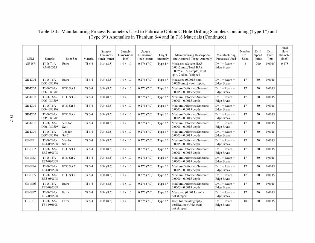
Table D-1. Manufacturing Process Parameters Used to Fabricate Option C Hole-Drilling Samples Containing (Type 1*) and (Type 6*) Anomalies in Titanium 6-4 and In 718 Materials (Continued)
OEM Sample User Set Material
Sample Thickness
(inch (mm))
Sample Dimensions
(inch)
Unique Dimension (inch (mm))
Target Anomaly
Manufacturing Description and Assumed Target Anomaly
Manufacturing Processes Used
Number Drill Used
Drill Speed (sfm)
Drill Feed (ipt)
Final Hole
Diameter (inch)
GE-R7 TI-D-T1A- R7-080325
Extra Ti 6-4 0.34 (8.5) 1.0 x 1.0 0.276 (7.0) Type 1* Measured (Severe HAZ 0.0012 max, Total HAZ 0.0025) - 1/2 sample, axial split, 2nd half shipped
Drill + Ream + Edge Break
3 200 0.0015 0.275
GE-DD1 TI-D-T6A- DD1-080508
Extra Ti 6-4 0.34 (8.5) 1.0 x 1.0 0.276 (7.0) Type 6* Measured (0.0015 nom, 0.0028 max) - not shipped
Drill + Ream + Edge Break
17 50 0.0015
GE-DD2 TI-D-T6A- DD2-080508
ETC Set 1 Ti 6-4 0.34 (8.5) 1.0 x 1.0 0.276 (7.0) Type 6* Medium Deformed/Smeared: 0.0005 - 0.0015 depth
Drill + Ream + Edge Break
17 50 0.0015
GE-DD3 TI-D-T6A- DD3-080508
ETC Set 2 Ti 6-4 0.34 (8.5) 1.0 x 1.0 0.276 (7.0) Type 6* Medium Deformed/Smeared: 0.0005 - 0.0015 depth
Drill + Ream + Edge Break
17 50 0.0015
GE-DD4 TI-D-T6A- DD4-080508
ETC Set 3 Ti 6-4 0.34 (8.5) 1.0 x 1.0 0.276 (7.0) Type 6* Medium Deformed/Smeared: 0.0005 - 0.0015 depth
Drill + Ream + Edge Break
17 50 0.0015
GE-DD5 TI-D-T6A- DD5-080508
ETC Set 4 Ti 6-4 0.34 (8.5) 1.0 x 1.0 0.276 (7.0) Type 6* Medium Deformed/Smeared: 0.0005 - 0.0015 depth
Drill + Ream + Edge Break
17 50 0.0015
GE-DD6 TI-D-T6A- DD6-080508
Vendor Set 1
Ti 6-4 0.34 (8.5) 1.0 x 1.0 0.276 (7.0) Type 6* Medium Deformed/Smeared: 0.0005 - 0.0015 depth
Drill + Ream + Edge Break
17 50 0.0015
GE-DD7 TI-D-T6A- DD7-080508
Vendor Set 2
Ti 6-4 0.34 (8.5) 1.0 x 1.0 0.276 (7.0) Type 6* Medium Deformed/Smeared: 0.0005 - 0.0015 depth
Drill + Ream + Edge Break
17 50 0.0015
GE-EE1 TI-D-T6A- EE1-080508
Vendor Set 3
Ti 6-4 0.34 (8.5) 1.0 x 1.0 0.276 (7.0) Type 6* Medium Deformed/Smeared: 0.0005 - 0.0015 depth
Drill + Ream + Edge Break
17 50 0.0015
GE-EE2 TI-D-T6A- EE2-080508
ETC Set 1 Ti 6-4 0.34 (8.5) 1.0 x 1.0 0.276 (7.0) Type 6* Medium Deformed/Smeared: 0.0005 - 0.0015 depth
Drill + Ream + Edge Break
17 50 0.0015
GE-EE3 TI-D-T6A- EE3-080508
ETC Set 2 Ti 6-4 0.34 (8.5) 1.0 x 1.0 0.276 (7.0) Type 6* Medium Deformed/Smeared: 0.0005 - 0.0015 depth
Drill + Ream + Edge Break
17 50 0.0015
GE-EE4 TI-D-T6A- EE4-080508
ETC Set 3 Ti 6-4 0.34 (8.5) 1.0 x 1.0 0.276 (7.0) Type 6* Medium Deformed/Smeared: 0.0005 - 0.0015 depth
Drill + Ream + Edge Break
17 50 0.0015
GE-EE5 TI-D-T6A- EE5-080508
ETC Set 4 Ti 6-4 0.34 (8.5) 1.0 x 1.0 0.276 (7.0) Type 6* Medium Deformed/Smeared: 0.0005 - 0.0015 depth
Drill + Ream + Edge Break
17 50 0.0015
GE-EE6 TI-D-T6A- EE6-080508
Extra Ti 6-4 0.34 (8.5) 1.0 x 1.0 0.276 (7.0) Type 6* Medium Deformed/Smeared: 0.0005 - 0.0015 depth
Drill + Ream + Edge Break
17 50 0.0015
GE-EE7 TI-D-T6A- EE7-080508
Extra Ti 6-4 0.34 (8.5) 1.0 x 1.0 0.276 (7.0) Type 6* Measured (0.0015 max) - not shipped
Drill + Ream + Edge Break
17 50 0.0015
GE-FF1 TI-D-T6A- FF1-080508
Extra Ti 6-4 0.34 (8.5) 1.0 x 1.0 0.276 (7.0) Type 6* Used for metallography verification (Unknown) - not shipped
Drill + Ream + Edge Break
18 50 0.0015
D-7

Table D-1. Manufacturing Process Parameters Used to Fabricate Option C Hole-Drilling Samples Containing (Type 1*) and (Type 6*) Anomalies in Titanium 6-4 and In 718 Materials (Continued)
OEM Sample User Set Material
Sample Thickness
(inch (mm))
Sample Dimensions
(inch)
Unique Dimension (inch (mm))
Target Anomaly
Manufacturing Description and Assumed Target Anomaly
Manufacturing Processes Used
Number Drill Used
Drill Speed (sfm)
Drill Feed (ipt)
Final Hole
Diameter (inch)
GE-FF2 TI-D-T6A- FF2-080508
ETC Set 1 Ti 6-4 0.34 (8.5) 1.0 x 1.0 0.276 (7.0) Type 6* Very High Deformed/Smeared: >0.002 depth
Drill + Ream + Edge Break
18 50 0.0015
GE-FF3 TI-D-T6A- FF3-080508
ETC Set 2 Ti 6-4 0.34 (8.5) 1.0 x 1.0 0.276 (7.0) Type 6* Very High Deformed/Smeared: >0.002 depth
Drill + Ream + Edge Break
18 50 0.0015
GE-FF4 TI-D-T6A- FF4-080508
ETC Set 3 Ti 6-4 0.34 (8.5) 1.0 x 1.0 0.276 (7.0) Type 6* Very High Deformed/Smeared: >0.002 depth
Drill + Ream + Edge Break
18 50 0.0015
GE-FF5 TI-D-T6A- FF5-080508
ETC Set 4 Ti 6-4 0.34 (8.5) 1.0 x 1.0 0.276 (7.0) Type 6* Very High Deformed/Smeared: >0.002 depth
Drill + Ream + Edge Break
18 50 0.0015
GE-FF6 TI-D-T6A- FF6-080508
Vendor Set 1
Ti 6-4 0.34 (8.5) 1.0 x 1.0 0.276 (7.0) Type 6* Very High Deformed/Smeared: >0.002 depth
Drill + Ream + Edge Break
18 50 0.0015
GE-FF7 TI-D-T6A- FF7-080508
Vendor Set 2
Ti 6-4 0.34 (8.5) 1.0 x 1.0 0.276 (7.0) Type 6* Very High Deformed/Smeared: >0.002 depth
Drill + Ream + Edge Break
18 50 0.0015
GE-GG5 TI-D-T6A- GG5-080508
Vendor Set 3
Ti 6-4 0.34 (8.5) 1.0 x 1.0 0.276 (7.0) Type 6* Very High Deformed/Smeared: >0.002 depth
Drill + Ream + Edge Break
18 50 0.0015
GE-GG6 TI-D-T6A- GG6-080508
Extra Ti 6-4 0.34 (8.5) 1.0 x 1.0 0.276 (7.0) Type 6* Very High Deformed/Smeared: >0.002 depth
Drill + Ream + Edge Break
18 50 0.0015
GE-GG7 TI-D-T6A- GG7-080508
Extra Ti 6-4 0.34 (8.5) 1.0 x 1.0 0.276 (7.0) Type 6* Measured (0.0014 nom, 0.0067 max) - not shipped
Drill + Ream + Edge Break
18 50 0.0015
GE-U1 IN-D-T1A- U1-080325
Extra In 718 0.34 (8.5) 1.0 x 1.0 0.276 (7.0) Type 1* Measured (0.0026" max (uniform)) - not shipped
Drill + Ream + Edge Break
1 55 0.0003 0.274-0.275
GE-U2 IN-D-T1A- U2-080325
ETC Set 1 In 718 0.34 (8.5) 1.0 x 1.0 0.276 (7.0) Type 1* High Heat + Deformation: >0.002 depth
Drill + Ream + Edge Break
2 55 0.0003 0.274-0.275
GE-U3 IN-D-T1A- U3-080325
ETC Set 2 In 718 0.34 (8.5) 1.0 x 1.0 0.276 (7.0) Type 1* High Heat + Deformation: >0.002 depth
Drill + Ream + Edge Break
2 55 0.0003 0.274-0.275
GE-U4 IN-D-T1A- U4-080325
Extra In 718 0.34 (8.5) 1.0 x 1.0 0.276 (7.0) Type 1* Failed drill Drill + Ream + Edge Break
Failed 55 0.0003
GE-U5 IN-D-T1A- U5-080325
ETC Set 3 In 718 0.34 (8.5) 1.0 x 1.0 0.276 (7.0) Type 1* High Heat + Deformation: >0.002 depth
Drill + Ream + Edge Break
4 55 0.0003 0.274-0.275
GE-U6 IN-D-T1A- U6-080325
ETC Set 4 In 718 0.34 (8.5) 1.0 x 1.0 0.276 (7.0) Type 1* High Heat + Deformation: >0.002 depth
Drill + Ream + Edge Break
4 55 0.0003 0.274-0.275
D-8

Table D-1. Manufacturing Process Parameters Used to Fabricate Option C Hole-Drilling Samples Containing (Type 1*) and (Type 6*) Anomalies in Titanium 6-4 and In 718 Materials (Continued)
OEM Sample User Set Material
Sample Thickness
(inch (mm))
Sample Dimensions
(inch)
Unique Dimension (inch (mm))
Target Anomaly
Manufacturing Description and Assumed Target Anomaly
Manufacturing Processes Used
Number Drill Used
Drill Speed (sfm)
Drill Feed (ipt)
Final Hole
Diameter (inch)
GE-U7 IN-D-T1A- U7-080325
Extra In 718 0.34 (8.5) 1.0 x 1.0 0.276 (7.0) Type 1* Failed drill Drill + Ream + Edge Break
Failed 55 0.0003
GE-V1 IN-D-T1A- V1-080325
Vendor Set 1
In 718 0.34 (8.5) 1.0 x 1.0 0.276 (7.0) Type 1* High Heat + Deformation: >0.002 depth
Drill + Ream + Edge Break
5 55 0.0003 0.274-0.275
GE-V2 IN-D-T1A- V2-080325
Vendor Set 2
In 718 0.34 (8.5) 1.0 x 1.0 0.276 (7.0) Type 1* High Heat + Deformation: >0.002 depth
Drill + Ream + Edge Break
5 55 0.0003 0.274-0.275
GE-V3 IN-D-T1A- V3-080325
Vendor Set 3
In 718 0.34 (8.5) 1.0 x 1.0 0.276 (7.0) Type 1* High Heat + Deformation: >0.002 depth
Drill + Ream + Edge Break
5 55 0.0003 0.274-0.275
GE-V4 IN-D-T1A- V4-080325
Extra In 718 0.34 (8.5) 1.0 x 1.0 0.276 (7.0) Type 1* Failed drill Drill + Ream + Edge Break
Failed 55 0.0003
GE-V5 IN-D-T1A- V5-080325
Extra In 718 0.34 (8.5) 1.0 x 1.0 0.276 (7.0) Type 1* High Heat + Deformation: >0.002 depth
Drill + Ream + Edge Break
6 55 0.0003 0.274-0.275
GE-V6 IN-D-T1A- V6-080325
Extra In 718 0.34 (8.5) 1.0 x 1.0 0.276 (7.0) Type 1* Measured (0.005" max - intermittent) - not shipped
Drill + Ream + Edge Break
7 55 0.0003 0.274-0.275
GE-V7 IN-D-T1A- V7-080325
Extra In 718 0.34 (8.5) 1.0 x 1.0 0.276 (7.0) Type 1* Failed drill Drill + Ream + Edge Break
Failed 55 0.0003
GE-W1 IN-D-T1A- W1-080414
TBD In 718 0.34 (8.5) 1.0 x 1.0 0.276 (7.0) Type 1* Waiting metallography verification
Drill + Ream + Edge Break
8 55 0.0003 0.276
GE-W2 IN-D-T1A- W2-080414
TBD In 718 0.34 (8.5) 1.0 x 1.0 0.276 (7.0) Type 1* Waiting metallography verification
Drill + Ream + Edge Break
8 55 0.0003 0.276
GE-W3 IN-D-T1A- W3-080414
Extra In 718 0.34 (8.5) 1.0 x 1.0 0.276 (7.0) Type 1* Failed drill Drill + Ream + Edge Break
Failed 55 0.0003
GE-W4 IN-D-T1A- W4-080414
TBD In 718 0.34 (8.5) 1.0 x 1.0 0.276 (7.0) Type 1* Waiting metallography verification
Drill + Ream + Edge Break
9 55 0.0003 0.276
GE-W5 IN-D-T1A- W5-080414
TBD In 718 0.34 (8.5) 1.0 x 1.0 0.276 (7.0) Type 1* Waiting metallography verification
Drill + Ream + Edge Break
9 55 0.0003 0.276
GE-W6 IN-D-T1A- W6-080414
Extra In 718 0.34 (8.5) 1.0 x 1.0 0.276 (7.0) Type 1* Failed drill Drill + Ream + Edge Break
Failed 55 0.0003
GE-X1 IN-D-T1A- X1-080414
TBD In 718 0.34 (8.5) 1.0 x 1.0 0.276 (7.0) Type 1* Waiting metallography verification
Drill + Ream + Edge Break
10 55 0.0003 0.276
GE-X2 IN-D-T1A- X2-080414
TBD In 718 0.34 (8.5) 1.0 x 1.0 0.276 (7.0) Type 1* Waiting metallography verification
Drill + Ream + Edge Break
10 55 0.0003 0.276
GE-X3 IN-D-T1A- X3-080414
Extra In 718 0.34 (8.5) 1.0 x 1.0 0.276 (7.0) Type 1* Failed drill Drill + Ream + Edge Break
Failed 55 0.0003
D-9

Table D-1. Manufacturing Process Parameters Used to Fabricate Option C Hole-Drilling Samples Containing (Type 1*) and (Type 6*) Anomalies in Titanium 6-4 and In 718 Materials (Continued)
OEM Sample User Set Material
Sample Thickness
(inch (mm))
Sample Dimensions
(inch)
Unique Dimension (inch (mm))
Target Anomaly
Manufacturing Description and Assumed Target Anomaly
Manufacturing Processes Used
Number Drill Used
Drill Speed (sfm)
Drill Feed (ipt)
Final Hole
Diameter (inch)
GE-X4 IN-D-T1A- X4-080414
TBD In 718 0.34 (8.5) 1.0 x 1.0 0.276 (7.0) Type 1* Used for metallography verification
Drill + Ream + Edge Break
11 55 0.0003 0.276
GE-X5 IN-D-T1A- X5-080414
TBD In 718 0.34 (8.5) 1.0 x 1.0 0.276 (7.0) Type 1* Waiting metallography verification
Drill + Ream + Edge Break
11 55 0.0003 0.276
GE-X6 IN-D-T1A- X6-080414
TBD In 718 0.34 (8.5) 1.0 x 1.0 0.276 (7.0) Type 1* Used for metallography verification
Drill + Ream + Edge Break
11 55 0.0003 0.276
GE-X7 IN-D-T1A- X7-080414
Extra In 718 0.34 (8.5) 1.0 x 1.0 0.276 (7.0) Type 1* Failed drill Drill + Ream + Edge Break
Failed 55 0.0003
GE-Y1 IN-D-T1A- Y1-080414
TBD In 718 0.34 (8.5) 1.0 x 1.0 0.276 (7.0) Type 1* Waiting metallography verification
Drill + Ream + Edge Break
12 55 0.0003 0.276
GE-Y2 IN-D-T1A- Y2-080414
TBD In 718 0.34 (8.5) 1.0 x 1.0 0.276 (7.0) Type 1* Waiting metallography verification
Drill + Ream + Edge Break
12 55 0.0003 0.276
GE-Y3 IN-D-T1A- Y3-080414
Extra In 718 0.34 (8.5) 1.0 x 1.0 0.276 (7.0) Type 1* Failed drill Drill + Ream + Edge Break
Failed 55 0.0003
GE-Y4 IN-D-T1A- Y4-080414
TBD In 718 0.34 (8.5) 1.0 x 1.0 0.276 (7.0) Type 1* Used for metallography verification
Drill + Ream + Edge Break
13 55 0.0003 0.276
GE-Y5 IN-D-T1A- Y5-080414
TBD In 718 0.34 (8.5) 1.0 x 1.0 0.276 (7.0) Type 1* Waiting metallography verification
Drill + Ream + Edge Break
13 55 0.0003 0.276
GE-Y6 IN-D-T1A- Y6-080414
TBD In 718 0.34 (8.5) 1.0 x 1.0 0.276 (7.0) Type 1* Used for metallography verification
Drill + Ream + Edge Break
14 55 0.0003 0.276
GE-Y7 IN-D-T1A- Y7-080414
TBD In 718 0.34 (8.5) 1.0 x 1.0 0.276 (7.0) Type 1* Waiting metallography verification
Drill + Ream + Edge Break
14 55 0.0003 0.276
GE-J10 IN-D-T6A-1- 071206
ETC Set 1 In 718 0.34 (8.5) 1.0 x 1.0 0.276 (7.0) Type 6* Medium Deformed/Smeared: 0.0005 - 0.0015 depth
Drill + Ream + Edge Break
GE-J11 IN-D-T6A- 2-071206
ETC Set 2 In 718 0.34 (8.5) 1.0 x 1.0 0.276 (7.0) Type 6* Medium Deformed/Smeared: 0.0005 - 0.0015 depth
Drill + Ream + Edge Break
GE-J12 IN-D-T6A- 3-071206
ETC Set 3 In 718 0.34 (8.5) 1.0 x 1.0 0.276 (7.0) Type 6* Medium Deformed/Smeared: 0.0005 - 0.0015 depth
Drill + Ream + Edge Break
GE-J13 IN-D-T6A- 4-071206
ETC Set 4 In 718 0.34 (8.5) 1.0 x 1.0 0.276 (7.0) Type 6* Medium Deformed/Smeared: 0.0005 - 0.0015 depth
Drill + Ream + Edge Break
GE-K2 IN-D-T6A- 5-071206
Vendor Set 1
In 718 0.34 (8.5) 1.0 x 1.0 0.276 (7.0) Type 6* Medium Deformed/Smeared: 0.0005 - 0.0015 depth
Drill + Ream + Edge Break
GE-K3 IN-D-T6A- 6-071206
Vendor Set 2
In 718 0.34 (8.5) 1.0 x 1.0 0.276 (7.0) Type 6* Medium Deformed/Smeared: 0.0005 - 0.0015 depth
Drill + Ream + Edge Break
D-10

Table D-1. Manufacturing Process Parameters Used to Fabricate Option C Hole-Drilling Samples Containing (Type 1*) and (Type 6*) Anomalies in Titanium 6-4 and In 718 Materials (Continued)
OEM Sample User Set Material
Sample Thickness
(inch (mm))
Sample Dimensions
(inch)
Unique Dimension (inch (mm))
Target Anomaly
Manufacturing Description and Assumed Target Anomaly
Manufacturing Processes Used
Number Drill Used
Drill Speed (sfm)
Drill Feed (ipt)
Final Hole
Diameter (inch)
GE-K4 IN-D-T6A- 7-071206
Vendor Set 3
In 718 0.34 (8.5) 1.0 x 1.0 0.276 (7.0) Type 6* Medium Deformed/Smeared: 0.0005 - 0.0015 depth
Drill + Ream + Edge Break
GE-K5 IN-D-T6A- 8-071206
Vendor Set 1
In 718 0.34 (8.5) 1.0 x 1.0 0.276 (7.0) Type 6* Medium Deformed/Smeared: 0.0005 - 0.0015 depth
Drill + Ream + Edge Break
GE-L2 IN-D-T6A- 9-071206
Vendor Set 2
In 718 0.34 (8.5) 1.0 x 1.0 0.276 (7.0) Type 6* Medium Deformed/Smeared: 0.0005 - 0.0015 depth
Drill + Ream + Edge Break
GE-L3 IN-D-T6A- 10-071206
Vendor Set 3
In 718 0.34 (8.5) 1.0 x 1.0 0.276 (7.0) Type 6* Medium Deformed/Smeared: 0.0005 - 0.0015 depth
Drill + Ream + Edge Break
GE-L4 IN-D-T6A- 11-071206
Extra In 718 0.34 (8.5) 1.0 x 1.0 0.276 (7.0) Type 6* Medium Deformed/Smeared: 0.0005 - 0.0015 depth
Drill + Ream + Edge Break
GE-L5 IN-D-T6A- 12-071206
Extra In 718 0.34 (8.5) 1.0 x 1.0 0.276 (7.0) Type 6* Medium Deformed/Smeared: 0.0005 - 0.0015 depth
Drill + Ream + Edge Break
GE-Z1 IN-D-T6A- Z1-080414
Extra In 718 0.34 (8.5) 1.0 x 1.0 0.276 (7.0) Type 6* Measured (0.0008 max) - not shipped
Drill + Ream + Edge Break
15 20 0.0002 0.274-0.275
GE-Z2 IN-D-T6A- Z2-080414
ETC Set 1 In 718 0.34 (8.5) 1.0 x 1.0 0.276 (7.0) Type 6* Light Deformation: <0.0005 depth
Drill + Ream + Edge Break
15 20 0.0002 0.274-0.275
GE-Z3 IN-D-T6A- Z3-080414
ETC Set 2 In 718 0.34 (8.5) 1.0 x 1.0 0.276 (7.0) Type 6* Light Deformation: <0.0005 depth
Drill + Ream + Edge Break
15 20 0.0002 0.274-0.275
GE-Z4 IN-D-T6A- Z4-080414
ETC Set 3 In 718 0.34 (8.5) 1.0 x 1.0 0.276 (7.0) Type 6* Light Deformation: <0.0005 depth
Drill + Ream + Edge Break
15 20 0.0002 0.274-0.275
GE-Z5 IN-D-T6A- Z5-080414
ETC Set 3 In 718 0.34 (8.5) 1.0 x 1.0 0.276 (7.0) Type 6* Light Deformation: <0.0005 depth
Drill + Ream + Edge Break
15 20 0.0002 0.274-0.275
GE-Z6 IN-D-T6A- Z6-080414
Vendor Set 1
In 718 0.34 (8.5) 1.0 x 1.0 0.276 (7.0) Type 6* Light Deformation: <0.0005 depth
Drill + Ream + Edge Break
15 20 0.0002 0.274-0.275
GE-Z7 IN-D-T6A- Z7-080414
Vendor Set 2
In 718 0.34 (8.5) 1.0 x 1.0 0.276 (7.0) Type 6* Light Deformation: <0.0005 depth
Drill + Ream + Edge Break
15 20 0.0002 0.274-0.275
GE-AA1 IN-D-T6A- AA1-080414
Vendor Set 3
In 718 0.34 (8.5) 1.0 x 1.0 0.276 (7.0) Type 6* Light Deformation: <0.0005 depth
Drill + Ream + Edge Break
15 20 0.0002 0.274-0.275
GE-AA2 IN-D-T6A- AA2-080414
ETC Set 1 In 718 0.34 (8.5) 1.0 x 1.0 0.276 (7.0) Type 6* Light Deformation: <0.0005 depth
Drill + Ream + Edge Break
15 20 0.0002 0.274-0.275
GE-AA3 IN-D-T6A- AA3-080414
ETC Set 2 In 718 0.34 (8.5) 1.0 x 1.0 0.276 (7.0) Type 6* Light Deformation: <0.0005 depth
Drill + Ream + Edge Break
15 20 0.0002 0.274-0.275
GE-AA4 IN-D-T6A- AA4-080414
Vendor Set 1
In 718 0.34 (8.5) 1.0 x 1.0 0.276 (7.0) Type 6* Light Deformation: <0.0005 depth
Drill + Ream + Edge Break
15 20 0.0002 0.274-0.275
D-11

Table D-1. Manufacturing Process Parameters Used to Fabricate Option C Hole-Drilling Samples Containing (Type 1*) and (Type 6*) Anomalies in Titanium 6-4 and In 718 Materials (Continued)
OEM Sample User Set Material
Sample Thickness
(inch (mm))
Sample Dimensions
(inch)
Unique Dimension (inch (mm))
Target Anomaly
Manufacturing Description and Assumed Target Anomaly
Manufacturing Processes Used
Number Drill Used
Drill Speed (sfm)
Drill Feed (ipt)
Final Hole
Diameter (inch)
GE-AA5 IN-D-T6A- AA5-080414
Vendor Set 2
In 718 0.34 (8.5) 1.0 x 1.0 0.276 (7.0) Type 6* Light Deformation: <0.0005 depth
Drill + Ream + Edge Break
15 20 0.0002 0.274-0.275
GE-AA6 IN-D-T6A- AA6-080414
Vendor Set 3
In 718 0.34 (8.5) 1.0 x 1.0 0.276 (7.0) Type 6* Light Deformation: <0.0005 depth
Drill + Ream + Edge Break
15 20 0.0002 0.274-0.275
GE-AA7 IN-D-T6A- AA7-080414
Extra In 718 0.34 (8.5) 1.0 x 1.0 0.276 (7.0) Type 6* Measured (0.0006 max) - not shipped
Drill + Ream + Edge Break
15 20 0.0002 0.274-0.275
GE-BB1 IN-D-T6A- BB1-080414
Extra In 718 0.34 (8.5) 1.0 x 1.0 0.276 (7.0) Type 6* Measured (0.001 max) - not shipped
Drill + Ream + Edge Break
16 20 0.0002 0.275-0.276
GE-BB2 IN-D-T6A- BB2-080414
ETC Set 1 In 718 0.34 (8.5) 1.0 x 1.0 0.276 (7.0) Type 6* Medium Deformed/Smeared: 0.0005 - 0.0015 depth
Drill + Ream + Edge Break
16 20 0.0002 0.275-0.276
GE-BB3 IN-D-T6A- BB3-080414
ETC Set 2 In 718 0.34 (8.5) 1.0 x 1.0 0.276 (7.0) Type 6* Medium Deformed/Smeared: 0.0005 - 0.0015 depth
Drill + Ream + Edge Break
16 20 0.0002 0.275-0.276
GE-BB4 IN-D-T6A- BB4-080414
ETC Set 3 In 718 0.34 (8.5) 1.0 x 1.0 0.276 (7.0) Type 6* Medium Deformed/Smeared: 0.0005 - 0.0015 depth
Drill + Ream + Edge Break
16 20 0.0002 0.275-0.276
GE-BB5 IN-D-T6A- BB5-080414
ETC Set 4 In 718 0.34 (8.5) 1.0 x 1.0 0.276 (7.0) Type 6* Medium Deformed/Smeared: 0.0005 - 0.0015 depth
Drill + Ream + Edge Break
16 20 0.0002 0.275-0.276
GE-BB6 IN-D-T6A- BB6-080414
Vendor Set 1
In 718 0.34 (8.5) 1.0 x 1.0 0.276 (7.0) Type 6* Medium Deformed/Smeared: 0.0005 - 0.0015 depth
Drill + Ream + Edge Break
16 20 0.0002 0.275-0.276
GE-BB7 IN-D-T6A- BB7-080414
Vendor Set 2
In 718 0.34 (8.5) 1.0 x 1.0 0.276 (7.0) Type 6* Medium Deformed/Smeared: 0.0005 - 0.0015 depth
Drill + Ream + Edge Break
16 20 0.0002 0.275-0.276
GE-CC1 IN-D-T6A- CC1-080414
Vendor Set 3
In 718 0.34 (8.5) 1.0 x 1.0 0.276 (7.0) Type 6* Medium Deformed/Smeared: 0.0005 - 0.0015 depth
Drill + Ream + Edge Break
16 20 0.0002 0.275-0.276
GE-CC2 IN-D-T6A- CC2-080414
ETC Set 1 In 718 0.34 (8.5) 1.0 x 1.0 0.276 (7.0) Type 6* Medium Deformed/Smeared: 0.0005 - 0.0015 depth
Drill + Ream + Edge Break
16 20 0.0002 0.275-0.276
GE-CC3 IN-D-T6A- CC3-080414
ETC Set 2 In 718 0.34 (8.5) 1.0 x 1.0 0.276 (7.0) Type 6* Medium Deformed/Smeared: 0.0005 - 0.0015 depth
Drill + Ream + Edge Break
16 20 0.0002 0.275-0.276
GE-CC4 IN-D-T6A- CC4-080414
Vendor Set 1 In 718 0.34 (8.5) 1.0 x 1.0 0.276 (7.0) Type 6* Medium Deformed/Smeared: 0.0005 - 0.0015 depth
Drill + Ream + Edge Break
16 20 0.0002 0.275-0.276
GE-CC5 IN-D-T6A- CC5-080414
Vendor Set 2
In 718 0.34 (8.5) 1.0 x 1.0 0.276 (7.0) Type 6* Medium Deformed/Smeared: 0.0005 - 0.0015 depth
Drill + Ream + Edge Break
16 20 0.0002 0.275-0.276
GE-CC6 IN-D-T6A- CC6-080414
Vendor Set 3
In 718 0.34 (8.5) 1.0 x 1.0 0.276 (7.0) Type 6* Medium Deformed/Smeared: 0.0005 - 0.0015 depth
Drill + Ream + Edge Break
16 20 0.0002 0.275-0.276
GE-CC7 IN-D-T6A- CC7-080414
Extra In 718 0.34 (8.5) 1.0 x 1.0 0.276 (7.0) Type 6* Measured (0.011 max) - not shipped
Drill + Ream + Edge Break
16 20 0.0002 0.275-0.276
D-12

Table D-1. Manufacturing Process Parameters Used to Fabricate Option C Hole-Drilling Samples Containing (Type 1*) and (Type 6*) Anomalies in Titanium 6-4 and In 718 Materials (Continued)
OEM Sample User Set Material
Sample Thickness
(inch (mm))
Sample Dimensions
(inch)
Unique Dimension (inch (mm))
Target Anomaly
Manufacturing Description and Assumed Target Anomaly
Manufacturing Processes Used
Number Drill Used
Drill Speed (sfm)
Drill Feed (ipt)
Final Hole
Diameter (inch)
GE-M1 IN-D-T6A- M1-080325
ETC Set 1 In 718 1.0 1.0 x 1.0 0.5 Type 6* Medium Deformed/Smeared: 0.0005 - 0.0015 depth - 1/2 sample, axial split, 2nd half shipped
Drill + Ream + Edge Break + Axial Split
1 20 0.0008
GE-M2 IN-D-T6A- M2-080325
ETC Set 2 In 718 1.0 1.0 x 1.0 0.5 Type 6* Medium Deformed/Smeared: 0.0005 - 0.0015 depth
Drill + Ream + Edge Break + Axial Split
1 20 0.0008 0.5
GE-M3 IN-D-T6A- M3-080325
ETC Set 3 In 718 1.0 1.0 x 1.0 0.5 Type 6* Medium Deformed/Smeared: 0.0005 - 0.0015 depth - failed drill
Drill + Ream + Edge Break + Axial Split
1 Failed 20 0.0008 0.5
GE-M4 IN-D-T6A- M4-080325
ETC Set 4 In 718 1.0 1.0 x 1.0 0.5 Type 6* Medium Deformed/Smeared: 0.0005 - 0.0015 depth - failed drill
Drill + Ream + Edge Break + Axial Split
2 Failed 20 0.0008 0.501
GE-M5 IN-D-T6A- M5-080325
Vendor Set 1
In 718 1.0 1.0 x 1.0 0.5 Type 6* Medium Deformed/Smeared: 0.0005 - 0.0015 depth
Drill + Ream + Edge Break + Axial Split
3 20 0.0008 0.498
GE-M6 IN-D-T6A- M6-080325
Vendor Set 2
In 718 1.0 1.0 x 1.0 0.5 Type 6* Medium Deformed/Smeared: 0.0005 - 0.0015 depth - failed drill
Drill + Ream + Edge Break + Axial Split
3 Failed 20 0.0008 0.498
GE-M7 IN-D-T6A- M7-080325
Vendor Set 3
In 718 1.0 1.0 x 1.0 0.5 Type 6* Medium Deformed/Smeared: 0.0005 - 0.0015 depth
Drill + Ream + Edge Break + Axial Split
4 20 0.0008 0.498
GE-N2 IN-D-T6A- N2-080325
n/a In 718 1.0 1.0 x 1.0 0.5 Type 6* ==> MISSING <== Medium Deformed/Smeared: 0.0005 - 0.0015 depth
Drill + Ream + Edge Break + Axial Split
5 20 0.0008 0.499
GE-S1 IN-D-T6A- S1-080325
ETC Set 1 In 718 1.0 1.0 x 1.0 0.5 Type 6* Medium Deformed/Smeared: 0.0005 - 0.0015 depth
Drill + Ream + Edge Break + Axial Split
5 20 0.0008 0.498
GE-S2 IN-D-T6A- S2-080325
ETC Set 2 In 718 1.0 1.0 x 1.0 0.5 Type 6* Medium Deformed/Smeared: 0.0005 - 0.0015 depth
Drill + Ream + Edge Break + Axial Split
5 20 0.0008 0.499
GE-S3 IN-D-T6A- S3-080325
ETC Set 3 In 718 1.0 1.0 x 1.0 0.5 Type 6* Medium Deformed/Smeared: 0.0005 - 0.0015 depth
Drill + Ream + Edge Break + Axial Split
5 20 0.0008 0.501
GE-S4 IN-D-T6A- S4-080325
ETC Set 4 In 718 1.0 1.0 x 1.0 0.5 Type 6* Medium Deformed/Smeared: 0.0005 - 0.0015 depth
Drill + Ream + Edge Break + Axial Split
5 20 0.0008 0.501
D-13

D-14
Table D-1. Manufacturing Process Parameters Used to Fabricate Option C Hole-Drilling Samples Containing (Type 1*) and (Type 6*) Anomalies in Titanium 6-4 and In 718 Materials (Continued)
OEM Sample User Set Material
Sample Thickness
(inch (mm))
Sample Dimensions
(inch)
Unique Dimension (inch (mm))
Target Anomaly
Manufacturing Description and Assumed Target Anomaly
Manufacturing Processes Used
Number Drill Used
Drill Speed (sfm)
Drill Feed (ipt)
Final Hole
Diameter (inch)
GE-S5 IN-D-T6A- S5-080325
Vendor Set 1
In 718 1.0 1.0 x 1.0 0.5 Type 6* Medium Deformed/Smeared: 0.0005 - 0.0015 depth
Drill + Ream + Edge Break + Axial Split
5 20 0.0008 0.501
GE-S6 IN-D-T6A- S6-080325
Vendor Set 2
In 718 1.0 1.0 x 1.0 0.5 Type 6* Medium Deformed/Smeared: 0.0005 - 0.0015 depth
Drill + Ream + Edge Break + Axial Split
5 20 0.0008 0.501
GE-S7 IN-D-T6A- S7-080325
Vendor Set 3
In 718 1.0 1.0 x 1.0 0.5 Type 6* Medium Deformed/Smeared: 0.0005 - 0.0015 depth
Drill + Ream + Edge Break + Axial Split
5 20 0.0008 0.501
GE-T5 IN-D-T6A- T5-080325
Extra In 718 1.0 1.0 x 1.0 0.5 Type 6* Medium Deformed/Smeared: 0.0005 - 0.0015 depth
Drill + Ream + Edge Break + Axial Split
5 20 0.0008 0.501
GE-T6 IN-D-T6A- T6-080325
Extra In 718 1.0 1.0 x 1.0 0.5 Type 6* Medium Deformed/Smeared: 0.0005 - 0.0015 depth
Drill + Ream + Edge Break + Axial Split
5 20 0.0008 0.501
GE-T7 IN-D-T6A- T7-080325
Extra In 718 1.0 1.0 x 1.0 0.5 Type 6* Used for metallography verification (Unknown) - not shipped
Drill + Ream + Edge Break + Axial Split
5 20 0.0008
GE = General Electric OEM = Original equipment manufacturer Ti 6-4 = Titanium alloy sfm = Surface feet per minute ipt = Inch per tooth HAZ = Heat-affected zone

The following formulas were used in calculating machining parameters for the hole-drilling operation. surface feet per minute (sfm) = PI() * Drill Diameter * (rpm)/12 inch per minute = (rpm) teeth per rev. * inch per tooth
- for drilling: teeth per revolution = 2
* *min min
in rev tooth in
rev tooth
π
* (for the drill diameter)min min 12
feet revin
A progression of semi-increasing material damage from very light to heavy for 7-mm-diameter holes containing (Type 6*) anomalies in In 718 and titanium alloy (Ti 6-4) materials are shown in figures D-1 through D-8.
Hole Z1Hole Z1
Exit (Side A) 200X Entrance (Side A) 200X Maximum Deformation (Side A) 0.0006″ 500X
Exit (Side B) 200X Entrance (Side B) 200X Maximum Deformation (Side B) 0.0006″ 500X
Figure D-1. Micrographs of Hole Sample GE -Z1, (In 718) (Type 6*) Anomaly Fabricated by
the Hole-Drilling Process Showing Damage to a Depth of 0.8 mil (Maximum) Representative of Light-Medium Material Deformation
D-15
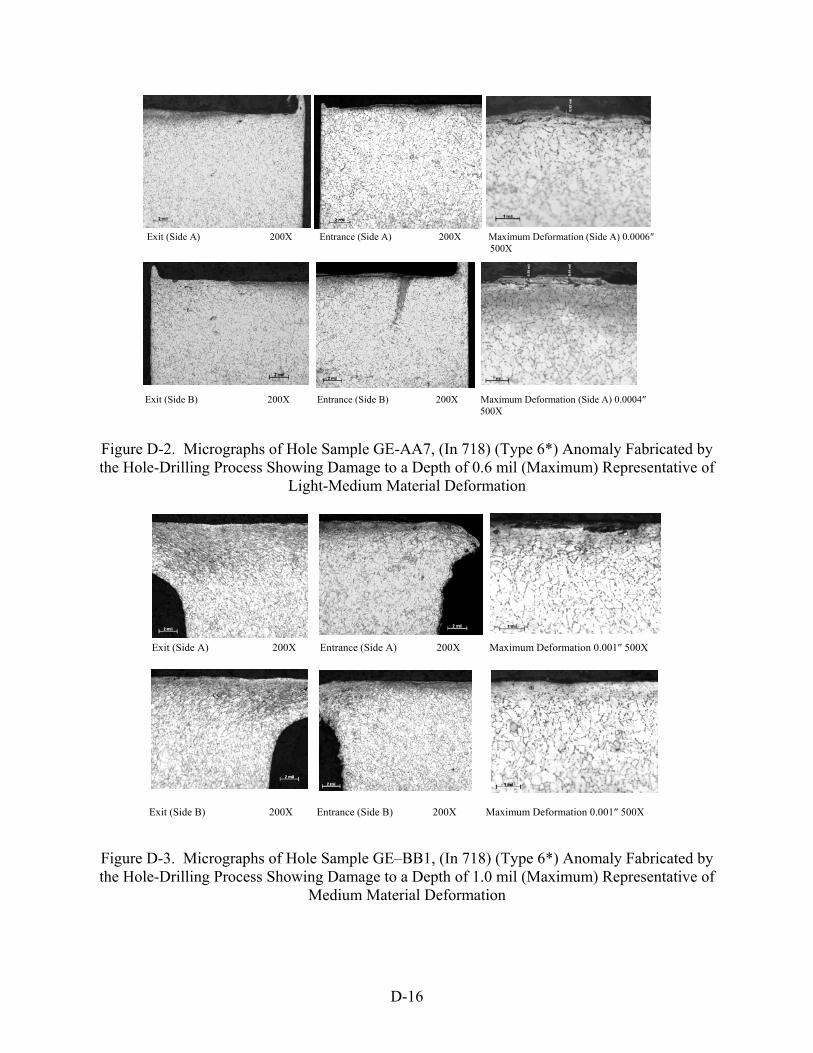
Exit (Side A) 200X Entrance (Side A) 200X Maximum Deformation (Side A) 0.0006″ 500X
Exit (Side B) 200X Entrance (Side B) 200X Maximum Deformation (Side A) 0.0004″ 500X
Figure D-2. Micrographs of Hole Sample GE-AA7, (In 718) (Type 6*) Anomaly Fabricated by the Hole-Drilling Process Showing Damage to a Depth of 0.6 mil (Maximum) Representative of
Light-Medium Material Deformation
Exit (Side A) 200X Entrance (Side A) 200X Maximum Deformation 0.001″ 500X
Exit (Side B) 200X Entrance (Side B) 200X Maximum Deformation 0.001″ 500X
Figure D-3. Micrographs of Hole Sample GE–BB1, (In 718) (Type 6*) Anomaly Fabricated by the Hole-Drilling Process Showing Damage to a Depth of 1.0 mil (Maximum) Representative of
Medium Material Deformation
D-16

Exit (Side A) 200X Entrance (Side A) 200X Maximum Deformation 0.0011″ 500X
Exit (Side B) 200X Entrance (Side B) 200X Maximum Deformation 0.001″ 500X
Figure D-4. Micrographs of Hole Sample GE–CC7, (In 718) (Type 6*) Anomaly Fabricated by the Hole-Drilling Process Showing Damage to a Depth of 1.1 mil (Maximum) Representative of
Medium Material Deformation
Exit (Side A) 200X Entrance (Side A) 200X Maximum Deformation 0.0028″ 500X
Exit (Side B) 200X Entrance (Side B) 200X Maximum Deformation 0.0015″ 500X
Figure D-5. Micrographs of Hole Sample GE–DD1, (Ti 6-4) (Type 6*) Anomaly Fabricated by the Hole-Drilling Process Showing Damage to a Depth of 2.8 mil (Maximum) Representative of
Medium-High Material Deformation
D-17

Exit (Side A) 200X Entrance (Side A) 200X Maximum Deformation 0.0013″ 500X
Exit (Side B) 200X Entrance (Side B) 200X Maximum Deformation 0.0015″ 500X
Figure D-6. Micrographs of Hole Sample GE–EE7, (Ti 6-4) (Type 6*) Anomaly Fabricated by the Hole-Drilling Process Showing Damage to a Depth of 1.5 mil (Maximum) Representative of
Medium Material Deformation
Exit (Side A) 200X Entrance (Side A) 200X Maximum Deformation 0.0015″ 500X
Exit (Side B) 200X Entrance (Side B) 200X Maximum Deformation 0.0053″ 500X
Figure D-7. Micrographs of Hole Sample GE–FF1, (Ti 6-4) (Type 6*) Anomaly Fabricated by the Hole-Drilling Process Showing Damage to a Depth of 5.3 mil (Maximum) Representative of
Very High Material Deformation
D-18

Exit (Side A) 200X Entrance (Side A) 200X Maximum Deformation 0.0067″ 500X
Exit (Side B) 200X Entrance (Side B) 200X Maximum Deformation 0.0014″ 500X
Figure D-8. Micrographs of Hole Sample GE–GG7, (Ti 6-4) (Type 6*) Anomaly Fabricated by the Hole-Drilling Process Showing Damage to a Depth of 6.8 mil (Maximum) Representative of
Very High Material Deformation D.2 OPTION C—MANUFACTURE OF TURNING SAMPLES. Option C targeted the manufacture of 42 Ti 6-4 coupons and 42 In 718 coupons. Of each material, 6 coupons were to be pristine; 18 Type 1 in low, medium, and high severity or depth of distorted grain layer; and 18 Type 6 in low, medium, and high severity. Option A concentrated on the manufacture of severe anomalies so experimentation and development work were required to attain the varying depth of severity required for Option C. D.2.1 Ti 6-4 MATERIAL. Three large disk forgings were acquired from General Electric (GE) for the purpose of producing the turning samples. These forgings were sliced into large washers of approximately 30 inches in diameter and 0.250 inch thick. All Option C turnings were performed by the Pratt & Whitney (PW) Tooling Services group using a Bullard vertical turret lathe (VTL). Ti 6-4 Option C coupons were machined to the parameters indicated in table D-2. The speed parameters could be continuously adjusted, whereas tool condition was less controlled. Other parameters such as rake angle and coolant were handled in a binary fashion. Table D-2 shows only the tests that made usable washers from which to produce coupons. Figure D-9 shows an example of a typical coupon.
D-19

Table D-2. Machining Parameters for Turning Coupons
Parameter Test 1 Test 2 Test 7 Test 10
Speed (sfm) 250 350 400 250
Feed rate (ipr) 0.007 0.007 0.007 0.007
Bulk depth of cut (in.) 0.020 0.02 0.02 0.020
Final depth of cut (in.) 0.01 0.01 0.01 0.01
Coolant (5%-8% oil concentration)
Yes Yes Yes Yes
Dull/truncated tool New New New New
Tool rake angle Positive Negative Negative Positive
Chips in tool path No No No Yes
Comments Insert burns out. Finish is not flat.
Pristine parameters (1), dull tool, negative rake, dam to channel chips.
Attempted anomaly 1 1 1 shallow 6
Anomaly achieved Pristine Type 1 deep Type 1 shallow Type 6
″2
″ 1
Figure D-9. Typical Turning Coupon Geometry
The first washer was turned using the pristine parameters for Test 1. The micrograph for a pristine Ti 6-4 coupon is shown in figure D-10.
D-20

Figure D-10. Pristine Coupon of Turning Ti 6-4 Shown at two Magnifications Test 2 achieved the deep Type 1 distorted microstructure anomaly with a distorted layer greater than 0.0015″ deep and is shown in figure D-11.
Figure D-11. Ti 6-4 Coupon With High Severity, Type 1 Damage at two Magnifications Several more turning tests were run before the next acceptable parameter set was determined. Test 7 yielded the Type 1 shallow anomaly, less than 0.005″ deep, and is shown in figure D-12.
\
Figure D-12. Ti 6-4 Coupon With Shallow, Type 1 Damage at two Magnifications
D-21

Several attempts were made to produce the Type 1 medium-severity anomaly, all unsuccessful. The medium-depth anomaly was finally produced by polishing severe-anomaly coupons from test 2 to the required depth for medium-severity anomalies, between 0.0015″ and 0.0005″. The micrograph for a polished, medium-severity coupon is shown in figure D-13.
Figure D-13. Ti 6-4 Type 1 With Medium Severity Produced by Polishing Coupons From a High-Severity Washer
Using pristine parameters and a negative rake tool, and channeling a large quantity of Ti chips directly into the tool cutting path, material was embedded into the turned surface achieving the Type 6 anomaly with embedded parent material, as shown in figure D-14. At this time, there is no way to vary the depth or severity of this anomaly.
Figure D-14. Ti 6-4 Type 6 Coupon With Embedded Parent Material The coupons were machined from the washers, serialized, and sent to Iowa State University (ISU).
D-22

D.2.2 In 718 MATERIAL. Three In 718 pancakes were identified at PW as being available for use in the program for the purpose of producing the turning samples. The pancakes were sectioned to produce washer shapes for production of turning anomalies and the production of pristine coupons. Two pancakes had diameters of 16″ and one had a diameter of 20″. The three pancakes were sectioned to create washers with 0.20″ thickness. All Option C turnings were performed by the PW Tooling Services group using a Bullard VTL. In 718 Option C coupons were machined to the parameters indicated in table D-3.
Table D-3. In 718 Option C Sample Parameters
Parameter Test 1 Test 6 Test 12 Test 20
Speed (sfm) 180 120 180 200
Feed rate (ipr) 0.006 0.006 0.006 0.015
Bulk depth of cut (in.) 0.010 0.010 0.010 0.080
Coolant Yes Yes Yes? No
Dull/truncated tool New New Dull Dull
Tool rake angle Positive Negative Negative Negative
Chips in tool path No No Yes No
Attempted anomaly Pristine 1 6 1 medium/deep
Anomaly achieved Pristine Type 1 shallow Type 6 Type 1 medium
Test washer 1 produced the desired finish for pristine coupons and the resulting metallographic image is shown in figure D-15.
Figure D-15. In 718 Pristine Machining Condition
D-23

Introducing anomalies into the In 718 washers proved a more difficult process than producing similar anomalies in the Ti 6-4 material. Five tests washers with varying parameter sets were turned to finally produce the first set of anomalies. The Type 1 shallow anomaly coupons were produced using parameter set 6, as shown in figure D-16.
Figure D-16. In 718 Type 1 Low-Severity, Machining-Induced Anomaly Several more parameter sets were used to attempt to machine medium- and high-severity anomalies into the washers. After experimenting with varying parameters, the extremely abusive parameters of test 20 finally produced a medium-severity, Type 1 anomaly but also severely damaged both the washer and the cutting tool. The resulting micrograph is shown in figure D-17. This parameter set produced a consistent anomaly layer that was approximately 0.0007″-0.0008″ deep, thus meeting the requirement for the medium-severity Type 1 anomaly.
Figure D-17. In 718 Type 1 Medium-Severity, Machining-Induced Anomaly
D-24

The Type 1 high-severity anomaly in In 718 could not be produced with any of the attempted parameter sets. Producing the Type 6 anomaly with embedded parent material in In 718 proved much simpler than the Type 1 anomalies. Similar techniques to achieve the anomaly type in the In 718 samples, including nominal conditions with a negative cutting tool angle, a dull cutting tool, and parent material chips forced into the path of the cutting tool were used to achieve the anomaly. This yielded the desired Type 6 anomaly and the resulting micrograph is shown in figure D-18. As with the Ti 6-4 washers, there was no way to vary the depth of the anomaly.
Figure D-18. In 718 Type 6 Machining-Induced Anomaly The coupons were machined from the washers, serialized, and sent to ISU. D.3 OPTION C—BROACHING SAMPLE FABRICATION. All broaching was performed on a production 15-120-HE Detroit Horizontal broach machine (figure D-19) at a Honeywell production supplier approved to broach Ti and Ni rotating disks. This machine is capable of broaching both Ti and Ni components and is capable of cutting speeds up to 22 ft/min. Figure D-20 shows a close-up of the roughing cutting tools passing through a blank, the typical coolant flow, and the fixture used to hold the blanks during broaching.
D-25

Figure D-19. Detroit Horizontal Broaching, Model 15-120-HE
Figure D-20. Close-Up of Roughing Cutting Tools, Coolant Flow, and Tooling Used to Hold Blanks
The typical broaching slot is created by a series of toothed cutting tools, which remove small amounts of material from the broaching slot. A broaching slot is the result of the cutting action of several hundred individual teeth that are pulled through the sample. Each individual cutting tool is designed to remove material from one area of the slot. The cutting tools work together as a group to create the complete broaching slot form. The first group of cutting tools is typically referred to as roughers, and remove relatively large amounts of material with each tooth. The final set of cutting tools makes less aggressive cuts and brings the broaching slot to the final dimensions. Figure D-21 shows the final crown shaver cutting tool used for the ETC samples.
D-26

Figure D-21. Crown Shaver Cutting Tool Segment The Type 1 anomalies were made using a dulled crown shaver cutting tool that was offset in the direction of the broaching blank. This offset resulted in a very aggressive cut in the crown region of the broaching slot. Figure D-22 shows a comparator screenshot of a sharp crown shaver tooth. Figure D-23 is a comparator screenshot of a dulled crown shaver tooth. The Type 1 anomalies were broached at production cutting speeds for both the Ti and Ni blanks.
Figure D-22. Comparator Images of a Sharp Crown Shaver Tooth
D-27
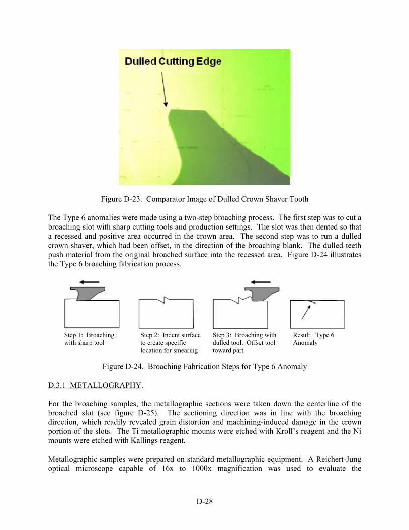
Figure D-23. Comparator Image of Dulled Crown Shaver Tooth The Type 6 anomalies were made using a two-step broaching process. The first step was to cut a broaching slot with sharp cutting tools and production settings. The slot was then dented so that a recessed and positive area occurred in the crown area. The second step was to run a dulled crown shaver, which had been offset, in the direction of the broaching blank. The dulled teeth push material from the original broached surface into the recessed area. Figure D-24 illustrates the Type 6 broaching fabrication process.
Step 1: Broaching Step 2: Indent surface Step 3: Broaching with Result: Type 6 with sharp tool to create specific dulled tool. Offset tool Anomaly location for smearing toward part.
Figure D-24. Broaching Fabrication Steps for Type 6 Anomaly
D.3.1 METALLOGRAPHY. For the broaching samples, the metallographic sections were taken down the centerline of the broached slot (see figure D-25). The sectioning direction was in line with the broaching direction, which readily revealed grain distortion and machining-induced damage in the crown portion of the slots. The Ti metallographic mounts were etched with Kroll’s reagent and the Ni mounts were etched with Kallings reagent. Metallographic samples were prepared on standard metallographic equipment. A Reichert-Jung optical microscope capable of 16x to 1000x magnification was used to evaluate the
D-28
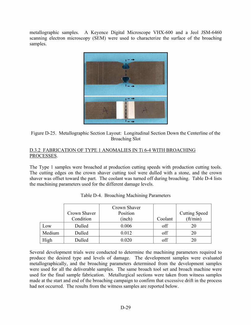
metallographic samples. A Keyence Digital Microscope VHX-600 and a Jeol JSM-6460 scanning electron microscopy (SEM) were used to characterize the surface of the broaching samples.
Figure D-25. Metallographic Section Layout: Longitudinal Section Down the Centerline of the Broaching Slot
D.3.2 FABRICATION OF TYPE 1 ANOMALIES IN Ti 6-4 WITH BROACHING PROCESSES. The Type 1 samples were broached at production cutting speeds with production cutting tools. The cutting edges on the crown shaver cutting tool were dulled with a stone, and the crown shaver was offset toward the part. The coolant was turned off during broaching. Table D-4 lists the machining parameters used for the different damage levels.
Table D-4. Broaching Machining Parameters
Crown Shaver
Condition
Crown Shaver Position (inch) Coolant
Cutting Speed (ft/min)
Low Dulled 0.006 off 20
Medium Dulled 0.012 off 20
High Dulled 0.020 off 20 Several development trials were conducted to determine the machining parameters required to produce the desired type and levels of damage. The development samples were evaluated metallographically, and the broaching parameters determined from the development samples were used for all the deliverable samples. The same broach tool set and broach machine were used for the final sample fabrication. Metallurgical sections were taken from witness samples made at the start and end of the broaching campaign to confirm that excessive drift in the process had not occurred. The results from the witness samples are reported below.
D-29

D.3.3 SUMMARY OF Ti 6-4 TYPE 1 ANOMALIES—BROACHING. The level of damage in the Type 1 samples varied along the length of the slot. For each sample, a picture was taken of the typical level of damage and the most severe level of damage. For the samples that had higher levels of damage, a layer of highly compressed grains was observed closest to the machined surface. Below this layer, the grains were distorted in the cutting direction. Figure D-26 shows the presample for the low setting. Figure D-27 shows the postsample for the low setting. In general, the damage is at a low setting; however, areas of medium-level damage may also be present in these samples.
200x (Typical) 200x (Worst)
Figure D-26. Broaching Anomalies for Sample 21A: Ti Type 1—Low
200x (Typical) 200x (Worst)
Figure D-27. Broaching Anomalies for Sample 29A: Ti Type 1—Low Figure D-28 shows the presample for the medium setting. Figure D-29 shows the postsample for the medium setting. The damage exhibited in these samples ranged between the low and medium levels.
D-30

200x (Typical) 200x (Worst)
Figure D-28. Broaching Anomalies for Sample 30A: Ti Type 1—Medium
200x (Typical) 200x (Worst)
Figure D-29. Broaching Anomalies for Sample 38A: Ti Type 1—Medium
Figure D-30 shows the presample for the high setting. Figure D-31 shows the postsample for the high setting. The damage exhibited in these samples ranged between the medium and high levels.
200x (Typical) 200x (Worst)
Figure D-30. Broaching Anomalies for Sample 1C: Ti Type 1—High
D-31

200x (Typical) 200x (Worst)
Figure D-31. Broaching Anomalies for Sample 9C: Ti Type 1—High
D.3.4 FABRICATION OF TYPE 6 ANOMALIES IN Ti 6-4 WITH BROACHING PROCESS. The Type 6 samples were broached at production cutting speeds with production cutting tools. An initial slot was broached using sharp cutting tools and the surface was indented to provide a location for smeared material. The cutting edges of a second crown shaver cutting tool were dulled with a stone, and the crown shaver was offset toward the part. The coolant was turned on during broaching. Table D-5 lists the machining parameters used for the different levels of damage.
Table D-5. Machining Parameters for Type 6 Ti 6-4 Broaching Samples
1st Pass
Sharpness 2nd Pass
Sharpness
2nd Pass Position (inch) Coolant
Cutting Speed (ft/min)
Low Sharp Dulled 0.011 On 20
Medium Sharp Dulled 0.010 On 20
High Sharp Dulled 0.009 On 20 Several development trials were conducted to determine the machining parameters required to produce the desired type and levels of damage. The development samples were evaluated metallographically, and the broaching parameters determined from the development samples were used for all the deliverable samples. The same broaching tool set and broaching machine were used for the sample fabrication. Metallurgical sections were taken from witness samples made at the start and end of the broaching campaign to confirm that excessive drift in the process had not occurred. The results from the witness samples are reported below. In addition to metallographic evaluations, the Type 6 anomalies were documented with high depth of field optical images (20x magnification) and with SEM images (100x magnification) in the scanning electron mode to capture topographical features. Figure D-32 shows the presample for the low setting. Figure D-33 shows the postsample for the low setting. The damage present at a low setting has no apparent geometric impact on the surface of the sample. As shown in the right-hand images of figures D-32 and D-33, the
D-32

anomaly can be detected with optical means due to a change in reflectivity in the anomaly region. A focused inspection is often required to locate the anomaly. However, when evaluated in the SEM for geometric features, the Type 6 anomalies were not detected (figure D-34).
200x 200x
Figure D-32. Broaching Anomaly for Sample 24C: Ti Type 6—Low
200x 200x
Figure D-33. Broaching Sample 25C: Ti Type 6—Low
Type 6 anomalies at the low level contain no apparent geometric component.
Geometric components were not
observed in samples evaluated in the SEM.
Figure D-34. The SEM Results for Ti Type 6 Sample
D-33

Figure D-35 shows the presample for the medium setting. Figure D-36 shows the postsample for the medium setting. The damage present in the medium setting samples can be detected with optical means.
200x 20x
Figure D-35. Broaching Sample 22C: Ti Type 6—Medium
200x 20x
Figure D-36. Broaching Sample 23C: Ti Type 6—Medium
Figure D-37 shows the presample for the high setting. Figure D-38 shows the postsample for the high setting. The damage present in the high-setting samples can be readily detected with optical means. The anomalies in the high-setting samples often had a relatively large geometric component, as shown in the metallographic sections and the SEM image (figure D-39).
D-34

200x 20x
Figure D-37. Broaching Sample 26C: Ti Type 6—High
200x 20x
Figure D-38. Broaching Sample 21C: Ti Type 6—High
Type 6 anomalies at the high level contain geometric component for several of the samples.
It is expected that anomalies with
geometric components will be readily detected using conventional nondestructive test techniques.
Figure D-39. Broaching Sample 41C: Ti Type 6—High
D-35

D.3.5 FABRICATION OF TYPE 1 ANOMALIES IN In 718 WITH BROACHING PROCESS. The Type 1 samples for In 718 were broached at production cutting speeds with production cutting tools. The cutting edges on the crown shaver cutting tool were dulled with a stone, and the crown shaver was offset toward the part. The coolant was turned off during broaching. Table D-6 lists the machining parameters used for the different levels of damage.
Table D-6. Machining Parameters for Type 1 In 718 Broaching Samples
Crown Shaver
Condition
Crown Shaver Position
(in.) Coolant Cutting Speed
(ft/min)
Low Dulled 0.004 Off 6
Medium Dulled 0.008 Off 6
High Dulled 0.012 Off 6 Several development trials were conducted to determine the machining parameters required to produce the desired type and levels of damage. The development samples were evaluated metallographically, and the broaching parameters determined from the development samples were used for all of the deliverable samples. The same broach tool set and broach machine were used for the sample fabrication. Metallurgical sections were taken from witness samples made at the start and end of the broaching campaign to confirm that excessive drift in the process had not occurred. The results from the witness samples are reported below. D.3.6 SUMMARY OF In 718 TYPE 1 ANOMALIES—BROACHING. As with the Ti 6-4 samples, the level of damage in the Type 1 In 718 samples varied along the length of the slot. For each sample, a picture was taken of the typical level of damage and the most severe level of damage. A white etching layer was observed on the surface of the samples, and below the surface distorted grains etched darker than the substrate material. The grains were clearly distorted in the cutting direction. Figure D-40 shows the presample for the low setting. Figure D-41 shows the postsample for the low setting. In general, the damage was at a low setting; however, areas of medium-level damage were observed in the areas with the worst damage. Figure D-42 shows the presample for the medium setting. Figure D-43 shows the postsample for the medium setting. The maximum damage exhibited in these samples ranged between the medium and high levels.
D-36

200x (Typical) 200x (Worst)
Figure D-40. Broaching Sample 31A: In 718 Type 1—Low Setting
200x (Typical) 200x (Worst)
Figure D-41. Broaching Sample 39A: In 718 Type 1—Low Setting
200x (Typical) 200x (Worst)
Figure D-42. Broaching Sample 40A: In 718 Type 1—Medium Scattering
D-37

200x (Typical) 200x (Worst)
Figure D-43. Broaching Sample 48A: In 718 Type 1—Medium Setting
Figure D-44 shows the presample for the high setting. Figure D-45 shows the postsample for the high setting. The damage exhibited in these samples was at the low level.
200x (Typical) 200x (Worst)
Figure D-44. Broaching Sample 11B: In 718 Type 1—High Setting
200x (Typical) 200x (Worst)
Figure D-45. Broaching Sample 19B: In 718 Type 1—High Setting
D-38

D.3.7 FABRICATION OF TYPE 6 ANOMALIES IN In 718 WITH BROACHING PROCESS. The Type 6 samples were broached at production cutting speeds with production cutting tools. An initial slot was broached using sharp cutting tools, and the surface was indented to provide a location for smeared material. The cutting edges of a second crown shaver cutting tool were dulled with a stone, and the crown shaver was offset toward the part. The coolant was turned on during broaching. Table D-7 lists the machining parameters used for the different levels of damage.
Table D-7. Machining Parameters for In 718 Type 6 Samples
1st Pass
Sharpness 2nd Pass
Sharpness
2nd Pass Position
(in.) Coolant Cutting Speed
(ft/min)
Low Sharp Dulled 0.0065 On 6
Medium Sharp Dulled 0.0045 On 6
High Sharp Dulled 0.0035 On 6 Several development trials were conducted to determine the machining parameters required to produce the desired type and levels of damage. The development samples were evaluated metallographically, and the broaching parameters determined from the development samples were used for all the deliverable samples. The same broach tool set and broach machine were used for the sample fabrication. Metallurgical sections were taken from witness samples made at the start and end of the broaching campaign to confirm that excessive drift in the process had not occurred. The results from the witness samples are reported below. D.3.8 SUMMARY OF In 718 TYPE 6 ANOMALIES—BROACHING. The Type 6 anomalies in the In 718 samples were documented with metallographic images at 200x magnification. An image of the anomaly was taken for each pre- and postsample. Figure D-46 shows the pre- and postsample for the low setting.
200x magnification 200x magnification
Figure D-46. Broaching Sample 43B and 50A: In 718 Type 6—Low
D-39

Figure D-47 shows the pre- and postsample for the medium setting.
200x magnification 200x magnification
Figure D-47. Broaching Sample 34B and 42B: In 718 Type 6—Medium
Figure D-48 shows the pre- and postsample for the high setting.
200x magnification 200x magnification
Figure D-48. Broaching Sample 25B and 33B: In 718 Type 6—High
In addition to the intentionally fabricated Type 6 anomalies, naturally occurring Type 6 anomalies were periodically observed in both the Type 1 and Type 6 samples. Figure D-49 is an example of naturally occurring Type 6 anomaly in In 718.
D-40

Figure D-49. Aligned Porosity/Smearing Observed in Both Type 1 and Type 6 Samples (The presence and extent of this Type 6 anomaly is not readily controllable.)
D.3.9 SUMMARY OF BROACHING FABRICATION PROCESSES.
The Type 1 anomaly was readily produced at production cutting speeds in both Ti and Ni broaching slots by using dull cutting tools and aggressive cutting depths. The Type 1 anomalies in these samples contained no geometric component and are expected to be undetectable with conventional nondestructive techniques. Consistent generation of the graduated levels of targeted damage was challenging with the broaching process, and varying levels of damage were observed in the samples. The Type 6 anomaly was difficult to produce with a conventional broaching process. Type 6 damage was observed in the Ni samples when using dulled broaching tools and aggressive cutting depths; however, the distribution and level of damage could not be readily controlled. Because of these challenges, a two-step broaching process was employed to force the smearing to occur in a specific location. With this approach, Type 6 damage was produced in both the Ti and Ni samples. The Type 6 anomalies at the medium and high levels of damage likely contain geometric components, which will be readily detectable with conventional NDE. The results from these broaching trials indicate that both the Type 1 and Type 6 anomalies are difficult to produce using aerospace manufacturing settings since the dulled tooling and the offsets on cutting depths were well beyond those used in a standard production. In addition, it was observed that the Type 1 anomaly is more readily produced than the Type 6 anomaly.
D-41/D-42

APPENDIX E—CHARACTERIZATION OF ANOMALOUSLY MACHINED SAMPLES
E.1 INTRODUCTION. To accomplish baseline surface metrology, an optical profilometer was used (as opposed to a stylus-type profilometer) because an optical profilometer is truly a nondestructive inspection tool. In the use of a stylus-type profilometer, there is a point of contact between the diamond stylus and the sample, which leaves a small permanent line inscribed into the sample. In an optical profilometer, there is no contact made with the surface of a sample, the measurement tool involves a digital-imaging camera and a movable stage in the Z axis. Software is written to adjust the stage in the Z direction to optimize the focal curve for each pixel in the system’s camera. While optimizing the focal curve for each pixel, the software records the Z position of the stage for each optimized pixel. This allows for a very highly detailed image of the sample, and allows for surface texture and condition to be documented in an analysis software program. The particular optical profilometer used in this work is capable of scanning with a resolution of up to 800 nm in the Z axis at 5x magnification, and up to a resolution of 10 nm in the Z axis at 100x magnification, over an extended X-Y range of 100 by 76 mm at 5x magnification, and 5 by 4 mm at 100x magnification. Rough surfaces can be easily quantified with accurate measurement of Ra (the arithmetical mean roughness of a measured surface), Rq (the root mean square roughness), and Rz (a result of International Organization for Standardization (ISO) 9000 standards and specifically is measured over 5 peaks and valleys at 10 points on the part). Measurement of roughness, waviness, and contour all conform to recognized ISO 4287 and 4288 ISO 4287—1997 Terms, Definition and Surface Texture Parameters [E-1], ISO 4288—1996 Rules and Procedures for Assessment of Surface Texture [E-2]. This instrument also allows for the accurate measurement of surfaces at steep angles of up to 80° from the X-Y plane. E.2 APPROACH. E.2.1 SURFACE PROFILE EXAMINATION. There are three types of surface texture profiles currently defined in the ISO standards: the primary profile, which is the initial condition of the surface of the sample itself, including the peaks and valleys as well as the overall shape of the sample; the roughness profile (Ra), which consists of the peaks and valleys of the sample; and the waviness profile (Wa), which is the general shape of the sample. E.2.1.1 Primary Profile. A primary profile is one that has had the nominal form removed, often referred to as leveling. Prior to the leveling process, the initial scan will often be slightly higher at one end of the scan from the other end (see figure E-1). The reason for this is primarily that it is nearly impossible to position the stage exactly perpendicular to the light and camera focal direction. By removing the form, it is implied that the surface of the sample to be examined has been made normal to the plane of the camera. This is important in setting up the parameters with which to employ the filters. Figure E-2 shows the effect of the leveling process on the sample data. The primary
E-1

profile is the basis for evaluation of the primary profile parameters. The sampling length lp is numerically equal to the evaluation length [E-3]. The calculation of the P-parameters (equation E-1) is determined over the entire measured sample length (lp).
Figure E-1. Primary Profile as Taken, Prior to Leveling
Figure E-2. Surface After Leveling
1
0
1( ) ( )Pa Z x d x
l (E-1)
To filter the primary data for roughness and waviness, a “smoothing” filter is run through the primary data. The extent of the smoothing is based on a “filter cutoff wavelength.” The cutoff wavelength is the wavelength value that separates the roughness from the waviness. The shorter wavelengths define the Ra and the longer wavelengths define the Wa. A Gaussian filter is recommended in the American Society of Mechanical Engineers and ISO standards. Gaussian filters are based on passing a Gaussian, weighted average through the primary profile—resulting in the Wa shown in figure E-3. The peaks and valleys, which remain after the filter is used, separate the Wa from the Ra.
E-2

Figure E-3. Separation of Waviness From the Primary Profile
Changing the filter cutoff value (which changes the amount of averaging and smoothing) can have a huge impact on the measurement of roughness and waviness. Choosing a smaller cutoff value will result in smaller roughness values even though the real surface could be very rough. The filter cutoff provides the means for defining roughness. There is a table of standard cutoff values used for this evaluation in ISO 4287 and 4288. Since the average roughness (Ra) is the average distance from the mean line, peaks and valleys are treated the same way. Because of this averaging, several profiles can all have the same Ra value, as shown in figure E-4 [E-4]. This is an important concept when looking at the roughness values of a set of samples. If different filters are employed for different measurements within a set of samples, it could become impossible to determine the conditions of the samples within the set.
Figure E-4. Example of Three Different Surfaces Having the Same Ra Values
All scans performed for this work conform to ISO 4287 and 4288, depending on the length of the scan.
E-3

E.2.1.2 Waviness Profile. To obtain the Wa, the primary profile is first filtered using the long-wave Gaussian profile filter with a cutoff wavelength value (Lc). This results in the loss of one sampling length (lw) at the beginning and one sampling length lw at the end of the profile. The remaining profile is then partitioned into adjacent segments. Apart from possibly the last segment at the end of the profile, each segment is equal in length to the sampling length. If the last segment is not equal in length to the sampling length then it is removed. The resulting profile is called the Wa (see figure E-5).
Figure E-5. Waviness Profile Extracted From Primary Profile Calculation of the Wa parameters (equation E-2) is over a previously specified number of segments, which here is called the calculation number (CN). There is no default CN given in current ISO standards. Current industrial practice uses 5 as the default CN. If the Wa contains more than CN segments, then only the first CN segments are used in subsequent calculations. If the Wa contains less than CN segments, then all segments are used in subsequent calculations together with a warning stating how many segments were actually used [E-1].
1
0
1( ) ( )Wa Z x d x
l (E-2)
with l = lw
E.2.1.3 Roughness Profile. To obtain the Ra, the primary profile is first filtered using the short-wave Gaussian profile filter with a cutoff wavelength value Lc. This results in the loss of one sampling length lr at the beginning and one sampling length lr at the end of the profile. The remaining profile is then partitioned into adjacent segments. Apart from possibly the last segment at the end of the profile, each segment is equal in length to the sampling length. If the last segment is not equal in length to the sampling length, then it is removed. The resulting profile is called the Ra.
E-4

Calculation of the Ra parameters (see equation E-3) is over a previously specified number of segments, which is the CN. The default CN given in ISO 4288-1996 is 5. If the Ra contains more than CN segments, then only the first CN segments are used in subsequent calculations. If the Ra contains less than CN segments, then all segments are used in subsequent calculations together with a warning stating how many segments were actually used.
1
0
1( ) ( )Ra Z x d
l x (E-3)
with l = lr
An Ra from reference E-1 was derived from the primary profile by suppressing the long-wave component using the short-wave Gaussian profile filter with a cutoff wavelength value Lc. The Ra (figure E-6) is the basis for evaluating the Ra parameters. The sampling length lr is numerically equal to the cutoff wavelength Lc.
Figure E-6. Roughness Profile After Filtering
E.3 RESULTS. E.3.1 ANALYSIS OF THE ENGINE TITANIUM CONSORTIUM ANOMALOUS MACHINING DAMAGE DATA. Analysis begins by doing an optical scan of the broaching and turning samples, approximately 1/2 inch in length (see figure E-7). For the hole-drilling samples, the length of the scan was according to the thickness of the samples. Each resulting scan produces a two-dimensional graph, representing the length of the scan in the X direction, and the height (or depth) of the surface of the roughness in the Z direction (see figure E-7).
E-5

Figure E-7. Scan Procedure for Broaching and Turning Samples
Once a two-dimensional profile was taken of the area of interest (figure E-8), a second software program was used to determine the Ra and Wa value of the sample. Each value was recorded, along with an image of the scan area, a graph of the surface roughness and Wa, and a table of values for the height in the Z direction for a particular displacement in the X direction used to calculate the roughness parameter.
Figure E-8. Two-Dimensional Profile of an Area of Examination With Roughness Chart Below
The following sections describe the Ra and Wa results for each sample type and alloy. Results of the Ra and Wa measurements for titanium (Ti 6-4) broaching samples are provided in figures E-9 through E-16. Table E-1 summarizes the average Ra values for pristine, Type 1, and Type 6 samples. Table E-2 provides the average Wa values for the Ti 6-4 broaching samples. Results for the nickel (In 718) broaching samples are shown in figures E-17 through E-24 with average values tabulated in tables E-3 and E-4.
E-6

Note: The average Ra is 20.14.
Figure E-9. Ra Results for Ti 6-4 Pristine Broaching Samples
Note: The average Wa is 105.50.
Figure E-10. Wa Results for Ti 6-4 Pristine Broaching Samples
Note: The average Ra is 29.30.
Figure E-11. Ra Results for Ti 6-4 Type 1 Broaching Samples
E-7

Note: The average Wa is 188.65.
Figure E-12. Wa Results for Ti 6-4 Type 1 Broaching Samples
Note: The average Ra is 21.33.
Figure E-13. Ra Results for Ti 6-4 Type 6 Broaching Samples
Note: The average Wa is 140.56.
Figure E-14. Wa Results for Ti 6-4 Type 1 Broaching Samples
E-8
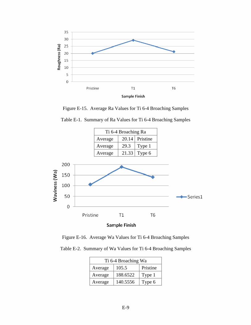
Figure E-15. Average Ra Values for Ti 6-4 Broaching Samples
Table E-1. Summary of Ra Values for Ti 6-4 Broaching Samples
Ti 6-4 Broaching Ra
Average 20.14 Pristine
Average 29.3 Type 1
Average 21.33 Type 6
Figure E-16. Average Wa Values for Ti 6-4 Broaching Samples
Table E-2. Summary of Wa Values for Ti 6-4 Broaching Samples
Ti 6-4 Broaching Wa
Average 105.5 Pristine
Average 188.6522 Type 1
Average 140.5556 Type 6
E-9

Note: The average Ra is 19.08.
Figure E-17. Ra Results for In 718 Pristine Broaching Samples
Note: The average Wa is 44.75.
Figure E-18. Wa Results for In 718 Pristine Broaching Samples
Note: The average Ra is 25.06.
Figure E-19. Ra Results for In 718 Type 1 Broaching Samples
E-10

Note: The average Wa is 112.47.
Figure E-20. Wa Results for In 718 Type 1 Broaching Samples
Note: The average Ra is 30.25.
Figure E-21. Ra Results for In 718 Type 1 Broaching Samples
Note: The average Wa is 134.1875. Figure E-22. Wa Results for In 718 Type 6 Broaching Samples
E-11

Figure E-23. Average Ra Values for In 718 Broaching Samples
Table E-3. Summary of Ra Values for In 718 Broaching Samples
In 718 Broaching Ra Average 19.08 Pristine Average 25.06 Type 1 Average 30.25 Type 6
Figure E-24. Average Wa Values for In 718 Broaching Samples
Table E-4. Summary of Wa Values for In 718 Broaching Samples
In 718 Broaching Wa
Average 044.75 Pristine
Average 112.4706 Type 1
Average 134.1875 Type 6
E-12

E.3.1.1 Turning Samples. Optical profilimetry of the turning samples revealed a degree of curvature on almost every sample. A three-dimensional view of the sample (shown in figure E-25) shows the extent of the curvature for one sample. (The noise in the lower left corner is the number “2” that was etched into the sample.)
mil
0
2
4
6
8
10
12
14
16
18
20
22
24
26
28
30
32
33.4 mil
1.83 in
0.833 in
Alpha = 45° Beta = 30°
Figure E-25. Laser Profilometry Showing Typical Curvature of the Turning Samples
An example line profile of the sample (figure E-26) going across the length of the sample shows the curvature to be 6 mil from the top of the crest to the edge of the sample.
mil
-6
-5
-4
-3
-2
-1
0
1
2
3
0 0.1 0.2 0.3 0.4 0.5 0.6 0.7 0.8 0.9 1 1.1 1.2 1.3 1.4 1.5 1.6 1.7 1.8 in
Length = 1.83 in Pt = 5.97 mil Scale = 10 mil
Figure E-26. Line Profile Showing Extreme Curvature on a Turning Sample
It is theorized that this curvature is due to the manner in which the samples were extracted from the bigger disk washer. The removal process, aside from creating a nonflat sample, also results in residual stress on both the upper and lower surfaces of the sample. It was suggested that future samples be extracted using an electro-discharging machine cutting, or a similar type of sample extraction, to eliminate or reduce residual stress and curvature issues. The results of the Ra and Wa measurements are shown in figures E-27 through E-34 for Ti 6-4 and in figures E-35 through E-42 for In 718. Tables E-5 through E-8 summarize the average values.
E-13

Note: The average Ra is 66.67.
Figure E-27. Ra Results for Ti 6-4 Pristine Turning Samples
Note: The average Wa is 44.25.
Figure E-28. Wa Results for Ti 6-4 Pristine Turning Samples
Note: The average Ra is 46.07.
Figure E-29. Ra Results for Ti 6-4 Type 1 Turning Samples
E-14
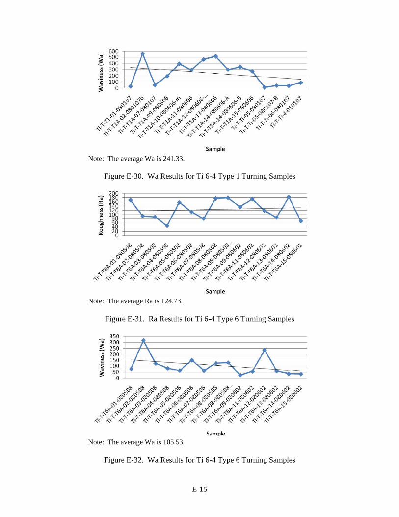
Note: The average Wa is 241.33.
Figure E-30. Wa Results for Ti 6-4 Type 1 Turning Samples
Note: The average Ra is 124.73.
Figure E-31. Ra Results for Ti 6-4 Type 6 Turning Samples
Note: The average Wa is 105.53.
Figure E-32. Wa Results for Ti 6-4 Type 6 Turning Samples
E-15
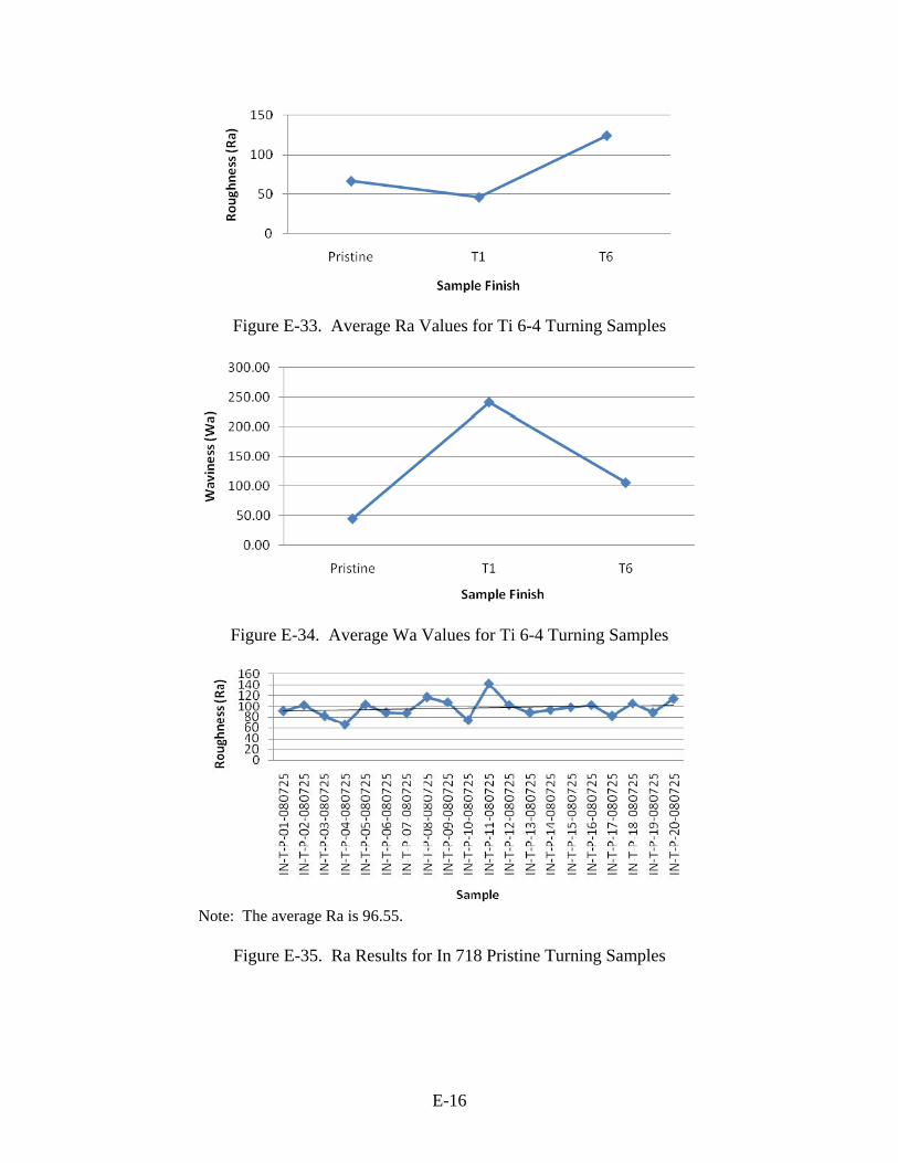
Figure E-33. Average Ra Values for Ti 6-4 Turning Samples
Figure E-34. Average Wa Values for Ti 6-4 Turning Samples
Note: The average Ra is 96.55.
Figure E-35. Ra Results for In 718 Pristine Turning Samples
E-16
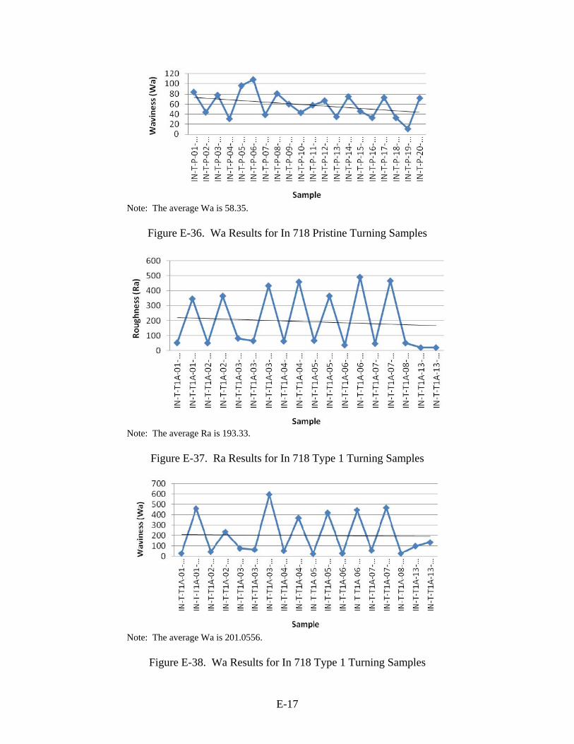
Note: The average Wa is 58.35.
Figure E-36. Wa Results for In 718 Pristine Turning Samples
Note: The average Ra is 193.33.
Figure E-37. Ra Results for In 718 Type 1 Turning Samples
Note: The average Wa is 201.0556.
Figure E-38. Wa Results for In 718 Type 1 Turning Samples
E-17

Note: The average Ra is 68.88.
Figure E-39. Ra Results for In 718 Type 6 Turning Samples
Note: The average Wa is 153.625.
Figure E-40. Wa Results for In 718 Type 6 Turning Samples
Figure E-41. Average Ra Values for In 718 Turning Samples
E-18

Figure E-42. Average Wa Values for In 718 Turning Samples
Table E-5. Summary of Ra Values for Ti 6-4 Turning Samples
Ti 6-4 Turning Ra
Average 66.67 Pristine
Average 46.07 Type 1
Average 124.73 Type 6
Table E-6. Summary of Wa Values for Ti 6-4 Turning Samples
Ti 6-4 Turning Wa
Average 044.25 Pristine
Average 241.33 Type 1
Average 105.53 Type 6
Table E-7. Summary of Ra Values of In 718 Turning Samples
In 718 Turning Ra
Average 96.55 Pristine
Average 193.33 Type 1
Average 68.88 Type 6
Table E-8. Summary of Wa Values for In 718 Turning Samples
In 718 Turning Wa
Average 058.35 Pristine
Average 201.0556 Type 1
Average 153.625 Type 6
E-19

E.3.1.3 Hole-Drilling Samples. The hole-drilling samples were more difficult to examine for roughness because the surface of interest was orientated 90° from the surface plane of the broaching and turning samples. Details of the measurement process and associated fixtures for measuring inside the drilled hole were described in the main body of the report. Of the six In 718 Type 1* samples, only two were measured because the holes on four of the samples were too small for the reflective device to be inserted without causing damage to the surface. The results for the Ti 6-4 hole-drilling samples are shown in figures E-43 through E-50, with the Ra and Wa averages tabulated in tables E-9 and E-10, respectively. The results for In 718 hole-drilling samples are shown in figures E-51 through E-58, with the Ra and Wa averages tabulated in tables E-11 and E-12, respectively.
Note: The average Ra is 86.85.
Figure E-43. Ra Results for Ti 6-4 Pristine Hole-Drilling Samples
Note: The average Wa is 361.74.
Figure E-44. Wa Results for Ti 6-4 Pristine Hole-Drilling Samples
E-20

Note: The average Ra is 152.74.
Figure E-45. Ra Results for Ti 6-4 Type 1 Hole-Drilling Samples
Note: The average Wa is 579.70.
Figure E-46. Wa Results for Ti 6-4 Type 1 Hole-Drilling Samples
Note: The average Ra is 174.67.
Figure E-47. Ra Results for Ti 6-4 Type 6 Hole-Drilling Samples
E-21
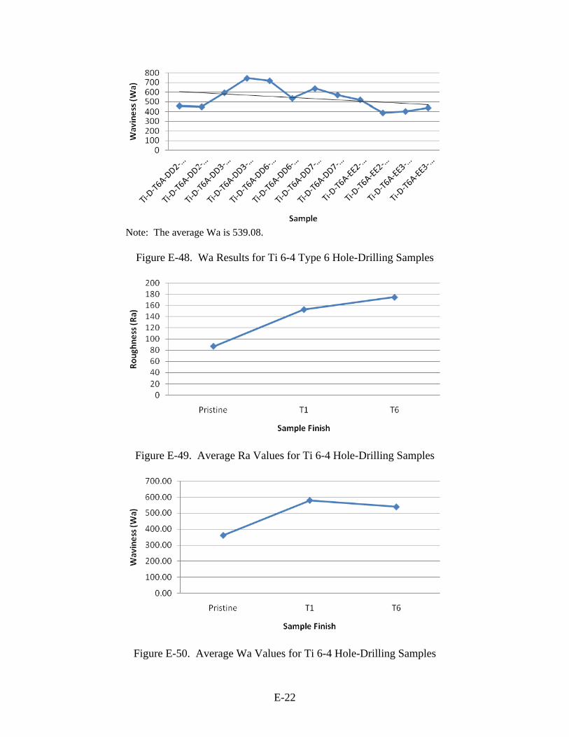
Note: The average Wa is 539.08.
Figure E-48. Wa Results for Ti 6-4 Type 6 Hole-Drilling Samples
Figure E-49. Average Ra Values for Ti 6-4 Hole-Drilling Samples
Figure E-50. Average Wa Values for Ti 6-4 Hole-Drilling Samples
E-22

Table E-9. Summary of Ra Values for Ti 6-4 Hole-Drilling Samples
Ti 6-4 Hole-Drilling Ra
Average 86.85 Pristine
Average 152.74 Type 1
Average 174.67 Type 6
Table E-10. Summary of Wa Values for Ti 6-4 Hole-Drilling Samples
Ti Hole-Drilling Wa
Average 361.74 Pristine
Average 579.70 Type 1
Average 539.08 Type 6
Note: The average Ra is 93.13.
Figure E-51. Ra Results for In 718 Pristine Hole-Drilling Samples
Note: The average Wa is 373.0417.
Figure E-52. Wa Results for In 718 Pristine Hole-Drilling Samples
E-23

Note: The average Ra is 132.5.
Figure E-53. Ra Results for In 718 Type 1 Hole-Drilling Samples
Note: The average Wa is 523.
Figure E-54. Wa Results for In 718 Type 1 Hole-Drilling Samples
Note: The average Ra is 165.15.
Figure E-55. Ra Results for In 718 Type 6 Hole-Drilling Samples
E-24

Note: The average Wa is 546.82.
Figure E-56. Wa Results for In 718 Type 6 Hole-Drilling Samples
Figure E-57. Average Ra Values for In 718 Hole-Drilling Samples
Figure E-58. Average Wa Values for In 718 Hole-Drilling Samples
E-25

E-26
Table E-11. Summary of Ra Values for In 718 Hole-Drilling Samples
In 718 Hole-Drilling Ra
Average 093.125 Pristine
Average 132.5 Type 1
Average 165.15 Type 6
Table E-12. Summary of Wa Values for In 718 Hole-Drilling Samples
In 718 Hole-Drilling Wa
Average 373.04 Pristine
Average 523.00 Type 1
Average 546.82 Type 6
E.4 REFERENCES.
E-1. ISO 4287 (1997), Geometrical Product Specifications (GPS)—Surface Texture: Terms Definitions and Surface Texture Parameters.
E-2. ISO 4288 (1996), Geometrical Product Specifications (GPS)—Surface Texture: Profile Method—Rules and Procedures for the Assessment of Surface Texture.
E-3. ISO 3274 (1996), Geometric Product Specifications (GPS)—Surface texture: Profile method—Nominal Characteristics of Contact (Stylus) Instruments.
E-4. Digital Metrology Solutions, Inc., 2024 Iroquois Trail, Columbus, IN 47203.
APPENDIX F—POSITRON ANNIHILATION
F.1 BACKGROUND. The Induced Positron Analysis (IPA) nondestructive inspection capabilities are being developed and commercialized by Positron Systems, Inc. IPA methods are sensitive to variation in material microstructure at the atomic scale. This enables a highly sensitive means for many practical nondestructive evaluation (NDE) applications of metal alloy conditions such as cold working, heat treatment, operational damage, and manufacturing process effects such as phase changes. IPA inspection involves two processes. Positrons are first induced in the material to be tested. As they diffuse through the material, they interact in anomaly regions of the otherwise geometrically ordered crystalline structure by an annihilation event with electrons that exist in vacancies, voids, dislocations, and other anomalies. The second part of the inspection process is detection of the annihilation activity. Gamma radiation spectroscopy is used to measure the proportion of these atomic level anomalies in the probed material when compared to a reference standard. Induced Positron Analysis-Surface (IPA-S) is used to measure material condition within a region of material beneath the surface. To generate positrons in the inspected material using IPA-S, external isotope sources are used that have useable lifetimes on the order of days or months, making their use practical for industrial application. Different isotopes are selected to tailor the specific inspection to different materials and penetration depths, up to approximately 5 millimeters maximum in aluminum. As positrons diffuse through a material, they are repelled by the positively charged protons in atomic nuclei. Positrons tend to trap in regions where atomic nuclei are further spaced, such as the monovacancy shown in figure F-1. Positron-electron annihilation in areas away from atomic nuclei tends to be with valence electrons, which travel at lower velocities. Annihilation events in areas free from lattice anomalies have a greater probability of occurring with core electrons, which have higher velocities. These anomalies can be a number of different phenomena, including vacancies, dislocations from fatigue damage or plastic strain, and changes in the lattice spacing due to the introduction of alloying elements or differences in material phase. In this study, a change in the number of dislocations in the material due to the plastic strain of the material under abusive machining is likely driving the response. The velocities of the electron in each annihilation event influence the Doppler broadening of the 511-keV peak, the energy level produced during each of the positron-electron annihilation events. Each measurement consists of data from a large number of annihilation events. In this study, nominally 650,000 positron–electron annihilation events occur during the course of each measurement.
F-1
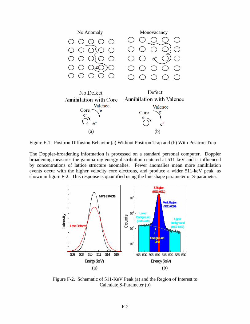
No Anomaly Monovacancy
(a) (b)
Figure F-1. Positron Diffusion Behavior (a) Without Positron Trap and (b) With Positron Trap The Doppler-broadening information is processed on a standard personal computer. Doppler broadening measures the gamma ray energy distribution centered at 511 keV and is influenced by concentrations of lattice structure anomalies. Fewer anomalies mean more annihilation events occur with the higher velocity core electrons, and produce a wider 511-keV peak, as shown in figure F-2. This response is quantified using the line shape parameter or S-parameter.
495 500 505 510 515 520 525 530
101
102
103
104
BackgroundLine
S Region(5993-6011)
Peak Region(5921-6096)
UpperBackground(6097-6197)C
ount
s
Energy (keV)
LowerBackground(5820-5920)
506 508 510 512 514 516
Inte
nsity
Energy (keV)
More Defects
Less Defects
506 508 510 512 514 516
Inte
nsity
Energy (keV)
More Defects
Less Defects
(a) (b)
Figure F-2. Schematic of 511-KeV Peak (a) and the Region of Interest to Calculate S-Parameter (b)
F-2

The S-parameter is calculated with equation F-1.
PP
SS
BC
BCS
(F-1)
Where, from figure F-2, CS is the count in the S region, BS is the background in the S region, CP is the count in the peak region, and BP is the background in the peak region. The background is considered all counts below the background line, which is determined by connecting the upper and lower background regions, as shown. Because such a large number of individual annihilation events occur in the course of one measurement, it is possible to calculate statistics on each measurement, including the error. Proprietary algorithms have been developed in Positron’s test software to compute S-parameter values with significantly lower measurement uncertainty relative to standard computations. F.2 EQUIPMENT USED.
The basic equipment setup required for IPA-S in a laboratory environment is shown in figure F-3. In the IPA-S test process, the positron-emitting probe is affixed to the sample being tested. The probe can be customized to adhere to specific component sizes and surface geometries. The probe emits positrons into the sample material, and the annihilation behavior between the positrons and electrons in the sample material is measured using a gamma ray detector and digital spectrometer (Items B and C in figure F-3). Figure F-4 shows the probe affixed to a broaching sample for this project.
Figure F-3. The IPA-S Hardware (A) Personal Computer, (B) Gamma Detector, (C) Spectrometer, and (D) Uninterruptible Power Supply
F-3

Figure F-4. A Germanium-68 Long-Life Probe
The IPA-S data acquisition and processing are performed using the Inspection Manager application software, developed by Positron Systems. Inspection Manager allows for organization and analysis of data specific to materials and test conditions into an SQL database. The software was designed with flexibility in mind and is, therefore, used for all internal research and development tests as well as by trained NDE technicians performing tests developed specifically for customer application. The browser-based user interface is shown in figure F-5. The database can be accessed remotely for data analysis or monitoring of automated tests. The automated hardware platform shown in figure F-6, the PS6100, can also be used with Inspection Manager to set up and perform automated IPA-S acquisitions under robotic control. Inspections performed using this system can provide surface profiles by mapping multiple measurements over the surface area of interest.
Figure F-5. Inspection Manager IPA Application Software
F-4
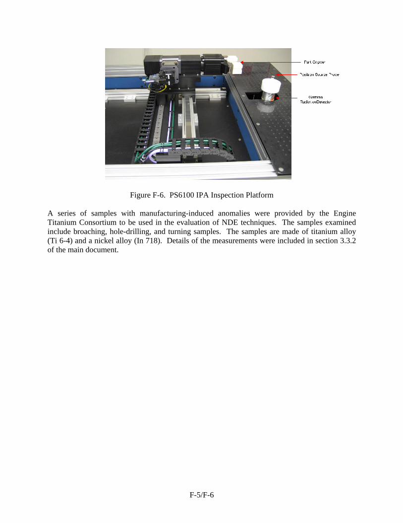
Figure F-6. PS6100 IPA Inspection Platform A series of samples with manufacturing-induced anomalies were provided by the Engine Titanium Consortium to be used in the evaluation of NDE techniques. The samples examined include broaching, hole-drilling, and turning samples. The samples are made of titanium alloy (Ti 6-4) and a nickel alloy (In 718). Details of the measurements were included in section 3.3.2 of the main document.
F-5/F-6

APPENDIX G—MAGNETIC REMANENCE METHOD
G.1 BACKGROUND. The Magnetic Remanence Method (MRM) method has previously shown the ability to detect very small ferromagnetic inclusions in a nonferromagnetic surrounding. Using the MRM, the device under test is brought into a strong direct current (DC) magnetic field. If ferromagnetic particles are present, they are magnetized near saturation. After this, the magnetic field, which acts on the device under test, is made zero and the ferromagnetic inclusions, if present, act as small permanent magnets with remnant magnetization. Then, the surface of the device under test is scanned by a highly sensitive magnetometer. Magnetic field signatures then indicate a ferromagnetic inclusion whose size and depth below the surface can be estimated. For the measurements, a magnetic gradiometer is used to suppress the influence of the extremely strong background fields, e.g., earth magnetic field and alternating current magnetic fields from power lines. In early experiments, a fluxgate or a Superconducting Quantum Interference Device gradiometer were used. In this work, an improved measurement system with a Giant Magneto-Resistance (GMR) gradiometer was used. For the magnetization of ferromagnetic inclusions, one or two DC magnets are mounted directly adjacent to the MRM probe. For this reason, magnetization and measurement are done in one pass. In cooperation with the Federal Aviation Administration (FAA) and the Engine Titanium Consortium (ETC), the working group for nondestructive testing (NDT) at the University of Applied Science in Magdeburg/Germany conducted measurements on Inconel 718 alloy (In 718) and titanium Ti-6Al-4V alloy (Ti 6-4) turning, hole-drilling, and broaching samples containing pristine, Type 1*, and Type 6* anomalies. The MRM system was developed for MTU Aero Engines GmbH by the company FI Test- und Messtechnik GmbH. The MRM system is used for detection of ferromagnetic inclusions. For use in boreholes, the MRM system patent was filed in Germany by MTU with the patent Number DE 10-2007-050-143.0. Based on DE 10-2007-050-143.0, further patents were filed in the USA and Canada. G.2 TEST SETUP FOR FLAT TURNING SAMPLES. For tests with the MRM method, a gradiometer AB 001-2 from the NVE Corporation was used. To adjust the magnetic working point, a permanent magnet was used near the GMR sensor (see figure G-1). The permanent magnet also serves for magnetic biasing of the smallest ferromagnetic particles, which can exist in the nonferromagnetic samples. Two GMR sensors were mounted on the printed circuit boards; however, only one of the sensors was used for the tests on the FAA ETC samples.
G-1

Figure G-1. Example GMR Sensor Used at the Working Group for NDT, Magdeburg, University of Applied Science, for Measurements on the Turning Samples
The output signal of the GMR sensor is transmitted to the GMR electronics, which contain a high-impedance amplifier with a gain of G = 100 and an operational amplifier with a gain of G = 103. The output signal of the GMR electronics is divided into an x signal and a y signal. These two signals are directed to a quadrature amplitude modulator (QAM). The QAM delivers a modulated signal for a personal computer (PC)-based eddy-current measurement system from the Rohmann Company. For this reason, a PC-4 eddy-current personal computer interface card delivers a 100-kHz signal, which is transmitted to the QAM (see figure G-2). For C-scan tests, the PC software SCANALYZER by Rohmann was used. The preset parameters used in SCANALYZER were: Modulation frequency 100 kHz Preamplifier 10 dB Main amplifier 10 dB High-pass frequency 10 Hz Low-pass frequency 3 Hz The GMR sensor was moved over the stationary sample in the x and y directions. The sensor was uniformly moved in the x direction and moved by steps of 0.1 mm in the y direction.
G-2

GMR electronic
Figure G-2. Test Setup for Flat Turning Samples
G.3 TEST SETUP FOR SAMPLES WITH BOLTHOLES. MTU Aero Engines GmbH provided special bolthole sensors for tests performed on the bolthole test samples. One sensor was used and mounted on a stepper motor that was moved in the z direction, i.e., the direction perpendicular to the sample surface. The sample tested was fixed on a rotating stepper motor. The bolthole sensor was then moved down and up uniformly in the z direction. Then, the specimen was rotated for a fixed-angle increment. The process is repeated until the specimen is rotated by 360° (see figure G-3).
GMR electronic
Figure G-3. Test Setup for Samples With Boltholes
The details of the results are included in section 3.3.3 of the main document.
G-3/G-4

APPENDIX H—PARALLEL BEAM X-RAY DIFFRACTION USING POLYCAPILLARY-COLLIMATING OPTICS
H.1 BACKGROUND. X-ray diffraction (XRD) relies on the coherent scatterings of x-rays to obtain information about the structure of crystalline materials. A primary use of the technique is the identification and characterization of compounds based on their diffraction pattern. The dominant effect that occurs when an incident beam of monochromatic x-rays interacts with a target material is scattering of those x-rays from atoms within the target material. In materials with regular structure (e.g., crystalline), the scattered x-rays undergo constructive and destructive interference. This is the process of diffraction. The diffraction condition of x-rays by crystals is described by Bragg’s Law, nλ=2d sinθ. The directions of diffractions depend on the size and symmetry of the unit cell of the material. However, most materials are not single crystals, but are composed of many tiny crystallites in all-possible orientations called a polycrystalline aggregate or powder. When a powder with randomly oriented crystallites is placed in an x-ray beam, the beam will see many possible interatomic planes. If the experimental angle is systematically changed, all possible diffraction peaks from the powder will be detected. The parafocusing (or Bragg-Brentano) diffractometer is the most common geometry for diffraction instruments. This geometry offers the advantages of high-resolution and high-beam intensity analysis at the cost of very precise alignment requirements and carefully prepared samples. Additionally, this geometry requires that the source-to-sample distance be constant and equal to the sample-to-detector distance. Alignment errors often lead to difficulties in phase identification and improper quantification. A mispositioned sample can lead to unacceptable specimen measurement errors. Sample flatness, roughness, and positioning constraints preclude in-line sample measurement. Additionally, traditional XRD systems are often based on bulky equipment with high-power x-ray sources to increase x-ray flux on the sample, thereby increasing the detected diffraction signals from the sample. These sources also have large excitation areas, which are often disadvantageous for the diffraction analysis of small samples or small sample features. Polycapillary-collimating x-ray optics can be used to overcome many of these drawbacks and constraints to enhance XRD applications. These optics convert a highly divergent beam into a quasi-parallel beam with low divergence. They can be used to implement a parallel beam XRD instrument geometry, which greatly reduces and removes many sources of errors in peak position and intensity inherent to the parafocusing geometry, such as sample position, shape, roughness, flatness, and transparency. Polycapillary-focusing optics collect x-rays from a divergent x-ray source and direct them to a small focused beam at the sample surface with diameters as small as tens of micrometers for micro x-ray diffraction applications of small samples or small specimen features. Both types of polycapillary optics direct very high x-ray intensities to the sample surface, such that XRD systems employing polycapillary optics can use low-power x-ray sources, reducing instrument size, cost, and power requirements.
H-1

X-ray diffraction using x-ray optics has been applied to many different types of applications including thin film analysis, sample texture evaluation, monitoring of crystalline phase and structure, and investigation of sample stress and strain. For most samples, the aim of x-ray diffraction analysis is to identify the crystalline phases present. Phase identification is accomplished by comparing the positions and intensities of the material’s x-ray diffraction peaks against a large library of “standard” diffraction data of known crystalline materials. In this way, the different phase components of the sample can be identified. Additionally, phase transformations can also be monitored by looking for changes in the diffraction pattern of a material over time as the sample is exposed to different conditions or stresses. Parallel beam XRD using polycapillary-collimating optics can be used to enhance phase XRD analysis of materials (see figure H-1). Due to the insensitivity of parallel beam XRD to sample geometry and displacement errors, minimal sample preparation is required for phase analysis of samples. For the same reasons, the technique can be used to monitor phase and structure changes in an in-line/on-line system. Furthermore, through the use of a polycapillary-collimating optic, the parallel beam XRD system can be combined with a low-power x-ray source, reducing instrument size and power requirements for in-line phase or structure measurements.
Figure H-1. Parallel Beam X-Ray Diffraction Geometry Using Polycapillary-Collimating Optics The nominal characteristics of the polycapillary-collimating x-ray optics used are listed in table H-1.
H-2

Table H-1. Characteristics of Polycapillary-Collimating Optics
Type Parallel Beam, Polychromatic
Useful x-ray energy range Typically 0.1-30 keV
Transmission efficiency Up to 40% (depending on optic design and x-ray energy)
Collection solid angle Up to 20°
Beam size Typically 0.5-20 mm
Output divergence 1-4 mrad (depending on x-ray energy) Typically 2 mrad @ Mo Kα, 3.5 mrad @ Cu Kα
It is quite conventional to investigate material states and damage contained in metallic samples through studying the sample’s residual stress by XRD. Residual stress is often purposely applied to metallic surfaces by mechanical or chemical treatment to improve the component’s fatigue life. By its very nature, the abusive machining processes creates unintentional surface conditions, thus the measurement of residual stress profiles may be used to detect and characterize the induced material damage. A change of residual stress from the nominal surface condition may be used as an indicator of the damage status of a measured component. In general, this is not simple because, for the resolution and sensitivity required, a high-resolution XRD and complicated data processing system is usually required to measure and analyze the residual stress data. To determine the stress in a material, the strain in the crystal lattice must be measured for at least two known orientations relative to the sample surface. There are two kinds of stresses: macroscopic and microscopic. Macroscopic stresses extend over distances that are large relative to the grain size of the material and are of general interest in design and failure analysis. Macrostresses strain many crystals uniformly in the surface. This uniform distortion of the crystal lattice shifts the angular positions of diffraction peaks selected for residual stress measurement. On the other hand, microstresses are scalar properties of the sample’s material structure; they are without a defined direction and result from imperfections in the crystal lattice. Microstresses vary from point to point within the crystal lattice, altering the lattice spacing and have an effect of broadening diffraction peaks. Macrostresses and microstresses can be determined separately from the diffraction peak position and width. In this preliminary study, macroscopic stress is the major interest. An XRD system was built with an advanced Bruker area detector to investigate the possible detectable shifts of diffraction peak angular positions. Besides the XRD application of residual stress measurements, XRD can also be employed to characterize the surface quality and damage from analyzing the diffracted beam profiles. For example, X-Ray Optical Solutions, Inc. (XOS®) developed a real-time XRD system to monitor the quality of single-crystal turbine blades. This system (as shown in figure H-2) was equipped with a low-power X-Beam to provide a large collimating incident beam from a large bundle polycapillary-collimating optic. An x-ray image intensifier coupled with a TV monitor was used to collect and show the diffraction patterns. The principal of this technology is the intensity distribution of the diffracted beam depends on the incident beam profile and the sample crystalline characteristics. The crystal quality, grain orientation, and other physical damages,
H-3

such as crack and boundary distortion, will be directly observed from the diffracted beam images.
Figure H-2. Real-Time XRD System to Monitor the Crystalline Quality of a Single-Crystal Turbine Blade
Figure H-3 demonstrates this diffraction system in the measurement of the crystal quality of a large portion of the single-crystal turbine blade. The short streak corresponds to the turbine blade edge. The dark gap corresponds to the turbine blade groove; while the blurred area corresponds to the curved face of the turbine blade with some residual amorphous coating layer. The bright streak may correspond to a large vertical grain. This former research experience has encouraged the investigation of the feasibility of using XRD to detect and characterize the anomalies of concern for aircraft critical components.
Figure H-3. A Tested Turbine Blade and Corresponding Diffraction Image With Low-Power System
H-4

H.2 EQUIPMENT USED. The prototype parallel beam XRD system with a polycapillary-collimating optic, shown in figure H-4, was used to measure the abusive machining damage present in the provided test samples. The x-ray source was an Oxford 5011 Cu x-ray tube aligned with polycapillary-collimating x-ray optics, giving 1.5-mm-diameter beam size and was equipped with a 10-micron nickel filter, a Bruker area detector, and a θ-2θ rotation base.
Figure H-4. Components of the Prototype Parallel Beam X-Ray Diffraction System Using Polycapillary-Collimating Optics
Proprietary algorithms are used within the test software to minimize measurement variation. The techniques, apparatus, and methods are protected by the following U.S. Patents: U.S. Patent Number 5570408 U.S. Patent Number 5192869 U.S. Patent Number 7236566 The data acquisition and processing are performed using the software Origin and ImageJ. H.3 FEASIBILITY TESTS. At the beginning of these measurements, diffraction peaks from the 331 plane for Inconel® 718 (In 718) coupons and from the 213 plane for titanium Ti-6Al-4V (Ti 6-4) coupons were searched with the prototype system shown in figure H-4. It was found that these large 2-diffraction peaks, which are typically suitable for residual stress measurements, were very weak compared with those diffraction peaks at relatively lower 2-θ angles. A bright-low index peak, shown in figure H-5, from a pristine Ti 6-4 turning sample was chosen for the following investigation.
H-5
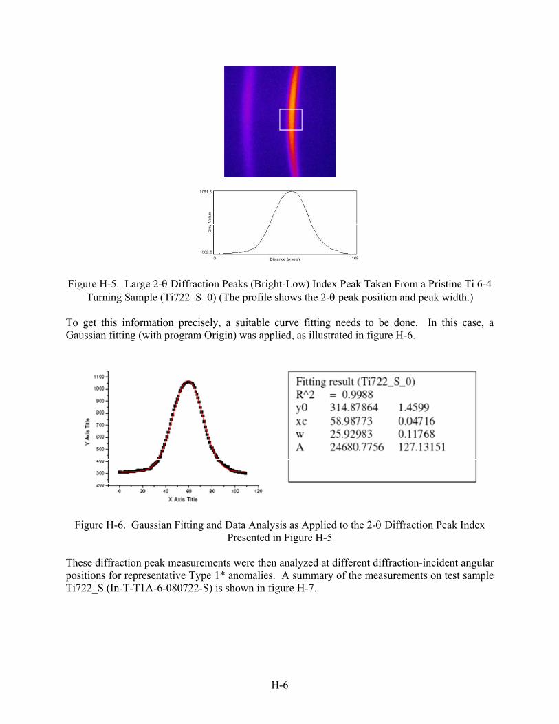
Figure H-5. Large 2-Diffraction Peaks (Bright-Low) Index Peak Taken From a Pristine Ti 6-4 Turning Sample (Ti722_S_0) (The profile shows the 2- peak position and peak width.)
To get this information precisely, a suitable curve fitting needs to be done. In this case, a Gaussian fitting (with program Origin) was applied, as illustrated in figure H-6.
Figure H-6. Gaussian Fitting and Data Analysis as Applied to the 2-Diffraction Peak Index Presented in Figure H-5
These diffraction peak measurements were then analyzed at different diffraction-incident angular positions for representative Type 1* anomalies. A summary of the measurements on test sample Ti722_S (In-T-T1A-6-080722-S) is shown in figure H-7.
H-6
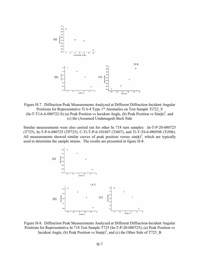
(c) (b)
(a)
Figure H-7. Diffraction Peak Measurements Analyzed at Different Diffraction-Incident Angular Positions for Representative Ti 6-4 Type 1* Anomalies on Test Sample Ti722_S
(In-T-T1A-6-080722-S) (a) Peak Position vs Incident Angle, (b) Peak Position vs Sin()2, and (c) the (Assumed Undamaged) Back Side
Similar measurements were also carried out for other In 718 turn samples: In-T-P-20-080725 (T725), In-T-P-6-080725 (TP725), C-Ti-T-P-6-101607 (Ti607), and Ti-T-T6-6-080508 (Ti506). All measurements showed similar curves of peak position versus sin()2, which are typically used to determine the sample strains. The results are presented in figure H-8.
(a)
(c) (b)
Figure H-8. Diffraction Peak Measurements Analyzed at Different Diffraction-Incident Angular Positions for Representative In 718 Test Sample T725 (In-T-P-20-080725); (a) Peak Position vs
Incident Angle, (b) Peak Position vs Sin()2, and (c) the Other Side of T725_B
H-7

The original goal of developing a semiquantitative approach was to obtain residual stress information through a quick comparison of those curves and to further qualitatively evaluate the sample damage status. Unfortunately, further analysis showed this approach was not simple since the prototype system did not meet the resolution requirement. In fact, the obtained curves were mostly due to sample positioning displacements. In general, the diffraction peak position will shift if the sample position has displacement, as shown in figure H-9.
Figure H-9. Diffraction Peak Position Shifts due to Sample Displacement
The geometric analysis shows D diffraction peak shift; beam incident angle; and S sample displacement. In the prototype XRD system, 2-= 45, producing D vs S, as shown in figure H-10 and compared in figure H-11 with the experimental data obtained above.
D = sin(2)/tg()S
Figure H-10. Geometric Analysis of the D vs S Diffraction Peak Shift
H-8

Figure H-11. Experimental Data vs Calculated Data of D vs S Diffraction Peak Shift The experimental data are for sample T725, the calculation data are based on the sample displacement. The displacements were determined to be 0.7 mm for the left chart, and 0.16 mm for the right chart from least square fitting analysis. The Bruker detector provides a very good spatial resolution, 0.05 to 0.1 mm. With the distance from the detector to the sample being 190 mm, this can be converted to an angular resolution of 0.015to 0.04. In principal, this could be used for residual stress preliminary analysis. It was very difficult for this prototype system to achieve sample position precision to be better than 0.05 to 0.1 mm. However, further analysis indicated that this developing approach could still be valid if a suitable mathematic tool could be developed to remove the sample displacement effect. Figure H-12 shows the primary diffraction peak shifts according to incident angles after the sample displacement effects have been removed. The results could be used for further analysis to determine the residual stress type and magnitudes, which could be used as an indicator to describe the component anomalies. Further analysis and development are needed to build a proper mathematical model and improve the system resolution for achieving this goal.
15 20 25 30 35 40 45-0.3
-0.2
-0.1
0.0
0.1
0.2
sample 1 sample 2
Pea
k p
ositi
on s
hift
Incident angle
Figure H-12. Diffraction Peak Position Shift After Removing Sample Displacement Effect
H-9
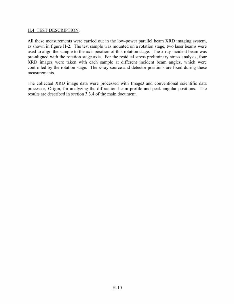
H-10
H.4 TEST DESCRIPTION. All these measurements were carried out in the low-power parallel beam XRD imaging system, as shown in figure H-2. The test sample was mounted on a rotation stage; two laser beams were used to align the sample to the axis position of this rotation stage. The x-ray incident beam was pre-aligned with the rotation stage axis. For the residual stress preliminary stress analysis, four XRD images were taken with each sample at different incident beam angles, which were controlled by the rotation stage. The x-ray source and detector positions are fixed during these measurements. The collected XRD image data were processed with ImageJ and conventional scientific data processor, Origin, for analyzing the diffraction beam profile and peak angular positions. The results are described in section 3.3.4 of the main document.

APPENDIX I—MAGNETIC CARPET PROBE
I.1 OVERVIEW. Recent advances of flexible printed circuit board techniques enabled the construction of very thin copper traces and spacings in very thin material layers. This has resulted in a large number of electromagnetic coils, or coil arrays, within a thin layer structure with reasonable coil size, impedance value, and inspection resolution. Additionally, advances in digital electronic devices have enabled control, using a very limited number of miniature chips, of complex and high-speed electronic and electromagnetic scans over a coil array containing large numbers of elements, or coils. These two techniques provide the capability for creating the Magnetic Carpet Probe (MCP). The MCP, originally designed to promote structural health monitoring, is a two-dimensional array of pancake-style eddy-current coils built on a very thin (~0.006″-0.0135″ (0.15-0.35 mm)), flexible, printed circuit board. The probe can be fabricated to a variety of dimension and geometrical array patterns to suit a designed test condition. Figure I-1 illustrates the MCP used within this study. The MCP used an array of 30 coils placed in a 10-column, 3-row pattern with regular spacing between coils. The measurements were made on each coil element of the coil array through an eddy-current instrument processed through multiplexers. A diagram of the overall system architecture is illustrated in figure I-2. The advantages of the MCP technique include: Absolute static inspection
No mechanical noise—ensuring high sensitivity
Electronic and magnetic scan—ensuring high-speed, or instant, inspection of large area
No mechanic parts/components, a pure electronic device—ensuring simplicity, robustness, lightweight, and reliability
Ease of use and low cost
Thin and flexible two-dimensional sensor array—providing capabilities in conforming to curved surface
Being attached to inaccessible or difficult accessible areas for nondestructive inspection (NDI) or heath monitoring
Possibility for future remote control of NDI and heath monitoring through networking and/or wireless techniques
Software controlled call/reject action with minimum human factors involved
I-1

Figure I-1. The MCP-1 V7 Used to Examine the Turning Samples (Two rows of coils were not used to match the active area of the array
to the geometrical size of the turning samples.)
Figure I-2. System Architecture of the MCP Data Acquisition and Analysis System Figure I-3 illustrates the hardware described within figure I-2 with a representative screen display from the multiplexed coils shown in figure I-4. As shown in figure I-4, individual coil elements can be displayed and processed to provide eddy-current data representative of the coil coverage area.
I-2
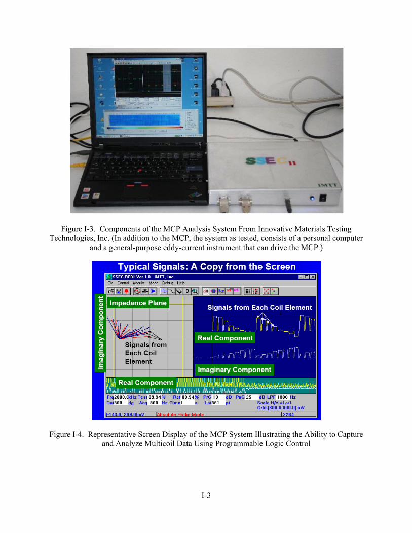
Figure I-3. Components of the MCP Analysis System From Innovative Materials Testing Technologies, Inc. (In addition to the MCP, the system as tested, consists of a personal computer
and a general-purpose eddy-current instrument that can drive the MCP.)
Figure I-4. Representative Screen Display of the MCP System Illustrating the Ability to Capture
and Analyze Multicoil Data Using Programmable Logic Control
I-3
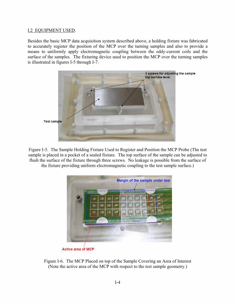
I.2 EQUIPMENT USED. Besides the basic MCP data acquisition system described above, a holding fixture was fabricated to accurately register the position of the MCP over the turning samples and also to provide a means to uniformly apply electromagnetic coupling between the eddy-current coils and the surface of the samples. The fixturing device used to position the MCP over the turning samples is illustrated in figures I-5 through I-7.
Figure I-5. The Sample Holding Fixture Used to Register and Position the MCP Probe (The test sample is placed in a pocket of a sealed fixture. The top surface of the sample can be adjusted to flush the surface of the fixture through three screws. No leakage is possible from the surface of
the fixture providing uniform electromagnetic coupling to the test sample surface.)
Figure I-6. The MCP Placed on top of the Sample Covering an Area of Interest (Note the active area of the MCP with respect to the test sample geometry.)
I-4

Figure I-7. Suction Device Holding the MCP Against the Surface of the Test Sample I.3 TEST DESCRIPTION. A series of flat turning samples with manufacturing-induced defects were provided by the Engine Titanium Consortium (ETC) to be used in the evaluation of nondestructive evaluation techniques. The samples are made of titanium Ti-6Al-4V alloy and Inconel 718 alloy. Within the scope of schedule and resources available, only the flat turning samples were investigated. This allowed for an existing MCP array design to be used. Because the MCP was smaller with respect to the turning sample, two columns of coil were not used during the investigation. Evaluations are performed by placing the MCP on top of a conducting or metallic surface and electronically measuring a two-dimensional scan of the test sample’s electromagnetic characteristics. I.3.1 PREPARATION OF TEST. The following list describes the steps required to prepare the samples for testing. 1. Insert reference sample into the pocket of the fixture and adjust the three screws to have
the top surface of the sample flush with the fixture surface (figure I-5).
2. Fix MCP, using a piece of tape, on top of the sample surface to have the active area of the MCP cover the area of interest of the sample (figure I-6).
3. Place suction device on top of the MCP, then apply the vacuum.
4. Null the system.
5. Click Button M on the upper right of the SSEC II-M main screen (figure I-8(a)), then the dialog and image screen appears (figure I-8(b)).
6. Set the screen and all checks to be the same as Option 2 in figure I-8(b).
I-5

7. Null the system.
8. Click the “no crack” button. A small window showing “Non-crack data have been successfully retrieved” will pop up after a couple of seconds.
(b)
(a)
Figure I-8. Screen Displays From MCP - SSEC II-M Main Screen (Note: The screen display, setup, and function were originally designed for crack detection. There are a number of buttons
not used in this test.) I.3.2 TEST PROCEDURE. The following list describes the test procedure. 1. Replace the reference sample with a sample under test. Then repeat steps 2-4 stated in
section I.3.1.
2. Click the “crack” button; a small window showing “Crack data have been successfully retrieved” will pop up after a couple of seconds.
3. Click the “display” button; an image will appear in the image window (figure I-8(b)), and a small window will pop up displaying the maximum and minimum values of the signal in the image. (This portion is not shown in this report).
4. Alternatively, after a threshold is determined through a large number of tests, a degree of damage can be shown in the small window.
Data is simultaneously acquired and displayed from all active eddy-current coils using the multiplexing hardware and algorithms. The time required for the test is very short. For the particular test carried out, the preparation time is about 5 to 10 minutes, while the actual test time is less than 40 seconds per sample. Details of the results for the ETC samples are in section 3.3.5 of the main document.
I-6

APPENDIX J—THERMOELECTRIC ANISOTROPIC MAGNETO-RESISTIVE
J.1 BACKGROUND. A thermoelectric data acquisition system developed at the General Electric (GE) Nondestructive Technologies laboratory has been used for data acquisition of Federal Aviation Administration (FAA) Engine Titanium Consortium (ETC) samples. The thermoelectric technique is based on the Seebeck effect. Two air guns with nozzles having a linear array of holes are used to generate a temperature gradient in a sample. Self-referencing thermoelectric measurement is conducted in a noncontact way by sensing the weak magnetic field due to the thermoelectric current around various types of imperfections and material variations. The method involves the creation of a temperature gradient at the boundary of the imperfection where the material properties are altered. Resultant gradient in the thermoelectric potentials produces thermoelectric currents inside and outside the imperfection. Recently, this method was investigated to evaluate various types of imperfections, such as foreign body inclusion, fatigue damage, excess heat damage, residual stresses, and fretting damage. For example, the maximum peak-to-peak amplitude of the magnetic signal achieved was about 22 nanotesla (nT) in the Almen 16 on shot-peened copper samples with a temperature gradient of about 2.5°C/cm. In the Inconel 718 samples, where the electrical conductivity is two orders of magnitude smaller than copper, a maximum peak-to-peak signal of about 7 nT was achieved in the Almen 16 samples with a temperature gradient of 25°C/cm. J.2 EQUIPMENT USED. The system (figure J-1) used noncontact thermoelectric measurements to assess small material properties variations, such as those due to machining-induced anomalies, in samples of low electrical conductivity metals, such as the high-strength, high-temperature superalloys used in aerospace engine materials. The geometry of the thermal gradient excitation system (vortex tube and air nozzles) was not suitable for the turning sample size. A special sample holder (figure J-1(b)) was built to provide heat/cold conduction to the sides of the samples. An FAA sample enclosed in the holder fixture was placed on top of the thermal gradient generation table to perform a linear surface scan with a magnetic sensor. Figure J-2 provides the basic concept for this method.
J-1

(b)
(a)
Figure J-1. Temperature Gradient Generation Vertex System and Mechanical Scanner (a) Overview of the Setup Included a Vortex Tube to Create Hot and Cold Air Jets Used for
Generating Temperature Gradient and a Computer-Controlled Scanner and (b) a Close-Up Image of the Sample Holder With Brass Plates (These high-heat capacity bars were heated and cooled using the hot and cold air jets and are in close thermal contact with the sample, thus creating a
temperature gradient across the test sample.)
Current and field distributions
Ty
Bx
Bz
Bx
Bz
Figure J-2. Thermoelectric Current and the Resulting Magnetic Field Distribution in the Sample in the Presence of Thermal Gradient (The light blue region has a different stress state compared to the host material (light pink). The coordinate system is defined in the inset at the top left and
the magnetic field profiles are shown on the right.) To conduct low field magnetic measurements that would be sensitive to the level of magnetic field changes due to the thermoelectric current, an anisotropic magneto-resistive (AMR) sensor was applied. Preliminary experiments on sensor comparison have been completed at the GE Nondestructive Technologies laboratory. A fluxgate magnetometer (FGM) was used as a
J-2

benchmark. It was found that AMR sensors are better suited for this application. AMR sensors are thin-film sensors, which enables a very small (1 mm or less) lift-off between the AMR sensor and the sample. This results in a greatly enhanced magnetic field strength measured at the sensor over FGM, which has a nominal lift-off distance of about 10 mm or more, even when the tip is placed on the sample surface. Since the thermoelectric current distribution is dipolar in nature, the field drops off very rapidly as a function of distance, which negates the additional sensitivity of FGM. Furthermore, the AMR’s close proximity to the sample, along with its well-defined planar sensing area and smaller lateral dimensions, can result in a much better spatial resolution. A comparison between the magnetic field amplitude for surface-breaking inclusions of various sizes for nominal lift-off distances, 1 mm for AMR and 12.5 mm for FGM, is presented in figure J-3. Here, the signal amplitude was normalized to its value at zero lift-off distance. It is evident that for the smallest inclusion shown here, i.e., the 1-mm-diameter inclusion, the ratio between the two signals is ~325, while for a 15-mm-diameter inclusion, the ratio is ~6.
Figure J-3. The Normalized Signal Amplitude for Inclusions of Various Sizes and at Lift-Off Distances of 1 mm (AMR) and 12.5 mm (Fluxgate) (The ratio of the amplitude of the two signals
is shown next to the bars.) It is clear that the AMR advantage over FGM gets bigger as the flaw size becomes smaller. From the signal-to-noise ratio perspective, even though FGM has much lower intrinsic noise (100 pT) compared to AMR (1 nT), the ambient environmental noise in the unshielded laboratory is about 1 to 10 nT in direct current and 10-Hz bandwidth, and thus, in this case, it is more important to increase the signal by reducing sensor lift-off than trying to use a more sensitive magnetometer.
J-3
J-4
J.3 TEST DESCRIPTION. The following conditions were set for the data acquisition process: The sample was installed between two brass blocks in good thermal contact
The side with sample markings is always on the side that is in contact with the hot block (right)
The rougher surface (or the one with numbers written) is always placed face up (away from the magnetometer)
The arrow in figure J-1(b) indicates scan direction from one edge to the other (2″ total)
Only the titanium Ti-6Al-4V alloy 6-4 sample was scanned using this method since residual stress in other materials can be easily detected by conventional eddy-current techniques. It was found that two of the samples tested were clearly free of any stress/heat-affected zone (HAZ) regions, while four others definitely indicated presence of stressed/HAZ-type regions along the central part of the sample. Data on the remaining two samples were inconclusive and require further measurements or other means to determine their states. The results of the ETC samples are reported in section 3.3.6 of the main document.
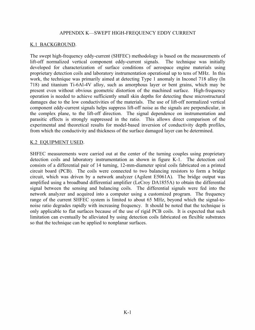
APPENDIX K—SWEPT HIGH-FREQUENCY EDDY CURRENT K.1 BACKGROUND. The swept high-frequency eddy-current (SHFEC) methodology is based on the measurements of lift-off normalized vertical component eddy-current signals. The technique was initially developed for characterization of surface conditions of aerospace engine materials using proprietary detection coils and laboratory instrumentation operational up to tens of MHz. In this work, the technique was primarily aimed at detecting Type 1 anomaly in Inconel 718 alloy (In 718) and titanium Ti-6Al-4V alloy, such as amorphous layer or bent grains, which may be present even without obvious geometric distortion of the machined surface. High-frequency operation is needed to achieve sufficiently small skin depths for detecting these microstructural damages due to the low conductivities of the materials. The use of lift-off normalized vertical component eddy-current signals helps suppress lift-off noise as the signals are perpendicular, in the complex plane, to the lift-off direction. The signal dependence on instrumentation and parasitic effects is strongly suppressed in the ratio. This allows direct comparison of the experimental and theoretical results for model-based inversion of conductivity depth profiles, from which the conductivity and thickness of the surface damaged layer can be determined. K.2 EQUIPMENT USED. SHFEC measurements were carried out at the center of the turning couples using proprietary detection coils and laboratory instrumentation as shown in figure K-1. The detection coil consists of a differential pair of 14 turning, 12-mm-diameter spiral coils fabricated on a printed circuit board (PCB). The coils were connected to two balancing resistors to form a bridge circuit, which was driven by a network analyzer (Agilent E5061A). The bridge output was amplified using a broadband differential amplifier (LeCroy DA1855A) to obtain the differential signal between the sensing and balancing coils. The differential signals were fed into the network analyzer and acquired into a computer using a customized program. The frequency range of the current SHFEC system is limited to about 65 MHz, beyond which the signal-to-noise ratio degrades rapidly with increasing frequency. It should be noted that the technique is only applicable to flat surfaces because of the use of rigid PCB coils. It is expected that such limitation can eventually be alleviated by using detection coils fabricated on flexible substrates so that the technique can be applied to nonplanar surfaces.
K-1

Figure K-1. Setup for SHFEC Measurements on Turning Sample K.3 TEST DESCRIPTION. During the measurements, a pristine sample was placed onto the balancing coil while a test sample was placed on the sensing coil (figure K-1). The coils remained stationary during the measurements. The detected signals therefore represented the average response of the regions of the samples that were covered by the coils. For each turning sample, three SHFEC signals were measured from 0.5 to 65.5 MHz in three steps: (1) on a pristine surface (usually the undamaged side of the test sample) with no additional lift-off, (2) at a known coil lift-off of 0.001″ (25.4 μm) on the pristine surface, and (3) on the machine-damaged surface of the test coupon to obtain the reference signal SRef, the lift-off signal SLift-off, and the test signal STest, respectively. The lift-off normalized vertical component signals were then obtained as the imaginary component V of the following complex ratio:
Test Ref EXPT
Lift-off Ref EXPT
S SH jV
S S
(K-1)
This three-step measurement was repeated five times on each coupon to obtain the average values and standard deviations of the vertical component signals. The lift-off normalized vertical component eddy-current signals measured from a Type 1 In 718 sample are shown as a function of frequency in figure K-2. The vertical component signals have negative values throughout the frequency range, indicating a lower conductivity of the machined side than the pristine/undamaged side. Interpretation of the SHFEC signals with respect to the sample surface condition has been established in a validation study using simulated layer specimens with known conductivity depth profiles. The results of the validation study are described in section 3.3.7 of the main document.
K-2
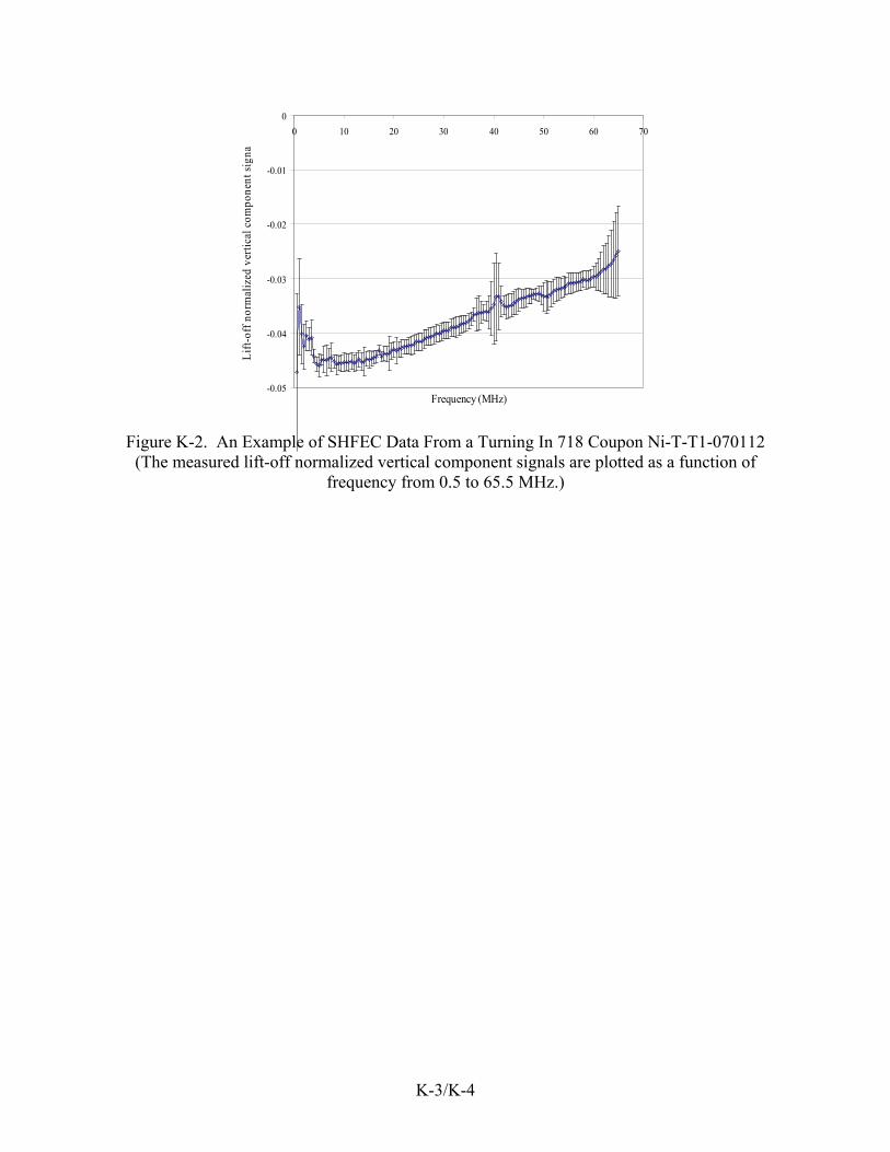
-0.05
-0.04
-0.03
-0.02
-0.01
0
0 10 20 30 40 50 60 7
Frequency (MHz)
Lif
t-of
f no
rmal
ized
ver
tica
l com
pone
nt s
igna
0
Figure K-2. An Example of SHFEC Data From a Turning In 718 Coupon Ni-T-T1-070112 (The measured lift-off normalized vertical component signals are plotted as a function of
frequency from 0.5 to 65.5 MHz.)
K-3/K-4

APPENDIX L—MULTIFREQUENCY EDDY-CURRENT ANALYSIS L.1 BACKGROUND. It has been proven that a combination of eddy-current signal components obtained with different frequencies yields a better defect detection. Further improvement can be achieved by using a multifrequency technique with the phase analysis. At least two excitation frequencies (F1 and F2) are required for this approach. Additional information provided by detecting the response from the F2 excitation is correlated with the F1 response to more effectively suppress undesired variations that are present in both signals. The data fusion procedure (figure L-1) includes phase adjustments of F1 and F2 responses, and scaling the horizontal and vertical components separately for noise suppression while maximizing the signal from a defect.
3. Identify a reference data set comprising multifrequency (at least two) response signal
4. Mix (linear combination) two or more frequency response signals to determine a set of processing parameters
5. Application of the processing parameters to the entire multifrequency response signal to generate a noise to filtered data set
6. Extract phase informative parameter from the noise-filtered data set
2. Acquire multifrequency response signal
1. Apply multifrequency excitation to eddy-current probe
Figure L-1. Sequence of Operations for Multifrequency Phase Analysis L.1.2 EQUIPMENT USED. Eddy-current images of the flat turning samples were obtained by two-dimensional (2D) raster-scanning sample surfaces with differential reflection probe Nortec R600. The probe was plugged into a Phase c2d eddy-current instrument. Horizontal and vertical components of the eddy-current response at 6 MHz were transferred to a computer during the scan every 0.1 mm while the probe tip was moving constantly at a velocity of 25 mm/s. Increments of 0.2 mm were made after each line scan. Hole-drilling samples were scanned using the Nortec R600 probe and a computer-controlled turntable with a sample holder. The relative position of the probe and internal surface of a sample is shown in figure L-2.
L-1

Figure L-2. Rotary Scanning Setup for Hole-Drilling Samples L.1.3 TEST DESCRIPTION. A linear combination of the horizontal and vertical components of the two-frequency signal leads to the creation of a new set of in-phase and quadrature components. Phase imaging of the processed multifrequency response provides further signal enhancement. To realize this method in practice, a commercial eddy-current instrument with a two-frequency excitation is used. An eddy-current probe is excited with a two-frequency mix and horizontal and vertical components are transferred to a computer for further processing. An example of 2D images obtained during this processing sequence is presented in figure L-3.
Multi-FrequencyEC
(2.5MHz&1MHz)
SingleFrequencyEC
2.5MHz 1MHz
MFPA Details
Figure L-3. Example of Multifrequency Analysis of a Turning Sample
L-2

L.2 PULSED EDDY CURRENT.
L.2.1 BACKGROUND. Pulsed excitation can provide improvements in the eddy-current method similar to the multifrequency technique with harmonic excitation. The pulsed eddy current (PEC) approach has been successfully applied for tasks of hidden corrosion and subsurface crack detection. A multifrequency analysis can be further applied to the transient response to selectively analyze material properties of different layers. Typically, a step, square, or triangular pulse of electrical current through a drive coil is employed to induce PECs into the material being tested. A magnetic field sensor (inductive coil or solid-state magnetic sensors) detects the secondary magnetic field. The difference between the responses over a reference area or sample and the currently evaluated point is then analyzed. Time or amplitude criteria are employed to analyze the transient response. Two-dimensional eddy-current images (C-scans) of a sample can be formed by mechanically scanning the probe over the surface. The PEC block diagram utilized at the General Electric Nondestructive Technologies laboratory is shown in figure L-4.
CO
NT
RO
LS
IGN
AL
COATEDSPECIMEN
PULSER
PE
C S
IGN
AL
SIGNALFILTER &LIFIER
EC PROBE
PULSESTIMULATION
COMPUTER
HIGH-SPEEDDIGITIZER BOARD
CO
NT
RO
LS
IGN
AL
COATEDSPECIMEN
PULSERPULSER
PE
C S
IGN
AL
SIGNALFILTER &LIFIER
SIGNALFILTER &LIFIER
EC PROBE
PULSESTIMULATION
COMPUTERCOMPUTER
HIGH-SPEEDDIGITIZER BOARD
Figure L-4. Block Diagram of the PEC Laboratory System A commercially available pulser was used to generate square voltage pulses of short duration (1 to 10 microseconds). A reflection-type probe with separate drive and pickup coils (figure L-5) was used for measurements. The PEC system and the probe shown in the figures were previously used to conduct an experimental study on the nickel-based samples with different coating properties. Degradation of the airfoil protective coatings after exposure to variable temperatures for extended periods of time was correlated to the PEC measurements.
L-3

Figure L-5. The PEC Reflection Probe for Testing Coating Layers Preliminary experiments on the turning samples demonstrated that this probe (figure L-5) does not provide sufficient spatial resolution needed to study the anomalies. In addition, it is not suitable for hole-drilling or broaching samples. A special probe was designed to resolve local variation in electromagnetic properties and is capable of scanning the internal surface of cylindrical holes (figure L-6).
Figure L-6. The PEC Probe Fixture set to Conduct Measurements in Hole-Drilling Samples Based on the results obtained with conventional eddy-current measurements, the probe construction was oriented to work with high-frequency (0.1- to 20-MHz) components of the pulsed response. The previously used pulser was producing excessive ringing around the pulse leading and trailing edges, which led to a noisy response in the high-frequency range. A special fast power switch was built and packaged into a shielded box right next to the drive and pickup coils (figure L-7). This integrated pulser configuration was tested on surface-treated Inconel® 718 (In 718) samples and provided an acceptable level of signal during a 2D surface scan.
L-4

Figure L-7. The PEC Probe Fixture on a 2D Automated Scanner The processing of the transient response was not ready by the time the Federal Aviation Administration (FAA) samples were available for inspection. While raw transient signals obtained from 2D scans of several FAA turning samples were digitized and recorded, some additional work needed to be done to process and analyze the collected data. A test scan was made over an In 718 plate with electro-discharging machine (EDM) notches of variable depth. An example of PEC data from 1-, 2-, 3-, and 4-mil-deep EDM notches processed to extract a 5-MHz signal from the transient response is given in figure L-8.
Figure L-8. Test PEC 2D Scans of a Sample With 1-, 2-, 3-, and 4-mil-Deep Notches Further developments include a program interface that would allow calibration of the probe and transient response based on a four-point calibration algorithm (1) before, (2) scan, (3) reconstructing apparent eddy-current conductivity in-depth maps in real time, or (4) immediately after the scan. The results for this method are provided in section 3.3.8 of the main document.
L-5/L-6

APPENDIX M—SINGLE-FREQUENCY EDDY-CURRENT ANALYSIS M.1 BACKGROUND. Conventional, single-frequency eddy-current inspection has common application to metal sorting, coating-thickness measurement, surface and near-surface flaw detection, and displacement measurement. In all cases, an alteration of the eddy-current probe’s electromagnetic field occurs by some change in the electromagnetic characteristics of the part under test (electrical conductivity, magnetic permeability, or anomaly) and/or a change in the physical attributes (geometry or orientation). The eddy-current probe is most sensitive to displacement, which makes it well suited as a displacement measurement device and which also affects the other inspection applications in a negative way. The displacement of the probe from the surface of a part is often referred to as lift-off. Lift-off needs to be controlled well when using the eddy-current probe to make measurements other than displacement. For the application of abusive machining damage (AMD) detection, it follows that the eddy-current inspection could be exposed to deformation of material at the surface (tearing or smearing) and distortion of the microstructure at and near the surface (deformation of grains, electromagnetic property changes due to temperature/pressure). The eddy current will be very sensitive to the tearing and smearing conditions since it will result in a lift-off response while the microstructural issues will behave more like bulk conductivity changes. For bulk-type properties, an absolute probe is a more suitable choice than a differential probe. The differential probe is better suited for discrete anomalies, like cracks, due to its bulk property canceling effect. Another aspect of eddy-current inspections is the use of filters to help reduce noise effects during the inspection. The noise can come from many sources, such as geometry, electrical, and surface roughness. Frequently, a high-pass filter is used to remove or reduce low-frequency effects, such as slight variations in lift-off or local geometric features, which are repeated, for example, when scanning an engine rotor. High-pass filters are typically used to remove electrical noise. For the AMD application, the high-pass filter is not used to allow for the detection of bulk property changes. Ultimately, the filter selection should not remove much of the energy associated with the target anomaly and so the filter settings should be selected with some knowledge of the signal bandwidths. M.2 EQUIPMENT USED. Conventional eddy-current data collection was performed on a standard four-axis scanner using simple pencil probes and fixturing. The eddy-current instrument used for the data collection is a UniWest US-454 with typical options and an upper frequency capability of 10 MHz. Two probe types were used in the data collection: an absolute (bridge-type) solenoid and a differential (reflection-type) eddy-current probe (ECP). The absolute solenoid was selected
M-1

because it has an omnidirectional field so that sensitivity is uniform in all directions. The differential ECP was selected because of its reduced sensitivity to lift-off and broadband frequency characteristics. M.3 TEST DESCRIPTION. Raster scans were performed on samples from various groups (ETC4 and VS2), covering their surfaces from edge to edge. The probes were calibrated on an electro-discharging machine (EDM) notch in an Inconel® 718 alloy (In 718) for the purpose of maintaining consistent inspection sensitivity. The EDM notch size was 0.020″ long and 0.010″ deep with a nominal width of 0.003″. C-scan data were collected on each sample. The in-phase and quadrature components of the eddy-current data were recorded. The absolute solenoid was operated at 6 MHz and the differential ECP at 10 MHz. The differential ECP has a preferential operating orientation so scans were performed with the probe in two angular orientations (0° and 90°). The eddy-current instrument filters were setup to 0-Hz high pass and 30-Hz low pass. As a wear surface for the eddy-current probes, an adhesive-backed Mylar® tape is typically used. However, many of the surfaces from this study were too rough for the tape to last even through a single sample. As an alternative, a 0.001″ thick Kapton® film was placed on top of the sample, and the probe was scanned without tape. Flat-plate configuration samples were scanned with Pratt & Whitney (PW) conventional single-frequency eddy current. No bolthole or simulated broaching samples were scanned. The particular samples scanned are listed in tables M-1 and M-2 and were from two groups, ETC4 and VS2.
Table M-1. The ETC4 Flat-Plate Samples Scanned With PW Conventional Eddy Current
Sample Material Anomaly
Type Intended Severity
C-Ti-T-P-4-101607 Ti 6-4 none Not applicable
Ti-T-P-12-080602 Ti 6-4 none Not applicable
In-T-P-4-080725 In 718 none Not applicable
In-T-P-11-080725 In 718 none Not applicable
In-T-P-18-080725 In 718 none Not applicable
Ti-T-T1-4-080107 Ti 6-4 Type 1* Low (<0.0005″ deep)
Ti-T-T1A-12-080606-M Ti 6-4 Type 1* Medium
C-Ti-T-T1D-4-101607* (side 1) Ti 6-4 Type 1* High (>0.0015″ deep)
C-Ti-T-T1D-4-101607 (side 2) Ti 6-4 Type 1* High
Ti-T-T6-4-080508* Ti 6-4 Type 6* Not controlled
In-T-T1A-4-080722* In 718 Type 1* Low
M-2

Table M-1. The ETC4 Flat-Plate Samples Scanned With PW Conventional Eddy Current (Continued)
Sample Material Anomaly
Type Intended Severity
In-T-T1A-4-081130-M In 718 Type 1* Medium
In-T-T6A-4-080916 In 718 Type 6* Not controlled
In-T-T6A-11-080916 In 718 Type 6* Not controlled
In-T-T6A-21-081006 In 718 Type 6* Not controlled
In-T-T6A-21-081201 Ti 6-4 Type 6* Not controlled
Table M-2. The VS2 Flat-Plate Samples Scanned With PW Conventional Eddy Current
Sample Material Anomaly
Type Intended Severity
In-T-T1A-6-081130-M In 718 Type 1* Medium
In-T-T1A-6-080722 In 718 Type 1* Low (shallow)
In-T-T6A-6-080916 In 718 Type 6* Not controlled
In-T-T6A-13-081006* In 718 Type 6* Not controlled
In-T-T6A-20-081006 In 718 Type 6* Not controlled
Ti-T-T6A-23-081201 Ti 6-4 Type 6* Not controlled All C-scan data from each of the three groups are presented in figures M-1 through M-22. Figures M-1 through M-16 are from the ETC4 set and figures M-17 through M-22 are from the VS2 set. The vertical channel eddy-current data is presented for the absolute and differential probes for each sample. The color scales are set for a maximum equal to the amplitude from the calibration EDM notch. Analysis of the eddy-current C-scan data was performed and two parameters of interest were selected for comparison. One was the maximum peak-to-peak voltage and the other is the standard deviation of the amplitude. As expected, the solenoid amplitude data provides a more significant indicator for the potential effect of the AMD. For the Type 6* samples, there was no means of controlling the severity, so the severities are not labeled on the plot. It is apparent that the Ti 6-4 samples produced a larger response for the Type 6* than the In 718 samples. The Ti 6-4 Type 1* samples did not show any appreciable differentiation in the amplitude data. The In 718 Type 1* samples showed a difference in response, but the order of the response does not correlate with the intended anomaly severity, which is shown next to each point with an L or M for low or medium severity.
M-3

Figure M-1. The ETC4 Flat-Plate Sample C-Ti-T-P-4-101607 Scanned With PW Conventional Eddy Current
Figure M-2. The ETC4 Flat-Plate Sample Ti-T-P-12-080602 Scanned With PW Conventional Eddy Current
M-4

Figure M-3. The ETC4 Flat-Plate Sample In-T-P-4-080725 Scanned With PW Conventional Eddy Current
Figure M-4. The ETC4 Flat-Plate Sample In-T-P-11-080725 Scanned With PW Conventional Eddy Current
M-5

Figure M-5. The ETC4 Flat-Plate Sample In-T-P-18-080725 Scanned With PW Conventional Eddy Current
Figure M-6. The ETC4 Flat-Plate Sample Ti-T-T1-4-080107 Scanned With PW Conventional Eddy Current
M-6

Figure M-7. The ETC4 Flat-Plate Sample Ti-T-T1A-12-080606-M Scanned With PW Conventional Eddy Current
Figure M-8. The ETC4 Flat-Plate Sample C-Ti-T-T1D-4-101607 (side 1) Scanned With PW Conventional Eddy Current
M-7
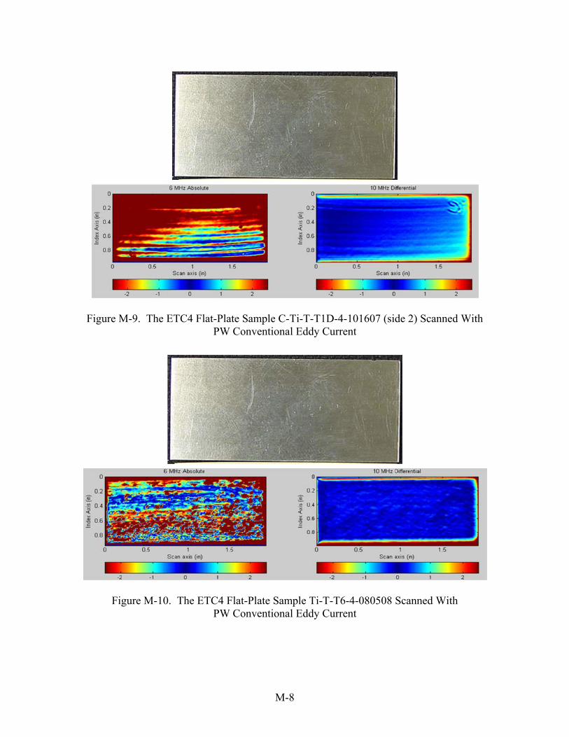
Figure M-9. The ETC4 Flat-Plate Sample C-Ti-T-T1D-4-101607 (side 2) Scanned With PW Conventional Eddy Current
Figure M-10. The ETC4 Flat-Plate Sample Ti-T-T6-4-080508 Scanned With PW Conventional Eddy Current
M-8
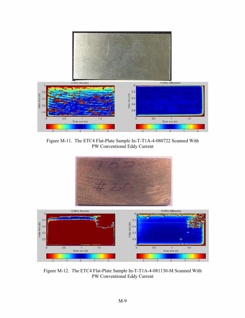
Figure M-11. The ETC4 Flat-Plate Sample In-T-T1A-4-080722 Scanned With PW Conventional Eddy Current
Figure M-12. The ETC4 Flat-Plate Sample In-T-T1A-4-081130-M Scanned With PW Conventional Eddy Current
M-9

Figure M-13. The ETC4 Flat-Plate Sample In-T-T6A-4-080916 Scanned With PW Conventional Eddy Current
Figure M-14. The ETC4 Flat-Plate Sample In-T-T6A-11-080916 Scanned With PW Conventional Eddy Current
M-10

Figure M-15. The ETC4 Flat-Plate Sample In-T-T6A-21-081006 Scanned With PW Conventional Eddy Current
Figure M-16. The ETC4 Flat-Plate Sample Ti-T-T6A-21-081201 Scanned With PW Conventional Eddy Current
M-11

Figure M-17. The VS2 Flat-Plate Sample In-T-T1A-6-081130-M Scanned With PW Conventional Eddy Current
Figure M-18. The VS2 Flat-Plate Sample In-T-T1A-6-080722 Scanned With PW Conventional Eddy Current
M-12

Figure M-19. The VS2 Flat-Plate Sample In-T-T6A-6-080916 Scanned With PW Conventional Eddy Current
Figure M-20. The VS2 Flat-Plate Sample In-T-T6A-13-081006 Scanned With PW Conventional Eddy Current
M-13

Figure M-21. The VS2 Flat-Plate Sample In-T-T6A-20-081006 Scanned With PW Conventional Eddy Current
Figure M-22. The VS2 Flat-Plate Sample Ti-T-T6A-23-081201 Scanned With PW Conventional Eddy Current
M-14

Metallography was performed on four samples, studying Type 1* and Type 6* anomalies of both alloys. The four samples used are indicated in tables M-1 and M-2 by asterisks next to the sample names. To maintain the integrity of the sample for future use, only a small section of the sample was removed, as shown in figure M-23. Two subsections were extracted: one to observe the microstructure parallel to the machining (A) and one for transverse observation of the microstructure (B). Figures M-24 through M-27 show the photomicrographs at 200x and 500x magnification for each sample for each orientation.
Figure M-23. Diagram for Sample Sectioning for Metallography
Figure M-24. Photomicrographs of C-Ti-T1D-4-101607
M-15

Figure M-25. Photomicrographs of In-T-T1A-6-080722
Figure M-26. Photomicrographs of In-T-T6A-13-081006
M-16
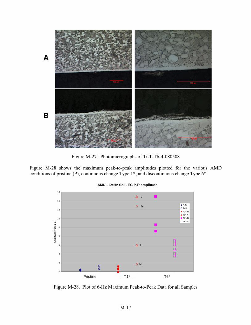
Figure M-27. Photomicrographs of Ti-T-T6-4-080508
Figure M-28 shows the maximum peak-to-peak amplitudes plotted for the various AMD conditions of pristine (P), continuous change Type 1*, and discontinuous change Type 6*.
AMD - 6MHz Sol - EC P-P amplitude
0
2
4
6
8
10
12
14
16
18
0 1 2 3 4 5 6 7
Specimen Types
Am
plit
ud
e (v
olt
s p
-p)
P-Ti
P-Ni
T1*-Ti
T1*-Ni
T6*-Ti
T6*-Ni
M
MPristine T1* T6*
L
M
L
Figure M-28. Plot of 6-Hz Maximum Peak-to-Peak Data for all Samples
M-17

Figure M-29 shows a standard deviation plot for the same data, and it appears that for the Ti 6-4 samples, the signal response may correlate with the intended anomaly severity. One sample was scanned on both sides and only one side could have intended high-severity anomaly. If, indeed, that side has the anomaly, then the order of the data correlates with the intended anomaly severity. However, the response for the In 718 coupons is switched, indicating no correlation if the intended anomaly severity was imparted on the samples. Full details of the results are in section 3.3.9 of the main document.
AMD - 6MHz Sol - EC standard deviation
0.0
0.5
1.0
1.5
2.0
2.5
0 1 2 3 4 5 6
P-Ti
P-Ni
M-18
7
Specimen
Sta
nd
ard
Dev
iati
on
(v
olt
s p
k)
T1*-Ti
T1*-Ni
T6*-Ti
T6*-Ni
Pristine T1* T6*
M
H (side 2)
LH (side 1) possibly the non-defect side
L
L
MM
Figure M-29. Plot of 6-MHz Standard Deviation Data for all Samples

APPENDIX N—SINGLE-FREQUENCY EDDY-CURRENT STATISTICAL NOISE ANALYSIS
N.1 BACKGROUND. Single-frequency eddy-current scans were performed using commercial eddy-current probes and commercial instruments to detect machining-induced surface anomalies, particularly Type 6* damages, in both turning and broaching Inconel 718 alloy (In 718) and titanium Ti-6Al-4V alloy samples. The objectives were to evaluate the feasibility of detecting anomalous machine damages by the conventional eddy-current technique, to devise a procedure for analyzing C-scan data, and to identify measurement parameters that can be used to characterize surface damages. To these ends, the C-scan eddy-current images were compared with surface morphology images obtained by laser profilometry to examine the detectability of surface anomalies by eddy current. To aid comparison between undamaged and damaged samples, the C-scan data were quantified in terms of their standard deviations, which characterize the spatial variations of the eddy-current signals. N.2 EQUIPMENT USED. Eddy-current scans were performed on both turning and broaching samples using a differential probe with split-D coils operated at 2 MHz and a commercial eddy-current instrument (Nortec NDT-19). The experimental setup is shown in figure N-1. The probe was mounted on a scanner stage under computer control. The eddy-current voltage outputs of the NDT-19 were acquired by the computer using a customized software program.
Broaching Sample
Turning Sample
Figure N-1. (a) Experimental Setup for Eddy-Current Scans on (b) Turning and (c) Broaching Samples
N.3 TEST DESCRIPTION. During the eddy-current scans, the probe was aligned in such a way that the coil gap was perpendicular to the scan direction. The lift-off direction was set to the left in the impedance plane. The signal gains were set to 75 dB for both the horizontal and vertical channels. For the turning coupons, the scan sizes used were either 30 by 15 mm or 42 by 18 mm. For the broaching samples, the scan areas were limited to a narrow part at the center of the broaching
N-1

region, typically 16 by 1.6 mm or smaller due to the geometrical constraints. The step sizes in both directions were 0.1 mm for all measurements on the turning and broaching samples. For turning samples with excessively rough surfaces, “fly-over” scans were made by lifting the probe by 60 to 100 m above the sample to avoid probe damage. The acquired C-scan images were processed using a Matlab® program to remove the background (as a second-order polynomial of the x and y coordinates) and to suppress noise by cubic spline filtering. As an example, the C-scan images of the horizontal and vertical component eddy-current signals obtained from the damaged side of a Type 6* In 718 turning coupon are shown in figure N-2. The characteristic dipole patterns observed in the vertical component signal correspond to Type 6* damage, which manifests as surface extrusions, as shown in figure N-2. The effects of surface waviness (e.g., bands of machining marks) on eddy-current signals are prominent in the horizontal component signal. The details of the results are in section 3.3.10 of the main document.
Figure N-2. C-Scan Images of the (a) Horizontal and (b) Vertical Components of the Eddy-Current Signals Measured From a Type 6* In 718 Turning Sample (In-T-T6-1-070112),
and (c) Observed Surface Anomalies (Circled) (Indications of the anomalies are numbered in the C-scan image of the vertical component signal in (b).)
N-2

APPENDIX O—SURFACE ACOUSTIC WAVE ULTRASONICS O.1 INTRODUCTION.
The use of surface acoustic wave ultrasonics for detecting machining-induced damage was studied at both Iowa State University (ISU) and Honeywell using different equipment and methods. The work at ISU included both traditional acoustic microscopy (AM) (at 50 MHz) and backscattered grain noise analysis (at 25 MHz), with a strong emphasis on the latter. The work at Honeywell emphasized AM using higher-frequency transducers (≥100 MHz), which were better suited to AM studies within thin damage layers. Appendix P contains the results for Honeywell. At both facilities, only turning samples were studied due to geometric constrains and available fixturing. O.2 EQUIPMENT USED. Various ultrasonic (UT) pulse-echo inspections were performed to examine the feasibility of using surface acoustic waves (Rayleigh waves) to detect the damage caused by anomalous machining. Figures O-1 through O-3 depict the equipment used for the measurements performed at ISU. A computer-controlled UT immersion scanning system was used, running Winspect software from UTEX Scientific Instruments, Inc. This system, pictured in figure O-1, had six degrees of freedom, namely, a scanning bridge with adjustable x, y, and z positions, a turntable, and a gimbal-gimbal manipulator for adjusting transducer angles in two orthogonal directions. In typical measurements, a test sample was placed on a level surface in the water tank, and a transducer was scanned over the stationary sample to obtain UT signals for analysis. As illustrated in figure O-2, two types of transducers were used to generate surface acoustic waves in the sample: (1) a highly focused AM transducer (aligned at normal incidence) and (2) a simple planar transducer (aligned at oblique incidence). For either transducer type, a UTEX pulser/receiver (Model UT340) was used to pulse the transducer and to amplify the returning responses from the test sample. As illustrated in figure O-3, the Winspect software was used to control scanning operations and to display UT A-scans and C-scans acquired during testing.
Gimbal-gimbal
manipulator
25-MHz planar
transducer
Machined coupon
Scanning bridge
Water tank
Control computer
(a) (b)
Gimbal-gimbal
manipulator
25-MHz planar
transducer
Machined coupon
Scanning bridge
Water tank
Control computer
(a) (b)
Figure O-1. (a) UT Scanning System and (b) Close-Up View of a Planar Transducer Positioned Above a 2″ by 2″ by 0.2″ Turning Sample
O-1
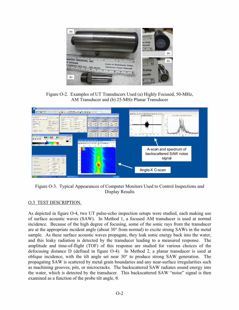
(a)
(b)
(b)
(a)
(a)
(b)
(b)
(a)
Figure O-2. Examples of UT Transducers Used (a) Highly Focused, 50-MHz, AM Transducer and (b) 25-MHz Planar Transducer
Angle-X C-scan
A-scan and spectrum of backscattered SAW noise
signal
Angle-X C-scan
A-scan and spectrum of backscattered SAW noise
signal
Figure O-3. Typical Appearances of Computer Monitors Used to Control Inspections and Display Results
O.3 TEST DESCRIPTION. As depicted in figure O-4, two UT pulse-echo inspection setups were studied, each making use of surface acoustic waves (SAW). In Method 1, a focused AM transducer is used at normal incidence. Because of the high degree of focusing, some of the sonic rays from the transducer are at the appropriate incident angle (about 30° from normal) to excite strong SAWs in the metal sample. As these surface acoustic waves propagate, they leak sonic energy back into the water, and this leaky radiation is detected by the transducer leading to a measured response. The amplitude and time-of-flight (TOF) of this response are studied for various choices of the defocusing distance D (defined in figure O-4). In Method 2, a planar transducer is used at oblique incidence, with the tilt angle set near 30° to produce strong SAW generation. The propagating SAW is scattered by metal grain boundaries and any near-surface irregularities such as machining grooves, pits, or microcracks. The backscattered SAW radiates sound energy into the water, which is detected by the transducer. This backscattered SAW “noise” signal is then examined as a function of the probe tilt angle, θ.
O-2

Method 2
50-MHz, 0.25”-diameter, F=0.2”
focused transducer, scanned in 2D
The SAW signal backscattered by
grain boundaries and surface irregularities
is studied.
Method 1A Method 1B
D is small. The direct front-wall and surface
wave signals merge into a single response. The
merged FW+SAW signal is studied.
FocusedTransducer
D
Defocusing Distance Defined
D is the distance between the top of
the specimen and the focal point in water
(if the specimen were not present).
FocusedTransducer
FW
SAW
D is large. The direct front-wall and surface wave signals are well separated. The SAW signal is gated and
studied.
FocusedTransducer
SAW
25-MHz, 0.25”-dia, planar transducer25-MHz, 0.25”-dia, planar transducer
Scan in X
Scan in
SAW
water
metal
Method 2
50-MHz, 0.25”-diameter, F=0.2”
focused transducer, scanned in 2D
The SAW signal backscattered by
grain boundaries and surface irregularities
is studied.
Method 1A Method 1B
D is small. The direct front-wall and surface
wave signals merge into a single response. The
merged FW+SAW signal is studied.
FocusedTransducer
D
FocusedTransducer
D
Defocusing Distance Defined
D is the distance between the top of
the specimen and the focal point in water
(if the specimen were not present).
FocusedTransducer
FW
SAW
FocusedTransducer
FW
SAW
D is large. The direct front-wall and surface wave signals are well separated. The SAW signal is gated and
studied.
FocusedTransducer
SAW
FocusedTransducer
SAW
25-MHz, 0.25”-dia, planar transducer25-MHz, 0.25”-dia, planar transducer
Scan in X
Scan in
SAW
25-MHz, 0.25”-dia, planar transducer25-MHz, 0.25”-dia, planar transducer
Scan in X
Scan in
SAW
water
metal
Figure O-4. The UT Inspection Setups at ISU Identifying the Transducers Typically Used With Each
The premise underlying either method is that any damage due to abusive machining will change the near-surface microstructure and thus affect surface acoustic wave propagation. Differences between undamaged and damaged surfaces can manifest themselves as changes in the amplitude or arrival time of the UT response (Method 1) or as changes in the angular dependence of the backscattered noise signal (Method 2). For the most sensitive test, it is desirable to confine the bulk of the surface acoustic wave energy to the very near-surface region (say upper 50 microns) where machining-induced damage, if present, is likely to occur. The depth of surface acoustic wave penetration depends on wavelength, with most of the sonic energy being confined within one wavelength (λ) of the surface. For a range of frequencies, table O-1 lists the surface acoustic wave penetration depth for generic titanium Ti-6Al-4V alloy (Ti 6-4) and Inconel 718 alloy (In 718). For the measurements at ISU, the highest-frequency transducers that were available were used, namely, the 50-MHz focused transducer and 25-MHz planar transducer shown in figure O-2. Although the surface acoustic wave penetration depths are somewhat larger than optimal, work by Hak-Joon Kim, et al., has shown that surface acoustic wave inspection techniques can often be successful even when the penetration distance is much larger than the thickness of the layer of interest [O-1 to O-3].
O-3

Table O-1. Surface Acoustic Wave Penetration Depth (i.e., One Wavelength) as a Function of Frequency for UT Inspections of Generic Ti 6-4 and In 718 Alloys
Generic Ti 6-4 Material
(V_surface = 0.93 V_shear Generic In 718 Material
(V_surface = 0.93 V_shear)
Frequency (MHz)
Penetration Depth
(microns)
Penetration Depth (mil)
Penetration Depth
(microns)
Penetration Depth (mil)
1 2930 115 2860 113
5 586 23 572 22.5
10 293 12 286 11
25 117 4.6 114 04.5
50 59 2.3 57 02.2
100 29 1.2 29 01.1
Measurements using Methods 1 and 2 on selected samples will now be described in detail. These “proof of method” measurements all made use of turning samples since they had the simplest geometry and required no special fixtures (such as reflecting mirrors) to insonify the machined surfaces. The measurements indicated that, although both methods could often distinguish between pristine and damaged coupons, Method 2 appeared to be more robust and to offer the better alternative for practical implementation. Thus, Method 2 was eventually applied to a larger set of samples for additional testing. Most of the initial proof-of-concept measurements at ISU were conducted using Ti 6-4 samples, since damaged In 718 samples did not become available until much later in the program. The measurement results will be summarized in the following order: Method 1A (normal-incidence inspection using a small defocusing distance) applied to
selected ETC-3 Ti 6-4 turning samples
Method 1B (normal-incidence inspection using a large defocusing distance) applied to selected ETC-3 Ti 6-4 turning samples
Methods 1A and 1B applied to a Ti 6-4 enlarged grain block (EGB) to investigate the source of variations observed in inspections of pristine material
Method 2 (oblique-incidence backscatter) applied to a heat-treated Ti 6-4 sample having a thick damage layer
Method 2 applied systematically to a large set ETC-3 Ti 6-4 turning samples
Method 2 applied systematically to a large set ETC-3 In 718 turning samples
Summary of findings for Method 2
O-4

It was found that the presence of machining grooves can affect UT inspections. Each turning sample contains regularly spaced grooves which, although slightly curved, run roughly parallel to the length of the sample. Surface roughness (Ra) values are largest when measured in the direction perpendicular to the grooves. Table O-2 lists the sample numbers and roughness values for the coupons cited in the figures appearing in this appendix.
Table O-2. Surface Roughness for Selected Turning Samples
Ra (microinches)
Alloy Type Sample Number Shorthand Side 1 Side 2
(damaged)
Ti 6-4 Option A pristine Ti-T-P-0611 51 42
Ti 6-4 Option A Type 1 Ti-T-T1-1-061031 148 223
Ti 6-4 Option A Type 6 Ti-T-T6-1-061031 75 >250
Ti 6-4 Option C pristine C-Ti-T-P-1-101607 P1 35 23
Ti 6-4 Option C pristine C-Ti-T-P-3-101607 P3 21 33
Ti 6-4 Option C pristine C-Ti-T-P-7-101607 P5 19 34
Ti 6-4 Option C Type 1 deep C-Ti-T1D-1-101607 D1 39 72
Ti 6-4 Option C Type 1 deep C-Ti-T1D-2-101607 D2 37 48
Ti 6-4 Option C Type 1 deep C-Ti-T1D-4-101607 D4 37 56
Ti 6-4 Option C Type 1 deep C-Ti-T1D-5-101607 D5 37 48
Ti 6-4 Option C Type 1 deep C-Ti-T1D-6-101607 D6 38 55
Ti 6-4 Option C Type 1 shallow Ti-T-T1-1-080107 S1 73
Ti 6-4 Option C Type 1 shallow Ti-T-T1-7-080107 S7 54
Ti 6-4 Option C Type 1 medium Ti-T-T1A-10-080606-M M10 33 26
Ti 6-4 Option C Type 1 medium Ti-T-T1A-12-080606-M M12 40
Ti 6-4 Option C Type 6 Ti-T-T6A-16-080602 T6-16 51 117
In 718 Option C Type 1 shallow In-T-T1A-7-080722-S S7 41 74
In 718 Option C Type 1 medium In-T-T1A-1-081130-M M1 52 346
In 718 Option C Type 1 medium In-T-T1A-2-081130-M M2 51 365
In 718 Option C Type 1 medium In-T-T1A-3-081130-M M3 433
In 718 Option C Type 6 In-T-T6A-7-080916 T6-7 86 74 Note: Roughness values are measured perpendicular to the groove direction.
O.3.1 METHOD 1—AN OVERVIEW OF NORMAL-INCIDENCE AM AT ISU. Method 1 uses a highly focused AM transducer oriented at normal incidence to the surface being inspected. As illustrated in figure O-5, two defocusing configurations were used for preliminary measurements. In the first configuration (Method 1A), the beam was focused just below the FW, with the defocusing distance D typically being 1 to 3 mil (referred to here as D ~0). In this case, the direct front-wall (FW) signal and the SAW have nearly the same travel times. The two signals then merge in time, and this merged FW + SAW signal is gated and studied. In the second configuration (Method 1B), the beam was focused well below the FW (D typically about
O-5

35 mil), and the properties of the gated SAW signal were studied. The 35-mil value for the defocusing distance produced a SAW signal that was sufficiently removed from the FW signal for easy isolation, and yet not too suppressed in amplitude by UT attenuation. In practice, the D = 0 point was identified as the water path for which the FW response had its highest amplitude (as measured using a smooth test sample).
FocusedTransducer
water
metalD
FocusedTransducer
3
50 MHz, F=0.2”, Diam.=0.25”, with delay rod
12
3
4
FocusedTransducer
1 24
FocusedTransducer
water
metalD
FocusedTransducer
water
metalD
water
metalD
FocusedTransducer
3
FocusedTransducer
3
50 MHz, F=0.2”, Diam.=0.25”, with delay rod
12
3
4
FocusedTransducer
1 24
FocusedTransducer
1 24
Figure O-5. Typical UT Signals Observed for Normal-Incidence AM (Method 1) (The A-scan shown is for Ti 6-4 pristine sample (Ti-T-P-1-0611) using a defocusing
distance of about 35 mil.) For the particular 50-MHz transducer used at ISU, figure O-5 displays a typical UT pulse-echo response when the defocusing distance is large. Here, the sample is a pristine Ti 6-4 anomalous machining damage coupon, and the D is near 35 mil. The transducer has a quartz buffer rod containing a spherical cavity at its bottom. The cavity, having a lateral diameter of 0.25 inch, acts to focus the sound beam at a depth of 0.20 inch in water. Four key signals are identified in figure O-5. Signals 1 and 2 are the FW echoes below the unfocused and focused portions of the transducer, respectively. Signal 3 is the SAW signal. Signal 4 is a back-wall signal from the 0.2-inch-thick sample. Signal 1 is useful for transducer alignment, as it is maximized when the central ray is perpendicular to the metal surface. Signals 2 and 3 are used for the actual inspection. Sound reverberations within the buffer rod act to complicate the full A-scan signal, but the signals of interest can be easily identified.
O-6

The manner in which the UT signals change with water path (i.e., with defocusing distance) is illustrated in figure O-6. If the water path is decreased, the SAW signal shifts to the right relative to the focused-FW echo, and the amplitude of the SAW signal decreases due to attenuation, which now acts over a longer metal travel path. Conversely, if the water path is increased, the SAW shifts to the left and increases in amplitude, eventually merging with the focused-FW signal when the defocusing distance is small.
4
D = 25 mil
D = 45 mil
3D = 35 mil
Focused
Transducer
Ti 6-4 sample Ti-T-P-1-0611. Gain = 23 dB
3
Focused Transducer
1 24
3
3
21
Figure O-6. Effect of Water Path Changes on AM Signals (Method 1) (Ti 6-4 pristine sample
(Ti-T-P-1-0611) with defocusing distances of about 25, 35, and 45 mil.) O.3.2 METHOD 1A—NORMAL-INCIDENCE INSPECTION USING A SMALL DEFOCUSING DISTANCE—APPLIED TO SELECTED Ti 6-4 TURNING SAMPLES. For the first configuration (D ~0), figure O-7 shows the measured UT time-domain signal and its spectrum at selected sites on pristine and damaged Ti 6-4 turning samples. For the pristine sample, the merged FW + surface acoustic wave response varied only modestly with position. Changes in peak-to-peak amplitude of about 10% were observed, reflecting systematic differences in the responses from the tops and bottoms of the machining grooves, which were easily imaged. In contrast, much larger variations in response with position were observed for the damaged sample. At isolated sites on the damaged coupon, the FW + SAW response amplitude was nearly as high as the pristine coupon (figure O-7(b)). At most other sites, the response was much smaller (figure O-7(c)).
O-7

Damaged Coupon High-Ampl. Site
Gain = -3 dB
2 + 3
Pristine Coupon Typical Site
Gain = -3 dB
2 + 3
Damaged Coupon Low-Ampl. Site
Gain = -3 dB
2 + 3
Each spectrum is normalized to a peak value of unity.
(a)
(b)
(c)
Damaged Coupon High-Ampl. Site
Gain = -3 dB
2 + 3
Damaged Coupon High-Ampl. Site
Gain = -3 dB
2 + 32 + 3
Pristine Coupon Typical Site
Gain = -3 dB
2 + 32 + 3
Damaged Coupon Low-Ampl. Site
Gain = -3 dB
2 + 3
Damaged Coupon Low-Ampl. Site
Gain = -3 dB
2 + 32 + 3
Each spectrum is normalized to a peak value of unity.
(a)
(b)
(c)
Figure O-7. Typical AM A-Scan Signals and Their Frequency Spectra (Method 1A, D ~0) (a) Typical Site on Ti 6-4 Pristine Coupon Ti-T-P-1-0611, (b) High, and (c) Low-Amplitude Sites
on Ti 6-4 (Type 1 (This is an Option A coupon.)) Damaged Coupon Ti-T-T1-1-061031 For the same pristine Ti 6-4 coupon, figure O-8(a) shows an UT C-scan obtained by displaying the amplitude of the rectified peak response of the merged FW + SAW signal. For this two-dimensional raster scan of the transducer over the sample, the scan area was 0.08″ by 0.05″ using a 0.0002″ step across the machining grooves and a 0.001″ step along the grooves. Note that the machining grooves on the pristine sample, which have an average spacing of 6 mil, are easily resolved. Using 1.03 λF/D to estimate the beam diameter (full wave half max) at the focal depth yields a spot size of about 1.2 mil for the effective center frequency of 40 MHz. By examining amplitude and TOF images, one concludes that the bottoms of the grooves yield the higher-amplitude signals, as depicted in figure O-8(b).
O-8

Lower Amplitude
(earlier TOF)
Higher
0.08” X 0.05”scan area
(a) Lateral Position, X (inches)
Lat
eral
Pos
ition
, Y (
inch
)
0.08″ by 0.05″scan area
Amplitude (later TOF)
(b)
Lower Amplitude
Higher Amplitude
Figure O-8. (a) Gated Peak Amplitude C-Scan of Ti 6-4 Pristine Coupon Ti-T-P-1-0611
Using a Defocusing Distance D Near Zero and (b) Relationship of Signal Amplitude to Groove Geometry
For a pair of Ti 6-4 coupons, one pristine and one damaged, amplitude and TOF images are compared in figure O-9. The same water path, time gate, scan area, and gain setting (-3 dB) were used for both coupons. Note that the average amplitude of the FW + SAW signal is much smaller for the damaged coupon. In addition, the dominant spacing of the grooves on the damaged sample (about 14.8 mil) is about twice that of the pristine sample (6.0 mil). Under a microscope, these wider grooves appear to have been cut over a set of narrower grooves, presumably as part of the final machining pass to remove some of the excessive roughness caused by the abusive machining operation. For the damaged coupon, blue-shaded areas in the TOF image are for (early-arriving) signals, which are too weak to trigger the TOF threshold.
Amplitude TOF
Amplitude TOF
Pris
tine
Typ
e-1
Da
ma
ge
Amplitude TOF
Amplitude TOF
Pris
tine
Typ
e-1
Da
ma
ge
Figure O-9. Gated Peak Amplitude and TOF C-Scans of Ti 6-4 Pristine Coupon Ti-T-P-1-0611 (top) and Ti 6-4 Type 1* Damaged Coupon Ti-T-T1-1-061031 (bottom)
(Defocusing distance D ~0)
O-9

Other comparisons of gated peak amplitude C-scans for damaged coupons are presented in figure O-10, using the same gain settings and scan area as in figure O-9. Thus, the images for the pristine coupon in figure O-9 can be directly compared to those of the damaged coupons in figure O-10. For each damaged coupon, one can observe the periodic groove structure and areas where that structure has been interrupted by localized damage. In figure O-10(a) and (b), an extended region (outlined in white) is shown on one damaged coupon, which has a low-amplitude response and an early TOF. This is likely associated with a partially re-embedded chip or other excess metal protruding slightly above the surrounding surface.
(a) (b)
Damaged, Type 1, Ti-T-T1-061031Site 1, Amplitude C-scan
(b)
Damaged, Type 1, Ti-T-T1-061031 Site 1, TOF C-scan
(a)
Damaged, Type 1, Ti-T1-061031 Site 2, Amplitude C-scan
(c) (d)(d)(c)
Damaged, Type 6, Ti-T-T6-061031 Site 3, Amplitude C-scan
Figure O-10. Gated Peak Amplitude C-Scans of Ti 6-4 Damaged Coupons Acquired Using D ~0 (a)-(c) Amplitude or TOF C-Scans at two Sites on Type 1* Damage Coupon
Ti-T-T1-1-061031, and (d) Amplitude C-Scan at one Site on Type 6* Damage Coupon Ti-T-T6-1-061031 (Gating, gain settings, and scan parameters were the same for all images.)
O-10

The UT response differences between the pristine and damaged coupons evident in figures O-9 and O-10 are presumably due to (1) the presence of a damage layer and (2) general differences in surface topology. Here, the topology differences are not insignificant. In figure O-9, for example, the Ra (measured across the machining grooves) is 50 microinches for the pristine coupon and 150 microinches for the damaged one. In addition, the dominant groove spacings are also considerably different (6.0 and 14.8 mil, respectively). Figure O-11 compares UT responses for a different pair of pristine and damaged surfaces that have much more similar topologies. The two surfaces in question are the upper (damaged) and lower (undamaged) surfaces of a Ti 6-4 Type 1* turning sample bearing sample number C-Ti-T1D-2-101607. Since each damaged coupon is only damaged on one side, the opposite side can serve as a pristine surface, as was done here. The roughness values for the damaged (Ra = 47 μin) and undamaged (Ra = 37 μin) sides of the coupon are reasonably similar and both within typical finishing tolerances (Ra <64 μin). This coupon was found to be slightly bowed or cup-shaped, with the damaged face having a convex curvature and being about 9 mil higher in the center than at the corners. This curvature is likely due to the relief of residual stress when the coupon was cut from the washer. In constructing figure O-11, the sample was placed atop a level platform, the sound beam was normalized to a surface point near the center of the sample, and the water path was adjusted to a defocusing distance of roughly 2 mil. Then the full 1″ by 2″ lateral area of the sample was scanned, gating the merged FW + SAW signal as usual. This procedure was repeated for each surface scanned. Because the transducer was scanned in a flat plane above the sample, the surface curvature caused the water path (and hence the defocusing distance) to vary slightly during scanning. In practice, the combined FW + SAW response is quite sensitive to the defocusing distance. For the 50-MHz transducer used here, a water path change of only a few mil can noticeably affect the amplitude of the response. Thus, both the TOF and the amplitude variations shown in the images of figure O-11 are primarily due to water path changes rather than to any underlying surface damage. For three locations on the damaged surface, figure O-12 displays the associated A-scan signals. Both the signal arrival time and signal amplitude change between these three locations. The amplitude changes are observed to be quite large for these modest water path changes of a few mil. By definition, the defocusing distance is zero when the largest amplitude response is observed (see figure O-4). For the damaged surface, this occurs along an oval ring surrounding the center of the sample. Inside this ring, the defocusing distance is small and positive; outside the ring, it is small and negative.
O-11

Damaged Face - TOF Damaged Face - Amplitude
Undamaged Face - TOF Undamaged Face - Amplitude
TOF Color Bar (usec) Amplitude Color Bar (Volts)
Damaged Face - TOF Damaged Face - Amplitude
Undamaged Face - TOF Undamaged Face - Amplitude
TOF Color Bar (usec) Amplitude Color Bar (Volts)
Figure O-11. Normal-Incidence AM (D ~0) Applied to the Damaged and Undamaged Surfaces
of Ti 6-4 Turning Sample C-Ti-T1D-2-101607 (Both TOF (left) and amplitude (right) C-scans are shown. All inspection settings were the same for both surfaces,
with the scan area being 1.5″ by 2.2″.)
O-12

Late
(i
ral Position, Y
nches)
Late
ral P
ositi
on,
Y (
inch
es)
Lateral Position, X (inches)
0.0
-0.2 -0.4
-
-
0.2
0.4
Vol
ts
μsec
μsec μsec
Figure O-12. Normal-Incidence AM (D ~0) Applied to the Damaged Surface Ti 6-4 Turning Sample C-Ti-T1D-2-101607 (The lower portion shows UT A-scans at three positions within the
gated peak amplitude C-scan image.) Because of surface curvature and the sensitivity of the merged FW + SAW signal to water path changes, care must be taken to use the same water path when comparing responses from different surfaces. A more careful comparison is shown in figure O-13 for the damaged and undamaged surfaces of Ti 6-4 turning sample C-Ti-T1D-2-101607. Only the relatively flat 0.5″ by 0.6″ central regions were scanned to limit water path variations, and the defocusing distance was carefully adjusted to 0.002″ at the scan center. Amplitude variations due to water path changes are now less pronounced, but are still evident in figure O-13. For the centermost regions of the two C-scan images, enclosed by the black rectangles, the water paths are very nearly identical (as judged by average TOF values). Machining grooves can be observed that run approximately from left to right in each image; with the grooves being a bit more pronounced for the damaged surface, which has a slightly higher roughness level. Vertical streaks in the images are artifacts of the inspection caused by very small water path changes due to a slight rhythmic bouncing of the transducer during scanning. Within the 0.15″ by 0.15″ rectangles where water paths are nearly constant and identical, measured amplitudes were about 5% lower for the damaged surface than for the undamaged surface (0.346V compared to 0.365V at the same inspection gain). In figure O-13, one can also observe a horizontal region of especially low amplitude (circled) that may be associated with enhanced damage.
O-13

Damaged Face - Amplitude
Amplitude Color Bar (Volts)
Undamaged Face - Amplitude
Ti64 turned couponC-Ti-T1D-2-101607
In the central boxed regions, defocusing distances for the two faces differ by no more than 0.6 mils, based on TOF analysis.
Lower amplitude regionaligned with grooves
Average amplitude = 0.346 Volts
Average amplitude = 0.365 Volts
Damaged Face - Amplitude
Amplitude Color Bar (Volts)
Undamaged Face - Amplitude
Ti64 turned couponC-Ti-T1D-2-101607
In the central boxed regions, defocusing distances for the two faces differ by no more than 0.6 mils, based on TOF analysis.
Lower amplitude regionaligned with grooves
Average amplitude = 0.346 Volts
Lower amplitude regionaligned with grooves
Average amplitude = 0.346 Volts
Average amplitude = 0.365 Volts
Average amplitude = 0.365 Volts
Figure O-13. Normal-Incidence AM (D ~0) Applied to Damaged and Undamaged Faces of Ti 6-4 Turning Sample C-Ti-T1D-2-101607 (Gated peak amplitude
C-scans of the central 0.5″ by 0.6″ region are shown.) The difference in average amplitudes between damaged and undamaged surfaces is much smaller for the coupon pair of figure O-13 than for the pair in figure O-9. Recall that for that pair, surface roughness differences were much larger, as were the measured amplitude differences. The tentative conclusion is that the merged FW + SAW signal is quite sensitive to surface topology, and damage conditions that involve major alterations of the topology should be readily detectable. However, using Method 1A to detect near-surface microstructural changes in the absence of surface topology changes will be difficult unless topology is tightly controlled. In addition, the FW + SAW signal is very sensitive to the defocusing distance, so the inspection water path (i.e., the probe liftoff) would have to be tightly controlled for such an inspection. O.3.3 METHOD 1B—NORMAL-INCIDENCE INSPECTION USING A LARGE DEFOCUSING DISTANCE—APPLIED TO SELECTED Ti 6-4 TURNING SAMPLES. In Method 1B, an alternate inspection configuration was considered in which the defocusing distance is sufficiently large to decouple the FW and surface acoustic wave signals, allowing the isolated surface acoustic wave signal to be gated and studied. The use of this configuration will be demonstrated using the same pairs of damaged and pristine coupons examined using the (D ~0) configuration. Again, pertinent roughness information for the coupons in question can be found in table O-2. For a Ti 6-4 pristine turning sample, figure O-14 shows a typical A-scan signal and the gating used to isolate the SAW signal. The defocusing distance is near 35 mil, placing the SAW signal about midway between the focused FW signal and the back-wall reflection. In this case, the start of the time gate for SAW signal acquisition is triggered by the arrival time of the FW signal from
O-14

the flat portion of the delay rod (Signal 1 in figure O-14(a)). Recall that for Method 1A, the focused FW signal is very sensitive to water path changes of a few mil. The SAW signals of Method 1B are much less sensitive to small water path changes, but care must be taken to keep the SAW signal centered within the time gate used. Having the SAW gate “follow” Signal 1 accomplishes this if the water path variations (due to sample curvature) are not too large. Also note that SAW signals are much smaller in amplitude than merged FW + SAW signals. For the 50-MHz transducer, inspection gains are typically about 35 dB higher for Method 1B than for Method 1A. Figure O-14 also shows a typical frequency spectrum for a gated SAW signal. It is much different in appearance from the spectrum of the merged FW + SAW signal used in Method 1A (see figure O-7). The SAW spectrum is characterized by a series of maxima and minima, which are (roughly) equally spaced in frequency. For the 35-mil defocusing distance used here, the beam foot print on the sample surface is about 40 mil in diameter, thus spanning several machining grooves (6-mil spacing). The peak/valley structure of the SAW spectrum arises from constructive/destructive interference between sound waves scattered laterally by the grooves. For surface acoustic wave propagation perpendicular to the grooves, interference maxima are expected when 2S = nλ = nv/f, or f = nv/2S, with n = 1, 2, 3, etc. S is the groove spacing, f is the frequency, and λ and v are surface acoustic wave wavelength and speed. Estimating v = 0.3 cm/μsec and S = 6 mil leads to Δf = 9.8 MHz for the interference maxima, in reasonable agreement with figure O-14(c). Generally speaking, the peak/valley structure of SAW spectra tended to be more regular for pristine surfaces than for damaged ones, since the pristine surfaces had a more periodic groove structure.
FocusedTransducer
3
FocusedTransducer
1 24
1 2 34
Gating the SAW signal
Spe
ctru
m
Am
plitu
de SAW signal
(a)
(b)
(c)
FocusedTransducer
3
FocusedTransducer
1 24
FocusedTransducer
3
FocusedTransducer
3
FocusedTransducer
1 24
FocusedTransducer
1 24
1 2 34
Gating the SAW signal
1 2 34
Gating the SAW signal
Spe
ctru
m
Am
plitu
de SAW signal
(a)
(b)
(c)
Figure O-14. Normal-Incidence AM (D ~35 mil) (a) Signal Identification, (b) Typical A-Scan Signal, Showing Gating Used for the SAW Signal, and (c) Typical SAW Spectrum (Results are
for Ti 6-4 pristine coupon Ti-T-P-1-0611.)
O-15

As illustrated in figure O-15 for a pristine Ti 6-4 sample, gated peak amplitude C-scans are much different in appearance for the two normal-incidence inspection configurations. For Method 1A (D ~0), the appearance of the C-scan is dominated by the machining groove structure. For Method 1B (D ~35 mil), individual machining grooves are generally not evident, due to the much wider beam footprint on the surface. However, significant longer-range amplitude variations are seen, giving the SAW C-scan a mottled appearance. On a percentage basis, the amplitude variations for the isolated SAW signal (D ~35 mil) are much larger than those for the merged FW + SAW signal (D ~0).
FW + SAW Signal Defocusing ~0, Gain = +33 dB
SAW SignalDefocusing ~35 mil, Gain = +33 dB
Ti 6-4 turning sample Ti-TP-1-0611
Figure O-15. Normal-Incidence AM of Pristine Ti 6-4 Turning Sample Ti-T-P-1-0611 Showing Gated Peak Amplitude xy C-Scans Using (a) the Merged FW + SAW
Signals (D ~0) and (b) the SAW Signal (D ~35 mil) (Scan area is 0.08″ by 0.05″.) SAW C-scans using D ~35 mil are compared in figure O-16 for two Ti 6-4 coupons, one pristine and one damaged, with both coupons scanned in the same manner at the same gain. This figure may be regarded as the SAW counterpart to figure O-9 (same coupon pair but using D ~0). In addition, the scan region has now been enlarged by a factor of three in each dimension to 0.24″ by 0.15″. Both coupons exhibit large percentage variations in the amplitude of the SAW signal, with the average SAW signal strength being significantly weaker for the damaged coupon. Recall that for the two coupons in question, Ra values (50 and 150 microinches) are considerably different, with the damaged coupon having the larger value.
O-16

Ti 6-4 Pristine Coupon Ti-T-P-1-0611 SAW Signal
Defocusing ~35 mil, Gain = +33 dB
Ti 6-4 Damaged Coupon Ti-T-T1-1-061031
SAW Signal
Figure O-16. Normal-Incidence AM of Pristine and Damaged Ti 6-4 Turning Samples Showing
Gated Peak Amplitude xy C-Scans Using the SAW Signal (D ~35 mil) (The scan area is 0.24″ by 0.15″.)
Another comparison of SAW C-scans (D ~35 mil) is shown in figure O-17, this time using the damaged and undamaged surfaces of Ti 6-4 coupon C-Ti-T1D-2-101607, which have more similar roughness values. This figure is the counterpart to figure O-13 (same surfaces, D ~0). The defocusing distance is about 35 mil in the central region of the scan, but varies slightly due to surface curvature. Machining grooves run from left to right, but are not prominent in these images. Both surfaces in figure O-17 show amplitude variations with position, with similar average amplitude values. For the damaged sample, some of these variations may be associated with machining-induced damage since their horizontal pattern is aligned with the tool movement direction. For the undamaged surface, the amplitude variations appear to be random rather than aligned with tool direction. For the damaged samples appearing in figures O-16 and O-17, the depth of the damage layer is thought to be roughly similar for both surfaces. However, there is a large difference between average SAW amplitude values for damaged and undamaged surfaces in figure O-16, but little difference in figure O-17. It can be tentatively concluded that the degree of surface roughness strongly impacts the SAW amplitude, and that the large amplitude difference in the two halves of figure O-16 is primarily due to the underlying difference in roughness values.
O-17

Amplitude Color Bar (Volts)
Damaged Face
Low Amplitude
High Amplitude
Vol
ts
SAW SAW
SAW SignalD ~35 mil, Gain = +32 dB
Undamaged Face SAW Signal
D ~35 mil, Gain = +32 dB
Figure O-17. Normal-Incidence AM Applied to Damaged and Undamaged Faces of
Ti 6-4 Turning Sample C-Ti-T1D-2-101607 Showing Gated Peak Amplitude xy C-Scans Using the SAW Signal (D ~35 mil) (The lower portion shows UT A-scans at two
positions on the damaged face.)
O.3.4 METHOD 1—NORMAL-INCIDENCE AM APPLIED TO THE EGB TO INVESTIGATE AMPLITUDE VARIATIONS IN PRISTINE COUPONS. It is clear from figures O-15 through O-17 that the amplitudes of surface acoustic wave signals vary significantly with position for pristine Ti 6-4 surfaces, and that these variations can easily mask signal changes due to abusive machining-induced damage. It was suspected that the amplitude variations observed for the undamaged surfaces were associated with near-surface microstructure variations on a distance scale of about 0.1″. Since macrograins in Ti 6-4 forgings can have, approximately, this length scale, it was suspected that Ti 6-4 macrograins were affecting SAW propagation, hence influencing the C-scan images. To investigate this possibility, the same 50-MHz focused transducer was used to examine the ETC Phase I EGB. A Ti 6-4 sample (approximately 4″ by 1.5″ by 0.3″ in size) had been specifically heat treated to grow large macrograins, and then polished and etched to reveal the
O-18

macrograin boundaries. In addition, Orientation Imaging Microscopy had been used to determine the crystalline orientations of the macrograins [O-4]. Since the macrograins were much larger in the EGB than in typical forging samples, and since their orientations were known, the EGB provided a good vehicle for investigating the influence of macrograins on Method 1 inspections. Figures O-18 and O-19 display gated peak amplitude C-scans of the EGB made using Method 1A and 1B, respectively. The defocusing distances were 3 mil for figure O-18 (gating the merged FW + SAW signals) and 30 mil for figure O-19 (gating only the SAW signal). In both C-scans, many of the macrograin boundaries can be easily distinguished. For Method 1A, the amplitude variations over the sample surface are not particularly large, generally within about ±5% of the average response. Much larger amplitude variations (of about an order of magnitude) are observed for the pure SAW signal, indicating that it can more easily distinguish microstructural changes. Within a given macrograin, the SAW response is relatively uniform, but that response may be large or small, depending on the crystalline orientation of the macrograin.
Enlarged Grain Block Normal-Incidence Acoustic Microscopy
Defocusing Distance D = 0.003″ C-scan of gated FW + SAW amplitudeGain = -2 dB-
FW + SAWFW + SAW
Lower amplitude responseresponse
Higher amplitude responseresponse
High Response
Low Response
Figure O-18. Normal-Incidence AM (Method 1A, D = 3 mil) Applied to the EGB (The lower portion shows UT A-scans at two positions in the xy C-scan image.)
O-19

SAW SAW
High Response
Low Response
Enlarged Grain Block Method 1B Normal-Incidence Acoustic MicroscopyDefocusing Distance D = 0.030″ C-scan of gated SAW amplitude Gain = 23 dBC-
SAWSAWFW FW
Loweramplitude response
Lower amplitude response
Higher amplitude response
Higher amplitude response
Figure O-19. Normal-Incidence SAW Microscopy (Method 1B, D = 30 mil) Applied to the EGB
(The lower portion shows UT A-scans at two positions in the xy C-scan image.) Forged Ti 6-4 material has a complex microstructure described by several length scales. At the smallest scale are individual alpha- or beta-phase crystallites, whose atomic lattices have hexagonal and cubic symmetry, respectively. On the largest scale are macrograins containing colonies of alpha-phase crystallites, which have their atomic lattice directions aligned. Such a macrograin possesses a near-hexagonal symmetry about a particular crystallite direction (commonly known as the C-axis direction). For macrograins in the EGB, the C-axis direction is known from electron backscatter diffraction measurements and the following behavior is found: (1) when the C-axis is perpendicular to the inspection surface, a large SAW signal is observed; and (2) when the C-axis is parallel to the inspection surface, a small SAW signal is observed. This behavior can be understood as follows, as illustrated in figure O-20. For sound propagation perpendicular to the C-axis, the SAW sound speed is independent of direction. On the other hand, when the C-axis is parallel to the inspection surface, the SAW sound speed depends on direction and the variation of speed when the angle is maximized. For the normal-incidence SAW inspection, the sonic footprint incident on the sample is a circle and SAWs travel along the radii of this circle, radiating into the water as they travel. Some of this radiation is received by the transducer, resulting in the observed SAW response. If the SAWs all travel at the same speed along different radii, their contributions to the received signal will add in phase, resulting in a large response. However, if the SAWs travel at different speeds, some destructive interference is likely to occur, lowering the observed response. Thus, the amplitude variations shown in figure O-19 (and to a lesser degree in figure O-18) are a result of different macrograins possessing different symmetry-axis orientations, with some orientations leading to more destructive interference of SAW signals than others.
O-20

Beam footprint on surface at about the proper incidence angle for surface acoustic wave production.
Surface acoustic wave speed is thesame for propagation in any direction within this plane.
C C
Surface acoustic wave speedvaries with direction for propagation in this plane.
0.312 cm/us 0.312 cm/us
0.258 cm/us
C-axis
(b)(a)
Figure O-20. (a) The Atomic Lattice for Hexagonal-Phase Titanium Identifying the C-Axis Direction and (b) Dependence of SAW Speed on Propagation Direction in Ti 6-4 Macrograins
(as estimated from ETC Phase I measurements) The EGB was also used to investigate the sensitivity of Methods 1A and 1B to the choice of defocusing distance. For Method 1A, figure O-21 compares C-scan images of the EGB made using three different defocusing distances (0, 3, and 10 mil). When employing Method 1A with the 50-MHz, F = 0.2″ transducer, both the strength of the merged FW + SAW response and the ability to distinguish microstructural variations is strongly dependent on the defocusing distance. Here, a defocusing distance near D = 3 mil was judged to work best for Method 1A. By definition, the peak amplitude for the FW + SAW response occurs for D = 0. At D = 3 mil, that response was reduced by about 15% on average, but the ability to distinguish microstructure variations was enhanced. Figure O-22 displays the results of a similar study using Method 1B. C-scan images of the EGB are compared at defocusing distances of 20, 30, and 50 mil. Neighboring macrograins are easily distinguished in each case, demonstrating that Method 1B works well for a fairly wide range of inspection water paths. However, shorter water paths (implying larger SAW travel paths along the metal surface) require larger gain settings to offset amplitude drops due to attenuation. For Method 1B, a defocusing distance near 30 ±5 mil seemed optimum for the EGB, producing sufficient separation between the direct FW and SAW signals without too much loss of SAW signal amplitude. For pristine Ti 6-4 turning samples, the optimal defocusing distance was similar, judged to be about 35 mil from various experimental trials.
O-21

D = 0.010+3 dB
D = 0.010″+3 dB
D = 0.003”-2 dB
D = 0.003″-2 dB
D = 0.000”-4 dB
D = 0.000″-4 dB
EGB Method 1A Normal-Incidence Acoustic MicroscopyVarious defocusing distances (D) C-scan of gated FW + SAW amplitude
Low Response
High Response
High Low
Gray scales having different contrasts have been used to try to emphasize macrograin differences in each case.
Figure O-21. Normal-Incidence AM (Method 1A) Applied to the EGB With Gated Peak
Amplitude xy C-Scans for Three Defocusing Distances
D = 0.02019 dB
D = 0.030”23 dB
D = 0.05030 dB
Enlarged Grain Block Method 1B Normal -Incidence Acoustic Microscopy Various defocusing distances (D)C-scan of gated SAW amplitude
Low Response
High Response
Same color bar used for each image.Same color bar used for each image.
High Response
Low Response
Enlarged Grain Block Method 1B Normal -Incidence Acoustic Microscopy Various defocusing distances (D)
scan of gated SAW amplitude-C
D = 0.020″19 dB
D = 0.030″23 dB
D = 0.050″30 dB
Figure O-22. Normal-Incidence AM (Method 1B) Applied to the EGB With Gated Peak Amplitude xy C-Scans for Three Choices of the Defocusing Distance
O-22
In summary, the EGB studies at ISU indicated that subsurface damage detection may be difficult in Ti 6-4 material for either Method 1A or 1B because of the presence of macrograins in undamaged metal. Different macrograins typically have different crystalline axes orientations, leading to different propagation speeds for SAWs, and hence, led to different responses for either FW + SAW or SAW signals. These differing response levels are magnified in the EGB, but are also present in undamaged engine material. Signal variations associated with macrograin structure will likely act to mask subsurface damage, making damage detection more difficult. However, damage detection in Ti 6-4 may be possible in some circumstances. If the damage is accompanied by surface topology changes (e.g., changes in the spacing and regularity of the machining grooves), such changes are readily detected by Method 1A. If near-surface microstructure damage exists, but the surface topology is similar to a pristine surface (e.g., due to cleanup by a subsequent machining pass), detection will be more difficult. However, in that circumstance, Type 1* damage, if deep enough, may homogenize the microstructure in the near-surface region, destroying the pre-existing microstructure differences between neighboring macrograins. In that case, the usual amplitude variations observed in C-scans due to the presence of macrograins (i.e., the macrograin speckle for Method 1B) may be reduced by the presence of subsurface damage. That is possibly the case in figure O-17. There, in the central regions of the two C-scans, the speckle appears smaller and weaker for the damaged surface compared to the pristine surface. The EGB studies also found using SAW signals (Method 1B) to be more robust and less influenced by small water path changes than using front-surface signals (Method 1A). The study also identified optimal defocusing distances for the ISU 50-MHz transducer, namely, about 3 ±1 mil and 30 ±5 mil for Methods 1A and 1B, respectively. O.3.5 METHOD 1 SUMMARY—NORMAL-INCIDENCE AM. The following points can be made in summary: The amplitudes of the signals observed using either Method 1A (FW + SAW) or
Method 1B (SAW only) are quite sensitive to surface topology (i.e., roughness and groove spacing). Thus, abusive machining-induced damage that is accompanied by surface topology changes should be readily detectable by either method, particularly Method 1A. For example, figure O-23 compares Method-1 C-scans and profilometry results for an In 718 turning sample. The regions identified by profilometry as having topology anomalies also stand out in the UT C-scans.
The size of the beam footprint on the surface is about 1.2 mil for Method 1A and 40 mil
for Method 1B for the ISU transducer. Thus, Method 1A is more suited for detecting damage-induced surface topology changes on a small scale, for example, a single re-embedded metal chip that juts slightly above the surface or a subtle change in the regularity of machining grooves. The small beam footprint allows for good resolution but requires lengthy scanning times, typically several minutes per square inch for the measurements reported here.
O-23

Subsurface microstructural damage in Ti 6-4 that is not accompanied by topology changes will be difficult to detect using either Method 1A or 1B. This is due to the presence of macrograins whose random crystallographic orientations lead to significant amplitude variations in undamaged metal. These variations are particularly severe for Method 1B where appreciable macrograin speckle is observed. In some cases, a decrease in the size of speckle fluctuations may indicate that the near-surface macrograin structure has been homogenized by smearing or heat-induced machining-induced damage.
The amplitude of the merged FW + SAW signals measured using Method 1A is quite
sensitive to the defocusing distance (i.e., to water path or probe liftoff). Thus, careful surface-following (to hold liftoff constant) is recommended when Method 1A is used. This ability was not readily available for the ISU scanning system. The SAW signal measured using Method 1B is less sensitive to small water path variations.
For the 50-MHz highly focused transducer used in the ISU measurements, optimal
defocusing distances for turned surfaces with typical roughness values were found to be about 3 mil (Method 1A) and 35 mil (Method 1B), respectively.
UT Time-of-Flight Image (FW + SAW with D ~2 mil) (Machine grooves suppressed by local averaging) Sample In-T-T1-1-070112 (white = surface valley, black = surface peak)
Specimen In-T-T1-1-070112 Surface morphology by optical Profilometry (machine grooves Suppressed by FTT filtering
(b)
1 1 1
(a)
UT Time-of-Flight Image. Detail of Feature 1 without suppressing grooves. Within this image the surface height varies by about 14 mil from deepest valley (blue) to highest peak (red)
UT Amplitude Image. (SAW signal only with D ~40 mils.)Detail of Feature 1 region without suppressing grooves.Within this image the amplitude varies by about a factorOf 2.5 from lowest (blue) to highest (red).
(c)(d)
Figure O-23. Normal-Incidence AM Applied to In 718 Option A Turning Sample In-T-T1-1-070112 (a) Optical Profilometry With Various Features Identified,
(b) and (c) TOF xy C-Scans Using the Merged FW + SAW Signal, and (d) Amplitude xy C-Scan Using the Gated SAW Signal
O-24

In all the previous discussions, Methods 1A and 1B have been used to look for amplitude variations that may signal changes in near-surface topology or microstructure arising from machining-induced damage. It is also possible to examine signal attributes other than amplitude. For example, in Method 1B, one could examine the arrival time of the SAW signal as a function of the defocusing distance. That would lead to an estimate of the surface acoustic wave speed, with the hope that SAW speed would correlate with damage level. However, Method 2, which will now be discussed, offers an alternative approach to gather data that relates directly to SAW speed. In addition, Method 2 has a much larger beam footprint on the metal surface, effectively resulting in a spatial average over macrograins, thus lessening the impact of individual macrograin properties on the inspection. O.3.6 METHOD 2—AN OVERVIEW OF OBLIQUE-INCIDENCE BACKSCATTER MEASUREMENTS. This inspection method was chosen for study based on conversations with Hak-Joon Kim of Sungkyunkwan University, South Korea. He had used the method with good success to characterize thin coatings on metal samples [O-1 through O-3]. As indicated below, this inspection method may be more suitable to practical applications than Method 1. Rather than proceeding directly to measurements on the turning samples, the report will (1) introduce the method and describe its physical underpinnings and (2) test the method using a heat-damaged Ti 6-4 sample whose near-surface microstructure systematically varies with depth. This allows better understanding of the method before proceeding to measurements on the ETC 3 turning samples. The basic elements involved in using oblique-incidence SAW backscatter are illustrated in figure O-24. Prior to backscatter measurements, the sample is placed on a level surface, and a gimbal-gimbal angular C-scan is performed to find the transducer angles for which the incident beam is exactly normal to the surface. The transducer is then tilted to near the critical angle for surface acoustic wave generation, about 30° for Ti 6-4 material or about 32° for In 718. When the probe is thus tilted, a SAW propagates along the sample surface and reflects from grain boundaries, scratches, or other surface imperfections producing backscattered signals, which are observed in UT A-scans. A two-dimensional scan is performed in which both the probe tilt angle (θ) and the lateral probe position (X) are varied (commonly called an Angle-X scan). For such a scan, the central ray from the transducer traverses a line along the sample surface. The area of the interrogated region depends on the scan length X and the lateral width of the beam footprint. This area was typically 0.8″ by 0.3″ for the ISU measurements. At each scan position, the observed signal resembles a rapidly oscillating noise bundle with a typical duration of about 5 microseconds. This signal is rectified (i.e., all negative voltages converted to positive voltages) and its average value within a specified time gate is then computed. This average rectified amplitude serves as the measurement of the total backscattered noise within the gate. Of chief interest is the tilt angle for which maximum backscattering is observed, as this is influenced by the near-surface microstructure of the sample. Changes in the near-surface microstructure that modify the sound speed (e.g., the conversion from one phase to another, heat-induced hardening, or distributed microcracking) will cause a corresponding change in the peak noise angle.
O-25

For a fixed scan coordinate X, as the angle is varied over its range, the water path varies over a few tenths of an inch, causing a TOF shift of up to +/- 10 usec.
For a fixed scan coordinate X, as the angle is varied over its range, the lateral position of the point P where the central ray strikes the surface shifts by several tenths of an inch left or right.
Scan in X (typically over a one-inch range)
Scan in θ
(typically over a 4 to 6 degree range)~ 4.5”
~1.7” at
mid
25-MHz, 0.25”-dia, planar transducer
#229202 (Panametrics)P
Angle-X Scan Side View
Gimbal-Gimbal Scan Top View
metal
waterVary tilt-angle θ
over a 1 to 2 degree range
Vary tilt-angle φover a 1 to 2 degree range
Transducermetal
(a) (b) For a fixed scan coordinate X, as the angle is varied over its range, the water path varies over a few tenths of an inch, causing a TOF shift of up to +/- 10 usec.
For a fixed scan coordinate X, as the angle is varied over its range, the lateral position of the point P where the central ray strikes the surface shifts by several tenths of an inch left or right.
Scan in X (typically over a one-inch range)
Scan in θ
(typically over a 4 to 6 degree range)~ 4.5”
~1.7” at
mid
25-MHz, 0.25”-dia, planar transducer
#229202 (Panametrics)P
Angle-X Scan Side View
Gimbal-Gimbal Scan Top View
metal
waterVary tilt-angle θ
over a 1 to 2 degree range
Vary tilt-angle φover a 1 to 2 degree range
Transducermetal
Vary tilt-angle θover a 1 to 2 degree range
Vary tilt-angle φover a 1 to 2 degree range
Transducermetal
(a) (b)
Figure O-24. Oblique-Incidence SAW Backscatter Setup and Typical Inspection Parameters (a) Gimbal-Gimbal Scanning for Transducer Normalization and (b) Angle-X Scanning
Again, it is preferable to work at a higher frequency so that the surface penetration depth is small. However, it is not necessary to confine the penetration solely to the damage layer. In his work using coatings applied to metal substrates [O-2 and O-3], Hak-Joon Kim reported clear changes in the peak response angle for situations in which the coating thickness is only one-tenth of the SAW wavelength. Planar transducers are preferable (compared to focused ones) because they launch a greater portion of their sound energy in the forward (central ray) direction. Planar transducers also produce a much broader sonic footprint on the surface than the focused transducer of Method 1. This broad footprint may span a large number of near-surface macrograins, so that, on average, sound speed differences between neighboring macrograins are averaged out by the measurement process. If near-surface damage is present over the area of the beam footprint, the damage may alter the average surface acoustic wave speed, thus leading to a change in the angle at which maximum backscatter is observed. The highest-frequency planar transducer available at ISU had a center frequency of 25 MHz, and hence, a SAW penetration depth of about 120 microns. That transducer is shown in figure O-24(b), together with typical water paths and angular and linear scan limits. The optimum tilt angle for SAW production, (i.e., the Rayleigh angle, θSAW) is related to the surface acoustic wave speed via Snell’s Law:
1sin waterSAW
SAW
(O-1)
Here, νwater is the speed of longitudinal waves in water and νSAW is the speed of Rayleigh surface acoustic waves in metal. This relationship is graphed in figure O-25 for metals with wave speeds similar to those of generic Ti 6-4 and In 718. Note that a higher surface acoustic wave speed (e.g., resulting from a larger elastic stiffness in metal) requires a more shallow probe tilt angle from normal. A 1° shift in the Rayleigh angle corresponds to a 3% change in surface acoustic wave speed. One must also be aware that the speed of sound in water is temperature dependent, so the Rayleigh angle will depend weakly on water temperature. As illustrated in figure O-25, a 5°F increase in water temperature increases the Rayleigh angle by about 0.2°. Thus, when comparing results for pristine and damaged surfaces, the water temperature should not vary significantly between measurements.
O-26
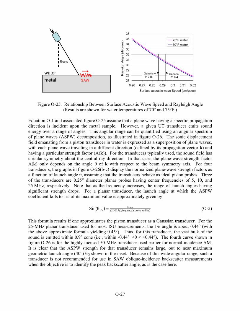
27
28
29
30
31
32
33
34
35
36
0.26 0.27 0.28 0.29 0.3 0.31 0.32
Surface acoustic wave Speed (cm/μsec)
Ray
leig
h A
ngle
(de
gree
s)
75°F water 70°F water
Generic Ti64
Generic IN718
metal
water
SAW
Generic Ti64
Generic IN718
Generic In 718
metal
θSAW
SAW
Generic Ti 6-4
Figure O-25. Relationship Between Surface Acoustic Wave Speed and Rayleigh Angle (Results are shown for water temperatures of 70° and 75°F.)
Equation O-1 and associated figure O-25 assume that a plane wave having a specific propagation direction is incident upon the metal sample. However, a given UT transducer emits sound energy over a range of angles. This angular range can be quantified using an angular spectrum of plane waves (ASPW) decomposition, as illustrated in figure O-26. The sonic displacement field emanating from a piston transducer in water is expressed as a superposition of plane waves, with each plane wave traveling in a different direction (defined by its propagation vector k) and having a particular strength factor (A(k)). For the transducers typically used, the sound field has circular symmetry about the central ray direction. In that case, the plane-wave strength factor A(k) only depends on the angle θ of k with respect to the beam symmetry axis. For four transducers, the graphs in figure O-26(b-c) display the normalized plane-wave strength factors as a function of launch angle θ, assuming that the transducers behave as ideal piston probes. Three of the transducers are 0.25″ diameter planar probes having center frequencies of 5, 10, and 25 MHz, respectively. Note that as the frequency increases, the range of launch angles having significant strength drops. For a planar transducer, the launch angle at which the ASPW coefficient falls to 1/e of its maximum value is approximately given by
1/ (2.3615)( )( )Sin( ) water
e frequency probe radius (O-2)
This formula results if one approximates the piston transducer as a Gaussian transducer. For the 25-MHz planar transducer used for most ISU measurements, the 1/e angle is about 0.44° (with the above approximate formula yielding 0.45°). Thus, for this transducer, the vast bulk of the sound is emitted within 0.9° cone (i.e., within -0.44° <θ < +0.44°). The fourth curve shown in figure O-26 is for the highly focused 50-MHz transducer used earlier for normal-incidence AM. It is clear that the ASPW strength for that transducer remains large, out to near maximum geometric launch angle (40°) θG shown in the inset. Because of this wide angular range, such a transducer is not recommended for use in SAW oblique-incidence backscatter measurements when the objective is to identify the peak backscatter angle, as is the case here.
O-27

ASPW Calculation For The 50-MHz FocusedTransducer
0.0
0.2
0.4
0.6
0.8
1.0
1.2
0 10 20 30 40 50 60Angle (degrees)
AS
PW
Str
en
gth
N
orm
aliz
ed
(M
ax
= 1
)
.
ASPW Calculations For 0.25"-Diameter Transducers
0.0
0.2
0.4
0.6
0.8
1.0
1.2
0 1 2 3 4 5Angle (degrees)
AS
PW
Str
en
gth
N
orm
aliz
ed
(M
ax
= 1
)
. 5 MHz planar
10 MHz planar
25 MHz planar
50 MHz focused
0.25”
F = 0.2”
Maximum geometric launch angle for focused transducer is = 38.7o
The emitted field is expressed as a sum of plane waves:
Each plane wave has a launch direction and a strength factor:
k
Strength A(θ)+
+
(a)
(b) (c)
G
ASPW Calculation For The 50-MHz FocusedTransducer
0.0
0.2
0.4
0.6
0.8
1.0
1.2
0 10 20 30 40 50 60Angle (degrees)
AS
PW
Str
en
gth
N
orm
aliz
ed
(M
ax
= 1
)
.
ASPW Calculations For 0.25"-Diameter Transducers
0.0
0.2
0.4
0.6
0.8
1.0
1.2
0 1 2 3 4 5Angle (degrees)
AS
PW
Str
en
gth
N
orm
aliz
ed
(M
ax
= 1
)
. 5 MHz planar
10 MHz planar
25 MHz planar
50 MHz focused
0.25”
F = 0.2”
0.25”
F = 0.2”
Maximum geometric launch angle for focused transducer is = 38.7o
The emitted field is expressed as a sum of plane waves:
Each plane wave has a launch direction and a strength factor:
k
Strength A(θ)
k
Strength A(θ)+
+
+
+
(a)
(b) (c)
G
Figure O-26. Angular Spectrum of Plane Waves Decomposition (a) Meaning, and Plane-Wave
Strength Factors for Four Transducers, (b) Three Planar, and (c) One Focused Before proceeding to actual measurements, it is useful to speculate on expected behaviors for SAW backscatter measurements conducted on three model microstructures. These scenarios are shown in figure O-27. For abusively machined surfaces as produced by the original equipment manufacturers (OEM), the situation appears to be intermediate between (2) and (3). (1) Undamaged microstructure that is uniform with depth.
(2) Surface damage where the near-surface microstructure gradually transforms with depth to that of the undamaged substrate.
(3) Surface damage where the near-surface microstructure abruptly transforms with depth to that of the undamaged substrate.
O-28

(1) (2) (3)
. # 2Microstr
Microstr
Gradual ChangeMicrostructure 2
Microstructur 1 ealone Microstructure 1
Microstructure 2
Microstructure 1 Microstructure 2
alone
Gra
du
al C
ha
nge
SA
W B
acks
catt
er
θ1 θ2 θ2 θ1 θ′2 θ′1
Figure O-27. Oblique Incidence SAW Backscatter for Different Microstructure Scenarios and
the Expected Dependence of Backscattering on the Probe Tilt Angle for Each (Here, the damage layer (Microstructure 2) is assumed to have a higher Rayleigh wave speed than the undamaged substrate (Microstructure 1), and the Rayleigh wave is assumed to penetrate into both layers.)
Based on discussions with Hak-Joon Kim [O-5], the following behaviors are expected: For (1): The peak backscatter angle will be independent of Rayleigh wave penetration
depth (i.e., independent of frequency), and approximately given by Snell’s law applied to the substrate. The angular width of the backscatter maximum will be near that expected from ASPW considerations.
For (2): The peak backscatter angle will depend on the Rayleigh wave penetration depth (i.e., depends on frequency). For low frequencies (large penetration depth), the peak angle will be near that for the undamaged microstructure. For high frequencies (shallow penetration depth), the peak angle will be that expected for the near-surface microstructure. The angular width of the backscatter maximum will generally be larger than that expected from ASPW considerations for a uniform microstructure, since for a given plane wave component, the Rayleigh angle depends upon depth.
For (3): The two separate microstructural regions likely have their own peak backscatter behaviors. The backscatter-versus-angle plot may display two separate maximum, one associated with each region. The relative strengths of the maxima will depend on the penetration depth, with the “undamaged microstructure” peak becoming more prominent as the penetration depth increases (i.e., as the frequency drops and more sound energy enters the substrate). For propagation within the plate-like damage layer, the peak backscatter angle can be expected to depend on both frequency and the damage layer thickness. The presence of the layer will perturb the peak backscatter angle for the substrate away from that expected for the substrate alone. Similarly, the presence of the substrate will perturb the peak backscatter angle away from that expected for guided waves within a free plate.
O-29

O.3.7 METHOD 2—OBLIQUE-INCIDENCE BACKSCATTER MEASUREMENTS ON A HEAT-TREATED Ti 6-4 SAMPLE. For the 25-MHz planar transducer of figure O-2(b), the surface acoustic wave penetration depth (about 120 microns) is considerably larger than the likely thickness of the damage layer in abusively machined turning samples (<50 microns). As previously discussed, the optimal use of Method 2 would confine most of the surface acoustic wave energy within the damage zone, requiring a higher-frequency planar transducer (not readily available). Alternatively, for proof-of-concept measurements, the available 25-MHz transducer could be used to study a sample having a deeper near-surface damage zone. Such a sample was produced via heat treatment, and then studied to gain further insight into the strengths and weaknesses of the oblique-incidence backscatter method. The sample in question, illustrated in figure O-28, became available from an ISU study involving the use of dye penetrants to detect fatigue cracks [O-6]. Measuring approximately 6 by 1 by 0.5, this Ti 6-4 rolled plate sample had fractured into two pieces during the fatigue process that was intended to promote crack growth. The upper surfaces of the two halves, which would serve as sound entry surfaces for UT measurements, were ground flat. Then, one half (denoted B1) was heat-treated to induce surface damage, and the other half (B2) was retained as an untreated reference sample. More specifically, sample B1 was heated in air at 950°C for 24 hours, causing an oxide scale to form, which was approximately 190 microns (7.5 mil) thick. Most of this scale flaked off easily after cooling, and the underlying surface was then lightly sanded with 400-grit sand paper to remove the remaining scale. Sample B1 lost about 14 mil of thickness during the heating/flaking/sanding operations, and displayed considerable surface pitting upon completion. Prior to heat treatment, samples B1 and B2 each had surface roughness values of Ra = 15 microinches. After heat treatment, sample B1 had a roughness of Ra = 115 microinches.
Specimen B2 (no heat treatment)
Specimen B1 (after heat treatmentand removal of oxide layer)
Large oxide flake (later removed)
Rolling direction
SAW pPropagation
Sample B2 (no heat treatment)
Sample B1 (after heat treatment and removal of oxide layer)
Large oxide flake (later removed)
direction
Ra = 115 microinches Ra = 15 microinches
Figure O-28. Ti 6-4 Rolled Plate Samples Used for SAW Backscatter Measurements (A large flake of the oxide layer was placed atop sample B1 to illustrate the color difference
between the oxide layer (dark brown) and the underlying metal (dark gray).) Metallography was not performed on sample B1 to determine the exact thickness of the damage layer. However, the heat treatment used here is identical to that used during an earlier ETC-1 program to produce an oxygen-enriched, hard alpha surface layer in Ti 6-4 samples. As
O-30

illustrated in figure O-29, the hard alpha layer in that earlier study was in excess of 100 microns deep [O-7].
(a) ETC-1 Ti 6-4
Heat-Treated Sample (Interior Region)
100
um
100
um
100
um
(b) ETC-1 Ti 6-4
Heat-Treated Sample (Near-Surface Region)
(c) ETC-3 Ti 6-4 Abusively
Machined Sample (Near-Surface Region)
Figure O-29. Microstructures of Base Metal (a) and Heat-Induced Surface Damage Layer, (b) Seen in an ETC-1 Ti 6-4 Sample After Similar Heat Treatment, and (c) The Near-Surface Microstructure of an Abusively Machined Ti 6-4 Turning Sample is Shown for Comparison
The oblique-incidence SAW backscatter method shown in figure O-24 was used to inspect samples B1 and B2. In this method, the absolute amplitude of the backscatter is not particularly important. Rather, microstructural differences (including surface damage) are signaled by a change in the transducer tilt angle for which the backscattered noise is maximized. Each measurement trial was begun by (1) leveling the sample; (2) performing a gimbal-gimbal angular scan to accurately locate the two probe tilt angles (θ and φ) for which the sound beam was normal to the sample; and (3) redefining each of these angles as 0° of absolute tilt. Figure O-30 shows the results of a typical gimbal-gimbal scan. There, the gated peak amplitude of the FW response from sample B2 is displayed as a function of the two probe tilt angles. The angles for which the maximum response was observed were subsequently redefined as θ = φ = 0.
O-31
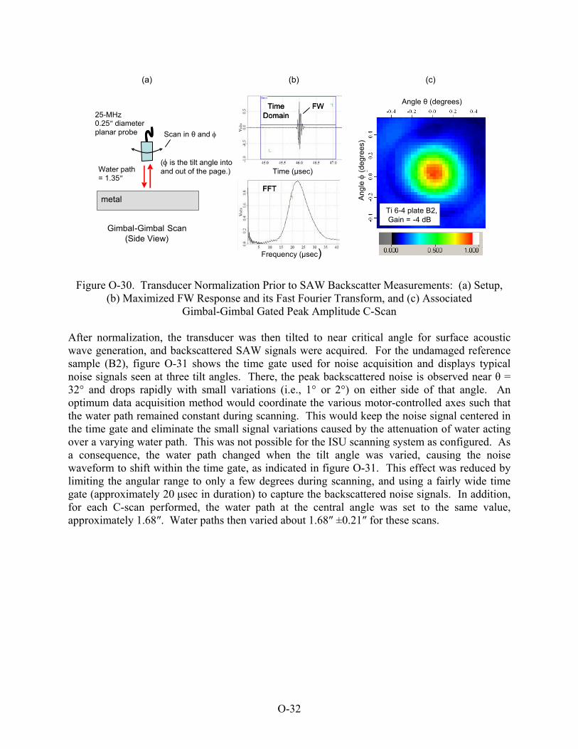
(a) (b) (c)
Time Domain
Time Domain
FFTFFT
Frequency (μsec)
Time (μsec)
FWAngle θ (degrees)
Ang
le (d
egre
es)
Ti64 plate B2, 4 dB Gain = -
FW
Ti 6-4 plate B2, - 4 dB Gain =
Water path = 1.35″
25-MHz 0.25″ diamet r eplanar probe Scan in θ and
( is the tilt angle into and out of the page.)
metal
Gimbal -Gimbal Scan (Side View)
Figure O-30. Transducer Normalization Prior to SAW Backscatter Measurements: (a) Setup, (b) Maximized FW Response and its Fast Fourier Transform, and (c) Associated
Gimbal-Gimbal Gated Peak Amplitude C-Scan After normalization, the transducer was then tilted to near critical angle for surface acoustic wave generation, and backscattered SAW signals were acquired. For the undamaged reference sample (B2), figure O-31 shows the time gate used for noise acquisition and displays typical noise signals seen at three tilt angles. There, the peak backscattered noise is observed near θ = 32° and drops rapidly with small variations (i.e., 1° or 2°) on either side of that angle. An optimum data acquisition method would coordinate the various motor-controlled axes such that the water path remained constant during scanning. This would keep the noise signal centered in the time gate and eliminate the small signal variations caused by the attenuation of water acting over a varying water path. This was not possible for the ISU scanning system as configured. As a consequence, the water path changed when the tilt angle was varied, causing the noise waveform to shift within the time gate, as indicated in figure O-31. This effect was reduced by limiting the angular range to only a few degrees during scanning, and using a fairly wide time gate (approximately 20 μsec in duration) to capture the backscattered noise signals. In addition, for each C-scan performed, the water path at the central angle was set to the same value, approximately 1.68″. Water paths then varied about 1.68″ ±0.21″ for these scans.
O-32

25 o 25°
30 o 30°
32 o 32°
SAW backscattered noise peaks when the probe tilt angle in water is near 32°.
SAW backscatter drops rapidly as the tilt angle is increased or decreased from32°. Here, the angle decreased by 2°.
If the tilt angle is reduced further, the backscattered noise will eventually begin to grow. This is now due to grain scattering from the bulk
wave in the metal. shear
Figure O-31. Oblique-Incident Backscatter Method Applied to Undamaged Ti 6-4 Plate Sample
B2 (Typical backscattered noise signals and their spectra are shown for three tilt angles. The 25-MHz, 0.25″ diameter planar transducer was used.)
Angle-X C-scans of backscattered SAW noise were then made using the setup shown in figure O-24(b). At each scan position, the observed A-scan noise signal was rectified, and its average value within the time gate was displayed in the C-scan image. For these C-scans, the surface acoustic waves propagated parallel to the long dimension of the sample, i.e., parallel to the rolling direction of the plate. For sample B1, some UT measurements were made after grinding but before heat treatment to verify that samples B1 and B2 had similar properties. Figure O-32 compares Angle-X C-scans of sample B1 made prior to and following heat treatment. The mean value of the peak backscattered noise angle is indicated by the vertical black line. Note in figure O-32 that measurements were made for both positive and negative tilt angles, but the regions of the sample scanned in the two trials, although overlapping, were not necessarily identical. Ideally, if the near-surface microstructure has translational symmetry in the x and y directions, then the magnitude of the peak noise angle should be the same for the scans over positive and negative angles. This is approximately the case in figure O-32.
O-33

Tilt Angle (degrees) Tilt Angle (degrees)
Late
ral P
osi
tion
X (
inch
es)
B1, before heat treat. Positive Tilt Angles.52 dB.
B1, before heat treat. Negative Tilt Angles.52 dB.
Tilt Angle (degrees) Tilt Angle (degrees)
Lat
eral
Pos
itio
n X
(in
ches
)
B1, after heat treat. Positive Tilt Angles.41 dB.
B1, after heat treat. Negative Tilt Angles.41 dB.
Low
Hig
hLo
wH
igh
Tilt Angle (degrees) Tilt Angle (degrees)
Late
ral P
osi
tion
X (
inch
es)
B1, before heat treat. Positive Tilt Angles.52 dB.
B1, before heat treat. Negative Tilt Angles.52 dB.
Tilt Angle (degrees) Tilt Angle (degrees)
Lat
eral
Pos
itio
n X
(in
ches
)
B1, after heat treat. Positive Tilt Angles.41 dB.
B1, after heat treat. Negative Tilt Angles.41 dB.
Low
Hig
hLo
wH
igh
Low
Hig
hLo
wH
igh
Figure O-32. Oblique-Incident Backscatter Method Applied to Ti 6-4 Plate Sample B1 Using a
25-MHz Planar Transducer Before (top) and After (bottom) Heat Treatment As shown in figure O-32, the heat-induced surface damage altered the Angle-X C-scans in four major ways: The probe angle that maximizes the surface acoustic wave backscatter is smaller after
heat treatment, having been reduced by about 2.8°. This implies that the heat treatment has increased the surface acoustic wave speed, in agreement with earlier ETC-1 studies, which found higher sonic wave speeds in oxygen-enriched hard alpha case material [O-7].
Backscattered noise amplitudes are about 13 dB higher after heat treatment, likely due to the much larger surface roughness (Ra = 115 μin after treatment compared to 15 μin prior to treatment). Because of the very smooth surface prior to heat treatment, backscattered noise there is presumably due to grain scattering only. After heat treatment, scattering from surface pitting also contributes.
After heat treatment, there is a broader range of angles for which backscattering is significant, i.e., the peak noise angle is less sharply defined. This is likely due to the variation of microstructure with depth. Before heat treatment, the surface acoustic wave
O-34

speed is presumably independent of depth, and that single speed is associated with a single optimal probe tilt angle for surface acoustic wave generation. After heat treatment, the near-surface microstructure varies with depth, as does the sound velocity. The range of sound velocities within the penetration depth of the surface acoustic wave is then associated with a range of optimal angles. In either case, the angular range is also broadened by the natural angular spectrum of the transducer about its central ray direction, as described in figure O-26.
After heat treatment, Angle-X C-scans contain strong diagonal features, i.e., regions of enhanced backscattering, which are elongated in a direction from upper left to lower right in the images. As illustrated in figure O-33, this is believed to be due to two effects: (1) backscatter from surface pitting and (2) details of the scanning method. A simple scanning algorithm was used for Angle-X C-scans at ISU in which the probe tilt angle (θ) and lateral probe coordinate (X) were varied independently. When θ is varied with X held constant, the surface point ensonified by the probe’s central ray shifts. During scanning, a fixed point on the surface is ensonified numerous times, corresponding to various combinations of the (θ, X) scan coordinates. Suppose there is a localized surface region of enhanced roughness (pitting) that generates enhanced surface acoustic wave noise. The locus of (θ, X) values for which the central ray strikes the center of this region defines an curved arc, which runs from upper left to lower right in figure O-33. Thus, a diagonal streak of high amplitude within the image is observed. The same effect is also at work in Angle-X C-scans made before heat treatment, but the scattering (from grain boundaries only) is evidently more uniform with lateral position. An optimal Angle-X scanning algorithm would, for a fixed scan coordinate X, adjust transducer motion in such a way that the central ray struck the same point on the surface (and with the same water path) as the tilt angle was varied. Such an optimal scanning method would simplify the interpretation of C-scan images, but was beyond the scope of the current program.
X
strong near-surface
scatterer
metal specimen
23 1
Late
ral P
ositi
on X
(in
ches
)
Tilt Angle θ (degrees)
Scan coordinates for which the central ray strikes a fixed
point on the surface.
(a) (b)
X
strong near-surface
scatterer
metal specimen
23 1
X
strong near-surface
scatterer
metal specimen
23 1
23 1
Late
ral P
ositi
on X
(in
ches
)
Tilt Angle θ (degrees)
Scan coordinates for which the central ray strikes a fixed
point on the surface.
Tilt Angle θ (degrees)
Scan coordinates for which the central ray strikes a fixed
point on the surface.
(a) (b)
Figure O-33. (a) A Strong SAW Scatterer, Such as a Surface Pit, Ensonified Multiple Times During an Angle-X Scan (b) (Those (θ, X) combinations form an arc in C-scan images.)
O-35

The measurements summarized in figure O-32 were made using the 25-MHz, 0.25″ diameter planar transducer operating at a 1.7″ water path. Figure O-34 displays the results of similar measurements made using a 10-MHz, 0.25″ diameter planar transducer operating at the same water path. Because these measurements were made after the heat treatment of sample B1, reference sample B2 was used to represent the “before heat treatment” condition. Angle-X C-scans were made for both positive and negative tilt angles. The effect of the heat treatment is to shift the peak noise angle downward. increase the magnitude of the backscattered noise. broaden the angular range of the noise peak. introduce more pronounced diagonal features into the C-scan images.
Low
Hig
hLo
wH
igh
Tilt Angle (degrees) Tilt Angle (degrees)
Lat
era
l Po
sitio
n X
(in
che
s)
B2, no heat treat. Positive Tilt Angles.54 dB.
B2, no heat treat. Negative Tilt Angles.54 dB.
Tilt Angle (degrees) Tilt Angle (degrees)
Late
ral P
ositi
on X
(in
ches
)
B1, after heat treat. Positive Tilt Angles.30 dB.
B1, after heat treat. Negative Tilt Angles.30 dB.
Figure O-34. Oblique-Incidence Backscatter Results for Ti 6-4 Plate Samples B2 (No Heat Treatment; Top) and B1 (After Heat Treatment; Bottom)
(A 10-MHz planar transducer was used.) As summarized in table O-3, the shift in the peak noise angle caused by the surface damage is 2.8° for the 25-MHz inspection, but only 0.5° for the 10-MHz inspection. This behavior can be understood from the penetration depth of the surface acoustic waves. At 25-MHz, the
O-36

penetration depth is approximately 120 microns. For the heat-damaged sample, much of the surface acoustic wave energy is then confined to the damage zone where the sound speed is appreciably higher than the undamaged material, leading to a large shift in the peak noise angle. For the 10-MHz measurement, the penetration depth is about 290 microns, so part of the surface acoustic wave senses the damage zone, and part propagates through the deeper undamaged metal. The average surface acoustic wave speed is then smaller and closer to that of undamaged metal, leading to a smaller shift in the peak backscattering angle. As indicated at the bottom of table O-3, Snell’s law can be used to relate the shift in the peak noise angle to a shift in the effective surface acoustic wave speed relative to undamaged metal. This velocity shift is 8.4% for the 25-MHz inspection, but only 1.4% for the 10-MHz inspection. These studies using the Ti 6-4 plate samples point out the benefits of varying the inspection frequency to obtain information about the depth of near-surface damage.
Table O-3. Angle at Which Peak Backscattering is Observed for Ti 6-4 Plate Samples B1 and B2
Sample/Frequency 25 MHz 10 MHz
Pristine (B1 or B2)
32.1° 32.2°
Heat-Treated (B1)
29.3° 31.7°
λSAW ~120 microns 8.6% difference in
νSAW
290 microns 1.4% difference in
νSAW
For the Ti 6-4 plate samples, it is clear that the peak backscatter angle depends on the surface acoustic wave propagation direction, which is (for the untreated surface) 32.1° in the rolling direction and 29.5° in the orthogonal (transverse) direction. This difference is evidently associated with texture (preferred crystalline axis directions) in the rolled plate samples. This finding further demonstrates that Method 2 is sensitive to microstructural differences in the SAW propagation direction if those differences influence sound velocity. The measurements on the Ti 6-4 plate samples also illustrate one major benefit of Method 2 (oblique-incidence backscatter) compared to Method 1 (normal-incidence AM). This concerns surface roughness. Roughness acts to modify the amplitudes of the responses observed with either method. As a general rule, roughness tends to decrease the FW and SAW signals observed using Method 1A or 1B, and to increase the backscattering observed using Method 2. For Method 1, such amplitude changes due to roughness can mask other amplitude changes due to machining-induced damage alone. Method 2, on the other hand, is not amplitude-based, but relies on the measurement of the peak noise angle. For Method 2, an increase in backscattering due to roughness can actually be beneficial, since it makes for larger noise signals that can be observed at lower inspection gain.
O-37

O.3.8 METHOD 2—OBLIQUE-INCIDENCE BACKSCATTER MEASUREMENTS ON Ti 6-4 TURNING SAMPLES. Method 2 was next applied to 34 Ti 6-4 turning samples having varying levels of near-surface damage. The 0.25″ diameter, 25-MHz planar transducer was again used. Because this inspection method relies on determining the angle at which peak backscattering is observed, care is required during setup to measure probe tilt angles accurately, taking into account the curvatures possessed by many of the turning samples. The procedure followed at ISU for this round of measurements is illustrated in figure O-35 and described below. 1. The sample was placed on a flat, level surface. At one location near the center of the
sample, the sound beam was made normal to the sample (see figure O-35(a)). This was done in the usual way by performing a gimbal-gimbal C-scan with the one-way water path near 1.35 inches. The pair of angles for which the FW response was maximized was defined as the origin for angular measurements: (θ, φ) = (0, 0).
2. With one angle fixed (φ = 0), the other angle (θ) was rotated in the positive direction to
near the proper angle for surface acoustic wave generation, about 30° (see figure O-35(b)). Generally speaking, the surface acoustic waves propagated parallel to the machining groove direction. This allowed for a longer scanning length in the X direction and reduced direct backscatter from the grooves. A preliminary Angle-X C-scan was performed in which both the tilt angle (θ) and lateral position (X) of the transducer were varied. The angle at which maximum backscatter was observed was noted, and a slight water path adjustment was made at this angle. After the adjustment, the arrival time of the peak backscattered response was at or very near 60 μsec, corresponding to a one-way water path of 1.75 inches. The goal was to have about the same arrival time for the peak backscattered response for each sample studied. As previously discussed, the water path changes when the probe angle is varied, and the attenuation of water thus acts over a different distance. This can affect the angular dependence of the backscattered response slightly. The water path adjustment procedure described here largely removes the effect of water attenuation changes on the peak response angle.
3. With the water path set, the Angle-X C-scan was repeated, with the probe tilt angle varying over a small positive range (about 6°). The tilt angle (θ+), at which the maximum backscatter was observed was recorded.
4. With no change to the water path, another Angle-X C-scan was performed, this time over a similar range of negative angles (see figure O-35(c)). Again, the tilt angle (θ-) for maximum backscatter was recorded. Note that for given scan coordinates (θ, X), the central ray will strike some specific point on the sample surface. In the course of the full Angle-X scan, all such points will form a line segment on the entry surface. For the C-scans of steps 3 and 4, “eyeball” adjustments were made to the lateral position of the transducer such that the two line segments were approximately overlapping.
5. From the results of the Angle-X scans over positive and negative angles, the average was computed: [ |θ+| + |θ-| ] / 2. This served as the best estimate of the probe tilt angle at which the maximum backscattered response was observed.
O-38

Side View (typically using a 1.35″ water path)
Scan in
metal specimen
scan in ( is tilt angle into and
out of page).
and Damaged samples are typically slightly bowed
Top View (positive θ) (typically using a 1.75″ waterpath at the central angle) (a)
(b)
(c)
Normalization performed near the center of the sample
metal sample
X
Top View (negative θ)
X
X machining grooves
Interrogated region on sample surface
X
measures approximately 0.3″ (beam width) by 8″ (X scan length
Figure O-35. Setup Details for UT Scans of ETC-3 Turning Samples (a) Gimbal-Gimbal Scan to Normalize Sound Beam to Sample, (b) Angle-X Scan Over Positive Tilt Angles, and
(c) Angle-X Scan Over Negative Tilt Angles Here damage, if any, is revealed by a change in the peak backscatter angle. Note that the full surface of a given coupon was not scanned. As illustrated in figure O-35, the beam footprint on the surface was about 0.3″ wide, and the interrogated surface region was roughly a 0.3″ wide by 0.8″ long strip near the coupon’s center. The measurement procedure was applied to both sides of 34 Ti 6-4, turned, forging coupons. The sample numbers, short-hand designations, and measured angles for these coupons are listed in table O-4. Nine coupons were identified as pristine, seven were identified as having shallow Type 1* damage (i.e., a near-surface amorphous layer), six as having medium Type 1* damage, seven as having deep Type 1* damage, and five as having Type 6* damage (re-embedded chips). Surface roughness in these coupons was primarily due to machining grooves. When measured in the direction perpendicular to the machining grooves, roughness values were generally modest, ranging from about Ra = 20 to 100 microinches within the suite of coupons. Each damaged coupon was only damaged on one face, so the opposite face effectively served as another pristine surface. In table O-4, the two principal sides of a given coupon were labeled A and B, using the convention that A is the upward facing surface when the sample number (punched into a smaller orthogonal face) is right-side-up (i.e., readily readable). From visual inspection, it was not always clear which face of a given coupon was intentionally damaged. Table O-4 and ensuing figures used “best guesses” as to which faces were pristine and which were damaged. Generally speaking, Side A was regarded as the damaged face unless there was some evidence to the contrary.
O-39

Table O-4. Ti 6-4, Option C Turning Samples Examined Using SAW Backscatter (The angle at which peak backscattering was observed is listed. The dimensions of each coupon were approximately 2″ by 1″ by 0.2″.)
Side A Peak Backscatter Angles
(degrees) Side B Peak Backscatter Angles
(degrees)
Alloy Damage
Type Full Sample Number
Shorthand Name Used in Figures
Round- Robin
Sample?
Positive Angles; Main Peak (2nd Peak)
Negative Angles; Main Peak (2nd Peak)
Positive Angles; Main Peak (2nd Peak)
Negative Angles; Main Peak (2nd Peak)
Damaged Side Notes
Ti 6-4 Pristine C-Ti-T-P-1-101607 P1 Yes 30.3 -30.2 30.1 -30.1 Neither
Ti 6-4 Pristine C-Ti-T-P-2-101607 P2 30.2 -29.9 30.2 -30.0 Neither
Ti 6-4 Pristine C-Ti-T-P-3-101607 P3 30.1 -29.9 30.2 -30.2 Neither
Ti 6-4 Pristine C-Ti-T-P-4-101607 P4 30.2 -30.2 30.2 -30.1 Neither
Ti 6-4 Pristine C-Ti-T-P-5-101607 P5 30.1 -30.1 30.2 -30.1 Neither
Ti 6-4 Pristine C-Ti-T-P-6-101607 P6 30.2 -30.0 30.2 -30.0 Neither
Ti 6-4 Pristine Ti-T-P-6-060208 P9 30.0 -30.1 30.1 -30.0 Neither
Ti 6-4 Pristine Ti-T-P-16-060208 P16 29.8 -29.9 29.8 -29.8 Neither
Ti 6-4 Pristine Ti-T-P-1-0611 P1A Yes 30.3 -30.3 30.4 -30.3 Neither
All measurements on pristine Option C coupons were taken during a 1-week period in early May 2008, except for P9 (30 September 2008) and P16 (09 Feb 2009). The water temperature was likely several degrees colder for P16 than for the others. P1A is the lone Option A coupon; it was cut from a different washer and measured on 28 March 2008. For P1A, the orientation of the sample number was not recorded.
Ti 6-4 Type 1 shallow
Ti-T-T1-1-080107 S1 Yes 30.0 -29.9 30.4 -30.4 Side A
Ti 6-4 Type 1 shallow
Ti-T-T1-2-080107 S2 30.2 -30.1 30.4 -30.4 Side A
Ti 6-4 Type 1 shallow
Ti-T-T1-3-080107 S3 30.3 -30.2 30.6 -30.5 Side A
Ti 6-4 Type 1 shallow
Ti-T-T1-4-080107 S4 30.1 -30.0 30.3 -30.3 Side A
Ti 6-4 Type 1 shallow
Ti-T-T1-5-080107 S5 30.3 -30.2 30.5 -30.4 Side A
Ti 6-4 Type 1 shallow
Ti-T-T1-6-080107 S6 30.0 -30.0 30.3 -30.3 Side A
Ti 6-4 Type 1 shallow
Ti-T-T1-7-080107 S7 Yes 30.0 -30.0 30.5 -30.4 Side A
All measurements on Type 1 shallow coupons were completed during a 3-day period in late April 2008. Based on visual inspection, the two sides of a given coupon were designated as either damaged or pristine. The orientation of the sample number was not recorded. Results for the apparently damaged side are reported in the Side A columns. Results for the pristine side are reported in the Side B columns.
Ti 6-4 Type 1 medium
Ti-T-T1A-9-080606-MED M9 Yes 28.8 (30.5) -28.7 (-30.3) 30.2 -30.2 Side A
Ti 6-4 Type 1 Medium
Ti-T-T1A-10-080606-MED M10 28.9 (30.7) -28.9 (-30.6) 30.3 -30.3 Side A
Ti 6-4 Type 1 Medium
Ti-T-T1A-11-080606-MED M11 28.7 (30.7) -28.7 (-30.8) 30.0 -30.0 Side A
Ti 6-4 Type 1 Medium
Ti-T-T1A-12-080606-MED M12 28.8 (30.7) -28.8 (-30.7) 30.3 -30.4 Side A
Ti 6-4 Type 1 Medium
Ti-T-T1A-15-080606-MED M15 Yes 28.9 (30.6) -28.8 (-30.6) 30.3 -30.3 Side A
Ti 6-4 Type 1 medium
Ti-T-T1A-16-080606-MED M16 28.9 (30.8) -28.8 (-30.7) 30.1 -30.0 Side A
All measurements on Type 1 medium coupons were completed during a 3-day period in late August 2008, except for M10 (01 August 08) and M15 (11 May 09). Relative to the sample number, the damaged side was always Side A.
O-40

O-41
Table O-4. The Ti 6-4, Option C, Turning Samples Examined Using SAW Backscatter (Continued) (The angle at which peak backscattering was observed is listed. The dimensions of each coupon were approximately 2″ by 1″ by 0.2″.)
Side A Peak Backscatter Angles
(degrees) Side B Peak Backscatter Angles
(degrees)
Alloy Damage
Type Full Sample Number
Shorthand Name Used in Figures
Round- Robin
Sample?
Positive Angles; Main Peak (2nd Peak)
Negative Angles; Main Peak (2nd Peak)
Positive Angles; Main Peak (2nd Peak)
Negative Angles; Main Peak (2nd Peak)
Damaged Side Notes
Ti 6-4 Type 1 deep
C-Ti-T-T1D-1-101607 D1 Yes 30.3 -30.3 30.7 (28.3) -30.6 (-28.2) Side B
Ti 6-4 Type 1 deep
C-Ti-T-T1D-2-101607 D2 30.3 -30.2 29.2 (30.6) -29.1 (-30.5) Side B
Ti 6-4 Type 1 deep
C-Ti-T-T1D-3-101607 D3 30.3 -30.3 29.1 (30.8) -29.0 (-30.6) Side B
Ti 6-4 Type 1 deep
C-Ti-T-T1D-4-101607 D4 30.3 -30.3 29.1 (30.8) -29.0 (-30.7) Side B
Ti 6-4 Type 1 deep
C-Ti-T-T1D-5-101607 D5 30.3 -30.3 29.3 (30.8) -29.0 (-30.6) Side B
Ti 6-4 Type 1 deep
C-Ti-T-T1D-6-101607 D6 30.2 -30.2 29.2 (30.8) -29.0 (-30.6) Side B
Ti 6-4 Type 1 deep
Ti-T-T1-2-080107b D2b Yes 30.4 -30.3 29.2 (31.0) -28.9 (-30.8) Side B
All measurements on Type 1 deep coupons were completed in a 2-week period from 21 April to 02 May 2008. Relative to the sample number orientation, the damaged side was Side B for all coupons. Coupon D1 differs from the others in that the higher-angle backscatter peak on the damaged side was the dominant of the two peaks.
Ti 6-4 Type 6 Ti-T-T6-1-080508 T6-1 Yes 30.5 -30.5 30.4 -30.3 Side B
Ti 6-4 Type 6 Ti-T-T6-2-080508 T6-2 Yes 30.3 -30.3 30.4 -30.4 Side A
Ti 6-4 Type 6 Ti-T-T6-7-080508 T6-7 Yes 30.2 -30.3 30.2 -30.2 Side A
Ti 6-4 Type 6 Ti-T-T6A-15-080602 T6-15 Yes 30.0 -30.0 30.3 -30.3 Side A
Ti 6-4 Type 6 Ti-T-T6A-16-080602 T6-16 30.1 -30.1 30.3 -30.3 Side A
Dates of measurements for Type 6 coupons were as follows: T6-1 (21 January 09); T6-1 (10 March 09); T6-7 (11 May 09); T6-15 (1 May 09); T6-16 (20 January 09).

Representative examples of the data acquired during the scans of Ti 6-4 coupons are shown in figures O-36 through O-40. Figure O-36 shows typical backscattered responses for one (θ, X) location each on the pristine and damaged sides of coupon C-Ti-T-T1D-5-101607 (deep Type 1* damage). The transducer tilt angle is 30.0° for each surface. This is near the peak backscattering angle for the pristine side (30.3°), but well above the peak angle for the damaged side (29.2°). As a consequence, the observed backscattered noise signal is much larger for the pristine side in figure O-36. As indicated in figure O-36, the time gate used for backscatter measurements typically ranged from 52 to 68 μsec, with the one-way water path being near 1.75 inches at the center of that gate. The primary quantity chosen to display in Angle-X C-scan images was again the rectified average voltage level within the gate, which served as a measure of the total observed backscattering.
SAW backscatter
signal
Time gate for backscatter
measurementelectronic noise
Pristine side of coupon D5
θ = 30 o, Gain = 56 dB
Damaged side of coupon D5
θ = 30 o, Gain = 56 dB
SAW backscatter
signal
Time gate for backscatter
measurementelectronic noise
Pristine side of coupon D5
θ = 30 o, Gain = 56 dB
Damaged side of coupon D5
θ = 30 o, Gain = 56 dB
Figure O-36. Examples of Backscattered SAW Signals and Their Spectra Observed in Inspections of Ti 6-4 Turning Surfaces: Pristine Side (top) and Damaged Side (bottom) of
Coupon D5 for an Inspection Angle of 30° (At this angle, backscatter from the pristine side is nearly maximized, but backscatter from the damaged side is weak.)
Figure O-37 shows Angle-X C-scans for four surfaces: two pristine and two with deep Type 1* damage. In such images, red indicates high and blue indicates low average backscatter response, but it should be noted that equipment gain settings and/or color-bar thresholds are often different for different images. The peak responses for the pristine surfaces are observed to occur at a
O-42

higher incidence angle (|θ| ≈ 30°) compared to those of the damaged surfaces (|θ| ≈ 29°). Such an angular difference would be expected if the effect of the damage increased the elastic stiffness in the near-surface region, and hence, increased the surface acoustic wave speed. Also note that the peak backscatter angle is approximately independent of the lateral position X for the upper two (pristine) surfaces in figure O-37, but the angle varies slightly with X for the lower two (damaged) surfaces. This is a consequence of coupon curvature, which was usually much more pronounced for damaged samples than for pristine samples. As noted earlier, for many Ti 6-4 turning samples the damaged face had a modest convex curvature, which was presumably due to stress relief when the coupon was cut from the turning washer.
Tilt Angle (degrees) Tilt Angle (degrees)
Late
ral P
ositi
on X
(in
ches
) Specimen D1.Pristine Face.Negative Tilt Angles53 dB.
Specimen P1. Pristine FacePositive Tilt Angles.53 dB.
Tilt Angle (degrees) Tilt Angle (degrees)
Late
ral P
ositi
on X
(in
ches
) Specimen D4 Damaged FacePositive Tilt Angles.53 dB.
Specimen D5.Damaged Face.Negative Tilt Angles56 dB.
Slanting of high-noise region is due to slight convex curvature of specimen surface.
High Backscatter
Low Backscatter
Tilt Angle (degrees) Tilt Angle (degrees)
Late
ral P
ositi
on X
(in
ches
) Specimen D1.Pristine Face.Negative Tilt Angles53 dB.
Specimen P1. Pristine FacePositive Tilt Angles.53 dB.
Tilt Angle (degrees) Tilt Angle (degrees)
Late
ral P
ositi
on X
(in
ches
) Specimen D4 Damaged FacePositive Tilt Angles.53 dB.
Specimen D5.Damaged Face.Negative Tilt Angles56 dB.
Slanting of high-noise region is due to slight convex curvature of specimen surface.
High Backscatter
Low Backscatter
High Backscatter
Low Backscatter
Figure O-37. Oblique-Incident Backscatter Method Applied to Four Ti 6-4, Option C, Turning
Samples Using a 25-MHz Planar Transducer (Angle-X C-scans are shown for inspections of two pristine surfaces (top) and two Type 1* deep-damaged surfaces (bottom).)
Other examples of Angle-X C-scans are shown in figure O-38. Where scans for the pristine and damaged sides of two Ti 6-4 coupons are compared, namely, S7 having shallow Type 1* damage and M10 having medium Type 1* damage. For coupon S7, the shift in the peak response angle for the two sides is small but noticeable, being about 0.3°. For coupon M10, the Angle-X C-scans of the pristine and damaged sides are markedly different, both in the angular location of the dominant peak and in the manner in which backscatter varies with angle.
O-43

Tilt Angle (degrees) Tilt Angle (degrees)
Late
ral P
ositi
on X
(in
ches
) Specimen S7.Pristine Face.Negative Angles56 dB.
Specimen M10. Pristine FacePositive Angles56 dB.
Tilt Angle (degrees) Tilt Angle (degrees)
Late
ral P
osi
tion
X (
inch
es) Specimen M10
Damaged FacePositive Angles.57 dB.
Specimen S7.Damaged Face.Negative Angles56 dB.
Slanting of high-noise region is due to slight convex curvature of specimen surface.
High Backscatter
Low Backscatter
Tilt Angle (degrees) Tilt Angle (degrees)
Late
ral P
ositi
on X
(in
ches
) Specimen S7.Pristine Face.Negative Angles56 dB.
Specimen M10. Pristine FacePositive Angles56 dB.
Tilt Angle (degrees) Tilt Angle (degrees)
Late
ral P
osi
tion
X (
inch
es) Specimen M10
Damaged FacePositive Angles.57 dB.
Specimen S7.Damaged Face.Negative Angles56 dB.
Slanting of high-noise region is due to slight convex curvature of specimen surface.
High Backscatter
Low Backscatter
High Backscatter
Low Backscatter
Figure O-38. Oblique-Incident Backscatter Method Applied to the Pristine (top) and Damaged (bottom) Sides of two Ti 6-4, Option C, Turning Samples (Angle-X C-Scans on the left-hand
side are for Type 1* shallow damage coupon S7. Right-hand side C-scans are for Type 1* medium damage coupon M10.)
For measurements made using the 25-MHz transducer, the backscattering-vs-angle function for each pristine surface generally has a single, strong backscatter peak, with that peak occurring in the range from 30.0° <|θ| <30.5°. As the angle |θ| is lowered from this dominant peak, the backscattered response first drops rapidly and then begins to slowly rise, eventually forming a broad secondary maximum. This secondary maximum occurs for tilt angles too shallow to excite surface acoustic waves, which is believed to be associated with grain noise scattering by the bulk shear wave propagating in the metal. For damaged surfaces, the situation is more complex. In addition to the sharp primary (surface acoustic wave) peak and the broad (shear wave) peak, a third peak is sometimes observed at a higher angle than the primary maximum. This extra peak can generally be observed in the deep- and medium-damaged Ti 6-4 coupons, but not the shallow-damaged coupons. Two examples are shown in figure O-39 with the various peaks labeled.
O-44

-30.6 -29.0
“Deep” Damage Specimen C-Ti-T-T1D-6-101607; 56 dB Gain
Tilt Angle (degrees)La
tera
l Pos
ition
X (
inch
es)
High Backscatter
Low Backscatter
-30.6 -29.0
Tilt Angle (degrees)
29.2 30.6
“Deep” Damage Specimen C-Ti-T-T1D-2-101607; 56 dB Gain
Late
ral P
ositi
on X
(in
ches
)
Primary SAW peak
Backscatter from bulk
shear waves ?
Primary SAW peak
Extra peak (SAW backscatter from
undamaged metal ?)
Extra peak
-30.6 -29.0
“Deep” Damage Specimen C-Ti-T-T1D-6-101607; 56 dB Gain
Tilt Angle (degrees)La
tera
l Pos
ition
X (
inch
es)
High Backscatter
Low Backscatter
High Backscatter
Low Backscatter
-30.6 -29.0
Tilt Angle (degrees)
29.2 30.6
“Deep” Damage Specimen C-Ti-T-T1D-2-101607; 56 dB Gain
Late
ral P
ositi
on X
(in
ches
)
-30.6 -29.0
Tilt Angle (degrees)
29.2 30.629.2 30.6
“Deep” Damage Specimen C-Ti-T-T1D-2-101607; 56 dB Gain
Late
ral P
ositi
on X
(in
ches
)
Primary SAW peak
Backscatter from bulk
shear waves ?
Primary SAW peak
Extra peak (SAW backscatter from
undamaged metal ?)
Extra peak
Figure O-39. Angle-X C-Scans for two Type 1* Deep-Damaged Surfaces, Showing Multiple Peaks in the Backscattered Response at Various Transducer Tilt Angles
The reason for the additional peak is not known, but various possibilities have been suggested. The damage layer is not uniform over the sample surface.
The double peak structure is a manifestation of a two-layer microstructure having a somewhat abrupt transition.
Backscatter from surface acoustic waves and direct backscatter from topological features have different peak angles.
Figure O-39 shows that the probe tilt angle at which the secondary (extra) maximum occurs is roughly the same as (but slightly higher than) the primary maximum of pristine surfaces. For a given damaged coupon, the damage may not be uniform across the surface. Visual inspection reveals that for some damaged coupons, the surface structure varies when scanning laterally in the direction perpendicular to the machining grooves (i.e., across the 1″ dimension of the coupon). The sound beam footprint on the surface is fairly wide, i.e., about 0.3″ in diameter. Part of the beam may be striking a damaged surface area and part may be striking a relatively undamaged area; and each of these may give rise to separate backscattered surface acoustic wave response peaks. Alternatively, the damaged surface may be relatively uniform in the lateral directions, but the change in sound speed with depth from the damaged to the undamaged microstructure may be rather abrupt. In that case, the microstructural depth profile will resemble that shown in figure O-27 (case 3), and two SAW noise peaks may occur with one associated with each layer of microstructure. A third possibility relies on the notion that there are actually two phenomena that contribute to the observed noise signal: (1) backscattering by propagating surface acoustic waves as they encounter grain boundaries and surface features (pits, scratches, etc.); and (2) direct backscatter of the longitudinal wave in water from the surface features themselves. It could be that each of these phenomena has its own peak backscattering angle, and
O-45

that there are differences in the topologies of pristine and damaged surfaces that lead to two separate peaks observed for the damaged surfaces. For proof-of-concept purposes, it is sufficient to observe that SAW backscatter measurements are able to distinguish damaged from undamaged surfaces of Ti 6-4. However, knowledge of the reasons behind the double-peak structures in figure O-39 could be useful for guiding future work to optimize the inspection method. The Angle-X scans illustrated thus far have all been for Type 1* damage (amorphous layer). Figure O-40 shows an example for Ti 6-4 coupons having intended Type 6* damage (re-embedded chips). For this and similar coupons, the peak backscatter angle for the pristine side is typically 30.4° ±0.1° while the damaged side is about 0.2° lower. Comparing figures O-25 and O-40, it is evident that the effect of the Type 6* damage on SAW backscatter is similar to shallow Type 1* damage, i.e., (1) the peak backscatter angle is slightly reduced, (2) the damaged side of the coupon exhibits a larger overall backscatter amplitude than the pristine side (presumably due to the greater surface roughness), and (3) the damaged side has a larger variation of backscatter with lateral position X (presumably due to the nonuniformity of the damage).
Tilt Angle (degrees) Tilt Angle (degrees)
La
tera
l Po
sitio
n X
(in
ches
)
Face “B”.Positive Angles.57 dB gain.
Face “A”Positive Angles57 dB.
30.330.1
High Backscatter
Low Backscatter
Face “B” (Pristine) (Ti-T-T6A-16-080602)
Face “A” (Damaged) (Ti-T-T6A-16-080602)
Tilt Angle (degrees) Tilt Angle (degrees)
La
tera
l Po
sitio
n X
(in
ches
)
Face “B”.Positive Angles.57 dB gain.
Face “A”Positive Angles57 dB.
30.330.1
High Backscatter
Low Backscatter
High Backscatter
Low Backscatter
Face “B” (Pristine) (Ti-T-T6A-16-080602)
Face “A” (Damaged) (Ti-T-T6A-16-080602)
Figure O-40. Oblique-Incident Backscatter Method Applied to the two Faces of Ti 6-4, Option C, Type 6* Turning Sample Ti-T-T6A-16-080602
For the 34 Ti 6-4 coupons that were studied, figure O-41 displays the measured probe tilt angles for peak backscatter. For pristine surfaces, there was always a single, well-defined angle at which peak backscattering was observed. For some damaged surfaces, two maxima were observed and both were plotted, as shown in figure O-41. The following points can be made in summary:
For the suite of pristine coupons, the peak angle was approximately the same for all
coupons, with similar results for both the Side A and Side B surfaces. Water temperature variations likely explain the minor difference between the 29.8° for coupon P16
O-46

(measured in winter) and the 30.0°-30.3° range for the other pristine coupons (measured during warmer months). Recall that a 5°F decrease in water temperature lowers the peak backscatter angle by 0.2°. In hindsight, it would have been best to record the water temperature for all measurements, and then to correct backscatter angles for temperature variations. Unfortunately, water temperatures were not recorded for all the measurements reported. Fortunately, in most cases involving damaged coupons, the measurements on the pristine and damaged sides of a given coupon were usually made on the same day.
For the suite of shallow damage Type 1* coupons, each coupon behaved similarly. A
single backscatter peak was observed on each side, with the angle for the damaged side always being slightly lower than the undamaged side. The average angular difference between the two sides was 0.3°. The behavior of Type 6* damaged coupons was similar, although the downward angular shift due to the damage was a bit smaller.
Deep and medium damage Type 1* coupons all behaved similarly, with the exception of
D1, whose damaged side had somewhat different backscatter properties. Damaged surfaces exhibited two maxima, with the one at the lower angle generally being the more prominent. The average angular difference between the single peak on the pristine side, and the prominent peak on the damaged side was about 1.3° (excluding D1).
For all damaged surfaces (except D1 and T6-7), if only the most prominent backscatter
peak is considered, the effect of the damage is to lower the peak response angle relative to the pristine side of the coupon (i.e., to increase the effective surface acoustic wave speed). This was also the case for the heat-damaged Ti 6-4 rolled plate sample B1 discussed earlier. In that case, the damage produced a drop in the peak noise angle of 2.8° for similar measurements using the same transducer. (However, the damage zone for the rolled plate sample is believed to be much thicker than the Option C turning samples.)
For the 25-MHz transducer used here, the surface acoustic wave penetrates about 120
microns below the surface. This is likely well beyond the damage zone, particularly for the shallow damage coupons. Thus, peak angle shifting in these coupons due to damage would likely be considerably larger at higher inspection frequencies.
O-47

Figure O-41. Transducer Tilt Angles Producing Maximized Backscattered Surface Acoustic Wave Responses Showing Results for Various Ti 6-4 Turning Samples
As noted above, the 34 coupons became available for study at different times, and water temperature variations over the measurement period likely contributed to some of the scatter in the peak angles for the pristine surfaces shown in figure O-41. However, texture variations within forgings may also be playing a role. In ETC-2 studies of Ti 6-4 forgings, UT properties were found to vary systematically with position and propagation direction within forgings [O-8]. An example is shown in figure O-42 for measured longitudinal velocities. Similar percentage variations would be expected for other wave types. Thus, surface acoustic wave speeds and hence peak backscattered response angles would be expected to vary with position within a forging. A pristine washer cut from a forging at one axial location may have different properties than a similar pristine washer cut at a different axial location. This may be one source of the small differences in the average peak response angles shown in figure O-41 for the five groups of undamaged surfaces. Fortunately, the two major surfaces on opposite sides of a given coupon are only separated by 0.2″, and thus their gross microstructures are expected to be very similar (before damage is induced). Therefore, comparative measurements on these two surfaces are expected to be unaffected by metal texture variations.
Pristine Type-1* “Shallow”
Type-6*
Type - 1* “Medium”
Type - 1* “ Deep ”
* * * * * *
Peak Backscatter Angle (25 MHz)
* * * ** *
Ti 6-4 Type-1 "Shallow" Coupons
28.0
28.5
29.0
29.5
30.0
30.5
31.0
31.5
32.0
S1 S2 S3 S4 S5 S6 S7
Specimen Designation
Peak Angle (degrees)
Undamaged
Damaged
Peak Backscatter Angle (25 MHz)Ti 6-4 Type-1 "Medium" Coupons
Peak Backscatter Angle (25 MHzs)
n Ti 6-4 Type-1 "Deep" Coupo
28.0 28.5 29.0 29.5 30.0 30.5 31.0 e31.5 32.0
D1 D2 D3 D4 D5 D6 D2b Specimen Designation
Peak Angl (degrees)
UndamagedDamaged (Peak 1)Damaged (Peak 2)
?
28.0
28.5
29.0
29.5
30.0
30.5
31.0
31.5
32.0
M9 M10 M11 M12 M15 M16
Specimen Designation
Peak Angle (degrees) UndamagedDamaged (Peak 1)Damaged (Peak 2)
Peak Backscatter Angle (25 MHz)Ti 6-4 Type-6 Coupons
28.0
28.5
29.0
29.5
30.0
30.5
31.0
31.5
32.0
T6-1 T6-2 T6-7 T6-15 T6-16
Specimen Designation
Peak Angle (degrees)
Undamaged
Damaged
Peak Backscatter Angle (25-MHz) Ti 6-4 Type 1 Shallow Coupons
28.0
28.5
29.0
29.5
30.0
30.5
31.0
31.5
32.0
S1 S2 S3 S4 S5 S6 S7
Sample Designation
Pe
ak
An
gle
(d
egre
es)
Undamaged
Damaged
Peak Backscatter Angle (25-MHz) Ti 6-4 Pristine Coupons
28.0 28.5 29.0 29.5 30.0 30.5 31.0 31.5 32.0
P1 P2 P4 P5 P6 P9
Sample Designation
Pe
ak
An
gle
(d
egre
es) Side B
Side A
P1AP16P3
Pristine
* *
Peak Backscatter Angle (25-MH ) zTi 6-4 Type 1 Deep Coupons
28.0 28.5 29.0 29.5 30.0 30.5 31.0 31.5 32.0
D1 D2 D3 D4 D5 D6 D2b Sample Designation
Pe
ak
An
gle
(d
egre
es)
UndamagedDamaged (Peak 1)Damaged (Peak 2)
Deep” 1* “Type
* *
Peak Backscatter Angle (25-MHz)Ti 6-4 Type 1 Medium Coupons
28.0
28.5
29.0
29.5
30.0
30.5
31.0
31.5
32.0
M9 M10 M11 M12 M15 M16Sample Designation
Pe
ak
An
gle
(d
egre
es)
UndamagedDamaged (Peak 1)Damaged (Peak 2)
”Medium1* “Type ”Shallow1* “Type
* ***
Peak Backscatter Angle (25-MHz)Ti 6-4 Type 6 Coupons
28.0
28.5
29.0
29.5
30.0
30.5
31.0
31.5
32.0
T6-1 T6-2 T6-7 T6-15 T6-16
Sample Designation
Pe
ak
An
gle
(d
egre
es)
Undamaged
Damaged
6*Type
** **?
O-48

Measured longitudinal wave sound velocities for propagation in the axial and radial directions through ETC-2 forging-flowline coupons. (Units are centimeters/microsec.)
HW: Velocity Vs. Coupon Number
0.614
0.615
0.616
0.617
0.618
0.619
0.62
0.621
0.622
0.623
HW1 HW2 HW3 HW4 HW5 HW6 HW7 HW8
Coupon Number
Velo m/us)city (c
Axial Radial
GE: Velocity Vs. Coupon Number
0.615
0.616
0.617
0.618
0.619
0.62ocity (
0.621
0.622
GE1 GE4 GE5 GE6 GE7Coupon Number
Vel cm/us)
AxialRadial
PW: Velocity Vs. Coupon Number
0.616
0.617
0.618
0.619
0.62
0.621ocity (
0.622
0.623
PW1 PW2 PW4 PW5 PW 6Coupon Number
PW7 PW8
Vel cm/us)
AxialRadial
HW: Velocity vs Coupon Number
0.614
0.615
0.616
0.617
0.618
0.619
0.62
0.621
0.622
0.623
HW1 HW2 HW3 HW4 HW5 HW6 HW7 HW8
Coupon Number
Ve
loc
ity
(c
m/u
s)
Axial Radial
GE: Velocity vs Coupon Number
0.615
0.616
0.617
0.618
0.619
0.62 0.621
0.622
GE1 GE4 GE5 GE6 GE7Coupon Number
Ve
loc
ity
(c
m/u
s)
AxialRadial
PW: Velocity vs Coupon Number
0.616
0.617
0.618
0.619
0.62 0.621
0.622
0.623
PW1 PW2 PW4 PW5 PW 6Coupon Number
PW7 PW8
Ve
loc
ity
(c
m/u
s)
AxialRadial
Figure O-42. Velocity Variations Observed in an ETC-2 Study of Coupons cut From
Three OEM-Supplied Ti 6-4 Forgings Because of texture variations within forgings, the optimal situation would be to base damage assessment at a given site solely on measurements performed at that site. In principle, this is possible by examining the frequency dependence of the backscattered response, since frequency determines the depth of surface acoustic wave penetration. For undamaged samples, the metal microstructure will be approximately independent of depth over short distances. However, for damaged samples, the near-surface microstructure will be altered, and the overall microstructure will vary with depth. If the damage alters the sound speed, as assumed here, one would expect that the peak angle for the backscattered response will depend on frequency for a damaged sample, but not for an undamaged one. Two approaches for damage detection and assessment at a fixed measurement site are possible. On the one hand, one can use two separate transducers having different center frequencies, and then look for differences between the two peak response angles. Alternatively, one can employ a single broadband transducer and develop analysis tools to extract a peak angle vs frequency curve from the raw backscattered responses. These are both topics for future research as they were beyond the scope of the present study. However, for one Ti 6-4 turning sample, the two-transducer approach was briefly investigated. The two-transducer approach has already been demonstrated using the heat-treated Ti 6-4 rolled plate samples, as summarized in table O-3. Figure O-43 shows the summary of an initial attempt at a similar two-transducer measurement using the damaged side of Ti 6-4 turning sample C-Ti-T-T1D-6-101607 (Type 1* deep damage). SAW backscatter measurements on that coupon, using the 25-MHz planar transducer, were already in hand. Given the thinness of the damage layer, it would be appropriate to choose a higher inspection frequency for the second
O-49

transducer. This was not possible with the available equipment, but a lower-frequency transducer was available (10 MHz, 0.25″ diameter). For the 25- and 10-MHz transducer pair, surface acoustic wave penetration depths in Ti 6-4 were about 120 and 300 microns, respectively. This compares to an expected damage layer thickness of about 50 microns.
-30.6 -29.0
“Deep” Damage Specimen C-Ti-T-T1D-6-101607; 56 dB Gain
Tilt Angle (degrees)
Lat
era
l Po
sitio
n X
(in
ches
)
High Backscatter
Low Backscatter
-30.3-28.8
Tilt Angle (degrees)
30.6
“Deep” Damage Specimen C-Ti-T-T1D-6-101607; 50 dB Gain
Lat
era
l Po
sitio
n X
(in
ches
)“Primary”
peak
Backscatter from bulk
shear waves
“Secondary”peak
25-MHz Inspection 10-MHz Inspection
“Primary”peak
“Secondary”peak
-30.6 -29.0
“Deep” Damage Specimen C-Ti-T-T1D-6-101607; 56 dB Gain
Tilt Angle (degrees)
Lat
era
l Po
sitio
n X
(in
ches
)
High Backscatter
Low Backscatter
High Backscatter
Low Backscatter
-30.3-28.8
Tilt Angle (degrees)
30.6
“Deep” Damage Specimen C-Ti-T-T1D-6-101607; 50 dB Gain
Lat
era
l Po
sitio
n X
(in
ches
)“Primary”
peak
Backscatter from bulk
shear waves
“Secondary”peak
25-MHz Inspection 10-MHz Inspection
“Primary”peak
“Secondary”peak
Figure O-43. Comparisons of Angle-X C-Scans for SAW Backscatter Measurements Made Using 25- (left) and 10-MHz (right) Planar Transducers (The damaged face of sample
C-Ti-T-T1D-6-101607 was examined (Ti 6-4 Type 1* deep).) Angle-X C-scans made using the 25- and 10-MHz transducers are compared in figure O-43. Both display the double-peak structure. For the 25-MHz inspection, of the two peaks that are visible, the primary one near |θ| = 29.0° clearly has the larger average backscatter amplitude. For the 10-MHz inspection, however, the two peaks are very similar in strength. Thus, by lowering the frequency, the relative strength of the secondary peak near |θ| = 30.3° grows at the expense of the primary peak. In addition, the angular locations of the two peaks shifted slightly. For the lower-frequency measurement, the secondary peak is now closer in angle to the single peak that is observed for 25-MHz inspections of Ti 6-4 pristine surfaces (|θ| = 30.3° ±0.2°). This behavior again suggests that the primary peak is most associated with the damage layer, and the secondary peak with the undamaged substrate. This conclusion is very tentative, and much more work will be required to understand the physical underpinnings of the double-peak structure and its dependence on inspection frequency. O.3.9 METHOD 2—OBLIQUE-INCIDENCE BACKSCATTER MEASUREMENTS ON In 718 TURNING SAMPLES. Once Option C In 718 turning samples became available for study at ISU, the backscattered SAW method was applied to both sides of 19 In 718 coupons, using the same procedure documented above for Ti 6-4. The sample numbers, short-hand designations, and measured peak backscatter angles for these coupons are listed in table O-5. Six coupons were identified as pristine, four as having shallow Type 1* damage, four as having medium Type 1* damage, and five as having Type 6* damage. Again, each damaged coupon was only damaged on one face, so the opposite face effectively served as another pristine surface.
O-50

Table O-5. In 718 Turning Samples Examined Using SAW Backscatter (The angles at which peak backscattering was observed are listed. The dimensions of each coupon were
approximately 2 by 1 by 0.2.)
Side A Peak Backscatter Angles (degrees)
Side B Peak Backscatter Angles (degrees)
Alloy Damage
Type Sample Number
Shorthand Name Used in Figures
Round- Robin
Sample
Positive Angles; Main Peak (2nd Peak)
Negative Angles; Main Peak (2nd Peak)
Positive Angles; Main Peak (2nd Peak)
Negative Angles; Main Peak (2nd Peak)
Damaged Side Notes
In 718 Pristine In-T-P-1-080725 P1 Yes 31.6 -31.4 31.8 -31.8 Neither
In 718 Pristine In-T-P-6-080725 P6 31.8 -31.7 31.8 -31.7 Neither
In 718 Pristine In-T-P-7-080725 P7 31.8 -31.8 31.8 -31.8 Neither
In 718 Pristine In-T-P-13-080725 P13 31.9 -31.8 31.8 -31.7 Neither
In 718 Pristine In-T-P-20-080725 P20 31.7 -31.6 31.8 -31.7 Neither
In 718 Pristine In-T-P1-0207 P1A Yes 31.5 -31.5 31.6 -31.6 Neither
Measurements on these In 718 pristine coupons were taken between August 15 and 26, 2008 (water temperature varied from 20.2° to 20.8°C). All are Option C coupons, except for P1A (Option A).
In 718 Type 1 shallow
In-T-T1A-1-080722-S S1 Yes 31.7 -31.6 31.6 -31.6 Side A
In 718 Type 1 shallow
In-T-T1A-6-080722-S S6 31.8 -31.7 31.8 -31.7 Side A
In 718 Type 1 shallow
In-T-T1A-7-080722-S S7 Yes 31.6 -31.6 31.7 -31.6 Side A
In 718 Type 1 shallow
In-T-T1A-8-080722-S S8 31.7 -31.6 31.8 -31.7 Side A
Measurements on these Type 1 shallow damage coupons were taken between August 13 and 15, 2008 (water temperature varied from 20.6° to 20.7°C). All are Option C coupons.
In 718 Type 1 medium
In-T-T1A-1-081130-M M1 Yes 29.3 (31.8) -29.4 (-31.8) 31.6 -31.4 Side A
In 718 Type 1 medium
In-T-T1A-2-081130-M M2 29.3 (31.9) -29.2 (-31.9) 31.5 -31.5 Side A
In 718 Type 1 medium
In-T-T1A-3-081130-M M3 29.4 (32.1) -29.4 (-31.8) 31.6 -31.4 Side A
In 718 Type 1 medium
In-T-T1A-7-081130-M M7 29.4 (31.9) -29.5 (-31.8) 31.5 -31.4 Side A
Measurements on these Type 1 medium damage coupons were taken between January 27 and March 9, 2008 (water temperature varied from 17.1° to 18.2°C). All are Option C coupons.
In 718 Type 6 In-T-T6-1-070112 T6-1A 31.4 -31.3 32.7 -32.7 Side B
In 718 Type 6 In-T-T6A-7-080916 T6-7 Yes 31.5 -31.4 32.2 -32.2 Side B
In 718 Type 6 In-T-T6A-8-080916 T6-8 Yes 31.6 -31.2 32.3 -32.3 Side B
In 718 Type 6 In-T-T6A-11-080916 T6-11 32.2 -32.2 31.3 -31.3 Side A
In 718 Type 6 In-T-T6A-14-081006 T6-14 Yes 31.4 -31.4 32.2 -32.2 Side B
Measurements on T6-1A (an Option A coupon) were taken on August 26, 2008 (water temperature was 19.8°C). Measurements on the other four Option C coupons were taken between January 21 and March 20, 2009 (water temperature varied from 17.9° to 18.1°C).
O-51

Representative examples of the data acquired during the scans of Option C In 718 coupons are shown in figures O-44 through O-46. For three coupons having different damage types, figure O-44 compares Angle-X scans of the damaged and pristine sides. For Type 1* shallow damage, peak backscatter angles are observed to be essentially the same for the pristine and damaged surfaces, and the Angle-X scans have very similar appearances. For Type 1* medium damage, however, large differences are observed. The damaged surface exhibits two backscatter peaks whose angle brackets are the same as the single peak observed for the pristine surface. For Type 6* damage in In 718, a single backscatter peak is observed whose angle is noticeably higher that the pristine side. A higher-peak backscatter angle is expected in situations where the nature of the damage acts to reduce the elastic stiffness of the near-surface layer.
Specimen In-T-T1A-7-080722-STilt Angle (degrees) Tilt Angle (degrees)
- 31.8 o
Side A 57 dB
- 29.4 o
- 32.2 o
Side B 57 dB
Tilt Angle (degrees)
- 31.4 o
Side A 54 dB
Tilt Angle (degrees)
- 31.4 o
Side B 57 dB
Tilt Angle (degrees)
Specimen In-T-T1A-1-081130-M
- 31.6
Side B 53 dB
- 31.6
Side A 53 dB
- 31.8 o
Side A 57 dB
Tilt Angle (degrees)
Late
ral P
ositi
on X
(in
ches
)
- 29.4 o
-
- 31.4 o
Side B 57 dBLa
tera
l Pos
ition
X (
inch
es)
Specimen In-T-T6A-7-080916
High Backscatter
Low Backscatter
Late
ral P
ositi
on X
(in
ches
) - 31.6
Side A 53 dB
- 31.6- 31.6
Side A 53 dB
- 31.6
Side B 53 dBSide B 53 dB
- 31.6
32.2 o
Side B 57 dB
Late
ral P
ositi
on X
(in
ches
)
-
Late
ral P
ositi
on X
(in
ches
)
Side A 54 dB
31.4 o
Late
ral P
ositi
on X
(in
ches
)
Pristine Side Damaged Side
Figure O-44. Oblique-Incident Backscatter Method Applied to the Damaged (left) and
Pristine (right) Surfaces of Three In 718 Turning Samples: Type 1* Shallow (top), Type 1* Medium (middle), and Type 6* (bottom) Damages, Respectively
O-52
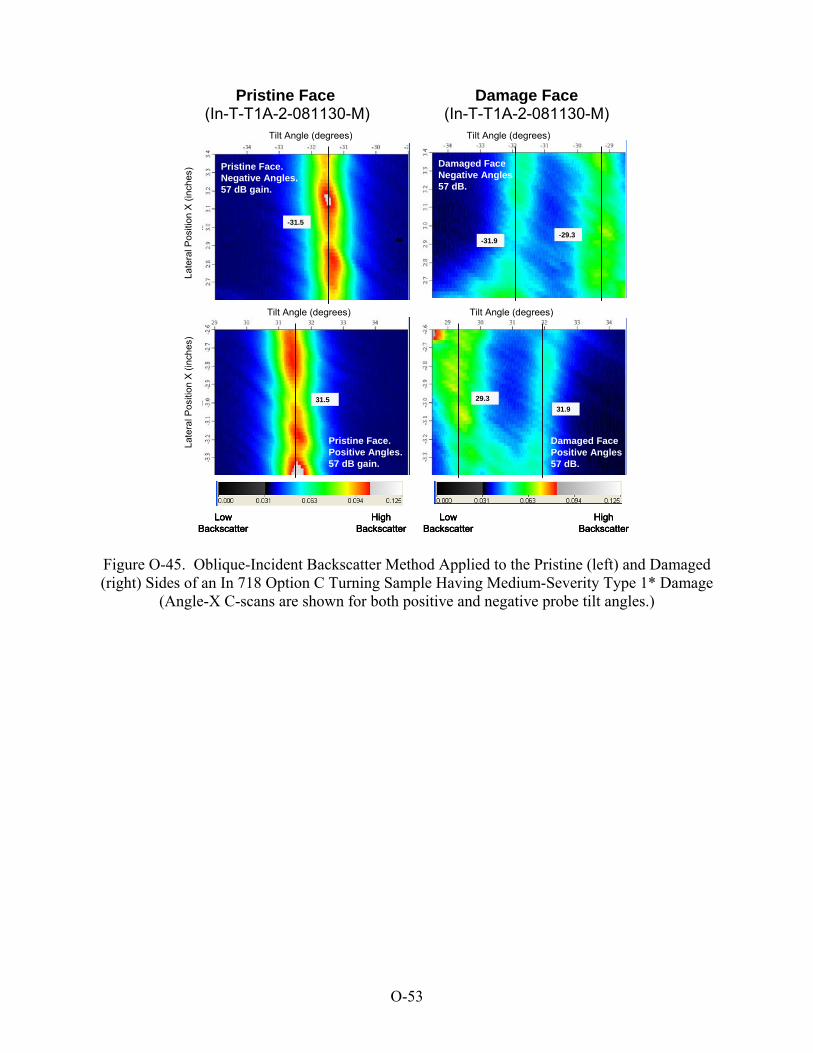
Pristine Face Damage Face (In-T-T1A-2-081130-M) (In-T-T1A-2-081130-M)
Tilt Angle (degrees) Tilt Angle (degrees)
Lat
eral
Po
sitio
n X
(in
ches
) Pristine Face.Negative Angles.57 dB gain.
Damaged FaceNegative Angles57 dB.
Tilt Angle (degrees) Tilt Angle (degrees)
Lat
era
l Pos
ition
X (
inch
es)
Pristine Face.Positive Angles.57 dB gain.
High Backscatter
Low Backscatter
Damaged FacePositive Angles57 dB.
31.5
-31.5
31.9
-31.9-29.3
29.3
Low Backscatter
High Backscatter
Tilt Angle (degrees) Tilt Angle (degrees)
Lat
eral
Po
sitio
n X
(in
ches
) Pristine Face.Negative Angles.57 dB gain.
Damaged FaceNegative Angles57 dB.
Tilt Angle (degrees) Tilt Angle (degrees)
Lat
era
l Pos
ition
X (
inch
es)
Pristine Face.Positive Angles.57 dB gain.
High Backscatter
Low Backscatter
Damaged FacePositive Angles57 dB.
31.5
-31.5
31.9
-31.9-29.3
29.3
Low Backscatter
High Backscatter
Figure O-45. Oblique-Incident Backscatter Method Applied to the Pristine (left) and Damaged (right) Sides of an In 718 Option C Turning Sample Having Medium-Severity Type 1* Damage
(Angle-X C-scans are shown for both positive and negative probe tilt angles.)
O-53

x
- 32.0 o
Side A Line 1
Tilt Angle (degrees)
Late
ral P
osi
tion
X (
inch
es)
- 29.4 o
- 31.7 o
Side A Line 2
Tilt Angle (degrees)
Late
ral P
osi
tion
X (
inch
es)
- 29.4 o
- 32.0 o
Side A Line 3L
ater
al P
osi
tion
X (
inch
es)
Tilt Angle (degrees)
- 29.4 o
- 31.5 o
Side B Line 3La
tera
l Pos
itio
n X
(in
ches
)
Tilt Angle (degrees)
- 31.4 o
Side B Line 2
Tilt Angle (degrees)
Lat
eral
Pos
itio
n X
(in
ches
)
- 31.5 o
Side B Line 1
Tilt Angle (degrees)
Late
ral P
ositi
on X
(in
ches
)
Serial number here and upside down
Line 2
Line 3
Line 1
Side BSerial number here
and right side up
Line 2
Line 3
Line 1
Side A
Pristine SideDamaged Side
x
- 32.0 o
Side A Line 1
Tilt Angle (degrees)
Late
ral P
osi
tion
X (
inch
es)
- 29.4 o- 32.0 o
Side A Line 1
Tilt Angle (degrees)
Late
ral P
osi
tion
X (
inch
es)
- 29.4 o
- 31.7 o
Side A Line 2
Tilt Angle (degrees)
Late
ral P
osi
tion
X (
inch
es)
- 29.4 o
- 31.7 o
Side A Line 2
Tilt Angle (degrees)
Late
ral P
osi
tion
X (
inch
es)
- 29.4 o
- 32.0 o
Side A Line 3L
ater
al P
osi
tion
X (
inch
es)
Tilt Angle (degrees)
- 29.4 o
- 32.0 o
Side A Line 3L
ater
al P
osi
tion
X (
inch
es)
Tilt Angle (degrees)
- 29.4 o
- 31.5 o
Side B Line 3La
tera
l Pos
itio
n X
(in
ches
)
Tilt Angle (degrees)
- 31.4 o
Side B Line 2
Tilt Angle (degrees)
Lat
eral
Pos
itio
n X
(in
ches
)
- 31.5 o
Side B Line 1
Tilt Angle (degrees)
Late
ral P
ositi
on X
(in
ches
)
Serial number here and upside down
Line 2
Line 3
Line 1
Side BSerial number here
and right side up
Line 2
Line 3
Line 1
Side A
Pristine SideDamaged Side
- 31.5 o
Side B Line 3La
tera
l Pos
itio
n X
(in
ches
)
Tilt Angle (degrees)
- 31.4 o
Side B Line 2
Tilt Angle (degrees)
Lat
eral
Pos
itio
n X
(in
ches
)
- 31.5 o
Side B Line 1
Tilt Angle (degrees)
Late
ral P
ositi
on X
(in
ches
)
- 31.5 o
Side B Line 3La
tera
l Pos
itio
n X
(in
ches
)
Tilt Angle (degrees)
- 31.5 o
Side B Line 3La
tera
l Pos
itio
n X
(in
ches
)
Tilt Angle (degrees)
- 31.4 o
Side B Line 2
Tilt Angle (degrees)
Lat
eral
Pos
itio
n X
(in
ches
)
- 31.4 o
Side B Line 2
Tilt Angle (degrees)
Lat
eral
Pos
itio
n X
(in
ches
)
- 31.5 o
Side B Line 1
Tilt Angle (degrees)
Late
ral P
ositi
on X
(in
ches
)
- 31.5 o
Side B Line 1
Tilt Angle (degrees)
Late
ral P
ositi
on X
(in
ches
)
Serial number here and upside down
Line 2
Line 3
Line 1
Side B
Serial number here and upside down
Line 2
Line 3
Line 1
Side BSerial number here
and right side up
Line 2
Line 3
Line 1
Side A
Serial number here and right side up
Line 2
Line 3
Line 1
Side A
Pristine SideDamaged Side
Figure O-46. Angle-X C-Scans of Backscattered Noise Response for In 718 Type 1* Medium Damage Coupon In-T-T1A-3-081130-M (For each side of the sample, scans were made along three lines (denoted line 1, 2, and 3). For each line, scans were made over both positive and negative probe tilt angles. Only the results for negative angles are shown. The results for
positive angles were generally very similar.)
O-54

For the examples in figure O-44, only Angle-X scans over negative probe tilt angles are shown. Scans for both positive and negative angles are illustrated in figure O-45 for a different Type 1* medium damage In 718 coupon. For both positive and negative angles, the damaged surface of that coupon exhibits (locally) maximal backscattering at two distinct angles, one near 29.4° (the dominant maximum) and one near 31.8° (the secondary maximum). By contrast, the single maximum on the pristine side occurs near 31.4°. The double-peak structure shown in figure O-45 is similar for Ti 6-4 coupons having medium or deep Type 1* damage (see figure O-39). For both alloys, the angles for the two backscatter peaks on the damaged face bracket are the same as the single peak on the pristine face, with the damage peak at the lower angle generally being the more prominent. One possible explanation for the double-peak structure is a lateral variation of the degree of damage across the sample. The beam footprint on the surface is about 0.3 wide. If this footprint encounters two large areas of damage having different depth profiles, each area could give rise to a separate backscatter peak. Limited measurements were performed to test this theory, and the results are summarized in figure O-46. The coupon studied was an In 718 Type 1* medium-damage sample, In-T-T1A-3-081130-M. As indicated in the top of figure O-46, three Angle-X C-scans were performed on both the damaged and pristine sides of the coupon. These three scans (identified as being centered along lines 1, 2, and 3 in the figure) ensonified different regions of the surface. This sample, like most of those with substantial intended damage, is not perfectly flat. Thus, prior to each of the six scans, the transducer beam was normalized to the front surface at a point near the center of the intended scan region. The six resulting Angle-X C-scans of backscattered grain noise response are shown in figure O-46. For the pristine side of the sample (right-hand half of the figure), the three C-scans are very similar in appearance, with each having a single pronounced noise peak near 31.5°. For the damaged side of the sample, however, the three Angle-X C-scans are quite different. Each displays two maxima, one near 29.4° and one near 32°. For the scan along line 1, the maximum near 32° is relatively strong, and the maximum near 29.4° is very weak. This situation is reversed for line 3. For line 2 (down the middle of the sample), both peaks are prominent. This finding is consistent with the hypothesis that the damage changes in character laterally across the sample from line 1 to line 3, and for line 2, both damage conditions are sensed. It is interesting to note that for the damaged side, one of the peak angles is well below the pristine-side peak angle, and one is about 0.5° above it. It could be argued that the damaged side consists of some regions of substantial damage, and other regions of virtually no damage, and that each of these regions gives rise to a separate noise peak for the scan down the center of the coupon. However, the ~0.5° shift between the peak noise angle associated with the supposedly undamaged region of the damaged face and that of the known pristine face would have to be explained. Alternatively, the damaged side of the coupon may contain both lightly damaged and heavily damaged regions, with the former tending to increase the peak backscatter angle, and the latter tending to decrease it. This topic, although interesting and deserving of future research, was beyond the scope of the present study. For the 19 In 718 Option C coupons that were studied, figure O-47 displays the measured probe tilt angles for peak backscatter. For pristine surfaces, there was always a single, well-defined angle at which peak backscattering was observed. For some damaged surfaces, two maxima
O-55

were observed and both are plotted in figure O-47. The following points can be made in summary: Four groups of coupons were studied (pristine, Type 1* shallow, Type 1* medium, and
Type 6*). Coupons within a given group tended to have very similar behaviors with regard to peak backscatter angles.
For the suite of pristine coupons, the peak angle was approximately the same for all
coupons, with minor differences likely attributable to water temperature variations. Note that the peak backscatter angles for the pristine sides of the In 718 coupons tend to be lower on the right-hand side than on the left-hand side of figure O-47. This is likely due to the fact that the more recent right-hand side measurements (Type 1* medium and Type 6*) were performed during the winter months when the ambient water temperature in the laboratory was lower. Recall that a 5°F decrease in water temperature lowers the peak backscatter angle by 0.2°.
For the shallow damage Type 1* coupons, no significant differences were observed
between the behaviors of the damaged and pristine surfaces. Medium damage Type 1* surfaces exhibited two backscatter maxima, with the more
prominent one at the lower angle. The average angular difference between the single peak on the pristine side, and the prominent peak on the damaged side was about 2.1°.
Type 6* damaged surfaces exhibited a single backscatter maximum with the peak angle
higher (by 0.9° on average) than the corresponding pristine surface.
O-56
Figure O-47. Transducer Tilt Angles Producing Maximized Backscattered Surface Acoustic Wave Responses
* * * ** *
* * *
* * *
In 718 SAW Backscatter Measurements (Both Sides of Various In 718 Turning Samples)
34
Side 2 (undamaged)
Side 1, main peak
Side 1, 2nd peak Side 1 is the damaged side for damaged couponsand is Side A for pristine coupons
Pea
k A
ngle
(de
gree
s)
33
32
31Type 1*Shallow
Type 1*Medium
*
Type 6* Pristine
30
M7
T6-
1A
T6-
7 T
6-8
T6-
11
T6-
1 4
** * *29
P20
P1
P6
P7
P13
P1A
S1
S6
S7
* * * *
M1
M2
M3
S8
Specimen*Denotes a round-robin coupon

O.3.10 METHOD 2—SUMMARY OF OBLIQUE-INCIDENCE SAW BACKSCATTER. The following points for Method 2 can be made in summary: Method 2 looks at the angular dependence of the backscattering, rather than the absolute
backscatter level itself. For this reason, Method 2 (unlike Method 1) is relatively insensitive to surface roughness and water path. In fact, a moderate level of surface roughness can be beneficial since it raises the absolute backscatter level, allowing the measurements to be performed at lower gain settings.
Since planar transducers are used, the size of the beam footprint on the surface (several
hundred mil) is much larger than that used for Method 1 (typically 1 to 40 mil). As a consequence, the measurement effectively averages over nearby Ti 6-4 macrograins, thus limiting the effect of speckle arising from macrograin orientation differences in that alloy. The scanning method used here effectively averages over a surface area of about 0.3 by 0.8. Over this area, the method returns a parameter (the average peak backscatter angle) that can be used to assess the surface damage condition.
The peak backscatter angle is sensitive to the speed of surface acoustic waves in the
depth region extending about 1 wavelength (λ) below the surface. If surface damage causes a change in surface acoustic wave speed, then the damage should be readily detectable using Method 2.
It is best to choose the inspection frequency where the SAW wavelength is roughly
matched to the damage layer thickness. That was not possible in this study using the available transducers. However, measurements with a lower than optimal center frequency (25 MHz) gave promising results for both Ti 6-4 and In 718 alloys. The ability to distinguish damaged from undamaged surfaces would likely be better at a higher frequency.
The key results for Method 2 are summarized in figure O-41 (for Ti 6-4) and figure O-47
(for In 718). In general, for shallow Type 1* damage in either alloy, it is difficult to distinguish between the pristine and damaged faces of a given coupon (although discrimination might be improved at higher inspection frequencies). For medium or deep Type 1* damage, pristine and damaged surfaces could readily be distinguished. For Type 6* damage, differences between pristine and damaged surfaces were larger for In 718 samples than for Ti 6-4 samples.
Care must be taken when comparing peak backscatter angles at different locations in a
forging, since normal texture differences can affect surface acoustic wave speeds and, hence, backscatter angles. The optimal procedure would be to base damage assessment solely on measurements made at a given site by looking at changes in the backscatter angular profile with frequency. Initial work along these lines appears promising, as demonstrated using a heat-damaged Ti 6-4 rolled plate sample.
O-57

O.4 REFERENCES. O-1. Song, S.J., Kim, Y.H., Bae, D.H., Jung, M.H., and Kwon, S.D., “Evaluation of Corrosion
Degradation of 12Cr Alloy Steel Using an Ultrasonic Backward Radiation,” International Journal of Modern Physics B, Vol. 17, 2003, pp. 1653-1658.
O-2. Kim, H.-J., Song, S.-J., Yang, D.-J., Kwon S.D., Wang, W-W., Takagi, T., Uchimoto, T., and Abe, T., “Interpretation of Back-Scattered Rayleigh Surface Wave Signals From Diamond Coating Layers,” Review of Progress in Quantitative Nondestructive Evaluation, Vol. 25, Thompson, D.O. and Chimenti, D.E., eds., AIP, New York, New York, 2006, pp. 1051-1058.
O-3. Kim, H.-J., Wang, W-W., Song, S.-J., and Kwon, S.D., “New Approaches to Backscattered Rayleigh Wave Signal Analysis for the Evaluation of CVD Diamond Coating Layers,” Review of Progress in Quantitative Nondestructive Evaluation, Vol. 26, Thompson, D.O. and Chimenti, D.E., eds., AIP, New York, New York, 2007, pp. 1127-1134.
O-4. Margetan, F.J., Gigliotti, M., Brasche, L., and Leach, W., “Fundamental Studies: Inspection Properties for Engine Titanium Alloys,” FAA report DOT/FAA/AR-02/114, December 2002.
O-5. Kim, Hak-Joon, Conversations at the 2008 QNDE Conference, Chicago, July 2008.
O-6. Brasche, L., et al., ISU-CASR study involving the use of dye penetrants to detect fatigue cracks.
O-7. Brasche, L.J.H, Margetan, F.J., and Thompson, R.B., “Sample Preparation Techniques and Material Property Measurements of Hard Alpha Titanium Samples,” Review of Progress in Quantitative Nondestructive Evaluation, Vol. 11B, Thompson, D.O. and Chimenti, D.E., eds., Plenum Press, New York, New York, 1992, pp. 1733-1738.
O-8. Margetan, F.J., Nieters, E., Brasche, L., Yu, L., Degtyar, A., Wasan, H., Keller, M., and Kinney, A., “Fundamental Studies of Titanium Forging Materials—Engine Titanium Consortium Phase II,” FAA report DOT/FAA/AR-05/22, June 2005.
O-58

APPENDIX P—ULTRASONIC MICROSCOPY IMAGING OF TURNING SAMPLES
In ultrasonic microscopy imaging (UMI), the frequency of the transducer is the most obvious factor in improving resolution. In general, high-ultrasonic frequency results in high resolution. However, there are other design factors that affect the resolution at a given frequency. These include water path, focal length, diameter, and interface. Shorter focal length with large diameter will decrease effective beam diameter (EBD) (and/or the transverse resolution) in addition to less attenuation of the high frequency. UMI resolution is defined as: Resolution = 0.707 by 1.22 by F# by (P-1)where: F# = Focal length/diameter of the transducer = Wavelength at given frequency Therefore, a higher-frequency transducer provides better resolution when everything else remains the same. This provides a basis for using UMI to characterize samples with small anomalies that are generally not detected at low frequency. Similarly, the F# of the transducer also affects the resolution. For example, two transducers having the same frequency characteristics will exhibit the same resolution if their F# is identical. A transducer with a low F# is suitable for studying features on or just below the surface with an improved resolution, whereas a high F# is more suitable for studying features in bulk structure. In the Honeywell study, a scanning technique that is capable of detecting and resolving any features equal to or greater than 50 m (0.002 inch) was used. The minimum number of pixels needed for achieving the desired 50-m resolution for studying a 2″ by 1″ area was 1000 by 1000 pixels squared. To achieve a scanning index or pixel size half the target resolution, 2048 by 2048 pixels for a 2′ by 1′ area were used. The logical steps used to define and select the scanning parameters are illustrated in figure P-1. Two transducers of 100 and 230 MHz were used in both pulse-echo and surface acoustic wave modes to study the capability of the technique. The ray tracing and EBD are shown in figures P-2 and P-3, respectively. Based on the basic surface acoustic wave theory, the sampling depth should be close to 0.90 27 m or close to 0.001 inch) assuming the peak frequency is close to 90 MHz, as shown in the Fast Fourier Transform (FFT) in figure P-4. The results are discussed in section 3.3.13 of the main document.
P-1

Figure P-1. Process Map for UMI
The generation of both pulse echo and surface acoustic wave is based on two approaches: Defocusing V(z)) The separation between pulse echo and surface acoustic wave is governed by microstructural noise and desired near-surface resolution. This also depends on the ring-down cycles. The pixel size resolution depends on ultrasonic and materials variables.
Figure P-2. Ray Tracing for Both Direct Pulse and Surface Acoustic Wave
(For illustrative purposes only)
P-2

Figure P-3. Improved Resolution at High Frequency
Figure P-4. Waveform and FFT for 100-MHz Surface Acoustic Waves
P-3/P-4

APPENDIX Q—HIGH-ENERGY X-RAY DIFFRACTION DEPTH PROFILING, CENTER FOR NONDESTRUCTIVE EVALUATION
Q.1 BACKGROUND. X-ray diffraction (XRD) is a standard technique for measuring lattice parameters in crystalline materials [Q-1]. The diffraction of x-rays by a crystal with lattice spacing d is described by Bragg’s Law nλ=2d sinθ (Q-1)
where is the x-ray wavelength, and 2 is the diffraction angle. The geometry for such a measurement is indicated in figure Q-1, with the surface of the sample positioned symmetrically with respect to the incident and diffracted beams. Traditional methods using low-energy x-ray sources are limited to a layer a few microns thick at the surface of a sample. By using higher x-ray energies, it is possible to probe deeper into a sample. Equation Q-1 can be rewritten in terms of the x-ray energy, E, as follows nhc/2d = Esin (Q-2)
where h is Planck’s constant and c is the speed of light. From equation Q-2, it is evident that using higher energies implies smaller diffraction angles for a given lattice spacing. Thus, accurate angular alignment and measurement is very important for implementation of high-energy x-ray diffraction (HEXRD) techniques.
Figure Q-1. Principle of X-Ray Diffraction The intersection of the incident and diffracted beams forms a probing volume with a diamond cross section, as indicated in figure Q-2. The dimensions of this probing volume will depend on the width of the x-ray beams as well as on the diffraction angle. The dimensions indicated in figure Q-2 are typical for 60-keV diffraction at an angle of a few degrees. The height of the probing volume depends on the size of the x-ray source and the vertical collimation of the beams. For inspection of flat samples, this height can be several millimeters to increase the statistics. Although, for inspecting curved surfaces, this height should be minimized to reduce geometric effects.
Q-1
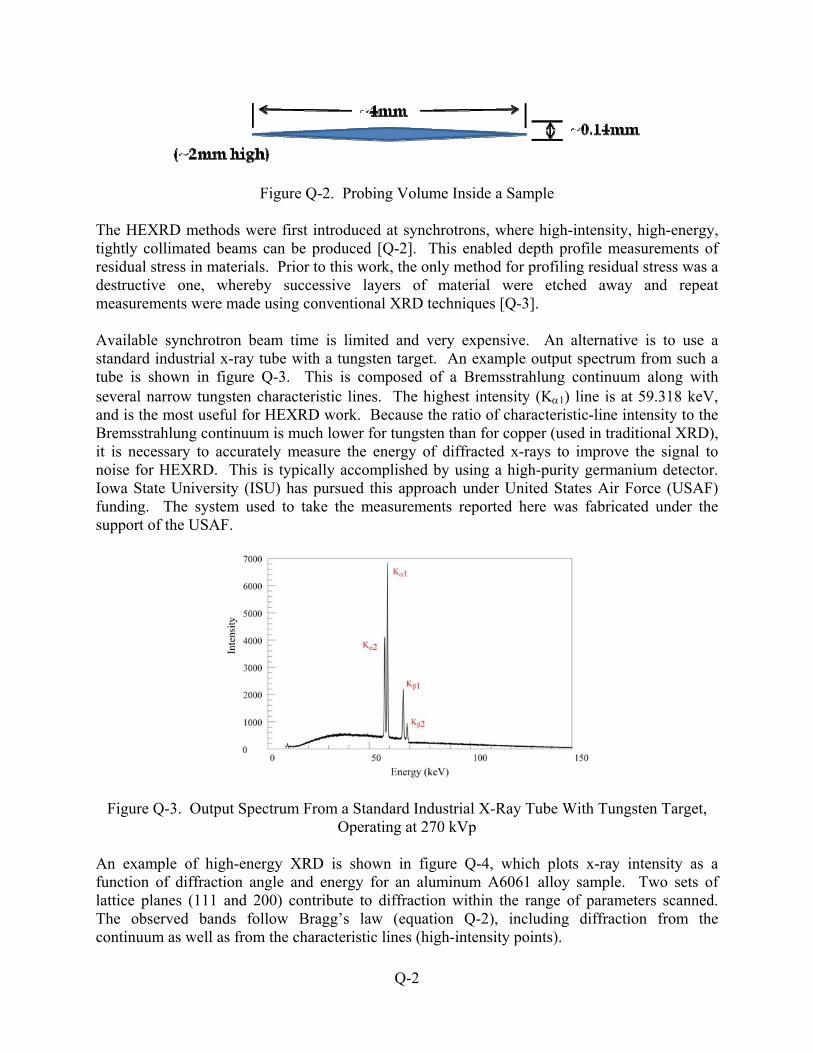
Figure Q-2. Probing Volume Inside a Sample The HEXRD methods were first introduced at synchrotrons, where high-intensity, high-energy, tightly collimated beams can be produced [Q-2]. This enabled depth profile measurements of residual stress in materials. Prior to this work, the only method for profiling residual stress was a destructive one, whereby successive layers of material were etched away and repeat measurements were made using conventional XRD techniques [Q-3]. Available synchrotron beam time is limited and very expensive. An alternative is to use a standard industrial x-ray tube with a tungsten target. An example output spectrum from such a tube is shown in figure Q-3. This is composed of a Bremsstrahlung continuum along with several narrow tungsten characteristic lines. The highest intensity (K1) line is at 59.318 keV, and is the most useful for HEXRD work. Because the ratio of characteristic-line intensity to the Bremsstrahlung continuum is much lower for tungsten than for copper (used in traditional XRD), it is necessary to accurately measure the energy of diffracted x-rays to improve the signal to noise for HEXRD. This is typically accomplished by using a high-purity germanium detector. Iowa State University (ISU) has pursued this approach under United States Air Force (USAF) funding. The system used to take the measurements reported here was fabricated under the support of the USAF.
Figure Q-3. Output Spectrum From a Standard Industrial X-Ray Tube With Tungsten Target, Operating at 270 kVp
An example of high-energy XRD is shown in figure Q-4, which plots x-ray intensity as a function of diffraction angle and energy for an aluminum A6061 alloy sample. Two sets of lattice planes (111 and 200) contribute to diffraction within the range of parameters scanned. The observed bands follow Bragg’s law (equation Q-2), including diffraction from the continuum as well as from the characteristic lines (high-intensity points).
Q-2

Figure Q-4. Diffraction From Two Sets of Lattice Planes in an Aluminum A6061 Alloy Sample By measuring the x-ray energy, the data can be restricted to a small range around one of the characteristic lines. In this manner, traditional -2 scans can be performed at a particular region in a sample. Figure Q-5 shows examples of such scans for an aluminum sample that has been shot peened to an intensity of 6A. As the probing depth changes, the peak of the diffraction angle shifts until, beyond a 350-m depth, the peak angle stabilizes. This indicates that the shot peening has modified the crystal structure in the top 350-m layer of the sample.
Figure Q-5. -2 Scans at Different Depths for a Shot-Peened Aluminum Sample Performing -2 scans at different depths in a sample is very time consuming. Another approach has been developed that takes advantage of the narrowness of the tungsten characteristic line. In this method, the HEXRD system is set at a fixed diffraction angle corresponding to that expected for tungsten K1 diffraction from a relaxed lattice. Any deviation in lattice parameter will cause the diffraction intensity to drop significantly. The sample is then scanned through the probing volume to map out the change in lattice parameter. Examples of such scans are shown in figure Q-6 for aluminum samples shot peened to different intensities. Deep in the sample, the intensity matches that of a pristine sample. The point of this match provides a measure of the shot-peen depth. Through the use of computer models, this data can be inverted to produce a strain versus depth profile [Q-4]. To date, this has only been done for aluminum materials.
Q-3

Figure Q-6. Depth Profile Scans for Aluminum Samples Subjected to Different Shot-Peening Intensities
Shot-peening and chemical treatments are used to modify the near-surface lattice structure of materials in a controlled manner to improve their fatigue life. Aggressive machining is a form of work-hardening that can also modify the grain structure in a material. As this may be localized and uncontrolled, it can have adverse effects on the lifetime of a component. The goal of this study was to determine how measurements of diffraction properties as a function of depth in a sample correlate with the extent of damage due to aggressive machining. Q.2 EQUIPMENT USED. The prototype high-energy diffraction system [Q-4] developed at t0966he ISU Center for nondestructive evaluation is shown in figure Q-7. A high-power industrial x-ray tube with tungsten target (Comet MXR 320/23) was used for the source. This was operated with a 1.2-mm-diameter beam spot at 270 kVp and 2.0 mA. Incident and diffraction beams are defined by pairs of slit collimators with 140-μm openings. This defines a small probing volume in a sample, as indicated previously in figure Q-2. The samples were scanned through this probing volume to measure diffraction at different depths. The diffraction angle and sample position are controlled by computer-interfaced precision motion stages from Parker/Daedel-Compumoter. The energy of scattered x-rays is measured by a high-purity germanium detector with an energy resolution of 500 eV full wave half max at 60 keV. This provides the capability to select x-rays of a specific energy range and to discriminate against x-rays that do not satisfy the diffraction conditions.
Figure Q-7. Computer-Aided Drawing of the Prototype HEXRD System
Q-4

Q.3 TEST DESCRIPTION. Studies concentrated on those samples chosen for round-robin measurements. Initial inconsistencies as to the identity of the damaged side led to taking measurements on both sides of the coupons. For most samples, measurements were made near the center of the 1″ by 2″ coupon. -2 measurements were made both near the surface and at a depth attainable with the available equipment (typically ~160 m in titanium Ti-6Al-4V alloy (Ti 6-4) and ~100 m in Inconel 718 alloy (In 718)). Depth profile measurements of each surface were then made at the “deep” diffraction angle. The time to complete a single scan ranged from 3 to 16 hours, with In 718 samples requiring longer time due to the greater x-ray attenuation in the sample. All diffraction measurements were made using a narrow band around the tungsten K1 characteristic line (59.318 keV). For Ti 6-4 samples, the Ti-101 planes gave the strongest signal, whereas for In 718, the Ni-111 planes produced the best results. To determine the nominal diffraction angle, the side thought to be undamaged was scanned at a depth ~160 m for Ti 6-4 and ~100 m for In 718. In some cases, there was a significant difference in the diffraction angle for the two sides due to bending, i.e., nonflatness, of the sample. For these samples, a different diffraction angle was used for the depth profile on each side. For comparison of the depth profiles on the two sides of the sample, alignment of the two surfaces was estimated to be within 20 m. All data are presented in terms of side A or B. Side A refers to the top when the sample number is right-side up. Several pristine Ti 6-4 samples were measured, and some variation in diffraction angle was noted. Two samples were scanned, both before and after annealing, to determine if there was any residual stress in the samples. In figure Q-8, depth profiles for both sides of sample Ti-T-P-1-0611 before and after annealing are shown. The closeness of the curves indicates that residual stress was small. Similar curves are shown in figure Q-9 for sample Ti-T-P-16-060208. In this case, the before and after curves are quite different, indicating that there was significant residual stress present in the as-machined sample. The presence of residual stress in some of the samples could bias the results of the measurements for damage.
Q-5

Figure Q-8. Depth Profiles for the two Sides of Pristine Sample Ti-T-P-1-0611 Before and After Annealing
Q-6

Figure Q-9. Depth Profiles for the two Sides of Pristine Sample Ti-T-P-16-060208 Before and After Annealing
Q-7

Typical diffraction-2 scans for a Ti 6-4 Type 1* sample with light deformation are shown in figure Q-10. The side of the sample assumed to be pristine (B) had the same peak diffraction angle at both depths, whereas the damaged side (A) showed a significant shift in the shallow diffraction angle. The green line on each plot indicates the diffraction angle used for the depth profile of the corresponding side. Depth profiles for this same sample are displayed in figure Q-11. Side B has a typical profile expected for pristine material. On side A, however, the intensity is greatly reduced near the surface due to the shift in diffraction angle. At a depth of ~160 m (0.006 inch), the intensity matches that of side B, indicating the depth of damage. This is considerably greater than the 0.0005-inch deformation depth estimated from the manufacturing process.
(a)
(b)
Figure Q-10. Typical Diffraction -2 Scans for a Ti 6-4 Type 1* Sample With Light
Deformation (a) Top and (b) Bottom Sides at two Depths
Q-8

Figure Q-11. Diffraction Depth Profile Scans for Both Sides of the Ti 6-4 Type 1* Sample of Figure Q-10
-2 scans for a Ti 6-4 Type 1* sample with high deformation are shown in figure Q-12. In this case, side B is clearly the damaged side, displaying very broad and shifted -2 plots for both shallow and deep scans. In addition, the shallow scan on side A is shifted, indicating that there may be some residual stress on that side. The depth profiles for this sample are shown in figure Q-13. This indicates that the damage extends to a depth of at least 250 m.
Q-9

(a)
(b)
Figure Q-12. Typical Diffraction -2 Scans for a Ti 6-4 Type 1* Sample With High
Deformation (a) Top and (b) Bottom Sides at two Depths (The green line indicates the angle chosen for the depth profile scan on the corresponding surface.)
Q-10
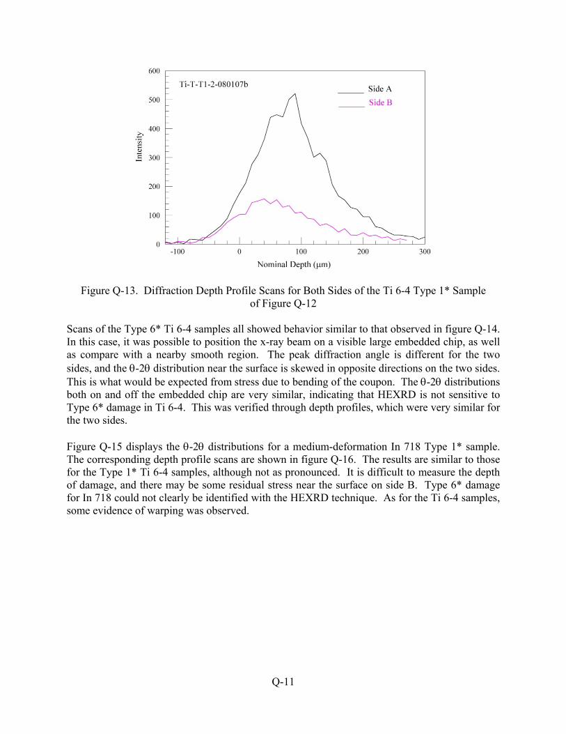
Figure Q-13. Diffraction Depth Profile Scans for Both Sides of the Ti 6-4 Type 1* Sample of Figure Q-12
Scans of the Type 6* Ti 6-4 samples all showed behavior similar to that observed in figure Q-14. In this case, it was possible to position the x-ray beam on a visible large embedded chip, as well as compare with a nearby smooth region. The peak diffraction angle is different for the two sides, and the -2 distribution near the surface is skewed in opposite directions on the two sides. This is what would be expected from stress due to bending of the coupon. The -2 distributions both on and off the embedded chip are very similar, indicating that HEXRD is not sensitive to Type 6* damage in Ti 6-4. This was verified through depth profiles, which were very similar for the two sides. Figure Q-15 displays the -2 distributions for a medium-deformation In 718 Type 1* sample. The corresponding depth profile scans are shown in figure Q-16. The results are similar to those for the Type 1* Ti 6-4 samples, although not as pronounced. It is difficult to measure the depth of damage, and there may be some residual stress near the surface on side B. Type 6* damage for In 718 could not clearly be identified with the HEXRD technique. As for the Ti 6-4 samples, some evidence of warping was observed.
Q-11

(a)
(b)
Figure Q-14. Typical Diffraction -2 Scans for a Ti 6-4 Type 6* Sample (a) Top Side at two Depths and two Surface Locations and (b) Bottom Side at two Depths (The green line indicates
the angle chosen for depth profile scan on the corresponding surface.)
Q-12
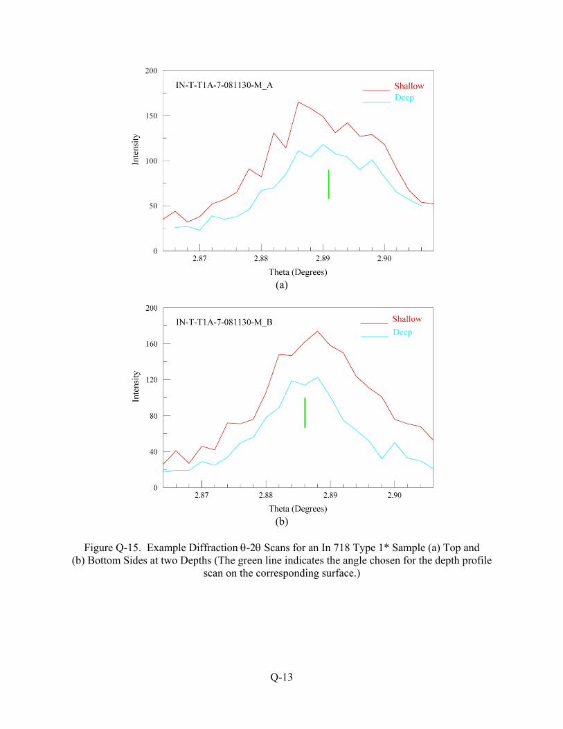
(a)
(b)
Figure Q-15. Example Diffraction -2 Scans for an In 718 Type 1* Sample (a) Top and
(b) Bottom Sides at two Depths (The green line indicates the angle chosen for the depth profile scan on the corresponding surface.)
Q-13

Figure Q-16. Diffraction Depth Profile Scans for Both Sides of the In 718 Sample of Figure Q-15
High-energy XRD shows good potential for characterizing Type 1* damage, especially in Ti 6-4. With design improvements, it is estimated that scan times can be reduced by an order of magnitude and that the sensitivity of HEXRD can be improved. Even with these projected improvements, this method will not be practical for scanning large areas. However, it should be very useful for confirming and measuring the depth of damage at specific points indicated by other methods. Based on the measurements on the available Type 6* samples, HEXRD does not show sensitivity to Type 6* damage. The results are discussed in section 3.3.14 of the main document. Q.4 REFERENCES.
Q-1. Cullity, B.D. and Stock, S.R., Elements of X-Ray Diffraction, 3rd Edition, Prentice Hall, 2001.
Q-2. Sato, M., Sano, Y., Kajiwara, K., Tanaka, H., and Akita, K., “Non-Destructive
Measurement of Residual Stress Depth Profile in Laser-Peened Steel,” SPring-8. Synchrotron Radiation Instrumentation: Ninth International Conference, Vol. 879, January 2007, pp. 1577-1580.
Q-3. Kandil, F.A., Lord, J.D., Fry, A.T., and Grant, P.V., “A Review of Residual Stress
Measurement Methods,” Technical Report NPL Report MATC(A)04, NPL Materials Centre, Queens Road, Teddington, Middlesex, UK TW11 0LW, February 2001.
Q-4. Al Shorman, M.Y., “Residual Stress Measurement Using High Energy X-Ray
Diffraction,” Ph.D. thesis, Iowa State University, Ames, Iowa, December 2008.
Q-14
Copyright © 2022 FDOKUMEN