Graduate Theses, Dissertations, and Problem Reports

2006

Nondestructive evaluation of fiber reinforced polymer bridge Nondestructive evaluation of fiber reinforced polymer bridge

decks using ground penetrating radar and infrared thermography decks using ground penetrating radar and infrared thermography

Cheng Lok Hing West Virginia University

Follow this and additional works at: https://researchrepository.wvu.edu/etd

Recommended Citation Recommended Citation Hing, Cheng Lok, "Nondestructive evaluation of fiber reinforced polymer bridge decks using ground penetrating radar and infrared thermography" (2006). Graduate Theses, Dissertations, and Problem Reports. 2715. https://researchrepository.wvu.edu/etd/2715

This Dissertation is protected by copyright and/or related rights. It has been brought to you by the The Research Repository @ WVU with permission from the rights-holder(s). You are free to use this Dissertation in any way that is permitted by the copyright and related rights legislation that applies to your use. For other uses you must obtain permission from the rights-holder(s) directly, unless additional rights are indicated by a Creative Commons license in the record and/ or on the work itself. This Dissertation has been accepted for inclusion in WVU Graduate Theses, Dissertations, and Problem Reports collection by an authorized administrator of The Research Repository @ WVU. For more information, please contact researchrepository@mail.wvu.edu.

Nondestructive Evaluation of Fiber Reinforced Polymer Bridge Decks Using

Ground Penetrating Radar and Infrared Thermography

by

Cheng Lok Hing

A DISSERTATION Submitted to the

College of Engineering and Mineral Resources

West Virginia University

in partial fulfillment of the requirements

for the degree of

Doctor of Philosophy

in

Civil and Environmental Engineering

Udaya B. Halabe, Ph.D., P.E., Chair

Hota V. GangaRao, Ph.D., P.E.

Powsiri Klinkhachorn, Ph.D.

Ruifeng Liang, Ph.D.

Hema J. Siriwardane, Ph.D., P.E.

West Virginia University

Morgantown, West Virginia

2006

Keywords: Ground Penetrating Radar, GPR, Infrared Thermography, IRT, Fiber

Reinforced Polymer, FRP, Nondestructive Evaluation, NDE

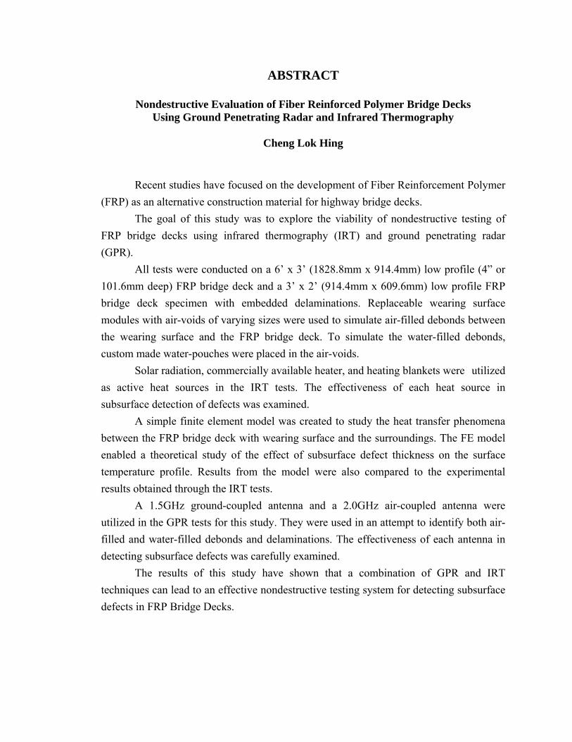
ABSTRACT

Nondestructive Evaluation of Fiber Reinforced Polymer Bridge Decks Using Ground Penetrating Radar and Infrared Thermography

Cheng Lok Hing

Recent studies have focused on the development of Fiber Reinforcement Polymer (FRP) as an alternative construction material for highway bridge decks. The goal of this study was to explore the viability of nondestructive testing of FRP bridge decks using infrared thermography (IRT) and ground penetrating radar (GPR). All tests were conducted on a 6’ x 3’ (1828.8mm x 914.4mm) low profile (4” or 101.6mm deep) FRP bridge deck and a 3’ x 2’ (914.4mm x 609.6mm) low profile FRP bridge deck specimen with embedded delaminations. Replaceable wearing surface modules with air-voids of varying sizes were used to simulate air-filled debonds between the wearing surface and the FRP bridge deck. To simulate the water-filled debonds, custom made water-pouches were placed in the air-voids.

Solar radiation, commercially available heater, and heating blankets were utilized as active heat sources in the IRT tests. The effectiveness of each heat source in subsurface detection of defects was examined.

A simple finite element model was created to study the heat transfer phenomena between the FRP bridge deck with wearing surface and the surroundings. The FE model enabled a theoretical study of the effect of subsurface defect thickness on the surface temperature profile. Results from the model were also compared to the experimental results obtained through the IRT tests. A 1.5GHz ground-coupled antenna and a 2.0GHz air-coupled antenna were utilized in the GPR tests for this study. They were used in an attempt to identify both air-filled and water-filled debonds and delaminations. The effectiveness of each antenna in detecting subsurface defects was carefully examined.

The results of this study have shown that a combination of GPR and IRT techniques can lead to an effective nondestructive testing system for detecting subsurface defects in FRP Bridge Decks.

ACKNOWLEDGEMENTS

I would like to extend my utmost appreciation to Dr. Udaya B. Halabe, my

academic and thesis advisor, as well as my mentor, for his kindness, encouragement, and

guidance through the entire journey. I would like to thank Dr. Hota V. GangaRao, Dr.

Powsiri Klinkhachorn, Dr. Ruifeng Liang, and Dr. Hema J. Siriwardane for serving in the

Ph.D. Advisory and Examining Committee (AEC) and for their time and effort in

reviewing this dissertation.

There are a number of people who had helped me in making this a successful

study. The assistance provided by Jerry Nestor and Bill Comstock, laboratory

technicians, are greatly appreciated. Thanks to Bhyrav Mutnuri for his help in

determining the FRP’s conductivity value. Without the help of Shashanka Dutta, Sandeep

Pyakurel, Manjunath Dasarath Rao, and Scott Mercer, this would have been a tall task to

fill. I would also like to thank Dr. Roger C. Viadero for his help in providing some of the

supplies necessary for the completion of this study.

I would like to thank my parents and all my family members for their constant

encouragement and support. Last but not the least, I would like to thank all my friends for

their help directly or indirectly in my research. They have made my stay at Morgantown

some of the best times of my life.

I would like to gratefully acknowledge the funding for this research provided by

the Federal Highway Administration (FHWA) under the CFC – FHWA Designated

Center of Excellence program.

iii

DEDICATIONS

This dissertation is dedicated to my wife Amanda Lee, who had stood by me

through thick and thin; my parents Kong Hock Hing, Kong Khim Leong; my brothers

Teik Chong Hing, Teik Sia Hing, Teik Khun Hing; my sisters Siew Eng Hing, Mee Lang

Hing, Amy Hing, Be Leng Hing, and Mee Lim Hing.

iv

TABLE OF CONTENTS

ABSTRACT ……………………………………………………………………… ii

ACKNOWLEDGEMENTS .................................................................................... iii

DEDICATION…………………………………………………………………….. iv

TABLE OF CONTENTS …………………………………………………….... v

LIST OF FIGURES ……………………………………………………………… viii

LIST OF TABLES ................................................................................................ xvii

CHAPTER 1 – INTRODUCTION ……………………………………………… 1

1.1 Background ……………………………………………………… 1

1.2 Research Objectives and Scope ……………………………………… 3

1.3 Organization ……………………………………………………… 5

CHAPTER 2 – LITERATURE REVIEW ……………………………………… 6

2.1 History of GPR and IRT ……………………………………………… 6

2.1.1 GPR ……………………………………………………… 6

2.1.2 IRT ……………………………………………………… 7

2.2 Infrared Thermography ……………………………………………… 9

2.3 Ground Penetrating Radar ……………………………………… 10

CHAPTER 3 – BASIC THEORY ……………………………………………… 13

3.1 Basics of Ground Penetrating Radar (GPR) ……………………… 13

3.1.1 Electromagnetic Properties and Radar

Wave Propagation ……………………………………… 14

3.1.2 Detection of Voids ……………………………………… 19

3.2 Basics of Infrared Thermography (IRT) ……………………………… 20

3.2.1 Conduction ……………………………………………… 21

3.2.2 Convection ……………………………………………… 21

3.2.3 Radiation ……………………………………………… 23

3.2.4 Infrared Measurement ……………………………………… 25

v

CHAPTER 4 – EQUIPMENT AND TEST SPECIMENS ……………… 27

4.1 GPR Equipment ……………………………………………………… 27

4.2 Infrared Equipment ……………………………………………… 31

4.2.1 Heating Sources ……………………………………………… 32

4.3 Test Specimens ……………………………………………………… 35

4.4 Preparation of Defects ……………………………………………… 38

CHAPTER 5 – EXPERIMENTAL RESULTS FROM INFRARED

THERMOGRAPHY …………………………………........ 45

5.1 IRT Using Commercially Available Heater As

Active Heat Source ……………………………………………… 45

5.2 IRT Using Solar Radiation as Active Heat Source……………………. 48

5.2.1 Solar Radiation Test Conducted in September 2005 ……… 48

5.2.2 Solar Radiation Test Conducted in March 2006……...……… 57

5.3 IRT Using Heating Blanket as Active Heat Source ……………… 61

5.4 Conclusions ……………………………………………………… 72

CHAPTER 6 – FINITE ELEMENT MODELING ……………………… 74

6.1 Thermographic Defect Recognition and

Measurement Theory ……………………………………………… 75

6.2 Thermal Properties ……………………………………………… 76

6.2.1 Conductivity ……………………………………………… 76

6.2.2 Emissivity ……………………………………………… 80

6.2.3 Specific Heat ……………………………………………… 81

6.3 FE Model ……………………………………………………………… 85

6.4 Results and Discussion ……………………………………………… 87

6.5 Conclusions ……………………………………………………… 97

CHAPTER 7 – EXPERIMENTAL RESULTS FROM

GROUND PENETRATING RADAR ……………… 98

7.1 Full Scale GPR Test ……………………………………………… 101

7.1.1 Detection of Water-filled and Air-filled Debonds ……… 101

7.1.2 Delamination Detection Using GPR ……………………… 134

7.2 Parameter Settings ……………………………………………… 142

vi

7.2.1 Record Length (512 Points versus 1024 Points)...…………… 142

7.2.2 Constant Gain versus Linear Gain ……………………… 143

7.3 Blind Test ……………………………………………………………… 144

7.4 Conclusions ……………………………………………………… 149

CHAPTER 8 – CONCLUSIONS AND RECOMMENDATIONS ……… 150

8.1 Conclusions ……………………………………………………… 150

8.2 Recommendations ………………………………………………………153

REFERENCES ……………………………………………………………….154

APPENDIX A – RADAN POST PROCESSING .................................................160

A.1 Finite Impulse Response (FIR) ……………………………………….160

A.2 3D Modeling ……………………………………………………….162

vii

LIST OF FIGURES Figure 2.1: Multi-component imaging results…………………………………............. 12 Figure 3.1: Electromagnetic spectrum showing the infrared measurement region……. 25 Figure 4.1(a): GPR system with 2.0 GHz horn antenna on the modified push-cart ...... 28 Figure 4.1(b): Hand-held 1.5 GHz ground-coupled antenna and survey wheel configuration…………………………………………………………………………... 28 Figure 4.2(a): Footprint of the 2.0 GHz air-coupled horn antenna……………………. 29 Figure 4.2(b): Footprint of the 1.5 GHz ground-coupled antenna…………………….. 30 Figure 4.3 ThermaCAM™ S60 infrared camera from FLIR Systems………………… 31 Figure 4.4: Heating blanket with external temperature control box…………………… 35 Figure 4.5: Cross-section of low-profile FRP bridge deck…………………………….. 36 Figure 4.6 Schematic Diagram of Pultrusion Process…………………………………. 37 Figure 4.7: Photographs showing manufacturing of FRP bridge deck in a factory using Pultrusion process……………………………………………………………….. 38 Figure 4.8: wearing surfaces module of dimensions 36” x 24” x 3/8” (914.4mm x 609.6mm x 9.525mm)………………………………………………………………….. 39 Figure 4.9: Pouch made using Press’N Seal Glad wrap……………………………….. 40 Figure 4.10: Photograph showing water-filled pouches……………………………….. 41 Figure 4.11: Glad pouch being filled with water using syringe……………………….. 41 Figure 4.12: Bottom side of a wearing surface with two water-filled simulated debonds attached………………………………………………………………………. 42 Figure 4.13: The machine drilling out voids to be used as delamination……………... 43 Figure 4.14: Cutting out the filling channel…………………………………………… 43 Figure 4.15: Two filling channels were cut out by the machine……………………… 44 Figure 4.16: The two FRP modules to be joined together…………………………….. 44

viii

Figure 5.1: Infrared image of 4” x 4” x 0.09” (101.6mm x 101.6mm x 2.25mm) air-filled debond………………………………………………………………………. 46 Figure 5.2: Debonds detected using infrared image…………………………………... 47 Figure 5.3: Defects map of delamination module for IRT solar radiation experiment.. 48 Figure 5.4: Defects map of debond module for IRT solar radiation experiment……... 49 Figure 5.5: The bridge deck module with wearing surfaces………………………….. 50 Figure 5.6: The setup of the solar radiation IRT test…………………………………. 50 Figure 5.7: IRT image of FRP module with delaminations…………………………... 51 Figure 5.8: IRT image #1 of the bridge deck at 11:30 AM…………………………… 52 Figure 5.9: IRT image #2 of the bridge deck at 11:30 AM…………………………… 52 Figure 5.10: IRT image taken after 5 hours of solar heating at 2:30 PM…………….. 53 Figure 5.11: Surface temperature of defects versus defect-free area on wearing surface #1……………………………………………………………………………... 54 Figure 5.12: Surface temperature of defects versus defect-free area on wearing surface #2…………………………………………………………………………...… 54 Figure 5.13: Temperature differences of various defects on wearing surface #1…….. 56 Figure 5.14(a): Temperature differences of various defects on all wearing surfaces.... 56 Figure 5.14(b): Temperature differences of various defects on all wearing surfaces, data only………………………………………………………………….…. 57 Figure 5.15: FRP bridge deck after 30 minutes of solar heating……………………… 58 Figure 5.16: FRP bridge deck after 30 minutes of solar heating……………………… 58 Figure 5.17: FRP bridge deck after 3 hours of solar heating………………………….. 59 Figure 5.18: Defects map of debond module for IRT solar radiation experiment……. 60 Figure 5.19: The experimental setup for IRT test using heating blanket as active heat source……………………………………………………………………... 61 Figure 5.20: The experimental setup for IRT test using heating blanket as active heat source…………………………………………………………………………….. 62

ix

Figure 5.21(a): Defects map for IRT using heating blanket as active heat source……. 63 Figure 5.21(b): Defects map for IRT using heating blanket as active heat source……. 64 Figure 5.22: Results of IRT on air-filled defects using heating blanket as active heat source……………………………………………………………………………... 65 Figure 5.23: Results of IRT on air-filled defects using heating blanket as active heat source……………………………………………………………………………... 65 Figure 5.24: Results of IRT on water-filled defects using heating blanket as active heat source……………………………………………………………………………... 66 Figure 5.25: Results of IRT on water-filled defects using heating blanket as active heat source……………………………………………………………………………... 66 Figure 5.26: Results of IRT on smaller size defects using heating blanket as active heat source……………………………………………………………………………... 67 Figure 5.27: Results of IRT on smaller size defects using heating blanket as active heat source……………………………………………………………………………... 67 Figure 5.28: Temperature profile of various air-filled debonds……..………………… 68 Figure 5.29: Temperature profile of defective minus defect-free for various air-filled debonds…………………………………………………………………………….…... 69 Figure 5.30: Temperature profile of various air-filled debonds..……………………… 69 Figure 5.31: Temperature profile of defective minus defect-free for various air-filled debonds...…………………………………………………………………………..…... 70 Figure 5.32: Temperature profile of defective minus defect-free for 12” x 12” x 0.03” water-filled debonds..………………………………………………………………...… 71 Figure 5.33: Temperature profile of defective minus defect-free for 8” x 8” x 0.09” water-filled debonds..………………………………………………………………...… 71 Figure 6.1: Heat flow due to a flash pulse. Initially the pulse causes thin layer of uniform heat on the surface (Left). Heat flows into the sample (Center). When a defect is encountered, the heat is trapped between the defect and the sample surface, giving rise to lateral heat flow above the defect……………………………… 76 Figure 6.2: Experimental set up of Unitherm 2022……………………………………. 77

x

Figure 6.3: Schematic model of Unitherm 2022………………………………………. 78 Figure 6.4(a): Circular Transpo wearing surface disc samples………………………... 78 Figure 6.4(b): Circular FRP disc samples…………………………………………...… 79 Figure 6.5: The digital deep fryer…………………...………………………………… 82 Figure 6.6: Weighing of the sample using a digital scale……………………………... 82 Figure 6.7: Triangular solid mesh of the FE model…………………………………… 86 Figure 6.8: FE mesh of wearing surface layer with embedded debond .......………….. 87 Figure 6.9: Temperature profile for a 0.1m x 0.1m x 0.0025m air-filled debond with 0.05m mesh, t=350s………………………………………………………………. 88 Figure 6.10: Temperature profile for a 0.1m x 0.1m x 0.0025m air-filled debond with 0.025m mesh, t=350s………………..……………………………………………. 88 Figure 6.11: Temperature profile for a 0.1m x 0.1m x 0.0025m air-filled debond with 0.05m mesh, t=350s………………………………………………………………. 89 Figure 6.12: Temperature profile for a 0.1m x 0.1m x 0.0025m air-filled debond with 0.025m mesh, t=350s…..…………………………………………………………. 89 Figure 6.13: Temperature profile for a 0.1m x 0.1m x 0.0015m air-filled debond with 0.025m mesh, t=350s.…..………………………………………………………… 90 Figure 6.14: Temperature profile for a 0.1m x 0.1m x 0.0015m air-filled debond with 0.025m mesh, t=350s. …..…………………………………………………...…… 91 Figure 6.15(a): Temperature profile of various 0.1m x 0.1m air-filled debonds minus defect-free………………………………………………………………………. 91 Figure 6.15(b): Temperature profile of various 0.1m x 0.1m air-filled debonds minus defect-free (after removal of heat, 200 seconds comparison)…..………………. 92 Figure 6.16: Temperature profile of various 0.05m x 0.05m air-filled debonds minus defect-free……………………………………………………………………..... 93 Figure 6.17: Temperature profile for a 0.1m x 0.1m x 0.0025m water-filled debond with 0.025m mesh, t=350s..…………………………………………………… 94 Figure 6.18: Temperature profile for a 0.1m x 0.1m x 0.0025m water-filled debond with 0.025m mesh, t=650s..…………………………………………………… 95

xi

Figure 6.19: Temperature profile of defective minus defect-free for 0.1m x 0.1m water-filled debonds……………………………………………………………………. 95 Figure 6.20: Temperature profile of defective minus defect-free for 0.1m x 0.1m partially water-filled debonds...…………………………………………………...…… 97 Figure 7.1: The setup of the preliminary GPR test…………………………………..... 98 Figure 7.2: GPR scan of the test deck……………………………………………….......99 Figure 7.3: Processed signals as Excel plot………………………………………...…. 100 Figure 7.4: Result of subtraction of defect-free signal from water-filled signal…….... 101 Figure 7.5: FRP Deck module with the wooden platform setup…………………….... 102 Figure 7.6: Hardware configuration of SIR-20 GPR system with 2.0GHz horn antenna……………………………………………………………………………….... 102 Figure 7.7: 1.5GHz ground-coupled antenna…………………………………………. 103 Figure 7.8: A typical GPR scan of an FRP deck using 1.5GHz ground-coupled antenna……………………………………………………………………………….... 105 Figure 7.9: A typical GPR scan of an FRP deck using 2.0GHz air-coupled horn antenna……………………………………………………………………………….... 106 Figure 7.10: 3D profile created by collecting three passes of GPR data at equal distances (9”) apart using ground-coupled antenna…………………………………… 107 Figure 7.11: GPR processed data after FIR filter was applied to the raw data in Figure 7.8…………………………………………………………………………… 108 Figure 7.12: 4” x 4” x 0.09” (101.6mm x 101.6mm x 2.25mm) water-filled debond shown in 3D profile using ground-coupled antenna………………………….. 108 Figure 7.13: 4” x 4” x 0.09” (101.6mm x 101.6mm x 2.25mm) air-filled debond in the central region of the FRP deck is not visible in this 3D profile obtained using ground-coupled antenna………………………………………………………… 109 Figure 7.14: 3D profile generated by the air-coupled horn antenna…………………... 109 Figure 7.15: 4” x 4” x 0.03” (101.6mm x 101.6mm x 0.75mm) water-filled debond seen in a 2D GPR scan obtained using ground-coupled antenna…………….. 111

xii

Figure 7.16: 2” x 2” x 0.06” (50.8mm x 50.8mm x 1.5mm) water-filled debond……. 112 Figure 7.17: Comparison of signal amplitudes for GPR waveforms (ground-coupled antenna) from various water-filled debonds………………………... 114 Figure 7.18: Waveforms corresponding to various debonds after subtraction of defect-free waveform (ground-coupled antenna)…………………………………... 114 Figure 7.19: Comparison of signal amplitudes for GPR waveforms (air-coupled horn antenna) from various water-filled debonds……………………….. 115 Figure 7.20: Layout of defects…………………………………………………….……117 Figure 7.21: 2D image of an air-filled debond scan………………………………...… 118 Figure 7.22: Signals corresponding to the original air-filled defects data after subtraction of defect-free waveform (horn antenna).…………………………………. 119 Figure 7.23: Waveforms corresponding to various water-filled debonds after subtraction of defect-free waveform (ground-coupled antenna)…………...……………………… 119 Figure 7.24: Signals corresponding to the air-filled defects data, after subtraction of defect-free waveform, with FIR (horn antenna)…………………..…………………... 120 Figure 7.25: 2D image of a water-filled debond scan………………………………… 121 Figure 7.26: 2D image of a water-filled debond scan with FIR………………………. 121 Figure 7.27: 2D image of the original scan for the 12” x 12” x 0.06” water-filled defect…………………………………………………………………..… 122 Figure 7.28: 2D image of the FIR scan for the 12” x 12” x 0.06” water-filled defect…………………………………………………………………..… 122 Figure 7.29: 2D image of modules with 8” x 8” x 0.03” and 8” x 8” x 0.09” water-filled debonds………………………………………………………………….. 122 Figure 7.30: 2D image of modules with 8” x 8” x 0.03” and 8” x 8” x 0.09” water-filled debonds with FIR………………………………………………………... 122 Figure 7.31: 3D plot of the entire deck module with various water-filled defects…… 123 Figure 7.32: FIR 3D plot of the entire deck module with various water-filled defects…………………………………………………………………………...……. 123 Figure 7.33: Signal analysis of the water-filled defects data…………………………. 124

xiii

Figure 7.34: Signal analysis of the water-filled defects data with FIR……………….. 125 Figure 7.35: Layout of the defect for 1.5GHz ground-coupled antenna GPR test……. 126 Figure 7.36: Results of GPR test showing 12” x 12” x 0.03” and 8” x 8” x 0.06” water-filled debonds...…………………………………………………………………. 127 Figure 7.37: Results of GPR test (FIR) showing 12” x 12” x 0.03” and 8” x 8” x 0.06” water-filled debonds...…………………………………………………………………. 127 Figure 7.38: Results of GPR test showing 12” x 12” x 0.06” water-filled debond…… 128 Figure 7.39: Results of GPR test (FIR) showing 12” x 12” x 0.06” water-filled debond…………………………………………………………………………………. 128 Figure 7.40: Results of GPR test showing 8” x 8” x 0.03” and 8” x 8” x 0.09” water-filled debond……………………………………………………………………. 129 Figure 7.41: Results of GPR test (FIR) showing 8” x 8” x 0.03” and 8” x 8” x 0.09” water-filled debond…………………………………………………… 129 Figure 7.42: 3D map showing all the water-filled debonds…………………………… 130 Figure 7.43: Layout of the defects for 1.5GHz ground-coupled antenna GPR test...…. 131 Figure 7.44: Results of GPR test showing smaller sized water-filled debonds..……… 132 Figure 7.45: Results of GPR test (FIR) showing smaller sized water-filled debonds.... 132 Figure 7.46: 3D map showing all the water-filled debonds…………………………… 133 Figure 7.47(a): 2D GPR data collected using linear gain setting……………………... 133 Figure 7.47(b): 2D GPR data (FIR) collected using linear gain setting…..…………... 134 Figure 7.48: Pictures showing 4” thick low profile deck that was loaded until failure.. 136 Figure 7.49: 3D GPR profile of the 4” thick low profile failed deck…………………. 137 Figure 7.50: 2D GPR profile of the “failed region” in the 4” thick low profile failed deck……………………………………………………………………………... 137 Figure 7.51: 2D GPR profile of the “defect-free region” in the 4” thick low profile failed deck……………………………………………………………………………... 138

xiv

Figure 7.52: Defect layout of delamination module………………………………...… 139 Figure 7.53: 2D scan of delamination embedded within top flange of FRP bridge deck module………………………………………………………………………………… 139 Figure 7.54: 2D scan of defect free FRP bridge deck module………………………... 140 Figure 7.55: 2D scan of delamination embedded within bottom flange of FRP bridge deck module…………………………………………………………………… 140 Figure 7.56: 2D linear scan of delamination embedded within top flange of FRP bridge deck module…………………………………………………………………… 141 Figure 7.57: 3D map of delamination module constructed by the constant gain data set………………………………………………………………………………… 141 Figure 7.58: (a) 512 points 2D scan (b) 1024 points 2D scan……………………….... 142 Figure 7.59: A constant gain 2D scan of 10ns range………………………………….. 143 Figure 7.60: Defect layout for blind test………………………………………………. 145 Figure 7.61: FIR 2D scan of blind test revealing first two defects……………………. 146 Figure 7.62: FIR 2D scan of blind test revealing third defect………………………… 146 Figure 7.63: FIR 2D scan of blind test revealing the fourth defect…………………… 146 Figure 7.64: FIR 2D scan of blind test revealing the fifth defect……………………... 146 Figure 7.65: FIR 2D scan of blind test revealing the sixth defect…………………….. 147 Figure 7.66: FIR 2D scan of blind test confirming the fifth defect shown in Figure 7.64………………………………………………………………………….. 148 Figure 7.67: 3D map showing the location of the water-filled defects……………….. 148 Figure A1: RADAN main operating screen……………………………………….….. 160 Figure A2: Click to apply FIR filter…………………………………………………... 161 Figure A3: Input necessary information for FIR filter application…………………… 162 Figure A4: Start a new project for 3D construction…………………………………... 162 Figure A5: Create a new RADAN bridge project…………………………………….. 163

xv

Figure A6: Adding necessary files for 3D construction………………………………. 164 Figure A7: Attach a dummy macro to all files………………………………………... 164 Figure A8: Provide 3D file parameters………………………………….…………….. 165 Figure A9: Pick the beginning of each file……………………………………………. 166 Figure A10: Initiate the stitching of the files………………………………………….. 166 Figure A11: 3D “stitched” file………………………………………………………… 167 Figure A12: 3D processing options…………………………………………………… 167

xvi

LIST OF TABLES

Table 3.1 Thermal properties of some materials……………………………………… 24

Table 6.1: The recorded data sheet for the specific heat value test…………………… 83

Table 6.2 Density table of round 2” diameter FRP and WS specimen……...………… 84 Table 6.3 Density table of square FRP specimen………………………………….….. 84 Table 6.4 Material properties of GFRP, wearing surface, and water…………………. 85

xvii

Chapter 1

INTRODUCTION

1.1 BACKGROUND

The advancement of Fiber Reinforced Polymer (FRP) technology has enabled the

use of FRP bridge decks as possible replacement for many obsolete in-service concrete

bridge decks. These composite decks are manufactured in factory through a pultrusion

process. The FRP composites can be pultruded into various shapes and sizes which make

it very attractive since it can cater to many different applications, such as bridge decks,

support beams, and rebars, just to name a few.

While all of these composite components are manufactured under a control

environment with high quality controls, subsurface defects such as cracks, voids,

debonds, and delaminations could still be developed during the manufacturing process.

Besides, subsurface defects could also develop during the installation phase, or during the

service life of the structure due to various factors, such as weather, vehicle loads, wear

and tear. The subsurface defects could adversely affect the integrity of the structure

locally and globally. Coupled with the fact that FRP is still a relatively new technology

with the in-service aging phenomena yet to be fully understood, it is imperative that an

effective yet economical inspection procedure be employed to inspect and evaluate all in-

service FRP structural components. At the same time, such inspection procedure could

elevate the overall quality of the FRP products during the manufacturing (pultrusion)

stage.

1

This study investigates the use of Infrared Thermography and Ground Penetrating

Radar as the two nondestructive evaluation (NDE) techniques for field inspection. Both

techniques enable rapid data collection in the field environment and have a great potential

for detecting subsurface defects.

The focus of this study is on the use of both Infrared Thermography (IRT) and

Ground Penetrating Radar (GPR) for the detection of air- and water-filled subsurface

debonds and delaminations in Fiber Reinforced Polymer (FRP) composite bridge decks.

A debond refers to the discontinuity between the wearing surface and the underlying FRP

deck while a delamination is a discontinuity within the flanges of the FRP deck.

The results of the previous research conducted at Constructed Facilities Center of

West Virginia University have demonstrated the usefulness as well as limitations of the

Infrared Thermography technique for subsurface defect detection in FRP bridge decks

(Halabe et al. 2004a, 2004b, 2004c, 2004d, 2003a, 2002). While Infrared Thermography

was found to be an excellent technique for detecting subsurface debonds between the

wearing surface and the underlying FRP deck, its capability is very limited in terms of

detecting delaminations within the flange of the FRP deck, specially for deck flanges

overlaid with wearing surface. Also, Infrared Thermography was found to be sensitive to

air-filled defects but the sensitivity reduced significantly for water-filled defects. On the

other hand, GPR is more sensitive to water-filled defects. Therefore, it is important to

combine the near-surface capability of Infrared Thermography with the deeper

penetration capability of Ground Penetrating Radar (GPR) in order to arrive at a more

robust hybrid system for detection of subsurface defects in FRP composites. However,

research still needs to be conducted on GPR data analysis for FRP bridge decks and on

2

developing a procedure to effectively combine the output of GPR and Infrared

Thermography based systems.

While Infrared Thermography is more sensitive to near-surface defects (Halabe et

al. 2004a, 2004b, 2004c), GPR uses electromagnetic waves to assess the condition at

greater depths (Halabe et al. 1995). Also, unlike ultrasonics, GPR allows rapid data

collection and does not require the use of a couplant between the antenna and the deck

surface. GPR has been used in an air-launched mode by several researchers for concrete

bridge deck and pavement applications and has great promise for field use (Maser et al.,

2002a, 2002b). Some researchers have highly recommended the combination of Infrared

Thermography and GPR as a more robust technique for concrete deck assessment (Maser

et al. 2002a). Preliminary investigation by Jackson et al. (2000) also indicates that such a

combination could be developed as a potentially effective tool for detection of debonds in

FRP wrapped members.

1.2 RESEARCH OBJECTIVES AND SCOPE

The objective of this research is to investigate the use of GPR as well as Infrared

Thermography for subsurface defect detection in FPR bridge deck specimens. Moreover,

a finite element heat transfer model will be used to compare theoretical predictions with

the actual results obtained from the IRT tests. The specific research objectives of this

study are as follows:

• Investigate the use of both Infrared Thermography and GPR for nondestructive

evaluation of FRP bridge decks using laboratory deck specimens. This

investigation includes the inspection using GPR and IRT on the following:

3

- deck specimens with debonds between the wearing surface and the FRP deck

- deck specimens with delaminations within the top flange of the FRP deck, with

and without wearing surface on the top

- deck specimens with delaminations within the bottom flange of the FRP deck

(GPR only)

• Compare the advantages and disadvantages of Ground Penetrating Radar with

Infrared Thermography based on the experimental results

• Investigate the usefulness and effectiveness of the 1.5 GHz ground-coupled

antenna and the 2.0 GHz horn antenna made by Geophysical Survey Systems, Inc.

(GSSI). The antennas will be used to test both water and air-filled subsurface

defects. The ability to locate the defects, the precision of the detection, and the

information extracted from both antennas pertaining to the defects will be

discussed.

• Develop a Finite Element (FEM) Heat Transfer Model for FRP bridge deck. The

goal of the FE modeling is to study the effect of various defects thickness. The

FEM results will be compared to the infrared images obtained in this study. The

FEM model requires input parameters such as density, emissivity and thermal

conductivity of the material. These parameters were measured in the laboratory

for wearing surface and flange of low-profile FRP deck.

• Propose a Test Procedure for FRP Bridge Decks using GPR and IRT techniques.

While GPR and IRT are proven nondestructive testing techniques, it is important

to standardize the testing procedure as well as the test settings. Such

standardization would help minimize many human errors while ensuring an

4

effective inspection. A test procedure will be proposed at the end of this study for

GPR and Infrared testing. This test procedure could be used in the future to

further develop a Standard Field Testing Procedure.

1.3 ORGANIZATION

This dissertation consists of 8 chapters. Chapter 1 presents an introduction of

nondestructive testing in general, as well as describes the objectives of this research.

Chapter 2 includes the literature review of nondestructive testing using infrared

thermography and ground penetrating radar. Chapter 3 discusses the underlying theories

behind infrared thermography and ground penetrating radar. Chapter 4 describes the

infrared and the ground penetrating radar equipment used in this study. The test

specimens and the procedure for creating defects are also discussed in details. Chapter 5

discusses the infrared thermography results. It covers the results of using heater, heating

blanket, and solar radiation as active heat sources. Chapter 6 presents the results from

Finite Element heat transfer modeling. Description of the finite element model, the

thermal properties obtained through experiments, and the results predicted using the

model are discussed in this chapter. Chapter 7 is devoted to the experimental study using

ground penetrating radar. The feasibility of using both ground- and air-coupled antennas

as subsurface defect detection tool for FRP bridge deck is carefully discussed. Chapter 8

summarizes the research findings of this study. Future recommendations are also

included in this chapter. This is followed by the Reference section and an appendix

describing the post-processing steps used for GPR data analysis.

5

Chapter 2

LITERATURE REVIEW

The history of ground penetrating radar (GPR) and infrared thermography (IRT)

has been briefly reviewed in this chapter. The advancement of technology has brought

incredible improvements for these nondestructive testing techniques. The applications as

a result of such advancement has also been discussed in this chapter.

2.1 HISTORY OF GPR AND IRT

2.1.1 GPR

The theory behind electromagnetic waves and its reflections were first developed

by James Clerk Maxwell in 1864. It was later confirmed by Heinrich Hertz in 1886. In

1924, Sir Edward Victor Appleton utilized the basic electromagnetic reflection principles

to estimate the height of the ionosphere, a layer in the upper atmosphere that reflects long

radio waves. In 1935, British physicist Sir Robert Watson-Watt created the first practical

radar system. Entering World War II, the British had constructed a network of radar

systems along England’s south and east coasts (Smemoe, 2000).

It is believed the first GPR survey was performed by German geophysicist W.

Stern in 1929 at Austria (Olhoeft, web site). GPR did not gain prominence until the late

1950’s when the radar systems in US Air Force planes penetrated through the ice in

Greenland. It caused the pilot to misinterpret the altitude of the planes and crash into the

ice. John C. Cook proposed to utilize radar for subsurface reflections detection in 1960

6

(Cook, 1960). Cook and others continued to develop radar systems to detect reflections

beneath the ground surface (Moffatt and Puskar, 1976).

The GPR system created by Moffatt and Puskar in 1976 used an improved

antenna that gave a better target-to-clutter ratio and was able to detect subsurface

reflections with great accuracy. Moffatt and Puskar (1976) were able to locate an

underground tunnel, a fault, and mines. They concluded that GPR is a useful tool for

detection of subsurface anomalies and exploration of subsurface soils variations. Moffatt

and Puskar (1976) also presented some basic theory on GPR and equations for computing

subsurface wave velocities.

2.1.2 IRT

Many ancient civilizations believed to have used their hands as a thermal imaging

system, with the fingers acting as sensors and the brain interpreting the changes in

temperature. The practice had enabled them to effectively evaluate, or even isolate, the

changes of temperature at a specific area.

Hippocrates wrote in 400 B.C., “In whatever part of the body excess of heat or

cold is felt, the disease is there to be discovered." The ancient Greeks immersed the body

in wet mud. The area that dried more quickly indicated a warmer region, and was

considered the diseased tissue (Hodge Jr., 1987).

The practice of sensing body temperature using hands continued well into the

sixteenth and seventeenth centuries. Galileo made a thermoscope from a glass tube,

which is believed to be the first thermometer. This device, however, did not have a scale

since a conforming set of temperature scale was not established at the time. Fahrenheit

7

then fixed a lower point by using salt with ice water and an upper point using boiling

water at 212 degrees. Obviously, this set of scale is formally denoted as the Fahrenheit

scale to honor Fahrenheit.

In 1742, Celsius created a decimal scale which focuses the zero degree as the

boiling point of water and 100 as the freezing point. That scale was later reversed by a

Swedish named Linnaeus. In 1868, Prof. Carl Wunderlich of Leipzig created the first set

of temperature charts on individual patients with a wide range of diseases. He also

proposed the creation of modern day clinical thermometer (Ring, 1997).

In 1877, Lehmann established that Cholesteric esters have the property of

changing color with temperature. This discovery established the use of liquid crystal as

another method of evaluating skin temperature. It is worth noting that the methods

described before are both contact methods. The use of infrared thermal imaging did not

gain popularity until the last 30 years.

The astronomer, Sir William Herschel, discovered the existence of infrared

radiation when he tried to measure the heat of each of the rainbow spectrum cast on a

table in a darkened room. He found the highest temperature to fall beyond the red end,

which he reported to the Royal Society as Dark heat in 1800. His son, Sir John Herschel,

managed to record the heat rays on the infra red side of red by creating an evaporograph

image using carbon suspension in alcohol. That was believed to be the very first thermo

image known to humans. By using the same principle, sophisticated thermal imaging

equipment were later developed to accommodate military, industrial, and medical

applications.

8

2.2 INFRARED THERMOGRAPHY

In 2001, Miceli et al. used infrared imaging as the tool for monitoring the health

of FRP structures with debonds and delaminations. They have found that surface

anomalies due to staining and non-uniform wear causes complication in the data

interpretation. They also concluded that the presence of moisture in the defects caused an

inaccurate estimation of the defects.

In recent years, seismic retrofitting of bridge columns and rehabilitation of

concrete structures using fiber reinforced polymer (FRP) wraps are becoming more and

more popular. Traditionally, there are three main methods of wrapping. These are hand

lay-up, pre-cured shells, and machine wraps. Though these additions to the existing

infrastructures provide great improvements, each of these wrapping methods may end up

creating voids or defects between the FRP sheet and the underlying structural component.

Infrared thermography has proven to be an excellent method to detect such subsurface

voids because of its remote inspection capability, its short inspection time, and its

convenient means of data archival (Johnson et al., 1999).

Mtenga et al. (2001) found infrared thermography to be a very efficient method

for quality assurance in FRP retrofitted structures. In their study, a double-tee (DT)

concrete beam retrofitted with a CFRP wrap was nondestructively tested. They’ve used

heat gun as their primary means of heat source. They have found IRT to be extremely

useful in the void detection.

Brown and Hamilton III (2003) have conducted infrared thermography NDE tests

on small-scale specimens created in the laboratory setting and on four full-scale

AASHTO Type II concrete girders that were loaded to failure. The damaged girders were

9

then strengthened by bonding FRP sheet on the bottom face of each girder. The

laboratory tests concluded that IRT thermography is useful in evaluating the bond

between FRP strengthening systems and concrete. They have also captured digital IRT

images containing pixel-by-pixel temperature data. These digital data enabled an

effective quantitative analysis of debonded areas. They also found that the effectiveness

of IRT thermography in detecting debonds between the FRP and concrete decreases as

the thickness of the FRP increases (Brown and Hamilton III, 2003).

2.3 GROUND PENETRATING RADAR

Barnes and Trottier (World Wide Web, 1999) surveyed seventy-two bridge decks

using ground penetrating radar from 1996 to 1999. They found that ground penetrating

radar can detect deterioration with a higher accuracy and less variability than that the

traditional method such as chain drag. This project further enhanced the accountability of

ground penetrating radar and also helped reduce the cost of future maintenance with a

more accurate procedure.

Ground penetrating radar has become an established technology for subsurface

exploration purposes that involved geological application as well as many Civil

Engineering applications. Applications such as groundwater investigations and road

inspection using GPR with 2-D data acquisition are considered normal practice in the

United States of America as well as many European countries. In recent years, however,

many researchers have been focusing on developing 3-D data acquisition methods for

alternative applications such as utility detection, landmine detection, just to name a few

(Groenenboom and Yarovoy, 2000). Since subsurface targets such as utility lines,

10

landmines, etc., may not necessarily be detected along a single line, broader plots of

subsurface profile become necessary. This essentially leads to a need for three-

dimensional data acquisition using ground penetrating radar (Groenenboom et. al., 2001).

The 3D GPR test has also greatly improved the traditional 2D GPR test as more

information can be obtained in a single pass.

Aside from utilizing 3D GPR data acquisition for various applications, such as

marine geology, many researchers are concentrating on developing imaging algorithms to

physically explain and describe the datasets obtained through 3D GPR data acquisition.

There are three important parameters that must be considered in the imaging algorithm in

order to obtain a good image of the subsurface. The three parameters are the wave speed,

the polarization, and the radiation characteristics of the source and the receiver antennas

(Van der Kruk, 2001). Radzevicius and Daniels (2000) showed that when the polarization

of the electric field is parallel to a pipe, a maximum reflection from that pipe would be

obtained.

Although there exist several 3D imaging algorithms for GPR data based on scalar

(seismic) imaging algorithms, many researchers turned their attention to incorporate the

radiation patterns of source and receiver antennas and the characteristic of

electromagnetic waves in the imaging algorithms for GPR data (Wang and Oristaglio,

2000). For instance, Van der Kruk et al. (2001) have compared the resolution functions of

3D multi-component imaging algorithms with 3D single-component imaging algorithms

for ground penetrating radar data. They have found that the multi-component imaging

algorithms were able to provide more information than that of single-component imaging

algorithms.

11

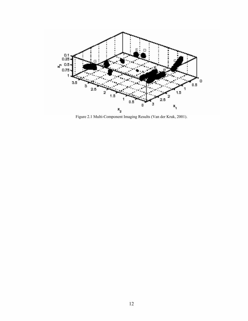
Figure 2.1 Multi-Component Imaging Results (Van der Kruk, 2001).

12

Chapter 3

BASIC THEORY

3.1 BASICS OF GROUND PENETRATING RADAR (GPR)

Ground Penetrating Radar (GPR) operates by transmitting electromagnetic energy

into the probed material and receiving the reflected pulses. The transmitted EM pulses are

reflected as they encounter discontinuities. The discontinuity could be a boundary or

interface between materials with different dielectrics or it could be a subsurface object

such as debond or delamination. The antenna receives the pulses with varying amplitudes

and arrival times. The amplitudes of the received echoes and the corresponding arrival

times can then be used to determine the nature and location of the discontinuity. It is

important to realize that the recorded arrival time is two-way travel time. The

measurements have to be conducted carefully in order to get meaningful post-processing

results. The reflected pulses are displayed on an oscilloscope as a time-series of pulses,

known as waveform. These waveforms have been used to determine the depth of the

asphalt layer, the thickness of the pavement, debonding of asphalt from concrete, and

delamination of concrete (Halabe et al. 2003c, Carter et al. 1995). With the advancement

in GPR technology, especially the increase in frequency of commercially available GPR

antennas and better data processing software, GPR can now be used for subsurface

condition assessment in materials consisting of thin layers such as Fiber Reinforced

Polymer (FRP). Careful analysis of GPR waveforms can potentially help detect

subsurface debonds between the wearing surface and the underlying FRP bridge deck,

and delaminations within the flanges of the FRP deck. A major advantage of GPR over

13

techniques such as Infrared Thermography is its ability to attain deeper penetration

including evaluation of the bottom flange from the top surface of the deck itself, with no

access required to the bottom side.

Velocity and attenuation of radar waves in the transmitted media directly affect

the output waveform. Both the velocity and the attenuation of radar waves depend on the

complex dielectric permittivity, which is related to the electromagnetic properties of solid

particles, porosity, moisture content, and salt content of the medium (Halabe et al. 1993).

Basically, most materials can be classified as either (a) conductors (e.g., metallic objects

such as rebars in concrete deck), or (b) insulators, also known as dielectrics, such as

asphalt, FRP, and concrete. Some media, such as water, are in between conductors and

dielectrics depending on their purity (Halabe et al. 1993).

3.1.1 Electromagnetic Properties and Radar Wave Propagation

An FRP deck consists of multiple layers of different material with different

dielectric properties. These layers include the wearing surface, FRP deck flanges and

webs, debonds between the wearing surface and the FRP deck and possible delaminations

within the deck flanges and/or web. The electromagnetic property of each of these layers

is characterized by a property known as the dielectric permittivity. The relative dielectric

permittivity (ε) of a material is defined as the ratio of the actual dielectric permittivity of

the medium (εactual) to the permittivity of free space or vacuum (εo).

o

actual

εε

ε = (3.1)

14

The dielectric permittivity is a complex quantity and can be expressed as (Halabe

et al. 1993):

ε = ε’ + iε” (3.2)

where,

ε = relative complex dielectric permittivity of the medium

ε’ = real part of relative dielectric permittivity

ε’’ = imaginary part of relative dielectric permittivity = oωε

σ

where,

σ = dielectric conductivity of the medium (mho/m)

ω = angular frequency (radian/sec) = 2πf

εo = dielectric permittivity of free space or vacuum = 8.854 x 10-12 farad/m

f = frequency of the radar wave (Hz)

The real part of the relative dielectric permittivity (ε’) in Equation 3.2 is

commonly known as the dielectric constant. The imaginary part (ε”) is known as the loss

factor. For one dimensional electromagnetic wave propagation along x-direction, the

amplitude of the wave is given by Halabe (1990):

A(x,t) = Aoei(kx – ωt) (3.3)

15

where,

Ao = initial wave amplitude

A(x,t) = wave amplitude at a distance ‘x’ and time ‘t’

k = complex wave number, which is related to ε as per the following

relationship (Halabe 1990):

k = kR + ikI = εεµω oo (3.4)

where,

kR = real part of complex wave number (m-1)

kI = imaginary part of complex wave number, also known as the

material attenuation coefficient (m-1)

µo = magnetic permeability of free space = 4π x 10-7 henry/m

The real part of the wavenumber (kR) is related to the wavelength (λ) of the

propagating radar wave as per the following equation (Halabe 1990):

kR = λπ2 (3.5)

For a medium with low conductivity, such as FRP decks, the attenuation

coefficient, kI, is given by (Halabe et al. 1993, Halabe 1990):

kI = '2

377εσ (3.6)

16

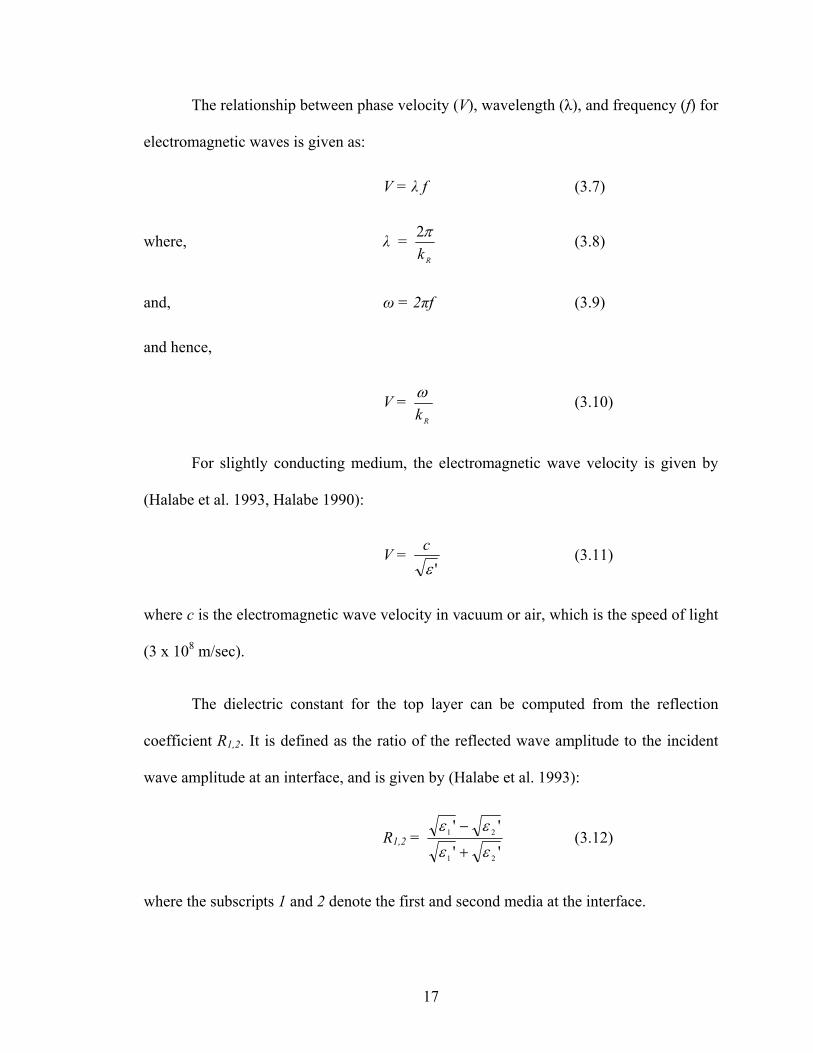
The relationship between phase velocity (V), wavelength (λ), and frequency (f) for

electromagnetic waves is given as:

V = λ f (3.7)

where, λ = Rkπ2 (3.8)

and, ω = 2πf (3.9)

and hence,

V = Rk

ω (3.10)

For slightly conducting medium, the electromagnetic wave velocity is given by

(Halabe et al. 1993, Halabe 1990):

V = 'ε

c (3.11)

where c is the electromagnetic wave velocity in vacuum or air, which is the speed of light

(3 x 108 m/sec).

The dielectric constant for the top layer can be computed from the reflection

coefficient R1,2. It is defined as the ratio of the reflected wave amplitude to the incident

wave amplitude at an interface, and is given by (Halabe et al. 1993):

R1,2 = ''

''

21

21

εε

εε

+

− (3.12)

where the subscripts 1 and 2 denote the first and second media at the interface.

17

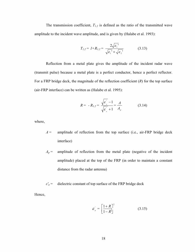
The transmission coefficient, T1,2 is defined as the ratio of the transmitted wave

amplitude to the incident wave amplitude, and is given by (Halabe et al. 1993):

T1,2 = 1+R1,2 = ''

'2

21

1

εε

ε

+ (3.13)

Reflection from a metal plate gives the amplitude of the incident radar wave

(transmit pulse) because a metal plate is a perfect conductor, hence a perfect reflector.

For a FRP bridge deck, the magnitude of the reflection coefficient (R) for the top surface

(air-FRP interface) can be written as (Halabe et al. 1995):

R = - R1,2 = 1

1'

'

+

−

a

a

ε

ε=

pAA (3.14)

where,

A = amplitude of reflection from the top surface (i.e., air-FRP bridge deck

interface)

Ap = amplitude of reflection from the metal plate (negative of the incident

amplitude) placed at the top of the FRP (in order to maintain a constant

distance from the radar antenna)

ε'a = dielectric constant of top surface of the FRP bridge deck

Hence,

'aε =

2

11

⎥⎦⎤

⎢⎣⎡

−+

RR (3.15)

18

A 3/8” (9.5mm) thick layer of wearing surface is usually placed on the top of the

FRP deck modules in field construction to provide a riding surface and prevent slip of

vehicles. For such decks, Equation (3.15) gives the dielectric constant of the wearing

surface. If the wearing surface has not yet been placed, the GPR measurements of A and

Ap would lead to dielectric constant of the FRP deck surface. It is important to note that

the measurements of A and Ap are only possible with the use of an air-launched antenna

and not with a ground-coupled antenna.

3.1.2 Detection of Voids

The detection of subsurface defects (voids, cracks, delaminations, etc.) is

primarily a function of the changes in dielectric permittivity. Subsurface voids, debonds,

or delaminations in FRP bridge decks may be filled with either air or water, which creates

a discontinuity in the dielectric permittivity of the medium. Thus, if the change in

dielectric permittivity is significant, then the gap (voids, debonds, or delaminations)

appears to the radar as two reflectors close to each other (Halabe et al. 1995). If the

entire wearing surface and/or the underlying deck have high moisture content, the

attenuation of the radar wave also increases. This adversely affects the waveform

amplitudes and makes it more difficult to analyze. Therefore, it is essential to conduct

radar survey only during relatively dry weather when the overall FRP deck may have low

moisture content. However, moisture inside the voids, debonds, or delaminations, are

beneficial for radar detection since water-filled defects produce high amplitude

reflections. Therefore, the optimal condition for conducting field GPR measurements is

few days after it has rained, that is, after the overall deck had time to dry up but still has

some moisture entrapped in the subsurface voids, debonds, or delaminations.

19

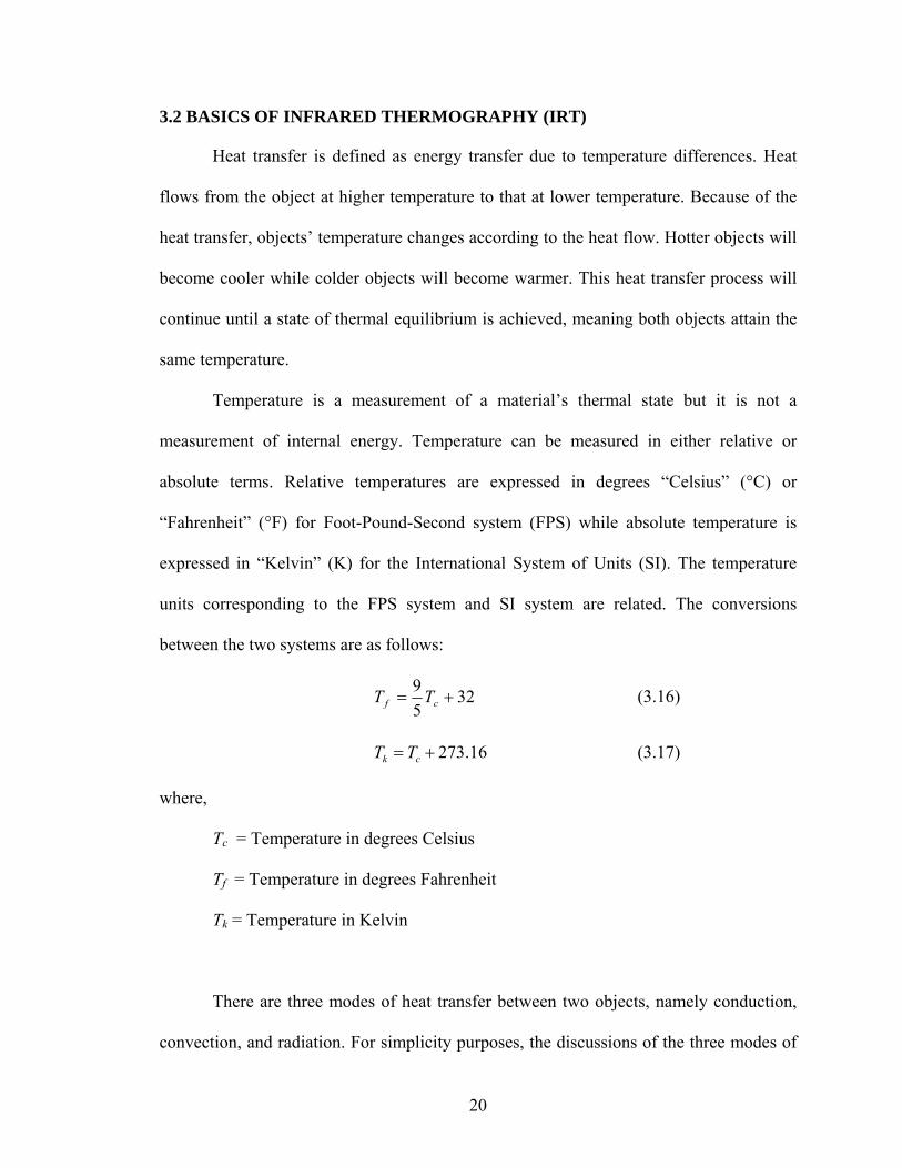
3.2 BASICS OF INFRARED THERMOGRAPHY (IRT)

Heat transfer is defined as energy transfer due to temperature differences. Heat

flows from the object at higher temperature to that at lower temperature. Because of the

heat transfer, objects’ temperature changes according to the heat flow. Hotter objects will

become cooler while colder objects will become warmer. This heat transfer process will

continue until a state of thermal equilibrium is achieved, meaning both objects attain the

same temperature.

Temperature is a measurement of a material’s thermal state but it is not a

measurement of internal energy. Temperature can be measured in either relative or

absolute terms. Relative temperatures are expressed in degrees “Celsius” (°C) or

“Fahrenheit” (°F) for Foot-Pound-Second system (FPS) while absolute temperature is

expressed in “Kelvin” (K) for the International System of Units (SI). The temperature

units corresponding to the FPS system and SI system are related. The conversions

between the two systems are as follows:

3259

+= cf TT (3.16)

16.273+= ck TT (3.17)

where,

Tc = Temperature in degrees Celsius

Tf = Temperature in degrees Fahrenheit

Tk = Temperature in Kelvin

There are three modes of heat transfer between two objects, namely conduction,

convection, and radiation. For simplicity purposes, the discussions of the three modes of

20

heat transfer in this chapter deal with steady-state heat transfer. These modes of heat

transfer occur on a molecular or subatomic scale.

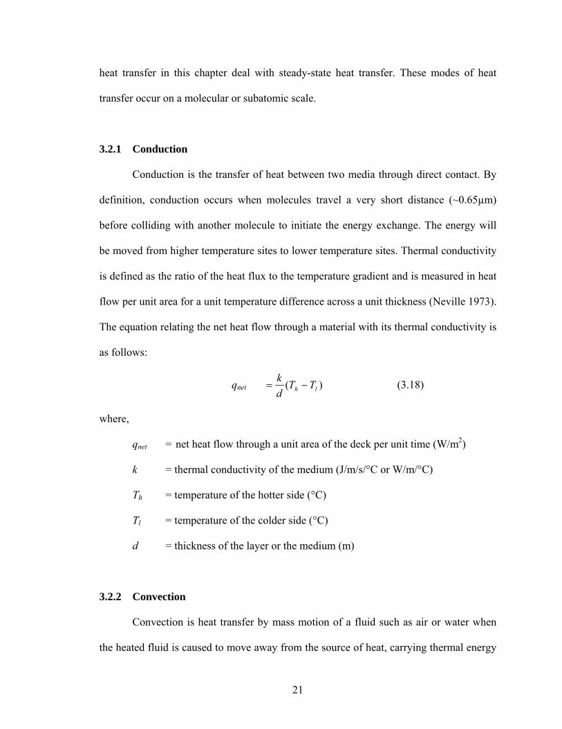
3.2.1 Conduction

Conduction is the transfer of heat between two media through direct contact. By

definition, conduction occurs when molecules travel a very short distance (~0.65µm)

before colliding with another molecule to initiate the energy exchange. The energy will

be moved from higher temperature sites to lower temperature sites. Thermal conductivity

is defined as the ratio of the heat flux to the temperature gradient and is measured in heat

flow per unit area for a unit temperature difference across a unit thickness (Neville 1973).

The equation relating the net heat flow through a material with its thermal conductivity is

as follows:

qnet )( lh TTdk

−= (3.18)

where,

qnet = net heat flow through a unit area of the deck per unit time (W/m2)

k = thermal conductivity of the medium (J/m/s/°C or W/m/°C)

Th = temperature of the hotter side (°C)

Tl = temperature of the colder side (°C)

d = thickness of the layer or the medium (m)

3.2.2 Convection

Convection is heat transfer by mass motion of a fluid such as air or water when

the heated fluid is caused to move away from the source of heat, carrying thermal energy

21

with it. Convection may arise from temperature differences either within the fluid or

between the fluid and its boundary, other sources of density variations (such as variable

salinity), or from the application of an external motive force. Convection is usually the

dominant form of heat transfer in liquids and gases. There are two primary convection

modes, namely the forced convection and the free convection. Forced convection

happens when motion of the fluid is imposed externally (such as by a pump or fan). Free

convection is convection in which motion of the fluid arises solely due to the temperature

differences existing within the fluid. Naturally, the temperature at the object’s surface,

the ambient temperature, and the speed of the motion fluid (e.g. wind) are the factors that

control the convective heat flow. The convective heat transfer between a deck surface and

the surrounding fluid (air) can be obtained through Langmuir’s equation, which is given

as follows (Malloy 1969):

35.0)35.0()(947.1 4

5

0+

−=vTTq ac (3.19)

where,

qc = convective heat transfer from the surface (W/m2)

v = wind velocity (m/s)

To = surface temperature of the deck (°C)

Ta = ambient air temperature (°C)

22

3.2.3 Radiation

Radiative heat transfer is the only form of heat transfer that can occur in the

absence of any form of medium and as such is the only means of heat transfer through

vacuum. Thermal radiation is a direct result of the movements of atoms and molecules in

a material. Since these atoms and molecules are composed of charged particles such as

protons and electrons, their movements result in the emission of electromagnetic

radiation, which carries energy away from the surface. The behavior of such radiant

emission can be described through Stefan-Boltzmann law, which states that the heat

radiated by a body is directly proportional to the fourth power of its absolute temperature

(Vanzetti 1972).

(3.20) 4Tqe σε=

where,

qe = total radiant emission from the radiating surface (W/m2)

σ = Stefan-Boltzmann constant = 5.673 x 10-8 W/m2/K4

ε = emissivity value of the radiant object

T = absolute temperature of the object (K)

While a body is radiating heat, its surface is also constantly receiving the radiation

from the surroundings, resulting in the transfer of energy into the surface. Since the

amount of emitted radiation increases with increasing temperature, a net transfer of

energy from higher temperatures to lower temperatures results. Through the variation of

the Stefan-Boltzmann law, the net radiation from any surface can be expressed as follows

(Halabe and Maser 1986):

23

(3.21) ])273()273[( 44 +−+= aor TTq σε

where,

qr = net radiation from the radiating surface (W/m2)

Ta = ambient air temperature (°C)

To = temperature of the radiating surface (°C)

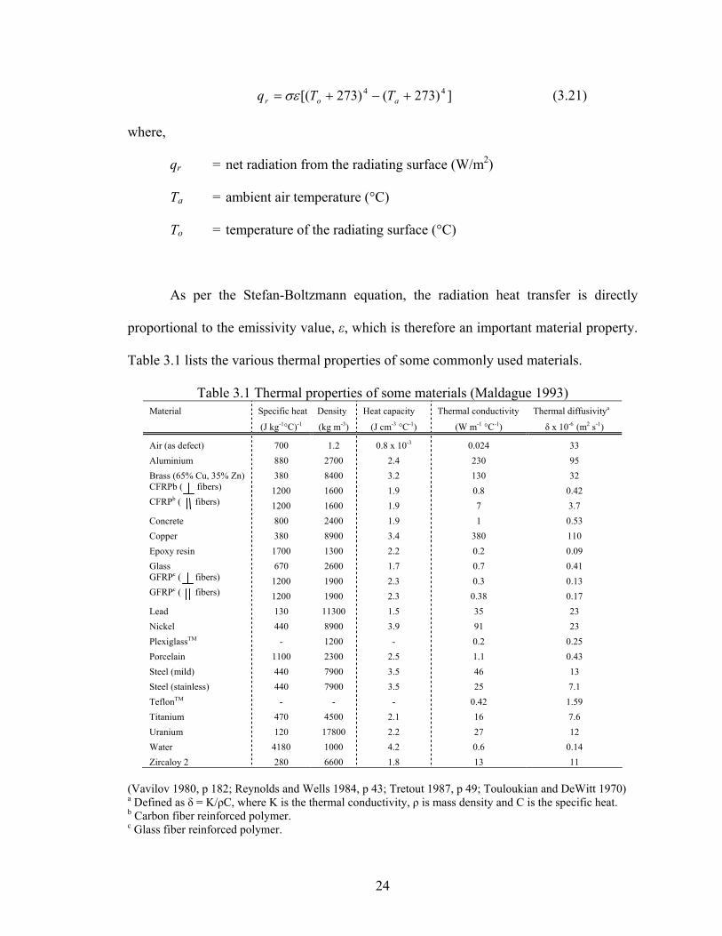
As per the Stefan-Boltzmann equation, the radiation heat transfer is directly

proportional to the emissivity value, ε, which is therefore an important material property.

Table 3.1 lists the various thermal properties of some commonly used materials.

Table 3.1 Thermal properties of some materials (Maldague 1993) Material Specific heat Density Heat capacity Thermal conductivity Thermal diffusivitya

(J kg-1°C)-1 (kg m-3) (J cm-3 °C-1) (W m-1 °C-1) δ x 10-6 (m2 s-1)

Air (as defect) 700 1.2 0.8 x 10-3 0.024 33 Aluminium 880 2700 2.4 230 95 Brass (65% Cu, 35% Zn) 380 8400 3.2 130 32 CFRPb ( fibers) 1200 1600 1.9 0.8 0.42 CFRPb ( fibers) 1200 1600 1.9 7 3.7 Concrete 800 2400 1.9 1 0.53 Copper 380 8900 3.4 380 110 Epoxy resin 1700 1300 2.2 0.2 0.09 Glass 670 2600 1.7 0.7 0.41 GFRPc ( fibers) 1200 1900 2.3 0.3 0.13 GFRPc ( fibers) 1200 1900 2.3 0.38 0.17 Lead 130 11300 1.5 35 23 Nickel 440 8900 3.9 91 23 PlexiglassTM - 1200 - 0.2 0.25 Porcelain 1100 2300 2.5 1.1 0.43 Steel (mild) 440 7900 3.5 46 13 Steel (stainless) 440 7900 3.5 25 7.1 TeflonTM - - - 0.42 1.59 Titanium 470 4500 2.1 16 7.6 Uranium 120 17800 2.2 27 12 Water 4180 1000 4.2 0.6 0.14 Zircaloy 2 280 6600 1.8 13 11

(Vavilov 1980, p 182; Reynolds and Wells 1984, p 43; Tretout 1987, p 49; Touloukian and DeWitt 1970) a Defined as δ = K/ρC, where K is the thermal conductivity, ρ is mass density and C is the specific heat. b Carbon fiber reinforced polymer. c Glass fiber reinforced polymer.

24

3.2.4 Infrared Measurement

At a temperature above absolute zero (-273.16 °C), all objects radiate

electromagnetic waves. The intensity of the radiation is directly proportional to the

object’s temperature and its emissivity value. Emissivity value is defined as the ratio of

radiation emitted by an object to that from a blackbody source, which theoretically refers

to the object that emits maximum amount of radiation at any given temperature.

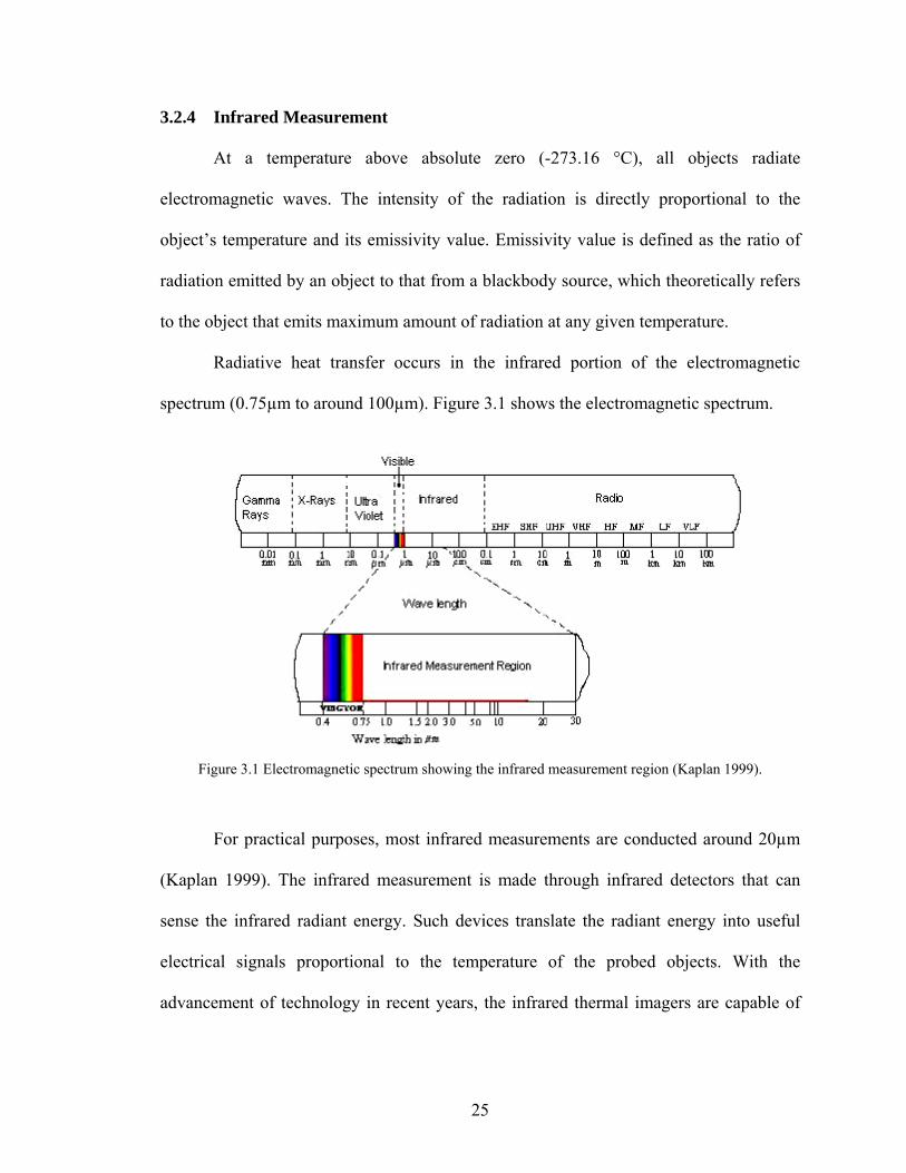
Radiative heat transfer occurs in the infrared portion of the electromagnetic

spectrum (0.75µm to around 100µm). Figure 3.1 shows the electromagnetic spectrum.

Figure 3.1 Electromagnetic spectrum showing the infrared measurement region (Kaplan 1999).

For practical purposes, most infrared measurements are conducted around 20µm

(Kaplan 1999). The infrared measurement is made through infrared detectors that can

sense the infrared radiant energy. Such devices translate the radiant energy into useful

electrical signals proportional to the temperature of the probed objects. With the

advancement of technology in recent years, the infrared thermal imagers are capable of

25

producing thermal maps (thermograms) with various color palettes, including black and

white scale.

Thermal imaging is conducted through two different approaches: the active

thermography and the passive thermography. In active thermography, heat flow is

produced with external heating or cooling of the structure. Because of this thermal

excitation, the object with subsurface anomalies will display non-uniform surface

temperatures. Conversely, the passive thermography relies solely on the existing

temperature differences within the object. The passive scheme is commonly used to

assess the state of industrial processes or during the manufacturing stage of certain

products (Maldague and Moore 2001).

26

Chapter 4

EQUIPMENT AND TEST SPECIMENS

4.1 GPR EQUIPMENT

The equipment used in the Ground Penetrating Radar portion of this study was

manufactured by Geophysical Survey Systems, Inc. The SIR-20 data acquisition system

was chosen based on the fact that it has two different channels that could accommodate

various antennas with different frequencies. The SIR-20 system is also capable of

integrating data collection and post-processing for instant results. Furthermore, the SIR-

20 system has the capability to take input from a geographic information system (GIS).

The associated data processing software, RADAN, is capable of 3D modeling, which

drastically improves the post-processing process.

The SIR-20 system comes with an industrial strength notebook computer made by

Panasonic and a mainframe, which serve as a bridge between the notebook computer and

the antennas. Two types of antenna were chosen for this study.

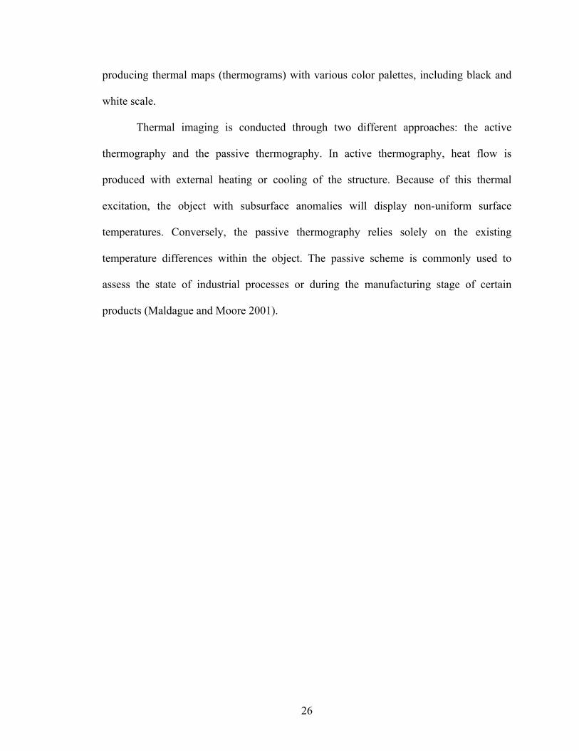
The first type is a 2.0 GHz air-coupled antenna, also commonly known as horn

antenna. The horn antenna is optimized for non-contact high-speed scanning, and is the

antenna with the highest frequency commercially available at this time. Typically, a horn

antenna is mounted to the back of a vehicle for field testing. Since the current research is

a laboratory study, a push-cart was modified to mount the horn antenna (Figure 4.1a).

Such configuration will allow the survey of a small bridge deck within laboratory setting.

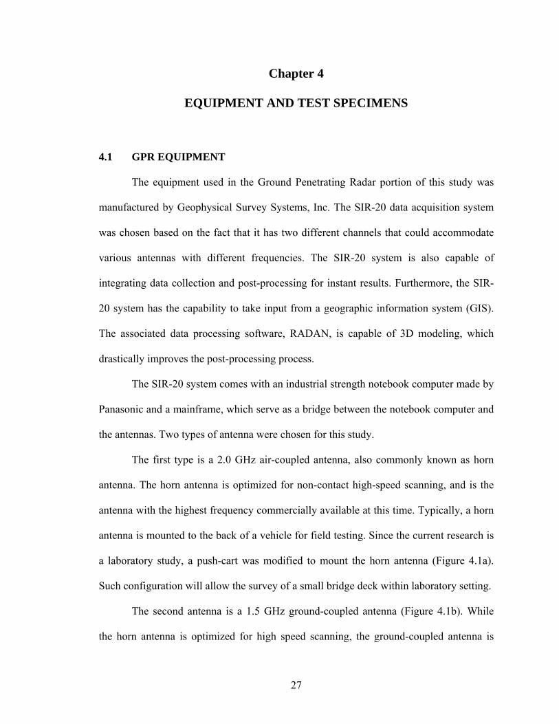
The second antenna is a 1.5 GHz ground-coupled antenna (Figure 4.1b). While

the horn antenna is optimized for high speed scanning, the ground-coupled antenna is

27

well known for the high resolution radar images it produces because it is capable of

transmitting more energy into the material. The 1.5 GHz frequency is the highest

commercially available frequency at this time for a ground-coupled antenna. The depth of

viewing window for the 1.5GHz antenna is approximately 18 inches in concrete.

SIR-20 Main Computer

SIR-20 Mainframe

2.0 GHz Horn Antenna

Modified Push Cart

Figure 4.1(a): GPR system with 2.0 GHz horn antenna on the modified push-cart.

1.5 GHz Ground-coupled Antenna

Survey Wheel

Figure 4.1(b): Hand-held 1.5 GHz ground-coupled antenna and survey wheel configuration.

28

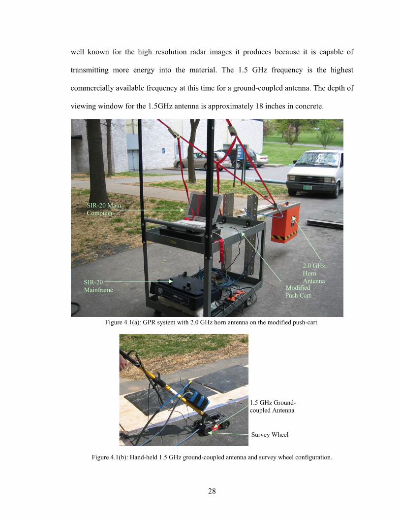
Figure 4.2(a) below shows the footprint of the 2.0GHz air-coupled antenna. The

footprint was obtained by moving a steel rebar underneath the antenna. When the rebar

reflects the electromagnetic energy sent by the antenna, the waveform of the scan will

change from its original state. Such changes would determine the outer most boundary

for the electric field generated by the antenna. The dimensions of this boundary, known

as the antenna’s footprint, is directly proportion to the height of the antenna from the

ground because of the beam spread as shown in Figure 4.2(a). Therefore, it is important

to calculate the beam spread angle, which is shown in the figure below.

GPR – Horn Antenna Dimensions

GPR Horn Antenna

21.375”

19.125”

7.875”

Air-coupled horn antenna’s effective footprint and angle:

8”

3.9375”

14”

5.5”θ1

10.6875”

θ2 5.5”

tan θ1 = (14 - 10.6875)/5.5 θ1 = 31.06o

tan θ2 = (8 – 3.9375)/5.5 θ2 = 36.45o

Figure 4.2(a): Footprint of the 2.0 GHz air-coupled horn antenna.

29

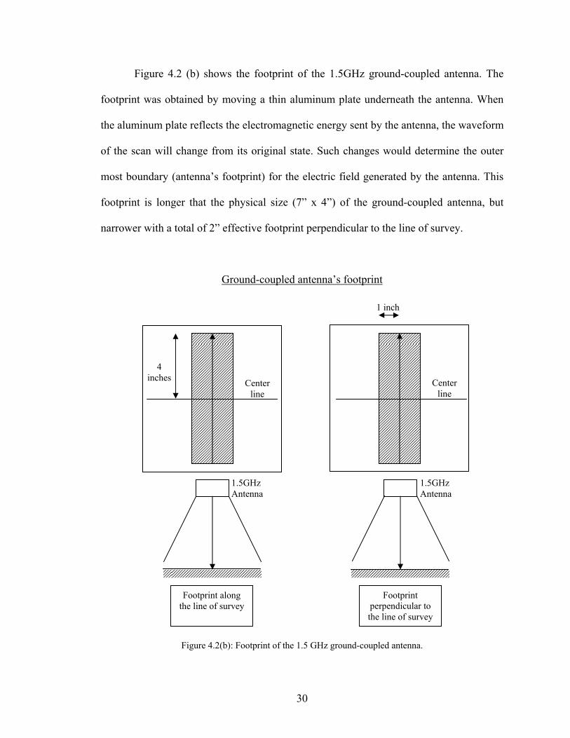
Figure 4.2 ed antenna. The

footprin

Ground-coupled antenna’s footprint

(b) shows the footprint of the 1.5GHz ground-coupl

t was obtained by moving a thin aluminum plate underneath the antenna. When

the aluminum plate reflects the electromagnetic energy sent by the antenna, the waveform

of the scan will change from its original state. Such changes would determine the outer

most boundary (antenna’s footprint) for the electric field generated by the antenna. This

footprint is longer that the physical size (7” x 4”) of the ground-coupled antenna, but

narrower with a total of 2” effective footprint perpendicular to the line of survey.

Figure 4.2(b): Footprint of the 1.5 GHz ground-co

1.5GHz Antenna

1.5GHz Antenna

1 inch

Footprint perpendicular to the ey line of surv

Footprint along the line of survey

Center line

4 inches Center

line

upled antenna.

30

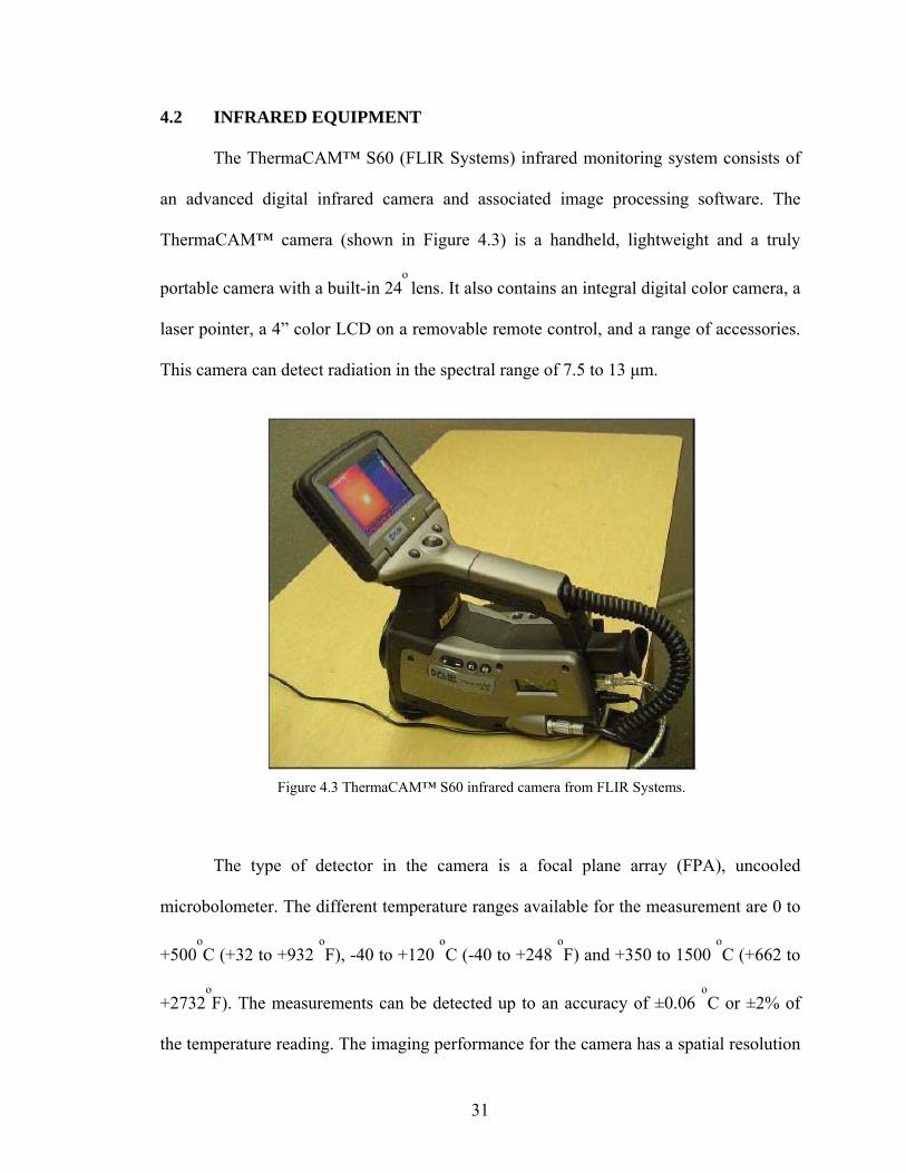
4.2 INFRARE

The ThermaCAM™ S60 (FLIR Systems) infrared monitoring system consists of

an advanced digital infrared camera and associated image processing software. The

ThermaCAM™ camera (shown in Figure 4.3) is a handheld, lightweight and a truly

portable camera with a built-in 24o

lens. It also contains an integral digital color camera, a

laser pointer, a 4” color LCD on a removable remote control, and a range of accessories.

This camera can detect radiation in the spectral range of 7.5 to 13 µm.

The type of detector in the camera is a focal plane array (FPA), uncooled

microbolometer. The different temperature ranges available for the measurement are 0 to

+500oC (+32 to +932

oF), -40 to +120

oC (-40 to +248

oF) and +350 to 1500

oC (+662 to

+2732oF). The measurements can be detected up to an accuracy of ±0.06

oC or ±2% of

the temperature reading. The imaging performance for the camera has a spatial resolution

D EQUIPMENT

Figure 4.3 ThermaCAM™ S60 infrared camera from FLIR Systems.

31

32

a capture rate of up to 60 frames per second, non-

interlac

markers built into

the cam Systems software (FLIR Systems 2002a).

he software that is used along with the camera is called as the ThermaCAM™

Researcher 2002. It deals with the live IRT images arriving through the camera interface

and can also receive IRT images from other media, such as PC card hard disk from the

camera. The software can be used to display the IRT images, record them on the disk, or

analyze them later during the replay. The measurements can be made with the analysis

tools like isotherm, spot meter, area and line. The images can be processed further to

enhance their contrast. Since the camera captures fully radiometric digital images, a

reference image can be subtracted from the full image sequence to achieve better results

in term of detectability of defects and to conduct a quantitative analysis (FLIR Systems

2002b).

4.2.1

of 1.3 mrad and can record images at

ed. It is possible to capture and store images on a removable flash card or directly

into a laptop computer which also houses the display software. The camera also features

burst recording functionality that allows the user to record sequences of events into the

internal RAM memory. Voice and/or text comments could be stored. The built-in digital

color camera captures critical details, making reporting and analysis easy. The images

can be analyzed either in the field by using the real-time measurement

era software, or in a PC using FLIR

T

s

Heating Sources

One of the objectives of this study is to advance the nondestructive testing

technology using Infrared Thermography. In order to attain the goal, it is vital to explore

both passive thermography and active thermography.

Solar Radiation

The sun has long been considered a massive energy source for the earth. On a

bright sunny day, solar radiation is often regarded as the perfect uniform heating source

provided the wind is not interfering with the process. As Maser et al. (1990) pointed out,

the sun produced excellent temperature differentials in concrete decks using IRT between

10 AM to 2 PM.

As good as it may be, though, solar radiation does indeed have weaknesses when

dealing with IRT nondestructive testing. First of all, the availability of solar heating is

heavily

lectrical/Gas Heater

To induce heat into the FRP bridge deck specimens thus creating an active

heating, both electrical and gas heaters can be used. Generally, the commercially

available heaters (both electrical and gas powered heaters) are capable of inducing a high

level of heat into any object over a short period of time, thus resulting in high thermal

dependent on the unpredictable weather. In order to conduct a successful solar

heating IRT test, the sky has to be clear most of the time. Also, as indicated in the

previous chapter, wind velocity is one of the parameters that affects the overall heat

transfer in convective mode. Therefore, it is important to have a relatively windless day

to ensure uniform heating. It should be noted that solar radiation is a gradually increasing

heat source (from morning to mid-day) which may not cause a sufficiently large thermal

perturbation over a small period that is often needed for successful IRT testing.

Nonetheless, the study of solar heating on FRP bridge decks is crucial in further

understanding and advancing the nondestructive testing using IRT.

E

33

stimulation. There are a wide range of heaters with various heating power available for

selectio

heating blanket of plan size 36” x 36” (914mm x 914mm) and 1”

(25mm

uced by

the blank

ent,

e control box with thermostatic control was used to cut off the

heating of coils, the heating blanket can be used in either vertical or horizontal position.

n. This provides an incredible amount flexibility to achieve a good active heating

on FRP bridge deck, which will enable field testing even during cold days.

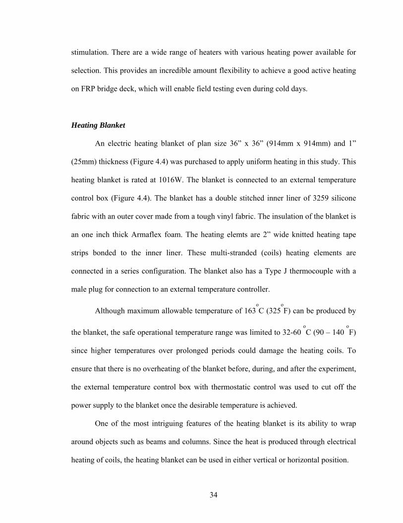
Heating Blanket

An electric

) thickness (Figure 4.4) was purchased to apply uniform heating in this study. This

heating blanket is rated at 1016W. The blanket is connected to an external temperature

control box (Figure 4.4). The blanket has a double stitched inner liner of 3259 silicone

fabric with an outer cover made from a tough vinyl fabric. The insulation of the blanket is

an one inch thick Armaflex foam. The heating elemts are 2” wide knitted heating tape

strips bonded to the inner liner. These multi-stranded (coils) heating elements are

connected in a series configuration. The blanket also has a Type J thermocouple with a

male plug for connection to an external temperature controller.

Although maximum allowable temperature of 163oC (325

oF) can be prod

et, the safe operational temperature range was limited to 32-60 oC (90 – 140

oF)

since higher temperatures over prolonged periods could damage the heating coils. To

ensure that there is no overheating of the blanket before, during, and after the experim

the external temperatur

power supply to the blanket once the desirable temperature is achieved.

One of the most intriguing features of the heating blanket is its ability to wrap

around objects such as beams and columns. Since the heat is produced through electrical

34

As attractive as it may sound, the heating blanket does take a longer time to

induce same amount of heat compared to the electrical or gas heaters in general. Also,

since the heating blanket was constructed by connecting the heating elements in series, it

important to handle the heating blanket with care to ensure that none of the heating

ged. A damaged heating element will cause the entire heating blanket

(or a pa

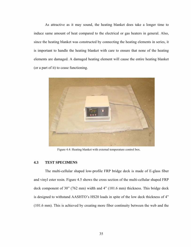
The multi-cellular shaped low-profile FRP bridge deck is made of E-glass fiber

his bridge deck

is designed to withstand AAS

is

elements are dama

rt of it) to cease functioning.

Figure 4.4: Heating blanket with external temperature contro box. l

4.3 TEST SPECIMENS

and vinyl ester resin. Figure 4.5 shows the cross section of the multi-cellular shaped FRP

deck component of 30” (762 mm) width and 4” (101.6 mm) thickness. T

HTO’s HS20 loads in spite of the low deck thickness of 4”

(101.6 mm). This is achieved by creating more fiber continuity between the web and the

35

flange as well as by reducing the weight. This low-profile deck is cost effective and is

manufactured with higher structural strength and lower weight than its predecessor.

The flanges and webs of the low-profile FRP bridge deck component were made

of triaxial fabrics, continuous rovings and mats. The fibers continue from the flange to

web and back to the flange. The resin used in this deck was vinyl ester resin which is a

high elongation resin. This low-profile deck weighs about 10 lb/ft2 and has fiber volume

fraction of approximately 50%.

Figure 4.5: Cross-section of low-profile FRP bridge deck.

The ability to manufacture bridge deck in a factory setting thus ensuring good

quality control k. Generally, the

manufactured through a pultrusion process.

olves direct conversion of continuous fibers and resins into

finished product of any size and shape, so l

wet-out bath and the injection chamber, where they are wetted by the thermoset resin,

is one of the most intriguing aspects of FRP bridge dec

FRP products are first designed, and then

Pultrusion is a process that inv

ong as a mold can be made. The first step to

be considered in pultrusion process is the design and manufacturing of pultrusion die to

strict tolerances of thickness, angularity and radius. The performing guides position the

roving and mat dispensed from the creel and mat racks in the specified location, in the

cross section of the product. Then the fiber reinforcements are made to pass through the

36

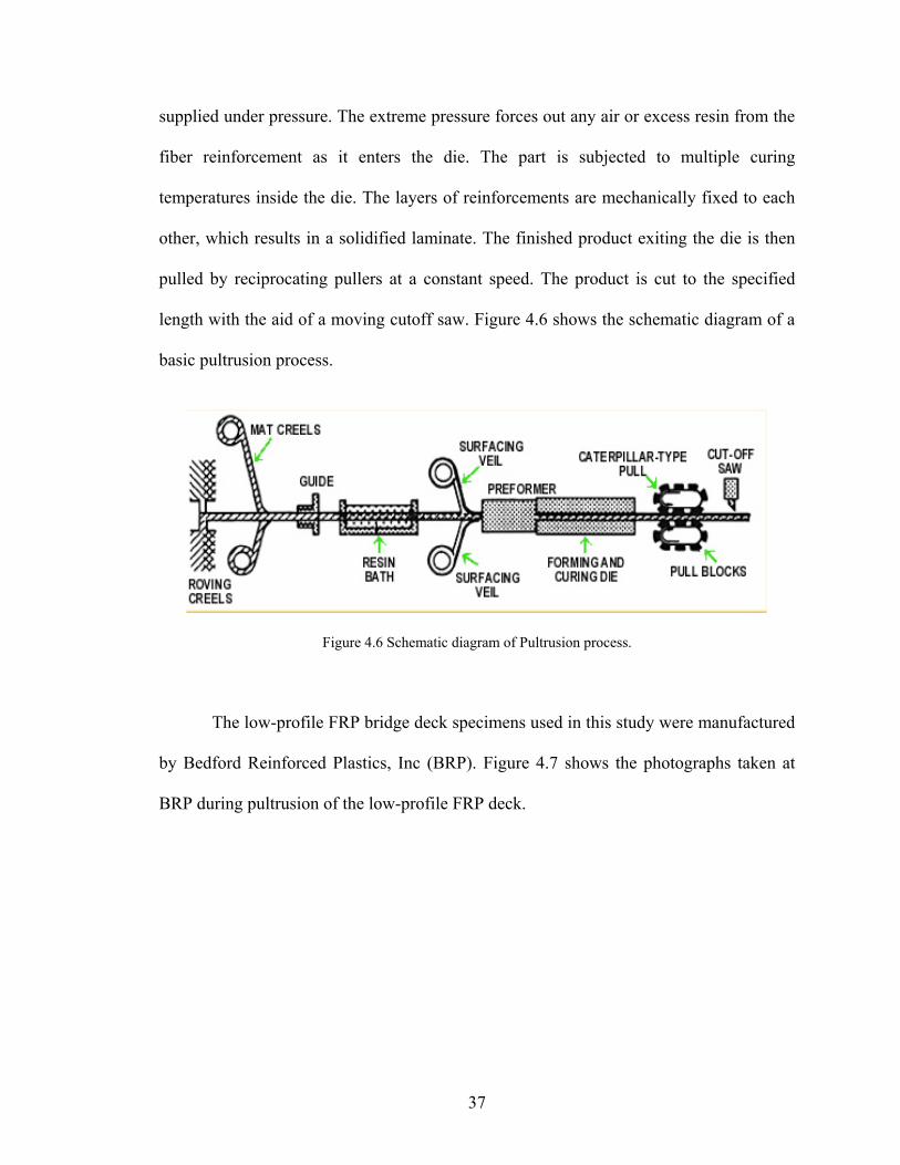
supplied under pressure. The extreme pressure forces out any air or excess resin from the

fiber reinforcement as it enters the die. The part is subjected to multiple curing

temperatures inside the die. The layers of reinforcements are mechanically fixed to each

other, which results in a solidified laminate. The finished product exiting the die is then

pulled by reciprocating pullers at a constant speed. The product is cut to the specified

length with the aid of a moving cutoff saw. Figure 4.6 shows the schematic diagram of a

basic pultrusion process.

The low-profile FRP bridge deck specimens used in this study were manufactured

BRP during pultrusion of the low-profile FRP deck.

Figure 4.6 Schematic diagram of Pultrusion process.

by Bedford Reinforced Plastics, Inc (BRP). Figure 4.7 shows the photographs taken at

37

Figure 4.7: Photographs showing manufacturing of FRP bridge deck in a factory using Pultrusion process.

This study evaluates the applicability of both ground penetrating radar and digital

infrared thermography systems to detect subsurface anomalies such as water-filled and

air-filled debonds and delaminations. Debonds refer to discontinuities between the

wearing surface and the underlying deck, while delaminations refer to discontinuities

within the flanges of the deck itself.

4.4 REPARATION OF DEFECTS

surfaces of dimensions 36” x 24” x

3/8” (914.4mm x 609.6mm x 9.525mm) (Figure 4.8) were cast. The wearing surface

module was made by mixing a gallon of Transpo Industries’ Transpo T-48A Epoxy

Resin, half a gallon of Transpo T-48B Hardener, and a 52 pounds bag of Transpo T-48

Powder component and cast over a light steel frame of dimensions 36” x 24” x 3/8”

(914.4mm x 609.6mm x 9.525mm).

P

Debonds refer to the subsurface defects that are present at the interface between

the wearing surface layer and the underlying FRP deck. In order to produce defects that

could be used over and over again, modular wearing

38

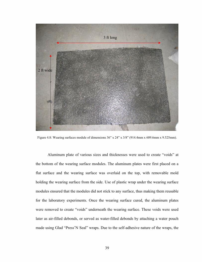
Figure 4.8: Wearing surfaces module of dim

3 ft long

2 ft wide

ensions 36” x 24” x 3/8” (914.4mm x 609.6mm x 9.525mm).

d thicknesses were used to create “voids” at

the bot

ps. Due to the self-adhesive nature of the wraps, the

Aluminum plate of various sizes an

tom of the wearing surface modules. The aluminum plates were first placed on a

flat surface and the wearing surface was overlaid on the top, with removable mold

holding the wearing surface from the side. Use of plastic wrap under the wearing surface

modules ensured that the modules did not stick to any surface, thus making them reusable

for the laboratory experiments. Once the wearing surface cured, the aluminum plates

were removed to create “voids” underneath the wearing surface. These voids were used

later as air-filled debonds, or served as water-filled debonds by attaching a water pouch

made using Glad “Press’N Seal” wra

39

pouch could be easily made by folding the wrap into half and gently pressing the sides

together to seal off the edges (Figure 4.9). of the pouch ranged from as large as

12” x 12” (304.8mm x 304.8mm) to as small as 1” x 1” (25.4mm x 25.4mm). The

pouches were made into three thicknesses: 0.75mm, 1.5mm, 2.25mm (Figure 4.10).

These pouches were then filled with water using a syringe (Figure 4.11). While

c were made to inject the exact amount of water to fill the entire void, some air

bubbles were trapped inside the water pouch as seen in Figure 4.10, which was due to

some human error. The bottom side of a typical wearing surface module with simulated

debonds is shown in Figure 4.12.

The size

alculations

Figure 4.9: Pouch made using Press’N Seal Glad wrap.

40

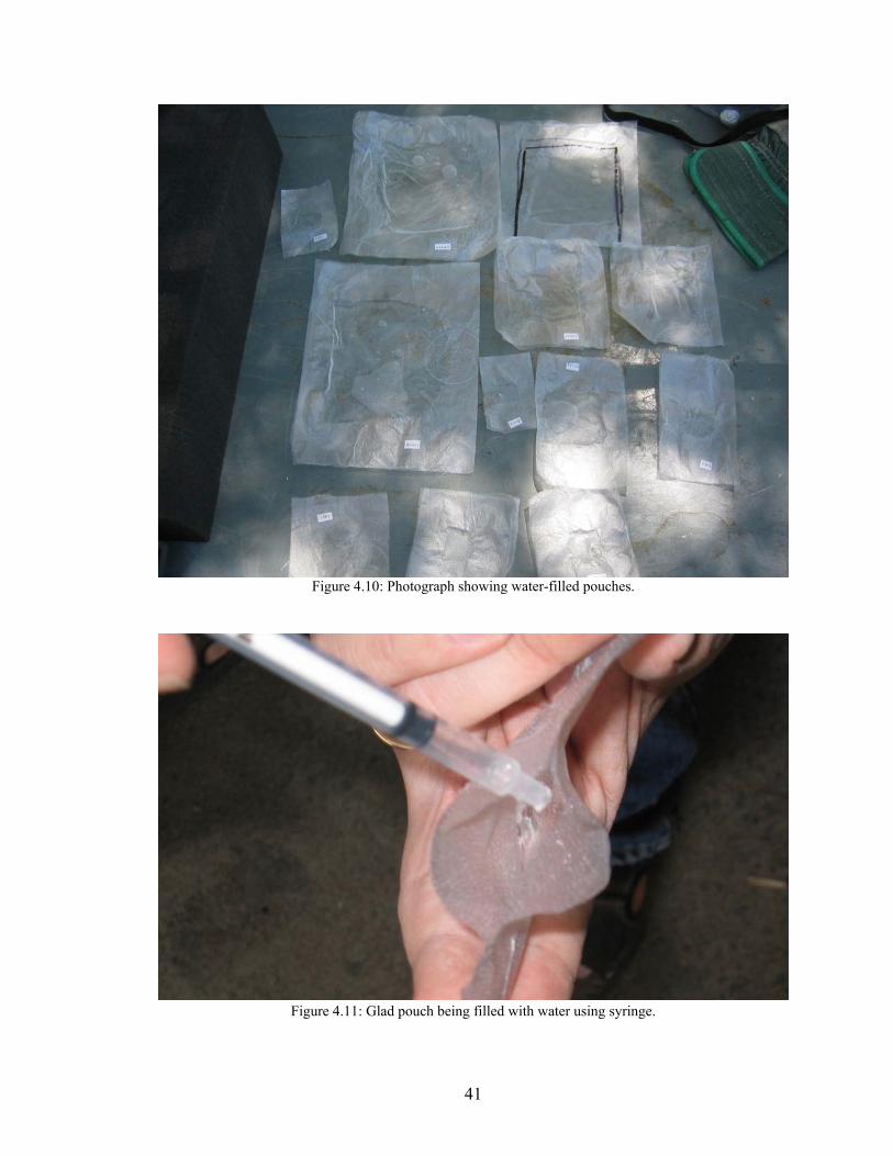
Figure 4.10: Photograph showing water-filled pouches.

Figure 4.11: Glad pouch being filled with water using syringe.

41

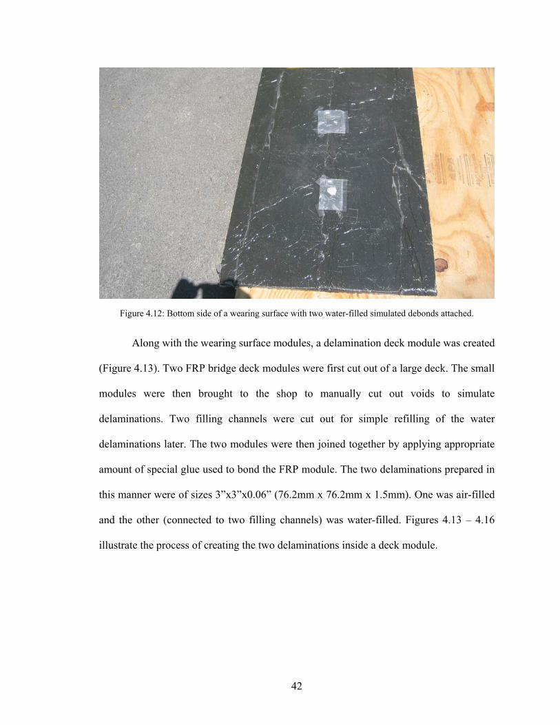
Figure 4.12: Bottom side of a wearing surface with two water-filled simulated debonds attached.

Along with the wearing surface modules, a delamination deck module was created

(Figure 4.13). Two FR arge deck. The small

manually cut out voids to simulate

P bridge deck modules were first cut out of a l

modules were then brought to the shop to

delaminations. Two filling channels were cut out for simple refilling of the water

delaminations later. The two modules were then joined together by applying appropriate

amount of special glue used to bond the FRP module. The two delaminations prepared in

this manner were of sizes 3”x3”x0.06” (76.2mm x 76.2mm x 1.5mm). One was air-filled

and the other (connected to two filling channels) was water-filled. Figures 4.13 – 4.16

illustrate the process of creating the two delaminations inside a deck module.

42

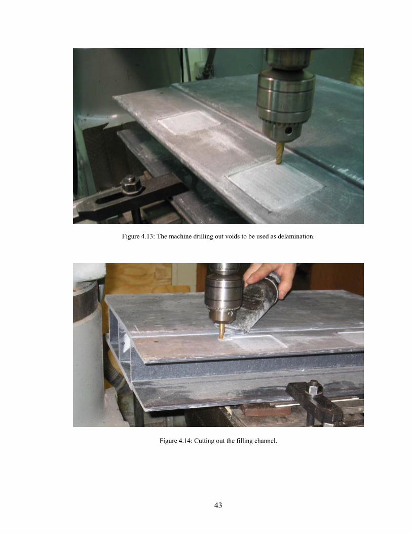
Figure 4.13: The machine drilling out voids to be used as delamination.

Figure 4.14: Cutting out the filling channel.

43

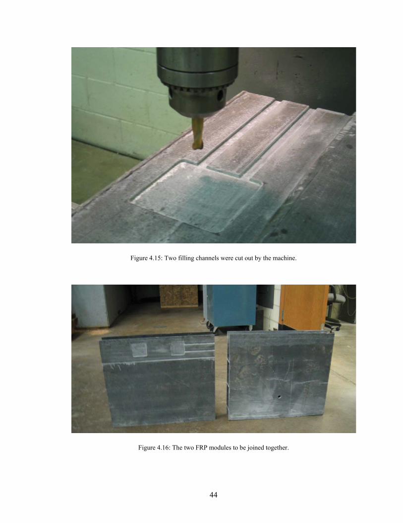
Figure 4.15: Two filling channels were cut out by the machine.

Figure 4.16: The two FRP modules to be joined together.

44

Chapter 5

EXPERIMENTAL RESULTS FROM INFRARED

THERMOGRAPHY

Previous studies have shown that commercially available heater is a useful tool to

help find debonds as small as 1” x 1” (25.4mm x 25.4mm) in small scale FRP bridge

deck specimens (Halabe et al. 2004d). To further evaluate the feasibility of utilizing

commercially available heating source in subsurface detection of defects on FRP bridge

decks, similar tests were conducted on a larger scale specimen (6’ x 3’, or 1828.8mm x

914.4mm). Furthermore, the same specimens were subjected to two rounds of solar

radiation tests during two different seasons. The first solar radiation test was conducted

during the early f tively calm wind

yielded excellent heating of the FRP deck. The second solar radiation test was conducted

during late winter/early spring season. The low ambient temperature provided a testing

environment with low rate of heat transfer between the FRP bridge deck specimen and

the surroundings. In addition to solar radiation tests, a heater and an electric heating

blanket were used as active heat sources.

5.1 IRT USING COMMERCIALLY AVAILABLE HEATER AS ACTIVE

HEAT SOURCE

Uniform heating was achieved by placing a 1500W heater few inches away from

the wearing surface tedly to ensure no

overheating of one region. Heat was applied for about 5 minutes. The infrared image of

all season. The abundance of solar energy and rela

and moving the heater back and forth repea

45

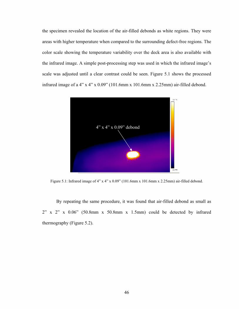
the specimen revealed the location of ebonds as white regions. They were

areas with hi egions. The

color scale showing the temperature variab area is also available with

the infrared image. A simple post-processing step was used in which the infrared image’s

scale was adjusted until a clear contrast could be seen. Figure 5.1 shows the processed

infrared image of a 4” x 4” x 0.09” (101.6mm x 101.6mm x 2.25mm) air-filled debond.

Figure 5.1: Infrared image of 4” x 4” x 0.09” (101.6mm x 101.6mm x 2.25mm) air-filled debond.

x 1.5mm) could be detected by infrared

ography (Figure 5.2).

the air-filled d

gher temperature when compared to the surrounding defect-free r

ility over the deck

4” x 4” x 0.09” debond

By repeating the same procedure, it was found that air-filled debond as small as

2” x 2” x 0.06” (50.8mm x 50.8mm

therm

46

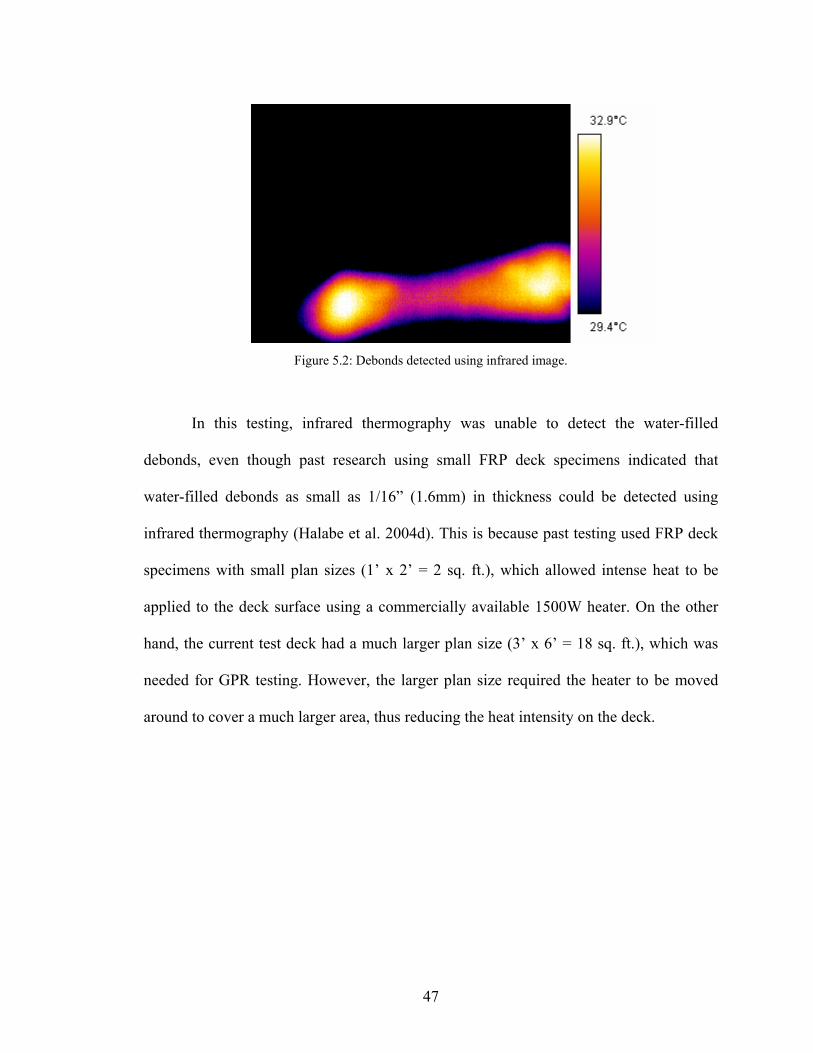
Figure 5.2: Debonds detected using infrared image.

In this testing, infrared therm was unable to detect the water-filled

all FRP deck specimens indicated that

all as 1/16” (1.6mm) in thickness could be detected using

et al. 2004d). This is because past testing used FRP deck

ens with small plan sizes (1’ x 2’ = 2 sq. ft.), which allowed intense heat to be

applied to the deck surface using a commerc

and, the current test deck had a much larger plan size (3’ x 6’ = 18 sq. ft.), which was

needed

ography

debonds, even though past research using sm

water-filled debonds as sm

infrared thermography (Halabe

specim

ially available 1500W heater. On the other

h

for GPR testing. However, the larger plan size required the heater to be moved

around to cover a much larger area, thus reducing the heat intensity on the deck.

47

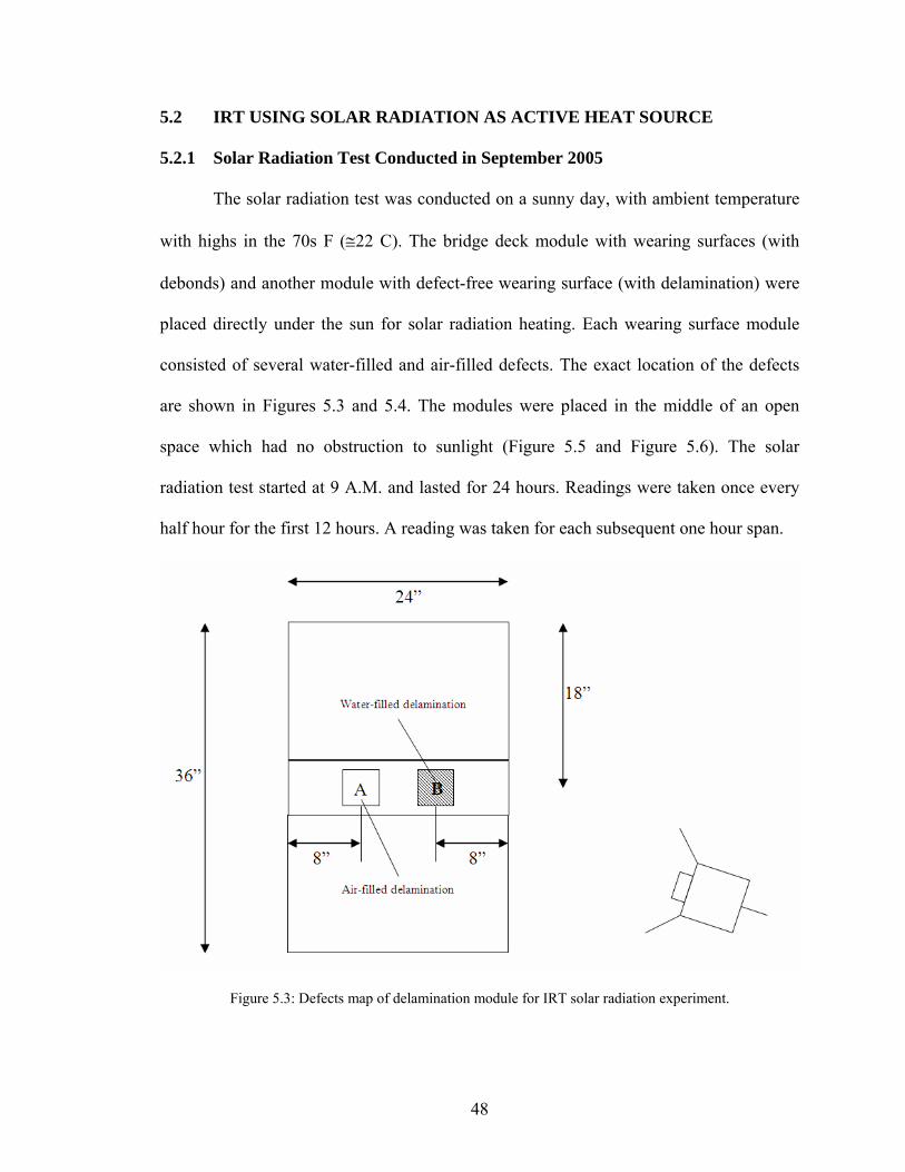
5.2 T US

.2.1 Solar Radiation Test Conducted in September 2005

The solar radiation test was conducted on a sunny day, with ambient temperature

ith highs in the 70s F (≅22 C). The bridge deck module with wearing surfaces (with

ebonds) and another module with defect-free wearing surface (with delamination) were

laced directly under the sun for solar radiation heating. Each wearing surface module

onsisted of several water-filled and air-filled defects. The exact location of the defects

are shown in Figures 5 he middle of an open

space which had no obstruction to sunlig t (Figure 5.5 and Figure 5.6). The solar

radiation test started at 9 A.M. and lasted for 24 hours. Readings were taken once every

half hour for the first 12 hours. A reading was taken for each subsequent one hour span.

IR ING SOLAR RADIATION AS ACTIVE HEAT SOURCE

5

w

d

p

c

.3 and 5.4. The modules were placed in t

h

Figure 5.3: Defects map of delamination module for IRT solar radiation experiment.

48

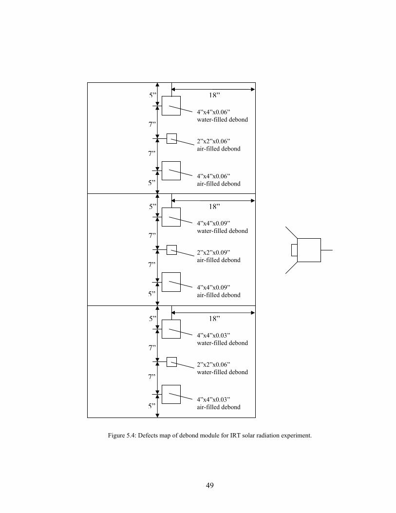
5” 18”

air-filled debond

4”x4”x0.06” water-filled debond

2”x2”x0.06”

4”x4”x0.06” air-filled debond

7”

7”

5”

5”

Figure 5.4: Defects map of debond module for IRT solar radiation experiment.

7”

7”

5”

18”

4”x4”x0.09”

2”x2”x0.09” air-filled debond

4”x4”x0.09” air-filled debond

water-filled debond

5”

7”

7”

5”

18”

4”x4”x0.03” water-filled debond

2”x2”x0.06” water-filled debond

4”x4”x0.03” air-filled debond

49

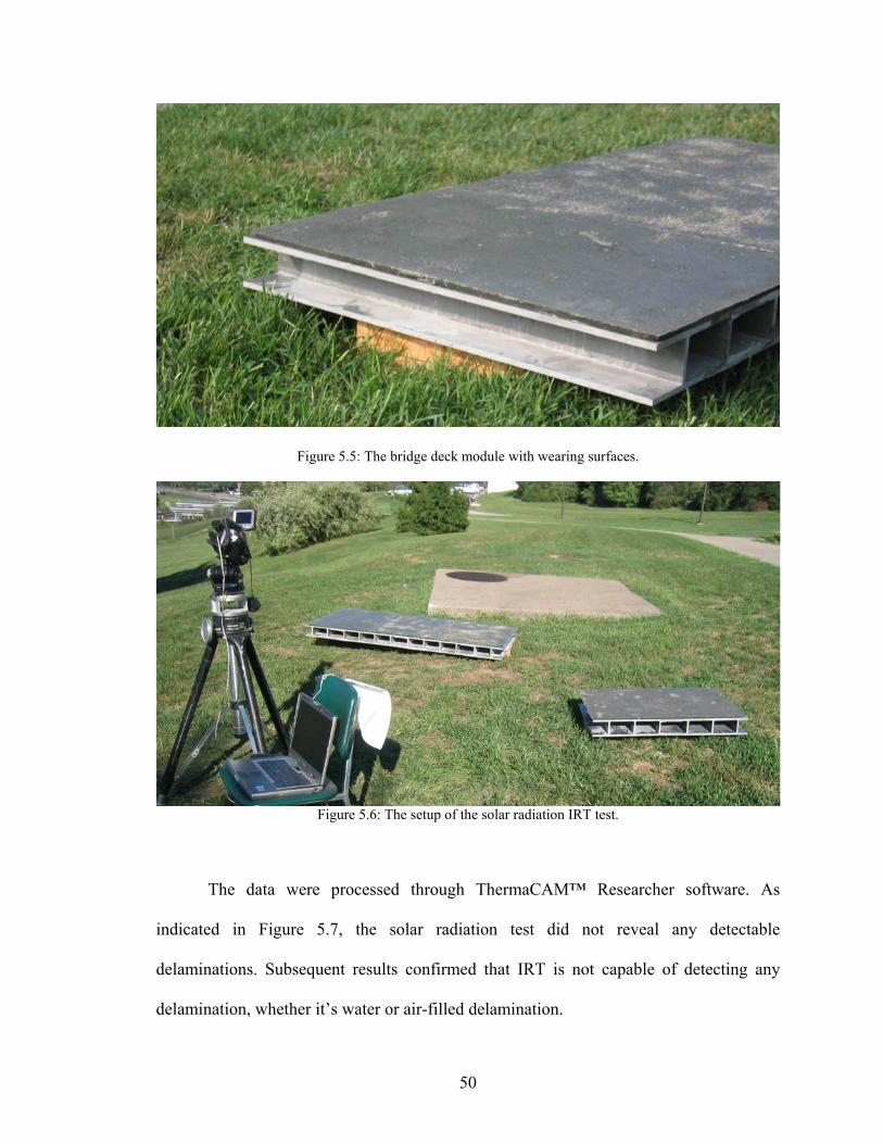
Figur he bridge deck le with wearing surfaces. e 5.5: T modu

Figure 5.6: The setup diation IRT test.

The data were processed through ThermaCAM™ Researcher software. As

indicated in Figure 5.7, the solar radiation test did not reveal any detectable

delaminatio ecting any

elamination, whether it’s water or air-filled delamination.

of the solar ra

ns. Subsequent results confirmed that IRT is not capable of det

d

50

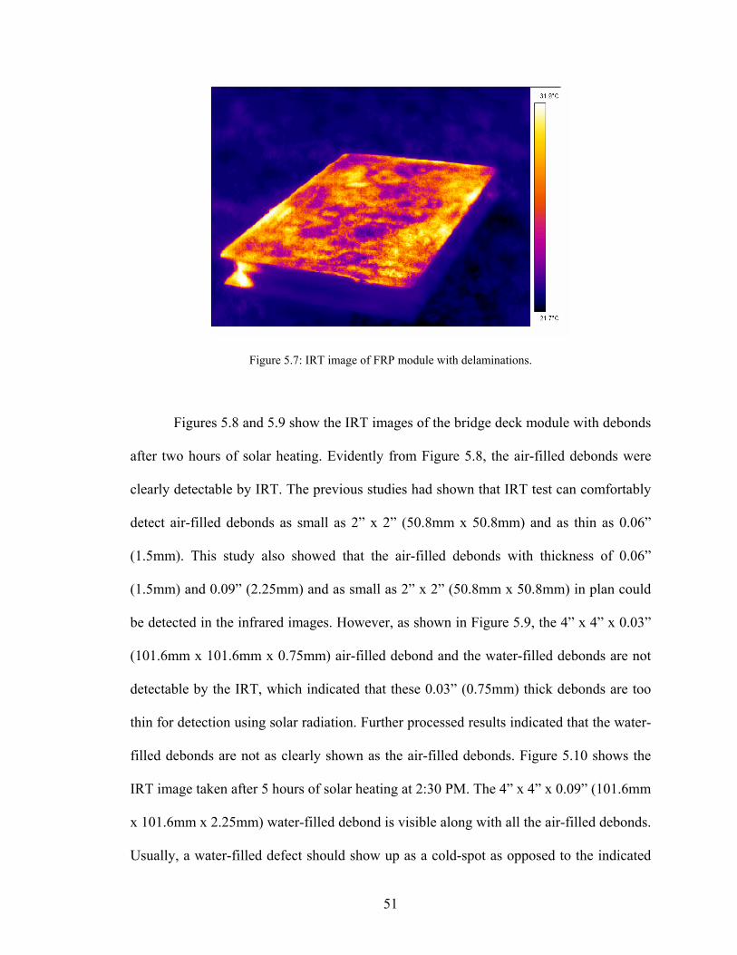
Figure 5.7: IRT image of FRP module with delaminations.

Figures 5.8 and 5.9 show the IRT images of the bridge deck module with debonds

after two hours of solar heating. Evidently from Figure 5.8, the air-filled debonds were

clearly detectable by IRT. The previous studies had shown that IRT test can comfortably

detect air-filled debonds as small as 2” x 2” (50.8mm x 50.8mm) and as thin as 0.06”

(1.5mm). This study also showed that the air-filled debonds with thickness of 0.06”

(1.5mm) and 0.09” (2.25mm) and as small as 2” x 2” (50.8mm x 50.8mm) in plan could

be detected in the infrared images. However, as shown in Figure 5.9, the 4” x 4” x 0.03”

(101.6mm x 101.6mm x 0.75mm) air-filled debond and the water-filled debonds are not

detectable by the IRT, which indicated th

thin for detection using solar radiation. Further processed results indicated that the water-

filled debonds are not as clearly shown as the air-filled debonds. Figure 5.10 shows the

IRT image taken after 5 hours of solar heating at 2:30 PM. The 4” x 4” x 0.09” (101.6mm

x 101.6mm x 2.25mm) water-filled debond is visible along with all the air-filled debonds.

Usually, a water-filled defect should show up as a cold-spot as opposed to the indicated

at these 0.03” (0.75mm) thick debonds are too

51

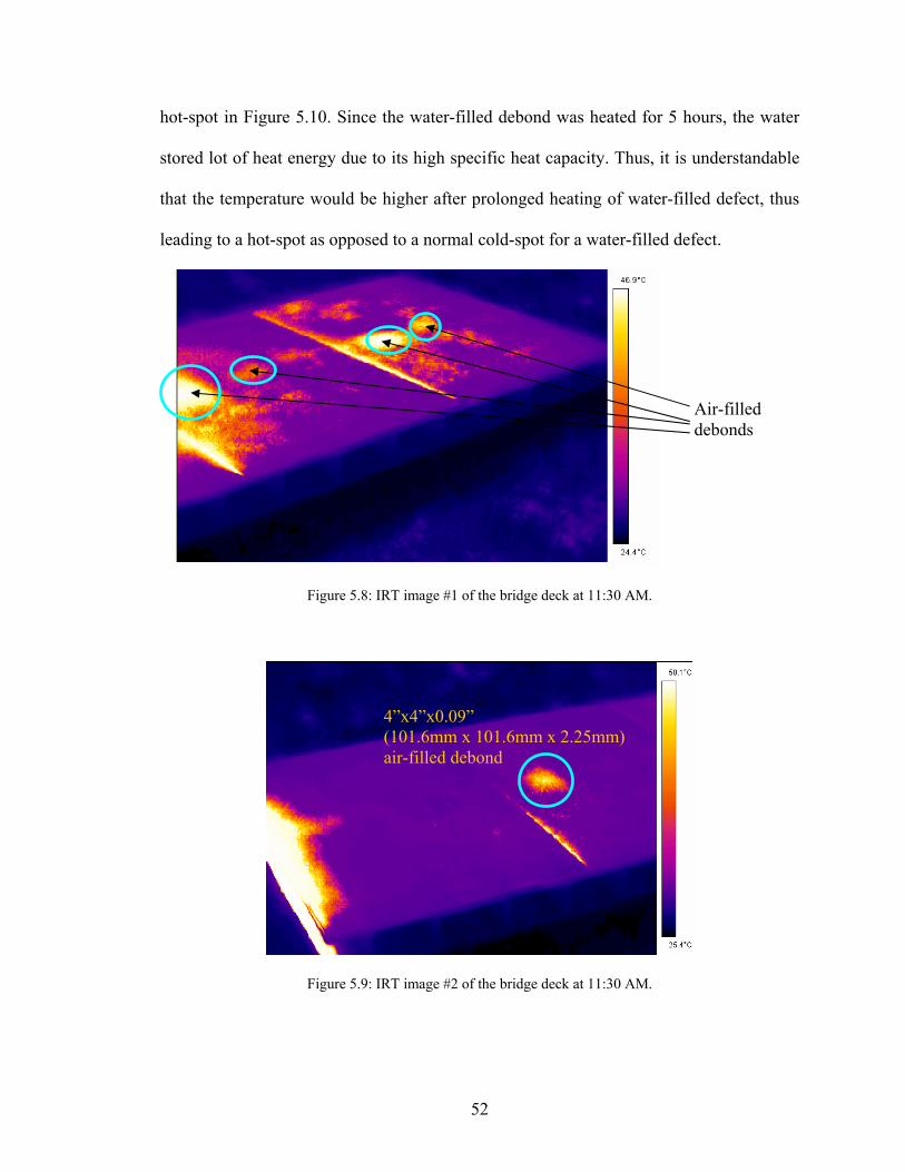
hot-spot in Figure 5.10. Since the water-filled debond was heated for 5 hours, the water

stored lot of heat energy due to its high specific heat capacity. Thus, it is understandable

that the temperature would be higher after prolonged heating of water-filled defect, thus

leading to a hot-spot as opposed to a normal cold-spot for a water-filled defect.

Figure 5.9: IRT image #2 of the bridge deck at 11:30 AM.

Figure 5.8: IRT image #1 of the bridge deck at 11:30 AM.

Air-filled debonds

4”x4”x0.09” (101.6mm x 101.6mm x 2.25mm) air-filled debond

52

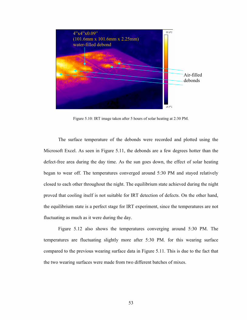
4”x4”x0.09” (101.6mm x 101.6mm x 2.25mm) water-filled debond

Air-filled debonds

Figure 5.10: IRT image taken after 5 hours of solar heating at 2:30 PM.

The surface temperature of the debonds were recorded and plotted using the

Microsoft Excel. As seen in Figure 5.11, the debonds are a few degrees hotter than the

defect-free area dur ct of solar heating

began to wear off. The temperatures conve ed around 5:30 PM and stayed relatively

closed to each other throughout the night. The equilibrium state achieved during the night

proved that cooling itself is no T detection of defects. On the other hand,

the equilibrium state is a perfec peratures are not

fluctuating as much as it were during the day.

Figure 5.12 also shows the temperatures converging around 5:30 PM. The

temperatures are fluctuating slightly more after 5:30 PM. for this wearing surface

compared to the previous wearing surface data in Figure 5.11. This is due to the fact that

the two wearing surfaces were made from two different batches of mixes.

ing the day time. As the sun goes down, the effe

rg

t suitable for IR

t stage for IRT experiment, since the tem

53

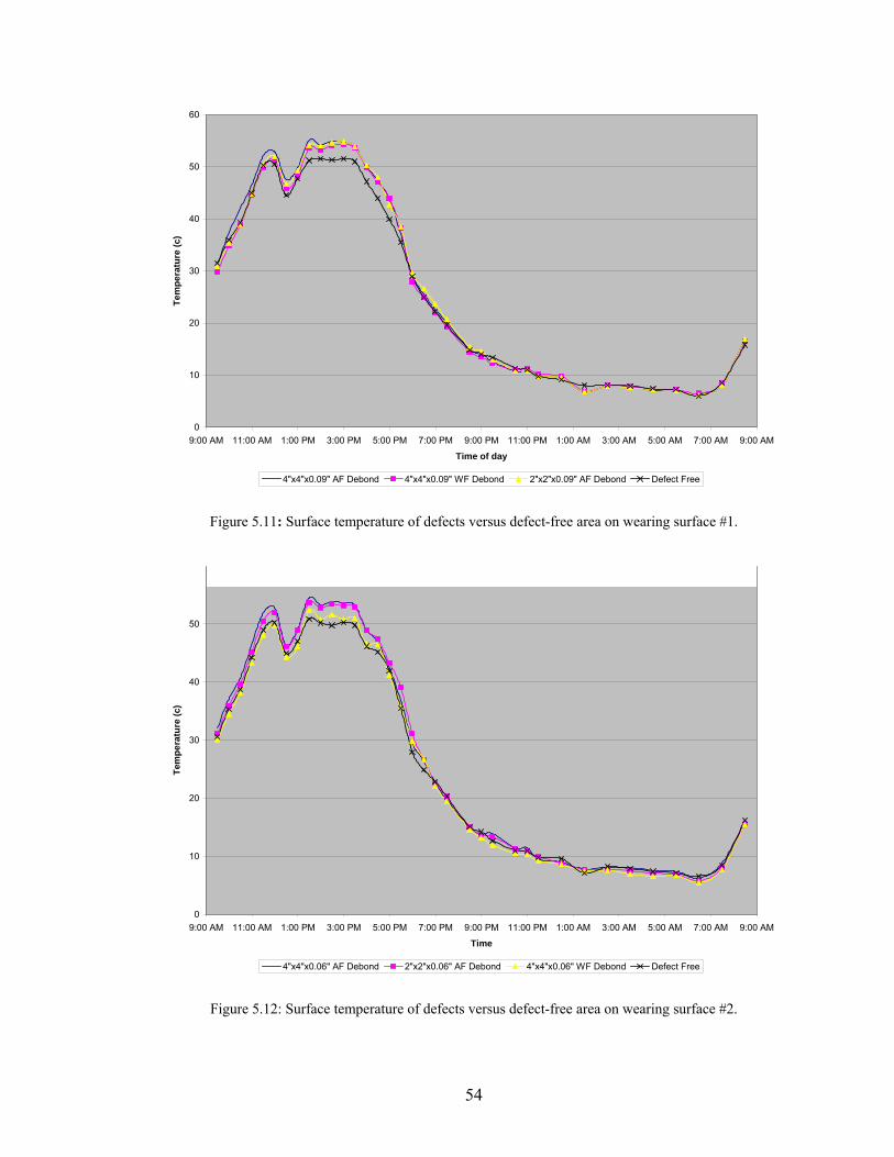
0

10

20

30

40

50

60

9:00 AM 11:00 AM 1:00 PM 3:00 PM 5:00 PM 7:00 PM 9:00 PM 11:00 PM 1:00 AM 3:00 AM 5:00 AM 7:00 AM 9:00 AM

Time of day

Tem

pera

ture

(c)

4"x4"x0.09" AF Debond 4"x4"x0.09" WF Debond 2"x2"x0.09" AF Debond Defect Free

Figure 5.11: Surface temperature of defects versus defect-free area on wearing surface #1.

20

30

40

50

mpe

r (c

)

0

10

Time9:00 AM 11:00 AM 1:00 PM 3:00 PM 5:00 PM 7:00 PM 9:00 PM 11:00 PM 1:00 AM 3:00 AM 5:00 AM 7:00 AM 9:00 AM

Teat

ure

4"x4"x0.06" AF Debond 2"x2"x0.06" AF Debond 4"x4"x0.06" WF Debond Defect Free

Figure 5.12: Surface temperature of defects versus defect-free area on wearing surface #2.

54

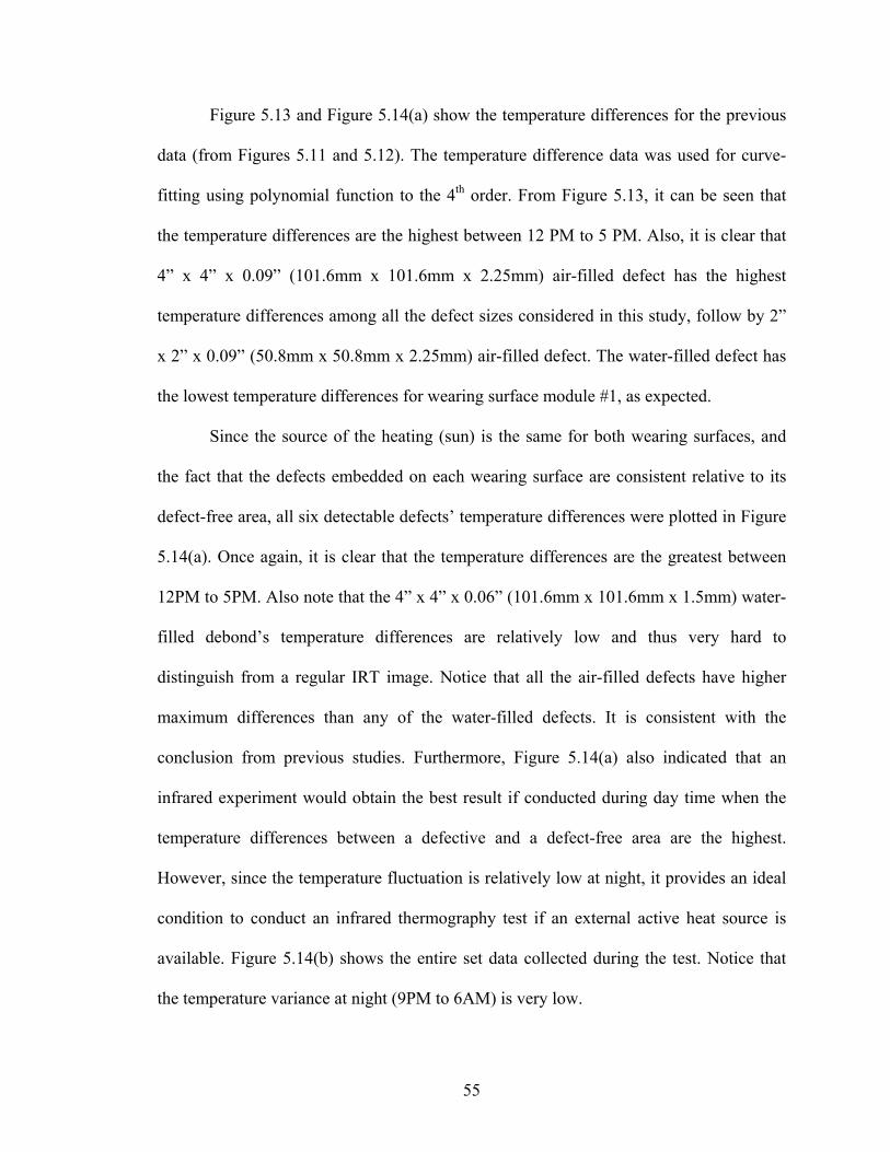
Figure 5.13 and Figure 5.14(a) show the temperature differences for the previous

data (from Figures 5.11 and 5.12). The temperature difference data was used for curve-

fitting using polynomial function to the 4th order. From Figure 5.13, it can be seen that

the temperature differences are the highest between 12 PM to 5 PM. Also, it is clear that

4” x 4” x 0.09” (101.6mm x 101.6mm x 2.25mm) air-filled defect has the highest

temperature differences among all the defect sizes considered in this study, follow by 2”

x 2” x 0.09” (50.8mm x 50.8mm x 2.25mm) air-filled defect. The water-filled defect has

the lowest temperature differences for wearing surface module #1, as expected.

Since the source of the heating (sun) is the same for both wearing surfaces, and

the fact that the defects embedded on each wearing surface are consistent relative to its

defect- igure

.14(a). Once again, it is clear that the temperature differences are the greatest between

12PM to 5PM. Also note that the 4” x 4” x 0.06” (101.6mm x 101.6mm x 1.5mm) water-

filled debond’s temperature differences are relatively low and thus very hard to

distinguish from a regular IRT image. Notice that all the air-filled defects have higher

maximum differences than any of the water-filled defects. It is consistent with the

conclusion from previous studies. Furthermore, Figure 5.14(a) also indicated that an

infrared experiment would obtain the best result if conducted during day time when the

temperature differences between a defective and a defect-free area are the highest.

However, since the temperature fluctuation is relatively low at night, it provides an ideal

condition to conduct an infrared thermography test if an external active heat source is

available. Figure 5.14(b) shows the entire set data collected during the test. Notice that

the tem

free area, all six detectable defects’ temperature differences were plotted in F

5

perature variance at night (9PM to 6AM) is very low.

55

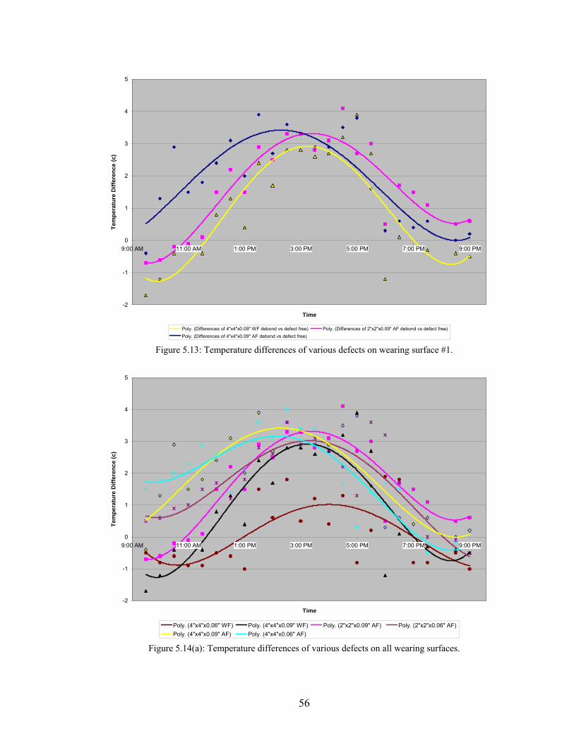
-1

0

4

5

1

2

3

9:00 AM 11:00 AM 1:00 PM 3:00 PM 5:00 PM 7:00 PM 9:0

Teer

atur

e D

iffer

ence

(c)

0 PM

mp

-2

Time

Poly. (Differences of 4"x4"x0.09" WF debond vs defect free) Poly. (Differences of 2"x2"x0.09" AF debond vs defect free)Poly. (Differences of 4"x4"x0.09" AF debond vs defect free)

Figure 5.13: Temperature differences of various defects on wearing surface #1.

-2

-1

0

1

3

4

5

9:00 AM

2

11:00 AM 1:00 PM 3:00 PM 5:00 PM 7:00 PM 9:00 PM

Time

empe

rre

Diff

eren

ce (c

)T

atu

Poly. (4"x4"x0.06" WF) Poly. (4"x4"x0.09" WF) Poly. (2"x2"x0.09" AF) Poly. (2"x2"x0.06" AF)Poly. (4"x4"x0.09" AF) Poly. (4"x4"x0.06" AF)

all wearing surfaces. Figure 5.14(a): Temperature differences of various defects on

56

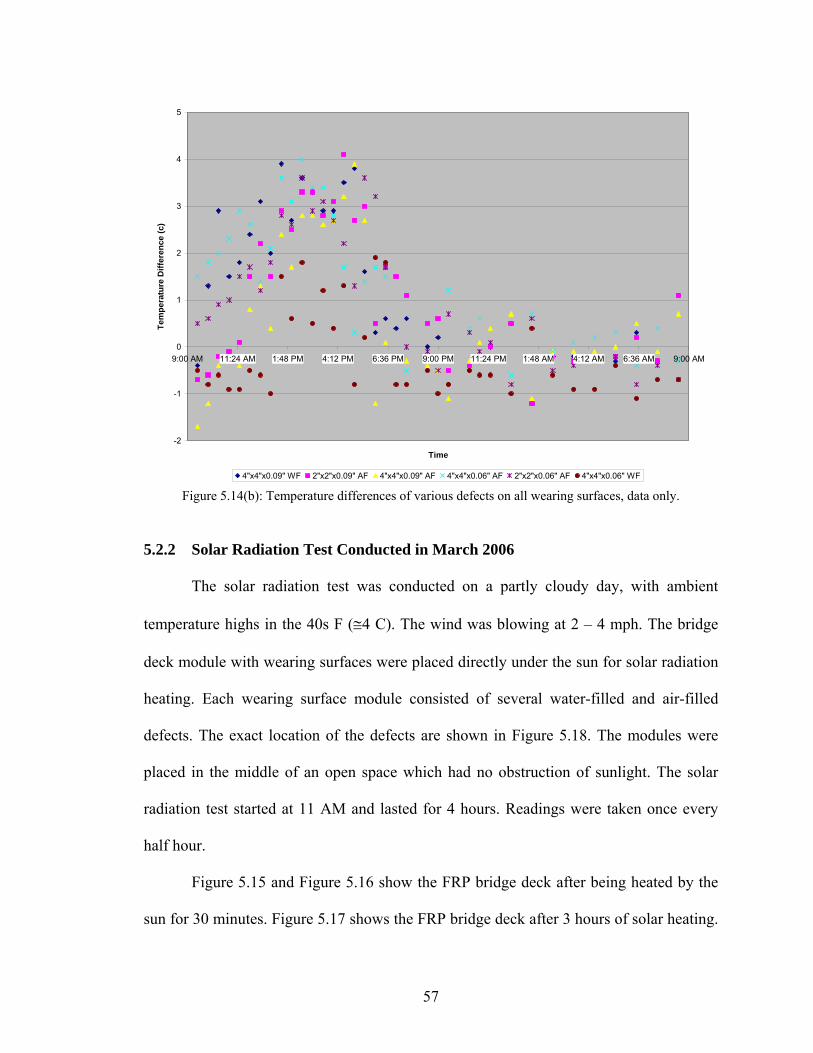
-2

-1

0

1

2

3

4

5

9:00 AM 11:24 AM 1:48 PM 4:12 PM 6:36 PM 9:00 PM 11:24 PM 1:48 AM 4:12 AM 6:36 AM 9:00 AM

Time

Tem

pera

ture

Diff

eren

ce (c

)

4"x4"x0.09" WF 2"x2"x0.09" AF 4"x4"x0.09" AF 4"x4"x0.06" AF 2"x2"x0.06" AF 4"x4"x0.06" WF Figure only.

5.2.2 Solar Radiation Test Conducted in March 2006

The solar radiation test was conducted on a partly cloudy day, with ambient

temperature highs in the 40s F (≅4 C). The wind was blowing at 2 – 4 mph. The bridge

deck module with wearing surfaces were placed directly under the sun for solar radiation

heating. Each wearing surface module consisted of several water-filled and air-filled

defects. The exact location of the defects are shown in Figure 5.18. The modules were

placed in the middle of an open space which had no obstruction of sunlight. The solar

radiation test started at 11 AM and lasted for 4 hours. Readings were taken once every

half hour.

Figure 5.15 and Figure 5.16 show the FRP bridge deck after being heated by the

sun for 30 r heating.

5.14(b): Temperature differences of various defects on all wearing surfaces, data

minutes. Figure 5.17 shows the FRP bridge deck after 3 hours of sola

57

58

Notice that the 4” x 4” x 0.09” (101.6mm x 101.6mm x 2.25mm) air-filled debond can

still be seen in Figure 5.17 while all other air-filled debonds disappeared. Furthermore,

the appearances of the defects in Figure 5.15 and Figure 5.16 are not as prominent as

those from the previous solar radiation test. More importantly, many of the smaller

f solar heating.

Figure 5.15: FRP bridge deck after 30 minutes o

Figure 5.16: FRP bridge deck after 30 minutes of solar heating.

4” x 4” x 0.03” air-filled debond

4” x 4” x 0.09” air-filled debond

4” x 4” x 0.06” air-filled debond

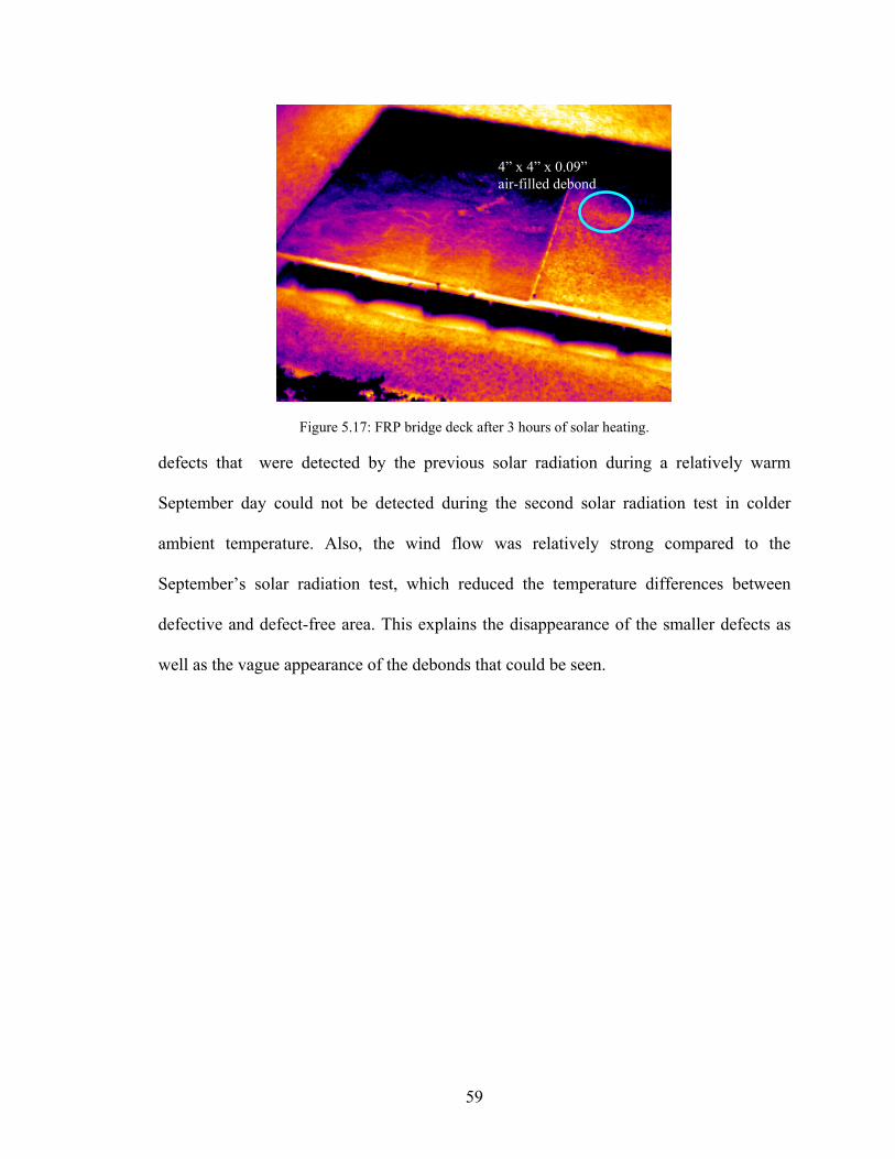
4” x 4” x 0.09” air-filled debond

Figure 5.17: FRP bridge deck after 3 hours of solar heating.

defects that were detected by the previous solar radiation during a relatively warm

September day could not be detected during the second solar radiation test in colder

ambient temperature. Also, the wind flow was relatively strong compared to the

September’s solar radiation test, which re

defective and defect-free area. This explains the disappearance of the smaller defects as

well as the vague appearance of th

duced the temperature differences between

e debonds that could be seen.

59

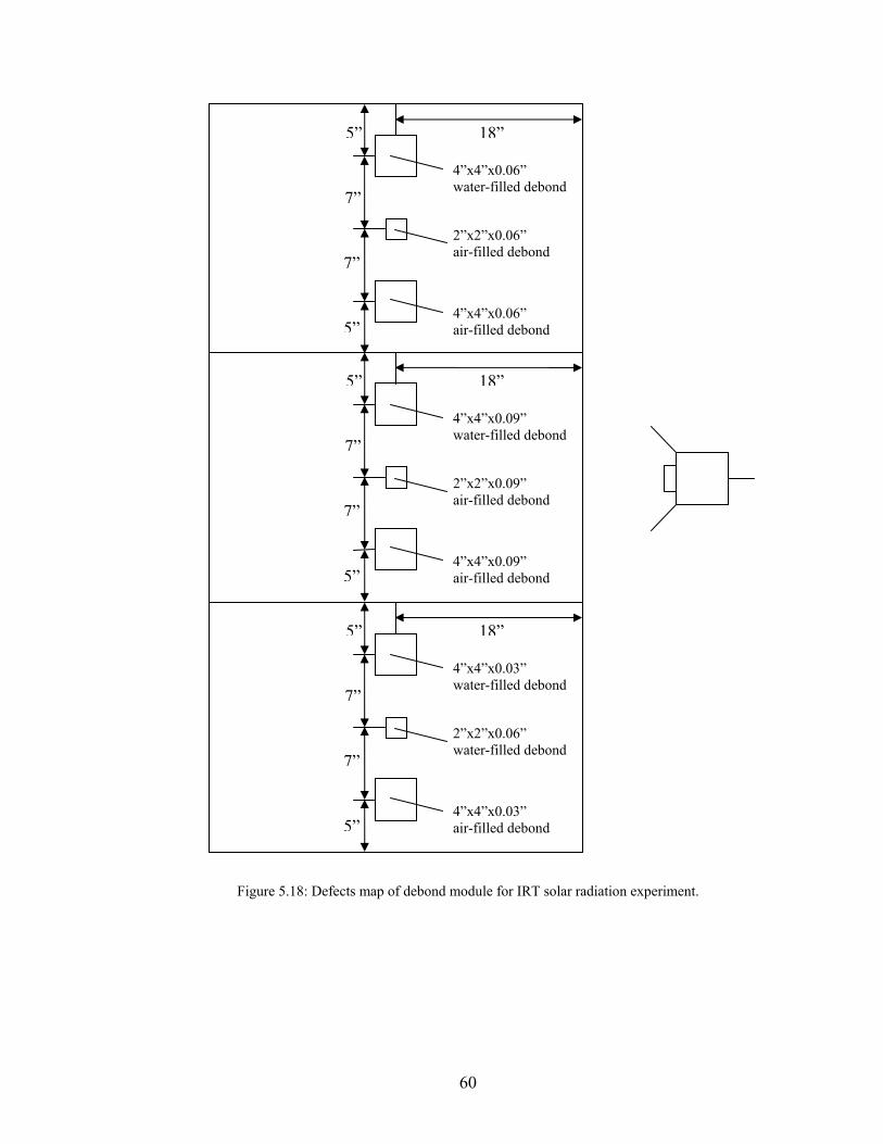
60

Figure 5.18: Defects map of debond module for IRT solar radiation experiment.

5”

7”

7”

5”

18”

4”x4water-

2”x2”x0.06” air-filled debond

4”x4”x0.06” air-filled debond

”x0.06” filled debond

5” 18”

4”x4”x0.09” water-filled debond

7”

7”

5”

2”x2”x0.09” air-filled debond

4”x4”x0.09” air-filled debond

5”

7”

7”

5”

18”

4”x4”x0.03” water-filled debond

2”x2”x0.06” water-filled debond

4”x4”x0.03” air-filled debond

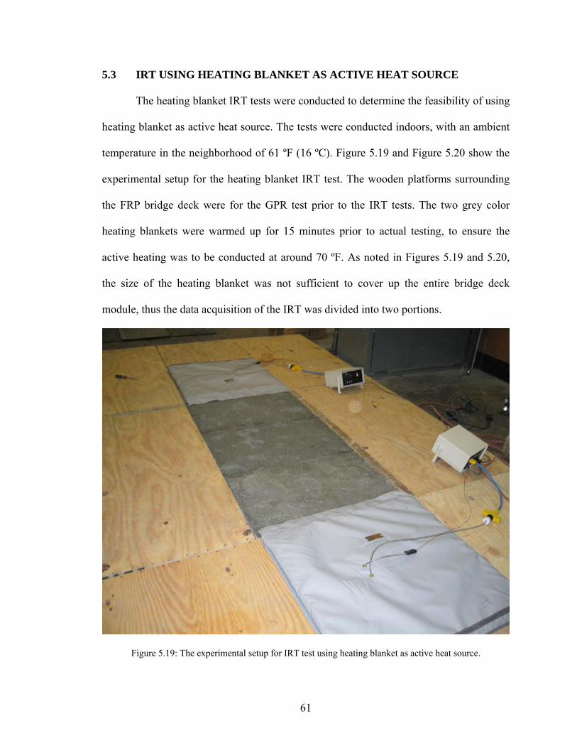
5.3 IRT USING HEATING BLANKET AS ACTIVE HEAT SOURCE

The heating blanket IRT tests were conducted to determine the feasibility of using

heating blanket as active h source. The ted indoors, with an ambient

temperature in the neighborhood of 61 ºF ure 5.19 and Figure 5.20 show the

experimental setup for the heating blanke IRT test. The wooden platforms surrounding

the FRP bridge deck were for the GPR t the IRT tests. The two grey color

heating blankets were warmed up for 15 minutes prior to actual testing, to ensure the

active heating was to be conducted at around 70 ºF. As noted in Figures 5.19 and 5.20,

the size of the heating blanket was not sufficient to cover up the entire bridge deck

module, thus the data acquisition of the IRT was divided into two portions.

eat tests were conduc

(16 ºC). Fig

t

est prior to

Figure 5.19: The experimental setup for IRT test using heating blanket as active heat source.

61

Infrared Camera

External Temperature Controller

Figure 5.20: The experimental setup for IRT test using heating blanket as active heat source.

The objective of this experiment was to determine the feasibility of IRT using

heating blanket as active heat source in defect detection. Therefore, various debond sizes

and thicknesses were used with the defect configuration shown in Figures 5.21 and 5.22.

Both air-filled and water-filled debonds were used in the experiments. Four minutes of

heating at 70 ºF was applied to one 3’ x 3’ portion of the FRP bridge deck. The thermo

image acquisition began immediately after the removal of the heating blankets. Three

minutes (180 seconds) of thermo images were acquired at one second interval. The

process was repeated for another 3’ x 3’ portion of the FRP bridge deck, and the same

proces

s was continued for the other defects configurations.

62

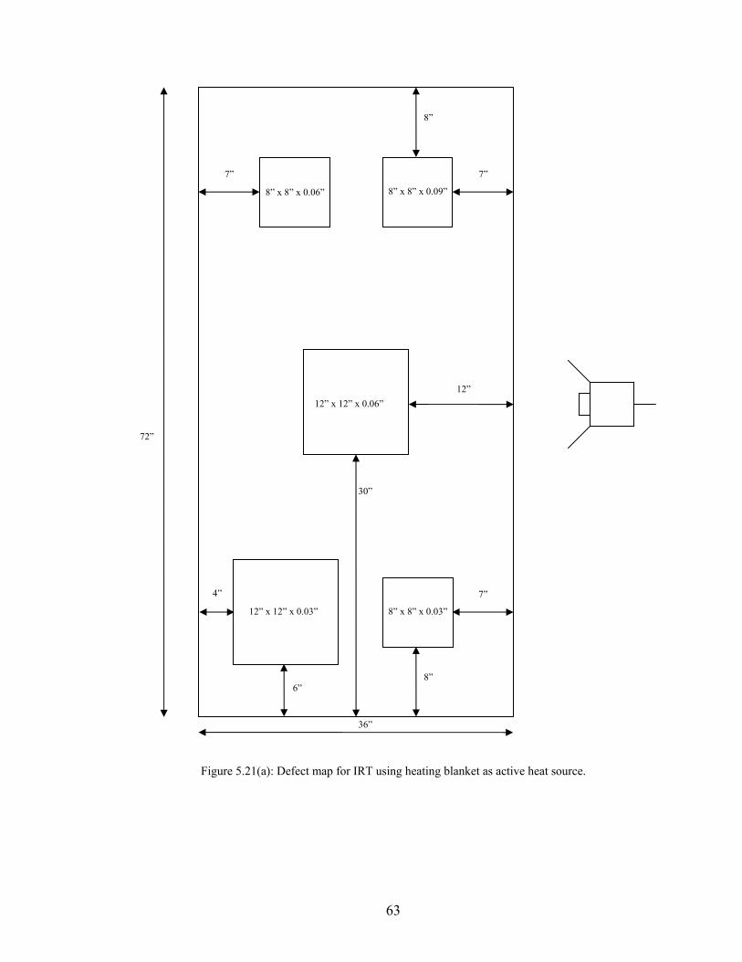
Figure 5.21(a): Defect map for IRT using heating blanket as active heat source.

12” x 12” x 0.03” 8” x 8” x 0.03”

12” x 12” x 0.06”

8” x 8” x 0.06” 8” x 8” x 0.09”

36”

72”

6” 8”

4” 7”

12”

30”

7” 7”

8”

63

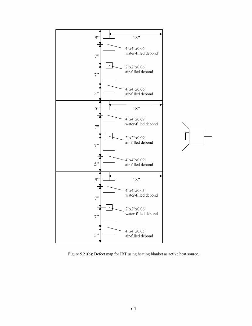
Figure 5.21(b): Defect map for IRT using heating blanket as active heat source.

5”

7”

7”

5”

18”

4”x4”x0.06” water-filled debond

2”xair-filled debond

4”x4”x0.06” air-filled debond

2”x0.06”

5”

7”

7”

5”

18”

4”x4”x0.09” water-filled debond

”x0.09” air-filled debond

4”x4”x0.09” r-filled debond

2”x2

ai

5”

7”

7”

5”

18”

4”x4”x0.03” water-filled debond

2”xwater-filled debond

4”x4”x0.03air-filled debond

2”x0.06”

”

64

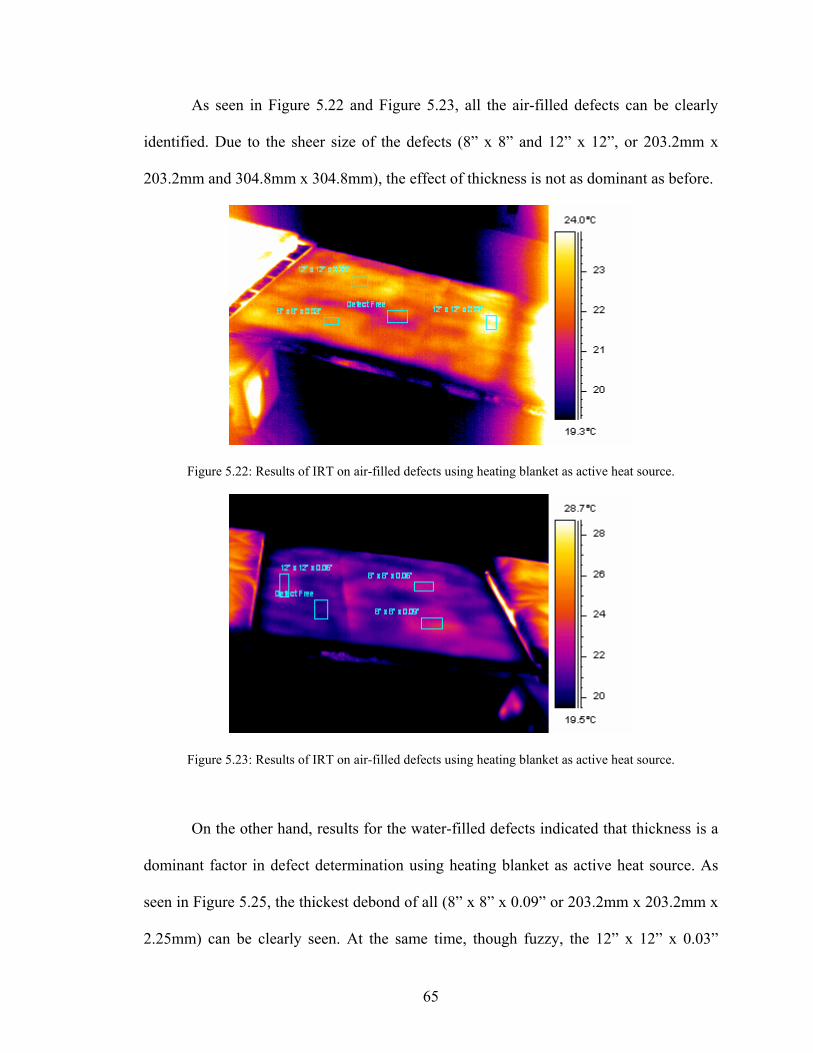
As seen in Figure 5.22 and Figure 5.23, all the air-filled defects can be clearly

identified. Due to the sheer size of the defects (8” x 8” and 12” x 12”, or 203.2mm x

203.2mm and 304.8mm x 4.8mm), the effect of thickness is not as dominant as before. 30

Figure 5.22: Results of IRT on air-filled ing blanket as active heat source. defects using heat

Figure 5.23: Results of IRT on air-filled g blanket as active heat source.

On ckness is a

dominant factor in defect determination using heating blanket as active heat source. As

seen in Figure 5.25, the thickest debond of all (8” x 8” x 0.09” or 203.2mm x 203.2mm x

2.25mm) can be clearly seen. At the same time, though fuzzy, the 12” x 12” x 0.03”

defects using heatin

the other hand, results for the water-filled defects indicated that thi

65

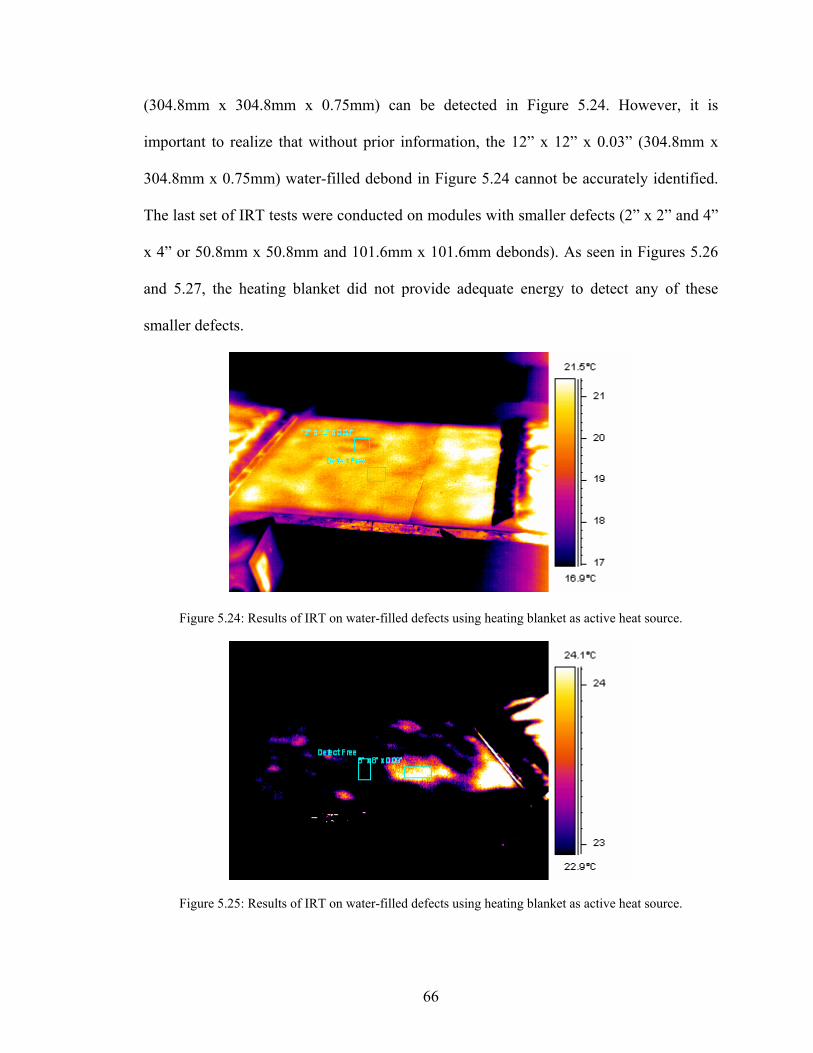
(304.8mm x 304.8mm x 0.75mm) can be detected in Figure 5.24. However, it is

important to realize that without prior information, the 12” x 12” x 0.03” (304.8mm x

304.8mm x 0.75mm) water-filled debond in Figure 5.24 cannot be accurately identified.

The last set of IRT tests were conducted on modules with smaller defects (2” x 2” and 4”

x 4” or 50.8mm x 50.8mm and 101.6mm x 101.6mm debonds). As seen in Figures 5.26

and 5.27, the heating blanket did not provide adequate energy to detect any of these

smaller defects.

Figure 5.24: Results of IRT on water-filled defects using heating blanket as active heat source.

Figure 5.25: Results of IRT on water-filled defects using heating blanket as active heat source.

66

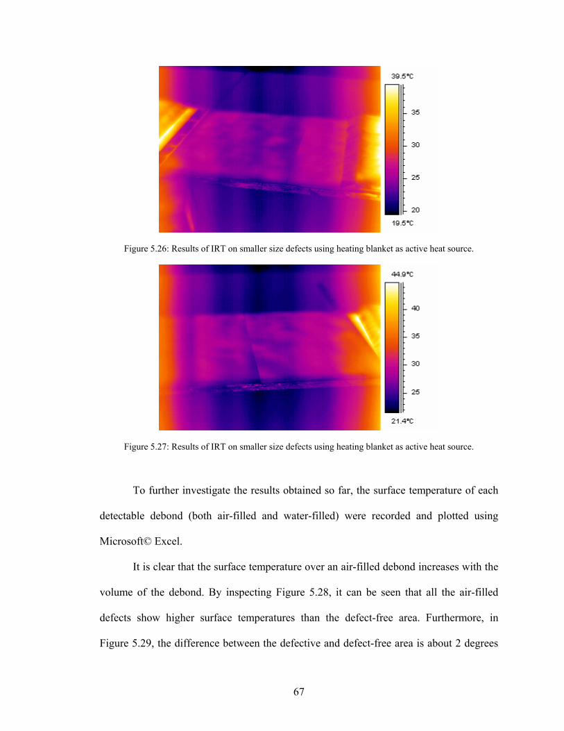
Figure 5.26: Results of IRT on smaller size defects using heating blanket as active heat source.

Figure 5.27: Results of IRT on smaller size defects using heating blanket as active heat source.

To further investigate the results obtained so far, the surface temperature of each

detectable debond (both air-filled and water-filled) were recorded and plotted using

Microsoft© Excel.

It is clear that the surface temperature over an air-filled debond increases with the

volume of the debond. By inspecting Figure 5.28, it can be seen that all the air-filled

defects show higher surface temperatures than the defect-free area. Furthermore, in

Figure 5.29, the difference between the defective and defect-free area is about 2 degrees

67

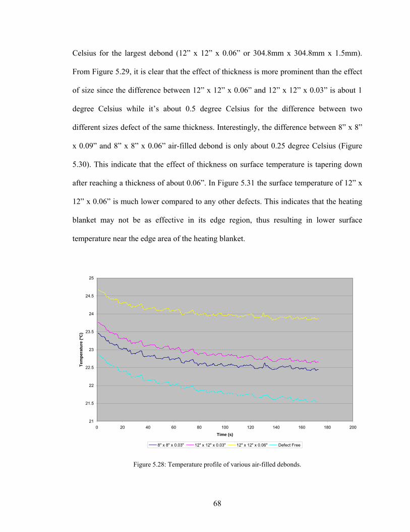
Celsius for the largest debond (12” x 12” x 0.06” or 304.8mm x 304.8mm x 1.5mm).

From Figure 5.29, it is clear that the effect of thickness is more prominent than the effect

of size since the difference between 12” x 12” x 0.06” and 12” x 12” x 0.03” is about 1

degree Celsius while it’s about 0.5 degree Celsius for the difference between two

different sizes defect of the same thickness. Interestingly, the difference between 8” x 8”

x 0.09” and 8” x 8” x 0.06” air-filled debond is only about 0.25 degree Celsius (Figure

5.30). This indicate that the effect of thickness on surface temperature is tapering down

after 2” x

12” x 0.06” is much lower compared to any other defects. This indicates that the heating

blanket may not be as effective in its edge region, thus resulting in lower surface

temperature near the edge area of the heating blanket.

reaching a thickness of about 0.06”. In Figure 5.31 the surface temperature of 1

21

21.5

22

22.5

23

23.5

24

24.5

25

0 20 40 60 80 100 120 140 160 180 200

Time (s)

Tem

pera

ture

(ºC

)

8" x 8" x 0.03" 12" x 12" x 0.03" 12" x 12" x 0.06" Defect Free

Figure 5.28: Temperature profile of various air-filled debonds.

68

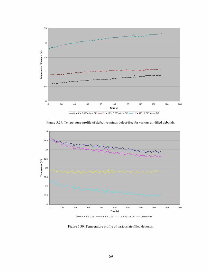
0

0.5

1

1.5

2

2.5

0 20 40 60 80 100 120 140 160 180 200

efe

renc

e (º

C

Time (s)

Tm

pera

ture

Dif

)

8" x 8" x 0.03" minus DF 12" x 12" x 0.03" minus DF 12" x 12" x 0.06" minus DF

Figure 5.29: Temperature profile of defective minus defect-free for various air-filled debonds.

20

20.5

21

21.5

22

22.5

23

23.5

24

0 20 40 60 80 100 120 140 160 180 200

Time (s)

Tem

pera

ture

(ºC

)

8" x 8" x 0.09" 8" x 8" x 0.06" 12" x 12" x 0.06" Defect Free

Figure 5.30: Temperature profile of various air-filled debonds.

69

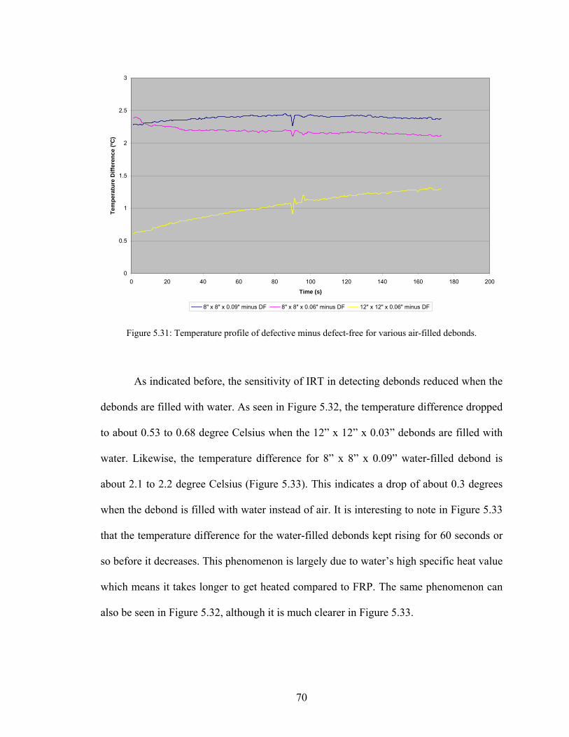
0

0.5

1

1.5

2

2.5

3

0 20 40 60 80 100 120 140 160 180 200

Time (s)

Tem

pera

ture

Diff

eren

ce (º

C)

8" x 8" x 0.09" minus DF 8" x 8" x 0.06" minus DF 12" x 12" x 0.06" minus DF

Figure 5.31: Temperature profile of defective minus defect-free for various air-filled debonds.

As indicated before, the sensitivity of IRT in detecting debonds reduced when the

debonds are filled with water. As seen in Figure 5.32, the temperature difference dropped

to about 0.53 to 0.68 degree Celsius when the 12” x 12” x 0.03” debonds are filled with

water. Likewise, the temperature difference for 8” x 8” x 0.09” water-filled debond is

about 2.1 to 2.2 degree Celsius (Figure 5.33). This indicates a drop of about 0.3 degrees

when the debond is filled with water instead of air. It is interesting to note in Figure 5.33

that the temperature difference for the water-filled debonds kept rising for 60 seconds or

so before it decreases. This phenomenon is largely due to water’s high specific heat value

which means it takes longer to get heated compared to FRP. The same phenomenon can

also be seen in Fig

ure 5.32, although it is much clearer in Figure 5.33.

70

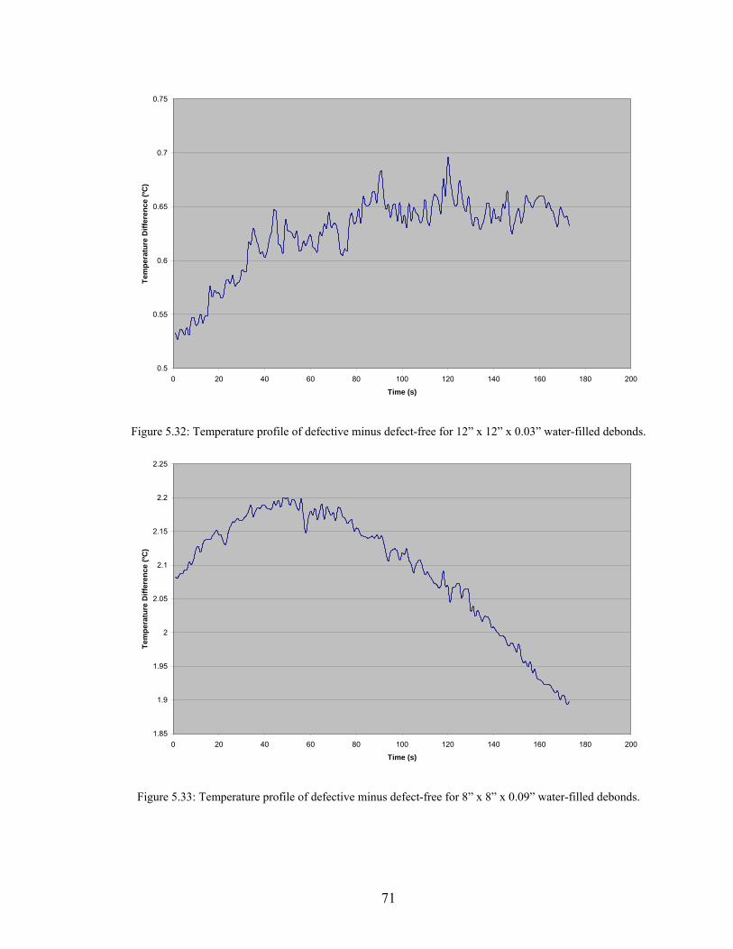
0.5

0.55

0.6

0.65

0.7

0.75

0 20 40 60 80 100 120 140 160 180 200

Time (s)

Tem

pera

ture

Diff

eren

ce (º

C)

Figure onds.

5.32: Temperature profile of defective minus defect-free for 12” x 12” x 0.03” water-filled deb

1.85

1.9

1.95

2

2.05

2.1

2.15

0 20 40 60 80 100 120 140 160 180 200

Time (s)

Tm

pera

ture

Diff

eren

ce (º

C)

Figure 5.33: Temperature profile of defective minus defect-free for 8” x 8” x 0.09” w

2.2

2.25

e

ater-filled debonds.

71

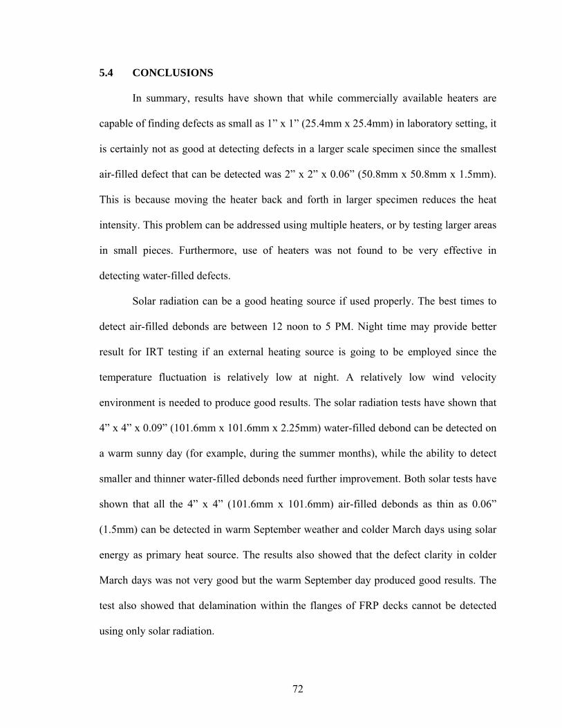
5.4 CONCLUSIONS

In summary, results have shown that while commercially available heaters are

capable of finding defects as small as 1” x 1” (25.4mm x 25.4mm) in laboratory setting, it

is certainly not as good at detecting defects in a larger scale specimen since the smallest

air-filled defect that can be detected was 2” x 2” x 0.06” (50.8mm x 50.8mm x 1.5mm).

This is because moving the heater back and forth in larger specimen reduces the heat

intensity. This problem can be addressed using multiple heaters, or by testing larger areas

in small pieces. Furthermore, use of heaters was not found to be very effective in

detecting water-filled defects.

Solar radiation can be a good heating source if used properly. The best times to

result for IRT testing if an external heating source is going to be employed since the

temperature fluctuation is relatively low at night. A relatively low wind velocity

environment is needed to produce good results. The solar radiation tests have shown that

4” x 4” x 0.09” (101.6mm x 101.6mm x 2.25mm) water-filled debond can be detected on

a warm sunny day (for example, during the summer months), while the ability to detect

smaller and thinner water-filled debonds need further improvement. Both solar tests have

shown that all the 4” x 4” (101.6mm x 101.6mm) air-filled debonds as thin as 0.06”

(1.5mm) can be detected in warm September weather and colder March days using solar

energy as primary heat source. The results also showed that the defect clarity in colder

March days was not very good but the warm September day produced good results. The

t

sing only solar radiation.

detect air-filled debonds are between 12 noon to 5 PM. Night time may provide better

est also showed that delamination within the flanges of FRP decks cannot be detected

u

72

The heating blankets proved to be the weakest active heat source explored in this

study.

ility to apply uniform heat to a large area while the heating

blanket

It was not capable of detecting any debonds (air-filled and water-filled) smaller

than 8” x 8” in size. Although the heating blankets were sending out 1200 W/m2 of

output (roughly the same amount of energy emitted by the sun on a hot sunny day in

June), it did not perform as well as the solar radiation test because the specimens were

heated by the sun for a much longer period of time compared to only 4 minutes using the

heating blanket. When comparing the heating blanket to the heaters, it is clear that heaters

provide a much greater heat intensity (≅ 2500 W/m2 output) for IRT. The only setback

regarding the heaters is its inab

s provided uniform heating of the specimens.

73

Chapter 6

FINITE ELEMENT MODELING

Finite element (FE) analysis is widely accepted as a powerful and versatile

analytical tool. While finite element could be a powerful tool in analyzing stress-strain

and thermal behavior for objects with complex geometry, the goal of this study is to

utilize a simple heat transfer finite element model that could be used for studying the

effect of subsurface defects on heat transfer through FRP bridge decks and the resulting

surface temperature differences.

Before thermal modeling of the FRP bridge deck, some essential information is

needed such as, the thermal properties of the FRP layers and wearing surface, the thermal

loading conditions (positive or negative heat input), and the boundary conditions for

thermal modeling. The thermal properties needed to create an FE model are the specific

heat, the emissivity, and the thermal conductivity. Radiation is assumed to be the

dominant mode of heat transfer between the wearing surface and the surrounding air

while conduction is the dominant mode of heat transfer between the wearing surface,

defects, and the FRP layer in this model. A time-step heat flux was used to simulate the

active heat source. There were no existing thermal properties available for the FRP used

in this study since it is a relatively new material. Although some published tables for

thermal properties (Table 3.1) are available, the FRP bridge deck specimens used in this

study were tested in order to experimentally determine the specific heat, the thermal

conductivity, and the emissivity for these specimens.

74

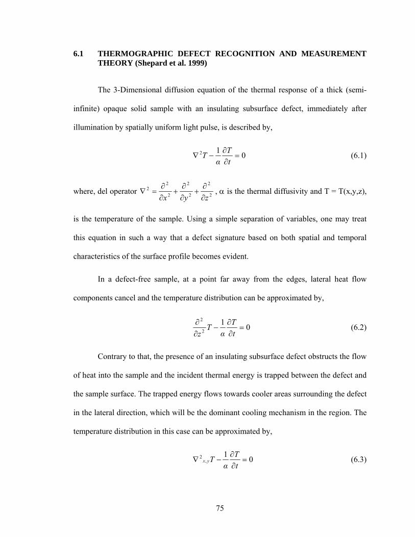
6.1 THERMOGRAPHIC DEFE NITION AND MEASUREMENT THEORY (Shepard et al. 1999)

The 3-Dimensional diffusion equation of the thermal response of a thick (semi-

infinite) opaque solid sample with an insulating subsurface defect, immediately after

illumination by spatially uniform light pulse, is described by,

CT RECOG

012 =∂∂

−∇tT

αT (6.1)

where, del operator 2222

zyx ∂+

∂+

∂=∇ , α is the thermal diffusivity and T = T(x,y,z),

is the temperature of the sample. Using a s

222 ∂∂∂

imple separation of variables, one may treat

this equatio

In a defect-free sample, at a point far away from the edges, lateral heat flow

components cancel and the temperature distribution can be approximated by,

n in such a way that a defect signature based on both spatial and temporal

characteristics of the surface profile becomes evident.

012

2

=∂

−∂∂

∂ TT (6.2)

Contrary to that, the presence of an insulating subsurface defect obstructs the flow

of heat into the sample and the incident thermal energy is trapped between the defect and

the sample surface. The trapped energy flows towards cooler areas surrounding the defect

in the lateral direction, which will be the dominant cooling mechanism in the region. The

temperature distribution in this case can be approximated by,

tαz

01,

2 =∂∂

−∇TTyxtα

(6.3)

75

Figure 6.1: Heat flow due to a flash pulse. Initially the pulse causes thin layer of uniform heat on the

The analysis of pulsed thermographic data ca

regimes as a result of the separation of the diffusion equation, a regime before the

he transition time, the dominant

influence on the surface temperature above the defect is the lateral heat flow as per

Equation 6.3.

6.2 THERMAL PROPERTIES

6.2.1 Conductivity

ental setup of the test.

surface (Left). Heat flows into the sample (Center). When a defect is encountered, the heat is trapped between the defect and the sample surface, giving rise to lateral heat flow above the defect (Shepard et al.

1999).

n be separated into two distinct time

incident heat reaches the buried defect and that after it reaches the buried defect. The time

at which the transition between the regimes occurs depends on the depth of the defect.

Until the transition time is reached, the surface above the defect and the rest of the area

behave in the same manner. After the elapse of t

Thermal conductivity means “The material property that describes the rate at

which heat flows within a body for a given temperature change.” To measure the thermal

conductivity, a thermal conductivity testing system (Unitherm model 2022 from ANTER

Corp., Pittsburgh, PA) was utilized. Figure 6.2 shows the experim

76

Figure 6.2: Experimental set up of Unitherm 2022.

This unit is supplied with a mid range flux module covering a thermal resistance

range from 0.002 to 0.02 m2 K/W and is able to measure the thermal conductivity of

materials in the range of 0.1 to 40 W/m-K as per the test standard ASTM E 1530.

Samples were cut in the form of two inch diameter circular discs from the Transpo

ace and the FRP deck’s top flange for thermal conductivity measurement.

ent of the system. The system is

functionalities. The heater on top and bottom

sample is placed between two polished surfaces and a pneumatic pressure of 10 psi is

applied on the top of the system as indicated in Figure 6.3. The entire system is

wearing surf

Figure 6.3 shows the schematic arrangem

essentially made up of parts with different

are used to create steady state heat transfer through the sample. The heat sink at the

bottom is to prevent excessive temperature from the system resulting in system failure. A

reference calorimeter is placed under the lower plate, which acts as a heat flux transducer.

The sample disks are first polished to ensure good thermal contact. Then the prepared

77

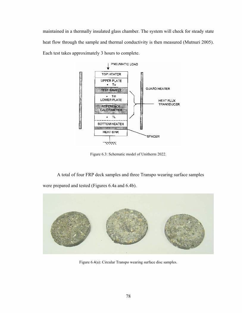
maintained in a thermally insulated glass chamber. The system will check for steady state

heat flow through the sample and thermal conductivity is then measured (Mutnuri 2005).

Each test takes approximately 3 hours to complete.

Figure 6.3: Schematic model of Unitherm 2022.

A total of four FRP deck samples and three Transpo wearing surface samples

were prepared and tested (Figures 6.4a and 6.4b).

Figure 6.4(a): Circular Transpo wearing surface disc samples.

78

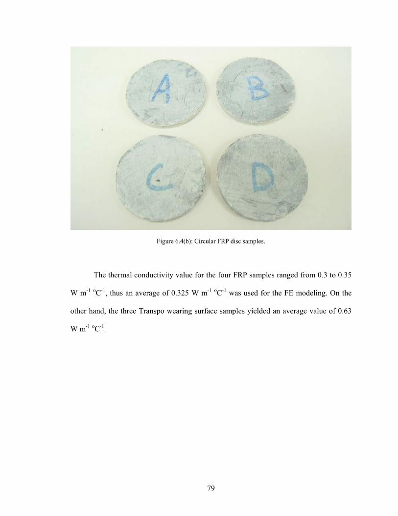
Figure 6.4(b): Circular FRP disc samples.

mal conductivity value for the four FRP samples ranged from 0.3 to 0.35

W m-1 the

ples yielded an average value of 0.63

W m-1 oC-1.

The ther

oC-1, thus an average of 0.325 W m-1 oC-1 was used for the FE modeling. On

other hand, the three Transpo wearing surface sam

79

6.2.2 Emissivity

Emissivity refers to the ratio of power radiated by a substance to the power

radiated by a blackbody at the same temperature. It is a measure of a material's ability to

absorb and radiate energy. Based on the definition, the emissivity value can be, in

principal, determined by knowing the apparent (measured) temperature of the interest

material and the temperature of a blackbody at the same temperature.

To achieve such goal, a small FRP bridge deck specimen (12” x 24” or 304.8mm

x 609.6mm) was prepared. Then wearing surface was placed on one half of the specimen,

leaving the other half surface of the bridge deck module a FRP surface. Half of the

wearing surface and half of the FRP surface were painted black using a special flat-black

paint. The flat-black paint produced a near perfect blackbody, which has an emissivity

value of 1.

The bridge deck specimen was then heated using solar energy to ensure uniform

heating. The temperature was recorded. The same procedure was then repeated for the

other face of the bridge deck specimen.

Through the use of infrared camera, the temperatures of the blackbody region as

well as the unaffected region were extracted from the original file. Base on the equation,

Total radiated energy = ε (T + 273)4 (6.4)

the emissivity value can be calculated with the help of Microsoft Excel. Here T is

measured in oC. The region with flat-black paint exhibited a higher temperature. With the

known emissivity value calibrated into the infrared camera and the temperature (average

80

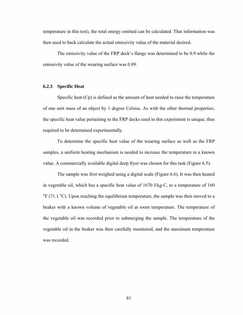
tempe ature in this tr est), the total energy emitted can be calculated. That information was

then us

niform heating mechanism is needed to increase the temperature to a known

value.

t value of 1670 J/kg-C, to a temperature of 160

°F (71.

the vegetable oil was recorded prior to submerging the sample. The temperature of the

vegetable oil in the beak

was recorded.

ed to back calculate the actual emissivity value of the material desired.

The emissivity value of the FRP deck’s flange was determined to be 0.9 while the

emissivity value of the wearing surface was 0.89.

6.2.3 Specific Heat

Specific heat (Cp) is defined as the amount of heat needed to raise the temperature

of one unit mass of an object by 1 degree Celsius. As with the other thermal properties,

the specific heat value pertaining to the FRP decks used in this experiment is unique, thus

required to be determined experimentally.

To determine the specific heat value of the wearing surface as well as the FRP

samples, a u

A commercially available digital deep fryer was chosen for this task (Figure 6.5).

The sample was first weighed using a digital scale (Figure 6.6). It was then heated

in vegetable oil, which has a specific hea

1 oC). Upon reaching the equilibrium temperature, the sample was then moved to a

beaker with a known volume of vegetable oil at room temperature. The temperature of

er was then carefully monitored, and the maximum temperature

81

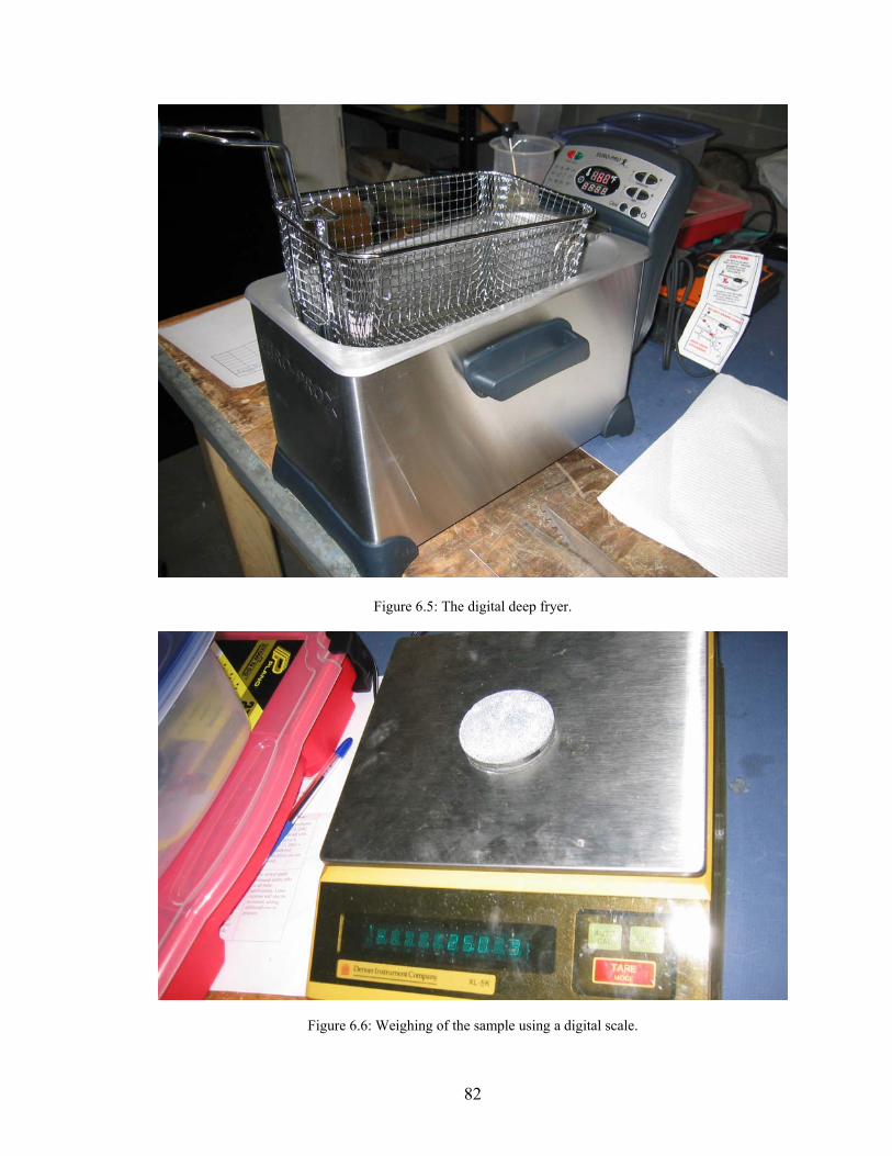
Figure 6.5: The digital deep fryer.

Figure 6.6: Weighing of the sample using a digital scale.

82

By knowing three sets of temperature as well as the specific heat value of the

vegetable oil and the weight of both vegetable oil and sample, the specific heat value of

the sample was easily calculated by using the following equation:

(weight of sample) (∆tsample) (Cpsample) = (weight of oil) (∆toil) (Cpoil) (6.5)

Table 6.1: The recorded data sheet for the specific heat value test

FRP 1 (A) FRP 2 (B) FRP 3 (C) FRP 4 (D)

Weight of Sample disc, (g) 21.8 18.6 18.8 21 Temperature of Fryer Oil, (F) 130 130 130 130 Weight of Vegetable oil, (g) 77.3 77.9 77.9 77.6 Initial Temperature of Veg. oil, (F) 78 78.7 78 78.2 Final Temperature of Veg. oil, (F) 85.8 85.5 84.8 85.9

∆tFRP 44.2 44.5 45.2 44.1

∆toil 7.8 6.8 6.8 7.7

Specific Heat Value, (J/kg-C) 1041.0 1077.5 1045.0 1068.8 WS 1 WS 2

Weight of Sample disc, (g) 42.9 39.6 Temperature of Fryer Oil, (F) 130 130 Weight of Vegetable oil, (g) 77.4 77.6 Initial Temperature of Veg. oil, (F) 77.5 81.1 Final Temperature of Veg. oil, (F) 88.4 90.3

∆tFRP 41.6 39.7

∆toil 10.9 9.2

Specific Heat Value, (J/kg-C) 789.5 758.4

∆tFRP = (Temperature of Fryer Oil) – (Final Temperature of Veg. oil)

∆toil = (Final Temperature of Veg. oil) – (Initial Temperature of Veg. oil) FRP = Fiber Reinforced Polymer Disc WS = Wearing Surface Disc

83

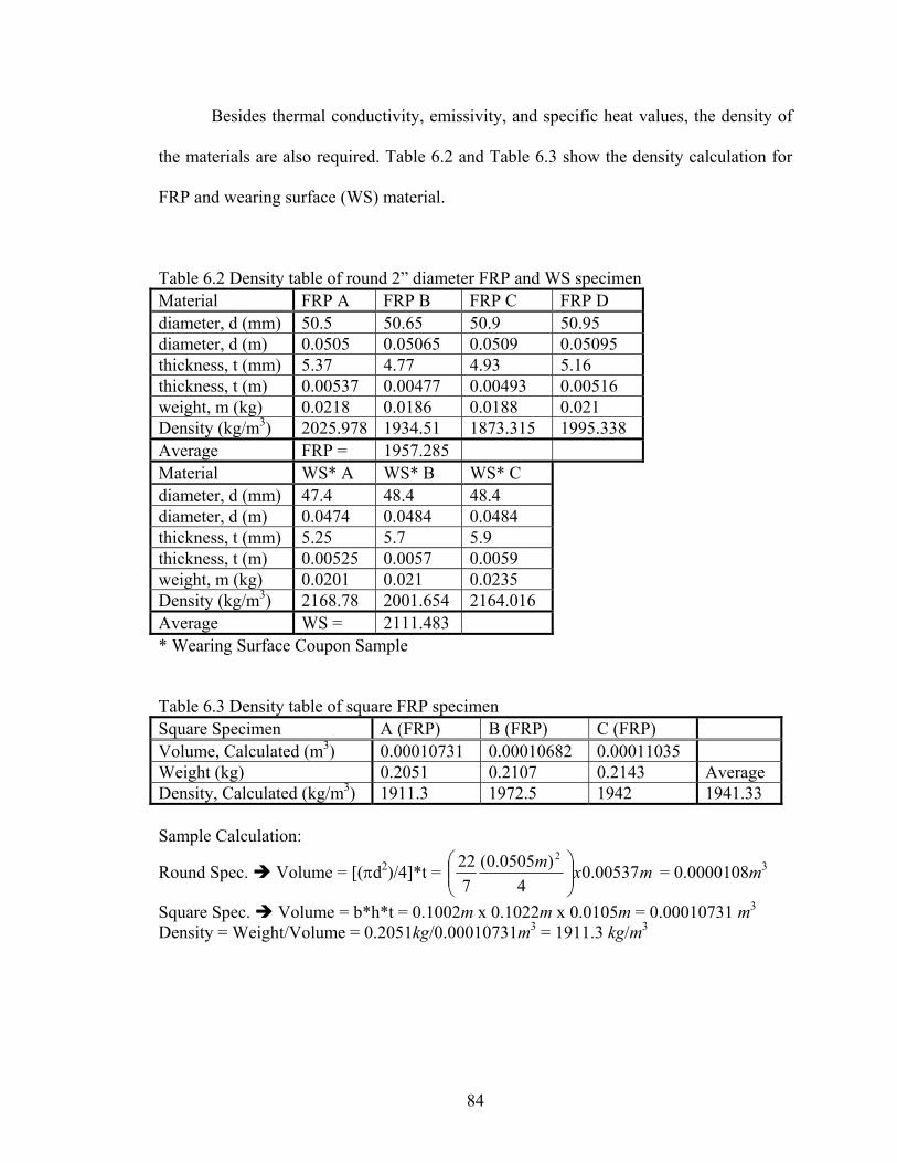
TaMaterial FRP A FRP B FRP C FRP D

Besides thermal conductivity, emissivity, and specific heat values, the density of

the materials are also required. Table 6.2 and Table 6.3 show the density calculation for

FRP and wearing surface (WS) material.

ble 6.2 Density table of round 2” diameter FRP and WS specimen

diameter, d (mm) 50.5 50.65 50.9 50.95 diameter, d (m) 0.0505 0.05065 0.0509 0.05095 thickness, t (mm) 5.37 4.77 4.93 5.16 thickness, t (m) 0.00537 0.00477 0.00493 0.00516 weight, m (kg) 0.0218 0 0 0..0186 .0188 021 D .978 1934.51 1873.315 1995.338 ensity (kg/m3) 2025Average FRP 1957 = .285M A WS* WS*aterial WS* B C d 48.4 48.4 iameter, d (mm) 47.4 d 0.04 0.048iameter, d (m) 0.0474 84 4 thickness, t (mm) 5.7 5.9 5.25 thickness, t (m) 0.00525 0.00 0.00557 9 weight, m (kg) 0.0201 0.021 0.023 5 Density (kg 3 2001.654 2164.016 /m ) 2168.78 Average WS 211 = 1.483 * Wearing Surface Coupon Sample Table 6.3 Density table of square FRP specimen S A (F B (FRP) C (FRP) quare Specimen RP) V 0.00010731 0.00010682 0.00011035 olume, Calculated (m3) Weight (kg) 0.2051 0.2107 0.2143 Average Density, Calculated (kg/m3) 1911.3 1972.5 1942 1941.33 S

R

ample Calculation:

ound Spec. Volume = [(πd2)/4]*t = mxm)0505.0(22⎟⎟⎞

⎜⎜⎛

00537.02

= 0.0000108m3

q m = 0.00010731 m3 .00010731m3 = 1911.3 kg/m3

47 ⎠⎝uare Spec. Volume = b*h*t = 0.1002m x 0.1022m x 0.0105S

Density = Weight/Volume = 0.2051kg/0

84

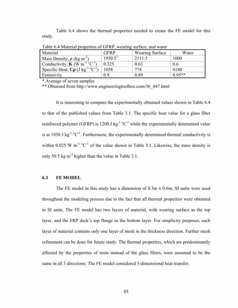
Table 6.4 shows the thermal properties needed to create the FE model for this

Material GFRP

study.

Table 6.4 Material properties of GFRP, wearing surface, and water Wearing Surface Water

Mass Density, ρ (kg m-3) 1950.5* 2111.5 1000 Conductivity, K (W m-1 oC-1) 0.325 0.63 0.6 Specific Heat, Cp (J kg-1 oC-1) 1058 774 4180 Emissivity 0.9 0.89 0.95** * Average of seven samples

/3 html

esti p per ob lues shown in Table 6.4

lis s le pe value for a glass fiber

polymer (GFRP) is 1200 J kg oC the experimentally determined value

-1 rmo xpe ly determined thermal conductivity is

-1 e ow le 3.1. Likewise, the mass density is

hig he a

.3 FE MODEL

ion of 0.3m x 0.6m. SI units were used

roce fa rm w re obtained

as ers of l, with ng surfac top

eck’s top flange as the bottom layer. For simplicity purposes, each

of mesh in the thickness dire sh

ntly

affected by the properties of resin instead of the glass fibers, were assumed to be the

same in all 3 directions. The FE model considered 3-dimensional heat transfer.

** Obtained from http://www.engineeringtoolbox.com 6_447.

It is inter ng to com are the ex imentally tained va

to that of the pub hed value from Tab 3.1. The s cific heat

reinforced -1 -1 while

is at 1058 J kg -1 oC . Furthe re, the e rimental

within 0.025 W m C of tho -1 value sh n in Tab

only 50.5 kg m -3 her than t value in T ble 3.1.

6

The FE model in this study has a dimens

throughout the modeling p ss due to the ct that all the al properties e

in SI units. The FE model h two lay materia weari e as the

layer, and the FRP d

layer of material contains only one layer ction. Further me

refinement can be done for future study. The thermal properties, which are predomina

85

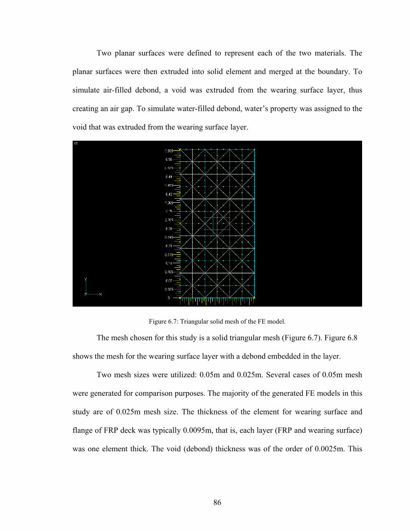
Two planar surfaces were defined to represent each of the two materials. The

planar surfaces were then extruded into solid element and merged at the boundary. To

air-filled debond, a void was extrude g surface layer, thus

e illed debond, water’s property was assigned to the

s extruded from the wearing surface layer.

simulate d from the wearin

creating an air gap. To simulat water-f

void that wa

Figure 6.7: Triangular solid mesh of the FE model.

The mesh chosen for this study is a solid triangular mesh (Figure 6.7). Figure 6.8

shows the mesh for the wearing surface layer with a debond embedded in the layer.

Two mesh sizes were utilized: 0.05m and 0.025m. Several cases of 0.05m mesh

were generated for comparison purposes. The majority of the generated FE models in this

study are of 0.025m mesh size. The thickness of the element for wearing surface and

flange of FRP deck was typically 0.0095m, that is, each layer (FRP and wearing surface)

was one element thick. The void (debond) thickness was of the order of 0.0025m. This

86

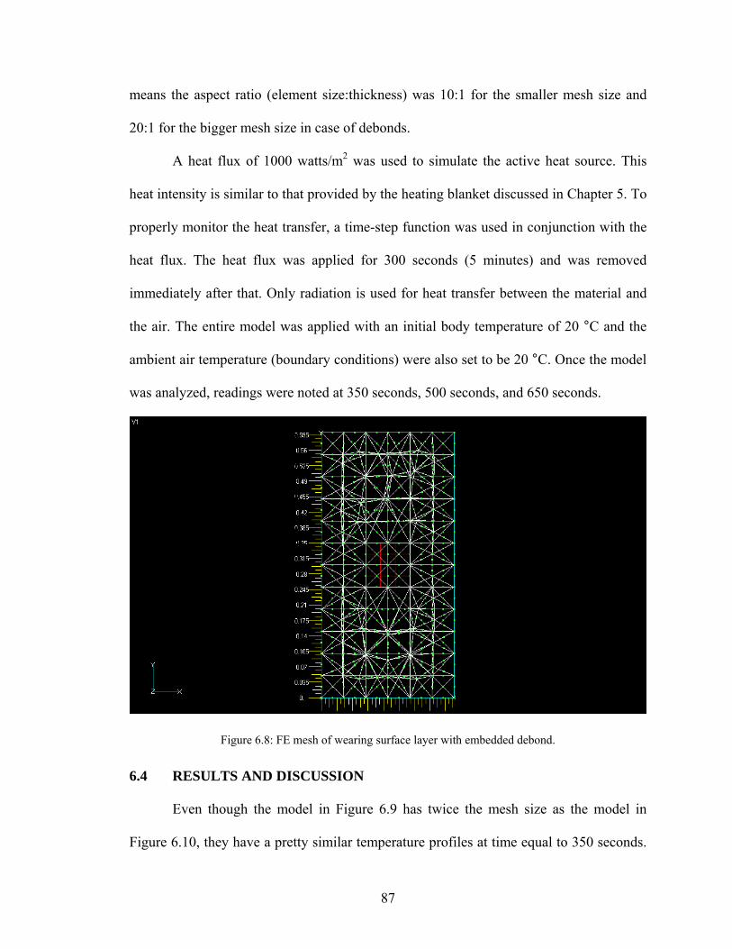
means

was used in conjunction with the

heat flux. The heat flux was applied for 300 seconds (5 minutes) and was removed

immediately after that. Only radiation is used for heat transfer between the material and

the air. The entire model was applied with an initial body temperature of 20 °C and the

ambient air temperature (boundary conditions) were also set to be 20 °C. Once the model

was analyzed, readings were noted at 350 seconds, 500 seconds, and 650 seconds.

the aspect ratio (element size:thickness) was 10:1 for the smaller mesh size and

20:1 for the bigger mesh size in case of debonds.

A heat flux of 1000 watts/m2 was used to simulate the active heat source. This

heat intensity is similar to that provided by the heating blanket discussed in Chapter 5. To

properly monitor the heat transfer, a time-step function

Figure 6.8: FE mesh of wearing surface layer with embedded debond.

6.4 RESULTS AND DISCUSSION

Even though the model in Figure 6.9 has twice the mesh size as the model in

Figure 6.10, they have a pretty similar temperature profiles at time equal to 350 seconds.

87

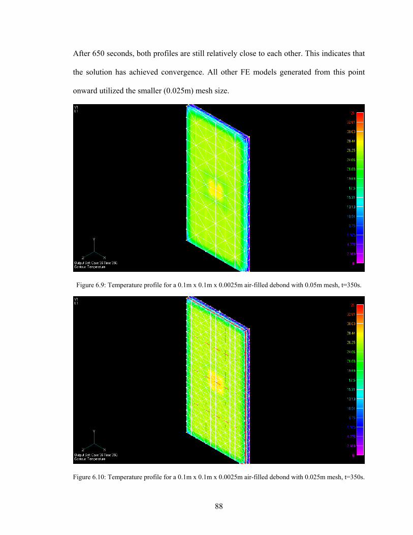
After 650 seconds, both profiles are still relatively close to each other. This indicates that

the solution has achieved convergence. All other FE models generated from this point

onward utilized the smaller (0.025m) mesh size.

Figure 6.9: Temperature profile for a 0.1m x 0.1m x 0.0025m air-filled debond with 0.05m mesh, t=350s.

Figure 6.10: Temperature profile for a 0.1m x 0.1m x 0.0025m air-filled debond with 0.025m mesh, t=350s.

88

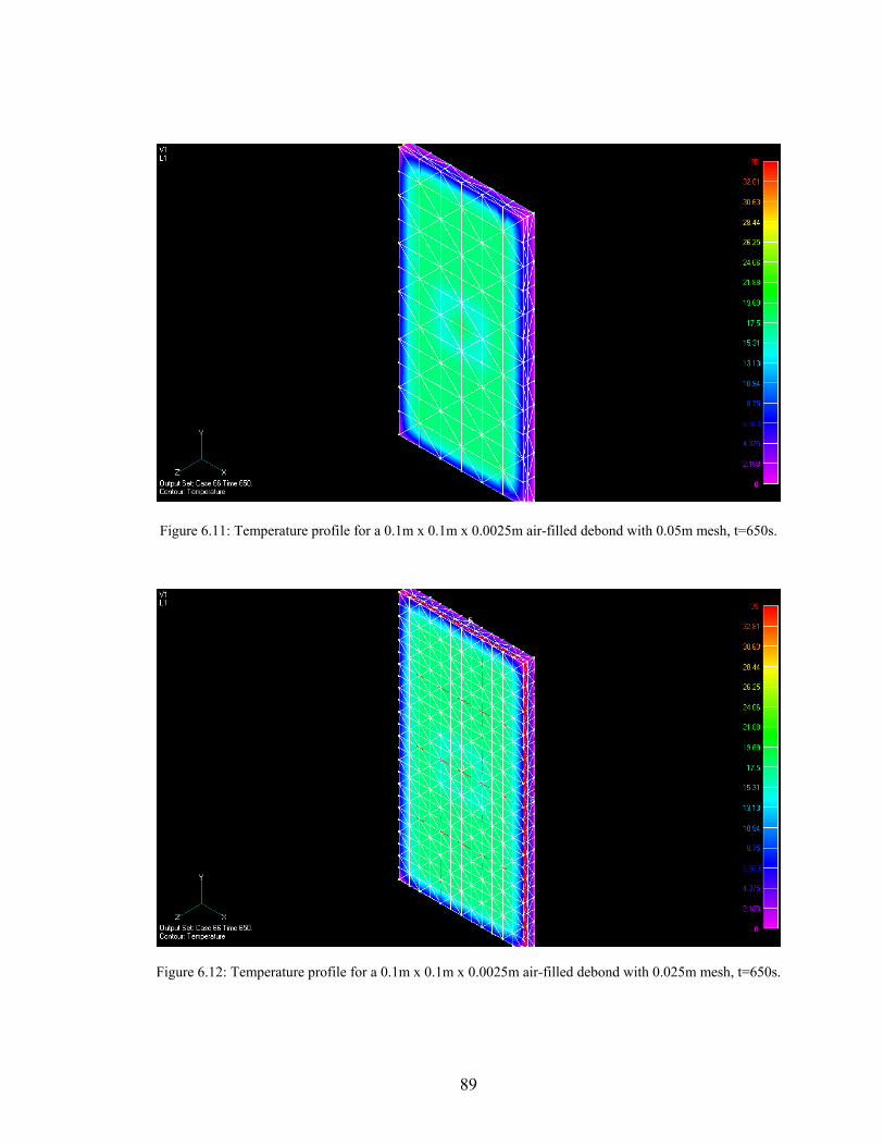
Figure 6.11: Temperature profile for a 0.1m x 0.1m x 0.0025m air-filled debond with 0.05m mesh, t=650s.

Figure 6.12: Temperature profile for a 0.1m x 0.1m x 0.0025m air-filled debond with 0.025m mesh, t=650s.

89

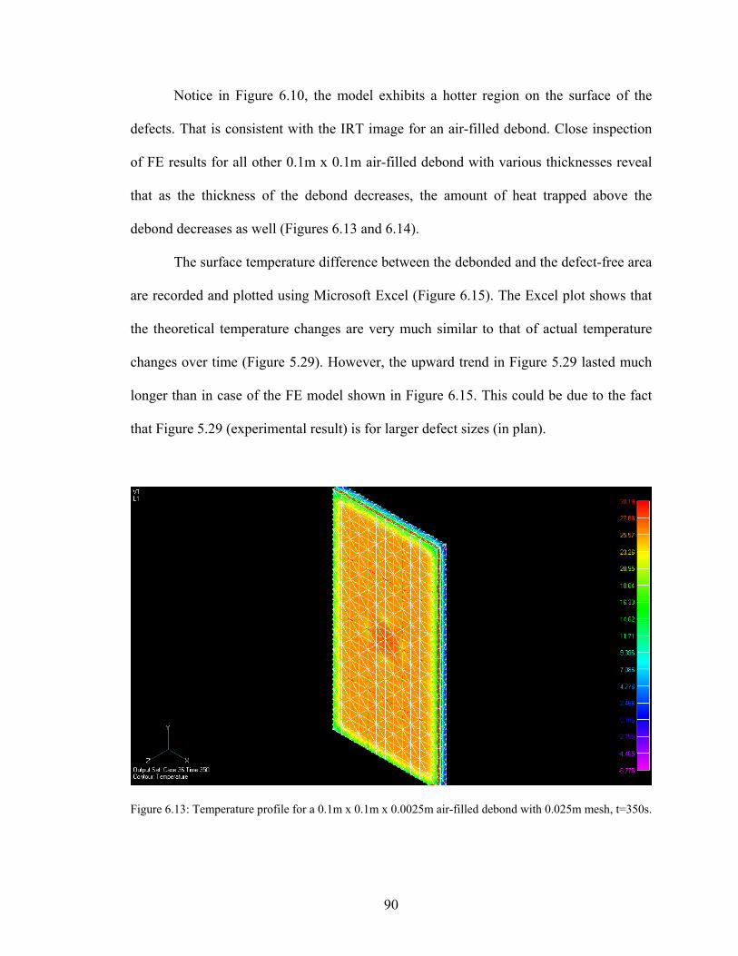
Notice in Figure 6.10, the model exhibits a hotter region on the surface of the

defects. That is consistent with the IRT image for an air-filled debond. Close inspection

of FE results for all other 0.1m x 0.1m air-filled debond with various thicknesses reveal

that as the thickness of the debond decreases, the amount of heat trapped above the

debond decreases as well (Figures 6.13 and 6.14).

The surface temperature difference between the debonded and the defect-free area

are recorded and plotted using Microsoft Excel (Figure 6.15). The Excel plot shows that

the theoretical temperature changes are very much similar to that of actual temperature

changes over time (Figure 5.29). However, the upward trend in Figure 5.29 lasted much

longer than in case of the FE model shown in Figure 6.15. This could be due to the fact

that Figure 5.29 (experimental result) is for larger defect sizes (in plan).

Figure 6.13: Temperature profile for a 0.1m x 0.1m x 0.0025m air-filled debond with 0.025m mesh, t=350s.

90

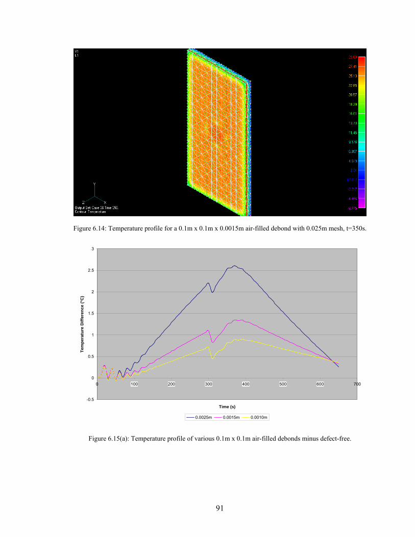
Figure 6.14: Temperature profile for a 0.1m x 0.1m x 0.0015m air-filled debond with 0.025m mesh, t=350s.

-0.5

0

0.5

1

1.5

2

2.5

3

0 100 200 300 400 500 600 700

Time (s)

Tem

pera

ture

Diff

eren

ce (°

C)

0.0025m 0.0015m 0.0010m

Figure 6.15(a): Temperature profile of various 0.1m x 0.1m air-filled debonds minus defect-free.

91

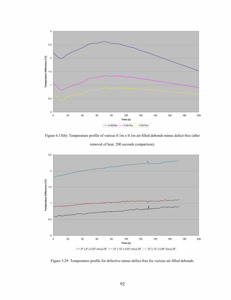
0

0.5

1

1.5

2

2.5

3

0 20 40 60 80 100 120 140 160 180 200

Time (s)

Tem

pera

ture

Diff

eren

ce (°

C)

0.0025m 0.0015m 0.0010m

Figure 6.15(b): Temperature profile of various 0.1m x 0.1m air-filled debonds minus defect-free (after

removal of heat, 200 seconds comparison).

0

0.5

1

1.5

2

2.5

0 20 40 60 80 100 120 140 160 180 200

Time (s)

Tem

pera

ture

Diff

eren

ce (º

C)

8" x 8" x 0.03" minus DF 12" x 12" x 0.03" minus DF 12" x 12" x 0.06" minus DF

Figure 5.29: Temperature profile for defective minus defect-free for various air-filled debonds.

92

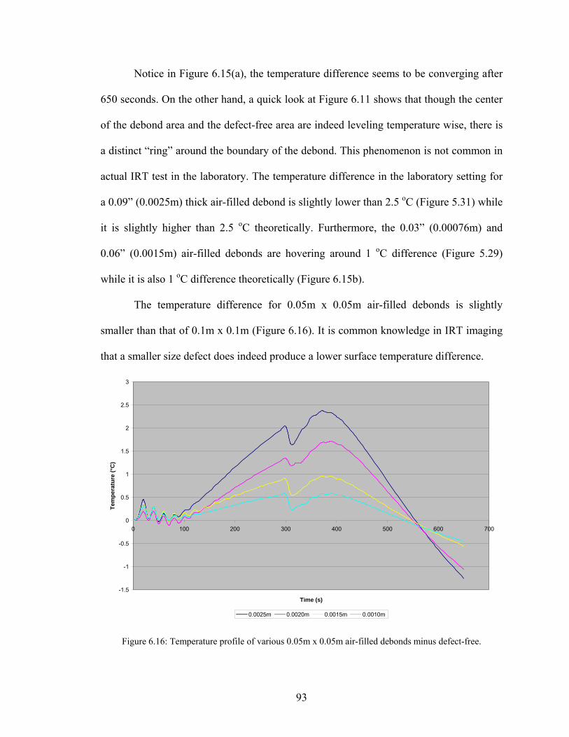
Notice in Figure 6.15(a), the temperature difference seems to be converging after

650 seconds. On the other hand, a quick look at Figure 6.11 shows that though the center

of the debond area and the defect-free area are indeed leveling temperature wise, there is

a distinct “ring” around the boundary of the debond. This phenomenon is not common in

actual IRT test in the laboratory. The temperature difference in the laboratory setting for

a 0.09” (0.0025m) thick air-filled debond is slightly lower than 2.5 oC (Figure 5.31) while

it is slightly higher than 2.5 oC theoretically. Furthermore, the 0.03” (0.00076m) and

0.06” (0.0015m) air-filled debonds are hovering around 1 oC difference (Figure 5.29)

while it is also 1 oC difference theoretically (Figure 6.15b).

The temperature difference for 0.05m x 0.05m air-filled debonds is slightly

sm g

that a smaller size defect d mperature difference.

aller than that of 0.1m x 0.1m (Figure 6.16). It is common knowledge in IRT imagin

oes indeed produce a lower surface te

-1.5

-1

-0.5

0

0.5

1

1.5

2

2.5

3

0 100 200 300 400 500 600 700

Time (s)

Tem

pera

ture

(°C

)

0.0025m 0.0020m 0.0015m 0.0010m

Figure 6.16: Temperature profile of various 0.05m x 0.05m air-filled debonds minus defect-free.

93

As seen in Figure 6.17, the FE model for the water-filled debond clearly exhibits a

lower surface temperature due to a much higher thermal conductivity. At the same time,

water has a high specific heat value of 4180 J kg-1 oC-1 and retains heat much better than

air, thus resulting in a higher temperature than the surrounding after a long period of time

(Figure 6.18). Once again, results from water-filled debond FE model shows the

characteristic pertaining to a water-filled debond. The temperature of the debond as well

as the defect-free area was noted and plotted using Microsoft Excel (Figure 6.19).

Unfortunately, there are no actual data of 4” x 4” (roughly 0.1m x 0.1m) water-filled

debonds available for direct comparison with Figure 6.19. However, the temperature

ore

profile of a theoretical water-filled debond does exhibit some characteristics that could be

found on actual water-filled debond. As seen in Figure 5.33 and Figure 6.19 (especially

the region after 300 seconds), the curves show a general upward trend bef

Figure 6.17: Temperature profile for a 0.1m x 0.1m x 0.0025m water-filled debond with 0.025m mesh, t=350s.

94

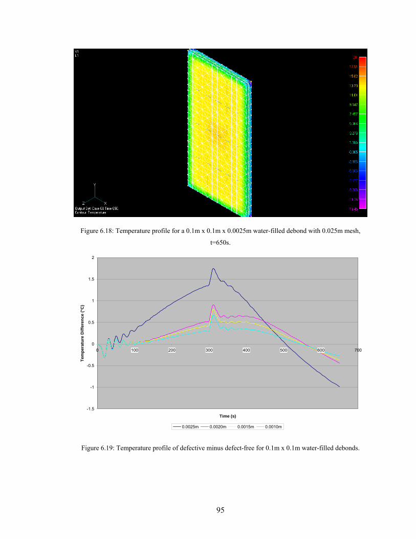
Figure 6.18: Temperature profile for a 0.1m x 0.1m x 0.0025m water-filled debond with 0.025m mesh,

t=650s.

-1.5

-1

-0.5

0

0.5

1

1.5

2

0 100 200 300 400 500 600 700

Time (s)

Tem

pera

ture

Diff

eren

ce (°

C)

0.0025m 0.0020m 0.0015m 0.0010m

Figure 6.19: Temperature profile of defective minus defect-free for 0.1m x 0.1m water-filled debonds.

95

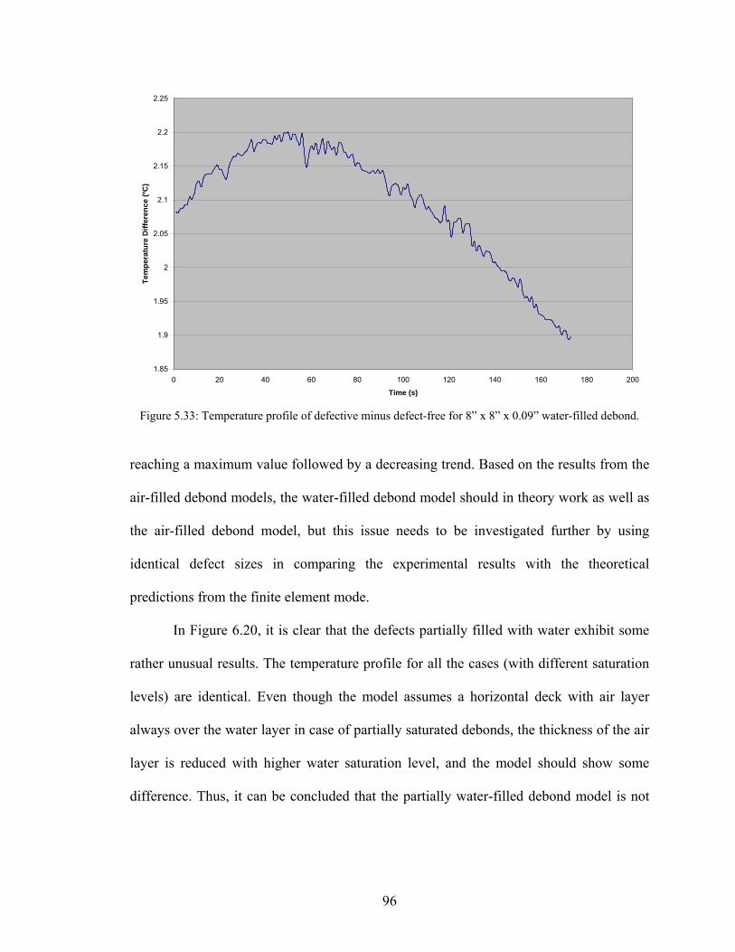
1.85

1.9

1.95

2

2.05

2.1

2.15

2.2

2.25

0 20 40 60 80 100 120 140 160 180 200

Time (s)

Tem

pera

ture

Diff

eren

ce (º

C)

Figure 5.33: Temperature profile of defective minus defect-free for 8” x 8” x 0.09” water-filled debond.

reaching a maximum value followed by a decreasing trend. Based on the results from the

air-filled debond models, the water-filled debond model should in theory work as well as

the air-filled debond model, but this issue needs to be investigated further by using

identical defect sizes in comparing the experimental results with the theoretical

predictions from the finite element mode.

In Figure 6.20, it is clear that the defects partially filled with water exhibit some

rather unusual results. The temperature profile for all the cases (with different saturation

levels) are identical. Even though the model assumes a horizontal deck with air layer

always over the water layer in case of partially saturated debonds, the thickness of the air

layer is reduced with higher water saturation level, and the model should show some

di t

fference. Thus, it can be concluded that the partially water-filled debond model is no

96

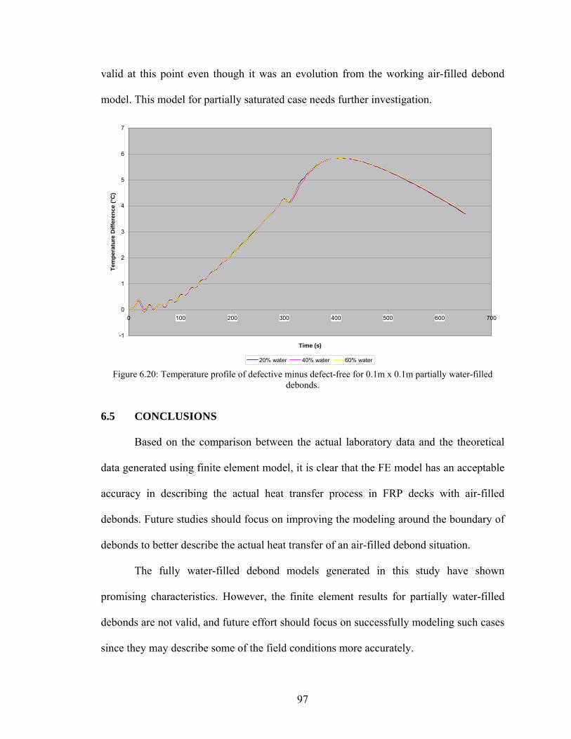
valid at this point even though it was an evolution from the working air-filled debond

model. This model for partially saturated case needs further investigation.

-1

0

1

2

3

4

5

6

7

0 100 200 300 400 500 600 700

Time (s)

Tem

pera

ture

Diff

eren

ce (°

C)

20% water 40% water 60% water debonds.

6.5 CONCLUSIONS

Based on the comparison between the actual laboratory data and the theoretical

data generated using finite element model,

Figure 6.20: Temperature profile of defective minus defect-free for 0.1m x 0.1m partially water-filled

it is clear that the FE model has an acceptable

since they may describe some of the field conditions more accurately.

accuracy in describing the actual heat transfer process in FRP decks with air-filled

debonds. Future studies should focus on improving the modeling around the boundary of

debonds to better describe the actual heat transfer of an air-filled debond situation.

The fully water-filled debond models generated in this study have shown

promising characteristics. However, the finite element results for partially water-filled

debonds are not valid, and future effort should focus on successfully modeling such cases

97

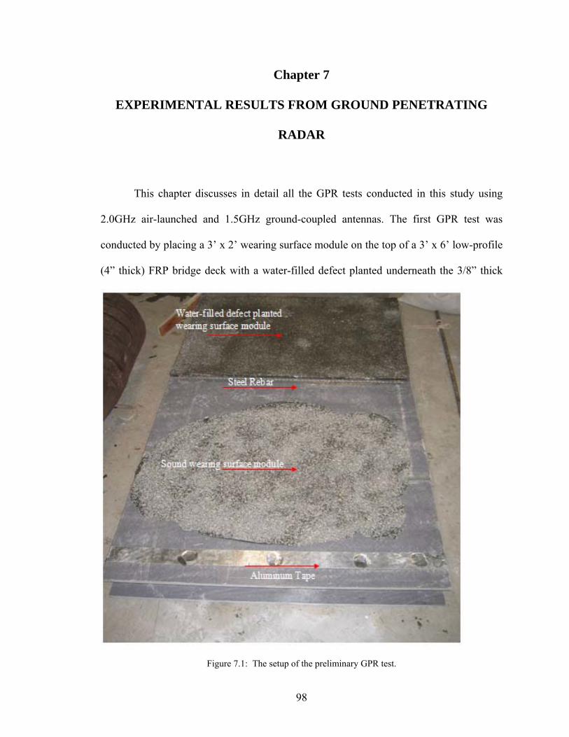
Chapter 7

EXPERIMENTAL RESULTS FROM GROUND PENETRATING

RADAR

This chapter discusses in detail all the GPR tests conducted in this study using

2.0GHz air-launched and 1.5GHz ground-coupled antennas. The first GPR test was

conducted by placing a 3’ x 2’ wearing surface module on the top of a 3’ x 6’ low-profile

(4” thick) FRP bridge deck with a water-filled defect planted underneath the 3/8” thick

Figure 7.1: The setup of the preliminary GPR test.

98

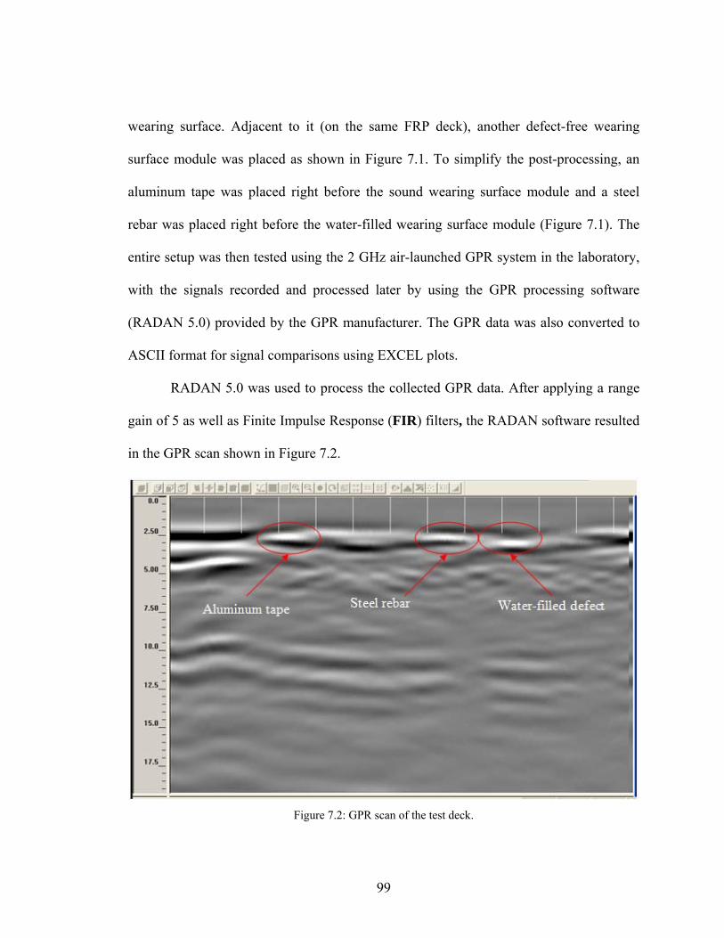
we g

surface module was placed as shown in Figur st-processing, an

aluminum tape was placed right before the sound wearing surface module and a steel

rebar was placed right before the water-filled wearing surface module (Figure 7.1). The

RADAN 5.0 was used to process the collected GPR data. After applying a range

gain of 5 as well as Finite Impulse Response (FIR) filters, the RADAN software resulted

in the GPR scan shown in Figure 7.2.

aring surface. Adjacent to it (on the same FRP deck), another defect-free wearin

e 7.1. To simplify the po

entire setup was then tested using the 2 GHz air-launched GPR system in the laboratory,

with the signals recorded and processed later by using the GPR processing software

(RADAN 5.0) provided by the GPR manufacturer. The GPR data was also converted to

ASCII format for signal comparisons using EXCEL plots.

Figure 7.2: GPR scan of the test deck.

99

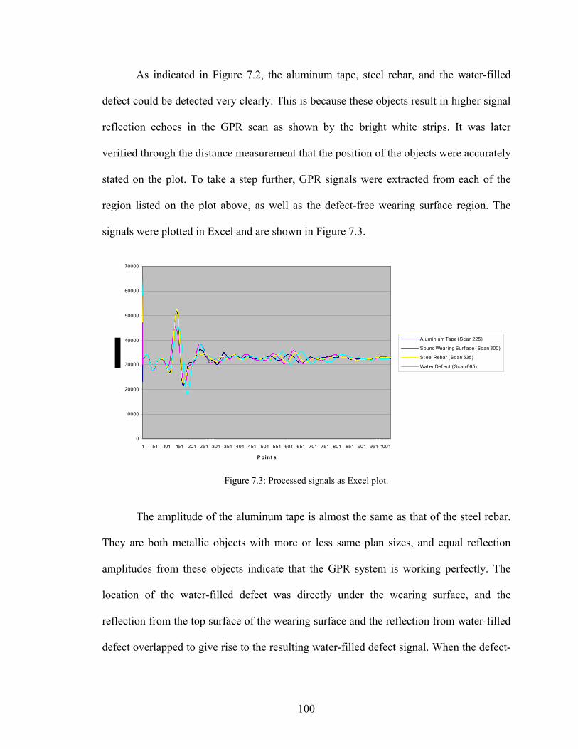
As indicated in Figure 7.2, the aluminum tape, steel rebar, and the water-filled

defect could be detected very clearly. This is because these objects result in higher signal

reflection echoes in the GPR scan as shown by the bright white strips. It was later

verified through the distance measurement that the position of the objects were accurately

stated on the plot. To take a step further, GPR signals were extracted from each of the

region listed on the plot above, as well as the defect-free wearing surface region. The

signals were plotted in Excel and are shown in Figure 7.3.

0

10000

20000

60000

70000

30000

40000

05000

1 51 101 151 201 251 301 351 401 451 501 551 601 651 701 751 801 851 901 951 1001

P oi nt s

Aluminium Tape (Scan 225)

Sound Wearing Surf ace (Scan 300)

St eel Rebar (Scan 535)

Wat er Def ect (Scan 665)

Figure 7.3: Processed signals as Excel plot.

The amplitude of the aluminum tape is almost the same as that of the steel rebar.

They are both metallic objects with more or less same plan sizes, and equal reflection

amplitudes from these objects indicate that the GPR system is working perfectly. The

location of the water-filled defect was directly under the wearing surface, and the

reflection from the top surface of the wearing surface and the reflection from water-filled

defect overlapped to give ris ect signal. When the defect-e to the resulting water-filled def

100

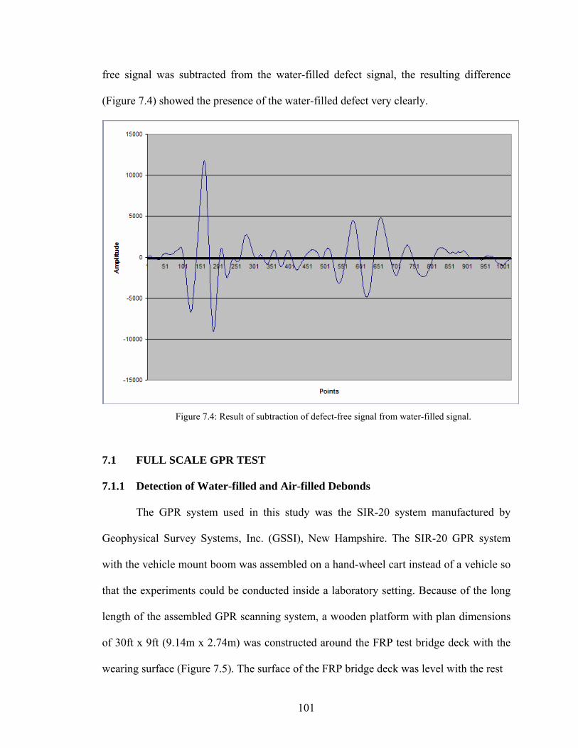
free signal was subtracted from the water-filled defect signal, the resulting difference

(Figure 7.4) showed the presence of the water-filled defect very clearly.

Figure 7.4: Result of subtraction of defect-free signal from water-filled signal.

7.1 FULL SCALE GPR TEST

7.1.1 Detection of Wate

wearing surface (Figure 7.5). The surface of the FRP bridge deck was level with the rest

r-filled and Air-filled Debonds

The GPR system used in this study was the SIR-20 system manufactured by

Geophysical Survey Systems, Inc. (GSSI), New Hampshire. The SIR-20 GPR system

with the vehicle mount boom was assembled on a hand-wheel cart instead of a vehicle so

that the experiments could be conducted inside a laboratory setting. Because of the long

length of the assembled GPR scanning system, a wooden platform with plan dimensions

of 30ft x 9ft (9.14m x 2.74m) was constructed around the FRP test bridge deck with the

101

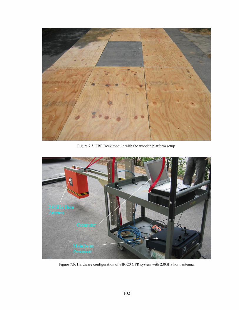
Figure 7.5: FRP Deck module with the wooden platform setup.

Figure 7.6: Hardware configuration of SIR-20 GPR system with 2.0GHz horn antenna.

2.0GHz Horn Ant

Processor

enna

Computer

Mainframe

102

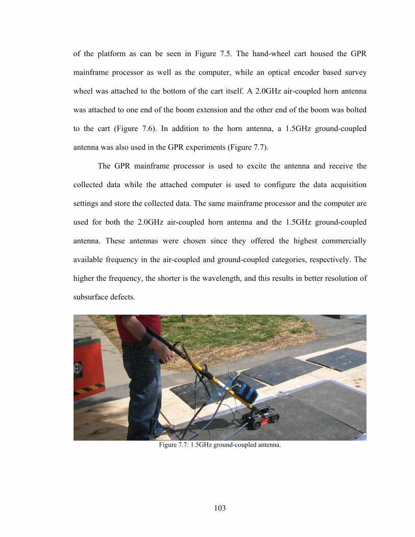
of the platform as can be seen in Figure 7.5. The hand-wheel cart housed the GPR

mainframe processor as well as the computer, while an optical encoder based survey

wheel was attached to the bottom of the cart itself. A 2.0GHz air-coupled horn antenna

was attached to one end of the boom extension and the other end of the boom was bolted

to the cart (Figure 7.6). In addition to the horn antenna, a 1.5GHz ground-coupled

antenna was also used in the GPR experiments (Figure 7.7).

The GPR mainframe processor is used to excite the antenna and receive the

collected data while the attached computer is used to configure the data acquisition

settings and store the collected data. The same mainframe processor and the computer are

used for both the 2.0GHz air-coupled horn antenna and the 1.5GHz ground-coupled

antenna. These antennas were chosen since they offered the highest commercially

available frequency in the air-coupled and ground-coupled categories, respectively. The

higher the frequency, the shorter is the wavelength, and this results in better resolution of

subsurface defects.

Figure 7.7: 1.5GHz ground-coupled antenna.

103

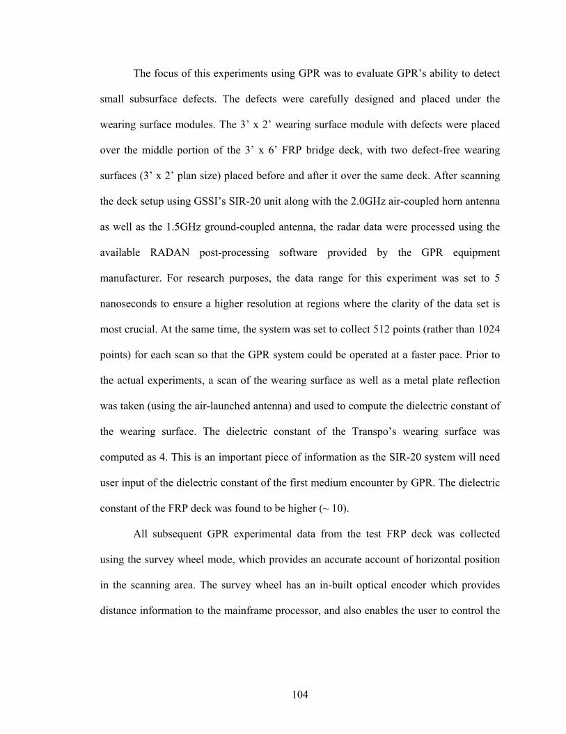
The focus of this experiments using GPR was to evaluate GPR’s ability to detect

small subsurface defects. The defects were carefully designed and placed under the

wearing surface modules. The 3’ x 2’ wearing surface module with defects were placed

over the middle portion of the 3’ x 6’ FRP bridge deck, with two defect-free wearing

surfaces (3’ x 2’ plan size) placed before and after it over the same deck. After scanning

the deck setup using GSSI’s SIR-20 unit along with the 2.0GHz air-coupled horn antenna

air-launched antenna) and used to compute the dielectric constant of

the wearing surface. The dielectric constant of the Transpo’s wearing surface was

computed as 4. This is an important piece of information as the SIR-20 system will need

user input of the dielectric constant of the first medium encounter by GPR. The dielectric

constant of the FRP deck was found to be higher (~ 10).

All subsequent GPR experimental data from the test FRP deck was collected

using the survey wheel mode, which provides an accurate account of horizontal position

in the scanning area. The survey wheel has an in-built optical encoder which provides

distance information to th es the user to control the

as well as the 1.5GHz ground-coupled antenna, the radar data were processed using the

available RADAN post-processing software provided by the GPR equipment

manufacturer. For research purposes, the data range for this experiment was set to 5

nanoseconds to ensure a higher resolution at regions where the clarity of the data set is

most crucial. At the same time, the system was set to collect 512 points (rather than 1024

points) for each scan so that the GPR system could be operated at a faster pace. Prior to

the actual experiments, a scan of the wearing surface as well as a metal plate reflection

was taken (using the

e mainframe processor, and also enabl

104

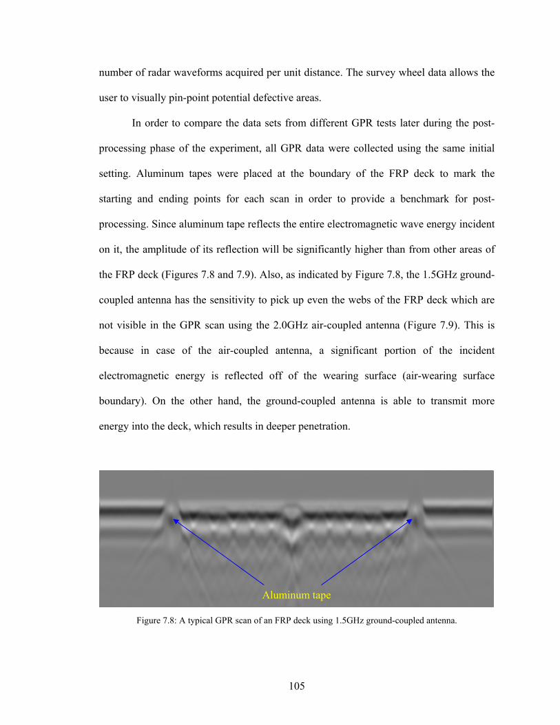
n of radar waveforms acquired per unit distance. The survey wheel data allows the

user to visually pin-point potential defective areas.

In order to compare the data sets from different GPR tests later during the post-

processing phase of the experiment, all GPR data were collected using the same initial

setting. Aluminum tapes were placed at the boundary of the FRP deck to mark the

starting and ending points for each scan in order to provide a benchmark for post-

processing. Since aluminum tape reflects the entire electromagnetic wave energy incident

on it, the amplitude of its reflection will be significantly higher than from other areas of

the FRP deck (Figures 7.8 and 7.9). Also, as indicated by Figure 7.8, the 1.5GHz ground-

coupled antenna has the sensitivity to pick up even the webs of the FRP deck which are

not visible in the GPR scan using the 2.0GHz air-coupled antenna (Figure 7.9). This is

because in case of the air-coupled antenna, a significant portion of the incident

electromagnetic energy is reflected off of the wearing surface (air-wearing surface

boundary). On the other hand, the ground-coupled antenna is able to transmit more

energy into the deck, which results in deeper penetration.

umber

Figure 7.8: A typical GPR scan of an FRP deck using 1.5GHz ground-coupled antenna.

Aluminum tape

105

Figure 7.9: A typical GPR scan of an FRP deck using 2.0GHz air-coupled horn antenna.

In this experiment, three passes of GPR scanning were conducted along the length

of the FRP deck. Each length pass included a defect-free wearing surface module

followed by a defective wearing surface module (with defect attached to the bottom side

of the wearing surface, thus simulating debonds) and then another defect-free module. By

collecting multiple (three in this case) GPR passes for the test deck at equal distances (9”

or 228.6mm) apart, RADAN post-processing software enabled the creation of a 3D

profile of the scanning project (Figure 7.10). This 3D profile (obtained using ground-

coupled antenna in this case) is very useful as it allows user to visually identify any

detectable defects and pinpoint its exact location through the 3D coordinate system. Most

3D data have to be gained (amplified) during the post-processing stage in order to

identify smaller defects.

Aluminum Tape

106

ground-coupled antenna.

was applied to all data sets. The data were then gained in order

to identify any subsurface defects. Figure 7.11 shows the GPR scan after the FIR was

applied to the original (raw) data set shown in Figure 7.8 (ground-coupled antenna). It

should be noticed that the uniform “top” layer that is visible in Figure 7.8 no longer exists

after the FIR was applied (Figure 7.11). Also, the application of gain has made the

features in the GPR scan look much sharper in Figure 7.11.

Figure 7.10: 3D profile created by collecting three passes of GPR data at equal distances (9”) apart using

There are several few post-processing options available through the use of the

post-processing software, RADAN. Process such as zero-correction, will remove the gap

between the antenna and the top surface of the first medium. This process essentially

enables the user to identify the depths of detectable defects. Another one of the many

post-processing options available is the Finite Impulse Response (FIR) filter. FIR

filtering removes any constant system noise generated within the GPR system. For this

experiment, the FIR filter

107

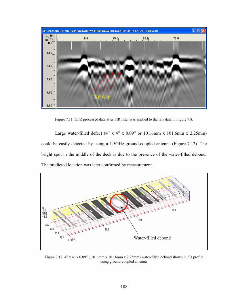
Figure 7.11: GPR processed data after FIR filter was applied to the raw data in Figure 7.8.

could be easily detected by using a 1.5GHz ground-coupled antenna (Figure 7.12). The

FRP Web

Large water-filled defect (4” x 4” x 0.09” or 101.6mm x 101.6mm x 2.25mm)

bright spot in the middle of the deck is due to the presence of the water-filled debond.

The predicted location was later confirmed by measurement.

Figure 7.12: 4” x 4” x 0.09” (101.6mm x 101.6mm x 2.25mm) water-filled debond shown in 3D profile using ground-coupled antenna.

Water-filled debond

108

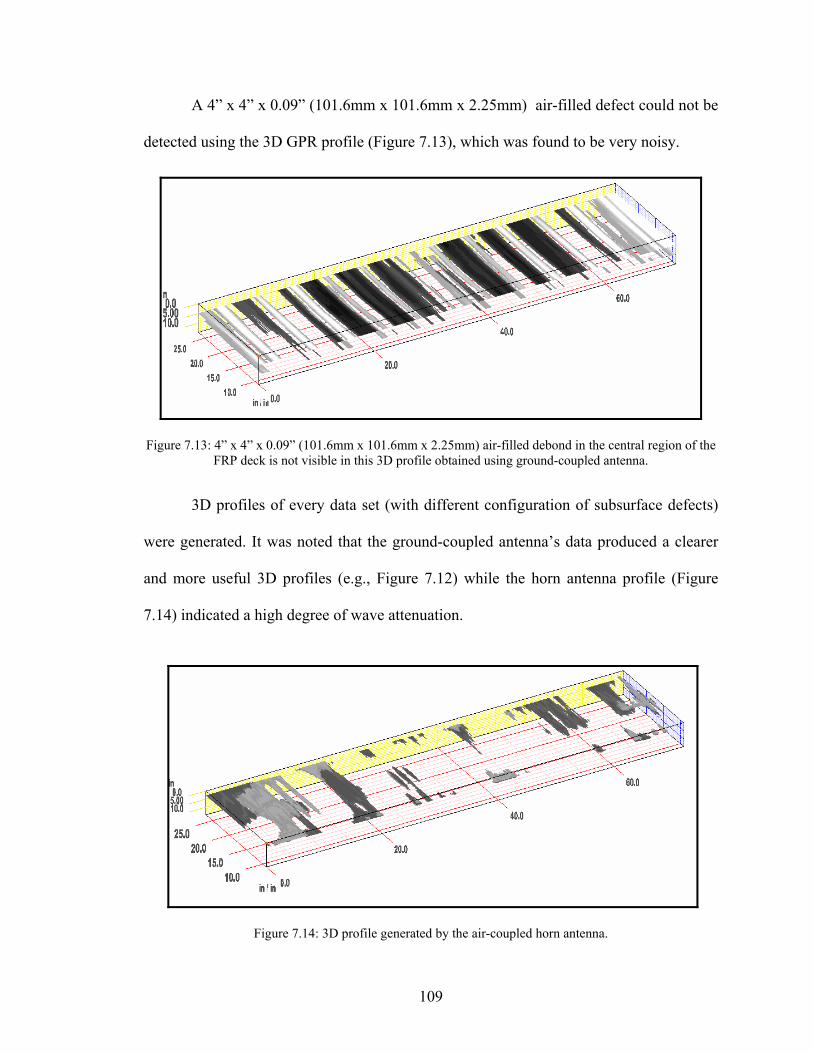
A 4” x 4” x 0.09” (101.6mm x 101.6mm x 2.25mm) air-filled defect could not be

detected using the 3D GPR profile (Figure 7.13), which was found to be very noisy.

Figure 7.13: 4” x 4” x 0.09” (101.6mm x 101.6mm x .25mm) air-filled debond in the central region of the

orn antenna profile (Figure

7.14) indicated a high degree of wave attenuation.

2FRP deck is not visible in this 3D profile obtained using ground-coupled antenna.

3D profiles of every data set (with different configuration of subsurface defects)

were generated. It was noted that the ground-coupled antenna’s data produced a clearer

and more useful 3D profiles (e.g., Figure 7.12) while the h

Figure 7.14: 3D profile generated by the air-coupled horn antenna.

109

As shown in Figure 7.14, the features were sparse and not uniform. The features

only show noise, and one cannot make a firm conclusion based on the 3D profile

obtained using the air-coupled antenna. The ground-coupled antenna’s 3D profile could

easily detect subsurface water-filled debonds (Figure 7.12) of size 4” x 4” x 0.09”

(101.6mm x 101.6mm x 2.25mm) and greater.

While 3D profile offers a user friendly way to identify subsurface defects, there

are many instances where inspecting and even processing the 2D scan profile could yield

better results. For instance, the amplified FIR scan of 4” x 4” x 0.03” (101.6mm x

101.6mm x 0.75mm) water-filled defect could be identified through the 2D profile

onclude t

easily b

nother characteristic of the water-filled debond is that it tends to create an

upward “wave”. The same upward wave is very obvious in the middle region of the scan

in Figure 7.11, which is once again the 4” x 4” x 0.09” (101.6mm x 101.6mm x 2.25mm)

water-filled defect. By inspecting the 2D scan, the smallest defect that could be detected

was 2” x 2” x 0.06” (50.8mm x 50.8mm x 1.5mm) water-filled debond (Figure 7.16). By

knowing the characteristic of a water-filled debond (upward “wave”) as well as obvious

visual indications, GPR proved to be an extremely useful tool in detecting subsurface

water-filled debonds between the wearing surface and the underlying FRP bridge deck

(Figure 7.15) but not via the 3D profile. By visual inspection of Figure 7.15, one can

hat the middle portion of the scan is unusual. Since the aluminum tapes can c

e spotted towards the beginning and the end of the 2D scan, the distance of the

“unusual” spot to one of the aluminum tapes could be measured. This measurement

confirmed that the unusual spot was indeed the 4” x 4” x 0.03” (101.6mm x 101.6mm x

0.75mm) water-filled debond.

A

.

110

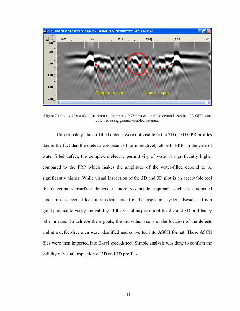
Figure 7.15: 4” x 4” x 0.03” (101.6mm x 101.6mm x 0.75mm) water-filled debond seen in a 2D GPR scan obtained using ground-coupled antenna.

Unfortunately, the air-filled defects were not visible in the 2D or 3D GPR profiles

due to the fact that the dielectric constant of air is relatively close to FRP. In the case of

water-filled defect, the complex dielectric permittivity of water is significantly higher

compared to the FRP which makes the amplitude of the water-filled debond to be

significantly higher. While visual inspection of the 2D and 3D plot is an acceptable tool

for detecting subsurface defects, a more systematic approach such as automated

algorithms is needed for future advancement of the inspection system. Besides, it is a

good practice to verify the validity of the visual inspection of the 2D and 3D profiles by

other means. To achieve these goals, the individual scans at the location of the defects

and at a defect-free area were identified and converted into ASCII format. These ASCII

files were then imported into Excel spreadsheet. Simple analysis was done to confirm the

validity of visual inspection of 2D and 3D profiles.

Unusual spot Aluminum tape

111

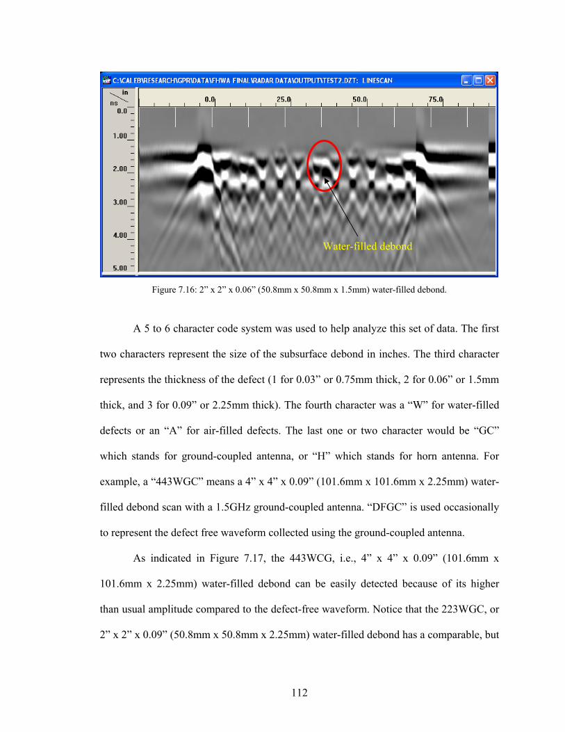
” x 0.06” (50.8mm x 50.8mm x 1.5mm) w

Water-filled debond

Figure 7.16: 2” x 2 ater-filled debond.

A 5 to 6 character code system was used to help analyze this set of data. The first

two characters represent the size of the subsurface debond in inches. The third character

represents the thickness of the defect (1 for 0.03” or 0.75mm thick, 2 for 0.06” or 1.5mm

thick, and 3 for 0.09” or 2.25mm thick). The fourth character was a “W” for water-filled

defects or an “A” for air-filled defects. The last one or two character would be “GC”

which stands for ground-coupled antenna, or “H” which stands for horn antenna. For

example, a “443WGC” means a 4” x 4” x 0.09” (101.6mm x 101.6mm x 2.25mm) water-

filled debond scan with a 1.5GHz ground-coupled antenna. “DFGC” is used occasionally

to represent the defect free waveform collected using the ground-coupled antenna.

As indicated in Figure 7.17, the 443WCG, i.e., 4” x 4” x 0.09” (101.6mm x

101.6mm x 2.25mm) water-filled debond can be easily detected because of its higher

than usual amplitude compared to the defect-free waveform. Notice that the 223WGC, or

2” x 2” x 0.09” (50.8mm x 50.8mm x 2.25mm) water-filled debond has a comparable, but

112

smaller amplitude waveform. Though the amplitude is smaller than the 443WGC case

(yet slightly higher than the defect free waveform), the 223WGC is obviously a water-

filled defect because its phase is similar to 443WGC. Also notice that the 222WGC

waveform, which corresponds to a 2” x 2” x 0.06” (50.8mm x 50.8mm x 1.5mm) water-

filled debond, is showing a slight time-shift. The waveforms corresponding to the 0.03”

(0.75mm) thick water-filled debonds (221WGC and 441WGC) are more or less aligned

with the defect-free waveform. While it is clear that the signal amplitudes in these

waveforms (221WGC and 441WGC) are slightly ct-free waveform

(DFGC), such distinction may not be obvious in the field data. Thus, it would be difficult

to detect 0.03” (0.75mm) thick water-filled debonds, while water-filled debonds with

larger t

higher than the defe

hicknesses (≥ 0.06” or 1.5 mm) could be detected.

To further investigate this result, signal subtraction was carried out. The defect-

free signal was subtracted from the signals corresponding to the various water-filled

debonds. Figure 7.18 shows the waveforms for the various water-filled debonds after the

subtraction was carried out.

113

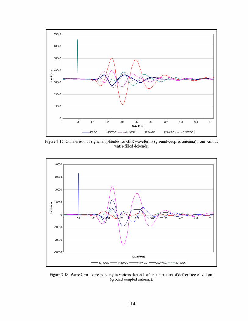
0

10000

50000

60000

70000

1 51 101 151 201 251 301 351 401 451 501

mpl

itu

20000

30000

40000

Data Point

Ade

DFGC 443WGC 441WGC 222WGC 223WGC 221WGC

Figure 7.17: Comparison of signal amplitudes for GPR waveforms (gwater-filled debonds.

round-coupled antenna) from various

-30000

-20000

-10000

0

10000

20000

30000

40000

1 51 101 151 201 251 301 351 401 451 501

Data Point

Am

plitu

de

223WGC 443WGC 441WGC 222WGC 221WGC

Figure 7.18: Waveforms corresponding to various debonds after subtraction of defect-free waveform (ground-coupled antenna).

114

As seen from Figure 7.18, 223WGC and 443WGC show higher amplitudes while

the other waveforms show significantly lower amplitudes. Though the laboratory setting

allows the smaller debonds to be detected through such GPR waveform comparisons, the

amplitude of such debonds are not significant enough to confidently classify as defect,

especially in the field setting when many other factors could give rise to signals of

comparable amplitude.

A similar analysis was conducted for the GPR waveform from subsurface

debonds obtained using air-coupled horn antenna. Unfortunately, as seen in Figure 7.19,

the horn antenna waveforms yield no useful information. Also, the spikes in Figure 7.19

are the result of noises introduced during the processing of GPR data.

0

10000

20000

30000

40000

50000

60000

70000

1 18 35 52 69 86 103 120 137 154 171 188 205 222 239 256 273 290 307 324 341 358 375 392 409 426 443 460 477 494

Data Point

Am

plitu

de

DFH 443WH 441WH 223WH 222WH 221WH

Figure 7.19: Comparison of signal amplitudes for GPR waveforms (air-coupled horn antenna) from variou

s water-filled debonds.

115

In lieu of previous results which indicated the inability of 2.0GHz air-coupled

antenna GPR system to detect smaller defects (2” x 2”, 4” x 4” defects with thickness

varies from 0.03” to 0.09”), various larger size defects, such as 8” x 8” (203.2mm x

203.2mm) and 12” x 12” (304.8mm x 304.8mm) debond, were created to accurately

identify the minimum size and thickness defect detectable by the 2.0GHz air-coupled

antenna GPR system. The defects’ thicknesses ranged from 0.03” (0.75mm) to 0.09”

(2.25m

ormity of the data

collected. In this case, the gain during the data acquisition was set to 10 times, while

lowering the range down to 5 ns with 1024 points collected with each pass.

The data were then analyzed by using the Radan 6.0 software. Finite Impulse

Response (FIR) was applied to all the data, and a 3D model was created as well. As noted

in the previous reports, the key to analyzing GPR data is to look at a combination of the

2D image, 3D image, and the signal analysis in order to draw conclusions.

Results show that the 2.0GHz horn antenna GPR system is not capable of

detecting subsurface air-filled defects (Figure 7.21). As such, the next logical step is to

apply the FIR in hope of eliminating the constant signal noise thus improving the quality

of the 2D plot. Unfortunately, the result of FIR did not reveal any helpful result either.

Finally, the files were stitched together to form a 3D image. As with the procedures

m). The layout of the defects is shown in Figure 7.20.

Data were collected by using the 2.0GHz horn antenna GPR system on the

modules with air-filled defects follow by water-filled defects. As with any other GPR

procedure, a set of fixed parameters were established to ensure unif

before, it too did not reveal any conclusive result. By knowing the exact location of the

116

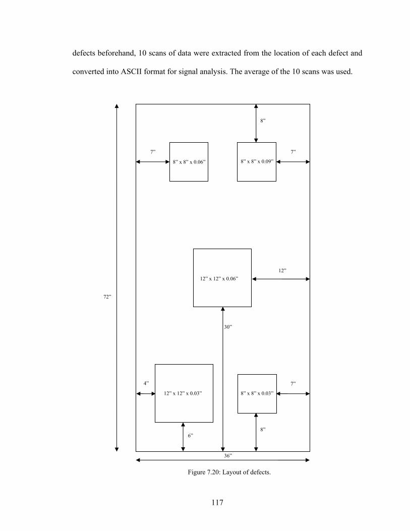
defects

Figure 7.20: Layout of defects.

beforehand, 10 scans of data were extracted from the location of each defect and

converted into ASCII format for signal analysis. The average of the 10 scans was used.

12” x 12” x 0.03” 8” x 8” x 0.03”

” 8” x 8” x 0.06” 8” x 8” x 0.09

12” x 12” x 0.06”

36”

7” 7”

8”

72”

6” 8”

4” 7”

12”

30”

117

Figure 7.21: 2D image of an air-filled debond scan.

Figure 7.22 shows the GPR signals corresponding to the air-filled defects data

prior to applying FIR. Each waveform corresponds to various air-filled debonds after

subtraction of defect-free waveform. The maximum amplitude of each waveform is about

4000 points within each other, hovering around the 6000 point mark. Compared to the

same signal analysis for a ground-coupled antenna (Figure 7.23), the signal amplitudes

(after subtraction of defect-free waveform) for the air-filled defects clearly is not

significant enough to show any promising results (note that all analysis figures use a

70,000 point scale for easy comparison). In hopes of getting better responses, a FIR

analysis was done to each set of data, prior to taking the average value. Once again, it did

not reveal any compelling results, since the resulting signals had comparable signal

strengths as the original data sets (Figures 7.24 and 7.22).

A result of an imperfection on the platform setup

118

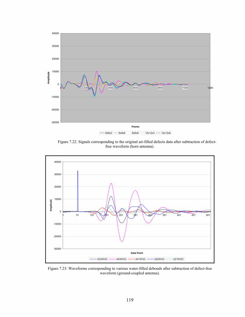
-30000

0-2000

-1000

0

10000

20000

30000

40000

0 200 400 600 800 1000 1200

Am

plitu

de

0

Points

8x8x3 8x8x6 8x8x9 12x12x3 12x12x6

Figure 7.22: Signals corresponding to the original air-filled defects data after subtraction of defect-

free waveform (horn antenna).

-30000

-20000

-10000

0

10000

20000

30000

40000

1 51 101 151 201 251 301

Am

plit

351 401 451 501

Data Point

ude

223WGC 443WGC 441WGC 222WGC 221WGC

Figure 7.23: Waveforms corresponding to various water-filled debonds after subtraction of defect-free waveform (ground-coupled antenna).

119

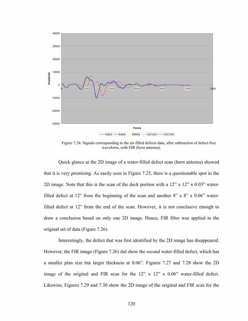
-30000

-20000

-10000

0

10000

20000

30000

40000

0 200 400 600 800 1000 1200

Points

Am

plitu

de

8x8x3 8x8x6 8X8X9 12X12X3 12X12X6

Figure 7.24: Signals corresponding to the air-filled defects data, after subtraction of defect-free veform, with FIR (horn antennawa ).

Quick glance at the 2D image of a water-filled defect scan (horn antenna) showed

that it is very promising. As easily seen in Figure 7.25, there is a questionable spot in the

2D image. Note that this is the scan of the deck portion with a 12” x 12” x 0.03” water-

filled defect at 12” from the beginning of the scan and another 8” x 8” x 0.06” water-

filled defect at 12” from the end of the scan. However, it is not conclusive enough to

draw a conclusion based on only one 2D image. Hence, FIR filter was applied to the

original set of data (Figure 7.26).

Interestingly, the defect that was first identified by the 2D image has disappeared.

However, the FIR image (Figure 7.26) did show the second water-filled defect, which has

a smaller plan size but larger thickness at 0.06”. Figures 7.27 and 7.28 show the 2D

im t.

Likewise, Figures 7.29 and 7.30 show the 2D image of the original and FIR scan for the

.

age of the original and FIR scan for the 12” x 12” x 0.06” water-filled defec

120

121

8” x 8” x 0.03” water-filled defect at 8” from the beginning of the scan and 8” x 8” x

0.09” water-filled defect at 8” from the end of the scan. Figures 7.27 and 7.28 clearly

show the 12” x 12” x 0.06” water-filled defect. Figure 7.29 did not reveal anything while

Figure 7.30 clearly shows the 8” x 8” x 0.09” water-filled defect.

To further evaluate the data, a 3D scan was constructed (Figure 7.31). As usual, a

FIR version of the 3D scan was constructed as well for comparison purposes (Figure

7.32).

Figure 7.25: 2D image of a water-filled debond scan.

Questionable spot

Figure 7.26: 2D image of a water-filled debond scan with FIR.

A result of an

water-filled defect 8” x 8” x 0.06” water-filled defect

imperfection on the platform setup

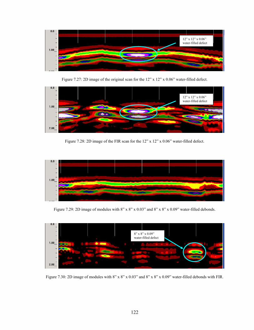
12” x 12” x 0.06” water-filled defect

Figure 7.27: 2D image of the original scan for the 12” x 12” x 0.06” water-filled defect.

Figure 7.28: 2D image of the FIR scan for the 12” x 12” x 0.06” water-filled defect.

Figure 7.29: 2D image of modules with 8” x 8” x 0.03” and 8” x 8” x 0.09” water-filled debonds.

12” x 12” x 0.06” water-filled defect

8” x 8” x 0.09” water-filled defect

Figure 7.30: 2D image of m

odules with 8” x 8” x 0.03” and 8” x 8” x 0.09” water-filled debonds with FIR.

122

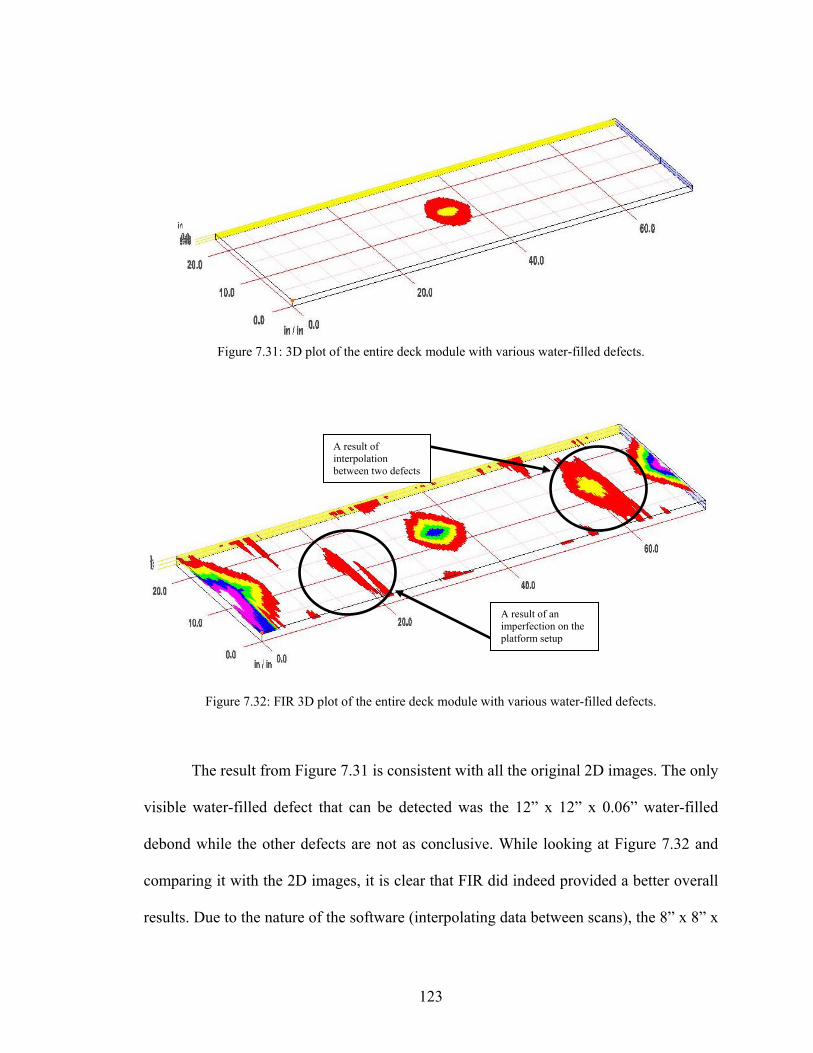
Figure 7.31: 3D plot of the entire deck module with various water-filled defects.

A result of an imperfection on the platform setup

A result of interpolation between two defects

Figure 7.32: FIR 3D plot of the entire dec dule with various water-filled defects.

The result from Figure 7.31 is consistent ages. The only

visible water-filled defect th

debond while the other defects are not as conclusive. While looking at Figure 7.32 and

results. Due to the nature of the software (interpolating data between scans), the 8” x 8” x

k mo

with all the original 2D im

at can be detected was the 12” x 12” x 0.06” water-filled

comparing it with the 2D images, it is clear that FIR did indeed provided a better overall

123

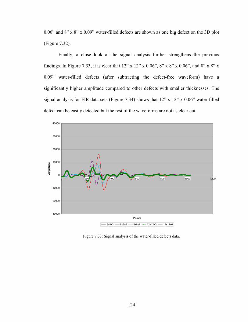
0.06” and 8” x 8” x 0.09” water-filled defects are shown as one big defect on the 3D plot

(Figure 7.32).

Finally, a close look at the signal analysis further strengthens the previous

findings. In Figure 7.33, it is clear that 12” x 12” x 0.06”, 8” x 8” x 0.06”, and 8” x 8” x

0.09” water-filled defects (after subtracting the defect-free waveform) have a

significantly higher amplitude compared to other defects with smaller thicknesses. The

signal analysis for FIR data sets (Figure 7.34) shows that 12” x 12” x 0.06” water-filled

defect can be easily detected but the rest of the waveforms are not as clear cut.

-30000

-20000

-10000

0

10000

20000

30000

40000

0 200 400 600 800 1000 1200

Points

Am

plitu

de

8x8x3 8x8x6 8x8x9 12x12x3 12x12x6

Figure 7.33: Signal analysis of the water-filled defects data.

124

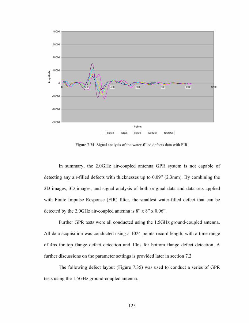
-30000

30000

40000

-20000

-10000

0

00

10000

2000

200 400 600 800 1000 1200

Am

plitu

d

Points

e

8x8x3 8x8x6 8x8x9 12x12x3 12x12x6

Figure 7.34: Signal analysis of the water-filled defects data with FIR.

In summary, the 2.0GHz air-coupled antenna GPR system is not capable of

detecting any air-filled defects with thicknesses up to 0.09” (2.3mm). By combining the

2D images, 3D images, and signal analysis of both original data and data sets applied

with Finite Impulse Response (FIR) filter, the smallest water-filled defect that can be

detected by the 2.0GHz air-coupled antenna is 8” x 8” x 0.06”.

Further GPR tests were all conducted using the 1.5GHz ground-coupled antenna.

All data acquisition was conducted using a 1024 e range

of 4ns for top flange defect detection and 10ns for bottom flange defect detection. A

further discussions on the parameter settings is provided later in section 7.2

The following defect layout (Figure 7.35) was used to conduct a series of GPR

tests using the 1.5GHz ground-coupled antenna.

points record length, with a tim

125

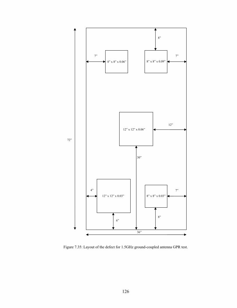
126

st.

12” x 12” x 0.03”

12” x 12” x 0.06”

8” x 8” x 0.03”

8” x 8” x 0.06” 8” x 8” x 0.09”

72”

7” 7”

8”

Figure 7.35: Layout of the defect for 1.5GHz ground-coupled antenna GPR te

36”

6” 8”

4” 7”

12”

30”

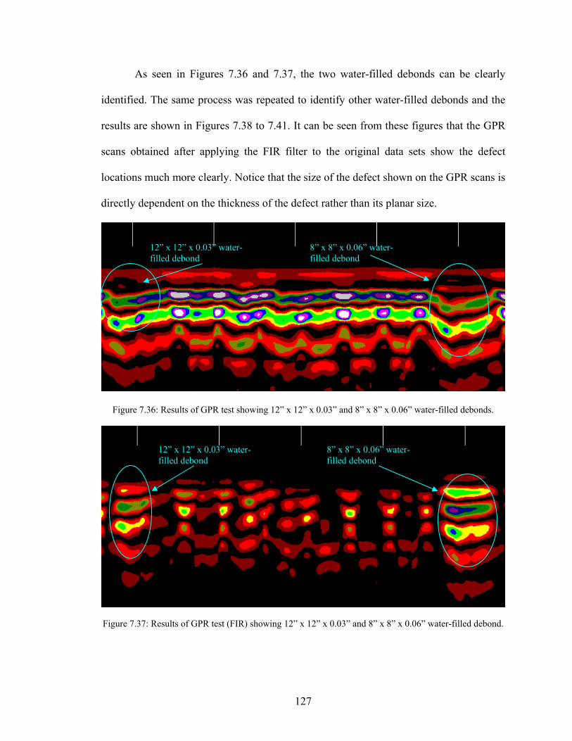
As seen in Figures 7.36 and 7.37, the two water-filled debonds can be clearly

identified. The same process was repeated to identify other water-filled debonds and the

results are shown in Figures 7.38 to 7.41. It can be seen from these figures that the GPR

scans obtained after applying the to the or sets show the defect

locations much more clearly. Notice that the size of the defect shown on the GPR scans is

directly dependent on the thickness of the defect rather than its planar size.

FIR filter iginal data

Figure 7.36: Results of GPR test showing 12” x 12” x 0.03” and 8” x 8” x 0.06” water-filled debonds.

Figure 7.37: Results of GPR test (FIR) showing 12” x 12” x 0.03” and 8” x 8” x 0.06” water-filled debond.

8” x 8” x 0.06” water-filled debond

12” x 12” x 0.03” water-filled debond

12” x 12” x 0.03” water-filled debond

8” x 8” x 0.06” water-filled debond

127

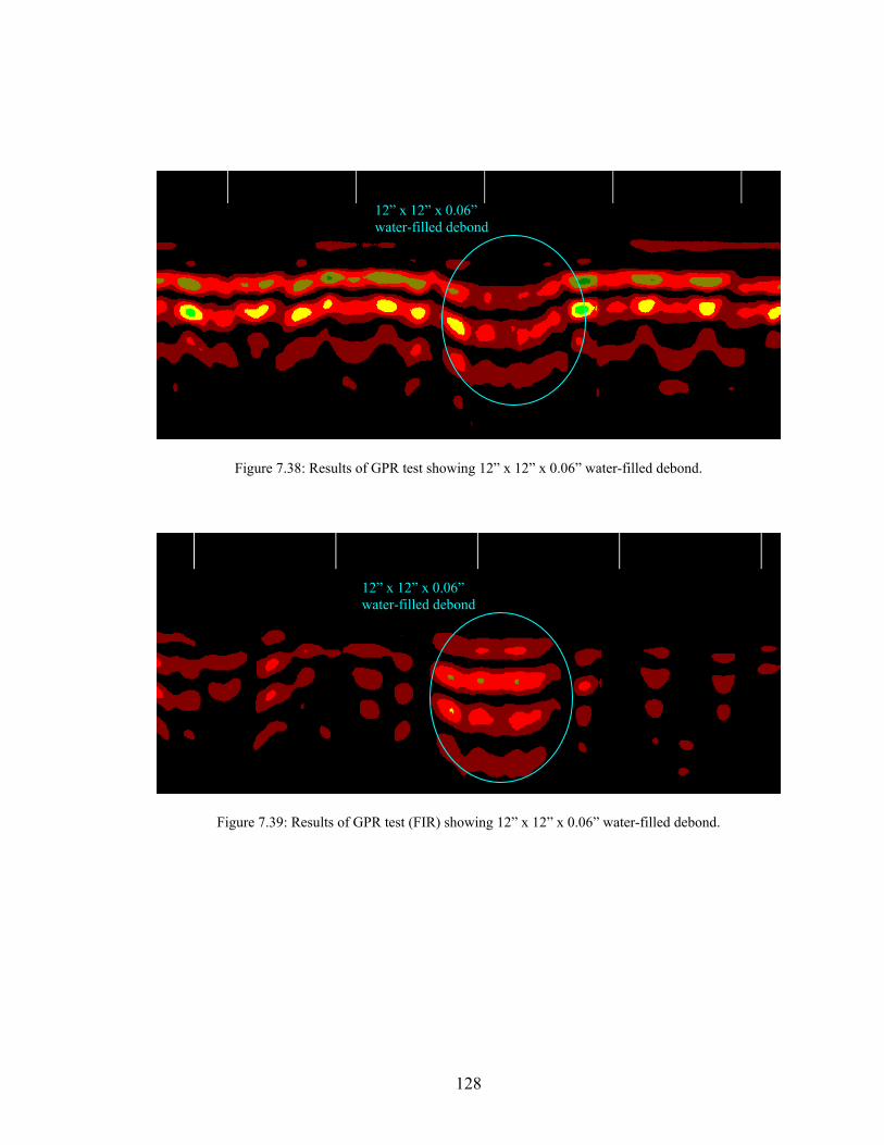
12” x 12” x 0.06” water-filled debond

Figure 7.38: Results of GPR test showing 12” x 12” x 0.06” water-filled debond.

12” x 12” x 0.06” water-filled debond

Figure 7.39: Results of GPR test (FIR) showing 12” x 12” x 0.06” water-filled debond.

128

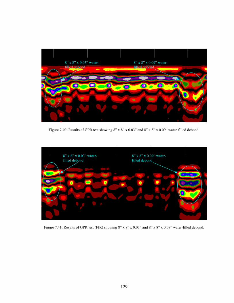
Figure 7.40: Results of GPR test showing 8” x 8” x 0.03” and 8” x 8” x 0.09” water-filled debond.

Figure 7.41: Results of GPR test (FIR) showing 8” x 8” x 0.03” and 8” x 8” x 0.09” water-filled debond.

8” x 8” x 0.03” watfilled debond

8” x 8” x 0.09” water-filled debond

er-

8” x 8” x 0.03” watfilled debond

water-er- 8” x 8” x 0.09”filled debond

129

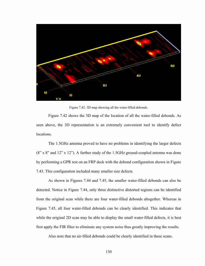
Figure 7.42: 3D map showing all the water-filled debonds.

As

en above, the 3D representation is an extremely convenient tool to identify defect

(8” x 8” and 12” x 12”). A further study of the 1.5GHz ground-coupled antenna was done

by performing a GPR test on an FRP deck with the debond configuration shown in Figure

7.43. This configuration included many smaller size defects.

As shown in Figures 7.44 and 7.45, the smaller water-filled debonds can also be

detected. Notice in Figure 7.44, only three distinctive distorted regions can be identified

f

Figure 7.45, all four water-filled debonds can be clearly identified. This indicates that

while the original 2D scan may be able to display the small water-filled defects, it is best

first apply the FIR filter to eliminate any system noise thus greatly improving the results.

Also note that no air-filled debonds could be clearly identified in these scans.

Figure 7.42 shows the 3D map of the location of all the water-filled debonds.

se

locations.

The 1.5GHz antenna proved to have no problems in identifying the larger defects

rom the original scan while there are four water-filled debonds altogether. Whereas in

130

5”

7”

7”

5”

18”

4”x4”x0.06” water-filled debond

2”x2”x0.06” air-filled debond

4”x4”x0.06” air-filled debond

5”

7”

Figure 7.43: Layout of the defects for 1.5GHz ground-coupled antenna GPR test.

7”

5”

18”

4”x4”x0.09” water-filled debond

4”x4”x0.09” air-filled debond

2”x2”x0.09” air-filled debond

5”

7”

18”

4”x4”x0.03” water-filled debond

2”x2”x0.0water-filled

6” debond

4”x4”x0.03” air-filled debond

7”

5”

131

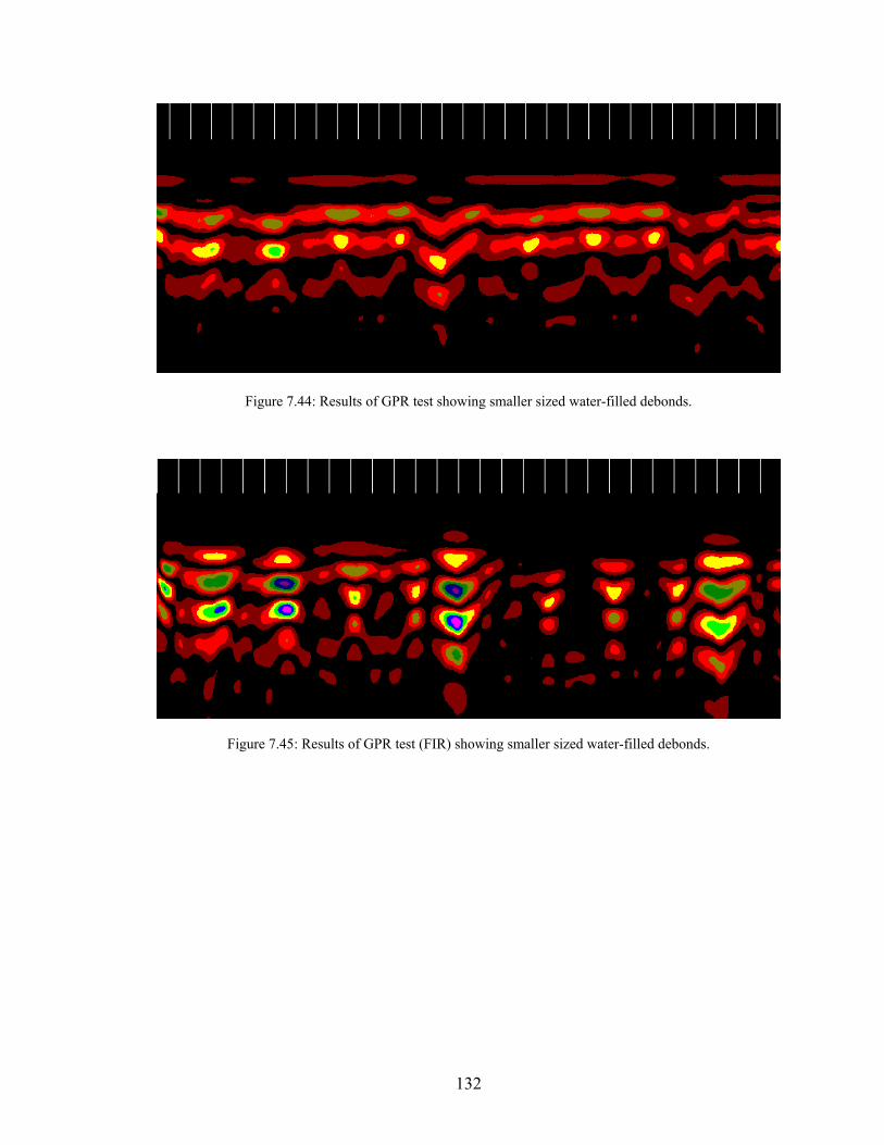
Figure 7.44: Results of GPR test showing smaller sized water-filled debonds.

Figure 7.45: Results of GPR test (FIR) showing sm d debonds. aller sized water-fille

132

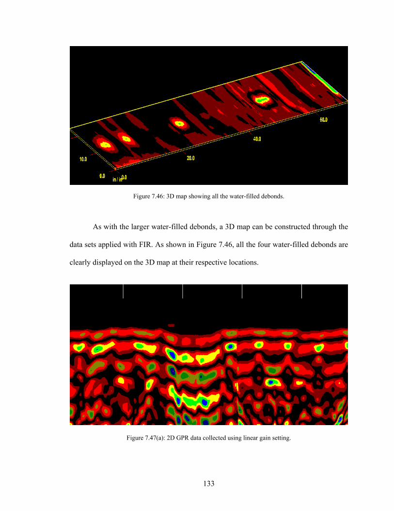
Figure 7.46: 3D map showin e water-filled debonds.

As with the larger water-filled debonds, a 3D map can be constructed through the

data sets applied with FIR. As shown in Figure 7.46, all the four water-filled debonds are

clearly displayed on the 3D map at their respective locations.

g all th

Figure 7.47(a): 2D GPR data collected using linear gain setting.

133

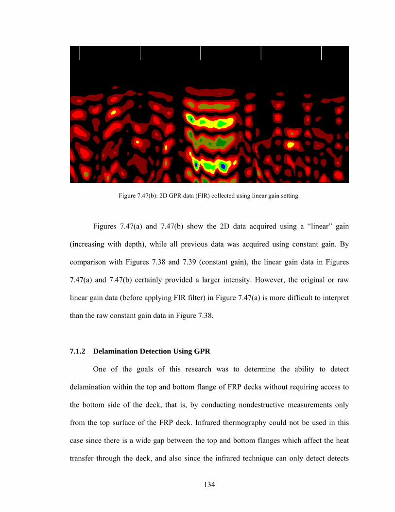
Figur ting.

ear gain data in Figures

7.47(a) and 7.47(b) certainly provided a larger intensity. However, the original or raw

linear gain data (before applying FIR filter) in Figure 7.47(a) is more difficult to interpret

than the raw constant gain data in Figure 7.38.

7.1.2 Delamination Detection Using GPR

One of the goals of this research was to determine the ability to detect

delamination within the top and bottom flange of FRP decks without requiring access to

the bottom side of the deck, that is, by conducting nondestructive measurements only

from the top surface of the FRP deck. Infrared thermography could not be used in this

case since there is ch affect the heat

transfer through the deck, and also since the infrared technique can only detect detects

e 7.47(b): 2D GPR data (FIR) collected using linear gain set

Figures 7.47(a) and 7.47(b) show the 2D data acquired using a “linear” gain

(increasing with depth), while all previous data was acquired using constant gain. By

comparison with Figures 7.38 and 7.39 (constant gain), the lin

a wide gap between the top and bottom flanges whi

134

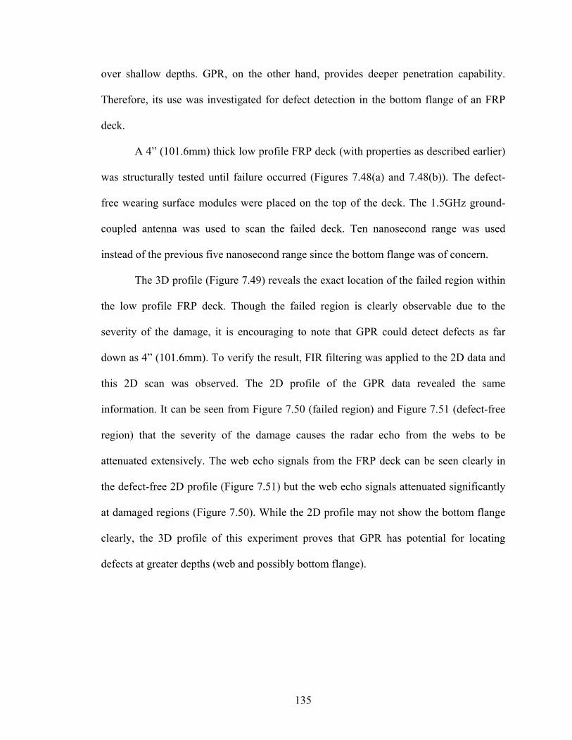
over shallow depths. GPR, on the other hand, provides deeper penetration capability.

Therefore, its use was investigated for defect detection in the bottom flange of an FRP

deck.

A 4” (101.6mm) thick low profile FRP deck (with properties as described earlier)

was structurally tested until failure occurred (Figures 7.48(a) and 7.48(b)). The defect-

free wearing surface modules were placed on the top of the deck. The 1.5GHz ground-

coupled antenna was used to scan the failed deck. Ten nanosecond range was used

instead of the previous five nanosecond range since the bottom flange was of concern.

The 3D region within

e low profile FRP deck. Though the failed region is clearly observable due to the

rom the FRP deck can be seen clearly in

e defect-free 2D profile (Figure 7.51) but the web echo signals attenuated significantly

a flange

profile (Figure 7.49) reveals the exact location of the failed

th

severity of the damage, it is encouraging to note that GPR could detect defects as far

down as 4” (101.6mm). To verify the result, FIR filtering was applied to the 2D data and

this 2D scan was observed. The 2D profile of the GPR data revealed the same

information. It can be seen from Figure 7.50 (failed region) and Figure 7.51 (defect-free

region) that the severity of the damage causes the radar echo from the webs to be

attenuated extensively. The web echo signals f

th

at dam ged regions (Figure 7.50). While the 2D profile may not show the bottom

clearly, the 3D profile of this experiment proves that GPR has potential for locating

defects at greater depths (web and possibly bottom flange).

135

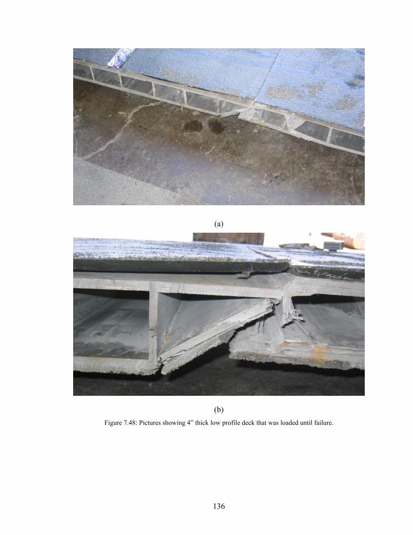
(a)

(b) Figure 7.48: Pictures showing 4” thick low profile deck that was loaded until failure.

136

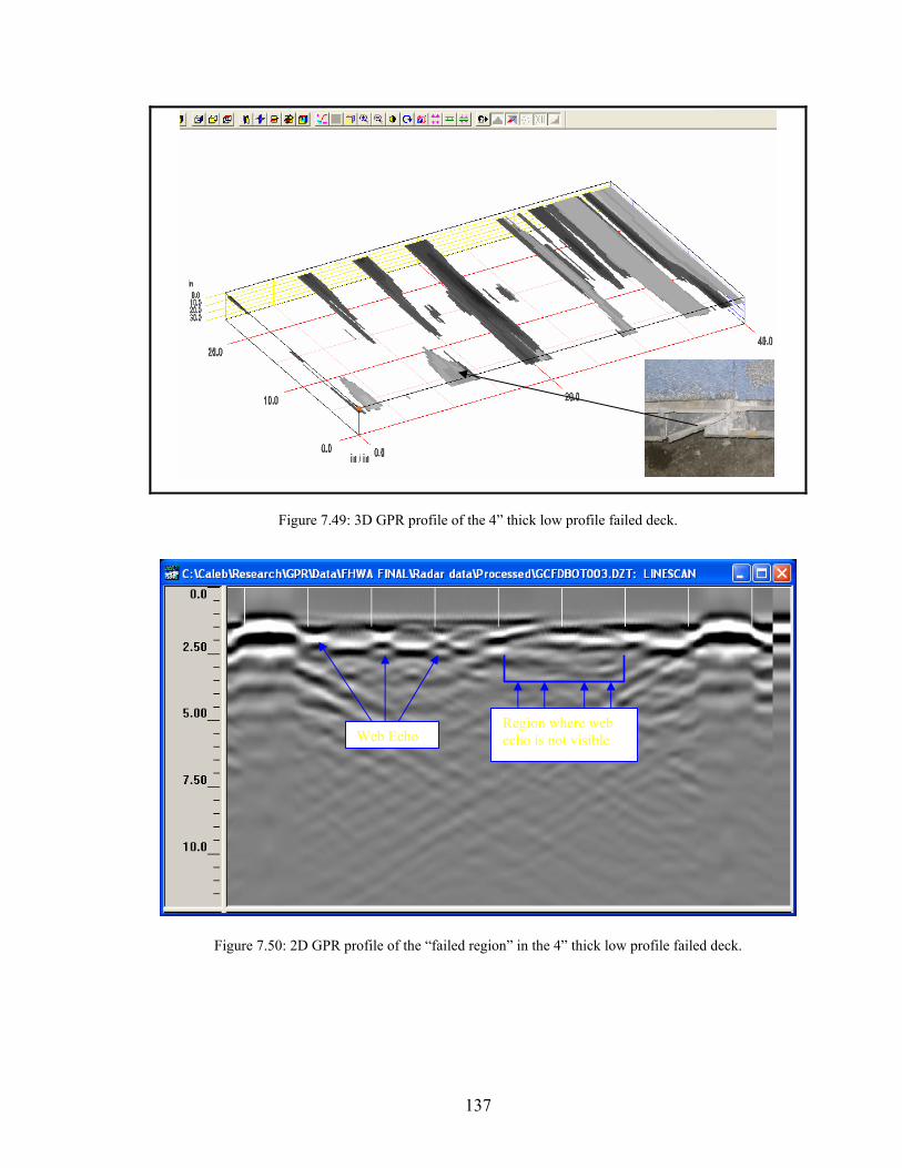
Figure 7.49: 3D GPR profile of the 4” thick low profile failed deck.

Figure 7.

50: 2D GPR profile of the “failed region” in the 4” thick low profile failed deck.

Web EchoRegion where web echo is not visible

137

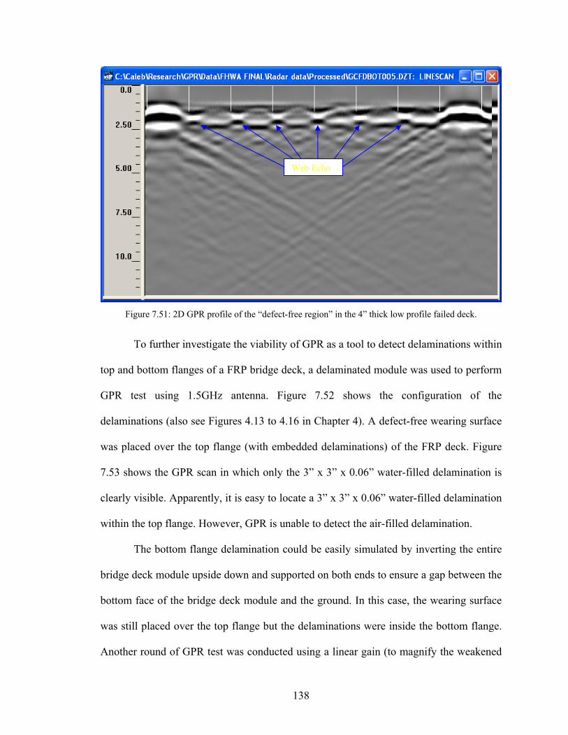
Figure 7.51: 2D GPR profile of the “defect-free ion” in the 4” thick low profile failed deck.

To further investigate the viability of GPR as a tool to detect delaminations within

top and bottom flanges of a FRP bridge deck, a delaminated module was used to perform

GPR test using 1.5GHz antenna. Figure 7.52 shows the configuration of the

delami . A defect-free wearing surface

was placed over the top ns) of the FRP deck. Figure

illed delamination is

clearly visible. Apparently, it is easy to locate a 3” x 3” x 0.06” water-filled delamination

within the top flange. However, GPR is unable to detect the air-filled delamination.

The bottom flange delamination could be easily simulated by inverting the entire

bridge deck module upside down and supported on both ends to ensure a gap between the

urface

was still placed over the top flange but the delaminations were inside the bottom flange.

Another round of GPR test was conducted using a linear gain (to magnify the weakened

Web Echo

reg

nations (also see Figures 4.13 to 4.16 in Chapter 4)

flange (with embedded delaminatio

7.53 shows the GPR scan in which only the 3” x 3” x 0.06” water-f

bottom face of the bridge deck module and the ground. In this case, the wearing s

138

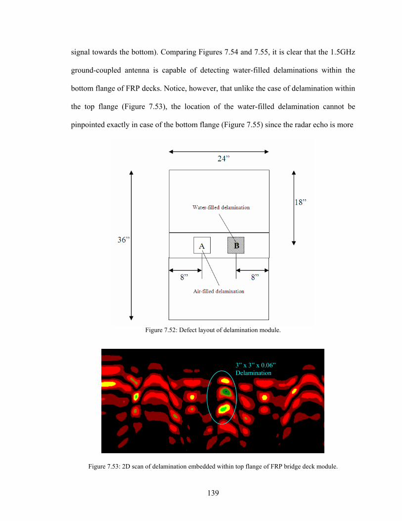
signal towards the bottom). Comparing Figures 7.54 and 7.55, it is clear that the 1.5GHz

ground-coupled antenna is capable of detecting water-filled delaminations within the

bottom flange of FRP decks. Notice, however, that unlike the case of delamination within

the top flange (Figure 7.53), the location of the water-filled delamination cannot be

pinpointed exactly in case of the bottom flange e radar echo is more (Figure 7.55) since th

Figure 7.52: Defect layout of delamination module.

3” x 3” x 0.06” Delamination

Figure 7.53: 2D scan of delamination embedded within top flange of FRP bridge deck module.

139

Figure 7.54: 2D scan of defect free FRP bridge deck module.

Figure 7.55: 2D scan of delamination embedded within bottom flange of FRP bridge deck module.

3” x 3” x 0.06” water-filled delamination

140

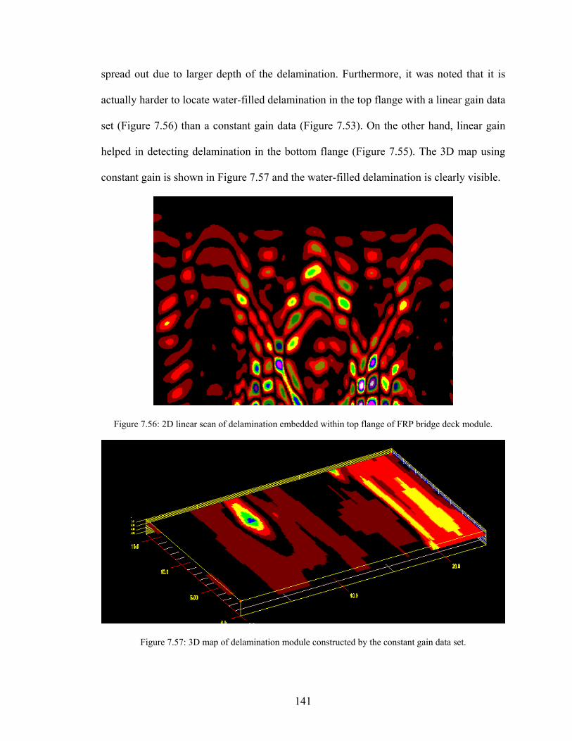
spread out due to larger depth of the delamination. Furthermore, it was noted that it is

actually harder to locate water-filled delamination in the top flange with a linear gain data

set (Figure 7.56) than a constant gain data (Figure 7.53). On the other hand, linear gain

helped in detecting delamination in the bottom flange (Figure 7.55). The 3D map using

constant gain is shown in Figure 7.57 and the water-filled delamination is clearly visible.

Figure 7.56: 2D linear scan of delamination embedded within top flange of FRP bridge deck module.

Figure 7.57: 3D map of delamination module constructed by the constant gain data set.

141

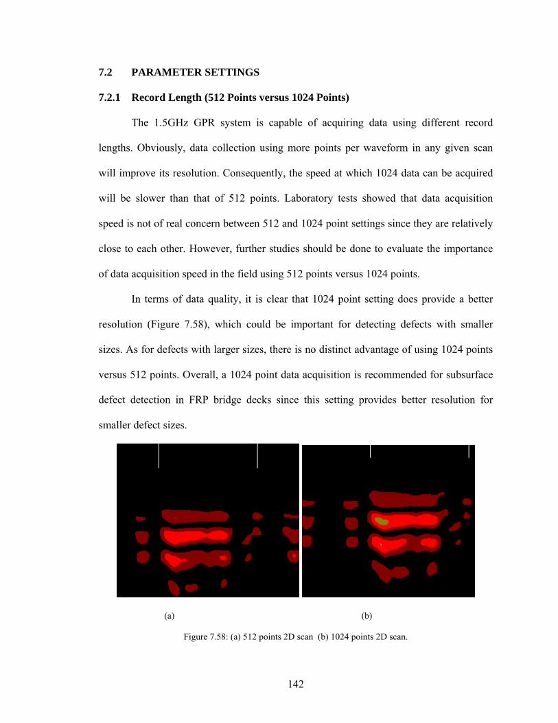
7.2 PARAMETER SETTINGS

7.2.1 Record Length (512 Points versus 1024 Points)

The 1.5GHz GPR system is capable of acquiring data using different record

lengths. Obviously, data collection using more points per waveform in any given scan

will improve its resolution. Consequently, the speed at which 1024 data can be acquired

will be slower than that of 512 points. Laboratory tests showed that data acquisition

speed is not of real concern between 512 and 1024 point settings since they are relatively

close to each other. However, further studies should be done to evaluate the importance

of data acquisition speed in the field using 512 points versus 1024 points.

In terms of data quality, it is clear that 1024 point setting does provide a better

resolution (Figure 7.58), which could be important for detecting defects with smaller

sizes. As for defects with larger sizes, there is no distinct advantage of using 1024 points

versus 512 points. Overall, a 1024 point data acquisition is recommended for subsurface

defect detection in FRP bridge decks since this setting provides better resolution for

smaller defect sizes.

(a) (b)

Figure 7.58: (a) 512 points 2D scan (b) 1024 points 2D scan.

142

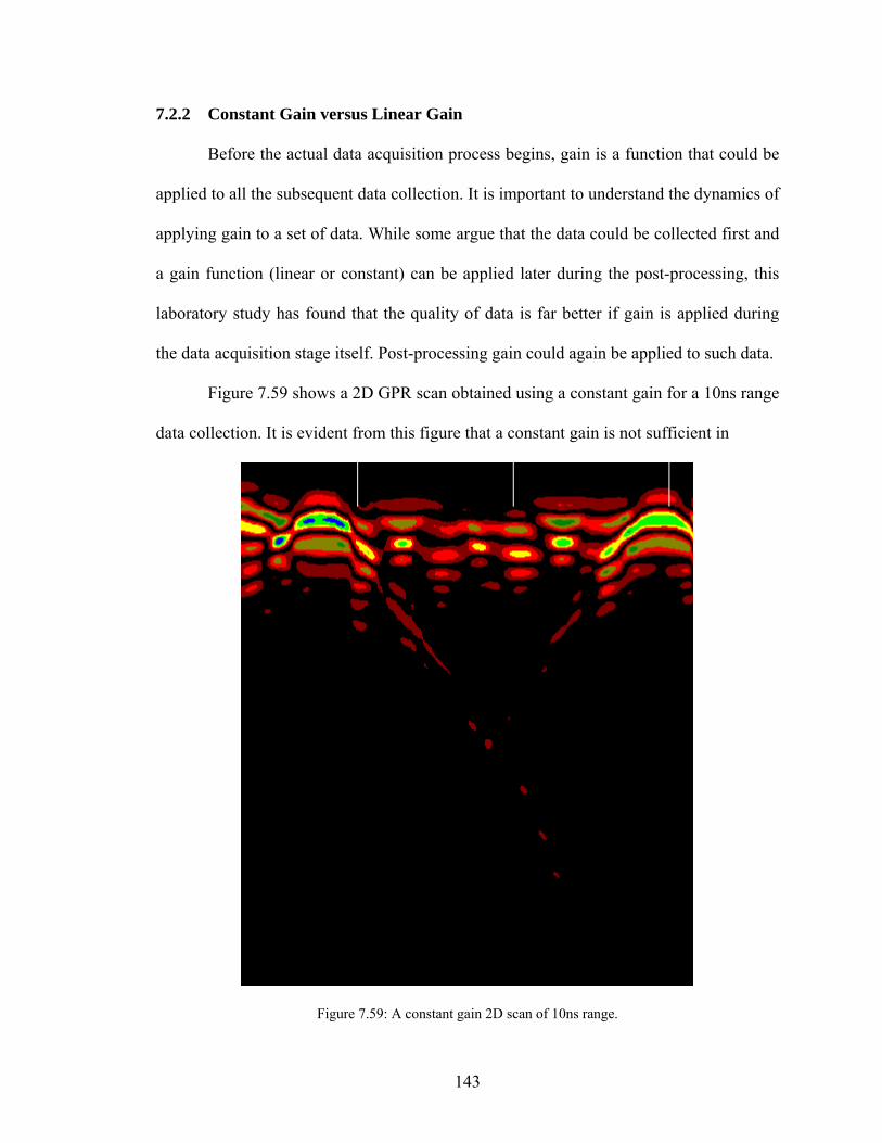
7.2.2 Constant Gain versus Linear Gain

gain is a function that could be

applied

cient in

Before the actual data acquisition process begins,

to all the subsequent data collection. It is important to understand the dynamics of

applying gain to a set of data. While some argue that the data could be collected first and

a gain function (linear or constant) can be applied later during the post-processing, this

laboratory study has found that the quality of data is far better if gain is applied during

the data acquisition stage itself. Post-processing gain could again be applied to such data.

Figure 7.59 shows a 2D GPR scan obtained using a constant gain for a 10ns range

data collection. It is evident from this figure that a constant gain is not suffi

Figure 7.59: A constant gain 2D scan of 10ns range.

143

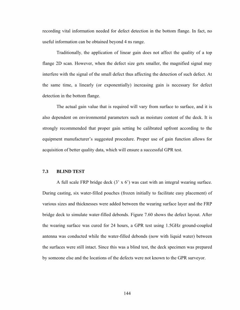
record ng vital information needed for defeci t detection in the bottom flange. In fact, no

useful i

. It is

strongly recommended that proper gain setting be calibrated upfront according to the

equipment manufacturer’s suggested procedure. Proper use of gain function allows for

acquisition of better quality data, which will ensure a successful GPR test.

7.3 BLIND TEST

A full scale FRP bridge deck (3’ x 6’) was cast with an integral wearing surface.

During casting, six water-filled pouches (frozen initially to facilitate easy placement) of

various sizes and thicknesses were added between the wearing surface layer and the FRP

bridge deck to simulate water-filled debonds. Figure 7.60 shows the defect layout. After

the wearing surface was cured for 24 hours, a GPR test using 1.5GHz ground-coupled

antenna was conducted while the water-filled debonds (now with liquid water) between

the surfaces were still intact. Since this was a blind test, the deck specimen was prepared

by someone else and the locations of the defects were not known to the GPR surveyor.

nformation can be obtained beyond 4 ns range.

Traditionally, the application of linear gain does not affect the quality of a top

flange 2D scan. However, when the defect size gets smaller, the magnified signal may

interfere with the signal of the small defect thus affecting the detection of such defect. At

the same time, a linearly (or exponentially) increasing gain is necessary for defect

detection in the bottom flange.

The actual gain value that is required will vary from surface to surface, and it is

also dependent on environmental parameters such as moisture content of the deck

144

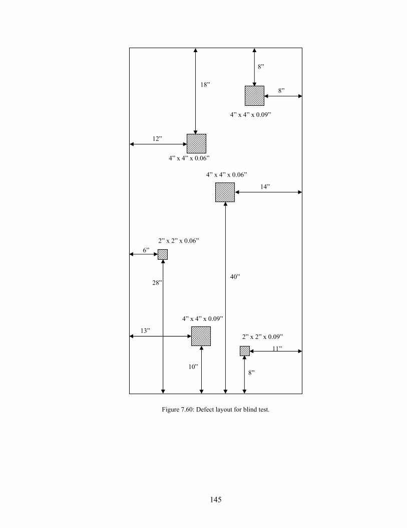
Figure 7.60: Defect layout for blind test.

6”

14”

2” x 2” x 0.06”

28”

8”

40”

8”

2” x 2” x 0.09”

4” x 4” x 0.09”

4” x 4” x 0.06”

x 4” x 0.06”

12”

18” 8”

4”

4” x 4” x 0.09”

13”

10”

11”

145

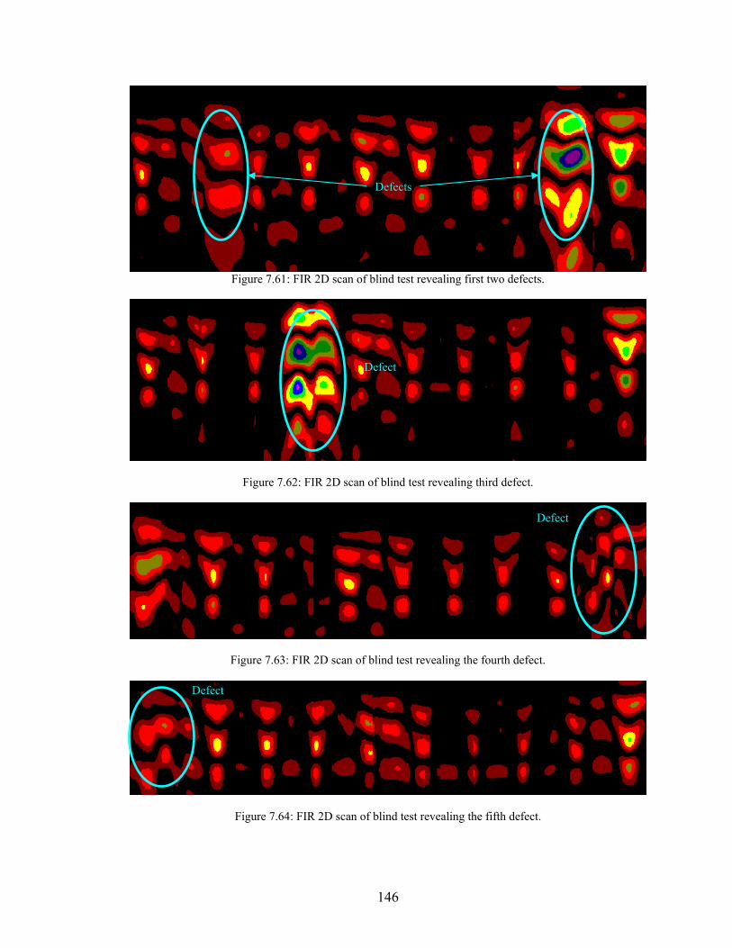
Figure 7.61: FIR 2D scan of blind test revealing first two defects.

Figure 7.62: FIR 2D scan of blind test revealing third defect.

Figure 7.63: FIR 2D s blind test reveali he fourth defect. can of ng t

Figure 7.64: FIR 2D scan of blind test revealing the fifth defect.

Defects

Defect

Defect

Defect

146

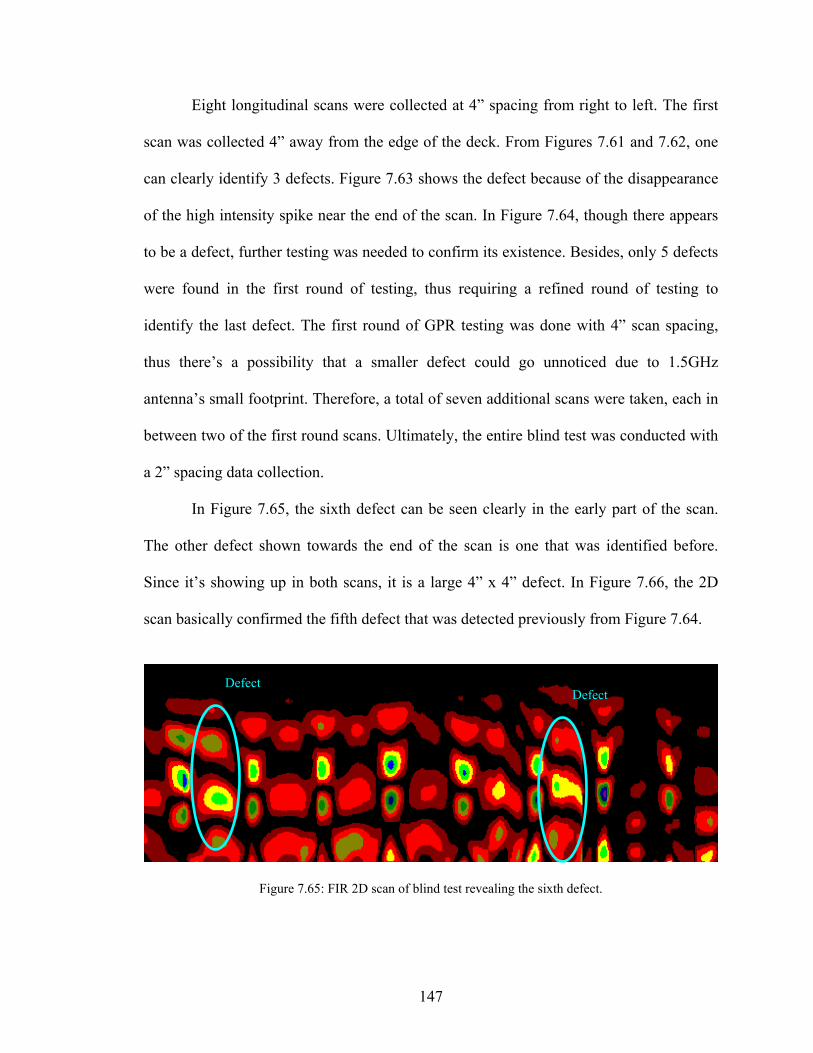
Eight longitudinal scans were collected at 4” spacing from right to left. The first

scan was collected 4” away from the edge of the deck. From Figures 7.61 and 7.62, one

can clearly identify 3 defects. Figure 7.63 shows the defect because of the disappearance

of the high intensity spike near the end of the scan. In Figure 7.64, though there appears

to be a defect, further testing was needed to confirm its existence. Besides, only 5 defects

were found in the first round of testing, thus requiring a refined round of testing to

identify the last defect. The first round of GPR testing was done with 4” scan spacing,

thus there’s a possibility that a sm defect could go unnoticed due to 1.5GHz

antenna’s sm

between two of the first round scans. Ultimately, the entire blind test was conducted with

a 2” spacing data collection.

In Figure 7.65, the sixth defect can be seen clearly in the early part of the scan.

The other defect s identified before.

Since it’s showing up in both scans, it is a large 4” x 4” defect. In Figure 7.66, the 2D

scan basically confirmed the fifth defect that was detected previous

aller

all footprint. Therefore, a total of seven additional scans were taken, each in

hown towards the end of the scan is one that was

ly from Figure 7.64.

Figure 7.65: FIR 2D scan of blind test revealing the sixth defect.

Defect Defect

147

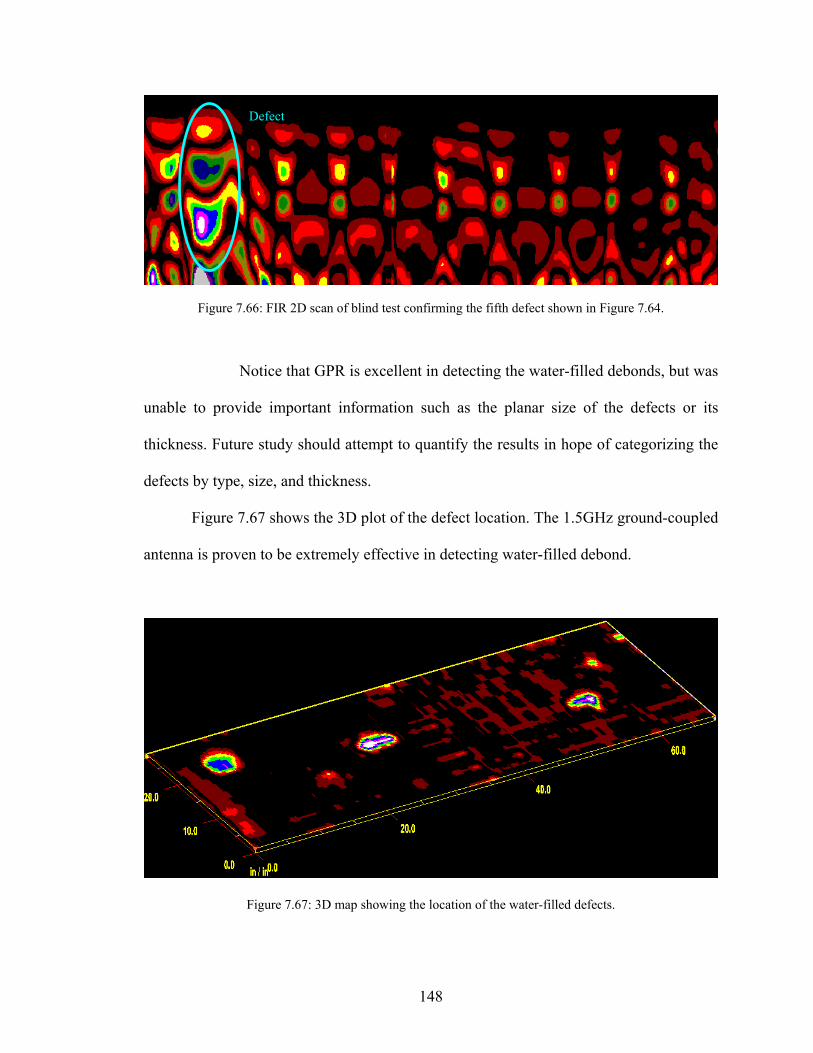
Notice that GPR is excellent in detecting the water-filled debonds, but was

unable to provide important information such as the planar size of the defects or its

thickness. Future study should attempt to quantify the results in hope of categorizing the

defects by type, size, and thic

Figure 7.66: FIR 2D scan of blind test confirming the fifth defect shown in Figure 7.64.

kness.

Figure 7.67 shows the 3D plot of the defect location. The 1.5GHz ground-coupled

antenna is proven to be extremely effective in detecting water-filled debond.

Figure 7.67: 3D map showing the location of the water-filled defects.

Defect

148

149

Based on the post processing results, it is concluded that 2.0GHz horn antenna

is not capable of detecting air-filled defects regardless of size and thickness.

e general consensus regarding the low effectiveness of any GPR

system efects. By combining the 2D images, 3D images, and signal

analysis of both original data and data sets applied with Finite Impulse Response (FIR)

the sma d horn

antenna was found to be 8” x 8” x 0.06”.

. Although it has a 1” footprint size on each side of

the center line, the signal decreases drastically. Hence, in order to detect a very small

defect, such as a 1” x 1” debond, the antenna has to go directly over the defect. Not only

ply not

ractical considering the large size of the area usually surveyed using GPR system.

In order to conduct a successful GPR test, a time range of 4ns is recommended for

defect detection in the top flange while 10ns range should be used for the bottom flange.

Furthermore, in conjunction with 10ns range, a linearly increasing gain is needed to

magnify the echo signals from the bottom flange and produce meaningful results.

Laboratory test did not find any advantage in using 512 point record length over 1024

points in terms of acquisition speed. However, the 1024 point record length provided

somewhat better resolution. Thus it is recommended that any GPR tests on FRP bridge

decks be conducted using 1024 points record length.

The blind test conducted in this study proves that 1.5GHz can easily detect water-

filled debonds as small as 2” x 2” x 0.06”.

7.4 CONCLUSIONS

GPR system

This is consistent with th

for air-filled d

,

llest water-filled defect that could be detected by the 2.0GHz air-couple

On the other hand, the 1.5GHz ground-coupled antenna proved to be an excellent

tool in detecting subsurface water-filled defects (both debonds and delaminations). The

smallest water-filled debond that could be detected was 2” x 2” x 0.06” given the

footprint size of the 1.5GHz antenna

is the probability of achieving such feat a monumental task in the field, it is sim

p

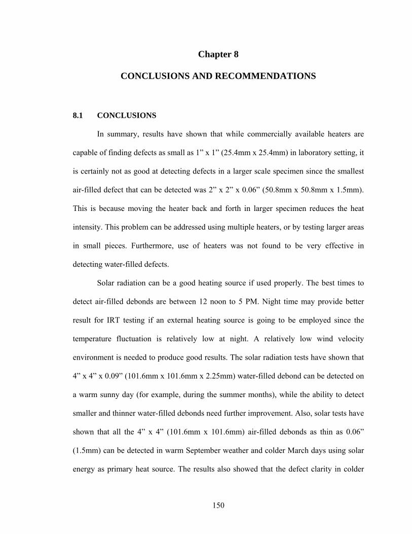
Chapter 8

In summary, results have shown that while commercially available heaters are

ts in a larger scale specimen since the smallest

air-fille

detecting water-filled defects.

better

result f

4” x 4” x 0.09” (101.6mm x 101.6mm x 2.25mm) water-filled debond can be detected on

(1.5mm

also showed that the defect clarity in colder

CONCLUSIONS AND RECOMMENDATIONS

8.1 CONCLUSIONS

capable of finding defects as small as 1” x 1” (25.4mm x 25.4mm) in laboratory setting, it

is certainly not as good at detecting defec

d defect that can be detected was 2” x 2” x 0.06” (50.8mm x 50.8mm x 1.5mm).

This is because moving the heater back and forth in larger specimen reduces the heat

intensity. This problem can be addressed using multiple heaters, or by testing larger areas

in small pieces. Furthermore, use of heaters was not found to be very effective in

Solar radiation can be a good heating source if used properly. The best times to

detect air-filled debonds are between 12 noon to 5 PM. Night time may provide

or IRT testing if an external heating source is going to be employed since the

temperature fluctuation is relatively low at night. A relatively low wind velocity

environment is needed to produce good results. The solar radiation tests have shown that

a warm sunny day (for example, during the summer months), while the ability to detect

smaller and thinner water-filled debonds need further improvement. Also, solar tests have

shown that all the 4” x 4” (101.6mm x 101.6mm) air-filled debonds as thin as 0.06”

) can be detected in warm September weather and colder March days using solar

energy as primary heat source. The results

150

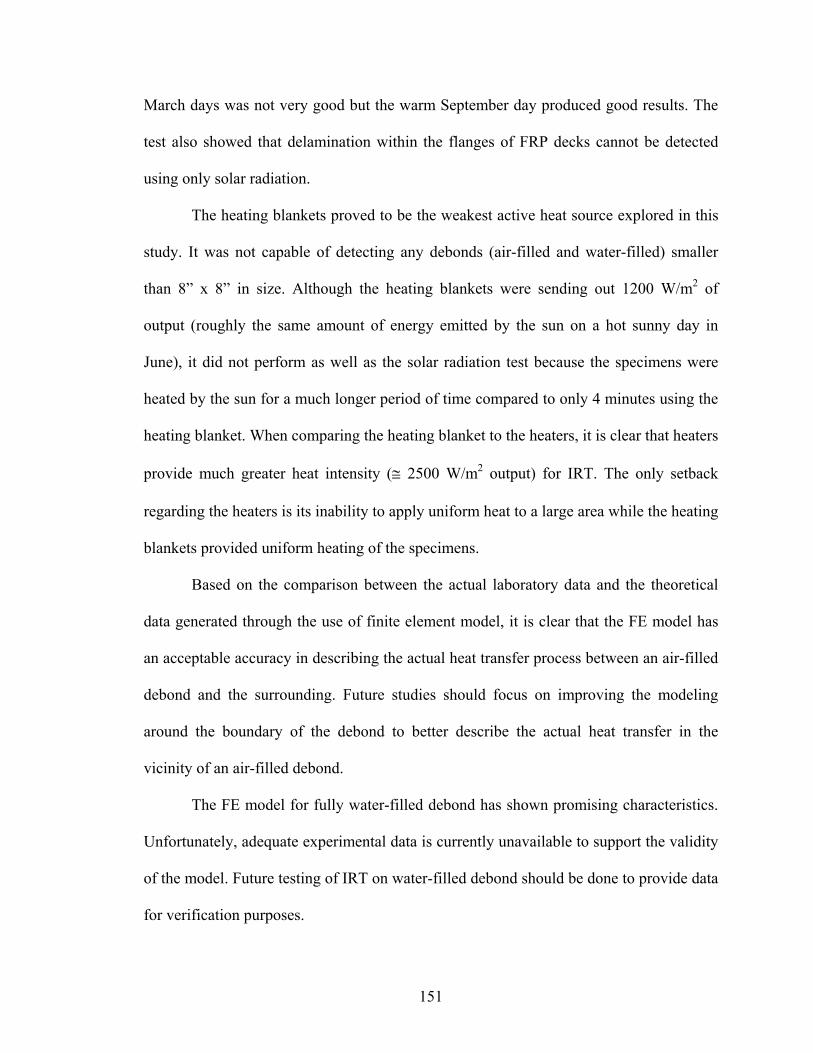
March days was not very good but th ber day produced good results. The

test also show t be detected

ved to be the weakest active heat source explored in this

study. It was not capable of

2

2

ility to apply uniform heat to a large area while the heating

blanke

e warm Septem

ed that delamination within the flanges of FRP decks canno

using only solar radiation.

The heating blankets pro

detecting any debonds (air-filled and water-filled) smaller

than 8” x 8” in size. Although the heating blankets were sending out 1200 W/m of

output (roughly the same amount of energy emitted by the sun on a hot sunny day in

June), it did not perform as well as the solar radiation test because the specimens were

heated by the sun for a much longer period of time compared to only 4 minutes using the

heating blanket. When comparing the heating blanket to the heaters, it is clear that heaters

provide much greater heat intensity (≅ 2500 W/m output) for IRT. The only setback

regarding the heaters is its inab

ts provided uniform heating of the specimens.

Based on the comparison between the actual laboratory data and the theoretical

data generated through the use of finite element model, it is clear that the FE model has

an acceptable accuracy in describing the actual heat transfer process between an air-filled

debond and the surrounding. Future studies should focus on improving the modeling

around the boundary of the debond to better describe the actual heat transfer in the

vicinity of an air-filled debond.

The FE model for fully water-filled debond has shown promising characteristics.

Unfortunately, adequate experimental data is currently unavailable to support the validity

of the model. Future testing of IRT on water-filled debond should be done to provide data

for verification purposes.

151

Since the results have shown that the FE predictions for partially water-filled

debond case are questionable, future effort should focus on successfully modeling such

cases since it may be more representative of the field conditions.

” x 0.06”. While results certainly

indicate

ld, it is simply not practical considering the large size of

Based on the post processing results, it is concluded that 2.0GHz horn antenna

GPR system is not capable of detecting air-filled defects regardless of size and thickness.

This is consistent with the general consensus regarding the lack of effectiveness of any

GPR system in detecting air-filled defects. By combining the 2D images, 3D images, and

signal analysis from both original data and data sets applied with Finite Impulse

Response (FIR), the smallest water-filled defect that can be detected by the 2.0GHz air-

launched horn antenna is 8” x 8” x 0.06”.

On the other hand, the 1.5GHz ground-coupled antenna proved to be an excellent

tool in detecting subsurface water-filled defects (debond and delamination). The smallest

water-filled debond that can be detected is 2” x 2

d the ability to detect even smaller defects using 1.5GHz ground-coupled

antenna, the problem remains due to footprint size of the 1.5GHz antenna. Although it

has a 1” footprint to each side from the center line, the signal decreases drastically away

from the center line. Hence, in order to detect a small defect, such as 1” x 1” debond, the

antenna has to go directly over the defect. Not only is the probability of achieving such

feat a monumental task in the fie

the areas usually surveyed by the GPR system.

In summary, the 1.5GHz ground-coupled antenna has out-performed the 2.0GHz

air-coupled horn antenna in subsurface defect detection for FRP bridge decks.

152

In order to conduct a successful GPR test, a time range of 4ns is recommended for

defect detection in the top flange while 10ns should be used for the bottom flange.

Furthermore, in conjunction with 10ns range, a linear gain is needed to magnify the

signals

ial to combine IRT’s ability to detect air-filled

debond

thickness. Such quantitative models will

also be

analysis of

IRT data should be explored to improve IRT’s performance in defect detection.

from the bottom flange of the FRP deck to produce meaningful results.

Laboratory test did not find any major advantage in terms of data acquisition speed in

using 512 points record length over 1024 points. However, the results clearly show that

1024 point data provided somewhat better resolution. Thus it is recommended that GPR

tests on FRP decks be conducted using 1024 points record length. The blind test results

proved that 1.5GHz antenna can detect water-filled debonds as small as 2” x 2” x 0.06”.

Finally, it has proved to be benefic

s if a proper active heat source is employed and GPR’s ability to detect water-

filled defects. GPR can even detect delaminations in the bottom flange of an FRP bridge

deck for a thorough nondestructive evaluation. By complementing each technique’s

short-coming, the combination of IRT and GPR will greatly improve the quality of

nondestructive evaluation and associated maintenance plan for FRP bridge decks, which

is necessary to ensure their long-term in-service performance.

8.2 RECOMMENDATIONS FOR FUTURE RESEARCH

It is recommended that future research be focused on quantitative analysis of GPR data

for extracting vital information such as defect

needed for automating the signal analysis procedure. As for IRT, a more powerful

yet efficient heat source should be explored for field use. Also, quantitative

153

REFERENCES

Barnes, C. L., and Trottier, J. F. (1999). “Use of Ground Penetrating Radar for Estimating

Deterioration Repair Quantities on Reinforced Concrete Bridge Decks.” Department of

Wide Web publication.

http://www.dal.ca/~barnesc/Quebec.html

with Fiber-Reinforced Polymer Composites using Infrared Thermography.” Proceedings

of the InfraMation 2003, Las Vegas, NV, October 13-16.

Civil Engineering, Dalhousie University, Daltech Halifax, Nova Scotia, Canada. World

Brown, J. R. and Hamilton III, H. R. (2003). “NDE Reinforced Concrete Strengthened

Carter, C. R., Chung, T., Reel, R., Tharmabala, T., and Wood, D. (1995). “Impulse Radar

Cook, J. C. (1960). “Proposed Monocycle-Pulse, VHF Radar for Airborne Ice and Snow

TM , Revision A, 14 June.

LIR SYSTEMS (2002b). ThermaCAMTM Researcher Operating Manual, Version A.

and the Influence of Positioning Errors on Image Quality.” Extended abstract EAGE, 63

Dedicated to GPR.” Proceedings of the Eight International Conference on Ground

Evaluation of Reinforced Concrete Bridge Decks.” Society of Photo-Optical

Instrumentation Engineers (SPIE), Vol. 2456, pp. 174-184.

Measurements.” AIEE Trans. Commun. And Electron., 79(2), 588-594.

FLIR SYSTEMS (2002a). ThermaCAM S60 Operator’s Manual

F

Groenenboom, J., van der Kruk, J. and Zeeman, J. H. (2001). “3D GPR Data Acquisition rd

Conference and Technical Exhibition, Amsterdam, Netherland. June, 2001.

Groenenboom, J. and Yaravoy, A. G. (2000) “Data Processing for A Landmine Detection

Penetrating Radar, May, 2000.

154

Halabe, U. B., Vasudevan, A., G linkhachorn, P., and Lonkar, G.

(2004a). "Subsurface Defect Detection in FRP Composites Using Infrared

ography." Proceedings of the Thirty-First Annual Review of Progress in

and GangaRao, H. V. S. (2004b). “Infrared

bonds and Delaminations in FRP Bridge

ging.” ASNT Fall Conference and Quality Testing

ography

dge Decks Subjected to Fatigue Loading.”

P., and Lonkar, G. (2004d). “Task 5.2.1.:

ederal Highway

inistration (FHWA), Washington, D.C., April, 183 pp.

H. V. S. (2003a). “Nondestructive Testing

ng Digital Infrared Therm

ng Show - 2003, Paper Summaries, Pittsburgh, PA, October

canning of FRP Composite Members." Proceedings of the Twenty-Ninth

angaRao, H. V. S., K

Therm

Quantitative Nondestructive Evaluation, Vol. 24 (American Institute of Physics - Vol.

CP760), Colorado School of Mines, Golden, Colorado, July 25 - 30, pp. 1477-1484.

Halabe, U. B., Vasudevan, A., Roy, M.,

Thermography for Detecting Subsurface De

Decks Subjected to Accelerated A

Show - 2004, Paper Summaries, Las Vegas, NV, November 15-19, pp. 129-131.

Halabe, U. B., Vasudevan, A., and GangaRao, H. V. S. (2004c). “Infrared Therm

for Monitoring Subsurface Debonds in FRP Bri

ASNT Fall Conference and Quality Testing Show - 2004, Paper Summaries, Las Vegas,

NV, November 15-19, pp. 132-134.

Halabe, U. B., Vasudevan, A., Klinkhachorn,

Develop an Infrared Thermography Based System to Detect Delaminations.” FHWA

Contract No. DTFH61-01-C-00002, Draft Final Report, submitted to F

Adm

Halabe, U. B., Vasudevan, A., and GangaRao,

of Composite Bridge Components Usi ography.” ASNT Fall

Conference and Quality Testi

13-17, 2003, pp. 120-122.

Halabe, U. B., Bangalore, G., GangaRao, H. V. S., and Klinkhachorn, P. (2002).

"Infrared S

Annual Review of Progress in Quantitative Nondestructive Evaluation, Vol. 22,

Bellingham, Washington, July 14 - 19, pp. 1003-1010.

155

Halabe, U. B., Maser, K. R., and Kausel, E. A. (1995). "Condition Assessment of

Reinforced Concrete Structures Using Electromagnetic Waves." American Concrete

Institute (ACI) Materials Journal, Vol. 92, No. 5, pp. 511-523.

Halabe, U. B. (1990). “Condition Assessment of Reinforced Concrete Structures Using

lectromagnetic Waves.” Ph.D. Dissertation, Department of Civil Engineering,

epartment of Civil and Environmental Engineering, Massachusetts Institute of

T Conference, Atlantic City,

J, February 28 – March 3.

ustralia, p. 367-372.

E

Massachusetts Institute of Technology (MIT), Cambridge, MA.

Halabe, U. B., and Maser, K. R. (1986). “Thermal Modeling of A Leaky Roof.” MIT

CCRE-Technical Note 86-4, Center for Construction Research and Education,

D

Technology, Cambridge, MA.

Hodge Jr., S. (1987). Thermography & Personal Injury Litigation. Wiley Law

Publications, pg. 71.

Jackson, D. R., Islam, M., and Alampalli, S. (2000). “Feasibility of Evaluating the

Performance of Fiber Reinforced Plastic (FRP) Wrapped Reinforced Concrete Columns

Using Ground Penetrating Radar (GPR), and Infrared (IR) Thermography Techniques.”

Proceedings of Structural Materials Technology IV – An ND

N

Johnson, E.C., Nokes, J. P., and Hawkins, G. F. (1999). “NDE of Composite Seismic

Retrofits to Bridges.” Nondestructive Characterization of Materials IX, AIP conference

proceedings 497, Sydney, A

Kaplan, H. (1999). Practical Applications of Infrared Thermal Sensors and Imaging

Equipment, SPIE – The International Society for Optical Engineering, Bellingham,

Washington, USA.

156

Maldague, X. P. V., and Moore, P. O. (2001). “Infrared and Thermal Testing.”

Nondestructive Testing Handbook. American Society for Nondestructive Testing, p. 3.

Maldague, X. (1993). Nondestructive Evaluation of Materials by Infrared Thermography,

aser, K. R., Horschel, M. G., and Grivas, D. A. (2002a). “Integration of Ground

nt.”

incinnati,

aser, K. R., Roberts, R., Kutrubes, D., and Holland, J. (2002b). “Technology for

Materials

T Conference, Cincinnati, OH, September 10-13, pp. 217-226.

d Duke, J. C. (2001). “Health Monitoring of FRP Bridge

ecks.” Advanced Nondestructive Evaluation for Structural and Biological Health

urface Electromagnetic Pulse Radar.”

eophysics, 41(3), 506-518.

red Thermography.” Proceedings of the 2001 Structural Congress

nd Exposition, Washington, D.C., May 21-23.

Springer-Verlag, London.

Malloy, J.F. (1969). Thermal Insulation. Reinhold Book Corporation, New York, NY.

M

Penetrating Radar and Infrared Thermography for Bridge Deck Assessme

Proceedings of Structural Materials Technology V – An NDT Conference, C

OH, September 10-13, pp. 119-128.

M

Quality Assurance of New Pavement Thickness.” Proceedings of Structural

Technology V – An ND

Maser, K. R., and Roddis, W. M. K. (1990). “Principles of Thermography and Radar For

Bridge Deck Assessment.” Journal of Transportation Engineering, 116(5), September-

October.

Miceli, M., Horne, M. R., an

D

Monitoring, Proceedings of SPIE, 4335, March 6-8, 100-105.

Moffatt, D. L., and Puskar, R. J. (1976). “A Subs

G

Mtenga, P.V., Parzych, J.G., and Limerick, R. (2001). “Quality Assurance of FRP

Retrofit Using Infra

a

157

Mutnuri, B. (2005). “Thermal Conductivity Characterization of Composite Mate

Master Thesis, Department of Mechanical Engineering, West Virginia University,

rials.”

organtown, WV.

rties of Concrete. John Wiley & Sons, Inc., New York, NY.

adzevicius, S., and Daniels, J. (2000). “Ground Penetrating Radar Polarization and

ing, E.F.J. (1997). Royal National Hospital for Rheumatic Diseases, Bath, England. th

. M., Rubadeux, B. A., and Ahmed, T. (1999). “Automated Thermographic

efect Recognition and Measurement.” Nondestructive Characterization of Materials IX,

d Penetrating Radar Data

r Assessing Natural Hydrogeologic Conditions.” World Wide Web publication.

ouloukian, Y.S., and DeWitt, D.P. (1970). Thermal Radiative Properties.

M

eville, A.M. (1973). PropeN

R

Scattering From Cylinders.” Journal of Applied Geophysics, 45, 111-125.

Olhoeft, G. R. GEORADAR: Ground Penetrating Radar. World Wide Web.

http://www.g-p-r.com/

Reynolds, W.N., and Wells, G.M. (1984). Video-compatible thermography. British

Journal of NDT, January, p. 40-44.

R

University of Glamorgan - Inaugural Lecture Jan. 28 .

Shepard, S

D

AIP Conference Proceedings 497, Sydney, Australia, p. 373-378.

Smemoe, C.M. (2000). “Processing and Visualization of Groun

fo

http://emrl.byu.edu/chris/gpr.htm#_Toc500291468

T

Thermophysical Properties of Matter, vol. 7, IFI/Plenum, New York, Washington.

158

Tretout, H. (1987). “Applications Industrielle De La Thermographie Infrarouge Au

Controle Non Destructif De Pieces En Materiaux Composites.” Rev. Gen. Therm. F

vol. 301, p. 47- 53.

r.,

omponent GPR Data.” Extended abstract SEG, 71st Conference and Technical

an der Kruk, J., Wapenaar, C., and Fokkema, J. (2001). “Comparison of Resolution

ithms for

ar Data.” Proceedings of 5th SEGJ International Symposium –

aging Technology – The Society of Exploration Geophysicists of Japan (SEGJ), Japan,

avilov (1980). “Infra-Red Non-Destructive Testing of Bonded Structures: Aspects of

anzetti, R. (1972). Practical Applications of Infrared Techniques. John Wiley & Sons,

eralized Radon

ransform.” Geophysics, 65, no. 5, 1553-1559.

Van der Kruk, J. (2001). “Use of Crossed Dipole Antennas in 3D Imaging of Multi-

C

Exhibition, San Antonio, Texas. September, 2001.

V

Functions of 3D Multi-Component with 3D Single-Component Imaging Algor

Ground Penetrating Rad

Im

229-236.

V

Theory and Practice.” British Journal of NDT, July, p. 175-183.

V

Inc., New York, NY.

Wang, T. and Oristaglio, M. (2000). “GPR Imaging using The Gen

T

159

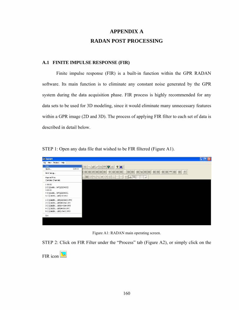
APPENDIX A

RADAN POST PROCESSING

A.1 FINITE IMPULSE RESPONSE (FIR)

Finite impulse response (FIR) is a built-in function within the GPR RADAN

ain function is to eliminate any constant noise generated by the GPR

any

s

in detail below.

software. Its m

system during the data acquisition phase. FIR process is highly recommended for

data sets to be used for 3D modeling, since it would eliminate many unnecessary feature

within a GPR image (2D and 3D). The process of applying FIR filter to each set of data is

described

STEP 1: Open any data file that wished to be FIR filtered (Figure A1).

Figure A1: RADAN main operating screen.

STEP 2: Click on FIR Filter under the “Process” tab (Figure A2), or simply click on the

FIR icon

160

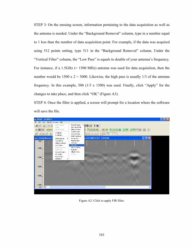
STEP 3: On the ensuing screen, inf to the data acquisition as well as

the antenna is needed. Un , type in a number equal

1 less than the number of data acquisition point. For example, if the data was acquired

ckground Removal” column. Under the

“Vertic

applied, a screen will prompt for a location where the software

ill save the file.

ormation pertaining

der the “Background Removal” column

to

using 512 points setting, type 511 in the “Ba

al Filter” column, the “Low Pass” is equals to double of your antenna’s frequency.

For instance, if a 1.5GHz (= 1500 MHz) antenna was used for data acquisition, then the

number would be 1500 x 2 = 3000. Likewise, the high pass is usually 1/3 of the antenna

frequency. In this example, 500 (1/3 x 1500) was used. Finally, click “Apply” for the

changes to take place, and then click “OK” (Figure A3).

STEP 4: Once the filter is

w

Figure A2: Click to apply FIR filter.

161

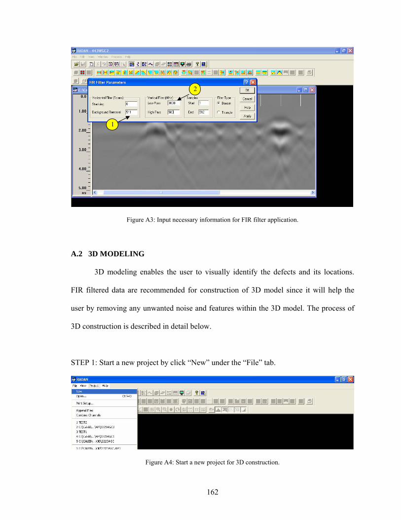
A.2 3D MODELING

3D modeling enables the user to visually identify the defects and its locations.

FIR filtered data are recommended for construction of 3D model since it will help the

user by removing any unwanted noise and features within the 3D model. The process of

3D construction is described in detail below.

STEP 1: Start a new project by click “New” under the “File” tab.

Figure A3: Input necessary information for FIR filter application.

Figure A4: Start a new project for 3D construction.

1

2

162

STEP 2: Provide a name for the 3D project, and check “RADBridge Project”.

Figure A5: Create a new RADAN bridge project.

STEP 3: After providing the file name and the location where the 3D file is going to be

ved, a list of required files need to be added one by one, starting from the file collected

). When the addition is

over, click “Done”.

STEP 4: A dummy macro is needed to proceed. A dummy macro is a macro which

multiplies the entire file set by 1 (essentially, not doing anything to the file set). This

macro can be created once and re-used forever. Select the files attached before and click

“Attach Macro” (Figure A7).

sa

on the far right of the surveyed area and proceed left (Figure A6

163

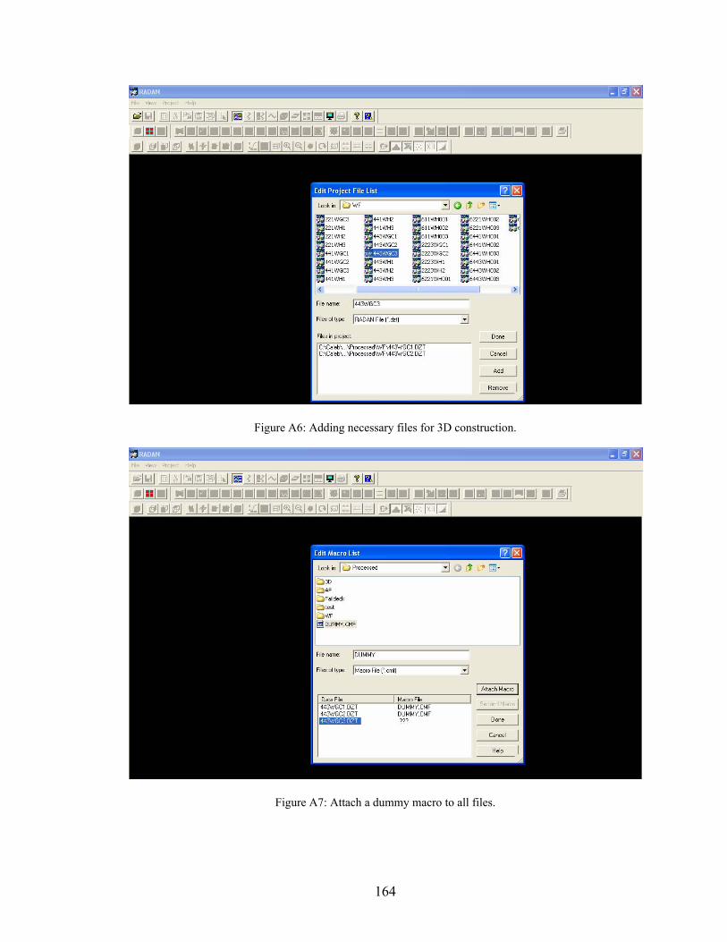
Figure A6: Adding necessary files for 3D construction.

Figure A7: Attach a dummy macro to all files.

164

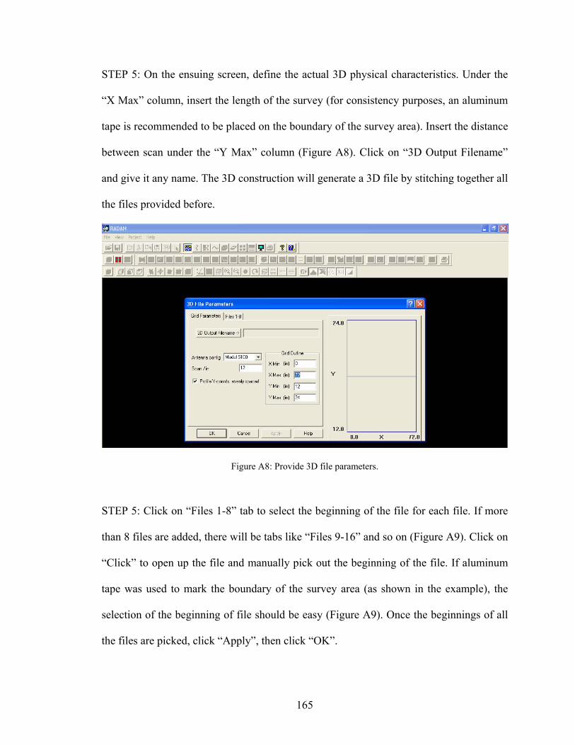
STEP 5: On the ensuing screen, define the actual 3D physical characteristics. Under the

“X Max” column, insert the length of the survey (for consistency purposes, an aluminum

tape is recommended to be placed on the boundary of the survey area). Insert the distance

between scan under the “Y Max” column (Figure A8). Click on “3D Output Filename”

and give it any name. The 3D construction will generate a 3D file by stitching together all

the files provided before.

Figure A8: Provide 3D file parameters.

STEP 5: Click on “Files 1-8” tab to select the beginning of the file for each file. If more

than 8 files are added, there will be tabs like “Files 9-16” and so on (Figure A9). Click on

“Click” to open up the file and manually pick out the beginning of the file. If aluminum

tape was used to mark the boundary of the survey area (as shown in the example), the

selection of the beginning of file should be easy (Figure A9). Once the beginnings of all

the files are picked, click

“Apply”, then click “OK”.

165

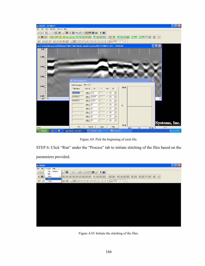
Figure A9: Pick the beginning of each file.

STEP 6: Click “Run” under the “Process” tab to initiate stitching of the files based on the

parameters provided.

Figure A10: Initiate the stitching of the files.

166

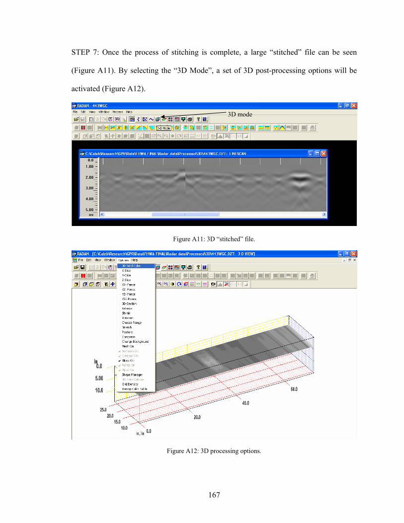
STEP 7: Once the process of stitching is complete, a large “stitched” file can be seen

(Figure A11). By selecting the “3D Mode”, a set of 3D post-processing options will be

activated (Figure A12).

Figure A11: 3D “stitched” file.

Figure A12: 3D processing options.

3D mode

167