1/24

�

�

�

�

�

�

Tacoma Narrows Bridge

Matt Bates and Sean DonohoeSpring Semester 2003

2/24

�

�

�

�

�

�

Introduction

Before the collapse of the Tacoma Narrows Bridge suspension bridges

were commonly constructed using rule of thumb. This method proved

dangerous, with many of these bridges exhibiting odd behavior consist-

ing of large vertical and torsional oscillations. In the case of Tacoma

Narrows, it is believed that not the vertical oscillations but the torsional

oscillations ultimately led to its destruction. We can model these tor-

sional oscillations with two different equations. These 2 equations will

derived from the kinetic and potential energy equations for the bridge.

3/24

�

�

�

�

�

�

PE and KE energy of the rod

Adding the physics equations for vertical kinetic energy and rotational

energy we get the total kinetic energy.

T =1

2mv2 +

1

6mL2θ2 (1)

Modelling a cross section of the bridge (with length 2L) will help us

visualize how we get our potential energy.

θθ

y

L

L

y1y1

There is a vertical deflection on both sides due to torsional oscillations.

4/24

�

�

�

�

�

�

On the left side the vertical deflection is:

yt = (y + y1)+, (2)

and on the right the vertical deflection is:

yt = (y − y1)+. (3)

The + exponet refers to the fact that the cables only act like springs

when pulled in the downward direction.

Looking at the picture depicting total displacement of a cross section of

the bridge we see that y1 is:

L sin θ, (4)

Subbing this into the yt equations above we get:

yt = (y − L sin θ)+

yt = (y + L sin θ)+.

(5)

5/24

�

�

�

�

�

�

From physics the total potential energy is:

PE =1

2ky2 −mgy. (6)

Plugging yt in for y we get:

PE = V =k

2[((y − L sin θ)2)+ + ((y + L sin θ)2)+]−mgy (7)

6/24

�

�

�

�

�

�

Energy to oscillation equations

Using the Lagrangian L = T − V we get:

L =my2

2+

1

6mL2θ2− 1

2k[((y−L sin θ)2)+ +((y +L sin θ)2)+] +mgy

(8)

Applying the Euler Lagrange equation

d

dt

(δLδθ

)=

δLδθ

(9)

and taking the partial derivatives we get:

δLδθ

=1

2k[2(y − L sin θ)+(−L cos θ) + 2(y + L sin θ)+(L cos θ)]

= kL cos θ[(y − L sin θ)+ − (y + L sin θ)+]

(10)

7/24

�

�

�

�

�

�

and

d

dt

δLδθ

=1

3mL2θ.

(11)

With some intense simplifications we come to:

θ =3k

mLcos θ[(y − L sin θ)+ − (y + L sin θ)+] (12)

8/24

�

�

�

�

�

�

Applying the Euler Lagrange equation

d

dt

(δLδy

)=

δLδy

, (13)

and taking the partial derivatives we get:

δLδy

= −1

2k[2(y − L sin θ)+ + 2(y + L sin θ)+] + mg

= −k[(y − L sin θ)+ + (y + L sin θ)+] + mg

(14)

and

d

dt

δLδy

=d

dt(my) = my. (15)

With some intense simplifications we get:

y = − k

m[(y − Lsinθ)+ + (y + L sin θ)+] + g. (16)

9/24

�

�

�

�

�

�

We then add a damping term, δθ and δy, and we also add a external

forcing term f(t) to the torsional equation. Doing this we get:

θ = −δθ +3k

mLcos θ[(y − L sin θ)+ − (y + L sin θ)+] + f (t) (17)

y = −δy − k

m[(y − Lsinθ)+ + (y + L sin θ)+] + g. (18)

Simplifying the torsional equation θ:

θ = −δθ +3k

mLcos θ[(y − L sin θ)− (y + L sin θ)] + f (t)

θ = −δθ +3k

mLcos θ[y − L sin θ − y − L sin θ] + f (t)

θ = −δθ +3k

mLcos θ(−2L sin θ) + f (t)

θ = −δθ − 6k

mcos θ(sin θ) + f (t). (19)

10/24

�

�

�

�

�

�

Torsional oscillations

The one we are really interested in is the θ equation because this is

what lead to the collapse of the bridge. Assuming that the cables never

lose tension and simplifying this equation we get:

θ = −δθ − 6k

mcos θ sin θ + f (t) (20)

This is the non-linear equation. We will then assume small oscillations

and say sinθ is approximately θ and cosθ is approximately 1 to linearize

it to get:

θ = −δθ − 6k

mθ + f (t) (21)

We chose the forcing term f(t) to be λsinµt, a term that accurately

models the frequency and amplitude of the oscillations observed before

the collapse.

11/24

�

�

�

�

�

�

Equation 21 is the linear model for the bridge and equation 20 is the

non-linear model.

The builders of the Tacoma Narrows Bridge should have used the non-

linear equation, but due to their inability to solve it they were forced to

use the linear.

This turned out to be a costly mistake. The linear equation gave them

bad data as the model showed eventual torsional stability no matter what

driving force and initial condition it was given.

Since the bridge actually acted according to the non-linear equation

not the linear, the bridge did not settle down like the engineers of the

bridge expected and the resulting torsional strain is believed to be a

major contributor to the failure of the bridge.

12/24

�

�

�

�

�

�

13/24

�

�

�

�

�

�

Non-linear vs. Linear

First we will explore the long-term behavior of the linear model, with

different initial conditions and driving terms of different periods (µ con-

trols the period).

0 200 400 600 800 1000−1.5

−1

−0.5

0

0.5

1

1.5

Figure 1a: Linear model with initial conditions θ = 1.2, θ = 0, and

λ = .05 (large push).

Note: vertical axis is theta in radians and horizontal is time for all graphs.

14/24

�

�

�

�

�

�

0 200 400 600 800 1000−2

−1

0

1

2

Figure 1b Linear model with initial conditions θ = 2, θ = 0 and λ = .05

(very large push).

15/24

�

�

�

�

�

�

0 200 400 600 800 1000−2

−1

0

1

2

Figure 1c Linear model, θ = 2, θ = 0 and λ = .08 (very large push and

large driving term).

We can easily see that the linear model always settles down when

given enough time.

16/24

�

�

�

�

�

�

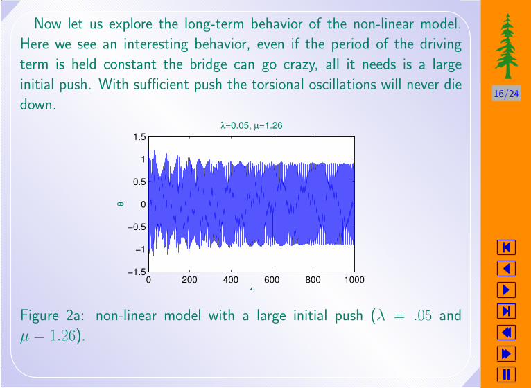
Now let us explore the long-term behavior of the non-linear model.

Here we see an interesting behavior, even if the period of the driving

term is held constant the bridge can go crazy, all it needs is a large

initial push. With sufficient push the torsional oscillations will never die

down.

0 200 400 600 800 1000−1.5

−1

−0.5

0

0.5

1

1.5

t

θλ=0.05, µ=1.26

Figure 2a: non-linear model with a large initial push (λ = .05 and

µ = 1.26).

17/24

�

�

�

�

�

�

0 200 400 600 800 1000−1

−0.5

0

0.5

1

t

θ

λ=0.05, µ=1.26

Figure 2b: non-linear model with a small initial push (λ = .05 and

µ = 1.26).

18/24

�

�

�

�

�

�

0 200 400 600 800 1000−1.5

−1

−0.5

0

0.5

1

1.5

t

θ

Figure 2c: non-linear model with a large initial push and a different

frequency than in Figure 2a or 2b (λ = .05 and µ = 1.35).

19/24

�

�

�

�

�

�

0 200 400 600 800 1000−0.2

−0.1

0

0.1

0.2

t

θ

Figure 2d: non-linear model with a small initial push and the same fre-

quency as Figure 2c (λ = .05 and µ = 1.35).

This is an important fact to remember. Over a range of frequencies

the non-linear model can exhibit behavior similar to the linear model or

very different. It all depends on the initial push.

20/24

�

�

�

�

�

�

Applied to Tacoma Narrows

At the time of the bridge’s construction, it was not possible to solve

the non-linear model so the engineers chose to use the linear model.

After seeing the behavior of the linear and non-linear model you can

probably guess where we are going. We will start by doing a direct

comparison of the linear and non-linear models. When given a large

initial push and no driving terms both the models are very similar, so

far so good.

21/24

�

�

�

�

�

�

The left graph is the linear model the right is the non-linear version.

0 200 400 600 800 1000−1.5

−1

−0.5

0

0.5

1

1.5

0 200 400 600 800 1000−1.5

−1

−0.5

0

0.5

1

1.5

Now we start both models at equilibrium but add a small driving term

(λ = .05). Once again both models appear very similar, and this is

good.

22/24

�

�

�

�

�

�

0 200 400 600 800 1000−0.1

−0.05

0

0.05

0.1

0 200 400 600 800 1000−0.1

−0.05

0

0.05

0.1

The top graph is the linear model the bottom is the non-linear version.

23/24

�

�

�

�

�

�

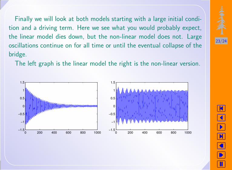
Finally we will look at both models starting with a large initial condi-

tion and a driving term. Here we see what you would probably expect,

the linear model dies down, but the non-linear model does not. Large

oscillations continue on for all time or until the eventual collapse of the

bridge.

The left graph is the linear model the right is the non-linear version.

0 200 400 600 800 1000−1.5

−1

−0.5

0

0.5

1

1.5

0 200 400 600 800 1000−1.5

−1

−0.5

0

0.5

1

1.5

24/24

�

�

�

�

�

�

In Conclusion

Had the engineers of the time been able to solve the non-linear equa-

tion the error of using a incorrect linear model would not have been

done. Using the correct non-linear model may have led to a more sturdy

bridge that could still be standing today.