Proceedings21st International Nondestructive Testing and Evaluation of Wood SymposiumFreiburg, Germany2019

United States Department of Agriculture

Forest Service, Forest Products LaboratoryForest Research Institute Baden-WürttembergForest Products SocietyInternational Union of Forest Research Organizations

General Technical ReportFPL–GTR–272

September2019

Forest Research Institute Baden-Württemberg

In accordance with Federal civil rights law and U.S. Department of Agriculture (USDA) civil rights regulations and policies, the USDA, its Agencies, offices, and employees, and institutions participating in or administering USDA programs are prohibited from discriminating based on race, color, national origin, religion, sex, gender identity (including gender expression), sexual orientation, disability, age, marital status, family/parental status, income derived from a public assistance program, political beliefs, or reprisal or retaliation for prior civil rights activity, in any program or activity conducted or funded by USDA (not all bases apply to all programs). Remedies and complaint filing deadlines vary by program or incident. Persons with disabilities who require alternative means of communication for program information (e.g., Braille, large print, audiotape, American Sign Language, etc.) should contact the responsible Agency or USDA’s TARGET Center at (202) 720–2600 (voice and TTY) or contact USDA through the Federal Relay Service at (800) 877–8339. Additionally, program information may be made available in languages other than English. To file a program discrimination complaint, complete the USDA Program Discrimination Complaint Form, AD-3027, found online at http://www.ascr.usda.gov/complaint_filing_cust.html and at any USDA office or write a letter addressed to USDA and provide in the letter all of the information requested in the form. To request a copy of the complaint form, call (866) 632–9992. Submit your completed form or letter to USDA by: (1) mail: U.S. Department of Agriculture, Office of the Assistant Secretary for Civil Rights, 1400 Independence Avenue, SW, Washington, D.C. 20250–9410; (2) fax: (202) 690–7442; or (3) email: program.intake@usda.gov.USDA is an equal opportunity provider, employer, and lender.

AbstractThe 21st International Nondestructive Testing and Evaluation of Wood Symposium was hosted by the Forest Research Institute Baden-Württemberg (FVA) in Freiburg, Baden-Württemberg, Germany, September 24–27, 2019. This symposium was a forum for those involved in nondestructive testing and evaluation (NDT/NDE) of wood and brought together many international researchers, NDT/NDE users, suppliers, representatives from various government agencies, and other groups to share research results, products, and technology for evaluating a wide range of wood products, including standing trees, logs, structural lumber, engineered wood products, and wood structures. Networking among participants encouraged international collaborative efforts and fostered the implementation of NDT/NDE technologies around the world. The technical content of the 21st symposium is captured in these proceedings. Full-length, in-depth technical papers for the oral presentations and several of the poster presentations are published herein. The papers were not peer reviewed and are reproduced here as they were submitted by the authors.

Keywords: International Nondestructive Testing and Evaluation of Wood Symposium, nondestructive testing, nondestructive evaluation, wood, wood products

September 2019 (revised October 2019)Wang, Xiping; Sauter, Udo H.; Ross, Robert J., eds. 2019. Proceedings: 21st International Nondestructive Testing and Evaluation of Wood Symposium. General Technical Report FPL-GTR-272. Madison, WI: U.S. Department of Agriculture, Forest Service, Forest Products Laboratory. 724 p.A limited number of free copies of this publication are available to the public from the Forest Products Laboratory, One Gifford Pinchot Drive, Madison, WI 53726-2398. This publication is also available online at www.fpl.fs.fed.us. Laboratory publications are sent to hundreds of libraries in the United States and elsewhere.The Forest Products Laboratory is maintained in cooperation with the University of Wisconsin. The use of trade or firm names in this publication is for reader information and does not imply endorsement by the United States Department of Agriculture (USDA) of any product or service.

ContentsPreface ..................................................................................3

General Session ....................................................................6

Session 1 Emerging Applications .....................................10

Session 2 In-Forest Assessment ........................................92

Session 3 Timbers and Lumber .......................................167

Session 4 Wood Material Characterization .....................276

Session 5 Urban Tree Assessment...................................358

Session 6 Structure Condition Assessment .....................445

Session 7 Roundwood .....................................................517

Session 8 Engineered Wood Products .............................612

Poster Session ..................................................................650

PrefaceThe International Nondestructive Testing and Evaluation of Wood Symposium Series started in Madison, Wisconsin, USA, in 1963. Since its inception, 20 symposia have been held in various countries around the world, including Brazil, China, Germany, Hungary, Switzerland, and the United States.

The 21st International Nondestructive Testing and Evaluation of Wood Symposium was hosted by the Forest Research Institute Baden-Württemberg (FVA). It was held in Freiburg, Baden-Württemberg, Germany, September 24–27, 2019. This symposium was a forum for those involved in nondestructive testing and evaluation (NDT/NDE) of wood and brought together many international researchers, NDT/NDE users, suppliers, representatives from various government agencies, and other groups to share research results, products, and technology for evaluating a wide range of wood products, including standing trees, logs, structural lumber, engineered wood products, and wood structures. Networking among participants encouraged international collaborative efforts and fostered the implementation of NDT/NDE technologies around the world.

After opening comments from the International Nondestructive Testing and Evaluation of Wood Symposium Organizing Committee, participants were welcomed by the Ministry of Rural Affairs and Consumer Protection Baden-Württemberg and from the State Forest Service Baden-Württemberg ForstBW, Mr. Max Reger. A warm welcome to the University was delivered by Prof. Thomas Seifert.

The Symposium’s general session included speakers from China, Germany, Italy, and the United States on topics including inspection of historic structures, use of NDE in industrial environments, and application of NDE around the world.

During the symposium’s banquet, special recognition awards were presented to the Forest Research Institute Baden-Württemberg for its outstanding efforts in hosting the 21st symposium and to Dr. Udo H. Sauter for his leadership as a co-chair in organizing the event. Special recognition awards were also presented to Dr. Raquel Gonçalves for her distinguished service in the symposium series and to Mr. Peter Carter for his outstanding technology transfer efforts in the field of nondestructive evaluation of wood.

Prior to the Symposium, a technical workshop, “Nondestructive Testing and Evaluation Opportunities in a Historic European City,” was held. It included coursework on the state-of-the-art in NDE as applied to historic structures, and a tour of the historic Freiburg Cathedral.

A post-symposium tour of the Black Forest was organized and led by the Forest Research Institute Baden-Württemberg.

The technical content of the 21st symposium is captured in the following proceedings. Full-length, in-depth technical papers for the oral presentations and several of the poster presentations are published herein. The papers were not peer reviewed and are reproduced here as they were submitted by the authors.

Proceedings

21st International Nondestructive Testing and Evaluation of Wood SymposiumFreiburg, Germany2019Edited byXiping Wang, Research Forest Products TechnologistForest Products Laboratory, Madison, WisconsinUdo H. Sauter, Head of Department of Forest Utilisation Forest Research Institute Baden-Württemberg, Freiburg, GermanyRobert J. Ross, Supervisory Research General Engineer and Research ProfessorForest Products Laboratory, Madison, Wisconsin and Michigan Technological University, Houghton, Michiga

3

The organization of the following proceedings follows that of the sessions at the 21st symposium. Technical sessions covered the following topics:

1. Emerging Applications2. In-Forest Assessment3. Timbers and Lumber4. Wood Materials Characterization5. Urban Tree Assessment6. Structure Condition Assessment7. Roundwood8. Engineered Wood Products

We express our sincere appreciation and gratitude to members of the Organizing Committee, International Nondestructive Testing and Evaluation of Wood Symposium Series, for their efforts in making this symposium a success:

Dr. Laszlo Bejo, University of West Hungary, HungaryDr. Ferenc Divos, University of West Hungary, HungaryDr. Raquel Gonçalves, University of Campinas, BrazilDr. Francisco Arriaga Martitegui, Universidad Politécnica de Madrid, SpainRoy F. Pellerin, Emeritus Professor, Washington State University, USADr. Robert J. Ross, FPL and Michigan Technological University, USADr. Udo H. Sauter, Forest Research Institute Baden-Württemberg, GermanyDr. C. Adam Senalik, FPL, USADr. Xiping Wang, FPL, USADr. Houjiang Zhang, Beijing Forestry University, China

We thank the International Union of Forest Research Organizations (IUFRO), Forest Products Society, USDA Forest Products Laboratory, and Forest Research Institute Baden-Württemberg for their support. Thanks also go to the following organizations for providing financial support in the form of sponsorships or who exhibited equipment:

• Microtec• Fakopp• Sägewerk Karl Streit GmbH and Co. KG• Sägewerk Schilliger Bois SAS• Rettenmeier• Holzwerk B. Keck GmbH• Dold Holzwerke GmbH• University of Freiburg• Beijing Forestry University• Washington State University• World Wood Day Foundation• Rinntech• Timbeter• Forest Products Society—Midwest Section

A very special thank you to Drs. Franka Brüchert and Stefan Stängle for their outstanding efforts—without their efforts this meeting would not have been possible. Thanks for being wonderfully gracious hosts!

We thank the following staff at FPL for their outstanding efforts in preparing these proceedings: Jim Anderson, Barb Hogan, and Karen Nelson.

A note of thanks to the many individuals who prepared papers for inclusion in the symposium. Your dedication and efforts make this Symposium Series a success!

We hope that these proceedings provide inspiration to those who read its papers. And welcome to new participants in the global wood NDT/NDE family!

Dr. Robert J. RossDr. Udo H. SauterSymposium Co-Chairs

4

Forest Products Laboratory

Thank you to this year’s hosts and sponsors

Forest Research Institute Baden-Württemberg

5

General Session

6

Nondestructive Testing and Evaluation of Wood in the Sawmill of the Future Federico Giudiceandrea President, Microtec, Brixen, Italy Abstract Through integrated and innovative solutions and the implementation of artificial intelligence (AI) in the sawmill of the future, every log can be traced to its boards through a “digital fingerprint.” The gapless traceability from a log to the boards is guaranteed by • CT Log 360°, the X-ray computed tomography for full digital 3D log reconstruction and virtual

grading; • Logeye Fingerprint, the X-ray log scanner for identification and rotation angle evaluation; • Truespin, the scanner for log rotation monitoring; and • Goldeneye 900, the multi-sensor scanner for boards for identification and quality grading. The integration of AI in the production processes of sawmills allows determining the value of the final product before breaking down the log, which translates to immediate cost savings and increased added value to the final product, which leads to an impressive return on investment.

Supply and Demand Factors Affecting NDT Adoption in North America Dan Seale James R. Moreton Fellow and Thompson Professor, Department of Sustainable Bioproducts, Mississippi State University, Starkville, Mississippi, USA Abstract In North American sawmills, the utilization of nondestructive testing has changed for some regions while other regions have remained relatively stable. The underlying causes for the changes will be examined. Some causal factors may include timber supply, insect infestations, mill ownership changes, timber quality and size, strength values for output products, capital expansion changing mill volume, and additional NDT grades available to mills. Although not all underlying causes are present in each producing region, some regions have responded to changing conditions while others seem to have ignored them. The existence of inexpensive NDT equipment for builders, architects, engineers, and some consumers will also be discussed relative to expanding NDT markets.

7

Nondestructive Testing in the Real World of Historic Building Preservation: Experiences from 30 Years of Inspecting Structural Timber Frank Rinn Physicist and Founder, Rinntech, Heidelberg, Germany Abstract Developing nondestructive techniques may be difficult but is simple compared to getting real innovations established on an established market. Even when technology and application concepts are validated, scientifically confirmed, and published, this does not mean that this will have any practical consequence in the real world of building timber. In the early 1990s, for example, the architecture and engineering faculty of Karlsruhe University recommended our timber inspection concept using resistance drilling as the best way to go because of its huge success (cost reductions of up to 70%, while at the same time preserving more historic fabric)—but markets react very specifically and differently to such innovations because of various “boundary” conditions. The same applies to many other nondestructive techniques, such as stress-wave timing, ultrasound, and X-ray-analysis. It is critically important to clearly specify possibilities and limitations of new methods and devices. In addition, practical application must be demonstrated in real world case studies, acknowledging the actual needs of the market. When a (historic) timber structure, for example, does not show significant deformations and no load-change occurs, then usually there is no need for a structural calculation and (local) strength measurements. In the vast majority of applications, detection and repair of decayed parts is sufficient, the more so as it is practically impossible to really assess the load carrying capacity of a structure nondestructively. Thus, before promoting or even standardizing new methods, the market has to be understood and addressed specifically, depending on local, regional, and national boundary conditions. Otherwise, even great NDT developments may fail or disappear.

8

Recent Research and Development on Nondestructive Testing and Evaluation of Wood in China Lihai Wang Professor, Northeast Forestry University, Harbin, China

Abstract

In recent years, research and development in the field of wood nondestructive testing and evaluation has grown rapidly in China. Relevant studies have been focused in the following areas: (1) quantitative characterization of internal decay of living trees; (2) nondestructive evaluation of strength loss of wood structural components in ancient timber structures; and (3) inspection and risk assessment of historical trees and urban roadside trees. More research institutes and researchers have begun research efforts in these areas, especially in the landscape and cultural heritage departments. In both research and field applications, using a combination of various technical methods is becoming a trend. Among many different nondestructive testing methods, the Risistograph and stress wave tomography technologies are gaining a wide acceptance in field applications and being rated favorably by many researchers and users. In the meantime, the advantages of geophysical radar imaging and electrical resistance tomography technologies are emerging and attracting attentions of researchers and engineers.

The Importance of Wood Products for the United States Department of Defense Ernest E. Hugh Director, Tropic Regions Test Center, Yuma Proving Ground, Yuma, Arizona, USA

Abstract

U.S. Department of Defense military trailers worldwide have been decked nearly exclusively in Apitong, an internationally sourced hardwood. The U.S. Army Ground Vehicle Systems Center (GVSC) organization has determined that the continued use of Apitong is untenable and initiated the TacticalWood trailer decking project to develop and test domestically sourced hardwoods to ensure that a renewable resource will be identified, while maintaining the same or an improved capability. This undertaking encourages conservation of woods and also promotes the U.S. domestic hardwood forestry workforce and industry in the spirit of the Buy American Act. This effort is a joint collaboration between GVSC, Michigan Technological University–School of Forest Resources and Environmental Science—Wood Protection Group (Houghton, Michigan, USA), U.S. Army Tropic Regions Test Center, USDA Forest Service, Forest Products Laboratory (Madison, Wisconsin, USA), in addition to numerous other industry and USG partners.

9

Session 1

Emerging Applications

10

Primary Results of the Use of GPR Coda Wave Interferometry in the Estimation of Biological Deterioration of Glulam and Crosslam Elements Alfonso Lozano Martínez-Luengas; Engineering Construction Department. University of Oviedo; alozano@uniovi.es José-Paulino Fernández-Álvarez. Department of Mining Exploitation and Prospecting, University of Oviedo; pauli@uniovi.es David Rubio-Melendi. Hydro-Geophysics and NDT Modelling Unit; University of Oviedo; david@hydrogeophysicsndt.com David Lorenzo Fouz; Forestry engineer. University of Santiago de Compostela; davidlorenzofouz@gmail.com Abstract During the last years, damage caused by xylophagous organisms (woodworms and termites) in timber structures has increased significantly. The reasons are several and among them can be mentioned the use of sapwood, wood species with less durability against fungal and xylophagous insects and because of the expansion of the radius of action of some of them because of the exchanges trade between countries and global warming. When it is necessary to estimate the level of biological degradation, devices such as resistographs, measurement of the speed of sonic or ultrasonic pulses, etc., are used. However, although this equipment is really useful, they have certain limitations. Most important are the fact of perform only local measurements or accessibility. So in some cases the evaluation of the biological deterioration, especially with incipient attacks on large elements, cannot be carried out accurately. In this situation are, for example, glued laminated and cross laminated structures. In order to improve the current devices used in the survey of these timber elements, the possibility of estimating the level of biological decay by means of coda interferometry based on radar techniques (GPR - Ground Penetrating Radar) has been analyzed. The paper presents the possibilities of the GPR coda wave interferometry (CWI) in the estimation of the degree of degradation by xylophagous organisms in glulam and crosslam structures in Use Classes 1, 2, an 3 and the primary results of the tests that have been carried out in the laboratory using this technology. Keywords: xylophagous, decay, GPR, coda wave interferometry Introduction to damages of biotic origin in timber structures in Spain Wood used in structures can be affected by pathological processes of biotic origin (insects and fungi) and abiotic (fire, UVA radiation, some acids, etc.).

11

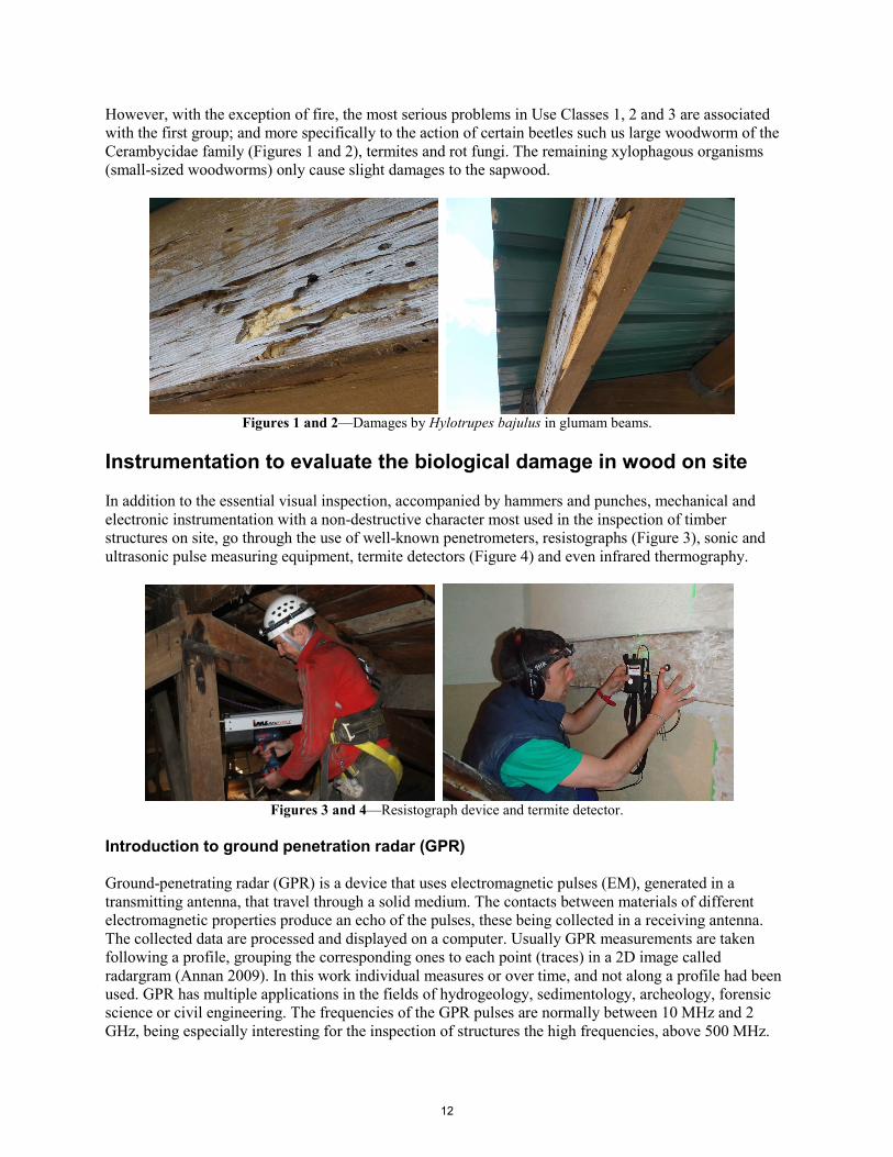
However, with the exception of fire, the most serious problems in Use Classes 1, 2 and 3 are associated with the first group; and more specifically to the action of certain beetles such us large woodworm of the Cerambycidae family (Figures 1 and 2), termites and rot fungi. The remaining xylophagous organisms (small-sized woodworms) only cause slight damages to the sapwood.

Figures 1 and 2—Damages by Hylotrupes bajulus in glumam beams.

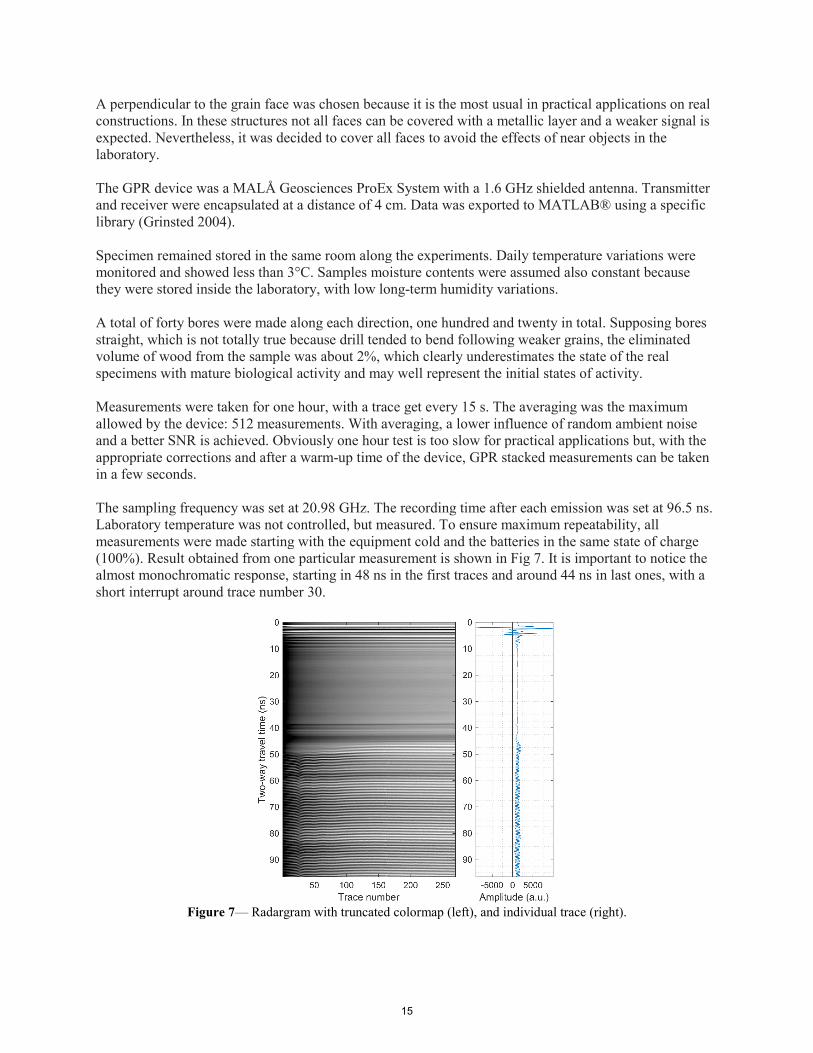
Instrumentation to evaluate the biological damage in wood on site In addition to the essential visual inspection, accompanied by hammers and punches, mechanical and electronic instrumentation with a non-destructive character most used in the inspection of timber structures on site, go through the use of well-known penetrometers, resistographs (Figure 3), sonic and ultrasonic pulse measuring equipment, termite detectors (Figure 4) and even infrared thermography.

Figures 3 and 4—Resistograph device and termite detector.

Introduction to ground penetration radar (GPR) Ground-penetrating radar (GPR) is a device that uses electromagnetic pulses (EM), generated in a transmitting antenna, that travel through a solid medium. The contacts between materials of different electromagnetic properties produce an echo of the pulses, these being collected in a receiving antenna. The collected data are processed and displayed on a computer. Usually GPR measurements are taken following a profile, grouping the corresponding ones to each point (traces) in a 2D image called radargram (Annan 2009). In this work individual measures or over time, and not along a profile had been used. GPR has multiple applications in the fields of hydrogeology, sedimentology, archeology, forensic science or civil engineering. The frequencies of the GPR pulses are normally between 10 MHz and 2 GHz, being especially interesting for the inspection of structures the high frequencies, above 500 MHz.

12

The depth reached with GPR equipment is very variable. Depending on the frequency and the medium to be surveyed, the maximum depth can range from hundreds of meters in glaciology, to a few centimeters in the inspection of concrete structures. The speed of electromagnetic pulses in a medium is a characteristic parameter of this. The speed can be affected by inclusions of another material, variations in moisture content, compaction or temperature. The characteristic speed of a medium can be estimated through multiple ways well known in the literature: adjustment of hyperbolas, Common Mid-Point (CMP) two-way travel time measurement, for example. GPR technics in the survey of timber structures In previous sections it has been exposed how timber elements are affected by various xylophage organisms such as beetles and fungi. In the first case the decay is associated with the galleries that dig the larvae inside the pieces. On the other hand, fungi cause a degradation of the fibers of the wood, which leads to a very relevant drop in its density. The galleries of woodworms and termites are usually too small (a few millimeters) compared to the wavelength of GPR pulses (of the order of 10 cm for a frequency of 1.6 GHz in wood) to produce an interpretable eco. That is why GPR is not widely use in timber structures evaluation, but some studies were performed in timber bridges, historical structures and laboratory experiments. The main objectives of those studies were defect detection, and moisture content evaluation and internal structure investigation of tree trunks (Ježová et al. 2016). Therefore, the GPR does not get enough resolution to get an image of the galleries individually. However, the presence of galleries implies a certain reduction in the density of the wood and, with it, a small variation in the speed of the pulses in the middle (Torgovnikov, 1993). Nevertheless, a very accurate measurement of the speed in the medium can detect a small deterioration in the timber section. Unfortunately, GPR speed measurements are not sufficiently adjusted over GPR signals, mainly because in most applications such precision is not needed. Dielectric properties of wood Materials response to electromagnetic waves can be characterized using three parameters: magnetic permeability (µ), electrical conductivity (σ) and dielectric permittivity (ε). Magnetic permeability is usually not taken into account in non-metallic materials. Electrical conductivity is dependent in the moisture content for slightly conductive media, as is wood. Dielectric permittivity is also highly influenced by moisture content due to the high permittivity of water (εr ≈ 78). In a non-metallic and slightly conductive medium, dielectric permittivity is the main parameter characterizing the material. Under this hypothesis, reasonable in low moisture wood, the propagation velocity of electromagnetic waves can be calculated as:

v = c/√ εr where c≈0.3 m/ns is the vacuum speed of light, and εr=ε/ε0 is the relative permittivity (with respect to the vacuum permittivity) of the medium. This is the reason why a material can be characterized both by εr and v. The dielectric properties of wood depend on density, moisture content, chemical composition and grain direction. As wood is an anisotropic material, three different dielectric permittivities can be defined for three orthogonal directions: longitudinal or parallel to the grain (ε∥), radial to the grain (εR) and tangential to the grain (εT). Various experiments have shown that radial and tangential permittivities are marginally different, reducing both to a single perpendicular permittivity (ε⊥). It is also experimentally shown that ε∥ is always higher than ε⊥ (Torgovnikov, 1993).

13

The most usually accessible faces of timber in real structures are those perpendicular to the grain, and this has been taken into account in this work where the antenna was placed in one of the tangential faces of the laboratory specimen. Coda wave interferometry (CWI) Coda Wave Interferometry (CWI) is a technique applied in the field of mechanical waves in ultrasonic and seismic survey (Schurr 2010; Planès and Larose 2013). Using the final part of the signals, with chaotic aspect and decreasing amplitude (called Coda), two signals taken in exactly the same conditions, but at different times, are compared. It has been proven that coda waves are reproducible as long as the medium does not change, since they are produced by diffracted waves and reflected several times inside the medium. This is also the reason why coda waves are very sensitive to small changes in the medium: indeed, having traveled a greater distance inside the medium, they are more affected than the first received echoes (although they have a wider and more easily recognizable). The main objective of this study has been to use waves that suffer multiple rebounds within several samples of glued laminated timber, in order to detect small artificial defects. For this purpose, speed variations smaller than those usually detected in the GPR technique have been determined. First tests: samples, devices and measurement procedures From unaltered samples of laminated wood (Fig 5 and 6) of beech (Fagus sylvatica) and red spruce (Picea abies), the galleries caused by the action of the xylophagous insects were simulated by perforations made with an IML RESI-B 450 resistograph device. Bores were drilled from one face to the opposite with a diameter of 3 mm. The sawdust was drained using a 2 mm diameter threaded rod and a battery operated hand drill. To evaluate the functionality of the CWI in the detection of the defects produced by the xylophages, drills were made progressively, followed by measurements with the GPR equipment. First tests were carried out on the beech cube, with eight different stages of simulated biodeterioration. The cube (20 cm alongside) was composed of two blocks along the tangential direction to the grain faces, glued using polyvinyl acetate. All faces of the specimen, except one tangential to the grain, were covered with aluminium tape. The antenna was always held fixed with a self-adhesive strap on a mark at the centre of the free face.

Figures 5 and 6—Antenna on beech specimen and Scots pine, respectively.

14

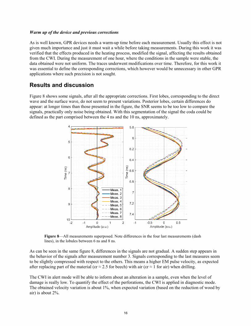
A perpendicular to the grain face was chosen because it is the most usual in practical applications on real constructions. In these structures not all faces can be covered with a metallic layer and a weaker signal is expected. Nevertheless, it was decided to cover all faces to avoid the effects of near objects in the laboratory. The GPR device was a MALÅ Geosciences ProEx System with a 1.6 GHz shielded antenna. Transmitter and receiver were encapsulated at a distance of 4 cm. Data was exported to MATLAB® using a specific library (Grinsted 2004). Specimen remained stored in the same room along the experiments. Daily temperature variations were monitored and showed less than 3°C. Samples moisture contents were assumed also constant because they were stored inside the laboratory, with low long-term humidity variations. A total of forty bores were made along each direction, one hundred and twenty in total. Supposing bores straight, which is not totally true because drill tended to bend following weaker grains, the eliminated volume of wood from the sample was about 2%, which clearly underestimates the state of the real specimens with mature biological activity and may well represent the initial states of activity. Measurements were taken for one hour, with a trace get every 15 s. The averaging was the maximum allowed by the device: 512 measurements. With averaging, a lower influence of random ambient noise and a better SNR is achieved. Obviously one hour test is too slow for practical applications but, with the appropriate corrections and after a warm-up time of the device, GPR stacked measurements can be taken in a few seconds. The sampling frequency was set at 20.98 GHz. The recording time after each emission was set at 96.5 ns. Laboratory temperature was not controlled, but measured. To ensure maximum repeatability, all measurements were made starting with the equipment cold and the batteries in the same state of charge (100%). Result obtained from one particular measurement is shown in Fig 7. It is important to notice the almost monochromatic response, starting in 48 ns in the first traces and around 44 ns in last ones, with a short interrupt around trace number 30.

Figure 7— Radargram with truncated colormap (left), and individual trace (right).

15

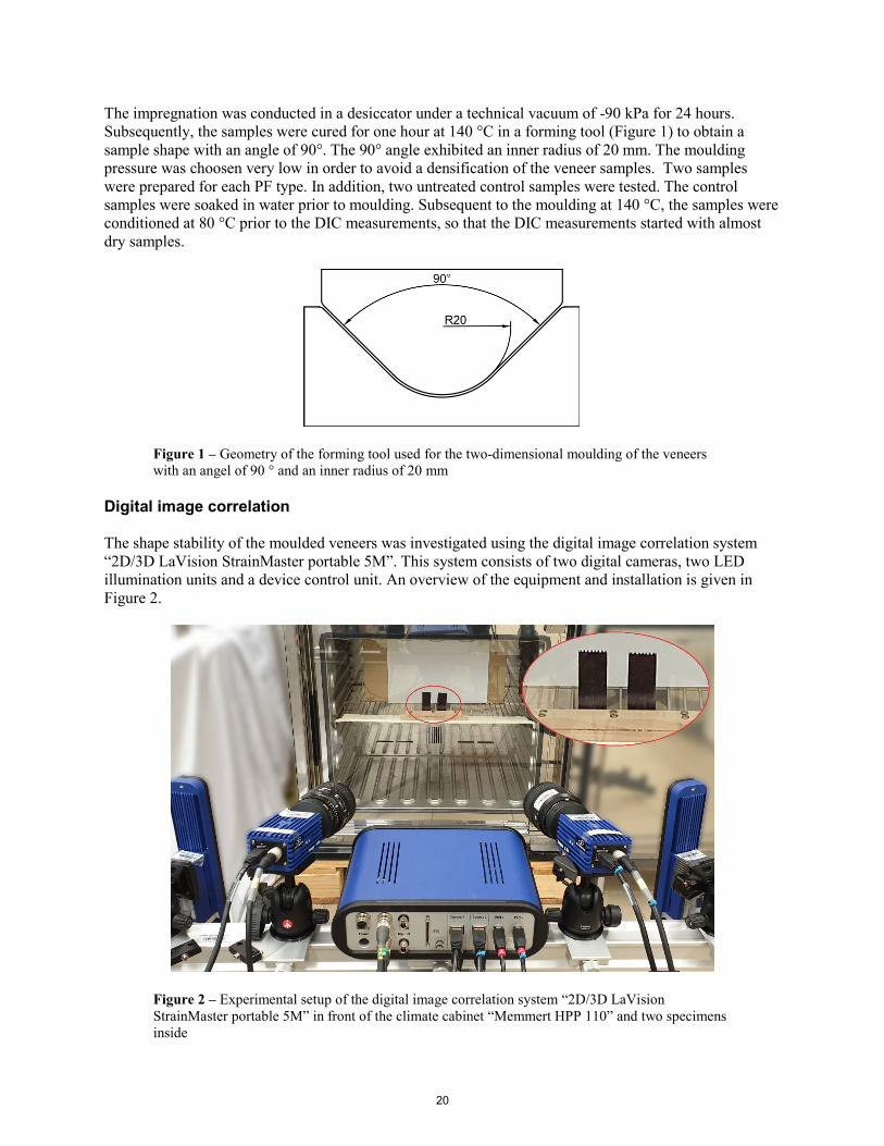
Warm up of the device and previous corrections As is well known, GPR devices needs a warm-up time before each measurement. Usually this effect is not given much importance and just it must wait a while before taking measurements. During this work it was verified that the effects produced in the heating process, modified the signal, affecting the results obtained from the CWI. During the measurement of one hour, where the conditions in the sample were stable, the data obtained were not uniform. The traces underwent modifications over time. Therefore, for this work it was essential to define the corresponding corrections, which however would be unnecessary in other GPR applications where such precision is not sought. Results and discussion Figure 8 shows some signals, after all the appropriate corrections. First lobes, corresponding to the direct wave and the surface wave, do not seem to present variations. Posterior lobes, certain differences do appear: at longer times than those presented in the figure, the SNR seems to be too low to compare the signals, practically only noise being obtained. With this segmentation of the signal the coda could be defined as the part comprised between the 4 ns and the 10 ns, approximately.

Figure 8—All measurements superposed. Note differences in the four last measurements (dash lines), in the lobules between 6 ns and 8 ns.

As can be seen in the same figure 8, differences in the signals are not gradual. A sudden step appears in the behavior of the signals after measurement number 3. Signals corresponding to the last measures seem to be slightly compressed with respect to the others. This means a higher EM pulse velocity, as expected after replacing part of the material (εr ≈ 2.5 for beech) with air (εr ≈ 1 for air) when drilling. The CWI in alert mode will be able to inform about an alteration in a sample, even when the level of damage is really low. To quantify the effect of the perforations, the CWI is applied in diagnostic mode. The obtained velocity variation is about 1%, when expected variation (based on the reduction of wood by air) is about 2%.

16

The analysis presented here is focused in the segment from 4 ns to 10 ns, approximately. However, unlike in seismic or ultrasonic testing, where the coda envelope follows a slow decaying, in these GPR signals the coda length is small. Two reasons could possibly explain this effect: the absence of wavelength like scatters in the sample and the faster attenuations of radar signals. CWI in ultrasonic testing is based in the presence of scatters, but at the employed GPR frequencies the wavelengths (about a decimeter) are too long. Nevertheless, being timber dimensions comparable to wavelengths, this allows the possibility of a short coda composed by the superposition of multiple reflected waves. Conclusions In the previous sections, the equipment and systems most used today for the evaluation of biological deterioration in wooden structures have been briefly exposed. Likewise, the limitations of these devices have also been explained; especially those that refer to the estimation of the level of damage (accessibility and detection with incipient damages, fundamentally). In this sense, GPR has proven to be a very useful tool for the detection of biological damage in glued laminated and crosslam structures at an early age. Indeed, after the initial tests carried out to date, the CWI seems to be able to detect very small levels of biological damage, just comparing the signals taken at different times, on the same position. That is, starting from a sample in good condition, the appearance of defects should be controlled over time. In summary, it can be affirmed that the improvement of this technique would enable quality control and preventive control of damage by fungal decay and attacks of xylophagous insects, even with minor degradations, in laminated and cross-laminated wood structures. This procedure would be especially interesting in buildings located in Use Classes 2 and 3. To do this, it would only be necessary to define a program of periodic inspections and maintenance (similar to that implemented in viaducts, settling ponds, walkways, etc.), in which, in addition to visual inspection, a record of the signals with the GPR would be made. This information would be compared with the initial measurements, taken immediately after its assembly in the workshop or its final implementation, for example. References Annan, A.P. 2009. Electromagnetic Principles of Ground Penetrating Radar. In: Jol HM (ed) Ground Penetrating Radar Theory and Applications. Elsevier, Amsterdam, pp 3–40. Ježová, J.; Mertens, L.; Lambot S. 2016. Ground-penetrating radar for observing tree trunks and other cylindrical objects. Construction Building Materials 123:214–225. Torgovnikov, G.I. 1993. Dielectric Properties of Wood and Wood-Based Materials. Springer-Verlag, Berlin Schurr, D.P. 2010. Monitoring damage in concrete using diffuse ultrasonic coda wave interferometry. Georgia Institute of Technology. Planès, T. and Larose, E. 2013. A review of ultrasonic Coda Wave Interferometry in concrete. Cement and Concrete Research 53:248–255.

17

Investigating the Shape Stability of Moulded Phenol-Formaldehyde Modified Beech Veneers by Means of Digital Image Correlation

Axel Mund Faculty of Wood Engineering, Eberswalde University for Sustainable Development, Eberswalde, Germany, axel.mund@hnee.de

Leo Felix Munier Faculty of Wood Engineering, Eberswalde University for Sustainable Development, Eberswalde, Germany, leofelix.munier@hnee.de

Tom Franke Department of Architecture, Wood, and Civil Engineering, Bern University of Applied Sciences, Biel, Switzerland, tom.franke@bfh.ch

Nadine Herold Faculty of Wood Engineering, Eberswalde University for Sustainable Development, Eberswalde, Germany, nadine.herold@hnee.de

Alexander Pfriem Faculty of Wood Engineering, Eberswalde University for Sustainable Development, Eberswalde, Germany, alexander.pfriem@hnee.de

Abstract

Within the present study, measurements by digital image correlation (DIC) were conducted to determine the effect of phenol-formaldehyde (PF) modification on the shape stability of moulded beech veneers (Fagus sylvatica L.) exposed to changing climatic conditions. For this purpose, thin beech veneers were impregnated with a low (lmwPF), a medium (mmwPF) and a high molecular weight PF (hmwPF). The impregnated veneers were cured for one hour at 140 °C in a moulding form to obtain a shaped veneer with an angle of 90°. Two samples were prepared for each PF type as well as two control samples. During the DIC measurements, the samples were exposed to two different sequential climatic conditions for 46 hours. In the first segment, the samples were conditioned at 90% relative humidity at a temperature of 20 °C for 23 hours. During the second segment, the samples were exposed for further 23 hours to 70 °C without controlled relative humidity to dry the samples. At the end of the first segment, the DIC measurements of the control samples revealed the greatest changing in angle (109.6°) coincident with the lowest shape stability, followed by the hmwPF samples (ca. 107.2°), the mmwPF samples (100.8°) and the lmwPF samples (97.6°). As a result of the second segment, the samples approach the initial shape of a 90° angle due to drying. Here, the hmwPF samples are closest to the initial shape (90.8°) followed by the lmwPF samples (92.4°), the mmwPF samples 92.6° and the control samples (96.1°).

Keywords: DIC, phenol-formaldehyde, shape stability, veneer moulding, wood modification

18

Introduction The modification of wood with phenol-formaldehyde to improve the material properties is commonly used in the wood working industry. The positive effects of a phenol-formaldehyde treatment were already largely evidenced by various studies. Stamm and Seborg have published various studies about the advantages of a wood modification by PF. They revealed significantly reduced water absorption (1936; 1942) and an improved dimensional stability (1942). Stamm and Seborg (1942) also reported on further improvements due to PF modifications. These include improvements in compressive strength, decay resistance, heat resistance and electrical resistivity. In 1955, they revealed plasticizing effects of unpolymerized PF by an enhanced densification of wood. These findings were later confirmed and supported by further authors (Furuno et al. 2004; Shams and Yano 2004; Gabrielli and Kamke 2009; Franke et al.2017 a; Franke et al. 2018). In particular, Franke et al. undertook a series of extensive research to investigate the plasticizing effects of PF. For example Franke et al. (2018) revealed an enhanced plasticization of PF impregnated (uncured) veneers even at low retentions compared to just water-soaked veneer samples by using two and three dimensional deformations at ambient temperature. That opportunity of plasticizing wood is particularly used in the furniture industry to create wood mouldings like wooden seat shells. Further application areas of PF modified wood are e.g. the transformer industry and mechanical engineering. However, the aim of the current study is to investigate the influence of PF wood modification on the shape stability of moulded beech veneers under changing climatic conditions. Special consideration will be paid on the role of the molecular weight of the used PFs. In order to determine the shape stability during two different climatic conditions, a digital image correlation (DIC) was used. Experimental Sample preparation The samples were made from beech wood veneers (Fagus sylvatica L.) with the dimensions of appr. 100 mm x 25 mm x 0.6 mm (longitudinal x radial x tangential). However, the used veneers were produced manually to ensure a defined anatomical orientation. After drying, the veneer samples were impregnated either with a low (lmwPF), a medium (mmwPF) or with a high molecular weight phenol-formaldehyde (hmwPF). All PF resins were water-based resols from Prefere Resins GmbH, Erkner, Germany. The original solid content of the mmwPF was 55.9%. Before impregnation, the solid content of the mmwPF was adapted by dilution with distilled water to the solid content of the other two resins (45.2%). The main technical specifications of the undiluted phenol-formaldehydes are given in the table 1. The resins differ particularly in the molecular weight and the viscosity having a significant effect on their ability to penetrate into the wood but also the in the amount of the catalyst sodium hydroxide. The hmwPF exhibit the most sodium hydroxide by far.

Table 1 – Specifications of the low (lmwPF), the medium (mmwPF) and the high molecular weight phenol-formaldehyde (hmwPF) in undiluted state PF-type Molecular

weight Mn Viscosity*

[mPas] lmwPF 246 13 mmwPF 449 196 hmwPF 889 242 *according to Hoeppler at 20 °C

19

The impregnation was conducted in a desiccator under a technical vacuum of -90 kPa for 24 hours. Subsequently, the samples were cured for one hour at 140 °C in a forming tool (Figure 1) to obtain a sample shape with an angle of 90°. The 90° angle exhibited an inner radius of 20 mm. The moulding pressure was choosen very low in order to avoid a densification of the veneer samples. Two samples were prepared for each PF type. In addition, two untreated control samples were tested. The control samples were soaked in water prior to moulding. Subsequent to the moulding at 140 °C, the samples were conditioned at 80 °C prior to the DIC measurements, so that the DIC measurements started with almost dry samples.

Figure 1 – Geometry of the forming tool used for the two-dimensional moulding of the veneers with an angel of 90 ° and an inner radius of 20 mm

Digital image correlation

The shape stability of the moulded veneers was investigated using the digital image correlation system “2D/3D LaVision StrainMaster portable 5M”. This system consists of two digital cameras, two LED illumination units and a device control unit. An overview of the equipment and installation is given in Figure 2.

Figure 2 – Experimental setup of the digital image correlation system “2D/3D LaVision StrainMaster portable 5M” in front of the climate cabinet “Memmert HPP 110” and two specimens inside

20

The procedure of the DIC is an optical und non-destructive measurement to detect 2D and 3D strains and displacements. The DIC measurements were carried out on samples exposed to defined changing climatic conditions. In a first segment, the samples were conditioned to 90% relative humidity (RH) and 20 °C for 23 hours. In the second segment, the samples were dried at 70 °C without controlled moisture for further 23 hours. The conditioning and drying were conducted in a climate chamber (Memmert HPP110) with a transparent pane for the camera system. During each DIC measurement, two samples were examined simultaneously. Both samples were fixed to the bottom (Fig. 2). The samples had to be marked with dots to enable a detection of deformation by the DIC system. During both segments, the DIC system documented the changes in shape once per hour. Weight percentage gain (WPG) Supplementary to the DIC measurements, the weight percentage gain (WPG) was determined as a result of the PF modification. The WPGgives information about the amount of PF solids in the wood substance and was determined according equation 1.

𝑊𝑊𝑊𝑊𝑊𝑊 =𝑚𝑚1 −𝑚𝑚0

𝑚𝑚0× 100 [%] (1)

where 𝑊𝑊𝑊𝑊𝑊𝑊 is the weight percentage gain in %; 𝑚𝑚1 is the dry weight after PF impregnation and curing in g; 𝑚𝑚0 is the dry weight of the untreated sample in g. Results Figure 3 illustrates the results from the DIC measurements. A large change in angle is synonymous with low shape stability. In consequence of the first climate segment (90% RH/ 20 °C, all investigated samples show the same trend: The angle becomes larger due to the increasing moisture content. At the end of the first segment, this effect is most pronounced for the control samples indicated by an average angle of 109.6°. The lower the molecular weight of the resins, the more stable is the shape (hmwPF: 107.2°; mmwPF: 100.8°; lmwPF: 97.6°). As a result of the second climate segment (uncontrolled humidity/ 70 °C) and the associated drying of the samples, the shape approaches to the initial angle of 90°. Here, the results are less distinct between the samples at the end of the drying process than after the first segment. However, the control samples show the highest angle coincident with the lowest shape stability after both climate segments. The samples impregnated with the lmwPF and the mmwPF reveal almost the same recovery during the drying process (92.4° respectively 92.6°). The hmwPF samples are closest to the initial shape at the end of the second segment with an angle of 90.8°. Thus, any PF modification used leads to an improvement in shape stability and memory effect.

21

Figure 3 – Shape stability of the samples impregnated with a low molecular weight phenol formaldehyde (lmwPF), a medium molecular weight phenol formaldehyde (mmwPF) and a high molecular weight phenol formaldehyde (hmwPF) as well as of the control samples during two different climatic conditions (20 °C/ 90% RH; 70 °C/ uncontrolled humidity); represented by the arithmetic mean angle of the samples as a function of time

The values of the WPGs and the moisture contents are given in Table 2 as arithmetic mean. The WPGs of the modified samples are very similar ranging from 27.8% to 32.8%. In contrast, the differences in moisture content are much more pronounced. For the untreated control samples the moisture content is about 18.8%. The moisture contents of the lmwPF and mmwPF treated samples are with 10.6% and respectively 12.4% below the moisture content of the control samples. In contrast, the moisture content of the hmwPF samples is considerably higher with 40.5%, which is probably related to the amount of sodium hydroxide.

Table 2 – Weight percentage gain (WPG) and moisture content as arithmetic mean

PF-type WPG Moisture content (after 23 h at 20 °C/ 90% RH)

Moisture content (after 23 h at 70 °C/– % RH)

[%] [%] [%] control 0 18.8 2.0 lmwPF 29.8 10.6 1.5 mmwPF 32.8 12.4 1.6 hmwPF 27.8 40.5 2.5

The behavior of the samples during the first climatic segment (0 h to 23 h) is caused by water absorption. According to Bariska (1971), water molecules cleave existing hydrogen bonds between the macromolecules of the wood. In contrast to the mostly crystalline cellulose, especially, the amorphous components hemicelluloses and lignin interact with the water molecules (Cave 1978). Hence, the

22

macromolecules are able to shift against each other and the wood is plasticized and loses its strength (Bariska 1971). Furthermore, the shaped samples are probably slightly compressed within the formed region which might relax due to moisture uptake and coincident cell wall swelling. In consequence, the angle of the moulded veneers becomes larger (memory effect). However, the results obtained show distinctly reduced movements of those samples modified with PF. As already mentioned, it is known that PF modified wood leads to reduced water absorption (Stamm and Seborg 1936, 1942). In addition, Furuno et al. (2004) reported about the ability of PF to penetrate into the wood cell structure, more precisely into the cell walls and pointed out the effect of the molecular weight on the penetration. PF resins with a low molecular weight are able to penetrate easier and in higher quantities into the cell walls than resins with a high molecular weight (Furuno et al. 2004). From the findings of Stamm and Seborg (1936, 1942) and Furuno et al. (2004) it can be concluded that the amount of water uptake during the conducted experiment depends on the initial molecular weight of the PF. That assumption is consistent with the obtained results and is most likely the explanation for the marked differences in shape stability between the samples modified with lmwPF, mmwPF and hmwPF and the untreated control samples. In contrast, the WPG is not suitable to explain the different shape stability in the current study, since the WPG is relatively similar for all PFs used. The samples modified with hmwPF show after the control samples the lowest shape stability due to probably very small quantities of PF fractions in the cell walls and the associated effect of the highest water absorption by far (40.5%). This hypothesis is supported by the findings of Furuno et al. (2004). They reported about higher molecular weight fractions of PF residing mostly inside the cell lumen unable to permeate into the cell walls. Only the lower molecular weight fractions of hmwPF are able to penetrate into the cell walls (Furuno et al. 2004). In contrast, lmwPF samples show the highest shape stability due to the highest amounts of PF fractions in the cell walls and the associated effect of the lowest water absorption (10.6%) after the first climatic segment. Why the moisture uptake of the hmwPF samples is more than twice as high as that of the control samples after the first climatic segment is not exactly clear. However, the catalyst sodium hydroxide, which is contained in the PFs used, can be considered as a possible cause. An attendant experiment has verified a strongly hygroscopic behaviour of sodium hydroxide. Since the hmwPF samples contain significantly more sodium hydroxide, it seems consistent that the samples have absorbed the most water by far. Furthermore, after conditioning (20 °C; 90% RH) the hmwPF samples white deposits were found which are probably ascribed to sodium hydroxide. The reason for the better shape stability of the hmwPF samples in comparison to the control samples - despite the highest moisture content - is still not fully understood. Besides the stabilizing effect of the polymer structure formed within the wood samples, also the local distribution of water molecules is assumed to have an effect on the shape stability. The observed high water uptake of the hmwPF samples suggests a water content above fibre saturation, especially as those samples most likely exhibit a cell wall bulking due to modification as shown previously (Franke et al. 2017 b). Thus, the water might be partially located inside the cell lumen having no considerable effect of cell wall swelling coincident with moisture-induced shape changes. The approach to the initial shape is the result of the re-drying process at 70 °C during the second climate segment. The results suggest that the ability of PF to penetrate into the cell walls is not the only parameter for an improved approach to the initial shape. It is possible that the accumulation of PF in the cell lumen may have positively supported the recovery of the initial shape. Furthermore, it is conceivable that PFs with a high molecular weight might mechanically protect the shape primarily against deformation whereas PFs with a low molecular weight might be more physically effective by reducing water absorption. Conclusions Based on the results obtained from the DIC measurements, the following conclusions can be derived regarding the shape stability of PF impregnated beech veneers:

23

• The results indicate an overall significantly enhanced shape stability of all modified samplescompared with the untreated control veneers.

• Thus, PF modification of wood veneers for moulding applications is a well suited method forimproving the shape stability under increased moisture, especially when lmwPF resins are used.

• The higher the molecular weight the lower is the shape stability when exposed to moisture.• The hmwPF samples show the best shape recovery after re-drying. A mechanical support of the

PF within the cell lumen might be the cause.

Acknowledgments

The authors gratefully acknowledge the German Federal Ministry for Education and Research (grant number: 13FH001PX4) and the Brandenburg Ministry of Science, Research and Cultural Affairs (grant number: 85016820) for the financial support. Furthermore, we like to acknowledge Prefere Resins® GmbH in Erkner, Germany for providing the PF resins.

References

Bariska, M. 1971. Die Ammoniakplastifizierung von Holz. Schweizerische Bauzeitung. 89(38): 947-949.

Cave, I. D. 1978. Modelling moisture-related mechanical properties of wood Part I. Properties of the wood constituents. Wood Science and Technology. 12(1): 75–86.

Furuno, T.; Imamura, Y.; Kajita, H. 2004. The modification of wood by treatment with low molecular weight phenol-formaldehyde resin: a properties enhancement with neutralized phenolic-resin and resin penetration into wood cell walls. Wood Science and Technology. 37(5): 349-361.

Franke, T.; Lenz, C.; Hertrich, S.; Kuhnert, N.; Kehr, M.; Herold, N.; Pfriem, A. 2017 a. Künstliche Bewitterung von Buchenfurnier imprägniert mit drei Phenolharzen unterschiedlichen Molekulargewichts. Holztechnologie. 55(1) :24-30.

Franke, T.; Mund, A.; Lenz, C.; Herold, N.; Pfriem, A. 2017 b. Mircoscopic and macrocopic swelling and dimensional stability of beech wood impregnated with phenol-formaldehyde. Pro Ligno. 13(4): 373-378.

Franke, T.; Herold, N.; Buchelt, B.; Pfriem, A. 2018. The potential of phenol-formaldehyde as plasticizing agent for moulding applications of wood veneer: two-dimensional and three-dimensional moulding. European Journal of Wood and Wood Products 76(5): 1409-1416.

Gabrielli, C.P.; Kamke, F.A. 2009. Phenol–formaldehyde impregnation of densified wood for improved dimensional stability. Wood Science and Technology. 44(1):95-104.

Shams, M.I.; Yano H. 2004. Compressive derformation of wood impregnated with low molecular weight phenol formaldehyde (PF) resin II: effects of processing parameters. IJournal of Wood Science. 50(4): 343-350.

Stamm, A.J.; Seborg R.M. 1936. Minimizing wood shinkage and swelling. Treating with synthetic resin-forming materials. Forest Product Laboratory. Report 1110.

Stamm, A. J.; Seborg R.M. 1942. Resin treated wood (Impreg). Forest Product Laboratory. Report 1380 (Revised 1962).

24

Partial Drilling Resistance in the Assessment of Basic Density of Eucalyptus Clones Rafael Gustavo Mansini Lorensani Laboratory of Nondestructive Testing – LabEND, College of Agricultural Engineering – FEAGRI – UNICAMP, Campinas, São Paulo, Brazil, rafaelmansini@hotmail.com Raquel Gonçalves Laboratory of Nondestructive Testing – LabEND, College of Agricultural Engineering – FEAGRI – UNICAMP, Campinas, São Paulo, Brazil, raquel@feagri.unicamp.br Mônica Ruy Laboratory of Nondestructive Testing – LabEND, College of Agricultural Engineering – FEAGRI – UNICAMP, Campinas, São Paulo, Brazil, monica.ruy@hotmail.com Nádia Schiavon da Veiga Laboratory of Nondestructive Testing – LabEND, College of Agricultural Engineering – FEAGRI – UNICAMP, Campinas, São Paulo, Brazil, nadiasveiga@gmail.com Abstract The monitoring of wood properties is important to the management of the productive cycle in industries of wood transformation. This monitoring is carried out to estimate the volume of wood to be used in pulp and paper processes or to certify the lumber properties produced by the forest. Therefore, the monitoring is an important tool to raw material management, both in the pulp and paper and in construction sector. In the case of commercial clones subjected to genetic modifications, follow-ups are important to check the effectiveness of it changes. The resistance to drilling has been studied as a tool to predict wood properties. In general, when applied to the tree trunk, the drilling is made across the diameter, named in this paper as total drilling. However, some new researches have proposed the use of partial drilling. The objective of this research was to evaluate the correlation between partial drilling resistance and the basic density in eucalyptus clones. A total of 150 commercial clones of eucalyptus produced to paper and cellulose industry were used, ranging in age from 1 to 6 years. The resistance obtained in partial perforation explained 51% of the variability of the basic density of the clones. The coefficient of correlation (R = 0.71) was 17.35% higher than that obtained with the use of total drilling resistance. Key words: pulp and paper industry, timber industry, tree trunk density. 1. Introduction The selection of trees through the wood basic density is one of the main ways used by pulp and paper companies to raw material management. This management involves not only the handling of the raw material still in the forest, but also the yield of the cellulose processing. Wood density is considered a qualitative characteristic in tree improvement programs due to its economic value and high degree of genetic control (Sprague et al., 1983). Currently, the determination of the basic density involves expensive laboratory tests, which require time and specialized personnel.

25

Drilling resistance assessment

The resistograph is a device that use a drill, with approximately 5 mm in diameter, to perforate a material and to measure the resistance of these material to this perforation. The measurement is made by the variation of the torque required by the drill bit to advance.

During the drilling process, the feed force and the feed rate can be measured continuously as a function of the position of the drill bit in its path. As the drill moves through the wood in a linear path, the penetration resistance along its path is measured and recorded. The pattern of change in relative resistance is recorded, in graphic form, through digital representation.

In a recent study, Oliveira et al. (2017) evaluated the use of the resistograph to evaluate the density of young eucalyptus destined to pulp production for cellulose. The researchers found a clear trend of correlation weakening as the drill penetration depth increases, which could be attributed to the increased friction acting on the drill axis, with the accumulation of chips generated during drilling.

Wood density assessment

Research has progressed rapidly to assess the potential of drilling resistance as an indirect method for measuring density or specific gravity of dry wood. Some initial studies demonstrate a strong linear correlation between the average perforation resistance and the dry density of dry wood (Görlacher and Hättich 1990, Rinn et al., 1996).

There is also a growing interest in using the drilling resistance method for field in genetic improvement programs. Isik and Li (2003) evaluated the use of the drilling resistance for rapid assessment of the relative density of pine wood in progeny tests. A total of 1477 trees were sampled from 14 pine families located at four test sites. They reported weak (R2 = 0.29) to moderate (R2 = 0.65) capacity of explain the variability of the density by the resistance to drilling. Similar results have also been reported Gwaze and Stevenson (2008), and Eckard et al. (2010).

The Wiemann Approximation

Due to the problems of friction and accumulation of chips in a drilling from the bark to the pith, alternative partial sampling techniques were developed to estimate the density of the tree even when the radial variation of the density is substantial. Wiemann and Williamson (2012) have suggested an innovative approach, based on stem geometry, to measure only the wood approaching the density of an entire disk. The concept is that if a function describing the radial variation of density is known then it can be used to determine the point along the radius where the density of the wood is equal to the weighted density of the area. In theory, the tree only needs to be drilled to that extent to estimate the density of the entire cross section. This methodology was called the Wiemann approximation.

For radial changes, which are linear, the approximation point is located at two-thirds of the radius of the trunk; that is, the wood density at two-thirds of the distance between the pith and the bark should be equal to the density of the entire disk (Wiemann and Williamson, 2012). In applying this method, the point one-sixth of the diameter into the bark-xylem interface would be used to correspond to two thirds of the distance from the pith to bark. This method has been proven for trees with linear (or not) changes in density around the radius (Wiemann and Williamson, 2012 and 2013).

Considering all the mentioned aspects, the objective of this article is to evaluate the correlation between the Basic Density and the Partial Drilling Resistance, obtained by semi-destructive methods.

26

2. Materials and Methods A total of 150 eucalyptus clones were selected, yielded by International Paper, ranging in age from 1 to 6 years. With the increment borer, a sample of each tree was taken for evaluation of the basic density, through NBR 7190/97 (Figure 1 and 2).

Figure 1. Increment borer.

Figure 2. Increment borer’s sample.

All trees were also tested with drilling resistance (F500-SX, IML, United States) - Figure 3, to obtain the drilling profile (Figure 4).

Figure 3. Resistograph.

Figure 4. Example of drilling profile. According to the Wiemann approximation method, the results of the resistographic profiles were evaluated at 1/3 of the radius, following the orientation bark-pith. Since the diameter of the trees varied with age, the value of the average profile adopted also varied. In order to analyze the relationship between basic density (dependent variable) and partial resistance to perforation (independent variable), firstly we used statistic correlation analysis. From this analysis, the linear regression models were evaluated, as well as alternatives models provided by the software (Statgraphics Centurion XV version 15.1.02), which indicate, among all the significant models (P <0.05), the one with the best coefficients of correlation (R) and determination (R2).

27

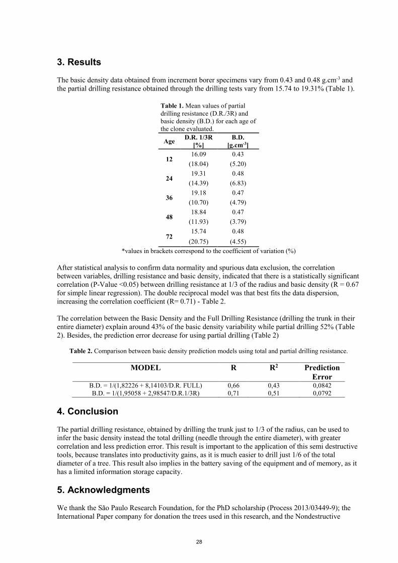
3. Results

The basic density data obtained from increment borer specimens vary from 0.43 and 0.48 g.cm-3 and the partial drilling resistance obtained through the drilling tests vary from 15.74 to 19.31% (Table 1).

Table 1. Mean values of partial drilling resistance (D.R./3R) and basic density (B.D.) for each age of the clone evaluated.

Age D.R. 1/3R[%]

B.D.[g.cm-3]

12 16.09 0.43

(18.04) (5.20)

24 19.31 0.48

(14.39) (6.83)

36 19.18 0.47

(10.70) (4.79)

48 18.84 0.47

(11.93) (3.79)

72 15.74 0.48

(20.75) (4.55) *values in brackets correspond to the coefficient of variation (%)

After statistical analysis to confirm data normality and spurious data exclusion, the correlation between variables, drilling resistance and basic density, indicated that there is a statistically significant correlation (P-Value <0.05) between drilling resistance at 1/3 of the radius and basic density (R = 0.67 for simple linear regression). The double reciprocal model was that best fits the data dispersion, increasing the correlation coefficient (R= 0.71) - Table 2.

The correlation between the Basic Density and the Full Drilling Resistance (drilling the trunk in their entire diameter) explain around 43% of the basic density variability while partial drilling 52% (Table 2). Besides, the prediction error decrease for using partial drilling (Table 2)

Table 2. Comparison between basic density prediction models using total and partial drilling resistance.

MODEL R R2 Prediction Error

B.D. = 1/(1,82226 + 8,14103/D.R. FULL) 0,66 0,43 0,0842 B.D. = 1/(1,95058 + 2,98547/D.R.1/3R) 0,71 0,51 0,0792

4. Conclusion

The partial drilling resistance, obtained by drilling the trunk just to 1/3 of the radius, can be used to infer the basic density instead the total drilling (needle through the entire diameter), with greater correlation and less prediction error. This result is important to the application of this semi destructive tools, because translates into productivity gains, as it is much easier to drill just 1/6 of the total diameter of a tree. This result also implies in the battery saving of the equipment and of memory, as it has a limited information storage capacity.

5. Acknowledgments

We thank the São Paulo Research Foundation, for the PhD scholarship (Process 2013/03449-9); the International Paper company for donation the trees used in this research, and the Nondestructive

28

Testing Laboratory of the School of Agricultural Engineering (FEAGRI) of University of Campinas (UNICAMP) for the facilities. Reference list Eckard, T.J.; Isik, F.; Bullock, B.; Li, B.; Gumpertz, M. 2010. Selection efficiency for solid wood traits in Pinus taeda using time-of-flight acoustic and micro-drill resistance methods. Forest Science. 56(3): 233-241. Görlacher, R.; Hättich, R. 1990. Untersuchung von altern Konstruktionsholz: Die Bohrwiderstandsmessung. Bauen mit Holz. 92: 455-459. Gwaze, D.; Stevenson, A. 2008. Genetic variation of wood density and its relationship with drill resistance in shortleaf pine. Southern Journal of Applied Forestry. 32(3): 130-133. Isik, F.; Li, B. 2003. Rapid assessment of wood density of live trees using the Resistograph for selection in tree improvement programs. Canadian Journal of Forestry Research. 33: 2427-2435. Oliveira, J.T.; Wang, X.; Vidaurre, G.B. 2017. Assessing specific gravity of young eucalyptus plantation trees using a resistance drilling technique. Holzforschung. 71(2):137-145. Rinn, F.; Schweingruber, F.H.; Schar, E. 1996. Resistograph and x-ray density charts of wood comparative evaluation of drill resistance profiles and x-ray density charts of different wood species. Holzforschung. 50(4): 303-311. SPRAGUE, J. R.; TALBERT, J. T.; JETT, J. B.; BRYANT, R. L. 1983. Utility of the Pilodyn in selection for mature wood specific gravity in loblolly pine. Forest Science. 29(4): 696-701. Wiemann, M.C.; Williamson, G.B. 2012. Testing a novel method to approximate wood specific gravity of trees. Forest Science. 58: 577-591. Wiemann, M.C.; Williamson, G.B. 2013. Biomass determination using wood specific gravity from increment cores. Gen. Tech. Rep. FPL–GTR–225. Madison, WI: U.S. Department of Agriculture, Forest Service, Forest Products Laboratory. 7p.

29

Measurement and Genetic Improvement Potential of Young Eucalypt Plantation Veneer-Wood Quality Jian-zhong Luo* China Eucalypt Research Centre, Chinese Academy of Forestry, Zhanjiang, Guangdong, China, luojz69@hotmail.com

Luo-xin Liu China Eucalypt Research Centre, Chinese Academy of Forestry, Zhanjiang, Guangdong, China, cnllx2015@163.com

Chu-biao Wang China Eucalypt Research Centre, Chinese Academy of Forestry, Zhanjiang, Guangdong, China, scauwcb@163.com

Wan-hong Lu China Eucalypt Research Centre, Chinese Academy of Forestry, Zhanjiang, Guangdong, China, luwanhong@outlook.com

Yan Lin e-mail: liny10000@126.com

Roger J Arnold China Eucalypt Research Centre, Chinese Academy of Forestry, Zhanjiang, Guangdong, China, contactroger@yahoo.com.au

* Corresponding author

Abstract China’s high production of plywood (50 million m3/yr) has created buoyant demand for domestically produced veneer logs. In recent years, China were intensively using fast-growing high-yielding eucalypt plantations to provide veneers for plywood. The eucalypt plantations supplying these logs were mostly established for pulpwood and harvested at age of 5-8 years. Study results showed there were significant potential to breed for eucalypt veneer-wood. But, not like pulp-wood traits, Veneer quality traits are harder to measure and less studied. A set of efficient nondestructive measurement method for important quality traits is critical to eucalypt veneer-wood breeding. To see if reliable prediction of important veneer traits can be made by standing tree measurement and their potential on genetic improvement . We measured 10 eucalypt clones from different taxa at 3 processing stages. The 1st was on standing trees. We measured wood density, growth strains, and acoustic wave velocity. The 2nd stage was when trees were cut down. We measured circularity, sweep and taper, knot index and end split on logs. The 3rd stage was on veneers after logs were rotary peeled, split, check, surface hole and knot, torn grain, width shrinkage on veneers were measured. Regression analyses were used to examine relationships of the traits from different stages’ measurements. The results showed if the measurements on standing trees can give promise to a breeding selection for veneer products. Genetic improvement potential on important veneer traits through variety selection also been discovered.

Keywords: veneer, eucalypt, nondestructive measurement, wood quality, genetic improvement

30

Introduction General information

The rapid increase in plywood production in China have brought us to use small logs (small end diameters down to 6 cm) from our fast-growing high-yielding eucalypt plantations to provide the veneers for industrial and construction grade plywood. As the majority of eucalypt plantation area was originally intended for pulpwood production, both the selection of clones and varieties by growers for plantation establishment and also the tree improvement effort in China has focused primarily key traits for pulp production – namely volume yield, wood basic density and pulp yield (Turnbull 2007; Luo et al. 2011). There are strong demands on eucalypt veneer breeding in China in regards to the upgrade and suitability for veneer production.

Whilst plantation grown eucalypt logs from Chinese plantations are known to have many desirable attributes such as generally low taper, good straightness, desirable average wood density, stiffness and wood surface texture (Jiang et al. 2007) that make them desirable for veneer production, there is little information available as to the variability of other important veneer traits and how such variation can affect both veneer qualities and recovery of veneers. As Veneer sheet traits such as dimension stability as well as hardness have important impacts on their products.

Determining the quality of trees and logs for veneer can be extremely difficult because a judgement has to be made on the quality of the wood without actually being able to see most of their intrinsic properties. But, like the relationship between other raw material and their products and semi-products, tree and log traits can be closely related with veneer qualities. If a set of efficient nondestructive measurement method on trees and logs for important veneer quality traits can be developed. Veneer-wood breeding will be vigorously promoted.

In this current study trees of 22 eucalypt families were sampled from a field trial at age 5 years – about the average rotation length for many eucalypt plantations in China. The standing trees were assessed for growth traits and their outer-wood properties non-destructively. After felling, the exterior form and quality of cut logs were assessed and then veneer obtained from the logs was assessed for a range of quality traits. These trait measures were then used to examine the relationships of the various traits with veneer recovery and quality.

Materials and methods

Trial site

The field trial was located in Fusui County of Congzuo City in the far south west of Guangxi Autonomous region – latitude 22° 24' N, longitude 107° 54' and elevation about 150 m above sea level. The climate of Fusui County is a humid, tropical, maritime monsoon climate with a mean annual temperature of 21.3oC; mean annual rainfall of 1250 mm; typhoon of different level can occur in Summer.

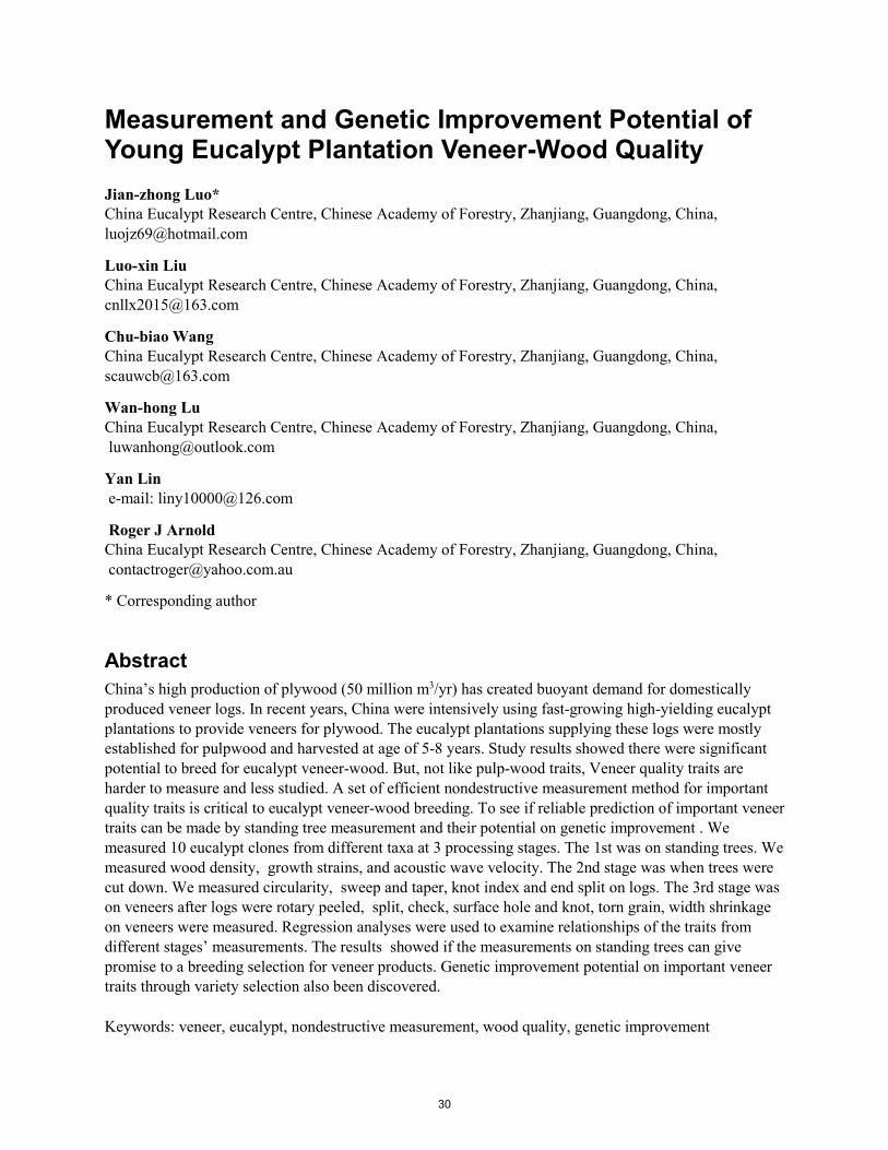
Genetic material This study included a total of 22 eucalypt families, mostly inter species hybrids – details of these clones

31

are provided in Table 1. All these families were control pollinated artificial progenies. Among them, E.urophylla × grandis is the most populary using hybrid both for pulp&paper and for veneer in warmer regions of southern China.

Table 1 Taxonomy of the eucalypt hybrids in the field trial in Suixi County, China, established in 2004.

Species type

Species Number of families

1 E. pellita × urophylla 4

2 E. urophylla × pellita 11

3 E. urophylla × grandis 3

4 E. urophylla × tereticornis 2

5 E. pellita × pellita 1

6 E. urophylla (open pollinated) 1

Trial design and establishment

The trial was planted in September 2014 and laid out with 6 replicates in a randomized complete block design. Each of the 22 families was represented as a block plot of one row of 5 trees in each replicate, with 2.0 m between trees within rows and 3.0 m between rows – a stocking of 1650 tree ha-1.

Assessments on standing trees

In May 2019, all living trees were assessed for diameter at breast height (1.3 m) over bark, total height

and assessed non-destructively or light destruct) for the following wood properties: 5mm wood core

taking at 1.3 m height for wood density measurement. Acoustic wave velocity – acoustic velocity

between two probes in the outer-wood of the trees was measured between 0.3 m and 1.6 m height on each

tree using a Fakopp 2D tool (Fakopp Enterprises, Hungary), three readings (t) were taken per tree and

averaged (to provide a single mean value for each tree). The value were use to calculate velocity ( V=D/t,

D=1.3m). Wood modulus of elasticity (MOE ) then be calculated (E=ρV2,ρ is wood density ).

(Grabianowski et al. 2004). Growth stain (GS) measured using France longitudinal growth stain device

(Zhao et al, 2007).

32

Destructive sampling and peeling

The first 5 acceptable trees (trees stunted or malformed were regarded as unacceptable) with around average DBH (family mean±30%) in the middle row of each plot in the first replicate were selected for felling and sampling . from the first replicate and, if necessary, also from the second replicate, were selected for felling.

Sample trees were felled to a stump height of approximately 20 cm. The felled trees were then cross cut into 1.3 m log lengths – the standard log length sought by many veneer manufactures in southern China. From each felled tree, the first and third log (progressing upwards from the butt) were collected and labeled. The logs were then transported into a shed for storage under shade to prevent excessive water loss.

A total of 110 trees were felled to provide 220 logs – 2 trees from each of the 22 families. Log identities were carefully marked and maintained for each of the logs through to completion of veneering. On each of these logs, the following traits were measured:

the exact length;

maximum and minimum diameter (under bark) of the large end of the log;

maximum and minimum diameter (under bark) of the small end of the log;

sweep – maximum deviation of the centre line of the log from a straight line between the midpoints of the two ends;

end splits at the big end，end splits of the small end； number of knots and branch stubs visible on log surface (before removing bark);

From this data, the following parameters were derived:

Log volume (V) = [((D1 + D2) / 4)2 + ((D3 + D4) / 4) 2 ] / 2 × π × L

Where: V is the log volume (m³);

D1 and D2 are the maximum and minimum diameters of the large end of the log (m);

D3 and D4 are the maximum and minimum diameters of the small end of the log (m);

L is the log length (m);

Sweep (Z) = S / L × 100

Where: Z is the % sweep;

S is the maximum deviation of the centre line of the log from a straight-line between the mid points of the two ends (m);

L is the length of the log (m)

Taper T = [((D1 + D2) / 2) – ((D3 + D4) / 100)] / L × 100

Where: T is log taper (%);

33

Circularity of the large end (CL) = (D2 / D1 ) x 100

Where: CL is the circularity of the large end of the log (%);

Circularity of the small end (CS) = (D3 / D4 ) x 100

Where: CS is the circularity (%);

Heart wood volume （VH）were calculated using the same equation as Log volume by measuring heart wood diameter of each log.

Veneer peeling and assessment All the sample logs were processed for veneer using a Chinese manufactured rotary veneer peeling lathe powered by a 20.3 KW electrical engine. This lathe was set to produce veneer of 2.2 mm green thickness for this study.

The veneer sheets produced by the lathe were cross-cut to sections of approximately 680 mm, so veneer sheets produced were approximately 1270 × 680 mm (longitudinal × tangential). For this study, only whole sheets of the latter dimension were collected for examination. Green volume recoveries for each log were calculated based on actual sheet dimensions of all individual whole sheets. Partial or incomplete sheets were discarded and not included in green recovery.

All sheets were visually graded according to the Chinese veneer grading standard “LY/T 1599-2002” . On each sheet quantitative measurements were also taken on fresh and air-dry with (to calculate width shrinkage), dead knots, live knots, holes, and end splits.

Statistical analyses Data were analysed using SAS statistical software (SAS 1999). The general linear models procedure (PROC GLM in SAS) was used to compute family trait means and then to examine the significance of differences between them for the traits assessed and estimate the Least Significant Differences (LSD, at P<0.05) between family means for each trait. The correlation procedure (PROC COR) was used to obtain simple correlations, and the significance of these, between pairs of traits for various tree, log and veneer quality traits.

Results and discussion

Correlations

Correlations of veneer recovery and quality traits with various tree and log traits are presented in Table 1. Of all the tree traits assessed, only 4 of them showed significant correlations with 2 veneer traits: MOE (r = -0.243) and wood density (r =-0.297) with split length; tree volume (r =- 0.615) and bark thickness (r = -0.263) with knot number. This means that higher MOE and higher wood density will result in lower veneer split length. As MOE is a function of wood density, and the correlation between wood density and split length is higher than that of MOE’s. So, wood density is a better indicator of veneer end split length. The correlations between tree volume and bark thickness with veneer knot number imply that larger and thicker bark trees tend to have less knot. It’s easy to understand that a same number of knots on big and small trees will result in smaller number of knots per area of peeled veneer on big trees. The correlation between bark thickness and knot is hard to explain and worth to do further study.

34

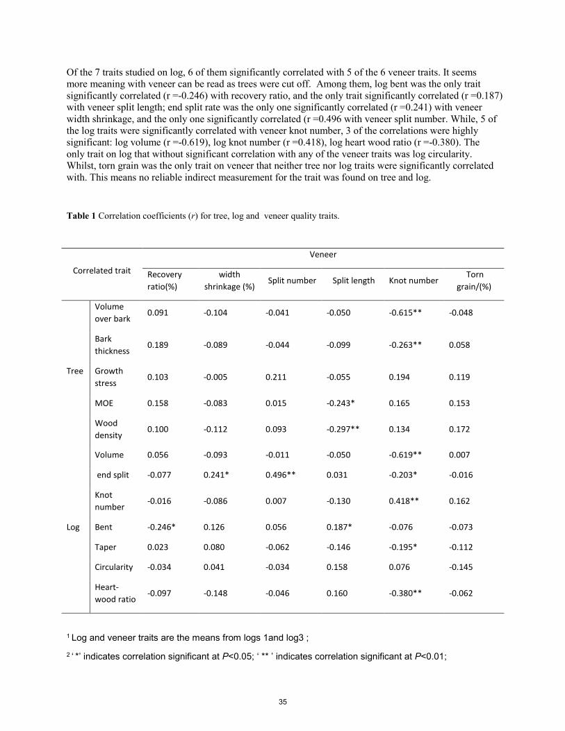
Of the 7 traits studied on log, 6 of them significantly correlated with 5 of the 6 veneer traits. It seems more meaning with veneer can be read as trees were cut off. Among them, log bent was the only trait significantly correlated (r =-0.246) with recovery ratio, and the only trait significantly correlated (r =0.187) with veneer split length; end split rate was the only one significantly correlated (r =0.241) with veneer width shrinkage, and the only one significantly correlated (r =0.496 with veneer split number. While, 5 of the log traits were significantly correlated with veneer knot number, 3 of the correlations were highly significant: log volume (r =-0.619), log knot number (r =0.418), log heart wood ratio (r =-0.380). The only trait on log that without significant correlation with any of the veneer traits was log circularity. Whilst, torn grain was the only trait on veneer that neither tree nor log traits were significantly correlated with. This means no reliable indirect measurement for the trait was found on tree and log.

Table 1 Correlation coefficients (r) for tree, log and veneer quality traits.

Correlated trait

Veneer

Recovery ratio(%)

width shrinkage (%)

Split number Split length Knot number Torn

grain/(%)

Tree

Volume over bark

0.091 -0.104 -0.041 -0.050 -0.615** -0.048

Bark thickness

0.189 -0.089 -0.044 -0.099 -0.263** 0.058

Growth stress

0.103 -0.005 0.211 -0.055 0.194 0.119

MOE 0.158 -0.083 0.015 -0.243* 0.165 0.153

Wood density

0.100 -0.112 0.093 -0.297** 0.134 0.172

Log

Volume 0.056 -0.093 -0.011 -0.050 -0.619** 0.007

end split -0.077 0.241* 0.496** 0.031 -0.203* -0.016

Knot number

-0.016 -0.086 0.007 -0.130 0.418** 0.162

Bent -0.246* 0.126 0.056 0.187* -0.076 -0.073

Taper 0.023 0.080 -0.062 -0.146 -0.195* -0.112

Circularity -0.034 0.041 -0.034 0.158 0.076 -0.145

Heart-wood ratio

-0.097 -0.148 -0.046 0.160 -0.380** -0.062

1 Log and veneer traits are the means from logs 1and log3 ;

2 ‘ *’ indicates correlation significant at P<0.05; ‘ ** ’ indicates correlation significant at P<0.01;

35

Genetic variation

Analyses of variance revealed different variation pattern between genetic material (testing families) for veneer quality traits (Table 3). The difference for veneer split number, split length and knot number were significant. But for veneer width shrinkage and torn grain were not significant.

Veneer width shrinkage varied from 4.99% to 8.34%. But the variation didn’t show it’s significance between the tested families. Hence can’t be improved by using different genetic material. It was also the case on veneer torn grain. Torn grain ratio of all the genetic material were general low (0~3.54%).

For the 3 traits with significant genetic difference, Veneer split number of the families were mainly between 3.1~6.6, only one family was 7.4 (fam 160). Split length of the families were between 8.5mm~21.8mm. There were 3 families’ split length were higher than 20mm. As the highest values of the 2 traits were more than double of the lowest. This means they can be improved more than 50% by using better genetic material. Veneer knot number was 33.0~58.0 for the families. Though the range was not very wide. The significance was very high (P<0.01). Previous study on eucalypt veneer found both dead knot grade and end splits in veneer sheets were associated with the largest percentage of the variance in veneer grade (Luo et al. 2013). And, our correlation analyses showed there were a number of tree and/or log traits higher correlated with these traits. Means they can be measured by nondestructive way on trees/logs. That can significantly facilitate they genetic improvement.

Table 3 Veneer sheet quality of the testing eucalytp families.

fam species N veneer shrinkage(%)

veneer split number

veneer split length(mm)

veneer knot number

veneer torn grain(%)

2 E.pellita×urophylla 5 6.56 5.7 18.3 42.8 0.54

3 E.pellita×urophylla 5 7.13 5.3 14.8 41.1 1.32

4 E.pellita×urophylla 5 7.03 5.5 16.1 40.9 1.02

7 E.pellita×urophylla 5 7.55 4.0 11.7 41.7 0.50

8 E.urophylla×grandis 5 4.99 4.9 15.7 37.1 2.46

10 E.urophylla×pellita 5 6.38 4.3 13.1 40.8 1.14

11 E.urophylla×pellita 2 5.65 3.1 13.7 48.2 0.00

14 E.urophylla×pellita 5 6.87 4.3 12.7 49.3 1.12

15 E.urophylla×pellita 5 7.55 6.4 21.3 44.2 0.78

16 E.urophylla×pellita 5 8.28 5.4 19.5 50.9 0.30

18 E.urophylla×pellita 5 6.51 4.4 13.4 41.9 0.54

19 E.urophylla×pellita 5 6.36 6.6 21.8 39.2 0.28

20 E.urophylla×pellita 5 7.22 4.9 20.5 33.0 0.46

36

25 E.pellita×pellita 3 5.77 3.2 8.5 48.8 3.33

26 E.urophylla×pellita 5 7.11 6.4 15.0 39.3 1.88

29 E.urophylla×grandis 5 6.18 3.3 11.7 46.8 1.72

31 E.urophylla×pellita 5 8.34 6.2 15.2 39.7 3.54

32 E.urophylla×pellita 5 5.86 3.3 12.7 39.2 3.38

33 E.urophylla(OP) 5 7.25 4.7 12.5 36.4 1.94

37 E.urophylla×grandis 5 6.32 4.2 12.7 42.5 1.74

40 E.urophylla×grandis 5 5.43 3.5 14.7 58.0 0.72

111 E.urophylla×tereticornis 5 6.70 5.8 13.9 52.4 1.04

160 E.urophylla×tereticornis 5 7.69 7.4 15.5 45.8 3.20

mean 6.73 4.90 15.00 43.49 1.43

Pr > F 0.1976 0.0130 0.0013 0.0040 0.1999

Conclusions Significant correlations were found between standing tree and/or log traits with veneer quality traits on young eucalypts. These will enable the nondestructive measurement on amount of veneer quality traits. Veneer end splits and knot number were the traits with higher significance and correlated with more tree and log traits.

Some young eucalypt veneer quality traits were significantly different between genetic materials. Such as veneer split number, split length and knot number. They have good potential on genetic improvement. But veneer width shrinkage and torn grain were not significantly different between genetic materials. This made them hard to improve by genetic selection method.

Didn’t find good nondestructive or indirect measurement way for some important veneer quality trait , such as torn grain. Many important veneer quality traits also need better nondestructive measurement method. Further study and progress on them can lead to constructive progress on their genetic improvement.

Acknowledgments We thank the China Eucalypt Research Center and Stora Enso Guangxi for the providing and supporting

the field trial establishment and management. Special thanks are also due to Li Peng, Cheng Youxu, Chen

Wenping and Jian ming for assistance with collection of data and processing of veneer .

37

References Arnold, R.J., Xie, Y.J., Midgley, S.J., Luo, J.Z., & Chen, X.F. 2013. Emergence and rise of eucalypt veneer production in china. International Forestry Review, 15(1), 33-47.

CNAS .2002. People’s Republic of China Veneer Grading Standard: Rotary Veneer (LY/T 1599–2002). Issued 12/10/2002. National Accreditation Service for Conformity Assessment, Beijing.

Hamilton, M. G., Blackburn, David P., McGavin, Robert L., Baillères, Henri, Vega, Mario, & Potts, Brad M. 2015. Factors affecting log traits and green rotary-peeled veneer recovery from temperate eucalypt plantations. Annals of Forest Science, 72(3), 357-365.

Jiang X, Ye K, Lu J, Zhao Y, Yin Y. 2007. Guide on utilisation of Eucalyptus and Acacia plantations in China for solid wood products. Science Press, Beijing

Luo, J., Roger Arnold, Shiqi Ren, Ying Jiang, & Wanhong Lu. 2013. Veneer grades, recoveries, and values from 5-year-old eucalypt clones. Annals of Forest Science, 70(4), 417-428.

Petry, M., Lei, Z., Zhan, S. 2010. China Forest Products Annual Report 2010. USDA Gain Report CH100042. USDA Foreign Agricultural Service, Beijing.

REN, S.Q., LUO, J.Z., PENG, Y., XIE, Y.J., LU, W.H., CAO,J.G. and JIANG, Y. 2010. A study on veneer recovery ratio and value of eucalypt clones. Acta Prataculturae Sinica 19(6): 46–54. [In Chinese].

Wan M .2009. Analysis of China’s primary wood products market—Sawnwood and Plywood Thesis, University of Helsinki

ZHAO, Rongjun, Benhua, JIANG, & Zehui. 2007. Eucalypt wood anatomical and physical properties and their effects on plywood veneer quality. Chinese Forestry Science and Technology(3), 33-39.

38

Automated Measurement of Stilbenes from Solid Scots Pine (Pinus sylvestris L.) Heartwood Anni Harju * Production Systems, Natural Resources Institute Finland (Luke), Savonlinna, Finland, anni.harju@luke.fi Martti Venäläinen Production Systems, Natural Resources Institute Finland (Luke), Savonlinna, Finland, martti.venalainen@luke.fi * Corresponding author Abstract Extractives provide Scots pine heartwood natural defense against fungal decay, which makes it a valuable renewable material for safe and ecological wood products. There is, however, high natural variation in extractive content and durability among individual trees and among pieces of sawn timber. In laboratory experiments, the content of phenolic stilbenes in the heartwood has been related to decay resistance against brown-rot fungi. A fast and reliable nondestructive technology to measure stilbene content from the surface of solid wood specimens would give potential to grade heartwood according to its predicted decay resistance. We studied whether an automated method based on UV-fluorescence of stilbenes would be a cost-effective approach to estimate stilbene content and to predict decay resistance of Scots pine heartwood. If so, the stilbene-rich heartwood suitable for demanding applications would be separated, and the rest would be used for less demanding applications. The direction of assorted timber for optimal applications would add the value of heartwood in the whole production chain. Optimal and sparing use of nonhazardous naturally decay resistant heartwood will enhance the green bioeconomy. Preliminary results from our project will be presented. Keywords: Optical measurement, decay resistance, grading, wood quality, extractives

39

Improving Knot Segmentation Using Deep Learning Techniques

Stefano Giovannini Department of Information Engineering (DEI), Università di Padova Davide Boschetto Microtec GmbH, Venice, Italy, davide.boschetto@microtec.eu Enrico Vicario Microtec GmbH, Venice, Italy, enrico.vicario@microtec.eu Mauro Cossi Microtec GmbH, Venice, Italy, mauro.cossi@microtec.eu Andrea Busatto Microtec GmbH, Venice, Italy, andrea.busatto@microtec.eu Stefano Ghidoni Department of Information Engineering (DEI), Università di Padova, ghidoni@dei.unipd.it Enrico Ursella * Microtec GmbH, Venice, Italy, enrico.ursella@microtec.eu Dipartimento di Scienze Ambientali, Informatica e Statistica, Università Ca’ Foscari Venezia

* Corresponding author

Abstract In the context of Computed Tomography scanning of logs, accurate detection of knots is key for delivering a successful product. Reliable detection of knots in the sapwood is hard with traditional computer vision techniques, because of the different density conditions between sapwood and heartwood. The advancements provided by deep learning in the field of semantic image segmentation kick-started a new way of approaching such problems: deep neural networks can be trained on large amounts of labelled data and successfully employed in production environments to improve the performances on knot detection. Adapting state-of-the-art network architectures and using more than 10.000 labelled knots from pine and spruce logs, we were able to develop a new two-step approach for identifying knots in CT scans of logs with unprecedented accuracy while at the same time satisfying the time constraints that a real-time industrial application needs. The first step runs on the log’s axis, while the second runs on each candidate knot’s axis. False positives from the first step are very rare (even with dry/dried logs), so no computational power is wasted for non-existing knots. Using this approach, we are able to see the internal defects of a log in real time in the production chain without having to cut it first, therefore being able to optimize even more the output of the chain on each client’s requirements.

Keywords: CNN, U-Net, semantic segmentation, knot detection, CT, dead knot border

Introduction Computed Tomography (CT) for production optimization in sawmills has been a reality for a few years. CT Log (Giudiceandrea et al., 2011) is a CT scanner produced by Microtec able to measure logs at up to 180m/min, compute a model of the internal features of each log and optimize the entire process based on the characteristics of the raw material and the production requests of the sawmill. The steps of bucking, sorting and optimizing the cutting pattern can be improved with the use of the internal information provided by computed tomography. Many works demonstrated the economic advantage of optimizing the sawing process with the use of CT images (Rais et al., 2017) (Berglund et al., 2013) (Stangle et al., 2015).

The automatic detection of the internal features of a log from CT images has been addressed by many works, especially for knots detection (Andreu at al 2003) (Breinig et al., 2012) (Fredriksson et al., 2017) (Cool et al., 2017) (Longuetaud et al., 2012). Only a few of them (Oja, 2000) (Johansson et al.,

40

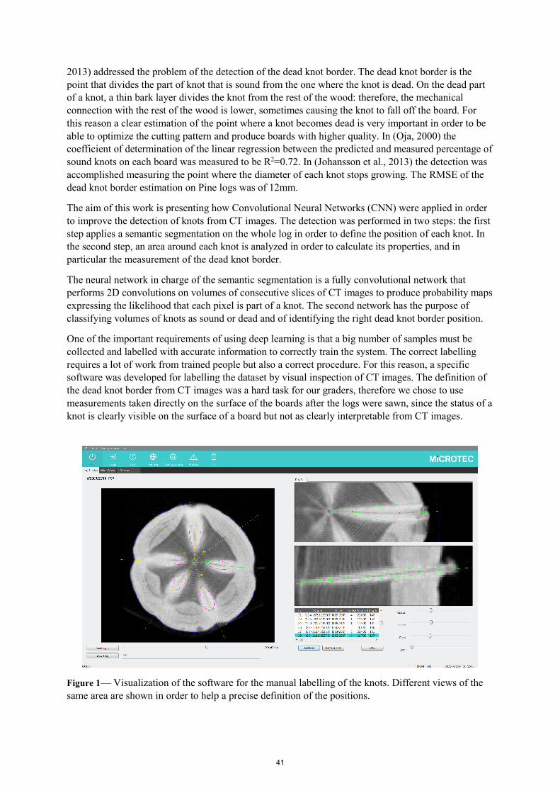
2013) addressed the problem of the detection of the dead knot border. The dead knot border is the point that divides the part of knot that is sound from the one where the knot is dead. On the dead part of a knot, a thin bark layer divides the knot from the rest of the wood: therefore, the mechanical connection with the rest of the wood is lower, sometimes causing the knot to fall off the board. For this reason a clear estimation of the point where a knot becomes dead is very important in order to be able to optimize the cutting pattern and produce boards with higher quality. In (Oja, 2000) the coefficient of determination of the linear regression between the predicted and measured percentage of sound knots on each board was measured to be R2=0.72. In (Johansson et al., 2013) the detection was accomplished measuring the point where the diameter of each knot stops growing. The RMSE of the dead knot border estimation on Pine logs was of 12mm.

The aim of this work is presenting how Convolutional Neural Networks (CNN) were applied in order to improve the detection of knots from CT images. The detection was performed in two steps: the first step applies a semantic segmentation on the whole log in order to define the position of each knot. In the second step, an area around each knot is analyzed in order to calculate its properties, and in particular the measurement of the dead knot border.

The neural network in charge of the semantic segmentation is a fully convolutional network that performs 2D convolutions on volumes of consecutive slices of CT images to produce probability maps expressing the likelihood that each pixel is part of a knot. The second network has the purpose of classifying volumes of knots as sound or dead and of identifying the right dead knot border position.

One of the important requirements of using deep learning is that a big number of samples must be collected and labelled with accurate information to correctly train the system. The correct labelling requires a lot of work from trained people but also a correct procedure. For this reason, a specific software was developed for labelling the dataset by visual inspection of CT images. The definition of the dead knot border from CT images was a hard task for our graders, therefore we chose to use measurements taken directly on the surface of the boards after the logs were sawn, since the status of a knot is clearly visible on the surface of a board but not as clearly interpretable from CT images.

Figure 1— Visualization of the software for the manual labelling of the knots. Different views of the same area are shown in order to help a precise definition of the positions.

41

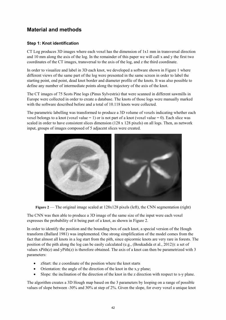
Material and methods

Step 1: Knot identification

CT Log produces 3D images where each voxel has the dimension of 1x1 mm in transversal direction and 10 mm along the axis of the log. In the remainder of this paper we will call x and y the first two coordinates of the CT images, transversal to the axis of the log, and z the third coordinate.

In order to visualize and label in 3D each knot, we developed a software shown in Figure 1 where different views of the same part of the log were presented in the same screen in order to label the starting point, end point, dead knot border and diameter profile of the knots. It was also possible to define any number of intermediate points along the trajectory of the axis of the knot.

The CT images of 75 Scots Pine logs (Pinus Sylvestris) that were scanned in different sawmills in Europe were collected in order to create a database. The knots of those logs were manually marked with the software described before and a total of 10.118 knots were collected.

The parametric labelling was transformed to produce a 3D volume of voxels indicating whether each voxel belongs to a knot (voxel value = 1) or is not part of a knot (voxel value = 0). Each slice was scaled in order to have consistent slices dimension (128 x 128 pixels) on all logs. Then, as network input, groups of images composed of 5 adjacent slices were created.

Figure 2 — The original image scaled at 128x128 pixels (left), the CNN segmentation (right)

The CNN was then able to produce a 3D image of the same size of the input were each voxel expresses the probability of it being part of a knot, as shown in Figure 2.

In order to identify the position and the bounding box of each knot, a special version of the Hough transform (Ballard 1981) was implemented. One strong simplification of the model comes from the fact that almost all knots in a log start from the pith, since epicormic knots are very rare in forests. The position of the pith along the log can be easily calculated (e.g., (Boukadida et al., 2012)): a set of values xPith(z) and yPith(z) is therefore obtained. The axis of a knot can then be parametrized with 3 parameters:

• zStart: the z coordinate of the position where the knot starts• Orientation: the angle of the direction of the knot in the x,y plane;• Slope: the inclination of the direction of the knot in the z direction with respect to x-y plane.

The algorithm creates a 3D Hough map based on the 3 parameters by looping on a range of possible values of slope between -30% and 30% at step of 2%. Given the slope, for every voxel a unique knot

42

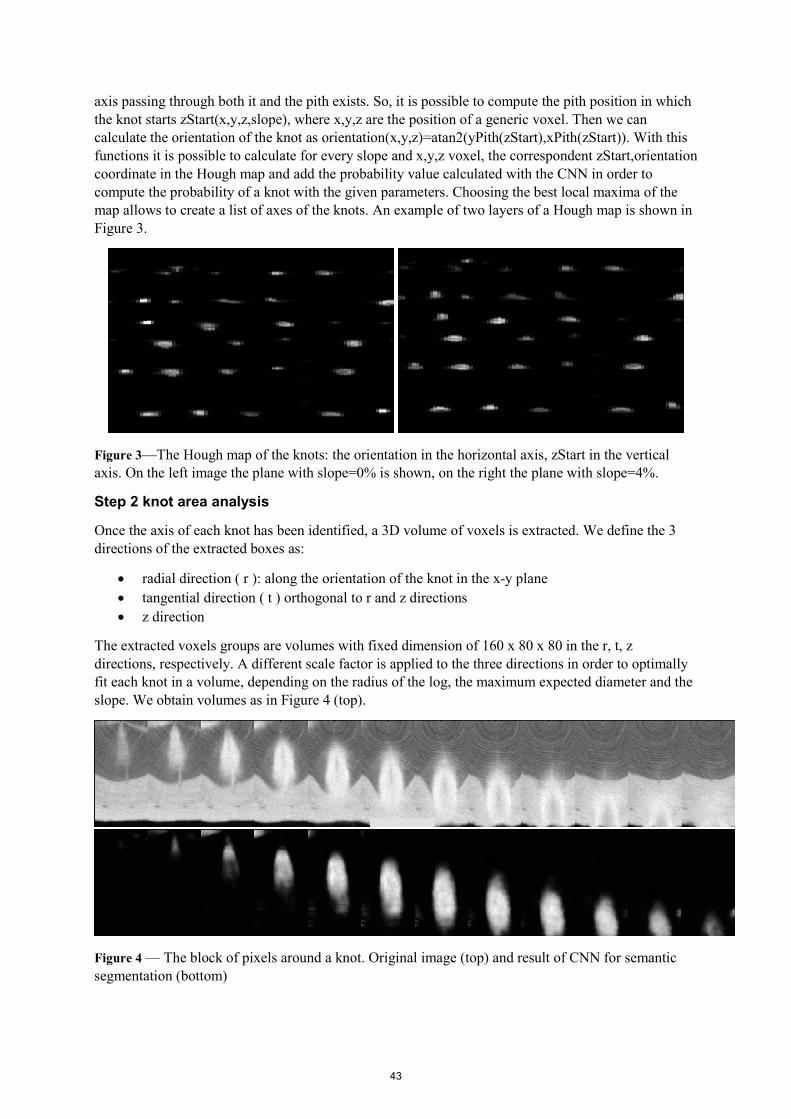
axis passing through both it and the pith exists. So, it is possible to compute the pith position in which the knot starts zStart(x,y,z,slope), where x,y,z are the position of a generic voxel. Then we can calculate the orientation of the knot as orientation(x,y,z)=atan2(yPith(zStart),xPith(zStart)). With this functions it is possible to calculate for every slope and x,y,z voxel, the correspondent zStart,orientation coordinate in the Hough map and add the probability value calculated with the CNN in order to compute the probability of a knot with the given parameters. Choosing the best local maxima of the map allows to create a list of axes of the knots. An example of two layers of a Hough map is shown in Figure 3.

Figure 3—The Hough map of the knots: the orientation in the horizontal axis, zStart in the vertical axis. On the left image the plane with slope=0% is shown, on the right the plane with slope=4%.

Step 2 knot area analysis

Once the axis of each knot has been identified, a 3D volume of voxels is extracted. We define the 3 directions of the extracted boxes as:

• radial direction ( r ): along the orientation of the knot in the x-y plane• tangential direction ( t ) orthogonal to r and z directions• z direction

The extracted voxels groups are volumes with fixed dimension of 160 x 80 x 80 in the r, t, z directions, respectively. A different scale factor is applied to the three directions in order to optimally fit each knot in a volume, depending on the radius of the log, the maximum expected diameter and the slope. We obtain volumes as in Figure 4 (top).

Figure 4 — The block of pixels around a knot. Original image (top) and result of CNN for semantic segmentation (bottom)

43

One possible solution is to perform a new semantic segmentation on these knot blocks. The analysis of the dimension and center of the segmented voxels along the r direction allowed to compute the direction, dimension and length. The dead knot border is calculated as the point where the dimension of the knot stops growing along the r direction.

In order to improve performances specifically on the detection of the dead knot border and knot diameter, a more reliable ground truth, specific to these two metrics, is needed. The only way to extract reliable ground truth on those metrics was to check the appearance of the knots on board surfaces instead of using CT images. 13 logs of Scots Pine were scanned with a CT Log scanner, sawn in thin boards 15mm thick and the knots were manually measured on the surface of the boards. A reference was taken on the logs by drilling some holes so that it was possible to compute the position of a knot in the CT image given the measured position on the board and vice versa. On the 13 logs, 2412 knots were measured on the surface of the boards.

Figure 5 — An example of reference taken on a log that is CT-scanned and then sawn in boards (left), the manual measurements superimposed on the CT image (right).

In Figure 5 (right) the original CT images are visible with the position of the boards and the measure of the knots taken manually superimposed. In particular, the minimal, maximal diameter, position and dead/sound status were annotated. The information related to each knot was reported in the reference system of the specific block of voxels extracted in order to train a neural network.

The problem is that the requested information (dead knot border and diameter profile) would require a dense ground truth along the radial direction, while only a few manual measurements are available depending on the thickness of the boards and their angle with respect to the knot axis. It was not possible to train a network on the whole knot volume when the ground truth was valid only for a few points along its length (only 1 or 2 points).

To correctly train the network we decided to extract sub-blocks of 11 slices along the r direction around positions where the ground truth was available. Two different networks were trained: one to compute the dead/sound status, the other for the computation of the diameter of the knot.

During the training of the sound/dead network it was possible to extend the ground-truth information also to other points of the knot. If a knot was marked as sound at a certain coordinate r_alive, for obvious biological reasons the knot was alive also at all r<r_alive. For the same reason, if a knot was marked as dead at a certain point, all the subsequent slices have to be marked as dead. This allowed to create a dataset with a high number of samples. At this point the network is able to classify the single slice of a knot to either dead or sound, but it is obviously faster to infer this information by comparing the actual distance of a slice from the pith with the dead knot border value of that knot. To find a

44

knot’s dead knot boder, for computational time constraints, one slice every six was tested. Once the point where the status passes from sound to dead is found, we then refine the detection to pinpoint the exact slice. After the calculation of the dead knot border we verified the performance of the system by comparing the predicted status with the status of the knots in the sawn boards.

As ground truth for the computation of the diameter we decided to use as training set only the slices of knots where there was a manual measurement. An interpolation of the measured diameter in the slices between two consecutive measurements were possible, but it could have reduced the precision of the system. As long as we can consider that branches are not elliptical, we use the minimal diameter measured on the board as the diameter of the knot in the 3D image.

Results

Knots segmentation

To design and train the networks, we used a computer running Windows 10 Pro, Keras 2.2.4 with Tensorflow 1.13.1 as backend. The first network, aimed at semantic segmentation, has a total of 1.962.913 parameters. It follows the U-Net architecture (Ronneberger et al., 2015) with skip connections and convolutional blocks consisting of 2 consecutive convolutional layers. The first layer interprets the channel axis as a depth axis. Starting from an image size of 128x128 with 5 channels, it compresses the image to a size of 8x8 with 256 channels in the center. Then, in the so-called “upward path” of U-Net, the image is upscaled to the original resolution with 1 output class as channel (the probability of a pixel part of the central slice to be part of a knot). Each convolutional layer applies 3x3 kernels, and for the optimization the Adam optimizer has been used with a learning rate of 0.0002 with binary crossentropy as the default loss function. Early stopping and learning rate reduction on plateau have been used during the training process. The inference time for the computation of a log 4.2 m long was 650 ms. All computation times were measured on a computer using an RTX 2080 GPU on an Intel Core i7-4770 3.4GHz.

Dead knot border

In total the 13 logs presented 634 knots. Each knot intersected one or more boards, the manual measurement were taken at those intersections. The 634 knots intersected the boards in 2412 measured points. 1835 knot intersections were randomly chosen for training and validation set (75% for training and 25% for validation). They generated 34917 knot slices with known dead/sound status and used for training and validation of the neural network. 577 knots intersections, belonging to 158 knots, were used for the test of the detection of the final algorithm estimating the dead knot border.

The test of the performance was done comparing the status of the knots manually measured on the boards with the expected status based on the estimated dead knot border. The results are presented in Table 1.

Table 1—Confusion matrix of the classification of the sound/dead knot classification

predicted Sound dead

actu

al

soun

d

301 (88.5%) 39 (16.4%)

dead

39 (11.4%) 198 (83.5%)

45

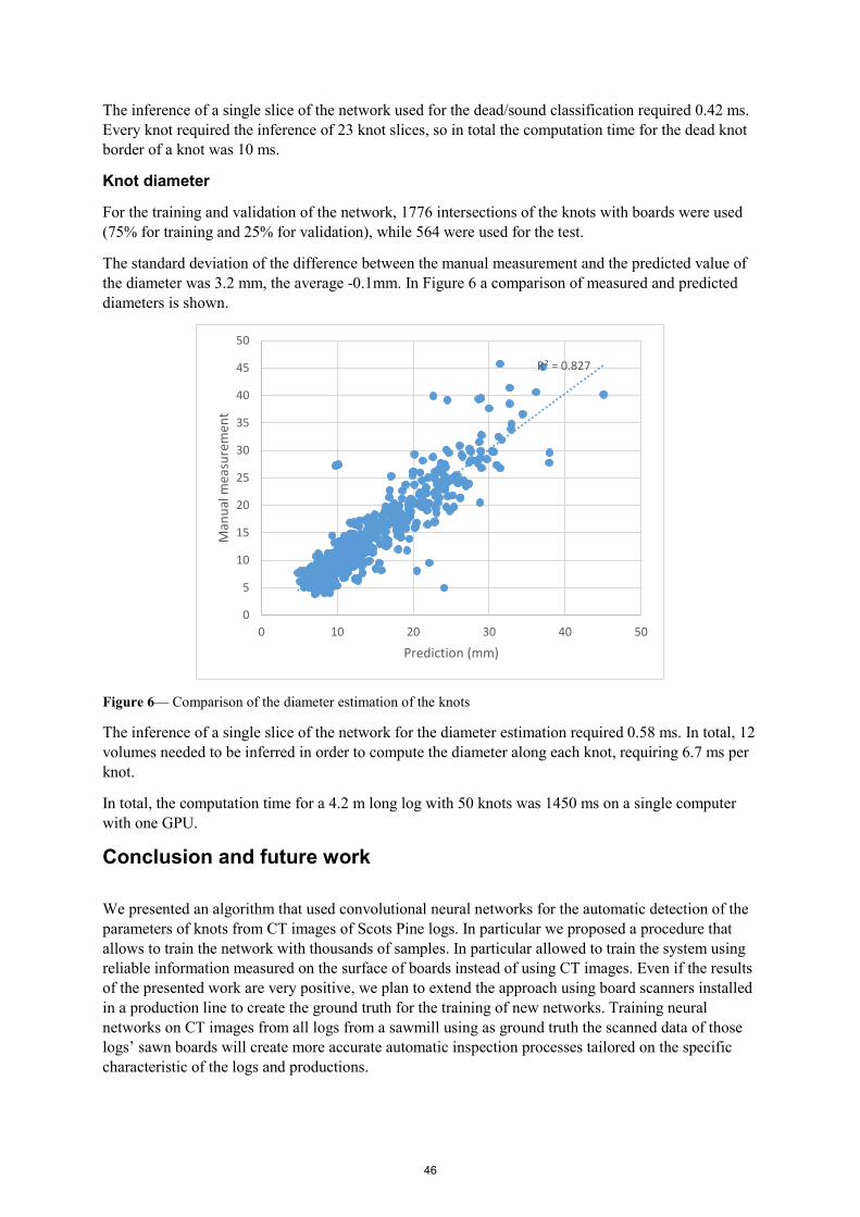
The inference of a single slice of the network used for the dead/sound classification required 0.42 ms. Every knot required the inference of 23 knot slices, so in total the computation time for the dead knot border of a knot was 10 ms.

Knot diameter

For the training and validation of the network, 1776 intersections of the knots with boards were used (75% for training and 25% for validation), while 564 were used for the test.

The standard deviation of the difference between the manual measurement and the predicted value of the diameter was 3.2 mm, the average -0.1mm. In Figure 6 a comparison of measured and predicted diameters is shown.

Figure 6— Comparison of the diameter estimation of the knots

The inference of a single slice of the network for the diameter estimation required 0.58 ms. In total, 12 volumes needed to be inferred in order to compute the diameter along each knot, requiring 6.7 ms per knot.

In total, the computation time for a 4.2 m long log with 50 knots was 1450 ms on a single computer with one GPU.

Conclusion and future work

We presented an algorithm that used convolutional neural networks for the automatic detection of the parameters of knots from CT images of Scots Pine logs. In particular we proposed a procedure that allows to train the network with thousands of samples. In particular allowed to train the system using reliable information measured on the surface of boards instead of using CT images. Even if the results of the presented work are very positive, we plan to extend the approach using board scanners installed in a production line to create the ground truth for the training of new networks. Training neural networks on CT images from all logs from a sawmill using as ground truth the scanned data of those logs’ sawn boards will create more accurate automatic inspection processes tailored on the specific characteristic of the logs and productions.

R² = 0.827

0

5

10

15

20

25

30

35

40

45

50

0 10 20 30 40 50

Man

ual m

easu

rem

ent

Prediction (mm)

46

References

Andreu, Jean-Philippe, and Alfred Rinnhofer. "Modeling of internal defects in logs for value optimization based on industrial CT scanning." Fifth International Conference on Image Processing and Scanning of Wood. Bad Waltersdorf Austria, 2003.

Ballard, D. H. (1981). Generalizing the Hough transform to detect arbitrary shapes. Pattern recognition, 13(2), 111-122.

Berglund, A., Broman, O., Grönlund, A., & Fredriksson, M. (2013). Improved log rotation using information from a computed tomography scanner. Computers and electronics in agriculture, 90, 152-158.

Boukadida, H., Longuetaud, F., Colin, F., Freyburger, C., Constant, T., Leban, J. M., & Mothe, F. (2012). PithExtract: A robust algorithm for pith detection in computer tomography images of wood–Application to 125 logs from 17 tree species. Computers and electronics in agriculture, 85, 90-98.

Breinig, L., Brüchert, F., Baumgartner, R., & Sauter, U. H. (2012). Measurement of knot width in CT images of Norway spruce (Picea abies [L.] Karst.)—evaluating the accuracy of an image analysis method. Computers and electronics in agriculture, 85, 149-156.

Cool, J., Fredriksson, M., & Avramidis, S. (2017). Knot detection in coarse resolution CT images of logs. In 23rd International Wood Machining Seminar, Warsaw, Poland, 28-31 May 2017.

Fredriksson, M., Cool, J., Duchesne, I., & Belley, D. (2017). Knot detection in computed tomography images of partially dried jack pine (Pinus banksiana) and white spruce (Picea glauca) logs from a Nelder type plantation. Canadian Journal of Forest Research, 47(7), 910-915.

Giudiceandrea, F., Ursella, E., & Vicario, E. (2011, September). A high speed CT scanner for the sawmill industry. In Proceedings of the 17th international non destructive testing and evaluation of wood symposium (pp. 14-16). Sopron, Hungary: University of West Hungary.

Johansson, E., Johansson, D., Skog, J., & Fredriksson, M. (2013). Automated knot detection for high speed computed tomography on Pinus sylvestris L. and Picea abies (L.) Karst. using ellipse fitting in concentric surfaces. Computers and electronics in agriculture, 96, 238-245.

Longuetaud, F., Mothe, F., Kerautret, B., Krähenbühl, A., Hory, L., Leban, J. M., & Debled-Rennesson, I. (2012). Automatic knot detection and measurements from X-ray CT images of wood: a review andvalidation of an improved algorithm on softwood samples. Computers and Electronics inAgriculture, 85, 77-89.

Oja, J. (2000). Evaluation of knot parameters measured automatically in CT-images of Norway spruce (Picea abies (L.) Karst.). European Journal of Wood and Wood Products, 58(5), 375-379.

Rais, A., Ursella, E., Vicario, E., & Giudiceandrea, F. (2017). The use of the first industrial X-ray CT scanner increases the lumber recovery value: case study on visually strength-graded Douglas-fir timber. Annals of forest science, 74(2), 28.

Ronneberger, O., Fischer, P., & Brox, T. (2015, October). U-net: Convolutional networks for biomedical image segmentation. In International Conference on Medical image computing and computer-assisted intervention (pp. 234-241). Springer, Cham.

Stängle, S. M., Brüchert, F., Heikkila, A., Usenius, T., Usenius, A., & Sauter, U. H. (2015). Potentially increased sawmill yield from hardwoods using X-ray computed tomography for knot detection. Annals of forest science, 72(1), 57-65.

47

Using Sonic Stress Wave as a Sustainable Intervention Technique in the Evaluation of Structural Wooden Members

Gülru Koca * Department of Interior Architecture and Environmental Design-Faculty of Fine Arts, Isik University, Istanbul, Turkey, gulru.koca@isikun.edu.tr

Türker Dündar Forest Industry Engineering-Faculty of Forestry, Istanbul University Cerrahpasa, Istanbul, Turkey, dundar@istanbul.edu.tr

Nusret As Forest Industry Engineering-Faculty of Forestry, Istanbul University Cerrahpasa, Istanbul, Turkey, nusretas@istanbul.edu.tr

Abstract

In the restoration and conservation of old masonry or wooden buildings, the knowledge of the mechanical properties of each structural member is crucial in order to preserve the structural integrity and sustainability. During restoration interventions a significant amount of wooden members are replaced due to lack of evaluation although they can be used or repaired. The main reason is because the organic structure of wood makes it difficult to be evaluated easily. Also the destructive test techniques, which can accurately determine the mechanical properties of wood, cannot be used in the evaluation of old buildings because of the permanent loss of the wooden members. This type of intervention is economically and environmentally unsustainable. Therefore non-destructive tests are being used for the evaluation of wooden members during the last decades. Non-destructive tests help to shorten the time of evaluation and reduce the energy and natural resource consumption during the restoration period.

In this paper, the accuracy of a restoration intervention was evaluated by using sonic stress wave technique. According to the restoration intervention a group of structural wooden members of an old masonry building were extracted and replaced by new structural members. In order to evaluate the accuracy of the intervention according to sustainable construction principles, which mainly aim to decrease the consumption of natural resources and CO2 emissions, the current situation of the structural members were evaluated by using visual inspection and stress wave technique was carried out as a non-destructive test. Compression strength parallel to grain test was also carried out in order to determine the accurate mechanical properties of the structural members. The results show that stress wave technique can be efficiently used in the evaluation of structural wooden members as a sustainable intervention technique to decrease the consumption of natural resources and CO2 emission.

Keywords: cultural heritage, traditional building systems, sustainable construction, non-destructive methods, stress wave technique

48

Introduction

Historical buildings are important cultural heritage items in urban planning which need conservation, maintenance and restoration. In the determination of safety and serviceability of the building and create an efficient repairing intervention it is crucial to accurately assess the residual structural capacity of the building members. In the case of existing old masonry or wooden structures there is usually insufficient information about the tree species and accordingly the mechanical properties of the members (Morales Conde et al. 2014, Machado et al. 2009). Wooden members may also have some specific problems due to wood’s inherent properties and can be deteriorated by biological agents such as insects and fungi under suitable conditions (Feio 2006, Morales Conde et al. 2014, Sharma and Shukla 2012). Therefore the evaluation of wood is usually more difficult than the other building materials and reliable techniques are needed in the assessment of structural wooden members.

Semi-destructive and non-destructive test methods protect the integrity of the buildings and therefore they are efficiently used in the evaluation of structural wooden members for the last decades (Riggio et al. 2014, Tannert et al. 2014). Although destructive tests cannot be carried out in the evaluation of existing old buildings as they cause the loss of structural integrity, they are usually used to support and verify non-destructive tests in the restorations of old masonry or wooden buildings (Calderoni et al. 2010). The combined use of these techniques help to understand the deterioration behavior of different tree species and lead to an accurate diagnosis of the structural wooden members. Otherwise, large-scale replacement of the structural members is inevitable (Morales Conde et al. 2014). Usually a significant amount of wooden members are extracted and replaced during the restoration interventions according to the established restoration program. Although the mechanical properties of the members are sufficient enough, the extracted members usually become idle after the replacement. The extracted wooden members are usually burned as fuel or left to decay by causing an increase in the consumption of natural sources and CO2 emission.

Sustainable construction approach mainly investigates the energy consumption, which is also named as “embodied energy”, during the manufacture, use and maintenance of the building materials. Most of the energy sources used in the manufacture of the building materials are non-renewable and also a great amount of greenhouse gas, mainly CO2, is emitted during the production process (Galvez et al. 2013). Therefore minimizing the energy cost, decreasing the greenhouse gas emissions and using renewable energy sources in construction has gained importance for the last years.

In this study, the structural wooden members which were extracted from an old masonry building according to a restoration intervention is investigated by non-destructive and destructive tests. The research was carried out in order to evaluate the accuracy of the applied intervention by investigating the current situation of the extracted members. Visual inspection and sonic stress wave test was carried out as non-destructive tests and compression strength parallel to grain test was carried out as destructive test. Due to a group of wooden members are extracted and replaced during the restoration intervention, the CO2 and energy consumption amounts were also analyzed.

Materials and Methods

The building and structural wooden members

The investigated structural members were extracted from a typical old masonry building located in the Kadıköy district of Istanbul, Turkey. The type of construction was very common at the beginning of the 20th century which is characterized by a rectangular plan and usually built semi-detached.

The masonry walls of the building are constructed with load-bearing solid brick at the lower floors. The floors are constructed with wood rafters and joists supported by masonry walls. Walls of the top floor is

49

constructed with wood frame covered by lath and the roof is also constructed with a timber framed double pitched roofing and ceramic tile covering.

Eleven structural member, which were replaced with new members, were taken from different parts of the building. Due to the structural members were extracted from the building and became idle, the non-destructive and destructive evaluation of the specimens were carried out in the laboratory. According to the experimental process firstly the species of the specimens were determined, then the moisture content and geometric properties of the specimens were evaluated.

Visual inspection was the first non-destructive test carried out in order to identify the defects, shape irregularities and degradations. Sonic stress wave test was carried out as the non-destructive evaluation technique. The density of the specimens was also measured by taking a small section from the full size specimen. The appropriate mechanical properties of the structural members were determined by means of compression strength parallel to grain test. The specimens were sawn to small sizes and kept in a room having similar conditions with a house before the destructive tests. Results of compression strength tests have been used to assess the reliability of the visual inspection and NDT results.

Species identification

The species identification was the first step in the evaluation of the structural wooden members. According to the microscopic identification, the wood species used in the construction was Cilician fir (Abies bornmuellerinana Mattf.) which was one of the most preferred wood species used in that period in Turkey.

Geometric assessment

Eleven structural member were taken from different parts of the building. There were a ridgepole and rafters taken from the roof; studs from the wall and beams from the floor. Most of the specimens were about 1.80 - 2.00 m in length with various cross sections.

Determination of moisture content

The measurement was performed according to the procedure defined in EN 13183-2, 2002 by using an electrical resistance equipment. The test was carried out by means of a Gann Hydromette HT 65 (Gann Mess, Gerlingen, Germany) with needle-shaped electrodes, which gives moisture readings between 4 – 60% with an accuracy of 0.1%. During the measurements the electrodes were inserted to a depth of 1/5 to the lateral surface of the specimens and a total number of 3 readings were taken for each specimen.

Table 1—Moisture content values of the members Building member Moisture content (%)

Ridgepole 13.2 Rafter 1 13.2 Rafter 2 13.4 Rafter 3 13.9 Rafter 4 13.8 Stud 1 13.3 Stud 2 13.1

Floor beam 1 15.0 Floor beam 2 16.0 Floor beam 3 17.3 Floor beam 4 17.5

50

According to moisture content measurements, the moisture amount of the specimens vary between 13.1-17.5%. The specimens which were extracted from the roof and wall present an average value of 13.4%, in line with the moisture content of woodwork used in slightly or occasionally heated spaces, which was mentioned as 14% (Domone and Illston 2001). However, the moisture content of floor beams were higher than the average values mentioned for their location. The high moisture values of the floor beams was thought to be from the lack of thermal insulation of the masonry walls.

When the biological risk of the specimens was determined with reference to the EN 335-2: 2006, the use class were defined as Class 1 (interior, covered) for the specimens with a maximum 20% exposure to wetting in service. The standard mentions that beetles and termites can occur in this type of use class (Class 1). Although there was no trace of a termite attack on the specimens, some of them had some beetle holes.

Visual inspection

In this stage firstly the current state of the specimens were evaluated with an initial visual inspection according to the presence of natural defects (knots, cracks, fiber deviation, etc.), sawing defects and biological attacks. Then a classification was done according to UNI 11119, 2004 which is used in the evaluation of the strength and durability of structural wooden members in historical buildings.

Current state of the structural members

According to the initial visual inspection, although the building was approximately a hundred years old, it was observed that the building members were considerably preserved due to the constant moisture amount and continuous residential and commercial use of the building. The specimens were affected by some defects, such as cracks, checks and insect attacks. Most of them had dead or sound knots, while several had knot holes. Some of the specimens consisted cracks, shakes, deteriorated parts and holes due to insect attacks and nails. Particularly, the rafters and floorings had some damages due to insect attacks. Nevertheless mechanical deformation (such as twisting, cupping, bowing) was not observed on any specimen.

Classification of structural members according to UNI 11119

The structural members were also visually inspected as described by UNI 11119, 2004. The qualification which was described in the standard divides the specimens into three classes (S1, S2 and S3) according to some defined properties. The specimens which do not provide the mentioned properties are grouped as non-classified. This classification procedure determine the quality of the member with the recognition of; natural defects which may result from the structure of wood, sawing or application defects and degradation signs. Table 2 presents the visual grading results of the structural timber members according to current state and according to UNI 11119.

Non-destructive evaluation

Sonic stress wave test

Stress wave test was carried out by using a Fakopp microsecond timer (Fakopp Enterprise, Hungary). The equipment consisted of a microsecond timer, two transducers and an impulse hammer to create the stress wave. The equipment generates a tomographic data through multiple transmission measurements at the cross section of the wood specimens. During the measurement the transducers were inserted into the specimens and then the stress wave was created by the hammer. The equipment emitted a wave that was transmitted through the specimen (L; m) from the transmitter probe to the receiver probe. The “time of

51

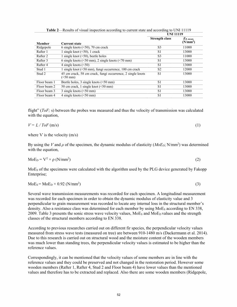
Table 2—Results of visual inspection according to current state and according to UNI 11119

Member Current state

UNI 11119 Strength class E0, mean.

(N/mm2) Ridgepole 6 single knots (˂50), 70 cm crack S3 11000 Rafter 1 1 single knot (˂50), 1 crack S1 13000 Rafter 2 1 single knot (˂50), beetle holes S3 11000 Rafter 3 6 single knots (˂50 mm), 2 single knots (˂70 mm) S1 13000 Rafter 4 4 single knots (˂50) S1 13000 Stud 1 1 single knot (˂50 mm), fungi occurrence, 100 cm crack S2 12000 Stud 2 45 cm crack, 58 cm crack, fungi occurrence, 2 single knots

(˂50 mm) S1 13000

Floor beam 1 Beetle holes, 3 single knots (˂50 mm) S1 13000 Floor beam 2 50 cm crack, 1 single knot (˂50 mm) S1 13000 Floor beam 3 3 single knots (˂50 mm) S1 13000 Floor beam 4 4 single knots (˂50 mm) S1 13000

flight” (ToF; s) between the probes was measured and thus the velocity of transmission was calculated with the equation,

Ѵ = L / ToF (m/s) (1)

where Ѵ is the velocity (m/s)

By using the Ѵ and ρ of the specimen, the dynamic modulus of elasticity (MoED; N/mm2) was determined with the equation,

MoED = Ѵ2 × ρ (N/mm2) (2)

MoES of the specimens were calculated with the algorithm used by the PLG device generated by Fakopp Enterprise;

MoES = MoED × 0.92 (N/mm2) (3)

Several wave transmission measurements was recorded for each specimen. A longitudinal measurement was recorded for each specimen in order to obtain the dynamic modulus of elasticity value and 3 perpendicular to grain measurement was recorded to locate any internal loss in the structural member’s density. Also a resistance class was determined for each member by using MoES according to EN 338, 2009. Table 3 presents the sonic stress wave velocity values, MoES and MoED values and the strength classes of the structural members according to EN 338.

According to previous researches carried out on different fir species, the perpendicular velocity values measured from stress wave tests (measured on tree) are between 910-1480 m/s (Dackermann et al. 2014). Due to this research is carried out on structural wood and the moisture content of the wooden members was much lower than standing trees, the perpendicular velocity values is estimated to be higher than the reference values.

Correspondingly, it can be mentioned that the velocity values of some members are in line with the reference values and they could be preserved and not changed in the restoration period. However some wooden members (Rafter 1, Rafter 4, Stud 2 and Floor beam 4) have lower values than the mentioned values and therefore has to be extracted and replaced. Also there are some wooden members (Ridgepole,

52

Table 3—Sonic stress wave results of the structural wooden members Member Perpendicular to grain Longitudinal MoED

(N/mm2) MoES

(N/mm2) Strength

class 1. point 2. point 3. pointRidgepole 839,16 1632,65 1276,60 4986,34 9010 8289 C16 Rafter 1 880,28 833,33 932,84 5287,36 14220 13082 C35 Rafter 2 1083,33 1101,69 860,93 5415,43 12420 11426 C24 Rafter 3 1120,69 1192,66 984,45 5683,23 14720 13542 C40 Rafter 4 844,59 833,33 531,91 5303,47 12090 11123 C24 Stud 1 1666,67 1776,32 1776,32 4227,27 7830 7204 C14 Stud 2 759,49 944,88 603,02 5263,16 13080 12034 C30

Floor beam 1 1372,55 1489,36 1296,30 5464,48 13040 11997 C30 Floor beam 2 744,05 1420,45 816,99 5361,93 10580 9734 C22 Floor beam 3 1031,01 943,26 904,76 5305,85 12820 11794 C30 Floor beam 4 796,18 880,28 992,85 5181,35 10850 9982 C22

Rafter 2, Floor beam 2, Floor beam 3) which have partial lower values. The parts which have lower values are in contact with the masonry wall and the reason of the low velocity is probably the effect of the high moist of the wall. These members can be reinforced or a partial repair can be carried out by replacing the problematic part.

The MoES values which were determined by using the longitudinal velocity values of the specimens are in accordance with the reference values given for structural wood in EN 338, 2009 as can be seen in Table 4. Although some of the specimens have lower values, all of the obtained MoES values are sufficient enough and can be used as a structural member.

Destructive evaluation

Determination of density

The density (ρ, kg/m3) of the wooden members was determined according to BS EN 408. A full cross section free from knots and resin pockets were taken from the structural member in order to measure the density. The MoE values of the specimens were estimated to be between 11000-13000 N/mm2 as mentioned in UNI 11119 standard which was used in the visual inspection. Correspondingly, a mean density value between 420-480 kg/m3 was expected for the specimens according to EN 338, 2009 which gives the characteristic values of different strength classes of structural wood. The measured density values of the structural members, which are given in Table 4, are between 362-508 kg/m3. It can be mentioned that ridgepole, rafter 2 and rafter 4 have lower values than the estimated values and moreover none of the measured values is lower than the minimum value stated for structural wood in the standard as 350 kg/m3.

Compression strength parallel to grain test

The mechanical properties of the structural members were evaluated by compression strength parallel to grain test. The test was carried out in order to determine the internal loss in the member’s density and to verify the results of visual inspection and non-destructive tests. A number of 5 to 8 specimens were randomly sawn (including also defects) from each member according to the size of the structural members. The specimens had a square cross section of at least 20 mm and length along the grain 1.5 to 4 times the cross sectional dimensions (Fig. 2).

53

Table 4—Density values of the structural members Member Density (kg/m3) Ridgepole 362,50 Rafter 1 436,70 Rafter 2 368,00 Rafter 3 455,40 Rafter 4 404,00 Stud 1 438,10 Stud 2 472,20 Floor beam 1 508,70 Floor beam 2 423,60 Floor beam 3 455,60 Floor beam 4 430,00

Figure 2—Compression strength parallel to gran test

The loading speed was set so that the failure will occur within 60-120 seconds. The compression strength (fC) is obtained by dividing the load cell value by the cross section area of the specimen. The results of the compression strength test can be seen in Table 5.

Table 5—Compression strength values of structural members Member Number of small

specimens taken out from the

structural member

Specimen with

defects

Compression Strength (N/mm2) Minimum Maximum Mean

Ridgepole 8 1 27,25 38,01

33,51 Rafter 1 6 2 30,54 46,51 37,01 Rafter 2 6 2 25,42 36,54 30,42 Rafter 3 6 1 26,38 34,60 31,26 Rafter 4 6 1 27,26 33,65 30,79 Stud 1 5 1 25,53 32,27 29,37 Stud 2 6 1 36,14 39,73 37,59

Floor beam 1 6 2 33,15 40,95 38,31 Floor beam 2 6 1 29,57 38,31 34,52 Floor beam 3 6 - 28,28 45,62 34,25 Floor beam 4 6 1 29,59 37,88 34,93

A compression strength value between 21-25 N/mm2 was expected for structural wood according to EN 338, 2009. In particular, the specimens with defects have the lowest compressive strength values,

54

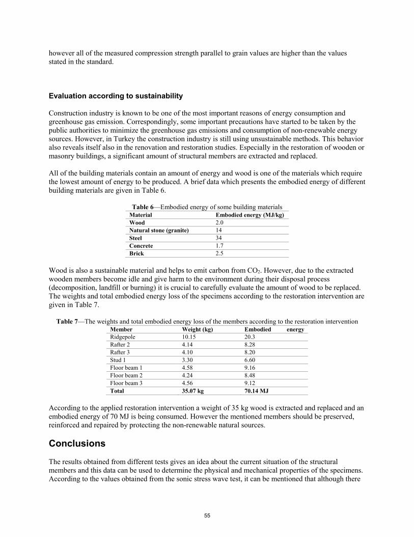
however all of the measured compression strength parallel to grain values are higher than the values stated in the standard.

Evaluation according to sustainability

Construction industry is known to be one of the most important reasons of energy consumption and greenhouse gas emission. Correspondingly, some important precautions have started to be taken by the public authorities to minimize the greenhouse gas emissions and consumption of non-renewable energy sources. However, in Turkey the construction industry is still using unsustainable methods. This behavior also reveals itself also in the renovation and restoration studies. Especially in the restoration of wooden or masonry buildings, a significant amount of structural members are extracted and replaced.

All of the building materials contain an amount of energy and wood is one of the materials which require the lowest amount of energy to be produced. A brief data which presents the embodied energy of different building materials are given in Table 6.

Table 6—Embodied energy of some building materials Material Embodied energy (MJ/kg) Wood 2.0 Natural stone (granite) 14 Steel 34 Concrete 1.7 Brick 2.5

Wood is also a sustainable material and helps to emit carbon from CO2. However, due to the extracted wooden members become idle and give harm to the environment during their disposal process (decomposition, landfill or burning) it is crucial to carefully evaluate the amount of wood to be replaced. The weights and total embodied energy loss of the specimens according to the restoration intervention are given in Table 7.

Table 7—The weights and total embodied energy loss of the members according to the restoration intervention Member Weight (kg) Embodied energy

Ridgepole 10.15 20.3 Rafter 2 4.14 8.28 Rafter 3 4.10 8.20 Stud 1 3.30 6.60 Floor beam 1 4.58 9.16 Floor beam 2 4.24 8.48 Floor beam 3 4.56 9.12 Total 35.07 kg 70.14 MJ

According to the applied restoration intervention a weight of 35 kg wood is extracted and replaced and an embodied energy of 70 MJ is being consumed. However the mentioned members should be preserved, reinforced and repaired by protecting the non-renewable natural sources.

Conclusions

The results obtained from different tests gives an idea about the current situation of the structural members and this data can be used to determine the physical and mechanical properties of the specimens. According to the values obtained from the sonic stress wave test, it can be mentioned that although there

55

are no visible sign of deterioration on the specimens a few of them had internal density losses and therefore should be extracted and replaced. Some of them had some partial density losses which need to be repaired. However, most of the structural members were well protected. Therefore most of the members had enough mechanical properties and could be used. The applied restoration intervention is not environmentally sustainable and financially feasible and a more sustainable intervention should be carried out by replacing a small of members, repairing a small group and preserving the others, which could preserve the consumed energy and natural sources.

References

Morales Conde M.J.; Rodriguez Liñan C.; Rubio de Hita P. 2014. Use of ultrasound as a nondestructive evaluation technique for sustainable interventions on wooden structures. Building and Environment. 82: 247-257.

Machado J.; Palma P.; Simões S. 2009. Ultrasonic indirect method for evaluating clear wood strength and stiffness. In NDTCE’09, Non-Destructive testing in civil engineering, Nantes, France. 30 June – 3 July.

Feio A. 2006. Inspection and diagnosis of historical timber structures: NDT correlations and structural behavior, University of Minho, PhD thesis.

Sharma S.K.; Shukla S.R. 2012. Property evaluation and defects detection in timbers by ultrasonic non-destructive technique. Journal of the Indian Academy of Wood Science. 9(1): 66-71.

Riggio M.; Anthony R.W.; Augelli F.[and others]. 2014. In situ assessment of structural timber using non-destructive techniques, Materials and Structures. 5(47): 749-766.

Tannert T.; Anthony R.W.; Kasal B., [and others]. 2014. In situ assessment of structural timber using semi-destructive techniques, Materials and Structures. 5(47): 767-785.

Calderoni C.; Matteis G.; Giubileo C. [and others]. 2010. Experimental correlations between destructive and non-destructive tests on ancient timber elements. Engineering Structures, 32(2): 442-448.

Galvez F.P.; Rubio de Hita P.; Ordonez Martin M. [and others]. 2013. Sustainable restoration of traditional building systems in the historical center of Sevilla. Energy and Buildings. 62: 648-659.

CEN. EN 13183-2: Moisture content of a piece of sawn timber – Part 2: Estimation by electrical resistance method. Brussels: European Committee for Standardization (CEN); 2002.

Domone P.; Illston J.M. 2001. Construction materials: Their nature and behavior. E&FN Spon, London.

BSI. BS EN 335-2: Durability of wood and wood-based products – Definition of use classes – Part 2: Application to solid wood. London: The British Standards Institution (BSI); 2006.

UNI. UNI 11119: Cultural heritage – Wooden artefacts – Load-bearing structures – On site inspections for the diagnosis of timber members. Milano: Ente Italiano di Normazione (UNI), 2004.

UNI. UNI EN 338: Structural timber strength classes. Milano: Ente Italiano di Normazione (UNI), 2009.

Dackermann U.; Crews K.; Kasal B.; [and others]. 2014. In situ assessment of structural timber using stress wave measurements. Materials and Structures. 47: 787-803.

56

New Technologies – Challenges and Barriers of the Market

Anna-Greta Tsahkna Timbeter, Tallinn, Estonia, anna-greta.tsahkna@timbeter.com

Abstract

New technologies are born every day and disrupting the traditional industries. In timber industry, most of the focus has been on the heavy machinery investment and digital development is lagging behind. As the demand for timber is growing (expected to quadruple by 2050) there's a clear need for solutions that make forestry more precise, transparent and maximize the value of each log. The technology world is developing rapidly, and this also demands the quicker reactions from the existing market players and regulators.

Keywords: timber industry, digital development, regulation

Introduction

Even though the world talks about the AI, ML, blockchain, optimization and digitalization, timber industry doesn't seem to keep the pace – long traditions, profitable business and availability of the supply seem to be the reasons why there is an urge for changes. But clearly, the situation is changing as there is expected the growth in demand for timber and new technologies are born every day, disrupting the traditional industries. There is a clear "boom" of agritech start-ups: companies operating in agriculture are clearly looking for solutions to overcome problems like climate change, water shortage and degradation of the fertile land.

In timber industry, most of the focus has been on the heavy machinery investment, which makes digital development lag behind. John Deere's representative mentioned at the Oregon Loggers Conference that "machines cannot go any stronger". Already now, 40% of the machine's capability is dependent on the operator's skills. The only way to increase the efficiency and optimize processes is via IT.

There are many blockers for the new technologies gaining a foothold on the market, even though there is a clear need for tools that make forestry more transparent, efficient and trackable. Companies are careful in testing out new technologies as none is ready to put their daily operations in risk. Even though Harsh Choudhry and Glen O’Kelly suggest to "start now, don't wait for the technology to mature" (Choudhry and O’Kelly 2018), it is still hard to find the pioneers. Technology is evolving daily, and this means that tests that were conducted even six months ago are quickly becoming outdated.

One typical problem for new technologies is that regulators lack the knowledge and work at low speed. So, even if companies are interested in using technologies, the regulators simply do not follow (not to mention even lead) the progress. Even more, in most countries, there is a difficulty of finding the institution willing to test the accuracy/validate the technology. Considering also that technology is usually used on a mobile device (smartphone, tablet) there's a question on how to differentiate the smart device from the technology itself?

57

Also, the problem is the incumbents who try to block the adoption of new technologies, as it is not in their interest to give the seller (mainly the private forest owners) a stronger position. Private forest owners are lacking experience, knowledge, and possibilities to control their buyers. As the demand for timber is growing – expected to quadruplicate by 2050 – there is a clear need for solutions that would make forestry more precise and transparent, while maximizing the value of each log. As technological world is developing rapidly and this also demands the quicker reactions from the existing market players and regulators.

New technology, but old methods

In timber industry, volume calculations differ from region to region. However, there are two main numeric variables that need to be taken into consideration: D – diameter (narrow, average or d1 and d2) L - length

Depending on the region, a formula can utilize either the small-end diameter (JAS, GOST, Nilson, etc.) or the middle diameter (Huber). Also, each and every formula has its specific rounding rules that have to be considered.

Most of the roundwood measurement instructions (Fonseca 2005) advise to measure two perpendicular diameters and, then, calculate the averages. In some cases, however, an individual only measures the narrowest diameter possible. Whenever the human factor is involved, there is always a risk of subjectivity.

AI instead of manual measurement

Photo-optical timber measurement which is based on AI and machine-learning technology enables the detection of the contour area of a log under the bark based on at least 2000 points and converts this area to a symmetrical circle; based on this, the average diameter is calculated. The average diameter of a log is calculated based on the total area of it. The process is designed to measure the log surface area as accurately as possible by converting the irregular shape of the contour area into a perfectly circular image.

AI is a perfect technology for timber measurement as the task of how to measure logs is well-defined – it is done in the same way every time and there is no need to use any creative problem-solving solutions. This is excellent for AI because machine learning algorithms rely on finding the set of rules for how to complete its job. As logs do look similar in appearance, recognizing them is something that is very much doable. Measuring logs tends to take an individual a substantial length of time. An algorithm can process the whole image at once, much in the same way a person can immediately guess the rough size of a pile merely by looking at it. But instead of vague volume, the exact data is provided: the log count, the diameter of each log and the volume are instantly available. All the data is available on a digital form, so it can be easily shared and controlled by the other parties.

But, whenever the manual measurement is being compared to the AI-based one, some differences may occur. These differences happen simply because logs are never perfectly round or symmetrical. Here, the question is – what is more important if we consider the maximization of the value of each log? The problem is that new innovative ways for timber measurement are only controlled and validated via old manual methods and rules that were developed more than a hundred years ago. Old methods are much more limited when compared to the new technologies available as they were based on a limited set of

58

samples. Technology enables measuring each log in a much more objective way – can manual measurement really complete with the digital one where one log is being detected based on at least 2000 points? Clearly, the results based on digital proof and made with the help of AI provide more transparency and better-quality control.

In comparison with the case when an individual is measuring logs manually, photo-optical measurement tool always measures objectively and in the same way. Since the detection is based on machine learning and artificial intelligence, the results are not dependent on the measurer. It is also a fact that some devices give better detection results (a camera with the resolution of 8 megapixels is our minimum requirement), but the detection process always works in the same way.

Certification

Currently, there is no methodology to certify the photo-optical measurements. The primary question in that regard is if the certification objects should be the software itself or a specific piece of hardware.

If the solution is based also on Android device, how it is possible to certify more than fifteen thousand different models if all of them are supported? On the other hand, for the academics, the certification of a software is a black box in a sense and constructing the methodology has not been successful. From the solution providers’ point of view, the certification of the reference object in the image should be done and the rest should be related to that object. In many EU countries, timber measurement law requires the tool/device/person to be certified. What exactly does it mean? Does the ruler need to be certified? Or does the person who has some previous experience and education in forestry needs to be certified?

If the technology acts itself as a ruler, and the only difference is its digital form – can we consider it as a normal ruler?

The issue is that the current methodological institutions don't have the demand for creating new methodologies or rules and, therefore, they would rather refuse from the task if it is being asked by the solution provider. Also, the unmatching requirements are presented. Have you ever seen a person who is capable of measuring manually under -70ºC or in +60ºC conditions? But why then the technology that is being used by the person is required to perform in such conditions?

For the newcomers, certification requirements – as there is no methodology for certification – are a dead end. Technology that is easy to use, quick and accurate, providing more transparency and efficiency should be in everybody's interest. But, unfortunately, this is not the case.

Benefits of the new technology

Manual measurements are hard to control and verifying those measurements is a time-consuming and labor-intensive process. Still, the process of adopting new technologies to replace manual measurement is slow. In addition to the obvious positive aspects (speed, accuracy, digital data), there are also some other advantages of using the new photo-optical timber measurement.

Healthier work environment

Fieldwork in open areas is always subject to different weather conditions. By using photo-optical solutions for field measurements, workers minimize the measurement time of each pile, making work faster and more effective. In addition, in the regions of extreme climates – such as for workers in remote areas of the planet who need to perform measurements in winters below -20ºC or those in tropical

59

climates, whose summers exceed 40ºC, a simple photo taken with the aid of our solution will take only 10% of the time that would be used in a manual measurement, plus the fact that there is the possibility of just taking a photo from the stack and performing the measurement in an enclosed location such as an office.

One of the most reported issues by log measurers at the field is related to repetitive strain injuries (RSI), since a single movement, performed countless times, is necessary for manual measurement – with arms and hands being stretched repetitively for measuring the diameters and the volume of the stacks. These injuries also involve bursitis and synovitis, which require specific treatment and take time to be fully recovered. By using photo-optical timber measurement as a preferred method, the log-by-log "measuring" movement ceases to exist due to the artificial intelligence system that performs the measurement of the stack at once only in 3 minutes and doesn't require human intervention directly on the pile.

Increased employee safety

One other issue presented by forest workers is related to direct contact with woodpiles, which can cause two distinct problems: the risk of falls and venomous animals. Firstly, it is not completely safe for the measurer to be at a very small distance from the stack, as imbalances in it can occur, causing crushing and fatal accidents. In addition, it is well known that areas with an abundance of wood are the natural habitat of several species of animals, fungi, and mosses. Workers in tropical areas who perform eucalyptus measurements, for example, are subject to unexpected encounters with scorpions, who prefer to lodge among logs – this is a situation of the extreme risk that can be very easily avoided if the worker makes measurements further from the piles.

Increased customer satisfaction

Transparent and objective timber trade benefits both sides as less time is spent on arguing and, even in case of disagreement, there's always clear digital proof available. Both sides have access to data and control everything happening in the "other side."

Larger picture

The volume of illegal logging and unfair trade in timber industry is extraordinarily high. By reports from the World Bank, illegal logging activity is estimated to cost developing countries $5 billion per year in lost timber revenues to governments alone. It is all due to the fact that there's simply no transparency and ability to control and monitor the harvesting areas. The main reason behind that has been the high human intervention and lack of control tools. The photo-optical timber measurement enables sustainable forest management: each and every transaction/measurement has a digital proof, meaning that all the measurements are done in an objective way based on AI-detection: therefore, there cannot be any more cheating or corruption, since tracking will always be provided to interest parts, such as law enforcement agencies. Human intervention is minimized and there's always the possibility to control (Police, Ministry of Environment, for example).

New technologies are also required to provide needed data for the governments to monitor and control the timber exports, making sure that there's no timber cut from protected areas or any endangered species being cut.

60

Conclusions

The technological world is developing rapidly, and this also demands the quicker reactions from the existing market players and regulators. Similarly to Uber and Bolt, which have disrupted the traditional taxi business and become ahead of current regulations, new technologies are demanding for the new rules in timber sector. Everything that enables more transparency, fair trade and reduction of the manual labor helps to increase the position and possibility to negotiate the private forest owner. Unfortunately, the voice of the private forest owners is still very weak, compared to the companies. Also, the committees and organizations dealing with timber measurement usually have representatives of the companies, not the private forest owners organizations. Therefore, it is not in their interest to change the status quo position and rather present barriers and requirements that block the new technologies coming to the market.

References

Fonseca, M.A. 2005. The measurement of roundwood: methodologies and conversion ratios. CABI Publishing, CAB International.

Harsh C. and O’Kelly G. 2018. Precision forestry: A revolution in the woods. https://www.mckinsey.com/industries/paper-and-forest-products/our-insights/precision-forestry-a-revolution-in-the-woods. Accessed 8.07.2019.

61

Identifying Incipient Decay in Douglas-fir Bridge Components using X-Ray Computerized Tomography Christopher Adam Senalik USDA Forest Service, Forest Products Laboratory, Madison, Wisconsin, USA, christopher.a.senalik@usda.gov James Wacker USDA Forest Service, Forest Products Laboratory, Madison, Wisconsin, USA, james.p.wacker@usda.gov Xiping Wang USDA Forest Service, Forest Products Laboratory, Madison, Wisconsin, USA, xiping.wang@usda.gov Xi Wu School of IoT Engineering, Jiangnan University, Wuxi, Jiangsu, China, xw20170909@gmail.com Abstract In this report, wooden members of sizes typically used in bridge construction are examined using x-ray computerized tomography (CT) to determine the presence of internal decay. This report is part of an overall study in which Douglas-fir (Pseudotsuga menziesii) glue-laminated (glulam) beams and solid sawn timbers were inoculated with brown rot fungus, Fomitopsis pinicola, and exposed to aboveground conditions approximately 25 miles (40 km) north of Gulfport, Mississippi, USA. The goal of the overall study is to develop interior decay within the test specimens and then identify and characterize the decay using a variety of nondestructive testing (NDT) techniques. One NDT technique used is x-ray CT. The pixel brightness (PB) of CT scan images is proportional to the specific gravity (SG) at that location; high SG materials appear brighter whereas low SG materials appear darker. The consumption of wood by fungus decreases the wood SG; however, fungal progression takes place in areas where sufficient moisture is present. The presence of moisture increases wood SG as detected by the CT scan, which masks the effect of the fungal decay, which is a common co-occurrence with many NDT techniques. To identify incipient decay, it is necessary to examine the ring structure both within and outside of the area of moisture. Quantifying the extent of the decay requires correlating the PB to known SG values for both dry wood and wood of varying moisture content. In this report, the relationship between wood SG, moisture content, and PB was quantified. Keywords: x-ray computerized tomography, wood timber, brown rot fungus, incipient decay Introduction Wood attacked by decay fungi often suffers drastic decreases in mechanical properties, which are relied upon for structural soundness. This degradation occurs because the fungus degrades components of the cell wall. Modulus of rupture (MOR), modulus of elasticity (MOE), compression strength, tension strength, toughness, and hardness are among the key properties compromised. The effect of brown rot and white rot fungi on both softwoods and hardwoods is well known. A concise summary of relevant publications was provided in Ross et al. (2018). For a 5% mass loss caused by brown rot, reductions to MOR, MOE, and tension strength parallel to grain can be 50% or more. For this reason, early detection of incipient fungal decay is of paramount importance. This report is part of an overall study using a variety of nondestructive testing (NDT) techniques to identify the presence of decay in timbers of sizes commonly used in bridge construction. In this report,

62

Douglas-fir (Pseudotsuga menziesii) glue-laminated (glulam) beams and solid sawn timbers were inoculated with brown rot fungus, Fomitopsis pinicola, and exposed to aboveground conditions approximately 25 miles (40 km) north of Gulfport, Mississippi, USA. The glulam beams and sawn timbers were of sizes typically used in bridge construction and hereafter are referred to collectively as bridge components. The bridge components were exposed to outdoor weather conditions from periods ranging from 6 to 30 months. A full description of the inspection methods, inoculation process, test setup, schedule of exposure, and postexposure nondestructive assessment can be found in Wacker et al. (2016) and Senalik et al. (2016). One postexposure technique used, x-ray computerized tomography (CT), is the focus of this report. The use of x-ray CT to examine wood for internal decay is not new. Bucur (2003) described the use of x-ray CT on wood. McGovern et al. (2010) used x-ray CT to assess the amount of internal mass lost on 1-in. (25-mm) cubes of loblolly pine that had been subjected to varying degrees of mass loss from rot. Senalik (2013) evaluated the soundness of wooden utility poles and glulam beams with x-ray CT. However, in the studies conducted by Senalik and McGovern, the wood specimens had a moisture content of 12% or lower. Moisture within the beams complicates the process of detecting internal decay. Many common forms of wood-attacking fungi require water to grow and thrive; therefore, fungal decay often occurs within moisture pockets. Fungi also produce water as a byproduct of their extracellular digestion process. As fungus progresses through the wood, it deteriorates the wood, leading to mass loss through extracellular digestion of the structural carbohydrates. In a CT scan, the specific gravity (SG) of a location is proportional to the pixel brightness (PB) of that region as it appears on the CT output. Areas of high SG appear bright, whereas areas of low SG appear dark. Wood with high moisture content appears bright, whereas wood that is deteriorated and suffering mass loss will appear dark. Unfortunately, when these two phenomena overlap, the apparent increase in SG from the moisture content can obscure the loss of mass from fungal attack. In this paper, the process of identifying areas of decreased mass within moisture pockets as shown in x-ray CT scans is described. Materials and Methods The Douglas-fir bridge components had one of four cross-sectional sizes: 5-1/8- by 9-in. (130- by 229-mm) glulam, 5-1/8- by 7.5-in. (130- by 191-mm) glulam, 3-1/2- by 5-1/2-in. (89- by 140-mm) sawn timber, and 3-1/2- by 7-1/4-in. (89- by 184-mm) sawn timber. Each specimen was 32 in. (0.8 m) in length. For brevity, the figures herein show only 5-1/8- by 9-in. (130- by 229-mm) glulam, but all cross sections were used in the analysis presented in this report. Each specimen was inoculated with brown rot fungus, Fomitopsis pinicola, prior to placement for field exposure. Figure 1 shows the specimen configuration. There were eight sets of specimens. Each set contained 12 specimens (three of each cross-sectional size). Each set was subjected to weather exposure in 6-month increments. The first set was exposed for 6 months, the second set was exposed for 12 months, through the final set which was exposed for 30 months. A full description of the specimen preparation and field exposure is given in Senalik et al. (2016). After the field exposure time period was completed, the specimens were shipped back to the Forest Products Laboratory (FPL) in Madison, Wisconsin. The x-ray CT scanning of select beams was performed at the University of Wisconsin, School of Veterinary Medicine, Madison, Wisconsin, using a General Electric Lightspeed Ultra 8-slice helical CT scanner (GE Medical Systems, Milwaukee, Wisconsin, USA). The x-ray CT energy level and intensity were 120 kV and 120 mA, respectively. CT scanners measure the radiodensity of materials. Radiodensity is the opacity of a material to the radio and x-ray portion of the spectrum. CT scanners express their measurements of radiodensity in terms of a dimensionless unit

63

known as the Hounsfield unit (HU). For reference, HU values for air, water at standard temperature and pressure, and dense bone are -1,000, 0, and +2,000, respectively. During postprocessing of the images, the width (W) of the HU window was chosen to be 1,500, and the center point of the window, known as the level (L), was set to -300. These values are commonly written shorthand as 1500W, -300L.

(a) (b)

Figure 1—Fungal cavity holes in specimens: (a) locations of drilled holes. Units shown are in inches (1 in. = 25.4 mm); (b) holes drilled in a six-layer glulam.

The width of the window determines the resolution between levels of SG that are apparent in the image. A wider window allows viewing a wider range of densities. A narrow window has as smaller range, but the resolution between levels of SG is sharper. The level is the midpoint of the window. In this report, the level was set to -300 and the window was set at 1,500; therefore, any values above 450 HU (-300 + 1,500/2 = 450) appear as white, and any values below -1,050 (-300 – 1,500/2 = -1,050) appear as black. All values in between appear as some shade of gray. The W and L values are chosen such that decayed low SG wood and moisture-saturated high SG wood fall within the range. It is important to note that HU is not the same as PB. HUs are used to construct the CT scan data file. The CT scan data file is then interpreted using specialized software (in this case, eFilmLite Ver. 4.0 from Merge Healthcare, Chicago, Illinois, USA) which converts the HU value to a PB for display on a computer screen. While the window of the images is 1,500 HU, a normal pixel has a brightness range between 0 (completely black) and 255 (completely white). Therefore, an increase in PB of 1 (say from 121 to 122) encompasses approximately 5.9 HU. An in-depth discussion of HU, CT scanners, and PB displays can be found in Romans (2010). The width and level can be adjusted to accentuate particular SG ranges if desired. It should be remembered that wood is an organic material with variability. It is easy to narrow the window such that small, natural variations in wood SG appear dramatic on the computer screen. Figure 2 shows three examples of glulam beam CT scans. Figure 2a shows a six-layer glulam after 6 months of exposure. The portion of the beam shown has no visible internal moisture pocket. The ring structure of each lamina is clearly visible. Pith is visible in the third layer from the top (all references to layers will assume the top layer is the first and the bottom is the sixth). The fifth layer contains a small knot. Figure 2b shows the same beam but in a region with a pocket of high moisture. Decay often grows in areas of high moisture, but the brief exposure time limits the likelihood of significant fungal attack. The moisture portion is visible as a bright spot that crosses layers 1 through 3. The tree rings are visible within the moisture region. Figure 2c shows a cross section with a moisture pocket after 24 months of

64

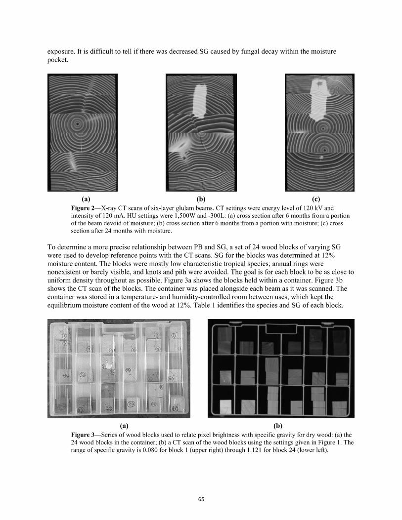
exposure. It is difficult to tell if there was decreased SG caused by fungal decay within the moisture pocket.

(a) (b) (c)

Figure 2—X-ray CT scans of six-layer glulam beams. CT settings were energy level of 120 kV and intensity of 120 mA. HU settings were 1,500W and -300L: (a) cross section after 6 months from a portion of the beam devoid of moisture; (b) cross section after 6 months from a portion with moisture; (c) cross section after 24 months with moisture.

To determine a more precise relationship between PB and SG, a set of 24 wood blocks of varying SG were used to develop reference points with the CT scans. SG for the blocks was determined at 12% moisture content. The blocks were mostly low characteristic tropical species; annual rings were nonexistent or barely visible, and knots and pith were avoided. The goal is for each block to be as close to uniform density throughout as possible. Figure 3a shows the blocks held within a container. Figure 3b shows the CT scan of the blocks. The container was placed alongside each beam as it was scanned. The container was stored in a temperature- and humidity-controlled room between uses, which kept the equilibrium moisture content of the wood at 12%. Table 1 identifies the species and SG of each block.

(a) (b)

Figure 3—Series of wood blocks used to relate pixel brightness with specific gravity for dry wood: (a) the 24 wood blocks in the container; (b) a CT scan of the wood blocks using the settings given in Figure 1. The range of specific gravity is 0.080 for block 1 (upper right) through 1.121 for block 24 (lower left).

65

Table 1—Wood specimen identification and specific gravity (SG)

ID Species SG ID Species SG 1 Heliocarpus appendiculatus Turcz. 0.081 13 Liquidambar sp. 0.507 2 Ochroma pyramidale (Cav. ex Lam.) Urb. 0.118 12 Trema micrantha (L.) Blume 0.561 3 Ochroma pyramidale (Cav. ex Lam.) Urb. 0.148 16 Mangifera sp. 0.580 4 Ochroma pyramidale (Cav. ex Lam.) Urb. 0.180 15 Alnus sp. 0.610 6 Ochroma pyramidale (Cav. ex Lam.) Urb. 0.194 17 Gonystylus sp. 0.624 5 Hampea Appendiculata (Donn. Sm.) Standl. 0.226 18 Betula sp. 0.648 7 Ochroma pyramidale (Cav. ex Lam.) Urb. 0.287 19 Nyssa 0.693 9 Ochroma pyramidale (Cav. ex Lam.) Urb. 0.313 20 Nyssa 0.707 8 Ochroma pyramidale (Cav. ex Lam.) Urb. 0.364 21 Julbernardia sp. 0.732 10 Hampea appendiculate (Donn. Sm.) Standl. 0.468 22 Laetia procera (Poepp.) Eichl. 0.801 11 Trema micrantha (L.) Blume 0.493 23 Shorea sp. 0.833 14 Laurelia sp. 0.504 24 Chrysophyllum sp. 1.121 Several of the blocks in Table 1 are of the same species. For example, Ochroma pyramidale (Cav. ex Lam.) Urb., commonly known as balsa wood, has seven entries. Balsa wood can have a range of SG from approximately 0.10 to 0.35. Personnel from the Center for Wood Anatomy Research at FPL identified a set of wood samples with SG from 0.08 to 1.121. This range should encompass any SG value likely to be encountered during the project. The container itself is constructed of high-density polyethylene (HDPE), which has an SG of between 0.93 and 0.97. The SG of the container is distinct from any of the blocks and easily removed from calculations. The PB assigned to each block is the average PB across all visible pixels. Edge pixels for each block were not used in the calculations as their brightness can be influenced by the density of surrounding materials (air, HDPE, etc.). To determine if the presence of moisture pockets exhibits nonlinear effects on the x-ray CT scan, a separate set of tests was conducted. Figure 4 shows fifteen 1-in. (25.4-mm) cubed wood blocks of Douglas-fir, which were cut from remnants of the sawn timbers used in the overall decay study. The blocks were soaked in water and then removed at different intervals prior to the CT scan to obtain the range of moisture contents. The blocks were weighed prior to and just after the CT scan, and all dimensions were measured. The blocks were then oven-dried to determine the dry weight of the wood alone. PB was determined in the same manner as those in Figure 3.

a. b.

Figure 4—Series of wood blocks used to relate pixel brightness with specific gravity for wet wood: (a) the 17 wood blocks in the container; (b) a computerized tomography scan of the wood blocks using the settings given in Figure 1.

66

Discussion and Results Figure 5 shows the relationship between PB and SG for both the dry and wet wood blocks. The dry wood blocks were used in 24 separate CT scans; the wet wood blocks were used in eight separate CT scans. Values from all CT scans are shown in Figure 5. Although the SG for each block does not change, the PB can vary slightly depending upon inconsistencies in the wood blocks themselves and minor differences in positioning of the blocks. Below each figure is the linear equation relating PB to SG. The equations yield SG values within 2% of each other for PB values of 50 or greater (SG of 0.3 or greater).

(a) (b)

Figure 5—Relationships between pixel brightness (PB) of x-ray CT scans and specific gravity (SG). CT scan settings match those given in Figure 1: (a) dry wood; (b) wet wood.

In Figure 6, all data points from Figures 5a and 5b are shown on a single chart. The equation for the combined data set is shown below the figure. The equation yields SG values with 1.5% of the wet and dry wood equations given in Figure 5 for a PB range of 50 or greater (SG of 0.3 or greater).

Figure 6—Relationships between pixel brightness (PB) of x-ray CT scans and specific gravity (SG) for all wood blocks. CT scan settings match those given in Figure 1.

0 20 40 60 80 100 120 140 160 180 200 220 240 255

Pixel Brightness

0

0.2

0.4

0.6

0.8

1.0

1.2

Spec

ific

Gra

vity

Dry Wood Blocks

Best Fit Curve, r 2 = 0.9968

70 80 90 100 110 120 130 140 150 160

Pixel Brightness

0.4

0.5

0.6

0.7

0.8

0.9

Spec

ific

Gra

vity

Wet Wood Blocks

Best Fit Curve, r 2 = 0.959

0 20 40 60 80 100 120 140 160 180 200 220 240 255

Pixel Brightness

0

0.2

0.4

0.6

0.8

1.0

1.2

Spec

ific

Gra

vity

All Wood Blocks

Best Fit Curve, r 2 = 0.9954

SG = 0.00611*PB-0.0511 SG = 0.00614*PB-0.0475

SG = 0.00613*PB-0.0514

67

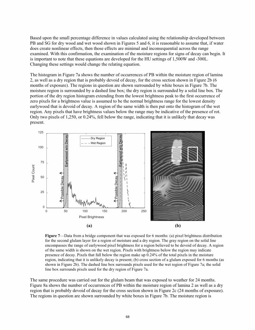
Based upon the small percentage difference in values calculated using the relationship developed between PB and SG for dry wood and wet wood shown in Figures 5 and 6, it is reasonable to assume that, if water does create nonlinear effects, then those effects are minimal and inconsequential across the range examined. With this confirmation, the examination of the moisture regions for signs of decay can begin. It is important to note that these equations are developed for the HU settings of 1,500W and -300L. Changing these settings would change the relating equation. The histogram in Figure 7a shows the number of occurrences of PB within the moisture region of lamina 2, as well as a dry region that is probably devoid of decay, for the cross section shown in Figure 2b (6 months of exposure). The regions in question are shown surrounded by white boxes in Figure 7b. The moisture region is surrounded by a dashed line box; the dry region is surrounded by a solid line box. The portion of the dry region histogram extending from the lowest brightness peak to the first occurrence of zero pixels for a brightness value is assumed to be the normal brightness range for the lowest density earlywood that is devoid of decay. A region of the same width is then put onto the histogram of the wet region. Any pixels that have brightness values below the range may be indicative of the presence of rot. Only two pixels of 1,250, or 0.24%, fell below the range, indicating that it is unlikely that decay was present.

(a) (b)

Figure 7—Data from a bridge component that was exposed for 6 months: (a) pixel brightness distribution for the second glulam layer for a region of moisture and a dry region. The gray region on the solid line encompasses the range of earlywood pixel brightness for a region believed to be devoid of decay. A region of the same width is shown on the wet region. Pixels with brightness below the region may indicate presence of decay. Pixels that fall below the region make up 0.24% of the total pixels in the moisture region, indicating that it is unlikely decay is present; (b) cross section of a glulam exposed for 6 months (as shown in Figure 2b). The dashed line box surrounds pixels used for the wet region of Figure 7a; the solid line box surrounds pixels used for the dry region of Figure 7a.

The same procedure was carried out for the glulam beam that was exposed to weather for 24 months. Figure 8a shows the number of occurrences of PB within the moisture region of lamina 2 as well as a dry region that is probably devoid of decay for the cross section shown in Figure 2c (24 months of exposure). The regions in question are shown surrounded by white boxes in Figure 7b. The moisture region is

0 50 100 150 200 250

Pixel Brightness

0

25

50

75

100

125

Pixe

l Cou

nt

Dry RegionWet Region

Early

woo

d w

/o D

ecay

Po

ssib

le D

ecay

Early

woo

d w

/o D

ecay

Po

ssib

le D

ecay

68

surrounded by a dashed line box; the dry region is surrounded by a solid line box. The portion of the dry region histogram extending from the lowest peak to the first occurrence of zero pixels for a brightness value was assumed to be the normal brightness range for the earlywood in that lamina of the beam. A region of the same width is then put onto the histogram of the wet region. Any pixels with brightness values below the range may be indicative of the presence of rot. For the 24-month exposed cross section, 45 of 2,145 pixels, or 2.1%, fell below the range, indicating that decay may have been present. Pixels that fall below the assumed normal range in Figure 8a are shown in black. In Figure 8b, the location of the low brightness (and therefore, low SG) pixels are shown in black. The low SG cannot be explained as splits or ring shake in the area. The NDT techniques used during postprocessing of the beams focus on this and similarly darkened areas as potential locations of decay. As a final step in the examination process, the beam was cut across the cross section and Janka hardness tests were performed. Hardness correlates well with strength (Green et al. 2006) and is severely decreased by the presence of fungal decay. The hardness should provide verification of whether the apparent decrease was caused by fungal decay.

(a) (b)

Figure 8—Data from a bridge component that was exposed for 24 months: (a) pixel brightness distribution for the second glulam layer for a region of moisture and a dry region. The gray region on the solid line encompasses the range of earlywood pixel brightness for a region believed to be devoid of decay. A region of the same width is shown on the wet region. Pixels with brightness values below the region may indicate presence of decay. Pixels that fall below the region make up 2.1% of the total pixels in the moisture region, indicating that decay may be starting to develop. The low brightness pixels are shown in the black region; (b) cross section of a glulam exposed for 24 months to weather (as shown in Figure 2c). The dashed line box surrounds pixels used for the wet region of Figure 8a; the solid line box surrounds pixels used for the dry region of Figure 8a. The pixels that may indicate the presence of decay are marked in black within the moisture region.

Conclusions Density increases caused by the presence of moisture can mask the density loss caused by fungal decay. In this paper, a method of finding probable areas of decayed wood within moisture pockets shown in x-ray CT scans of the cross section is described. A linear relationship between PB and SG was developed. The relationship was found to be valid for both wet and dry wood. A threshold of 5% reduction of SG was assumed to be an indicator of the presence of fungal decay. Based upon the assumed threshold, a CT scan from a timber beam exposed to outdoor conditions for 24 months was found to have characteristics

0 50 100 150 200 250

Pixel Brightness

0

25

50

75

100

125

Pixe

l Cou

nt

Dry RegionWet Region

Early

woo

d w

/o D

ecay

Po

ssib

le D

ecay

Early

woo

d w

/o D

ecay

Po

ssib

le D

ecay

69

shared with decayed wood. Future examination of the beam should focus on the areas identified using the method described here. Acknowledgments This study was conducted under a joint agreement between the Federal Highway Administration (FHWA) – Turner–Fairbank Highway Research Center and the USDA Forest Service, Forest Products Laboratory (FPL). The study was part of the Research, Technology, and Education portion of the National Historic Covered Bridge Preservation (NHCBP) program administered by the FHWA. The NHCBP program includes preservation, rehabilitation, and restoration of covered bridges that are listed or are eligible for listing on the National Register of Historic Places, research for better means of restoring and protecting these bridges, development of educational aids, and technology transfer to disseminate information on covered bridges in order to preserve the Nation’s cultural heritage. Michael C. Wiemann of the Center for Wood Anatomy Research at FPL identified species of wood to use in the wood-based image phantom described in Figure 2 and Table 1. References Bucur, V. 2003. Nondestructive characterization and imaging of wood. Berlin Heidelberg New York: Springer. Green, D.W.; Begel, M.; Nelson, W. 2006. Janka hardness using nonstandard specimens. Research Note FPL-RN-0303. Madison, WI: U.S. Department of Agriculture, Forest Service, Forest Products Laboratory. 13 p. McGovern, M.; Senalik, A.; Chen, G.; Beall, F.; Reis, H. 2010. Detection and assessment of wood decay using x-ray computer tomography. In: Proceedings SPIE Smart Structures/NDE/Sensors and Smart Structures Technologies for Civil, Mechanical, and Aerospace Systems Conference. Paper number 7647-152. San Diego, CA. DOI: 10.1117/12.843709. Romans, L.E. 2010. Computed tomography for technologists: a comprehensive text, 1st ed. Baltimore, MD: Lippincott Williams & Wilkins. Ross, R.J.; Wang, X.; Senalik, C.A. 2018. Nondestructive assessment of wood members in a viewing tower in Potawatomi State Park, Door County, Wisconsin, USA. Res. Note FPL-RN-0366. Madison, WI: U.S. Department of Agriculture, Forest Service, Forest Products Laboratory. 14 p. Senalik, C. 2013. Detection and assessment of wood decay – glulam beams and wooden utility poles. University of Illinois Urbana-Champaign. Doctoral thesis. http://hdl.handle.net/2142/44281. Senalik, C.A.; Wacker, J.P.; Wang, X.; Jalinoos, F. 2016. Assessing the ability of ground-penetrating radar to detect fungal decay in Douglas-fir beams. In: 25th ASNT research symposium: summaries and abstracts. New Orleans. Columbus, OH: American Society for Nondestructive Testing, Inc.: 110-116. Wacker, J.P.; Senalik, C.A.; Wang, X.; Jalinoos, F. 2016. Effectiveness of several NDE technologies in detecting moisture pockets and artificial defects in sawn timber and glulam. In: world conference on timer engineering, WCTE 2016. 22-25 August 2016; Vienna, Austria.

70

Simultaneous Measurement of Density and Moisture Content Using Microwave Radar: Preliminary Results

Laszlo Bejo * Associate Professor, Institute of Wood Based Products and Technologies, University of Sopron, Hungary, bejo.laszlo@uni-sopron.hu

Mihaly Jakocs MSc. Student, University of Sopron, Hungary, alceyaon@gmail.com

Ferenc Divos Head, Fakopp Enterprise Inc., Sorpon, Hungary, office@fakopp.com

Shadabeh Fathi Doctorate Student, Institute of Wood Based Products and Technologies, University of Sopron, Hungary, shadabeh.fathi@gmail.com

* Corresponding author

Abstract

A new method of measuring the density and the moisture content of wood using a single measurement is being developed. The method is based on using both signal attenuation and time lag of a microwave signal transmitted through the material. The two independent variables allow the simultaneous prediction of both parameters. Several wood species have been measured at various moisture content levels, and two-parameter linear regression models were fit on the experimental data. Based on the preliminary results, the method seems to be working very accurately for moisture content determination, and reasonably well when estimating density. Microwave measurements are sensitive to temperature; therefore the moisture content of dry specimens straight out of the oven was overestimated. Further measurements using cooled specimens are expected to improve accuracy.

Keywords: density, moisture content, microwave, multi-parameter regression

Introduction

Density and moisture content measurements are crucial in many applications in the wood industries. Fast, reliable and accurate determination of these parameters is required for seasoning, gluing, surface treatment and composite manufacturing and in many other areas.

Since the direct determination of these parameters is time-consuming and often not practical, many alternative (mostly nondestructive) methods have been developed. Resistance and capacitive moisture meters are now traditional for moisture content measurement, as well as NIR scanners for surface moisture content determination. Density is typically estimated using electromagnetic radiation, mostly radar or gamma rays. There are many established methods and instruments with reasonable accuracy. However, in many situations, the simultaneous determination of these two parameters is desirable.

71

The purpose of this study was to develop a novel nondestructive method that can be used to determine wood density and moisture content simultaneously, from a single measurement, based on the dielectric properties of the material. The ultimate goal is to create a practical instrument that can reliably estimate these two parameters across different species. This paper reports the results of our preliminary experiments.

Literature review

Beginning with the 1950’s, there has been several studies on the dielectric properties of wood (e.g. Trapp and Pungs 1956; Tsunami and Watanbe 1965, 1968; Beldi et al. 1965, 1968). Various applications of radar equipment were also studied, including recent experiments for the detection of knots (Kaestner and Baath 2005) and even the determination of fiber orientation (Schanjen and Orhan 2006).

In 1993, Torgovnikov published a comprehensive book that systematically catalogues the dielectric constants of various wood species and their relationship to wood density, moisture content, temperature and frequency. Based on his work, it is possible to use electromagnetic waves to estimate both density and moisture content.

There have been several recent Japanese studies on moisture content determination using radar equipment. One such study examined the effect of moisture content on the phase shift of the radar signal, for developing a moisture sensor for Japanese cedar (Cryptomeria japonica) lumber (Ikeda et al. 2013). Later, 52 MHz signals were used to measure moisture variation in large diameter logs, based on signal damping and phase shift. Based on the results gross moisture variation in logs may be measured using a nondestructive, non-contact method (Ikeda et al. 2017). A Hungarian study was aimed at measuring the moisture content of large diameter logs or stacks of logs of various species using a high capacity microwave radar. The moisture content of the material can be accurately estimated (Major and Divos 2016).

American researchers (Senalik et al. 2017) used radar to nondestructively determine the moisture content and find hidden fungal decay in Douglas fir beams. Microwave radar was also used to estimate the density of wet wood above the fibre saturation point (Divos, Tsalagkas and Koutsianis 2013). Another study used microwave radar to measure the density of different species and compare it to measured and literature density data (Divos and Buza 2015).

Theoretical background

The purpose of our experiment is the simultaneous determination of two variables, namely, density and moisture content, both of which affect the dielectric properties of the material. In addition to geometry, the propagation and reflection of electromagnetic waves through and from a specimen are governed by the dielectric characteristics of the material. Therefore, the measured parameters of the transmitted or reflected radiation are related to the dielectric properties, and thus, indirectly, to the density and moisture content of wood.

The simultaneous determination of density and moisture content requires two independent predictor parameters. In case of electromagnetic radiation, the propagation velocity and the attenuation of the transmitted signals can be regarded more or less independent. These two variables were used for the estimation.

The propagation velocity of electromagnetic waves depends on the material it goes through. In vacuum, the velocity equals the speed of light, and in gases it is not much lower. However, in solids it changes

72

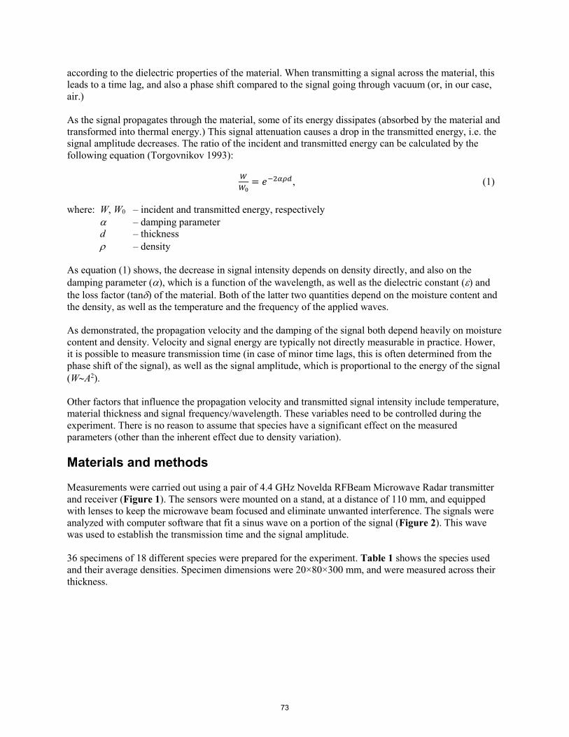
according to the dielectric properties of the material. When transmitting a signal across the material, this leads to a time lag, and also a phase shift compared to the signal going through vacuum (or, in our case, air.)

As the signal propagates through the material, some of its energy dissipates (absorbed by the material and transformed into thermal energy.) This signal attenuation causes a drop in the transmitted energy, i.e. the signal amplitude decreases. The ratio of the incident and transmitted energy can be calculated by the following equation (Torgovnikov 1993):

𝑊𝑊𝑊𝑊0

= 𝑒𝑒−2𝛼𝛼𝛼𝛼𝛼𝛼, (1)

where: W, W0 – incident and transmitted energy, respectively α – damping parameter d – thickness ρ – density

As equation (1) shows, the decrease in signal intensity depends on density directly, and also on the damping parameter (α), which is a function of the wavelength, as well as the dielectric constant (ε) and the loss factor (tanδ) of the material. Both of the latter two quantities depend on the moisture content and the density, as well as the temperature and the frequency of the applied waves.

As demonstrated, the propagation velocity and the damping of the signal both depend heavily on moisture content and density. Velocity and signal energy are typically not directly measurable in practice. Hower, it is possible to measure transmission time (in case of minor time lags, this is often determined from the phase shift of the signal), as well as the signal amplitude, which is proportional to the energy of the signal (W∼A2).

Other factors that influence the propagation velocity and transmitted signal intensity include temperature, material thickness and signal frequency/wavelength. These variables need to be controlled during the experiment. There is no reason to assume that species have a significant effect on the measured parameters (other than the inherent effect due to density variation).

Materials and methods

Measurements were carried out using a pair of 4.4 GHz Novelda RFBeam Microwave Radar transmitter and receiver (Figure 1). The sensors were mounted on a stand, at a distance of 110 mm, and equipped with lenses to keep the microwave beam focused and eliminate unwanted interference. The signals were analyzed with computer software that fit a sinus wave on a portion of the signal (Figure 2). This wave was used to establish the transmission time and the signal amplitude.

36 specimens of 18 different species were prepared for the experiment. Table 1 shows the species used and their average densities. Specimen dimensions were 20×80×300 mm, and were measured across their thickness.

73

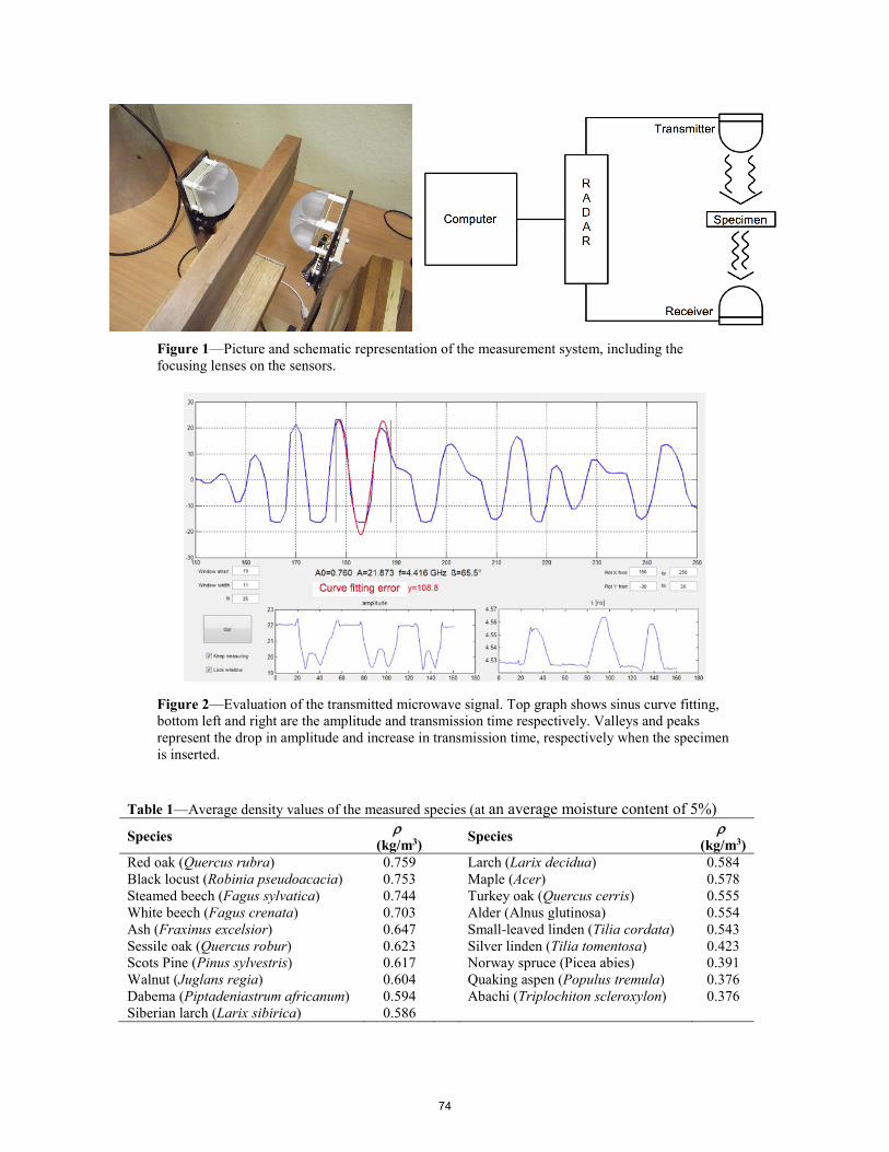
Figure 1—Picture and schematic representation of the measurement system, including the focusing lenses on the sensors.

Figure 2—Evaluation of the transmitted microwave signal. Top graph shows sinus curve fitting, bottom left and right are the amplitude and transmission time respectively. Valleys and peaks represent the drop in amplitude and increase in transmission time, respectively when the specimen is inserted.

Table 1—Average density values of the measured species (at an average moisture content of 5%)

Species ρ (kg/m3) Species ρ

(kg/m3) Red oak (Quercus rubra) 0.759 Larch (Larix decidua) 0.584 Black locust (Robinia pseudoacacia) 0.753 Maple (Acer) 0.578 Steamed beech (Fagus sylvatica) 0.744 Turkey oak (Quercus cerris) 0.555 White beech (Fagus crenata) 0.703 Alder (Alnus glutinosa) 0.554 Ash (Fraxinus excelsior) 0.647 Small-leaved linden (Tilia cordata) 0.543 Sessile oak (Quercus robur) 0.623 Silver linden (Tilia tomentosa) 0.423 Scots Pine (Pinus sylvestris) 0.617 Norway spruce (Picea abies) 0.391 Walnut (Juglans regia) 0.604 Quaking aspen (Populus tremula) 0.376 Dabema (Piptadeniastrum africanum) 0.594 Abachi (Triplochiton scleroxylon) 0.376 Siberian larch (Larix sibirica) 0.586

74

Each specimen was measured 4 times, after conditioning to different moisture contents levels, as follows:

• T = 20 °C, ϕ = 65%, ue ≅ 12%;• T = 20 °C, ϕ = 45%, ue ≅ 5%;• T = 20 °C, ϕ = 20%, ue ≅ 2%;• Oven dry (after drying at 100 °C)

After each conditioning stage, specimens were measured by placing them in-between the radar sensors. Changes in amplitude and transmission time (∆A and ∆t respectively) were recorded relative to the baseline transmission time and amplitude measured without the specimen inserted (see Figure 2). After the radar measurement, the mass of the specimen was also recorded, using a laboratory measuring scale with an accuracy of .01 g. Specimen dimensions were also recorded after the second and third measurements (ue ≅ 5% and 2%, respectively) for calculating the density. At ue ≅ 12% and in oven dry state, densities were calculated using linear extrapolation. The actual moisture content was calculated using the wet and oven dry masses for each measurement point.

Results and discussion

After the measurements were completed, two-parameter linear regression was performed on the data set, using ∆A and ∆t as the independent variable. The regression was carried out using the Statistica® program for both density and moisture content as dependent variables. Figures 3 and 4 show the results.

According to Figure 3, we were able to predict the moisture content of the specimens fairly accurately from the time shift and signal amplitude. Points that fell on the horizontal axis represent oven dry specimens. These data points exhibit an unusually high variation, and are also biased, the estimated moisture content being consistently higher than 0%. The reason for this anomaly is that the specimen were measured at 100 °C, rather than at room temperature. High temperatures affect the dielectric

Figure 3—Moisture content values measured using the oven dry method vs. predicted from the amplitude and transmission time.

u = 3.423 - 4.652 ∆A - 38.930 ∆tR² = 0.796

0.0

2.0

4.0

6.0

8.0

10.0

12.0

14.0

16.0

0.0 2.0 4.0 6.0 8.0 10.0 12.0 14.0 16.0

Mea

sure

d m

oist

ure

cont

ent (

%)

Predicted moisture content (%)

75

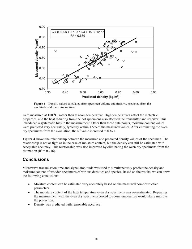
Figure 4—Density values calculated from specimen volume and mass vs. predicted from the amplitude and transmission time.

were measured at 100 °C, rather than at room temperature. High temperatures affect the dielectric properties, and the heat radiating from the hot specimens also affected the transmitter and receiver. This introduced a systematic bias in the measurement. Other than these data points, moisture content values were predicted very accurately, typically within 1.5% of the measured values. After eliminating the oven dry specimens from the evaluation, the R2 value increased to 0.871.

Figure 4 shows the relationship between the measured and predicted density values of the specimen. The relationship is not as tight as in the case of moisture content, but the density can still be estimated with acceptable accuracy. This relationship was also improved by eliminating the oven dry specimens from the estimation (R2 = 0.716).

Conclusions

Microwave transmission time and signal amplitude was used to simultaneously predict the density and moisture content of wooden specimens of various densities and species. Based on the results, we can draw the following conclusions:

• Moisture content can be estimated very accurately based on the measured non-destructiveparameters.

• The moisture content of the high temperature oven dry specimens was overestimated. Repeatingthe measurement with the oven dry specimens cooled to room temperature would likely improvethe prediction.

• Density was predicted with reasonable accuracy.

ρ = 0.0956 + 0.1377 ∆A + 15.3512 ∆tR² = 0.689

0.30

0.40

0.50

0.60

0.70

0.80

0.90

0.30 0.40 0.50 0.60 0.70 0.80 0.90

Mea

sure

d de

nsity

(kg/

m3 )

Predicted density (kg/m3)

76

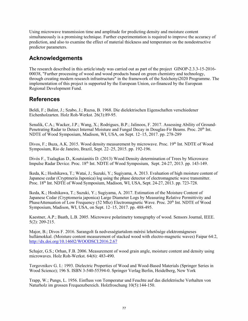
Using microwave transmission time and amplitude for predicting density and moisture content simultaneously is a promising technique. Further experimentation is required to improve the accuracy of prediction, and also to examine the effect of material thickness and temperature on the nondestructive predictor parameters.

Acknowledgements

The research described in this article/study was carried out as part of the project GINOP-2.3.3-15-2016-00038, "Further processing of wood and wood products based on green chemistry and technology, through creating modern research infrastructure" in the framework of the Széchenyi2020 Programme. The implementation of this project is supported by the European Union, co-financed by the European Regional Development Fund.

References

Beldi, F.; Balint, J.; Szabo, J.; Ruzsa, B. 1968. Die dielektrischen Eigenschaften verschiedener Eichenholzarten. Holz Roh-Werkst. 26(3):89-95.

Senalik, C.A.; Wacker, J.P.; Wang, X.; Rodrigues, B.P.; Jalinoos, F. 2017. Assessing Ability of Ground-Penetrating Radar to Detect Internal Moisture and Fungal Decay in Douglas-Fir Beams. Proc. 20th Int. NDTE of Wood Symposium, Madison, WI, USA, on Sept. 12–15, 2017. pp. 278-289

Divos, F.; Buza, A.K. 2015. Wood density measurement by microwave. Proc. 19th Int. NDTE of Wood Symposium, Rio de Janeiro, Brazil, Sept. 22–25, 2015. pp. 192-196.

Divós F., Tsalagkas D., Koutsianitis D. (2013) Wood Density determination of Trees by Microwave Impulse Radar Device. Proc. 18th Int. NDTE of Wood Symposium, Sept. 24-27, 2013. pp. 143-149.

Ikeda, K.; Hoshikawa, T.; Watai, J.; Suzuki, Y.; Sugiyama, A. 2013. Evaluation of high moisture content of Japanese cedar (Cryptmeria Japonica) log using the phase detector of electromagnetic wave transmitter. Proc. 18th Int. NDTE of Wood Symposium, Madison, WI, USA, Sept. 24-27, 2013. pp. 723-728.

Ikeda, K.; Hoshikawa, T.; Suzuki, Y.; Sugiyama, A. 2017. Estimation of the Moisture Content of Japanese Cedar (Cryptomeria japonica) Large Diameter Logs by Measuring Relative Permittivity and PhaseAttenuation of Low Frequency (52 Mhz) Electromagnetic Wave. Proc. 20th Int. NDTE of Wood Symposium, Madison, WI, USA, on Sept. 12–15, 2017. pp. 488-495.

Kaestner, A.P.; Baath, L.B. 2005. Microwave polarimetry tomography of wood. Sensors Journal, IEEE. 5(2): 209-215.

Major, B.; Divos F. 2016. Sarangolt fa nedvességtartalom mérési lehetősége elektromágneses hullámokkal. (Moisture content measurement of stacked wood with electro-magnetic waves) Faipar 64:2, http://dx.doi.org/10.14602/WOODSCI.2016.2.67

Schajer, G.S.; Orhan, F.B. 2006. Measurement of wood grain angle, moisture content and density using microwaves. Holz Roh-Werkst. 64(6): 483-490.

Torgovnikov G. I.: 1993. Dielectric Properties of Wood and Wood-Based Materials (Springer Series in Wood Science); 196 S. ISBN 3-540-55394-0. Springer Verlag Berlin, Heidelberg, New York

Trapp, W.; Pungs, L. 1956. Einfluss von Temperatur und Feuchte auf das dielektrische Verhalten von Naturholz im grossen Frequenzbereich. Holzfroschung 10(5):144-150.

77

Tsusumi, J.; Watanabe, H. 1965. Studies on Dielectric Behavior of Wood. I. Effects of frequency and tempereature on ε' and tan δ. Journal of Japanese Wood Research Society 11(6):232-236.

Tsusumi, J.; Watanabe, H.: 1966. Studies on Dielectric Behavior of Wood. II. Effects of Moisture Content on Dielectri Constant ε' and Dielectric Loss Factor ε". Journal of Japanese Wood Research Society 12(3):115-118.

78

Nondestructive Wood Density Testing in Downy Birch and Silver Birch Genetics Field Trial, Southern Sweden

Grace Jones * Department of Forestry and Wood Technology, Linnaeus University, Växjö, Sweden, grace.jones@lnu.se

Stergios Adamopoulos * Department of Forestry and Wood Technology, Linnaeus University, Växjö, Sweden, stergios.adamopoulos@lnu.se

Mateusz Liziniewicz Skogforsk, Swedish Forestry Research Institute, Svalöv, Sweden, mateusz.liziniewicz@skogforsk.se

Johan Lindeberg Department of Forestry and Wood Technology, Linnaeus University, Växjö, Sweden, johan.lindeberg@lnu.se

Abstract

Non-destructive testing of wood density, as is already done for Eucalyptus, can allow for early selection of birch trees for breeding programmes and stands for harvesting. In this work, external stem quality traits were visually assessed in a family trial of downy (Betula pendula) and silver (B. pubescens) birch in southern Sweden. A subsample of trees was measured for wood density using the Pilodyn resistometer portable NDT tool. An X-ray microdensitometric analysis of the subsample of trees was completed using the Itrax X-ray machine for increment cores taken from the south face, through the pith to the north bark at 1.3 m stem height. The Pearson’s r value for Itrax density and Pilodyn density was high (0.580 for downy birch and 0.795 for silver birch), and this correlation means Pilodyn should provide a good estimate of average birch wood density. Neither species had stable wood density values at age 13 and both species’ density increased over time from pith to bark. Ring width influence on stem density was minor or non-existant, and may vary between birch species.

Keywords: Wood Density; Pilodyn; X-ray Densitometry; Birch Families; Plantations

Introduction

Birch has a long history in Sweden as a timber species, but mainly for furniture and non-structural uses. It is now predominantly used for firewood, pulp and paper production. These are low value uses for a species which covers over 10% of Sweden’s total forest area (Götmark et al. 2005). The solid wood properties of birch growing in Sweden are considered too low for structural use and limited works accurately measure or aim to improve birch solid wood properties. Wood density is considered to be an important solid wood property (Johansson et al. 2013), and Skogforsk (the forestry research institute in Sweden) has already worked to incorporate density into their breeding program (Stener and Hedenberg 2003). Other studies have included variation in birch wood density within the stem (Heräjärvi 2004; Repola 2006) but limited work is available comparing density between growth rings. There is also a shortage of studies on birch species which relate wood density between different ages, which can be used to select the best individuals earlier (Apiolaza 2009). The Pilodyn wood tester is used to provide a standing estimate of outermost density for a given stem. The tool provides an estimate of density by relating penetration depth to wood density (resistance to force). Previously, this tool has been used in breeding programmes for Eucalyptus (Raymond and

79

MacDonald 1998; Wu et al. 2010) and birch (Stener and Hedenberg, 2003), but is commonly used for conifers (Chen et al. 2015). The Pilodyn tool is simple to apply, and measured values are strongly correlated with wood density (Gao et al. 2017). It only measures the outer-most wood at a single point but is still used in tree breeding programmes today to indicate differences between families.

Wood density can quickly and with relatively minimal damage be gained from X-ray densitometry on radial cores (Bergsten et al. 2001; Fries and Ericsson 2009). An advantage of taking cores is that the radial density profile will include the pith and avoid any defects or anomalies, since these can be checked visually in the field. A radial density profile also allows the comparison of wood density and growth rate between years, but identifying ring boundaries is particularly difficult for birch (Vanhellemont et al. 2016). Different X-ray machines available for this purpose include the SilviScan, QTRS-01X Tree Ring scanner, the Itrax Multiscanner that combines digital X-ray radiography and XRF multi-element analysis, medical CT scanners and micro-CT scanners (Jacquin et al. 2017).

For many species it is beneficial to select trees with higher density at younger ages to reduce the total volume of low density wood produced. If denser wood occurs earlier, or if density between ages is related, early assessments can be used to find higher density stems earlier. This study investigates the range of density values between growth rings for two birch species in a genetic field trial with 13 year-old trees. It is desirable to establish fast and accurate determinations of wood density, so the relationship between density estimates from Pilodyn and the Itrax core scanner was also investigated.

Method

Description of the site

This work is part of a larger project investigating the wood quality of birch in Skogforsk’s south Swedish tree breeding programme. The 13 year old downy (Betula pendula) and silver (B. pubescens) birch trial at the Nybro site (56.836 N, 16.023 E; close to Åsmundsryd, Sweden) was visually and mechanically assessed (NDT) in October 2018. The site was planted in 2004 at 2 × 2 m spacing with completely randomized single tree plot design using Skogforsk’s bred silver and downy birch families. Mortality, uprooting and suppression meant that some additional stems were missing or too small to count. Family ID and tree plot, row and stem position were recorded for each tree and have been actively monitored over time. Nybro usually has monthly temperature values between -5 ˚C and +22˚C, but can reach extremes of -22 ˚C and +27 ˚C. Monthly rainfall is usually 13 to 58 mm, but itcan exceed 113 mm rainfall in a single month. There is usually no water deficit during the growingseason, which in an average year is between the 11th of May and October 1st (data for 1980-2016,weatherspark.com). Figure 1 is the site layout map and GPS coordinates.

Figure 1 – Map of Nybro site layout where each square represents 2 × 2 m and trees were planted at each corner. The site also has a row of buffer trees which were not measured.

80

Stem assessment

The stem diameter of all birch trees in the site was measured in a north-south direction at a height of 1.3 m using callipers. This measurement height was shifted slightly above or below if there were defects like branches or a multileader preventing accurate measurement. The height at which rough brown bark changed to smooth white bark was recorded for each tree from the ground to the average height where the stem ceased to have rough bark dominating. This rougher bark is often referred to as ‘fissured bark’ and is a darker brown.

Trees were ranked for some stem quality traits on a scale of 1-9 where 1 is the worst and 9 is the best. These traits included straightness: a score of 9 would be a perfect bole; branch angle: a score of 9 is a 90˚ angle to the stem; branch frequency: a score of 9 is for the lowest 8 m of the stem is branch free; and branch diameter: a score of 9 is an insignificant branch diameter compared to the stem diameter at the same height, while a score of 1 is a branch almost the same diameter as the stem.

Pilodyn measurement

The Pilodyn 6J Forest (PROCEQ, Zurich, Switzerland) was used at 1.3 m height on the north and south stem face of birch trees. For both stem faces, the average value from two Pilodyn measurements was recorded. If any extreme or failed measurements occurred, more measurements were taken, and on some occasions the bark was peeled to see if the striker pin had entered the wood. Pilodyn was then converted from mm penetration to g/cm3 using the formula in Chen et al. (2015).

Itrax analysis

For X-ray microdensitometry, 5 mm cores were collected at 1.3 m height from south-north to ensure the pith was included in the sample. Cores were stored in paper tubes until they were glued into a wooden frame with a 6 mm rivet. The glued cores were sawn to a thickness of 2 mm using a fine grade circular saw. The sawn samples were placed into the Itrax flatbeam core scanner (Cox Analytical Systems, Mölndal, Sweden) for an analysis according to Bergsten et al. (2001). The X-ray images were processed using the software LIGNOVISION™ (RINNTECH, Heidelberg, Germany). The ring boundaries were determined by peak density values or visual sample assessment where boundaries were smooth or blurred. The output from LIGNOVISION™ includes ring number, an average light intensity value, and ring width for automatically selected or user defined ring boundaries. The output light intensity value was corrected using a moisture calibration value based on average temperature and humidity during the Itrax operation, and a plastic calibration sample of known thickness and density measured at the same time. Sample thickness was measured using a digital point calliper along the sample length, and light intensities values were also corrected using the actual sample thickness.

Statistical analysis performed

A subsample of 20 trees were selected from a larger dataset for the analysis in this paper. Considering only defect free stems, 10 silver birch trees and 10 downy birch trees were selected, for which at least 13 tree rings had been identified and measured in LIGNOVISION™ in both the north and south direction. Pilodyn and Itrax values were compared between the north and south stem faces using MicroSoft Excel (MicroSoft Office 2016) paired and unpaired two-tailed t-tests in their data analysis add-on, with a significance level of α=0.05. The Pearson function in Microsoft Excel (MicroSoft Office 2016) was used for calculating the Person r value for correlations between variables, where above 0.5 was considered indicative of a likely relationship between variables. The software package R version 3.6.0 (R core team, 2019) was used for graphics, with the tidyverse package used for line graphs and scatterplots. Scatter plots had a trendline fitted using the trendline function and included a 95% confidence interval (calculated by R).

81

Results

Range of values

Values from the stem quality assessment are summarized by species in Table 1. Silver birch has a higher level of variability for diameter at 1.3 m height (DBH) and the height of rough brown bark (Bark height). The qualitative traits are straightness (straight), branch angle, branch thickness and branch frequency. Since these were ranked from 1-9 and for only 10 trees per species, the key thing they show for this subsample is that downy birch had slightly higher average quality than silver birch for straightness. Branch angle, thickness and frequency were similar between species, but slightly higher for silver birch than for downy birch.

Table 1 – Average and standard deviation (StDev) for stem quality assessment of downy and silver birch Species Value DBH (mm) Bark height (cm) Straight Branch

angle Branch

thickness Branch

frequency Downy Average 106.9 22.0 5.7 4.4 5.1 4.7

StDev 20.7 16.9 1.0 0.8 0.7 0.7 Silver Average 126.3 70.0 4.9 4.7 5.3 5.5

StDev 22.4 29.3 0.9 1.0 0.7 1.3

It should be noted that no statistically significant difference was found between wood density values for north and south from Pilodyn and Itrax (average for rings 2-13) according to a t-test with significance level α=0.05. With 19 degrees of freedom, the t critical for two tailed t-test was 2.09, which was higher than the test statistics -0.68 for Pilodyn, and 1.54 for Itrax (rings 2-13 averaged). Therefore, an average value was used for Pilodyn (north and south) and Itrax (north and south) during subsequent analysis.

Table 2 shows the overall average ring widths, and Pilodyn and Itrax wood densities for downy and silver birch. Density values from Itrax are presented as an average of rings 2 to 13 (R2-13) and for rings 12 to 13 (R12-13). Pilodyn should be most comparable to Itrax outermost rings since it measures the outermost wood (10-20 mm penetration depth), and here rings 12 and 13 were chosen since all trees in the the subsample had these values recorded. The average also smooths out some possible issues due to incorrect ring identification. Birch is a diffuse-porous species and distinguishing between year rings can be difficult since the growth ring is fairly uniform. Wood density values were lower for downy birch than for silver birch, and were lower from Itrax (0.429 g/cm3 for downy and 0.439 g/cm3 for silver) than from Pilodyn (0.528 g/cm3 for downy and 0.537 g/cm3 for silver). Silver birch had more variation in Itrax density values than downy birch, which is presented in Table 2 as higher standard deviations. The t-statististics for two tailed t-tests comparing downy birch to silver birch all had a t-critical value of 2, so the the two species were not considered significantly different, for a significance level of α=0.05.

Table 2 – Average and standard deviation (StDev) for ring width and wood density (Itrax and Pilodyn) of downy and silver birch for rings 2 to 13 (R2-13) and 12 to 13 (R12-13).

Species Value Ring width (mm) Density (g/cm3) R2-13 R12-13 Itrax: R2-13 Itrax: R12-13 Pilodyn

Downy Average 3.597 2.835 0.387 0.429 0.528 StDev 1.159 0.877 0.039 0.035 0.058

Silver Average 3.727 2.798 0.396 0.439 0.537 StDev 1.299 0.583 0.048 0.043 0.057

Two tailed t-stat -0.385 0.140 -0.615 -0.560 -0.372

Ring width average for rings 2-13 did not seem to be related to Itrax wood density average for rings 2-13 since the Pearson r values were below 0.5 (0.153 for downy birch and 0.114 for silver birch). A weak relationship existed between Pilodyn density values and average ring widths, and the direction

82

of this relationship was different between the two species (-0.278 for downy birch and 0.245 for silver birch).

Radial wood density

The Itrax wood density values by ring number are plotted in figure 2. The distribution is wider for the silver birch sample than for the downy birch sample, which was previously shown by a higher standard deviation. Neither species appears to have levelled off and both are still increasing in density. The black line for both species is the average wood density for that ring number, and they closely resemble each other in shape and slope.

Figure 2 – Radial variation of Itrax wood density for individual downy and silver birch trees. Solid black lines are the average species wood density values (AvDowny and AvSilver, respectively).

Pilodyn values plotted against Itrax values

The wood density values from Pilodyn were plotted as a function of Itrax density for rings 2-13 and 12-13 in figure 3. Figure 3 also shows trendlines with shaded regions representing the 95% confidence intervals for the fitted values. The trend lines for both species are extremely similar and the confidence intervals overlap. For rings 2-13 the silver birch trend line has a slightly less steep slope than the downy birch trend line, but it reduced further when the most extreme value was removed. In a small sample however all points have high leverage so this individual was retained. When correlating Itrax values with Pilodyn values, the Pearson’s r was higher for the average density of rings 2-13 (0.580 for downy birch and 0.795 for silver birch) than for just an average of rings 12-13 (0.548 and 0.691 respectively). In figure 3 where the Itrax wood density of rings 12-13 is plotted against Pilodyn density (left), the downy birch trendline predicting Pilodyn from average Itrax density has a slope of 1.072 and an intercept of 0.064, while the silver birch trendline has a slope of 1.059 and an intercept of 0.082. The trendlines for rings 2-13 (right) had a slope of 1.336 and intercept of 0.006 for downy birch, and a slope of 1.390 and intercept of -0.004 for silver birch.

83

Figure 3 – Relationships between Pilodyn and Itrax wood density for rings 2-13 (right) and 12-13 (left). The fitted trend lines and have 95% confidence intervals in shaded region.

Discussion

In this sample all trees were planted at the same time and are the same age, so differences in wood density must be due to other factors like species, family growth and physical form. Here, our work focused on the differences between birch species as well on the effects of growth rate (ring width) on density. Silver birch had higher density values than downy birch in this study, which agrees with previous studies in Scandinavia (Bhat 1980; Heräjärvi 2002; Luostarinen and Verkasalo, 2000). The greater variation of density for the silver birch sample is possibly due to greater variation in stem size or growth rate, since age was constant for all trees. The wood density of diffuse-porous species is usually not influenced by the width of the growth rings (Hoadley 1990; Panshin and De Zeeuw 1980), yet some studies have found a relationship between birch growth rate and density (Bhat 1980; Velling 1979). A significant negative relationship between ring width and density was previously found in juvenile silver birch (Liepiòð and Rieksts-Riekstiòð 2013) for Latvia. Our findings potentially show for Skogfork’s young Swedish birch a weak correlation between ring width and wood density that was different for the two species. Since the Pearson’s r values were well below 0.5, it is also possible that there is no correlation between ring width and density. A larger data set would help to confirm this and see if the direction of the relationship is different for the two birch species.

Wood density varies throughout a tree from pith to bark and base to top (Heräjärvi 2004). Birch wood near the pith is less dense than the wood at the outer rings near the bark (Luostarinen and Verkasalo 2000). The density values had not yet peaked in our sample and were still highly variable at age 13. However, for each individual tree there is a similar trend for increasing density from pith to bark (ring 2 to 13) which indicates that it should be possible to select better stems during earlier measurements. The average density profile for each species showed that the general pattern of density increase was similar for the two birch species, but here the range was wider for silver birch. The pattern of increasing density from pith to bark also resembled the pattern for two Betula spp. described by Fukazawa (1984).

The high Pearson’s r for Itrax values compared to Pilodyn indicates that the Pilodyn tool measurements are related to Itrax values, but the lower value for the outermost rings is unusual. It could be that the outer rings were more likely to have damage from sampling, and it is possible that averaging more growth rings slightly stabilized the values. Identifying ring boundaries in diffuse porous species is very hard without preparation of microscope sections, and this may also have hidden relationships between ring width and density that would show up in a larger sample.

84

Conclusions

Pilodyn and Itrax wood density values were related, which validates the use of Pilodyn in field for rapid assessment of stem density. Pilodyn values were however overestimated, so it would be better used as indicative of the true stem density. It is not possible to conclude from this study the earliest age that Pilodyn could be used to predict final wood density. More studies are needed with mature trees for wood density determination in the juvenile and mature wood zones that would provide evidence of the predictive potential of Pilodyn.

Pilodyn seems to be strongly related to Itrax density values and this relationship was similar between the two birch species. Values of ring width and density had no statistically significant difference between birch species. Ring width and density had a low Pearson’s r for both species meaning it is possible that ring density is independent of width. Although the two species did not have statistically significant differences in density and ring width, it would be worth treating the two species seprerately during further studies since averages and deviations were different.

References

Apiolaza, L. 2009. Very early selection for solid wood quality: screening for early winners. Annals of Forest Science, 66(6), 601-601. doi:10.1051/forest/2009047

Bergsten, U., Lindeberg, J., Rindby, A., & Evans, R. 2001. Batch measurements of wood density on intact or prepared drill cores using x-ray microdensitometry. Wood Science Technology, 35(5), 435-452.

Bhat, K. 1980. Variation in structure and selected properties of Finnish birch wood. 1: Interrelationships of some structural features, basic density and shrinkage [Betula pendula, B. pubescens]. Silva Fennica.

Chen, Z.-Q., Karlsson, B., Lundqvist, S.-O., García Gil, M. R., Olsson, L., & Wu, H. X. 2015. Estimating solid wood properties using Pilodyn and acoustic velocity on standing trees of Norway spruce. Annals of Forest Science, 72(4), 499-508. doi:10.1007/s13595-015-0458-9

Fries, A., & Ericsson, T. 2009. Genetic parameters for earlywood and latewood densities and development with increasing age in Scots pine. Annals of Forest Science, 66(4), 1-8.

Fukazawa, K. (1984). Juvenile wood of hardwoods judged by density variation. IAWA Journal, 5(1), 65-73.

Gao, S., Wang, X., Wiemann, M. C., Brashaw, B. K., Ross, R. J., & Wang, L. 2017. A critical analysis of methods for rapid and nondestructive determination of wood density in standing trees. Annals of Forest Science, 74(2), 27.

Götmark, F., Fridman, J., Kempe, G., & Norden, B. 2005. Broadleaved tree species in conifer-dominated forestry: Regeneration and limitation of saplings in southern Sweden. Forest Ecology and Management, 214(1), 142-157. doi:https://doi.org/10.1016/j.foreco.2005.04.001

Heräjärvi, H. 2002. Properties of birch (Betula pendula, B. pubescens) for sawmilling and further processing in Finland: Metsäntutkimuslaitos.

Heräjärvi, H. 2004. Variation of basic density and Brinell hardness within mature Finnish Betula pendula and B. pubescens stems. Wood and Fiber Science, 36(2), 216-227.

85

Hoadley, R. B. 1990. Identifying wood: accurate results with simple tools: Taunton Press.

Jacquin, P., Longuetaud, F., Leban, J.-M., & Mothe, F. 2017. X-ray microdensitometry of wood: A review of existing principles and devices. Dendrochronologia, 42, 42-50. doi:https://doi.org/10.1016/j.dendro.2017.01.004

Johansson, M., Säll, H., & Lundqvist, S.-O. 2013. Properties of materials from Birch–Variations and relationships: Part 2. Mechanical and physical properties: Linnaeus University.

Liepiòð, K., & Rieksts-Riekstiòð, J. 2013. Stemwood density of juvenile silver birch trees (Betula pendula Roth) from plantations on former farmlands.

Luostarinen, K., & Verkasalo, E. 2000. Birch As Sawn Timber and in Mechanical Further Processing in Finland. A Literature Study.

Panshin, A., & De Zeeuw, C. 1980. Textbook of wood technology. Part 1. Formation, anatomy, and properties of wood. In: McGraw-Hill, New York, USA.

Raymond, C. A., & MacDonald, A. C. 1998. Where to shoot your pilodyn: within tree variation in basic density in plantation Eucalyptus globulus and E. nitens in Tasmania. New Forests, 15(3), 205-221. doi:10.1023/a:1006544918632

Repola, J. 2006. Models for vertical wood density of Scots pine, Norway spruce and birch stems, and their application to determine average wood density.

Stener, L.-G., & Hedenberg, Ö. 2003. Genetic parameters of wood, fibre, stem quality and growth traits in a clone test with Betula pendula. Scandinavian Journal of Forest Research, 18(2), 103-110.

Vanhellemont, M., Van Acker, J., & Verheyen, K. 2016. Exploring life growth patterns in birch (Betula pendula). Scandinavian Journal of Forest Research, 31(6), 561-567. doi:10.1080/02827581.2016.1141978

Velling, P. 1979. Wood density in two Betula pendula Roth progeny trials. Folia Forestalia, 416, 1-24.

Wu, S.-j., Xu, J.-m., Li, G.-y., Risto, V., Lu, Z.-h., Li, B.-q., & Wang, W. 2010. Use of the Pilodyn for assessing wood properties in standing trees of Eucalyptus clones. Journal of Forestry Research, 21(1), 68-72.

86

Development and Commercialization of a Locally Designed Digital Wood Moisture Meter

Marina A. Alipon* Department of Science and Technology (DOST) – Forest Products Research and Development Institute (FPRDI), College, Laguna 4031, Philippines, alipon07marinaa@yahoo.com.ph/aliponmarina@gmail.com

Gil B. Dolotina DOST-FPRDI, College, Laguna 4031, Philippines, gilbdolotina@gmail.com

Gerwin P. Guba DOST-Advanced Science and Technology (ASTI), Diliman, Quezon City, Philippines, gerwin.guba@gmail.com

Alvin E. Retamar DOST – ASTI, Diliman, Quezon City, Philippines, retamare@gmail.com

Grecelda A. Eusebio DOST – FPRDI, College, Laguna 4031, Philippines, ycelaeusebio@yahoo.com

*Corresponding author

Abstract

The Forest Products Research and Development Institute (FPRDI) in collaboration with the Advanced Science and Technology Institute (ASTI) of the Department of Science and Technology (DOST) and YONGDEN Company developed a digital resistance type wood moisture meter for the furniture and handicraft industry.

The digital moisture meter is an improved version of the analog resistance type moisture meter developed by FPRDI in 2001. Similar to the analog type, it equipped with a parallel pair of needle - type electrodes 25 mm apart that can detect moisture content (MC) in wood to about 25 mm depth. The digital meter can measure can measure wood MC within 6 to 25%. The MC reading is automatically displayed and read without adjusting any selector switch as in analog. In addition to the 12.5 mm built-in needle to the meter for measuring thin wood, it has a probe hammer with 50 mm needles that can replace the small needle to measure MC’s of thicker wood samples/products.

The wood moisture meter case design measures 60 mm x 43.0 mm, twice smaller than the analog. The operation is much simpler and the cost is cheaper than the analog.

_________________________________ Keywords: digital wood moisture meter, analog resistance meter, moisture content

87

Introduction

The Philippine is a major global player in the furniture industry. Philippine furniture ranks among the world's best, earning for the country the distinction of being the "Milan of Asia" because of its elegance and high quality craftsmanship. In an industry dominated by small and medium entrepreneurs, it has succeeded in becoming a dollar earning industry (www.cfipnet.com).

An estimated 15,000 local furniture companies are actively supporting the industry and provide employment to a total of 481,500 direct workers and 300,000 sub-contractors. Only 10% of these establishments are considered large companies. The remaining 90% are classified as small and medium enterprises (SMEs). Notably, SME's make- up bulk of the 2,500 furniture companies engaged in exports (Furnitureman 2017).

On the other hand, the handicraft industry is one of the oldest industries in the country. The handicraft manufacturers are also dominated by SME's. with ninety-six (96) percent of the country's handicraft firms classified as either cottage and small enterprises. For basketry alone, there are about 5,000 basket manufacturers with l50 firms classified, as large scale and the rest are as small and medium scale firms. The industry is labor intensive, directly employing 40,000 and 1,000,000 workers indirectly, spread over the basket producing regions in the country (Pearl 2 2004)

The international competitiveness of the wood-based furniture and handicraft industry depends on product quality. In turn, product quality depends largely on the moisture content (MC) of the materials used. The most convenient and fastest way of determining moisture content is with the use of moisture meter.

Moisture meters, however, are all imported and could be expensive. Moreover, imported meters are calibrated using foreign wood species as reference points, i.e. American-made moisture meters are calibrated using Douglas fir while European-made moisture meters are calibrated using beech. When used with local wood species, these moisture meters give large discrepancies in moisture content readings necessitating recalibration of the meters to give accurate MC readings. The calibration process is time consuming and can be costly (P1,500 (US$30) - P2,000 (US$40/species).

Most of the small and medium furniture and handicraft enterprises do not have moisture meters. There is thus a need to develop moisture meters that are cheaper than imported ones and calibrated to local species. With the moisture meters, the SME's could afford to buy this utility for a more reliable measurement of wood's moisture content, thus eventually improving the quality of their products.

The Forest Products Research and Development Institute (FPRDI) developed in 2001 a needle-type resistance analog moisture meter for wood (Figure 1). The moisture meters is made of a simple transistorized circuit supplied with a 9 volts battery, equipped with a pair of parallel needle-type electrodes 25.4 mm apart and a sliding hammer the drives the needles into the wood. The needle-type electrodes can be used for specimens up to about 25.4 mm in depth. The meter reads the resistance of wood samples to electric current and correlates this resistance to moisture content which values were previously obtained through the standard oven-drying method of MC determination. The FPRDI-developed moisture meter can be used effectively within a range of 6 - 25% moisture content. The meter was calibrated to yemane (Gmelina arborea Roxb.) (Verbenaceae), an industrial tree plantation species widely planted in the Philippines, and correction factor for other 9 wood species commonly used for furniture making were derived.

Around 400 units of the FPRDI-developed analog moisture meter have been fabricated and availed of by various wood-using firms. The introduction an application of the FPRDI moisture meter has been serving as an important tool in enhancing production capabilities and product quality of small and medium enterprises wood manufacturers. The following change in the level of productivity was met:

88

1. Increased production – A moisture meter is necessary in monitoring the quality of woodenfurniture. It provides a means of guaranteeing that the wood used in the product has been dried to the required moisture content (MC). This prevents guesswork to the producers and acquires the confidence to claim that his products met the required MC standards. Quality products improve a firm’s reputation and encourage repeat purchases and referrals from satisfied buyers.

2. Decreased cost of production – Back jobs are common in small firms that cannot affordgood quality wood moisture meters. Back jobs are usually in the form of checking and or cracking of wood in fabricated furniture. Adoptors of FPRDI moisture meter estimate that the average cost of these back jobs are 20% of production cost. For dining chair with an average production of PhP2,000.00 (US$40), cost of back job is P400.00 (US$8) per chair. Thus, savings arising from the reduction of back jobs.

Some users found the use of the FPRDI-developed analog moisture meter complicated because it involves 3 switches for 3 ranges of MC limits, namely: A= 7 - 12% MC; B= 12 - 17% MC and C= 17-25% MC. If the MC reading is over 12% MC, then the switch should be turned from A to B; and if over 17% MC, from B to C. Moisture content value should also be read approximately 5 seconds after the needles have penetrated the wood sample. Thus in 2007- 2008, the Forest Products Research and Development Institute (FPRDI) in collaboration with the Advanced Science and Technology Institute (ASTI) of the Department of Science and Technology (DOST) and YONGDEN company developed a digital resistance type wood moisture meter for the furniture and handicraft industry (Figure 2).

The digital moisture meter is an improved version of the analog resistance type moisture meter developed by FPRDI in 2001. Similar to the analog type, it equipped with a parallel pair of needle - type electrodes 25 mm apart that can detect moisture content (MC) in wood to about 25 mm depth. MC reading is automatically displayed and read without adjusting any selector switch as in analog.

The wood moisture meter case design measures 60 mm x 43.0 mm, twice smaller than the analog. The operation is much simpler and the cost is cheaper than the analog. As of 29 February 2008, several companies have expressed desire to avail of the unit. There had been numerous orders received from phone calls and e-mail. The digital wood moisture meter is expected to be out in the market on or before March 30, 2008.

With the development and introduction of the FPRDI wood moisture meter in the local market, the importation of the expensive moisture meter will provide opportunities to local manufacturers to buy and make use of the equally efficient and low cost meter. It is not only the community that benefited but the national economy as well.

89

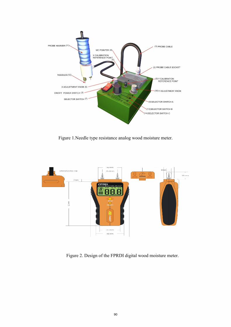
Figure 1.Needle type resistance analog wood moisture meter.

Figure 2. Design of the FPRDI digital wood moisture meter.

90

Figure 3. FPRDI digital wood moisture meter box casing.

Conclusion and Recommendation

• This pioneering local research invention helps the wood based-industry especially thesmall and medium enterprises in improving the quality of their wood products andeliminate back jobs.

• The meter provides local wood manufacturers to buy and use equally to even moreefficient meter at affordable price.

• The meter is highly recommended for more extensive promotion and marketing bothlocal and abroad.

Acknowledgment

ASTI, for serving as co-project implementer Yongden/Alexan Company, for serving as project cooperator DOST- TECHNICOM Program, for providing project funds. PCASTRD, for monitoring and coordinating the project implementation.

Reference FURNITUREMAN. 2017. 3rd and 4th Quarter Issue. Philippine Report on Furniture Industry.

91

Session 2

In-Forest Assessment

92

Predicting Bending Properties of Planted Acacia mangium Using MOE Evaluator Xin Yao, Teng* Applied Forest Science & Industry Development Division, Sarawak Forestry Corporation Sdn Bhd, Lot 218, KCLD, Jalan Tapang, Kota Sentosa, 93250 Kuching, Sarawak, Malaysia. xyteng@sarawakforestry.com King Boh, Ting Applied Forest Science & Industry Development Division, Sarawak Forestry Corporation Sdn Bhd, Lot 218, KCLD, Jalan Tapang, Kota Sentosa, 93250 Kuching, Sarawak, Malaysia. kbting@sarawakforestry.com Abstract Acacia mangium is one of the major fast-growing timber species used by plantation programs which accounted for an about 69% of the total planted forest areas in Sarawak, Malaysia as an alternative source of material for wood based industries. These plantation logs are of fast grown, small diameter with high growth stress and high variability that would affect the timber strength properties. In this study, modulus of elasticity (MOE) was used to predict bending properties of planted 10 years old Acacia mangium in Sarawak. MOE of the samples were obtained by performing Non-Destructive Testing (NDT) using MOE Evaluator and were compared with static bending tests. A total of 100 pieces 2000mm length x 100mm width x 25mm thickness lumber were used in this study. Tested samples had mean density of 462 kg/m3 at mean moisture content of 13.5 %. According to Malaysian Standard MS 544 Part 2, Acacia mangium is classified under strength group SG5. The coefficient of determination (R2) between dynamic MOE and static MOE is 0.8527. Coefficient of determination between dynamic MOE and static MOR bending was measured as 0.8544 and coefficient of determination between static MOE and static MOR bending was measured as 0.8097. The R2 of the established correlation between dynamic MOE and static MOR bending is very close to the R2 of the established correlation between static MOE and static MOR bending. Thus, it can be concluded that bending properties of Acacia mangium wood can be predicted using MOE Evaluator. Keywords: Acacia mangium, Non-destructive testing (NDT), Modulus of elasticity (MOE), MOE Evaluator, bending properties Introduction Acacia mangium has been planted widely in Malaysia particularly in Sarawak which covers a total of about 69% of Sarawak’s forests plantation. It is primarily for wood based industry such as furniture, plywood and medium density fiberboard (MDF). This species is also known for its fast-growing character, tolerance to poor soil condition, promising growth and as a sustainable natural resource for timber products which makes it good for plantation species. In the last two decades, non-destructive testing (NDT) technique has been widely used in wood industry for mechanical property evaluation. The major advantage of the NDT technique is that the physical and mechanical properties of a material are quantified without altering its end-use capability. NDT methods have developed from laboratory testing to an essential production tool. Often components are too costly, or destructive testing is not possible, thus NDT is becoming increasingly important as a quality control management tool in almost every manufacturing process.

93

Objective The objective of this study was to predict bending properties of planted Acacia mangium wood lumber in Sarawak using MOE Evaluator. Materials and Methods Materials preparation A licensed planted forest (LPF) site within Sarawak state LPF 0042, Sampadi Lundu was chosen. A total of 10 Acacia mangium trees of similar diameter (20 - 30 cm DBH over bark) were felled and collected. The age of the trees was 10 years old. To perform the laboratory work, the sampling of specimens was made from bottom to top portion of the tree logs. The log was ripped into half through the pith to obtain the flitches. Some allowance was given for solar kiln drying and machining processes. Next, the flitches undergone the planing process. The flitches were subsequently ripped across the diameter and converted to the lumber. The small specimen from each lumber was taken to test its moisture content and basic density. Moisture content determination Moisture content determination was conducted directly after the processing was completed. This was to ensure that the moisture content inside the samples was maintained. At that point, the initial weights were taken. Then, samples were placed in the oven at 103±2°C until the constant weight was achieved. Afterward, the oven-dried weights were taken. Therefore, the moisture content values were determined by using the formula (1) below:

MC= mi - m0

m0 𝑥𝑥 100% (1)

where, MC = the moisture content of wood, in percentage mi = the initial weight of test specimen, in grams mo = the oven-dry weight of test specimen, in grams Basic density determination For density determination, the test pieces obtained after cutting will be weighed immediately to an accuracy of 0.01 g. If the specimens cannot be weighed immediately, they should be placed in a plastic bag or tightly wrapped in cellophane to protect them from moisture change until they can be weighed. Measure the sides of cross-section and length of test pieces along the axes of symmetry to the nearest 0.1 mm. Oven dry the test pieces at 103±2 oC to constant mass. Weigh the test pieces to obtain their oven-dry weights. Measure again the dimensions of the test pieces to obtain their oven-dry volumes. Therefore, the basic density values were determined by using the formula (2) below:

ρo = Wo

LoBoHo= Wo

Vo (2)

94

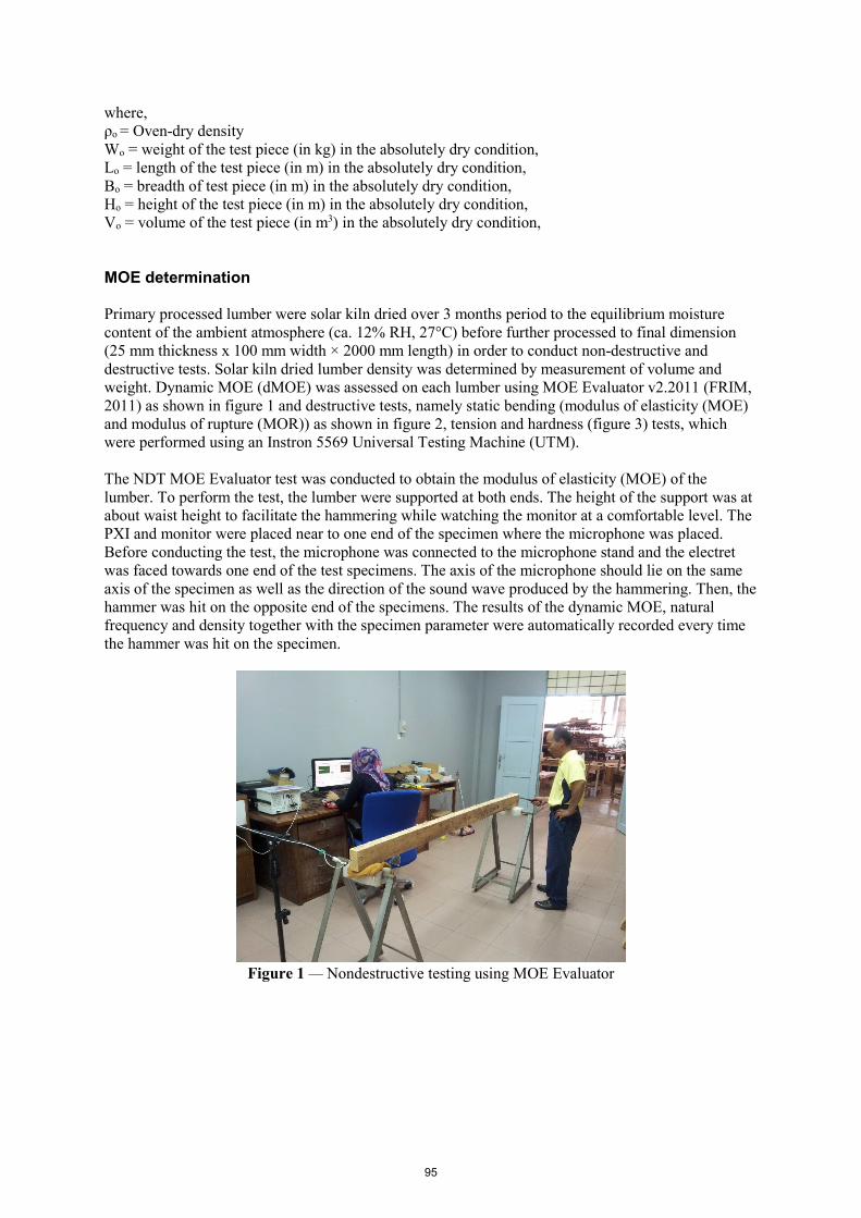
where, ρo = Oven-dry density Wo = weight of the test piece (in kg) in the absolutely dry condition, Lo = length of the test piece (in m) in the absolutely dry condition, Bo = breadth of test piece (in m) in the absolutely dry condition, Ho = height of the test piece (in m) in the absolutely dry condition, Vo = volume of the test piece (in m3) in the absolutely dry condition, MOE determination Primary processed lumber were solar kiln dried over 3 months period to the equilibrium moisture content of the ambient atmosphere (ca. 12% RH, 27°C) before further processed to final dimension (25 mm thickness x 100 mm width × 2000 mm length) in order to conduct non-destructive and destructive tests. Solar kiln dried lumber density was determined by measurement of volume and weight. Dynamic MOE (dMOE) was assessed on each lumber using MOE Evaluator v2.2011 (FRIM, 2011) as shown in figure 1 and destructive tests, namely static bending (modulus of elasticity (MOE) and modulus of rupture (MOR)) as shown in figure 2, tension and hardness (figure 3) tests, which were performed using an Instron 5569 Universal Testing Machine (UTM). The NDT MOE Evaluator test was conducted to obtain the modulus of elasticity (MOE) of the lumber. To perform the test, the lumber were supported at both ends. The height of the support was at about waist height to facilitate the hammering while watching the monitor at a comfortable level. The PXI and monitor were placed near to one end of the specimen where the microphone was placed. Before conducting the test, the microphone was connected to the microphone stand and the electret was faced towards one end of the test specimens. The axis of the microphone should lie on the same axis of the specimen as well as the direction of the sound wave produced by the hammering. Then, the hammer was hit on the opposite end of the specimens. The results of the dynamic MOE, natural frequency and density together with the specimen parameter were automatically recorded every time the hammer was hit on the specimen.

Figure 1 — Nondestructive testing using MOE Evaluator

95

Figure 2 — 3-point bending test Figure 3 — Hardness test Statistical analysis was performed in order to interpret relationship among dynamic MOE and static MOE and static MOR bending properties. Results and Discussion The results on physical properties of solar kiln dried at mean moisture content 13.5% lumber are presented in Table 1. The results indicated that the values of the dynamic MOE were slightly higher than static MOE in bending of the Acacia mangium lumber. The dynamic MOE of Acacia mangium (11589 MPa) obtained in this study was lower than that of Eucalyptus pellita (17700 MPa) collected from Kapit, Sarawak as reported by Hii et al. (2017) and Rubberwood (14590 MPa) collected from Gedung, Serian as reported by Emilia & Gaddafi (2015) so far in Sarawak, Malaysia. The relationship between static MOE and dynamic MOE is shown in figure 4. The relationship between static MOR bending and dynamic MOE is shown in figure 5. The relationship between static MOR bending static MOE is presented in figure 6. There was a reasonable correlation between the dynamic MOE values determined through non-destructive test and the static MOE values determined through destructive test on the lumber observed. Table 1 — Physical properties of solar kiln dried (13.5% MC) lumber

Species Mean

density (kg/m3)

Dynamic MOE (MPa)

Static MOE (MPa)

Static MOR (MPa)

Tensile stress (MPa)

Janka hardness – Tangential

(kN)

Janka hardness –

Radial (kN)

Acacia mangium 462 11589 11368 94.32 132 4.25 4.13

Janka Hardness tests that conducted on the tangential and radial faces showed results of 4.25 kN and 4.13 kN respectively. These results are similar to that for planted Eucalyptus pellita in Sarawak (Hii et al., 2017) which is utilized extensively for flooring and furniture making. According to Malaysian Standard MS 544 Part 2, Acacia mangium is classified under strength group SG5.

96

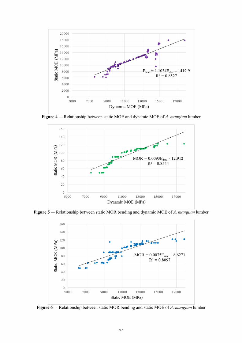
Figure 4 — Relationship between static MOE and dynamic MOE of A. mangium lumber

Figure 5 — Relationship between static MOR bending and dynamic MOE of A. mangium lumber

Figure 6 — Relationship between static MOR bending and static MOE of A. mangium lumber

97

Conclusions Acacia mangium lumbers were tested in order to evaluate bending properties using both nondestructive and destructive methods. Tested samples had mean density of 462 kg/m3 at mean moisture content of 13.5 %. Acacia mangium is classified under strength group SG5 as accordance with Malaysian Standard MS 544 Part 2. The coefficient of determination (R2) between dynamic MOE and static MOE is 0.8527. Coefficient of determination between dynamic MOE and static MOR bending was measured as 0.8544 and coefficient of determination between static MOE and static MOR bending was measured as 0.8097. The R2 of the established correlation between dynamic MOE and static MOR bending is very close to the R2 of the established correlation between static MOE and static MOR bending. Thus, it can be concluded that bending properties of Acacia mangium wood can be predicted using MOE Evaluator. Acknowledgments The authors would like to gratefully acknowledge Dr. Alik Duju for his guidance and support, technical staff of Sawmill and Woodworking Section, Mechanical Testing Section of Timber Technology Centre, Sarawak Forestry Corporation. References Emilia, A. & Gaddafi, I. 2015. Strength Performance of Hevea brasiliensis at Structural Size, International Advanced Research Journal in Science, Engineering and Technology Vol. 2, Issue 11. Forest Research Institute of Malaysia (FRIM). 2011. NDT MOE EVALUATOR, Dr. Omar Khaidzir, Kepong, Selangor, Malaysia. Hii, S.Y., Ha, K.S., Ngui, M.L., Penguang, J.S., Duju, A., Teng, X.Y. & Meder, R. 2017. Assessment of plantation-grown Eucalyptus pellita in Borneo, Malaysia for solid wood utilisation, Australian Forestry, 80:1, 26-33.

98

Wood Density Variations between Tree Components Should Be Considered to Correctly Estimate Tree Biomass Available for Different Uses Antoine Billard * Université de Lorraine, AgroParisTech, INRA, Silva, 54000 Nancy, France, antoine.billard@inra.fr Rodolphe Bauer Université de Lorraine, AgroParisTech, INRA, Silva, 54000 Nancy, France, rodolphe.bauer@inra.fr Frédéric Mothe Université de Lorraine, AgroParisTech, INRA, Silva, 54000 Nancy, France, frederic.mothe@inra.fr Francis Colin Université de Lorraine, AgroParisTech, INRA, Silva, 54000 Nancy, France, francis.colin@inra.fr Fleur Longuetaud Université de Lorraine, AgroParisTech, INRA, Silva, 54000 Nancy, France, fleur.longuetaud@inra.fr * Corresponding author Abstract Although biomass depends as much on volume as on density, in the case of trees, only the volume of the stem and the density at breast height have been studied quite extensively. The rare existing works and our preliminary analyses showed that, according to the species, the density could vary strongly between and within tree components. There is a need to better know the forest resource in terms of wood density and biomass of the different tree components (clear wood, knots, bark, branches). Such work will contribute to refine biomass estimates to evaluate carbon sequestration in forests and to optimize the use of wood resource (lumber, pulp, panel, fuelwood, new utilisations such as extractives for chemistry), with a particular attention paid to the recovering of “waste” woods. Wood samples of stem, knots and branches were X-rayed in oven-dried state with a medical CT scanner. For each type of sample, a specific image analysis procedure was developed under ImageJ software to measure wood density. We present here our results for the stem and knot components for three major softwood species in France. This was done within the frame of a project about the developement of a chemical industry. Knots are particulary rich in lignans, used in the cosmetics, medicine and nutrition industries. Knots have a much greater wood density than stem wood, whereas most wood density measurements, on which wood density databases are based, were performed at breast height. Depending on the species, it would be necessary to take into account theses variations to estimate correctly the biomass of tree components. Keywords: computed tomography, knots, extractives, forest resource

99

Introduction Accurate and non-biased estimate of biomass is necessary to meet several objectives. It is for example usual to estimate carbon sequestration of forest trees directly from total tree biomass. However, in the context of sustainable development, it becomes necessary to optimize the use of our resources. To optimize the use of forest biomass, it is needed to better know how it is distributed between and within the different tree components (stem, bark, knots, and branches). This last point is important to know if there is a need and an opportunity to develop a wood chemistry industry based on waste wood recovery. Bark and knots contain an important quantity of extractives (Kebbi-Benkeder, 2017). In particular, knots are a source of lignans, which can be used in cosmetics, medicine and alimentation. Such chemistry industry must not interfere with the already existing wood industry. Today, we are not able to estimate correctly the amount of biomass of the different tree components for two main reasons. We are not able to estimate the volume of some tree components due to a lack of available measurements. It is in particular the case for the knots. For all tree components, we have a lack of knowledge on the wood density variations (most density measurements were done at breast height and the number of trees per species in the databases is quite limited). Moreover the methods used for density measurements are often questionable (Williamson and Wiemann, 2010). Recent studies (Repola, 2006; Nogueira and al., 2008; Wiemann, 2013; Wassenberg, 2015; Wiemann and Williamson, 2014; Bastin et al., 2015) have proved that it was important to consider the variability of the wood density within the tree to have a good estimation of the biomass The density of knots was little studied. For spruce, Gartner (1995) showed that the knots are denser than the stem. A mean oven-dried density calculated from the article is 766 kg/m3 in comparison with the wood density provided for this species by the Global Wood Density Database of 370 kg/m3 (Chave et al. 2009, Zanne et al. 2009) for example. Lehtonen (1979) has studied pine and spruce of Finland. He found that the knots are denser than the stem of 351 kg/m3 for pine and 490 kg/m3 for spruce. Also, he found for pine that bigger is the knot, denser it is. It is the opposite for spruce. Boutelje (1966) obtained the same results for the density of the same species. In this study we measured the wood density of stem and knots for three softwood species (Norway spruce, silver fir and Douglas fir). We also estimated biomass for the knot component in our trees and compared our results with what would be done with breast height density measurement on our trees or with the usual wood density databases. Materials and methods Three softwood species were studied: Abies alba, Picea abies and Pseudotsuga menziesii. Each species was sampled in different experimental forests in France. Eight trees per species were harvested: four in an intensive thinning plot and four in a control plot which was not thinned. Trees were chosen in different diameter classes. The girth at 1m30 and the height of the crown base (the first whorl with at least 3/4 of living branches) were measured. For each tree, 15 stem discs were sampled along the stem avoiding knots. The height of the first three discs was fixed at 0.3m, 0.8m and 1.3m. The 12 other discs were evenly spaced along the stem. Radial cut was done within each disc for avoiding cracks. Seven short logs containing each a whorl of knots were sampled in addition. Five were taken above the crown base and two below the crown base.

100

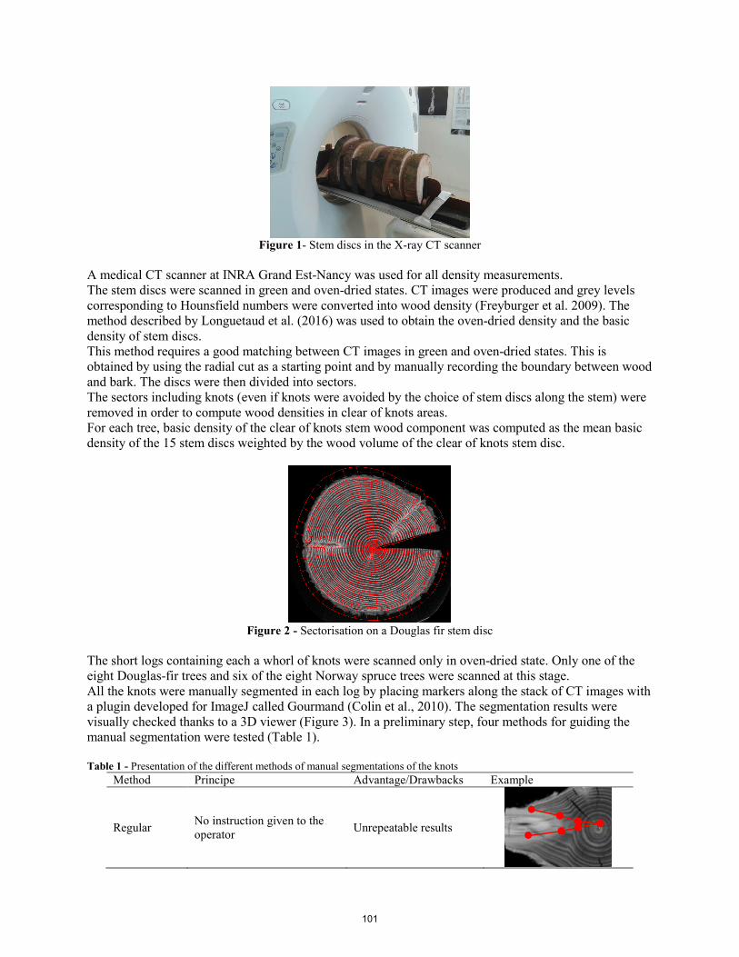
Figure 1- Stem discs in the X-ray CT scanner

A medical CT scanner at INRA Grand Est-Nancy was used for all density measurements. The stem discs were scanned in green and oven-dried states. CT images were produced and grey levels corresponding to Hounsfield numbers were converted into wood density (Freyburger et al. 2009). The method described by Longuetaud et al. (2016) was used to obtain the oven-dried density and the basic density of stem discs. This method requires a good matching between CT images in green and oven-dried states. This is obtained by using the radial cut as a starting point and by manually recording the boundary between wood and bark. The discs were then divided into sectors. The sectors including knots (even if knots were avoided by the choice of stem discs along the stem) were removed in order to compute wood densities in clear of knots areas. For each tree, basic density of the clear of knots stem wood component was computed as the mean basic density of the 15 stem discs weighted by the wood volume of the clear of knots stem disc.

Figure 2 - Sectorisation on a Douglas fir stem disc

The short logs containing each a whorl of knots were scanned only in oven-dried state. Only one of the eight Douglas-fir trees and six of the eight Norway spruce trees were scanned at this stage. All the knots were manually segmented in each log by placing markers along the stack of CT images with a plugin developed for ImageJ called Gourmand (Colin et al., 2010). The segmentation results were visually checked thanks to a 3D viewer (Figure 3). In a preliminary step, four methods for guiding the manual segmentation were tested (Table 1). Table 1 - Presentation of the different methods of manual segmentations of the knots

Method Principe Advantage/Drawbacks Example

Regular No instruction given to the operator Unrepeatable results

101

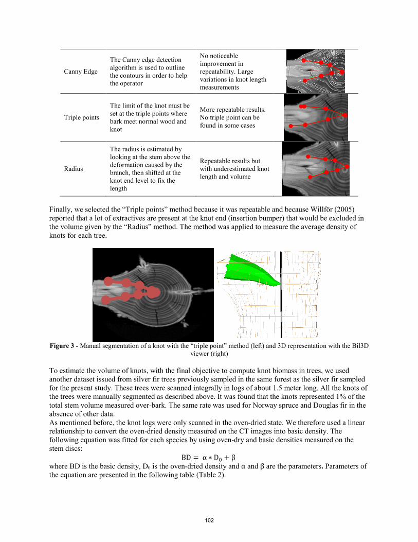
Canny Edge

The Canny edge detection algorithm is used to outline the contours in order to help the operator

No noticeable improvement in repeatability. Large variations in knot length measurements

Triple points

The limit of the knot must be set at the triple points where bark meet normal wood and knot

More repeatable results. No triple point can be found in some cases

Radius

The radius is estimated by looking at the stem above the deformation caused by the branch, then shifted at the knot end level to fix the length

Repeatable results but with underestimated knot length and volume

Finally, we selected the “Triple points” method because it was repeatable and because Willför (2005) reported that a lot of extractives are present at the knot end (insertion bumper) that would be excluded in the volume given by the “Radius” method. The method was applied to measure the average density of knots for each tree.

Figure 3 - Manual segmentation of a knot with the “triple point” method (left) and 3D representation with the Bil3D

viewer (right)

To estimate the volume of knots, with the final objective to compute knot biomass in trees, we used another dataset issued from silver fir trees previously sampled in the same forest as the silver fir sampled for the present study. These trees were scanned integrally in logs of about 1.5 meter long. All the knots of the trees were manually segmented as described above. It was found that the knots represented 1% of the total stem volume measured over-bark. The same rate was used for Norway spruce and Douglas fir in the absence of other data. As mentioned before, the knot logs were only scanned in the oven-dried state. We therefore used a linear relationship to convert the oven-dried density measured on the CT images into basic density. The following equation was fitted for each species by using oven-dry and basic densities measured on the stem discs:

BD = α ∗ D0 + β where BD is the basic density, D0 is the oven-dried density and α and β are the parameters. Parameters of the equation are presented in the following table (Table 2).

102

Table 2 - Parameters of the linear relationship fitted using stem disc data to convert oven-dried density into basic density.

Species β (kg/m3)

α (Unitless)

Silver fir (Abies alba) 38 **

0.790 ***

Norway spruce (Picea abies)

67 ***

0.710 ***

Douglas fir (Pseudotsuga menziesii)

- NS

0.879 ***

Results Differences in the manual segmentation of knots made by two operators with the “Triple points” method and the effects on basic density, mean diameter and volume are presented in Fig. 4. Very few discrepancies between operators were observed. It confirmed that the “Triple point” method was repeatable and efficient for assessing knot wood density and volume.

Figure 4 – Mean diameters, volumes and oven-dried densities of knots obtained by two operators. The black line is

the “y=x” line.

The basic density of knot wood and clear wood is represented for each species in Figure 5. It appears that the density of knots is much higher than the normal stem wood. In average, the basic density of knots was 685 kg/m3 for silver fir, 676 kg/m3 for Norway spruce, and 705 kg/m3 for Douglas fir whereas the density of normal stem wood was 374 kg/m3, 353 kg/m3, and 430 kg/m3, respectively. Moreover, it would appear that there is no influence of the knot diameter on the knot basic density. The effects of diameter at breast height and silvicultural treatment were assessed independently on the wood density of stem and knot components with regression and t-test, respectively. No effect of DBH was found. Only the effect of the treatment was statistically significant for silver fir with a greater density for thinning plot. The biomass values were computed by using the measured density of each component and compared with the biomass that would have been obtained with the basic density measured at 1m30. Table 3 shows the difference between both values. For the three species, applying the density of normal wood measured at 1.30 m to the knots would lead to underestimate by more than 60 % the available quantity of knot extractives.

103

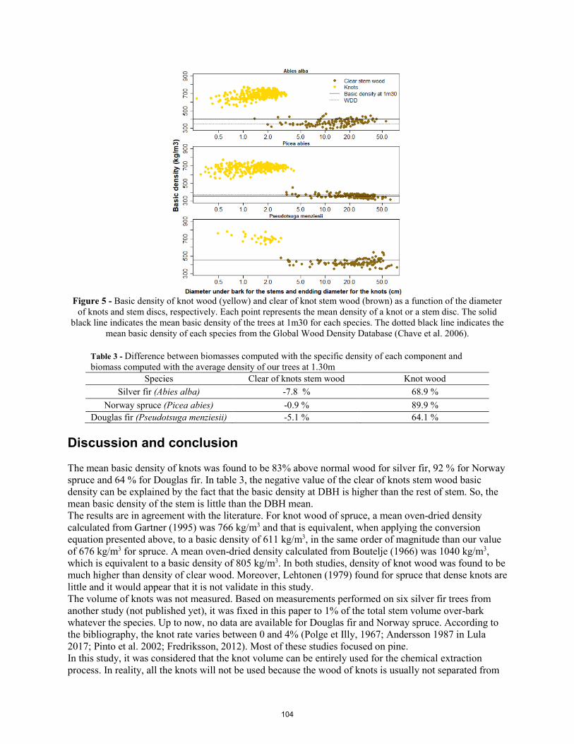
Figure 5 - Basic density of knot wood (yellow) and clear of knot stem wood (brown) as a function of the diameter

of knots and stem discs, respectively. Each point represents the mean density of a knot or a stem disc. The solid black line indicates the mean basic density of the trees at 1m30 for each species. The dotted black line indicates the

mean basic density of each species from the Global Wood Density Database (Chave et al. 2006).

Table 3 - Difference between biomasses computed with the specific density of each component and biomass computed with the average density of our trees at 1.30m

Species Clear of knots stem wood Knot wood Silver fir (Abies alba) -7.8 % 68.9 %

Norway spruce (Picea abies) -0.9 % 89.9 % Douglas fir (Pseudotsuga menziesii) -5.1 % 64.1 %

Discussion and conclusion The mean basic density of knots was found to be 83% above normal wood for silver fir, 92 % for Norway spruce and 64 % for Douglas fir. In table 3, the negative value of the clear of knots stem wood basic density can be explained by the fact that the basic density at DBH is higher than the rest of stem. So, the mean basic density of the stem is little than the DBH mean. The results are in agreement with the literature. For knot wood of spruce, a mean oven-dried density calculated from Gartner (1995) was 766 kg/m3 and that is equivalent, when applying the conversion equation presented above, to a basic density of 611 kg/m3, in the same order of magnitude than our value of 676 kg/m3 for spruce. A mean oven-dried density calculated from Boutelje (1966) was 1040 kg/m3, which is equivalent to a basic density of 805 kg/m3. In both studies, density of knot wood was found to be much higher than density of clear wood. Moreover, Lehtonen (1979) found for spruce that dense knots are little and it would appear that it is not validate in this study. The volume of knots was not measured. Based on measurements performed on six silver fir trees from another study (not published yet), it was fixed in this paper to 1% of the total stem volume over-bark whatever the species. Up to now, no data are available for Douglas fir and Norway spruce. According to the bibliography, the knot rate varies between 0 and 4% (Polge et Illy, 1967; Andersson 1987 in Lula 2017; Pinto et al. 2002; Fredriksson, 2012). Most of these studies focused on pine. In this study, it was considered that the knot volume can be entirely used for the chemical extraction process. In reality, all the knots will not be used because the wood of knots is usually not separated from

104

normal wood in the industrial process (except in paper industry). Moreover, it was shown that the boundary between wood and knots is not clearly defined. This is probably not a serious problem, since in the case where knot extraction would be performed for feeding a chemical process, the wood around the knot would certainly be included into the extracted volume. The “Gourmand” plugin makes it possible to modify the diameter of the manually segmented knots to compute density with including more or less wood framing knots. Other tree components (bark and branches) will be analysed in a further study. Until now, the analyses were mainly descriptive, but in the future we intend to model the density of each component as a function of tree characteristics. The density variations within tree components will also be studied. In conclusion, the lack of volume data of the knots and the utilisation of the stem wood density for the knots make it hard to have a good estimation of the basic density of the knots and underestimate the biomass of knots. Acknowledgments SILVA laboratory is supported by a grant overseen by the French National Research Agency (ANR) as part of the “Investissements d’Avenir” program (ANR-11-LABX-0002-01, Lab of Excellence ARBRE). Antoine Billard’s PhD is funded by ADEME and Région Grand-Est. This work was done in the framework of the ExtraFor Est project coordinated by Francis Colin. We would like to thank Christine Deleuze (ONF) for her help in achieving this study, Vincent Rousselet, Frédéric Bordat, Loïc Dailly and Adrien Contini for the sampling in the forest and measuremets at the laboratory, part and Charline Mola for the CT scanner acuisitions. Also, we thank Chloé Agro, Lucie Heim and Leopold Bergé who worked during their Master thesis on basic density and volume of knots, and Anaëlle Rajaonarivo, Léa Bissieux and Bernard Poirot for the manual segmentation of knots. Finally, thanks to the LERMAB laboratory for the yield of extractives. References Bastin, J.F.; Fayolle, A.; Tarelkin, Y.; Van Den Bulcke, J.; De Haulleville, T.; Mortier, F.; Beeckman, H.; Van Acker, J.; Serckx, A.; Bogaert, J.; De Canniere, C. 2015. Wood specific gravity variations and biomass of central african tree species: the simple choice of the outer wood. PloS one. 10(11). Boutelje, J.B. 1966. On anatomical structure moisture content density shrinkage and resin content of wood in and around knots in Swedish pine (Pinus Silvestris L) and in Swedish spruce (Picea Abies Karst). Svensk Papperstidning-Nordisk Cellulosa. 69(1): 1-10. Chave, J., Coomes, D., Jansen, S., Lewis, S. L., Swenson, N. G., & Zanne, A. E. 2009. Towards a worldwide wood economics spectrum. Ecology letters, 12(4), 351-366. Colin, F.; Mothe, F.; Freyburger, C.; Morisset, J.-B; Leban, J.-M.; Fontaine, F. 2010. Tracking rameal traces in sessile oak trunks with X-ray computer tomography: biological bases, preliminary results and perspectives. Trees. 24(5): 953-967. Fredriksson, M. 2012. Reconstruction of Pinus Sylvestris knots using measurable log features in the Swedish Pine Stem Bank. Scandinavian journal of forest research, 27(5): 481-491. Freyburger, C.; Longuetaud, F.; Mothe, F.; Constant, T.; Leban, J.M. 2009. Measuring wood density by means of X-ray computer tomography. Annals of forest science. 66(8), 804.

105

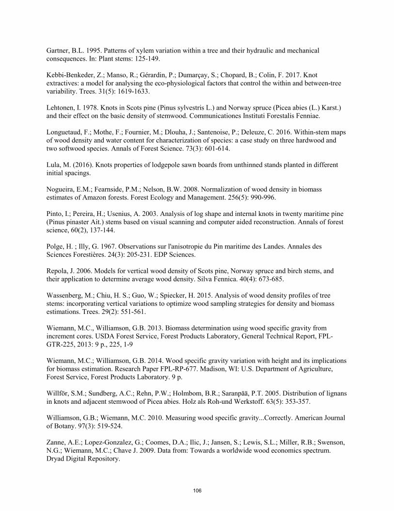
Gartner, B.L. 1995. Patterns of xylem variation within a tree and their hydraulic and mechanical consequences. In: Plant stems: 125-149. Kebbi-Benkeder, Z.; Manso, R.; Gérardin, P.; Dumarçay, S.; Chopard, B.; Colin, F. 2017. Knot extractives: a model for analysing the eco-physiological factors that control the within and between-tree variability. Trees. 31(5): 1619-1633. Lehtonen, I. 1978. Knots in Scots pine (Pinus sylvestris L.) and Norway spruce (Picea abies (L.) Karst.) and their effect on the basic density of stemwood. Communicationes Instituti Forestalis Fenniae. Longuetaud, F.; Mothe, F.; Fournier, M.; Dlouha, J.; Santenoise, P.; Deleuze, C. 2016. Within-stem maps of wood density and water content for characterization of species: a case study on three hardwood and two softwood species. Annals of Forest Science. 73(3): 601-614. Lula, M. (2016). Knots properties of lodgepole sawn boards from unthinned stands planted in different initial spacings. Nogueira, E.M.; Fearnside, P.M.; Nelson, B.W. 2008. Normalization of wood density in biomass estimates of Amazon forests. Forest Ecology and Management. 256(5): 990-996. Pinto, I.; Pereira, H.; Usenius, A. 2003. Analysis of log shape and internal knots in twenty maritime pine (Pinus pinaster Ait.) stems based on visual scanning and computer aided reconstruction. Annals of forest science, 60(2), 137-144. Polge, H. ; Illy, G. 1967. Observations sur l'anisotropie du Pin maritime des Landes. Annales des Sciences Forestières. 24(3): 205-231. EDP Sciences. Repola, J. 2006. Models for vertical wood density of Scots pine, Norway spruce and birch stems, and their application to determine average wood density. Silva Fennica. 40(4): 673-685. Wassenberg, M.; Chiu, H. S.; Guo, W.; Spiecker, H. 2015. Analysis of wood density profiles of tree stems: incorporating vertical variations to optimize wood sampling strategies for density and biomass estimations. Trees. 29(2): 551-561. Wiemann, M.C., Williamson, G.B. 2013. Biomass determination using wood specific gravity from increment cores. USDA Forest Service, Forest Products Laboratory, General Technical Report, FPL-GTR-225, 2013: 9 p., 225, 1-9 Wiemann, M.C.; Williamson, G.B. 2014. Wood specific gravity variation with height and its implications for biomass estimation. Research Paper FPL-RP-677. Madison, WI: U.S. Department of Agriculture, Forest Service, Forest Products Laboratory. 9 p. Willför, S.M.; Sundberg, A.C.; Rehn, P.W.; Holmbom, B.R.; Saranpää, P.T. 2005. Distribution of lignans in knots and adjacent stemwood of Picea abies. Holz als Roh-und Werkstoff. 63(5): 353-357. Williamson, G.B.; Wiemann, M.C. 2010. Measuring wood specific gravity...Correctly. American Journal of Botany. 97(3): 519-524. Zanne, A.E.; Lopez-Gonzalez, G.; Coomes, D.A.; Ilic, J.; Jansen, S.; Lewis, S.L.; Miller, R.B.; Swenson, N.G.; Wiemann, M.C.; Chave J. 2009. Data from: Towards a worldwide wood economics spectrum. Dryad Digital Repository.

106

Research into Nondestructive Test Methods Used on Standing Trees. Practical Use in Populus alba var. bolleana Guadalupe Olvera* Department of Forest and Environmental Engineering and Management, MONTES (School of Forest Engineering and Natural Environment). Universidad Politécnica de Madrid, Madrid, Spain. g.olvera@alumnos.upm.es Carlos Coba Master in Structural Wood Engineering, Structural Timber Engineering Platform (PEMADE), Universidad de Santiago de Compostela, Lugo, Spain. carlos.coba.rubiato@gmail.com Ignacio Bobadilla Department of Forest and Environmental Engineering and Management, MONTES (School of Forest Engineering and Natural Environment). Universidad Politécnica de Madrid, Madrid, Spain. i.bobadilla@upm.es Miguel Esteban Department of Forest and Environmental Engineering and Management, MONTES (School of Forest Engineering and Natural Environment). Universidad Politécnica de Madrid, Madrid, Spain. miguel.esteban@upm.es Carlos Osuna Department of Forest and Environmental Engineering and Management, MONTES (School of Forest Engineering and Natural Environment). Universidad Politécnica de Madrid, Madrid, Spain. caosseq@gmail.com * Corresponding author Abstract In the present work, the applicability of the ultrasonic propagation in the longitudinal and transverse directions to the fiber was verified, as well as inspection by drill to a specimen of Populus alba L. var. bolleana obtained from the Parque del Oeste in Madrid . This test aims to serve as a tool in the expert assessments that assess the phytosanitary status of trees, and thus contribute to minimize the risks that this generates on the population. The selection of the logs was simultaneous to the felling and bucking of the tree, trying that the sample was sufficiently representative of the parts that contain pathologies, as well as of completely healthy parts; It was also sought to obtain wood from different parts of the tree, understanding that it would allow to study the different types of efforts to which the foot was subject throughout its structure. The results show that there is a strong relationship between the degree of degradation caused by pathogens and the speed drops that ultrasound presents when passing through the affected areas; the same effect was had when relating the attacked zones with the resistance that offered the wood attacked to the perforation, with the drill of inspection; It was also found that the factor that determines the previous results is the density of the wood, which decreases when the attack of the pathogens increases. Finally, as part of this research, a trial protocol is proposed to transfer all this information to practice. Keywords: conference, abstract, instructions, template

107

Introduction The tree suffers the interaction with each of the processes that occur every day in the environment that surrounds it, and it is usual that this coexistence affects its dynamics and, consequently, its vitality and stability. These conditions result in the alteration of the contributions that a tree can bring to their environment, but also, to be affected in its own structure, generates a risk around by the possible fall of branches and even of your entire body. Thus, the phytosanitary status of urban trees represents a fundamental role in the management of any space that contains it. This condition has generated numerous different formulas for the analysis of the feet and the risk they generate, however, there is no generalized methodology, but depending on the region, some guidelines or others are followed. There are methods that are contextualized on economic factors that condition the result [Villota, 2015]. The search for a neutrality has led to complement traditional methods, based on the visual analysis of the outside of the individual, with methods that provide information about what happens also in the interior, without the need to use invasive techniques for the tree. These techniques are estimates and are investigated to demonstrate and improve the degree of correlation between the methods and the deterioration of the pieces analyzed. Some researchers have been able to demonstrate that the level of the condition can be perceived by ultrasound techniques with statistically significant results [Weilera, et al. 2013; Martins, et al., 2015]. Robert J. Ross [2015] also collects numerous background information on the application of non destructive techniques for the analysis of wood. Among these references numerous studies can be found on the influence of multiple factors that affect the application of ultrasound. The motivation of this work is to provide information on the usefulness of Nondestructive Testing (NDT) as a complement to the visual inspection methodologies commonly used in phytosanitary diagnosis, in order to objectify the evaluations of technicians. In this sense, this project has analyzed the ultrasound technique by applying it on specimen of Populus alba L. var. bolleana, complementing it with the test with inspection drill and visual inspection prior to felling. The main objective was to evaluate the usefulness and applicability of these methods in the case of the specimen studied. Materials and Methods This project has had the collaboration of the managing body of the Parque del Oeste in Madrid . This collaboration allowed obtaining specimen of Populus alba L. var. bolleana. The individual had been selected to be dislodged for generating a risk of fracture in the trunk, diagnosed by the technicians in charge of the expertise. Description of the samples obtained Once the object of study was selected, a previous visit was made to the moment of felling to obtain the graphic information of the environment and the situation of the tree, and the geographical north was marked to conserve knowledge of the position of the tree at all times. The selection of the logs was simultaneous to the felling and cutting of the tree, executed by the gardeners of the maintenance service of the Parque del Oeste in Madrid, following a series of previously agreed upon cabinet criteria. The sample would try to be sufficiently representative of the parts that contain pathologies, as well as of completely healthy parts. It was also sought to obtain wood from different parts of the tree, understanding that it would allow to study the different types of stresses to which the tree was subjected throughout its structure (Figure 1). Finally, mechanical trials that could estimate these efforts would not be developed because they were considered sufficient to be developed in future studies independently.

108

Figure 1. Identification of logs. Of these five logs, it was decided to use only the three (A, B and C) and to keep pieces 1 and 2 for the identification of the organisms that had caused the different pathologies that the tree presented [Coba, 2018].

Test methodology The tests were carried out once the logs and samples were selected and marked, following the scheme presented below:

Humidity estimation The calculation of the humidity was carried out following the EN 13183-1: 2002. Moisture content of a piece of sawn timber - Part 1: Determination by oven dry method. For the weighing of the samples, a precision balance were used. For drying, a controlled laboratory drying oven was used to meet the standard, that is, at 103 ± 2˚C for 48 hours. Estimation of density The density was determined based on the EN 384: 2010 standard: Structural timber - Determination of characteristic values of mechanical properties and density. The dimensions of the test pieces were measured with a caliper of scale division equal to 0.01 mm. The value of each dimension was estimated as the average of two measured values.

109

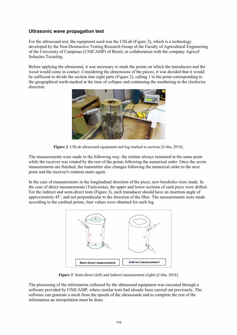
Ultrasonic wave propagation test For the ultrasound test, the equipment used was the USLab (Figure 2), which is a technology developed by the Non-Destructive Testing Research Group of the Faculty of Agricultural Engineering of the University of Campinas (UNICAMP) of Brazil, in collaboration with the company Agricef Soluções Tecnológ. Before applying the ultrasound, it was necessary to mark the points on which the transducers and the wood would come in contact. Considering the dimensions of the pieces, it was decided that it would be sufficient to divide the section into eight parts (Figure 2), calling 1 to the point corresponding to the geographical north marked at the time of collapse and continuing the numbering in the clockwise direction.

Figure 2. USLab ultrasound equipment and log marked in sections [Coba, 2018].

The measurements were made in the following way: the emitter always remained at the same point while the receiver was rotated by the rest of the points following the numerical order. Once the seven measurements are finished, the transmitter also changes following the numerical order to the next point and the receiver's rotation starts again. In the case of measurements in the longitudinal direction of the piece, new boreholes were made. In the case of direct measurements (Testa-testa), the upper and lower sections of each piece were drilled. For the indirect and semi-direct tests (Figure 3), each transducer should have an insertion angle of approximately 45˚, and not perpendicular to the direction of the fiber. The measurements were made according to the cardinal points, four values were obtained for each log.

Figure 3. Semi-direct (left) and indirect measurement (right) [Coba, 2018].

The processing of the information collected by the ultrasound equipment was executed through a software provided by UNICAMP, where similar tests had already been carried out previously. The software can generate a mesh from the speeds of the ultrasounds and to complete the rest of the information an interpolation must be done.

110

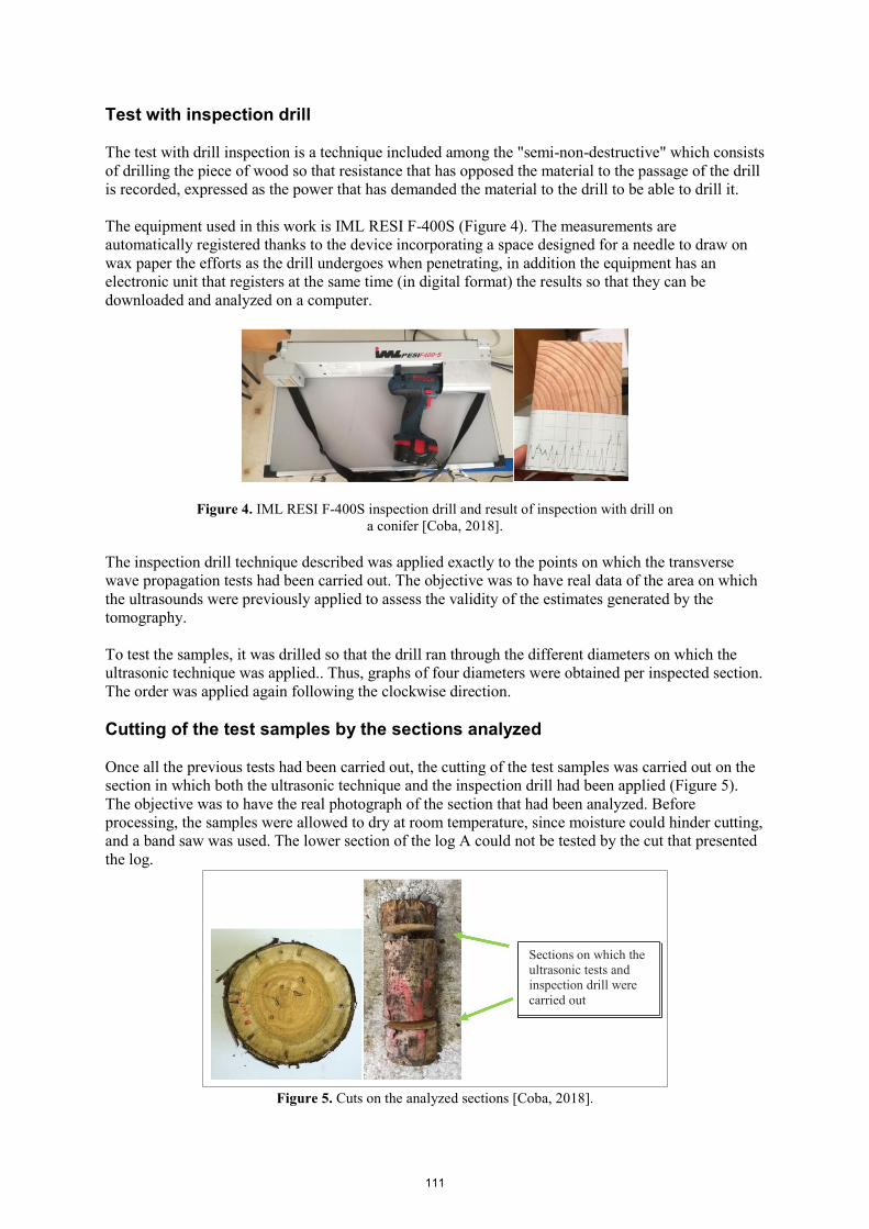
Test with inspection drill The test with drill inspection is a technique included among the "semi-non-destructive" which consists of drilling the piece of wood so that resistance that has opposed the material to the passage of the drill is recorded, expressed as the power that has demanded the material to the drill to be able to drill it. The equipment used in this work is IML RESI F-400S (Figure 4). The measurements are automatically registered thanks to the device incorporating a space designed for a needle to draw on wax paper the efforts as the drill undergoes when penetrating, in addition the equipment has an electronic unit that registers at the same time (in digital format) the results so that they can be downloaded and analyzed on a computer.

Figure 4. IML RESI F-400S inspection drill and result of inspection with drill on a conifer [Coba, 2018].

The inspection drill technique described was applied exactly to the points on which the transverse wave propagation tests had been carried out. The objective was to have real data of the area on which the ultrasounds were previously applied to assess the validity of the estimates generated by the tomography. To test the samples, it was drilled so that the drill ran through the different diameters on which the ultrasonic technique was applied.. Thus, graphs of four diameters were obtained per inspected section. The order was applied again following the clockwise direction. Cutting of the test samples by the sections analyzed Once all the previous tests had been carried out, the cutting of the test samples was carried out on the section in which both the ultrasonic technique and the inspection drill had been applied (Figure 5). The objective was to have the real photograph of the section that had been analyzed. Before processing, the samples were allowed to dry at room temperature, since moisture could hinder cutting, and a band saw was used. The lower section of the log A could not be tested by the cut that presented the log.

Figure 5. Cuts on the analyzed sections [Coba, 2018].

Sections on which the ultrasonic tests and inspection drill were carried out

111

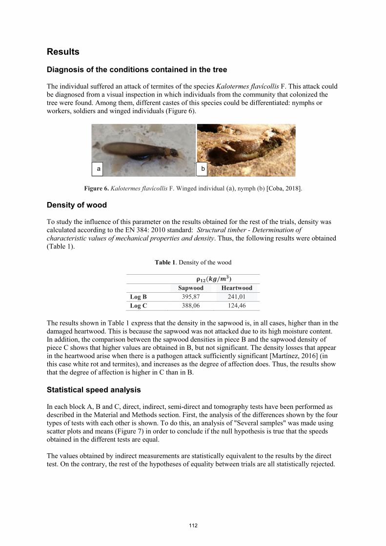
Results Diagnosis of the conditions contained in the tree The individual suffered an attack of termites of the species Kalotermes flavícollis F. This attack could be diagnosed from a visual inspection in which individuals from the community that colonized the tree were found. Among them, different castes of this species could be differentiated: nymphs or workers, soldiers and winged individuals (Figure 6).

Figure 6. Kalotermes flavícollis F. Winged individual (a), nymph (b) [Coba, 2018].

Density of wood To study the influence of this parameter on the results obtained for the rest of the trials, density was calculated according to the EN 384: 2010 standard: Structural timber - Determination of characteristic values of mechanical properties and density. Thus, the following results were obtained (Table 1).

Table 1. Density of the wood

𝛒𝛒𝟏𝟏𝟏𝟏(𝒌𝒌𝒌𝒌/𝒎𝒎𝟑𝟑) Sapwood Heartwood Log B 395,87 241,01 Log C 388,06 124,46

The results shown in Table 1 express that the density in the sapwood is, in all cases, higher than in the damaged heartwood. This is because the sapwood was not attacked due to its high moisture content. In addition, the comparison between the sapwood densities in piece B and the sapwood density of piece C shows that higher values are obtained in B, but not significant. The density losses that appear in the heartwood arise when there is a pathogen attack sufficiently significant [Martínez, 2016] (in this case white rot and termites), and increases as the degree of affection does. Thus, the results show that the degree of affection is higher in C than in B. Statistical speed analysis In each block A, B and C, direct, indirect, semi-direct and tomography tests have been performed as described in the Material and Methods section. First, the analysis of the differences shown by the four types of tests with each other is shown. To do this, an analysis of "Several samples" was made using scatter plots and means (Figure 7) in order to conclude if the null hypothesis is true that the speeds obtained in the different tests are equal. The values obtained by indirect measurements are statistically equivalent to the results by the direct test. On the contrary, the rest of the hypotheses of equality between trials are all statistically rejected.

a b

112

Figure 7. Scatter charts and averages [Coba, 2018]. Specific analysis of the diametrical speeds Speed maps were obtained on the five surfaces that were measured. To determine the degree of similarity between reality and digitalization, the different images of each analyzed surface are compared with zenith photographs of the real section. For these comparisons, five color ranges were generated (Figure 8).

Figure 8. Tomographs of the cross section of the logs [Coba, 2018]. The concordance between the images of the tomography and the zenith photographs could not be analyzed in numerical terms. However, an analysis was made by visual comparison and by superposition of the two types of images. In general, a high relation between the percentages of speed with respect to the maximum and the degree of affection is shown. That is, a relationship between the changes in density and velocity of ultrasound is appreciated. Thus, the zones with decay and galleries or hollows gather most of the lower speeds, usually concentrated in the heartwood. This location is explained, as already mentioned before, taking into account that the area of heartwood and, therefore, of lower moisture content on the standing tree, is more easily attacked by fungi that do not support humidity contents as large as those that occur in the sapwood of a foot like the one described. Analysis of the test with inspection drill In general, the same effect is produced in all the pieces; the result of the drill inspection can be summarized in that the wood did not offer resistance in the affected areas, even in those that did not contain holes, only decay (Figure 9).

Figure 9. Inspection with drill in the sections of the logs [Coba, 2018].

A1 B2 C1 C2 B1

A1 B2 B1 C2 C1

113

When the test with an inspection drill detects little or no resistance in the rotting zone, said zones are also detected with considerable speed drops that vary according to the level of degradation. It agrees that for logs B and C the speeds are lower the lower the resistance offered by the wood in the test with inspection drill. These results also coincide with those offered by the calculation of the density in the rotten zones of logs B and C. The density is lower in the decays of C, that is, this log had a higher level of development of the fungus than the log B, and this is reflected both in the speeds and in the resistances offered to the inspection drill. Conclusions It has been possible to put into practice the use of non-destructive techniques to analyze the phytosanitary status of the trees. It is shown that the combination of NDT provides much more information than its individualized use. Secondly, it is concluded that the direct and indirect propagation tests are not able to detect conditions inside the tree since they develop on the sapwood, generally healthy. The speed of the ultrasound decreases when the angle increases with respect to the fiber. This fact is corroborated with the data obtained in the present work. It has also been proven that the speed is reduced proportionally to the loss of density of the wood. Said density losses were associated, in this case, with the degree of involvement of the decay and termites. Thus, the significant differences that have been found between the theoretical speeds for healthy wood, and those obtained in practice, have been associated with affections of the rot type and / or attack of xylophages, in this project. Finally, it is concluded that the ultrasonic tomography is able to detect and estimate the extent and location of affected areas within the standing tree. On the other hand, the test with inspection drill provides precise but accurate information of the internal state of the foot. Reference list Coba, R. C. (2018). Research into nondestructive test methods used on standing trees. Practical use in Populus alba var. bolleana. Final Degree Project. Polytechnic University of Madrid. ETSI Montes. 89 pp. EN 384: 2010. Structural timber - Determination of characteristic values of mechanical properties and density EN 13183-1: 2002. Moisture content of a piece of sawn timber - Part 1: Determination by oven dry method. Martínez, R. (2016). Non-destructive methods for estimating wood density. Doctoral thesis. Santiago de Compostela University. Higher Polytechnic School of Lugo. 210 pp. Martins, D., Corassa, J., Gatto, D.A., Roberto Lessa and R., Rigatto, P. (2015). Mechanical characterization of wood deteriorated in the field by static ultrassom and flexão. Communicata Scientiae. 6 (3), pp. 365-372. Ross, R. (2015). Non destructive evaluation of Wood. Ed. 2ª. General Technical Report FPL-GTR-238. Madison, WI: U.S. Department of Agriculture, Forest Service, Forest Product Laboratoty. 169 p Villota Gálvez, M. (2015). The unique trees in the landscape. Proposal of a model for its evaluation: The case of the historical territory of Álava. Doctoral thesis. Polytechnic University of Madrid. ETSI Montes. 286 p. Weilera, M., Missio, A.L., Gattob, D.A., Güths, W.G. (2013). Nondestructive Evaluation of Wood Decayed by Xylophagous Organisms. Materials Research, 16(5), Pp. 1203-1208.

114

Acoustic Tomography for Evaluation of Wood Quality in Chestnut Trees A.R. Proto* Department of Agriculture, University “Mediterranea” of Reggio Calabria, Reggio Calabria, Italy, andrea.proto@unirc.it S. Papandrea Department of Agriculture, University “Mediterranea” of Reggio Calabria, Reggio Calabria, Italy, M.F. Cataldo Department of Agriculture, University “Mediterranea” of Reggio Calabria, Reggio Calabria, Italy, G. Zimbalatti Department of Agriculture, University “Mediterranea” of Reggio Calabria, Reggio Calabria, Italy, gzimbalatti@unirc.it * Corresponding author Abstract Sweet chestnut (Castanea sativa Mill.) is one of the most important forest tree species in Europe; it grows commonly in hilly and mountainous areas, where it is traditionally used as timber in construction. Secondary products are furniture, floorings, windows, external doors, and barrels. In fact, the use of the wood of chestnut tree is potentially unlimited: from the smallest objects up to biggest, and the cultivation and use of chestnut fruit and wood has a long tradition. This wood is appreciated for its durability due to extractives: heartwood shows a pleasant colour and a natural durability against biotic and abiotic agents. In Italy, the species is currently cultivated for wood production using coppice silvicultural management, in which new trees (shoots) grow from the stumps. One of the main problems, that affect negatively the exploitation of chestnut and decrease the value of its timber, is the risk of ring shake, a defect which occurs as detachment between the annual rings. In certain cases, the frequency of this defect is so high that it causes extended qualitative falloff of the produced timber. Several previous studies have reported the presence of ring shake in sample plots observed immediately after felling and the prediction models for its presence before felling are based related to growth parameters. The aim of this preliminary study is to assess the possibility of ring shake appearance on standing chestnut trees using a tomography approach. Keywords: standing tree, tomography, sensors, ring shake, non-destructive method Introduction Sweet chestnut (Castanea sativa Mill.) is one of the most important forest tree species in Europe; it grows commonly in hilly and mountainous areas, where it is traditionally used as timber in construction. Secondary products are furniture, floorings, windows, external doors, and barrels. In fact, the use of the wood of chestnut tree is potentially unlimited: from the smallest objects up to biggest, and the cultivation and use of chestnut fruit and wood has a long tradition. This wood is appreciated for its durability due to

115

extractives: heartwood shows a pleasant colour and a natural durability against biotic and abiotic agents. In Italy, the species is currently cultivated for wood production using coppice silvicultural management, in which new trees (shoots) grow from the stumps. One of the main problems, that affect negatively the exploitation of chestnut and decrease the value of its timber, is the risk of ring shake, a defect which occurs as detachment between the annual rings. The study of the internal state of this species have a long tradition in Italy (Romagnoli and Spina 2013), as in Europe, due to the high merchantable value of his wood products. The defect of ring shake occurrence greatly reduces the value of the timber assortment and in the worst case, the incidence of ring shake is so high that only few logs of a stand can be brought to the sawmill (Fonti et al. 2002). In certain cases, the frequency of this defect is so high that it causes extended qualitative falloff of the produced timber. Several previous studies have reported the presence of ring shake in sample plots observed immediately after felling and the prediction models for its presence before felling are based related to growth parameters. The aim of this preliminary study is to assess the possibility of ring shake appearance on standing chestnut trees using a tomography approach. Assessing wood quality inn standing trees has been a long – time interest to wood products manufactures end forest managers worldwide. A significant effort has been devoted to develop to develop robust NDT technologies that are capable of predicting intrinsic wood proprieties of individual trees and assessing wood quality by stands and forest (Wang et al. 2007; Brashaw et al. 2009, Divos 2010; Proto et al. 2017). The research started four years ago and was funded by the Ministry of Education, University and Research-MIUR, under the National Operative Programme (PON) Research and Competitiveness 2007-2013, to support development and innovation in forestry and wood industry, in Calabrian region by the Mediterranean University with private companies working in the field of wood, computer science and remote sensing. One of the most important object has been to assess the wood quality using NDT methods in the principal’s forestry area of the Calabria region to obtain a correct economic value of Calabrian wood (Proto et al. 2014; Proto et al. 2015). This study present a preliminary examination of the applicability of sonic tomography for evaluate the chestnut wood in standing trees. Material and Methods Study sites and tree samples The test site was situated in Southern Italy (Calabria Region) in the Serre Massif. The study area covering a total area of 5 hectares with an altitude ranged of 610 and 680 m (Table 1). The site study was coppiced with first class standards which derive from coppice shoots growing from the previous cut. The age of the shoots ranged was 12 years, whereas those of the standards were 24 (II cycle) and 36 (III cycle) years. The breast height (DBH) was measured by using a classic diameter caliper and tree height with a vertex IV hypsometer. Thirty chestnut standards, with a regular cross-section, were randomly selected and each tree was marked and assigned a tracking number, useful to conduct the tomographic study and the subsequent felling phase. The choice of this population was dictated not only by the characteristics favorable to a silviculture of a productive type, but also by the assured presence of ring shake in the trees, identified through a historical inquiry among the local users (Macchioni and Pividori 1996). The main characteristics of the study site are shown in the Table 1. At the conclusion of acoustic measurements, the trees were subsequently harvested by a local company and cross-sectioned in correspondence of acoustic tests and a disk 5-cm thick was collected from each stem and taken to a laboratory where the ring shake characteristics were measured. In particular, ring shake position and the extent of the defect were measured for each wood disk defected. Field Acoustic Tomography Test and Data analysis All 30 standards were first nondestructively tested using a commercial ArborSonic 3D acoustic tomograph device (Fakopp Enterprise Ltd., Hungary). Each monitored tree had regular form of the stem

116

and then the position of sensor was calculated dividing the circumference with the number of the sensors applied (Figure 1a). At height of 50 cm, the circumference and distances between sensors were measured using a tape measure and this data were used to map the approximate geometric form of the cross-section. During testing, each position of sensors was marked so that they could be traced back to the original location in the stem disk in order to assess the actual condition of the wood at the area of sampling. After the test, the velocity of acoustic wave transmission measured from each chestnut trees was finding, studied and used to predict the ring shake presence respect the typical application of tomograms for detect cavity or decay. The comparison between the paths of stress wave measurements on one cross section (sound wood vs. defect wood) was used to determine and localize the area affect by ring shake. Using tomographic technique, a complete data matrix was obtained through measurement of stress wave transmission time and in Figure 1b.

Table 1 - Study area characteristics and dendrometric parameters

Parameters Unit Measure Value Altitude – Range a.s.l. m 610 - 680 Slope - Range % 15 - 20 Average Basal area for tree m2 0.102 Average Basal area for hectare m2 ha-1 26.14 Volume for hectare m3 ha-1 214.15 Coppice shoots diameter cm 20.12 Standard diameter cm 33.03 Number of stump n ha-1 370 Shoots – number of tree n ha-1 1720 Standards – number of tree n ha-1 65

Figure 1 - Acoustic tomography test on standing tree (a) and stress wave propagation paths (b)

117

Results and discussions Based on the relationship between elastic modulus and wood density, the accuracy of reconstructed tomography is sensitive to the density of acoustic wave path within the cross section (Qin et al. 2018). For this reason, the preliminary results separated and catalogued the paths derived from in sound wood compared to the paths identify with internal defects. From 30 trees examined, 19 standards were affected by ring shake and only 11 were intact. In Tables 2 and 3, as examples, the velocity measurements of sample n. 11 and 25 are reported with the different and sequential paths generated by using of 8 sensors. The average of the line velocities of the measurement paths with same angle ɵ from all the 8 source points was calculated. For solid cross section, the velocity in radial direction VR (with θ = 0) was the highest, and the velocity in tangential direction VT (with θ = ±67.5°) was the lowest. Consider the tangential velocity at θ = ±67.5° as a reference velocity, then the ratio of VT to VR reflects the wave velocity patterns in a tree cross section. The identification of position of the ring shake was correctly measured in laboratory and confirm that it is possible assess it if compare the different acoustic velocity between the different paths. For each defected wood sample the distance and position of ring shake along the disk and the data were compared with equivalent tomogram. In Figure 2, the tomogram (a) and the stress wave propagation paths (b) do not show immediately in which position (annual year and extension) there is a ring shake or other defect because there are many paths in contrast each other but only after a correct analysis of each path and the laboratory test has been possible detect it. In fact, the use of 8 sensors has generated 28 paths and the comparison between the different directions (1→2,3,…; 2→3,4,..; 3→4,5,..; etc.) has shown different speeds of paths. A correct interpretation (Table 5) of the speed of stress wave propagation suggested that the defect is identifiable following the paths 2→5, 2→6, 2→7, 3→6, 3→7 in the annual year in winch do not across the green paths (1→4, 3→8) that circumscribe the area defected. The lower speed measured of path 2→7 (-14%) respect similar path 4→7 or 2→6 path (-22%) respect 4→8 identify the ring shake in a defined area (Figure 3). A complete statistical analysis of different paths will be done when will be concluded the sampling of other fifty tree selected of the project and authorized to be felled for comparative laboratory test.

Table 2 - Acoustic velocity data for sound wood – n. 11

Angle Sensors Average Velocity Vt/Vr

θ 1 2 3 4 5 6 7 8 67.5 1787 1699 1707 1720 1677 1611 1728 1728 1707.13 0.89 45 1843 1726 1724 1863 1687 1840 1784 1771 1779.75 0.93

22.5 1899 1735 1886 1900 1890 1869 1899 1886 1870.50 0.98 0 1907 1900 1902 1936 1907 1900 1902 1936 1911.25 1.00

-22.5 1869 1899 1886 1899 1735 1886 1900 1890 1870.50 0.98 -45 1784 1771 1843 1726 1724 1863 1687 1840 1779.75 0.93

-67.5 1728 1787 1699 1707 1720 1677 1611 1728 1707.13 0.89

118

Table 3 - Acoustic velocity data for defect wood – n. 25

Angle Sensors Average Velocity Vt/Vr

θ 1 2 3 4 5 6 7 8 67.5 1742 1761 1806 1846 1821 1817 1810 1837 1805.00 1.17 45 2060 1885 2012 2028 1987 2054 1730 1830 1948.25 1.26

22.5 1919 1631 1641 1724 2024 1722 1520 1839 1752.50 1.13 0 1635 1405 1468 1684 1635 1405 1468 1684 1548.00 1.00

-22.5 1722 1520 1839 1919 1631 1641 1724 2024 1752.50 1.13 -45 1730 1830 2060 1885 2012 2028 1987 2054 1948.25 1.26

-67.5 1837 1742 1761 1806 1846 1821 1817 1810 1805.00 1.17

Table 4 – Physical properties of tress: sound wood (SW – n. 11) and defected (D - n. 25)

Property Tree Type Mean SD N.

βr SW 3.28 0.85 11 D 3.13 0.75 19

βt SW 6.91 0.89 11 D 6.95 0.81 19

βa SW 0.41 0.41 11 D 0.36 0.51 19

βv SW 10.38 1.27 11 D 10.22 0.98 19

ρ12 SW 597.84 63.15 11 D 585.25 55.17 19

ρy SW 501.22 44.25 11 D 497.64 39.57 19

ψ SW 2.21 0.62 11 D 2.37 0.61 19

βr, radial shrinkage (%); βt, tangential shrinkage (%); βa, axial shrinkage (%); βv, volumetric shrinkage (%); ρ12, density at 12% moisture content (kg/m3); ρy, basic density (kg/m3); ψ, coefficient of anisotropy.

Figure 2 – Tomograms elaborated by software (a) and registered paths (b) - n. 25

119

Table 5 – Acoustic velocity data of sample tree - n. 25

Paths Speed Paths Speed Paths Speed Paths Speed 67.5° m s-1 45° m s-1 22.5° m s-1 0° m s-1

1→2 1742 1→3 2060 1→4 1919 1→5 1635 2→3 1761 2→4 1885 2→5 1631 2→6 1405 3→4 1806 3→5 2012 3→6 1641 3→7 1468 4→5 1846 4→6 2028 4→7 1724 4→8 1684 5→6 1821 5→7 1987 5→8 2024

6→7 1817 6→8 2054 6→1 1722 7→8 1810 7→1 1730 7→2 1520 8→1 1837 8→2 1830 8→3 1839

Figure 4 – Tomogram edited after data analysis and laboratory test

Conclusions This preliminary study confirms the limitations of sonic tomography method if the data obtained are not completed with another method or analysis to get additional information. In fact, different defects generated the same tomogram. Ring shake defect was assessment as a cavity and only a full range of competences about trees and NDT methods permitted to assessment the correct defect. The use of laboratory test supported the idea of a correct use of tomograms to identify the ring shake but it is necessary the use of dendrochronological system to localize and quantify the defect until at time in which the ratio between paths (defected and health) is not demonstrated statistically. The study will continue to establish a correct ratio between the different and sequential paths, using a major number of trees samples and evaluating the correct number of sensors to use and additional parameters useful to assess the possibility of ring shake appearance on standing chestnut trees using a tomography approach.

120

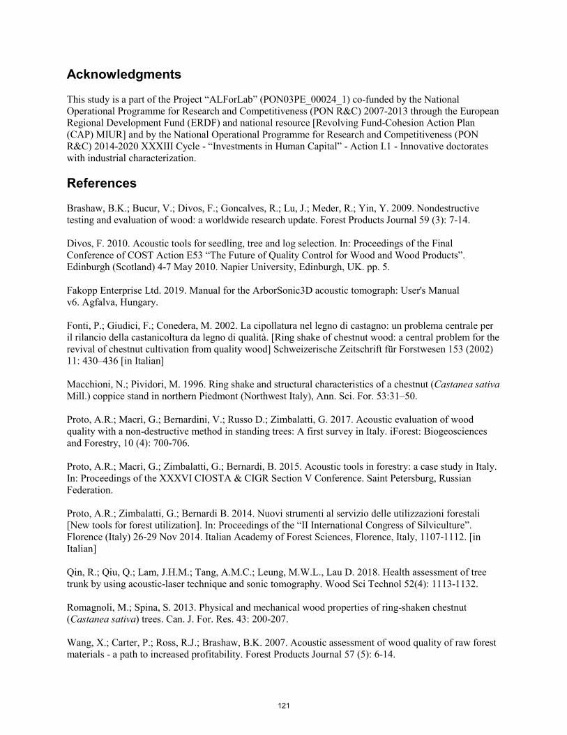
Acknowledgments This study is a part of the Project “ALForLab” (PON03PE_00024_1) co-funded by the National Operational Programme for Research and Competitiveness (PON R&C) 2007-2013 through the European Regional Development Fund (ERDF) and national resource [Revolving Fund-Cohesion Action Plan (CAP) MIUR] and by the National Operational Programme for Research and Competitiveness (PON R&C) 2014-2020 XXXIII Cycle - “Investments in Human Capital” - Action I.1 - Innovative doctorates with industrial characterization. References Brashaw, B.K.; Bucur, V.; Divos, F.; Goncalves, R.; Lu, J.; Meder, R.; Yin, Y. 2009. Nondestructive testing and evaluation of wood: a worldwide research update. Forest Products Journal 59 (3): 7-14. Divos, F. 2010. Acoustic tools for seedling, tree and log selection. In: Proceedings of the Final Conference of COST Action E53 “The Future of Quality Control for Wood and Wood Products”. Edinburgh (Scotland) 4-7 May 2010. Napier University, Edinburgh, UK. pp. 5. Fakopp Enterprise Ltd. 2019. Manual for the ArborSonic3D acoustic tomograph: User's Manual v6. Agfalva, Hungary. Fonti, P.; Giudici, F.; Conedera, M. 2002. La cipollatura nel legno di castagno: un problema centrale per il rilancio della castanicoltura da legno di qualità. [Ring shake of chestnut wood: a central problem for the revival of chestnut cultivation from quality wood] Schweizerische Zeitschrift für Forstwesen 153 (2002) 11: 430–436 [in Italian] Macchioni, N.; Pividori, M. 1996. Ring shake and structural characteristics of a chestnut (Castanea sativa Mill.) coppice stand in northern Piedmont (Northwest Italy), Ann. Sci. For. 53:31–50. Proto, A.R.; Macrì, G.; Bernardini, V.; Russo D.; Zimbalatti, G. 2017. Acoustic evaluation of wood quality with a non-destructive method in standing trees: A first survey in Italy. iForest: Biogeosciences and Forestry, 10 (4): 700-706. Proto, A.R.; Macrì, G.; Zimbalatti, G.; Bernardi, B. 2015. Acoustic tools in forestry: a case study in Italy. In: Proceedings of the XXXVI CIOSTA & CIGR Section V Conference. Saint Petersburg, Russian Federation. Proto, A.R.; Zimbalatti, G.; Bernardi B. 2014. Nuovi strumenti al servizio delle utilizzazioni forestali [New tools for forest utilization]. In: Proceedings of the “II International Congress of Silviculture”. Florence (Italy) 26-29 Nov 2014. Italian Academy of Forest Sciences, Florence, Italy, 1107-1112. [in Italian] Qin, R.; Qiu, Q.; Lam, J.H.M.; Tang, A.M.C.; Leung, M.W.L., Lau D. 2018. Health assessment of tree trunk by using acoustic-laser technique and sonic tomography. Wood Sci Technol 52(4): 1113-1132. Romagnoli, M.; Spina, S. 2013. Physical and mechanical wood properties of ring-shaken chestnut (Castanea sativa) trees. Can. J. For. Res. 43: 200-207. Wang, X.; Carter, P.; Ross, R.J.; Brashaw, B.K. 2007. Acoustic assessment of wood quality of raw forest materials - a path to increased profitability. Forest Products Journal 57 (5): 6-14.

121

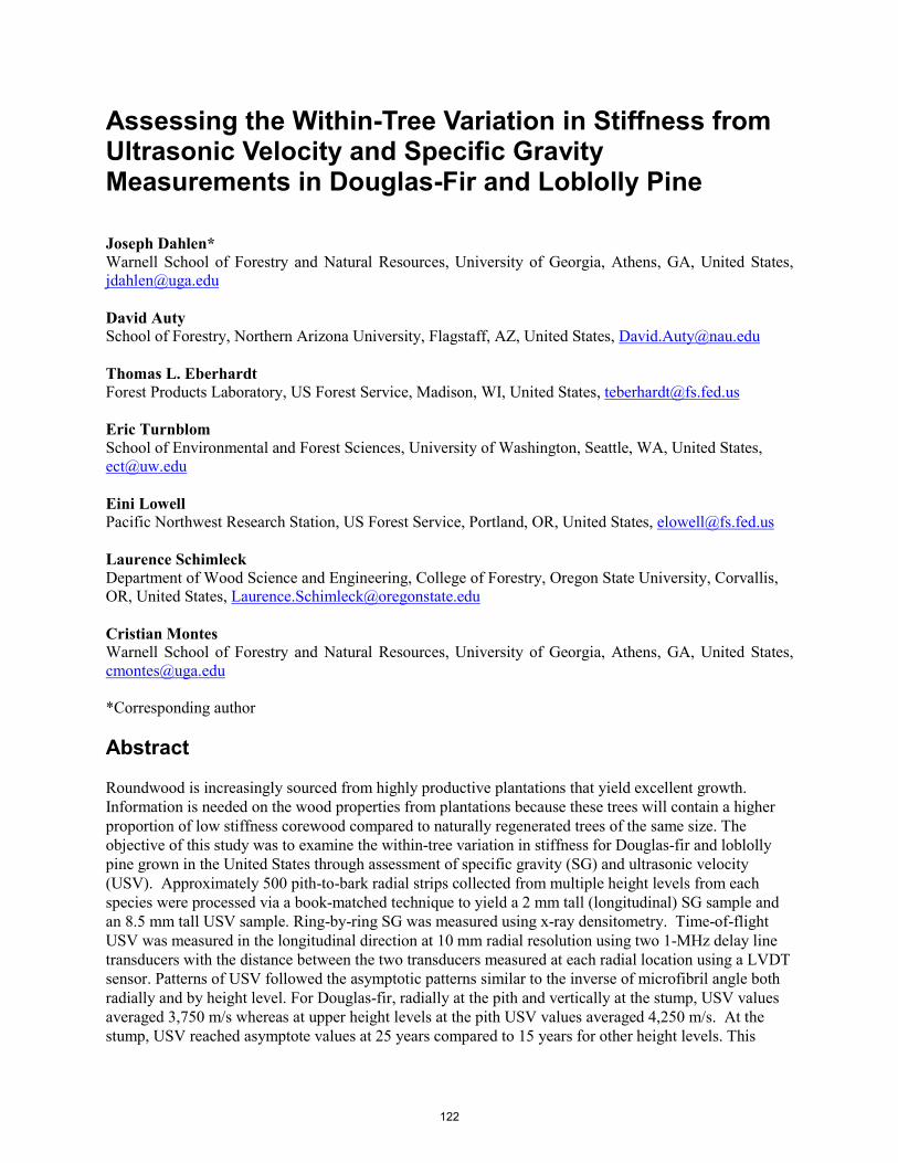
Assessing the Within-Tree Variation in Stiffness from Ultrasonic Velocity and Specific Gravity Measurements in Douglas-Fir and Loblolly Pine Joseph Dahlen* Warnell School of Forestry and Natural Resources, University of Georgia, Athens, GA, United States, jdahlen@uga.edu David Auty School of Forestry, Northern Arizona University, Flagstaff, AZ, United States, David.Auty@nau.edu Thomas L. Eberhardt Forest Products Laboratory, US Forest Service, Madison, WI, United States, teberhardt@fs.fed.us Eric Turnblom School of Environmental and Forest Sciences, University of Washington, Seattle, WA, United States, ect@uw.edu Eini Lowell Pacific Northwest Research Station, US Forest Service, Portland, OR, United States, elowell@fs.fed.us Laurence Schimleck Department of Wood Science and Engineering, College of Forestry, Oregon State University, Corvallis, OR, United States, Laurence.Schimleck@oregonstate.edu Cristian Montes Warnell School of Forestry and Natural Resources, University of Georgia, Athens, GA, United States, cmontes@uga.edu *Corresponding author Abstract Roundwood is increasingly sourced from highly productive plantations that yield excellent growth. Information is needed on the wood properties from plantations because these trees will contain a higher proportion of low stiffness corewood compared to naturally regenerated trees of the same size. The objective of this study was to examine the within-tree variation in stiffness for Douglas-fir and loblolly pine grown in the United States through assessment of specific gravity (SG) and ultrasonic velocity (USV). Approximately 500 pith-to-bark radial strips collected from multiple height levels from each species were processed via a book-matched technique to yield a 2 mm tall (longitudinal) SG sample and an 8.5 mm tall USV sample. Ring-by-ring SG was measured using x-ray densitometry. Time-of-flight USV was measured in the longitudinal direction at 10 mm radial resolution using two 1-MHz delay line transducers with the distance between the two transducers measured at each radial location using a LVDT sensor. Patterns of USV followed the asymptotic patterns similar to the inverse of microfibril angle both radially and by height level. For Douglas-fir, radially at the pith and vertically at the stump, USV values averaged 3,750 m/s whereas at upper height levels at the pith USV values averaged 4,250 m/s. At the stump, USV reached asymptote values at 25 years compared to 15 years for other height levels. This

122

presentation will focus primarily on the measurement of the USV and the relationships discussed between USV with SG, tracheid length and microfibril angle. Keywords: acoustic velocity, nondestructive testing, Pinus taeda, Pseudotsuga menziesii, wood and fiber quality Introduction Trees in forest plantations grow faster than their natural counterparts, and thus plantations allow for much shorter rotation lengths than in the past. As such, roundwood is increasingly being sourced from short rotation plantations as they provide a sustainable and consistent source of roundwood. However, the reductions in rotation age result in wood having a much larger proportion of corewood (juvenile wood) in the merchantable trees (Burdon et al. 2004; Moore and Cown 2017). Corewood, starting from the pith, and laid down outward, is the wood formed in young trees, while outerwood is formed later on as the tree matures (Burdon et al. 2004; Lachenbruch et al. 2011). Corewood is characterized by lower stiffness and strength, and higher longitudinal shrinkage, compared to outerwood (Larson et al. 2001). The specific mechanism for the lower stiffness is dependent on a particular species because of different patterns of wood variability. Douglas-fir (Pseudotsuga menziesii) has arguably the most typical specific gravity (SG) radial trend whereby SG is high near the pith, decreases in the transition wood, and then increases in the outerwood (Kimberley et al. 2017). Hard pines, including loblolly pine, have an increasing trend of SG from pith to bark (Dahlen et al. 2018). For loblolly pine, the reason for the low SG near the pith is due to the low proportion of latewood to earlywood tracheids, lower cell wall thicknesses, and lower latewood SG (Megraw 1985; Larson et al. 2001; Dahlen et al. 2018). As the SG increases for loblolly pine, the width of the rings decrease (Dahlen et al. 2018). For Douglas-fir, the reasons for the decrease in SG are debatable, but it likely corresponds to an increase in the diameter of the tracheids without a comparative increase in cell wall thickness. Douglas-fir also has a decrease in ring width in approximately the first ten years, which corresponds to the decreasing SG during this period. While SG has variable patterns of radial variability, microfibril angle (MFA) appears to have a universal pattern radially regardless of species. MFA decreases from pith to bark and this decrease corresponds to an increase in wood stiffness (Larson et al. 2001). In addition to radial variation, wood properties of softwoods also vary with height for a given cambial age; Burdon et al. (2004) illustrated this point by differentiating between mature corewood higher in a tree and juvenile corewood at the base, the latter being formed when the tree was young. For a given cambial age, both Douglas-fir and loblolly pine displays a decrease in SG with increasing height (Megraw 1985). Regarding MFA, values of MFA are high in the butt log and decrease with increasing height (Jordan et al. 2007). Measuring radial and longitudinal variation in SG is routine with the use of X-ray densitometry systems, and numerous laboratories have access to a variety of densitometer systems at reasonable costs (Jacquin et al. 2017). Measuring MFA is less routine due to the expensive hardware required for X-ray diffraction instruments (Evans 1999), and thus relatively few laboratories have access to in-house systems. One alternative to X-ray diffraction is to not measure MFA, and instead measure a surrogate property. To this end, measuring the longitudinal acoustic velocity is a promising alternative to measuring MFA since increasing AV is associated with decreasing MFA and increasing tracheid length (Hasegawa et al. 2011). The increasing AV is independent of changes in SG (Mason et al. 2017). Longitudinal velocity increases from pith to bark, whereas radial and tangential velocity do not (Hasegawa et al. 2011). Dynamic modulus of elasticity (MOE) can also be assessed by:

MOEdyn = ρAV2 (1)

123

where MOEdyn is dynamic MOE, p is the density and V is the acoustic velocity (Ross 2015). Acoustic evaluation is common on standing trees using time of flight techniques. Here, a transmitting transducer sends a sound wave via a mechanical impact to a receiving transducer and the time to send is recorded (Grabianowski et al. 2006; Auty and Achim 2008; Mora et al. 2009; Wessels et al. 2011; Paradis et al. 2013). The time to send is combined with the length of the signal path to determine the acoustic velocity. Acoustics is also frequently employed in evaluating the velocity of logs, lumber and small clear samples using resonance techniques whereby the 1st harmonic frequency of an acoustic wave signal is measured (Carter et al. 2013; Moore et al. 2013; Wang 2013; Wang et al. 2013; Yang et al. 2015). Resonance approaches would not be suitable for assessing radial variability on in-tact samples, however the technique could be used if individual samples were cut from pith to bark. Most researchers want to avoid cutting a radial strip into smaller samples, since doing so will result in the radial measurements to not be automated, and care must be also taken with regards to keeping track of samples. Thus, time of flight systems are the most appropriate for assessing radial variability in acoustic velocity but challenges need to be overcome before doing so. One challenge with using time of flight approaches on small samples is the frequency of the transducer must be much higher than comparable tree-based systems; these systems typically employ transducers with frequencies in the low kHz ranges. Such an approach would be unsuitable for assessing samples collected from cores and disks due to the length of the wavelength generated at these frequencies, calculated by:

𝛬𝛬 = 𝑣𝑣𝑓𝑓 (2)

where Λ is wavelength with units of m, v is velocity with units of m s-1, and f is frequency with units of Hz (s-1). For example, measuring the velocity of wood near the pith with 3500 m s-1 velocity using a 10 kHz transducer would result in wavelength being approximately 350 mm in length, clearly much larger than the diameter of any core sample. To decrease the length of the wavelength, transducers with much higher frequencies are employed. Ultrasonic transducers utilize frequencies greater than 20 kHz (Senalik et al. 2014), and when assessing samples prepared from cores or disks frequencies between 500 kHz and 1 MHz are typically employed (Mason et al. 2017; Schimleck et al. 2019). For example, Mason et al. (2017) used 500 kHz transducers on disk samples 60 mm thick to evaluate MFA variability in disks, and they concluded this was an effective and lower cost alternative to an x-ray diffraction system. For assessing samples collected from 12-mm cores, a 1 MHz transducer would be suitable (Schimleck et al. 2019). Another challenge that needs to be overcome is the coupling between the transducer and the sample (Schimleck et al. 2019). The objective of this work is to measure the longitudinal ultrasonic velocity (USV) from pith to bark and at multiple height levels for Douglas-fir and loblolly pine. The long-term objective of this work is to develop relationships between USV and MFA as well as tracheid length, and to develop models that explain the changes that occur with cambial age and height in the tree for USV. Combining USV models with models developed for SG will allow for the generation of tree maps for wood stiffness, similar to the SG maps generated by Dahlen et al. (2018). Materials and Methods Wood Samples The Douglas-fir samples were acquired from a 41-year-old plantation from the Stand Management Cooperative (SMC) Type 1 installations. The objective of the Type 1 study was to provide data on the impact of pre-commercial thinning, commercial thinning, and fertilization on Douglas-fir grown throughout the Northwest United States. From the plantation sampled, eleven trees from nine plots were

124

felled, and disks were collected at two fixed heights and three variable heights. The fixed height locations were at the stump and at the top of the first log (4.9 m height). The variable locations were at the base of the live crown, mid-point between the base of the live crown and the 10 cm top, and the 10 cm top. The loblolly pine samples were collected as part of a lumber study focused on assessing the quality of lumber produced from the most intensively managed operational plantations available for loblolly pine at the time (Butler et al. 2016; Butler et al. 2017; Dahlen et al. 2018). Trees from five stands, age 24 to 33 years, were felled and the 93 trees in the study were cut into 5.2 m logs for use in the lumber study. A 50 mm thick disk was cut from the bottom and top of each log at the stump (0.15 m), 5.2 m, 10.4 m, 15.6 m height, towards the top of the tree at the height equal to 13 cm stem diameter, and at 20.8 m if the 13 cm diameter height was above 20.8 m. The disks were stored in plastic bags and frozen until processing. To process the disks, radial strips were cut from bark-to-bark using a band saw, gently dried at 40°C until the moisture content was below 20%, and then left to air dry until approximately 12%. The strips were cut in half at the pith, and glued in between two wood coreholders. The samples were then cut on a four-blade table saw with a power feed to yield a book-matched acoustic sample measuring 8.5 mm (longitudinal), a densitometry sample measuring 2 mm (longitudinal), and a third sample that was designated for tracheid analysis (15 mm). Some samples were not tall enough to yield a tracheid sample and thus were cut to yield only the densitometer and acoustic sample. The length of the coreholders was approximately 0.9 m and thus multiple samples were prepared at one time. After the book-matched cutting process but prior to cutting out the individual samples from the processed coreholders, the 8.5 mm tall (longitudinal) acoustic velocity samples were sanded with 320-grit sandpaper on both transverse faces using a modified Brynes thickness sander (Brynes Model Machines, United States). Sanding improves the contact between the transducers by correcting any surface quality issues that may have occurred during processing. The samples were equalized in a room at approximately 22°C at 52% relative humidity, equivalent to approximately 10% moisture content. X-Ray Densitometry The densitometry strips were scanned on a QTRS-01X Tree Ring Scanner (Quintek Measurement Systems, United States). The instrument was setup to scan with a 0.06 mm radial step resolution and the X-ray beam passed through the sample on the transverse face. The instrument was calibrated to express SG on an oven dry weight and green volume basis (basic specific gravity). On the instrument, latewood was differentiated from earlywood for ring counting purposes based on a threshold SG value of 0.45 for Douglas-fir and 0.48 for loblolly pine. Ultrasonic Velocity The acoustic velocity samples were scanned on an OPUS instrument (SoniSys, United States) at 10-mm radial resolution. The instrument uses two 1-MHz longitudinal delay line transducers with the top transducer transmitting the acoustic signal to the bottom transducer which receives the acoustic signal. The surface diameter of the delay lines is 10-mm, and they are attached to a 0.9 mm layer of neoprene using 3M #453 transfer tape (3M, United States). Neoprene as a couplant was first selected as alternative to gel couplants for testing paper, since gel couplants would absorb into paper and thus affect the velocity readings (Habeger et al. 1988). We have found that the neoprene is an effective couplant for solid wood samples, as well as the calibration materials tested here. The instrument is calibrated for thickness measurements using two reference shims using a linear variable differential transformer (LVDT) sensor, and calibrated against reference materials of aluminum (6320 m s-1), brass (4430 m s-1), and PVC (2395 m s-1) blocks approximately 7.5 mm in height. For each acoustic reading, the instrument measures the thickness of the sample using the LVDT sensor, and the time required to transmit from the sending to

125

receiving transducer; each time reading is an average value of 100 readings taken on the instrument. The acoustic velocity is then calculated by the time and the thickness measurements. To move the sample from pith to bark, an automated movement system was built specific to the instrument. The system consists of a linear stage using a stepper motor which is controlled using a programmable logic controller and a touch screen interface. The programmable logic controller is programmed using C++ and the touch screen interface is programmed using Python, with communication between the two using serial communication. The touchscreen interface is used to input the length of the sample. When the last measurement reading is less than the 10 mm transducer diameter, the sample is moved the remaining distance of a sample. For example, if a sample is 127 mm, the sample is moved 12 times at 10 mm radial increments, and the final time at a 7 mm radial increment. The programmable logic control system will move the linear stage after each reading when the top transducer returns to the home position; this is done by way of a photoelectric U-Frame fork sensor. Data Analysis The statistical analysis and associated graphics were done in R statistical software (R Core Team 2019) with RStudio interface (RStudio 2019) and the tidyverse series of packages (Wickham and RStudio 2017) and gridExtra (Auguie 2016). At the time of writing this conference paper, two pieces of the studies are incomplete. The first is the densitometer work on the loblolly pine samples, and the second is the calibrations between the USV measurements and MFA using the SilviScan system (Evans 1999). As a temporary solution to this, we will report USV values in distance from the pith for both loblolly pine and Douglas-fir. And we will report estimated MFA using the model developed by Mason et al. (2017) on radiata pine. Following completion of the densitometry measurements, the USV data at 10 mm radial resolution will be matched with the densitometer data, and then the ring counts from the densitometer will be used to calculate ring, earlywood, and latewood level measurements for SG and width, and ring level USV measurements. Results and Discussion A total of 5,390 10 mm USV readings were conducted on Douglas-fir, and 4,387 readings for loblolly pine. A summary of the USV measurements for Douglas-fir and loblolly pine is shown in Table 1. The table shows the mean, minimum, and maximum USV values by height level for the first reading at the pith, and the last reading at the bark. Generally, the values for Douglas-fir are higher than loblolly pine, which matches the literature whereby Douglas-fir has generally lower MFA than loblolly pine. The values are particularly evident at the stump height, where the pith readings for Douglas-fir average 3738 m/s versus the 3261 m/s values for loblolly pine. Based on the USV to MFA equation developed by Mason et al. (2017), for Douglas-fir the mean predicted MFA at the pith is 26 degrees, with the stump having a predicted MFA of 29 degrees and the other height levels approximately 25 degrees. The MFA predictions are reasonable given that MFA was measured on breast height samples using an X-ray diffraction instrument at the Weyerhaeuser company, the pith samples at breast height averaged 28 degrees for these samples.

126

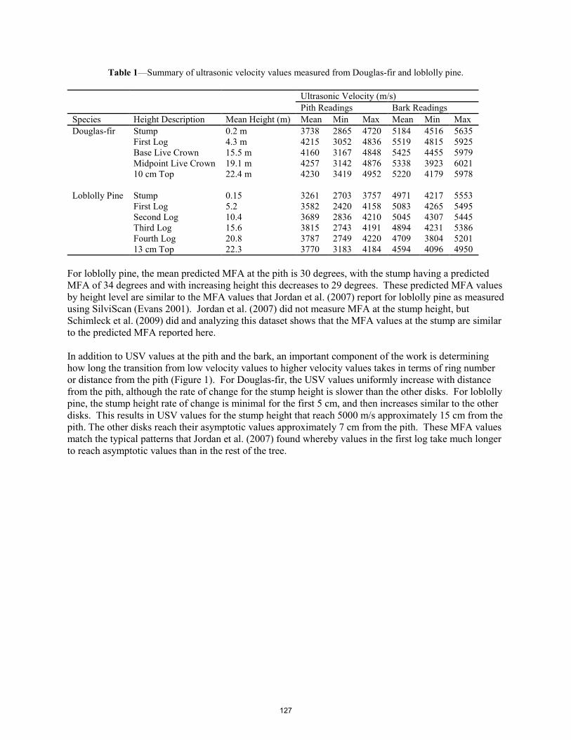
Table 1—Summary of ultrasonic velocity values measured from Douglas-fir and loblolly pine.

Ultrasonic Velocity (m/s) Pith Readings Bark Readings

Species Height Description Mean Height (m) Mean Min Max Mean Min Max Douglas-fir Stump 0.2 m 3738 2865 4720 5184 4516 5635

First Log 4.3 m 4215 3052 4836 5519 4815 5925 Base Live Crown 15.5 m 4160 3167 4848 5425 4455 5979 Midpoint Live Crown 19.1 m 4257 3142 4876 5338 3923 6021 10 cm Top 22.4 m 4230 3419 4952 5220 4179 5978

Loblolly Pine Stump 0.15 3261 2703 3757 4971 4217 5553

First Log 5.2 3582 2420 4158 5083 4265 5495 Second Log 10.4 3689 2836 4210 5045 4307 5445 Third Log 15.6 3815 2743 4191 4894 4231 5386 Fourth Log 20.8 3787 2749 4220 4709 3804 5201 13 cm Top 22.3 3770 3183 4184 4594 4096 4950

For loblolly pine, the mean predicted MFA at the pith is 30 degrees, with the stump having a predicted MFA of 34 degrees and with increasing height this decreases to 29 degrees. These predicted MFA values by height level are similar to the MFA values that Jordan et al. (2007) report for loblolly pine as measured using SilviScan (Evans 2001). Jordan et al. (2007) did not measure MFA at the stump height, but Schimleck et al. (2009) did and analyzing this dataset shows that the MFA values at the stump are similar to the predicted MFA reported here. In addition to USV values at the pith and the bark, an important component of the work is determining how long the transition from low velocity values to higher velocity values takes in terms of ring number or distance from the pith (Figure 1). For Douglas-fir, the USV values uniformly increase with distance from the pith, although the rate of change for the stump height is slower than the other disks. For loblolly pine, the stump height rate of change is minimal for the first 5 cm, and then increases similar to the other disks. This results in USV values for the stump height that reach 5000 m/s approximately 15 cm from the pith. The other disks reach their asymptotic values approximately 7 cm from the pith. These MFA values match the typical patterns that Jordan et al. (2007) found whereby values in the first log take much longer to reach asymptotic values than in the rest of the tree.

127

Figure 1—Ultrasonic velocity values based on distance from the pith for Douglas-fir and loblolly pine. The data points and smoothed lines are shown by disk height.

Conclusions This work showed that USV measurements match the values that would be expected for MFA for Douglas-fir and loblolly pine. Generally, Douglas-fir had higher USV at the pith than did loblolly pine. The implication from this is that Douglas-fir would have lower MFA, higher stiffness and lower longitudinal shrinkage than loblolly pine. Future work will report USV values with cambial age rather than distance from the pith, however at the time of writing this the densitometer work for loblolly pine was not complete and thus the paper reports USV values in distance from the pith. Future work will also correlate USV readings with MFA measured using SilviScan, and tracheid length on macerated samples measured using a commercial fiber analyzer. Models will be developed that predict USV as a function of cambial age and height within tree and these models will be used to construct within tree variation maps for USV and wood stiffness calculated from SG and USV. Acknowledgments This research was possible through support from the Wood Quality Consortium (WQC) at the University of Georgia, the Plum Creek Timber Company (now Weyerhaeuser), the Stand Management Cooperative (SMC) at the University of Washington, the National Science Foundation (NSF) Center for Advanced Forest Systems (CAFS), and the NIFA McIntire-Stennis project 1006098. The authors wish to thank the organizations for funding this project.

128

References Auguie, B. 2016. gridExtra: Miscellaneous functions for “grid” graphics. R package version 2.2.1 https://CRAN.R-project.org/package=gridExtra Auty, D.; Achim, A. 2008. The relationship between standing tree acoustic assessment and timber quality in Scots pine and the practical implications for assessing timber quality from naturally regenerated stands. Forestry 81 (4): 475-487. Burdon, R.D.; Kibblewhite, R.P.; Walker, J.C.F.; Megraw, R.A.; Evans, R.; Cown, D.J. 2004. Juvenile versus mature wood: a new concept, orthogonal to corewood versus outerwood, with special reference to P. radiata and P. taeda. Forest Sci 50(4):399-415. Butler, A.; Dahlen, J.; Daniels, R.F.; Eberhardt, T.L.; Antony, F. 2016. Bending strength and stiffness of loblolly pine lumber from intensively managed stands located on the Georgia Lower Coastal Plain. Eur. J. Wood Prod. 47 (1), 91-100. Butler, A.; Dahlen, J.; Eberhardt T.L.; Montes C.; Antony F.; Daniels, R.F. 2017. Acoustic evaluation of loblolly pine tree- and lumber-length logs allows for segregation of lumber modulus of elasticity, not for modulus of rupture. Ann. For. Sci. 74 (1), 20. Carter, P.; Chauhan, S.; Walker, J. 2006. Sorting logs and lumber for stiffness using Director HM200. Wood Fiber Sci. 38 (1), 49-54. Dahlen, J.; Auty, D.; Eberhardt, T.L. 2018. Models for predicting specific gravity and ring width for loblolly pine from intensively managed plantations and implications for wood utilization. Forests. 9(6):292. Evans, R. 1999. A variance approach to the X-ray diffractometric estimation of microfibril angle in wood. Appita J. 52(4): 283-289,294. Grabianowski, M.; Manley, B.; Walker, J.C.F. 2006. Acoustic measurements on standing trees, logs and green lumber. Wood Sci. Technol. 40 (3), 205-216. Habeger, C.C.; Wink, W.A.; Van Zummeren, M.L. 1988. Using neoprene-faced, PVDF transducers to couple ultrasound into solids. Institute of Paper Chemistry, IPC Technical Paper Series Number 269. Hasegawa, M.; Takata, M.; Matsumura, J.; Oda, K. 2011. Effect of wood properties on within-tree variation in ultrasonic wave velocity in softwood. Ultrasonics 51 (3), 296-302. Jacquin, P.; Longuetaud, F.; Leban, J.M.; Mothe, F. X-ray microdensitometry of wood: A review of existing principles and devices. Dendrochronologia 2017, 42, 42-50, doi: Jordan, L.; He, R.; Hall, D.B.; Clark A, III; Daniels, R.F. 2007. Variation in loblolly pine ring microfibril angle in the southeastern United States. Wood Sci Tech 39(2): 352-363. Kimberley, M.O.; McKinley, R.B.; Cown, D.J.; Moore, J.R. 2017. Modelling the variation in wood density of New Zealand-grown Douglas-fir. NZ J Forestry Sci. 47:15.

129

Lachenbruch, B.; Moore, J.R.; Evans, R. 2011. Radial variation in wood structure and function in woody plants, and hypotheses for its occurrence. In Size- and Age-Related Changes in Tree Structure and Function; Meinzer, F.C.; Lachenbruch, B.; Dawson, T.E., Eds.; Springer-Verlag: Berlin, Germany, pp. 121-164. Larson, P.R.; Kretschmann, D.E.; Clark III, A.; Isebrands, J.G. 2001. Formation and properties of juvenile wood in southern pines. US For Serv. Forest Products Laboratory. FPL-TR-129. Mason, E.G.; Hayes, M.; Pink, N. 2017. Validation of ultrasonic velocity estimates of wood properties in discs of radiata pine. NZ J Forestry Sci 47:16. Megraw, R.A. 1985. Wood quality factors in loblolly pine. TAPPI, United States. 88 p. Moore, J.R.; Lyon, A.J.; Searles, G.J.; Lehneke, S.A.; Ridley-Ellis, D.J. 2013. Within- and between-stand variation in selected properties of Sitka spruce sawn timber in the UK: implications for segregation and grade recovery. Ann. For. Sci. 70 (4), 403-415. Moore JR, Cown D (2017) Corewood (juvenile wood) and its impact on wood utilisation. Current Forestry Reports 3(2):107-118. Mora, C.R.; Shimleck, L.R.; Isik, F.; Mahon Jr., J.M.; Clark III, A.; Daniels, R.F. 2009. Relationships between acoustic variables and different measures of stiffness in standing Pinus taeda trees. Can. J. For. Res. 39, 1421-1429. Paradis, N.; Auty, D.; Carter, P.; Achim, A. 2013. Using a standing-tree acoustic tool to identify forest stands for the production of mechanically-graded lumber. Sensors 13 (3), 3394-3408. R Core Team. 2019. R: A language and environment for statistical computing. R Foundation for Statistical Computing, Vienna, Austria. URL http://www.R-project.org/. RStudio. 2019. RStudio: Integrated development environment for R. Boston, MA. https://www.rstudio.com/ Ross R.J. 2015. Nondestructive testing and evaluation of wood. Ross R.J., ed Nondestructive evaluation of wood: second edition. General Technical Report FPL-GTR-238. Madison, WI: U.S. Department of Agriculture, Forest Service, Forest Products Laboratory, 169 pp. Schimleck, L.R.; Mora, C.R.; Jordan, L.; White, D.E.; Courchene, C.E.; Purnell, R.C. 2009. Determination of within-tree variation of Pinus taeda wood properties by near infrared spectroscopy. Part 1: Development of multiple height calibration. Appita J. 62(2):130-136. Schimleck, L.R.; Apiolaza, L.A.; Dahlen, J.; Downes, G.; Emms, G.; Evans, R.; Moore, J.; Pâques, L.; Van den Bulcke, J.; Wang, X. 2019. Non-destructive evaluation techniqjues and what they tell us about wood property variation. In preparation. Senalik, C.A.; Schueneman, G.; Ross, R.J. 2014. Ultrasonic-based nondestructive evaluation methods for wood: a primer and historical review. General Technical Report FPL-GTR-235. Madison WI: U.S. Department of Agriculture, Forest Service, Forest Products Laboratory, 31 p.

130

Wang, X. 2013. Acoustic measurements on trees and logs: a review and analysis. Wood Sci. Technol. 47, 965-975. Wang, X.; Verrill, S.; Lowell, E.; Ross, R.J.; Herian, V.L. 2013. Acoustic sorting models for improved log segregation. Wood Fiber Sci. 45 (4), 343-352. Wessels, C.B.; Malan, F.S.; Rypstra, T. 2011. A review of measurement methods used on standing trees for the prediction of some mechanical properties of timber. Eur. J. Forest Res. 130, 881-893. Wickham and Rstudio (2017) tidyverse: Easily install and load the ‘tidyverse’ R package version 1.2.1 https://cran.r-project.org/web/packages/tidyverse/index.html Yang, B.Z., Seale, R.D., Shmulsky, R., Dahlen, J., Wang, X. 2015. Comparison of nondestructive testing methods for evaluating No. 2 southern pine lumber: Part A, Modulus of elasticity. Wood Fiber Sci. 47 (4), 375-384.

131

Effects of Climate and Stand Density on Wood Density of Ponderosa Pine in the Southwestern USA Damon Vaughan School of Forestry, Northern Arizona University, Flagstaff, Arizona, USA, drv59@nau.edu David Auty School of Forestry, Northern Arizona University, Flagstaff, Arizona, USA, david.auty@nau.edu Thomas E. Kolb School of Forestry, Northern Arizona University, Flagstaff, Arizona, USA, tom.kolb@nau.edu Andrew J. Sánchez Meador School of Forestry, Northern Arizona University, Flagstaff, Arizona, USA, andrew.sanchezmeador@nau.edu Kurt H. Mackes Warner College of Natural Resources, Colorado State University, Fort Collins, Colorado, USA, kurt.mackes@colostate.edu Joseph Dahlen Warnell School of Forestry and Natural Resources, University of Georgia, Athens, Georgia, USA, jdahlen@uga.edu W. Keith Moser Forest and Woodland Ecosystems Science, U.S.D.A Forest Service Rocky Mountain Research Station, Flagstaff, Arizona, USA, wkmoser@fs.fed.us Abstract Restoration treatments in the southwestern United States, aimed at reducing stand density to pre-settlement levels, are producing large volumes of ponderosa pine woody byproducts. The highly variable and often low density of ponderosa pine wood may limit its potential for use in high-value wood products. Application of the wood to higher-valued markets would increase the economic sustainability of restoration treatments, but a major barrier is a lack of understanding about the wood’s fundamental properties. Growth increment and wood density in ponderosa pine are highly variable year-to-year and are influenced by climatic variation, stand density, and management actions. In this study, we investigated wood density variation of ponderosa pine from a replicated stand density experiment near Flagstaff, AZ, USA. The stand was initially thinned heavily when the trees were approximately 43 years old, then thinned lightly at 10-year increments until the present. Using X-ray densitometry, we analyzed pith-to-bark trends in mean ring density, latewood proportion, and maximum latewood density of 267 samples from 54 trees, representing six different growing stock levels (GSL; 7, 14, 18, 23, 28, and 35 m2 ha-1). Density components were not significantly different among the six GSLs for the 53 years following the initial thinning. Climatic variation strongly influenced all density components, causing spikes in mean ring density during drought years. The implications of these findings are that stand thinning can produce higher wood volume without a reduction in wood density, and forecasted conditions of future drought may result in the formation of higher density wood. Keywords: X-ray densitometry, forest restoration, wood density, ponderosa pine, growing stock level, dendroecology

132

Introduction Restoration treatments in the southwestern United States, aimed at reducing stand density to pre-settlement levels, are producing large volumes of ponderosa pine (Pinus ponderosa) woody byproducts. The markets available for these byproducts, including pallet stock, molding, post and pole, and clean or dirty chips, rarely cover the cost of timber harvest and transportation (Hjerpe and Kim 2008). Application of the wood to higher-valued markets would increase the economic sustainability of restoration treatments, but a major barrier is a lack of understanding about the wood’s fundamental properties. Wood density is an important wood property that is often used as an indicator of mechanical properties such as strength and stiffness (Kretschmann 2010). Wood density varies at multiple scales, but the greatest variation is often seen within an individual tree. Within a tree, density values vary within rings (earlywood [EW] to latewood [LW] transition), from pith-to-bark (corewood to outerwood transition), and from stump-to-crown (Burdon et al. 2004; Lachenbruch et al. 2011). A greater understanding of this within-tree variation in southwestern ponderosa pine will aid in selecting appropriate end-uses for the material, and thus increase the economic sustainability of restoration efforts. Many internal and external controls can influence wood density and lead to its variation within a stem. First, wood density follows a pith-to-bark developmental pattern often described as the “typical radial profile” (TRP). This arises from changing hydraulic and mechanical needs as the tree ages (Lachenbruch et al. 2011). Second, stand density and competition for resources may influence wood density. Studies show mixed results regarding the effect of stand density on wood density in pines. Some studies have shown a negative correlation between growth rate and wood density in loblolly pine (Pinus taeda) (Jordan et al. 2008) and radiata pine (Pinus radiata) (Nicholls and Wright 1976). Meanwhile, no such correlation has been found in loblolly pine (Megraw 1985) and ponderosa pine (Voorhies 1969). Finally, annual climatic variation can have a strong effect on wood density. The southwestern United States is subject to periodic droughts that have the effect of reducing crown growth (Adams and Kolb 2005) which can increase latewood proportion and therefore ring density (Larson 1969). The goal of this study was to quantify the influence of stand density, management history, and historical climate variability on the radial profile of wood density in southwestern ponderosa pine. Specifically, we address the following questions: 1) Does stand density affect ring density or other wood density components?, and 2) Do climatic variables affect ring density or other wood density components? Methods Site description and sample collection The study was located at Taylor Woods (TW), a replicated stand density experiment near Flagstaff, Arizona, USA. The TW experiment was established in 1962, when trees were approximately 43 years old. At this time, treatment units were thinned from approximately 47.9 m2 ha-1 to a basal area determined by their respective Growing Stock Level (GSL). The GSL is the basal area that the residual stand will have when the mean tree diameter is 25.4 cm. Three treatment units were established for each GSL of 6.9, 13.8, 18.4, 23.0, 27.5, and 34.4 m2 ha-1 and have been subsequently thinned approximately every 10 years to maintain the target stand density. The most recent thinning occurred in 2017 and provided the material for this study. TW has a rich history of research, and detailed site descriptions can be found in Bailey (2008). For information on stand history and stocking levels, consult Myers (1967), Schubert (1971), or Ronco et al. (1985).

133

Prior to the thinning in 2017, we randomly installed three 0.04 ha fixed-radus plots in each of the 18 treatment units at TW. We measured diameter at breast height (DBH, 1.37 m above the ground level) for all trees in the subplots to determine stand basal area. We used an inventory list of all trees scheduled for removal at TW to randomly select three trees for destructive sampling from each of the 18 treatment units, for a total of 54 trees with 9 trees from each GSL treatment. Before felling, we measured total tree height and height to the base of the live crown. After felling, we collected 2.54 cm-thick cross-sectional disks every 2.4 m from ground-level to a height of 7.32 m, with an additional sample taken at breast height. In total, we collected 267 disks from 54 trees. X-ray strip processing and testing To produce X-ray densitometry samples from the disks, we first cut a pith-to-bark strip from the north side of each sample. We repeatedly soaked the strips in acetone until the solution ran clear (typically two soaks) to remove extractives (Eberhardt and Samuelson 2015). Additionally, we measured air-dry density of each sample to aid in calibrating the densitometer. We then cut the radial strips to approximately 5 mm in the tangential direction, mounted them on hardwood strips, and cut the assembly to approximately 2.3 mm in the longitudinal direction. We conditioned the samples at 20°C and 29% relative humidity to bring them to a testing moisture content of around 6%. We tested the samples on a Quintek QTRS-01X Tree Ring Scanner (Quintek Measurement Systems, Knoxville, TN) with a step size of 25 microns and the X-ray beam passing through the sample on the transverse face. We used the QMS Tree Ring Scanner software to make initial ring boundary delineations. Due to occasional errors arising from missing and false rings, we first visually corrected these initial marks, then statistically cross-validated them using the R package dplR (Bunn 2008). A total of 22 scans had a mean inter-series correlation below 0.35 (Adams and Kolb 2005) and we removed them from the study, leaving us with 245 samples from 53 trees. We excluded the first ten rings from each sample because of high ring curvature near the pith and a higher incidence of compression wood. Finally, we assigned the latewood boundary to the point in the ring where the density reached 80% of the difference between the minimum and maximum values (Lundqvist et al. 2018). We summarized the data to produce several response variables; here we will focus on basal area increment (BAI; cm2), ring density (RD; kg m-3), LW proportion (LWP), and maximum LW density (MXD; kg m-3). For analysis of additional response variables, see Vaughan et al. (2019). Statistical analysis For each of the six response variables, we produced mean chronologies of the de-trended series following methods described in Cook (1985) and using the R package dplR (Bunn 2008). For more detail on these methods, see Vaughan et al. (2019). We downloaded precipitation and temperature data for the Flagstaff Pulliam Airport weather station from the National Centers for Environmental Information (NCEI, National Oceanic and Atmospheric Administration [NOAA]). We downloaded Palmer Drought Severity Index (PDSI; Arizona Division 2), from the National Climatic Data Center (NCDC, NOAA). To test for an effect of GSL on wood density (Question #1), we modeled the wood density responses as a function of GSL and several other relevant covariates. We fit linear mixed-effects models with a random effect for tree and fixed effects of sample height, GSL, the sample height x GSL interaction, and the 5-year pre-1962 average. To account for annual variability, we included terms for year of ring formation and PDSI. If Type III ANOVA tables showed a significant effect of GSL (alpha = 0.05), we investigated Tukey-adjusted pairwise comparisons. We modeled autocorrelation with a first-order continuous autoregressive term.

134

To explore climatic effects (Question #2), we used the R package treeclim (Zang and Biondi 2015). We calculated response coefficients, which represent the strength of the correlation between response (density components) and predictors (climate variables). To build confidence intervals, we used bootstrapped response functions with 1000 resamples. We investigated the influence of climatic variables by quarter for the water year and at an annual scale; the first quarter of the water year was defined as October – December of the previous year, the second quarter as January – March of the current year, the third quarter as April – June, and the fourth quarter as July – September. If the confidence interval produced by the bootstrapped response function did not overlap zero, we considered the effect of the climate variable to be significant. To allow for differing responses among the GSLs, we grouped GSLs into low (6.9 and 13.8 m2 ha-1), mid (18.4 and 23 m2 ha-1), and high (27.5 and 34.4 m2 ha-1) levels. Results Stands with higher GSLs had increased basal area and trees per hectare, and reduced mean tree diameter when compared to low GSL stands. Of the 16,844 tree rings analyzed, the mean values for LWP, RD, and MXD were 12%, 446 kg m-3, and 763 kg m-3, respectively. Drought years were associated with spikes in density components, and the influence of drought on LWP was reduced after the initial thinning in 1962 (Figure 1).

Figure 1— PDSI and two measures of wood density (RD, kg m-3; LWP) at breast height, averaged over the six GSLs, vs. year (1940-2016). Dashed lines indicate drought years commonly used as marker years in the Southwest (1951, 1956, 1963, 1977, 1989, 1996, 2002).

In the GSL models, GSL had no effect on wood density components, but did influence BAI (Table 1). Year of ring formation was significant in most models and PDSI was significant in all models. GSL did have a significant effect on LWP, but none of the pairwise comprisons were significant. Results are summarised in Figure 2, which shows that GSL strongly influenced the long-term trend in BAI but had no effect on the long-term trend for RD.

135

Table 1— P-values of fixed effects terms and model fit statistics. The sample height x GSL interaction, PDSI, and pre-1962 values were significant at <0.0001 for all models, so for clarity they are not included in the table. Model GSL Year sample height R2-adja RMSE |%E|b

BAI <0.000 <0.000 <0.000 0.50 9.10 41.46 RD 0.142 0.051 <0.000 0.49 46.72 7.82 LWP 0.019 <0.000 <0.000 0.13 0.072 37.50 MXD 0.083 0.002 0.649 0.22 94.37 9.57 a percent variation in the response that is explained by the fixed effects of the predictors b mean absolute percent error

Figure 2— Long-term trends in BAI (top), RD (middle), and LWP (bottom) for breast height samples.

The treeclim analysis revealed that precipitation strongly affected the response variables (Figure 3). Total precipitation had a significant effect on RD in the second (current year January – March) and third (current year April – June) quarters of the water year, as well as at the annual level. These effects were similar between the three GSL groupings. Second quarter precipitation correlated negatively with LWP, leading to a significant annual effect at the highest two GSL classes. First quarter precipitation had a positive correlation with MXD in all three GSL groupings, while fourth quarter (current year July – August) precipitation in the lowest GSL correlated negatively with MXD.

136

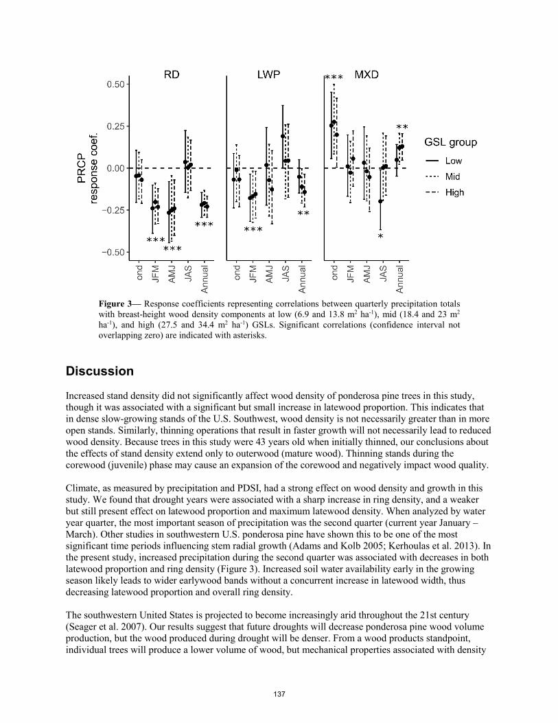
Figure 3— Response coefficients representing correlations between quarterly precipitation totals with breast-height wood density components at low (6.9 and 13.8 m2 ha-1), mid (18.4 and 23 m2 ha-1), and high (27.5 and 34.4 m2 ha-1) GSLs. Significant correlations (confidence interval not overlapping zero) are indicated with asterisks.

Discussion Increased stand density did not significantly affect wood density of ponderosa pine trees in this study, though it was associated with a significant but small increase in latewood proportion. This indicates that in dense slow-growing stands of the U.S. Southwest, wood density is not necessarily greater than in more open stands. Similarly, thinning operations that result in faster growth will not necessarily lead to reduced wood density. Because trees in this study were 43 years old when initially thinned, our conclusions about the effects of stand density extend only to outerwood (mature wood). Thinning stands during the corewood (juvenile) phase may cause an expansion of the corewood and negatively impact wood quality. Climate, as measured by precipitation and PDSI, had a strong effect on wood density and growth in this study. We found that drought years were associated with a sharp increase in ring density, and a weaker but still present effect on latewood proportion and maximum latewood density. When analyzed by water year quarter, the most important season of precipitation was the second quarter (current year January – March). Other studies in southwestern U.S. ponderosa pine have shown this to be one of the most significant time periods influencing stem radial growth (Adams and Kolb 2005; Kerhoulas et al. 2013). In the present study, increased precipitation during the second quarter was associated with decreases in both latewood proportion and ring density (Figure 3). Increased soil water availability early in the growing season likely leads to wider earlywood bands without a concurrent increase in latewood width, thus decreasing latewood proportion and overall ring density. The southwestern United States is projected to become increasingly arid throughout the 21st century (Seager et al. 2007). Our results suggest that future droughts will decrease ponderosa pine wood volume production, but the wood produced during drought will be denser. From a wood products standpoint, individual trees will produce a lower volume of wood, but mechanical properties associated with density

137

will likely improve. Regional wood supply, however, will likely be reduced by drought-driven disturbances, such as wildfire and bark beetle outbreaks that can rapidly kill many trees (McDowell et al. 2015). It is worth noting that our results are valid only for the range of climate conditions explored in this study. Extreme and prolonged droughts in the future may not have the same effects on wood density as the relatively short-term and episodic droughts we investigated in this study between years 1919 and 2016. Conclusions In this study, we investigated whether long-term management of stand basal area and short-term climate fluctuations affected growth and wood density components in a replicated ponderosa pine stand density experiment in Northern Arizona. We found that increased stand basal area did not affect any of the density responses but did have a strong negative effect on tree growth and a small but significant positive effect on latewood proportion of annual rings. Climate strongly affected the responses, mainly by increasing ring density in drought years. Future droughts, at least within the ranges of duration and severity explored in this study, may lead to decreased tree volume growth but higher wood density in ponderosa pine. Acknowledgments We would like to thank the ARCS Foundation, the Kay and Irene Hafen Forestry Scholarship, the Wally Covington Travel award, and the NAU Graduate Student Government International Travel Award for generous contributions. Additionally, thanks to two anonymous reviewers at Annals of Forest Science who provided detailed and constructive comments on the longer version of this manuscript. References Adams, H.D.; Kolb, T.E. 2005. Tree growth response to drought and temperature in a mountain landscape in northern Arizona, USA. J Biogeogr 32:1629–1640. Bailey, J.D. 2008. Forty Years Later at Taylor Woods: Merging the Old and New. Fort Val Exp For - a Century Res 1908-2008, Conf Proc 100–105 Bunn, A.G. 2008. A dendrochronology program library in R (dplR). Dendrochronologia 26:115–124. Burdon, R.D.; Kibblewhite, R.P.; Walker, J.C.F. [and others]. 2004. Juvenile versus mature wood: A new concept, orthogonal to corewood versus outerwood, with special reference to Pinus radiata and P. taeda. For Sci 50:399–415 Cook, E.R. 1985. A time series analysis approach to tree ring standardization. Tucson, AZ: University of Arizona. 171 pp. PhD Dissertation. Eberhardt, T.L.; Samuelson, L.J. 2015. Collection of wood quality data by X-ray densitometry: a case study with three southern pines. Wood Sci Technol 49:739–753. Hjerpe, E.E.; Kim, Y-S. 2008. Economic impacts of southwestern national forest fuels reductions. J For 106:311–316

138

Jordan, L.; Clark, A.; Schimleck, L.R. [and others]. 2008. Regional variation in wood specific gravity of planted loblolly pine in the United States. Can J For Res 38:698–710. Kerhoulas, L.P.; Kolb, T.E.; Koch, G.W. 2013. Tree size, stand density, and the source of water used across seasons by ponderosa pine in northern Arizona. For Ecol Manage 289:425–433. Kretschmann, D.E. 2010. Mechanical Properties of Wood. In: Wood Handbook - Wood as an engineering material. pp 1–46 Lachenbruch, B.; Moore, J.R.; Evans, R. 2011. Radial variation in wood structure and function in woody plants, and hypotheses for its occurrence. In: Size- and age-related changes in tree structure and function. Tree Physiology, pp 121–164 Larson, P. 1969. Wood formation and the concept of wood quality. Yale Univ Sch For Bull 1–54 Lundqvist, S-O.; Seifert, S.; Grahn, T. [and others]. 2018. Age and weather effects on between and within ring variations of number, width and coarseness of tracheids and radial growth of young Norway spruce. Eur J For Res. McDowell, N.G.; Williams, A.P.; Xu, C. [and others]. 2015. Multi-scale predictions of massive conifer mortality due to chronic temperature rise. Nat Clim Chang 6:295–300. Megraw, R.A. 1985. Wood quality factors in loblolly pine - the influence of tree age, position in tree, and cultural practice on wood specific gravity, fiber length, and fibril angle. TAPPI Press 1–88 Myers, C.A. 1967. Growing stock levels in even-aged ponderosa pine Nicholls, J.W.P.; Wright, J.P. 1976. The effect of environmental factors on wood characteristics. 3. The influence of climate and site on young Pinus radiata material. Can J For Resour 6:113–121 Ronco, F.; Edminster, C.B.; Trujillo, D.P. 1985. Growth of ponderosa pine thinned to different stocking levels in northern Arizona. Res Pap - US Dep Agric For Serv. Schubert, G.H. 1971. Growth response of even-aged ponderosa pines related to stand density levels. J For 69:857–860 Seager, R.; Lau, N-C.; Li, C. [and others]. 2007. Model Projections of an Imminent Transition to a More Arid Climate in Southwestern North America. Science (80- ) 316:1181–1184. Vaughan, D.R.; Auty, D.; Kolb, T.E. [and others]. Climate alters ponderosa pine (Pinus ponderosa) wood density more than stand basal area in a replicated stand density experiment in the southwestern USA. Accepted for publication in Annals of Forest Science (Accepted May 2019) Voorhies, G. 1969. Specific gravity studies of young growth southwestern ponderosa pine. For Prod J 19:45–46 Zang, C.; Biondi, F. 2015. Treeclim: An R package for the numerical calibration of proxy-climate relationships. Ecography (Cop) 38:431–436.

139

Monitoring Moisture Content and Ice Content in Standing Tree Stems using Time Domain Reflectometry Huadong Xu * College of Engineering and Technology, Northeast Forestry University, Harbin , P.R.China, huadongxu@yahoo.com Qizhe Li College of Engineering and Technology, Northeast Forestry University, Harbin , P.R.China, 909717103 @qq.com Yuting Wang College of Engineering and Technology, Northeast Forestry University, Harbin , P.R.China, 2856881758 @qq.com Lihai Wang College of Engineering and Technology, Northeast Forestry University, Harbin , P.R.China, lihaiwang@yahoo.com Dawei Qi College of Engineering and Technology, Northeast Forestry University, Harbin , P.R.China, Qidw9806@126.com * Corresponding author To investigate the effect of environmental temperature on moisture content (MC) and ice content (IC) of standing trees, time domain reflectometry (TDR), an electromagnetic wave-based device, was employed to test larch and poplar tree specimens at different temperatures (between -26 ~ 10 °C). The continuous change data of temperature and electromagnetic wave propagation time (EWPT) in trees were monitored and recorded for a long time. EWPT data were used to predict tree MC based on some regression models. IC data of standing trees were also calculated by analyzing the change of MC at different temperatures. Finally, the diurnal and seasonal variations of MC and IC of standing trees were also discussed. The results indicate that it is feasible to evaluate MC and IC of standing trees using TDR. Keywords: Standing trees, moisture content, environmental temperature, ice content, time domain reflectometry

140

On-Site and Laboratorial Investigation of Pannónia Poplar Plantation Wood from Three Different Hungarian SitesNorbert Horváth* University of Sopron, Institute of Wood Science, Sopron, Hungary, horvath.norbert@uni-sopron.hu

Antal Kánnár University of Sopron, Institute for Applied Mechanics and Structures, Sopron, Hungary, kannar.antal@uni-sopron.hu

Csilla Csiha University of Sopron, Institute of Wood Products and Technologies, Sopron, Hungary, csiha.csilla@uni-sopron.hu

*corresponding author

Abstract

In the frame of the OTKA project no. 116226 supported by the Hungarian National Research,- Development and Innovation Office, we have carried out complex investigation of some properties of Pannónia poplar ( Populus × euramericana cv. Pannónia ) wood with special regard to the influence of the plantation site’s characteristics. During this research we have evaluated timber material of the same Pannónia poplar species originating from 3 different Hungarian poplar plantation sites from West Hungary: the 22 years old “Újrónafő 11G” site, the 24 years old “Győr 540B” site, and the 29 years old “Kapuvár 35A” site, with spacing of trees of 3×4 m, 3,25×6,5 m and 4×10 m. We have used stress wave nondestructive test technique with “Fakopp” TreeSonic device to test the standing trees. Afterwards we have performed laboratorial analysis of the samples from harvested logs (3 logs/site, random sample) in order to determine the bending strength and compression strength of the samples. Fifty trees pro every site have been investigated to determine the diameter at breast height, and the wave velocity in sapwood parallel to grain. The results showed that there were no significant differences in stress wave velocities between the trees of the sites investigated. However, we established that the higher the average value of stress wave velocity in case of standing trees, the higher the average value of bending strength and compression strength of the samples at normal climate is. The highest strength and density values were observed in case of Újrónafő 11G site samples.

Keywords: stress wave, nondestructive testing, TreeSonic, density, strength, poplar, plantation wood

Introduction

Willows and poplars belong botanically to the same family, the Salicaceae. The genus Populus is represented in the northern hemisphere with about 40 species. Sections such as Aigerios and partially Leuce in Hungary (Tóth and Erdős 1988), Aigeros, Leuce and Tacamahaca in Austria (Nebenführ 2007) have forestry importance. The European black poplar (Populus nigra L.) and the American black poplar (Populus deltoides Bartr. Ex Marsh.) And their clones (Populus × euramericana) are systematically

141

assigned to the poplar section Aigerios. The Pannónia poplar (Populus × euramericana cv. Pannónia) is an artificial variety that has been hybridized by Ferenc Kopeczky, forest scientist at the Hungarian Forest Research Institute (ERTI) in Sárvár. According to Tóth and Erdős (1988), the parents of Pannónia poplar were Populus deltoides S-1-54 Belgium and Populus nigra Lébény 211. It has a similar rapid growth as the variety 'I 214' (Populus × euramericana cv. 214), and can reach a similar density as the wood of Robusta poplar (Populus × euramericana cv. Robusta) (Molnár and Bariska 2006). The industrial poplar breeding was started in Hungary mainly at the floodplain of the Danube in the 1920s. According to Tóth and Erdős (1988) the datas show a marked increase (more than 115.000 ha) in the total area of Poplar populations between 1949 and 1986. Thanks to its outstanding characteristics, the poplar variety 'Pannónia' was one of the most important planting goods in Hungary in the 1990s (Tóth 2006).

Under the title "Complex analysis of the physico-mechanical and surface-physical properties of wood with low density", the Institute of Wood Sciences at the University of Sopron (former name University of West Hungary) has launched a research project in 2015. Figure 1 shows the selected plantations (n=8) for our investigations. In this publication, we briefly summarized some wood anatomical, and mechanical partial results with regard to the measurement data of West Hungarian plantations (n = 3). The relevant three plantations of KAEG Zrt. were marked by red, green and blue colors (Figure 1, red circle) and indicated with their GPS coordinates.

Figure 1— All in our project selected (n = 8), and the relevant West Hungarian (n=3, red circle) Pannónia poplar plantations

Material and methods

Based on the information in the relevant literature, the researchers have mainly dealt with juvenile wood of Pannónia poplar (Molnár et al. 2006, Horváth 2008). Therefore, our investigations have focused on over 20 years old plantations. The spacing of trees of the 22 years old “Újrónafő 11G”, the 24 years old “Győr 540B” and the 29 years old “Kapuvár 35A” plantation sites were 3×4 m, 3,25×6,5 m and 4×10 m.

142

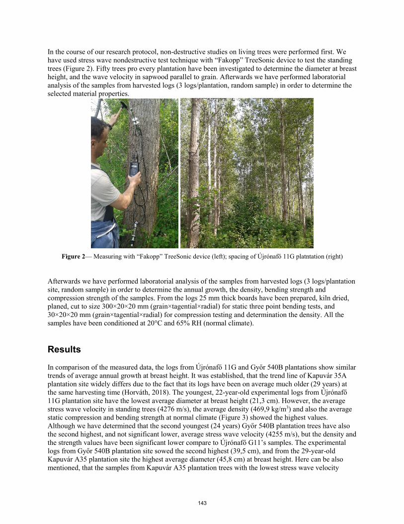
In the course of our research protocol, non-destructive studies on living trees were performed first. We have used stress wave nondestructive test technique with “Fakopp” TreeSonic device to test the standing trees (Figure 2). Fifty trees pro every plantation have been investigated to determine the diameter at breast height, and the wave velocity in sapwood parallel to grain. Afterwards we have performed laboratorial analysis of the samples from harvested logs (3 logs/plantation, random sample) in order to determine the selected material properties.

Figure 2— Measuring with “Fakopp” TreeSonic device (left); spacing of Újrónafő 11G platntation (right)

Afterwards we have performed laboratorial analysis of the samples from harvested logs (3 logs/plantation site, random sample) in order to determine the annual growth, the density, bending strength and compression strength of the samples. From the logs 25 mm thick boards have been prepared, kiln dried, planed, cut to size 300×20×20 mm (grain×tagential×radial) for static three point bending tests, and 30×20×20 mm (grain×tagential×radial) for compression testing and determination the density. All the samples have been conditioned at 20°C and 65% RH (normal climate).

Results

In comparison of the measured data, the logs from Újrónafő 11G and Győr 540B plantations show similar trends of average annual growth at breast height. It was established, that the trend line of Kapuvár 35A plantation site widely differs due to the fact that its logs have been on average much older (29 years) at the same harvesting time (Horváth, 2018). The youngest, 22-year-old experimental logs from Újrónafő 11G plantation site have the lowest average diameter at breast height (21,3 cm). However, the average stress wave velocity in standing trees (4276 m/s), the average density (469,9 kg/m3) and also the average static compression and bending strength at normal climate (Figure 3) showed the highest values. Although we have determined that the second youngest (24 years) Győr 540B plantation trees have also the second highest, and not significant lower, average stress wave velocity (4255 m/s), but the density and the strength values have been significant lower compare to Újrónafő G11’s samples. The experimental logs from Győr 540B plantation site sowed the second highest (39,5 cm), and from the 29-year-old Kapuvár A35 plantation site the highest average diameter (45,8 cm) at breast height. Here can be also mentioned, that the samples from Kapuvár A35 plantation trees with the lowest stress wave velocity

143

(4139 m/s) have also the lowest average density (381,1 kg/m3) and static strength values at normal climate.

Figure 3— The average stress wave velocity in standing trees (left); and static strength values of Pannónia poplar samples at normal climate (right)

Conclusions

Although the Újrónafő 11G and Győr 540B plantations sites have similar growing trends at breast height, and the stress wave velocity in standing trees have not been significant too, but these similarities on mechanical properties could not be observed. According to the evaluation, the samples from Kapuvár 35A and Győr 540B Pannónia poplar plantation sites showed almost similar mechanical properties. However it could not be predict from the stress wave velocity values alone.

Acknowledgments

The research work (IdNr .: OTKA K 116226) was financially supported by the National Research, Development and Innovation Office Hungary (NKFIH). The authors also gratefully acknowledge the technical support from KAEG Zrt. and István Schnatl technician.

References

Horváth, N. 2008. The effect of thermal treatment on wood properties with special emphasis on wood resistance to fungal decay, PhD. Dissertation, University of West Hungary. Sopron. http://doktori.nyme.hu/240/1/disszertacio.pdf .

Horváth, N. 2018. Materialwissenschaftliche Untersuchungen an Pannónia Pappel aus Ungarn In: Proceedings: 4. Holzanatomisches Kolloquium. Dresden: 140-142. http://publicatio.uni-sopron.hu/1677/1/05_13_Horvath.pdf .

Molnár, S.; Bariska, M. 2006: Magyarország ipari fái. Publisher: Szaktudás Kiadó Ház, Budapest.

Molnár, S.; Fehér, S.; Komán, Sz.; Ábrahám, J. 2006. Nyárfajták összehasonlító faanyagjellemzői az ipari felhasználás tükrében. In: Poceedings, Alföldi Erdőkért Egyesület Kutatói Nap, Szeged:101-109.

144

Nebenführ, W. 2007. Biomassegewinnung durch Pappel und Weide im Kurzbetrieb, eine Frage der Sorte. http://bfw.ac.at/050/pdf/Folien_Nebenfuehr.pdf

Tóth, B.; Erdős, L.; 1988. Nyár fajtaismertető. Publisher: Állami Gazdaságok Országos Egyesülése Erdőgazdálkodási és Fafeldolgozási Szakbizottsága, Budapest.

Tóth, B. 2006. Nemesnyár-fajták ismertetője – Irányelvek a nemesnyár-fajták kiválasztásához. Publisher: Agroinform Kiadó.

145

Remote Sensing Technologies as Proxy Forecast of Wood Technological Properties: Preliminary Results Esther Merlo Sánchez * Innovation Department, Madera Plus Calidad Forestal S.L., Ourense, España, maderaplus@maderaplus.es Miguel Piñeiro García Forest Department, Madera Plus Calidad Forestal S.L., Ourense, España, maderaplus@maderaplus.es Oscar Santaclara Estévez Forest Department, Madera Plus Calidad Forestal S.L., Ourense, España, maderaplus@maderaplus.es María Julia Yagüe Ballester Remote Sensing Services and Exploitation Platforms Division. GMV Innovating Solutions. Madrid, España. mjyague@gmv.com * Corresponding author Abstract The forest industry seeks greater competitiveness. The spatial characterization of wood quality attributes, such as density or modulus of elasticity, increases the chances of optimizing the wood added-value chain through more efficient forest management plans. To date, several models for predicting modulus of elasticity and wood density have been developed at plot level, using field inventory data for various species. This team developed a prototype tool to estimate stand-level variations in wood attributes, suggesting the possibility of large-scale mapping for wood quality. Results showed links between wood fiber attributes and related variables obtained from satellite earth observation missions combined with other environmental variables describing climate and geography. Values for all bands and five indexes (EVI, GNDVI, NDVI, NDWI, and SAVI) were collected for Sentinel II from the months of May to September 2017 and 2018. A series of high-resolution daily precipitation and temperature was used. A statistical analysis was done using the stepwise regression methodology to find the best fit. We were able to build a model with an r2 of 0.68 and a root mean square error of 31 kg/m3, which is composed of data from the sentinel II bands and climatic data. The analysis was carried out in the context of MySustainableForest project (H2020 No. 776045), which provides Earth Observation geo-information products across the wood sector to support the production chain from sustainable forest management procedures to wood quality entering sawmills, pulp mills, or other transforming industries. Keywords: Satellite data, Sentinel II, basic density, spatial characterization

146

Acoustic Technology – Development and Validation of Resonance-Based Tools for Research and Operations

Peter Carter * Chief Executive, Fibre-gen Limited, Auckland, New Zealand, peter.carter@fibre-gen.com Logan Stephens, InFact Limited, Christchurch, New Zealand. logan.stephens@infact.co.nz

Abstract

Research and commercial application of acoustic technologies has continued in the forestry and wood processing sector where end wood product values are dependent upon stiffness. Hitman™ technology was initially developed 20 years ago and has been progressively deployed in laboratory and field operations where harsh conditions demand robust waterproof tools. The technology has become an essential element of comercial operations in structural solid wood sectors of the industry including stress graded MSG/MSR lumber, LVL veneer, and CLT engineered wood products. Measurement of acoustic speed allows structural related value to be captured through better decision-making, allocation of resource to highest value uses, and application of best processing methods dependent upon log-by-log measures. This paper reviews the validation of recent improvements in two commercial resonance based tools confirming their suitability for the measurement of the stiffness of logs in harvesting, mill yard, and engineered wood product processing operations. It demonstrates the successful application of technology improvements for enhanced useability and precision of results.

Keywords: acoustic technology, structural lumber, MSR, MSG, LVL, CLT, Hitman™, HM200, HM220, LG640 stiffness, robust ruggedised tools, value, mill yard, wood processing

Introduction

Background

Acoustic technology has become a significant quality measure in the selection and segregation of log supplies for the production of structural wood products where stiffness and strength properties affect end product value. Typical examples of such structural products include MSG/MSR lumber, laminated beams, laminated veneer lumber (LVL), and cross laminated timber (CLT). Hitman™ technology is relied upon to enable the measurement of longitudinal acoustic speed in logs in all weathers, extreme temperatures, mud, dust, and harsh environmental conditions, typically encountered in the production of log supplies in a wide range of forest and log yard workplaces.

Ongoing improvement is in constant demand to deliver more for improved productivity. Underpinning technologies have advanced, resulting in the opportunity for tool and equipment design to be upgraded with enhancements to deliver improved precision and reliability, delivering greater value to the user, enhanced user experience and reliability. Carter and Doidge (2017) reported on the upgrade of the Hitman™ ST300 electronics and software to deliver quantifiable improvements in the precision and performance of the ‘acoustic time-of-flight’ standing tree Hitman™ ST330 tool.

147

Further development and improvements have since been made to the resonance based Hitman™ HM200 log tool (Figure 1) resulting in the release of the upgraded Hitman™ HM220 tool in late 2018. Improvements include the following:

1. Updated electronics platform2. New operating system providing 5x faster processing speed3. Auto power saving resulting in extended battery life4. Brighter display5. USB connection to PC providing easy access to stored results and wave forms

Figure 1 Hitman™ HM200 in typical logyard application

Field evaluation has confirmed that based on a range of criteria, the performance of the upgraded Hitman™ HM220 tool is improved relative to that of the original tool.

Technology improvements have also been applied to the Hitman™ LG640 log grader (Figure 2 and 3), designed to work automatically on a log chain of structural wood processing facilities.This mechanised version of the Hitman™ HM220 tool is typically installed downstream of the debarker, near the scanner, and prior to multiple log sort bins. Enhancements to the Hitman™ LG640 log grader include the following:

1. Adoption of an industrial National Instruments Compact DAQ data acquisition platform andcontroller

2. Real time operating system and improved processing speed to allow faster line speeds andreduced data processing times

3. Improved connectivity with upgraded remote panel accessible via web browsers from any pc onthe same Network

4. Integrated camera feed for status and monitoring5. TCP/IP output for easy integration with plant PLC’s and optimisers

Figure 2 Hitman LG640™ display screen

148

The first of these upgraded Hitman™ LG640 log grader installations was carried in April 2019 on a log chain in the logyard of an MSG structural sawmill in the State of West Australia (Figure 3).

Figure 3 Hitman LG640™ installed on log chain in MSG log processing facility

Performance validation was carried out with details of the study outlined below.

Hitman™ LG640 validation study

A comparative study was undertaken at the structural sawmill in Western Australia to compare the performance of the Hitman™ LG640 log grader against that of the Hitman™ HM200 and HM220 tools.

Objectives

1. To determine the relative performance of a newly installed Hitman™ LG640 on a noisyoperational sawmill log chain against that of the Hitman™ HM200 and HM220™ tools

2. Determine comparative length measurement of Hitman LG640 encoder and Scanmeg PE3. Determine whether target performance was met

Method

Required Tools 1. 1 x Hitman™ HM200 tool2. 1 x Hitman™ HM220 tool3. Testing hammer4. Tape measure5. 1 x recently installed Hitman™ LG640 tool

Log Selection One population of 36 logs running on the operational log chain at the time of validation was selected. Logs excluded were those with severe sweep, or were too small a diameter to be hit by the hammer, or were not presented to the Log Grader in the ‘HIT’ zone defined by the extremities of the swinging pendulum action of the hammer.

149

Target performance Target accuracy for the Log Grader was for its output velocity to be within ± 5% of the Hitman™ HM200 velocity, measured at standard log length, for at least 90% of the agreed 36 log populations.

Testing length and acoustic speed The method used to carry out the validation in the logyard was as follows:

1. A plastic pipe of 2950mm length was used to check the length measuring encoder calibrationusing the plant PLC scanner calibration program, which runs the test ‘log’ through the system 5times

2. Two audit trials were conducted over a population of 36 logs of varying diameters, total 72. Thelogs were manually measured with both a HM200 and HM220 tool on the log chain whiletemporarily stationary

3. Logs were then run through the LG640 at production speed on the log chain and results recorded

Results and discussion

Hitman™ HM200 vs HM220 measurement Results across the 36 sample logs show identical output acoustic speed results from each of the tools on 22 logs, and differences respectively of 0.01km/sec on 11 logs, 0.02km/sec on 1 log, and 0.03km/sec on 1 log. These relatively small differences are so small as to be considered to have no economic impact on the commercial segregation performance of the tools.

Hitman™ LG640 Length measurement It was found that the length measured using the PE was within 1% of that measured by the USNR scanner (Table 1 and Figure 4). While this difference is considered acceptable, and is consistent in direction, it could potentially be improved once a proposed new Scanmeg PE is installed, or a systematic adjustment could be made.

Table 1 Length calibration results

It is recommended that this length check is casrried out as a part of regular maintenance.

150

Figure 4 LG640 and USNR Scanner user interfaces showing length outputs

Acoustic speed measurement During the first 36 log trial, it was noted that the velocity measurement did not correlate on some logs (Table 2). This was identified as being the result of the length measurement being incorrect due to the scanner tunnel curtains as depicted in Figure 5 interfering with the photo-eye (PE) detection of log start and finish as it was conveyed longitudinally on the log chain. For logs that did have the correct length measurement the velocities compared as expected. The scanner tunnel curtains were subsequently restrained for the second trial.

Figure 5 Scanmeg Activation PE showing proximity to curtains

During the second trial there were two logs which did not result in a valid measurement. These two logs were small diameter and skewed on the line, such that the microphone was not directed at the end of the log, ie the log end was not presented correctly in the hit-zone. When excluding the results from the test with known issues, which were subsequently resolved, the performance of the LG640 is within the target performance criteria of 90% with 5%. The true performance of the LG640 is 98% within 5% when the results with incorrect length measurements due to the PE issue, and logs that were not correctly presented to the hit-zone are excluded (Table 3).

Radiata

151

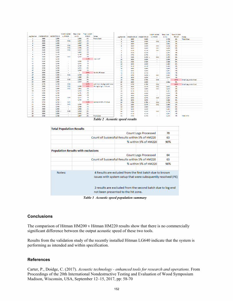
Table 2 Acoustic speed results

Table 3 Acoustic speed population summary

Conclusions

The comparison of Hitman HM200 v Hitman HM220 results show that there is no commercially significant difference between the output acoustic speed of these two tools.

Results from the validation study of the recently installed Hitman LG640 indicate that the system is performing as intended and within specification.

References

Carter, P., Doidge, C. (2017). Acoustic technology - enhanced tools for research and operations. From Proceedings of the 20th International Nondestructive Testing and Evaluation of Wood Symposium Madison, Wisconsin, USA, September 12–15, 2017, pp: 58-70

152

Modelling the Volume of Bark from Thickness Measurement Obtained by Swedish Gauge—Application to the Quantification of Extractives

Rodolphe Bauer Université de Lorraine, AgroParisTech, Inra, Silva, F-54000 Nancy, France, rodolphe.bauer@inra.fr Antoine Billard Université de Lorraine, AgroParisTech, Inra, Silva, F-54000 Nancy, France, antoine.billard@inra.fr Fleur Longuetaud Université de Lorraine, AgroParisTech, Inra, Silva, F-54000 Nancy, France, fleur.longuetaud@inra.fr Frédéric Mothe Université de Lorraine, AgroParisTech, Inra, Silva, F-54000 Nancy, France, frederic.mothe@inra.fr Francis Colin Université de Lorraine, AgroParisTech, Inra, Silva, F-54000 Nancy, France, francis.colin@inra.fr

Abstract

Today, climate change, scarcity of fossil fuels and new regulations (as the European REACH regulation) lead chemical industry to find new resources in order to make its conversion toward green chemistry. Use of forest resources makes this conversion possible. Indeed, in addition to the ligno-cellulosic material, wood contains molecules, called extractives. These molecules, of little size compared to the wood polymers, lignin and cellulose, are easy to recover and can be used as a feedstock for the fine chemistry, for example pharmaceutics or cosmetics. In order to assess the feasibility of installing regional extraction plants, the quantity of available extractives must be first estimated. This study, aims to estimate the volume of bark in Pseudotsuga menziesii, Picea abies et Abies alba, and combine it subsequently with density and concentration in extractives. Several French bark databases have been merged including a total of 12 000 trees measured. Both stem diameter were measured regularly all along the stem. A modelling approach is presented to predict bark volume from tree measurements, like DBH or tree height. This model is applied to the forests of North-Eastern France measured by the National Forest Inventory service (IGN). A first estimation of the resource of bark extractives is delivered from our bark volume estimates, density values and extractives concentrations.

Keywords: volume, bark, extractives, modeling, X-ray scanner

Introduction

Modelling tree volume is at the base of research approaches in the fields of forest and wood sciences. Indeed, the ability to know precisely the quantity of wood within each tree component (bark, knot, branch), directly from external tree measurement, like Diameter at Breast Height (DBH) or total Height (H) of the tree, allows forest manager to predict how much wood he is able to provide for several types of demand. In order to achieve this purpose, two ways of modelling have been explored. First, several studies developed models that allows to know directly the volume of the stem without bark from these external measurements (Dhôte et al 2000, Jenkins et al 2003). The advantage of this method is that it directly predict the volume of wood saleable without intermediary calculations; but, in the other hand, it is not very useful to describe the other compartment of the tree (like bark). The second approach to predict stem volume is to develop a model of bark volume and associate it with a model of stem volume with bark. Several studies follows this path and produce different models (

153

Meyer (1946), Loetsh et al (1973),Gordon (1983),Stängle et al (2017)), predicting either bark thickness at different heights or directly bark volume.

It turns out that, bark very rich in extractives (Trivelata et al (2016)). Extractives are molecules which can be extract by organic solvents or water from wood. They are naturally produced by the tree in order to defend himself against outdoor aggression, like bacteria, fungus or parasite (Theander O. (1985)). These molecules can become a new source for green chemistry in pharmaceutical and medicinal industry (Andersson (1955)), replacing with a serious ecological advantage, the use of petroleum-base products. This is the context of the project ExtraFor_Est in which this work takes place. The final purpose of this project is to predict the quantity of these molecules available in the forest resources of North-East of France. And in order to achieve this goal, knowing the volume of tree component containing a lot of these molecules is an essential work, along with the density and the extractives concentration of these parts.

In order to measure bark thickness alongside the tree trunk, the most common measurement method used is the Swedish bark gauge (Meyer (1946), Gordon (1983)) even if its accuracy have already been discussed (Stängle et al (2016)). With the progress of engineering it is possible today to pass sample in a X-ray scanner and so obtain more precise data (Stängle et al (2017))

Finally this studies has three purposes: 1. Deliver a model in order to describe more precisely the internal structure of stem, 2. allow a faithful estimation of extractives resources and 3. determine the statistical difference between X-ray measurement and bark gauge measurements. The studies deals weight five species: Silver fir (Abies alba), Norway spruce (Picea abies), Douglas fir (Pseudotsuga menziesii), Beech (Fagus sylvatica) and Oak (Quercus petraea et Quercus robur).

Materiel and method

Database

Different databases have been used to provide enough measurements. All databases include bark thickness measurements obtained at different heights along the stem (including 1.3m) and tree measurement. Several methods for measuring bark thickness were used. Table 1 summarises all these sources.

Table 1: Data summary

Database Species Data subset Number of data Number of trees Measurement method

Emerge

Fir CTFT 17 262 751 Swedish bark gauge INRA 3 959 173 Debarking Total 2 1221 924

Spruce

CTFT 20 536 836 Swedish bark gauge FCBA 1 198 155 INRA 924 41 Debarking Total 22 658 1032

Douglas Fir

CTFT 2 080 81 Swedish bark gauge FCBA 2 553 233 INRA 298 21 Debarking Total 4 931 375

154

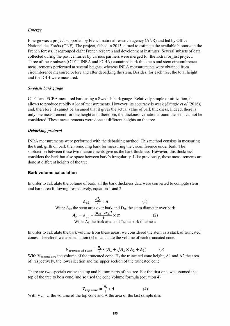
Emerge

Emerge was a project supported by French national research agency (ANR) and led by Office National des Forêts (ONF). The project, fished in 2013, aimed to estimate the available biomass in the French forests. It regrouped eight French research and development institutes. Several subsets of data collected during the past centuries by various partners were merged for the ExtraFor_Est project. Three of these subsets (CTFT, INRA and FCBA) contained bark thickness and stem circumference measurements performed at several heights, whereas INRA measurements were obtained from circumference measured before and after debarking the stem. Besides, for each tree, the total height and the DBH were measured.

Swedish bark gauge

CTFT and FCBA measured bark using a Swedish bark gauge. Relatively simple of utilization, it allows to produce rapidly a lot of measurements. However, its accuracy is weak (Stängle et al (2016)) and, therefore, it cannot be assumed that it gives the actual value of bark thickness. Indeed, there is only one measurement for one height and, therefore, the thickness variation around the stem cannot be considered. These measurements were done at different heights on the tree.

Debarking protocol

INRA measurements were performed with the debarking method. This method consists in measuring the trunk girth on bark then removing bark for measuring the circumference under bark. The subtraction between these two measurements give us the bark thickness. However, this thickness considers the bark but also space between bark’s irregularity. Like previously, these measurements are done at different heights of the tree.

Bark volume calculation

In order to calculate the volume of bark, all the bark thickness data were converted to compute stem and bark area following, respectively, equation 1 and 2.

𝑨𝑨𝒐𝒐𝒐𝒐 = 𝑫𝑫𝒐𝒐𝒐𝒐𝟐𝟐

𝟒𝟒× 𝝅𝝅 (1)

With: Aob the stem area over bark and Dob the stem diameter over bark

𝑨𝑨𝑏𝑏 = 𝐴𝐴𝑜𝑜𝑏𝑏 −(𝑫𝑫𝑜𝑜𝑜𝑜−𝟐𝟐𝑇𝑇𝒐𝒐)𝟐𝟐

𝟒𝟒× 𝝅𝝅 (2)

With: Ab the bark area and Tb the bark thickness

In order to calculate the bark volume from these areas, we considered the stem as a stack of truncated cones. Therefore, we used equation (3) to calculate the volume of each truncated cone.

𝑽𝑽𝒕𝒕𝒕𝒕𝒕𝒕𝒕𝒕𝒕𝒕𝒕𝒕𝒕𝒕𝒕𝒕𝒕𝒕 𝒕𝒕𝒐𝒐𝒕𝒕𝒕𝒕 = 𝑯𝑯𝒕𝒕𝟑𝟑∗ (𝑨𝑨𝟏𝟏 + 𝑨𝑨𝟏𝟏 × 𝑨𝑨𝟐𝟐 + 𝑨𝑨𝟐𝟐) (3)

With Vtruncated cone the volume of the truncated cone, Hc the truncated cone height, A1 and A2 the area of, respectively, the lower section and the upper section of the truncated cone.

There are two specials cases: the top and bottom parts of the tree. For the first one, we assumed the top of the tree to be a cone, and so used the cone volume formula (equation 4)

𝑽𝑽𝒕𝒕𝒐𝒐𝒕𝒕 𝒕𝒕𝒐𝒐𝒕𝒕𝒕𝒕 = 𝑯𝑯𝒕𝒕𝟑𝟑∗ 𝑨𝑨 (4)

With Vtop cone the volume of the top cone and A the area of the last sample disc

155

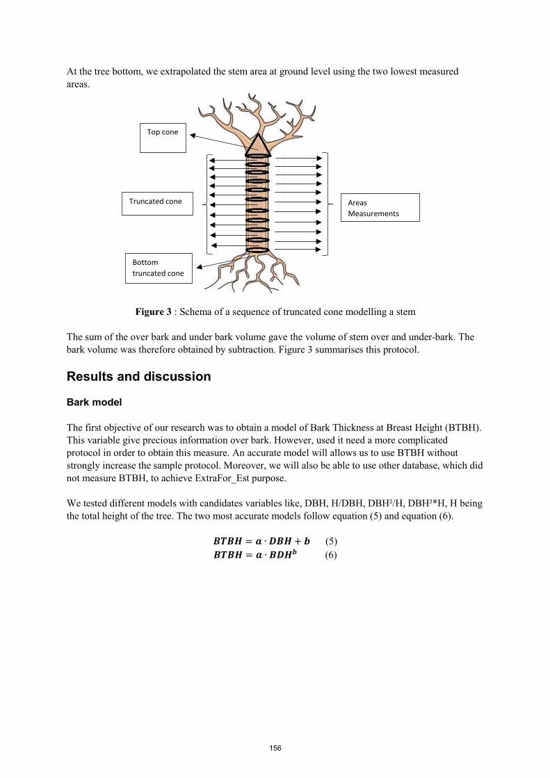
At the tree bottom, we extrapolated the stem area at ground level using the two lowest measured areas.

Figure 3 : Schema of a sequence of truncated cone modelling a stem

The sum of the over bark and under bark volume gave the volume of stem over and under-bark. The bark volume was therefore obtained by subtraction. Figure 3 summarises this protocol.

Results and discussion

Bark model

The first objective of our research was to obtain a model of Bark Thickness at Breast Height (BTBH). This variable give precious information over bark. However, used it need a more complicated protocol in order to obtain this measure. An accurate model will allows us to use BTBH without strongly increase the sample protocol. Moreover, we will also be able to use other database, which did not measure BTBH, to achieve ExtraFor_Est purpose.

We tested different models with candidates variables like, DBH, H/DBH, DBH²/H, DBH²*H, H being the total height of the tree. The two most accurate models follow equation (5) and equation (6).

𝑩𝑩𝑩𝑩𝑩𝑩𝑯𝑯 = 𝒕𝒕 ∙ 𝑫𝑫𝑩𝑩𝑯𝑯+ 𝒐𝒐 (5) 𝑩𝑩𝑩𝑩𝑩𝑩𝑯𝑯 = 𝒕𝒕 ∙ 𝑩𝑩𝑫𝑫𝑯𝑯𝒐𝒐 (6)

Areas Measurements

Truncated cone

Top cone

Bottom truncated cone

156

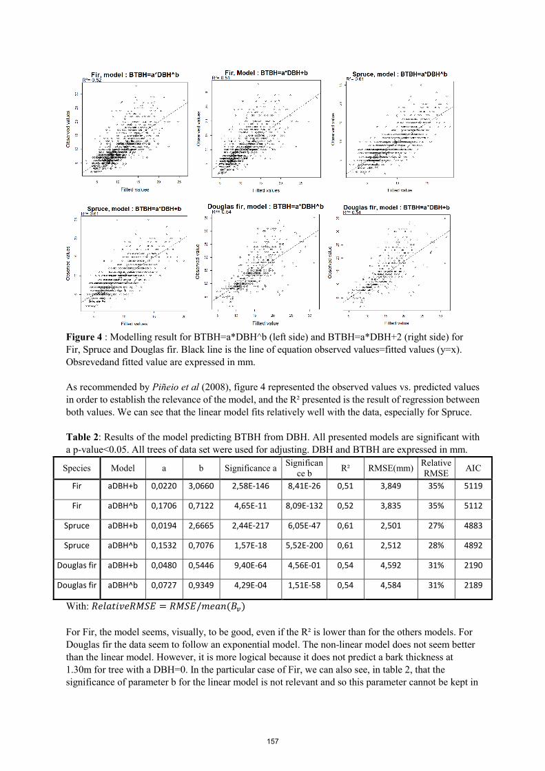
Figure 4 : Modelling result for BTBH=a*DBH^b (left side) and BTBH=a*DBH+2 (right side) for Fir, Spruce and Douglas fir. Black line is the line of equation observed values=fitted values (y=x). Obsrevedand fitted value are expressed in mm.

As recommended by Piñeio et al (2008), figure 4 represented the observed values vs. predicted values in order to establish the relevance of the model, and the R² presented is the result of regression between both values. We can see that the linear model fits relatively well with the data, especially for Spruce.

Table 2: Results of the model predicting BTBH from DBH. All presented models are significant with a p-value<0.05. All trees of data set were used for adjusting. DBH and BTBH are expressed in mm.

Species Model a b Significance a Significance b R² RMSE(mm) Relative

RMSE AIC

Fir aDBH+b 0,0220 3,0660 2,58E-146 8,41E-26 0,51 3,849 35% 5119

Fir aDBH^b 0,1706 0,7122 4,65E-11 8,09E-132 0,52 3,835 35% 5112

Spruce aDBH+b 0,0194 2,6665 2,44E-217 6,05E-47 0,61 2,501 27% 4883

Spruce aDBH^b 0,1532 0,7076 1,57E-18 5,52E-200 0,61 2,512 28% 4892

Douglas fir aDBH+b 0,0480 0,5446 9,40E-64 4,56E-01 0,54 4,592 31% 2190

Douglas fir aDBH^b 0,0727 0,9349 4,29E-04 1,51E-58 0,54 4,584 31% 2189

With: 𝑅𝑅𝑅𝑅𝑅𝑅𝑅𝑅𝑅𝑅𝑅𝑅𝑅𝑅𝑅𝑅𝑅𝑅𝑅𝑅𝑅𝑅𝑅𝑅 = 𝑅𝑅𝑅𝑅𝑅𝑅𝑅𝑅/𝑚𝑚𝑅𝑅𝑅𝑅𝑚𝑚(𝐵𝐵𝑣𝑣)

For Fir, the model seems, visually, to be good, even if the R² is lower than for the others models. For Douglas fir the data seem to follow an exponential model. The non-linear model does not seem better than the linear model. However, it is more logical because it does not predict a bark thickness at 1.30m for tree with a DBH=0. In the particular case of Fir, we can also see, in table 2, that the significance of parameter b for the linear model is not relevant and so this parameter cannot be kept in

157

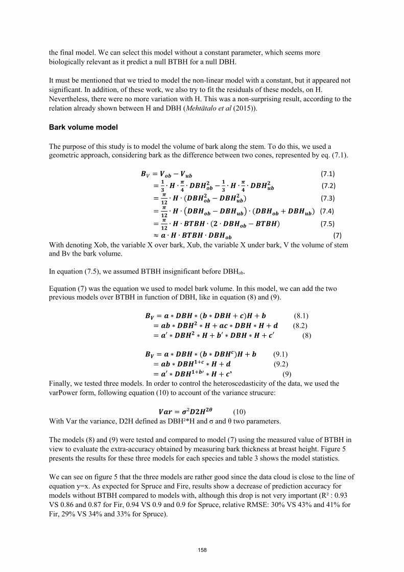
the final model. We can select this model without a constant parameter, which seems more biologically relevant as it predict a null BTBH for a null DBH.

It must be mentioned that we tried to model the non-linear model with a constant, but it appeared not significant. In addition, of these work, we also try to fit the residuals of these models, on H. Nevertheless, there were no more variation with H. This was a non-surprising result, according to the relation already shown between H and DBH (Mehtätalo et al (2015)).

Bark volume model

The purpose of this study is to model the volume of bark along the stem. To do this, we used a geometric approach, considering bark as the difference between two cones, represented by eq. (7.1).

𝑩𝑩𝑉𝑉 = 𝑽𝑽𝒐𝒐𝒐𝒐 − 𝑽𝑽𝒕𝒕𝒐𝒐 (7.1)

= 𝟏𝟏𝟑𝟑∙ 𝑯𝑯 ∙ 𝝅𝝅

𝟒𝟒∙ 𝑫𝑫𝑩𝑩𝑯𝑯𝒐𝒐𝒐𝒐

𝟐𝟐 − 𝟏𝟏𝟑𝟑∙ 𝑯𝑯 ∙ 𝝅𝝅

𝟒𝟒∙ 𝑫𝑫𝑩𝑩𝑯𝑯𝒕𝒕𝒐𝒐

𝟐𝟐 (7.2)

= 𝝅𝝅𝟏𝟏𝟐𝟐∙ 𝑯𝑯 ∙ (𝑫𝑫𝑩𝑩𝑯𝑯𝒐𝒐𝒐𝒐

𝟐𝟐 − 𝑫𝑫𝑩𝑩𝑯𝑯𝒕𝒕𝒐𝒐𝟐𝟐 ) (7.3)

= 𝝅𝝅𝟏𝟏𝟐𝟐∙ 𝑯𝑯 ∙ 𝑫𝑫𝑩𝑩𝑯𝑯𝒐𝒐𝒐𝒐 − 𝑫𝑫𝑩𝑩𝑯𝑯𝒕𝒕𝒐𝒐 ∙ (𝑫𝑫𝑩𝑩𝑯𝑯𝒐𝒐𝒐𝒐 + 𝑫𝑫𝑩𝑩𝑯𝑯𝒕𝒕𝒐𝒐) (7.4)

= 𝝅𝝅𝟏𝟏𝟐𝟐∙ 𝑯𝑯 ∙ 𝑩𝑩𝑩𝑩𝑩𝑩𝑯𝑯 ∙ (𝟐𝟐 ∙ 𝑫𝑫𝑩𝑩𝑯𝑯𝒐𝒐𝒐𝒐 − 𝑩𝑩𝑩𝑩𝑩𝑩𝑯𝑯) (7.5)

≈ 𝒕𝒕 ∙ 𝑯𝑯 ∙ 𝑩𝑩𝑩𝑩𝑩𝑩𝑯𝑯 ∙ 𝑫𝑫𝑩𝑩𝑯𝑯𝒐𝒐𝒐𝒐 (7) With denoting Xob, the variable X over bark, Xub, the variable X under bark, V the volume of stem and Bv the bark volume.

In equation (7.5), we assumed BTBH insignificant before DBHob.

Equation (7) was the equation we used to model bark volume. In this model, we can add the two previous models over BTBH in function of DBH, like in equation (8) and (9).

𝑩𝑩𝑽𝑽 = 𝒕𝒕 ∗ 𝑫𝑫𝑩𝑩𝑯𝑯 ∗ (𝒐𝒐 ∗ 𝑫𝑫𝑩𝑩𝑯𝑯+ 𝒕𝒕)𝑯𝑯 + 𝒐𝒐 (8.1) = 𝒕𝒕𝒐𝒐 ∗ 𝑫𝑫𝑩𝑩𝑯𝑯𝟐𝟐 ∗ 𝑯𝑯 + 𝒕𝒕𝒕𝒕 ∗ 𝑫𝑫𝑩𝑩𝑯𝑯 ∗ 𝑯𝑯 + 𝒕𝒕 (8.2) = 𝒕𝒕′ ∗ 𝑫𝑫𝑩𝑩𝑯𝑯𝟐𝟐 ∗ 𝑯𝑯 + 𝒐𝒐′ ∗ 𝑫𝑫𝑩𝑩𝑯𝑯 ∗ 𝑯𝑯 + 𝒕𝒕′ (8)

𝑩𝑩𝑽𝑽 = 𝒕𝒕 ∗ 𝑫𝑫𝑩𝑩𝑯𝑯 ∗ (𝒐𝒐 ∗ 𝑫𝑫𝑩𝑩𝑯𝑯𝒕𝒕)𝑯𝑯+ 𝒐𝒐 (9.1) = 𝒕𝒕𝒐𝒐 ∗ 𝑫𝑫𝑩𝑩𝑯𝑯𝟏𝟏+𝒕𝒕 ∗ 𝑯𝑯 + 𝒕𝒕 (9.2) = 𝒕𝒕′ ∗ 𝑫𝑫𝑩𝑩𝑯𝑯𝟏𝟏+𝒐𝒐′ ∗ 𝑯𝑯 + 𝒕𝒕’ (9)

Finally, we tested three models. In order to control the heteroscedasticity of the data, we used the varPower form, following equation (10) to account of the variance strucure:

𝑽𝑽𝒕𝒕𝒕𝒕 = 𝝈𝝈²𝑫𝑫𝟐𝟐𝑯𝑯𝟐𝟐𝟐𝟐 (10) With Var the variance, D2H defined as DBH²*H and σ and θ two parameters.

The models (8) and (9) were tested and compared to model (7) using the measured value of BTBH in view to evaluate the extra-accuracy obtained by measuring bark thickness at breast height. Figure 5 presents the results for these three models for each species and table 3 shows the model statistics.

We can see on figure 5 that the three models are rather good since the data cloud is close to the line of equation y=x. As expected for Spruce and Fire, results show a decrease of prediction accuracy for models without BTBH compared to models with, although this drop is not very important (R² : 0.93 VS 0.86 and 0.87 for Fir, 0.94 VS 0.9 and 0.9 for Spruce, relative RMSE: 30% VS 43% and 41% for Fir, 29% VS 34% and 33% for Spruce).

158

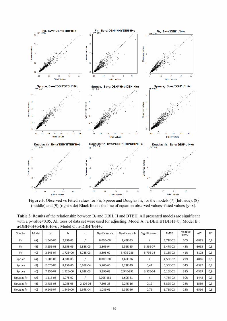
Figure 5: Observed vs Fitted values for Fir, Spruce and Douglas fir, for the models (7) (left side), (8) (middle) and (9) (right side) Black line is the line of equation observed values=fitted values (y=x).

Table 3: Results of the relationship between Bv and DBH, H and BTBH. All presented models are significant with a p-value<0.05. All trees of data set were used for adjusting. Model A : a∙DBH∙BTBH∙H+b ; Model B : a∙DBH²∙H+b∙DBH∙H+c ; Model C : a∙DBH^b∙H+c

Species Model a b c Significancea Significance b Significance c RMSE Relative RMSE AIC R²

Fir (A) 1,64E-06 2,99E-03 / 0,00E+00 2,43E-33 / 6,71E-02 30% -3825 0,9

Fir (B) 3,65E-08 5,15E-06 2,83E-03 2,86E-94 5,51E-15 3,56E-07 9,47E-02 43% -3093 0,9

Fir (C) 2,64E-07 1,72E+00 3,73E-03 3,89E-07 5,47E-286 5,79E-14 9,15E-02 41% -3102 0,9

Spruce (A) 1,50E-06 4,88E-03 / 0,00E+00 1,65E-36 / 4,58E-02 29% -4816 0,9

Spruce (B) 2,07E-08 8,15E-06 5,68E-04 5,70E-66 1,21E-49 0,44 5,30E-02 34% -4327 0,9

Spruce (C) 7,35E-07 1,52E+00 2,62E-03 3,39E-08 7,94E-291 3,37E-04 5,16E-02 33% -4319 0,9

Douglas fir (A) 1,11E-06 1,27E-02 / 2,09E-181 1,60E-31 / 4,76E-02 30% -1448 0,9

Douglas fir (B) 3,48E-08 1,05E-05 -2,10E-03 7,60E-23 2,24E-16 0,19 3,82E-02 24% -1559 0,9

Douglas fir (C) 9,64E-07 1,54E+00 5,64E-04 1,08E-03 1,35E-96 0,71 3,71E-02 23% -1566 0,9

159

However, for Douglas fir results are unexpected. Indeed, for R², AIC, RMSE and relative RMSE the models (B) and (C) that do not require BTBH are even better than model (A) using the measured value for BTBH. We can explain this considering the roughness of Douglas fir’s bark at breast height. This property can introduce a high variability between measures from the same tree. A single measurement is thus probably not very representative of the mean BTBH.

It can be seen also that the constant parameter (c) is not significant (p-value superior of 0.05) for three models (third models for Spruce and second and third ones for Douglas fir). It make sense from a biological point of view since it predicts a null bark volume for a null DBH. In addition, with the results presented in table 2, we can compare both models for predicting BTBH. The accuracy is not very different between the two models and for each species. Finally models (C) seem the more suitable for predicting bark volume for the three species

Conclusion and perspectives

In this study we tested several models in order to predict bark thickness at breast height BTBH and and bark volume Bv. The models predicting BTBH are quite good even if modelling estimators (especially R²) could be improved. The models predicting Bv, on the other hand, fits strikingly good with the data measured with or without the use of BTBH. These models can thus bring more knowledge on bark of these species. However, the work is not finished yet. The models have to be validated using a cross-validation procedure or using an independent dataser. At least, these results are very encouraging and can lead us to very interesting models.

Acknowledgement

SILVA laboratory is supported by a grant overseen by the French National Research Agency (ANR) as part of the “Investissements d’Avenir” program (ANR-11-LABX-0002-01, Lab of Excellence ARBRE).This work could not have been done without the support of the different office that provide the dataset. We will so thanks Alain Bouvet from the FCBA and Christine Deleuze from the ONF who help us to deals with the different origin of data. We also like to thanks Pierre Montpied, Philippe Saintenoise and Jean-Baptiste Pichancourt for their help in managing the heteroscedasticy of the measurements. Also we will thank Adam Schnitzer who worked on bark area and volume measurement.

References

Anderson, A. B. 1955. Recovery and utilization of tree extractives. Economic Botany, 9(2), 108.

Gordon, A. 1983 Estimating bark thickness of Pinus radiata. New Zeal. J. For. Sci 13, 340–348.

Loetsch, F., Zöhrer, F. and Haller, K.E. 1973 Forest Inventory Vol. II. BLV Verl. Ges, 436.

Meyer A. 1946. Bark volume Determination in Tree. Journal Forestry 1067-1070

Piñeiro, G., Perelman, S., Guerschman, J. P., & Paruelo, J. M. 2008. How to evaluate models: observed vs. predicted or predicted vs. observed ?. Ecological Modelling, 216(3-4), 316-322.

Stängle S,Weiskittel A,Dormann C, Brüchert F. 2016 : Measurement and prediction of bark thickness in Picea abies: assessment of accuracy, precision, and sample size requirements Can. J. For. Res . 46: 39–47

160

Stängle S, Dormann C. 2017 : Modelling the variation of bark thickness within and between European silver fir (Abies alba Mill.) trees in southwest Germany. Forestry 2017; 00, 1–12, Theander, O. 1985. Cellulose, hemicellulose and extractives. Fundamentals of thermochemical biomass conversion 35-60. Trivelato, P., Mayer, C., Barakat, A., Fulcrand, H., & Aouf, C. 2016. Douglas bark dry fractionation for polyphenols isolation: From forestry waste to added value products. Industrial Crops and Products, 86, 12-15.

161

Nondestructive Technique to Infer Wood Density in Trees*Mônica RuyLaboratory of Nondestructive Testing - LabEND, College of Agricultural Engineering - FEAGRI - University of Campinas - UNICAMP, Campinas, São Paulo, Brazil, monica.ruy@hotmail.com.

Raquel Gonçalves LabEND - Feagri,Unicamp, Campinas, São Paulo, Brazil, raquelg@g.unicamp.br

Roberto Diego Martinez Lopes Departamento de Construcciones Arquitectónicas, Ingeniería del Terreno y Mecánica de los Medios continuos y Teoría de Estructuras, E.T.S. de Arquitectura - Universidad de Valladolid, Valladolid, Spain, robertodmartinezlopez@gmail.com

Cinthya Bertoldo Pedroso LabEND - Feagri,Unicamp, Campinas, São Paulo, Brazil, cinthyab@unicamp.br

Rafael Gustavo Mansini Lorensani LabEND - Feagri,Unicamp, Campinas, São Paulo, Brazil, rafaelmansini@hotmail.com

Rafaela Marina Leite LabEND - Feagri,Unicamp, Campinas, São Paulo, Brazil, rafaelamleite@gmail.com

Abstract

Knowledge of wood properties, obtained directly from trees, is extremely important for forest industry and inspection of urban forest. Among these properties, density stands out for having correlation with different other material properties. Nondestructive testing is increasingly used by forest industry to anticipate the inference of wood properties without the need of cutting trees. Increment borers are generally used to extract specimens directly from trees to determine wood density. Recently, a new nondestructive method to estimate wood density was developed, the Wood Extractor (WoodEx). It had obtained accurate result for dry wood. This new method consists in extracting a specimen (wood chip) through a commercial drilling machine, knowing volume extracted. The weight of the material extract allows obtain apparent density of the wood. The problem in green wood is the loss of the material that get stuck in the drill bit affecting the accuracy of the results. Thus, the aim of this study was to compare wood density obtained by samples extracted directly from trees by increment borer and by WoodEx. We collected specimens, by both methods, from Brazilian urban trees and we used the samples to determine the average of basic density for each species. Results from WoodEx sample were compared to those obtained from the increment borer sample. Although there was a significant loss of material during the use of WoodEx, it was possible to obtain a correction factor. Applying this factor, we got density values for WoodEx sample statiscally equivalent to the density obtained from increment borer sample.

Keywords: wood extractor, increment borers, density.

162

Introduction

Non-destructive testing has been used as a quality control tool in forest industry and in urban forest. These techniques are used to infer physical and mechanical properties of the tree wood. The density (ρ) is one of the most important properties for forest industries, as pulp and paper, and also for obtain the stiffness coefficient (Cii) by nondestructive techniques using velocity of wave propagation (Cii = ρVii2). According to Padua (2009) wood density is an important qualitative parameter for different uses, because it is correlated with a lot of other wood properties.

It is possible to determine the wood density in alive trees using samples provides by increment borers. According to Downes et al. (1997), apud Padua (2009), the determination of density using a single disk from trees, procedure usually used by forest industry, consumes much more money and time than the increment borer technique. Increment borer is the most commonly used manual tree sample extractor tool (Martinez, 2018). The equipment extracts a cylindrical sample of the tree, with diameter approximately 5mm. However, the author emphasizes that it is an invasive technique and leaves holes in the wood, which may represent entry points of moisture and insects (Martinez, 2018).

Martinez et al 2015 developed a device (WoodEx) to be coupled to a commercial drill that collects the wood chips extracted during drilling. The extracts volume is known, because the diameter and length of the drill used is also know (Martínez et al, 2015). During drilling, the wood chips is collected in tea bags and then used for density calculation.

Martínez (2018) used WoodEx equipment to estimate the density of dry wood from 10 different species. The author found a statistically significant association and high coefficient of correlation (R² = 97.74%) between this density (With WoodEx) and the density obtained using traditional prismatic sample. In the same study, Martinez (2018) found R² = 98.08% correlating the traditional test specimens with samples taken by the increment borer.

Considering the mentioned aspects, this research aimed to compare the density results obtained by WoodEx equipment with those obtained by increment borer (already used for this purpose), both applied directly to alive urban trees.

Material and Methods

We used 18 specimens obtained from 4 different species used in urban areas in Brazil (Table 1).

Table 1— Sample descripción Specie Number of specimens

Parapiptadenia zehntneri 1

Lafoensia glyptocarpa 2

Caesalpinia peltophoroides 6

Leucaena leucocephala 9

TOTAL 18

From each tree we collected specimens with increment borer (Figure 1 a) and with WoodEx (Figure 1 b). To calculate the density of each specimen it was necessary to measure the dimensions of all increment borer´s specimens (Figura 2a). By the diameter and the length of the drill used on WoodEX (Figure 1 c) it was possible to calculate the volume of its sample. The weight of all specimen was measured. In the case of

163

the WoodEx the material was collected in tea bags (Figure 2b), whose are weighed before use (reference weigh) and after drilling and its difference was considered the weight of the wood chips.

(a) (b) (c)

Figure 1—a. Increment borer and b. WoodEX. c. drill used on WoodEx sample extraction.

(a) (b) Figure 2— Specimen obtained by a. Increment borer and b. WoodEX

All specimens, from increment borer and WoodEx, were dryed according to NBR 7190/1997. The samples were kept in an oven until reaching a constant mass. The data collected were used to calculate the specimens basic density.

Statistical analyzes were carried out in order to compare the results obtained by the two methods. The result of the statistical analysis was used to evaluate the efficiency of WoodEx in determining the density of the wood obtained direct from urban trees.

Results and discussions

The normality of the data was analyzed before performing the statistical comparison of the results obtained through the two methods (Table 2). For analyzed the hypothesis of data normality we use the skewness and kurtosis for density values of each specie. Values between -2 to +2 indicating that normality hypothesis can be accepted.

164

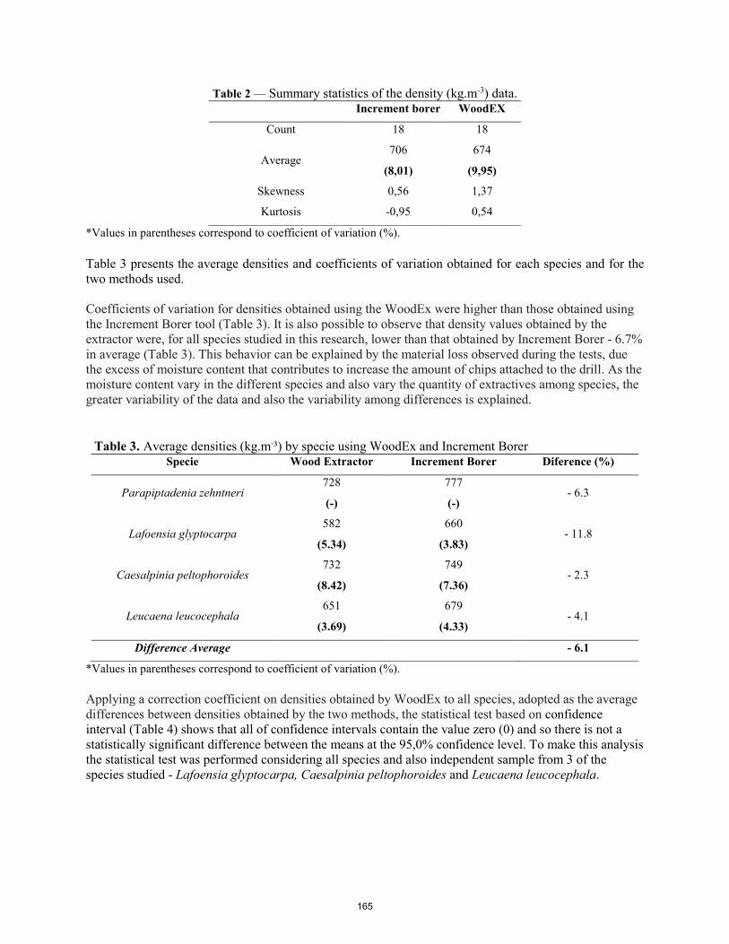
Table 2 — Summary statistics of the density (kg.m-3) data. Increment borer WoodEX

Count 18 18

Average 706 674

(8,01) (9,95)

Skewness 0,56 1,37

Kurtosis -0,95 0,54

*Values in parentheses correspond to coefficient of variation (%).

Table 3 presents the average densities and coefficients of variation obtained for each species and for the two methods used.

Coefficients of variation for densities obtained using the WoodEx were higher than those obtained using the Increment Borer tool (Table 3). It is also possible to observe that density values obtained by the extractor were, for all species studied in this research, lower than that obtained by Increment Borer - 6.7% in average (Table 3). This behavior can be explained by the material loss observed during the tests, due the excess of moisture content that contributes to increase the amount of chips attached to the drill. As the moisture content vary in the different species and also vary the quantity of extractives among species, the greater variability of the data and also the variability among differences is explained.

Table 3. Average densities (kg.m-³) by specie using WoodEx and Increment Borer Specie Wood Extractor Increment Borer Diference (%)

Parapiptadenia zehntneri 728

(-)

777

(-) - 6.3

Lafoensia glyptocarpa 582

(5.34)

660

(3.83) - 11.8

Caesalpinia peltophoroides 732

(8.42)

749

(7.36) - 2.3

Leucaena leucocephala 651

(3.69)

679

(4.33) - 4.1

Difference Average - 6.1

*Values in parentheses correspond to coefficient of variation (%).

Applying a correction coefficient on densities obtained by WoodEx to all species, adopted as the average differences between densities obtained by the two methods, the statistical test based on confidence interval (Table 4) shows that all of confidence intervals contain the value zero (0) and so there is not a statistically significant difference between the means at the 95,0% confidence level. To make this analysis the statistical test was performed considering all species and also independent sample from 3 of the species studied - Lafoensia glyptocarpa, Caesalpinia peltophoroides and Leucaena leucocephala.

165

Table 4. Confidence Intervals obtained comparing densities from samples using WoodEx and Increment Borer.

Specie Intervalo de Confiança

All species [-47,8688; 41,2382]

Lafoensia glyptocarpa [-76,5962; 174,716]

Caesalpinia peltophoroides [-31,7389; 23,1233]

Leucaena leucocephala [-109,195; 70,6246]

Despite of the material loss during the Wood Extractor use, the results obtained in this research indicate that this tool shows feasibility to be used as an alternative to the traditional methods for obtaining the density of both dry wood (Martinez, 2018) and green wood.

Conclusions

There is a material loss during the specimen extraction using WoodEx. As a consequence, the density is, in average, 6% smaller than density values obtained using the increment borer.

Although the differences vary among species, the application of a 6% increase coefficient on density values obtained with WoodEx allows obtain, for each specie individually analyzed and for one group composed by all species, density values statistically equivalent to the ones obtained with increment borer.

This was a preliminary study. It is necessary to increase the number of species to obtain conclusive results.

Acknowledgments

We thank the “Coordination of Improvement of Higher Level Personnel” (CAPES) for the undergraduate research scholarship and the Research and Extension Support Fund (FAEPEX/UNICAMP) for the Visitant Professor grant.

References Downes, g. M.; hudson, i. L. Raymond, c. A.; dean, g. H.; michell, a. J.; schimleck, r.; evans, r.; muneri, e. Sampling plantation eucalypts for wood and fiber properties. Melbourne: csrio, 1997. 126 p.

Martínez, r.; arriaga, f.; llana, d. F.; gallego, j.; bobadilla, i. Ndt to identify biological damage in wood. In: 19th international nondestructive testing and evaluation of wood symposium, 2015, rio de janeiro, brasil.

Martínez, r. D. L. Métodos no destructivos de estimación de la densidad de la madera. 2018. Tese (doutorado) – universidade de santiago de compostel, madri.

Pádua, f. A. Amostragem para avaliação da densidade básica da madeira de um híbrido de eucalyptus grandis w. Hill ex maiden x eucalyptus urophylla s.t. blake. 2009. 99 f. Tese pós-doutorado – universidade federal lavras.

166

Session 3

Timbers and Lumber

167

Acoustic Emission Analysis and Synchrotron-Based Microtomography on Glued Shear Strength Samples from Spruce Solid Wood

Peter Niemz * Eidgenössische Technische Hochschule Zürich, Institut für Baustoffe, Zurich, Switzerland, niemzp@ethz.ch; Berner Fachhochschule, Architektur, Bau und Holz, Institut für Holzwerkstoffe und Holz, Biel, Switzerland Czech University of Live Sciences, Faculty of Forestry and Wood Sciences, Prague, Czech Republic Franziska Baensch Bundesanstalt für Materialforschung und -Prüfung, Berlin, Germany, franziska.baensch@bam.de Andreas J. Brunner Eidgenössische Materialprüfungs-und Forschungsanstalt, Dübendorf, Switzerland Andreas.Brunner@empa.ch Milan Gaff Czech University of Live Sciences, Prague, Faculty of Forestry and Wood Sciences, Czech Republic gaffmilan@gmail.com

* Corresponding author

Abstract

For a better understanding of the damage of glued wood tensile tests on miniature specimens made of glued spruce wood with acoustic emission and in-situ synchrotron-based X-ray computer microtomography has been monitored. As adhesive, urea-formaldehyde resin was used. For comparison purposes, tensile tests were carried out on solid wood and bonded miniature tensile shear samples with acoustic emission. The acoustic emission signals of all experiments were with classified pattern recognition. This resulted in two classes of signals for each two frequency peaks. In one class was the low-frequency, in the other the higher-frequency peak of higher intensity, but this essentially independent from the structure (solid wood or plywood) and the size scale of the test specimens. The influence of the adhesive layers was determined on plywood test specimens in laboratory scale and on miniature test specimens with an adhesive layer and selected fiber orientations examined. This gave evidence that the sound emission signals from the failure of the adhesive layer presumably of the class with low frequency signals peak in the range of services can be assigned.

Keywords: bondline, insitu test, acoustic emission, synchrotron tomography

168

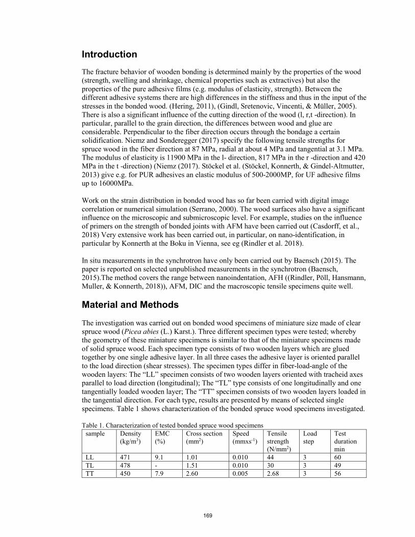
Introduction The fracture behavior of wooden bonding is determined mainly by the properties of the wood (strength, swelling and shrinkage, chemical properties such as extractives) but also the properties of the pure adhesive films (e.g. modulus of elasticity, strength). Between the different adhesive systems there are high differences in the stiffness and thus in the input of the stresses in the bonded wood. (Hering, 2011), (Gindl, Sretenovic, Vincenti, & Müller, 2005). There is also a significant influence of the cutting direction of the wood (l, r,t -direction). In particular, parallel to the grain direction, the differences between wood and glue are considerable. Perpendicular to the fiber direction occurs through the bondage a certain solidification. Niemz and Sonderegger (2017) specify the following tensile strengths for spruce wood in the fiber direction at 87 MPa, radial at about 4 MPa and tangential at 3.1 MPa. The modulus of elasticity is 11900 MPa in the l- direction, 817 MPa in the r -direction and 420 MPa in the t -direction) (Niemz (2017). Stöckel et al. (Stöckel, Konnerth, & Gindel-Altmutter, 2013) give e.g. for PUR adhesives an elastic modulus of 500-2000MP, for UF adhesive films up to 16000MPa.

Work on the strain distribution in bonded wood has so far been carried with digital image correlation or numerical simulation (Serrano, 2000). The wood surfaces also have a significant influence on the microscopic and submicroscopic level. For example, studies on the influence of primers on the strength of bonded joints with AFM have been carried out (Casdorff, et al., 2018) Very extensive work has been carried out, in particular, on nano-identification, in particular by Konnerth at the Boku in Vienna, see eg (Rindler et al. 2018).

In situ measurements in the synchrotron have only been carried out by Baensch (2015). The paper is reported on selected unpublished measurements in the synchrotron (Baensch, 2015).The method covers the range between nanoindentation, AFH ((Rindler, Pöll, Hansmann, Muller, & Konnerth, 2018)), AFM, DIC and the macroscopic tensile specimens quite well.

Material and Methods

The investigation was carried out on bonded wood specimens of miniature size made of clear spruce wood (Picea abies (L.) Karst.). Three different specimen types were tested; whereby the geometry of these miniature specimens is similar to that of the miniature specimens made of solid spruce wood. Each specimen type consists of two wooden layers which are glued together by one single adhesive layer. In all three cases the adhesive layer is oriented parallel to the load direction (shear stresses). The specimen types differ in fiber-load-angle of the wooden layers: The “LL” specimen consists of two wooden layers oriented with tracheid axes parallel to load direction (longitudinal); The “TL” type consists of one longitudinally and one tangentially loaded wooden layer; The “TT” specimen consists of two wooden layers loaded in the tangential direction. For each type, results are presented by means of selected single specimens. Table 1 shows characterization of the bonded spruce wood specimens investigated.

Table 1. Characterization of tested bonded spruce wood specimens sample Density

(kg/m3) EMC (%)

Cross section (mm2)

Speed (mmxs-1)

Tensile strength (N/mm2)

Load step

Test duration min

LL 471 9.1 1.01 0.010 44 3 60 TL 478 - 1.51 0.010 30 3 49 TT 450 7.9 2.60 0.005 2.68 3 56

169

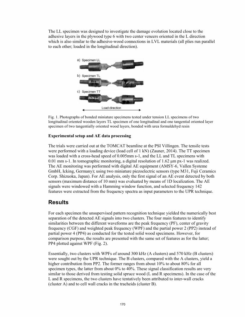
The LL specimen was designed to investigate the damage evolution located close to the adhesive layers in the plywood type 6 with two center veneers oriented in the L direction which is also similar to the adhesive-wood connections in LVL materials (all plies run parallel to each other; loaded in the longitudinal direction).

Fig. 1. Photographs of bonded miniature specimens tested under tension LL specimens of two longitudinal oriented wooden layers TL specimen of one longitudinal and one tangential oriented layer specimen of two tangentially oriented wood layers, bonded with urea formaldehyd resin

Experimental setup and AE data processing

The trials were carried out at the TOMCAT beamline at the PSI Villingen. The tensile tests were performed with a loading device (load cell of 1 kN) (Zauner, 2014). The TT specimen was loaded with a cross-head speed of 0.005mm s-1, and the LL and TL specimens with 0.01 mm s-1. In tomographic monitoring, a digital resolution of 1.62 μm px-1 was realized. The AE monitoring was performed with digital AE equipment (AMSY-6, Vallen Systeme GmbH, Icking, Germany); using two miniature piezoelectric sensors (type M31, Fuji Ceramics Corp. Shizuoka, Japan). For AE analysis, only the first signal of an AE event detected by both sensors (maximum distance of 10 mm) was evaluated by means of 1D localization. The AE signals were windowed with a Hamming window function, and selected frequency 142 features were extracted from the frequency spectra as input parameters to the UPR technique.

Results

For each specimen the unsupervised pattern recognition technique yielded the numerically best separation of the detected AE signals into two clusters. The four main features to identify similarities between the different waveforms are the peak frequency (PF), center of gravity frequency (CGF) and weighted peak frequency (WPF) and the partial power 2 (PP2) instead of partial power 4 (PP4) as conducted for the tested solid wood specimens. However, for comparison purpose, the results are presented with the same set of features as for the latter; PP4 plotted against WPF (Fig. 2).

Essentially, two clusters with WPFs of around 300 kHz (A clusters) and 570 kHz (B clusters) were sought out by the UPR technique. The B clusters, compared with the A clusters, yield a higher contribution from PP2. The former ranges from about 10% to about 80% for all specimen types, the latter from about 0% to 40%. These signal classification results are very similar to those derived from testing solid spruce wood (L and R specimens). In the case of the L and R specimens, the two clusters have tentatively been attributed to inter-wall cracks (cluster A) and to cell wall cracks in the tracheids (cluster B).

170

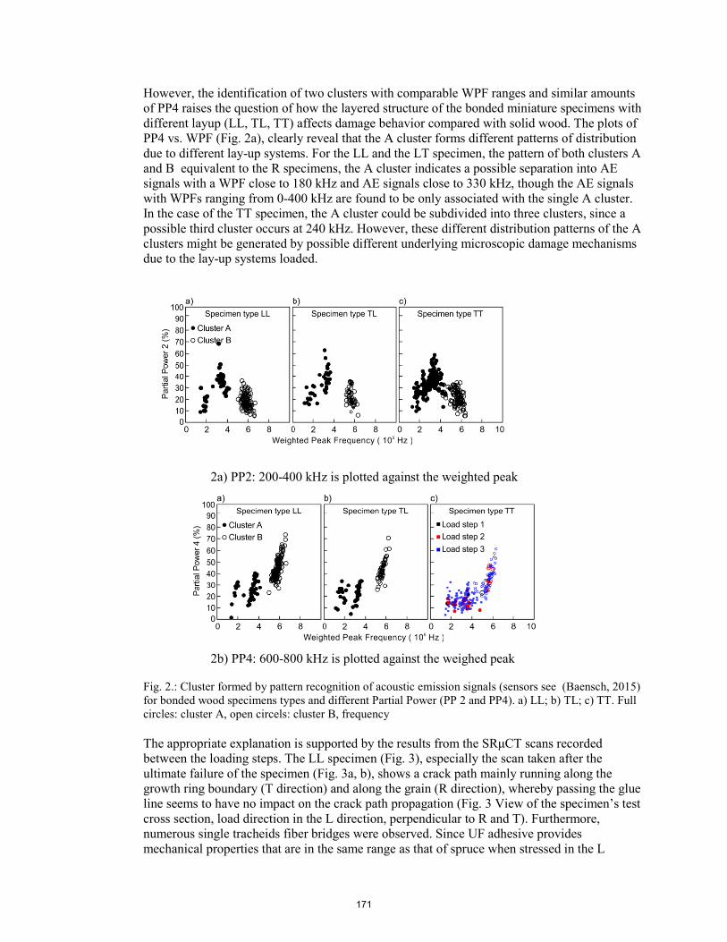
However, the identification of two clusters with comparable WPF ranges and similar amounts of PP4 raises the question of how the layered structure of the bonded miniature specimens with different layup (LL, TL, TT) affects damage behavior compared with solid wood. The plots of PP4 vs. WPF (Fig. 2a), clearly reveal that the A cluster forms different patterns of distribution due to different lay-up systems. For the LL and the LT specimen, the pattern of both clusters A and B equivalent to the R specimens, the A cluster indicates a possible separation into AE signals with a WPF close to 180 kHz and AE signals close to 330 kHz, though the AE signals with WPFs ranging from 0-400 kHz are found to be only associated with the single A cluster. In the case of the TT specimen, the A cluster could be subdivided into three clusters, since a possible third cluster occurs at 240 kHz. However, these different distribution patterns of the A clusters might be generated by possible different underlying microscopic damage mechanisms due to the lay-up systems loaded.

2a) PP2: 200-400 kHz is plotted against the weighted peak

2b) PP4: 600-800 kHz is plotted against the weighed peak

Fig. 2.: Cluster formed by pattern recognition of acoustic emission signals (sensors see (Baensch, 2015) for bonded wood specimens types and different Partial Power (PP 2 and PP4). a) LL; b) TL; c) TT. Full circles: cluster A, open circels: cluster B, frequency

The appropriate explanation is supported by the results from the SRμCT scans recorded between the loading steps. The LL specimen (Fig. 3), especially the scan taken after the ultimate failure of the specimen (Fig. 3a, b), shows a crack path mainly running along the growth ring boundary (T direction) and along the grain (R direction), whereby passing the glue line seems to have no impact on the crack path propagation (Fig. 3 View of the specimen’s test cross section, load direction in the L direction, perpendicular to R and T). Furthermore, numerous single tracheids fiber bridges were observed. Since UF adhesive provides mechanical properties that are in the same range as that of spruce when stressed in the L

171

direction, significant weakening or reinforcing effects by the adhesive might be excluded. Instead, the line of least resistance mainly progressed within the two longitudinal loaded wood layers (the load bearing elements in the LL lay-up). The same conclusion was derived by means of Environmental Scanning Electron Microscopy (ESEM) images of the fractured cross section, as the complex fracture pattern was formed within both wood layers, whereas the adhesive reveals a smooth fracture surface . However, it has to be pointed out, that the bonded miniature specimens tested herein, do not provoke the typical tension shear failure, since wood and adhesive layers are loaded equally as described by Hooke springs connected parallel and exposed to pure tension load. In the case of the TT specimen, the fracture surface of the adhesive looks the same and the wood parts reveal a smooth fracture surface. However, the complexity of its failure behavior is more visible after observation of the tomographic scans taken after each applied load step. In the Fig. 4 a section of the specimen after the second loading is presented whereby the reconstruction was cut through the glue line to show one half of the specimen with adjacent adhesive. Within the UF adhesive layer, small crack lines induced during hardening are observed see also (Hass et al. 2012).

Fig 3: Fracture pattern of the bonded LL specimen with the view a) parallel and b) perpendicular to load after load step 4. c) The microscopic structure after the previous loading step 3. The position within the specimen is the same in b) and c). Wood layer W1 and W2 bonded together with urea formaldehyde adhesive (A). Early wood (EW), transition wood (TW) and latewood (LW) tissue are distinguished

172

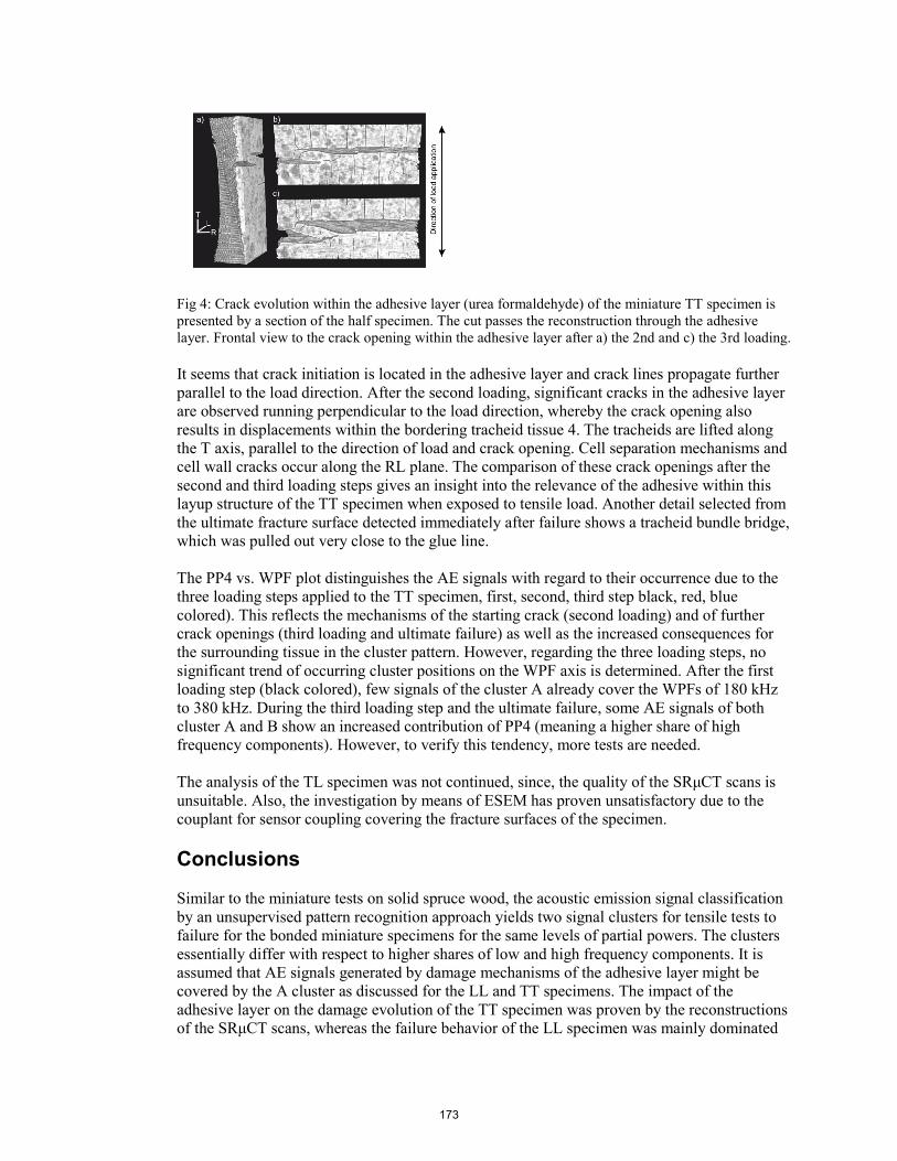
Fig 4: Crack evolution within the adhesive layer (urea formaldehyde) of the miniature TT specimen is presented by a section of the half specimen. The cut passes the reconstruction through the adhesive layer. Frontal view to the crack opening within the adhesive layer after a) the 2nd and c) the 3rd loading.

It seems that crack initiation is located in the adhesive layer and crack lines propagate further parallel to the load direction. After the second loading, significant cracks in the adhesive layer are observed running perpendicular to the load direction, whereby the crack opening also results in displacements within the bordering tracheid tissue 4. The tracheids are lifted along the T axis, parallel to the direction of load and crack opening. Cell separation mechanisms and cell wall cracks occur along the RL plane. The comparison of these crack openings after the second and third loading steps gives an insight into the relevance of the adhesive within this layup structure of the TT specimen when exposed to tensile load. Another detail selected from the ultimate fracture surface detected immediately after failure shows a tracheid bundle bridge, which was pulled out very close to the glue line.

The PP4 vs. WPF plot distinguishes the AE signals with regard to their occurrence due to the three loading steps applied to the TT specimen, first, second, third step black, red, blue colored). This reflects the mechanisms of the starting crack (second loading) and of further crack openings (third loading and ultimate failure) as well as the increased consequences for the surrounding tissue in the cluster pattern. However, regarding the three loading steps, no significant trend of occurring cluster positions on the WPF axis is determined. After the first loading step (black colored), few signals of the cluster A already cover the WPFs of 180 kHz to 380 kHz. During the third loading step and the ultimate failure, some AE signals of both cluster A and B show an increased contribution of PP4 (meaning a higher share of high frequency components). However, to verify this tendency, more tests are needed.

The analysis of the TL specimen was not continued, since, the quality of the SRμCT scans is unsuitable. Also, the investigation by means of ESEM has proven unsatisfactory due to the couplant for sensor coupling covering the fracture surfaces of the specimen.

Conclusions

Similar to the miniature tests on solid spruce wood, the acoustic emission signal classification by an unsupervised pattern recognition approach yields two signal clusters for tensile tests to failure for the bonded miniature specimens for the same levels of partial powers. The clusters essentially differ with respect to higher shares of low and high frequency components. It is assumed that AE signals generated by damage mechanisms of the adhesive layer might be covered by the A cluster as discussed for the LL and TT specimens. The impact of the adhesive layer on the damage evolution of the TT specimen was proven by the reconstructions of the SRμCT scans, whereas the failure behavior of the LL specimen was mainly dominated

173

by the wooden layers with the tracheid axes oriented parallel to the load direction. This different outcome of the rather brittle UF adhesive is a result of the different grain orientations of the adhered wooden layers. Compared to the UF adhesive, the longitudinally loaded layers have stronger load bearing capabilities, whereas the tangential loaded wood layers reveal greater weakness. The cluster results plotted as PP4 against WPF prove these observations, since the cluster patterns of the TT specimen shows a more individual pattern compared to the solid spruce tested in L and R direction (Fig. 6.32) than the LL specimen. It is assumed that AE signals generated by crack mechanisms of the adhesive are among the signals of the low frequency cluster. This tentative conclusion, however, will have to be verified by further investigations, possibly by performing similar tests using other combinations of adhesives and wood species with greater difference in mechanical performance and with a larger number of specimens.

Acknowledgments The authors acknowledge the financial support of Swiss National Foundation under grant SNF –Project 177`134. Also, the authors like to thank for the support of "Advanced research supporting the forestry and wood-processing sector´s adaptation to global change and the 4th industrial revolution", No. CZ.02.1.01/0.0/0.0/16_019/0000803 financed by OP RDE

References

Baensch, F. (2015). Damage evolution in wood and layered wood composites monitored in situ by acoustic emission, digital image correlation and synchrotron based tomographic microscopy. Zürich: Diss., ETH Zürich.

Casdorff, K., Kläusler, Gabriel, J., Amen, C., Lehringer, C., Burgert, I., & Keplinger, T. (2018). About the influence of a water-based priming system on the interactions. International Journal of Adhesion and Adhesives, 52-59.

Clauss, S. (2011). Structure-property relationships of one-component moisture-curing polyurethane adhesives under thermal load. Zürich: Diss., ETH Zürich.

Gindl, W., Sretenovic, A., Vincenti, A., & Müller, U. (2005). Direct measurement of strain distribution along a wood bond. Part 2.The Effect of Adhesive penetration on strain distribution. Holzforschung, 3007-310.

Hass, P. F. (2012). Penetration behavior of adhesives into solid wood and micromechanics of the bondline. Zürich: Diss. ETH Zürich.

Hering, S. (2011). Charakterisierung und Modellierung der Materialeigenschaften von Rotbuchenholz zur Simulation von Holzverklebungen. Zürich: Diss., ETH Zürich.

Kläusler, O. F. (2014). Improvement of one-component polyurethane bonded wooden joints under wet conditions. Zürich: Diss., ETH Zürich.

Niemz, P. (2017). Zur Orthotropie der physikalisch-mechanischen Eigenschaften von Fichtenholz. Annals of Warsaw University of Life Science - SGGW. Forestry and Wood Technology, 174-183.

Niemz, P., & Sonderegger, W. (2003). Untersuchungen zur Korrelation ausgewählter Holzeigenschaften untereinander und mit der Rohdichte unter Verwendung von 103 Holzarten. Schweizerische Zeitschrift für Forstwesen, 154(12), pp. 489-493.

Niemz, P., & Sonderegger, W. (2017). Holzphysik-Physik des Holzes und der Holzwerkstoffe. Leipzig: Fachbuchverlag leipzig im Carl Hanser Verlag.

Rindler, A., Pöll, C., Hansmann, C., Müller, U., & Konnerth, J. (2018). Moisture related elastic and viscoelastic behaviour of wood adhesives bymeans of in-situ nanoindentation. International Journal of Adhesion and Adhesives, 123-129.

174

Serrano, E. (2000). Adhesive joints in timber engineering. Lund: PhD Theisis, Lun University. Stöckel, F., Konnerth, J., & Gindel-Altmutter, W. (2013). Mechanical properties of adhesives

for bonding wood - A review. International Journal of Adhesion and Adhesives, 45, 32-41.

Wimmer, R., Kläusler, O., & Niemz, P. (2013). Water sorption mechanisms of commercial wood adhesive films. Wood Science and Technology, 47(4), pp. 763-775.

Zauner, M. (2014). In-situ synchrotron based tomographic microscopy of uniaxially loaded wood: in-situ testing device, procedures and experimental investigations. Zürich: Diss. ETH Zürich.

175

Towards Flexible Machine Strength Grading: Predicting the Outcomes of Destructive Tension Tests for Spruce by Acoustic NDT of the Green Sawn Timber

Andreas Weidenhiller * Holzforschung Austria, Franz Grill-Str. 7, 1030 Vienna, Austria, a.weidenhiller@holzforschung.at

Abstract

Pre-sorting of the green sawn timber by means of acoustic scanning is an attractive option for the wood processing industry – the dynamic modulus of elasticity of the green timber (Edyn,u) strongly correlates with the Edyn of the dried timber, which in turn is a good predictor for strength and static modulus of elasticity obtained from destructive tests. Using Edyn,u, unsuitable material can be removed prior to the energy-intensive process of drying. However, if the timber should subsequently undergo machine strength grading, opportunities to also segregate superior strength material from moderately strong timber are currently limited – this is due to representativity requirements inherent to machine strength grading. This paper shows that the good correlations of Edyn,u with the grade determining properties (GDP) established by destructive tension tests for spruce (Picea abies) can be used to assess the quality of a batch of green timber, whether pre-sorted or as a whole, and that Edyn,u can be used to predict these GDP. This is a first step towards adapting machine strength grading both to changing qualities and to the effects of pre-sorting, which will provide the wood processing industry with new flexible data-driven methods to improve the quality and efficiency of construction timber production.

Keywords: acoustic NDT, dynamic modulus of elasticity, green sawn timber, destructive tension test, spruce (Picea abies)

Introduction

Sawn timber that is required to have certain properties can only be obtained by a grading process that identifies the boards with the appropriate quality. An important use case is strength grading for construction timber. In many cases, this strength grading is accomplished by using different types of NDT, e.g. X-ray scanning (Bacher 2008), natural frequency measurement (Bacher 2008) or laser scanning (Brännström et al. 2008). While strength grading often is performed on the dried and planed sawn timber, it could be interesting to apply NDT technology earlier in the process to steer and optimize the material flow through the sawmill. For example, Brännström (2009) expected that critical improvements of raw material efficiency and of the quality of the final product could be achieved if sawing decisions were based on reliable predictions of sawing outcome.

Even after sawing, a presorting step could improve sawmill efficiency by removing unsuitable timber prior to the energy intensive drying process or by segregating timber into high-performance batches and lower qualities. An NDT approach suitable for such a segregation is to measure eigenfrequency and board density for determining 𝐸𝐸𝑑𝑑𝑑𝑑𝑑𝑑,𝑢𝑢, i.e. the dynamic modulus of elasticity (dynamic MOE) of the green timber. Above fiber saturation point, 𝐸𝐸𝑑𝑑𝑑𝑑𝑑𝑑,𝑢𝑢 is nearly independent of the actual moisture content (MC) of the timber (Kollmann and Krech 1960, Neumüller et al. 2007, Unterwieser and Schickhofer 2011). Therefore, there is a simple and close linear relationship between 𝐸𝐸𝑑𝑑𝑑𝑑𝑑𝑑,𝑢𝑢 and 𝐸𝐸𝑑𝑑𝑑𝑑𝑑𝑑,12%, i.e. the dynamic

176

MOE in the dry state (at 12% MC). Neumüller et al. (2007) reported a coefficient of determination of 𝑟𝑟2 = 98% for this relationship. 𝐸𝐸𝑑𝑑𝑑𝑑𝑑𝑑,12%, in turn, has good correlations with the grade determining properties (GDPs), foremost with static MOE (𝑟𝑟2 = 91% according to Viguier et al. 2015, tested in tension), but also with strength (𝑟𝑟2 = 58% according to Viguier et al. 2015, tested in tension). Olsson and Oscarsson (2017) also reported an acceptable correlation with density (𝑟𝑟2 = 53%). Therefore, 𝐸𝐸𝑑𝑑𝑑𝑑𝑑𝑑,𝑢𝑢 can be used to predict timber quality even in the green state and can be a useful tool for presorting of the green sawn timber.

In Europe, a system called "machine controlled strength grading" (MCSG) has been developed which allows a producer to grade timber with a wide variety of cross-sections into different strength grades, without needing to destructively verify the timber properties, or needing only a very limited amount of verification (Ridley-Ellis et al. 2016). This allows for high production efficiency even when producing timber with many different cross-sections. The downside of this approach is twofold: First, in order to establish the relationship between the NDT assessment and the required GDPs for a grade, an extensive initial testing program is necessary (EN 14081-2:2018). Second, for the machine settings derived during such a testing program to work as expected, the timber in the testing program needs to be representative for the timber graded during daily production – this means that there are only limited options for strength related presorting of the timber before MCSG (Ridley-Ellis et al. 2016). Approaches to adapt the machine settings to quality shifts in the processed timber, based on the continuous evaluation of the machine readings, have been discussed in the literature (e.g. Deublein et al. 2010, Ranta-Maunus and Turk 2010) and even implemented in the relevant European standard (EN 14081-2:2018). However, it is unclear whether the implemented approach can deal with the potentially massive quality shift induced by strength-based presorting of the raw material.

To sum up: Early strength-based presorting is expected to improve production efficiency. For the green sawn timber, 𝐸𝐸𝑑𝑑𝑑𝑑𝑑𝑑,𝑢𝑢 is a suitable quantity to base such a presorting on. The European MCSG approach requires that machine settings are adapted to the presorted material. Adaptive methods have been defined for MCSG, but they are probably not powerful enough to automatically accommodate a presorting step.

We propose an alternative approach – instead of adapting the MCSG in the course of the grading process, we assume that a presorting step (or at least a "pre-scanning" step) based on 𝐸𝐸𝑑𝑑𝑑𝑑𝑑𝑑,𝑢𝑢 has taken place, and that GDP value predictions for the presorted timber (also based on 𝐸𝐸𝑑𝑑𝑑𝑑𝑑𝑑,𝑢𝑢) can be used to adapt the settings for the MCSG to the actual quality of this timber. The contribution of the present paper is to study how well the quality of the timber (in terms of GDPs) can be predicted using 𝐸𝐸𝑑𝑑𝑑𝑑𝑑𝑑,𝑢𝑢, and how a presorting step influences such a prediction. We expect this approach to work well for different testing conditions, target products, and wood species; for the present paper, however, we focus on Norway spruce (Picea abies) timber of cross-sections suitable for glulam production and tested in tension.

Material and methods

Material

In the project SiOSiP (short for "Simulation-based Optimization of Sawn timber Production"), a representative dataset of the Austrian Norway spruce (Picea abies) timber resource was created. The data encompassed round timber properties, machine strength grading data of the green and of the dried sawn timber and the results from the lab tests and destructive strength tests. One part of the sawn timber was tested in tension, another in edgewise bending, and a third part in flatwise bending. In the present study, only the data from the timber tested in tension is used – the following description is restricted to this part of the data and to those variables which were used in the study.

177

The logs were selected directly in the forest in three Austrian regions with different growth conditions: Upper Austria (agricultural lowlands), the Tyrol (mountains) and Styria (hills influenced by the Pannonian climate). Log qualities were chosen to be representative for material used in constructive wood products. Top diameters ranged from 15 cm to 56 cm with an average of 28 cm.

The timber was sawn to four cross-sections: 40x80 mm, 40x140 mm, 50x200 mm and 40x250 mm. The green sawn timber was measured with a MiCROTEC GoldenEye 706 machine. The following data from this scan were used: green density (𝜌𝜌𝑢𝑢) and dynamic modulus of elasticity (𝐸𝐸𝑑𝑑𝑑𝑑𝑑𝑑,𝑢𝑢). After drying (and further scans which are not relevant for this study), the timber was tested in tension according to EN 408:2012. Tensile strength (𝑓𝑓𝑡𝑡), modulus of elasticity in tension (𝐸𝐸𝑡𝑡), dry density (𝜌𝜌) and moisture content of the dried timber (𝑢𝑢12) were determined according to EN 408:2012 and adjustments according to EN 384:2016 were applied.

Modelling of relationships

Relationships of 𝐸𝐸𝑑𝑑𝑑𝑑𝑑𝑑,𝑢𝑢 with 𝑓𝑓𝑡𝑡, 𝐸𝐸𝑡𝑡 and 𝜌𝜌 were established by least squares linear regression. The aim was to predict the GDPs for batches of timber, i.e. the 5th percentiles of strength (𝑓𝑓𝑡𝑡,𝑘𝑘) and density (𝜌𝜌𝑘𝑘) and the mean value of the modulus of elasticity (𝐸𝐸𝑡𝑡,𝑚𝑚𝑚𝑚𝑚𝑚𝑑𝑑). Calculation of these GDPs was done according to EN 384:2016 and EN 14358:2016. As linear regression predicts the central tendency, the output of the regression model for 𝐸𝐸𝑡𝑡 could be used directly for predicting a batch's 𝐸𝐸𝑡𝑡,𝑚𝑚𝑚𝑚𝑚𝑚𝑑𝑑 by averaging over the individual 𝐸𝐸𝑡𝑡 predictions.

However, to accurately predict a batch's characteristic strength (𝑓𝑓𝑡𝑡,𝑘𝑘) and characteristic density (𝜌𝜌𝑘𝑘), a further step was necessary. Simulated residuals had to be added to the output of the regression models for 𝑓𝑓𝑡𝑡 and 𝜌𝜌 – calculating 5th percentile values from these individual simulated values led to roughly unbiased estimates of 𝑓𝑓𝑡𝑡,𝑘𝑘 and 𝜌𝜌𝑘𝑘. For a proper simulation of residuals, it is important that the standard deviation of the regression residuals is constant over the whole range of the predictor variable 𝐸𝐸𝑑𝑑𝑑𝑑𝑑𝑑,𝑢𝑢 (homoscedasticity). To ensure homoscedasticity for the 𝑓𝑓𝑡𝑡 model, both 𝑓𝑓𝑡𝑡 and 𝐸𝐸𝑑𝑑𝑑𝑑𝑑𝑑,𝑢𝑢 were log-transformed before calculating the regression model. To get an objective measure of homoscedasticity, the Breusch-Pagan test for heteroscedasticity was used (Breusch and Pagan 1979; Klein et al. 2016).

As the aim of this study was to predict GDPs of presorted batches for a wide range of presorting thresholds, we obtained some batches containing a very small number of specimens. At the same time, our analysis contained a random element – the simulated residuals mentioned in the previous paragraph. Random influences become more severe the smaller a sample is. To alleviate this random influence, we repeated the calculation of simulated residuals 100 times for each analysis, calculated the 5th percentile values for each of the 100 iterations and then averaged over these 100 values. To illustrate the range of simulated values, the 2.5% percentile and the 97.5% percentile of these 100 values were calculated as well, giving 95% coverage of the simulated residuals.

Influence of presorting

As a simple model of presorting based on 𝐸𝐸𝑑𝑑𝑑𝑑𝑑𝑑,𝑢𝑢, we assumed a single presorting threshold 𝑇𝑇, by which a batch of timber is split in two presorted batches: the one above (𝐸𝐸𝑑𝑑𝑑𝑑𝑑𝑑,𝑢𝑢 ≥ 𝑇𝑇) and the one below the threshold (𝐸𝐸𝑑𝑑𝑑𝑑𝑑𝑑,𝑢𝑢 < 𝑇𝑇). For both presorted batches and for all values of 𝑇𝑇 for which there are at least 20 specimens in the respective part, the GDPs were predicted using the approach described in the previous section. For reference, the true GDP values were also calculated.

178

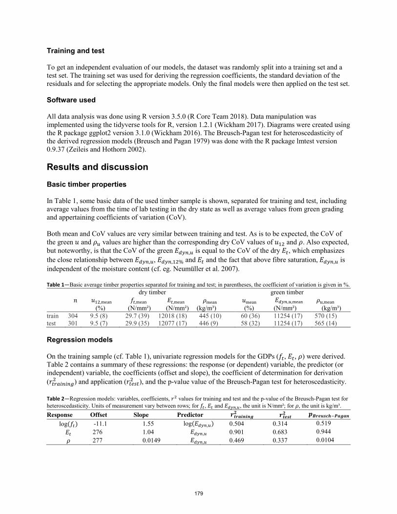
Training and test

To get an independent evaluation of our models, the dataset was randomly split into a training set and a test set. The training set was used for deriving the regression coefficients, the standard deviation of the residuals and for selecting the appropriate models. Only the final models were then applied on the test set.

Software used

All data analysis was done using R version 3.5.0 (R Core Team 2018). Data manipulation was implemented using the tidyverse tools for R, version 1.2.1 (Wickham 2017). Diagrams were created using the R package ggplot2 version 3.1.0 (Wickham 2016). The Breusch-Pagan test for heteroscedasticity of the derived regression models (Breusch and Pagan 1979) was done with the R package lmtest version 0.9.37 (Zeileis and Hothorn 2002).

Results and discussion

Basic timber properties

In Table 1, some basic data of the used timber sample is shown, separated for training and test, including average values from the time of lab testing in the dry state as well as average values from green grading and appertaining coefficients of variation (CoV).

Both mean and CoV values are very similar between training and test. As is to be expected, the CoV of the green 𝑢𝑢 and 𝜌𝜌𝑢𝑢 values are higher than the corresponding dry CoV values of 𝑢𝑢12 and 𝜌𝜌. Also expected, but noteworthy, is that the CoV of the green 𝐸𝐸𝑑𝑑𝑑𝑑𝑑𝑑,𝑢𝑢 is equal to the CoV of the dry 𝐸𝐸𝑡𝑡, which emphasizes the close relationship between 𝐸𝐸𝑑𝑑𝑑𝑑𝑑𝑑,𝑢𝑢, 𝐸𝐸𝑑𝑑𝑑𝑑𝑑𝑑,12% and 𝐸𝐸𝑡𝑡 and the fact that above fibre saturation, 𝐸𝐸𝑑𝑑𝑑𝑑𝑑𝑑,𝑢𝑢 is independent of the moisture content (cf. eg. Neumüller et al. 2007).

Table 1—Basic average timber properties separated for training and test; in parentheses, the coefficient of variation is given in %. dry timber green timber

𝑛𝑛 𝑢𝑢12,mean 𝑓𝑓𝑡𝑡,mean 𝐸𝐸𝑡𝑡,mean 𝜌𝜌mean 𝑢𝑢mean 𝐸𝐸𝑑𝑑𝑑𝑑𝑑𝑑,𝑢𝑢,mean 𝜌𝜌𝑢𝑢,mean (%) (N/mm²) (N/mm²) (kg/m³) (%) (N/mm²) (kg/m³)

train 304 9.5 (8) 29.7 (39) 12018 (18) 445 (10) 60 (36) 11254 (17) 570 (15) test 301 9.5 (7) 29.9 (35) 12077 (17) 446 (9) 58 (32) 11254 (17) 565 (14)

Regression models

On the training sample (cf. Table 1), univariate regression models for the GDPs (𝑓𝑓𝑡𝑡, 𝐸𝐸𝑡𝑡, 𝜌𝜌) were derived. Table 2 contains a summary of these regressions: the response (or dependent) variable, the predictor (or independent) variable, the coefficients (offset and slope), the coefficient of determination for derivation (𝑟𝑟𝑡𝑡𝑡𝑡𝑚𝑚𝑡𝑡𝑑𝑑𝑡𝑡𝑑𝑑𝑡𝑡2 ) and application (𝑟𝑟𝑡𝑡𝑚𝑚𝑡𝑡𝑡𝑡2 ), and the p-value value of the Breusch-Pagan test for heteroscedasticity.

Table 2—Regression models: variables, coefficients, 𝑟𝑟2 values for training and test and the p-value of the Breusch-Pagan test for heteroscedasticity. Units of measurement vary between rows; for 𝑓𝑓𝑡𝑡, 𝐸𝐸𝑡𝑡 and 𝐸𝐸𝑑𝑑𝑑𝑑𝑑𝑑,𝑢𝑢, the unit is N/mm²; for 𝜌𝜌, the unit is kg/m³. Response Offset Slope Predictor 𝒓𝒓𝒕𝒕𝒓𝒓𝒕𝒕𝒊𝒊𝒏𝒏𝒊𝒊𝒏𝒏𝒏𝒏𝟐𝟐 𝒓𝒓𝒕𝒕𝒕𝒕𝒕𝒕𝒕𝒕𝟐𝟐 𝒑𝒑𝑩𝑩𝒓𝒓𝒕𝒕𝑩𝑩𝒕𝒕𝑩𝑩𝑩𝑩−𝑷𝑷𝒕𝒕𝒏𝒏𝒕𝒕𝒏𝒏

log(𝑓𝑓𝑡𝑡) -11.1 1.55 log(𝐸𝐸𝑑𝑑𝑑𝑑𝑑𝑑,𝑢𝑢) 0.504 0.314 0.519 𝐸𝐸𝑡𝑡 276 1.04 𝐸𝐸𝑑𝑑𝑑𝑑𝑑𝑑,𝑢𝑢 0.901 0.683 0.944 𝜌𝜌 277 0.0149 𝐸𝐸𝑑𝑑𝑑𝑑𝑑𝑑,𝑢𝑢 0.469 0.337 0.0104

179

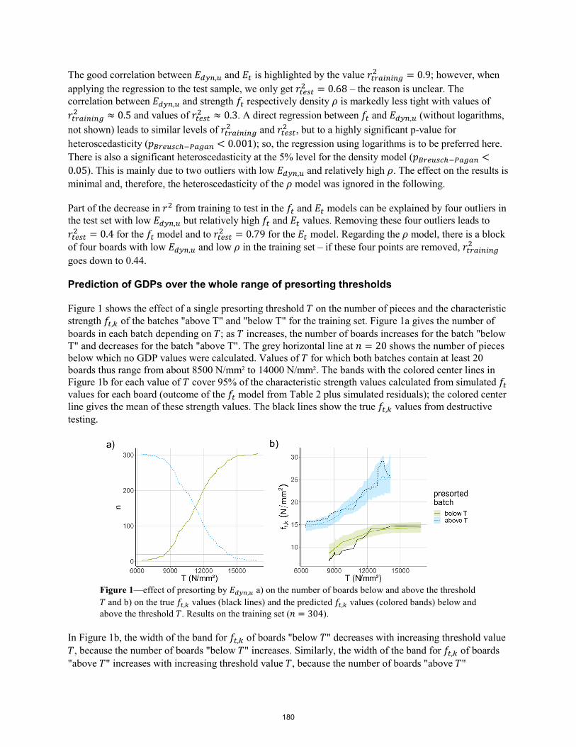
The good correlation between 𝐸𝐸𝑑𝑑𝑑𝑑𝑑𝑑,𝑢𝑢 and 𝐸𝐸𝑡𝑡 is highlighted by the value 𝑟𝑟𝑡𝑡𝑡𝑡𝑚𝑚𝑡𝑡𝑑𝑑𝑡𝑡𝑑𝑑𝑡𝑡2 = 0.9; however, when applying the regression to the test sample, we only get 𝑟𝑟𝑡𝑡𝑚𝑚𝑡𝑡𝑡𝑡2 = 0.68 – the reason is unclear. The correlation between 𝐸𝐸𝑑𝑑𝑑𝑑𝑑𝑑,𝑢𝑢 and strength 𝑓𝑓𝑡𝑡 respectively density 𝜌𝜌 is markedly less tight with values of 𝑟𝑟𝑡𝑡𝑡𝑡𝑚𝑚𝑡𝑡𝑑𝑑𝑡𝑡𝑑𝑑𝑡𝑡2 ≈ 0.5 and values of 𝑟𝑟𝑡𝑡𝑚𝑚𝑡𝑡𝑡𝑡2 ≈ 0.3. A direct regression between 𝑓𝑓𝑡𝑡 and 𝐸𝐸𝑑𝑑𝑑𝑑𝑑𝑑,𝑢𝑢 (without logarithms, not shown) leads to similar levels of 𝑟𝑟𝑡𝑡𝑡𝑡𝑚𝑚𝑡𝑡𝑑𝑑𝑡𝑡𝑑𝑑𝑡𝑡2 and 𝑟𝑟𝑡𝑡𝑚𝑚𝑡𝑡𝑡𝑡2 , but to a highly significant p-value for heteroscedasticity (𝑝𝑝𝐵𝐵𝑡𝑡𝑚𝑚𝑢𝑢𝑡𝑡𝐵𝐵ℎ−𝑃𝑃𝑚𝑚𝑡𝑡𝑚𝑚𝑑𝑑 < 0.001); so, the regression using logarithms is to be preferred here. There is also a significant heteroscedasticity at the 5% level for the density model (𝑝𝑝𝐵𝐵𝑡𝑡𝑚𝑚𝑢𝑢𝑡𝑡𝐵𝐵ℎ−𝑃𝑃𝑚𝑚𝑡𝑡𝑚𝑚𝑑𝑑 <0.05). This is mainly due to two outliers with low 𝐸𝐸𝑑𝑑𝑑𝑑𝑑𝑑,𝑢𝑢 and relatively high 𝜌𝜌. The effect on the results is minimal and, therefore, the heteroscedasticity of the 𝜌𝜌 model was ignored in the following.

Part of the decrease in 𝑟𝑟2 from training to test in the 𝑓𝑓𝑡𝑡 and 𝐸𝐸𝑡𝑡 models can be explained by four outliers in the test set with low 𝐸𝐸𝑑𝑑𝑑𝑑𝑑𝑑,𝑢𝑢 but relatively high 𝑓𝑓𝑡𝑡 and 𝐸𝐸𝑡𝑡 values. Removing these four outliers leads to 𝑟𝑟𝑡𝑡𝑚𝑚𝑡𝑡𝑡𝑡2 = 0.4 for the 𝑓𝑓𝑡𝑡 model and to 𝑟𝑟𝑡𝑡𝑚𝑚𝑡𝑡𝑡𝑡2 = 0.79 for the 𝐸𝐸𝑡𝑡 model. Regarding the 𝜌𝜌 model, there is a block of four boards with low 𝐸𝐸𝑑𝑑𝑑𝑑𝑑𝑑,𝑢𝑢 and low 𝜌𝜌 in the training set – if these four points are removed, 𝑟𝑟𝑡𝑡𝑡𝑡𝑚𝑚𝑡𝑡𝑑𝑑𝑡𝑡𝑑𝑑𝑡𝑡2 goes down to 0.44.

Prediction of GDPs over the whole range of presorting thresholds

Figure 1 shows the effect of a single presorting threshold 𝑇𝑇 on the number of pieces and the characteristic strength 𝑓𝑓𝑡𝑡,𝑘𝑘 of the batches "above T" and "below T" for the training set. Figure 1a gives the number of boards in each batch depending on 𝑇𝑇; as 𝑇𝑇 increases, the number of boards increases for the batch "below T" and decreases for the batch "above T". The grey horizontal line at 𝑛𝑛 = 20 shows the number of pieces below which no GDP values were calculated. Values of 𝑇𝑇 for which both batches contain at least 20 boards thus range from about 8500 N/mm² to 14000 N/mm². The bands with the colored center lines in Figure 1b for each value of 𝑇𝑇 cover 95% of the characteristic strength values calculated from simulated 𝑓𝑓𝑡𝑡 values for each board (outcome of the 𝑓𝑓𝑡𝑡 model from Table 2 plus simulated residuals); the colored center line gives the mean of these strength values. The black lines show the true 𝑓𝑓𝑡𝑡,𝑘𝑘 values from destructive testing.

Figure 1—effect of presorting by 𝐸𝐸𝑑𝑑𝑑𝑑𝑑𝑑,𝑢𝑢 a) on the number of boards below and above the threshold 𝑇𝑇 and b) on the true 𝑓𝑓𝑡𝑡,𝑘𝑘 values (black lines) and the predicted 𝑓𝑓𝑡𝑡,𝑘𝑘 values (colored bands) below and above the threshold 𝑇𝑇. Results on the training set (𝑛𝑛 = 304).

In Figure 1b, the width of the band for 𝑓𝑓𝑡𝑡,𝑘𝑘 of boards "below 𝑇𝑇" decreases with increasing threshold value 𝑇𝑇, because the number of boards "below 𝑇𝑇" increases. Similarly, the width of the band for 𝑓𝑓𝑡𝑡,𝑘𝑘 of boards "above 𝑇𝑇" increases with increasing threshold value 𝑇𝑇, because the number of boards "above 𝑇𝑇"

180

decreases. Also, the differences between the real strength values (black lines in Figure 1b) and the center lines of the prediction bands are smaller (2-3 N/mm²) when the number of boards in the presorted batch is large (𝑛𝑛 ≥ 130 or so), but become visibly larger (up to 4 N/mm²) for small numbers of boards in the presorted batch.

It is important to bear in mind that 𝐸𝐸𝑑𝑑𝑑𝑑𝑑𝑑 explains between 30% and 50% of the observed variation in 𝑓𝑓𝑡𝑡 (𝑟𝑟𝑡𝑡𝑡𝑡𝑚𝑚𝑡𝑡𝑑𝑑𝑡𝑡𝑑𝑑𝑡𝑡/𝑡𝑡𝑚𝑚𝑡𝑡𝑡𝑡2 in Table 2) – thus, there are between 50% and 70% of unexplained variation. From the

point of view of our 𝑓𝑓𝑡𝑡 model, this amounts to random influence which we modeled using simulated (i.e. random) residuals, which, in turn, influenced the width of the prediction band for 𝑓𝑓𝑡𝑡,𝑘𝑘. This also means that we cannot expect the true strength values to perfectly align with the center line of the prediction bands – the true strength values are just one realization of a random process and, therefore, they result in a much more irregular curve than the center line of the prediction band. This becomes even more obvious when we compare with the results for the test set and with the results for the other GDPs (Figure 2).

In Figure 2, the change in GDP values (𝑓𝑓𝑡𝑡,𝑘𝑘, 𝐸𝐸𝑚𝑚𝑚𝑚𝑚𝑚𝑑𝑑, 𝜌𝜌𝑘𝑘) depending on the presorting threshold 𝑇𝑇 is shown both for the training set and the test set, in a similar manner to Figure 1b. As described in the methods section, residuals were simulated for 𝑓𝑓𝑡𝑡,𝑘𝑘 and 𝜌𝜌𝑘𝑘, but not for 𝐸𝐸𝑚𝑚𝑚𝑚𝑚𝑚𝑑𝑑 – therefore, the width of the colored band for 𝐸𝐸𝑚𝑚𝑚𝑚𝑚𝑚𝑑𝑑 is zero.

Figure 2— effect of presorting by 𝐸𝐸𝑑𝑑𝑑𝑑𝑑𝑑,𝑢𝑢. on the true GDP values (black lines) and the predicted GDP values (colored bands) below and above the threshold 𝑇𝑇. Results on the training set (𝑛𝑛 = 304) and on the test set (𝑛𝑛 = 301).

For 𝑓𝑓𝑡𝑡,𝑘𝑘 and 𝜌𝜌𝑘𝑘 and both for training and test, the black lines corresponding to the true characteristic strength or density values have quite irregular shapes in comparison to the colored bands which correspond to the estimated characteristic strength or density values. This emphasizes that from the point of view of the prediction models for strength and density, the true strength and density values have a certain "randomness", due to other influencing factors beside 𝐸𝐸𝑑𝑑𝑑𝑑𝑑𝑑,𝑢𝑢. This randomness, however, is no

181

stronger in the test set than it is in the training set – this indicates that the models for predicting characteristic strength and density are stable and valid.

Regarding 𝐸𝐸𝑚𝑚𝑚𝑚𝑚𝑚𝑑𝑑, true value and prediction match far better than for 𝑓𝑓𝑡𝑡,𝑘𝑘 and 𝜌𝜌𝑘𝑘 – this has two reasons: First, prediction of mean values is more stable than prediction of characteristic 5th percentile values. Second, 𝐸𝐸𝑡𝑡 has a much better correlation with 𝐸𝐸𝑑𝑑𝑑𝑑𝑑𝑑,𝑢𝑢 than 𝑓𝑓𝑡𝑡 or 𝜌𝜌 (cf. 𝑟𝑟𝑡𝑡𝑡𝑡𝑚𝑚𝑡𝑡𝑑𝑑𝑡𝑡𝑑𝑑𝑡𝑡/𝑡𝑡𝑚𝑚𝑡𝑡𝑡𝑡

2 in Table 2). Therefore, it was unexpected that prediction and true value of 𝐸𝐸𝑚𝑚𝑚𝑚𝑚𝑚𝑑𝑑 were so far apart in the left part of the curve for "below 𝑇𝑇" in the test set. Closer inspection revealed that the four test set outlier boards mentioned in the previous section are responsible for this effect – excluding them from the analysis removed the observed deviation between prediction and true value.

Conclusions

This paper showed how one can use 𝐸𝐸𝑑𝑑𝑑𝑑𝑑𝑑,𝑢𝑢, i.e. the dynamic modulus of elasticity (MOE) of the green timber, to predict the grade determining properties (GDPs) of a batch of spruce timber tested in tension. As expected, the accuracy is best for the mean static MOE. For the characteristic values of strength and density, prediction accuracy more strongly depends on the number of pieces in the timber (𝑛𝑛). For 𝑛𝑛 ≥170, the deviation between true and predicted tension strength was below 2 N/mm², while the largest deviation (for smaller 𝑛𝑛) was about 4 N/mm². For 𝑛𝑛 ≥ 120, the deviation between true and predicted clear density was below 10 kg/m³ as opposed to a maximal deviation of more than 30 kg/m³ (for smaller 𝑛𝑛).

These kinds of predictions can help to accurately assess the timber quality already in the green state. Timber segregation based on these predictions could help to optimize the material flow in the sawmill and to save energy by removing unsuitable material prior to the drying process.

As these predictions also work for batches which are presorted based on 𝐸𝐸𝑑𝑑𝑑𝑑𝑑𝑑,𝑢𝑢, it should be possible to use them to adapt machine strength grading to the effect of presorting as well as to the effect of changing qualities both on presorted and unsorted material. To develop such an adaptation method will be the next step in providing the wood processing industry with a new flexible data-driven approach for machine strength grading, further improving the quality and efficiency of timber production.

Acknowledgments

The research for this article was done within the InnoGrading project funded by the Austrian Research Promotion Agency (FFG, grant no. 869170). The data was created within the SiOSiP project (funded by FFG in the research program "Production of the Future", grant no. 843678) with the support of the project partners Rubner Holzindustrie and the Association of the Austrian Wood Industries.

References

Bacher, M. 2008. Comparison of different machine strength grading principles. In: Gard WF, van de Kuilen J-WG (eds) End user's needs for wood material and products: Proceedings of the Conference in COST E53 Quality control for wood and wood products, pp 183–193

Brännström, M. 2009. The impact of a strength grading process on sawmill profitability and product quality. BioResources 4:1430–1454

182

Brännström, M.; Manninen, J.; Oja, J. 2008. Predicting the strength of sawn wood by tracheid laser scattering. BioResources 3:437–451

Breusch, T.S.; Pagan, A.R. 1979. A Simple Test for Heteroscedasticity and Random Coefficient Variation. Econometrica 47:1287. doi: 10.2307/1911963

EN 408: 2012. Timber structures – Structural timber and glued laminated timber – Determination of some physical and mechanical properties. CEN European Committee for Standardization, Brussels

EN 384: 2016. Structural timber – Determination of characteristic values of mechanical properties and density. CEN European Committee for Standardization, Brussels

EN 14358: 2016. Timber structures – calculation and verification of characteristic values. CEN European Committee for Standardization, Brussels

EN 14081-2: 2018. Timber structures – Strength graded structural timber with rectangular cross section – Part 2: Machine grading; additional requirements for type testing. CEN European Committee for Standardization, Brussels

Deublein, M.; Mauritz, R.; Köhler, J. 2010. Real-time quality evaluation of structural timber. In: Ceccotti A, van de Kuilen J-WG (eds) 11th World Conference on Timber Engineering 2010 (WCTE 2010)

Klein, A.G.; Gerhard, C.; Büchner, R.D.; Diestel, S.; Schermelleh-Engel, K. 2016. The detection of heteroscedasticity in regression models for psychological data. Psychological Test and Assessment Modeling 58:567–592

Kollmann, F.; Krech, H. 1960. Dynamische Messung der elastischen Holzeigenschaften und der Dämpfung. Ein Beitrag zur zerstörungsfreien Werkstoffprüfung [Dynamic Measurement of Damping Capacity and Elastic Properties of Wood]. Holz Roh Werkst 18:41–54. doi: 10.1007/BF02615616

Neumüller, A.; Schauer, R.; Saida, E.; Wolfsbauer, M. 2007. Festigkeitssortierung von Rundholz und frischem Schnittholz: Verfahren und Potenzial [Strength grading of round timber and green sawn timber. Method and potential]. In: Tagungsband / Wiener Leimholz-Symposium 2007, 22. - 23. März 2007, Wien. Holzforschung Austria, Wien, pp 3–11

Olsson, A.; Oscarsson, J. 2017. Strength grading on the basis of high resolution laser scanning and dynamic excitation: a full scale investigation of performance. Eur. J. Wood Prod. 75:17–31. doi: 10.1007/s00107-016-1102-6

R Core Team 2018. R: A Language and Environment for Statistical Computing. https://www.R-project.org/

Ranta-Maunus, A.; Turk, G. 2010. Approach of dynamic production settings for machine strength grading. In: Ceccotti A, van de Kuilen J-WG (eds) 11th World Conference on Timber Engineering 2010 (WCTE 2010)

Ridley-Ellis, D.; Stapel, P.; Baño, V. 2016. Strength grading of sawn timber in Europe: an explanation for engineers and researchers. Eur. J. Wood Prod. 74:291–306. doi: 10.1007/s00107-016-1034-1

183

Unterwieser, H.; Schickhofer, G. 2011. Influence of moisture content of wood on sound velocity and dynamic MOE of natural frequency- and ultrasonic runtime measurement. Eur. J. Wood Prod. 69:171–181

Viguier, J.; Jehl, A.; Collet, R.; Bleron, L.; Meriaudeau, F. 2015. Improving strength grading of timber by grain angle measurement and mechanical modeling. Wood Material Science and Engineering 10:145–156. doi: 10.1080/17480272.2014.951071

Wickham, H. 2016. ggplot2: Elegant Graphics for Data Analysis. Springer-Verlag New York

Wickham, H. 2017. tidyverse: Easily Install and Load the ’Tidyverse’. https://CRAN.R-project.org/package=tidyverse

Zeileis, A.; Hothorn, T. 2002. Diagnostic Checking in Regression Relationships. R News 2:7–10

184

Relationship between Dimensional Change and Strain Values in Eucalyptus pellita Wood Exposed to an Intermittent Drying Process

Karnita Yuniarti Center of Forest Products Research and Development, Forestry and Environment Research, Development and Innovation Agency, Ministry of Environment and Forestry, Jl Gunung Batu 5 Bogor, West Java, INDONESIA. E-mail : karnitayuniarti2015@gmail.com

Abstract

Minimal control of strain development during drying of wood could lead to serious defect affecting the final quality. However, monitoring the strain development during wood drying is not an easy task and involve destructive method to obtain the result. This preliminary study assesed the relationship between dimensional change and drying strain values in E. pellita in order to see if the dimensional change can be used as potential predictor for the drying strain developed in a wood. The trial used sawn boards from 2 provenances of E. pellita exposed to an intermittent regime, consisting of 8-hour heating phase at 50oC and non-heating phase at ambient condition. The parameters being investigated and linearly correlated to final dimension change (at width and thickness directions) were the instantaneous strain, viscoelastic strain/creep, mechanosorptive strain and shrinkage strain. The results show all R2 values for the relationship between each strain and final dimension change were still less than 50%. The results indicate either the power of the relationship between parameters should be escalated to different models, other than linear relationship or the final dimension changes are not the proper predictor for drying strain values

Keywords: drying strain values, dimensional change, intermittent drying, Eucalyptus pellita, linear regression

Introduction

Eucalyptus pellita is a native species to North Queensland, Papua New Guinea and Irian Jaya (Bristow 2008). It has been selected for plantation program development in Indonesia or other South East Asia countries due to its fast growing and short rotation characters. Though it is considered potential for construction production, its use is still limited by its tendency to develop drying defects.

Intermittent drying is potential to reduce the tendency of Pellita to get drying defects. In intermittent, a cooling phase is introduced between the heating sessions which allows the redistribution of moisture content that provokes internal relaxation in wood. Nevertheless, regardless of the drying technique applied, control of stress/strain development will still be required because minimal control could lead to serious defect affecting the final quality. If the drying stress/strain can be well controlled, defects can be avoided and the drying quality of wood can be improved (Dagang and Lianbai 1998).

M onitoring the strain development during wood drying is currently still a difficult task to carry out. The mechanosorptive behaviour of wood, which refers to the effects resulted from the interaction between the developed stress in wood and moisture change, is often applied to understand the stress development in wood during drying (Erickson and Seavey 1992; Erickson 1994; Zhan and Avramidis 2011a, 2011b). According to this theory, the drying strain in wood can be differentiated into 4 types w h i c h a r e instantaneous or elastic strain, shrinkage strain, viscoelastic-creep

185

strain and mechano-sorptive strain (Wu and Milota 1994; Dagang and Lianbai 1998; Chen and Gu 2006; Zhan and Avramidis 2011a). Instantaneous or elastic strain is a strain which develops immediately following the stress formation (Wu and Milota 1994). The mechanosorptive strain develops when the moisture content of the wood is still above FSP. It indicates an increasing deformation as a response to the change in moisture content, temperature, and developed internal stress (Dagang and Lianbai 1998; Zhan and Avramidis 2011b).When the moisture content of the timber reaches fiber saturation point (FSP), shrinkage strain starts to develops (Chen and Gu 2006). Visco-elastic strain develops under constant moisture and i n d i c a t e s a delayed deformation (Dagang and Lianbai 1998; Chen and Gu 2006). Different species s has different strain development (Wu and Milota 1994; Dagang and Lianbai 1998; Yuniarti 2019).

The knowledge of mechanosorptive behavior of wood could be used when one determine and/or optimizate a drying schedule for a timber. Nevertheless, up to now, many attempts to determine mechanosorptive behaviour of wood still uses desructive method, i.e McMillen’s slicing method (Wu and Milota 1994; Dagang and Lianbai 1998; Yuniarti 2019). It is a destructive technique, in which the wood is further cut to produce several small biscuits which are then sliced also.

A non-destructive method that can be developed is by correlating the mechanosorptive behavior of wood with estimator variables. In this study, the dimensional changes at width and thickness direction, due to the easiness in obtaining these variables during a drying process, were opted as the estimators. Wood will undergo some shrinkage or dimensional change during drying process and the degrees varies with the moisture content of the wood. Therefore, this preliminary research was carried out to assess the correlation between dimensional change and mechanosorptive behaviour of wood. This investigation focused firstly on the correlation between both properties at final moisture content as more stress/strain is usually released and easy to be examined at this stage.

Research method

Main material and equipment

The main material used was 10-year old Eucalyptus pellita logs of 2 Papua New Guinea provenances collected from one of the research forest areas of the Ministry of Environment and Forestry of Indonesia (MoEF) in Wonogiri, Central Jawa. The equipment used included oven, band saw, fridge, caliper, moisture meter, ruler, measuring tape, vape, plastic spatula, and scale.

Sample preparation

Each log was cut to produce drying samples, flat sawn boards, each measuring 500 mm (L) x 100 mm (W) x 25 mm (T) and free shrinkage samples measuring 20 mm (L) x 100 mm (W) x 25 mm (T) (Figure 1). Approximately 24 samples from each provenance were randomly collected for the drying trial and were end-sealed with sealant and aluminum foil.

Experiment method

The drying samples w e r e exposed to one intermittent regime, consisting of heating phase at 50oC for 8 hours and non-heating phase at ambient condition. The heating period was employed on 8am-4pm and the non-heating period was applied on 4pm-8am. A group of 24 samples from each provenance was dried in the same oven. All drying trials were run until the samples reached the target moisture content (10-15%).

186

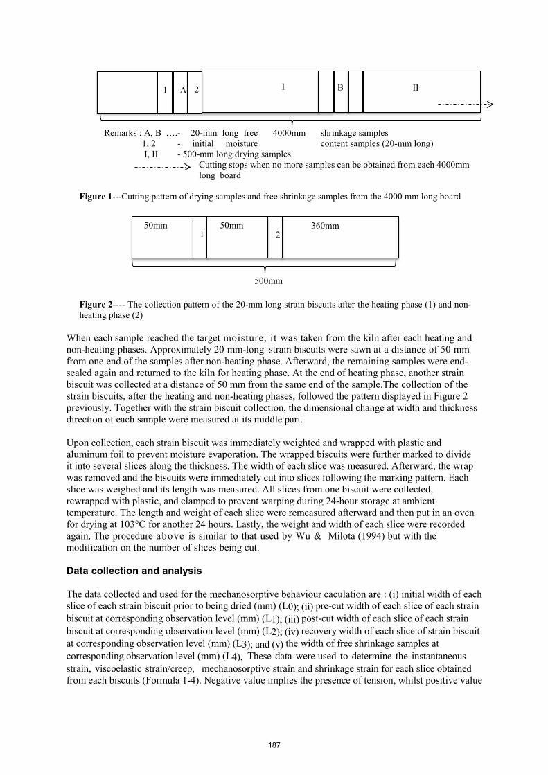
Remarks : A, B ….- 20-mm long free shrinkage samples 1, 2 - initial moisture content samples (20-mm long) I, II - 500-mm long drying samples

Cutting stops when no more samples can be obtained from each 4000mm long board

Figure 1---Cutting pattern of drying samples and free shrinkage samples from the 4000 mm long board

Figure 2---- The collection pattern of the 20-mm long strain biscuits after the heating phase (1) and non-heating phase (2)

When each sample reached the target moisture, it was taken from the kiln after each heating and non-heating phases. Approximately 20 mm-long strain biscuits were sawn at a distance of 50 mm from one end of the samples after non-heating phase. Afterward, the remaining samples were end-sealed again and returned to the kiln for heating phase. At the end of heating phase, another strain biscuit was collected at a distance of 50 mm from the same end of the sample.The collection of the strain biscuits, after the heating and non-heating phases, followed the pattern displayed in Figure 2 previously. Together with the strain biscuit collection, the dimensional change at width and thickness direction of each sample were measured at its middle part.

Upon collection, each strain biscuit was immediately weighted and wrapped with plastic and aluminum foil to prevent moisture evaporation. The wrapped biscuits were further marked to divide it into several slices along the thickness. The width of each slice was measured. Afterward, the wrap was removed and the biscuits were immediately cut into slices following the marking pattern. Each slice was weighed and its length was measured. All slices from one biscuit were collected, rewrapped with plastic, and clamped to prevent warping during 24-hour storage at ambient temperature. The length and weight of each slice were remeasured afterward and then put in an oven for drying at 103°C for another 24 hours. Lastly, the weight and width of each slice were recorded again. The procedure above is similar to that used by Wu & Milota (1994) but with the modification on the number of slices being cut.

Data collection and analysis

The data collected and used for the mechanosorptive behaviour caculation are : (i) initial width of each slice of each strain biscuit prior to being dried (mm) (L0); (ii) pre-cut width of each slice of each strain biscuit at corresponding observation level (mm) (L1); (iii) post-cut width of each slice of each strain biscuit at corresponding observation level (mm) (L2); (iv) recovery width of each slice of strain biscuit at corresponding observation level (mm) (L3); and (v) the width of free shrinkage samples at corresponding observation level (mm) (L4). These data were used to determine the instantaneous strain, viscoelastic strain/creep, mechanosorptive strain and shrinkage strain for each slice obtained from each biscuits (Formula 1-4). Negative value implies the presence of tension, whilst positive value

1 2 A B I II

4000mm

1 2 50mm 50mm 360mm

500mm

187

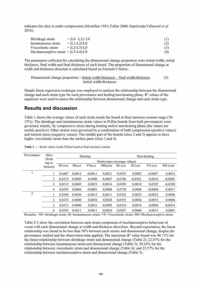
indicates the slice is under compression (Mcmillen 1955; Fuller 2000; Sepulveda-Villarroel et al. 2016).

Shrinkage strain = (L0 –L1)/ L0 (1) Instantaneous strain = (L1-L2)/L0 (2) Viscoelastic strain = (L2-L3)/L0 (3) Mechanosorptive strain = (L3-L4)/L0 (4)

The parameters collected for calculating the dimensional change proportion were initial width, initial thickness, final width and final thickness of each board. The proportion of dimensional change at width and thickness direction is calculated based on Formula 5 below:

Dimensional change proportion = Initial width/thickness – final width/thickness (5) Initial width/thickness

Simple linear regression technique was employed to analyze the relationship between the dimensional change and each strain type for each provenance and heating/non-heating phase. R2 values of the equations were used to assess the relationship between dimensional change and each strain type.

Results and discussion

Table 1 shows the average values of each strain inside the board at final moisture content range (10-15%). The shrinkage and instantaneous strain values in Pellita boards from both provenances were governed, mainly, by compressive stress during heating and/or non-heating phase (the values are mainly positive). Other strains were governed by a combination of both compression (positive values) and tension stress (negative values). The middle part of the boards (slice 2 and 3) appears to have higher viscoelastic strain than the surface parts (slice 1 and 4).

Table 1 ---- Strain values inside Pellita board at final moisture content

Provenance Slice (from top to

bottom)

Heating Non-heating Strain types (average values)

SS (εs) IS(εe) VS(εc) MS(εm) SS (εs) IS (εe) VS (εc) MS (εm)

1 1 0,0407 0,0012 -0,0011 0,0021 0,0435 0,0002 -0,0007 0,0014 2 0,0325 0,0009 0,0400 -0,0007 0,0786 -0,0361 0,0018 -0,00033 0,0315 0,0005 0,0023 -0,0014 0,0389 0,0018 0,0392 -0,03804 0,0295 0,0006 -0,0001 0,0004 0,0750 0,0008 -0,0004 0,0017

2 1 0,0380 0,0030 -0,0012 -0,0011 0,0362 0,0025 -0,0025 0,0006 2 0,0325 0,0000 0,0030 0,0028 0,0355 0,0004 0,0053 0,0006 3 0,0315 0,0000 0,0031 0,0005 0,0324 0,0010 0,0048 -0,00144 0,0295 0,0011 0,0011 0,0010 0,0307 0,0006 0,0015 0,0003

Remarks : SS=shrinkage strain; IS=Instantaneous strain; VS=Viscoelastic strain; MS=Mechanosorptive strain

Table 2-5 show the correlation between each strain component of mechanosorptive behaviour of wood with each dimensional change at width and thickness directions. Beyond expectation, the linear relationship was found to be less than 50% between each strains and dimensional change, despite the provenance studied and the observation time applied. The maximum R2 value found was 48.71% for the linear relationship between shrinkage strain and dimensional change (Table 2); 22.87% for the relationship between instantaneous strain and dimensional change (Table 3); 30.63% for the relationship between viscoelastic strain and dimensional change (Table 4); and 23.37% for the relationship between mechanosorptive strain and dimensional change (Table 5).

188

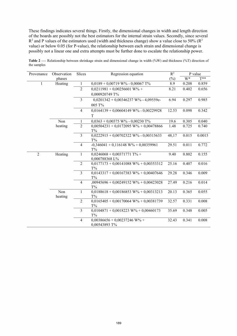
These findings indicates several things. Firstly, the dimensional changes in width and length direction of the boards are possibly not the best estimators for the internal strain values. Secondly, since several R2 and P values of the estimators used (width and thickness change) show a value close to 50% (R2 value) or below 0.05 (for P-value), the relationship between each strain and dimensional change is possibly not a linear one and extra attempts must be further done to escalate the relationship power.

Table 2 ---- Relationship between shrinkage strain and dimensional change in width (%W) and thickness (%T) direction of the samples

Provenance Observation phases

Slices Regression equation R2 (%)

P value W* T**

1 Heating 1 0,0189 + 0,00719 W% - 0,00067 T% 8.9 0.208 0.859 2 0,0211981 + 0,00256601 W% +

0,000920749 T% 8.21 0.402 0.656

3 0,0201342 + 0,00346237 W% - 4,09559e-005 T%

6.94 0.297 0.985

4 0,0164139 + 0,00604149 W% - 0,00229928 T

12.53 0.098 0.342

Non heating

1 0,0363 + 0,00375 W% - 0,00230 T% 19.6 0.305 0.040 2 0,00504231 + 0,0172095 W% + 0,00478866

T% 1.48 0.725 0.740

3 0,0222915 + 0,00702322 W% - 0,00315633 T%

48,17 0.015 0.0015

4 -0,346041 + 0,116148 W% + 0,00359961T%

29.51 0.011 0.772

2 Heating 1 0,0246068 + 0,00371771 T% + 0,000788368 L%

9.40 0.802 0.155

2 0,0177173 + 0,00141088 W% + 0,00353312 T%

25.16 0.407 0.016

3 0,0143317 + 0,00167383 W% + 0,00407646 T%

29.28 0.346 0.009

4 ,00945696 + 0,00249152 W% + 0,00423028 T%

27.49 0.216 0.014

Non heating

1 0,0188618 + 0,00186853 W% + 0,00313213 T%

20.13 0.365 0.055

2 0,0165405 + 0,00170064 W% + 0,00381739 T%

32.57 0.331 0.008

3 0,0104871 + 0,0018223 W% + 0,00460173 T%

35.69 0.348 0.005

4 0,00386656 + 0,00237246 W% + 0,00543893 T%

32.43 0.341 0.008

189

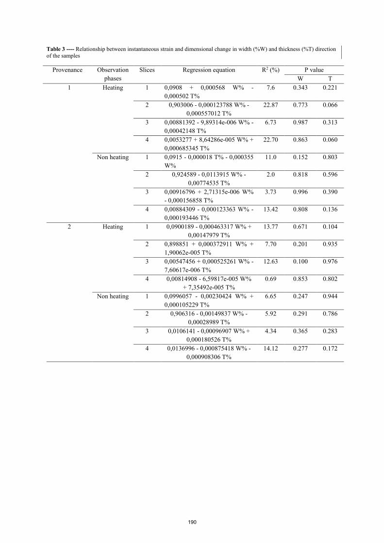
Table 3 ---- Relationship between instantaneous strain and dimensional change in width (%W) and thickness (%T) direction of the samples

Provenance Observation phases

Slices Regression equation R2 (%) P value W T

1 Heating 1 0,0908 + 0,000568 W% - 0,000502 T%

7.6 0.343 0.221

2 0,903006 - 0,000123788 W% - 0,000557012 T%

22.87 0.773 0.066

3 0,00881392 - 9,89314e-006 W% - 0,00042148 T%

6.73 0.987 0.313

4 0,0053277 + 8,64286e-005 W% + 0,000685345 T%

22.70 0.863 0.060

Non heating 1 0,0915 - 0,000018 T% - 0,000355 W%

11.0 0.152 0.803

2 0,924589 - 0,0113915 W% - 0,00774535 T%

2.0 0.818 0.596

3 0,00916796 + 2,71315e-006 W% - 0,000156858 T%

3.73 0.996 0.390

4 0,00884309 - 0,000123363 W% - 0,000193446 T%

13.42 0.808 0.136

2 Heating 1 0,0900189 - 0,000463317 W% + 0,00147979 T%

13.77 0.671 0.104

2 0,898851 + 0,000372911 W% + 1,90062e-005 T%

7.70 0.201 0.935

3 0,00547456 + 0,000525261 W% - 7,60617e-006 T%

12.63 0.100 0.976

4 0,00814908 - 6,59817e-005 W% + 7,35492e-005 T%

0.69 0.853 0.802

Non heating 1 0,0996057 - 0,00230424 W% + 0,000105229 T%

6.65 0.247 0.944

2 0,906316 - 0,00149837 W% - 0,00028989 T%

5.92 0.291 0.786

3 0,0106141 - 0,00096907 W% + 0,000180526 T%

4.34 0.365 0.283

4 0,0136996 - 0,000875418 W% - 0,000908306 T%

14.12 0.277 0.172

190

Table 4----Relationship between Viscoelastic/creep strain and dimensional change in width (%W) and thickness (%T) direction of the samples

Provenance Observation phases

Slices Regression equation R2 (%) P Value W T

1 Heating 1 0,0583 + 0,000960 W% - 0,000860 T%

22.5 0.085 0.027

2 -0,084732 + 0,0129924 W% +0,0372269 T%

8.30 0.811 0.319

3 0,033688 - 6,41377e-006 W% - 0,000458361 T%

16.05 0.987 0.106

4 0,0190782 + 0,00071419 W% - 0,000541031 T%

19.24 0.093 0.072

Non heating 1 0,0599 + 0,000072 T% - 0,000204 W%

5.2 0.454 0.372

2 0,034691 - 0,00097696 W% + 0,000202153 T%

18.83 0.060 0.176

3 0,150339 - 0,0187941 W% - 0,00554704 T%

1.83 0.704 0.703

4 0,0211391 - 0,000439688 W% - 4,91095e-005 T%

3.59 0.498 0.759

2 Heating 1 0,0597298 + 0,000515307 W% - 0,000844378 T%

5.41 0.654 0.368

2 0,0330074 + 0,000313026 W% - 0,000312424 T%

13.13 0.311 0.215

3 0,032018 + 0,000657611 W% - 0,000298646 T%

30.63 0.022 0.179

4 0,0210709 + 0,000283902 W% - 0,000227452 T%

3.11 0.632 0.641

Non heating 1 0,0710099 - 0,00112459 T% - 0,00280624 W%

1.62 0.618 0.793

2 0,0367981 - 0,00123359 W% + 0,00100754 T%

2.29 0.644 0.620

3 0,0294492 + 1,10322e-007 W% + 0,00168185 T%

3.97 1 0.374

4 0,0169617 + 6,60991e-005 W% + 0,00133417 T%

2.88 0.977 0.474

191

Table 5---- Relationship between mechanosorptive strain and dimensional change in width (%W) and thickness (%T) direction of the samples

Provenance Observation phases

Slices Regression equation R2 % P values W T

1 Heating 1 0,0618 - 0,00198 W% - 0,00104 T%

4.7 0.584 0.672

2 1,02853 + 0,0496569 W% - 0,064593 T%

6.64 0.531 0.235

3 0,900121 + 0,00035073 W% - 0,00087899 T%

0.65 0.924 0.727

4 0,0419346 + 0,00226452 W% - 0,00307674 T%

7.06 0.541 0.245

Non heating 1 0,0637 - 0,00315 W% - 0,000453 T%

11.3 0.204 0.528

2 1,01209 - 0,00348827 W% - 5,97326e-006 T%

9.67 0.161 0.993

3 0,796072 + 0,014482 W% + 0,00556925 T%

1.46 0.769 0.702

4 0,0486934 - 0,00161379 W% - 0,00048947 T%

8.53 0.463 0.371

2 Heating 1 0,03333 + 0,00241542 W% + 0,00278096 T%

8.18 0.411 0.247

2 0,992462 + 0,000613233 W% + 0,00284945 T%

12.85 0.762 0.093

3 0,895159 - 9,23473e-005 W% + 0,0018907 T%

6.93 0.962 0.233

4 0,0288925 + 0,00135848 W% + 0,00256971 T%

7.90 0.592 0.226

Non heating 1 0,0544797 + 0,000307356 W% - 0,00191178 T%

3.37 0.920 0.416

2 1,00949 - 0,00100134 W% - 0,00211403 T%

8.29 0.654 0.222

3 0,921011 - 0,00343232 W% - 0,00335907 T%

23.37 0.147 0.067

4 0,064483 - 0,00508145 W% - 0,00211831 T%

15.19 0.110 0.405

Conclusions

This study aims to examine the relationship between final dimension change and the mechanosorptive behavior in Pellita wood exposed to intermittent drying. A weak linear relationship (R2 values were less than 50%) was found between the strains and dimensional change at width and thickness direction. Extra attempts would be required to escalate the relationship power.

Acknowledgments

The author would like to convey her gratitude to ACIAR for providing both research and conference grant; and technicians (Rahmat, Aftoni, Darta, and Pardiono) for their assistance in the laboratory.

References

Bristow, M. 2008. Growth of Eucalyptus pellita in mixed species and monoculture plantations (Thesis). Lismore, New South Wales: Southern Cross University.

Chen, T; Gu, L. 2006. Development of elastic strain and mechano-sorptive strain during conditioning of Eucalyptus camaldulensis lumber in batch kiln. Maderas. Ciencia y tecnología 8(1): 49-56.

192

Dagang, L; Lianbai, G. 1998. The mechano-sorptive behavior of poplar during high-temperature drying. Drying Technology 17(9): 1947-1958. Erickson, RW. 1994. The effect of drying temperature on the mechano-sorptive behavior of red oak lumber. Drying Technology 12(8): 1943-1961. Erickson, RW; Seavey, RT. 1992. Energy quantification and mechano-sorptive behavior in the kiln drying of 2.5 cm thick red oak lumber. Drying Technology 10(5): 1183-1206. Fuller, J. 2000. Determining the source of changing shrinkage rates during kiln drying. Drying Technology 18(1-2): 261-278. McMillen, JM. 1955. Drying stresses in red oak: effect of temperature. Forest Products Journal 5: 230-241. Sepulveda-Villarroel, V; Perez-Peña, N; Salinas-Lira, C.[and others]. 2016. The development of moisture and strain profiles during predrying of Eucalyptus nitens. Drying Technology 34(4): 428-436. Wu, Q; Milota, MR. 1994. Effect of creep and mechano-sorptive effect on stress development during drying. Drying Technology 12(8): 2057-2085. Yuniarti, K. 2019. Mechano-sorptive behaviour of Eucalyptus pellita during intermittent and continuous drying. Journal of Tropical Forest Science 31(1): 63-77. Zhan, JF; Avramidis, S. 2011a. Mechanosorptive creep of hemlock under conventional drying: I. The determination of free shrinkage strain. Drying Technology 29(7): 789-796. Zhan, JF; Avramidis, S. 2011b. Mechanosorptive creep of hemlock under conventional drying: II. Description of actual creep behavior in drying lumber. Drying Technology 29: 1140–1149.

193

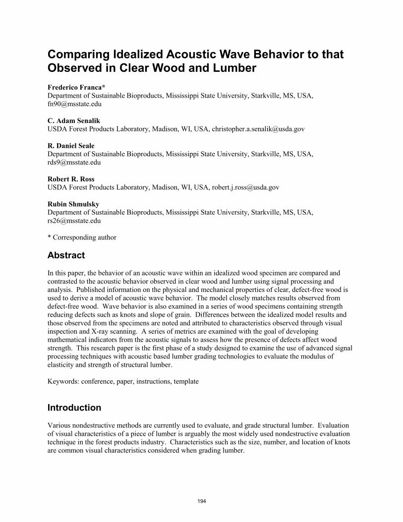
Comparing Idealized Acoustic Wave Behavior to that Observed in Clear Wood and Lumber Frederico Franca* Department of Sustainable Bioproducts, Mississippi State University, Starkville, MS, USA, fn90@msstate.edu C. Adam Senalik USDA Forest Products Laboratory, Madison, WI, USA, christopher.a.senalik@usda.gov R. Daniel Seale Department of Sustainable Bioproducts, Mississippi State University, Starkville, MS, USA, rds9@msstate.edu Robert R. Ross USDA Forest Products Laboratory, Madison, WI, USA, robert.j.ross@usda.gov Rubin Shmulsky Department of Sustainable Bioproducts, Mississippi State University, Starkville, MS, USA, rs26@msstate.edu * Corresponding author Abstract In this paper, the behavior of an acoustic wave within an idealized wood specimen are compared and contrasted to the acoustic behavior observed in clear wood and lumber using signal processing and analysis. Published information on the physical and mechanical properties of clear, defect-free wood is used to derive a model of acoustic wave behavior. The model closely matches results observed from defect-free wood. Wave behavior is also examined in a series of wood specimens containing strength reducing defects such as knots and slope of grain. Differences between the idealized model results and those observed from the specimens are noted and attributed to characteristics observed through visual inspection and X-ray scanning. A series of metrics are examined with the goal of developing mathematical indicators from the acoustic signals to assess how the presence of defects affect wood strength. This research paper is the first phase of a study designed to examine the use of advanced signal processing techniques with acoustic based lumber grading technologies to evaluate the modulus of elasticity and strength of structural lumber. Keywords: conference, paper, instructions, template Introduction Various nondestructive methods are currently used to evaluate, and grade structural lumber. Evaluation of visual characteristics of a piece of lumber is arguably the most widely used nondestructive evaluation technique in the forest products industry. Characteristics such as the size, number, and location of knots are common visual characteristics considered when grading lumber.

194

Research has shown that several physical and mechanical characteristics can be used to grade lumber (Senft et al. 1962; McKean and Hoyle, 1964; Ross, 1984a; Ross, 1985b; Ziegler, 1997; Galligan and McDonald 2000; França et at., 2017a; França et al., 2018b; França et al., 2019c). Products of this research have evolved into commercially available, rugged equipment that is used in the lumber grading process. One of the technologies that is currently in use is based on measurement of the acoustic properties of a lumber specimen. Specifically, the speed at which a mechanically induced acoustic wave flows along the length of a specimen is measured and coupled with its density to determine its modulus of elasticity (MOE). This information, along with certain visual characteristics, can result in the assignment of a grade to the piece of lumber. The flow of an acoustic wave in a lumber specimen is influenced by a variety of factors, such as the size, number, and location of knots. It is widely accepted that these factors have an influence on the MOE of a particular piece of lumber. Consequently, determination of MOE with this technique is useful from a practical viewpoint (Hoyle, 1968; Galligan et al. 1986). The measurement system currently employed to determine MOE yields an electronic signature that contains additional information regarding the movement of an acoustic wave in a lumber specimen. While a significant number of published research findings exist on the measurement and use of acoustic-based MOE for evaluating lumber and other wood products (Beall, 1987; Kánnár, 2000; Sandoz et al. 2000; Ballarin et al., 2002; Seeling, 2002), little more than cursory information is published on the effects that naturally occurring characteristics have on acoustic wave behavior in lumber and the potential impact these have on evaluating lumber strength. The objectives of the research presented in this research paper were to: 1. Examine fundamental acoustic wave behavior in clear wood and lumber; 2. Explore the effect that naturally occurring defects such as knots have on acoustic wave behavior in lumber, and; 3. Investigate the possibility of using advanced signal processing techniques to enhance acoustic-based lumber processing. Material and Methods The specimens utilized in the experimental phase of this study were cut from a sample of visually graded (No. 2) southern pine 2 by 8 in (nominal) lumber. Sixty-one (61) 1.5 in. by 1.5 in by 96 in (38 x 38 x 2438 mm) specimens were used (Figure 1). These specimens were conditioned to approximately 12 percent equilibrium moisture content prior to testing. Each specimen’s dimensions and weight were measured prior to testing. Specimens were selected based upon visual inspection with the goal of obtaining a wide range of characteristics. The specimens included several that were visually free from significant strength reducing defects, including knots. Other specimens contained large knots.

195

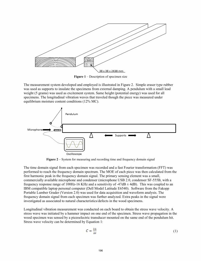
Figure 1 – Description of specimen size

The measurement system developed and employed is illustrated in Figure 2. Simple eraser type rubber was used as supports to insulate the specimens from external damping. A pendulum with a small lead weight (5 grams) was used as excitement system. Same height (potential energy) was used for all specimens. The longitudinal vibration waves that traveled though the piece was measured under equilibrium moisture content conditions (12% MC).

Figure 2 – System for measuring and recording time and frequency domain signal

The time domain signal from each specimen was recorded and a fast Fourier transformation (FFT) was performed to reach the frequency domain spectrum. The MOE of each piece was then calculated from the first harmonic peak in the frequency domain signal. The primary sensing element was a small, commercially available microphone and condenser (microphone USB 2.0, condenser SF-555B, with a frequency response range of 100Hz-16 KHz and a sensitivity of -47dB ± 4dB). This was coupled to an IBM compatible laptop personal computer (Dell Model Latitude E6540). Software from the Fakopp Portable Lumber Grader (Version 2.0) was used for data acquisition and waveform analysis. The frequency domain signal from each specimen was further analyzed. Extra peaks in the signal were investigated as associated to natural characteristics/defects in the wood specimens. Longitudinal vibration measurement was conducted on each board to obtain the stress wave velocity. A stress wave was initiated by a hammer impact on one end of the specimen. Stress wave propagation in the wood specimen was sensed by a piezoelectric transducer mounted on the same end of the pendulum hit. Stress wave velocity can be determined by Equation 1:

(1)

196

where C is stress wave velocity (m.s-1), L is length of specimen (m), and Δt is time of flight (s). The relation between acoustic velocity, density and wood stiffness is described by the fundamental wave equation (Bucur, 2003). The dynamic MOE of the specimens obtained by stress wave timer were determined using one-dimensional propagation waves, based on Equation 2.

(2)

where Esw is stress wave modulus of elasticity, ρ is the density at 12% moisture content (kg.m-3), and C is stress wave velocity (m.s-1). Wave attenuation (logarithmic decrement) can be determined from the rate of decay of the amplitude of pulses using the following equation:

(3)

where 𝝀𝝀 is the logarithmic decrement, T is the period of the damped oscillation, xn+1 and xn are the maximum amplitudes of two successive oscillations. Tensile tests were conducted according to ASTM D 198-15 (2015) to evaluate the tensile strength of each specimen. The tensile test machine (Metriguard Model 401) was used for the tension test. The tension proof machine was equipped with serrated plates to grip the specimens. Test span was 1500 mm and the loading rate set to cause failure was between 1 to 3 minutes. An extensometer was attached to the specimen to determine the tension modulus of elasticity. Ultimate tension stress (UTS) was determined using the following equation:

(4)

where UTS is the ultimate tensile stress (MPa), P is the maximum load (N), t is the thickness (m), and w is the width (m) of the specimen. Tensile modulus of elasticity (MOEt) was determined using the following equation:

(5)

where MOEt is the tensile modulus of elasticity (MPa), P𝛥𝛥 is the load at the elongation 𝛥𝛥t (MPa), an is the gage length (m), t is the thickness (m), w is the width (m) of the specimen, and 𝛥𝛥t is the elongation (m). Results and Discussion Table 1 summarizes the testing data. The average density of the pieces was 578 kg·m-3, ranging from 416 to 744. The stress wave velocity ranged from 2982 to 5667 m·s-1. Stress wave MOE ranged between 4203 and 20764 MPa. Logarithmic decrement ranged between 0.0312 and 0.0899. Ultimate tensile stress range from 13.61 to 125.76 MPa. Tensile modulus of elasticity ranged between 5271 and 24525 MPa.

197

Table 1. Summary of testing data

ID Density (kg·m-3)

Velocity (m·s-1)

dMOE (MPa)

MOEt (MPa)

UTS (MPa)

Log decr. ID Density

(kg·m-3) Velocity (m·s-1)

dMOE (MPa)

MOEt (MPa)

UTS (MPa)

Log decr.

1 571 5233 15634 15998 69.64 0.0466 32 744 5067 19091 15933 125.76 0.0502 2 554 3930 8558 10607 60.71 0.0551 33 728 5130 19170 20930 105.17 0.0437 3 465 4350 8805 11021 23.27 0.0621 34 664 5447 19701 19938 109.91 0.0451 4 581 5355 16655 16832 73.44 0.0392 35 479 5018 12066 12005 36.39 0.0522 5 547 4265 9953 9976 51.69 0.0564 36 416 4515 8479 8304 17.94 0.0522 6 648 5482 19465 24963 50.08 0.0431 37 570 5579 17737 20275 77.74 0.0367 7 560 4853 13187 12745 20.79 0.0702 38 556 5603 17466 22756 73.47 0.0419 8 629 4984 15636 13761 93.61 0.048 39 590 5564 18256 22528 76.00 0.0338 9 441 5174 11800 13134 25.30 0.0454 40 597 5584 18622 21936 91.57 0.0416 10 601 5087 15554 16200 49.63 0.0709 41 609 5521 18572 21294 46.25 0.0375 11 554 5145 14658 15099 54.34 0.0563 42 578 5628 18317 19716 81.72 0.0454 12 541 4708 11992 11007 40.38 0.0685 43 578 5521 17608 20851 87.50 0.0446 13 628 4847 14762 14164 63.93 0.0622 44 571 5525 17440 19558 86.89 0.0391 14 566 5189 15236 15274 52.97 0.0414 45 601 5589 18778 25402 47.62 0.0383 15 525 4161 9083 10030 52.64 0.0835 46 488 2982 4335 6746 15.61 0.0899 16 479 4789 10993 13618 27.87 0.0706 47 570 5438 16866 17617 94.83 0.05 17 593 4804 13686 18077 62.06 0.056 48 615 5482 18489 17367 42.85 0.0495 18 464 4562 9656 6500 20.48 0.0499 49 599 5667 19234 22975 47.86 0.0362 19 605 4437 11908 18619 32.37 0.0702 50 460 4555 9537 11285 17.66 0.0563 20 653 5038 16577 16072 44.85 0.0558 51 555 4955 13629 13393 52.95 0.0398 21 706 5023 17821 15871 84.92 0.0587 52 549 4807 12695 9260 20.67 0.0496 22 627 4916 15149 19945 104.64 0.0513 53 464 4552 9626 13062 27.54 0.0601 23 591 5496 17845 19618 83.29 0.0385 54 510 4492 10295 10935 14.79 0.0577 24 540 4916 13060 13549 45.20 0.054 55 484 4495 9784 8498 36.35 0.0524 25 671 5394 19512 17301 111.14 0.038 56 535 5486 16115 13482 95.53 0.0391 26 681 5443 20176 25472 81.60 0.0312 57 556 5062 14240 18614 101.34 0.0389 27 551 4179 9623 6396 26.79 0.0594 58 560 5525 17104 18280 92.70 0.0401 28 687 5399 20025 20839 78.76 0.0433 59 446 3069 4203 5861 13.61 0.0829 29 697 5379 20159 17513 89.58 0.035 60 603 4687 13251 17393 45.89 0.0402 30 691 5482 20764 23287 101.65 0.0387 61 593 4644 12796 11884 15.70 0.0488 31 738 4911 17804 15729 115.67 0.0463

Mean trends in the relationship between stress wave MOE and tensile MOE for the 2 by 2 southern pine pieces are shown in Figure 3. Linear regression was significant.

198

Figure 3 – Tensile MOE versus stress wave MOE

Mean trends in the relationship between stress wave MOE and ultimate tensile stress (UTS) for the 2 by 2 southern pine pieces are shown in Figure 4.

Figure 4 – Ultimate Tensile Stress versus stress wave MOE

Mean trends in the relationship between logarithmic decrement density-1 and ultimate tensile stress (UTS) for the 2 by 2 southern pine pieces are shown in Figure 5. The combination of logarithmic decrement and density exhibited potential for ultimate tensile stress estimation. There was no significant difference compared to the UTS estimation using the dynamic MOE. Dynamic MOE is recommended for being a common variable in lumber industry. A theoretical longitudinal vibration of a prismatic bar was generated using physical and mechanical property data for loblolly pine. Figure 6 exhibits a time domain with 9 harmonics of the fundamental frequency and frequency domain analysis, showing the relative magnitude of each harmonic.

199

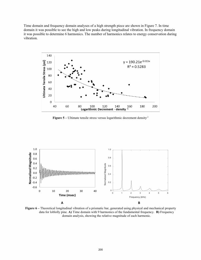
Time domain and frequency domain analyses of a high strength piece are shown in Figure 7. In time domain it was possible to see the high and low peaks during longitudinal vibration. In frequency domain it was possible to determine 6 harmonics. The number of harmonics relates to energy conservation during vibration.

Figure 5 – Ultimate tensile stress versus logarithmic decrement density-1

-0.6

-0.4

-0.2

0.0

0.2

0.4

0.6

0.8

1.0

0 10 20 30 40

Nor

mal

ized

Mag

nitu

de

Time (msec) 0 1 2 3 4 5 6

Frequency (kHz)

0

0.2

0.4

0.6

0.8

1.0

Nor

mal

ized

Mag

nitu

de

A B

Figure 6 – Theoretical longitudinal vibration of a prismatic bar, generated using physical and mechanical property data for loblolly pine. A) Time domain with 9 harmonics of the fundamental frequency. B) Frequency

domain analysis, showing the relative magnitude of each harmonic.

200

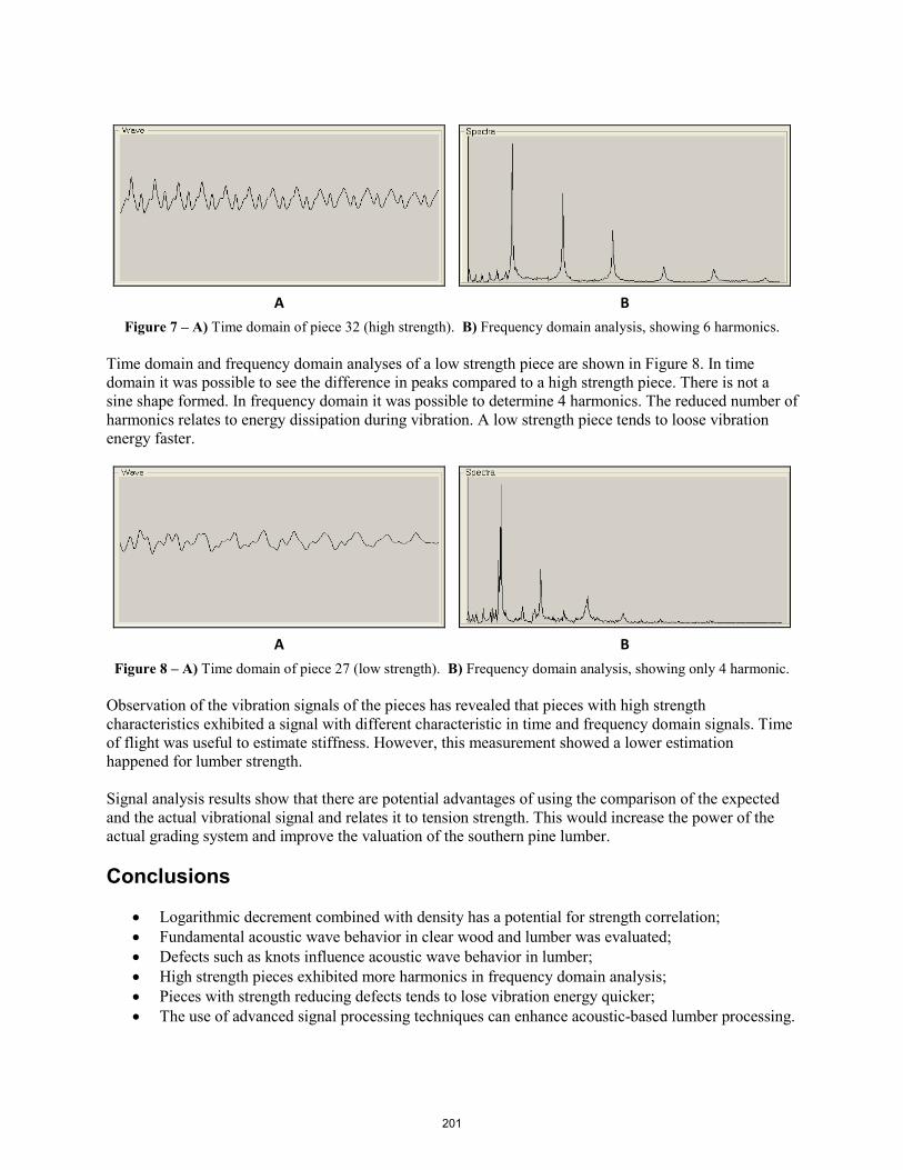
A B

Figure 7 – A) Time domain of piece 32 (high strength). B) Frequency domain analysis, showing 6 harmonics. Time domain and frequency domain analyses of a low strength piece are shown in Figure 8. In time domain it was possible to see the difference in peaks compared to a high strength piece. There is not a sine shape formed. In frequency domain it was possible to determine 4 harmonics. The reduced number of harmonics relates to energy dissipation during vibration. A low strength piece tends to loose vibration energy faster.

A B

Figure 8 – A) Time domain of piece 27 (low strength). B) Frequency domain analysis, showing only 4 harmonic. Observation of the vibration signals of the pieces has revealed that pieces with high strength characteristics exhibited a signal with different characteristic in time and frequency domain signals. Time of flight was useful to estimate stiffness. However, this measurement showed a lower estimation happened for lumber strength. Signal analysis results show that there are potential advantages of using the comparison of the expected and the actual vibrational signal and relates it to tension strength. This would increase the power of the actual grading system and improve the valuation of the southern pine lumber. Conclusions

• Logarithmic decrement combined with density has a potential for strength correlation; • Fundamental acoustic wave behavior in clear wood and lumber was evaluated; • Defects such as knots influence acoustic wave behavior in lumber; • High strength pieces exhibited more harmonics in frequency domain analysis; • Pieces with strength reducing defects tends to lose vibration energy quicker; • The use of advanced signal processing techniques can enhance acoustic-based lumber processing.

201

Acknowledgments The authors wish to acknowledge the support of the United States Department of Agriculture (USDA), Research, Education, and Economics (REE), Agriculture Research Service (ARS), Administrative and FinancialManagement (AFM), Financial Management and Accounting Division (FMAD) Grants and Agreements Management Branch (GAMB), under Agreement No. 17-JV-11111133-030. Any opinions, findings, conclusion, or recommendations expressed in this publication are those of the author(s) and do not necessarily reflect the view of the “USDA.” The authors acknowledge the support from USDA Forest Service Forest Products Laboratory (FPL) in Madison, Wisconsin, as a major contributor of technical assistance, advice, and guidance to this research. This paper was approved as journal article SB295 of the Forest & Wildlife Research Center, Mississippi State University. References ASTM D 198-15 (2015) Standard test methods of static tests of lumber in structural sizes. ASTM,West Conshohocken, PA. Ballarin, A.W.; Seeling, U.; Beall, F.C. 2002. Process and analysis of signals through clear wood using acousto-ultrasonics. In: Proceedings, 13th Symposium Nondestructive Testing of Wood. Berkeley, CA. 167–171. Beall, F. C. 1987. Fundamentals of acoustic emission and acousto-ultrasonics. In: Proceedings, 6th Symposium Nondestructive Testing of Wood. Pullman, WA. 3–28. França, F. J. N.; Seale, R. D.; Ross, R. J.; Shmulsky, R.; França T. S. F. A. 2018b. Using transverse vibration nondestructive testing techniques to estimate stiffness and strength of southern pine lumber. Research Paper FPL-RP-695. Madison, WI: U.S. Dept. of Agriculture, Forest Service, Forest Products Laboratory, 8 p. França, F. J. N.; Seale, R. D.; Shmulsky, R.; França T. S. F. A. 2017a. Modeling Mechanical Properties of 2 by 4 and 2 by 6 Southern Pine Lumber Using Longitudinal Vibration and Visual Characteristics. Forest Products Journal, 68(3):286–294. França, F. J. N.; Seale, R. D.; Shmulsky, R.; França T. S. F. A. 2019c. Assessing southern pine 2x4 and 2x6 lumber quality: longitudinal and transverse vibration. Wood and Fiber Science, 51(1):1–14. Galligan W.L.; Hoyle R. J.; Pellerin R. F.; Haskell J. H.; Taylor J. R. 1986. Characterizing the properties of 2-inch softwood dimension lumber with regressions and probability distributions: Project completion rep. U.S. Department of Agriculture, Forest Service, Forest Products Laboratory, Madison, WI. Galligan, W.L.; McDonald, K.A. 2000. Machine grading of lumber: Practical concerns for lumber producers. Gen. Tech. Rep. 7 (Rev.). Madison, WI: U.S. Department of Agriculture, Forest Service, Forest Products Laboratory. Hoyle, R.J. Jr. 1968. Background to machine stress grading. Forest Products Journal. 18(4): 87–97. Kánnár, A. 2000. Kaiser effect experiments in wood by acoustic emission testing. In: Proceedings, 12th Symposium Nondestructive Testing of Wood. Sopron, Hungary. 393–401.

202

McKean, H. B.; Hoyle, R. J. 1964. Stress grading method for dimension lumber. Special Tech. Pub. 353. Philadelphia, PA: American Society for Testing Materials. Ross, R.J. 1984a. Stress wave speed and attenuation as predictors of the tensile and flexural properties of wood-based particle composites. Ph.D. Dissertation, Washington State University, Pullman, WA. 72 p. Ross, R.J. 1985b. Propagation of stress waves in wood products. Proceedings, 5th Symposium on Nondestructive Testing of Wood. Washington State University, Pullman, WA, p. 291-317. Sandoz, J.L.; Benoit, Y. 2002. AUS timber grading: industrial applications. In: Proceedings, 13th

Symposium Nondestructive Testing of Wood. Berkeley, CA. 137–142. Seeling, U.; Ballarin, A.W.; Beall, F.C. 2002. Process and analysis of signals through dimension wood using acoustoultrasonics. In: Proceedings, 13th Symposium Nondestructive Testing of Wood. Berkeley, CA. 213–219.Senft, J. S.; Suddarth, S. K.; Angleton, H. D. 1962. A new approach to stress grading of lumber. Forest Products Journal, 12(4): 183–186. Ziegler, G. 1997. Machine grading processes for softwood lumber. Madison, WI: Forest Products Society. Wood Design Focus. 8(2):7–14.

203

Properties and Grading of Oil Palm Lumber

Katja Fruehwald-Koenig Department of Production Engineering and Management, OWL University of Applied Sciences and Arts, Lemgo, Germany, katja.fruehwald@th-owl.de

Abstract

Oil palms are cultivated in large plantations for oil production. Because oil productivity decreases drasti-cally after 25 years of palm age, the plantations are felled and replanted resulting each year in 160 – 200 million cubic meters of unused trunks worldwide. Recent research has explored potential commercial uses for oil palm wood (OPW). It was shown that defined mechanical properties and grading of lumber are a prerequisite for optimal use, especially for load bearing use. The anatomic structure of palms (being mon-ocotyledons) differs significantly from common trees, with no knots and high density vascular bundles embedded in low density parenchymatous ground tissue. The density depends on the age of palm and tis-sue as well as the number of vascular bundles and varies over trunk height and cross section. Therefore, the elastomechanical properties differ in palm trunks much more than in common tree trunks. The palm tissue is similar to fiber composites and elastomechanical properties correlate with density following a power law equation. The applicability of X-ray, ultrasonic transmission measurements with longitudinal waves, longitudinal and flexural vibration measurements for grading oil palm wood was examined using kiln dry boards. The density gradient over cross section and length can be measured by X-ray and opti-mized for lengthwise ripping and cross cutting for products with homogeneous properties. Dynamic MOEs from ultrasonic and vibration measurements show higher values compared to static MOE but are applicable for strength grading of dry material. In industrial production longitudinal vibration in particular seems well suited for measuring dry, X-ray optimized stripes.

Keywords: Oil palm wood, X-ray, ultrasonic velocity, natural frequency, dynamic MOE

Introduction

Oil palms (Elaeis guineensis JACQ.) are mainly cultivated in large plantations for palm oil production to be used for food, chemicals, pharmaceuticals and energy. Worldwide, oil palms cover an area of nearly 25 million hectares of which 75 % is located in Asia. Due to declining oil production, the palms are felled after an age of 25 years and the area is replanted. Like all other biomass, the trunks remain on the planta-tion site for nutrient recycling. This leads to increased insect and fungi populations causing problems for the new palm generation. Many regions where oil palms grow currently suffer from a decline in timber harvested from their tropical forests. The average annual total volume of trunks from oil palm plantation clearings amounts to more than 100 million cubic meters. Recent research has explored the potential com-mercial uses for OPW. In many cases the wood can be used as a substitute for tropical hardwoods, e.g. in panels (block-boards, flash doors, multi-layer solid wood panels) and construction timber. Appropriate use of the wood requires defined elastomechanical properties and therefore grading of the lumber.

Properties of Oil Palm Wood

Being monocotyledons, palms show distinct differences in the anatomical structure compared to common wood species. Because stem growth occurs laterally and not radially there are no growth rings, no wood

204

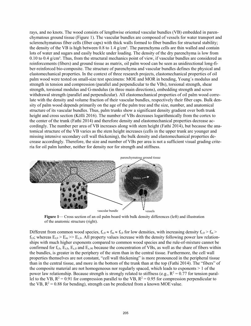
rays, and no knots. The wood consists of lengthwise oriented vascular bundles (VB) embedded in paren-chymatous ground tissue (Figure 1). The vascular bundles are composed of vessels for water transport and sclerenchymatous fiber cells (fiber caps) with thick walls formed to fiber bundles for structural stability; the density of the VB is high between 0.8 to 1.4 g/cm³. The parenchyma cells are thin walled and contain lots of water and sugars and easily buckle under loading. The density of the dry parenchyma is low from 0.10 to 0.4 g/cm³. Thus, from the structural mechanics point of view, if vascular bundles are considered as reinforcements (fibers) and ground tissue as matrix, oil palm wood can be seen as unidirectional long-fi-ber-reinforced bio-composite. The structure of parenchyma and vascular bundles defines the physical and elastomechanical properties. In the context of three research projects, elastomechanical properties of oil palm wood were tested on small-size test specimens: MOE and MOR in bending, Young´s modulus and strength in tension and compression (parallel and perpendicular to the VBs), torsional strength, shear strength, torsional modulus and G-modulus (in three main directions), embedding strength and screw withdrawal strength (parallel and perpendicular). All elastomechanical properties of oil palm wood corre-late with the density and volume fraction of their vascular bundles, respectively their fiber caps. Bulk den-sity of palm wood depends primarily on the age of the palm tree and the size, number, and anatomical structure of its vascular bundles. Thus, palm trunks show a significant density gradient over both trunk height and cross section (Kölli 2016). The number of VBs decreases logarithmically from the cortex to the center of the trunk (Fathi 2014) and therefore density and elastomechanical properties decrease ac-cordingly. The number per area of VB increases along with stem height (Fathi 2014), but because the ana-tomical structure of the VB varies as the stem height increases (cells in the upper trunk are younger and missing intensive secondary cell wall thickening), the bulk density and elastomechanical properties de-crease accordingly. Therefore, the size and number of VBs per area is not a sufficient visual grading crite-ria for oil palm lumber, neither for density nor for strength and stiffness.

Figure 1— Cross section of an oil palm board with bulk density differences (left) and illustration of the anatomic structure (right).

Different from common wood species, fc,0 ≈ fm ≈ ft,0 for low densities, with increasing density fc,0 > fm > ft,0; whereas Et,0 > Em >> Ec,0. All property values increase with the density following power law relation-ships with much higher exponents compared to common wood species and the rule-of-mixture cannot be confirmed for ft,0, Et,0, Ec,0 and Ec,90 because the concentration of VBs, as well as the share of fibers within the bundles, is greater in the periphery of the stem than in the central tissue. Furthermore, the cell wall properties themselves are not constant, “cell wall thickening” is more pronounced in the peripheral tissue than in the central tissue, and more in the bottom of the trunk than at the top (Fathi 2014). The “fibers” of the composite material are not homogeneous nor regularly spaced, which leads to exponents > 1 of the power law relationship. Because strength is strongly related to stiffness (e.g., R2 = 0.77 for tension paral-lel to the VB, R2 = 0.91 for compression parallel to the VB, R2 = 0.95 for compression perpendicular to the VB, R2 = 0.88 for bending), strength can be predicted from a known MOE value.

parenchymatous ground tissue

vessels vascular bundle

fibres

205

Due to the material availability as well as to the large property gradients over the cross section and the length of the lumber, the tensile properties of oil palm lumber (in component size) have been examined on 10 glulam lamellas (20 x 100 mm cross section) on a ZUMWALD – GEZU 850 tensile testing machine (850 kN) at heig-vd / HES-SO in Yverdon-les-Bains, Switzerland. The tensile strength is highly influ-enced by the property gradient within the lamellas and determined by the area with the lowest properties, respectively density. Therefore, testing the material properties (and of course industrial usage of the mate-rial) seems only reasonable for narrow strips with homogeneous properties, respectively density (or graded strips glued together to composite materials like lamellas, GLT, CLT, …). Because the grading parameters “cell wall thickening” and density are not visible, in addition to visual grading non-destructive test methods such as X-ray, ultrasonic testing or vibration measurements were evaluated in an exploratory study for kiln dried oil palm lumber.

Density Determination with X-Ray Technique

The most appropriate method to determine density is to X-ray along and across the board length. The ab-sorption of X-rays in materials is directly related to the material density (and dimensions). If properly cal-ibrated (Solbrig et al. 2014), existing X-ray devices could also be used for oil palm lumber. Along with the X-ray absorption-rate information, it is necessary to know the dimension and a homogeneous moisture content is needed. The density gradient over the width of oil palm boards was measured using the DENSE-LAB X from Electronic Wood Systems. An example for the density profile along the width is given in Figure 2. The peripheral board from the lower three meters of the trunk shows at the upper end around half of the density than at the lower end, the density gradient over the width is greater at the lower end. With regression functions between elastomechanical properties and density a calculation tool was developed to define density class boarders for ripping the boards lengthwise into strips with defined elas-tomechanical properties.

Figure 2— Density gradient (without smoothing) over the width of oil palm boards measured with the DENSE-LAB X. Peripheral board from the lower three meters of the trunk, lower end (at left) and upper end (at right).

Grading Dry Lumber using Ultrasonic and Vibration Measurements

The applicability of ultrasonic and natural frequency measurements for grading purposes of oil palm wood were evaluated by comparing the dynamic MOE from ultrasound (MOEUS) and longitudinal (MOENF, long) as well as flexural vibration (MOENF, flex) with static MOE (MOEstat) using a three-point-bending test (span-to-depth ratio of 50) and bulk density. Studies on coconut palm wood (Wolters et al. 2015) and oil palm wood (Götza 2016) showed significant effects of the span-to-depth ratio on the static MOE up to a span-to-depth ratio of 40.

0

100

200

300

400

500

600

700

800

900

0 20 40 60 80 100 120

ρ[k

g/m³

]

width [mm]

0

50

100

150

200

250

300

350

0 20 40 60 80 100 120 140 160

ρ[k

g/m³

]

width [mm]

206

To examine the influence of different span-to-depth ratios in the three-point-bending test (span-to-depth ratio up to 50), 120 small-sized specimens (1,150 × 22 × 22 mm³) were prepared from dry material (origin Kluang, Malaysia) using preferably even cross-sectional bulk density distribution. All samples were con-ditioned to a constant weight at 20 °C and 65 % relative humidity.

For all test specimens, ultrasonic time-of-flight and natural frequency were measured with subsequent dy-namic modulus of elasticity (MOEdyn) computation. Ultrasonic time-of-flight measurements in longitudi-nal direction were carried out using the ultrasonic device STEINKAMP BP 5, with plane and conical probes for longitudinal waves (50 kHz). Coupling was performed directly without a coupling agent. The samples were fixed free-floating between spring-loaded conical probes in order to keep testing conditions (especially contact pressure) constant. MOE computation was done following the equation presented by Steiger (1991). The natural frequency of longitudinal and flexural vibrations was determined using Grin-doSonic MK5, J.W. Lemmens N.V. (MOENF, long and MOENF, flex). Longitudinal vibrations were used to compare the ultrasound results (MOEUS). Flexural vibrations were determined to illustrate the differences between respective vibration modes and for the comparison with the three-point bending test. During vi-bration measurements, the test specimens were supported on rectangular foam stripes in the region of the nodal points. Impulse was initiated using a small impact hammer. Dynamic MOE for flexural and longitu-dinal vibrations were calculated following the equations presented by Görlacher (1984). Because of higher frequencies, the flexural vibrations on large-sized test specimens were determined by the 3rd order vibration. The low frequencies resulting from the large dimensions of the boards of the 1st order vibra-tions could not be detected by the testing device. Three-point-bending tests (using a support span of 50 × thickness) were carried out on the small-sized test specimens for comparative purposes.

Figure 3 shows a strong correlation between the ultrasonic velocity and MOR (R2 = 0.7) and the fre-quency from longitudinal/ flexural vibration and the MOR (R2 = 0.8 and R2 = 0.7).

Figure 3— Relation between ultrasonic velocity respectively natural frequency from longitudi-nal/flexural vibration and MOR.

Ultrasonic velocity and natural frequency are the basis for calculating the dynamic MOE. To evaluate ul-trasonic velocity and natural frequency as an own grading criteria, their relation to bulk density is ana-lyzed in Figure 4. Both dynamic methods show a strong correlation with R² = 0.6 (ultrasonic velocity / natural frequency with longitudinal vibration) and a moderate correlation with R² = 0.5 for natural fre-quency with flexural vibration (3rd order).

Natural frequency [2]:(longitudinal measurements)

y = 30.018x + 1003.6R² = 0.769

Natural frequency [3]:(flexural measurements 3rd oder)

y = 5.0948x + 208.14R² = 0.7445

Ultrasonic [1]:(conical probes)

y = 0.0641x + 2.6577R² = 0.6618

0

1

2

3

4

5

6

7

0

500

1000

1500

2000

2500

0 10 20 30 40 50 60

soun

d ve

loci

tyU

S[k

m/s

]

freq

uenc

y NF,

flex

, lon

g [H

z]

MOR [MPa]

[1]

[2]

[3]

207

Divergence of absolute dynamic and static MOE values with increasing bulk density becomes obvious in Figure 5. Furthermore, a strong correlation between all dynamic MOEs, respectively the static MOE and the density, is shown.

Figure 4— Relation between sound velocity by ultrasonic respectively natural frequency with lon-gitudinal/flexural vibration and bulk density.

Figure 5— Relation between dynamic MOEs by ultrasonic respectively natural frequency with longitudinal vibration and static MOE by bending test.

The close linear relation between both dynamic MOE and static MOE is apparent in Figure 6 (R2 = 0.96 for ultrasonic, R2 = 0.99 for natural frequency measurement with longitudinal vibration and R2 = 0.98 for

Natural frequency [2]:(longitudinal measurements)

y = 2.7559x + 514.4R² = 0.5215

Natural frequency [3]:(flexural measurements 3rd order)....

y = 0.5275x + 106.18R² = 0.6313

Ultrasonic [1]:(conical probes)

y = 0.0066x + 1.3797R² = 0.578

0

1

2

3

4

5

6

7

0

500

1000

1500

2000

2500

3000

100 200 300 400 500 600

soun

d ve

loci

tyU

S[k

m/s

]

freq

uenc

y NF,

flex

, lon

g[H

z]

density [kg/m³]

[1][2]

[3]

Ultrasonic [1]:(conical probes)

y = 29.982x - 5189.9R² = 0.8109

Natural frequency [2]: (longitudinal measurement):

y = 26.689x - 4811.1R² = 0.7567

Natural frequency [3]:m(flexural measurements)m

y = 22,511x - 4005.9R² = 0.8295

Static bending test [4]: (span-to-depth ratio l/h=50):

y = 22.297x - 4066.9R² = 0.7829

0

1000

2000

3000

4000

5000

6000

7000

8000

9000

10000

11000

12000

13000

150 200 250 300 350 400 450 500 550

MO

E dyn

(US;

NF,

long

, fle

x) &

MO

E sta

tic [M

Pa]

density [kg/m³]

[1]

[2]

[3][4]

208

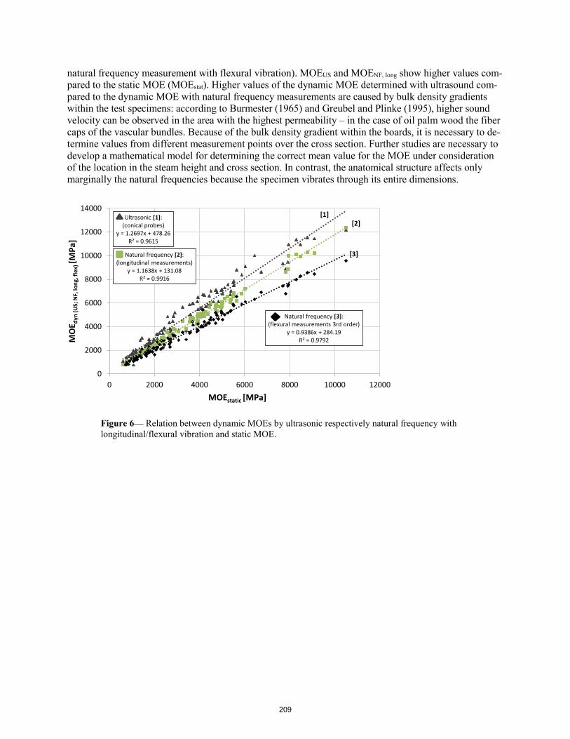
natural frequency measurement with flexural vibration). MOEUS and MOENF, long show higher values com-pared to the static MOE (MOEstat). Higher values of the dynamic MOE determined with ultrasound com-pared to the dynamic MOE with natural frequency measurements are caused by bulk density gradients within the test specimens: according to Burmester (1965) and Greubel and Plinke (1995), higher sound velocity can be observed in the area with the highest permeability – in the case of oil palm wood the fiber caps of the vascular bundles. Because of the bulk density gradient within the boards, it is necessary to de-termine values from different measurement points over the cross section. Further studies are necessary to develop a mathematical model for determining the correct mean value for the MOE under consideration of the location in the steam height and cross section. In contrast, the anatomical structure affects only marginally the natural frequencies because the specimen vibrates through its entire dimensions.

Figure 6— Relation between dynamic MOEs by ultrasonic respectively natural frequency with longitudinal/flexural vibration and static MOE.

Ultrasonic [1]:(conical probes)

y = 1.2697x + 478.26R² = 0.9615

Natural frequency [2]:(longitudinal measurements)

y = 1.1638x + 131.08R² = 0.9916

Natural frequency [3]:(flexural measurements 3rd order)

y = 0.9386x + 284.19R² = 0.9792

0

2000

4000

6000

8000

10000

12000

14000

0 2000 4000 6000 8000 10000 12000

MO

E dyn

(US;

NF,

long

, fle

x) [M

Pa]

MOEstatic [MPa]

[1][2]

[3]

209

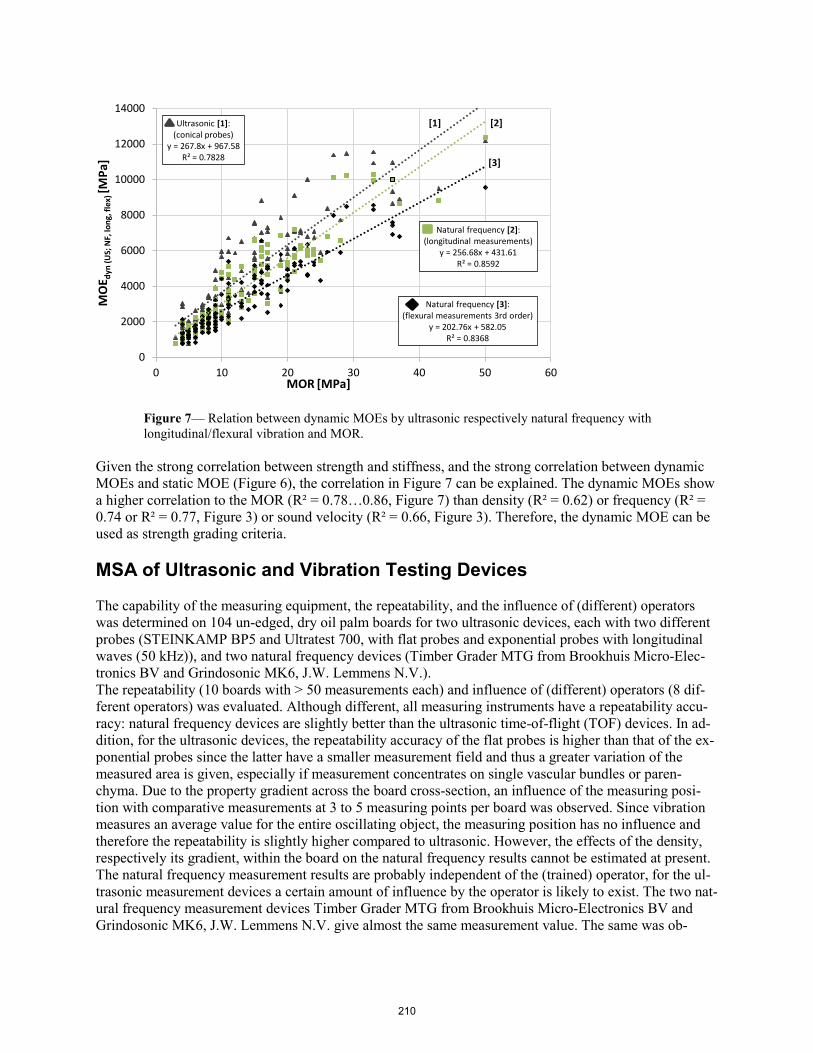
Figure 7— Relation between dynamic MOEs by ultrasonic respectively natural frequency with longitudinal/flexural vibration and MOR.

Given the strong correlation between strength and stiffness, and the strong correlation between dynamic MOEs and static MOE (Figure 6), the correlation in Figure 7 can be explained. The dynamic MOEs show a higher correlation to the MOR (R² = 0.78…0.86, Figure 7) than density (R² = 0.62) or frequency (R² = 0.74 or R² = 0.77, Figure 3) or sound velocity (R² = 0.66, Figure 3). Therefore, the dynamic MOE can be used as strength grading criteria.

MSA of Ultrasonic and Vibration Testing Devices

The capability of the measuring equipment, the repeatability, and the influence of (different) operators was determined on 104 un-edged, dry oil palm boards for two ultrasonic devices, each with two different probes (STEINKAMP BP5 and Ultratest 700, with flat probes and exponential probes with longitudinal waves (50 kHz)), and two natural frequency devices (Timber Grader MTG from Brookhuis Micro-Elec-tronics BV and Grindosonic MK6, J.W. Lemmens N.V.). The repeatability (10 boards with > 50 measurements each) and influence of (different) operators (8 dif-ferent operators) was evaluated. Although different, all measuring instruments have a repeatability accu-racy: natural frequency devices are slightly better than the ultrasonic time-of-flight (TOF) devices. In ad-dition, for the ultrasonic devices, the repeatability accuracy of the flat probes is higher than that of the ex-ponential probes since the latter have a smaller measurement field and thus a greater variation of the measured area is given, especially if measurement concentrates on single vascular bundles or paren-chyma. Due to the property gradient across the board cross-section, an influence of the measuring posi-tion with comparative measurements at 3 to 5 measuring points per board was observed. Since vibration measures an average value for the entire oscillating object, the measuring position has no influence and therefore the repeatability is slightly higher compared to ultrasonic. However, the effects of the density, respectively its gradient, within the board on the natural frequency results cannot be estimated at present. The natural frequency measurement results are probably independent of the (trained) operator, for the ul-trasonic measurement devices a certain amount of influence by the operator is likely to exist. The two nat-ural frequency measurement devices Timber Grader MTG from Brookhuis Micro-Electronics BV and Grindosonic MK6, J.W. Lemmens N.V. give almost the same measurement value. The same was ob-

Ultrasonic [1]:(conical probes)

y = 267.8x + 967.58R² = 0.7828

Natural frequency [2]:(longitudinal measurements)

y = 256.68x + 431.61R² = 0.8592

Natural frequency [3]:(flexural measurements 3rd order)

y = 202.76x + 582.05R² = 0.8368

0

2000

4000

6000

8000

10000

12000

14000

0 10 20 30 40 50 60

MO

E dyn

(US;

NF,

long

, fle

x) [M

Pa]

MOR [MPa]

[1] [2]

[3]

210

served for coconut palm wood with the Viscan from Microtec. When comparing the dynamic MOE val-ues, significantly lower values are obtained from vibration measurements compared to those from ultra-sonic measurements. This was observed earlier for oil palm wood (see above) and for common wood spe-cies.

Conclusion

For the grouping of wood with defined elastomechanical properties, it is advisable to rip the boards lengthwise and transversely into strips based on density using X-ray measurements. The strips should be graded according to their density and, if necessary, their dynamic modulus of elasticity and glued together based on their properties to produce laminated elements. In general, both ultrasonic and natural frequency measurements in longitudinal and flexural vibration are suitable for developing industrial strength grading of dry oil palm lumber. Flexural 3rd order vibration measurements are appropriate especially for tests conducted under laboratory conditions with a large length to thickness ratio. To achieve reliable data for large-sized timber, the boards must be square-edged. Longitudinal vibrations seem well suited to determine the dynamic MOE of dry large-sized specimens in component dimensions in an industrial production environment. For an industrial application, the in-line implementation of natural frequency measurements is less complicated than for ultrasonic devices. A high speed in-line system for industrial applications needs to be developed. In cases involving small-sized specimens the coupling of conical ultrasonic probes on either ground tissue or vascular bundles, ultrasonic coupling leads to high variation of measurements results (Wolters et al. 2015). Therefore, flat probes, especially for large-sized lumber, have to be examined further in an indus-trial context.

Acknowledgments

The author thankfully acknowledges the financial support provided by the German Federal Ministry of Education and Research, project 02PK2458 and project 031B0767A and the German Development Agency, project ´OPT in Asia´.

References

Burmester, A. 1965. Zusammenhang zwischen Schallgeschwindigkeit und morphologischen, physikalischen und mechanischen Eigenschaften von Holz. Holz als Roh- und Werkstoff. 23(6): 227-236.

Fathi, L. 2014. Structural and Mechanical Properties of the Wood from Coconut Palms, Oil Palms and Date Palms. University Hamburg, Germany. 248 p. PhD thesis.

Görlacher, R. 1984. Ein neues Meßverfahren zur Bestimmung des Elastizitätsmoduls von Holz. European Journal of Wood and Wood Products. Springer, Berlin, Germany 42(6): 219-222.

Götza, M. 2016. Einfluss des Schubmoduls bei der Ermittlung des Elastizitätsmoduls von Ölpalmenholz im statischen Biegeversuch. University of Applied Science Ostwestfalen-Lippe, Lemgo, Germany. Unpublished B.Sc. thesis.

Götza, M. 2018. Beitrag zur Messmittelanalyse von zerstörungsfreien Messsystemen am Holz der Ölpalme. University of Applied Science Ostwestfalen-Lippe, Lemgo, Germany. Unpublished report of the Scientific Internship.

211

Greubel, D.; Plinke, B. 1995. Zerstörungsfreie Festigkeitsuntersuchungen an Spanplatten mit Ultraschallmeßtechniken. Holz als Roh-und Werkstoff. 53(3): 193-200.

Harnisch, J. 2016. Untersuchungen zum Trocknungsverhalten von Ölpalmen-Schnittholz. University of Hamburg, Germany. M.Sc. thesis.

Kölli, N. 2016. Density and Moisture Distribution in Oil Palm Trunks from Peninsular Malaysia. University Hamburg, Germany. Unpublished B.Sc. thesis.

Solbrig, K., Fuchs, M., Frühwald, K., Ressel, J. B. 2014. Accuracy of the radiometric determination of raw density gradients on wood-based composites. Holztechnologie 55(6): 27-34.

Steiger, R. 1991. Festigkeitssortierung von Kantholz mittels Ultraschall. Holzforschung und Holzverwertung. Österreichische Gesellschaft für Holzforschung, Vienna, Austria. 43(2): 40-46.

Wolters, M.; Hüls, T.; Solbrig, K.; Frühwald, K. 2015. Nondestructive evaluation of coconut palm wood by means of ultrasonic and natural frequency methods. In: Proceedings: 19th International Nondestructive Testing and Evaluation of Wood Symposium, Rio de Janeiro, Brazil, United States Department of Agriculture General Technical Report FPL-GTR-239: 618-625.

212

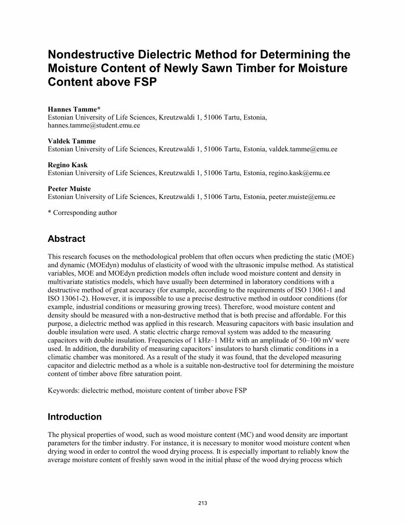
Nondestructive Dielectric Method for Determining the Moisture Content of Newly Sawn Timber for Moisture Content above FSP Hannes Tamme* Estonian University of Life Sciences, Kreutzwaldi 1, 51006 Tartu, Estonia, hannes.tamme@student.emu.ee Valdek Tamme Estonian University of Life Sciences, Kreutzwaldi 1, 51006 Tartu, Estonia, valdek.tamme@emu.ee Regino Kask Estonian University of Life Sciences, Kreutzwaldi 1, 51006 Tartu, Estonia, regino.kask@emu.ee Peeter Muiste Estonian University of Life Sciences, Kreutzwaldi 1, 51006 Tartu, Estonia, peeter.muiste@emu.ee * Corresponding author Abstract This research focuses on the methodological problem that often occurs when predicting the static (MOE) and dynamic (MOEdyn) modulus of elasticity of wood with the ultrasonic impulse method. As statistical variables, MOE and MOEdyn prediction models often include wood moisture content and density in multivariate statistics models, which have usually been determined in laboratory conditions with a destructive method of great accuracy (for example, according to the requirements of ISO 13061-1 and ISO 13061-2). However, it is impossible to use a precise destructive method in outdoor conditions (for example, industrial conditions or measuring growing trees). Therefore, wood moisture content and density should be measured with a non-destructive method that is both precise and affordable. For this purpose, a dielectric method was applied in this research. Measuring capacitors with basic insulation and double insulation were used. A static electric charge removal system was added to the measuring capacitors with double insulation. Frequencies of 1 kHz–1 MHz with an amplitude of 50–100 mV were used. In addition, the durability of measuring capacitors’ insulators to harsh climatic conditions in a climatic chamber was monitored. As a result of the study it was found, that the developed measuring capacitor and dielectric method as a whole is a suitable non-destructive tool for determining the moisture content of timber above fibre saturation point. Keywords: dielectric method, moisture content of timber above FSP Introduction The physical properties of wood, such as wood moisture content (MC) and wood density are important parameters for the timber industry. For instance, it is necessary to monitor wood moisture content when drying wood in order to control the wood drying process. It is especially important to reliably know the average moisture content of freshly sawn wood in the initial phase of the wood drying process which

213

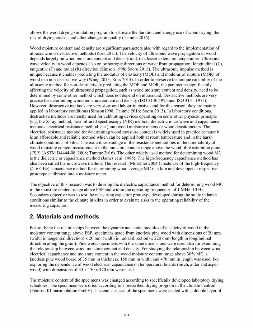
allows the wood drying simulation program to estimate the duration and energy use of wood drying, the risk of drying cracks, and other changes in quality (Tamme 2016). Wood moisture content and density are significant parameters also with regard to the implementation of ultrasonic non-destructive methods (Ross 2015). The velocity of ultrasonic wave propagation in wood depends largely on wood moisture content and density and, to a lesser extent, on temperature. Ultrasonic wave velocity in wood depends also on orthotropic directions of wave front propagation: longitudinal (L), tangential (T) and radial (R) direction (Simson 1998; Sooru 2013). The ultrasonic impulse method is unique because it enables predicting the modulus of elasticity (MOE) and modulus of rupture (MOR) of wood in a non-destructive way (Wang 2013; Ross 2015). In order to preserve the unique capability of the ultrasonic method for non-destructively predicting the MOE and MOR, the parameters significantly affecting the velocity of ultrasound propagation, such as wood moisture content and density, need to be determined by some other method which does not depend on ultrasound. Destructive methods are very precise for determining wood moisture content and density (ISO 3130:1975 and ISO 3131:1975). However, destructive methods are very slow and labour-intensive, and for this reason, they are mainly applied in laboratory conditions (Simson1998; Tamme 2016; Sooru 2013). In laboratory conditions, destructive methods are mostly used for calibrating devices operating on some other physical principle (e.g. the X-ray method, near infrared spectroscopy (NIR) method, dielectric microwave and capacitance methods, electrical resistance method, etc.) into wood moisture meters or wood densitometers. The electrical resistance method for determining wood moisture content is widely used in practice because it is an affordable and reliable method which can be applied both at room temperature and in the harsh climate conditions of kilns. The main disadvantage of the resistance method lies in the unreliability of wood moisture content measurement in the moisture content range above the wood fibre saturation point (FSP) (ASTM D4444-08. 2008; Tamme 2016). The other widely used method for determining wood MC is the dielectric or capacitance method (James et al. 1985). The high-frequency capacitance method has also been called the microwave method. The research (Moschler 2004 ) made use of the high-frequency (4–6 GHz) capacitance method for determining wood average MC in a kiln and developed a respective prototype calibrated into a moisture meter. The objective of this research was to develop the dielectric capacitance method for determining wood MC in the moisture content range above FSP and within the operating frequencies of 1 MHz–10 Hz. Secondary objective was to test the measuring capacitor prototype developed during the study in harsh conditions similar to the climate in kilns in order to evaluate risks to the operating reliability of the measuring capacitor. 2. Materials and methods For studying the relationships between the dynamic and static modulus of elasticity of wood in the moisture content range above FSP, specimens made from knotless pine wood with dimensions of 20 mm (width in tangential direction) x 20 mm (width in radial direction) x 220 mm (length in longitudinal direction along the grain). Pine wood specimens with the same dimensions were used also for examining the relationship between wood moisture content and density. For studying the relationship between wood electrical capacitance and moisture content in the wood moisture content range above 30% MC, a knotless pine wood board of 35 mm in thickness, 150 mm in width and 470 mm in length was used. For exploring the dependence of wood electrical capacitance on temperature, boards (birch, alder and aspen wood) with dimensions of 35 x 150 x 470 mm were used. The moisture content of the specimens was changed according to specifically developed laboratory drying schedules. The specimens were dried according to a prescribed drying program in the climate Feutron (Feutron Klimasimulation GmbH). The end surfaces of the specimens were coated with a double layer of

214

nitro lacquer and additionally with aluminium foil to prevent moisture loss while drying. The used drying programs were supposed to ensure differences as small as possible (moisture gradients) in the specimens. For drying small specimens with dimensions of 20 x 20 x 220 mm, the drying program specified in the paper (Sooru 2013) was used. For drying large specimens with dimensions of 35 x 150 x 470 mm, the drying program specified in the paper (Tamme 2016) was used in the case of all four tree species used in the experiments. To determine the average moisture content of wood, the specimens were weighed at various randomly selected moments of time in the drying process using the weight Precisa with a resolution of 0.1 g. Other required measurements (the volume of the specimens, ultrasonic velocity, static modulus of elasticity and electrical capacitance) were carried out immediately after weighing. Finally, the oven-dry weight of the specimens was determined and the absolute moisture content of the specimens calculated by a well-known formula: he paper should be 4 to 8 pages in length, including figures, tables, acknowledgments, references, abbreviations list, and any other material.

100⋅−

=B

BAWabs (1)

where A is weight of wet wood specimen and B is weight of absolutely dry wood specimen. The mathematical relationships between wood moisture content and density are presented in the reference work (Ross 2010). If the specimen has a moisture content m, the density of the specimen is expressed as:

(2)

where ρwood is relative density of the specimen and Sm is volume shrinkage of the wood of the specimen from wet wood to wood moisture content m. The relationship between wood MC and density as adapted for use only above FSP is given in the paper (Briggs et al. 2005): 𝜌𝜌 = 𝜌𝜌𝐻𝐻20 ∗ 𝑆𝑆𝐺𝐺𝑔𝑔 ∗ (1 +𝑀𝑀Cod) (3) where ρ is density (kg/m3 ), ρH2O is water density (kg/m3 ), SGg is wood relative density and MCod is wood moisture content (owen dry basis, in decimal form). The formula (3) is derived from the formula (2), if the volume shrinkage of wood Sm is equalled to zero. However, the topic of the relationship between MC and density of wood with theoretical formulae (2 and 3) is still under discussion. In fact, MC and density of wood are measurable in the experiment, both of them have their random and sometimes also a systematic error of measurement (Laaneots and Mathiesen, 2006). Regression analysis of measurement results indirectly considers the characteristics of tree species as well as the influence of possible moisture gradients in wood. Therefore, the actual relationship between MC and density is shown by the measuring function obtained as a result of the regression analysis (ISO 3534-1:1993). Theory may only describe apparent trends. The same logic applies also in the case of other theoretical expressions (e.g. formulae of the dynamic and static modulus of elasticity) used in the paper. The static modulus of elasticity of wood was determined with the testing machine Instron 3369 according to the standard (ISO 3349:1975). The static modulus of elasticity for a single specific specimen is expressed by the formula:

)1(

)100

1(

mwoodm S

m

−

+= ρρ

215

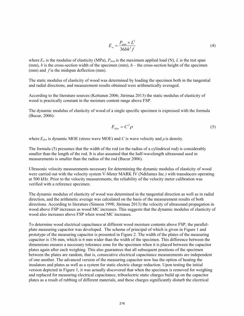
(4)

where Ew is the modulus of elasticity (MPa), Pmax is the maximum applied load (N), L is the test span (mm), b is the cross-section width of the specimen (mm), h – the cross-section height of the specimen (mm) and f is the midspan deflection (mm). The static modulus of elasticity of wood was determined by loading the specimen both in the tangential and radial directions, and measurement results obtained were arithmetically averaged. According to the literature sources (Kettunen 2006; Jürimaa 2013) the static modulus of elasticity of wood is practically constant in the moisture content range above FSP. The dynamic modulus of elasticity of wood of a single specific specimen is expressed with the formula (Bucur, 2006): ρ2CEdyn = (5) where Edyn is dynamic MOE (stress wave MOE) and C is wave velocity and ρ is density. The formula (5) presumes that the width of the rod (or the radius of a cylindrical rod) is considerably smaller than the length of the rod. It is also assumed that the half-wavelength ultrasound used in measurements is smaller than the radius of the rod (Bucur 2006). Ultrasonic velocity measurements necessary for determining the dynamic modulus of elasticity of wood were carried out with the velocity system V-Meter MARK IV (NdtJames Inc.) with transducers operating at 500 kHz. Prior to the velocity measurements, the reliability of the velocity meter calibration was verified with a reference specimen. The dynamic modulus of elasticity of wood was determined in the tangential direction as well as in radial direction, and the arithmetic average was calculated on the basis of the measurement results of both directions. According to literature (Simson 1998; Jürimaa 2013) the velocity of ultrasound propagation in wood above FSP increases as wood MC increases. This suggests that the dynamic modulus of elasticity of wood also increases above FSP when wood MC increases. To determine wood electrical capacitance at different wood moisture contents above FSP, the parallel-plate measuring capacitor was developed. The scheme of principal of which is given in Figure 1 and prototype of the measuring capacitor is presented in Figure 2. The width of the plates of the measuring capacitor is 156 mm, which is 6 mm wider than the width of the specimen. This difference between the dimensions ensures a necessary tolerance zone for the specimen when it is placed between the capacitor plates again after each weighing. This also guarantees that all subsequent positions of the specimen between the plates are random, that is, consecutive electrical capacitance measurements are independent of one another. The advanced version of the measuring capacitor now has the option of heating the insulators and plates as well as a system for static electric charge reduction. Upon testing the initial version depicted in Figure 1, it was actually discovered that when the specimen is removed for weighing and replaced for measuring electrical capacitance, triboelectric static charges build up on the capacitor plates as a result of rubbing of different materials, and these charges significantly disturb the electrical

fbhLPEw 3

3max

36×

=

216

Figure 1—Circuit diagram for determining the electrical capacitance of the parallel-plate measuring capacitor. 1 - signal connector, 2 - capacitor plate, 3 - wood specimen, 4 - capacitor insulator, FRA - frequency response analyser

Figure 2—Photo of the measuring capacitor prototype. 1 - signal connector, 2 - capacitor plate, 3 - wood specimen, 4 - capacitor insulator

capacitance measurement process. The prototype of the measuring capacitor with parallel plates was additionally tested in the climate chamber Feutron under conditions similar to the climate in kilns. The experiments were carried out at a temperature of 50 degrees Celsius and at relative air humidity of RH=98%. The purpose of these experiments was to verify the operating reliability of the measuring capacitor in harsh climate conditions. Based on literature ((Moschler 2004) the prototype of a microwave parallel-plate measuring capacitor was tested at room temperature as well as at temperatures of 40°C and 60°C. Data regarding the air humidity in the chamber during the experiments are unavailable in the given literature source. Electrical capacitance measurements in this paper were done with the capacitance meter LCR-55 (Wavetek Meterman). The operating frequency of the LCR-55 capacitance meter was 1,000 Hz as measured with an oscilloscope. More precise values of electrical capacitance were calculated according to the measurement data of impedance spectrometry with the formula (7). The impedance analyser AUTOLAB PGSTAT 302N with the software NOVA 1.8 (MetrOhm Autolab) was used. Any interference in the operating reliability of the measuring capacitor during testing in harsh climate conditions was registered with impedance spectra. Frequency scanning within 1 MHz–10 Hz and the sinusoidal signal amplitude of 50 and 100 mV were applied. Twenty frequencies were used for a single spectrum, whereas the selected frequency range was distributed over a logarithmic scale. The direct voltage component was not added to the sinusoid signal.

217

Impedance spectrometry is an informative measuring technique for analysing several electrical processes (Krause 2003). Impedance has a magnitude (ZA = EA/IA) and phase angle and is thus a vector quantity Z = ZA(cos Φ + jsin Φ) = Z’ + jZ’’ (6) where j= √-1 , Z’ is the real part of impedance, ZA is the amplitude of impedance and Z’’ the imaginary part of impedance. If sinusoidal voltage is applied across a pure capacitor, impedance can be calculated according to the relationship

1 jj

ZC Cω ω

= = − (7)

where C is the capacitance and the phase angle Φ = −900, that is, impedance depends on frequency and is entirely imaginary (Krause 2003). 3. Results and discussion Based on the data presented in the paper (Jürimaa, 2013), the following regression model may be developed for predicting the static modulus of elasticity with its parameters given in Table 1, row CM4, and graphical depiction in Figure 3. Table 1—Regression models for non-destructively predicting wood moisture content, wood density and the static modulus of elasticity of wood in the moisture content range above the fibre saturation point (that is, above 30% MC) Obs. No Model type,

(Fig. No) Model equations, fitting curve and narrow (RMSE) interval

R2 p- value

RMSE

N=25 C(pF)~MC(%) Fig. 6

f(x) = p1x + p2 ; p1 = 1.075; p2 = -194.3 ylower = 1.097x - 202.4 yupper = 1.053x -186.3

0.97 <0.001 3.8

N=24 MC(%)~density Fig. 4

f(x) = p1x + p2 ; p1 = 0.004166; p2 = 0.5675 ylower = 0.004138 x + 0.5506 yupper = 0.004193 x + 0.5844

0.94 <0.001 0.026

N=24 Edyn~a/Edyn Fig. 5

f (x) = p1x2 + p2x + p3 p1 = 7.164e-06; p2 = -0.02453; p3 = 27.2 ylower = 6.601e-06 x2 - 0.02321x + 26.38 yupper = 7.727e-06 x2 - 0.02584 x + 28.03

0.999 <0.001 0.078

N=24 Edyn~Estat Fig. 3

f(x) = -1.5114x + 11338

0.32 <0.001 466.5

The model only describes 32% of the variability of properties (R2 = 0.32). This figure is clearly insufficient and therefore, possibilities for improving the model should be explored. Analysis of the

218

formula (5) indicates that quantities included the formula, such as ρ (density) and Edyn (dynamic modulus of elasticity), could be predicted separately and in stages by applying good-quality measuring models (ISO 3534-1:1993) or calibration models (CM). The R2 of the calibration models could be at least 0.94–0.99.

Figure 3—Direct prediction of the static modulus of elasticity (MOE static) via the dynamic modulus of elasticity (data source: Jürimaa 2013). The independent x-variable of the model is Edyn. Number of repeated measurements N=24

At first, density was predicted on the basis of wood moisture content. The respective calibration function along with essential parameters is given in Table 1, row CM2 and in Figure 4. Since the moisture content in model CM2 must be determined by a non-destructive method independent of ultrasound, a calibration function with sufficiently good quality (CM1) was developed for determining wood moisture content in a non-destructive manner on the basis of wood electrical capacitance measurement results. Essential parameters of the calibration model CM1 are presented in Table 1, row CM1. CM1 is graphically depicted in Figure 6.

Figure 4—Regression model MC(%)~density(g/cm3). The independent x-variable of the model is MC(%). Number of repeated measurements N=24

In conclusion, the calibration function CM3 was prepared for determining the ratio a/Edyn. Essential parameters of the model CM3 are given in Table 1, row CM3. CM3 is graphically depicted in Figure 5. When the ratio is known, it is easy to express from it the static modulus of elasticity given as the constant a (a=Estatic).

y = -1.5114x + 11338R² = 0.3243

8000850090009500

100001050011000

500 1500 2500

Esta

t (M

Pa)

Edyn (MPa)

E stat

Linear (Estat)

20 40 60 80 100 120 140

Wood moisture content ( %)

0.6

0.7

0.8

0.9

1

1.1

1.2

Woo

d de

nsity

(g/c

m3)

R 2 = 0.94

RMSE = 0.026

Confidence 95%

Data (24points)

219

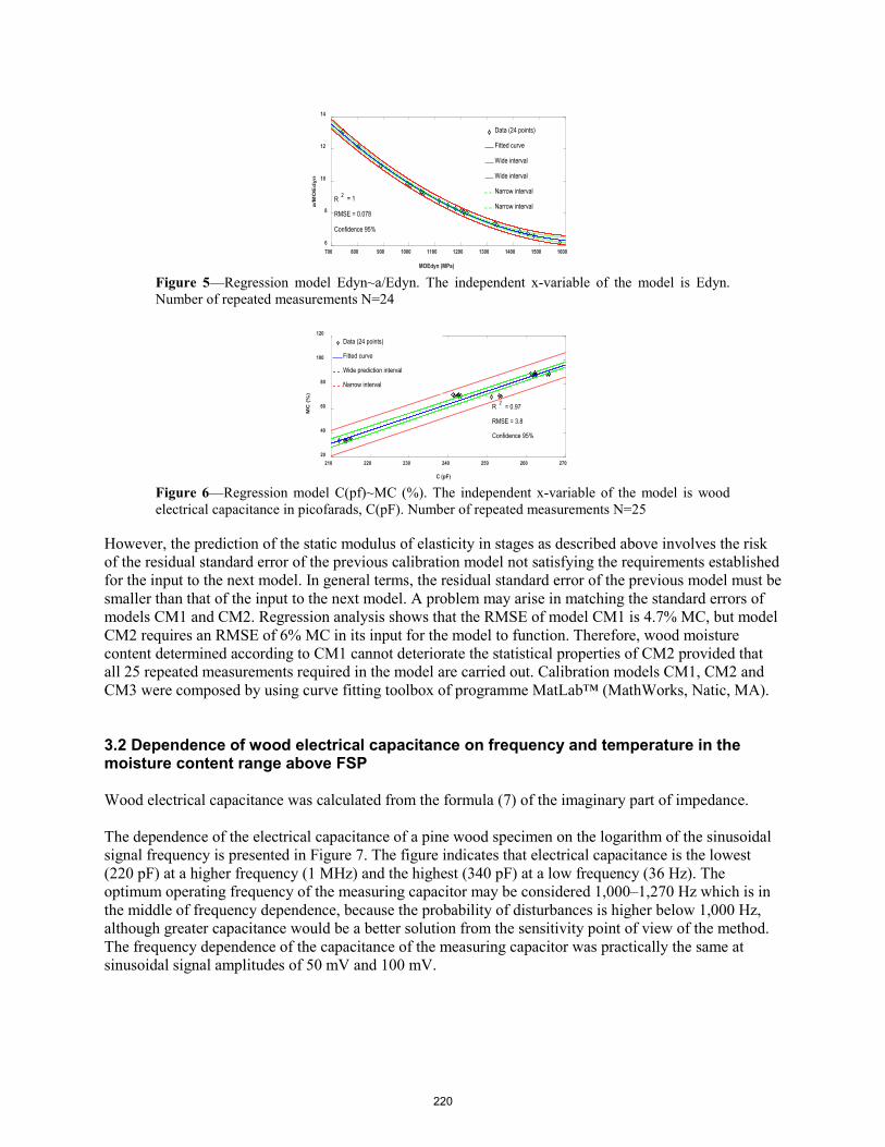
Figure 5—Regression model Edyn~a/Edyn. The independent x-variable of the model is Edyn. Number of repeated measurements N=24

Figure 6—Regression model C(pf)~MC (%). The independent x-variable of the model is wood electrical capacitance in picofarads, C(pF). Number of repeated measurements N=25

However, the prediction of the static modulus of elasticity in stages as described above involves the risk of the residual standard error of the previous calibration model not satisfying the requirements established for the input to the next model. In general terms, the residual standard error of the previous model must be smaller than that of the input to the next model. A problem may arise in matching the standard errors of models CM1 and CM2. Regression analysis shows that the RMSE of model CM1 is 4.7% MC, but model CM2 requires an RMSE of 6% MC in its input for the model to function. Therefore, wood moisture content determined according to CM1 cannot deteriorate the statistical properties of CM2 provided that all 25 repeated measurements required in the model are carried out. Calibration models CM1, CM2 and CM3 were composed by using curve fitting toolbox of programme MatLab™ (MathWorks, Natic, MA). 3.2 Dependence of wood electrical capacitance on frequency and temperature in the moisture content range above FSP Wood electrical capacitance was calculated from the formula (7) of the imaginary part of impedance. The dependence of the electrical capacitance of a pine wood specimen on the logarithm of the sinusoidal signal frequency is presented in Figure 7. The figure indicates that electrical capacitance is the lowest (220 pF) at a higher frequency (1 MHz) and the highest (340 pF) at a low frequency (36 Hz). The optimum operating frequency of the measuring capacitor may be considered 1,000–1,270 Hz which is in the middle of frequency dependence, because the probability of disturbances is higher below 1,000 Hz, although greater capacitance would be a better solution from the sensitivity point of view of the method. The frequency dependence of the capacitance of the measuring capacitor was practically the same at sinusoidal signal amplitudes of 50 mV and 100 mV.

700 800 900 1000 1100 1200 1300 1400 1500 1600

MOEdyn (MPa)

6

8

10

12

14

a/M

OE

dyn

R 2 = 1

RMSE = 0.078

Confidence 95%

Data (24 points)

Fitted curve

Wide interval

Wide interval

Narrow interval

Narrow interval

210 220 230 240 250 260 270

C (pF)

20

40

60

80

100

120

MC

(%

)

R 2 = 0.97

RMSE = 3.8

Confidence 95%

Data (24 points)

Fitted curve

Wide prediction interval

Narrow interval

220

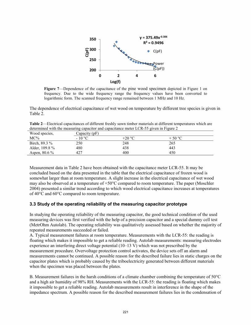
Figure 7—Dependence of the capacitance of the pine wood specimen depicted in Figure 1 on frequency. Due to the wide frequency range the frequency values have been converted to logarithmic form. The scanned frequency range remained between 1 MHz and 10 Hz.

The dependence of electrical capacitance of wet wood on temperature by different tree species is given in Table 2. Table 2—Electrical capacitances of different freshly sawn timber materials at different temperatures which are determined with the measuring capacitor and capacitance meter LCR-55 given in Figure 2 Wood species, MC%

Capacity (pF) - 10 °C +20 °C + 50 °C

Birch, 89.3 % 250 248 265 Alder, 109.8 % 480 438 443 Aspen, 80.6 % 427 400 450 Measurement data in Table 2 have been obtained with the capacitance meter LCR-55. It may be concluded based on the data presented in the table that the electrical capacitance of frozen wood is somewhat larger than at room temperature. A slight increase in the electrical capacitance of wet wood may also be observed at a temperature of +50°C compared to room temperature. The paper (Moschler 2004) presented a similar trend according to which wood electrical capacitance increases at temperatures of 40°C and 60°C compared to room temperature. 3.3 Study of the operating reliability of the measuring capacitor prototype In studying the operating reliability of the measuring capacitor, the good technical condition of the used measuring devices was first verified with the help of a precision capacitor and a special dummy cell test (MetrOhm Autolab). The operating reliability was qualitatively assessed based on whether the majority of repeated measurements succeeded or failed. A. Typical measurement failures at room temperature. Measurements with the LCR-55: the reading is floating which makes it impossible to get a reliable reading. Autolab measurements: measuring electrodes experience an interfering direct voltage potential (10–13 V) which was not prescribed by the measurement procedure. Overvoltage protection control activates, the device sets off an alarm and measurements cannot be continued. A possible reason for the described failure lies in static charges on the capacitor plates which is probably caused by the triboelectricity generated between different materials when the specimen was placed between the plates. B. Measurement failures in the harsh conditions of a climate chamber combining the temperature of 50°C and a high air humidity of 98% RH. Measurements with the LCR-55: the reading is floating which makes it impossible to get a reliable reading. Autolab measurements result in interference in the shape of the impedance spectrum. A possible reason for the described measurement failures lies in the condensation of

y = 375.49x-0.306

R² = 0.9496

200

250

300

350

0 2 4 6

C(pF

)Log(f)

C(pF)

Power(C(pF))

221

water vapour on the measuring capacitor parts due to the near-saturation conditions present in the climate chamber and in the appearance of water film which is highly conductive. If the water film appears on the insulator of the measuring capacitor, this is called insulator leakage. If the water film appears on the internal surface of the capacitor plates (that is, on the side of the specimen to be measured), this is considered interfering electrical capacitance which electrically merges with the measured electrical capacitance and thus distorts the actual measurement result. Insulator leakage can be distinguished from the occurrence of interfering capacitance only in the conditions of a special experiment. Figure 8 shows the dynamics of insulator leakage of an empty (that is, without wood between the plates) measuring capacitor in a coordinate grid of the imaginary part of impedance Z’’ and the real part of impedance Z’ (that is, a Nyquist plot). The line with the marker (filled square) illustrates a well-operating insulator. The second line with the marker (square at a 45-degree angle) illustrates the start of the insulator leakage. The figure shows that low frequencies are the most sensitive to leakages. The third line with the marker (filled triangle) depicts a stable and strong insulator leakage, and is unfortunately untraceable in Figure 8 due to a difference in scale.

Figure 8—Nyquist plot of an empty (without wood, see Figure 2) measuring capacitor with well-functioning insulation (see the top plot; the squares are the markers). Start of insulator leakage (see the middle plot, squares at an angle). Plot of the phase displacement angle of the insulator with major leakage (see the bottom plot; filled triangle is the marker). Conditions in the climate chamber: relative air humidity RH=95%, temperature T= +50°C.

A Nyquist plot of the empty measuring capacitor with the leaking insulator corresponding to the third line is presented in Figure 9.

Figure 9—Typical Nyquist plot of an empty measuring capacitor with major insulator leakage. Conditions in the climate chamber: relative air humidity RH=95%, temperature T= +50°C.

Figures 8 and 9 indicate that only the imaginary part of impedance Z’’ of the measuring capacitor decreases in the initial phase of the insulator leakage (see lines in Figure 8 with the markers “square” and “square at an angle”). As the leakage progresses, the imaginary part of impedance decreases drastically (ca 400 times), and the real part of impedance Z’ is added to the Nyquist plot (see Figure 9).

0

1

2

3

4

-2 0 2 4

Z´´(Ω

)x

10E+

06

Z´ (Ω) x 10E+06

-Z'' (Ω)

-Z'' (Ω)

-Z'' (Ω)

0

5

10

15

0 20 40

Z´´(Ω

)x

1000

0

Z´ (Ω) x 10000

-Z'' (Ω)

222

Conclusions The dielectric capacitance method in the optimum operating frequency range of 1,000–1,200 Hz is an appropriate tool for determining wood moisture content above FSP in a non-destructive way. In the practical use of the capacitance method for determining wood MC in the moisture content range above FSP, attention should be focused on improving the signal to noise ratio of the calibration model. Improving the signal to noise ratio will also lead to a reduction in the number of repeated measurements needed for achieving the required measuring accuracy. This research showed that dielectric impedance spectrometry is an appropriate tool for studying the various interference of the capacitance method with the objective of improving the signal to noise ratio of the model. Acknowledgements The work was supported by the Environmental Investment Centre of Estonia (grant No. 906). References ASTM D4444-08. 2008. Standard Test Method for Laboratory Standardization and Calibration of Hand-Held Moisture Meters. Annual Book of ASTM Standards, ASTM International, West Conshohocken, PA. 10 p. Briggs, T., Carter, P., Ross, R.J., Wang, X. 2005. Acousting testing to enchance western values and meet customr wood quality needs. - Productivity of Western forests: a forest products focus. U.S. Department of Agriculture. p. 121-129. http://www.fpl.fs.fed.us/documnts/pdf2005/fpl_2005_carter001.pdf (21.05.2019) Bucur, V. 2006. Acoustics of Wood. 2nd Edition. Springer-Verlag., Berlin, 393 p. ISO 3131:1975. 1975. Wood – Determination of density for physical and mechanical tests. International Otganization for Standardization, Switzerland, 2 p. ISO 3130:1975. 1975. Wood – Determination of moisture content for physical and mechanical tests. International Organization for Standardization, Switzerland. 2 p. ISO 3349:1975. 1975. Wood – Determination of Modulus of Elasticity In Static Bending. International Organization for Standardization, Switzerland, 3 p. ISO 3534-1:1993. 1993. Statistics – Vocabulary and symbols – Part 1: Probability and general statistical terms. International Organization for Standardization, Geneva. 105 p. James, W.L., Yen, Y.-H., King, R.J. 1985. A Microwave Method for Measuring Moisture Content, Density and Grain Angle of Wood. United States Department of Agriculture. – URL http://www.treesearch.fs.fed.us/pubs/5792 (accessed 13 05 2019). James Instruments Inc. [ http://www.ndtjames.com/V-Meter-MK-IV-p/v-c-4.htm ] (21.05.2019)

223

Jürimaa, R. 2013. Pine sapwood dynamic and static modulus of elasticity comparison on different moisture levels. (in Estonian). Bachelor Thesis, Estonian University of Life Sciences, Tartu, 46 p. Kettunen, O. P. 2006. Wood structure and properties. Trans Tech Publications Ltd., Switzerland, 401 p. Krause, S. 2003. in: A. J. Bard, M. Stratmann (Eds.), Encyclopedia of Electrochemistry, vol. 3, Wiley, New York: 196-229. Laaneots, R., Mathiesen, O. 2006. An Introduction to Metrology. TUT Press, Tallinn, 271p. Moschler W. W. 2004. Wireless Microwave Wood Moisture Measurement System for Wood Drying Kilns. Final Technical Report, University of Tennessee, 18 p. https://www1.eere.energy.gov/manufacturing/resources/forest/pdfs/wireless_microwave_frpt.pdf (21.05. 2019) Ross, R., J. 2015. Nondestructive evaluation of wood: second edition. USA: Forest Products Laboratory. 176 p.. Ross, R.J. 2010. Wood handbook - Wood as an Engineering Material. USDA Forest Service, Forest Products Laboratory, 508 p. Simpson, W. T. 1998. Relationship between speed of sound and moisture content of red oak and hard maple during drying. Wood and FiberScience, 30(4): 405 – 413. USDA Forest Service. http://www.fpl.fs.fed.us/documnts/pdf1998/simps98c.pdf (21.05.2019) Sooru, M. 2013. Relationships between pine sapwood density, moisture content and ultrasonic velocity at different moisture levels (in Estonian). Bachelor Thesis, Estonian University of Life Sciences, Tartu, 35 p. Tamme, V. 2016. Development of Resistance-Type Control Methods for Wood Drying. PhD Thesis, Kuma Print OÜ, Tartu, Estonia. 135 p. Wang, X. 2013.Stress Wave E-Rating of Structural Timber-Size and Moisture Content effects. Proceedings 18th International Nondestructive Testing and Evaluation of Wood Symposium, September 24-27, Madison, Wisconsin, USA: 38-46.

224

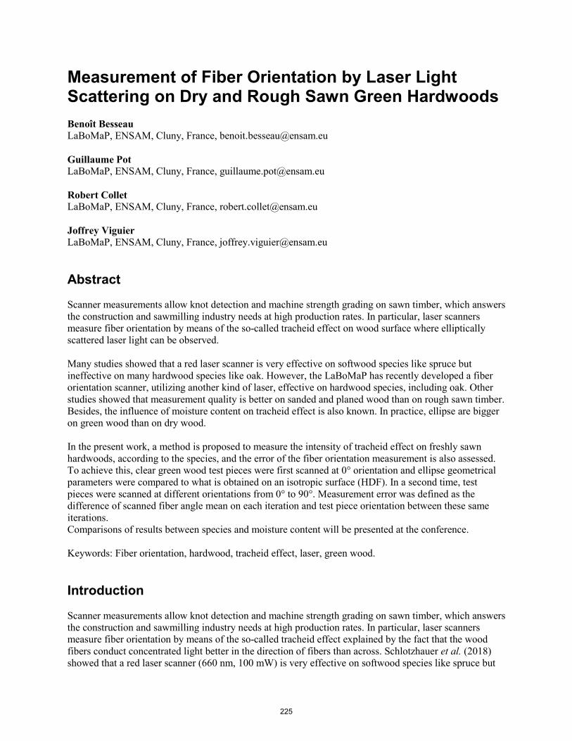
Measurement of Fiber Orientation by Laser Light Scattering on Dry and Rough Sawn Green HardwoodsBenoît Besseau LaBoMaP, ENSAM, Cluny, France, benoit.besseau@ensam.eu

Guillaume Pot LaBoMaP, ENSAM, Cluny, France, guillaume.pot@ensam.eu

Robert Collet LaBoMaP, ENSAM, Cluny, France, robert.collet@ensam.eu

Joffrey Viguier LaBoMaP, ENSAM, Cluny, France, joffrey.viguier@ensam.eu

Abstract

Scanner measurements allow knot detection and machine strength grading on sawn timber, which answers the construction and sawmilling industry needs at high production rates. In particular, laser scanners measure fiber orientation by means of the so-called tracheid effect on wood surface where elliptically scattered laser light can be observed.

Many studies showed that a red laser scanner is very effective on softwood species like spruce but ineffective on many hardwood species like oak. However, the LaBoMaP has recently developed a fiber orientation scanner, utilizing another kind of laser, effective on hardwood species, including oak. Other studies showed that measurement quality is better on sanded and planed wood than on rough sawn timber. Besides, the influence of moisture content on tracheid effect is also known. In practice, ellipse are bigger on green wood than on dry wood.

In the present work, a method is proposed to measure the intensity of tracheid effect on freshly sawn hardwoods, according to the species, and the error of the fiber orientation measurement is also assessed. To achieve this, clear green wood test pieces were first scanned at 0° orientation and ellipse geometrical parameters were compared to what is obtained on an isotropic surface (HDF). In a second time, test pieces were scanned at different orientations from 0° to 90°. Measurement error was defined as the difference of scanned fiber angle mean on each iteration and test piece orientation between these same iterations. Comparisons of results between species and moisture content will be presented at the conference.

Keywords: Fiber orientation, hardwood, tracheid effect, laser, green wood.

Introduction

Scanner measurements allow knot detection and machine strength grading on sawn timber, which answers the construction and sawmilling industry needs at high production rates. In particular, laser scanners measure fiber orientation by means of the so-called tracheid effect explained by the fact that the wood fibers conduct concentrated light better in the direction of fibers than across. Schlotzhauer et al. (2018) showed that a red laser scanner (660 nm, 100 mW) is very effective on softwood species like spruce but

225

ineffective on some hardwood species like oak. However, after the work of Daval et al. (2015), the LaBoMaP has developed a fiber orientation scanner effective on hardwood species, including oak (Olsson et al. 2018). It is, to the best of authors’ knowledge, the first to use a laser wavelength of 1064 nm and a modulable power (up to 1 W).

Mechanical properties of sawn timber are well in correlation with local fiber orientation (Jehl et al. 2011, Viguier et al. 2015) and assessing the measurement error of fiber orientation is important for strength grading purposes. Hu et al. (2004) did this work for sugi and Japanese beech species. To the best of authors’ knowledge, there is no such study focusing on European species such as oak, beech, Douglas fir, spruce, etc. Furthermore, Hu et al. (2004) and other similar studies focused only on the angle measurement but did not discuss the intensity of the tracheid effect, nor study the influence of laser power.

In the present work, the behavior of the light scattering effect is studied according to the species and the orthotropic plane (longitudinal-radial (LR) or longitudinal-tangential (LT)). Rough sawn green oak and planed dry oak are also compared because it meets industrial needs. Moreover, a method to assess the measurement error of fiber orientation is proposed.

Materials and methods

Samples

For this work, four wood species have been studied at “dry” (12% moisture content) state: Sweet Chestnut (Castanea), Douglas fir (Pseudotsuga menziesii), Poplar (Populus) and Oak (Quercus petraea and Quercus robur L). Oak have also been studied just after sawing and will be called green oak (with a moisture content above fiber saturation point and a rough sawn surface).

From each of these five cases, 10 test pieces (100 x 100 x 20 mm3) coming from 2 orthotropic planes have been chosen: 5 samples from longitudinal-radial plane (named Quarter sawn in this paper) and 5 from longitudinal-tangential plane (named Flat sawn in this paper). Every sample was made of clear wood, free from knots. Dry sample surfaces were planed to have low surface roughness. Green oak sample surfaces were rough sawn.

In addition, a sample in High Density Fiberboard (HDF) was chosen for its isotropic properties and to compare with solid wood samples.

Scanner

The fiber orientation scanner (BobiScan) used was developed in Cluny (France) . This is a laboratory scanner by which researchers were able to perform a fine-tuning of the laser, optics, and image processing. The principle is based on the so-called tracheid effect. The wavelength of the laser was 1064 nm, and its power was approximately 100 mW. The laser was divided in 24 dots by an optical system to have 10 mm space between dots (Figure 1-a). But when fibers are oriented near 90°, light spots can overlap if their length exceeds the distance between 2 lasers dots (10 mm). A near infrared camera (Basler acA2000-340kmNIR) was used to record the laser light scattering, and a software was developed to record the individual position of each laser dot while the board was longitudinally moving on a conveyor below the system, resulting in a resolution of 1 mm in the direction along the board.

226

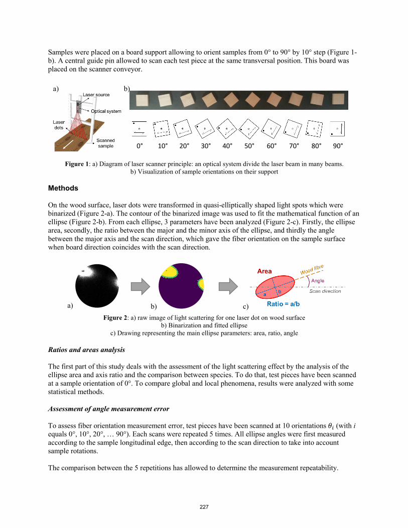
Samples were placed on a board support allowing to orient samples from 0° to 90° by 10° step (Figure 1-b). A central guide pin allowed to scan each test piece at the same transversal position. This board was placed on the scanner conveyor.

Figure 1: a) Diagram of laser scanner principle: an optical system divide the laser beam in many beams. b) Visualization of sample orientations on their support

Methods

On the wood surface, laser dots were transformed in quasi-elliptically shaped light spots which were binarized (Figure 2-a). The contour of the binarized image was used to fit the mathematical function of an ellipse (Figure 2-b). From each ellipse, 3 parameters have been analyzed (Figure 2-c). Firstly, the ellipse area, secondly, the ratio between the major and the minor axis of the ellipse, and thirdly the angle between the major axis and the scan direction, which gave the fiber orientation on the sample surface when board direction coincides with the scan direction.

Figure 2: a) raw image of light scattering for one laser dot on wood surface b) Binarization and fitted ellipse

c) Drawing representing the main ellipse parameters: area, ratio, angle

Ratios and areas analysis

The first part of this study deals with the assessment of the light scattering effect by the analysis of the ellipse area and axis ratio and the comparison between species. To do that, test pieces have been scanned at a sample orientation of 0°. To compare global and local phenomena, results were analyzed with some statistical methods.

Assessment of angle measurement error

To assess fiber orientation measurement error, test pieces have been scanned at 10 orientations 𝜃𝜃𝑖𝑖 (with i equals 0°, 10°, 20°, … 90°). Each scans were repeated 5 times. All ellipse angles were first measured according to the sample longitudinal edge, then according to the scan direction to take into account sample rotations.

The comparison between the 5 repetitions has allowed to determine the measurement repeatability.

0° 10° 20° 30° 40° 50° 60° 70° 80° 90°

a) b)

a) b) c)

227

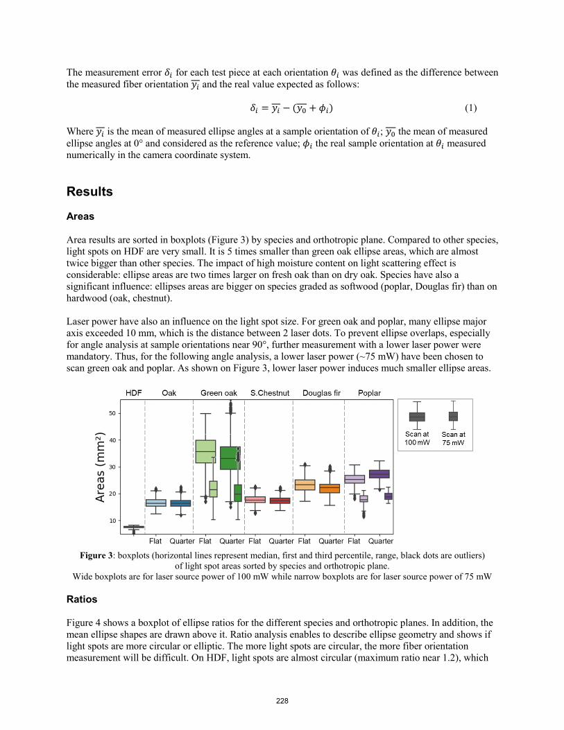
The measurement error 𝛿𝛿𝑖𝑖 for each test piece at each orientation 𝜃𝜃𝑖𝑖 was defined as the difference between the measured fiber orientation 𝑦𝑦𝑖𝑖 and the real value expected as follows:

𝛿𝛿𝑖𝑖 = 𝑦𝑦𝑖𝑖 − (𝑦𝑦0 + 𝜙𝜙𝑖𝑖) (1)

Where 𝑦𝑦𝑖𝑖 is the mean of measured ellipse angles at a sample orientation of 𝜃𝜃𝑖𝑖; 𝑦𝑦0 the mean of measured ellipse angles at 0° and considered as the reference value; 𝜙𝜙𝑖𝑖 the real sample orientation at 𝜃𝜃𝑖𝑖 measured numerically in the camera coordinate system.

Results

Areas

Area results are sorted in boxplots (Figure 3) by species and orthotropic plane. Compared to other species, light spots on HDF are very small. It is 5 times smaller than green oak ellipse areas, which are almost twice bigger than other species. The impact of high moisture content on light scattering effect is considerable: ellipse areas are two times larger on fresh oak than on dry oak. Species have also a significant influence: ellipses areas are bigger on species graded as softwood (poplar, Douglas fir) than on hardwood (oak, chestnut).

Laser power have also an influence on the light spot size. For green oak and poplar, many ellipse major axis exceeded 10 mm, which is the distance between 2 laser dots. To prevent ellipse overlaps, especially for angle analysis at sample orientations near 90°, further measurement with a lower laser power were mandatory. Thus, for the following angle analysis, a lower laser power (~75 mW) have been chosen to scan green oak and poplar. As shown on Figure 3, lower laser power induces much smaller ellipse areas.

Figure 3: boxplots (horizontal lines represent median, first and third percentile, range, black dots are outliers) of light spot areas sorted by species and orthotropic plane.

Wide boxplots are for laser source power of 100 mW while narrow boxplots are for laser source power of 75 mW

Ratios

Figure 4 shows a boxplot of ellipse ratios for the different species and orthotropic planes. In addition, the mean ellipse shapes are drawn above it. Ratio analysis enables to describe ellipse geometry and shows if light spots are more circular or elliptic. The more light spots are circular, the more fiber orientation measurement will be difficult. On HDF, light spots are almost circular (maximum ratio near 1.2), which

228

means light was not scattering in specific direction and confirm that HDF have an isotropic behavior regarding light scattering. All tested wood samples show most of their ratio values higher than what is observed on HDF, but quarter sawn dry oak and green oak have their lower values below 1.2. The differences of behavior between species are also significant with, for instance, narrow and long ellipses on poplar, while on oak shorter ellipses with the same width as poplar. For all species, ratios are smaller on quarter sawn, which is due to the fact that, on average, ellipse minor axis are bigger on quarter sawn than on flat sawn samples.

Figure 4: Boxplots of ellipse ratios sorted by species and orthotropic plane at a laser source power of 100 mW. Shorter ratios (<1.2) are located in red rectangle.

Repeatability

Figure 5 represents distribution diagrams for the 50 scans of one sample: 5 scans at the 10 tested orientations. For this sample, the standard deviation of measured angles is around 2°. The standard deviation of measured angles for all species is between 1° and 18°. Indeed, even if samples are clear wood, there are still variations of fiber orientation, which explains these angle dispersions. The 5 scans per sample orientation are superposed, which shows that the measurements with the BobiScan are repeatable. This repeatability is verified for every sample orientations.

Figure 5: Oak angle distribution diagrams depending on sample orientation. 50 diagrams are shown: 5 diagrams are superposed for each of the 10 sample orientations.

Prob

abili

ty

Angle (°)

Sample position (°) 0° 10° 20° 30° 40° 50° 60° 70° 80° 90°

229

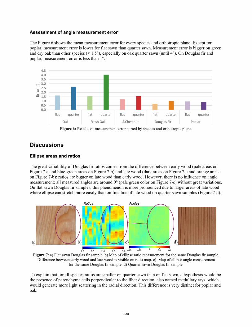
Assessment of angle measurement error

The Figure 6 shows the mean measurement error for every species and orthotropic plane. Except for poplar, measurement error is lower for flat sawn than quarter sawn. Measurement error is bigger on green and dry oak than other species (< 1.5°), especially on oak quarter sawn (until 4°). On Douglas fir and poplar, measurement error is less than 1°.

Figure 6: Results of measurement error sorted by species and orthotropic plane.

Discussions

Ellipse areas and ratios

The great variability of Douglas fir ratios comes from the difference between early wood (pale areas on Figure 7-a and blue-green areas on Figure 7-b) and late wood (dark areas on Figure 7-a and orange areas on Figure 7-b): ratios are bigger on late wood than early wood. However, there is no influence on angle measurement: all measured angles are around 0° (pale green color on Figure 7-c) without great variations. On flat sawn Douglas fir samples, this phenomenon is more pronounced due to larger areas of late wood where ellipse can stretch more easily than on fine line of late wood on quarter sawn samples (Figure 7-d).

Figure 7: a) Flat sawn Douglas fir sample. b) Map of ellipse ratio measurement for the same Douglas fir sample. Difference between early wood and late wood is visible on ratio map. c) Map of ellipse angle measurement

for the same Douglas fir sample. d) Quarter sawn Douglas fir sample.

To explain that for all species ratios are smaller on quarter sawn than on flat sawn, a hypothesis would be the presence of parenchyma cells perpendicular to the fiber direction, also named medullary rays, which would generate more light scattering in the radial direction. This difference is very distinct for poplar and oak.

0.00.51.01.52.02.53.03.54.04.5

flat quarter flat quarter flat quarter flat quarter flat quarter

Oak Fresh Oak S.Chestnut Douglas Fir Poplar

Erro

r (°)

a) b) c) d)

230

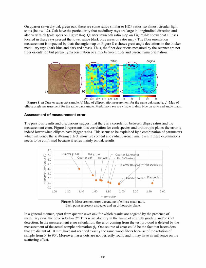
On quarter sawn dry oak green oak, there are some ratios similar to HDF ratios, so almost circular light spots (below 1.2). Oak have the particularity that medullary rays are large in longitudinal direction and also very thick (pale spots on Figure 8-a). Quarter sawn oak ratio map on Figure 8-b shows that ellipses located in these rays present the lower ratios (dark blue areas on ratio map). The fiber orientation measurement is impacted by that: the angle map on Figure 8-c shows great angle deviations in the thicker medullary rays (dark blue and dark red areas). Thus, the fiber deviations measured by the scanner are not fiber orientation but parenchyma orientation or a mix between fiber and parenchyma orientation.

Figure 8: a) Quarter sawn oak sample. b) Map of ellipse ratio measurement for the same oak sample. c) Map of ellipse angle measurement for the same oak sample. Medullary rays are visible in dark blue on ratio and angle maps.

Assessment of measurement error

The previous results and discussions suggest that there is a correlation between ellipse ratios and the measurement error. Figure 9 represents this correlation for each species and orthotropic plane: the error is indeed lower when ellipses have bigger ratios. This seems to be explained by a combination of parameters which influence the scattering effect: moisture content and radial parenchyma, even if these explanations needs to be confirmed because it relies mainly on oak results.

Figure 9: Measurement error depending of ellipse mean ratio. Each point represent a species and an orthotropic plane.

In a general manner, apart from quarter sawn oak for which results are negated by the presence of medullary rays, the error is below 2°. This is satisfactory in the frame of strength grading and/or knot detection. In the measurement error calculation, the error coming from the test protocol is deleted by the measurement of the actual sample orientation 𝜙𝜙𝑖𝑖. One source of error could be the fact that lasers dots, that are distant of 10 mm, have not scanned exactly the same wood fibers because of the rotation of sample from 0° to 90°. Moreover, laser dots are not perfectly round and it may have an influence on the scattering effect.

Flat oakQuarter oakFlat g. oakQuarter g. oak

Flat S.ChestnutQuarter S.Chestnut

Flat Douglas f.Quarter Douglas f.

Flat poplarQuarter poplar

0.01.02.03.04.05.06.07.08.0

1.00 1.20 1.40 1.60 1.80 2.00 2.20 2.40 2.60

mea

sure

men

t err

or (°

)

mean ratio

a) b) c)

231

Conclusion

This study about the fiber orientation measurement by laser light scattering shows that this technology works on some European hardwoods and softwoods, including dry oak and rough sawn green oak. Moreover, measurements are repeatable, which show that the used scanner is reliable. The kind of species and the considered orthotropic plane influence the light scattering effect, which is visible by the study of light spot shape. Indeed, the ellipse axis ratio have an effect on the measurement error which is lower for bigger ellipse axis ratio. On clear wood, the measurement error is between 0.5° and 1.5°, which is quite low, and can reach 4° on quarter sawn oak when medullary rays are well visible. On these rays, the light spot is more circular and deviate from the main direction of fibers which is the measurement purpose. Therefore, in medullary rays, scanner does not measure the fiber orientation but parenchyma orientation or a mix between fiber and parenchyma orientation

Some perspectives of this study are to scan and study other species like beech which could confirm observation about the influence of medullary rays and moisture content on fiber orientation measurement. A work about the distinction between medullary rays and knots have to be done in order to do strength grading or knot purge.

Acknowledgments

The authors thank the regional council of Bourgogne Franche-Comté, Ducerf Groupe and the Association Nationale Recherche Technologie (ANRT) (CIFRE N°2018/0987)

References

Daval et al. 2015. « Automatic measurement of wood fiber orientation and knot detection using an optical system based on heating conduction ». Optics express 23 (26): 33529–33539.

Hu et al. 2004. « On-Line Determination of the Grain Angle Using Ellipse Analysis of the Laser Light Scattering Pattern Image ». Journal of Wood Science 50 (4): 321‑26.

Jehl et al. 2011, Contribution of slope of grain information in lumber strength grading, 17th International Nondestructive Testing and evaluation of wood symposium, Sopron, Hungary.

Olsson et al. 2018. « Performance of Strength Grading Methods Based on Fibre Orientation and Axial Resonance Frequency Applied to Norway Spruce (Picea Abies L.), Douglas Fir (Pseudotsuga Menziesii (Mirb.) Franco) and European Oak (Quercus Petraea (Matt.) Liebl./Quercus Robur L.) ». Annals of Forest Science 75 (4).

Schlotzhauer et al. 2018: “Comparison of three systems for automatic grain angle determination on European hardwood for construction use”. European Journal of Wood and Wood Products, 76, 911-923.

Viguier et al. 2015, « Improving strength grading of timber by grain angle measurement and mechanical modeling ». Wood Material Science & Engineering 10 (1): 145–156.

232

Use of Nondestructive Techniques for Determination of Tension Parallel-to-Grain Properties of Spruce

David Gil-Moreno* School of Engineering and Ryan Institute, National University of Ireland Galway, Galway, Ireland, david.gil-moreno@nuigalway.ie

Conan O'Ceallaigh School of Engineering and Ryan Institute, National University of Ireland Galway, Galway, Ireland, conan.oceallaigh@nuigalway.ie

Dan Ridley-Ellis Centre for Wood Science and Technology, Edinburgh Napier University, Edinburgh, UK, d.ridleyellis@napier.ac.uk

Annette M. Harte School of Engineering and Ryan Institute, National University of Ireland Galway, Galway, Ireland, annette.harte@nuigalway.ie

* Corresponding author

Abstract

The paper presents a study of the tension properties of Irish-grown Sitka spruce. Fifty timber pieces were destructively tested having resonant frequency and knots measured. The aim was to improve knowledge of the performance of spruce in tension and to check the suitability of the equations given in the European standards to calculate secondary properties from grade determining properties. Static stiffness, which limited the grading of the dataset, was largely predicted using dynamic modulus of elasticity (MoEdyn). Tension strength was modelled using density and tKAR index. It was found also that adding MoEdyn in a linear regression was not useful. The research reveals that the equation given in EN384:2018 for tension strength, based on populations of higher stiffness than Irish spruce, results in values that may not be appropriate for Irish-grown spruce timber.

Keywords: grading, NDT, sawn timber, spruce, tension, wood properties, strength, standards

Introduction

General information

The interest in timber construction has increased in recent years, largely motivated by the demands of society for renewable and more environmentally-sensitive construction materials to mitigate climate change. The WoodProps programme in NUIG is aiming to increase knowledge on Irish timber to support its use in construction.

Sitka spruce (Picea sitchensis (Bong) Carr.) occupies 51.1% of the forest area in Ireland (Forest Service 2019). More than half of the output from Irish sawmills in 2015 was used in the construction sector

233

(IFFPA, 2016), and it is also the main commercial species in the UK. It was the only species machine graded until Douglas fir machine grading settings were approved in 2018 (Gil-Moreno et al., 2019). Historically, most of the research in Ireland and the UK have addressed the grading determining properties of bending strength, bending modulus of elasticity (MoE) and density. There is very little information published on tension properties parallel to the grain, and they are typically estimated from bending tests using empirical relationships, which has proved reasonably satisfactory for most cases (Walker, 1993). This is partially due to the difficulties in measuring tension properties as it is not uncommon that test pieces fail out of the prescribed test section as a result of the clamping conditions.

Another empirical approach to predict mechanical properties in tension is the use of non-destructive techniques (NDT). Measurement of density and knots is typically more important for strength prediction than for MoE prediction.

NDT based on acoustic measurements are widely used for prediction of mechanical properties, particularly MoE, due to the direct link between MoE and the acoustic behaviour of a wave travelling through the material (Bucur, 2006). The Newton-Laplace equation calculates dynamic modulus of elasticity (MoEdyn) from density (ρ) and speed propagation of a wave (v) as shown in Equation 1:

𝑀𝑀𝑀𝑀𝑀𝑀𝑑𝑑𝑑𝑑𝑑𝑑 = 𝜌𝜌 ∗ 𝑣𝑣2 (1)

In particular, the use of the resonance speed to calculate MoEdyn has offered accurate estimations of static MoE (Gil-Moreno and Ridley-Ellis, 2015). This method, generally applied in the longitudinal direction, calculates the speed of a wave measuring the frequency and wavelength (Equation 2).

𝑆𝑆𝑆𝑆𝑆𝑆𝑆𝑆𝑆𝑆 = 𝑊𝑊𝑊𝑊𝑣𝑣𝑆𝑆𝑊𝑊𝑆𝑆𝑊𝑊𝑊𝑊𝑊𝑊ℎ ∗ 𝐹𝐹𝐹𝐹𝑆𝑆𝐹𝐹𝐹𝐹𝑆𝑆𝑊𝑊𝐹𝐹𝐹𝐹 (2)

The importance of tension properties is reflected in the new European standard EN338:2016 (CEN,2016) which now includes strength classes based on tension tests. Strength classes are defined by characteristic values: fifth percentile strength and density, and mean MoE. The superseded EN338:2009 and EN384:2010 gave an equation (ft,0,k = 0.6 *fm,0,k) to calculate the characteristic values of tension strength (ft,0,k) from edgewise bending characteristic values (fm,0,k). The revised EN384:2018 (CEN,2018) uses a new relationship (ft,0,k = -3.07+0.73* fm,0,k) that for fm,0,k below 23,6 N/mm2 reduces the associated tension strength values, and increases it for those above.

A problem of using a general linear equation for material across different grades is that the relationships between bending and tension properties may vary depending on the timber quality. The Gradewood project agreed that the relationship given in EN338:2009 was generally correct for lower grades (internal document N0832 CEN/TC 124/WG02). Irish timber typically achieves C16 strength class quality (fm,0,k = 16 N/mm2), and the new relationship in EN 338:2016 was established based on testing of Scandinavian and central European timber, that typically achieves strength classes higher than C16 and for which grading is usually strength limited. Irish and British spruce is typically limited by stiffness, and as a result, the relationship may not adjust well to the Irish and British timber quality.

The aim of this WoodProps study is twofold. First, it examines the characteristic grading properties in tension of Sitka spruce grown in Ireland. Second, it examines the suitability of the equation given in EN384:2018 applied to Irish timber to derive bending properties from tension. The research is ongoing, but there is already enough data to make some preliminary recommendations.

234

Material and methods

This investigation comprised 50 ungraded pieces of sawn timber of Sitka spruce grown in Ireland, with cross section 100 x 47 mm. Most specimens (42 pieces) were offcuts of a previous study and were between 1346 mm and 2215 mm long (mean of 1724 mm), which was enough for the purposes of this study. The dataset was completed with eight pieces of 3600 ± 1 mm, donated by a local sawmill.

After conditioning the timber pieces to approximately 12% moisture content, the resonance frequency was measured with a grading machine MTG960 (Brookhuis Microelectronics BV, Holland). Density was obtained from mass and average dimensions of three points along the piece, and the MoEdyn calculated using equations 1 and 2. For the destructive testing, the expected weakest section was selected based on the size and location of knots, that were measured using the online software Web Knot Calculator v2.2 (Microtec, Italy) to obtain the tKAR index (Figure 2), and model the mechanical properties. Due to the limitations on the length that the testing machine can accommodate, the pieces were cut to 1.26 m, centring in the test section. The mass and resonance frequency was measured again to calculate the MoEdyn. This paper will use the term specimen to refer to the tested piece, and board to refer to the material before cutting.

The specimens were destructively tested in tension parallel to the grain according to EN408:2010 (Figure 1) using a Dartec 250 kN (Zwick Roell, Germany). One transducer was placed on each face of thespecimen, and the average displacement was used to calculate the modulus of elasticity (MoEt). Thetransducers remained on the board throughout the test until the failure load was reached.

Figure 1—Set up of tension test.

Gau

ge le

ngth

= 5

00 m

m

Test

spec

imen

leng

th =

126

0 m

m

Test

leng

th =

900

mm

Figure 2—Web knot calculator interface.

235

A density sample approximately 50-mm long, spanning the full cross-section and cut near the failure point, was used to calculate the clear density (Density384), and the moisture content using the oven drying method according to EN13183 (CEN, 2002). The MoEt and density values were corrected to a reference moisture content of 12%, and the strength values adjusted to a reference depth of 150 mm according to EN384.

Results and discussion

The results presented here are the descriptive statistics of the tension properties, the correlations between them, models for prediction of mechanical properties, and the grading performance as well as a comparison with results in the Gradewood project.

Thirty-five specimens broke within the test length, seven others slipped in the clamps, and eight pieces broke as a result of the clamping pressure. The MoEt was measured in the range of the 10%-40% of maximum load, and therefore was not influenced by the failure of specimens that broke as a result of the clamping pressure or slipped. The strength could have however been underestimated on those pieces that slipped without breaking and those that failed as a result of the clamping pressure. Due to the relatively small sample size, it was decided to include all the specimens in the dataset. The tKAR index was only used for 30 pieces because the measurements were either missed or the test specimens slipped.

Descriptive results

Table 1 summarises some of the properties measured, and shows the Gradewood project for comparison.

Table 1— Summary of properties Property WoodProps Gradewood1

min mean (CoV) max mean MoE (kN/mm2) 5.32 9.44 (23.4%) 13.8 10.6 Tension strengh (N/mm2) 7.5 22.3 (27.9%) 32.5 26.9 Density384 (kg/m3) 306 418 (13.3%) 538 422 Fmax (kN) 36.7 110.4 (27.7%) 160 Density test specimen (kg/m3) 351 437 (10.5%) 534 Density board (kg/m3) 340 434 (14.1%) 531 tKAR 0.40 (45.8%) 0.28

1(Stapel and Denzler, 2010); min: minimum value; max: maximum value

Density was very similar in both datasets, but the mechanical properties were higher in the Gradewood project. On 63 boards of Irish-grown Sitka spruce of 25x96 mm2, Raftery (Raftery, 2010) obtained mean values of 7890 N/mm2 for MoEt, 22.8 kN/mm2 for tension strength and 404 kg/m3 for density. Tension strength was slightly higher than in the current study, but the results were not adjusted to the reference depth of 150 mm, which would have reduced the values by about 9%.

The strength of the linear association between the three grading properties, and with MoEdyn was measured with Pearson’s correlation. This is shown in Table 2. Regressions between the grade determining properties explained between 34% and 49% of the variations. Raftery and Harte (2014) found that Density384 only explained 5% of the variation of MoEt and 9% of strength, which was 59% explained by MoEt. In this WoodProps study, Density384 had a stronger correlation with strength than any of the MoE measured.

236

Table 2— Pearson’s correlation (r) between variables

Properties r R2 Density384 - MoEt 0.70 0.49 Density384 - Strength 0.63 0.40 MoEt - Strength 0.59 0.34 MoEdyn, specimen - MoEt 0.96 0.92 MoEdyn, board - MoEt 0.94 0.88 MoEdyn, specimen - Strength 0.58 0.34 MoEdyn, board - Strength 0.56 0.32

The MoEdyn, calculated both in specimens and boards, was very strong with MoEt. On two different studies on beech, Ehrhart et al. (2016; 2018) reported poor relationships between MoEdyn and tension strength (R2=0.22 and 0.16). For the same species, Westermayr (2018) reported a moderate relationship between strength and MoEdyn (R2 =0.51). In this study, the MoEdyn of the specimens explained 92% of the variation in MoEt (RMSE = 690 N/mm2) using a linear regression, and 88% (RMSE = 874 N/mm2) using the MoEdyn of the boards. The MoEdyn represents the average properties of a piece, and the different lengths measured explains the differences of measuring the MoEdyn of the full boards and the tested specimens. The MoEdyn of the specimens (mean of 10.4 kN/mm2) was slightly smaller than in boards (mean of 10.6 kN/mm2). The relationships of MOEdyn in boards and specimens with MOEt are shown in Figure 3.

Figure 3—Relationship between MoEdyn of the test specimen and the board with the MoEt.

When used to predict tension strength, MoEdyn of the test specimens was only able to explain 34% of the variation (RMSE=5.1 N/mm2), and 32% if MoEdyn was applied to full boards (RMSE=5.2 N/mm2). Using only the boards that broke in the test length, the relationship did not improve. The prediction of strength presented more difficulties compared to MoEt as it is influenced by knots. Using Swiss-grown Norway spruce, Steigher and Arnold (2009) reported relationships (R2) of 0.80 between MOEdyn and MoEt, and 0.34 between MOEdyn and tension strength, similar to this WoodProps study.

Based on Pearson’s correlation in Table 2, board and specimen density were assessed as an independent variable for prediction of tension strength, explaining 44% of the variation (RMSE=4.7 N/mm2).

MOEdyn of specimens

MOEdyn of boards

237

Including MoEdyn did not usefully improve the relationship. Applying a stepwise regression, the best model used the board density and tKAR index as variables, explaining 52% of the variation of the strength (RMSE=4.6 N/mm2). Table 3 shows some of the coefficients of determination investigated.

Table 3— Variables for tension strength prediction Model Variables and p-values R2 and RMSE

1 MoEdyn specimen*** R2 = 34%, RMSE=5.1 N/mm2 2 MoEdyn board*** R2 = 32%, RMSE=5.2 N/mm2 3 Density384*** R2 = 40%, RMSE=4.9 N/mm2 4 Board density*** R2 = 44%, RMSE=4.7 N/mm2 5 Specimen density*** R2 = 44%, RMSE=4.7 N/mm2 6 Board density** + tKAR* R2 = 50%, RMSE=4.7 N/mm2 7 Specimen density** + tKAR* R2 = 52%, RMSE=4.6 N/mm2

***p-value<0.001; **p-value<0.01; *p-value<0.05;

In practical terms, the prediction of tension strength will use the full length of boards. The following models have been developed based on the dataset studied (50 and 30 boards for equations 3 and 4, respectively).

𝑓𝑓𝑡𝑡,0 = −15.9 + 0,088 ∗ 𝐷𝐷𝑆𝑆𝑊𝑊𝐷𝐷𝐷𝐷𝑊𝑊𝐹𝐹 𝑏𝑏𝑏𝑏𝑊𝑊𝐹𝐹𝑆𝑆 (𝑘𝑘𝑊𝑊/𝑚𝑚3) (3)

𝑓𝑓𝑡𝑡,0 = −3.7 + 0,07 ∗ 𝐷𝐷𝑆𝑆𝑊𝑊𝐷𝐷𝐷𝐷𝑊𝑊𝐹𝐹 𝑏𝑏𝑏𝑏𝑊𝑊𝐹𝐹𝑆𝑆 𝑘𝑘𝑘𝑘𝑚𝑚3 − 13.3 ∗ 𝑊𝑊𝑡𝑡𝑡𝑡𝑡𝑡 (4)

Results for grading

The characteristic values of the dataset were 12.3 kN/mm2 for strength, 340 kg/m3 for density and 9435 kN/mm2 for stiffness. Therefore, the MoE achieved values of T11 strength class, whereas strength and density achieved T12 and T13, respectively. The limiting factor was stiffness, which favours the use of MoEdyn as an indicating property.

For the thirty boards on which tKAR values were measured, the mean tension strength was 21.3 N/mm2. Equation 5 explained 69% of tension strength in the Gradewood project (Ranta-Maunus, 2009), and applied to WoodProps dataset gave a mean tension strength of 19.7 N/mm2. The model predicts a negative value for a piece of low MoEdyn and density and a high tKAR value. A specific model for the dataset in this study (Equation 6), using the same variables as the Gradewood model, gave a mean tension strength of 21.3 N/mm2, and explained 48% of the strength variation, but only density and tKAR were statistically significant. The MoEdyn was measured on the board.

𝑓𝑓𝑚𝑚1 = 6.85 − 0.0078b − 0.0057h − 0.0286𝐷𝐷𝑆𝑆𝑊𝑊384 − 29.7tKAR + 3.648 ∗ 10−3𝑀𝑀𝑏𝑏𝑀𝑀𝑑𝑑𝑑𝑑𝑑𝑑 (5)

𝑓𝑓𝑚𝑚2 = −153.3 + 2.007b + 0.667h + 0.0531𝐷𝐷𝑆𝑆𝑊𝑊384 − 13tKAR + 1.774 ∗ 10−5𝑀𝑀𝑏𝑏𝑀𝑀𝑑𝑑𝑑𝑑𝑑𝑑 (6)

Timber grading operates on the basis of the properties of a population rather than the individual boards. The values resulting from equations 5 and 6 were used for simulating a sorting exercise based on tension strength comparing the performance of both equations against the measured values. For illustration, this process used the mean of the population instead of the fifth percentile. The specimens were ranked in ascending order by fm1 and fm2 values, and their means and the mean of the corresponding measured tension strength values calculated. Subsequently, the lowest fm1 and fm2 values were removed from the

238

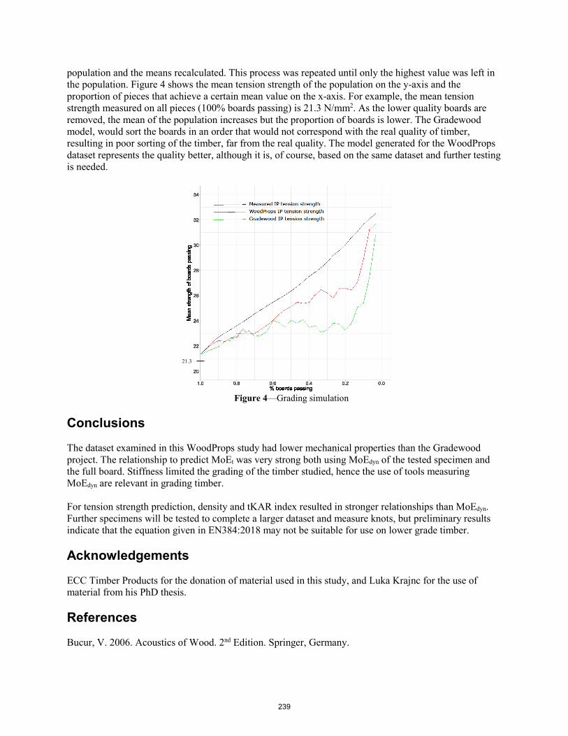
population and the means recalculated. This process was repeated until only the highest value was left in the population. Figure 4 shows the mean tension strength of the population on the y-axis and the proportion of pieces that achieve a certain mean value on the x-axis. For example, the mean tension strength measured on all pieces (100% boards passing) is 21.3 N/mm2. As the lower quality boards are removed, the mean of the population increases but the proportion of boards is lower. The Gradewood model, would sort the boards in an order that would not correspond with the real quality of timber, resulting in poor sorting of the timber, far from the real quality. The model generated for the WoodProps dataset represents the quality better, although it is, of course, based on the same dataset and further testing is needed.

Figure 4—Grading simulation

Conclusions

The dataset examined in this WoodProps study had lower mechanical properties than the Gradewood project. The relationship to predict MoEt was very strong both using MoEdyn of the tested specimen and the full board. Stiffness limited the grading of the timber studied, hence the use of tools measuring MoEdyn are relevant in grading timber.

For tension strength prediction, density and tKAR index resulted in stronger relationships than MoEdyn. Further specimens will be tested to complete a larger dataset and measure knots, but preliminary results indicate that the equation given in EN384:2018 may not be suitable for use on lower grade timber.

Acknowledgements

ECC Timber Products for the donation of material used in this study, and Luka Krajnc for the use of material from his PhD thesis.

References

Bucur, V. 2006. Acoustics of Wood. 2nd Edition. Springer, Germany.

21.3

239

CEN. 2002. Moisture content of a piece of sawn timber—Part 1: Determination by oven dry method. EN 13183-1:2002. European Committee for Standardisation, Brussels, p.5.

CEN. 2016. Structural timber - strength classes. EN338:2016. European committee for standardisation, Brussels. p. 11.

CEN. 2018. Structural timber-determination of characteristic values of mechanical properties and density. EN 384:2016 + A1:2018. European committee for standardization, Brussels, p 22.

Ehrhart T, Fink G, Steiger R, Frangi A. 2016. Experimental investigation of tensile strength and stiffness indicators regarding European beech timber. Proceedings of the World Conference on Timber Engineering (WCTE 2016), Aug. 22-25, 2016, Vienna, Austria.

Ehrhart, T., Steiger, R., Palma, P., & Frangi, A. 2018. Estimation of the tensile strength of European beech timber boards based on density, dynamic modulus of elasticity and local fibre orientation. World Conference on Timber Engineering (WCTE 2018), Aug. 20-23, 2018 Seoul, Rep. of Korea.

Forest Statistics Ireland 2019. 2019. Department of Agriculture, Food and the Marine, Ireland. Available at:https://www.agriculture.gov.ie/media/migration/forestry/forestservicegeneralinformation/ForestStatisticsIreland280519.pdf.

Gil-Moreno, D., & Ridley-Ellis, D. 2015. Comparing usefulness of acoustic measurements on standing trees for segregation by timber stiffness. Proceedings of 19th International Nondestructive Testing and Evaluation of Wood Symposium, Sep. 22-25, 2015 Rio de Janeiro, Brazil.

Gil-Moreno, D., D. Ridley-Ellis, and A. M. Harte, 2019, Timber grading potential of Douglas fir in the Republic of Ireland and the UK: International Wood Products Journal, p. 1-6.

IFFPA. 2016. An overview of the Irish forestry and forest products sector 2016. Irish Forestry and Forest Products Association. Dublin.

Raftery G. 2010. The use of advanced composite materials in the flexural reinforcement of low-grade glulam. PhD Thesis. National University of Ireland, Galway.

Raftery G, Harte AM. 2014. Material characterisation of fast-grown plantation spruce. Structures and Buildings 167: 380-386.

Ranta-Maunus, A., 2009, Strength of European timber: Part 1. Analysis of growth areas based on existing test results. VTT Publications 706. Finland.

Stapel P, Denzler J. 2010. Influence of the origin on specific properties of european spruce and pine. Final Conference COST Action E53, May 4-7, 2010 Edinburgh, UK.

Steiger R, Arnold M. 2009. Strength grading of Norway spruce structural timber: Revisiting property relationships used in en 338 classification system. Wood science and technology. 43(3-4):259-278.

Walker JC. 1993. Primary wood processing: Principles and practice. 1st Edition. Chapman and Hall, UK.

Westermayr, M., P. Stapel, and J. W. van de Kuilen, 2018, Tensile strength and stiffness of low quality beech (Fagus sylvatica) sawn timber. World Conference on Timber Engineering (WCTE 2018), Aug. 20-23, 2018 Seoul, Rep. of Korea.

240

Multiple Modes Modal Test on Lumber Far-Ching Lin* School of Forestry and Resource Conservation, National Taiwan University, Taipei, TAIWAN, farching@ntu.edu.tw Gwo-Liang Yang Institute of Engineering Science and Oceanic Engineering, National Taiwan University, Taipei, TAIWAN, d00525010@ntu.edu.tw Zi-Yu Chen School of Forestry and Resource Conservation, National Taiwan University, Taipei, TAIWAN, r06625035@ntu.edu.tw Chun-Wei Chen Institute of Manufacturing Technology, National Taipei University of Technology, Taipei, TAIWAN, et280002@yahoo.com.tw Min-Jay Chung Administration of Experimental Forest, National Taiwan University, Nantou Hsien, TAIWAN, jasonchung@ntu.edu.tw * Corresponding author Abstract Measurement of longitudinal and transverse vibration of wood specimens is an effective nondestructive test to obtain accurate resonance frequency for calculating wood strength quality. Early researchers found that stress wave parameters were relative to the strength of wood pieces. This study shows an efficient way by tapping different locations of the end cross section of the lumber to excite several modes of the specimen simultaneously. With fingertip equipment and sets of algorithms, the acoustic measurement was produced in a quiet efficient way to assure modules of elastic properties were applied at an industrial level in a short period (less than one second). In the practical experiment, a real machine was made with a controllable tapping stage. Four different grades of 2 by 4 lumber, 120 cm in length, were put in the rotary testing machine. With modal simulation of the finite element method, the results were quite similar among theory derivation, experiment, and FEM simulation with only single percentage differences. A controlled tapping stage machine provides more reliable validity and precision of testing. The variance of testing results was down to a range of 0.2% to 2% for different grades of wood specimens. The preliminary investigation and experiment provide a new concept of a production industrial-level testing machine to measure and grade every single product piece with competitive costs of testing and in very short time. Keywords: Modal test, tap tone, finite element method, nondestruction testing

241

Predicting Tensile Strength in Sawn Timber Using In-Plane Fibre Directions and Dynamic Modulus of Elasticity

Andreas Briggert Department of Building Technology, Linnaeus University, Växjö, Sweden, andreas.briggert@lnu.se

Anders Olsson Department of Building Technology, Linnaeus University, Växjö, Sweden, anders.olsson@lnu.se

Jan Oscarsson Department of Building Technology, Linnaeus University, Växjö, Sweden, jan.oscarsson@lnu.se

Abstract

Machine strength grading of sawn timber is based on the relationship between indicating properties (IPs) and so-called grade determining properties (GDPs). The former are calculated using board properties measured non-destructively whereas the latter are determined by destructive tests. For T-classes, applied GDPs are tensile strength, density and modulus of elasticity in tension. Efficient utilisation of sawn timber thus require IPs predicting the GDPs with high accuracy. This study aims at deriving an IP for tensile strength in the board direction using multiple linear regression based on board properties and at applying this new IP in a grading method and calculating corresponding yield in T-classes. The non-destructive and destructive testing were performed for more than 900 boards of Norway spruce originating from Finland, Norway and Sweden. Board properties necessary for calculating this new IP were density, axial resonance frequency and in-plane fibre directions at the board’s longitudinal surfaces, and these properties were determined using X-ray scanning, dynamic excitation and optical scanning, respectively. A high coefficient of determination between IP and tensile strength was obtained, implying that this new IP predicts tensile strength better than IPs used in industry today. Furthermore, since only a part of the board is destructively tested, settings can be determined using either IPs calculated for the tested part of the boards or IPs calculated for the entire length of the boards. Employing the latter resulted in higher yields but lower coefficients of determination. Several grading machines on the market are based on this approach.

Keywords: grade determining properties, grading, indicating properties, Norway spruce, T-classes

Introduction

Machine strength grading in Europe is based on the relationship between indicating properties (IPs) and grade determining properties (GDPs). Sawn timber used as glulam lamellae are graded to T-classes and the GDPs applied for these classes are tensile strength parallel to grain (ft,0), modulus of elasticity (MOE) parallel to grain in tension (Et,0), and density (ρ). The former two are for a board determined using measurement results from a destructive tensile test and the latter by dimensions and weight of a small specimen of clear wood cut near the board’s fracture zone (EN 384:2016 and EN 408:2010). IPs are calculated by means of one or several board properties measured non-destructively.

242

By means of IPs and GDPs of a sample of boards, limits, or settings as these limits are referred to in the standards, are determined for each IP applied such that the boards assigned to a class fulfil the minimum requirements of characteristic values of that class. The minimum requirements of characteristic values of each strength class are given in EN 338:2016 and are defined by 5-percentile characteristic tensile strength parallel to grain (ft,0,k), 5-percentile characteristic density (ρk) and mean characteristic MOE parallel to grain (Et,0,mean). There are additional requirements that need to be fulfilled for boards assigned to a strength class, see EN 14081-2:2018. The IP settings resulting in fulfillment of the requirements of a strength class for investigated boards are later applied in daily grading at sawmills.

Several machines are approved for grading sawn timber to T-classes. An example of an IP, which is used in some of these machines to predict grade determining tensile strength and grade determining tensile MOE, is based on application of axial resonance frequency (f1), board length (l), board density, (ρs) and board moisture content (μs) and is calculated as

𝐸𝐸𝑑𝑑𝑑𝑑𝑑𝑑 = 𝜌𝜌𝑠𝑠 ∙ (2𝑓𝑓1𝑙𝑙)2 ∙ 1 + 1100

∙ 𝜇𝜇𝑠𝑠 − 𝜇𝜇𝑟𝑟𝑟𝑟𝑟𝑟 (1)

This IP is usually referred to as axial dynamic MOE or simply dynamic MOE. The term μref included in Eq. 1 is the investigate species reference moisture content at a relative humidity of 65 % and a temperature of 20˚C, which for Norway spruce (Picea abies) corresponds to a moisture content of 12 %. Hanhijärvi & Ranta-Maunus (2008) evaluated the performance of this IP by single linear regression using a sample of 457 Norway spruce boards originating from Finland and Russia. For prediction of grade determining tensile strength, this IP resulted in a coefficient of determination (r2) of 0.58, and for prediction of grade determining tensile MOE in an r2 of 0.91. As regards the grade determining density, Hanhijärvi & Ranta-Maunus (2008) showed that an r2 of 0.91 can be achieved using board density as IP.

In one of the most accurate and commercially available grading methods, the prediction of grade determining tensile strength is based on an IP calculated on the basis of high-resolution density data, board dimensions and axial resonance frequency, see e.g. Bacher (2008), Hanhijärvi & Ranta-Maunus (2008) and Rais et al. (2010). Since the density of knots is about twice as high as the density of the surrounding clear wood, such high-resolution density data enables inclusion of positions and locations of knots in the definition of this IP. For the same sample as discussed in the previous paragraph, an r2 of 0.64 was obtained between this IP and the grade determining tensile strength.

Board density and dynamic MOE are good predictors of the grade determining density and the grade determining tensile MOE, respectively. However, to acquire a better material utilization of sawn timber graded to T-classes, it is necessary to develop IPs by which grade determining tensile strength are predicted with higher accuracy.

In the early 1920s, Hankinson (1921) showed that there is a strong relationship between fibre direction and strength of wood. Today there exists commercial equipment that can measure fibre directions on board’s longitudinal surfaces at production speed by utilizing the so-called tracheid effect, which can be explained as follows. When a circular laser spot illuminates a wood surface, the laser light will scatter into the cell structure and transmit mainly in the longitudinal direction of the tracheids. Some of this light will be reflected back to the surface and there enter a shape that resembles an ellipse. The major axis of this ellipse is then oriented in a direction that is parallel with a projection of the fibres longitudinal direction onto the plane of the surface, see e.g. Briggert et al. (2018).

Olsson et al. (2013) suggested an IP based on knowledge of fibres direction at the surfaces, axial resonance frequency, board dimensions and weight for prediction of bending strength. The procedure of calculating this IP can be summarized as follows. Firstly, the in-plane fibre directions at the longitudinal

243

surfaces and the resonance frequency are determined by means of the tracheid effect and dynamic excitation, respectively. Secondly, on the basis of observed in-plane fibre directions, board dimensions and axial dynamic MOE, a bending MOE-profile is calculated along the longitudinal direction of the board. The IP applied for prediction of bending strength is then determined as the lowest value along a board’s MOE-profile. For a sample including a total number of 936 boards, single linear regression between the described IP and bending strength resulted in an r2 of 0.69 (Olsson & Oscarsson 2017); the r2 between axial dynamic MOE and bending strength was for the same sample 0.53. These results indicate that this IP is one of the most accurate IPs for prediction of bending strength developed this far.

The objectives of the present research were to apply a similar IP as the one presented in Olsson et al. (2013), for prediction of tensile strength and evaluate if such an IP can be used for more accurate grading of glulam lamellae. Presented in this paper are two different procedures/models that can be used for an IP based on a local board property when determining settings for a strength class. Settings and thus the yields presented in this paper are determined in accordance with EN 14081-2:2010.

Glulam lamellae are usually graded before planing. However, previous research has shown that very similar numerical values of the IP suggested in Olsson et al. (2013) are obtained before and after planing, see Briggert (2014). The evaluation presented in this paper is therefore limited to measurement results obtained after planing.

Material and equipment

Material

The sample used in this study consisted of a total number of 967 boards of Norway spruce originating from Finland, Norway and Sweden. The thickness and width of the boards were between 20−46 mm and 60−245 mm, respectively. A drying scheme aiming at a 12 % moisture content was applied for all boards before any measurements were carried out. The mean moisture content at the time of non-destructive measurements was 12.4 % and at the time of the destructive tests 12.2 %.

Equipment

Local in-plane fibre directions on board surfaces were determined by means of an optical wood scanner of make WoodEye 5. This scanner is equipped with colour cameras, multi-sensor cameras, line lasers and dot-lasers, one set for each longitudinal board surface. Each dot-laser is installed with a diffraction beam splitter, which scatters the laser light into 64 laser beams distributed along a line in the transverse board direction. A number of these laser beams will, as a board is fed through the scanner, see Figure 1a, illuminate the longitudinal board surfaces. By means of photographs taken of the spread of laser light on board surfaces, in-plane fibre directions are determined by utilization of the tracheid effect, see Figure 1b.

Each board’s first axial longitudinal resonance frequency was determined by a Viscan of make MiCROTEC. As a board passes by this machine, it is subjected to a hammer blow at one of the ends. At the same time, the oscillation at the same end is measured by a laser interferometer. By means of the measured vibrations and utilization of Fast Fourier transform, the board’s first axial longitudinal resonance frequency is calculated.

A Goldeneye 706 of make MiCROTEC was used to obtain each board’s density. When a board is fed through this machine, it is exposed to radiation which is partially absorbed depending on the board’s local density and moisture content. Board density is then calculated as the average of all local density observations.

244

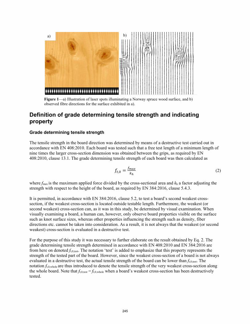
Figure 1—a) Illustration of laser spots illuminating a Norway spruce wood surface, and b) observed fibre directions for the surface exhibited in a).

Definition of grade determining tensile strength and indicating property

Grade determining tensile strength

The tensile strength in the board direction was determined by means of a destructive test carried out in accordance with EN 408:2010. Each board was tested such that a free test length of a minimum length of nine times the larger cross-section dimension was obtained between the grips, as required by EN 408:2010, clause 13.1. The grade determining tensile strength of each board was then calculated as

𝑓𝑓𝑡𝑡,0 = 𝑟𝑟𝑚𝑚𝑎𝑎𝑎𝑎𝑘𝑘ℎ

(2)

where fmax is the maximum applied force divided by the cross-sectional area and kh a factor adjusting the strength with respect to the height of the board, as required by EN 384:2016, clause 5.4.3.

It is permitted, in accordance with EN 384:2016, clause 5.2, to test a board’s second weakest cross-section, if the weakest cross-section is located outside testable length. Furthermore, the weakest (or second weakest) cross-section can, as it was in this study, be determined by visual examination. When visually examining a board, a human can, however, only observe board properties visible on the surface such as knot surface sizes, whereas other properties influencing the strength such as density, fiber directions etc. cannot be taken into consideration. As a result, it is not always that the weakest (or second weakest) cross-section is evaluated in a destructive test.

For the purpose of this study it was necessary to further elaborate on the result obtained by Eq. 2. The grade determining tensile strength determined in accordance with EN 408:2010 and EN 384:2016 are from here on denoted ft,0,test. The notation ‘test’ is added to emphasize that this property represents the strength of the tested part of the board. However, since the weakest cross-section of a board is not always evaluated in a destructive test, the actual tensile strength of the board can be lower than ft,0,test. The notation ft,0,whole are thus introduced to denote the tensile strength of the very weakest cross-section along the whole board. Note that ft,0,test = ft,0,whole when a board’s weakest cross-section has been destructively tested.

a) b)

245

Indicating properties

The in-plane fibre directions observed by means of the optical wood scanner were assumed valid for a certain volume dAdx of a board, see Figure 2a−b. Using the constitutive relation for an orthotropic material, a transformation matrix based on the angle φ, see Figure 2b, and nominal material parameters for Norway spruce (Olsson et al. 2013) local MOEs in the board direction, i.e. Ex(x,y,z), were calculated for each volume dAdx. Example of such calculated local MOEs are shown in Figure 2d. Photographs of the corresponding wood surfaces are shown in Figure 2c. An edgewise bending stiffness (EI) was then, for each position x, calculated as

𝐸𝐸𝐸𝐸𝑑𝑑(𝑥𝑥) = ∬𝐸𝐸𝑥𝑥 ∙ (𝑧𝑧 − 𝑧𝑧)2𝑑𝑑𝑑𝑑𝑑𝑑𝑧𝑧 (3)

where

𝑧𝑧 = ∬𝐸𝐸𝑎𝑎∙𝑧𝑧 𝑑𝑑𝑑𝑑𝑑𝑑𝑧𝑧∬𝐸𝐸𝑎𝑎 𝑑𝑑𝑑𝑑𝑑𝑑𝑧𝑧

(4)

Each cross-section’s bending MOE was calculated by dividing the result of Eq. 3 by the edgewise second moment of inertia (Iy), and compiled such that a high-resolution bending MOE-profile for the entire board was obtained. A moving average over a length of 90 mm was then applied to obtain a bending MOE-profile of a lower resolution. Figure 2e shows an example of such a bending MOE-profile. The vertical dashed lines marked by p1 and p2 in this figure exhibit the start- and the stop position of the part of the board destructively tested. As mentioned previously, it is not always that the weakest cross-section of a board is actually evaluated in a destructive test. A board property determined from an MOE-profile can, therefore, when applied for setting calculations, be selected in two ways; either by only considering the part of the board destructively tested (Eb,90,nom,test) or by considering the whole board (Eb,90,nom,whole). Note that Eb,90,nom,test= Eb,90,nom,whole if the weakest cross-section, according to the MOE-profile, is evaluated in the destructive test.

The IP suggested in this investigation for prediction of grade determining tensile strength were derived using local bending MOE and axial dynamic MOE as predictor variables and ft,0,test as dependent variable in an multiple linear regression. Since the calculated bending MOE could be determined in two ways, see Figure 2e, for a number of boards, two functions for the IPs were obtained. Mathematically these functions are describe as

𝐸𝐸𝐼𝐼𝐸𝐸,𝑏𝑏,1(𝑢𝑢1, v1) = 𝑘𝑘1,1 + 𝑘𝑘1,2 ∙ u1 + 𝑘𝑘1,3 ∙ v1 (5)

and

𝐸𝐸𝐼𝐼𝐸𝐸,𝑏𝑏,2(𝑢𝑢2, v2) = 𝑘𝑘2,1 + 𝑘𝑘2,2 ∙ u2 + 𝑘𝑘2,3 ∙ v2 (6)

where k1,1−k1,3 and k2,1−k2,3 are the constants describing the planes best fitted to the scatters between the predictor variables u1= Eb,90,nom,test and v1= Edyn and the dependent variable ft,0,test, and the predictor variables u2= Eb,90,nom,whole and v2= Edyn and the dependent variable ft,0,test, respectively, by the least square method. It must be particularly noted that Eq. 5, in contrast to Eq. 6, can be used for prediction of ft,0,whole

when inserting u1=Eb,90,nom,whole.

246

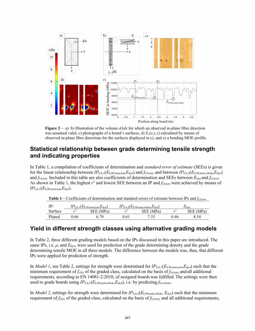
Figure 2— a)−b) Illustration of the volume dAdx for which an observed in-plane fibre direction was assumed valid, c) photographs of a board’s surfaces, d) Ex(x,y,z) calculated by means of observed in-plane fibre directions for the surfaces displayed in c), and e) a bending MOE profile.

Statistical relationship between grade determining tensile strength and indicating properties

In Table 1, a compilation of coefficients of determination and standard error of estimate (SEEs) is given for the linear relationship between IPE,b,1(Eb,90,nom,test,Edyn) and ft,0,test, and between IPE,b,2(Eb,90,nom,whole,Edyn) and ft,0,test. Included in this table are also coefficients of determination and SEEs between Edyn and ft,0,test. As shown in Table 1, the highest r2 and lowest SEE between an IP and ft,0,test were achieved by means of IPE,b,1(Eb,90,nom,test,Edyn).

Table 1—Coefficients of determination and standard errors of estimate between IPs and ft,0,test.

IP/ Surface

IPE,b,1(Eb,90,nom,test,Edyn) IPE,b,2(Eb,90,nom,whole,Edyn) Edyn r2 SEE (MPa) r2 SEE (MPa) r2 SEE (MPa)

Planed 0.66 6.79 0.61 7.33 0.46 8.54

Yield in different strength classes using alternative grading models

In Table 2, three different grading models based on the IPs discussed in this paper are introduced. The same IPs, i.e. ρs and Edyn, were used for prediction of the grade determining density and the grade determining tensile MOE in all three models. The difference between the models was, thus, that different IPs were applied for prediction of strength.

In Model 1, see Table 2, settings for strength were determined for IPE,b,1(Eb,90,nom,test,Edyn) such that the minimum requirement of ft,0,k of the graded class, calculated on the basis of ft,0,test, and all additional requirements, according to EN 14081-2:2010, of assigned boards was fulfilled. The settings were then used to grade boards using IPE,b,1(Eb,90,nom,whole,Edyn), i.e. by predicting ft,0,whole.

In Model 2, settings for strength were determined for IPE,b,2(Eb,90,nom,whole, Edyn) such that the minimum requirement of ft,0,k of the graded class, calculated on the basis of ft,0,test, and all additional requirements,

247

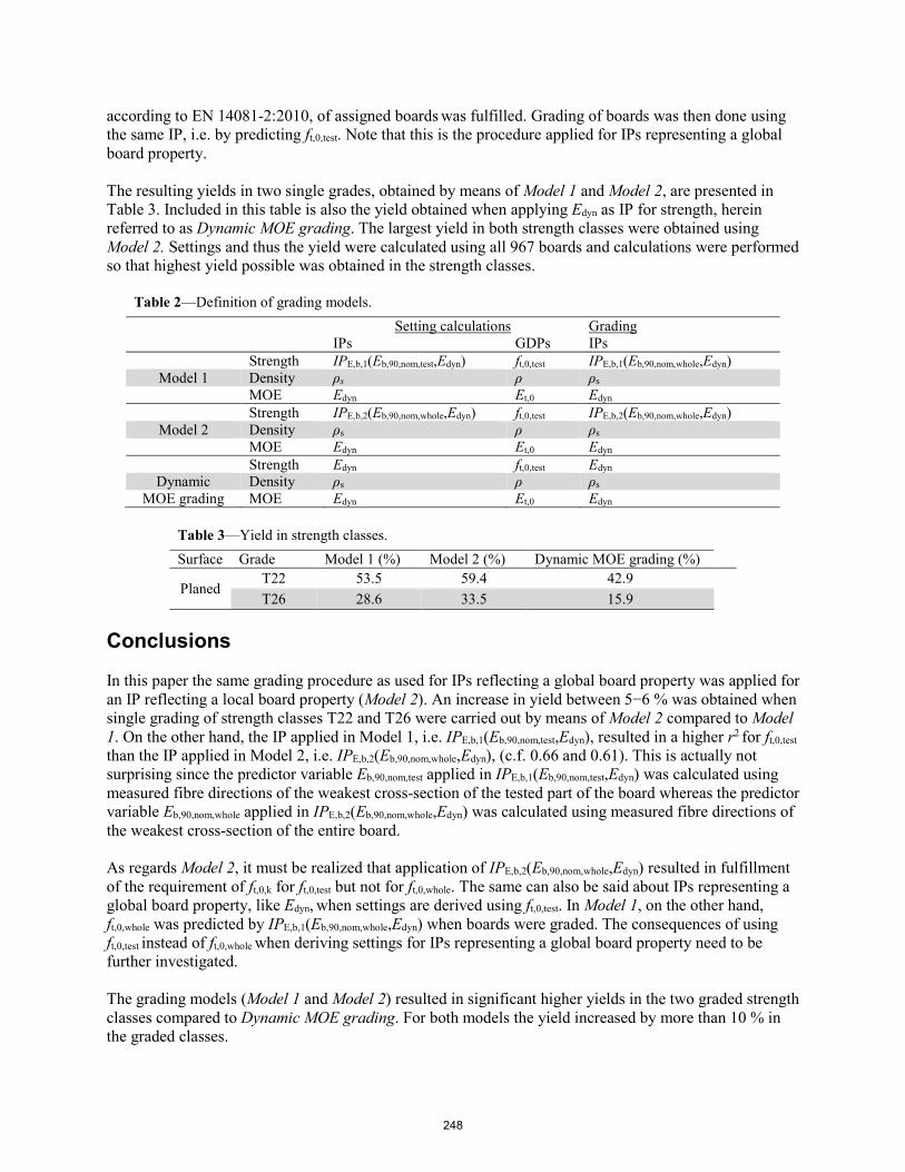
according to EN 14081-2:2010, of assigned boards was fulfilled. Grading of boards was then done using the same IP, i.e. by predicting ft,0,test. Note that this is the procedure applied for IPs representing a global board property.

The resulting yields in two single grades, obtained by means of Model 1 and Model 2, are presented in Table 3. Included in this table is also the yield obtained when applying Edyn as IP for strength, herein referred to as Dynamic MOE grading. The largest yield in both strength classes were obtained using Model 2. Settings and thus the yield were calculated using all 967 boards and calculations were performed so that highest yield possible was obtained in the strength classes.

Table 2—Definition of grading models. Setting calculations Grading

IPs GDPs IPs Strength IPE,b,1(Eb,90,nom,test,Edyn) ft,0,test IPE,b,1(Eb,90,nom,whole,Edyn)

Model 1 Density ρs ρ ρs MOE Edyn Et,0 Edyn Strength IPE,b,2(Eb,90,nom,whole,Edyn) ft,0,test IPE,b,2(Eb,90,nom,whole,Edyn)

Model 2 Density ρs ρ ρs MOE Edyn Et,0 Edyn Strength Edyn ft,0,test Edyn

Dynamic Density ρs ρ ρs MOE grading MOE Edyn Et,0 Edyn

Table 3—Yield in strength classes. Surface Grade Model 1 (%) Model 2 (%) Dynamic MOE grading (%)

PlanedT22 53.5 59.4 42.9 T26 28.6 33.5 15.9

Conclusions

In this paper the same grading procedure as used for IPs reflecting a global board property was applied for an IP reflecting a local board property (Model 2). An increase in yield between 5−6 % was obtained when single grading of strength classes T22 and T26 were carried out by means of Model 2 compared to Model 1. On the other hand, the IP applied in Model 1, i.e. IPE,b,1(Eb,90,nom,test,Edyn), resulted in a higher r2 for ft,0,test

than the IP applied in Model 2, i.e. IPE,b,2(Eb,90,nom,whole,Edyn), (c.f. 0.66 and 0.61). This is actually notsurprising since the predictor variable Eb,90,nom,test applied in IPE,b,1(Eb,90,nom,test,Edyn) was calculated usingmeasured fibre directions of the weakest cross-section of the tested part of the board whereas the predictorvariable Eb,90,nom,whole applied in IPE,b,2(Eb,90,nom,whole,Edyn) was calculated using measured fibre directions ofthe weakest cross-section of the entire board.

As regards Model 2, it must be realized that application of IPE,b,2(Eb,90,nom,whole,Edyn) resulted in fulfillment of the requirement of ft,0,k for ft,0,test but not for ft,0,whole. The same can also be said about IPs representing a global board property, like Edyn, when settings are derived using ft,0,test. In Model 1, on the other hand, ft,0,whole was predicted by IPE,b,1(Eb,90,nom,whole,Edyn) when boards were graded. The consequences of using ft,0,test instead of ft,0,whole when deriving settings for IPs representing a global board property need to be further investigated.

The grading models (Model 1 and Model 2) resulted in significant higher yields in the two graded strength classes compared to Dynamic MOE grading. For both models the yield increased by more than 10 % in the graded classes.

248

References

Bacher, M. 2008. Comparison of different machine strength grading principles. In: Proceedings of 2nd Conference of COST Action E53 – Quality control for wood and wood products, Delft, Netherlands, October 29–30.

Briggert, A. 2014 Fibres orientation on sawn surfaces – Can fibre orientation on sawn surfaces be determined by means of high resolution scanning. Master Thesis in Structural Engineering 15 hp, Department of Building Technology. Växjö, Sweden: Linnaeus University.

Briggert, A.; Olsson, A.; Oscarsson, J. 2018. Tracheid effect scanning and evaluation of in-plane and out-of-plane fibre direction in Norway spruce timber. Wood Science and Technology. 50(4): 411-429.

EN 338 2016. Structural timber – Strength classes. European Committee for Standardization.

EN 384 2016 + A1 2018. Structural timber – Determination of characteristic values of mechanical properties and density. European Committee for Standardization.

EN 408 2010 + A1 2012. Timber structures – Structural timber and glued laminatied timber – Determination of some physical and mechanical properties. European Committee for Standardization.

EN 14081-2 2010 + A1 2012. Timber structures – Strength graded structural timber with rectangular cross section –Part 2: Machine grading; additional requirements for initial type testing. European Committee for Standardization.

EN 14081-2 2018. Timber structures – Strength graded structural timber with rectangular cross section –Part 2: Machine grading; additional requirements for initial type testing. European Committee for Standardization.

Hanhijärvi, A.; Ranta-Maunus. A. 2008. Development of strength grading of timber using combined measurement techniques. Report of the Combigrade-project – phase 2. VTT Publications 686:55.

Hankinson, R. L. 1921. Investigation of crushing strenght of spruce at varying angles of grain. Air Service Information Circular, 3(259), Material Section Report No. 130, US Air Service, USA.

Olsson, A.; Oscarsson, J.; Serrano, E.; Källsner, B.; Johansson, M.; Enquist, B. 2013. Prediction of timber bending strength and in-member cross-sectional stiffness variation on the basis of local wood fibre orientation. European Journal of Wood and Wood Products, 71: 319–333.

Olsson, A.; Oscarsson, J. 2017. Strength grading on the basis of high resolution laser scanning and dynamic excitation: a full scale investigation of performance. European Journal of Wood and Wood Products, 75:17–31.

Rais, A.; Stapel, P.; van de Kuilen, J.W.G. 2010. The influence of knot size and location on yield of grading machines. In Proceedings of The Final Conference of COST Action E53 – The future of Quality Control for Wood & Wood Products, Edingburgh, Scotland, May 4–7.

249

Nondestructive Evaluation of Tensile Properties of Structural Lumber from the Spruce–Pine–Fir Species Grouping: Phase 1. Evaluation of Modulus of Elasticity

Nusret As Istanbul University, Istanbul, Turkey, nusretas@istanbul.edu.tr

Robert J. Ross USDA Forest Service, Forest Products Laboratory, Madison, Wisconsin, USA, robert.j.ross@usda.gov Michigan Technological University, Houghton, Michigan, USA Mississippi State University, Starkville, Mississippi, USA

Xiping Wang USDA Forest Service, Forest Products Laboratory, Madison, Wisconsin, USA, xiping.wang@ usda.gov

Christopher Adam Senalik USDA Forest Service, Forest Products Laboratory, Madison, Wisconsin, USA, christopher.a.senalik@ usda.gov

Abstract

The study summarized in this report was conducted to examine the relationships between nondestructive evaluation parameters and the modulus of elasticity (MOE) of spruce–pine–fir structural lumber. A random sample of lumber was obtained from a local lumber yard and conditioned to approximately 10% equilibrium moisture content in the laboratory. Static bending and vibration (transverse and longitudinal) nondestructive tests were conducted on each specimen, and MOE was calculated. The relationship between static and dynamic modulus values was examined, and empirical models were developed using statistical regression analysis techniques. Results revealed excellent correlative relationships between MOE values. Coefficients of determination obtained were 0.92, 0.96, and 0.93 for MOE of static–transverse vibration, MOE of static–longitudinal vibration, MOE of longitudinal–transverse vibration, respectively.

Keywords: nondestructive evaluation, modulus of elasticity, spruce–pine–fir lumber

Introduction

The tensile strength of wood and lumber products is important in the design of engineered components and structural systems. For example, the bottom chord of a wood truss is stressed in tension as are the undersides of large glued-laminated timbers. The tensile strength of wood is 20 to 50 times greater along the grain (fibers generally aligned with the long axis of a lumber specimen) than in the radial or tangential directions for softwood species and species groupings that are commonly used in structural applications. The grain angle is the angle between the wood fibers and the edges of a piece of wood. Variations in grain orientation are especially great around knots and are a major factor governing the ultimate strength of a piece of lumber in tension.

250

A search of the literature in the USDA Forest Products Laboratory’s library collection, Web of Science, and Engineering Index yielded several technical papers that summarize attempts to investigate the use of nondestructive testing (NDT) techniques to predict the tensile strength of structural lumber.

Hoyle (1968) summarized early research efforts from a variety of laboratories that resulted in the technology referred to as machine stress rating (MSR) of lumber. He presented results from several studies specifically designed to examine the relationship between the modulus of elasticity (MOE) (measured in a flat-wise orientation, utilizing a center span dead load) and the corresponding strength of softwood structural lumber. He reported that the statistical models relating MOE and tensile strength yielded correlation coefficients ranging from 0.74 to 0.82.

Orosz (1977) and Green and McDonald (1993a, 1993b) utilized transverse vibration NDT techniques to measure the MOE of structural lumber. Green and McDonald reported correlation coefficients for the models relating MOE to tensile strength that ranged from 0.46 to 0.60.

Kaiserlik and Pellerin (1977) examined the use of a longitudinal vibration NDT method to evaluate the tensile strength of softwood lumber. They reported a correlation coefficient of 0.84 when MOE was compared with tensile strength values. It is interesting to note that in addition to measuring the longitudinal MOE, they measured the attenuation rate of the stress wave as it travelled through the lumber specimens. When incorporating this additional parameter in their prediction equation, they reported a correlation coefficient of 0.90.

Cramer and Fohrell (1990) reported on a series of studies that developed fundamental information on the physical and mechanical properties of wood in knots and fiber deviation observed around knots. Knots significantly reduce the tensile strength of structural lumber. Although this work provided excellent information on stress distributions in the vicinity of knots, it did not provide a commercially useful methodology for evaluating lumber properties.

Rajeshwar et al. (1997) provided details on the use of an ultrasonic technique for estimating the strength of Southern Pine structural lumber. Ultrasounds through transmission measurements were made at several locations in the vicinity of knots and used to predict strength.

An NDT method for measuring the grain orientation is based on the difference in dielectric constant (permittivity) of wood between the parallel direction (lower dielectric constant) and the perpendicular direction (higher dielectric constant) to the grain. The dielectric constant is simply the ability of a material to concentrate an applied electric field. Measuring a material’s dielectric constant can be as simple as measuring the current flow between two conductors with an alternating voltage applied. At low moisture content levels, wood can be considered a dielectric material (Kellogg 1981, James and Hamill 1965, Lin 1967, Skaar 1948). The dielectric constant of a nonconducting material determines the amount of electric potential energy that is stored in a given volume of the material within an electric field. It is expressed as the ratio of the dielectric permittivity of the material relative to that of a vacuum or dry air. Experimentally, it is determined as the ratio of the capacity of a condenser with the material acting as the dielectric relative to the capacity of the condenser when the space between the plates is dry air. The dielectric constant for wood varies with grain (fiber) direction, and commercial equipment has been developed that utilizes this fact to determine fiber orientation in wood products. Knots, spiral grain, and other defects can be detected by measuring dielectric properties.

Pellerin and Ross (2015) provided a review of the concept and development of tension proof loading, a technology that focuses on testing each piece of lumber to a predetermined load level near its design load.

251

Pieces of lumber having a strength below the set design load would fail, thereby eliminating them from the lumber to be used.

The preceding review reveals the following: 1. There has not been a systematic evaluation of the relationships between widely used NDT parameters and the tensile properties of structural lumber. 2. There is no reported research focused on the potential of using combinations of these techniques to predict the strength of structural lumber.

The overarching objective of our cooperative work is to systematically evaluate relationships between several NDT parameters and the tensile properties of softwood structural lumber. This report summarizes the first phase of our work. It summarizes our examination of the relationships between several measurements of MOE of a sample of spruce–pine–fir lumber.

Materials and Methods

Materials

One hundred nominal 2- by 4-in. (38- by 89-mm), 12-ft- (3.66-m-) long lumber specimens (visual grade No. 2 or better, spruce–pine–fir species group) were obtained from a local lumber yard. All specimens were stickered and equilibrated at a temperature of 70 °F (21 °C) and relative humidity (RH) of 50% (Figure 1).

Figure 1—Lumber specimens used in this study.

Nondestructive test methods

The following briefly describes the test setups that were used for measurement of MOE. Detailed descriptions of each setup, and subsequent analysis, are presented in Ross (2015).

252

Flatwise bending

Figure 2 illustrates the center-point loading test setup that was used. Each specimen was simply supported at both ends, a load applied, and the midspan deflection that resulted from the load measured. A span of 3.5 m was used. A load of 4.54 kg was applied at midspan, and the specimen’s corresponding deflection was measured.

(a)

(b)

(c) Figure 2—Flatwise bending test setup: (a) test setup; (b) specimen being tested; and (c) load being applied and corresponding deflection measurement.

The flatwise bending MOE of a specimen was calculated using the following formula:

3MOE =

48PL

Iδ

where P is applied load (N), L is span (mm), I is moment of inertia (mm4), and δ is midspan deflection (mm).

253

Transverse vibration

Figure 3 illustrates the free transverse vibration test setup we used. A specimen was simply supported at both ends. A slight deflection was introduced at the midspan of the specimen. The specimen was then allowed to freely oscillate in the vertical (transverse) direction. Frequency of oscillation was measured, coupled with the specimen’s weight and dimensions, and used to compute MOE.

(a)

(b)

(c)

Figure 3—Transverse vibration test setup used in this study: (a) transverse vibration test setup; (b) specimen being tested; and (c) typical signal observed in response to transverse vibration.

254

Transverse vibration MOE was calculated using the following formula:

2 3rMOE

2.46F WL

Ig=

where MOE is dynamic modulus of elasticity (Pa), Fr is resonant frequency (Hz), W is beam weight (kg), L is beam span (m), I is beam moment of inertia (m4), and g is acceleration due to gravity (9.8 m/s2).

Longitudinal vibration

Figure 4 illustrates the pulse echo test setup utilized in this study. An impact or “pulse” on one end of the specimen induced a wave to flow along its length. The pulse “echoed” from the opposite end of the specimen. A fibre-gen Model HM 200 Hitman NDT tool (fibre-gen, Ltd., Christchurch, New Zealand) was used for conducting the tests. Frequency of oscillation was determined and, along with a specimen’s weight and dimensions, was used to compute MOE.

(a)

(b)

Figure 4—Longitudinal vibration test setup used in this study: (a) test setup; (b) fibre-gen model HM 200 Hitman equipment used to conduct longitudinal vibration tests.

255

Velocity (C, speed of sound transmission) was measured. MOE was computed using velocity (C) and density (ρ) of a specimen using the following formula:

2MOE ρC=

Statistical analysis

Linear regression analysis techniques were used to examine the relationship between MOE values obtained.

Results and Discussion

A summary of results obtained is given in Table 1. Note that the sample had an average moisture content of 10.7% (oven-dry basis). Flatwise static bending MOE values ranged from 4.6 to 13.4 GPa, with an average value of 8.8 GPa. Transverse vibration MOE values ranged from 9.9 to 15.5 GPa, and longitudinal vibration MOE values ranged from 5.2 to 15.4 GPa.

Table 1—Summary of some physical and mechanical properties of the lumber sample used in this study

Dimension

Density (g/cm3)

Static MOE (GPa)

Longitudinal vibration

Transverse vibration

Statistics MC (%)

Weight (kg)

Thickness (mm)

Width (mm)

Length (m)

Velocity (m/s)

MOE (GPa)

f (Hz)

MOE (GPa)

Mean 10.7 5.4 38 88 3.68 0.43 8.79 4,596 9.24 6.48 9.91 Std. dev. 0.37 5.4 0.4 0.9 0.004 0.043 1.95 487.8 2.07 0.662 2.10 Max. 11.8 7.3 39 91 3.68 0.58 13.43 5,491 15.35 7.71 15.47 Min. 9.7 4.1 37 86 3.66 0.34 4.61 3,461 5.20 4.96 5.60 COV (%) 3.5 10.0 1.1 1.1 0.11 10.0 22.2 10.6 22.4 10.2 21.2

Results obtained from our statistical analyses are illustrated in Figures 5 through 7. Strong correlative relationships were observed between flatwise static bending, transverse vibration, and longitudinal vibration MOE values. It is important to note that both transverse and longitudinal vibration MOE values were found to be greater than corresponding flatwise bending MOE values. This phenomenon has been observed in similar studies conducted with lumber from different species of wood.

256

Figure 5—Observed relationship between transverse vibration and flatwise bending modulus of elasticity (MOE) values for the spruce–pine–fir lumber specimens used in this study.

Figure 6—Observed relationship between longitudinal vibration and flatwise bending modulus of elasticity (MOE) values for the spruce–pine–fir lumber specimens used in this study.

257

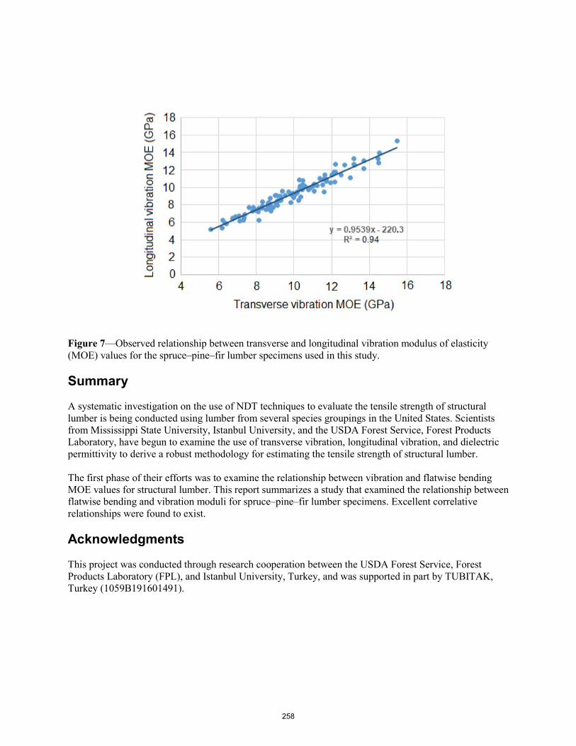
Figure 7—Observed relationship between transverse and longitudinal vibration modulus of elasticity (MOE) values for the spruce–pine–fir lumber specimens used in this study.

Summary

A systematic investigation on the use of NDT techniques to evaluate the tensile strength of structural lumber is being conducted using lumber from several species groupings in the United States. Scientists from Mississippi State University, Istanbul University, and the USDA Forest Service, Forest Products Laboratory, have begun to examine the use of transverse vibration, longitudinal vibration, and dielectric permittivity to derive a robust methodology for estimating the tensile strength of structural lumber.

The first phase of their efforts was to examine the relationship between vibration and flatwise bending MOE values for structural lumber. This report summarizes a study that examined the relationship between flatwise bending and vibration moduli for spruce–pine–fir lumber specimens. Excellent correlative relationships were found to exist.

Acknowledgments

This project was conducted through research cooperation between the USDA Forest Service, Forest Products Laboratory (FPL), and Istanbul University, Turkey, and was supported in part by TUBITAK, Turkey (1059B191601491).

258

Literature Cited

Cramer, S.M.; Fohrell, W.B. 1990. Method for simulating tension performance for lumber members. Journal of Structural Engineering. 116(10): 2719-2745.

Green, D.W.; McDonald, K.A. 1993a. Investigation of the mechanical properties of red oak 2 by 4’s. Wood and Fiber Science. 25(1): 35-45.

Green, D.W.; McDonald, K.A. 1993b. Mechanical properties of red maple structural lumber. Wood and Fiber Science. 25(4): 365-374.

Hoyle, R.J. 1968. Background to machine stress rating. Forest Products Journal. 18(4): 87-97.

James, W.L.; Hamill, D.W. 1965. Dielectric properties of Douglas-fir measured at microwave frequencies. Forest Products Journal. 15(2): 51-56.

Kaiserlik, J.H.; Pellerin, R.F. 1977. Stress wave attenuation as an indicator of lumber strength. Forest Products Journal. 27(6): 39-43.

Kellogg, R.M. 1981. Physical properties of wood. In: Wood — Its structure and properties. Volume 1. Clark C. Heritage Memorial Series on Wood. F.F. Wangaard, ed. Educational Modules for Materials Science and Engineering, Materials Research Laboratory, The Pennsylvania State University, University Park, PA. pp. 195-223.

Lin, R.T. 1967. Review of the dielectric properties of wood and cellulose. Forest Products Journal. 17(7): 61-66.

Orosz, I. 1977. Relationships between transverse free vibration E and other properties as affected by knots. Forest Products Journal. 27(1): 23-27.

Pellerin, R.F.; Ross, R.J. 2015. Proof loading. In: Nondestructive evaluation of wood. Second Edition. Gen. Tech. Rep. FPL-GTR-238. Madison, WI: U.S. Department of Agriculture, Forest Service, Forest Products Laboratory: 53-57. Chapter 4.

Rajeshwar, B.; Bender, D.A.; Brey, D.E.; McDonald, K.A. 1997. An ultrasonic technique for predicting tensile strength of southern pine lumber. Transactions of the American Society of Agricultural Engineers. 40(4): 1153-1159.

Ross, R.J. 2015. Nondestructive evaluation of wood. Second Edition. Gen. Tech. Rep. FPL-GTR-238. Madison, WI: U.S. Department of Agriculture, Forest Service, Forest Products Laboratory. 167 p.

Skaar, C. 1948. The dielectric properties of wood at several radio frequencies. NY State College of Forestry Technical Publication No. 69.

Additional References

Athey, T.W. 1982. Measurement of RF permittivity of biological tissues with an open-ended coaxial line. IEEE Trans. MTT. 30: 82-86.

259

Beall, F.C. 2007. Industrial applications and opportunities for nondestructive evaluation of structural wood members. Maderas: Ciencia y Tecnologia. 9(2): 127-134.

Daval, V. 2015. Automatic measurement of wood fiber orientation and knot detection using an optical system based on heating conduction. Optics Express. 23(26): 33529.

Divos, F.; Tanaka, T. 2005. Relation between static and dynamic modulus of elasticity of wood. Acta Silvatica Lignaria Hungarica. 1: 105-110.

Gupta, R. 2012. Effect of grain angle on shear strength of Douglas-fir wood. Holzforschung. 66: 655-658.

Hollertz, R. 2014. Dielectric properties of wood fibre components relevant for electrical insulation applications. Stockholm: KTH Royal Institute of Technology. 38 p.

Ilic, J.; Ozarska, B. 1996. Nondestructive evaluation of properties of reconstituted wood products used in Australia. In: 10th International Symposium on Nondestructive Testing of Wood. Swiss Federal Institute of Technology, Lausanne, Switzerland: 269-278.

Jayne, B.A. 1959. Vibrational properties of wood as indices of quality. Forest Products Journal. 9: 413-416.

Kabir, M.F. 1997. Dielectric properties or rubber wood at microwave frequencies measured with an open-ended coaxial line. Wood and Fiber Science. 29(4): 319-324.

Kabir, M.F. 2001. Temperature dependence of the dielectric properties of rubber wood. Wood and Fiber Science. 33(2): 233-238.

Kliger, R.; Perstorper, M.; Johansson G. 1992. Stiffness in structural timber - effect according to position in the stem. In: Proc. IUFRO S5.02 Timber Engineering Meeting, Laboratorie de Rheologie du Bois de Bordeaux, Bordeaux, France.

Schajer, G.S. 2006. Measurement of wood grain angle, moisture content and density using microwaves. Holz als Roh-und Werkstoff. 64: 483-490.

Shupe, T.E. 1998. Effect of wood grain and veneer side on loblolly pine veneer wettability. Forest Products Journal. 48(6): 95-97.

Simonaho, S-P. 2004. Determination of wood grain direction from laser light scattering pattern. Optics and Lasers in Engineering. 41: 95-103.

Perstorper, M. 1994. Strength and stiffness prediction of timber using conventional and dynamic methods. In: Proc. first European symposium on nondestructive evaluation of wood. University of Sopron, Sopron, Hungary.

Ross, R.J. 2015. Nondestructive evaluation of wood. Second edition. Gen. Tech. Rep. FPL-GTR-238. Madison, WI: U.S. Department of Agriculture, Forest Service, Forest Products Laboratory.

Ross, R.J.; Pellerin, R.F. 1994. Nondestructive testing for assessing wood members in structures: A review. Gen. Tech. Rep. FPL-GTR-70 (Rev.). Madison, WI: U.S. Department of Agriculture, Forest Service, Forest Products Laboratory.

260

Tanaka, T.; Nagao, H.; Nakai, T. 1991. Nondestructive evaluation of bending and tensile strength by longitudinal and transverse vibration of lumber. Proc. 8th international symposium on nondestructive testing of wood. Conferences and Institutes, Washington State University, Pullman, USA.

Winning, M. 2005. Transition between low and high angle grain boundaries. Acta Materialia. 53: 2901-2907.

Yapici, F. 2011. The effect of grain angle and species on thermal conductivity of some selected wood species. BioResources. 6(3): 2757-2762.

261

Comparison of Nondestructive Visual Grading and Proof Loading Systems on Low-Grade Yellow-Poplar Lumber for CLT Panel Production.Rafael Azambuja Division of Forestry and Natural Resources, West Virginia University, Morgantown, WV, USA, rdazambuja@mix.wvu.edu

David B. DeVallance* InnoRenew CoE and University of Primorska, Koper, Slovenia, devallance@innorenew.eu

Joseph McNeel Division of Forestry and Natural Resources, West Virginia University, Morgantown, WV, USA, jmcneel@wvu.edu

Curt Hassler Division of Forestry and Natural Resources, West Virginia University, Morgantown, WV, USA, chasslerwv@gmail.com

* Corresponding author

Abstract

Currently, low quality material from hardwood logs is used to produce pallets, cross ties, and other industrial grade products. The cross laminated timber (CLT) panel market has the potential to increase the use of this material in a higher value “composite” product. However, the current CLT standard in North America (ANSI/APA PRG 320-2018) restricts the use of hardwoods and low structural visual grades. As US hardwoods are not traditionally sawn, graded, or used in building construction applications, there exists questions related whether or not the current supply of “appearance” grade hardwoods can supply the structural grades needed for CLT panels. This study examined the current state of this emerging market relative to raw material availability and compared nondestructive visual grades of yellow-poplar based on appearance (NHLA) and structural (NELMA) grading rules. Specifically, low-grade lumber (NHLA Grade 2A, 2B, 3A, and 3B) intended for the pallet market was selected and evaluated using NELMA structural grading, before and after surfacing and edging for CLT lumber stock. Additionally, the resulting material was nondestructively proof loaded to evaluate the flat-wise bending, modulus of elasticity (MOE). The results of the study found that within the pallet grade material, 55% of the lumber met structural grades and could potentially be used in CLT panels. In respect to MOE, a majority of the lumber possessed a value greater than the minimum 1.2 x 106 psi as required under the current CLT standard. Further details related to grade distribution and improvement after finishing will be presented.

Keywords: Visual lumber grading, cross laminated timbers, proof loading

262

Introduction

Luppold and Bumgardner (2008) reported that between 1984 and 2002, the largest use of hardwood lumber was the pallet industry. To remain competitive, the Appalachian region must be innovative with marketing plans and reaching out to new markets (Naka et al. 2009). A way to achieve this competitive advantage is by developing new technologies that add value to the regional raw material, such as CLT panels, an emergent product.

Hardwoods are typically graded according to NHLA rules, a visual grade based on the amount of clear face area units, without defects, that a board can produce. This set of rules does not guarantee structural resistance of the board, although it can be said that there is decrease in mechanical resistance with the presence of defects. This assumption is what the NELMA system is based on, and this visual set of rules qualify boards for structural use based on the presence of defects and their location in the board.

Nondestructive evaluations (NDE) have been used to obtain information for lumber, with machine stress rated (MSR) as the most common. NDE simulate strains in the lumber before damaging the tested object. Some properties of lumber are used to predict its strength, mainly its specific gravity and elasticity.

Therefore, the objective of this research was to examine a low-grade Appalachian hardwood, yellow-poplar, to be used to produce CLT panels. Specifically, it set out to determine the structural visual grade (NELMA) distribution of low-grade NHLA (2A Common and below); determine mechanical properties (modulus of elasticity) of low-grade NHLA; and assess the potential of this material to be used in CLT.

Materials and Methods

To achieve the objectives described, eight packs of rough-cut yellow-poplar boards classified as “Pallet grade” (lower grade available) with dimensions of approximately 6 7/8” x 1” x 10’ (width, depth, and length, respectively) were obtained. Defects that limit board usage in the CLT panels, such as crook and bow, were measured and used to obtain a final cut. Replicating the processing in a CLT plant, the boards were planned to approximately 7/8”, then cut in a gang rip saw to a width of 6”. From these boards, respective NHLA and NELMA grades were collected by professional lumber graders. The range of the grades descending from high to low for NHLA are: NHLA are FAS, 1Face (1F), No. 1 Common (1C), No. 2A Common (2A), No. 2B Common (2B), No. 3A Common (3A), No. 3B Common (3B); the range of grade descending from high to low for NELMA are: Select Structural (SS), No. 1, No. 2, No. 3, Below grade. For the purpose of this study, only boards that met NHLA Grade No. 2A Common (2A), No. 2B Common (2B), No. 3A Common (3A), No. 3B Common (3B) were included in the analysis presented, as we were interested in the percentage of structural grades (in this case, NELMA) in this “low-grade” material.

The boards were then brought to the WVU laboratory to be mechanically evaluated. The NDE was proof loading, bending flatwise. The choice of doing flatwise instead of edgewise was to simulate the most common forces that a board would be submitted to in a CLT panel. The boards were deflected 3” in the center point of a span of 87”. Load through the deflection was collected and slope was obtained. Both measurements were used in Equation 1 to obtain the modulus of elasticity (MOE) in bending. Figure 1 presents a rough scheme of each evaluation from this research.

𝑀𝑀𝑀𝑀𝑀𝑀 = 𝑀𝑀×𝐿𝐿3

48𝐼𝐼 (1)

Where M is slope of the load deflection curve, L is the test span, and I is the moment of inertia.

263

Figure 1—Summary of the board classification performed in this research where: a. NHLA visual grade, based on amount of clear area a board can produce; b. NELMA visual grade, based on the decrease of strength a defect can cause, note that stains do not affect this grade; c. Machine stress rated, values used in Equation 1 in addition to board dimensions.

Boards used in the analysis were restricted to the target of the study, available low-grade Appalachian hardwoods, therefore yellow-poplar NHLA grade 2A, 2B, 3A, and 3B, after processing. Some boards were damaged during processing and did not present a homogeneous shape for the NDE, caused by splits, wane, or holes. The comparison of NDE was performed within the grading system. Statistical analysis was performed, first ANOVA, followed by HSD Tukey test.

Results and Discussion

The distribution of visual structural grade of low-grade NHLA yellow-poplar is presented in Table 1. Boards are presented with their initial NHLA grade and respective NELMA grade before and after processing. After processing, an adaptation of the NELMA grade was made to fit boards into NELMA grade No.3.

Table 1—Distribution of low-grade NHLA in NELMA grades. NHLA Grade

NELMA Grade Total SSa No.1 No.2 No.3 B.G.a

2A 69 31 58 72 117 347 2B 31 28 84 67 114 324 3A 24 9 37 39 124 233 3B 11 17 46 36 187 297 Total 135 85 225 214 542 1,201

a. SS: Select Structural; BG: Below Grade.

264

The distribution of low-grade (NHLA Grade 2A, 2B, 3A, and 3B) yellow-poplar in NELMA grades after processing are Select Structural: 11%; No.1: 7%; No.2: 19%; No.3: 18%; and Below grade: 45%. NELMA grade is related to defect size and location. The cut in width had two effects: when the defect was located in the peripheral areas it could be cut out, upgrading the piece to Select Structural; when the defect was located in central areas it could not be cut out, and, in a smaller surface area, the same defect size will be more representative, decreasing the board grade. Also, splits can be the result of poor methods in the transportation and handling, causing damage to the boards. These are assumptions and further investigation is required. A possibility is the use of digital image comparison prior to and after processing for a better understanding of defect occurrence.

In a similar grading study, Pahl et al. (1992) graded yellow-poplar according to NHLA and NELMA standards. No conclusive correlation between grading systems was found in the study. The study also found approximately 11% of Below grade boards, data that corroborate the potential use of hardwood in structural purposes. The most frequent of NHLA grade found in Pahl et al. (1992) was 2B, 59% from a total number of 389 boards, higher grade when compared to what was found in this research (2A: 29%; 2B: 27%; 3A: 19%; 3B: 25%). That may justify the final quantity of 45% Below grade boards found.

Some boards were taken from the data pool because they either: i) had an NHLA grade FAS, 1F or 1C, and are not the target of this research; or ii) were unsuited for the nondestructive test due to uneven shape. It is noteworthy that most of these boards were graded structurally as Below grade (46 out of 52 boards), while in NHLA there was a more even spread in grades: 2A (10), 2B (7), 3A (16) or 3B (19). The uneven shape is expected in the boards that did not achieve a structural grade, but the six boards that achieve this were probably damaged during transportation after grading.

The results of the boards that met the parameters of the research (low-grade NHLA yellow-poplar) are presented in the following tables. Table 2 shows the nondestructive evaluation results grouped in the structural grade (NELMA), while Table 3 groups the results in the aesthetic grade (NHLA).

Table 2—NDE results on Modulus of Rupture (MOE) grouped within NELMA grades. Variable Select Structural No. 1 No. 2 No. 3 Below grade Sample Size 134 85 224 210 493 Mean MOE (x106 psi) 1.74 1.72 1.68 1.66 1.61 Minimum MOE (x106 psi) 1.19 1.10 0.89 0.86 0.77 Maximum MOE (x106 psi) 2.36 2.37 2.43 2.46 2.38 5th Percentile MOE (x106 psi) 1.36 1.38 1.28 1.29 1.12 Coefficient of Variance (%) 0.14 0.13 0.15 0.15 0.17 Tukey HSD* a ab ab bc c

*Tukey honest significant difference between columns with p<0.05

The one-way ANOVA analyses of MOE within the grading systems show significant difference between grades. From the analysis of MOE within groups, there was a significant difference at the p<0.05 level for the NELMA grades [F(4, 1141) = 9.93, p < 0.001] and significant difference at the p<0.05 level for the NHLA grades [F(3, 1142) = 35.81, p < 0.001]. Also, the relatively low coefficient of variance, between 0.13 and 0.17, shows that the data was concise and within range.

265

Table 3—NDE results Modulus of Rupture (MOE) grouped within NHLA grades Variable 2A 2B 3A 3B Sample Size 337 317 217 275 Mean MOE (x106 psi) 1.70 1.74 1.60 1.55 Minimum MOE (x106 psi) 0.80 1.05 0.86 0.77 Maximum MOE (x106 psi) 2.43 2.46 2.14 2.21 5th Percentile MOE (x106 psi) 1.30 1.35 1.22 1.11 Coefficient of Variance (%) 0.16 0.14 0.15 0.16 Tukey HSD* a a b b

*Tukey honest significant difference between columns withp<0.01

The NDE results showed for the NELMA structural grade no significant difference in MOE between grades Select Structural, No. 1, and No. 2; no difference between No. 1, No. 2, and No. 3; and no significant difference between No. 3 and Below grade. Although the last assumption can be bias, because 46 (9.33% of the population) of the most defective boards from Below grade were not tested due to uneven shape, and a direct comparison would not reflect the real population. The results of MOE showed that the grade parameters that differentiate grades NELMA Select Structural, 1, and 2, which are based on defect size and location, did not represent enough to cause significant decrease of elasticity in the boards. The results of fifth percentile show that, except for Below grade, the results would surpass the 1.2x106 psi E required by ANSI/APA PRG 320 (2018) to be used in parallel layers.

In the NDE results for NHLA grouped grades, no significant difference between grades 2A and 2B were found and no significant difference between grades 3A and 3B were found. Since in this grade the unsettled non-tested boards were evenly spread in the grades, no bias towards a population can be stated. The results of fifth percentile show that except for 3B, the results would surpass the 1.2x106 psi E required by ANSI/APA PRG 320 (2018) to be used in parallel layers. In this grading system, which is not focused on mechanical properties, it is possible to notice that grade 2A had a lower average than an inferior grade 2B. The differences between grade 2A and 2B are the presence of sound cuttings in 2B. Defects accepted in the sound cutting classification include sound knots, stains, bird pecks, streaks, worm holes, and limited size holes (diameter<1/2”). This kind of defect would decrease a piece’s aesthetic value, but, as the data showed, it did not cause a decrease in MOE. From these results, it can be said that the distinction in NHLA grade that involves sound cutting would not restrict the use of that piece in structural purposes; therefore, grouping 2A and 2B in the same structural grade is possible.

If, instead of grouped by grades, the boards were evaluated individually, only 37 boards (3% of all tested boards) would be below the standard requirement of 1.2E of ANSI/APA PRG 320 (2018) to be used in parallel layers. No elasticity requirement is suggested by ANSI/APA PRG 320 for the usage of boards in the perpendicular layers of CLT panels, only a visual grade requirement according to structural grade rules. If a value was attributed to the use in perpendicular layers, MSR could be used improve the yield of low-grade lumber to be used in these layers.

The percentage of boards from low-grade yellow-poplar that would be approved by standard requirements present in ANSI/APA PRG 320 (2018) in structural visual grade is 56.98%, while the NDE is 96.77%. This considerable percentage could be justifying the investment in mechanization of the industry in machine stress rate of the boards.

266

Conclusion

From the results of the grading and NDE in low-grade yellow-poplar, it is possible to draw the following conclusions:

- Low-grade Appalachian hardwood, yellow-poplar NHLA graded 2A and below haveconsiderable amounts of structural capability according to NELMA grades with 56% of thematerial meeting a NELMA structural grade category.

- NELMA structural grades Select Structural, 1, and 2 presented similar results of MOE for thespecies. Therefore, for this species, these grades could be grouped or used for similar purposes.

- NHLA grades 2A and 2B presented similar results, showing that sound cuttings did not affect theMOE properties for this species.

- To produce CLT panels from low-grade yellow-poplar, a higher yield will be encountered innondestructive evaluation in proof loading than in visual grades such as NELMA or NHLA.

Acknowledgements

This work was supported by the USDA Forest Service, Wood Innovation Grant Program (Grant No. 7-DG-14200004-290). Any opinions, findings, conclusions, or recommendations expressed are those of the authors and do not necessarily reflect the view of the USDA Forest Service.

References

ANSI/APA. 2018. PRG 320: Standard for Performance-Rated Cross-Laminated Timber. Tacoma: APA – The Engineered Wood Association.

Luppold, W.; Bumgardner, M. 2008. Forty Years of Hardwood Lumber Consumption: Forest Products Journal, 58(5), 6–13.

Naka, K.; Parsons, B.A.; Hammett, A.L.T. 2009. Hardwood lumber industry in the Appalachian region: Focus on exports. The Forestry Chronicle, 85(1), 75–81.

Pahl, T.L., Hawkins, J.E., Hassler, C.C., & Slahor, J. 1992. Efficient Utilization of Hardwoods for Timber Bridges. Morgantown.

267

Detection of Pith Location of Norway Spruce Timber Boards on the Basis of Optical Scanning

Tadios Habite * Building Technology, Linnaeus University, Växjö, Sweden, tadios.sisayhabite@lnu.se

Anders Olsson Building Technology, Linnaeus University, Växjö, Sweden, anders.olsson@lnu.se

Jan Oscarsson Building Technology, Linnaeus University, Växjö, Sweden, jan.oscarsson@lnu.se

Abstract

Optical scanners are used in the woodworking industry to detect various defects, such as dead and live knots, cracks, and fibre distortions, which are important for the visual appearance grading of wood. Data from scanning is also used to assess mechanical properties such as bending and tensile strength, for the purpose of machine strength grading of sawn timbers. Knowledge of annular ring width and location of pith in relation to board cross-sections, and how these properties vary in the longitudinal direction of boards, is relevant for many purposes, such as assessment of shape stability and mechanical properties of timber. Therefore, the purpose of the present research is to evaluate possibilities to determine annular ring width and location of pith on the basis of scanning of surfaces parallel to the longitudinal board direction. The first step of this novel method is to identify clear wood sections, free of defects along boards. Then time-frequency analysis is applied to assess the variation of light intensity over surfaces of these sections, such that local wavelengths, related to the annular ring width patterns are detected on all four surfaces around the board. Finally, the location of pith is calculated by comparing annular ring width distributions on the different surfaces, and assuming that annular rings are concentric circles with the pith in the centre. Results indicate that optical scanners and the suggested method allow for accurate detection of annular ring width and location of pith along boards.

Keywords: pith location, annual ring width, continuous wavelet transform

Introduction

Background

Different mechanical and physical properties of a Norway spruce timber board can be related to its distance from the pith of the log, from which the board is sawn (Blouin et al. 2007, Ormarsson et al. 1999, and Kliger et al. 1998). For instance, density, longitudinal modulus of elasticity (MOE), and clear wood modulus of rupture (MOR) increase significantly in the radial direction from pith to bark, whereas the longitudinal shrinkage coefficient and annual ring width decrease from pith to bark (Blouin et al. 2007 and Ormarsson et al. 1999). Thus, knowledge of annular ring width and location of pith, and how such properties vary in the longitudinal direction of boards, is relevant for many purposes, such as assessment of shape stability (Ormarsson et al. 1999) and mechanical properties of timber (Hu et al. 2018).

268

Over the years a few attempts have been made to automatically detect the pith location of timber boards (Briggert et al. 2016 and Perlin et al. 2018). Briggert et al. 2016 developed a method to reconstruct the three-dimensional (3D) geometry of knots on the basis of data from surface laser scanning of Norway spruce timber boards. The method involved detection of knot areas visible on the surface of the board by means of tracheid effect scanning. Since branches of Norway spruce grow from the pith of the log towards the bark, Brigget et al. 2016 further utilized the resulting detected orientation of knots to estimate the pith location along the length direction of the board. Moreover, Perlin et al. 2018 proposed a method to locate the pith position of timber cross-section by utilizing an ultrasonic tomography measurement technique. The basis for the proposed method was that acoustic waves travel faster in a radial direction than in tangential direction. Therefore, according to Perlin et al. 2018, by mapping the direction of the highest ultrasonic pulse velocity values the pith can be located at a position where most of these high-velocity paths intersect.

In addition, Longuetaud et al. 2004 suggested an automatic method to predict the pith location of logs. For this work, Longuetaud et al. 2004 utilized the cross-sectional images of knot-free log slices generated from computed tomography (CT). The proposed method involved the detection of growth rings on the cross-sectional CT images of the log slices. By assuming that the growth rings are concentric circles centred at the pith, a Hough transform (HT) is then applied on the detected growth rings to estimate the pith location of the log slices. The results from Longuetaud et al. 2004 showed a 95th and 99th percentile of 1.97 mm and 3.62 mm accuracy, respectively. In general, as compared to the proposed methods in Briggert et al. 2016 and Perlin et al. 2018, the prediction results obtained in Longuetaud et al. 2004 by utilizing a CT scanner are rather accurate. However, the total cost including the initial investment, maintenance and running cost of a CT scanner is still very high. Moreover, most of such CT-based research works have been limited to predicting the pith location of logs, where the pith is certainly located within the cross-section.

So far, only a few attempts regarding non-destructive prediction of pith location along timber boards have been presented in literature. Thus, the current work aims at developing an algorithm capable of non-destructively detecting the pith location along the length direction of Norway spruce boards.

Purpose and objectives

The purpose of the present study is to examine the possibility of developing an algorithm to detect the pith location along the length direction of Norway spruce timber boards. The algorithm utilizes the surface information of the board, which includes fibre direction and high-resolution images of the four sides, obtained from an optical scanning device. The current study has two specific objectives:

1. To detect the annual ring width patterns, i.e. local annual ring wavelengths, on the plane surfacesof Norway spruce timber boards, and

2. To predict, on the basis of local annular ring wavelengths, the pith location and the averageannual ring width along the timber boards.

Assumptions and limitations

In this work, annual growth rings at clear-wood sections are assumed to be concentric circles, centred at the pith, with a constant radial distance between them. The scope of the current study is limited to application for only the clear-wood cross-sections of planed Norway spruce timber boards. However, the pith location for cross-sections with knots can be determined on the basis of linear interpolation of the locations of pith of adjacent clear-wood sections.

269

Material and Method

The study comprises a single planed Norway spruce timber board with dimensions 45 × 145 × 4000 mm3. For the purpose of verifying the results of this work, the board was selected with a requirement that its pith should be located within the section of the board. The basic input data for the current study is obtained from a surface scanning procedure performed on the board using an industrial scanner. The scanner is equipped with LED lights, colour cameras, multi-sensor cameras, and line and dot lasers. In the scanning procedure, the timber board is fed, length-wise, through the scanner by using an external conveyor belt attached to the machine. From the scanning procedure, in-plane fibre angle information of the Norway spruce board is obtained by means of the so-called tracheid effect. The tracheid effect is a phenomenon which occurs when a softwood surface is illuminated by a concentrated light source, e.g. a laser beam. Due to the presence of the tracheid, the light propagates more in the direction parallel to the fibre (tracheid) than perpendicular to it, see Fig. 1(a). In addition to the fibre direction data, high-resolution colour (RGB) images of the four sides of the timber board can be obtained from the optical scanning, see Fig. 1(b). The longitudinal resolution of both the fibre direction results and the RGB images depend on the feeding speed of the board into the scanner. However, the transversal resolution of both the fibre direction and the RGB images are fixed. In this study, the conveyor belt speed is fixed to get a resolution, longitudinal × transversal, of around 1 × 4.4 mm2 for fibre direction and an approximate pixel size of 0.8 x 0.07 mm2 for the colour images.

Procedure for detection of pith location

Detection of clear-wood sections

The in-plane fibre angle information gathered from the laser scanning is utilized to detect the clear-wood sections of the timber board, see Fig. 1(a). In this work, a certain section along the longitudinal direction of a board is considered to be a clear-wood section if at least 90 % of all the determined fibre directions on all the four sides within a 10 mm strip, i.e. +/- 5 mm from the selected cross-section, have a fibre deviation of less than 12o. The sections on the surface of the board, shown in Fig. 1(b), without the red lines, indicate the detected clear-wood portions of the board and sections marked by the red lines indicate portions with significant fibre distortion, see Fig. 1(a).

Figure 1— Detected clear wood sections; (a) fibre angle data, and (b) RGB images of the board.

Detection of local annual ring wavelengths on board surfaces

After detection of clear-wood sections along the timber board, the next step is to detect local annual ring wavelengths, i.e. annual ring width patterns, on the plane surfaces of the four sides of the identified clear-

(b) (a)

270

wood sections. For this task, the high-resolution (RGB) image results obtained from the optical scanning are used, see Fig. 2(a). As can be seen from Fig. 2(a), a specific clear-wood section in the RGB image is represented by a single line of image pixels running around the four sides of the board, see the broken line in Fig. 2(a). The size of a pixel in this work is 0.8 x 0.07 mm2 and each pixel has a light intensity value between 0 (very dark) and 1 (very bright). The light intensity variation of a single line of image pixels, for all the four sides, can be plotted separately. Fig. 2(c) shows the light intensity variation, also called colour intensity plot, of a pixel line shown in Fig. 2(b) for a specific clear-wood section on side D.

As can be seen in Fig. 2(b), the boundaries between latewood and earlywood, indicating the growth rings, are represented by local minima of the colour intensity plot in Fig. 2(c). As a result, the distance between consecutive annual growth rings is considered to be equivalent to the local wavelength content of the colour intensity plot. The local wavelength content, i.e. local ring widths, can be obtained by applying a time-frequency analysis on the colour intensity plot. A continuous wavelet transform (CWT) as presented in Lilly and Olhede 2012 is used for the time-frequency analysis. The main reason to choose CWT rather than the simpler and well-known fast Fourier transform is the capability of CWT in transforming a time domain signal with both time (in the current application ‘time’ is the position in the transversal direction of a board surface) and frequency localization. According to Lilly and Olhede 2012 the CWT of a time domain signal 𝑥𝑥(𝑡𝑡), which in our case is the colour intensity curve, can be expressed as:

𝑊𝑊ѱ(𝜏𝜏, 𝑠𝑠) = 1𝑠𝑠

ѱ𝑡𝑡 − 𝜏𝜏𝑠𝑠

𝑥𝑥(𝑡𝑡)𝑑𝑑𝑡𝑡∞

−∞

(1)

where 𝑊𝑊ѱ(𝜏𝜏, 𝑠𝑠) is a convolution of the time domain signal 𝑥𝑥(𝑡𝑡) with the mother wavelet, i.e. ѱ(𝜏𝜏, 𝑠𝑠), which is scaled by a factor 𝑠𝑠 and translated by a factor 𝜏𝜏. The scaling factor s controls the frequency localization, whereas the translating factor 𝜏𝜏 controls the time localization of the time domain signal 𝑥𝑥(𝑡𝑡).

Figure 2— (a) RGB images of the board, (b) grayscale image of the selected section, (c) colour intensity plot of the selected clear-wood section from side (D), and (d) annual ring width result.

271

The generalized Morse wavelet presented in Lilly and Olhede 2012 is used as a mother wavelet for the CWT. For a more detailed explanation of the generalized Morse wavelet please refer to Lilly and Olhede 2012. Fig. 2(d) shows the calculated annual ring widths, i.e. extracted local wavelengths, from the continuous wavelet transform of the colour intensity plot shown in Fig. 2 (c). Fig. 3 shows an example where CWT is applied on the colour intensity of pixel lines around the four sides of the clear-wood section indicated by the broken line plotted over the grayscale images. The resulting annual ring width patterns visible on the four sides of the board are also shown in Fig. 3. As can be seen from all the four annual ring patterns, the ring width is at its maximum on the position corresponding to the tangential plane, which can also be confirmed visually.

Figure 3— Detected surface annual ring width patterns of the four sides of the board obtained from a CWT time-frequency analysis.

Estimation of pith location and average annual ring width

The surface annual ring width pattern which can be visible on the surfaces of a spruce board depends on the growth rate of the tree and the board’s relative distance to the pith of the log, i.e. the position and orientation of the board within the log where the timber board is sawn. Since growth rings in this work are assumed to be concentric circles with a constant radial distance between them, the surface annual ring width patterns of a clear-wood section can be expressed as a function of the following three factors;

1. The board’s orientation and relative distance to the pith of the log, i.e pith location,2. The average annual ring width in the section, i.e. annual ring width, and3. The cross-sectional dimensions of the board, i.e. width and height of the cross-section.

According to the defined coordinate system, see Fig. 4(a), the pith location and the average annual ring width can be expressed as an x-z coordinate point (𝑥𝑥, 𝑧𝑧) and annual ring width 𝑟𝑟, respectively. In this section, for known cross-sectional dimensions and detected annual ring width patterns, an iterative procedure by which pith location and annual ring width, i.e. (𝑥𝑥, 𝑧𝑧, 𝑟𝑟), can be determined is proposed. In the proposed algorithm, the first step of an iteration (jth-iteration) is to generate artificial growth rings for assumed initial parameters (𝑥𝑥𝑗𝑗 , 𝑧𝑧𝑗𝑗, 𝑟𝑟𝑗𝑗), see Fig. 4(b). Secondly, to calculate the resulting artificial annual

272

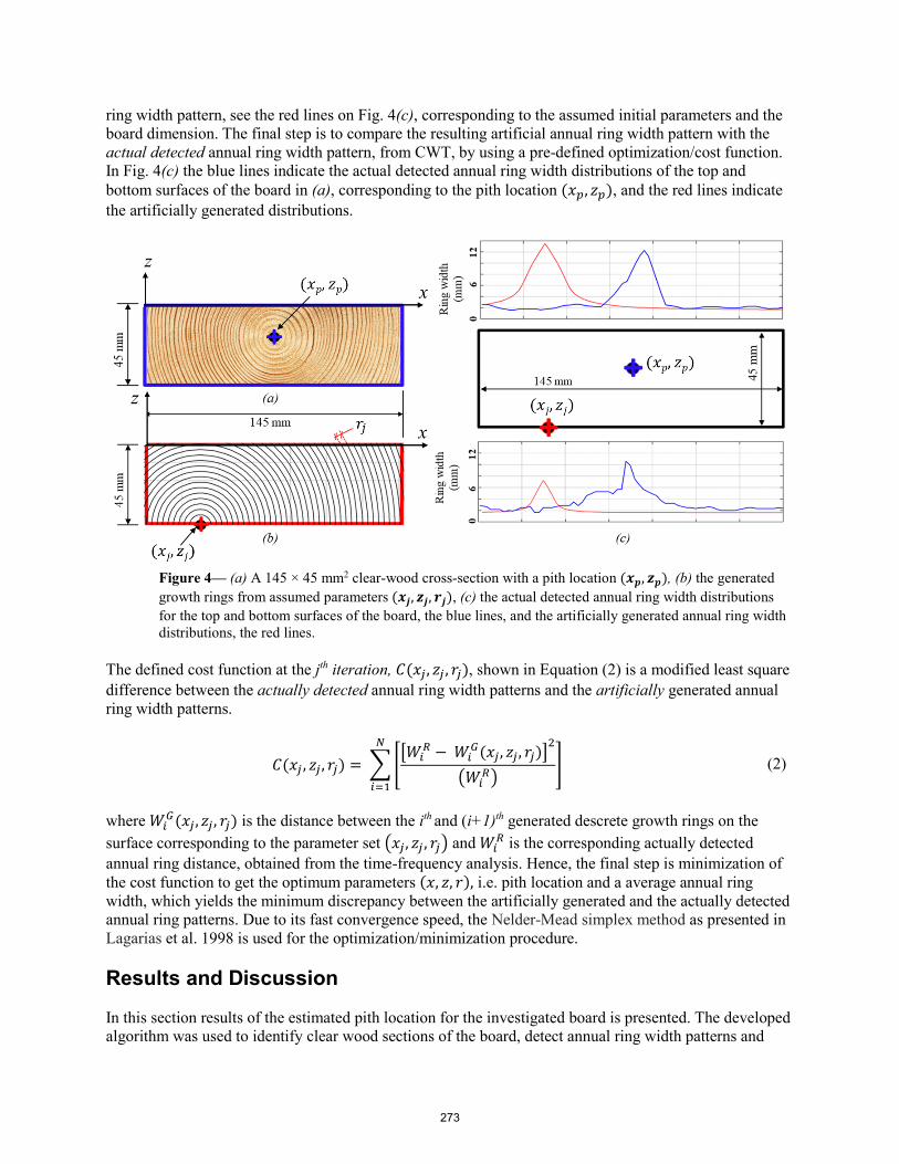
ring width pattern, see the red lines on Fig. 4(c), corresponding to the assumed initial parameters and the board dimension. The final step is to compare the resulting artificial annual ring width pattern with the actual detected annual ring width pattern, from CWT, by using a pre-defined optimization/cost function. In Fig. 4(c) the blue lines indicate the actual detected annual ring width distributions of the top and bottom surfaces of the board in (a), corresponding to the pith location (𝑥𝑥𝑝𝑝, 𝑧𝑧𝑝𝑝), and the red lines indicate the artificially generated distributions.

Figure 4— (a) A 145 × 45 mm2 clear-wood cross-section with a pith location (𝒙𝒙𝒑𝒑, 𝒛𝒛𝒑𝒑), (b) the generated growth rings from assumed parameters (𝒙𝒙𝒋𝒋, 𝒛𝒛𝒋𝒋, 𝒓𝒓𝒋𝒋), (c) the actual detected annual ring width distributions for the top and bottom surfaces of the board, the blue lines, and the artificially generated annual ring width distributions, the red lines.

The defined cost function at the jth iteration, 𝐶𝐶(𝑥𝑥𝑗𝑗, 𝑧𝑧𝑗𝑗 , 𝑟𝑟𝑗𝑗), shown in Equation (2) is a modified least square difference between the actually detected annual ring width patterns and the artificially generated annual ring width patterns.

𝐶𝐶(𝑥𝑥𝑗𝑗 , 𝑧𝑧𝑗𝑗, 𝑟𝑟𝑗𝑗) = 𝑊𝑊𝑖𝑖

𝑅𝑅 − 𝑊𝑊𝑖𝑖𝐺𝐺(𝑥𝑥𝑗𝑗, 𝑧𝑧𝑗𝑗, 𝑟𝑟𝑗𝑗)2

𝑊𝑊𝑖𝑖𝑅𝑅

𝑁𝑁

𝑖𝑖=1

(2)

where 𝑊𝑊𝑖𝑖𝐺𝐺(𝑥𝑥𝑗𝑗, 𝑧𝑧𝑗𝑗, 𝑟𝑟𝑗𝑗) is the distance between the ith and (i+1)th generated descrete growth rings on the

surface corresponding to the parameter set 𝑥𝑥𝑗𝑗, 𝑧𝑧𝑗𝑗 , 𝑟𝑟𝑗𝑗 and 𝑊𝑊𝑖𝑖𝑅𝑅 is the corresponding actually detected

annual ring distance, obtained from the time-frequency analysis. Hence, the final step is minimization of the cost function to get the optimum parameters (𝑥𝑥, 𝑧𝑧, 𝑟𝑟), i.e. pith location and a average annual ring width, which yields the minimum discrepancy between the artificially generated and the actually detected annual ring patterns. Due to its fast convergence speed, the Nelder-Mead simplex method as presented in Lagarias et al. 1998 is used for the optimization/minimization procedure.

Results and Discussion

In this section results of the estimated pith location for the investigated board is presented. The developed algorithm was used to identify clear wood sections of the board, detect annual ring width patterns and

273

finally estimate the pith location and annual ring width of the individually identified clear-wood sections. Out of the identified clear-wood sections, the algorithm was applied on a total of 12 clear-wood sections and the results are presented in this section.

Figure 5— Estimated vs. manually measured actual pith locations.

The presented results are verified against true pith locations of the considered cross-section obtained by slicing the timber board at the corresponding 12 clear-wood sections and manually measuring the x- and z-coordinates of the actual pith according to the defined coordinate system. Fig. 5 show the results of the estimated pith location, as black dots, versus the actual pith location, as red dots, for the 12 clear wood-sections.

Table 1— Comparison between the actual and predicted pith locations

Section No.

y-location[mm]

Error - x [mm]

Error - z [mm]

Error magnitude [mm]

1 80 0.7 0.6 0.9 2 300 5.3 2.3 5.8 3 490 4.6 0.2 4.6 4 720 5.2 1.5 5.4 5 820 5.1 3.2 6.0 6 1390 1.7 3.1 3.6 7 1685 4.8 2.2 5.3 8 1990 5.0 7.3 8.8 9 2350 1.8 0.6 1.9 10 2700 6.5 1.9 6.8 11 3250 5.3 0.6 5.3 12 3790 1.3 5.9 6.1

274

Table 1 shows the results of the individual errors between the predicted pith location and the actual measured location in the x- and z-directions for all the 12 clear wood sections. A maximum error magnitude of 8.8 mm is determined for the 8th section, Sec. 8, and a minimum error magnitude of 0.9 mm is determined for the first section, Sec. 1.

Conclusions

A new non-destructive method to determine the pith location and estimate the average annual ring width of Norway spruce clear-wood sections along the longitudinal direction of the board was presented. The method, which is based on surface optical scanning of the four sides of timber boards, is designed to be able to estimate the pith location, even in cases where the pith is located outside the cross-section. According to the presented results, the proposed method yields an accurate estimation of pith location. However, future work has to be done regarding the verification of the proposed method using a larger test specimen.

References

Blouin, D., Beaulieu, J., Daoust, G. and Poliquin, J., 2007. Wood quality of Norway spruce grown in plantations in Quebec. Wood and Fiber Science, 26(3), pp.342-353.

Briggert, A., Olsson, A. and Oscarsson, J., 2016. Three-dimensional modelling of knots and pith location in Norway spruce boards using tracheid-effect scanning. European Journal of Wood and Wood Products, 74(5), pp.725-739.

Hu, M., Olsson, A., Johansson, M. and Oscarsson, J., 2018. Modelling local bending stiffness based on fibre orientation in sawn timber. European Journal of Wood and Wood Products, 76(6), pp.1605-1621.

Kliger, I.R., Perstorper, M. and Johansson, G., 1998. Bending properties of Norway spruce timber. Comparison between fast-and slow-grown stands and influence of radial position of sawn timber. In Annales des sciences forestières (Vol. 55, No. 3, pp. 349-358). EDP Sciences.

Lagarias, J.C., Reeds, J.A., Wright, M.H. and Wright, P.E., 1998. Convergence properties of the Nelder--Mead simplex method in low dimensions. SIAM Journal on optimization, 9(1), pp.112-147.

Lilly, J.M. and Olhede, S.C., 2012. Generalized Morse wavelets as a superfamily of analytic wavelets. IEEE Transactions on Signal Processing, 60(11), pp.6036-6041.

Longuetaud, F., Leban, J.M., Mothe, F., Kerrien, E. and Berger, M.O., 2004. Automatic detection of pith on CT images of spruce logs. Computers and Electronics in Agriculture, 44(2), pp.107-119.

Ormarsson, S., Dahlblom, O. and Petersson, H., 1999. A numerical study of the shape stability of sawn timber subjected to moisture variation Part 2: Simulation of drying board. Wood Science and Technology, 33(5), pp.407-423.

Perlin, L.P., do Valle, Â. and de Andrade Pinto, R.C., 2018. New method to locate the pith position in a wood cross-section based on ultrasonic measurements. Construction and Building Materials, 169, pp.733-739.

275

Session 4

Wood Material Characterization

276

Prediction of Bending and Hardness Strength Properties of Oil Palm (Elaeis guineensis Jacq.) Trunk using Nondestructive Evaluation of Ultrasonic Testing MethodLina Karlinasari* Department of Forest Products, Faculty of Forestry, IPB University (Bogor Agricultural University), Bogor 16680, Indonesia, karlinasari@apps.ipb.ac.id

Rasis Putra Ritonga Department of Forest Products, Faculty of Forestry, IPB University (Bogor Agricultural University), Bogor 16680, Indonesia, rasisputra06@gmail.com

Akhiruddin Maddu Department of Physics, Faculty of Mathematics and Natural Sciences, IPB University (Bogor Agricultural University), Bogor 16680, Indonesia, akhiruddin@ipb.ac.id

Abstract

Oil-palm trunk has a great potential to be a product because of its abundance, especially of their "wood" waste after about 25 years of productivity. However, the oil palm trunk has a low quality and in a wide variation among the inner, middle, and outer part of the cross –section transversal position. The objective of this study was to evaluate the dynamic modulus of elasticity (MOEd) of oil palm wood (Elaeis guineensis Jacq.) wood nondestructively through longitudinal ultrasonic wave propagation and to determine the relationship between MOEd and static bending properties [static modulus of elasticity (MOEs) and modulus of rupture (MOR)] as well as hardness strength properties. The results showed that the cross-section transversal position was significantly influenced the properties of the oil palm trunk. The MOEd values were higher about 2 times than the static modulus of elasticity (MOEs) but both were highly correlated. The ultrasonic velocity (Vus) had significant correlation with the MOEs (r = 0.73), MOR (r = 0.73), as well as the hardness strength properties (r = 0.76). There was a strong and significant correlation between the dynamic modulus of elasticity (MOEd) and static bending properties (MOEs, MOR) and hardness strength properties. The correlation coefficient was (r = 0.85, r = 0.86, and r = 0.86) for MOEs, MOR, and hardness, respectively. Based on the study, this nondestructive testing may encourage the uses of this technique to predict the strength of oil palm trunk in the field as the fast and reliable method.

Keywords: oil palm trunk wood, MOEd, static modulus, hardness properties, horizontal position

Introduction

The harvesting of oil palm begins two to three years after planting in the field, and it has an economic life of 25 to 30 years, upon which the tree is chopped for replanting (Rosli et al. 2016). The large production of oil palm can actually cause environmental problems, especially after rejuvenation. Oil palm trunks are normally left to burn or decay in the plantation area. However, freshly felled trunks, with their high moisture content, cannot easily be burned in the field. The utilization of oil palm trunks can solve environmental problems by converted the waste to become a valuable product. Oil palm trunk waste has

277

the potential to be used as a substitute product for timber forest products because of its abundance and similar anatomic characteristics to wood (Dungani et al. 2013). Some of the weaknesses of oil palm stems include relatively low density and strength, very high water content and high starch content which causes oil palm trunks to be very susceptible to mold attack, blue stain, weathering fungi and insects. For that reasons, there are many studies have been conducted to improve the quality of oil palm trunk through modification treatments such as impregnation, densification, etc. (Sulaiman et al. 2012), and converting becoming the various products produced from oil palm trunk such as plywood (Hoong and Paridah 2013), particleboard (Saari et al. 2014, Lamaming et al. 2014), LVL (Sulaiman et al. 2009).

Oil palm tree are produced from monocotyledonous plants which have various properties from the outside to the center of the trunk. Oil palm trunk is not truly a woody material. The properties that vary from the outside to the center of the stem are caused by the anatomical arrangement of the oil palm trunk which has two main components, namely vascular bundle and parenchyma (Rahayu 2001). Only one third of the outer portion (edge) of the horizontal cross section is dominated by vascular tissue and the remainder is dominated by parenchymal tissue. Those outer oil palm trunk is suitable for use as a lightweight construction material and furniture because it has good mechanical physical properties. Through good sawn pattern as mention by Bakar et al. (1998) it can be obtained the suitable part for appropriate product. The aim of this study was to evaluate the dynamic modulus of elasticity (MOEd) of oil palm wood (Elaeis guineensis Jacq.) wood nondestructively through longitudinal ultrasonic wave propagation and to determine the relationship between MOEd and static bending properties [static modulus of elasticity (MOEs) and modulus of rupture (MOR)] as well as hardness strength properties.

Methodology

The natural materials used in this research were oil palm (Elaeis guineensis Jacq.) trunk in about 30 years old with ± 25 cm in diameter and 800 cm in length obtained from National Plantation Estate in Jasinga, Bogor, West Java. The trunk had been unproductive and for regeneration reason, the company has started to have new seedling plants. The oil palm trunk is not truly a woody material which consists of three zones: outer, middle, and inner, with the outside part has cortex with bark. Immediately after felling, the trunk was divided in three for about 200 cm in length to have bottom, middle, and up parts. The samples were then cut out into dimension length, width, and thickness about (80 x 25 x 5) cm. Drying process were conducted in kiln drying with the temperature ±50 °C for two weeks followed by natural drying to reduce moisture content and obtain air-dried moisture content. The ASTM D 143 (ASTM 2014) for secondary method was referred to produce the sample tested which was divided into outer (L), middle (T), and inner (D) parts (Figure 1). The physical properties of density, ultrasonic velocity, and specific gravity were measured as well as mechanical properties of dynamic modulus of elasticity, static MOE and MOR, and hardness of wood. The longitudinal ultrasonic wave velocity were determined by nondestructive testing of Sylvatest Duo equipment. The moisture content was determined by gravimetric method, whereas density as well as specific gravity were calculated based on weight divided by sample volume for air dried weight and oven-dried weight, respectively. The ultrasonic velocity (Vus) was measure using the following formula:

(m/s) (1)

where d is the distance between the two transducers, and t is the time of flight of ultrasonic waves.

The dynamic MOE was calculated by the following equations

kg/cm2) (2)

278

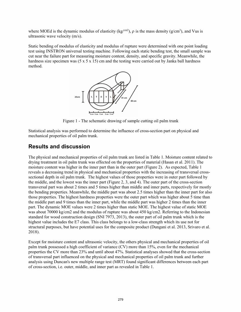
where MOEd is the dynamic modulus of elasticity (kg/cm2), ρ is the mass density (g/cm3), and Vus is ultrasonic wave velocity (m/s).

Static bending of modulus of elasticity and modulus of rupture were determined with one point loading test using INSTRON universal testing machine. Following each static bending test, the small sample was cut near the failure part for measuring moisture content, density, and specific gravity. Meanwhile, the hardness size specimen was (5 x 5 x 15) cm and the testing were carried out by Janka ball hardness method.

Figure 1 - The schematic drawing of sample cutting oil palm trunk

Statistical analysis was performed to determine the influence of cross-section part on physical and mechanical properties of oil palm trunk.

Results and discussion

The physical and mechanical properties of oil palm trunk are listed in Table 1. Moisture content related to drying treatment in oil palm trunk was effected on the properties of material (Hasan et al. 2011). The moisture content was higher in the inner part than in the outer part (Figure 2). As expected, Table 1 reveals a decreasing trend in physical and mechanical properties with the increasing of transversal cross-sectional depth in oil palm trunk. The highest values of those properties were in outer part followed by the middle, and the lowest was the inner part (Figure 2, 3, and 4). The outer part of the cross-section transversal part was about 2 times and 5 times higher than middle and inner parts, respectively for mostly the bending properties. Meanwhile, the middle part was about 2.5 times higher than the inner part for also those properties. The highest hardness properties were the outer part which was higher about 5 time than the middle part and 9 times than the inner part, while the middle part was higher 2 times than the inner part. The dynamic MOE values were 2 times higher than static MOE. The highest value of static MOE was about 70000 kg/cm2 and the modulus of rupture was about 450 kg/cm2. Referring to the Indonesian standard for wood construction design (SNI 7973, 2013), the outer part of oil palm trunk which is the highest value includes the E7 class. This class belongs to a low-class strength which its use not for structural purposes, but have potential uses for the composite product (Dungani et al. 2013, Srivaro et al. 2018).

Except for moisture content and ultrasonic velocity, the others physical and mechanical properties of oil palm trunk possessed a high coefficient of variance (CV) more than 15%, even for the mechanical properties the CV more than 23% and until about 47%. Statistical analyses showed that the cross-section of transversal part influenced on the physical and mechanical properties of oil palm trunk and further analysis using Duncan's new multiple range test (MRT) found significant differences between each part of cross-section, i.e. outer, middle, and inner part as revealed in Table 1.

279

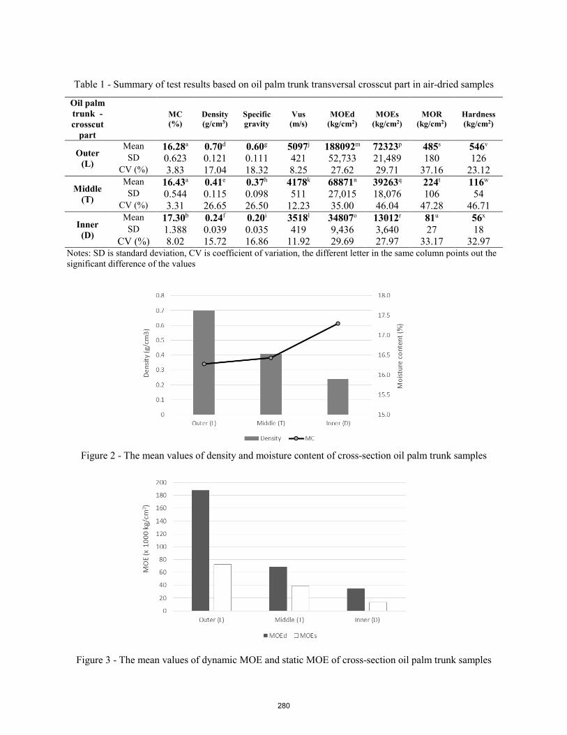
Table 1 - Summary of test results based on oil palm trunk transversal crosscut part in air-dried samples

Notes: SD is standard deviation, CV is coefficient of variation, the different letter in the same column points out the significant difference of the values

Figure 2 - The mean values of density and moisture content of cross-section oil palm trunk samples

Figure 3 - The mean values of dynamic MOE and static MOE of cross-section oil palm trunk samples

Oil palm trunk - crosscut

part

MC (%)

Density (g/cm3)

Specific gravity

Vus (m/s)

MOEd (kg/cm2)

MOEs (kg/cm2)

MOR (kg/cm2)

Hardness (kg/cm2)

Outer (L)

Mean 16.28a 0.70d 0.60g 5097j 188092m 72323p 485s 546v SD 0.623 0.121 0.111 421 52,733 21,489 180 126

CV (%) 3.83 17.04 18.32 8.25 27.62 29.71 37.16 23.12

Middle (T)

Mean 16.43a 0.41e 0.37h 4178k 68871n 39263q 224t 116w SD 0.544 0.115 0.098 511 27,015 18,076 106 54

CV (%) 3.31 26.65 26.50 12.23 35.00 46.04 47.28 46.71

Inner (D)

Mean 17.30b 0.24f 0.20i 3518l 34807o 13012r 81u 56x SD 1.388 0.039 0.035 419 9,436 3,640 27 18

CV (%) 8.02 15.72 16.86 11.92 29.69 27.97 33.17 32.97

280

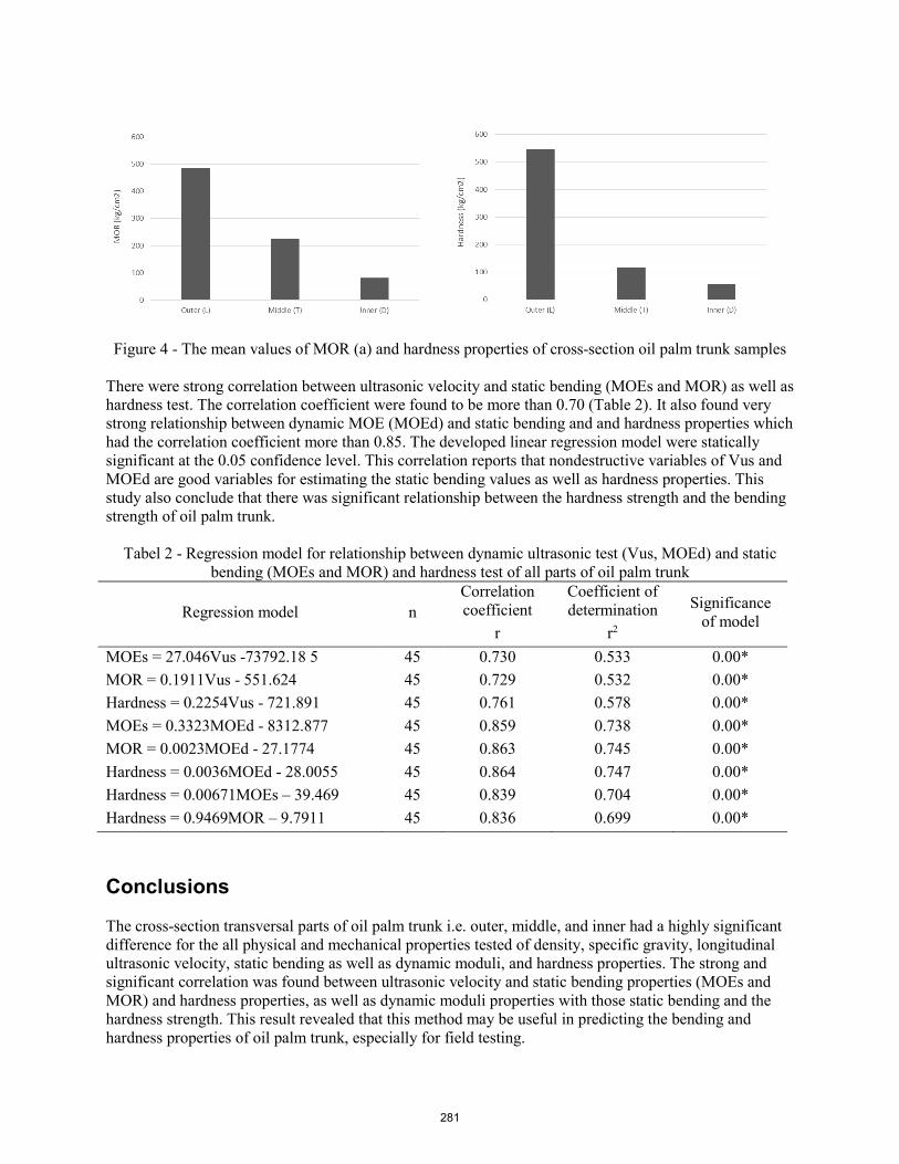
Figure 4 - The mean values of MOR (a) and hardness properties of cross-section oil palm trunk samples

There were strong correlation between ultrasonic velocity and static bending (MOEs and MOR) as well as hardness test. The correlation coefficient were found to be more than 0.70 (Table 2). It also found very strong relationship between dynamic MOE (MOEd) and static bending and and hardness properties which had the correlation coefficient more than 0.85. The developed linear regression model were statically significant at the 0.05 confidence level. This correlation reports that nondestructive variables of Vus and MOEd are good variables for estimating the static bending values as well as hardness properties. This study also conclude that there was significant relationship between the hardness strength and the bending strength of oil palm trunk.

Tabel 2 - Regression model for relationship between dynamic ultrasonic test (Vus, MOEd) and static bending (MOEs and MOR) and hardness test of all parts of oil palm trunk

Regression model n Correlation coefficient

r

Coefficient of determination

r2

Significance of model

MOEs = 27.046Vus -73792.18 5 45 0.730 0.533 0.00* MOR = 0.1911Vus - 551.624 45 0.729 0.532 0.00* Hardness = 0.2254Vus - 721.891 45 0.761 0.578 0.00* MOEs = 0.3323MOEd - 8312.877 45 0.859 0.738 0.00* MOR = 0.0023MOEd - 27.1774 45 0.863 0.745 0.00* Hardness = 0.0036MOEd - 28.0055 45 0.864 0.747 0.00* Hardness = 0.00671MOEs – 39.469 45 0.839 0.704 0.00* Hardness = 0.9469MOR – 9.7911 45 0.836 0.699 0.00*

Conclusions

The cross-section transversal parts of oil palm trunk i.e. outer, middle, and inner had a highly significant difference for the all physical and mechanical properties tested of density, specific gravity, longitudinal ultrasonic velocity, static bending as well as dynamic moduli, and hardness properties. The strong and significant correlation was found between ultrasonic velocity and static bending properties (MOEs and MOR) and hardness properties, as well as dynamic moduli properties with those static bending and the hardness strength. This result revealed that this method may be useful in predicting the bending and hardness properties of oil palm trunk, especially for field testing.

281

References

[ASTM] American Society for Testing and Materials. 2014. ASTM D 143. Standard Test Methods for Small Clear Specimens of Timber. USA

Bakar, E.S; Rachman, O.; Hermawan, D.; Karlinasari, L.; Rosdiana, N. 1998. Pemanfaatan batang kelapa sawit sebagai bahan bangunan dan furniture. Ilmu dan Teknologi Hasil Hutan. 11(1): 1-12.

Dungani, R.; Jawaid, M.; Abdul Khalil, H.P.S.; Jasni, Aprilia, S.; Hakeem, K.R.; Hartati, S.; Islam, M.N. 2013. A review on quality enhancement of oil palm trunk waste by resin impregnation: Future materials. BioResource. 8(2): 3136-3156.

Hasan, K.; Kasim, J.; Mokhtar, A.; Aziz, A.A. 2011. Characterisation of oil palm trunks and their holocellulose fibres for the manufacture of industrial commodities. Oil Palm Bulletin 63: 11 – 23.

Hoong, Y.B.; Paridah, M.T. 2013 Development a new method for pilot scale production of high grade oil palm plywood: Effect hot pressing time. Materials and Design. 45: 142-147.

Lamaming, J.; Hashim, R.; Sulaiman, O.; Sugimoto, T.; Sato, M.; Hiziroglu S. 2014. Measurement of some properties of binderless particleboards made from young and old oil palm trunks. Measurement. 47: 813-819.

Rahayu, I.S. 2001. Sifat dasar vascular bundles dan parenchyme batang kelapa sawit dalam kaitannya dengan sifat fisis, mekanis serta keawetan. Bogor: Institut Pertanian Bogor. M.S. Thesis.

Rosli, F.; Ghazali, C.M.R.; Abdullah, M.M.A.B., Hussin, K. 2016. A review: Characteristics of oil palm trunk (OPT) and quality improvement of palm trunk plywood by resin impregnation. BioResource. 11(2): 5565-5580.

Saari, N.; Hashim, R.; Sulaiman, O.; Hiziroglu, S., Sato, M.; Sugimoto, T. 2014. Properties of steam treated binderless particleboard made from oil palm trunks. Composites Part B: Engineering. 56: 344-349.

[SNI] Standar Nasional Indonesia. 2013. SNI 7973. Spesifikasi Desain untuk Kontruksi Kayu. Indonesia.

Srivaro, S.; Rattanarat, J.; Noothong, P. 2018. Comparison of the anatomical characteristics and physical and mechanical properties of oil palm and bamboo trunks. Journal of Wood Science. 64:186–192.

Sulaiman, O.: Salim, N.; Hashim, R.; Tusof, L.H.; Razak, W.; Yunus, N.Y.M.; Hashim, W.S.; Azmy, M.H. 2009. Evaluation on the suitability of some adhesive for laminated veneer lumber from oil palmtrunks. Materials and Design. 30: 3572-3580.

Sulaiman, O.; Salim, N.; Nordin, N.A; Ibrahim, M.; Sato, M. 2012. The potential of oil palm trunk biomass as an alternative source for compresses wood. BioResource. 7 (2): 2688-2706.

282

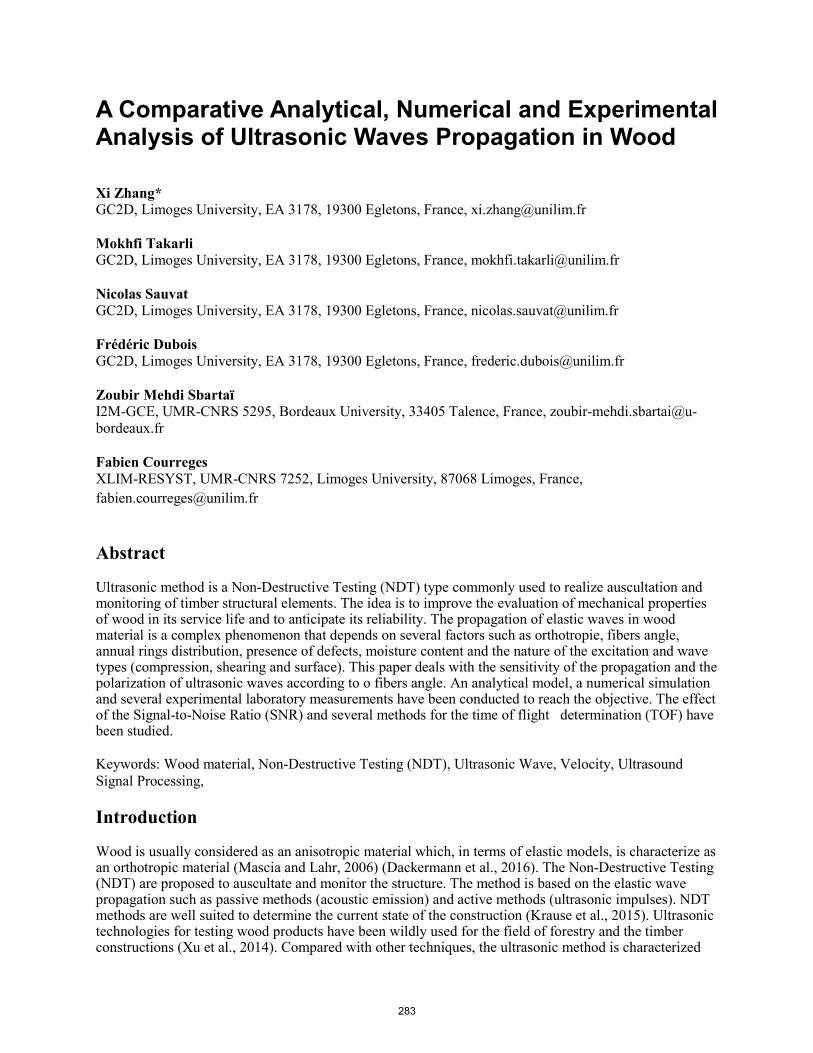
A Comparative Analytical, Numerical and Experimental Analysis of Ultrasonic Waves Propagation in Wood

Xi Zhang* GC2D, Limoges University, EA 3178, 19300 Egletons, France, xi.zhang@unilim.fr

Mokhfi Takarli GC2D, Limoges University, EA 3178, 19300 Egletons, France, mokhfi.takarli@unilim.fr

Nicolas Sauvat GC2D, Limoges University, EA 3178, 19300 Egletons, France, nicolas.sauvat@unilim.fr

Frédéric Dubois GC2D, Limoges University, EA 3178, 19300 Egletons, France, frederic.dubois@unilim.fr

Zoubir Mehdi Sbartaï I2M-GCE, UMR-CNRS 5295, Bordeaux University, 33405 Talence, France, zoubir-mehdi.sbartai@u-bordeaux.fr

Fabien Courreges XLIM-RESYST, UMR-CNRS 7252, Limoges University, 87068 Limoges, France, fabien.courreges@unilim.fr

Abstract

Ultrasonic method is a Non-Destructive Testing (NDT) type commonly used to realize auscultation and monitoring of timber structural elements. The idea is to improve the evaluation of mechanical properties of wood in its service life and to anticipate its reliability. The propagation of elastic waves in wood material is a complex phenomenon that depends on several factors such as orthotropie, fibers angle, annual rings distribution, presence of defects, moisture content and the nature of the excitation and wave types (compression, shearing and surface). This paper deals with the sensitivity of the propagation and the polarization of ultrasonic waves according to o fibers angle. An analytical model, a numerical simulation and several experimental laboratory measurements have been conducted to reach the objective. The effect of the Signal-to-Noise Ratio (SNR) and several methods for the time of flight determination (TOF) have been studied.

Keywords: Wood material, Non-Destructive Testing (NDT), Ultrasonic Wave, Velocity, Ultrasound Signal Processing,

Introduction

Wood is usually considered as an anisotropic material which, in terms of elastic models, is characterize as an orthotropic material (Mascia and Lahr, 2006) (Dackermann et al., 2016). The Non-Destructive Testing (NDT) are proposed to auscultate and monitor the structure. The method is based on the elastic wave propagation such as passive methods (acoustic emission) and active methods (ultrasonic impulses). NDT methods are well suited to determine the current state of the construction (Krause et al., 2015). Ultrasonic technologies for testing wood products have been wildly used for the field of forestry and the timber constructions (Xu et al., 2014). Compared with other techniques, the ultrasonic method is characterized

283

by its low-cost safety and its rapidity to obtain quantitative results. Moreover, it can be used to assess structure without impact could cause damage (Xu et al., 2014). For ultrasonic method, a wave is propagating into the material with a known distance between transmitter and receiver sensors. The transmission time between transmitter and receiver is called the Time Of Flight (TOF). The wave velocity is deduced by the ratio between the distance and the TOF. The velocity data is the basis for determining various material properties. Due to the wood orthotropy, the waves travel is characterized by different velocities which depend on the fiber angle direction. The velocities in radial and tangential direction are usually around a third of the velocity in longitudinal direction (Dackermann et al., 2013). Regarding timber element auscultation, the work target is to obtain a cartography of the mechanical properties (E, G, υ) by integrating the effects of the orthotropie and the presence of defects. The results obtained by experimental measurements of elastic wave velocities (compression and shear) performed on massive beams (Douglas) and glulam beams (Douglas and Spruce) are presented. Two methods are used according to the Signal-to-Noise Ratio (SNR) to determine the TOF: The Akaike Criterion (AIC) and the Hinkley criterion (Hinkley).

In this way, this work aims to compare these two approaches (theoretical and experimental) dealing with the correction of the fiber angle, the impact of species and scales on the propagation velocity of compression waves. A theoretical approach is also carried out. It allows us to develop predictive finite element mechanical model in order to confirm experimental and analytical results. In conclusion, an example of the elastic moduli determination using a solving method between experimental measurements and analytic model is proposed.

Propagation and polarization of mechanical waves in an orthotropic elastic model

Analytical approach

Basically, the material elastic moduli can be determined by studying its elastic wave propagation velocity be considering compression wave “P” and shear wave “S” (Espinosa et al., 2018) (Cuxac, 1991). The ultrasonic wave propagation in wood can be expressed via the equation of wave motion. The combination of Newton’s second and Hooke’s law give the following expression:

2 2

2i l

ijklj k

u uCt x x

ρ ∂ ∂⋅ = ⋅∂ ∂ ∂

(1)

𝜌𝜌 is the specific gravity. ijklC designates the 81 stiffness tensor components in a three-dimensional

configuration. iu is the displacement components of a point M. As shown in Figure 1, material axes (L,

R, T) are coincident with the Cartesian coordinate system ( )1 2 3, ,X X X .

Figure 1— Local referential

284

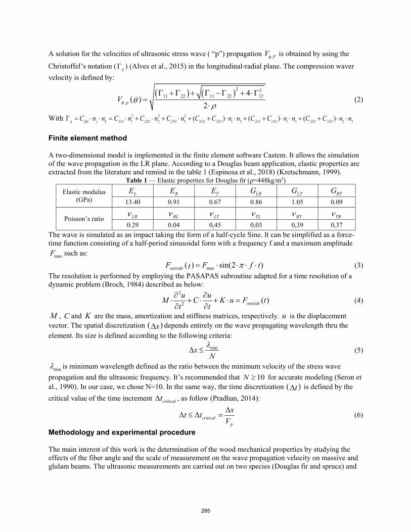
A solution for the velocities of ultrasonic stress wave ( “p”) propagation ,PVφ is obtained by using the

Christoffel’s notation ( ijΓ ) (Alves et al., 2015) in the longitudinal-radial plane. The compression waver velocity is defined by:

( )( ) ( )2 2

1211 22 11 22,

42pVφ θρ

+ + ⋅ΓΓ +Γ Γ −Γ=

⋅(2)

With 2 2 211 1 22 2 33 3 12 21 1 2 13 31 1 3 23 32 2 3( ) ( ) ( )ij ijkl j k i l i l i l i l i l i l i l i l i lC n n C n C n C n C C n n C C n n C C n nΓ = ⋅ ⋅ = ⋅ + ⋅ + ⋅ + + ⋅ ⋅ + + ⋅ ⋅ + + ⋅ ⋅

Finite element method

A two-dimensional model is implemented in the finite element software Castem. It allows the simulation of the wave propagation in the LR plane. According to a Douglas beam application, elastic properties are extracted from the literature and remind in the table 1 (Espinosa et al., 2018) (Kretschmann, 1999).

Table 1 — Elastic properties for Douglas fir (𝜌𝜌=448kg/m3)

Elastic modulus (GPa)

LE RE TE LRG LTG RTG13.40 0.91 0.67 0.86 1.05 0.09

Poisson’s ratio LRν RLν LTν TLν RTν TRν0.29 0.04 0,45 0,03 0,39 0,37

The wave is simulated as an impact taking the form of a half-cycle Sine. It can be simplified as a force-time function consisting of a half-period sinusoidal form with a frequency f and a maximum amplitude

maxF such as: ( ) max sin(2 )outsideF F f tt π= ⋅ ⋅ ⋅ ⋅ (3)

The resolution is performed by employing the PASAPAS subroutine adapted for a time resolution of a dynamic problem (Broch, 1984) described as below:

2

2 ( )outsideu uM C K u F t

t t∂ ∂⋅ + ⋅ + ⋅ =∂ ∂

(4)

M , C and K are the mass, amortization and stiffness matrices, respectively. u is the displacement vector. The spatial discretization ( )x∆ depends entirely on the wave propagating wavelength thru the element. Its size is defined according to the following criteria:

minxNλ

∆ ≤ (5)

minλ is minimum wavelength defined as the ratio between the minimum velocity of the stress wave propagation and the ultrasonic frequency. It’s recommended that 10N ≥ for accurate modeling (Seron et al., 1990). In our case, we chose N=10. In the same way, the time discretization ( )t∆ is defined by the critical value of the time increment criticalt∆ , as follow (Pradhan, 2014):

criticalp

xt tV∆

∆ ≤ ∆ (6)

Methodology and experimental procedure

The main interest of this work is the determination of the wood mechanical properties by studying the effects of the fiber angle and the scale of measurement on the wave propagation velocity on massive and glulam beams. The ultrasonic measurements are carried out on two species (Douglas fir and spruce) and

285

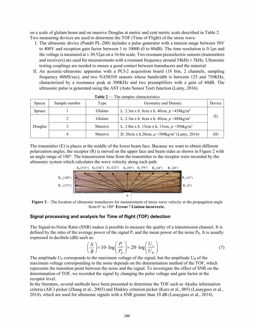
on a scale of glulam beam and on massive Douglas at metric and cent metric scale described in Table 2. Two measuring devices are used to determine the TOF (Time of Flight) of the stress wave.

I. The ultrasonic device (Pundit PL-200) includes a pulse generator with a tension range between 50Vto 400V and reception gain factor between 1 to 10000 (0 to 80dB). The time resolution is 0.1𝜇𝜇s andthe voltage is measured at ± 30.52𝜇𝜇s on a 16-bit scale. Two resonant piezoelectric sensors (transmittersand receivers) are used for measurements with a resonant frequency around 54kHz ± 5kHz. Ultrasonictesting couplings are needed to ensure a good contact between transducers and the material.

II. An acoustic-ultrasonic apparatus with a PCI-2 acquisition board (18 bits, 2 channels, samplingfrequency 40MS/sec), and two NANO30 sensors whose bandwidth is between 125 and 750KHz,characterized by a resonance peak at 300KHz and two preamplifiers with a gain of 40dB. Theultrasonic pulse is generated using the AST (Auto Sensor Test) function.(Lamy, 2016).

Table 2 — The samples characteristics Specie Sample number Type Geometry and Density Device

Spruce 1 Glulam L. 2.3m x b. 8cm x h. 40cm, 𝜌𝜌 =438kg/m3

(I)

Douglas

2 Glulam L. 2.3m x b. 8cm x h. 40cm, 𝜌𝜌 =488kg/m3

3 Massive L. 3.0m x b. 15cm x h. 15cm, 𝜌𝜌 =504kg/m3

4 Massive D. 20cm x h.20cm, 𝜌𝜌 =500kg/m3 (Lamy, 2016) (II)

The transmitter (E) is places at the middle of the lower beam face. Because we want to obtain different polarization angles, the receptor (R) is moved on the upper face and beam sides as shown in Figure 2 with an angle range of 180°. The transmission time from the transmitter to the receptor were recorded by the ultrasonic system which calculates the wave velocity along each path.

Figure 2—The location of ultrasonic transducers for measurement of stress wave velocity at the propagation angle from 0° to 180° Erreur ! Liaison incorrecte..

Signal processing and analysis for Time of flight (TOF) detection

The Signal-to-Noise Ratio (SNR) makes it possible to measure the quality of a transmission channel. It is defined by the ratio of the average power of the signal Ps and the mean power of the noise PB. It is usually expressed in decibels (dB) such as:

10 log 20 logs s

B B

P USP UB

= ⋅ = ⋅ (7)

The amplitude US corresponds to the maximum voltage of the signal, but the amplitude UB of the maximum voltage corresponding to the noise depends on the determination method of the TOF, which represents the transition point between the noise and the signal. To investigate the effect of SNR on the determination of TOF, we recorded the signal by changing the pulse voltage and gain factor at the receptor level. In the literature, several methods have been presented to determine the TOF such as Akaike information criteria (AIC) picker (Zhang et al., 2003) and Hinkley criterion picker (Kurz et al., 005) (Lasaygues et al., 2014), which are used for ultrasonic signals with a SNR greater than 10 dB (Lasaygues et al., 2014).

286

a) The “Hinkley criterion Picker” (Hinkley) is a method used for the concrete NDT (Kurz et al., 2005).It is based on the comparison between the partial energy and the total energy of the signal:

[ ] ( ) ( )2 2

1 1

k N

p pp p

kS x xk Nα= =

= − ⋅⋅∑ ∑ (8)

𝛼𝛼 is an adjustment parameter to minimize the dispersion of the TOF measurements. For 𝛼𝛼=1, the criterion is based on the analysis of the instantaneous power of the signal. In this case, the TOF is determined by the minimum of the Hinkley function.

b) The “AIC picker” (AIC) is a method used to estimate the order of autoregressive (AR) models todetermine the trigger time. In this case, signal intervals are assumed to be two time-series (i.e., noiseand signal), different before and after the trigger time point. The TOF is given by the minimum ofthe AIC function (Zhang et al., 2003) such as:

( ) ( ) ( ) log log1,..., 1,...,AIC k Var x Var xk k NN k= ⋅ + ⋅ +− (9)

[ ]x k is the signal at the index k . n represents the variable. N designates the length of the signal and Var the variance.

In our study, the Hinkley and AIC picker are used for detecting and picking TOF. In addition, a new method (MS: Maximum Sliding) have also been proposed. It includes the evolution of the maximum amplitude for a given waveform as a function of recording time, Figure 3. The first low platform corresponding to the noise level N and the largest platform corresponding to the maximum amplitude of the signal S.

Figure 3—Ultrasonic signal waveform and determination of SNR

Figure 4 shows a logarithmic increasing in the SNR as a function of the pulse voltage and the gain factor. This increase is greater depending to the gain.

(a) (b) Figure 4—(a). Evolution of the SNR according to the pulse voltage with a gain factor 1000; (b). Evolution of the

SNR according to the gain factor with a pulse voltage 200V.

287

Figure 5 presents the TOF evolution according to the SNR. It is determined with the SNR equation according to the three methods (Hinkley, AIC and MS). The amplitude of UB depends on the method TOF calculation. This evolution allows to do two remarks:

i. Firstly, the Hinkley method is distinguished by the highest TOF and the lowest SNR. This fact stemsfrom an overestimation of the noise level. Furthermore, TOF values are highly dispersed for a verysmall SNR band.

ii. Secondly, results given with AIC and MS methods are similar. This fact highlights that the TOFdecreases with a SNR increasing. However, it becomes to be stable from SNR approximately to20dB. Nevertheless, we note a TOF dispersion that fade between 20dB and 27dB.

(a) (b) Figure 5—(a) Evolution of the TOF vs SNR; (b) Evolution of the stress wave propagation velocity vs SNR.

Figure 5 (b) gives the evolution of the stress wave propagation velocity according to SNR. We can note that the velocity increasing starts to stabilize between 20dB and 30dB. Between the minimum value of the SNR (9.4dB) and its maximum value (42.1dB), we can note an error around 400m/s in the estimation of the velocity VP.

Results and discussion

Comparison of the wave propagation velocity Figure 6 (a) shows the evolution of the stress wave propagation velocity ( PV ) according to the fiber angle on the plane LR. The measurements were carried out on Doulas Glulam and Douglas massive in two different scales. Measures were made on a beam of 2 meters long, and on the other hand on a cylindrical sample of 20 centimeters in diameter, Fig. 2. In general, these three curves show a similar evolution with a good fitting with the empirical Hankinson’s law (Xu et al., 2014).

( ) ( )

,0 ,90

,0 ,90sin cosp p

Hankinson n np p

V VV

V Vθ θ° °

°

⋅=

⋅ + ⋅(10)

(a) (b) Figure 6— Evolution of pV according to the fiber angle on the LR plan (a) for Douglas massive in two different

scales et Douglas Glulam; (b) for Spruce and Douglas Glulam in metric scale

288

Figure 6 (b) presents results obtained on glulam beams (Douglas and Spruce). The same trend could be observed for these two samples. The small differences can probably be justified by the differences in density. Combining Figure 6, we can conclude that the similarity of the results between massive wood and glulam shows that the effect of orthotropie on velocities is mainly governed by the natural fibers direction. Moreover, the presence of the lamellae parallel to these fibers does not seem to add a considerable effect on the propagation velocities. The effect of the lamellae can be seen possibly by introducing the attenuation parameter of waves induced by the diffraction and reflection effects at the glued interfaces.

Identification of the mechanical properties

The elastic parameters ( ), ,E G υ could be determined by several experimental measurements due to the fiber angle variation. Therefore, the results, in terms of propagation velocity, were chosen to recover its elastic parameters posted in Table 3. Thus, with at least three experimental measurements, 5 mechanical parameters can be determined by a solver operation. With a transverse isotropic hypothesis in the longitudinal direction, RE and TE are combined. The density was measured by overall mass and volume. For all specimens, results are posted as Table 2. Comparing with Table 1, parameters determined by solving function are in the normal range. Moreover, shear modulus RTG and LTG could be recover by experimental measurements in the plane RT and in the plane LT, respectively.

Table 3—The characteristics of samples (m: metric scale; cm: cent metric scale).

Wood samples Elastic Modules(GPa) Poisson’s ratio Density (kg/m3)

LE RE TE LRG LRν RTν LTν ρ

Spruce Glulam (m) 13.5 1.15 1.15 0.96 0.81 0.12 0.81 428 Douglas Glulam (m) 13.95 2.19 2.19 0.91 0.44 0.22 0.44 488 Douglas Massive (m) 13.16 2.32 2.32 1.05 0.50 0.18 0.50 504 Douglas Massive (cm) 12.49 1.86 1,86 0.84 0.43 0.32 0.43 500

So for in future works, Douglas massive characteristics in scale cent metric (as Table 3) were applied for the analytical and numerical model that are presented previously in order to verify our three approaches. Comparing inverse analysis for these three approaches, we can find that it’s correct because we recue the same results for the propagation velocity, as shown in Figure 7. Owing to the imprecision of mesh, there is a standard deviation between the numerical and analytical results, the average of this standard deviation is about 1.87%. This proven numerical model will be able to integrate material variations (humidity, density, mechanical properties, etc.).

Figure 7—Evolution of pV for the Douglas Massive via the experimental, analytical and numerical model.

289

Conclusion On the scale of the structural elements, the wood is represented as an orthotropic material in consideration of a relatively cylindrical growth ring. The effect of wood orthotropy on compression velocities VP shows a good concordance between experimental approaches (metric scale and centimeter scale, massif wood and glulam wood) and the theory (analytical and numerical developments). The standard deviation between analytical and numerical model can be decreased by decreasing spatial and temporal discretization. In the plane LR, five mechanical parameters can be determined by at least three experimental measurements of the compression velocities. Due to the wood orthotropy, there is the possibility to find all the mechanical constants by more measurements on the plane RT and LT.

However, for the study of specimens of different scale, positioned far from the center, it is often used an orthotropie accompanied by a transverse isotropic RT symmetry. Applying this modeling on the plane (LR), it allows us to highlight the influence of the fiber angle on the velocity of ultrasonic wave propagation. Thus, it appears that the stress waves are substantially affected by the rotation of the direction of propagation. This evolution of VP is in accordance with the Hankinson’s law and does not depends on either of the scale effect nor the lamellae presence. The determination of the TOF depends mainly on the SNR, and the results obtained show a favorable agreement between the method AIC and that method MS developed in this work, the TOF begins to be stable from a SNR that is between 20dB and 30dB.

References Alves, R.C., Mantilla, J.N.R., Bremer, C.F., and Carrasco, E.V.M. 2015. Application of Acoustic Tomography and Ultrasonic Waves to Estimate Stiffness Constants of Muiracatiara Brazilian Wood.

Broch, J.T. 1984. Mechanical Vibration and shock measurement.

Cuxac, P. 1991. Propagation et atténuation des ondes ultrasoniques dans des roches fissurées et anisotropes (Vandœuvre-lès-Nancy, INPL).

Dackermann, U., Crews, K., Kasal, B., Li, J., Riggio, M., Rinn, F., and Tannert, T. 2013. In situ assessment of structural timber using stress-wave measurements.pdf.

Dackermann, U., Elsener, R., Li, J., and Crews, K. 2016. A comparative study of using static and ultrasonic material testing methods to determine the anisotropic material properties of wood. ELSEVIER.

Espinosa, L., Brancheriau, L., Prieto, F., and Lasaygues, P. 2018. Sensitivity of Ultrasonic Wave Velocity Estimation Using the Christoffel Equation for Wood Non-Destructive Characterization. 11.

Krause, M., Dackermann, U., and Li, J. 2015. Elastic wave modes for the assessment of structural timber: Ultrasonic echo for building elements and guided waves for pole and pile structures.

Kretschmann, D.E. 1999. Mechanical Properties of Wood. J. Inst. Wood Sci. 46.

Kurz, J.H., Grosse, C.U., and Reinhardt, H.-W. 2005. Strategies for reliable automatic onset time picking of acoustic emissions and of ultrasound signals in concrete.

Lamy, F. 2016. Analyse du Processus de Fissuration dans le Bois sous Sollicitations Mécanique et Climatique : Apports de l’Emission Acoustique. Université de Limoges.

Lasaygues, P., Arciniegas, A., and Brancheriau, L. 2014. Comparaison de méthodes de détection de temps de vol adaptées à la tomographie ultraonore des arbres sur pied.

Mascia, N.T., and Lahr, F.A.R. 2006. Remarks on Orthotropic Elastic Models Applied to Wood.

290

Pradhan, T. 2014. Finite Element Modeling of Impact-Generated stress wave propagation in cncrete olates for non-destructive evaluation. Lehigh University.

Seron, F.J., Sanz, F.J., Kindelan, M., and Badal, J.I. 1990. Finite-Element Method for Elastic Wave Propagation.

Xu, H., Xu, G., Wang, L., and Yu, L. 2014. Propagation behavoir of acoustic wave in wood. J. For. Res.

Zhang, H., Thurber, C., and Rowe, C. 2003. Automatic P-Wave Arrival Detection and Picking with Multiscale Wavelet Analysis for single component recording.

291

Dual-Energy X-Ray Absorptiometry for Measuring Moisture Content in Wood – Is It Possible? José Couceiro * Division of Wood Science and Engineering, Department of Engineering Sciences and Mathematics, Luleå University of Technology, Skellefteå, Sweden, jose.couceiro@ltu.se Lars Hansson Department of Ocean Operations and Civil Engineering, Faculty of Engineering, Norwegian University of Science and Technology, Ålesund, Norway, laha@ntnu.no Dick Sandberg Division of Wood Science and Engineering, Department of Engineering Sciences and Mathematics, Luleå University of Technology, Skellefteå, Sweden, dick.sandberg@ltu.se * Corresponding author Abstract Medical computer tomography (CT) uses dual-energy x-ray absorptiometry (DXA) for basis material differentiation. DXA is based on the different interactions between x-ray photons and the scanned material based on the energy of the x ray, the effective atomic number of the material components, and their electron density. Considering wood and water as the only components of a wood specimen at a given moisture content (MC), DXA has been suggested for quantification of the wood-water proportion and thus for the determination of MC. Such an approach can provide great improvements and advantages in the use of CT technology in the sawmill industry, for example, detection of fresh knots in sapwood and optimization of timber drying. However, the approach in wood science is recent and still presents doubts. This study tries to clarify the possibilities of dual-energy CT for estimation of moisture in wood through the approach of the ratio method, which has been used as the theoretical basis for establishing the feasibility of the DXA in wood science and which is often used for differentiation between components of a scanned material. Two-dimensional x-ray measurements were confronted with theoretical calculations. The theoretical calculations show that the attenuation of water and wood at different acceleration voltages differs enough to apply the ratio method, but the practical experiments cannot prove it. The authors suggest that the inhomogeneity in wood introduces large errors that cause misleading results. Also, the equipment providing measurements of photon count could present different results. Keywords: wood moisture content, dual-energy x-ray absorptiometry

292

Micro CT Scanning to Detect Fibre Orientation around Knots in Structural Timber Thomas Seifert Department of Building Technology, Linnaeus University, Växjö Sweden Chair of Forest Growth, Albert-Ludwigs-University Freiburg, thomas.seifert@iww.uni-freiburg.de

Min Hu Department of Building Technology, Linnaeus University, Växjö Sweden, min.hu@lnu.se

Anders Olsson Department of Building Technology, Linnaeus University, Växjö Sweden, anders.olsson@lnu.se

Erich Seifert Scientes Mondium UG (haftungsbeschränkt) , Ruppertskirchen 5, Germany, e.seifert@scimond.com

Abstract

Fibre orientation in wood is one of the main determinants of strength, stiffness and shape stability of structural timber. Knots alter the fibre direction in their vicinity, which reduces timber strength substantially and make knots the wood property with the largest impact on bending strength. In current grading procedures knots and the related local fibre deviations are, however, considered in a rough and unsophisticated way. Refined knowledge of knot morphology, the local fibre directions and the local material properties of the tissue, can enable effective utilization of the data that industry log and timber scanners deliver, and enable more accurate grading of timber with respect to strength and other engineering properties than what is currently possible.

Within the larger scope of understanding the influence of knots on mechanical timber a pattern recognition method was developed and implemented to determine of fibre angles automatically from CT scanned wood samples of Picea abies (L.) Karst) that were taken at around 15 μm voxel resolution on an industrial micro-CT scanner.

The developed pattern recognition method for determining fibre direction is based on structural a tensor approach and was optimised to fit to wood samples of that resolution. In particular the problem of tree ring borders that constitute extremely hard edges as compared to fibre angles had to be solved in the process by making use of anisotropic filtering techniques.

The development and implementation in the programming language Python resulted in a robust algorithm that showed a good detection rate of fibre angles from CT scans.

Keywords: Fibre direction, fibre angle, Picea abies, image analysis, pattern recognition, computed tomography (CT), structural tensor method, x-ray scanning.

293

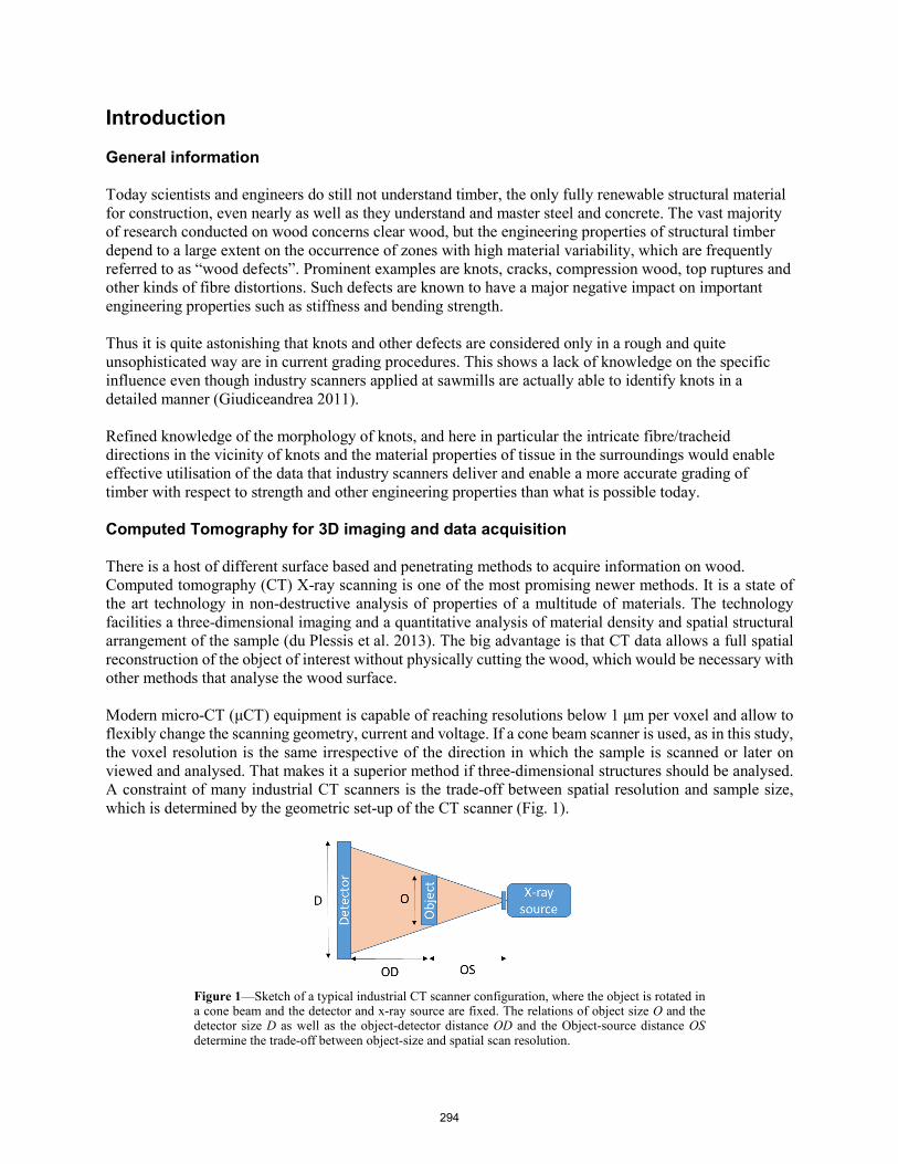
Introduction

General information

Today scientists and engineers do still not understand timber, the only fully renewable structural material for construction, even nearly as well as they understand and master steel and concrete. The vast majority of research conducted on wood concerns clear wood, but the engineering properties of structural timber depend to a large extent on the occurrence of zones with high material variability, which are frequently referred to as “wood defects”. Prominent examples are knots, cracks, compression wood, top ruptures and other kinds of fibre distortions. Such defects are known to have a major negative impact on important engineering properties such as stiffness and bending strength.

Thus it is quite astonishing that knots and other defects are considered only in a rough and quite unsophisticated way are in current grading procedures. This shows a lack of knowledge on the specific influence even though industry scanners applied at sawmills are actually able to identify knots in a detailed manner (Giudiceandrea 2011).

Refined knowledge of the morphology of knots, and here in particular the intricate fibre/tracheid directions in the vicinity of knots and the material properties of tissue in the surroundings would enable effective utilisation of the data that industry scanners deliver and enable a more accurate grading of timber with respect to strength and other engineering properties than what is possible today.

Computed Tomography for 3D imaging and data acquisition

There is a host of different surface based and penetrating methods to acquire information on wood. Computed tomography (CT) X-ray scanning is one of the most promising newer methods. It is a state of the art technology in non-destructive analysis of properties of a multitude of materials. The technology facilities a three-dimensional imaging and a quantitative analysis of material density and spatial structural arrangement of the sample (du Plessis et al. 2013). The big advantage is that CT data allows a full spatial reconstruction of the object of interest without physically cutting the wood, which would be necessary with other methods that analyse the wood surface.

Modern micro-CT (μCT) equipment is capable of reaching resolutions below 1 μm per voxel and allow to flexibly change the scanning geometry, current and voltage. If a cone beam scanner is used, as in this study, the voxel resolution is the same irrespective of the direction in which the sample is scanned or later on viewed and analysed. That makes it a superior method if three-dimensional structures should be analysed. A constraint of many industrial CT scanners is the trade-off between spatial resolution and sample size, which is determined by the geometric set-up of the CT scanner (Fig. 1).

Figure 1—Sketch of a typical industrial CT scanner configuration, where the object is rotated in a cone beam and the detector and x-ray source are fixed. The relations of object size O and the detector size D as well as the object-detector distance OD and the Object-source distance OS determine the trade-off between object-size and spatial scan resolution.

294

The imaging is an optical process that follows the rule of proportions (Equation 1).

(1)

Where O is the object size, D is the detector size and OS and OD are the object-sample distance and the object-detector distance respectively. Ideally, to maximise the spatial scan resolution the object should be close to the x-ray source, minimising OS as much as possible. OD is adjusted accordingly so that the maximum of the detector area is covered by the projection of the object on the detector. This way also small object structures are represented by many detector cells thus ensuring a hight spatial resolution of the image.

If highest resolutions should be achieved the sample can thus only be of small size. In the used CT configuration of this study the object size – resolution was roughly 1:1000, i.e. a maximum object size of 1 mm is necessary to achieve spatial voxel resolutions of 1 μm. For a 15 μm scan resolution the object should not be substantially larger than approximately 15 mm. However, to a certain degree it is also possible to work with larger sample sizes by only scanning a part of the object geometry. This way a region of interest can be scanned in a larger object. However, the changed penetration and potential beam hardening effects should be taken into consideration.

Due to its flexibility CT scanning has been successfully applied to fresh and dry wood in multiple studies of different purpose such as the quantification of knots, sapwood, decay, resin pockets, tree rings and general moisture content (e. g. Grundberg and Grönlund 1992, Oja and Temnerud 1999, Seifert 2004, 2005, Nikolova et al. 2009, Seifert et al. 2010, Longuetaud et al. 2012, Lindgren et al. 2016, Ngubeni et al. 2016). It has also been used for visualisation and quantification of the hygroscopic swelling and shrinkage behaviour of wood (Taylor et al. 2013) and for adhesive characterisation (Kamke et al. 2013). The spatial levels that were covered range from the macroscopic scale of logs and stem discs to the microscopic scale of wood tissues. Also spiral grain in tree stems was successfully analysed based on macro structures derived from a modified medical CT scanner (Supelveda, 2001; Sepulveda et al. 2002).

Numerical modelling with data from different sources

However, hardly any research activities have been related to the development of numerical models based on μCT measurements (Pyrkosz et al. 2010), which is an active field of research in other research communities (e. g. biomechanics, see e. g. Tsouknidas et al. 2011). An important issue in the conversion process of μCT data to mechanical models and finite element (FE) analysis is the assignment of local material properties based on X-ray attenuation coefficients.

In recent years several researchers have addressed needs and possibilities on modelling of timber including the influence of knots (Hackspiel, 2010; Lukacevic et al., 2014). Briggert et al. (2016) and Kandler et al. (2016) suggested to detect knots on wood surfaces on the basis of tracheid effect scanning and presented alternative strategies to determine the 3D knot geometry. Olsson (2016) showed that more accurate detection of knot surfaces can be obtained using grey scale light intensity in combination with tracheid effect scanning.

Models have been suggested for how growth layers and fibres are orientated in timber close to knots. One of the most elaborate models was presented by Foley (2003) who first developed a model for the geometry of growth layers and then, by using equations corresponding to flow analogies for the fibre direction within such layers. Of course, this involves model parameters that must be set in accordance to experimental data. The authors have addressed this need and used laser scanning to investigate the 3D fibre direction in the surroundings of knots in previous studies (Hu et al. 2015, 2016, 2018). When

295

softwood is illuminated by a dot laser the light on the wood surface will spread more along tracheids than across and indicate the fibre direction in the plane of the surface. A novel method to assess the 3D fibre direction around a knot was suggested and some results are visualized. However, the resolution of laser scanning cannot compare with the resolution of μCT and it does not provide information of local density.

Objectives

The objective of this research project within the bigger scope of understanding the influence of knots on mechanical wood properties was to establish a link between CT data and numerical modelling by developing a method that enables the automatic extraction of fibre orientation from μCT data of wood as a base for model calibration and validation.

Material and Methods

Data acquisition

Selected samples of dried Norway spruce were cut to the necessary size and were then scanned on a General Electric V|Tome|X L240 μCT scanner at different resolutions at the CT scanning facility at Stellenbosch University, South Africa. The scan was performed without filtering with 300µA current and 100 kV voltage at a spatial scan resolution of 15 μm. The scanned part of the wood sample was around 15 mm × 15 mm in its cross-section. For the reconstruction the proprietary DATOS software of General Electrics was used. The automated beam hardening correction of DATOS software was applied.

Image analysis and pattern recognition

The image analysis pipeline was developed in Python (van Rossum 1995), based on the library scikit-image (van der Walt et al. 2014). It was designed to optimally detect fibre directions in wood which has distinct structural features such as tree rings and thus requires specific solutions. The analysis was done as a consecutive of 2D slices in cross- sectional slices to create a fully three-dimensional result. It followed six major steps and was performed on image stacks of cross-sectional slices that were produced by the scanning process (Fig. 2)

296

Figure 2—Processing pipeline to calculate fibre orientation from μCT scans.

In Step (1) an image was read from the images stack originating from the CT scan. A density threshold was then applied on the image to separate wood and background. For this a mask was created to exclude areas that were outside of the object based on the x-ray attenuation value close to zero. Due to slight system inherent variations in the x-ray source and sensor electronics noise artefacts are created in CT images which wrongly indicate voxels with a low but notable x-ray attenuation value outside of the object geometry where no objects should exist. Thus in Step (2) a simple threshold was not sufficient and was amended by morphological operations like dilation and erosion in Step (3) to remove the noise. The resulting mask that masked the non-object areas plausibly now was applied in further processing steps to separate object and non-object areas. In the next Step (4), larger structures like annual rings were removed by subtracting the previous image from the currently processed image. This step was necessary and was specifically developed for wood scanning because the hard edges of tree ring borders exerted a too strong gradient for the local tensor algorithm and without this step rather tree ring borders were detected than local fibre orientation. But with subtracting two consecutive image layers of the distance of 15 μm in longitudinal direction the hard edges were removed efficiently, without removing the fibre orientation information, which typically does not change rapidly in longitudinal direction. This way the anisotropic nature wood wood was utilised to filter the image.

In Step (5) the local orientation of fibres was finally estimated by applying a structural tensor (Formulas 2 and 3). For a reference on the structural tensor method please see van Vliet and Verbeek (1995) and Jähne (2002). Finally, the resulting fibre orientation was colour coded for visualisation and exported in Step (6).

Read image from list

Separating image from background

Morphologic operators to reduce noise

Subtracting previous image in stack

Calculating edge direction with structural tensor

Colour code and export direction information

①

②

③

④

⑤

⑥

297

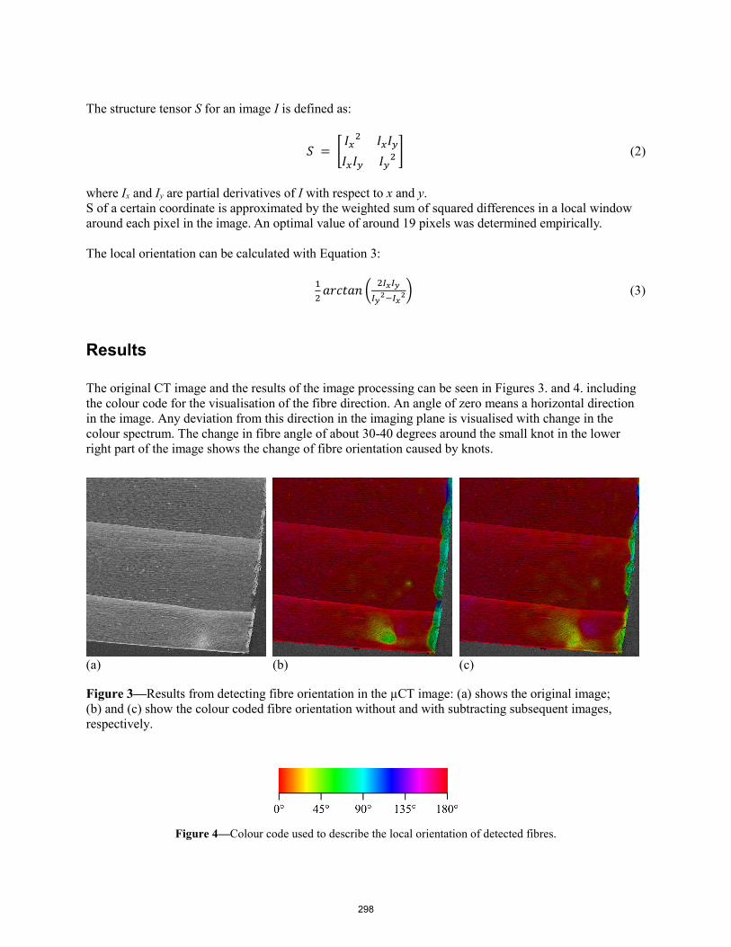
The structure tensor S for an image I is defined as:

𝑆𝑆 = 𝐼𝐼𝑥𝑥2 𝐼𝐼𝑥𝑥𝐼𝐼𝑦𝑦𝐼𝐼𝑥𝑥𝐼𝐼𝑦𝑦 𝐼𝐼𝑦𝑦2

(2)

where Ix and Iy are partial derivatives of I with respect to x and y. S of a certain coordinate is approximated by the weighted sum of squared differences in a local window around each pixel in the image. An optimal value of around 19 pixels was determined empirically.

The local orientation can be calculated with Equation 3:

12𝑎𝑎𝑎𝑎𝑎𝑎𝑎𝑎𝑎𝑎𝑎𝑎 2𝐼𝐼𝑥𝑥𝐼𝐼𝑦𝑦

𝐼𝐼𝑦𝑦2−𝐼𝐼𝑥𝑥2 (3)

Results

The original CT image and the results of the image processing can be seen in Figures 3. and 4. including the colour code for the visualisation of the fibre direction. An angle of zero means a horizontal direction in the image. Any deviation from this direction in the imaging plane is visualised with change in the colour spectrum. The change in fibre angle of about 30-40 degrees around the small knot in the lower right part of the image shows the change of fibre orientation caused by knots.

(a) (b) (c)

Figure 3—Results from detecting fibre orientation in the µCT image: (a) shows the original image; (b) and (c) show the colour coded fibre orientation without and with subtracting subsequent images,respectively.

Figure 4—Colour code used to describe the local orientation of detected fibres.

298

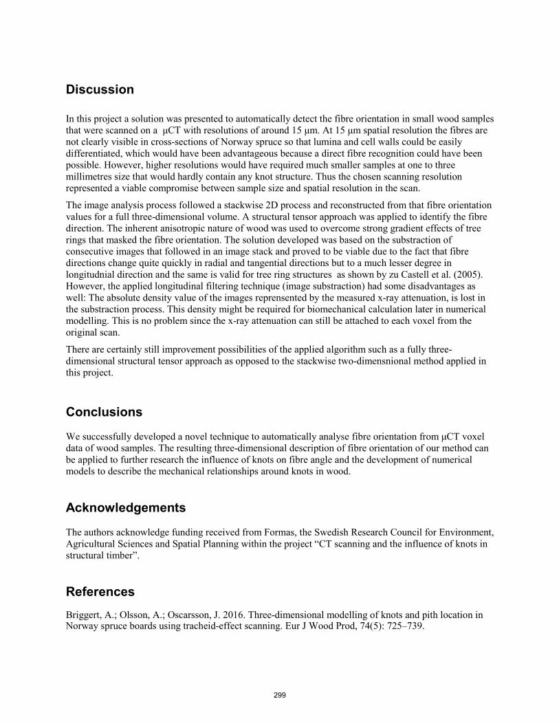
Discussion

In this project a solution was presented to automatically detect the fibre orientation in small wood samples that were scanned on a μCT with resolutions of around 15 μm. At 15 μm spatial resolution the fibres are not clearly visible in cross-sections of Norway spruce so that lumina and cell walls could be easily differentiated, which would have been advantageous because a direct fibre recognition could have been possible. However, higher resolutions would have required much smaller samples at one to three millimetres size that would hardly contain any knot structure. Thus the chosen scanning resolution represented a viable compromise between sample size and spatial resolution in the scan.

The image analysis process followed a stackwise 2D process and reconstructed from that fibre orientation values for a full three-dimensional volume. A structural tensor approach was applied to identify the fibre direction. The inherent anisotropic nature of wood was used to overcome strong gradient effects of tree rings that masked the fibre orientation. The solution developed was based on the substraction of consecutive images that followed in an image stack and proved to be viable due to the fact that fibre directions change quite quickly in radial and tangential directions but to a much lesser degree in longitudnial direction and the same is valid for tree ring structures as shown by zu Castell et al. (2005). However, the applied longitudinal filtering technique (image substraction) had some disadvantages as well: The absolute density value of the images reprensented by the measured x-ray attenuation, is lost in the substraction process. This density might be required for biomechanical calculation later in numerical modelling. This is no problem since the x-ray attenuation can still be attached to each voxel from the original scan.

There are certainly still improvement possibilities of the applied algorithm such as a fully three-dimensional structural tensor approach as opposed to the stackwise two-dimensnional method applied in this project.

Conclusions

We successfully developed a novel technique to automatically analyse fibre orientation from μCT voxel data of wood samples. The resulting three-dimensional description of fibre orientation of our method can be applied to further research the influence of knots on fibre angle and the development of numerical models to describe the mechanical relationships around knots in wood.

Acknowledgements

The authors acknowledge funding received from Formas, the Swedish Research Council for Environment, Agricultural Sciences and Spatial Planning within the project “CT scanning and the influence of knots in structural timber”.

References Briggert, A.; Olsson, A.; Oscarsson, J. 2016. Three-dimensional modelling of knots and pith location in Norway spruce boards using tracheid-effect scanning. Eur J Wood Prod, 74(5): 725–739.

299

Du Plessis, A.; Meincken, M.; Seifert, T. 2013. Quantitative Determination of Density and Mass of Polymeric Materials Using Microfocus Computed Tomography. Journal of Nondestructive Evaluation 32(4): 413–417.

Foley, C. 2003. Modelling the effects of knots in structural timber. PhD thesis, Lund Univ.

Giudiceandrea, F.; Ursella E.; Vicario, E. 2011. A high speed CT scanner for the sawmill industry. Proc. Intern. Non. Destr. Testing and Eval, of Wood Symp. 14th–16th Sept. Sopron, Hungary.

Grundberg, S.; Grönlund, A. 1992. Log Scanning – Extraction of Knot Geometry. Seminar/Workshop on Scanning Technology and Image Processing on Wood. August 30 – September 1, 1992, Skellefteå.

Gustavsson, L.; Joelsson, A.; Sathre, R. 2010. Life cycle primary energy use and carbon emissions of an eight-storey wood-framed apartment building. Energy and Buildings 42(2): 230–42.

Hackspiel, C. 2010. A numerical simulation tool for wood grading. PhD thesis, Vienna Univ. of Tech.

Hu, M.; Johansson, M.; Olsson, A.; Oscarsson, J.; Enquist, B. 2015. Local variation of modulus of elasticity in timber determined on the basis of non-contact deformation measurement and scanned fibre orientation. Eur J Wood Products, 73(1): 17–27.

Hu, M.; Olsson, A.; Johansson, M.; Oscarsson, J.; Serrano, E. 2016. Assessment of a three-dimensional fibre orientation model for timber. Wood Fibre Sci, 48(4): 271–290.

Hu., M.; Briggert, A.; Olsson, A.; Johansson, M.; Oscarsson, J.; Säll H. 2018. Growth layer and fibre orientation around knots in Norway spruce – a laboratory investigation. Wood Sci Technol. 52(1): 7–27

Jähne, B. 2002. Digital Image Processing. Springer-Verlag Berlin, Heidelberg, 585 p.

Johansson, C.-J. 2003. Grading of timber with respect to mechanical properties. In: Thelandersson, S. and Larsen H.-J. (eds) Timber Engineering, J Wiley & Sons, England, 23–43.

Kamke, F.; Nairn, J.; Muszynski, L.; Paris, J.; Schwarzkopf, M.; Xiao, X. 2013. Methodology for micro-mechanical analysis of an adhesive bond using micro computed x-ray tomography and numerical modeling. WoodFibre Sci, 46(1): 15–28.

Kandler, G. 2016. Probabilistic modelling of the elastic behaviour of glued laminated timber. PhD thesis, Vienna Univ. of Tech.

Lindgren, O.; Seifert, T.; du Plessis, A. 2016. Moisture Content Measurements in Wood Using Dual Energy CT-scanning – A Feasibility Study. Material Science & Engineering 11 (5), 312–317.

Longuetaud, F.; Mothe, F.; Kerautret, B.; Krähenbühl, A.; Hory, L.; Leban, J.M. DebledRennesson, I. 2012. Automatic knot detection and measurements from X-ray CT images of wood: a review and validation of an improved algorithm on softwood samples. Computers and Electronics in Agriculture 85, 77–89.

Lukacevic, L.; Füssl, J. 2014. Numerical simulation tool for wooden boards with a physically based approach to identify structural failure. Eur J Wood Prod, 72: 497–508.

Ngubeni, N.; Jacobs, S.; Seydack, A.; Vermeulen, W.; Sass, G.; Seifert, T. 2016. Trade-off relationships between tree growth and defense: a comparison of Ocotea bullata and Curtisia dentata following bark harvesting in an evergreen moist South African Forest. Trees 31(1): 339–348.

300

Nikolova, P.; Blaschke, H.; Matyssek, R.; Pretzsch, H.; Seifert, T. 2009. Combined application of computer tomography and light microscopy for analysis of conductive xylem area of beech and spruce coarse roots. European Journal of Forest Research. 128(2): 145–153.

Olsson, A.; Oscarsson, J.; Serrano, E.; Källsner, B.; Johansson, M.; Enquist, B. 2013. Prediction of timber bending strength and in-member cross-sectional stiffness variation on basis of local wood fibre orientation. Eur J Wood Prod, 71(3): 319–333.

Olsson, A. 2016. Determination of sawn timber properties using laser scanning – Development potentials and industrial applications. Proc. World Conf. Timber Eng., 22–25 Aug., Vienna.

Olsson, A.; Oscarsson, J. 2016. Strength grading on the basis of high resolution laser scanning and dynamic excitation – a full scale investigation of performance. Eur J. Wood Prod, 75(1): 17–31.

Oja, J.;, Temnerud, E. 1999.The appearance of resin pockets in CT-images of Norway spruce (Picea abies (L.) Karst.). Holz als Roh- und Werkstoff 57: 400–406.

Pyrkosz, M.; Van Karsen, C.; Bissinger, G. 2010. Converting CT Scans of a Stradivari Violin to a FE. Proc. of IMAC-XXVIII, 1–4 Feb., Jacksonville, Florida, USA.

Seifert, E. 2005. Automatische Jahrringerkennung in CT-Aufnahmen von Baumstämmen. Diploma thesis, University of Applied Sciences Augsburg, 122 p.

Seifert, T. 2004. Computertomographie zur Analyse der Stammstruktur von Bäumen. Tagungsband der Jahrestagung der Sektion Ertragskunde im Deutschen Verband Forstlicher Forschungsanstalten, 97–103

Seifert, T.; Nickel, M.; Pretzsch, H. 2010. Analysing the long-term effects of artificial pruning of wild cherry by computer tomography. Trees 24(5): 797–808.

Sepulveda, P. 2001. Measurement of spiral grain with computed tomography. J Wood Sci. 47:289–293.

Sepulveda, P.; Oja, J.; Grönlund , A. 2002. Predicting spiral grain by computed tomography of Norway spruce. J. Wood Sci. 48: 479–483.

Taylor, A.; Plank, B.; Standfest, G.; Petutschnigg, A. 2013. Beech wood shrinkage observed at the microscale by a time series of X-ray computed tomographs (μXCT). Holzforschung, 67: 201–205.

Tsouknidas, A.; Michailidis, N.; Savvakis, S.; Anagnostidis, K.; Bouzakis, K. D.; Kapetanos, G. 2011. A high accuracy CT based FEM model of the lumbar spine to determine its biomechanical response. Bioinformatics 2011: 222–227.

van der Walt, S.; Schönberger J.L.; Nunez-Iglesias J.; Boulogne, F.; Warner, J.D.; Yager, N.; Gouillart, E.; Yu, T.; the scikit-image contributors. 2014. scikit-image: Image processing in Python. PeerJ 2:e453

van Rossum, G. 1995. Python tutorial, Technical Report CS-R9526, Centrum voor Wiskunde en Informatica (CWI).

van Vliet, L.J.; Verbeek P.W. 1995. Estimators for Orientation and Anisotropy in Digitized Images. In: ASCI’95, Proceedings of the first Conference of the Advanced School for Computing and Imaging, Heijen (The Netherlands), May 16–18, 442–450.

zu Castell, W.; Schrödl, S.; Seifert,T. 2005 Volume Interpolation of CT Images from Tree Trunks. Plant Biology,7, 737 – 744.

301

Effect of Heat Treatment on Water Absorption of Chinese Fir Using Low Field Nuclear Magnetic Resonance

Yulei Gao Research Institute of Wood Industry of Chinese Academy of Forestry, Hunan Collaborative Innovation Center for Effective Utilizing of Wood & Bamboo Resources, Beijing, China, gaoyl90@163.com

Kang Xu College of Material Science and Engineering, Central South University of Forestry and Technology, Changsha, Hunan, China, xkang86@126.com

Jianxiong Lyu * Research Institute of Wood Industry of Chinese Academy of Forestry, Hunan Collaborative Innovation Center for Effective Utilizing of Wood & Bamboo Resources, Beijing, China, jianxiong@caf.ac.cn

Abstract

Knowledge of the dynamic changes in the water absorption process of heat-treated wood is important for providing a scientific basis for the reasonable application of heat-treated wood, especially for outdoor applications. Nuclear magnetic resonance (NMR) techniques can provide detailed information about the moisture states and moisture transport processes in wood, which are hardly available with other methods. According to spin–spin relaxation time (T2) the water states can be easily distinguished and quantitatively analyzed, the water distribution can be revealed by NMR imaging as well. In this study, the absorption of water in untreated and heat-treated Chinese fir (Cunninghamia lanceolata [Lamb.] Hook.) heartwood in longitudinal direction were investigated using various NMR techniques. The specimens were treated with temperatures between 160°C and 220°C for 2 hours. The results show that a new component of free water with a T2 of about 20ms was found in the samples heat-treated at 200°C and 220°C which was differ from other samples. Compared to the untreated ones, both the contents of bound water and free water in heat-treated samples were less, and the amount decreased correspondingly with the increasing heat-treated temperature. NMR images revealed that, after immersion for 60 days, water signal could be detected both in earlywood and latewood in the middle of the untreated samples, but only in latewood for the samples heat-treated at 220°C.

Keywords: water absorption, moisture content, free water, bound water, relaxation time, NMR imaging

Introduction

Wood is a porous material which has a complex hierarchical structure, and the hygroscopic nature makes it sensitive to moist conditions. The amount of moisture contained within wood affects its durability, stability, physical properties, and so on (Bal 2015). Of all the methods for wood modification, heat treatment is an important method to improve timber performance by changing the wood-water relationship without using chemicals. The changes of wood due to high-temperature might affect the amount of accessible hydroxyl sites and the pore structure of wood. Consequently, the water state and water content adsorbed in heat-treated wood would be influenced when wood is situated in a humid environment or immersed in water.

302

Being utilized for the noninvasive, quick and quantitative characterization, the nuclear magnetic resonance (NMR) technique is known as a powerful tool, which can be used to understand wood structure and the dynamics of water in wood (Zhang et al. 2013). Since the decay rate of the NMR signal is relevant to the mobility and local environment of molecules, the bound water and free water can easily be separated by the different spin–spin relaxation time (T2) values for either hardwood or softwood (Telkki et al. 2013). The spatial distribution of water in wood can be reflected visually by magnetic resonance imaging in a nondestructive way, which is difficult to achieve using other methods (Javed et al. 2014).

The water absorption performances are extremely important factors defining the dimensional stability, decay resistance and other physical properties of timber. Though a number of experiments have been carried out to investigate the effects of heat treatment on the water absorption performance of wood (Scheiding et al. 2016), the whole progress of changes in the water absorption process needs further investigation. For example, it is still unclear whether the heat treatment caused the absorption amount change of both bound water and free water, or only one of these two water components is influenced. In addition, further research of the water distribution in heat-treated wood is needed. Therefore, it is necessary to use NMR technology to give insights into the dynamic change of water absorption process of heat-treated wood, which was expected to provide a scientific basis for the reasonable application of heat-treated wood, especially for outdoor applications.

Materials and methods

In this study, a 4 m long log was cut at breast height from a freshly felled 20 year old Chinese fir (Cunninghamia lanceolata [Lamb.] Hook.) from a forest in Kaihua, China. The log was first cut off into eight 500-mm-long sections after air drying. Then 8 sticks with a cross section dimension of 15×15mm2 were sawn from the 6-8 annual rings of each section. Finally, each stick was cut into three parts with dimensions of 150mm×15mm×15mm (L×R×T), and 115 defect-free wood specimens in total were chosen to conduct the experiment. These specimens were randomly divided into 5 groups. There were 15 specimens for the control group and 25 for the other 4 groups for heat treatment. The heat treatments proceed at four different temperatures (160, 180, 200 and 220°C) for 2h in the high temperature drying chamber with the oxygen controller, and the inside atmosphere controls within comprising no more than 2 percent oxygen content.

In order to pick out the specimens to undergo time domain nuclear magnetic resonance (TD-NMR) detection, samples with dimensions of 10mm×15mm×15mm (L×R×T) were cut from the middle of the 115 specimens mentioned above. Then the two tangential sections and two radial sections of the samples were sealed by epoxy resin to make the water uptake only occur through the cross sections when immerse in distilled water. After the water adsorption experiment, the average MC change of each group could be calculated by means of statistical analysis and samples whose MC changes were close to the average MC of its group were chosen to conduct the TD-NMR experiment.

The TD-NMR experiments were carried out by a MesoMR23-060H-I NMR instrument (Niumag Co., Ltd., Suzhou, China) with a 0.52 Tesla permanent magnet, operating at 32.00°C. The dimension of samples was 50mm×15mm×15mm (L×R×T), which were cut from the rest part of the chosen specimens and sealed as the same method mentioned above. Samples were immersed in distilled water in transparent vessels with the aid of a stainless steel net to prevent them from floating. At certain time intervals, the samples were taken out of the vessels and removed extra water on the surface. Then samples were placed into the probe one at a time after weighting. The Carr–Purcell–Meiboom–Gill (CPMG) pulse sequence was used to measure the T2 of the samples. 15,000 echoes with 64 scans were acquired, the echo time and repetition time between two successive scans were 0.15ms and 4s, respectively. To perform 2D NMR

303

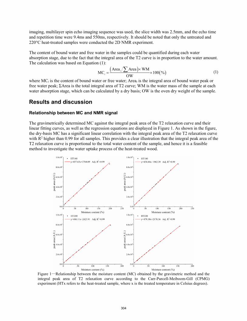
imaging, multilayer spin echo imaging sequence was used, the slice width was 2.5mm, and the echo time and repetition time were 9.4ms and 550ms, respectively. It should be noted that only the untreated and 220°C heat-treated samples were conducted the 2D NMR experiment.

The content of bound water and free water in the samples could be quantified during each water absorption stage, due to the fact that the integral area of the T2 curve is in proportion to the water amount. The calculation was based on Equation (1):

( ) ( )Area Area WM

MC 100 %OW

ii

×= ×∑ (1)

where MCi is the content of bound water or free water; Areai is the integral area of bound water peak or free water peak; ΣArea is the total integral area of T2 curve; WM is the water mass of the sample at each water absorption stage, which can be calculated by a dry basis; OW is the oven dry weight of the sample.

Results and discussion

Relationship between MC and NMR signal

The gravimetrically determined MC against the integral peak area of the T2 relaxation curve and their linear fitting curves, as well as the regression equations are displayed in Figure 1. As shown in the figure, the dry-basis MC has a significant linear correlation with the integral peak area of the T2 relaxation curve with R2 higher than 0.99 for all samples. This provides a clear illustration that the integral peak area of the T2 relaxation curve is proportional to the total water content of the sample, and hence it is a feasible method to investigate the water uptake process of the heat-treated wood.

Figure 1—Relationship between the moisture content (MC) obtained by the gravimetric method and the integral peak area of T2 relaxation curve according to the Carr-Purcell-Meiboom-Gill (CPMG) experiment (HTx refers to the heat-treated sample, where x is the treated temperature in Celsius degrees).

304

Water states and migration

Water states in softwood were distinguished with relaxation analysis by several researchers (Cox et al. 2010). According to the research results, the T2 was within 10ms of bound water and greater than 10ms of free water. Whereas T2 of the wood proton was about 10–15μs shorter than the dead time of the spectrometer in this study, thus the signal of the wood proton could not be detected. Figure 2 illustrates

Figure 2—The change of water relaxation behavior during the water absorption process of untreated and heat-treated wood samples.

the relaxation behavior of water in wood during the process of water uptake. There are two peaks which correspond to two components in water states in the 160°C and 180 °C heat-treated samples and the untreated control samples. The component with shorter relaxation time showed that the water became more restricted in motion, which belonged to bound water in the wood cell walls, and the other one with

305

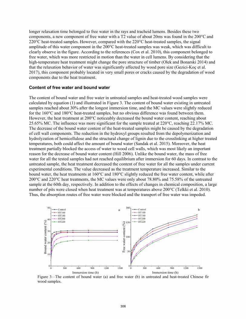
longer relaxation time belonged to free water in the rays and tracheid lumens. Besides these two components, a new component of free water with a T2 value of about 20ms was found in the 200°C and 220°C heat-treated samples. However, compared with the 220°C heat-treated samples, the signal amplitude of this water component in the 200°C heat-treated samples was weak, which was difficult to clearly observe in the figure. According to the references (Cox et al. 2010), this component belonged to free water, which was more restricted in motion than the water in cell lumens. By considering that the high-temperature heat treatment might change the pore structure of timber (Olek and Bonarski 2014) and that the relaxation behavior of water was significantly affected by wood pore size (Gezici-Koç et al. 2017), this component probably located in very small pores or cracks caused by the degradation of wood components due to the heat treatment.

Content of free water and bound water

The content of bound water and free water in untreated samples and heat-treated wood samples were calculated by equation (1) and illustrated in Figure 3. The content of bound water existing in untreated samples reached about 30% after the longest immersion time, and the MC values were slightly reduced for the 160°C and 180°C heat-treated samples, but no obvious difference was found between them. However, the heat treatment at 200°C noticeably decreased the bound water content, reaching about 25.65% MC. The influence was more significant for the sample treated at 220°C, reaching 22.17% MC. The decrease of the bound water content of the heat-treated samples might be caused by the degradation of cell wall components. The reduction in the hydroxyl groups resulted from the depolymerization and hydrolyzation of hemicellulose and the structural change of lignin due to the crosslinking at higher treated temperatures, both could affect the amount of bound water (Sandak et al. 2015). Moreover, the heat treatment partially blocked the access of water to wood cell walls, which was most likely an important reason for the decrease of bound water content (Hill 2006). Unlike the bound water, the mass of free water for all the tested samples had not reached equilibrium after immersion for 60 days. In contrast to the untreated sample, the heat treatment decreased the content of free water for all the samples under current experimental conditions. The value decreased as the treatment temperature increased. Similar to the bound water, the heat treatments at 160°C and 180°C slightly reduced the free water content, while after 200°C and 220°C heat treatments, the MC values were only about 78.80% and 75.58% of the untreated sample at the 60th day, respectively. In addition to the effects of changes in chemical composition, a large number of pits were closed when heat treatment was at temperatures above 200°C (Telkki et al. 2010). Thus, the absorption routes of free water were blocked and the transport of free water was impeded.

Figure 3—The content of bound water (a) and free water (b) in untreated and heat-treated Chinese fir wood samples.

306

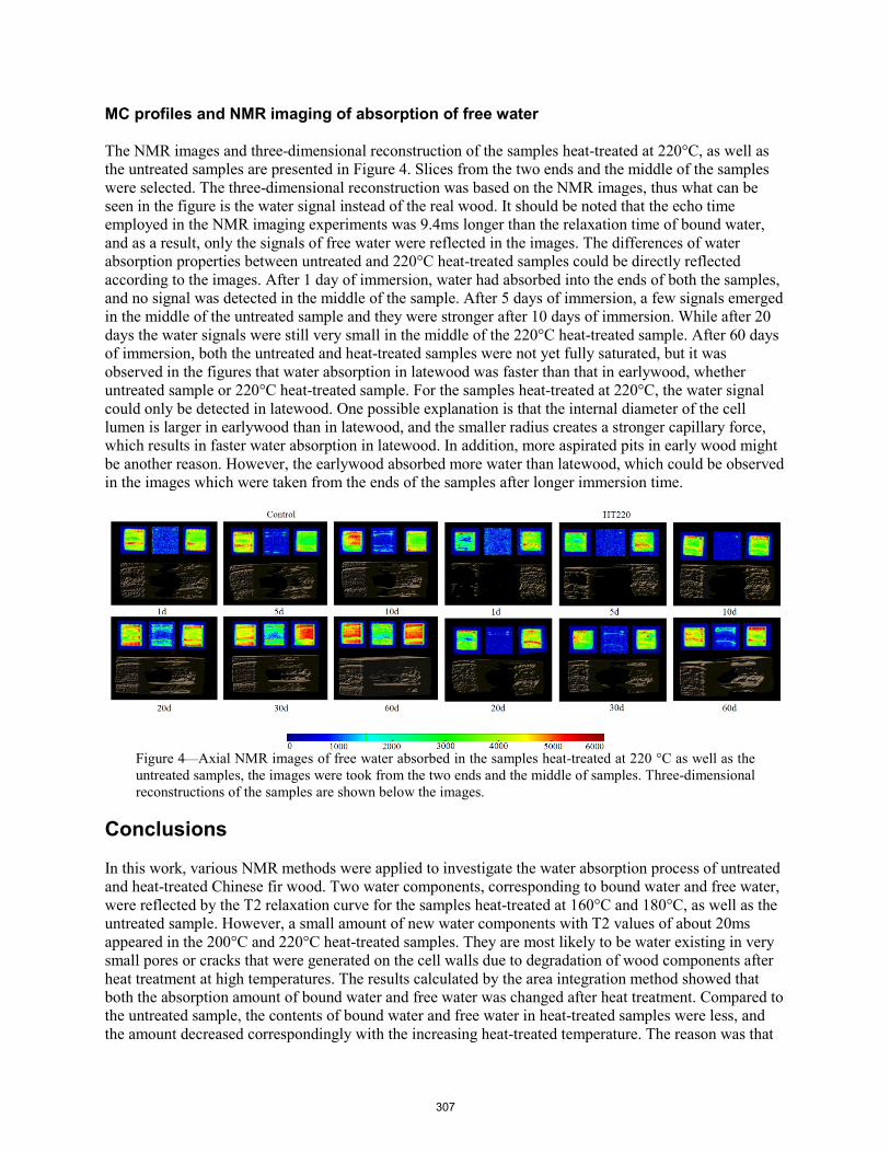
MC profiles and NMR imaging of absorption of free water

The NMR images and three-dimensional reconstruction of the samples heat-treated at 220°C, as well as the untreated samples are presented in Figure 4. Slices from the two ends and the middle of the samples were selected. The three-dimensional reconstruction was based on the NMR images, thus what can be seen in the figure is the water signal instead of the real wood. It should be noted that the echo time employed in the NMR imaging experiments was 9.4ms longer than the relaxation time of bound water, and as a result, only the signals of free water were reflected in the images. The differences of water absorption properties between untreated and 220°C heat-treated samples could be directly reflected according to the images. After 1 day of immersion, water had absorbed into the ends of both the samples, and no signal was detected in the middle of the sample. After 5 days of immersion, a few signals emerged in the middle of the untreated sample and they were stronger after 10 days of immersion. While after 20 days the water signals were still very small in the middle of the 220°C heat-treated sample. After 60 days of immersion, both the untreated and heat-treated samples were not yet fully saturated, but it was observed in the figures that water absorption in latewood was faster than that in earlywood, whether untreated sample or 220°C heat-treated sample. For the samples heat-treated at 220°C, the water signal could only be detected in latewood. One possible explanation is that the internal diameter of the cell lumen is larger in earlywood than in latewood, and the smaller radius creates a stronger capillary force, which results in faster water absorption in latewood. In addition, more aspirated pits in early wood might be another reason. However, the earlywood absorbed more water than latewood, which could be observed in the images which were taken from the ends of the samples after longer immersion time.

Figure 4—Axial NMR images of free water absorbed in the samples heat-treated at 220 °C as well as the untreated samples, the images were took from the two ends and the middle of samples. Three-dimensional reconstructions of the samples are shown below the images.

Conclusions

In this work, various NMR methods were applied to investigate the water absorption process of untreated and heat-treated Chinese fir wood. Two water components, corresponding to bound water and free water, were reflected by the T2 relaxation curve for the samples heat-treated at 160°C and 180°C, as well as the untreated sample. However, a small amount of new water components with T2 values of about 20ms appeared in the 200°C and 220°C heat-treated samples. They are most likely to be water existing in very small pores or cracks that were generated on the cell walls due to degradation of wood components after heat treatment at high temperatures. The results calculated by the area integration method showed that both the absorption amount of bound water and free water was changed after heat treatment. Compared to the untreated sample, the contents of bound water and free water in heat-treated samples were less, and the amount decreased correspondingly with the increasing heat-treated temperature. The reason was that

307

heat treatment might partially block the access of water to wood cell walls, and in consequence improve the dimensional stability of heat-treated wood. 2D NMR images of the untreated and 220°C heat-treated samples revealed that after immersion for 60 days, water signal could be detected both in earlywood and latewood in the middle of the untreated samples, but only in latewood for the samples heat-treated at 220°C.

Acknowledgments

The authors would like to thank the National Key Research and Development Program of China (2017YFD0600202) for the financial support.

References

Bal, B.C. 2015. Wood-water relationships and biological durability of heat-treated Taurus Fir wood. Pro Ligno. 11:, 3–10.

Cox, J.; Mcdonald, P.J.; Gardiner, B.A. 2010. A study of water exchange in wood by means of 2D NMR relaxation correlation and exchange. Holzforschung. 64(2): 259–266.

Gezici-Koç, Ö.; Erich, S.J.F.; Huinink, H.P. [and others]. 2017. Bound and free water distribution in wood during water uptake and drying as measured by 1D magnetic resonance imaging. Cellulose. 24(2): 535–553.

Hill, C.A.S. 2006. Wood Modification: Chemical, Thermal and other Processes; John Wiley & Sons: Hoboken, NJ, USA, pp. 99–127.

Javed, M.A.; Kekkonen, P.M.; Ahola, S. 2014. Magnetic resonance imaging study of water absorption in thermally modified pine wood. Holzforschung. 69(7): 899–907.

Olek, W.; Bonarski, J.T. 2014. Effects of thermal modification on wood ultrastructure analyzed with crystallographic texture. Holzforschung. 68(6): 721–726.

Sandak, A.; Sandak, J.; Allegretti, O. 2015. Quality control of vacuum thermally modified wood with near infrared spectroscopy. Vacuum. 114: 44–48.

Scheiding, W.; Direske, M.; Zauer, M. 2016. Water absorption of untreated and thermally modified sapwood and heartwood of Pinus sylvestris L. Eur. J. Wood Wood Prod. 74(4): 585–589.

Telkki, V.V.; Saunavaara, J.; Jokisaari, J. 2010. Time-of-flight remote detection MRI of thermally modified wood. J. Magn. Reson. 202(1): 78–84.

Telkki, V.V.; Yliniemi, M.; Jokisaari, J. 2013. Moisture in softwoods: Fiber saturation point, hydroxyl site content, and the amount of micropores as determined from NMR relaxation time distributions. Holzforschung. 67(3): 291–300.

Zhang, M.; Wang, X.; Gazo, R. 2013. Water states in yellow poplar during drying studied by time-domain nuclear magnetic resonance. Wood Fiber Sci. 45(4): 423–428.

308

Experimental Study of Pin Penetration Depth in Evaluating Termite-Infested Shorea spp. Lumber Shofi Fauziyyah * Department of Forest Products, IPB University, Bogor, West Java, Indonesia, shofi_fauziyyah14@apps.ipb.ac.id Lina Karlinasari Department of Forest Products, IPB University, Bogor, West Java, Indonesia, karlinasari@apps.ipb.ac.id Dodi Nandika Department of Forest Products, IPB University, Bogor, West Java, Indonesia, nandikadodi@gmail.com * Corresponding author Abstract A laboratory study was conducted to explore the feasibility of using the nondestructive testing (NDT) method of pin penetration to evaluate the condition of termite-infested structural lumber. This investigation concentrated on revealing characteristics of termite infestation on light red meranti (Shorea spp.) lumber. The relationship between visual evaluation and pin penetration damage assessment of elemental physical-mechanical properties of wood was examined. A distribution map of infested wood based on pin penetration was also developed. Samples used for this study were derived from Shorea spp. commercial lumber. The samples were exposed to reared subterranean termites (Coptotermes curvignathus Holmgren). Characteristics of termite-infested samples were observed and visual evaluation of termite infestation severity was appraised according to the American Society for Testing and Materials (ASTM) D3345. Weight loss percentage of the samples was measured. Pilodyn® was used to evaluate the residual surface area of the exposed and unexposed samples by subjecting the ground intact surface of the samples to pin penetration tests. The following characteristics of the infested samples were established: (1) termite galleries found varied in length, (2) termite galleries were long flat tunnels, longitudinal in direction, clean, not decayed, and had no termite mud trails. Weight loss percentage and pin penetration depth from this study were related to increasing exposure period. Longer exposure periods resulted in higher weight loss percentage and deeper pin indentation of Pilodyn®. Pin indentation results might be used to generate a distribution model for a pin penetration contour map. This result portrayed wood condition and properties. Keywords: Coptotermes curvignathus, meranti lumber, nondestructive, pin penetration, termite gallery

309

Evaluation and Comparison of Optical Gauging Techniques in Terms to Characterize Wood Material Properties Applying Nondestructive TestingCedou Kumpenza* Institute of Wood Technology and Renewable Materials, Department of Material Science and Process Engineering, University of Natural Resources and Life Sciences (BOKU), Vienna, Austria, cedou.kumpenza@boku.ac.at

Thomas Krenke Innovationszentrum W.E.I.Z, Weiz, Austria, thomas.krenke@innovationszentrum-weiz.at

Florian Linkeseder Institute of Wood Technology and Renewable Materials, Department of Material Science and Process Engineering, University of Natural Resources and Life Sciences (BOKU), Vienna, Austria, florian.linkeseder@boku.ac.at

Florian Feist Vehicle Safety Institute, Graz University of Technology, Graz, Austria florian.feist@tugraz.at

Ulrich Müller Institute of Wood Technology and Renewable Materials, Department of Material Science and Process Engineering, University of Natural Resources and Life Sciences (BOKU), Vienna, Austria, ulrich.mueller@boku.ac.at

*Corresponding author

Abstract

In state-of-the-art wood science, computerized engineering methods like finite-element modelling (FEM) are commonly used to engineer and optimize high quality products and structures. Some of these mainly wood-based structures are analysed, improved and evaluated within the research project WoodC.A.R. (Wood – Computer Aided Research) by applying FEM. Reliable FEM is based on valid material descriptions, which include linear-elastic material coefficients, established with non-destructive material tests by applying different kind of strain gauging techniques. Strain gauging and testing is a complex procedure, which can be biased by several factors. Especially, for inhomogeneous materials like wood, strain measurement includes several challenges. However, only few studies are available that established and compared the linear-elastic material coefficients by means of optical gauging techniques. Therefore, in the present study different optical gauging techniques, like digital image correlation (DIC), electronic speckle pattern interferometry (ESPI), laser extensometry (lasEx) and video extensometry (vidEx) are applied, to compare and evaluate the gauging results. Measurements were done on the same sample set by performing non-destructive mechanical tests. Tensile and shear tests were designed for evaluating measurement reliability, data acquisition and -evaluation, versatility, and flexibility of the applied gauging techniques. Furthermore, the aim of this research study is to obtain consistent and reliable data that can be used for future FEM.

Keywords: Digital Image Correlation, Electronic Speckle Pattern Interferometry, Laser Extensometry, Optical Strain Measurement, Video Extensometry, Wood Material Characterization

310

Introduction

Recently renewable materials like wood are getting more and more in the focus for the usage as structural parts for example in vehicles to face the current challenges of the automotive industry, i.e. CO2-balance, fuel-reduction, design of small city cars etc. (Kohl et al. 2016; Jost et al. 2018). Before these wood and wood-based structures might be used as structural parts in vehicles, the mechanical performance must be understood and described in terms to have the ability to predict the material behaviour under different load-cases. Computer-aided engineering (CAE) methods like finite-element modelling (FEM) are applied to design, engineer and optimize these high-performance wood structures. A sound implementation of FEM is based on reliable and valid material data, which include linear-elastic material coefficients such as the Young’s moduli (EL, ER, ET), Shear moduli (GRT, GTL, GRL) and Poisson’s ratios (νRT, νTL, νRL). To make sure that consistent and trustable material data are used in FEM it is therefore of main importance to validate and evaluate the gauging techniques that are applied to obtain the linear-elastic material data. Especially for wood as a highly heterogeneous and anisotropic material special care must be taken to guarantee the reliability of the gauging results. Nowadays, optical gauging techniques are becoming more convenient to use compared to other common gauging techniques, i.e. strain gauges, mechanical extensometers, ultrasound spectroscopy etc. (Davis 2004; Majano-Majano et al. 2012; Vorobyev et al. 2016; Bachtiar et al. 2017; Kroworz and Katunin 2018). Therefore, in the present study common applied non-contact optical gauging techniques named Digital Image Correlation (DIC), Electronic Speckle Pattern Interferometry (ESPI), laser Extensometry (lasEx) and video Extensometry (vidEx) are compared and analysed in terms to gauge wood material deformations and also strains caused by tensile- and shear forces. Former studies also proved that optical gauging techniques are suitable to establish consistent linear-elastic material coefficients by applying non-destructive testing (Zink et al. 2007; Majano-Majano et al. 2012; Xavier et al. 2013; Bachtiar et al. 2017). In order to compare head-to-head the measurement reliability, versatility, flexibility etc. of DIC, ESPI, lasEx and vidEx, uniaxial tensile and shear experiment were done on the same sample set.

DIC and ESPI are non-contact optical gauging techniques that can provide detail full-field surface information of an object at micro- or even nanoscale. The core of these techniques is the detection of changes of surface patterns, which are taken prior to and during the object is stressed. For DIC a (artificially added) random speckle pattern must be applied on the surface that is tracked by specific detection algorithm. On the contrary, ESPI relies on Michelson Interferometry, which means that the sample is illuminated from two different directions with coherent light. The reflected light waves are detected and converted to a speckle pattern image. Compared to that lasEx and vidEx are punctual gauging techniques, which means that two measurement points or markers are tracked continuously while the specimen is stressed. With lasEx two generated speckle pattern areas that represent the measurement markers are monitored by a camera. The idea behind lasEx is to establish the specimen displacements by continuously comparing the location of the pattern areas while the specimen is stressed. VidEx works like lasEx with the main difference that the specimens need to be marked on two different positions for example with a pen before applying the forces. Afterwards the pixel distances between these markers are tracked continuously by the vidEx system. Further fundamentals in terms to characterize wood material properties by applying these techniques can be found in literature (Eberhardsteiner 1995; Gingerl 1998; Valla et al. 2011; Müller et al. 2015; Kumpenza et al. 2018).

The main objectives in this research study were to look at the main differences between DIC, ESPI, lasEx and vidEx with a focus on the pre/post-processing procedure in order to obtain consistent and reliable linear elastic material data that can be used for FEM.

311

Materials and Methods

Materials Specimens made of birch wood (Betula pendula) were used in tensile and shear experiments. A CNC-machine, circular saw, planning and a milling machine were used to obtain the desired shape out of the timber boards. After finishing the samples, they were conditioned at a temperature of 20 ± 2 °C and a relative humidity of 65 ± 5% (according to ISO 554) to an average moisture content of ω ≈ 12%, resulting in an average sample density of ρ = 638 ± 25 kg/m³. For the tensile experiments, strip-shaped specimens with a uniform cross section of Atensile = 20 × 6 mm² (width × height) and a length of ltensile = 150 mm were utilized (Figure 1a). The shear experiments were performed with so- called arcan-shear samples (Figure 1b) which have a typical rectangular shape with two symmetrical V-notches that might provide uniform shear stress distribution at the minimum cross-section of the specimens (Xavier et al. 2009). For the tensile experiments the load was applied on the specimens in radial wood grain direction (cf. Figure 1a) and for the shear experiments rolling shear were tested (cf. Figure 1b). Respectively, one sample set with 7 specimens were used for the tensile tests and 7 specimens for the shear tests.

Figure 1—Illustration of the specimens; (a) representative specimen for tensile tests; (b) representative specimen for the shear tests

Experimental set-up All tensile and shear experiments were performed on a Zwick/Roell Z020 universal testing machine (Ulm, Germany), equipped with the control software Zwick/Roell TestXpert 2 V3.5. (Ulm, Germany). For all tests a constant crosshead speed of 1 mm/min was adjusted with a maximal specimen load corresponding to maximal 50% of the tested specimen strength, i.e. in tensile with Ftensile = 1000 N and in shear with Fshear = 300 N. One after the other, the specimen force-deflection curves of all specimens were measured by means of DIC-, ESPI-, lasEx- or vidEx-technique. Depending on the gauging techniques specimens and measuring set-ups were prepared differently. Figure 2 shows the three different experimental measuring set-ups.

Figure 2— Scheme of the experimental set-up

312

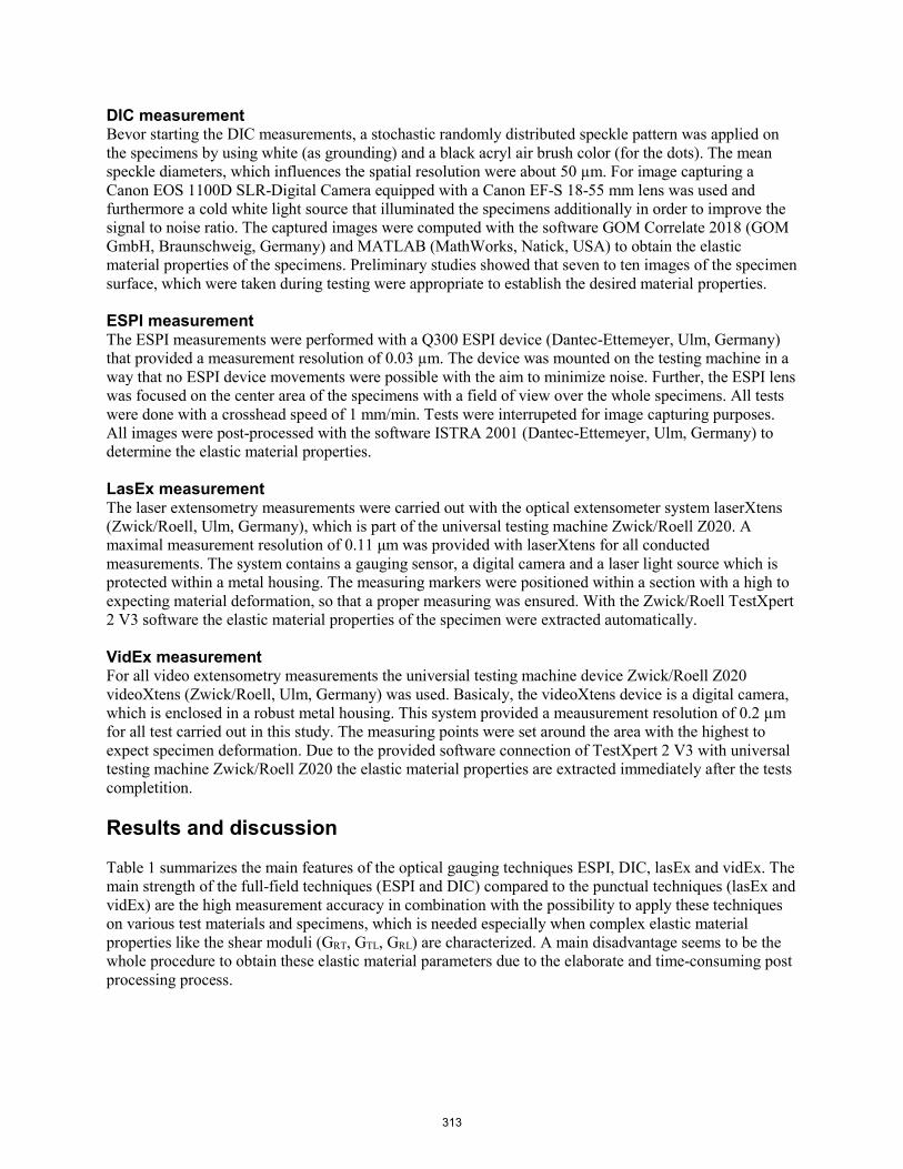
DIC measurement Bevor starting the DIC measurements, a stochastic randomly distributed speckle pattern was applied on the specimens by using white (as grounding) and a black acryl air brush color (for the dots). The mean speckle diameters, which influences the spatial resolution were about 50 µm. For image capturing a Canon EOS 1100D SLR-Digital Camera equipped with a Canon EF-S 18-55 mm lens was used and furthermore a cold white light source that illuminated the specimens additionally in order to improve the signal to noise ratio. The captured images were computed with the software GOM Correlate 2018 (GOM GmbH, Braunschweig, Germany) and MATLAB (MathWorks, Natick, USA) to obtain the elastic material properties of the specimens. Preliminary studies showed that seven to ten images of the specimen surface, which were taken during testing were appropriate to establish the desired material properties.

ESPI measurement The ESPI measurements were performed with a Q300 ESPI device (Dantec-Ettemeyer, Ulm, Germany) that provided a measurement resolution of 0.03 µm. The device was mounted on the testing machine in a way that no ESPI device movements were possible with the aim to minimize noise. Further, the ESPI lens was focused on the center area of the specimens with a field of view over the whole specimens. All tests were done with a crosshead speed of 1 mm/min. Tests were interrupeted for image capturing purposes. All images were post-processed with the software ISTRA 2001 (Dantec-Ettemeyer, Ulm, Germany) to determine the elastic material properties.

LasEx measurement The laser extensometry measurements were carried out with the optical extensometer system laserXtens (Zwick/Roell, Ulm, Germany), which is part of the universal testing machine Zwick/Roell Z020. A maximal measurement resolution of 0.11 μm was provided with laserXtens for all conducted measurements. The system contains a gauging sensor, a digital camera and a laser light source which is protected within a metal housing. The measuring markers were positioned within a section with a high to expecting material deformation, so that a proper measuring was ensured. With the Zwick/Roell TestXpert 2 V3 software the elastic material properties of the specimen were extracted automatically.

VidEx measurement For all video extensometry measurements the universial testing machine device Zwick/Roell Z020 videoXtens (Zwick/Roell, Ulm, Germany) was used. Basicaly, the videoXtens device is a digital camera, which is enclosed in a robust metal housing. This system provided a meausurement resolution of 0.2 µm for all test carried out in this study. The measuring points were set around the area with the highest to expect specimen deformation. Due to the provided software connection of TestXpert 2 V3 with universal testing machine Zwick/Roell Z020 the elastic material properties are extracted immediately after the tests completition.

Results and discussion

Table 1 summarizes the main features of the optical gauging techniques ESPI, DIC, lasEx and vidEx. The main strength of the full-field techniques (ESPI and DIC) compared to the punctual techniques (lasEx and vidEx) are the high measurement accuracy in combination with the possibility to apply these techniques on various test materials and specimens, which is needed especially when complex elastic material properties like the shear moduli (GRT, GTL, GRL) are characterized. A main disadvantage seems to be the whole procedure to obtain these elastic material parameters due to the elaborate and time-consuming post processing process.

313

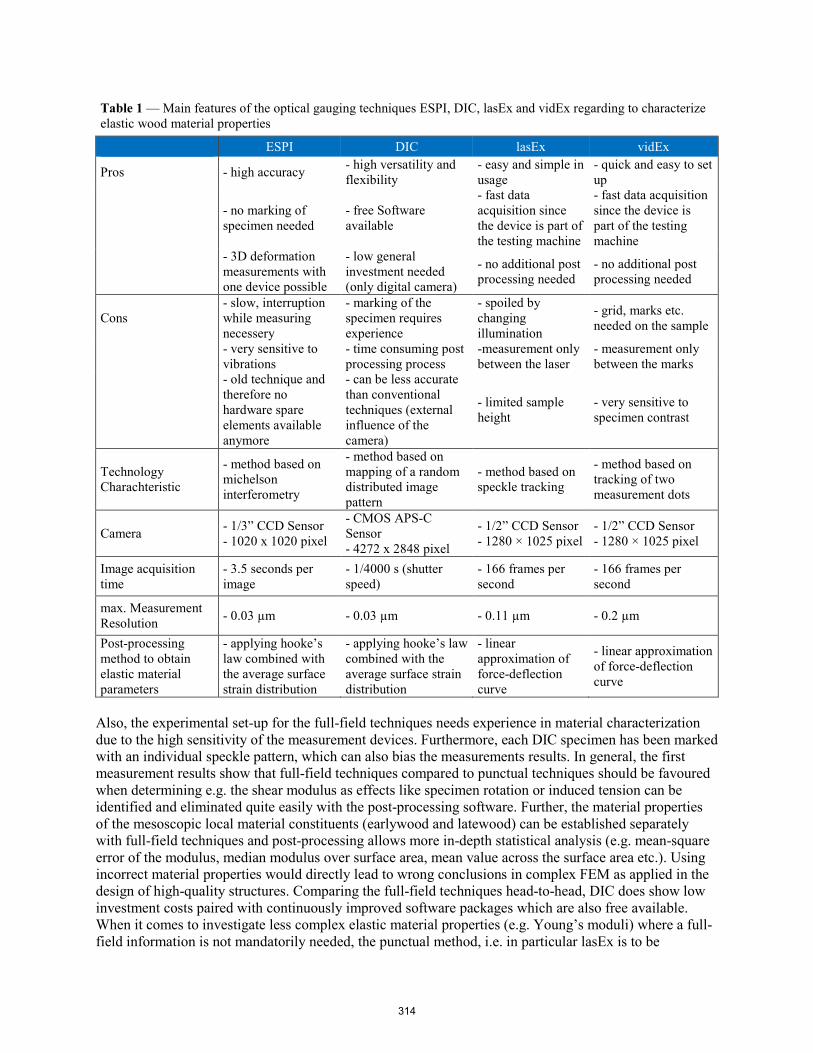
Table 1 — Main features of the optical gauging techniques ESPI, DIC, lasEx and vidEx regarding to characterize elastic wood material properties

ESPI DIC lasEx vidEx

Pros - high accuracy - high versatility andflexibility

- easy and simple inusage

- quick and easy to setup

- no marking ofspecimen needed

- free Softwareavailable

- fast dataacquisition sincethe device is part ofthe testing machine

- fast data acquisitionsince the device ispart of the testingmachine

- 3D deformationmeasurements withone device possible

- low generalinvestment needed(only digital camera)

- no additional postprocessing needed

- no additional postprocessing needed

Cons - slow, interruptionwhile measuringnecessery

- marking of thespecimen requiresexperience

- spoiled bychangingillumination

- grid, marks etc.needed on the sample

- very sensitive tovibrations

- time consuming postprocessing process

-measurement onlybetween the laser

- measurement onlybetween the marks

- old technique andtherefore nohardware spareelements availableanymore

- can be less accuratethan conventionaltechniques (externalinfluence of thecamera)

- limited sampleheight

- very sensitive tospecimen contrast

Technology Charachteristic

- method based onmichelsoninterferometry

- method based onmapping of a randomdistributed imagepattern

- method based onspeckle tracking

- method based ontracking of twomeasurement dots

Camera - 1/3” CCD Sensor- 1020 x 1020 pixel

- CMOS APS-CSensor- 4272 x 2848 pixel

- 1/2” CCD Sensor- 1280 × 1025 pixel

- 1/2” CCD Sensor- 1280 × 1025 pixel

Image acquisition time

- 3.5 seconds perimage

- 1/4000 s (shutterspeed)

- 166 frames persecond

- 166 frames persecond

max. Measurement Resolution - 0.03 µm - 0.03 µm - 0.11 µm - 0.2 µm

Post-processing method to obtain elastic material parameters

- applying hooke’slaw combined withthe average surfacestrain distribution

- applying hooke’s lawcombined with theaverage surface straindistribution

- linearapproximation offorce-deflectioncurve

- linear approximationof force-deflectioncurve

Also, the experimental set-up for the full-field techniques needs experience in material characterization due to the high sensitivity of the measurement devices. Furthermore, each DIC specimen has been marked with an individual speckle pattern, which can also bias the measurements results. In general, the first measurement results show that full-field techniques compared to punctual techniques should be favoured when determining e.g. the shear modulus as effects like specimen rotation or induced tension can be identified and eliminated quite easily with the post-processing software. Further, the material properties of the mesoscopic local material constituents (earlywood and latewood) can be established separately with full-field techniques and post-processing allows more in-depth statistical analysis (e.g. mean-square error of the modulus, median modulus over surface area, mean value across the surface area etc.). Using incorrect material properties would directly lead to wrong conclusions in complex FEM as applied in the design of high-quality structures. Comparing the full-field techniques head-to-head, DIC does show low investment costs paired with continuously improved software packages which are also free available. When it comes to investigate less complex elastic material properties (e.g. Young’s moduli) where a full-field information is not mandatorily needed, the punctual method, i.e. in particular lasEx is to be

314

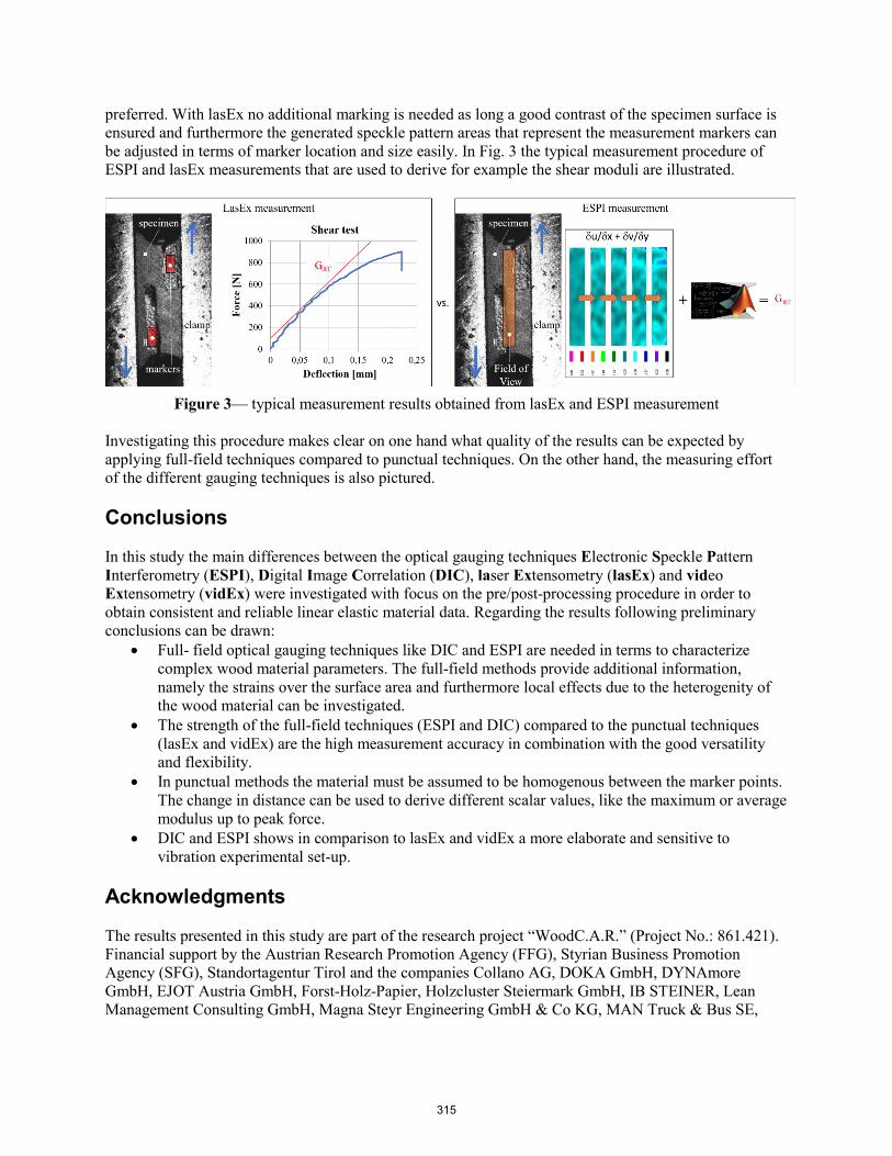
preferred. With lasEx no additional marking is needed as long a good contrast of the specimen surface is ensured and furthermore the generated speckle pattern areas that represent the measurement markers can be adjusted in terms of marker location and size easily. In Fig. 3 the typical measurement procedure of ESPI and lasEx measurements that are used to derive for example the shear moduli are illustrated.

Figure 3— typical measurement results obtained from lasEx and ESPI measurement

Investigating this procedure makes clear on one hand what quality of the results can be expected by applying full-field techniques compared to punctual techniques. On the other hand, the measuring effort of the different gauging techniques is also pictured.

Conclusions

In this study the main differences between the optical gauging techniques Electronic Speckle Pattern Interferometry (ESPI), Digital Image Correlation (DIC), laser Extensometry (lasEx) and video Extensometry (vidEx) were investigated with focus on the pre/post-processing procedure in order to obtain consistent and reliable linear elastic material data. Regarding the results following preliminary conclusions can be drawn:

• Full- field optical gauging techniques like DIC and ESPI are needed in terms to characterizecomplex wood material parameters. The full-field methods provide additional information,namely the strains over the surface area and furthermore local effects due to the heterogenity ofthe wood material can be investigated.

• The strength of the full-field techniques (ESPI and DIC) compared to the punctual techniques(lasEx and vidEx) are the high measurement accuracy in combination with the good versatilityand flexibility.

• In punctual methods the material must be assumed to be homogenous between the marker points.The change in distance can be used to derive different scalar values, like the maximum or averagemodulus up to peak force.

• DIC and ESPI shows in comparison to lasEx and vidEx a more elaborate and sensitive tovibration experimental set-up.

Acknowledgments

The results presented in this study are part of the research project “WoodC.A.R.” (Project No.: 861.421). Financial support by the Austrian Research Promotion Agency (FFG), Styrian Business Promotion Agency (SFG), Standortagentur Tirol and the companies Collano AG, DOKA GmbH, DYNAmore GmbH, EJOT Austria GmbH, Forst-Holz-Papier, Holzcluster Steiermark GmbH, IB STEINER, Lean Management Consulting GmbH, Magna Steyr Engineering GmbH & Co KG, MAN Truck & Bus SE,

315

Mattro Mobility Revolutions GmbH, Volkswagen AG and Weitzer Parkett GmbH & Co KG is gratefully acknowledged. References

Bachtiar E V., Sanabria SJ, Mittig JP, Niemz P (2017) Moisture-dependent elastic characteristics of walnut and cherry wood by means of mechanical and ultrasonic test incorporating three different ultrasound data evaluation techniques. Wood Sci Technol 51:47–67. https://doi.org/10.1007/s00226-016-0851-z

Davis JR (2004) Tensile Testing. ASM international Eberhardsteiner J (1995) Biaxial testing of orthotropic materials using electronic speckle pattern

interferometry. Measurement 16:139–148. https://doi.org/10.1016/0263-2241(95)00019-4 Gingerl M (1998) Realisierung eines optischen Deformationsmeßsystems zur experimentellen

Untersuchung des orthotropen Materialverhaltens von Holz bei biaxialer Beanspruchung (Realization of an optical deformation measuring system for the experimental investigation of the . Technische Universität Wien

Jost T, Müller U, Feist F (2018) Wood Composites for Future Automotive Engineering? – Basic Requirement: Crash Simulation of Wood-Based Components Holzverbundwerkstoffe im Automobilbau der Zukunft? – Grundvoraussetzung: Crashsimulation von Holzkomponenten. Konstruktion 10:74–82

Kohl D, Link P, Böhm S (2016) Wood as a Technical Material for Structural Vehicle Components. Procedia CIRP 40:557–561. https://doi.org/10.1016/j.procir.2016.01.133

Kroworz A, Katunin A (2018) Non-Destructive Testing Of Structures Using Optical And Other Methods : A Review. Sdhm 12:1–17. https://doi.org/10.3970/sdhm.2018.012.001

Kumpenza C, Matz P, Halbauer P, et al (2018) Measuring Poisson’s ratio: mechanical characterization of spruce wood by means of non-contact optical gauging techniques. Wood Sci Technol 52:1451–1471. https://doi.org/10.1007/s00226-018-1045-7

Majano-Majano A, Fernandez-Cabo JL, Hoheisel S, Klein M (2012) A Test Method for Characterizing Clear Wood Using a Single Specimen. Exp Mech 52:1079–1096. https://doi.org/10.1007/s11340-011-9560-6

Müller U, Ringhofer A, Brandner R, Schickhofer G (2015) Homogeneous shear stress field of wood in an Arcan shear test configuration measured by means of electronic speckle pattern interferometry: description of the test setup. Wood Sci Technol 49:1123–1136. https://doi.org/10.1007/s00226-015-0755-3

Valla A, Konnerth J, Keunecke D, et al (2011) Comparison of two optical methods for contactless, full field and highly sensitive in-plane deformation measurements using the example of plywood. Wood Sci Technol 45:755–765. https://doi.org/10.1007/s00226-010-0394-7

Vorobyev A, Arnould O, Laux D, et al (2016) Characterisation of cubic oak specimens from the Vasa ship and recent wood by means of quasi-static loading and resonance ultrasound spectroscopy (RUS). Holzforschung 70:457–465. https://doi.org/10.1515/hf-2015-0073

Xavier J, Belini U, Pierron F, et al (2013) Characterisation of the bending stiffness components of MDF panels from full-field slope measurements. Wood Sci Technol 47:423–441. https://doi.org/10.1007/s00226-012-0507-6

Xavier J, Oliveira M, Morais J, Pinto T (2009) Measurement of the shear properties of clear wood by the Arcan test. Holzforschung 63:217–225. https://doi.org/10.1515/HF.2009.034

Zink AG, Davidson RW, Hanna RB (2007) Strain measurement in wood using a digital image correlation technique. Wood Fiber Sci 27:346–359

316

TeraHertz Observation of Moisture Convection-Diffusion in Wood

Ahmad Alkadri * Laboratoire de Mécanique et Génie Civil (LMGC), University of Montpellier, CNRS, Montpellier, France, ahmad.alkadri@outlook.com

Nina Dyakonova Laboratoire Charles Coulomb (L2C), University of Montpellier, CNRS, Montpellier, France

Dominique Coquillat Laboratoire Charles Coulomb (L2C), University of Montpellier, CNRS, Montpellier, France

Olivier Arnould Laboratoire de Mécanique et Génie Civil (LMGC), University of Montpellier, CNRS, Montpellier, France

Delphine Jullien Laboratoire de Mécanique et Génie Civil (LMGC), University of Montpellier, CNRS, Montpellier, France

Joseph Gril Université Clermont Auvergne, CNRS, SIGMA Clermont, Institut Pascal, Clermont-Ferrand, France

* Corresponding author

Abstract

In spite of its abundance and widespread utilization, wood as a material still poses some challenges for those seeking to use it. Particularly, because of its hygroscopic properties, mechanical strain and stress can be induced by the water movement in wood, either during the drying process (pre-utilization) or during the life service of the products. That is why the topic of water transport in wood, which also includes the wood drying study, is a well-documented research topic. Various kinds of tools and methods have been developed to observe the movement of water in wood, and here we employed terahertz (THz) spectroscopy and imaging techniques to study it. The interest for the use of this technique is based on its relative safety compared to other techniques, such as X-rays, and also on its ease of installation, which makes it easily implementable in an industrial environment. Our studies confirm the feasibility of THz techniques to observe one- and two-dimensional moisture transport phenomena in wood. A mathematical model was developed to process and analyse the THz measurements and compared it with conventional water diffusion models based on gravimetric methods. Future works would consist of taking into account the convolution effect linked to the THz’s non-negligible spot size and border effect, which is a very important point, and the simultaneous measurement of moisture changes and strain generated through the drying or humidification process.

Keywords: wood, water diffusion, terahertz, experiment, modelling

Introduction

The abundance of wood in nature, coupled with its versatility, makes it one of the most well-utilized biological materials. Earliest evidence of wood as construction material can be traced back to the Neolithic age, about 8000–6000 years ago (Tegel et al. 2012). However, wood is not without its own problems. Being a hygroscopic material, it is susceptible to changes caused by the variation of humidity

317

of its environment (Skaar 1988). Not only its dimensions, its properties––physical and mechanical––could be affected too (Bergman et al. 2010). This led to the necessity for determining the hygromechanical properties, which includes the hygroscopic and mechanical properties, of a given wood species before its utilization.

One of the most important hygroscopic properties of wood is its moisture transfer characteristics. Mechanical strain and/or stress, induced by water movement in wood, either during the drying (pre-utilization) or even during the use-phase could induce damages on the structure (Mukudai and Yata 1986). This is why a lot of studies had been conducted regarding moisture transfer in wood, particularly for wood drying. Various tools and methods, particularly nondestructive techniques, have been developed to observe water movement in wood, such as X-ray and NMR (nuclear magnetic resonance) (Alkan et al. 2007; Zhou et al. 2018). Here, we focused on a relatively new method, called Terahertz technique, for observing and measuring the moisture transfer.

Terahertz is a category of frequency ranging between the infra- and visible light. Recently, a growing number of studies have been conducted on its utilization for measuring moisture content in wood (Federici 2012; Inagaki et al. 2014). Further development of this technique also enables us to conduct consecutive scan in short time delay, thus allowing us to observe the moisture distribution changes in the wood linked to the atmospheric humidity changes (Bensalem et al. 2018). It produces a potential application for measuring and observing the moisture profile in pieces of wood during the diffusion process at a quasi-real-time condition. It could allow us to determine the drying speed of wood and, coupled with its relative safeness to other nondestructive techniques such as NMR or X-ray, making it implementable for industrial use. Therefore, the objectives of our study here are to explore those potentials, observing the moisture diffusion profile, and see its applicability on various wood species.

Methods

Mathematical Principles

Diffusion Equation

In the case of wood, in which its moisture content (W) lies below its fiber saturation point (Wsp), it could be assumed that there is no convection or transport of free water. Because of this, the moisture transport model could be written as:

𝜕𝜕𝜕𝜕/𝜕𝜕𝜕𝜕 = ∇ ∙ (𝐷𝐷∇𝜕𝜕), (1)

where W is the total moisture content in wood, D refers to the diffusion tensor, and t the time (Perkowski et al. 2017). This equation is comparable to that of the Fick’s law of diffusion (Crank 1979). Because wood is an orthotropic material, its D diffusion tensor could be written in the principal axes as:

𝐷𝐷𝐿𝐿 0 00 𝐷𝐷𝑅𝑅 00 0 𝐷𝐷𝑇𝑇

, (2)

where DL, DR, and DT refer to the coefficient of diffusion in longitudinal, radial and tangential direction, respectively.

To simulate the three-dimensional moisture transport in wood, we need to determine, firstly, those three coefficients of diffusion. To do that, we have adapted the methods used in previous studies (Olek et al.

318

2005; Olek and Weres 2007), which are fitting the moisture profiles on varying time t of diffusion with the profiles obtained through solving the diffusion equation.

To do that, here we used the analytical approach and the finite differences, implicit method approach to solve the diffusion equation and obtain the moisture profile. In the case of unidimensional diffusion, equation (1) could be written as (Crank 1979; Siau 1984):

𝜕𝜕𝜕𝜕𝜕𝜕𝜕𝜕

= ∂∂x𝐷𝐷𝑎𝑎

𝜕𝜕𝜕𝜕𝜕𝜕𝜕𝜕, (3)

with a refers to the diffusion direction measured (either L, R, or T). The schemes (analytical and numerical) for solving the equation above has been implemented as R (R Core Team 2019) package.

Analytical Model for Terahertz Absorption

In a multiphase material such as moisturized wood, assuming a unidimensional transmission and a negligible changes in the specimen dimension caused by the moisture absorption, the Beer-Lambert law can be rewritten as (Bensalem et al. 2018):

𝜇𝜇𝑦𝑦 = 𝐴𝐴ℎ𝑠𝑠

= 𝜇𝜇𝑠𝑠 + 𝜇𝜇𝑤𝑤 × ℎ𝑤𝑤ℎ𝑠𝑠

, with 𝐴𝐴 = −ln 𝐼𝐼𝐼𝐼0 , (4)

where µy is the absorption coefficient of the multiphase material (in m-1), µs and µw are the absorption coefficients of the wood and water respectively, hw is the water’s equivalent thickness, hs is the dry wood specimen thickness, I and I0 are the transmitted and emitted signal’s intensity (V). Further, by assuming a point unit surface of the material, its moisture content (W) could be written as:

𝜕𝜕 = 𝑚𝑚𝑤𝑤𝑚𝑚𝑠𝑠

= 𝜌𝜌𝑤𝑤×ℎ𝑤𝑤𝜌𝜌𝑠𝑠×ℎ𝑠𝑠

, (5)

where mw is water mass, ms dry solid wood mass, ρw moisture density and ρs dry wood density (Bensalem et al. 2018). By combining equations (4) and (5), we obtain:

𝜕𝜕 = 𝐴𝐴ℎ𝑠𝑠− 𝜇𝜇𝑠𝑠 × 𝜌𝜌𝑤𝑤

𝜌𝜌𝑠𝑠×𝜇𝜇𝑤𝑤. (6)

Experimental Setup

Specimen Preparation

We prepared wood specimens with length × width × thickness (l × w × h for R × L × T directions, respectively) of 25 mm × 25 mm × 5 mm. To obtain the moisture diffusion on only each one of those wood’s axes, we cut them so that their lengths are on the desired diffusion direction. The surfaces of those specimens were all isolated using polypropylene adhesive tape except for the two edges where the moisture exchanges with the atmosphere desired to occur. With these specimens, assuming a unidimensional diffusion and the absence of convection, and also assuming a relative homogeneity of the wood specimen used, we could obtain a unidimensional moisture diffusion profile.

Tools Setup

The setup consisted of a THz wave system and a hermetic home-made box, with the specimen inside, in which its internal air relative humidity was controlled by a Preservatech PMCG II humidity generator. In

319

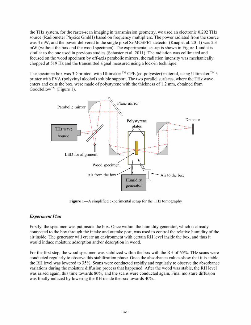
the THz system, for the raster-scan imaging in transmission geometry, we used an electronic 0.292 THz source (Radiometer Physics GmbH) based on frequency multipliers. The power radiated from the source was 4 mW, and the power delivered to the single pixel Si-MOSFET detector (Knap et al. 2011) was 2.3 mW (without the box and the wood specimen). The experimental set-up is shown in Figure 1 and it is similar to the one used in previous studies (Schuster et al. 2011). The radiation was collimated and focused on the wood specimen by off-axis parabolic mirrors, the radiation intensity was mechanically chopped at 519 Hz and the transmitted signal measured using a lock-in technique.

The specimen box was 3D printed, with Ultimaker TM CPE (co-polyester) material, using Ultimaker TM 3 printer with PVA (polyvinyl alcohol) soluble support. The two parallel surfaces, where the THz wave enters and exits the box, were made of polystyrene with the thickness of 1.2 mm, obtained from GoodfellowTM (Figure 1).

Figure 1—A simplified experimental setup for the THz tomography

Experiment Plan

Firstly, the specimen was put inside the box. Once within, the humidity generator, which is already connected to the box through the intake and outtake port, was used to control the relative humidity of the air inside. The generator will create an environment with certain RH level inside the box, and thus it would induce moisture adsorption and/or desorption in wood.

For the first step, the wood specimen was stabilized within the box with the RH of 65%. THz scans were conducted regularly to observe this stabilization phase. Once the absorbance values show that it is stable, the RH level was lowered to 35%. Scans were conducted rapidly and regularly to observe the absorbance variations during the moisture diffusion process that happened. After the wood was stable, the RH level was raised again, this time towards 80%, and the scans were conducted again. Final moisture diffusion was finally induced by lowering the RH inside the box towards 40%.

320

Afterwards, the wood specimen was oven-dried to remove all moisture inside and obtain an anhydrous mass. The now dry specimen’s surfaces were all isolated completely to prevent moisture contact and transport. The specimen was then scanned again in order to obtain its real, dry absorbance value (As). From there, knowing hs ≈ h, we determined the absorption coefficient of dry wood (µs). Finally, through the referenced value of µw, which is 104 m-1 (Bertie and Lan 1996), and the density of water which is 1000 kg/m3, we could then determine the moisture content (W) for each measured surface point during various times of diffusion.

Results

The first imaging results, conducted on a specimen with moisture diffusion occurring in radial direction (exchanges happening on left and right edge of the specimen), had shown us several interesting and important points, and also several new problems to note. Firstly, there is a convolution phenomenon, as made evident in Figure 2a and 2b on all four borders of the specimen. The probable primary cause of this is the effect of the THz spot itself and the border effect, which diffracted a part of the THz ray. It thus “blurred” the border between the area where there is no specimen (air) and the specimen itself. These phenomena pose an important question on how to fit the profile against the diffusion model and would be addressed subsequently before we could conduct the fitting operation.

(a) (b) Figure 2—(a) THz imaging result obtained on t = 150 min , with the colours representing the values of –ln(I/I0), or A, the white lines indicating the specimen’s isolated sides, and the arrows representing the direction of water

entering the specimen, and (b) mean values of –ln(I/I0) inside the specimens for each x-coordinate (in pixel with 1 pixel = 300 µm) on t = 150 min.

Secondly, we saw that there is a diverse range of absorbance (A) values inside the specimen, even for the same t. There are three possible ways to look at this: (a) the first is by regarding the moisture values (W) inside the specimen as widely varied, thus indicating a possible incompatibility with classic diffusion profile, (b) we regard the µs values of each point inside the specimen as varying (e.g. due to change in local density, earlywood vs. latewood), and the W values as constant, or (c) the combination between the two of them.

To answer this problem, we took into account of the fact that the wood itself is not a homogenous material. For example, in the specimen we used above, we found a “tip” for the absorbance values between 50 < x < 60 pixels. This is caused by the presence of an exceptionally dense latewood as we later observed visually, directly. Further, by assuming a relatively homogenous moisture content W in a wood at equilibrium, it was therefore assumed that the varying values of A come mostly from µs variations at

321

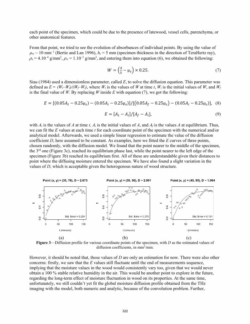
each point of the specimen, which could be due to the presence of latewood, vessel cells, parenchyma, or other anatomical features.

From that point, we tried to see the evolution of absorbances of individual points. By using the value of µw ~ 10 mm–1 (Bertie and Lan 1996), hs = 5 mm (specimen thickness in the direction of TeraHertz ray), ρs = 4.10–4 g/mm3, ρw = 1.10–3 g/mm3, and entering them into equation (6), we obtained the following:

𝜕𝜕 = 𝐴𝐴5− µ𝑠𝑠 × 0.25. (7)

Siau (1984) used a dimensionless parameter, called E, to solve the diffusion equation. This parameter was defined as E = (Wt–Wi)/(Wf–Wi), where Wt is the values of W at time t, Wi is the initial values of W, and Wf is the final value of W. By replacing W inside E with equation (7), we got the following:

𝐸𝐸 = [(0.05𝐴𝐴𝜕𝜕 − 0.25µ𝑠𝑠)− (0.05𝐴𝐴𝑖𝑖 − 0.25µ𝑠𝑠)]/[0.05𝐴𝐴𝑓𝑓 − 0.25µ𝑠𝑠 − (0.05𝐴𝐴𝑖𝑖 − 0.25µ𝑠𝑠)], (8)

𝐸𝐸 = [𝐴𝐴𝜕𝜕 − 𝐴𝐴𝑖𝑖]/[𝐴𝐴𝑓𝑓 − 𝐴𝐴𝑖𝑖], (9)

with At is the values of A at time t, Ai is the initial values of A, and Af is the values A at equilibrium. Thus, we can fit the E values at each time t for each coordinate point of the specimen with the numerical and/or analytical model. Afterwards, we used a simple linear regression to estimate the value of the diffusion coefficient D, here assumed to be constant. As examples, here we fitted the E curves of three points, chosen randomly, with the diffusion model. We found that the point nearer to the middle of the specimen, the 3rd one (Figure 3c), reached its equilibrium phase last, while the point nearer to the left edge of the specimen (Figure 3b) reached its equilibrium first. All of these are understandable given their distances to point where the diffusing moisture entered the specimen. We have also found a slight variation in the values of D, which is acceptable given the heterogenous nature of wood structure.

(a) (b) (c) Figure 3—Diffusion profile for various coordinate points of the specimen, with D as the estimated values of

diffusion coefficients, in mm2/min.

However, it should be noted that, those values of D are only an estimation for now. There were also other concerns: firstly, we saw that the E values still fluctuate until the end of measurements sequence, implying that the moisture values in the wood would consistently vary too, given that we would never obtain a 100 % stable relative humidity in the air. This would be another point to explore in the future, regarding the long-term effect of moisture fluctuation in wood on its properties. At the same time, unfortunately, we still couldn’t yet fit the global moisture diffusion profile obtained from the THz imaging with the model, both numeric and analytic, because of the convolution problem. Further,

322

although we could fit the Y and E curves, those are only dimensionless parameters designed to visualize the diffusion and not for determining the moisture contents itself.

To be able to determine the moisture content of the specimen at every point of the specimen, we should determine, first of all, the values of µs of the specimen itself. This could be conducted by first oven-drying the specimen in order to obtain its ms value, and then stabilizing it in a particular humidity, for example T = 20°C and RH = 65%. Once stable, we measured its new mass, which consists of ms + mw, and so we would obtain its W using equation (5). Afterwards, all of its surface should be isolated so that no moisture exchange with the atmosphere could happen, and then we scan the specimen again with the THz. We would then obtain the values of A for each points of the specimen and, assuming a uniform W, we could then determine the µs, hs and ρs at each point. Once we obtain those µs values, we could then use this specimen on another batch of test.

Conclusions

The first results obtained through this study showed to us the feasibility of THz technique to perform two-dimensional imaging for observing the moisture diffusion in wood during both the adsorption and desorption phases. However, many challenges remained. Further efforts would be directed concerning: (a) the convolution effect, which should be taken into account in order to obtain a true moisture profile in the specimen, (b) the calibration of the THz absorbance with the moisture content (W) values, (c) the presence of a non-linear or even non-Fickian diffusion, and (d) the test of the THz technique capability on other wood species with varying density and/or microstructural diversity (presence of figured wood, extractives, high density etc.)

Acknowledgments

The first author of this study would like to thank Henri SELMER Paris and ANRT for funding, at the time of this writing, his Ph.D. thesis. The authors would also like to thank Pro3D Montpellier for the 3D printing of specimen box used in the experiments. The THz experiments in this study were also financially supported by the Montpellier University of Excellence I-Site MUSE (PRIME@MUSE), La Région Occitanie, and by the “Gepeto TeraHertz platform”.

References

Alkan, S.; Zhang, Y.; Lam, F. 2007. Moisture Distribution Changes and Wetwood Behavior in Subalpine Fir Wood during Drying Using High X-Ray Energy Industrial CT Scanner. Drying Technology. 25(3): 483–488.

Bensalem, M.; Sommier, A.; Mindeguia, J.C.; Batsale, J.C.; Pradere, C. 2018. Terahertz Measurement of the Water Content Distribution in Wood Materials. Journal of Infrared, Millimeter, and Terahertz Waves. 39(2): 195–209.

Bergman, R.; Cai, Z.; Carll, C.G.; Clausen, C.A.; Dietenberg, M.A.; Falk, R.H.; Frihart, C.R.; Glass, S.V.; Hunt, C.G.; Ibach, R.E.; Kretschmann, D.E.; Rammer, D.R.; Ross, R.J.; Star 2010. WoodHandbook, Wood as an Engineering Material. General Technical Report FPL-GTR-190. USDA ForestService, Forest Products Laboratory. 509 p.

Bertie, J.E.; Lan, Z. 1996. Infrared Intensities of Liquids XX: The Intensity of the OH Stretching Band of Liquid Water Revisited, and the Best Current Values of the Optical Constants of H2O(l) at 25°C between 15,000 and 1 cm-1. Applied Spectroscopy. 50(8): 1047–1057.

323

Crank, J. 1979. The Mathematics of Diffusion. Oxford science publications. 2. ed., reprinted. Oxford: Oxford Univ. Press.

Federici, J.F. 2012. Review of Moisture and Liquid Detection and Mapping using Terahertz Imaging. Journal of Infrared, Millimeter, and Terahertz Waves. 33(2): 97–126.

Inagaki, T.; Ahmed, B.; Hartley, I.D.; Tsuchikawa, S.; Reid, M. 2014. Simultaneous prediction of density and moisture content of wood by terahertz time domain spectroscopy. Journal of Infrared, Millimeter, and Terahertz Waves. 35(11): 949–961.

Knap, W.; Nadar, S.; Videlier, H.; Boubanga-Tombet, S.; Coquillat, D.; Dyakonova, N.; Teppe, F.; Karpierz, K.; Łusakowski, J.; Sakowicz, M.; Kasalynas, I.; Seliuta, D.; Valusis, G.; Otsuji, T.; Meziani, Y.; El Fatimy, A.; Vandenbrouk, S.; Madjour, K.; Théron, D.; Gaquière, C. 2011. Field Effect Transistors for Terahertz Detection and Emission. Journal of Infrared, Millimeter, and Terahertz Waves. 32(5): 618–628.

Mukudai, J.; Yata, S. 1986. Modeling and simulation of viscoelastic behavior (tensile strain) of wood under moisture change. Wood Science and Technology. 20(4): 335–348.

Olek, W.; Perré, P.; Weres, J. 2005. Inverse analysis of the transient bound water diffusion in wood. Holzforschung. https://www.degruyter.com/view/j/hfsg.2005.59.issue-1/hf.2005.007/hf.2005.007.xml (November 15, 2017).59(1)

Olek, W.; Weres, J. 2007. Effects of the method of identification of the diffusion coefficient on accuracy of modeling bound water transfer in wood. Transport in Porous Media. 66(1–2): 135–144.

Perkowski, Z.; Świrska-Perkowska, J.; Gajda, M. 2017. Comparison of moisture diffusion coefficients for pine, oak and linden wood. Journal of Building Physics. 41(2): 135–161.

R Core Team 2019. R: A Language and Environment for Statistical Computing. Vienna, Austria: R Foundation for Statistical Computing.

Schuster, F.; Coquillat, D.; Videlier, H.; Sakowicz, M.; Teppe, F.; Dussopt, L.; Giffard, B.; Skotnicki, T.; Knap, W. 2011. Broadband terahertz imaging with highly sensitive silicon CMOS detectors. Optics Express. 19(8): 7827–7832.

Siau, J.F. 1984. Transport Processes in Wood. Berlin, Heidelberg: Springer Berlin Heidelberg.

Skaar, C. 1988. Wood-Water Relations. Berlin, Heidelberg: Springer Berlin Heidelberg.

Tegel, W.; Elburg, R.; Hakelberg, D.; Stäuble, H.; Büntgen, U. 2012. Early Neolithic Water Wells Reveal the World’s Oldest Wood Architecture. PLOS ONE. 7(12): e51374.

Zhou, M.; Caré, S.; Courtier-Murias, D.; Faure, P.; Rodts, S.; Coussot, P. 2018. Magnetic resonance imaging evidences of the impact of water sorption on hardwood capillary imbibition dynamics. Wood Science and Technology. 52(4): 929–955.

324

Rapid Identification of Five Similar Wood Species of Cinnamomum Using Near Infrared Spectroscopy

Xi Pan Research Institute of Wood Industry, Chinese Academy of Forestry, Beijing, China, 2934154957@qq.com

Jian Qiu Southwest Forestry University, Kunming, Yunnan, China, 437057148@qq.com

Yewei Zhu Beijing Great Tech Technology Co. , Ltd. yewei. zhu@beijinggt.com

Zhong Yang* Research Institute of Wood Industry, Chinese Academy of Forestry, Beijing, China, zyang@caf.ac.cn

Abstract The feasibility of using hand-held near infrared spectroscopy (NIR) (wavelength: 950-1650nm)

combined with partial least squares discrimination analysis (PLS-DA) to identify five similar wood species (Cinnamomum porrectum, Cinnamomum tenuipilum, Cinnamomum camphora, Cinnamomum glanduliferum and Cinnamomum longipetiolatum) was investigated in present work. To improve the accuracy of identify, the effect of different spectra preprocess methods was examined. The results showed that the accuracy of C. porrectum, C. tenuipilum, C. camphora, C. glanduliferum, C. longipetiolatum was 100%, 100%, 85%, 55%, and 100% by raw spectra, respectively. The accuracy of smoothing preprocess was same as raw spectral; the effect of standard normal variate (SNV) preprocessed on the accuracy was inconsistent, the accuracy of C. glanduliferum and C. porrectum reduced to 95%, C. camphora reduced to 55%, and C.glanduliferum increased to 75%, relative to raw spectral; 1st derivative preprocessed could improve the accuracy, the accuracy of C. porrectum, C. tenuipilum, C. camphora, C. glanduliferum, C.longipetiolatum was 100%, 100%, 80%, 100%, and 90%, respectively. Meanwhile, the combination of two or more spectral preprocess methods can improve accuracy. Among them, the accuracy more than 80% by smoothing and 1st derivative combined. The accuracy more than 85% by SNV and 1st derivative combined. The accuracy greater than 95% by smoothing, 1st derivative and SNV coupled, and the accuracy was the highest overall. In summary, the portable near infrared spectroscopy technology can effectively identify wood species, near infrared spectroscopy combined with PLS-DA and scientific preprocess methods can be used to rapidly and accurately identify five similar wood species at species-level.

Keywords: wood identification, similar wood, near infrared spectroscopy, spectral preprocess method, partial least squares discriminant analysis (PLS-DA)

Introduction Cinnamomum is a genus belongs to the Lauraceae family that is composed of approximately 250

known species mainly distributed in warm temperature and tropical regions (Cheng et al, 2015). There are about 46 species in China and mainly distributed in the south of Qinling mountains, especially in the southwestern, central and southern provinces. The genus Cinnamomum is one of the most popular and important species, the products are used in food flavorant, cosmetics, and medicines, the timber is widely used for furniture, carving, and building construction materials (Singh et al, 2015). The identification of wood species is extremely significant for the materials optimal utilize and the quality control of the final products (Yang et al, 2015). The Cinnamomum species are

325

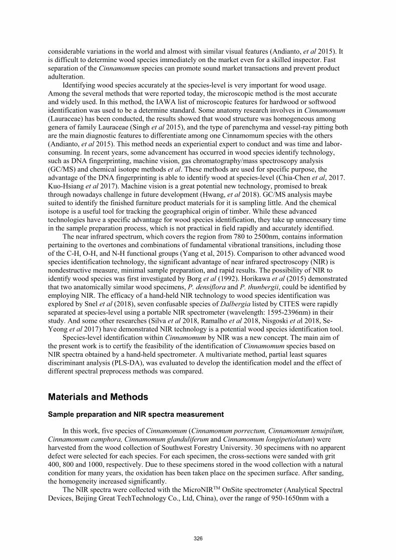
considerable variations in the world and almost with similar visual features (Andianto, et al 2015). It is difficult to determine wood species immediately on the market even for a skilled inspector. Fast separation of the Cinnamomum species can promote sound market transactions and prevent product adulteration.

Identifying wood species accurately at the species-level is very important for wood usage. Among the several methods that were reported today, the microscopic method is the most accurate and widely used. In this method, the IAWA list of microscopic features for hardwood or softwood identification was used to be a determine standard. Some anatomy research involves in Cinnamomum (Lauraceae) has been conducted, the results showed that wood structure was homogeneous among genera of family Lauraceae (Singh et al 2015), and the type of parenchyma and vessel-ray pitting both are the main diagnostic features to differentiate among one Cinnamomum species with the others (Andianto, et al 2015). This method needs an experiential expert to conduct and was time and labor-consuming. In recent years, some advancement has occurred in wood species identify technology, such as DNA fingerprinting, machine vision, gas chromatography/mass spectroscopy analysis (GC/MS) and chemical isotope methods et al. These methods are used for specific purpose, the advantage of the DNA fingerprinting is able to identify wood at species-level (Chia-Chen et al, 2017. Kuo-Hsiang et al 2017). Machine vision is a great potential new technology, promised to break through nowadays challenge in future development (Hwang, et al 2018). GC/MS analysis maybe suited to identify the finished furniture product materials for it is sampling little. And the chemical isotope is a useful tool for tracking the geographical origin of timber. While these advanced technologies have a specific advantage for wood species identification, they take up unnecessary time in the sample preparation process, which is not practical in field rapidly and accurately identified.

The near infrared spectrum, which covers the region from 780 to 2500nm, contains information pertaining to the overtones and combinations of fundamental vibrational transitions, including those of the C-H, O-H, and N-H functional groups (Yang et al, 2015). Comparison to other advanced wood species identification technology, the significant advantage of near infrared spectroscopy (NIR) is nondestructive measure, minimal sample preparation, and rapid results. The possibility of NIR to identify wood species was first investigated by Borg et al (1992). Horikawa et al (2015) demonstrated that two anatomically similar wood specimens, P. densiflora and P. thunbergii, could be identified by employing NIR. The efficacy of a hand-held NIR technology to wood species identification was explored by Snel et al (2018), seven confusable species of Dalbergia listed by CITES were rapidly separated at species-level using a portable NIR spectrometer (wavelength: 1595-2396nm) in their study. And some other researches (Silva et al 2018, Ramalho et al 2018, Nisgoski et al 2018, Se-Yeong et al 2017) have demonstrated NIR technology is a potential wood species identification tool.

Species-level identification within Cinnamomum by NIR was a new concept. The main aim of the present work is to certify the feasibility of the identification of Cinnamomum species based on NIR spectra obtained by a hand-held spectrometer. A multivariate method, partial least squares discriminant analysis (PLS-DA), was evaluated to develop the identification model and the effect of different spectral preprocess methods was compared.

Materials and Methods

Sample preparation and NIR spectra measurement

In this work, five species of Cinnamomum (Cinnamomum porrectum, Cinnamomum tenuipilum, Cinnamomum camphora, Cinnamomum glanduliferum and Cinnamomum longipetiolatum) were harvested from the wood collection of Southwest Forestry University. 30 specimens with no apparent defect were selected for each species. For each specimen, the cross-sections were sanded with grit 400, 800 and 1000, respectively. Due to these specimens stored in the wood collection with a natural condition for many years, the oxidation has been taken place on the specimen surface. After sanding, the homogeneity increased significantly.

The NIR spectra were collected with the MicroNIRTM OnSite spectrometer (Analytical Spectral Devices, Beijing Great TechTechnology Co., Ltd, China), over the range of 950-1650nm with a

326

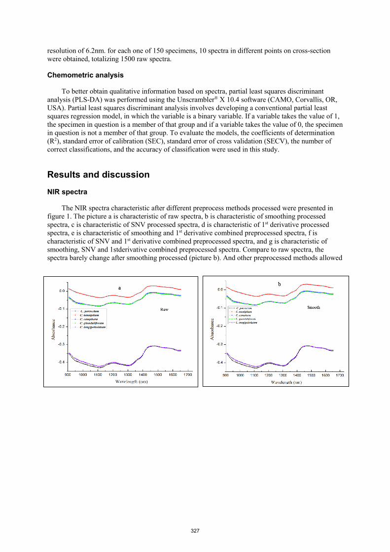
resolution of 6.2nm. for each one of 150 specimens, 10 spectra in different points on cross-section were obtained, totalizing 1500 raw spectra.

Chemometric analysis

To better obtain qualitative information based on spectra, partial least squares discriminant analysis (PLS-DA) was performed using the Unscrambler® X 10.4 software (CAMO, Corvallis, OR, USA). Partial least squares discriminant analysis involves developing a conventional partial least squares regression model, in which the variable is a binary variable. If a variable takes the value of 1, the specimen in question is a member of that group and if a variable takes the value of 0, the specimen in question is not a member of that group. To evaluate the models, the coefficients of determination (R2), standard error of calibration (SEC), standard error of cross validation (SECV), the number of correct classifications, and the accuracy of classification were used in this study.

Results and discussion

NIR spectra

The NIR spectra characteristic after different preprocess methods processed were presented in figure 1. The picture a is characteristic of raw spectra, b is characteristic of smoothing processed spectra, c is characteristic of SNV processed spectra, d is characteristic of 1st derivative processed spectra, e is characteristic of smoothing and 1st derivative combined preprocessed spectra, f is characteristic of SNV and 1st derivative combined preprocessed spectra, and g is characteristic of smoothing, SNV and 1stderivative combined preprocessed spectra. Compare to raw spectra, the spectra barely change after smoothing processed (picture b). And other preprocessed methods allowed

327

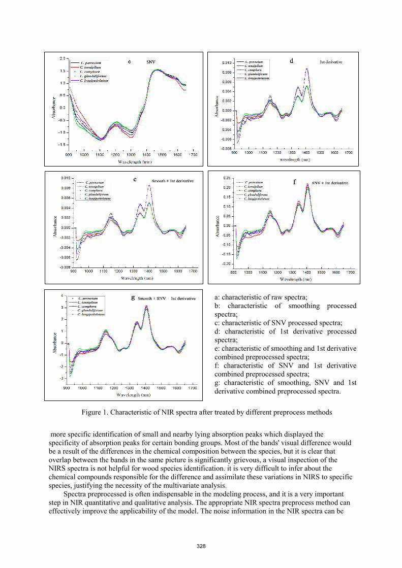
more specific identification of small and nearby lying absorption peaks which displayed the specificity of absorption peaks for certain bonding groups. Most of the bands' visual difference would be a result of the differences in the chemical composition between the species, but it is clear that overlap between the bands in the same picture is significantly grievous, a visual inspection of the NIRS spectra is not helpful for wood species identification. it is very difficult to infer about the chemical compounds responsible for the difference and assimilate these variations in NIRS to specific species, justifying the necessity of the multivariate analysis.

Spectra preprocessed is often indispensable in the modeling process, and it is a very important step in NIR quantitative and qualitative analysis. The appropriate NIR spectra preprocess method can effectively improve the applicability of the model. The noise information in the NIR spectra can be

a: characteristic of raw spectra; b: characteristic of smoothing processed spectra; c: characteristic of SNV processed spectra; d: characteristic of 1st derivative processed spectra; e: characteristic of smoothing and 1st derivative combined preprocessed spectra; f: characteristic of SNV and 1st derivative combined preprocessed spectra; g: characteristic of smoothing, SNV and 1st derivative combined preprocessed spectra.

Figure 1. Characteristic of NIR spectra after treated by different preprocess methods

328

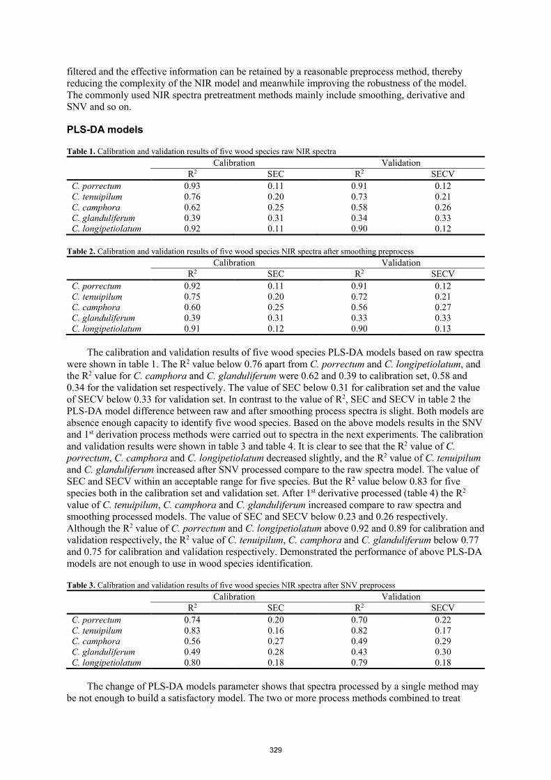
filtered and the effective information can be retained by a reasonable preprocess method, thereby reducing the complexity of the NIR model and meanwhile improving the robustness of the model. The commonly used NIR spectra pretreatment methods mainly include smoothing, derivative and SNV and so on.

PLS-DA models

Table 1. Calibration and validation results of five wood species raw NIR spectra Calibration Validation

R2 SEC R2 SECV C. porrectum 0.93 0.11 0.91 0.12 C. tenuipilum 0.76 0.20 0.73 0.21 C. camphora 0.62 0.25 0.58 0.26 C. glanduliferum 0.39 0.31 0.34 0.33 C. longipetiolatum 0.92 0.11 0.90 0.12

Table 2. Calibration and validation results of five wood species NIR spectra after smoothing preprocess Calibration Validation

R2 SEC R2 SECV C. porrectum 0.92 0.11 0.91 0.12 C. tenuipilum 0.75 0.20 0.72 0.21 C. camphora 0.60 0.25 0.56 0.27 C. glanduliferum 0.39 0.31 0.33 0.33 C. longipetiolatum 0.91 0.12 0.90 0.13

The calibration and validation results of five wood species PLS-DA models based on raw spectra were shown in table 1. The R2 value below 0.76 apart from C. porrectum and C. longipetiolatum, and the R2 value for C. camphora and C. glanduliferum were 0.62 and 0.39 to calibration set, 0.58 and 0.34 for the validation set respectively. The value of SEC below 0.31 for calibration set and the value of SECV below 0.33 for validation set. In contrast to the value of R2, SEC and SECV in table 2 the PLS-DA model difference between raw and after smoothing process spectra is slight. Both models are absence enough capacity to identify five wood species. Based on the above models results in the SNV and 1st derivation process methods were carried out to spectra in the next experiments. The calibration and validation results were shown in table 3 and table 4. It is clear to see that the R2 value of C. porrectum, C. camphora and C. longipetiolatum decreased slightly, and the R2 value of C. tenuipilum and C. glanduliferum increased after SNV processed compare to the raw spectra model. The value of SEC and SECV within an acceptable range for five species. But the R2 value below 0.83 for five species both in the calibration set and validation set. After 1st derivative processed (table 4) the R2 value of C. tenuipilum, C. camphora and C. glanduliferum increased compare to raw spectra and smoothing processed models. The value of SEC and SECV below 0.23 and 0.26 respectively. Although the R2 value of C. porrectum and C. longipetiolatum above 0.92 and 0.89 for calibration and validation respectively, the R2 value of C. tenuipilum, C. camphora and C. glanduliferum below 0.77 and 0.75 for calibration and validation respectively. Demonstrated the performance of above PLS-DA models are not enough to use in wood species identification.

Table 3. Calibration and validation results of five wood species NIR spectra after SNV preprocess Calibration Validation

R2 SEC R2 SECV C. porrectum 0.74 0.20 0.70 0.22 C. tenuipilum 0.83 0.16 0.82 0.17 C. camphora 0.56 0.27 0.49 0.29 C. glanduliferum 0.49 0.28 0.43 0.30 C. longipetiolatum 0.80 0.18 0.79 0.18

The change of PLS-DA models parameter shows that spectra processed by a single method may be not enough to build a satisfactory model. The two or more process methods combined to treat

329

spectra were carried out to obtain great PLS-DA model in the following study. The model parameter based on smoothing and 1st derivative combined processed spectra were showed in table 5. The R2

Table 4. Calibration and validation results of five wood species NIR spectra after 1st derivative preprocess Calibration Validation

R2 SEC R2 SECV C. porrectum 0.94 0.09 0.93 0.10 C. tenuipilum 0.77 0.19 0.75 0.20 C. camphora 0.70 0.22 0.63 0.25 C. glanduliferum 0.66 0.23 0.60 0.26 C. longipetiolatum 0.92 0.12 0.89 0.13

Table 5. Calibration and validation results of five wood species NIR spectra after smoothing and 1st derivative combined preprocess

Calibration Validation R2 SEC R2 SECV

C. porrectum 0.94 0.10 0.92 0.11 C. tenuipilum 0.78 0.19 0.79 0.20 C. camphora 0.70 0.22 0.65 0.24 C. glanduliferum 0.69 0.22 0.66 0.23 C. longipetiolatum 0.91 0.12 0.88 0.14

Table 6. Calibration and validation results of five wood species NIR spectra after SNV and 1stderivative combined preprocess

Calibration Validation R2 SEC R2 SECV

C. porrectum 0.79 0.18 0.74 0.20 C. tenuipilum 0.84 0.16 0.83 0.17 C. camphora 0.75 0.20 0.69 0.22 C. glanduliferum 0.77 0.19 0.73 0.21 C. longipetiolatum 0.86 0.15 0.83 0.16

value of C. porrectum and C. longipetiolatum was 0.94 and 0.91 for calibration set, and 0.92 and 0.88 for the validation set, the value change within ±1 compare to smoothing processed model and 1st

derivative processed model. The R2 value of C. tenuipilum, C. camphora and C. glanduliferum after smoothing and 1st derivative combined processed was increase slightly compared to one method to processed spectra model (table 2 or table 4), but the value below 0.78 and 0.79 for calibration set and validation set respectively. And the value of SEC and SECV within an acceptable range for five species. The calibration and validation results of spectra after SNV and 1st combined processed were showed in table 6. The R2 value of C. porrectum and C. longipetiolatum was 0.79 and 0.86 for the calibration set, and 0.74 and 0.83 for the validation set, the value significant increase compare to the SNV processed spectra model, but the value significant decrease compares to 1st derivative processed spectra model. The R2 value of C. tenuipilum, C. camphora and C. glanduliferum after SNV and 1st derivative combined processed increase to varying degrees compared to the single method to processed spectra model (table 3 or table 4), but the value below 0.84 and 0.83 for calibration set and validation set respectively. The result demonstrated the PLS-DA models based on the above two combined preprocessed methods are absence ability to identify wood species also.

330

Table 7. Calibration and validation results of five wood species NIR spectra after smoothing, SNV and 1st derivative combined preprocess

Calibration Validation R2 SEC R2 SECV

C. porrectum 0.93 0.10 0.88 0.14 C. tenuipilum 0.88 0.14 0.85 0.16 C. camphora 0.90 0.13 0.84 0.16 C. glanduliferum 0.86 0.15 0.86 0.17 C. longipetiolatum 0.93 0.10 0.90 0.13

Comparing to the calibration and validation results of different methods processed spectra models, the smoothing, SNV and 1st derivative combined to process spectra was carry out. The calibration and validation results of the PLS-DA model was shown in table 7. The R2 value vary from 0.86 to 0.93for calibration set, and 0.84 to 0.90 for validation set respectively. The value of SEC and SECV vary from 0.10 to 0.15 for the calibration set and 0.13 to 0.17 for validation. The parameter value is increased to varying degrees compared to the aforementioned different methods of processed spectra models. The performance of the PLS-DA model after smoothing, SNV and 1st derivative combined processed is satisfying overall.

Table 8 lists the identify results for the seven PLS-DA models regarding the identification of unknown samples of the five wood species. The identify accuracy of seven models is consistent with performance reflected by the parameter of seven PLS-DA models. It is obvious that C. camphora and C. glanduliferum were difficult to identify with low accuracy relatively. In the model based on rawspectra and the smoothing processed, only 17 samples for C. camphora and 11 samples for C.landuliferum were identified correctly. In the model based on the SNV processed model, only11samples for C. camphora and 15 samples for C. landuliferum were identified correctly. And in the

Table 8. Identification results of unknown samples from different species using the seven PLS-DA models

Preprocess methods

C. porrectum(n=20)

C. tenuipilum(n=20)

C. camphora(n=20)

C.glanduliferum(n=20)

C.longipetiolatum(n=20)

ncorrect accuracy ncorrect accuracy ncorrect accuracy ncorrect accuracy ncorrect accuracy

raw 20 100% 20 100% 17 85% 11 55% 20 100% smooth 20 100% 20 100% 17 85% 11 55% 20 100% SNV 19 95% 20 100% 11 55% 15 75% 19 95%

1st 20 100% 20 100% 16 80% 20 100% 18 90% Smooth

+1st 20 100% 20 100% 16 80% 19 95% 18 90% SNV+1st 17 85% 20 100% 19 95% 20 100% 18 90%

Smooth+1st+SNV 20 100% 20 100% 19 95% 19 95% 19 95%

model based on the 1st derivative, though all the samples of C. glanduliferum was identified correctly, only 16 samples for C. camphora and 18 samples for C. longipetiolatum identified correctly. The model based on the smoothing and 1st derivative combined processed, 16 samples of C. camphora was identified correctly. And the model based on the SNV and 1st derivative combined processed, 17 samples of C. porrectum was identified correctly. In the model based on smoothing, 1st derivative and SNV combined processed, the 20 samples of C. porrectum and C. tenuipilum were all classified into a correct group, 1 sample of C. camphora, C. glanduliferum and C. longipetiolatum was misclassified into other wood species respectively. The accuracy of the model was above 95%, the highest accuracy was obtained among seven PLS-DA models overall.

Conclusion The ability of a hand-held near infrared spectroscopy (wavelength: 950-1650nm) to interspecies

identify five similar wood species of Cinnamomum from the wood collection was investigated and the effect of different spectral preprocess methods was compared. In the PLS-DA model based on smoothing, 1st derivative and SNV combined processed spectra, five species achieved identification

331

accuracy of 95%, with high R2 value of 0.93, 0.88, 0.90, 0.86, 0.93 for calibration set, 0.88, 0.85, 0.84, 0.86, 0.90 for validation, and low SEC and SECV of 0.10 to 0.15, and 0.13 to 0.17, respectively. From the above results, it can be concluded that near infrared spectroscopy combined with PLS-DA and scientific preprocess methods can be used to rapidly and accurately identify five similar wood species of Cinnamomum at species- level. And portable near infrared spectroscopy technology has the potential to non-destructive, rapidly identify wood species at the species-level.

Acknowledgments

The study was supported by China National Natural Science Found (Grant Numbers 31770766 and Grant Numbers 31370711). The authors thank wood collection of Southwest Forestry University for the wood specimens supported.

References Cheng, Lin, Yang, et al. (2015). Chemical Polymorphism and Composition of Leaf Essential Oils

ofCinnamomum kanehiraeUsing Gas Chromatography/Mass Spectrometry, Cluster Analysis, and Principal Component Analysis. Journal of Wood Chemistry and Technology, 35(3): 207–219.

Singh, Sharma, Sharma, (2015). Wood anatomy of some members of family Lauraceae with reference to their identification. Journal of the Indian Academy of Wood Science, 12(2): 137–144.

Yang Z, Liu Y, Pang X, Li K, (2015). Preliminary investigation into the identification of wood species from different locations by near infrared spectroscopy. BioResources, 10: 8505-8517.

Andianto, Imam, Totok kartono, et al. (2015). Wood Anatomical from Indonesian Genus Cinnamomum (Lauraceae) and their Identification Key. Asian Journal of Plant Sciences, 14(1): 11-19.

Chia-Chen W, Fang-Hua C, Cheng-Kuen, et al. (2017). Comparative analysis of the complete chloroplast genomic sequence and chemical components of Cinnamomum micranthum and Cinnamomum kanehirae. Holzforschung, 71(3):189-197.

Kuo-Hsiang, Chia-Hung L, Li-Ping J. (2017). Tracking the geographical origin of timber by DNA fingerprinting: a study of the endangered species Cinnamomum kanehirae in Taiwan. Holzforschung,

71(11):853–862. Hwang, Kayoko, Shengcheng Z, et al. (2018). Automated identification of Lauraceae by scale-

invariant feature transform. Journal of Wood Science, 64:69–77. Borga, Hämäläinen, Theander. (1992). Correlations Between Near-Infrared Spectra of Wet-Stored

Timber and the StorageTime in Relation to the Water Quality. Holzforschung, 46(4):299-303. Horikawa, Mizuno-Tazuru,Sugiyama. (2015). Near-infrared spectroscopy as a potential method for

identification of anatomically similar Japanese diploxylons. Journal of Wood Science, 61(3): 251–261.

Snel, Braga, Silva, et al. (2018). Potential field-deployable NIRS identification of seven Dalbergia species listed by CITES. Wood Science and Technology, 52(5);1411–1427.

Silva, Pastore, Soares, et al. (2018). Determination of the country of origin of true mahogany (Swietenia macrophylla King) wood in five Latin American countries using handheld NIR devices and multivariate data analysis. Holzforschung, 72(7), 521–530.

Ramalho, Andrade, Hein, et al. (2018) .Rapid discrimination of wood species from native forest and plantations using near infrared spectroscopy. Forest Systems..27(2).

Nisgoski, Silvana;Batista, et al. (2018). Discrimination of wood and charcoal from six Caatinga species by near-infrared spectroscopy[J].Maderas. Ciencia y tecnología. 20(2):199-210.

Se-Yeong, Jong-Chan, Jong-Hwa, et al. (2017). Possibility of Wood Classification in Korean Softwood Species Using Near-infrared Spectroscopy Based on Their Chemical Compositions. Journal of the Korean Wood Science and Technology, 45(02): 202-2212.

332

Swelling Interactions of Earlywood and Latewood across a Growth Ring Probed by White Light Microscope Imaging Technology Combined with a Dynamic Vapor Sorption Analysis

Bai Ouyang Research Institute of Wood Industry, Chinese Academy of Forestry, Beijing, P.R. China, 1823264434@qq.com

Jiali Jiang * Research Institute of Wood Industry, Chinese Academy of Forestry, Beijing, P.R. China, Corresponding author: jialiwood@caf.ac.cn

Abstract

The hygroscopicity and swelling behavior of earlywood, latewood and the growth ring of Catalpa bungei wood samples was documented by white light microscope imaging technology combined with a dynamic vapor sorption (DVS) analysis. In particular, the actual moisture content at each stage of hygroscopic loading and the images needed for the swelling strain evaluation were recorded simultaneously. The swelling strain was calculated by the images analysis. Three kinds of wood samples were extracted at the same growth ring: separated earlywood (EW), separated latewood (LW) and the combined samples (ELW). The results showed that: LW exhibited a slightly higher equilibrium moisture content (EMC) than EW at the range of 0-90%RH. In the radial direction, the EW and the earlywood tissue within ELW both showed a obviously lower swelling strain than that of ELW, and the LW and the latewood tissue within the ELW exhibied a similar situation as the ELW. In the tangential direction, the EW showed a obviously lower swelling strain than the earlywood tissue within ELW, however, LW, earlywood tissue and latewood tissue within the ELW exhibied a similar situation as the ELW. Radial and tangential swelling behavior of the growth ring seems to be dominated by the LW behavior. In addition, the swelling anisotropy ratio in LW is lower than the one seen in EW. Finally, under each RH level, the EMC and corresponding stable swelling strain was reached at the same time, that means no hysteresis in the swelling behavior was observed for EW, LW and ELW.

Keywords: Catalpa bungei, earlywood, latewood, growth ring, moisture adsorption, swelling behavior

Introduction

Catalpa bungei C.A.Mey is one of the precious timber species in China and belongs to Catalpa of Bignoniaceae. It in use, for example in high grade furniture and cabinetry, civil engineering and buildings, is often subjected to moisture loads which may lead to swelling, differential movement and eventually degradation and damage. Understanding the swelling behavior of wood is important for improving the design of new and durable wooden components and structures and interventions on the existing ones.

Two aspects that study of swelling behavior on the same growth ring are earlywood and latewood combined and separated. For combined earlywood and latewood: swelling behavior of earlywood (Picea abies) was lower than latewood in the radial, and in the tangential was similar to latewood (Patera et al.

333

2018). In addition, Derome et al. (2011) showed that the ratios of tangential to radial swelling for earlywood and latewood were 2.50 and 1.32, respectively. The anisotropy of earlywood was stronger presence. Conversely, the latewood was quasi-isotropy (Lanvermann et al. 2014). For separated earlywood and latewood: dimension in the tangential direction of earlywood and latewood cells (Picea jezoensis) swelled linearly. However, dimension of latewood cells in the radial deformed irregularly: they swelled, did not change, or shrink. Dimension of earlywood cells in the radial shrink in most cases (Taguchi et al. 2010). This situation with increasing numbers of cells, became more distinct (Taguchi et al. 2011).

However, there is a dearth of studies where specimens are hardwood, getting the equilibrium moisture content data and swelling behavior data, simultaneously. This work aims to understand the difference and interaction between the swelling behavior of the two tissues, earlywood and latewood of Catalpa wood, separated and combined in a single sample by using DVS Resolution with white light microscope imaging technology Microscope.

Material and methods

Sample preparation

The wood species selected for this study was the 32nd growth ring of 45-years-old catalpa wood (Catalpa bungei C.A.Mey). The average oven-dried density of earlywood and latewood were0.33 g/cm3 and 0.48 g/cm3.The name ELW referred to combined earlywood and latewood sample. The name EW referred to earlywood sample. The name LW referred to latewood sample. The ELW, EW, and LW samples were cut into dimensions of 4mm (L) × 4mm (T) × 8mm (R), 4mm (L) × 4mm (T) × 2.5mm (R), and 4mm (L) × 4mm (T) ×5mm (R), respectively. The name ELW-E referred to earlywood tissue in ELW sample. The name ELW-L referred to latewood tissue in ELW sample. Samples repeated for 3 groups and a total of 9 groups were prepared. All the groups with the same weigh (50±1mg) were prepared. All samples were conditioned in climatic chambers at 25°C and 0% relative humidity (RH) until equilibrium moisture content (EMC) was reached.

Experimental procedure

Adsorption isotherm and swelling behavior measurement

The water vapor sorption behavior of the wood samples was determined using a dynamic vapor sorption apparatus (DVS Resolution, Surface Measurement Systems, UK). Data on weight change were acquired every 20s. The experiment process in this study was divided into the water vapor sorption period (The end of the period was T1. In this period, radial and tangential swelling strain were measured) and EMC constant period (The end of the period was T2. In this period, the change of swelling strain and EMC were compared). The measurements were taken at a constant temperature of 25 ± 0.1C, starting at 0% RH and increasing in increments of 10% RH up to 90% RH. During the water vapor sorption period, samples were maintained at a constant RH, until the weight change was less than 0.002% per 10min. During the EMC constant period, RH kept constant sequentially for 360 min.

During the water vapor sorption behavior of the wood samples, the DVS Resolution coupling white light microscope imaging technology (AnMo Electronics Corporation, Taiwan) with a resolution of 1280× 960 pixels was applied to capture the images needed for the swelling strain evaluation. Images were taken every 1 min over the experiment process, which were required for the determination of the radial and tangential swelling strain.

334

Determination of swelling behavior from Image data analysis

Images from white light microscope imaging technology were processed and analyzed. ELW, EW, LW, ELW-E and ELW-L outlines determined by means of Adobe Photoshop CS1 (Adobe Systems Incorporated) and Auto CAD (Autodesk). Dimensional data was then obtained by open processing and finding 4 pixel-tiles of vessels (Figure 1). On the basis of the pixel-tiles of vessels, dimensional data were calculated concerning the swelling dimension of ELW, EW, LW, ELW-E and ELW-L in the tangential and radial directions.

Figure 1— Sketch map of image processing

Results and discussion

Adsorption isotherm of earlywood and latewood

The EMC values measured of EW (a), LW (b) and ELW (c) are shown in Figure 2. There were obvious differences among 3 samples of EW, and the maximum difference was 3.33%. However, there were

Figure 2— The sorption isotherm of earlywood (EW), latewood (LW) and the growth ring (ELW) a. separated earlywood samples (EW); b. separated latewood samples (LW); c. the growth ring samples (ELW); d.

mean values of earlywood (EW), latewood (LW) and the growth ring (ELW).

335

similar situations among 3 samples of LW and ELW, and the maximum difference were 0.34% and 0.35%, respectively. This difference may be due to the effect of tylosis. There were more tylosis in EW than in LW (Figure 1), and the vessels would be blocked by tylosis, which mainly caused the small adsorption capacity in EW. Therefore, the EMC of the EW was different due to the amount of tylosis, and LW was in contrast (Wu 2015). The area ratio of latewood was 76.92%, but earlywood just was 23.08%. It is obvious that the area ratio of latewood is much larger than earlywood. As a result, effect of tylosis for ELW was similar to LW, and less than EW.

The EMC average values of EW, LW and ELW are shown in Figure 2d. At RH between 0% and 90%, the difference of EW, LW and ELW increased first and then decreased and the maximum difference was 0.66% among them. The higher EMC for LW was probably due to a higher cellulose content and a lower lignin content compared to EW (Bertaud and Holmbom 2004). The amorphous region of cellulose had higher sorption capacity than lignin, and had a positive correlation with swelling strain (Zhou et al. 2017). However, at RH above 50%, the different EMC average values of EW and LW was reduced from 0.65% to 0.03%. This may be caused by capillary action, which could trap some free water within the very fine porous structures and around cell wall corners (Huang and Wang 2014).

Radial swelling behavior of earlywood and latewood

The swelling dimensional changes of EW, LW, ELW-E, ELW-L and ELW are illustrated in Figure 3. It is clearly observed that the radial swelling dimensional changes of EW was less than LW. At RH 90%, the radial swelling dimensional changes in EW is 1.98%, while for LW it is 3.11%, and with the RH increased, the gap between EW and LW was getting wider. ELW-E and ELW-L were shown the similar situation. To pursue the discussion, at the same RH, EMC of latewood was higher than earlywood. It meant that there were more sorption sites in latewood, which can got more water to make more swelling dimensional. In the other hand, special attention needed to be given to the presence and distribution of ray cells in the studied samples (Cramer et al. 2005). It is observed that the ray cells are randomly distributed in the two tissues, earlywood and latewood. The thickness of the ray cell walls was larger than EW cell walls, and similar to LW cell walls (Patera et al. 2018). The ray cells seem to play an important role in making the displacement less strain in the wood cellular structure, especially in low cell wall thickness and low stiffness of earlywood. It can be concluded that rays act as a restraint on the free swelling of EW (Ma and Rudolph 2006; Patera et al. 2018).

Figure 3—The radial swelling dimensional change of EW, LW and ELW.

At RH between 0% and 90%, the radial swelling dimensional changes of EW was similar to ELW-E. It meant that radial swelling behavior of EW were similar to the behavior of ELW-E. The analysis shows that radial swelling behavior of ELW-E is not affected by ELW-L (Patera et al. 2013). At RH below 70%, the radial swelling dimensional changes of ELW-L was lower than LW. However, at RH above 70%,

336

situation was reversed. It showed that ELW-L was suppressed by ELW-E at RH below 70%, but when RH above 70%, ELW-E didn’t suppress the radial swelling behavior of ELW-L, instead of accelerating the radial swelling behavior of ELW-L. At each RH level, the radial swelling dimensional changes of ELW were between ELW-E and ELW-L, also between EW and LW. The values of ELW were slightly lower than ELW-L, and higher than ELW-E. In the radial, earlywood and latewood were in series, and the density and cell wall thickness of latewood were all obviously higher compared to earlywood (Wu 2015). It is speculated that latewood was dominant effect for radial swelling in the growth ring.

Tangential swelling behavior of earlywood and latewood

The tangential dimensional changes of EW, LW, ELW-E, ELW-L and ELW with respect to RH are shown in Figure 4. The tangential swelling dimensional changes of EW was lower than LW, and as the RH increased, the gap between EW and LW was getting wider. At RH 90%, the tangential swelling dimensional changes of LW was 1.3 times higher than EW. However, the tangential swelling dimensional changes of ELW-E and ELW-L were similar. The analysis shows that in tangential direction, higher stresses are located at the interface of ELW-E/ELW-L (Patera et al. 2018). These regions of combined compressive/tensile stresses point to a local bending occurring in these zones. For this reason, the ELW-L, with cell wall thickness higher than the ELW-E cell walls, play a more important role in tangential behavior (Ma and Rudolph 2006).

Figure 4 also shows that at RH 90%, the tangential dimensional changes of ELW-E is 1.3 times higher than EW, and the tangential dimensional changes of ELW-L is similar than LW. It indicated that in the tangential, ELW-E was exhibited the same swelling behavior as ELW, by effect of ELW-L. At RH 90%, the tangential swelling dimensional change of ELW was 1.3 times higher than EW, but similar to ELW-E, ELW-L and LW. In conclusion, the tangential swelling behavior of ELW is dominated by ELW-L (Lanvermann et al. 2014).

Figure 4— The tangential swelling dimensional change of EW, LW and ELW.

The ratio of tangential to radial swelling for earlywood and latewood

The ratio of tangential to radial (T/R) swelling for EW, LW, ELW-E, ELW-L and ELW, an indicator of transverse dimensional anisotropy, was determined at all humidity levels in order to understand the anisotropic behavior during different state of sorption (Figure 5). At RH 10%, ratio of T/R swelling for ELW, ELW-L and LW were 1.52, 1.40 and 1.52, respectively, meaning that they had similar ratio. As the RH increased, the ratio value only a modest increased. This indicates that the dimension in tangential direction changes at relatively greater rate than radial direction when the RH increased (Chauhan and Aggarwal 2004). On the other hand, at RH below 40%, ratio of T/R swelling for ELW-E and EW were similar to ELW. However, At RH above 40%, ratio of T/R swelling for ELW-E and EW suddenly

337

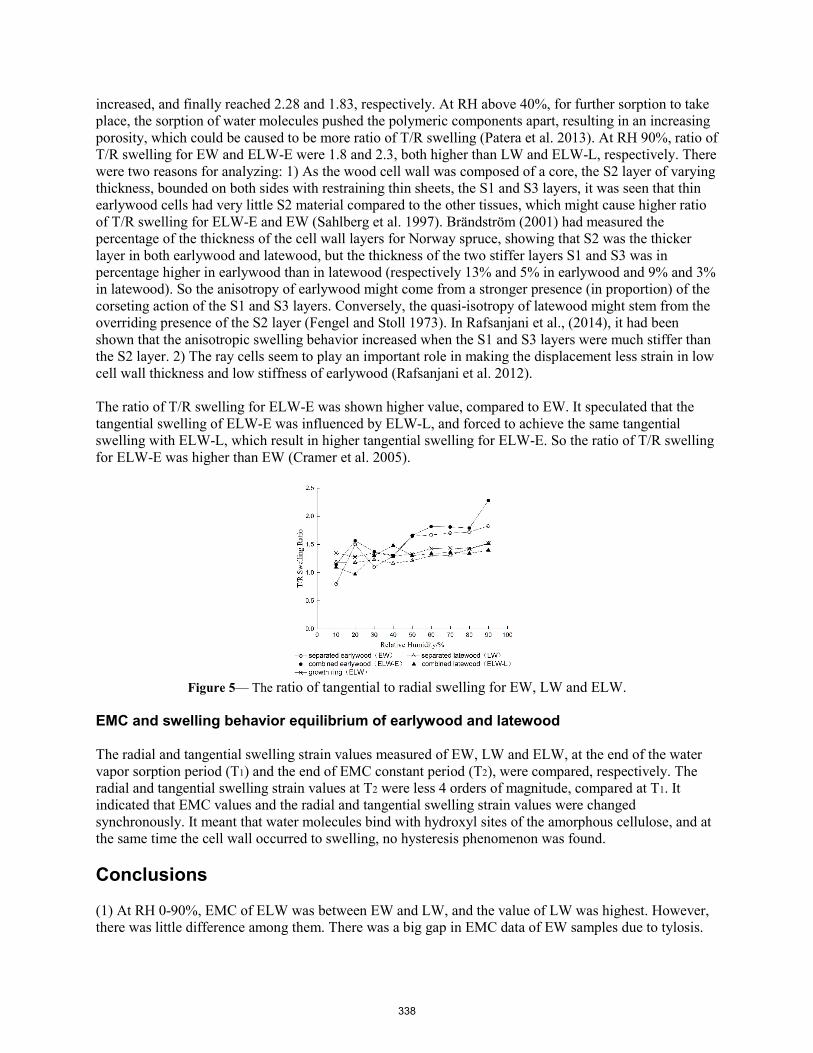
increased, and finally reached 2.28 and 1.83, respectively. At RH above 40%, for further sorption to take place, the sorption of water molecules pushed the polymeric components apart, resulting in an increasing porosity, which could be caused to be more ratio of T/R swelling (Patera et al. 2013). At RH 90%, ratio of T/R swelling for EW and ELW-E were 1.8 and 2.3, both higher than LW and ELW-L, respectively. There were two reasons for analyzing: 1) As the wood cell wall was composed of a core, the S2 layer of varying thickness, bounded on both sides with restraining thin sheets, the S1 and S3 layers, it was seen that thin earlywood cells had very little S2 material compared to the other tissues, which might cause higher ratio of T/R swelling for ELW-E and EW (Sahlberg et al. 1997). Brändström (2001) had measured the percentage of the thickness of the cell wall layers for Norway spruce, showing that S2 was the thicker layer in both earlywood and latewood, but the thickness of the two stiffer layers S1 and S3 was in percentage higher in earlywood than in latewood (respectively 13% and 5% in earlywood and 9% and 3% in latewood). So the anisotropy of earlywood might come from a stronger presence (in proportion) of the corseting action of the S1 and S3 layers. Conversely, the quasi-isotropy of latewood might stem from the overriding presence of the S2 layer (Fengel and Stoll 1973). In Rafsanjani et al., (2014), it had been shown that the anisotropic swelling behavior increased when the S1 and S3 layers were much stiffer than the S2 layer. 2) The ray cells seem to play an important role in making the displacement less strain in low cell wall thickness and low stiffness of earlywood (Rafsanjani et al. 2012).

The ratio of T/R swelling for ELW-E was shown higher value, compared to EW. It speculated that the tangential swelling of ELW-E was influenced by ELW-L, and forced to achieve the same tangential swelling with ELW-L, which result in higher tangential swelling for ELW-E. So the ratio of T/R swelling for ELW-E was higher than EW (Cramer et al. 2005).

Figure 5— The ratio of tangential to radial swelling for EW, LW and ELW.

EMC and swelling behavior equilibrium of earlywood and latewood

The radial and tangential swelling strain values measured of EW, LW and ELW, at the end of the water vapor sorption period (T1) and the end of EMC constant period (T2), were compared, respectively. The radial and tangential swelling strain values at T2 were less 4 orders of magnitude, compared at T1. It indicated that EMC values and the radial and tangential swelling strain values were changed synchronously. It meant that water molecules bind with hydroxyl sites of the amorphous cellulose, and at the same time the cell wall occurred to swelling, no hysteresis phenomenon was found.

Conclusions

(1) At RH 0-90%, EMC of ELW was between EW and LW, and the value of LW was highest. However,there was little difference among them. There was a big gap in EMC data of EW samples due to tylosis.

338

(2) The radial swelling behavior for EW and ELW-E were both lower than ELW. However, ELW wassimilar to LW and ELW-L. We presumed ELW-L played an important role for radial swelling.

(3) The tangential swelling behavior for EW was lowest. LW, ELW-E, ELW-L, ELW were shown thesimilar situation. ELW-E was effected by ELW-L, and ELW-L dominated tangential swelling.

(4) The ratio of T/R swelling for ELW-E was the highest, with EW followed. Both kinds of earlywoodwere anisotropy. Conversely, LW, ELW-L and ELW were quasi-isotropy.

(5) The water sorption and the swelling strain were occurred at the same time, no hysteresis phenomenonwas found.

Acknowledgments

This work was financially supported by the National Natural Science Foundation of China (No. 31570548).

References

Bertaud, F.; Holmbom, B. 2004. Chemical composition of earlywood and latewood in Norway spruce heartwood, sapwood and transition zone wood. Wood Science and Technology, 38(4): 245-256.

Brändström, J. 2001. Micro and ultrastructural aspects of Norway spruce tracheids: a review. IAWA Journal, 22(4): 333-353.

Cramer, S.; Kretschmann, D.; Lakes, R. [and others]. 2005. Earlywood and latewood elastic properties in loblolly pine. Holzforschung, 44(5): 531-538.

Derome, D.; Griffa, M.; Koebel, M. [and others]. 2011. Hysteretic swelling of wood at cellular scale probed by phase-contrast X-ray tomography. Journal of Structural Biology, 173(1): 180-190.

Fengel, D.; Stoll, M. 1973. Variation in cell cross-sectional area, cell-wall thickness and wall layers of spruce tracheids within an annual ring. Holzforschung, 27: 1–7.

Huang, Y. K.; Wang, X. M. 2014. Wood hygroscopic mechanism and its application. World Forestry Research, 27(3): 35-40.

Joffre, T.; Isaksson, P.; Dumont, P. J. J. [and others]. 2016. A method to measure moisture induced swelling properties of a single wood cell. Experimental Mechanics, 56(5): 723-733.

Lanvermann, C.; Wittel, F. K.; Niemz, P. 2014. Full-field moisture induced deformation in Norway spruce: intra-ring variation of transverse swelling. European Journal of Wood and Wood Products, 72(1): 43-52.

Ma, Q.; Rudolph, V. 2006. Dimensional change behavior of Caribbean pine using an environmental scanning electron microscope. Drying Technology, 24(11): 1397-1403.

Patera, A.; Bulcke, J. V. D.; Boone, M. N. [and others]. 2018. Swelling interactions of earlywood and latewood across a growth ring: global and local deformations. Wood Science and Technology, 52(7): 91-114.

339

Patera, A.; Derome, D.; Griffa, M. [and others]. 2013. Hysteresis in swelling and in sorption of wood tissue. Journal of Structural Biology, 182(3): 226–234.

Rafsanjani, A.; Derome, D.; Wittel, F. K. [and others]. 2012. Computational up-scaling of anisotropic swelling and mechanical behavior of hierarchical cellular materials. Composites Science and Technology, 72(6): 744-751.

Rafsanjani, A.; Stiefel, M.; Jefimovs, K. [and others]. 2014. Hygroscopic swelling and shrinkage of latewood cell wall micropillars reveal ultrastructural anisotropy. Journal of The Royal Society Interface, 11(95): 1-10.

Sahlberg, U.; Salmén, L.; Oscarsson, A. 1997. The fibrillar orientation in the S2-layer of wood fibres as determined by X-ray diffraction analysis. Wood Science and Technology, 31(2): 77-86.

Schulgasser, K.; Witztum, A. 2015. How the relationship between density and shrinkage of wood depends on its microstructure. Wood Science and Technology, 49(2):389-401.

Taguchi, A.; Murata, K.; Nakamura, M. [and others]. 2011. Scale effect in the anisotropic deformation change of tracheid cells during water adsorption. Holzforschung, 65(2): 253-256.

Taguchi, A.; Murata, K.; Nakano, T. 2010. Observation of cell shapes in wood cross-sections during water adsorption by confocal laser-scanning microscopy (CLSM). Holzforschung, 64(2): 627-631.

Thithanh, C.; Erni, M.; Jinzhen, C. 2015. Moisture Adsorption and Hygroexpansion of Paraffin Wax Emulsion-treated Southern Pine (Pinus spp.). BioResources, 10(2): 2719-2731.

Wu, W. 2015. Study on the Variance of Wood Structure and Properties of Catalpa bungei C.A.Mey.

Zhou, H. Z.; Yang, T. T.; Ma, E. 2017. Dynamic Moisture Sorption of Poplar Wood Subject to Partial Removal of Chemical Component. Scientia Silvae Sinicae, 53(8): 94-100.

340

FT-NIR Spectroscopic Assessment of Compressive Strength of Wood of Eucalyptus tereticornis Aasheesh Raturi* Department of Physics, Dolphin(PG) Institute of Biomedical and Natural Sciences, Dehradun, Uttarakhand, India, quark6ashu@gmail.com. Vimal Kothiyal Research and Planning Division, Indian Council of Forestry Research and Education, Dehradun, uttarakhand, India, vimal_kothiyal@yahoo.com. P.D.Semalty Department of Physics, SRT campus HNB Garhwal University,Tehri, Uttarakhand,India semaltypd@gmail.com * Corresponding author Abstract In this study, Near infrared spectroscopy (NIRS) coupled with multivariate data analysis has been used to

predict Maximum cursing strength (MCS) and compressive strength at limit of proportionality (CS at LP)

in compressive strength test on radial and tangential strip wood samples obtained from dry wood

specimen of Eucalyptus tereticornis. Partial least squares regression (PLSR) calibrations were developed

for each wood property. Calibrations had good relationships between values measured in laboratory and

NIRS predicted values obtained from small clear samples. The coefficient of determination of cross

validation (R2cv) for MCS of wood varies from 0.55 to 0.80. Calibration equations when applied to test

set resulted in coefficient of determination (R2 TS) that varies from 0.66 to 0.77. The RPD varies from 1.7

to 2.1 and RER values for MCS were found in the range of 6.6 to 9.9. The wave number regions 7502 to

6098cm-1, 5450 to 4597 cm-1, 6102 to 5446 cm-1 and 4601 to 4246 cm-1 were found suitable for radial

and tangential face. The R2cv for CS at LP of dry wood varies from 0.73 to 0.91. However; R2TS varies

from 0.77 to 0.85. The value of RPD and RER varies from 2.1 to 2.6 and 7.4 to 9.0 respectively. The

models with MSC and second derivative preprocessing method have acceptable PLS statistics for radial

and tangential face of wood.

Keywords: NIRS, PLS, wood properties

341

Introduction Generally, the mechanical property is obtained through destructive experimentation with the help

of mechanical testing machines in the laboratory. A method using an approach entirely different from

conventional techniques was first introduced to nondestructive mechanical testing of wood by Hoffmeyer

and Pedersen (1995) using near infrared spectroscopy (Tsuchikawa 2007). NIR spectroscopy is utilized to

estimate chemical composition of the sample; interestingly, in the case of the application to wood, many

researchers have reported the applicability of NIR technique to nondestructive method of mechanical

properties (Kelley et al. 2004a, Kelley et al. 2004b, Tsuchikawa et al. 2005, Fujimoto et al. 2007,

2008,Schimleck et al. 2007, Mora et al. 2008). Previous studies have used NIRS to predict MOR and

MOE of wood samples from wood species as Norway spruce, Pinus radiate and Eucalyptus delegatensis

(Hoffmeyer and Pederson 1995, Thumm and Meder 2001). The potential of Near Infrared Spectroscopy

(NIR) to evaluated specific mechanical characterization were modulus of elasticity (MOE), and modulus

of rupture (MOR) in bending tests, maximum crushing strength (MCS) in compression parallel to grain

(CS), dynamic modulus of elasticity of air dried and green timbers has been demonstrated by number of

researchers (Hoffmeyer and Pedersen 1995, Schimleck et al. 2001a, 2001b, Schimleck et al. 2002,

Thumm and Meder 2001, Gindl et al. 2001, Kelley et al. 2004a, Kelley et al. 2004b, Tsuchikawa et al.

2005, Fujimoto et al. 2007, 2008, Schimleck et al. 2007, Mora et al. 2008, Schimleck , 2008, Schimleck

et al. 2009, Hein et al. 2009, Mora and Schimleck 2010, Kothiyal and Raturi 2011) with reasonable and

acceptable results. These studies demonstrated that NIR spectroscopy could predict wood mechanical

properties with high accuracy in the case of small and full length clear wood specimens. Kelley et al.

(2004a) conducted a large scale study to estimate modulus of elasticity (MOE) and modulus of rupture

(MOR) in static bending tests using six softwood species. They obtained correlation coefficients (R2)

greater than 0.80. This work also showed that the mechanical properties of the different species could be

predicted from a single calibration. In another study, Fujimoto et al. (2007) found it 0.82 to 0.69 for MOE

and MOR respectively for small clear wood specimens. Most of the studies have established NIR models

based on stiffness measured by the Silviscan device (Schimleck et al. 2001a, Jones et al. 2005a, 2005b,

2007, 2008) and very few studies used classical testing equipment to obtain the dynamic and static

modulus of elasticity and develop NIR- based calibration (Via et al. 2003, 2005a, Tsuchikawa et al. 2005

and Hein et al. 2009, 2010). In the continuation of mechanical properties estimation by NIR spectroscopy,

recent work done in this field by Kothiyal and Raturi (2011) tried to short out the problem, regarding

limitation of NIR spectroscopy application with variation in moisture content of wood in timber yards.

They obtained NIR models for predicting MOR, MOE and fiber stress at limit of proportionality (FS at

LP) of samples with varying moisture content of wood specimens. The NIR calibrations have been also

made for dynamic elastic properties based on the resonance technique. Fujimoto et al. (2008) and Hein et

342

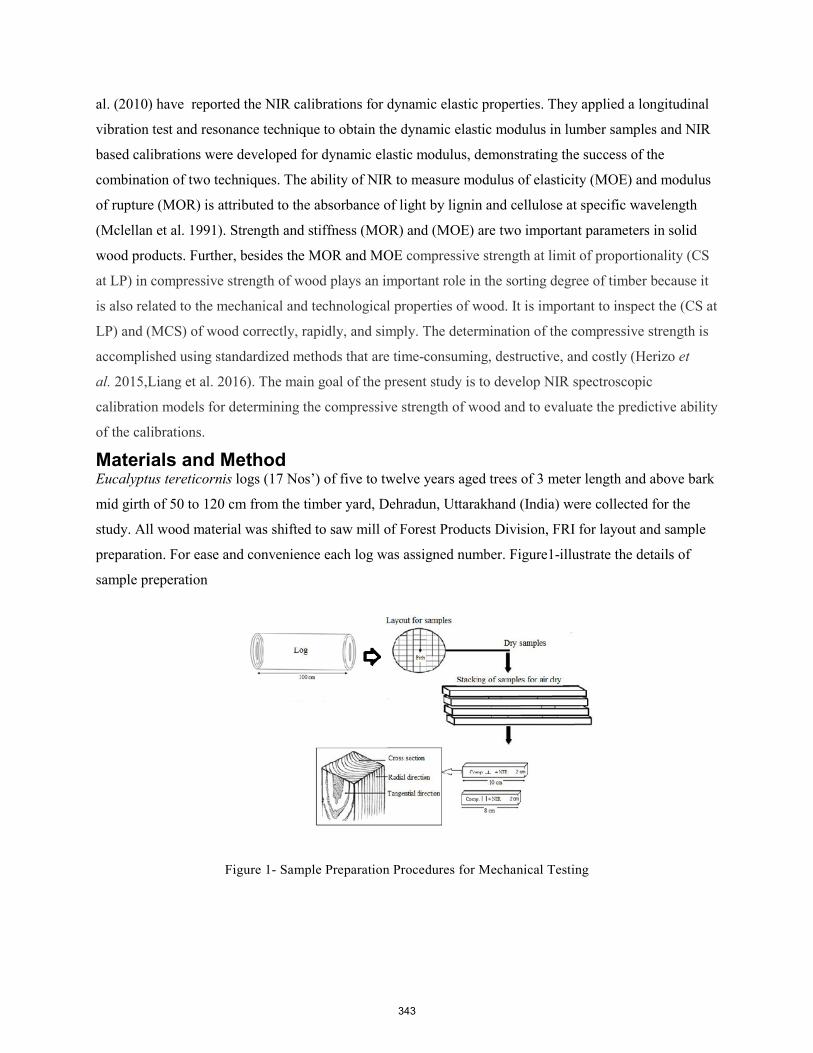
al. (2010) have reported the NIR calibrations for dynamic elastic properties. They applied a longitudinal

vibration test and resonance technique to obtain the dynamic elastic modulus in lumber samples and NIR

based calibrations were developed for dynamic elastic modulus, demonstrating the success of the

combination of two techniques. The ability of NIR to measure modulus of elasticity (MOE) and modulus

of rupture (MOR) is attributed to the absorbance of light by lignin and cellulose at specific wavelength

(Mclellan et al. 1991). Strength and stiffness (MOR) and (MOE) are two important parameters in solid

wood products. Further, besides the MOR and MOE compressive strength at limit of proportionality (CS

at LP) in compressive strength of wood plays an important role in the sorting degree of timber because it

is also related to the mechanical and technological properties of wood. It is important to inspect the (CS at

LP) and (MCS) of wood correctly, rapidly, and simply. The determination of the compressive strength is

accomplished using standardized methods that are time-consuming, destructive, and costly (Herizo et

al. 2015,Liang et al. 2016). The main goal of the present study is to develop NIR spectroscopic

calibration models for determining the compressive strength of wood and to evaluate the predictive ability

of the calibrations.

Materials and Method Eucalyptus tereticornis logs (17 Nos’) of five to twelve years aged trees of 3 meter length and above bark

mid girth of 50 to 120 cm from the timber yard, Dehradun, Uttarakhand (India) were collected for the

study. All wood material was shifted to saw mill of Forest Products Division, FRI for layout and sample

preparation. For ease and convenience each log was assigned number. Figure1-illustrate the details of

sample preperation

Figure 1- Sample Preparation Procedures for Mechanical Testing

343

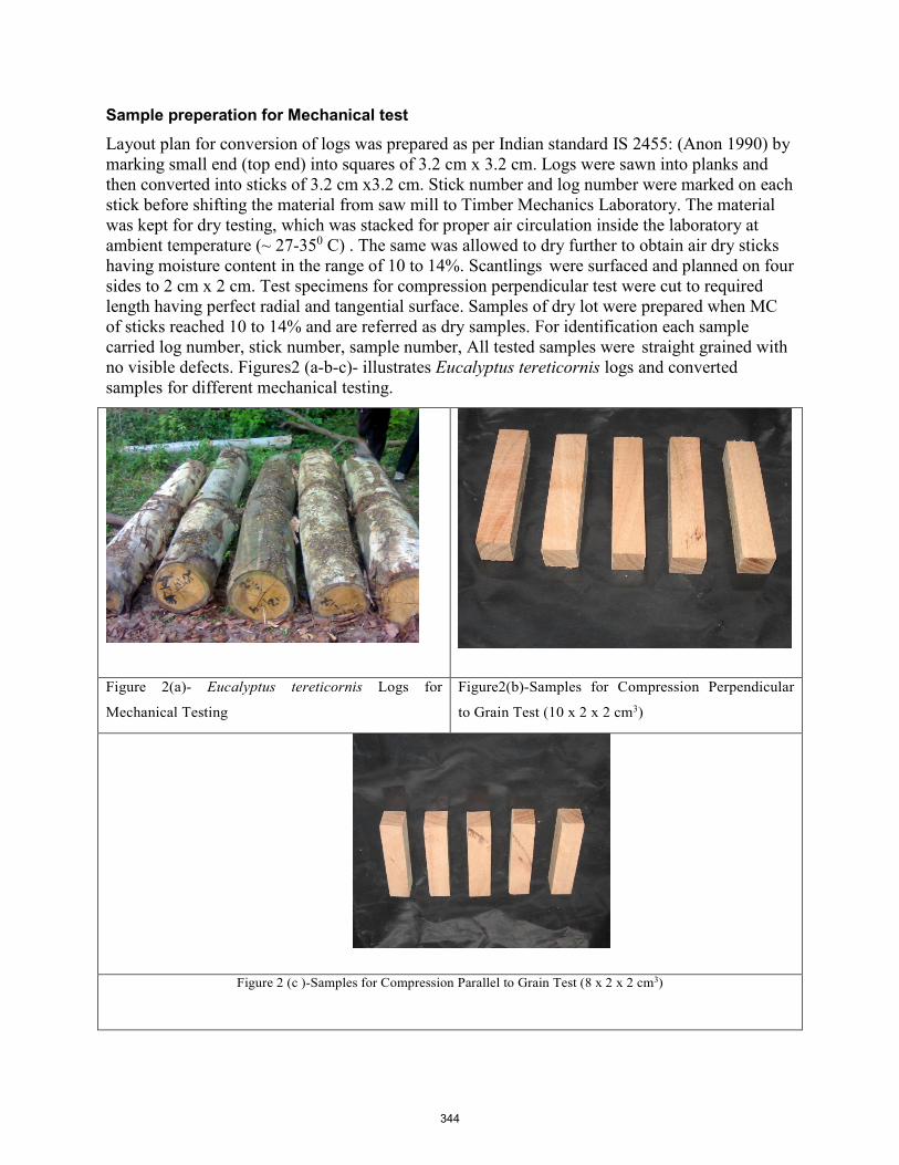
Sample preperation for Mechanical test Layout plan for conversion of logs was prepared as per Indian standard IS 2455: (Anon 1990) by marking small end (top end) into squares of 3.2 cm x 3.2 cm. Logs were sawn into planks and then converted into sticks of 3.2 cm x3.2 cm. Stick number and log number were marked on each stick before shifting the material from saw mill to Timber Mechanics Laboratory. The material was kept for dry testing, which was stacked for proper air circulation inside the laboratory at ambient temperature (~ 27-350 C) . The same was allowed to dry further to obtain air dry sticks having moisture content in the range of 10 to 14%. Scantlings were surfaced and planned on four sides to 2 cm x 2 cm. Test specimens for compression perpendicular test were cut to required length having perfect radial and tangential surface. Samples of dry lot were prepared when MC of sticks reached 10 to 14% and are referred as dry samples. For identification each sample carried log number, stick number, sample number, All tested samples were straight grained with no visible defects. Figures2 (a-b-c)- illustrates Eucalyptus tereticornis logs and converted samples for different mechanical testing.

Figure 2(a)- Eucalyptus tereticornis Logs for

Mechanical Testing Figure2(b)-Samples for Compression Perpendicular

to Grain Test (10 x 2 x 2 cm3)

Figure 2 (c )-Samples for Compression Parallel to Grain Test (8 x 2 x 2 cm3)

344

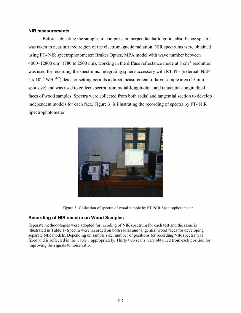
Z

NIR measurements

Before subjecting the samples to compression perpendicular to grain, absorbance spectra

was taken in near infrared region of the electromagnetic radiation. NIR spectrums were obtained

using FT- NIR spectrophotometer: Bruker Optics, MPA model with wave number between

4000–12800 cm-1 (780 to 2500 nm), working in the diffuse reflectance mode at 8 cm-1 resolution

was used for recording the spectrums. Integrating sphere accessory with RT-Pbs (external, NEP

5 x 10-10 WH -1/2) detector setting permits a direct measurement of large sample area (15 mm

spot size) and was used to collect spectra from radial-longitudinal and tangential-longitudinal

faces of wood samples. Spectra were collected from both radial and tangential section to develop

independent models for each face. Figure 3 is illustrating the recording of spectra by FT- NIR

Spectrophotometer.

Figure 3- Collection of spectra of wood sample by FT-NIR Spectrophotometer

Recording of NIR spectra on Wood Samples Separate methodologies were adopted for recoding of NIR spectrum for each test and the same is illustrated in Table 1- Spectra were recorded on both radial and tangential wood faces for developing separate NIR models. Depending on sample size, number of positions for recording NIR spectra was fixed and is reflected in the Table 1 appropriately. Thirty two scans were obtained from each position for improving the signals to noise ratio.

345

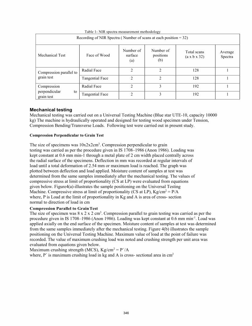
Table 1- NIR spectra measurement methodology Recording of NIR Spectra ( Number of scans at each position = 32)

Mechanical Test Face of Wood Number of

surface (a)

Number of positions

(b)

Total scans (a x b x 32)

Average Spectra

Compression parallel to grain test

Radial Face 2 2 128 1

Tangential Face 2 2 128 1

Compression perpendicular to grain test

Radial Face 2 3 192 1

Tangential Face 2 3 192 1

Mechanical testing Mechanical testing was carried out on a Universal Testing Machine (Blue star UTE-10, capacity 10000 kg) The machine is hydraulically operated and designed for testing wood specimen under Tension, Compression Bending/Transverse Loads. Following test were carried out in present study.

Compression Perpendicular to Grain Test

The size of specimens was 10x2x2cm3. Compression perpendicular to grain testing was carried as per the procedure given in IS 1708–1986 (Anon 1986). Loading was kept constant at 0.6 mm min-1 through a metal plate of 2 cm width placed centrally across the radial surface of the specimens. Deflection in mm was recorded at regular intervals of load until a total deformation of 2.54 mm or maximum load is reached. The graph was plotted between deflection and load applied. Moisture content of samples at test was determined from the same samples immediately after the mechanical testing. The values of compressive stress at limit of proportionality (CS at LP) were evaluated from equations given below. Figure4(a)-illustrates the sample positioning on the Universal Testing Machine. Compressive stress at limit of proportionality (CS at LP), Kg/cm2 = P/A where, P is Load at the limit of proportionality in Kg and A is area of cross- section normal to direction of load in cm Compression Parallel to Grain Test The size of specimen was 8 x 2 x 2 cm3. Compression parallel to grain testing was carried as per the procedure given in IS 1708–1986 (Anon 1986). Loading was kept constant at 0.6 mm min-1. Load was applied axially on the end surface of the specimen. Moisture content of samples at test was determined from the same samples immediately after the mechanical testing. Figure 4(b) illustrates the sample positioning on the Universal Testing Machine. Maximum value of load at the point of failure was recorded. The value of maximum crushing load was noted and crushing strength per unit area was evaluated from equations given below. Maximum crushing strength (MCS), Kg/cm2 = P´/A where, P´ is maximum crushing load in kg and A is cross- sectional area in cm2

346

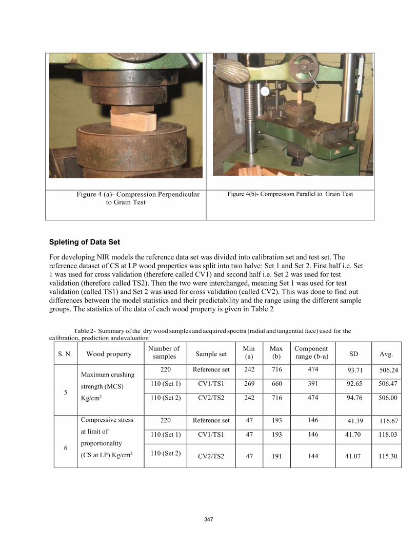
Spleting of Data Set

For developing NIR models the reference data set was divided into calibration set and test set. The reference dataset of CS at LP wood properties was split into two halve: Set 1 and Set 2. First half i.e. Set 1 was used for cross validation (therefore called CV1) and second half i.e. Set 2 was used for test validation (therefore called TS2). Then the two were interchanged, meaning Set 1 was used for test validation (called TS1) and Set 2 was used for cross validation (called CV2). This was done to find out differences between the model statistics and their predictability and the range using the different sample groups. The statistics of the data of each wood property is given in Table 2

Table 2- Summary of the dry wood samples and acquired spectra (radial and tangential face) used for the calibration, prediction and evaluation

S. N. Wood property Number of

samples Sample set Min (a)

Max (b)

Component range (b-a) SD Avg.

5

Maximum crushing

strength (MCS)

Kg/cm2

220 Reference set 242 716 474 93.71 506.24

110 (Set 1) CV1/TS1 269 660 391 92.65 506.47

110 (Set 2) CV2/TS2 242 716 474 94.76 506.00

6

Compressive stress

at limit of

proportionality

(CS at LP) Kg/cm2

220 Reference set 47 193 146 41.39 116.67

110 (Set 1) CV1/TS1 47 193 146 41.70 118.03

110 (Set 2) CV2/TS2 47 191 144 41.07 115.30

Figure 4 (a)- Compression Perpendicular to Grain Test

Figure 4(b)- Compression Parallel to Grain Test

347

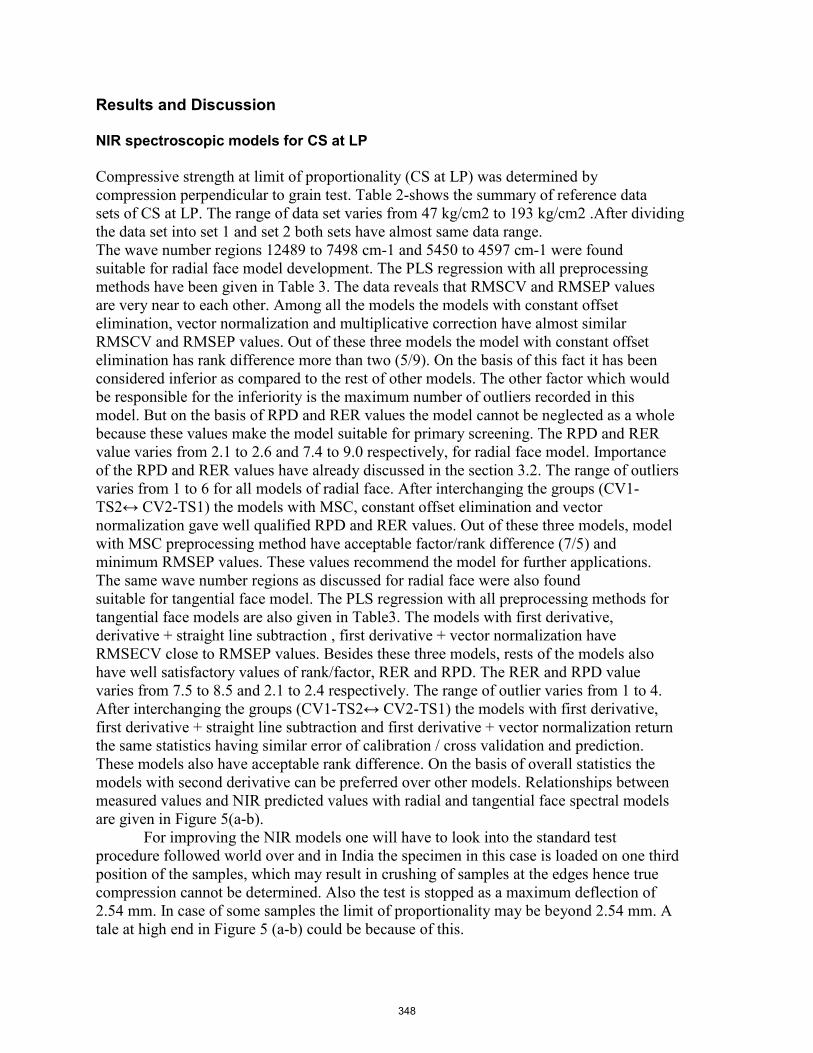
Results and Discussion

NIR spectroscopic models for CS at LP

Compressive strength at limit of proportionality (CS at LP) was determined by compression perpendicular to grain test. Table 2-shows the summary of reference data sets of CS at LP. The range of data set varies from 47 kg/cm2 to 193 kg/cm2 .After dividing the data set into set 1 and set 2 both sets have almost same data range. The wave number regions 12489 to 7498 cm-1 and 5450 to 4597 cm-1 were found suitable for radial face model development. The PLS regression with all preprocessing methods have been given in Table 3. The data reveals that RMSCV and RMSEP values are very near to each other. Among all the models the models with constant offset elimination, vector normalization and multiplicative correction have almost similar RMSCV and RMSEP values. Out of these three models the model with constant offset elimination has rank difference more than two (5/9). On the basis of this fact it has been considered inferior as compared to the rest of other models. The other factor which would be responsible for the inferiority is the maximum number of outliers recorded in this model. But on the basis of RPD and RER values the model cannot be neglected as a whole because these values make the model suitable for primary screening. The RPD and RER value varies from 2.1 to 2.6 and 7.4 to 9.0 respectively, for radial face model. Importance of the RPD and RER values have already discussed in the section 3.2. The range of outliers varies from 1 to 6 for all models of radial face. After interchanging the groups (CV1- TS2↔ CV2-TS1) the models with MSC, constant offset elimination and vector normalization gave well qualified RPD and RER values. Out of these three models, model with MSC preprocessing method have acceptable factor/rank difference (7/5) and minimum RMSEP values. These values recommend the model for further applications. The same wave number regions as discussed for radial face were also found suitable for tangential face model. The PLS regression with all preprocessing methods for tangential face models are also given in Table3. The models with first derivative, derivative + straight line subtraction , first derivative + vector normalization have RMSECV close to RMSEP values. Besides these three models, rests of the models also have well satisfactory values of rank/factor, RER and RPD. The RER and RPD value varies from 7.5 to 8.5 and 2.1 to 2.4 respectively. The range of outlier varies from 1 to 4. After interchanging the groups (CV1-TS2↔ CV2-TS1) the models with first derivative, first derivative + straight line subtraction and first derivative + vector normalization return the same statistics having similar error of calibration / cross validation and prediction. These models also have acceptable rank difference. On the basis of overall statistics the models with second derivative can be preferred over other models. Relationships between measured values and NIR predicted values with radial and tangential face spectral models are given in Figure 5(a-b).

For improving the NIR models one will have to look into the standard test procedure followed world over and in India the specimen in this case is loaded on one third position of the samples, which may result in crushing of samples at the edges hence true compression cannot be determined. Also the test is stopped as a maximum deflection of 2.54 mm. In case of some samples the limit of proportionality may be beyond 2.54 mm. A tale at high end in Figure 5 (a-b) could be because of this.

348

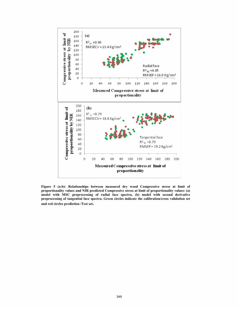
Figure 5 (a-b): Relationships between measured dry wood Compressive stress at limit of proportionality values and NIR predicted Compressive stress at limit of proportionality values: (a) model with MSC preprocessing of radial face spectra, (b) model with second derivative preprocessing of tangential face spectra. Green circles indicate the calibration/cross validation set and red circles prediction /Test set.

349

Table 3- PLS regression between measured dry wood CS at LP and Fourier transform near infrared spectroscopy

Spectrum Treatment Rank CV1/TS1 R2cvRMSECV (kg/cm2) R2TS

RMSEP (kg/cm2)

Outliers (CV + TS)

RPD RER

Radial face Models wave number range (12489 -7498 cm-1 and 5450- 4597 cm-1)

No spectrum prep. 3/2 0.78 19.5 0.82 17.7 3+2=5 2.4 8.2 Str. line subtr. 4/3 0.79 19.3 0.82 17.4 2+1=3 2.4 8.4 Const. offset elim. 5/9 0.79 19.1 0.78 19.3 3+3=6 2.2 7.6 Vector norm. 5/3 0.80 18.8 0.77 19.8 1+1=2 2.1 7.4 Min-Max norm. 4/3 0.73 21.9 0.78 19.6 2+0=2 2.1 7.4 1st der. 3/3 0.78 19.8 0.83 17.1 3+2=5 2.4 8.5 2nd der. 2/2 0.76 20.5 0.80 18.4 3+1=4 2.3 7.9 1st der. + str. line subtr.

3/3 0.78 19.9 0.82 17.4 3+2=5 2.4 8.4

1st der. + vector norm.

3/3 0.79 19.4 0.82 17.5 3+2=5 2.4 8.3

1st der. + MSC 4/3 0.80 19.0 0.82 17.6 4+2=6 2.4 8.3 MSC 7/5 0.82 17.7 0.80 18.6 2+0=2 2.2 7.8 MSC CV2/TS2=7/5 0.90 13.4 0.85 16.0 3+1=4 2.6 9.0 Const. offset elim. CV2/TS2=8/5 0.91 12.7 0.80 18.0 0+1=1 2.3 8.0 Vector norm. CV2/TS2=8/4 0.91 12.5 0.83 17.0 1+1=2 2.4 8.5

Tangential face models wave number range (12489 -7498 cm-1and 5450- 4597 cm-1) No spectrum prep. 5/6 0.76 21.0 0.80 18.3 0+1=1 2.3 8.0 Str. line subtr. 4/4 0.79 19.4 0.81 17.9 0+1=1 2.3 8.2 Const. offset elim. 4/6 0.76 20.6 0.80 18.4 0+2=2 2.3 7.9 Vector norm. 5/5 0.77 20.2 0.80 18.2 0+1=1 2.3 8.0 Min-Max norm. 5/5 0.78 20.0 0.80 18.3 0+1=1 2.3 8.0 1st der. 1/1 0.78 19.9 0.80 18.2 3+1=4 2.3 8.0 2nd der. 2/2 0.82 17.9 0.78 19.2 3+0=3 2.2 7.6 1st der. + str. Line subtr.

2/2 0.81 18.4 0.82 17.5 2+2=4 2.4 8.3

1st der. + vector norm.

2/1 0.80 18.8 0.79 18.7 1+3=4 2.2 7.8

1st der. + MSC. 2/3 0.79 19.4 0.89 17.2 1+1=2 2.4 8.5 MSC 4/4 0.80 18.9 0.82 17.3 0+1=1 2.4 8.4 2nd der. CV2/TS2= 2/2 0.79 18.8 0.79 19.2 1+1=2 2.1 7.5 1st der. CV2/TS2=4/5 0.77 19.7 0.84 17.2 1+1=2 2.4 8.4 1st der. + str. Line subtr.

CV2/TS2=4/4 0.78 19.7 0.82 18.0 2+1=3 2.3 8.0

1st der. + vector norm.

CV2/TS2=3/3 0.80 19.0 0.83 18.0 2+1=3 2.3 8.0

CV: cross-validation, TS: test set validation, R2CV: correlation coefficient of cross validation, R2

TS: correlation coefficient of test-set, RMSECV: root mean square error of cross validation; RMSEP: root mean square error of prediction; RPD: ratio performance deviation (SD/ RMSEP); RER: range error ratio (range of test set/ RMSEP), der: derivative, Const: constant, elim: elimination, Str.: straight, subtr: subtraction, norm: normalization, prep: preprocessing, MSC: multiplicative correction

350

NIR spectroscopic models for MCS The reference values for MCS lies in the range of 242 kg/cm2 to 716 kg/cm2 Table 2. On

dividing the reference data into two equal sets (set 1 and set 2) the range of set 1 varies from 269

kg/cm2 to 660 kg/cm2 while it varies from 242 kg/cm2 to 716 kg/cm2 in case of set 2. The range

of set 2 is wider as compared to set 1. The overall range of data set in present study is wider as

compared to earlier studies carried out on hybrid larch (Fujimoto et al. 2008) which would be

due to selection of varying age group of Eucalyptus tereticornis wood specimen. The wave

number regions 7502 to 6098 cm-1 and 5450 to 4597 cm-1 were found suitable for PLS models

development with different preprocessing methods. These wave number regions which were

selected under the current study are well associated with the range of chemical constituents

present in the wood. Table 4 represents the statistical analysis of partial least squares (PLS)

models with different preprocessing methods. The correlation coefficient of determination of

cross validation (R2cv) for MCS varies from 0.55 to 0.80. The calibration equations when applied

to test set resulted in correlation coefficient of determination (R2TS) that varies from 0.69 to 0.76

for radial face models. The numbers of outliers in all models varies from 0 to 2. The models with

straight line subtraction, vector normalization, first derivative + MSC and MSC have RMSECV

values, which were closed to RMSEP values. When groups were inter changed (CV1-TS2↔

CV2-TS1) as discussed in Chapter 2, the model developed with straight line subtraction, vector

normalization and MSC revealed the statistics similar error of calibration and prediction and

difference in number of factor/rank was less than 2. Out of these three models mentioned above,

the model with MSC has identical RMSECV and RMSEP values. On the basis of used

factor/rank, RMSEP, RPD and RER values, the overall performance of the model proves it as the

best PLS model among the all. The wave number regions from 6102 to 5446 cm-1 and 4601 to

4246 cm-1 has accounted their suitability for tangential face model of MCS .These regions were

also found suitable for tangential face models of SPGV. These wave number regions which were

selected under the current study are well associated with the range of chemical constituents

present in the wood. The R2cv varies from 0.59 to 0.76 and R2TS is in the range of 0.66 to 0.77

for tangential face models. The RMSECV and RMSEP are near to each other for all PLS models.

However the PLS models with constant offset elimination, first derivative + vector

normalization, first derivative + MSC, multiplicative correction have very close RMSECV and

RMSEP values. Besides these models the model with no spectrum preprocessing has also similar

351

RMSECV and RMSEP values but difference in factor/rank is more than two which is generally

not recommended for further evaluation process. The number of outliers varies from 1 to 4 which

are slightly in higher side as compared to radial face models. When groups were interchanged

(CV1-TS2↔ CV2-TS1) the model with constant offset elimination gave similar RMSECV and

RMSEP values. The rest of above three models do not have the adequate difference in error

values, so they are not reported here. The ratio performance of deviation (RPD) varies from 1.8

to 2.0 for radial face and 1.7 to 2.1 for tangential face. The RER values for MCS lies in between

7.7 to 9.9 for radial face and 6.6 to 8.7 for tangential face. In the previous study the correlation

coefficient of determination (R2) was observed 0.87 and 0.77 for radial and tangential face

respectively, however correlation coefficient of determination of prediction (R2TS) was 0.81

for radial face and 0.71 for tangential face (Fujimoto et al. 2008). This shows that our results in

the present study are in good agreement with the studies as reported by the earlier researchers.

Relationships between measured values and NIR predicted values with radial and tangential face

spectral models are given in Figure 6 (a-b). Models of this test can be further improved by

looking at test procedure and failure in samples. Along with crushing of samples, buckling of

samples and tilt in samples could result in values different from true values. A tail at high end in

Figure 6 (a-b) could be because of this.

352

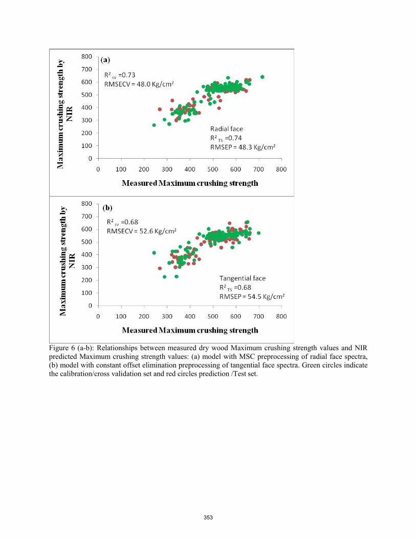
Figure 6 (a-b): Relationships between measured dry wood Maximum crushing strength values and NIR predicted Maximum crushing strength values: (a) model with MSC preprocessing of radial face spectra, (b) model with constant offset elimination preprocessing of tangential face spectra. Green circles indicatethe calibration/cross validation set and red circles prediction /Test set.

353

Table 4- PLS regression between measured dry wood MCS and Fourier transform near infrared spectroscopy

Spectrum Treatment Rank CV1/TS1 R2cvRMSECV (kg/cm2) R2TS

RMSEP (kg/cm2)

Outliers (CV + TS)

RPD RER

Radial face Models wave number range (7502 to 6098cm-1 and 5450 to 4597 cm-1 )

No spectrum prep. 8/6 0.67 54.2 0.73 48.1 0+1=1 1.9 8.1 Str. line subtr. 9/7 0.75 47.6 0.75 46.0 0+0=0 2.0 8.5 Const. offset elim. 8/6 0.69 52.2 0.75 46.2 0+0=0 2.0 8.5 Vector norm. 8/6 0.72 49.6 0.73 48.1 1+1=2 1.9 8.1 Min-Max norm. 8/7 0.72 49.7 0.74 46.7 1+1=2 2.0 8.4 1st der. 9/7 0.76 46.2 0.76 44.9 0+1=1 2.1 8.7 2nd der. 3/5 0.55 63.2 0.69 51.0 1+1=2 1.8 7.7 1st der. +str. line subtr.

7/6 0.70 51.2 0.75 46.3 1+1=2 2.0 8.4

1st der. + vector norm.

7/5 0.80 42.6 0.76 45.2 0+2=2 2.0 8.7

1st der. + MSC 7/5 0.76 46.1 0.75 45.8 0+1=1 2.0 8.5 MSC 8/6 0.74 47.9 0.72 48.6 0+2=2 1.9 8.0

Str. line subtr. CV2/TS2 7/9 0.73 48.2 0.74 47.7 2+0=2 2.0 9.9

Vector norm. CV2/TS2 7/8 0.73 49.2 0.74 48.5 1+0=1 2.0 9.8

MSC CV2/TS2=7/8 0.73 48.0 0.74 48.3 1+1=2 2.0 9.8

Tangential face models wave number range (6102-5446 cm-1 and 4601- 4246 cm-1) No spectrum prep. 10/7 0.74 49.6 0.70 50.9 0+1=1 1.8 7.7 Str. line subtr. 9/8 0.74 49.1 0.77 45.0 1+1=2 2.1 8.7 Const. offset elim. 9/7 0.72 51.8 0.69 51.4 0+1=1 1.8 7.6 Vector norm. 9/6 0.73 50.1 0.68 52.3 0+1=1 1.8 7.5 Min-Max norm. 9/9 0.76 47.9 0.72 58.8 0+4=4 1.6 6.6 1st der. 7/7 0.71 52.2 0.76 45.9 2+2=4 2.0 8.5 2nd der. 3/6 0.59 62.5 0.66 54.3 2+0=2 1.7 7.2 1st der. + str. line subtr.

8/6 0.71 52.2 0.71 49.7 1+0=1 1.9 7.9

1stder. + vector norm. 7/6 0.74 49.3 0.72 49.1 0+0=0 1.9 8.0 1st der.+ MSC 7/5 0.75 48.3 0.72 49.6 0+0=0 1.9 7.9 MSC 9/9 0.75 48.3 0.71 49.7 0+1=1 1.9 7.9

Const. offset elim. CV2/TS2=5/6 0.68 52.6 0.68 54.5 1+1=2 1.7 8.7 1st der. + vector norm.

CV2/TS2=7/7 0.72 49.0 0.68 54.3 0+2=2 1.7 8.7

CV: cross-validation, TS: test set validation, R2CV: correlation coefficient of cross validation, R2

TS: correlation coefficient of test-set, RMSECV: root mean square error of cross validation; RMSEP: root mean square error of prediction; RPD: ratio performance deviation (SD/ RMSEP); RER: range error ratio (range of test set/ RMSEP), der: derivative, Const: constant, elim: elimination, Str.: straight, subtr: subtraction, norm: normalization, prep: preprocessing, MSC: multiplicative correction

354

Acknowledgments: Authors are thankful to staff of Timber Mechanics Laboratory, Forest Products Division FRI for sample preparation

References

Anon (1986) Indian standard specification IS 1708-1986: Method of testing small clear specimens of timber, Bureau of Indian standards, New Delhi

Anon (1990) Indian standard specification IS 2455-1990: Method of sampling of model trees and logs for testing and their conversion, Bureau of Indian standards, New Delhi.

Fujimoto T, Kurata Y, Matsumoto K, Tsuchikawa S (2008) Application of near infrared spectroscopy for estimating wood mechanical properties of small clear and full length lumber specimens. J. Infrared Spectrosc. 16: 529-537.

Fujimoto T, Yamamoto H, Tsuchikawa S (2007). Estimation of wood stiffness and strength properties of hybrid larch by near-infrared spectroscopy. Appl Spectrosc. 61(8): 882-888.

Gindl W, Teischinger A, Schwanninger M, Hinterstoisser B (2001) Th relationship between near infrared spectra of radial wood surfaces and wood mechanical properties. J. Infrared Spectrosc. 9: 255–261.

Hein PRG, Brancheriau L, Trugilho PF, Limba JT, Chaix G (2010) Resonance and near infrared spectroscopy for evaluating dynamic wood properties. J. Near Infrared Spectrosc. 18: 443-454.

Hein PRG, Campos ACM, Trugilho PF, Limba JT, Chaix G (2009) Near infrared spectroscopy for estimating wood basic density in Eucalyptus urophylla and Eucalyptus grandis. Cerne Lavras. 15(2): 133-141.

Hein PRG, Campos ACM, Trugilho PF, Limba JT, Chaix G (2009) Near infrared spectroscopy for estimating wood basic density in Eucalyptus urophylla and Eucalyptus grandis. Cerne Lavras. 15(2): 133-141.

Herizo R, Gilles, C, Loïc B, Tahiana R, Marie FT (2015) A novel method to correct for wood MOE ultrasonics and NIRS measurements on increment cores in Liquidambar styraciflua L Annals of Forest Science 72(6): 753-761. DOI 10.1007/s13595-015-0469-6

Hoffmeyer P, Pedersen JG (1995) Evaluation of density and strength of Norway spruce wood by near infrared reflectance spectroscopy. Holz Als Roh-Und Werkstoff. 53 (1): 165–170

Jones PD, Schimleck LR, Daniels RF, Clark AIII, Purnell RC (2008) Comparison of Pinus taeda L. whole-tree wood property calibrations using diffuse reflectance near infrared spectra obtained using a variety of sampling options. Wood Sci Technol. 42:385–400. Jones PD, Schimleck LR, Peter GF, Daniels RF, Clark A III (2005b) Nondestructive estimation of Pinus taeda L. wood properties for samples from a wide range of sites in Georgia. Can J For Res-Rev Can Rech For. 35:85–92.

355

Jones PD, Schimleck LR, Peter GF, Daniels RF, Clark AIII (2005a) Non-destructive estimation of Pinus taeda L. tracheid morphological characteristics for samples from a wide range of sites in Georgia. Wood Sci. Technol. 39:529–545.

Jones PD, Schimleck LR, So CL, Clark A, Daniels RF (2007) High resolution scanning of radial strips cut from increment cores by near infrared spectroscopy. IAWA Journal. 28 (4): 473-484

Kelley SS, Rials TG, Groom LR, So CL (2004a) Use of near infrared spectroscopy to predict the mechanical properties of six softwoods. Holzforschung. 58(3): 252– 260.

Kelley SS, Rials TG, Groom LR, So CL (2004a) Use of near infrared spectroscopy to predict the mechanical properties of six softwoods. Holzforschung. 58(3): 252– 260.

Kelley SS, Rials TG, Snell R, Groom LH, Sluiter A (2004b) Use of near infrared spectroscopy to measure the chemical and mechanical properties of solid wood. Wood Sci. Technol. 38(4): 257–276.

Kelley SS, Rials TG, Snell R, Groom LH, Sluiter A (2004b) Use of near infrared spectroscopy to measure the chemical and mechanical properties of solid wood. Wood Sci. Technol. 38(4): 257–276.

Kothiyal V, Raturi A (2011) Estimating mechanical properties and specific gravity for five year old Eucalyptus tereticornis having broad moisture content range by NIR spectroscopy. Holzforschung. 65(5): 757-762.

Liang H, Cao J, Tu W, Lin X, Zhang Y (2016) Nondestructive determination of the compressive strength of wood using near-infrared spectroscopy. BioRes. 11(3): 7205-7213.

Mclellan TM, Aber JD, Martin ME, Melillo JM, Nadelhoffer KJ (1991) Determination of nitrogen, lignin, and cellulose content of decomposing leaf material by near infrared reflectance spectroscopy. Can. J. For. Res. 21(11): 1684- 1688.

Mora CR, Schimleck LR (2010) Kernel regression methods for the prediction of wood properties of Pinus taeda using near infrared spectroscopy. Wood Sci. Technol. 44:561-578.

Mora CR, Schimleck LR, Isik F (2008) Near infrared calibration models for the estimation of wood density in Pinus taeda using repeated sample measurements. J. Near Infrared Spectrosc. 16: 517-528.

Schimleck LR (2008) Near infrared spectroscopy: A rapid, non-destructive method for measuring wood properties and its application to tree breeding. N. Z. J. For. Sci. 38(1): 14-35.

Schimleck LR, Espey C, Mora CR, Evans R, Taylor A, Muniz G (2009) Characterisation of wood quality of pernambuco (Caesalpinia echinata Lam) by measurements of density, extractive content, microfibril angle, stiffness, color, and NIR spectroscopy. Holzforschung. 63: 457-463

Schimleck LR, Evans R, Ilic J (2001a) Estimation of Eucalyptus delegatensis clear wood properties by near infrared spectroscopy. Can. J. For. Res. 31: 1671-1675.

356

Schimleck LR, Evans R, Ilic J (2001b) Application of near infrared spectroscopy to a diverse range of species demonstrating wide density and stiffness variation. IAWA J. 22(4): 415-429.

Schimleck LR, Evans R, Ilic J, Matheson, AC (2002) Estimation of wood stiffness of increment cores by near-infrared spectroscopy. Can. J. For. Res. 32: 129–135.

Schimleck LR, Tyson JA, Jones PD, Peter GF, Daniels RF, Clark III A (2007) Pinus taeda L. wood property calibrations based on variable numbers of near infrared spectra per core and cores per plantation. J. Near Infrared Spectrosc. 15: 261-268.

Thumm A, Meder R (2001) Stiffness prediction of Radiata pine clear wood test species using near infrared spectroscopy. J. Near Infrared Spectrosc. 9:117-122

Tsuchikawa S (2007) A review of recent near infrared research for wood and paper. Appl. Spectrosc. Rev. 42: 43-71.

Tsuchikawa S, Hirashima Y, Sasaki Y, Ando K (2005) Near infrared spectroscopic study of the physical and mechanical properties of wood with meso and microscale anatomical observation. Appl. Spectrosc. 59 (1): 86-93.

Tsuchikawa S, Hirashima Y, Sasaki Y, Ando K (2005) Near infrared spectroscopic study of the physical and mechanical properties of wood with meso and microscale anatomical observation. Appl. Spectrosc. 59 (1): 86-93.

Via BK, Shupe TF, Groom LH, Stine M & So CL (2003) Multivariate modeling of density, strength and stiffness from near infrared spectra for mature, juvenile and pith wood of longleaf pine (Pinus palustris). J. Near Infrared Spectrosc. 11(5): 365–378.

Via BK, So C, Shupe TF, Eckhardt LG, Stine M, Groom LH (2005a) Prediction of wood mechanicaland chemical properties in the presence and absence of blue stain using two near infrared instruments. J. Near Infrared Spectrosc. 13(4): 201- 212.

357

Session 5

Urban Tree Assessment

358

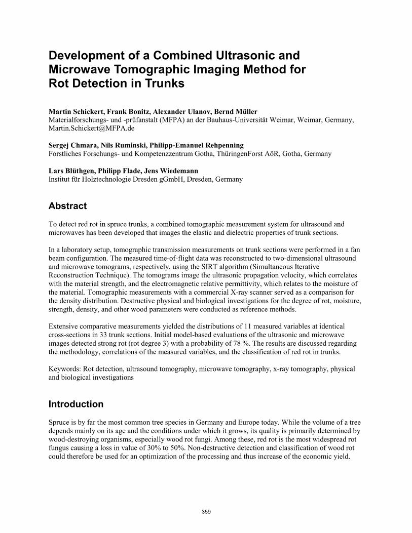
Development of a Combined Ultrasonic and Microwave Tomographic Imaging Method for Rot Detection in Trunks

Martin Schickert, Frank Bonitz, Alexander Ulanov, Bernd Müller Materialforschungs- und -prüfanstalt (MFPA) an der Bauhaus-Universität Weimar, Weimar, Germany, Martin.Schickert@MFPA.de

Sergej Chmara, Nils Ruminski, Philipp-Emanuel Rehpenning Forstliches Forschungs- und Kompetenzzentrum Gotha, ThüringenForst AöR, Gotha, Germany

Lars Blüthgen, Philipp Flade, Jens Wiedemann Institut für Holztechnologie Dresden gGmbH, Dresden, Germany

Abstract

To detect red rot in spruce trunks, a combined tomographic measurement system for ultrasound and microwaves has been developed that images the elastic and dielectric properties of trunk sections.

In a laboratory setup, tomographic transmission measurements on trunk sections were performed in a fan beam configuration. The measured time-of-flight data was reconstructed to two-dimensional ultrasound and microwave tomograms, respectively, using the SIRT algorithm (Simultaneous Iterative Reconstruction Technique). The tomograms image the ultrasonic propagation velocity, which correlates with the material strength, and the electromagnetic relative permittivity, which relates to the moisture of the material. Tomographic measurements with a commercial X-ray scanner served as a comparison for the density distribution. Destructive physical and biological investigations for the degree of rot, moisture, strength, density, and other wood parameters were conducted as reference methods.

Extensive comparative measurements yielded the distributions of 11 measured variables at identical cross-sections in 33 trunk sections. Initial model-based evaluations of the ultrasonic and microwave images detected strong rot (rot degree 3) with a probability of 78 %. The results are discussed regarding the methodology, correlations of the measured variables, and the classification of red rot in trunks.

Keywords: Rot detection, ultrasound tomography, microwave tomography, x-ray tomography, physical and biological investigations

Introduction

Spruce is by far the most common tree species in Germany and Europe today. While the volume of a tree depends mainly on its age and the conditions under which it grows, its quality is primarily determined by wood-destroying organisms, especially wood rot fungi. Among these, red rot is the most widespread rot fungus causing a loss in value of 30% to 50%. Non-destructive detection and classification of wood rot could therefore be used for an optimization of the processing and thus increase of the economic yield.

359

Non-destructive methods for the investigation of wood have been researched for years. An overview of available methods is given by Bucur 2003 and Brashaw et al. 2009. While most methods provide information about local or integral wood properties, tomographic methods (Kak 1988) can generate spatially resolved images of specific properties of trunk wood sections. A well-developed example is the commercial X-ray computer tomography (CT) system for the imaging of complete logs (MiCROTEC 2019). This imaging system can generate three-dimensional density images of the log, which can be used to optimize the sawing process. But especially the investigation of wood rot, which is caused by fungal attack, is not necessarily accompanied by density changes and therefore requires a sensitivity for other wood parameters and the use of other wave types.

Elastic ultrasonic waves were used in a number of investigations. Tomographic measurements and reconstructions in transmission were performed by Sambuelli et al. 2003. Brancheriau et al. 2011 showed an automated laboratory setup integrating tomographic backprojection. Turpening et al. 2011 reconstructed the longitudinal pulse velocity taking curved propagation paths into account. Wang et al. 2011 implemented the tomographic ART algorithm (Algebraic Reconstruction Technique) and applied it to several planes in logs, from which they calculated a three-dimensional image.

Electromagnetic microwaves have been used much less frequently. Sambuelli et al. 2003 carried out radar measurements in a reflection arrangement. Their results as well as those of Nicolotti et al. 2003 showed the possibility to distinguish healthy and damaged wood qualitatively by radar measurements. Butnor et al. 2009 suggested the applicability of radar measurements for determining the quality of wood, but also emphasize the influence of cross sensitivities which have to be eliminated by calibration.

In this paper, image information from transmission tomograms of elastic ultrasonic waves (ultrasound) and electromagnetic microwaves are combined. The aim is to evaluate the quality of spruce trunks with regard to damage caused by red rot. X-ray tomograms as well as wood-physical and wood-biological results serve as reference measurements. The combination of ultrasound and microwaves seems promising, as both have different sensitivities which are expected to complement each other. Ultrasonic waves are elastic waves whose propagation speed is mainly influenced by the elastic properties of the wood and thus react to the wood strength. Microwaves are electromagnetic waves whose propagation speed depend mainly on the permittivity and thus, due to the high relative permittivity of water, on the moisture content of the wood.

Wood Rot and Rot Grade

In forestry, Rotfäule (“red rot”) refers to discoloration and damage to the heartwood of low-resin coniferous species such as spruce (Picea abies) and fir, caused by various species of fungi. By far the most economically important is the fungus Heterobasidion annosum (Bohn 2009). Trees are often infected via the root. In spruce, the mycelium penetrates into the trunk after infection. It then grows mainly in a vertical direction and can cover more than 30 cm per year in the heartwood, while its radial spread is relatively slow (Schmidt-Vogt 1986). The sapwood is attacked much later.

The degree of decay is visually determined on the basis of a cross-section of the trunk that is evaluated according to a scheme based on the RVR (Framework Agreement for the Raw Timber Trade in Germany) forestry grading rules. The extent of wood damage is described by the “rot grade” scale (Fäulegrad, FG), ranging from FG 0 (healthy) over FG 1 (discolored) and FG 2 (mechanical impairment) to FG 3 (rotten). Figure 1 shows typical characteristics of the different rot grades. In addition, a wood-biological characterization was carried out during the work. The classification of rot grades was justified macroscopically and microscopically by wood-biological investigations, and the existing fungi were identified by molecular biological analysis.

360

Figure 1—Cross sections of spruce trunks with rot grades FG 0, FG 1, FG 2, and FG 3 (from left to right)

Measurement Setup

Ultrasound and Microwave Tomography

A vertical test stand with axial fixing of the trunk sections and two swivel arms for the transmission and reception sensors (Figure 2, left) was designed for the tomographic measurements of both methods (Schickert and Bonitz 2016). For measurement, the trunks are fitted with adapters at their ends and inserted into the measuring mechanism. The antennas are attached to the arms so that they can be moved radially. The geometry of the positions of the transmitter and receiver sensor is captured in a cylindrical ρ-ϕ-z coordinate system by mechanical height adjustment, mechanical angle adjustment with a scale in 2° steps and by a laser-optical, radial distance measurement. The data acquisition takes place as a manual scanning process with one transmitter and one receiver sensor each.

During the measurements, first the microware measurements are recorded with a UWB (Ultra Wide Band) M sequence measuring system from Meodat, Ilmenau, Germany, and antennas in the frequency range 1.2 to 2.5 GHz developed in-house. Coupling is done either via an air gap with all antenna positions positioned on a circle, or via direct coupling to the stem surface (Figure 2, top right). The ultrasonic measurements are carried out at the same measuring points as the microwave measurements. The ultrasonic transducers with a nominal frequency of 75 kHz are coupled to the wood via coupling nails (Figure 2, bottom right); a low-frequency ultrasonic instrument from Ing.-Büro Dr. Hillger, Braunschweig, Germany, is used as the measuring system. The ultrasonic measurements were carried out outside the test stand after completion of the geometry measurement, so that two logs can be measured in parallel with both procedures.

All tomographic measurements were carried out in transmission in a tomographic fan beam arrangement, in which measurements with several receiver positions are recorded for each transmitter position (Figure 3, left). In preliminary experiments, fan beam arrangements with 9 receiver positions on a 10° grid (±40°) or on a 20° grid (±80°) were investigated, of which the former was finally used.

The microwave and ultrasound measurements were then recorded according to the following scheme: For each transmission position, 9 receiver positions were recorded in 10° steps from -40° to +40°. The entire array was then rotated in 10° increments and the next fan beam arrangements were measured until the entire cross-section was recorded. Using the reciprocity principle of wave propagation, which was also proven by test measurements, each signal path was recorded in only one direction, so that the number of measurements was reduced by half. Thus, 162 transmission measurements were carried out per trunk cross-section, requiring approximately 60 minutes for each.

361

Figure 2—Test stand for ultrasound and microwave tomography (left), cantilever holding a microwave antenna (top right) and ultrasonic transducer with coupling pins (bottom right).

The 162 measurements with the selected 10° grid lead to the cross-sectional coverage shown in Figure 3, right. The core area of the trunks, in which rot infection is mainly expected, is finely resolved. A reduced resolution is to be expected closer to the surface of the trunk.

For the evaluation of the ultrasonic and microwave measurements, self-developed picking techniques for the time-of-flight determination were used. The tomographic reconstructions were calculated with the commercial program ReflexW in a 2 mm x 2 mm grid. The program uses the SIRT algorithm (Simultaneous Interative Reconstruction Technique) for tomographic image reconstruction.

Figure 3—Principle measurement layout of the transmission measurements in a fan beam arrangement (left) and coverage of the trunk cross-section with signal paths (right).

362

X-ray Tomography

Comparative measurements using X-ray computed tomography (X-ray CT) were carried out by the Forstliche Versuchs- und Forschungsanstalt Baden-Württemberg (FVA) in Freiburg, Germany. The CT LOG computer tomograph from Microtec, Brixen, Italy, used for the investigations was specially designed for measurements on wood. The trunk section is scanned spirally, and the measured values are reconstructed to a three-dimensional image of the trunk which is saved as cross-sectional images with a pixel size of 1.107 mm x 1.107 mm. The trunk sections were scanned with a tube voltage of 180 kV and 5 mm/sec feed at 60 revolutions per minute.

The evaluation of the X-ray CT results shows possibilities for qualitative red rot detection based on the density distribution. Especially rot grades FG 2 and 3 differ from undamaged strains. The images also served as a density reference for the interpretation of ultrasound and microwave tomograms.

Comparative Measurements

With these methods, extensive investigations were carried out on spruce logs with different growth conditions. Trunk sections with a length of 80 cm and diameters from about 20 to 30 cm were used as test specimens. In addition to the preliminary and partial tests on 48 trunk sections, in the main investigations a total of 33 trunk sections were examined with all methods in three measurement campaigns. On each trunk section, 11 variables were determined on a measuring grid in a common cross-sectional area. In addition to the imaging methods ultrasonic tomography (pulse velocity), microwave tomography (relative permittivity) and X-ray CT (density value, sapwood/heartwood discrimination), wood-physical quantities (bulk density, moisture content, compressive strength, nail impression force, middle annual ring width) and wood-biological quantities (rot grade, sapwood/heartwood discrimination) were determined. The wood physical and wood biological parameters were measured destructively on samples with a cross-section of 20 mm by 20 mm taken from a predefined sample grid on the trunk cross-section. For comparison, the image values of the tomograms of the three non-destructive imaging methods were averaged over the sample cross-sections.

Figure 4 shows exemplary computer tomographies of the ultrasound, microwave, and X-ray methods, respectively; they are also shown in simplified form in Figure 5. In all tomograms the sample grid is drawn, in the ultrasound and microwave tomograms the trunk contour and the measuring positions are additionally depicted. The imaging area of the ultrasonic tomograms is smaller than the trunk cross-section since the transmission and reception points are located at the tips of the coupling pins.

Figure 4—Sample tomograms of the methods ultrasound (left), microwaves (center), and X-ray (right).

363

In all ultrasound tomograms, the colour scale covers a pulse speed range from 600 (red) to 2000 m/s (blue). The imaging range of the microwave tomograms extends to the trunk surface when directly coupled to the trunk (Figure 6) and stretches beyond the trunk surface when coupled via an air gap (Figure 4, Figure 5). The colour scale of all microwave tomograms shows a relative permittivity range from 6 (red) to 33 (blue). The X-ray tomogram is shown here as a false-colour image; the sample number and the mean value of the X-ray grey value are also included in the sample grid.

Figure 5 shows results of the four methods ultrasound CT, microwave CT, X-ray CT, and visual representation for a representative trunk of rot grade FG 0. The sapwood/heartwood distribution is clearly visible from the visual representation and the X-ray CT, and it is also imaged in the microwave and ultrasound tomograms. At the three o'clock position, a marking notch was sawn. At this position the trunk section is more dried out. The notch is clearly visible in the X-ray and the ultrasound tomograms. Additionally, the ultrasound tomogram exhibits reduced pulse speeds at 12 o'clock and between 7 and 9 o'clock. When comparing with the visual representation, it becomes clear that the bark was missing in these areas, which in turn led to drying out. The microwave tomogram was recorded in a non-contact measurement with the red line showing the trunk contour. In the outer areas, the tomogram smears due to the lower resolution. The dried-out areas are also visible, whereby the 12 o'clock position shows only a slight gradient.

Figure 5—Image comparison of rot grade FG 0: ultrasound (top left), microwaves (top right), X-ray (bottom left), and visual (bottom right).

A partially differing result from the expected tomograms of rot grade FG 3 is shown in Figure 6. Both the microwave and the ultrasound tomogram show clear deviations from the normal sapwood/heartwood distribution. A lower pulse velocity in the core with expansion towards the 2 o'clock position indicates rot grade FG 3. The microwave tomogram shows very dry areas as well as the sapwood/heartwood distribution. Looking at the X-ray tomogram and the visual image, it becomes clear that the trunk section deviates strongly from a homogeneous sapwood/heartwood distribution. The drier heartwood extends far

364

outwards at the 7 o'clock position, which is reflected in the microwave tomogram. The decay infestation is far advanced, so that in the heartwood an almost homogeneously decayed area exists, the extension of which in the direction of the 2 o'clock position can be found in the ultrasound tomogram.

Figure 6—Image comparison of rot grade FG 3: ultrasound (top left), microwaves (top right), X-ray (bottom left), and visual (bottom right).

Correlation and Classification

After completion of the comparison measurements, 1060 data sets were available for evaluation. One objective of the evaluation was to find correlations between the variables, one other to enable rot detection on the basis of ultrasound and microwave tomography or other measured quantities.

Correlative Relationships of Wood Physical Quantities

In view of the fluctuation of material parameters in wood with different growth conditions, the physical parameters determined during the project showed considerable variation within a given cross-section and between different trunk sections. As a result, it was generally not possible or reasonable to specify single rot grade values. Instead, general correlations between the recorded physical quantities are presented.

Correlations of the compressive strength, the bulk density, or the nail impression force with the rot grade turned out to be relatively weak due to the fluctuations immanent to the wood.

Stronger interrelations were found in the correlations between some of the physical quantities. The correlative relationship between compressive strength and bulk density is strong (Figure 7, left). If one colors the data points according to the rot grade, rot grade FG 3 scatters almost completely below the fitted straight line. The same applies to the correlation between bulk density and annual ring width, where

365

rot grade FG 3 also mainly scatters below the fitted straight line (Figure 7, right). Both the compressive strength and the bulk density show a tendency to increase as the distance from the pith increases.

Figure 7—Correlation of compressive strength and bulk density (left), correlation of bulk density and annual ring width (right).

The wood moisture content varies strongly across the trunk cross-section (Figure 8, left). With up to 200 %, the sapwood was always clearly more humid than the heartwood. In areas where the bark had detached, the sapwood moisture was lower than in other areas. At the transition between sapwood and heartwood an abrupt change in wood moisture occurred. In the trunk center close to the pith, the wood moisture was usually between about 30 and 50 % for healthy and also for only slightly rotten wood (rot grades FG 1 or FG 2). Higher values of the wood moisture in the immediate center of a trunk cross-section (up to 80 %) are almost exclusively associated with a high rot grade.

Figure 8—Correlation of wood moisture and pith distance (left), correlation of D-R-N value and maximum measured heartwood moisture (right, numbers indicate trunk ID).

Figure 8, right, shows an evaluation approach at trunk level which is based on the consideration that with advanced rot infestation larger differences in the measured values within a trunk are to be expected. For this purpose, the quotients of maximum and minimum values measured for compressive strength, bulk density and nail impression force were calculated for each trunk cross-section. If the product of these quotients (D-R-N value) is plotted against the maximum measured heartwood moisture, it is noticeable that for the tested logs the lowest and highest rot grades can be completely separated.

366

Rot Grade classification

For the detection and classification of rot on the basis of ultrasound and microwave tomography, several approaches were tested based on the correlation of pulse velocity and/or permittivity with the rot grade or on a classification of these variables. A model-based approach for the classification of pulse velocity or permittivity to the rot grade was pursued by adapting the parameters of a two-dimensional Gaussian distribution to the respective sapwood and heartwood areas of the tomograms. If this approach is combined with the integral correlation of the ultrasonic sound velocity to the rot grade, rot grade FG 3 can be correctly identified at a rate of 78 % with a false detection rate of 3 % using only ultrasound tomography. Further improvements are to be expected if the permittivity from microwave tomograms is included in the evaluation.

Conclusions

This paper presents a non-destructive evaluation of spruce trunk wood using a combination of transmission tomographic ultrasound and microwave imaging systems. The method was demonstrated on a single-channel measuring set-up, and comparative measurements with 11 measured variables on identical cross-sectional planes in 33 trunk sections were described. Initial evaluation comprised correlations between the measured variables and approaches for rot detection and rot grade classification. The combination of the primary sensitivities of ultrasound and microwave tomograms for wood strength and wood moisture seems promising.

Future work will further investigate correlations between the measured variables and will introduce formal classification methods, building on the solid set of acquired non-destructive and destructive data. The effect of anisotropic elastic and electromagnetic wave propagation, which was investigated in the work but not presented here, will further be evaluated.

One concrete goal will be the demonstration of an automated, combined multi-channel ultrasonic/microwave tomography system suitable for mobile harvester use. Parallel, electronically switched ultrasonic and microwave hardware and adapted software is expected to limit the measurement and evaluation time to a few seconds, which would enable rapid measurement of the rot extend.

Acknowledgments

This work was carried out as part of the AiF/IGF project 18241 BR. The authors would like to thank for this support. The companies Ing.-Büro Dr. Hillger, Braunschweig, Germany, and Meodat, Ilmenau, Germany, as well as the Forstliche Versuchs- und Forschungsanstalt Baden-Württemberg (FVA), Freiburg, Germany, supported the work by lending equipment and consulting.

References

Bohn, C. 2009. Verwendung von biotechnologisch durch den Rotfäulepilz Heterobasidion annosum in vivo degradiertem Fichtenholz als Rohstoff für die Herstellung von Holzwerkstoffen. Universität Göttingen, dissertation (in German).

Brancheriau, L.; Gallet, Ph.; Lasaygues, Ph. 2011. Ultrasonic Imaging of Defects in Standing Trees. In: 17th International Nondestructive Testing and Evaluation of Wood Symposium, Sopron, Hungary, 14.–16.9.2011. Sopron, Hungary: University of West Hungary.

367

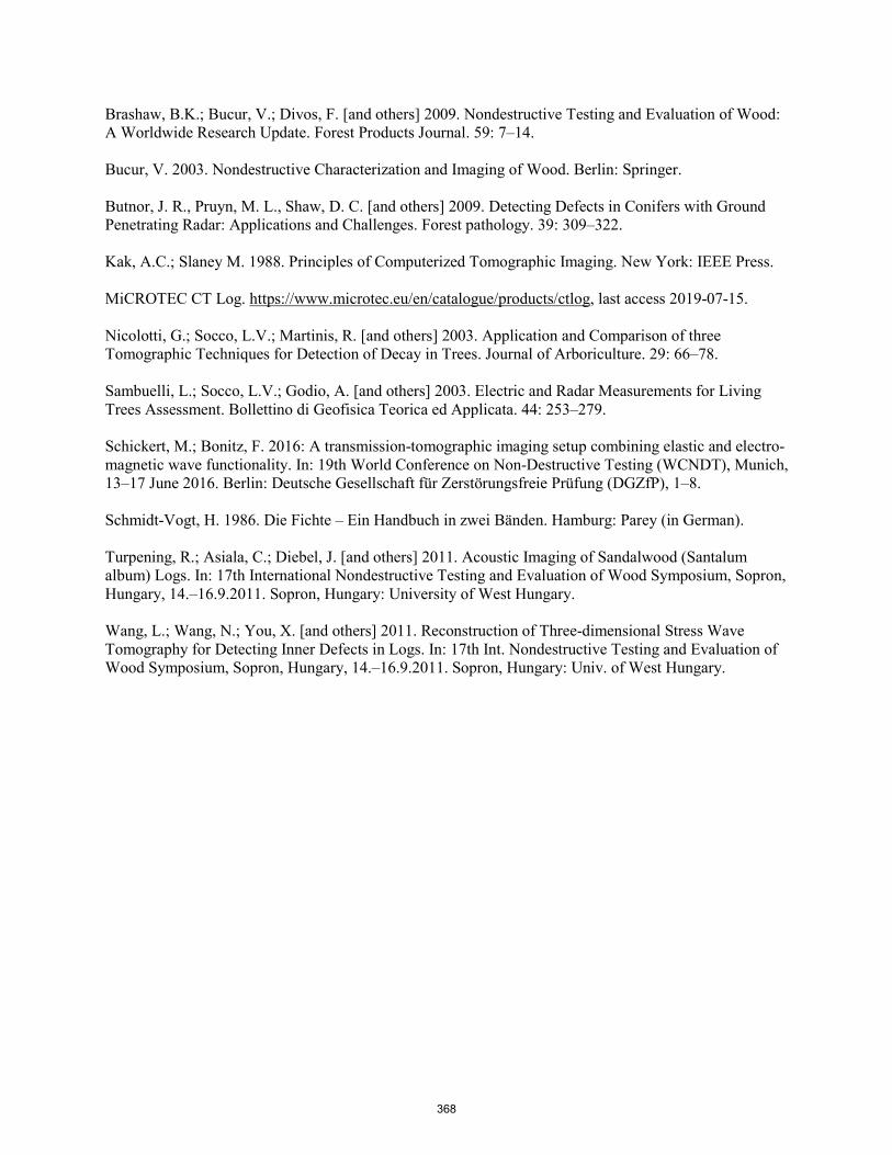
Brashaw, B.K.; Bucur, V.; Divos, F. [and others] 2009. Nondestructive Testing and Evaluation of Wood: A Worldwide Research Update. Forest Products Journal. 59: 7–14.

Bucur, V. 2003. Nondestructive Characterization and Imaging of Wood. Berlin: Springer.

Butnor, J. R., Pruyn, M. L., Shaw, D. C. [and others] 2009. Detecting Defects in Conifers with Ground Penetrating Radar: Applications and Challenges. Forest pathology. 39: 309–322.

Kak, A.C.; Slaney M. 1988. Principles of Computerized Tomographic Imaging. New York: IEEE Press.

MiCROTEC CT Log. https://www.microtec.eu/en/catalogue/products/ctlog, last access 2019-07-15.

Nicolotti, G.; Socco, L.V.; Martinis, R. [and others] 2003. Application and Comparison of three Tomographic Techniques for Detection of Decay in Trees. Journal of Arboriculture. 29: 66–78.

Sambuelli, L.; Socco, L.V.; Godio, A. [and others] 2003. Electric and Radar Measurements for Living Trees Assessment. Bollettino di Geofisica Teorica ed Applicata. 44: 253–279.

Schickert, M.; Bonitz, F. 2016: A transmission-tomographic imaging setup combining elastic and electro-magnetic wave functionality. In: 19th World Conference on Non-Destructive Testing (WCNDT), Munich, 13–17 June 2016. Berlin: Deutsche Gesellschaft für Zerstörungsfreie Prüfung (DGZfP), 1–8.

Schmidt-Vogt, H. 1986. Die Fichte – Ein Handbuch in zwei Bänden. Hamburg: Parey (in German).

Turpening, R.; Asiala, C.; Diebel, J. [and others] 2011. Acoustic Imaging of Sandalwood (Santalum album) Logs. In: 17th International Nondestructive Testing and Evaluation of Wood Symposium, Sopron, Hungary, 14.–16.9.2011. Sopron, Hungary: University of West Hungary.

Wang, L.; Wang, N.; You, X. [and others] 2011. Reconstruction of Three-dimensional Stress Wave Tomography for Detecting Inner Defects in Logs. In: 17th Int. Nondestructive Testing and Evaluation of Wood Symposium, Sopron, Hungary, 14.–16.9.2011. Sopron, Hungary: Univ. of West Hungary.

368

Case Study of Honey Fungus (Armillaria Mellea) Attack on Norway Spruce (Picea abies)

Ferenc Divos PhD School, University of Sopron, Sopron, Hungary, ferenc.divos@gmail.com

Agnes Kinga Buza Fakopp Enterprise Bt., Sopron, Hungary, agnes.kinga.buza@gmail.com

Mohamad Saadat Nia Faculty of Natural Resources,University of Behbahan, Khuzestan Province, Iran, msaadatnia92@gmail.com

Abstract

The effects of fungi attack variable widely. Honey fungus (Armillaria mellea) is considered to be dangerous infection. While the weakening in stability is obvious defence against the attack can be observed as well. Since 2013 an infected Norway spruce (Picea abies) have been measured repeatedly during the years. Acoustic tomograms were recorded at 30 cm, 100 cm and 170 cm heights. The spread of the fungi attack can be followed in the images. Compartmentalization can also be observed. The decayed area seems to be limited on the lower levels, while the fungi is spreading successfully along the trunk. Pulling tests were also implemented showing the root system’s capability to defend itself. Safety was estimated as well. Safety decreased more in higher levels.

Keywords: acoustic tomography, honey fungus, pulling test, safety, fungi attack

Introduction

A six-year measurement is presented while several methods were used; acoustic tomography, pulling test and electric impedance tomography. This period gives us a glace about trees defending themselves against fungi attacks on a longer time scale. The safety of the tree was in the focus as it is one of the most important aspects regarding trees in urban areas.

The fungi involved in the infection is a honey fungus, Armillaria mellea. Honey fungi are well-spread almost around the whole world, and common infectors of trees, forests and other plants. (Cruickshank et al. 2011) Usually these fungi attack via the root system, damaging it and spreading upward into and along the trunk. As Honey fungus usually, Armillaria mellea is a “white rot” fungi degrading lignin while bleaching the wood material (Pointing 2001). Lost of load holding capacity can be another effect of fungi attack however buttress or widened base can appear as well.

Many researches on fungi infections were performed in laboratories, on testing field (Bieker et al. 2009, Cruickshank et al. 2011) and not in real life situation. Thus, the concept about the topic may be well-completed by the measurements done on an occasionally (naturally) infected tree.

369

The previous results were published already in the first year as comparison of the attacked and a healthy spruce and after the first 3 years of the measurement. (Buza and Goncz 2015, Buza and Divos 2016)

Materials and Methods

The examined tree

The research started with a 92 years old Norway spruce (Picea abies) in 2013. The location is in the Botanical Garden of the University of Sopron on a side of a walking path. The honey fungus (Armillaria mellea s.l.) fruiting bodies, as the consequence of the infection, were noticed on the tree. The height of the tree was 20.0 m in 2013 while the crown area was 30.4 m2, the height of the crown centre was at 12.7 m at the same year. The trunk has 1° incline. At 2019 the tree was 21.4 m tall and the crown centre was at 15.2 m while the crown area was almost the same 31.2 m2.

Acoustic tomography

The velocity of sound waves in the wood of trees is a condition due to the specie, anatomical orientation, temperature and moisture content below fibre saturation point. Acoustic waves have to go “around” the decay or the damaged area in the wood material. Thus, the observed velocity decreases. Therefore, acoustic sound velocity, or time-of-flight (tof) measurements can be well-used to decide if the measured wood is decayed or not. (Of course, the technique has its limitations, usually 3 cm in diameter is the smallest decay which can be found this way.)

If measurements are performed not along only one line (between two sensors) but on several lines a tomogram can be calculated from the data. Fig 1.

Figure 1— a) Time-of-flight (TOF) measurement on a healthy trunk. b) TOF measurement on a decayed trunk. c) The schematic image of a tomography with 8 sensors with the measuring paths. d) Tomography on a decayed trunk. The travelling paths become longer. Tomogram and decay canbe evaluated.

Acoustic tomograms are in good correlation with the real conditions of trunks as it was proved several times. (Feng et al., 2014; Li et al., 2014; Ostrovsky et al. 2017)

In our study ArborSonic 3D acoustic tomogram with the ArborSonic software were used.

Pulling Test

For testing the root system’s stability tomographies are not suitable tools. The pulling test is a method simulating the wind load via a pull of a cable. The technique is used for evaluation of safety of the root system, to investigate the root-soil system, but it is also used for evaluations of stem conditions and as calibrations and comparison for other tests and techniques. (Wessolly 1991; Peltola et al. 2000)

370

The examined tree should be pulled at as close to the crown center as it is possible, while the other end of the cable should be fixed to an anchorage point (another tree, building, truck, etc.). A winch and a force-meter are placed on the cable while inclinometer(s) are placed onto the root collar, as close to ground as it is possible. The anchorage should bear the force (Peltola et al., 2000). It is seen in Fig 2.

Figure 2— Pulling test setup

(Using elastometers put onto the trunk the trunk’s conditions can be examined as well during pulling test.) Pulling test is non-destructive if the pull stops when the inclination (at ground level) reaches 0.2°.

The applied system was an inclino-type pulling test (measuring inclinations and force) developed by the Fakopp Company. Sampling rate was 1Hz both for inclination and for force. Software for measurement and evaluation were PullingCollect and PullingView. Safety evaluations based on the work of Brudi and Wassenaer (2002) were included in the program.

Electric impedance tomography

Electric impedance tomography is a technique to get electric resistivity tomograms about a layer of a trunk. This tomogram refers to electric conditions, presence of ions. The shape appearing on the tomograms of healthy trees depend on species (, on the number of used electrodes, and the so-called electrode distance as well). If you keep the setup and setting the same, difference between healthy and not-healthy (probably fungi attacked) can be seen on tomogram. As change in ionic concentrates or electric field are not only due to fungi attack, seasonal changes in resistivity and even hourly changes can be observed. (Fakopp 2019)

In our measurements ArborElectro hardware and software was used.

Results

Acoustic tomograms

Acoustic measurements were done since 2013. The tomograms were recorded layer at 30 cm, 100 cm and 170 cm heights.

As the tree grew, also the circumferences in the layers grew 5-12 cm. The Safety Factors calculated for the layers were 5.86 (30 cm), 3.92 (100 cm) and 4.88 (170 cm) at 2013.

As the number of sensors used during the measurement may have an effect on the detection of the decay’s shape and size this data is also represented in Table 1.

371

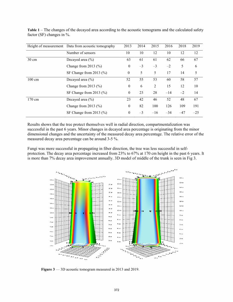
Table 1 – The changes of the decayed area according to the acoustic tomograms and the calculated safety factor (SF) changes in %.

Height of measurement Data from acoustic tomography 2013 2014 2015 2016 2018 2019

Number of sensors 10 10 12 10 12 12

30 cm Decayed area (%) 63 61 61 62 66 67

Change from 2013 (%) 0 –3 –3 –2 5 6

SF Change from 2013 (%) 0 5 5 17 14 5

100 cm Decayed area (%) 52 55 53 60 58 57

Change from 2013 (%) 0 6 2 15 12 10

SF Change from 2013 (%) 0 23 28 –14 –2 14

170 cm Decayed area (%) 23 42 46 52 48 67

Change from 2013 (%) 0 82 100 126 109 191

SF Change from 2013 (%) 0 –3 –16 –34 –47 –25

Results shows that the tree protect themselves well in radial direction, compartmentalization was successful in the past 6 years. Minor changes in decayed area percentage is originating from the minor dimensional changes and the uncertainty of the measured decay area percentage. The relative error of the measured decay area percentage can be around 3-5 %.

Fungi was more successful in propagating in fiber direction, the tree was less successful in self-protection. The decay area percentage increased from 23% to 67% at 170 cm height in the past 6 years. It is more than 7% decay area improvement annually. 3D model of middle of the trunk is seen in Fig 3.

Figure 3 — 3D acoustic tomogram measured in 2013 and 2019.

372

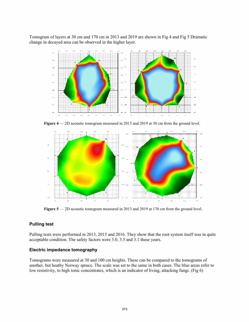
Tomogram of layers at 30 cm and 170 cm in 2013 and 2019 are shown in Fig 4 and Fig 5 Dramatic change in decayed area can be observed in the higher layer.

Figure 4 — 2D acoustic tomogram measured in 2013 and 2019 at 30 cm from the ground level.

Figure 5 — 2D acoustic tomogram measured in 2013 and 2019 at 170 cm from the ground level.

Pulling test

Pulling tests were performed in 2013, 2015 and 2016. They show that the root system itself was in quite acceptable condition. The safety factors were 3.0, 3.5 and 3.1 these years.

Electric impedance tomography

Tomograms were measured at 30 and 100 cm heights. These can be compared to the tomograms of another, but heathy Norway spruce. The scale was set to the same in both cases. The blue areas refer to low resistivity, to high ionic concentrates, which is an indicator of living, attacking fungi. (Fig 6)

373

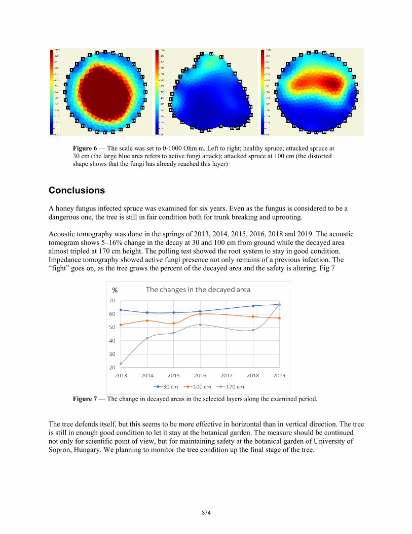
Figure 6 — The scale was set to 0-1000 Ohm m. Left to right; healthy spruce; attacked spruce at 30 cm (the large blue area refers to active fungi attack); attacked spruce at 100 cm (the distorted shape shows that the fungi has already reached this layer)

Conclusions

A honey fungus infected spruce was examined for six years. Even as the fungus is considered to be a dangerous one, the tree is still in fair condition both for trunk breaking and uprooting.

Acoustic tomography was done in the springs of 2013, 2014, 2015, 2016, 2018 and 2019. The acoustic tomogram shows 5–16% change in the decay at 30 and 100 cm from ground while the decayed area almost tripled at 170 cm height. The pulling test showed the root system to stay in good condition. Impedance tomography showed active fungi presence not only remains of a previous infection. The “fight” goes on, as the tree grows the percent of the decayed area and the safety is altering. Fig 7

Figure 7 — The change in decayed areas in the selected layers along the examined period.

The tree defends itself, but this seems to be more effective in horizontal than in vertical direction. The tree is still in enough good condition to let it stay at the botanical garden. The measure should be continued not only for scientific point of view, but for maintaining safety at the botanical garden of University of Sopron, Hungary. We planning to monitor the tree condition up the final stage of the tree.

%

374

Acknowledgments

The first 4 years of the research was done within a PhD research while the last two years was done within the framework of the development and testing for Fakopp Enterprise.

References

Bieker, D.; Kehr, R.; Weber, G.; Rust, S. 2009. Non-destructive monitoring of early stages of white rot by Trametes versicolor in Fraxinus excelsior. Annals of Forest Science. 67(210):1-7.

Brudi, E.; Van Wassenaer, P.J. 2002. Trees and statics: nondestructive failure analysis. In: Tree structure and mechanics conference proceedings: how trees stand up and fall down. Savannah, Georgia, U.S., October 2001. Champaign, Illinois, USA: International Society of Arboriculture, 53-70.

Buza, A.K.; Divos F. 2016. Spruce tree fighting back – study of honey fungus infection. Folia Oecologica. 43(2): 204-207.

Buza, A.K.; Goncz B. 2015. Comparison of trees and NDT methods. Wood Research 60(1):45-58.

Cruickshank, M.G.; Morrison, D.J.; Lalumiere, A. 2011. Site, plot, and individual tree yield reduction of interior Douglas-fir associated with non-lethal infection by Armillaria root disease in southern British Columbia. Forest Ecology and Management, 261: 297– 307.

Fakopp Enterprise, Manual for ArborElectro 2019, http://fakopp.com/docs/products/arborelectro/ArborElectroManual_ver1.0.6.pdf [Date accessed: 05. 06. 2019]

Feng, H.; Li G.; Fu, S.; Wang, X. 2014. Tomographic image reconstruction using an interpolation method for tree decay detection. BioResources 9(2): 3248-3263.

Li, G.; Wang, X.; Feng, H.; Wiedenbeck, J.; Ross, R.J. 2014. Analysis of wave velocity patterns in black cherry trees and its effect on internal decay detection. Computers and Electronics in Agriculture 104: 32–39.

Ostrovsky, R.; Kobza, M.; Gazo, J. 2017. Extensively damaged trees tested with acoustic tomography considering tree stability in urban greenery. Trees. 31:1015.

Peltola, H.; Kellomaki, S.; Hassinen, A.; Granander, M. 2000. Mechanical stability of Scots pine, Norway spruce and birch: an analysis of tree-pulling experiments in Finland. Forest Ecology and Management 135: 143-153.

Pointing, S. 2001. Feasibility of bioremediation by white-rot fungi. Applied Microbiology and Biotechnology. 57(1-2): 20-33.

Wessolly, L. 1991. Verfahren zur Bestimmung der Stand- und Bruchsicherheit von Baumen. Holz als Roh- und Werkstoff 49: 99-104.

375

“Time-lapse” Case Study of Impedance Tomography on Beech

Agnes Kinga Buza Fakopp Enterprise Bt., Sopron, Hungary, agnes.kinga.buza@gmail.com

Ferenc Divos PhD School, University of Sopron, Sopron, Hungary, ferenc.divos@gmail.com

Abstract

Impedance tomography can show the differences in ionic concentrates via the different electric conditions. As resistivity is measured and a resistivity tomogram is calculated low and high resistant areas can be distinguished. Impedance tomography is a tool to find active fungi attacks (as it changes the ionic distribution). Different tree species show different typical tomograms. So even when looking for fungi it is important to know the healthy, the non-attacked situation. Not only the presence of fungi changes the measured resistivities. For example, dead knots, wound reactions and even the life of the tree changes the tomogram. A beech tree was measured since March of 2018 to follow the seasonal changes of the resistivity tomogram. The resistivity values changed while the typical look of the tomogram stayed the same during the months.

Keywords: impedance tomography, beech, seasonal change, electric resistivity

Introduction

What is the benefit of electric impedance tomography? Why did we use it instead of the well-known acoustic devices? Time-of-flight measurements and acoustic tomography are great tools to find damaged wood, decays or hollows in trees (Feng et al., 2014; Li et al., 2014; Ostrovsky et al. 2017). Electric impedance tomograms require more training and experience while the results are… Well, can be more interesting.

Changes in the electric resistivity tomograms refers to changes in the electric field, in the electric situation. This can happen according to the damages in cell walls (Martin and Günther 2013) or change in the ionic concentrates, presence of water, etc. Fungi both damages the cell walls and changes the concentrates of ions and water. Although catching a fungi attack seems to be obvious by impedance tomography. Finding active fungi attack is possible while in the other hand similar changes may happen caused by seasonal, daily or other changes as well… In our case a trial of visualizing the seasonal and hourly changes was performed by electric impedance tomography.

Materials and methods

The examined tree

The measurements were done on a healthy beech tree (Fagus sylvatica) which is about 100 years old. The circumference of the trunk at 130 cm is 276 cm. The location is in the Botanical Garden of the University

376

of Sopron on a side of a walking path. The tree is in great conditions, no fungi infection or serious damage could be noticed during the measuring period.

Electric impedance tomography

Electric impedance tomography is a technique to get electric resistivity tomograms about a layer of a trunk. This tomogram refers to electric conditions, presence of ions. The wood itself is not a homogenous material. As the inhomogeneity depends on the specie, the shape appearing on the tomograms of healthy trees depends on species as well. (The resulting image depends on the number of used electrodes and the so-called electrode distance as well). If you keep the setup and software settings the same, difference between healthy and not-healthy (probably fungi attacked) can be seen on tomogram. As change in ionic concentrates or electric field are not only due to fungi attack, seasonal changes in resistivity and even hourly changes can be observed. (Fungi attack more likely to change the shapes of the appearing tomogram, while seasonal and daily changes were noticeable in the change of values.)

The measurement started at March 2018. The hourly measurements were performed on 23 and 24 May 2019. In our measurements we used ArborElectro hardware and software. All the measurements were done with 32 electordes, with electrode distance 8, while the geometry and the resolution of the iteration was the same for the evaluations. (Fakopp 2019)

Temperature measurement

The temperature dependence of the electric resistivity was checked as well. Daily average air temperature was measured. Temperature 1 cm under the bark was measured during the hourly measurement series.

Results

In general, we can say that the tomograms are well-repeatable, measurements done right after each other shows about 1.3% difference in values.

For the measurements done during for more than a year, five areas, based on the “dumbbell shape” on the image, were chosen on the tomograms, averages of them were calculated. (Fig 1.) Global maximum and minimum values were recorded as well. The data are shown in Table 1.

Table 1—Date, temperature and elecric resistivity values in the selected areas Date Temperature (°C) Resistivities (Ω*m)

Area 1 Area 2 Area 3 Area 4 Area 5 Min Max 23/03/2018 2.4 1265.8 1039.9 197.7 150.2 137.1 28.2 1332.4 24/05/2018 21.1 575.7 521.2 92.3 83.2 85.0 82.3 595.3 02/07/2018 16.8 536.7 477.6 92.0 85.2 82.9 82.1 562.2 11/10/2018 16.7 751.0 574.4 113.0 87.5 83.8 72.5 778.7 10/12/2018 6.5 939.3 689.1 167.8 126.8 133.3 125.1 984.8 07/01/2019 -0.2 1245.3 913.9 177.6 123.1 132.4 121.7 1263.6 07/02/2019 1.6 1308.1 948.8 192.4 129.2 144.2 127.2 1350.0 06/03/2019 9.9 817.6 670.7 125.8 104.1 101.0 84.8 844.9 04/04/2019 13.1 620.8 564.3 97.0 85.6 78.3 66.9 647.1 24/04/2019 16.6 648.4 489.2 93.7 86.5 87.5 70.3 667.5 23/05/2019 16.2 615.4 490.1 89.7 88.1 87.0 66.4 626.7 12/06/2019 27.0 579.2 443.6 91.0 80.4 88.7 61.7 602.9

377

Figure 1 — The five chosen areas. The two highest and lowest resistivity areas and one area on a side were examined closer. The same measure with different scales, auto scale on the left. The high resistivity areas can be found easily as they are colored to orange / red. Scale set from 80 to 100 Ω*m on the right side to highlight the less resistive areas.

Figure 2 — The changes in the resistivity in the five chosen areas. Left side – the average values in the first and second areas as a function of time; right side – same with the other areas.

Resistivity tomogram for area selection is seen in Fig 1. While tomograms recorded during the measurement are in Fig 4. The selected areas’ values (Fig 2) and global minimum and maximum data were checked as well. Averages measured from March 2018 to June 2019 were also linked with the temperature. (Fig 3).

378

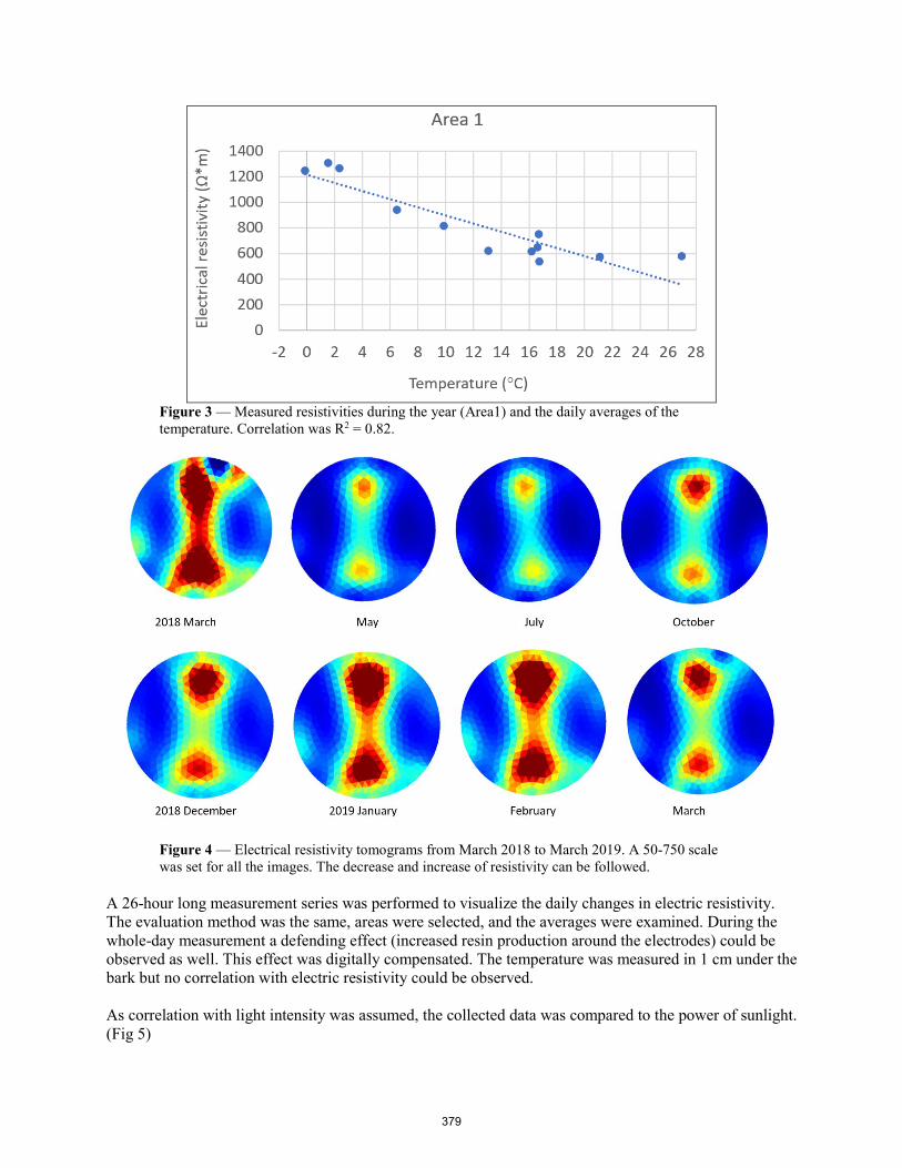
Figure 3 — Measured resistivities during the year (Area1) and the daily averages of the temperature. Correlation was R2 = 0.82.

Figure 4 — Electrical resistivity tomograms from March 2018 to March 2019. A 50-750 scale was set for all the images. The decrease and increase of resistivity can be followed.

A 26-hour long measurement series was performed to visualize the daily changes in electric resistivity. The evaluation method was the same, areas were selected, and the averages were examined. During the whole-day measurement a defending effect (increased resin production around the electrodes) could be observed as well. This effect was digitally compensated. The temperature was measured in 1 cm under the bark but no correlation with electric resistivity could be observed.

As correlation with light intensity was assumed, the collected data was compared to the power of sunlight. (Fig 5)

379

Figure 5 — a) the power of sunlight was measured by solar panels b) negated changes in electric resistivity is performed to help comparison. (A baseline 376 Ω*m was subtracted, and the data mirrored to the y axis.) c) time-adjusted photosynthetic activity (Nemky 1976).

Electric resistivity correlation to sunlight can be observed while the negative peak early in the morning can be noticed both in changes of resistivity and in photosynthetic activity as well.

380

Conclusions

Seasonal and daily changes were recorded successfully. The usability of electric impedance tomography in this area was proved.

Seasonal changes are in correlation with the average of air temperature. Similar effect could not be observed during the hourly test, no correlation with temperature (air or wood, 1 cm under bark) was found.

Seasonal changes show lower resistivity, higher conducting capacity during spring, summer and the beginning of autumn. This can refer to the presence of more free ions, to faster transportations. Period characterized by higher resistivity, less free ions and probably slower transportations starts during fall and lasts till end of freezing.

Daily changes in electric resistivity shows correlation to light intensity while the most resistance observed around 2 am can refer to the change in photosynthetic activation (Nemky 1976). See Fig 5. This phenomenon might be related to monoterpene emission as it also has negative peak early in the morning. (Bourtsoukidis et al. 2014.)

Acknowledgments

The research was done within the framework of the development and testing the ArborElectro impedance tomograph.

References

Bourtsoukidis, E.; Bonn, B.; Noe, S.M. 2014. On-line field measurements of BVOC emissions from Norway spruce (Picea abies) at the hemiboreal SMEAR-Estonia site under autumn conditions. Boreal Environment Research. 9: 153–167

Fakopp Enterprise, Manual for ArborElectro 2019, http://fakopp.com/docs/products/arborelectro/ArborElectroManual_ver1.0.6.pdf [Date accessed: 05. 06. 2019]

Feng, H.; Li G.; Fu, S.; Wang, X. 2014. Tomographic image reconstruction using an interpolation method for tree decay detection. BioResources 9(2): 3248-3263.

Li, G.; Wang, X.; Feng, H.; Wiedenbeck, J.; Ross, R.J. 2014. Analysis of wave velocity patterns in black cherry trees and its effect on internal decay detection. Computers and Electronics in Agriculture 104: 32–39.

Martin, T.; Günther, T. 2013. Complex resistivity tomography (CRT) for fungus detection on standing oak trees. European Journal of Forest Research. 132. 765-776.

Nemky, E. 1976. The effect of light conditions on the development of oak seedling [Hungarian, original title: A fényviszonyok hatása a tölgycsemeték fejlődésére]. Az Erdő 111:6 251-256.

Ostrovsky, R.; Kobza, M.; Gazo, J. 2017. Extensively damaged trees tested with acoustic tomography considering tree stability in urban greenery. Trees. 31:1015.

381

Wind Tipping Curves – Assessing the Anchorage and Wind Load of Urban Trees by Motion Monitoring

Steffen Rust Faculty of Resource Management, University of Applied Science and Art, Göttingen, Germany, steffen.rust@hawk.de

Lothar Göcke lothar.goecke@web.de

Dipl.-Ing. Andreas Detter Brudi & Partner TreeConsult, Gauting, Germany, a.detter@tree-consult.org

Abstract

To date, the anchorage and wind load of urban trees can only be assessed in static load tests. These are complex and expensive, and the reliability of wind load estimates has been questioned. Monitoring the basal inclination of trees in natural winds yields a wind tipping curve, which can be used to inexpensively assess anchorage. Combining this with static load test allows to estimate real wind loads, which can be used to assess the conventionally used wind load estimates. Our analyses show that wind speed data can be taken from weather stations several kilometers away from the tree. The quality of the wind speed-tilt correlation does vary, depending on local conditions and topography.The differences between measured and estimated wind loads were rather modest between 4 % and 31 %. Thus, our results show that dynamic loads in gusts are comparable to the results of a wind load analysis. They cause a maximum reaction that can be reproduced in static load tests.

Keywords: tree risk assessment, anchorage, root plate inclination, wind, static load tests

Introduction In many parts of the world, there is a legal obligation to assess the risk posed by urban and roadside trees (Smiley et al. 2012, Rust 2016). Frequently, failure is initiated by damages to the root system compromising the anchorage of trees. Consequently, there is a need for cost-effective ways to assess the anchorage strength of large numbers of trees.

Wind is the major load on trees and a principal cause of their failure (Metzger 1893, Jacobs 1936, Mergen 1952). The wind load in the crown causes a turning moment at the base of the tree that inclines the stem base. This stem base inclination is a function of the turning moment and the stiffness of the root-soil system (Coutts 1983, Lundström et al. 2007).

The initial stiffness of the root-soil system correlates with the anchorage strength of a tree (Neild and Wood 1999, Jonsson et al. 2006, Detter and Rust 2013). Results from static pulling tests on several European and North American tree species show a close correlation of the bending moment required to tilt a tree to 0.25° and the bending moment at failure (Detter and Rust 2013).

Thus, measurements of the rotational angle of the root plate in winds can be used to assess the anchorage strength of trees (James et al. 2013). Until recently, however, the tilt data have been evaluated without using wind data quantitatively and depended on wind measurements as close to the tree as possible. Yet,

382

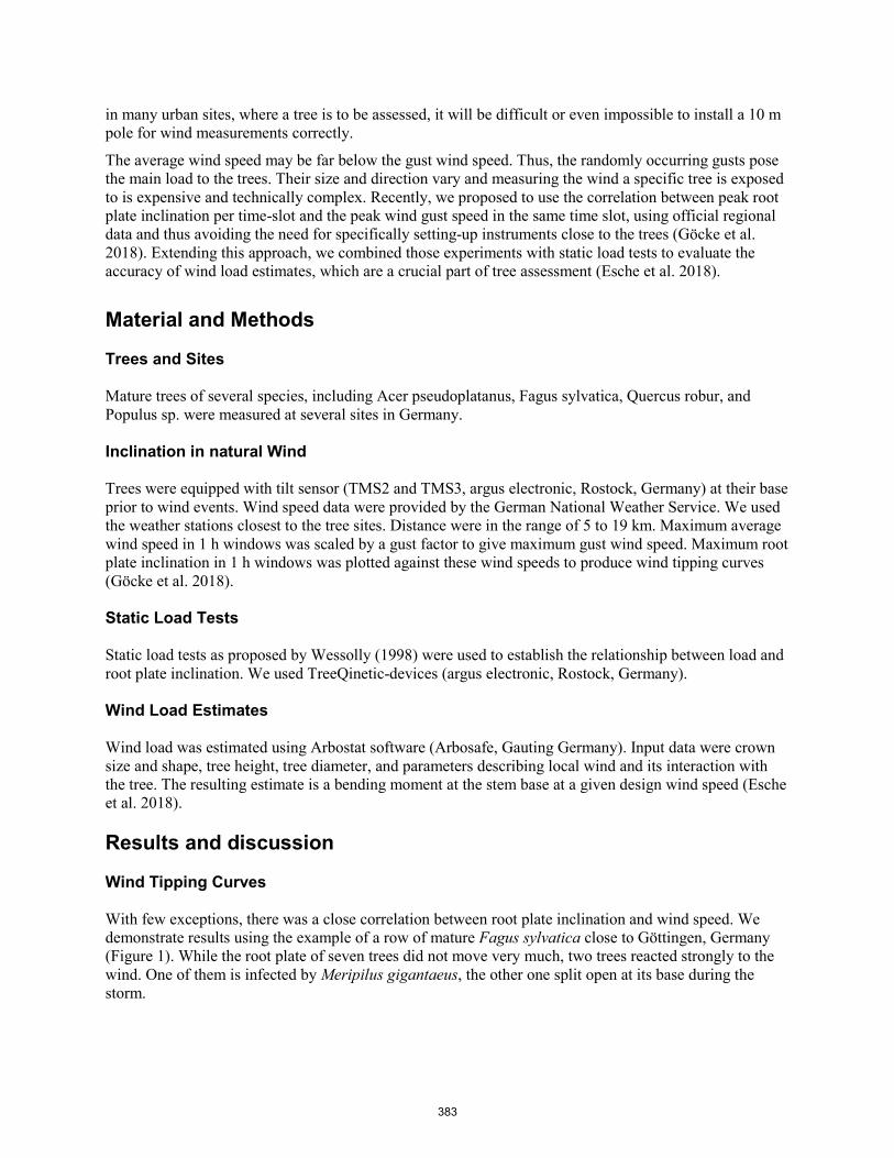
in many urban sites, where a tree is to be assessed, it will be difficult or even impossible to install a 10 m pole for wind measurements correctly.

The average wind speed may be far below the gust wind speed. Thus, the randomly occurring gusts pose the main load to the trees. Their size and direction vary and measuring the wind a specific tree is exposed to is expensive and technically complex. Recently, we proposed to use the correlation between peak root plate inclination per time-slot and the peak wind gust speed in the same time slot, using official regional data and thus avoiding the need for specifically setting-up instruments close to the trees (Göcke et al. 2018). Extending this approach, we combined those experiments with static load tests to evaluate the accuracy of wind load estimates, which are a crucial part of tree assessment (Esche et al. 2018).

Material and Methods

Trees and Sites

Mature trees of several species, including Acer pseudoplatanus, Fagus sylvatica, Quercus robur, and Populus sp. were measured at several sites in Germany.

Inclination in natural Wind

Trees were equipped with tilt sensor (TMS2 and TMS3, argus electronic, Rostock, Germany) at their base prior to wind events. Wind speed data were provided by the German National Weather Service. We used the weather stations closest to the tree sites. Distance were in the range of 5 to 19 km. Maximum average wind speed in 1 h windows was scaled by a gust factor to give maximum gust wind speed. Maximum root plate inclination in 1 h windows was plotted against these wind speeds to produce wind tipping curves (Göcke et al. 2018).

Static Load Tests

Static load tests as proposed by Wessolly (1998) were used to establish the relationship between load and root plate inclination. We used TreeQinetic-devices (argus electronic, Rostock, Germany).

Wind Load Estimates

Wind load was estimated using Arbostat software (Arbosafe, Gauting Germany). Input data were crown size and shape, tree height, tree diameter, and parameters describing local wind and its interaction with the tree. The resulting estimate is a bending moment at the stem base at a given design wind speed (Esche et al. 2018).

Results and discussion

Wind Tipping Curves

With few exceptions, there was a close correlation between root plate inclination and wind speed. We demonstrate results using the example of a row of mature Fagus sylvatica close to Göttingen, Germany (Figure 1). While the root plate of seven trees did not move very much, two trees reacted strongly to the wind. One of them is infected by Meripilus gigantaeus, the other one split open at its base during the storm.

383

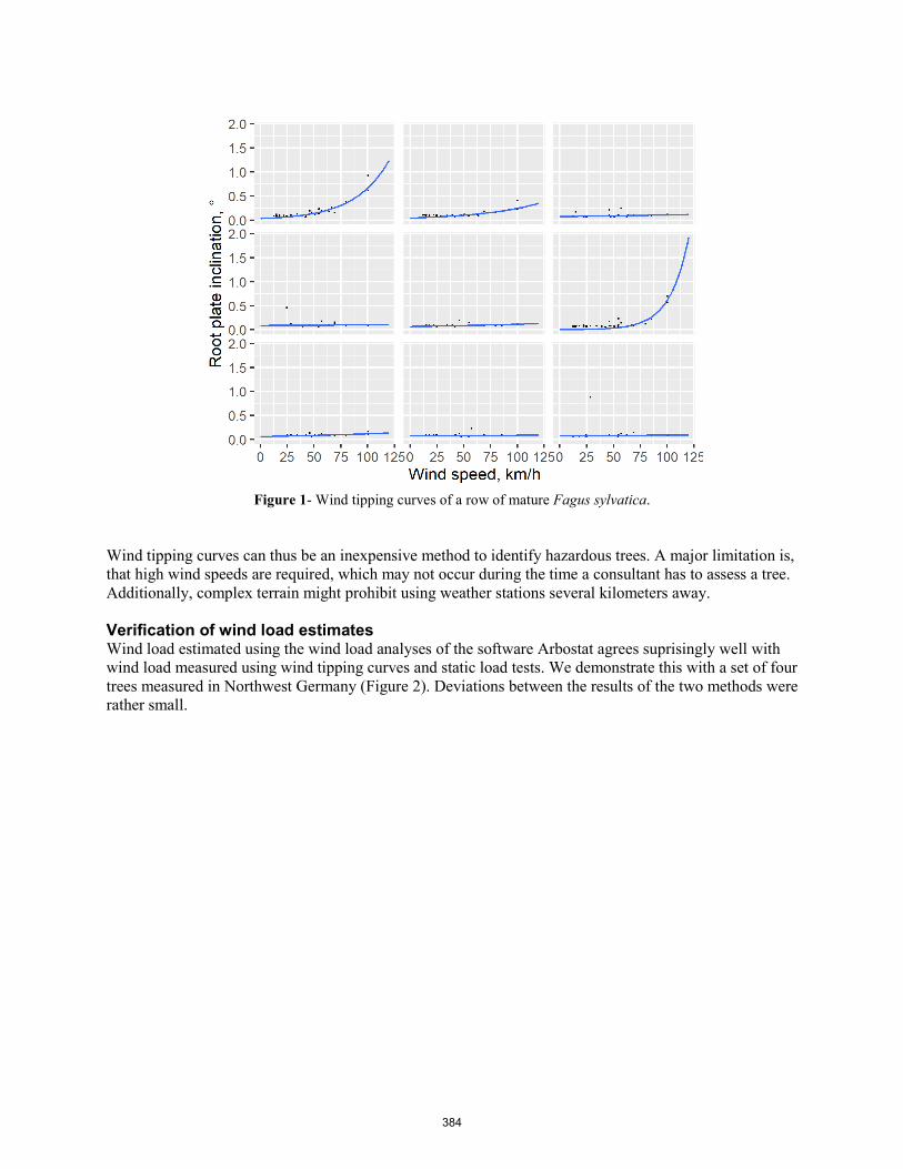
Wind tipping curves can thus be an inexpensive method to identify hazardous trees. A major limitation is, that high wind speeds are required, which may not occur during the time a consultant has to assess a tree. Additionally, complex terrain might prohibit using weather stations several kilometers away.

Verification of wind load estimates Wind load estimated using the wind load analyses of the software Arbostat agrees suprisingly well with wind load measured using wind tipping curves and static load tests. We demonstrate this with a set of four trees measured in Northwest Germany (Figure 2). Deviations between the results of the two methods were rather small.

Figure 1- Wind tipping curves of a row of mature Fagus sylvatica.

384

Conclusions Concurrent measurements of root plate inclination and wind speed – wind tipping curves – can be a valuable extension of static load tests. They can be used to identify potentially hazarduos trees alone, or in combination with load tests. Furthermore, they can support the sometimes questioned wind load analyses, which are an integral part of the method.

References Coutts, M.P. 1983. “Root architecture and tree stability.” Plant and Soil 71: 171–88. Detter, A., and S. Rust. 2013. “Neue wissenschaftliche Ergebnisse zu Zugversuchen.” In Jahrbuch der

Baumpflege, edited by D. Dujesiefken, 87–100. Esche, D. ; Schumacher, P. ; Detter, A. ; Rust, S.: Experimentelle Überprüfung der Windlastanalyse für

statische Zugversuche. In: DUJESIEFKEN, D. (Hrsg.): Jahrbuch der Baumpflege. Braunschweig : Haymarket Media, 2018, S. 229–236

Göcke, L. ; Rust, S. ; Ruhl, F.: Assessing the anchorage and critical wind speed of urban trees using root-plate inclination in high winds. In: Arboriculture and Urban Forestry Bd. 44 (2018), Nr. 1

Jacobs, M., 1936. “The effect of wind on trees.” Australian Forestry, 1(2), pp.25–32. James, K.R., C. Hallam, and C. Spencer. 2013. “Measuring tilt of tree structural root zones under static

and wind loading.” Agricultural and Forest Meteorology 168 (January). Elsevier B.V.: 160–67.

Figure 2. Wind load estimates using tree movement in natural wind and static load tests compared those generated by the software Arbostat.

385

Jonsson, M.J.J., A. Foetzki, M. Kalberer, T. Lundström, W. Ammann, and V. Stöckli. 2006. “Root-soil rotation stiffness of Norway spruce (Picea abies (L.) Karst) growing on subalpine forested slopes.” Plant and Soil 285 (1-2): 267–77.

Lundström, T., T. Jonas, V. Stöckli, and W. Ammann. 2007. “Anchorage of Mature Conifers: Resistive Turning Moment, Root–soil Plate Geometry and Root Growth Orientation.” Tree Physiology 27 (9). Oxford University Press: 1217–27.

Mergen, F., 1954. “Mechanical Aspects of Wind-Breakage and Windfirmness.” Journal of Forestry, pp.119–125.

Metzger, C., 1893. „Der Wind als maßgebender Faktor für das Wachsthum der Bäume“. Mündener Forstliche Hefte, pp.35–86.

Neild, S.A., and C.J. Wood. 1999. “Estimating Stem and Root-Anchorage Flexibility in Trees.” Tree Physiology 19 (3): 141.

Rust, S. 2016. “Tree Inventory, Risk Aessessment and Management.” In Urban Tree Management, edited by A. Roloff, 111–34. Oxford: Jon Wiley.

Smiley, E.T., N. Matheny, and S. Lilly. 2012. “Qualitative Tree Risk Assessment.” Arborist News, 12–18. Wessolly, L. ; Erb, M.: Handbuch der Baumstatik und Baumkontrolle. Berlin : Patzer Verlag, 1998 —

ISBN 3876170931

386

Optimum Ratio between Number of Diffraction Mesh Measurement Points and Trunk Diameter for Use in Ultrasound Tomography

Stella S.A. Palma * PhD student, Laboratory of Nondestructive Testing – LabEND, College of Agricultural Engineering – FEAGRI – University of Campinas – UNICAMP, Brazil – E-mail:ssapalma@gmail.com

Raquel Gonçalves Professor, Coordinator of the Laboratory of Nondestructive Testing – LabEND, College of Agricultural Engineering – FEAGRI – University of Campinas – UNICAMP, Brazil – E-mail: raquelg@unicamp.br

Rafael G. M. Lorensani Post-doctoral training, Laboratory of Nondestructive Testing – LabEND, College of Agricultural Engineering – FEAGRI – University of Campinas – UNICAMP, Brazil – E-mail: rafaelmansini@hotmail.com

Ruan O. B. Silva Graduate student, College of Agricultural Engineering – FEAGRI – University of Campinas – UNICAMP, Brazil – E-mail: ruanbueno1997@gmail.com

* Corresponding author

Abstract

The use of ultrasound tomography for tree trunks evaluation has shown good results. Regarding this topic, the Group of Nondestructive Testing from School of Agricultural Engineering (FEAGRI) of University of Campinas (UNICAMP), Brazil, has carried out several researches. Specifically concerning to ultrasonic tomography, there is a research line focused on the development of a national technology. Many advances have already been made, such as the development of ultrasound equipment and software to produce images representative of the velocity variation obtained in the field test on trees or timber. Despite these advances, there are challenges to overcome in order to complete the knowledge cycle. For this reason, the group has a lot of ongoing research related to the tree inspection. Considering the suitability of the diffraction mesh used in ultrasonic tomography with the equipment and software developed by the group, the objective of this research was to obtain the optimum relation between the number of diffraction mesh measurement points to be used during the field test, and the diameter of the tree trunk, so that it is possible to obtain adequate accuracy for a correct diagnosis without increasing too much the field work, considering that the trunk diameter of Brazilian trees have huge variation.

Keywords: ultrasonic wave propagation velocity; tree inspection; ultrasound

Introduction

Knowledge of the phytosanitary status of trees helps to prevent accidents and is particularly important in large urban centers where the trees are more likely to fall and cause human and material losses. This

387

knowledge is possible using methods capable of reproducing, with a high degree of confidence, the real condition of the tree without the use invasive tests that harming the tree.

There are several ways to obtain a high-resolution image of the internal structure of wood, such as the use of ultrasound, where the images can be reconstructed from characteristic parameters of the wave, such as propagation time, amplitude, or spectrum frequency (Bucur, 2004). The propagation of waves is affected by the presence of materials with different acoustic impedance, resulting in different velocities (Bucur 2006). The velocity of waves propagation in solids with defects decreases because the wave surrounds the defect, causing increase of the propagation time (Wang et al., 2004).

The research group in Non-Destructive Testing from FEAGRI/UNICAMP has been advancing in researches with the objective of composing representative images of the tree internal conditions using ultrasonic tomography (Secco et al., 2010; Gonçalves et al., 2011; Secco et al., 2011 a e b; Secco et al., 2012; Trinca et al., 2013 a, b e c; Reis, 2017, Strobel et al., 2018, Palma et al., 2018). However, despite all advances obtained so far, tomography involves many details related to the field tests and to the image software, whose have influences on the image accuracy and are not yet been quantified.

The measurement mesh used in the tests was proposed by Divos and Szalai, 2002 (Figure 1). For this mesh it is logical to imagine that, increasing the number of measurement points there will be increase of the image accuracy but, this implies substantially increasing fieldwork. In the research group, considering the most frequently adopted diffraction mesh, with n = 8 measurement points (Figure 1), and the test in all directions (Ex: 1-2 and 2-1), we measured 56 routes, (n2-n). With 16 routes, the number of measurements becomes 240, and so on. Thus, it is important to evaluate a way to obtain an optimal number of measurement points, improving the image accuracy without increase too much the field work.

Figure 1- Diffraction mesh with 8 measurement points.

In order to improve the accuracy of the images generated by ultrasound tomography, this research aimed to determine the optimum ratio between the number of measurement points and the diameter of the tree trunk.

Material and methods

We used 10 images (Figure 2) simulating different size and position defects and adopting a fix diameter (500 mm). The measurement points in the diffraction mesh varied from 6 to 14.

388

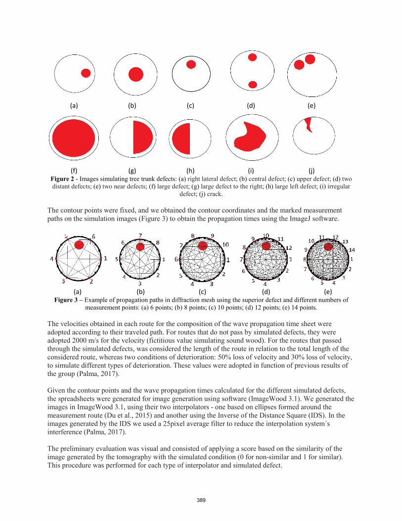
(a) (b) (c) (d) (e)

(f) (g) (h) (i) (j) Figure 2 - Images simulating tree trunk defects: (a) right lateral defect; (b) central defect; (c) upper defect; (d) two distant defects; (e) two near defects; (f) large defect; (g) large defect to the right; (h) large left defect; (i) irregular

defect; (j) crack.

The contour points were fixed, and we obtained the contour coordinates and the marked measurement paths on the simulation images (Figure 3) to obtain the propagation times using the ImageJ software.

(a) (b) (c) (d) (e) Figure 3 – Example of propagation paths in diffraction mesh using the superior defect and different numbers of

measurement points: (a) 6 points; (b) 8 points; (c) 10 points; (d) 12 points; (e) 14 points.

The velocities obtained in each route for the composition of the wave propagation time sheet were adopted according to their traveled path. For routes that do not pass by simulated defects, they were adopted 2000 m/s for the velocity (fictitious value simulating sound wood). For the routes that passed through the simulated defects, was considered the length of the route in relation to the total length of the considered route, whereas two conditions of deterioration: 50% loss of velocity and 30% loss of velocity, to simulate different types of deterioration. These values were adopted in function of previous results of the group (Palma, 2017).

Given the contour points and the wave propagation times calculated for the different simulated defects, the spreadsheets were generated for image generation using software (ImageWood 3.1). We generated the images in ImageWood 3.1, using their two interpolators - one based on ellipses formed around the measurement route (Du et al., 2015) and another using the Inverse of the Distance Square (IDS). In the images generated by the IDS we used a 25pixel average filter to reduce the interpolation system´s interference (Palma, 2017).

The preliminary evaluation was visual and consisted of applying a score based on the similarity of the image generated by the tomography with the simulated condition (0 for non-similar and 1 for similar). This procedure was performed for each type of interpolator and simulated defect.

389

For the two best results we applied the confusion matrix, using the comparison between the tomographic image and the simulated image of the disk. This matrix has two dimensions: the first one is related to the actual class (in this case the density and visual maps) and the second one represents the predicted class (in this case the tomographic images). The number of correct predictions for each class is located on the diagonal of the matrix and the other elements of the confusion matrix represent errors in the classification (Strobel et al. 2018). There are four possible combinations of a classification system with two classes, positive and negative. Considering C1 as the positive class, if an instance of C1 is classified as positive the corresponding result is called True Positive (TP); if it is classified as negative, the result is considered a False Negative (FN). On the other hand, if an instance of C2, the negative class, is classified as negative, this corresponds to a True Negative (TN) and, finally, if it is classified as positive, the result is called a False Positive (FP) (Strobel et al. 2018). This analyze allows calculate the accuracy (A), which provides the number of correct predictions (Equation 1).

Accuracy=(TP+TN)/(TP+FN+FP+TN) Equation 1

This preliminary analysis used a coarse mesh (8 x 8) because the calculation was manual, but it will be refined, since we will use an automatic analysis, and so the results will be more accurate.

Results and discussion

Considering the use of 10 different simulations, 5 diffraction meshes (Figure 3), two interpolators (IDS and ellipses) and two different conditions (30% and 50% velocity reduction), 200 tomographic images were generated and analyzed. In Figure 4 we show a example: a simulation of a defect in the upper part of the disk (Figure 2c) and using 50% reduction in velocity.

(a) (b) (c) (d) (e)

(f) (g) (h) (i) (j) Figure 4 – Images generated by software ImageWood 3.1 simulating a defect at the top of the disc using two

interpolators: (a) to (e) Interpolator using ellipses (Du et al. 2015) with 6, 8, 10, 12 and 14 measurement points respectively; (f) to (j) IDS Interpolator with 6, 8, 10, 12 and 14 measurement points, respectively.

*Colors indicating the percentage of the maximum velocity obtained in the disk

The images generally indicated the actual position of the defect (Figure 4), although some were undersized, and others were oversized. In the case of acoustic tomography using stress waves, it was verified that for central main defect, the image tends to underestimate its size (Wang et al., 2009; Socco et al., 1998), whereas for cracks the image tends to overestimate the size of the defect (Wang et al., 2009; Allison & Wang, 2015).

390

The colors, that represent the velocities ranges in each image, are dependent on the interpolator used. Du et al (2015) use compensation in velocities to form the ellipses and these compensations seems to affect the velocity, reducing it. For these images (Figure 4) it is expected no reduction of the velocity around the defect because the wood is sound but the color (lilac – Figures 4a to 4d) represent 20% to 30% velocity reduction and dark blue (Figure 4d) 30% to 40% velocity reduction. Using the IDS there is no such compensation, and the color around the defect (brown) represent a sound wood. For this analysis, for the IDS the number of measurements points have no influence on results and for Du et al. (2015) methods, the increasing of measurements points had no influence up to 12 points. In this case (Du et al. (201%) 14 measurements points produced a worse result.

Using the score system in the analysis we conclude that, excepted for the deterioration simulated with 30% velocity reducing, the optimum measurement points is 10, corresponding to 2% of the diameter (adopted as 500 mm) – Table 1. Above this quantity of measurements points there are no gain in score so, the image will not get better.

Table 1. – Score obtained by each velocity reduction simulation (average score obtained in each type of defects) and interpolation system

Velocity reduction simulated/interpolation

system

6 points 8 points 10 points 12 points 14 points

50% / Du et al. (2015) 2 5 6 6 7 30% / Du et al. (2015) 1 7 4 5 5 50%/ IDS 0 7 10 10 10 30% IDS 0 5 10 10 8

Total 3 24 30 31 30

As the use of 8 measurements points (1.6% of the diameter) have also a good result in this preliminary analysis, we apply the confusion matrix to both, 8 and 10 points. The results show that the accuracy obtained using 8 or 10 measurement point is statistically equivalent (Table 2). The accuracy of the IDS is approximately 7% and 3% higher than Du et al. (2015) for 8 and 10 measurements points, respectively (Table 2).

Interpolator Accuracy 8 points 10 points

Du et al (2015) 0,7305 ± 0,1464 0,7344 ± 0,1662 IDS 0,7813 ± 0,1122 0,7578 ± 0,1308 Total 0,7559 ± 0,1313 0,7344 ± 0,1495

To validate these initial results, in the continuation of the research, accuracy analyzes are planned for all the number of measurement points, as well as the individual analysis for the different defect types. Accuracy analyzes will be performed with refiner mesh and with computerized calculation.

Conclusions

Considering these preliminary tests and data evaluation, we conclude that the adoption of approximately 2% of the trunk diameter for the number of measurement points allow obtain near 75% accuracy in tomography images.

391

Acknowledgments

The authors thank the São Paulo State Research Foundation for the financial support (FAPESP – Proc. 2015/05692-3; Proc. 2017/07904-3) and the National Council of Technological and Scientific Development (CNPq) – Proc. 309511/2014-3 for the financial support, PhD and scientific initiation scholarships.

References List

Allison, R. B.; Wang, X. 2015. Nondestructive Testing in the Urban Forest. USDA Forest Service, Forest Products Laboratory, General Technical Report, FPL-GTR-238, Madison, Charpter 7, p. 77-86.

Bucur,V. 2004. Ultrassonic techniques for nondestructive testing of standing trees. Ultrassonics, 43: 237-238.

Bucur, V. 2006. Acoustics of wood. Springer Science & Business Media.

Divos, F.; Szalai, L. 2002. Tree evaluation by acoustic tomography. In: Proceedings of the 13th International symposium on nondestructive testing of wood, WI: Forest Products Society, August 19– 21; Berkeley, CA, p. 251–256.

Du, X.; Li, S.; Li G.; Feng, H.; Chen, S. 2015. Stress Wave tomography of wood internal defects using ellipse-based spatial interpolation and velocity compensation. BioResources, v.10, n.3, p. 3948-3962.

Gonçalves, R.; Secco, C. B.; Cerri, D. G. P.; Batista, F. 2011. Behavior of Ultrasonic Wave Propagation in Presence of Holes on Pequia (Aspidosperma desmanthum) Wood. In: Proc. 17th Symp. Nondestructive Testing of Wood, Vol. 1. Sept. Sopron, Hungary. 159-165.

Palma S. S. A. 2017. Reconhecimento de padrões em imagens geradas por ultrassom. Campinas, SP: Universidade Estadual de Campinas, Campinas, SP. M.S. thesis.

Palma S. S. A.; Gonçalves, R.; Trinca, A. J.; Costa, C. P.; dos Reis, M. N.; Martinis, G. A. 2018. Ultrasound tomography of wood. BioResources, v.13, n.12, p. 2834-2845.

Reis, M. N. 2017. Associação de métodos não destrutivos para inspeção de árvores Campinas, SP: Universidade Estadual de Campinas, Campinas, SP. M.S. thesis.

Secco, C. B.; Gonçalves, R.; Cerri, D. G. P.; Batista, F. A. B. Avaliação de dois tipos de medição na detecção da condição interna da madeira por ultrassom. Madeira: Arquitetura e Engenharia, v.11(27), p.1-5, 2010.

Secco, C. B.; Cerri, D. G. P.; Batista, F. A. F.; Vasques, E. C. 2011. Metodologia de inspeção da condição interna de toras de madeira por ultrassom. In: Congresso Ibero-Latino-Americano da Madeira na Construção, Coimbra.

Secco, C. B.; Gonçalves, R.; Cerri, D. G. P.; Vasques, E. C.; Batista, F. A. F. 2011. Tree holes detecting by ultrasound. In: Efficient and safe production processes in sustainable agriculture and forestry, Viena. XXXIV CIOSTA CIGR V Proceedings.

392

Secco, C. B.; Gonçalves, R.; Cerri, D. G. P.; Vasques, E. C.; Batista, F. A. F. 2012. Behavior of ultrasonic waves in wood with presence of voids. Cerne, n. 18, v. 3, p.1-8.

Socco, L. V.; Martinis, R.; Comino, E.; Nicolotti, G.; Sambuelli, L. 1998. Open problems concerning ultrassonic tomography for wood decays diagnosis. In: 11th International Nondestructive Testing and Evaluation of Wood Symposium.

Strobel, J. R. A.; de Carvalho, M. A. G.; Gonçalves, R.; Pedroso, C. B.; dos Reis, M. N.; Martins, P. S. 2018. Quantitative image analysis of acoustic tomography in woods. European Journal of Wood and Wood Products, 1-11.

Trinca, A. J.; Gonçalves, R.; Agustino, D. M.; Van Dijk, R.2013. Interference of Pith in Ultrasonic Tomography. In: 18th Symp. Nondestructive Testing of Wood, Sept. Madison, USA, v. 1.

Trinca, A. J.; Gonçalves, R.; Linhares, C. S. F. 2013. Ultrasonic Tomography in Detecting Knots. In: 18th Symp. Nondestructive Testing of Wood, Sept. Madison, USA, v. 1.

Trinca, A. J.; Gonçalves, R.; Lima, A. V.; Carvalho, M. A. G.; Filiange, E. S. 2013. Algorithms for the Generation of Ultrasonic Tomography. In: 18th Symp. Nondestructive Testing of Wood, Sept. Madison, USA, v. 1.

Wang, X.; Divos, F.; Pilon, C.; Brashaw, B. K.; Ross, R. J.; Pellerin, R. F. 2004. Assessment of decay in standing timber using stress wave timing nondestructive evaluation tools: A guide for use and interpretation. Gen. Tech. Rep. FPL-GTR-147. Madison, WI: US Department of Agriculture, Forest Service, Forest Products Laboratory, v. 12, p. 147.

Wang, X.; Wiedenbeck, J.; Liang, S. 2009. Acoustic tomography for decay detection in black cherry trees. Wood and Fiber Science, n.41, v.2, p.127-137.

393

Dynamic and Static Root System Evaluation Fathi Shadabeh University of Sopron, Sopron, Hungary, shadabeh.fathi@gmail.com

Mag. Katharina Schwanda Federal Research and Training Centre for Forests, Natural Hazards and Landscape, Department of Forest Protection, Unit Phytopathology, Vienna, Austria, katharina.schwanda@bfw.gv.at

Remy Gschwandtner BAUMPARTNER Arboristik GmbH, 4400 Steyr, Austria, remy.gschwandtner@baumpartner.at

DI Nikolaus Nemestóthy Federal Research and Training Centre for Forests, Natural Hazards and Landscape, Forest Training Centre Traunkirchen, 4810 Gmunden, Austria, nikolaus.nemestothy@bfw.gv.at

Laszlo Bejo University of Sopron, Hungary, bejo.laszlo@uni-sopron.hu

Agnes Buza Fakopp Enterprise Inc., Sorpon, Hungary, agnes.buzaakopp.com

Ferenc Divos * University of Sopron, Sopron, PhD School, Hungary, ferenc.divos@gmail.com

* Corresponding author

Abstract

The conditions of root systems of trees and thereby the chance for uprooting are important questions in case of hazard identification. For the evaluation of the root system several non-destructive methods exist. The pulling test is a well-known and proven method used for decades, while dynamic measurements, using real wind as factor, have become available in recent years In total ten fungi attacked ash (Fraxinus excelsior) trees were measured with the two tests and subsequently uprooted. By direct comparison of the two different methods, as well as considering the health status of the ash trees, new knowledge regarding the advantages and disadvantages of the pulling test and the dynamic measurement can be gained. The conditions of root systems of trees and thereby the chance for uprooting are important questions in case of hazard identification. For the evaluation of the root system several non-destructive methods exist. The pulling test is a well-known and proven method used for decades, while dynamic measurements, using real wind as factor, have become available in recent years In total ten fungi attacked ash (Fraxinus excelsior) trees were measured with the two tests and subsequently uprooted. By direct comparison of the two different methods as well as considering the health status of the ash trees new knowledge regarding the advantages and disadvantages of the pulling test and the dynamic measurement can be gained.

Keywords: pulling test, dynamic test, ash, fungi attack, uprooting

394

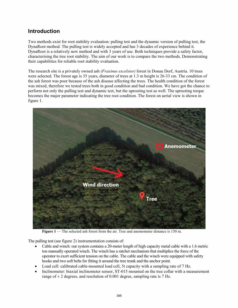
Introduction

Two methods exist for root stability evaluation: pulling test and the dynamic version of pulling test, the DynaRoot method. The pulling test is widely accepted and has 3 decades of experience behind it. DynaRoot is a relatively new method and with 3 years of use. Both techniques provide a safety factor, characterising the tree root stability. The aim of our work is to compare the two methods. Demonstrating their capabilities for reliable root stability evaluation.

The research site is a privately owned ash (Fraxinus excelsior) forest in Donau Dorf, Austria. 10 trees were selected. The forest age is 35 years, diameter of trees at 1.3 m height is 26-33 cm. The condition of the ash forest was poor because of the ash disease affecting the trees. The health condition of the forest was mixed, therefore we tested trees both in good condition and bad condition. We have got the chance to perform not only the pulling test and dynamic test, but the uprooting test as well. The uprooting torque becomes the major parameter indicating the tree root condition. The forest on aerial view is shown in figure 1.

Figure 1 — The selected ash forest from the air. Tree and anemometer distance is 150 m.

The pulling test (see figure 2) instrumentation consists of: • Cable and winch: our system contains a 20-meter length of high capacity metal cable with a 1.6 metric

ton manually operated winch. The winch has a ratchet mechanism that multiplies the force of theoperator to exert sufficient tension on the cable. The cable and the winch were equipped with safetyhooks and two soft belts for fitting it around the tree trunk and the anchor point.

• Load cell: calibrated cable-mounted load cell, 5t capacity with a sampling rate of 7 Hz.• Inclinometer: biaxial inclinometer sensor, ST-015 mounted on the tree collar with a measurement

range of ± 2 degrees, and resolution of 0.001 degree, sampling rate is 7 Hz.

395

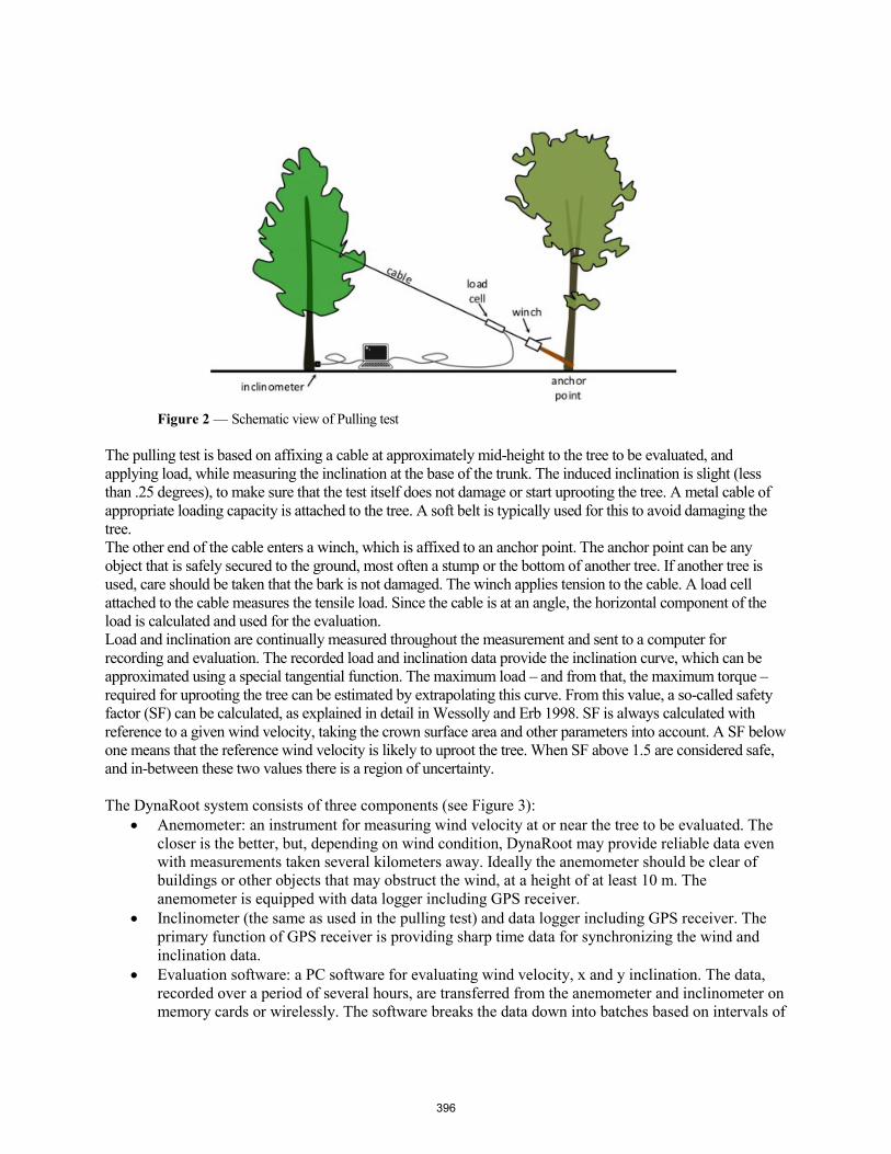
Figure 2 — Schematic view of Pulling test

The pulling test is based on affixing a cable at approximately mid-height to the tree to be evaluated, and applying load, while measuring the inclination at the base of the trunk. The induced inclination is slight (less than .25 degrees), to make sure that the test itself does not damage or start uprooting the tree. A metal cable of appropriate loading capacity is attached to the tree. A soft belt is typically used for this to avoid damaging the tree. The other end of the cable enters a winch, which is affixed to an anchor point. The anchor point can be any object that is safely secured to the ground, most often a stump or the bottom of another tree. If another tree is used, care should be taken that the bark is not damaged. The winch applies tension to the cable. A load cell attached to the cable measures the tensile load. Since the cable is at an angle, the horizontal component of the load is calculated and used for the evaluation. Load and inclination are continually measured throughout the measurement and sent to a computer for recording and evaluation. The recorded load and inclination data provide the inclination curve, which can be approximated using a special tangential function. The maximum load – and from that, the maximum torque – required for uprooting the tree can be estimated by extrapolating this curve. From this value, a so-called safety factor (SF) can be calculated, as explained in detail in Wessolly and Erb 1998. SF is always calculated with reference to a given wind velocity, taking the crown surface area and other parameters into account. A SF below one means that the reference wind velocity is likely to uproot the tree. When SF above 1.5 are considered safe, and in-between these two values there is a region of uncertainty.

The DynaRoot system consists of three components (see Figure 3): • Anemometer: an instrument for measuring wind velocity at or near the tree to be evaluated. The

closer is the better, but, depending on wind condition, DynaRoot may provide reliable data evenwith measurements taken several kilometers away. Ideally the anemometer should be clear ofbuildings or other objects that may obstruct the wind, at a height of at least 10 m. Theanemometer is equipped with data logger including GPS receiver.

• Inclinometer (the same as used in the pulling test) and data logger including GPS receiver. Theprimary function of GPS receiver is providing sharp time data for synchronizing the wind andinclination data.

• Evaluation software: a PC software for evaluating wind velocity, x and y inclination. The data,recorded over a period of several hours, are transferred from the anemometer and inclinometer onmemory cards or wirelessly. The software breaks the data down into batches based on intervals of

396

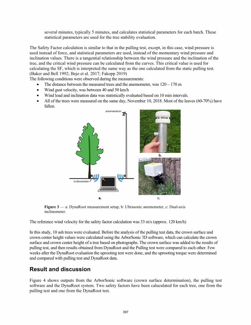
several minutes, typically 5 minutes, and calculates statistical parameters for each batch. These statistical parameters are used for the tree stability evaluation.

The Safety Factor calculation is similar to that in the pulling test, except, in this case, wind pressure is used instead of force, and statistical parameters are used, instead of the momentary wind pressure and inclination values. There is a tangential relationship between the wind pressure and the inclination of the tree, and the critical wind pressure can be calculated from the curves. This critical value is used for calculating the SF, which is interpreted the same way as the one calculated from the static pulling test. (Baker and Bell 1992; Bejo et al. 2017; Fakopp 2019) The following conditions were observed during the measurements:

• The distance between the measured trees and the anemometer, was 120 – 170 m• Wind gust velocity, was between 40 and 50 km/h• Wind load and inclination data was statistically evaluated based on 10 min intervals.• All of the trees were measured on the same day, November 10, 2018. Most of the leaves (60-70%) have

fallen.

Figure 3 — a: DynaRoot measurement setup, b: Ultrasonic anemometer, c: Dual-axis inclinometer.

The reference wind velocity for the safety factor calculation was 33 m/s (approx. 120 km/h)

In this study, 10 ash trees were evaluated. Before the analysis of the pulling test data, the crown surface and crown center height values were calculated using the ArborSonic 3D software, which can calculate the crown surface and crown center height of a tree based on photographs. The crown surface was added to the results of pulling test, and then results obtained from DynaRoot and the Pulling test were compared to each other. Few weeks after the DynaRoot evaluation the uprooting test were done, and the uprooting torque were determined and compared with pulling test and DynaRoot data.

Result and discussion

Figure 4 shows outputs from the ArborSonic software (crown surface determination), the pulling test software and the DynaRoot system. Two safety factors have been caluculated for each tree, one from the pulling test and one from the DynaRoot test.

397

a. b.

c.

Figure 4 — Example test result. a. Crown Surface and crown midpoint height is calculated using the ArborSonic software, b. DynaRoot results analysis, c. Pulling test curve analysis

Pulling test determines not only the safety factor, but predicts the uprooting torque. The uprooting test provided the measured uprooting torque. It is an excellent opportunity to validate the pulling test torque prediction capabilities. It is a validation of the applied generalized tipping form (a modified tangent function) and the inclination and force sensors as well. Figure 5 shows the relation between the predicted and measured uprooting torque. The correlation coefficient is 0.9! This is a clear demonstration, that the

398

uprooting torque prediction of pulling test is correct. The measured uprooting torque is always higher – 23% higher - than the predicted one. This is good coincidence with the earlier findings, that the predicted uprooting torque is always a bit lower than the real one.

Figure 5 Comparison graphs. a. The predicted and measured uprooting torque,b. Safety factors determined by pulling test and dynamic test,c. Measured uprooting torque versus pulling test safety factor,d. Measured uprooting torque versus DynaRoot safety factor.

At the first glance the two safety factors determined by pulling test and Dynamic test need to be identical. However, it must be noted that the safety factor determined by pulling test is not sensitive to the surroundings of the tree. The safety factor calculation is done under the assumption that the tree is standing alone exposed to the wind directly. The dynamic safety factor determined by the DynaRoot system is sensitive to the surroundings of the tree. For this reason, the two safety factors are not necessarily identical. The link between the safety factors is indicated on figure 5b, with the correlation coefficient of 0.74.

Figure 5 c. and d. are indicating the link between the measured uprooting torque and safety factor. The link is meaningful only if the trees geometry conditions, crown surface area, crown centre height, tree height, tree species are similar. In the forest we measured these conditions are roughly uniform. For this reason, we got high correlation coefficients: 0.84 (Pulling test) and 0.93 (DynaRoot). Higher correlation was found in case of the dynamic safety factor. The number of trees involved in the test is not enough for declaring that the dynamic test provides a more realistic safety factor, relative to pulling test. It is possible that the higher correlation coefficient is indicative of this case.

399

Conclusions

The root stability has been tested for 10 ash (Fraxinus excelsior) trees by pulling test and dynamic tests. After the tests an uprooting test were done. Strong correlation has been found (0.9) between the predicted uprooting torque and measured uprooting torque. Strong correlation has been found between the safety factors (0.74) measured by pulling test and dynamic test. Strong correlation has been found between the measured uprooting torque and the safety factors (0.84 and 0.93). The results are indicating that the pulling test and dynamic test performed by the DynaRoot system are reliable methods for tree root stability assessment.

Acknowledgments

We would like to thank Mr. Michael Bubna-Litic for providing his ash forest for our research project. Instruments were supplied by FAKOPP Enterprise.

References

Bejo, L.; Divos, F.; Fathi., S. 2017. Dynamic root stability assessment – basics and practical examples. In: Proc. 20th International Nondestructive Testing and Evaluation of Wood Symposium. Madison (WI), USA, 2017.09.12-15. 7pp.

Baker, C.J.; Bell, H.J. 1992. Aerodynamics of urban trees. Journal of Wind Engineering and Industrial Aerodynamics 44:2655–2666.

Fakopp Ltd., DynaRoot Dynamic Root Evaluation System, User’s manual http://fakopp.com/docs/products/dynaroot/UserManualDynaRoot.pdf [Date accessed: 10. 05. 2019]

Wessolly, L.; Erb, M. 1998. Handbuch der Baumstatik und Baumkontrolle. Patzer Verlag, Berlin, Germany.

400

Patrimonial Trees of Bogota and Its Assessment

Yolima Cortés-Cortés Independent researcher, Bogotá, Colombia, yocortesco@gmail.com

Jeimy Blanco-Florez Independent researcher, Bogotá, Colombia, jeicoblanco@hotmail.com

Abstract

The environmental authority in Bogota, Colombia, issued an administrative decision through which patrimonial trees and trees of cultural interest are singled out for conservation because of their historical, environmental and cultural importance. The administrative decision covers certain trees of the species cedar, cypress and palm trees like the wax palm and the Fenix palm. Some of these trees are more than 100 years old.

A project designed for the preservation and improvement of the physical state and general health conditions of the particular trees was carried. The project involved 19 nondestructive tests determining the internal status of each tree and determining which were the more adequate treatment. The project also included the integration of different environmental variables, drawing from different scientific fields, as well as the monetary valuation of the patrimonial trees.

Keywords: Q23: Forestry; Natural Heritage; Patrimonial trees; urban trees

Introduction

Even when society has acknowledged the cultural importance of urban ornamental trees and their natural heritage the estimated monetary value is many times inadequate. The purpose of this paper is the generation of methodological elements, with the inclusion of Nondestructive Tests as well as environmental evaluation, as comprehensive information of patrimonial elements. The use of the proposed model can be a tool for the management thereof that helps to draw the landscape of the cities in a way that guarantees the permanence of patrimonial trees for its appreciation and conservation as symbols of the history and culture of societies.

Field visits were carried out in the city of Bogota to trees that had been designated as patrimonial trees for the collection of dasometric, ecological and cultural parameters, obtained through nondestructive tests. This helps assess if there exists any deteriorated internal tissue which could influence the monetary value and cost of maintenance of the trees in question.

The valuation model was applied to the arboreal individuals selected as patrimonial in Bogota, by Resolution 6971 of 2011 of the Secretary of Environment, in which it is observed that the highest monetary values are reported in the individuals of native species: Cedar (Cedrela montana) and wax palm (Ceroxylon quidiuense), access to specimens affects a greater value of the trees located in institutional spaces than in those located in public space.

401

The patrimonial trees in cities and their integral economic valuation For an integrated analysis of the valuation of environmental goods and services, some authors have highlighted the feasibility of combining different aspects. Gómez-Baggethum & de Groot (2007) merge fundamental approaches in the Straton´s (2006) theory of the value of natural capital and ecosystem services and argue that it is essential to bridge the gap between market-based methods and those based on the science of ecology. This is a gap also identified by Sagoff (2010) who argues that the integrated and accurate estimation of the monetary value of ecosystems and ecosystem services, can only be achieved through bridging said gap. Gaaff and Reinhard (2012) examine the feasibility of transferring ecological values into economic values by closing the gap through the use of input from a wide variety of scientific advances from different fields, creating a transdisciplinary understanding of the use and value of ecological aspects. The trend in ecological economy is summarized in the argument of Straton (2006), who states that there are two elements necessary to build an economic value: intrinsic qualities (biophysical conditions) of ecological resources and the subjective evaluation, that is, the perceived notion of value. These elements must be integrated since it is important to consider the properties of a resource in relation to what the resource is worth to people living off or with the resource. Urban trees are considered natural goods of importance for the well-being and quality of life of city-dwellers. Therefore, the knowledge and understanding of the economic, ecological, cultural, scientific and historical value of these trees is an essential tool in the work for conservation. The natural patrimonial concept became commonplace in the middle of the 19th century, when greater value was attributed to natural spaces that denoted monumentality and scenic beauty associated with a national and cultural identity (Larrosa Rocamora, 2003).The monumental value of a tree is nourished by its physical dimensions, visual distinction and aesthetics (Efe et al., 2011). Trees have accompanied humanity for thousands of years, and have been important to the foundation of towns and cities as well as their cultural traditions such as art, religion and oral legends, which indicates that society assigns great symbolic value to these natural beings (Ferro Medina 2010). Within the urban forest management plans, the preservation of patrimonial trees is a point of interest, which involves identification, technical evaluation and declaratory or cataloging. The characterizing of trees as cultural patrimony one has traditionally considered age, species, rarity phenotype and historical importance. Lafuente (2007), highlights the importance of defining the tree’s category, which allows creating a legal framework for its regulation. In the end the important thing is that the municipality and national administrations are interested in the subject and undertake actions for the conservation and protection of patrimonial trees. However, the criterion of size, expressed in height or diameter, cannot be applied to all species, since some arboreal individuals reach maturity and high age without expressing that in their physical dimensions. A tree can be 70 or 80 years old without having reached any extraordinary physical dimensions, in terms of height or diameter, for example, native species of cloud forests, high Andean or subparamous as Encenillo (Weinmania tomentosa), Hayuelo (Dodonea viscosa) or Alder (Alnus jourullensis) that reach a maximum of 25 meters high in their adulthood. There is a range of aspects, or criteria, used for the identification of individual trees of cultural and ecological value. These include: age and special morphological or physiological characteristics, rarity:

402

ecological or environmental significance, significance in the landscape, symbolic significance, historical significance. When a tree is considered patrimonial, the species does not necessarily have to be native or exotic, but in the opinion of ISA (2011), which is associated with an aspect or value of the community. Ecological importance in terms of a particular tree’s relationship and interconnectivity to the surrounding landscape and ecosystem, such as providing habitat and food to the local fauna, is also considered relevant.

In the declaration or cataloging of a patrimonial tree, an individualized study of the morphophysiological, biomechanical and pathological aspects of the environment in which it is located and its history is required (Observatorio de árboles singulares, 2012). However, what is more important than the act of categorizing it as a patrimonial tree, is the existence of a legal framework which guarantees its protection and conservation.

Evaluations which include the use of specialized equipment such as tomographs, allow for the expansion of knowledge of these trees and their status, and thereby apply more appropriate evaluation and management methodologies.

Bogotá and its arboreal heritage

Bogota has 1'177,882 arboreal individuals located in public space, according to the information system for the management of the urban arboreal de Bogotá SIGAU (JBB, 2012). In Bogota the patrimonial tree is a arboreal specimen of environmental significance, important for the surrounding landscape, of a considerable size, as well as with historical and cultural value (one or more of the following aspects: 60 years or more, a native species of environmental significance and landscape or singular or rare exotic species and outstanding size or shape (phenotype), as well as historical or cultural value (Resolution SDA 6971 of 2011)).

In the year 2010, the District Decree 531, regulated by Resolution 6971 of 2011 and based on a study by Bermúdez (2004), in the city of Bogota, 19 trees were declared as patrimonial and 24 as specimens of public interest, adding up to a total of 43 arboreal individuals, distributed over 13 species. The Fenix Palm (Phoenix canariensis) is the most prevalent one with ten individuals, whilst the native species with the greatest number of declared trees is the wax palm, (Ceroxylon quindiuense), the national tree of Colombia. According to the District Decree 531 it is stated that 65.12% of the declared trees, that is to say 28 specimens, are located on institutional lands 34.88% in the public space (15 specimens).

The District Decree 531indicates that the District Secretary of the Environment must have the available technological equipment to carry out a prioritized diagnosis of the identified plant individuals.

With regard to the physical and sanitary status of the trees, a better level of conservation can be observed of the individuals who are located on institutional lands, compared to those who are in public spaces. This mainly due to the restrictions of development and access by the public, implied by institutional lands (such as museums), whilst the public space involves higher exposure to stressors such as citizens, traffic, pets and vandalization. The management of patrimonial trees is under the responsibility of the José Celestino Mutis Botanical Garden, in accordance with the provisions of Resolution 531 of 2010.

403

Material and Methods

19 nondestructive tests were carried out to asses patrimonial trees, with using Resistograph® measuring devices for palm species and Rinntech® acoustic tomographs devices for tree species . These devices are used to determine the most appropriate forest management methods through more accurate assessments of tree diagnostics and detecting the risk that defective trees may represent in an urban area. The tests with the Rinntech® acuostic tomographs evaluate internal health of trees by placing a certain number of transmitting and receiving sensors around the tree or palm trunk perimeter and with a special software measures the sound impulses’ received values. The Resistograph®, works like a micro drill when is introduced into a trunk to measure the wood drill resistance.

In this sense, a methodological approach is used for the environmental valuation of patrimonial trees in the city of Bogotá, estimating a non-monetary value as a basic value; evaluation factors are linked by tree from different parameters: dimension, condition, location, species, tree qualification and special ecological and cultural characters, giving greater weight to the values obtained in the exceptional nature and cultural scores; as well as the incidence of the results of non-destructive tests in their economic valuation.

In the elaboration of the proposed model in this paper, an adaptation of the method used by Jim (2006), (Formulaic Expert Method FEM), for special trees in Hong Kong and the method used in New Zealand (Standard Tree Evaluation Method STEM) was developed. The proposed method is aimed at weighting values in terms of dimension, condition, location, species, tree qualification and special ecological and cultural characteristics, giving greater weight to the values obtained in exceptional nature and cultural scores because they are considered patrimonial trees.

The basic method includes seven qualification components: the first group of components describe A. Dimension (dasometric aspects), B. Species (origin, distribution and aesthetic value), C. Tree structure (quality and ecological value), D. Condition (physical and sanitary) that includes the results of non-destructives test. In a second group of components one can find, E. Location (importance of the tree in the location site, landscape and functional value, in this, a deductible value is taken into account, for conflict with respect to existing constructions, that can affect both the tree conservation and survival and the nearby structure),

One last group of components are related to special aspects like F. Exceptionality (special connotation) and G. Cultural importance (added to the model proposed by Jim, highlights the characteristics such as recognition by communities or the relationship of the tree or species with traditional or ancestral knowledge).

In these seven components, 29 valuation criteria are distributed, in ranges between 0 and 5, which express qualitative values, based on quantitative data.

Results and Discussion

When carrying out a review and analysis on the valuation of patrimonial trees it is observed that a specific methodology has not been addressed, the same methodology is used for ornamental trees in general, both in Bogota and in other parts of the world.

The results of the tests can be observed in Table 1.

404

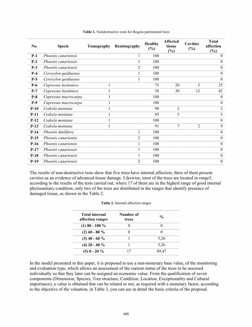
Table 1. Nondestructive tests for Bogota patrimonial trees

No. Specie Tomography Resistography Healthy (%)

Affected tissue (%)

Cavities (%)

Total affection

(%) P-1 Phoenix canariensis 1 100 0 P-2 Phoenix canariensis 1 100 0 P-3 Phoenix canariensis 2 100 0 P-4 Ceroxylon quidiuense 1 100 0 P-5 Ceroxylon quidiuense 1 100 0 P-6 Cupressus lusitanica 1 75 20 5 25 P-7 Cupressus lusitánica 1 58 30 12 42 P-8 Cupressus macrocarpa 1 100 0 P-9 Cupressus macrocarpa 1 100 0

P-10 Cedrela montana 1 98 2 2 P-11 Cedrela montana 1 95 5 5 P-12 Cedrela montana 1 100 0 P-13 Cedrela montana 1 91 7 2 9 P-14 Phoenix datilifera 1 100 0 P-15 Phoenix canariensis 2 100 0 P-16 Phoenix canariensis 1 100 0 P-17 Phoenix canariensis 1 100 0 P-18 Phoenix canariensis 1 100 0 P-19 Phoenix canariensis 2 100 0

The results of non-destructive tests show that five trees have internal affection, three of them present cavities as an evidence of advanced tissue damage. Likewise, most of the trees are located in range5, according to the results of the tests carried out, where 17 of them are in the highest range of good internal phytosanitary condition, only two of the trees are distributed in the ranges that identify presence of damaged tissue, as shown in the Table 2.

Table 2. Internal affection ranges

Total internal affection ranges

Number of trees %

(1) 80 - 100 % 0 0 (2) 60 - 80 % 0 0 (3) 40 - 60 % 1 5,26 (4) 20 - 40 % 1 5,26 (5) 0 - 20 % 17 89,47

In the model presented in this paper, it is proposed to use a non-monetary base value, of the monitoring and evaluation type, which allows an assessment of the current status of the trees to be assessed individually so that they later can be assigned an economic value. From the qualification of seven components (Dimension, Species, Tree structure, Condition, Location, Exceptionality and Cultural importance), a value is obtained that can be related or not, as required with a monetary factor, according to the objective of the valuation, in Table 3, you can see in detail the basic criteria of the proposal.

405

Table 3. Non monetary environmental values obtained

No. Qualification components (%) Environmental value (%)

A B C D E F G P - 1 45 47,37 91,43 100 86,67 72 60 70,50 P - 2 85 47,37 91,43 100 80 72 60 74,20 P - 3 80 47,37 91,43 100 80 72 60 73,64 P - 4 85 78,95 94,29 100 80 84 88 86,91 P - 5 85 78,95 94,29 100 80 84 88 86,91 P - 6 90 36,84 85,71 96,67 73,33 80 64 74,51 P - 7 90 36,84 85,71 93,33 73,33 80 64 74,14 P - 8 65 47,37 85,71 96,67 73,33 80 64 72,90 P - 9 65 36,84 85,71 100 73,33 80 64 72,10 P - 10 90 73,68 91,43 93,33 80 88 84 85,83 P - 11 100 73,68 94,29 100 80 88 84 88,00 P - 12 95 73,68 94,29 100 76,67 88 84 87,07 P - 13 85 73,68 91,43 93,33 80 88 84 85,27 P - 14 85 47,37 91,43 93,33 86,67 76 52 73,31 P - 15 80 47,37 88,57 93,33 86,67 76 52 72,44 P - 16 80 47,37 91,43 90 86,67 76 52 72,38 P - 17 75 47,37 91,43 90 86,67 76 52 71,83 P - 18 75 47,37 91,43 93,33 86,67 76 52 72,20 P - 19 90 47,37 88,57 93,33 93,33 76 56 75,18

The proposed monetary valuation approach involves the monetary value of the land in the area in which the trees are located and the maintenance costs incurred in the management of each tree.

The result of monetary valuation yields values between USD $ 26,912 and USD $ 699,454, noting that whilst the highest monetary values correspond to native species trees due to their ecological and cultural importance, one also notices a high value assigned to trees with internal tissue deterioration have higher values due to the cost of maintenance of these.

The application of the proposed methodology can provide information of importance for the management of patrimonial trees in the city, applying this scale can help in the decision-making process to prioritize the application of silvicultural treatments to arboreal individuals in accordance with the technical requirements for each case. The proposed methodology applies to the moment in which the assessment is made, because aspects such as dimensional or cultural perception may vary over time. Over time the internal and external characteristics of the trees may change, so the results of the economic valuation method may also vary.

The economic value of a patrimonial tree must reflect the environmental dimension, that is, it must integrate social, economic and ecological aspects as a whole. The empirical approach focuses on the values according to the situation in which they are valued and the objective of the valuation process.

This valuation approach is considered an integral method since it in its elemental qualification the condition criterion is interrelated with the other qualified criteria., according to Sagoff (2010), the values

406

obtained must reflect characteristic elements of the trees, as its internal health, depending on the state of the specimen at the time of the assessment and on the other hand, the location criterion.

Conclusions

It is important to highlight the need to value environmental goods and services, fundamentally with a broad knowledge of them, to represent their complexity and incommensurability in their relationship with society.

The study and conservation of patrimonial trees should be a priority in the development of infrastructure project in cities worldwide. However, the physical or health conditions of the tree it may impact the cultural values for which it would have been declared as patrimonial or cultural interest. The planning and design of the city must match the location and space requirements for the preservation of trees with special connotation, from its cultural importance to its ecological value in harmony with other elements of the landscape.

Acknowledgments

The authors would like to thank for mobility to the agreement between the Center for Development Research (ZEF) of the University of Bonn and the Institute of Environmental Studies (IDEA) of the National University of Colombia, with the financial support of the German Academic Exchange Service (DAAD) in its program of Bilateral Graduate Schools - Sustainable Development Goals and the Federal Ministry of Economic Cooperation and Development of Germany.

References

Bermúdez, E. (2004). Árboles Patrimoniales Etapa I. Bogotá: Jardín Botánico José Celestino Mutis.

Efe, R., Soykan, A., Curebal, I., & Sonmez, S. (2011). Dede Korkut monument oak (Quercus infectoria Olivier) (Kadiköy - Edremit - Balikesir, Turkey). Procedia Social and behaviorial sciences, 19, 627 - 636.

Ferro Medina, G. (2010). Árboles Ciudadanos en la memoria y en el paisaje cultural de Bogotá. Bogotá: Instituto Distrital de Patrimonio Cultural.

Gaaff, A., & Reinhard, S. (2012). Incorporating the value of ecological networks into cost-benefit analysis to improve spatiality explicit land-use planning. Ecological economics, 73(15), 66 – 74.

Gómez-Baggethun, E., & de Groot, R. (2007). Capital natural y funciones de los ecosistemas: explorando las bases ecológicas de la economía. Ecosistemas, 16(3), 4 – 14

ISA, I. S. (2011). Guidelines for Developing and Evaluating Tree Ordinances.

JBB, J. B. (7 de octubre de 2012). Número de árboles por localidad. Bogotá, Distrito Capital, Colombia.

Jim, C. (2006). Formulaic expert method to integrate evaluation and valuation of heritage trees in compact city. Environmental Monitoring and Assessment(116), 53 - 80. Lafuente B., M. (2007). Concepto y protección del patrimonio arbóreo monumental. Revista de administración pública(172), 403 – 437.

407

Larrosa Rocamora, J. A. (2003). El palmeral de Elche> Patrimonio, gestión y turismo. Investigaciones geográficas(30), 77 - 96.

Observatorio de árboles singulares. (30 09 2012). runa. Naturaleza rural: http://www.ruralnaturaleza.com

Sagoff, M. (2010). The quantification and valuation of ecosystem services. Ecological economics, 70(3), 497 – 502.

Straton, A. (2006). A complex systems approach to the value of ecological resources. Ecological economics, 56, 402 – 411.

408

Nondestructive Testing Methods for Risk Assessment of Standing Trees at a Historic Site, Forest Lodge, Chequamegon-Nicolet National Forest, Wisconsin USA

Richard B Allison* Forest and Wildlife Ecology Department, University of Wisconsin-Madison, rbruceallison@tds.net

Mark Rickenbach Forest and Wildlife Ecology Department, University of Wisconsin-Madison

Sean Stevenson Fischer Forest and Wildlife Ecology Department, University of Wisconsin-Madison

Abigail Walther Forest and Wildlife Ecology Department, University of Wisconsin-Madison

Fenglu Liu Beijing Forestry University, Beijing, China, 429198174@qq.com

Xi Wu School of IoT Engineering, Jiangnan University, Wuxi, Jiangsu, China, xw20170909@gmail.com

Abstract

The USDA Forest Service was recently bequeathed an historic log building lodge that has been incorporated into the Chequamegon-Nicolet National Forest to be used as a public forestry educational facility. With the change in use, investment in building upgrades and introduction of public use, the US Forest Service has contracted with The University of Wisconsin-Madison Department of Forest and Wildlife Ecology to conduct a risk assessment of the trees adjacent to the historic buildings using nondestructive testing equipment. This case study is a model for use of NDT methods for tree risk assessment at historic properties.

Keywords: nondestructive testing, tree risk assessment, historic sites, Forest Lodge, Chequamegon-Nicolet National Forest

Introduction and background

The United States Department of Agriculture Forest Service Chequamegon-Nicolet National Forest (US Forest Service) contracted with the University of Wisconsin -Madison (FS Agreement 18-PA-11091300-096) to have the Department of Forest and Wildlife Ecology conduct a nondestructive conditionassessment on select trees adjacent to buildings at a historic private lakefront lodge that had been gifted tothe US Forest Service. Faculty member Dr. R. Bruce Allison brought a student team to the location inSeptember 2018 to survey the property and begin testing trees within the building compound known as

409

Forest Lodge. With the transfer of property ownership from limited use private family to a federal government owned facility the historic grounds were repurposed to a public forestry educational center available to students and educational events. This presented the opportunity to observe how nondestructive tree condition analysis and tree risk assessment can be applied to historic properties transformed from limited use private property to public facilities governed by government-appointed committee planning documents.

The historical significance and current planned use of forest lodge

Upon receipt of the land gift the US Forest Service established the Forest Lodge Historic District Master Site and Management Plan (Plan). The Plan states, “Forest Lodge stands proud and tall like a first-growth tree the lumberjacks missed, a spectacular and extraordinary living link to our heritage and another era.” Forest Lodge was listed in the National Register of Historic Places in 2002. Located on Garmisch Road, Namakagon Township, Bayfield County it is on the south shore of Lake Namakagon approximately 8 miles east of Cable. It had been the hunting, fishing and recreational retreat of the Crawford Livingston family of St. Paul, MN. The National Register of Historic Places, (reference number 02000031) describes the property:

“The Rustic Style complex blends into the naturally landscaped grounds and wooded setting. Stone walls, a picnic area, recreational areas, and an elaborate path and road system contribute to the idyllic setting…The main lodge was begun in 1893 as a log cabin, substantial remodeling in 1914, the late 1920s and in the 1930s expanded its size, providing amenities for its affluent owners. While modest in its décor and outward appearance, this log building …symbolically expressed a harmonious relationship between people and the wilderness.”

The land on which the estate is located had been a logging camp, established by the Northern Wisconsin Lumber Company around 1884. In 1889 Crawford Livingston (1848-1925) of St. Paul, Minnesota, together with a group of hunters and fishermen from Chicago, leased the old logging camp as a retreat. Crawford Livingston was born on May 6, 1848 to Crawford and Caroline (Chapman) Livingston. He was an ambitious descendant of a notable New York family whose ancestors include Phillip Livingston, a signatory of the United States Declaration of Independence and Robert Livingston, a signatory of the United States Constitution. At age 16 he worked for a New York City brokerage company, then served briefly as deputy treasurer of New Jersey before, in 1870, at 22 years old, he migrated to St. Paul, Minnesota where he met his future wife Mary Steele Potts. She was the daughter of a prominent St. Paul physician, Thomas Reeds Potts, who had brought the family from Galena, Ohio in 1849 to become the surgeon at Fort Snelling. Her uncle was Henry H. Sibley, Minnesota’s first governor. Crawford and Mary married on January 28, 1875. He was manager of a life insurance company at the time and later formed a brokerage firm and founded the St. Paul Gas Light Company. He partnered in the construction of several railroads in Minnesota and the Pacific Northwest, was president of the Como Railway and the St. Paul District Telegraph plus was a director of the Merchant’s National Bank.

In 1915, their daughter Mary Livingston, was married to Theodore Wright Griggs. Theodore’s father was Chauncey Wright Griggs, who had built a very successful wholesale grocery business, Griggs, Cooper and Company plus a lumbering business in St. Paul and Tacoma, Washington. Theodore had graduated from Yale University in 1895, served as first lieutenant in the Spanish American War in 1898. Their daughter Mary Griggs was born June 20, 1916.Upon the death of both parents in 1925, Mary Livingston Griggs inherited Forest Lodge.

Mary L. Griggs developed Forest Lodge buildings and landscape with a creative, artistic flourish during her tenure well integrated with the natural Northwoods environment. Her daughter Mary Griggs Burke (1916-2012) inherited Forest Lodge upon her mother’s death in 1943. Though in adulthood she made Manhattan, New York City her primary residence Forest Lodge was formative in her youth and became

410

her summer residence. In 1999 she donated the property, with a life estate, to the Trust for Public Land with stewardship assigned to the USDA Forest Service. An archaeological survey conducted at that time revealed evidence of previously unrecorded pre-contact American Indian sites around the property (Kim Potaracke, Forest Service Archaeological Technician (1999).) Following Burke’s death in 2012 the USDA Forest Service began building rehabilitation and landscape management under direction of the Forest Lodge Historic District Master Site and Management Plan. Mary Burke’s wish for Forest Lodge was stated in the Plan, “that the property transition into an environmental center for use by generations to come.” Endowment funds to assist in accomplishing that intention were provided in her bequests to the US Forest Service and to Northland College.

The planned use for the property will bring many students, conferences, tourists and the general public to the property plus a major investment in rehabilitating buildings and their adaptive reuse. The change in relationship of the existing trees to the increased human occupation and the remodeled structures are a consideration in evaluating the structural condition of the trees and the potential risks from failure. The directive of the Plan stated in the Executive summary is that “The focus of this planning effort for Forest Lodge has been to balance the needs of the historic resource with those of compatible contemporary use. Through this blending of historic preservation efforts and low intervention adaptive contemporary reuse, the legacy of the past may be maintained for future generations.”

In the unique circumstances and context of this tree condition assessment and recommendations for action, special consideration and weighting is applied to the Plan’s intention of “historic preservation” and “low intervention.” This requires a careful consideration of the facts gathered from individual tree measurements and location considerations to arrive at an imperfect but reasonable prediction on likelihood of structural failure and consequences. This report’s goal is to then balance that conclusion with the requirement to preserve “the legacy of the past” in proposing recommendations for tree management compatible with contemporary use of Forest Lodge. The intent of this study was to provide the US Forest Service Forest Lodge managers with useful information and discussion for them to arrive at action plans regarding tree preservation, tree removal, tree pruning or other risk mitigation strategies they deem appropriate in the overall management of this property.

Methods and Procedures

A scaled site plan of the property was created locating the relative position of the structures and the trees including GPS coordinates to position them in a GIS file for the use of property managers. A tree identification numbering system was established in the field and placed on the site plan. A steel measuring tape was used to determine the trees’ trunk diameter at 4.5 feet elevation and also to determine the elevation of the test sites along the trunk. An iPhone X was used to determine compass direction and for photography. A rubber mallet was used for initial trunk soundings. Upper trunk and canopies were observed using Eagle Optics 8.5 x 32 Raven model binoculars. A visual examination looked for structural anomalies as described in the book by Claus Mattheck and Helge Breloer, The Body Language of Trees, A handbook for failure analysis (TSO Publishing, London:2010) A tree’s growth is responsive to its environment. It is a self-optimizing, mechanical structure. To allow uniform mechanical stress over its entire surface, additional wood is laid down over decayed or damaged areas. Thus, trunk bulges, wound wood, or extreme lower trunk flair at the root collar area can indicate concealed cavities, cracks or decay. Crown retrenchment, fungal conks or open cavities are further visual evidence of decay and structural defects.

The following advanced measurement tools were used in this structural evaluation: Tree Check Sonic Wave Tree Decay Detector (Allison Tree, LLC: USA) Arborsonic Acoustic Tomography (Fakopp: Hungary)

411

IML PD400 Microdrill (IML: Germany)

Tree Check is a stress wave timer. It consists of two accelerometers placed on opposite sides of the trunk or limb being sampled. They are attached to the shaft of two screws that have penetrated the bark and firmly embedded in the sap wood. Both are connected by electric cables to a main electronic board that is designed to display the time that it takes an impact induced stress wave to travel from one accelerometer to the other across the trunk wood. The measurement is displayed in microseconds. That number is divided by the number of inches or centimeters between the sensors to determine a time of flight per inch or centimeter. The use of stress waves to detect tree defects and decay is based on the observation that sound waves movement through wood is directly related to the physical and mechanical properties of wood. Stress waves travel slower in decayed or deteriorated wood than sound wood. On hardwood wood trees such as oak and maple, one can expect a stress wave time of flight across the diameter to be from 20-28 microseconds per inch. Numbers higher than that indicate an obstruction interfering with the passage of the sound wave. This could be a crack, a cavity, or decay. On softwood trees with lower wood density, such as spruce, pine or hemlock, the stress wave will take longer often producing numbers in the 25-30 microseconds per inch range. The stress wave timer is a qualitative tool indicating either solid wood or a problem requiring further quantitative investigation to determine the location and extent of the problem.

The Arborsonic Acoustic Tomography uses the same principle as the single path stress wave timer but uses as many as twelve accelerometers evenly spaced around the trunk diameter to create a matrix of measurements. Each of the twelve accelerometers has a turn to serve as the sending one and the computer measures the time of flight to each of the other accelerometers. That information is processed by a projection software program on the field computer creating a computed tomograph representation of the varying stress wave velocities across the trunk slice or transverse section measured. It is a self-calibrating scale showing four colors representing quadrants of perceived change in density from most dense to least (i.e. green, yellow, violet, blue). In interpreting test results, it is important to know that the tomograph picture is not an exact representation of the exact location and area of any internal defect but rather a display of the measured changes in sound velocity across the transverse section. A crack for example might cause a sound wave shadow larger than the actual defect. With careful interpretation however, the acoustic tomographic tool can assist in gauging the extent, type and approximate location of the defect and the amount of remaining solid wood.

The IML PD400 microdrill detects the torsion and thrust resistance on a 40 cm long drill shaft that is 1.5mm in diameter with a 3mm head as it passes through the wood. The change in the resistance is displayed on an electronic graph. The two graphs displayed, one for torsional resistance (blue graph) and the other for thrust resistance (green graph) show changes in resistance with higher amplitude indicating greater resistance. As the drill passes through cavities, narrow cracks or incipient decay, the graph amplitude is lower or flat. This provides a quantitative measurement of location and extent of defects along the linear area tested.

Observations and Data

Table 1 is a sampling of the spread sheet generated to represent test results and recommendations.

412

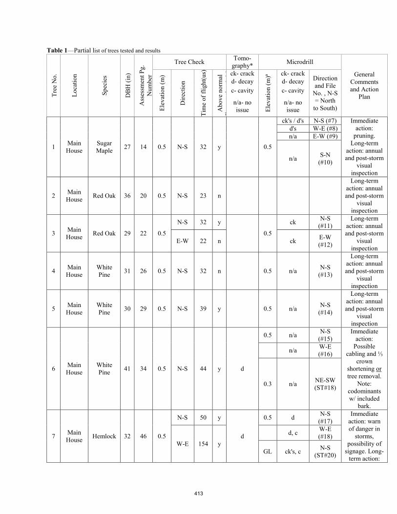
Table 1—Partial list of trees tested and results Tr

ee N

o.

Loca

tion

Spec

ies

DB

H (i

n)

Ass

essm

ent P

g.

Num

ber

Tree Check Tomo-graphy* Microdrill

General Comments and Action

Plan

Elev

atio

n (m

)

Dire

ctio

n

Tim

e of

flig

ht(u

s)

Abo

ve n

orm

al

Et

ti(

/) ck- crack

Elev

atio

n (m

)ª ck- crack Direction and File

No. , N-S = North

to South)

d- decay d- decayc- cavity c- cavity

n/a- no issue

n/a- no issue

1 Main House

Sugar Maple 27 14 0.5 N-S 32 y 0.5

ck's / d's N-S (#7) Immediate action:

pruning. Long-term

action: annual and post-storm

visual inspection

d's W-E (#8)n/a E-W (#9)

n/a S-N(#10)

2 Main House Red Oak 36 20 0.5 N-S 23 n

Long-term action: annual and post-storm

visual inspection

3 Main House Red Oak 29 22 0.5

N-S 32 y

0.5

ck N-S(#11)

Long-term action: annual and post-storm

visual inspection

E-W 22 n ck E-W(#12)

4 Main House

White Pine 31 26 0.5 N-S 32 n 0.5 n/a N-S

(#13)

Long-term action: annual and post-storm

visual inspection

5 Main House

White Pine 30 29 0.5 N-S 39 y 0.5 n/a N-S

(#14)

Long-term action: annual and post-storm

visual inspection

6 Main House

White Pine 41 34 0.5 N-S 44 y d

0.5 n/a N-S(#15)

Immediate action:

Possible cabling and ⅓

crown shortening or tree removal.

Note: codominants w/ included

bark.

n/a W-E(#16)

0.3 n/a NE-SW (ST#18)

7 Main House Hemlock 32 46 0.5

N-S 50 y

d

0.5 d N-S(#17)

Immediate action: warn of danger in

storms, possibility of

signage. Long-term action:

W-E 154 y

d, c W-E(#18)

GL ck's, c N-S(ST#20)

413

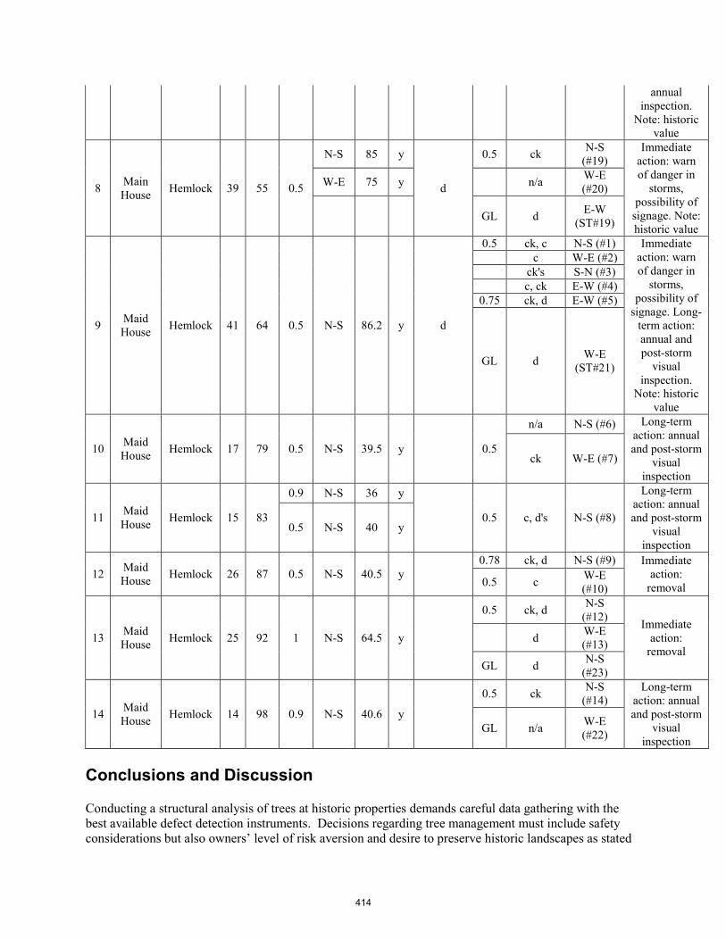
annual inspection.

Note: historic value

8 Main House Hemlock 39 55 0.5

N-S 85 y

d

0.5 ck N-S (#19)

Immediate action: warn of danger in

storms, possibility of

signage. Note: historic value

W-E 75 y n/a W-E (#20)

GL d E-W (ST#19)

9 Maid House Hemlock 41 64 0.5 N-S 86.2 y d

0.5 ck, c N-S (#1) Immediate action: warn of danger in

storms, possibility of

signage. Long-term action: annual and post-storm

visual inspection.

Note: historic value

c W-E (#2) ck's S-N (#3) c, ck E-W (#4)

0.75 ck, d E-W (#5)

GL d W-E (ST#21)

10 Maid House Hemlock 17 79 0.5 N-S 39.5 y 0.5

n/a N-S (#6) Long-term action: annual and post-storm

visual inspection

ck W-E (#7)

11 Maid House Hemlock 15 83

0.9 N-S 36 y

0.5 c, d's N-S (#8)

Long-term action: annual and post-storm

visual inspection

0.5 N-S 40 y

12 Maid House Hemlock 26 87 0.5 N-S 40.5 y

0.78 ck, d N-S (#9) Immediate action:

removal 0.5 c W-E (#10)

13 Maid House Hemlock 25 92 1 N-S 64.5 y

0.5 ck, d N-S (#12) Immediate

action: removal

d W-E (#13)

GL d N-S (#23)

14 Maid House Hemlock 14 98 0.9 N-S 40.6 y

0.5 ck N-S (#14)

Long-term action: annual and post-storm

visual inspection

GL n/a W-E (#22)

Conclusions and Discussion Conducting a structural analysis of trees at historic properties demands careful data gathering with the best available defect detection instruments. Decisions regarding tree management must include safety considerations but also owners’ level of risk aversion and desire to preserve historic landscapes as stated

414

in their use and planning documents. Forest Lodge presents a situation in which evaluators must consider all of those factors in not only gathering data but also in presenting recommendations for immediate and ongoing tree management.

References

Dunster, J.A. 2017. ISA Tree Risk Assessment Manual. Champaign, IL: Martin One Source.

Falk, R.H; Patton-Mallory, M.; McDonald, K.A. 1990. Nondestructive Testing of Wood Products and Structures: State-of-the-Art and Research Needs. Madison, Wi: USDA Forest Service, Forest Products Laboratory.

Mattheck, C. 1996. Body Language of Trees: A Handbook for Failure Analysis. London: Stationery Office Books.

Ross, R.J. 2010. Wood handbook: wood as an engineering material. Centennial ed. General technical report FPL; GTR-190. Madison, WI: U.S. Dept. of Agriculture, Forest Service, Forest Products Laboratory. 590 p.

Wang, Xiping; Allison, R. Bruce. 2008. Decay detection in red oak trees using a combination of visual inspection, acoustic testing, and resistance microdrilling. Arboriculture & urban forestry. Vol. 34, no. 1 (Jan. 2008): Pages 1-4.

415

Nondestructive Testing of Internal Decay for Standing Trees Based on Three Methods—Electric Resistance Tomography, Stress Wave Imaging, and Resistograph Lihai Wang Qi Dawei Yue Xiaoque Shi Xiaolong Hao Quanling College of Engineering and Technology, Northeast Forestry University, Harbin 150040, China Abstract Decay of standing trees causes tremendous loss, about 10% to 15% of tree growth every year in northeast of China. So using nondestructive testing techniques to detect internal decay of standing trees has attracted more and more attention of researchers. In this paper electric resistance tomography, stress wave imaging, and resistograph were employed to detect and quantitatively characterize the internal decay for standing trees. Then these three nondestructive testing (NDT) techniques were compared to find the appropriate technique matched with specific conditions of standing trees in the field. An investigation of the accuracy of different NDT methods was carried out in the experiment forest of Northeast Forestry University in Harbin, Heilongjiang Province. A hundred cross-sections of Fraxinus mandshurica and Populus beijingensis standing trees were tested by four methods: electric resistance tomography, stress wave tomography, resistograph, and estimation weight loss ratios of wooden increment cores. Es, determined by estimating weight loss ratios of wooden cores, was regarded as the true value of decay extent. Using ordinary least squares regression to analyze the relationship between Es and Ed, degree of decay determined by electric resistance tomography, as well as Es and Ey (degree of decay determined by stress wave), and Es and Ez (degree of decay determined by resistograph). Results showed that three NDT methods were able to estimate the different degree of decay for Fraxinus mandshurica and Populus beijingensis standing trees. As a whole, the fitting degree of Ed and Es, Ey and Es were both lower than that of Ez and Es. In different decay degree, when Es < 30%, Ed had a strong positive correlation with Es (R = 0.823, P > 0. 01), while when 30% ≤ Es < 50%, Ey had a significant positive correlation relationship with Es (R = 0. 658, P < 0. 01), electric resistance tomography was more sensitive to detecting incipient decay of standing trees, and stress wave had more accurate diagnosis on detecting middle decay of standing tress. Ez had a strong positive correlation relationship with Es, and when Es ≥ 50%, Ez had a more positive correlation relationship with Es (R = 0. 914, P < 0. 01). Therefore electric resistance tomography showed better diagnosis than the other two methods for incipient decay of standing trees, while stress wave imaging method used in the middle stage of decay testing was best, and Resistograph can be used in the different stages of decay. It was suggested that each technique could be employed in practical internal decay testing for standing trees according to the decay stage and operational conditions. Key words: Internal decay, nondestructive testing, standing trees, electric resistance tomography, velocity of stress wave, wood core resistance loss.

416

Experimental Test of Nondestructive Methods to Assess the Anchorage of Urban Trees Prof. Dr. Steffen Rust HAWK Hochschule für angewandte Wissenschaften und Künste, Fakultät Resourcenmanagement, Göttingen, Germany, steffen.rust@hawk.de

Dipl.-Ing. Andreas Detter * Brudi & Partner TreeConsult, Gauting, Germany, a.detter@tree-consult.org

* Corresponding author

Abstract

For risk assessment of trees in forests and urban areas an estimate of anchorage may be required. To this end, the results of non-destructive static load tests have been used for more than 20 years. Data of applied bending moments and root plate inclination are extrapolated to the point of failure in at least three ways. However, almost no studies have been published comparing estimated failure loads to measured ones. Here, we present results of almost 100 trees pulled to failure, and evaluate the accuray of non-destructive estimates.

Keywords: trees, risk assessment, anchorage, pulling test

Introduction

The failure of trees with root systems compromised by decay, storm damage or construction related damage can pose risk to significant targets and human beings in an urban setting and may also pose a risk to those involved in climbing or dismantling trees. Assessing this structural characteristic of a tree is very difficult. In many cases, when a tree is observed to have significant root issues, the recommendation is to remove the tree. This mitigates risk but also removes the stream of valuable social, environmental and economic benefits that a tree provides.

Root systems are complex subterranean structures that direct a major portion of the wind load collected by the crown into the ground. Below-ground damage to structural roots can often occur due to root decay or root severance, and may also be caused by overloading during storm events, by snow loads, or even by heavy impacts (e.g. during road accidents or avalanches).

Static load tests, as introduced by Sinn and Wessolly (WESSOLLY, 1989), can be effectively utilized to inform tree risk assessments on trees with compromised rooting stability. A tree’s rooting characteristics can be assessed by applying a moderate non-destructive load with a winch, measuring the tree’s reactions with a high-precision inclinometer, and extrapolating those data to determine the minimum strength of the root system (WESSOLLY, 1989; DETTER and RUST, 2013; BUZA ET AL., 2016). Estimations of resistance to uprooting are based on comparing this load capacity of the root system with modelled wind loading scenarios for a tree at its actual location, as informed by statistical wind data and local wind conditions (ESCHE ET AL., 2018).

The anchorage of trees has been studied in many scientific experiments (for an overview DAHLE ET AL., 2017) and was modelled by several authors (e.g. DUPUY ET AL., 2005; RAHARDJO ET AL., 2014). Tree

417

uprooting is often described as a progressive failure process that occurs in different stages (O’Sullivan and Ritchie 1993), where a number of components play different roles (COUTTS, 1983). When the change in stem base inclination does not exceed 0.5° during pulling tests, the process is reversible and non-destructive (Coutts 1983; James et al. 2013).

To date, there have been no studies testing and comparing the predictive abilities of the methods used in commercial static load tests on a larger number of trees. In this paper, we compare load at failure estimated by methods published by WESSOLLY (1989) and BUZA ET AL. (2016) with load at failure measured in destructive tests.

Material and Methods

The experiments described in this paper were undertaken at several sites across Germany between 2011 and 2018. (Tab 1) summarizes the trees used and lists their average diameter and height. All trees were pulled non-destructively to 0.25° of inclination at the root plate before they were pulled to ultimate failure.

While the winching tests were underway, the applied load was measured continuously with a forcemeter (load cell) in the pulling line and the resulting root plate rotation was measured with 2 bi-axial inclinometers (one at the side of the stem base, one at the back). The instruments used are part of the TreeQinetic system (Argus Electronic GmbH, Germany). Inclinometers had a resolution of 0.001° (accuracy 0.002°) and the forcemeter had a resolution of 0.1 kN (accuracy 0.3 kN). The rope angle from the horizontal was measured either by using a digital level or data provided by the forcemeter.

The test was configured according to the Static Integrated Method or Pulling Test Method (WESSOLLY, 1989). The applied force was converted into its lateral component by the cosine of the rope angle. The bending moment was determined as the product of the lateral force component (in kN) and the lever arm length as the vertical distance from the stem base to the anchor point of the rope (in m).

The force and inclination data gathered from the non-destructive portion of those trials (up to 0.25° of inclination) was used estimated anchorage strength according to WESSOLLY and ERB (1998) (eq.1) and BUZA ET AL. (2016) (eq.2). Anchorage strength was defined as the maximum bending moment that occurred during the winching tests. We either multiplied bending moment at 0.25° with 2.5 (WESSOLLY and ERB, 1998) or fitted the formula published by BUZA ET AL. (2016) to the data measured up to 0.25° basal inclination.

𝐹𝐹tilt = 2.5𝐹𝐹(𝜙𝜙 = 0.25°) eq. 1

𝜙𝜙 = 13

tan 𝐹𝐹𝐹𝐹tilt

+ ( 𝐹𝐹𝐹𝐹tilt

)2 − 0.1 𝐹𝐹𝐹𝐹tilt

eq. 2

Where F is force, Ftilt is force at failure, and Φ is root plate inclination. Data were analyzed using the statistical analysis software R (R CORE TEAM, 2018).

418

Table 1-Tree species and average sizes used in the experiment.

Species n d in cm h in m Betula pendula 27 40 20 Fraxinus excelsior 20 33 24 Populus sp. 19 62 29 Fagus sylvatica 10 30 25 Platanus acerifolia 9 27 18 Picea abies 2 56 27 Acer platanoides 2 32 12 Acer pseudoplatanus 1 28 27 Quercus robur 1 40 14 Tilia cordata 1 43 11

Results and Discussion

Using the method described in WESSOLLY and ERB (1998), there was a good correlation between estimated and measured anchorage strength (Fig. 1), although anchorage strenght was systematically understimated. Fitting the formula of BUZA ET AL. (2016) to the first portion of the data resulted in a poor fit and a systematic overestimation of anchorage strength (fig. 2).

(Fig. 3) demonstrates how eq. 2 fails to describe the failure process of the trees, when it is fitted to the data up to 0.25° basal inclination. When static load tests are applied in hazard tree assessment, the maximum inclination may often be even lower.

When static load tests are used to assess the safety of urban trees, it is important not to overestimate the strength of trees, because this may result in hazardous trees remaining in public areas.

419

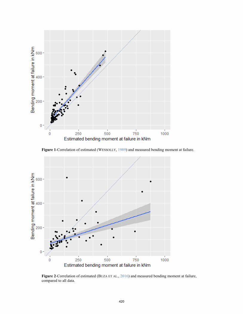
Figure 1-Correlation of estimated (WESSOLLY, 1989) and measured bending moment at failure.

Figure 2-Correlation of estimated (BUZA ET AL., 2016) and measured bending moment at failure, compared to all data.

420

Figure 3-Fit of eq. 2 (red) to the lower part of data (0° to 0.25°), extrapolated up to true failure.

Literature BUZA, Á.K.; DIVÓS, F.; DIVOS, F. 2016. Root Stability Evaluation with Non-Destructive Techniques. ActaSilv Lign Hung 12(2): 125–134, https://doi.org/10.1515/aslh-2016-0011.

COUTTS, M.P. 1983. Root architecture and tree stability. Plant and Soil 71: 171–188, http://www.springerlink.com/index/F6Q2XH81950N1334.pdf.

DAHLE, G.A.; JAMES, K.R.; KANE, B.; GRABOSKY, J.C.; DETTER, A. 2017. A review of factors that affect the static load- bearing capacity of urban trees. Arboriculture and Urban Forestry 43(3): 89–106.

DETTER, A.; RUST, S. 2013. Aktuelle Untersuchungsergebnisse zu Zugversuchen. In Jahrbuch der baumpflege, pp. 9–22.

DUPUY, L.; FOURCAUD, T.; STOKES, A.; DANJON, F. 2005. A density-based approach for the modelling of root architecture: application to Maritime pine (Pinus pinaster Ait.) root systems. Journal of theoretical biology 236(3): 323–34, https://doi.org/10.1016/j.jtbi.2005.03.013.

ESCHE, D.; SCHUMACHER, P.; DETTER, A.; RUST, S. 2018. Experimentelle Überprüfung der Windlastanalyse für statische Zugversuche. In Dujesiefken, D. (ed.), Jahrbuch der baumpflege, pp. 229–236. Braunschweig: Haymarket Media.

RAHARDJO, H.; HARNAS, F.R.; INDRAWAN, I.G.B.; LEONG, E.C.; TAN, P.Y.; FONG, Y.K.; OW, L.F. 2014. Understanding the stability of Samanea saman trees through tree pulling, analytical calculations and numerical models. Urban Forestry and Urban Greening 13(2): 355–364, https://doi.org/10.1016/j.ufug.2013.12.002.

R CORE TEAM. 2018. R: A language and environment for statistical computing. Vienna, Austria: R Foundation for Statistical Computing, https://www.R-project.org/.

WESSOLLY, L. 1989. Zwei neue zerstörungsfreie messverfahren. Das Gartenamt 34: 587–591.

WESSOLLY, L.; ERB, M. 1998. Handbuch der Baumstatik und Baumkontrolle. Berlin: Patzer Verlag.

421

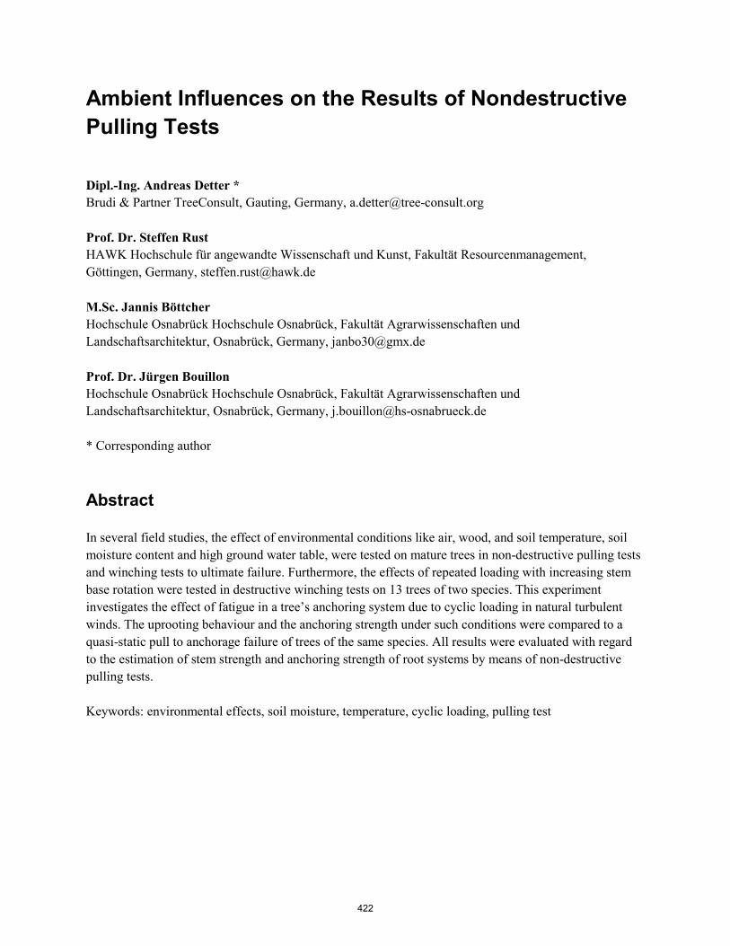
Ambient Influences on the Results of Nondestructive Pulling Tests

Dipl.-Ing. Andreas Detter * Brudi & Partner TreeConsult, Gauting, Germany, a.detter@tree-consult.org

Prof. Dr. Steffen Rust HAWK Hochschule für angewandte Wissenschaft und Kunst, Fakultät Resourcenmanagement, Göttingen, Germany, steffen.rust@hawk.de

M.Sc. Jannis BöttcherHochschule Osnabrück Hochschule Osnabrück, Fakultät Agrarwissenschaften undLandschaftsarchitektur, Osnabrück, Germany, janbo30@gmx.de

Prof. Dr. Jürgen Bouillon Hochschule Osnabrück Hochschule Osnabrück, Fakultät Agrarwissenschaften und Landschaftsarchitektur, Osnabrück, Germany, j.bouillon@hs-osnabrueck.de

* Corresponding author

Abstract

In several field studies, the effect of environmental conditions like air, wood, and soil temperature, soil moisture content and high ground water table, were tested on mature trees in non-destructive pulling tests and winching tests to ultimate failure. Furthermore, the effects of repeated loading with increasing stem base rotation were tested in destructive winching tests on 13 trees of two species. This experiment investigates the effect of fatigue in a tree’s anchoring system due to cyclic loading in natural turbulent winds. The uprooting behaviour and the anchoring strength under such conditions were compared to a quasi-static pull to anchorage failure of trees of the same species. All results were evaluated with regard to the estimation of stem strength and anchoring strength of root systems by means of non-destructive pulling tests.

Keywords: environmental effects, soil moisture, temperature, cyclic loading, pulling test

422

Introduction

Pulling tests are used in arboriculture to non-destructively assess the strength of open grown trees (Sinn and Wessolly 1989). A tree’s strength characteristics can be assessed by applying a moderate non-destructive load with a winch, measuring the tree’s reactions with high-precision sensors for fibre strain and stem base inclination, and extrapolating those data to determine the minimum resistance of the stem against fracture (Wessolly 1991, Detter and Rust 2013, Detter et al. 2014) and anchoring strength of the root system (Wessolly 1996, Detter and Rust 2013, Buza and Divós 2016).

The tests are usually performed under moderate climatic conditions, but the fracture resistance in bending and the anchoring strength of the root system of the subject tree may be challenged by natural storms under more extreme temperatures and humidity. On the other hand, for reasons that are not at the discretion of the appraiser, e.g. to identify a potential immediate hazard, the tests must be carried out during periods with extremely high or low temperatures as well as during droughts or after periods of intense rainfall. How the changes in temperature and soil moisture content affect the load response of the trees in the non-destructive range has not been subject to intensive research so far.

For tomographic and drilling methods it has already been shown that the results can be significantly affected by frost (Rust, 1999, 2003). In Finland and North America, it was found that trees subjected to bending were up to 50 percent stiffer during frost (Silins et al. 2000). Freezing also changed the sway behaviour of standing conifers (Granucci et al. 2012). Schmidt and Pomeroy (1990) found a significant increase in the flexural stiffness of frozen conifer branches. In a moderate climate, Roodbaraky et al. (1994) did not find great variations in load vs. deflection curves for the same trees in different seasons. But from material science it may be expected that the MOE of green wood rises with decreasing wood temperature and decreases with rising wood temperature (Kretschmann 2010).

The effect of temperature on soil properties was described earlier for specific soil types (Jefferson 1994). The anchoring strength of trees is the result of the deformability of the root soil matrix. Temperature may affect the load response of the soil and the wooden body of the roots differently, eventually changing their interaction and the contribution of these components to the uprooting strength of the tree. As soon as the soil is frozen, the increased soil stiffness alters the failure patterns of trees (Peltola et al. 2000).

Material tests on specimen of green wood indicate that above the fibre saturation point changes of moisture content do not affect strength properties (Kretschmann 2010; Niklas and Spatz 2012). Since pulling tests in arboriculture are exclusively performed to assess the strength of living trees, we did not expect an effect on the measured strain values in the stem under bending (Spatz and Pfisterer 2013).

Yet, a strong increase in soil moisture content sometimes significantly affected the stability estimated from non-destructive pulling test during investigations at the Nürtingen University of Applied Sciences (Wohn 2003). Experiments in Japan with a massive irrigation of the root zone showed initially a higher, later reduced stability of forest trees (Kamimura et al. 2011). But in another experiment on soils that are typically not water saturated, soil moisture had very little discernible effect on tree stability until very high levels of soil moisture were reached (Peterson and Classen 2013). In the Netherlands, practitioners of the pulling test method reported that trees growing on sites with high ground water table showed high

423

inclinations at low load levels (Mol and Goederen 2017). Therefore, the standard extrapolation from non-destructive levels of tilt to the anchoring strength of the root system of such trees was questioned.

In addition, the test procedure of a pulling test does not mimic the behaviour of trees during uprooting. In field experiments it was shown that during the failure process, the stem base inclination of the trees increased with each load cycle until the tree finally tipped over (James 2014). For forest trees, it was presumed that the resistance to this cyclic loading was lower than to a single static pull (Jonsson et al. 2006; Leigh 2014; O’Sullivan and Ritchie 1993; Rodgers et al. 1995). But preliminary experiments by Coutts (1983) indicated that uprooting trees by a series of pulls and relaxations rendered similar results to continuous pulling.

We presume that temperature and soil moisture content may affect the load response of trees in the non-destructive range. It is not subject to this paper how the ultimate strength may be altered by those influences. We also investigated how high ground water tables may affect the estimations of stability based on pulling tests and tested if a static pulling test can be adequate to estimate anchorage strength of trees gradually failing in a sequence of increasing cyclic root plate tilt.

Material and Methods

In order to study the effect of such ambient conditions on the result of pulling tests, we conducted a number of experiments on road side trees, urban trees and plantation trees. The experiments reported in the present paper are:

1. Seasonal effects on the results of arboricultural pulling tests2. Effects of wood temperature on apparent flexural stiffness in stem bending3. Rotational stiffness at soil temperatures above and around freezing point4. Differences in rotational stiffness at increased soil moisture content5. Rotational stiffness and anchoring strength of trees growing on water saturated soils6. Uprooting behaviour under cyclic loading with rising inclinations

Each experiment will be briefly described in the following. All sensors used in the experiments are part of the TreeQinetic set (Argus electronics GmbH, Rostock, Germany) which consists of a forcemeter (accuracy 25 N), sensors for fibre strain (Elastometers, accuracy 1 µm) and sensors for root plate tilt (Inclinometers, accuracy 0.002°) as well as a communication unit for wireless data transfer and the measurement software for logging data (Treeqinetic Measure). All pulling tests were carried out according to the Elasto-Inclino-Method or SIM (Wessolly and Erb 2016) following the standard setup (Brudi and Wassenaer 2002, Detter and Rust 2013).

Seasonal effects within 12 months

Pulling tests were carried out with identical setup on a row of 9 mature urban Linden trees (T. x europea) at 5 dates within 12 months from 2011 to 2012 under changing climatic conditions, including summer drought and deep winter frost. The trees had stem diameters at 1 m height between 38 and 56 cm (mean

424

48.4 cm, sd 5.8 cm) and heights between 14 and 20 m (mean 16.9 m, sd 1.6 m). The climatic conditions during each pulling test are listed in Table 1.

Table 1 climatic conditions at pulling tests investigating seasonal effects within 12 months

Property Feb ‘11 June ‘11 Aug ‘11 Nov ‘11 Feb ‘12 mean ambient temperature in °C 13 26 26 10 -10mean air humidity in % 30 43 47 72 61 mean soil temperature in °C 2.3 22.5 22.1 13.9 -3.3Mean soil moisture content in % - 5.0 4.7 6.2 - Mean stem surface temperature 15.9 23.2 26.9 14.9 -14.0

The site has a deep rooting space and the soil consists of a gravel-sand mixture with less than 10% fine grain content. Therefore, the soil has a very low field capacity and was very dry at all times, even though heavy rain occurred prior to the tests in June and November 2011. The pulling tests in February 2012 were preceded by a period of severe frost during which ambient temperature did not exceed -10°C for more than two weeks. Therefore, stems and soil were frozen.

The anchoring strength of the root system and the resistance of the stem against fracture were estimated from the non-destructive pulling test and compared to a wind load estimation as described by Detter & Rust (2013). Safety factors were deducted using Arbostat evaluation software (Arbosafe GmbH, Gauting, Germany) by using the same wind load estimation but evaluating different data from one force meter, 4 Elastometers and 2 Inclinometers for each test date.

Wood temperature

In a nursery near Dachau, Germany, 8 Birch trees (B. pendula) standing in one line were exposed to non-destructive pulling tests on four days between January and July 2012. Diameters at 1 m height ranged from 18 cm to 29 cm and heights from 16.4 to 17.4 m. Air temperature and wood temperature in the stem at a depth of 2 cm below the stem surface were recorded. The wood temperatures in this test series ranged from -21 to 23° C. Two measurements were carried out with frozen wood, one above freezing point with wood temperatures between 2 and 4°C and one with wood temperatures between 17 and 23°C.

Soil temperature

The effect of sinking soil temperature until the freezing point was investigated at of 10 semi-mature Linden trees (T. x europea) growing along a road-side in an urban setting. The mean stem diameters at 1 m height ranged from 34 to 51 cm (mean 39.5 cm, sd 4.2 cm) and tree height from 10 to 13 m (mean 11.6 m, sd 0.8 m). Soil temperature was measured at 4 depths (2, 10, 20 and 30 cm) at the stem base of 3 trees at each test day. Soil moisture content was also measured as a control and ranged from 0.20 in October 2014 to 0.33 in February 2014.

Non-destructive pulling tests were carried out at 7 different dates from October 2014 to February 2015 on all 10 trees. From the load vs. tilt data, the rotational stiffness was derived and the anchorage strength (in kNm) was estimated based on the extrapolation methods described in literature (Detter and Rust 2013, Rust and Detter 2019) using Arbostat evaluation software.

425

Soil moisture content

Seven experimental trees of similar age, size and morphology were selected in a lime tree avenue (T. cordata) along a village road. The trees had diameters ranging from 47 to 67 cm (mean 58.1 cm, sd 6.4 cm) and heights from 13 to 18 m (mean 16.4 m, sd 1.7 m).The natural soil was a loamy brown earth fromPleistocene river sediments, but during the construction of the road, the subsoil was partly replaced bymineral material. In the rooting space between the stem base of the trees and an adjacent meadow, thetopsoil (0-20 cm) contained only little organic matter and about 20 percent clay. From 20 cm downwards,the proportion of organic matter even decreased and the clay content increased to roughly 30 percent.Since the ground has been changed by road construction, high variability in the soil properties occurred.

One series of tests was carried out in September 2011. On every tree non-destructive pulling tests were performed prior and after irrigating the trees. Root plate tilt and applied force were measured continuously. After the irrigation, the same load was exerted as prior to the test and inclination was measured with inclinometers at the same positions as prior to the irrigation. After two weeks, at the beginning of October 2011, the same procedure of pulling tests and irrigation was repeated on every tree.

Since all tested trees had a similar trunk diameter, the trees were uniformly irrigated on an area of 2.5 m x 2.5 m around the stem base. The soil was sufficiently porous to accommodate for 500 l per tree during each watering cycle. The soil was just able to absorb this quantity without water running beyond the irrigated surface. The soil moisture was measured at different depths in a hole (depth 45 cm and diameter 30 cm) drilled with an earth boring device. An electronic moisture meter was pricked into the sides of the borehole at depths of 5, 10, 20, 30, 40 cm, thus determining the volume fraction of water in the soil at the respective depth.

Water saturated soils

In order to assess the stability of trees under water saturated soil conditions, we selected two sets of Hybrid Poplars (P. x canadensis) growing on sites in Northern Germany and The Netherlands. At site 1, the water table was usually 50 cm below surface, but at the time of testing it had fallen to 90 cm due to a sequence of droughts. At site 2, the water table usually reached 30 to 50 cm below ground level and even the top soil was water saturated. In the sandy soil at site 1, roots reached depths of 70 to 120 cm below the surface. On site 2, the clay soil showed a colouration layer at 45 cm depth indicating anaerobic conditions. No roots were growing below this layer. The test trees had diameters ranging from 34 to 84 cm (mean 56.4 cm, sd 12.5 cm) and heights from 25 to 36 m (mean 30.5 m, sd2.8 m). Prior to winching the trees to failure, non-destructive pulling tests were carried out.

Cyclic loading

13 plantation trees were pulled in a sequence of winching tests to rising inclinations in each load cycle. The increments in stem base tilt were roughly 0.25° until the peak tilt either exceeded 2.5° or the maximum load was decreasing in subsequent load cycles. Then, the trees were pulled to primary anchorage failure, i.e. until either the stem base tilt exceeded 5° or the applied load decreased during the load cycle. All trees were growing on Ravenna Silt loam in Shalerville, Ohio, USA, and were roughly 40 years old. Tests were carried out under dry summer conditions within 4 days in 2013.

426

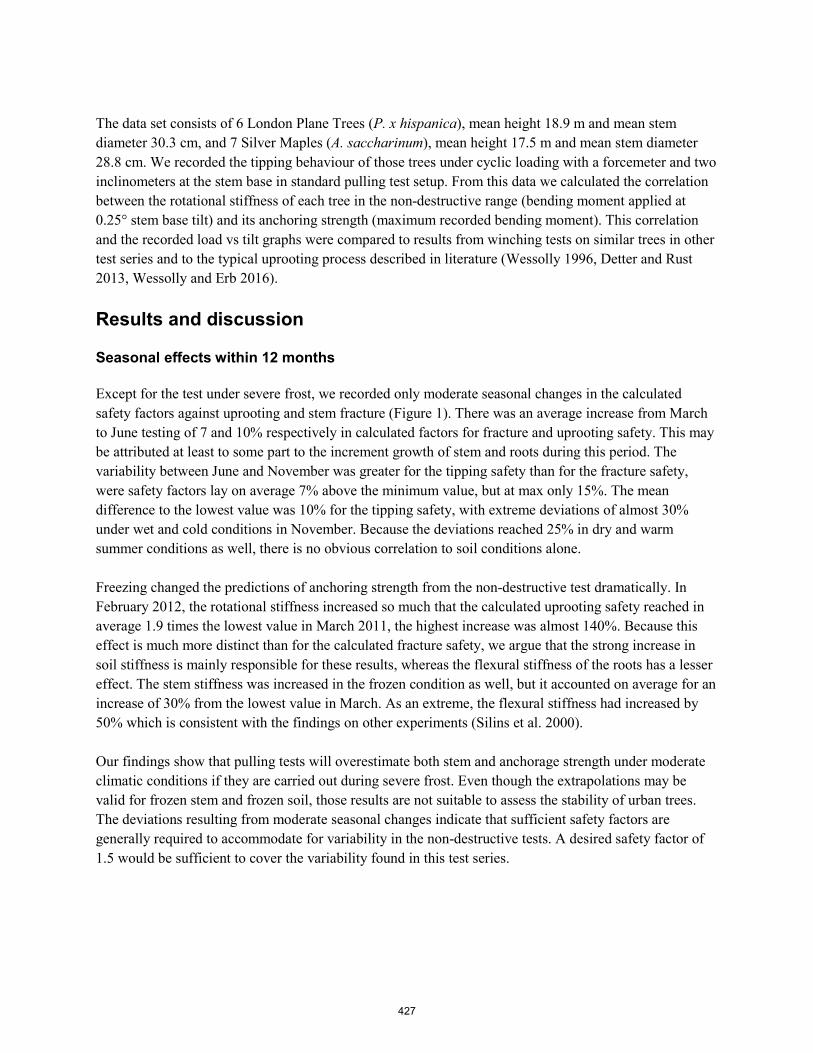
The data set consists of 6 London Plane Trees (P. x hispanica), mean height 18.9 m and mean stem diameter 30.3 cm, and 7 Silver Maples (A. saccharinum), mean height 17.5 m and mean stem diameter 28.8 cm. We recorded the tipping behaviour of those trees under cyclic loading with a forcemeter and two inclinometers at the stem base in standard pulling test setup. From this data we calculated the correlation between the rotational stiffness of each tree in the non-destructive range (bending moment applied at 0.25° stem base tilt) and its anchoring strength (maximum recorded bending moment). This correlation and the recorded load vs tilt graphs were compared to results from winching tests on similar trees in other test series and to the typical uprooting process described in literature (Wessolly 1996, Detter and Rust 2013, Wessolly and Erb 2016).

Results and discussion

Seasonal effects within 12 months

Except for the test under severe frost, we recorded only moderate seasonal changes in the calculated safety factors against uprooting and stem fracture (Figure 1). There was an average increase from March to June testing of 7 and 10% respectively in calculated factors for fracture and uprooting safety. This may be attributed at least to some part to the increment growth of stem and roots during this period. The variability between June and November was greater for the tipping safety than for the fracture safety, were safety factors lay on average 7% above the minimum value, but at max only 15%. The mean difference to the lowest value was 10% for the tipping safety, with extreme deviations of almost 30% under wet and cold conditions in November. Because the deviations reached 25% in dry and warm summer conditions as well, there is no obvious correlation to soil conditions alone.

Freezing changed the predictions of anchoring strength from the non-destructive test dramatically. In February 2012, the rotational stiffness increased so much that the calculated uprooting safety reached in average 1.9 times the lowest value in March 2011, the highest increase was almost 140%. Because this effect is much more distinct than for the calculated fracture safety, we argue that the strong increase in soil stiffness is mainly responsible for these results, whereas the flexural stiffness of the roots has a lesser effect. The stem stiffness was increased in the frozen condition as well, but it accounted on average for an increase of 30% from the lowest value in March. As an extreme, the flexural stiffness had increased by 50% which is consistent with the findings on other experiments (Silins et al. 2000).

Our findings show that pulling tests will overestimate both stem and anchorage strength under moderate climatic conditions if they are carried out during severe frost. Even though the extrapolations may be valid for frozen stem and frozen soil, those results are not suitable to assess the stability of urban trees. The deviations resulting from moderate seasonal changes indicate that sufficient safety factors are generally required to accommodate for variability in the non-destructive tests. A desired safety factor of 1.5 would be sufficient to cover the variability found in this test series.

427

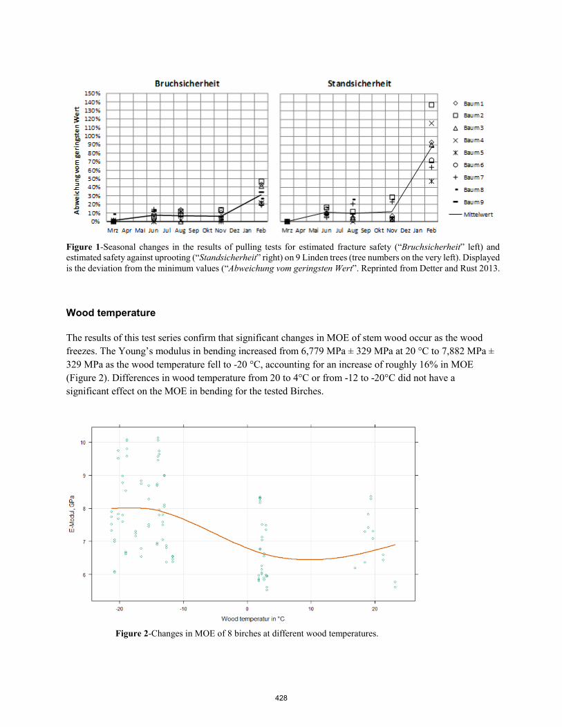
Wood temperature

The results of this test series confirm that significant changes in MOE of stem wood occur as the wood freezes. The Young’s modulus in bending increased from 6,779 MPa ± 329 MPa at 20 °C to 7,882 MPa ± 329 MPa as the wood temperature fell to -20 °C, accounting for an increase of roughly 16% in MOE (Figure 2). Differences in wood temperature from 20 to 4°C or from -12 to -20°C did not have a significant effect on the MOE in bending for the tested Birches.

Figure 2-Changes in MOE of 8 birches at different wood temperatures.

Figure 1-Seasonal changes in the results of pulling tests for estimated fracture safety (“Bruchsicherheit” left) and estimated safety against uprooting (“Standsicherheit” right) on 9 Linden trees (tree numbers on the very left). Displayed is the deviation from the minimum values (“Abweichung vom geringsten Wert”. Reprinted from Detter and Rust 2013.

428

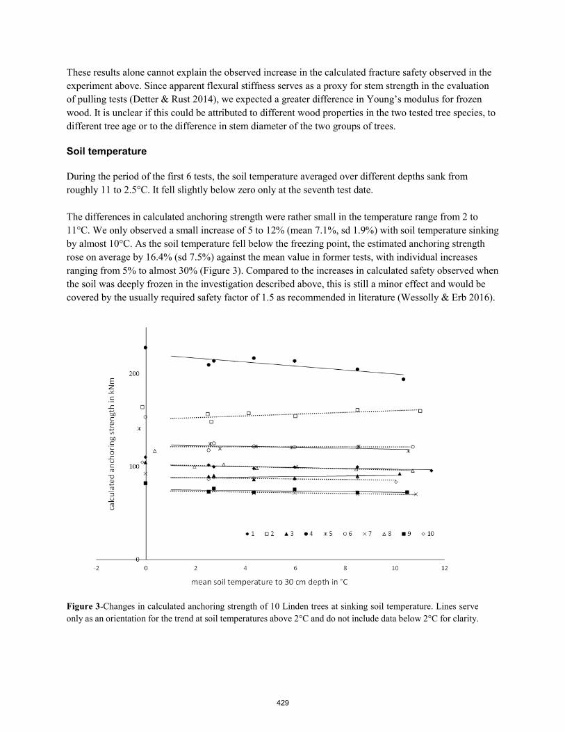
These results alone cannot explain the observed increase in the calculated fracture safety observed in the experiment above. Since apparent flexural stiffness serves as a proxy for stem strength in the evaluation of pulling tests (Detter & Rust 2014), we expected a greater difference in Young’s modulus for frozen wood. It is unclear if this could be attributed to different wood properties in the two tested tree species, to different tree age or to the difference in stem diameter of the two groups of trees.

Soil temperature

During the period of the first 6 tests, the soil temperature averaged over different depths sank from roughly 11 to 2.5°C. It fell slightly below zero only at the seventh test date.

The differences in calculated anchoring strength were rather small in the temperature range from 2 to 11°C. We only observed a small increase of 5 to 12% (mean 7.1%, sd 1.9%) with soil temperature sinking by almost 10°C. As the soil temperature fell below the freezing point, the estimated anchoring strength rose on average by 16.4% (sd 7.5%) against the mean value in former tests, with individual increases ranging from 5% to almost 30% (Figure 3). Compared to the increases in calculated safety observed when the soil was deeply frozen in the investigation described above, this is still a minor effect and would be covered by the usually required safety factor of 1.5 as recommended in literature (Wessolly & Erb 2016).

Figure 3-Changes in calculated anchoring strength of 10 Linden trees at sinking soil temperature. Lines serve only as an orientation for the trend at soil temperatures above 2°C and do not include data below 2°C for clarity.

429

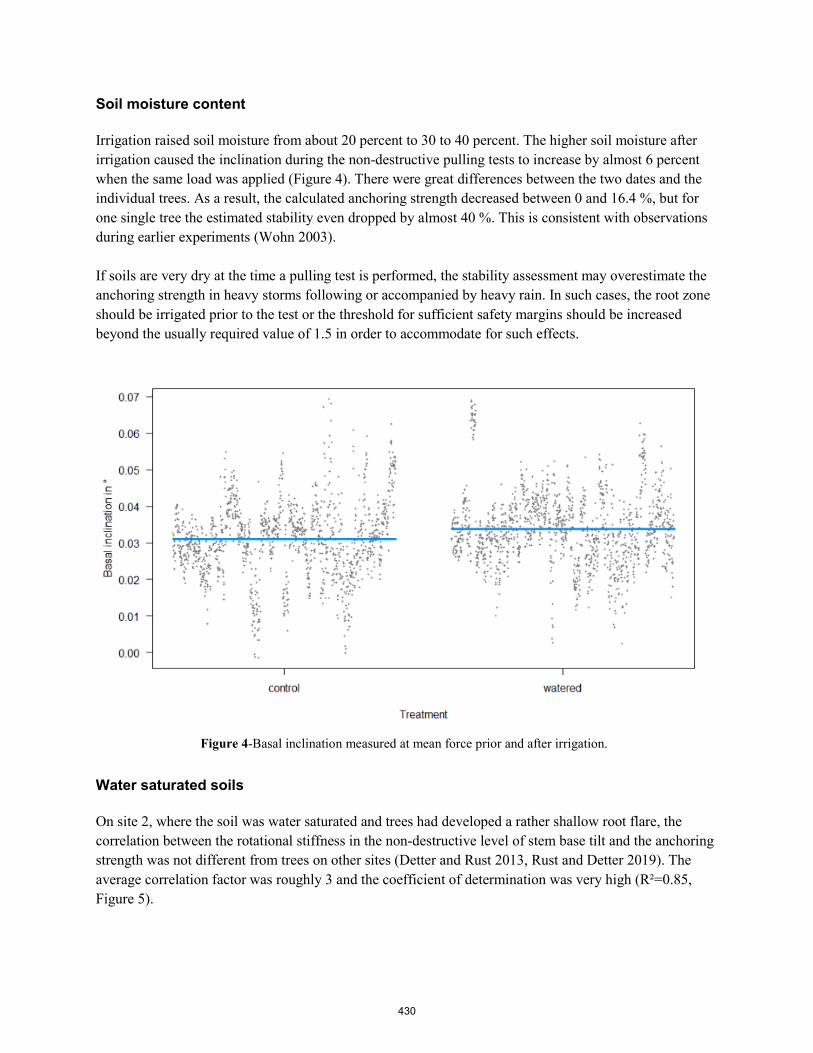
Soil moisture content

Irrigation raised soil moisture from about 20 percent to 30 to 40 percent. The higher soil moisture after irrigation caused the inclination during the non-destructive pulling tests to increase by almost 6 percent when the same load was applied (Figure 4). There were great differences between the two dates and the individual trees. As a result, the calculated anchoring strength decreased between 0 and 16.4 %, but for one single tree the estimated stability even dropped by almost 40 %. This is consistent with observations during earlier experiments (Wohn 2003).

If soils are very dry at the time a pulling test is performed, the stability assessment may overestimate the anchoring strength in heavy storms following or accompanied by heavy rain. In such cases, the root zone should be irrigated prior to the test or the threshold for sufficient safety margins should be increased beyond the usually required value of 1.5 in order to accommodate for such effects.

Water saturated soils

On site 2, where the soil was water saturated and trees had developed a rather shallow root flare, the correlation between the rotational stiffness in the non-destructive level of stem base tilt and the anchoring strength was not different from trees on other sites (Detter and Rust 2013, Rust and Detter 2019). The average correlation factor was roughly 3 and the coefficient of determination was very high (R²=0.85, Figure 5).

Figure 4-Basal inclination measured at mean force prior and after irrigation.

430

For the trees on site 1, where the usually high water table had dropped at the time of testing, the correlation was different from the findings on other sites. While rotational stiffness still was an excellent indicator for anchoring strength (R²=0.98), the correlation factor fell below 2.5. As a consequence, standard extrapolations of anchoring strengths would have slightly overestimated the stability of the tested trees. On average, the anchoring strength fell below the expected value by roughly 10%.

This indicates that changes in the height of the ground water table may affect the predictions from non-destructive pulling tests, but deviations were covered by the regularly required safety margin of 1.5. From practical arboriculture it is understood, that flooding can have a more severe effect on the stability of trees. Especially as the flood level sinks again, trees frequently fall over, presumably as a result of increased deformability of the subsoil serving as a foundation for the anchoring root system.

Cyclic loading

We observed in all trees that the typical uprooting behaviour was resumed in the next loading cycle as soon as the load was reached where the former loading cycle had been aborted. Until this load was reached, the tangent to the load vs. tilt curves (i.e. the momentary rotational stiffness) had a lesser slope than during the last load cycle if the maximum tilt at the stem base had already once exceeded 0.5° in a

Figure 5-Extrapolation factors from rotational stiffness (bending moment at the stem base at 0.25°) to the anchoring strength of the root system (maximum moment at the base) for site 1 (green, Saerbeck) and site 2 (blue, Leeuwarden). The red line indicates the correlation factor proposed in literature (Detter & Rust 2013, Wessolly & Erb 2016).

y = 2,4232x - 14,705R² = 0,9845

y = 3,056x + 58,075R² = 0,8541

0

100

200

300

400

500

600

700

800

900

0 100 200 300 400

Max

imum

ben

ding

mom

ent a

t the

bas

e [k

Nm

]

Bending moment at the base at 0,25° [kNm]

Saerbeckcomplete

Leeuwardencomplete

Linear (Saerbeckcomplete)

Linear(Leeuwardencomplete)

Linear (PrognoseWessolly)

431

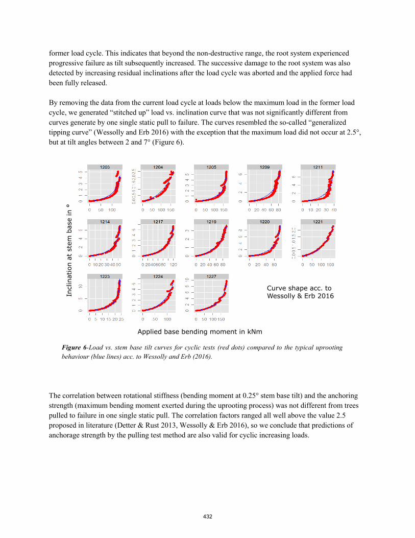
former load cycle. This indicates that beyond the non-destructive range, the root system experienced progressive failure as tilt subsequently increased. The successive damage to the root system was also detected by increasing residual inclinations after the load cycle was aborted and the applied force had been fully released.

By removing the data from the current load cycle at loads below the maximum load in the former load cycle, we generated “stitched up” load vs. inclination curve that was not significantly different from curves generate by one single static pull to failure. The curves resembled the so-called “generalized tipping curve” (Wessolly and Erb 2016) with the exception that the maximum load did not occur at 2.5°, but at tilt angles between 2 and 7° (Figure 6).

The correlation between rotational stiffness (bending moment at 0.25° stem base tilt) and the anchoring strength (maximum bending moment exerted during the uprooting process) was not different from trees pulled to failure in one single static pull. The correlation factors ranged all well above the value 2.5 proposed in literature (Detter & Rust 2013, Wessolly & Erb 2016), so we conclude that predictions of anchorage strength by the pulling test method are also valid for cyclic increasing loads.

Figure 6-Load vs. stem base tilt curves for cyclic tests (red dots) compared to the typical uprooting behaviour (blue lines) acc. to Wessolly and Erb (2016).

Applied base bending moment in kNm

Incl

inat

ion

at s

tem

base

in °

Curve shape acc. toWessolly & Erb 2016

432

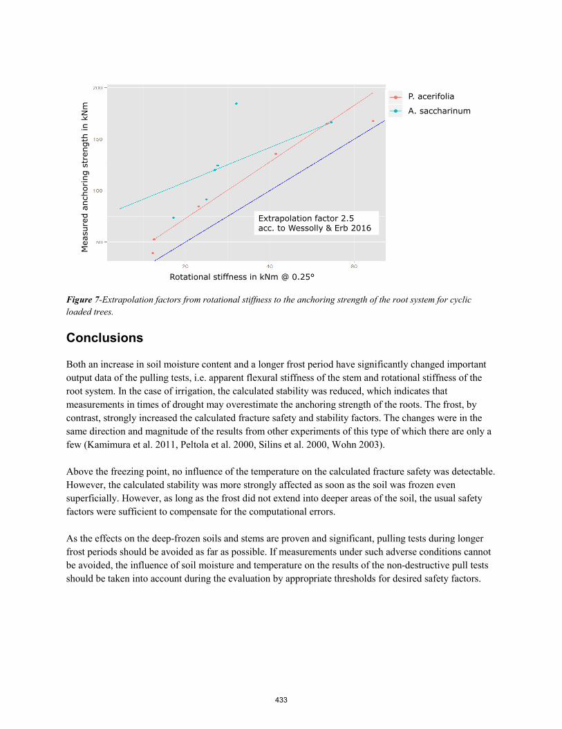
Conclusions

Both an increase in soil moisture content and a longer frost period have significantly changed important output data of the pulling tests, i.e. apparent flexural stiffness of the stem and rotational stiffness of the root system. In the case of irrigation, the calculated stability was reduced, which indicates that measurements in times of drought may overestimate the anchoring strength of the roots. The frost, by contrast, strongly increased the calculated fracture safety and stability factors. The changes were in the same direction and magnitude of the results from other experiments of this type of which there are only a few (Kamimura et al. 2011, Peltola et al. 2000, Silins et al. 2000, Wohn 2003).

Above the freezing point, no influence of the temperature on the calculated fracture safety was detectable. However, the calculated stability was more strongly affected as soon as the soil was frozen even superficially. However, as long as the frost did not extend into deeper areas of the soil, the usual safety factors were sufficient to compensate for the computational errors.

As the effects on the deep-frozen soils and stems are proven and significant, pulling tests during longer frost periods should be avoided as far as possible. If measurements under such adverse conditions cannot be avoided, the influence of soil moisture and temperature on the results of the non-destructive pull tests should be taken into account during the evaluation by appropriate thresholds for desired safety factors.

Figure 7-Extrapolation factors from rotational stiffness to the anchoring strength of the root system for cyclic loaded trees.

Rotational stiffness in kNm @ 0.25°

Mea

sure

dan

chor

ing

stre

ngth

in k

Nm

Extrapolation factor 2.5 acc. to Wessolly & Erb 2016

P. acerifolia

A. saccharinum

433

Acknowledgements

Without the support of numerous colleagues, arborists and other helpers the experiments would not have been possible. Thank you for your contribution! We would also like to thank all students involved in these projects, especially Ph. Michaelis, Chr. Scharl and V. Graf at the University of Applied Sciences Weihenstephan as well as Chr. Fuchs, B. Schirutschke and B. Mohrbach at HAWK Göttingen. Thank you for making these experiements the topic of your theses and for putting so much effort into these projects. Furthermore we would like to thank Prof. Dr. F. Luz at the University of Applied Sciences Weihenstephan for the fruitful and long lasting cooperation. One experiment was carried out at the second Tree Biomechanics Research Week 2013 in Ohio which was organised by the International Society of Arboriculture and funded by the TREE Fund and several other donors. Part of this work was funded by the German Ministry of Education and Research (research grant 17021X11).

References

Brudi, E., & Wassenaer, P. van. (2002). Trees and statics: Non-destructive failure analysis. How trees stand up and fall down. Tree structure and mechanics conference proceedings, 5369. Savannah, Georgia.

Buza, Á. K., & Divós, F. (2016). Root Stability Evaluation with Non-Destructive Techniques. Acta Silvatica et Lignaria Hungarica, 12(2), 125–134.

Coutts, M. P. (1983). Root architecture and tree stability. Plant and Soil, (71), 171―188.

Detter A. and S. Rust (2013). Aktuelle Untersuchungsergebnisse zu Zugversuchen. In: Dujesiefken, D. (ed.) (2013). Jahrbuch der Baumpflege 2013

Detter, A., Rust, S., Rust, C., & Maybaum, G. (2014). Determining strength limits for standing tree stems from bending tests. 18th international nondestructive testing and evaluation of wood symposium. Madison, USA.

Granucci, D., Rudnicki, M., Hiscox, A., Miller, D., & Su, H.-B. (2012). Quantifying the effects of freezing on tree sway frequencies. Agricultural and Forest Meteorology, 168, 10–14.

James, K. (2014). Tree Stability in Wind Storms. Presentation at the UK Arboricultural conference on 14th to 17th September 2014 in Royal Holloway, Egham, Surrey

Jefferson, I. (1994). Temperature effects on clay soils. Diss. Loughborough University of Technology.

Jonsson, M. J., Foetzki, A., Kalberer, M., Lundström, T., Ammann, W., & Stöckli, V. (2006). Root-soil rotation stiffness of Norway spruce (Picea abies (L.) Karst) growing on subalpine forested slopes. Plant and Soil, 285(1–2), 267–277.

434

Kamimura, K., K. Kitagawa, S. Saito und H. Mizunaga (2011). Root anchorage of hinoki (Chamaecyparis obtuse (Sieb. et Zucc.) Endl.) under the combined loading of wind and rapidly supplied water on soil: analyses based on tree-pulling experiments. In: European Journal of Forest Research 131.1, S. 219–227.

Kretschmann, D. (2010). Mechanical Properties of Wood. In Wood Handbookâ”Wood as an Engineering Material (S. 508).

Leigh, W. B. (2014). Low Cycle Fatigue Failure of a Sitka Spruce Tree in Hurricane Winds. Arboriculture & Urban Forestry, 40(5), 272–285.

Mol, M. de and D. de Goederen (2017). pers. comm.

Niklas, K. J., & Spatz, H.-Ch. (2012). Plant Physics. Chicago: The University of Chicago Press.

O’Sullivan, M. F., & Ritchie, R. M. (1993). Tree Stability in Relation to Cyclic Loading. Forestry: An International Journal of Forest Research, 66(1), 69–82.

Peltola, H., S. Kellomäki, A. Hassinen und M. Granander (2000). Mechanical stability of Scots pine, Norway spruce and birch: an analysis of tree-pulling experiments in Finland. In: Forest Ecology and Management 135.1-3, S. 143–153.

Peterson, C. J., & Classen, V. (2013). An evaluation of the stability of Quercus lobata and Populus fremontii on river levees assessed using static winching tests. Forestry, 86(2), 201–209.

Rodgers, M., Casey, A., McMenamin, C., & Hendrick, E. (1995). An experimental investigation of the effects of dynamic loading on coniferous trees planted on wet mineral soils. Wind and Trees, 204–219.

Roodbaraky, H. J., Baker, C. J., Dawson, A. R., & J, W. C. (1994). Experimental observations of the aerodynamic characteristics of urban trees. Journal of Wind Engineering and Industrial Aerodynamics, 52, 171–184.

Rust, S. (1999). Comparison of three Methods for determining the conductive Xylem Area of Scots pine (Pinus sylvestris L.) In: Forestry 72, S. 103–108.

Rust, S. (2003). Baumdiagnose bei Frost. In: Grünforum LA 33(5), S. 36–38.

Rust, S. and Detter, A. (2019). Experimental test of non-destructive methods to assess the anchorage of urban trees. 21st international nondestructive testing and evaluation of wood symposium. Freiburg, Germany (this issue)

Schmidt RA and Pomeroy JW (1990). Bending of a conifer branch at subfreezing temperatures: implications for snow interception. Can J For Res 20:1250–1253

435

Silins, U., Lieffers, V. J., & Bach, L. (2000). The effect of temperature on mechanical properties of standing lodgepole pine trees. Trees - Structure and Function, 14(8), 424-428.

Sinn, G., & Wessolly, L. (1989). A Contribution to the Proper Assessment of the Strength and Stability of. Trees. Arboricultural Journal, 13, 45―65.

Spatz, H.-Chr., & Pfisterer, J. (2013). Mechanical Properties of Green Wood and Their Relevance for Tree Risk Assessment. Arboriculture & Urban Forestry, 39(5), 218–225.

Wessolly, L. (1991). Verfahren zur Bestimmung der Stand- und Bruchsicherheit von Bäumen. Holz als Roh- und Werkstoff, 49, 99–104.

Wessolly, L. (1996). Standsicherheit von Bäumen. Der Kippvorgang ist geklärt. Stadt und Grün, (4), 268―272.

Wessolly, L., & Erb, M. (2016). Manual of tree statics and tree inspection. Patzer-Verlag GmbH & Co. KG.

Wohn, J. 2003. Untersuchungen zur Standsicherheit von Bäumen bei Wassergehaltsänderungen im Boden. Diplomarbeit at FH Nürtingen. Nürtingen.

436

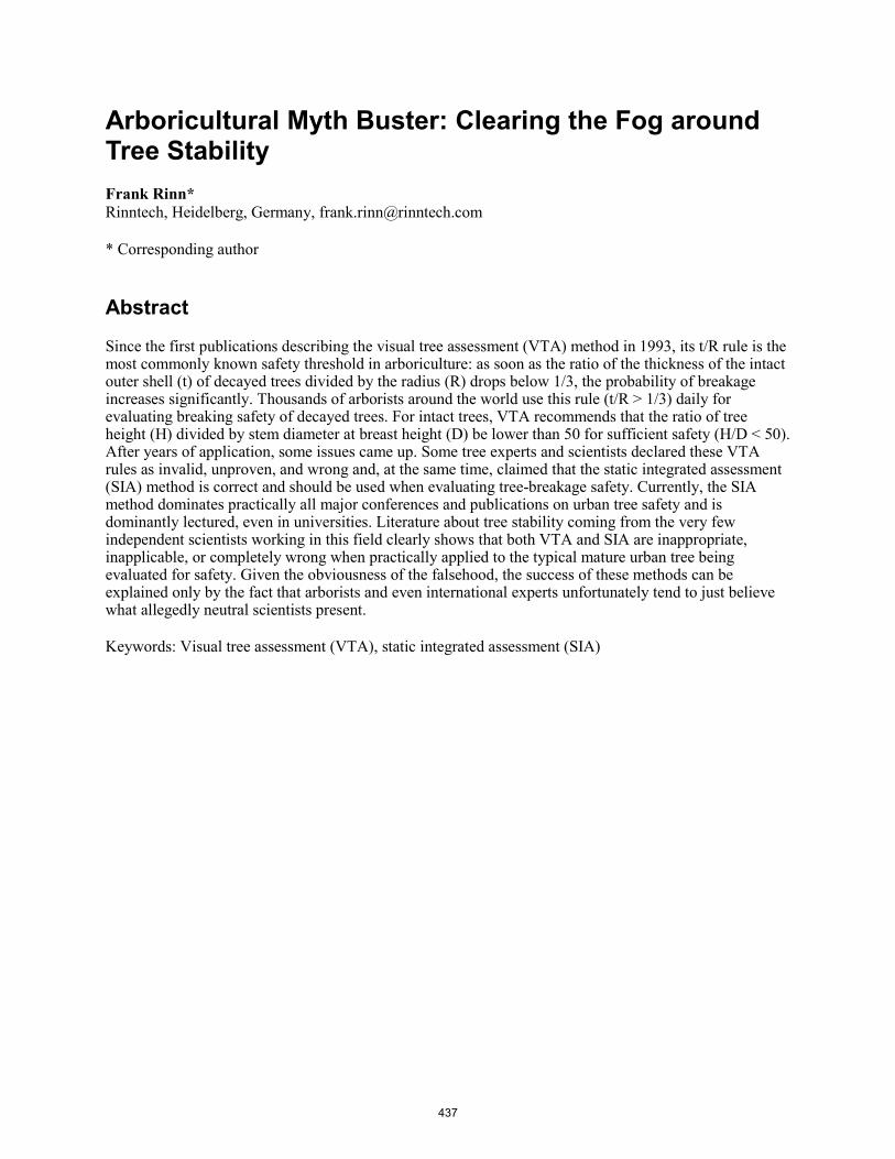
Arboricultural Myth Buster: Clearing the Fog around Tree Stability Frank Rinn* Rinntech, Heidelberg, Germany, frank.rinn@rinntech.com * Corresponding author Abstract Since the first publications describing the visual tree assessment (VTA) method in 1993, its t/R rule is the most commonly known safety threshold in arboriculture: as soon as the ratio of the thickness of the intact outer shell (t) of decayed trees divided by the radius (R) drops below 1/3, the probability of breakage increases significantly. Thousands of arborists around the world use this rule (t/R > 1/3) daily for evaluating breaking safety of decayed trees. For intact trees, VTA recommends that the ratio of tree height (H) divided by stem diameter at breast height (D) be lower than 50 for sufficient safety (H/D < 50). After years of application, some issues came up. Some tree experts and scientists declared these VTA rules as invalid, unproven, and wrong and, at the same time, claimed that the static integrated assessment (SIA) method is correct and should be used when evaluating tree-breakage safety. Currently, the SIA method dominates practically all major conferences and publications on urban tree safety and is dominantly lectured, even in universities. Literature about tree stability coming from the very few independent scientists working in this field clearly shows that both VTA and SIA are inappropriate, inapplicable, or completely wrong when practically applied to the typical mature urban tree being evaluated for safety. Given the obviousness of the falsehood, the success of these methods can be explained only by the fact that arborists and even international experts unfortunately tend to just believe what allegedly neutral scientists present. Keywords: Visual tree assessment (VTA), static integrated assessment (SIA)

437

Ultrasound Test for Root and Branch Wood Elastomechanical Characterization Raquel Gonçalves* Laboratory of Nondestructive Testing - LabEND, School of Agricultural Engineering - FEAGRI - University of Campinas – UNICAMP, Brazil. E-mail: raquelg@unicamp.br * Corresponding author

Gustavo Henrique Lopes Garcia Laboratory of Nondestructive Testing - LabEND, School of Agricultural Engineering - FEAGRI - University of Campinas – UNICAMP, Brazil. E-mail: Gustavo.garcia@gmail.com

Nina Maria Ornelas Cavalcanti Laboratory of Nondestructive Testing - LabEND, School of Agricultural Engineering - FEAGRI - University of Campinas – UNICAMP, Brazil. E-mail: nina.cavalcanti@gmail.com

Sergio Brazolin Center for Forest Resource Technologies, Institute for Technological Research – IPT, São Paulo, Brazil E-mail: brazolin@ipt.br

Cinthya Bertoldo Laboratory of Nondestructive Testing - LabEND, School of Agricultural Engineering - FEAGRI - University of Campinas – UNICAMP, Brazil. E-mail: cinthya.bertoldo@feagri.unicamp.br

Abstract The lack of knowledge about the mechanical properties of wood from species used in urban arborization and of green wood has been an important obstacle to the development of studies related to biomechanics. This lack of knowledge is related to the small or nonexistent commercial appeal of these species and of the green moisture condition because they are not important for the construction sector, which is the primary area of demand for mechanical properties. This lack of knowledge is even worse for wood from branches and roots. The objective of this study was to verify the applicability and preliminary results of an ultrasound methodology for the complete characterization of root and branches wood. The tests utilized four species: Gallesia integrifólia, Swietenia sp., Schinus molle and Acrocarpus fraxinifolius. The results show expected elastic ratios between properties. The ultrasound tests allow obtain 12 elastic constants of root and brunch wood and, because only one specimen is required, the methodology is feasible for these parts of the tree, that present smaller dimension compared with trunk.

Keywords: Ultrasound test;Wood root stiffness, wood branch stiffness

438

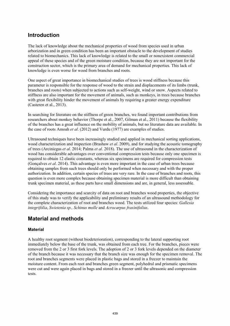
Introduction

The lack of knowledge about the mechanical properties of wood from species used in urban arborization and in green condition has been an important obstacle to the development of studies related to biomechanics. This lack of knowledge is related to the small or nonexistent commercial appeal of these species and of the green moisture condition, because they are not important for the construction sector, which is the primary area of demand for mechanical properties. This lack of knowledge is even worse for wood from branches and roots.

One aspect of great importance in biomechanical studies of trees is wood stiffness because this parameter is responsible for the response of wood to the strain and displacements of its limbs (trunk, branches and roots) when subjected to actions such as self-weight, wind or snow. Aspects related to stiffness are also important for the movement of animals, such as monkeys, in trees because branches with great flexibility hinder the movement of animals by requiring a greater energy expenditure (Casteren et al., 2013).

In searching for literature on the stiffness of green branches, we found important contributions from researchers about monkey behavior (Thorpe et al., 2007, Gilman et al., 2011) because the flexibility of the branches has a great influence on the mobility of animals, but no literature data are available. In the case of roots Amoah et al. (2012) and Vurdu (1977) are examples of studies.

Ultrasound techniques have been increasingly studied and applied in mechanical sorting applications, wood characterization and inspection (Brashaw et al. 2009), and for studying the acoustic tomography of trees (Arciniegas et al. 2014; Palma et al. 2018). The use of ultrasound in the characterization of wood has considerable advantages over conventional compression tests because only one specimen is required to obtain 12 elastic constants, whereas six specimens are required for compression tests (Gonçalves et al. 2014). This advantage is even more important in the case of urban trees because obtaining samples from such trees should only be performed when necessary and with the proper authorization. In addition, certain species of trees are very rare. In the case of branches and roots, this question is even more complex because obtaining specimen material is more difficult than obtaining trunk specimen material, as these parts have small dimensions and are, in general, less assessable.

Considering the importance and scarcity of data on root and branches wood properties, the objective of this study was to verify the applicability and preliminary results of an ultrasound methodology for the complete characterization of root and branches wood. The tests utilized four species: Gallesia integrifólia, Swietenia sp., Schinus molle and Acrocarpus fraxinifolius.

Material and methods

Material

A healthy root segment (without biodeterioration), corresponding to the lateral supporting root immediately below the base of the trunk, was obtained from each tree. For the branches, pieces were removed from the 2 or 3 first fork levels. The adoption of 2 or 3 fork levels depended on the diameter of the branch because it was necessary that the branch size was enough for the specimen removal. The root and branches segments were placed in plastic bags and stored in a freezer to maintain the moisture content. From each root and branches green segment, polyhedral and prismatic specimens were cut and were again placed in bags and stored in a freezer until the ultrasonic and compression tests.

439

Ultrasound tests

The polyhedral specimens, with 26 faces and 50-mm edges, were subjected to ultrasound tests. For the compression tests, the prismatic specimens, with dimensions corresponding to standard proportions (height = three times the edge of transversal sections), as indicated in the Brazilian Standard NBR 7190 (1997), were adopted. To facilitate the bonding of the strain gauges, a minimum nominal size of 30 mm × 30 mm × 90 mm was adopted.

For the ultrasound test, the longitudinal transducers were positioned on the specimen faces, parallel to the axis, allowing the propagation and polarization of the wave on the main axes: L (longitudinal), R (radial) or T (tangential). From these tests, the velocities VLL, VRR and VTT were obtained. Similarly, the shear transducers were positioned on the same faces of the specimen, allowing propagation on one of the main axes, L, R or T, and perpendicular polarization. With these measurements, we calculated the velocities VLR, VLT, VRL, VRT, VTR and VRT. Considering the theoretical aspects related to the symmetries of stresses and strain expected in orthotropic materials, the velocities Vij should be equal to Vji. In practice, there are small differences because the growth rings are not perfectly positioned nor totally free of curvature in the transverse section of the specimens. Thus, for the calculations, the average of the velocities obtained in Vij and Vji is adopted. To obtain the velocities outside the symmetry axes, the transducers were positioned on the inclined faces to each of the planes. Using the velocities obtained in the tests carried out along the symmetry axes (straight faces of the specimens), the stiffness coefficients of the diagonal of the matrix (Equation 1) were calculated.

Cii = ρ.Vii2 Eq 1

where i = 1, 2, 3, 4, 5 and 6; ρ = density; and V = velocity of wave propagation.

The 3 off-diagonal terms (C12, C13 and C23) were obtained using the Christoffel equations (Eqs 2, 3 and 4). For this, the velocities obtained in the inclined faces of the polyhedron, as previously described, were used.

(C12 + C66) n1 n2 = ± [(C11 n12 + C66 n2

2 - ρ Vα 2) (C66 n12 + C22 n2

2 - ρ Vα 2)]1/2 Eq 2

(C23 + C44) n2 n3 = ± [(C22 n22 + C44 n3

2 - ρ Vα 2) (C44 n22 + C33 n3

2 - ρ Vα 2)]1/2 Eq 3

(C13 + C55) n1 n3 = ± [(C11 n12 + C55 n3

2 - ρ Vα 2) (C55 n12 + C33 n3

2 - ρ Vα 2)]1/2 Eq 4

where α = wave propagation angle (out of symmetric axes); n1 = cos α, n2 = sen α and n3 = 0 if α is taken with respect to axis 1 (Plane 12); n1 = cos α, n3 = sen α and n2 = 0 if α is taken with respect to axis 1 (Plane 13); and n2 = cos α, n3 = sen α and n1 = 0 if α is taken with respect to axis 2 (Plane 23).

The stiffness matrix was reversed to obtain the compliance matrix, and all the elastic parameters of the wood in the branches were calculated according to elasticity theory.

Compression tests

The compression tests were performed in a universal test machine (DL 30000, EMIC, Brazil) only in longitudinal direction. The strain was obtained using electric resistance strain gauges (KFG-5-120-C1-11, KYOWA, Japan) with a length of 5 mm, gage factor of 2.10 +/- 1.0% and gage resistance of 119.8 +/- 0.2 Ω. For each direction, strain gauges were attached to two parallel faces of the specimen. Both the load cell and the terminals of the strain gauges were coupled to a data acquisition system (Spider8, HBM, Germany) that allowed automated readings of load and strain. The test methodology (speed and load cycles) was performed according to ABNT (NBR 7190, 1997). The Young’s moduli in the longitudinal direction (EL) were determined from the slope of the stress/strain curve (σL/εL), and the data were fitted such that the curve was linear in a section between approximately 20% and 60%

440

of the maximum stress with a determination coefficient (R2) above 0.99 (UNE 56535). The Poisson ratio was calculated from the relations between the radial and longitudinal strain (υLR) and between the tangential and longitudinal strain (υLT) within the same linear stretch.

Basic density

The same specimens used for the compression test were used for the determination of basic density. Therefore, the basic density of wood from branches and roots was calculated using the relation between the green volume and oven-dried mass.

Results analysis

The parameters obtained from the ultrasound and compression tests were initially analyzed considering, if available, values from the literature. Because of the scarcity of data on the wood parameters for tree branches and roots of urban tree species, the results were also analyzed using relationships between parameters proposed considering the expected behavior of the wood. This procedure allows evaluation of the presence of distorted results or results that are far from the expected values, according to theoretical conditions of the material.

Results

Density

The density variation in the branch pieces removed from different fork levels was not statistically significant (P-value = 0.44). Numerically, the tree density slightly increased from the first (458 kg.m-

3) to the second fork level (463 kg.m-3) and decreased in the third level (428 kg.m-3). Densityvariations along the axes of branches are compatible with the results from analyses of anatomicalvariations in the axial direction of the branch (Bhat et al., 1989; Gartner, 1995; He and Deane, 2016),including those related to the location of the reaction wood and branch hydraulic functions.

For roots, the average basic density was near 85% higher than that obtained for branches. Amoah et al. (2012) investigated the physical and mechanical properties of branch, stem, and root wood from the tropical trees Iroko (Milicia excelsa) and Emire (Terminalia ivorensis) and concluded that the root woods of both species exhibited the highest basic densities compared with those of branch and trunk. The same results were obtained by Lemay et al. (2018), who showed that the density of the root wood of the black spruce (Picea mariana) was higher than that of the trunk wood. These authors argued that the greater density protects the xylem of the roots, which present higher hydraulic stress, thereby avoiding the process of cavitation (Cavalcanti et al. 2018).

Modulus of Elasticity

The individual results for the longitudinal elastic moduli (EL) of the tree branches on different species obtained by ultrasound varied from 1675 to 6522 MPa, while those obtained by static compression varied from 2100 to 6600 MPa. These results are comparable, in order of magnitude, with those obtained by Casteren et al. (2013), who studied 30 green branches from 10 species of tropical hardwood, of which the longitudinal elastic modulus obtained in static bending tests (EM) ranged from 900 to 4000 MPa. For roots the average EL obtained among species by ultrasound vary from 5000 to 10000 MPa and by compression test from 4800 to 6200 MPa. As obtained for basic density, the EL was greater for roots than for branches but the differences were superior for the EL obtained by ultrasound (near 80%) than by compression test (near 30%).

441

Elastic constants

One way to validate the results is to verify the existence of discrepant results using ranges of expected values for relations between the terms of the compliance matrix. These expected relations are proposed considering the theoretical bases that govern the behavior of the wood. For the longitudinal and shear modulus of elasticity, it was verified that there was no discrepancy between the relationships obtained in this research and the relationships proposed in the literature both for roots and branches (Table 1).

Table 1 - Relationship between the terms of the compliance matrix (10-5) obtained in this research using ultrasound tests and the interval obtained by other authors for wood from branches (first line) and roots (second line)

Specie/Literature source EL/ET ER/ET GLR/GRT GLT/GRT EL/GLR

Swietenia sp 14.6 10.4

1.4 1.2

4.6 4.6

3.3 3.4

8.8 6.9

Gallesia integrifolia 12.0 10.9

1.2 1.3

4.0 3.0

3.1 2.6

8.7 9.5

Schinus molle 7.4 6.5

1.4 1.1

3.3 2.8

2.2 2.1

6.6 7.2

Acrocarpus fraxinifolius 12.6 8.4

1.4 1.6

5.4 3.6

4.3 2.6

8.4 6.0

Bucur (2006)* 4.5 to 33.1 1.0 to 2.1 2.9 to 16.9 2.4 to 13.1 4.9 to 7.6

Bodig and Jayne (1982)** 20 1.6 10 9.4 14

Preziosa et al. (1981)*** 7.1 to 8.5 1.5 to 1.7 2.3 to 5.4 1.8 to4.4 6.8 to 9.8 *Tulip tree, Oak, Beech and Douglas fir**Proposed values***Oak and Douglas fir

Concerning the Poisson ratios, Bodig and Jayne (1982) indicate that lower values should be obtained for υRL and υTL (0.040 and 0.027 as references) while a larger value should be obtained for υRT (0.67 as a reference). For υLR and υTR, Bodig and Jayne (1982) proposed reference values for hardwood of υLT = 0.50, υLR = 0.37, and υTR = 0.33. In any method, there is an inherent difficulty in obtaining reliable Poisson ratios for wood, especially in the case of υRL and υTL because they are very small (Bodig and Jayne, 1982) and in all cases because they require that the growth rings are very well aligned with the axes and as straight as possible on the transverse section. Therefore, the values obtained in this research using ultrasound and compression tests may be considered adequate for both, branches and roots.

Ultrasound and Compression tests

For branches, the longitudinal elastic moduli obtained from the ultrasound tests were statistically equivalent to those obtained from the compression tests for Swietenia sp. and Acrocarpus fraxinifolius. For Swietenia sp., it is important to highlight the great variability of the results from the static compression test, which may have contributed to the statistical equivalence. The Poisson ratio υLR obtained by ultrasound and compression test was not statistically equivalent for the specie Schinus molle, while υLT obtained by ultrasound and compression test was statistically equivalent for all species. However, it is also important to highlight the high variability of these parameters.

For roots the longitudinal modulus of elasticity (EL) obtained by ultrasound and compression tests was statistically equivalent (at 95% confidence) to Schinus mole, Gallesia integrifolia and Acrocarpus

442

fraxinifolius. Except for υLR in Swietenia sp., the Poisson ratios obtained by ultrasound were statistically equivalent to those obtained by compression test at the 95% confidence level.

Considering the practical aspects of applying the methodologies used to characterize branch wood, the ultrasound test is simpler and more inexpensive than the other tests, but the preparation of the test specimen is more complex (polyhedron x prism). The use of strain gages requires a gage bonding step and cable soldering, which is laborious and requires extra time. In addition, when testing green wood, it is necessary to carry out the bonding and the test sequentially to avoid drying the wood because it is not possible to saturate the specimen with the gages. Additional care should be taken with the glue because the wood has a high moisture content. Finally, there were many problems with the operation of the gages, making it impossible to use automated spreadsheets to calculate the elastic modulus and Poisson ratios because a detailed and individualized analysis of the results is necessary to eliminate bad results. It is possible that, despite the careful analysis, the moisture content affected the glue in some cases.

Conclusions 1.The elastic ratios for properties of root and branch wood are consistent with the expected valuesbased on their orthotropic behavior and the anatomic structure of wood in general. This result showsthat the ultrasound test had a consistent result.2.The root densities and the root longitudinal modulus of elasticity (EL) are higher than branch densityand EL of same species of wood.3.Ultrasound tests has potential to be used to obtain the stiffness properties of roots and branches. Theultrasonic test, as presented, allows 12 elastic constants of root and branch wood to be obtained and isfeasible for these parts of the tree, with less volume of material available, because only one specimenis required.

Acknowledgment

The authors would like to thank the Sao Paulo Research Foundation (FAPESP), São Paulo, Brazil (Proc. 2015/05692-3 and Proc. 2019/09748-4) for the research funding and for the support to participate in the Symposium and National Council for Scientific and Technological Development (CNPQ – Proc. 131331/2017-5) and Coordination for the Improvement of Higher Education Personnel (Capes) for the scholarships.

Reference list

ASSOCIAÇÃO BRASILIERA DE NORMAS TÉCNICAS. 1997. NBR 7190: Projeto de estruturas de madeira. Rio de Janeiro, 107 p.

Amoah, M., Appiah-Yeboahand, R., and Okai, R. (2012). “ Characterization of physical and mechanical properties of branch, stem and root wood of iroko and emire tropical trees,” Research Journal of Applied Sciences, Engineering and Technology 4(12), 1755-1761.

Arciniegas, A., Prieto, F., Brancheriau, L., and Lasaygues, P. (2014). “Literature review of acoustic and ultrasonic tomography in standing trees,” Trees 28(6), 1559-1567. DOI: 10.1007/s00468-014-1062-6

Bhat KM. Bhat KV. Dhamodaran TK. 1989: Fiber length variation in steam and branches of eleven tropical hardwoods. IAWA Journal 10(1): 63-70.

Bodig, J., and Jayne, B. A. (1982). Mechanics of Wood and Wood Composites, Van Nostrand Reinhold Company, New York, USA

Brashaw, B. K., Bucur, V., Divos, F., Gonçalves, R., Lu, J., Meder, R., Pellerin, R. F., Potter, S.,

443

Ross, R. J., Wang, X., and Yin, Y. (2009). “Nondestructive testing and evaluation of wood: A worldwide research update,” Forest Products J. 59(3) 7-14.

Cavalcanti, N. M. O., Gonçalves, R., Brazolin, S., Bertholdo, C., Ruy, M. (2018). Ultrasound test for root wood elastomechanical characterization. Bioresources 13(3), 5818-5835.

Gartner BL. 1995. Patterns of xylem variation within a tree and their hydraulic and mechanical consequences. In: Gartner, B.L. (Ed.), Plant Stems: Physiology and Functional Morphology. Academic Press, San Diego, 125–149.

Gilman CA, Bartlett MD, Gillis GB, Irschick DJ. 2011. Total recoil: Perch compliance alters jumping performance and kinematics in green anole lizards (Anolis carolinensis). Journal of Experimental Biology 215: 220–226.

Gonçalves R, Trinca AJ, Pellis BP. 2014. Elastic constants of wood determined by ultrasound using three geometries of specimens. Wood Science and Technology 48: 269 - 287. https://doi.org/10.1007/s00226-013-0598-8

He D, Deane DC. 2016. The relationship between trunk and twigwood density shifts with tree size and species stature. Forest Ecology and Management 372: 137-142.

Lemay, A., Krause, C., and Achim, A. (2018). “Comparison of wood density in roots and stem of black spruce before and after commercial thinning,” For. Ecol. Manage. 408, 94-102. DOI: 10.1016/j.foreco.2017.10.042

Palma, S. A., Gonçalves, R., Trinca, A. J., Costa, C. P., Reis, M. N., Martins, G. A. (2018). Interference from knots, wave propagation direction and effect of juvenile and reaction wood on velocities in ultrasound tomograhpy. Bioresources 13(2), 2834-2845.

Thorpe SKS, Crompton RH, Alexander R McN. 2007. Orangutans use compliant branches to lower the energetic cost of locomotion. Biology Letters 3, 253 – 256. DOI: 10.1098/rsbl.2007.0049

Vurdu, R. (1977) “Anatomical characteristics of stem, branch and root wood in European black alder (Alnus glutinosa L. Gaertn.)”. Iowa State University.

444

Session 6

Structure Condition Assessment

445

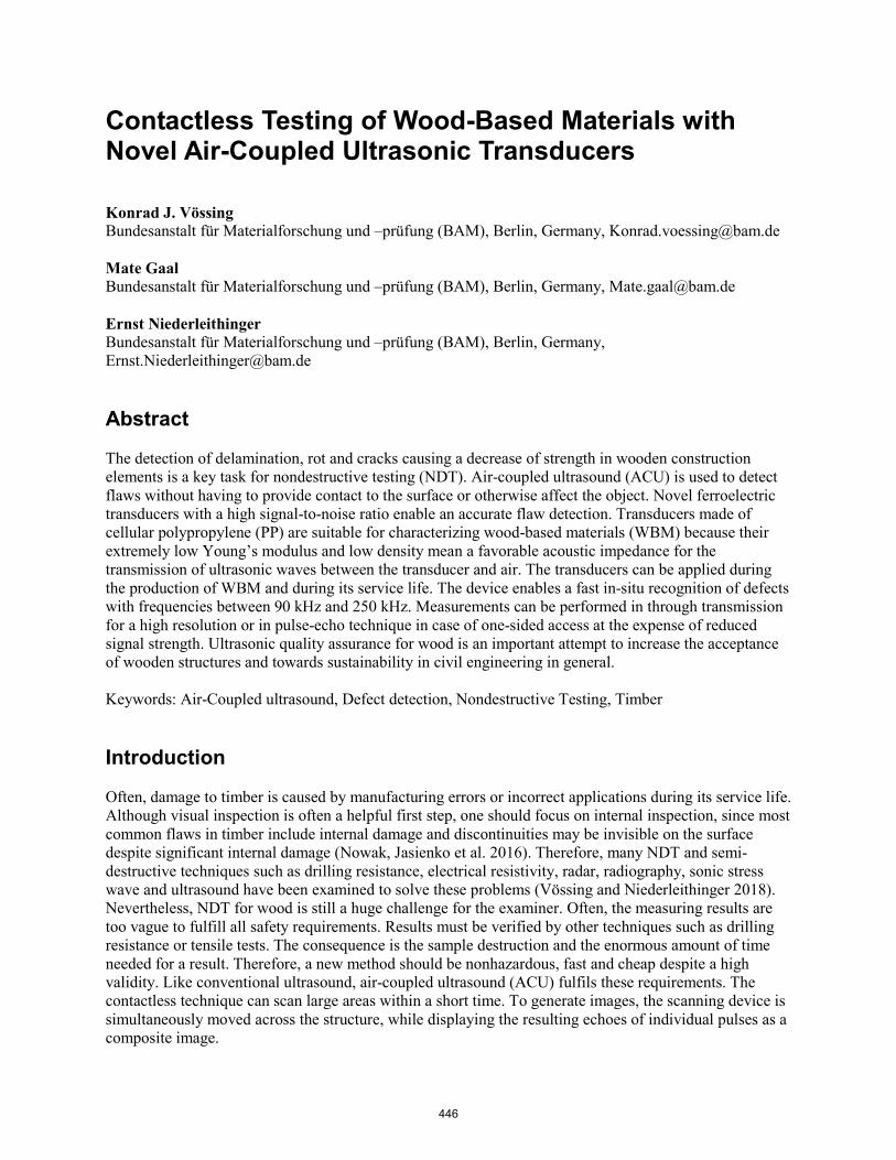
Contactless Testing of Wood-Based Materials with Novel Air-Coupled Ultrasonic Transducers

Konrad J. Vössing Bundesanstalt für Materialforschung und –prüfung (BAM), Berlin, Germany, Konrad.voessing@bam.de

Mate Gaal Bundesanstalt für Materialforschung und –prüfung (BAM), Berlin, Germany, Mate.gaal@bam.de

Ernst Niederleithinger Bundesanstalt für Materialforschung und –prüfung (BAM), Berlin, Germany, Ernst.Niederleithinger@bam.de

Abstract

The detection of delamination, rot and cracks causing a decrease of strength in wooden construction elements is a key task for nondestructive testing (NDT). Air-coupled ultrasound (ACU) is used to detect flaws without having to provide contact to the surface or otherwise affect the object. Novel ferroelectric transducers with a high signal-to-noise ratio enable an accurate flaw detection. Transducers made of cellular polypropylene (PP) are suitable for characterizing wood-based materials (WBM) because their extremely low Young’s modulus and low density mean a favorable acoustic impedance for the transmission of ultrasonic waves between the transducer and air. The transducers can be applied during the production of WBM and during its service life. The device enables a fast in-situ recognition of defects with frequencies between 90 kHz and 250 kHz. Measurements can be performed in through transmission for a high resolution or in pulse-echo technique in case of one-sided access at the expense of reduced signal strength. Ultrasonic quality assurance for wood is an important attempt to increase the acceptance of wooden structures and towards sustainability in civil engineering in general.

Keywords: Air-Coupled ultrasound, Defect detection, Nondestructive Testing, Timber

Introduction

Often, damage to timber is caused by manufacturing errors or incorrect applications during its service life. Although visual inspection is often a helpful first step, one should focus on internal inspection, since most common flaws in timber include internal damage and discontinuities may be invisible on the surface despite significant internal damage (Nowak, Jasienko et al. 2016). Therefore, many NDT and semi-destructive techniques such as drilling resistance, electrical resistivity, radar, radiography, sonic stress wave and ultrasound have been examined to solve these problems (Vössing and Niederleithinger 2018). Nevertheless, NDT for wood is still a huge challenge for the examiner. Often, the measuring results are too vague to fulfill all safety requirements. Results must be verified by other techniques such as drilling resistance or tensile tests. The consequence is the sample destruction and the enormous amount of time needed for a result. Therefore, a new method should be nonhazardous, fast and cheap despite a high validity. Like conventional ultrasound, air-coupled ultrasound (ACU) fulfils these requirements. The contactless technique can scan large areas within a short time. To generate images, the scanning device is simultaneously moved across the structure, while displaying the resulting echoes of individual pulses as a composite image.

446

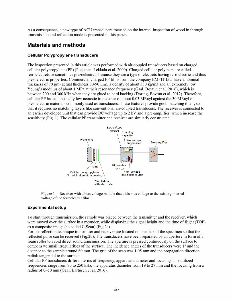
As a consequence, a new type of ACU transducers focused on the internal inspection of wood in through transmission and reflection mode is presented in this paper.

Materials and methods

Cellular Polypropylene transducers

The inspection presented in this article was performed with air-coupled transducers based on charged cellular polypropylene (PP) (Paajanen, Lekkala et al. 2000). Charged cellular polymers are called ferroelectrets or sometimes piezoelectrets because they are a type of electrets having ferroelectric and thus piezoelectric properties. Commercial charged PP films from the company EMFIT Ltd. have a nominal thickness of 70 μm (actual thickness 80-90 μm), a density of about 330 kg/m3 and an extremely low Young’s modulus of about 1 MPa at their resonance frequency (Gaal, Bovtun et al. 2016), which is between 200 and 300 kHz when they are glued to hard backing (Döring, Bovtun et al. 2012). Therefore, cellular PP has an unusually low acoustic impedance of about 0.03 MRayl against the 30 MRayl of piezoelectric materials commonly used as transducers. These features provide good matching to air, so that it requires no matching layers like conventional air-coupled transducers. The receiver is connected to an earlier developed unit that can provide DC voltage up to 2 kV and a pre-amplifier, which increase the sensitivity (Fig. 1). The cellular PP transmitter and receiver are similarly constructed.

Figure 1— Receiver with a bias voltage module that adds bias voltage to the existing internal voltage of the ferroelectret film.

Experimental setup

To start through transmission, the sample was placed between the transmitter and the receiver, which were moved over the surface in a meander, while displaying the signal height and the time of flight (TOF) as a composite image (so called C-Scan) (Fig.2a). For the reflection technique transmitter and receiver are located on one side of the specimen so that the reflected pulse can be received (Fig.2b). The transducers have been separated by an aperture in form of a foam roller to avoid direct sound transmission. The aperture is pressed continuously on the surface to compensate small irregularities of the surface. The incidence angles of the transducers were 1° and the distance to the sample around 60 mm. The grid of the scan was 1.05 mm and the propagation direction radial/ tangential to the surface. Cellular PP transducers differ in terms of frequency, apparatus diameter and focusing. The utilized frequencies range from 90 to 250 kHz, the apparatus diameter from 19 to 27 mm and the focusing from a radius of 0–50 mm (Gaal, Bartusch et al. 2016).

447

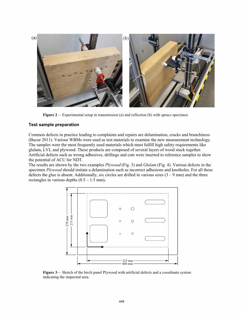
Figure 2— Experimental setup in transmission (a) and reflection (b) with spruce specimen.

Test sample preparation

Common defects in practice leading to complaints and repairs are delamination, cracks and branchiness (Bucur 2011). Various WBMs were used as test materials to examine the new measurement technology. The samples were the most frequently used materials which must fulfill high safety requirements like glulam, LVL and plywood. These products are composed of several layers of wood stuck together. Artificial defects such as wrong adhesives, drillings and cuts were inserted to reference samples to show the potential of ACU for NDT. The results are shown by the two examples Plywood (Fig. 3) and Glulam (Fig. 4). Various defects in the specimen Plywood should imitate a delamination such as incorrect adhesions and knotholes. For all these defects the glue is absent. Additionally, six circles are drilled in various sizes (3 – 9 mm) and the three rectangles in various depths (0.5 – 1.5 mm).

Figure 3— Sketch of the birch panel Plywood with artificial defects and a coordinate system indicating the inspected area.

448

The specimen Glulam has the dimensions of 500 × 400 × 90 mm3 and is composed of 16 square timbers stuck together. At the bottom, 12 drillings are located at various depths and shapes. They range from 10 mm to 50.1 mm and have either blind holes or countersinks.

Figure 4— principal setup and measuring field of the spruce specimen Glulam1 with twelve test-drillings in 3D view.

Results and discussion

Cellular PP transducers allow the detection of delamination, glued joints, knots and wood degradation by fungi & insect attack. Due to the improved signal-to-noise ratio (SNR) the amplitude of the receiving signal is up to three times higher than from commercially available ACU transducers. Thus, measurements in reflection mode are possible and lead to comparable results to previous used point contact transducers but up to 200 times faster (Krause, Mayer et al. 2014). In through transmission samples with thicknesses of even 300 mm can be scanned (Vössing, Gaal et al. 2018). Figure 5 shows a measurement displaying the advantage of ferroelectret transducers in contrast to piezoceramics. The ferroelectrets were compared with market-based piezoceramic transducers from the ULTRAN company. The measurements were taken at the same position in through transmission using a self-built and defect-free test specimen equivalent to the specimen Glulam. The signal with a frequency of 90 kHz is up to three times higher than those from commercial transducers. The differences are especially significant for lower frequencies.

Figure 5— Comparison of piezoceramic (a) and cellular PP (b) transducers. Receiver signals with frequencies of 90 kHz. The signals are normalized on the same noise level to compare the SNR.

Another ultrasonic measurement was performed using the test specimen Plywood. The measurements compare once again cellular PP and piezoceramic transducers with the aim to detect delamination in

449

wood-based materials. Figure 6 shows the attenuation of the ultrasonic measurement as a C-Scan. All defects can be detected with no differences between delamination on the left and milling on the right. The missing adhesive leads to a higher attenuation of the signal. The resolution on the left side with cellular PP transducers is better: the defects of the specimen are displayed more precisely.

Figure 6—C-Scans, i.e. signal heights in dB with a frequency of 120 kHz with cellular PP (a) and piezoceramic transducers (b).

Figure 7 shows the measurement of the specimen Glulam in reflection (Fig. 7a) and transmission (Fig. 7b). In reflection the drillings 1–3 and 10-12 can be located because of their position near the surface and their blind hole shape. With increasing depth, the attenuation is increasing, too, so that the other drillings cannot be seen. Moreover, countersinks lead to an enhanced scatter of the signal. The anisotropy of wood has in reflection mode a doubled influence on the ultrasonic signal due to a doubled sound path. Moreover, the gap between transmitter and receiver distort the signal. The result is a distorted scan caused by different sound velocities in all three anatomic directions. Another challenge are the surface waves which are overlapping the backwall echo of the specimen. In transmission all drillings can be detected. Even the glueline of the individual battens and the fibre orientation can be seen. With the imaging results of the TOF the depth of the holes can be determined by the colour value analysis.

Figure 7— Ultrasonic imaging results with frequencies of 130 kHz in reflection (a) and through transmission (b).

450

Conclusions

Cellular PP transducers are a promising new type of transducers for ACU testing. They allow for regular and reliable inspection and the possibility to detect delamination, rot and cavities in timber structures so that suitable remediation can be initiated. These transducers have many advantages – they are powerful, non- hazardous and their production is simple. The receiving signal is up to three times higher than from piezoceramic transducers. Therefore, cellular PP transducers can produce usable inspection results where piezoceramic transducers fail due to a lower SNR. The measurements are both in through transmission and in reflection mode possible. The reflection technique delivers poor results but is basically possible. An improved signal processing (e.g. data fusion) of this technique is super important for a better validity.

Acknowledgments

The research work was subsidized by the Cusanuswerk, Episcopal Study Sponsorship.

References

Bucur, V. 2011. Delamination in Wood, Wood Products and Wood-Based Composites. Dordrecht, Heidelberg, London, New York, Springer Netherlands.

Döring, J., V. Bovtun, M. Gaal, J. Bartusch, A. Erhard, M. Kreutzbruck and Y. Yakymenko. 2012. Piezoelectric and electrostrictive effects in ferroelectret ultrasonic transducers. Journal of Applied Physics. 112(8): 6.

Gaal, M., J. Bartusch, E. Dohse, F. Schadow and E. Köppe. 2016. Focusing of Ferroelectret Air-Coupled Ultrasound Transducers. AIP Conference Proceedings, American Institute of Physics. 1706.

Gaal, M., V. Bovtun, W. Stark, A. Erhard, Y. Yakymenko and M. Kreutzbruck. 2016. Viscoelastic properties of cellular polypropylene ferroelectrets. Journal of Applied Physics. 119(12).

Krause, M., K. Mayer, G. Ballier, K. Borchardt, P. Chinta, U. Effner, B. Milmann, S. Müller and T. Nowak. 2014. Hochgenaue Strukturerkennung von Holzbauteilen mit 3D-Ultraschall. Bauforschung für die Praxis. Stuttgart, Forschungsinitiative Zukunft Bau. 109: 105.

Nowak, T. P., J. Jasienko and K. Hamrol-Bielecka. 2016. In situ assessment of structural timber using the resistance drilling method – Evaluation of usefulness. Construction and Building Materials. 102: 403-415.

Paajanen, M., J. Lekkala and K. Kirjavainen. 2000. ElectroMechanical Film (EMFi) - a new multipurpose electret material. Sensors Actuators, A Physical. 84(1): 95-102.

Vössing, K. and E. Niederleithinger. 2018. Nondestructive assessment and imaging methods for internal inspection of timber. A review. Holzforschung 72(6): 467–476.

Vössing, K. J., M. Gaal and E. Niederleithinger. 2018. Air-coupled ferroelectret ultrasonic transducers for nondestructive testing of wood-based materials. Wood Science and Technology. 52(6): 1527-1538.

451

Resistance and Sorption Methods to Monitor Moisture Content in Timber Structures — A Comparison Based on Case Studies

Marcus Schiere* Institute for Architecture, Wood, and Civil Engineering, Bern University of Applied Sciences, Biel, Switzerland, marcusjacob.schiere@bfh.ch

Bettina Franke Institute for Architecture, Wood, and Civil Engineering, Bern University of Applied Sciences, Biel, Switzerland, bettina.franke@bfh.ch

Steffen Franke Institute for Architecture, Wood, and Civil Engineering, Bern University of Applied Sciences, Biel, Switzerland, steffen.franke@bfh.ch

Andreas Müller Institute for Architecture, Wood, and Civil Engineering, Bern University of Applied Sciences, Biel, Switzerland, andreas.mueller@bfh.ch

* Corresponding author

Abstract

Wood moisture content is a practical indicator of the structural condition of load bearing timber elements. Apart from the destructive oven-dry methods, it can be determined in a non-destructive way using physical or sorptive properties of wood. The resistance method, where the electrical resistance is measured between two electrodes inserted into wood, is one of the most commonly deployed methods in long-term monitoring campaigns. The sorption method relies the measurement of temperature and humidity measured inside a small cavity in the wood and is less common in monitoring campaigns. The moisture content is then derived using sorption isotherms, which is a well-known relation for many wood species. Both the resistance method and sorption method were deployed in the monitoring of recently erected timber buildings: One riding hall, two alpine ski stations, and a reinforced historic road bridge. Glued laminated spruce and laminated beech veneer elements were monitored. The instrumentation allows a direct comparison between the two moisture content monitoring methods. The accuracy of both monitoring methods lies around 1 M% in normal conditions, but accuracy is still governed by the quality of the conversion data from both electrical resistance to moisture content and similarly for the sorption characteristics. The choice of monitoring methods in future applications depends on requirements set to the monitoring campaign such as duration of the monitoring campaign, temperatures experienced during operation, risk of saturation of the wood fibers by water, and available equipment.

Keywords: long-term monitoring, electrical resistance method, sorption method, structural health, timber structures

452

Introduction

Moisture content monitoring is, amongst others, performed for two reasons. The first reason is that wood moisture content is a first indicator of the condition of a timber structure. Risk of wood decay is high when moisture contents are close to -or over- fiber saturation point. Monitoring methods allow early detection of increased moisture content levels caused by leakage or condensation of water in the timber structure. The second reason is that moisture content also affects mechanical properties of timber below fiber saturation point. Knowledge of the expected moisture content levels is important during an early design stage. It helps to determine allowable load levels and the expected deformations. Through the system of Service Classes described in the Eurocode 5 (EN 1995-1-1, 2004). Architects, engineers and planners want to know what moisture content levels can be expected in (new) building types.

Moisture content in timber structures follows relative humidity variations due to seasonal climate and building use. One of the most common physical properties that allows measurement of moisture content variations is the electrical resistance (Skaar, 1988 and Siau, 1995). The dependency of resistance on wood moisture content is a known relation programmed into many hand-held moisture content meters. Another method to monitor moisture content is the so-called sorption method (Dietsch et al. (2015) or bore hole method (Li et al., 2018). The method uses sorption isotherms to convert relative humidity measured in a small cavity in the wood to moisture content. Sorption isotherms are often well known for common wood species as well.

The paper presents the comparison between the method electrical resistance and sorption method through measurements made in four different structures located in Switzerland: a riding hall (Figure 1), two cable car stations located in the Alps (Figure 2 and Figure 3) at altitudes of 1500 m.a.s.l. (meters above sea level) and more, and a historic bridge (Figure 4). The background of the two methods is compared first after which the used instrumentation is presented. This is the followed by the comparison of the electrical resistance method and the sorption method in the presented structures. Finally, the advantages and disadvantages are discussed, followed by conclusions.

Moisture content monitoring

Moisture content

Moisture content u is be expressed as a mass percentage (M%) in this work. It is calculated by using the wet and dry mass of wood, mwet and mdry, respectively:

wet dry

dry

m mu

m−

= (1)

The dry mass is obtained by oven-drying the wood sample at a temperature of 103°C (SN EN 13183-1, 2002). The wet mass is measured shortly before drying. Although accurate, the so-called oven-dry method is considered destructive and not practical for long term monitoring applications.

Electrical resistance method

The electrical resistance method (SN EN 13183-2, 2002) is the most common non-destructive method to monitor moisture content developments. The method allows measurement of moisture content in different depths from the surface and measured resistances can logged over extended periods of time. The accuracy of the method is about 1 M% (Dietsch et al., 2015). Factors affecting the accuracy concern amongst others the grain orientation, type of electrodes, wood density, and temperature (Skaar, 1988). Resistance between two electrodes roughly ranges between 100 kΩ to 100 GΩ from the fiber saturation point to

453

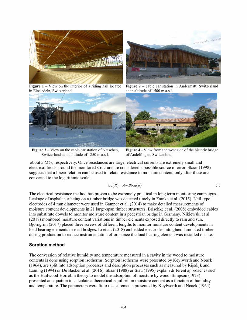
about 5 M%, respectively. Once resistances are large, electrical currents are extremely small and electrical fields around the monitored structure are considered a possible source of error. Skaar (1998) suggests that a linear relation can be used to relate resistance to moisture content, only after these are converted to the logarithmic scale.

( ) ( )log logR A B u= − (1)

The electrical resistance method has proven to be extremely practical in long term monitoring campaigns. Leakage of asphalt surfacing on a timber bridge was detected timely in Franke et al. (2015). Nail-type electrodes of 4 mm diameter were used in Gamper et al. (2014) to make detailed measurements of moisture content developments in 21 large-span timber structures. Brischke et al. (2008) embedded cables into substitute dowels to monitor moisture content in a pedestrian bridge in Germany. Niklewski et al. (2017) monitored moisture content variations in timber elements exposed directly to rain and sun. Björngrim (2017) placed three screws of different lengths to monitor moisture content developments in load bearing elements in road bridges. Li et al. (2018) embedded electrodes into glued laminated timber during production to reduce instrumentation efforts once the load bearing element was installed on site.

Sorption method

The conversion of relative humidity and temperature measured in a cavity in the wood to moisture contents is done using sorption isotherms. Sorption isotherms were presented by Keylwerth and Noack (1964), are split into adsorption processes and desorption processes such as measured by Rijsdijk and Laming (1994) or De Backer et al. (2016). Skaar (1988) or Siau (1995) explain different approaches such as the Hailwood-Horrobin theory to model the adsorption of moisture by wood. Simpson (1973) presented an equation to calculate a theoretical equilibrium moisture content as a function of humidity and temperature. The parameters were fit to measurements presented by Keylwerth and Noack (1964).

Figure 1 – View on the interior of a riding hall located in Einsiedeln, Switzerland

Figure 2 – cable car station in Andermatt, Switzerland at an altitude of 1500 m.a.s.l.

Figure 3 – View on the cable car station of Nätschen, Switzerland at an altitude of 1850 m.a.s.l.

Figure 4 - View from the west side of the historic bridge of Andelfingen, Switzerland

454

Melin et al. (2016) converts the relative humidity and temperature into wood moisture content using adsorption curves, desorption curves, and moisture scanning curves like suggested by Rode and Clorius (2004). The work is based on ad- and desorption isotherms by Hedlin (1968) and Ahlgren (1972) and temperature dependency measured by Kelsey (1957). Hedlin (1968) performed an important part of the work measuring moisture contents at -12°C. Rode and Clorius (2004) suggested that in continuously varying climates, use of hysteresis effects was not necessary to determine a practical moisture content.

The most common application of long-term monitoring performed with the sorption method is that of the moisture content monitoring of timber bridges in Norway (Dyken and Kepp, 2010). The authors fit a second-order polynomial through measurements made in different relative humidities and temperatures (from -20 °C to 20 °C). The calculated fit relation allowed the determination of wood moisture content for Nordic pine (Pinus sylvestris). Melin et al. (2016) used the sorption method to monitor moisture content variations in wooden objects of cultural significance located in museums.

Comparison of the electrical resistance method and sorption method in literature

The sorption method is especially suited for sub-zero temperatures as the electrical resistance method becomes unreliable below zero (Björngrim et al., 2017). Fortino et al. (2016) specified that uncertainties in the electrical resistance method can still be acceptable around -5 ºC, but unreliable below -10 ºC. Melin et al. (2016) also mentions that gage depth could be better controlled, and that moisture content is derived more accurately compared to the electrical resistance method. The sorption method enables moisture content monitoring in salt domes, typical environments where electrical resistance methods should be avoided (Dietsch et al., 2015). Li et al. (2018) mentions though that the sorption method can only be applied in the hygroscopic domain, whereas electric resistance methods can also be used over-hygroscopic range. Niklewski et al. (2017) adds that conversion curves need to be determined accurately in this range, because small variations in measured resistance lead to large errors in moisture content readings. The electrical resistance method is a more robust method over a long time (Li et al., 2018).

Instrumented structures, instrumentation, and used conversion of physical parameters to moisture content

Instrumented structures

The monitored structures were part of a larger monitoring campaign of which results were published in Schiere et al. (2018) and Franke et al. (2019). The first structure concerns a riding hall (Figure 1) in a humid, pre-alpine area of Switzerland. Riding halls are known to have a humid climate due to soil that is sprinkled to minimize dust development during horse-riding. The building was well ventilated throughout the whole year. The building envelope contained large window surfaces. Moisture content was measured in spruce (Picea abies) load bearing members that spanned the entire 36-meter-wide hall. Moisture content was measured close to the glass façade (MS1) and center of the hall (MS2).

The second and third structure are two alpine cable car stations on altitudes of 1500 m.a.s.l. (meter above sea level) in Andermatt (Figure 2) and 1900 m.a.s.l. in Nätschen (Figure 3). Climate in the Alps is known to be dryer than in the Swiss Central Plateau or northern pre-Alps. Temperatures at these altitudes were below zero for a couple of months a year. Moisture content was measured on Spruce (Picea abies) load bearing members. In the cable car station of Andermatt, moisture content was monitored close to a large opening in the structure (MS1) and more in the center of the structure (MS2). In Nätschen, an element penetrating the building envelope was monitored (MS1). The second instrumented location (MS2) was situated more in the center of the structure. Both cable car stations were well ventilated throughout the entire year.

455

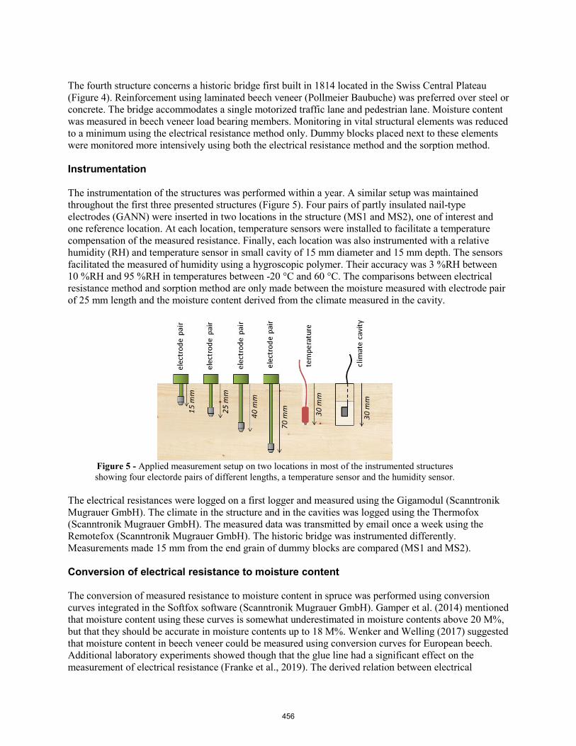
The fourth structure concerns a historic bridge first built in 1814 located in the Swiss Central Plateau (Figure 4). Reinforcement using laminated beech veneer (Pollmeier Baubuche) was preferred over steel or concrete. The bridge accommodates a single motorized traffic lane and pedestrian lane. Moisture content was measured in beech veneer load bearing members. Monitoring in vital structural elements was reduced to a minimum using the electrical resistance method only. Dummy blocks placed next to these elements were monitored more intensively using both the electrical resistance method and the sorption method.

Instrumentation

The instrumentation of the structures was performed within a year. A similar setup was maintained throughout the first three presented structures (Figure 5). Four pairs of partly insulated nail-type electrodes (GANN) were inserted in two locations in the structure (MS1 and MS2), one of interest and one reference location. At each location, temperature sensors were installed to facilitate a temperature compensation of the measured resistance. Finally, each location was also instrumented with a relative humidity (RH) and temperature sensor in small cavity of 15 mm diameter and 15 mm depth. The sensors facilitated the measured of humidity using a hygroscopic polymer. Their accuracy was 3 %RH between 10 %RH and 95 %RH in temperatures between -20 °C and 60 °C. The comparisons between electrical resistance method and sorption method are only made between the moisture measured with electrode pair of 25 mm length and the moisture content derived from the climate measured in the cavity.

Figure 5 - Applied measurement setup on two locations in most of the instrumented structures showing four electorde pairs of different lengths, a temperature sensor and the humidity sensor.

The electrical resistances were logged on a first logger and measured using the Gigamodul (Scanntronik Mugrauer GmbH). The climate in the structure and in the cavities was logged using the Thermofox (Scanntronik Mugrauer GmbH). The measured data was transmitted by email once a week using the Remotefox (Scanntronik Mugrauer GmbH). The historic bridge was instrumented differently. Measurements made 15 mm from the end grain of dummy blocks are compared (MS1 and MS2).

Conversion of electrical resistance to moisture content

The conversion of measured resistance to moisture content in spruce was performed using conversion curves integrated in the Softfox software (Scanntronik Mugrauer GmbH). Gamper et al. (2014) mentioned that moisture content using these curves is somewhat underestimated in moisture contents above 20 M%, but that they should be accurate in moisture contents up to 18 M%. Wenker and Welling (2017) suggested that moisture content in beech veneer could be measured using conversion curves for European beech. Additional laboratory experiments showed though that the glue line had a significant effect on the measurement of electrical resistance (Franke et al., 2019). The derived relation between electrical

456

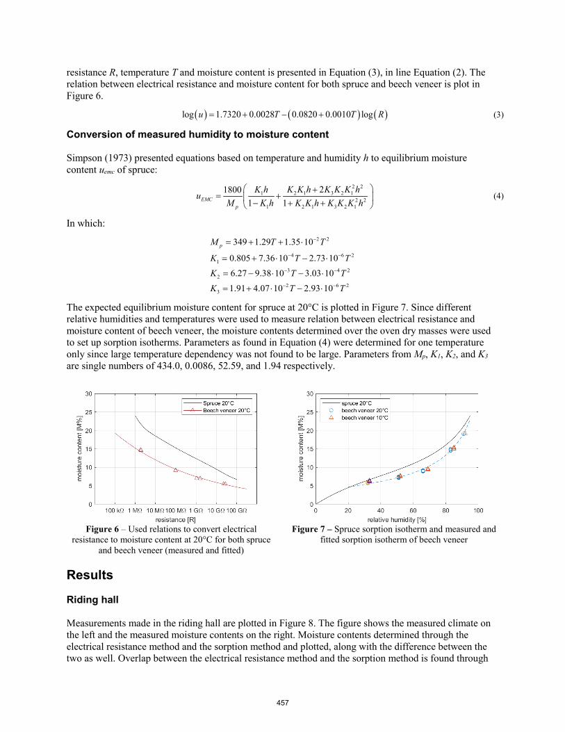
resistance R, temperature T and moisture content is presented in Equation (3), in line Equation (2). The relation between electrical resistance and moisture content for both spruce and beech veneer is plot in Figure 6.

( ) ( ) ( )log 1.7320 0.0028 0.0820 0.0010 logu T T R= + − + (3)

Conversion of measured humidity to moisture content

Simpson (1973) presented equations based on temperature and humidity h to equilibrium moisture content uemc of spruce:

2 22 1 3 2 11

2 21 2 1 3 2 1

218001 1EMC

p

K K h K K K hK huM K h K K h K K K h

+= + − + +

(4)

In which: 2 2

4 6 21

3 4 22

2 6 23

349 1.29 1.35 10

0.805 7.36 10 2.73 106.27 9.38 10 3.03 101.91 4.07 10 2.93 10

pM T T

K T TK T TK T T

−

− −

− −

− −

= + + ⋅

= + ⋅ − ⋅

= − ⋅ − ⋅

= + ⋅ − ⋅

The expected equilibrium moisture content for spruce at 20°C is plotted in Figure 7. Since different relative humidities and temperatures were used to measure relation between electrical resistance and moisture content of beech veneer, the moisture contents determined over the oven dry masses were used to set up sorption isotherms. Parameters as found in Equation (4) were determined for one temperature only since large temperature dependency was not found to be large. Parameters from Mp, K1, K2, and K3 are single numbers of 434.0, 0.0086, 52.59, and 1.94 respectively.

Figure 6 – Used relations to convert electrical resistance to moisture content at 20°C for both spruce

and beech veneer (measured and fitted)

Figure 7 – Spruce sorption isotherm and measured and fitted sorption isotherm of beech veneer

Results

Riding hall

Measurements made in the riding hall are plotted in Figure 8. The figure shows the measured climate on the left and the measured moisture contents on the right. Moisture contents determined through the electrical resistance method and the sorption method and plotted, along with the difference between the two as well. Overlap between the electrical resistance method and the sorption method is found through

457

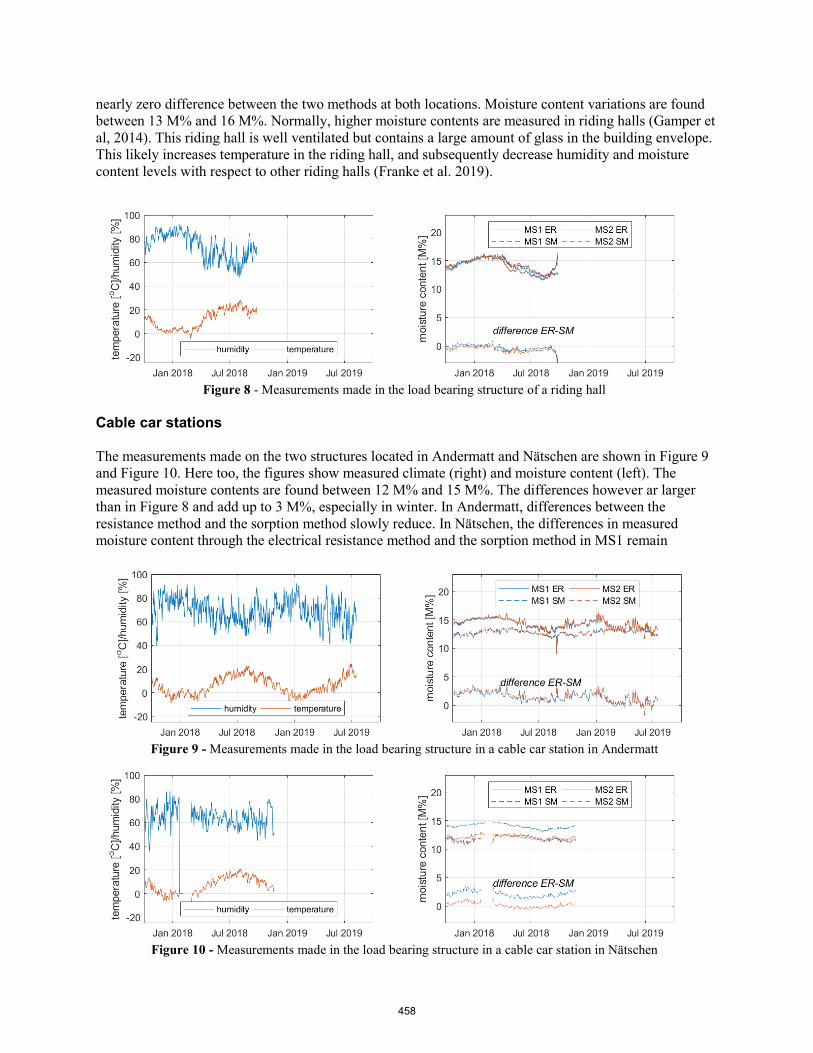
nearly zero difference between the two methods at both locations. Moisture content variations are found between 13 M% and 16 M%. Normally, higher moisture contents are measured in riding halls (Gamper et al, 2014). This riding hall is well ventilated but contains a large amount of glass in the building envelope. This likely increases temperature in the riding hall, and subsequently decrease humidity and moisture content levels with respect to other riding halls (Franke et al. 2019).

Figure 8 - Measurements made in the load bearing structure of a riding hall

Cable car stations

The measurements made on the two structures located in Andermatt and Nätschen are shown in Figure 9 and Figure 10. Here too, the figures show measured climate (right) and moisture content (left). The measured moisture contents are found between 12 M% and 15 M%. The differences however ar larger than in Figure 8 and add up to 3 M%, especially in winter. In Andermatt, differences between the resistance method and the sorption method slowly reduce. In Nätschen, the differences in measured moisture content through the electrical resistance method and the sorption method in MS1 remain

Figure 9 - Measurements made in the load bearing structure in a cable car station in Andermatt

Figure 10 - Measurements made in the load bearing structure in a cable car station in Nätschen

458

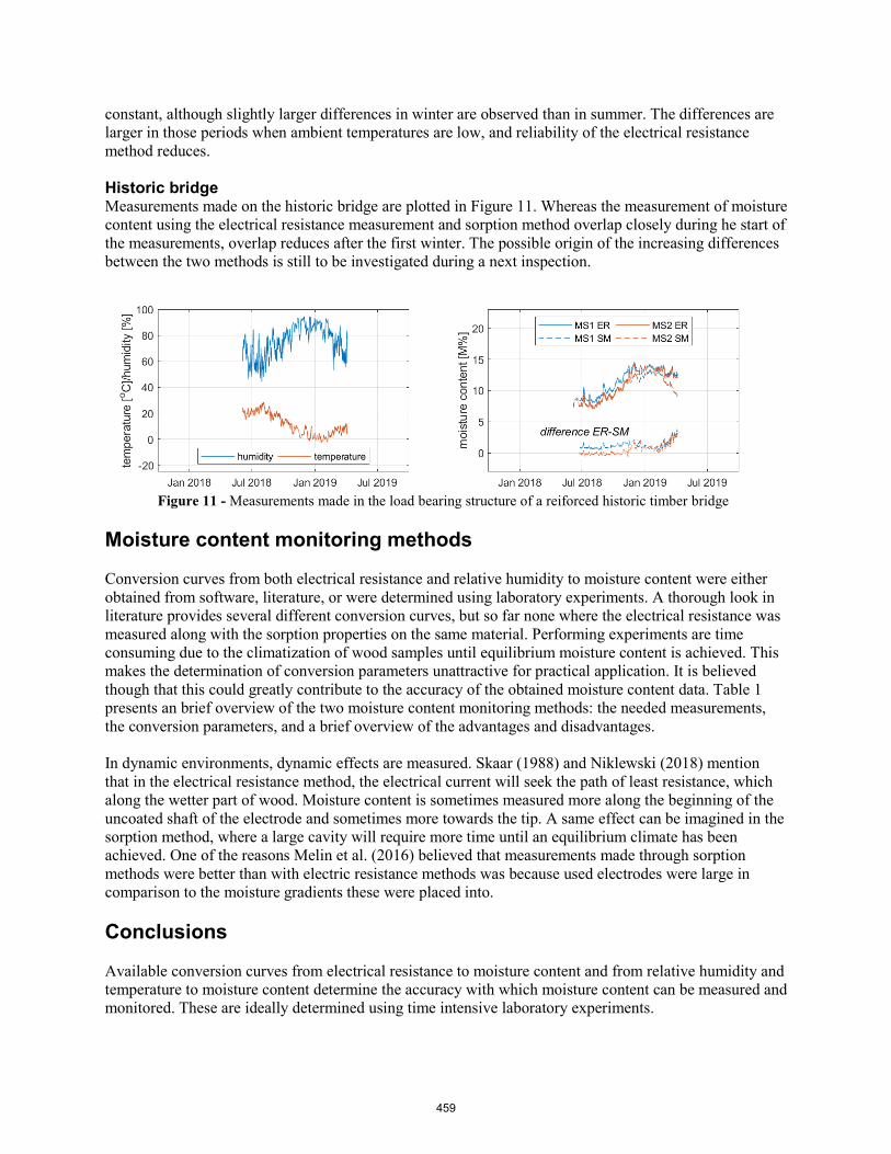
constant, although slightly larger differences in winter are observed than in summer. The differences are larger in those periods when ambient temperatures are low, and reliability of the electrical resistance method reduces.

Historic bridge Measurements made on the historic bridge are plotted in Figure 11. Whereas the measurement of moisture content using the electrical resistance measurement and sorption method overlap closely during he start of the measurements, overlap reduces after the first winter. The possible origin of the increasing differences between the two methods is still to be investigated during a next inspection.

Figure 11 - Measurements made in the load bearing structure of a reiforced historic timber bridge

Moisture content monitoring methods

Conversion curves from both electrical resistance and relative humidity to moisture content were either obtained from software, literature, or were determined using laboratory experiments. A thorough look in literature provides several different conversion curves, but so far none where the electrical resistance was measured along with the sorption properties on the same material. Performing experiments are time consuming due to the climatization of wood samples until equilibrium moisture content is achieved. This makes the determination of conversion parameters unattractive for practical application. It is believed though that this could greatly contribute to the accuracy of the obtained moisture content data. Table 1 presents an brief overview of the two moisture content monitoring methods: the needed measurements, the conversion parameters, and a brief overview of the advantages and disadvantages.

In dynamic environments, dynamic effects are measured. Skaar (1988) and Niklewski (2018) mention that in the electrical resistance method, the electrical current will seek the path of least resistance, which along the wetter part of wood. Moisture content is sometimes measured more along the beginning of the uncoated shaft of the electrode and sometimes more towards the tip. A same effect can be imagined in the sorption method, where a large cavity will require more time until an equilibrium climate has been achieved. One of the reasons Melin et al. (2016) believed that measurements made through sorption methods were better than with electric resistance methods was because used electrodes were large in comparison to the moisture gradients these were placed into.

Conclusions

Available conversion curves from electrical resistance to moisture content and from relative humidity and temperature to moisture content determine the accuracy with which moisture content can be measured and monitored. These are ideally determined using time intensive laboratory experiments.

459

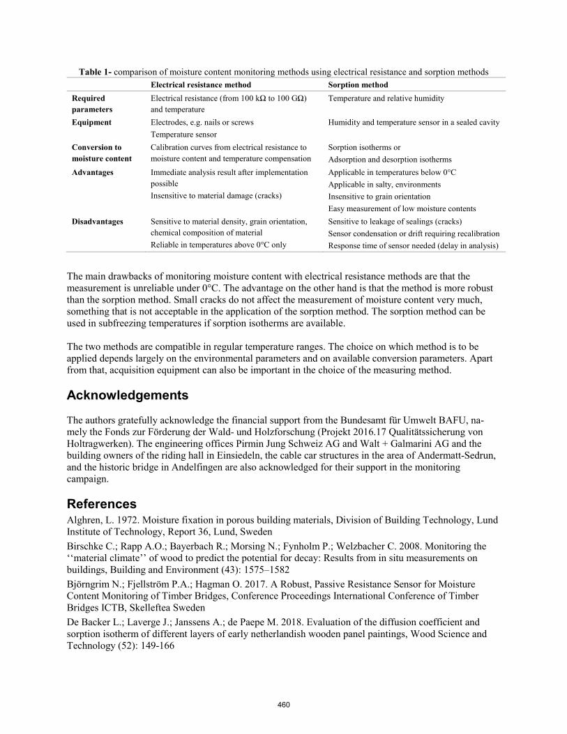
The main drawbacks of monitoring moisture content with electrical resistance methods are that the measurement is unreliable under 0°C. The advantage on the other hand is that the method is more robust than the sorption method. Small cracks do not affect the measurement of moisture content very much, something that is not acceptable in the application of the sorption method. The sorption method can be used in subfreezing temperatures if sorption isotherms are available.

The two methods are compatible in regular temperature ranges. The choice on which method is to be applied depends largely on the environmental parameters and on available conversion parameters. Apart from that, acquisition equipment can also be important in the choice of the measuring method.

Acknowledgements

The authors gratefully acknowledge the financial support from the Bundesamt für Umwelt BAFU, na-mely the Fonds zur Förderung der Wald- und Holzforschung (Projekt 2016.17 Qualitätssicherung von Holtragwerken). The engineering offices Pirmin Jung Schweiz AG and Walt + Galmarini AG and the building owners of the riding hall in Einsiedeln, the cable car structures in the area of Andermatt-Sedrun, and the historic bridge in Andelfingen are also acknowledged for their support in the monitoring campaign.

References Alghren, L. 1972. Moisture fixation in porous building materials, Division of Building Technology, Lund Institute of Technology, Report 36, Lund, Sweden Birschke C.; Rapp A.O.; Bayerbach R.; Morsing N.; Fynholm P.; Welzbacher C. 2008. Monitoring the ‘‘material climate’’ of wood to predict the potential for decay: Results from in situ measurements on buildings, Building and Environment (43): 1575–1582 Björngrim N.; Fjellström P.A.; Hagman O. 2017. A Robust, Passive Resistance Sensor for Moisture Content Monitoring of Timber Bridges, Conference Proceedings International Conference of Timber Bridges ICTB, Skelleftea Sweden De Backer L.; Laverge J.; Janssens A.; de Paepe M. 2018. Evaluation of the diffusion coefficient and sorption isotherm of different layers of early netherlandish wooden panel paintings, Wood Science and Technology (52): 149-166

Table 1- comparison of moisture content monitoring methods using electrical resistance and sorption methods Electrical resistance method Sorption method

Required parameters

Electrical resistance (from 100 kΩ to 100 GΩ) and temperature

Temperature and relative humidity

Equipment Electrodes, e.g. nails or screws Temperature sensor

Humidity and temperature sensor in a sealed cavity

Conversion to moisture content

Calibration curves from electrical resistance to moisture content and temperature compensation

Sorption isotherms or Adsorption and desorption isotherms

Advantages Immediate analysis result after implementation possible Insensitive to material damage (cracks)

Applicable in temperatures below 0°C Applicable in salty, environments Insensitive to grain orientation Easy measurement of low moisture contents

Disadvantages Sensitive to material density, grain orientation, chemical composition of material Reliable in temperatures above 0°C only

Sensitive to leakage of sealings (cracks) Sensor condensation or drift requiring recalibration Response time of sensor needed (delay in analysis)

460

Dietsch P.; Franke S.; Franke B.; Gamper A.; Winter S. 2015. Methods to determine wood moisture content and their applicability in monitoring concepts, Journal of Civil Structural Health Monitoring 5 (2), pp. 115-127 EN 1995-1-1:2004: Eurocode 5: Design of timber structures - Part 1-1: General Common rules and rules for buildings, European Committee for Standardization, Brussels, Belgium, 2004 Franke B.; Franke S.; Müller A. 2014. Case studies: long-term monitoring of timber bridges, Journal of Civil Structural Health Monitoring 5 (2): 195-202 Franke B.; Franke S.; Schiere M.; Müller A. 2019. Quality assurance of timber structures – research report, Bern University of Applied Sciences, Switzerland, ISBN 978-3-906878-04-1 Gamper A.; Dietsch P.; Merk, M. 2014. Building Climate – Long-term measurements to determine the effect on the moisture gradient in timber structures, Research Report, Technical University of Munich, Germany Hedlin C.P. 1968. Sorption Isotherms of twelve species at subfreezing temperatures, Forest Products Journal (17): 43-48 Kelsey K. 1957. Sorption of water vapour by wood, Australian Journal of Applied Sciences (8): 42-54 Keylwerth R.; Noack D. 1964 Kammertrocknung von Schnittholz, Holz als Roh- und Werkstoff (22): 29-36 Li H.; Perrin M.; Eyma F.; Jacob X.; Gibiat V. 2018. Moisture content monitoring in glulam structures by embedded sensors via electrical methods, Wood Science and Technology (52): 733–752 Melin C.; Gebäck T.; Heintz A.; Bjurman J. 2016. Monitoring dynamic moisture gradients in wood using inserted relative humidity and temperature sensors, e-Preservation Science, 1581-9280 (eISSN) (13): 7-14 Niklewski J.; Isaksson T.; Frühwald Hansson E.; Thelandersson S. 2017. Moisture conditions of rain-exposed glue-laminated timber members: the effect of different detailing, Wood Material Science & Engineering (13): 129-140 Niklewski J. 2018. Durability of timber members: moisture conditions and service life assessment of bridge detailing, Dissertation Lund University, Sweden Rijsdijk J.F.; Laming B.L. 1994. Physical and Related Properties of 145 Timbers; Information for practice. Kluwer Academic Publishers, Dordrecht, The Netherlands, ISBN 0-7923-2875-2. Rode C.; Clorius C. 2004. Modeling of Moisture Transport in Wood with Hysteresis and Temperature Dependent Sorption Characteristics, Performance of Exterior Envelopes of Whole Buildings IX: International Conference, Oak Ridge, TN, USA Schiere M., Franke B., Franke S. 2018. Antworten zur Tragfähigkeit infolge dynamischer Klima-wechsel, S-WIN Tagung Von der Forschung zur Praxis, Biel/Bienne, Switzerland Simpson W. 1973. Predicting equilibrium moisture content of wood by mathematical models, Wood and Fiber (5): 41-49. SN EN 13183-1 2002. Feuchtegehalt eines Stückes Schnittholz - Teil 1: Bestimmung durch Darrverfahren, Schweizerischer Ingenieur- und Architektenverein, Zürich, Switzerland 2002 (in German) SN EN 13183-2 2002. Feuchtegehalt eines Stückes Schnittholz - Teil 2: Schätzung durch elektrisches Widerstands-Messverfahren, Schweizerischer Ingenieur- und Architektenverein, Zürich, Switzerland 2002 (in German) Skaar C. 1988. Wood-water relations, Springer Verlag, Germany, ISBN 3-540-19258-1 Wenker J. and Welling J. 2017. Klimaversuche für den Baustelleneinsatz, Bauen mit Holz, November 2017

461

Nondestructive Measurements in Reclaimed Timber from Existing Structures

Guillermo Íñiguez-González Department of Forestry and Environmental Engineering and Management, MONTES (School of Forest Engineering and Natural Environment), Universidad Politécnica de Madrid, Spain. Calle José Antonio Novais, 10. 28040. Madrid, Spain, ORCID: 0000-0003-2917-842X, guillermo.iniguez@upm.es

Francisco Arriaga Department of Forestry and Environmental Engineering and Management, MONTES (School of Forest Engineering and Natural Environment), Universidad Politécnica de Madrid, Spain. Calle José Antonio Novais, 10. 28040. Madrid, Spain, ORCID: 0000-0001-5535-0786, francisco.arriaga@upm.es

Carlos Osuna-Sequera Department of Forestry and Environmental Engineering and Management, MONTES (School of Forest Engineering and Natural Environment), Universidad Politécnica de Madrid, Spain. Calle José Antonio Novais, 10. 28040. Madrid, Spain, ORCID 0000-0002-9227-3035, caosseq@gmail.com

Miguel Esteban Department of Forestry and Environmental Engineering and Management, MONTES (School of Forest Engineering and Natural Environment), Universidad Politécnica de Madrid, Spain. Calle José Antonio Novais, 10. 28040. Madrid, Spain, ORCID: 0000-0003-3364-9044, miguel.esteban@upm.es

Dan Ridley-Ellis Edinburgh Napier University, Centre for Wood Science and Technology, 37 Bankhead Crossway South, Edinburgh, EH11 4EP, United Kingdom, ORCID: 0000-0001-9866-5649, d.ridleyellis@napier.ac.uk

Abstract

Deconstruction and demolition waste are a concern today because many timber components have a high resource value, providing both environmental and economic motivations for recovery and reuse. Reclaimed timber is therefore an important potential source of timber for new construction, and one for which nondestructive techniques have a key role to play. Assessment of timber properties by nondestructive measurements is not new. A lot of research has been carried out, and much work has gone into developing industrial devices for timber grading, but still some special considerations that should be analysed. This is especially true for less usual products such as reclaimed wood, and new wood from uncommon species or less usual sources.

Large cross-section and long members are commonly found in existing structures. But it should be noted that these pieces have specific characteristics that make them different from smaller ones. On the other hand, various research studies have confirmed that timbers from dismantled structures with large cross-section have very good reuse potential. Therefore, this paper presents some considerations to be done during data collection and properties assessment in reclaimed timber, measuring its high reuse potential. It also covers the problem that current standards require strength grading on a basis that is not compatible with such products.

Keywords: existing structures, nondestructive testing, large cross-section, reclaimed timber, in-situ measurements

462

Introduction

Timber construction

The use of timber as a building material is part of a global strategy trying to reduce the impact of the building sector on the environment, including climate change. Timber construction is growing and innovating, with new methods of building and new engineered wood products and treatments. In recent years, a large amount of multi-story timber buildings (6-8 stories) have been erected, and designers have begun to look at the possibility of building much taller with timber. Very large volumes of wood have being put into those buildings, and the quantity used is often seen as a virtue (as sequestered carbon). There are, however, limits to sustainable use, and reuse and recycling are key points that must not be overlooked.

The eight story residential building “Limnologen” (Växjö, Sweden) consists of seven Cross-Laminated Timber (CLT) stories with some timber frame internal walls, on a concrete foundation and ground floor (Serrano 2009). An apartment of 125 m2 in that building used approximately 28 m3 of timber (Ramage et al. 2017). This ratio of 0.22 m3/m2 is at the lower end of the range (0.2 - 0.3 m3/m2) for similar apartments in multi-storey cross-laminated timber buildings in Spain (Núñez 2019), and for two-storey family houses with special structural solutions (free spans of 16 m or cantilevers of 3.5 m) requirements ratios are up to 0.35 m3/m2 (Rodríguez 2019).

The EU28 produces 110 million m3 of sawn timber per year (Eurostat 2018), and so it takes less than 8 seconds to grow enough wood for such a three person apartment. However, to house the more than 500 million people who live in the EU, this would require nearly 5 billion m3 of timber - almost 40 years worth of sawn timber production, even if that did not also go to the other important markets it serves. England alone has a house building target of 300,000 per year, which would require 7.6 % of the sawn timber production for the whole of Europe (Spain, 140,000 per year, 3.6 %).

Thus, accounting also for growing markets for wood with rising world living standards, and the use of wood for other products such as plastics alternatives and fuel, the alternative sources of construction timber should be taken into account as a matter of urgency.

Residues and reclaimed timber

The amount of construction and demolition waste is increasing in parallel with on-going construction activities and its harmful impacts on the environment have been widely discussed. Thus increasing the proportion of waste that is reused is one of the key challenges facing society. In 2016, the Spanish economy generated 129 million tonnes of residues. 36 million tonnes corresponding to construction sector of which 140,327 tonnes (0.4%), was wood (INE 2016).

So, the potential for cascading wood from demolished buildings seems very hopeful (Sakaguchi et al. 2016; Höglmeier et al. 2017) and it highlights that to conceive a more environmentally sustainable society, it is important to create a circular economy in which the efficiency of material resource use is improved and waste is reduced. Studies conducted in Japan (Nakajima and Futaki 2001; Miyazaki et al. 2003) have demonstrated that timbers from dismantled post and beam houses with large cross-section, no damage, no notches and little attached materials have good reuse/recycling potential.

463

Existing standards

In Europe, structural timber is produced under the standard EN 14081-1, which is also required by the harmonized standards for manufacturing glulam and CLT. Whether grading visually, by machine-controlled grading, or by output-controlled grading EN 14081-1 requires that species (or species group) and timber source (meaning growth area) are known (Ridley-Ellis et al. 2016). Re-grading of timber that has already been graded is not allowed, unless the basis of grading has made allowances to the changes to the timber population caused by the previous grading, which would require an unrealistic level of knowledge about the timber source, including how it was originally graded, and whether there was subsequent quality sorting (deliberate or incidental). Even relying on grade marks or records of Declaration of Performance is not guaranteed safe, since these do not say whether the timber cross-section has been changed by post-grading reprocessing within the limit of EN 14081-1 and whether the timber properties have deteriorated since that grading. The standard is also limited to sawn timber of rectangular cross-section.

Data collection and properties assessment

The estimation of structural properties in timber could be done by visual methods or by means of machine assisted nondestructive techniques, or by combination of both. Different approaches present some important peculiarities with respect to their application and often differ strongly depending the raw material to be assessed. Since the grading indicators are not direct, or deterministic, measurements of all grade determining properties (especially strength) the results can be expected to be quite different for new timber, and reclaimed timber, even when comparing the same species and growth area.

Homogeneous batch definition

The first step to grade a timber batch, in a way that is useful for further use, would be to assemble a group of timbers that is consistent in terms of appearance, properties, moisture content and dimensions (cross-section and length). It is also important that this timber has the same indicative relationship between the variables assessed nondestructively and the grade determining properties. In the case of new timber that requirement is easily reached, but in reclaimed timber this could be a problem in some cases. Each different group (batches) should be considered as independent, giving rise to specific estimation of their mechanical properties.

Species and source identification

According to the standardized procedures, species and source identification of each piece is required to apply any grading method and to establish its mechanical properties. The identification of many hardwoods is not so difficult by means of macroscopic analysis, but for coniferous wood macroscopic identification is often not enough and microscopic identification is also required. In both cases, the possible identification may be less specific about species than grading normally requires. The procedure also takes time and would be unviable due to economic reasons, even where technical feasible. In Spain, only few species can generally found as reclaimed timber:

Coniferous species

Scots pine (Pinus sylvestris L.), Salzmann pine (Pinus nigra ssp. salzmannii (Dunal) Franco) and maritime pine (Pinus pinaster Ait. ssp. mesogeensis Fieschi&Gaussen), are the main local species used in the past. It should be noted that Scots and Salzmann pine wood cannot be differentiated even by microscopic sample analysis, and both species are usually considered together. However, using

464

alternative methods based on other properties and features, may it possible to differentiate them. The mean density of Spanish Salzmann pine is 559-589 kg m-3 which is higher than the mean density of Spanish Scots pine (499-504 kg m-3) in large cross-section pieces (Íñiguez 2007; Llana 2016). On the other hand, the proportion of heartwood rings and total ring number (observed in pieces with pith and wane) is a parameter that has been used in some works to differentiate both species (Rodríguez-Trobajo 2008, 2018). These features, together with the high resin content of Salzmann pine can help to differentiate between them. Furthermore, in some situations it is possible to find a mix of these coniferous species (maritime and Scots or Salzmann pine), sampling is required within the batch.

Looking at imported timber, less frequently can be found Southern yellow pine (Pinus echinata Mill, Pinus elliottii Engelm, Pinus palustris Mill., Pinus taeda L.) mainly in the North of Spain. Due to wood shortages in Europe, important volumes of slow growth pitch pine were imported from the United States of America along the XIX century and until the first decade of the XX century with the peaks of the timber cuttings by the 1880s and 1890s. Although the timber was exported under many commercial names, the most important species were “Longleaf pine” or “Georgia pitch pine” (Pinus palustris Mill.). The commercial name “pitch pine” comprises several species in the group of Southern Yellow Pines, being the “Longleaf pine” or “Georgia pitch pine” (Pinus palustris Mill.) the most important species. That species was very appreciated for its rigidity, density, strength properties and natural durability (Soilán et al. 2016).

Hardwood species

Most common species used in the past and found nowadays as reclaimed timber are: European oak (Quercus robur L., Quercus petraea Liebl.) and sweet chestnut (Castanea sativa Mill.) in the North of Spain, together with poplar (Populus alba L., Populus nigra L.). A real market of reclaimed timber in Spain exists around valued species, as European oak, gross cross section structural timber pieces coming from demotion or deconstruction of existing building and to be used as structural or non-structural elements in rehabilitation and refurbishment of traditional buildings without any processing or grading procedure.

Geometry determination of cross-section

The load-carrying capacity of a timber piece depends on the mechanical properties of the material (strength and modulus of elasticity) and on its cross-section dimensions. Timber coming from the sawmill presents regular shape and little dimensional variation of its cross-section. By contrast, reclaimed timber generally does not present a regular prismatic squared shape (due to processing methods used in the past, such as hand carving, or manufacturing imperfections as wanes, or some parts missing due to now-inactive pathogen attacks).

As a consequence, reclaimed timber pieces vary widely in cross-section within the same batch or type of member (joists, rafters, etc.) and within the same member. Therefore, it is not a simple task to measure cross-section dimensions in reclaimed timber, and the measurement method used will affect the final results.

Cross-section variability

Table 1 shows the geometrical properties of several batches of “new timber” from mechanical characterization tests of large cross-section pieces. The average cross-section dimensions (width and depth) variation coefficients are 1.3 and 1.1 % respectively, and the average moment of inertia variation coefficient is 3.5 %. However, the same table shows the geometrical properties of five batches of timber pieces from existing and old buildings (approximately from 1951 to 1769). The average cross-section

465

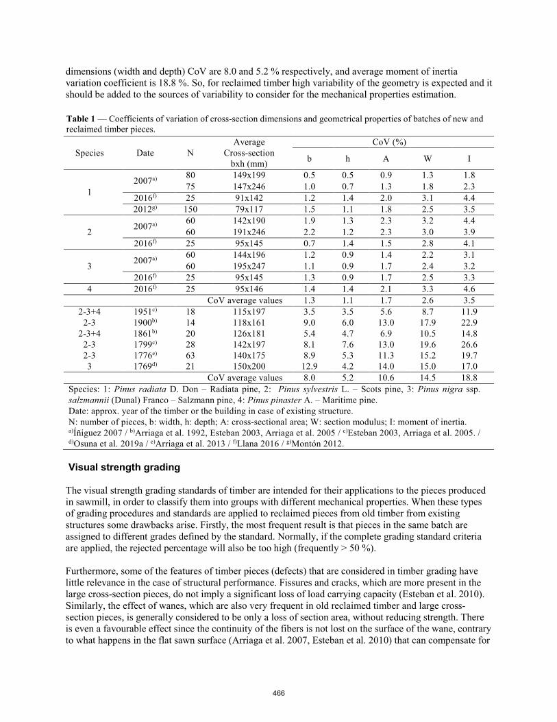
dimensions (width and depth) CoV are 8.0 and 5.2 % respectively, and average moment of inertia variation coefficient is 18.8 %. So, for reclaimed timber high variability of the geometry is expected and it should be added to the sources of variability to consider for the mechanical properties estimation.

Table 1 — Coefficients of variation of cross-section dimensions and geometrical properties of batches of new and reclaimed timber pieces.

Species Date N Average

Cross-section bxh (mm)

CoV (%)

b h A W I

1 2007a) 80 149x199 0.5 0.5 0.9 1.3 1.8

75 147x246 1.0 0.7 1.3 1.8 2.3 2016f) 25 91x142 1.2 1.4 2.0 3.1 4.4 2012g) 150 79x117 1.5 1.1 1.8 2.5 3.5

2 2007a) 60 142x190 1.9 1.3 2.3 3.2 4.4 60 191x246 2.2 1.2 2.3 3.0 3.9

2016f) 25 95x145 0.7 1.4 1.5 2.8 4.1

3 2007a) 60 144x196 1.2 0.9 1.4 2.2 3.1 60 195x247 1.1 0.9 1.7 2.4 3.2

2016f) 25 95x145 1.3 0.9 1.7 2.5 3.3 4 2016f) 25 95x146 1.4 1.4 2.1 3.3 4.6

CoV average values 1.3 1.1 1.7 2.6 3.5 2-3+4 1951c) 18 115x197 3.5 3.5 5.6 8.7 11.9

2-3 1900b) 14 118x161 9.0 6.0 13.0 17.9 22.9 2-3+4 1861b) 20 126x181 5.4 4.7 6.9 10.5 14.8

2-3 1799c) 28 142x197 8.1 7.6 13.0 19.6 26.6 2-3 1776e) 63 140x175 8.9 5.3 11.3 15.2 19.7 3 1769d) 21 150x200 12.9 4.2 14.0 15.0 17.0

CoV average values 8.0 5.2 10.6 14.5 18.8 Species: 1: Pinus radiata D. Don – Radiata pine, 2: Pinus sylvestris L. – Scots pine, 3: Pinus nigra ssp. salzmannii (Dunal) Franco – Salzmann pine, 4: Pinus pinaster A. – Maritime pine. Date: approx. year of the timber or the building in case of existing structure. N: number of pieces, b: width, h: depth; A: cross-sectional area; W: section modulus; I: moment of inertia. a)Íñiguez 2007 / b)Arriaga et al. 1992, Esteban 2003, Arriaga et al. 2005 / c)Esteban 2003, Arriaga et al. 2005. /d)Osuna et al. 2019a / e)Arriaga et al. 2013 / f)Llana 2016 / g)Montón 2012.

Visual strength grading

The visual strength grading standards of timber are intended for their applications to the pieces produced in sawmill, in order to classify them into groups with different mechanical properties. When these types of grading procedures and standards are applied to reclaimed pieces from old timber from existing structures some drawbacks arise. Firstly, the most frequent result is that pieces in the same batch are assigned to different grades defined by the standard. Normally, if the complete grading standard criteria are applied, the rejected percentage will also be too high (frequently > 50 %).

Furthermore, some of the features of timber pieces (defects) that are considered in timber grading have little relevance in the case of structural performance. Fissures and cracks, which are more present in the large cross-section pieces, do not imply a significant loss of load carrying capacity (Esteban et al. 2010). Similarly, the effect of wanes, which are also very frequent in old reclaimed timber and large cross-section pieces, is generally considered to be only a loss of section area, without reducing strength. There is even a favourable effect since the continuity of the fibers is not lost on the surface of the wane, contrary to what happens in the flat sawn surface (Arriaga et al. 2007, Esteban et al. 2010) that can compensate for

466

the effect of loss of section area. On the other hand, the most relevant defects in the structural performance will be knots and the slope of grain. Some experimental studies propose grading models based solely on these two parameters for timber from existing structures (Arriaga et al. 2005). Finally, and crucially, assigning a visual grade of reclaimed timber to a strength class is formally not possible under EN 14081-1, since even if the species and growth area can be determined, the effect of previous grading (both direct and incidental) cannot be accounted for.

To summarize, although visual timber grading in reclaimed timber is a procedure that can help to estimate its mechanical properties, actual standards based on studies carried out over thousands of “new timber” pieces do not represent the features presented in reclaimed timber, or provide a route to safely assigning a strength class. As part of the solution, one way of avoiding this high percent of rejected pieces could be to establish lower visual qualities (with lower mechanical properties), that allow in practice not to reject pieces, but to determine their carrying capacity.

Nondestructive measurements for density estimation

Density is a physical property related to some mechanical properties, and it is defined as the relationship between mass and volume. Its determination in laboratory could be done gravimetrically, by x-ray, or estimated by some other method, over different amount of wood: smaller than the cross-section method (e.g. coupons or cores, standard ISO 13061-2), cross-section method (local density, standard EN 408) or the whole piece methods (global density).

Table 2 shows the density values of several batches of large cross-section sawn timber of four coniferous species with different sizes. The global density is 2.5 % greater than average local density, and the coefficient of variation of global density (8.7 %) is slightly lower than local density (10.2 %).

Regarding to reclaimed timber, global density is slightly greater than local density because the volume calculation procedure in the whole piece is the apparent volume including air space. This tendency is contrary to the new timber`s result and, additionally, volume estimation (and density) in reclaimed timber will present high variability due to the geometry is expected.

Although there exist many non and semi destructive methods for estimating density in wood, the most practical for in situ use are the following:

- Pilodyn 6J Forest (Proceq, Switzerland) and WOODPecker (DRC, Italy). Penetration testers designed toestimate density by probing technique;

- Screw Withdrawal Resistance Meter (SWRM) (Fakopp, Hungary). Screw withdrawal device designed toestimate density by means of pullout resistance

- RML Wood Extractor (GICM, Spain), it is a wood extractor device used for the estimation of moisturecontent and density in timber by drilling technique.

- Core drilling: cylindrical cores extracted from the pieces with a diameter from 8 to 16 mm and a lengthof 30 to 50 mm to measure density directly. The effect of the resulting hole in the piece is smaller than ofa knot, although is greater than that of the others devices (Íñiguez-González et al. 2015).

467

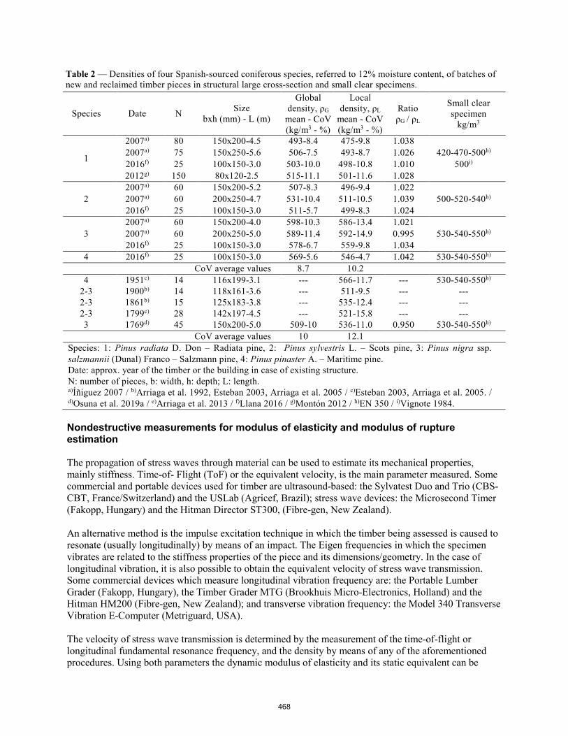
Table 2 — Densities of four Spanish-sourced coniferous species, referred to 12% moisture content, of batches of new and reclaimed timber pieces in structural large cross-section and small clear specimens.

Species Date N Size bxh (mm) - L (m)

Global density, ρG

mean - CoV (kg/m3 - %)

Local density, ρL

mean - CoV (kg/m3 - %)

Ratio ρG / ρL

Small clear specimen

kg/m3

1

2007a) 80 150x200-4.5 493-8.4 475-9.8 1.038 2007a) 75 150x250-5.6 506-7.5 493-8.7 1.026 420-470-500h)

2016f) 25 100x150-3.0 503-10.0 498-10.8 1.010 500i)

2012g) 150 80x120-2.5 515-11.1 501-11.6 1.028

2 2007a) 60 150x200-5.2 507-8.3 496-9.4 1.022 2007a) 60 200x250-4.7 531-10.4 511-10.5 1.039 500-520-540h)

2016f) 25 100x150-3.0 511-5.7 499-8.3 1.024

3 2007a) 60 150x200-4.0 598-10.3 586-13.4 1.021 2007a) 60 200x250-5.0 589-11.4 592-14.9 0.995 530-540-550h)

2016f) 25 100x150-3.0 578-6.7 559-9.8 1.034 4 2016f) 25 100x150-3.0 569-5.6 546-4.7 1.042 530-540-550h)

CoV average values 8.7 10.2 4 1951c) 14 116x199-3.1 --- 566-11.7 --- 530-540-550h)

2-3 1900b) 14 118x161-3.6 --- 511-9.5 --- ---2-3 1861b) 15 125x183-3.8 --- 535-12.4 --- --- 2-3 1799c) 28 142x197-4.5 --- 521-15.8 --- --- 3 1769d) 45 150x200-5.0 509-10 536-11.0 0.950 530-540-550h)

CoV average values 10 12.1 Species: 1: Pinus radiata D. Don – Radiata pine, 2: Pinus sylvestris L. – Scots pine, 3: Pinus nigra ssp. salzmannii (Dunal) Franco – Salzmann pine, 4: Pinus pinaster A. – Maritime pine. Date: approx. year of the timber or the building in case of existing structure. N: number of pieces, b: width, h: depth; L: length. a)Íñiguez 2007 / b)Arriaga et al. 1992, Esteban 2003, Arriaga et al. 2005 / c)Esteban 2003, Arriaga et al. 2005. /d)Osuna et al. 2019a / e)Arriaga et al. 2013 / f)Llana 2016 / g)Montón 2012 / h)EN 350 / i)Vignote 1984.

Nondestructive measurements for modulus of elasticity and modulus of rupture estimation

The propagation of stress waves through material can be used to estimate its mechanical properties, mainly stiffness. Time-of- Flight (ToF) or the equivalent velocity, is the main parameter measured. Some commercial and portable devices used for timber are ultrasound-based: the Sylvatest Duo and Trio (CBS-CBT, France/Switzerland) and the USLab (Agricef, Brazil); stress wave devices: the Microsecond Timer (Fakopp, Hungary) and the Hitman Director ST300, (Fibre-gen, New Zealand).

An alternative method is the impulse excitation technique in which the timber being assessed is caused to resonate (usually longitudinally) by means of an impact. The Eigen frequencies in which the specimen vibrates are related to the stiffness properties of the piece and its dimensions/geometry. In the case of longitudinal vibration, it is also possible to obtain the equivalent velocity of stress wave transmission. Some commercial devices which measure longitudinal vibration frequency are: the Portable Lumber Grader (Fakopp, Hungary), the Timber Grader MTG (Brookhuis Micro-Electronics, Holland) and the Hitman HM200 (Fibre-gen, New Zealand); and transverse vibration frequency: the Model 340 Transverse Vibration E-Computer (Metriguard, USA).

The velocity of stress wave transmission is determined by the measurement of the time-of-flight or longitudinal fundamental resonance frequency, and the density by means of any of the aforementioned procedures. Using both parameters the dynamic modulus of elasticity and its static equivalent can be

468

estimated for an individual timber. While the density and stiffness estimates of the batch can be combined to compare to a strength class, the situation for strength itself is more complicated. However, the dynamic stiffness, density and visual grading characteristics (such as knottiness parameters like CKDR) do, individually and combined, have predictive potential for strength. Models could be found with testing, but do not necessarily (or at all) translate to other batches of timber. However, bending strength is not always required for all structural uses of timber, and design may be sufficient with stiffness, density, and secondary properties estimated from those.

Table 3 — Velocity (Sylvatest Duo, end to end) of four Spanish-sourced coniferous species, referred to 12% moisture content, of batches of new and reclaimed timber pieces.

Species Date N Size bxh (mm) - L (m)

Velocity SyL, Vel12 mean - CoV (kg/m3 - %)

1

2007a) 80 150x200-4.5 4859-6.0 2007a) 75 150x250-5.6 4943-4.9 2016f) 25 100x150-3.0 5369-6.0 2012g) 150 80x120-2.5 4968-9.9

2 2007a) 60 150x200-5.2 5022-6.1 2007a) 60 200x250-4.7 4979-6.5 2016f) 25 100x150-3.0 5311-5.6

3 2007a) 60 150x200-4.0 4871-8.8 2007a) 60 200x250-5.0 4744-7.5 2016f) 25 100x150-3.0 4658-8.2

4 2016f) 25 100x150-3.0 4427-8.2 CoV average value 7.1

4 1951c) 14 116x199-3.1 3980-11.9 2-3 1799c) 28 142x197-4.5 4773-5.8 3 1769d) 10 150x200-11.0 4858-5.0

CoV average value 7.6 Species: 1: Pinus radiata D. Don – Radiata pine, 2: Pinus sylvestris L. – Scots pine, 3: Pinus nigra ssp. salzmannii (Dunal) Franco – Salzmann pine, 4: Pinus pinaster A. – Maritime pine. Date: approx. year of the timber or the building in case of existing structure. N: number of pieces, b: width, h: depth; L: length. a)Íñiguez 2007 / b)Arriaga et al. 1992, Esteban 2003, Arriaga et al. 2005 / c)Esteban 2003,Arriaga et al. 2005. / d)Osuna et al. 2019b / e)Arriaga et al. 2013 / f)Llana 2016 / g)Montón2012 / h)EN 350 / i)Vignote 1984.

Conclusions

Although wood is a renewable resource, it is not unlimited. With rising use of timber in construction, especially in products like CLT, it is necessary to both plant new timber, but also consider efficient use and reuse of the timber available now. In order to meet the growing demands for wood generally, the efficiency of the wood as a resource has to be enhanced and additional sources for raw material have to be identified. Reclaimed wood has large potential for construction, but grading and testing standards are not keeping up with technology or practice in reclaimed timber, so a special standardised framework is needed.

Reclaimed timber presents higher variability in cross section dimensions, which also contributes to its higher variability of the mechanical properties in comparison to new timber. It is necessary to analyze

469

what would be the impact of this variability on the stress grading assessment and the characteristic values of mechanical properties used.

Density values of the reclaimed wood do not differ from the values of new timber, except slightly by imprecision in the measurement of the volume. The global density calculated from the weight and volume of the whole piece is the most recommended, providing the estimated volume as accurate as possible.

The stress wave velocity presents low variability in reclaimed and new timber, and values are similar. Therefore, this nondestructive variable has the same predictor capacity in both products. However, there are additional steps for using this to indicate strength.

Acknowledgments

Ministerio de Ciencia, Innovación y Universidades, España. Plan Estatal de Investigación Científica y Técnica y de Innovación 2017-2020, Programa Estatal de I+D+i Orientada a los Retos de la Sociedad, Proyectos de I+D+i «Programación Conjunta Internacional», convocatoria 2019. Título del proyecto: Diseño innovador para el futuro - uso y reutilización de componentes de edificación de madera. Referencia Administrativa: PCI2019-103544.

References

Arriaga, F.; Esteban, M.; Argüelles, R.; Bobadilla, I.; Íñiguez-González, G. 2007. The effect of wanes on the bending strength of solid timber beams. Materiales de Construcción. 57 (288): 61-76.

Arriaga, F., Esteban, M., Íñiguez-González, G., Bobadilla, I., Llana, D.F., González-Sanz, M. 2013. Structural assessment of the timber structure of the Casa Grande building in the Real Cortijo de San Isidro, Aranjuez, Madrid (Spain). Proceeding of the 18th International Nondestructive Testing and Evaluation of Wood Symposium. General Technical Report FPL-GTR-226. Madison, WI: U.S. Department of Agriculture, Forest Service, Forest Products Laboratory: 233 – 244.

Arriaga, F.; Esteban, M.; Relea, E. 2005. Evaluation of the load carrying capacity of large cross section coniferous timber in standing structures. Materiales de Construcción. 55 (280): 43-52.

Arriaga, F.; García, L.; Gebremedhin, K.G.; Peraza, F. 1992. Grading and load carrying capacity of old timber beams. International Summer Meeting, American Society of Agricultural Engineers ASAE. Charlotte, North Carolina, USA. 21-24th June 1992.

EN 350:2016. Durability of wood and wood-based products. Testing and classification of the durability to biological agent of wood and wood-based materials. CEN, Brussels.

EN 408:2010+A1:2012. Timber structures-Structural timber and glued laminated timber-Determination of some physical and mechanical properties. CEN, Brussels.

EN 14081-1:2016. Timber structures. Strength graded structural timber with rectangular cross section. Part 1: General requirements. CEN, Brussels. (Note: the harmonised standard is considered to be EN 14081-1:2005+A1:2011 since the 2016 version is not cited in the Official Journal of the European Union).

Esteban, M.; Arriaga, F.; Íñiguez, G.; Bobadilla, I.; Mateo, R. 2010. The effect of fissures on the strength of structural timber. Materiales de Construcción. 60 (299): 115-132. DOI: 10.3989/mc.2010.48208.

470

Eurostat. 2018. https://ec.europa.eu/eurostat/statistics-explained/index.php/Wood_products_-_production_and_trade#Primary_wood_products

Höglmeier, K.; Weber-Blaschke, G.; Richter, K. 2017. Potentials for cascading of recovered wood from building deconstruction - A case study for south-east Germany. Resources, Conservation and Recycling. 117: 304-314.

Instituto Nacional de Estadística. 2016. Otras cuentas medioambientales: Cuenta de los residuos. 7 p.

Íñiguez, G. 2007. Clasificación mediante técnicas no destructivas y evaluación de las propiedades mecánicas de la madera aserrada de coníferas de gran escuadría para uso estructural (Grading by non destructive techniques and assessment of the mechanical properties of large cross section coniferous sawn timber for structural use). Doctoral thesis. Universidad Politécnica de Madrid, ETS de Ingenieros de Montes. 223 p. PDF file: http://oa.upm.es/415

Íñiguez-González, G., Montón, J., Arriaga, F., Segués, E. 2015. In-situ assessment of structural timber density using non-destructive and semi-destructive testing. BioResources 10(2): 2256-2265.

ISO 13061-2:2014+A1. Physical and mechanical properties of wood. Test methods for small clear wood specimens. Part 2: Determination of density for physical and mechanical tests.

Llana, D.F. 2016. Influencia de factores físicos y geométricos en la clasificación estructural de la madera mediante técnicas no destructivas (The influence of physical and geometrical factors on timber stress-grading by non-destructive techniques). Doctoral thesis. Universidad Politécnica de Madrid, ETSI de Montes, Forestal y del Medio Natural. 412 p. DOI and pdf file: https://doi.org/10.20868/UPM.thesis.43696

Miyazaki, H.; Tanaka, K.; Inoue, M.; Takanashi, H.; Hirata, M.; Hano, T. 2003. Recycling of timbers from wooden house by handworked demolition system. Proceedings of JSCE. 748: 81–89.

Montón, J. 2012. Clasificación estructural de la madera de Pinus radiata D. Don procedente de Cataluña mediante métodos no destructivos y su aplicabilidad en la diagnosis estructural (Structural grading of Pinus radiata D. Don timber from Catalonia using nondestructive methods and their applicability in structural diagnosis). Doctoral thesis. Universitat Politécnica de Catalunya, Escola Tècnica Superior D'Arquitectura de Barcelona. 160-309 p. PDF file: http://hdl.handle.net/10803/96423

Nakajima, S.; Futaki, M. 2001. National R&D project to promote recycle and reuse of timber construction in Japan, Deconstruction and Material reuse. Available at: http://www.irbnet.de/daten/iconda/CIB753.pdf

Núñez, D. 2019. Personal Communication.

Osuna-Sequera, C.; Llana, D.F.; Esteban, M.; Arriaga, F. 2019a. Improving density estimation in large cross-section timber from existing structures optimizing the number of non-destructive measurements. Construction and Building Materials. 211: 199-206. https://doi.org/10.1016/j.conbuildmat.2019.03.144

Osuna-Sequera, C., Arriaga, F., Esteban, M., Íñiguez-González, I. 2019b. Consideraciones sobre la medición de la velocidad de ondas de ultrasonidos en piezas de madera puesta en obra. Congreso Lignomad 2019, Santiago de Compostela. Publication pending.

471

Osuna-Sequera, C.; Llana, D.F.; Íñiguez-González, G.; Arriaga, F. xxxx. The influence of cross-section variation on load carrying capacity assessment in existing timber structures. In revision.

Ramage, M.H.; Burridge, H; Busse-Wicher, M.; Fereday, G.; Reynolds, T.; Shah, D.U.; Wu, G.; Yu, L.; Fleming, P.; Densley-Tingley, D.; Allwood, J.; Dupree, P.; Linden, P.F.; Scherman, O. 2017. The wood from the trees: The use of timber in construction. Renewable and Sustainable Energy Reviews. 68. 333-359.

Ridley-Ellis, D.; Stapel, P.; Baño, V. 2016. Strength grading of sawn timber in Europe: an explanation for engineers and researchers. European Journal of Wood and Wood Products. 74:291. https://doi.org/10.1007/s00107-016-1034-1

Rodríguez, M. 2019. Personal Communication.

Rodríguez-Trobajo, E. 2008. Procedencia y uso de madera de pino silvestre y pino laricio en edificios históricos de Castilla y Andalucía (Origin and use of Scots and Black timber pine in historic buildings from Castile and Andalucía). Arqueología de la arquitectura 5: 33-53.

Rodríguez-Trobajo, E. 2018. Personal Communication.

Sakaguchi, D.; Takano, A.; Hughes, M. 2016. The potential for cascading wood from demolished buildings: the condition of recovered wood through a case study in Finland. International Wood Products Journal. 7:3: 137-143. DOI: 10.1080/20426445.2016.1180495

Serrano, E. 2009. Documentation of the Limnologen Project: Overview and Summaries of Sub Projects Results. Report no. 56, ISBN 978-91-7636-672-1, School of Technology and Design, Växjö University.

Soilán Cañas, A.; Touza Vázquez, M.C.; Arriaga F.; Guaita, M. 2016. Bending stiffness increasing of existing pitch pine beams by means of LVL reinforcement. Proceedings of the World Conference on Timber Engineering (WCTE 2016), Vienna, Austria, Eds. J. Eberhardsteiner, W. Winter, A. Fadai, M. Pöll, Publisher: Vienna University of Technology, Austria, ISBN: 978-3-903039-00-1.

Vignote, S. 1984. Características físico-mecánicas del pino insignis y su influencia con la edad y el crecimiento (Physical and mechanical properties of Pinus insignis and the influence of age and rate of grown. Doctoral thesis. Universidad Politécnica de Madrid, ETS de Ingenieros de Montes.

472

Procedure for Estimating the Physical and Mechanical Properties of Existing Timber Structures, Applied to an Historic Building in Cava De San Miguel, Madrid, Spain Francisco Arriaga Department of Forestry and Environmental Engineering and Management, MONTES (School of Forest Engineering and Natural Environment), Universidad Politécnica de Madrid, Spain, ORCID: 0000-0001-5535-0786, francisco.arriaga@upm.es

Carlos Osuna-Sequera Department of Forestry and Environmental Engineering and Management, MONTES (School of Forest Engineering and Natural Environment), Universidad Politécnica de Madrid, Spain, ORCID 0000-0002-9227-3035, caosseq@gmail.com

Miguel Esteban Department of Forestry and Environmental Engineering and Management, MONTES (School of Forest Engineering and Natural Environment), Universidad Politécnica de Madrid, Spain, ORCID: 0000-0003-3364-9044, miguel.esteban@upm.es

Guillermo Íñiguez-González Department of Forestry and Environmental Engineering and Management, MONTES (School of Forest Engineering and Natural Environment), Universidad Politécnica de Madrid, Spain, ORCID: 0000-0003-2917-842X, guillermo.iniguez@upm.es

Ignacio Bobadilla Department of Forestry and Environmental Engineering and Management, MONTES (School of Forest Engineering and Natural Environment), Universidad Politécnica de Madrid, Spain, ORCID: 0000-0002-4627-3130, i.bobadilla@upm.es

Abstract

Physical and mechanical properties of the timber structure of a seven-story building from the end of 18th century, located in Madrid, Spain, were estimated using nondestructive techniques. These consisted of stress wave measurements and probing tests based on needle penetration depth and drilling residue collection, to estimate the modulus of elasticity, modulus of rupture and density. The structure consists on timber framed brick walls and heavy timber floors with mortar filling. For the development of the inspection and data collection a protocol based on previous research works has been defined. First, the wood species were identified as Pinus sylvestris L. or Pinus nigra Arnold ssp. salzmannii (Dunal) Franco and Pinus pinaster Ait. Measurements were taken in five areas of floors and in eight areas of framed walls, distributed between the third and sixth floors. In each of these samples, detailed measurements of at least three pieces were taken. The Time-of-Flight were measured over three distances in each piece, and the punctual measurements for the estimation of density were taken in three cross-sections of the piece. Mean values of density and modulus of elasticity were estimated for each sample. Finally, it was proposed to adopt a mean value for joists and another slightly smaller for pillars. The characteristic value of bending strength was conservatively estimated from the previous values.

Keywords: assessment, case study, non-destructive testing, timber structure, protocol

473

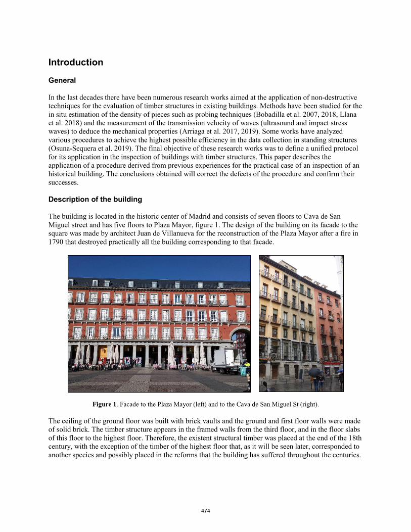
Introduction

General

In the last decades there have been numerous research works aimed at the application of non-destructive techniques for the evaluation of timber structures in existing buildings. Methods have been studied for the in situ estimation of the density of pieces such as probing techniques (Bobadilla et al. 2007, 2018, Llana et al. 2018) and the measurement of the transmission velocity of waves (ultrasound and impact stress waves) to deduce the mechanical properties (Arriaga et al. 2017, 2019). Some works have analyzed various procedures to achieve the highest possible efficiency in the data collection in standing structures (Osuna-Sequera et al. 2019). The final objective of these research works was to define a unified protocol for its application in the inspection of buildings with timber structures. This paper describes the application of a procedure derived from previous experiences for the practical case of an inspection of an historical building. The conclusions obtained will correct the defects of the procedure and confirm their successes.

Description of the building

The building is located in the historic center of Madrid and consists of seven floors to Cava de San Miguel street and has five floors to Plaza Mayor, figure 1. The design of the building on its facade to the square was made by architect Juan de Villanueva for the reconstruction of the Plaza Mayor after a fire in 1790 that destroyed practically all the building corresponding to that facade.

Figure 1. Facade to the Plaza Mayor (left) and to the Cava de San Miguel St (right).

The ceiling of the ground floor was built with brick vaults and the ground and first floor walls were made of solid brick. The timber structure appears in the framed walls from the third floor, and in the floor slabs of this floor to the highest floor. Therefore, the existent structural timber was placed at the end of the 18th century, with the exception of the timber of the highest floor that, as it will be seen later, corresponded to another species and possibly placed in the reforms that the building has suffered throughout the centuries.

474

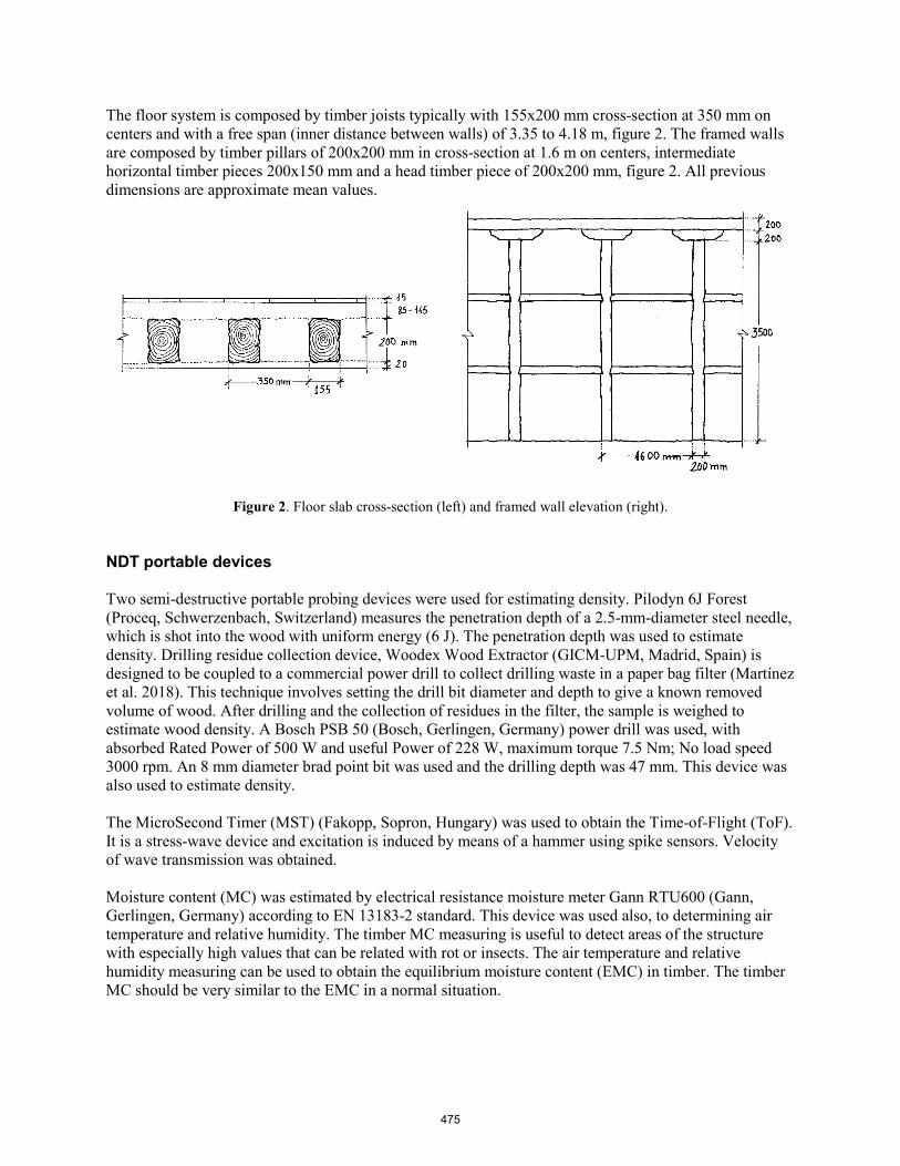
The floor system is composed by timber joists typically with 155x200 mm cross-section at 350 mm on centers and with a free span (inner distance between walls) of 3.35 to 4.18 m, figure 2. The framed walls are composed by timber pillars of 200x200 mm in cross-section at 1.6 m on centers, intermediate horizontal timber pieces 200x150 mm and a head timber piece of 200x200 mm, figure 2. All previous dimensions are approximate mean values.

Figure 2. Floor slab cross-section (left) and framed wall elevation (right).

NDT portable devices

Two semi-destructive portable probing devices were used for estimating density. Pilodyn 6J Forest (Proceq, Schwerzenbach, Switzerland) measures the penetration depth of a 2.5-mm-diameter steel needle, which is shot into the wood with uniform energy (6 J). The penetration depth was used to estimate density. Drilling residue collection device, Woodex Wood Extractor (GICM-UPM, Madrid, Spain) is designed to be coupled to a commercial power drill to collect drilling waste in a paper bag filter (Martínez et al. 2018). This technique involves setting the drill bit diameter and depth to give a known removed volume of wood. After drilling and the collection of residues in the filter, the sample is weighed to estimate wood density. A Bosch PSB 50 (Bosch, Gerlingen, Germany) power drill was used, with absorbed Rated Power of 500 W and useful Power of 228 W, maximum torque 7.5 Nm; No load speed 3000 rpm. An 8 mm diameter brad point bit was used and the drilling depth was 47 mm. This device was also used to estimate density.

The MicroSecond Timer (MST) (Fakopp, Sopron, Hungary) was used to obtain the Time-of-Flight (ToF). It is a stress-wave device and excitation is induced by means of a hammer using spike sensors. Velocity of wave transmission was obtained.

Moisture content (MC) was estimated by electrical resistance moisture meter Gann RTU600 (Gann, Gerlingen, Germany) according to EN 13183-2 standard. This device was used also, to determining air temperature and relative humidity. The timber MC measuring is useful to detect areas of the structure with especially high values that can be related with rot or insects. The air temperature and relative humidity measuring can be used to obtain the equilibrium moisture content (EMC) in timber. The timber MC should be very similar to the EMC in a normal situation.

475

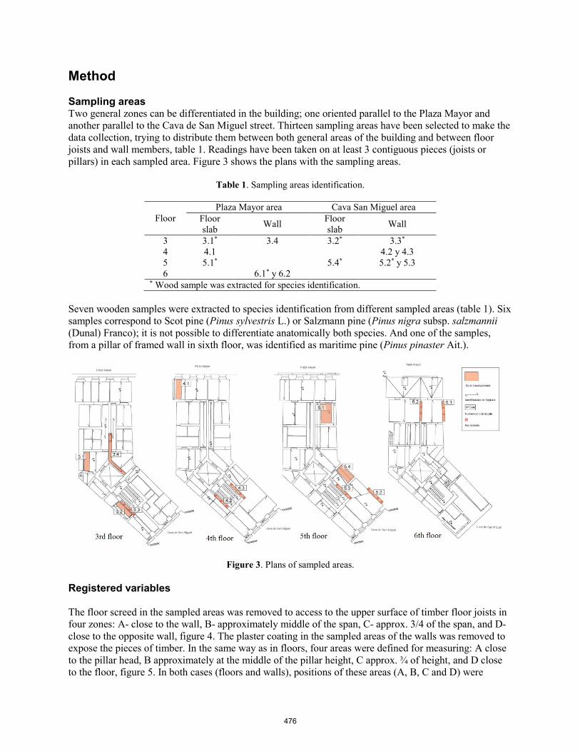
Method

Sampling areas Two general zones can be differentiated in the building; one oriented parallel to the Plaza Mayor and another parallel to the Cava de San Miguel street. Thirteen sampling areas have been selected to make the data collection, trying to distribute them between both general areas of the building and between floor joists and wall members, table 1. Readings have been taken on at least 3 contiguous pieces (joists or pillars) in each sampled area. Figure 3 shows the plans with the sampling areas.

Table 1. Sampling areas identification.

Floor Plaza Mayor area Cava San Miguel area

Floor slab Wall Floor

slab Wall

3 3.1* 3.4 3.2* 3.3*

4 4.1 4.2 y 4.3 5 5.1* 5.4* 5.2* y 5.3 6 6.1* y 6.2

* Wood sample was extracted for species identification.

Seven wooden samples were extracted to species identification from different sampled areas (table 1). Six samples correspond to Scot pine (Pinus sylvestris L.) or Salzmann pine (Pinus nigra subsp. salzmannii (Dunal) Franco); it is not possible to differentiate anatomically both species. And one of the samples, from a pillar of framed wall in sixth floor, was identified as maritime pine (Pinus pinaster Ait.).

Figure 3. Plans of sampled areas.

Registered variables

The floor screed in the sampled areas was removed to access to the upper surface of timber floor joists in four zones: A- close to the wall, B- approximately middle of the span, C- approx. 3/4 of the span, and D- close to the opposite wall, figure 4. The plaster coating in the sampled areas of the walls was removed to expose the pieces of timber. In the same way as in floors, four areas were defined for measuring: A close to the pillar head, B approximately at the middle of the pillar height, C approx. ¾ of height, and D close to the floor, figure 5. In both cases (floors and walls), positions of these areas (A, B, C and D) were

476

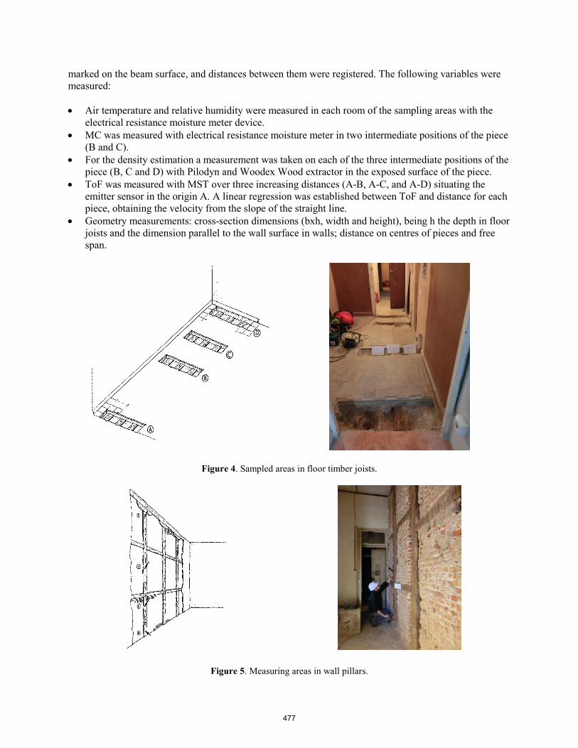
marked on the beam surface, and distances between them were registered. The following variables were measured:

• Air temperature and relative humidity were measured in each room of the sampling areas with theelectrical resistance moisture meter device.

• MC was measured with electrical resistance moisture meter in two intermediate positions of the piece(B and C).

• For the density estimation a measurement was taken on each of the three intermediate positions of thepiece (B, C and D) with Pilodyn and Woodex Wood extractor in the exposed surface of the piece.

• ToF was measured with MST over three increasing distances (A-B, A-C, and A-D) situating theemitter sensor in the origin A. A linear regression was established between ToF and distance for eachpiece, obtaining the velocity from the slope of the straight line.

• Geometry measurements: cross-section dimensions (bxh, width and height), being h the depth in floorjoists and the dimension parallel to the wall surface in walls; distance on centres of pieces and freespan.

Figure 4. Sampled areas in floor timber joists.

Figure 5. Measuring areas in wall pillars.

477

Physical and mechanical properties estimation

The density ρpil (kg/m3) has been estimated from depth penetration z (mm) with Pilodyn 6J Forest according to equation (1):

ρpil = a + b·z (1)

being for Scot pine, a = 708.7, b = -19.03 (Íñiguez 2007); Salzmann pine, a = 771.9, b = -19.03 (Íñiguez 2007); Maritime pine, a = 646.3, b = -9.71 (Martínez 2016). In case of Scot/Salzmann pines, Scots pine parameters have been used in favor of safety.

The density ρwdx (kg/m3) has been estimated from mass m (g) extracted with Woodex Wood Extractor according to equation (2) (Martínez 2016):

ρwdx = 428.66·m – 107.9 (2)

The density value assigned to each piece was obtained as the average value of the three measurements with Woodex and Pilodyn devices. The Woodex values were selected as representative because of its greater prediction capacity. Pilodyn results were used as a supplementary information.

The dynamic MOE Ed (N/mm2) for each piece was obtained from wave transmission velocity v (m/s) and density ρwdx (kg/m3) according to equation (4) (Timoshenko et al. 1934):

Ed = ρwdx·v2·10-6 (4)

The mean value of static bending MOE (E0,mean) was obtained from Ed according to equation (5):

E0,mean = Ed/kdyn (5)

where, kdyn is a factor to adjust the MOE, due to the differences between both test procedures: Ed (short duration compression test) and E0,mean (30-300 s duration standard bending test). The kdyn value depend on the device and it has been deduced in previous works (Arriaga et al. 2017, 2019, Osuna-Sequera et al. 2019) for MST with an average value of 1.24 (1.15-1.32).

Results

The average value of air temperature was 14ºC (11-16%) and relative humidity 50% (44-59%). The corresponding EMC in timber is 9.6%. The average MC estimated with electrical moisture meter was 11.6%, what is close to the EMC. Table 3 summarizes the values and coefficients of variation (CoV %) of main properties for each sample. The values were obtained as the mean value of the 3 (in some cases 2 or 5) pieces that constitute each sample.

The estimated value of density by Woodex varies between 461 and 598 kg/m3 with a global mean value of 514 kg/m3 (CoV = 11.1%). There are not relevant differences between density of pillars and floor joists. Then, 514 kg/m3 was proposed as mean value of density for all the pieces. The density estimated by Pilodyn gave lower values varying between 436 and 537 kg/m3 with a global mean value of 488 kg/m3 (CoV = 6%). A linear regression between density estimated by Woodex and by Pilodyn showed a coefficient of determination r2 = 0.33.

478

Table 3. Mean properties for each sample (density estimated by Woodex).

Floo

r Plaza Mayor area Cava San Miguel area

Floor Wall Floor Wall sa

mpl

e ρwdx kg/m3 CoV %

E0,mean N/mm2 CoV %

sam

ple

ρwdx kg/m3 CoV %

E0,mean N/mm2 CoV %

sam

ple

ρwdx kg/m3 CoV %

E0,mean N/mm2 CoV %

sam

ple

ρwdx kg/m3 CoV %

E0,mean N/mm2 CoV %

3 3.1 504 5

8568 14 3.4 526

8 10154

2 3.2 541 11

10442 17 3.3 542

10 10501

39

4 4.1 466

15 8852

23 4.2 522 11

9922 29

4.3 498 8

8718 14

5 5.1 598

13 11077

27 5.4 493 7

10267 20 5.2 524

18 7971

39

5.3 484 15

7113 20

6 6.1 524

5 9317

1

6.2 461 17

9927 11

Mean 523 9499 504 9799 517 10354 514 8845

The gross time consumed in the inspection and data collection in the work for the 13 sampling areas was 52 h with a team of three people, which represent 4 h per sample (normally formed by 3 pieces of wall pillars or floor joists). The time exclusively dedicated to the measurement (geometry, Pilodyn, Woodex, MST and MC) was approximately 45 minutes per sample. Therefore, most of the time is consumed in the auxiliary operations of movement inside the building, preparation and collection of portable equipment.

Conclusions

It is proposed a planning of the inspection tasks consisting of a first possible differentiation of parts of the building that could have different constructive characteristics; secondly, a selection of the representative sampling areas of each part of the building; and, finally, the data collection of at least 3 pieces in each sample. The time consumed by each sampling area was of the order of 4 h. The greater part is due to the auxiliary tasks of preparation and displacement in the work. Less than a quarter of the time corresponds to the data collection. An average value should be assigned for the properties of each sample obtained from measurements on, at least, three pieces in each sample. In practice there is a load sharing behavior due to the effect of transverse stiffness in the floor slabs. It would be interesting to differentiate the species Scot and Salzmann pine. This would allow a greater precision in the estimation of the mechanical properties.

Timber density estimation using the Pilodyn 6J Forest requires much less time than with the Woodex (about half), but its prediction capacity is lower. However, the differences found in MOE estimation would be in the order of 5%.

Acknowledgments

Ministerio de Economía y Competitividad (The Spanish Ministry of the Economy and Competitiveness). Plan Nacional I + D 2013-2016. Proj.: BIA 2014-55089-P. Mrs. Pilar Llarena, owner of the building and

479

Mr. Miguel A. Rodríguez and Mr. Félix Fuertes of the R-Torices Office for the facilities and help provided for the realization of this study.

Reference list

Arriaga, F., Llana, D.F., Esteban, M., Iñiguez-González, G. 2017. Influence of length and sensor positioning on acoustic time-of-flight (ToF) measurement in structural timber. Holzforschung. Published online. DOI: 10.1515/hf-2016-0214.

Arriaga, F., Montón, J., Bobadilla, I., Llana D.F. 2019. Influence of length on acoustic time-of-flight (ToF) measurement in built-in structures of Norway spruce timber. Holzforschung, 2019, 73(4):339-352. DOI: 10.1515/hf-2018-0122.

Bobadilla, I., Esteban, M., Íñiguez-González, G., Arriaga, F., Ballarín, D., Palacios, J. 2007. Estimación de la densidad de la madera aserrada de conífera mediante técnicas no destructivas de arranque de tornillos y penetrómetro y su aplicación en la estimación del módulo de elasticidad (Density estimation by screw withdrawal resistance and probing in structural sawn coniferous timber and modulus of elasticity assessment). In Spanish Inf. Constr. 59 (2007) 107–116, DOI: 10.3989/ic.2007.v59.i506.513.

Bobadilla, I., Martínez, R.D., Esteban, M., Llana, D.F. 2018. Estimation of wood density by the core drilling technique. Holzforschung 72(12):1051-1056. ISSN: 0018-3830. DOI: 10.1515/hf-2018-0036.

European Standard 2002. EN 13183-2. Moisture content of a piece of sawn timber. Estimation by electrical resistance method. European Committee of Standardization, Brussels, Belgium.

D.F. Llana, G. Íñiguez-González, J. Montón, F. Arriaga 2018. In-situ density estimation by fournondestructive techniques on Norway spruce from built in wood structures, Holzforschung. 72 871–879,https://doi.org/10.1515/hf-2018-0027.

Íñiguez G. 2007. Clasificación mediante técnicas no destructivas y evaluación de las propiedades mecánicas de la madera aserrada de coníferas de gran escuadría para uso estructural (Grading by non destructive techniques and assessment of the mechanical properties of large cross section coniferous sawn timber for structural use) [Doctoral thesis]. Universidad Politécnica de Madrid, ETS de Ingenieros de Montes; p. 223. PDF file: http://oa.upm.es/415.

Martínez, R.D. 2016. Métodos no destructivos de estimación de la densidad de madera. [Timber density estimation by non-destructive methods]. PhD Dissertation. Universidad de Santiago de Compostela, EPS de Lugo. 214 p.

Martínez, R., Calvo, J., Arriaga, F., Bobadilla, I. (2018). In situ density estimation of timber pieces by drilling residue analysis, Eur. J. Wood and Wood Prod. 76:509–515. doi:10.1007/s00107-017-1214-7.

Osuna-Sequera, C., Llana, D. F., Esteban, M., Arriaga, F. 2019. Improving density estimation in large cross-section timber from existing structures optimizing the number of non-destructive measurements (Published Online). Const. Build. Mater. 211:199-206.

Timoshenko, S., Goodier, J.N 1934. Theory of elasticity. United Engineering Trustees, Inc.

480

The Effect of Length on Stress-Wave Velocity in Long Pieces of Salzmann Pine from Existing Structures Carlos Osuna-Sequera * Department of Forestry and Environmental Engineering and Management, MONTES (School of Forest Engineering and Natural Environment), Universidad Politécnica de Madrid, Spain, caosseq@gmail.com Francisco Arriaga Department of Forestry and Environmental Engineering and Management, MONTES (School of Forest Engineering and Natural Environment), Universidad Politécnica de Madrid, Spain, francisco.arriaga@upm.es Miguel Esteban Department of Forestry and Environmental Engineering and Management, MONTES (School of Forest Engineering and Natural Environment), Universidad Politécnica de Madrid, Spain, miguel.esteban@upm.es Guillermo Íñiguez-González Department of Forestry and Environmental Engineering and Management, MONTES (School of Forest Engineering and Natural Environment), Universidad Politécnica de Madrid, Spain, guillermo.iniguez@upm.es Ignacio Bobadilla Department of Forestry and Environmental Engineering and Management, MONTES (School of Forest Engineering and Natural Environment), Universidad Politécnica de Madrid, Spain, i.bobadilla@upm.es * Corresponding author Abstract The use of non-destructive techniques (NDT) to estimate physical-mechanical timber properties is an effective way of assessing and conservation of built heritage. Some research works have applied NDTs in different species with different piece’s dimensions and have showed good correlations between timber properties and the Time-of-Flight (ToF) with portable stress-wave devices. Nevertheless, there are certain parameters that need to be studied deeper, such as the effect of the pieces' dimensions on the ToF estimation.Usually, timber structures of existing buildings in Spain present large cross-section pieces as well as a cross-section variation along the piece. Frequently, in-situ assessments accessibility to structural members is complicated and measurements may only be made on 1 or 2 surfaces of the piece. The test material used in this research study consisted of 21 structural timber pieces (rafters) with 150x200 mm2 in average cross-section and 9.53 to 11.00 m in length of Salzmann pine species (Pinus nigra Arnold ssp. salzmannii (Dunal) Franco). The material comes from an existing structure built in 1768 (Royal Coliseum of Charles III in Aranjuez, Madrid, Spain).In this work, the ToF has been obtained from end to end and in different lengths ranging from 0.5 to 10.5 m at one edge of the piece and also their corresponding transmission velocities. In addition, stress velocity has been determined based on both the ToF corrected with time lag and the ToF in intermediate sections to avoid the local effect of the initial wave path. Keywords: non-destructive testing, stress waves, length effect, Salzmann pine.

481

Introduction Acoustic methods applied to structural timber have demonstrated to be an effective tool in the estimation of mechanical properties. These methods allow an accurate estimation of dynamic modulus of elasticity (MOEdyn) in timber from existing structures as well as in new buildings. Their application in the in-situ assessments have a great potential both for grading structural timber members and to predict their mechanical behaviour (Arriaga et al. 2017; Branco et al. 2017). This plays a critical key in the conservation of built heritage. Nevertheless, there are several parameters that affect acoustic readings, such as moisture content, temperature, member’s dimensions, and the devices used (Gonçalves and Leme 2008; Llana et al. 2014, 2018; Osuna-Sequera et al. 2017). In in-situ assessments, the accessibility to all surfaces of the pieces is often complicated or sometimes even impossible. Therefore, the determination of dimensions of the pieces and its influence on the measurements must be taken into account when planning the sampling areas. Some research works have studied the effect of geometry of the pieces using acoustic methods (Bucur and Böhnke 1994; Bartholomeu et al. 2003; Oliveira et al. 2006; Osuna-Sequera et al. 2017). The aim of this work is to study the effect of length on acoustic measurements with stress waves in pieces from a historic building as well as to compare the acoustic parameters obtained by applying different measurement methods. Materials and method Material The tested material are ten rafters from the Royal Coliseum of Charles III in Aranjuez, Madrid, Spain, designed by the French architect Jaime Marquet and built in 1768. The wood species was identified as Salzmann pine (Pinus nigra ssp. salzmannii (Dunal) Franco) by the Forest Timber Industries Laboratory of the Universidad Politécnica de Madrid and the Structural Timber Laboratory of INIA-CIFOR (National Agricultural Research Institute), Madrid, Spain. These pieces with 150x200x11000 mm3 nominal dimensions have already been studied in previous works (Osuna-Sequera et al. 2017, 2019 a; 2019 b). Device The MicroSecond Timer (MST) (Fakopp, Sopron, Hungary): It is an impact-induced stress wave timing device that allows to measure the ToF using two spike sensors (transmitter and receiver) and obtain an accuracy of 1 μs. The excitation is generated by a blow of a 100-gram hammer. Time-of-Flight and wave velocity The ToF is timed from the wave is generated by the hammer hitting the transmitter until it reaches the receiver. The wave stress velocity (V) in m s-1 is obtained from the Equation 1 according to the following parameters: length between the sensors (L) and ToF.

V =L

ToF (1)

Sensor positioning The ToF was obtained by positioning the sensors in two configurations:

482

- End-to-end measurement: Sensors were positioned perpendicularly on the ends. Two end-to-end measurements have been made: an upper measurement located at one third of the height, h, and a lower measurement positioned at two thirds of h, both on the vertical axis of the section as shown in Fig. 1a. - Surface measurement: The two sensors are positioned at the same piece surface with 45º above the horizontal axis, Fig. 1b, c. This positioning of the sensors may be the most suitable in an in-situ assessment, due to the limited access to one of three faces of the piece, where the ends are hidden and inaccessible. 11 cross-sections (numbered from 0 to 10) were marked in each piece at 1 m intervals, leaving 20 cm margin at each end, Fig. 1. In addition, when the receiver was positioned in the cross section 0, the measurements were denominated ascendants, Fig 1b. On the other hand, when the receiver was positioned in the cross section 10, the measurements were denominated descendants, Fig 1c.

Figure 1. Details of the marking of the pieces, end-to-end (a) and surface (b) measurement.

Wave velocity determination Wave velocity was obtained following several criteria. The end-to-end velocity (V0) was determined from the average value of upper and lower ToF measurements in each piece, Equation (1), Fig 1a. The global surface velocity (Vs, glo) was obtained from the coefficient b of Equation (2), which is the slope of the linear correlation between ToF and L for each piece. ToF = a + b · L (2) Where a and b are the coefficients of linear regression between ascendant or descendant ToFi and Li. The inverse value of b is the Vs, glo ascendant or descendant, which represents the Time Lag (tL). The ascendant surface velocity (Vs, asc, i) was obtained for each L with the method referred in Fig. 1b and, similarly, descendant surface velocity (Vs, des, i) was calculated using the method referred in Fig. 1c.

483

The local velocity (Vi-j) was obtained from the increment of ToF and L between two surface measurements, Fig. 2, in order to remove the errors of measurement produced in the output and arrival of the wave, Equation (3). In this work, the local velocity was calculated from 3 to 8 m (V3-8) according to Equation (3) with the TTO from the ascendant measurement with the aim of simplifying the results. Vi−j =

L𝑗𝑗 − L𝑖𝑖TTO𝑗𝑗 − TTO𝑖𝑖

(3)

Figure 2. Details of local velocity measurement.

Results and discussion End-to-end velocity Table 1 shows the results of the end-to-end velocities in m s-1 and the distance between the sensors in m for each piece.

Table 1. End-to-end velocities using MST device and distance between sensors. Piece Nº L [m] V0 [m s-1]

1 10.83 5189 2 10.90 4903 3 10.89 4728 4 10.90 5290 5 10.38 4823 6 9.69 4532 7 9.53 5009 8 10.89 4730 9 10.77 4498

10 10.24 5176 The average V0 of the batch is 4888 m s-1 with 6% of coefficient of variation (CoV) and an average length between sensors of 10.50 m. Arriaga et al. (2017) showed a mean V0 value of 5229 m s-1 with 6% CoV in 30 sawn Salzmann pine timber pieces with MST and a 4 m sensor length. In a previous work, Osuna-Sequera et al. (2019 a) presented an average V0 of 4858 m s-1 and CoV of 5% measured in the same pieces at this work but this time using Sylvatest Duo (SYL) (CBS-CBT, France-Switzerland) device. Comparing both devices, the ratio between MST and SYL average V0 is 1.006, which means that V0 obtained with MST and SYL have similar results in this case. The ratio between MST and SYL V0 average is 1.031 using the results of Arriaga et al. (2017) in 30 4 m sawn Salzmann pine timber pieces.

484

Surface velocity Global ascendant and descendant surface velocities The Vs, glo ascendant and descendant obtained from Equation 2 are showed in Fig. 3.

Figure 3. Ascendant and descendant apparent surface velocities in each piece with MST.

The results of taking the measurements in ascendant or descendant direction, show similar values with a maximun and minimum difference of 126 and -7.4 µs. Nevertheless, the tL presents different values depending on the direction, being higher in descendant way. A linear regression was carried out between both Vs, glo with a coefficient of determination r2 = 0.98 and a standard error (StE) 40.5 m s-1. In a previous work, Osuna-Sequera et al. (2019 a) revealed a similar behaviour with ultrasounds. It can be concluded that there is not a significant effect with stress-wave measurement depending on the direction of measurement. In order to simplify the explanation, in the following analysis only the ascendant velocity Vs, asc, i will be considered. In this work, the ratio between V0 and Vs, glo presents an average value of 1.014, with a linear regression with r2 = 0.92 and StE 84 m s-1. Arriaga et al. (2017) presented a relation between Vo and Vs, glo of 1.010 in 30 sawn Salzmann pine pieces with dimensions 90x140x4000 mm3. This reinforces the idea that there is a fixed proportion between both measurements depending on the device used. Ascendant and descendant surface velocities In order to analyze the effect of length in stress-waves transmission velocity along the piece, relative velocities were calculated as a quotient between Vs, asc, i and Vs, glo in each piece, Fig. 4.

4200

4400

4600

4800

5000

5200

1 2 3 4 5 6 7 8 9 10

V s, g

lo[m

s-1

]

Piece NºAscendant velocity Descendant velocity

485

Figure 4. Relative velocities depending on the piece length, Vs, i / Vs, glo.

The tendency to the value 1.00 observed in Fig. 4 is clearer when the distance between the sensors is higher. From 2 to 10 m of L, the ratio between Vs, asc, i and Vs, glo is equal or less than 1.040, and from 3 to 10 m equal or less than 1.020. Approximately, this ratio keeps constant from 2 m L. This variation is smaller in short distances than results obtained with SYL in Osuna-Sequera et al. (2019 a). Local velocity Local velocity (Vi-j) was analyzed from 3 to 8 m (V3-8). Fig. 5 shows the values of velocity obtained for V0, Vs, glo and V3-8 in m s-1 for each piece.

Figure 5. End-to-end velocity (V0), Global surface velocity (Vs, glo), Local velocity (V3-8) comparison for each piece.

0.95

1.00

1.05

1.10

1.15

1.20

1 2 3 4 5 6 7 8 9 10

V s, i

/ Vs

, glo

Piece length (m)

Piece 1 Piece 2 Piece 3 Piece 4 Piece 5

Piece 6 Piece 7 Piece 8 Piece 9 Piece 10

486

Fig. 5 shows very similar values among the three velocities represented. V0 values seems to be slightly higher than Vs, glo in almost all pieces (except in piece Nº 8) with an average ratio of 1.014. The linear regression between Vs, glo and V3-8 presented a r2 = 0.93 and StE = 70.4 m s-1. It may be possible to estimate Vs, glo with a local measurement from 3 to 8 m with a high accuracy. Comparing the results obtained with other previous works, Osuna-Sequera et al. (2019 a) presented a relationship between V0 and the other velocities, Vs, glo and V3-8, more differentiated with SYL, where V0 was clearly higher. Nevertheless, as discussed in the previous section “Global ascendant and descendant surface velocities”, Arriaga et al. (2017) presented a ratio between surface velocities and end-to-end velocities measured with SYL of 1.045 and with MST of 1.010. In the present work, the average ratio between V0 and Vs, glo was 1.014. As this MST ratio is lower than in SYL, the end-to-end velocity may not as distinguish from the other two. Conclusions The surface velocity obtained measuring in both directions presents similar values. It can be concluded that the measurement of velocity with the stress-wave method is not affected by the direction of grown of the tree. Nevertheless, the time lag has different values in each case, being higher in descendant way, which will be studied in future works. Surface velocities obtained with 1 m sensor distance showed a maximum difference between the ascendant surface velocity and the global surface velocity of 17%. From 2 m sensor distance to 10 m, the maximum difference was 4%. The average end-to-end velocity presented a slighter higher value (1.41%) than global surface velocity. End-to-end velocity was not corrected with the tL, whereas the global surface velocity was corrected. As consequence of tL correction, it is considered the global surface velocity as the most representative. The linear regression between the global surface velocity and the local velocity between 3 and 8 m showed that could be a simple way to obtain an accurate approximation to global surface velocity with only two surface measurements. Furthermore, the local velocity avoids the tL correction and the effect of the output and arrival of the wave. Acknowledgments Ministerio de Economía y Competitividad [Spanish Ministry of Economy and Competitiveness]. Plan Nacional I + D 2013-2016. Proj.: BIA 2014-55089-P. Mr. Antonio Arce from Intrama S.A. for the free supply of timber. References Arriaga, F., Llana, D. F., Esteban, M., Íñiguez-González, G. 2017. Influence of length and sensor positioning on acoustic time-of-flight (ToF) measurement in structural timber. Holzforschung. 71:713–723. Bartholomeu, A., Gonçalves, R., Bucur, V. 2003. Dispersion of ultrasonic waves in Eucalyptus lumber as a function of the geometry of boards. Sci. For. Sci. 63:235–240. Branco, J. M., Sousa, H. S., Tsakanika, E. 2017. Non-destructive assessment, full-scale load-carrying tests and local interventions on two historic timber collar roof trusses. Eng. Struct. 140:209–224.

487

Bucur, V., Böhnke, I. 1994. Factors affecting ultrasonic measurements in solid wood. Ultrasonics. 32:385–390. Gonçalves, R., Leme, O. A. 2008. Influence of moisture content on longitudinal, radial, and tangential ultrasonic velocity for two brazilian wood species. Wood Fiber Sci. 40:580–586. Llana, D. F., Iñiguez-González, G., Arriaga, F., Niemz, P. 2014. Influence of temperature and moisture content in Non-destructive values of Scots pine (Pinus sylvestris L.). Proceedings of 18th International Symposium on Nondestructive Testing and Evaluation of Wood, September 24-27. Madison, USA. 59:451–458. Llana, D. F., Iñiguez-González, G., Arriaga, F., Wang, X. 2016. Time-of-Flight adjustment procedure for acoustic measurements in structural timber. BioResources. 11:3303–3317. Llana, D. F., Íñiguez-González, G., Martínez, R. D., Arriaga, F. 2018. Influence of timber moisture content on wave time-of-flight and longitudinal natural frequency in coniferous species for different instruments. Holzforschung. 72:405–411. Oliveira, F. G. R. de, Miller, K. P., Candian, M., Sales, A. 2006. Efeito do comprimento do corpo-de-prova na velocidade ultra-sônica em madeiras [Effect of the size of the specimen on ultrasonic velocity]. Rev. Árvore. 30:141–145. Osuna-Sequera, C., Íñiguez-González, G., Esteban, M., Llana, D. F., Arriaga, F. 2017. Particularidades de la aplicación de las técnicas no destructivas en piezas de madera de gran longitud procedentes de estructuras existentes [Particularities of the application of non-destructive techniques in the estimation of mechanical properties in long timber pieces from existing structures]. Congr. LIGNOMAD17, Barcelona, Spain., pp. 53–57. Osuna-Sequera, C., Arriaga, F., Esteban, M., Íñiguez-González, G., Bobadilla, I. 2019a. Consideraciones sobre la medición de la velocidad de ondas de ultrasonidos en piezas de madera puesta en obra [Considerations on measuring the velocity of ultrasonic waves in timber pieces on site]. Congr. LIGNOMAD19. Santiago de Compostela, Spain, p. 9. Osuna-Sequera, C., Llana, D. F., Esteban, M., Arriaga, F. 2019b. Improving density estimation in large cross-section timber from existing structures optimizing the number of non-destructive measurements. Constr. Build. Mater. 211:199–206.

488

The Song Dynasty Shipwreck Monitoring and Protection using Acoustic Emission Techniques

Qi Zhao School of Technology, Beijing Forestry University, Beijing, China, luckxiaoqi@126.com

Dong Zhao * School of Technology, Beijing Forestry University, Beijing, China, zhaodong68@bjfu.edu.cn

Jian Zhao School of Technology, Beijing Forestry University, Beijing, China, zhaojian1987@bjfu.edu.cn

* Corresponding author

Abstract

The monitoring of acoustic emission (AE) has allowed direct tracing of the damage in wooden cultural objects exposed to variations in ambient relative humidity (RH). A year-long on-site AE monitoring of the Song Dynasty Shipwreck confirmed the usefulness of the technique in tracing climate-induced damage in wood. As sensitive parameter of wood damage caused by variations RH, the accumulated ringing counting is tend to increase with the increase of daily fluctuation of RH (DFRH). In addition, the damage of wooden cultural objects during shrinkage is stronger than that during swelling. Finally, it is determined that the daily variation of RH for long-term protection of the Song Dynasty Shipwreck should be controlled within 4%, and an early warning will be given if it exceeds 10%.

Keywords: ambient relative humidity (RH), acoustic emission technique (AET), marine archaeological wood, Song Dynasty Shipwreck, the daily fluctuation of RH (DFRH)

Introduction

The Song Dynasty Shipwreck in Quanzhou Bay is one of the most important archaeological discoveries in China. In spite of the fact that the technicians adopt various effective protective measures by using physical and chemical techniques under the limited condition, The Song Dynasty Shipwreck remains, basically, intact for nearly 40 years. However, in the open display environment for many years, the deterioration trend for shipwreck wood is intensifying, and the long-term stable preservation of the shipwreck has encountered impossibly difficult. Cracks, deformation and other physical damage caused by stress-induced by changes in RH and moisture content. From the degree and scope of damage to shipwreck wood, cracking, deformation and other physical damage caused by moisture content and RH are common. The change of moisture content will result in the uneven distribution of moisture on the surface and inside of the material, which has a great influence on the structure

489

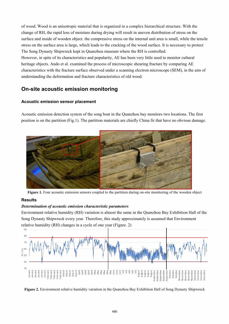
of wood. Wood is an anisotropic material that is organized in a complex hierarchical structure. With the change of RH, the rapid loss of moisture during drying will result in uneven distribution of stress on the surface and inside of wooden object. the compressive stress on the internal unit area is small, while the tensile stress on the surface area is large, which leads to the cracking of the wood surface. It is necessary to protect The Song Dynasty Shipwreck kept in Quanzhou museum where the RH is controlled. However, in spite of its characteristics and popularity, AE has been very little used to monitor cultural heritage objects. Ando et al. examined the process of microscopic shearing fracture by comparing AE characteristics with the fracture surface observed under a scanning electron microscope (SEM), in the aim of understanding the deformation and fracture characteristics of old wood.

On-site acoustic emission monitoring

Acoustic emission sensor placement

Acoustic emission detection system of the song boat in the Quanzhou bay monitors two locations. The first position is on the partition (Fig.1). The partition materials are chiefly China fir that have no obvious damage.

Figure 1. Four acoustic emission sensors coupled to the partition during on-site monitoring of the wooden object

Results Determination of acoustic emission characteristic parameters Environment relative humidity (RH) variation is almost the same in the Quanzhou Bay Exhibition Hall of the Song Dynasty Shipwreck every year. Therefore, this study approximately is assumed that Environment relative humidity (RH) changes in a cycle of one year (Figure. 2)

Figure 2. Environment relative humidity variation in the Quanzhou Bay Exhibition Hall of Song Dynasty Shipwreck

490

After monitoring all year, AE tracing system collected 73 AE events. As shown in Figure. 2, the fluctuation of the annual RH of the exhibition hall is roughly the same range (within the red line). And it also be seen from the Fig.6 that the RH fluctuation frequency from June to September is significantly higher than of other months. As a result, RH was pretreated as the daily fluctuation of RH (DFRH) before being compared with the AE parameters (Figure. 3).

(a) (b)

(c) (d)

Figure. 3. The relationship between acoustic emission parameters and DFRH after monthly average

Based on Figure.2, accumulated energy (Figure. 3a), RMS value (Figure. 3b) and accumulated up-counting (Figure. 3d) are significantly correlated with DFRH after monthly average. Further, accumulated ringing counting (Figure. 3c) is strongly correlated with DFRH after monthly average. In order to quantify this relationship, correlation coefficients between AE parameters and DFRH after monthly average were calculated, as shown in Table 1.

Table 1 correlation coefficients between AE parameters and DFRH after monthly average

AE parameter name Correlation coefficient

Accumulated energy 0.83

RMS value 0.65

Accumulated ringing counting 0.98

Accumulated up-counting 0.77

491

For the Table 1, with increasing of DFRH, accumulated ringing counting is increase. Moreover, as one of the important the AE parameter, accumulated ringing counting can reflect the intensity and frequency of damage signals, thereby, being used in the evaluation of AE activity widely. Taken together, the ringing counting can be used as the characteristic parameter to trace the evolution of damage caused by climate-induced stress in wooden cultural objects.

Analysis of acoustic emission characteristic parameters

Next, RH was pretreated as DFRH after weekly average that compared with the accumulated ringing counting (Figure. 4).

(a) (b)

(c) (d)

Figure. 4. Relationship between DFRH after weekly average and the accumulated ringing counting in spring, summer autumn and winter.

As in the Figure. 4, the black broken line represents DFRH after weekly average, and the red square represents the accumulated ringing counting received by AE sensors. As can be seen from Figure. 4, there is a significant positive correlation between DFRH after weekly average and the accumulated ringing counting, that is, the accumulated ringing counting increases with the increase of DFRH. On account of the accumulated ringing counting can represent the AE activity, the physical meaning shown in Figure.4 is that the larger DFRH is, the more active the AE activity is, and the more frequent and severe the damage to Ancient Wooden Ship. In order to analyze the relationship between accumulated ringing counting and DFRH clearly, the four pictures in Fig. 8 were combined (Figure. 5).

492

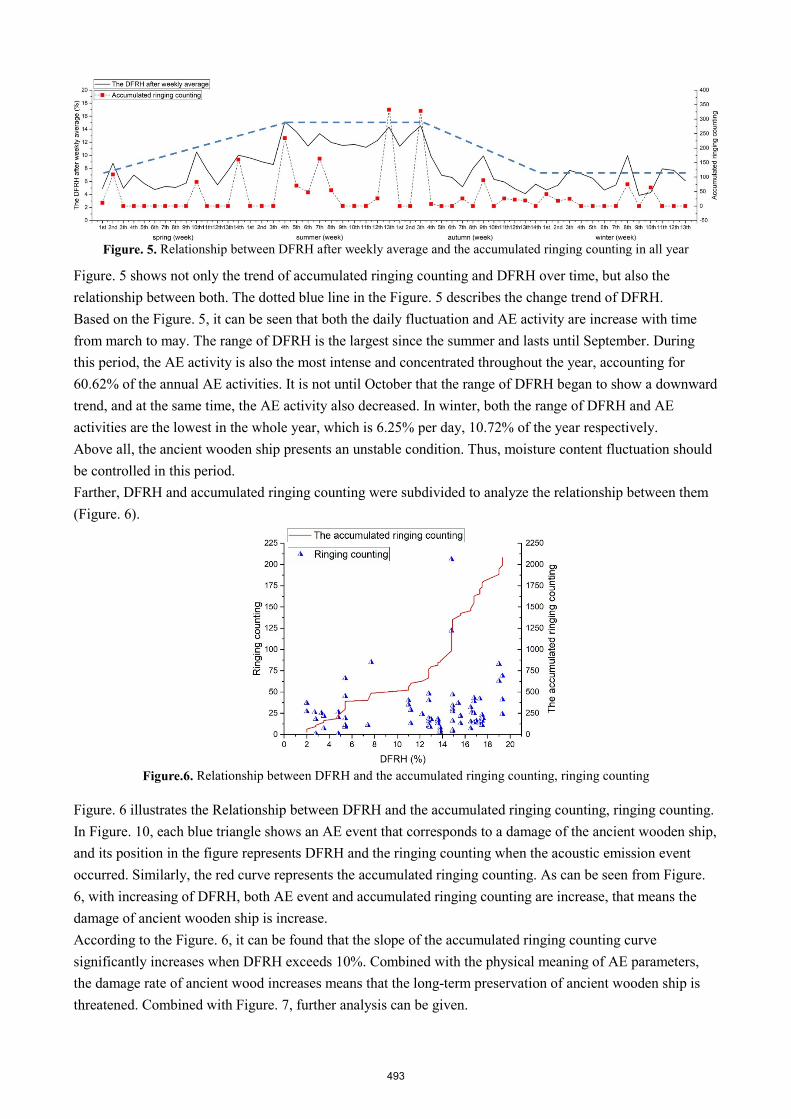
Figure. 5. Relationship between DFRH after weekly average and the accumulated ringing counting in all year

Figure. 5 shows not only the trend of accumulated ringing counting and DFRH over time, but also the relationship between both. The dotted blue line in the Figure. 5 describes the change trend of DFRH. Based on the Figure. 5, it can be seen that both the daily fluctuation and AE activity are increase with time from march to may. The range of DFRH is the largest since the summer and lasts until September. During this period, the AE activity is also the most intense and concentrated throughout the year, accounting for 60.62% of the annual AE activities. It is not until October that the range of DFRH began to show a downward trend, and at the same time, the AE activity also decreased. In winter, both the range of DFRH and AE activities are the lowest in the whole year, which is 6.25% per day, 10.72% of the year respectively. Above all, the ancient wooden ship presents an unstable condition. Thus, moisture content fluctuation should be controlled in this period. Farther, DFRH and accumulated ringing counting were subdivided to analyze the relationship between them (Figure. 6).

Figure.6. Relationship between DFRH and the accumulated ringing counting, ringing counting

Figure. 6 illustrates the Relationship between DFRH and the accumulated ringing counting, ringing counting. In Figure. 10, each blue triangle shows an AE event that corresponds to a damage of the ancient wooden ship, and its position in the figure represents DFRH and the ringing counting when the acoustic emission event occurred. Similarly, the red curve represents the accumulated ringing counting. As can be seen from Figure. 6, with increasing of DFRH, both AE event and accumulated ringing counting are increase, that means the damage of ancient wooden ship is increase. According to the Figure. 6, it can be found that the slope of the accumulated ringing counting curve significantly increases when DFRH exceeds 10%. Combined with the physical meaning of AE parameters, the damage rate of ancient wood increases means that the long-term preservation of ancient wooden ship is threatened. Combined with Figure. 7, further analysis can be given.

493

Figure. 7. The probability of AE activity of ancient wooden ship under different range of DFRH As shown in Figure. 7, with increasing the range of DFRH, the probability of AE activity increase and approximately presents exponential growth. From the perspective of the probability of AE activity, this paper proposes to take RH control measures and preferably control DFRH within 4% and no more than 10%. DFRH has two kinds of situations, one is shrinkage, the other is swelling.

(a) (b)

Figure. 8. The daily variation trend of RH in typical shrinkage (a) and swelling (b) process of the exhibition hall

Due to the phenomenon of wood shrinkage and swelling, both of them have a certain probability to damage the wood. Therefore, this paper studies the damage conditions of ancient wood caused by two different states.

Figure. 9. AE activity of ancient wood under the condition of shrinkage and swelling

494

It is apparent from the Figure. 9, each red square represents an AE event caused by swelling, which its position in the figure shows DFRH and the ringing counting when the AE event occurred. Similarly, each blue triangle represents an AE event caused by shrinkage, which its position in the figure shows DFRH and the ringing counting when the AE event occurred. It can be seen from Fig. 13 that the AE activity of ancient wood during shrinkage is higher than swelling significantly, and AE activity of ancient wood have 84% of the total AE activities (occupy absolute proportion). As shown by the blue dotted line in Figure. 9, At the same time, the minimum diurnal variation in RH causing AE event under shrinkage status is 2.0%, while the data under swelling reaches up to 14.8% (red dotted line in Figure. 9).

Conclusion

The tracing of acoustic emission proved an effective non-destructive method of indicating the damage in wooden cultural objects exposed to variations in RH, at historic sites or during their transportation. The accumulated ringing counting is positively correlated with DFRH that are known to be one of the main factors that contribute to the deterioration of wooden objects, so it can be used for tracing the damage of ancient wooden cultural heritage. The range of DFRH directly affects the health status of ancient wood: the more it is, the higher the probability of damage, and the more harm to the long-term preservation of ancient ship. DFRH is equal to 10%, which can be used as a critical condition for judging whether the health condition of ancient wooden ship is threatened. Compared with the state of swelling, The damage of Ancient wooden ship is more likely to occur in the state of shrinkage. It is recommended that the scope of DFRH should be controlled within 4%, and if 10% is exceeded, an alarm would be activated, warning the staff of the increased risk of mechanical damage to ancient wooden ship.

Acknowledgments

This work was funded by Beijing Natural Science Foundation (No. 2182045).

References

Franziska Ristschel, Andreas J. Brunner, Peter Niemz, 2013. Nondestructive evaluation of damage accumulation in tensile test specimens made from solid wood and layered wood materials, Composite Structures. 9544-52.

V. Bucur, 2006 . Acoustics of Wood, Springer Berlin, Heidelberg, (T. E. Timell and R. Wimmer).

Frederic Lamy, Mokhfi Takarli, Nicolas Angellier, 2015.Frederic Dubois, Octavian Pop, Acoustic emission technique for fracture analysis in wood matrials, Int J Fract, 192: 57-70.

M.P. Ansell, 1982. Acoustic emission from softwoods in tension, Wood Sci. Technol. 16 (1) 35-57.

R.W. Rice, C. Skaar, 1990.Acoustic emission patterns from the surfaces of red oak wafers under transverse bending stress, Wood Sci. Technol. 24 (2):123-129.

S.H. Lee, S.L. Quarles, A.P. Schniewind, Wood fracture, acoustic emission, and the drying process. Part 2. Acoustic emission pattern recognition analysis, Wood Sci. Technol. 38 (1) (1996) 283-292.

A.P. Schniewing, S.L Quarles, S.H. Lee,1996. Wood fracture, acoustic emission, and the drying process. Part

495

1. Wood Sci. Technol. 30 (4) : 273-281.

Magdalena Nowakowska, Adam Krajewski, Piotr Witomski, Piotr Bobinski, 2017.Thermic limitation of AE detection method of old house borer larvae (Hyloturpes bajulus L.) in wooden structures, Construction and Building Materials, 136 : 446-449

S.Kowalski, W. Molinski, G. Musielak, 2004.The identification of fracture in dried wood based on theoreticalmodelling and acoustic emission, Wood Sci. Technol. 38 (1) : 35-52.

Frederia Lamy. Mokhfi Takarli. Nicolas Angellier. Frederic Dubois. Octavian Pop, 2015..Acoustic emission technique for fracture analysis in wood materials, Int J Fract, 192: 57-70.

A.P. Schniewing, S. L. Quarles, S. -H. Lee, 1996. Wood fracture, acoustic emission, and the drying process: Part 1. Acoustic emission associated with fracture, Wood Sci. Technol, 30: 273-281.

S. -H, S. L. Quarles, A. P. Schniewind, 1996.Wood fracture, acoustic emission, and the drying process: Part2. Acoustic emission pattern recognition analysis, Wood Sci. Technol, 30: 283-292.

S. J. Kowalski, Wolinski, G. Musielak, 2004.The identification of fracture in dried wood based on theoretical modelling and acoustic emission, Wood Sci. Technol, 38: 35-52.

Francisco J. Rescalvo, Elisabet Suarez, Ignacio Valverde-Palacios, Juan Manuel Santiago-Zaragoza, Antolino Gallego, 2018. Health monitoring of timber beams retrofitted with carbon fiber composites via the acoustic emission technique, Composite Structures, 206 : 392-402

Francisco J. Rescalvo, Antonio Aguilar-Aguilera, Elisabet Suarez, Ignacio Valverde-Palacios, Antolino Gallego, 2018.Acoustic emission during wood-CFRP adhesion tests, International Journal of Adhesion and Adhesives, 87 : 79-90.

K. Ando, Y. Hirashima, M. Sugihara. et al, 2006.Microscopic processes of shearing fracture of old wood,examined using the acoustic emission technique, J. Wood Sci, 52: 483-489.

A. Reiterer, S.E. Stanzl-Tschegg, E. K. Tschegg, 2000.Mode I fracture and acoustic emission of softwoodand hardwood, Wood Sci. Technol, 34: 417-430.

F. Lamy, M. Takarli, N. Angellier, F. Dubois, O. Pop, 2015.Acoustic emission technique for fracture analysisin wood materials, Int. J. Fract, 192: 57-70.

496

Investigation on Screening Internal Defects of Historic Wood Structural Members Based on the Tap Impact Force

Houjiang Zhang School of Technology, Beijing Forestry University, Beijing, China, hjzhang6@bjfu.edu.cn

Kailong Guo School of Technology, Beijing Forestry University, Beijing, China, 674879898@qq.com

Cheng Guan School of Technology, Beijing Forestry University, Beijing, China, 648911029@qq.com

Abstract

China has a very long history, and there are a large number of historic timber structures. How to protect these historic timber structures has always been an important issue. The main load-bearing elements in the historic timber structures are columns, beams, tiebeams, and purlins. With hundreds of years of history, most of these wood members got different defects, such as cracks, decay, voids and so on, due to the influence of environment, pathogens and other factors. Among them, the voids and decay inside wood members are the most difficult to find, which seriously affects the safety of the whole building. The tap method is the main method used in the preliminary screening stage. It is a method for the inspectors to tap on the surface of a wood member with a small hammer and distinguish whether the wood member has internal defects by sound. However, this method mainly depends on the operator’s experience, and the probability of missed or wrong judgment is very high. When a hammer was used to tap surface of a wood member, except for producing sound, there was also a impact force existed between the hammer and the surface of the wood member. In this paper, starting with the impact force signal, a series of tap experiments on lumbers and circular section wood columns with void defects were carried out. It was found that impact time τ between the hammer and the wood surface could be used as parameters for judging the existence or absence of internal defects. After investigating the relationship between the parameter and impact forces, defect stiffness and surface hardness, it was found that reasonable range of the impact forces were 150-450N; the closer the internal defects were to the surface of wood members, the larger the defect size, the smaller the defect stiffness and the easier to be identified the internal defects were. In a word, the experimental results show that it is hopeful to judge whether there are internal defects in wood members by some characteristics of impact force signals.

Keywords: historic wood structural members, internal defects, impact forces, impact time τ, stiffness

Introduction

China has a very long history, and there are a large number of historic timber structures. How to protect these historic timber structures has always been an important issue. The main load-bearing elements in the historic timber structures are columns, beams, tiebeams, and purlins. With hundreds of years of history, most of these wood members got different defects, such as cracks, decay, voids and so on, due to the influence of environment, pathogens and other factors (Ross et al. 2004). Among them, the voids and decay inside wood members are the most difficult to find, which seriously affects the safety of the whole

497

building. The procedure of nondestructive detecting of the internal defects is generally divided into three steps: preliminary screening, verifiable screening and accurate detection (Liao 2015).

The tap method is the main method used in the preliminary screening stage, and is also a basis of subsequent verifiable screening. Traditional tap detection mainly relies on the operators to listen to the sound produced by knocking the surfaces of wood members with a small hammer to distinguish whether there are internal defects. However, this method mainly depends on the operator’s experience, and the probability of missed or wrong judgment is very high (Zhang et al. 2016, White et al. 2014).

Modern local tap detection theory based on force signals was developed by Professor Cawley of Imperial College of Technology and Professor Adams of Bristol University (Cawley and Adams 1988, 1989). In 1988, they studied principle, theoretical model and criterion of this detection method. In the tap test of honeycomb structural carbon fibre panels, it was found that the impact force signals had obvious differences in time domain and frequency domain. After that, more scientists took fibre reinforced plastics as their object of study, and carried out the tap detection of internal defects, so that this detection method gradually improved and got practical (Peters et al. 2000, Wu et al. 2000, Leng et al. 1995). In 2015, Chunhui used a constant-force hammer to tap detect internal defects of historic wood members, and he found that the main source of tap sound was hammer impact and local vibration of defective parts of the wood members. Through acquisition and analysis of sound signals, he also found that root mean square value in time domain and frequency value in frequency domain of signals had a certain relationship with the existence of internal defects in wood members (Liao 2015).

In summary, the greatest shortcoming of current research on tap screening of internal defects of historic wood members is very few. This paper intends to study mechanism of tap screening from angle of the impact force signal, clarify the relationship between impact force and surface stiffness and defect stiffness of wood members, select the characteristic parameters that can be used for defect screening, and form the basis for discriminating whether there are internal defects or not. The final goal is to improve the scientificity and accuracy of tap screening method, as well as to lay a certain theoretical foundation to develop a screening instrument and get rid of restraint of human factors for the future.

Theoretical basis

As shown in Fig. 1, when there is not any internal defect under tap position, the material tapped can be simplified to a spring with stiffness kc. In this paper, the stiffness kc is called surface contact stiffness, or surface stiffness for short. When there is an internal cavity defect under the tap position, the material from the surface to top surface of the cavity defect can be simplified to another spring with stiffness kd, which is called defect stiffness here. The larger the defect is, or the closer to surface of the object, the smaller kd is. In summary, the stiffness of the object at tap position is as follows:

without internal defect

with internal defect

c

c d

c d

k kk kk

k k

= = +

The tap impact time τ, at position without internal defects and position with internal defects is below respectively:

+==

defect internal with defect internal without

dc

c

τττττ

where τc is impact time caused by surface stiffness kc, τd is impact time caused by defect stiffness kd. If value of the impact time τc caused by the surface stiffness of wood member is determined first, when the value of

498

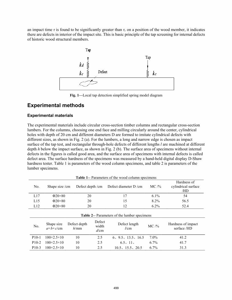
an impact time τ is found to be significantly greater than τc on a position of the wood member, it indicates there are defects in interior of the impact site. This is basic principle of the tap screening for internal defects of historic wood structural members.

Fig. 1—Local tap detection simplified spring model diagram

Experimental methods

Experimental materials

The experimental materials include circular cross-section timber columns and rectangular cross-section lumbers. For the columns, choosing one end face and milling circularly around the center, cylindrical holes with depth of 20 cm and different diameters D are formed to imitate cylindrical defects with different sizes, as shown in Fig. 2 (a). For the lumbers, a long and narrow edge is chosen as impact surface of the tap test, and rectangular through-hole defects of different lengths l are machined at different depth h below the impact surface, as shown in Fig. 2 (b). The surface area of specimens without internal defects in the figures is called good area, and the surface area of specimens with internal defects is called defect area. The surface hardness of the specimens was measured by a hand-held digital display D-Shaw hardness tester. Table 1 is parameters of the wood column specimens, and table 2 is parameters of the lumber specimens.

Table 1-- Parameters of the wood column specimens

No. Shape size /cm Defect depth /cm Defect diameter D /cm MC /% Hardness of

cylindrical surface /HD

L17 Φ20×80 20 17 6.1% 54 L15 Φ20×80 20 15 8.2% 56.5 L12 Φ20×80 20 12 6.2% 52.4

Table 2-- Parameters of the lumber specimens

No. Shape size a×b×c/cm

Defect depth h/mm

Defect width d/cm

Defect length l/cm MC /% Hardness of impact

serface /HD

P10-1 100×2.5×10 10 2.5 6、9.5、13.5、16.5 7.0% 41.2 P10-2 100×2.5×10 10 2.5 6.5、11、 6.7% 41.7 P10-3 100×2.5×10 10 2.5 10.5、15.5、20.5 6.7% 31.3

499

(a) Wood column specimens (unit: cm)

(b) Lumber specimensFig. 2—Experimental materials and diagrams of the defects

Experimental setup

The Experimental setup consists of impulse hammer, signal amplifier, data acquisition card and computer. The pulse hammer is used to tap the specimens, and it is equipped with piezoelectric crystal force sensor, which can sense the tap pulse force as a pulse charge signal. The software is installed in the computer, and it is compiled by LabVIEW, which completes acquisition, analysis, display and storage of the pulse force signals.

Conclusions

The tap impact time can be used as a characteristic parameter to screen the internal defects of wood members. At the same impact point, the impact force has little effect on the impact time in the range of 150-450N.

The tap impact time is related to surface stiffness and defect stiffness of wood members. Under a certain surface stiffness, the smaller the defect stiffness is, the longer the impact time is.

There is a good correlation between impact time τc formed by surface stiffness and surface Shaw hardness HD. The correlation equation between them is -0.0412 3.094y x= + , and the determination coefficient reaches 0.9341.

500

References

Ross Robert J, Brashaw Brian K, Wang Xiping, White Robert H, Pellerin Roy F. 2004. Wood and timber condition assessment manual. USDA Forest Service, Forest Products Laboratory, Madison, WI.

Liao Chunhui. 2015. Study on Non-destructive Screening Internal Defects of Historic Wood Structural Members. Ph.D. thesis of Beijing Forestry University.

Zhang Houjiang, Guan Cheng, Wen Jian. 2016. Applications and research development of nondestructive testing of wood based materials. Journal of Forestry Engineering. 1(6): 1-9.

White Robert H, Ross Robert J. Wood and timber condition assessment manual (second edition). 2014. General Technical Report FPL-GTR-234. Madison, WI: US Department of Agriculture, Forest Service, Forest Products Laboratory.

Cawley P, Adams R D. 1988. The mechanics of the coin-tap method of nondestructive testing. Journal of Sound Vibration. 122(2): 299-316.

Cawley P, Adams R D. 1989. Defect types and non-destructive testing techniques for composites and bonded joints. Metal Science Journal. 5(5): 413-425.

Peters J J. Barnard D J. Hudelson N A. Simpson T S. Hsu D K. 2000. A prototype tap test imaging system: Initial field test results. AIP Conference Proceedings. 509(1): 2053.

Wu H, Mel S. 2000. Correlation of Accelerometer and Microphone Data in the “Coin Tap Test”. IEEE Transactions on Instrumentation and Measurement. 49(3): 493-497.

Leng Jinsong, Du Shanyi, Wang Dianfu. 1995. Sensitivity of the coin-tap method of nondestructive testing for composite structures. ACTA Materiae Compositae Sinica. 12(4): 99-105.

501

Using Ground Penetrating Radar to Classify Features within Structural Timbers Xi Wu School of IoT Engineering, Jiangnan University, Wuxi, Jiangsu, China, 335722038@qq.com Christopher Adam Senalik USDA Forest Service, Forest Products Laboratory, Madison, Wisconsin, USA, christopher.a.senalik@usda.gov James Wacker USDA Forest Service, Forest Products Laboratory, Madison, Wisconsin, USA, james.p.wacker@usda.gov Xiping Wang USDA Forest Service, Forest Products Laboratory, Madison, Wisconsin, USA, xiping.wang@usda.gov Guanghui Li School of IoT Engineering, Jiangnan University, Wuxi, Jiangsu, China, ghli@jiangnan.edu.cn Abstract Recent developments in image processing play a significant role in identifying and classifying features on ground penetrating radar (GPR) radargrams. Two groups of timber specimens were examined in this study. The first group comprised laboratory prepared Douglas-fir (Pseudotsuga menziesii) timber sections with inserts of known internal characteristics. The second group comprised timber girders salvaged from timber bridges on historic Route 66 that had been exposed to weather for more than 80 years. A subsurface interface radar system with a 2-GHz palm antenna was used to scan these two groups of specimens. GPR sensed differences in dielectric constants along the scan path caused by the presence of water, metal, or air within the wood. This study focused on two procedures: feature identification and classification. Image processing was used to identify the presence of defect features, which was then classified based upon machine learning. GPR radargrams proved to be an excellent tool to detect and define characteristics within structural timbers. Keywords: ground penetrating radar, timber, metal, moisture content, image processing, feature classification Introduction Nondestructive testing (NDT) techniques are needed by engineers and inspection professionals to evaluate the internal condition of wood structures. This study used ground penetrating radar (GPR), a GSSI (Nashua, New Hampshire, USA) Subsurface Interface Radar (SIR) 4000 with a 2-GHz palm antenna, to scan two groups of timber beam specimens. Results of the radar wave tests on controlled specimens were calibrated and used to develop recognition methods on beams that had served out their lives in an actual bridge structure.

502

GPR technology has been widely used for detecting buried objects of various materials such as sand, timber, concrete, etc. It has been clearly illustrated that GPR can detect anomalous electromagnetic responses associated with a variety of significant physical conditions (Pettinelli et al. 2009). GPR uses an antenna to generate short bursts of electromagnetic energy in solid materials.Waveforms are transmitted into the structure using an antenna positioned at the surface. A portion of the wave is reflected, refracted, and/or diffracted when encounterring the boundary of objects with different dielectric constant and then is received by the antenna. Schad et al. (1996) investigated three nondestructive evaluation techniques for detecting internal wood defects. Both sound wave transmission and impulse radar were able to detect large voids and areas of degradation. The use of radar requires an experienced operator because of the difficulty of interpreting the data. Brashaw (2014) researched the signal analyzing of the radar data in both the longitudinal direction (antenna front to back) and the transverse direction (antenna side to side). This research was designed to be an early assessment of the potential for using GPR to identify known defects in longitudinal timber bridge decks and slab spans. The results of their experiments provide ideas for future study in GPR. The incident wave propagates through the material and partially reflects at interfaces presenting a dielectric contrast (Benson 1995, Rodríguez-Abad et al. 2011). The electromagnetic response of all the reflected waves could be processed and analyzed to estimate propagation velocities or depth of objects. The wave forms visible in one-dimensional data (A-scan) and two-dimensional radargrams (B-scan) contain information about internal characteristics of the analyzed specimen. Unfortunately, the wave forms also contain a variety of complex interference waves, increasing the difficulty of feature identification. In order to obtain high quality signals, the noise level must be suppressed. One method of signal denoising is the empirical mode decomposition (EMD). EMD was proposed by Huang et al. (1998). The EMD method has had significant impact and is widely used in a broad variety of time-frequency analysis applications (Dragomiretskiy and Zosso 2014) as well as signal processing. It has the advantage of determining the amplitude of the signal and adaptively decomposing the signal into a stationary signal. The finite number of IMF (Intrinsic Mode Function) components decomposed represents the physical characteristic information of the signal. Battista et al. (2007) used EMD to remove cable strum noise from seismic data. Narayanan et al. (2010) used the EMD method to mitigate both coherent and random noise in wall radar human detection. After denoising the signal data, regions containing defects must be located. Dynamic time warping (DTW) is a way to measure the similarity of two time series of different lengths. DTW is a typical optimization problem; it uses the time-warping function to demonstrate the time corresponding relation between a test template and reference template. Warping one (or both) of the sequences in the timeline can achieve better alignment. Then, the time-warping function corresponding to the minimum cumulative distance between the two templates can be calculated. DTW is a commonly used technique to accomplish this task. This method plays an important role in speech recognition and machine learning convenience. Jazayeri et al. (2018) proposed a cutting-edge expert system by setting a threshold on DTW values and monitoring them online. A significant deviation of the DTW values from the reference signal is detected prior to reaching an object. Feature extraction plays an important role in target recognition and classification of GPR signals. Selecting appropriate features can not only reduce the computational complexity of GPR echo signal analysis but also improve target detection and classified performance. Feature extraction after denoising and similarity analyzing was conducted based on the discrete wavelet transformation (DWT). Baili et al. (2009) presented the use of DWT to denoise the GPR signals. Various other wavelets were used in this study to denoise experimental GPR signals collected from flexible pavements. Bruce et al. (2002) used

503

DWT for hyperspectral feature extraction and signature classification. Wavelet-based feature extraction, specifically the use of subsets of DWT coefficients, was developed and applied to two precision agricultural applications. Their experimental results show a superior performance of the proposed wavelet-based features for the hyperspectral classification compared with more conventional methods. The main purpose of this paper is to recognize and locate the defects. Some of the many methods used for GPR data were used on our data. A list of processing steps was used to analyze the A-scan and B-scan data. Materials and Methods Materials There are two groups of data obtained from Douglas-fir (Pseudotsuga menziesii). The first group was based on a timber bridge project. A unique set of aged highway timber bridges are located along a portion of the historic U.S. Route 66 in southern California. This stretch of historic Route 66 in the Mojave Desert is currently the focus of extensive efforts by the County of San Bernardino to preserve its iconic legacy and protect its key cultural and historical resources, which include the timber bridge structures (Wacker et al. 2017). A total of 18 timbers beams were used in this study. Prior to testing, the beams were brought to a moisture content (MC) equilibrium of 10% in a temperature- and humidity-controlled room. The second group was five core samples at varying moisture contents and two samples with metal bars (nails and screws) inserted parallel to the length of the cores. The scanning process of bridge timbers is shown in Figure 1. The diameter of the bars were 1.6, 4.8, and 7.9 mm (1/16, 3/16, and 5/16 in.) as shown in Figure 2a. Placement of the core samples into the cavity of timber sections is shown in Figure 2b. The GPR antenna was placed on top of the timber section, and the scan was performed down through the inserted core. The majority of the defects in the Route 66 bridge timbers are the metal bars that were used to strengthen and secure the bridge. The presence of the metal bars commonly resulted in holes and cracks throughout the timbers. Figure 3 shows the defect statistics of the 18 timbers, which were calculated based on the defect mapping documents and camera pictures. Methods The object detection algorithm can be divided into five steps: (1) using EMD to decompose A-scan data into IMFs; (2) calculating the similarities using DTW based on IMF1; (3) estimating the position of defects by comparing the similarities of data from each scan; (4) selecting some windows on B-scan including defects as a portion of the database, according to the location of each defect and the analyzed data; and (5) extracting the features of each region. A flowchart of this proposed strategy is given in Figure 4.

Figure 1—Display of the scanning process.

504

(a) (b)

Figure 2—(a) The core samples with inserted metal nails and bars of different sizes; (b) the testing environment of core samples.

Figure 3—Defect accounts of 18 timbers tested in laboratory.

To ensure the accuracy of processing, we analyzed the raw data (.dzt format files) under the MATLAB environment. Detailed procedures are subsequently shown: (1) Find the maximum values (Rmax) and minimum values (Rmin) of the raw signal R(n). From these

extreme points, the upper and lower curves are called Rmax(n) and Rmin(n), and the average envelope Avg(n) between these two envelopes could be calculated by Equation (1):

Avg(𝑛𝑛) = 𝑅𝑅𝑚𝑚𝑚𝑚𝑚𝑚(𝑛𝑛)+𝑅𝑅𝑚𝑚𝑚𝑚𝑛𝑛(𝑛𝑛)

2 (1)

(2) The variable Rl(n) = R(n) - Avg(n) sets the reference function that satisfies the IMF condition as c(n).

Then, repeat Steps (1) and (2) until the first IMF is obtained.

505

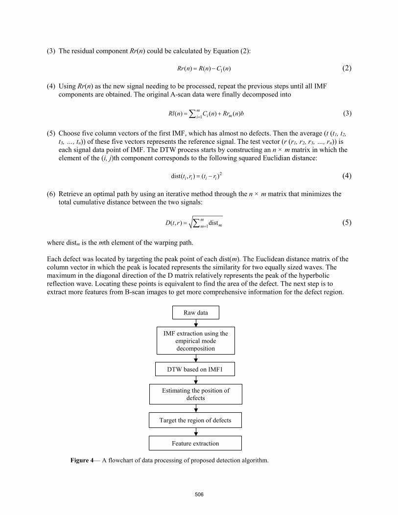
(3) The residual component Rr(n) could be calculated by Equation (2): 1( ) ( ) ( )Rr n R n C n= − (2) (4) Using Rr(n) as the new signal needing to be processed, repeat the previous steps until all IMF

components are obtained. The original A-scan data were finally decomposed into

1( ) ( ) ( )mi miRl n C n Rr n b

== +∑ (3)

(5) Choose five column vectors of the first IMF, which has almost no defects. Then the average (t (t1, t2,

t3, …, tn)) of these five vectors represents the reference signal. The test vector (r (r1, r2, r3, …, rn)) is each signal data point of IMF. The DTW process starts by constructing an n × m matrix in which the element of the (i, j)th component corresponds to the following squared Euclidian distance:

2dist( , ) ( )i i i it r t r= − (4) (6) Retrieve an optimal path by using an iterative method through the n × m matrix that minimizes the

total cumulative distance between the two signals:

1( , ) distmmmD t r

== ∑ (5)

where distm is the mth element of the warping path. Each defect was located by targeting the peak point of each dist(m). The Euclidean distance matrix of the column vector in which the peak is located represents the similarity for two equally sized waves. The maximum in the diagonal direction of the D matrix relatively represents the peak of the hyperbolic reflection wave. Locating these points is equivalent to find the area of the defect. The next step is to extract more features from B-scan images to get more comprehensive information for the defect region.

Figure 4— A flowchart of data processing of proposed detection algorithm.

Raw data

IMF extraction using the empirical mode decomposition

DTW based on IMF1

Estimating the position of defects

Target the region of defects

Feature extraction

506

Results Five core samples with 68.26-mm- (2-11/16-in.-) and 133.35-mm- (5-1/4-in.-) diameter were soaked for several hours. After soaking, they were weighed and then scanned as shown in Figure 2b. After scanning, the cores were returned to the water bath to continue soaking. After the tests were completed, the cores were oven-dried to calculate the exact MC. Five soak times were chosen (2, 7.5, 24, 55.5, and 120 h) based on the expert’s advice. The weights at different times are shown in Table 1. It is obvious that the MC was increasing with a relatively stable state, about 7% incremental value.

Table 1—Moisture content of the soaked core samples by hours of soaking.

Sample Moisture content (%)

0 h 2 h 7.5 h 24 h 55.5 h 120 h

1 6 14 20 27 35 46 2 6 14 19 23 36 47 3 6 15 21 28 35 45 4 6 14 18 25 31 39 5 6 14 19 26 33 42

(a)

(b) Figure 5—(a) The DTW data of the No. 6 core sample; (b) the radargrams when the No. 6 core sample was inserted (1 in. = 25.4 mm).

507

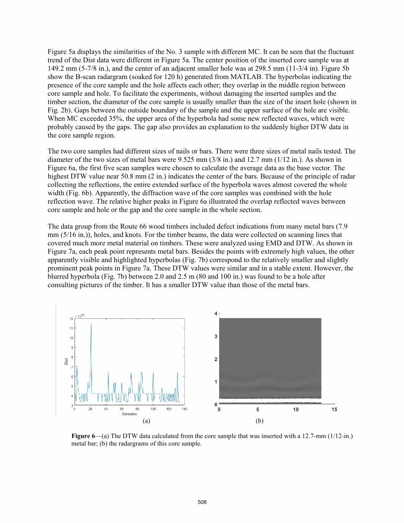
Figure 5a displays the similarities of the No. 3 sample with different MC. It can be seen that the fluctuant trend of the Dist data were different in Figure 5a. The center position of the inserted core sample was at 149.2 mm (5-7/8 in.), and the center of an adjacent smaller hole was at 298.5 mm (11-3/4 in). Figure 5b show the B-scan radargram (soaked for 120 h) generated from MATLAB. The hyperbolas indicating the presence of the core sample and the hole affects each other; they overlap in the middle region between core sample and hole. To facilitate the experiments, without damaging the inserted samples and the timber section, the diameter of the core sample is usually smaller than the size of the insert hole (shown in Fig. 2b). Gaps between the outside boundary of the sample and the upper surface of the hole are visible. When MC exceeded 35%, the upper area of the hyperbola had some new reflected waves, which were probably caused by the gaps. The gap also provides an explanation to the suddenly higher DTW data in the core sample region. The two core samples had different sizes of nails or bars. There were three sizes of metal nails tested. The diameter of the two sizes of metal bars were 9.525 mm (3/8 in.) and 12.7 mm (1/12 in.). As shown in Figure 6a, the first five scan samples were chosen to calculate the average data as the base vector. The highest DTW value near 50.8 mm (2 in.) indicates the center of the bars. Because of the principle of radar collecting the reflections, the entire extended surface of the hyperbola waves almost covered the whole width (Fig. 6b). Apparently, the diffraction wave of the core samples was combined with the hole reflection wave. The relative higher peaks in Figure 6a illustrated the overlap reflected waves between core sample and hole or the gap and the core sample in the whole section. The data group from the Route 66 wood timbers included defect indications from many metal bars (7.9 mm (5/16 in.)), holes, and knots. For the timber beams, the data were collected on scanning lines that covered much more metal material on timbers. These were analyzed using EMD and DTW. As shown in Figure 7a, each peak point represents metal bars. Besides the points with extremely high values, the other apparently visible and highlighted hyperbolas (Fig. 7b) correspond to the relatively smaller and slightly prominent peak points in Figure 7a. These DTW values were similar and in a stable extent. However, the blurred hyperbola (Fig. 7b) between 2.0 and 2.5 m (80 and 100 in.) was found to be a hole after consulting pictures of the timber. It has a smaller DTW value than those of the metal bars.

(a) (b)

Figure 6—(a) The DTW data calculated from the core sample that was inserted with a 12.7-mm (1/12-in.) metal bar; (b) the radargrams of this core sample.

508

The sudden extremely high DTW value usually appeared in the areas that include at least two hyperbolas. These hyperbolas were close to each other, and in some cases, overlapped within the adjacent regions. The timbers were placed on two wood supports during testing. Each timber was 101.6 mm (4 in.) thick. This situation commonly produces noise in the raw data. Even after the denoising process on the A-scan data, the noise in the reflected waves cannot be completely removed. In total, 737 peak points were found based on the data of Figure 7a. These peaks represent the metal bars, holes, knots, etc. Then the range of DWT values corresponding to different defects should be separately recorded. The approximate location of defects on the radargrams is converted from the position of the peak on a single channel signal. According to the locations, extracting an area with 70 * 270 pixels around the points. After that, features could be extracted on the radargrams with different types of defects. All the peaks seen in Figure 7a correspond to nails. The values for knots are relatively small and cannot be seen in the figure.

(a)

(b)

Figure 7—(a) The line chart of DTW values; (b) the radargrams generated from RADAN 7.

Conclusions and Discussion This study demonstrated the effectiveness of using a combination processing method to locate and define the defects of wood timbers. The Route 66 bridge timbers are complex, real-world specimens. The timbers are inhomogeneous, containing cracks, splits, holes, metal bars, and naturally occuring decay from years of exposure and use, all of which increases the complexity of the analysis process. Some detection methods were not capable of identifying these conditions, such as some image segmentation methods to target the hyperbola regions. We used a list of processing steps that could locate the defects, including some defects that are invisible in the radargrams. EMD and DTW are efficient for the GPR data of wood timbers. These results display the ability to illustrate some invisible feature information of signals after comparing with radargrams. At the same time, these works play an important role before extracting the features of defect regions on the radargrams. Although EMD and DTW have shown positive results in locating and classifying defects, some vague regions still exist. In the future, there is a

Nail

Nail

509

need to further improve these methods and add signal gain processing steps to enhance the brightness and contrast of radargrams for easy observation and comparison. Obtaining additional specimens with reduced complexity would aid in analysis. Acknowledgments This paper describes a study conducted by the USDA Forest Service, Forest Products Laboratory, in cooperation with the County of San Bernardino (California) and Biggs Cardosa Associates, Inc. Ms. Xi Wu’s participation in this project was supported by the China Scholarship Council. References Baili, J.; Lahouar, S.; Hergli, M.; Al-Qadi, I.L.; Besbes, K. 2009. GPR signal de-noising by discrete wavelet transform. NDT & E International. 42(8): 696-703. Battista, B.M.; Knapp, C.; McGee, T.; Goebel, V. 2007. Application of the empirical mode decomposition and Hilbert–Huang transform to seismic reflection data. Geophysics. 72(2): 29-37. Benson, A.K. 1995. Applications of ground penetrating radar in assessing some geological hazards: examples of groundwater contamination, faults, cavities. Journal of Applied Geophysics. 33: 177-193. Brashaw, B.K. 2014. Inspection of timber bridge longitudinal decks with ground penetrating radar. Ph.D. Dissertation. Mississippi State University, ProQuest Dissertations Publishing. 3665457. Bruce, L.M.; Koger, C.H.; Li, J. 2002. Dimensionality reduction of hyperspectral data using discrete wavelet transform feature extraction. In: IEEE Transactions on Geoscience and Remote Sensing. 40(10): 2331-2338. Dragomiretskiy, K.; Zosso, D. 2014. Variational mode decomposition. In: IEEE Transactions on Signal Processing. 62(3): 531-544. Huang, N.E.; Shen, Z.; Long, S.R.; [and others]. 1998 The empirical mode decomposition and the Hilbert spectrum for nonlinear and non-stationary time series analysis. Proceedings of the Royal Society of London A: Mathematical, Physical and Engineering Sciences. 454: 903-995. Jazayeri, S.; Saghafi, A.; Esmaeili, S.; Tsokos, C. 2018. Automatic object detection using dynamic time warping on ground penetrating radar signals. Expert Systems with Applications. 122: 102-107. Narayanan, R.M.; Shastry, M.C.; Chen, P.-H.; Levi, M. 2010. Through -the-wall detection of stationary human targets using Doppler radar. Progress in Electromagnetics Research B. 20: 147-166. Pettinelli, E.; Matteo, A.D.; Mattei, E.; Crocco, L.; [and others]. 2009. GPR response from buried pipes: measurement on field site and tomographic reconstructions. IEEE Transactions on Geoscience and Remote Sensing. 47(8): 2639-2645. Rodríguez-Abad, I.; Martínez-Sala, R.; Capuz, R.; Díez, R.; García, F. 2011. Assessment of the variation of the moisture content in the Pinus pinaster Ait. using the non destructive GPR technique. Materiales De Construccion. 61(301): 143-156. Schad, K.C.; Schmold, D.L.; Ross, R.J. 1996. Nondestructive methods for detecting defects in softwood logs. Research Paper FPL‐RP‐546. Madison, WI: U.S. Department of Agriculture, Forest Service, Forest Products Laboratory. Wacker J, Mikhail M, Dizon G (2017) Evaluation of Bridge Components Salvaged from Historic Route 66 in California. Research in Progress RIP-4719-038. USDA Forest Service, Forest Products Laboratory, Madison, WI. https://www.fpl.fs.fed.us/documnts/rips/fplrip-4719-038-Wacker-Mikhail-Dizon.pdf.

510

Measuring the Lengths of Wooden Piles with Nondestructive Methods

Dr. Krisztián Andor * Institute of Applied Mechanics and Structures, Faculty Simonyi Károly of Technology, Wood Science and Art, University of Sopron, Sopron, Hungary, andor.krisztian@uni-sopron.hu Dr. Ferenc Divós Fakopp Enterprise LP., Ágfalva, Hungary, office@fakopp.com Botond Őry PhD student, Institute of Applied Mechanics and Structures, Faculty Simonyi Károly of Technology, Wood Science and Art, University of Sopron, Sopron, Hungary, ory.botond@gmail.com Dániel Jenei BSc student, Faculty Simonyi Károly of Technology, Wood Science and Art, University of Sopron, Sopron, Hungary, ory.botond@gmail.com^ * Corresponding author Abstract The operators of the Hévíz thermal lake ordered full static examination of a spa building in the lake. A part of this was the examination of the timber pile grounding. To determine the bearing capacity of the piles, it is necessary to know their lengths. After determining the lengths, it is possible to identify the exact soil layer in which the individual piles are supported. The only option was a non-destructive method to determine these lengths. We used sound vibration sensitive measuring oscilloscope to examine reflections. The base of the measurement is the acoustic impedance, which tells the acoustic resistance of materials against the acoustic flow. We placed the measuring instrument on the walking surface, above the piles. Here we measured the reflections of the sound. We generated sound vibrations near the sensor. The measured reflections made by a hammer, granted the time it took the sound to travel from the walking surface to the bottom of the pile and back to the sensor. To determine the precise length of the piles in addition we needed to measure the P-wave velocity in the measured piles. For this we used a Fakopp Microsecond Timer acoustic measuring device. Divers pierced two probes in the piles, and generated vibrations in a probe. With these time data could be reached, and it was possible to calculate the velocity in the piles. With the help of the velocity and the reflection data the length of the piles became determinable and by this the pile resistances. Structural analysis of the offshore building on a thermal lake

Structural, building constructional, and geotechnical examinations, as well as wood engineering diagnostics have been carried out in order to reveal the existing problems in the structure, to enable the prediction of future tasks related to it, and to determine the necessary actions.

During the examinations the properties of the load-bearing structures had to be determined: geometry of the horizontal load-bearing structure of the building, exact location, eccentricity, and capacity of the piles, available strength of concrete and steel components in beams and slabs, layout of the existing reinforcement bars, and the layer sequence of the floors. An additional aim is to reveal possible damages of structural members that can affect load-

511

bearing capacity, and to document the general conditions of the structure. Independently of the stability of the existing structure, potential development of the building is planned.

As an additional task, the in situ examinations and explorations were meant to provide fundamental data for the static calculations and for structural movements in the preceding period.

In order to support the structural examinations, a geotechnical expert report was prepared, which determined the layer sequence of the load-bearing soils.

The position of the tip of the piles supporting the offshore building had to be determined prior to the structural examinations, since it was required for the point supports. It was particularly important in view of the large settlements occurring during test loading of other buildings due to the crushing of the thin (0.3-1.4m) rocky layer under the peat layer.

During the examination the main task was to determine the length of the piles without disrupting the building. Since the piles were usually made of spruce, larch, or oak, the lengths were determined by wood physics methods.

Furthermore, strength properties of the wooden piles, which had 20 to 29 cm diameter, had also to be determined within the full-scale examination of the structure, since the entire structure rests on this pincushion-like array of piles, the capacity of which may be relevant for the comparison with the stresses arising from internal forces computed in the analysis of loads, or for the future alteration of loads.

Samples were extracted from the piles using increment borer to determine the species. The analysis was performed by macroscopic and microscopic examinations. The macroscopic examinations were done by a Nikon stereo microscope, then slices were prepared from the sample, and the species were determined using light microscope. Spruce, larch, and oak were identified.

Stress analysis of piles

In order to determine the load-bearing capacity of the piles, the strength properties of the pile material need to be known, and it is achieved by strength classification of the species of the piles. The strength classification primarily requires the elastic modulus, which in turn requires the density and the velocity of sound propagating in grain direction in the piles. Since most of the piles were made of spruce (and a smaller amount of larch or oak), and the measurement of density was not possible due to inaccessibility under water, we provided mean values of density characteristic to the species, as shown below. This value was 𝜌𝜌𝑠𝑠𝑠𝑠𝑠𝑠𝑠𝑠𝑠𝑠𝑠𝑠,m = 470 𝑘𝑘𝑘𝑘

𝑚𝑚3 (Molnár, 2004).

In order to determine the elastic modulus, we employed a method developed in the Bódig József Non-destructive Wood-testing Laboratory at the University of Western Hungary, which is capable of measuring the dynamic elastic modulus of the built-in wood material and estimating the bending strength. The calculation of the dynamic elastic modulus requires the data mentioned in the previous paragraph. Once computed, the strength properties can be concluded and then classified according to standard MSZ EN 338.

To determine sound velocity in grain direction, we applied an instrument called FAKOPP Microsecond Timer, which consists of two sensors and a time meter unit. The instrument measures the duration in µs of sound waves generated by a hammer strike travelling along the shortest path between the sensors. Knowing the distance between the sensors, the propagation

512

velocity of the sound can be determined. The application of the instrument under general conditions is shown in Fig. 1. and in situ in Fig. 2.

Figure 1. Figure 2. In our case the examination of piles above water level was not possible due to the concrete

pile caps mentioned earlier. Therefore, the measurements had to be carried out with the collaboration of divers, that were provided by the management of Hévíz lake spa. The measured data were recorded using boats escorting the diver. The diver installed the sensors on one side of the vertical pile above each other as shown in Fig. 27. In order to determine the sound velocity accurately, the distance between the sensors had to be known, which was intended to set at 80 cm in all cases. After the placement of the sensors, the diver tapped the START sensor with the hammer generating sound waves, which we recorded in the boat by reading the time meter. In order to determine the sound velocity more accurately, the diver repeated the process 3 to 5 times for each pile. After removing the sensors, the diver also measured the diameter of the piles using a calliper and examined the softened surface with an awl for the purpose of future computation of the effective cross-section.

Based on the sound velocity and the density data given earlier, the instantaneous (dynamic) elastic modulus can be derived using the formula

𝐸𝐸𝑑𝑑𝑑𝑑𝑑𝑑 = 𝑐𝑐2 ∙ 𝜌𝜌, (1) where

𝐸𝐸𝑑𝑑𝑑𝑑𝑑𝑑 is the dynamic elastic modulus [Pa], c is propagation velocity of sound in the wood [m/s],

𝜌𝜌 is the density [kg/𝑚𝑚3]. Based on the data, the piles can be classified into strength classes according to standard MSZ EN 338.

The static and the dynamic elastic moduli are closely related. For the most accurate approximation we applied the formula

𝐸𝐸𝑠𝑠𝑐𝑐𝑐𝑐𝑠𝑠 = 0.7875 ∙ 𝐸𝐸𝑑𝑑𝑑𝑑𝑑𝑑 + 1.3857, (2)

where

𝐸𝐸𝑠𝑠𝑐𝑐𝑐𝑐𝑠𝑠 is the calculated elastic modulus [GPa],

𝐸𝐸𝑑𝑑𝑑𝑑𝑑𝑑 is the dynamic elastic modulus [GPa].

513

Though the relationship between the bending strength and the elastic modulus is not as strong as the one between the static and dynamic elastic moduli, the bending strength can be estimated with a standard error of 10.5 MPa by the formula

𝜎𝜎𝑠𝑠𝑐𝑐𝑐𝑐𝑠𝑠 = 2.9638 ∙ 𝐸𝐸𝑑𝑑𝑑𝑑𝑑𝑑 + 4.6019 (3)

where

𝜎𝜎𝑠𝑠𝑐𝑐𝑐𝑐𝑠𝑠 is the instantaneous bending strength [MPa],

𝐸𝐸𝑑𝑑𝑑𝑑𝑑𝑑 is the dynamic elastic modulus [GPa]. Formulas (1) to (3) were taken from a non-destructive study [1] and [3]. The piles are

categorized into strength classes based on the calculated strength data. Measurement data and strength classifications are given in Appendix 3. Cells marked with red refer to cases when the strength of the pile could not be determined.

Pile length studies

We needed data on the length of the piles in order to determine how each of them is embedded in the soil layers, and then to calculate side friction and tip resistance. The pile lengths enable to determine the parameters at which the soil mechanics data of the geotechnical exploration can be used.

In order to measure the pile lengths, oscilloscopes were needed further to the FAKOPP sensors (Fig. 28). The oscilloscope is a versatile tool essential in measuring technology. It displays direct time-voltage functions or phase diagrams. We also apply sound waves for the measurements of lengths. The properties can be easily read in the oscilloscope. The phases and harmonics of the vibration can be studied through the electric signals generated by the vibration.

The oscilloscope contains a closed conical vacuum cathode-ray tube. The electron beam is emitted from an electron gun travelling between an anode and the heated cathode aided by focusing. The deflection of electrons is provided by electric fields between capacitor plates depending on the input signal voltage. The electrons collide with the wide part of the tube, where the fluorescent screen surface displays an image. Since the oscilloscope is mostly used to analyse periodic functions in time, the signal needs to be made continuous, which is achieved by a saw wave generator. It also contains a trigger circuit and various amplifiers to analyse both small and large frequencies. It can be multi-channelled to display several time functions simultaneously. We used digital oscilloscope for the measurements.

The pile lengths were determined using the FAKOPP acoustic device and an oscilloscope. First the locations of the piles were determined using maps, then examined individually. The sensor was fixed on the floor above the piles using bee wax. The sensor was directly attached to the oscilloscope. After that the floor board was hit with a blunt hammer near the sensor, and then the oscilloscope displayed the generated sound vibration and its properties. Usually several hits were necessary to obtain clear signals with small amount of noise. The signals had to be analysed to determine the instant of the return of the signal made by the hammer. In most cases it was easy to obtain from the scaled time-voltage diagram. The distance is computed by the elapsed time, which then gives the depth of the pile. In certain cases, several perturbing signals (layers between the flooring and the pile, defects, air gaps) hindered the reading of the received signal.

514

The propagation velocity of sound in wood can be given by the values of elastic modulus and density using formula (1), then the length of the pile is computed as

𝐿𝐿𝑠𝑠𝑑𝑑𝑐𝑐𝑠𝑠 = 𝑐𝑐 ∙ 𝑡𝑡2 (4)

where

𝐿𝐿𝑠𝑠𝑑𝑑𝑐𝑐𝑠𝑠 is the length of the pile [m],

𝑐𝑐 is the velocity of sound in wood [m/s],

𝑡𝑡 is the time elapsed between emission and reception of the signal [s]. Results

During the structural analysis, once the coordinates of the pile tips were identified, their positions in the soil layers became known enabling the calculation of the resistance of the piles. Also using the pile lengths, as well as the strength properties, buckling analysis was performed.

After evaluating the results, recommendations for annual structural inspection of the offshore building are made.

Acknowledgements

This article was made in frame of the „EFOP-3.6.1-16-2016-00018 – Improving the role of research+development+innovation in the higher education through institutional developments assisting intelligent specialization in Sopron and Szombathely”.

References 1. Divós F., Tanaka T., 2005: Relation between static and dynamic modulus of elasticity of

wood Acta Silvatica et Lignaria Hungarica: An International Journal in Forest, Wood and Environmental Sciences (1) 105-110.

2. Andor K., Lengyel A., Polgár R., Fodor T., Karácsonyi Zs., 2015: Experimental and statistical analysis of spruce timber beams reinforced with CFRP fabric, Construction and Building Materials 99 200-207.

3. Sismándy-Kiss F., 2012. PhD work, Western Hungarian University Faculty of Wood Technology

515

Ultrasonic Technology for Groundline Testing of Wooden Utility Poles Wayne Hall President, Utility Asset Management, Inc., Denver, Colorado, USA Abstract Utility Asset Management, Inc (UAM) is a leading provider of ultrasonic technology to electric and communications utilities. Its UB1000 (Ultrasonic Bluetooth 1000) system has been developed for the groundline testing of wooden utility poles. The system allows the entire signal profile to be downloaded via bluetooth with an algorithm-derived diagnosis of the pole provided to the pole inspector while he or she is still in the field at the pole. An ultrasonic tomography image can also be generated as a secondary inspection process. Using ultrasound to inspect wooden poles provides several key advantages compared with traditional inspection processes, including not damaging good poles, providing an auditable record of the base signal, as well as being able to detect incipient decay. By uploading the results and diagnostic report to the cloud, an auditable record of the inspection is stored for future reference and analysis by both the utility and other organizations. The UB1000 system has been used by more than 30 utilities and has tested tens of thousands of utility poles since its release in 2018. It can be used on both distribution and transmission poles. It was developed in conjunction with the engineering school of Denver University. Keywords: Utility poles, electric, communications, ultrasound, distribution poles, transmission poles

516

Session 7

Roundwood

517

A New Algorithm to Automatically Detect the Pith on Rough Log-End Images

Rémi Decelle Université de Lorraine, LORIA, UMR 7503, 54506 Vandœuvre-lès-Nancy, France, remi.decelle@loria.fr

Phuc Ngo Université de Lorraine, LORIA, UMR 7503, 54506 Vandœuvre-lès-Nancy, France

Isabelle Debled-Rennesson Université de Lorraine, LORIA, UMR 7503, 54506 Vandœuvre-lès-Nancy, France

Frederic Mothe Université de Lorraine, AgroParisTech, Inra, Silva, F-54000 Nancy, France

Fleur Longuetaud Université de Lorraine, AgroParisTech, Inra, Silva, F-54000 Nancy, France

Abstract

X-ray computer tomography has proved to be efficient for measuring internal and external characteristics of logs that are relevant for estimating wood quality at the sawmill. However, this technology remains expensive (two sawmills in France are equipped) and there is a need to provide low-cost tools for smaller sawmills. It could help them become more competitive. There is also a need for new tools available everywhere, for example to estimate wood quality on the harvester, at the road side, or on the log yard (e.g. with mobile-phone cameras). Contrary to X-ray scans, cameras provide very different images.

Moreover few works have been done on such rough images so far. The pith in log end images is an important feature. It is usually required to detect other wood characteristics (for example annual rings) and to process further toward wood quality assessment. The pith’s location is a real challenging problem for untreated log ends. In this context, we propose a robust and efficient algorithm to address this challenge. It consists of a mixture between two classical Hough Transform based algorithms.

We validated the proposed method on RGB images of Douglas fir taken with a digital camera after harvesting trees in the forest. The obtained results show a better detection of the pith on rough log end images than some state-of-the-art algorithms. The algorithm may process images in real-time which is compatible with sawmill requirements.

Keywords: Wood, Pith Detection, Tree Rings Analysis, Hough Transform

Introduction

The quality of wood influences both its price and its use. For wood quality assessment, one of the key features to detect is the pith location. More precisely, pith location allows to analyze tree rings easier. For instance, detecting tree rings or computing average annual ring width require pith location. Annual ring width is an indicator of wood quality. Moreover, knowing how far the pith is located from the geometric center of a cross-section is an other important information related to wood quality. It is an indicator of the presence of reaction wood that may affect mechanical properties of wood material. Reaction wood is a special wood that helps the tree to straighten vertically.

The problem of detecting automatically the pith has already been studied in the literature. Many methods have been developed for X-ray computed tomographic (CT) images (Hanning et al. 2003, Longuetaud et al.

518

2004, Entacher et al. 2007, Boukadida et al. 2012). A CT scanner is an investment too heavy for most sawmills. In parallel, low-cost cameras such as RGB cameras provide images at lower cost with higher resolution. But dirt or sawing marks are visible on such images, which makes analysis harder. Three studies (Norell and Borgefors 2008, Schraml and Uhl 2013, Kurdthongmee et al. 2018) have proposed algorithms for pith detection on such images of untreated wood cross-sections. Wei et al. (2012) provide a short survey of pith location estimation.

The three methods developed for untreated log ends cross-section images are robust and give the pith location with a millimetric precision. But they need some requirements. Norell and Borgefors (2008) manually segment wood cross-sections on their images. Both Kurdthongmee et al. (2018) and Schraml and Uhl (2013) assume that the wood section is centered in the image.

In our study, the wood section is neither segmented nor need to be centered in the image. Moreover, we would like to develop a method that can be used anywhere, both in forest and sawmill environments. To the best of our knowledge, such a method has not been developed so far. In this paper, we propose a robust method for detecting the pith location on untreated cross-sections images. It consists of two steps. The first one aims at looking for a point on the wood section. It uses Hough Transform (HT) for circle detection. HT performs well on CT cross-section images. The second step which is also based on HT is then used to refine pith estimation.

We first describe image sets and algorithm developed to estimate the pith position. Then, we present the obtained results. After that we discuss about our method and we finally conclude.

Materials and method

Imagesets

We evaluated our method with two different image sets. These two datasets were created to have raw RGB images of Douglas fir, for which pith detection was never achieved. Indeed, Norell and Borgefors (2008) used Norway spruce and Scots pine Schraml and Uhl (2013) used spruce logs and Kurdthongmee et al.(2018) used rubberwood raw images.

The first imageset (called Besle) consists of 65 log end images of Douglas fir. Their size is 4320 by 3240 pixels. Images were captured just after harvesting in forest with a digital camera (Panasonic Model DMC-FZ45). Some images are shown in Figure 1. The second one (called BBF) consists of 16 log end images of Douglas fir. Their size is 4608 by 3456 pixels. Images were captured with a smartphone (Huawei Model ANE-LX1). Some examples are shown in Figure 1. The main differences between this two datasets are ambient light, colors and noise (dirt, wood sap, …).

As we are interested to deal with ambient light variations, dirt or sawing marks, we captured images as raw as possible. Each log was taken several times (from 3 to 5 times) by slightly rotating or moving the camera between each view. In average, a pixel stands for 0.194mm. In our study, we considered that pith position is a unique pixel even if from a biological point of view it may occupy a larger area. Ground truths, i.e. the pith center position, were manually assessed by two different operators.

519

Figure 1 — Example of images of both image sets. The first two rows of images show some images from Besle dataset and the last row shows images from BBF dataset. Red crosses shows ground truths.

A first pith estimation

Our algorithm proceeds in two steps. The first step searches for a pixel located on the wood section. We assume that the wood section can be approximated by circles. Thus, to retrieve such a point, our method relies on a Hough Transform (HT).

More precisely, we first need to detect cross-section edges. For that, the images are converted into grayscale then downsampled (by four their initial size). It reduces both computational time and noise between tree rings. After that, Canny Edge operator is used to retrieve the wood section outline. As it can be described by circles, HT is then used to estimate them. Normally a circle need three parameters, its center and its radius. This may lead to a very long computational time. To address that drawback, only circles with a radius within a certain range are searched. Let R be the minimum radius, then our range is from R to R plus 10 pixels. For our experiments, we fix R at the value of:

R= 0.33 MIN (height , width)where height and width are image dimension. Indeed, we noticed that in our dataset, log ends constitute around a third of an image.

Once circles have been found, we need to retrieve a first pith estimation. In order to achieve that, each circles’ center assign a weight to each pixel. Those weights are equal to a 2D gaussian with a standard deviation of σ and centered at circle’s center. We sum all weights for a pixel. After normalizing these weights, we could interpret weights as the conditional probability of the pith to be there given circles’ center. We fix σ at the value of 50. Figure 2 shows detected circles and the results of all weights for one image.

Figure 2 — On left, all detected circles by Hough Transform. On right, results after summing all weights for each circles’ center.

520

A second more accurate pith estimation

We assume that the previous computed point is located on the wood section. If it is not the case, this second step leads to a wrong estimation of the pith location. This second step provides a more accurate pith location than the previous one. We assume that it could provide the expected results as we are now in an area close to the pith. Here is how we process:

1. Process the original image: convert into grayscale image, approximate laplacian filter (by thedifference of two gaussian filters) and downsample the image;

2. Compute the gradient, its norm and the associated orientation;3. Extract sub-image (preprocessed image and gradient orientation) of size ω by ω centered on the

previous pith position; 4. Threshold the sub-image of the preprocessed image. We choose an triangle threshold (Zack 1977);5. For each edge point (pixels above the previous threshold), draw a line in the gradient orientation

previously computed. An accumulation is then obtained; 6. Filter the accumulation image with a median filter. It has to reduce local peaks due to wrongly

computed gradient orientation (Norell and Borgefors 2008); 7. Threshold the filtered accumulation image with a level of τ times its maximum (only values above

are kept). A similar step has been proposed by Norell and Borgefors (2008); 8. Estimate new pith position, the barycenter of remaining pixels after the previous threshold;9. Compute the euclidean distance between the new position and the old one. If it is below a thresh,

stop the algorithm, otherwise iterate steps 3-9 again with the new pith position. Stop the process no matter what happens after some iterations.

Results and discussion

We optimized our algorithm on Besle dataset then we validated it on BBF dataset. To set the parameters we defined arbitrarily a set of values for each parameter and tried each possible combination. We minimized, over the whole Besle dataset, the sum of distances between ground truths and results. We have compared our results with those obtained by our implementation of the algorithm of Kurdthongmee et al. (2018) on our datasets after optimizing the required parameters. Both Schraml’s algorithm and Norell’s one have not been experimented but they will be.

Figure 3 shows results for both datasets and both algorithms. Our proposed method is more accurate. On Besle dataset, our method outputs a mean of 14.29mm while Kurdthongmee’s algorithm outputs a mean of 25.05mm. Our results are confirmed by BBF dataset (see respectively Figure 3 and Figure 4) with a mean of 22.77mm against 27.81mm. We consider that a pith estimation is not accurate if the distance between ground truths and the estimation is over 5mm. Therefore, our method is able to provide a precise pith estimation for 53 images, i.e. 65% of both datasets. Kurdthongmee’s method provides such results for 8 images, i.e. 10% of both datasets.

Our algorithm is slower than Kurgthongmee's one but still able to process in real-time. In average, one image is processed in 4956ms for our algorithm and 667ms for Kurdthongmee's one. Our experiments were performed on an Intel Core i7 with 2,5 GHz and 16GB RAM.

Figure 4 shows some examples in which our method failed to find the pith. This lack of precision is due to the second step. Indeed, the first pith estimation (pink cross) is on the cross-section, but the second estimation (yellow star) do not stay on the real pith. This error may be imputable to parameters which are not enough optimized.

521

Figure 3 — Comparison of the distance (mm) between ground truths and estimated pith location for Besle dataset on left and BBF on right. In red line, our results after the full process. In blued line, obtained results with method

developed by Kurdthongmee et al. (2018).

Figure 4 — Some worst cases where our method fails to detect precisely (less than 5mm) the pith. In red cross results of the first step, and in yellow star the results after the second step. Errors can be explained by a high presence of

sawing marks, knot near the pith (third image). The first failure can be explained by the cross-section outline that is not circular.

Conclusions

In this paper, we proposed a method able to estimate pith location on images captured by digital cameras or smartphone's camera. The raw images were processed directly with no prior segmentation nor cropping. We do not assume that the geometric center of the image is located on wood cross-section. Despite this, we compared our method with another one. Experiments were performed on two datasets of log end images of Douglas fir. The results showed a better accurate estimation on both datasets.

However, this accuracy leads to more computational time and some pith estimation are not as precise as we have aimed. At the moment only one wood species has been processed.

Future works should focus on improving the first step of detection which may lead to a better pith estimation.

Acknowledgments

Thanks to W. Kurdthongmee for sharing its image set. The TreeTrace project is financed by the National French Agency of Research, ANR.

References

Boukadida, H.; Longuetaud, F.; Colin, F.; Freyburger, C.; Constant, T.; Leban, J.; Mothe, F. 2012. Pithextract: A robust algorithm for pith detection in computer tomography images of wood–application to 125 logs from 17 tree species. Computers and electronics in agriculture 85, 90–98

522

Campbell, R.; McCarroll, D.; Loader, N.J.; Grudd, H.; Robertson, I.; Jalkanen, R. 2007. Blue intensity in pinus sylvestris tree-rings: developing a new palaeoclimate proxy. The Holocene 17(6), 821–828

Entacher, K., Planitzer, D., Uhl, A. 2007. Towards an automated generation of tree ring profiles from ct-images. In: Image and Signal Processing and Analysis (ISPA). 5th International Symposium on. pp. 174–179. IEEE

Fabijanska, A., Danek, M., Barniak, J., Piorkowski, A. 2017. Towards automatic tree rings detection in images of scanned wood samples. Computers and Electronics in Agriculture 140, 279–289

Hanning, T., Kickingereder, R., Casasent, D. 2003. Determining the average annual ring width on the front side of lumber. In: Optical Measurement Systems for Industrial Inspection III. vol. 5144, pp. 707–717

Kurdthongmee, W., Suwannarat, K., Panyuen, P., Sae-Ma, N. 2018. A fast algorithm to approximate the pith location of rubberwood timber from a normal camera image. In: 15th International Joint Conference on Computer Science and Software Engineering (JCSSE). pp. 1–6. IEEE

Longuetaud, F., Leban, J.M., Mothe, F., Kerrien, E., Berger, M.O. 2004. Automatic detection of pith on ct images of spruce logs. Computers and Electronics in Agriculture 44(2), 107–119

Norell, K., Borgefors, G. 2008. Estimation of pith position in untreated log ends in sawmill environments. Computers and Electronics in Agriculture 63(2), 155 – 167

Schraml, R., Uhl, A. 2013. Pith estimation on rough log end images using local fourier spectrum analysis. In: Proceedings of the 14th Conference on Computer Graphics and Imaging (CGIM’13), Innsbruck, AUT.

Wei, Q., Leblon, B., La Rocque, A. 2011. On the use of x-ray computed tomography for determining wood properties: a review. Canadian journal of forest research 41(11), 2120–2140

Zack, G., Rogers, W., Latt, S. 1977. Automatic measurement of sister chromatid ex- change frequency.

523

Using X-Ray Computed Tomography to Identify Wood Quality Parameters of High-Value Teak Roundwood

Franka Brüchert Department of Forest Utilization, Forest Research Institute of Baden-Württemberg, Freiburg, Baden-Württemberg, Germany, franka.bruechert@forst.bwl.de

Tobias Biechele Novelteak Costa Rica S.A., P.O. Box 63-5000, Liberia, Guanacaste, Costa Rica, tobias.biechele@novelteak.com

Bruna Laís Longo* Department of Forest Utilization, Forest Research Institute of Baden-Württemberg, Freiburg, Baden-Württemberg, Germany, bruna.longo@fobawi.uni-freiburg.de

Udo Hans Sauter Department of Forest Utilization, Forest Research Institute of Baden-Württemberg, Freiburg, Baden-Württemberg, Germany, udo.sauter@forst.bwl.de

Mario Espinoza Pizarro Novelteak Costa Rica S.A., P.O. Box 63-5000, Liberia, Guanacaste, Costa Rica, mario.espinoza@novelteak.com

Abstract

Teak (Tectona grandis) is a high-value hardwood species often used in furniture and shipbuilding because of its durability and elegance in appearance. The natural oil and rubber content of teak wood protects it from wood decomposition making it also suitable for outdoor use. Sapwood on the outer layer of the tree trunk has a bright color but has lower durability compared with heartwood in the inner core. The heartwood with its honey brown colour and durable properties is the high-value portion of a teak log. This project intended to use x-ray computed tomography to nondestructively identify internal roundwood structures that define teak wood quality, such as pith, knots, cracks, and heartwood percentage of the log volume. The identification and subsequent quantification of such internal structures could improve teak sawmill production by maximizing the valuable heartwood yield. For this preliminary study, four teak debarked roundwood sections with lengths up to 1.5 m were scanned with a research Microtec CT LOG scanner. Wood quality parameters such as pith, cracks, heartwood core, sapwood boundary, and knots could be identified by visual inspection of the CT scans. For an automated detection algorithm to be used as a digital assessment tool for teak log inspection, the position of the pith seemed easy to locate, whereas ingrown knots were more difficult to distinguish because of low-density contrast to the stem wood. Automated detection of the sapwood–heartwood boundary will require further investigation for an accurate volume quantification of heartwood.

Keywords: Teak, CT, Tectona grandis, feature detection, sapwood–heartwood boundary, pith

524

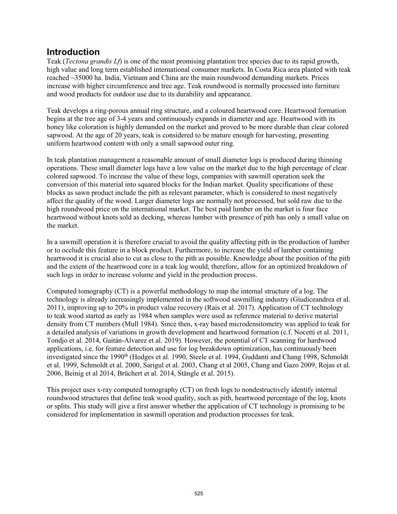
Introduction Teak (Tectona grandis Lf) is one of the most promising plantation tree species due to its rapid growth, high value and long term established international consumer markets. In Costa Rica area planted with teak reached ~35000 ha. India, Vietnam and China are the main roundwood demanding markets. Prices increase with higher circumference and tree age. Teak roundwood is normally processed into furniture and wood products for outdoor use due to its durability and appearance.

Teak develops a ring-porous annual ring structure, and a coloured heartwood core. Heartwood formation begins at the tree age of 3-4 years and continuously expands in diameter and age. Heartwood with its honey like coloration is highly demanded on the market and proved to be more durable than clear colored sapwood. At the age of 20 years, teak is considered to be mature enough for harvesting, presenting uniform heartwood content with only a small sapwood outer ring.

In teak plantation management a reasonable amount of small diameter logs is produced during thinning operations. These small diameter logs have a low value on the market due to the high percentage of clear colored sapwood. To increase the value of these logs, companies with sawmill operation seek the conversion of this material into squared blocks for the Indian market. Quality specifications of these blocks as sawn product include the pith as relevant parameter, which is considered to most negatively affect the quality of the wood. Larger diameter logs are normally not processed, but sold raw due to the high roundwood price on the international market. The best paid lumber on the market is four face heartwood without knots sold as decking, whereas lumber with presence of pith has only a small value on the market.

In a sawmill operation it is therefore crucial to avoid the quality affecting pith in the production of lumber or to occlude this feature in a block product. Furthermore, to increase the yield of lumber containing heartwood it is crucial also to cut as close to the pith as possible. Knowledge about the position of the pith and the extent of the heartwood core in a teak log would, therefore, allow for an optimized breakdown of such logs in order to increase volume and yield in the production process.

Computed tomography (CT) is a powerful methodology to map the internal structure of a log. The technology is already increasingly implemented in the softwood sawmilling industry (Giudiceandrea et al. 2011), improving up to 20% in product value recovery (Rais et al. 2017). Application of CT technology to teak wood started as early as 1984 when samples were used as reference material to derive material density from CT numbers (Mull 1984). Since then, x-ray based microdensitometry was applied to teak for a detailed analysis of variations in growth development and heartwood formation (c.f. Nocetti et al. 2011, Tondjo et al. 2014, Gaitán-Alvarez et al. 2019). However, the potential of CT scanning for hardwood applications, i.e. for feature detection and use for log breakdown optimization, has continuously been investigated since the 1990th (Hodges et al. 1990, Steele et al. 1994, Guddanti and Chang 1998, Schmoldt et al. 1999, Schmoldt et al. 2000, Sarigul et al. 2003, Chang et al 2005, Chang and Gazo 2009, Rojas et al. 2006, Beinig et al 2014, Brüchert et al. 2014, Stängle et al. 2015).

This project uses x-ray computed tomography (CT) on fresh logs to nondestructively identify internal roundwood structures that define teak wood quality, such as pith, heartwood percentage of the log, knots or splits. This study will give a first answer whether the application of CT technology is promising to be considered for implementation in sawmill operation and production processes for teak.

525

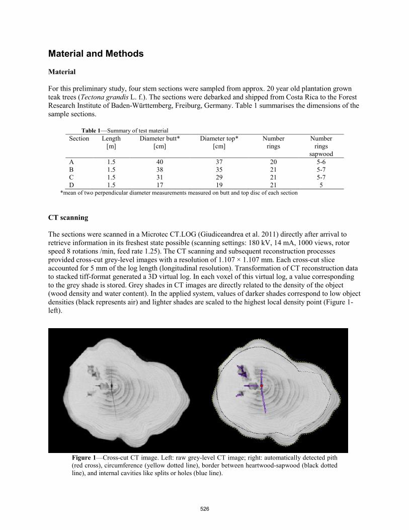
Material and Methods

Material

For this preliminary study, four stem sections were sampled from approx. 20 year old plantation grown teak trees (Tectona grandis L. f.). The sections were debarked and shipped from Costa Rica to the Forest Research Institute of Baden-Württemberg, Freiburg, Germany. Table 1 summarises the dimensions of the sample sections.

Table 1—Summary of test material Section Length

[m] Diameter butt*

[cm] Diameter top*

[cm] Number

rings Number

rings sapwood

A 1.5 40 37 20 5-6B 1.5 38 35 21 5-7C 1.5 31 29 21 5-7D 1.5 17 19 21 5

*mean of two perpendicular diameter measurements measured on butt and top disc of each section

CT scanning

The sections were scanned in a Microtec CT.LOG (Giudiceandrea et al. 2011) directly after arrival to retrieve information in its freshest state possible (scanning settings: 180 kV, 14 mA, 1000 views, rotor speed 8 rotations /min, feed rate 1.25). The CT scanning and subsequent reconstruction processes provided cross-cut grey-level images with a resolution of 1.107 × 1.107 mm. Each cross-cut slice accounted for 5 mm of the log length (longitudinal resolution). Transformation of CT reconstruction data to stacked tiff-format generated a 3D virtual log. In each voxel of this virtual log, a value corresponding to the grey shade is stored. Grey shades in CT images are directly related to the density of the object (wood density and water content). In the applied system, values of darker shades correspond to low object densities (black represents air) and lighter shades are scaled to the highest local density point (Figure 1-left).

Figure 1—Cross-cut CT image. Left: raw grey-level CT image; right: automatically detected pith (red cross), circumference (yellow dotted line), border between heartwood-sapwood (black dotted line), and internal cavities like splits or holes (blue line).

526

Wood quality parameters such as pith, cracks, heartwood core, sapwood boundary, and knots were identified by visual inspection of the CT scans. In a second step, an automated algorithm for softwood was adopted and applied which detects the pith position throughout the log (Boukadida et al. 2012), the borders between heartwood-sapwood and the wood cylinder-outside (Longuetaud et al. 2007; Baumgartner et al. 2010). For the automated detection of internal splits or cracks the algorithm by Wehrhausen et al. (2013) was tested (Figure 1-right).

From the automated heartwood-sapwood border detection, the heartwood percentage of the cross section was calculated and compared to the heartwood percentage derived from visual inspection and manual measurement.

For the calculation of the heartwood content in the cross section of the stem sections, the sapwood-heartwood boundary was visually determined on two diameters perpendicular from each other. On two discs per stem section (butt and top) the diameters were orientated in a way that D1 represented the largest diameter of the disc and D2 was positioned perpendicular to D1. On these two diameters (= 4 radii) the distance between pith and outer boundary (R1, R2, R3, R4,) and between pith and heartwood-sapwood boundary (r1, r2, r3, r4,) was measured. Assuming an elliptic shape of the cross section, the heartwood percentage was calculated as mean of relative share in the cross section of the two discs.

Results and Discussion

Visual inspection

The differentiation of grey-scale levels in the CT images allows distinguishing between different internal wood structures and features. Figures 2 – 6 show examples of the cross sections of the test stem sections.

Figure 2—Exemplary cross section of stem section D “knot hole”: Cross-cut CT image (left). Corresponding colour image of the cross-cut (right).

527

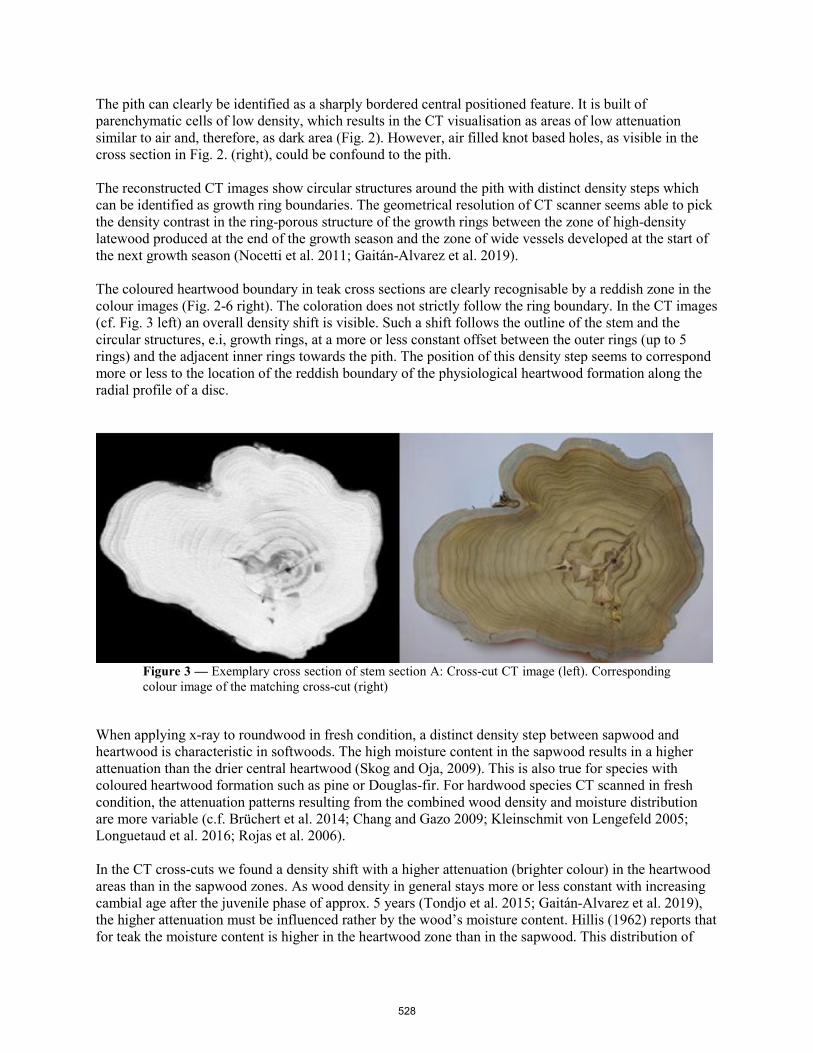
The pith can clearly be identified as a sharply bordered central positioned feature. It is built of parenchymatic cells of low density, which results in the CT visualisation as areas of low attenuation similar to air and, therefore, as dark area (Fig. 2). However, air filled knot based holes, as visible in the cross section in Fig. 2. (right), could be confound to the pith.

The reconstructed CT images show circular structures around the pith with distinct density steps which can be identified as growth ring boundaries. The geometrical resolution of CT scanner seems able to pick the density contrast in the ring-porous structure of the growth rings between the zone of high-density latewood produced at the end of the growth season and the zone of wide vessels developed at the start of the next growth season (Nocetti et al. 2011; Gaitán-Alvarez et al. 2019).

The coloured heartwood boundary in teak cross sections are clearly recognisable by a reddish zone in the colour images (Fig. 2-6 right). The coloration does not strictly follow the ring boundary. In the CT images (cf. Fig. 3 left) an overall density shift is visible. Such a shift follows the outline of the stem and the circular structures, e.i, growth rings, at a more or less constant offset between the outer rings (up to 5 rings) and the adjacent inner rings towards the pith. The position of this density step seems to correspond more or less to the location of the reddish boundary of the physiological heartwood formation along the radial profile of a disc.

Figure 3 — Exemplary cross section of stem section A: Cross-cut CT image (left). Corresponding colour image of the matching cross-cut (right)

When applying x-ray to roundwood in fresh condition, a distinct density step between sapwood and heartwood is characteristic in softwoods. The high moisture content in the sapwood results in a higher attenuation than the drier central heartwood (Skog and Oja, 2009). This is also true for species with coloured heartwood formation such as pine or Douglas-fir. For hardwood species CT scanned in fresh condition, the attenuation patterns resulting from the combined wood density and moisture distribution are more variable (c.f. Brüchert et al. 2014; Chang and Gazo 2009; Kleinschmit von Lengefeld 2005; Longuetaud et al. 2016; Rojas et al. 2006).

In the CT cross-cuts we found a density shift with a higher attenuation (brighter colour) in the heartwood areas than in the sapwood zones. As wood density in general stays more or less constant with increasing cambial age after the juvenile phase of approx. 5 years (Tondjo et al. 2015; Gaitán-Alvarez et al. 2019), the higher attenuation must be influenced rather by the wood’s moisture content. Hillis (1962) reports that for teak the moisture content is higher in the heartwood zone than in the sapwood. This distribution of

528

water in the cross section could explain the attenuation variation and distribution in the CT cross-cuts found in the test material. Ingrown knots and other irregularities in the wood structure like rot were also visible due to changes in attenuation (Fig. 3, 4, 5). Attenuation contrasts due to knot pith and drying effects due to pruning allow the localisation of such structures in the stem. Sound knots are difficult to distinguish in the CT reconstruction as knot wood in hardwoods often consists of a similar wood density in relation to the stem wood; therefore, no contrast can be detected between knot wood and stem wood (Fig. 4, Fig. 6).

Figure 4 — Exemplary cross section of stem section C: Cross-cut CT image (left). Corresponding colour image of the cross-cut (right).

Other quality-relevant internal stem structures such as heart shakes and splits can also be detected based on existing attenuation contrast. However, corresponding changes in colour are not visible in the CT cross-cuts (Fig. 4).

Figure 5 — Exemplary cross section of stem section A “rot”: Cross-cut CT image (left). Corresponding colour image of the cross-cut (right).

529

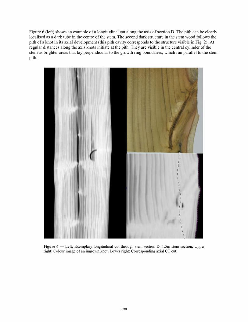
Figure 6 (left) shows an example of a longitudinal cut along the axis of section D. The pith can be clearly localised as a dark tube in the centre of the stem. The second dark structure in the stem wood follows the pith of a knot in its axial development (this pith cavity corresponds to the structure visible in Fig. 2). At regular distances along the axis knots initiate at the pith. They are visible in the central cylinder of the stem as brighter areas that lay perpendicular to the growth ring boundaries, which run parallel to the stem pith.

Figure 6 — Left: Exemplary longitudinal cut through stem section D. 1.5m stem section; Upper right: Colour image of an ingrown knot; Lower right: Corresponding axial CT cut.

530

Automated detection of pith and heartwood-sapwood boundary

Figure 7 shows results of an automated detection of pith, heartwood-sapwood boundary and splits, the algorithms originally developed for softwoods. The algorithm seems to find the pith with good precision in all four cases.

The heartwood-sapwood boundary usually runs parallel to the circumference of the log. The applied algorithm, developed for more or less round softwoods, seems to detect the attenuation contrast between the two zones better in regular cross section shapes closer to circular shapes (Fig 7 lower line: section C, D) than for irregular shapes (section A). For the detection in section B (Fig. 7 upper right) the algorithmappears to follow closely the contrast line with slight deviations. The obvious deviations might resultfrom a smoothing or blurring configuration of the algorithm, which was not yet adapted for teak.

An algorithm developed for split detection in sapwood and heartwood of softwoods recognized splits very well, but also ingrown bark, occluded knots, pruning scars and other features that might consist of rot stages.

Figure 7 — Exemplary cross section of stem sections with automated detected pith (red dot), heartwood-sapwood boundary (black dotted line) and other internal structures (blue line): upper left: section A; upper right: section B; lower left: section C; lower right: section D.

531

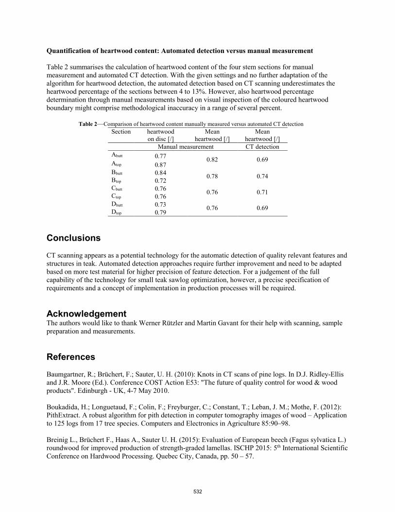
Quantification of heartwood content: Automated detection versus manual measurement

Table 2 summarises the calculation of heartwood content of the four stem sections for manual measurement and automated CT detection. With the given settings and no further adaptation of the algorithm for heartwood detection, the automated detection based on CT scanning underestimates the heartwood percentage of the sections between 4 to 13%. However, also heartwood percentage determination through manual measurements based on visual inspection of the coloured heartwood boundary might comprise methodological inaccuracy in a range of several percent.

Table 2—Comparison of heartwood content manually measured versus automated CT detection Section heartwood

on disc [/] Mean

heartwood [/] Mean

heartwood [/] Manual measurement CT detection

Abutt 0.77 0.82 0.69 Atop 0.87

Bbutt 0.84 0.78 0.74 Btop 0.72 Cbutt 0.76 0.76 0.71 Ctop 0.76 Dbutt 0.73 0.76 0.69 Dtop 0.79

Conclusions

CT scanning appears as a potential technology for the automatic detection of quality relevant features and structures in teak. Automated detection approaches require further improvement and need to be adapted based on more test material for higher precision of feature detection. For a judgement of the full capability of the technology for small teak sawlog optimization, however, a precise specification of requirements and a concept of implementation in production processes will be required.

Acknowledgement The authors would like to thank Werner Rützler and Martin Gavant for their help with scanning, sample preparation and measurements.

References

Baumgartner, R.; Brüchert, F.; Sauter, U. H. (2010): Knots in CT scans of pine logs. In D.J. Ridley-Ellis and J.R. Moore (Ed.). Conference COST Action E53: "The future of quality control for wood & wood products". Edinburgh - UK, 4-7 May 2010.

Boukadida, H.; Longuetaud, F.; Colin, F.; Freyburger, C.; Constant, T.; Leban, J. M.; Mothe, F. (2012): PithExtract. A robust algorithm for pith detection in computer tomography images of wood – Application to 125 logs from 17 tree species. Computers and Electronics in Agriculture 85:90–98.

Breinig L., Brüchert F., Haas A., Sauter U. H. (2015): Evaluation of European beech (Fagus sylvatica L.) roundwood for improved production of strength-graded lamellas. ISCHP 2015: 5th International Scientific Conference on Hardwood Processing. Quebec City, Canada, pp. 50 – 57.

532

Brüchert, F.; Maschler, T.; Müller, C. (2014): CT-SPEC: Von der röntgengestützten Rundholzver-messung direkt zur Konstruktionsplanung. Abschlussbericht Teil 2: Erkennung innerer Holzmerkmale von Kastanie Eiche und Robinie mittels Computertomographie. Berichte Freiburger Forstliche Forschung, H. 98, 13-75.

Chang, S. J.; Gazo, R. (2009): Measuring the Effect of Internal Log Defect Scanning on the Value of Lumber Produced. Forest Products Journal 59: 56-59.

Chang S.J., Cooper C., Guddanti S. (2005): Effects of the log’s rotational orientation and the depth of the opening cut on the value of lumber produced in sawing hardwood logs. Forest Products Journal 55: 49–55.

Gaitán-Alvarez J., Moya R. A., Berrocal A. (2019): The use of X-ray densitometry to evaluate the wood density profile of Tectona grandis trees growing in fast-growth plantations. Dendrochronologia. 55:71-79.

Giudiceandrea, Federico; Ursella, Enrico; Vicario, Enrico (2011): A high speed CT-scanner for the sawmill industry. In. 17th International Nondestructive Testing and Evaluation of Wood Symposium. Sopron, Hungary, 4–16 September 2011: University of West Hungary.

Guddanti, S., Chang, S. (1998). Replicating sawmill sawing with TOPSAW using CT images of a full-length hardwood log. Forest Products Journal. 48: 72-75.

Hillis W.E. (ed.) (1962): Wood Extractives and Their significance to the Pulp and Paper Industry. Academic press, New York and London.

Hodges D.G., Anderson W.C., McMillin C.W. (1990): The economic potential of CT scanners for hardwood sawmills. Forest Products Journal 40: 65–69.

Kleinschmit von Lengefeld, A. N. (2005): Untersuchungen zur hochauflösenden Bestimmung von qualitätsbeeinflussenden Rundholzmerkmalen am Beispiel von Fichten- und Buchenholz (High resolutional determination of roundwood quality parameters tested on spruce and beech wood). Dissertation, Technische Universität München, Fakultät Wissenschaftszentrum Weihenstephan, 188 p.

Longuetaud F.; Mothe F., Fournier M., Dlouha J., Santenoise P., Deleuze C. (2016): Within-stem maps of wood density and water content for characterization of species: a case study on three hardwood and two softwood species. Annals of Forest Science 73: 601–614.

Longuetaud F.; Mothe F., Leban J.-M. (2007): Automatic detection of the heartwood/sapwood boundary within Norway spruce (Picea abies (L.) Karst.) logs by means of CT images. Computers and Electronics in Agriculture 58: 100–111.

Mull, R. T. 1984. Mass Estimates by Computed Tomography: Physical Density from CT Numbers. American Journal of Roentgenology, 143: 1101-1104.

Nocetti M., Rozenberg, P., Chaix G. (2011): Provenance effect on the ring structure of teak (Tectona grandis L.f.) wood by X-ray microdensitometry. Annals of Forest Science 68: 1375-1383.

Rais, A., Ursella, E., Vicario, E., Giudiceandres F. (2017): The use of the first industrial X-ray CT scanner increases the lumber recovery value: case study on visually strength-graded Douglas-fir timber. Annals of Forest Science 74: 1-9.

533

Rojas, G., Condal, A., Beauregard,·R., Verret, D. , Hernández, R.E. (2006) Identification of internal defect of sugar maple logs from CT images using supervised classification methods. Holz als Roh- und Werkstoff 64: 295–303.

Sarigul, E., Abbott, A.L. and Schmoldt, D.L. (2003): Rule-driven defect detection in CT images of hardwood logs. Computers and Electronics in Agriculture 41: 101–119.

Schmoldt D. L., Occena L. G., Abbot A. L., Gupta N. K. (1999): Nondestructive evaluation of hardwood logs: CT scanning, machine vision and data utilisation. Nondestr. Test. Eval.,Vol. 15: 279-309.

Schmoldt, D.L., Scheinmann, E., Rinnhofer, A., Occeña L.G. (2000): Internal Log Scanning: Research to Reality. Proceedings of the Twenty-eighth Annual Hardwood Symposium, May 11–13, 2000, Davis, West Virginia, 103–114.

Skog J.; Oja J. (2009): Heartwood diameter measurements in Pinus sylvestris sawlogs combining X-ray and three-dimensional scanning. Scandinavian Journal of Forest Research 24(2):182-188.

Steele, P.H., Harless, T.E.G., Wagner, F.G., Kumar, L. and Taylor, F.W. (1994): Increased lumber value from optimum orientation of internal defects with respect to sawing pattern in hard- wood sawlogs. Forest Products Journal 44: 69–72.

Stängle S. M., Brüchert F., Heikkila A., Usenius T., Usenius A., Sauter U. H. (2015). Potentially increased sawmill yield from hardwoods using X-ray computed tomography for knot detection. Annals of Forest Science 72: 57-65. ⟨10.1007/s13595-014-0385-1⟩.

Tondjo K., Brancheriau L., Sabatier S., Kokutse A.D., Akossou A., Kokou K., Fourcaud T. (2015). Is the variability of key wood properties linked with the variability of key architectural traits? Case of planted Teak in Togo regarding thinning and provenance. Annals of Forest Science 72: 717-729.

Wehrhausen M., Laudon N., Brüchert F., Sauter U.H. (2013): Crack detection in computertomographic scans of softwood tree discs. Forest Products Journal 62 No 6: 434-442.

534

Using Computed Tomography Density Profiles to Identify Whorls in Douglas-fir Trees: A Graphical Based Approach

Bruna Laís Longo* Department of Forest Utilization, University of Freiburg, Freiburg, Baden-Württemberg, Germany, bruna.longo@fobawi.uni-freiburg.de

Franka Brüchert Department of Forest Utilization, Forest Research Institute of Baden-Württemberg, Freiburg, Baden-Württemberg, Germany, franka.bruechert@forst.bwl.de

Anne-Sophie Stelzer Department of Biometry and Informatics, Forest Research Institute of Baden-Württemberg, Freiburg, Baden-Württemberg, Germany, anne-sophie.stelzer@forst.bwl.de

Gero Becker Department of Forest Utilization, University of Freiburg, Freiburg, Baden-Württemberg, Germany, gero.becker@fob.uni-freiburg.de

Udo Hans Sauter Department of Forest Utilization, Forest Research Institute of Baden-Württemberg, Freiburg, Baden-Württemberg, Germany, udo.sauter@forst.bwl.de

Abstract

Whorl knots play an important role on growth models, as they typically delimit annual shoots. They are on average larger than internodes, and usually have a higher impact on wood quality grading. In this context, an automatic classification of knots into whorls is primordial to connect internal and external tree attributes using computed tomography (CT) technology. This case study aimed to identify whorls in Douglas-fir trees based on CT longitudinal density profiles. The material was sampled from three trial sites in southwest Germany and consisted of 92 logs from 17 trees, considering three age ranges (30-35, 40-50, 75-80). The analysis comprehended the portion from DBH height to usable timber height (minimum stem diameter of 7cm). Logs were scanned in a MiCROTEC CT.LOG, generating a mean heartwood density value per log´s cross-section, comprising 5 mm (slice) of the log length. Whorl identification started by plotting slice mean density against its known stem height. A peak in such a plot reveals the presence of knots. Based on this longitudinal density profile, a peak-and-pit detection was performed using the “turnpoints” function from the “pastecs” package in R. To exclude lower peaks (internodes), cubic splines were fitted to the detected peak and pit points. Results showed a high accuracy of the method, demonstrating its ability to detect whorls, especially of mature Douglas-fir logs. However, based on the false positives rate, adjustments focusing on the smoothing operation and the spacing between whorls might improve the overall performance of this method.

Keywords: 3D-scanning, knot structure, branch distribution, wood quality, peak detection

535

Introduction

Models and simulators that estimate growth and quality of stands are usually applied in forestry as a tool for control and decision making. These models often account for different conditions and traits at the site, stand and tree levels. Whorl related variables play an important role on such models, as they delimit annual shoots, which are accounted as one of the expressions of height growth. Since whorl knots are on average larger than internodes, and usually have a higher impact on wood quality grading, these models have potential to extrapolate the forest scope and approach roundwood quality by incorporating internal variables.

Computed tomography (CT) is regarded as one of the most successful techniques to map the internal structure of a log. In sawmills, its utilization is well known to be able to determine, for example, the optimal breakdown positions, focusing on the optimization in terms of volume or value. The value optimization is due to the unveiling of features such as cracks, resin pockets, indentations, rot areas, and knots. Among these, the presence of knots is considered the feature that most affects the wood quality, leading to the development of various methods to detect knots in CT images (Andreu and Rinnhofer 2003; Breinig et al. 2012; Johansson et al. 2013; Longuetaud et al. 2012; Roussel et al. 2014).

In this context, an automatic classification of knots into whorls enables the use of large datasets to connect standing tree models and wood quality in sawmills. In this case study, the aim was to test an approach to automatically detect groups of knots (whorls) that present a greater local density footprint compared to the surrounding heartwood area. The use of knot size data based on another automatic detection algorithm was avoided at this stage, in order to reduce the accumulation of errors. The intention at this point was to develop a solution to identify whorls based directly on the longitudinal density profiles the CT scanner provides and indirectly on the heartwood-sapwood boundary detection.

Material and Methods

Material origin and description

The material used in this study was part of two prior projects and was originated from three trial sites in southwest Germany. Interventions in these sites were performed according to the objectives of the former projects, which led to complete areas with and without pruning, as well as areas where only selected trees were pruned. For this study, Douglas-fir (Pseudotsuga menziesii (Mirb.) Franco) trees were randomly selected using the “sample” function in base R (R Core Team 2016). The descriptive summary of the selected material is presented in table 1.

Table 1—Summary of material origin and description. Trial site Latitude Longitude Trees Logs Age range (years) Intervention Odenwald 49º33’ 9º16’ 7 21 30-35 No pruning Kandern 47º42’ 7º42’ 6 34 45-50 Pruning (selective) Höllental 47º56’ 8º00’ 4 37 75-80 Pruning (all trees) Total 17 92

After felling, trees were bucked into 4-5m-length logs, with the first log starting at 1.3m of height and the last log being sampled up until the minimum stem diameter of 7cm. The bucking and measurement operations followed a protocol (Brüchert et al. 2017), in which a disc of 5-10cm width was sampled at the 1.3m position in height and at the end of each log thereafter.

536

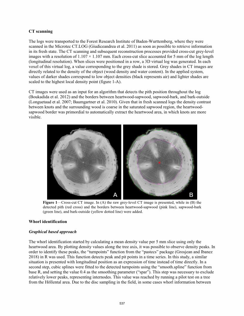
CT scanning

The logs were transported to the Forest Research Institute of Baden-Wurttemberg, where they were scanned in the Microtec CT.LOG (Giudiceandrea et al. 2011) as soon as possible to retrieve information in its fresh state. The CT scanning and subsequent reconstruction processes provided cross-cut grey-level images with a resolution of 1.107 × 1.107 mm. Each cross-cut slice accounted for 5 mm of the log length (longitudinal resolution). When slices were positioned in a row, a 3D virtual log was generated. In each voxel of this virtual log, a value corresponding to the grey shade is stored. Grey shades in CT images are directly related to the density of the object (wood density and water content). In the applied system, values of darker shades correspond to low object densities (black represents air) and lighter shades are scaled to the highest local density point (figure 1-A).

CT images were used as an input for an algorithm that detects the pith position throughout the log (Boukadida et al. 2012) and the borders between heartwood-sapwood, sapwood-bark, and bark-outside (Longuetaud et al. 2007; Baumgartner et al. 2010). Given that in fresh scanned logs the density contrast between knots and the surrounding wood is coarse in the saturated sapwood region, the heartwood-sapwood border was primordial to automatically extract the heartwood area, in which knots are more visible.

Figure 1—Cross-cut CT image. In (A) the raw grey-level CT image is presented, while in (B) the detected pith (red cross) and the borders between heartwood-sapwood (pink line), sapwood-bark (green line), and bark-outside (yellow dotted line) were added.

Whorl identification

Graphical based approach

The whorl identification started by calculating a mean density value per 5 mm slice using only the heartwood area. By plotting density values along the tree axis, it was possible to observe density peaks. In order to identify these peaks, the “turnpoints” function from the “pastecs” package (Grosjean and Ibanez 2018) in R was used. This function detects peak and pit points in a time series. In this study, a similar situation is presented with longitudinal position as an expression of time instead of time directly. In a second step, cubic splines were fitted to the detected turnpoints using the “smooth.spline” function from base R, and setting the value 0.4 as the smoothing parameter (“spar”). This step was necessary to exclude relatively lower peaks, representing internodes. This value was reached by running a pilot test on a tree from the Höllental area. Due to the disc sampling in the field, in some cases whorl information between

537

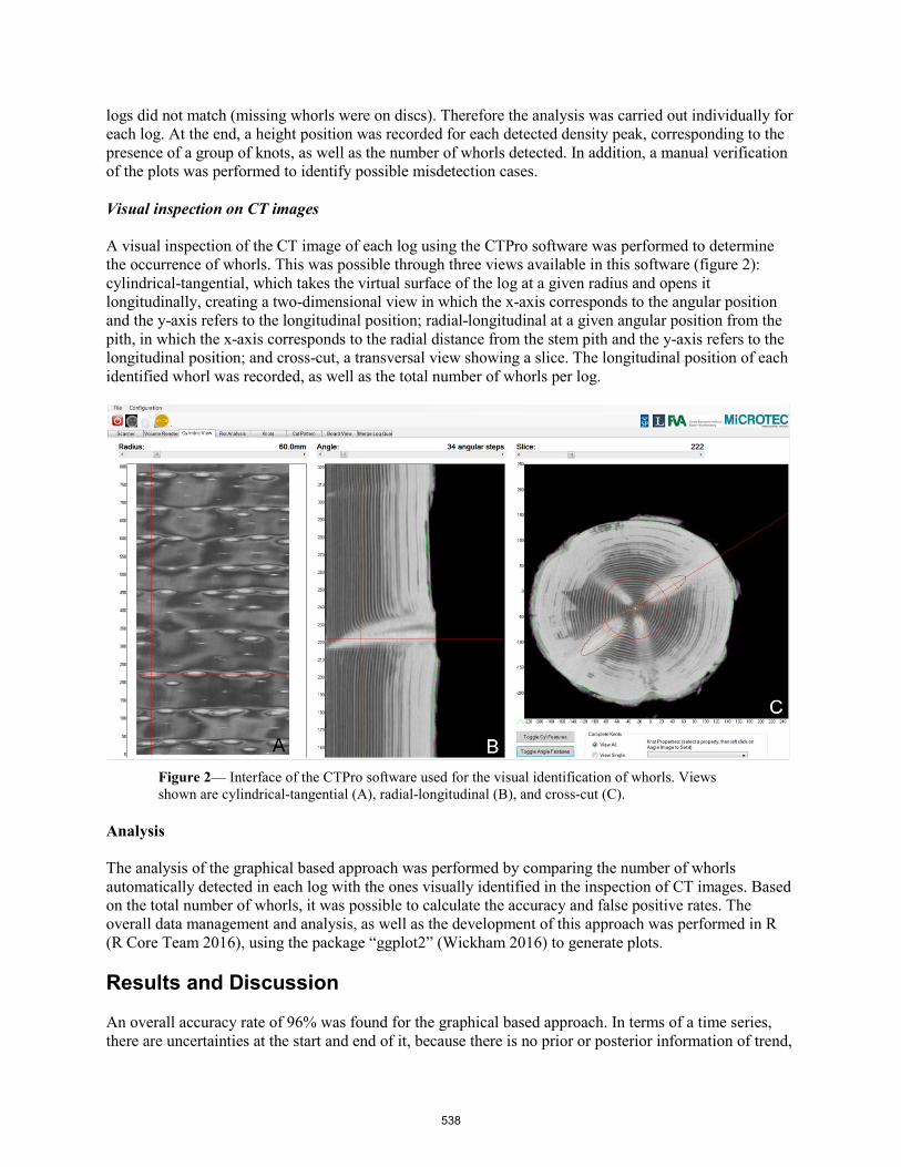
logs did not match (missing whorls were on discs). Therefore the analysis was carried out individually for each log. At the end, a height position was recorded for each detected density peak, corresponding to the presence of a group of knots, as well as the number of whorls detected. In addition, a manual verification of the plots was performed to identify possible misdetection cases.

Visual inspection on CT images

A visual inspection of the CT image of each log using the CTPro software was performed to determine the occurrence of whorls. This was possible through three views available in this software (figure 2): cylindrical-tangential, which takes the virtual surface of the log at a given radius and opens it longitudinally, creating a two-dimensional view in which the x-axis corresponds to the angular position and the y-axis refers to the longitudinal position; radial-longitudinal at a given angular position from the pith, in which the x-axis corresponds to the radial distance from the stem pith and the y-axis refers to the longitudinal position; and cross-cut, a transversal view showing a slice. The longitudinal position of each identified whorl was recorded, as well as the total number of whorls per log.

Figure 2— Interface of the CTPro software used for the visual identification of whorls. Views shown are cylindrical-tangential (A), radial-longitudinal (B), and cross-cut (C).

Analysis

The analysis of the graphical based approach was performed by comparing the number of whorls automatically detected in each log with the ones visually identified in the inspection of CT images. Based on the total number of whorls, it was possible to calculate the accuracy and false positive rates. The overall data management and analysis, as well as the development of this approach was performed in R (R Core Team 2016), using the package “ggplot2” (Wickham 2016) to generate plots.

Results and Discussion

An overall accuracy rate of 96% was found for the graphical based approach. In terms of a time series, there are uncertainties at the start and end of it, because there is no prior or posterior information of trend,

538

i.e. if the density will drop or increase. In the current state, we have already integrated a solution for casesat the end of the time series, i.e. a peak after the last pit. As for the other end, a solution can be slightlymore intricate, as it requires a run backwards to detect the peak before the first pit. Although this solutionis not implemented, it was possible to quantify its occurrence (see “First whorl ignored” in table 2 andfigure 3-A). In general, accuracy values were high and considering that this additional improvementmight add almost 3.8% to this rate, this approach shows high potential for the automatic detection ofwhorls.

Table 2—Accuracy results of the graphical based approach. Trial site N Accuracy False positive First whorl ignored Odenwald 114 98.25% 39.47% 1.75% Kandern 170 96.47% 48.82% 3.53% Höllental 246 94.72% 08.54% 4.88% Total 530 96.04% 28.87% 3.77% N: number of whorls identified by visual inspection on CT images.

Figure 3—CT density profiles of four logs. Each black point corresponds to the mean heartwood density of a CT slice. Colored dots indicate correct whorls (blue) and false positives (red) detected by the tested approach. (A) shows data from the fifth log (18.4-22.6m height) of a tree from Höllental as an example of the “first whorl ignored” instance. (B) shows data from the third log (11.6-16.7m height) of a tree from Odenwald, illustrating pre-whorl knots and their effect in the

539

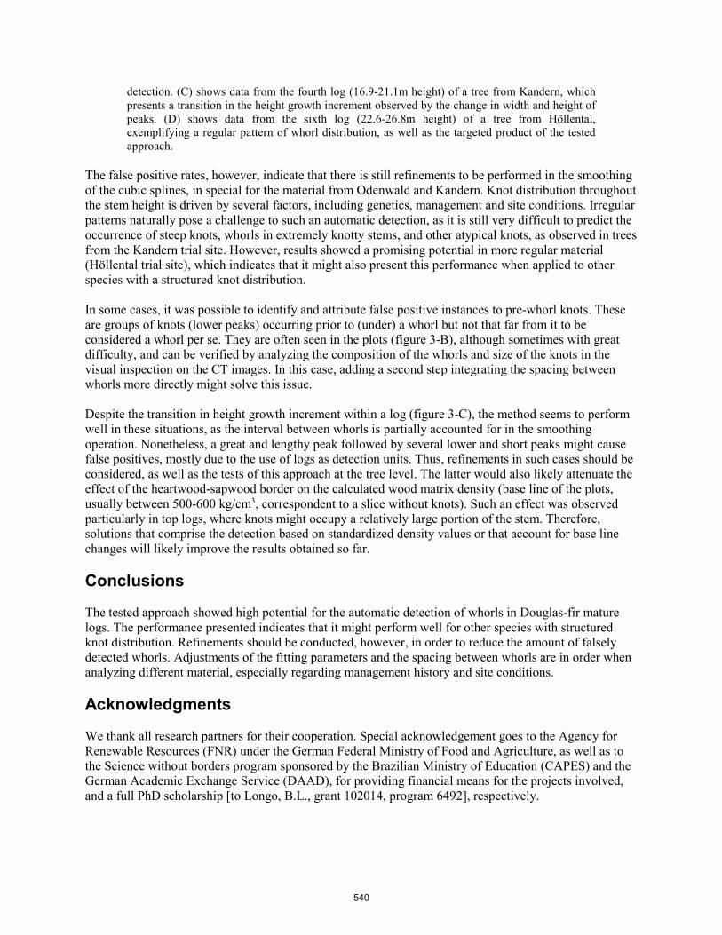
detection. (C) shows data from the fourth log (16.9-21.1m height) of a tree from Kandern, which presents a transition in the height growth increment observed by the change in width and height of peaks. (D) shows data from the sixth log (22.6-26.8m height) of a tree from Höllental, exemplifying a regular pattern of whorl distribution, as well as the targeted product of the tested approach.

The false positive rates, however, indicate that there is still refinements to be performed in the smoothing of the cubic splines, in special for the material from Odenwald and Kandern. Knot distribution throughout the stem height is driven by several factors, including genetics, management and site conditions. Irregular patterns naturally pose a challenge to such an automatic detection, as it is still very difficult to predict the occurrence of steep knots, whorls in extremely knotty stems, and other atypical knots, as observed in trees from the Kandern trial site. However, results showed a promising potential in more regular material (Höllental trial site), which indicates that it might also present this performance when applied to other species with a structured knot distribution.

In some cases, it was possible to identify and attribute false positive instances to pre-whorl knots. These are groups of knots (lower peaks) occurring prior to (under) a whorl but not that far from it to be considered a whorl per se. They are often seen in the plots (figure 3-B), although sometimes with great difficulty, and can be verified by analyzing the composition of the whorls and size of the knots in the visual inspection on the CT images. In this case, adding a second step integrating the spacing between whorls more directly might solve this issue.

Despite the transition in height growth increment within a log (figure 3-C), the method seems to perform well in these situations, as the interval between whorls is partially accounted for in the smoothing operation. Nonetheless, a great and lengthy peak followed by several lower and short peaks might cause false positives, mostly due to the use of logs as detection units. Thus, refinements in such cases should be considered, as well as the tests of this approach at the tree level. The latter would also likely attenuate the effect of the heartwood-sapwood border on the calculated wood matrix density (base line of the plots, usually between 500-600 kg/cm3, correspondent to a slice without knots). Such an effect was observed particularly in top logs, where knots might occupy a relatively large portion of the stem. Therefore, solutions that comprise the detection based on standardized density values or that account for base line changes will likely improve the results obtained so far.

Conclusions

The tested approach showed high potential for the automatic detection of whorls in Douglas-fir mature logs. The performance presented indicates that it might perform well for other species with structured knot distribution. Refinements should be conducted, however, in order to reduce the amount of falsely detected whorls. Adjustments of the fitting parameters and the spacing between whorls are in order when analyzing different material, especially regarding management history and site conditions.

Acknowledgments

We thank all research partners for their cooperation. Special acknowledgement goes to the Agency for Renewable Resources (FNR) under the German Federal Ministry of Food and Agriculture, as well as to the Science without borders program sponsored by the Brazilian Ministry of Education (CAPES) and the German Academic Exchange Service (DAAD), for providing financial means for the projects involved, and a full PhD scholarship [to Longo, B.L., grant 102014, program 6492], respectively.

540

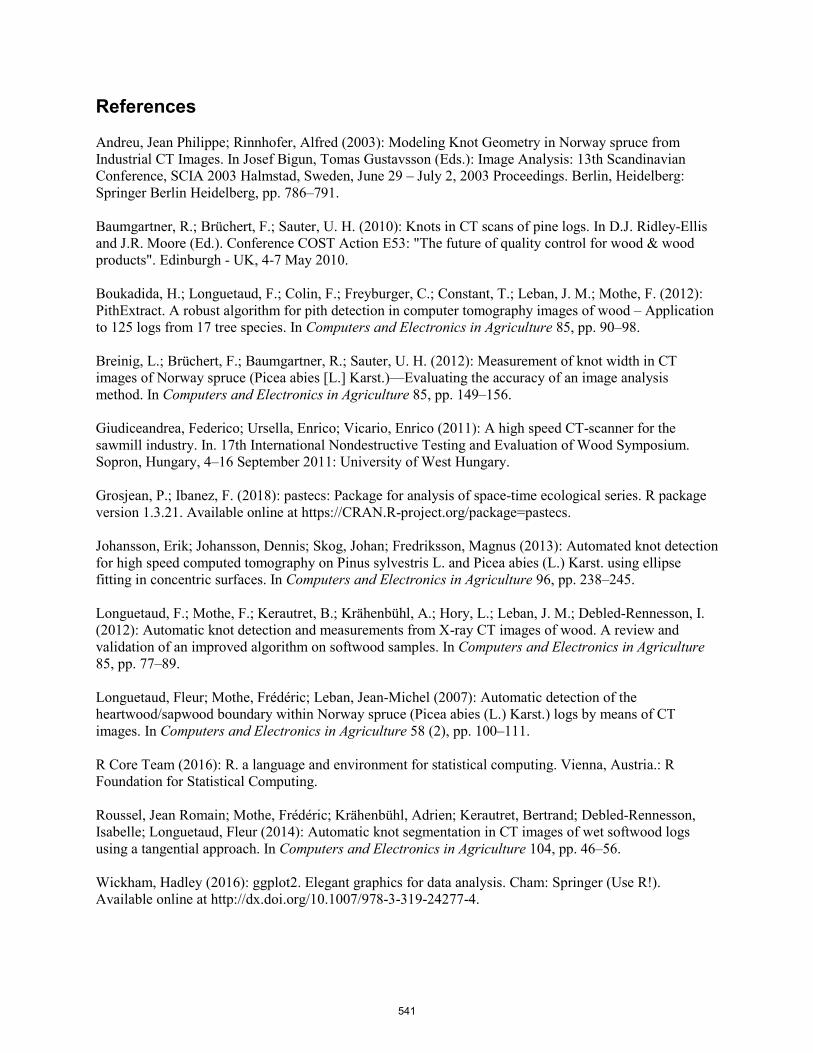
References

Andreu, Jean Philippe; Rinnhofer, Alfred (2003): Modeling Knot Geometry in Norway spruce from Industrial CT Images. In Josef Bigun, Tomas Gustavsson (Eds.): Image Analysis: 13th Scandinavian Conference, SCIA 2003 Halmstad, Sweden, June 29 – July 2, 2003 Proceedings. Berlin, Heidelberg: Springer Berlin Heidelberg, pp. 786–791.

Baumgartner, R.; Brüchert, F.; Sauter, U. H. (2010): Knots in CT scans of pine logs. In D.J. Ridley-Ellis and J.R. Moore (Ed.). Conference COST Action E53: "The future of quality control for wood & wood products". Edinburgh - UK, 4-7 May 2010.

Boukadida, H.; Longuetaud, F.; Colin, F.; Freyburger, C.; Constant, T.; Leban, J. M.; Mothe, F. (2012): PithExtract. A robust algorithm for pith detection in computer tomography images of wood – Application to 125 logs from 17 tree species. In Computers and Electronics in Agriculture 85, pp. 90–98.

Breinig, L.; Brüchert, F.; Baumgartner, R.; Sauter, U. H. (2012): Measurement of knot width in CT images of Norway spruce (Picea abies [L.] Karst.)—Evaluating the accuracy of an image analysis method. In Computers and Electronics in Agriculture 85, pp. 149–156.

Giudiceandrea, Federico; Ursella, Enrico; Vicario, Enrico (2011): A high speed CT-scanner for the sawmill industry. In. 17th International Nondestructive Testing and Evaluation of Wood Symposium. Sopron, Hungary, 4–16 September 2011: University of West Hungary.

Grosjean, P.; Ibanez, F. (2018): pastecs: Package for analysis of space-time ecological series. R package version 1.3.21. Available online at https://CRAN.R-project.org/package=pastecs.

Johansson, Erik; Johansson, Dennis; Skog, Johan; Fredriksson, Magnus (2013): Automated knot detection for high speed computed tomography on Pinus sylvestris L. and Picea abies (L.) Karst. using ellipse fitting in concentric surfaces. In Computers and Electronics in Agriculture 96, pp. 238–245.

Longuetaud, F.; Mothe, F.; Kerautret, B.; Krähenbühl, A.; Hory, L.; Leban, J. M.; Debled-Rennesson, I. (2012): Automatic knot detection and measurements from X-ray CT images of wood. A review and validation of an improved algorithm on softwood samples. In Computers and Electronics in Agriculture 85, pp. 77–89.

Longuetaud, Fleur; Mothe, Frédéric; Leban, Jean-Michel (2007): Automatic detection of the heartwood/sapwood boundary within Norway spruce (Picea abies (L.) Karst.) logs by means of CT images. In Computers and Electronics in Agriculture 58 (2), pp. 100–111.

R Core Team (2016): R. a language and environment for statistical computing. Vienna, Austria.: R Foundation for Statistical Computing.

Roussel, Jean Romain; Mothe, Frédéric; Krähenbühl, Adrien; Kerautret, Bertrand; Debled-Rennesson, Isabelle; Longuetaud, Fleur (2014): Automatic knot segmentation in CT images of wet softwood logs using a tangential approach. In Computers and Electronics in Agriculture 104, pp. 46–56.

Wickham, Hadley (2016): ggplot2. Elegant graphics for data analysis. Cham: Springer (Use R!). Available online at http://dx.doi.org/10.1007/978-3-319-24277-4.

541

Evaluation of Nondestructive Techniques and Visual Assessments to Grade Fibre-Grown Eucalyptus Logs for Structural Products

Michelle Balasso* School of Natural Sciences and ARC Training Centre for Forest Value, University of Tasmania, Hobart, Tasmania, Australia, Michelle.Balasso@utas.edu.au

* Corresponding author

Mark Hunt School of Natural Sciences and ARC Training Centre for Forest Value, University of Tasmania, Hobart, Tasmania, Australia, M.Hunt@utas.edu.au

Gregory Nolan

School of Technology, Environments & Design, ARC Training Centre for Forest Value and Centre for Sustainable Architecture with Wood, University of Tasmania, Launceston, Tasmania, Australia, gregory.nolan@utas.edu.au

Nathan Kotlarewski

School of Technology, Environments & Design and ARC Training Centre for Forest Value, University of Tasmania, Launceston, Tasmania, Australia, nathan.kotlarewski@utas.edu.au

Andrew Jacobs, Forico Pty Limited, Launceston, Tasmania, Australia, andrew.jacobs@forico.com.au

Julianne O’Reilly-Wapstra School of Natural Sciences and ARC Training Centre for Forest Value, University of Tasmania, Hobart, Tasmania, Australia, julianne.oreilly@utas.edu.au

Abstract Eucalypt plantations occur worldwide, occupying almost 22 million hectares of land. These plantations are predominantly managed for fibre-based products, and their use for other product types is of increasing interest. While native forest eucalypt material is mainly sawn for timber for appearance application, the potential use of a plantation-based resource for structural products is currently being investigated.

Structural products require stiff forest material and the timber industry may exploit advantageously Non-Destructive Techniques (NDT) to identify the timber qualities most suited for these products.

Adequate studies are needed to support the use of NDT as segregation tools and evaluate their potential to reliably indicate important wood quality variables.

To support better integration of NDT into the segregation of the resource for preferred uses, a study was conducted in a fibre-managed Eucalyptus nitens plantation in Tasmania, Australia. Forty trees were assessed with NDT acoustic techniques, harvested and bucked to sawlog lengths. Logs were measured and evaluated with both acoustic resonance techniques and by visual assessments. Positive

542

and significant correlations were found between the tree and the log measurements, while NDT measures on logs were correlated with visual features.

Results highlight the potential for the integration of visual grading and NDT testing for assessing plantation eucalypt logs and batching them into quality classes according to their characteristics. An accurate classification of the material would support a more efficient use of a low-grade resource which might satisfy different markets such as that for structural Engineered Wood Products (EWP).

Keywords: NDT, acoustics, Eucalyptus, plantations, hardwood, structural products

Introduction Eucalyptus plantations are planted worldwide mostly for the production of fibre, and in Tasmania they occupy almost 234,000 ha (Downham & Gavran 2019). The silvicultural management practices applied for pulpwood production is markedly different than that required for production of logs for the timber industry, and as consequence, the quality of the timber sourced from short-rotation regimes is specific to these systems (Zobel 1984). In general, logs tend to be smaller, less dense, and have significantly more features; all characteristics that impact both the volume and value recovery of the timber.

Stiffness, strength, density and durability are preferred properties for structural products. These characteristics are usually tested on the final material, once the production cycle is almost concluded. However, the use of techniques to depict wood quality when trees are standing or at the landing at harvesting time has been investigated (Ross 2015). Acoustic techniques can be used for in-forest assessments of stiffness of trees, as well as for log assessments (Wang 2013) and timber products characterisation. The use of acoustic tools as a means of segregating material has also been applied (Farrell, Innes & Hardwood 2012; Dickson et al. 2003).

Grading of logs at the landing, in order to batch material of different qualities, is performed according to grading handbook rules, or in-house grading systems which meet the final users’ requirements. The assessment of log characteristics is critical, as an accurate description of the material will be expected for the final end-user of the material. In this study visual methods and non-destructive techniques (NDT) were considered (Ridoutt et al. 1999) to segregate Eucalyptus timber in both standing trees and logs at harvesting. The current study aimed to (1) understand the potential application of non-destructive acoustic techniques to assess the quality of logs, (2) correlate standing tree measurements with log measurements and (3) identify quality characteristics that could be potentially used to appropriately grade eucalypt plantation logs.

Materials and Methods Materials

The material for this study was selected from a fibre-grown plantation of Eucalyptus nitens (H. Deane & Maiden) Maiden, located in southern Tasmania, Australia (43°03’S, 146°59’E). Trees were 21 years of age at harvesting, and no pruning or thinning treatment was applied in the plantation. Forty harvestable trees were selected for intensive assessments, avoiding those visibly lining, forking, or presenting growth defects. Diameters at breast height over bark (1.3-m, DBH) and tree heights were measured on each tree. Each standing tree was measured acoustically using the Director ST300 (Fibre-gen, New Zealand) on both sides of the stem perpendicularly to the slope gradient. Three readings were taken per side, then averaged to obtain the mean acoustic wave velocity per tree.

543

Measurements on logs

The standing trees were cut into logs 5.5-m long, tagged to track tree number and log position in the stem and then delivered to a mill yard. Up to four logs per tree were recovered. At the mill 105 logs were delivered, placed on bearers 50-cm apart and tested with the acoustic resonance device Director HM200 (Fibre-gen, New Zealand) to obtain an acoustic wave velocity (AWV) reading per log. Log length, diameters at the large and small ends, and log sweep at the midpoint 2.6-m were all measured. At each long end a disk 2.5-cm thick was cut to be used for the density measurements according to the water displacement method described in AS/NZS 1080.3:2000 (Standards Australia 2000). The log end splitting was measured in each log face and on the side surface. Logs were qualitatively evaluated also according to the natural occurring features: the number and diameter of alive knots were noted per each log, and the total count of the alive knots was reported in an index (Kn).

From the above measurements, the following variables were calculated: volume (Equation 1), taper (cm/m) (Equation 2), sweep (Z) (cm/m) (Equation 3) log cilindricity (CLOG) (Equation 4) (Belleville et al. 2018; Warensjö & Rune 2004). Log-end splitting was measured at both long-ends and calculated according to Equation 5 (Yang 2005).

𝑉𝑉 = 𝐷𝐷1+𝐷𝐷2+𝐷𝐷3+𝐷𝐷44

× 122

× 𝜋𝜋 × 𝐿𝐿 (Equation 1)

Where V is the log volume in m3, D1 (smaller) and D2 (larger) are large end diameters, in m, D3 (smaller) and D4 (larger) are the small end diameters, L is log length (m).

𝑇𝑇 = 𝐷𝐷1+𝐷𝐷22

− 𝐷𝐷3+𝐷𝐷42

/𝐿𝐿 (Equation 2)

Where T is taper, in cm/m, and the D the already defined diameters.

𝑍𝑍 = 𝑆𝑆/𝐿𝐿 (Equation 3)

Where Z is sweep, in cm/m, and S is the maximum deviation of the centre line of the log from a straight line between the mid-points of the two ends (cm).

𝐶𝐶𝐿𝐿𝐿𝐿𝐿𝐿 = 12

× 𝐷𝐷3𝐷𝐷4

+ 𝐷𝐷1𝐷𝐷2 (Equation 4)

Where CLOG is the cilindricity of the log.

SPLITindex defined the split of each end, and the two log end values were then averaged per each log.

𝑆𝑆𝑆𝑆𝐿𝐿𝑆𝑆𝑇𝑇𝑖𝑖𝑖𝑖𝑖𝑖𝑖𝑖𝑖𝑖 = (𝑆𝑆𝐿𝐿𝐸𝐸𝐸𝐸𝐸𝐸2 /2)+ 𝑆𝑆𝐿𝐿𝑆𝑆𝑆𝑆𝑆𝑆𝑆𝑆×𝑆𝑆𝐿𝐿𝐸𝐸𝐸𝐸𝐸𝐸

𝑅𝑅2 (Equation 5)

With SLEND being the split length on the log end, SLSURF the split length on the log surface and R the mean radius of the log end.

Analysis Data were analysed using R software (RStudio Team 2016). The Pearson correlation coefficient between acoustic wave velocity of trees and acoustic wave velocity of logs was computed to test the correlation between the two variables.

Linear mixed modelling was used to test the effects of log position in the stem (A-first log from the stump, B-second log, C-third log, D-fourth log) on acoustic wave velocity. A post-hoc Tukey test was conducted to perform multiple comparisons between log positions. Individual tree was included as a random effect in the model.

𝑌𝑌𝑖𝑖𝑖𝑖 = 𝜇𝜇 + 𝛼𝛼𝑖𝑖 + 𝜖𝜖𝑖𝑖𝑖𝑖

544

Where Yij is the acoustic wave velocity value of the jth log, μ is the overall mean for log position, αi is the random effect of the ith tree and ϵij is the error term. The random effect model was employed to estimate the percentage of total variation in AWV of logs due to between-tree differences in the acoustic readings.

Multiple linear modelling was used to relate the acoustic wave velocity value of the logs with measurable log quality traits (volume, taper, sweep, cilindricity, Split Index, density, number of alive knots). The set of best independent variables was selected with the stepwise selection method, after preliminary graphic testing and correlation analysis between variables. The presence of multicollinearity among variables was also evaluated with the VIF (variance inflation factor) as:

𝑉𝑉𝑆𝑆𝑉𝑉 = 1

1 − 𝑅𝑅𝑖𝑖2

Where 𝑅𝑅𝑖𝑖2 is the multiple correlation coefficient obtained when the ith predictor Xi is regressed against all the remaining ones in the model (Merlo et al. 2014). The threshold for the correlation values was 0.7 and the VIF was contextually evaluated, with a maximum threshold of 4 (Dormann et al. 2013). The VIF values were consistent with the individual correlation tests and no multicollinearity was detected between the variables. The level of significance used was 0.05 and the coefficient of determination (R2) and the root mean square error (RMSE) were determined for the model. The model performance was evaluated on the basis of graphical analysis of residual plots.

The exploration of the variability in log quality indexes and AWV values allowed batching of logs within classes, exemplifying the potential of integrating multiple segregation indexes into the grading procedure.

Results and Discussion The AWV measurements between trees and logs were significantly correlated (r = 0.61, p < .0001).

Descriptive statistics of logs are outlined in Table 1. Average volume of logs was between 0.37 m3 and 0.5 m3, and their AWV values ranged from an absolute minimum value of 3.12 km/s (bottom log) to the highest 4.21 km/s of a second log.

Linear mixed model analysis showed that there were significant differences in terms of volume and acoustic velocity of logs coming from different positions in the stem. For the acoustic readings, second logs-B (3.82 km/s) had significantly lower AWV than butt logs-A (3.51 km/s), as well as being significantly higher than third logs-C (3.81 km/s) and fourth ones-D (3.77 km/s) (p < .001). Third logs were significantly lower in AWV than second logs (p < .05). The increasing pattern of the acoustic wave velocities of logs along the stems’ height is shown in Figure 1, where log sections are ordered according to their position in the trees.

Table 1- Descriptive statistics of logs measurements

Log class No. of logs Volume (m3) Acoustic Wave Velocity (km/s)

Average Min. Max. Average and standard deviation Min. Max.

A 40 0.50a 0.35 0.94 3.51a (0.23) 3.12 4.02 B 38 0.36b 0.24 0.65 3.82b (0.16) 3.51 4.21 C 27 0.30c 0.18 0.55 3.81c (0.13) 3.61 4.13 D 4 0.37d 0.24 0.32 3.77a (0.12) 3.69 3.95

Letters A, B, C, D indicate the log position in the stem (first near the stump, second, third and fourth), while letters a, b, c denote significant differences (α< 0.05) given by the Tukey test

545

Figure 1- Pattern of increase in acoustic wave velocities of the logs (A- first, B- second, C- third, D- fourth log in the stem)

This pattern might be related to the known increase of density along the height of Eucalyptus trees (Kibblewhite et al. 2004; Medhurst et al. 2012), even though it is not supported by the decrease in acoustic values of the uppermost portions of the trees; hence, explaining stiffness variation with density alone might be misleading (Chauhan & Walker 2006). The random effect model indicated that individual trees contributed for the 80.2% in the overall variation of acoustic wave velocity of logs.

A full multiple linear model to estimate log AWV from log quality traits was fitted with all the variables that showed a significant correlation. In a stepwise variable selection method, the log quality variables that showed the highest and significant correlations with log AWV were log taper (partial R2 = 0.16), split index (partial R2 = 0.11) and the number of alive knots per log (partial R2 = 0.23). The final model explained 38% (R2 = 0.38) of the total variability observed in the acoustic wave velocity values of the logs (p < .0001, RMSE = 0.173). Plot of the residuals showed random patterns around zero, homogeneous variance and any specific trend was detectable.

The nature of the movements of acoustic waves inside the timber has been found related to physical variations of the wood as the grain angle, the amount and type of knots and branches and the spiral grain (Legg & Bradley 2016). It has been found that knots have an influence on the stiffness of logs (Jones & Emms 2010) and on the timber (Olsson et al. 2012), as the change in the grain around the knots might impact the behaviour of the waves, as well as being influenced by the changes in local wood density of the alive knots. This was confirmed in the current study, where the presence of alive knots influenced the acoustic wave velocity of the uppermost portions of the trees. Those portions were also considerably less tapered (p < .0001) than the bottom parts of the trees, which tendentially show buttressing, moving the shape of the log from a cylinder towards a conical shape. Log split also tends to increase towards the upper part of stems of Eucalyptus species (Vega et al. 2016), even though in the case of this study this difference was not significant for second logs, and just slightly significant for third logs (p = 0.02).

The variability in the values of log quality indexes, as well as that one of log acoustic wave velocity values, suggests the possibility to use those as means of classification of logs for different products. Batching the logs of the current study for three acoustic classes, which threshold are 3.5 km/s and 4 km/s, would result into 18% of the logs classified as low stiff, 74% of average stiffness, and 8% of the logs would satisfy high stiffness requirements.

Stiffness and density are the most important quality traits for structural products, hence, a first sorting of material on the basis of those traits would ensure that high-quality logs are located and destined to the most appropriate production stream. Segregation of logs, based on volumetric measurements and

546

visual assessments, could also provide a means to batch the logs into categories destined to different products. Log characteristics such as taper, sweep, cilindricity and split of the ends affect volume recovery, the processing of the material and the final product qualities. For example, veneer logs would require different characteristics than sawlogs. Hence, segregation per log volumetric and visual indexes would also need to take into account acoustic sorting of material.

Conclusions Non-Destructive acoustic testing of standing trees proved to be reliable in assessing the acoustic wave velocity of eucalypt logs grown in pulpwood plantations. The use of NDT techniques on logs revealed an increase of acoustic velocity values along the stems’ height, which has a significant impact on the opportunity to use portions of eucalypt trees for different types of products. Log volumetric indexes were not related to the acoustic measure, while it was found that the taper, the split in the logs and the number of features (alive knots) had a positive correlation with the log stiffness.

Variability in log quality indexes opens up the possibility to batch eucalypt plantation logs according to volumetric and visual assessments. The use of an acoustic NDT to first sort plantation material, that then might be batched in quality classes for different production lines, has been demonstrated. Log measurements and the integration of acoustic techniques into grading procedures may improve the recovery of material and better utilisation of the logs, as the quality of the material would be matched with the one expected for the processing and the final use. Furthermore, the appropriate use of commonly used descriptors would lean the grading procedure and render the application of a grading system fit-for-purpose accordingly to the targeted production stream.

Acknowledgments This research was supported by the Australian Research Council Industrial Transformation Centre for Forest Value (Grant no. ICI 50100004) and the Centre for Sustainable Architecture with wood at the University of Tasmania. We would like to acknowledge Michael Lee for the technical support and advice in the study.

We acknowledge Forico Pty Lim. and Neville Smith Forest Products Pty Ltd that generously provided the study material, support for milling and transport.

The authors express their gratitude to the staff of Forico Pty Lim., SFM- Environmental Solutions and NSFP- Neville Smith Forest Products Pty Ltd for the ongoing help and assistance in the trial.

References Belleville, B, Redman, A, Chounlamounty, P, Phengthajam, V, Xiong, S, Boupha, L and Ozarska, B

2018, ‘Potential of Veneer Peeled from Young Eucalypts in Laos’, BioResources, vol. 13, no. 4, pp. 7581–7594.

Chauhan, SS and Walker, JCF 2006, ‘Variations in acoustic velocity and density with age, and their interrelationships in Radiata pine’, Forest Ecology and Management, vol. 229, no. 1, pp. 388–394.

Dickson, RL, Raymond, CA, Joe, W and Wilkinson, CA 2003, ‘Segregation of Eucalyptus dunnii logs using acoustics’, Forest Ecology and Management, vol. 179, no. 1, pp. 243–251.

Dormann, CF, Elith, J, Bacher, S, Buchmann, C, Carl, G, Carré, G, Marquéz, JRG, Gruber, B, Lafourcade, B, Leitão, PJ, Münkemüller, T, McClean, C, Osborne, PE, Reineking, B, Schröder, B, Skidmore, AK, Zurell, D & Lautenbach, S 2013, ‘Collinearity: a review of methods to deal with it and a simulation study evaluating their performance’, Ecography, vol. 36, no. 1, pp. 27–46.

547

Downham, R and Gavran, M 2019, Australian plantation statistics 2019, Australian Bureau of Agricultural Resource Economics and Sciences (ABARES), accessed June 21, 2019, from <http://agriculture.gov.au/abares/research-topics/forests/forest-economics/plantation-and-log-supply>.

Farrell, R, Innes, TC and Hardwood, CE 2012, ‘Sorting Eucalyptus nitens plantation logs using acoustic wave velocity’, Australian Forestry, vol. 75, no. 1, pp. 22–30.

Jones, TG and Emms, GW 2010, ‘Influence of Acoustic Velocity, Density, and Knots on the Stiffness Grade Outturn of Radiata pine Logs’, Wood and Fiber Science, vol. 42, no. 1, pp. 1–9.

Kibblewhite, RP, Evans, R, Riddell, MJC and Shelbourne, CJA 2004, ‘Changes in density and wood-fibre properties with height position in 15/16-year-old Eucalyptus nitens and E. fastigata’, Appita Journal, vol. 57, no. 3, pp. 240–247.

Legg, M and Bradley, S 2016, ‘Measurement of stiffness of standing trees and felled logs using acoustics: A review’, The Journal of the Acoustical Society of America, vol. 139, no. 2, pp. 588–604.

Medhurst, JL, Downes, G, Harwood, C, Ottenschlaeger, M, Evans, R and Beadle, C 2012, ‘Intra-specific competition and the radial development of wood density, microfibril angle and modulus of elasticity in plantation-grown Eucalyptus nitens’, Trees, vol. 26, pp. 1771–1780.

Merlo, E, Alvarez, JG, Santaclara, O and Riesco, G 2014, ‘Modelling modulus of elasticity of Pinus pinaster Ait. in northwestern Spain with standing tree acoustic measurements, tree, stand and site variables’, Forest Systems, vol. 23, no. 1, p. 153.

Olsson, A, Oscarsson, J, Johansson, M and Källsner, B 2012, ‘Prediction of timber bending strength on basis of bending stiffness and material homogeneity assessed from dynamic excitation’, Wood Science and Technology, vol. 46, no. 4, pp. 667–683.

Ridoutt, BG, Wealleans, KR, Booker, RE, McConchie, DL and Ball, RD 1999, ‘Comparison of log segregation methods for structural lumber yield improvement’, Forest products journal, vol. 49, no. 11, pp. 63–66.

Ross, RJ 2015, Nondestructive Evaluation of Wood: Second Edition, Department of Agriculture, Forest Service, Forest Product Laboratory, Madison, WI.

RStudio Team 2016, RStudio: Integrated Development Environment for R, RStudio, Inc., Boston, MA, accessed from <http://www.rstudio.com/>.

Vega, M, Hamilton, MG, Blackburn, DP, McGavin, RL, Baillères, H and Potts, BM 2016, ‘Influence of site, storage and steaming on Eucalyptus nitens log-end splitting’, Annals of Forest Science, vol. 73, no. 2, pp. 257–266.

Wang, X 2013, ‘Acoustic measurements on trees and logs: a review and analysis’, Wood Science and Technology, vol. 47, no. 5, pp. 965–975.

Warensjö, M and Rune, G 2004, ‘Stem straightness and compression wood in a 22-year-old stand of container-grown Scots pine trees’, Silva Fennica, vol. 38, no. 2.

Yang, JL 2005, ‘The impact of log-end splits and spring on sawn recovery of 32-year-old plantation Eucalyptus globulus Labill.’, Holz als Roh- und Werkstoff, vol. 63, no. 6, pp. 442–448.

Zobel, B 1984, ‘The changing quality of the world wood supply’, Wood Science and Technology, vol. 18, no. 1, pp. 1–17.

548

Growth Characteristics of Heartwood and Sapwood in Manchurian Catalpa

Rongjun Zhao* Research Institute of Wood Industry, Chinese Academy of Forestry, Beijing, China, rongjun@caf.ac.cn

Liping Deng Research Institute of Wood Industry, Chinese Academy of Forestry, Beijing,China,rosedlp@sina.com

Suhong Ren Research Institute of Wood Industry, Chinese Academy of Forestry, Beijing, China, rensuh@sina.com

Jianxiong Lv Research Institute of Wood Industry, Chinese Academy of Forestry, Beijing, China, jianxiong@caf.ac.cn

Yurong Wang Research Institute of Wood Industry, Chinese Academy of Forestry, Beijing, China, yurwang@caf.ac.cn

Zhangjing Chen Department of Sustainable Biomaterials, Virginia Tech University, 1650 Research Center Drive Blacksburg, VA, USA, chengo@vt.edu

* Corresponding author

Abstract

Manchurian catalpa is precious species. To better utilize this wood, it is important to understand the growth characteristics of heartwood and sapwood, and transformation process of from sapwood to heartwood of Manchurian catalpa (Catalpa bungei C. A. Mey). A series of experiments were conducted to measure the ring numbers, widths of heartwood and sapwood at different tree heights. The statistical analysis was used to establish regression model between heartwood and tree growth. The study results confirmed that Catalpa bungei C. A. Mey has the maximum annual ring width at tree age about 10 to15 years and large annual ring widths last for the next 10 years. At the tree age of 5.3 years, the heartwood starts to appear with the heartwood formation rate of 0.90 rings /year. Manchurian catalpa is a hardwood species with fast growing rate and heartwood forming early in the tree life.

Keywords: Catalpa bungei C. A. Mey, heartwood, sapwood, growth characteristics, variation

549

Introduction

Heartwood is the major material part of tree, and it usually reflects the quality and value of tree species. By contrast, the sapwood affects tree growth, moisture-use efficiency and the stem respiratory potential. Manchurian catalpa, Catalpa bungei C. A. Mey, is a native precious hardwood species growing in China. It is mainly distributed in 22~42° N and 88~123° E. Under natural hybridization with genetic modification and artificial selection, new varieties of catalpa with different morphological characteristics, material properties and growth rates were cultivated.

Many studies focus on the main biological characteristics, the status of germplasm resources, tree classification, breeding improved variety and seedling production. Relatively little is reported about the formation and vertical variation of heartwood.

The objective of this paper was to analyze the growth characteristics and variation in the heartwood and sapwood of Catalpa bungei C. A. Mey along the tree stem direction. The findings can provide scientific basis for directive breeding and to construct the heartwood growth and yield model and to a high-value use of lumber resources.

2 Materials and methods

2.1 Study site characteristics

Five plantation catalpa trees were felled at Luoning County, Henan Province, Central China (34°28´~34°37´N，111°26´~111°47´E). The site has an average altitude of 620 m above sea level and the soil is cinnamon soil. The climate is warm temperate continental monsoon climate with mean annual values: 560 mm precipitation, 13.9 air temperature, 2006 h sunshine hours. Trees were randomly selected with normal growth and no obvious defects. The size of trees was measured and presented in Table 1. Totally 27 stem discs of 5-cm thickness were cut from the trees at five different heights. Five heights are at the stem base and breast height (1.3m above ground) (b.h.), and every 2.5m up to the tree top above breast height.

Table 1—Tree age, height, diameter at 1.3 m (d.b.h.) and discs cut from the tree

Tree Age /year Height /m d.b.h. /cm Disc /piece

1 33 14.9 27.6 4 2 31 17.0 25.4 5 3 44 20.3 30.4 9 4 44 15.8 29.1 5 5 36 15.8 25.5 4

550

2.2 Experimental method

Each disc was planed and polished until the annual rings were clearly determined, and then the LINTAB TM 6 tree ring analyzer was used to analyze the polished discs surface. The sapwood and heartwood were distinguished according to the darker color of the heartwood. The annual ring widths at the four orientation (N, S, E and W) were calculated by high-resolution stereo microscope and supporting TSAP-Win analysis software from pith to cambium ring by ring.

The parameters measured for statistical analysis include heartwood radius (HR), sapwood width (SW), xylem radius (XR, the sum of HR and SW), annual rings number of heartwood (HRN) and sapwood (SRN), and tree age (TA, the sum of HRN and SRN). The sapwood area (SWA) and heartwood/sapwood percentage (H/SWP) were calculated using eq. (1) and (2) (Fleur et al. 2006, Kennedy et al. 2013), respectively.

SWA = 2 ∗ π ∗ XR ∗ SW− π ∗ SW2 (1)

HWP or SWP = HWADA

𝑜𝑜𝑜𝑜 SWA𝐷𝐷𝐷𝐷

(2)

Where DA is the disc area, HWA is the heartwood area. These parameters were used to investigate the relationship among heartwood, sapwood and growth.

3 Results and discussion 3.1 The relationship between annual ring width and the tree age of Manchurian catalpa

Figure 1 displayed the annual ring widths of 27 discs. Tree growth state is unstable at the juvenile period, and the annual ring width is narrow during this period (Climent et al. 2003, 1993). When the trees enter mature state, the annual ring width gradually increases. In the xylem of 10 to 15 years old, the annual ring width reaches a peak value and holds for about 10 years, and then decreases as the tree age increases.

Figure 1—Radial variation in growth ring width.

551

Figure 1 also showed the relationship between annual ring width and tree age at different height. In general, the higher the location is, the less the annual ring width. The maximum ring width was observed at the stem base. One exception is at the height of 11.3 m, there was a larger annual ring, which may be caused by the external environment or human disturbance during the growth of the trees (Zabuga V.F.and Zabuga G.A. 2007).

The annual ring width reflects the growth of trees each year. The variation of the annual ring width in the radial direction reflects its growth character, and it can also be used to predict the growth potential of trees in the next few years. The annual ring width has irregular changes to a certain extent due to the interference of climate, environment and human factors (Kennedy et al. 2013). This feature is similar to tree. The initial annual ring width of larch, Pinus sylvestris, is generally the minimum of the growth width of the whole growth cycle, and it usually takes 5 to 10 years to reach the peak (Liu 2013).

3.2 The heartwood formation age and the tree age of Manchurian catalpa

A linear model was used to estimate the initial forming age of the heartwood with tree age. Figure 2a shows the relationship between the heartwood ring number (HRN) and the tree age (TA) at height of the trunk. A linear regression could be adjusted with coefficient of correlation: HRN = 0.90285TA-4.75579 (R2 = 0.96264). The heartwood initial age (HIA) was estimated by extrapolating the regressive curve of HRN against TA to zero HRN.

Figure 2—The relationship between heartwood ring numbers with tree age (a); variation of heartwood radius with xylem radius (b).

With the increase of the number of annual rings, the number of heartwood rings generally showed an increasing trend, which indicated that the growth of catalpa heartwood was gradually transformed from sapwood as the age of the tree increased. According to the slope of the regression curve, the average rate of HFR was 0.90 rings /year, and HIA was calculated to be 5.3 years.

Figure 2b shows the relationship between the heartwood radius (HR) and xylem radius (XR), which is consistent with the change trend of the HRN and TA, with R2>0.99, indicating a significant linear correlation between HR and XR. The slope of the function of HR against XR represented the radial heartwood formation rate, and the extrapolation was the heartwood initiation xylem radius. The

552

heartwood formation started when the XR of the disc cross-section reached 0.85 cm, and then the stem XR developed by 1 cm, the HR increased by 0.92 cm. The fitting result based on the HR and XR was more accurate than the fitting result of the HRN and TA.

The tree age at that sapwood turns into heartwood and HFR among different tree species are significantly different, and the formation pattern of the heartwood of different provenances of the same tree species is also different (Kennedy et al. 2013). Compared with other hardwood tree shown in Table 2, the Manchurian catalpa was a species with early heartwood formation age and high heartwood formation rate.

Table 2—The heartwood initiation age (HIA) and the heartwood formation rate (HFR) in different tree species

Species HIA /y HFR /(rings·y-1) Reference Manchurian Catalpa 5.3 0.90 This work

Manchurian ash 8.5 0.97 (Wang et al. 2010). Manchurian walnut 5.4 0.93 (Wang et al. 2010).

Amur cork-tree 5.9 1.04 (Wang et al. 2010).

3.3 The growth rate of heartwood and sapwood

In Figure 3, when the height of the tree increases, the heartwood proportion of the catalpa decreases and the sapwood rate increases. Near the base of the trunk, the heartwood rate fluctuated around 75% and gradually decreased at the tree height over 5 m, and the heartwood rate dropped to 3.80% at 18.8 m near the tree top. After the tree height ≥13.8 m, the variation of heartwood and sapwood rate was more closely correlated.

Figure 3—Variation of average heartwood rate and sapwood rate with tree height.

Figure 4—Variation of the ratio of heartwood radius to sapwood width with tree height.

The ratio of the heartwood radius to the sapwood width of the sampled discs were shown in Figure 4. When the height level of ＜5 m, the ratio of HR to SW was in the large range of 7 to 12, and the tree height was above 5 m, and the HR/SW ratio reduced significantly. The ratio of HR/SW was even less than 1 at the top of the trunk. It revealed that the top of tree was almost composed of the newly formed xylem without heartwood material, which showed the same growth characteristics of

553

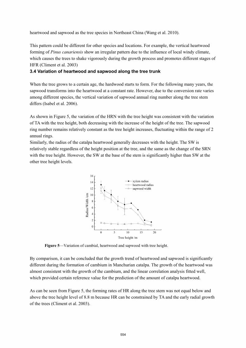
heartwood and sapwood as the tree species in Northeast China (Wang et al. 2010).

This pattern could be different for other species and locations. For example, the vertical heartwood forming of Pinus canariensis show an irregular pattern due to the influence of local windy climate, which causes the trees to shake vigorously during the growth process and promotes different stages of HFR (Climent et al. 2003) 3.4 Variation of heartwood and sapwood along the tree trunk

When the tree grows to a certain age, the hardwood starts to form. For the following many years, the sapwood transforms into the heartwood at a constant rate. However, due to the conversion rate varies among different species, the vertical variation of sapwood annual ring number along the tree stem differs (Isabel et al. 2006).

As shown in Figure 5, the variation of the HRN with the tree height was consistent with the variation of TA with the tree height, both decreasing with the increase of the height of the tree. The sapwood ring number remains relatively constant as the tree height increases, fluctuating within the range of 2 annual rings. Similarly, the radius of the catalpa heartwood generally decreases with the height. The SW is relatively stable regardless of the height position at the tree, and the same as the change of the SRN with the tree height. However, the SW at the base of the stem is significantly higher than SW at the other tree height levels.

Figure 5—Variation of cambial, heartwood and sapwood with tree height.

By comparison, it can be concluded that the growth trend of heartwood and sapwood is significantly different during the formation of cambium in Manchurian catalpa. The growth of the heartwood was almost consistent with the growth of the cambium, and the linear correlation analysis fitted well, which provided certain reference value for the prediction of the amount of catalpa heartwood.

As can be seen from Figure 5, the forming rates of HR along the tree stem was not equal below and above the tree height level of 8.8 m because HR can be constrained by TA and the early radial growth of the trees (Climent et al. 2003).

554

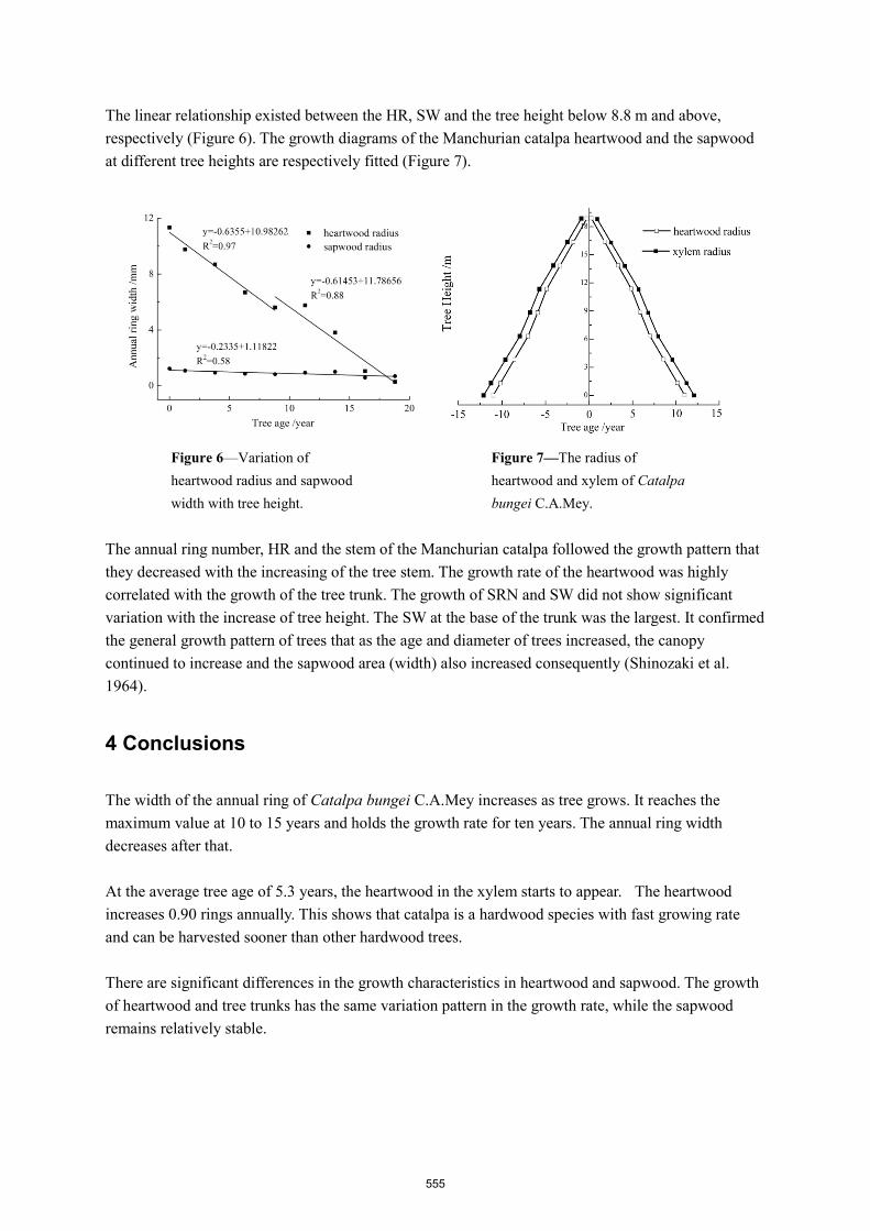
The linear relationship existed between the HR, SW and the tree height below 8.8 m and above, respectively (Figure 6). The growth diagrams of the Manchurian catalpa heartwood and the sapwood at different tree heights are respectively fitted (Figure 7).

Figure 6—Variation of heartwood radius and sapwood width with tree height.

Figure 7—The radius of heartwood and xylem of Catalpa bungei C.A.Mey.

The annual ring number, HR and the stem of the Manchurian catalpa followed the growth pattern that they decreased with the increasing of the tree stem. The growth rate of the heartwood was highly correlated with the growth of the tree trunk. The growth of SRN and SW did not show significant variation with the increase of tree height. The SW at the base of the trunk was the largest. It confirmed the general growth pattern of trees that as the age and diameter of trees increased, the canopy continued to increase and the sapwood area (width) also increased consequently (Shinozaki et al. 1964).

4 Conclusions

The width of the annual ring of Catalpa bungei C.A.Mey increases as tree grows. It reaches the maximum value at 10 to 15 years and holds the growth rate for ten years. The annual ring width decreases after that.

At the average tree age of 5.3 years, the heartwood in the xylem starts to appear. The heartwood increases 0.90 rings annually. This shows that catalpa is a hardwood species with fast growing rate and can be harvested sooner than other hardwood trees.

There are significant differences in the growth characteristics in heartwood and sapwood. The growth of heartwood and tree trunks has the same variation pattern in the growth rate, while the sapwood remains relatively stable.

555

Acknowledgements

This research was supported by the foundation CAFYBB2017 ZX003 and 2017YFD0600202. We thank Junhui Wang and Jiangtao Zhang for the experimental site and samples collection.

Reference

Climent, J.; Gil, L.; Pardos, J. 1993. Heartwood and sapwood development and its relationship to growth and environment in Pinus canariensis Chr.Sm ex DC. Forest Ecology and Management. 59: 165-174.

Climent, J.; Chambel, M.R.; Gil, L. [and others]. 2003. Vertical heartwood variation patterns and prediction of heartwood volume in Pinus canariensis Sm. Forest Ecology and Management. 174: 203-211.

Fleur, L.; Frédéric, M,; Jean, M. L. [and others]. 2006. Picea abies sapwood width: Variations within and between trees. Scandinavian Journal of Forest Research. 21: 41-53.

Isabel, M.; Jorge, G.; Ana, L. [and others]. 2006. The influence of irrigation and fertilization on heartwood and sapwood contents in 18-year-old Eucalyptus globulus trees. Can. J. For. Res. 36: 2675-2683.

Kennedy, S.G.; Yanchuk, A.D.; Jefferson, P.A. 2013. Relationship of heartwood traits with diameter growth, implications for genetic selection in Pinus radiata. Tree Genetics & Genomes. 9: 1313-1319.

Liu M.Y. 2013.The variation of the artificial Larch and Pinus sylvestris internal strucyure and wood density. Beijing: Northeast Forestry University. 31p.

Sofia, K.; Fátima, T.; Helena, P. 2006. Heartwood and sapwood variation in Acacia melanoxylon R. Br. Trees in Portugal. Forestry. 79(4): 371-380.

Shinozaki, K.; Yoda, K.; Hozumi, K. 1964. A quantitative analysis of plant form_the pipe model theory I. Basic analysis. Japanese Journal of Ecology. 14(30): 95-105.

Wang, X.C.; Wang, C.K.; Zhang, Q.Z. [and others]. 2010. Heartwood and sapwood allometry of seven Chinese temperate tree species. Ann. For. Sci. 67: 410.

Zabuga, V.F.; Zabuga, G.A. 2007. Specific Features of the Growth of Scots Pine Vegetative Organs in the Forest–Steppe Zone of Cisbaikalia. Russian Journal of Ecology. 38(6): 381-387.

556

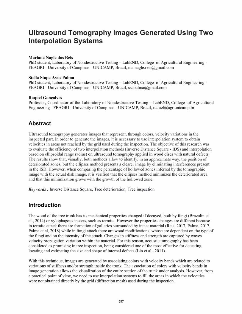
Ultrasound Tomography Images Generated Using Two Interpolation Systems

Mariana Nagle dos Reis PhD student, Laboratory of Nondestructive Testing – LabEND, College of Agricultural Engineering - FEAGRI - University of Campinas - UNICAMP, Brazil, ma.nagle.reis@gmail.com

Stella Stopa Assis Palma PhD student, Laboratory of Nondestructive Testing – LabEND, College of Agricultural Engineering - FEAGRI - University of Campinas - UNICAMP, Brazil, ssapalma@gmail.com

Raquel Gonçalves Professor, Coordinator of the Laboratory of Nondestructive Testing – LabEND, College of Agricultural Engineering - FEAGRI - University of Campinas - UNICAMP, Brazil, raquel@agr.unicamp.br

Abstract

Ultrasound tomography generates images that represent, through colors, velocity variations in the inspected part. In order to generate the images, it is necessary to use interpolation system to obtain velocities in areas not reached by the grid used during the inspection. The objective of this research was to evaluate the efficiency of two interpolation methods (Inverse Distance Square - IDS) and interpolation based on ellipsoidal range radius) on ultrasound tomography applied in wood discs with natural defects. The results show that, visually, both methods allow to identify, in an approximate way, the position of deteriorated zones, but the ellipses method presents a clearer image by eliminating interferences present in the ISD. However, when comparing the percentage of hollowed zones inferred by the tomographic image with the actual disk image, it is verified that the ellipses method minimizes the deteriorated area and that this minimization grows with the growth of the hollowed zone.

Keywords : Inverse Distance Square, Tree deterioration, Tree inspection

Introduction

The wood of the tree trunk has its mechanical properties changed if decayed, both by fungi (Brazolin et al., 2014) or xylophagous insects, such as termite. However the properties changes are different because in termite attack there are formation of galleries surrounded by intact material (Reis, 2017, Palma, 2017, Palma et al, 2018) while in fungi attack there are wood modifications, whose are dependent on the type of the fungi and on the intensity of the attack. Changes in stiffness and strength are captured by waves velocity propagation variation within the material. For this reason, acoustic tomography has been considered as promising in tree inspection, being considered one of the most effective for detecting, locating and estimating the size and shape of internal defects (Lin et al., 2011).

With this technique, images are generated by associating colors with velocity bands which are related to variations of stiffness and/or strength inside the trunk. The association of colors with velocity bands in image generation allows the visualization of the entire section of the trunk under analysis. However, from a practical point of view, we need to use interpolation systems to fill the areas in which the velocities were not obtained directly by the grid (diffraction mesh) used during the inspection.

557

The objective of this research was to evaluate the efficiency of two interpolation methods on ultrasound tomography applied in wood discs with natural defects.

Material and methods

We used wood discs with approximately 0.2 m thickness, extracted from tree trunks of the species Tabebuia ochraceae, Platanus sp. and Poencianella pluviosa. The discs presented different deterioration conditions (Figure 1). To perform the tests, conventional ultrasound equipment (USLab, Agricef, Brazil) and longitudinal 45-kHz frequency transducers and exponential faces were used.

Figure 1 – discs with different types of deterioration.

The measurements were made in 8-point diffraction mesh (Divos and Szalai, 2002) and the tomographic images obtained using the software ImageWood 3.1. Both the ultrasound equipment and the software were developed by the research group.

The interpolation methods evaluated were the Inverse Distance Square (IDS) and a method that adopts the concept based on the radius of ellipses comprehension, proposed by Du et al. (2015).

The images generated by ultrasound tomography were evaluated by comparison with the actual condition of the disc, using two steps. The first one, using visual analysis of the images generated with 10 color bands, representing percentages of the maximum velocity. These images were used to identify the recurring colors in the affected areas of the discs, which were used in the second step to generate images with only two colors. The images generated with two colors were used for quantitative comparison between deteriorated areas inferred by each of the methods and the actual deteriorated area of the disc.

Results and discussion

The patterns of color variation as a function of the defects (Figure 2) indicated that areas with more than 50% (green) of velocity loss correspond to the areas with cavities in the disc wood (Figure 1a, b, c). The bands with a reduction of 40% to 50% of velocity (light blue) are coincident with regions of severe deterioration in the discs (Figure 2) while losses of 30% to 40% of the velocity with moderate deteriorations in agreement with the conclusion of the USDA (2014).

In the case of the Tabebuia ochracea disc, the hollows were not identified by the tomographic image (green color does not appear), a result already expected because the wavelength (≅ 56 mm) was very large compared to the small holes interspersed with wood in good condition (Figure 2 (a)). However, the appearance of light blue colors (Figure 2, g) and dark blue (Figure 2, d) indicate the existence of severe and moderate deterioration, respectively. As the images are not handled by any filter, there is a characteristic interference pattern observed in the images generated with the use of ISD. This interference

558

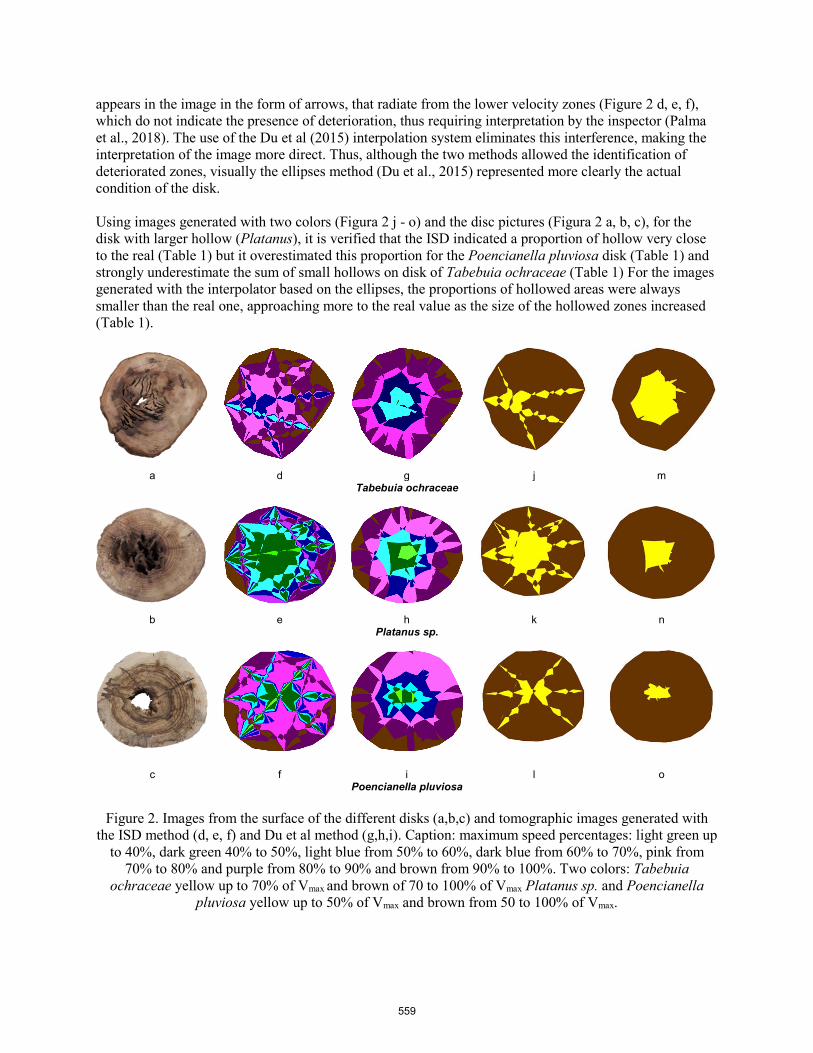
appears in the image in the form of arrows, that radiate from the lower velocity zones (Figure 2 d, e, f), which do not indicate the presence of deterioration, thus requiring interpretation by the inspector (Palma et al., 2018). The use of the Du et al (2015) interpolation system eliminates this interference, making the interpretation of the image more direct. Thus, although the two methods allowed the identification of deteriorated zones, visually the ellipses method (Du et al., 2015) represented more clearly the actual condition of the disk.

Using images generated with two colors (Figura 2 j - o) and the disc pictures (Figura 2 a, b, c), for the disk with larger hollow (Platanus), it is verified that the ISD indicated a proportion of hollow very close to the real (Table 1) but it overestimated this proportion for the Poencianella pluviosa disk (Table 1) and strongly underestimate the sum of small hollows on disk of Tabebuia ochraceae (Table 1) For the images generated with the interpolator based on the ellipses, the proportions of hollowed areas were always smaller than the real one, approaching more to the real value as the size of the hollowed zones increased (Table 1).

a d g j m Tabebuia ochraceae

b e h k n Platanus sp.

c f i l o Poencianella pluviosa

Figure 2. Images from the surface of the different disks (a,b,c) and tomographic images generated with the ISD method (d, e, f) and Du et al method (g,h,i). Caption: maximum speed percentages: light green up

to 40%, dark green 40% to 50%, light blue from 50% to 60%, dark blue from 60% to 70%, pink from 70% to 80% and purple from 80% to 90% and brown from 90% to 100%. Two colors: Tabebuia

ochraceae yellow up to 70% of Vmax and brown of 70 to 100% of Vmax Platanus sp. and Poencianella pluviosa yellow up to 50% of Vmax and brown from 50 to 100% of Vmax.

559

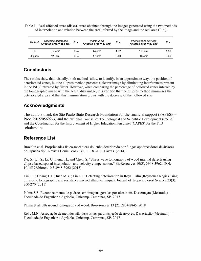
Table 1 - Real affected areas (disks), areas obtained through the images generated using the two methods of interpolation and relation between the area inferred by the image and the real area (R.a.)

Method Tabebuia ochraceaeAffected area = 154 cm2 R.a. Platanus sp

Affected area = 43 cm2 R.a. Poencianella pluviosa Affected area = 80 cm2 R.a.

ISD 37 cm2 0,24 44 cm2 1,02 118 cm2 1,50

Ellipses 129 cm2 0,84 17 cm2 0,40 46 cm2 0,60

Conclusions

The results show that, visually, both methods allow to identify, in an approximate way, the position of deteriorated zones, but the ellipses method presents a clearer image by eliminating interferences present in the ISD (untreated by filter). However, when comparing the percentage of hollowed zones inferred by the tomographic image with the actual disk image, it is verified that the ellipses method minimizes the deteriorated area and that this minimization grows with the decrease of the hollowed size.

Acknowledgments

The authors thank the São Paulo State Research Foundation for the financial support (FAPESP –Proc. 2015/05692-3) and the National Counsel of Technological and Scientific Development (CNPq) and the Coordination for the Improvement of Higher Education Personnel (CAPES) for the PhD scholarships

Reference List

Brazolin et al. Propriedades físico-mecânicas do lenho deteriorado por fungos apodrecedores de árvores de Tipuana tipu. Revista Cerne. Vol 20 (2). P.183-190. Lavras. (2014)

Du, X., Li, S., Li, G., Feng, H., and Chen, S. “Stress wave tomography of wood internal defects using ellipse-based spatial interpolation and velocity compensation,” BioResources 10(3), 3948-3962. DOI: 10.15376/biores.10.3.3948-3962 (2015).

Lin C.J.; Chang T.T.; Juan M.Y.; Lin T.T. Detecting deterioration in Royal Palm (Roystonea Regia) using ultrasonic tomographic and resistance microdrilling techniques. Journal of Tropical Forest Science 23(3): 260-270 (2011)

Palma,S.S. Reconhecimento de padrões em imagens geradas por ultrassom. Dissertação (Mestrado) – Faculdade de Engenharia Agrícola, Unicamp. Campinas, SP. 2017

Palma et al. Ultrasound tomography of wood. Bioresources 13 (2), 2834-2845. 2018

Reis, M.N. Associação de métodos não destrutivos para inspeção de árvores. Dissertação (Mestrado) – Faculdade de Engenharia Agrícola, Unicamp. Campinas, SP. 2017

560

Acoustic Measurement Differences on Trees and Logs from Hardwoods in Wet and Dry Condition

Daniel F. Llana* Timber Engineering Research Group, National University of Ireland Galway, Galway, Ireland, daniel.llana@nuigalway.ie

Ian Short Teagasc, Ashtown, Dublin, Ireland, ian.short@teagasc.ie

Annette M. Harte Timber Engineering Research Group, School of Engineering & Ryan Institute, National University of Ireland Galway, Galway, Ireland, annette.harte@nuigalway.ie

* Corresponding author

Abstract

Acoustic velocities measured on standing trees using time-of-flight (TOF) devices have been found to be between 7% and 36% higher for softwoods than those in logs using resonance techniques based on longitudinal frequencies. This effect was explained in three different ways: (1) TOF devices on standing trees measure outerwood containing more mature wood while resonance methods assess the whole cross-section, (2) the variation in the velocity is due to loading conditions in standing trees, while logs are free of loads and (3) the acoustic waves are dilatational waves in the case of TOF measurements on standing trees and one-dimensional longitudinal waves in the case of resonance on logs. This is an important topic considering the fact that resonance methods are considered more accurate for predicting mechanical properties and it has been proposed that correction factors should be applied on TOF measurements.

In the present work, four hardwoods from Irish forests were studied and, on average, TOF velocities measured in the forest above fibre saturation point (FSP) were 19.8% higher than those from resonance measurements taken on logs immediately after felling. However, this difference reduced to 5.4% when the measurements were repeated at a moisture content (MC) of about 18% in the laboratory. Therefore, there is a MC effect on the velocity differences. Furthermore, higher differences were systematically found in older specimens in wet condition. However, this age effect was small in most cases.

Keywords: acoustic velocity, hardwoods, logs, moisture content influence, standing trees

Introduction

Measurement of acoustic velocity on standing trees and resonance on green logs has been successfully used to grade and estimate properties of logs and sawn timber (Wang et al. 2002; Moore et al. 2013; Gil-Moreno and Ridley-Ellis 2015; Krajnc et al. 2019). While the resonance method has the advantage of being more accurate than acoustic time-of-flight (TOF) measurements based on stress wave techniques in applications on logs and sawn timber, the resonance method can be not used on standing trees as measurements should be made on unloaded specimens.

561

It is well known that velocities obtained by acoustic methods measuring TOF are higher than those obtained from resonance methods in sawn timber (Haines et al. 1996; Íñiguez 2007; Llana et al. 2016). In the case of stress wave measurements on standing trees and resonance measurements in green logs, velocities between 7% and 36% higher were reported by several authors (Chauhan and Walker 2006; Grabianowski et al. 2006; Lasserre et al. 2007; Wang et al. 2007; Mora et al. 2009; Yin et al. 2010; Bertoldo 2014) most of them studying softwoods. Furthermore, Wang (2013) suggested that tree diameter, stand age, operating temperature and wood moisture content (MC) affect tree-log velocity relationships.

The objective of the present work is to study the velocity differences between TOF and resonance measurements on hardwoods in the forest (in wet condition) and in the laboratory (in dry condition) and the influence of age and MC on these differences.

Materials and Methods

Materials

A total of 36 trees with diameters at breast height (DBH) between 80 and 180 mm and logs from the bottom part of these trees (butt log) with an overall length of 25 times its DBH were selected from thinnings of four Irish hardwood species: common alder (Alnus glutinosa (L.) Gaertn.), European ash (Fraxinus excelsior L.), European birch (Betula pendula Roth. & Betula pubescens Ehrh.) and sycamore (Acer pseudoplatanus L.).

NDT experiments

The TOF of acoustic stress waves over a length (L) of 1 m was measured on standing trees using a TreeSonic (Fakopp, Sopron, Hungary) device and the acoustic velocity (Vel) was determined using Equation (1).

Vel = L / TOF (1)

A Mechanical Timber Grader MTG (Brookhuis, Enschede, The Netherlands) was then used to determine the fundamental frequency (f ) in the longitudinal direction of wet logs, above Fiber Saturation Point (FSP), just after harvesting. The velocity for the logs was calculated using Equation (2):

Vel = 2 · f · Llog (2)

where Llog is the log length.

Both NDT measurement procedures were subsequently carried out on dry logs (around 18% MC) in the National University of Ireland Galway Timber Engineering Laboratory.

Results and discussion

Velocities obtained from TOF measurements on standing trees and dry logs were higher than those obtained from the corresponding resonance measurements. Figure 1 shows the differences between TOF and resonance velocities by specimen in the forest (wet) and in the laboratory (dry).

562

Figure 1 – Differences between TOF velocity and resonance velocity in percentage: Above FSP (wet) and around 18% MC (dry).

Figure 1 shows that velocity differences were higher in the wet than in the dry condition. Velocities obtained from TOF measurements were on average 19.8% higher than resonance velocities in the forest and 5.4% higher in the laboratory. Average differences were circa three and half times higher in wet than in dry conditions. A moisture content effect on the relationship between tree and log NDT measurement has been suggested by Wang (2013). Table 1 shows published results by other authors and the present research findings for measurements in the wet condition.

Table 1 – Differences in acoustic velocity predictions (wet) NDT device Species* Velocity

difference (%) Reference Stress waves (TOF) Resonance Fakopp 2D Hitman HM200 Radiata pine 8.7 to 17.5 Chauhan & Walker 2006 Fakopp 2D WoodSpec Radiata pine 12.0 Grabianowski et al. 2006 TreeTap Hitman HM200 Radiata pine 16.0 to 31.0 Lasserre et al. 2007

Scopemeter Hitman HM200

Sitka spruce Western hemlock Jack pine Ponderosa pine Radiata pine

7.0 to 36.0 Wang et al. 2007

TreeSonic Hitman HM200 Loblolly pine 32.0 Mora et al. 2009 MicroSecond Timer Microphone Chinese fir 9.5 Yin et al. 2010

Hitman ST300 Hitman HM200 Daintree stringybark (H) Lemon-scented gum (H)

Saligna gum (H) 20.3 Bertoldo 2014

Hitman ST300 MTG Sitka spruce 11.2 Simic et al. 2019

TreeSonic MTG

Common alder (H) European ash (H) European birch (H) Sycamore (H)

19.8 Present work

(H) Hardwood species*Species common names according to standard EN13556:2003 when possible; when not, according to Miller & Ilic (1992)

-10

-5

0

5

10

15

20

25

30

35

40

1 2 3 4 5 6 7 8 9 10 11 12 13 14 15 16 17 18 19 20 21 22 23 24 25 26 27 28 29 30 31 32 33 34 35 36

Diffe

renc

e TO

F &

reso

nanc

e ve

loci

ty (%

)

No. of specimen

In the forest (wet) In the laboratory (dry)

563

As shown in Table 1, differences between TOF and resonance velocities vary between authors. The velocity difference for temperate hardwoods found in the present work (19.8%) is similar to the value of 20.3% found in tropical hardwoods by Bertoldo (2014). Nevertheless, according to Wang (2013) different TOF measurement devices used on standing trees may have different algorithms and trigger settings making it difficult to compare results between authors using different devices. Chauhan and Walker (2006) and Wang et al. (2007) found that differences are related to age and diameter. In Figure 2, the difference in the average velocity measurements by species in the wet condition are seen to increase with age. However, for ash and sycamore, these increases are negligible. In the dry condition, small increases are seen for three species but a decrease was found in the case of alder. It should be noted that this study was carried out on forest thinnings that were young and the differences may be much greater as the age increases.

Figure 2 – Average differences between TOF velocity and resonance velocity in percentage by age

Figure 3 shows that the relationship between TOF and resonance velocities is stronger in the wet than in the dry condition. The coefficient of determination for wet specimens at 0.71 is just in the limit of the range from 0.71 to 0.93 reported by Wang et al. (2007) and weaker than 0.91 found by Grabianowski et al. (2006) and 0.81 reported by Mora et al. (2009). As resonance velocity is considered more accurate for estimating mechanical properties (Grabianowski et al. 2006; Wang 2013), relationship models can be used to convert TOF velocity to resonance velocity.

0

5

10

15

20

25

30

10 12 14 16 18 20 22 24 26

Aver

age

diffe

renc

e TO

F &

reso

nanc

e ve

loci

ty (%

)

Age (years)

Alder wet Ash wet Birch wet Sycamore wet

Alder dry Ash dry Birch dry Sycamore dry

564

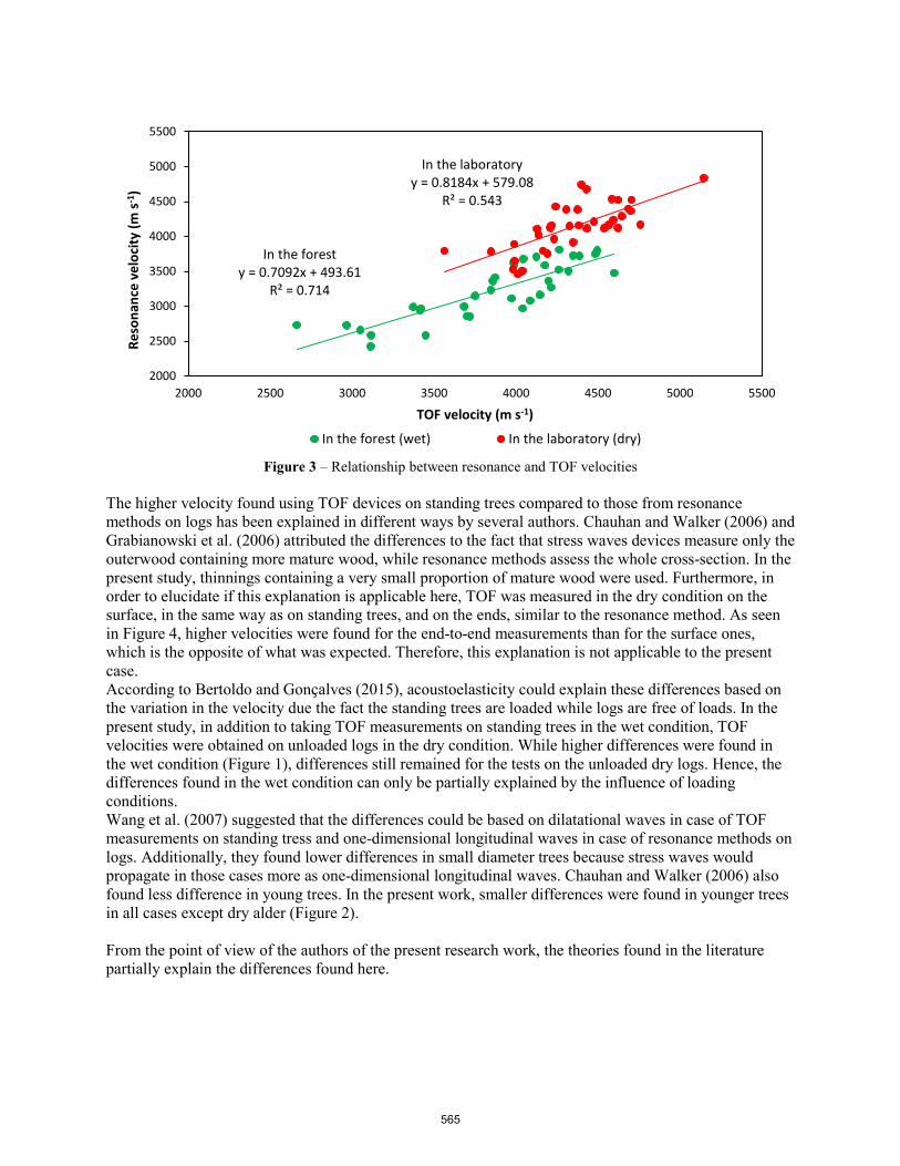
Figure 3 – Relationship between resonance and TOF velocities

The higher velocity found using TOF devices on standing trees compared to those from resonance methods on logs has been explained in different ways by several authors. Chauhan and Walker (2006) and Grabianowski et al. (2006) attributed the differences to the fact that stress waves devices measure only the outerwood containing more mature wood, while resonance methods assess the whole cross-section. In the present study, thinnings containing a very small proportion of mature wood were used. Furthermore, in order to elucidate if this explanation is applicable here, TOF was measured in the dry condition on the surface, in the same way as on standing trees, and on the ends, similar to the resonance method. As seen in Figure 4, higher velocities were found for the end-to-end measurements than for the surface ones, which is the opposite of what was expected. Therefore, this explanation is not applicable to the present case. According to Bertoldo and Gonҫalves (2015), acoustoelasticity could explain these differences based on the variation in the velocity due the fact the standing trees are loaded while logs are free of loads. In the present study, in addition to taking TOF measurements on standing trees in the wet condition, TOF velocities were obtained on unloaded logs in the dry condition. While higher differences were found in the wet condition (Figure 1), differences still remained for the tests on the unloaded dry logs. Hence, the differences found in the wet condition can only be partially explained by the influence of loading conditions. Wang et al. (2007) suggested that the differences could be based on dilatational waves in case of TOF measurements on standing tress and one-dimensional longitudinal waves in case of resonance methods on logs. Additionally, they found lower differences in small diameter trees because stress waves would propagate in those cases more as one-dimensional longitudinal waves. Chauhan and Walker (2006) also found less difference in young trees. In the present work, smaller differences were found in younger trees in all cases except dry alder (Figure 2).

From the point of view of the authors of the present research work, the theories found in the literature partially explain the differences found here.

In the foresty = 0.7092x + 493.61

R² = 0.714

In the laboratoryy = 0.8184x + 579.08

R² = 0.543

2000

2500

3000

3500

4000

4500

5000

5500

2000 2500 3000 3500 4000 4500 5000 5500

Reso

nanc

e ve

loci

ty (m

s-1)

TOF velocity (m s-1)

In the forest (wet) In the laboratory (dry)

565

Figure 4 – Velocity obtained from TOF in dry condition: on the ends and on the surface

Conclusions

Acoustic velocities measured on standing trees using TOF measurements have been found to be 19.8% higher than those in wet logs using resonance techniques based on longitudinal frequencies and 5.4% higher when measurements were repeated at 18% MC. These values show a clear MC effect on the differences between TOF and resonance velocities.

As has been reported in the literature in case of softwoods, velocity differences in hardwood thinnings were found to be dependent of the age of the trees. However, this effect was small in most cases.

There is a clear relationship between velocities from TOF and resonance measurements allowing conversion between one and the other. This relationship is stronger in wet than in dry conditions, but weaker than the softwood relationships found in the literature.

The results, based on 36 logs from four hardwood species, require validation with a larger sample, but give indications regarding TOF and resonance velocities differences and the influence of MC.

Acknowledgments

This work has been carried out as part of the project Exploitation And Realisation of Thinnings from Hardwoods (E.A.R.T.H.) funded by the Department of Agriculture, Food and Marine of the Republic of Ireland under the 2015 Call for Research Proposals (Project Ref: 15-C-666).

The authors would like to thank Mr. Jerry Campion and Mr. Derek Gibson from Teagasc for their technical support in the fieldwork, Mr. Dan Connolly, Mr. John P. Gill, Mr. Liam Mooney, Mr. Kevin O’Connell and Mr. Ivan Ryall for freely supplying the material and Mr. Conor Fahy from ECC Teoranta for kindly allowing us to dry the timber in their facilities. Furthermore, Ms. Rachel Keane and Mr Colm Walsh from National University of Ireland Galway for their helpful technical assistance in the laboratory testing.

2000

2500

3000

3500

4000

4500

5000

5500

1 2 3 4 5 6 7 8 9 10 11 12 13 14 15 16 17 18 19 20 21 22 23 24 25 26 27 28 29 30 31 32 33 34 35 36

TOF

velo

city

in d

ry c

ondi

tion

(m s-1

)

No. of specimen

End to end measurements Surface measurements

566

References

Bertoldo, C. 2014. Propriedades de resistência e de rigidez da madeira obtidas a partir da avaliação acústica na árvore [Predicting of strength and stiffness of wood using acoustic measurement in trees]. PhD Dissertation. Faculdade de Engenharia Agrícola. Universidade Estadual de Campinas, SP, Brazil. 146 p. PDF File: http://repositorio.unicamp.br/jspui/handle/REPOSIP/257101. [In Portuguese]

Bertoldo, C.; Gonҫalves, R. 2015. Influence of measurement position, tree diameter, and bulk wood density on models that predict wave propagation velocity in logs according to the velocity in trees. Forest Prod. J. 65(3):166-172.

Chauhan, S.S.; Walker, J.C.F. 2006. Variations in acoustic velocity and density with age, and their interrelationships in radiata pine. Forest Ecol. Manag. 229:388-394.

EN 13556:2003. Round and sawn timber – Nomenclature of timber used in Europe. European Committee of Standardization (CEN), Brussels, Belgium.

Gil-Moreno, D.; Ridley-Ellis, D.J. 2015. Comparing usefulness of acoustic measurements on standing trees for segregation by timber stiffness. Proceedings of 19th International nondestructive testing and evaluation of wood symposium. September 22-25. Rio de Janeiro, Brazil. Pp. 378-385.

Grabianowski, M.; Manley, B.; Walker, J.C.F. 2006. Acoustic measurements on standing trees, logs and green lumber. Wood Sci. Technol. 40:2005-2016.

Haines, D.W.; Leban, J.M.; Herbé, C. 1996. Determination of Young's modulus for spruce, fir and isotropic materials by the resonance flexure method with comparisons to static flexure and other dynamic methods. Wood Sci. Technol. 30:253-263.

Íñiguez, G. 2007. Clasificación mediante técnicas no destructivas y evaluación de las propiedades mecánicas de la madera aserrada de coníferas de gran escuadría para uso estructural. [Grading by non-destructive techniques and assessment of the mechanical properties of large cross section coniferous sawn timber for structural use]. PhD Dissertation. ETS de Ingenieros de Montes. Universidad Politécnica de Madrid, Madrid, Spain 223p. PDF File: http://oa.upm.es/415. [In Spanish]

Krajnc, L.; Farrelly, N.; Harte, A.M. 2019. Evaluating timber quality in larger-diameter standing trees: rethinking the use of acoustic velocity. Holzforschung. In press.

Lasserre, J.P.; Mason, E.G.; Watt, M.S. 2007. Assessing corewood acoustic velocity and modulus of elasticity with two impact based instruments in 11-year-old trees from a clonal-spacing experiment of Pinus radiata D. Don. Forest Ecol. Manag. 239:217-221.

Llana, D.F.; Íñiguez-González, G.; Arriaga, F.; Wang, X. 2016. Time-of-flight adjustment procedure for acoustic measurements in structural timber. Bioresources 11(2):3303-3317.

Miller, R.B.; Ilic, J. 1992. A comprehensive database of common and scientific names of world woods. Forest Products Laboratory Website: https://www.fpl.fs.fed.us/search/commonname_request.php (July 3, 2019).

567

Moore, J.R.; Lyon, A.J.; Searles, G.J.; Lehneke, S.A.; Ridley-Ellis, D.J. 2013. Within- and between-stand variation in selected properties of Sitka spruce sawn timber in the UK: implications for segregation and grade recovery. Ann. For. Sci. 70:403-415.

Mora, C.R.; Schimleck, L.R.; Isik, F.; Mahon jr., J.M.; Clark III, A.; Daniels, R.F. 2009. Relationships between acoustic variables and different measures of stiffness in standing Pinus taeda trees. Can. J. For. Res. 39:1421-1429.

Simic, K.; Gendvilas, V.; O’Reilly, C.; Harte, A.M. 2019. Predicting structural timber grade-determining properties using acoustic and density measurements on young Sitka spruce trees and logs. Holzforschung. 73(2):139-149.

Wang, X.; Ross, R.J.; Mattson, J.A.; Erickson, J.R.; Forsman, J.W.; Geske, E.A.; Wehr, M.A. 2002. Nondestructive evaluation techniques for assessing modulus of elasticity and stiffness of small-diameter logs. Forest Prod. J. 52(2):79-85.

Wang, X.; Ross, R.J.; Carter, P. 2007. Acoustic evaluation of wood quality in standing trees. Part I. Acoustic wave behavior. Wood Fiber Sci. 39(1):28-38. Wang, X. 2013. Acoustic measurements on trees and logs: a review and analysis. Wood Sci. Technol. 47:965-975.

Yin, Y.; Nagao, H.; Liu, X.; Nakai, T. 2010. Mechanical properties assessment of Cunninghamia lanceolata plantation wood with three acoustic-based nondestructive methods. J. Wood Sci. 56:33-40.

568

New Possibilities with CT Scanning in the Forest Value Chain

Linus Olofsson* Wood Science and Engineering, Luleå University of Technology, Skellefteå, Västerbotten, Sweden, linus.olofsson@ltu.se

Carl-Johan Möller Department of Physics, Umeå University, Umeå, Västerbotten, Sweden, mollercarlj@gmail.com

Charlotta Wendel Department of Physics, Umeå University, Umeå, Västerbotten, Sweden, charlottawendel@hotmail.com

Johan Oja Technical Manager, Norra Timber, johan.oja@norra.se

Olof Broman Wood Science and Engineering, Luleå University of Technology, Skellefteå, Västerbotten, Sweden, olof.broman@ltu.se

* Corresponding author

Abstract

Industrial high-resolution X-ray computed tomography (CT) scanners have recently been installed at several sawmills worldwide for the description of roundwood interior features and external log shape. These CT scanners represent a technological advancement for sawmill businesses that open a way to higher volume and value yields and new production planning strategies. This paper will present an indicative study of innovative use of non-destructive CT log data in a Swedish softwood sawmill, linking high-quality information of the wood material along the wood-value chain. Sawn timber was observed throughout the sawmill process line, i.e. from the log yard through the sawmill process until grading after the timber was dried. Before sawing, the CT scanner scanned the logs and calculated knot measurements from the 3D CT log data of simulated value-optimized center yield. A corresponding set of knot measurements were later calculated from the camera-based grading of the dried timber. Only considering knots from the two sets of measurements, the sawn timber was automatically given a quality assessment based on CT data, by camera-based scanning data, and by manual visual grading for reference. Partial least squares regression was used to create prediction models by correlating the two sets of knot measurements with the automatically determined grade from the dry-sorting. The prediction models tested increased the grading consistency between the grading based on CT data of virtual planks and based on camera data of the same planks. Furthermore, a traceability algorithm was tested as a tool to generate large data sets for future studies.

Keywords: sawn timber grading, computed tomography, partial least squares

569

Introduction

Sawmills perform several quality assessments and product classifications along the entire sawline process—e.g. classifying the incoming logs (roundwood) by size, and the outgoing sawn timber by visual appearance or strength. A recent high-technological quality-assessment tool added to the sawline at Sävar Sawmill in northern Sweden is a high-resolution X-ray computed tomography (CT) scanner from Microtec (CT Log), which is used to create 3D CT images of the incoming logs. Giudiceandrea et al. (2011), and Longuetauda et al. (2012) presented both an overview and an insight in the difficulties and requirements of implementing an industrial CT-scanner in sawmills, capable of continuous high-speed operation, but also the potential benefits of increased value and volume yields. Fredriksson et al. (2017) presented a state of the art of the CT-scanning technology in the wood value chain, showing additional possibilities of using CT-scanner technology in modern sawmills apart from increased value and volume yields. Fredriksson (2014) calculated that fully utilizing CT-data of logs to determine optimal sawing parameters increased the value yield on average by 13% compared to sawing positioning based on outer shape only, and by 21% compared to the horns-down sawing position, based on 269 logs.

Once incoming logs to the sawmill have been CT-scanned, some algorithm is used to determine how the log should be sawn. In the case of Sävar sawmill, detected features, especially knot features, in the 3D CT-image of each log is used to determine optimal sawing conditions, i.e. a sawing pattern and positioning parameters. The detected features are projected onto sawn planks in the virtual 3D CT-image and are used to determine the grade and value of each plank. The grade and value are determined by rule-based automatic grading (RBAG), following the grading standard Nordic Timber Grading Rules (NTGR) (Swedish Sawmill Managers Association 1994) used at Sävar sawmill. By testing a large number of possible sawing patterns and positioning parameters the intended optimal sawing conditions can be found. The sawing pattern and positioning parameters are then sent to the sawing system that cuts the logs as decided by the CT Log.

After sawing and drying, the sawn timber is sorted at the sawmill’s dry-sorting station where the final grade of the sawn timber is determined. In the case of Sävar sawmill, this is done using a camera-based automatic scanning and grading system called Boardmaster from Finscan. The Boardmaster uses cameras to detect features, e.g. knot features, cracks, wane, and so on, to determine the visual grade of each plank by RBAG in accordance with NTGR. The NTGR governs all possible wood features, but only knot features will be considered in this study, due to their importance to the final appearance grade and the difficulty of detecting and describing knot features in a concise way.

The functionality of the CT Log when grading a virtual plank inside a scanned log is by design very similar to the visual grading of the same plank performed by the Boardmaster at the dry sorting station, i.e. the two systems use the same grading rules in their respective grading operations. The difference is that the CT Log compares a lot of different grading outcomes to find the best sawing conditions while the Boardmaster assigns the final grade. In theory, given identical input parameters from a single plank, the two systems should give the plank the same grade. However, in practice, the CT Log and the Boardmaster will never see the same identical plank as the virtual plank selected by the CT Log to be sawn is separated from the actual plank, as seen by the Boardmaster’s cameras, by the sawing process. The sawing process can introduce errors such as rotation or positioning errors during sawing, which becomes more difficult as the speed of the sawing increases. The separation between the virtual plank and the actual plank is made worse by possible detection errors. Longuetauda et al. (2012) presented an algorithm to detect knots in CT-images, as well as an overview of previous work regarding automatic knot detection using CT-imaging, showing an example of the difficulty of accurately describing knot features in CT-images. Using cameras to accurately describe plank features is no effortless task either for the Boardmaster. The differences between the virtual plank and the actual plank can result in a disagreement between the intended plank grade given by the CT Log and the grade assigned by the Boardmaster.

570

The goal of this study was to utilize the high-quality information extracted by the CT Log when calculating the intended grade of a virtual plank in a 3D CT-image in a way that better agree with the grade assigned by the Boardmaster, as to minimize the effect of detection errors and errors during sawing on the final value yield. Furthermore, this study will investigate the use of a traceability algorithm of individual planks between the CT Log and the Boardmaster as a means to create large data sets in the future for similar studies where information from both the CT Log and Boardmaster is important.

This study suggests the use of multivariate partial least-squares regression (PLS) models (Geladi and Kowalski 1986), similar to the ones used by Lycken and Oja (2006), Berglund et al. (2015), Olofsson et al. (2017, 2019a, 2019b), and in related studies by Broman (2000) and Breinig et al. (2015). PLS regression models have in previous studies been shown to be noise-resistant and capable of creating prediction (grading) models base on a large number of highly colinear variables using a relatively small number of observations.

Materials and methods

The material

A total of 238 pieces of Scots pine (Pinus sylvestris L.) sawn timber was studied at Sävar sawmill in northern Sweden. The planks originated from logs that had previously been scanned using X-ray computed tomography by the CT Log, from Microtec (Anon 2019a), installed directly before the sawing system at Sävar sawmill. The CT Log fitted a sawing pattern with two 75x125 mm center-yield planks and calculated value-optimized rotational and positioning parameters to be used during the following cant sawing process. After drying the sawn timber to 18% moisture content, the material was scanned and graded at the dry-sorting station by the camera-based and rule-based automatic grading (RBAG) system Boardmaster from Finscan (Anon 2019b). Manual grading of the material was also performed and throughout this study, only knot measurements were considered.

PLS modeling

The PLS modeling performed in this study, for both the CT Log and the Boardmaster, is very similar to PLS modeling performed by Wendel (2019), who presents a similar study to this one but with a different approach. Similar PLS modeling has been performed by the references at the end of the introduction, most notably by Olofsson et al. (2019a), Berglund et al. (2015), and Lycken and Oja (2006), where Olofsson et al. (2019a) includes a very detailed explanation of how this kind of PLS-based grading was implemented for sawn timber grading by a Boardmaster at Kåge sawmill (also a Boardmaster, using the same grading rules). Conceptually, the same process is performed here for the sawn timber grading by both the CT Log and Boardmaster and below follows a short description of the specifics about this implementation. For a more detailed description of a similar implementation, as well as performance evaluation by 5-fold cross-validation, see Olofsson et al. (2019a).

Knot variables

The aggregated knots variables used in this study, created by Wendel (2019), are 23 variables, detailed in Table 1, calculated in each of the 9 zones shown in Figure 1, for each of the 4 plank faces, resulting in 23×4×9=828 variables. The 828 aggregated knot variables were calculated separately for both the CT Log and the Boardmaster, based on measurements from each system.

571

Table 1—Description of the 23 aggregated knot-variables used in this study. Each X marks one variable with the corresponding description and knot-type. Variable description All knots Sound knots Dead knots Total number of knots X X X Number of knots per meter X X X Maximum size in longitudinal direction (mm) X X X Maximum size in axial direction (mm) X X X Mean size in longitudinal direction (mm) X X X Mean size in axial direction (mm) X X X Covered area (%) X X X The proportion of knots compared to all knots (%) X X

Figure 1—Zone partitioning of each plank. Each variable in Table 1 is calculated in each of the 9 zones shown.

Grading

Knot measurement data from both the CT Log and the Boardmaster was stored for each of the 238 planks. The grade of each virtual plank output by the CT Log—the intended sawing outcome grade—as well as the grade assigned to each plank by the Boardmaster was also stored. Manual grading of each plank was performed as a reference. Note that all grading was only based on knot features. Three different grades were used by each system and during the manual grading, called A, B, and C (Tabel 4, NTGR), where grade A represents a grade with few and small knots and high value and vice versa. Previous studies by Olofsson et al. (2019a), and Lycken and Oja (2006) estimated that approximately 100 planks per grade could be considered a minimum for training statistical grading models. To avoid underrepresenting the limiting number of 65 grade A planks (by manual grading) in a three-class classification problem, only the grades A and “other” were considered. In this study, the “other”-grade will be labeled grade B for a simple A vs B discussion, even though B here includes grade C.

To associate the correct CT-grade and Boardmaster-grade given to each plank with the corresponding ID number, a fingerprinting-traceability algorithm was used (Möller 2019). The study by Möller (2019) was performed in parallel to this study on 154 of the planks. The traceability algorithm used in the study by Möller (2019), called CPF, projected all knots detected by the CT Log and by the Boardmaster onto two one-dimensional binary vectors, creating a vector visually would look like a sparse bar-code. This bar-code-vector was then used as a fingerprint to match 96% of the 154 planks between the CT Log and the Boardmaster. This algorithm was used in this study to match 92% of the 238 planks to indicate the possibilities of using such a traceability algorithm, but in practice, all matches were manually checked to keep the CT Log-Boardmaster matching 100% for this study.

Both during the value-optimization process performed by the CT Log and during the final grading by the Boardmaster a customer-adapted implementation of the visual-appearance-grading-standard Nordic Timber Grading Rules (NTGR) (Swedish Sawmill Managers Association 1994) was used. This standard defines rules (limits) as the maximum number and size of plank features allowed in different grades. The standard defines rules for all types of wood features but this study will only use knot features, as knots are the main deciding factor that determines the visual grade of sawn timber. Knots are also of particular interest as a common belief in the sawmill industry is that customers tend to accept a few slightly larger than specified defects (knots) if the rest of the plank is better than the average of a particular grade (Berglund et al. 2015). The opposite is also true where customers might find a plank

572

unsatisfactory if the overall appearance is not representative of a given grade, even though all features are within the specified limits.

PLS model construction and testing procedure

Two PLS models were created, called the CT-PLS model and the BM-PLS model for the CT Log and the Boardmaster, respectively. For each system, the corresponding set of aggregated knot variables were correlated to the A/B-grade determined by the Boardmaster by multivariate PLS regression. For the CT-PLS model, this means that the aggregated knot-variables from the CT Log was correlated to the A/B-grade set by the Boardmaster by traditional RBAG. For the BM-PLS model, this means that the aggregated knot-variables from the Boardmaster were correlated to the grade set by the Boardmaster by traditional RBAG. Once the two PLS-models were trained on the known data, the PLS models could be used to predict the grade of new planks with an unknown grade with some grading accuracy.

The performance of each PLS model was evaluated by 5-fold cross-validation, where the PLS model was trained on four-fifths of the available data and tested on the remaining fifth, using the RBAG grade from the Boardmaster. This is done to test the performance of the PLS model on data it has not been trained on. This procedure is repeated five times and the cumulative prediction results on the entire data set are presented as the PLS model’s performance on this, limited, dataset.

Results

RBAG agreement comparison

To establish a baseline for comparison, the RBAG performed by the CT Log and the Boardmaster are compared to manual grading in Table 2, and to each other in Table 3.

Table 2—Misclassification table (confusion matrix) where the agreement of RBAG from both the Boardmaster (BM-RBAG) and the CT Log (CT-RBAG) is compared to manual grading, where the systems agree to 81% and 79% with the manual grading. Do note the Discussion section, regarding the low grading accuracy of grade A planks, and how these grading outcomes should not be interpreted as actual grading outcomes.

BM-RBAG CT-RBAG

Man

ual Grade Members A B Correct A B Correct

A 65 37 28 57% 24 41 37% B 173 17 156 90% 10 163 94% Total 238 54 184 81% 34 204 79%

Table 3—Misclassification table (confusion matrix) where the agreement of RBAG from the Boardmaster (BM-RBAG) is compared to the RBAG from the CT Log (CT-RBAG), showing a 77% agreement. Do note the Discussion section, regarding the low grading accuracy of grade A planks, and how these grading outcomes should not be interpreted as actual grading outcomes.

CT-RBAG

BM

-RB

AG

Grade Members A B Correct

A 54 17 37 31% B 184 17 163 91% Total 238 34 204 77%

573

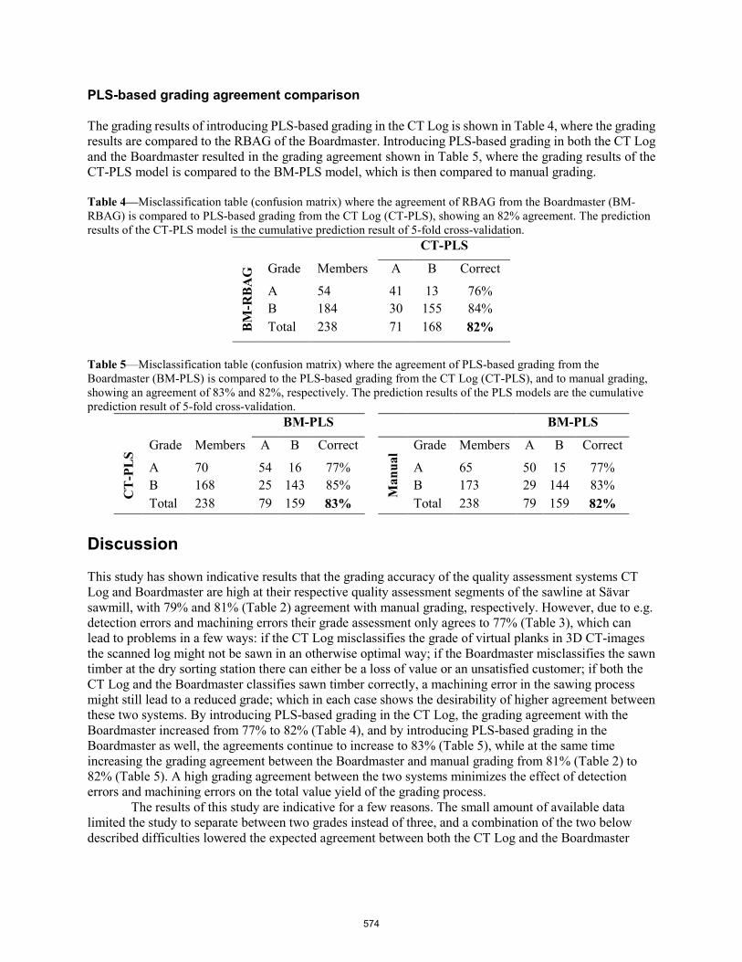
PLS-based grading agreement comparison

The grading results of introducing PLS-based grading in the CT Log is shown in Table 4, where the grading results are compared to the RBAG of the Boardmaster. Introducing PLS-based grading in both the CT Log and the Boardmaster resulted in the grading agreement shown in Table 5, where the grading results of the CT-PLS model is compared to the BM-PLS model, which is then compared to manual grading.

Table 4—Misclassification table (confusion matrix) where the agreement of RBAG from the Boardmaster (BM-RBAG) is compared to PLS-based grading from the CT Log (CT-PLS), showing an 82% agreement. The prediction results of the CT-PLS model is the cumulative prediction result of 5-fold cross-validation.

CT-PLS B

M-R

BA

G Grade Members A B Correct

A 54 41 13 76% B 184 30 155 84% Total 238 71 168 82%

Table 5—Misclassification table (confusion matrix) where the agreement of PLS-based grading from the Boardmaster (BM-PLS) is compared to the PLS-based grading from the CT Log (CT-PLS), and to manual grading, showing an agreement of 83% and 82%, respectively. The prediction results of the PLS models are the cumulative prediction result of 5-fold cross-validation.

BM-PLS BM-PLS

CT

-PL

S

Grade Members A B Correct

Man

ual Grade Members A B Correct

A 70 54 16 77% A 65 50 15 77% B 168 25 143 85% B 173 29 144 83% Total 238 79 159 83% Total 238 79 159 82%

Discussion

This study has shown indicative results that the grading accuracy of the quality assessment systems CT Log and Boardmaster are high at their respective quality assessment segments of the sawline at Sävar sawmill, with 79% and 81% (Table 2) agreement with manual grading, respectively. However, due to e.g. detection errors and machining errors their grade assessment only agrees to 77% (Table 3), which can lead to problems in a few ways: if the CT Log misclassifies the grade of virtual planks in 3D CT-images the scanned log might not be sawn in an otherwise optimal way; if the Boardmaster misclassifies the sawn timber at the dry sorting station there can either be a loss of value or an unsatisfied customer; if both the CT Log and the Boardmaster classifies sawn timber correctly, a machining error in the sawing process might still lead to a reduced grade; which in each case shows the desirability of higher agreement between these two systems. By introducing PLS-based grading in the CT Log, the grading agreement with the Boardmaster increased from 77% to 82% (Table 4), and by introducing PLS-based grading in the Boardmaster as well, the agreements continue to increase to 83% (Table 5), while at the same time increasing the grading agreement between the Boardmaster and manual grading from 81% (Table 2) to 82% (Table 5). A high grading agreement between the two systems minimizes the effect of detection errors and machining errors on the total value yield of the grading process.

The results of this study are indicative for a few reasons. The small amount of available data limited the study to separate between two grades instead of three, and a combination of the two below described difficulties lowered the expected agreement between both the CT Log and the Boardmaster

574

with the manual reference grade. Furthermore, the focus of this study was to maximize grading accuracy, which affects grading outcome.

The limitation introduced in this study to use only knot features is outside normal operations for the sawmill which affects the grading outcome. Furthermore, the sawn timber used in this study had to be handled by trucks and conveyors more than usual due to repeated runs through the dry sorting station to ensure intended functionality. The extra handing introduced more scuffs, dust, and oil-stains on the planks than usual, which resulted in a lower agreement between the Boardmaster’s grading and the manual grade reference than expected. Möller (2019)—who developed the traceability algorithm used in this study, which involved partially the same material as in this study—showed in Figure 13 a set of planks that could be considered the worst-case scenario.

During the CT-scanning and sawing process of this study, an error occurred with the positioning mechanisms in the sawing system. This caused approximately 9% of the planks to be sawn with a rotational error above 10°, which is much higher than during normal operation. This rotational error could change on which face of the planks the knots inside the logs appear, which resulted in a lower agreement between the CT Log’s grading and the manual grade reference than expected.

Conclusions

The indicative results of this study have shown that PLS-based grading increases the grading agreement compared to RBAG between the two grading systems CT Log and Boardmaster. This was achieved by introducing PLS-based grading in the CT Log, and by introducing PLS-based grading in the Boardmaster as well, the grading agreement between the two systems and the agreement between the Boardmaster and a manual reference grading either retained the same level of agreement or slightly increased it.

Each individual piece of sawn timber in this study required to be traced from the moment of the CT-scanning by the CT Log, throughout the entire sawline process, including drying, until the dry-sorting station where the Boardmaster scanned the same piece. This was done to 92% by a traceability algorithm and the remaining 8% was traced manually—showing the potential of creating similar studies like this one with the help of traceability algorithms.

Future studies should investigate the use of a traceability algorithm, like the one used in this study, to recreate this study on a new, larger, data set to further validate the findings made here.

Acknowledgments

Financial support from the Swedish Innovation Agency (VINNOVA), project Sawmill 4.0 – Customised flexible sawmill production by integrating data-driven models and decisions tools 2018-02749, is gratefully acknowledged. We thank all authors for their cooperation.

References

Anon (2019a) CT Log. Microtec. https://microtec.eu/ (Accessed: 2019-07-05).

Anon (2019b) Boardmaster. Finscan. https://finscan.fi (Accessed: 2019-07-05).

Anon (2019c) SIMCA. https://umetrics.com (Accessed: 2019-07-05).

Berglund, A.; Broman, O.; Oja, J.; Grönlund, A. 2015. Customer adapted grading of Scots pine sawn timber using a multivariate method. In: Scandinavian journal of forest research. 30(1): 87-97.

575

Breinig, L.; Leonhart, R.; Broman, O.; Manuel, A.; Brüchert, F.; & Becker, G. 2015. Classification of wood surfaces according to visual appearance by multivariate analysis of wood feature data. In: Journal of wood science. 61(2): 89-112.

Broman, O. 2000. Means to measure the aesthetic properties of wood. Doctoral dissertation, Luleå tekniska universitet. Available in DiVA diva2:989959 (Accessed: 2019-07-05).

Fredriksson, M.; Broman, O.; Sandberg, D. 2017. The use of CT-scanning technology in wood value-chain research and in wood industry: a state of the art. In: Pro Ligno. 13(4): 533-539.

Fredriksson, M. 2014. Log sawing position optimization using computed tomography scanning. In: Wood Material Science & Engineering. 9(2): 110-119.

Geladi, P.; Kowalski, B. R. 1986. Partial least-squares regression: a tutorial. In: Analytica chimica acta. (185): 1-17.

Giudiceandrea, F,; Ursella, E.; Vicario, E. 2011. A high speed CT scanner for the sawmill industry. In: Proceedings of the 17th International Nondestructive Testing and Evaluation of Wood Symposium, Sopron, Hungary.

Longuetauda, F.; Mothea, F.; Kerautretc, B.; Krähenbühlc, A.; Horyc, L.; Leband, J.M.; Debled-Rennesson, I. 2012. Automatic knot detection and measurements from X-ray CT images of wood: A review and validation of an improved algorithm on softwood samples. In: Computers and Electronics in Agriculture. 85(1): 77-89.

Lycken, A.; Oja, J. 2006. A multivariate approach to automatic grading of Pinus sylvestris sawn timber. In: Scandinavian Journal of Forest Research. (21)2: 167-174.

Möller, C.J. 2019. Development of Fingerprint Traceability in a Modern Sawmill. Master thesis, Umeå Universitet. Available in DiVA diva2:1305467 (Accessed: 2019-07-05).

Olofsson, L.; Broman, O.; Fredriksson, M.; Skog, J.; & Sandberg, D. 2017. Customer adapted grading of Scots pine sawn timber: a multivariate method approach. In: 23rd International Wood Machining Seminar (IWMS-23), Warsaw, Poland, May 28-31 2017 (pp. 360-361). Warsaw university of life sciences.

Olofsson, L.; Broman, O.; Skog, J.; Fredriksson, M.; Sandberg, D. 2019a. Multivariate product adapted grading of Scots pine sawn timber for an industrial customer, part 1: Method development. In: Wood Material Science & Engineering.

Olofsson, L.; Broman, O.; Skog, J.; Fredriksson, M.; & Sandberg, D. 2019b. Multivariate product adapted grading of Scots Pine sawn timber for an industrial customer, part 2: Robustness to disturbances. Wood Material Science & Engineering.

Swedish Sawmill Managers Association (NTGR). 1994. Nordic Timber: Grading Rules for Pine (Pinus sylvestris) and Spruce (Picea abies) Sawn Timber: Comercial Grading Based on Evaluation of the Four Sides of Sawn Timber. Markaryd: Föreningen Svenska Sågverksmän.

Wendel, C. 2019. Multivariate modeling improves quality grading of sawn timber. Master thesis, Umeå University. Available in DiVA diva2:1329008 (Accessed: 2019-07-07).

576

Prediction of the Sawing Yield of Pinus pinaster and Pinus radiata Structural Timber from Thinning Operations through Nondestructive Techniques

Abel Vega Cueto* Fundación CETEMAS. Carbayín (Asturias), Spain, avega@cetemas.es

Laura González Sánchez Fundación CETEMAS. Carbayín (Asturias), Spain, lgonzalez@cetemas.es

Soledad Rodríguez Lazcano Fundación CETEMAS. Carbayín (Asturias), Spain, srodriguez@cetemas.es

Andrea Hevia Cabal Fundación CETEMAS. Carbayín (Asturias), Spain, ahevia@cetemas.es

* Corresponding author

Abstract

Thinning and pruning operations are an essential silvicultural treatments in order to obtain high-quality timber. However, these thinning operations result in small-diameter logs without an economic return, because of the low quality and dimensions of the extracted trees. This work aims the early estimation of the percentage of structural sawn timber (graded into the normative strength classes) obtained from thinning operations of 15 years-old Pinus radiata and Pinus pinaster forests located in the North-West of Spain. For this, acoustic non-destructive techniques (NDTs) were employed in a three-steps modelling methodology: stand trees, logs and sawn boards. In one hand, the application of the NDT techniques in all three phases allowed the development and evaluation of the accuracy of prediction models in order to estimate the mechanical properties of the sawn timber before tree felling. In addition, prediction models were developed in order to estimate the yield of strength graded sawn timber using NDT measurements in the logs at industry.

Keywords: non-destructive techniques, silvicultural operations, structural sawn timber, sawing yield, Pinus radiata, Pinus pinaster

Introduction

Thinning and pruning operations are an essential silvicultural treatments in order to obtain high-quality timber. However, these thinning operations result in small-diameter logs without an economic return, because of the low quality and dimensions of the extracted trees. In order to maximize the benefit, it would be interesting the evaluation of the potential structural timber that can be obtained from these thinning operations. Structural timber is defined by its Strength Class (EN 338), and it must be selected according to the different national standards of visual grading. However, and given the high degree of subjectivity implicit in these methodologies, the new techniques based on non-destructive acoustic measurements appears to be more efficient and precise. In addition, it is interesting the possibility of

577

predicting the mechanical properties of the sawn wood from the log, before sawing, and even from the standing tree. Despite the great number of variables that influence these early predictions from standing trees, several authors have made this approach, with different results (Arciniegas et al. 2015, Merlo et al 2014, Proto et al. 2017, Wang 2011, Yin et al 2010). In addition to the NDT prediction of the mechanical properties, the sawing yield is another important factor when evaluating wood from thinning operations. This yield, understood as a percentage of volume of sawn wood obtained from a certain log volume, it is a relevant variable to know the real potential of usable wood.

For this, the main objective of this work is the evaluation of the sawing yield and the definition of models based on NDT acoustic measurements in order to predict the mechanical properties of the wood obtained from thinning operations on Pinus pinaster and Pinus radiata forests. The results obtained will be used as first approximation in terms of sawing yield and NDT prediction potential in pine structural timber for the project GO SigCA (Sistemas de gestión forestal en bosques productores de madera de calidad, 2018-2020), developed by CETEMAS, CESEFOR, HAZI, Madera Plus, Föra Technologies and AGRESTA and founded by the Spanish Government (Ministerio de Agricultura, Pesca y Alimentación, Fondo PNDR).

Material and methods

Material

The wood used in this study comes from two experimental plots located in Asturias (Northwest of Spain), of Pinus pinaster and Pinus radiata respectively. Both masses have an age between 15 and 20 years, and are being subjected to different pruning and thinning treatments. From each plot the number of trees shown in Table 1, corresponding to a second thinning, was extracted:

Table 1 - Number of trees extracted from Pinus pinaster and Pinus radiate plots Location Species Extracted trees

Barcia Pinus pinaster 21 Villaviciosa Pinus radiata 23

The trees were cut in 3-meter long logs, and were transported to the sawmill. Sawing was made according to the standard pattern usually employed in the sawmill. Four section sizes were obtained (100x21 mm2, 31x100 mm2, 31x126 mm2 and 31x147 mm2), trying to optimize the log volumes.

Sawing yield

In order to calculate the sawing yield, al logs were evaluated by measuring their dimensions: maximum and minimum diameter (Dlog1 and Dlog2, respectively), mean diameter (Dlogm) and length (Llog). From these measurements, the volume of each log was calculated. Then, during the sawing process, the boards obtained from each log were identified in order to maintain the traceability tree-log-board.

Table 2 - Number of trees, logs and boards employed for the sawing yield evaluation Location Species Trees Logs Boards

Barcia Pinus pinaster 21 27 80 Villaviciosa Pinus radiata 23 31 143

The volume of sawn timber from all four cross section previously defined was calculated for each processed log, and the sawing yield was obtained (percentage of sawn timber volume/log volume without bark).

578

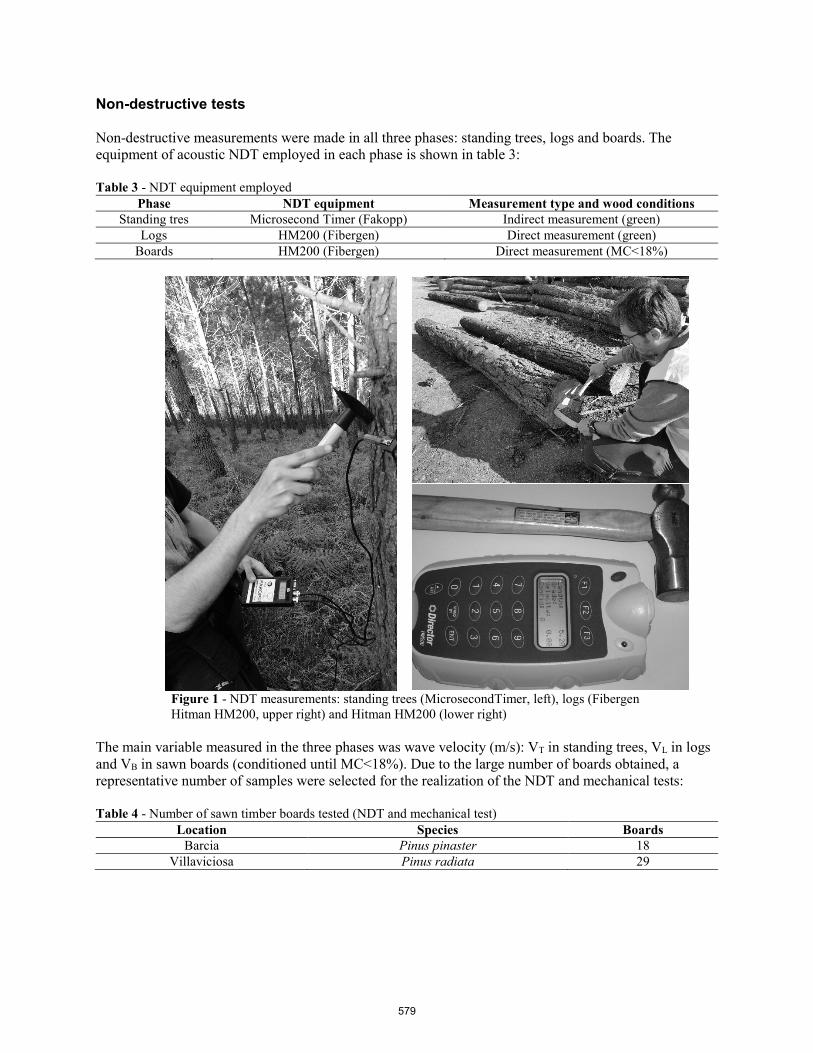
Non-destructive tests

Non-destructive measurements were made in all three phases: standing trees, logs and boards. The equipment of acoustic NDT employed in each phase is shown in table 3:

Table 3 - NDT equipment employed Phase NDT equipment Measurement type and wood conditions

Standing tres Microsecond Timer (Fakopp) Indirect measurement (green) Logs HM200 (Fibergen) Direct measurement (green)

Boards HM200 (Fibergen) Direct measurement (MC<18%)

Figure 1 - NDT measurements: standing trees (MicrosecondTimer, left), logs (Fibergen Hitman HM200, upper right) and Hitman HM200 (lower right)

The main variable measured in the three phases was wave velocity (m/s): VT in standing trees, VL in logs and VB in sawn boards (conditioned until MC<18%). Due to the large number of boards obtained, a representative number of samples were selected for the realization of the NDT and mechanical tests:

Table 4 - Number of sawn timber boards tested (NDT and mechanical test) Location Species Boards

Barcia Pinus pinaster 18 Villaviciosa Pinus radiata 29

579

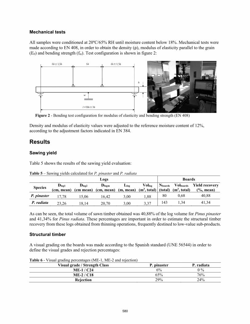
Mechanical tests

All samples were conditioned at 20ºC/65% RH until moisture content below 18%. Mechanical tests were made according to EN 408, in order to obtain the density (ρ), modulus of elasticity parallel to the grain (E0) and bending strength (fm). Test configuration is shown in figure 2:

Figure 2 - Bending test configuration for modulus of elasticity and bending strength (EN 408)

Density and modulus of elasticity values were adjusted to the reference moisture content of 12%, according to the adjustment factors indicated in EN 384.

Results

Sawing yield

Table 5 shows the results of the sawing yield evaluation:

Table 5 – Sawing yields calculated for P. pinaster and P. radiata Logs Boards

Species Dlog1

(cm, mean) Dlog2

(cm mean) Dlogm

(cm, mean) Llog

(m, mean) Vollog

(m3, total) Nboards

(total) Volboards

(m3, total) Yield recovery

(%, mean) P. pinaster 17,78 15,06 16,42 3,00 1,88 80 0,68 40,88

P. radiata 23,26 18,14 20,70 3,00 3,37 143 1,34 41,34

As can be seen, the total volume of sawn timber obtained was 40,88% of the log volume for Pinus pinaster and 41,34% for Pinus radiata. These percentages are important in order to estimate the structural timber recovery from these logs obtained from thinning operations, frequently destined to low-value sub-products.

Structural timber

A visual grading on the boards was made according to the Spanish standard (UNE 56544) in order to define the visual grades and rejection percentages:

Table 6 - Visual grading percentages (ME-1, ME-2 and rejection) Visual grade / Strength Class P. pinaster P. radiata

ME-1 / C24 6% 0 % ME-2 / C18 65% 76% Rejection 29% 24%

580

Rejection percentages obtained were slightly higher than usual for these species (around 15-20%). Because of the characteristics of the trees (small-diameter logs with a significant amount of knots), the best ME-1 visual grade (C24 strength class) was practically null, being the majority of the pieces graded as ME-2 (C18) for both species. Table 7 shows the characteristic values of these ME-2 boards, checking that they meet the values associated with Strength Class C18:

Table 7 - Characteristic values of the ME-2 graded pieces E0 (kN/mm2) fm (N/mm2) f05 (N/mm2) ρ (kg/m3) ρ05 (kg/m3)

P. pinaster 9,33 29,07 22,84 433 401 P. radiata 8,99 32,39 19,81 477 388

C18 (EN 338) 8,50 -- 18,00 380 320

NDT modelling

From NDT measurements in standing trees, logs and boards were defined linear correlation models in order to evaluate the precision of the estimation in each phase. A total of six linear models were constructed, three for P. pinaster and three for P. radiata, corresponding to the three phases defined: standing tree-log, log-sawn board and sawn board-stiffness (modulus of elasticity):

Phase / Species Linear model R2 Tree-Log / P. pinaster VL = 0,1696·VT + 2350,3 0,1419

Log-Board / P. pinaster VB = 0,9285·VL + 1118,2 0,3282 Board-Stiffness / P. pinaster E0 = 0,002·VB + 2,1598 0,4345

Tree-Log / P. radiata VL = 0,5439·VT + 1315,1 0,2631 Log-Board / P. radiata VB = 0,6792· VL + 2180,6 0,3106

Board-Stiffness / P. radiata E0 = 0,0034· VB - 5,3531 0,5043

Figure 3 - Wave velocity linear regression tree-log (P. pinaster)

Figure 4 - Wave velocity linear regression tree-log (P. radiata)

581

Figure 5 - Wave velocity linear regression log-board (P. pinaster)

Figure 6 - Wave velocity linear regression log-board (P. radiata)

Figure 7 - Linear regression wave velocity log-board stiffness (P. pinaster)

Figure 8 - Linear regression wave velocity log-board stiffness (P. radiata)

The models of the first phase (standing tree-log) provide low determination coefficients (0,14 and 0,26), expected results due to the variability of moisture content of the wood and the discrete measurement area in standing trees. The correlation improves in the next phase (log-board) with R2 of 0,33 and 0,31, and reach the best results in the estimation of the modulus of elasticity from wave velocity measured in the board with R2 of 0,43 and 0,50. These correlations are similar to those indicated by various authors in structural wood classification works using NDT (Acuña et al. 2006, Iñiguez 2007, Vega et al. 2012). As is known, these models can be significantly improved including the variable density and the calculation of the dynamic modulus of elasticity (Edyn=ρ·V2).

Conclusions

- Pinus pinaster and Pinus radiata timber from small-diameter logs from thinning operations wasevaluated in order to study the sawing yield and the potential early prediction of the mechanicalproperties through non-destructive techniques.

- Sawing yields obtained were 40,88% for Pinus pinaster and 41,34% for Pinus radiata. Theserelative high values justify the evaluation of the structural timber obtained from these small-diameter logs.

- For Pinus pinaster, 65% of the sawn timber was graded as ME-2, corresponding to a StrengthClass C18, with a rejection percentage of 29% (only 6% of ME-1/C24). For Pinus radiata, 76%

582

of the pieces were graded as ME-2/C18, while the remaining 24% were rejected (no ME-1/C24 pieces).

- Relative good prediction linear models were defined in order to estimate the stiffness dependingon the acoustic wave velocity measured on the board (R2 = 0,43 in P. pinaster and 0,50 in P.radiata). However, the models in previous phases (standing tree and log), oriented to the earlyevaluation of wood quality, need to be improved by evaluating a larger number of samples andincluding new variables.

- The results indicate a potential use of wood from thinning operations to obtain a certainpercentage of structural timber, increasing the value of these small-diameter logs, frequentlyemployed for low-value sub-products.

Acknowledgments

The authors would like to thank the Spanish Government (Ministerio de Agricultura, Pesca y Alimentación) and IDEPA (Agencia de Desarrollo Económico del Principado de Asturias). They also would like to thank the company Maderas García S.L. (Cadavedo, Asturias) for the collaboration in the wood processing.

References Acuña, L.; Díez, M.; Casado, M. 2006. Ultrasounds and structural timber quality. Application to Pinus Pinaster Ait. CIDEU 2:7–26

Arciniegas, A.; Brancheriau, L.; Lasaygues, P. 2015. Tomography in standing trees: revisiting the determination of acoustic wave velocity. Annals of Forest Science, Volume 72, Issue 6, pp 685–691

Iñiguez, G. 2007. Classification by non-destructive techniques and evaluation of mechanical properties of softwood large cross section sawn timber for structural use. Dissertation, Polytechnic University of Madrid

Merlo, E.; Alvarez-Gonzalez, J.G.; Santaclara, O.; Riesco, G. 2014. Modelling modulus of elasticity of Pinus pinaster Ait. in northwestern Spain with standing tree acoustic measurements, tree, stand and site variables. Forest Systems 23(1): 153-166

Proto, A.; Macri, G.; Bernardini, V.; Russo, D.; Zimbalatti, G. 2017. Acoustic evaluation of wood quality with a non-destructive method in standing trees: a first survey in Italy. Italian Society of Silviculture and Forest Ecology. DOI: 10.3832/ifor2065-010

Vega, A.; Dieste, A.; Guaita, M.; Majada, J.; Baño, V. 2012. Modelling of the mechanical properties of Castanea sativa Mill. structural timber by a combination of non-destructive variables and visual grading parameters. Holz als Roh- und Werkstoff Eur. J. Wood Prod.(6) DOI: 10.1007/s00107-012-0626-7

Wang, X. 2011. Fundamentals of Acoustic Measurements on Trees and Logs and Their Implication to Field Application. Proceedings of the 17th lnternational Symposium on Nondestructive Tesing and Evaluation of Wood; pp 25-33.

Yin, Y.; Nagao, H.; Liu, X.; Nakai, T. 2010. Mechanical properties assessment of Cunninghamia lanceolata plantation wood with three acoustic-based nondestructive methods. Journal of Wood Science, Volume 56, Issue 1, pp 33–40

583

High-Precision Determination of Round Wood Diameters and Cross-Section Areas

Udo Hans Sauter Department of Forest Utilisation, Forest Research Institute Baden-Württemberg, Freiburg, Germany, udo.sauter@forst.bwl.de

Jörg Staudenmaier Department of Forest Utilisation, Forest Research Institute Baden-Württemberg, Freiburg, Germany, joerg.staudenmaier@forst.bwl.de

Martin Huber Department of Forest Utilisation, Forest Research Institute Baden-Württemberg, Freiburg, Germany, martin.huber@forstbwl.de

Abstract

The importance of electronic round wood measurement systems used in saw mills for accounting and optimizing purposes has increased continuously in the past decades. Today many softwood processing saw mills are equipped with high-precise 3D-scanning systems. Based on the recorded high-resolution data the outer shape of each single log can be described in detail. Using the scanning results cross-sections areas and predefined diameters can be identified at nearly any position along the log axis.

For an efficient processing of the extensive 3D-scanning data, an appropriate preprocessing has to be done at first: Measuring errors have to be identified and corrected, missing points have to be added respectively interpolated and data reduction has to be considered as well as smoothing the raw data in order to enable a fast and robust data processing.

For calculating cross-section areas and especially for determining diameters there are various geometrical and mathematical approaches: Cross-section areas can be determined by using all available points (calculating the area of a polygon) or geometrical shapes, such as circles or ellipses, can be assumed for describing and calculating cross-sections. Concerning the determination of diameters, geometrical principles are applied usually, e.g. simulation of a mechanical caliper. Moreover the shape of real cross-sections can be assessed concerning their circularity.

Based on a representative data set, relevant guidelines and theoretical approaches for calculating cross-section areas and diameters are simulated and evaluated. As a result the effects of different methods and approaches can be assessed in terms of quality and quantity.

Keywords: round wood measurement, scaling, grading

584

Introduction

Data recording

For the studies carried out in this paper, the default settings for the data recording were chosen in a way that every cross-section is described by 360 X and Y coordinates. Depending on the diameter of a log, the absolute distance between two coordinates is approximately 1 to 5 millimeters (angular distance is 1°). The distance between these cross-sections is depending on the conveying velocity. As the measurements are carried out in real time during live operations in the saw mills, a distance between two sequent cross-sections of 5 to 10 mm could be realised (Z-axis). The X and Y coordinates are measures by a tenth of a millimeter, the Z resolution is 1 millimeter.

Figure 1—3D-laser scanner at the entrance of a saw mill

Figure 2—3D-Point cloud of a scanned log combined with centres of gravity for each cross-section

Calculating cross-section areas

Area of a polygon

In case of calculating log volumes for accounting purposes very often simplified cylinder models are used. The demanded precise log volume depends on precise determination of relevant cross-section areas by using valid mathematical approaches e.g. calculating the area of a polygon involving all available measuring points or alternatively the adaption of geometrical shapes, such as circles or ellipses. Concerning the determination of diameters, usually geometrical principles are applied, such as the simulation of a mechanical caliper. Moreover the shape of real cross-sections can be assessed concerning their circularity.

The most accurate way to determine cross-section areas is calculating the real area of a polygon based on 360 X-/Y-contour points (Gauss quadrature, based on triangles).

As the real contour between two neighbouring is unknown, the implementation of splines to obtain a better approximation to the real cross-section areas was considered as not constructive. Analyses have shown that differences between polygon-areas and spline-areas tend to be extremely small due to the high number of measured points.

585

Derivation of circles, ellipses and diameters

Commonly cross-sections of trees are assumed to be circular. As this is not the case in reality, two questions take centre stage: Which circles are appropriate to describe the real cross-section areas? And which measurement method is most suitable to determine diameters? For deriving circles and diameters from the real cross-section area several different approaches were considered and implemented.

- Circle of equivalent area:Based on the area of the polygon the circle with the equivalent area is calculated. The centre pointof this circle is not defined.

- Arithmetic mean circle:For calculating the arithmetic mean circle the centre of the polygon has to be determined first.Based on this point (centre of gravity) the radius for each single contour point can be calculated.The arithmetic mean of all radii is the radius of the mean circle.

- Best fit circle:Based on the least squares method a circle is fitted into the 360 polygon points. The centre pointof this circle differs from the centre point of the polygon (Gander et al. 1994).

- Best fit ellipse:Based on the least squares method an ellipse is fitted into the 360 polygon points (Gander et al.1994).

Figure 3—Visualisation of the best fit circle and best ellipse for two cross-sections

- Minimum circumscribed circle:The minimum circumscribed circle is the smallest circle including all 360 polygon coordinates.The centre point of this circle differs from the centre point of the polygon.

- Maximum inscribed circle:The maximum inscribed circle is the largest possible circle inside the polygon. The centre pointof this circle differs from the centre point of the polygon.

586

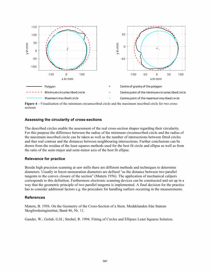
Figure 4—Visualisation of the minimum circumscribed circle and the maximum inscribed circle for two cross-sections

Assessing the circularity of cross-sections

The described circles enable the assessment of the real cross-section shapes regarding their circularity. For this purpose the difference between the radius of the minimum circumscribed circle and the radius of the maximum inscribed circle can be taken as well as the number of intersections between fitted circles and ther real contour and the distances between neighbouring intersections. Further conclusions can be drawn from the residua of the least squares methods used for the best fit circle and ellipse as well as from the ratio of the semi-major and semi-minor axis of the best fit ellipse.

Relevance for practice

Beside high precision scanning at saw mills there are different methods and techniques to determine diameters. Usually in forest mensuration diameters are defined “as the distance between two parallel tangents to the convex closure of the section” (Matern 1956). The application of mechanical calipers corresponds to this definition. Furthermore electronic scanning devices can be constructed and set up in a way that the geometric principle of two parallel tangents is implemented. A final decision for the practice has to consider additional factors e.g. the procedure for handling outliers occurring in the measurements.

References

Matern, B. 1956. On the Geometry of the Cross-Section of a Stem. Meddelanden från Statens Skogforskninginstitut, Band 46, Nr. 11.

Gander, W.; Golub, G.H.; Strebel, R. 1994. Fitting of Circles and Ellipses Least Squares Solution.

587

Automatic Sweep Measurement, as Used for Payment of Logs in SwedenFrancesco Fontanini Certification & Intellectual Property, Microtec srl GmbH, Bressanone/Brixen, Italy, francesco.fontanini@microtec.eu

Martin Bacher Certification & Intellectual Property, Microtec srl GmbH, Bressanone/Brixen, Italy, martin.bacher@microtec.eu

Abstract

Straightness is one of the basic quality requirements for saw-logs, therefore precise and reliable measures of sweep play a key role in the development and optimization of automatic grading techniques with the purpose of assigning an appropriate price to every single piece. The sweep of a log in Sweden is defined in terms of loss of saw yield due to its crookedness and it is numerically quantified as the length of the portion of log that due to its lack of straightness does not fit into an ideal scaling cylinder. Such a measure is known in Sweden with the acronym of UBF (“utbytesförlust”) and is traditionally performed by means of visual assessment. A method for the automatic assessment of sweep was implemented on the 3D true-shape log scanner Logeye. In order for the computed UBF values to be compliant with the results obtained by means of manual measurements on control logs randomly sampled from production (as imposed by Swedish rules), some of the parameters used in the automatic measurements are adjusted. Periodic inspections, control procedures and data analysis techniques will be described in terms of their reliability, robustness and repeatability. With these purposes actual production data of Norway spruce (Picea abies) from one large Swedish sawmill will be presented.

Keywords: automatic, sweep, straightness, measure, UBF, Utbytesförlust, Sweden, scanner, Logeye

Introduction

Timber measurement in Sweden is regulated by special legislation, the Swedish Timber Measurement Act (SFS, 2014:2015). This Act and the regulations of the Swedish Forest Agency (SKSFS, 2014:11) on timber measurement form a fundamental regulatory framework for timber measurement and timber reporting in Sweden (SDC, 2018). Logs may be measured manually or automatically in scanners, provided that the measuring devices are approved by VMK (“Virkesmätningskontroll”). VMK board is the supervisory and decision-making body for control matters (Biometria, 2019). Especially for measures involving payment (i.e. estimation of a price/value) accuracy, repeatability and reliability of measures are regularly controlled by means of manual measurements, performed by two check-scalers.

588

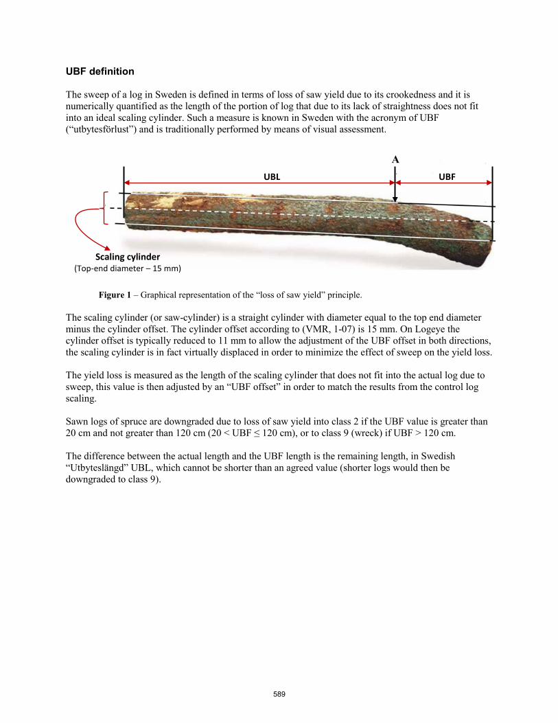
UBF definition

The sweep of a log in Sweden is defined in terms of loss of saw yield due to its crookedness and it is numerically quantified as the length of the portion of log that due to its lack of straightness does not fit into an ideal scaling cylinder. Such a measure is known in Sweden with the acronym of UBF (“utbytesförlust”) and is traditionally performed by means of visual assessment.

Figure 1 – Graphical representation of the “loss of saw yield” principle.

The scaling cylinder (or saw-cylinder) is a straight cylinder with diameter equal to the top end diameter minus the cylinder offset. The cylinder offset according to (VMR, 1-07) is 15 mm. On Logeye the cylinder offset is typically reduced to 11 mm to allow the adjustment of the UBF offset in both directions, the scaling cylinder is in fact virtually displaced in order to minimize the effect of sweep on the yield loss.

The yield loss is measured as the length of the scaling cylinder that does not fit into the actual log due to sweep, this value is then adjusted by an “UBF offset” in order to match the results from the control log scaling.

Sawn logs of spruce are downgraded due to loss of saw yield into class 2 if the UBF value is greater than 20 cm and not greater than 120 cm (20 < UBF ≤ 120 cm), or to class 9 (wreck) if UBF > 120 cm.

The difference between the actual length and the UBF length is the remaining length, in Swedish “Utbyteslängd” UBL, which cannot be shorter than an agreed value (shorter logs would then be downgraded to class 9).

A UBF

Scaling cylinder (Top-end diameter – 15 mm)

UBL

589

Microtec Logeye

Microtec’s Logeye 300 is a Multi-Sensor Quality Scanner that determines geometric, optical and structural qualities of a log and recognizes wood characteristics on the wood surface and inside the log. This permits to sort logs according to diameter, length, curvature, taper and inner quality features.

Figure 2 – Logeye 300 multi-sensor quality scanner

Curvature is measured by the optical modules of Logeye by means of laser triangulation, and the complete reconstruction of a 3D shape of the measured log is utilized to measure the log, and to compute a UBF value, i.e. measure sweep according to the “loss of saw yield” principle.

Figure 3 – 3D laser triangulation and reconstruction of a tridimensional shape of a measured log.

590

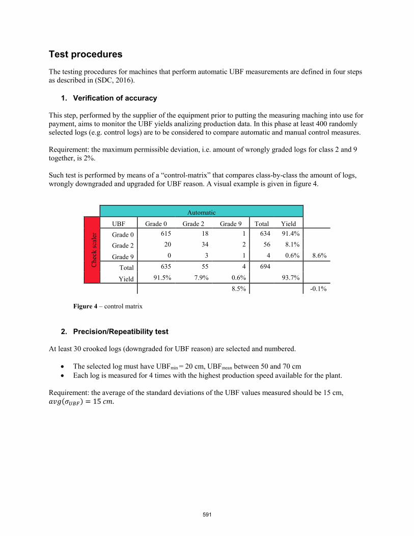
Test procedures The testing procedures for machines that perform automatic UBF measurements are defined in four steps as described in (SDC, 2016).

1. Verification of accuracy

This step, performed by the supplier of the equipment prior to putting the measuring maching into use for payment, aims to monitor the UBF yields analizing production data. In this phase at least 400 randomly selected logs (e.g. control logs) are to be considered to compare automatic and manual control measures.

Requirement: the maximum permissible deviation, i.e. amount of wrongly graded logs for class 2 and 9 together, is 2%.

Such test is performed by means of a “control-matrix” that compares class-by-class the amount of logs, wrongly downgraded and upgraded for UBF reason. A visual example is given in figure 4.

Automatic

Che

ck sc

aler

UBF Grade 0 Grade 2 Grade 9 Total Yield Grade 0 615 18 1 634 91.4%

Grade 2 20 34 2 56 8.1%

Grade 9 0 3 1 4 0.6% 8.6%

Total 635 55 4 694

Yield 91.5% 7.9% 0.6% 93.7% 8.5% -0.1%

Figure 4 – control matrix

2. Precision/Repeatibility test

At least 30 crooked logs (downgraded for UBF reason) are selected and numbered.

• The selected log must have UBFmin = 20 cm, UBFmean between 50 and 70 cm• Each log is measured for 4 times with the highest production speed available for the plant.

Requirement: the average of the standard deviations of the UBF values measured should be 15 cm, 𝑎𝑎𝑎𝑎𝑎𝑎(𝜎𝜎𝑈𝑈𝑈𝑈𝑈𝑈) = 15 𝑐𝑐𝑐𝑐.

591

3. Test body

Appropriate test bodies of durable material (e.g. pipes of plastic material) are employed in this test.

Figure 5 – UBF test body, 6 different test positions.

• The test bodies must have a UBF length in the range 40-80 cm.• The test bodies are measured for 6 times, running the system at low speed, modifying their

position so that 3 times the crooked portion passes first (with bend facing up, left and right) and 3times last (with bend facing up, left and right), e.g. Fig.5.

Requirement: the difference between the maximum and minimum measured UBF values must not exceed 10 cm (UBFmax - UBFmin < 10 cm).

4. Test of the conveyor’s stability

In order to check the stability of the conveyor belt and dogs, at least 100 logs are randomly selected, 70 of which are straight (UBF ≤ 20 cm), while the remaining 30 have different levels of curvature. The logs are run 4 times at full speed through the measure.

Requirement: maximum 4 false UBF logs are allowed (a false UBF log is defined a log for which one of the 4 measures returned UBF > 20 cm while the other three returned UBF = 0).

Type approval test

This test is performed according to the instructions of the previous four tests.

Requirements: same requirements as in tests no. 1, 2 and 3. Testing the conveyor’s stability (test no. 4) is not a formal requirement, but a good practice.

Installation test

This test is performed exactly as type approval tests, with the only difference that the requirement on test no.4 (conveyor stability) is in this case mandatory.

592

The installation test sums-up the single tests described in the four previous sections in a single main test, combining for practical reasons tests no. 2 and 4:

• 100 logs (at least) are selected to be representative of the usual diameter distribution.• 30 UBF logs (UBF > 20 cm, as in test no. 2).• 70 straight logs (UBF ≤ 20 cm, as in test no. 4).• The logs are numbered and run 4 times in the measurement system with maximum speed.

Requirements: same requirements as in tests no. 1, 2, 3 and 4.

Periodic tests

Periodic tests should be carried out at least annually, anyway it is a good practice to regularly monitor the amount of UBF downgrade and its stability over time. Microtec performs regular tests on UBF data comparing the results of automatic and check-scaler’s measures on control logs, using as a primary evaluation tool the matrix in Figure 4, which compares the amount of logs downgraded due to sweep.

As already specified before for the approval and installation test procedures, the requirements allows a difference of 2% between the automatic and manually-obtained yields for all logs downgraded for UBF (class 2+9). The matrix in Figure 4 shows that such difference is -0.1%, thus well below the maximum discrepancy allowed. Should this difference rise above the 2% limit, the manufacturer will adjust the measuring system in order to correct such discrepancies. Anyways, if during periodic controls (performed at least yearly) one should find out that systematic discrepancies exceed 1%, then proper adjustments should be considered. In order to make sure that the estimated amounts of logs downgraded for UBF reason are compatible, as imposed by Swedish rules, with the results obtained by a check scaler (by means of manual measurement on control logs), some of the parameters used in the Logeye software can be adjusted. These adjustments are implemented for Logeye by means of threshold parameters for each UBF class and by an offset value. Appropriate parameter values are empirically tested, performing a simulation which re-computing UBF values allows to obtain a new “adapted” matrix and to verify that the corrected parameters are yielding discrepancies within the allowed range.

Weekly test body

The UBF test body should be measured at least weekly, with a similar procedure to what has been described above for approval. The test body is tested changing every week the position in the measuring frame, with a “rolling schedule”. Maximum allowed discrepancy with the reference UBF (i.e. mean value of the UBF values measured during installation test) is 5 cm.

UBF Yields

Table 1 and 2 report the monthly results of Logeye for all logs measured in the years 2017 and 2018. Part of the same data is displayed in Figure 6 and 7, where the amount of UBF downgrade is compared for all production and control logs only. The amount of UBF downgraded logs (cyan-solid line in Fig.6 and 7) appears to be stable, with a standard deviation of 0.79 for logs with UBF > 20 cm and 0.11 for logs with UBF > 120 cm. The stability of automatic measures shows especially when compared with the results of the logs sampled for check scaling, which show higher fluctuations (6.08 and 2.10 respectively for UBF > 20 cm and UBF > 120 cm).

593

Table 1 – UBF downgrade for the year 2017 ordinary graded logs. 2017 Jan Feb Mar Apr May Jun Jul Aug Sep Oct Nov Dec

Pieces 60179 58438 65365 48587 48951 72301 3601 50809 42785 71739 84471 65264 UBF > 20 cm 4624 4492 4861 3308 3676 6050 323 4046 2888 4630 5656 5025 UBF > 120 cm 235 265 267 183 243 425 33 299 192 270 309 262 Grade 2+9 [%] 7.7 7.7 7.4 6.8 7.5 8.4 9.0 8.0 6.8 6.5 6.7 7.7 Grade 2 [%] 7.3 7.2 7.0 6.4 7.0 7.8 8.1 7.4 6.3 6.1 6.3 7.3 Grade 9 [%] 0.4 0.5 0.4 0.4 0.5 0.6 0.9 0.6 0.4 0.4 0.4 0.4

Table 2 – UBF downgrade for the year 2018 ordinary graded logs. 2018 Jan Feb Mar Apr May Jun Jul Aug Sep Oct Nov Dec

Pieces 59884 64660 67409 55653 53029 57650 4948 62096 63590 76343 66916 35741 UBF > 20 cm 3945 4828 5599 4088 4888 5343 484 5233 5394 5513 5339 2950 UBF > 120 cm 212 286 349 245 328 394 22 420 392 324 360 232 Grade 2+9 [%] 6.6 7.5 8.3 7.3 9.2 9.3 9.8 8.4 8.5 7.2 8.0 8.3 Grade 2 [%] 6.2 7.0 7.8 6.9 8.6 8.6 9.3 7.8 7.9 6.8 7.4 7.6 Grade 9 [%] 0.4 0.4 0.5 0.4 0.6 0.7 0.4 0.7 0.6 0.4 0.5 0.6

Please consider that the month of July is not statistically representative and should be considered as an outlier since the stop in the production causes a reduction in size of the analyzed population, thus a way lower statistical significance.

0

5

10

15

20

25

% c

lass

2+9 ALL mean = 7.7

CTRL mean = 9

Jan

17

Feb

17

Mar

17

Apr

17

May

17

Jun

17

Jul 1

7

Aug

17

Sep

17

Oct

17

Nov

17

Dec

17

Jan

18

Feb

18

Mar

18

Apr

18

May

18

Jun

18

Jul 1

8

Aug

18

Sep

18

Oct

18

Nov

18

Dec

18

ALL logsCTRL logs

Figure 6 – UBF downgrade for grade 2+9, data of all logs (solid cyan line) compared with the control logs only (dashed red line)

0

1

2

3

4

5

6

% c

lass

9

ALL mean = 0.5CTRL mean = 0.8

Jan

17

Feb

17

Mar

17

Apr

17

May

17

Jun

17

Jul 1

7

Aug

17

Sep

17

Oct

17

Nov

17

Dec

17

Jan

18

Feb

18

Mar

18

Apr

18

May

18

Jun

18

Jul 1

8

Aug

18

Sep

18

Oct

18

Nov

18

Dec

18

ALL logsCTRL logs

Figure 7 – UBF downgrade for grade 9, data of all logs (solid cyan line) compared with the control logs only (dashed red line)

594

Confidence Intervals

The comparison between the actual yields of all the automatically graded logs, and the estimated yields based on the control logs measured by the check-scaler needs to be carefully evaluated considering the effect of the population size (i.e. the number of control logs) on the accuracy of the estimates. The following equation is used to evaluate the confidence intervals:

𝐶𝐶. 𝐼𝐼. = 𝑝 ± 𝐸𝐸𝑚𝑚 (1) where:

• 𝑝 is the sample proportion given by the ratio between the number of logs in a class and the samplesize (i.e. the percentage of logs in a class)

• 𝑧𝑧∗ is the inverse of the normal cumulative distribution

𝐸𝐸𝑚𝑚 = 𝑧𝑧∗𝑝𝑝(1−𝑝𝑝)𝑛𝑛𝑡𝑡𝑡𝑡𝑡𝑡

(2)

where the margin of error 𝐸𝐸𝑚𝑚 expresses the amount of sampling error in the result of the survey and 𝑛𝑛𝑡𝑡𝑡𝑡𝑡𝑡 is the sample size.

In order to evaluate the confidence intervals relative to a 75% level of confidence, an averaged and rounded number of logs will be used, representative of the actual monthly quantities for control logs (CTRL) and all automatically graded logs (ALL). If for example we consider an average of 55000 logs being automatically measured every month, 55 of which are selected to be control logs (ctrl-logs rate of 1/1000) we can compute the margins of error using Equation (2), obtaining the values in Table 3.

Table 3 – margins of error for all/ctrl logs ALL CTRL

pieces 𝐸𝐸𝑚𝑚 pieces 𝐸𝐸𝑚𝑚 class 2+9 4300 0.13% 4 4.03% class 9 350 0.04% 1 2.07%

Figure 8 shows that the limited sample size of the manually graded control logs causes the confidence intervals to be ≈30 times bigger for class 2+9 logs (and ≈50 times bigger for class 9) than those expected for the automatically measured logs.

595

Figure 8 – confidence intervals (black brackets) and UBF-yields comparison between all logs (cyan) and control logs (red).

We therefore have a high likelihood that the error on the estimated number of control logs in each class, will be of the same order of magnitude of the measure itself (e.g. the estimated percentage of class-9 ctrl-logs is 1.8% with an error of ~2%). Such an effect can be reduced increasing the population and averaging on longer time windows, the latter is an easy solution to implement since one simply needs to collect more data over time. Anyways, the optimal strategy would be to increase the ctrl-logs ratio, thus allowing a better temporal resolution of the whole control logs analysis process. Unfortunately controlling a higher number of logs, heavily increases the workload of check-scalers and the relative costs of the whole check-scaling process. This requires in practice to reach a compromise between accuracy and feasibility.

Conclusions

We proved that UBF can be fully automatically measured by means of scanners such as Microtec’s Logeye. These procedures used for log payment lead to high stability of the measured values and reliability in time. Comparing production and control measures for testing purposes, one should take into account heavy sampling effects. Inference on the performance of automatic grading machines should be done considering such effects, i.e. not based on short observation periods. Sampling rate should be increased where possible, compatibly with time and resources needed to perform check-measures.

Acknowledgements

Microtec would like to thank Gustaf Röhfors from Sandåsa Timber AB in Åkers Styckebruk for providing the data for this analysis and for the ongoing fruitful cooperation.

0.13%

0.04%

4.03%

2.07%

0 %

2 %

4 %

6 %

8 %

10 %

12 %

ALL 2+9 ALL 9 CTRL 2+9 CTRL 9

Sam

ple

prop

ortio

n

596

References

Biometria. 2019. Standard Procedures for checking timber measurement and timber reporting. 01 01, 2019.

SDC. 2016. Kontroll av automatisk bestämning av utbytesförlust. 04 29, 2016.

SDC. 2018. Nationella instruktioner för virkesmätning. Mätning av stocks volym under bark. 01 01, 2018.

SFS. 2014:2015. Swedish Timber Measurement Act . 2014:2015.

SKSFS. 2014:11. Skogsstyrelsens författningssamling - Skogsstyrelsens föreskrifter om virkesmätning. Swedish Forest Agency, 2014:11.

VMR. 1-07. Mätningsinstruktion för sågtimmer av tall och gran. 1-07.

597

Acoustic and Elastic Properties of Leucaena leucocephala Wood as a Function of Longitudinal Position in the Tree Trunk

Cinthya Bertoldo * Laboratory of Nondestructive Testing - LabEND, College of Agricultural Engineering - FEAGRI - University of Campinas - UNICAMP, Campinas, São Paulo, Brazil, cinthyab@unicamp.br

Ryuji Soma Laboratory of Nondestructive Testing - LabEND, College of Agricultural Engineering - FEAGRI - University of Campinas - UNICAMP, Campinas, São Paulo, Brazil, jujuliosoma@gmail.com

Matheus Bragadin Garrido Laboratory of Nondestructive Testing - LabEND, College of Agricultural Engineering - FEAGRI - University of Campinas - UNICAMP, Campinas, São Paulo, Brazil, matheusbgarrido@hotmail.com

Gustavo Henrique Garcia Laboratory of Nondestructive Testing - LabEND, College of Agricultural Engineering - FEAGRI - University of Campinas - UNICAMP, Campinas, São Paulo, Brazil, gustavohlgarcia@gmail.com

* Corresponding author

Abstract

Leucaena leucocephala (leucena) is a small/medium size invasive tree, this specie has few studies about its acoustic and mechanical properties. Most of the studies are mainly focused to comprehend its invasive behavior. Beyond the tree invasive condition, the absence of knowledge about the wood mechanical properties, its limited size and its stem full of branches since small heights, favors the massive suppression of the trees and the directly discard of the wood to landfills. Considering that the wood stress and strength properties vary according to several factors, such as the tree age and the longitudinal position which the sample is removed from the tree, measuring these variations is important to characterize species. Therefore, the objective of this study, that belongs to a broader research, was evaluate the variation of acoustic and mechanical properties of leucena wood varying the height of the tree stem. The experimental design was composed by three trees, 26 faces polyhedrons were made according to different heights of these tree stem, it was considered only the useful height (before the first bifurcation) as the stem. The polyhedrons were tested through ultrasound equipment and longitudinal and shear transducers of 1,0 MHz frequency. The results indicate that there is no alteration of the acoustic and elastic properties of the leucena wood according to the variation of the longitudinal position of the tree stem. This result can be explained by the limited dimension of the useful leucena tree stem and indicates that the whole wood of this area can be fully destinate to the same purpose.

Keywords: wood characterization; elastic modulus; Poisson’s ratio.

598

Introduction

There are few studies committed to characterize acoustically or elastically the wood of Leucaena leucocephala. However, there are researches that describes the invasive behavior and the environmental damages caused by the improper establishment of this tree in different regions (Chen et al., 2012; Costa et al., 2015; Yoshida and Oka, 2004). Leucena is an invasive tree of small/medium size that presents many branches on its trunk (Parrotta, 1992), this specie is distributed widely and in abundance in many environments. Brazilian environments institutions adopts a legislation that supports the suppression of this tree as a strategy to contain leucena proliferation, however, the absence of studies related to its acoustical and elastical properties, and also the own anatomical characteristics of this specie, such as the medium size and a trunk full of branches and turns, favors the massive discard of leucena wood to sanitary landfills. Therefore, the knowledge of leucena elastic properties supports an appropriate and sustainable destination to the wood and with a higher value associated. In order to avoid waste of this material, there is a broader research being conducted in the Laboratory of Non-Destructive Testing of the Faculdade de Engenharia Agrícola, of the Universidade Estadual de Campinas (UNICAMP), aiming to study the physics, mechanics and acoustics properties of this specie.

The wood characterization through ultrasound is precise to determine the elastic parameters and presents correlations with data obtained from destructive static tests. Through ultrasound is possible to repeat a test on specimens previously tested and use smaller specimens, besides, the tests are less expensive and require a reduced number of specimens. The advantages described motivate several researches in the area (Bucur 1983, 2006; Keunecke et al., 2007; Longo et al., 2012; Ozyhar et al., 2013; Gonçalves et al., 2011, 2014; Vázquez et al., 2015).

The employment of the 26 faces polyhedron to characterize wood was initially proposed by François (1995) as a specimen that would make possible the complete characterization of the wood using only one sample. Therefore, is possible to determine the three elastic modulus (EL, ER e ET), the three-shear modulus (GLR, GLT e GRT) and the six Poisson ratio (VLR, VLT, VRL, VRT, VTL e VTR) involved in the complete elastic characterization of the wood.

Nevertheless, the mechanical and acoustic properties of the wood are vulnerable to the influence of some factors, such as the tree age or the height of the trunk which the specimens was removed (Zhu et al., 2005; Kijidani and Kitahara, 2009). These factors are mainly determinate by anatomical characteristics of the wood, such as the proportion of juvenile and late wood and by the angle of the microfibers of conductive elements. Therefore, is fundamental to evaluate the variation of properties of the wood along the height of the trunk, especially to destine properly the material, considering the variation of properties from the different sections and their future uses.

In order to propose a better and sustainable destination to the wood of Leucaena leucocephala (leucena), the aim of this study, that integrate a broader research, was to evaluate the variation of the acoustic and elastic properties of leucena wood along the height of the tree stem.

The experimental design was composed by three trees of Leucaena leucocephala, from each tree it was obtained a trunk which was divided equally into three sections (nominated by base, middle and top). Two polyhedron specimens were made from each section, totaling six specimens from each tree and eighteen for the complete research. Through the test of ultrasound waves propagation, the polyhedron specimens were characterized, and the elastic properties were compared considering the longitudinal position removal of the specimens from the tree.

599

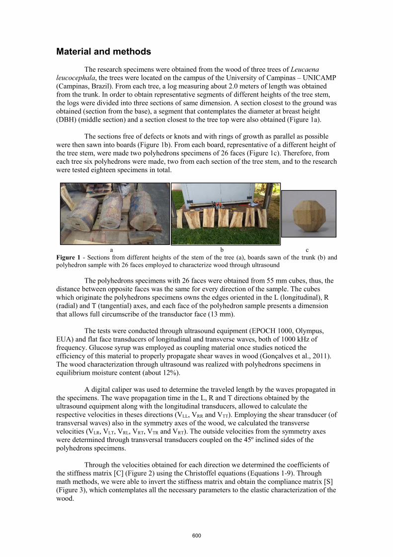
Material and methods

The research specimens were obtained from the wood of three trees of Leucaena leucocephala, the trees were located on the campus of the University of Campinas – UNICAMP (Campinas, Brazil). From each tree, a log measuring about 2.0 meters of length was obtained from the trunk. In order to obtain representative segments of different heights of the tree stem, the logs were divided into three sections of same dimension. A section closest to the ground was obtained (section from the base), a segment that contemplates the diameter at breast height (DBH) (middle section) and a section closest to the tree top were also obtained (Figure 1a).

The sections free of defects or knots and with rings of growth as parallel as possible were then sawn into boards (Figure 1b). From each board, representative of a different height of the tree stem, were made two polyhedrons specimens of 26 faces (Figure 1c). Therefore, from each tree six polyhedrons were made, two from each section of the tree stem, and to the research were tested eighteen specimens in total.

a b c Figure 1 - Sections from different heights of the stem of the tree (a), boards sawn of the trunk (b) and polyhedron sample with 26 faces employed to characterize wood through ultrasound

The polyhedrons specimens with 26 faces were obtained from 55 mm cubes, thus, the distance between opposite faces was the same for every direction of the sample. The cubes which originate the polyhedrons specimens owns the edges oriented in the L (longitudinal), R (radial) and T (tangential) axes, and each face of the polyhedron sample presents a dimension that allows full circumscribe of the transductor face (13 mm).

The tests were conducted through ultrasound equipment (EPOCH 1000, Olympus, EUA) and flat face transducers of longitudinal and transverse waves, both of 1000 kHz of frequency. Glucose syrup was employed as coupling material once studies noticed the efficiency of this material to properly propagate shear waves in wood (Gonçalves et al., 2011). The wood characterization through ultrasound was realized with polyhedrons specimens in equilibrium moisture content (about 12%).

A digital caliper was used to determine the traveled length by the waves propagated in the specimens. The wave propagation time in the L, R and T directions obtained by the ultrasound equipment along with the longitudinal transducers, allowed to calculate the respective velocities in theses directions (VLL, VRR and VTT). Employing the shear transducer (of transversal waves) also in the symmetry axes of the wood, we calculated the transverse velocities (VLR, VLT, VRL, VRT, VTR and VRT). The outside velocities from the symmetry axes were determined through transversal transducers coupled on the 45º inclined sides of the polyhedrons specimens.

Through the velocities obtained for each direction we determined the coefficients of the stiffness matrix [C] (Figure 2) using the Christoffel equations (Equations 1-9). Through math methods, we were able to invert the stiffness matrix and obtain the compliance matrix [S] (Figure 3), which contemplates all the necessary parameters to the elastic characterization of the wood.

600

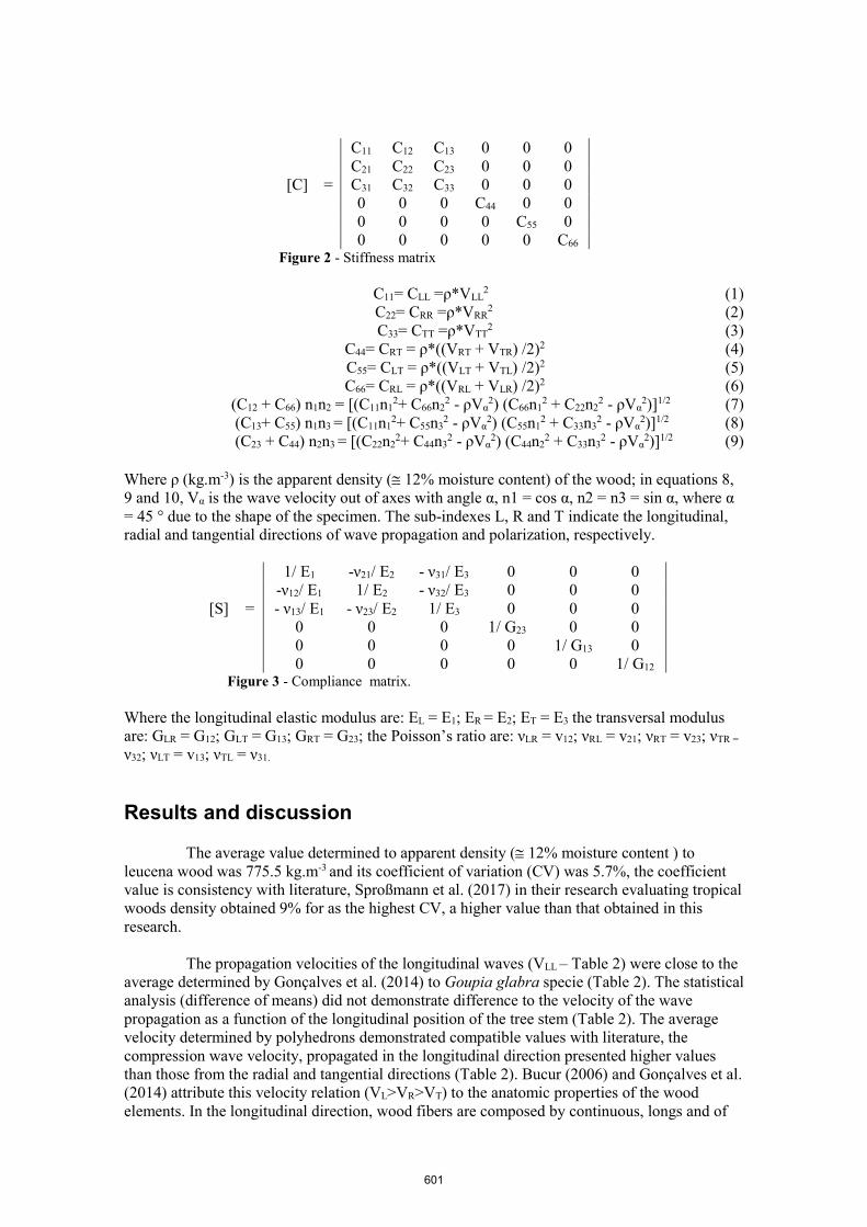
C11 C12 C13 0 0 0 C21 C22 C23 0 0 0

[C] = C31 C32 C33 0 0 0 0 0 0 C44 0 0 0 0 0 0 C55 0 0 0 0 0 0 C66

Figure 2 - Stiffness matrix

C11= CLL =ρ*VLL2 (1)

C22= CRR =ρ*VRR2 (2)

C33= CTT =ρ*VTT2 (3)

C44= CRT = ρ*((VRT + VTR) /2)2 (4) C55= CLT = ρ*((VLT + VTL) /2)2 (5) C66= CRL = ρ*((VRL + VLR) /2)2 (6)

(C12 + C66) n1n2 = [(C11n12+ C66n2

2 - ρVα2) (C66n1

2 + C22n22 - ρVα

2)]1/2 (7) (C13+ C55) n1n3 = [(C11n1

2+ C55n32 - ρVα

2) (C55n12 + C33n3

2 - ρVα2)]1/2 (8)

(C23 + C44) n2n3 = [(C22n22+ C44n3

2 - ρVα2) (C44n2

2 + C33n32 - ρVα

2)]1/2 (9)

Where ρ (kg.m-3) is the apparent density (≅ 12% moisture content) of the wood; in equations 8, 9 and 10, Vα is the wave velocity out of axes with angle α, n1 = cos α, n2 = n3 = sin α, where α = 45 ° due to the shape of the specimen. The sub-indexes L, R and T indicate the longitudinal, radial and tangential directions of wave propagation and polarization, respectively.

1/ E1 -ν21/ E2 - ν31/ E3 0 0 0 -ν12/ E1 1/ E2 - ν32/ E3 0 0 0

[S] = - ν13/ E1 - ν23/ E2 1/ E3 0 0 0 0 0 0 1/ G23 0 0 0 0 0 0 1/ G13 0 0 0 0 0 0 1/ G12

Figure 3 - Compliance matrix.

Where the longitudinal elastic modulus are: EL = E1; ER = E2; ET = E3 the transversal modulus are: GLR = G12; GLT = G13; GRT = G23; the Poisson’s ratio are: νLR = v12; νRL = v21; νRT = v23; νTR =

ν32; νLT = v13; νTL = ν31.

Results and discussion

The average value determined to apparent density (≅ 12% moisture content ) to leucena wood was 775.5 kg.m-3 and its coefficient of variation (CV) was 5.7%, the coefficient value is consistency with literature, Sproßmann et al. (2017) in their research evaluating tropical woods density obtained 9% for as the highest CV, a higher value than that obtained in this research.

The propagation velocities of the longitudinal waves (VLL – Table 2) were close to the average determined by Gonçalves et al. (2014) to Goupia glabra specie (Table 2). The statistical analysis (difference of means) did not demonstrate difference to the velocity of the wave propagation as a function of the longitudinal position of the tree stem (Table 2). The average velocity determined by polyhedrons demonstrated compatible values with literature, the compression wave velocity, propagated in the longitudinal direction presented higher values than those from the radial and tangential directions (Table 2). Bucur (2006) and Gonçalves et al. (2014) attribute this velocity relation (VL>VR>VT) to the anatomic properties of the wood elements. In the longitudinal direction, wood fibers are composed by continuous, longs and of

601

great diameter tubes, which confers adequate acoustic waves propagation. The anatomic wood elements are smaller in radial directions, nevertheless, those are still capable to properly propagate acoustic waves, however the velocities are slower than the velocities propagated in the longitudinal direction. In the tangential direction the structures do not present continuity with each other, therefore the waves propagated in this direction presents slower velocities.

Table 2 - Average velocities and their respective coefficients of variation (CV) determined by polyhedron specimens from different sections of the tree stem (base, middle and top) and velocities obtained by Gonçalves et al., 2014 to Goupia glabra. Position of

the tree trunk

VLL(m*s-1)

VRR (m*s-1)

VTT (m*s-1)

VLR(m*s-1)

VLT(m*s-1)

VRT(m*s-1)

VLT45º(m*s-1)

VRL45º(m*s-1)

VRT45º(m*s-1)

Base 4673a 2453a 1963a 1559a 1347a 944a 1625a 1398a 880a CV (%) 4 7 4 3 5 1 5 2 8 Middle 4828a 2355a 1930a 1608a 1366a 862a 1617a 1403a 905a CV (%) 2 8 4 8 6 9 6 4 10

Top 4839a 2333a 1949a 1579a 1381a 896a 1562a 1358a 891a CV (%) 5 9 12 7 8 5 7 8 7

Goupia glabra (Gonçalves et al. 2014) Average 4727 2109 1862 1495 1131 869 1195 1166 576 CV (%) 2.8 5 3.6 1.8 4.2 4.1 3.3 2.4 5.5

The letters refer to difference of means between the distinct sections where the specimens were obtained from the tree stem.

The highest value to EL obtained was 14040 MPa, to ER was 2474 MPa and to ET was 1613 MPa (Table 3). The leucena wood presented values of longitudinal and shear modulus close to Goupia glabra (cupíuba) wood, determined by Gonçalves et al. (2014) through ultrasound tests on 26 faces polyhedrons specimens and static tests (Table 4). The longitudinal elastic modulus of leucena wood determined by ultrasound also presents similar values to Dalbergia latifolia (indian rosewood) and Cordia dodecandra (ziricote) wood, obtained by Sproßmann et al. (2017) through bending tests and nondestructive tests (Table 4). Comparing the EL obtained for leucena with this parameter obtained from others researches (Table 4), the highest difference (7%) was that presented from to the Goupia glabra (Gonçalves et al., 2014). On the other hand, the leucena longitudinal elastic modulus was close to Dalbergia latifolia specie, a difference of 0.7% in relation to this property obtained through dynamic test by Sproßmann et al., 2017. Therefore, the leucena wood demonstrates mechanical and acoustic properties comparable to species employed on civil construction (Goupia glabra) and to species destinated for confection of musical instruments (Dalbergia latifolia and Cordia dodecandra).

To the polyhedrons evaluated, the coefficient of variation of elastic modulus in the symmetry axes (EL, ER and ET) varied between 3% and 21% (Table 3). Gonçalves et al. (2014) obtained to 26 faces polyhedrons of tropical species, coefficients of variation values between 0.8% and 5.7% to the same parameters. Vázquez et al. (2015) obtained coefficients of variation in the range of 21.5% - 27.7% to 26 faces polyhedrons of Castanea sativa wood.

Though the Poisson coefficient presented high values of coefficient of variation (values between 7% and 53% - Table 3), the values are consistent with the literature (Gonçalves et al., 2011, 2014; Vázquez et al., 2015). Many researches (Gonçalves et al., 2011, 2014; Ozyhar et al., 2013; Vázquez et al., 2015) demonstrate that the Poisson’s ratio presents the less precise values, either determinate through destructives tests or by nondestructive tests. Vázquez et al. (2015) indicates the high variation of orientation of fiber and the lack of parallelism of growth rings as determinants factors that contributes to obtain high values of coefficients of variation. Ozyhar et al. (2013) concludes that the applicability of the ultrasound methods to determine the Poisson’s ratios remains uncertain due to its lack of precision.

602

Through the statistical analysis (difference of the means), it was possible to verify, at the 95% confidence level, that there is no statistically significant difference between the elastic constants with the longitudinal position of obtaining the specimen along the stem of the tree. Although there is a statistical difference to the longitudinal elastic modulus according to the longitudinal position of obtaining the specimen in the tree stem, this difference was not statistically significant, once the P-value presented a higher than 0.05 (P-value=0.12). Zhu et al. (2005) through bending test on Cryptomeria japonica wood, noticed the influence of height of the tree to the elastic modulus and in the strength. In this study the specimens were taken every 2 meters from the DBH (Zhu et al. 2005). Kijidani and Kitahara (2009) also concluded that the tree height influences mechanical properties of wood. The research demonstrated better mechanical properties of the wood at 5.0 meters above the ground than at 1.5 meters. Although the literature demonstrates that the mechanical properties of wood is influenced of longitudinal position in the tree stem, this influence was not observed in our research. A possible explanation can be associated with characteristics of the studied tree specie, leucena is a small/medium size tree with many bifurcations and emergence of branches from relatively small height. The result obtained demonstrates that the wood of the tree stem of leucena, presents similar elastic properties, therefore, all the material can be used to the same purpose.

Conclusion

The characterization of Leucaena leucocephala wood through ultrasound in 26 faces polyhedrons, indicated that this tree owns elastic properties compatible to species employed in construction and to species used for confection of musical instruments. It was not observed influence of height of the tree stem in the acoustic and elastic parameters of leucena wood, enabling the employment of the full stem for the same purpose.

Acknowledgments

The authors would like to thank the National Council for Scientific and Technological Development (CNPq) for the scholarship, the São Paulo Research Foundation (FAPESP), São Paulo, Brazil (Proc. 2016/00658-4) for the research funding and the Coordination of Improvement of Higher-Level Personnel (CAPES, Brazil) for financing part of this study.

603

Tab

le 3

- A

vera

ge v

alue

s and

its c

oeffi

cien

ts v

aria

tion

of th

e el

astic

mod

ulus

for t

he lo

ngitu

dina

l dire

ctio

n (E

L), r

adia

l (E R

) and

tang

entia

l (E T

); sh

ear m

odul

us in

the

tang

entia

l-ra

dial

(GTR

), ta

ngen

tial-l

ongi

tudi

nal (

GTL

) and

long

itudi

nal-r

adia

l (G

LR) p

lane

s and

Poi

sson

coe

ffic

ient

in th

e lo

ngitu

dina

l-rad

ial (

v LR a

nd v

RL)

, lon

gitu

dina

l-tan

gent

ial (

v LT a

nd

v TL)

and

tang

entia

l-rad

ial (

v RT

and

v TR) p

lane

s, ac

cord

ing

to th

e he

ight

of t

he tr

ee st

em.

Posi

tion

of th

e tr

ee tr

unk

EL

(MPa

) E

R

(MPa

) E

T

(MPa

) G

TR

(MPa

) G

TL

(MPa

) G

RL

(MPa

) v L

R

v LT

v RT

v RL

v TL

v TR

Bas

e 14

040b

24

74a

1613

a 67

0a

1460

a 19

55a

0.56

a 0.

58a

0.73

a 0.

09a

0.07

a 0.

48a

CV

(%)

3 15

7

5 7

4 25

24

7

19

29

13

Mid

dle

1329

0ab

2334

a 15

93a

561a

14

05a

1950

a 0.

59a

0.63

a 0.

66a

0.10

a 0.

07a

0.45

a C

V (%

) 8

18

15

14

10

14

30

31

13

34

30

12

Top

11

934a

22

56a

1571

a 62

4a

1479

a 18

11a

0.57

a 0.

59a

0.65

a 0.

10a

0.09

a 0.

46a

CV

(%)

18

13

21

23

21

8 54

35

7

53

48

20

The

lette

rs re

fer t

o th

e m

eans

diff

eren

ce b

etw

een

the

sect

ions

whe

re th

e sp

ecim

ens w

ere

obta

ined

from

the

tree

stem

.

Tab

le 4

- C

ompa

rison

of a

vera

ge v

alue

s (M

Pa)

of s

ome

elas

tic p

aram

eter

s an

d its

res

pect

ive

coef

ficie

nt o

f va

riatio

n (%

) fo

r di

ffer

ent s

peci

es. T

he e

last

ic p

aram

eter

s w

ere

dete

rmin

ed th

roug

h di

ffer

ent m

etho

dolo

gies

. Pa

ram

eter

s (M

Pa)

EL (M

Pa)

ER (M

Pa)

ET (M

Pa)

GT

R (M

Pa)

GT

L (M

Pa)

GR

L (M

Pa)

Leuc

aena

leuc

ocep

hala

Po

lyhe

dron

26

Face

s 13

088

(10)

23

55 (1

5)

1592

(14)

61

5 (1

7)

1448

(14)

19

11 (1

0)

Gou

pia

glab

ra (G

onça

lves

et a

l. 20

14)

Poly

hedr

on 2

6 Fa

ces

1412

4 (3

) 20

19 (2

) 16

91 (4

) 64

2 (8

) 10

89 (8

) 19

00 (4

) G

oupi

a gl

abra

(Gon

çalv

es e

t al.

2011

) St

atic

test

13

583

(2)

2113

(22)

18

13 (9

) 64

2 (5

,1)

892

(20)

19

50 (3

) D

albe

rgia

latif

olia

(Spr

obm

ann

et a

l. 20

17)

Stat

ic te

st

1330

0 (2

2)

- -

- -

- D

ynam

ic te

st

1300

0 (2

3)

- -

- -

1640

0 (1

2)

Cor

dia

dode

cand

ra (S

prob

man

n et

al.

2017

) St

atic

test

13

300

(15)

-

- -

- -

Dyn

amic

test

13

600

(15)

-

- -

- 16

500

(10)

V

alue

s in

brac

kets

are

the

coef

ficie

nt o

f var

iatio

n (%

).

604

Reference list Bucur, V. An ultrasonic method for measuring the elastic constants of wood increment cores bored from living trees. Ultrasonics 21, 116–126 (1983).

Bucur, V. Acoustics of Wood Second Edition. (2006).

Costa, J. T., Fonseca, I. C. B. & Bianchini, E. Population structure of the invasive species Leucaena leucocephala (Fabaceae) in a seasonal semi-deciduous forest, southern Brazil. Australian Journal of Botany. 63, 590-596 (2015).

Chen, J. C., Chen, C. T., Jump, A. S. & Author, C. Forest Disturbance Leads to the Rapid Spread of the Invasive Leucaena Leucocephala in Taiwan. XXXIX, 35–40 (2012).

Fran, M. & Fran, M. Identification des sym ´ etries mat ´ erielles de mat ´ eriaux anisotropes To cite this version : (1995).

Gonçalves, R., Trinca, A. J. & dos Ferreira, G. C. S. Effect of coupling media on velocity and attenuation of ultrasonic waves in Brazilian wood. J. Wood Sci. 57, 282–287 (2011).

Gonçalves, R., Trinca, A. J. & Cerri, D. G. P. Comparison of Elastic Constants of Wood Determined by Ultrasonic Wave Propagation and Static Compression Testing. Wood Fiber Sci. 43, 64–75 (2011).

Gonçalves, R., Trinca, A. J. & Pellis, B. P. Elastic constants of wood determined by ultrasound using three geometries of specimens. Wood Sci. Technol. 48, 269–287 (2014).

Keunecke, D., Sonderegger, W., Pereteanu, K., Lüthi, T. & Niemz, P. Determination of Young’s and shear moduli of common yew and Norway spruce by means of ultrasonic waves. Wood Sci. Technol. 41, 309–327 (2007).

Kijidani, Y. & Kitahara, R. Journal of Wood Science. J. Wood Sci. 55, 198–206 (2009).

Longo, R. et al. Wood elastic characterization from a single sample by resonant ultrasound spectroscopy. Ultrasonics 52, 971–974 (2012).

Ozyhar, T., Hering, S., Sanabria, S. J. & Niemz, P. Determining moisture-dependent elastic characteristics of beech wood by means of ultrasonic waves. Wood Sci. Technol. 47, 329–341 (2013).

Parotta, J. A. Leucaena Ieucocephala (Lam.) de wit. Forest Service Research Note (1992).

Sproßmann, R., Zauer, M. & Wagenführ, A. Characterization of acoustic and mechanical properties of common tropical woods used in classical guitars. Results Phys. 7, 1737–1742 (2017).

Vázquez, C. et al. Determination of the mechanical properties of Castanea sativa Mill. using ultrasonic wave propagation and comparison with static compression and bending methods. Wood Sci. Technol. 49, 607–622 (2015).

Yoshida, K. & Oka, S. Invasion of Leucaena leucocephala and its Effects on the Native Plant Community in the Ogasawara ( Bonin ) Islands Symposium Invasion of Leucaena leucocephala and its Effects on the Native Plant Community in. 18, 1371–1375 (2004).

Zhu, J., Tadooka, N., Takata, K. & Koizumi, A. Growth and wood quality of sugi (Cryptomeria japonica) planted in Akita prefecture (II). Juvenile/mature wood determination of aged trees. J. Wood Sci. 51, 95–101 (2005).

605

Association of Biodeterioration and Density Maps with Images Generated by Ultrasound Tomography

Mariana Nagle dos Reis PhD student, Laboratory of Nondestructive Testing – LabEND, College of Agricultural Engineering - FEAGRI - University of Campinas - UNICAMP, Brazil, ma.nagle.reis@gmail.com

Raquel Gonçalves Professor, Coordinator of the Laboratory of Nondestructive Testing – LabEND, College of Agricultural Engineering - FEAGRI - University of Campinas - UNICAMP, Brazil, raquel@agr.unicamp.br

Sérgio Brazolin PhD in Forestry Engineering. Researcher at the Institute for Technological Research of São Paulo – IPT, Brazil, brazolin@ipt.br

Abstract

Researches related to falling tree risk were initiated a long time ago, but they are still current due to the complexity, uncertainties and instrumental need for quantification and qualification of defects. Visual analyzes associated with non-destructive or semi destructive tools such as ultrasound and ultrasound tomography are used to determine the tree´s phytosanitary status. However, in addition to inferring if the tree is deteriorated or even the level of deterioration, it is important to associate this condition with the physical and mechanical properties of the wood. The objective of this research was to evaluate the aptitude of ultrasound tomography to infer different zones and density variation of the wood within a disc. In order to reach this objective, images generated by ultrasonic tomography were associated to the biodeterioration and density maps obtained from tree discs of Poincianella pluviosa (Sibipiruna) trees, specie of great representativeness and importance in Brazilian cities. we conclude that velocities reduction around 75% in ultrasound tomography image allow predict the existence of a hollow in the wood with average accuracy around 80%. We also conclude that velocities in sapwood are superior to heartwood and the ultrasound tomography image is able to show the distinction of these two parts with average accuracy around to 80%. Considering deteriorated zones as the ones where velocity reduction is between 50 to 75%, ultrasonic tomography images can predict the positions and dimension of this zones with accuracy around 60%.

Keywords: ultrasound, image pattern, wood deterioration.

Introduction

In biomechanics, the tree is considered a structural element subject to gravitational and wind forces, which makes it necessary to know the physical and mechanical properties of wood in green condition and from different parts that compose it; its stability and the normal and shear stresses (Mattheck 2007).

There are technological tools (equipment) that have been used to assist the inspection of the trees. These tools allows to obtain parameters that can be used in the calculation of the risk of fall, contributing to the

606

decision about the maintenance or removal of a tree, safely to the community and respecting the need to maintain the environmental services provided by the trees to the cities.

Trees are living organisms whose characteristics vary with species, places and growing conditions, so it is very difficult to accurately predict when and under what conditions it will fail. Thus, a great deal of effort has been devoted in order to increase the precision of the analysis of this complex and important problem (Wilcox 1978, Gilbert & Smiley 2004, Fraedrich 1999).

With the ultrasound tomography, images are generated by associating colors with velocity bands, expecting that it is related to variations of stiffness, strength and density inside the trunk. The association of colors with velocity bands in image generation allows the visualization of the entire section of the trunk under analysis. However, there are few studies that aim evaluate the accuracy of these images to represent these proprieties.

The objective of this research was to evaluate the aptitude of ultrasound tomography to infer different zones and density variation of the wood within a disc.

Material and methods

In this preliminar analysis we used two wood discs with approximately 0.4 m thickness, extracted from Poencianella pluviosa tree trunks.

Immediately after tree cutting, we performed de ultrasound tests, so, with the discs in saturated condition to better represente the actual tree condition. To perform the tests, conventional ultrasound equipment (USLab, Agricef, Brazil) and longitudinal 45-kHz frequency transducers and exponential faces were used. The measurements were made in 8-point diffraction mesh (Divos and Szalai, 2002) and the tomographic images was obtained using the software ImageWood 2.1. Both, the ultrasound equipment and the software, were developed by the research group.

After ultrasound tests each disc was sanded and polished for better visualization of the sapwood, heartwood and zones with biodeterioration process. The zones were marked, measured and then photographed to produce a visual disc map of the surface. On the photos of the discs we used a free software (Image J) to “draw” a mask representative of the different regions (sapwood, heartwood and deteriorated zone). If there was color differentiation in sapwood or in heartwood, we also detached these regions. The mask allows to determine the exact area of each detached region.

After this process the discs were maintained dipped in water to preserve the saturated conditions. Specimens (around 15 x 15 x 40 mm) were obtained from the different regions of the disc and were used to calculate the apparent densities, in order to generate a density map. The apparent density was calculated using the relation between the mass and volume in the current (saturated) moisture condition. Using the software Statgraphics, we compared, statistically the density values from the different parts of the discs (1 =sapwood; 2 and 3 = heartwood considering different colors if there is and 4 = deterioration). The statistical results are used to construct the density maps.

For each disc, the tomographic images were compared, using confusion matrix, with its respective density maps. This matrix has two dimensions: the first one is related to the actual class (in this case the density and visual maps) and the second one represents the predicted class (in this case the tomographic images). The number of correct predictions for each class is located on the diagonal of the matrix and the other elements of the confusion matrix represent errors in the classification (Strobel et al. 2018). There are four possible combinations of a classification system with two classes, positive and negative. Considering C1

607

as the positive class, if an instance of C1 is classified as positive the corresponding result is called True Positive (TP); if it is classified as negative, the result is considered a False Negative (FN). On the other hand, if an instance of C2, the negative class, is classified as negative, this corresponds to a True Negative (TN) and, finally, if it is classified as positive, the result is called a False Positive (FP) (Strobel et al. 2018). This analyze allows calculate the accuracy (A), which provides the number of correct predictions (Equation 1).

𝐴𝐴𝐴𝐴𝐴𝐴𝐴𝐴𝐴𝐴𝐴𝐴𝐴𝐴𝐴𝐴 = 𝑇𝑇𝑇𝑇+𝑇𝑇𝑇𝑇𝑇𝑇𝑇𝑇+𝐹𝐹𝑇𝑇+𝐹𝐹𝑇𝑇+𝑇𝑇𝑇𝑇

Equation 1

This preliminary analysis used a coarse mesh (8 x 8) because the calculation was manual, but it will be refined, since we will use an automatic analysis, and so the results will be more accurate. The density maps were overlap the tomography image and so, we identify the four condition and two classes (TP, TN, FN and FP) – Example for deterioration in Disc 1 (Figure 1).

Figure 1. Example of confusion matrix – Deterioration in Disc 1

Results and discussion

Using the average values of density obtained for different regions of the discs (1 =sapwood; 2 and 3 = heartwood and 4 = deterioration) we observe that, numerically, density from sapwood are smaller than from heartwood but greater than from deteriorated zone (Figure 2). The two heartwood parts, visually with different colors, presented similar values of density (Figure 2). The Disc 2 do not present deteriorated zone (Figure 2).

608

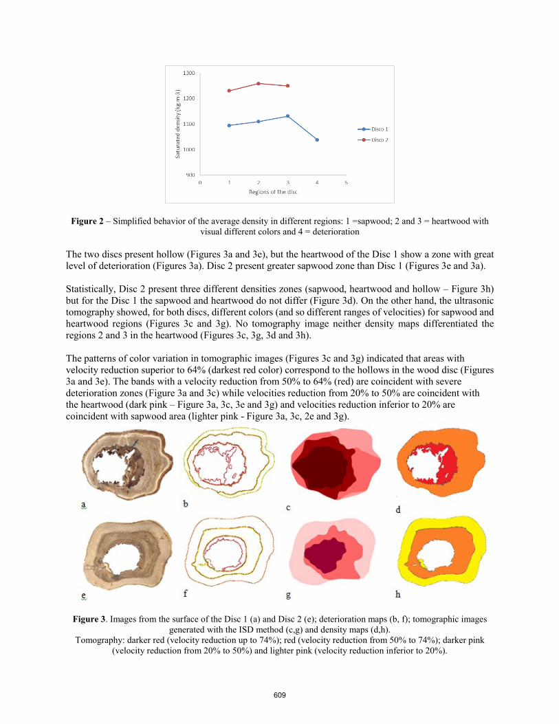
Figure 2 – Simplified behavior of the average density in different regions: 1 =sapwood; 2 and 3 = heartwood with visual different colors and 4 = deterioration

The two discs present hollow (Figures 3a and 3e), but the heartwood of the Disc 1 show a zone with great level of deterioration (Figures 3a). Disc 2 present greater sapwood zone than Disc 1 (Figures 3e and 3a).

Statistically, Disc 2 present three different densities zones (sapwood, heartwood and hollow – Figure 3h) but for the Disc 1 the sapwood and heartwood do not differ (Figure 3d). On the other hand, the ultrasonic tomography showed, for both discs, different colors (and so different ranges of velocities) for sapwood and heartwood regions (Figures 3c and 3g). No tomography image neither density maps differentiated the regions 2 and 3 in the heartwood (Figures 3c, 3g, 3d and 3h).

The patterns of color variation in tomographic images (Figures 3c and 3g) indicated that areas with velocity reduction superior to 64% (darkest red color) correspond to the hollows in the wood disc (Figures 3a and 3e). The bands with a velocity reduction from 50% to 64% (red) are coincident with severe deterioration zones (Figure 3a and 3c) while velocities reduction from 20% to 50% are coincident with the heartwood (dark pink – Figure 3a, 3c, 3e and 3g) and velocities reduction inferior to 20% are coincident with sapwood area (lighter pink - Figure 3a, 3c, 2e and 3g).

Figure 3. Images from the surface of the Disc 1 (a) and Disc 2 (e); deterioration maps (b, f); tomographic images generated with the ISD method (c,g) and density maps (d,h).

Tomography: darker red (velocity reduction up to 74%); red (velocity reduction from 50% to 74%); darker pink (velocity reduction from 20% to 50%) and lighter pink (velocity reduction inferior to 20%).

609

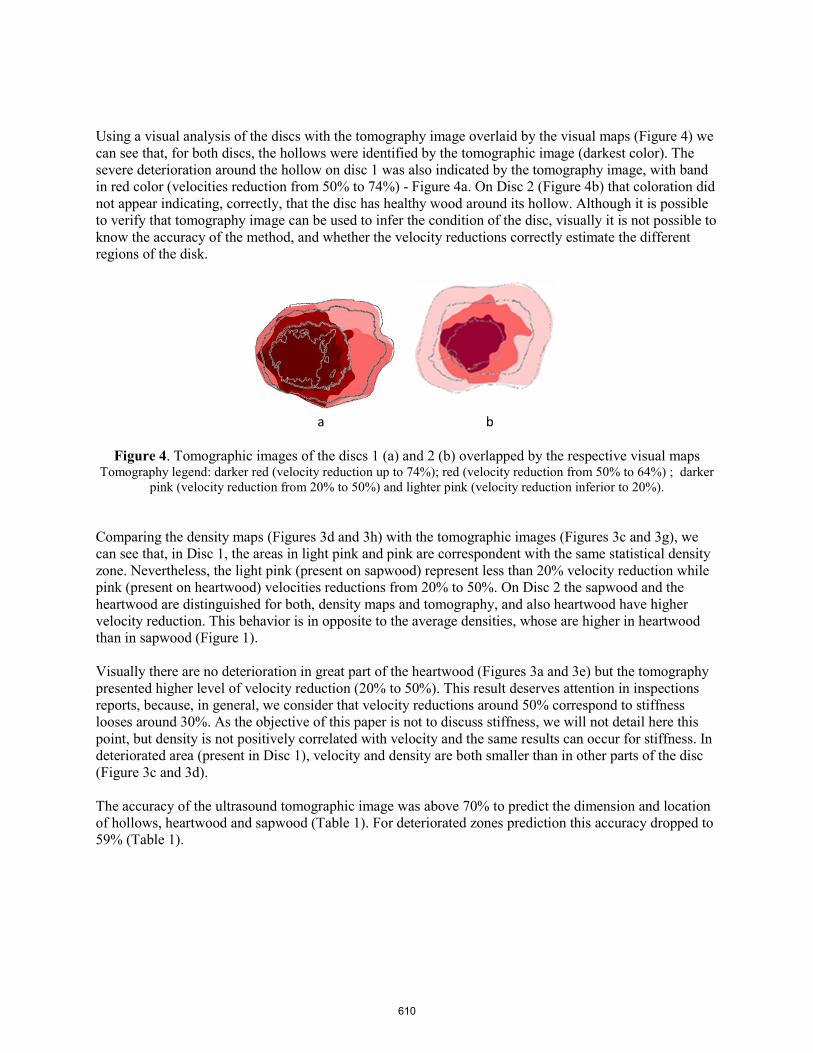
Using a visual analysis of the discs with the tomography image overlaid by the visual maps (Figure 4) we can see that, for both discs, the hollows were identified by the tomographic image (darkest color). The severe deterioration around the hollow on disc 1 was also indicated by the tomography image, with band in red color (velocities reduction from 50% to 74%) - Figure 4a. On Disc 2 (Figure 4b) that coloration did not appear indicating, correctly, that the disc has healthy wood around its hollow. Although it is possible to verify that tomography image can be used to infer the condition of the disc, visually it is not possible to know the accuracy of the method, and whether the velocity reductions correctly estimate the different regions of the disk.

a b

Figure 4. Tomographic images of the discs 1 (a) and 2 (b) overlapped by the respective visual maps Tomography legend: darker red (velocity reduction up to 74%); red (velocity reduction from 50% to 64%) ; darker

pink (velocity reduction from 20% to 50%) and lighter pink (velocity reduction inferior to 20%).

Comparing the density maps (Figures 3d and 3h) with the tomographic images (Figures 3c and 3g), we can see that, in Disc 1, the areas in light pink and pink are correspondent with the same statistical density zone. Nevertheless, the light pink (present on sapwood) represent less than 20% velocity reduction while pink (present on heartwood) velocities reductions from 20% to 50%. On Disc 2 the sapwood and the heartwood are distinguished for both, density maps and tomography, and also heartwood have higher velocity reduction. This behavior is in opposite to the average densities, whose are higher in heartwood than in sapwood (Figure 1).

Visually there are no deterioration in great part of the heartwood (Figures 3a and 3e) but the tomography presented higher level of velocity reduction (20% to 50%). This result deserves attention in inspections reports, because, in general, we consider that velocity reductions around 50% correspond to stiffness looses around 30%. As the objective of this paper is not to discuss stiffness, we will not detail here this point, but density is not positively correlated with velocity and the same results can occur for stiffness. In deteriorated area (present in Disc 1), velocity and density are both smaller than in other parts of the disc (Figure 3c and 3d).

The accuracy of the ultrasound tomographic image was above 70% to predict the dimension and location of hollows, heartwood and sapwood (Table 1). For deteriorated zones prediction this accuracy dropped to 59% (Table 1).

610

Table 1 – Accuracy of the ultrasound tomographic image to predict different discs zones and densities

Disc Accuracy (%) using Visual maps as reference Accuracy (%) using density

maps as reference Hollow Deteriorated Zone heartwood sapwood

1 75 59 69 77 81

(heartwood and sapwood statistical equivalent)

2 89 - 73 89 -

Conclusions

Considering these preliminary results (only two discs and coarse mesh to confusion matrix analysis) we conclude that velocities reduction around 75% in ultrasound tomography image allow predict the existence of a hollow in the wood with average accuracy around 80%.

We also conclude that velocities in sapwood are superior to heartwood and the ultrasound tomography image is able to show the distinction of these two parts with average accuracy around to 80%.

Considering deteriorated zones as the ones where velocity reduction is between 50 to 75%, ultrasonic tomography images can predict the positions and dimension of this zones with accuracy around 60%.

Acknowledgments

The authors thank the São Paulo State Research Foundation for the financial support (FAPESP – Proc. 2015/05692-3; Proc. 2017/07904-3); the National Council of Technological and Scientific Development (CNPq) – Proc. 309511/2014-3 and the Coordination for the Improvement of Higher Education Personnel (CAPES) for the PhD scholarships.

Reference List

MATTHECK C. Field Guide for Visual Tree Assessment. Forschungzentrum Karlsruhe GmbH. Germany, 170p. (2007).

Reis, M.N. Associação de métodos não destrutivos para inspeção de árvores. Dissertação (Mestrado) – Faculdade de Engenharia Agrícola, Unicamp. Campinas, SP. 2017

WILCOX, W.W. (1978) Review of literature on the effects of early stages of decay on wood strength, Wood and Fiber, p. 252-257

GILBERT, E. A.; SMILEY, T. Picus Sonic tomography for the quantification of decay in white oak (Quercus alba) and hickory (Carya sp.). Journal of Arboriculture, Champaign, v. 30, n. 5, p. 277-281, Sept. 2004

FRAEDRICH, B. R. (1999) Compartmentalization of decay in trees, TR-18, Technical Report, Bartlett Tree Research Laboratories, Charlotte, NC

611

Session 8

Engineered Wood Products

612

Evaluation of Elastic Constants of Full-Size Wood Composite Panels Supported on Four Nodes Using a Vibration Method Cheng Guan School of Technology, Beijing Forestry University, Beijing, China, 648911029@qq.com

Jinhao Liu* School of Technology, Beijing Forestry University, Beijing, China, liujinhao@bjfu.edu.cn

Houjiang Zhang* School of Technology, Beijing Forestry University, Beijing, China, hjzhang6@bjfu.edu.cn

Xiping Wang USDA Forest Service, Forest Products Laboratory, Madison, Wisconsin, USA, xwang@fs.fed.us

* Corresponding author

Abstract

Traditionally, elastic constants of full-size wood composite panels (WCPs) are determined by mechanically testing multiple small specimens cut from the panels. This evaluation procedure is destructive in nature, time-consuming, only suitable for product sampling and not suitable for non-destructive and in-line rapid detection. Modulus of elasticity (MOE) and shear modulus are two key indexes for evaluating the mechanical performance of WCPs. In order to assess mechanical properties of full-size WCPs rapidly and nondestructively, this study presented a new four-node support condition, which refers to a full-size WCP being supported on four node points. Based on transverse vibration of thin plate, the calculation formulas were derived between MOE in the length and width direction as well as the in-plane shear modulus of full-size WCPs supported on four nodes and characteristic parameters using sensitivity analysis and Rayleigh method. The first nine modal parameters (natural frequency and mode shape) of the vibration of full-size WCPs under the completely free boundary condition and supported on four nodes were tested by experimental modal analysis, respectively. To examine the validity of the vibration testing method, the dynamic and static tests for determining elastic constants of full-size WCPs including medium density fiberboard (MDF), oriented strand board (OSB) and plywood (PW) were conducted, and the test results were compared and analyzed. The results indicated elastic constants of the three types of panel tested using the vibration method agreed well with those corresponding values measured by verification tests. This study demonstrates that simultaneous nondestructive determination of MOE in the length and width direction as well as the in-plane shear modulus of full-size WCPs supported on four nodes based on transverse vibration of thin plate theory using a free vibration method is feasible.

Keywords: full-size wood composite panels, modulus of elasticity, shear modulus, four-node support, vibration testing

613

Introduction

Wood composite panels (WCPs), such as medium density fibreboard (MDF), oriented strand board (OSB) and plywood (PW), are engineered wood products that are widely used in furniture manufacture, packaging, building construction, musical instruments and other industrial sectors. Full-size WCPs with a nominal size of 2440 mm × 1220 mm (length × width) are most universal in the production and global market. For full-size WCPs, mechanical properties such as modulus of elasticity (MOE) and in-plane shear modulus are important performance characteristics that should be taken into consideration during manufacturing and quality control processes. Rapid and accurate determination of these elastic properties in full size panels is therefore very important to meeting the product specifications and ensuring satisfactory performance under different service conditions.

In the current production industry of WCP, full-size panels are generally selected randomly from production line and small standard specimens cut from these panels are then tested destructively using an off-line laboratory machine by a static bending method to obtain their elastic properties according to standard procedures. The elastic properties of full-size panels derived from the results of several small specimens are compared with the minimum requirements specified in the standard. While the method does provide valuable information, it has the drawbacks of being destructive, low testing efficiency, and infrequent sampling apparently. Moreover, studies have found that the static test results of samples cut out from full-size panels have a large variability existed in the mechanical properties both between panels and within panels (Mcnatt 1984; Ganev 1998). As a result, small-sample tests don’t reflect average panel properties accurately. Direct testing of the whole full-size panels instead of small-sample tests is essential to ensuing that panel mechanical performance are assessed more accurately. Non-destructive vibration techniques have been used for several decades to evaluate mechanical properties of solid wood and WCPs in scientific research (Zhang et al.2016).

In recent years, property assessment of small beam-like wood composite specimens through vibration method has made considerable advances (Yoshihara 2011; Wang et al. 2012; Hunt et al.2013; Guan et al.2016) and a dynamic cantilever beam apparatus for elastic properties (static and dynamic MOE, dynamic viscoelasticity and shear modulus) determination of small and thin wood composite materials was developed. Although this method proved fast and convenience of use, it has the same shortcomings of cutting small samples from full-size WCPs as the standard static bending method does. At present, the American standard ASTM D3043-00 (2011) describes a pure moment method for testing structural-use full-size panels to acquire MOE of the panels. In addition, machine stress rating (MSR) equipment have been developed to non-destructively determine MOE of full-size WCPs under production conditions in accordance with the principle of static mid-point bending tests (Nakamura et al.1985). However, vibration technique for MOE evaluation of full-size WCP is not widely used. More recently, some studies have been done to evaluate elastic constants (MOE in the length and width direction as well as the in-plane shear modulus) of full-size WCP through vibration techniques, such as longitudinal vibration and modal testing (Mirbolouk et al.2015; Zhou et al.2016; 2017). Nevertheless, in view of poor operation, these reported vibration techniques are only applicable to conduct in the laboratory and not used for MOE evaluation of full-size WCPs in manufacturing facilities.

The objective of this study was to determine the feasibility of using a vibration method based on the principle of transverse free vibration of a thin plate to directly evaluate the mechanical properties (MOE in the length and width direction as well as the in-plane shear modulus) of full-size WCPs. The validity of this vibration method was tested in comparison with the results from the existing test method.

614

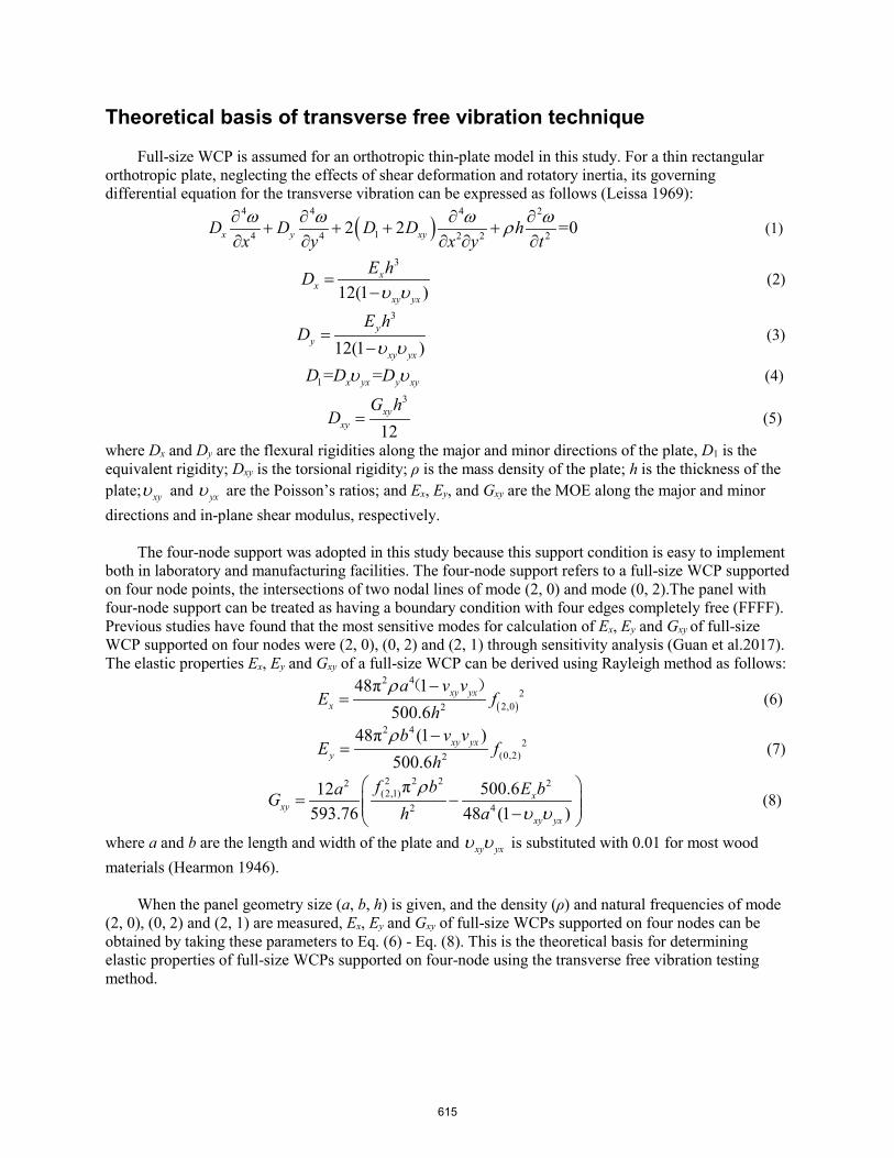
Theoretical basis of transverse free vibration technique

Full-size WCP is assumed for an orthotropic thin-plate model in this study. For a thin rectangular orthotropic plate, neglecting the effects of shear deformation and rotatory inertia, its governing differential equation for the transverse vibration can be expressed as follows (Leissa 1969):

( )4 4 2

14 24 2

4

22 2 =0x y xyD D D Dx

hy yx t

ω ω ωω ρ∂ ∂ ∂+ + + +

∂ ∂ ∂∂

∂ ∂ (1)

3

12(1 )x

yx

xy x

E hDυ υ

=−

(2)

3

12(1 )y

yy

xy x

E hD

υ υ=

− (3)

1= =yx xx yyD D Dυ υ (4) 3

12xy

xy

G hD = (5)

where Dx and Dy are the flexural rigidities along the major and minor directions of the plate, D1 is the equivalent rigidity; Dxy is the torsional rigidity; ρ is the mass density of the plate; h is the thickness of the plate; xyυ and yxυ are the Poisson’s ratios; and Ex, Ey, and Gxy are the MOE along the major and minor directions and in-plane shear modulus, respectively.

The four-node support was adopted in this study because this support condition is easy to implement both in laboratory and manufacturing facilities. The four-node support refers to a full-size WCP supported on four node points, the intersections of two nodal lines of mode (2, 0) and mode (0, 2).The panel with four-node support can be treated as having a boundary condition with four edges completely free (FFFF). Previous studies have found that the most sensitive modes for calculation of Ex, Ey and Gxy of full-size WCP supported on four nodes were (2, 0), (0, 2) and (2, 1) through sensitivity analysis (Guan et al.2017). The elastic properties Ex, Ey and Gxy of a full-size WCP can be derived using Rayleigh method as follows:

( )

2 42

2,02

48π 1500.6

xy yxx

a v vf

hE

ρ −=

（ ） (6)

2 42

(0,2)2

48π 1 )500.6

( xy yxy

b v vfE

hρ −

= (7)

2 2 2 22(2,1)

2 4

π 500.612593.76 48 (1 )

xxy

xy yx

f b E baGh aρ

υ υ

= − − (8)

where a and b are the length and width of the plate and xy yxυ υ is substituted with 0.01 for most wood materials (Hearmon 1946).

When the panel geometry size (a, b, h) is given, and the density (ρ) and natural frequencies of mode (2, 0), (0, 2) and (2, 1) are measured, Ex, Ey and Gxy of full-size WCPs supported on four nodes can be obtained by taking these parameters to Eq. (6) - Eq. (8). This is the theoretical basis for determining elastic properties of full-size WCPs supported on four-node using the transverse free vibration testing method.

615

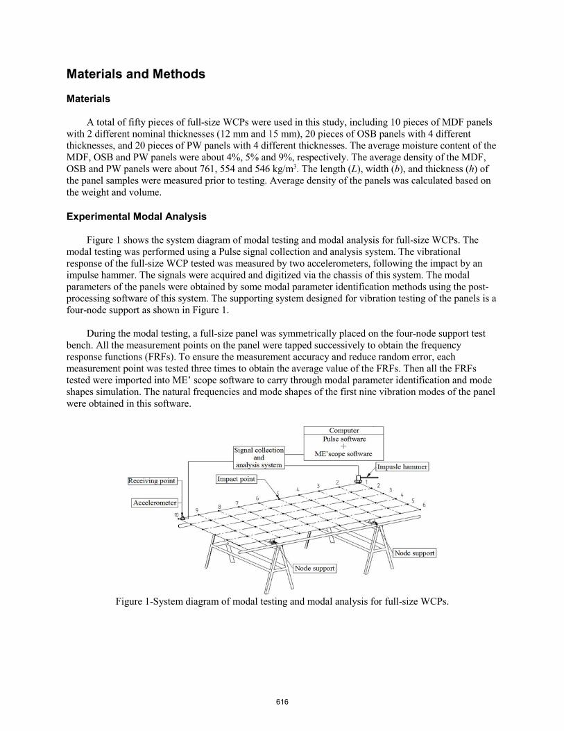
Materials and Methods

Materials

A total of fifty pieces of full-size WCPs were used in this study, including 10 pieces of MDF panels with 2 different nominal thicknesses (12 mm and 15 mm), 20 pieces of OSB panels with 4 different thicknesses, and 20 pieces of PW panels with 4 different thicknesses. The average moisture content of the MDF, OSB and PW panels were about 4%, 5% and 9%, respectively. The average density of the MDF, OSB and PW panels were about 761, 554 and 546 kg/m3. The length (L), width (b), and thickness (h) of the panel samples were measured prior to testing. Average density of the panels was calculated based on the weight and volume.

Experimental Modal Analysis

Figure 1 shows the system diagram of modal testing and modal analysis for full-size WCPs. The modal testing was performed using a Pulse signal collection and analysis system. The vibrational response of the full-size WCP tested was measured by two accelerometers, following the impact by an impulse hammer. The signals were acquired and digitized via the chassis of this system. The modal parameters of the panels were obtained by some modal parameter identification methods using the post-processing software of this system. The supporting system designed for vibration testing of the panels is a four-node support as shown in Figure 1.

During the modal testing, a full-size panel was symmetrically placed on the four-node support test bench. All the measurement points on the panel were tapped successively to obtain the frequency response functions (FRFs). To ensure the measurement accuracy and reduce random error, each measurement point was tested three times to obtain the average value of the FRFs. Then all the FRFs tested were imported into ME’ scope software to carry through modal parameter identification and mode shapes simulation. The natural frequencies and mode shapes of the first nine vibration modes of the panel were obtained in this software.

Figure 1-System diagram of modal testing and modal analysis for full-size WCPs.

616

Transverse free vibration test

The full-size panel tested was simply placed on four supporting points of the laboratory testing apparatus and these supporting points were located at the intersections of two nodal lines of mode (2, 0) and mode (0, 2). The testing software was then run to measure the weight of the panel by collecting load sensors signal. We applied a mechanical displacement using force hammer to achieve a free vibration condition (first-order flexion mode) of the panel. The vibration displacement signal recorded by the laser sensor was transmitted to the testing software in the computer. The software determined the natural frequencies of mode (2, 0), (0, 2) and (2, 1), then calculated the dynamic elastic constants (Ex, Ey and Gxy) of the panel based on Eq. (6) - Eq. (8).

Comparison test

To examine the validity of the vibration testing method that we proposed, we conducted static bending for the full size panel tested to obtain static MOE in the length and width direction (Es

x and Esy)

according to Eq. (9) and Eq. (10). The twist test was carried out to determine in-plane shear modulus (Gd

xy ) based on Eq. (11) .

3

3

14

s xx

LPEf bh

∆=

∆ (9)

3

3

14

ysy

LPEf ah

∆=

∆ (10)

2 22

20.9dxy t

a bG fh

ρ= (11)

where Lx and Ly are the span of full-size panel tested, ft is the torsional frequency of the plate; ΔP/Δf is the slope of the load-deflection curve from 10% to 40% maximum load Pmax.

Conclusions

This study introduced a vibration testing method based on transverse free vibration of thin plate principle that could be used to evaluate elastic constants (MOE in the length and width direction as well as the in-plane shear modulus) of full-size WCPs supported on four nodes.

Acknowledgments

This project was supported by “the Fundamental Research Funds for the Central Universities (NO. BLX201817)”, China Postdoctoral Science Foundation (NO. 2018M641225) and the Special Research Funds for Public Welfare (NO. 201304512).

References

ASTM D3043-00.2011. Standard Test Methods for Structural Panels in Flexure, ASTM, West Conshohocken, PA, USA. Ganev, S.1998. Variability in OSB, Report, Forintek Canada Corp., Sainte-Foy, Canada. Guan, C.; Zhang, H.J.; Hunt, J.F. [and others].2016. Determining shear modulus of thin wood composite materials using a cantilever beam vibration method, Constr. Build. Mater. 121:285-289.

617

Guan, C.; Zhang, H.J.; Wang, X.P. [and others].2017. Experimental and theoretical modal analysis of full-sized wood composite panels supported on four nodes, Materials 10(6):683. Hearmon, R. F. S. 1946. The fundamental frequency of vibration of rectangular wood and plywood plates, Proceedings of the Physical Society. 58(1):78-92. Hunt, J.F.; Zhang, H.J.; Guo, Z.R.[and others].2013. Cantilever beam static and dynamic response comparison with mid-point bending for thin MDF composite panels, BioResources. 8 (1):115-129. Leissa, A.W.1969. Vibration of plates, Ohio State University, Columbus, OH, USA. Mcnatt, J. D. 1984. Static bending properties of structural wood-base panels: large-panel versus small-specimen tests, Forest Prod. J. 34(4):50-54. Mirbolouk, P.; Roohnia, M.2015. Evaluation of dynamic modulus of elasticity of medium density fiberboard panel from longitudinal vibration tests on specimens, BioResources. 10 (1):613-621. Nakamura, N.; Okuma, M.1985. Development of continuous MOE tester for structural plywood and evaluation of the strength performance of plywood by the machine, 1: Development of continuous MOE tester for structural plywood. J. Jpn. Wood Res. Soc. 31(12):998-1003. Wang, Z. ; Li, L. ; Gong, M. 2012. Measurement of dynamic modulus of elasticity and damping ratio of wood-based composites using the cantilever beam vibration technique, Constr. Build. Mater. 28(1):831-834. Yoshihara, H. 2011.Measurement of the Young’s modulus and shear modulus of in-plane quasi-isotropic medium-density fiberboard by flexural vibration, BioResources. 6(4):4871-4885. Zhang, H.J.; Guan, C.; Wen, J. 2016. Applications and research development of nondestructive testing of wood based materials, Journal of Forestry Engineering. 1 (6) :1-9. Zhou, J. H.; Chui, Y. H.; Gong, M. [and others]. 2016. Simultaneous measurement of elastic constants of full-size engineered wood-based panels by modal testing, Holzforschung 70 (7):673-682.

618

Unsupervised Pattern Recognition of Acoustic Emission Signals of Adhesively Bonded Wood G. Clerc*BFH, Bern University of Applied Sciences, Architecture, Wood and Civil Engineering, Solothurnstrasse102, CH-2500 Biel, Switzerland, gaspard.clerc@bfh.chM.G.R. SauseUniversity of Augsburg, Institute of Materials Resource Management, Universitätstrasse 1, DE-86159Augsburg, Germany, markus.sause@mrm.uni-augsburg.deA.J. BrunnerEmpa, Swiss Federal Laboratories for Materials Science and Technology, Mechanical SystemsEngineering, Überlandstrasse 129, CH-8600 Dübendorf, Switzerland, Andreas.Brunner@empa.chP. NiemzBFH, Bern University of Applied Sciences, Architecture, Wood and Civil Engineering, Solothurnstrasse102, CH-2500 Biel, Switzerland, peter.niemz@bfh.chJ.W. G. Van de KuilenTechnical University of Munich, Wood Technology, Winzererstrasse 45, DE-80797 München, Germany,vandekuilen@hfm.tum.deTU Delft, faculty of civil Engineering and Geosciences, Biobased Structures and Materials, Delft, TheNetherlands* Corresponding author

Abstract

Modern timber constructions require high performance adhesives satisfying the various demands with respect to mechanical and physical loads. In order to develop such adhesives, a deep knowledge of the fracture behavior of the bonded wood joints and, more specifically, of the influence of the adhesive is needed. In order to better understand these points, quasi-static delamination growth experiments were conducted on four point end-notched flexure specimens (4-ENF) and monitored using acoustic emission measurements. An unsupervised pattern recognition algorithm was used to classify transient wave signals into different clusters based on frequency based criteria. Fractographic analyses of fracture surfaces were used to identify different failure mechanisms for each cluster. By comparing a rather ductile one-component polyurethane (1C-PUR) to a brittle phenol resorcinol formaldehyde (PRF) adhesive, it was possible to distinguish between wood fracture generally occuring in a brittle adhesive system and failure at the adhesive interface for a ductile 1C-PUR. These results suggest that the use of cluster analysis of AE signals combined with fractography is appropriate to identify different failure mechanisms in the bondline, allowing to gain a better understanding of the influence of the adhesive on the fracture and failure behavior of adhesively bonded wood.

Keywords: Wood adhesive, Acoustic Emission, Pattern recognition, Fractography

619

Introduction

Timber industry is looking for new adhesives with high mechanical performance, high moisture resistance and low ecological/environmental impact. Until now, phenol resorcinol formaldehyde (PRF) is one of the best performing wood adhesive (Kläusler et al. 2014). Health concerns have, however, been raised regarding the high quantity of formaldehyde contained in this adhesive. One of the best challenger are 1C-PUR adhesives, which are relatively easy to use and are not based on formaldehyde (Lehringer et al. 2014). However, until now the performance of 1C-PUR is still below that of PRF. To explain why PRF is performing better, mainly chemical aspects have been considered (Datta et al. 1999), (Weaver and Owen 1995). A still open question is whether a fracture in the wood is advantageous over a fracture in the adhesive (or at the interface). Generally, only a low correlation is found between the percentage of fracture surface occurring in the wood (Wood Fracture Percentage WFP) compared to the adhesive and the strength of the adhesive joint (Hass et al. 2014). Most of these results are however based on lap-shear samples where the geometry of the specimen and the specific orientation of the wood has a great influence on the failure location. Furthermore, on lap-shear samples, the crack propagation is highly unstable (meaning the crack will propagate almost instantaneously, making any investigation of the crack propagation difficult to achieve. In this paper, four-point end-notched-flexure specimens were tested under quasi-static and cyclic loading. This type of sample has the advantage of having a simpler geometry and offering a stable crack propagation which was monitored using Acoustic Emission (AE). This technique is an interesting addition to classical mechanical experiments as it allows to detect the associated accumulation and interaction of damage in the full specimen volume with sub micro-second time resolution (Aicher et al. 2001), (Reiterer et al. 2000). One challenge is the difficulty to associate the AE signals with the corresponding microscopic source mechanism and its location (Baensch et al. 2015a) Using unsupervised pattern recognition methods based on AE frequency and/or AE amplitudes it is possible to group similar AE signals into clusters, and therefore to obtain an indication of the source mechanism of the signals. To associate these clusters to physical features a detailed Multiphysics finite element method (FEM) (Sause et al. 2012b) simulating a model wave source, wave propagation and sensor transfer function for comparison with the features of the clusters, or X-ray micro-computed tomography (Baensch et al. 2015b) can be used. In this work, unsupervised pattern recognition of AE signals was combined with fractography to investigate the major failure phenomenon occurring in the bond line.

Material and Method

Mechanical testing setup

Beech wood (Fagus sylvatica L.) with a density of 714 kg/m3 at a wood moisture content of 12% was used for the tests. The lumber has no defects such as knots and grain deviation. Before the adhesive bonding, a 15 μm thick fluoropolymer (ETFE230N) foil was applied between the lamellae on the first 120 mm to simulate a starter crack. Two adhesives are compared in the tests, the first a relatively brittle phenol resorcinol formaldehyde (PRF, trade name «Aerodux 185») and one ductile one component polyurethane (1C-PUR) adhesive (LOCTITE HB 110 PURBOND) with a low Modulus of Elasticity (MOE). Once cured, the front-position of the foil was referenced as position of the crack tip and the pre-crack length was set to 110 mm. The samples were then cut to a width of 20 mm and a length of 317mm. The adhesively bonded wood joints were stored for several days in the test climate of 23°C and 50% relative humidity before testing. The end notched flexure (ENF) specimens were loaded under quasi-static displacement control at 1 mm/min in 4 point bending Mode II. The cyclic tests were performed using the same setup at a frequency of 5 Hz and an amplitude 13.4 +- 2.1 mm. The machine used for the test was a servo-hydraulic test machine (type 1237 Instron) equipped with a 1 kN load cell with a load and displacement accuracy of at least 1% of the measured value.

620

AE testing setup

Figure 1: Scaled schematic representation of the testing setup, with the type and position of each AE sensor

AE equipment (type AMSY-6) and preamplification (type AEP-3 with a hardware band-pass between 30 and 1000 kHz), both from Vallen Systeme GmbH with 150 kHz resonant sensors (type SE-150M from Dunegan Engineering Corporation) and one broad-band sensor (type S9208 from physical Acoustics corp) have been used. Data acquisition settings were: acquisition threshold 40 dBAE, duration discrimination time 400 μs, and a rearm time of 1 ms. Two SE-150M AE sensors were placed on top and bottom each between the bottom and top loading rollers, and between the top loading rollers, respectively. In addition, the S9208 sensor was placed on the bottom side between the distance of the top loading rollers (see figure 1 for details). All sensors were coupled with a silicone-free vacuum grease and mounted with metal springs. For assessing the delamination length as a function of time, linear AE signal source location has been performed with the four sensors mounted on the bottom side of the joint. The signal sources were localized using two different 1-D localization processors to find signals which were correctly identified by the four sensors 2-7-4-6 (see figure 1). Using this method, only AE wave propagation in the longitudinal direction was considered, meaning that only one speed of sound propagation (v = 4250 m/s) could be used. The AE source location accuracy was checked via the so-called autocalibration for which each sensor in turn was used as emitter of elastic waves, which was recorded by the other sensors and localized, respectively.

Unsupervised Pattern recognition methodology (UPR) The UPR used in this work is adapted from earlier use in composites (Sause et al. 2012a) and has been previously applied for wood fracture (Baensch et al. 2015a). The algorithm is based on an exhaustive search procedure of AE features and identifies the most suitable partition without initial assumptions regarding the number of AE features used and the number of clusters. To this end, we defined a list of K = 9 standard frequency based AE features to use for the investigation (see Table 1). Boundary constraints for the algorithm were chosen as M = 3 minimum number of features to use for a partition and P = 10 as maximum number of clusters expected. Based on these boundary constraints, the algorithm investigates all 𝑀𝑀𝐾𝐾 ∙ (𝑃𝑃 − 1) partitions and ranks the obtained result using cluster validity metrics (see (Sause et al. 2012a) for details). For this investigation Gaussian mixture models were chosen as clustering algorithm with normalization of features using their unit variance.

621

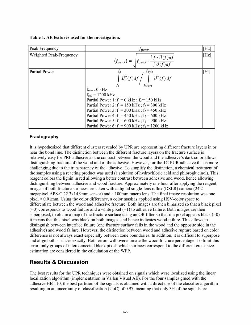
Table 1. AE features used for the investigation.

Peak Frequency 𝑓𝑓𝑝𝑝𝑝𝑝𝑝𝑝𝑝𝑝 [Hz] Weighted Peak-Frequency

𝑓𝑓𝑝𝑝𝑝𝑝𝑝𝑝𝑝𝑝 = 𝑓𝑓𝑝𝑝𝑝𝑝𝑝𝑝𝑝𝑝 ⋅∫ 𝑓𝑓 ⋅ 𝑈𝑈(𝑓𝑓)𝑑𝑑𝑓𝑓∫𝑈𝑈(𝑓𝑓)𝑑𝑑𝑓𝑓

[Hz]

Partial Power 𝑈𝑈2(𝑓𝑓)𝑑𝑑𝑓𝑓

𝑓𝑓2

𝑓𝑓1

𝑈𝑈2(𝑓𝑓)

𝑓𝑓𝑒𝑒𝑒𝑒𝑒𝑒

𝑓𝑓𝑠𝑠𝑠𝑠𝑠𝑠𝑠𝑠𝑠𝑠

𝑑𝑑𝑓𝑓

fstart = 0 kHzfend = 1200 kHz Partial Power 1: f1 = 0 kHz ; f2 = 150 kHz Partial Power 2: f1 = 150 kHz ; f2 = 300 kHz Partial Power 3: f1 = 300 kHz ; f2 = 450 kHz Partial Power 4: f1 = 450 kHz ; f2 = 600 kHz Partial Power 5: f1 = 600 kHz ; f2 = 900 kHz Partial Power 6: f1 = 900 kHz ; f2 = 1200 kHz

[%]

Fractography

It is hypothesized that different clusters revealed by UPR are representing different fracture layers in or near the bond line. The distinction between the different fracture layers on the fracture surface is relatively easy for PRF adhesive as the contrast between the wood and the adhesive’s dark color allows distinguishing fracture of the wood and of the adhesive. However, for the 1C-PUR adhesive this is more challenging due to the transparency of the adhesive. To simplify the distinction, a chemical treatment of the samples using a reacting product was used (a solution of hydrochloric acid and phloroglucinol). This reagent colors the lignin in red allowing a better contrast between adhesive and wood, hence allowing distinguishing between adhesive and wood fracture. Approximately one hour after applying the reagent, images of both fracture surfaces are taken with a digital single-lens reflex (DSLR) camera (24.2-megapixel APS-C 22.3x14.9mm sensor) and a 100mm macro lens. The final image resolution was one pixel ≈ 0.01mm. Using the color difference, a color mask is applied using HSV-color space to differentiate between the wood and adhesive fracture. Both images are then binarized so that a black pixel (=0) corresponds to wood failure and a white pixel (=1) to adhesive failure. Both images are then superposed, to obtain a map of the fracture surface using an OR filter so that if a pixel appears black (=0) it means that this pixel was black on both images, and hence indicates wood failure. This allows to distinguish between interface failure (one fracture surface fails in the wood and the opposite side in the adhesive) and wood failure. However, the distinction between wood and adhesive rupture based on color difference is not always exact especially between zone boundaries. In addition, it is difficult to superpose and align both surfaces exactly. Both errors will overestimate the wood fracture percentage. To limit this error, only groups of interconnected black pixels which surfaces correspond to the different crack size estimation are considered in the calculation of the WFP.

Results & Discussion

The best results for the UPR techniques were obtained on signals which were localized using the linear localization algorithm (implementation in Vallen Visual AE). For the four samples glued with the adhesive HB 110, the best partition of the signals is obtained with a direct use of the classifier algorithm resulting in an uncertainty of classification (UoC) of 0.97, meaning that only 3% of the signals are

622

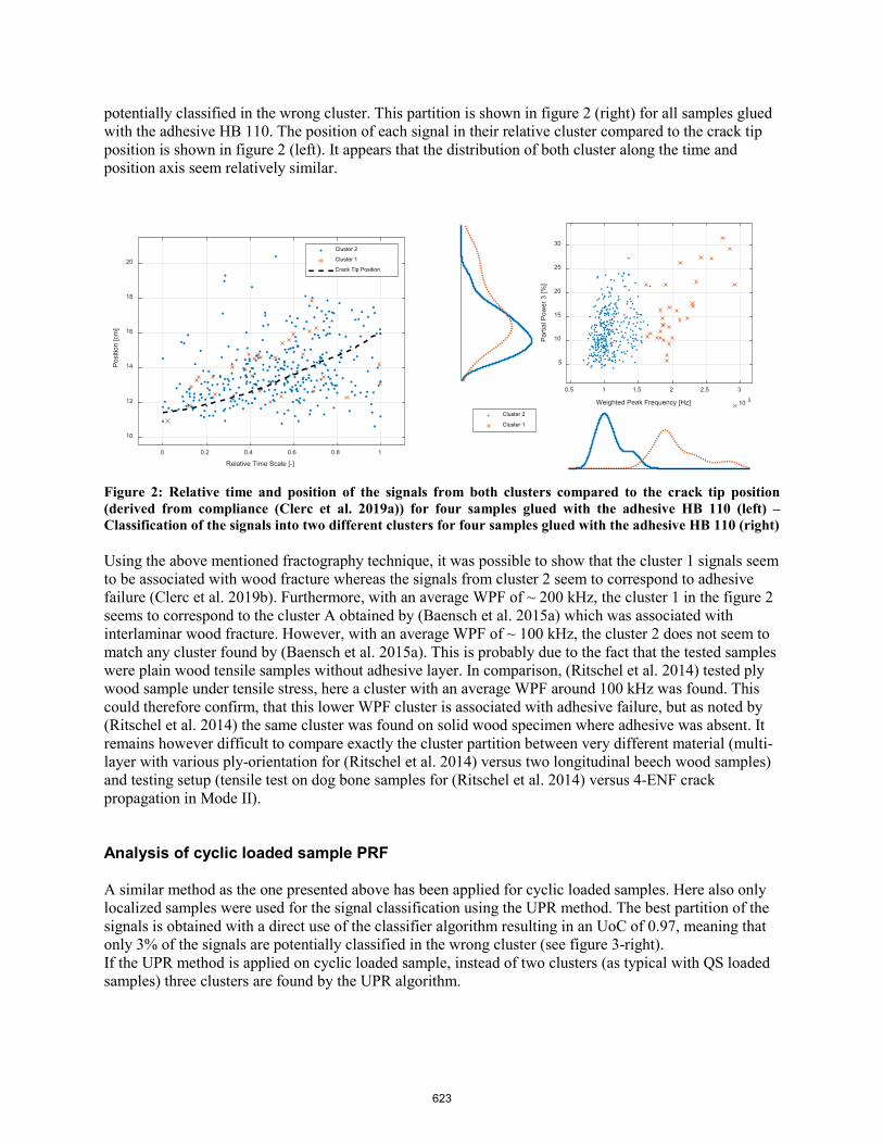
potentially classified in the wrong cluster. This partition is shown in figure 2 (right) for all samples glued with the adhesive HB 110. The position of each signal in their relative cluster compared to the crack tip position is shown in figure 2 (left). It appears that the distribution of both cluster along the time and position axis seem relatively similar.

Figure 2: Relative time and position of the signals from both clusters compared to the crack tip position (derived from compliance (Clerc et al. 2019a)) for four samples glued with the adhesive HB 110 (left) – Classification of the signals into two different clusters for four samples glued with the adhesive HB 110 (right)

Using the above mentioned fractography technique, it was possible to show that the cluster 1 signals seem to be associated with wood fracture whereas the signals from cluster 2 seem to correspond to adhesive failure (Clerc et al. 2019b). Furthermore, with an average WPF of ~ 200 kHz, the cluster 1 in the figure 2 seems to correspond to the cluster A obtained by (Baensch et al. 2015a) which was associated with interlaminar wood fracture. However, with an average WPF of ~ 100 kHz, the cluster 2 does not seem to match any cluster found by (Baensch et al. 2015a). This is probably due to the fact that the tested samples were plain wood tensile samples without adhesive layer. In comparison, (Ritschel et al. 2014) tested ply wood sample under tensile stress, here a cluster with an average WPF around 100 kHz was found. This could therefore confirm, that this lower WPF cluster is associated with adhesive failure, but as noted by (Ritschel et al. 2014) the same cluster was found on solid wood specimen where adhesive was absent. It remains however difficult to compare exactly the cluster partition between very different material (multi-layer with various ply-orientation for (Ritschel et al. 2014) versus two longitudinal beech wood samples) and testing setup (tensile test on dog bone samples for (Ritschel et al. 2014) versus 4-ENF crack propagation in Mode II).

Analysis of cyclic loaded sample PRF

A similar method as the one presented above has been applied for cyclic loaded samples. Here also only localized samples were used for the signal classification using the UPR method. The best partition of the signals is obtained with a direct use of the classifier algorithm resulting in an UoC of 0.97, meaning that only 3% of the signals are potentially classified in the wrong cluster (see figure 3-right). If the UPR method is applied on cyclic loaded sample, instead of two clusters (as typical with QS loaded samples) three clusters are found by the UPR algorithm.

0 0.2 0.4 0.6 0.8 1

Relative Time Scale [-]

10

12

14

16

18

20

Posi

tion

[cm

]

Cluster 2

Cluster 1

Crack Tip Position

0.5 1 1.5 2 2.5 3

Weighted Peak Frequency [Hz] 10 5

5

10

15

20

25

30

Parti

al P

ower

3 [%

]

Cluster 2

Cluster 1

623

It seems that the signals of the cluster 1 correspond to crack growth as the position of the signals is in majority positioned near the crack tip and at the beginning of the crack growth. Also, the WPF and PP3 of the cluster 1 seem to correspond to QS which was attributed to wood fracture.

The signals associated to cluster 2 could correspond to friction signals. Indeed, compared to the cluster 2 found for QS samples (figure 2) which show a similar low WPF, most of the signals have a lower proportion of the frequency spectrum associated to the PP3 (5 % against 10 % for the QS). Also, the samples tested with the PRF adhesive typically showed a cluster 2 with an average WPF higher than 100 kHz, probably due to the higher Modulus of Elasticity of this adhesive compared to the 1C-PUR adhesive. Furthermore, the signals’ position seems to correspond to both upper support location (figure 3). For these reasons, it seems more likely to associate these signals to friction signals than to adhesive failure. The signals associated with cluster 3 are more difficult to interpret as most of the signals are positioned near the crack tip but also near 140 mm (second upper support). It shall however be noted that, cluster 3 signals localized near the second upper support mainly appear directly after 30’000 cycles. This corresponds to an interruption in the test (for changing the data acquisition file). It could therefore be that this burst of signals is due to the test interruption and that they are not representative for the rest of the test. With a very narrow WPF distribution around 150 kHz and a relatively high PP3 distribution, cluster 3 signals seem more to correspond to a fracture than to a friction phenomenon. It can however be, as mentioned by (Momon et al. 2012), that different mechanisms (here friction and fracture) are superposed in one cluster. But as the majority of the cluster 3 signals are localized near the crack tip, it seems more likely that these signals are associated with a fracture mechanism. As observed by (Momon et al. 2012), specific fracture mechanisms (yarn/yarn debonding on ceramic matrix composites) were observed during cyclic tests. Hence suggesting, that signals from cluster 3 could correspond to a mechanism specific to cyclic test such as signals resulting from the opening/closing of the crack or fiber bridging phenomenon. On the other hand, it could also be that cluster 3 signals correspond to adhesive failure in the bondline (hence corresponding to the cluster 2 signals of the QS samples shown in figure 2). Indeed, a small plateau around a WFP of 150 kHz can be observed in figure 2, hence suggesting that during QS test, friction and adhesive failure are mixed in the same cluster. Due to the higher number of signals associated with friction during the cyclic test, a better cluster partition could be reached allowing to differentiate both clusters. To distinguish both hypotheses further tests are needed to gain a more profound knowledge about different fracture mechanisms occurring in adhesively bonded wood specimen.

Figure 3: Position of the signals from the three clusters compared to the crack tip position (derived from compliance (Clerc et al.)) (left) – Classification of the signals in the three different clusters with histogramm

0.5 1 1.5 2 2.5

Weighted Peak Frequency [Hz] 10 5

0

5

10

15

20

25

30

Parti

al P

ower

3 [%

]

Cluster 1

Cluster 2

Cluster 3

624

Conclusion

It was shown, that the UPR could be succesfully applied to crack propagation in adhesively bonded wood. The use of UPR combined with fractography on quasi-static loaded samples gave good results and indicate possible different fracture mechanisms coresponing to wood (cluster 2) and respectively adhesive failure (cluster 1) in the bond line. The same method applied on cyclic loaded sample revealed a higher number of cluster than for QS tested samples, therefore suggesting additional mechanisms occuring during cyclic tests. One cluster was associated to wood fracture occuring during the crack propagation (cluster 1), the second cluster was associated to friction signals (cluster 2) whereas the interpreation of the origin of the signals for the last cluster remain ambiguous (cluster 3). This cluster may possibly be associated with friction and fracture mechanisms, but additional experiments are needed to establish more precisely which damages mechanisms are occuring in adhesively bonded wood, specially under cyclic loading.

References Aicher, S.; Höfflin, L.; Dill-Langer, G. (2001): Damage evolution and acoustic emission of wood at tension perpendicular to fiber. In Holz als Roh- und Wekstoff 59, pp. 104–116. DOI: 10.1007/s001070050482.

Baensch, F.; Sause, M. G.R.; Brunner, A. J.; Niemz, P. (2015a): Damage evolution in wood – pattern recognition based on acoustic emission (AE) frequency spectra. In Holzforschung 69 (3), pp. 357–365. DOI: 10.1515/hf-2014-0072.

Baensch, F.; Zauner, M.; Sanabria, S. J.; Sause, M. G. R.; Pinzer, B. R.; Brunner, A. J. et al. (2015b): Damage evolution in wood: synchrotron radiation micro-computed tomography (SRμCT) as a complementary tool for interpreting acoustic emission (AE) behavior. In Holzforschung 69 (8), pp. 1015–1025. DOI: 10.1515/hf-2014-0152.

Clerc, G.; Brunner, A. J.; Josset, S.; Niemz, P.; Pichelin, F.; van de Kuilen, J. W.G. (2019a): Adhesive wood joints under quasi-static and cyclic fatigue fracture Mode II loads. In International Journal of Fatigue 123, pp. 40–52. DOI: 10.1016/j.ijfatigue.2019.02.008.

Clerc, G.; Sause, M. G. R; Brunner, A. J.; Niemz, P.; Van de Kuilen, J. W. G (2019b): Fractography combined with unsupervised pattern recognition of acoustic emission signals for a better understanding of crack propagation in adhesively bonded wood. - in preparation.

Datta, Sudip Kumar; Higuchi, Mitsuo; Morita, Mitsuhiro (1999): Analysis of phenol-resorcinol-formaldehyde resins. In J Wood Sci 45 (5), pp. 411–416. DOI: 10.1007/BF01177914.

Hass, P.; Kläusler, O.; Schlegel, S.; Niemz, P. (2014): Effects of mechanical and chemical surface preparation on adhesively bonded wooden joints. In International Journal of Adhesion and Adhesives 51, pp. 95–102. DOI: 10.1016/j.ijadhadh.2014.02.014.

Kläusler, O.; Hass, P.; Amen, C.; Schlegel, S.; Niemz, P. (2014): Improvement of tensile shear strength and wood failure percentage of 1C PUR bonded wooden joints at wet stage by means of DMF priming. In Eur. J. Wood Prod. 72 (3), pp. 343–354. DOI: 10.1007/s00107-014-0786-8.

Lehringer, C.; Gabriel, J.; Lehringer, Christian; Gabriel, Joseph (2014): Review of Recent Research Activities on One-Component PUR-Adhesives for Engineered Wood Products. Materials and Joints in Timber Structures 103, pp. 405–420. DOI: 10.1007/978-94-007-7811-5_37.

Momon, S.; Godin, N.; Reynaud, P.; R’Mili, M.; Fantozzi, G. (2012): Unsupervised and supervised classification of AE data collected during fatigue test on CMC at high temperature. In Composites Part A: Applied Science and Manufacturing 43 (2), pp. 254–260. DOI: 10.1016/j.compositesa.2011.10.016.

625

Reiterer, A.; Stanzl-Tschegg, S. E.; Tschegg, E. K. (2000): Mode I fracture and acoustic emission of softwood and hardwood. In Wood Science and Technology 34 (417-430).

Ritschel, F.; Sause, M. G. R.; Brunner, A. J.; Niemz, P. (2014): Acoustic Emission (AE) Signal Classification from Tensile Tets on Plywood and Layered Wood. In Proc. 31st Conference of the European Working Group an Acoustic Emission Fr.3.A.2.

Sause, M.G.R.; Gribov, A.; Unwin, A. R.; Horn, S. (2012a): Pattern recognition approach to identify natural clusters of acoustic emission signals. In Pattern Recognition Letters 33 (1), pp. 17–23. DOI: 10.1016/j.patrec.2011.09.018.

Sause, M.G.R.; Müller, T.; Horoschenkoff, A.; Horn, S. (2012b): Quantification of failure mechanisms in mode-I loading of fiber reinforced plastics utilizing acoustic emission analysis. In Composites Science and Technology 72, pp. 167–174. DOI: 10.1016/j.compscitech.2011.10.013.

Weaver, F. William; Owen, Noel L. (1995): Isocyanate-Wood Adhesive Bond. In Applied Spectroscopy 49 (2), pp. 171–176. DOI: 10.1366/0003702953963751.

626

Nondestructive Testing of Fiber-Cement Composites Reinforced with Nanosilica Modified Cellulose Fibers

Joabel Raabe Department of Forest Engineering, University of Brasília, DF, Brazil, joabeljr@hotmail.com

Cláudio Henrique Soares Del Menezzi * Department of Forest Engineering, University of Brasília, DF, Brazil, cmenezzi@unb.br

Gustavo Henrique Denzin Tonoli Department of Forest Sciences, Federal University of Lavras, MG, Brazil, gustavotonoli@yahoo.com.br

Danillo Wisky Silva Department of Forest Sciences, Federal University of Lavras, MG, Brazil, danilowisky@hotmail.com

* Corresponding author

Abstract

In this work, the dynamic modulus of elasticity (E) of fiber-cement composites reinforced with modified (MF) and unmodified (UMF) fiber cellulose pulp was determined in various contents (0, 1, 3 and 5% by mass), before and after accelerated aging cycles. The composites were produced by extrusion and the molded specimens were subjected to humid curing for 28 days. After this period, the "E" was determined by the analysis of natural frequencies of flexural vibration using the Sonelastic® (ATCP) equipment. Then the test specimens were subjected to accelerated aging cycles in laboratory equipment and the "E" was determined again. At 28 days, it was observed that the "E" decreased with the addition and increase of the content of cellulose pulp fibers in the fiber cement composites. On the other hand, after the accelerated aging the presence of fibers in the fiber cement composites yielded a higher "E". In addition, it was found that MF-reinforced composites had higher mean values of "E" than the UMF-reinforced homologues. This indicates that the addition of cellulose pulp fibers in cementations matrices allows for better mechanical performances of the composites after exposure to weathering conditions.

Keywords: fiber-cement, cellulose pulp, dynamic modulus of elasticity

Introduction

In recent years there has been a rapid growth in research and innovation in the area of cementitious composites reinforced with vegetable fibers. Interest is guaranteed due to the environmental advantages of vegetable fibers compared to metallic and synthetic fibers (conventionally used), which for their production require non-renewable resources and high energy consumption. Many efforts have been made to ensure good mechanical performance and good durability of fiber-cement composites reinforced with vegetable fibers, and to expand the capacities and applications of this group of materials (Pickering et al. 2016). The main challenges to be overcome are the high sensitivity to humidity and the dimensional instability of the vegetable fibers when mixed with the cement. These characteristics impair the physical properties and the mechanical performance of the composites as it

627

enables the acceleration of fiber mineralization by the permeation of calcium hydroxide through the cell wall (Mohr et al. 2005; Mohr et al. 2006; Ardanuy et al. 2011; Khan et al. 2017). In this sense, several approaches have been explored, among which the superficial treatment of the fibers stands out. This is based on the protection, coating or pretreatment of the fibers to avoid the destructive effects of the alkalinity of the cement (Vo and Navard 2016). With the advent of nanotechnology, the deposition of nanoparticles on the surface of the fibers, can be an interesting alternative to minimize the adverse effects of the fibers in this type of composites (Raabe et al. 2018). The use of fibers as a reinforcement in composites has the main purpose to overcome the fragility of the cementitious materials which, of course, have low tensile strength and deformation capacity. The inclusion of fibers avoids the propagation of existing and / or cracked cracks, improving the crack tip plasticity that increases the fracture resistance of composites (Khan et al. 2017). Mechanical properties, such as modulus of elasticity (MOE), modulus of rupture (MOR), among others, are very important characteristics of fiber-cement composites and usually need to be determined before its practical application. To evaluate these properties, different test methods can be used: conventional tests (destructive methods) and non-destructive tests (Wahab et al. 2019). Non-destructive techniques refer to the inspection of materials and equipment, which include methods capable of determining information about products and technological characteristics of the materials without damaging them or wasting them, and thus validate the variation of properties in the material evaluated. Non-destructive tests have some advantages over conventional tests, such as: easy and quick to perform; save time and material; make it possible to test the material again when necessary; allow repeated checks over a period of time through which their relationship to service failure can be accurately established; several non-destructive tests, each with precision on different properties of the material, can be applied concurrently or in sequence (Wahab et al. 2019). The impulse excitation technique is used for the fast, precise and non-destructive characterization of the elastic modulus and the damping of materials, such as: ceramic and refractory (Minatto et al. 2017; Moñoz and Martinez 2016); concrete and cementitious materials (Otoni and Pereira 2017; Marques et al. 2014); composites and wood (Feiferis and d'Almeida 2016; Otani et al. 2015); biomaterials and polymers (Martins Jr. et al. 2018; Monich et al. 2017). The objective of this study was to determine the dynamic modulus of elasticity (E), before and after the accelerated aging, of fiber-cement composites reinforced with modified cellulose pulp (MF) and unmodified (UMF) using non-destructive test.

Materials and methods

The materials used for the processing and confection of fiber-cement composites were: (i) Portland cement CPV ARI and ground limestone (filler), which formed the cementitious matrix; (ii) hydroxypropylmethylcellulose (HPMC), rheological modifier and carboxylated polyester (ADVATM 175) surfactant, used as additive materials to promote the pseudo plastic behavior of mortars and to enable the processing of the mixture; (iii) distilled water, used for the hydration of the composites; (iv) modified (MF) and unmodified (UMF) cellulosic pulp fibers, which formed the reinforcement of the composites. The cellulosic pulp fibers used were from Eucalyptus sp. obtained from bleached kraft pulp, provided by Eldorado Brasil Celulose. The chemical agents used for the modification of the fibers were: tetraethyl orthosilicate (C8H20O4Si - TEOS, 98%) inorganic precursor for the synthesis of nano-silica; ammonia hydroxide (NH4OH - 30 to 32% v.v-1), synthesis catalyst; and ethanol (CH3CH2OH - 95% P.A.) and water, reaction solvents. The agents employed to promote the modification and the process used (sol - gel method), were the same described in detail in Raabe et al. (2018).

628

Production of fiber-cement composites

The fiber-cement composites were produced and molded in a monorail laboratory extruder (Verdés brand, model 051), with a screw speed of approximately 25 rpm. Rectangular fiber-cement samples with nominal dimensions of 200 mm in length, 28 mm in width and 18 mm in thickness were prepared by the extruder. The compositions of the blends used to produce the composites are shown in Table 1.

Table 1 – Formulations of the fiber cement composites produced.

Treatments Cement Limestone MF UMF Water *

--------------------- % in mass --------------------

Control 70.0 30.0 0.0 0.0 34.0

MF1% 69.3 29.7 1.0 0.0 34.0

UMF1% 69.3 29.7 0.0 1.0 34.0

MF3% 67.9 29.1 3.0 0.0 42.0

UMF3% 67.9 29.1 0.0 3.0 42.0

MF5% 66.5 28.5 5.0 0.0 49.0

UMF5% 66.5 28.5 0.0 5.0 49.0

* Percentage in relation to cement mass

The additives (HPMC and ADVA) were added (1% to the mass of the matrix) to each formulation produced. The matrix formulation (cement + limestone), mixing of the components before processing, the molding process of the test bodies (by extrusion) and curing (28 days in a moisture saturated environment) of the molded fiber-cement composites were based on previous studies (Farrapo et al. 2017).

Accelerated aging

Accelerated aging was performed in an accelerated weather chamber of the brand EQUILAM (series EQUV-RC). In this equipment, exposure cycles, simulating solar irradiation, rain and dew, were programmed. The purpose was to simulate eventual degradation of the composites by the prolonged exposure to natural elements. The accelerated aging cycle was established and adapted from the ASTM G154-6 (ASTM, 2006) standard for cover materials (Type 5 test). A total of 20 cycles were performed, with each cycle corresponding to 24 h of exposure. The sequential order of elements was:

i) 19:30 h of irradiation in UV-B 313 lamp, with 0.62 W.m-2.nm-1 of irradiation power andtemperature of 80 °C;

ii) 0:15 h of water spray, concurrently with UV-B 313 irradiation, with 0.62 W.m-2.nm-1 ofirradiation power and temperature of 25 °C;

iii) 4:00 h of condensation of water vapor with a temperature of 50 °C;iv) 0:15 h of water spray at 25 °C.

The accelerated aging was applied with the purpose of evaluating the mechanical behavior of the composites after undergoing intensive cycles of irradiation, heating and moistening.

Determination of the dynamic modulus of elasticity (E)

The dynamic modulus of elasticity (E) was determined by applying the impulse excitation technique using the Sonelastic® (ATCP) equipment, which analyzes the natural frequencies of flexural vibration.

629

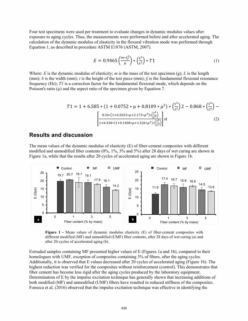
Four test specimens were used per treatment to evaluate changes in dynamic modulus values after exposure to aging cycles. Thus, the measurements were performed before and after accelerated aging. The calculation of the dynamic modulus of elasticity in the flexural vibration mode was performed through Equation 1, as described in procedure ASTM E1876 (ASTM, 2007).

𝐸𝐸 = 0.9465 𝑚𝑚∗𝑓𝑓𝑓𝑓

2

𝑏𝑏 ∗ 𝐿𝐿

3

𝑡𝑡3 ∗ 𝑇𝑇1 (1)

Where: E is the dynamic modulus of elasticity; m is the mass of the test specimen (g); L is the length (mm); b is the width (mm); t is the height of the test piece (mm); ff is the fundamental flexional resonance frequency (Hz); T1 is a correction factor for the fundamental flexional mode, which depends on the Poisson's ratio (µ) and the aspect ratio of the specimen given by Equation 7.

𝑇𝑇1 = 1 + 6.585 ∗ (1 + 0.0752 ∗ μ + 0.8109 ∗ 𝜇𝜇2) ∗ 𝑡𝑡2

𝐿𝐿22 − 0.868 ∗ 𝑡𝑡

4

𝐿𝐿4 −

8.34∗1+0.2023∗𝜇𝜇+2.173∗𝜇𝜇2∗𝑡𝑡

4

𝐿𝐿4

1+6.338∗(1+0.1408∗𝜇𝜇+1.536∗𝜇𝜇2)∗𝑡𝑡2

𝐿𝐿2 𝛼𝛼 (2)

Results and discussion

The mean values of the dynamic modulus of elasticity (E) of fiber-cement composites with different modified and unmodified fiber contents (0%, 1%, 3% and 5%) after 28 days of wet curing are shown in Figure 1a, while that the results after 20 cycles of accelerated aging are shown in Figure 1b.

Figure 1 - Mean values of dynamic modulus elasticity (E) of fiber-cement composites with different modified (MF) and unmodified (UMF) fiber contents, after 28 days of wet curing (a) and after 20 cycles of accelerated aging (b).

Extruded samples containing MF presented higher values of E (Figures 1a and 1b), compared to their homologues with UMF, exception of composites containing 3% of fibers, after the aging cycles. Additionally, it is observed that E values decreased after 20 cycles of accelerated aging (Figure 1b). The highest reduction was verified for the composites without reinforcement (control). This demonstrates that fiber cement has become less rigid after the aging cycles produced by the laboratory equipment. Determination of E by the impulse excitation technique has generally shown that increasing additions of both modified (MF) and unmodified (UMF) fibers have resulted in reduced stiffness of the composites. Fonseca et al. (2016) observed that the impulse excitation technique was effective in identifying the

19.7 20.7 19.1 19.117.9 16.1

14.2

0

5

10

15

20

25

0 1 3 5

E (G

pa)

Fiber content (% by mass)

Control MF UMF

a

11.9

17.4 16.7 15.9 16.614.5

13.6

0

5

10

15

20

25

0 1 3 5

E (G

pa)

Fiber content (% by mass)

Control MF UMF

b

630

influence of the inclusion of micro/nanofibrils on the stiffness of extrusion-produced fiber-cement composites. For the samples extruded with FMU the greatest residual percentage of E is observed when compared to its homologues with MF, as shown in Table 2.

Table 2 - Residual percentage of E of composites after 20 cycles of accelerated aging

Residual % of E

Control MF1% UMF1% MF3% UMF3% MF5% UMF5%

60.4 84.1 87.4 83.2 92.7 90.1 95.8

Additionally, it was found that the composites with the highest fiber content were the ones with the lowest E reduction after application of the accelerated aging cycles. This makes it possible to infer that the fibers help in less loss of E property after accelerated aging. At 28 days of cure, it was observed that the composites obtained E smaller when fibers (MF and FMU) were present. This may be associated with the greater volume of voids present in the fiber-reinforced composites, which alters the path of the mechanical waves, increasing the damping, increasing the amplitude of vibration in the resonance and the time of persistence of the vibration after ceasing the excitement. This fact justifies the reduction of the stiffness of cementitious materials when reinforced with fibers of cellulosic pulp. After accelerated aging, there is a reduction of E for all materials produced. Repeated cycles of irradiation, water spray and condensation, associated with changes in temperature, can contribute directly to physical, mechanical, microstructural and chemical modifications of fibro-cement composites. For composites without reinforcement, it is clearer that the aging cycles strongly contributed to drastic reduction of stiffness, indicating the occurrence of changes in this material. On the other hand, when fibers were present, such changes were milder, considering the lower residual percentage of E, especially for composites with 5% of fibers (Table 2).

Conclusions

Through this study it can be concluded that: - At 28 days, the modulus of dynamic elasticity (E) decreased with the addition and increase of thecontent of cellulose fibers in the fiber-cement composites;- After the 20 cycles of accelerated aging, the presence of fibers in the fiber-cement composites providedhigher "E";- It was found that modified fiber (MF) reinforced composites had higher means of "E" than non-modifiedfiber (UMF) reinforced homologues.- The addition of cellulose pulp fibers in cementations matrices allows for better mechanicalperformances of the composites after exposure to weathering conditions.

Acknowledgments

The authors are grateful for the support of the Reference Center for Nature Conservation and Recovery of Degraded Area (CRAD), and the financial support of the Foundation for Research Support of the Federal District (FAP-DF), Foundation for Research Support of Minas Gerais (FAPEMIG), National Council for Scientific and Technological Development (CNPq), and the Coordination of Improvement of Higher Education Personnel (CAPES). The authors also thank for Foundation of Scientific and Technological Developments (FINATEC) and Deanship of Graduate Studies (DPG/UnB) for travel funds which have made it possible to attend this conference.

631

References

American Society for Testing and Materials. ASTM 2006 G 154-6. Standard practice for operating fluorescent light apparatus for UV exposure of nonmetallic materials. ASTM International, West Conshohocken, PA, 2006.

American Society for Testing and Materials. ASTM 2007 E 1876: standard test method for dynamic young’s modulus, shear modulus and poisson’s ratio y impulse excitation of vibration. West Conshohocken, 2007..

Ardanuy, M.; Claramunt, J.; García-Hortal, J.A.; Barra, M. 2011. Fiber-matrix interactions in cement mortar composites reinforced with cellulosic fibers. Cellulose. 18: 281–289.

Farrapo, C.L.; Fonseca, C.S.; Perreira, T.G.T. [and others]. 2017. Cellulose associated with pet bottle waste in cement based composites. Materials Research. 20(5): 1380-1387.

Feiferis, A.R.; d’Almeida, J.R.M. 2016. Evaluation of Water Absorption Effects on the Mechanical Properties and Sound Propagation Behavior of Polyester Matrix- Sponge Gourd Reinforced Composite. Journal of Composites and Biodegradable Polymers. 4: 26-31.

Fonseca, C.S.; Silva, T.F.da; Silva, M.F.; [and others]. 2016. Micro/nanofibrilas celulósicas de Eucalyptus em fibrocimentos extrudados. Cerne. 22(1): 59-68.

Khan, M.I.; Abbas, Y.M.; Fares, G. 2017. Review of high and ultrahigh performance cementitious composites incorporating various combinations of fibers and ultrafines. Journal of King Saud University – Engineering Sciences. 29: 339–347.

Marques, M.G dos S.; Melo Filho, J. de A.; Molina, J.C. [and others]. 2014. Numerical-Experimental Assessment of the Arumã Fiber as Reinforcement to the Cementitious Matrix. Key Engineering Materials, 600: 460-468.

Martins Jr., J.R.S.; Matos, A.A.; Oliveira, R.C.; [and others]. 2018. Preparation and characterization of alloys of the Ti–15Mo–Nb system for biomedical applications. J Biomed Mater Res Part B. 1068(2): 639-648.

Minatto, F.D.; Alexandre, E. da S.; Noni Jr., A. de; Montedo, O.R.K. 2017. Estudo de composições cerâmicas à base de alumina e vitrocerâmico do sistema LZSA para obtenção de estruturas multicamadas por tape casting. Cerâmica, 63(366): 178-186.

Mohr, B.J.; Biernacki, J.J.; Kurtis, K.E. 2006. Microstructural and chemical effects of wet/dry cycling on pulp fiber–cement composites. Cement and Concrete Resource, 36: 1240–51.

Mohr, B.J.; Nanko, H.; Kurtis, K.E. 2005. Durability of kraft pulp fiber–cement composites to wet/dry cycling. Cement & Concrete Composites. 25: 435–48.

Monich, P.R.; Berti, F.V.; Porto, L.M.; [and others]. 2017. Physicochemical and biological assessment of PEEK composites embedding natural amorphous silica fibers for biomedical applications. Materials Science & Engineering: C. 79: 354-362.

632

Muñoz, V.; Analía G. 2016. Tomba Martinez. Factors controlling the mechanical behavior of alumina–magnesia–carbon refractories in air. Ceramics International. 42(9): 11150-11160.

Otani, L.B.; Pereira, A.H.A. 2017. Estimativa do módulo de elasticidade estático de concretos utilizando a Técnica de Excitação por Impulso - Informativo técnico-científico ITC-07. ATCP Engenharia Física, Divisão Sonelastic. Revisão 1.2. http://dx.doi.org/10.13140/RG.2.2.26010.24001

Otani, L.B.; Segundinho, P.G.A.; Morales, E.A.M.; Pereira, A.H.A. 2015. Caracterização dos módulos elásticos de madeiras e derivados utilizando a Técnica de Excitação por Impulso. ATCP Engenharia Física, Divisão Sonelastic. Revisão 1.3. http://dx.doi.org/10.13140/RG.2.1.4647.8242

Pickering, K.L.; Aruan Efendy, M.G.; Le, T.M.A. 2016. Review of recent developments in natural fiber composites and their mechanical performance. Composites: Part A. 83: 98–112.

Raabe, J.; Santos, L.P. dos; Del Menezzi, C.H.S.; Tonoli, G.H.D. 2018. Effect of nano-silica deposition on cellulose fibers on the initial hydration of the Portland cement. BioResources. 13(2): 3525-3544.

Vo, L.T.T.; Navard, P. Treatments of plant biomass for cementitious building materials – A review. Construction and Building Materials. 121: 161–176.

Wahab, A.; Aziz, M.M.A.; Sam, A.R.M. [and others]. 2019. Review on microwave nondestructive testing techniques and its applications in concrete technology. Construction and Building Materials. 209:135–146

633

Estimation of Elastic Properties of CLT Panels by Applying Transverse Vibration and Global Sensitivity Techniques

Alexander Opazo-Vega * Department of Civil and Environmental Engineering, Universidad del Bío-Bío, Concepción, Chile, aopazove@ubiobio.cl Department of Civil Engineering, Universidad Católica de la Santísima Concepcion, Concepcion, Chile, aopazo@doctorado.ucsc.cl

Claudio Oyarzo Vera Department of Civil Engineering, Universidad Católica de la Santísima Concepcion, Concepcion, Chile, coyarzov@ucsc.cl

Mario Nuñez Decap Department of Civil and Environmental Engineering, Universidad del Bío-Bío, Concepción, Chile, mnunez@ubiobio.cl

* Corresponding author

Abstract

Cross-laminated (CLT) panels are generating considerable interest in Chile due to its high potential to achieve the goals of sustainable construction in a country with high seismicity. Companies that are starting to manufacture CLT panels require evaluating the structural quality of their products to avoid post-sale problems. However, they need fast and non-destructive evaluation techniques that can be complemented with traditional mechanical tests. The study presented here aims to estimate the elastic mechanical properties of CLT panels by applying vibration based non-destructive methods. Three radiata pine CLT panels were built in the laboratory and subjected to a series of modal tests using low energy impacts as an excitation source. Modal properties of the CLT elements were estimated through Stochastic Subspace Identification (SSI) method. A series of finite element models of the panels were successively updating through regional sensitivity analysis (RSA) techniques until the differences between experimental and numerically simulated modal properties were minimal. The ranges of values obtained for some orthotropic elastic properties were quite close to those obtained with traditional destructive bending tests. Finally, the results suggest that this approach can be extended to more complicated CLT structures.

Keywords: xlam, massive timber, model updating, experimental modal analysis, orthotropic properties.

Introduction

Cross-laminated (CLT) panels are generating considerable interest in Chile due to its high potential to achieve the goals of sustainable construction in a country with high seismicity. Companies that are starting to manufacture CLT panels require evaluating the structural quality of their products to avoid

634

post-sale problems. However, they need fast and non-destructive evaluation techniques that can be complemented with traditional mechanical tests.

Based on the preceding, a series of non-destructive vibration-based assessment techniques for wood-based panels have emerged as an attractive alternative for both laboratory and field investigations (Steiger et al. 2012; Zhou et al. 2015; Giaccu et al. 2017; Guan et al. 2017; Zhou et al. 2017a; Zhou et al. 2017b). Combining these techniques with finite element model updating make it possible to estimate the elastic properties of this kind of elements. However, due to the inherent high heterogeneity of CLT panels (knots, orthotropic behavior, adhesion loss), it is necessary to perform complementary model updating analysis.

Global sensitivity analysis (GSA) is a technique suitable for updating model variables even in the case of high uncertainty about the material characteristics (Boscato et al. 2015). In general terms, GSA investigates how the variability in input factors affects the results of numerical models. GSA techniques considers the entire variability space of input factors. Hence, GSA model updating methods are less dependent initial conditions chosen for the input factors.

This paper describes a new approach to estimate the elastic properties of CLT panels based on the combination of operational modal analysis, model updating, and global sensitivity analysis. This new approach was applied to a set of CLT panel prototypes with the purpose of identifying some relevant orthotropic elastic properties that minimize the differences between numerical estimations and its experimental response.

Materials and Methods

CLT panel prototype description and instrumentation

The tested specimens consisted of 3 three-layer CLT panels, constructed with C24 grade Radiata Pine lumber boards with dimensions of 2400 mm in length, 120 mm in width and 30 mm in thickness, glued through different kind of adhesives. The configuration of the lumber boards had a typical cross laminated arrangement. The final nominal dimensions of the panels were 2400 mm long, 400 mm wide and 90 mm thick. Table 1 shows the construction details of the CLT panels tested.

Table 1—Construction characteristics of CLT panels

Panel number

Dimensions Density (kg/m3)

Gluing length (mm)

width (mm)

thickness (mm) face edge

1 2400 400 91.26 473.71 PUR ULXJ-803 MD-33812 2400 394 90.24 467.58 PUR 5082 PUR 5089 3 2400 394 90.26 468.64 PUR 5082 n/a

This study aimed to analyse the out-of-plane behaviour of the panel. Therefore, ten low energy impacts were applied perpendicular to the plane of the panel and eight uniaxial accelerometers were installed in the same direction. The objective of this setup was to identify the first two out-of-plane modes of the specimen. A typical CLT panel and its instrumentation are presented in Figure 1.

635

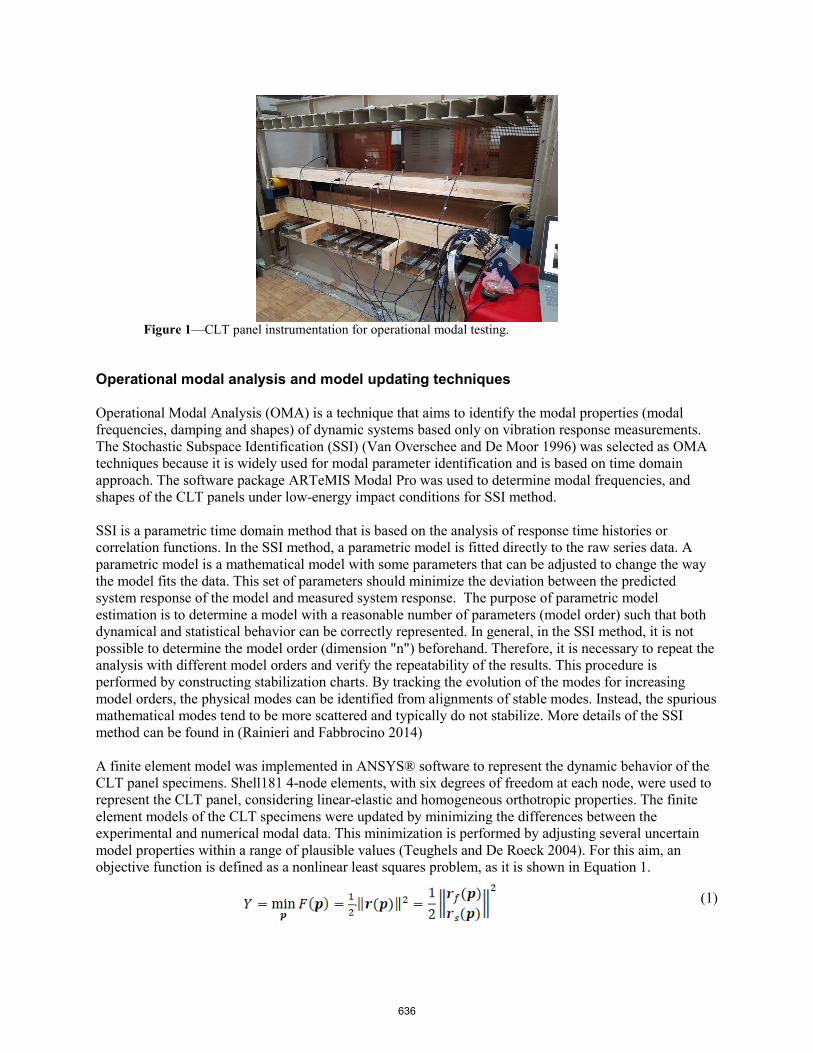
Figure 1—CLT panel instrumentation for operational modal testing.

Operational modal analysis and model updating techniques

Operational Modal Analysis (OMA) is a technique that aims to identify the modal properties (modal frequencies, damping and shapes) of dynamic systems based only on vibration response measurements. The Stochastic Subspace Identification (SSI) (Van Overschee and De Moor 1996) was selected as OMA techniques because it is widely used for modal parameter identification and is based on time domain approach. The software package ARTeMIS Modal Pro was used to determine modal frequencies, and shapes of the CLT panels under low-energy impact conditions for SSI method.

SSI is a parametric time domain method that is based on the analysis of response time histories or correlation functions. In the SSI method, a parametric model is fitted directly to the raw series data. A parametric model is a mathematical model with some parameters that can be adjusted to change the way the model fits the data. This set of parameters should minimize the deviation between the predicted system response of the model and measured system response. The purpose of parametric model estimation is to determine a model with a reasonable number of parameters (model order) such that both dynamical and statistical behavior can be correctly represented. In general, in the SSI method, it is not possible to determine the model order (dimension "n") beforehand. Therefore, it is necessary to repeat the analysis with different model orders and verify the repeatability of the results. This procedure is performed by constructing stabilization charts. By tracking the evolution of the modes for increasing model orders, the physical modes can be identified from alignments of stable modes. Instead, the spurious mathematical modes tend to be more scattered and typically do not stabilize. More details of the SSI method can be found in (Rainieri and Fabbrocino 2014)

A finite element model was implemented in ANSYS® software to represent the dynamic behavior of the CLT panel specimens. Shell181 4-node elements, with six degrees of freedom at each node, were used to represent the CLT panel, considering linear-elastic and homogeneous orthotropic properties. The finite element models of the CLT specimens were updated by minimizing the differences between the experimental and numerical modal data. This minimization is performed by adjusting several uncertain model properties within a range of plausible values (Teughels and De Roeck 2004). For this aim, an objective function is defined as a nonlinear least squares problem, as it is shown in Equation 1.

(1)

636

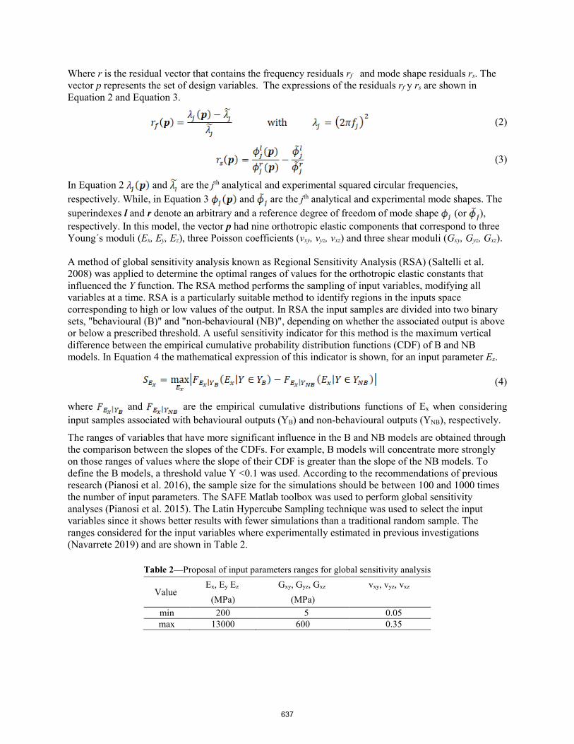
Where r is the residual vector that contains the frequency residuals rf and mode shape residuals rs. The vector p represents the set of design variables. The expressions of the residuals rf y rs are shown in Equation 2 and Equation 3.

(2)

(3)

In Equation 2 and are the jth analytical and experimental squared circular frequencies, respectively. While, in Equation 3 and are the jth analytical and experimental mode shapes. The superindexes l and r denote an arbitrary and a reference degree of freedom of mode shape (or ), respectively. In this model, the vector p had nine orthotropic elastic components that correspond to three Young´s moduli (Ex, Ey, Ez), three Poisson coefficients (vxy, vyz, vxz) and three shear moduli (Gxy, Gyz, Gxz).

A method of global sensitivity analysis known as Regional Sensitivity Analysis (RSA) (Saltelli et al. 2008) was applied to determine the optimal ranges of values for the orthotropic elastic constants that influenced the Y function. The RSA method performs the sampling of input variables, modifying all variables at a time. RSA is a particularly suitable method to identify regions in the inputs space corresponding to high or low values of the output. In RSA the input samples are divided into two binary sets, "behavioural (B)" and "non-behavioural (NB)", depending on whether the associated output is above or below a prescribed threshold. A useful sensitivity indicator for this method is the maximum vertical difference between the empirical cumulative probability distribution functions (CDF) of B and NB models. In Equation 4 the mathematical expression of this indicator is shown, for an input parameter Ex.

(4)

where and are the empirical cumulative distributions functions of Ex when considering input samples associated with behavioural outputs (YB) and non-behavioural outputs (YNB), respectively.

The ranges of variables that have more significant influence in the B and NB models are obtained through the comparison between the slopes of the CDFs. For example, B models will concentrate more strongly on those ranges of values where the slope of their CDF is greater than the slope of the NB models. To define the B models, a threshold value Y <0.1 was used. According to the recommendations of previous research (Pianosi et al. 2016), the sample size for the simulations should be between 100 and 1000 times the number of input parameters. The SAFE Matlab toolbox was used to perform global sensitivity analyses (Pianosi et al. 2015). The Latin Hypercube Sampling technique was used to select the input variables since it shows better results with fewer simulations than a traditional random sample. The ranges considered for the input variables where experimentally estimated in previous investigations (Navarrete 2019) and are shown in Table 2.

Table 2—Proposal of input parameters ranges for global sensitivity analysis

Value Ex, Ey Ez Gxy, Gyz, Gxz vxy, vyz, vxz

(MPa) (MPa) min 200 5 0.05 max 13000 600 0.35

637

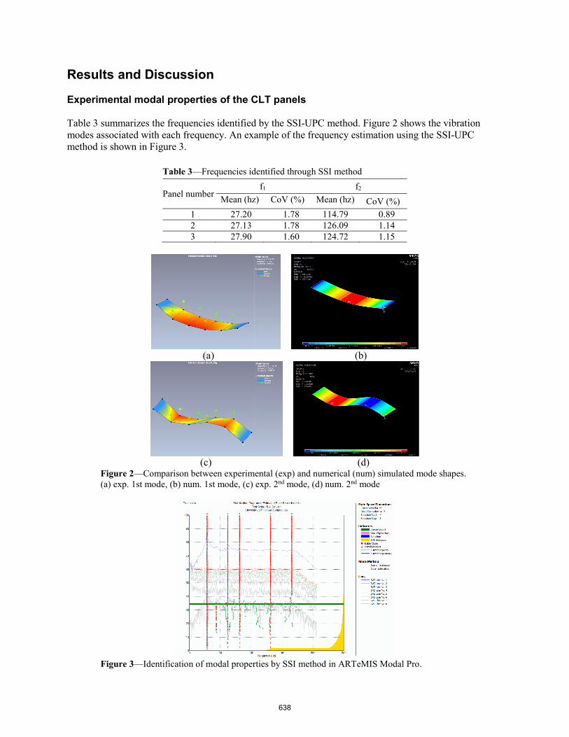
Results and Discussion

Experimental modal properties of the CLT panels

Table 3 summarizes the frequencies identified by the SSI-UPC method. Figure 2 shows the vibration modes associated with each frequency. An example of the frequency estimation using the SSI-UPC method is shown in Figure 3.

Table 3—Frequencies identified through SSI method

Panel number f1 f2

Mean (hz) CoV (%) Mean (hz) CoV (%) 1 27.20 1.78 114.79 0.89 2 27.13 1.78 126.09 1.14 3 27.90 1.60 124.72 1.15

(a) (b)

(c) (d) Figure 2—Comparison between experimental (exp) and numerical (num) simulated mode shapes. (a) exp. 1st mode, (b) num. 1st mode, (c) exp. 2nd mode, (d) num. 2nd mode

Figure 3—Identification of modal properties by SSI method in ARTeMIS Modal Pro.

638

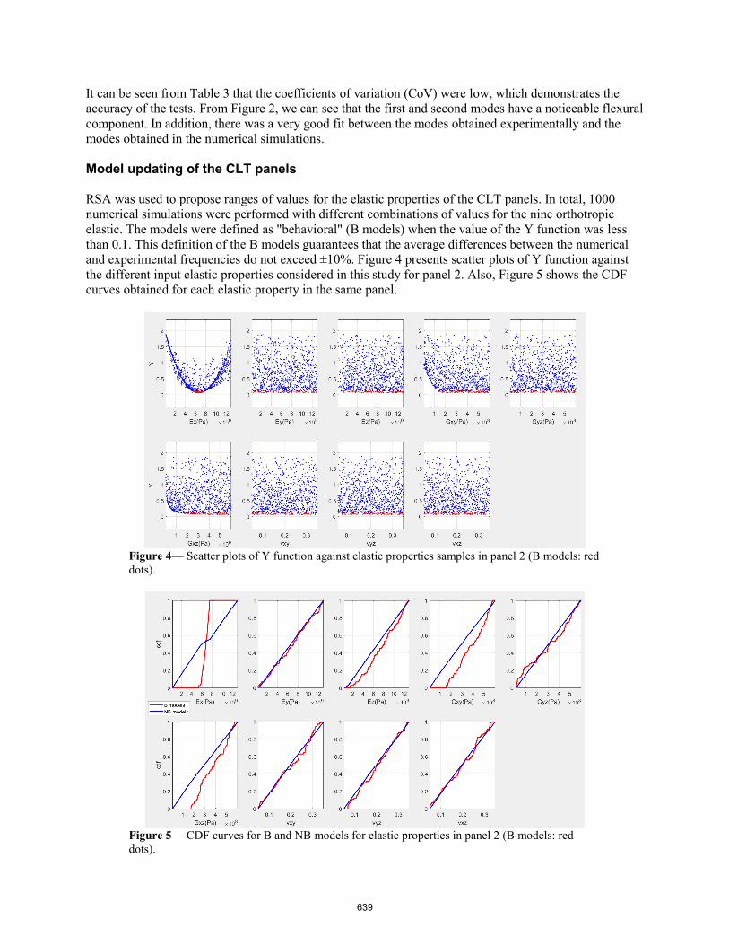
It can be seen from Table 3 that the coefficients of variation (CoV) were low, which demonstrates the accuracy of the tests. From Figure 2, we can see that the first and second modes have a noticeable flexural component. In addition, there was a very good fit between the modes obtained experimentally and the modes obtained in the numerical simulations.

Model updating of the CLT panels

RSA was used to propose ranges of values for the elastic properties of the CLT panels. In total, 1000 numerical simulations were performed with different combinations of values for the nine orthotropic elastic. The models were defined as "behavioral" (B models) when the value of the Y function was less than 0.1. This definition of the B models guarantees that the average differences between the numerical and experimental frequencies do not exceed ±10%. Figure 4 presents scatter plots of Y function against the different input elastic properties considered in this study for panel 2. Also, Figure 5 shows the CDF curves obtained for each elastic property in the same panel.

Figure 4— Scatter plots of Y function against elastic properties samples in panel 2 (B models: red dots).

Figure 5— CDF curves for B and NB models for elastic properties in panel 2 (B models: red dots).

639

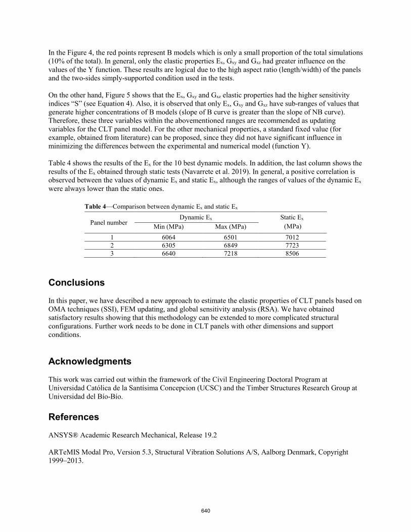
In the Figure 4, the red points represent B models which is only a small proportion of the total simulations (10% of the total). In general, only the elastic properties Ex, Gxy and Gxz had greater influence on the values of the Y function. These results are logical due to the high aspect ratio (length/width) of the panels and the two-sides simply-supported condition used in the tests.

On the other hand, Figure 5 shows that the Ex, Gxy and Gxz elastic properties had the higher sensitivity indices “S” (see Equation 4). Also, it is observed that only Ex, Gxy and Gxz have sub-ranges of values that generate higher concentrations of B models (slope of B curve is greater than the slope of NB curve). Therefore, these three variables within the abovementioned ranges are recommended as updating variables for the CLT panel model. For the other mechanical properties, a standard fixed value (for example, obtained from literature) can be proposed, since they did not have significant influence in minimizing the differences between the experimental and numerical model (function Y).

Table 4 shows the results of the Ex for the 10 best dynamic models. In addition, the last column shows the results of the Ex obtained through static tests (Navarrete et al. 2019). In general, a positive correlation is observed between the values of dynamic Ex and static Ex, although the ranges of values of the dynamic Ex were always lower than the static ones.

Table 4—Comparison between dynamic Ex and static Ex

Panel number Dynamic Ex Static Ex

(MPa) Min (MPa) Max (MPa) 1 6064 6501 7012 2 6305 6849 7723 3 6640 7218 8506

Conclusions

In this paper, we have described a new approach to estimate the elastic properties of CLT panels based on OMA techniques (SSI), FEM updating, and global sensitivity analysis (RSA). We have obtained satisfactory results showing that this methodology can be extended to more complicated structural configurations. Further work needs to be done in CLT panels with other dimensions and support conditions.

Acknowledgments

This work was carried out within the framework of the Civil Engineering Doctoral Program at Universidad Católica de la Santísima Concepcion (UCSC) and the Timber Structures Research Group at Universidad del Bío-Bío.

References

ANSYS® Academic Research Mechanical, Release 19.2

ARTeMIS Modal Pro, Version 5.3, Structural Vibration Solutions A/S, Aalborg Denmark, Copyright 1999–2013.

640

Boscato, G.; Russo, S.; Ceravolo, R. [and others]. 2015. Global sensitivity‐based model updating for heritage structures. Computer‐Aided Civil and Infrastructure Engineering. 30(8): 620-635

Giaccu, G. F.; Meloni, D.; Valdès, M. [and others]. 2017. Dynamic determination of the modulus of elasticity of maritime pine cross-laminated panels using vibration methods. WIT Transactions on Ecology and the Environment. 226: 571-579.

Guan, C.; Zhang, H.; Wang, X. [and others]. 2017. Experimental and Theoretical Modal Analysis of Full-Sized Wood Composite Panels Supported on Four Nodes. Materials. 10(6): 683.

Navarrete, A. 2019. Estudio del tipo de adhesivo estructural y del encolado de canto sobre las propiedades mecanicas de la madera contralaminada. Concepcion: Universidad del Bío-Bío. Civil Engineering thesis.

Pianosi, F.; Sarrazin, F.; Wagener, T. 2015. A Matlab toolbox for global sensitivity analysis. Environmental Modelling & Software. 70: 80-85.

Pianosi, F.; Beven, K.; Freer, J. [and others]. 2016. Sensitivity analysis of environmental models: A systematic review with practical workflow. Environmental Modelling & Software. 79: 214-232.

Rainieri, C.; Fabbrocino, G. 2014. Operational modal analysis of civil engineering structures. 1st ed.; New York: Springer: 103-210.

Saltelli, A., Ratto, M.; Andres, T. [and others]. 2008. Global sensitivity analysis: the primer. John Wiley & Sons.

Steiger, R.; Gülzow, A.; Czaderski, C. [and others]. 2012. Comparison of bending stiffness of cross-laminated solid timber derived by modal analysis of full panels and by bending tests of strip-shaped specimens. European Journal of Wood and Wood Products. 70(1): 141-153.

Teughels, A.; De Roeck, G. 2004. Structural damage identification of the highway bridge Z24 by FE model updating. Journal of Sound and Vibration. 278(3): 589-610.

Van Overschee, P.; De Moor, B.L. 1996. Subspace identification for linear systems: Theory—Implementation—Applications, 1st ed.; The Netherlands, Dordrecht: Kluwer Academic Publishers: 55-91.

Zhou, J.; Chui, Y. H.; Gong, M. [and others]. 2015. Simultaneous measurement of elastic constants of full-size engineered wood-based panels by modal testing. Holzforschung. 70(7): 673–682.

Zhou, J.; Chui, Y. H.; Gong, M. [and others]. 2017b. Elastic properties of full-size mass timber panels: Characterization using modal testing and comparison with model predictions. Composites Part B: Engineering. 112: 203-212.

641

Delamination Detection in Cross-Laminated Timber Panels Using Ultrasound and Resistograph Tools Xiping Wang USDA Forest Service, Forest Products Laboratory, Madison, Wisconsin, USA, xiping.wang@ usda.gov Robert J. Ross USDA Forest Service, Forest Products Laboratory, Madison, Wisconsin, USA, robert.j.ross@usda.gov Michigan Technological University, Houghton, Michigan, USA Mississippi State University, Starkville, Mississippi, USA Brian K Brashaw USDA Forest Service, Forest Products Laboratory, Madison, Wisconsin, USA, brian.k.brashaw@ usda.gov Xiaoquan Yue College of Transportation and Civil Engineering, Fujian Agriculture and Forestry University, Fuzhou, Fujian, China, yxqzrh@foxmail.com Fenglu Liu School of Technology, Beijing Forestry University, Beijing, China, liufenglu39@126.com Xi Wu School of IoT Engineering, Jiangnan University, Wuxi, Jiangsu, China, xw20170909@gmail.com Abstract Cross-laminated timber (CLT) as a novel engineered wood product has gained acceptance in both residential and commercial structural applications, particularly in tall timber building construction. With the rapid development of CLT manufacturing capacity around the world, concerns arise on the quality assurance of adhesive bonding in CLT manufacturing. The recent failure of a CLT floor panel during a new building construction in the United States indicates the need for developing reliable and advanced nondestructive methods for monitoring bonding performance of CLT panels in production and during service. The objective of this study was to examine the feasibility of using ultrasound waves and resistance micro-drilling techniques to detect poor bonding and delamination in CLT panels. Four five-ply and six seven-ply CLT test panels with the sizes ranging from 91- by 60- cm (3- by 2-ft.) to 91- by 122-cm (3- by 4-ft) were obtained from the construction site. The test panels were visually identified as “good,” “bad,” and “iffy” by construction engineers. Upon arrival at the laboratory, grid lines (51- by 51-cm or 102- by 102-cm) were drawn on each test panel and ultrasound transmission times (UTTs) were obtained through thickness at each grid point. The measured UTT data was then converted to a value of time per unit thickness (µs/m). An UTT contour map was subsequently developed for each test panel. A Resistograph tool was used to perform resistance micro-drilling tests on selected locations of the test panels and a resistance profile was obtained for each test point. The results indicated that UTT measurement was able to detect the spots or areas that had no glue or poor bonding. However, the resistance profiles failed to identify delamination and small air gaps between the laminations.

Keywords: Adhesive bond, cross-laminated timber, delamination, inspection, ultrasound, micro-drilling resistance.

642

Utility of Image Software in Quantification of Termite Damage on Cross-Laminated Timber (CLT) Tamara S.F.A. França* Department of Sustainable Bioproducts, Mississippi state University, Mississippi State University, Mississippi, USA, tsf97@msstate.edu C. Elizabeth Stokes Department of Sustainable Bioproducts, Mississippi state University, Mississippi State University, Mississippi, USA, ces8@msstate.edu Juliet D. Tang USDA Forest Service, Forest Products Laboratory, Starkville, Mississippi, USA, juliet.d.tang@usda.gov Rachel A. Arango USDA Forest Service, Forest Products Laboratory, Madison, Wisconsin, USA, rrachel.arango@usda.gov * Corresponding author Abstract Cross Laminated Timber (CLT) is part of a new generation of engineered wood products that are now widespread across Europe, Australia, and Canada. As this trend is now growing in the United States, manufacturers are looking to expand the use of CLT into the North American market, which includes states located in the southeastern U.S. As this region is known to have an increased risk of termite attack, standards should be developed to evaluate termite damage on CLT products prior to extensive use of the product in this region. However, existing standard test methods cannot be applied directly to CLT specimens as current standard test sample sizes are too small to adequately represent CLT constructed materials. Therefore, larger sample sizes were examined to determine resistance of CLT products against termite attack. Large sample size made it difficult to evaluate termite damage using weight loss as a variable as termite damaged specimens showed relatively low weight loss values. The objective of this work was to examine the use of the image analysis software, ImageJ, in determining the extent of termite damage on CLT blocks. Results showed that evaluation of void volume percent could be used in conjunction with weight loss and visual rating to obtain a more accurate measurement of overall termite damage in CLT. Keywords: mass timber products, subterranean termites, image measurements, mass loss. Introduction Cross-laminated timber or CLT is a mass timber product that was first developed in Austria in the 1990s and has since expanded through the European construction market. As CLT is manufactured with wood, which is a renewable material, it is seen as highly desirable in the ‘green’ building movement (Singh and Page, 2016). The volume of lumber used in the material allows for a high level of carbon sequestration within a structure, a highly desirable characteristic in today’s sustainable-focused construction market. Additionally, CLT provides all the excellent characteristics associated with wood products including a

643

high strength to weight ratio, an exceptional sound insulator, and a significantly lower carbon footprint than steel and concrete (Smyth, 2018). These panels can compete with pre-cast concrete, as they can be handled on-site, and are lower in weight compared to concrete which makes CLT ideal for rapid construction of modular buildings, including apartment/condominium structures (Van de Kuilen et al., 2011). Due to the strong establishment of CLT in Europe, investors are searching for new markets and growth opportunities (Grasser, 2015). Recently, it has become common to find CLT buildings proposed in the mid-rise and tall building construction market in Canada and northwestern parts of the U.S (CLT Handbook, 2013). As the adoption of CLT construction expands, so does the need for research focused on specific regional hazards or conditions. To date, studies conducted with CLT panels are mainly focused on seismic design factors, elastic properties, responses to fire, structural properties, and strength properties (Steiger et al., 2008; Frangi et al., 2009; Gulzow et al., 2009; Ceccotti et al., 2010; Popvski and Karacabeyli, 2012; Pei et al., 2012; Gavric et al., 2013; Shen et al., 2013; Cao et al., 2019). However, limited studies have evaluated the resistance of CLT to termite attack in laboratory assays (França et al., 2018a; França et al., 2018b). Because CLT is a new product in the market and is a mass timber product, there is a need to not only determine specific vulnerabilities of the product to termite damage, but also develop new methods to measure termite damage. The goal of this study was to modify existing test small sample size methods to be used for evaluating the resistance of CLT to termite feeding and to assess the use of image analysis for prediction of product resistance to termite attack. Material and Methods AWPA Standard E1-17 (AWPA, 2019) was selected as the basis for the test design. However, this protocol uses a smaller specimen size that would not be representative of a CLT panel, so it was determined that the product should be tested using its full thickness. An assay was developed specifically for testing mass timber products. Modifications included sample size, size of test container, amount of sand and water added to the test containers, number of termites, and the test duration (Table 1). Table 1. Modifications made to the AWPA Standard E1-17 test method for evaluating termite damage to CLT materials. AWPA Standard Modifications for evaluation of CLT Wood sample size 2.5 cm x 2.5 cm x 0.6 cm (1 in x 1 in

x ¼ in) 10 cm x 10 cm x 2.5 cm (4 in x 4 in x 1 in)

Test container 80 x 100 mm glass screw-top jars 4 L food-safe container Amount of sand/water 150g/27mL 1000g/180 mL Number of termites 400 1000 Test duration 4 weeks 4 weeks

A total of five replicates were cut from 3-ply pine/spruce/fir CLT panels obtained from a commercial manufacturer. Samples were placed in test containers and exposed to feeding by the eastern subterranean termites, Reticulitermes sp. for 4 weeks. For this test, food-safe containers (4 L capacity) were used. All test specimens were oven dried at 60°C until constant weight was reached and weighed both before and after the exposure period to determine mass loss. At the end of each test, percent mass loss was determined for the CLT block, and each block was examined and visually rated using the AWPA E1 visual ratings (Table 2). Additionally, the CLT block face in contact with sand substrate of each specimen was photographed and the digital images were

644

analyzed using ImageJ software (Version 1.32j, US National Institutes of Health, Bethesda, Maryland; Rasband 2004). On each image, areas of termite feeding, and outer boundaries were manually outlined on the digital image and used to calculate percentage of the block face damaged by termites. Table 2. Visual rating system according to AWPA Standard E1-17 (AWPA, 2019)

Visual rating classification Rating Sound 10 Trace, surface nibbles permitted 9.5 Slight attack, up to 3% of cross-sectional area affected 9 Moderate attack 3–10 % of cross-sectional area affected 8 Moderate/severe attack, penetration, 10–30%, of cross-sectional area affected 7 Severe attack, 30–50% of cross-sectional area affected 6 Very severe attack, 50–75% of cross-sectional area affected 4 Failure 0

Results and Discussion The AWPA E1 Standard is used to evaluate the resistance of wood materials to subterranean termites. This standard uses small sized samples (2.5 cm x 2.5 cm x 0.6 cm), and mass loss calculations are easy to determine. Figure 1 shows a comparison between the size of the CLT test sample used in this study and the test sample used in the AWPA E1-17 Standard (AWPA, 2019). Figure 1. Comparison between samples: (a) CLT test block face with dimensions of 10 cm x 10 cm x 2.5 cm; (b) AWPA E1-17 cross-section with sample size of 2.5 cm x 2.5 cm x 0.6 cm Table 3 shows visual ratings, percent mass loss and percentage of termite damage to the CLT block face as measured by ImageJ analysis. Studies evaluating the resistance of pine, spruce and fir alone using AWPA E1-17 (2019) sample dimensions showed mass loss percentages around 40%, 23%, and 25%, respectively (Arango et al., 2006; Kose and Tylor, 2012; França et al., 2016). However, the mass loss on CLT is harder to detect since the sample size is so large relative to the amount of wood consumed by termites and scaling up the termites would require adding more termites than was feasible to collect. The average mass loss of CLT samples in this study was 1.7% (Table 3). These results are in accordance with

A

B

645

other studies that evaluated the resistance of CLT to termites, which showed a mass loss percentage of approximately 1.5% (França et al., 2018a; França et al., 2018b). Table 3. Data summary for visual rating, percent mass loss, and percent cross section damaged measured with ImageJ software for CLT samples exposed to Reticulitermes sp.

Sample ID Mass Loss (%) Visual Rating Cross sectional area damaged* (%)

1 1.6 6 24.3 2 1.3 6 30.2 3 2.0 6 30.2 4 2.0 6 36.2 5 1.6 6 32.2

*Calculated using ImageJ software. The visual rating system described in the AWPA E1-17 (2019) Standard is based on small sample size dimensions. When CLT samples were evaluated using this system, it required a level of consideration and experience to accurately determine the degree of termite damage on larger specimens. After testing, specimens exposed to termites were classified according to the visual rating system described in AWPA E1-17 (2019). All CLT specimens exposed to termites received a score of 6, which is considered severe attack with 30 to 50% of cross-sectional area affected (Table 3). However, when samples were analyzed with ImageJ software, it showed that specimen 1 would have been graded as 7 with moderate/severe attack and penetration, having 10 to 30% of sectional area affected. A contrast based on mass loss percentages was also found after evaluation of the images. Samples 3 and 4 showed the highest mass loss (2.0% for both samples). ImageJ analysis, however, showed that samples 4 (36.2%) and 5 (32.2%) had substantial damaged area percentages, while sample 3 showed a 30.2% damaged area, similar to sample 2. Figure 2 shows the five CLT block faces that were in contact with sand substrate during the test. By a simple visual comparison of these images, it is not visually apparent that samples 3 and 4 were the samples with highest mass loss percentage.

646

Figure 2. CLT samples exposed for four weeks: 1 to 5 = specimens exposed to Reticulitermes sp.; 6 = control sample. Previous studies show that image software analyses can be useful to determine termite and decay damage, influence of treatments on wood, and other tests where mass loss does not fully describe the amount of damage. Lebow et al. (2010a, 2013b) used ImageJ to determine preservative formulation, wood moisture content, and diffusion time after treatment of borate penetration in framing lumber of southern pine species. Arango et al. (2016) used image software to evaluate if laser marking on dip-treatment blocks increased susceptibility to termite feeding. The authors evaluated termite damage by percent of surface attack using ImageJ software rather than weight loss due to the large size of specimens. Kim and Lloyd (2017) also used ImageJ to determine diffusion of borate inside bridge ties. Conclusions Cross-laminated timber is a new generation of engineered wood product, and it has attracted the attention of investors to expand its use throughout the southeastern U.S. wood market. CLT is gaining prominence in the wood industry and provides the same benefits that other wood products do including thermal insulation properties, cost effectiveness, environmental advantages, and less waste than other building materials including steel and concrete. Most studies conducted on CLT panels are focused on evaluation of mechanical properties. However, as a wood material, CLT panels are susceptible to biological degradation, and it is extremely important to understand the resistance of this product to biological agents such as termites. To better evaluate the performance of CLT products against termite attack, modifications to the AWPA E1-17 (AWPA, 2019) standard are needed, and new methods should be created to better predict the natural resistance of this new product. Since larger specimens are needed to properly simulate mass

1 2 3

4 5 6

647

timber product materials, mass loss data alone does not appear to be the most accurate way to describe damage throughout the product. CLT test blocks can be evaluated using the visual rating system used by the AWPA E1-17 Standard, but evaluation requires more experience from the grader due to the non-standard sample size. Surface excavations from termites can be visualized easily, but it is more difficult to quantify internal tunneling to the mass of wood. The use of other techniques such as image software analysis combined with weight loss and visual evaluation, appear to be a better combination than mass loss data or visual rating only. Future research will be conducted to create technologies to facilitate the examination of termite activity on CLT products in-use. References American Wood Protection Association (AWPA). 2019. Laboratory methods for evaluating the termite resistance of wood-based materials. Standard E1-17. AWPA book of standards. American Wood Protection Association, Birmingham, AL. Arango, R.A.; Green, F.; Hintz, K.; Lebow P.K.; Miller R.B. 2006. Natural durability of tropical and native woods against termite damage by Reticulitermes flavipes (Kollar). International Biodeterioration & Biodegradation, 57:46–150. Arango, R.A.; Woodward, B.M.; Lebow, S.T. 2016. Evaluating the effects of post dip-treatment laser marking on resistance to feeding by subterranean termites. In: Proceedings IRG Annual Meeting (ISSN 2000-8953) 2016 The International Research Group on Wood Protection; IRG/WP 16-10854 The International Research Group on Wood Protection; Section 1 Biology. Cao, Y.; Street, J.; Li, Minghao, L.; Hyungsuk, L. 2019. Evaluation of the effect of knots on rolling shear strength of cross laminated timber (CLT). Construction and Building Materials, 222(20):579–587. Ceccotti, A.; Sandhaas, C.; and Yasumura, M. 2009. Seismic behavior of multistory cross-laminated timber buildings. In: International Convention of Society of Wood Science and Technology, Geneva, Switzerland CSA S-16. (2009). Design of Steel Structures. Ottawa: Canadian Standards Association. 2010. CLT Handbook: cross-laminated timber (US Edition). 2013. E. Karacebeyli and B. Douglas ed. Special Publication SP-529E. 572 pp. França, T.S.F.A.; França, F.J.N.; Arango, R.A.; Woodward, B.M.; Arantes, M.D.C. 2016. Natural resistance of plantation grown African mahogany (Khaya ivorensis and Khaya senegalensis) from Brazil to wood-rot fungi and subterranean termites. International Biodeterioration & Biodegradation, 107:88–91. França, T.S.F.A.; Stokes, C.E.; Tang, J.D. 2018a. Durability of cross laminated timber against termite damage. In: Proceedings, 61st international convention of society of wood science and technology and Japan wood research society. Monona, WI: Society for Wood Science and Technology. 10 p. França, T.S.F.A.; Stokes, C.E.; Tang, J.D. 2018b. Evaluation of cross-laminated timber resistance to termite attack. In: Proceedings of the American Wood Protection Association Annual Meeting. 114:266–271.

648

Frangi, A.; Fontana M.; Hugi, E.; and Jübstl R. 2009. Experimental analysis of cross-laminated timber panels in fire. Fire Safety Journal 44(8):078–1087. Gavric, I.; Fragiacomo M.; Popovski M.; and Ceccotti, A. 2014. Behaviour of cross-laminated timber panels under cyclic loads. In: Materials and Joints in Timber Structures, pp. 689-702. Springer Netherlands. Grasser, K.K. 2015. Development of Cross Laminated Timber in the United States of America. Knoxville, TN: University of Tennessee. 115 p. M.S. thesis. Gülzow, Arne, Klaus Richter, and René Steiger. 2011. Influence of wood moisture content on bending and shear stiffness of cross laminated timber panels. European Journal of Wood and Wood Products 69(2): 193-197. Kim, J.W.; and Lloyd, J.D. 2017. Borate and Copper Naphthenate Dual Treatment of Bridge Timbers-Borate movement over time. In: Proceedings IRG Annual Meeting (ISSN 2000-8953) 2017 The International Research Group on Wood Protection; IRG/WP 17-40795 The International Research Group on Wood Protection; Section 4 Processes and properties… Kose, C.; Tylor, A.M. 2012. Evaluation of mold and termite resistance of included sapwood in eastern redcedar. Wood and Fiber Science, 44(3):319–324. Lebow, S.T.; Lebow, P.K.; Halverson, S.A. 2010a. Penetration of boron from topically applied borate solutions. Forest Products Journal, 60(1):13–22. Lebow, S.T.; Lebow, P.K.; Halverson, S.A. 2012b. Boron diffusion in surface-treated framing lumber. Forest Products Journal, 63(7/8):275–282. Pei, S.; Van de Lindt J.W.; and Popovski M. 2012. Approximate R-factor for cross-laminated timber walls in multistory buildings. Journal of Architectural Engineering 19(4):245–255. Popovski, M.; and Karacabeyli E. 2012. Seismic behavior of cross-laminated timber structures. In Proceedings of the World Conference on Timber Engineering, Auckland, New Zealand. Rasband, W. S. 2004. ImageJ. US National Institutes of Health, Bethesda, Maryland. http://rsb.info.nih.gov/ij. Singh, T.; Page, D. 2016. The durability of manufactured structural building materials. Proceedings IRG-WP Annual Meeting. ISSN 2000-8953. Shen, Y.; Schneider, L.; Tesfamariam, S.; Stiemer, S.F.; and Mu, Z. 2013. Hysteresis behavior of bracket connection in cross-laminated-timber shear walls. Construction and Building Materials 48:980–991. Steiger, R.; Gülzow, A.; and Gsell, D. 2008.Non-destructive evaluation of elastic material properties of cross-laminated timber (CLT). In: Conference COST E, 53:29-30. Smyth, M. 2018. Cross laminated timber for residential construction. Stockholm, Sweden: KTH Royal Institute of Technology. 95 p. M.S. thesis. Van de Kuilen, J.W.G.; Ceccotti, A.; Zhouyan X.; Minjuan H. 2011. Very tall wooden buildings with cross laminated timber. Procedia Engineering 14:1621–1628.

649

Poster Session

650

Machine Developed for Nondestructive Cyclic Bending Tests of Wood

Pablo Altoé Amorim * Mechanical Engineering Department, Centro Universitário FAESA, Av. Vitória, 2220, 29053-360 Vitória, ES, Brazil, pablo.altoe@faesa.br

Lorenzo Lube dos Santos Mechanical Engineering Department, Centro Universitário FAESA, Av. Vitória, 2220, 29053-360 Vitória, ES, Brazil, lorenzo.lube@faesa.br

Victor Hugo Moreira Salles Mechanical Engineering Department, Universidade Federal do Espírito Santo, Av. Fernando Ferrari, 514, 29075-910 Vitória, ES, Brazil, victor.hugoms@outlook.com

Gustavo Soares Krohling Mechanical Engineering Department, Universidade Federal do Espírito Santo, Av. Fernando Ferrari, 514, 29075-910 Vitória, ES, Brazil, gustavokroh@gmail.com

Isabela Lovatti Dalvi Mechanical Engineering Department, Universidade Federal do Espírito Santo, Av. Fernando Ferrari, 514, 29075-910 Vitória, ES, Brazil, isabeladalvi@hotmail.com

* Corresponding author

Abstract

Changes in mechanical properties of materials caused by cyclic loads are well known and have been the objective of study for a long time. For wood-based structures, one key property is the elastic modulus (Young’s modulus) because it is strictly correlated with stress calculus in beams. It is known that wood materials suffer a greater change in elastic modulus than other materials, such as metals and ceramics. Whereas static tests are well studied and described by norms (e.g. ISO 13910, Brazilian standard NBR 7190, and EURONORM), there is a lack of standardization in determining the loss of elasticity in wood beams caused by cyclic loads. This paper presents a machine designed for an also proposed methodology for nondestructive determination of elastic modulus change/stiffness loss in wood specimens subject to cyclic loads. Both the structure and equipment were designed to allow minimal deformation and error on specimen deflection under 1%. The machine consists of a rod that applies a load to the test specimen. The specimen is a simply supported beam. Both deflection (load) and oscillation frequency are adjustable, allowing deflections up to 10 mm in specimens with cross section of 2,500 mm2. Differential of this methodology is the compatibility of the specimen with ISO and the Brazilian standard for further testing of static properties.

Keywords: Wood, beam, cyclic load, machine, equipment, nondestructive test

651

Use of Impulse Tomography to Analyze the Health of Planted Trees on Carahá River Banks, Lages-SC, Brazil Alexsandro Bayestorff da Cunha * Forestry Department, Santa Catarina State University, Lages, Santa Catarina, Brazil, alexsandro.cunha@udesc.br Vinícius Steffen De Betio Forestry Department, Santa Catarina State University, Lages, Santa Catarina, Brazil, viniciusengfl@gmail.com Carolina Alves Carvalho Forestry Department, Santa Catarina State University, Lages, Santa Catarina, Brazil, carol.carvalho3@hotmail.com Ricardo Ritter de Souza Barnasky Forestry Department, Santa Catarina State University, Lages, Santa Catarina, Brazil, ricardo.barnasky@gmail.com * Corresponding author Abstract This work aimed to analyze the health of planted trees in an urban space, on the Carahá river banks, in the city of Lages, Santa Catarina State, Brazil, by the nondestructive method of impulse tomography. The methodology involved height measurement, using a TruePulse hypsometer, and selection of trees with a circumference greater than 80 cm. The impulse tomography was applied using an ARBOTOM machine and generated 2D images of the transversal section of tree trunks, which allowed distinguishing different parts of the section through different colorations. According to the images, a descriptive analysis was done, classifying the images as bad, moderate, good, and optimal. A total of 55 trees of five species were analyzed and presented the following characteristics: (i) Populus nigra, 37 trees, 13 (35.2%) classified as bad, 15 (40.5%) as moderate, 5 (13.5%) as good, and 4 (10.8%) as optimal; (ii) Ligustrum lucidum, 11 trees, with 4 (36.4%) classified as bad, 4 (36.4%) as moderate, 1 (9.1%) as good, and 2 (18.2%) as optimal; (iii) Platanus acerifolia, 5 trees, with 3 (60%) classified as bad, 1 (20%) as moderate, and 1 (20%) as good; (iv) Salix babylonica, 5 trees, with 3 (60%) classified as bad, 1 (20%) as moderate, and 1 (20%) as good; (v) Araucaria angustifolia with only one tree classified as moderate. Thus, we observed that 39% of all trees presented were classified as bad, which may represent an imminent risk of tree fall, generating physical and economic damage to the population. Keywords: Urban forestry, river banks, tree health, impulse tomography, falling risk

652

Analysis of External Condition Variables of Trees Compared with Results of Nondestructive Testing of Wood

Jeimy Blanco-Florez * Independent researcher, Bogotá, Colombia, jeicoblanco@hotmail.com

Yolima Cortés-Cortés Independent researcher, Bogotá, Colombia, yocortesco@gmail.com

* Corresponding author

Abstract

Bogota is a city that has more than two million trees in its urban area, of which 42,153 correspond to the species Australian blackwood and are located in public space, which has presented a high frequency of trees overturning in the city. As a precaution as well as for conservation, measurements have been made on the trees of this species that have been identified as overturning risks. Another reason to preserve these trees is to promote a quality woodland because of the environmental importance of the species. It fulfills functions such as regulation of the climate, habitat of bird fauna, and mitigation of pollution in a city that produces high levels of it. In the tests carried out with the equipment of the forestry mobile unit, acoustic tomographs and external characteristics such as physical deterioration, inclination, localized rot, cavities, and poor anchorage were analyzed as indications of the internal state of the trees, in individuals of the species Australian blackwood. This species is among the 10 species with the highest frequency of overturning, with an index of 2.23 fallen trees per 1,000 located in public space. Forty-one tomographic tests were performed on Acacia trees, and the results of the numerical matrix of wave propagation, visual evaluation of the tomographic image, and external condition of the tree were analyzed. Based on these analyses, it was determined that Acacia is the species most affected by trunk and root decay, which can be corroborated by nondestructive analysis.

Keywords: Nondestructive testing, acoustic tomography, decay detection, Australian blackwood

653

Evaluation of Internal Decay in Standing Oak Trees in Korea using Stress Waves Yoon-Seong Chang * Department of Forest Products, National Institute of Forest Science, Seoul 02455, Republic of Korea, jang646@korea.kr Hyun-Kyeong Shin Department of Forest Products, National Institute of Forest Science, Seoul 02455, Republic of Korea, kandau@korea.kr Min-Ji Kim Department of Forest Products, National Institute of Forest Science, Seoul 02455, Republic of Korea, pg24k@korea.kr Chul-Ki Kim Department of Forest Products, National Institute of Forest Science, Seoul 02455, Republic of Korea, ckkim0407@korea.kr Chang-Deuk Eom Department of Forest Products, National Institute of Forest Science, Seoul 02455, Republic of Korea, willyeom@korea.kr * Corresponding author Abstract Most broadleaf forests (mostly oak) in Korea have been under-managed compared with the coniferous forests. Therefore, diameters of oak trees are relatively small and the trees have lots of flaws, such as inside decay, discoloration, etc., because many of them were reproduced by sprouting. For this reason, it is necessary to detect internal defects and keep only healthy trees. To solve this problem, we aimed to explore the possibility of using a stress wave technique for detecting internal defects in standing oak trees. Nine oak trees in Hwacheon-gun, Kangwon Province, were selected for nondestructive testing with FAKOPP Arbosonic 3D. They were measured three times at 50-cm intervals from the ground level. After the nondestructive test, each layer was cut into a disk and the physical and mechanical properties were measured. The threshold value of decay was determined to be 1,034 m/s by comparing the physical and mechanical properties with the stress wave velocity. The accuracy of nondestructive testing compared with visual inspection was 65%. Nondestructive evaluation with a stress wave technique for the prediction of decay in standing oak trees could lead to significant labor and economic savings for the government. Keywords: Stress wave technique, internal defects, oak tree

654

Nondestructive Evaluation of Thermo-Mechanically Treated Commercial OSB Boards Exposed to Natural Weathering

Matheus Couto Crisóstomo Department of Forest Engineering, University of Brasília, DF, Brazil, matheuscc50@hotmail.com

Cláudio Henrique Soares Del Menezzi * Department of Forest Engineering, University of Brasília, DF, Brazil, cmenezzi@unb.br

* Corresponding author

Abstract

Commercial oriented strandboard (OSB) boards were modified through the application of a thermo-mechanical treatment (densification), and then the behavior of the acoustic and mechanical properties was evaluated during 12-month period of natural weathering. The thermo-mechanical treatment involved the combination of 190ºC temperature and 1.5 MPa pressure, resulting in a rate compression of 12.01%, densification of 6.02%, and weight loss of 6.74%. Nondestructive evaluation was made through the stress wave method for both untreated and densified samples in all periods of exposure to natural weathering to determine stress wave velocity (V0) and the dynamic modulus of elasticity (Ed). Results indicated that the thermo-mechanical treatment improved both V0 and Ed, which remained higher in all the evaluated periods of exposure to natural weathering. It was identified that the thermo-mechanical treatment provoked a thermal degradation of the material due to its exposure to high temperatures. However, the pressure applied caused a reduction in voids present in the boards, allowing the stress wave to travel faster through a denser material and, consequently, reach a higher V0. Also, the densified samples presented better performance in the natural weathering test, by the reduction of dimensional instability in comparison to the untreated samples, which presented a higher thickness swelling when exposed to rain and higher humidity, factors that cause a reduction in the Ed of the OSB panel when used in outdoors environments

Keywords: stress waves, nondestructive testing, densification, thermo-mechanical treatment

655

Mechanical Diagnostic by Vibratory Analysis at Tree Scale on the Efficiency and Continuity of the Forest Protection Function Vivien Cros * LESSEM, IRSTEA, Grenoble, France, vivien.cros@irstea.fr Franck Bourrier ETNA, IRSTEA, Grenoble, France, franck.bourrier@irstea.fr Frédéric Berger LESSEM, IRSTEA, Grenoble, France, frederic.berger@irstea.fr Jean-baptiste Barré LESSEM, IRSTEA, Grenoble, France, jean-baptiste.barre@irstea.fr * Corresponding author Abstract A protection forest is a barrier against rockfall that reduces both the frequency and the magnitude of the hazard downstream in the forest. The protection function depends on the trees and stand characteristics. At the tree scale, the impact entails energy transfers and dissipations that decrease the block energy. The objective of this work was to study the response of spruce (Picea abies) to impact-like dynamic loadings at the stem level for assessing the tree’s ability to slow or stop rockfall over time. This research will first focus on the tree vibratory response to pull-release tests and second to impact loadings. The tree vibratory response is the superposition of vibratory modes over a reduced frequency range smaller than 10 Hz, which makes their identification complex. The core of work will be identification and analysis of the modes and associated shapes, the coupling between modes, and the analysis of the damping sources. In practice, the response of coniferous trees will be studied using dendrometric measures, combined with numerical modelling based on the finite element method (FEM), and using experimental tests. First, FEM models will be developed to analyze the response of trees to impact and pull-release loadings. Second, an experimental campaign will study the vibratory response of trees to pull-release tests. Finally, from the analysis of pull-release tests, the numerical and experimental results will be compared to identify the measurement relevant for predicting the response of a tree to impact. Keywords: Rock fall, protection forest, impact-like dynamic, vibratory analysis

656

Simplified Methodology for the Inference of Drag Coefficient Applied in Species of Tropical Zone

Camila Stephanie Fernandes Linhares Master’s student, Laboratory of Nondestructive Testing – LabEND, School of Agricultural Engineering - FEAGRI - University of Campinas - UNICAMP, Brazil, e-mail: camilalinhares.w1@gmail.com – Phone: +55 (19) 99120-2279

Raquel Gonçalves Professor, Coordinator of the Laboratory of Nondestructive Testing – LabEND, School of Agricultural Engineering - FEAGRI - University of Campinas - UNICAMP, Brazil, e-mail: raquelg@g.unicamp.br

Takashi Yojo Researcher at the Institute for Technological Research of São Paulo – IPT, Brazil, e-mail: yojos@ipt.br

Abstract

The definition of the drag coefficient (CD), directed to trees, can be described as the dimensionless number that relates the induced drag on the trunk and the wind force exerted on the tree canopy. High drag coefficients imply greater transfers of wind force to the stem. Considering that wind-induced forces are the main causes of tree fall, knowledge of the approximate magnitude of the drag coefficients is fundamental. However, studies on the drag coefficient involve methodological difficulties, making the data scarce, especially for species with no commercial interest. The objective of this research was to propose and test a simplified methodology for the calculation of the drag coefficient. As a case study, the methodology was applied to two species of hardwood grown in Brazil - Spathodea campanulata and Khaya ivorensi. The values of the drag coefficients obtained with thesimplified method are consistent with expected values for this parameter based on the literature. Inaddition, the expected reduction in drag coefficient with increasing velocity was also verified. Thisresult indicates that the simplified method is adequate, being a viable alternative to facilitate theobtaining of the CD and, thus, to enlarge studies to obtain this parameter.

Keywords: Spathodea campanulata, Khaya ivorensi, stiffness factor, wind pressure on trees

Introduction

Falling trees is an important problem in cities and wind action is one of the factors that prevails in the occurrence of these falls. Wind forces are transmitted to the roots by induced momentum in the trunk. The magnitude of the forces that reach the trunk depends on the canopy characteristics (architecture and leaf density), because branches and leaves curl against the wind, reducing drag forces (Coutts, 1983). In order to know the drag force induced in the trunk of trees from the wind pressure exerted on their crown (q) it is necessary to know the drag coefficient (CD). The drag coefficient (CD) is a dimensionless number used to quantify the resistance to air or fluid medium by an object. This coefficient is always associated with a surface and, in the case of trees, can be calculated by Equation 1.

𝐶𝐶𝐷𝐷 = 𝐹𝐹𝑉𝑉𝑞𝑞𝐴𝐴𝑐𝑐

(1)

where FV is drag force; q is wind pressure in the crown; Ac is area of the front surface of the tree

657

Thus, knowing the drag coefficient associated with the crown characteristics (Ac), it is possible to infer the induced force in the trunk (Fv) (Equation 1).The wind pressure (q) is directly associated with the wind velocity (V) and the air density (ρ). Assuming the air density as approximately 1,225 kg.m-3 (at sea level and 15 ° C) and considering the gravity acceleration (ms-2) the wind pressure value (q) is obtained in N.m-2 (Equation 2).

𝑞𝑞 = 0,613 𝑉𝑉2 (2)

In structures the wind pressure calculations are performed using the characteristic velocity (Vk), which incorporates parameters related to the location of the structure under analysis (prevailing wind velocity, topography and surrounding conditions) and safety factors, that consider the severity of the ruin consequences to structures and people. Since trees are also structures, the same guidelines can also be adopted in wind load analyzes. According to the Brazilian Standard for calculating wind loads in structures (ABNT NBR 6123), the wind velocity (Vk) is calculated from the basic velocity (V0), obtained as a function of the geographic location (map of isopleths of the country), and coefficients that take into account the topography of the terrain (factor S1), the height of the structure and the mean height and density of natural or artificial obstacles (factor S2) and aspects related to safety (factor S3),Equation 3.

𝑉𝑉𝑘𝑘 = 𝑆𝑆1𝑆𝑆2𝑆𝑆3𝑉𝑉0 (3)

In order to be able to infer about the forces induced by the wind in trees, one of the fundamental factors is to know the drag coefficient (CD). However, this coefficient is still little known for trees, mainly of species used in urban afforestation, and the few existing data are obtained for forest conifers of high commercial value (Smiley and Brian 2006).Different methodologies for the determination of this coefficient have been proposed by the researchers. These methodologies are based on dynamic or static studies. Wind is a dynamic load, and the response of the tree to this load is also essentially dynamic, involving inertial loads due to movement, damping, energy dissipation and natural frequency of vibration (James et al., 2014). However, dynamic analyzes of trees exposed to wind load are complex, and for this reason many studies adopt static analyzes as an approximation of reality (James et al., 2004, Brudi and Wassenaer 2002), moreover, there are few studies that use dynamic analyzes (James et al., 2004, Sellier and Fourcaud 2009, James 2003, James et al., 2006). Due to the difficulties involved in dynamic analyzes of the wind in trees, the methodologies that use static methods arise. Although static studies are considered to be good approximations, it is important to keep in mind that dynamically applied loads can amplify movement and / or cause effects much higher than those promoted by static loads (James 2003). The use of a wind tunnel has been one of the proposed ways of determining the CD (Morinaga et al. 2012, Vollsinger et al. 2005, Gardiner et al.1997, Mayhead 1973). The advantages are wind velocity control, allowing to reach a wide range of magnitudes, as well as the more detailed monitoring of the canopy movement, allowing more accurate calculations of the canopy´s front surface area during these movements. However, wind tunnel researches generally do not allow the use of the entire tree, with generally small pieces of wood, twigs, or small plants. Mayhead (1973) concluded that trees smaller than 3.5 m in height were morphologically different from larger trees, and that these differences affect how trees deform in the face of wind loads. This conclusion is potentially of concern for wind tunnel studies. In addition to the wind tunnel methods for determining the drag coefficient, there are also methodological proposals involving the use of field test, such as those adopted by Koizumi et al. (2010 and 2016), as well as field tests with a numerical simulation model, as proposed by Borisevich and Vikhrenko (2018). The objective of this study was to propose simplification in field methodology and to apply this methodology to the inference of the drag coefficient in two hardwood species.

658

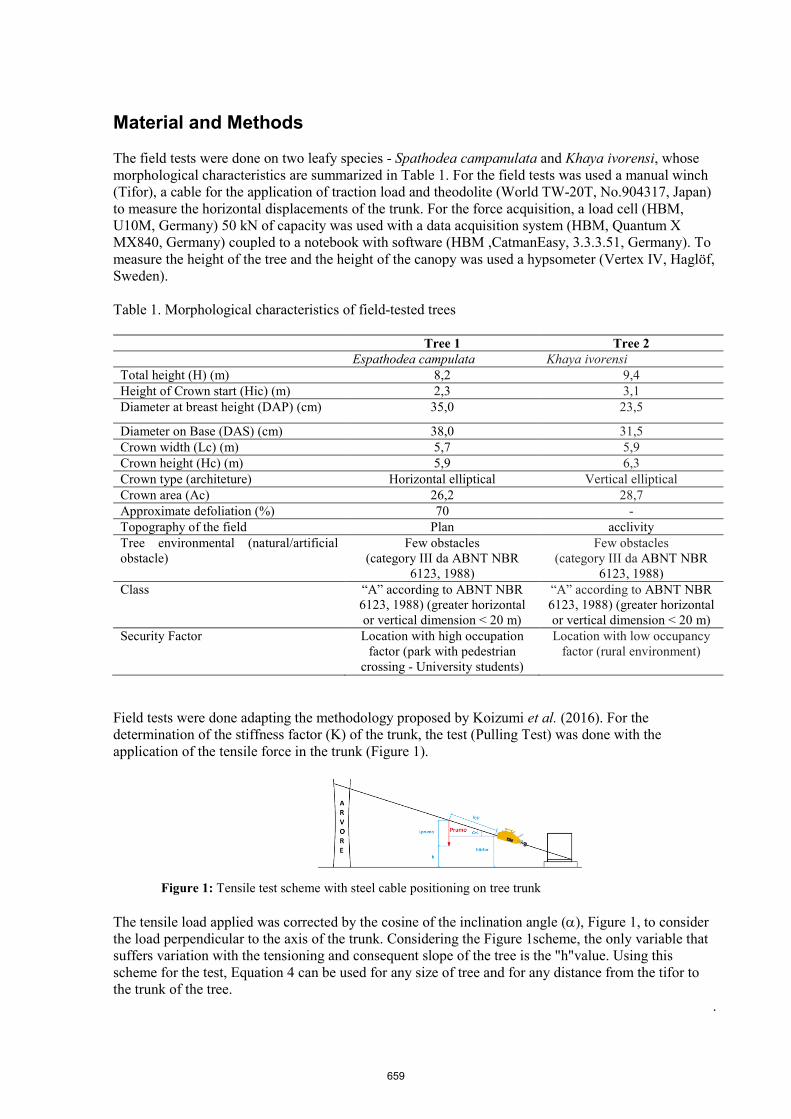
Material and Methods

The field tests were done on two leafy species - Spathodea campanulata and Khaya ivorensi, whose morphological characteristics are summarized in Table 1. For the field tests was used a manual winch (Tifor), a cable for the application of traction load and theodolite (World TW-20T, No.904317, Japan) to measure the horizontal displacements of the trunk. For the force acquisition, a load cell (HBM, U10M, Germany) 50 kN of capacity was used with a data acquisition system (HBM, Quantum X MX840, Germany) coupled to a notebook with software (HBM ,CatmanEasy, 3.3.3.51, Germany). To measure the height of the tree and the height of the canopy was used a hypsometer (Vertex IV, Haglöf, Sweden).

Table 1. Morphological characteristics of field-tested trees

Tree 1 Tree 2 Espathodea campulata Khaya ivorensi

Total height (H) (m) 8,2 9,4 Height of Crown start (Hic) (m) 2,3 3,1 Diameter at breast height (DAP) (cm) 35,0 23,5

Diameter on Base (DAS) (cm) 38,0 31,5 Crown width (Lc) (m) 5,7 5,9 Crown height (Hc) (m) 5,9 6,3 Crown type (architeture) Horizontal elliptical Vertical elliptical Crown area (Ac) 26,2 28,7 Approximate defoliation (%) 70 - Topography of the field Plan acclivity Tree environmental (natural/artificial obstacle)

Few obstacles (category III da ABNT NBR

6123, 1988)

Few obstacles (category III da ABNT NBR

6123, 1988) Class “A” according to ABNT NBR

6123, 1988) (greater horizontal or vertical dimension < 20 m)

“A” according to ABNT NBR 6123, 1988) (greater horizontal or vertical dimension < 20 m)

Security Factor Location with high occupation factor (park with pedestrian

crossing - University students)

Location with low occupancy factor (rural environment)

Field tests were done adapting the methodology proposed by Koizumi et al. (2016). For the determination of the stiffness factor (K) of the trunk, the test (Pulling Test) was done with the application of the tensile force in the trunk (Figure 1).

Figure 1: Tensile test scheme with steel cable positioning on tree trunk

The tensile load applied was corrected by the cosine of the inclination angle (α), Figure 1, to consider the load perpendicular to the axis of the trunk. Considering the Figure 1scheme, the only variable that suffers variation with the tensioning and consequent slope of the tree is the "h"value. Using this scheme for the test, Equation 4 can be used for any size of tree and for any distance from the tifor to the trunk of the tree.

.

659

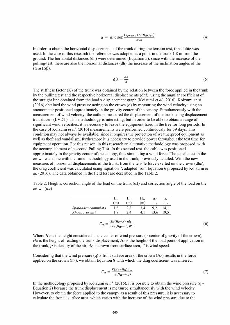
𝛼𝛼 = 𝑎𝑎𝑎𝑎𝑎𝑎 sen 𝐿𝐿𝑝𝑝𝑝𝑝𝑝𝑝𝑝𝑝𝑝𝑝+ℎ−ℎ𝑡𝑡𝑡𝑡𝑝𝑝𝑡𝑡𝑝𝑝𝑝𝑝ℎ𝑦𝑦𝑦𝑦

(4)

In order to obtain the horizontal displacements of the trunk during the tension test, theodolite was used. In the case of this research the reference was adopted as a point in the trunk 1.8 m from the ground. The horizontal distances (dh) were determined (Equation 5), since with the increase of the pulling-test, there are also the horizontal distances (dh) the increase of the inclination angles of the stem (Δβ).

∆β = 𝑑𝑑ℎ

𝑑𝑑 (5)

The stiffness factor (K) of the trunk was obtained by the relation between the force applied in the trunk by the pulling test and the respective horizontal displacements (dhf), using the angular coefficient of the straight line obtained from the load x displacement graph (Koizumi et al., 2016). Koizumi et al. (2016) obtained the wind pressure acting on the crown (q) by measuring the wind velocity using an anemometer positioned approximately in the gravity center of the canopy. Simultaneously with the measurement of wind velocity, the authors measured the displacement of the trunk using displacement transducers (LVDT). This methodology is interesting, but in order to be able to obtain a range of significant wind velocities, it is necessary to leave the equipment fixed in the tree for long periods. In the case of Koizumi et al. (2016) measurements were performed continuously for 39 days. This condition may not always be available, since it requires the protection of weatherproof equipment as well as theft and vandalism; furthermore it is necessary to provide power throughout the test time for equipment operation. For this reason, in this research an alternative methodology was proposed, with the accomplishment of a second Pulling Test. In this second test the cable was positioned approximately in the gravity center of the canopy, thus simulating a wind force. The tensile test in the crown was done with the same methodology used in the trunk, previously detailed. With the new measures of horizontal displacements of the trunk, from the tensile force exerted on the crown (dhc), the drag coefficient was calculated using Equation 7, adapted from Equation 6 proposed by Koizumi et al. (2016). The data obtained in the field test are described in the Table 2. Table 2. Heights, correction angle of the load on the trunk (αf) and correction angle of the load on the crown (αc)

HD

(m) HF (m)

HW (m)

αf (°)

αc

(°) Spathodea campulata 1,8 2,3 3,4 9,2 14,1 Khaya ivorensi 1,8 2,4 4,1 13,6 19,5

𝐶𝐶𝐷𝐷 = 2𝐾𝐾(𝐻𝐻𝐹𝐹−𝐻𝐻𝐷𝐷)𝑑𝑑ℎ𝑐𝑐

𝜌𝜌𝐴𝐴𝐶𝐶(𝐻𝐻𝑊𝑊−𝐻𝐻𝐷𝐷)𝑉𝑉2 (6)

Where HW is the height considered as the center of wind pressure (≅ center of gravity of the crown), HD is the height of reading the trunk displacement, HF is the height of the load point of application in the trunk, ρ is density of the air, AC is crown front surface area, V is wind speed. Considering that the wind pressure (q) x front surface area of the crown (AC) results in the force applied on the crown (FC), we obtain Equation 8 with which the drag coefficient was inferred.

𝐶𝐶𝐷𝐷 = 𝐾𝐾(𝐻𝐻𝐹𝐹−𝐻𝐻𝐷𝐷)𝑑𝑑ℎ𝑐𝑐

𝐹𝐹𝑐𝑐(𝐻𝐻𝑊𝑊−𝐻𝐻𝐷𝐷) (7)

In the methodology proposed by Koizumi et al. (2016), it is possible to obtain the wind pressure (q - Equation 2) because the trunk displacement is measured simultaneously with the wind velocity. However, to obtain the force applied to the canopy as a result of this pressure, it is necessary to calculate the frontal surface area, which varies with the increase of the wind pressure due to the

660

reconfiguration of the canopy (Mayhead 1973, Jalonen and Jarvela 2014). This reconfiguration also affects the gravity center of the crown, considered the pressure center of the wind (Beer and Johnston 1988). In addition, by simplifying the calculation of the area only based on the geometric shape of the crown, even using bitmap images converted from photos of the canopy as Koizumi et al. (2016), the permeability of the canopy is not considered. The permeability is a very important factor for analysis involving the effect of the wind load (Jalonen and Jarvela 2014). Mayhead (1973) and Koizumi et al. (2016) comment the difficulty to obtain most accurate calculation of the crown area, necessary for CD calculation. Hedden et al. (1995) indicated that in trees subject to hurricanes, removal of 25% to 50% of the crown is an effective way to reduce the fall. Authors such as Rudnicki et al. (2004), Vollsinger et al. (2005), Smiley and Brian (2006) analyzed the permeability using prunings as methodology of variation of the leaves amount. Smiley and Brian (2006) quantified the influence of four types of pruning in the wind load of Acer rubrum (Red maples) trees: 1. Removal of 25% of the leaves and small branches without changing the height or diameter of the canopy, 2. Reduction of 25% of the height and the diameter of the canopy, 3. Reduction of leaves and small branches of the canopy upper half and 4. Manual removal of all leaves by keeping the branches. The authors concluded that all types of pruning have a statistically significant reduction of the wind loads, for all velocities tested, considering the canopy without pruning as a reference. Rudnicki et al. (2004) and Vollsinger et al. (2005) also analyzed the variation of the crown frontal area as a function of the leaf loss, considering velocities up to 20 m.s-1 for 3 conifers and 3 hardwood species. For the analysis, they used the condition of the canopy with leaves and after approximately 30% and 70% pruning. The areas reduced about 20% for 30% defoliation and about 50% for 70% defoliation Wind load reductions increase with increasing wind velocity because of crown reconfiguration, and a limit velocity is expected, from which the canopy can no longer reconfigured and so, the wind load is maintained (Vogel 1989). This behavior changes according to the age of the tree, since younger trees, such as those used in the research by Smiley and Brian (2006), have greater flexibility than adult trees. For the drag coefficient, this same behavior, related with the branches and trunk flexibility is also observed (Koizumi et al, 2016). In the methodology proposed in this study, tensile forces were applied in the canopy to simulate the wind action. In order to make these forces representative of the wind pressure in the canopy and, consequently, to infer the wind velocity capable of mobilizing this force, it was necessary to take into account the canopy condition in terms of permeability, since the canopy of the Sphatodea campanulata was quite defoliated. Considering the results of Rudnicki et al. (2004) and Vollsinger et al. (2005), for the defoliation condition of the Sphatodea campanulata tree (about 70%) it was necessary to increase the magnitude of the applied force near 50% to correct the wind pressure. With this correction in the wind pressure, the corresponding wind velocities (Equation 3) were calculated, allowing a more direct comparison of CD behavior with the literature. For the species Kaya ivorensis this correction was not necessary because the tree had no loss of leaves. To evaluate the influence of the tree environment, the basic wind velocity (V0) was inferred using Equation 3. Results and Discussions Load-displacement graphs showed a linear behavior for both species with correlation coefficients (R) higher than 0.97. The values of the stem rigidity factors (K), obtained by the angular coefficient of the load-displacement plot, were 190713 N.m-2 for Spathodea campulata and 250283 N.m-2 for Khaya ivorensi (1.3 times higher). Although the literature on mechanical properties of these two species is not extensive, especially in the case of Spathodea campanulata, the higher stiffness value for the Khaya ivorensi is consistent with literature information. Also it was found the value of 730 kg.m-3 for average density (12% moisture content) for Khaya ivorensi wood (Silva 2013) and 357 kg.m-3 for Spathodea campanulata wood (Castellanos and Jurado 2016). In the same moisture contet conditions (12%) the average modulus of elasticity was 9700 MPa for Khaya ivorensi wood (Krestschmann

661

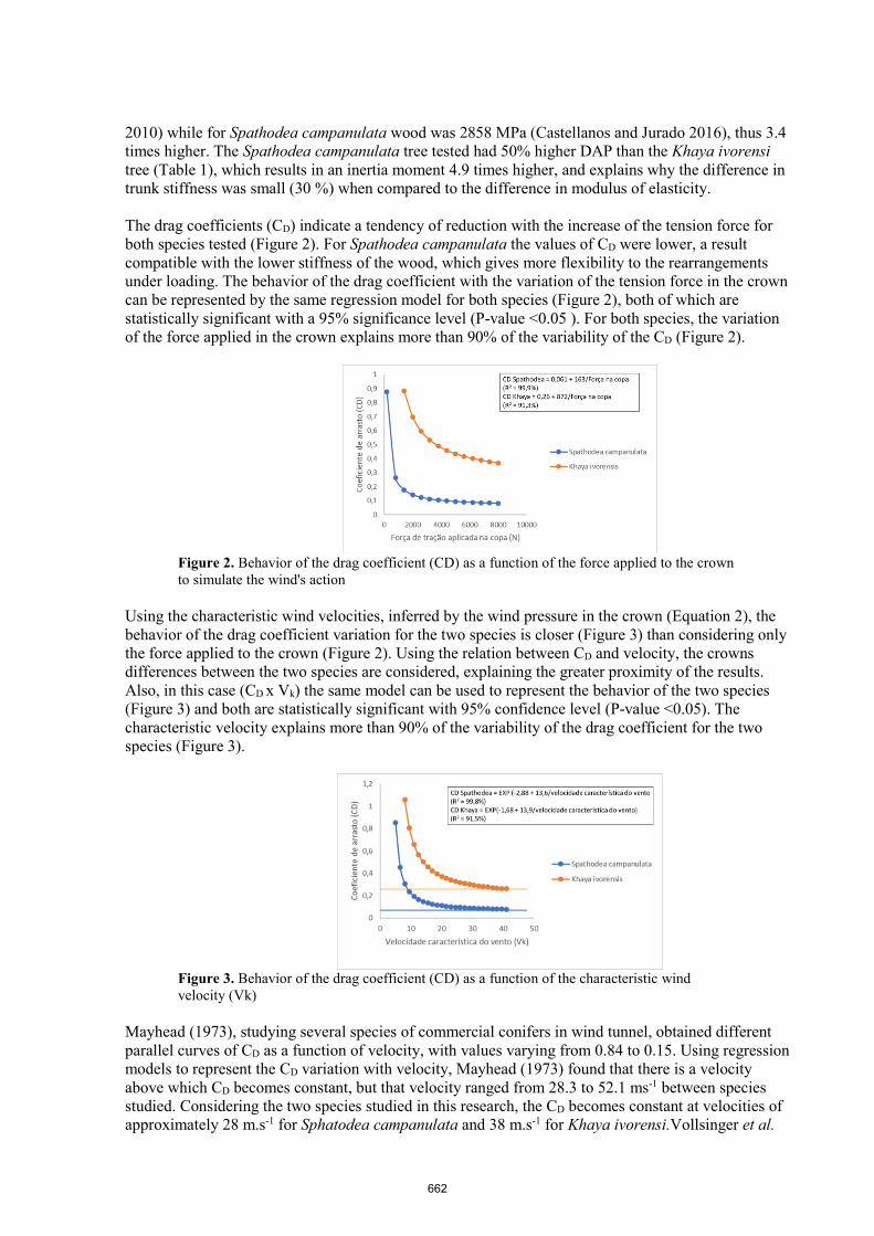
2010) while for Spathodea campanulata wood was 2858 MPa (Castellanos and Jurado 2016), thus 3.4 times higher. The Spathodea campanulata tree tested had 50% higher DAP than the Khaya ivorensi tree (Table 1), which results in an inertia moment 4.9 times higher, and explains why the difference in trunk stiffness was small (30 %) when compared to the difference in modulus of elasticity. The drag coefficients (CD) indicate a tendency of reduction with the increase of the tension force for both species tested (Figure 2). For Spathodea campanulata the values of CD were lower, a result compatible with the lower stiffness of the wood, which gives more flexibility to the rearrangements under loading. The behavior of the drag coefficient with the variation of the tension force in the crown can be represented by the same regression model for both species (Figure 2), both of which are statistically significant with a 95% significance level (P-value <0.05 ). For both species, the variation of the force applied in the crown explains more than 90% of the variability of the CD (Figure 2).

Figure 2. Behavior of the drag coefficient (CD) as a function of the force applied to the crown to simulate the wind's action

Using the characteristic wind velocities, inferred by the wind pressure in the crown (Equation 2), the behavior of the drag coefficient variation for the two species is closer (Figure 3) than considering only the force applied to the crown (Figure 2). Using the relation between CD and velocity, the crowns differences between the two species are considered, explaining the greater proximity of the results. Also, in this case (CD x Vk) the same model can be used to represent the behavior of the two species (Figure 3) and both are statistically significant with 95% confidence level (P-value <0.05). The characteristic velocity explains more than 90% of the variability of the drag coefficient for the two species (Figure 3).

Figure 3. Behavior of the drag coefficient (CD) as a function of the characteristic wind velocity (Vk)

Mayhead (1973), studying several species of commercial conifers in wind tunnel, obtained different parallel curves of CD as a function of velocity, with values varying from 0.84 to 0.15. Using regression models to represent the CD variation with velocity, Mayhead (1973) found that there is a velocity above which CD becomes constant, but that velocity ranged from 28.3 to 52.1 ms-1 between species studied. Considering the two species studied in this research, the CD becomes constant at velocities of approximately 28 m.s-1 for Sphatodea campanulata and 38 m.s-1 for Khaya ivorensi.Vollsinger et al.

662

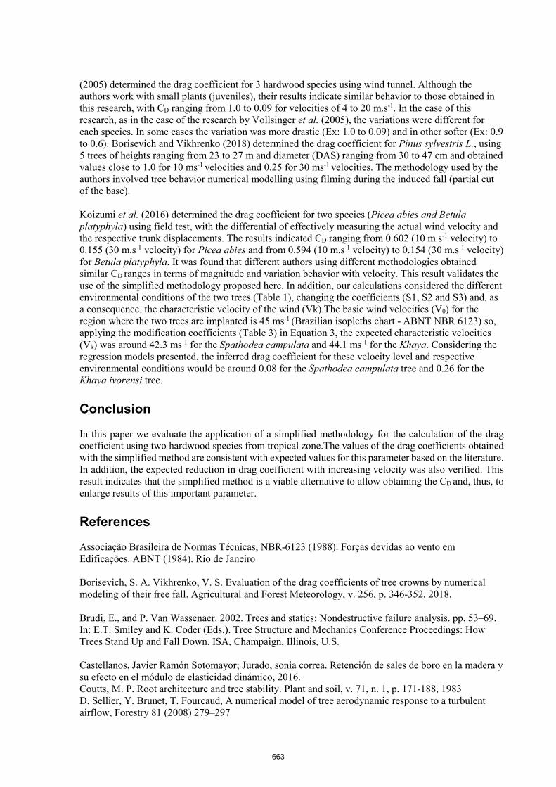
(2005) determined the drag coefficient for 3 hardwood species using wind tunnel. Although the authors work with small plants (juveniles), their results indicate similar behavior to those obtained in this research, with CD ranging from 1.0 to 0.09 for velocities of 4 to 20 m.s-1. In the case of this research, as in the case of the research by Vollsinger et al. (2005), the variations were different for each species. In some cases the variation was more drastic (Ex: 1.0 to 0.09) and in other softer (Ex: 0.9 to 0.6). Borisevich and Vikhrenko (2018) determined the drag coefficient for Pinus sylvestris L., using 5 trees of heights ranging from 23 to 27 m and diameter (DAS) ranging from 30 to 47 cm and obtained values close to 1.0 for 10 ms-1 velocities and 0.25 for 30 ms-1 velocities. The methodology used by the authors involved tree behavior numerical modelling using filming during the induced fall (partial cut of the base). Koizumi et al. (2016) determined the drag coefficient for two species (Picea abies and Betula platyphyla) using field test, with the differential of effectively measuring the actual wind velocity and the respective trunk displacements. The results indicated CD ranging from 0.602 (10 m.s-1 velocity) to 0.155 (30 m.s-1 velocity) for Picea abies and from 0.594 (10 m.s-1 velocity) to 0.154 (30 m.s-1 velocity) for Betula platyphyla. It was found that different authors using different methodologies obtained similar CD ranges in terms of magnitude and variation behavior with velocity. This result validates the use of the simplified methodology proposed here. In addition, our calculations considered the different environmental conditions of the two trees (Table 1), changing the coefficients (S1, S2 and S3) and, as a consequence, the characteristic velocity of the wind (Vk).The basic wind velocities (V0) for the region where the two trees are implanted is 45 ms-1 (Brazilian isopleths chart - ABNT NBR 6123) so, applying the modification coefficients (Table 3) in Equation 3, the expected characteristic velocities (Vk) was around 42.3 ms-1 for the Spathodea campulata and 44.1 ms-1 for the Khaya. Considering the regression models presented, the inferred drag coefficient for these velocity level and respective environmental conditions would be around 0.08 for the Spathodea campulata tree and 0.26 for the Khaya ivorensi tree.

Conclusion In this paper we evaluate the application of a simplified methodology for the calculation of the drag coefficient using two hardwood species from tropical zone.The values of the drag coefficients obtained with the simplified method are consistent with expected values for this parameter based on the literature. In addition, the expected reduction in drag coefficient with increasing velocity was also verified. This result indicates that the simplified method is a viable alternative to allow obtaining the CD and, thus, to enlarge results of this important parameter.

References

Associação Brasileira de Normas Técnicas, NBR-6123 (1988). Forças devidas ao vento em Edificações. ABNT (1984). Rio de Janeiro Borisevich, S. А. Vikhrenko, V. S. Evaluation of the drag coefficients of tree crowns by numerical modeling of their free fall. Agricultural and Forest Meteorology, v. 256, p. 346-352, 2018. Brudi, E., and P. Van Wassenaer. 2002. Trees and statics: Nondestructive failure analysis. pp. 53–69. In: E.T. Smiley and K. Coder (Eds.). Tree Structure and Mechanics Conference Proceedings: How Trees Stand Up and Fall Down. ISA, Champaign, Illinois, U.S. Castellanos, Javier Ramón Sotomayor; Jurado, sonia correa. Retención de sales de boro en la madera y su efecto en el módulo de elasticidad dinámico, 2016. Coutts, M. P. Root architecture and tree stability. Plant and soil, v. 71, n. 1, p. 171-188, 1983 D. Sellier, Y. Brunet, T. Fourcaud, A numerical model of tree aerodynamic response to a turbulent airflow, Forestry 81 (2008) 279–297

663

Gardiner, B.A., Stacey, G.R., Belcher, R.E., Wood, C.J., 1997: Field and wind tunnel assessments of the implications of respacing and thinning for tree stability. Forestry 70, 233-252. Hedden, R.L., Fredricksen, T.S., Williams, S.A., 1995. Modelling the effect of crown shedding and streamlining on the survival of loblolly pine exposed to acute wind. Can. J. For. Res. 25, 704–712. Jalonen, Johanna; JÄRVELÄ, Juha. Estimation of drag forces caused by natural woody vegetation of different scales. Journal of Hydrodynamics, v. 26, n. 4, p. 608-623, 2014. Johnston, E. Russell; BEER, Ferdinand; Eisenberg, Elliot. Vector Mechanics for Engineers: Statics and Dynamics. 5th Edition. McGraw-Hill, NY, 533, 1988. Kenneth R. James; Dynamic loading of trees. Journal of arboriculture, v. 29, n. 3, p. 165-171, 2003. Kenneth R. James; HARITOS, Nicholas; ADES, Peter K. Mechanical stability of trees under dynamic loads. American journal of Botany, v. 93, n. 10, p. 1522-1530, 2006. Kenneth R. James, Gregory A. Dahle, Jason Grabosky, Brian Kane, and Andreas Detter (2014). Tree biomechanics literature review: Dynamics. Arboriculture & Urban Forestry 40(1): 1-15. Koizumi A., Motoyama J., Sawata K., Sasaki Y. & Hirai T. (2010). Evaluation of drag coefficients of poplar-tree crowns by a field test method. J. Wood Sci. 56, 189–193 Koizumi, A., Shimizu, M., Sasaki, Y., & Hirai, T. (2016). In situ drag coefficient measurements for rooftop trees. Journal of wood science, 62(4), 363-369. Kretschmann, D. E. Mechanical properties of wood. In: Wood handbook: wood as an engineering material. Madison: USDA, Forest Service, 2010. p. 100-145. (FPL General Technical Report, 190) Mayhead g.j. (1973) some drag coefficients for British forest trees derived from wind tunnel studies. Agric. Meteorol. 12:123-130 Morinaga, T; Tanaka N; Yagisawa J; Karunaratne S; Weerakoon W.M.S.B. Estimation of drag coefficient of trees considering the tree bending or overturning situations. In: nternational Symposium on Advances in Civil and Environment Engineering practices for sustainable development. University Of Ruhuna. Galle 2012. Rudnicki, M., Mitchell, S.J., and Novak, M.D. 2004. Wind tunnel measurements of crown streamlining and drag relationships for three conifer species. Can. J. For. Res. 34: 666–676. Sellier, D., and T. Fourcaud. 2009. Crown structure and wood properties: Influence on tree sway and response to high winds. American Journal of Botany 96:885–896. Silva, Luana Nunes da. Correlações entre propriedades tecnológicas da madeira de mogno africano (Cedrela odorata L.) determinadas por metodologias destrutivas e não destrutivas. 2017. Smiley, E. Thomas; Kane, Brian. The effects of pruning type on wind loading of Acer rubrum. Journal of Arboriculture, v. 32, n. 1, p. 33, 2006. Vogel, S., 1989. Drag and reconfiguretion of broad leaves in high wind. J. Exper. Bot. 40, 941–948. Vollsinger, Stephan et al. Wind tunnel measurements of crown streamlining and drag relationships for several hardwood species. Canadian Journal of Forest Research, v. 35, n. 5, p. 1238-1249, 2005.

664

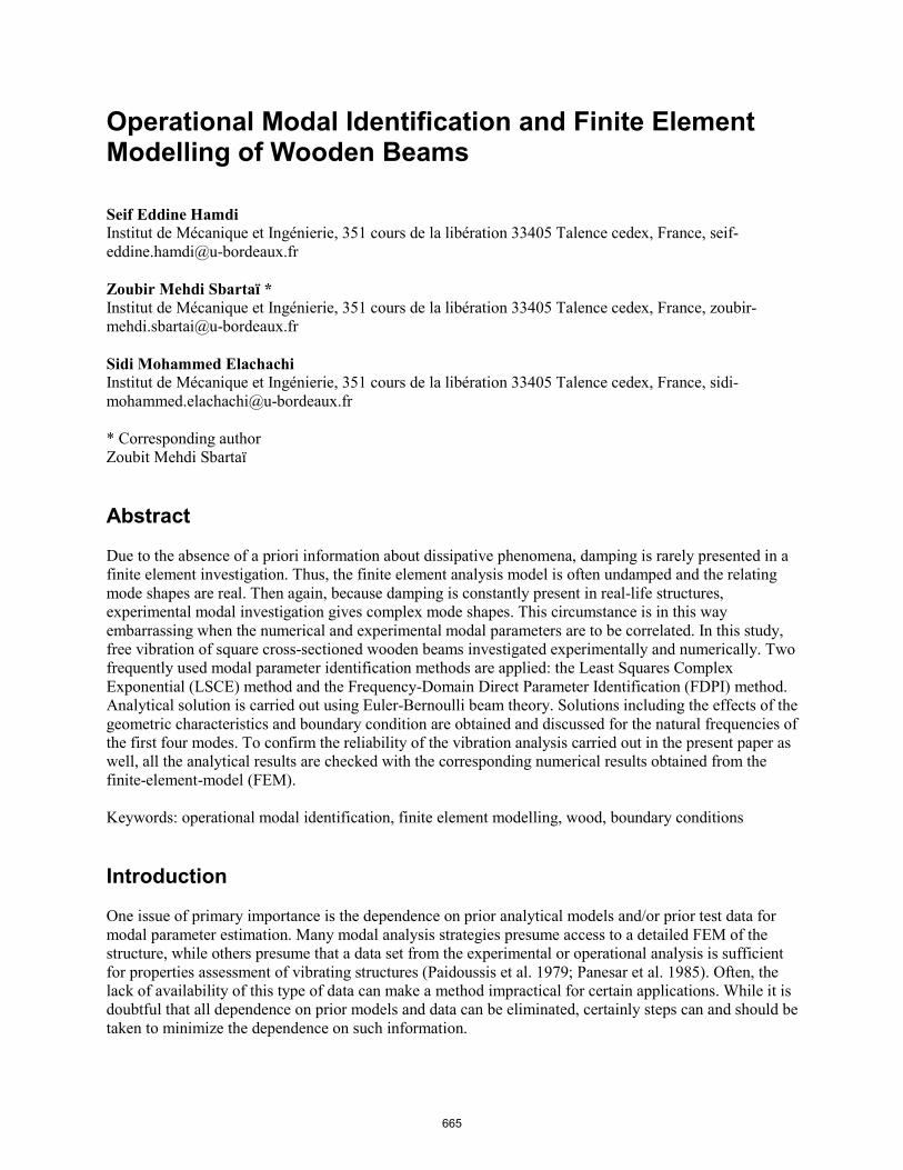
Operational Modal Identification and Finite Element Modelling of Wooden Beams Seif Eddine Hamdi Institut de Mécanique et Ingénierie, 351 cours de la libération 33405 Talence cedex, France, seif-eddine.hamdi@u-bordeaux.fr Zoubir Mehdi Sbartaï * Institut de Mécanique et Ingénierie, 351 cours de la libération 33405 Talence cedex, France, zoubir-mehdi.sbartai@u-bordeaux.fr Sidi Mohammed Elachachi Institut de Mécanique et Ingénierie, 351 cours de la libération 33405 Talence cedex, France, sidi-mohammed.elachachi@u-bordeaux.fr * Corresponding author Zoubit Mehdi Sbartaï Abstract Due to the absence of a priori information about dissipative phenomena, damping is rarely presented in a finite element investigation. Thus, the finite element analysis model is often undamped and the relating mode shapes are real. Then again, because damping is constantly present in real-life structures, experimental modal investigation gives complex mode shapes. This circumstance is in this way embarrassing when the numerical and experimental modal parameters are to be correlated. In this study, free vibration of square cross-sectioned wooden beams investigated experimentally and numerically. Two frequently used modal parameter identification methods are applied: the Least Squares Complex Exponential (LSCE) method and the Frequency-Domain Direct Parameter Identification (FDPI) method. Analytical solution is carried out using Euler-Bernoulli beam theory. Solutions including the effects of the geometric characteristics and boundary condition are obtained and discussed for the natural frequencies of the first four modes. To confirm the reliability of the vibration analysis carried out in the present paper as well, all the analytical results are checked with the corresponding numerical results obtained from the finite-element-model (FEM). Keywords: operational modal identification, finite element modelling, wood, boundary conditions Introduction One issue of primary importance is the dependence on prior analytical models and/or prior test data for modal parameter estimation. Many modal analysis strategies presume access to a detailed FEM of the structure, while others presume that a data set from the experimental or operational analysis is sufficient for properties assessment of vibrating structures (Paidoussis et al. 1979; Panesar et al. 1985). Often, the lack of availability of this type of data can make a method impractical for certain applications. While it is doubtful that all dependence on prior models and data can be eliminated, certainly steps can and should be taken to minimize the dependence on such information.

665

Therefore, it is of primary interest to numerically investigate the performance of the modal identification methods (MPI). As a case study, free vibration of square cross-sectioned wooden beams is investigated analytically and numerically. Finite element analysis is carried out using the finite element based software ANSYS® (ANSYS® Academic Research, Release 18.1). To confirm the reliability of the MPI performance benchmark carried out in the present paper as well, all the numerical results are checked with the corresponding analytical results carried out using Euler-Bernoulli beam theory. Finite element solution Vibration wave propagation in wood structures is a complicated dynamic procedure controlled by the properties, orientation and microstructure of the fiber, and perhaps more importantly, by the geometry of the material (Xu et al. 2014). As a result, accurate modeling of wood materials is the priority issue to get insight into wave propagation behavior in wooden beam. To investigate the influence of the material characteristics on the wave behavior, the FE model should consider the orthotropic properties of wood (Ohmichi et al. 2017). In this subsection, a three dimensional linear elastic FE model to determine numerical solution of square cross-sectioned white fir beams obtained using the ANSYS software, is presented. Solid model of the beams with different geometric profiles is used. Mechanical properties obtained from the material database of Ansys library and parameters of the beam are presented in Table 1.

Parameters Beam 1 Beam 2 Length (mm) 80 120

Cross-Sectional Area (mm² ) 50 50 50 50

Material White fir White fir

Density (kg/m3) 450 450

Moisture content (%) 12 12

Poison’s ratio 0.3 0.3

Elastic modulus (MPa) 1024 49 87

1024 49 87

Shear modulus (MPa) 71.68 2.84 0.52

71.68 2.84 0.52

To simulate the acoustic wave propagation, an elastic linear model is built up (Hamdi et al. 2018). The elastic linear model is on basis of the assumption of wave-structure interactions are linear elastic. However, since the beams are supposed to undergo free vibration behavior under various boundary conditions in this study, a refined MultiZone Quad/Tri mesh elements (quads and/or triangles) are used for modeling the 3D structure (Hamdi et al. 2018). Numerical analysis is carried out for approximately 1000-5000 node points and 10000-500000 mesh elements. In this study, only Free- Free (F-F) boundary condition is used. The natural frequency values for the first four modes of the white fir beams are obtained for each combination of beam length L and boundary condition. As an example, Figure 1 show a view from Ansys simulation of free ends vibration analysis of white fir beam.

666

Figure 2—Ansys free vibration simulation (F-F) of white fir beam (L=240 mm). To validate the performance of the MPI methods to describe vibration waves propagation in the wooden beam, the analytical results were compared with the results of the FE based ANSYS model in the next subsection. First four natural frequencies are investigated under F-F boundary condition. Modal parameter Identification methods This section introduces common ways of modeling linear time-invariant vibrating structures. Frequently used EMA and OMA are presented. Least Squares Complex Exponential method The Least Squares Complex Exponential (LSCE) method is considered as an "industry-standard" time domain estimation technique. The LSCE presented in 1979 (Brown et al. 1979), is the extension of the Complex Exponential method (CE) to a global methodology (Spitznogle et al. 1970). It is therefore a single input multi output (SIMO) technique, handling at the same time several impulse response functions (IRFs) gotten by exciting a structure at one single point and estimating the responses at several locations. With such a methodology, a reliable arrangement of global parameters (natural frequencies and damping ratios) are estimated. The LSCE is considered as a common form of curve fitting experimental information. It estimates the system poles in the time space by using several IRFs obtained from FRFs by an inverse Fourier transform (IFFT). Frequency-Domain Direct Parameter Identification method The Frequency-Domain Direct Parameter Identification (FDPI) technique has traditionally been used to analyze data from highly damped structures (Heylen et al. 1998), (Verboven, 2002). The FDPI operates in the frequency domain. It belongs to the group of direct methods since physical system matrices are identified in a first step and the corresponding modal parameters are calculated in a second step (Lembregts et al. 1988). The FDPI estimator identifies the frequency-domain low order complete direct (state space) model from FRF measurements. The poles, mode shapes and participation factors are derived from the system matrices of a state model. In practice, a data reduction based on a Principal Component Analysis (PCA) of the frequency response function matrix is necessary for computation speed and memory requirements as well as to construct a proper stabilization diagram for proper model order detection. The algorithm assumes that the number of modes within the analysis band is less than or equal to the number of outputs (Lembregts et al. 1986).

667

Free-Free boundary condition In this section, the LSCE and FDPI methods were used for modal parameters estimation of free-vibration behavior of square cross-sectioned white fir beams with different geometric profiles under F-F boundary condition. The natural frequencies were obtained for the first four modes (n=1, 2, 3, 4), including the effects of the geometric characteristics, i.e., length and cross sectional area, and the boundary conditions. Analytical and FEM natural frequencies obtained with MPI methods are presented in Table 2. The obtained results show that the natural frequencies increase with the increase in mode number. In addition, it’s to be noticed that the change in mode numbers increases the natural frequencies. The natural frequency of the first mode number differs from that of the second and third mode numbers by 14% for LSCE method and 8% for FDPI method.

Table 2—Analytical and FEM natural frequencies obtained with MPI methods for different geometric profiles of white fir beams under free-free boundary condition. Length (mm)

Mode id

Anl. Freq (Hz)

LSCE method FDPI method FEM Freq. (Hz)

Err FEM-Anal (%)

Freq. (Hz)

Err FEM-Anal (%)

80 Mod1 1.15e3 1.39e3 17.27 1.03e3 10.43 Mod2 3.16e3 3.28e3 3.66 3.21e3 1.58 Mod3 6.21e3 6.46e3 3.87 6.37e3 2.58 Mod4 1.03e4 1.36e4 24.26 1.29e4 25.24

120 Mod1 765 742 3.10 772 0.92 Mod2 2.11e3 2.47e3 14.57 2.26e3 7.11 Mod3 4.14e3 4.37e3 5.26 4.31e3 4.11 Mod4 6.84e3 6.56e3 4.27 6.53e3 4.53

Conclusions In this study we depicted two modal parameter identification techniques for natural frequencies estimation: the Least Squares Complex Exponential (LSCE) method and the Frequency-Domain Direct Parameter Identification (FDPI) method. The free vibration of square cross- sectioned wooden beams is described analytically and numerically. Analytical solution is completed utilizing Euler-Bernoulli beam theory. The impacts of the geometric attributes and boundary conditions are investigated for the natural frequencies of the first four modes. The got outcomes demonstrate that the natural frequencies increase with the increase in mode number. Likewise, it's to be seen that the change in mode numbers has the biggest impact on the natural frequency under F-F boundary conditions. At last, it's to be advised that the adjustment long of the beams constantly affects its natural frequencies for different boundary conditions and lengths. Future work will be situated for tentatively approved the limited component displaying of the impact of modular parameter estimation of wood vibrating structures under different boundary conditions. Acknowledgments This work was supported by the region Nouvelle-Aquitaine in the frame of the QualiPin project. The authors thank also all the project partners for their critical discussion of the paper.

668

References Brown, D. L.; Allemang, R. J.; Zimmerman, R.; Mergeay, M. 1979. Parameter Estimation Techniques For Modal Analysis” SAE Technical Paper Series, No. 790221. Hamdi, S.; Sbartai, Z-M.; Elachachi S.M.. Mechanical characterization of standing tree by the use of different non-destructive methods, internal report 2018 (in French). Heylen, W.; Lammens, S.; Sas. P. 1998. Modal Analysis Theory and Testing, KULeuven, ISBN 90-73802-61-X. Lembregts, F. Frequency domain identification techniques for experimental multiple input modal analysis. PhD thesis, dept. PMA, KULeuven, Leuven (Belgium), december 1988. Lembregts, F.; Leuridan, J.; Zhang, L.; Kanda, H. 1986. Multiple Input Modal Analysis of Frequency Response Functions Based Direct Parameter Identification. Proceedings of IMAC 4, the International Modal Analysis Conference, 589-598, Los Angeles, CA, USA. Ohmichi, M.; Noda, N.; Sumi, N. 2017. Plane heat conduction problems in functionally graded orthotropic materials. J. Therm. Stresses. 40: 747-764. Paidoussis, M.; Helleur, C. 1979. Ovalling oscillations of cylindrical-shells in cross-flow. Journal of Sound and Vibration. 63(4): 527-542. Panesar, A.; Johns, D. 1985. Ovalling oscillations of thin circular cylindrical shells in cross flow - an experimental study. Journal of Sound and Vibration. 103(2): 201-209. Spitznogle, F. R.; Quazi, A. H. 1970. Representation And Analysis Of Time-Limited Signals Using A Complex Exponential Algorithm” The Journal of The Acoustical Society of America. 47(5), 1150-l155. Verboven, P. 2002. Frequency Domain System Identification for Modal Analysis. Ph.D. Thesis, Vrije Universiteit Brussel, Belgium. Xu, H.; Xu, G.; Wang, L.; Yu, L. 2014. Propagation behavior of acoustic wave in wood. J. Forestry Res. 25: 671-676.

669

Effect of Tensile Stress on Velocity of Surface Waves Generated Using Air-Coupled Ultrasonic Sensor Masumi Hasegawa * Department of Agro-environemental Sciences, Faculty of Agriculture, Kyushu University, Fukuoka, Japan, kmgtmsm@agr.kyushu-u.ac.jp Hiroyuki Okamura Interior Design Research Institute, Fukuoka Industrial Technology Center, Ohkawa, Japan, okamura-h0259@fitc.pref.fukuoka.jp Kazutoshi Takeuchi Interior Design Research Institute, Fukuoka Industrial Technology Center, Ohkawa, Japan, takeuchi-k2269@ fitc.pref.fukuoka.jp Junji Matsumura Department of Agro-environemental Sciences, Faculty of Agriculture, Kyushu University, Fukuoka, Japan, matumura@agr.kyushu-u.ac.jp * Corresponding author Abstract Drying stress causes surface and internal checks during the wood drying process. These checks cause a drop in the ornamental value of lumber. It is difficult to nondestructively determine the drying stress in wood. The authors considered the application of an acoustoelastic technique to nondestructively measure stress. The acoustoelastic technique is a method for analyzing the stress state in materials using ultrasonic waves. Acoustoelasticity implies that the velocities of ultrasonic waves that propagate through an elastic material under stress conditions change because of the applied stress. The final objective was to establish the noncontact and nondestructive technique of measuring drying stress in lumber with surface waves generated using an air-coupled ultrasonic sensor. First, the optimal measurement condition of the surface wave was experimentally investigated. The air-coupled ultrasonic wave was made in the longitudinal and tangential directions in wood. Surface wave velocity was measured using an ultrasonic pulsar-receiver, preamplifier, and monolithic composite transducers of size 14 by 20 mm with a resonant frequency of 200 kHz. Second, tensile load was applied parallel to the longitudinal and tangential axes. Surface waves were generated along the direction of the tensile loading. Surface wave velocity changed with tensile stress. The relative changes in velocity varied linearly with the tensile stress. The acoustoelastic constants obtained in the tension test were in good agreement with those in the previous study. These findings suggest the potential of applying surface waves to determine drying stress in wood. Keywords: Drying stress, surface wave, air-coupled ultrasonics, noncontact method, acoustoelasticity

670

Review of Measurements and Digital Data Flows for Swedish Forest Products Kari Hyll * Skogforsk, The Forestry Research Institute of Sweden, Uppsala, Sweden, kari.hyll@skogforsk.se Maria Nordström Skogforsk, The Forestry Research Institute of Sweden, Uppsala, Sweden, maria.nordstrom@skogforsk.se * Corresponding author Abstract This study reviews current measurements of timber, pulpwood, and fuelwood in Sweden, with focus on methods and digital data flows. In Sweden, more than 72 million m3 of timber, pulpwood, and fuelwood are being harvested each year. The collection of digital data ideally starts before the harvest, with information such as tree species, dimension, age, and damages. The harvester measures stem diameter and length during processing, and additional measurements are done at the sawmill for pricing and process control. Today, measurement data are not always well propagated through the production chain, resulting in information loss or duplicate measurements. Although the Swedish forestry sector is highly automated, measurements remain that would benefit from noncontact rather than contact methods and automation rather than manual labor. One example is measurement of bulk moisture content in chip piles, which is currently done with sampling and drying. Here, radar measurements present a promising alternative. Development of new measurement methods must navigate constraints on cost, speed, and logistics while maintaining high accuracy. This study shows that volume and diameter are increasingly measured with image-based stereoscopic measurement and/or laser scanners. In sawmills, 3D laser scanners and x-ray tomography are increasingly used for dimensional and quality measurements. Image-based methods with remote or automated analysis have potential to widely increase measurement efficiency and accuracy. Multispectral methods such as NIR or Raman are likely to be evaluated for measurement of wood species and rot. Log freshness, degree of frozenness, and bulk/inner temperature currently lack suitable measurement techniques. Keywords: Roundwood, forest fuels, imaging, remote analysis, digital data flow

671

Estimation of the Moisture Content Distribution of Japanese Cedar (Cryptomeria japonica :D.Don）Large Diameter Log by the Measuring Gamma Ray Kiyohiko Ikeda Shizuoka Prefectural Research Institute of Agriculture and Forestry, Negata2542-8 Hamakita, Hamamatsu, Shizuoka Japan, kiyohiko1_ikeda@pref.shizuoka.lg.jp Akihiro Sugiyama Micro Measure Co., Ltd. Shimada, Shizuoka, Japan, sugia@micromes.com Takeshi Hoshikawa Shizuoka Prefectural Research Institute of Agriculture and Forestry, Hamamatsu, Shizuoka, Japan, hoshikawa.T@gmail.com Youki Suzuki Forestry and Forest Products Research Institute, Tsukuba, Ibaraki, Japan, youki@ffpri.affrc,go,jp Yuka Miyoshi Forestry and Forest Products Research Institute, Tsukuba, Ibaraki, Japan, ymiyoshi@ffpri.affrc.go.jp Kiyohiko Fujimoto Forestry and Forest Products Research Institute, Tsukuba, Ibaraki, Japan, kiyopi@ffpri.affrc,go,jp Abstract The purpose of this research is to develop a method and apparatus for noncontact and nondestructive evaluation of the distribution of moisture content (especially heartwood MC) inside the large diameter Japanese cedar log, leading to efficient lumber production by log grading of MC. In this research, we developed a device to measure the gamma ray count number, when gamma ray (source: cesium 137 or cobalt 60) is used as a nondestructive index and the distance between sensors is transferred. We evaluated the relationship between gamma ray transmission numbers of large diameter logs and MC of each site specimens sampled from them and relation of MC of large cross section timber beams which were sawed and kiln dried from them. A high correlation was found between the gamma ray transmission number of each part of cedar logs and the MC by the oven dry method. In addition, a high correlation was confirmed between the minimum value of the gamma ray transmission numbers and the large cross section timber beams after kiln drying. Furthermore, the gamma ray is linearly transmitted through the log and is a value corresponding to the water content (apparent density) of the count number, and from the variation of the gamma ray count number when the log moves between the sensors, log's moisture content it was clarified that the distribution can be estimated. Keywords: gamma ray, large diameter log, heartwood moisture content, greenwood, Japanese cedar Introduction The wood quality of Japanese cedar is known to vary widely among individuals, and particularly from previous researches the moisture content of heartwood is known different1,2). For this reason, when manufacturing a large cross section material such as a beam or a girder from medium large diameter logs, variation in drying performance or cracking may occur, which may be a hindrance to stable production of

672

reliable products of quality and performance. In the project research currently underway, we have developed methods for evaluating the moisture content, density, and Young's modulus distribution of cedar large diameter logs that are expected to increase supply in the future, and based on them, for horizontal timbers such as beam girder and frame wall construction timbers, we are developing technology to sort large diameter logs suitable for timbers with a probability of 90% or more 3). So far, the authors have been developing methods and devices for evaluating the moisture content of the log from the phase and attenuation of the relative permittivity or the low frequency range electromagnetic wave 4). In the evaluation of high moisture content area by gamma rays, basic experiments have been tried on standing trees so far, but no studies have been conducted on practical application and application to the field 5). Here, we report the method of evaluating the moisture content or moisture content distribution of a large-diameter Japanese cedar logs with nondestructive and non-contact by gamma rays and the results of trial manufacture of these evaluation devices. And also, we report noncontact evaluation of moisture content distribution of Japanese cedar large diameter log by gamma ray and the result of trial manufacture of these evaluation devices. Outline of prototype gamma ray measurement system The prototype gamma ray measuring apparatus used cesium 137 or cobalt 60 as a radiation source, and used sodium iodide for a scintillator having a diameter and a length of 2 inches. The prototype apparatus consists of a control board for gamma rays, a monitor panel that controls the emission time, and displays the number of transmissions. In the control substrates, energy absorption of gamma rays, incidence of light emission photons to PMT (photoelectron multiplier), conversion to photoelectrons, amplification by dynodes, and change of pulse width are performed (Figure 1).

Method and specimen Measurement of gamma ray (source: Cesium 137) in fixed state of large diameter Japanese cedar logs. The test samples are 70 cedar large diameter logs (about 4 m in length, 30 to 40 cm in end diameter) about one month after harvest. The weight was measured using the diameter, length and load cell (2 ton) of those logs to calculate the greenwood density. After that, the center of the log surface was positioned between the gamma ray sensors, and transmission numbers of gamma rays was measured by emitting gamma rays (source: cesium 137) for 1 minute in a stationary fixed state.

673

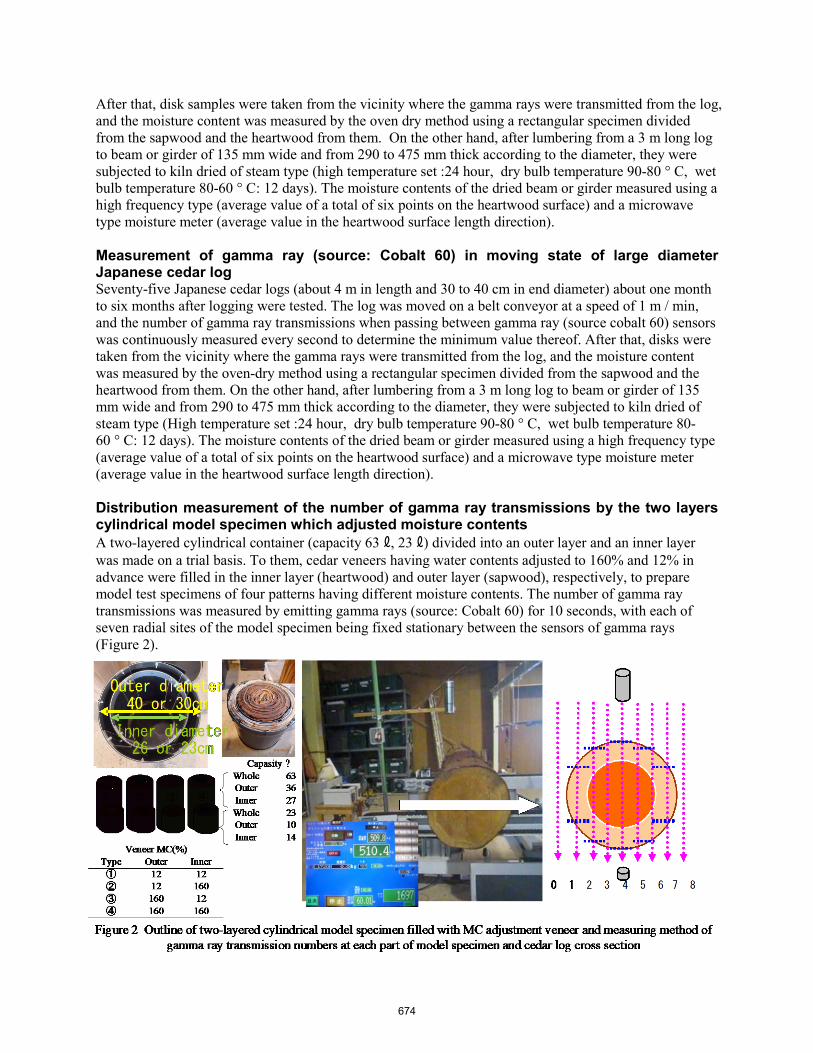
After that, disk samples were taken from the vicinity where the gamma rays were transmitted from the log, and the moisture content was measured by the oven dry method using a rectangular specimen divided from the sapwood and the heartwood from them. On the other hand, after lumbering from a 3 m long log to beam or girder of 135 mm wide and from 290 to 475 mm thick according to the diameter, they were subjected to kiln dried of steam type (high temperature set :24 hour, dry bulb temperature 90-80 ° C, wet bulb temperature 80-60 ° C: 12 days). The moisture contents of the dried beam or girder measured using a high frequency type (average value of a total of six points on the heartwood surface) and a microwave type moisture meter (average value in the heartwood surface length direction). Measurement of gamma ray (source: Cobalt 60) in moving state of large diameter Japanese cedar log Seventy-five Japanese cedar logs (about 4 m in length and 30 to 40 cm in end diameter) about one month to six months after logging were tested. The log was moved on a belt conveyor at a speed of 1 m / min, and the number of gamma ray transmissions when passing between gamma ray (source cobalt 60) sensors was continuously measured every second to determine the minimum value thereof. After that, disks were taken from the vicinity where the gamma rays were transmitted from the log, and the moisture content was measured by the oven-dry method using a rectangular specimen divided from the sapwood and the heartwood from them. On the other hand, after lumbering from a 3 m long log to beam or girder of 135 mm wide and from 290 to 475 mm thick according to the diameter, they were subjected to kiln dried of steam type (High temperature set :24 hour, dry bulb temperature 90-80 ° C, wet bulb temperature 80-60 ° C: 12 days). The moisture contents of the dried beam or girder measured using a high frequency type (average value of a total of six points on the heartwood surface) and a microwave type moisture meter (average value in the heartwood surface length direction). Distribution measurement of the number of gamma ray transmissions by the two layers cylindrical model specimen which adjusted moisture contents A two-layered cylindrical container (capacity 63 ℓ, 23 ℓ) divided into an outer layer and an inner layer was made on a trial basis. To them, cedar veneers having water contents adjusted to 160% and 12% in advance were filled in the inner layer (heartwood) and outer layer (sapwood), respectively, to prepare model test specimens of four patterns having different moisture contents. The number of gamma ray transmissions was measured by emitting gamma rays (source: Cobalt 60) for 10 seconds, with each of seven radial sites of the model specimen being fixed stationary between the sensors of gamma rays (Figure 2).

674

Distributed measurement of gamma ray transmission number of large diameter Japanese cedar logs Ten Japanese cedar logs were used as test specimens. The number of gamma ray transmissions was measured when the radiation time of gamma rays (source cesium 137 and cobalt 60) was 1, 2, 10, 20, 30, 60 seconds for each portion in the log radial direction. Thereafter, test pieces were collected from each site where gamma rays were emitted from the log, and the moisture content was measured by the oven-dried method. In addition, another test, with respect to 30 cedar logs, seven parts in the cross-sectional direction were kept stationary between sensors of gamma rays (source cobalt 60), and the transmittance was measured by irradiating gamma rays (source: cobalt 60) for 10 seconds. (Figure 2) Result & discussion Estimation of moisture content of large-diameter logs of Japanese cedar by gamma ray (source: Cesium 137, Cobalt-60) transmission Figure 3 shows the relationship between the number of gamma ray transmissions and the moisture content measured by the oven-drying method when gamma ray (source: cesium 137) is emitted for 1 minute while the center of the cedar log is fixed stationary. The correlation coefficients between the two were 0.78 for the whole, 0.67 for the heartwood, and 0.55 for the sapwood, and significant correlations were observed. On the other On the other hand, the relative dielectric constant has a correlation coefficient of 0.82 with the core moisture content, and a correlation coefficient of the low frequency electromagnetic wave (52 MHz) with the total moisture content is 0.70, these compared with them, correlation of transmission numbers of gamma ray was somewhat low. The relationship between the gamma ray transmission number minimum value when cedar logs moved on gamma ray (source cobalt 60) sensors and heartwood moisture content by the oven-drying method between is shown in Figure 3:right.

This result is presumed to be due to the fact that, in logs that were tested in a stationary state, the elapsed time after felling differed among individuals, and the variation in sapwood moisture content of the logs increased accordingly.

Figure 3 Relationship between the number of gamma rays transmission numbersand moistture content of Japanese cedar logs.

y = -0.0219x + 227R2 = 0.6098

y = -0.024x + 219R2 = 0.4518

y = -0.0182x + 225R2 = 0.2442

0

50

100

150

200

250

300

2000 3000 4000 5000 6000 7000 8000Numbers of gamma ray transmission per minute

Cecium 137, Measure with log stationary between sensors

Moi

stur

e C

onte

nt o

f log

s (%

)

All

Heartwood

Sapwood

y = -0.8561x + 409R² = 0.3613

y = -0.6833x + 317R² = 0.5179

0

50

100

150

200

250

300

200 250 300 350 400 450Numbers of gamma ray transmission per second

Cobalt 60, Measure when log moves between sensors

Hea

rtwoo

d M

C o

f log

s (%

)

Max

Average

675

The correlation coefficient between the gamma ray transmission number and the greenwood density of the log was less than 38 cm in diameter of the log, 0.76, 38 cm or more and 0.83 when measured in a stationary state using cesium 137 as a radiation source. In addition, when cobalt 60 was used as a radiation source and logs were moved and measured, a significant correlation substantially equal to a diameter of less than 36 cm less than 0.73, 38 cm or more and 0.78 was observed (Figure 4). The slope and the intercept of the regression equation were different between the diameters of the log less than 38 cm and 38 cm or more. This result is estimated that the gamma ray transmission rate was affected by the difference in core material ratio between the two, that is, the difference in the ratio of density of sapwood and heartwood.

Relationship between gamma ray transmission number of large diameter Japanese cedar logs and moisture content of kiln dried large dimension timbers Figures 5 and 6 were showed the relationship between the gamma ray transmission number of logs and the moisture content of kiln dried beams and girders. The moisture content of beams and girders sawed from logs with large gamma ray transmission numbers tended to be low regardless of the gamma ray

Figure 4 Relationship between numbers of gamma ray transmissionsand greenwood density of Japanese cedar logs.

y = -2.0151x + 1417R2 = 0.5306

y = -1.8132x + 1312R2 = 0.585

400

500

600

700

800

900

1000

1100

200 250 300 350 400 450Numbers of gamma ray transmissions per second

(Source: Cobalt 60)

Gre

enw

ood

dens

ity o

f log

s (k

g/m

3 ) Diameter< 38cm

Diametr≧ 38cm

y = -0.092x + 1223R2 = 0.6811

y = -0.077x + 1101R2 = 0.5795

400

500

600

700

800

900

1000

1100

2000 3000 4000 5000 6000 7000 8000Numbers of gamma ray transmissions per minute

(Source: Cecinm 137)

Gre

enw

ood

dens

ity o

f log

s (kg

/m3 ) daimeter

< 38cm

diameter≧38cm

Figure 5 Relationship between transmission numbers of gamma ray and MC of largecross section kiln dried timbers by moisture meter

y = -0.0129x + 71.636R2 = 0.7486

0

10

20

30

40

50

60

1000

1500

2000

2500

3000

3500

4000

4500

5000

5500

Gamma ray (Cecium137) transmissionnumber per minute

Hea

rtwoo

d M

C o

f lar

ge d

imen

sion

bea

ms

by m

icro

wav

e m

oist

ure

met

er (%

)

y = -0.0115x + 61.265R2 = 0.6127

0

10

20

30

40

50

60

1000

1500

2000

2500

3000

3500

4000

4500

5000

5500

Gamma ray (Cecium137) transmissionnumbers per minute

Hea

rtwoo

d M

C o

f lar

ge d

imen

sion

bea

ms b

yhi

gh fr

eque

ncy

moi

stur

e m

eter

(%)

676

source, measurement time, and drying method. The moisture content by the microwave moisture meter was found to be highly correlated with the number of gamma ray transmissions of cedar log as compared with that of the high frequency type. In addition, differences in moisture content of beams and girders were appeared due to differences in lumbering from logs and kiln drying methods. When measured with cobalt source 60, it was suggested that logs with a gamma ray transmission number of approximately 340 to 360 or less had a high probability that the moisture content of dried beams and girders would be 20% or less. As this factor, it was considered that the number of gamma ray transmissions was related to the moisture content in the vicinity where the gamma rays were emitted, and the moisture content of the log in the radial direction and the length direction was not reflected. Evaluation of moisture content distribution by gamma ray with by model cylindrical specimen The number of gamma ray transmissions at each part of the model cylindrical test body showed a difference in fluctuation pattern according to the moisture content of the veneers packed in the outer layer

Figure 6 Relationship between traonsmission number of gamma ray in 1secondand MC of kiln dried beam by moisture meter

y = -0.103x + 51.8R2 = 0.5433

0

5

10

15

20

25

30

35

220 240 260 280 300 320 340 360 380 400 420Transmission numbers of gamma ray

（cobult 60）1second

Hea

rtwoo

d M

C o

f kiln

drie

d be

am b

y m

icro

wav

em

oist

ure

met

er (%

)

y = -0.2077x + 89.883R2 = 0.4424

0

10

20

30

40

50

60

70

220 240 260 280 300 320 340 360 380 400 420

Transmission numbers of gamma ray(cobult 60) in 1second

Hea

rtwoo

d M

C o

f ki

ln d

ried

beam

s by

high

freq

uenc

y m

oist

ure

met

er (%

)

　Figure 7　 Gamma ray transmission numbers of cylindrical model specimens filledwith veneers of different MC in the outer layer and the inner layer.

3000

3500

4000

4500

5000

5500

6000

6500

7000

0 1 2 3 4 5 6 7 8 9Measurement Position

Tram

smiss

ion

num

ber o

f gam

ma

ray

(cob

alt 6

0) in

10

seco

nds

Sapwood MC：160%　Heartwood MC：12%Sapwood MC：160%　Heartwood MC：160%Sapwood MC：12%　 Heartwood MC：160%Sapwood MC：12%　 Heartwood MC：12%

3000

3500

4000

4500

5000

5500

6000

6500

7000

0 1 2 3 4 5 6 7 8 9Measurement Position

Sapwood MC：160%　Heartwood MC：12%Sapwood MC：160%　Heartwood MC：160%Sapwood MC：12%　 Heartwood MC：160%Sapwood MC：12%　 Heartwood MC：12%

Conical containerWhale capacity 63ℓOuter layer capacity 36ℓInner layer capacity 27ℓ

Conical containerWhale capacity 23ℓOuter layer capacity 10ℓInner layer capacity 14ℓ

677

and the inner layer. On the other hand, the variation pattern of the gamma ray transmission number did not show a clear difference even when the cylinder capacity was different. From these results, it was suggested that the emitted gamma rays linearly transmitted through the measurement object, and the number of gamma ray transmissions was a value corresponding to the apparent density including the amount of moisture near the transmitted site 6). Evaluation of moisture content distribution by gamma ray of cedar large diameter log When the number of gamma ray transmissions with different irradiation times was compared with a conversion value per 60 seconds, no difference was found in the number of transmissions per unit radiation time for any of cesium 137 and cobalt 60. In addition, even when the measurement time is short, the variation in the number of gamma ray transmissions between the parts showed. In particular, with cobalt 60, it seemed the measurement is possible even when the measurement time is 1 second or less (Figure 8). The variation in the number of transmissions of gamma rays (source cobalt 60: radiation for 10 seconds) at seven locations in the cross-sectional direction of the cedar log is shown (Figure 9). A decrease in the number of gamma ray transmissions was confirmed from the 1 to 7 parts of cedar logs outer periphery (sapwood) to the 2 to 6 center parts (heartwood) where the proportion of the core parts increased. In addition, the individual differences of 2500 to 4000 were observed in their minimum value, and a relatively large difference was observed in the number of gamma ray transmission among the logs in the portions 1 and 7 corresponding to the sapwood of the log. On these results, it was suggested that the moisture content distribution of each core material area could be estimated by correction using the variation pattern of the transmission number of each area and the transmission number of the sapwood.

Conclusions ・In order to show the moisture content distribution of the large diameter log nondestructively and without contact in the estimation evaluation, we manufactured a device for measuring the number of transmission when gamma rays (source: cesium 137 or cobalt 60) were emitted into the log.

Figure 8 Comparison with different measurement time of thenumber of gamma ray transmission (60 second conversion value)

3000

5000

7000

9000

11000

0 1 2 3 4 5 6

60

20

10

5

2

1

5000

10000

15000

20000

0 1 2 3 4 5 6

60

20

10

5

2

1N

umbe

r of g

amm

a ra

y tra

nsm

issi

ons

Sapwood Hear t wood Pi t h Hear t wood Sapwood

Cobalt 60

Cecium 137

(second)

(second)

Measurement Position 1&4:Sapwood, 2～6：HeartwoodFigure 9 Transmission number of gamma ray (cobalt 60) at each part of Japanese cedar log cross section

2000

3000

4000

5000

6000

7000

0 1 2 3 4 5 6 7 8Measurement position

Num

bers

of g

amm

a ra

y tr

ansm

issi

ons p

er 1

0 se

cond

s

2000

3000

4000

5000

6000

7000

0 1 2 3 4 5 6 7 8Measurement position

2000

3000

4000

5000

6000

7000

0 1 2 3 4 5 6 7 8Measurement position

678

・A significant correlation was found between the gamma ray transmission numbers of cedar logs and moisture content of the specimens sawn from the logs, and moisture content of kiln dried large dimension timber for beams or girders. ・The transmission numbers of gamma ray increases linearly according to the time of emission, and with cobalt 60, which has a large amount of release per unit time, the possibility of water content evaluation being obtained even when it is measured in 1 second or less. The transmission numbers of gamma ray increases linearly according to the time of emission, and with cobalt 60, which has a large amount of release per unit time, the possibility of water content evaluation obtained even when it was measured in 1 second or less. ・It was found that the moisture content distribution of each part in the diameter direction in cylindrical models and logs where the moisture content of the inner and outer layers was different can be estimated from the fluctuation with transmission numbers of gamma ray. Acknowledgments This research was supported by grants from the project of the Bio-oriented technology research Advancement Institution, NARO (the special scheme project on advanced research and development for next-generation technology). In addition, at the lumber plant in Shizuoka Prefecture, we received a great deal of cooperation when conducting the test. References 1) Yasuhiko, H. 1997. Wood properties of Sugi trees. (Cryptomeria japonica D.Don), FFPRI scientific

meeting report, vol2,38-41. 2) Ryogo, N. 2014. Wetwood in trees appearance and definition , Mokuzai Gakkaisi 60(2)：63-79. 3) www.naro.affrc.go.jp/laboratory/brain/h27kakushin/files/kenkyu-kaihatsu-keikaku28.pdf . 4) Kiyohiko, I. Youki, S. Akihiro, S. Takeshi, H. 2017. Estimation of the moisture content of Japanese

Cedar (Cryptomeria japonica）large diameter logs by the measuring relative permittivity and the phase, attenuation of low frequency (52 MHz) electromagnetic wave, Proceeding of 20th international NTEW symposium, 488-495.

5) Naoki, O. Yasuhiko, H. Ken, F. Katuhikio, T. 1993. Application of γ-ray to nondestructive moisture measurement of standing trees, 43th Proceedings of the Annual Meeting of the Japan Wood Science Society, 463.

6) Manami, T. Satoshi, S. Ikuo, H. 2007, Relationship between gamma ray and density､57th Proceedings of the Annual Meeting of the Japan Wood Science Society, CD-ROM E08-0930.

679

Estimating Microfibril Angle of S2 Layer Tracheids in Japanese Cedar (Cryptomeria japonica D. Don) with Near Infrared Spectroscopy Tiichi Iki * Tohoku Breeding Office, Forest Tree Breeding Center, Forestry and Forest Products Research Institute, Takizawa, Iwate, Japan, iki@affrc.go.jp Takaaki Fujimoto Tottori University, Tottori, Tottori, Japan Yuichiro Hiraoka Forest Tree Breeding Center, Forestry and Forest Products Research Institute, Hitachi, Ibaraki, Japan Yuya Takashima Forest Tree Breeding Center, Forestry and Forest Products Research Institute, Hitachi, Ibaraki, Japan Eitaro Fukatsu Kyusyu Breeding Office, Forest Tree Breeding Center, Forestry and Forest Products Research Institute, Koshi, Kumamoto, Japan * Corresponding author Abstract Genome-wide association studies have become common for many tree species in recent years to detect genes related to target traits. To proceed with such analysis, it is necessary to evaluate target traits for a large number of samples. Therefore, a method that can evaluate the traits quickly, nondestructively, and with high accuracy is required. Japanese cedar (Cryptomeria japonica D. Don) is one of the important plantation trees in Japan. The improvement of wood stiffness is an important objective in the tree breeding program of Japanese cedar. The microfibril angle (MFA) of the S2 layer tracheids is highly related to wood stiffness in Japanese cedar and an important trait for understanding the genetic mechanism of wood stiffness variation. However, direct measurement of MFA took a lot of time, and it was unsuitable for measuring a large number of samples. Therefore, indirect estimation methods, such as x-ray diffraction or near infrared spectroscopy (NIR), has been studied in many tree species as a method for rapid measurement of MFA. In this study, we examined the accuracy of indirect estimation of MFA using NIR with the aim of applications to the genetic analysis and tree breeding of Japanese cedar. Keywords: Near infrared spectroscopy, microfibril angle of S2 layer tracheid, Japanese cedar

680

Relationship between Modulus of Elasticity (EL) and Shear Moduli (GLR) Determined by Destructive (Compression Test) and Nondestructive (Resonance and Ultrasound) Methods for Seven Boreal Wood Species Wiem Jarboui * MSc student, Université du Québec in Abitibi-Témiscamingue, Rouyn-Noranda, Québec, Canada, wiem.jarboui@uqat.ca Ahmed Koubaa Professor, Université du Québec in Abitibi-Témiscamingue, Rouyn-Noranda, Québec, Canada ahmed.koubaa@uqat.ca Besma Bouslimi Research associate, Université du Québec in Abitibi-Témiscamingue, Rouyn-Noranda, Québec, Canada besma.bouslimi2@uqat.ca * Corresponding author Abstract In certain fields of applications, a good mechanical characterization of a wood material requires the determination of two independent properties such as the longitudinal elastic modulus (EL) and the longitudinal-radial shear modulus (GLR). The aim of this research was to study the relationship between these two independent properties measured by the static compression test (Ec L and Gc, LR), the ultrasound (Eu L and Gu, LR), and the resonance (Er L and Gr, LR) methods. These static and dynamic measurements were performed on seven wood species (white spruce, white birch, hybrid poplar, trembling aspen, jack pine, eastern larch, and eastern white cedar). The results indicate that the correlation between EL and GLR varies according to the type of method applied. Nondestructive methods are useful for predicting the GLR

modulus from EL modulus of wood, where R2 is about 0.79 and 0.95 with ultrasound and resonance methods, respectively. However, the correlation coefficient (R2) between Ec L and Gc, LR is approximately 0.37 by applying the static compression test. This weak correlation makes us rely mainly on either the strong relationship obtained between the static and dynamic modulus of elasticity (R2 ≥ 0.80) or on the ratio between Ec L and Gc, LR (≈13 to 29) to estimate the static shear modulus (Gc, LR). These results show the effectiveness of nondestructive methods to predict the elastic properties of wood, in particular the shear modulus. Keywords: Shear modulus, elastic modulus, nondestructive methods, ultrasound, resonance method, static compression test

681

Relationship between Drilling Resistance and Wood Density under Several Moisture Conditions in Radial Direction in Young Eucalypt Daiana Souza de Jesus * Forest and Wood Science Department, Federal University of Espírito Santo, Jerônimo Monteiro, Espírito Santo, Brazil, daysouza9@hotmail.com José Tarcísio da Silva Oliveira Forest and Wood Science Department, Federal University of Espírito Santo, Jerônimo Monteiro, Espírito Santo, Brazil, jose.t.oliveira@ufes.br Pedro Gutemberg de Alcântara Segundinho Forest and Wood Science Department, Federal University of Espírito Santo, Jerônimo Monteiro, Espírito Santo, Brazil, pedro.segundinho@ufes.br * Corresponding author Abstract The objective of this study was to evaluate the relationship between resistograph amplitude and apparent density under several moisture conditions in eucalypt wood in the radial direction (periphery to pith). Twelve clones of the 6-year-old Eucalyptus grandis x Eucalyptus urophylla provenance from plantations located in the north of Espírito Santo, Brazil, were studied. Five trees were harvested per clone, totaling 60 trees, from which disks were drilled and analyzed in different humidity conditions. For all wood moisture conditions, Pearson’s correlations (p < 0.05) were positive and strong for the first two positions from the periphery of the stem, or in the first 2.0 cm. The correlation between drilling resistance and specific gravity was high, with a value equal to 0.73 for the completely dried samples, followed by 0.69 in the hygroscopic equilibrium content in the second position (at 2.0 cm from the periphery of the stem). In addition, the anhydrous density correlated positively with drilling resistance in the completely dried wood samples and in the hygroscopic equilibrium content for the first two radial positions, or up to 2.0 cm from the periphery of the stem. Correlations between resistance to drilling and apparent density in the hygroscopic equilibrium content were high and significant in the second radial position, with values of 0.76, 0.70, and 0.73, respectively, for completely dry woods, hygroscopic equilibrium moisture content, and samples in complete saturation. Keywords: Young eucalypt wood, resistograph® amplitude, density, Pearson`s correlations, radial variation

682

Effects of Moisture Content on the Anisotropy of Dielectric Permittivity of Glued-Laminated Timber Andreas Kaus * Georadar Dr. Kaus, Göttingen, Niedersachsen, Germany, info@georadar-drkaus.de Prof. Dr. Steffen Rust Fakultät Ressourcenmanagement, HAWK, Göttingen, Niedersachsen, Germany, steffen.rust@hawk.de * Corresponding author Abstract Moisture content of untreated wood is a critical factor governing its affinity toward biological degradation. In this work, the effect of moisture content on the dielectric permittivity of glued-laminated timber is described. Ground penetrating radar (GPR) measurements using a 1.6-Ghz monostatic antenna were performed on multiple beam sections of varying dimensions. The samples were submerged in water to their respective saturation points. Subsequently, the dielectric permittivity and signal attenuation were derived multiple times from recorded radargrams during various stages of the drying process. To assess the spatial moisture distribution within the beams, electrical resistance tomography measurements were conducted repeatedly on selected samples throughout the course of the experiment. The weights of the samples were taken at each of the GPR measurements. In a final step, the samples were kiln-dried and average moisture contents were calculated. To investigate the effect of varying moisture content on the anisotropy of dielectric permittivity, findings from measurements performed at parallel and perpendicular orientations of the antenna polarization plane to the general wood fiber direction are presented. Taking the effect of the intrinsic lamination of the beams and its potential impact during nondestructive testing with GPR into account, all four long sides of the samples were considered and respective results are reported. Keywords: GPR, ground penetrating radar, electrical resistance tomography, dielectric permittivity, anisotropy, glued-laminated timber

683

Can Ground Penetrating Radar Be Used to

Detect Defects in Standing Trees? Andreas Kaus* Georadar Dr. Kaus, Göttingen, Niedersachsen, Germany, info@georadar-drkaus.de Prof. Dr. Steffen Rust Fakultät Ressourcenmanagement, HAWK, Göttingen, Niedersachsen, Germany, steffen.rust@hawk.de * Corresponding author Abstract Mapping decay in standing trees nondestructively is a common component of advanced tree risk assessment. Although penetrometers and tomographs based on stress wave velocity and electrical resistivity are well studied, the use of ground penetrating radar has received much less attention. We used published and newly developed methods to map decay in large Fagus and Aesculus trees and compared the results to stress wave and electrical resistivity tomograms. Although results are promising, this required much more complex experimental setups than previously reported. Keywords: GPR, ground penetrating radar, electrical resistance tomography, tree risk assessment

684

Multiple Regression Analysis for Predicting Modulus of Rupture of Large-Dimension Solid Timber Chul-Ki Kim * Department of Forest Products, National Institute of Forest Science, Seoul, Republic of Korea, ckkim0407@korea.kr Hyeon-Jeong Lee Department of Forest Sciences, Seoul National University, Seoul, Republic of Korea, dlguswjd0816@snu.ac.kr Yoon-Seong Chang Department of Forest Products, National Institute of Forest Science, Seoul, Republic of Korea, jang646@korea.kr Hyun-Kyeong Shin Department of Forest Products, National Institute of Forest Science, Seoul, Republic of Korea, kandau@korea.kr * Corresponding author Abstract There are few studies to estimate modulus of rupture (MOR) of a large-dimension solid timber, although solid timbers have been continuously used to make traditional-style wooden building called Han-ok in Korea. Therefore, this study was conducted to predict MOR of beam members, which is usually made by the solid member. Pine (Pinus densiflora) was prepared as specimens because it is usually used for beams in Han-ok. Air-dried specific gravity and moisture content measured after test were 0.47% and 14.4%, respectively. Size of the specimen was 150 (w) by 210 (d) by 4,000 (l) mm. Before a third-point bending test, a crack in the bottom of the beam and knot size in pure bending moment zone were checked. With this information, modulus of elasticity (MOE) and air-dry density were used to predict MOR of the beam. It was found that some cracks appeared in the surface as a result of seasoning condition. To confirm the effect of the crack on MOR, a significance test was done at the 5% level. However, the effect of the crack was not found to be significant on MOR. Among knot volume in the beam and size of knot parallel or perpendicular in loading direction, the most influential factor on MOR was the volume as a result of correlation analysis. Multiple regression analysis was conducted to predict MOR of beam for given air-dry density, knot volume, and MOE. As a result, R-square was about 0.66 with quite high accuracy. Keywords: Large-dimension solid timber, bending test, crack, knot, modulus of rupture

685

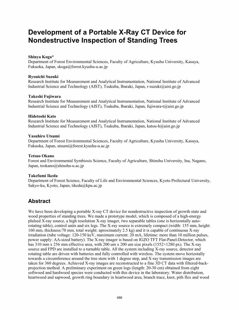
Development of a Portable X-Ray CT Device for Nondestructive Inspection of Standing Trees Shinya Koga* Department of Forest Environmental Sciences, Faculty of Agriculture, Kyushu University, Kasuya, Fukuoka, Japan, skoga@forest.kyushu-u.ac.jp Ryouichi Suzuki Research Institute for Measurement and Analytical Instrumentation, National Institute of Advanced Industrial Science and Technology (AIST), Tsukuba, Ibaraki, Japan, r-suzuki@aist.go.jp Takeshi Fujiwara Research Institute for Measurement and Analytical Instrumentation, National Institute of Advanced Industrial Science and Technology (AIST), Tsukuba, Ibaraki, Japan, fujiwara-t@aist.go.jp Hidetoshi Kato Research Institute for Measurement and Analytical Instrumentation, National Institute of Advanced Industrial Science and Technology (AIST), Tsukuba, Ibaraki, Japan, katou-h@aist.go.jp Yasuhiro Utsumi Department of Forest Environmental Sciences, Faculty of Agriculture, Kyushu University, Kasuya, Fukuoka, Japan, utsumi@forest.kyushu-u.ac.jp Tetsuo Okano Forest and Environmental Symbiosis Science, Faculty of Agriculture, Shinshu University, Ina, Nagano, Japan, teokano@shinshu-u.ac.jp Takefumi Ikeda Department of Forest Science, Faculty of Life and Environmental Sciences, Kyoto Prefectural University, Sakyo-ku, Kyoto, Japan, tikeda@kpu.ac.jp Abstract We have been developing a portable X-ray CT device for nondestructive inspection of growth state and wood properties of standing trees. We made a prototype model, which is composed of a high-energy plulsed X-ray source, a high resolution X-ray imager, two separable tables (one is horizontally auto-rotating table), control units and six legs. The X-ray source is extremely compact (width: 155 mm, height: 160 mm, thickness:70 mm, total weight: aproximately 2.5 kg) and it is capable of continuous X-ray irradiation (tube voltage: 120-150 keV, maximum current: 20 mA, lifetime: more than 10 million pulses, power supply: AA-sized battery). The X-ray imager is based on IGZO TFT Flat-Panel-Detector, which has 310 mm x 256 mm effective area, with 200 um x 200 um size pixels (1552×1280 px). The X-ray source and FPD are installed to a turnable table. All the system including X-ray source, detector and rotating table are driven with batteries and fully controlled with wireless. The system move horizotally towards a circumference around the tree stem with 1 degree step, and X-ray transmission images are taken for 360 degrees. Achieved X-ray images are reconstructed to a fine 3D CT data with filtered-back-projection method. A preliminary experiment on green logs (length: 20-30 cm) obtained from eight softwood and hardwood species were conducted with this device in the laboratory. Water distribution, heartwood and sapwood, growth ring boundary in heartwood area, branch trace, knot, pith flex and wood

686

decay were detectable in three dimensions based on the reconstructed images, although the image quality depends on species. This study indicated that this device has a potential as a useful tool for nondestructive inspection. Keywords: portable X-ray source, growth ring, heartwood and sapwood, water distribution, wood decay Introduction In Japan, forests cover approximately 25 million hectares and account for two-thirds of national land area (Forestry Agency 2018). Plantation forests are approximately 10 million hectares (42%). Main species of planation forests are Cryptomeria japonica, Chamaecyparis obtusa and Larix kaempferi, and more than half of these planted forests are mature, namely over 46 years old (Forestry Agency 2018). It is necessary to evaluate wood properties of timber, log and standing tree in order to utilize these forest resource effectively. Especially when evaluate wood properties of standing tree, nondestructive technique is significantly important. Many development researches on nondestructive techniques and methods for the wood property evaluation have been conducted [e.g. X-ray, thermal, microwave, ultrasonic, Nuclear Magnetic Resonance (NMR) and neutron, and near infrared spectroscopy (Bucur 2003, Tsuchikawa and Kobori 2015)]. In 2008, one of authors has developed a high-energy pulsed X-ray source (Suzuki 2008, 2009, Katoh et al. 2014) (Figure 1). It had the potential to use in the outside field, because the power supply is AA-sized battery and it is portable (i.e. compact and lightweight). Then, we initiated a project on the development of a portable X-ray CT device for nondestructive inspection of growth and wood properties of standing tree. We made a prototype model in 2018. The objective of this study is to conduct a preliminary experiment using small logs of several species in the laboratory adn assess the potential of this device.

Figure 1—High-energy pulsed X-ray source has developed by Suzuki in 2008.

687

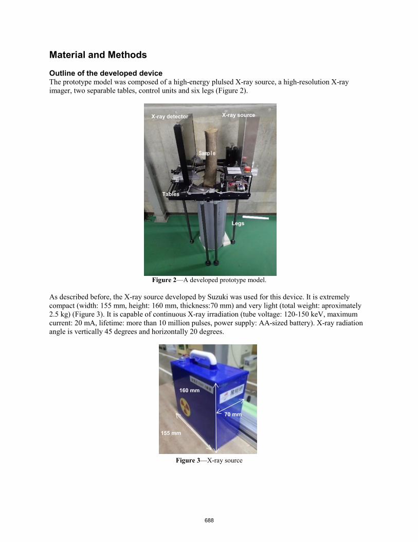
Material and Methods Outline of the developed device The prototype model was composed of a high-energy plulsed X-ray source, a high-resolution X-ray imager, two separable tables, control units and six legs (Figure 2).

Figure 2—A developed prototype model.

As described before, the X-ray source developed by Suzuki was used for this device. It is extremely compact (width: 155 mm, height: 160 mm, thickness:70 mm) and very light (total weight: aproximately 2.5 kg) (Figure 3). It is capable of continuous X-ray irradiation (tube voltage: 120-150 keV, maximum current: 20 mA, lifetime: more than 10 million pulses, power supply: AA-sized battery). X-ray radiation angle is vertically 45 degrees and horizontally 20 degrees.

Figure 3—X-ray source

X-ray detector X-ray source

Sample

Tables

Legs

155 mm

70 mm

160 mm

688

A high resolution X-ray imager based on IGZO TFT Flat-Panel-Detector developed by National Institute of Advanced Industrial Science and Technology (AIST) was used (Figure 2). The FPD has 310 mm x 256 mm effective area, with 200um x 200um size pixels (1552×1280 px).

Figure 4—Rotation table and fixed table. The are separable to sandwich a standing tree.

The X-ray source and flat panel detector are installed to a auto-rotation table (stage size: mm x mm, hole size: mm x mm) (Figures 1 and 4). All the system including X-ray source, detector and rotating table are driven with batteries and fully controlled with wireless. The system move towards a circumference around the tree sample with 1.03 degree step, and X-ray transmission images are taken for 360 degrees. It takes aproximately 30 minitues to revolve around the object. Achieved X-ray images are reconstructed to a fine 3D CT data with filtered-back-projection method. Samples and experiment

Four softwood species (Pinus densiflora, Larix kaempferi, Cryptomeria japonica and Chamaecyparis obtusa) and four hardwood species (Betula platyphylla, Castanea crenata, Quercus crispula and Quercus crispula) were used for this experiment. One sample tree from each species was obtained from the Kasuya Research Forest and the Ashoro Research Forestm Kyushu University, Japan. One logs (length: 20-30 cm) and one disck (thikness: aproximately 1cm) were cut off at the breast height (1.3 m) of each sample tree. Immediate after cutting them, both of the butt and top end of log were sealed with vaseline in order to prevent drying and then, wrapped with a cling wrap. All green logs were put into a plastic bag and moved to the laboratory. Transverse plane of the green disk was scanned by a flat head image scanner (Seiko Epson Corporation, GT-X970, Japan). After the disk was divided into heartwood and sapwood, moisture content (%) and basic wood density (kg/m3) was measured. As a preliminary experiment, an X-ray transmitting experiment was conducted for these log samples with this device in the laboratory of AIST (Figure 5).

689

Figure 5—X-ray transmitting experiment in the laboratory.

Results and discussion Both scanner image and X-ray image obtained from Cryptomeria japonica and Castanea crenata are shown in Figures 6, by way of samples. Water distribution within stem was clearly detected for every softwood species (Pinus densiflora, Larix kaempferi, Cryptomeria japonica, Chamaecyparis obtusa). Heartwood and intermediate wood which had low moisture content and sapwood which had higher moisture content could be classified clearly. Additionally, low moisture area where cavitation would be induced in sapwood and the neighborhood of knot was also detectable (Figure 6). Growth ring boundary in heartwood area, namely lower moisture area was clearly detected, but that in sapwood, namely higher moisture area, was not clearly detectable.

a. Cryptomeria japonica (diameter: 12cm)

b. Castanea crenata (diameter: 12cm)

690

C. Quercus crispula (diameter: 12cm)

Figure 6—Scanner images (left) and corresponding X-ray images (right) of cross section of Cryptomeria japonica (a), Castanea crenata (b) and Quercus crispula (C) .

Hardwood and sapwood areas in every hardwood species (Betula platyphylla, Castanea crenata, Quercus crispula, Quercus serrata) could not be classified easily (Figure 6). Growth ring boundary depend on species. It is detectable clearly for Castanea crenata (Figure 6) and Betula platyphylla (Figure 7) and, but that for Quercus crispula and Quercus serrata was not clearly detectable (Figure 6). There results would be related with wood anatomy and structure, wood density, water distribution and total amount of water. Some wood defects such as branch trace, knot, decay area and pith fleck related with wood density and moisture content were clearly detectable. In addition, Chamaecyparis obtusa sample tree has compression wood and Betula platyphylla sample tree has tension wood in growth rings. Reaction wood was also detectable (Figure 7).

Figure 7—X-ray image of cross section of Betula platyphylla (diameter: 12cm). Arrow indicates tension wood.

Conclusions Water distribution, heartwood and sapwood area, growth ring boundary in heartwood, some wood defects were clearly detectable in three dimensions based on the images obtained from the portable X-ray CT device devloped, although the detectable level of each charateristic depended on species. This study indicated that this device has the potential as a useful tool for nondestructive inspection. We will improve the image quality and apply large trees by further high power of X-ray source, increasing in effective area and high-resolution of X-ray imager and so on. Additionally we try to conduct a X-ray transmitting experiment for standing trees growing in forest field.

691

Acknowledgments We would like to thank the Kasuya Research Forest and Ashoro Research Forest of Kyushu University for providing us with the sample trees. This work was supported by JSPS KAKENHI Grant Numbers JP 22580186, JP25292105 and JP17H03847. References Bucur, V. 2003. Nondestructive Characterization and Imaging of Wood (Springer Series in Wood Science). 354p., Springer. Berlin, Heidelberg Forestry Agency 2018. Annual Report on Forest and Forestry in Japan. Fiscal Year 2017. p.3 Kato, H., O’Rourke, B. E., Suzuki, R. 2014. Electron gun using coniferous carbon nano-structure JJAP Conference Proceedings 2:011302 Suzuki, R. 2008.Development of a compact electron accelerator operated by AA-sized batteries (in Japanese). Isotope News 646: 16-17 Suzuki, R. 2008. Development of a portable high-energy pulsed X-ray source operated by AA-sized batteries．Synthesiology 2: 237-243 Suzuki, R. 2011. Electron beam generater, X-ray generater and X-ray device. Japan patent JP4756283 Tsuchikawa, S. and Koborim H, 2015 A review of recent application of near infrared spectroscopy to wood science and technology. Journal of Wood Research 61(3): 213–220

692

Neutron Imaging as a Tool for the Study of Spatial and Time-Dependent Moisture Sorption Processes in Varnished Wood Sarah L. Lämmlein Swiss Federal Laboratories for Materials Science and Technology (Empa), Dübendorf, Switzerland, Sarah.Laemmlein@empa.ch Francis W. M. R. Schwarze Swiss Federal Laboratories for Materials Science and Technology (Empa), St. Gallen, Switzerland francis.schwarze@empa.ch Ingo Burgert Institute for Building Materials, ETH Zurich, Zurich, Switzerland, iburgert@ethz.ch David Mannes * Laboratory for Neutron Scattering and Imaging, Paul Scherrer Institut, Villigen Switzerland, david.mannes@psi.ch * Corresponding author Abstract Neutron imaging is a nondestructive testing method that is based on working principles similar to x-ray imaging but with a higher sensitivity to hydrogen and therefore moisture. This is caused by the opposite interaction between radiation and matter: whereas x-ray photons interact with the atomic electron shell, neutrons interact merely with the atomic nuclei. As a result, the two radiation types show partially complementary attenuation characteristics. Certain light elements such as hydrogen, lithium, and boron have a high neutron attenuation, whereas other heavy elements such as lead or tungsten are relatively easily penetrated. These properties make neutron imaging a unique option for in situ investigations of moisture changes in materials such as wood. In this study, we demonstrate how neutron imaging can be used to study the moisture content changes in varnished wood. The focus was on the influence of varnishes on the wood sorption dynamics of wooden stringed instruments. Wood samples, with several varnish systems, were tested in a neutron transparent climatic chamber with variable climatic conditions. This setup allowed in situ determination of spatial and time-dependent moisture content changes in the varnished wood specimens at radiographic (2D) and tomographic (3D) modes under controlled climatic conditions. Keywords: Neutron imaging, varnish, wooden stringed instruments, wood sorption dynamics

693

Assessing Manufacturing Variability of Wooden Pallets by Vibrational Continuous Measurement to Prevent Static and Dynamic Behavior to Optimize Safety of Goods and Users Jean-Denis Lanvin * Primary Processing & Supply Department, Institut Technologique FCBA, Allée de Boutaut BP 228 - 33028 Bordeaux Cedex, France, jean-denis.lanvin@fcba.fr Maxime Robin Recherche & Développement, InnoduraTB, 62 Boulevard Niels Bohr - CS 52132, Villeurbanne Cedex, France, maxime.robin@innodura.fr Patrice Chanrion Pôle Professionnel Palettes, SYPAL, 6 rue François 1er - 75008 PARIS, France, patrice.chanrion@fnbois.com * Corresponding author Abstract Wooden pallets are an integral part of the supply chain, facilitating the transport and protection of products. However, sawmills, which produce pallet components, are not able to carry out P1 or P2 classifications essential to reach mechanical performance. To prevent failure, pallet producers apply safety factors (*2) on nominal loads to protect themselves. The objective of this study was to verify the feasibility of a unitary control of the mechanical strength of pallets. A batch of 40 new pallets were analyzed by a nondestructive vibratory system developed by INNODURA. Shocks by acoustic hammer were made at different points on the pallet to characterize both global and local behavior of its various components. The pallets were bent to failure (ISO 8611-1) and the ultimate loads were then correlated with the NDT information. According to ISO 8611-2, a batch of 40 pallets is considered compliant (threshold of 3,000 kg, payload should reach 1,500 kg with safety factor). However, the statistical correlation between NDT and failure tests was not sufficiently robust. The range of result was between 2,100 and 3,700 kg. However, the control of each pallet by vibration would make possible to decrease the normative safety factor with NDT prediction of the real performance. The machine could certify that the controlled pallet will be able to support 1,500 kg as well as the low point of the batch (more than 2,100 kg). In this case, the reject yield estimated at 20% for this prestudy is completely erased. Keywords: Pallets, mechanical strength, NDT measurement, vibration, nominal load

694

Evaluating Bamboo Stem Elastic Modulus with the Longitudinal Vibration Method Lorenzo Lube dos Santos * Civil Engineering Department, Centro Universitário FAESA, Av. Vitória, 2220, 29053-360 Vitória, ES, Brazil, lorenzo.lube@faesa.br Pablo Altoé Amorim Mechanical Engineering Department, Centro Universitário FAESA, Av. Vitória, 2220, 29053-360 Vitória, ES, Brazil, pablo.altoe@faesa.br Fabíola Angela Ferrari Civil Engineering Department, Centro Universitário FAESA, Av. Vitória, 2220, 29053-360 Vitória, ES, Brazil, faferrari@hotmail.com Leonardo Galavote Rosseto Civil Engineering Department, Centro Universitário FAESA, Av. Vitória, 2220, 29053-360 Vitória, ES, Brazil, leonardorossetto9@hotmail.com * Corresponding author Abstract Bamboo is a versatile material and widely used in construction. Its application as a structural element requires knowledge of its physical and mechanical properties. Because the material has great dimensional variability, the elastic properties can vary greatly when tested conventionally. This study aimed to evaluate the bamboo dynamic elastic modulus using the longitudinal vibration method. For this purpose, 30 specimens of the bamboo Dendrocalamus giganteus were prepared in small dimensions (10 by 30 by 300 mm) and selected in five different heights of the stem. The samples were rectangular shaped to reduce the natural variability of the material and to facilitate analysis. The specimens were positioned on elastomeric supports, and the longitudinal vibration test was performed based on the recommendations of ASTM E-1876 and ASTM C-215, with the aid of FFT Analyzer Software from Fakopp enterprise. The static bending test was performed following the recommendations of ASTM D-143, in the flatwise position. Subsequently, analysis of variance (ANOVA) was performed for independent groups, complemented by the Tukey multiple comparisons test at the 5% significance level. A small variance of the results obtained by the vibrational method was verified, with an average increase of 22% compared with the static test. The averages of the stem height groups did not vary, demonstrating that there was no significant variation of the dynamic modulus of elasticity. The correlations between the static and dynamic elastic modulus were not satisfactory because of the great variability of the static results. Keywords: Bamboo, longitudinal vibration, elastic modulus

695

Evaluation of Industrial Nondestructive Parameters in Determination of Visual Grading in Structural Timber Boards of Pinus spp. Lorenzo Lube dos Santos Department of Structural Engineering, Sao Carlos School of Engineering-Sao Paulo University, Sao Carlos, Sao Paulo State, Brazil, lorenzolube@yahoo.com.br Antonio Alves Dias * Department of Structural Engineering, Sao Carlos School of Engineering-Sao Paulo University, São Carlos, Sao Paulo State, Brazil, dias@sc.usp.br Carlito Calil Jr. Department of Structural Engineering, São Carlos School of Engineering-Sao Paulo University, Sao Carlos, Sao Paulo State, Brazil, calil@sc.usp.br Adriano Wagner Ballarin College of Agronomical Sciences, Sao Paulo State University, Botucatu, Sao Paulo State, Brazil, adriano.ballarin@unesp.br Sergio Augusto Rodrigues College of Agronomical Sciences, Sao Paulo State University, Botucatu, Sao Paulo State, Brazil, sergio.rodrigues@unesp.br * Corresponding author Abstract The use of nondestructive methods for grading of wood is an intelligent solution in the optimization of industrial processes. Visual grading is the initial step for grouping batches of wood with similar qualities. Recently, with the development of high-precision industrial scanners, it is possible to perform this grouping by means of x-ray image parameters. These devices have the advantage of measuring defects that are invisible to human eyes. The objective of this work was to evaluate the visual grading recommended by the SPIB (2014) regarding the observed results of the parameter Knot_18 generated by the industrial scanner GoldenEye 706. This work would verify possible differences between the average answers of each grade. About 1,500 boards of a mixed lot of Pinus taeda and Pinus elliottii grown in Brazil, with dimensions 38 by 89 by 3,960 mm, were measured by the scanner and visually graded by a single person. The lot was separated into five visual grades: SS, S1, S2, S3, and F. These grades were attributed to the worst visual node, besides having relative dimensions measured according to the Knot_18 parameter. Subsequently, analysis of variance (ANOVA) was performed for independent groups, complemented by the Tukey multiple comparison test at the 5% level of significance. It was observed that all the visual grades differed in relation to the mean size of the Knot_18 parameter, allowing the conclusion that there is a matching between Knot_18 and the visual grades. Keywords: Timber grading, structural grading, timber boards

696

Monitoring Wood Quality of African Mahogany Using Nondestructive Techniques: Preliminary Evaluation João Gabriel Missia da Silva * Forest and Wood Science Department, Federal University of Espírito Santo, Jerônimo Monteiro, Espírito Santo, Brazil, j.gabrielmissia@hotmail.com Graziela Baptista Vidaurre Forest and Wood Science Department, Federal University of Espírito Santo, Jerônimo Monteiro, Espírito Santo, Brazil, grazividaurre@gmail.com José Tarcísio da Silva Oliveira Forest and Wood Science Department, Federal University of Espírito Santo, Jerônimo Monteiro, Espírito Santo, Brazil, jose.t.oliveira@ufes.br Alexa Barglini de Melo Forest and Wood Science Department, Federal University of Espírito Santo, Jerônimo Monteiro, Espírito Santo, Brazil, alexabmelo@hotmail.com Ramon Ferreira Oliveira Forest and Wood Science Department, Federal University of Espírito Santo, Jerônimo Monteiro, Espírito Santo, Brazil, oliveira.r.eim@gmail.com * Corresponding author Abstract African mahogany plantations in Brazil have been intensified in the last decade, but scientific studies of the wood properties are still scarce. The wood quality can be described as the association of the intrinsic properties of this material with a particular use. Therefore, the natural variability of wood properties should be considered to achieve excellence in forest management procedures, processing operations, and end use. The aim of this study was to evaluate the radial variability of wood basic density (BD) and dynamic modulus of elasticity (MOE) in standing trees of Khaya spp., at 57 months old, of a commercial plantation (5- by 5-m spacing) in Capinópolis, state of Minas Gerais, Brazil. Increment cores were removed at breast height (west face of the stem) of 15 trees with an increment borer to evaluate the wood BD in the laboratory. Stress wave propagation time was measured with a Microsecond Timer Fakkop in the transverse and longitudinal directions at breast height in 30 trees. The mean BD was 0.49 g cm-3 (coefficient of variation = 11.01%), which was classified as moderately heavy, and increased 20.45% from the pith toward the tree bark. The MOE was 11.25 and 2.55 GPa in the longitudinal and transverse directions, respectively. The MOEd in the direction of the diameter of the trees was low, since the wood was juvenile and the anatomical characteristics and physical properties of the wood were still in formation. Keywords: Wood quality, density, dynamic modulus of elasticity, African mahogany, nondestructive evaluation

697

Optimization of Resistograph Drilling Depth in Eucalyptus Young Trees João Gabriel Missia da Silva * Forest and Wood Science Department, Federal University of Espírito Santo, Jerônimo Monteiro, Espírito Santo, Brazil, j.gabrielmissia@hotmail.com Graziela Baptista Vidaurre Forest and Wood Science Department, Federal University of Espírito Santo, Jerônimo Monteiro, Espírito Santo, Brazil, grazividaurre@gmail.com José Tarcísio da Silva Oliveira Forest and Wood Science Department, Federal University of Espírito Santo, Jerônimo Monteiro, Espírito Santo, Brazil, jose.t.oliveira@ufes.br Djeison Cesar Batista Forest and Wood Science Department, Federal University of Espírito Santo, Jerônimo Monteiro, Espírito Santo, Brazil, djeison.batista@ufes.br Lourdes Maria Hilgert Santos Forest and Wood Science Department, Federal University of Espírito Santo, Jerônimo Monteiro, Espírito Santo, Brazil, lourdesmaria.engflorestal@yahoo.com.br * Corresponding author Abstract The drilling resistance technique (DR) has great potential and operational efficiency to predict the wood density (WD) of eucalyptus young trees. However, there are some factors that need to be better understood to increase its use. Recent research has shown that friction on the shaft of the drill increases as a function of penetration depth, particularly for hardwood species. The aim of this study was to optimize drilling depth for WD estimation by DR in eucalyptus trees. DR readings (full diameter and in the first 5 cm from the bark) were made with the resistograph (R650-SC) at breast height of 80 trees of two clones of Eucalyptus grandis x Eucalyptus urophylla (76 months old), planted in Aracruz, Espírito Santo State, Brazil. At the same position of the drillings, disks were taken and WD was evaluated in samples every 5 mm. The ideal drilling depth was the one in which the WD modeling by linear regression returned the higher adjusted coefficient of determination (R²aj.) and smaller standard error of estimate (Syx). DR at depths of 0.5 to 1.0 cm and closer to the pith were not efficient in WD prediction, and the estimates were not significant. The predictive potential of WD increased up to 1.5 cm from the bark and then decreased with advancing drilling depth. The drilling depth at 1.5 cm from the bark was the most efficient (R²aj. = 0.68, Syx =0.029 g cm-3) in estimating WD from eucalyptus clones. Keywords: Wood quality, drilling resistance, wood density, drill penetration depth, Eucalyptus

698

Improvement of Seed Orchards with Progeny Tests and Nondestructive Wood Property Testing in a Tree Breeding Project in Kenya Hisaya Miyashita * Forest Tree Breeding Center, Forestry and Forest Products research Institute, Okayama, Japan, hmiyasi@affrc.go.jp James K. Ndufa Drylands Eco-regional Research Programme, Kenya Forestry Research Institute, Nairobi, Kenya, jkndufa@yahoo.com * Corresponding author Abstract In Kenya, a tree breeding project on Melia volkensii (an indigenous tree species in Kenya) for adaptation to climate change has been implemented with collaboration between Kenya Forest Research Institute (KEFRI) and Forest Tree Breeding Center (FTBC) since 2012. One hundred trees have been selected as plus trees with good performance of growth from the arid and semi-arid lands (ASALs) in Kenya. By the end of 2012, two clonal seed orchards introducing the Melia plus trees were established at ASAL sites. Four progeny test sites (PTSs) were established using seeds derived from the seed orchards in ASALs in 2014, and eight more progeny test sites were established in 2015. The tree height and diameter at breast height (DBH) were measured at PTSs every half year after planting. At 18 months after planting, average tree height reached 4 m and average DBH was 8 cm. To improve seed orchards according to the progeny test, we investigated the variation of Pilodyn penetration and stress wave velocity at PTS as a trial nondestructive wood property testing in 2018. At two PTSs, 1,037 trees were measured by Pilodyn, and at one PTS, 274 trees were measured by Fakopp. As the result of analysis on the growth and wood properties, we were able to identify superior Melia plus trees with both qualities, which will lead to further improvement of seeds and seedlings for Melia planting by tree breeding. Keywords: Melia volkensii, tree breeding, progeny test, Pilodyn penetration, stress wave velocity

699

Evaluation of C40 Eucalyptus Wood from Static Bending Tests and by Impulse Excitation Technique Julio Cesar Molina * School of Timber Industrial Engineering, UNESP, Itapeva, Sao Paulo, Brazil, julio.molina@unesp.br Nádia Barros Gomes Department of Mechanical Engineering, FEG-UNESP, Guaratinguetá, São Paulo, Brazil, nadiabarrosg@gmail.com Rafael de Araújo Cerdeira School of Timber Industrial Engineering, UNESP, Itapeva, Sao Paulo, Brazil, rafaelcerdeiraa@gmail.com Daniel Villas Bôas School of Timber Industrial Engineering, UNESP, Itapeva, Sao Paulo, Brazil, daniel.villas@unesp.br * Corresponding author Abstract The aim of this work was to characterize, from nondestructive tests, the stiffness of eucalyptus lamellae (resistance class C40) for use in glulam beams. The wood lamellae were analyzed with moisture content of 12% as recommended by the ABNT NBR 7190: 1997. Two different methods were used to determine the elasticity modulus of the lamellae: the three-point bending test performed on the Universal Test Machine (EMIC) with a capacity of 300 kN and the sonelastic equipment, which works based on the technique of impulse excitation. In the technique of impulse excitation, from the sound emitted by the material, it is possible to determine its elastic properties. A total of 100 wood lamellae with dimensions of 5 cm × 1 cm × 115 cm were analyzed. A hypothesis test with confidence level of 95% was performed using the minitab software. The average values obtained for the elasticity modulus of wood using the technique of impulse excitation and the bending test were 18156 MPa and 16263 MPa, respectively. The observed difference between the means in this case was 10.42% and the coefficients of variation of these results were 0.14 and 0.15, respectively. However, the coefficient of determination R2 was 0.549, indicating a moderate correlation, and the hypothesis test indicated the existence of significant differences between the mean values of the elasticity modulus obtained by the two evaluated methods. Keywords: Eucalyptus, elasticity modulus, bending test, impulse excitation technique

700

Influence of Different Wood Species, Different Moisture Contents on Pin Penetration Depth Ryu Noda * Graduate School of Engineering Science, Akita University, Akita-city, Akita, Japan, noda@gipc.akita-u.ac.jp Humihiko Gotou Graduate School of Engineering Science, Akita University, Akita-city, Akita, Japan * Corresponding author Abstract We propose to evaluate deterioration using an inexpensive and easy-to-handle testing device that utilizes a deterioration diagnostic method in which a driver pin is attached to a load measuring instrument. We investigated the pin penetration depth using various types of driver pins, wood species, and wood moisture contents to evaluate degree of deterioration by this method. We found that diagnosis using a load measuring instrument and driver pins could sufficiently estimate a certain degree of deterioration. Keywords: Deterioration, deterioration diagnostic method, load measuring instrument, driver pin

701

Sonic Root Detector to Reveal the Distribution of Tree Coarse Roots in Soil: A First Case Study in Italy A.R. Proto * Department of Agriculture, University “Mediterranea” of Reggio Calabria, Reggio Calabria, Italy, andrea.proto@unirc.it A. Di Iorio Department of Biotechnologies and Life Sciences, University of Insubria, Varese, Italy, antonino.diiorio@uninsubria.it L.M. Abenavoli Department of Agriculture, University “Mediterranea” of Reggio Calabria, Reggio Calabria, Italy, S. Papandrea Department of Agriculture, University “Mediterranea” of Reggio Calabria, Reggio Calabria, Italy, R. Vescio Department of Agriculture, University “Mediterranea” of Reggio Calabria, Reggio Calabria, Italy, A. Sorgonà Department of Agriculture, University “Mediterranea” of Reggio Calabria, Reggio Calabria, Italy, asorgona@unirc.it * Corresponding author Abstract The root architecture—the root radial and vertical distribution in the soil—is involved in different plant functional roles, such as nutrient and water acquisition and mechanically active anchorage. Due to the underground growth habitat, tree root architecture has been mainly determined by destructive methods that require root excavation from the soil and the three-dimensional digitizing by different 3D digitizers (FASTRAK®, GTCO Freepoint 3D). However, these root techniques are extremely time consuming, labor intensive, and impratical, especially in urban environments. Fortunately, in the past decade, portable and noninvasive methods to detect and visualize the root system have been used commercially. This communication describes a pilot study to investigate the reliability of a nondestructive method (i.e., the Root-Detector, Fakopp Enterprise Bt) for detection and determining the radial distribution of individual roots of olive trees in the soil, by statistical linear and radial correlations of the sonic speed data with those obtained from the real root horizontal and vertical distribution by 3D digitizer (Fastrak®, Polhemus). Outcomes clearly showed that the Root Detector was able to map the olive roots in the soil environment, but with some conditions. First, the detection of roots by the Root Detector was more efficient within 30 cm of soil depth. Second, at the farthest distance from the trunk (>120 cm), the sonic speed and detection of the roots were reduced. Third, the Root Detector technology fails to detect the root size in terms of geometric parameters such as root diameter. Keywords: Roots, sensors, 3D digitizer, nondestructive method

702

Acoustic Emission Analysis Based on Centroid Frequency of Culm Bamboo Subjected to Tensile Test Francisco J. Rescalvo * Building Engineering School. University of Granada. Campus Fuentenueva s/n. 18071. Granada, Spain. rescalvo@ugr.es Alba Fernández Building Engineering School. University of Granada. Campus Fuentenueva s/n. 18071. Granada, Spain. albali@correo.ugr.es Ana Cruz Building Engineering School. University of Granada. Campus Fuentenueva s/n. 18071. Granada, Spain. anacru@ugr.es Antolino Gallego Building Engineering School. University of Granada. Campus Fuentenueva s/n. 18071. Granada, Spain. antolino@ugr.es * Corresponding author Abstract Bamboo has been used since ancient times, especially in parts of Asia. Now, in Europe and America, attention is being paid to this type of wood. In particular, the bamboo wood samples used in this work were extracted from the full culm of Bambusa species, grown at the tropical coast of the province of Granada (Spain). A comparison of samples with and without nodes at the central part was carried out. The samples were subjected to monotonic tensile tests and monitored with the acoustic emission technique. The acoustic emission signals were recorded with multiresonant sensors, analyzing different features in the frequency domain. A specific failure mode was observed, with significant plasticization prior to the breakage of the inner part. From this load until the final break of the outer part, a significant increase in acoustic emissions and signals with a high centroid frequency were observed. Acoustic emission was correlated with visual inspection of the breakage progress throughout the test. Keywords: Wood, bamboo, acoustic emission, signal analysis

703

Acoustic Behavior of Standing Poplar Trees: Influence of Site in Spain, Cultivar, and Measurement Season Francisco J. Rescalvo * Building Engineering School. University of Granada. Campus Fuentenueva s/n. 18071. Granada, Spain. rescalvo@ugr.es María A. Ripoll Instituto de Formación e Investigación Agraria y Pesquera de Andalucía. Camino del Purchil. Granada, Spain. mariaa.ripoll@juntadeandalucia.es Antolino Gallego Building Engineering School. University of Granada. Campus Fuentenueva s/n. 18071. Granada, Spain. antolino@ugr.es * Corresponding author Abstract For the wood industry, being able to perform quality grading of wood prior to harvesting is greatly important and appealing because it impacts the purchase price directly. The grade depends on physical variables such as density, fiber orientation, bending capacity, and modulus of elasticity. One of the parameters that allows evaluation of wood in standing trees is elastic wave propagation velocity, which has acquired more popularity recently because it allows nondestructive evaluation. This work shows how the velocity is affected by the cultivar, the location of the crop, and the measurement season, in the case of planted poplar trees. To accurately determine the arrival time of the waves, the Akaike method based on the entropy of the signals recorded with the piezoelectric sensors was applied. Measurements were carried out in several plots located in the north and south of Spain. Keywords: Wood, poplar, elastic waves, signal analysis, propagation velocity, entropy

704

Eucalyptus grandis Apparent Density, Characterized by Digital X-Ray Images, with Mineral Fertilization and Water Availability Vinicius Resende de Castro * Departamento de Engenharia Florestal, Universidade Federal de Viçosa, Viçosa, Minas Gerais, Brazil, vinicius.castro@ufv.br Mario Tomazello Filho Departamento de Engenharia Florestal, Escola Superior de Agricultura, Luiz de Queiroz, Piracicaba, São Paulo, Brazil, mtomazel@usp.br Paula Gabriella Surdi

Departamento de Engenharia Florestal, Universidade Federal de Viçosa, Viçosa, Minas Gerais, Brazil, paulasurdi@gmail.com * Corresponding author Abstract Extensive areas of eucalyptus plantations in Brazil and other regions of the world are subject to climate change, water stress, and low soil fertility. Forest nutrition, such as K and Na, and its interaction with water availability in the growth and wood properties of the eucalyptus, should be studied. This work aimed to evaluate the apparent wood density at 12% humidity of Eucalyptus grandis trees at 12, 24, 36, and 48 months old under different rainfall conditions and K and Na nutrition. The treatments were two water regimes (100% and 66% of the rainfall) and three nutrition types: K (4.5 kmol/ha), Na (4.5 kmol/ha), and the control. The apparent density, at 12% relative humidity, of the samples from the diameter-at-breast-height (1.3-m) position of the tree trunk was determined by x-ray densitometry and digital images. The apparent density at 12% relative humidity of eucalyptus trees differed between treatments with different nutrition and water availability. The radial profile of density was higher from the 3-year-old trees. The digital images showed radial variation of the wood apparent density. The results provide support for the adoption of silvicultural practices in forest plantations with water stress, affected by climatic changes, or submitted to K and Na nutrition. Keywords: Nutrition, x-ray densitometry, water stress, wood quality

705

Predicting Wood Properties with Drilling Resistance Measurements at Different Speeds and Directions of Drilling Evgenii Sharapov * Volga State University of Technology, Yoshkar-Ola, Mari El Republic, Russian Federation, e-mail: sharapoves@volgatech.net Christian Brischke Wood Biology and Wood Products, University of Goettingen, Goettingen, Germany, christian.brischke@uni-goettingen.de Sascha Bicke Wood Biology and Wood Products, University of Goettingen, Goettingen, Germany, sascha.bicke@forst.uni-goettingen.de Holger Militz Wood Biology and Wood Products, University of Goettingen, Goettingen, Germany, hmilitz@gwdg.de Elena Smirnova Volga State University of Technology, Yoshkar-Ola, Mari El Republic, Russian Federation Johannes A. Herbener Wood Biology and Wood Products, University of Goettingen, Goettingen, Germany * Corresponding author Abstract Advanced tools for drilling resistance (DR) measurements operate at various constant (preselected) or automatically varied drilling speeds: feed rate and rotational speed. Every variation of drilling speed will influence the uncut chip thickness, cutting speeds, and cutting angles and thus DR and feeding resistance (FR). Inspection of wooden construction and materials by DR measurements can be done also at different directions of drill bit penetration in relation to the wood grain direction. In this case, longitudinal and transverse (radial and tangential) drillings are distinguished. The main objectives of the laboratory study were to determine the correlation between DR and FR and uncut chip thickness for major cutting edges (feed rate and rotational speed) as well as the impact of the drilling direction on DR measurements depending on the grain direction. The experiment consisted of two separate drilling tests on Scots pine (Pinus sylvestris L.), European beech (Fagus sylvatica L.), poplar (Populus alba L.), and English oak (Quercus robur L.) conditioned in normal climate (20°C/65% RH). To conduct the DR measurements, an IML-RESI PD 400 tool and new standard spade drill bits for each test were used (IML System GmbH, Wiesloch, Germany). One part of the DR measurements was carried out with 25 combinations of feed rate and rotational speed and the other with five variations of angles between drill bit penetration and grain direction: radial-tangential and tangential-longitudinal drilling. Positive, nonlinear correlations between uncut chip thickness and DR and FR for the individually tested wood species were investigated (R2 = 0.93 to 0.99). It was found that drilling direction in relation to grain orientation had a minor impact on the DR measurements. Keywords: Drilling resistance, wood properties, feed rate, rotational speed, chip thickness, wood cutting

706

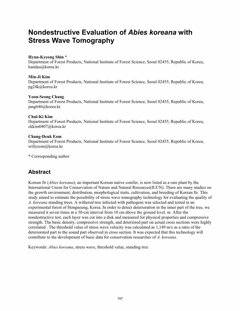
Nondestructive Evaluation of Abies koreana with Stress Wave Tomography Hyun-Kyeong Shin * Department of Forest Products, National Institute of Forest Science, Seoul 02455, Republic of Korea, kandau@korea.kr Min-Ji Kim Department of Forest Products, National Institute of Forest Science, Seoul 02455, Republic of Korea, pg24k@korea.kr Yoon-Seong Chang Department of Forest Products, National Institute of Forest Science, Seoul 02455, Republic of Korea, jang646@korea.kr Chul-Ki Kim Department of Forest Products, National Institute of Forest Science, Seoul 02455, Republic of Korea, ckkim0407@korea.kr Chang-Deuk Eom Department of Forest Products, National Institute of Forest Science, Seoul 02455, Republic of Korea, willyeom@korea.kr * Corresponding author Abstract Korean fir (Abies koreana), an important Korean native conifer, is now listed as a rare plant by the International Union for Conservation of Nature and Natural Resources(IUCN). There are many studies on the growth environment, distribution, morphological traits, cultivation, and breeding of Korean fir. This study aimed to estimate the possibility of stress wave tomography technology for evaluating the quality of A. koreana standing trees. A withered tree infected with pathogens was selected and tested in an experimental forest of Hongneung, Korea. In order to detect deterioration in the inner part of the tree, we measured it seven times at a 30-cm interval from 10 cm above the ground level. m After the nondestructive test, each layer was cut into a disk and measured for physical properties and compressive strength. The basic density, compressive strength, and deteriored part on actual cross sections were highly correlated . The threshold value of stress wave velocity was calculated as 1,149 m/s as a ratio of the deteriorated part to the sound part observed in cross section. It was expected that this technology will contribute to the development of basic data for conservation researches of A. koreana. Keywords: Abies koreana, stress wave, threshold value, standing tree

707

Determination of Bonding Strength of Glulam Finger Joints by Mechanical Dynamic Testing Aleš Straže * University of Ljubljana, Biotechnical Faculty, Ljubljana, Slovenia, ales.straze@bf.uni-lj.si Bogdan Šega University of Ljubljana, Biotechnical Faculty, Ljubljana, Slovenia, bogdan.sega@bf.uni-lj.si Milan Šernek University of Ljubljana, Biotechnical Faculty, Ljubljana, Slovenia, milan.sernek@bf.uni-lj.si * Corresponding author Abstract Strength testing of gluelam finger joints is carried out at the EU market in accordance with requirements of the EN 14080 standard. However, the quality control procedure of the production of glulam is static, time-consuming, and destructive. For these reasons, we studied the possibility to predict the bending strength of finger-jointed spruce (Picea abies Karst.) lamellae by fast dynamic mechanical tests. Free-free bending and longitudinal vibration tests were carried out on 105 specimens, 48 mm in thickness and 900 mm in length, with a finger joint at half-length of the lamellae. Static four-point bending tests to determine modulus of elasticity (MOE) and bending strength followed afterwards according to the EN 408 standard procedure. We confirmed the linear relationship between wood density and both static and dynamic moduli of elasticity. The statistically significant relationship between MOE and bending strength of finger-jointed lamellae was also confirmed, better at static MOE (R2 = 0.51) than the dynamic MOE (R2 = 0.25 to 0.39). Prediction of bending strength of finger-jointed lamellae was improved by adding vibration damping (tan δ) and the acoustic coefficient (K) into the multivariate regression model (R2 = 0.71). Multi-peak frequency spectra were detected in basic vibration modes of less homogeneous specimens having variable wood density, growth characteristics, and fibre orientation. Keywords: Glulam, finger joints, dynamic testing, bending strength

708

Effect of Grain Angle on Reflection and Transmission of Visible Light in Wood Hiroyuki Sugimoto * Ehime University Graduate School of Agriculture, Tarumi, Matsuyama 790 8566, Japan, sugimoto.hiroyuki.rw@ehime-u.ac.jp Kazushi Ohshima Ehime University Graduate School of Agriculture, Tarumi, Matsuyama 790 8566, Japan, g653003m@mails.cc.ehime-u.ac.jp Masatoshi Sugimori Ehime University Graduate School of Agriculture, Tarumi, Matsuyama 790 8566, Japan, sugimori.masatoshi.mx@ehime-u.ac.jp Joseph Gril CNRS, Université Clermont Auvergne, Sigma Clermont, Institut Pascal, Campus des Cezeaux, 2 av. Blaise Pascal, TSA 60206, CS 60026, 63178 Aubière Cedex, France, joseph.gril@cnrs.fr * Corresponding author Abstract In a previous paper, we showed that reflections at the interfaces between cell wall and lumen influence the reflection and transmission of light in wood in the long wavelength range of visible light. The effect of grain angle, likely to greatly affect the number of interfaces, should be considered from that viewpoint. In this study, the effect of grain angle (θ) on reflection and transmission of visible light in wood was measured and interpreted through a model of interfaces predicting the reflection and transmission of light passing through wood. For a wavelength of 780 nm, transmittance decreased and the reflectance increased with increasing θ and sample thickness, while the lowest influence of thickness was observed for θ = 22.5°. A model for the relationship between transmission and θ, based on cellular geometry and repartition of light path through cell wall or lumen, agreed with experimental values. Therefore, it was suggested that wood cellular morphology determines the light path and transmission through the sample. Keywords: Reflection, transmission, visible light, grain angle

709

Density Profile of Particleboard Made from Amazonian Wood Residues Paula Gabriella Surdi * Department of Forest Engineering, Universidade Federal de Viçosa, Viçosa, MG, Brazil, paulasurdi@gmail.com Geraldo Bortoletto Júnior Department of Forest Sciences, Universidade de São Paulo, Piracicaba, SP, Brazil, gbjunior@usp.br Vinicius Resende de Castro Department of Forest Engineering, Universidade Federal de Viçosa, Viçosa, MG, Brazil, vresende@gmail.com Mario Tommasiello Filho Department of Forest Sciences, Universidade de São Paulo, Piracicaba, SP, Brazil, mtomazel@usp.br * Corresponding author Abstract The purpose of this research was to evaluate the density profile by x-ray attenuation and to determine the apparent density of particleboard produced using Amazonian wood residues from mechanical processing of Mezilaurus itauba (Meisn.) Taub. Ex Mez and Tachigali myrmecophyla Ducke. The panels were produced with nominal density of 850 kg m-3, nominal thickness of 15.7 mm, and phenol formaldehyde adhesive. The evaluation of the density profile of the panels was performed by x-ray attenuation methodology, using the equipment QDP-01X. The average density of the panels produced was also determined by the methodology of x-ray densitometry and by the gravimetric method, using four specimens (50 by 50 mm) per treatment. The gravimetric method applied for the determination of apparent density of the panels presented significantly higher results compared with the densitometric method. The panels showed higher values of density in faces and lower values in core, forming a characteristic profile, in the shape of the letter M. Keywords: Apparent density, wood panels, x-ray

710

Laboratory Automation for Nondestructive Testing of Wood Hannes Tamme * Estonian University of Life Sciences, Kreutzwaldi 1, 51006 Tartu, Estonia, hannes.tamme@student.emu.ee Peep Miidla University of Tartu, Ülikooli 18, 50090 Tartu, Estonia, peep.miidla@ut.ee Valdek Tamme Estonian University of Life Sciences, Kreutzwaldi 1, 51006 Tartu, Estonia, valdek.tamme@emu.ee Peeter Muiste Estonian University of Life Sciences, Kreutzwaldi 1, 51006 Tartu, Estonia, peeter.muiste@emu.ee * Corresponding author Abstract Nondestructive testing laboratory equipment production time varies from decades to hours but they often must work together. The universal thing that connects them all is the highly expensive and error-prone human labor. The industry already got that the key to success is well-spent time. A common problem is even if equipment has a computer interface and some sort of graphical user interface, it is usually missing a documented programmable interface, and defiantly you cannot take input from one piece of equipment and feed it in into another piece of equipment. Our option is to use exactly the same tested interface and tools that we are used to. Namely, if there is need to click some button, we are letting a robot click that button or flip that switch. And if there is need to write down some output, process it, and type it in somewhere else, we are letting a robot do exactly this. An approach like this requires some computer power to do image recognition plus cheap computers to control equipment and low-end networking between them. Graphical user interface automation is done by a program called Sikuli. The communication protocol between computers is usually SSH or RDP over ethernet, and various subtasks are commonly fused together by Linux utilities. An approach like this allows us to quickly change the experiment and do self-contained documentation about what is currently done. Our philosophy is “If you are doing it twice, then automate.” Keywords: Automation, prototyping

711

Can Stress-Wave Velocity Be a Good Indicator to Evaluate Wood Properties Related to Dimensional Stability in Lithocarpus edulis, a Less Utilized Species of Fagaceae? Jun Tanabe * Faculty of Education, Chiba University, Chiba, Chiba, Japan, tanabe_j@chiba-u.jp Satoru Kuroda Forestry Research Institute, Chiba Prefectural Agriculture and Forestry Research Center, Samu, Chiba, Japan, s.krd9@pref.chiba.lg.jp Ryota Endo Forestry Research Institute, Chiba Prefectural Agriculture and Forestry Research Center, Samu, Chiba, Japan, r.endu@pref.chiba.lg.jp Futoshi Ishiguri Faculty of Agriculture, Utsunomiya University, Utsunomiya, Tochigi, Japan, ishiguri@cc.ustunomiya-u.ac.jp * Corresponding author Abstract The Japanese furniture industry mainly depends on wood imported from outside of Japan, indicating the opportunity to increase the domestic wood demand. Recently, fast-growing hardwood species have been of interest to supply these new wood demands. In these species, wood properties, which affect the quality of end-products, are generally unknown or not well known. In this study, we focused on Lithocarpus edulis, an evergreen species of Fagaceae native to the southern part of Japan. The wood of this species has been used for firewood, charcoal making, and mushroom cultivation but not often as timber. Because value-added products of wood, such as furniture, generally require dimensional stability of wood, dimensional stability and a nondestructive estimation method should be investigated. The objective of this study is to explore the variation of wood properties and the possibility of wood property evaluations by a nondestructive acoustic tool for the potential use of L. edulis as furniture. Ten trees of L. edulis were harvested from a plantation forest. The stress-wave velocity of standing tree (Vs), dynamic Young’s modulus of log (DMOE), basic density, moisture content, and radial and tangential shrinkage were measured for each tree from 0.5 to 2.3 m above the ground. The Vs was highly correlated with DMOE, but it was not correlated with basic density and moisture content of the disk. This result indicates that Vs can be a good estimator tool to evaluate longitudinal Young’s modulus, which increases structural reliability and may increase longitudinal stress during the drying process in Lithocarpus edulis. Keywords: Deformation of wood, less-utilized hardwood, stress-wave velocity, wood quality evaluation

712

Prediction of Lumber Quality by Stress-Wave Velocity of Stems and Dynamic Young’s Modulus of Logs in Larix sibirica Trees Naturally Grown in Mongolia Bayasaa Tumenjargal United Graduate School of Agricultural Science, Tokyo University of Agriculture and Technology, Fuchu, Tokyo 183-8509, Japan, s175876q@st.go.tuat.ac.jp Futoshi Ishiguri * Faculty of Agriculture, Utsunomiya University, Utsunomiya, Tochigi 321-8505, Japan, ishiguri@cc.utsunomiya-u.ac.jp Haruna Aiso-Sanada Forestry and Forest Products Research Institute, Tsukuba, Ibaraki 305-8687, Japan, haiso@ffpri.affic.go.jp Jyunichi Ohshima

Faculty of Agriculture, Utsunomiya University, Utsunomiya, Tochigi 321-8505, Japan, joshima@cc.utsunomiya-u.ac.jp Shinso Yokota Faculty of Agriculture, Utsunomiya University, Utsunomiya, Tochigi 321-8505, Japan, yokotas@cc.utsunomiya-u.ac.jp * Corresponding author Abstract Stress-wave velocity of stems in standing trees is known as one of the major measurement methods for evaluating Young’s modulus of logs or lumber. In addition, dynamic Young’s modulus of logs measured by tapping method is also used for evaluating mechanical properties of lumber. The objective of this study is to predict lumber quality of Sibirian larch (Larix sibirica) trees naturally grown in Mongolia using stress-wave velocity of stems and dynamic Young’s modulus of logs. A significant correlation (r = 0.751) was found between the stress-wave velocity of 25 standing trees and the average dynamic Young’s modulus of lumber. In 111 logs from 25 trees, dynamic Young’s modulus of logs was significantly correlated with modulus of elasticity (r = 0.697) and modulus of rupture of lumber (r = 0.581), respectively. These results indicate that lumber quality can be predicted by the stress-wave velocity of stems and dynamic Young’s modulus of logs in L. sibirica trees naturally grown in Mongolia. Keywords: Dynamic Young’s modulus, lumber quality, nondestructive testing, stress-wave velocity, tapping method

713

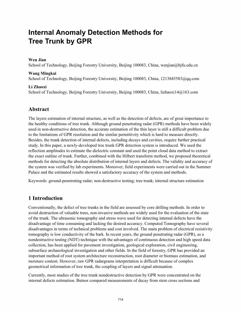
Internal Anomaly Detection Methods for Tree Trunk by GPR

Wen Jian School of Technology, Beijing Forestry University, Beijing 100083, China, wenjian@bjfu.edu.cn

Wang Mingkai School of Technology, Beijing Forestry University, Beijing 100083, China, 1213845583@qq.com

Li Zhaoxi School of Technology, Beijing Forestry University, Beijing 100083, China, lizhaoxi14@163.com

Abstract The layers estimation of internal structure, as well as the detection of defects, are of great importance to the healthy conditions of tree trunk. Although ground penetrating radar (GPR) methods have been widely used in non-destructive detection, the accurate estimation of the thin layer is still a difficult problem due to the limitations of GPR resolution and the similar permittivity which is hard to measure directly. Besides, the trunk detection of internal defects, including decays and cavities, require further practical study. In this paper, a newly-developed tree trunk GPR detection system is introduced. We used the reflection amplitudes to estimate the dielectric constant and used the point cloud data method to extract the exact outline of trunk. Further, combined with the Hilbert transform method, we proposed theoretical methods for detecting the absolute distribution of internal layers and defects. The validity and accuracy of the system was verified by lab experiments. Moreover, field experiments were carried out in the Summer Palace and the estimated results showed a satisfactory accuracy of the system and methods.

Keywords: ground-penetrating radar; non-destructive testing; tree trunk; internal structure estimation

1 Introduction Conventionally, the defect of tree trunks in the field are assessed by core drilling methods. In order to avoid destruction of valuable trees, non-invasive methods are widely used for the evaluation of the state of the trunk. The ultrasonic tomography and stress wave used for detecting internal defects have the disadvantage of time consuming and lacking the desired accuracy. Computed Tomography have several disadvantages in terms of technical problems and cost involved. The main problem of electrical resistivity tomography is low conductivity of the bark. In recent years, the ground penetrating radar (GPR), as a nondestructive testing (NDT) technique with the advantages of continuous detection and high speed data collection, has been applied for pavement investigation, geological exploration, civil engineering, subsurface archaeological investigation and other fields. In the field of forestry, GPR has provided an important method of root system architecture reconstruction, root diameter or biomass estimation, and moisture content. However, raw GPR radargrams interpretation is difficult because of complex geometrical information of tree trunk, the coupling of layers and signal attenuation.

Currently, most studies of the tree trunk nondestructive detection by GPR were concentrated on the internal defects estimation. Butnor compared measurements of decay from stem cross sections and

714

increment cores for three conifer species (Pseudotsuga menziesii, Thuja plicata and Tsuga heterophylla), and found that near-surface decay, air-filled voids and desiccated boles had unique electromagnetic signatures, which could be separated from other defects. GPR successfully estimated the percent area of air-filled cavities and was not significantly different than results from destructive sampling. Fu presented a ray-based tomography method using ground penetrating radar (GPR) to reconstruct the internal structure of the trunk cross-section of a living oak tree. Lv tested four typical trees trunks (polar, willow, pine, eucalyptus) moisture content and dielectric constant under the radar wave frequency respectively, and established models of the relationship between moisture content and dielectric constant of the trees trunks. Hamza Reci carried out to study how the ground penetrating radar (GPR) signal is affected by moisture variation in wood material, and investigated the effects of the wood fibre direction with respect to the polarisation of the electromagnetic field. Jana investigated particularities of tree trunks radar images, considering the circumferential data acquisition geometry, and described the reflection curve gained from a cylindrical medium. Liu and Gan applied GPR to examine the trunk decay situations and the thick root distribution characteristics of the ancient Platycladus orientalis trees occurring in Xuanyuan Temple of the Tomb of Yellow Emperor, and the results indicated that Tree radar unit could detect trunk rotten situations effectively, with high accuracy, which could be used as a reliable method of trunk nondestructive testing. Chen used GPR to detect the cavity cracking of Masson pine, and the results indicated that the moisture content of timber have an impact on the radar detection results and that the estimated boundary of the cavity damages may be offset slightly. Nevertheless, there are no suitable non-invasive methods for precisely detecting the internal defects in tree trunks in real time presently.

In this paper, a tree trunk GPR detection system was introduced. The system could investigate the layers of tree trunk and the defects inside by GPR images. An accurate imaging characterization method combined the Hilbert transform and the absolute localization of internal defect region was described, on the basis of particular features of tree trunk radar images, estimations of static dielectric constant from reflection amplitudes and exact irregular outlines of trunk. Besides, we developed the tree radar analysis software for imaging the internal structure and three-dimensional stereoscopic structure of trunk. Finally, numerical simulations, laboratory measurements and field experiments were carried out and the estimated results showed a satisfactory accuracy, which proved that the system and methods could be applied for the detection of layers and defects of tree trunk.

2 Instruments and Methods 2.1 GPR Systems

A tree trunk GPR detection system was developed to detect the layers and defects of tree trunk. The research conducted the survey with the TRU (Tree Radar) System of the TreeWin Corporation in America. The system consists of two separate procedures. The one is collecting the field data by radar antenna. The other is analyzing the echo data by its software. The TRU system contains two major components, SIR series data collector from GSSI (Geophysical Survey Systems, Inc) Company in America and coupling antenna radar with 900MHz. Data collector is used for displaying the digital waveform with the echo data and storing data. Radar antenna is grouped with the host (Fig.1).

715

Figure 1—Detection antenna and data acquisition system

The principle of radar wave detection is to send high frequency electromagnetic waves into the skin of trees through the antenna, and electromagnetic waves propagate inside trees. There are differences in dielectric constants at the juncture of normal structural layers or cavity, decay and other defects, which result in electromagnetic wave reflection, and then the receiving antenna receives the echo signal. The internal structure and defects of the trunk can be analyzed according to the radar echo waveform, intensity, time and other parameters.

In order to analytically describe the target reflection curves for different initial antenna position around the trunk, one starts from Eqs.(1) and (2), where v is the velocity of waves in the medium (m/s), c is the speed of light in free space (m/s), ε’ is the relative permittivity of the medium (dimensionless), t is the propagation time of the waves (s), and Z is the distance from the antenna to the target (m):

2v tZ ×

= (1)

cvε

=′ (2)

The amplitude of the reflected echo mainly depended on the electrical difference of the two dielectric layer. The higher the electrical difference was, the stronger the reflected signal was. The variation of radar echo in different dielectric layers was shown in Figure 1. The characteristic of reflected wave was obvious through the heartwood layer in the center, the active sapwood layer, the bark of living phloem and dead cork layer.

716

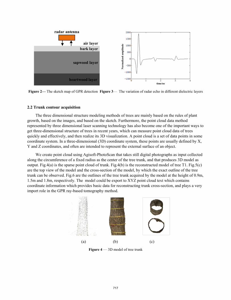
radar antenna

bark layer

sapwood layer

heartwood layer

air layer

time/ns

Nor

mal

ized

am

plitu

de

Figure 2— The sketch map of GPR detection Figure 3— The variation of radar echo in different dielectric layers

2.2 Trunk contour acquisition

The three dimensional structure modeling methods of trees are mainly based on the rules of plant growth, based on the images, and based on the sketch. Furthermore, the point cloud data method represented by three dimensional laser scanning technology has also become one of the important ways to get three-dimensional structure of trees in recent years, which can measure point cloud data of trees quickly and effectively, and then realize its 3D visualization. A point cloud is a set of data points in some coordinate system. In a three-dimensional (3D) coordinate system, these points are usually defined by X, Y and Z coordinates, and often are intended to represent the external surface of an object.

We create point cloud using Agisoft-PhotoScan that takes still digital photographs as input collected along the circumference of a fixed radius as the center of the tree trunk, and that produces 3D model as output. Fig.4(a) is the sparse point cloud of trunk. Fig.4(b) is the reconstructed model of tree T1. Fig.5(c) are the top view of the model and the cross-section of the model, by which the exact outline of the tree trunk can be observed. Fig.6 are the outlines of the tree trunk acquired by the model at the height of 0.9m, 1.5m and 1.8m, respectively. The model could be export to XYZ point cloud text which contains coordinate information which provides basic data for reconstructing trunk cross-section, and plays a very import role in the GPR ray-based tomography method.

(a) (b) (c)

Figure 4 — 3D model of tree trunk

717

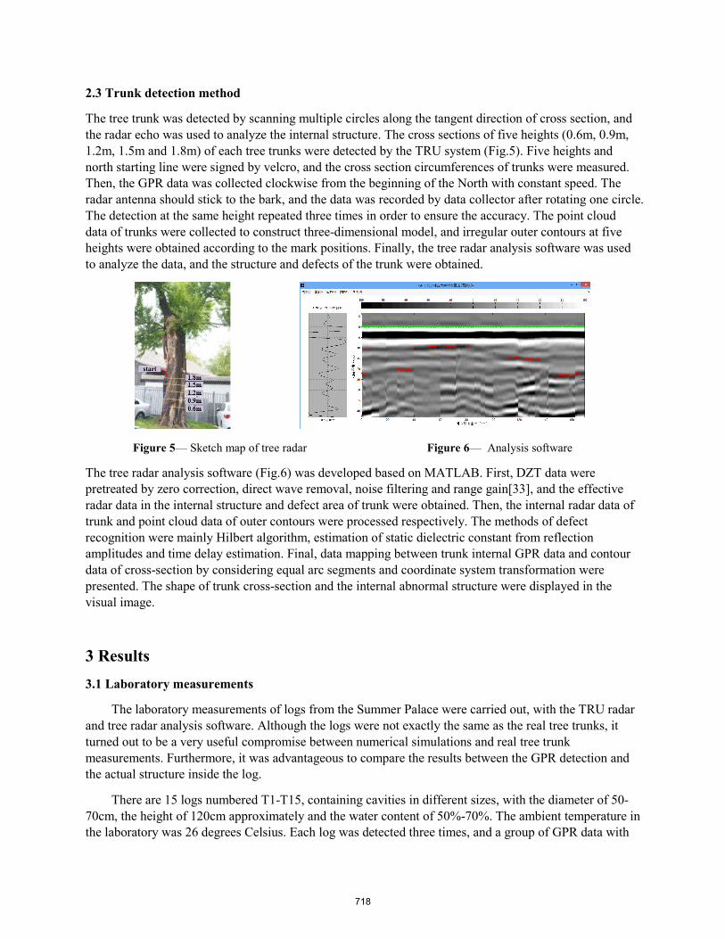
2.3 Trunk detection method

The tree trunk was detected by scanning multiple circles along the tangent direction of cross section, and the radar echo was used to analyze the internal structure. The cross sections of five heights (0.6m, 0.9m, 1.2m, 1.5m and 1.8m) of each tree trunks were detected by the TRU system (Fig.5). Five heights and north starting line were signed by velcro, and the cross section circumferences of trunks were measured. Then, the GPR data was collected clockwise from the beginning of the North with constant speed. The radar antenna should stick to the bark, and the data was recorded by data collector after rotating one circle. The detection at the same height repeated three times in order to ensure the accuracy. The point cloud data of trunks were collected to construct three-dimensional model, and irregular outer contours at five heights were obtained according to the mark positions. Finally, the tree radar analysis software was used to analyze the data, and the structure and defects of the trunk were obtained.

Figure 5— Sketch map of tree radar Figure 6— Analysis software

The tree radar analysis software (Fig.6) was developed based on MATLAB. First, DZT data were pretreated by zero correction, direct wave removal, noise filtering and range gain[33], and the effective radar data in the internal structure and defect area of trunk were obtained. Then, the internal radar data of trunk and point cloud data of outer contours were processed respectively. The methods of defect recognition were mainly Hilbert algorithm, estimation of static dielectric constant from reflection amplitudes and time delay estimation. Final, data mapping between trunk internal GPR data and contour data of cross-section by considering equal arc segments and coordinate system transformation were presented. The shape of trunk cross-section and the internal abnormal structure were displayed in the visual image.

3 Results 3.1 Laboratory measurements

The laboratory measurements of logs from the Summer Palace were carried out, with the TRU radar and tree radar analysis software. Although the logs were not exactly the same as the real tree trunks, it turned out to be a very useful compromise between numerical simulations and real tree trunk measurements. Furthermore, it was advantageous to compare the results between the GPR detection and the actual structure inside the log.

There are 15 logs numbered T1-T15, containing cavities in different sizes, with the diameter of 50-70cm, the height of 120cm approximately and the water content of 50%-70%. The ambient temperature in the laboratory was 26 degrees Celsius. Each log was detected three times, and a group of GPR data with

718

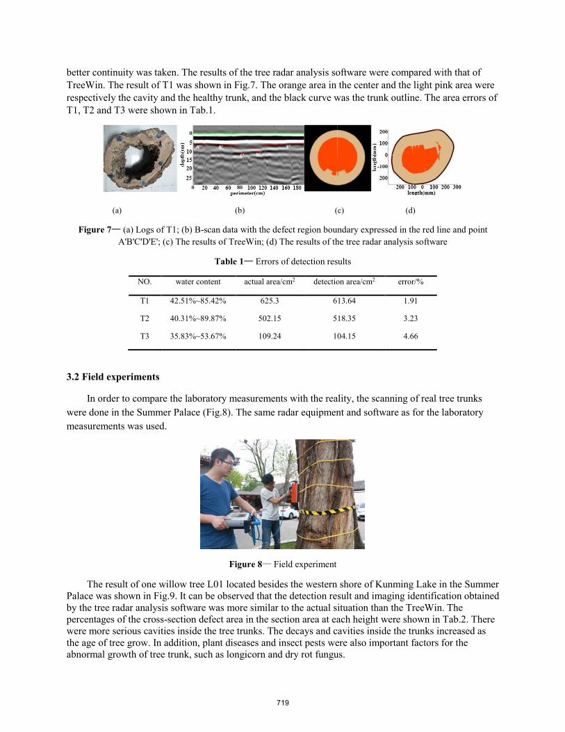
better continuity was taken. The results of the tree radar analysis software were compared with that of TreeWin. The result of T1 was shown in Fig.7. The orange area in the center and the light pink area were respectively the cavity and the healthy trunk, and the black curve was the trunk outline. The area errors of T1, T2 and T3 were shown in Tab.1.

(a) (b) (c) (d)

Figure 7— (a) Logs of T1; (b) B-scan data with the defect region boundary expressed in the red line and point A'B'C'D'E'; (c) The results of TreeWin; (d) The results of the tree radar analysis software

Table 1— Errors of detection results

NO. water content actual area/cm2 detection area/cm2 error/%

T1 42.51%~85.42% 625.3 613.64 1.91

T2 40.31%~89.87% 502.15 518.35 3.23

T3 35.83%~53.67% 109.24 104.15 4.66

3.2 Field experiments

In order to compare the laboratory measurements with the reality, the scanning of real tree trunks were done in the Summer Palace (Fig.8). The same radar equipment and software as for the laboratory measurements was used.

Figure 8— Field experiment

The result of one willow tree L01 located besides the western shore of Kunming Lake in the Summer Palace was shown in Fig.9. It can be observed that the detection result and imaging identification obtained by the tree radar analysis software was more similar to the actual situation than the TreeWin. The percentages of the cross-section defect area in the section area at each height were shown in Tab.2. There were more serious cavities inside the tree trunks. The decays and cavities inside the trunks increased as the age of tree grow. In addition, plant diseases and insect pests were also important factors for the abnormal growth of tree trunk, such as longicorn and dry rot fungus.

719

Figure 9— Detection result of tree L01 in the Summer Palace

Table 2— Field experiment results

NO. average perimeter of cross-section/m

ratio of abnormal area at different heights

0.6 0.9 1.2 1.5 1.8

L01 4.35 65.71% 70.31% 68.75% 74.19% 73.53%

L02 2.74 60.32% 54.37% 55.32% 63.16% ⁄

L03 4.91 68.89% 65.79% 74.68% 69.89% ⁄

L04 5.02 71.74% 75.61% 76.92% 76.60% ⁄

L05 4.91 71.68% 73.68% 72.22% 68.42% ⁄

L06 4.89 62.33% 66.67% 58.93% 57.14% ⁄

L07 3.66 58.12 53.19 58.91 50.83 52.65

L08 1.81 59.26 51.85 69.77 59.20 59.86

L09 1.95 67.28 56.15 53.94 62.94 69.14

L10 2.17 60.15 61.75 62.68 59.42 52.75

The protection of ancient trees had long been dependent on the experience of experts. It was difficult to accurately identify its internal growth status, as most erosion was started from the inside of trunk. There were a lot of trees(e.g. L05, shown in Fig.10(a)) after rejuvenation in the Summer Palace, which can hardly see the internal defects from the exterior. The GPR detection technology can be used to characterize the internal structure of tree trunks non-destructively. The trunk reconfiguration model of L05 was shown in Fig.10(b), and the three dimensional analysis results taken detection height as the longitudinal axis was shown in Fig.10(c), where the orange areas represented cavities. The three dimensional results were more intuitive.

(a) (b) (c) (d) Figure 10— Detection result of tree L05 in the Summer Palace

720

Fig.10(d) showed the rejuvenation of L05. It can be observed that there was almost completely empty inside the trunk, which supported rely on iron stents and ceramsites. The external bark was incomplete, and needed to be repaired with false barks. It was verified that GPR technology can detect the defects inside the trunk non-invasively by comparing the detection results and the actual situations in rejuvenation. The method provided a theoretical basis for the health assessment and rejuvenation of the trunk.

4. Discussion Accurate tree trunk structure estimation is an important issue to prevent collapses of trees in urban

areas or around roads. The destructive inspection of core drilling or in an extreme case chopping down of the tree cannot apply to living trees. Typical example of nondestructive inspection is stress wave technology, which might cause slight damage to the bark. GPR represents a prominent alternative since it can be used for nondestructive trunk profiling. The tree trunk GPR detection system we developed in this paper included the TRU radar and tree radar analysis software. The system showed the internal structure images at different height and three-dimensional stereoscopic images of the tree trunk, and helped to make a better prediction of the positions of holes and decays in tree trunks.

It is very important to know the propagation path of the electromagnetic waves for determining the position, shape and size of an observed target inside a circular trunk. The internal structure of trunks plotted according to tree radar analysis software fitted very well the structure of the numerical simulations and also of laboratory measurements. In laboratory measurements, the detected thicknesses of trunk layers were consistent with the measured values, which showed an acceptable effect in contrast detection. In field experiments, the comparison between observed results from field rejuvenation and predicted results from GPR suggested a satisfactory accuracy, which could satisfy the requirements of tree trunk detection non-invasively.

References

Attia, A.H.S. Geophysical imaging of root-zone, trunk, and moisture heterogeneity. Journal of Experimental Botany, 2007, 58(4):839-854.

Butnor J R, Pruyn M L, Shaw D C, et al. Detecting defects in conifers with ground penetrating radar: applications and challenges. Forest Pathology, 2009,39(5),309-322.

Butnor, J.R.; Pruyn, M.L.; Shaw, D.C.; Harmon, M.E.; Mucciardi, A.N.; . Detecting defects in conifers with ground penetrating radar: applications and challenges. Forest Pathology, 2009,39(5):309-322.

Carling, P.A.; Bristow, C.S.; Litvinov, A.S. Ground-penetrating radar stratigraphy and dynamics of megaflood gravel dunes. Journal of the Geological Society, 2016,173(3):550-559.

CHEN Yongping, GAO Tian, LI Deshan, et al. Preliminary study on radar detection and imaging of cavities and cracks of Pinus massoniana[J]. Journal of Beijing Forestry University, 2017,39(3): 112-118. ( in Chinese)

721

Davis JL, Annan AP. 1989. Ground penetrating radar for highresolution mapping of soil and rock stratigraphy. Geophysical Prospecting 37, 531–551.

Dong, Z.; Ye, S.; Gao, Y.; Fang, G.; Zhang, X.; Xue, Z.; Zhang T. Rapid detection methods for asphalt pavement thicknesses and defects by a vehicle-mounted ground penetrating radar (GPR) system. Sensors, 2016,16(12),2067.

Fang, Y.M.; Feng, H.L.; Li, J.; Li, G.H. Stress wave signal denoising using ensemble empirical mode decomposition and an instantaneous half period model. Sensors, 2011,11, 7554-67.

Feng, D.; Dai, Q. Application of ground penetrating radar in the survey of the pavement thickness in highway. PROGRESS IN GEOPHYSICS, 2008,23(1):289-294.

Fu, L.; Liu, S.; Liu, L. Internal structure characterization of living tree trunk cross-section using GPR: numerical examples and field data analysis. In 15th International Conference on Ground Penetrating Radar, Brussels, ,155-160 2014.

GAN Mingxu, SUN Tao, Kang Yongxiang, et al. Examination of the trunk cvity and thick root distribution of ancient Platycladus orientalis in the Tomb of Yellow Emperor by ground penetrating radar technology. Journal of Northwest Forestry University, 2016,31(4):182-187. ( in Chinese)

Guo, L.; Lin, H.; Fan, B.; Cui, X.; Chen, J. Impact of root water content on root biomass estimation using ground penetrating radar: Evidence from forward simulations and field controlled experiments. Plant Soil, 2013,371,503-520.

Harding, G.; Harding, E. Compton scatter imaging: A tool for historical exploration. Applied Radiation & Isotopes Including Data Instrumentation & Methods for Use in Agriculture Industry & Medicine, 2010, 68(6):993-1005.

Hamza Reci, Tien Chinh Maï, Zoubir Mehdi Sbartaï, et al. Non-destructive evaluation of moisture content in wood using ground-penetrating radar. Geosci. Instrum. GEOSCIENTIFIC INSTRUMENTATION METHODS AND DATA SYSTEMS vol. 5 no.2 pp.575-581, DEC 16 2016.

HU Chunhua, LI Pingping. A survey of 3D visualization modeling technologies for trees[J]. Journal of Nanjing Forestry University (Natural Sciences Edition) ,2015,39(6),148-154.

Huang, N. E.; Liu, H. H.; Huang, n. e et al.: the empirical mode decomposition and the hilbert spectrum for nonlinear and non-stationary time series analysis. proc. r. soc. lond. a 454, 903-995. Proceedings of the Royal Society A Mathematical Physical & Engineering Sciences, 1971,454, 903-995

H. Lorenzo, V. Pérez-Gracia2, et al. Forestry applications of ground-penetrating radar [J]. Forest Systems, 2010,19(1),5-17.

Jana Jez ˇová, Laurence Mertens, Sébastien Lambot. Ground-penetrating radar for observing tree trunks and other cylindrical objects. Construction and Building Materials 123 (2016) 214–225

Kim, K.H.; Kim, S.J. A wavelet-based method for action potential detection from extracellular neural signal recording with low signal-to-noise ratio. IEEE Transactions on Biomedical Engineering, 2003,50,999-1011.

Li, W.; Cui, X.; Guo, L.; Chen, J.; Chen, X.; Cao, X. Tree Root Automatic Recognition in Ground Penetrating Radar Profiles Based on Randomized Hough Transform. Remote Sensing, 2016, 8(5),430

722

LIU Xingdan, KANG Yongxiang, GAN Mingxu, et al. A study on trunk decay of ancient platycladus orientalis in tomb of yellow emperor[J]. Journal of Northwest Forestry University, 2017,32(2):180-187. ( in Chinese)

Li Qiang. Research on Automatic Pavement Thickness Measurement Using Ground Penetrating Radar. The University of Chinese Academy of Sciences, 2014.

Lv, J.; Gao, Lin.; Wen, Jian. Research on the relationship between moisture content and the dielectric constant of the tree trunk by the radar wave. Computer Modelling & New Technologies, 2014,18(11):1171-1175.

Mechbal, Z.; Khamlichi A. Determination of concrete rebars characteristics by enhanced post-processing of GPR scan raw data. NDT&E International, 2017,89:30-39

Méndez, V.; Rosell-Polo, J.R.; Sanz, R.; et al. Deciduous tree reconstruction algorithm based on cylinder fitting from mobile terrestrial laser scanned point clouds. Biosystems Engineering, 2014, 124(4),78-88.

Schultz, J.J.; Walter, B.S.; Healy, C. Long-term sequential monitoring of controlled graves representing common burial scenarios with ground penetrating radar: years 2 and 3. Journal of Applied Geophysics, 2016,132, 60-74.

Shortle, W.C. Decaying Douglas-fir wood: Ionization associated with resistance to a pulsed electric current. Wood Science, 1982, 15(1):29-32.

Solla, M.; Asorey-Cacheda, R.; Núñez-Nieto, X.; Conde-Carnero, B. Evaluation of historical bridges through recreation of GPR models with the FDTD algorithm. NDT E Int. 2016,77,19-27.

Sun, T.; Wang, L.; Hou, J.; Ge, X. Effect of timber moisture content and terrain conditions on the decay degree of Korean pine live standing trees. Chinese Journal of Applied Ecology, 2015,26(2):349-355.

Xiao, Z.; Wen, J.; Gao, L.; Xiao X.; Li W.; Li, C. Method of tree radar signal processing based on Curvelet transform[J]. Rev. Tec. Ing. Univ. Zulia, 2016,39(7),243-250.

Yan Yongbin. Image identification and disposal of ground penetrating radar[D]. Beijing: Beijing University of Chemical Technology, 2008.

Zhang, H.; Wang, X.; Su, J. Experimental investigation of stress wave propagation in standing trees. Holzforschung, 2011, 65(5):192.

723

Feasibility Study on In-Line Species and Moisture-Based Sorting of Green Timber Mix by Near Infrared Spectroscopy and Least-Squares Support Vector Machines Zhu Zhou * School of Information Engineering, Zhejiang A&F University, Hangzhou, Zhejiang, China, zhouzhu@zafu.edu.cn Department of Wood Science, University of British Columbia, Vancouver, British Columbia, Canada Key Laboratory of State Forestry and Grassland Administration in Forestry Perception Technology and Intelligent Equipment, Zhejiang A&F University, Hangzhou, Zhejiang, China Zhejiang Provincial Key Laboratory of Forestry Intelligent Monitoring and Information Technology, Zhejiang A&F University, Hangzhou, Zhejiang, China Sohrab Rahimi Department of Wood Science, University of British Columbia, Vancouver, British Columbia, Canada sohrab.rahimi@alumni.ubc.ca Stavros Avramidis Department of Wood Science, University of British Columbia, Vancouver, British Columbia, Canada stavros.avramidis@ubc.ca Yiming Fang School of Information Engineering, Zhejiang A&F University, Hangzhou, Zhejiang, China, ymfang@zafu.edu.cn Key Laboratory of State Forestry and Grassland Administration in Forestry Perception Technology and Intelligent Equipment, Zhejiang A&F University, Hangzhou, Zhejiang, China Zhejiang Provincial Key Laboratory of Forestry Intelligent Monitoring and Information Technology, Zhejiang A&F University, Hangzhou, Zhejiang, China * Corresponding author Abstract This study explores the application of near infrared spectroscopy (NIRS) and least-squares support vector machines (LS-SVM) for in-line determination and classification of green timber mix with respect to species and moisture content (MC). In total, 1200 sapwood and heartwood samples (hem-fir mix) with radial, tangential, and transverse sections are divided into calibration and prediction sets. Reflectance spectra are collected using a fiber spectrometer in the wavelength range of 350–2500 nm at moving speeds of 0.1, 0.2, and 0.4 m/s. LS-SVM for both regression (LS-SVR) and classification (LS-SVC) with different spectral preprocessing methods involving smooth, first derivative, second derivative, and standard normal variate transformation are implemented for calibration models. The performance of models at different moving speeds for regression and classification is compared. Results show that the performance is decreased as the moving speed increases irrespective of spectral preprocessing methods for both regression and classification models. The best LS-SVR model for MC prediction in the moisture range of 30% to 253% is at moving speed of 0.1 m/s with R2

p and RMSEP of 0.97% and 11.3%, respectively. The best LS-SVC model for sorting timbers based on species and moisture level is also at moving speed of 0.1 m/s with overall accuracy of 98.3% in the prediction set, when all the samples are divided into four classes. Collectively, NIRS combined with LS-SVM has potential for on-line qualitative and quantitative analysis of green hem-fir mix before kiln drying. Keywords: Amabilis fir; green timber; hemlock; least squares-support vector machines (LS-SVM); moisture; near infrared spectroscopy (NIRS); sorting; species; in-line

724