
Market Interactions in Gold and Stock Markets: Evidences from ...
Upload
khangminh22Category
view
3download
0
Edited by
Efficiency and Anomalies in Stock Markets
Wing-Keung Wong
Printed Edition of the Special Issue Published in Economies
www.mdpi.com/journal/economies

Efficiency and Anomalies in Stock Markets


Efficiency and Anomalies in Stock Markets
Editor
Wing-Keung Wong
MDPI • Basel • Beijing • Wuhan • Barcelona • Belgrade • Manchester • Tokyo • Cluj • Tianjin

EditorWing-Keung Wong
Asia University
TaiwanChina Medical University HospitalTaiwanThe Hang Seng University of Hong KongHong Kong
Editorial Office
MDPISt. Alban-Anlage 66
4052 Basel, Switzerland
This is a reprint of articles from the Special Issue published online in the open access journal Economies (ISSN 2227-7099) (available at: https://www.mdpi.com/journal/economies/special issues/anomalies-stockmarkets).
For citation purposes, cite each article independently as indicated on the article page online and as indicated below:
LastName, A.A.; LastName, B.B.; LastName, C.C. Article Title. Journal Name Year, Volume Number,
Page Range.
ISBN 978-3-0365-3080-2 (Hbk)
ISBN 978-3-0365-3081-9 (PDF)
© 2022 by the authors. Articles in this book are Open Access and distributed under the Creative
Commons Attribution (CC BY) license, which allows users to download, copy and build upon
published articles, as long as the author and publisher are properly credited, which ensures maximum
dissemination and a wider impact of our publications.
The book as a whole is distributed by MDPI under the terms and conditions of the Creative Commons
license CC BY-NC-ND.

Contents
About the Editor . . . . . . . . . . . . . . . . . . . . . . . . . . . . . . . . . . . . . . . . . . . . . . vii
Preface to ”Efficiency and Anomalies in Stock Markets” . . . . . . . . . . . . . . . . . . . . . . . ix
Wing-Keung Wong
Editorial Statement and Research Ideas for Efficiency and Anomalies in Stock MarketsReprinted from: Economies 2020, 8, 10, doi:10.3390/economies8010010 . . . . . . . . . . . . . . . . 1
Xu Guo, Xuejun Jiang and Wing-Keung Wong
Stochastic Dominance and Omega Ratio: Measures to Examine Market Efficiency, Arbitrage Opportunity, and AnomalyReprinted from: Economies 2017, 5, 38, doi:10.3390/economies5040038 . . . . . . . . . . . . . . . . 5
Fahad Ali, RongRong He and YueXiang Jiang
Size, Value and Business Cycle Variables. The Three-Factor Model and Future EconomicGrowth: Evidence from an Emerging MarketReprinted from: Economies 2018, 6, 14, doi:10.3390/economies6010014 . . . . . . . . . . . . . . . . 21
Hee-Joon Ahn, Jun Cai and Cheol-Won Yang
Which Liquidity Proxy Measures Liquidity Best in Emerging Markets?Reprinted from: Economies 2018, 6, 67, doi:10.3390/economies6040067 . . . . . . . . . . . . . . . . 45
Thomas C. Chiang
Market Efficiency and News Dynamics: Evidence from International Equity MarketsReprinted from: Economies 2019, 7, 7, doi:10.3390/economies7010007 . . . . . . . . . . . . . . . . 75
Kizito Uyi Ehigiamusoe and Hooi Hooi Lean
Influence of Real Exchange Rate on the Finance-Growth Nexus in the West African RegionReprinted from: Economies 2019, 7, 23, doi:10.3390/economies7010023 . . . . . . . . . . . . . . . . 93
Sangram Keshari Jena, Aviral Kumar Tiwari and Amarnath Mitra
Put–Call Ratio Volume vs. Open Interest in Predicting Market Return: A Frequency DomainRolling Causality AnalysisReprinted from: Economies 2019, 7, 24, doi:10.3390/economies7010024 . . . . . . . . . . . . . . . . 115
Chong-Chuo Chang, Tai-Yung Kam, Chih-Chung Chien and Wan Ting Su
The Impact of Financial Constraints on the Convertible Bond Announcement ReturnsReprinted from: Economies 2019, 7, 32, doi:10.3390/economies7020032 . . . . . . . . . . . . . . . . 125
Ziyi Zhang and Wai Keung Li
An Experiment on Autoregressive and Threshold Autoregressive Models with Non-GaussianError with Application to Realized VolatilityReprinted from: Economies 2019, 7, 58, doi:10.3390/economies7020058 . . . . . . . . . . . . . . . . 135
Keith S. K. Lam, Liang Dong and Bo Yu
Value Premium and Technical Analysis: Evidence from the China Stock MarketReprinted from: Economies 2019, 7, 92, doi:10.3390/economies7030092 . . . . . . . . . . . . . . . . 147
Kai-Yin Woo, Chulin Mai, Michael McAleer and Wing-Keung Wong
Review on Efficiency and Anomalies in Stock MarketsReprinted from: Economies 2020, 8, 20, doi:10.3390/economies8010020 . . . . . . . . . . . . . . . . 169
v


About the Editor
Professor Wing-Keung Wong obtained his Ph.D. from the University of Wisconsin-Madison, the
USA with a major in Business Statistics (Statistics and Finance) and obtained his Bachelor degree from
the Chinese University of Hong Kong, Hong Kong, with a major in Mathematics and a double minor
in Economics and Statistics. Currently, he is a Chair Professor at the Department of Finance, Asia
University. He was a Full Professor at the Department of Economics, Hong Kong Baptist University,
and Deputy Director at Risk Management Institute, National University of Singapore.
He appears in “Who’s Who in the World”. He is ranked top 1% by SSRN and in the list of top
Taiwan economists and Asian economists and top economists by RePEc. He has published more
than three hundred papers including papers published in some top journals. He has more than
11100 citations in Google Scholar, and more than 9600 citations in Researchgate. His h-index is 59,
and i10-index is 225 by Google Scholar citation.
He has been providing consultancy to several Government departments and corporations,
giving lectures and seminars to several universities, serving as editor, guest leading editor, advisor,
associate editor for some international journals, and appointed as an external examiner.
vii


Preface to ”Efficiency and Anomalies in Stock
Markets”
The Efficient Market Hypothesis believes that it is impossible for an investor to outperform the
market because all available information is already built into stock prices. However, some anomalies
could persist in stock markets, while some other anomalies could appear, disappear, and re-appear
again without any warning. To explore new theories with applications in this direction, this Special
Issue on “Efficiency and Anomalies in Stock Markets”, edited by Wing-Keung Wong, is devoted to
advancements in developing theories on market efficiency and anomalies in stock markets, as well as
applications in market efficiency and financial anomalies in 2019. We invite investigators to submit
manuscripts of original innovative research in theory, practice, and applications in the areas of market
efficiency and anomalies in stock markets to be considered for publication in Economies. We are open
to interesting and imaginative ideas that fit within the spirit and scope of the call for papers that
should have a quantitative orientation.
Wing-Keung Wong
Editor
ix


economies
Editorial
Editorial Statement and Research Ideas for Efficiencyand Anomalies in Stock Markets
Wing-Keung Wong 1,2,3
1 Department of Finance, Fintech Center, and Big Data Research Center, Asia University, Taichung 40447,Taiwan; [email protected]
2 Department of Medical Research, China Medical University Hospital, Taichung 41354, Taiwan3 Department of Economics and Finance, The Hang Seng University of Hong Kong, Hong Kong, China
Received: 17 January 2020; Accepted: 1 February 2020; Published: 10 February 2020
Abstract: The Efficient Market Hypothesis states that it is impossible for an investor to outperform themarket because all available information is already built into stock prices. However, some anomaliescould persist in stock markets while some other anomalies could appear, disappear and re-appearagain without any warning. To explore new theories with applications in this direction, in thiseditorial, we suggest ideas to authors on what types of papers we will accept for publication in theareas of on Efficiency and Anomalies in Stock Markets. We will discuss some papers published in thespecial issue of Efficiency and Anomalies in Stock Markets.
Keywords: market efficiency; anomaly; stock market; finance; applications
The Efficient Market Hypothesis believes that it is impossible for an investor to outperform themarket because all available information is already built into stock prices. However, some anomaliescould persist in stock markets while some other anomalies could appear, disappear and re-appear againwithout any warning. To explore new theories with applications in this direction, the special issue onEfficiency and Anomalies in Stock Markets edited by Wing-Keung Wong is devoted to advancementsin the theory development on market efficiency and anomalies in stock markets as well as applicationsin market efficiency and financial anomalies in 2019. We invite investigators to submit manuscripts oforiginal innovative research in theory, practice and applications in the areas of market efficiency andanomalies in stock markets to be considered for publication in Economies. We are open to interestingand imaginative ideas that fit within the spirit and scope of the call for papers that should have aquantitative orientation.
The special issue of Efficiency and Anomalies in Stock Markets has published 10 papers including(Guo et al. 2017; Ali et al. 2018; Ahn et al. 2018; Chiang 2019; Ehigiamusoe and Lean 2019; Jena et al.2019; Lam et al. 2019; Zhang and Li 2019; Chang et al. 2019; Woo et al. 2019; Wong 2020).
Among them, (Woo et al. 2019) review the theory and literature on market efficiency and marketanomalies. (Chiang 2019) examines the efficient market hypothesis for 15 international equity markets,and (Guo et al. 2017) develop the theory to test for market efficiency and check whether there is anyexpected arbitrage opportunity and anomaly in the market. market. (Ehigiamusoe and Lean 2019)examine the moderating effects of the real exchange rate and its volatility on the finance-growth nexusand determine the marginal effects of financial development on economic growth at various levels ofthe real exchange rates and its volatility, (Zhang and Li 2019) explore the fitting of Autoregressive (AR)and Threshold AR (TAR) models with a non-Gaussian error structure and propose to use a Gammarandom error to cater for the non-negativity of the realized volatility, and (Ahn et al. 2018) examine theeffects of low-frequency liquidity, high-frequency spread measures and price impact measures. On theother hand, (Lam et al. 2019) examine whether there is any value premium in the Chinese stock marketby using the conventional buy-and-hold approach to buy long the portfolio with the highest BM ratio
Economies 2020, 8, 10; doi:10.3390/economies8010010 www.mdpi.com/journal/economies1

Economies 2020, 8, 10
and sell short the one with the lowest BM ratio, (Ali et al. 2018) use three methods to construct factorsand identify pitfalls that arise in the application of Fama-French’s three-factor model and examinethe ability of the three factors to predict the future growth of economy, (Jena et al. 2019) examine theefficacy of the Put–Call Ratio (PCR) measured in terms of volume and open interest in predictingmarket return at different time scale, and (Chang et al. 2019) study the effect of financial constraints onshort-term performance.
We first discuss more detail about the work by (Woo et al. 2019; Chiang 2019; Guo et al. 2017).(Woo et al. 2019) review the theory and literature on market efficiency and market anomalies. Theyfirst review market efficiency, define clearly the concept of market efficiency and efficient-markethypothesis (EMH), and discuss some efforts that challenge EMH. Thereafter, they review differentmarket anomalies and review different theories of Behavioral Finance that could be used to explainmarket anomalies. Their review is useful to academics for their studies in EMH, anomalies, andBehavioral Finance, useful to investors for their decisions on their investment, and useful to policymakers in reviewing their policies in stock markets. (Chiang 2019) examines the efficient markethypothesis by applying monthly data for 15 international equity markets. He finds that the null for theabsence of autocorrelations of stock returns is rejected except Canada and the U.S, the independence ofmarket volatility correlations is rejected. However, the existence of correlations between stock returnsand lagged news measured by lagged economic policy uncertainty is not rejected for all markets,implying that a change of lagged EPUs positively predicts conditional variance. In addition, (Guo etal. 2017) study the relationship between stochastic dominance and the Omega ratio. They find thatsecond-order stochastic dominance (SD) and/or second-order risk-seeking SD (RSD) alone for any twoprospects is not sufficient to imply Omega ratio dominance insofar that the Omega ratio of one asset isalways greater than that of the other one. They extend the theory of risk measures by proving that thepreference of second-order SD implies the preference of the corresponding Omega ratios only whenthe return threshold is less than the mean of the higher return asset. They also find that the preferenceof the second-order RSD implies the preference of the corresponding Omega ratios only when thereturn threshold is larger than the mean of the smaller return asset and observe that first-order SD doesimply Omega ratio dominance. Applying their theory to examine the relationship between propertysize and property investment in the Hong Kong real estate market, they conclude that the Hong Kongreal estate market is not efficient and there are expected arbitrage opportunities and anomalies in theHong Kong real estate market.
We turn to discuss the work by (Ehigiamusoe and Lean 2019; Zhang and Li 2019; Ahn et al.2018) on volatility and liquidity. (Ehigiamusoe and Lean 2019) examine the moderating effects ofthe real exchange rate and its volatility on the finance-growth nexus in the West African region anddetermine the marginal effects of financial development on economic growth at various levels of thereal exchange rates and its volatility. They find that financial development has a long-term positiveimpact on economic growth, but this impact is weakened by real exchange rate and its volatility. Theyalso find that the marginal effects of financial development on economic growth vary with the levels ofthe real exchange rate and its volatility: the higher the real exchange rate and its volatility, the lessfinance spurs growth. Their findings imply that the development of the financial sector would notprovide the desirable economic benefits except it is accompanied by a reduction and stability in the realexchange rates. Motivated by the problem of finding a possible probabilistic model for the realizedvolatility, (Zhang and Li 2019) explore the fitting of Autoregressive (AR) and Threshold AR (TAR)models with a non-Gaussian error structure. They propose to use a Gamma random error to cater forthe non-negativity of the realized volatility, apply the maximum likelihood estimation and employ anon-gradient numerical Nelder–Mead method for optimization and a penalty method, introduced forthe non-negative constraint imposed by the Gamma distribution, in their analysis. In their simulation,they show that their proposed fitting method fits the true AR or TAR model with insignificant biasand mean square error (MSE). They also test the AR and TAR models with Gamma random erroron empirical realized volatility data of 30 stocks and find that one third of the cases are fitted quite
2
Economies 2020, 8, 10
well, implying that the models have potential as a supplement for current Gaussian random errormodels with proper adaptation. On the other hand, (Ahn et al. 2018) conduct a comprehensive analysison 1183 stocks from 21 emerging markets to examine the low-frequency liquidity proxies that bestmeasure liquidity in emerging markets and compare several low-frequency liquidity proxies withhigh-frequency spread measures and price impact measures. They find that the Lesmond, Ogden, andTrzcinka measure is the most effective spread proxy in most of the emerging markets. In addition, theAmihud measure is the most effective one among the price impact proxies.
Lastly, we discuss the work done by (Lam et al. 2019; Ali et al. 2018; Jena et al. 2019;Chang et al. 2019) on value premium, the application of Fama-French’s three-factor model, the efficacyof the Put–Call Ratio, and the effect of financial constraints on short-term performance. (Lam et al. 2019)examine whether there is any value premium in the Chinese stock market by using a conventionalbuy-and-hold approach to buy long the portfolio with the highest BM ratio and sell short the onewith the lowest BM ratio. They propose a new strategy by combining the value premium effect andtechnical analysis. To trade the objective portfolio or risk-free asset according to the moving averagetiming signals, they find excess return from such a zero-cost trading strategy. They perform variousrobustness tests and find that the excess returns remain significantly positive after adjusting for risks(on three factor models) and transaction costs and find that the combined trading strategy can generatesignificant positive risk-adjusted returns after the transaction costs. (Ali et al. 2018) use three methodsto construct factors and identify pitfalls that arise in the application of Fama-French’s three-factormodel to the Pakistani stock returns and examine the ability of the three factors to predict the futuregrowth of Pakistan’s economy. They find that the special features in Pakistan significantly affect bothsize and value factors and influence the explanatory power of the three-factor model. They find thatsize and book-to-market factors exist in the Pakistani stock market and two mimic portfolios SMB andHML generate a return of 9.15% and 12.27% per annum, respectively. They observe that includingboth SMB and HML factors into the model will increase the explanatory power of the model. Theyalso find that except for value factor, the model’s factors predict future gross domestic product (GDP)growth of Pakistan and remain robust. (Jena et al. 2019) examine the efficacy of the Put–Call Ratio(PCR) measured in terms of volume and open interest in predicting market return at different timescale. They find that volume PCR is an efficient predictor of the market return in a short period of2.5 days and open interest PCR in a long period of 12 days. Their findings suggest that traders andportfolio investors should use the appropriate PCR depending upon the time horizon of their tradeand investment. In addition, (Chang et al. 2019) hypothesize that when companies have investmentplans, they are expected to have higher future cash flows and they will become increasingly morevaluable regardless of the fact that they raise funds through the issue of convertible bonds (due tofinancial constraints), positively affecting the performance of companies. Their findings show thatfinancial constraints have no effect on short-term performance but have a significantly positive impacton the long-term performance of companies after their issuance of convertible bonds.
Acknowledgments: The author would like to thank Robert B. Miller and Howard E. Thompson for their continuousguidance and encouragement. For financial and research support, the author acknowledges Asia University,China Medical University Hospital, The Hang Seng University of Hong Kong, the Research Grants Councilof Hong Kong (project number 12500915), and Ministry of Science and Technology (MOST, Project Numbers106-2410-H-468-002 and 107-2410-H-468-002-MY3), Taiwan.
Conflicts of Interest: The authors declare no conflict of interest.
References
Ahn, Hee-Joon, Jun Cai, and Cheol-Won Yang. 2018. Which Liquidity Proxy Measures Liquidity Best in EmergingMarkets? Economies 6: 67. [CrossRef]
Ali, Fahad, Rongrong He, and Yuexiang Jiang. 2018. Size, Value and Business Cycle Variables. The Three-FactorModel and Future Economic Growth: Evidence from an Emerging Market. Economies 6: 14. [CrossRef]
3

Economies 2020, 8, 10
Chang, Chong-Chuo, Tai-Yung Kam, Chih-Chung Chien, and Wan Su. 2019. The Impact of Financial Constraintson the Convertible Bond Announcement Returns. Economies 7: 32. [CrossRef]
Chiang, Thomas C. 2019. Market Efficiency and News Dynamics: Evidence from International Equity Markets.Economies 7: 7. [CrossRef]
Ehigiamusoe, Kizito Uyi, and Hooi Hooi Lean. 2019. Influence of Real Exchange Rate on the Finance-GrowthNexus in the West African Region. Economies 7: 23. [CrossRef]
Guo, Xu, Xuejun Jiang, and Wing-Keung Wong. 2017. Stochastic Dominance and Omega Ratio: Measures toExamine Market Efficiency, Arbitrage Opportunity, and Anomaly. Economies 5: 38. [CrossRef]
Jena, Sangram Keshari, Aviral Kumar Tiwari, and Amarnath Mitra. 2019. Put-Call Ratio Volume Vs. Open Interestin Predicting Market Return: A Frequency Domain Rolling Causality Analysis. Economies 7: 24. [CrossRef]
Lam, Keith S. K., Liang Dong, and Bo Yu. 2019. Value Premium and Technical Analysis: Evidence from the ChinaStock Market. Economies 7: 92. [CrossRef]
Wong, Wing-Keung. 2020. Editorial Statement and Research Ideas for Efficiency and Anomalies in Stock Markets.Economies 8: 10. [CrossRef]
Woo, Kai Yin, Chulin Mai, Michael McAleer, and Wing-Keung Wong. 2019. Review on Efficiency and Anomaliesin Stock Markets. Economies 8: 20. [CrossRef]
Zhang, Ziyi, and Wai Keung Li. 2019. An Experiment on Autoregressive and Threshold Autoregressive Modelswith Non-Gaussian Error with Application to Realized Volatility. Economies 7: 58. [CrossRef]
© 2020 by the author. Licensee MDPI, Basel, Switzerland. This article is an open accessarticle distributed under the terms and conditions of the Creative Commons Attribution(CC BY) license (http://creativecommons.org/licenses/by/4.0/).
4

economies
Article
Stochastic Dominance and Omega Ratio: Measures toExamine Market Efficiency, Arbitrage Opportunity,and Anomaly
Xu Guo 1, Xuejun Jiang 2 and Wing-Keung Wong 3,4,5,6,*
1 School of Statistics, Beijing Normal University, Beijing 100875, China; [email protected] Department of Mathematics, South University of Science and Technology of China, Shenzhen 518055, China;
[email protected] Department of Finance and Big Data Research Center, Asia University, Taichung 41354, Taiwan4 Department of Economics and Finance, Hang Seng Management College, Hong Kong, China5 Department of Economics, Lingnan University, Hong Kong, China6 Department of Finance, College of Management, Asia University, 500, Lioufeng Rd., Wufeng,
Taichung 41354, Taiwan* Correspondence: [email protected]
Academic Editor: Ralf FendelReceived: 23 August 2017; Accepted: 2 October 2017; Published: 19 October 2017
Abstract: Both stochastic dominance and Omegaratio can be used to examine whether the market isefficient, whether there is any arbitrage opportunity in the market and whether there is any anomalyin the market. In this paper, we first study the relationship between stochastic dominance and theOmega ratio. We find that second-order stochastic dominance (SD) and/or second-order risk-seekingSD (RSD) alone for any two prospects is not sufficient to imply Omega ratio dominance insofar thatthe Omega ratio of one asset is always greater than that of the other one. We extend the theoryof risk measures by proving that the preference of second-order SD implies the preference of thecorresponding Omega ratios only when the return threshold is less than the mean of the higherreturn asset. On the other hand, the preference of the second-order RSD implies the preference of thecorresponding Omega ratios only when the return threshold is larger than the mean of the smallerreturn asset. Nonetheless, first-order SD does imply Omega ratio dominance. Thereafter, we applythe theory developed in this paper to examine the relationship between property size and propertyinvestment in the Hong Kong real estate market. We conclude that the Hong Kong real estate marketis not efficient and there are expected arbitrage opportunities and anomalies in the Hong Kong realestate market. Our findings are useful for investors and policy makers in real estate.
Keywords: stochastic dominance; Omega ratio; risk averters; risk seekers; utility maximization;market efficiency; anomaly
JEL Classification: C0, D81, G10
1. Introduction
It is well known that the standard deviation is not a good measure of risk because it penalizesupside deviation, as well as downside deviation. Additionally, it is also poor at measuring riskwith asymmetric payoff profiles. The poor performance of the standard deviation will lead topoor performance of the Sharpe ratio, which establishes a relationship between the ratio of returnversus volatility (Kapsos et al. (2014); Guastaroba et al. (2016)). A number of studies developedsome theories that propose to circumvent the limitations. For example, Homm and Pigorsch (2012)develop an economic performance measure based on Aumann and Serrano’s (2008) index of
Economies 2017, 5, 38; doi:10.3390/economies5040038 www.mdpi.com/journal/economies5

Economies 2017, 5, 38
riskiness. They prove that the proposed economic performance measure is consistent with first-and second-order stochastic dominance (SD). Keating and Shadwick (2002) propose to use the Omegaratio, the probability weighted ratio of gains versus losses to a prospect or the ratio of upside returns(good) relative to downside returns (bad), to replace the Sharpe ratio to measure the risk returnperformance of a prospect. Thus, the Omega ratio considers all moments, while the Sharpe ratioconsiders only the first two moments of the return distribution in the construction. According toCaporin et al. (2016), Bellini et al. (2017) and the references provided therein, the Omega ratios arestrongly related to expectiles, which are a type of inverse of the Omega ratio and present interestingproperties as risk measures. Guastaroba et al. (2016) discuss the advantages of using the Omega ratiofurther. Thus, the Omega ratio has been commonly used by academics and practitioners as noted byKapsos et al. (2014) and the references therein.
It is well known that the SD theory can be used to examine whether the market is efficient, whetherthere is any arbitrage opportunity in the market, and whether there is any anomaly in the market(Sriboonchitta et al. (2009); Levy (2015)), and thus, academics are interested in checking whether thereis any relationship between any risk measure with SD. The work from Darsinos and Satchell (2004)and others can be used to establish the relationship between the second-order SD (SSD) and theOmega ratio. By using two counterexamples, we first demonstrate that SSD and/or second-orderrisk-seeking SD (SRSD) alone for any two prospects is not sufficient to imply Omega ratio dominance(OD) and that the Omega ratio of one asset is always greater than that of the other one. We thenextend the work of Darsinos and Satchell (2004) and others by proving that the preference of SSD(for risk averters) implies the preference of the corresponding Omega ratios are selected only when thereturn threshold is less than the mean of the higher return asset. On the other hand, the preferenceof SRSD (for risk seekers) implies the preference of the corresponding Omega ratios only when thereturn threshold is larger than the mean of the smaller return asset. Lastly, we develop the relationshipbetween the first-order SD (FSD) and the Omega ratio in such a way that the preference of FSD for anyinvestor with increasing utility functions does imply the preference of the corresponding Omega ratiosfor any return threshold.
Qiao and Wong (2015) apply SD tests to examine the relationship between property size andproperty investment in the Hong Kong real estate market. They do not find any FSD relationship intheir study. Tsang et al. (2016) extend their work to reexamine the relationship between property sizeand property investment in the same market. They suggest to analyze both rental and total yields andfind the FSD relationship of rental yield in adjacent pairings of different housing classes in Hong Kong.Based on their analysis on both rental and total yields, they conclude that investing in a smaller houseis better than a bigger house. We note that analyzing both rental and total yields is not sufficient todraw such a conclusion. To circumvent the limitation, we extend their work by applying the Omegaratio to examine the relationship between property size and property investment in the Hong Kongreal estate market. In addition to analyzing the rental yield, we recommend analyzing the price yieldsof different houses. We find that a smaller house dominates a bigger house in terms of rental yield,and there is no dominance between smaller and bigger houses in price yield. Our findings lead usto conclude that regardless of whether the buyers are risk averse or risk seeking, they will not onlyachieve higher expected utility, but also obtain higher expected wealth when buying smaller properties.This implies that the Hong Kong real estate market is not efficient, and there are expected arbitrageopportunities and anomalies in the Hong Kong real estate market. Our findings are useful for realestate investors in their investment decision making and useful to policy makers in real estate for theirpolicy making to make the real estate market become efficient.
The rest of this paper is organized as follows: Section 2 presents the formal definitions of the SDrules and Omega ratios. We then show our main results about the consistency of Omega ratios withrespect to the SD in Section 3. In Section 4, we discuss how to apply the theory developed in this paperto examine whether the market is efficient, whether there is any arbitrage opportunity in the market
6

Economies 2017, 5, 38
and whether there is any anomaly in the market. An illustration of the Hong Kong housing market isincluded in Section 5. The final section offers our conclusion.
2. Definitions of Stochastic Dominance and Omega Ratios
We first define cumulative distribution functions (CDFs) for X and Y:
F(1)Z (η) = FZ(η) = P(Z ≤ η) , for Z = X, Y . (1)
We define the second-order integral of Z, F(2)Z ,
F(2)Z (η) =
∫ η
−∞F(1)
Z (ξ)dξ for Z = X, Y ; (2)
and define the second-order reverse integral, F(2)RZ , of Z
F(2)RZ (η) =
∫ ∞
η(1 − F(1)
Z (ξ))dξ for Z = X, Y . (3)
If Z is the return, then F(1)Z (η) is the CDF of the return up to η and F(2)
Z (η) is the second-order
integral of Z up to η, that is the probability of the CDF of the return up to η, and F(2)RZ (η) is the
second-order reverse integral of Z up to η, that is the reverse integration of the reverse CDF ofthe return up to η. We call F(i)
Z the i-th-order integral of Z, which will be used to define the SDtheory for risk averters (see, for example, Quirk and Saposnik (1962)). On the other hand, we callF(i)R
Z the i-th-order reversed integral, which will be used to define the SD theory for risk seekers(see, for example, Hammond (1974)). Risk averters typically have a preference for assets with a lowerprobability of loss, while risk seekers have a preference for assets with a higher probability of gain.When choosing between two assets X or Y, risk averters will compare their corresponding i-th orderSD integrals F(i)
X and F(i)RY and choose X if F(i)
X is smaller, since it has a lower probability of loss. On the
other hand, risk seekers will compare their corresponding i-th order RSD integrals F(i)RX and F(i)R
Y and
choose X if F(i)RX is larger since it has a higher probability of gain.
Following the definition of stochastic dominance (Hanoch and Levy (1969)), prospect X first-orderstochastically dominates prospect Y:
if and only if F(1)X (η) ≤ F(1)
Y (η) for any η ∈ R, (4)
which is denoted by X �FSD Y; prospect X second-order stochastically dominates prospect Y:
if and only if F(2)X (η) ≤ F(2)
Y (η) for any η ∈ R, (5)
which is denoted by X �SSD Y. Here, FSD and SSD denote first- and second-order stochasticdominance, respectively.
Next, we follow Levy (2015) to define risk-seeking stochastic dominance (RSD)1 for risk seekers.Prospect X stochastically dominates prospect Y in the sense of second-order risk seeking:
if and only if F(2)RX (η) ≥ F(2)R
Y (η) for any η ∈ R, (6)
which is denoted by X �SRSD Y. Here, SRSD denotes second-order RSD.
1 Levy (2015) denotes it as RSSD, while we denote it as RSD.
7

Economies 2017, 5, 38
Quirk and Saposnik (1962), Hanoch and Levy (1969), Levy (2015) and Guo and Wong (2016)have studied various properties of stochastic dominance (for risk averters), whileHammond (1974), Meyer (1977), Stoyan and Daley (1983), Li and Wong (1999), Wong and Li (1999),Wong (2007), Levy (2015) and Guo and Wong (2016) have developed additional properties ofrisk-seeking stochastic dominance for risk seekers. One important property for SD is that SSDand SRSD are equivalent to the expected-utility maximization for (second-order) risk-averseand risk-seeking investors, respectively, while FSD is equivalent to the expected-utility/wealthmaximization for any investor with increasing utility functions.
We turn to define ΩX(η) as follows:
ΩX(η) =
∫ ∞η (1 − FX(ξ))dξ∫ η
−∞ FX(ξ)dξ. (7)
Here, η is called the return threshold. For any investor, returns below (above) her/his returnthreshold are considered as losses (gains). Thus, the Omega ratio is the probability weighted ratio ofgains to losses relative to a return threshold.
According to Darsinos and Satchell (2004), we can also rewrite ΩX(η) as follows:
ΩX(η) =F(2)R
X (η)
F(2)X (η)
=F(2)
X (η)− (η − μX)
F(2)X (η)
= 1 +μX − η
F(2)X (η)
. (8)
We state the following Omega ratio dominance (OD) rule by using the Omega ratio:
Definition 1. For any two prospects X and Y with Omega ratios, ΩX(η) and ΩY(η), respectively, X is saidto dominate Y by the Omega ratio or X is said to Omega ratio dominate Y, denote by:
X �OD Y if ΩX(η) ≥ ΩY(η) for any η ∈ R. (9)
3. Consistency Results
We will use the term “theorem” to state new results obtained in this paper and “proposition” tostate some well-known results. Some academics may believe that the SSD is consistent with the Omegaratio because they assert the following:
if X �SSD Y , then ΩX(η) ≥ ΩY(η) for any η ∈ R , (10)
where ΩX(η) is the Omega ratio for X defined in (7) or (8). The above assertion is in Darsinos andSatchell (2004) and others. We first establish the following property to state that the argument in (10)may not be correct:
Property 1. SSD alone is not sufficient to imply ΩX(η) ≥ ΩY(η) for any η.
Property 1 implies that the assertion made by Darsinos and Satchell (2004) and others may not bealways correct. We construct the following example to support the argument stated in Property 1.
Example 1. Consider two prospects X and Y having the following distributions:
X = 10 with prob. 1, and Y =
{1 with prob. 2/311 with prob. 1/3
. (11)
8

Economies 2017, 5, 38
Then, we get μX = 10 and μY = 13/3 and obtain the following:
F(2)X (η) =
{0 if η < 10η − 10 if η ≥ 10
, F(2)Y (η) =
⎧⎪⎨⎪⎩
0 if η < 12(η − 1)/3 if 1 ≤ η < 11η − 13/3 if η ≥ 11
,
F(2)RX (η) =
{10 − η if η < 100 if η ≥ 10
, F(2)RY (η) =
⎧⎪⎨⎪⎩
13/3 − η if η < 1(11 − η)/3 if 1 ≤ η < 110 if η ≥ 11
.
It follows that F(2)X (η) ≤ F(2)
Y (η), for all η ∈ R. That is, X �SSD Y. However, for any 10 ≤ η < 11, we have
F(2)RX (η) ≡ 0 < F(2)R
Y (η). Recalling the definition of ΩX(η), we can conclude that ΩX(η) ≡ 0 < ΩY(η) forany 10 ≤ η < 11, and thus, the statement “ΩX(η) ≥ ΩY(η) for any η” does not hold.
To complement Property 1, we establish the following property:
Property 2. SRSD alone is not sufficient to imply ΩX(η) ≥ ΩY(η) for any η.
We construct the following example to support the argument stated in Property 2.
Example 2. Consider two prospects X and Y as follows:
X =
{2 with prob. 1/28 with prob. 1/2
and Y =
{3 with prob. 2/36 with prob. 1/3
. (12)
We have μX = 5 and μY = 4 and obtain the following:
F(2)X (η) =
⎧⎪⎨⎪⎩
0 if η < 2(η − 2)/2 if 2 ≤ η < 8,η − 5 if η ≥ 8
F(2)Y (η) =
⎧⎪⎨⎪⎩
0 if η < 32(η − 3)/3 if 3 ≤ η < 6,η − 4 if η ≥ 6
F(2)RX (η) =
⎧⎪⎨⎪⎩
5 − η if η < 24 − η/2 if 2 ≤ η < 8,0 if η ≥ 8
F(2)RY (η) =
⎧⎪⎨⎪⎩
4 − η if η < 32 − η/3 if 3 ≤ η < 6.0 if η ≥ 6
It follows that F(2)RX (η) ≥ F(2)R
Y (η), for all η ∈ R. This concludes that X �SRSD Y. However, for η = 3.3,we can get:
ΩX(η) =F(2)R
X (η)
F(2)X (η)
=4 − η/2(η − 2)/2
=8 − η
η − 2= 3.615.
ΩY(η) =F(2)R
Y (η)
F(2)Y (η)
=2 − η/3
2(η − 3)/3=
6 − η
2η − 6= 4.5.
That is, ΩX(η) < ΩY(η). In fact, for any 3 < η < 7 − √13, we have ΩX(η) < ΩY(η), and thus,
the statement “ΩX(η) ≥ ΩY(η) for any η” does not hold.
Properties 1 and 2 tell us that SSD and SRSD alone are not sufficient to imply ΩX(η) ≥ ΩY(η)
for any η. Then, one may ask: what is the relationship between ΩX(η) and ΩY(η) when there isSSD or SRSD? Guo et al. (2016) and Balder and Schweizer (2017) provide an answer. In this paper,we restate their result to extend the work by Darsinos and Satchell (2004) and others by first derivingthe relationship between SSD (for risk averters) and the Omega ratio:
9

Economies 2017, 5, 38
Proposition 1. For any two returns X and Y with means μX and μY and Omega ratios ΩX(η) and ΩY(η),respectively, if X �SSD Y, then ΩX(η) ≥ ΩY(η) for any η ≤ μX.
Now, it is clear that Proposition 1 extends the results of Darsinos and Satchell (2004) by restrictingthe range of the return threshold. We note that Balder and Schweizer (2017) obtain a similar resultof Proposition 1. However, we have independently derived Proposition 1 and reported the results inGuo et al. (2016). Moreover, our proof is different from Balder and Schweizer (2017).
In addition, we also study the relationship of second-order risk-seeking stochastic dominanceand the corresponding Omega ratios. A dual result as stated in Theorem 1 is obtained. Finally,the relationship between first-order stochastic dominance and the Omega ratios is established inCorollary 2. Some simple examples (Examples 1 and 2) are presented to show that SSD or SRSD aloneare not sufficient to imply ΩX(η) ≥ ΩY(η) for any η.
Here, we provide a short proof2 as follows: although it is true that if X �SSD Y, then μX −η ≥ μY − η for any η. However, the sign of μX − η and μY − η can be negative. To be precise,for η > μX ≥ μY, 0 > μX − η ≥ μY − η. In this situation, we can get:
μX − η
F(2)X (η)
≤ μX − η
F(2)Y (η)
.
Furthermore, we note that:
μY − η
F(2)Y (η)
=μY − μX
F(2)Y (η)
+μX − η
F(2)Y (η)
≤ μX − η
F(2)Y (η)
.
Consequently, we cannot determine the sign of μX−η
F(2)X (η)
− μY−η
F(2)Y (η)
. Thus, we cannot determine the
sign of ΩX(η)− ΩY(η). However, for any η ≤ μX , we can have μX − η ≥ 0, and thus, we have:
μX − η
F(2)X (η)
≥ μX − η
F(2)Y (η)
≥ μY − η
F(2)Y (η)
.
This implies that ΩX(η) ≥ ΩY(η), and thus, the assertion of Proposition 1 holds.In the proof of Proposition 1, one could conclude that if X �SSD Y, then ΩX(η) ≥ ΩY(η) for any
η ≤ μX . However, for η > μX , we cannot determine which one is larger if we are using SSD. However,one could consider employing the SD (RSD) theory for risk seeking (refer to Equation (6)) in the study.By doing so, we establish the following theorem to state the relationship between the SRSD and Omegaratio:
Theorem 1. For any two returns X and Y with means μX and μY and Omega ratios ΩX(η) and ΩY(η),respectively, if X �SRSD Y, then ΩX(η) ≥ ΩY(η) for any η ≥ μY.
Here, we give a short proof as follows: assume that X �SRSD Y. This is equivalent toF(2)R
X (η) =∫ ∞
η (1 − FX(ξ))dξ ≥ F(2)RY (η). Recall that F(2)R
X (η) = F(2)X (η)− (η − μX) ≥ 0. This yields
the following equation:
1ΩX(η)
=F(2)
X (η)
F(2)RX (η)
=F(2)R
X (η) + (η − μX)
F(2)RX (η)
= 1 +η − μX
F(2)RX (η)
.
2 We note that our proof is different from that of Balder and Schweizer (2017).
10

Economies 2017, 5, 38
Further, we note that X �SRSD Y implies μX ≥ μY. Thus, for η ≥ μY, we obtain:
η − μX
F(2)RX (η)
=η − μY
F(2)RX (η)
+μY − μX
F(2)RX (η)
≤ η − μY
F(2)RX (η)
≤ η − μY
F(2)RY (η)
.
In other words, we can get ΩX(η) ≥ ΩY(η) for any η ≥ μY, and thus, the assertion of Theorem 1 holds.
We note that Darsinos and Satchell (2004) assert that SSD is consistent with the Omega ratio;that is, the relationship in Equation (10) holds. However, we find that the consistency of SSD and theOmega ratio holds only when we restrict the range of return threshold, as stated in our Proposition 1and Theorem 1. From Proposition 1 and Theorem 1, one could then derive the following theorem tostate the relationship between the FSD and Omega ratio:
Theorem 2. If the SSD and SRSD hold, then the Omega ratio dominance also holds. In particular, this is thecase when the FSD holds.
We give a short proof as follows: if X �FSD Y, by using the hierarchy property(Levy (1992, 1998, 2015); Sriboonchitta et al. (2009)), we obtain both X �SSD Y and X �SRSD Y.From Proposition 1 and Theorem 1, we have ΩX(η) ≥ ΩY(η) for any η ≤ μX and η ≥ μY. SinceμX ≥ μY, we have ΩX(η) ≥ ΩY(η) for any η ∈ R, and thus, the assertion of Theorem 2 holds.
4. Testing Market Efficiency, Arbitrage Opportunity and Anomaly
In this section, we will discuss how to apply the theory developed in this paper to examinewhether the market is efficient, whether there is any arbitrage opportunity in the market and whetherthere is any anomaly in the market. To do so, we consider the following four pairs of hypotheses:
HSSD0 : X �SSD Y versus HSSD
1 : X SSD Y (13)
HSRSD0 : X �SRSD Y versus HSRSD
1 : X SRSD Y (14)
HFSD0 : X �FSD Y versus HFSD
1 : X FSD Y (15)
HOD0 : X �OD Y versus HOD
1 : X OD Y (16)
To test whether there is any SSD in two assets as stated in (13), we can apply Proposition 1 totest whether ΩX(η) ≥ ΩY(η) for any η ≤ μX . If this is true, then we could have X SSD Y. Similarly,to test whether there is any SRSD in two assets as stated in (14), we can apply Theorem 1 to testwhether ΩX(η) ≥ ΩY(η) for any η ≥ μY. If this is true, then we could have X SRSD Y. Last, to testwhether there is any FSD in two assets as stated in (15), we can apply Theorem 2 and Definition 1 totest whether X �OD Y. If this is true, then we could have X FSD Y. Readers may ask: why shouldwe test HSSD
1 in (13), HSRSD1 in (14), HFSD
1 in (15), and HOD1 in (16)? The answer is that we want to test
whether there is any arbitrage opportunity in the market, whether there is any anomaly and whetherthe market is efficient. We first discuss testing arbitrage opportunity and anomaly, and, thereafter,discuss testing market efficiency and investor rationality in the next subsections.
4.1. Arbitrage Opportunity and Anomaly
It is well known from the market efficiency hypothesis that if one can get an abnormal return,then the market is considered inefficient, and there could exist arbitrage opportunity and anomaly.Thus, in order to test arbitrage opportunity and anomaly, one can apply Theorem 2 and Definition 1 totest HOD
1 in (16) and check whether X �OD Y. If X �OD Y, then applying Theorem 2, we can concludethat X FSD Y could be true. Jarrow (1986) and Falk and Levy (1989) have claimed that if FSD exists,under certain conditions, arbitrage opportunities also exist, and investors will increase not only their
11

Economies 2017, 5, 38
expected utilities, but also their wealth if they shift from holding the dominated asset to the dominantone. One may consider it a financial anomaly.
However, Wong et al. (2008) have shown that if FSD exists statistically, arbitrage opportunitiesmay not exist, but investors can increase their expected utilities, as well as their expected wealth,but not their wealth if they shift from holding the dominated asset to the dominant one. In this paper,we call this situation “expected arbitrage opportunity” or “arbitrage opportunity in expectation”;this means that if X �OD Y appears many times and if investors could buy X and short sell Y each time,then on average, they could not only increase their expected utility, but also increase their expectedwealth. In this situation, one may believe that there could be arbitrage opportunity and anomaly.
Falk and Levy (1989), Bernard and Seyhun (1997) and Larsen and Resnick (1999) comment thatif there exists first-order dominance of a particular asset over another, but the dominance does not lastfor a long period, market efficiency and market rationality cannot be rejected. In general, the first-orderdominance should not last for a long period of time because if the market is rational and efficient, thenmarket forces will adjust the market so that there is no FSD. For example, if Property A dominatesProperty B at the FSD, then all investors would buy Property A and sell Property B. This will continuedriving up the price of Property A relative to Property B, until the market price of Property A relativeto Property B is high enough to make the marginal investor indifferent between Properties A and B.In this situation, we conclude that the market is still efficient and that investors are still rational. In thetraditional theory of market efficiency, if one is able to earn an abnormal return for a considerablelength of time, the market is considered inefficient. If new information is either quickly made public oranticipated, the opportunity to use the new information to earn an abnormal return is of very limitedvalue. On the other hand, if the first-order dominance can hold for a long time and all investors canincrease their expected wealth by switching their asset choice, we claim that the market is inefficientand that investors are irrational. However, sometimes FSD could still be held for a long period ifinvestors do not realize such dominance exists or there are some reasons for the investors to buy thedominated asset. For example, investors could prefer to buy a bigger property for their status, even ifthe price is too high. If the FSD relationship among some assets still exists over a long period of time,then we could have arbitrage opportunity and anomaly, that market is inefficient and that investorsare not rational.
4.2. Market Efficiency and Rationality
In last section, if HOD1 in (16) such that X �OD Y is not rejected over a long period of time, then
we conclude that there could be arbitrage opportunity and anomaly, that the market is inefficient, andthat investors are not rational. Nonetheless, if HOD
1 in (16) is rejected, should we conclude that themarket is efficient and that investors are rational? Here, we would like to recommend academics andpractitioners to further examine the higher order SD, say, for example, the second-order SD, beforethey conclude that the market is efficient.
Falk and Levy (1989) have argued that, given two assets, X and Y, if by switching from X to Y(or by selling X short and holding Y long), an investor can increase expected utility, the market isinefficient. SSD does not imply any arbitrage opportunity, but it does imply the preference of oneasset over another by risk-averse investors. For example, if we apply Proposition 1 to test whetherΩA(η) ≥ ΩB(η) for any η ≤ μA and find that it is true, then we could have A SSD B, and thus,Property A dominates Property B by SSD. In this situation, one would not make an expected profit byswitching from Property B to Property A, but switching would allow risk-averse investors to increasetheir expected utility. In this situation, could we conclude that the property market is not efficient?
We suggest that this claim could be made if one believes that the market only containsrisk-averse investors. However, it is well known that the market could have other types of investors(see, for example, Friedman and Savage (1948), Markowitz (1952), Thaler and Johnson (1990),Broll et al. (2010) and Egozcue et al. (2011) for more discussion). Under the assumption that themarket could contain more than one type of investor, such as risk averters, as well as risk seekers,
12

Economies 2017, 5, 38
in this situations, academics could apply Theorem 1 to test whether ΩB(η) ≥ ΩA(η) for any η ≥ μA.If this is true, then we could have B SRSD A, and thus, Property A dominates Property B by SSD andProperty B dominates Property A by SRSD. If this is the case, then risk averters could prefer to buyProperty A, while risk seekers prefer to invest in Property B. Then, equilibrium could be reached in thesense that both Properties A and B can be sold well, and there is no upward or downward pressureon the price of both Properties A and B, while both risk averters and risk seekers could get what theywant. Under these conditions, Qiao et al. (2012) argue that the market is still efficient and investorsare still rational. On the other hand, if Property A dominates Property B by both SSD and SRSD, thenone could conclude that the market is inefficient. However, if Property A dominates Property B byboth SSD and SRSD, then Property A dominates Property B by FSD. We have discussed this case inthe above.
5. Illustration
Investment in property is important in both consumption and investment decisions (Hendersonand Ioannides (1987)). Ziering and McIntosh (2000) argue that housing size is important indetermining the risk and return of housing and conclude that the largest class of housing providesinvestors with the highest return and the greatest volatility. However, Flavin and Nakagawa (2008)document that investing in larger houses does not reduce risk, while Kallberg et al. (1996) show thatsmaller property offers impactful diversification benefits for investment portfolios with high returnaspirations. On the other hand, Cannon et al. (2006) explain housing returns by volatility, price leveland stock-market risk, and Ghent and Owyang (2010) investigate supply and demand to explainmovements in the housing market.
The housing market in Hong Kong plays a very important role in the Hong Kong economy(Haila (2000)), and Hong Kong is one of the most expensive housing markets in the world in termsof both prices and rents (Tsang et al. (2016)). Qiao and Wong (2015) apply SD tests to examine therelationship between property size and property investment in the Hong Kong real estate market. Theydo not find any FSD relationship in their study. Tsang et al. (2016) extend their work to reexaminethe relationship between property size and property investment in the same market and find the FSDrelationship in rental yield in any adjacent pairing of the five well-defined housing classes in HongKong. In empirical studies, very few studies could discover the existence of any FSD relationship,and it is very important to obtain the FSD relationship (if there is any) because this information isvery helpful to investors. For example, the findings from Tsang et al. (2016) imply that by shiftinginvesting from the largest class of housing to the smallest class of housing, investors could obtainhigher expected utility, as well as higher expected wealth from rental income.
In this paper, we extend their work by applying the Omega ratio to examine the relationshipbetween property size and property investment in the Hong Kong real estate market. We recommendthat analysts apply the Omega ratio to examine whether there is any FSD relationship between anypair of variables being studied because it is easier to obtain the Omega ratio. The Omega ratio couldserve as a complementary tool for the FSD test, and thus, we recommend that analysts use both theOmega ratio and FSD test in their analysis. The existence of dominance from both the Omega ratioand FSD test could assert the existence of the FSD relationship between the variables being examined.In addition, our illustration could also serve our purpose to demonstrate whether the theory developedin this paper holds true.
In order to readdress the issue studied by Tsang et al. (2016), we first use the same rental yielddata used in Tsang et al. (2016) to compare monthly property-market rental yields in private domesticunits of five different housing classes from January 1999–December 2013 in Hong Kong. The data areobtained from the Rating and Valuation Department of the Hong Kong SAR. The monthly rental yieldsfor each class are calculated by dividing the average rent within the class by the average sale price forhouses in the class for that month. Private domestic units are defined as independent dwellings withseparate cooking facilities and bathrooms (and/or lavatories). They are sub-divided into five classes
13

Economies 2017, 5, 38
by reference to floor area: Class A salable area less than 40 m2; Class B salable area of 40–69.9 m2;Class C salable area of 70–99.9 m2; Class D salable area of 100–159.9 m2; and Class E salable area of160 m2 or above.
To analyze the rental yield and to illustrate Theorem 2, we set A = rental yield of Class A andE = rental yield of Class E and present the summary statistics of the rental yields for Classes A and Ein Table 1.
Table 1. Summary statistics for X and Y.
Class Mean std Skewness Kurtosis JBtest t-test/F-test
A 0.0041 0.0008 −0.1957 1.9615 1 0.0000E 0.0028 0.0008 0.4521 1.8709 1 0.7059
Note: A = the rental yield of Class A, E = the rental yield of Class E, and std = standard deviation. t- and F-tests report thep-values of the tests.
We first test the following hypotheses:
Hμ0 : μA = μE versus Hμ
1 : μA > μE (17)
for rental yield. The result of the t-test in Table 1 concludes that the mean rental yield of A issignificantly higher than that of E. Thereafter, we test the following hypotheses:
Hσ0 : σA = σE versus Hσ
1 : σA < σE (18)
for rental yield. The result of the F-test in Table 1 does not reject that the variances of the rental yieldsof both A and E are the same. Applying the mean-variance rule for risk averters Markowitz (1952)that A is better than E if μA ≥ μE, σA ≤ σE and there is at least one strictly inequality, we concludethat risk averters prefer Property A to Property E based on rental yield. On the other hand, if we applythe mean-variance rule for risk seekers (Wong (2006, 2007); Guo et al. (2017)) that A is better than Eprovided that μA ≥ μE, σA ≥ σE and there is at least one strict inequality, we conclude that risk seekersprefer Property Ato Property E based on rental yield under the condition that A and E belong to thesame location-scale family or the same linear combination of location-scale families Wong (2006, 2007).Nonetheless, this conclusion cannot imply the existence of the first-order SD relationship betweenProperties A and E based on rental yield if A and E do not belong to the same location-scale familyor the same linear combination of location-scale families. To circumvent the limitation, this paperrecommends that academics and practitioners use the Omega ratio rule as discussed in this paper. Thus,we turn to applying the Omega ratio rule to analyze whether there is any first-order SD relationshipbetween Properties A and E based on rental yield.
We note that for the existence of the Omega ratio, we need Z < η with Z = A, E. To satisfythis condition, we choose η > max(min(A), min(E)). In addition, the term (η − Z)+ should notbe too small. If not, the Omega ratios will be very large. Thus, in this illustration, we set η ≥max(min(A), min(E)) + 0.5%. Furthermore, for η ≥ max(max(A), max(E)), we have (Z − η)+ ≡ 0.Thus, we set the upper-bound for η as max(max(A), max(E)). We exhibit the plot in Figure 1.
From the figure, it is clear that ΩA(η) ≥ ΩE(η) for any η ∈ R. We skip displaying plots of otherpairs of variables because all the plots draw the same conclusion. We find that Class A dominatesClasses B, C, D and E, Class B dominates Classes C, D and E, Class C dominates Classes D and Eand Class D dominates Class E, by using the Omega ratio rule. We summarize the results of the Omegaratio dominance in Table 2. The results in the table are read based on row versus column. For example,the cell in Row A and Column B tells us that Class A dominates Class B by the Omega ratio and isdenoted by OD, while the cell in Row B and Column A means that Class B does not dominate Class Aby the Omega ratio, as denoted by ND.
14

Economies 2017, 5, 38
3 3.5 4 4.5 5 5.5
x 10−3
0
5
10
15
20
25
η
The
Om
ega
ratio
Class AClass E
Figure 1. The plots of Omega ratios of rental yields of Class A and Class E. The dotted and solid linerepresent the results of Class A and Class E, respectively.
Table 2. Pairwise comparison between rental yields.
Class A B C D E
A OD OD OD ODB ND OD OD ODC ND ND OD ODD ND ND ND ODE ND ND ND ND
OD is Omega ratio dominance defined in Definition 1. ND means no Omega ratio dominance.
To check whether a smaller house (any house in the group with the smaller size) is better than abigger house (any house in the group with the bigger size), only comparing their rental yields is notgood enough. Tsang et al. (2016) suggest analyzing both rental and total yields. Based on their analysison both rental and total yields, they conclude that investing in a smaller house is better than a biggerhouse. We note that analyzing both rental and total yields is not sufficient to draw such a conclusion.We explain the reasons as follows: Tsang et al. (2016) find that (a) the smaller house dominates thebigger house in terms of rental yield, and (c) there is no dominance between the smaller and biggerhouses in total yield where total yield = rental yield + price yield. Under (a) and (c), it is possiblethat (b’) the bigger house dominates the smaller house in terms of the price yield, and thus, under (a),(b’) and (c), we cannot conclude that the smaller house is a better investment than the bigger house.To circumvent the limitation, in addition to analyzing the rental yield, we recommend analyzing theprice yield as follows: We set A = price yield of Class A and E = price yield of Class E and present thesummary statistics of the price yields for Classes A and E in Table 3.
Table 3. Summary statistics of the price yield for Classes A and E.
Class Mean std Skewness Kurtosis JB test t-test/F-test
A 0.0054 0.0233 −0.2194 3.6554 0 0.5327E 0.0056 0.0308 −0.1495 3.9346 1 0.0001
Note: A = the price yield of Class A and E = the price yield of Class E. t- and F-tests report the p-values of the tests.
15

Economies 2017, 5, 38
We first test the null hypothesis Hμ0 that μA = μE versus the alternative hypothesis Hμ
1 thatμA > μE as shown in (17) for the price yield. The result of the t-test in Table 3 does not reject that themean price yields for A and E are the same. Thereafter, we test the null hypothesis Hσ
0 that σA = σEversus the alternative hypothesis Hσ
1 that σA < σE as shown in (18) for the price yield. The result of theF-test in Table 3 concludes that the variance of the price yield of A is significantly smaller that that of E.Thus, applying the mean-variance rules, we can conclude that risk averters prefer to invest in A ratherthan E, but risk seekers are indifferent between A and E. Nonetheless, this conclusion cannot implyany first-order SD relationship between Properties A and E based on the price yield. In this paper,we recommend that academics and practitioners use the Omega ratio rule as discussed in this paper.
Continuing with our analysis in the rental yield, we find that when η ≥ 0.0054, ΩA(η) is smallerthan ΩE(η), while when η < 0.0054, ΩA(η) is larger. Thus, there is no OD relationship between A andE. To illustrate our results empirically, we set η ∈ [0.0054, max(max(A), max(E))]. The related resultsare exhibited in Figure 2. From this figure, it is clear that the Omega ratio of Class E is larger thanthat of Class A. For the Omega ratio dominance, different from the analysis for the rent yields, thereis no dominance relationship between A and E in terms of the price yield by using the Omega ratio,and thus, we conclude that there is no FSD relationship between A and E in terms of the price yield.
0 0.02 0.04 0.06 0.08 0.10
0.2
0.4
0.6
0.8
1
1.2
1.4
η
The
Om
ega
ratio
Class AClass E
Figure 2. The plots of Omega ratios of the price yield of Class A and Class E. The dotted and solid linerepresent the results of Class A and Class E, respectively.
Tsang et al. (2016) find that Class A SSD dominates Class E in terms of total yield. We conductthe Omega ratio test analysis for this issue. Our findings are consistent with Tsang et al. (2016). Sinceusing both rental yield and price yield could draw the conclusion that investing in the smaller house isbetter than the bigger house, we skip reporting the OD results for the total yield.
Recall that Tsang et al. (2016) have shown that (a) the smaller house dominates the bigger housein terms of rental yield and (c) there is no dominance between smaller and bigger houses in total yield.Under (a) and (c), it is possible that (b’) the bigger house dominates the smaller house in terms of theprice yield.
In this paper, we find that (a) the smaller house dominates the bigger house in terms of rentalyield, and (b) there is no dominance between smaller and bigger houses in price yield. We note thattotal yield = rental yield + price yield. Findings (a) and (b) can get either (c) that the smaller housedominates the bigger house in terms of total yield or (c’) there is no dominance between smaller andbigger houses in terms of the total yield. No matter under (a), (b) and (c) or under (a), (b) and (c’)(actually, we find (c’) in our paper), we conclude that regardless of whether the buyers are risk averseor risk seeking, they will not only achieve higher expected utility, but also obtain higher expectedwealth when buying smaller properties. This implies that the Hong Kong real estate market is notefficient, and there are expected arbitrage opportunities and anomalies in the Hong Kong real estate
16

Economies 2017, 5, 38
market. Our findings are useful for real estate investors and policy makers in real estate for their policymaking to make the real estate market become efficient.
Last, we note that though our paper finds that there exists “expected arbitrage opportunity” in theHong Kong real estate market, however, it is very difficult, if not impossible, to short sell a propertyin Hong Kong. Thus, it is not easy to explore this “expected arbitrage opportunity”. Nonetheless,if an investor would like to buy a big house to stay in Hong Kong and sell it a couple years later, then,she/he may consider buying a few smaller houses with the same amount of funds in total, rent out allthe smaller houses she/he bought, rent a bigger house for her/him to stay and sell all the propertiesshe/he bought as her/his plan a couple of years later. In this way, she/he will get positive net rentalincome each month (since the rental yield of the smaller house OD dominates that of the bigger house),while the price yield has no difference when she/he sells the big house or the small houses (since thereis OD dominance between smaller and bigger houses in terms of price yield). Thus, when she/he sellsall her/his properties, she/he still gets net profit by the rental rental if she/he chooses to buy smallhouses.
6. Concluding Remarks
This paper first develops the relationship between the first- and second-order SD with the Omegaratio dominance. We then illustrate the applicability of the theory developed in this paper to examinethe relationship between property size and property investment in the Hong Kong real estate marketand draw the conclusion that the Hong Kong real estate market is inefficient, and there are expectedarbitrage opportunities and anomalies in the Hong Kong real estate market. Our findings are usefulfor real estate investors and policy makers in real estate for their policy making to make the real estatemarket become efficient.
We note that the stochastic dominance tests have been well developed by now. For example,one could apply the SD tests developed by Bai et al. (2015) to examine whether there is any FSD,SSD or SRSD relationship between any two prospects. Then, one could apply the theory developedin this paper to draw inference on the preference of the corresponding Omega ratios under differentconditions and for different types of investors, including risk averters, risk seekers and investors withincreasing utility functions. We note that recently, Hoang et al. (2015) hypothesized that the preferenceof the Omega ratios implies the preference of the corresponding assets for risk averters or risk seekers.We note that this is not so straight-forward, and this is another good direction of further study in thisarea (Guo and Wong (2017)). Another direction of related research is to extend Niu et al. (2016, 2017)and others to develop risk measures with a different order of stochastic dominance. This could furtherbe used to examine whether the market is efficient and whether there is arbitrage opportunity inthe market.
Acknowledgments: The authors are grateful to the Editor and two anonymous referees for constructive commentsand suggestions that led to a significant improvement of an early manuscript. The third author would like tothank Robert B. Miller and Howard E. Thompson for their continuous guidance and encouragement. Xu Guo’swork is partially supported by the China Postdoctoral Science Foundation (2017M610058), the National NaturalScience Foundation of China (No. 11601227 and No. 11626130) and the Natural Science Foundation of JiangsuProvince, China (No. BK20150732). Xuejun Jiang’s work is partially supported by the National Natural ScienceFoundation of China (No. 11101432) and the Natural Science Foundation of Guangdong Province, China (No.2016A030313856). Wing-Keung Wong’s work is partially supported by grants from Asia University, Hang SengManagement College, Lingnan University, Ministry of Science and Technology (MOST), Taiwan, and the ResearchGrants Council (RGC) of Hong Kong.
Author Contributions: Xu Guo presents the basic ideas and obtains the main results in Section 3; Xuejun Jiangconducts the Illustration section; Wing-keung Wong writes the Section 4 and also the whole paper.
Conflicts of Interest: The authors declare no conflicts of interests.
17

Economies 2017, 5, 38
References
Aumann, Robert J., and Roberto Serrano. 2008. An economic index of riskiness. Journal of Political Economy116: 810–36.
Bai, Zhidong, Hua Li, Michael McAleer, and Wing-Keung Wong. 2015. Stochastic Dominance Statistics forRisk Averters and Risk Seekers: An Analysis of Stock Preferences for USA and China. Quantitative Finance15: 889–900.
Balder, Sven, and Nikolaus Schweizer. 2017. Risk aversion vs. the Omega ratio: Consistency results.Finance Research Letters 21: 78–84.
Bellini, Fabio, Bernhard Klar, and Alfred Müller. 2017. Expectiles, Omega ratios and Stochastic Orderings.Methodology and Computing in Applied Probability. 1–19. doi:10.1007/s11009-016-9527-2.
Bernard, Victor, and H. Nejat Seyhun. 1997. Does post-earnings-announcement drift in stock prices reflect a marketinefficiency? A stochastic dominance approach. Review of Quantitative Finance and Accounting 9: 17–34.
Broll, Udo, Martín Egozcue, Wing-Keung Wong, and Ricardas Zitikis. 2010. Prospect theory, indifference curves,and hedging risks. Applied Mathematics Research Express 2: 142–53.
Cannon, Susanne E., Norman G. Miller, and Gurupdesh S. Pandher. 2006. Risk and return in the U.S. housingmarket: A cross-sectional asset-pricing approach. Real Estate Economics 34: 519–52.
Caporin, Massimiliano, Michele Costola, Gregory Mathieu Jannin, and Bertrand Bruno Maillet. 2016. On the(Ab)Use of Omega? Social Science Research Network Working Paper Series 2559216. Available online:https://ssrn.com/abstract=2559216 (accessed on 18 October 2017).
Darsinos, Theo, and Stephen Satchell. 2004. Generalizing universal performance measures. Risk 17: 80–84.Egozcue, Martín, Luis Fuentes García, Wing-Keung Wong, and Ricardas Zitikise. 2011. Do investors like to
diversify? A study of Markowitz preferences. European Journal of Operational Research 215: 188–93.Guastaroba, Gianfranco, Renata Mansini, Wlodzimierz Ogryczak, and M. Grazia Speranza. 2016. Linear
programming models based on Omega ratio for the enhanced index tracking problem. European Journal ofOperational Research 251: 938–56.
Ghent, Andra C., and Michael T. Owyang. 2010. Is housing the business cycle? Evidence from US cities. Journal ofUrban Economics 67: 336–51.
Guo, Xu, Xuejun Jiang, and Wing-Keung Wong. 2016. A note on Stochastic Dominance and theOmega Ratio. Social Science Research Network Working Paper Series 2827058. Available online:https://ssrn.com/abstract=2827058 (accessed on 18 October 2017).
Guo, Xu, Andreas Wagener, Wing-Keung Wong, and Lixing Zhu. 2017. The Two-Moment Decision Model withAdditive Risks. Risk Management, forthcoming.
Guo, Xu, and Wing-Keung Wong. 2016. Multivariate Stochastic Dominance for Risk Averters and Risk Seekers.RAIRO-Operations Research 50: 575–86.
Guo, Xu, and Wing-Keung Wong. 2017. The Preferences of Omega Ratio for Risk Averters andRisk Seekers. Social Science Research Network Working Paper Series 2938547. Available online:https://ssrn.com/abstract=2938547 (accessed on 18 October 2017).
Haila, Anne. 2000. Real estate in global cities: Singapore and Hong Kong as property states. Urban Studies37: 2241–56.
Hammond, John S. 1974. Simplifying the choice between uncertain prospects where preference is nonlinear.Management Science 20: 1047–72.
Hanoch, Giora, and Haim Levy. 1969. The Efficiency Analysis of Choices Involving Risk. Review of EconomicStudies 36: 335–46.
Henderson, J. Vernon, and Yannis M. Ioannides. 1987. Owner occupancy: Consumption vs. investment demand.Journal of Urban Economics 21: 228–41.
Hoang, Thi-Hong-Van, Wing-Keung Wong, and Zhenzhen Zhu. 2015. Is gold different for risk-averse andrisk-seeking investors? An empirical analysis of the Shanghai Gold Exchange. Economic Modelling 50: 200–11.
Homm, Ulrich, and Christian Pigorsch. 2012. Beyond the Sharpe ratio: An application of the AumannC-Serranoindex to performance measurement. Journal of Banking & Finance 36: 2274–84.
Falk, Haim, and Haim Levy. 1989. Market reaction to quarterly earnings’ announcements: A stochastic dominancebased test of market efficiency. Management Science 35: 425–46.
18

Economies 2017, 5, 38
Flavin, Marjorie, and Shinobu Nakagawa. 2008. A model of housing in the presence of adjustment costs:A structural interpretation of habit persistence. American Economic Review 98: 474–95.
Friedman, Milton, and L. J. Savage. 1948. The Utility Analysis of Choices Involving Risk. Journal of Political Economy56: 279–304.
Jarrow, Robert. 1986. The relationship between arbitrage and first order stochastic dominance. Journal of Finance41: 915–21.
Kallberg, Jarl G., Crocker H. Liu, and D. Wylie Greig. 1996. The role of real estate in the portfolio allocationprocess. Real Estate Economics 24: 359–77.
Keating, Con, and William F. Shadwick. 2002. A universal performance measure. Journal of Performance Measurement6: 59–84.
Kapsos, Michalis, Nicos Christofides, and Berç Rustem. 2014. Worst-case robust Omega ratio. European Journal ofOperational Research 234: 499–507.
Larsen, Glen A., and Bruce G. Resnick. 1999. A performance comparison between cross-sectional stochasticdominance and traditional event study methodologies. Review of Quantitative Finance and Accounting12: 103–12.
Levy, Haim. 1992. Stochastic dominance and expected utility: Survey and analysis. Management Science 38: 555–93.Levy, Haim. 1998. Stochastic Dominance: Investment Decision Making under Uncertainty. Boston: Kluwer.Levy, Haim. 2015. Stochastic Dominance: Investment Decision Making Under Uncertainty, 3rd ed. New York: Springer.Li, Chi-Kwong, and Wing-Keung Wong. 1999. Extension of Stochastic Dominance Theory to Random Variables.
RAIRO-Operations Research 33: 509–24.Markowitz, Harry. 1952. The Utility of Wealth. Journal of Political Economy 60: 151–6.Meyer, Jack. 1977. Second Degree Stochastic Dominance with Respect to a Function. International Economic Review
18: 476–87.Niu, Cuizhen, Wing-Keung Wong, and Lixing Zhu. 2016. First Stochastic Dominance and Risk Measurement.
MPRA Paper 75027, University Library of Munich, Munich, Germany.Niu, Cuizhen, Wing-Keung Wong, and Qunfang Xu. 2017. Kappa Ratios and (Higher-Order) Stochastic Dominance.
Risk Management 19: 245–53.Qiao, Zhuo, Ephraim Clark, and Wing-Keung Wong. 2012. Investors’ Preference towards Risk: Evidence from the
Taiwan Stock and Stock Index Futures Markets. Accounting & Finance 54: 251–74.Qiao, Zhuo, and Wing-Keung Wong. 2015. Which is a better investment choice in the Hong Kong residential
property market: A big or small property? Applied Economics 47: 1670–85.Quirk, James P., and Rubin Saposnik. 1962. Admissibility and measurable utility functions. Review of
Economic Studies 29: 140–46.Sriboonchitta, Songsak, Wing-Keung Wong, Sompong Dhompongsa, and Hung T. Nguyen. 2009. Stochastic
Dominance and Applications to Finance, Risk and Economics. Boca Raton: Chapman and Hall/CRC.Stoyan, Dietrich, and Daryl J. Daley. 1983. Comparison Methods for Queues and Other Stochastic Models. New York:
John Wiley & Sons.Thaler, Richard H., and Eric J. Johnson. 1990. Gambling with the House Money and Trying to Break Even:
The Effects of Prior Outcomes on Risky Choice. Management Science 36: 643–60.Tsang, Chun-Kei, Wing-Keung Wong, and Ira Horowitz. 2016. Arbitrage opportunities, efficiency, and the role of
risk preferences in the Hong Kong property market. Studies in Economics and Finance 33: 735–54.Wong, Wing-Keung. 2006. Stochastic Dominance Theory for Location-Scale Family. Advances in Decision Sciences
2006: 1–10. doi:10.1155/JAMDS/2006/82049.Wong, Wing-Keung. 2007. Stochastic dominance and mean-variance measures of profit and loss for business
planning and investment. European Journal of Operational Research 182: 829–43.Wong, Wing-Keung, and Chi-Kwong Li. 1999. A note on convex stochastic dominance. Economics Letters
62: 293–300.
19

Economies 2017, 5, 38
Wong, Wing-Keung, Kok Fai Phoon, and Hooi Hooi Lean. 2008. Stochastic dominance analysis of Asian hedgefunds. Pacific-Basin Finance Journal 16: 204–23.
Ziering, Barry, and Willard McIntosh. 2000. Property size and risk: Why bigger is not always better. Journal ofProperty Management 5: 62–70.
© 2017 by the authors. Licensee MDPI, Basel, Switzerland. This article is an open accessarticle distributed under the terms and conditions of the Creative Commons Attribution(CC BY) license (http://creativecommons.org/licenses/by/4.0/).
20

economies
Article
Size, Value and Business Cycle Variables.The Three-Factor Model and Future EconomicGrowth: Evidence from an Emerging Market
Fahad Ali 1,*, RongRong He 2 and YueXiang Jiang 1
1 College of Economics, Zhejiang University, Hangzhou 310027, China; [email protected] School of Business, Hong Kong Baptist University, Kowloon 999077, Hong Kong, China;
[email protected]* Correspondence: [email protected]; Tel.: +86-132-5081-2926
Received: 1 November 2017; Accepted: 14 February 2018; Published: 28 February 2018
Abstract: The paper empirically investigates three different methods to construct factors and identifiessome pitfalls that arise in the application of Fama-French’s three-factor model to the Pakistani stockreturns. We find that the special features in Pakistan significantly affect size and value factors andalso influence the explanatory power of the three-factor model. Additionally, the paper examinesthe ability of the three factors to predict the future growth of Pakistan’s economy. Using monthlydata of both financial and non-financial companies between 2002 and 2016, the article empiricallyinvestigates and finds that: (1) size and book-to-market factors exist in the Pakistani stock market,two mimic portfolios SMB and HML generate a return of 9.15% and 12.27% per annum, respectively;(2) adding SMB and HML factors into the model meaningfully increases the explanatory power ofthe model; and (3) the model’s factors, except for value factor, predict future gross domestic product(GDP) growth of Pakistan and remain robust. Our results are robust across sub-periods, risk regimes,and under three different methods of constructing the factors.
Keywords: emerging markets; KSE Pakistan; three-factor model; size and value premiums; futureeconomic growth
JEL Classification: G11; G12; O10
1. Introduction
Asset pricing models are used to evaluate risk and return structure of stocks, and facilitateindividual investors and institutions in planning and managing their portfolios. A list of models isavailable to assist investors and financial managers in predicting the expected return for their targetedstocks. However, two models are alternatively and widely used for this purpose. The first one is theCapital Asset Pricing Model (CAPM), developed by Sharpe (1964), Lintner (1965) and Mossin (1966).The second one is the three-factor model proposed by Fama and French (1993).
CAPM measures the sensitivity by a single factor: security’s beta coefficient with a mean-variancecoefficient of the market portfolio. In the early 1970s, CAPM, with its single factor to measure riskfor a security, was widely used to facilitate the investors. Later, studies related to intertemporalasset pricing models (Merton 1973; Breeden 1979), arbitrage pricing theory (Ross 1976), size effect(Banz 1981; Reinganum 1981; Keim 1983), and book to market (value) effect (Rosenberg et al. 1985)and (Chan et al. 1991), highlighted some other variables having considerable effect on the relationshipbetween average returns and systematic risk, that had remained unconsidered employing the singlefactor model, CAPM. These contributions helped to identify systematic risk empirically, which wouldnot have been possible with the former abstracted and theoretical model.
Economies 2018, 6, 14; doi:10.3390/economies6010014 www.mdpi.com/journal/economies21

Economies 2018, 6, 14
The empirical validity of CAPM was struck down by the Fama and French (1992), whichsuggested that beta (β) is unable to fully capture the variations in cross-sectional expected returns.Later on, size (SMB) and book-to-market (HML) factors were also added as an extension of theCAPM (Fama and French 1993). It has been discussed that the three-factor model provides a betterexplanation as compared to CAPM in many countries.
Recently, Fama and French (2015) proposed a five-factor model which added investment (CMA)and profitability (RMW) as new factors into the existing three-factor model. However, the model isreportedly unable to explain the low average returns on small stocks, the returns of which are similarto those of firms with low profitability but high investment level. Elliot et al. (2016) discussed thatsuch stocks are only a small fraction of the US market, but the case is different across global markets.They demonstrated that the newly added factors have limited explanatory power for these stocks.Moreover, the contribution of the value factor has been significantly diluted by the two new factors interms of explaining the average returns; therefore, it has been suggested that the three-factor modelgenerally fits well with Shanghai stock exchange (SSE) A-share market (Xie and Qu 2016).
The economic rationale (risk-based interpretation) behind the newly added factors (i.e., investmentand profitability factors) has been criticized in recent studies (Ülkü 2017) and (Ali and Ülkü 2018). It hasbeen explained that factors generally represent risk attributes (e.g., SMB and HM), while CMA andRMW are derived from the dividend discount model. Further, these factors capture mispricing awayfrom ‘value’, caused by noise trading and the weekend sound-mind effect. Kubota and Takehara (2017)examined the five-factor model for the Japanese market. They concluded that the Fama-French’sfive-factor model is not the best benchmark for stocks traded at the Japanese stock market. Thus, thepaper focuses on the three factors; size premium, value premium and the market risk premium.
In the context of Pakistan, Iqbal and Brooks (2007) analyzed the Fama-French three-factor modeland CAPM for the stocks traded at Karachi stock exchange (KSE). They discussed that risk factorsin the three-factor model are more significant. Mirza and Shahid (2008) deployed a multivariateframework to test the validity of the three-factor model. They included the stocks of financial firms aswell; the results generally supported the three-factor model.
The Fama-French three-factor model has been widely applied to most of the developed andemerging markets; however, the model has been least applied to the emerging south-Asian market,Pakistan. This might be due to the small size of the market and the difficulty in assembling enoughstocks to construct the underlying portfolios of this model in earlier decades. For instance, priorstudies on KSE such as Iqbal and Brooks (2007), Mirza and Shahid (2008) and Javid and Ahmad (2008),which used a fixed number of stocks, ranging between 49 and 90 stocks, may have suffered from smallsample problems. Moreover, the sample period in these studies either includes only bull rally between2003 and 2007 or includes Asian-crises (1997), political instability in Pakistan (1999) and US-Afghanwar (9/11); due to these events investment behaviors remained alert and risk averse. Hence, theirresults cannot be considered robust.
Fama-French excluded financial firms from their series of studies. They stated that “the stocks offinancial firms are thinly traded and the financial firms tend to have higher financial leverage, but fornon-financial firms, high leverage has a different meaning and can be considered as financial distress”(Fama and French 1992). Most of the studies followed the same approach and excluded the stocks offinancial firms while empirically testing the three-factor model on various stock markets.
Pakistan shares the ‘typical characteristics’ and features of an emerging market, such as thick tailsaccompanied with excess kurtosis in the return distribution, high return with excessive volatility, andlow market capitalization but high trading volume (Khwaja and Mian 2005). The special characteristicsof financial firms in Pakistan, such as liquidity, active participation, and a large fraction of themarket value of these firms to total market value of the index are rarely discussed in the literature.These characteristics are different as compared to the US and other developed stock markets discussedin Fama and French (1998, 2017), where stocks of financial firms are thinly traded and do not make upa large fraction of the total market value of the index.
22

Economies 2018, 6, 14
Modigliani and Miller (1958, 1963) explain in theoretical language that the risk profile (beta) ofthe firm can be affected by leverage but it does not invalidate the fundamental principal of the assetpricing model. Therefore, it is better if the pricing model is generally applied, rather than restricted tononfinancial firms only. Motivated by the Modigliani-Miller theory, Baek and Bilson (2015) assessedthe size and value factors to measure the cross-section of expected stock return in financial andnon-financial firms of US stock market. The empirical results suggested that size and value premiumscommonly exist in both financial and non-financial firms. Therefore, we include both (financial andnonfinancial firms), as we believe that exclusion of financial sector firms is not justified in the caseof Pakistan.
For the application of the three-factor model, factors formation methodology plays the mostimportant role. In this regard, Xu and Zhang (2014) document the empirical evidence and identify somedrawbacks that arise in the application of the three-factor model to Chinese stock returns. In order toevaluate the effect of several special features in China, they experiment with different ways to constructthe three factors. Their results illustrate that the construction of the three factors can have a significantimpact in empirical studies that apply the Fama-French’s three-factor model. Further, Vo (2015) andXie and Qu (2016) also discussed the applicability of the three-factor model by considering the specialfeatures of the Australian stock market and the SSE (A shares) China, respectively.
However, in the context of the Pakistani stock market, it is still unclear whether the portfolioconstruction should be based on Fama-French (i.e., to exclude the stocks of financial firms), or onadapting the strategy of keeping fixed number of stocks, similar to the previous studies on KSE, or onincluding stocks of both financial and non-financial companies as well as new firms.
To adjust for the small sample problem, a unique feature of KSE and the investment behaviorsacross the diverse economic conditions, this article uses a larger dataset (2002–2015) as compared toany previous study on KSE. A comparatively larger dataset containing all the liquid stocks to avoid theilliquidity factor (zero returns), is expected to improve the power of the tests and will capture variationin stock returns beyond any previous study on KSE. The paper argues for the importance of the specialfeatures in the Pakistani market and compares three different factors construction methodologies whichmay significantly affect the performance of the three-factor model. The three different constructedbaskets of stocks are: ‘fixed basket’, ‘non-financial basket’ and ‘variable basket’. The fixed basketincludes only those stocks which survive the entire sample period, the non-financial basket andvariable basket include (exclude) companies into (from) the basket every year upon meeting (differingfrom) the sample selection and criteria limitations. The variable basket includes all the stocks, whilstthe non-financial basket only includes non-financial stocks.1
The summary statistics, reported in Table 1, confirm that the monthly returns on the factorportfolios in three different scenarios are somewhat different from each other. For example, thefixed basket generates approximately 5.66% per annum size premium, whereas the non-financial andvariable baskets generate approximately 9.14% and 9.15% per annum, respectively. The value premiumfor the fixed basket is approximately 11.25% per annum, whereas the non-financial and variablebaskets generate approximately 15.04% and 12.27% per annum, respectively. The significance of thesefactors also varies. The value premium is significant at a 5% level in each of the portfolio constructionmethodologies. Conversely, SMB is statistically insignificant for the fixed basket, significant at 10%level for the non-financial basket, and significant at 5% level for the variable basket.
1 See Section 3.4 of this paper for further details.
23

Economies 2018, 6, 14
Table 1. Descriptive statistics: comparing three different methods of constructing factors.
Fixed Basket Non-Financial Basket Variable Basket
SMB HML SMB HML SMB HML
Mean (%) 0.471 0.938 0.762 1.254 0.763 1.022STD (%) 5.252 6.197 5.759 7.017 5.323 6.529t-statistic 1.163 1.961 ** 1.715 *** 2.315 ** 1.858 ** 2.029 **
Note: Authors calculation. The table reports the comparison of descriptive statistics of size (SMB) and value (HML)premiums between the fixed basket, non-financial basket and variable basket. The sample period is 2002:01–2015:12,*** and ** indicate significance at 10 and 5% level, respectively. Source: the official website of the Pakistan stockexchange (https://www.psx.com.pk/) and the official website of the State Bank of Pakistan (http://sbp.org.pk/).
Liew and Vassalou (2000) analyzed the relationship between future economic growth andthe Fama–French three-factor model. Their findings suggest that size and book-to-market factorsare positively related to future economic growth. Vassalou (2003) and Petkova (2006) observed amoderated explanatory power of the Fama–French factors in the existence of macro-economic risk.The findings by Boamah (2015) provide a further indication of the relevance of SMB and HML to futureeconomic growth.
There is no known study that has observed the predictive ability of these risk factors for futureeconomic growth in the GDP of the Pakistani economy. However, Javid and Ahmad (2008) examine aset of macroeconomic variables in addition to market risk premium (single factor). The results supportthe proposal that a few economic variables play an additional role in explaining the variation in stockreturns and this variability has some business cycle correlations.
The paper offers several pioneering contributions. It: (1) constructs and compares the risk factorsand the three-factor model under three different methods; (2) examines the robustness of the modelacross different risk regimes and subsamples; (3) analyses the performance of the term structurepremium augmented four-factor model; and (4) links the information content of the Fama–Frenchfactors and the business cycle variables to predict future economic growth of Pakistan. The evidencewill enhance our understanding of whether or not these factors relate to underlying economicrisk factors.
Our results show that: (1) size and value premiums exist in the KSE. In terms of returns, smallsize firms outperform big size firms while value stocks (high book-to market equity ratio) outperformgrowth stocks (low book-to-market equity ratio); (2) the three-factor model can explain the variationsin average stock returns on six size-B/M portfolios, the average adjusted R squared meaningfullyincreased by including two additional factors into the model; (3) the three-factor model by constructingportfolios in different ways, is applicable to KSE, as all the models capture size and book-to-marketeffects significantly; (4) the significance of the regression coefficients are time variant. However, theexistence of these factors is stable across the three sub-periods; (5) the three-factor model captures thesize and book-to-market effects significantly for the six risk-based (categorized based on market beta)portfolios; (6) loadings on the term structure premium (TSP) mostly remain statistically significantbut do not improve the explanatory power of the augmented four-factor model, contrarily it increasesthe significance of the intercept. However, SMB and HML remain robust in the presence of the TSP;and (7) the market and SMB factors possess the predictive ability for one-year ahead growth of thePakistani economy and remain robust in the presence of the business cycle variables.
This paper proceeds as follows. Section 2 provides a related literature review of prior studies,Section 3 describes the data and the methodologies used in the paper. Section 4 discusses empiricalresults and analysis. Section 5 investigates the relevance of the risk factors to predict future economicgrowth. Section 6 summarizes the research findings and concludes the paper.
24

Economies 2018, 6, 14
2. Prior Related Studies
Success of the Fama-French three factor model is, basically, a divergence in CAPM and emerged asa most popular explanation for the ongoing argument on asset pricing. However, several studies in thefinancial literature (e.g., Groenewold Fraser 1997; Beltratti and Tria 2002; Drew and Veeraraghan 2002;Mirza and Shahid 2008; Guo et al. 2008; Lischewski and Voronkova 2012; Cakici et al. 2013; Minovicand Živkovic 2014; Baek and Bilson 2015; Boamah 2015; Ceylan et al. 2015; Zaremba and Konieczka2015; Elgammal et al. 2016; Chung et al. 2016; Xie and Qu 2016; Kubota and Takehara 2017) attributemixed evidence regarding the existence, significance, augmented versions and time varying behaviorof the risk premiums and the three-factor model in the stock markets of USA, Europe, Australia, Asiaand Africa by applying various models and portfolio construction methodologies.
Daniel and Titman (1997) examined the Fama and French (1993) and demonstrated that size andbook-to-market factors are highly correlated with the average stocks returns but there is no separatedistress and most of the co-movement of the value stocks is not due to distressed stocks being exposedto a unique distress factor. They explained that it is characteristics rather than factor loadings thatappear to explain the cross-sectional variation in stock returns. Davis et al. (2000) thoroughly studiedthe characteristics, co-variances and average returns for the period (1929–1997). By dividing thesample into two sub-periods, their findings confirmed that value premium (HML) factor was 0.50% permonth in the first sub-period (1929–1963) and 0.43% per month in the second sub-period (1963–1997).The Value premium observed in the first sub-period was statistically significant at (t = 2.8) while thesecond sub-period presented higher significance at (t = 3.38). They confirmed a strong relationshipbetween value premium and average stock returns. They discovered that the results of Daniel andTitman (1997) appeared to be supporting characteristics of the model due to the shorter time span.
Connor and Sehgal (2001) analyzed the results of the Fama-French three-factor model and CAPM.Stocks traded at the CRISIL 500 Indian stock market were taken as a sample. The results after usingwald statistics showed that three out of six portfolios had significant intercepts for CAPM, whereas,in the Fama-French model all six portfolios had insignificant intercepts. Finally, on the basis of theirfindings, it was concluded that the three-factor model performs better for the Indian stock market thanthe CAPM.
In their study of three developed markets, Griffin (2002) found that the three-factor model cansignificantly explain the variations in the cross-section of expected stock returns in the stock marketsof Canada, England and Japan. Drew and Veeraraghan (2002) detected size and value premiums inthe Malaysian stock market. De Groot and Verschoor (2002) analyzed the influence of size and valuefactors on stocks’ average returns in five Asian emerging markets. Their findings suggested a strongsize effect for all of the markets (India, Korea, Malaysia, Taiwan and Thailand), while value effect onlyexists in Thailand, Malaysia and Korea.
For the Australian stock market, O’ Brien et al. (2008) compared the CAPM with the three-factormodel. Their results suggested that the three-factor model explained nearly 70% of the variations inreturn and led to the formation of an opinion that the three-factor model is a very effective and usefulmodel for explaining the variation in expected stock returns. Brown et al. (2008) detected time-varyingvalue premium in the stock markets of Hong Kong, Korea and Singapore. However, they found avalue discount in the Taiwanese stock market.
Malkiel and Jun (2009) studied the Chinese stocks and confirmed the existence of size andbook-to-market effects for returns on Chinese stocks. Lischewski and Voronkova (2012) examinedthe factors determining the stock prices on the Polish stock market (WSE). Findings supported theexistence of the size and value factors along with the market risk premium, while liquidity factor wasnot priced in Polish stocks.
Xu and Zhang (2014) empirically investigated the Fama-French three-factor model and identifiedsome downsides that can arise in the application of the three-factor model to the Chinese stock returns.In order to evaluate the effect of several special features in China, they experiment with different waysto construct the three factors. They concluded that formation of the three factors can have a significant
25

Economies 2018, 6, 14
impact in empirical studies that apply the three-factor model to Chinese stock market. In the sameway, Vo (2015) examined various approaches to construct portfolios and proposed further evidence forthe Australian market.
Therefore, Xie and Qu (2016) performed an empirical study, by focusing on the unique featuresof the Chinese stock market. Their study consisted of stocks traded at SSE A-share between 2005and 2012. The findings suggested that size and value premiums are significant for China’s stockmarket (SSE A-share market) and the three-factor model generally fits well. They did not include theinvestment and profitability factors in the model as these factors dilute the value factor. Similarly,Kubota and Takehara (2017) empirically investigated and rejected the Fama-French’s five-factor modelas a benchmark for the Japanese stock market.
In a Pakistani context, Iqbal and Brooks (2007) analyzed the conditional Fama-French three-factormodel and CAPM for the stocks traded at KSE-Pakistan. The GARCH and EGARCH methods areused on monthly, weekly and daily data of 89 stocks during the period between 1992 and 2006.They illustrated in a graphical analysis that conditioning variables generally result in upward bias.They concluded that the unconditional three-factor model performs better. Mirza and Shahid (2008)deployed a multivariate framework to test the validity of the three-factor model. The sample consistedof 81 stocks traded on KSE from January 2003 to December 2007. The results confirmed the sizepremium but reported a value discount. Their findings, in general, supported the three-factor model.Javid and Ahmad (2008) examined a set of macroeconomic variables along with the market riskpremium on 49 stocks traded at KSE during the period between 1993 and 2004. The results supportedthat the economic variables play an incremental part in explaining the variation in stock returns andthis variability has some business cycle correlations.
Within a broad international analysis Liew and Vassalou (2000) examined the relationship betweenthe Fama–French’s three factors and future economic growth in ten countries. The results indicatedthat SMB and HML are positively related to future economic growth. The predictive ability of theFama–French factors is found independent on the market factor. They contended that their findingssupport the risk-based interpretation of the Fama–French factors. Further, a moderate explanatorypower of the Fama–French factors for stock returns in the presence of macroeconomic risk factors isnoticed by several studies (Aleati et al. 2000; Lettau and Ludvigson 2001; Vassalou 2003; Petkova 2006).Similarly, Boamah (2015) examined the applicability of the Fama-French factors and explore the abilityof these factors to predict future economic growth (GDP) of South Africa. The findings show therelevance of small firms and value stocks on the South-African stock market. Additionally, the resultsshow a significantly positive relationship between future economic growth and SMB, HML, and themarket factor. The findings remain robust to the inclusion of business cycle variables in the model.
3. Data and Methodology
Emerging markets have their own dynamics, significantly different from developed markets(Bruner et al. 2002). KSE was declared as an open market in 1991 but the pace of the market wasstagnant until 2001. However, the market has shown a tremendous growth in recent years; the indexhas grown by more than 715% in the last eight years (December 2008 to December 2016). Our datasetconsists of stocks traded at KSE from January 2002 to December 2015 and GDP growth rates between2003 and 2016.2 We start from January 2002 due to a number of reasons, such as: (1) the availablyof the data on the official website of the KSE; (2) the stocks remain actively traded at KSE in thisperiod; and (3) in preceding years, the market was illiquid and influenced by other global and regional
2 Pakistan has three stock markets, the other two stock markets are Islamabad stock exchange and Lahore stock exchange,however all these three markets were merged on 11 January 2016 and renamed as Pakistan stock exchange. Source:https://www.psx.com.pk/.
26

Economies 2018, 6, 14
factors.3 Thus, it is better to include a lag of a few months to avoid potential bias and begin taking datafrom January 2002. The study which spans the period of 168 months, including bearish, bull, superbull, recession, recovery and, again, rapid growth in the market, covers all characteristics of marketperformance and is long enough to ensure stability and efficacy of the model.
3.1. Types and Sources of Data
Data on stock prices and index closing points are obtained from the official website of KSE.4
The cut-off yield on the Pakistani Treasury bill rate (T-bill), Pakistan investment bonds (PIBs), andfinancial statements of financial sector data are obtained from the official website of the State Bankof Pakistan (SBP).5 The financial daily Business Recorder is used for the data related to number ofoutstanding shares, market capitalizations and any other missing information.6 The KSE-100 indexis a market capitalization weighted index and is used as the market return, whereas 6 month T-billscut-off yields are converted into monthly values and used as a risk-free rate, similar to the previousstudies on KSE (Iqbal and Brooks 2007; Mirza and Shahid 2008). Overall, more than 630 stocks arecarefully observed. However, after screening the stocks as per criteria limitations, the number ofstocks included are reduced to 330.7 Table 2 shows the number of stocks considered in each case.A continuous change in the number of stocks can be noticed across different baskets and this maypresent different results. We include delisted firms in the sample up to the delisting year to control thesurvivorship bias. The dataset is modified on December 31 each year. In order to estimate the monthlyreturns, the closing price of the last day of each month is used.
Table 2. Year-over-year sample size (2002 to 2015).
Year Fixed Basket Non-Financial Basket Variable Basket
2002 192 162 1952003 192 168 2022004 192 188 2262005 192 200 2492006 192 210 2582007 192 212 2692008 192 214 2772009 192 234 3052010 192 243 3132011 192 248 3202012 192 253 3262013 192 254 3272014 192 257 3302015 192 257 330
Note: Author’s calculation. The table reports the number of companies considered for the reformation of six sizeand book-to-market (B/M) sorted portfolios each year-end from 2002 to 2015.
3.2. Selection Criteria and Limitations
For selected companies, monthly price data, market value of equity, book value and otherfundamental information should be available; selected stock must survive for a complete year and betraded for at least 85% of the trading days with non-zero returns during the year.
3 These factors include, but are not limited to Asian crises (1997), political uncertainty in Pakistan (1999) and US-Afghan(9/11) war.
4 The official website of Karachi stock exchange is www.kse.com.pk (new: https://www.psx.com.pk/).5 The official website of the State Bank of Pakistan (SBP) is www.sbp.org.pk.6 Source: http://www.brecorder.com/market-data/karachi-stocks/.7 See, Section 3.2 for selection criteria and limitations.
27

Economies 2018, 6, 14
3.3. Model Specification
In order to test the significance and existence of the diverse factors on asset pricing in the Pakistanistock market (KSE), we employ numerous pricing models and follow a stepwise approach. We startwith a standard CAPM:
E(Ri)− R f = αi + βi
[E(Rm)− R f
]+ εi (1)
Next, we add SMBL and HML factors into the CAPM:
E(Ri)− R f = αi + βi
[E(Rm)− R f
]+ si(SMB) + hi(HML) + εi (2)
where, E(Ri) − R f is the portfolio i’s return in excess of risk-free rate R f , αi is the intercept of theregression equation representing the non-market return component, E(Rm)− R f is the market riskpremium (market portfolio return in excess of risk-free rate), SMB (small minus big) is the returnon small size stocks minus return on big size stocks captures size premium, HML (high minus low)incorporates value premium that is the difference between returns of value stocks (high B/M ratio)and growth stocks (low B/M ratio). βi, si and hi, are the slopes of expected risk premium of portfolio ito the market, size and value factors in the regression, respectively, while εi represents the randomreturn component due to unexpected events related to a particular portfolio. It is supposed that εi hasa multivariate normal distribution and is identically and independently distributed over time.
3.4. Variable Construction and Portfolio Formation
In order to examine the three factors for Pakistani stocks, we experiment with three ways ofconstructing size and value factors to explore the impact of the special features in the Pakistani stockmarket. The three portfolio construction methods (baskets of stocks) are: ‘fixed basket’, ‘non-financialbasket’ and ‘variable basket’. By following the previous studies on KSE, we construct the fixed basket;which includes only those stocks which have survived the entire sample period. Next, we followFama and French (1993) and construct the non-financial basket. The non-financial basket excludesstocks of financial companies, however, every year new companies are included into the basket uponmeeting the sample selection and criteria limitations. The variable basket is based on the specialfeatures of KSE, such as: liquidity of the financial companies, active participation, and fraction of themarket value of the financial firms to the total market value of the index. It includes both non-financialand financial companies into the basket every year upon meeting the sample selection and criterialimitations. The variable and the non-financial baskets include delisted firms in the sample up to thedelisting year to control the survivorship bias, whilst the fixed basket does not include.
The dependent variable of the three factor model is the excess return on equal weighted sixportfolios. 2 pcs (small and big) portfolios are determined for size effect and 3 pcs (high, medium,low) portfolios are determined for value effect. A total of six intersection portfolios (SL, SM, SH, BL,BM, BH) are created with the following criteria: shares classified according to market value havebeen subdivided using the median market cap as breakpoint, while shares classified according tobook-to-market have been divided by the 30th and 70th percentiles as breakpoints. In the case ofrisk-based portfolios, i.e., constructing portfolio by categorizing the stock’s sensitivity to marketmovements, six portfolios on the basis of risk profile of the stocks are carefully considered as thedependent variables.
The independent variables consist of market, size and value premiums. For the market riskpremium, we find the difference between the return on market portfolio and risk free rate, and showthat it exists in both Fama-French three factor model and CAPM. Size premium (SMB) is the averagereturn on three small portfolios SL, SM and SH minus the average return on the three big portfolios BL,
28

Economies 2018, 6, 14
BM and BH, while HML is the average return on two value portfolios SH and BH minus the averagereturn on the two growth portfolios SL and BL. SMB and HML are computed as follows:
SMB =(SL + SM + SH)
3− (BL + BM + BH)
3(3)
HML =(SH + BH)
2+
(SL + BL)2
(4)
4. Empirical Results and Discussion
The descriptive statistics in Table 1 report that the average monthly returns on the SMB arestatistically insignificant in the fixed basket, and significant at 10% and 5% levels in non-financialand variable baskets, respectively. In contrast, value premium is significant at 5% level across all themethodologies. To understand the changes in the results caused by construction methodologies, westart with a detailed analysis of the variable basket, because it is significant for both factors at 5%level. Afterwards, we compare the performance of these factors obtained by three different portfolioconstruction methodologies. Table 3 reports the descriptive statistics of the monthly excess return andvolatility of the six size-B/M sorted portfolios from January 2002 to December 2015 obtained by usingvariable basket.
Table 3. Descriptive statistics on the excess return (and volatility).
Low B/M Medium B/M High B/M
SmallCapitalization
1.384(9.008)
1.689(7.193)
3.462(10.375)
Big Capitalization 1.427(7.297)
1.426(8.285)
1.394(11.150)
Note: Author’s calculation. The table reports the descriptive statistics on monthly average excess returns betweensix size-B/M portfolios for the Pakistani stock market. The values of standard deviation are reported in parentheses.The sample period is 2002:01–2015:12 (168 monthly observations). Source: the official website of the Pakistan stockexchange (https://www.psx.com.pk/) and the official website of the State Bank of Pakistan (http://sbp.org.pk/).
Holding group size constant, the average return and volatility of the portfolios increase withthe portfolio’s B/M ratio. The average monthly return on portfolios containing low B/M is 1.41%and the standard deviation is 8.15%, whereas stocks with high B/M ratio have an average return of2.43% and a standard deviation of 10.76%. Conversely, when the B/M ratio is constant, the averagereturn on small capitalization firms is 2.42% and the standard deviation is 9.69%, whereas stocks withbig capitalization have an average return of 1.41% and a standard deviation 9.22%. Average returnson all portfolios are positive in our study, but are contradictory to the results reported by Mirza andShahid (2008). Their results for KSE during the bull rally between 2003 and 2007 report negativeaverage monthly returns on portfolios SH, BH and BM. The monthly average returns are the highest inthe small value category (SH), approximately 3.46%, while the lowest in the small growth category (SL)is approximately 1.38%. The monthly standard deviation is the highest in the big value category (BH),approximately 11.15% and the lowest in the small medium-B/M category (SM), approximately 7.19%.
Table 4 represents the summary statistics of all three portfolios for time period from January 2002to December 2015. The monthly average returns of the three explanatory variables are all positive andsignificant. The annual average return on the market, size and value factors is approximately 18.22%,9.15% and 12.27%, respectively, whereas the standard deviation is approximately 7.60%, 5.32% and6.53%, respectively. It is evident from the results that small stocks and values stocks outperform thebig stocks and growth stocks, respectively.
29

Economies 2018, 6, 14
Table 4. Summary statistics of independent variables (factors).
Rm − Rf SMB HML
Mean (%) 1.518 0.763 1.022STD (%) 7.596 5.323 6.529t-statistic 2.591 1.858 2.029
Note: Author’s calculation. The table reports the summary statistics of the market risk premium (Rm − R f ), sizepremium (SMB) and value premium (HML). The sample period is 2002:01–2015:12 (168 monthly observations).Source: the official website of the Pakistan stock exchange (https://www.psx.com.pk/) and the official website ofthe State Bank of Pakistan (http://sbp.org.pk/).
Table 5 reports the correlation coefficients among the independent variables. We did not notice anyexcessively high values of the correlation coefficients that may arise a concern about any multicollinearityproblem. The observed correlation shows that SMB and HML can be regarded as separate measures ofrisk premium, which are not dependent on market risk premium. The correlation between SMB andHML also shows a valid justification for considering size and value risk factors separately.
Table 5. Correlation coefficients of monthly factor returns.
Rm − Rf SMB HML
Rm − R f 1SMB −0.445 1HML 0.365 −0.176 1
Note: Author’s calculation. The table reports the correlation coefficients between market, size and value factors.The sample period is 2002:01–2015:12 (168 monthly observations). Source: the official website of the Pakistan stockexchange (https://www.psx.com.pk/) and the official website of the State Bank of Pakistan (http://sbp.org.pk/).
4.1. Regression Results
In this section, we analyze the standard CAPM and the Fama-French three-factor model byemploying time-series regression for each of the six size-B/M portfolios (SL, SM, SH, BL, BM, BH).The objective of this approach is to identify the role of size and value factors to capture variation instock returns during the period from January 2002 to December 2015. We start from the traditionalsingle factor CAPM in Table 6, in order to make a comparison with the three-factor model later.
Table 6. Capital Asset Pricing Model (CAPM) regressions on monthly excess returns of portfoliosformed on size and B/M ratio (variable basket).
Ri − Rf α β R2 Adj. R2
SL0.006 0.528 0.198 0.193
(0.915) (6.406) *
SM0.008 0.597 0.397 0.393
(1.778) *** (10.454) *
SH0.023 0.786 0.331 0.327
(3.387) * (9.070) *
BL0.002 0.795 0.684 0.682
(0.682) (18.971) *
BM0.001 0.887 0.662 0.659
(0.208) (18.014) *
BH−0.004 1.165 0.629 0.627
(−0.698) (16.789) *
Note: Author’s calculation. The table reports the estimation results of the single factor CAPM. Stocks are sorted intosix size-B/M portfolios (SL, SM, SH, BL, BM, BH). t-stats are in parenthesis, *** and * indicate significance at 10%and 1% level, respectively. The sample period is 2002:01–2015:12 (168 monthly observations). Source: the officialwebsite of the Pakistan stock exchange (https://www.psx.com.pk/) and the official website of the State Bank ofPakistan (http://sbp.org.pk/).
30

Economies 2018, 6, 14
The results reported in Table 6 show that the average adjusted R2 value of the CAPM isapproximately 48%, suggesting that the CAPM does not explain most of the time-series variations instock returns. The intercept of the CAPM is statistically significant for two out of six portfolios, i.e.,small stocks with medium B/M ratio (SM) and small value stocks (SH). The portfolios containing smallstocks generate higher average intercept and lower R2. Thus, the results of the CAPM regressionsprovide some preliminary indication for a size premium.
Next, we include size and book-to-market factors into the model. Table 7 reports the results ofthe Fama-French three-factor model based on variable basket. The R2 of the six regressions, withan average of approximately 71.74%, are much higher than those of the CAPM regressions. Usually,adding an independent factor into regression increases R2. If the change is meaningfully higher, it isconsidered to be an improvement in the model. The average value of R2 for small size group increasesfrom approximately 30.88% to 71.08%, signifying that the three-factor model provides a massiveimprovement in the explanatory power over the CAPM. Therefore, our regression results support theargument that the three-factor model is a much better fit for KSE, Pakistan.
Table 7. Three factor regression on monthly excess returns of portfolios formed on size and B/M ratio(variable basket).
Ri − Rf α β s h R2 Adj. R2
SL−0.007 0.988 1.182 −0.291 0.632 0.625
(−1.599) (14.889) * (13.197) * (−4.149) *
SM−0.002 0.762 0.737 0.205 0.663 0.657
(−0.695) (15.023) * (10.764) * (3.821) *
SH0.004 0.906 1.187 0.796 0.838 0.835
(1.067) (17.861) * (17.330) * (14.824) *
BL0.003 0.860 0.025 −0.183 0.708 0.703
(0.895) (17.961) * (0.381) (−3.615) *
BM−0.001 0.855 0.061 0.164 0.677 0.671
(−0.220) (14.952) * (0.788) (2.706) *
BH−0.008 0.942 0.020 0.729 0.787 0.783
(−1.882) *** (15.082) * (0.235) (11.036) *
Note: Author’s calculation. The table reports the estimation results of the three-factor model (variable basket).Stocks are sorted into six size-B/M portfolios (SL, SM, SH, BL, BM, BH). t-Stats are in parenthesis, *** and * indicatesignificance at 10% and 1% level, respectively. The sample period is 2002:01–2015:12 (168 monthly observations).Source: the official website of the Pakistan stock exchange (https://www.psx.com.pk/) and the official website ofthe State Bank of Pakistan (http://sbp.org.pk/).
Theoretically, if a model satisfactorily explains the changes in the expected returns, then theintercept produced by regression results will tend towards zero. Table 7 reports that the six size-B/Mportfolios produce intercepts, ranging from −0.0072 to 0.0037, are close to zero. Only the portfoliocontaining stocks with a high market capitalization and a high book-to-market value (BH) shows asignificant (negative) intercept. The significant intercept for portfolio BH indicates that the big valuefirms have something not predicted by the model.
The loadings on the market factor are all significant at 1% level and thus reflect a positivesensitivity to market risk. HML has significantly positive coefficients for high B/M firms andsignificantly negative for low B/M firms. The coefficients of value stocks have both a large andpositive sensitivity to HML, whereas growth stocks have a low and negative sensitivity to HML.Our results support the existence of value premium. Similarly, the coefficients of small firms haveboth a large and positive sensitivity to SMB, whereas the big firms have insignificant sensitivity.The coefficients of big firms are very small, ranging from approximately 0.019 to 0.061, whereasthe coefficients of small firms range from approximately 0.737 to 1.187. Although the insignificantsensitivity of big firms to SMB is different from Fama-French’s findings, the coefficient of small firms
31

Economies 2018, 6, 14
are highly significant both in the economic and statistically sense. This finding also indicates adequateevidence to support the existence of a size premium.
4.2. Comparative Analysis of the Three-Factor Model
In this section, we examine the three-factor model based on ‘fixed’ and ‘non-financial’ baskets.For comparison, Table 8 represents the three factor model regression results.
Table 8. Three factor regression on monthly excess returns of portfolios formed on size and B/M ratio(fixed basket and non-financial basket).
Ri − Rf α β s h R2 Adj. R2
Panel A: Fixed basket
SL−0.002 0.937 1.286 −0.442 0.657 0.651
(−0.341) (14.412) * (14.043) * (−5.945) *
SM0.001 0.703 0.704 0.100 0.591 0.584
(0.397) (13.838) * (9.829) * (1.717) ***
SH0.007 0.876 1.175 0.758 0.789 0.785
(1.708) *** (16.413) * (15.623) * (12.428) *
BL0.007 0.789 −0.003 −0.240 0.635 0.629
(1.826) *** (15.741) * (−0.044) (−4.180) *
BM0.001 0.877 0.060 0.095 0.648 0.641
(0.343) (15.481) * (0.747) (1.468)
BH−0.002 0.850 0.108 0.561 0.683 0.677
(−0.355) (13.821) * (1.250) (7.976) *
Panel B: Non-financial basket
SL−0.003 1.076 1.231 −0.348 0.643 0.636
(−0.509) (14.413) * (13.013) * (−4.502) *
SM0.000 0.690 0.717 0.135 0.626 0.619
(0.035) (13.701) * (11.221) * (2.580) *
SH0.008 0.842 1.145 0.807 0.813 0.810
(2.024) ** (15.513) * (16.654) * (14.367) *
BL0.008 0.748 −0.007 −0.200 0.582 0.574
(1.997) ** (14.334) * (−0.103) (−3.705) *
BM0.010 0.877 0.021 0.150 0.653 0.647
(0.220) (15.0450) * (0.280) (2.480) **
BH−0.003 0.983 0.079 0.645 0.724 0.719
(−0.635) (14.338) * (0.911) (9.083) *
Note: Author’s calculation. The table reports the estimation results of the three-factor model (fixed and non-financialbasket). Stocks are sorted into six size-B/M portfolios (SL, SM, SH, BL, BM, BH). t-stats are in parenthesis, ***, ** and* indicate significance at 10%, 5% and 1% level, respectively. The sample period is 2002:01–2015:12 (168 monthlyobservations). Source: the official website of the Pakistan stock exchange (https://www.psx.com.pk/) and theofficial website of the State Bank of Pakistan (http://sbp.org.pk/).
The average R2 value of fixed basket and non-financial basket is 66.71% and 67.72%, respectively.Two portfolios, namely SH and BL, represent statistically significant intercepts for both of the baskets.The intercepts of SH and BL range from −0.0016 to 0.0065 and −0.0027 to 0.0079, respectively.The coefficients of the market factor are all positive and significant at 1% level. The coefficientsof small portfolios have a large and positive sensitivity to SMB, whereas big portfolios have a smallerand positive sensitivity to SMB. Finally, the coefficients of high B/M portfolios have a large and positivesensitivity to HML factor, while the low B/M portfolios have a smaller and negative sensitivity to HML.Our regression results are mostly similar to the variable basket. Similarly, we analyze CAPM based onfixed and non-financial baskets, in order to make a reasonable comparison with the CAPM-variable
32

Economies 2018, 6, 14
basket. However, the primary interest in the CAPM regression is the R2 values and the intercept term.The results reported in Table A1 (Panel A and Panel B) in the appendix demonstrate that the fixed andnon-financial baskets exhibit similar patterns as the variable basket. That is, the portfolios containingsmall stocks generate higher average intercept and lower R2.
4.3. Model Performance Summary
One of our primary tasks is to test how well the three different types of factors constructionexplain average excess returns on the portfolios. Table 9 (Panel A and Panel B) examines the averageabsolute intercept (A|αi|), a measure of unexplained proportion of time series return variance (1 − R2),and the number of portfolios with statistically significant intercept (NPSIs). Panel C of Table 9 estimatesthe mean, standard deviation, Sharpe ratio and cumulative wealth of size and value factors.
Table 9. Summary statistics for tests of CAPM, three-factor model, and size and value premiums.
Factor Construction Type A|αi| A (1 − R2) NPSIs
Panel A: CAPM
CAPM- fixed basket 0.008 0.568 2CAPM- non-financial basket 0.009 0.565 2
CAPM- variable basket 0.007 0.516 2
Panel B: Three-factor model
Fama-French- fixed basket 0.003 0.333 2Fama-French- non-financial basket 0.004 0.327 2
Fama-French- variable basket 0.004 0.283 1
Panel C: Size and value premiums
Factors Mean% Std. Dev.% Sharpe RatioCumulative
Wealth
SMB (FB) 0.4714 5.252 0.089 1.792SMB (NB) 0.7618 *** 5.759 0.132 2.279SMB (VB) 0.7628 ** 5.323 0.143 2.282HML (FB) 0.9375 ** 6.197 0.151 2.575HML (NB) 1.2535 ** 7.017 0.179 3.106HML (VB) 1.0222 ** 6.529 0.157 2.717
Note: Author’s calculation. Panel A and Panel B show the average absolute intercept A|αi |, the measure ofunexplained proportion of time-series return variance (1 − R2), and the number of portfolios with statisticallysignificant intercepts NPSIs of CAPM and the three-factor model, respectively. Panel C reports the mean, standarddeviation, Sharpe ratio and cumulative wealth of size and value factors based on three different portfolio constructionmethodologies. FB, NB and VB represent the fixed basket, non-financial basket and variable basket, respectively.t-stats are in parenthesis, *** and ** indicate significance at 10% and 5% level, respectively. The sample period is2002:01–2015:12 (168 monthly observations). Source: the official website of the Pakistan stock exchange (https://www.psx.com.pk/) and the official website of the State Bank of Pakistan (http://sbp.org.pk/).
Panel A of Table 9 shows that the average absolute intercepts and the average unexplained portionof the time-series returns variance of CAPM are the lowest in the variable basket. Similarly, the averagevalues of (1 − R2) across the 6 LHS portfolios, measuring the unexplained portion of the time-seriesreturn variance of the three-factor model are approximately 33.29%, 32.65% and 28.26% for fixed,non-financial and variable baskets, respectively. These findings confirm that the explanatory power ofthe variable basket for both the three-factor model and CAPM is higher than the other two methods offactors construction. Table 9 (Panel B) further validates that the average absolute intercepts and theaverage values of (1 − R2) of the three-factor model are generally smaller than those of the CAPM.The variable basket produces only one portfolio that generates statistical significant intercept, whereasthe other two baskets produce two portfolios with significantly positive intercepts. Further, Panel Cof Table 9 shows that the Sharpe ratio, cumulative wealth and the significance level (5%) of SMB arehigher in variable basket than non-financial and fixed baskets. The HML is significant at 5% level in all
33

Economies 2018, 6, 14
the three baskets, however the Sharpe ratio and cumulative wealth are higher if HML is constructedby including only non-financial stocks.
Figure 1 plots the cumulated monthly value of one rupee (nPKR) invested at the start of January2002 and compounded at the monthly returns of the two factors (SMB and HML) in the KSE,Pakistan. The solid lines represent the two factors constructed by using fixed basket (SMBf and HMLf).The round-dotted lines represent the non-financial basket (SMBn and HMLn), and the square-dottedlines represent the variable basket (SMBv and HMLv). The time period is from January 2002 toDecember 2015. Figure 1 shows that both factors follow the same pattern under all the three ways ofconstructing the factors. The cumulative wealth of SMB factor is the highest when it is constructedbased on the variable basket, whereas the cumulative wealth of HML factor is the highest when it isconstructed based on the non-financial basket.
0
0.5
1
1.5
2
2.5
3
3.5
1stJanuary2002
May02
Oct02
Mar03
Aug03
Jan04
Jun04
Nov04
Apr05
Sep05
Feb06
Jul06
Dec06
May07
Oct07
Mar08
Aug08
Jan09
Jun09
Nov09
Apr10
Sep10
Feb11
Jul11
Dec11
May12
Oct12
Mar13
Aug13
Jan14
Jun14
Nov14
Apr15
Sep15
SMBf HMLf SMBn HMLn SMBv HMLv
Figure 1. Cumulative value of the size and value factors using three different methodologies. Source:Author’s own plotting. The sample period is 2002:01–2015:12. Source: the official website of thePakistan stock exchange (https://www.psx.com.pk/) and the official website of the State Bank ofPakistan (http://sbp.org.pk/).
Overall, the results reveal that the three-factor model based on each of the basket of stocks explainsthe time-series variation in Pakistani stock returns very well. The fixed basket, used by most of theprevious studies on the Pakistani stock market, performs the worst in terms of explanatory powerand significance of the risk factors. The explanatory power of the three-factor model is relatively highwhen the portfolios include both financial and non-financial stocks (variable basket) as comparedto when the portfolios include only non-financial stocks. Based on the explanatory power of themodel, Sharpe ratio, cumulative wealth, and significance of the intercepts and the risk factors, weconsider size and value factors constructed by using a variable basket of stocks for further analysisand robustness checks.
34

Economies 2018, 6, 14
4.4. Robustness Test
As discussed earlier in this paper, our sample period includes the Global financial crises(2007–2009). Therefore, we break the sample into three sub-periods based on a combination ofglobal and domestic market conditions, to confirm that our findings are robust. From January 2002 toDecember 2006 (pre-crises), from January 2007 to December 2010 (crises period) and from January 2011to December 2015 (post-crises). Table A2 (Panel A, Panel B, and Panel C) in the appendix examines thetime varying behavior of the three-factor model and size and book-to-market factors.
The R2 of the six size-B/M portfolios’ regressions in the post-crises period, with an averageof approximately 81.82%, is higher than the other sub-periods, followed by crises (79.12%) andpre-crises (65.1%) periods, respectively. In the first sub-period (pre-crises), two out of six portfolioshave statistically significant intercepts, whereas, in the second sub-period (crises), one portfolio hassignificant intercept, and in the third sub-period (post-crises), all the portfolios have insignificantintercepts. However, the magnitude of the intercepts is very nominal, ranging from 0.0001 to 0.0153 inthe first sub-period, from −0.0143 to −0.0014 in the second sub-period, and from −0.0038 to 0.0039 inthe third sub-period. All the coefficients on market factor across all the three sub-periods are significantat 1% level. With regard to size factor, the six size-B/M portfolios across the sub-periods exhibit varyingdegrees of sensitivity to the size factor, SMB. However, generally, the small portfolios have a large andpositive sensitivity to SMB, whereas big portfolios have a small and negative sensitivity in first twosub-periods, and a nominal but positive sensitivity in the last sub-period. The average coefficients onsmall portfolios in each sub-period; pre-crises, crises and post-crises, are comparatively higher (0.762,0.933 and 1.788, respectively) than the average coefficients on big portfolios (0.238, −0.067 and 0.288,respectively).
Our results show that size premium is getting stronger over the time period in terms of boththe coefficients and the significance. Finally, value factor across the three sub-periods; pre-crises,crises and post-crises, high B/M ratio portfolios have a positive and large sensitivity to HML(0.908, 0.267 and 0.780, respectively), while low B/M stocks have a small and negative sensitivity toHML (−0.092, −0.733 and −0.220, respectively). The significance of the value factor is the highest inthe post-crises period with approximately similar magnitude as in the pre-crises period. Our results forvalue factor confirm the findings of Davis et al. (2000), where significance of value premium increasedfrom (t = 2.8) to (t = 3.38) in the recent sub-period. The value premium in our study is getting strongerover the time period. This is in contrast to the finding of Chung et al. (2016), where it was concludedthat value premium is getting weaker over the time period in the Australian market.
It has been discussed that the data from the low-risk state are consistent with CAPM, whereasdata from the high-risk state are inconsistent with CAPM (Huang 2000). The sample was divided intotwo different regimes (low risk and high risk). The results suggested that the data from the high riskregime violate CAPM. However, the data from the low risk state are consistent with CAPM. First, weregressed all the stocks on the market beta and classified them into 6 risk-based portfolios (B1 (high),B2, B3, B4, B5 and B6 (low)) to measure whether size and value premiums exist in all risk regimes.B1 represents stocks of the highest risk category (market beta), whereas B6 represents stocks at thelowest risk level. All portfolios contain an equal number of stocks.
Table 10 represents the estimation results of the three-factor model within a time-series context foreach of the six risk-based portfolios. The regression results show that the coefficients of the market, sizeand value premiums are positive and significant at 1% level. The intercept is statistically insignificantfor all the six portfolios and the R2 values ranges between 36.56% and 74.68%. Our results supportthe existence and significance of the size and value premiums across all the risk profiles (regimes).However, the medium-ranked portfolios (B2, B3 and B4) have a higher explanatory power, and ahigher level of significance for loadings on SMB and HML, with somewhat similar magnitude.
35

Economies 2018, 6, 14
Table 10. Three factor regression on monthly excess returns of portfolios formed on risk profile (marketbeta).
Ri − Rf α β s h R2 Adj. R2
B1 (High) 0.004 1.286 0.644 0.206 0.606 0.599(0.697) (19.073) * (5.227) * (2.132) **
B2−0.004 1.147 0.528 0.259 0.747 0.742
(−0.976) (18.865) * (6.435) * (4.026) *
B3−0.003 0.924 0.545 0.250 0.730 0.725
(−0.900) (17.903) * (7.827) * (4.585) *
B4−0.002 0.784 0.460 0.307 0.673 0.667
(−0.539) (14.738) * (6.411) * (5.453) *
B50.002 0.641 0.559 0.264 0.536 0.528
(0.387) (10.930) * (7.066) * (4.261) *
B6 (Low)0.005 0.454 0.507 0.213 0.366 0.354
(1.112) (7.329) * (6.070) * (3.244) *
Note: Author’s calculation. The table reports the estimation results of the three-factor model. Stocks are sorted intosix risk-based portfolios. B1 contains securities of the highest risk level (highest market beta) whereas B6 containsthe lowest risky securities. t-stats are in parenthesis, ** and * indicate significance at 5% and 1% level, respectively.The sample period is 2002:01–2015:12 (168 monthly observations). Source: the official website of the Pakistan stockexchange (https://www.psx.com.pk/) and the official website of the State Bank of Pakistan (http://sbp.org.pk/).
Petkova (2006) noticed a moderate explanatory power of the Fama–French factors on stock returnsin the presence of macroeconomic risk factors. Elgammal et al. (2016) investigated the relationshipbetween default premium and size and value premiums in the US market. They suggested that thedefault premium has explanatory power for value and size premiums. Baek and Bilson (2015) confirmedthe existence of size and value premiums in both financial and nonfinancial firms. Additionally, theyclarified that the financial firms are also sensitive to interest rate risk premium. Since our sample alsoincludes financial firms, we examine the augmented four-factor model by including term structurepremium into the Fama French three-factor model. The term structure premium (TSP) is calculatedby finding the difference between the cut-off yield on ten-year Pakistan investment bonds (PIBs) andthree-month Pakistani Treasury bill rate. By introducing TSP into the model, the relationship betweenexcess returns and risk factors is modelled as:
E(Ri)− R f = αi + βi
[E(Rm)− R f
]+ si(SMB) + hi(HML) + tsi(TSP) + εi (5)
where, E(Ri) − R f is the portfolio i’s return in excess of risk-free rate R f , αi is the intercept of theregression equation representing the non-market return component, E(Rm)− R f is the market riskpremium (market portfolio return in excess of risk-free rate), SMB (small minus big) is the returnon small size stocks minus return on big size stocks captures size premium, HML (high minus low)incorporates value premium that is the difference between returns of value stocks (high B/M ratio)and growth stocks (low B/M ratio), and TSP (term structure premium) is calculated by finding thedifference between the cut-off yield on ten-year PIBs and three-month T-bills of Pakistan. βi, si, hi,and tsi are the slopes of expected risk premium of portfolio i to the market factor, size factor, valuefactors and term structure premium in the regression, respectively, while εi represents the randomreturn component due to unexpected events related to a particular portfolio.
Results reported in Table 11 show that there is a negligible increase in the average adjusted R2 dueto the addition of TSP (from 71.23% to 71.73%). In contrast, there is a huge increase in the significanceof the average intercept (from one portfolio to three portfolios) and magnitude of the average intercept(from 0.004 to 0.008). Our results demonstrate that SMB, HML and market factors remain robust to theinclusion of the term structure premium. Our findings for the three-factor model are robust acrossvarious portfolio construction techniques.
36

Economies 2018, 6, 14
Table 11. Augmented four-factor regression on monthly excess returns of portfolios formed on sizeand B/M ratio (variable basket).
Ri − Rf α β s h ts R2 Adj. R2
SL−0.014 0.970 1.186 −0.294 3.735 0.639 0.630
(−2.402) * (14.544) * (13.331) * (−4.220) * (1.818) ***
SM(−0.009 0.744 0.741 0.202 3.707 0.674 0.666
(−2.066) ** (14.697) * (10.972) * (3.817) * (2.377) **
SH−0.001 0.894 1.189 0.794 2.581 0.840 0.837
(−0.230) (17.496) * (17.454) * (14.856) * (1.640)
BL−0.003 0.845 0.028 −0.186 2.978 0.715 0.708
(−0.599) (17.612) * (0.434) (−3.695) * (2.013) **
BM−0.006 0.840 0.064 0.161 2.914 0.682 0.675
(−1.224) (14.606) * (0.833) (2.680) * (1.643) ***
BH−0.016 0.921 0.024 0.726 4.131 0.793 0.788
(−2.836) * (14.745) * (0.291) (11.102) * (2.146) **
Note: Author’s calculation. The table reports the estimation results of an augmented Fama-French four-factormodel that includes term structure premium. Stocks are sorted into six size-B/M portfolios (SL, SM, SH, BL, BMand BH). Term structure premium is calculated by finding the difference between the cut-off yield on ten-year PIBsand three-month T-bill of Pakistan. t-stats are in parenthesis, ***, ** and * indicate significance at 10%, 5% and 1%level, respectively. The sample period is 2002:01–2015:12 (168 monthly observations). Source: the official websiteof the Pakistan stock exchange (https://www.psx.com.pk/) and the official website of the State Bank of Pakistan(http://sbp.org.pk/).
5. Predictive Ability of the Three Factors for Future Economic Growth
Fama and French (1992, 1993, 1996, 1998) argue that SMB and HML act as state variables thatpredict future variations in the investment opportunities established in the context of intertemporalcapital asset pricing model (Merton 1973). Liew and Vassalou (2000) attempt to link the return-basedfactors with future growth in the macro-economy. They conclude that HML and SMB contain significantinformation about future GDP growth, and risk-based explanation for the returns of SMB and HMLis plausible. The evidence will enhance our understanding of whether or not these factors relate tounderlying economic risk factors.
In this section, we discuss the third main objective of the study. This objective is to examine therelevance of the market factor, SMB, and HML with future GDP growth of Pakistan using univariateand multivariate regression analysis. Along with these factors, we include Treasury bill rate andterm structure premium to predict Pakistan’s GDP growth one year ahead. That is, we explore theability of these factors at year Yt−1 to forecast the GDP growth for year Yt. The annual GDP data isobtained from the official website of the Asian development bank, whereas the data for T-bills andPIBs are obtained from the official website of the State Bank of Pakistan. Term structure premium iscalculated by finding the difference between the cut-off yield on ten-year Pakistan investment bondsand three-month Pakistani Treasury bill rate, while GDP growth is calculated as the continuouslycompounded growth rate in Pakistan’s gross domestic product. To obtain the yearly values, we havecalculated the average (mean) of the monthly market risk premium (MKT), SMB, HML, Treasury billrate (TB) and term structure premium (TSP) within each year (12 months).8 The following equationrepresents the model:
GDPg,t = α + β[
E(Rm,t−1)− R f ,t−1
]+ sSMBt−1 + hHMLt−1 + f BCVt−1 + εt (6)
8 See Boamah (2015) and Liew and Vassalou (2000) for an extensive overview of the methodology.
37

Economies 2018, 6, 14
where, GDPg,t represents the GDP growth at time t and BCVt−1 represents the business cycle variables,which refers to the term structure premium and the three-month Treasury bill rate.
Before we proceed with the main test, we examine the stationarity of the variables. The marketfactor and HML are stationary, while SMB, GDP growth, T-bill and term structure premium are takenas first-order difference. The absence of a unit root in the series of returns is confirmed by augmentedDickey-Fuller test and Phillips-Perron test, with trend and intercept. It is carefully observed that allthe variables are stationary at the time we perform regressions. Next, we examine various versionsof Equation (6) and present the results in Table 12. To check whether the remaining residuals areindependent and identically distributed (i.i.d.), we have conducted the BDS test by Broock et al. (1996)and no nonlinearity is found.
The evidence shows that in univariate regressions, the market factor and size premium showsignificant association with future growth of the Pakistani GDP, whereas value premium, Treasury billand term structure premium indicate an insignificant relationship with future growth in GDP.
It is further evident that only the coefficient of the market factor is positive, whereas the coefficientsof SMB, HML, TB and TSP are negative. The explanatory power of the univariate regressions is 63.03%,32.79%, 1.30%, 9.32% and 1.02% for the market, SMB, HML, TB and TSP, respectively. The findingsindicate that the predictive ability of the market factor and SMB for the growth of the Pakistan’s GDPis non-trivial.
In a two-factor model consisting of market factor and SMB, HML, TB and TSP, the result indicatesthat the coefficients of market factor are all positive and statistically significant. The loadings on HML,SMB, Treasury bill and term structure are negative, but insignificant. The R2 values are relativelyhigher in the two-factor regression, ranging from 63.32% (market and TSP) to 68.86% (market and TB).The two-factor model consisting of SMB and HML indicates that including HML into the regressionmodel does not subsume the significance of SMB factor. The negative coefficients of SMB are similar tothe findings of Liew and Vassalou (2000) for Switzerland and Japan.
Table 12. The information content of market, SMB and HML for future economic growth.
Model α MKT SMB HML TB TSP R2
1 0.095 0.170 * 0.6302 0.040 −0.217 ** 0.3283 0.015 −0.003 0.0134 0.018 −1.533 0.0935 0.013 −0.647 0.0106 0.093 0.155 * −0.041 0.6377 0.092 0.183 * −0.040 0.6598 0.100 0.166 * −1.217 0.6899 0.083 0.169 * −0.342 0.63310 0.011 −0.241 ** −2.566 ** −1.453 0.54311 0.034 0.006 −2.046 −1.687 0.15412 0.062 −0.250 ** 0.068 0.41213 0.075 −0.272 * 0.058 −1.988 0.56214 0.065 −0.250 ** 0.068 0.079 0.41215 0.092 0.200 ** 0.035 −0.052 0.66216 0.096 0.170 ** 0.023 −0.041 −1.397 0.73017 0.073 0.206 ** 0.049 −0.058 −0.541 0.66918 0.036 −0.265 * 0.051 −2.361 *** −1.156 0.58819 0.049 0.177 * −0.004 −0.054 −1.829 −1.411 0.769
Note: Author’s calculation. The table reports the estimation results of the Fama-French three-factor model topredict future GDP growth of Pakistan. The MKT, SMB, HML and BC are correspondingly the excess return tothe market risk premium, size premium, value premium, and business cycle variables (Treasury bill (TB) andterm structure premium (TSP)). t-stats are in parenthesis, ***, ** and * are the 10%, 5% and 1% significance level,respectively. The sample period is 2002–2016 (168 monthly observations of risk factors (converted into annualvalues), and 14 annual observations of GDP growth). Source: the official website of the Pakistan stock exchange(https://www.psx.com.pk/), the official website of the State Bank of Pakistan (http://sbp.org.pk/) and the Asiandevelopment bank (https://www.adb.org/data/south-asia-economy).
38

Economies 2018, 6, 14
In a multivariate regression analysis, Table 12 further reports that including Treasury bill, termstructure premium or both in the model does not subsume the relevance of the SMB. The marketfactor has the strongest relevance with the GDP and deteriorates all the other factors. However,inclusion of HML and business cycle variables (TB and TSP) does not eliminate the forecasting of SMB.The evidence in this study suggests that the market factor and SMB possess the information content forone year ahead Pakistan’s GDP growth. The negative relation of SMB with future economic growth,presumably, indicates that the investors would rather hold the big capitalization stocks when theynotice that the economy is in bad state (low or instable growth).
6. Conclusions
Using monthly data from Pakistan’s Karachi stock exchange (KSE) between 2002 and 2016, thearticle conducts an empirical investigation of the Fama-French’s three-factor model. Specifically,this article inspects three different ways (fixed basket, non-financial basket, and variable basket) ofconstructing size and value factors in order to gauge the effects of the special features in Pakistanistock market. Our main findings are as follows.
First, the findings demonstrate that the formation of the Fama-French factors can have asignificant impact in empirical studies that apply the Fama-French models to Pakistani stock returns.We recommend that the risk factors be constructed by including both financial and non-financialcompanies, where the model explains about 71.23% of the variations in the stock returns on Pakistanimarket. It is noticed that the average R2 values of the three-factor model are meaningfully higherthan those of the CAPM. Since our sample includes financial firms, an augmented four-factormodel that includes term structure premium (TSP) is tested. Although the loadings on TSP aremostly significantly positive, but the relevance of size (SMB), value (HML) and market factors is notdeteriorated. The four-factor model does not improve the explanatory power of the model, whilst itincreases the significance and the magnitude of the average intercept.
Second, the study explores the ability of the SMB, HML and market factors to predict futuregrowth of the Pakistani economy (GDP). The paper provides evidence of statistically significant andpositive relation between future growth of the Pakistani economy and the market factor, which is robustin the presence of SMB, HML and the business cycle variables in the models. Further evidence showsnegative and statistically significant relationship between future growth of the Pakistani economy andSMB, whilst the loadings on the HML, T-bill and term structure premium are negative, but statisticallyinsignificant. The market and size factors are robust to the inclusion of the business cycle variables inthe model. The negative relation of SMB with future economic growth, presumably, indicate that theinvestors would rather hold the big capitalization stocks when they notice that the economy is in a badstate (low or instable growth).
Third, the robustness test confirms that the three-factor model captures the time-series variationsin stock returns across the three sub-periods (pre-, during-, and post-crises), six risk regimes (portfolios’risk profile), and across three different portfolio construction methodologies (baskets of stocks).However, the significance and coefficients vary over time, across risk-profile of the portfolio, andacross portfolio construction methodology. The three-factor model performs better in the post-crisesperiod (2010–2015): (1) the average value for R2 is the highest, approximately 81.82%; (2) intercepts arestatistically insignificant for all the six LHS portfolios; and (3) loadings on the market, SMB and HMLfactors are mostly significant at 1% level.
By and large, considering the empirical evidence, across the different estimation techniquesand methodologies, we find that the size and book-to-market (value) are the factors significantlyand consistently exist in the Pakistani equity returns; however, the significance and magnitude ofthese factors and the three-factor model vary. Most importantly, these factors, except for HML, haverelevance with the future growth of the Pakistani economy. Being a small open economy, factors suchas foreign investors trading (Ceylan et al. 2015) may have influence on the stock prices and future
39

Economies 2018, 6, 14
economic growth of Pakistan. The study of these factors will be worth doing in the future to furtherunderstand special characteristics of KSE, Pakistan.
Author Contributions: Fahad Ali and RongRong He contributed to data collection and management, andinterpreted the results; YueXiang Jiang contributed to the analysis of the estimation results; Fahad Ali andYueXiang Jiang provided analytical materials and methodological tools; Fahad Ali, RongRong He and YueXiangJiang wrote the manuscript. All authors read and approved the final manuscript.
Conflicts of Interest: The authors declare no conflict of interest.
Appendix A
Table A1. CAPM regression on monthly excess returns of portfolios formed on size and B/M ratio(fixed basket and non-financial basket).
Ri − Rf α β R2 Adj. R2
Panel A: Fixed basket
SL0.007 0.503 0.154 0.150
(0.985) (5.510) *
SM0.008 0.538 0.346 0.342
(1.844) ** (9.367) *
SH0.021 0.727 0.597 0.594
(3.177) * (8.338) *
BL0.005 0.739 0.597 0.594
(1.372) (15.667) *
BM0.002 0.881 0.642 0.640
(0.343) (15.481) *
BH0.003 0.940 0.558 0.556
(0.567) (14.491) *
Panel B: Non-financial basket
SL0.009 0.661 0.209 0.204
(1.117) (6.625) *
SM0.009 0.549 0.332 0.328
(2.017) * (9.074) *
SH0.028 0.792 0.297 0.293
(3.770) * (8.382) *
BL0.006 0.691 0.547 0.544
(1.541) (14.150) *
BM0.002 0.916 0.640 0.638
(0.573) (17.188) *
BH0.003 1.154 0.585 0.583
(0.506) (15.301) *
Note: Author’s calculation. The table reports the estimation results of the CAPM (fixed and non-financial basket).Stocks are sorted into six size-B/M portfolios (SL, SM, SH, BL, BM, BH). t-stats are in parenthesis, ** and * indicatesignificance at 5% and 1% level, respectively. The sample period is 2002:01–2015:12 (168 monthly observations).Source: the official website of the Pakistan stock exchange (https://www.psx.com.pk/) and the official website ofthe State Bank of Pakistan (http://sbp.org.pk/).
40

Economies 2018, 6, 14
Table A2. Three factor regression on monthly excess returns of portfolios formed on size and B/Mratio (subperiods).
Ri − Rf α β s h R2 Adj. R2
Panel A: January 2002 to December 2006 (pre-crises)
SL0.002 0.796 0.815 −0.114 0.449 0.420
(0.207) (6.462) * (4.369) * (−0.838)
SM0.004 0.638 0.652 0.401 0.637 0.618
(0.687) (7.145) * (4.822) * (4.057) *
SH0.015 0.695 0.819 0.852 0.763 0.751
(2.226) ** (7.315) * (5.690) * (8.112) *
BL0.014 0.711 −0.160 −0.069 0.658 0.639
(2.120) ** (8.054) * (−1.197) (−0.708)
BM0.008 0.607 −0.391 0.244 0.601 0.579
(0.941) (5.180) * (−2.203) ** (1.883) ***
BH0.000 0.812 −0.164 0.964 0.802 0.791
(0.010) (6.984) * (−0.930) (7.502) *
Panel B: January 2007 to December 2010 (crises period)
SL−0.014 1.001 1.124 −0.831 0.769 0.754
(−1.609) (10.077) * (6.863) * (−4.979) *
SM−0.006 0.804 0.667 −0.182 0.705 0.685
(−0.951) (10.204) * (5.131) * (−1.372)
SH−0.001 0.895 1.009 0.357 0.816 0.803
(−0.233) (13.075) * (8.935) * (3.106) *
BL−0.002 0.836 −0.207 −0.635 0.841 0.830
(−0.379) (12.792) * (−1.919) *** (−5.781) *
BM−0.005 0.923 0.097 −0.198 0.805 0.792
(−0.755) (12.171) * (0.776) (−1.553)
BH−0.014 0.942 −0.091 0.177 0.811 0.798
(−1.904) *** (10.630) * (−0.626) (1.191)
Panel C: January 2011 to December 2015 (post-crises)
SL−0.004 1.152 1.345 −0.279 0.799 0.788
(−0.727) (10.336) * (12.522) * (−3.578) *
SM0.001 0.799 0.766 0.206 0.747 0.733
(0.185) (7.805) * (7.755) * (2.876) *
SH0.003 1.128 1.465 0.825 0.959 0.957
(0.925) (14.975) * (20.171) * (15.662) *
BL0.004 0.987 0.224 −0.161 0.727 0.713
(1.019) (11.919) * (2.809) * (−2.775) *
BM−0.001 1.080 0.246 0.177 0.836 0.827
(−0.132) (13.473) * (3.186) * (3.149) *
BH−0.003 1.011 0.105 0.736 0.841 0.833
(−0.586) (8.935) * (0.963) (9.299) *
Note: Author’s calculation. The table reports the estimation results of the three-factor model. Stocks are sorted intosix size-B/M portfolios (SL, SM, SH, BL, BM, BH). t-stats are in parenthesis, ***, ** and * indicate significance at 10%,5% and 1% level, respectively. The sample period is 2002:01–2015:12 (168 monthly observations). Source: the officialwebsite of the Pakistan stock exchange (https://www.psx.com.pk/) and the official website of the State Bank ofPakistan (http://sbp.org.pk/).
41

Economies 2018, 6, 14
References
Aleati, Annalisa, Pietro Gottardo, and Maurizio Murgia. 2000. The pricing of italian equity returns. Economic Notes29: 153–77. [CrossRef]
Ali, Fahad, and Numan Ülkü. 2018. Monday Effect in the RMW and the Short-term Reversal Factors. InternationalReview of Finance. [CrossRef]
Baek, Seungho, and John F. O. Bilson. 2015. Size and value risk in financial firms. Journal of Banking & Finance 55:295–326. [CrossRef]
Banz, Rolf W. 1981. The relationship between return and market value of common stocks. Journal of FinancialEconomics 9: 3–18. [CrossRef]
Beltratti, Andrea, and Massimo Di Tria. 2002. The cross–section of risk premia in the italian stock market. EconomicNotes 31: 389–416. [CrossRef]
Boamah, Nicholas Addai. 2015. Robustness of the Carhart four-factor and the Fama-French three-factor modelson the South African stock market. Review of Accounting and Finance 14: 413–30. [CrossRef]
Breeden, Douglas T. 1979. An intertemporal asset pricing model with stochastic consumption and investmentopportunities. Journal of Financial Economics 7: 265–96. [CrossRef]
Broock, William A., José A. Scheinkman, W. Davis Dechert, and Blake LeBaron. 1996. A test for independencebased on the correlation dimension. Econometric Reviews 15: 197–235. [CrossRef]
Brown, Stephen, S. Ghon Rhee, and Liang Zhang. 2008. The return to value in asian stock markets. EmergingMarkets Review 9: 194–205. [CrossRef]
Bruner, Robert, Robert Conroy, Javier Estrada, Mark Kritzman, and Wei Li. 2002. Introduction to ‘valuation inemerging markets’. Emerging Markets Review 3: 310–24. [CrossRef]
Cakici, Nusret, Frank J. Fabozzi, and Sinan Tan. 2013. Size, value, and momentum in emerging market stockreturns. Emerging Markets Review 16: 46–65. [CrossRef]
Ceylan, Nildag Basak, Burak Dogan, and M. Hakan Berument. 2015. Three-factor asset pricing model andportfolio holdings of foreign investors: Evidence from an emerging market—Borsa Istanbul. EconomicResearch-Ekonomska Istraživanja 28: 467–86. [CrossRef]
Chan, Louis K. C., Yasushi Hamao, and Josef Lakonishok. 1991. Fundamentals and stock returns in japan. TheJournal of Finance 46: 1739–64. [CrossRef]
Chung, Yi-Tsai, Chuan-Hao Hsu, Mei-Chu Ke, Tung Liang Liao, and Yi-Chein Chiang. 2016. The weakeningvalue premium in the Australian and New Zealand stock markets. Pacific-Basin Finance Journal 36: 123–33.[CrossRef]
Connor, Gregory, and Sanjay Sehgal. 2001. Tests of the Fama and French Model in India. Financial Markets GroupDiscussion Paper No.379; London: London School of Economics and Political Science.
Daniel, Kent, and Sheridan Titman. 1997. Evidence on the characteristics of cross sectional variation in stockreturns. The Journal of Finance 52: 1–33. [CrossRef]
Davis, James L., Eugene F. Fama, and Kenneth R. French. 2000. Characteristics, covariances, and average returns:1929 to 1997. The Journal of Finance 55: 389–406. [CrossRef]
De Groot, Caspar G. M., and Willem F. C. Verschoor. 2002. Further evidence on Asian stock return behavior.Emerging Markets Review 3: 179–93. [CrossRef]
Drew, Michael E., and Madhu Veeraraghan. 2002. A closer look at the size and value premium in emergingmarkets: Evidence from the Kuala Lumpur stock exchange. Asian Economic Journal 16: 337–51. [CrossRef]
Elgammal, Mohammed M., Tugba Bas, Orla Gough, Neeta Shah, and Stefan van Dellen. 2016. Do financial distressand liquidity crises affect value and size premiums? Applied Economics 48: 3734–51. [CrossRef]
Elliot, Brendan, Paul Docherty, Steve Easton, and Doowon Lee. 2016. Profitability and investment-based factorpricing models. Accounting & Finance. [CrossRef]
Fama, Eugene F., and Kenneth R. French. 1992. The cross-section of expected stock returns. The Journal of Finance47: 427–65. [CrossRef]
Fama, Eugene F., and Kenneth R. French. 1993. Common risk factors in the returns on stocks and bonds. Journal ofFinancial Economics 33: 3–56. [CrossRef]
Fama, Eugene F., and Kenneth R. French. 1996. Multifactor explanations of asset pricing anomalies. The Journal ofFinance 51: 55–84. [CrossRef]
42

Economies 2018, 6, 14
Fama, Eugene F., and Kenneth R. French. 1998. Value versus growth: The international evidence. The Journal ofFinance 53: 1975–99. [CrossRef]
Fama, Eugene F., and Kenneth R. French. 2015. A five-factor asset pricing model. Journal of Financial Economics 116:1–22. [CrossRef]
Fama, Eugene F., and Kenneth R. French. 2017. International tests of a five-factor asset pricing model. Journal ofFinancial Economics 123: 441–63. [CrossRef]
Griffin, John M. 2002. Are the Fama and French factors global or country specific? The Review of Financial Studies15: 783–803. [CrossRef]
Groenewold Fraser, Nicolaas P. 1997. Share prices and macroeconomic factors. Journal of Business Finance &Accounting 24: 1367–83. [CrossRef]
Guo, Hui, Christopher J. Neely, and Jason Higbee. 2008. Foreign exchange volatility is priced in equities. FinancialManagement 37: 769–90. [CrossRef]
Huang, Ho-Chuan. 2000. Tests of regimes-switching CAPM. Applied Financial Economics 10: 573–78. [CrossRef]Iqbal, Javed, and Robert Brooks. 2007. Alternative beta risk estimators and asset pricing tests in emerging markets:
The case of Pakistan. Journal of Multinational Financial Management 17: 75–93. [CrossRef]Javid, Attiya Yasmin, and Eatzaz Ahmad. 2008. Testing multifactor capital asset pricing model in case of Pakistani
market. International Research Journal of Finance and Economics 25: 114–38.Keim, Donald B. 1983. Size-related anomalies and stock return seasonality. Journal of Financial Economics 12: 13–32.
[CrossRef]Khwaja, Asim Ijaz, and Atif Mian. 2005. Unchecked intermediaries: Price manipulation in an emerging stock
market. Journal of Financial Economics 78: 203–41. [CrossRef]Kubota, Keiichi, and Hitoshi Takehara. 2017. Does the Fama and French five-factor model work well in japan?
International Review of Finance. [CrossRef]Lettau, Martin, and Sydney Ludvigson. 2001. Resurrecting the (c)capm: A cross-sectional test when risk premia
are time-varying. Journal of Political Economy 109: 1238–87. [CrossRef]Liew, Jimmy, and Maria Vassalou. 2000. Can book-to-market, size and momentum be risk factors that predict
economic growth? Journal of Financial Economics 57: 221–45. [CrossRef]Lintner, John. 1965. The valuation of risk assets and the selection of risky investments in stock portfolios and
capital budgets. The Review of Economics and Statistics 47: 13–37. [CrossRef]Lischewski, Judith, and Svitlana Voronkova. 2012. Size, value and liquidity. Do they really matter on an emerging
stock market? Emerging Markets Review 13: 8–25. [CrossRef]Malkiel, Burton, and Derek Jun. 2009. The “value” effect and the market for Chinese stocks. Emerging Markets
Review 10: 227–41. [CrossRef]Merton, Robert C. 1973. An intertemporal capital asset pricing model. Econometrica 41: 867–87. [CrossRef]Minovic, Jelena, and Boško Živkovic. 2014. CAPM augmented with liquidity and size premium in the Croatian
stock market. Economic Research-Ekonomska Istraživanja 27: 191–206. [CrossRef]Mirza, Nawazish, and S. Shahid. 2008. Size and value premium in Karachi stock exchange. Lahore Journal of
Economics 13: 1–26. [CrossRef]Modigliani, Franco, and Merton Miller. 1958. The cost of capital, corporate finance and the theory of investment.
American Economic Review 48: 261–97.Modigliani, Franco, and Merton Miller. 1963. Corporate income taxes and the cost of capital: A correction.
American Economic Review 53: 433–43.Mossin, Jan. 1966. Equilibrium in a capital asset market. Econometrica 34: 768–83. [CrossRef]O’ Brien, Michael, Tim Brailsford, and Clive Gaunt. 2008. Size and book-to-market factors in Australia. Paper
presented at 21st Australasian Finance and Banking Conference, Sydney, Australia, December 16–18.Petkova, Ralitsa. 2006. Do the Fama–French factors proxy for innovations in predictive variables? The Journal of
Finance 61: 581–612. [CrossRef]Reinganum, Marc R. 1981. Misspecification of capital asset pricing. Journal of Financial Economics 9: 19–46.
[CrossRef]Rosenberg, Barr, Kenneth R. Reid, and Ronald Lanstein. 1985. Persuasive evidence of market inefficiency. Journal
of Portfolio Management 11: 9–16. [CrossRef]Ross, Stephan A. 1976. The arbitrage theory of capital asset pricing. Journal of Economic Theory 13: 341–60.
[CrossRef]
43

Economies 2018, 6, 14
Sharpe, William F. 1964. Capital asset prices: A theory of market equilibrium under conditions of risk. The Journalof Finance 19: 425–42. [CrossRef]
Ülkü, Numan. 2017. Monday effect in Fama–French’s rmw factor. Economics Letters 150: 44–47. [CrossRef]Vassalou, Maria. 2003. News related to future GDP growth as a risk factor in equity returns. Journal of Financial
Economics 68: 47–73. [CrossRef]Vo, Duc Hong. 2015. Which factors are priced? An application of the Fama French three-factor model in Australia.
Economic Papers: A Journal of Applied Economics and Policy 34: 290–301. [CrossRef]Xie, Shiqing, and Qiuying Qu. 2016. The three-factor model and size and value premiums in china’s stock market.
Emerging Markets Finance and Trade 52: 1092–105. [CrossRef]Xu, Jin, and Shaojun Zhang. 2014. The Fama-French three factors in the Chinese stock market. China Accounting
and Finance Review 16: 210–27. [CrossRef]Zaremba, Adam, and Przemyslaw Konieczka. 2015. Are value, size and momentum premiums in Cee emerging
markets only illusionary? Czech Journal of Economics and Finance (Finance a uver) 65: 84–104.
© 2018 by the authors. Licensee MDPI, Basel, Switzerland. This article is an open accessarticle distributed under the terms and conditions of the Creative Commons Attribution(CC BY) license (http://creativecommons.org/licenses/by/4.0/).
44

economies
Article
Which Liquidity Proxy Measures Liquidity Best inEmerging Markets?
Hee-Joon Ahn 1, Jun Cai 2 and Cheol-Won Yang 3,*
1 Business School, Sungkyunkwan University, 25-2, Sungkyunkwan-ro, Seoul 110-745, Korea;[email protected]
2 Department of Economics and Finance, City University of Hong Kong, Tat Chee Avenue, Kowloon,Hong Kong, China; [email protected]
3 School of Business Administration, Dankook University, 152 Jukjeon-ro, Suji-gu, Yongin-si,Gyeonggi-do 16890, Korea
* Correspondence: [email protected]
Received: 12 October 2018; Accepted: 4 December 2018; Published: 11 December 2018
Abstract: This study empirically investigates the low-frequency liquidity proxies that best measureliquidity in emerging markets. We carry out a comprehensive analysis using tick data that cover1183 stocks from 21 emerging markets, while also comparing various low-frequency liquidity proxieswith high-frequency spread measures and price impact measures. We find that the Lesmond, Ogden,and Trzcinka (LOT) measure is the most effective spread proxy in most emerging markets. Amongthe price impact proxies, the Amihud measure is the most effective.
Keywords: liquidity proxy; emerging market; transaction cost; price impact
JEL Classification: G12; G15; G20
1. Introduction
The importance of liquidity extends far beyond the traditional domain of market microstructureresearch. There is mounting evidence that liquidity is important in asset pricing. Numerous studiesdocument the pricing of illiquidity, and how it affects stock returns (Amihud and Mendelson 1986;Brennan and Subrahmanyam 1996; Chalmers and Kadlec 1998; Eleswarapu 1997; Amihud 2002),among others. Other studies report that liquidity commonality systematically affects expected returns(Acharya and Pedersen 2005; Pástor and Stambaugh 2003; Sadka 2006). The importance of liquidity isnot limited to asset pricing; it is an important factor in corporate finance as well. When the liquidity ofa company affects its required return and cost of capital, it has important implications for corporatefinancial policies. Empirical studies examine how liquidity is linked to capital structure decisions(Lesmond et al. 2008; Lipson and Mortal 2007; Bharath et al. 2009), payout policies (Amihud and Li2006; Banerjee et al. 2007), information disclosure (Coller and Yohn 1997), and corporate governance(Brockman and Chung 2003).
Most literature on liquidity, including the studies mentioned above, focuses on the markets inthe United States (U.S.) or developed markets. However, liquidity may have even greater impactson emerging markets, as emphasized by Bekaert et al. (2007). Emerging markets are generallycharacterized by low transparency and limited portfolio choices due to a lack of diversity in availablesecurities (Bekaert et al. 2007). When compared to investors in developed markets, investors inemerging markets tend to be more short-term oriented. Short-term investors are more likely to beconcerned about the liquidity of securities. Besides, corporations in emerging markets are characterizedby more concentrated ownership than those in developed markets, and they often face severe corporate
Economies 2018, 6, 67; doi:10.3390/economies6040067 www.mdpi.com/journal/economies45

Economies 2018, 6, 67
governance problems. All of these considerations imply that liquidity may have a greater role to playin emerging markets than in developed markets.
While the role of liquidity is instrumental in emerging markets, research on emerging marketliquidity is scant at best. This is in contrast to the attention being paid to liquidity in emergingmarkets lately, due to the dramatic growth of these markets, and the steady global capital marketliberalization that has been underway for the past two decades. The primary reason for this lackof research is the paucity of transaction level data on emerging stock markets. To circumvent thisproblem, some researchers use proxies for liquidity that were obtained from daily return and/orvolume data. However, the efficacy of their analysis critically hinges upon the effectiveness of theliquidity proxies that they employ. The most comprehensive study so far regarding the effectiveness ofvarious low-frequency liquidity proxies is by Goyenko et al. (2009).1
The study by Goyenko et al. (2009) considers horse races with more than a dozen low-frequencyliquidity proxies. It evaluates the correlation between each of the proxies and various benchmarkliquidity measures that were retrieved from high-frequency data on the U.S. markets. The studyconcludes that many low-frequency liquidity measures perform reasonably well, but also adds a caveatby pointing out that the results may not apply to international markets, particularly emerging markets.Goyenko et al. (2009) state, “We do not know whether the measures are effective on international data,especially in relation to those stocks with extremely thin trading” (p. 180).
Our study takes up the analysis of this statement and evaluates whether some popularlow-frequency liquidity proxies capture high-frequency liquidity measures effectively in emergingmarkets, and if they do, which proxy best measures liquidity.
This study is not the first to analyze the effectiveness of low-frequency liquidity proxies in emergingmarkets. Lesmond (2005) carries out comprehensive stock level comparisons of low-frequency liquidityproxies in 23 emerging markets. Lesmond’s (2005) high-frequency liquidity benchmark relies on quarterlyrecorded quoted spreads. The quoted spread recorded at the end of the day (more specifically, the lastday of each quarter) may overstate the average spread in the market because of its well-knownU-shaped intraday pattern (McInish and Wood 1992). This problem is exacerbated in the case of smallfirms and infrequently traded stocks, both of which are common attributes of firms in emerging markets.More importantly, the quoted spread reveals only partial information about liquidity. The quotedspread measures the pre-trade transaction costs (i.e., potential transaction costs) but not the post-tradecosts (i.e., actual transaction costs). The actual transaction costs that are borne by investors are measuredmore accurately by the effective spread, and there is no guarantee that a liquidity proxy that measuresthe quoted spread best would also measure the effective spread most efficiently. Moreover, extantliterature on market microstructure breaks up the spread into post-trade price reversal, and adverseprice change—the former being pure immediacy costs and the latter being the loss to the informed, or,simply, price impact.
Understanding these two sources of liquidity costs is of particular importance for emergingmarkets investors. Since many stocks in emerging markets are traded infrequently, the levels ofimmediacy costs could be multiple times higher than usually observed in developed markets. Investorsin emerging markets could also face substantial information costs because of the lack of transparencyin the information environment. Knowledge of the effectiveness of various low-frequency liquiditymeasures as proxies for different aspects of liquidity costs, such as the effective spread, pure immediacycosts, and price impact, offers invaluable information to emerging market investors.
This paper uses unique and comprehensive tick-by-tick data sets on 1183 stocks from 21 emergingstock markets, spanning four continental regions. The data are electronically fed by the BloombergTerminals in real time for about three months, and include all quote revisions and transactions at the
1 Hasbrouck (2009) also evaluates the effectiveness of transaction costs estimated from daily data using the Bayesian Gibbssampling approach that he developed (Hasbrouck 2004, 2009).
46

Economies 2018, 6, 67
individual stock level. The comprehensiveness of our data allows us to estimate various intradaymeasures for transaction costs and the price impact for each trade. We then use these estimates as thebenchmarks against which we compare various low-frequency liquidity proxies.
We analyze two groups of benchmark liquidity measures that are calculated using the intradaydata. Our classification is motivated by the study of Goyenko et al. (2009). The first groupincludes spread measures such as effective spread (ES), quoted spread (QS), and realized spread(RS). We call this group the “spread benchmarks.” The second group consists of trade inducedprice impacts, the lambda coefficient LAMBDA (Hasbrouck 2009), the five-minute price impact IMP(Goyenko et al. 2009), and adverse selection costs ASC (Huang and Stoll 1996). This group is called the“price impact benchmarks.”
The low-frequency liquidity proxies are all calculated using daily data. Specifically, we select threespread proxies, and three price impact proxies that are relatively easy to calculate, and have been widelyused in empirical studies.2 The three spread proxies include ROLL (Roll 1984), HASB (Hasbrouck 2009),and LOT (Lesmond et al. 1999), while the three price impact proxies include AMIHUD (Amihud 2002),AMIVEST (Cooper et al. 1985), and PASTOR (Pástor and Stambaugh 2003).
To assess the effectiveness of spread proxies, we compare low-frequency spread proxies withhigh-frequency spread benchmarks. Similarly, to assess the effectiveness of price impact proxies,we compare low-frequency price impact measures with high-frequency price impact benchmarks.We partition 21 emerging markets into four groups (G1 to G4) that are based on the cross-sectionalaverage of the daily turnover of all the stocks within each country. We implement the analysis foreach group individually and sort the values by average daily turnover. We consider three measuresto examine the effectiveness of liquidity proxies. First, we measure the absolute difference betweenthe median of the liquidity benchmark value and of liquidity proxy from each group. We interpreta smaller difference as evidence of a more effective proxy. Furthermore, we measure the absolutedifference between the liquidity benchmark and liquidity proxy at the individual stock level, and wecarry out a variety of Wilcoxon rank-sum tests. Second, we calculate the average cross-sectionalcorrelation between a benchmark and a proxy across individual stocks within each group. Third,using regression, we compute the proxy-induced improvement in the coefficient of determination R2.The regression originally includes only popular determinants of liquidity, such as stock price, firm size,country dummies, and industry dummies. Thereafter, we add liquidity proxies one at a time, and seehow much the adjusted R2 has improved.
When we compare spread benchmarks and spread proxies, all three measures (absolute difference,correlation, and incremental R2) generate meaningful economic interpretation. This is because threespread proxies (ROLL, HASB, and LOT) measure round-trip trading costs as a percentage of stockprice in a similar manner, and can be directly compared with three spread benchmarks (ES, QS,and RS). We can also arrive at meaningful economic interpretations of the second and third measures(correlation and incremental R2) when we compare the price impact benchmarks and price impactproxies. The first measure, which is absolute difference, is interpreted with care. For example, LAMBDAcaptures the sensitivity of return of the signed squared volume. IMP is measured as continuouslycompounded return. ASC is the percentage change of returns. AMIHUD captures the average ratio ofabsolute return to the U.S. dollar trading volume. The inverse of AMIVEST is similar to the AMIHUDmeasure. PASTOR captures the sensitivity of excess return on the lagged signed U.S. dollar tradingvolume. Therefore, in our empirical analysis of the price impact benchmark and price impact proxies,the correlation and incremental R2 measures carry more weight.
In our study, we analyze 21 emerging markets comprising eight stock markets in the Asia Pacific,four in Eastern Europe, six in Latin America, and three in Africa and the Middle East. While many ofthese markets show similarities in that they have generally low levels of liquidity, lack of transparency,
2 The selection of proxies is made from the set of low-frequency measures evaluated in Goyenko et al. (2009).
47

Economies 2018, 6, 67
and poor investor protection, they also display substantial dissimilarities in terms of trading rulesand systems, legal systems, the degree of market openness, and investor composition. We runcross-sectional regressions to examine what factors influence the effectiveness of the liquidity proxies.
The remaining paper is organized as follows. Section 2 explains various high-frequency liquiditybenchmarks and low-frequency liquidity proxies. Section 3 describes the datasets and sampleconstruction, while Section 4 contains the empirical results. Finally, Section 5 concludes the paper.
2. Liquidity Variables
2.1. Liquidity Benchmarks Using High-Frequency Data
2.1.1. Spread Benchmarks
We use three spread benchmarks—the quoted spread (QS), the effective spread (ES), and therealized spread (RS). For easier comparison across different countries, we measure the spread as thepercentage of the quote midpoint for all the three spread measures. As discussed in detail below,the three spread measures distinctly represent the different aspects of transaction costs.
The quoted spread at time t is calculated as follows, as the difference between the ask quote andthe bid quote at time t, divided by the average of the two quotes.
QSt = (at − bt)/mi,
where at and bt are the posted ask price and bid price, respectively at time t, and mt is the quotemidpoint, or the mean of at and bt.
The quoted spread measures the pre-trade transaction costs. Even when the quoted spreadprovides important information about transaction costs, it is not necessarily translated into actualtransaction costs. For example, in a quote driven market, where market makers intervene in the tradingprocess, transactions are frequently made within the bid and ask price. Even in an order driven marketwhere most trades take place either at the ask or bid price, traders who are wary of transaction costswill avoid trading on a wide bid-ask spread, waiting until the spread narrows sufficiently. This impliesthat the transaction costs that investors actually bear could be different from the quoted spread.
Thus, the actual transaction costs that are borne by investors are measured better using theeffective spread. The effective spread is defined as the absolute value of the difference between thetransaction price and the midpoint of the quotes prevailing at the time of the transaction, divided bythe midpoint quote. The round-trip effective spread conditional on a trade that takes place at time t is:
ESt = 2Dt(pt − mt)/mt,
where pt is the transaction price at time t, and Dt is an indicator variable that equals one for customerbuy orders, and negative one for customer sell orders.
Our third spread benchmark is the realized spread. The realized spread matches the price of atrade with its post-trade true value. More specifically, it is the effective spread net of the price impactof a trade. We calculate the percentage realized spread as:
RSt = 2Dt(pt − mt+τ)/mt,
where mt+τ is the midpoint of the bid and ask quotes recorded τ minutes after transaction time t. τ isbetween 5 and 15 min after the trade. The quote midpoint serves as a proxy for the true economic valueof the stock after the trade. This spread measure can be interpreted as compensation to the liquidityproviders. In other words, it is the price that the liquidity consumers pay to liquidity providers fortheir immediacy of consumption.
48

Economies 2018, 6, 67
2.1.2. Price Impact Benchmarks
In this study, we employ three high-frequency price impact measures: Hasbrouck’s (2009) λcoefficient (LAMBDA), Goyenko et al.’s (2009) five-minute price impact (IMP), and Huang and Stoll’s(1996) adverse selection costs (ASC). Hasbrouck (2009) estimates that, while using a regression ofreturns, the slope of the price function is measured over five-minute time intervals while consideringthe aggregate signed square root of the dollar volume during the same intervals. It is measured as thecoefficient λ in the following regression model:
rn = λ
[∑
tsign(volumet,n)
√volumet,n
]+ εn,
where rn is the return over the nth five-minute interval, volumet,n is the dollar volume of the tth tradeduring the nth interval, and sign(volumet,n) takes the value +1 if the tth transaction is a buy order,and −1 if it is a sell order.
Our next price impact benchmark is the five-minute price impact that was introduced byGoyenko et al. (2009). This measure captures the permanent price change over a five-minute windowsubsequent to a trade. It measures the change in quote midpoints from the time of the trade to fiveminutes after the trade.
IMPt = 2Dt[ln(mt+5)− log(mt)],
In the above specification, mt and mt+5 are the quote midpoints at t and five minutes aftert, respectively.
Our last price impact benchmark is adverse selection costs, as developed by Huang and Stoll (1996).Huang and Stoll (1996) calculate adverse selection costs by subtracting the realized spread from theeffective spread. This measure captures the portion of investors’ transaction costs attributable to thepermanent price change, as follows:
ASCt = ESt − RSt = 2Dt(mt+τ − mt)/mt.
2.2. Liquidity Proxies from Low-Frequency Data
2.2.1. Spread Proxies
We choose three spread proxies—Roll’s (1984) spread (ROLL), Hasbrouck’s (2009) Gibbs estimate(HASB), and Lesmond et al.’s (1999) LOT measure. Our choice of the proxies is based on whetherthe measures are commonly used and are relatively easy to estimate. Roll (1984) develops a spreadmeasure that is based on serial covariance in daily returns. Roll’s spread is defined as:
ROLL =
{2√−COV(rt, rt−1), if COV(rt, rt−1) ≤ 0,2√
COV(rt, rt−1), if COV(rt, rt−1) > 0,
where COV denotes covariance, and rt, rt−1 are daily returns on day t and t − 1, respectively.In accordance with the study by Lesmond (2005), we calculate the spread separately dependingon the sign of the serial covariance. This is to avoid the problem of a negative serial return covariance,resulting in an undefined spread.3
The next proxy we use is a spread estimate that is generated numerically using the Gibbs sampler, asimulation procedure based on the Markov Chain Monte Carlo simulation technique. Hasbrouck (2009)
3 Roll (1984), and Goyenko et al. (2009) assign 0 to the value of the spread when the covariance is negative.
49

Economies 2018, 6, 67
applies the Bayesian Gibbs sampling method to compute the effective costs of trading based on thefollowing variant of Roll’s (1984) model:
rt = cΔqt + βmrmt + μt,
where rt is the change in observed trade prices on day t, Δqt is the change in trade directions fromt − 1 to t (i.e., qt − qt−1), and rmt is the market return on t. The last term, μt, is an innovation inthe efficient price m (i.e., mt − mt−1) or the change in the efficient price due to the arrival of newpublic information. The model has two parameters c and βm along with latent data on trade directionindicators q = {q1, . . . , qT}, and efficient prices m = {m1, . . . , mT}. We use the programs that areavailable on Hasbrouck’s website.4 The estimated parameter c is the half spread that is implied by themodel. Thus, our spread proxy for the round-trip spread is:
HASB = 2c.
Our third spread proxy is the LOT measure developed by Lesmond et al. (1999). The LOTmeasure estimates the effective spread while considering the notion that informed trading takes placeonly on nonzero return days. The idea behind it is simple. A zero return on a day implies thatthe accumulated value of information generated during the day is not large enough to justify thetransaction costs imposed during the day. Lesmond et al. (1999) assume the market model as thereturn generating process for informed traders. Specifically, rt, the observed return of the firm on dayt, and, r∗t , the unobserved true return of the firm on the same day, are given below in the framework ofa limited dependent variable model:
r∗t = β × rmt + εt,
where
rt =
⎧⎨⎩
r∗t − α1, if r∗t < α10, if α1 ≤ r∗t ≤ α2
r∗t − α2, if r∗t > α1.,
In the above equation, rmt is the market return on day t. εt is the random error term representingthe public information shock. α1 and α2 are the sell-side transaction cost and the buy-side transactioncost, respectively. The round-trip transaction cost for informed traders can be calculated as the gapbetween α2 and α1, as follows:
LOT = α2 − α1.
Given rt and rmt, parameters, including α1, α2, β, and σ can be estimated by maximizing thefollowing log-likelihood function:
ln L(α1, α2, β, σ|rt, rmt) = ∑region=1
ln 1(2πσ2)1/2 − ∑
region=1
12σ2 (rt + α1 − β × rmt)
2+
∑region=2
ln 1(2πσ2)1/2 − ∑
region=1
12σ2 (rt + α2 − β × rmt)
2+
∑region=0
ln(Φ2 − Φ1),
where 0, 1, and 2 represent the regions where the measured daily return is zero, nonzero negative,and nonzero positive, respectively. σ is the standard deviation based on nonzero returns. Lastly,Φ1 and Φ2 are the standard normal cumulative distribution functions evaluated at Regions 1 and 2,respectively.5
4 Gibbs sampler estimation programs are available at www.stern.nyu.edu/~{}jhasbrou. We draw 2000 times for each Gibbssampler. Like Hasbrouck (2009), we discard the first 200 draws to “burn in the sampler” (Hasbrouck 2009, p. 1451).Hasbrouck points out that 1000 sweeps are sufficient to produce reliable estimates.
5 Lesmond et al. (1999) also develop measures (ZEROS and ZEROS2) that are similar to, but much simpler than the LOTmeasure, utilizing zero return days. ZEROS and ZEROS2 are based on the rationale that low liquidity and less-informed
50

Economies 2018, 6, 67
2.2.2. Price Impact Proxies
For price impacts, we examine three well-known low-frequency proxies, including theAmihud (2002) measure or AMIHUD, the Amivest measure (Cooper et al. 1985) or AMIVEST, and thePástor and Stambaugh (2003) estimate PASTOR. AMIHUD captures the lack of liquidity by dividingthe daily returns by the daily dollar volume. The measure shows the price shock that is triggered by aunit of dollar volume. For a given stock, AMIHUD is calculated as
AMIHUD =1T
T
∑t=1
|rt|Dollar Volumet
,
where T is the number of days with trading volume and rt is the return on day t.AMIVEST compares the daily returns with daily volume measured as the number of shares:
AMIVEST =1T
T
∑t=1
|Share Volum|et
|rt| ,
where T includes only the days with nonzero returns. The above two measures, even if constructed in asimilar manner, differ in several aspects. For example, one uses the dollar volume, while the other usesthe share volume. While AMIHUD represents illiquidity, AMIVEST shows liquidity. Besides, AMIHUDdoes not incorporate the days without trading, which contain important information regardingilliquidity. Although AMIVEST does not suffer from this particular limitation, it is limited in that itdoes not include information from days with a zero return. We use both proxies, since they complementeach other.
Our third price impact proxy is a measure that was developed by Pástor and Stambaugh (2003).This measure is obtained after regression of the daily returns in excess of the daily market index returnson signed daily dollar volume. The Pástor and Stambaugh measure is calculated as the coefficient γ,using the following regression model:
ret+1 = α + β × rt + γ × Sign(re
t )× Volumet + εt,
where rt and ret are a stock’s return and the stock’s excess return net of the market index return on
day t, respectively. Sign(ret ) is the sign of the excess return. Volumet is the dollar volume on day t.
The value of the coefficient γ proxies for the magnitude of the price impact:6
PASTOR =|γ|.
3. Data and Sample
This section describes the data sources and the construction of the sample that we use in this study.The data are derived from three different sources. We collect intraday trade and quote data from realtime data feeds in the Bloomberg Terminals. The tick data contain detailed trade and quote information,including the time of quotes to the nearest second, bid and ask prices, bid and ask sizes, trade price andsize in number of shares, as well as the condition codes of the bid and ask quotes. We use various filtersto ensure that the trade and quote information that we use is not erroneous or affected by outliers:
(1) Quotes and transactions are used only if they are recorded during the exchange opening hours,and if the quotes or trades have positive prices and positive shares.
trading lead to a zero daily return. The result using ZEROS and ZEROS2 are slightly weaker than the results using theLOT measure.
6 Originally, Pástor and Stambaugh (2003) used the coefficient to measure the liquidity. They anticipated the minus (−) valueof the coefficient, where the lower minus value represented the lower liquidity. We take the absolute value to measure thedegree of illiquidity in this study. Moreover, we confirm that the latter performs better than the former in the analyses.
51

Economies 2018, 6, 67
(2) Only valid quotes and trades are used, where a valid quote or trade is defined, as follows:
(a) If a quote is not the first quote of the day, its price should be within the range of 50–150%of its previous quote.
(b) If a trade is not the first trade of the day, its price should be within the range of 50–150%of the price of the trade prior to it.
(3) To obtain a reliable time series average of the daily average spreads, we impose a conditionthat there should be at least 20 valid trading days for each stock during the entire investigationwindow. A valid trading day is a day that has at least one valid quoted spread and one valideffective spread. A valid quoted spread is a spread whose size in currency unit is within 0.2 ×(quote midpoint) and a valid effective spread is an effective spread whose size in currency unit iswithin 0.2 × (quote midpoint in effect at the time of the trade).
(4) For the quoted, effective, and realized spreads, we calculate the daily average spread first(an equal weight average of all spreads, not time weighted), and then calculate the average ofthese daily spreads over the entire period. For each stock, these average spreads in currency unitsmust be smaller than 10% the time series average of the daily prices during the period.
We also use Standard and Poor’s (S&P) Emerging Markets Database (EMDB) for information onemerging markets. We retrieve stock codes, security type codes, market capitalization, and industrysector classification codes from the database. Furthermore, we screen out sample firms by deleting thestocks that experienced stock splits during our sample period, while using the stock split informationavailable from the EMDB database.
We rely on the Datastream International (DS) data to retrieve daily returns. Even if the DS dataprovide daily volume information, we use the Bloomberg Terminals tick data as the primary source ofinformation on the daily volume. The reason is as follows. All volume information from the DS datais given in units of 1000 shares. However, a unit of 1000 shares is sometimes too large to accuratelycapture the daily volumes of many stocks in our sample. This is a result of infrequent trading, whereinonly a few hundred shares of these stocks are typically traded per day. The DS data record 0 or 1 inthe daily trading volume cells for these firms. This eventually leads to too small a variation in thedaily volume to guarantee a reasonable estimation of some of the liquidity proxies that utilize dailyvolume information.
Initially, we collect the trade and quote information for 2105 firms in 23 countries from theBloomberg Terminal data feed. However, only 1629 of these firms are covered by the EMDB. Furthermore,many of the 1629 firms whose information is available on both the Bloomberg Terminal and EMDB arenot covered by the DS data. Even if they are covered in the DS data, some liquidity benchmarks orproxy variables cannot be estimated for various reasons. In our sample, we discard any firm that isnot fully covered by all three databases, or it does not produce all liquidity benchmarks and proxies.Finally, two markets, Russia and Turkey, are excluded, since the number of the surviving firms is toosmall to carry out a reasonable intra-country analysis. Our final sample consists of 1183 firms from21 emerging markets.
Among the above countries, China has the largest sample with 222 stocks, followed by South Koreawith 145 stocks. Czech Republic has the smallest number of stocks at only seven. The number ofstocks in each country is reported in Table 1. The Bloomberg Terminal tick data cover relatively largeand liquid firms. This, along with the availability of information from the other data sources, and ourrestrictive data screening and sample selection procedure, leads to the composition of our final sampleof firms. This composition tends to include more liquid firms than average emerging market firms.Nevertheless, even for these more liquid and representative firms, spreads are, in general, substantiallyhigher when compared to the levels that were observed in developed markets.
52

Economies 2018, 6, 67
Ta
ble
1.
Cou
ntry
-by-
Cou
ntry
Sum
mar
ySt
atis
tics
.P
anel
Aof
Tabl
e1
rep
orts
the
cros
s-se
ctio
nalm
edia
nsof
the
spre
adbe
nchm
arks
calc
ula
ted
usi
ngin
trad
ayd
ata,
and
the
spre
adpr
oxie
ses
tim
ated
usin
gd
aily
dat
a.T
hehi
gh-f
requ
ency
spre
adbe
nchm
arks
incl
ude
the
quot
edsp
read
QS,
effe
ctiv
esp
read
ES,a
ndre
aliz
edsp
read
RS.
The
low
-fre
quen
cysp
read
prox
ies
incl
ude
RO
LL(R
oll1
984)
,HA
SB(H
asbr
ouck
2009
),an
dLO
T(L
esm
ond
etal
.199
9).P
anel
Bof
the
tabl
ere
port
sth
ecr
oss-
sect
iona
lmed
ians
ofpr
ice
impa
ctbe
nchm
arks
calc
ulat
edus
ing
intr
aday
data
and
pric
eim
pact
prox
ies
esti
mat
edus
ing
daily
data
.The
high
-fre
quen
cypr
ice
impa
ctbe
nchm
arks
incl
ude
LAM
BDA
(Has
brou
ck20
09),
IMP
(Goy
enko
etal
.200
9),a
ndA
SC(H
uang
and
Stol
l199
6).T
helo
w-f
requ
ency
spre
adpr
oxie
sin
clud
eA
MIH
UD
(Am
ihud
2002
),A
MIV
EST
(Coo
per
etal
.198
5),a
ndPA
STO
R(P
ásto
ran
dSt
amba
ugh
2003
).Pa
nelC
ofth
eta
ble
repo
rts
the
cros
s-se
ctio
nalm
edia
nva
lues
offi
rmch
arac
teri
stic
s(s
tock
pric
e,fi
rmsi
ze,t
urno
ver,
vola
tilit
y,an
din
vest
abili
ty),
and
mar
ketf
eatu
res
(mar
ketv
olat
ility
,leg
alor
igin
,and
trad
ing
mec
hani
sm).
The
lega
lori
gin
take
sa
valu
eof
one
ifth
eco
untr
y’s
lega
lsys
tem
isba
sed
onco
mm
onla
ws,
and
isco
nsid
ered
zero
othe
rwis
e.T
hetr
adin
gm
echa
nism
take
sth
eva
lue
ofon
efo
ra
pure
limit
-ord
ersy
stem
,and
zero
for
ade
aler
ora
hybr
idsy
stem
.Pan
elD
ofth
eta
ble
repo
rts
the
min
imum
tick
size
,whe
ther
tick
size
vari
esby
stoc
kpr
ice,
curr
ency
code
,and
aver
age
mon
th-e
ndex
chan
gera
tes
duri
ngou
rsa
mpl
epe
riod
.The
sam
ple
cove
rs11
83fir
ms
from
21em
ergi
ngm
arke
ts.T
hesa
mpl
epe
riod
isfr
omFe
brua
ryto
May
2004
.
Pa
ne
lA
:S
pre
ad
Be
nch
ma
rks
an
dS
pre
ad
Pro
xie
s
Ma
rke
tH
igh
-Fre
qu
en
cyS
pre
ad
Be
nch
ma
rkL
ow
-Fre
qu
en
cyS
pre
ad
Pro
xy
Re
gio
nC
ou
ntr
yN
QS
(%)
ES(%
)R
S(%
)R
OLL
HA
SBLO
T
Asi
aC
hina
222
0.18
00.
177
0.03
61.
086
2.23
90.
176
Indi
a10
10.
318
0.23
40.
103
2.50
62.
942
0.00
1In
done
sia
432.
973
1.99
61.
036
2.24
63.
372
4.07
5So
uth
Kor
ea14
50.
301
0.27
30.
096
1.53
92.
654
0.51
5M
alay
sia
890.
929
0.70
60.
524
1.32
42.
298
1.26
5Ph
ilipp
ines
392.
590
1.76
00.
879
1.79
72.
995
4.51
4Ta
iwan
106
0.46
40.
463
0.21
11.
956
2.84
10.
674
Thai
land
570.
710
0.65
60.
262
1.59
32.
632
1.03
0
East
ern
Euro
peC
zech
Rep
ublic
71.
672
0.61
20.
241
1.52
62.
092
0.26
3G
reec
e63
0.74
00.
647
0.23
81.
176
2.19
20.
554
Hun
gary
130.
916
0.76
50.
378
1.69
12.
550
0.47
3Po
land
260.
534
0.45
00.
229
1.06
72.
041
0.60
2
Lati
nA
mer
ica
Arg
enti
na12
0.93
80.
643
0.14
11.
694
1.57
30.
527
Braz
il23
2.47
11.
486
0.27
31.
830
2.30
20.
132
Chi
le35
1.93
31.
568
0.58
30.
732
1.90
51.
333
Mex
ico
351.
053
0.70
10.
145
1.07
61.
967
0.26
9Pe
ru18
4.09
72.
914
0.59
11.
340
2.55
24.
297
Vene
zuel
a11
6.76
14.
500
1.21
11.
150
3.74
88.
635
Oth
ers
Egyp
t48
2.18
71.
479
0.77
91.
710
2.53
50.
699
Isra
el40
0.42
90.
299
0.12
11.
068
1.72
60.
103
Sout
hA
fric
a50
0.70
70.
560
0.18
51.
124
2.06
20.
583
53

Economies 2018, 6, 67
Ta
ble
1.
Con
t.
Pa
ne
lB
:P
rice
Imp
act
Be
nch
ma
rks
an
dP
rice
Imp
act
Pro
xie
s
Ma
rke
tH
igh
-Fre
qu
en
cyP
rice
Imp
act
Be
nch
ma
rkL
ow
-Fre
qu
en
cyP
rice
Imp
act
Pro
xy
LAM
BD
AIM
PA
SCA
MIH
UD
AM
IVES
TPA
STO
R
Asi
aC
hina
222
1.21
60.
140
0.13
60.
140
0.01
70.
011
Indi
a10
11.
477
0.17
70.
119
0.23
30.
027
0.00
7In
done
sia
430.
020
1.18
01.
159
0.00
41.
166
0.00
0So
uth
Kor
ea14
50.
073
0.21
70.
185
0.00
04.
415
0.00
0M
alay
sia
891.
984
0.24
10.
182
1.63
90.
002
0.07
0Ph
ilipp
ines
390.
438
0.96
80.
832
4.29
20.
001
0.05
9Ta
iwan
106
0.32
10.
237
0.23
40.
009
0.31
00.
000
Thai
land
570.
157
0.42
00.
394
0.04
00.
038
0.00
4
East
ern
Euro
peC
zech
Rep
ublic
70.
458
0.37
00.
311
0.09
30.
128
0.00
2G
reec
e63
12.5
190.
459
0.35
810
.120
0.00
00.
813
Hun
gary
130.
789
0.40
20.
194
0.09
70.
038
0.00
2Po
land
262.
869
0.29
30.
226
1.38
50.
002
0.04
5
Lati
nA
mer
ica
Arg
enti
na12
5.20
70.
530
0.50
33.
187
0.00
10.
145
Braz
il23
0.04
61.
281
0.95
40.
253
0.01
00.
020
Chi
le35
0.05
30.
694
0.56
40.
013
1.01
70.
000
Mex
ico
350.
807
0.56
10.
468
0.14
60.
031
0.01
0Pe
ru18
11.5
451.
703
1.71
231
.924
0.00
00.
893
Vene
zuel
a11
1.88
72.
493
2.29
30.
267
0.01
40.
007
Oth
ers
Egyp
t48
4.92
40.
534
0.48
77.
518
0.00
00.
512
Isra
el40
0.14
00.
266
0.16
20.
366
0.00
90.
015
Sout
hA
fric
a50
0.05
40.
382
0.34
00.
231
0.03
00.
008
54

Economies 2018, 6, 67
Ta
ble
1.
Con
t.
Pa
ne
lC
:F
irm
an
dM
ark
et
Ch
ara
cte
rist
ics
Ma
rke
tS
tock
Pri
ce($
)F
irm
Siz
e($
Mil
lio
n)
Tu
rno
ve
rV
ola
tili
tyIn
ve
sta
bil
ity
Ma
rke
tV
ola
tili
tyL
eg
al
Ori
gin
Tra
din
gM
ech
an
ism
Asi
aC
hina
0.89
571
0.34
30.
018
0.00
01.
147
01
Indi
a5.
7071
90.
123
0.03
20.
490
2.21
01
1In
done
sia
0.07
166
0.16
80.
026
0.00
01.
742
01
Sout
hK
orea
13.6
367
60.
663
0.02
20.
837
1.69
00
1M
alay
sia
1.04
496
0.10
10.
014
0.50
30.
890
11
Phili
ppin
es0.
2822
80.
024
0.01
80.
000
1.15
50
1Ta
iwan
0.78
1521
0.84
00.
025
0.70
71.
951
01
Thai
land
0.40
507
0.29
60.
023
0.43
51.
933
11
East
ern
Euro
peC
zech
Rep
ublic
15.0
926
580.
218
0.01
90.
569
1.13
30
0G
reec
e7.
4662
20.
142
0.02
00.
759
1.07
90
1H
unga
ry18
.13
289
0.24
10.
015
0.00
01.
342
00
Pola
nd13
.94
656
0.14
70.
014
0.68
41.
124
01
Lati
nA
mer
ica
Arg
enti
na1.
1842
70.
048
0.02
00.
000
2.56
10
0Br
azil
0.93
949
0.12
60.
023
0.92
32.
211
00
Chi
le1.
9098
60.
047
0.01
40.
643
0.63
40
1M
exic
o1.
9716
120.
110
0.01
60.
718
1.18
40
1Pe
ru0.
5618
10.
039
0.02
70.
000
0.98
30
0Ve
nezu
ela
0.26
189
0.00
50.
021
0.00
00.
906
01
Oth
ers
Egyp
t2.
9786
0.12
10.
022
0.00
00.
602
01
Isra
el10
.58
698
0.24
30.
014
0.66
30.
904
11
Sout
hA
fric
a3.
4890
90.
166
0.01
40.
877
1.00
71
1
55

Economies 2018, 6, 67
Ta
ble
1.
Con
t.
Pa
ne
lD
:M
inim
um
Tic
kS
ize
an
dF
ore
ign
Ex
cha
ng
eR
ate
s
Ma
rke
tM
inim
um
Tic
kin
Lo
cal
Cu
rre
ncy
Min
imu
mT
ick
inU
SC
urr
en
cy(C
en
ts)
Tic
kS
ize
Va
rie
sb
yS
tock
Pri
ceL
oca
lC
urr
en
cyE
xch
an
ge
Ra
te(L
oca
lC
urr
en
cy/U
SD
)
Asi
aC
hina
0.01
0.12
08N
oC
NY
8.28
Indi
a0.
01/0
.05
0.02
24/0
.112
0Ye
sIN
R44
.63
Indo
nesi
a1
0.01
14Ye
sID
R87
68.8
8So
uth
Kor
ea1
0.08
58Ye
sK
RW
1165
.19
Mal
aysi
a0.
005
0.13
16Ye
sM
YR
3.80
Phili
ppin
es0.
0001
0.00
02Ye
sPH
P56
.10
Taiw
an0.
010.
0301
Yes
TWD
33.2
1Th
aila
nd0.
010.
0251
Yes
THB
39.7
9
East
ern
Euro
peC
zech
Rep
ublic
0.01
0.03
77Ye
sC
ZK
26.5
0G
reec
e0.
001
0.12
20Ye
sEU
R0.
82H
unga
ry1
0.48
52Ye
sH
UF
206.
12Po
land
0.01
0.25
64Ye
sPL
N3.
90
Lati
nA
mer
ica
Arg
enti
na0.
001
0.03
45Ye
sA
RS
2.90
Braz
il0.
010.
3367
No
BRL
2.97
Chi
le0.
001
0.00
02Ye
sC
LP61
6.77
Mex
ico
0.00
10.
0089
Yes
MX
N11
.26
Peru
0.00
10.
0288
Yes
PEN
3.48
Vene
zuel
a0.
010.
0004
No
VEF
3067
.58
Oth
ers
Egyp
t0.
010.
1616
No
EGP
6.19
Isra
el0.
010.
2203
Yes
ILS
4.54
Sout
hA
fric
a1
15.1
286
No
ZA
R6.
61
56

Economies 2018, 6, 67
Our data spans approximately three months from February to May 2004. However, the dataperiods for each country do not exactly match. For most countries, the starting date is one of 25, 26, or27 February, while the ending date is one of 3, 4, or 5 May. The number of trading days ranges fromapproximately 46 to 51 for most countries.
All variables are measured in terms of U.S. dollars. We obtain exchange rates from Factset. Duringour sample period from February to May 2004, the changes in exchange rates are small. The maximumand minimum in average monthly exchange rate returns from the 21 emerging markets are 1.97% forthe Indian Rupee and −0.44% for the Korean Won, respectively.
Our study focuses on the cross-sectional relation between high-frequency liquidity benchmarksand low-frequency liquidity proxies. Existing studies on the U.S. equity markets demonstrate thatthe cross-sectional patterns of forecasting errors and the correlation between various liquidity proxieshave been stable over time (Chung and Zhang 2014; Abdi and Ranaldo 2017). The results from thesetwo studies clearly indicate that the cross-sectional pattern of the effectiveness of liquidity proxies istime invariant. Therefore, we believe that, despite the limitation in our sample period, our analysisstill gives valid and valuable information to researchers and practitioners.
4. Empirical Results
4.1. Spread Benchmarks and Spread Proxies
4.1.1. Spread Benchmarks and Spread Proxies
Panel A of Table 1 presents the median spread benchmarks and median spread proxies for eachof the 21 emerging markets in our sample. The reported quoted spread displays rich cross-countryvariation. For example, Venezuela has the highest median quoted spread at 6.76%, while China has thelowest median quoted spread at 0.18%. In fact, for many countries, the median quoted spreads aresubstantial, reaching as high as 3%. Meanwhile, not all emerging markets have large transaction costs.There are a number of markets with substantially low spreads. While South Korea has the secondlargest number of sample stocks, its median quoted spread is only 0.30%. Spreads are generally higherin South America than in other regions.
The median quoted spreads that are shown in Table 1 are significantly smaller than those reportedby Lesmond (2005). There are two possible reasons for this substantial difference. First, quoted spreadsthat are reported in Lesmond’s study are based on daily closing quotes, which could overstate themedian quoted spread level during the day. The median quoted spreads in our sample are all compliedfrom intraday quotes. Second, our stringent requirements in the sampling and the data filtering processmay exclude many firms with extremely large spreads.
The effective spread also exhibits rich cross-sectional dispersion across markets. As expected,a substantial gap exists between the quoted spread and the effective spread for most countries.Furthermore, the proportion of the effective spread to the quoted spread differs dramatically fromcountry to country. In the case of the Czech Republic, the effective spread is slightly more thanone-third, or 37% (0.612%/1.672%) of the quoted spread. China is at the other extreme, with aneffective spread to quoted spread ratio of 98% (0.177%/0.180%). The median proportion for thewhole sample is 76%, which indicates that, in general, post-trade transaction costs are significantlysmaller than pre-trade transaction costs. The realized spread also displays an interesting cross-countrydistribution. The realized spread is interpreted as the proportion of the effective spread attributable tothe cost of immediacy. The proportion of the realized spread in the effective spread also shows largevariations, ranging from 11% (0.273%/2.471%) for Brazil to 56% (0.524%/0.929%) for Malaysia.
Panel A of Table 1 also reports the medians of the three low-frequency proxies of the spreads.Among the three proxies, ROLL and HASB display the least amount of cross-country dispersion.Both measures are generally between 1% and 2% for most countries. This is in contrast to the richcross-country dispersion in the effective spread, in which both measures are intended proxies. The LOTmeasure displays greater variation. For example, the median LOT measure for Venezuela (8.64) is
57

Economies 2018, 6, 67
much larger than the median LOT measure for China (0.18). While the magnitudes of the proxies differsignificantly from market to market, they show some consistency in that countries with a larger ROLLmeasure also have generally larger HASB and LOT measures.
4.1.2. Price Impact Benchmarks and Price Impact Proxies
Now, we turn to the summary statistics for price impact benchmarks and price impact proxies.Panel B of Table 1 shows the medians of both high-frequency benchmarks (LAMBDA, IMP, and ASC)and low-frequency proxies (AMIHUD, 1/AMIVEST, and PASTOR). Rich cross-country dispersion isevident in the price impact benchmarks. IMP and ASC are quite similar in magnitude, while LAMBDAis somewhat different from IMP and ASC. Greece has the largest LAMBDA with a value of 12.52.Venezuela has the largest IMP at 2.49 and the largest ASC at 2.29. The larger the price impact measures,the more illiquid the market is.
With respect to price impact proxies, Peru has the largest AMIHUD at 31.92. A larger value ofAMIHUD indicates greater illiquidity. It does not take much volume to move the stock price andgenerate large returns. On the other hand, AMIVEST measures liquidity. South Korea has the highestAMIVEST at 4.42, and the lowest AMIHUD value at 0.00. This indicates that South Korea is the mostliquid market among the 21 countries in our sample. A high PASTOR value indicates illiquidity. Peruhas the highest PASTOR value at 0.89. While Pástor and Stambaugh (2003) warn against using theirmeasure for individual stocks, the PASTOR measure is constructed keeping in mind liquidity at theportfolio level.
4.1.3. Firm Characteristics, Market Features, Minimum Tick Size, and Foreign Exchange Rate
Panel C of Table 1 reports the cross-sectional median values of firm characteristics (stock price,firm size, turnover, volatility, and investability), and market features (market volatility, legal origin,and trading mechanism). The legal origin takes a value of one if the country’s legal system is based oncommon laws or it is zero otherwise. The trading mechanism takes the value one for a pure limit-ordersystem, and zero for a dealer or a hybrid system. Panel D of Table 1 reports the minimum tick size,whether tick size varies by stock price, currency code, and the average month-end exchange ratesduring our sample period.
4.2. The Best Liquidity Proxies
4.2.1. The Best Spread Proxies
In this section, we examine which liquidity proxies act as the best proxies for liquidity benchmarks.We first partition all countries four groups (G1 to G4) based on the average daily turnover of eachcountry.7 G1, which has the highest turnover, includes China, South Korea, Taiwan, and Thailand.G2 includes Brazil, Hungary, Indonesia, Israel, Mexico, and Poland. G3 includes Argentina, CzechRepublic, Egypt, Greece, India, Malaysia, and South Africa. G4, which has the lowest turnover,includes Chile, Peru, Philippines, and Venezuela. The number of stocks in each group are 530, 180, 370,and 103, respectively.
To examine which among ROLL, HASB, and LOT more accurately proxy spread benchmarks (ES,QS, and RS), we calculate a minimum gap measure, which is the smallest absolute difference betweenthe median spread proxy and median spread benchmark.
GAPROLL = |Median (ROLLi) − Median (Benchmarki)|,GAPHASB = |Median (HASBi) − Median (Benchmarki)|,
GAPLOT = |Median (LOTi) − Median (Benchmarki)|,
7 Turnover is calculated as the daily average number of traded shares divided by market capitalization.
58

Economies 2018, 6, 67
where the median is calculated using sample stocks in each group, for example, i = 1, 2, . . . , 530 for theG1 group. The results are reported in Panel A of Table 2 under the headings ROLL, HASB, and LOT.For each group, the spread proxy that has the smallest gap is indicated by **. The three proxies exhibitstark differences in their effectiveness. The LOT measure is by far the most effective one, dominatingthe other two proxies in three out of the four groups when the spread benchmark is ES. Furthermore,LOT dominates the other two proxies in two out of the four groups when the spread benchmark is QS,and in three out of the four groups when the spread benchmark is RS. Thus, it appears that LOT ismore effective, particularly in active and liquid markets from Groups G1 to G3.
Table 2. The Best Spread Proxies and Price Impact Proxies of Countries sorted by Turnover. All countriesare partitioned into four groups (G1 to G4) based on the average daily turnover of each country. G1,which has the highest turnover, includes China, South Korea, Taiwan, and Thailand. G2 includesBrazil, Hungary, Indonesia, Israel, Mexico, and Poland. While G3 includes Argentina, Czech Republic,Egypt, Greece, India, Malaysia, and South Africa, G4, which has the lowest turnover, incudes Chile,Peru, Philippines, and Venezuela. Panel A of the table reports the cross-sectional medians of spreadbenchmarks and spread proxies. Spread benchmarks include QS, ES, and RS. Spread proxies includeROLL, HASB, and LOT. Panel B of the table reports the cross-sectional medians of price impactbenchmarks, and price impact proxies. Price impact benchmarks include LAMBDA, IMP, and ASC.Price impact proxies include AMIHUD, the inverse of AMIVEST, and PASTOR. The median spread(price impact) proxy that best approximates the median spread (price impact) benchmark in eachgroup is indicated by **. In Panel A for example, the gap GAPLOT = |Median (LOTi) − Median (ESi)|is smallest in G1. Furthermore, in Panel B, the gap GAPAMIHUD = |Median (AMIHUDi) − Median(LAMBDAi)| is smallest in G1. The sample covers 1183 firms from 21 emerging markets. The sampleperiod is from February to May 2004.
Panel A: Spread Benchmarks and Spread Proxies
Group ES (%) ROLL HASB LOT
G1 0.274 1.380 2.490 0.396 **G2 0.760 1.423 2.204 0.454 **G3 0.599 1.532 2.422 0.522 **G4 1.909 1.210 2.492 ** 3.368
QS (%)
G1 0.297 1.380 2.490 0.396 **G2 1.074 0.423 ** 2.204 0.454G3 0.792 1.532 2.422 0.522 **G4 2.620 1.210 2.492 ** 3.368
RS (%)
G1 0.096 1.380 2.490 0.396 **G2 0.263 1.423 2.204 0.454 **G3 0.313 1.532 2.422 0.522 **G4 0.783 1.210 ** 2.492 3.368
Panel B: Price Impact Benchmarks and Price Impact Proxies
Group LAMBDA AMIHUD 1/AMIVEST PASTOR
G1 0.365 0.029 ** 0.010 0.002G2 0.184 0.213 ** 0.046 0.007G3 2.087 1.135 ** 0.336 0.054G4 0.268 0.404 0.225 ** 0.008
IMP
G1 0.191 0.029 ** 0.010 0.002G2 0.560 0.213 ** 0.046 0.007G3 0.277 1.135 0.336 ** 0.054G4 0.955 0.404 ** 0.225 0.008
ASC
G1 0.179 0.029 ** 0.010 0.002G2 0.390 0.213 ** 0.046 0.007G3 0.224 1.135 0.336 ** 0.054G4 0.832 0.404 ** 0.225 0.008
59

Economies 2018, 6, 67
Now, we repeat the analysis and calculate GAPROLL, GAPHASB, and GAPLOT for each of the21 emerging markets. Figure 1 plots the dominating proxy against the average daily turnover in eachmarket. If LOT dominates the other proxies in a specific market, then the market is plotted with a circlesymbol ( ) on the upper parallel line. If ROLL is dominant in a market, then the market is plottedwith a triangular delta symbol (�) on the middle parallel line. If HASB is dominant, then the market isplotted with a diamond symbol (�) on the bottom parallel line. For example, South Korea, which has adaily turnover of 1.24, the highest among the countries in the sample, and, at the same time, has LOTas the dominating proxy, is plotted as a circle to the far right on the upper parallel line. The patternin Figure 1 clearly indicates that LOT is the best proxy for effective spread ES in 14 out 21 emergingmarkets. Our unreported results indicate that LOT is the best proxy for quoted spread QS and realizedspread RS in 14 and 16 out of 21 emerging markets, respectively.
Figure 1. Turnover and the Best Proxy for Effective Spread in each Country. This figure plots the bestproxy for the effective spread in each of the 21 emerging markets against the average daily turnoverof the market. The spread proxies include ROLL, HASB, and LOT. The effectiveness, or minimumgap, is measured as the absolute difference in median values between the proxy, and the effectivespread. GAPROLL = |Median (ROLLi) − Median (ESi)|, GAPHASB = |Median (HASBi) − Median (ESi)|,and GAPLOT = |Median (LOTi) − Median (ESi)|, where the median is calculated from sample stocksindexed by subscript i in each country.
Figure 1 also suggests that LOT is more accurate in markets with the highest turnover. For eachof the four markets in Group G1, i.e., China, Korea, Taiwan, and Thailand, with the highest turnover,LOT is the dominating proxy for ES. The number of stocks in G1 is 530. This accounts for 45% of thetotal sample of 1183 stocks. ROLL is the dominating proxy for ES in Venezuela and Peru, while HASBis the dominating proxy for ES in Philippines, Mexico, Egypt, Indonesia, and Brazil.
4.2.2. The Best Price Impact Proxies
To examine which among AMIHUD, 1/AMIVEST, and PASTOR is a more accurate proxy for priceimpact benchmarks (LAMBDA, IMP, and ASC), we also calculate the following minimum gap measures:
GAPAMIHUD =|Median (AMIHUDi) − Median (Benchmarki)|,GAP1/AMIVEST = |Median (1/AMIVESTi) − Median (Benchmarki)|,
GAPPASTOR = |Median (PASTORi) − Median (Benchmarki)|,
60

Economies 2018, 6, 67
where the median is calculated using sample stocks in each group. The results are reported in Panel Bof Table 2 under the headings AMIHUD, 1/AMIVEST, and PASTOR. Here, notice that we use theinverse of AMIVEST because this has a positive correlation with AMIHUD. For each group, the priceimpact proxy that has the smallest gap is indicated by **. The pattern is clear. AMIHUD is by far themost effective measure, dominating the other two proxies in three out of the four groups, when theprice impact benchmark is LAMBDA. AMIHUD also dominates the other two proxies in three out ofthe four groups when the price impact measures are IMP and ASC, respectively.
Similarly, we repeat the analysis and calculate GAPAMIHUD, GAP1/AMIVEST, and GAPPASTOR foreach of the 21 emerging markets. Figure 2 plots the dominating proxy against the average dailyturnover in each market. If PASTOR dominates the other proxies in a specific market, then the marketis plotted with a circle symbol ( ) on the upper parallel line. If 1/AMIVEST is dominant in a market,then the market is plotted with a triangular delta (�) on the middle parallel line. If AMIHUD isdominant, then the market is plotted with a diamond symbol (�) on the bottom parallel line. Forexample, South Korea, which has a daily turnover of 1.24, the highest among the countries in thesample, and, at the same time, has AMIHUD as the dominating proxy, is plotted with a circle to thefar right on the lower parallel line. The pattern in Figure 2 clearly indicates that AMIHUD is the bestproxy for the price impact benchmark LAMBDA in 16 out 21 emerging markets. Our unreportedresults indicate that AMIHUD is the best proxy for IMP and ASC in 14 and 12 out of 21 emergingmarkets, respectively.
Figure 2. Turnover and the Best Proxy for Price Impact LAMBDA in each Country. This figureplots the best proxy for the price impact LAMBDA in each of the 21 emerging markets against theaverage daily turnover of the market. The price impact proxies include AMIHUD, 1/AMIVEST,and PASTOR. The effectiveness, or minimum gap, is measured as the absolute difference in medianvalues between the proxy, and the price impact LAMBDA. GAPAMIHUD = |Median (AMIHUDi) − Median(LAMBDAi)|, GAP1/AMIVEST = |Median (1/AMIVESTi) − Median (LAMBDAi)|, and GAPPASTOR =|Median (PASTORi) − Median (LAMBDAi)|, where the median is calculated from sample stocksindexed by subscript i in each country.
Figure 2 also suggests that AMIHUD is more accurate in markets with the highest turnover.For each of the four markets in Group G1, i.e., China, Korea, Taiwan, and Thailand, with the highestturnover, AMIHUD is the dominating proxy for LAMBDA.
61

Economies 2018, 6, 67
4.3. Wilcoxon Rank-Sum Tests for the Effectiveness of Liquidity Proxies
4.3.1. Effectiveness of Spread Proxies
An analysis of the accuracy of the spread proxies in Figures 1 and 2 is descriptive, without anyformal statistical test. To see whether the pattern that is described above is statistically discernible,we calculate the absolute difference (MERR) between the spread proxies (ROLL, HASB, and LOT),and spread benchmarks (ES, QS, and RS) for each stock i, as follows:
MERRROLL,i = |ROLLi − Benchmarki|,MERRHASB,i = |HASBi − Benchmarki|,
MERRLOT,i = |LOTi − Benchmarki|.MERR is similar to the GAP measure introduced earlier except that, for each group from G1 to
G4, GAP calculates the difference in cross-sectional medians between a spread proxy and a spreadbenchmark, while MERR calculates the difference for each individual stock.
Panel A of Table 3 displays the median MERR for each stock group partitioned by turnover.The results are generally consistent with those that are displayed in Panel A of Table 2 and Figure 1.LOT is the most accurate proxy for ES, QS, and RS. For example, in the top section of Panel A wherethe spread benchmark is ES, and the turnover is the highest (G1), the median |LOTi − ESi| is 0.181%.The median |ROLLi − ESi|, and |HASBi − ESi| are 1.029% and 2.193%, respectively. We implementthe Wilcoxon rank-sum test to see if the median |ROLLi − ESi|, and the median |LOTi − ESi| arestatistically different. The result indicates that the difference between 1.029% and 0.181% is highlysignificant. A significance level of *** is assigned to the corresponding number corresponding numberin the |ROLLi − ESi| column. The median |HASBi − ESi| of 2.193% and the median |LOTi − ESi|of 0.181% are also statistically different. A significance level of *** is assigned to the correspondingnumber in the |HASBi − ESi| column.
Table 3. Measurement Errors of Spread Proxies and Price Impact Proxies of Countries sorted byTurnover. All countries are partitioned into four groups (G1 to G4) based on the average daily turnoverof each country. Panel A of the table reports the median values of the measurement error (MERR)between the spread benchmarks (ES, QS, and RS), and spread proxies (ROLL, HASB, and LOT),respectively. For example, MERRROLL,i = |ROLLi − ESi|. Panel A then implements the Wilcoxonrank-sum tests for equality between (i) the median |ROLLi − ESi| and median |LOTi − ESi|,and (ii) the median |HASBi − ESi| and median |LOTi − ESi|. The significance levels are assigned tothe |ROLLi − ESi| and |HASBi − ESi| columns, respectively. Panel B reports the measurement errorbetween the price impact benchmarks (LAMBDA, IMP, and ASC), and price impact proxies (AMIHUD,1/AMIVEST, and PASTOR), respectively. For example, MERRAMIHUD,i = |AMIHUDi − LAMBDAi|.Panel B also implements the Wilcoxon rank-sum tests for equality between (i) the median |AMIHUDi −LAMBDAi| and median |1/AMIVESTi − LAMBDAi|, and (ii) the median |AMIHUDi − LAMBDAi|and median |PASTORi – LAMBDAi|. The significance levels are assigned to the |1/AMIVESTi −LAMBDAi| and |PASTORi − LAMBDAi| columns, respectively. The sample covers 1183 firms from21 emerging markets. The sample period is from February to May 2004. *, **, and *** represent statisticalsignificance at 10%, 5%, and 1%, respectively.
Panel A: Spread Proxies
Group Median Measurement Error
|ROLLi − ESi| |HASBi − ESi| |LOTi − ESi|G1 1.029 *** 2.193 *** 0.181G2 0.811 *** 1.316 *** 0.464G3 0.877 *** 1.673 *** 0.300G4 1.008 ** 1.195 *** 1.604
62

Economies 2018, 6, 67
Table 3. Cont.
Panel A: Spread Proxies
Group Median Measurement Error
|ROLLi − QSi| |HASBi − QSi| |LOTi − QSi|G1 1.003 *** 2.165 *** 0.181G2 0.892 * 1.162 *** 0.656G3 0.752 *** 1.545 *** 0.399G4 1.760 1.199 1.442
|ROLLi − RSi| |HASBi − RSi| |LOTi − RSi|G1 1.273 *** 2.388 *** 0.290G2 1.066 *** 1.839 *** 0.256G3 1.149 *** 1.997 *** 0.328G4 0.921 *** 1.793 ** 2.398
Panel B: Price Impact Proxies
Group Median Measurement Error
|AMIHUDi − LAMBDAi| |1/AMIVESTi − LAMBDAi| |PASTORi − LAMBDAi|G1 0.326 0.360 0.366G2 0.355 0.188 * 0.145 *G3 1.515 1.645 2.028G4 0.957 0.740 0.682
|AMIHUDi − IMPi| |1/AMIVESTi − IMPi| |PASTORi − IMPi|G1 0.184 0.171 0.185 **G2 0.598 0.522 0.524G3 0.847 0.265 *** 0.230 ***G4 1.902 0.953 0.928 ***
|AMIHUDi − ASCi| |1/AMIVESTi − ASCi| |PASTORi − ASCi|G1 0.170 0.156 0.171 *G2 0.546 0.423 ** 0.372 ***G3 0.878 0.265 *** 0.183 ***G4 1.702 0.874 0.784 ***
4.3.2. Effectiveness of Price Impact Proxies
Now, we calculate the absolute difference (MERR) between the price impact proxies (AMIHUD,1/AMIVEST, and PASTOR), and price impact benchmarks (LAMBDA, IMP, and ASC) for each stock i,as follows:
MERRAMIHUD,i = |AMIHUDi − Benchmarki|,MERR1/AMIVEST,i =
∣∣1/AMIVESTi − Benchmarki∣∣,
MERRPASTOR,i = |PASTORi − Benchmarki|.Panel B of Table 3 displays the median MERR for each stock group partitioned by turnover.
The results are notably different from those displayed in Panel B of Table 2 and Figure 2, whereinAMIHUD is the dominating proxy for the price impact benchmarks LAMBDA, IMP, and ASC. Whenwe examine the effectiveness of the price impact proxies at the individual stock level, there is noclear winner, when the price impact benchmark is LAMBDA in the top section of Panel B. However,there is some evidence that when the price impact benchmark is either IMP or ASC, PASTOR turnsout to be the winner for less liquid markets in G3 and G4. We conjecture that the results might bedriven by larger dispersion in price impact proxy measures, as compared to the results for spreadproxy measures. We examine this issue further when we analyze the correlation structure and conductregression analysis.
4.4. Correlation Analysis
In this section, we examine the cross-sectional correlations between the spread benchmarks andthe spread proxies. The correlation is calculated across firms in each country group for each pairof spread benchmark and spread proxy. The correlations with both a predicted sign and statisticalsignificance at the 5% level are indicated with **. In addition, if the correlation is greater than 0.50, it is
63

Economies 2018, 6, 67
further indicated with a bold color. We consider that, even if somewhat arbitrary, a correlation of 0.50or greater is a good indication that the proxy captures the benchmark reasonably well.
Panel A of Table 4 reports the pairwise correlation between the spread proxies (ROLL, HASB,and LOT), and the spread benchmarks (ES, QS, and RS) for each stock group from G1 to G4. It isclear that LOT dominates both ROLL and HASB. The correlation between ROLL and the spreadbenchmarks are in general between 0.20 and 0.40. The same conclusion can be drawn for HASB, exceptin Group G2.8 The correlation between LOT and the spread benchmarks are much higher. In general,the correlations are between 0.50 and 0.80 for all four stock groups from G1 to G4. In the unreportedresults, we repeat the correlation analysis on a country-by-country basis. Overall, the results confirmthat the LOT measure tends to do better than either ROLL or HASB. The evidence from the correlationstructure is consistent with that based on measurement error at the individual stock level from Panel Aof Table 3.
Table 4. Cross-Sectional Correlations between Liquidity Benchmarks and Liquidity Proxies. All countriesare partitioned into four groups (G1 to G4) based on the average daily turnover of each country. Panel A ofthe table reports the Spearman cross-sectional correlations between spread benchmarks (ES, QS, and RS),and spread proxies (ROLL, HASB, and LOT). Panel B reports the Spearman cross-sectional correlationsbetween price impact benchmarks (LAMBDA, IMP, and ASC), and price impact proxies (AMIHUD,1/AMIVEST, and PASTOR). Among the spread proxies that have a significant correlation, the oneslarger than 0.50 are in bold. The sample covers 1183 firms from 21 emerging markets. The sampleperiod is from February to May 2004. ** indicates statistical significance at the 5% level.
Panel A: Correlation between Spread and Spread Proxies
Spread Spread Proxy
Benchmark ROLL HASB LOT
G1 ES 0.274 ** 0.255 ** 0.582 **QS 0.265 ** 0.246 ** 0.575 **RS 0.210 ** 0.118 ** 0.544 **
G2 ES 0.351 ** 0.609 ** 0.622 **QS 0.311 ** 0.578 ** 0.576 **RS 0.260 ** 0.503 ** 0.691 **
G3 ES −0.081 0.062 0.636 **QS −0.077 0.054 0.551 **RS −0.084 0.055 0.620 **
G4 ES 0.261 ** 0.449 ** 0.818 **QS 0.258 ** 0.438 ** 0.802 **RS 0.060 0.211 ** 0.457 **
Panel B: Correlation between Price Impact and Price Impact Proxies
Price Impact Price Impact Proxy
Benchmark AMIHUD 1/AMIVEST PASTOR
G1 LAMBDA 0.800 ** 0.787 ** 0.713 **IMP −0.113 −0.115 −0.168 **ASC −0.079 −0.080 −0.137 **
G2 LAMBDA 0.606 ** 0.633 ** 0.550 **IMP 0.069 0.006 −0.026ASC −0.049 −0.090 −0.098
G3 LAMBDA 0.715 ** 0.759 ** 0.716 **IMP 0.705 ** 0.613 ** 0.583 **ASC 0.636 ** 0.563 ** 0.534 **
G4 LAMBDA 0.487 ** 0.490 ** 0.504 **IMP 0.510 ** 0.475 ** 0.467 **ASC 0.534 ** 0.502 ** 0.498 **
8 The generally low Spearman correlations of the HASB estimate are somewhat unexpected. Hasbrouck (2009) reports aSpearman correlation of 0.89 for the U.S. markets. The difference might be due to differences in liquidity characteristicsbetween the U.S. and emerging markets.
64

Economies 2018, 6, 67
Panel B of Table 4 presents the pairwise correlations between price impact proxies (AMIHUD,1/AMIVEST, and PASTOR), and price impact benchmarks (LAMBDA, IMP, and ASC). Two clearpatterns emerge. First, there is no clear winner among the three price impact proxies when we examinetheir correlations with price impact benchmarks. Therefore, evidence from the correlation structureconfirms the evidence from the measurement error in Panel B of Table 3, regarding the effectiveness ofprice impact proxies. Second, in the more liquid markets of Groups G1 and G2, the correlation betweenthe price impact proxies and LAMBDA is much higher than the correlation between price impactproxies and either IMP or ASC. Third, the performance of PASTOR is as good as either AMIHUD or1/AMIVEST. This result is in contrast to the findings by Hasbrouck (2009) and Goyenko et al. (2009),although these two studies draw their conclusions from the U.S. market.
4.5. Incremental Regression R2
4.5.1. The Determinants of Spread Benchmarks
The correlation analysis offers some interesting results. However, these results alone may notfully reveal how much variation in a liquidity benchmark is captured by a variation in a liquidityproxy. This is because a covariate variable can affect both the benchmark and the proxy, spuriouslyincreasing or decreasing the correlation. One needs to control for covariate variables while examiningthe associations between liquidity benchmarks and liquidity proxies.
One variable is known to affect measured liquidity is price. Another variable is firm size.We include both the log of stock price (PRICE) and the log of firm size (SIZE) as control variables in across-sectional regression framework. The dependent variable is one of the high-frequency liquiditybenchmarks, while the independent variables are the control variables and a low-frequency liquidityproxy, added one at a time. We run the regressions using all sample stocks. Specifically, the regressiontakes the following form:
SPREADi = ϕ0 + ϕ1PRICEi + ϕ2SIZEi + ∑ CDUMs + ∑ IDUMs+εi, (1)
where SPREAD = QS, ES, and RS, respectively. Subscript i refers to individual stocks, i = 1, ..., 1183.Country dummies and industry dummies are included. We obtain the adjusted R2, R2
ADJ1 from theabove regressions. Subsequently, we run the following regressions, adding spread proxies:
SPREADi = ϕ0 +ϕ1 log (PRICE)i + ϕ2 log (SIZE)i + ϕ3SPREAD_PROXYi+∑ CDUMs + ∑ IDUMs+εi,
(2)
where SPREAD_PROXY = ROLL, HASB, and LOT, respectively. The corresponding adjusted R2 isR2
ADJ2. The incremental adjusted R2 is calculated as:
Incremental R2 = R2ADJ2 − R2
ADJ1. (3)
Panel A of Table 5 summarizes the regression results. The estimated coefficient of log(PRICE)is insignificant, but the estimated coefficient of log(SIZE) has the predicted negative sign, and ishighly significant in all regressions. In the case when ES is the dependent variable, the benchmarkregression of Equation (1) has an adjusted R2 of 0.325. When ROLL, HASB, and LOT are added one ata time as in Equation (2), then the corresponding estimates (t-statistics) are 0.296 (3.84), 0.256 (4.73),and 0.122 (3.94), respectively. Furthermore, the corresponding adjusted R2 increases to 0.361, 0.343,and 0.464, respectively. The incremental R2 are 0.036, 0.018, and 0.139, respectively. The notable largestincremental R2 comes from adding LOT in the regression. The results that were obtained using QS andRS as dependent variables are similar. The largest incremental R2 values, 0.134 and 0.082, respectively,again come from adding LOT in the regression. The conclusion from the incremental R2 analysis is fullyconsistent with the conclusions drawn from measurement error and the correlation structure analysis.
65

Economies 2018, 6, 67
Ta
ble
5.
Incr
emen
talR
egre
ssio
nR
2 s.P
anel
Aof
the
tabl
eex
amin
esth
ein
crem
enta
lexp
lana
tory
pow
erof
spre
adpr
oxie
sin
pred
icti
ngsp
read
benc
hmar
ks,a
fter
cont
rolli
ngfo
rst
ock
pric
ean
dfir
msi
ze.I
nth
efir
stre
gres
sion
,the
dep
end
entv
aria
ble
ison
eof
the
spre
adbe
nchm
arks
(ES,
QS,
and
RS)
,whi
leth
ein
dep
end
ent
vari
able
sar
eth
eco
ntro
lva
riab
les,
nam
ely
the
stoc
kp
rice
(PR
ICE
)an
dfi
rmsi
ze(S
IZE
).T
heco
rres
pon
din
gad
just
edR
2is
R2 A
DJ1
.In
the
seco
ndre
gres
sion
,th
ed
epen
den
tvar
iabl
eis
one
ofth
esp
read
benc
hmar
ks(E
S,Q
S,an
dR
S),w
hile
the
ind
epen
den
tvar
iabl
esar
eth
eco
ntro
lvar
iabl
es,s
tock
pric
ean
dfi
rmsi
zein
addi
tion
toon
eof
the
spre
adpr
oxie
s(R
OLL
,HA
SB,a
ndLO
T).T
heco
rres
pond
ing
adju
sted
R2
isR
2 AD
J2.T
hein
crem
enta
ladj
uste
dR
2is
calc
ulat
edas
:R2 A
DJ2−
R2 A
DJ1
.P
anel
Bex
amin
esth
ein
crem
enta
lexp
lana
tory
pow
erof
pri
ceim
pac
tp
roxi
es(A
MIH
UD
,1/
AM
IVE
ST,a
ndPA
STO
R)
inp
red
icti
ngp
rice
imp
act
benc
hmar
ks(L
AM
BD
A,I
MP
,and
ASC
).T
hesa
mp
leco
vers
1183
firm
sfr
om21
emer
ging
mar
kets
.T
hesa
mp
lep
erio
dis
from
Febr
uar
yto
May
2004
.T
het-
stat
isti
csar
ein
pare
nthe
sis.
*,**
,and
***
repr
esen
tsta
tist
ical
sign
ifica
nce
at10
%,5
%,a
nd1%
leve
ls,r
espe
ctiv
ely.
Pan
el
A:T
he
Incr
em
en
tal
Exp
lan
ato
ryP
ow
er
of
Sp
read
Pro
xie
s
Inte
rcep
tP
RIC
ESI
ZE
RO
LLH
ASB
LOT
Ad
just
ed
R2
Incr
em
en
tal
R2
ES5.
956
***
0.00
9−0
.306
***
0.32
5(1
0.23
)(0
.22)
(−6.
48)
5.34
5**
*0.
022
−0.2
52**
*0.
296
***
0.36
10.
036
(8.9
7)(0
.57)
( −7.
17)
(3.8
4)4.
879
***
0.02
3−0
.265
***
0.25
6**
*0.
343
0.01
8(8
.45)
(0.5
3)(−
5.66
)(4
.73)
3.69
9**
*−0
.001
−0.1
75**
*0.
122
***
0.46
40.
139
(5.6
9)(−
0.01
)(−
5.61
)(3
.94)
QS
8.85
2**
*0.
026
−0.4
02**
*0.
439
(11.
26)
(0.6
3)( −
8.24
)8.
242
***
0.04
0−0
.348
***
0.29
5**
0.46
30.
024
(10.
15)
(1.0
2)(−
9.12
)(3
.74)
7.67
1**
*0.
041
−0.3
57**
*0.
280
***
0.45
30.
014
(9.8
8)(0
.98)
(−7.
34)
(4.9
1)6.
197
***
0.01
5−0
.248
***
0.14
4**
*0.
573
0.13
4(7
.79)
(0.5
7)(−
6.91
)(4
.27)
RS
2.43
1**
*0.
017
−0.1
87**
*0.
133
(4.3
2)(0
.49)
( −4.
59)
1.97
1**
*0.
027
−0.1
46**
*0.
223
***
0.16
50.
032
(3.5
2)(0
.83)
(−4.
87)
(3.1
9)1.
860
***
0.02
4−0
.165
***
0.13
6**
*0.
140
0.00
7(3
.15)
(0.6
9)(−
4.00
)(2
.75)
1.04
20.
011
−0.1
07**
*0.
075
***
0.21
50.
082
(1.4
4)(0
.41)
(−3.
95)
(2.9
4)
66

Economies 2018, 6, 67
Ta
ble
5.
Con
t.
Pan
el
B:T
he
Incr
em
en
tal
Exp
lan
ato
ryP
ow
er
of
Pri
ceIm
pact
Pro
xie
s
Inte
rcep
tP
RIC
ESI
ZE
AM
IHU
D1/
AM
IVES
TPA
STO
RA
dju
sted
R2
Incr
em
en
tal
R2
LAM
BDA
19.5
50**
*−1
.313
*−3
.495
**0.
087
(2.7
3)(−
1.76
)(−
2.25
)15
.592
***
−1.4
54*
−2.7
24**
0.04
70.
160
0.07
3(2
.62)
(−1.
91)
(−2.
15)
(1.5
1)6.
907
***
−0.7
13**
−0.7
67**
0.40
3**
*0.
671
0.58
4(2
.69)
( −2.
18)
(−2.
23)
(3.1
2)17
.158
**−1
.274
*−3
.007
**0.
914
0.11
40.
027
(2.4
5)(−
1.72
)(−
1.98
)(1
.42)
IMP
6.56
1**
*0.
024
−0.1
59**
*0.
405
(3.4
8)(0
.64)
(−5.
99)
6.53
4**
*0.
023
−0.1
53**
*0.
001
0.40
60.
001
(3.4
6)(0
.62)
( −5.
72)
(0.7
1)6.
486
***
0.02
8−0
.142
***
0.00
2*
0.41
40.
009
(3.4
3)(0
.74)
(−5.
44)
(1.9
3)6.
471
***
0.02
6−0
.140
***
0.03
4**
*0.
423
0.01
8(3
.43)
(0.6
8)(−
5.41
)(3
.92)
ASC
3.43
3**
*−0
.009
−0.1
11**
*0.
523
(6.1
2)(−
0.63
)(−
7.59
)3.
383
***
−0.0
11−0
.101
***
0.00
10.
539
0.01
6(6
.00)
(−0.
76)
(−7.
51)
(1.0
6)3.
337
***
−0.0
04−0
.090
***
0.00
3*
0.56
90.
046
(5.9
1)(−
0.31
)(−
7.34
)(1
.72)
3.31
0**
−0.0
07−0
.086
***
0.04
7**
*0.
621
0.09
8(5
.85)
(−0.
50)
(−7.
24)
(14.
54)
67

Economies 2018, 6, 67
4.5.2. The Determinants of Price Impact Benchmarks
Now, we examine the determinants of price impact benchmarks. We first run the followingregression:
PRICE_IMPCTi = ϕ0 + ϕ1 log(PRICEi) + ϕ2 log (SIZE)i + ∑ CDUMs + ∑ IDUMs+ εi, (4)
where PRICE_IMPACT = LAMBDA, IMP, and ASC, respectively. Subscript i refers to individual stocks,i = 1, ..., 1183. Country dummies and industry dummies are included. Thereafter, we run the followingregressions, adding price impact proxies:
PRICE_IMPACTi = ϕ0 + ϕ1 log(PRICEi) + ϕ2 log (SIZE)i + ϕ3PRICE_IMPACT_PROXYi+∑ CDUMs + ∑ IDUMs+εi,
(5)where PRICE_IMPACT_PROXY = AMIHUD, 1/AMIVEST, and PASTOR, respectively. The incrementaladjusted R2 is calculated as in Equation (3).
Panel B of Table 5 summarizes the regression results. Overall, the results for price impactsare weaker than those for spreads. In the case when LAMBDA is the dependent variable, the basicregression in Equation (4) yields an adjusted R2 of 0.087. When AMIHUD, 1/AMIVEST, and PASTORare added one at a time as in Equation (5), the corresponding estimates (t-statistics) are 0.047 (1.51),0.403 (3.12), and 0.914 (1.42), respectively. The corresponding adjusted R2 increase to 0.160, 0.671,and 0.114, respectively. The incremental R2 values are 0.073, 0.584, and 0.027, respectively. The notablelargest incremental R2 come from adding 1/AMIVEST in the regression.
To understand why the results from adding price impact proxies are weaker when LAMBDA isused as the price impact benchmark, we run the same regressions for each of the four country groupspartitioned by turnover. Group G1 has a total of 530 stocks. The regression results from the G1 groupnow become much stronger. When AMIHUD, 1/AMIVEST, and PASTOR are added one at a time,the corresponding estimates (t-statistics) are 1.097 (13.21), 1.988 (10.15), and 5.045 (7.12), respectively.The incremental R2 values become 0.389, 0.396, and 0.319, respectively. Therefore, for emerging liquidmarkets in the G1 group, all three price impact proxies do a very good job in predicting the priceimpact benchmark, LAMBDA. The weak results are driven by less liquid markets. The notably largeincremental R2 value of 0.587, by adding 1/AMIVEST in the regression, is driven by stocks in theG3 group.
The results using IMP and ASC as dependent variables yield a different conclusion. Panel Bshows that the largest incremental R2 values at 0.018 and 0.098, respectively, come by adding PASTORin the regression. Both of these results are driven by the stocks in the G3 group, where the countriesare less liquid. To some extent, the conclusion regarding PASTOR is consistent with the measurementerror analysis for price impact in Panel B of Table 3, where PASTOR turns out to be the better proxy forless liquid markets in the G3 and G4 groups.
4.6. Firm and Market Characteristics and Accuracy of Liquidity Proxies
The analysis so far focuses on how accurately various low-frequency liquidity proxies predicthigh-frequency liquidity variables. Here, we examine which firm and market characteristics determinethe effectiveness of liquidity proxies. Specifically, we run regressions to see if the accuracy of individualliquidity proxies depends on firms and market characteristics that are known to affect liquidity.The dependent variable in the regression is calculated as:
ACCURACYi = log(1/|Low Frequency Proxyi − High Frequency Benchmarki|) (6)
Since the denominator of Accuracyi is the measurement error of a liquidity proxy, the smaller theerror, the larger the value of Accuracyi. We apply log transformation because Accuracyi exhibits extremedistribution. The regression is run as follows:
68

Economies 2018, 6, 67
ACCURACYi = φ0+ φ1 log(PRICEi) + φ2Turnoveri + φ3Stock Volatilityi + φ5 log(SIZEi)
+φ6 Investabilityi + φ7MarketVolatilityi + φ8Legal Origini+φ9Trading Mechanismi + CDUMs + IDUMs + εi.
(7)
In constructing the dependent variables, spread proxies include ROLL, HASB, and LOT. Spreadbenchmarks include ES, QS, and RS. Furthermore, price impact proxies include AMIHUD, 1/AMIVEST,and PASTOR, while price impact benchmarks include LAMBDA, IMP, and ASC. The independentvariables include five firm characteristic variables and three market characteristic variables. The firmcharacteristics include stock price, turnover, return volatility, firm size, and investability. The investabilityportrays accessibility by foreign investors and takes a value between zero (non-accessible to foreigners)and one (fully accessible).
The variables that capture market characteristics include market volatility, legal origin, and tradingmechanism. Market volatility is the daily return standard deviation of the leading market index ineach market. A country’s legal origin is from La Porta et al. (1998). The legal origin variable takes thevalue of one if the country’s legal system is based on common laws, and zero otherwise. La Porta et al.(1998) report that countries with common law systems generally have a stronger investor protectionsystem than those with other legal systems. The degree of information asymmetry is lower. The dataon trading mechanisms are from Jain (2005). We assign a value of one for a pure limit-order system,and zero for a dealer or a hybrid system.
The regression results of Equation (6) for spread proxies appear in Panel A of Table 6. For brevity,we only report the results when the spread benchmark is ES. The evidence shows that volatilityis significantly related to the accuracy of spread proxies. Individual firms’ return volatilities havesignificant and negative signs for all the three spread proxies. Obviously, volatility adds noise tothe estimates of the proxies. Thus, high volatility is associated with less accuracy. Firm size has apositive sign and it is highly significant. Spread proxies are more accurate when the firms are larger.Investability has a positive sign and is highly significant. This suggests that spread proxies are moreaccurate when firms are more accessible to foreign investors. When LOT is used as a proxy for ES,the model performs the best with an R2 exceeding 0.40. LOT portrays spread better when a firm has ahigher stock price, a higher turnover, a smaller return volatility, a larger market capitalization, and ismore accessible to foreigners.
Among the market characteristics, market volatility displays a positive and highly significantcoefficient in all three models with ROLL, HASB, and LOT being the spread proxies, respectively.The results show that when individual stock volatility is accounted for, greater market volatilityincreases the accuracy of a spread proxy. One possible explanation is that higher market volatility is anindicator of market development (Bekaert and Harvey 1995). Greater market level volatility increasesthe effectiveness of spread proxies. The legal origin exhibits a significant and positive coefficient inmodels when ROLL and HASB are used as the proxies for ES.
Now, we turn to the regressions for price impact proxies in Panel B of Table 6. For brevity, we onlyreport the results when the price impact benchmark is LAMBDA. Overall, the set of firm and marketcharacteristics explains the variations in the accuracy of price impact proxies reasonably well. The R2
values range from 0.529 to 0.816, much higher than the R2 values from the regressions for spreadproxies that range from 0.316 to 0.409. In general, the accuracy increases with turnover, firm size,and investability. The accuracy decreases with individual stock return volatility. The indicator variablefor legal origin is positive and highly significant in all three regressions. This suggests that all the threeprice impact proxies are more effective in markets with common law legal systems. The indicatorvariable for the trading mechanism is positive and highly significant in all three regressions as well.This suggests that all three price impact proxies work better in a limit-order based system than indealer or hybrid systems.
69

Economies 2018, 6, 67
Ta
ble
6.
Det
erm
inan
tsof
accu
racy
ofLi
quid
ityPr
oxie
s.Th
eta
ble
pres
ents
the
coef
ficie
nts
(t-s
tatis
tics)
from
the
cros
s-se
ctio
nalr
egre
ssio
nsof
the
accu
racy
mea
sure
sof
liqui
dity
prox
ies
onfir
man
dm
arke
tcha
ract
eris
tics.
The
accu
racy
mea
sure
isca
lcul
ated
aslo
g(1/
|Pro
xy−
Benc
hmar
k|).
The
spre
adbe
nchm
ark
isES
.The
spre
adpr
oxie
sin
clud
eR
OLL
,HA
SB,a
ndLO
T.T
hepr
ice
impa
ctbe
nchm
ark
isLA
MBD
A.T
hepr
ice
impa
ctpr
oxie
sin
clud
eA
MIH
UD
,1/
AM
IVES
T,an
dPA
STO
R.F
irm
char
acte
rist
ics
incl
ude
stoc
kpr
ice,
turn
over
,ret
urn
vola
tilit
y,fir
msi
ze,a
ndin
vest
abili
ty.M
arke
tcha
ract
eris
tics
incl
ude
mar
ketv
olat
ility
,leg
alor
igin
,and
trad
ing
mec
hani
sm.C
ount
ryd
umm
ies
and
ind
ustr
yd
umm
ies
are
also
incl
uded
.*,*
*,an
d**
*re
pres
ents
tati
stic
alsi
gnifi
canc
eat
the
10%
,5%
,and
1%le
vels
,res
pect
ivel
y.Th
esa
mpl
eco
vers
1183
firm
sfr
om21
emer
ging
mar
kets
.The
sam
ple
peri
odis
from
Febr
uary
toM
ay20
04.
Th
eD
ep
en
den
tV
ari
ab
leIs
log
(1/|
Pro
xy−
Ben
chm
ark
|)
Pro
xy
=R
OLL
Pro
xy
=H
ASB
Pro
xy
=LO
TP
roxy
=A
MIH
UD
Pro
xy
=1/A
MIV
EST
Pro
xy
=PA
STO
R
Ben
chm
ark
=ES
Ben
chm
ark
=ES
Ben
chm
ark
=ES
Ben
chm
ark
=LA
MB
DA
Ben
chm
ark
=LA
MB
DA
Ben
chm
ark
=LA
MB
DA
Inte
rcep
t−2
.079
***
−2.6
25**
*−2
.90
***
−6.1
63**
*−4
.189
**−5
.389
***
( −2.
58)
(−3.
46)
(−3.
56)
(−8.
93)
(−5.
02)
(−10
.14)
Stoc
kPr
ice
0.05
20.
004
0.12
0**
*−0
.046
0.03
8−0
.016
(1.1
5)(0
.08)
(2.6
4)(−
1.19
)(0
.82)
(−0.
53)
Turn
over
5.18
66.
535
22.1
93**
*34
.789
***
4.93
733
.427
***
(0.6
4)(0
.85)
(2.7
0)(5
.00)
(0.5
9)(6
.23)
Stoc
kVo
lati
lity
−13.
734
***
−11.
402
**−1
5.98
4**
*−2
.128
−12.
097
**−1
1.66
8**
*(−
2.71
)(−
2.39
)(−
3.12
)(−
0.49
)(−
2.31
)(−
3.49
)Fi
rmSi
ze0.
091
*0.
158
***
0.15
8**
*0.
699
***
0.04
20.
599
***
(1.8
5)(3
.40)
(3.1
7)(1
6.52
)(0
.82)
(18.
37)
Inve
stab
ility
0.37
1**
0.09
10.
371
**0.
803
***
0.31
3*
0.53
2**
*(2
.04)
(0.5
3)(2
.01)
(5.1
4)(1
.66)
(4.4
2)M
arke
tVol
atili
ty1.
437
***
1.77
5**
*1.
253
**−0
.857
*1.
616
***
−0.4
41(2
.64)
(3.4
6)(2
.28)
(−1.
84)
(2.8
7)(−
1.23
)Le
galO
rigi
n0.
443
*0.
481
**−0
.032
1.95
2**
*1.
119
***
1.65
6**
*(1
.78)
(2.0
6)( −
0.13
)(9
.16)
(4.3
5)(1
0.09
)Tr
adin
gM
echa
nism
−0.1
93−0
.696
0.17
72.
678
***
2.15
5**
*2.
379
***
(−0.
27)
(−1.
04)
(0.2
5)(4
.40)
(2.9
3)(5
.07)
Cou
ntry
Dum
mie
sYe
sYe
sYe
sYe
sYe
sYe
sIn
dust
ryD
umm
ies
Yes
Yes
Yes
Yes
Yes
Yes
R2
0.31
60.
324
0.40
90.
699
0.52
90.
816
Obs
erva
tion
s11
8311
8311
8311
8311
8311
83
70

Economies 2018, 6, 67
5. Conclusions
This paper empirically investigates whether popular low-frequency liquidity proxies captureliquidity effectively in emerging markets, and, if they do, which proxy measures liquidity best.We carry out a comprehensive analysis using tick-by-tick trade and quote data covering 1183 stocksfrom 21 emerging markets, spanning four continental regions. Our study complements those byLesmond (2005), and Goyenko et al. (2009) in important ways. While Lesmond (2005) relies onquarterly quoted spreads, we use comprehensive market microstructure data, which allows us tocompare various low-frequency liquidity proxies using various measures of transaction costs and priceimpact, exclusively from market microstructure data. Our study extends the analysis of Goyenko et al.(2009) for the U.S. market to emerging markets.
Our major findings are summarized as follows. We find rich dispersion in transaction costsand price impacts across emerging markets. Furthermore, we find that most of the spread proxies,including the Roll’s (1984) spread, Hasbrouck’s (2009) estimate, and Lesmond et al.’s (1999) LOTmeasure performs relatively well. The LOT measure has an obvious edge over the other two spreadproxies in a majority of the markets. With respect to price impact proxies, the Amihud (2002)measure, Cooper et al.’s (1985) Amivest measure and Pástor and Stambaugh’s (2003) measure areclose substitutes, with the Amihud measure being more effective in some cases. Our regressionanalysis shows that certain firm and market characteristics significantly influence how accurately alow-frequency spread proxy captures a high-frequency spread benchmark. Turnover, stock volatility,firm size, openness to foreign investors, market volatility, legal origin, and trading mechanism allaffect the measurement accuracy of a proxy significantly.
Our coverage of emerging market stocks is quite comprehensive. However, the timeseries islimited to about three to four months in the year 2004. Studies by Abdi and Ranaldo (2017) andChung and Zhang (2014) show that the cross-sectional pattern of the effectiveness of liquidity proxies,is quite stable over time. Therefore, the findings of our paper should still hold valid and offer valuableinformation to researchers and practitioners.
Our sample firms represent a greater number of liquid firms than the average firms in emergingmarkets. One distinct characteristic of emerging markets is that a small number of large corporationsoften make up the majority of the total market capitalization and trading activity. Therefore, althoughin some of the markets, our sample includes only the largest firms, they represent their respectivemarkets reasonably well. Further, foreign investors in emerging markets generally deal with largefirms because of better liquidity, greater visibility, and easier access to firm-specific information (Kangand Stulz 1997; Chiyachantana et al. 2004). Our sample stocks are likely to become primary targets ofglobal investments. In this regard, our findings offer useful information to global investors.
Author Contributions: Formal analysis, C.Y.; Original draft preparation, H.A.; revision and editing, J.C.; fundingacquisition, H.A., C.Y. and J.C.
Funding: This research has greatly benefitted from the financial support by IREC at the Institute of Finance andBanking at Seoul National University and by City University of Hong Kong.
Acknowledgments: We are grateful to Ki Beom Binh, Joon Ho Hwang, Dongcheol Kim, Sheng-Yung Yang,Seung Dong You, and seminar participants at the first IREC symposium, the 2011 Korea Allied FinanceAssociations Joint Conference, the 2nd KFA-TFA Joint Conference in Finance, and Korea University for theirhelpful comments and discussions. All errors are our own.
Conflicts of Interest: The authors declare no conflict of interest.
References
Abdi, Farshid, and Angelo Ranaldo. 2017. A simple estimation of bid-ask spreads from daily close, high, and lowprices. Review of Financial Studies 30: 4437–80. [CrossRef]
Acharya, Viral, and Lasse Heje Pedersen. 2005. Asset pricing with liquidity risk. Journal of Financial Economics77: 375–410. [CrossRef]
71

Economies 2018, 6, 67
Amihud, Yakov. 2002. Illiquidity and stock returns: Cross-section and time series effects. Journal of FinancialMarkets 5: 31–56. [CrossRef]
Amihud, Yakov, and Kefei Li. 2006. The declining information content of dividend announcements and the effectsof institutional holdings. Journal of Financial and Quantitative Analysis 41: 637–60. [CrossRef]
Amihud, Yakov, and Haim Mendelson. 1986. Asset pricing and the bid-ask spread. Journal of Financial Economics17: 223–49. [CrossRef]
Banerjee, Suman, Vladimir A. Gatchev, and Paul A. Spindt. 2007. Stock market liquidity and firm dividend policy.Journal of Financial and Quantitative Analysis 42: 369–98. [CrossRef]
Bekaert, Geert, and Campbell R. Harvey. 1995. Time-varying world market integration. Journal of Finance50: 403–44. [CrossRef]
Bekaert, Geert, Campbell R. Harvey, and Christian Lundblad. 2007. Liquidity and expected returns: Lessons fromemerging markets. Review of Financial Studies 20: 1783–831. [CrossRef]
Bharath, Sreedhar, Paolo Pasquariello, and Guojun Wu. 2009. Does asymmetric information drive capital structuredecisions? Review of Financial Studies 22: 3211–43. [CrossRef]
Brennan, Michael, and Avanidhar Subrahmanyam. 1996. Market microstructure and asset pricing: On thecompensation for illiquidity in stock returns. Journal of Financial Economics 41: 441–64. [CrossRef]
Brockman, Paul, and Dennis Y. Chung. 2003. Investor Protection and Firm Liquidity. Journal of Finance 58: 921–37.[CrossRef]
Chalmers, John, and Gregory Kadlec. 1998. An empirical examination of the amortized spread. Journal of FinancialEconomics 48: 159–88. [CrossRef]
Chiyachantana, Chiraphol, Pankaj Jain, Christine Jiang, and Robert Wood. 2004. International evidence oninstitutional trading behavior and price impact. Journal of Finance 59: 869–98. [CrossRef]
Chung, Kee, and Hao Zhang. 2014. A simple approximation of intraday spreads using daily data. Journal ofFinancial Markets 17: 94–120. [CrossRef]
Coller, Maribeth, and Teri Lombardi Yohn. 1997. Management forecasts and information asymmetry:An examination of bid-ask spreads. Journal of Accounting Research 35: 181–91. [CrossRef]
Cooper, S. Kerry, John C. Groth, and William E. Avera. 1985. Liquidity, exchange listing and common stockperformance. Journal of Economics and Business 37: 19–33. [CrossRef]
Eleswarapu, Venkat R. 1997. Cost of transacting and expected returns in the NASDAQ market. Journal of Finance52: 2113–27. [CrossRef]
Goyenko, Ruslan Y., Craig W. Holden, and Charles A. Trzcinka. 2009. Do liquidity measures measure liquidity?Journal of Financial Economics 92: 153–81. [CrossRef]
Hasbrouck, Joel. 2004. Liquidity in the futures pits: Inferring market dynamics from incomplete data. Journal ofFinancial and Quantitative Finance 39: 305–26. [CrossRef]
Hasbrouck, Joel. 2009. Trading costs and returns for US equities: Estimating effective costs from daily data. Journalof Finance 64: 1445–77. [CrossRef]
Huang, Roger D., and Hans R. Stoll. 1996. Dealer versus auction markets: A paired comparison of execution costson NASDAQ and the NYSE. Journal of Financial Economics 41: 313–57. [CrossRef]
Jain, Pankaj K. 2005. Financial market design and the equity premium: Electronic vs. floor trading. Journal ofFinance 60: 2955–85. [CrossRef]
Kang, Jun-Koo, and René Stulz. 1997. Why is there a home bias? An analysis of foreign portfolio equity ownershipin Japan. Journal of Financial Economics 46: 2–28. [CrossRef]
La Porta, Rafael, Florencio Lopez-de-Silanes, Andrej Shleifer, and Robert W. Vishny. 1998. Law and Finance.Journal of Political Economy 106: 1113–55. [CrossRef]
Lesmond, David A. 2005. Liquidity of emerging markets. Journal of Financial Economics 77: 411–52. [CrossRef]Lesmond, David A., Joseph P. Ogden, and Charles A. Trzcinka. 1999. A new estimate of transaction costs. Review
of Financial Studies 12: 1113–41. [CrossRef]Lesmond, David A., Philip F. O’Connor, and Lemma W. Senbet. 2008. Capital Structure and Equity Liquidity.
Working Paper. New Orleans, LA, USA: Tulane University.Lipson, Marc L., and Sandra Mortal. 2007. Liquidity and capital structure. Journal of Financial Markets 12: 611–44.
[CrossRef]McInish, Thomas H., and Robert A. Wood. 1992. An analysis of intraday patterns in bid/ask spreads for NYSE
stocks. Journal of Finance 47: 753–64. [CrossRef]
72

Economies 2018, 6, 67
Pástor, L’uboš, and Robert F. Stambaugh. 2003. Liquidity risk and expected stock returns. Journal of PoliticalEconomy 111: 642–85. [CrossRef]
Roll, Richard. 1984. A simple implicit measure of the effective bid-ask spread in an efficient market. Journal ofFinance 39: 1127–39. [CrossRef]
Sadka, Ronnie. 2006. Liquidity risk and asset pricing. Journal of Financial Economics 80: 309–49. [CrossRef]
© 2018 by the authors. Licensee MDPI, Basel, Switzerland. This article is an open accessarticle distributed under the terms and conditions of the Creative Commons Attribution(CC BY) license (http://creativecommons.org/licenses/by/4.0/).
73


economies
Article
Market Efficiency and News Dynamics: Evidencefrom International Equity Markets
Thomas C. Chiang
Department of Finance, LeBow College of Business, Drexel University, Philadelphia, PA 19104, USA;[email protected]
Received: 14 November 2018; Accepted: 24 January 2019; Published: 1 February 2019
Abstract: This paper examines the efficient market hypothesis by applying monthly data for15 international equity markets. With the exceptions of Canada and the U.S., the null for the absenceof autocorrelations of stock returns is rejected for 13 out of 15 markets. The evidence also rejectsthe independence of market volatility correlations. The null for testing the absence of correlationsbetween stock returns and lagged news measured by lagged economic policy uncertainty (EPU) isrejected for all markets under investigation. The evidence indicates that a change of lagged EPUspositively predicts conditional variance.
Keywords: efficient market; economic policy uncertainty; random walk; news; Asian market;G7 market
1. Introduction
The aim of this paper is to present empirical evidence to evaluate the efficient market hypothesis(EMH) by using economic policy uncertainty (EPU) as a news variable. Specifying a regression modelwith longer lags of EPU allows us to test whether the EPU has a prolonged negative effect or beingable to track a phenomenon for markets to rebound. A successful empirical finding from this studywill help to inform investors of whether market damage is continually worsening or if they are to berewarded by an uncertainty premium. Departing from conventional approaches that have focused onrisk variables derived from financial market (Bali et al. 2009; Chen et al. 2018)1, this study employs abroader definition of news variables by including consideration for EPU, which contains informationof social event, political risk, or headline commentary news that can influence stock market. Thus,the results will be enriched by using EPU innovations to derive empirical regularities that can provideinsight to investors about the stock return behavior.
In a highly integrated financial market system, a shock in one market will soon spillover to othermarkets. For instance, headline news on 10 October 2018 that the Nasdaq index suddenly dropped4.08% in the U.S. market led to a corresponding 1.62% plunge in the UK FTSE and a drop of 1.09%,1.54%, and 2.2.66%, in the German DAX 30, French CAC 40 and Russia MOER indices, respectively.The retreat in the U.S. caused declines in the Asian markets where China’s Shanghai stock A-shareplunged 5.22%, Hong Kong HSI fell 3.54%, and Japanese’s Nikkei index was down 3.89%.
The above news observations provide us with some insight for analyzing the global marketbehavior. As news is released, regardless of whether its focus is financial or political, it will createuncertainty and hence fear among investors, regardless of whether the news comes from the domestic
1 This may stem from Frank Knight’s statement (Knight 1921) regarding uncertainty that suggests economic agents haveno historical data from which a probability distribution is developed. If there is any measure of uncertainty, which can beused as a proxy for the unexpected component of the state variable (Cornell 1983; Chiang 1985; Lauterbach 1989), then theomitted variable problem may arise.
Economies 2019, 7, 7; doi:10.3390/economies7010007 www.mdpi.com/journal/economies75

Economies 2019, 7, 7
market or the foreign market. By employing the monthly data to test the news-based EPU indices(Baker et al. 2016; Davis 2016) on stock returns, this study finds that EPUs are positively correlated withstock returns beyond the current period, which allows us to reject the EMH and suggests the existenceof an uncertainty premium. This is the case for nearly all markets, although the evidence is moreconsistent for the G7 markets. Further, with some minor exceptions, the evidence suggests that EPUinnovations provide significant information that can be used to predict variance in a subsequent period.This finding leads us to reject the assumption that the error series is independently and identicallydistributed on monthly data. Following this introduction, Section 2 presents the essence of efficientmarket theory and sets up hypotheses to test the uncertainty premiums; Section 3 describes the data;Section 4 tests the monthly return autocorrelations. Section 5 presents a regression model to examinethe effect of news on stock returns and reports the empirical results. Section 6 concludes the findings.
2. News and Market Efficient Market Theory
2.1. Efficient Market Hypothesis
In his Foundations of Finance (1976), Fama wrote: “An efficient capital market is a market that isefficient in processing information. The prices of securities observed at any time are based on ‘correct’evaluation of all information available at that time. In an efficient market, prices ‘fully reflect’ availableinformation.” (Fama 1976, p. 134). This statement provides a central message regarding the importanceof the timing of price information and market efficiency. Under this mechanism, stock prices providean accurate signal to traders, which allows them to evaluate the value of firms. That is, firms can raisefunds to finance their activities by selling securities at fair prices, and investors are able to acquirethese assets at prices that fully reflect their underlying intrinsic values. In this sense, prices play asignificant and effective function in allocating resources.
The essence of efficient market can be seen from its pricing process. This assumes that marketparticipants at time t − 1 use market information φm,t−1 to assess a joint distribution of security pricesfor time t as of fm{ p1t, p2t, . . . , pntI φm,t−1}, where pit is the price of security i at time t and i = 1, 2,. . . , n. From this assessment of the distribution of prices, the market observes appropriate prices{ p1t−1, p2t−1, . . . , pnt−1} for individual securities, which in turn gives rise to the aggregate marketprice, Pt−1. Note that the information given by φm,t−1 includes not only the prices per se, but also theprocess that describes the evolution of the state of the market over time. It follows that the marketprice, Pt−1, can be used to predict the expected price in t given by:
Et−1[Pt I φm,t−1] = Pt−1. (1)
The above expression can be written as:
Et−1[Pt − Pt−1I φm,t−1] = Et−1[εtI φm,t−1] = 0. (2)
This expression implies that errors in forecasting Pt using Pt−1 on average approach zero. Thisalso informs investors that if there are deviations by using Pt−1 in predicting the future stock price, Pt,the errors must be associated with random news that hits the market between time t − 1 and t.2
Since price is sensitive to news, which arrives randomly in the market, the stock price can be saidto wander along a random course. An analysis of an efficient market then tends to explore whether ornot the market does, in fact, use available information in setting stock prices. One way to approach
2 This statement is based on Fama’s perception (1976) of market efficiency. However, Ohlson (1995); Glezakos et al. (2012) andJianu et al. (2014) find that financial statements provide a significant source information for predicting the stock price.
76

Economies 2019, 7, 7
this issue is to explore whether the source of information for future price movements is associated withpast prices. Let us consider that the one-period price evolves with a constant equilibrium rate, μ, as:
Pt = Pt−1e(μ+εt) (3)
Taking the natural logarithm using pt = ln(Pt), we obtain:
pt = μ + pt−1 + εt (4)
where μ is the constant rate of an expected price change in the natural logarithm, εt is independentlyand identically distributed (iid) with mean 0 and variance σ2 and is expressed as εt ∼ iid (0,σ2). The above expression in Equation (4) can be called a random walk with a drift, which canbe alternatively expressed as:
Rmt = μ + εt
where Rmt = pt − pt−1.Taking expectation on prices, the notion of Equation (2) then can be expressed as:
Et−1[RmtI φm,t−1]− μ = Et−1[εtI φm,t−1] = 0. (5)
Equation (5) suggests that an expected stock return deviates from its equilibrium is expected tobe zero, which implies there are no systematic excess profits that can be explored by checking theevolution of stock returns over time. To test this proposition, a linear regression function can be usedand expressed as:
Et−1[RmtI φm,t−1] = μ + ρsRmt−s. (6)
It follows that market efficiency, in combination with the assumption of constant expected returnsover time, implies an absence of autocorrelation of the returns with s order of lags. Thus, the nullhypothesis is: ρs = 0 for s = 1, 2, . . . , S. A further test of market efficiency can be achieved by examiningwhether {Et−1[RmtI φm,t−1]− μ} is orthogonal to any lagged news.
In analyzing the market efficiency, researchers opt to apply the random walk process to describethe possible correlations of information dependency. Campbell et al. (1997) clearly distinguish thenotion of independent assumption from that of a serial correlation and note that the assumption ofincremental iid is too strong (Campbell et al. 1997), since even though Cov[εt, εt−s] = 0 for all s �= 0cannot be rejected, Cov[ε2
t ,ε2t−s] = 0 for some s �= 0 is usually rejected. This has been displayed in stock
return series where large returns tend to be followed by large returns, or the volatility of stock returnsappears to be highly dependent, presenting a clustering phenomenon shown in most GARCH-typeconditional variance (Ding et al. 1993; Chen and Chiang 2016; Chen et al. 2018).
2.2. The Model with News Information
Empirical analysis of the impact of news on stock returns follows two approaches. The first is toderive a news variable from rational expectations. Known as an efficient markets-rational expectationshypothesis (Mishkin 1982), it posits that investors are rational, and are able to use econometric modelsand available information to form an optimal forecast of a state variable. Thus, the unpredictedcomponent is nothing but the result of news hitting market. This approach has been proposed byMishkin (1982); Cornell (1983); Chiang (1985); Pearce and Roley (1985) and Lauterbach (1989). Clearly,this approach simply relies on a policy/state variable, such as an unexpected change in money supplyor a change in interest rates as a proxy for measuring monetary policy uncertainty, which in turn isused to test the news impact on stock returns.
The second approach is based on survey data of market participants or headlinenews, which forms the future economic prospects that influence stock returns. For instance,McQueen and Roley (1993) find that good news in an industrial production index raises stock
77

Economies 2019, 7, 7
prices. Boyd et al. (2005); Leduc and Liu (2016) and Caggiano et al. (2014) report that news of risingunemployment leads to contraction and lower expected earnings and hence results in lower stockprices. Birz and Lott (2011) choose newspaper articles as a measure of news. These authors indicatethat news about GDP and unemployment affects stock returns.
Despite their success in linking macroeconomic news (Birz and Lott 2011) to the stock returns,their choice of news variables is restricted to macroeconomic indicators and fails to include broadcoverage of news, such as the political risk, changes in immigration policy, and trade wars amongothers, which could significantly disrupt prevailing economic conditions and therefore affect investors’expectations and investment decisions. To alleviate the weakness arising from narrow news content,this study employs EPU indices which reflect broader news coverage as described in earlier. Further,most studies are focused on daily data; as a result, the impact of news has been treated as short lived.This approach ignores the longer-term effects on stock returns without investigating the delayedreactions to news. Finally, with the exception of Flannery and Protopapadakis (2002), very few studiespay attention to the issue of stock return heteroskedasticity. From an efficient market point of view,examining the dependency of volatility appears to be an integral part of analyzing investors’ behavior.
Motivated by the above empirical issues, this study employs EPU indices to serve as newsvariables. The literature suggests that EPU affects both stock returns (Bansal et al. 2005; Ozoguz 2009;Antonakakis et al. 2013; Lopez de Carvalho 2017) and stock variance (Liu and Zhang 2015;Chiang 2019). To incorporate this notion into the test equations, we write:
Rmt = α +n
∑i=0
βiηt−i +n
∑i=0
γizt−i + ρ1Rm,t−1 + εt (7)
σ2t = ω + b1ε2
(t−1) + b3Δηt−1 + b4Δzt−1 (8)
where Equation (7) is the mean equation, Rmt is the stock return, ηt denotes the local EPUt and zt
represents the global EPUt. The AR(1) term is included in Equation (7) to capture either the momentumeffect resulted from a price ceiling or the positive feedback of trading. Equation (8) is the varianceequation, which assumes the GARCH(1,1)3 process. However, the EPU innovations from respectivelocal markets and the global market are included in the variance equation to capture the local newsshock and contagious effect from global markets (Chiang et al. 2007; Forbes 2012; Bali and Cakici 2010).Finally, following Nelson (1991); Li et al. (2005); Chiang and Zhang (2018), the error series is assumedto follow the GED distribution, specified as εtΩt−1 ~ GED(0,σ2
t , ν), which accommodates the thicknessof the tails of a distribution.
2.3. Uncertainty Premium Hypotheses
Equation (7) provides a dynamic regression framework pertinent to test uncertainties and stockreturns, this section outlines each hypothesis as follows:
(i) Local uncertainty premium hypothesis
If a rise in ηt−i signifies a potential deterioration of economic activities that endangers futurecash flows (Bloom 2009; Leduc and Liu 2016), it is expected that Et−1[Rmt, ηt−i ] = 0 would be rejected.Note a rejection of Et−1[Rmt, ηt] = 0 is consistent with the EMH (Li 2017; Chen et al. 2017; Lopez deCarvalho 2017). However, if Et−1[Rmt, ηt−i] = 0 for i ≥ 1 is rejected and there is a positive relation,
3 The popularity of this model is due to Bollerslev et al. (1992). Bollerslev (2010) provides different specifications of theconditional volatility models. In addition, some papers (Glosten et al. 1993; Chiang and Doong 2001) prefer to add anasymmetric term to the conditional variance equation to capture the bad news, which has a more profound impact onvariance as compared to an equal amount of good news. Our specification indicates that this is redundant, since theinclusion of Δηt−1 and Δzt−1 already captures the effect arising from bad news.
78

Economies 2019, 7, 7
then the market is inefficient and investors will be rewarded by an uncertainty premium from thelocal market.
(ii) Global uncertainty premium hypothesis
It is observed that an increase in uncertainty over the global market is soon learned by localinvestors via mass media, digital devices, trade connections or financial institution linkages, whichwill induce investors to reassess their portfolio positions (Chiang et al. 2007; Forbes 2012; Klößner andSekkel 2014; Chen et al. 2018). This spillover hypothesis can be tested by examining Et−1[Rmt, zt−i] =
0. A rejection of Et−1[Rmt, zt] = 0 is consistent with the efficient-market hypothesis. However, ifEt−1[Rmt, zt−i] = 0 is rejected, that is, γi = 0 for i ≥ 1 is rejected and γi > 0, evidence would go againstthe EMH, and investors will be rewarded by an uncertainty premium from a rise in lagged global EPU.
(iii) Uncertainty innovation hypothesis
The literature suggests that uncertainty causes higher stock market volatility. Liu and Zhang (2015)show that the inclusion of EPU helps to improve forecasting ability of existing volatility models; andTsai (2017) reports that EPU has a predictive ability not only to explain local stock volatility butalso to describe cross market volatility. Testing these phenomena involves examining Cov[σ2
t ,Δηt−1]
= 0 and Cov[σ2t ,Δzt−1] = 0. In terms of Equation (8), the null hypothesis tests joint significance of
Δηt−1 = Δzt−1 = 0 in a variance equation, which can be examined by Lagrange Multiplier (LM) testusing the chi-squared distribution.
3. Description of Data and Variables
The empirical analyses in this study cover the data of the world stock index and 15 individualcountry/market indices, which include G7: Canada (CA), France (FR), Germany (GM), Italy (IT), Japan(JP), the United Kingdom (UK), the United States (US); Asian-Pacific markets: Australia (AU), China(CN), Hong Kong (HK), India (IN), South Korea (KO) and Singapore (SG); South American markets:Brazil (BR) and Chile (CL). Since most global EPU data start from January 1997, the estimations mainlyuse a sample for the period from January 1997 to June 2016. However, the stated times of stock indicesfor China and Brazil are later than other markets. The stock indices (including the total return index (RI)as defined in Datastream includes dividends, interest, rights offerings and other distributions realizedover a given month) are downloaded from the database of DataStream, and the EPU news indices areobtained from www.PolicyUncertainty.com provided by Baker et al. (2016) and Davis (2016). The U.S.EPU index is constructed from three underlying components: (i) newspaper coverage of policy-relatedeconomic uncertainty based on major local newspapers; (ii) the number of tax code provisions setto expire in future years; (iii) disagreement among economic forecasters, which is used as a proxyfor uncertainty. In constructing the EPU, Baker et al. (2016) search the digital archives of each paperto obtain a monthly count of articles that contain the following terms: “uncertainty” or “uncertain”;“economic” or “economy”; and one or more of the terms “deficit”, “the Fed,” or “uncertainties” or itsvariants. They find this uncertainty index is reliable, unbiased, and consistent since the uncertaintyindex is highly correlated with a market’s implied volatility, VIX (Whaley 2009), and closely relatedto other measures of policy uncertainty. Following Bekaert and Harvey (1995), the stock prices aremeasured using the U.S. dollar.4
Table 1 reports summary statistics of monthly stock returns for the G7 market (Panel A) andAsian-Pacific and Latin American (APLA) markets (Panel B). The statistics indicate that the U.S. marketperforms well as compared with the other advanced markets; Japan, on the other hand, displays anegative return and high volatility as indicated by the standard deviation. The statistics in Panel B
4 Appendix A provides a description of a list of variables and data sources.
79

Economies 2019, 7, 7
show that Chile, which has the highest return, performs very well, while China and South Korea,which have moderate returns, are relatively more volatile. In general, the returns in the group of APLAare much higher than those in G7 markets for the period of investigation.
Table 1. Summary statistics of monthly stock market returns: September 1990–June 2016.
Panel A. G7 Market
CA FR GM IT JP UK US Global
Mean 0.55 0.30 0.55 0.11 −0.19 0.37 0.57 0.39Median 0.62 0.90 0.95 0.04 0.24 0.66 1.00 0.78
Maximum 13.89 12.59 19.37 21.09 18.29 9.89 10.58 10.35Minimum −25.53 −19.23 −29.33 −16.80 −27.22 −13.95 −18.56 −21.13Std. Dev. 5.56 5.30 6.02 6.00 6.02 3.95 4.08 4.23Skewness −0.62 −0.50 −0.94 0.15 −0.49 −0.62 −0.84 −0.94Kurtosis 4.77 3.58 6.22 3.80 4.40 3.93 5.17 5.56Jarque-Bera 60.37 17.49 179.73 9.47 37.72 31.28 97.13 130.74Observations 310 310 310 310 310 310 310 310
Panel B. Asian-Pacific and Latin America markets
AU CN HK IN KO SG BZ CL
Mean 0.79 0.75 0.90 1.11 0.67 0.50 1.11 1.27Median 1.25 0.63 1.51 1.04 0.26 0.84 1.54 0.52
Maximum 9.73 92.34 25.30 53.79 42.89 21.33 20.54 17.44Minimum −22.58 −32.94 −34.50 −38.14 −33.29 −26.61 −35.56 −26.06Std. Dev. 4.02 10.63 7.17 9.28 8.21 5.78 7.24 5.29Skewness −0.89 2.33 −0.30 0.13 0.41 −0.47 −0.81 0.14Kurtosis 5.99 23.54 5.66 7.74 6.23 5.89 6.30 5.62Jarque-Bera 156.67 4898.77 96.29 291.48 142.93 118.76 148.43 89.56Observations 310 265 310 310 310 310 263 310
To visualize the stock returns, the monthly stock returns are plotted in Figures 1 and 2. These timeseries evidently present some degree of comovements and capture the major turning points, especiallyfor the G7 markets, suggesting that these series could be driven by some common factors.
Figure 1. Time series plots of the percentage of stock returns (vertical axis) vs. time for G7 andglobal markets.
80

Economies 2019, 7, 7
Figure 2. Time series plots of the percentage of stock returns (vertical axis) vs. time for Asia-Pacificand Latin American markets.
Let us turn to the EPU series, which are plotted in Figure 3 for the G7 market and Figure 4 for theAPLA markets. The time paths of G7 markets exhibit some degree of comovements over time, andtheir correlations with global EPU (GEPU) are in the range from 0.48 (for Italy) to 0.88 (for the U.S.).It is evident that the EPU index for the UK spiked during the time of Brexit. Similarly, correlationcoefficients of EPUs shown in the APLA group in Figure 4 range from 0.67 (for India) to 0.98 (forSingapore); the high correlation may reflect some sort of global contagions as shocks occur in the globalmarkets (Chiang et al. 2007; Forbes 2012). The time paths show that EPUs for China, Hong Kong andSouth Korea occasionally act more volatile.
Figure 3. Time series plots of EPU (vertical axis) vs. time for G7 and global markets.
81

Economies 2019, 7, 7
Figure 4. Time series plots of EPU (vertical axis) vs. time for Asia-Pacific and Latin American markets.
4. Test of Return Autocorrelations
A simple approach to testing the EMH is to examine the autocorrelations at the lagged s periodsby t-statistics or examine the joint significance for ρs = 0 for s = 1, 2, . . . , S by χ2 distribution.Tables 2 and 3 report the autocorrelations of monthly stock market returns up to 12 orders for theG7 and APLA markets, respectively. Interestingly, only Canada and the U.S. lack autocorrelations,regardless of whether testing is on the individual lags or the lagged coefficients as a group. The resultsfor Canada and the U.S. seem consistent with the EMH if we just look at the autocorrelation pattern.For the other markets, the evidence shows that at least some autocorrelations are significant, whichleads to a rejection of the EMH. However, conclusions for the other G7 markets, with the exception ofItaly, should be made with caution, since they do not display a consistent pattern, but rather exhibitsignificant autocorrelations in higher orders. This may result from a spurious correlation due to anomitted variable. If we look at the autocorrelations of the APLA markets in Table 3, five marketsare statistically significant at the AR(1) term, which could result from price ceilings imposed bygovernment or some sort of market frictions.
In testing whether the volatility is independent, that is, Cov[ε2t ,ε2
t−s] = 0 for s �= 0 as noted byCampbell et al. (1997), Table 4 reports the autocorrelations for absolute values of Rmt. Apparently,the null is uniformly rejected, as evidenced by the level of significance of the Ljung-Box Q-statistics upto 12 lags. Thus, the testing results show an absence of an independent assumption for volatility isinvalid and suggest some type of GARCH model may be considered to describe the return residuals.
82

Economies 2019, 7, 7
Ta
ble
2.
Aut
ocor
rela
tion
sof
mon
thly
stoc
km
arke
tret
urns
upto
12or
ders
:Gro
up7
mar
kets
.
Ma
rke
tρ
1ρ
2ρ
3ρ
4ρ
5ρ
6ρ
7ρ
8ρ
9ρ
10
ρ1
1ρ
12
Q1
2
CA
0.08
60.
097
0.09
2−0
.002
−0.0
81−0
.062
−0.0
170.
100
0.04
60.
018
0.04
7−0
.081
18.5
81.
471.
641.
55−0
.03
−1.3
7−1
.06
−0.2
81.
700.
780.
300.
81−1
.38
[0.1
0]FR
0.12
5−0
.081
0.09
50.
029
−0.0
060.
025
−0.0
760.
146
−0.0
720.
110
−0.0
500.
101
13.1
82.
13*
−1.3
71.
620.
49−0
.10
0.43
−1.3
22.
53*
−1.2
31.
90−0
.86
1.77
[0.3
6]G
M0.
068
0.00
60.
045
0.03
50.
017
0.03
7−0
.079
0.09
8−0
.049
0.00
5−0
.004
0.11
610
.00
1.17
0.11
0.76
0.60
0.29
0.64
−1.3
61.
68−0
.83
0.09
−0.0
62.
03*
[0.6
2]IT
0.03
60.
004
0.12
00.
099
−0.1
11−0
.004
−0.1
190.
148
0.09
9−0
.019
0.03
40.
040
23.4
60.
610.
062.
03*
1.68
−1.9
0−0
.07
−2.0
5*
2.55
*1.
70−0
.33
0.58
0.70
[0.0
2]*
JP0.
086
−0.0
210.
103
0.03
20.
004
−0.1
28−0
.027
0.05
30.
028
0.03
8−0
.012
−0.0
377.
361.
46−0
.35
1.76
0.54
0.07
−2.1
7*
−0.4
50.
910.
480.
66−0
.22
−0.6
7[0
.83]
UK
0.04
4−0
.034
−0.0
220.
136
−0.0
15−0
.011
0.00
50.
068
0.01
5−0
.003
−0.0
240.
036
12.6
30.
75−0
.58
−0.3
82.
31*
−0.2
6−0
.18
0.08
1.16
0.25
−0.0
5−0
.42
0.62
[0.4
0]U
S0.
073
−0.0
170.
105
0.04
70.
052
−0.0
790.
051
0.03
5−0
.010
0.01
00.
038
0.07
011
.47
1.24
−0.2
91.
790.
800.
88−1
.34
0.87
0.60
−0.1
70.
180.
661.
20[0
.49]
Not
es:T
his
tabl
eex
amin
esst
ock
mar
kete
ffici
ency
byte
stin
gth
ede
pend
ency
ofst
ock
retu
rns;
ρs
isth
eco
effic
ient
ofau
toco
rrel
atio
nw
ithor
der
s(s
=1,
2,..
.,12
).Q
12is
the
Ljun
d-Bo
xst
atis
tics
for
test
ing
join
tsig
nific
ance
of12
orde
rla
gs.T
henu
mbe
rsin
the
brac
kets
are
the
p-va
lues
.The
valu
esin
the
first
row
are
the
estim
ated
coef
ficie
nts
and
inth
ese
cond
row
are
the
t-st
atis
tics
.*in
dica
tes
stat
isti
cally
sign
ifica
ntat
the
5%le
vel.
Ta
ble
3.
Aut
ocor
rela
tion
sof
mon
thly
stoc
km
arke
tret
urns
upto
12or
ders
:Asi
an-P
acifi
can
dLa
tin
Am
eric
anm
arke
ts.
Ma
rke
tρ
1ρ
2ρ
3ρ
4ρ
5ρ
6ρ
7ρ
8ρ
9ρ
10
ρ1
1ρ
12
Q1
2
AU
0.00
20.
079
0.13
00.
041
−0.0
62−0
.045
0.12
60.
019
0.06
1−0
.035
−0.0
560.
061
8.68
0.04
1.35
2.23
0.70
−1.0
5−0
.77
2.17
*0.
331.
04−0
.61
−0.9
61.
04[0
.73]
CN
0.13
10.
136
−0.0
590.
123
0.03
3−0
.138
0.07
30.
002
0.00
2−0
.041
0.06
8−0
.024
9.44
2.05
*2.
12*
−0.9
21.
900.
51−2
.11
*1.
110.
030.
04−0
.79
1.33
−0.4
7[0
.67]
HK
0.08
40.
037
0.00
4−0
.032
0.02
3−0
.019
0.13
20.
026
0.05
00.
049
−0.1
10−0
.076
21.2
51.
440.
640.
06−0
.56
0.41
−0.3
22.
32*
0.45
0.87
0.85
−1.9
0−1
.32
[0.0
5]*
IN0.
121
0.05
0−0
.010
−0.0
680.
097
0.06
1−0
.046
−0.0
34−0
.038
0.00
30.
043
−0.0
8316
.96
2.08
*0.
86−0
.17
−1.1
61.
661.
03−0
.79
−0.5
8−0
.65
0.05
0.75
−1.4
5[0
.15]
KO
0.15
2−0
.069
0.03
0−0
.092
0.03
00.
010
0.04
0−0
.016
0.06
1−0
.063
0.06
0−0
.084
9.75
2.61
*−1
.18
0.52
−1.5
80.
520.
180.
69−0
.28
1.07
−1.1
21.
05−1
.49
[0.6
4]SG
0.12
00.
142
−0.0
430.
058
−0.0
31−0
.037
0.03
60.
007
−0.0
05−0
.042
−0.0
910.
042
17.3
82.
06*
2.43
*−0
.73
0.99
−0.5
3−0
.64
0.63
0.12
−0.0
8−0
.74
−1.6
00.
74[0
.14]
BR0.
089
0.04
60.
033
0.10
8−0
.099
−0.0
690.
057
0.00
3−0
.003
0.12
40.
026
−0.0
1315
.17
1.38
0.71
0.50
1.66
−1.5
2−1
.06
0.87
0.04
−0.0
41.
930.
41−0
.20
[0.2
3]C
L0.
201
−0.0
12−0
.005
0.17
0−0
.036
0.00
90.
148
0.05
70.
041
−0.0
25−0
.017
0.01
443
.84
3.48
*−0
.20
−0.0
92.
93*
−0.6
10.
152.
53*
0.96
0.70
−0.4
3−0
.29
0.25
[0.0
0]*
Not
es:T
his
tabl
ete
sts
the
depe
nden
cyof
stoc
kre
turn
s;ρ
sis
the
coef
ficie
ntof
auto
corr
elat
ion
upto
the
12th
orde
r.Q
12is
the
Ljun
d-Bo
xst
atis
tics
for
test
ing
join
tsig
nific
ance
of12
orde
rla
gs.T
henu
mbe
rsin
the
brac
kets
are
the
p-va
lues
.The
valu
esin
the
first
row
are
the
estim
ated
coef
ficie
nts
and
inth
ese
cond
row
are
the
t-st
atis
tics.
*in
dica
tes
stat
istic
ally
sign
ifica
ntat
the
5%le
velo
rbe
tter
.
83

Economies 2019, 7, 7
Ta
ble
4.
Aut
ocor
rela
tion
sof
mon
thly
abso
lute
valu
esof
stoc
km
arke
tret
urns
upto
12or
ders
.
Ma
rke
tρ
1ρ
2ρ
3ρ
4ρ
5ρ
6ρ
7ρ
8ρ
9ρ
10
ρ1
1ρ
12
Q(1
2)P
(s)
Pane
lA
CA
0.23
10.
291
0.25
50.
149
0.26
90.
266
0.21
50.
276
0.17
00.
168
0.21
80.
142
195.
880.
00FR
0.20
30.
242
0.18
90.
092
0.16
40.
170
0.14
20.
085
0.14
70.
124
0.06
40.
133
90.8
40.
00G
M0.
124
0.22
20.
195
0.08
40.
167
0.19
10.
123
0.09
80.
169
0.14
80.
046
0.11
884
.33
0.00
IT0.
134
0.14
00.
241
0.09
00.
076
0.17
40.
088
0.11
30.
139
0.06
80.
030
0.07
966
.36
0.00
JP0.
147
0.10
10.
101
0.10
10.
098
0.01
90.
043
0.04
70.
110
0.03
20.
040
0.05
026
.49
0.01
UK
0.17
70.
177
0.22
20.
117
0.15
50.
153
0.10
10.
090
0.09
10.
132
0.03
80.
005
69.1
10.
00U
S0.
235
0.21
30.
215
0.24
10.
231
0.21
60.
175
0.11
00.
089
0.18
20.
050
0.12
512
8.92
0.00
Pane
lB
Au
0.08
10.
152
0.06
40.
055
0.10
80.
003
0.03
3−0
.036
0.11
90.
045
0.05
20.
012
22.1
60.
04C
N0.
142
0.15
90.
048
0.08
70.
105
0.04
40.
130.
041
0.12
40.
10.
117
0.03
434
.69
0.00
HK
0.04
90.
118
0.16
20.
126
0.09
90.
150.
160.
190.
086
0.03
0.12
50.
1159
.96
0.00
IN0.
109
0.32
80.
101
0.11
90.
202
0.10
10.
139
0.08
40.
018
0.07
30.
031
0.15
579
.69
0.00
KO
0.05
30.
190.
265
0.18
90.
219
0.20
90.
169
0.16
30.
290.
092
0.17
50.
127
137.
450.
00SG
0.22
70.
122
0.08
10.
091
0.10
20.
207
0.22
20.
183
0.15
50.
100
0.02
40.
049
80.7
30.
00BZ
0.14
80.
094
0.12
50.
112
0.06
50.
036
0.15
20.
124
0.09
50.
125
0.11
40.
088
40.2
90.
00C
L0.
247
0.16
70.
250.
183
0.12
30.
164
0.33
10.
133
0.09
30.
082
0.00
40.
085
119.
240.
00
Not
es:T
hest
anda
rder
ror
for
the
estim
ated
coef
ficie
ntis
1/√
T=
1/√ 31
0=
0.05
679,
e.g.
,the
t-st
atis
ticof
ρ1
for
CA
is0.
231/
0.05
679
=4.
068.
Test
ing
for
abse
nce
ofau
toco
rrel
atio
nsof
the
abso
lute
Rm
tw
ith
12la
gsby
Q(1
2 ),t
henu
llis
unif
orm
lyre
ject
edat
the
1%le
velf
oral
lmar
kets
show
nin
p-va
lues
.
84

Economies 2019, 7, 7
5. Empirical Results
5.1. Evidence from the Regression Method
The regression results of Equation (7), which use the Newey–West estimator(Newey and West 1987), are reported in Tables 5 and 6 that show negative and statisticallysignificant values for all the coefficients of news variables, except those for Australia and Singaporein the global news at the current period. In the case of Australia, however, the negative impact hasbeen extended to the lagged one period. The testing results also show that none of the AR(1) terms issignificant. The evidence seems inconsistent with our earlier finding in testing the autocorrelations.In fact, this may be attributable to the fact that the AR(1) effect has been picked up by the lagged newsvariables in a multivariate regression procedure. In addition, the use of the Newey–West method alsohelps to reduce the significance of AR(1). However, the significance of the lagged news variables canbe viewed as evidence against the EMH.
Table 5. Regression results of stock returns on domestic EPU (ηt) and global EPU (zt) for G7 marketsfor the period of January 1997–June 2016.
Markets α ηt ηt−1 ηt−2 zt zt−1 zt−2 ρ1−R
2
CA 1.751 −0.042 0.009 0.024 −0.082 0.052 0.020 0.05 0.111.87 −3.57 0.78 2.38 −3.46 2.00 0.90 0.71
FR 0.745 −0.029 0.019 0.006 −0.111 0.073 0.016 0.01 0.141.11 −4.27 2.34 0.90 −5.60 2.91 0.80 0.14
GM 0.676 −0.072 0.046 0.024 −0.130 0.059 0.033 −0.07 0.160.63 −5.14 2.40 1.96 −5.09 1.73 1.24 −1.08
IT −0.198 −0.070 0.031 0.041 −0.093 0.063 0.003 −0.07 0.16−0.16 −5.34 1.91 3.09 −5.05 2.56 0.14 −1.03
JP 2.006 −0.089 0.029 0.043 −0.062 0.032 0.043 −0.02 0.191.92 −4.47 1.34 2.57 −3.85 1.24 1.81 −0.30
UK −0.334 −0.017 0.022 −0.001 −0.081 0.037 0.015 −0.09 0.15−0.75 −2.42 2.48 −0.21 −4.98 1.77 0.95 −1.27
US 0.975 −0.053 0.020 0.030 −0.053 0.043 0.034 −0.02 0.121.11 −5.22 1.16 2.38 −1.85 1.49 1.37 −0.18
Notes: The dependent variable is stock return. The values in the first row are the estimated coefficients and in thesecond row are the t-statistics.
Table 6. Regression results of stock returns on domestic EPU (ηt) and global EPU (zt) for G7 marketsfor the period of January 1997–June 2016.
Markets α ηt ηt−1 ηt−2 zt zt−1 zt−2 ρ1−R
2
AU 2.079 −0.010 −0.039 0.035 −0.007 −0.042 0.054 −0.089 0.153.71 −1.04 −2.46 5.64 −0.33 −1.93 3.14 −0.96
CN 0.848 −0.026 0.005 0.018 −0.076 0.030 −0.009 0.058 0.030.90 −2.44 0.33 1.61 −2.44 0.92 −0.22 0.86
HK 1.539 −0.038 0.009 0.022 −0.087 0.068 0.009 0.052 0.131.62 −4.45 0.68 2.15 −3.40 1.99 0.38 0.72
IN 3.956 −0.080 0.024 0.030 −0.017 −0.058 0.073 0.003 0.173.16 −4.16 1.10 1.43 −0.56 −1.45 1.82 0.03
KO −0.605 −0.055 0.039 0.029 −0.079 0.057 0.019 0.090 0.06−0.33 −3.32 1.46 1.65 −2.79 1.35 0.62 1.59
SG 2.346 −0.057 0.003 0.041 −0.087 0.051 0.057 0.159 0.152.19 −2.80 0.10 1.72 −1.26 0.71 0.59 1.53
BR 0.862 −0.027 0.012 0.016 −0.095 0.049 0.022 −0.023 0.060.80 −2.84 1.04 1.73 −3.89 1.51 0.88 −0.33
CL 1.109 −0.035 0.007 0.025 −0.034 0.025 0.002 −0.006 0.081.48 −2.95 0.52 2.37 −2.11 1.23 0.12 −0.07
Notes: The values in the first row are the estimated coefficients and in the second row are the t-statistics.
85

Economies 2019, 7, 7
5.2. GARCH(1,1)-X Method
The estimated results reported in Tables 5 and 6 omit the terms of Δη_(t − 1) and Δz_(t − 1),implyingthe ignorance of EPU innovations on conditional variance. The system Equations (7)and (8) address this issue, and the estimated results using GED-GARCH(1,1)-M are reported inTables 7 and 8. Several important findings are now summarized. First, in examining the coefficientof AR(1), autocorrelations are not significant in the G7 markets. However, autocorrelations for fourmarkets in the Pacific-Asian group, including Australia, China, South Korea and Singapore, aresignificant. Viewed from this perspective, the G7 markets appear to behave more consistently withmarket efficiency than other markets do.
Second, the coefficients for the news variables at the current period, ηt and zt, are all negativeand statistically significant; the exception is the U.S. market where the coefficient of global newsis insignificant. This evidence, which shows current news variables are significant, does not goagainst market efficiency. However, in checking the lagged news, either one of ηt−1, ηt−2, zt−1, zt−2 orcombinations of these lagged variables, we find the null should be rejected, indicating a lack of marketefficiency. However, the patterns among the G7 markets (except for CA in the ηt−1; JP and US in zt−1)
appear to be more consistent as lagged one-period news are all positive and significant. This patternreflects a market phenomenon, which shows that although the news has a negative effect on stockreturns in the current period, the markets do rebound in the subsequent two periods. This pattern isalso shown in the PALA markets, although the effect is not as uniform as it is in the G7 markets. Thus,the evidence in general supports the uncertainty premium hypothesis.
Third, the coefficients in the variance equation indicate that the GARCH(1,1) model in general isappropriate although some variations are found across different markets. Interestingly, testing resultsindicate that both Δηt−1 and Δzt−1 firmly contribute to explain variations in the variance, as evidencedby positive and significant coefficients for each market. The only exception is the Chinese marketwhere no evidence exists to support the proposition that the variance in Chinese market volatilitycan be significantly predicated by EPU innovation or by its historical pattern. We further test thejoint significance of all the lagged news variables in the system by setting the null as ηt−1 = ηt−2 =zt−1 = zt−2 = 0. The joint tests from the χ(4) indicate that the null is strongly rejected. Likewise, thejoint test for Δηt−1 = Δzt−1 = 0 in the conditional variance by χ(2) also indicates the rejection ofthe null (except in the case in China); this evidence goes against the studies by Li (2017); Lopez deCarvalho (2017) and Chen et al. (2017), who fail to include the lagged EPU innovations in their modelsfor predicting the conditional variance. The testing results thus conclude that the null hypothesis thatstock returns are independent of lagged EPU innovations is rejected.
86

Economies 2019, 7, 7
Ta
ble
7.
Reg
ress
ion
esti
mat
esof
the
G7
stoc
kre
turn
son
dom
esti
cEP
Uan
dgl
obal
EPU
wit
hG
ED-G
AR
CH
(1,1
)-M
proc
edur
e:Ja
nuar
y19
97–J
une
2016
.
Mark
ets
αη
tη
t−1
ηt−
2z t
z t−
1z t
−2
ρ1
ωε2 t −
1σ
2 t −1
Δη
t−1
Δz t
−1
χ(4
)χ
(2)
− R2
CA
1.88
7−0
.038
0.01
20.
017
−0.0
880.
068
0.01
4−0
.006
17.4
100.
116
0.34
30.
241
0.51
410
93.0
025
.20
0.10
2.37
−3.7
00.
851.
68−4
.10
2.24
0.57
−0.0
82.
731.
601.
934.
713.
17[0
.03]
[0.0
0]FR
0.37
7−0
.025
0.02
00.
003
−0.0
860.
056
0.01
10.
014
0.26
90.
017
0.96
30.
080
0.32
016
.33
34.4
90.
130.
65−4
.48
2.23
0.33
−4.0
72.
220.
470.
201.
130.
9940
.10
2.07
5.32
[0.0
0][0
.00]
GM
−0.1
75−0
.066
0.04
70.
022
−0.1
350.
076
0.01
6−0
.054
19.5
780.
186
0.17
80.
170
0.54
760
.83
34.8
00.
15−0
.19
−8.9
73.
621.
95−5
.82
2.58
0.73
−0.6
95.
111.
721.
692.
614.
09[0
.00]
[0.0
0]IT
−0.0
24−0
.054
0.03
40.
021
−0.0
810.
080
−0.0
11−0
.021
1.64
10.
159
0.78
80.
153
0.29
342
.26
16.7
10.
14−0
.02
−5.3
32.
811.
90−7
.16
4.05
−0.6
3−0
.27
1.69
2.72
11.2
32.
662.
55[0
.00]
[0.0
0]JP
1.65
4−0
.100
0.05
10.
034
−0.0
380.
022
0.03
7−0
.104
1.36
50.
115
0.82
70.
245
0.00
252
.34
9.81
0.16
1.74
−6.6
32.
382.
36−2
.65
1.01
1.97
−1.4
92.
383.
964.
542.
810.
01[0
.00]
[0.0
0]U
K−1
.211
−0.0
150.
022
0.00
1−0
.106
0.06
7−0
.003
−0.0
914.
946
0.22
00.
472
−0.0
400.
166
55.3
96.
960.
12−3
.23
−3.9
84.
700.
16−6
.78
2.99
−0.1
5−1
.33
2.64
2.11
2.50
−1.4
72.
47[0
.00]
[0.0
3]U
S−0
.348
−0.0
360.
001
0.03
9−0
.029
0.02
40.
032
−0.0
971.
537
0.04
60.
868
0.31
7−0
.097
51.7
659
.55
0.07
−0.4
0−4
.86
4.90
5.64
−1.3
00.
961.
24−1
.15
2.32
1.20
16.0
07.
32−1
.20
[0.0
0][0
.00]
Not
es:T
hede
pend
entv
aria
ble
isst
ock
retu
rn.T
heva
lues
inth
efir
stro
war
eth
ees
timat
edco
effic
ient
san
din
the
seco
ndro
war
eth
et-
stat
istic
s.Th
eη
tis
the
dom
estic
EPU
attim
et,
and
z tis
the
glob
alE
PU
atti
me
t.χ(4)
isth
ech
i-sq
uare
dd
istr
ibut
ion
for
test
ing
join
tsig
nifi
canc
eof
lagg
edne
ws
inth
em
ean
equa
tion
.Tha
tis,
ηt−
1=η
t−2
=z t−1
=z t−2
=0.
χ(2)
isth
ech
i-sq
uare
ddi
stri
buti
onfo
rte
stin
gjo
ints
igni
fican
ceof
Δη
t−1=
Δz t−1
=0
inth
eva
rian
ceeq
uati
on.
Ta
ble
8.
Reg
ress
ion
esti
mat
esof
stoc
kre
turn
son
dom
esti
cEP
Uan
dgl
obal
EPU
wit
hG
ED-G
AR
CH
(1,1
)-M
proc
edur
e:A
sian
-Pac
ific
and
Lati
nA
mer
ican
mar
kets
:Ja
nuar
y19
97–J
une
2016
.
Mark
ets
αη
tη
t−1
ηt−
2z t
z t−
1z t
−2
ρ1
ωε2 t −
1σ
2 t −1
Δη
t−1
Δz t
−1
χ(4
)χ
(2)
− R2
AU
2.05
2−0
.024
−0.0
210.
033
−0.0
28−0
.018
0.03
9−0
.168
0.34
50.
110
−0.1
950.
145
0.03
218
.41
7.85
0.13
4.24
−3.0
5−1
.82
3.76
−1.9
6−1
.010
2.71
−2.2
80.
121.
008
−0.5
52.
800.
42[0
.00]
[0.0
2]C
N1.
039
−0.0
270.
005
0.01
8−0
.070
0.02
1−0
.008
0.02
162
.381
1.61
70.
749
−1.2
31−1
.748
192.
730.
160.
034.
65−1
6.40
2.74
9.31
−13.
0611
.80
−2.2
12.
010.
360.
531.
57−0
.29
−0.1
5[0
.00]
[0.9
3]H
K1.
563
−0.0
420.
009
0.02
5−0
.052
0.01
60.
019
0.10
21.
849
0.07
80.
861
0.00
10.
345
12.7
79.
270.
101.
62−5
.04
1.23
3.06
−2.4
70.
520.
791.
052.
321.
4413
.98
0.02
2.43
[0.0
1][0
.01]
IN2.
593
−0.0
570.
014
0.02
70.
039
−0.0
910.
034
0.04
43.
870
0.15
30.
761
0.23
60.
269
37.6
97.
980.
132.
23−3
.96
0.71
1.60
1.67
−4.4
32.
160.
402.
121.
506.
081.
761.
62[0
.00]
[0.0
2]K
O2.
566
−0.0
710.
054
0.00
2−0
.056
0.04
90.
052
0.04
014
.088
0.35
00.
548
0.51
40.
057
19.2
225
.69
0.01
1.59
−5.6
03.
060.
10−1
.83
1.00
1.61
20.5
03.
974.
039.
235.
010.
16[0
.00]
[0.0
0]SG
1.79
1−0
.033
−0.0
100.
028
0.01
5−0
.035
0.06
40.
271
5.79
70.
478
0.42
60.
330
−0.1
9225
.54
28.4
30.
101.
29−3
.17
−0.4
82.
870.
32−0
.59
1.19
2.15
3.92
3.66
6.25
5.18
−0.8
3[0
.00]
[0.0
0]BR
−1.4
77−0
.020
0.01
70.
015
−0.0
890.
066
0.02
40.
022
19.7
230.
497
0.34
80.
211
0.54
514
.40
10.4
90.
02−1
.86
−1.8
21.
261.
89−2
.87
1.71
0.89
0.21
2.49
4.82
2.47
3.17
2.00
[0.0
1][0
.01]
CL
2.29
4−0
.036
−0.0
010.
023
−0.0
390.
060
−0.0
220.
006
9.51
10.
221
0.42
60.
055
0.53
312
.89
26.1
90.
041.
93−3
.93
−0.1
11.
67−3
.86
2.55
−1.5
50.
052.
931.
802.
471.
404.
50[0
.02]
[0.0
0]
Not
es:T
hede
pend
entv
aria
ble
isst
ock
retu
rn.T
heva
lues
inth
efir
stro
war
eth
ees
timat
edco
effic
ient
san
din
the
seco
ndro
war
eth
et-
stat
istic
s.Th
eη
tis
the
dom
estic
EPU
attim
et,
and
z tis
the
glob
alE
PUat
tim
et.
χ(4)
isth
ech
i-sq
uare
dd
istr
ibut
ion
for
test
ing
join
tsig
nific
ance
ofla
gged
new
sin
the
mea
neq
uati
on.T
hati
s,η
t−1
=η
t−2
=z t−1
=z t−2
=0.
χ(2)
isth
ech
i-sq
uare
ddi
stri
buti
onfo
rte
stin
gjo
ints
igni
fican
ceof
Δη
t−1=
Δz t−1
=0
inth
eva
rian
ceeq
uati
on.
87

Economies 2019, 7, 7
6. Conclusions
This paper examines EMH and tests the news impact on stock returns by employing monthlydata for 15 international equity markets. A simple way to test market efficiency is by examiningthe dependency of return series. By focusing on the univariate correlation analysis of stock returns,the statistics suggest that the null for the absence of correlations up to 12 months is rejected for 13 out of15 markets; the exceptions are the U.S. and Canada. However, tests of the absence of autocorrelationsof absolute values of stock returns are uniformly rejected for all markets under investigation.
We also test whether the news variables have significant effects on the stock returns. By usingEPU indices as news variables, this study concludes that stock returns are negatively correlatedwith EPU in the current period, but are positively correlated in the following two periods, and theestimated coefficients are statistically significant in the majority of cases. This finding reflects a patternof behavior among investors whose fears about the market, following bad news and the accompanyinguncertainty, prompt them to sell off their stocks. This sell-off results in a fall in prices. However,rational traders may take advantage of declining prices and place orders, causing a bounce back inprices in the following two months. This phenomenon produces positive relations between stockreturns and lagged news; this group of investors will receive uncertainty premiums, regardless ofwhether the news originates from a local market or the global market.
In placing the EPU innovations in the variance equation, the evidence consistently shows apredictive power in projecting stock volatility, not only using local news but also global lagged news.The only exception to this finding is the Chinese market, where we are unable to find a significanteffect of EPU innovation in predicting variance. In sum, the evidence drawn from this study concretelyshows that the news is significant in predicting future stock returns, which allows us to reject the EMH.
Since this study focuses on the time series dynamics to examine the EMH, the impact of accountinginformation on stock prices has been excluded from this study, but will be considered in future studyby factoring in the quality of financial reporting along the line of Ohlson (1995); Glezakos et al. (2012)and Jianu et al. (2014).
Funding: This research was partly funded by the Marshal M. Austin Endowed Chair established in March 1996,Le Bow College of Business, Drexel University.
Conflicts of Interest: The author declares no conflicts of interest.
Appendix A
Table A1. Summary of notations of variables.
Variable Description Source
pt= ln(Pt) Pt is the market stock index for each country. Datastream
Rm,tMarket stock returns, which is obtained by taking thenatural log-difference of stock price index times 100. Datastream
φm,t−1 Market information set up to time t − 1.
σ2t
Variance of stock returns generated from theGARCH(1,1)-M process
ρs Autocorrelation coefficient with s period lag.
ηt−i
Economic policy uncertainty index at time t − i fromBaker et al. (2016). This variable was transformed by
taking the natural logarithm.Baker et al. (2016) *
Δηt−1EPU innovation measured by natural log-difference of
the EPU index.
zt−i
Global economic policy uncertainty index at time t − ifrom Davis (2016). This variable was transformed by
taking the natural logarithm.Davis (2016) *
88

Economies 2019, 7, 7
Table A1. Cont.
Variable Description Source
Δzt−1Global EPU innovation measured by the natural
log-difference of GEPU index.εt Random error term.
Ωt−1Information set conditional on time t − 1 in the empirical
test.CED (·) Generalized error distribution.
G7 Group 7 industrial marketsAPLA Asian-Pacific and Latin American (APLA) markets
* http://www.policyuncertainty.com Website information has been updated to the current. Source: ‘MeasuringEconomic Policy Uncertainty’ by Scott Baker, Nicholas Bloom and Steven J. Davis at www.PolicyUncertainty.com.
References
Antonakakis, Nikolaos, Ioannis Chatziantoniou, and George Filis. 2013. Dynamic co-movements of stock marketreturns, implied volatility and policy uncertainty. Economics Letters 120: 87–92. [CrossRef]
Baker, Scott R., Nicholas Bloom, and Steven J. Davis. 2016. Measuring economic policy uncertainty.Quarterly Journal of Economics 131: 1593–636. [CrossRef]
Bali, Turan G., and Nusret Cakici. 2010. World market risk, country-specific risk and expected returns ininternational stock markets. Journal of Banking and Finance 34: 1152–65. [CrossRef]
Bali, Turan G., K. Ozgur Demirtas, and Haim Levy. 2009. Is there an intertemporal relation between downsiderisk and expected returns? Journal of Financial and Quantitative Analysis 44: 883–909. [CrossRef]
Bansal, Ravi, Varoujan Khatchatrian, and Amir Yaron. 2005. Interpretable asset markets? European EconomicReview 49: 531–56. [CrossRef]
Bekaert, Geert, and Campbell R. Harvey. 1995. Time-varying world market integration. Journal of Finance50: 403–44. [CrossRef]
Birz, Gene, and John R. Lott Jr. 2011. The effect of macroeconomic news on stock returns: New evidence fromnewspaper coverage. Journal of Banking & Finance 11: 2791–800.
Bloom, Nicholas. 2009. The impact of uncertainty shocks. Econometrica 77: 623–85.Bollerslev, Tim. 2010. Glossary to ARCH (GARCH). In Volatility and Time Series Econometrics: Essays in Honor of
Robert Engle. Edited by Tim Bollerslev, Jeffrey Russell and Mark Watson. Oxford: Oxford University Press.Bollerslev, Tim, Ray Y. Chou, and Kenneth F. Kroner. 1992. ARCH modeling in finance: A review of the theory
and empirical evidence. Journal of Econometrics 52: 5–59. [CrossRef]Boyd, John H., Jian Hu, and Ravi Jagannathan. 2005. The Stock market’s reaction to unemployment news: Why
bad news is usually good for stocks. Journal of Finance 60: 649–70. [CrossRef]Caggiano, Giovanni, Efrem Castelnuovo, and Nicolas Groshenny. 2014. Uncertainty shocks and unemployment
dynamics in U.S. recessions. Journal of Monetary Economics 67: 78–92. [CrossRef]Campbell, John Y., Andrew W. Lo, and Archie Craig MacKinlay. 1997. The Econometrics of Financial Markets.
Princeton: Princeton University Press.Chen, Xiaoyu, and Thomas C. Chiang. 2016. Stock returns and economic forces—An empirical investigation of
Chinese markets. Global Finance Journal 30: 45–65. [CrossRef]Chen, Jian, Fuwei Jiang, and Guoshi Tong. 2017. Economic policy uncertainty in China and stock market expected
returns. Accounting & Finance 57: 1265–86.Chen, Cathy Yi-Hsuan, Thomas C. Chiang, and Wolfgang Karl Härdle. 2018. Downside risk and stock returns
in the G7 countries: An empirical analysis of their long-run and short-run dynamics. Journal of Banking &Finance 93: 21–32.
Chiang, Thomas C. 1985. The Impact of unexpected macro-disturbances on exchange rates in monetary models.Quarterly Review of Economics and Business 25: 49–57.
Chiang, Thomas C. 2019. Empirical Analysis of Economic Policy Uncertainty and Stock Returns in Asian Markets.In Advances in Pacific Basin Business, Economics and Finance. Bingley: Emerald Group Publishing.
89

Economies 2019, 7, 7
Chiang, Thomas C., and Shuh-Chyi Doong. 2001. Empirical Analysis of Stock Returns and Volatilities: Evidencefrom Seven Asian Stock Markets Based on TAR-GARCH Model. Review of Quantitative Finance and Accounting17: 301–18. [CrossRef]
Chiang, Thomas C., and Y. Zhang. 2018. An Empirical Investigation of Risk-Return Relations in Chinese EquityMarkets: Evidence from Aggregate and Sectoral Data. International Journal of Financial Studies 6: 35. [CrossRef]
Chiang, Thomas C., Bang Nam Jeon, and Huimin Li. 2007. Dynamic correlation analysis of financial contagion:Evidence from Asian markets. Journal of International Money and Finance 26: 1206–28. [CrossRef]
Cornell, Bradford. 1983. The Money supply announcements puzzle: Review and interpretation. American EconomicReview 73: 644–58.
Davis, Steven J. 2016. An Index of Global Economic Policy Uncertainty. NBER Working Paper 22740.Available online: http://faculty.chicagobooth.edu/steven.davis/pdf/GlobalEconomic.pdf (accessed on30 November 2018).
Ding, Zhuanxin, Clive W. J. Granger, and Robert F. Engle. 1993. A long memory property of stock market returnsand a new model. Journal of Empirical Finance 1: 83–106. [CrossRef]
Fama, Eugene. 1976. Foundations of Finance. New York: Basic Books.Flannery, Mark J., and Aris Protopapadakis. 2002. Macroeconomic factors do influence aggregate stock returns.
Review of Financial Studies 15: 751–82. [CrossRef]Forbes, Kristin J. 2012. The “Big C”: identifying and mitigating contagion. In Proceedings—Economic Policy
Symposium. Jackson Hole: Federal Reserve Bank of Kansas City, pp. 23–87.Glezakos, Michalis, John Mylonakis, and Charalampos Kafouros. 2012. The Impact of Accounting Information
on Stock Prices: Evidence from the Athens Stock Exchange. International Journal of Economics and Finance4: 55–68. [CrossRef]
Glosten, Lawrence R., Ravi Jagannathan, and David E. Runkle. 1993. On the relation between the expected valueand volatility of the nominal excess return on stocks. Journal of Finance 48: 1779–801. [CrossRef]
Jianu, Iulia, Ionel Jianu, Bogdan V. Ileanu, Monica V. Nedelcu, and Claudiu Herteliu. 2014. The Value Relevance ofFinancial Reporting in Romania. Economic Computation and Economic Cybernetics Studies and Research/Academyof Economic Studies 48: 167–82. [CrossRef]
Klößner, Stefan, and Rodrigo Sekkel. 2014. International spillovers of policy uncertainty. Economics Letters 124:508–12. [CrossRef]
Knight, Frank. 1921. Risk, Uncertainty, and Profit, 5th ed. New York: Dover Publications.Lauterbach, Beni. 1989. Consumption volatility, production volatility, spot-rate volatility, and the returns on
treasury bills and bonds. Journal of Financial Economics 24: 155–79. [CrossRef]Leduc, Sylvain, and Zheng Liu. 2016. Uncertainty shocks are aggregate demand shocks. Journal of Monetary
Economics 82: 20–35. [CrossRef]Li, Xiao-Ming. 2017. New evidence on economic policy uncertainty and equity premium. Pacific-Basin Finance
Journal 46: 41–56. [CrossRef]Li, Qi, Jian Yang, Cheng Hsiao, and Young-Jae Chang. 2005. The relationship between stock returns and volatility
in international stock markets. Journal of Empirical Finance 12: 650–65. [CrossRef]Liu, Li, and Tao Zhang. 2015. Economic policy uncertainty and stock market volatility. Finance Research Letter
15: 99–105. [CrossRef]Lopez de Carvalho, Teresa. 2017. Economic Policy Uncertainty and Return on Financial Assets—The G7 Case.
Master’s thesis, ISCTE Business School, Lisbon, Portugal.McQueen, Grant, and V. Vance Roley. 1993. Stock prices, news and business conditions. Review of Financial Studies
6: 683–707. [CrossRef]Mishkin, Frederic S. 1982. Monetary policy and short-term interest rates: An efficient markets-rational expectations
approach. Journal of Finance 37: 63–72.Nelson, Daniel B. 1991. Conditional heteroskedasticity in asset returns: A new approach. Econometrica 59: 347–70.
[CrossRef]Newey, Whitney K., and Kenneth D. West. 1987. A simple, positive semi-definite, heteroskedasticity and
autocorrelation consistent covariance matrix. Econometrica 55: 703–8. [CrossRef]Ohlson, J. 1995. Earnings, book values and dividends in quality valuations. Contemporary Accounting Research
11: 661–88. [CrossRef]
90

Economies 2019, 7, 7
Ozoguz, Arzu. 2009. Good times or bad times? Investors’ uncertainty and stock returns. Review of Financial Studies22: 4377–422. [CrossRef]
Pearce, Douglas K., and V. Vance Roley. 1985. Stock prices and economic news. Journal of Business 58: 49–67.[CrossRef]
Tsai, I-Chun. 2017. The source of global stock market risk: A viewpoint of economic policy uncertainty.Economic Modelling 60: 122–31. [CrossRef]
Whaley, Robert E. 2009. Understanding the VIX. Journal of Portfolio Management 35: 98–105. [CrossRef]
© 2019 by the author. Licensee MDPI, Basel, Switzerland. This article is an open accessarticle distributed under the terms and conditions of the Creative Commons Attribution(CC BY) license (http://creativecommons.org/licenses/by/4.0/).
91


economies
Article
Influence of Real Exchange Rate on theFinance-Growth Nexus in the West African Region
Kizito Uyi Ehigiamusoe 1 and Hooi Hooi Lean 2,*
1 School of Finance and Economics, Taylor’s University, Selangor 47500, Malaysia; [email protected] Economics Program, School of Social Sciences, Universiti Sains Malaysia, Penang 11800, Malaysia* Correspondence: [email protected] or [email protected]; Tel.: +604-653-2663
Received: 10 January 2019; Accepted: 18 March 2019; Published: 25 March 2019
Abstract: This study examines the moderating effects of the real exchange rate and its volatilityon the finance-growth nexus in the West African region. It also determines the marginal effectsof financial development on economic growth at various levels of the real exchange rates and itsvolatility. The findings show that financial development has a long-term positive impact on economicgrowth, but this impact is weakened by real exchange rate and its volatility. The marginal effectsof financial development on economic growth vary with the levels of the real exchange rate and itsvolatility. The higher the real exchange rate and its volatility, the less finance spurs growth. We alsoprovide evidence of this scenario in individual specific countries in the region. The implication ofthis study is that the development of the financial sector would not provide the desirable economicbenefits except it is accompanied by a reduction and stability in the real exchange rates. Based on thefindings, the study makes some policy recommendations.
Keywords: real exchange rate; volatility; financial development; economic growth
JEL Classification: G20; F31; O47
1. Introduction
Some empirical studies have emphasized the fundamental role of institutional quality, levelof financial development, per capita income and inflation in moderating the impact of financialdevelopment on economic growth in developed and developing countries (e.g., Arcand et al. 2015;Ehigiamusoe et al. 2018; Law et al. 2018; Law and Singh 2014). However, the role of the real exchangerate or its volatility on the finance-growth nexus has not been thoroughly explored. The economicbenefits of financial development could vary with the level of the real exchange rate. This is becausereal exchange rate has the capacity to influence economic growth. For instance, some studies reportedthat real exchange rate has a positive impact on economic growth (e.g., Razmi et al. 2012; Rodrik 2008;Tarawalie 2010), whereas other studies documented a negative linkage (e.g., Bleaney and Greenaway2001; Conrad and Jagessar 2018; Elbadawi et al. 2012) or insignificant relationship (e.g., Tang 2015).Moreover, Aghion et al. (2009) showed that real exchange rate volatility has a negative impact onproductivity growth, while Vieira et al. (2013) revealed that high real exchange rate volatility hasa negative impact on economic growth, albeit the impact of low volatility is positive. However,Comunale (2017) noted that exchange rate volatility does not have any robust effect on GDP growth.
Besides its direct effect on economic growth, studies have shown that real exchange rate andfinancial development could have a dynamic relationship. Lin and Ye (2011) posited that financialdevelopment has a significant effect on the choice of exchange rate regime, whereas Katusiime (2018)reported that exchange rate has a significant effect on the growth of private sector credit. Thus,countries with less developed financial markets are more likely to adopt a fixed exchange rate, whilecountries with higher levels of financial development are more likely to adopt a flexible system, which
Economies 2019, 7, 23; doi:10.3390/economies7010023 www.mdpi.com/journal/economies93

Economies 2019, 7, 23
in turn determines the exchange rate. Moreover, Fujiwara and Teranishi (2011) reported that financialmarket friction replicates persistent, volatile and realistic hump-shaped responses of the real exchangerates. They concluded that financial market development is a strategic component to understand realexchange rate dynamics. Specifically, Tang and Yao (2018) showed that financial structure, whichreflects the proportion of direct financing and indirect financing, plays a crucial role in the relationshipbetween exchange rates and stock prices.
Furthermore, Jayashankar and Rath (2017) argued that there is a significant relationship amongthe stock market, foreign exchange market and money market in emerging economies to the extentthat positive or negative shocks that affect one market could be quickly transmitted to another marketvia contagious effect. However, they concluded that the empirical connection among these markets isinsignificant at lower scales, but robust at higher scales. Moreover, it had been argued that financialdevelopment has the capacity to alleviate the adverse effects of the real exchange rate and its volatilityon productivity growth. Uncertainty in the real exchange rate worsens the negative effect of domesticcredit market constraints (see Aghion et al. 2009). Particularly, Elbadawi et al. (2012) showed thatfinancial development has the capacity to alleviate the negative effects of the real exchange rateovervaluation on economic growth.
Therefore, the specific objective of this paper is to examine the effects of the real exchange rateand its volatility on the finance-growth nexus in the West Africa region. Fundamentally, it seeks todetermine the marginal effects of financial development on economic growth at various levels of thereal exchange rate and its volatility. In this regard, this paper differs from previous studies and makes asignificant contribution to the existing literature. Unlike Levine et al. (2000) that focused mainly on thefinance-growth nexus in some selected developed and developing countries, our paper focuses on thefinance-growth nexus in developing economies (i.e., West African region). In addition, we augment thefinance-growth nexus with real exchange rate (or its volatility) as well as the interaction term betweenfinancial development and real exchange rate (or its volatility). This enables us to determine whetherthe finance-growth nexus varies with the level of the real exchange rate (or its volatility), an issue thatwas not explored in Levine et al. (2000). To the best of our knowledge, the only paper that used aninteraction term between real exchange rate and financial development is Aghion et al. (2009), butthey focused on whether the effects of the real exchange rate on productivity growth vary with thelevel of financial development in some selected countries. However, our paper focuses on whetherthe impact of financial development on economic growth varies with the level of the real exchangerate (or its volatility) in the West African region. Moreover, we determine the marginal effects offinancial development on economic growth at various levels of the real exchange rate (or its volatility),an issue that was not explored in Aghion et al. (2009). This is fundamental because the marginaleffect enables us to determine the changes in economic growth caused by simultaneous changes inboth financial development and real exchange rate (or its volatility), which is essential for policyformulation (see Brambor et al. 2006; Law et al. 2018; Ehigiamusoe et al. 2018).
Hence, the motivation of this paper is that previous studies have neglected the moderating roleof the real exchange rate or its volatility on the finance-growth nexus. Although some studies haveshown that financial development has a positive impact on economic growth in the West Africanregion (see Ehigiamusoe and Lean 2018; Ratsimalahelo and Barry 2010), it remains unclear whetherthis impact varies with the level of the real exchange rate or its volatility. Moreover, most paststudies on real exchange rate and its volatility focused mainly on their direct effects on economicgrowth (see Elbadawi et al. 2012; Iyke 2018; Rodrik 2008; Vieira et al. 2013), while their indirecteffects via the financial sector have not been thoroughly explored. To capture the indirect effects, weemploy multiplicative interaction model where we interact real exchange rate (or its volatility) withfinancial development. Brambor et al. (2006) recommended the use of multiplicative interaction modelwhenever there is a conditional hypothesis (when the relationship between two variables depends onthe value of another variable).
94

Economies 2019, 7, 23
The scope of this study is limited to the West African region because several West Africancountries have employed financial sectors reforms and policies to stimulate greater depth and breadthof the financial markets, create better access to financial resources, and provide efficient supervisoryand regulatory frameworks. In recent decades, there have been privatization of commercial banks,liberalization of interest rates, recapitalization of financial institutions and technological innovationsaimed at repositioning the sector with a view to enhancing economic growth. The recent reformsnotwithstanding, the financial system in the West African region is still largely bank-based, small andundiversified compared to the financial systems in advanced and emerging economies. For instance,during the 1980–2014 period, the average level of financial development (measured by credit to theprivate sector relative to GDP) in the region was 15.43% compared to 29.85%, 36.32%, 86.06% and124.28% in South Asia, Middle East and North African region, European Union and high incomecountries, respectively.
Secondly, in the past three decades, many West African countries have attained significantimprovements in their economic growth compared to the 1960s and 1970s. The region has experiencedaverage annual GDP growth of 5 percent, which is higher than the average GDP growth rate in severaladvanced and emerging economies (see IMF 2014). Therefore, the financial sector could probably beone of the sectors that contribute to this impressive growth.
Moreover, this paper is further motivated by the high and volatile real exchange rate in the WestAfrican region. For instance, the real exchange rate has plummeted significantly in the past threedecades averaging 1639.9 in 2015 compared to 41.3 in 1980. On a country-by-county basis, the realexchange rate deteriorated from 9.7 to 99.3 in Cape Verde; from 83.5 to 597.8 in Benin; from 124.5 to 600in Mali; and from 78.7 to 7834 in Sierra Leone in 1980 and 2015, respectively. In addition, most of thesecountries experienced substantial volatility in their real exchange rates during the period. Hence, thisstudy seeks to provide insights into the influence of the real exchange rate on the finance-growth nexusin the West African region, an issue that has not received adequate attention in the extant literature.
Finally, since West Africa is the largest region in Sub-Sahara Africa in terms of population, it isfundamental to study this region since anything that adversely affects it could have negative effectson the African continent or the larger international community. Hence, the findings on West Africancountries could be invaluable to other developing or emerging economies that want to accelerateeconomic growth via financial sector development and the real exchange rate.
Besides this introduction, the remaining parts of the paper are divided into four sections.The methodology is contained in Section 2, while the empirical results are presented in Section 3.The discussion and policy implications of the findings are presented in Section 4, while Section 5concludes the study with some policy recommendations.
2. Data and Methodology
2.1. Data Description
The study uses annual data1 of West African countries for the 1980–2014 period. The countriesinclude Benin, Burkina Faso, Cape Verde, Cote D’ Ivoire, Gambia, Ghana, Liberia, Guinea, GuineaBissau, Mali, Mauritania, Niger, Nigeria, Sierra Leone, Senegal and Togo. The estimation period islimited because of the unavailability of data for some West African countries prior to this period.The data on economic growth, credit to the private sector, government consumption expenditureand trade openness were sourced from the World Development Indicators (2016) of the World Bank,while the data for the inflation rate were obtained from the World Economic Outlook (2015) ofthe International Monetary Fund. In addition, the data for the liquid liabilities were sourced from
1 We attempt to use different frequency data such as quarterly or monthly data to check the robustness of our annual data;unfortunately, the quarterly or monthly data for all variables in our model are unavailable for the sample period. When thequarterly or monthly data become readily available in the future, further research could utilize them for comparison.
95

Economies 2019, 7, 23
the Economic Data (2016) of the Federal Reserve Bank of St Louis, USA, while the data on humancapital were taken from the Human Development Reports (2015) of the United Nations DevelopmentProgramme. Data on the real exchange rate were computed from an official nominal exchange rateand consumer price index drawn from World Development Indicators (2016), while real exchange ratevolatility was computed as the standard deviation of the 5-year moving average of the logarithm ofthe real exchange rate.
Figure 1 shows the trend analysis of average GDP per capita, financial development indicatorsand the real exchange rate of the West African region during the 1980–2014 period. It is obviousthat financial development indicators were low and experienced no remarkable increase during theperiod. Although the level of GDP was high relative to the levels of both financial development andreal exchange rate, but there was only a marginal increase in the level of GDP during the period.Conversely, the graph shows a significant increase in the real exchange rate in the West African regionduring the period. These remarkable changes in the real exchange rate could have both direct andindirect effects on economic growth via the financial sector.
Figure 1. Trends analysis of GDP, financial development and real exchange rate in the West African region.
2.2. Model Specification
This study employs the finance-growth model in extant literature (e.g., Levine et al. 2000;Beck et al. 2000) as the baseline model to examine the impact of financial development on economicgrowth in the West African region given as follows:
Yit = α1FDit + δ′Zit + ηi + μt + εit (1)
where Y = real GDP per capita, FD = financial development (proxy by credit to the private sectorrelative to GDP, and alternatively by liquid liabilities relative to GDP), Z = a set of control variables(namely government consumption expenditure relative to GDP, trade openness relative to GDP,human capital, and inflation rate), ηi = unobserved country-specific effect; μt = time specific-effect,and εi,t = independent and identically distributed error term. All the variables except inflation aretransformed into natural logarithm before analysis.
Moreover, we augment the finance-growth model with real exchange rate (or its volatility) aswell as the interaction term between financial development and real exchange rate or its volatility(see Aghion et al. 2009) given as follows:
Yit = α1FDit + α2RERit + α3(FDit ∗ RERit) + δ′Zit + ηi + μt + εit (2)
96

Economies 2019, 7, 23
where RER = real exchange rate2 (alternatively as real exchange rate volatility), and FD ∗ RER =interaction term between financial development and real exchange rate (alternatively as real exchangerate volatility).
The interaction term enables us to ascertain whether the growth effect of financial developmentvaries with the levels of the real exchange rate or its volatility. Hence, the study seeks to test thehypothesis that financial development has a larger impact on economic growth in the environment oflower real exchange rate or its volatility compared to the environment of high real exchange rate or itsvolatility. The interaction term between the two variables captures the marginal effects via the partialderivatives of the economic growth equation (Equation (2)) with respect to financial developmentgiven as follows:
∂Yit∂FDit
= α1 + α3RERit (3)
Our conditional hypothesis focuses on the sign of the coefficients of α1 and α3. If α1 > 0 andα3 > 0, it implies that financial development has a positive impact on economic growth, and realexchange rate favourably influences that positive impact. If α1 > 0 and α3 < 0, it suggests thatfinancial development has a positive impact on economic growth, and real exchange rate adverselyinfluences that positive impact. If α1 < 0 and α3 > 0, it denotes that financial development has anegative impact on economic growth, and real exchange rate mitigates that negative impact. If α1 < 0and α3 < 0, it implies that financial development has a negative impact on economic growth, and realexchange rate aggravates that negative impact. However, if the entire marginal effect (α1 + α3RER) ispositive, it implies that more financial development and real exchange rate or its volatility enhanceeconomic growth, but the opposite holds if the marginal effect is negative. To determine the statisticalsignificance of the marginal effects, Brambor et al. (2006) suggested that the corresponding standarderrors and t-statistics should be computed for inferences.
To compute the corresponding t-statistics of the marginal effects, we first employ the followingformula to compute the variance from the coefficient covariance matrix:
σ2∂Y
∂FD= var(α1) + RER2var(α3) + 2RERcov(α1α3) (4)
The square root of the variance gives the standard error, and the marginal effect dividedby the standard error gives the t-statistics. A large t-statistic suggests that the marginal effect isstatistically significant.
2.3. Justification of the Variables in the Model
The model follows the finance-growth nexus but augmented with real exchange rate or itsvolatility. The dependent variable is economic growth (proxy by real GDP per capita) followingsome previous studies (e.g., Demetriades and Law 2006; Ehigiamusoe et al. 2018; Gries et al. 2009;Kar et al. 2011; Law et al. 2018). This study uses the preferred and commonly used proxy of financialdevelopment in the finance literature, namely domestic credit to the private sector as a ratio of GDP3
2 The real exchange rate between West Africa currencies and the United States dollar is the product of the nominal exchangerate (the units of West Africa currencies given up for one United States dollar) and the ratio of consumer price index betweenWest Africa and United States. The core equation is RER = eP*/P, where e = the nominal West Africa currencies − US dollarexchange rate, P* = the consumer price index in West Africa, and P = the consumer price index in the United States.
3 We thank the anonymous reviewer for this comment. We are aware that, at a low level of financial development (proxyby credit to the private sector relative to GDP), an increase in credit to the private sector could suggest a higher financialdevelopment and probably greater economic growth. However, at a high level of financial development, an increase incredit to the private sector (e.g., from 150% to 200% of GDP) may not indicate a positive development in the financialsector, rather it might probably suggest that the financial sector could undermine economic growth (see Arcand et al. 2015;Law and Singh 2014; Samargandi et al. 2015; Law et al. 2018). Specifically, Arcand et al. (2015) showed that the impactof financial development on economic growth turns negative when financial development (proxy by credit to the privatesector) reaches 100% of GDP. However, our study focuses on developing economies of the West African region with a
97

Economies 2019, 7, 23
(see Arcand et al. 2015; Beck et al. 2000; Demetriades and Law 2006; Ehigiamusoe and Lean 2018;Ehigiamusoe et al. 2018; King and Levine 1993; Law and Singh 2014; Law et al. 2018; Levine et al. 2000;Rioja and Valev 2004; Samargandi et al. 2015). It measures the credits issued by the banking institutionsto the private sector and excludes credits issued to governments, its agencies, public enterprises as wellas credits issued by the central bank (Beck et al. 2000; Levine et al. 2000). In order to check the robustnessof the results, liquid liabilities relative to GDP is used as alternative proxy of financial development(see Hassan et al. 2011; Loayza and Ranciere 2006). Liquid liabilities are commonly referred to asM3/GDP. It is a measure of financial depth and the overall size of the financial intermediary sector4.It is the addition of currency, demand and interest-bearing liabilities of both banks and non-bankfinancial institutions. It consists of broad money supply (M2) plus commercial paper, travelers’ checks,foreign currency time deposits and shares of mutual funds or market funds held by residents as a ratioof GDP (see World Development Indicators 2016). It is a better measure of financial depth becauseM2 may be a poor proxy of financial development in countries with underdeveloped financial system.M3/GDP is more concerned with the capacity of the financial system to provide transaction servicesrather than the capacity to channel funds from savers to borrowers (see Khan and Senhadji 2003).
First, theoretical literature on the finance-growth nexus posited that financial developmentaccelerates economic growth by enhancing the sources of growth such as capital accumulation andproductivity growth (see King and Levine 1993; Levine and Zervos 1998; Beck et al. 2000; Rioja andValev 2004). Specifically, Levine and Zervos (1998) noted that a financial system is considered asdeveloped when it can efficiently and effectively perform the resource mobilization and allocationfunctions aimed at promoting capital accumulation, productivity improvement and, ultimately,economic growth. Beck et al. (2000) reported that financial development has a positive impacton productivity growth and physical capital growth, which feeds through to economic growth (albeitthe impact of the latter is tenuous). Rioja and Valev (2004) also revealed that financial development hasa positive impact on economic growth; and the channel is primarily through capital accumulation indeveloping countries but mainly through productivity growth in more developed countries. The capitalaccumulation channel suggests that an efficient financial system mobilizes savings and allocatesresources to domestic and foreign capital investments thereby boosting capital accumulation. Throughsaving mobilization, the financial sector overcomes the indivisibilities’ problems. Conversely, theproductivity channel stresses the importance of innovative financial technologies, which decreasethe problem of information asymmetry that hinders efficient allocation of financial resources andinvestment project monitoring (see King and Levine 1993). This channel suggests that a well-developedfinancial system provides efficient credit facilities and other financial services that promote the adoptionof modern technology to boost knowledge- and technology-intensive industries.
Second, theoretical literature has also underscored the influence of the real exchange rateon economic growth. Accordingly, an increase in the real exchange rate could have a negativeeffect on economic growth, while a decrease in the real exchange rate could have a positive effect(Habib et al. 2017). This present study employs the level of the real exchange rate in line with extantliterature (e.g., Gala 2008; Habib et al. 2017; Rautava 2004; Tang 2015), and real exchange rate volatilitythat is consistent with previous studies (e.g., Aghion et al. 2009; Bleaney and Greenaway 2001;Rapetti et al. 2012; Vieira et al. 2013). The level of the real exchange rate has the capacity to reduceboth capital accumulation and productivity growth, thereby weakening the channels through whichfinancial development enhances economic growth. It also affects saving, investment, private
relatively low level of financial development as indicated in Table 1. It shows that the average credit to the private sectorrelative to GDP was 15.4%, while liquid liabilities relative to GDP were 25.6% during the 1980–2014 period. Therefore,financial system development in the West African region has not reached the level of excessive financial development, whichcould undermine economic growth in the region.
4 Although credit to the private sector relative to GDP and liquid liabilities relative to GDP are the two most commonly usedproxies of financial development in the literature, but unavailability of data on other proxies (e.g., stock market indicators,commercial-central bank assets, etc.) in the West African region limited our choice of proxies.
98

Economies 2019, 7, 23
consumption and trade balance. For instance, a high and volatile real exchange rate has thepotential to diminish international trade, weaken macroeconomic stability, distort price transparencyand inhibit international financial integration (see Bleaney and Greenaway 2001; Razmi et al. 2012;Rodriguez 2017). Thus, real shocks and financial shocks are related, since the latter are significantlyamplified in countries with high exchange rate fluctuations. In turn, exchange rate fluctuationis the outcome of both real and financial aggregate shocks. It affects the growth performance ofcredit-constrained firms.
Third, extant literature has posited that financial development and real exchange rate have adynamic relationship. For instance, Aghion et al. (2009) posited that the growth interaction betweenfinancial development and real exchange rate stems from the fact that an increase in exchangerate causes a reduction in the firms’ current earnings, their ability to borrow in order to surviveliquidity shocks, and long-term investments in innovation. They argued that although a decline inthe real exchange rate has the opposite effect, but the existence of credit constraint suggests that thepositive effects which a decline in the real exchange rate have on innovation may not be adequatelycompensated for by the negative effect of an increase in the real exchange rate. In other words, a greateranticipation of exchange rate fluctuation has the capacity to discourage investments in R&D, whichultimately decreases the level of financial development and economic growth. Hence, a high exchangerate fluctuation could dampen the positive impact of financial development on economic growth,especially in countries with a low level of financial development. From the foregoing discussion,therefore, this study seeks to test the hypothesis that financial development has a larger impact oneconomic growth in an environment of a lower real exchange rate (or its volatility) compared to anenvironment of a high real exchange rate (or its volatility).
The set of control variables included in the models is government consumption expenditurerelative to GDP (used as an indicator of government policy), trade openness relative to GDP (capturesthe degree of a country’s openness), human capital (proxy by average years of schooling), whichaccounts for the effect of human capital accumulation on growth, and inflation rate (capturesmacroeconomic instability). These control variables are generally used in finance literature(see Beck et al. 2000; Levine et al. 2000). They are expected to be positively related to economicgrowth except inflation rate.
2.4. Estimation Techniques
The estimation techniques employed in this study are the Mean Group (MG) proposed by Pesaranand Smith (1995), and the Pooled Mean Group (PMG) proposed by Pesaran et al. (1999). The latterestimator assumes homogeneous long-term coefficients across countries but allows for variations inthe short-term coefficients, speed of adjustment and error variances. However, the MG estimatorallows the long-term and short-term coefficients, the speed of adjustment and the error variances todiffer across countries. After estimation, the study conducts the Hausman test of homogeneity oflong-term coefficients to determine the appropriate model between MG and PMG estimators. The MGand PMG estimators are chosen for this study for three reasons: (i) the MG and PMG estimators can beapplied irrespective of the order of integration of the variables in the model because they are basedon Autoregressive Distributed Lag (ARDL) models. In this study, some of the variables in the modelare integrated in order zero [I (0)], while some variables are integrated in order one [I (1)]. (ii) TheMG and PMG estimators provide both short-term and long-term estimation results. By distinguishingbetween short-term and long-term impacts, these estimators provide viable options for policy making.(iii) While the PMG estimator accounts for heterogeneity in short-term coefficients, the MG estimatoraccounts for heterogeneity in both short-term and long-term coefficients.
To complement the MG and PMG estimators, this study also employs an Instrumental Variable(IV) approach based on Two Stage Least Squares (TSLS), which is capable of controlling for possibleendogeneity. The instruments used are the legal origin of the countries as well as the initial valuesof financial development, inflation rate, government expenditure, trade openness and human capital
99

Economies 2019, 7, 23
(see Asongu 2014; La Porta et al. 1997; Levine et al. 2000; Rousseau and Wachtel 2002). To ensure thatthe IV approach satisfies the order condition for identification, we perform the tests for endogeneityand over-identifying restrictions. The former shows whether the dependent variable is endogenous inthe original model, whereas the latter indicates whether the instruments are uncorrelated with theerror process.
Additionally, this study also utilizes the Seemingly Unrelated Regression (SUR) estimatorproposed by Zellner (1962) on the disaggregated data to examine the influence of the real exchangerate or its volatility on the finance-growth nexus for individual country. SUR estimator enables us toaccount for possible cross-sectional dependence. Pesaran (2006) revealed that parameters estimatescould be substantially biased, and their sizes could be distorted if cross-sectional dependence is ignored.The SUR estimator is a generalization of a linear regression model, which comprises many regressionequations with each having its own dependent and independent variables. Each of the regressionequations is a valid linear regression that could be estimated separately, but the regression equations areassumed to be correlated with respect to the error terms (see Bittencourt 2011; Ehigiamusoe et al. 2018).After estimating the equations, the study examines the statistical significance of the Lagrange Multiplier(LM) test in order to determine the presence of cross-sectional dependence among the countries in thepanel and the suitability of the SUR estimator.
3. Empirical Results
3.1. Preliminary Data Analysis
3.1.1. Summary of Descriptive Statistics and Correlations
Table 1 presents a summary of the descriptive statistics and correlations of West African region forthe 1980–2014 period. It is shown that average real GDP per capita, credit to the private sector relativeto GDP and liquid liabilities relative to GDP were USD566.73, 15.43% and 25.64%, respectively. It alsoindicates that the respective average real exchange rate and its volatility were 1144.3 and 61.67 duringthe period. There are wide variations among the variables as indicated by the standard deviations,which are highest in the real exchange rate, its volatility and GDP. The lower panel in Table 1 showsthe correlation analysis, as financial development indicators and the control variables are positivelycorrelated with GDP per capita, while real exchange rate, its volatility and inflation rate are negativelyrelated to GDP per capita. Moreover, real exchange rate and its volatility are negatively related tofinancial development.
Table 1. Summary of descriptive statistics and correlations.
Variables Y CPS LLY GOV TOP HCA INF RER RERV
Minimum 64.810 0.802 0.416 3.542 6.320 0.400 −35.525 0.001 0.535Mean 566.729 15.432 25.642 14.807 68.979 2.602 11.858 1144.32 61.667
Maximum 3766.11 65.278 83.026 54.515 321.63 7.004 178.70 88103.8 3939.1Standard Dev. 527.875 10.774 12.759 5.926 34.172 1.481 19.030 5281.9 412.87
CPS 0.630 ***LLY 0.692 *** 0.696 ***GOV 0.112 ** 0.390 *** 0.172 ***TOP 0.112 ** 0.217 *** 0.244 *** 0.145 ***HCA 0.370 *** 0.200 *** 0.275 *** −0.200 *** 0.301 ***INF −0.187 *** −0.295 *** −0.267 *** −0.295 *** −0.036 0.074RER −0.066 ** −0.172 *** −0.132 *** −0.156 *** −0.124 *** −0.058 0.054
RERV −0.078 ** −0.059 −0.046 −0.054 0.129 *** −0.097 ** 0.105 ** −0.031
Notes: *** and ** indicates statistically significant at 1% and 5%, respectively. Y = real GDP per capita, CPS = creditto the private sector relative to GDP, LLY = liquid liabilities relative to GDP, GOV = government consumptionexpenditure relative to GDP, TOP = trade openness relative to GDP, HCA = human capital, INF = inflation rate,RER = real exchange rate, RERV = real exchange rate volatility.
100

Economies 2019, 7, 23
3.1.2. Panel Unit Root Tests
We conduct unit root tests using the traditional panel data unit root tests (that assume homogeneityor account for heterogeneity) developed by Im et al. (2003); Levin et al. (2002) and Maddala andWu (1999) as well as the Pesaran (2007) panel data unit root test that accounts for cross-sectionaldependence. The results reported in Table 2 show that all the variables in the model are I(0) exceptGDP per capita, credit to the private sector, liquid liabilities and human capital, which are I(1).This implies that the variables in the model are a mixture of I(0) and I(1) processes, and the appropriatetechnique would be the ARDL approach.
Table 2. Panel unit root tests.
Variables ADF–Fisher PP–Fisher LLC IPS Pesaran
Y 12.068 9.606 2.203 3.183 −1.457 *CPS 27.357 27.059 −1.109 −0.059 −0.541LLY 33.193 31.748 0.317 0.215 −2.662 **RER 48.882 ** 92.522 *** −4.376 *** −2.224 ** −2.549 **
RERV 55.457 *** 44.719 * −2.788 *** −3.102 *** −0.793GOV 78.280 *** 84.061 *** −2.533 *** −1.361 * −3.235 ***TOP 54.206 *** 55.684 *** −1.511 * −2.265 ** −1.496 *HCA 9.365 11.915 −0.553 5.817 4.443INF 122.431 *** 174.348 *** −7.999 *** −7.612 *** −6.787 ***ΔY 179.439 *** 276.720 *** −9.498 *** −11.005 *** −10.704 ***
ΔCPS 180.387 *** 363.000 *** −10.724 *** −10.873 *** −9.191 ***ΔLLY 184.236 *** 286.182 *** −11.242 *** −11.267 *** −9.709 ***ΔRER 169.106 *** 257.976 *** −8.619 *** −10.494 *** −8.912 ***
ΔRERV 122.787 *** 250.541 *** −8.368 *** −7.903 *** −8.647 ***ΔGOV 228.511 *** 403.824 *** −12.234 *** −13.619 *** −10.520 ***ΔTOP 213.345 *** 366.959 *** −10.752 *** −12.801 *** −9.818 ***ΔHCA 149.526 *** 306.169 *** −3.248 *** −8.169 *** −2.831 ***ΔINF 350.181 *** 507.739 *** −16.868 *** −19.922 *** −16.381 ***
Notes: ***, ** and * indicates statistically significant at 1%, 5% and 10%, respectively, and a rejection of nullhypothesis of unit root. Δ = first differenced notation, ADF-Fisher = Augmented Dickey Fuller-Fisher test,LLC = Levin et al. (2002), IPS = Im et al. (2003), Pesaran = Pesaran (2007) test. Y = real GDP per capita, CPS = creditto the private sector relative to GDP, LLY = liquid liabilities relative to GDP, RER = real exchange rate, RERV = realexchange rate volatility, GOV = government consumption expenditure relative to GDP, TOP = trade opennessrelative to GDP, HCA = human capital, INF = inflation rate.
3.2. Estimation Results
3.2.1. Panel Estimation Results
The results of the impact of financial development, real exchange rate and their interaction termon economic growth are reported in Table 3. Column 1 is the baseline model without interaction term,and it shows that financial development has a positive and significant long-term impact on economicgrowth, suggesting that variations in financial development can explain variations in economic growthin the West African region. In the short term, however, the impact of financial development oneconomic growth is not statistically significant at conventional level. In Column 2, the interactionterm between financial development and real exchange rate is included in the model, and we find thatthe interaction term enters with a negative coefficient, in both the long term and short term, whilethe coefficient of financial development remains positive. This suggests that real exchange rate hasan adverse effect on economic growth through the financial sector. In essence, the positive sign ofthe coefficient of financial development and the negative sign of the coefficient of interaction termsuggest that the positive impact of financial development on economic growth is adversely influencedby real exchange rate. In Column 3, the linear real exchange rate is included in the model, and theresults reveal that both the linear real exchange rate and the interaction term enter with negativecoefficients in both the short term and long term, while the coefficient of financial development remainspositive (albeit statistically insignificant at conventional level). Thus, the inclusion of both the linear
101

Economies 2019, 7, 23
real exchange rate and the interaction term in the model weakens the positive impact of financialdevelopment on economic growth.
Table 3. Pooled Mean Group (PMG) estimation results.
Variables (1) (2) (3) (4) (5)
Long-term coefficients
CPS 0.213 ***(0.047)
0.615 ***(0.183)
0.189(0.436)
0.423 ***(0.049)
0.570 ***(0.055)
RER −0.026(0.261)
CPS*RER −0.049(0.035)
−0.031(0.070)
RERV 0.079(0.022)
CPS*RERV −0.001(0.001)
−0.022 **(0.009)
GOV 0.296 ***(0.107)
−0.099(0.144)
−0.131(0.191)
0.244 **(0.123)
0.212 **(0.116)
TOP 0.447 ***(0.118)
0.653 ***(0.155)
0.538 ***(0.206)
0.829 ***(0.131)
0.671 ***(0.116)
HCA 0.586 ***(0.195)
−0.164(0.279)
−0.267(0.393)
0.357 **(0.192)
0.664 ***(0.219)
INF −0.003(0.002)
0.089 ***(0.018)
0.144 ***(0.039)
0.003(0.003)
−0.002(0.003)
Convergence coefficient −0.224 ***(0.035)
−0.090 ***(0.019)
−0.062 ***(0.013)
−0.228 ***(0.043)
−0.227 ***(0.056)
Short-term coefficients
ΔCPS −0.086(0.048)
0.644 ***(0.234)
0.694(0.482)
−0.061(0.048)
−0.094 **(0.049)
ΔRER −0.082(0.189)
ΔCPS*RER −0.154 ***(0.030)
−0.161 **(0.069)
RERV −0.021(0.026)
ΔCPS*RERV −0.001(0.001)
0.007(0.009)
ΔGOV 0.037(0.049)
0.017(0.049)
0.018(0.044)
0.055(0.076)
0.088(0.073)
ΔTOP −0.301 ***(0.073)
−0.184 ***(0.063)
−0.139 **(0.067)
−0.304 ***(0.083)
−0.283 ***(0.087)
ΔHCA −0.283 ***(0.108)
−0.237 ***(0.079)
−0.265 ***(0.098)
−0.344 **(0.147)
−0.439 ***(0.122)
ΔINF −0.001(0.001)
−0.001(0.001)
−0.002(0.001)
−0.002(0.001)
−0.002(0.002)
Time trend 0.005 ***(0.001)
0.006 ***(0.001)
0.004 ***(0.001)
0.003 **(0.002)
0.002(0.002)
Constant −0.829(0.573)
−1.854 ***(0.529)
−1.506 ***(0.376)
−0.905(0.656)
−0.339(0.740)
Hausman test 3.47 5.90 10.41 5.20 2.07Log Likelihood 473.64 625.73 648.89 467.007 498.619
Marginal effects
Minimum 1.332 0.642 0.422 0.558Mean 0.397 *** 0.051 0.361 −0.787
Maximum 0.057 −0.164 −3.516 −86.089
Notes: ***, ** and * indicate statistically significant at 1%, 5% and 10%, respectively. Standard errors are in parenthesis.Dependent variable = economic growth; CPS = credit to the private sector relative to GDP, RER = real exchange rate,CPS*RER = interaction term between credit to the private sector and real exchange rate, RERV = real exchange ratevolatility, CPS*RERV = interaction term between credit to the private sector and real exchange rate volatility, GOV= government consumption expenditure relative to GDP, TOP = trade openness relative to GDP, HCA = humancapital, INF = inflation rate.
102

Economies 2019, 7, 23
In Columns 4 and 5, we replace real exchange rate with real exchange rate volatility. This isnecessary because volatility in the real exchange rate could have effect on various dimensions ofthe economy, one of which is the finance-growth nexus. Hence, we measure real exchange ratevolatility as the standard deviation of the 5-year moving average of the logarithm of the real exchangerate (see Aghion et al. 2009; Serenis and Tsounis 2013; Sharifi-Renani and Mirfatah 2012), The resultspresented in Columns 4 and 5 indicate that the coefficient of the real exchange rate volatility is negativeimplying that volatility in the real exchange rate is repugnant to economic growth through the financialsector. This suggests that the impact of financial development on economic growth varies with thelevel of the real exchange rate volatility, the higher the level of volatility, the lower the impact of financeon growth.
In all the models, the convergence coefficients are negative and statistically significant, whichsuggest the presence of cointegration relationship between economic growth and the independentvariables. It shows the speed of adjustment from short-term disequilibrium to long-term equilibrium.The Hausman tests of homogeneity indicate that the PMG models are the appropriate models5.In selecting the lag orders for the models, the study uses the unrestricted models based on SchwarzInformation Criteria (SIC) subject to a maximum lag of 2.
The lower panel of Table 3 shows the computed marginal effects of financial development oneconomic growth at various levels of the real exchange rate and its volatility using Equation (2) and theestimated long-term coefficients. We find that the marginal effects diminish with higher real exchangerate and higher volatility. We also compute the corresponding standard errors and t-statistics todetermine the statistical significance of the marginal effects. Thus, real exchange rate and its volatilityhave diminishing effects on the impact of financial development on economic growth in the WestAfrican region.
As for the control variables, there is evidence of positive growth-effect from governmentconsumption expenditure, trade openness and human capital, which are consistent with economictheory. The endogenous growth model posited that access to global markets via international trademakes an open economy more likely to grow rapidly and efficiently than a closed economy. It alsostressed the importance of human capital accumulation in the process of economic growth. Finally, theeffect of inflation rate on economic growth is mixed. Theoretical and empirical literature contendedthat inflation rate begins to have a negative impact on economic growth when it exceeds a certainthreshold level (see Rousseau and Wachtel 2002).
3.2.2. Robustness Checks
This study conducts some checks to ascertain the robustness of the regression results. First, weuse alternative estimation techniques, namely an Instrumental Variable (IV) approach based on TwoStage Least Squares (TSLS) to control for possible endogeneity. The results reported in Table 4 areconsistent with the PMG results, with financial development positively related to economic growth,whereas the interaction term is negatively related. It also shows that the marginal effects of financialdevelopment on economic growth diminish as real exchange rate and its volatility increase.
5 Hence, the results of the MG model are not presented to conserve space but available upon request.
103

Economies 2019, 7, 23
Table 4. Robustness checks using Instrumental Variables (IV) regressions.
Variables (1) (2) (3) (4) (5)
CPS 0.339 ***(0.058)
0.289 ***(0.067)
0.311 **(0.133)
0.502 ***(0.077)
0.481 ***(0.077)
RER 0.033(0.032)
CPS*RER −0.006(0.005)
−0.002(0.018)
RERV −0.002(0.003)
CPS*RERV −0.001(0.001)
−0.001(0.001)
GOV −0.148 *(0.089)
−0.119(0.092)
−0.087(0.093)
−0.232 *(0.126)
−0.258 *(0.139)
TOP −0.078(0.072)
−0.072(0.072)
−0.105(0.094)
−0.085(0.115)
−0.168(0.102)
HCA 0.453 ***(0.035)
0.476 ***(0.036)
0.518 ***(0.037)
0.359 ***(0.067)
0.422 ***(0.056)
INF −0.006 ***(0.002)
−0.005 ***(0.001)
−0.005 **(0.001)
−0.005 **(0.002)
−0.006 **(0.003)
Time Trend −0.001 ***(0.001)
−0.001 ***(0.001)
−0.001 ***(0.001)
−0.001 ***(0.001)
−0.001 ***(0.001)
Constant 5.963 ***(0.300)
5.899 ***(0.306)
5.834 ***(0.188)
5.941 ***(0.511)
6.341 ***(0.528)
F-test 1.02 7.08 *** 1.87 * 6.502 *** 5.536 ***Eigenvalue stat. 51.62 *** 52.28 *** 64.69 *** 50.647 *** 49.332 ***
Marginal effects
Minimum 0.377 *** 0.340 0.501 *** 0.480 ***Mean 0.262 *** 0.302 *** 0.440 *** 0.419 ***
Maximum 0.221 *** 0.288 −3.437 *** −3.458
Notes: ***, ** and * indicates statistically significant at 1%, 5% and 10%, respectively. Heteroscedasticity–correctedstandard errors are in parenthesis. The instruments used are the legal origins of the countries as well as theinitial values of financial development, government expenditure, trade openness, human capita and inflation rate.Dependent variable = economic growth; CPS = credit to the private sector relative to GDP, RER = real exchangerate, CPS*RER = interaction term between credit to the private sector and real exchange rate, RERV = real exchangerate volatility, LLY*RERV = interaction term between liquid liabilities and real exchange rate volatility, GOV =government consumption expenditure relative to GDP, TOP = trade openness relative to GDP, HCA = humancapital, INF = inflation rate.
Second, we use an alternative proxy of financial development (namely, liquid liabilities relative toGDP) and redo the analysis. The results presented in Table 5 also provided evidence that real exchangerate volatility is deleterious to the finance-growth nexus in the West African region. It also shows thatthe inclusion of the real exchange rate and the interaction term in the model diminishes the positiveimpact of financial development on economic growth.
104

Economies 2019, 7, 23
Table 5. Robustness checks using alternative proxy of financial development (liquid liabilities relativeto GDP).
Variables (1) (2) (3) (4) (5)
Long-term coefficients
LLY 0.566 ***(0.087)
0.236(0.259)
−1.735 ***(0.567)
0.631 ***(0.081)
0.564 ***(0.082)
RER −1.090 ***(0.271)
LLY*RER 0.071(0.060)
0.395(0.102)
RERV −0.009(0.016)
LLY*RERV −0.001 *(0.001)
0.003(0.005)
GOV 0.144(0.106)
−0.273(0.184)
−0.356 **(0.149)
0.286 **(0.135)
0.229 **(0.137)
TOP 0.464 ***(0.117)
0.427 ***(0.194)
0.470 ***(0.155)
0.658 ***(0.146)
0.789 ***(0.155)
HCA 0.688 ***(0.209)
0.319(0.384)
0.460(0.307)
0.627 **(0.257)
0.606 **(0.248)
INF −0.004(0.002)
0.115 **(0.026)
0.081 ***(0.017)
0.003(0.003)
−0.006 **(0.003)
Convergence coefficient −0.199 ***(0.037)
−0.068 ***(0.016)
−0.093 ***(0.019)
−0.205 ***(0.039)
−0.197 ***(0.040)
Short-term coefficients
ΔLLY −0.288 ***(0.037)
0.431 **(0.227)
−0.237(0.780)
−0.241 ***(0.076)
−0.236 ***(0.086)
ΔRER −0.312(0.428)
ΔLLY*RER −0.135 ***(0.028)
−0.034(0.132)
ΔRERV −0.126(0.107)
ΔLLY*RERV −0.002(0.001)
0.038(0.035)
ΔGOV 0.085(0.057)
0.043(0.049)
0.051(0.049)
0.025(0.076)
0.042(0.078)
ΔTOP −0.331 ***(0.075)
−0.183 ***(0.071)
−0.199 ***(0.068)
−0.229 **(0.091)
−0.251 ***(0.090)
ΔHCA −0.288 ***(0.084)
−0.305 ***(0.088)
−0.295 **(0.072)
−0.358 **(0.145)
−0.327 ***(0.116)
ΔINF −0.002(0.002)
−0.001(0.001)
−0.001(0.001)
−0.002(0.002)
−0.002(0.002)
Time trend 0.003(0.002)
0.003 ***(0.001)
0.003 ***(0.001)
0.002(0.002)
0.002(0.002)
Constant −0.686(0.723)
−0.865(0.445)
−0.164(0.449)
−0.817(0.859)
−0.491(0.823)
Hausman test 4.80 5.47 3.70 5.30 3.83Log Likelihood 491.06 631.62 653.93 472.231 493.481
Notes: ***, ** and * indicate statistically significant at 1%, 5% and 10%, respectively. Standard errors in parenthesis.Dependent variable = economic growth; LLY = liquid liabilities relative to GDP, RER = real exchange rate, LLY*RER= interaction term between liquid liabilities and real exchange rate, RERV = real exchange rate volatility, LLY*RERV= interaction term between liquid liabilities and real exchange rate volatility, GOV = government consumptionexpenditure relative to GDP, TOP = trade openness relative to GDP, HCA = human capital, INF = inflation rate.
Thirdly, in order to account for structural breaks in the series, we conduct a structural breaktest using the test developed by Bai and Perron (2003), and found significant structural breaks insome countries. To account for the breaks, we include dummy variables that take the value of 1from the years of the breaks and 0 otherwise in the model (see Wallack 2003), and redo the analysis.
105

Economies 2019, 7, 23
The estimation results6 are similar to the earlier results in terms of the sign and significant of thecoefficients (albeit the magnitude somewhat differ).
3.2.3. SUR Estimation Results for Individual Country
Tables 6 and 7 show the SUR estimation results of the influence of the real exchange rate and itsvolatility on the finance-growth nexus in West African countries using disaggregated data. This isnecessary to control for cross sectional dependence among the countries in the panel. In essence, theLM test statistic confirms the existence of cross-sectional dependence among the countries in the paneland the suitability of SUR estimator. In Table 6, the interaction term between financial developmentand real exchange rate enters with a negative coefficient in 12 countries suggesting that the impactof financial development on economic growth is adversely influenced by real exchange rate in thesecountries7 (Benin, Burkina Faso, Cape Verde, Cote D’Ivoire, Gambia, Guinea, Mali, Mauritania, Niger,Senegal, Sierra Leone and Togo). The computed marginal effects diminish as real exchange ratesincrease in these countries. However, there is evidence that the real exchange rate is harmful to thefinance-growth nexus in four countries (Ghana, Guinea Bissau, Liberia and Nigeria).
Similarly, Table 7 reveals that the interaction term between financial development and realexchange rate volatility enters with a negative coefficient in 13 countries (Benin, Burkina Faso, CapeVerde, Cote D’Ivoire, Ghana, Guinea, Liberia, Mauritania, Niger, Nigeria, Senegal, Sierra Leone andTogo), implying that real exchange rate volatility reduces the impact of financial development oneconomic growth. The computed marginal effects are lower at higher levels of volatility relative tolower levels in these West African countries.
6 The results are not reported to conserve space, but available upon request.7 The results of the SUR model with the linear real exchange rate are not reported to conserve space, but available upon
request. The results are similar to the ones presented in Table 6, as the interaction term enters with a negative coefficient in12 countries.
106

Economies 2019, 7, 23
Ta
ble
6.
Seem
ingl
yU
nrel
ated
Reg
ress
ion
(SU
R)e
stim
atio
nre
sult
sof
inte
ract
ion
term
betw
een
finan
cial
deve
lopm
enta
ndre
alex
chan
gera
te.
Co
un
try
CP
SC
PS
*RE
RG
OV
TO
PH
CA
INF
Co
nst
an
tR
2M
arg
inal
Eff
ect
s
Min
imu
mM
ean
Maxim
um
Beni
n0.
346
**(0
.148
)−0
.017
(0.0
22)
−0.1
66(0
.122
)0.
233
*(0
.129
)0.
585
***
(0.0
50)
−0.0
04(0
.003
)4.
629
***
(0.6
05)
0.80
90.
259
0.24
20.
234
Burk
ina
Faso
0.77
1**
*(0
.183
)−0
.001
(0.0
28)
0.50
5**
*(0
.110
)0.
525
***
(0.1
35)
−1.4
75(1
.979
)0.
001
(0.0
04)
0.74
7(0
.659
)0.
790
0.76
60.
765
0.76
4
Cap
eVe
rde
1.79
0**
*(0
.289
)−0
.296
***
(0.0
63)
0.51
5(0
.464
)0.
319
(0.2
30)
0.24
6(0
.574
)−0
.022
***
(0.0
07)
2.77
4(1
.835
)0.
905
0.71
80.
520
0.36
4
Cot
ed’
Ivoi
re0.
588
***
(0.1
03)
−0.0
88**
*(0
.023
)−0
.018
(0.1
17)
0.46
3**
*(0
.116
)0.
403
***
(0.0
65)
−0.0
02(0
.003
)4.
281
***
(0.6
87)
0.65
90.
152
0.06
70.
010
Gam
bia
−0.2
45**
*(0
.041
)−0
.046
***
(0.0
12)
0.02
9(0
.055
)−0
.583
***
(0.0
83)
0.26
2**
(0.1
06)
−0.0
09**
*(0
.001
)9.
342
***
(0.3
16)
0.87
1−0
.191
−0.3
32−0
.422
Gha
na0.
122(
0.13
9)0.
051
***
(0.0
14)
0.45
4**
*(0
.147
)−0
.554
**(0
.117
)1.
128
**(0
.518
)−0
.002
(0.0
01)
5.53
4**
*(0
.726
)0.
751
−0.6
24−0
.101
0.17
3
Gui
nea
0.30
6**
*(0
.109
)−0
.023
***
(0.0
08)
0.08
9(0
.074
)−0
.129
(0.1
09)
0.55
8**
*(0
.190
)−0
.003
***
(0.0
01)
5.95
4**
*(0
.429
)0.
187
0.23
80.
154
0.09
2
Gui
nea-
Biss
au−0
.329
***
(0.1
08)
0.05
1**
*(0
.019
)−0
.141
(0.1
15)
−0.0
86(0
.225
)1.
486
(1.3
92)
−0.0
05**
*(0
.002
)5.
319
***
(1.5
66)
0.49
4−0
.231
−0.0
690.
007
Libe
ria
0.08
8(0
.116
)0.
178
***
(0.0
19)
−0.2
62*
(0.1
46)
0.19
7**
(0.0
99)
−2.8
11**
*(0
.337
)−0
.018
(0.0
17)
7.06
5**
*(0
.628
)0.
657
0.01
00.
451
0.91
7
Mal
i0.
637
***
(0.1
46)
−0.0
96**
*(0
.019
)−0
.065
(0.0
75)
−0.3
39**
*(0
.101
)0.
701
***
(0.0
32)
−0.0
02(0
.002
)7.
255
***
(0.4
76)
0.91
30.
124
0.05
20.
004
Mau
rita
nia
−0.7
66**
*(0
.177
)−0
.012
(0.0
18)
−0.1
96**
*(0
.049
)0.
081
(0.0
73)
0.80
8**
*(0
.204
)−0
.001
(0.0
05)
8.65
3**
*(0
.682
)0.
825
−0.8
06−0
.820
−0.8
35
Nig
er0.
842
***
(0.1
43)
−0.1
01**
*(0
.025
)0.
008
(0.1
13)
0.48
7**
*(0
.098
)0.
150
***
(0.0
56)
−0.0
03(0
.002
)3.
187
***
(0.5
48)
0.78
90.
312
0.22
80.
175
Nig
eria
−0.0
18(0
.241
)0.
026
**(0
.012
)0.
342
(0.2
25)
−0.5
01**
(0.2
56)
8.80
9**
*(3
.268
)−0
.012
***
(0.0
04)
−6.5
83(5
.959
)0.
591
−0.1
510.
013
0.12
1
Sene
gal
1.33
3**
*(0
.230
)−0
.099
***
(0.0
30)
−1.3
94**
*(0
.307
)−0
.341
**(0
.147
)0.
585
***
(0.1
16)
0.00
1(0
.003
)8.
739
***
(0.8
92)
0.66
30.
822
0.73
20.
676
Sier
raLe
one
0.62
6**
*(0
.122
)−0
.025
**(0
.013
)0.
146
(0.2
39)
−0.3
01**
(0.1
36)
0.71
7**
*(0
.229
)−0
.001
(0.0
01)
5.49
2**
*(0
.632
)0.
676
0.62
50.
431
0.34
1
Togo
0.69
7**
*(0
.147
)−0
.067
***
(0.0
22)
−0.1
79(0
.140
)0.
140
(0.1
06)
0.42
1**
*(0
.081
)−0
.001
(0.0
02)
4.30
4**
*(0
.453
)0.
634
0.36
00.
300
0.25
8
LMTe
st46
6.28
7**
*
Not
es:*
**,*
*an
d*
indi
cate
stat
isti
cally
sign
ifica
ntat
1%,5
%an
d10
%,r
espe
ctiv
ely.
Stan
dard
erro
rsin
pare
nthe
sis.
Dep
ende
ntva
riab
le=
econ
omic
grow
th;C
PS=
cred
itto
the
priv
ate
sect
orre
lati
veto
GD
P,C
PS*R
ER
=in
tera
ctio
nte
rmbe
twee
ncr
edit
toth
epr
ivat
ese
ctor
and
real
exch
ange
rate
,GO
V=
gove
rnm
entc
onsu
mpt
ion
expe
ndit
ure
rela
tive
toG
DP,
TOP
=tr
ade
open
ness
rela
tive
toG
DP,
HC
A=
hum
anca
pita
l,IN
F=
infla
tion
rate
.
107

Economies 2019, 7, 23
Ta
ble
7.
SUR
esti
mat
ion
resu
lts
ofin
tera
ctio
nte
rmbe
twee
nfin
anci
alde
velo
pmen
tand
real
exch
ange
rate
vola
tilit
y.
Co
un
try
CP
SC
PS
*RE
RV
RE
RV
GO
VT
OP
HC
AIN
FC
on
stan
tR
2M
arg
inal
Eff
ect
s
Min
imu
mM
ean
Maxim
um
Beni
n0.
426
***
(0.0
69)
−0.0
72**
*(0
.016
)0.
164
***
(0.0
37)
0.04
9(0
.126
)0.
134
(0.0
92)
0.67
8**
*(0
.052
)−0
.008
***
(0.0
02)
3.91
9**
*(0
.384
)0.
922
0.36
20.
179
−0.4
32
Burk
ina
Faso
1.14
5**
*(0
.139
)−0
.152
***
(0.0
29)
0.32
7**
*(0
.073
)−0
.145
(0.1
92)
0.33
6**
*(0
.106
)−3
.656
***
(1.3
12)
0.00
1(0
.003
)3.
151
***
(0.6
86)
0.88
51.
025
0.73
6−0
.077
Cap
eVe
rde
0.52
9**
*(0
.072
)−0
.101
***
(0.0
27)
0.20
8**
*(0
.068
)−0
.212
(0.3
15)
0.45
5**
(0.2
07)
0.65
5(0
.581
)−0
.002
(0.0
08)
3.66
6**
(1.5
07)
0.74
60.
424
0.33
30.
144
Cot
ed’
Ivoi
re0.
481
**(0
.190
)−0
.025
(0.0
87)
0.07
9(0
.238
)−0
.042
(0.1
32)
0.58
3**
*(0
.193
)0.
457
***
(0.1
13)
−0.0
08**
(0.0
04)
2.55
2**
(1.1
88)
0.77
20.
462
0.41
80.
278
Gam
bia
−0.1
32*
(0.0
72)
0.00
1**
(0.0
01)
−0.0
01**
*(0
.001
)0.
269
***
(0.0
74)
−0.2
22*
(0.1
28)
−0.1
42(0
.103
)−0
.017
***
(0.0
03)
7.08
7**
*(0
.552
)0.
900
−0.1
310.
548
3.80
7
Gha
na0.
586
***
(0.1
38)
−0.0
09(0
.010
)0.
029
(0.0
28)
0.65
9**
*(0
.147
)−1
.354
***
(0.1
56)
1.90
4**
*(0
.411
)−0
.002
(0.0
02)
5.74
7**
*(0
.716
)0.
896
0.57
30.
378
−0.4
63
Gui
nea
0.21
6*
(0.1
21)
−0.0
39(0
.025
)0.
054
(0.0
35)
0.13
1(0
.088
)−0
.309
***
(0.1
13)
0.38
3**
(0.1
97)
0.00
2(0
.002
)6.
538
***
(0.4
09)
0.21
90.
172
−0.1
00−0
.597
Gui
nea-
Biss
au0.
059
(0.0
56)
0.00
3(0
.004
)−0
.016
(0.0
11)
0.69
5**
*(0
.176
)−0
.016
(0.2
05)
3.44
9**
*(1
.335
)0.
001
(0.0
02)
1.17
1(1
.566
)0.
484
0.06
00.
085
0.16
5
Libe
ria
−0.1
64(0
.236
)−0
.002
**(0
.001
)0.
003
**(0
.001
)0.
247
(0.2
69)
−0.0
01(0
.231
)0.
492
(0.5
63)
−0.0
59**
(0.0
29)
5.13
7**
*(1
.119
)0.
241
−0.1
65−0
.447
−1.6
69
Mal
i0.
249
(0.1
82)
0.00
2(0
.037
)0.
007
(0.0
95)
−0.0
07(0
.175
)−0
.803
***
(0.1
86)
0.56
8**
*(0
.070
)−0
.002
(0.0
04)
8.37
2**
*(0
.861
)0.
852
0.25
00.
254
0.26
4
Mau
rita
nia
−0.9
06**
(0.4
74)
−0.0
69(0
.296
)0.
144
(0.9
85)
−0.3
98**
*(0
.071
)0.
384
***
(0.0
94)
0.27
2(0
.184
)−0
.006
(0.0
05)
8.91
8**
*(1
.722
)0.
871
−0.9
42−1
.067
−1.2
41
Nig
er0.
427
***
(0.0
59)
−0.0
21(0
.018
)0.
049
**(0
.026
)0.
219
**(0
.109
)0.
221
**(0
.104
)0.
242
***
(0.0
86)
−0.0
07**
(0.0
03)
3.22
5**
*(0
.522
)0.
863
0.41
00.
368
0.23
6
Nig
eria
−0.0
79(0
.262
)−0
.004
**(0
.002
)0.
007
(0.0
05)
0.60
7**
(0.3
03)
−0.0
92(0
.264
)14
.96
***
(3.1
56)
−0.0
06(0
.042
)−1
8.35
***
(5.6
31)
0.60
6−0
.081
−0.4
29−1
.931
Sene
gal
0.72
6**
*(0
.130
)−0
.025
(0.0
38)
0.08
1(0
.105
)0.
409
*(0
.229
)0.
689
***
(0.1
91)
0.39
2**
*(0
.102
)−0
.007
**(0
.003
)−0
.135
(1.0
54)
0.82
30.
711
0.66
00.
516
Sier
raLe
one
0.46
8**
*(0
.157
)−0
.016
*(0
.009
)0.
011
(0.0
11)
−0.1
32(0
.232
)−0
.069
(0.1
32)
0.75
3**
*(0
.205
)−0
.001
(0.0
01)
5.21
6**
*(0
.625
)0.
767
0.40
40.
223
−0.2
81
Togo
0.60
1**
*(0
.136
)−0
.139
*(0
.081
)0.
393
*(0
.232
)−0
.018
(0.1
30)
0.19
5**
(0.1
03)
0.20
2*
(0.1
11)
−0.0
02(0
.003
)3.
112
***
(0.5
35)
0.70
70.
476
0.21
1−0
.679
LMTe
st35
8.36
6**
*
Not
es:*
**,*
*an
d*
indi
cate
stat
isti
cally
sign
ifica
ntat
1%,5
%an
d10
%,r
espe
ctiv
ely.
Stan
dard
erro
rsin
pare
nthe
sis.
Dep
ende
ntva
riab
le=
econ
omic
grow
th;C
PS=
cred
itto
the
priv
ate
sect
orre
lati
veto
GD
P,C
PS*
RE
RV
=in
tera
ctio
nte
rmbe
twee
ncr
edit
toth
epr
ivat
ese
ctor
and
real
exch
ange
rate
vola
tilit
y,R
ER
V=
real
exch
ange
rate
vola
tilit
y,G
OV
=go
vern
men
tco
nsum
ptio
nex
pend
itur
ere
lati
veto
GD
P,TO
P=
trad
eop
enne
ssre
lati
veto
GD
P,H
CA
=hu
man
capi
tal,
INF
=in
flati
onra
te.
108

Economies 2019, 7, 23
4. Discussion and Policy Implications
The findings of this study are summarized as follows: first, financial development enhanceseconomic growth in the West African region. This implies that variations in financial development canexplain variations in economic growth in the region. This is consistent with empirical literature, whichopined that financial development enhances economic growth in developing countries by acceleratingthe sources of growth such as capital accumulation and productivity growth (see Ehigiamusoe andLean 2018; Ehigiamusoe et al. 2018; Karimo and Ogbonna 2017; Ratsimalahelo and Barry 2010; Riojaand Valev 2004; Sanogo and Moussa 2017). This suggests that the financial system in the West Africanregion is capable of mobilizing savings and allocating resources to domestic and foreign capitalinvestments, which boost capital accumulation. In recent times, the financial system in many WestAfrican countries have embarked on innovative financial technologies which decrease the problemof information asymmetry (which hinders efficient allocation of financial resources and investmentproject monitoring), thereby facilitating economic growth.
Second, the findings on the link between real exchange rate and economic growth are consistentwith Aghion et al. (2009), Elbadawi et al. (2012) and Vieira et al. (2013) who reported a negative impactof the real exchange rate on economic growth. Specifically, Aghion et al. (2009) reported that realexchange rate volatility has deleterious effects on economic variables such as productivity growth,investment and private consumption. They argued that uncertainty in the real exchange rate worsensthe negative effect of domestic credit market constraints on investments. Jayashankar and Rath (2017)also posited that the relationship between the foreign exchange market and money market in emergingeconomies could make positive or negative shocks that affect one market to be quickly transmitted toanother market via the contagious effect.
Apart from its direct adverse effect on economic growth, this study also reveals that real exchangerate weakens the impact of financial development on economic growth in the West African region.The level of the real exchange rate has the capacity to reduce both capital accumulation and productivitygrowth, thereby weakening the channels through which financial development enhances economicgrowth. It also affects saving, investment, private consumption and trade balance (see Razmi et al. 2012;Rodriguez 2017).
Similarly, this study shows that real exchange rate volatility has a deleterious effect on theimpact of financial development on economic growth in the West African region. This is consistentwith the theoretical literature which contended that high and volatile real exchange rate has thepotential to diminish international trade, weaken macroeconomic stability, distort price transparencyand inhibit international financial integration (see Bleaney and Greenaway 2001; Katusiime 2019;Razmi et al. 2012). Thus, real shocks and financial shocks are related, since the latter are significantlyamplified in countries with high exchange rate fluctuations. In turn, exchange rate fluctuationis the outcome of both real and financial aggregate shocks. It affects the growth performance ofcredit-constrained firms.
Unlike previous studies, this present study shows that the impact of financial development oneconomic growth varies with the level of the real exchange rate and its volatility. In other words,besides their direct effects, real exchange rate and its volatility have indirect effects on economicgrowth through the financial sector. This study represents a novel idea by showing the marginaleffects of financial development on economic growth at various levels of the real exchange rate (or itsvolatility), an issue that was not explored in previous literature. This is fundamental because themarginal effect enables us to determine the changes in economic growth caused by simultaneouschanges in both financial development and real exchange rate (or its volatility), which is essential forpolicy formulation.
The implication of this study is that high real exchange rate and high volatility adversely affect thefinance-growth nexus in the West African region. Hence, a reduction or stability in the real exchangerate is fundamental for financial development to enhance economic growth in West African countries.This suggests that the existing policies on real exchange rate have not been able to reduce the variable
109

Economies 2019, 7, 23
to the level that it would have beneficial effects on the finance-growth nexus. Hence, West Africancountries need to re-evaluate the policies as well as formulate the necessary fiscal and monetarypolicies that would ensure reduction in the real exchange rate.
5. Conclusions
This paper focuses on the influence of the real exchange rate and its volatility on thefinance-growth nexus using both panel and disaggregated data of West African countries. It employsdifferent econometric techniques such as MG, PMG, IV and SUR estimators8. The study reveals thatfinancial development has a positive impact on economic growth, but the impact is weakened by thereal exchange rate and its volatility. Thus, the marginal effects of financial development on economicgrowth computed at lower levels of the real exchange rate or its volatility are larger than the marginaleffects computed at higher levels. The higher the real exchange rate and its volatility, the less thatfinance spurs growth.
The implication of this study is that high real exchange rate and high volatility adversely affect thefinance-growth nexus in the West African region. Hence, a reduction or stability in the real exchangerate is fundamental for financial development to enhance economic growth in West African countries.This study has succeeded in revealing the impact of the real exchange rate and its volatility on thefinance-growth nexus within panel and disaggregated data framework. Therefore, future study maycomplement this study by examining the threshold levels of the real exchange rate and its volatilitybeyond which the marginal effects of financial development on economic growth turn negative. Apartfrom the level and volatility of the real exchange rate, future research could also investigate theinfluence of the real exchange rate misalignment, currency overvaluation (undervaluation) or realexchange rate regimes on the finance-growth nexus.
Author Contributions: Both authors contributed equally to the paper.
Funding: This research received no external funding.
Conflicts of Interest: The authors declare no conflict of interest.
References
Aghion, Philippe, Philippe Bacchetta, Romain Ranciere, and Kenneth Rogoff. 2009. Exchange Rate Volatilityand Productivity Growth: The Role of Financial Development. Journal of Monetary Economics 56: 494–513.[CrossRef]
Arcand, Jean, Enrico Berkes, and Ugo Panizza. 2015. Too much finance? Journal of Economic Growth 20: 105–48.[CrossRef]
Asongu, Simplice. 2014. Law, Finance and Investment: Does legal origin matter in Africa? The Review of BlackPolitical Economy 41: 145–75. [CrossRef]
Bai, Jushan, and Pierre Perron. 2003. Computation and analysis of multiple structural change models. Journal ofApplied Econometrics 18: 1–22. [CrossRef]
Beck, Thorsten, Ross Levine, and Norman Loayza. 2000. Finance and the Sources of Growth. Journal of FinancialEconomics 58: 261–300. [CrossRef]
Bittencourt, Manoel. 2011. Inflation and Financial Development: Evidence from Brazil. Economic Modelling 28:91–99. [CrossRef]
Bleaney, Michael, and David Greenaway. 2001. The impact of terms of trade and real exchange rate volatility oninvestment and growth in sub-Saharan Africa. Journal of Development Economics 65: 491–500. [CrossRef]
Brambor, Thomas, William Clark, and Matt Golder. 2006. Understanding interaction models: Improving empiricalanalyses. Political Analysis 14: 63–82. [CrossRef]
8 The approach employed in this study is to examine the impact of real exchange rate and its volatility on the finance-growthnexus in the West African region. It is not proposed for forecasting.
110

Economies 2019, 7, 23
Comunale, Mariarosaria. 2017. Dutch disease, real effective exchange rate misalignments and their effect on GDPgrowth in EU. Journal of International Money and Finance 73: 350–70. [CrossRef]
Conrad, Daren, and Jaymieon Jagessar. 2018. Real Exchange Rate Misalignment and Economic Growth: The Caseof Trinidad and Tobago. Economies 6: 52. [CrossRef]
Demetriades, Panicos, and Hook Siong Law. 2006. Finance, institutions and economic development. InternationalJournal of Finance and Economics 11: 245. [CrossRef]
Economic Data. 2016. Published by the Federal Reserve Bank of St Louis, USA. Available online: https://fred.stlouisfed.org (accessed on 20 October 2016).
Ehigiamusoe, Kizito Uyi, and Hooi Hooi Lean. 2018. Finance-growth nexus: New insights from West AfricanRegion. Emerging Markets Finance and Trade 54: 2596–613. [CrossRef]
Ehigiamusoe, Kizito Uyi, Hooi Hooi Lean, and Chien-Chiang Lee. 2018. Moderating effect of inflation on thefinance–growth nexus: Insights from West African countries. Empirical Economics, 1–24. [CrossRef]
Elbadawi, Ibrahim, Linda Kaltani, and Raimundo Soto. 2012. Aid, Real Exchange Rate Misalignment, andEconomic Growth in Sub-Saharan Africa. World Development 40: 681–700. [CrossRef]
Fujiwara, Ippei, and Yuki Teranishi. 2011. Real exchange rate dynamics revisited: A case with financial marketimperfections. Journal of International Money and Finance 30: 1562–89. [CrossRef]
Gala, Paulo. 2008. Real exchange rate levels and economic development: Theoretical analysis and econometricevidence. Cambridge Journal of Economics 32: 273–88. [CrossRef]
Gries, Thomas, Manfred Kraft, and Daniel Meierrieks. 2009. Linkages between financial deepening, tradeopenness, and economic development: causality evidence from Sub-Saharan Africa. World Development 37:1849–60. [CrossRef]
Habib, Maurizio, Elitza Mileva, and Livio Stracca. 2017. The real exchange rate and economic growth: Revisitingthe case using external instruments. Journal of International Money and Finance 73: 386–98. [CrossRef]
Hassan, Kabir, Benito Sanchez, and Jung Yu. 2011. Financial Development and Economic Growth: New Evidencefrom Panel Data. The Quarterly Review of Economics and Finance 51: 88–104. [CrossRef]
Human Development Reports. 2015. Human Development Reports 2015 published by the United NationsDevelopment Programme. Available online: http://hdr.undp.org/sites/default/files/2015_human_development_report.pdf (accessed on 20 October 2016).
Im, Kyung So, Hashem Pesaran, and Yongcheol Shin. 2003. Testing for unit roots in Heterogeneous Panels. Journalof Econometrics 115: 53–74. [CrossRef]
IMF. 2014. World Economic Outlook Database of the International Monetary Fund. Available online: http://www.imf.org/external/pubs/ft/weo/2015/02/weodata/index.aspx (accessed on 20 October 2016).
Iyke, Bernard. 2018. The real effect of currency misalignment on productivity growth: evidence frommiddle-income economies. Empirical Economics 55: 1637–59. [CrossRef]
Jayashankar, Malepati, and Badri Narayan Rath. 2017. The dynamic linkage between exchange rate, stock priceand interest rate in India. Studies in Economics and Finance 34: 383–406. [CrossRef]
Kar, Muhsin, Saban Nazlıoglu, and Huseyin Agır. 2011. Financial development and economic growth nexus inthe MENA countries: Bootstrap panel granger causality analysis. Economic Modelling 28: 685–93. [CrossRef]
Karimo, Tari, and Oliver Ogbonna. 2017. Financial deepening and economic growth nexus in Nigeria:Supply-leading or demand-following? Economies 5: 4. [CrossRef]
Katusiime, Lorna. 2018. Private Sector Credit and Inflation Volatility. Economies 6: 1. [CrossRef]Katusiime, Lorna. 2019. Investigating Spillover Effects between Foreign Exchange Rate Volatility and Commodity
Price Volatility in Uganda. Economies 7: 1. [CrossRef]Khan, Moshin, and Abdelhak Senhadji. 2003. Financial development and economic growth: A review and new
evidence. Journal of African Economies 12: 89–110. [CrossRef]King, Robert, and Ross Levine. 1993. Finance, Entrepreneurship and Growth: Theory and Evidence. Journal of
Monetary and Economics 32: 513–42. [CrossRef]La Porta, Rafael, Florence Lopez-de-Silanes, Andrei Shleifer, and Robert Vishny. 1997. Legal Determinants of
External Finance. Journal of Finance 52: 1131–50. [CrossRef]Law, Siong Hook, and Nirvikar Singh. 2014. Does too much Finance Harm Economic Growth? Journal of Banking
and Finance 41: 36–44. [CrossRef]Law, Siong Hook, Ali Kutan, and Ahmad Mohd Naseem. 2018. The role of institutions in finance curse: Evidence
from international data. Journal of Comparative Economics 46: 174–91. [CrossRef]
111

Economies 2019, 7, 23
Levin, Andrew, Chien-Fu Lin, and Chia-Shang Chu. 2002. Unit Root Tests in Panel Data: Asymptotic andFinite-sample Properties. Journal of Econometrics 108: 1–24. [CrossRef]
Levine, Ross, and Sara Zervos. 1998. Stock Markets, Banks and Economic Growth. American Economic Review 88:537–58.
Levine, Ross, Norman Loayza, and Thorsten Beck. 2000. Financial Intermediation and Growth: Causality andCauses. Journal of Monetary Economics 46: 31–77. [CrossRef]
Lin, Shu, and Haichun Ye. 2011. The role of financial development in exchange rate regime choices. Journal ofInternational Money and Finance 30: 641–59. [CrossRef]
Loayza, Norman, and Romain Ranciere. 2006. Financial development, financial fragility, and growth. Journal ofMoney, Credit and Banking 38: 1051–76. [CrossRef]
Maddala, Gangadharrao, and Shaowen Wu. 1999. A comparative study of unit root tests with panel data and anew simple test. Oxford Bulletin of Economics and Statistics 61: 631–52. [CrossRef]
Pesaran, Hashem. 2006. Estimation and inference in large heterogeneous panels with a multifactor error structure.Econometrica 74: 967–1012. [CrossRef]
Pesaran, Hashem. 2007. A simple panel unit root test in the presence of cross-section dependence. Journal ofApplied Econometrics 22: 265–312. [CrossRef]
Pesaran, Hashem, and Ron Smith. 1995. Estimating long-term relationships from dynamic heterogeneous panels.Journal of Econometrics 68: 79–113. [CrossRef]
Pesaran, Hashem, Yongcheol Shin, and Ron Smith. 1999. Pooled mean group estimation of dynamic heterogeneouspanels. Journal of the American Statistical Association 94: 621–34. [CrossRef]
Rapetti, Martin, Peter Skott, and Arslan Razmi. 2012. The real exchange rate and economic growth: are developingcountries different? International Review of Applied Economics 26: 735–53. [CrossRef]
Ratsimalahelo, Zaka, and Mamadou Barry. 2010. Financial development and economic growth: Evidence fromWest Africa. Economics Bulletin 30: 2996–3009.
Rautava, Jouko. 2004. The role of oil prices and the real exchange rate in Russia’s economy—A cointegrationapproach. Journal of Comparative Economics 32: 315–27. [CrossRef]
Razmi, Arslan, Martin Rapetti, and Peter Skott. 2012. The real exchange rate and economic development. StructuralChange and Economic Dynamics 23: 151–69. [CrossRef]
Rioja, Felix, and Neven Valev. 2004. Finance and the sources of growth at various stages of economic development.Economic Inquiry 42: 127–40. [CrossRef]
Rodriguez, Cesar. 2017. The growth effects of financial openness and exchange rates. International Review ofEconomics and Finance 48: 492–512. [CrossRef]
Rodrik, Dani. 2008. The real exchange rate and economic growth. Brookings Papers on Economic Activity 2: 365–412.[CrossRef]
Rousseau, Peter, and Paul Wachtel. 2002. Inflation thresholds and the finance–growth nexus. Journal of InternationalMoney and Finance 21: 777–93. [CrossRef]
Samargandi, Nahla, Jan Fidrmuc, and Sugata Ghosh. 2015. Is the relationship between financial development andeconomic growth monotonic? Evidence from a sample of middle-income countries. World Development 68:66–81. [CrossRef]
Sanogo, Vassiki, and Richard Moussa. 2017. Financial reforms, financial development, and economic growth inthe Ivory Coast. Economies 5: 1. [CrossRef]
Serenis, Dimitrios, and Nicholas Tsounis. 2013. Exchange rate volatility and foreign trade: The case for Cyprusand Croatia. Procedia Economics and Finance 5: 677–85. [CrossRef]
Sharifi-Renani, Hosein, and Maryam Mirfatah. 2012. The impact of exchange rate volatility on foreign directinvestment in Iran. Procedia Economics and Finance 1: 365–73. [CrossRef]
Tang, Bo. 2015. Real Exchange Rate and Economic Growth in China: A Cointegrated VAR Approach.China Economic Review 34: 293–310. [CrossRef]
Tang, Xiaobo, and Xingyuan Yao. 2018. Do financial structures affect exchange rate and stock price interaction?Evidence from emerging markets. Emerging Markets Review 34: 64–76. [CrossRef]
Tarawalie, Abu. 2010. Real exchange rate behaviour and economic growth: evidence from Sierra Leone.South African Journal of Economic and Management Sciences 13: 8–25. [CrossRef]
Vieira, Flavio, Marcio Holland, Cleomar da Silva, and Luiz Bottecchia. 2013. Growth and Exchange Rate Volatility:A Panel Data Analysis. Applied Economics 45: 3733–41. [CrossRef]
112

Economies 2019, 7, 23
Wallack, Jessica. 2003. Structural breaks in Indian macroeconomic data. Economic and Political Weekly 38: 4312–15.World Development Indicators. 2016. Published by the World Bank. Available online: https://datacatalog.
worldbank.org/dataset/world-development-indicators (accessed on 20 October 2016).World Economic Outlook. 2015. Published by the International Monetary Fund. Available online: https:
//www.imf.org/external/pubs/ft/weo/2016/01/weodata/index.aspx (accessed on 20 October 2016).Zellner, Arnold. 1962. An efficient method of estimating seemingly unrelated regressions and tests for aggregation
bias. Journal of American Statistical Association 57: 348–68. [CrossRef]
© 2019 by the authors. Licensee MDPI, Basel, Switzerland. This article is an open accessarticle distributed under the terms and conditions of the Creative Commons Attribution(CC BY) license (http://creativecommons.org/licenses/by/4.0/).
113


economies
Article
Put–Call Ratio Volume vs. Open Interest in PredictingMarket Return: A Frequency Domain RollingCausality Analysis
Sangram Keshari Jena 1,*, Aviral Kumar Tiwari 2 and Amarnath Mitra 3
1 Department of Finance, IBS Hyderabad, IFHE University, Hyderabad 501203, India2 Department of Finance, Control and Law, Montepellier Business School, 34000 Montepelllier, France;
[email protected] Department of Operations and Quantitative Methods, International Management Institute, New Delhi
110016, India; [email protected]* Correspondence: [email protected]; Tel.: +91-8826568572
Received: 22 September 2018; Accepted: 12 March 2019; Published: 25 March 2019
Abstract: This study examined the efficacy of the Put–Call Ratio (PCR), a widely used informationratio measured in terms of volume and open interest, in predicting market return at different timescale. Volume PCR was found to be an efficient predictor of the market return in a short period of2.5 days and open interest PCR in a long period of 12 days. Thus, traders and portfolio managersshould use the appropriate PCR depending upon the time horizon of their trade and investment. Theresults are robust even after controlling for the information generated from the futures market.
Keywords: Put–Call Ratio; volume; open interest; frequency-domain roiling causality
1. Introduction
Options are a conduit of carrying information into the market, which subsequently leads to stockprice changes Grossman (1988). Because informed traders prefer to trade in options market for leverageand low transaction cost Black (1975) and Easley et al. (1998)1, trading activities of options marketmeasured in terms of volume and open interest are informative to predict the future price of theirrespective underlying assets. Both options volume and open interest have been used in addition toother factors in modeling early warning system for market crisis Li et al. (2015). Further, as per Jenaand Dash (2014), trading volume and open interest represent the strength and potential of price changeof the underlying asset, respectively. In addition, traders and technical analysts use open interest datato study the behavior of the underlying asset and design appropriate options strategies. Fodor etal. (2011) found individual call and put open interest have the power to predict future stock return.Most often PCR remains in the news as one of the important and parsimonious information variablesused by traders to predict the market return2. This ratio is a contrarian indicator of the market bylooking at build up options. That means, if there is excessive fall or rise in the market, PCR will move
1 Informational role of derivative markets was discussed by Back (1993), Biais and Hillion (1994), Brennan and Cao (1996) andJohn et al. (2000) and others who further enriched the linkage among trade, price and private information in derivativemarket. In addition, few empirical studies support the informational role of derivative markets (e.g., Du et al. (2018), Ryu(2015), Cao and Ye (2016) and Chordia et al. (2018)).
2 https://economictimes.indiatimes.com/markets/stocks/news/rising-nifty-put-call-ratio-bringssolace-for-bulls-no-big-fall-likely/articleshow/60456238.cmshttps://economictimes.indiatimes.com/markets/stocks/news/spike-in-put-call-ratio-shows-niftymay-correct-1-or-more-in-a-single-session/articleshow/59484386.cmshttps://economictimes.indiatimes.com/markets/stocks/news/rising-put-call-ratio-falling-volatilitysupporting-the-bulls/articleshow/60727912.cms
Economies 2019, 7, 24; doi:10.3390/economies7010024 www.mdpi.com/journal/economies115

Economies 2019, 7, 24
towards an extreme value based on which the traders can take a contrarian call. Thus, the direction ofthe market can be determined from the options market by using this most popular indicator, i.e., PCR,which is estimated as follows on a given day for both the measures of trading activity such tradingvolume and open interest.
PCR (OI) = open interest of put options on a given day/open interest of call options on the samegiven day
PCR (VOL) = volume of put options on a given day/volume of call options on the same given dayThe objective of our study was to discern the efficacy of PCR (OI) and PCR VOL) in predicting
the market return. However, is the predictability power of PCR stable across different time scales?Therefore, to answer this question, we investigated the strength and direction of causality at differentfrequencies using the novel frequency domain causality methodology of Breitung and Candelon (2006)in a rolling framework.
However, few academic studies are found in the literature related to this ratio. Billingsley andChance (1988) found volume PCR as an effective forecasting tool in predicting the direction of themarket. Blau and Brough (2015) in the US market found that current daily PCR of stock options isnegatively related to next day’s return, thus, as a contrarian trading strategy, PCR has the power ofreturn predictability. Pan and Poteshman (2006) stated that the PCR constructed from buyer initiatedvolume (signed volume) contains information about future stock prices. Economically, stocks withlow PCR are outperforming their higher counterpart stocks by 40 basis points and 1% on the next dayand one week, respectively. However, this relative predictability of the PCR is short-lived Pan andPoteshman (2006). Therefore, in our study, we investigated whether the predictability of this ratio isconsistent at a different frequencies over a period of time. Unlike Pan and Poteshman (2006), Blau et al.(2014) used unsigned trading volume in their study and investigated the relative information contentof PCR and Option to Stock (O/S) ratio. They found that the nature of the information content of PCRsis fleeting at different frequencies. In our study, we tested this fleeting property of PCR at differentfrequencies in a time-varying framework.
Although information content of option ratios was studied by Roll et al. (2010) and Johnson andSo (2012), they both used Option to Stock (O/S) volume ratio3. Further, in the literature, only PCRbased on volume is studied, ignoring open interest, which is an important trading activity variable.Thus, in our study, in addition to volume PCR, we studied the efficacy of PCR open interest ratioin predicting the future market return. Thus far, existing literature provides one-shot statistic in thetime domain in predicting the market return, thereby ignoring the causality dynamics at differentfrequencies. Thus, we applied Breitung and Candelon’s (2006) frequency domain causality for thiscomparative study of predictability of PCR in both the short and long run. Since in sample frequencydomain causality is not robust to structural changes4 Batten et al. (2017) and Bouri et al. (2017), weestimated out of sample rolling frequency domain causality using a fixed window size of 250 daysof observations.
Our contribution to the literature of the derivative market in general and options market, inparticular, is threefold.
First, horizon heterogeneity requires information regarding the market at different time periodsfor trading and investment at different time horizon. We investigated the predictability of option ratiosat different frequencies, thereby providing a robust measure for trading and investment at differenttime horizon for the investors. Second, in addition to volume PCR, we took PCR based on openinterest, it being one of the important measures of investors’ activity in the derivative market that iscurrently missing in the literature. Finally, we studied the robustness of our results at the differenttime periods as well as in the presence of the futures market.
3 Other studies on markets include those by Roll et al. (2009) and Chang et al. (2009).4 We estimated the Bai and Perron (2003) test and the results show five breakpoints in both the cases, i.e., volume PCR and
market return, and open interest PCR and market return. The results are available on request.
116

Economies 2019, 7, 24
We found that open interest PCR is an efficient predictor of market return in the long period of12 days and volume PCR in the short period of 2.5 days. The results are robust after controlling for theinformation generated in the futures market.
The rest this paper is outlined as follows. Section 2 describes the data and methodology usedin the study. The empirical results are presented and discussed in Section 3. Section 4 concludesthe paper.
2. Data and Methodology
Daily volume and open interest data were collected for the Nifty Index5 call and put option fromthe official website of National Stock Exchange of India (NSE)6 from 1 June 2001 to 16 May 2013. Thedaily volume and open interest were aggregated across expiry and moneyness for both call and putoptions and taken for further calculation of daily PCR, the information variable for our study, byfollowing Blau et al. (2014) and Bandopadhyaya and Jones (2008). Put–Call volume (open interest)ratio is the total volume (open interest) of put divided by total volume of call for the day. Log (Pt/Pt−1)was taken as market return, where Pt and Pt−1 are closing price of the Nifty index at t and t − 1,respectively. To control for the information originating from futures trading, we took the tradingvolume of the NIFTY index futures as a control variable. The descriptive statistics of the variables arepresented in Table 1.
Table 1. Descriptive statistics of volume put–call ratio (PCRTO), open interest put–call ratio (PCROI),market return (RET) and log Nifty index futures volume (LFTO).
PCROI PCRTO RET LFTO
Mean 1.124 0.904 0.001 12.790Median 1.140 0.911 0.001 13.473
Maximum 3.049 2.773 0.162 14.944Minimum 0.210 0.136 −0.163 6.862Std. Dev. 0.414 0.264 0.019 1.703Skewness 0.155 0.370 −0.136 −1.420Kurtosis 3.177 4.969 12.447 3.840
Jarque–Bera 11.491 399.741 8065.200 791.801Probability 0.003 *** 0.000 *** 0.000 *** 0.000 ***
Observations 2168 2168 2167 2168Augmented Dickey–Fuller test
statistic (p-values)−7.892
(0.000 ***)−7.682
(0.000 ***)−46.776
(0.000 ***)−3.314
(0.014 **)
*** and ** represent significance at 1% and 5% levels, respectively.
An average PCROI (PCRTO) greater than one (less than one) indicates a positive (negative)market sentiment. This justifies the PCROI taken in this study in addition to PCRTO. All the serieswere stationary. Moreover, since all the series were non-normal and fat-tailed, it further justifiedour methodology.
For the purpose of estimation, we used the frequency domain Granger causality (GC) test byfollowing Bouri et al. (2017) as the widely utilized GC test (Granger 1969) is the one-shot measure ofGC, which is assumed to be constant over time and frequency. Hosoya (1991) suggested that the causalinfluence may change across frequencies; nonetheless, they pointed out estimation difficulties owing tononlinearities of the data to measure GC, which was made possible by Breitung and Candelon (2006)7
by imposing linear restrictions on the autoregressive parameters in a VAR model and thus allowing
5 The bellwether index of National Stock Exchange of India (NSE) represents 65% of the total market capitalization and 12sectors of the economy.
6 www.nseindia.com.7 Yamada and Yanfeng (2014) through theoretical evaluation tested the usefulness of the methodology even at a frequency
close to zero.
117

Economies 2019, 7, 24
for the estimation of the frequency domain approach to causality at different frequency bands. Severalstudies have used this approach (for example, Tiwari et al. 2014, 2015 and references therein), thereforewe provide a small introduction to the approach.
Let us present an equation of a stationary VAR framework of two series xt and yt as follows:
xt = a1xt−1 + . . . + apxt−p + β1yt−1 + . . . + βpyt−p + εt (1)
The null hypothesis that yt does not Granger-cause xt at frequency (ω) in Equation (1) is tested by,
H0 : R(ω)β = 0 (2)
where β is the vector of the coefficients of yt i.e., β = [β1, β1, . . . βp] and
R(ω) =
[cos(ω) cos(2ω) . . . cos(pω)
sin(ω) sin(2ω) . . . sin(pω)
](3)
According to the Breitung and Candelon (2006), an ordinary F statistic for Equation (2) can be usedto test the hull hypothesis at any frequency interval (i.e., ω ∈ (0, π)) as it is approximately distributedas F(2, T − 2p). Further, for the purpose of interpretations in time framework, the frequency parameterω (omega) can be used to obtain the time period of the causality in days (T) by using formula T =2π/ω.
3. Empirical Analysis
First, we estimated the VAR granger causality8 (both unconditional and conditional on indexfutures volume) for the purpose of comparisons with the results of causality estimated at the frequencydomain. The results are presented in Table 2.
Table 2. VAR Granger causality.
UnconditionalChi-sq. Test Statistic
(p-Values)
ConditionalChi-sq. Test Statistic
(p-Values)
PCR TO �=> RET 3.548 (0.470) 5.887 (0.207)NIFTY RET �=> PCR TO 23.403 (0.000 ***) 26.213 (0.000 ***)PCR OI �=> RET 9.326 (0.009 ***) 15.999 (0.000 ***)NIFTY RET �=> PCR OI 27.469 (0.000 ***) 36.878 (0.000 ***)
*** indicates significance at 1% level. �=> refers to “does not granger cause”.
No causality was observed from PCRTO to market return. PCROI Granger causes market return.However, this one-shot measure of GC may not hold across frequencies owing to nonlinearitiesof the data Hosoya (1991). This further justifies the application of Breitung and Candelon’s (2006)methodology and the results are discussed in the following section.
Figure 1 presents the frequency domain causality from put–call ratio volume (PCRTO) and openinterest (PCROI) to market return9. The blue solid line shows the Granger causality from PCRTOto market return, which is insignificant throughout at both 5% and 10% levels. That means volumePCR does not have predictive power of market return, which is against the popular belief of being asentiment indicator Open interest put–call ratio (PCROI) significantly (at 5% level) Granger causesmarket return in long run at a frequency band 0.51 corresponding to 12 days and above. At the 10%
8 We are thankful to the anonymous referees for this suggestion.9 The descriptive statistics of the F-statics of the frequency domain causality results are presented in Appendix A Table A1.
118

Economies 2019, 7, 24
level of significance, it leads the market return between a frequency bands of 0.93–0.51 correspondingto 6–12 days. It implies that open interest PCR is a better predictor of market return than its volumecounterpart in the long run. None of these ratios can predict in the short run.
Figures 2 and 3 present the rolling frequency domain causality from PCR volume and open interestto market return. Notably, short term causalities were estimated at frequency of 2.5 correspondingto 2–3 days, as presented in Figure 3, and long-term causality at frequency of 0.50 corresponding to12–13 days is estimated, aas presented in Figure 2.
The long-term rolling causality in Figure 2 is consistent with the results reported in the in-sampleanalysis. The predictability of open interest PCR dominates its volume counterparts, as indicatedby the dominant and significant peak of its frequency curve from June 2003 to June 2006 and fromDecember 2010 to February 2012. One thing that stands out is that, during the 2008 financial crisis andafter the 2012 European sovereign debt crisis, none of the indicators is significant in predicting themarket return. Thus, the traders should carefully use these ratios during market crisis.
However, over a short period of 2.5 days, the reported rolling causality in Figure 3 volume PCRdominates its open interest counterpart, which is in stark contrast to the in-sample result. Anotherinteresting thing that stands out from the figures is that, in the short term, volume PCR is a goodpredictor of market return. Moreover, it is a good predictor during the 2008 financial crisis, as evidentfrom the higher amplitude volume PCR frequency curve, which is significant at 5% level. However,open interest PCR in the short run dominates for a brief period from April 2011 to November 201110.Our results supplement the findings of Pan and Poteshman (2006) and Blau et al. (2014) that thevolume PCR is short lived and fleeting, respectively.
10 We also estimated conditional frequency domain rolling causality analysis after controlling for the futures market activities.The results are quite similar and available upon request.
119

Economies 2019, 7, 24
Fig
ure
1.
Full
sam
ple
peri
odfr
eque
ncy
dom
ain
caus
alit
yfr
omvo
lum
epu
t–ca
llra
tio
(PC
RTO
)to
mar
ketr
etur
nis
repr
esen
ted
bybl
ueso
lidlin
e(F
C1
TO)a
ndth
eye
llow
solid
line
(FC
1O
I)sh
ows
from
open
inte
rest
put–
call
rati
o(P
CR
OI)
tom
arke
tret
urn.
The
freq
uenc
ies
(om
ega,
ω)a
reon
x-ax
is,a
ndF-
stat
isti
cste
stin
gth
enu
llhy
poth
esis
ofno
Gra
nger
caus
alit
yar
eon
y-ax
is.T
heho
rizo
ntal
red
solid
line
and
grey
solid
line
indi
cate
the
5%an
d10
%cr
itic
alva
lues
,res
pect
ivel
y.
120

Economies 2019, 7, 24
F
igu
re2
.Lo
ng-r
un(ω
=0.
50or
12da
ys)r
ollin
gw
indo
wfr
eque
ncy
dom
ain
caus
ality
.The
x-ax
isre
pres
ents
the
date
and
y-ax
issh
ows
the
F-st
atis
tics
test
ing
the
null
hypo
thes
isof
noG
rang
erca
usal
ityfr
omvo
lum
ePu
t–ca
llra
tio(F
C1
TO)a
ndop
enin
tere
stPu
t–ca
llra
tio(F
C1
OI)
tom
arke
tret
urn.
The
hori
zont
alre
dso
lidlin
ean
dgr
eyso
lidlin
ein
dica
teth
e5%
and
10%
criti
calv
alue
s,re
spec
tivel
y.Th
ebl
ueso
lidlin
e(F
C1
TO)a
ndye
llow
solid
line
(FC
1O
I)sh
owlo
ngru
nca
usal
ityfr
omvo
lum
ePC
Ran
dop
enin
tere
stpu
trat
io,r
espe
ctiv
ely,
tom
arke
tret
urn.
121

Economies 2019, 7, 24
F
igu
re3
.Sh
ort-
run
(ω=
2.5
or2.
5da
ys)r
ollin
gw
indo
wfr
eque
ncy
dom
ain
caus
ality
.The
x-ax
isre
pres
ents
the
date
and
y-ax
issh
ows
the
F-st
atis
tics
test
ing
the
null
hypo
thes
isof
noG
rang
erca
usal
ityfr
omvo
lum
ePu
t–ca
llra
tio(F
C1
TO)a
ndop
enin
tere
stPu
t–ca
llra
tio(F
C1
OI)
tom
arke
tret
urn.
The
hori
zont
alre
dso
lidlin
ean
dgr
eyso
lidlin
ein
dic
ate
the
5%an
d10
%cr
itic
alva
lues
,res
pec
tive
ly.
The
blu
eso
lidlin
e(F
C1
TO)a
ndye
llow
solid
line
(FC
1O
I)sh
owsh
ortr
un
cau
salit
yfr
omvo
lum
ePC
Ran
dop
enin
tere
stpu
trat
io,r
espe
ctiv
ely,
tom
arke
tret
urn.
122

Economies 2019, 7, 24
4. Conclusions
Extending the prior research relating to informational role of derivative market in general andoption market in particular, this study examined the informational efficiency of volume and openinterest PCR in predicting the market return and its implication for traders and portfolio managers.First, we studied the efficiency of the PCR at different frequencies and the results were tested in anout of sample forecasting exercises in a rolling frequency domain causality framework. The Grangercausality from PCR to market return varies across the frequencies. Long-run causality was observedfrom open interest PCR to market return corresponding to time period of 12 days. In the short run,corresponding to 2.5 days, volume PCR Granger causes market return. Thus, traders and portfoliomanagers should use the appropriate PCR at the different time period in predicting a market returnfor trading and investment. In addition, unlike in the long run, the short-run volume PCR holdsthe predictability of market return during crisis period. Further, our findings are robust even aftercontrolling for the information generated from futures market. In the future, this study could beextended to effectiveness of PCR ratios across maturity and moneyness of the index options as well asstock options.
Author Contributions: All authors contributed equally to this work.
Acknowledgments: This is an original research work. We are thankful to the anonymous reviewers for theirconstructive comments which have contributed to the improvement in the quality of the manuscript.
Conflicts of Interest: The authors declare no conflict of interest.
Appendix A
Table A1. Descriptive statistics of the F-statics of the frequency domain causality.
In Sample Out of Sample (Freq. 0.5) Out of Sample (Freq. 2.5)
FC1 TO FC1 OI FC1 TO FC1 OI FC1 TO FC1 OIMean 2.195 2.785 1.953 2.955 1.942 1.323Median 1.332 1.026 1.359 2.571 1.350 0.565Standard Deviation 1.441 2.772 1.888 2.112 2.157 1.849Kurtosis −1.783 −0.620 3.032 0.621 4.114 5.483Skewness 0.140 0.929 1.719 0.948 2.050 2.380Minimum 0.308 0.232 0.002 0.009 0.000 0.001Maximum 4.046 8.662 11.784 11.674 10.391 9.919No of Obs. 314 314 1917 1917 1917 1917
References
Back, Kerry. 1993. Asymmetric information and options. The Review of Financial Studies 6: 435–72. [CrossRef]Bai, Jushan, and Pierre Perron. 2003. Computation and analysis of multiple structural change models. Journal of
Applied Econometrics 18: 1–22. [CrossRef]Bandopadhyaya, Arindam, and Anne Leah Jones. 2008. Measures of investor sentiment: A comparative analysis
put-call ratio vs. volatility index. Journal of Business & Economics Research 6: 27–34.Batten, Jonathan A., Cetin Ciner, and Brian M. Lucey. 2017. The dynamic linkages between crude oil and natural
gas markets. Energy Economics 62: 155–70. [CrossRef]Biais, Bruno, and Pierre Hillion. 1994. Insider and liquidity trading in stock and options markets. The Review of
Financial Studies 7: 743–80. [CrossRef]Billingsley, Randall S., and Don M. Chance. 1988. Put-call ratios and market timing effectiveness. Journal of
Portfolio Management 15: 25. [CrossRef]Black, Fischer. 1975. Fact and Fantasy in the Use of Options. Financial Analysts Journal 31: 36–41. [CrossRef]Blau, Benjamin M., and Tyler J. Brough. 2015. Are put-call ratios a substitute for short sales? Review of Derivatives
Research 18: 51–73. [CrossRef]Blau, Benjamin M., Nga Nguyen, and Ryan J. Whitby. 2014. The information content of option ratios. Journal of
Banking & Finance 43: 179–87.
123

Economies 2019, 7, 24
Bouri, Elie, David Roubaud, Rania Jammazi, and Ata Assaf. 2017. Uncovering frequency domain causalitybetween gold and the stock markets of China and India: Evidence from implied volatility indices. FinanceResearch Letters 23: 23–30. [CrossRef]
Breitung, Jörg, and Bertrand Candelon. 2006. Testing for short-and long-run causality: A frequency-domainapproach. Journal of Econometrics 132: 363–78. [CrossRef]
Brennan, Michael J., and H. Henry Cao. 1996. Information, trade, and derivative securities. The Review of FinancialStudies 9: 163–208. [CrossRef]
Cao, H. Henry, and Dongyan Ye. 2016. Transaction Risk, Derivative Assets, and Equilibrium. Quarterly Journal ofFinance 6: 1650001. [CrossRef]
Chang, Chuang-Chang, Pei-Fang Hsieh, and Hung-Neng Lai. 2009. Do informed option investors predict stockreturns? Evidence from the Taiwan stock exchange. Journal of Banking & Finance 33: 757–64.
Chordia, Tarun, Alexander Kurov, Dmitriy Muravyev, and Avanidhar Subrahmanyam. 2018. Index OptionTrading Activity and Market Returns. Available online: http://dx.doi.org/10.2139/ssrn.2798390 (accessedon 17 May 2018).
Du, Brian, Scott Fung, and Robert Loveland. 2018. The Informational Role of Options Markets: Evidence fromFOMC Announcements. Journal of Banking & Finance 92: 237–56.
Easley, David, Maureen O’hara, and Pulle Subrahmanya Srinivas. 1998. Option volume and stock prices: Evidenceon where informed traders trade. The Journal of Finance 53: 431–65. [CrossRef]
Fodor, Andy, Kevin Krieger, and James S. Doran. 2011. Do option open-interest changes foreshadow future equityreturns? Financial Markets and Portfolio Management 25: 265–80. [CrossRef]
Granger, Clive W. J. 1969. Investigating causal relations by econometric models and cross-spectral methods.Econometrica: Journal of the Econometric Society 37: 424–38. [CrossRef]
Grossman, Sanford J. 1988. An analysis of the implications for stock and futures price volatility of program tradingand dynamic hedging strategies. Journal of Business 61: 275–98. [CrossRef]
Hosoya, Yuzo. 1991. The decomposition and measurement of the interdependency between second-orderstationary processes. Probability Theory and Related Fields 88: 429–44. [CrossRef]
Jena, Sangram Keshari, and Ashutosh Dash. 2014. Trading activity and Nifty index futures volatility: An empiricalanalysis. Applied Financial Economics 24: 1167–76. [CrossRef]
John, Kose, Apoorva Koticha, Ranga Narayanan, and Marti Subrahmanyam. 2000. Margin Rules, Informed Tradingand Price Dynamics. Working Paper. New York: Stern School of Business, New York University.
Johnson, Travis L., and Eric C. So. 2012. The option to stock volume ratio and future returns. Journal of FinancialEconomics 106: 262–86. [CrossRef]
Li, Wei-Xuan, Clara Chia-Sheng Chen, and Joseph J. French. 2015. Toward an early warning system of financial crises:What can index futures and options tell us? The Quarterly Review of Economics and Finance 55: 87–99. [CrossRef]
Pan, Jun, and Allen M. Poteshman. 2006. The information in option volume for future stock prices. The Review ofFinancial Studies 19: 871–908. [CrossRef]
Roll, Richard, Eduardo Schwartz, and Avanidhar Subrahmanyam. 2009. Options trading activity and firmvaluation. Journal of Financial Economics 94: 345–60. [CrossRef]
Roll, Richard, Eduardo Schwartz, and Avanidhar Subrahmanyam. 2010. O/S: The relative trading activity inoptions and stock. Journal of Financial Economics 96: 1–17. [CrossRef]
Ryu, Doojin. 2015. The information content of trades: An analysis of KOSPI 200 index derivatives. Journal ofFutures Markets 35: 201–21. [CrossRef]
Tiwari, Aviral Kumar, Mohamed Arouri, and Frederic Teulon. 2014. Oil prices and trade balance: A frequencydomain analysis for India. Economics Bulletin 34: 663–80.
Tiwari, Aviral Kumar, Mihai Ioan Mutascu, Claudiu Tiberiu Albulescu, and Phouphet Kyophilavong. 2015.Frequency domain causality analysis of stock market and economic activity in India. International Review ofEconomics & Finance 39: 224–38.
Yamada, Hiroshi, and Wei Yanfeng. 2014. Some theoretical and simulation results on the frequency domaincausality test. Econometric Reviews 33: 936–47. [CrossRef]
© 2019 by the authors. Licensee MDPI, Basel, Switzerland. This article is an open accessarticle distributed under the terms and conditions of the Creative Commons Attribution(CC BY) license (http://creativecommons.org/licenses/by/4.0/).
124

economies
Article
The Impact of Financial Constraints on theConvertible Bond Announcement Returns
Chong-Chuo Chang 1, Tai-Yung Kam 2,*, Chih-Chung Chien 3 and Wan Ting Su 3
1 Department of Banking and Finance, National Chi Nan University, Nantou County 545, Taiwan;[email protected]
2 International College, Guangzhou College of Commerce, Guangzhou 511363, China3 Department of Finance, Asia University, Taichung City 413, Taiwan; [email protected] (C.-C.C.);
[email protected] (W.T.S.)* Correspondence: [email protected]; Tel.: +861-8620-753-975
Received: 4 January 2019; Accepted: 1 April 2019; Published: 8 April 2019
Abstract: As of now, very few research studies have examined the effects of financial constraints onthe short- and long-term performances of companies after their announcement of convertible bonds.Due to asymmetric information, previous studies consider issuance of convertible bonds as negativenews. As a result, the short- and long-term performances of companies generally decline after theirconvertible bond announcement. This study argues that when companies have investment plans,they are expected to have higher future cash flows. They will become increasingly more valuableregardless of the fact that they raise funds through the issue of convertible bonds (due to financialconstraints), positively affecting the performance of companies. The results indicate that financialconstraints have no effect on short-term performance, but did have a significantly positive impact onthe long-term performance of companies after their issuance of convertible bonds.
Keywords: convertible bond; financial constraints; stock performance
1. Motivation
The previous literature has pointed out that financial constraints significantly influence companies.Fazzari et al. (1988), Kaplan and Zingales (1997), and Cleary (1999) proved that financial constraintsaffect the investment decisions of a company. Hoshi et al. (1991), Fohlin (1998), and Houston andJames (2001) stated that the relationship between companies and banks affects the degree of financialconstraints. Fazzari et al. (1988), Hoshi et al. (1991), Hubbard et al. (1995), and Cleary (1999) assumedthat dividend payout ratio also affects the degree of financial constraints. Chen and Wang (2012)suggested that companies with financial constraints have poor stock repurchase performance oftreasury stock because they face a high financial risk.
Convertible bonds, with the dual characteristics of stocks and bonds, help alleviate the problemof information and agency costs caused by the external financing of companies. However, numerousstudies have specified that the release and announcement of convertible bonds generate unfavorablemessages, which in turn, have a negative effect on stock prices, causing issuing firms to receivenegative stock performance (e.g., Dann and Mikkelson 1984; Mikkelson and Partch 1986; Stein 1992;Wolfe et al. 1999; Hillion and Vermaelen 2004; Ammann et al. 2006; Duca et al. 2012). For example,Duca et al. (2012) showed that convertible offerings announced between 1984 and 1999 inducedaverage abnormal stock returns of −1.69%, and convertible announcement effects over the periodsfrom 2000–2008 are more than twice as negative (−4.59%) in US convertible debt. However, Kim andHan (2019) indicated that convertible bond issues have significantly positive cumulative abnormalreturns around the announcement in Korea. In particular, issuing firms that state capital expenditure
Economies 2019, 7, 32; doi:10.3390/economies7020032 www.mdpi.com/journal/economies125

Economies 2019, 7, 32
as the use of proceeds have significantly higher cumulative abnormal returns compared to firms thatstate other purposes.
Among past literature, very few studies have been done examining the effects of financialconstraints on the short- and long-term performance of companies after their announcement ofissuing convertible bonds. The results of these limited research studies show that the bond issueannouncement has a negative effect on the performance of companies. Theoretically, a company’sperformance is reflected in its stock price movement—a company that has better performance impliesbetter returns and dividends, which in turn will be reflected in its stock price. The aim of this study isto investigate the relationship between the announcement of issuing convertible bonds and the stockprice performance of a company with financial constraints.
Additionally, Luo (2011) argues that in comparison with companies without financial constraints,companies with financial constraints would more effectively use the limited capital that they raisein the future. The result indicates that the executives of the companies with financial constraints arerelatively effective in terms of managing capital spending. Therefore, this study argues that companieswith financial constraints tend to raise their funds by issuing convertible bonds that have a positiveinfluence on innovation and investment activities, which in turn are expected to cause higher futurecash flows and increases in asset value. Thus, the objective of this study is to also investigate theeffects of financial constraints on the short- and long-term performances of companies after theirannouncement of convertible bond issuance.
The remainder of this paper is arranged as follows. Section 2 describes the data and model,Section 3 introduces the empirical variables, and Section 4 presents the empirical results. Findings aresummarized in Section 5.
2. The Model
This study adopts the pooled ordinary least squares regression approach to investigate therelationship between the financial constraint and firm stock performance of convertible bond issuance.1
The specifications of the model are as follows:
CAR(τ1, τ2) = β0 + β1HFCi,t + β2SIZEi,t + β3MBi,t + β4FCFratioi,t+β5STDARi,t + β6LEVi,t + β7Rm_R fi,t + εi,t
(1)
where subscripts i and t indicate a sampled company and current period, respectively. In this study,the cumulative abnormal returns (CAR) was considered as the dependent variable, and the financialconstraint indicator (HFC) was set as the independent variable. If CAR is influenced by financialconstraint, the coefficient β1 will be statistically significant. β1 is expected to be positive. This impliesthat companies with financial constraints tend to raise their funds by issuing convertible bonds thathave a positive influence on innovation and investment activities, which in turn are expected to havehigher future cash flows and increases in asset value.
Following the works of Marsh (1982), McConnell and Muscarella (1985), Jensen (1986), Lakonishokand Vermaelen (1990), Pilotte (1992), Spiess and Affleck-Graves (1995), and Pettengill et al. (2002),this study adopted company size (SIZE), market net value ratio (MB), free cash flow ratio (FCFratio),information asymmetry (STDAR), debt ratio (LEV), and market trend (RmRf ). SIZE refers to the naturallogarithm of a firm’s market value. MB refers to the ratio of market value of a company to its net worth.FCFratio refers to the ratio of free cash flow to total assets. STDAR is the residual standard deviationof the daily rate of return, measured according to market mode. LEV is the ratio of total debt to totalassets. RmRf is the difference between the monthly return on Weighted Stock Index and risk-free rate.
1 Panel data regression was run with fixed effect in addition to pooled ordinary least regression approach. This yieldedfavorable results which support our claim, that companies with high financial constraints have higher long-term performanceafter issuing convertible bonds.
126

Economies 2019, 7, 32
Moreover, using the heteroscedasticity consistent estimator introduced by White (1980), this studyadjusted the standard error of the estimated parameters and modified the heterogeneity variation.Considering the date of announcement and the completeness of the variables, there were a total of418 TAIEX-listed and OTC-listed companies issuing convertible bonds in Taiwan collected from TaiwanEconomics Journal covering the period from 2005 to 2009.
3. Empirical Variables
3.1. Financial Constraint
Adopting the Financial Constraint Index (FCindex), formulated by Kaplan and Zingales (1997)2,this study divided the samples into two groups: high financial constraints HFC and low financialconstraints LFC. HFC was set to1 if the FCindex of a sample company was higher than the mean valueof the industry; otherwise, it was 0. The FCindex estimated by Kaplan and Zingales (1997) is denoted as
FCindex = −1.002(0.23)
× (Cash f lowK ) + 0.283
(0.08)× Q + 3.139
(0.45)× (Dedt
K )
−39.368(6.10)
× (DividendsK )− 1.315
(0.29)× (Cash
K )(2)
where K refers to the total assets; Cashflow represents the net profit after the tax subtracted by theabnormal item and depreciation; Q is the proxy variable of Tobin’Q, that is, the sum of the marketvalue of equity and the book value of debt divided by the book value of the asset; Debt is the total debt;Dividends refers to the total cash dividends paid by the enterprise; Cash is the cash and cash equivalents;and the figures in brackets below the coefficients in Equation (2) are the standard deviations.
3.2. Performance Index
The market model was used to measure the short- and long-term performances after theannouncement of convertible bonds. OLS was adopted to establish the regression model of individualsecurities on the market portfolio.
Ri,t = αi + βiRm,t + εi,t (3)
where Ri,t is the rate of return of the stock of company i in day (month) t; Rm,t is the rate of return of themarket portfolio in day (month) t regarding the daily (monthly) rate of return of the Taiwan weightedstock index; α and β are regression coefficients; and ε is the error term.
The date (month) of the announcement of the convertible bonds was regarded as the event day(month); 30 days after the announcement was set as the short-term event period; and 60 monthsafter the announcement was regarded as the long-term event period. The period from 31 days to210 days before the announcement was considered the short-term estimating period and the periodfrom 12 months to 60 months was regarded as the long-term estimating period. A total of 180 daysand 49 months comprised the observation period.
Abnormal returns (ARs) was calculated with the actual return in event period minus the expectedreturn estimated by the market model. Mean ARs refers to the mean value of the ARs of all samplecompanies. The short-term (long-term) cumulative abnormal returns SCAR0_t (LCAR0_t) denote theaccumulated AR by company i from the day (month) of announcement of convertible bonds, 0, to day(month) t. The cumulative mean ARs represent the cumulative value of the mean ARs from the day(month) of announcement of convertible bonds 0 to day (month).
2 The index measuring the degree of companies’ financial constraints were widely used, including by Lamont et al. (2001),Baker et al. (2003), Chen et al. (2007), and Hennessy et al. (2007). In following Whited and Wu (2006), the WW index wasincluded to measure whether a company has financial constraints. The result is consistent with the empirical results.
127

Economies 2019, 7, 32
4. Empirical Analysis
4.1. Industrial Distribution of Sample Companies and Events
Table 1 shows the sample companies, events of the announcement of convertible bonds,and industrial distribution. The table particularly indicates 418 sample companies and 643 events ofannouncements of convertible bonds.
Table 1. Sample companies, events of the announcement of convertible bonds, and industrial distribution.
IndustryNumber ofCompanies
%Number of
Events%
Food 4 0.96% 4 0.62%Plastic 4 0.96% 7 1.09%Textile 9 2.15% 15 2.33%
Electric Machinery 18 4.31% 25 3.89%Electric and Cable 6 1.44% 8 1.24%
Biotechnology 23 5.50% 32 4.98%Glass and Ceramic 1 0.24% 2 0.31%
Paper and Pulp 5 1.20% 7 1.09%Iron and Steel 15 3.59% 28 4.35%
Rubber 4 0.96% 5 0.78%Automobile 2 0.48% 5 0.78%Electronics 267 63.88% 408 63.45%
Building Material and Construction 23 5.50% 37 5.75%Shipping and Transportation 5 1.20% 13 2.02%
Tourism 2 0.48% 2 0.31%Trading and Consumers’ Goods 6 1.44% 11 1.71%
Oil, Gas, and Electricity 4 0.96% 5 0.78%others 20 4.78% 29 4.51%
Total 418 100.00% 643 100.00%
4.2. Analysis on the Difference in Short- and Long-Term Performances after the Announcement of ConvertibleBonds between High and Low Financial Constraints
Table 2 demonstrates that the announcements of convertible bonds by low- and high-financialconstraint companies negatively affect their short- and long-term performances. However, the negativeeffect of high-financial constraint companies is lower than that of low-financial constraint companies.For long-term performance, the cumulative AR, LCAR0_36 of high-financial constraint companiesis −25.53%, whereas that of low-financial constraint companies is −46.97%. The difference betweenthe high and low financial constraints is 21.44%, with a significance level of 5%. The cumulative ARsLCAR0_24, (LCAR0_48), and (LCAR0_60) have the same empirical result. These findings suggest thatthe companies with high financial constraints have higher long-term performance than those with lowfinancial constraints.
Table 2. The effects of announcement of convertible bonds by low- and high-financial constraintcompanies on their short- and long-term performances.
Panel A Short-Term Cumulative Abnormal Returns 1
PerformanceHigh Financial
ConstraintsLow Financial
ConstraintsDifference p-Value
SCAR0_5 −1.10 −0.65 −0.46 0.3639SCAR0_10 −1.29 −1.56 0.27 0.6796SCAR0_15 −1.27 −1.65 0.38 0.6358SCAR0_20 −1.77 −2.35 0.58 0.5399SCAR0_25 −2.15 −2.21 0.06 0.9616SCAR0_30 −2.06 −2.62 0.56 0.6502
128

Economies 2019, 7, 32
Table 2. Cont.
Panel B Long-Term Cumulative Abnormal Returns 2
PerformanceHigh Financial
ConstraintsLow Financial
ConstraintsDifference p-Value
LCAR0_12 −12.68 −19.08 6.40 0.1951LCAR0_24 −21.35 −35.21 13.86 * 0.0656LCAR0_36 −25.53 −46.97 21.44 ** 0.0347LCAR0_48 −38.09 −62.73 24.64 * 0.0546LCAR0_60 −47.85 −78.79 30.94 ** 0.0425
Note: * significant at 10% level; ** significant at 5% level. 1 The short-term performance including the cumulativeAR from 0 to 5 days (SCAR0_5), from 0 to 10 days (SCAR0_10), from 0 to 15 days (SCAR0_15), from 0 to 20 days(SCAR0_20), from 0 to 25 days (SCAR0_25), and from 0 to 30 days (SCAR0_30). 2 The long-term performance,including the cumulative AR from 0 to 12 months (LCAR0_12), from 0 to 24 months (LCAR0_24), from 0 to 36 months(LCAR0_36), from 0 to 48 months (LCAR0_48), and from 0 to 60 months (LCAR0_60).
4.3. Short-Term Performance from High and Low Financial Constraints
Table 3 illustrates that the short-term cumulative AR of high-financial constraint companies isnegative. The cumulative ARs SCAR0_5, SCAR0_10, SCAR0_20, and SCAR0_30 are −1.20%, −1.38%,−1.96%, and −2.31%, respectively, with statistical significance. The companies with low financialconstraints have the same empirical results. These findings are consistent with the negative ARafter the announcement of convertible bonds obtained by Dann and Mikkelson (1984), Stein (1992),Wolfe et al. (1999), Hillion and Vermaelen (2004), Ammann et al. (2006), and Duca et al. (2012).
Table 3. Short-term performances of high and low financial constraints.
Performance High Financial Constraints Low Financial Constraints
SCAR0_t Rate of Return t-Value Rate of Return t-Value
SCAR0_0 −0.09 −0.64 −0.25 * −1.65SCAR0_1 −0.43 ** −2.10 −0.36 −1.55SCAR0_2 −0.73 *** −2.92 −0.60 ** −2.15SCAR0_3 −0.78 *** −2.62 −0.66 ** −2.04SCAR0_4 −0.89 *** −2.60 −0.53 * −1.53SCAR0_5 −1.20 *** −3.34 −0.65 * −1.71SCAR0_6 −1.49 *** −3.92 −0.96 ** −2.40SCAR0_7 −1.55 *** −3.76 −1.12 *** −2.69SCAR0_8 −1.60 *** −3.81 −1.24 *** −2.83SCAR0_9 −1.67 *** −3.77 −1.41 *** −3.02
SCAR0_10 −1.38 *** −3.05 −1.63 *** −3.33SCAR0_11 −1.24 ** −2.56 −1.44 *** −2.72SCAR0_12 −1.24 ** −2.46 −1.64 *** −2.91SCAR0_13 −1.34 ** −2.54 −1.61 *** −2.77SCAR0_14 −1.31 ** −2.35 −1.67 *** −2.87SCAR0_15 −1.43 ** −2.53 −1.57 ** −2.57SCAR0_16 −1.50 *** −2.66 −1.56 ** −2.41SCAR0_17 −1.80 *** −3.06 −1.64 ** −2.51SCAR0_18 −1.90 *** −3.08 −1.90 *** −2.88SCAR0_19 −1.93 *** −3.03 −2.06 *** −3.02SCAR0_20 −1.96 *** −2.97 −2.28 *** −3.20SCAR0_21 −1.90 *** −2.80 −2.32 *** −3.17SCAR0_22 −2.04 *** −2.93 −2.22 *** −2.99SCAR0_23 −2.23 *** −3.06 −2.23 *** −2.95SCAR0_24 −2.27 *** −3.07 −2.16 *** −2.83SCAR0_25 −2.42 *** −3.24 −2.20 *** −2.80SCAR0_26 −2.24 *** −2.90 −2.06 *** −2.60SCAR0_27 −2.28 *** −2.90 −2.20 *** −2.71SCAR0_28 −2.24 *** −2.79 −2.31 *** −2.72SCAR0_29 −2.17 *** −2.64 −2.51 *** −2.96SCAR0_30 −2.31 *** −2.76 −2.69 *** −3.07
Note: * significant at 10% level; ** significant at 5% level; *** significant at 1% level.
129

Economies 2019, 7, 32
4.4. Long-Term Performance from High and Low Financial Constraints
Table 4 shows that the cumulative ARs of the companies with high and low financial constraintsare negative. However, the comparative analysis indicates that the cumulative ARs of thecompanies with high financial constraints, namely LCAR0_10, LCAR0_20, LCAR0_30, LCAR0_40,LCAR0_50, and LCAR0_60, are −9.72%, −21.03%, −23.83%, −31.99%, −43.00%, and −49.84%,respectively. For the same set of cumulative ARs, the companies with low financial constraintshave −13.26%, −28.57%, −39.68%, −49.46%, −65.08%, and −78.66%. In summary, the cumulative ARof high-financial constraint companies is higher than that of low-financial constraint companies, withan increasing difference.
Table 4. Long-term performances of high and low financial constraints.
PerformanceHigh Financial
ConstraintsLow Financial
ConstraintsPerformance
High FinancialConstraints
Low FinancialConstraints
SCAR0_t Return t-Value Return t-Value LCAR0−t Return t-Value Return t-Value
LCAR0_0 −1.39 ** −2.02 −1.66 ** −1.87 LCAR0_31 −24.38 *** −3.88 −40.01 *** −5.68LCAR0_1 −1.59 −1.42 −2.49 ** −2.02 LCAR0_32 −24.84 *** −3.87 −40.38 *** −5.59LCAR0_2 −3.28 ** −2.31 −3.32 ** −2.04 LCAR0_33 −25.09 *** −3.85 −40.94 *** −5.50LCAR0_3 −3.66 ** −2.12 −4.05 * −2.19 LCAR0_34 −25.71 *** −3.86 −41.43 *** −5.41LCAR0_4 −4.55 ** −2.30 −4.12 ** −1.91 LCAR0_35 −25.57 *** −3.74 −42.06 *** −5.42LCAR0_5 −4.99 ** −2.25 −5.33 ** −2.20 LCAR0_36 −26.54 *** −3.79 −44.48 *** −5.60LCAR0_6 −5.66 ** −2.37 −7.34 *** −2.83 LCAR0_37 −28.51 *** −3.98 −46.34 *** −5.69LCAR0_7 −7.57 *** −2.88 −9.49 *** −3.54 LCAR0_38 −28.88 *** −3.95 −47.34 *** −5.64LCAR0_8 −8.38 *** −2.95 −10.23 *** −3.49 LCAR0_39 −30.58 *** −4.13 −48.85 *** −5.66LCAR0_9 −8.99 *** −3.00 −11.99 *** −3.84 LCAR0_40 −31.99 *** −4.26 −49.46 *** −5.61
LCAR0_10 −9.72 *** −2.94 −13.26 *** −4.03 LCAR0_41 −32.89 *** −4.29 −50.94 *** −5.67LCAR0_11 −10.57 *** −3.11 −16.49 *** −4.98 LCAR0_42 −34.89 *** −4.46 −52.21 *** −5.73LCAR0_12 −13.68 *** −3.72 −17.83 *** −5.00 LCAR0_43 −35.89 *** −4.53 −52.69 *** −5.74LCAR0_13 −16.02 *** −4.24 −19.04 *** −5.13 LCAR0_44 −36.87 *** −4.52 −54.61 *** −5.84LCAR0_14 −16.86 *** −4.31 −21.37 *** −5.38 LCAR0_45 −36.77 *** −4.44 −55.44 *** −5.81LCAR0_15 −18.35 *** −4.54 −22.78 *** −5.37 LCAR0_46 −37.53 *** −4.5 −57.24 *** −5.87LCAR0_16 −20.61 *** −4.95 −24.84 *** −5.67 LCAR0_47 −37.31 *** −4.44 −59.54 *** −5.94LCAR0_17 −20.96 *** −4.86 −25.23 *** −5.54 LCAR0_48 −40.10 *** −4.68 −60.64 *** −5.92LCAR0_18 −21.84 *** −4.92 −26.14 *** −5.56 LCAR0_49 −42.24 *** −4.85 −63.98 *** −6.17LCAR0_19 −21.15 *** −4.60 −26.43 *** −5.43 LCAR0_50 −43.00 *** −4.87 −65.08 *** −6.16LCAR0_20 −21.03 *** −4.49 −28.57 *** −5.59 LCAR0_51 −44.90 *** −5.00 −66.14 *** −6.15LCAR0_21 −21.74 *** −4.54 −30.19 *** −5.60 LCAR0_52 −45.75 *** −5.03 −67.73 *** −6.22LCAR0_22 −22.26 *** −4.49 −30.98 *** −5.50 LCAR0_53 −46.54 *** −5.05 −69.73 *** −6.33LCAR0_23 −22.79 *** −4.44 −33.12 *** −5.89 LCAR0_54 −46.19 *** −4.93 −71.03 *** −6.27LCAR0_24 −22.65 *** −4.32 −33.42 *** −5.74 LCAR0_55 −47.39 *** −4.96 −72.71 *** −6.29LCAR0_25 −23.35 *** −4.32 −34.08 *** −5.72 LCAR0_56 −47.46 *** −4.91 −73.11 *** −6.26LCAR0_26 −23.34 *** −4.17 −35.07 *** −5.80 LCAR0_57 −48.07 *** −4.96 −73.82 *** −6.21LCAR0_27 −23.93 *** −4.10 −36.49 *** −5.95 LCAR0_58 −48.65 *** −4.97 −74.48 *** −6.19LCAR0_28 −24.84 *** −4.14 −38.68 *** −6.15 LCAR0_59 −48.94 *** −4.96 −75.88 *** −6.23LCAR0_29 −25.04 *** −4.08 −37.96 *** −5.83 LCAR0_60 −49.84 *** −4.98 −78.66 *** −6.31LCAR0_30 −23.83 *** −3.84 −39.68 *** −5.91
Note: * significant at 10% level; ** significant at 5% level; *** significant at 1% level.
4.5. Effect of Financial Constraints on Short-Term Performance after the Announcement of Convertible Bonds
The results of the regression analysis in Table 5 imply that the regression coefficients of the effectsof financial constraints (HFC) on the cumulative ARs SCAR0_5, SCAR0_10, SCAR0_15, SCAR0_20,SCAR0_25, and SCAR0_30 are −0.0064, 0.0034, 0.0020, 0.0100, 0.0074, and 0.0100, respectively, withoutstatistical significance. This finding shows that financial constraints insignificantly affect the short-termperformance of companies after their announcement of convertible bonds.
130

Economies 2019, 7, 32
Table 5. Effects of financial constraints on the short-term performances of companies after their issuanceof convertible bonds.
Independent VariablePerformance
SCAR0_5 SCAR0_10 SCAR0_15 SCAR0_20 SCAR0_25 SCAR0_30
Intercept0.0188 −0.0211 −0.0106 −0.0065 −0.0253 −0.0157(0.0179) (0.0244) (0.0300) (0.0349) (0.0393) (0.0446)
HFC−0.0064 0.0034 0.0020 0.0100 0.0074 0.0100(0.0064) (0.0079) (0.0097) (0.0113) (0.0131) (0.0142)
SIZE−0.0029 0.0015 −0.0005 −0.0004 0.0031 0.0017(0.0020) (0.0027) (0.0034) (0.0040) (0.0044) (0.0050)
MB −0.0014 −0.0033 −0.0009 −0.0008 −0.0011 −0.0035(0.0019) (0.0028) (0.0035) (0.0043) (0.0049) (0.0056)
FCFratio0.0237 0.0248 0.0303 0.0371 0.0196 0.0343(0.0152) (0.0225) (0.0303) (0.0296) (0.0386) (0.0372)
STDAR−0.0161 0.0001 0.0208 0.0225 0.0119 −0.0378(0.0280) (0.0486) (0.0620) (0.0673) (0.0746) (0.0986)
LEV 0.0008 −0.0105 −0.0095 −0.0491 −0.0688 −0.0583(0.0244) (0.0318) (0.0386) (0.0439) (0.0516) (0.0586)
RmRf0.0071 0.0714 0.1458 ** 0.1244 * 0.1761 ** 0.2784 ***(0.0398) (0.0515) (0.0638) (0.0713) (0.0826) (0.0950)
Adj.R20.0115 0.0096 0.0136 0.0113 0.0133 0.0225F-value0.4344 0.5657 0.311 0.4433 0.3262 0.0569
Note: * significant at 10% level; ** significant at 5% level; *** significant at 1% level.
4.6. Effect of Financial Constraints on Long-Term Performance after the Announcement of Convertible Bonds
Table 6 shows that the regression coefficients of the effects of financial constraints (HFC) on thecumulative ARs LCAR0_12, LCAR0_24, LCAR0_36, LCAR0_48, and LCAR0_60 are 0.1199, 0.2043, 0.2587,0.2378, and 0.3127, respectively, with statistical significance. This observation suggests that financialconstraints positively affect the long-term cumulative AR of companies, thus the companies with highfinancial constraints have higher long-term performance after they issue convertible bonds.3
Table 6. Effects of financial constraints on the long-term performances of companies after their issuanceof convertible bonds.
Independent VariablePerformance
LCAR0_12 LCAR0_24 LCAR0_36 LCAR0_48 LCAR0_60
Intercept 0.1850 0.2522 0.6774 ** 0.7336 * 0.9665 **(0.1777) (0.2498) (0.3276) (0.3994) (0.4852)
HFC 0.1199 ** 0.2043 ** 0.2587 ** 0.2378 * 0.3127 *(0.0571) (0.0877) (0.1133) (0.1415) (0.1681)
SIZE −0.0015 0.0118 −0.0332 −0.0455 −0.0685(0.0219) (0.0292) (0.0379) (0.0471) (0.0562)
MB −0.0663 * −0.1439 *** −0.1839 *** −0.2376 *** −0.3031 ***(0.0363) (0.0387) (0.0471) (0.0621) (0.0747)
FCFratio 0.4405 ** 0.4677 * 0.6997 ** 0.7404 * 0.8466 *(0.1791) (0.2558) (0.3144) (0.3864) (0.4332)
STDAR −2.4905 *** −5.0979 *** −7.1942 *** −8.6716 *** −9.6888 ***(0.6469) (0.8699) (1.2583) (1.6700) (2.0607)
LEV −0.4961 ** −0.7041 ** −0.7173 * −0.5391 −0.6762(0.2105) (0.3011) (0.4190) (0.5418) (0.6353)
RmRf −0.0640 −0.5177 −0.3523 −0.3101 −0.4929(0.4306) (0.5495) (0.6946) (0.8714) (1.0643)
Adj.R2 0.1136 0.1982 0.2278 0.225 0.2304F-value 8.18 *** 15.78 *** 18.84 *** 18.54 *** 19.12 ***
Note: * significant at 10% level; ** significant at 5% level; *** significant at 1% level.
3 Panel data regression was run with fixed effect in addition to pooled ordinary least regression approach. This yieldedfavorable results which support our claim that companies with high financial constraints have higher long-term performanceafter issuing convertible bonds.
131

Economies 2019, 7, 32
5. Conclusions
The previous literature posits that convertible bonds negatively affect stock performance. Theyargue that investors believe that stock prices are overvalued and that companies have high riskbecause of the existence of information asymmetry. Therefore, stock performance becomes poor afterthe announcement of convertible bonds. By arguing that companies under financial constraint willcautiously and efficiently use their funds. This study investigates the effects of financial constraintson short- and long-term performances of companies after their announcement of convertible bonds.The empirical results demonstrate that financial constraints do not have any significant short-termeffects, but they do have significant positive long-term effects on the performances of companies.In addition, high financial constraints have higher long-term cumulative AR than those with lowfinancial constraints.
Past literature have shown that the companies’ convertible bond announcement negativelyaffect their stock prices. However, the result of our study shows the opposite. Thus, investors arerecommended to choose companies with high financial constraints if they are considering investingin those that are going to issue convertible bonds, which is beneficial with regards to planninginvestment strategies.
Author Contributions: C.-C.C., T.-Y.K., C.-C.C. and W.-T.S. contributed to the conception and writing of thearticle; C.-C.C. and W.-T.S. performed the empirical analysis; C.-C.C. and T.-Y.K. responded to the reviewers’comments and conducted critical revision of the article; T.-Y.K. was responsible for compiling and editing thefinal version.
Funding: This research was funded by the college student research project of Ministry of Science and Technology(MOST 104-2815-C-468-038-H).
Acknowledgments: We sincerely thank the two anonymous referees for their valuable comments and suggestions.
Conflicts of Interest: The authors declare that there is no conflict of interest regarding the publication of this article.
References
Ammann, Manuel, Martin Fehr, and Ralf Seiz. 2006. New Evidence on the Announcement Effect of Convertibleand Exchangeable Bonds. Journal of Multinational Financial Management 16: 43–63. [CrossRef]
Baker, Malcolm, Jeremy C. Stein, and Jeffrey Wurgler. 2003. When Does the Market Matter? Stock Prices and theInvestment of Equity-Dependent Firms. Quarterly Journal of Economics 118: 969–1005. [CrossRef]
Chen, Sheng-Syan, and Yanzhi Wang. 2012. Financial Constraints and Share Repurchases. Journal of FinancialEconomics 105: 311–31. [CrossRef]
Chen, Qi, Itay Goldstein, and Wei Jiang. 2007. Price Informativeness and Investment Sensitivity to Stock Price.Review of Financial Studies 20: 619–50. [CrossRef]
Cleary, Sean. 1999. The Relationship between Firm Investment and Financial Status. Journal of Finance 54: 673–92.[CrossRef]
Dann, Larry Y., and Wayne H. Mikkelson. 1984. Convertible Debt Issuance, Capital Structure Change andFinancing-Related Information. Journal of Financial Economics 13: 157–86. [CrossRef]
Duca, Eric, Marie Dutordoir, Chris Veld, and Patrick Verwijmeren. 2012. Why are Convertible BondAnnouncements Associated with Increasingly Negative Abnormal Stock Returns? An Arbitrage-BasedExplanation. Journal of Banking and Finance 36: 2884–99. [CrossRef]
Fazzari, Steven, R. Glenn Hubbard, and Bruce C. Petersen. 1988. Financing Constraints and Corporate Investment.Brookings Papers on Economics Activity 19: 141–206. [CrossRef]
Fohlin, Caroline. 1998. Relationship Banking, Liquidity, and Investment in the German Industrialization. Journalof Finance 53: 1737–58. [CrossRef]
Hennessy, Christopher A., Amnon Levy, and Toni M. Whited. 2007. Testing Q Theory with Financing Frictions.Journal of Financial Economics 83: 691–717. [CrossRef]
Hillion, Pierre, and Theo Vermaelen. 2004. Death Spiral Convertibles. Journal of Financial Economics 71: 381–415.[CrossRef]
132

Economies 2019, 7, 32
Hoshi, Takeo, Anil Kashyap, and David Scharfstein. 1991. Corporate Structure, Liquidity, and Investment:Evidence from Japanese Industrial Groups. Quarterly Journal of Economics 106: 33–60. [CrossRef]
Houston, Joel F., and Christopher M. James. 2001. Do Relationships Have Limits? Banking Relationships, FinancialConstraints and Investment. Journal of Business 74: 347–74. [CrossRef]
Hubbard, R. Glenn, Anil K. Kashyap, and Toni M. Whited. 1995. Internal Finance and Firm Investment. Journal ofMoney, Credit and Banking 27: 683–701. [CrossRef]
Jensen, Michael C. 1986. Agency Costs of Free Cash Flow, Corporate Finance, and Takeovers. American EconomicReview 76: 323–29.
Kaplan, Steven N., and Luigi Zingales. 1997. Do Investment-Cash Flow Sensitivity Provide Useful Measures ofFinancing Constraints? Quarterly Journal of Economics 112: 169–215. [CrossRef]
Kim, Hyeong Joon, and Seung Hun Han. 2019. Convertible Bond Announcement Returns, Capital Expenditures,and Investment Opportunities: Evidence from Korea. Pacific-Basin Finance Journal 53: 331–48. [CrossRef]
Lakonishok, Josef, and Theo Vermaelen. 1990. Anomalous Price Behavior around Repurchase Tender Offers.Journal of Finance 45: 455–77. [CrossRef]
Lamont, Owen, Christopher Polk, and Jesús Saaá-Requejo. 2001. Financial Constraints and Stock Returns. Reviewof Financial Studies 14: 529–54. [CrossRef]
Luo, Mi. 2011. A Bright Side of Financial Constraints in Cash Management. Journal of Corporate Finance 17: 1430–44.[CrossRef]
Marsh, Paul. 1982. The Choice between Equity and Debt: An Empirical Study. Journal of Finance 37: 121–44. [CrossRef]McConnell, John J., and Chris J. Muscarella. 1985. Corporate Capital Expenditure Decisions and the Market Value
of the Firm. Journal of Financial Economics 14: 399–422. [CrossRef]Mikkelson, Wayne H., and M. Megan Partch. 1986. Valuation of Effects of Security Offerings and the Issuance
Process. Journal of Financial Economics 15: 31–60. [CrossRef]Pettengill, Glenn, Sridhar Sundaram, and Ike Mathur. 2002. Payment for Risk: Constant Beta vs. Dual-beta
Models. Financial Review 37: 123–35. [CrossRef]Pilotte, Eugene. 1992. Growth Opportunities and the Stock Price Response to New Financing. Journal of Business
65: 371–94. [CrossRef]Spiess, D. Katherine, and John Affleck-Graves. 1995. Underperformance in Long-Run Stock Return Following
Seasoned Equity Offerings. Journal of Financial Economics 38: 243–67. [CrossRef]Stein, Jeremy C. 1992. Convertible Bonds as Backdoor Equity Financing. Journal of Financial Economics 32: 3–21.
[CrossRef]White, Halbert. 1980. A Heteroskedasticity-Consistent Covariance Matrix Estimator and a Direct Test for
Heteroskedasticity. Econometrica 48: 817–38. [CrossRef]Whited, Toni M., and Guojun Wu. 2006. Financial Constraints Risk. Review of Financial Studies 19: 531–59.
[CrossRef]Wolfe, Simon, Stavros Daliakopoulos, and Owain AP Gwilym. 1999. Equity Valuation Effects of the Issuance of
Convertible Bonds: U.K. Evidence. Journal of Fixed Income 9: 7–18. [CrossRef]
© 2019 by the authors. Licensee MDPI, Basel, Switzerland. This article is an open accessarticle distributed under the terms and conditions of the Creative Commons Attribution(CC BY) license (http://creativecommons.org/licenses/by/4.0/).
133


Article
An Experiment on Autoregressive and ThresholdAutoregressive Models with Non-Gaussian Error withApplication to Realized Volatility
Ziyi Zhang †,‡ and Wai Keung Li *,‡
Department of Statistics and Actuarial Science, University of Hong Kong, Hong Kong, China;[email protected] or [email protected]* Correspondence: [email protected]† Current address: Room C, Front Portion, 2/F, No.425Z Queen’s Road West, Hong Kong.‡ These authors contributed equally to this work.
Received: 27 February 2019; Accepted: 11 June 2019; Published: 17 June 2019
Abstract: This article explores the fitting of Autoregressive (AR) and Threshold AR (TAR) models witha non-Gaussian error structure. This is motivated by the problem of finding a possible probabilisticmodel for the realized volatility. A Gamma random error is proposed to cater for the non-negativity ofthe realized volatility. With many good properties, such as consistency even for non-Gaussian errors,the maximum likelihood estimate is applied. Furthermore, a non-gradient numerical Nelder–Meadmethod for optimization and a penalty method, introduced for the non-negative constraint imposedby the Gamma distribution, are used. In the simulation experiments, the proposed fitting methodfound the true model with a rather insignificant bias and mean square error (MSE), given the true ARor TAR model. The AR and TAR models with Gamma random error are then tested on empiricalrealized volatility data of 30 stocks, where one third of the cases are fitted quite well, suggestingthat the model may have potential as a supplement for current Gaussian random error models withproper adaptation.
Keywords: Autoregressive Model; non-Gaussian error; realized volatility; Threshold AutoregressiveModel
1. Introduction
As the financial market and investment instruments grow more sophisticated, the need for theproper risk management of financial activities and the modeling of financial volatility has become morecrucial. As there is no unique and unambiguous definition for volatility, observable quantities (suchas daily high-lows or intra-day price changes) are used to approximate the quantity, thus dividingvolatility modeling techniques into two sub-groups: Parametric and non-parametric (Anderson et al.2002; Zheng et al. 2014). The first group are the traditional parametric latent volatility models, suchas the Generalized Autoregressive Conditional Heteroscedastic (GARCH) model or the StochasticVariance (SV) model. However, these parametric models have become increasingly restrictive in use,due to growing complexity. As mentioned in McAleer and Medeiros (2008), as the traditional standardlatent volatility models cannot adequately describe the slowly decreasing auto-correlations of squaredreturns and as the usage of Gaussian standardized error has been criticized by many, the RealizedVolatility (RV) model, as an alternative non-parametric method, has received increasing attention. Inits simplest form, the RV model can be simply defined as
RVt =nt
∑i=0
r2t,i, (1)
Economies 2019, 7, 58; doi:10.3390/economies7020058 www.mdpi.com/journal/economies135

Economies 2019, 7, 58
where RVt denotes the realized volatility at day t, rt,i denotes the ith intra-period return at day t, and nt
is the number of high frequency data observed. It has been shown that the RV model more accuratelymeasures the ’true volatility’ than daily squared returns (Anderson et al. 1999; Kambouroudis etal. 2016) and it is among the best for modeling the volatilities of the U.S. and E.U. stock indices(Kambouroudis et al. 2016). It is also a good measure for market risk, due to its ability to showclustering and fat-tail behavior for price fluctuations (Zheng et al. 2014).
A lot of work has been done towards constructing the realized volatility; seeMcAleer and Medeiros (2008) for a review. The focus of this article is to consider possible probabilisticmodels, given RVt; particularly if it is possible to model it with a non-Gaussian random error structure. Asmodels based on the Wishart distribution have been proposed for multi-variate realized volatility (Golosnoyet al. 2012) and multi-variate stochastic volatility (Gouriéroux et al. 2009), and as the Wishart distributionis the multi-variate analog of the chi-square distribution (which is a member of the Gamma distributionfamily), a Gamma random error structure in the univariate case has become of interest. Thus, traditionalAutoregressive (AR) and Threshold-type non-linear AR (TAR) models with Gamma random error areexplored. This article can be regarded as an extension of Li and McLeod (1988).
2. Materials and Methods
This section aims to provide the specification for the proposed model and the fitting methodology.It will also briefly touch on the materials and methods for conducting the empirical data analysis.
2.1. Model Specification
Time-series models with non-Gaussian error were previously considered, in some detail, by Liand McLeod (1988), and earlier in Lawrance and Lewis (1980) and Ledolter (1979). In this article,specifically, the AR and TAR models are further explored. The AR(p) model is defined as follows:
RVt =p
∑i=1
ϕi ∗ RVt−i + εt , (2)
where εt is the random error, assumed to follow a Gamma distribution; thus, εt ∼ Γ(α, β), where thedensity function is defined as
f (x) =1
Γ(α) ∗ βα∗ xα−1 ∗ e−
xβ . (3)
It should be noted that it is assumed that there is no drift term in the AR model; yet, the driftterm could be easily incorporated into the model. The TAR(p) model, similar to that introduced inTong (1978) but with a modification in the random error term, is defined as follows:
RVt =p
∑i=1
ϕ1,i ∗ RVt−i + ε1,t i f RVt−d ≤ T ,
RVt =p
∑i=1
ϕ2,i ∗ RVt−i + ε2,t i f RVt−d > T ,
(4)
where d ≥ 1 is the lag of the model and T is the threshold, such that the model is divided into tworegimes, according to the observations at d time periods earlier. The pivot element RVt−d determineswhich regime RVt falls into, with RVt falling into the first regime if RVt−d is less than or equal to thethreshold and into the second regime, otherwise. Each regime follows an AR(p) model, as definedabove, with different AR and Gamma parameters.
2.2. Model Estimation
The fitting of the AR(p) model is introduced in this part, followed by the extension of the procedureto the fitting of the TAR(p) model. Both procedures are fitted with the maximum likelihood procedure,
136

Economies 2019, 7, 58
as it has been shown that the maximum likelihood estimators (MLE) are consistent for Gamma randomerror (Li and McLeod 1988).
The MLE for AR(p) model are derived by l(α, β, ϕ) = argmin(−l), where l denotes thelog-likelihood function, in the form of
l(α, β, ϕ) = −n ∗ ln(Γ(α))− n ∗ α ∗ ln(β) + (α − 1) ∗n
∑t=1
ln(εt)− ∑nt=1 εt
β, (5)
where
εt = RVt −p
∑i=1
ϕi ∗ RVt−i (6)
is the random error.To further reduce the dimension of estimation, a profile likelihood method is used. The Gamma
parameters α and β are replaced by the MLE of α and β, using the result of Wilk et al. (1962) and theapproximation dln(γ(α))
dα ≈ ln(α − 12 ). Thus, the final estimates of α and β are as follows:
α =A
2 ∗ (A − G)and β =
Aα
, (7)
where A stands for the arithmetic mean of the random error and G is the geometric mean. Thus,the estimation of the model is achieved by estimating ϕ = argmin(−l), where
l(ϕ) = −n ∗ ln(Γ(α))− n ∗ α ∗ ln(β) + (α − 1) ∗n
∑t=1
ln(εt)− ∑nt=1 εt
β, (8)
where α and β are estimated by Equation (7) and, by Equation (6), thus depend on ϕ .The Nelder–Mead method, which is a non-gradient optimization method, is proposed to optimize
the negative log-likelihood function. Although such a procedure is heuristic and may converge tonon-stationary points, its performance is much more stable than traditional gradient methods, suchas the Hessian matrix method, which may not be easily calculated (even numerically) given thedependency of the log-likelihood function and as ϕ is quite complicated.
Additionally, before simply applying the method and carrying out the optimization, it should benoticed that, as the random error εt is assumed to be Gamma, it is required to be greater than zero,which is also evident from the term ln(εt) in the expression of the log-likelihood function. To reflectthis non-negativity constraint, a penalty method is applied and the log-likelihood function becomes:
l = (−n ∗ ln(Γ(α))− n ∗ α ∗ ln(β) + (α − 1) ∗n
∑t=1
ln(εt)− ∑nt=1 εt
β) ∗ Iall εt≥0 − M ∗ Isome εt<0 , (9)
where M is some large-enough number.As the Nelder–Mead method is a heuristic search method, the choice of initial point may greatly
affect the result and, thus, the estimation process takes various initial points and returns the resultthat yields a best fit, using the AIC or BIC . Furthermore, a candidate set of AR order p is given andthe procedure searches for the best AR order within the set, again by AIC and BIC. Specifically, in thescope of the simulation study in this report, the initial points for ϕ are set uniformly within [0,1] andthe initial points for T are set within [μ − n ∗ σ, μ + n ∗ σ], where μ the sample mean of the RV, σ is thesample variance, and n is a pre-determined number to control the range, here set as 0.5. The step sizeof ϕ is set to be 0.25 and that of T to be 0.05σ. For empirical data analysis, values of ϕ in the ranges[0,0.5] and [0.5,1] are tested, with step size 0.125, and the results showed that the outcome from [0,0.5]
137

Economies 2019, 7, 58
almost always dominated that from [0.5,1] and, thus, the range [0,0.5] and step size 0.125 were usedfor ϕ.
The fitting of the TAR(p) model is essentially the same, except that the random errors are classifiedinto two different regimes. Thus, the log-likelihood function is expressed as:
l = (−n1 ∗ ln(Γ(α1))− n1 ∗ α1 ∗ ln(β1) + (α1 − 1) ∗n1
∑t=1
ln(ε1,t)− ∑n1t=1 ε1,t
β1
−n2 ∗ ln(Γ(α2))− n2 ∗ α2 ∗ ln(β2) + (α2 − 1) ∗n2
∑t=1
ln(ε2,t)− ∑n2t=1 ε2,t
β2)
∗Iall ε1,t ,ε2,t≥0 − M ∗ Isome ε1,t ,ε2,t<0 ,
(10)
where ε1,t are the random errors corresponding to the observations in the first regime, n1 is the numberof observations in the first regime, and ε2,t and n2 the corresponding counterparts in the second regime,respectively.
A final concern regarding the model estimation would be that, for the first few observations,the AR model may not be properly initiated, as there are no earlier observations. Therefore, the sampleestimates are essentially estimated by a sample, with the first few observations serving only as theindependent variable, but not the dependent variable; that is,
RVt+n =p
∑i=1
ϕi ∗ RVt+n−i + εt+n , (11)
with n being the truncated size. Additionally, as the AIC and BIC are typically applied on the samesample with the same sample size, to allow for the comparison between models of different AR orderand lag, a common truncation of size 10 is applied in the scope of this study, as the AR order and laginvestigated did not exceed this reasonably.
As with the process of fitting the AR(p) model, the fitting for TAR(p) searches for the best model ofAR order p and lag d, where p and d are given in the pre-determined candidate set and the threshold T.
2.3. Empirical Data Analysis Preparation
The data used in this paper were the consolidated realized volatility data from Shen et al. (2018),which are the realized volatilities for 30 stocks traded on the New York Stock Exchange (NYSE).
Graphs of PACF and the corresponding naive 95% confidence bound, proposed byQuenouille (1949), were first examined for the stock data, which showed that the PACF of thestocks were mostly significant within a lag of 5 and demonstrated a somewhat cut-off property;thus suggesting the fitting the AR model was potentially a good starting point. Non-linear thresholdtype AR models were also considered as a supplement to the AR model.
After considering the practical reasonableness of the model and the computational poweravailable, an AR order up to 5 and lag order up to 3 were considered.
The final model for each stock was determined by both considering the AIC and BIC and theassociated Ljung–Box test for each criterion. If the model selected by the two criteria differed witha similar goodness of fit, a simpler model was preferred. Otherwise, the model that gave a bettergoodness of fit result was preferred.
The data set and R code used for the study are available upon request, from either author.
3. Results
This section aims to briefly describe how the proposed AR and Threshold AR (TAR) models werefitted with a simulation study and some empirical data.
138

Economies 2019, 7, 58
3.1. Simulation Study
A simulation study was conducted, by running the model-fitting process on batches of randomlygenerated AR or TAR models of observation length 500 and batch size 50 for all the results in thissection (i.e., 50 simulated observations of length 500 were considered in each simulation experiment).The completion of each simulation took around half a day on a laptop. The following tables give theresults for the bias and mean square error in the simulation study. Tables 1 and 2 give the results for thethreshold models and Table 3 gives the result for AR models. The correct estimation of AR order andlag meant that the estimation of both the AR order p and the lag d were in line with the true parameters.The bias and MSE were calculated with the results in the simulations which gave the correct estimationof AR order and lag. The parameter for the true TAR model was selected such that the TAR structurewas reasonably demonstrated (i.e., there were not too few observations in any regime).
Table 1. Simulation results for the threshold Autoregressive (TAR) (2) model with d = 2.
True Model α1 β1 α2 β2 ϕ1,1 ϕ1,2 ϕ2,1 ϕ2,2 T
5 2 5 2 0.5 0.3 0.3 0.2 30
AIC Proportion of correct estimation of Autoregressive (AR) order and Lag: 44/50AIC Bias 0.032 0.023 0.341 −0.022 0.013 −0.007 0.003 −0.004 0.001AIC MSE 1.245 0.083 2.759 0.123 0.002 0.003 0.002 0.002 0.001
BIC Proportion of correct estimation of AR order and Lag: 50/50BIC Bias 0.015 0.022 0.384 −0.015 0.012 −0.006 0.004 −0.005 0.001BIC MSE 1.198 0.08 3.887 0.143 0.002 0.003 0.002 0.002 0.001
Table 2. Simulation results for the TAR (1) model with d = 1.
True Model α1 β1 α2 β2 ϕ1,1 ϕ2,1 T
4 2 4 2 0.7 0.3 15
AIC Proportion of correct estimation of AR order and Lag: 36/50AIC Bias 0.34 −0.074 0.068 −0.006 −0.008 0.007 0.019AIC MSE 0.929 0.086 0.722 0.078 0.003 0.001 0.002
BIC Proportion of correct estimation of AR order and Lag: 50/50BIC Bias 0.199 −0.035 0.016 0.024 −0.002 0.007 0.019BIC MSE 0.825 0.079 0.711 0.082 0.003 0.001 0.002
Table 3. Simulation results for the AR (2) model.
True Model α β ϕ1 ϕ2
5 2 0.6 0.2
AIC Proportion of correct estimation of AR order and Lag: 7/50AIC Bias 0.627275 −0.08103 0.020833 −0.02968AIC MSE 2.004022 0.087312 0.001747 0.002992
BIC Proportion of correct estimation of AR order and Lag: 46/50BIC Bias 0.137581 −0.02197 0.006732 −0.00646BIC MSE 0.605966 0.037434 0.001058 0.001104
The estimates of the AR order and lag were generally good, except the AIC criterion for the ARmodel, as the AIC tends to pick a more complicated model. In fact, the AIC estimated the AR ordercorrectly in 36 out of 50 cases; yet, in most of these cases, it preferred a threshold structure.
The simulation results show that the model could identify the correct AR order p and the lag dwith good accuracy in general, the estimate for the threshold T was very consistent; and the resultsfor the AR parameters ϕ were rather accurate when p and d were estimated correctly. It should be
139

Economies 2019, 7, 58
noted that the accuracy here is defined as the probability of identifying the correct AR model orderand correct threshold, given that the underlying model was indeed an AR/TAR model.
3.2. Empirical Data Analysis
The realized volatilities of 30 stocks traded on the New York Stock Exchange (NYSE) were testedby the proposed models. Please kindly refer to Appendix A–C for the best model selected by the AIC,BIC, and the final model.
From the results, the AR/TAR model seemed to be a good fit for around 33% of the cases, withalmost all of the final models having a threshold structure and a marginally good fit for another 10%of the cases, where the Ljung–Box test was marginally significant. This demonstrates that, overall, theproposed model has the potential to explain a little less than half of the empirical data, in this case,and further investigation, through other data sets or improved fitting algorithms, is worthwhile.
4. Discussion
This section aims to provide a brief discussion as a supplement to the results found above. It isdivided into discussions regarding the simulation study and the empirical data, respectively.
4.1. Simulation Study
While, as mentioned before, the bias and MSE were acceptable overall, with consistent estimatesfor the AR parameter and threshold, it can be noticed that the estimates for Gamma parameters weremore volatile. This is possibly due to the profile likelihood methodology adopted for estimation, whichincreases the complexity in estimating the Gamma parameters.
Additionally, as the simulation study was constructed in such a way that the true model waswithin the set of candidate models, the BIC would select the true model with probability tending toone and, thus, outperformed the AIC. However, in practice, the true model may not reside within thecandidate set, and the AIC may give a better result, yet may also choose a more complicated model (asmentioned above), while the BIC would prefer a simpler model. Therefore, in terms of forecastingMSE, both criteria are considered, in practice, for model selection.
4.2. Empirical Data Analysis
A residual analysis was conducted by looking at the PACF plots for the models with significantgoodness of fit test results. It was observed that, in some cases, the PACF still demonstrated a ratherclear cut-off at a higher order, suggesting that the AR order of the model could be further increased.Thus, it is suggested that, in this case, it is possible that the model was not a good enough fit, as itdid not select a high enough order. This was possible, as the model fitting limited the highest ARorder to be less than five, for practical concerns, and as the optimization process was sensitive to theselection of initial points and the initial points were evaluated in a sparser set at higher AR orders,thus resulting in a less-than-ideal fit.
Alternative models with non-Gaussian error provide another perspective of improvement.A Buffered Threshold Autoregressive (BAR) model, as described in Li et al. (2015), has been examined,using a fitting methodology similar to that of the TAR model. However, as the goodness of fit didnot improve much, and as it is natural to choose a simpler model given similar goodness of fit, theresults of BAR model have not yet been reported. However, other models (such as the AutoregressiveMoving-Average model (ARMA)) could still be considered.
5. Conclusions
In this article, the model fitting of a non-Gaussian model on the realized volatility is explored.As the definition of realized volatility requires it to be positive, previous works established a Wishartmodel (a multi-variate analog of the chi-square distribution) that belongs to the Gamma family;
140

Economies 2019, 7, 58
considering this selection, a univariate Gamma random error is proposed and the AR and TAR modelsare explored. MLE estimation, based on the AIC and BIC, and with some adjustment, is proposed.A profile likelihood method, which replaces the Gamma parameters with their MLE counterparts, isused to reduce the dimension of the estimation and a non-gradient numerical optimization methodis employed, as the calculation of gradient may not be feasible. A penalty method is introducedinto the likelihood function, to enforce the non-negative constraint imposed by Gamma randomerror. The proposed process manages to find the true model with a rather insignificant bias and MSE,when the true model is AR or TAR. Finally, the model is tested on the empirical realized volatilitydata of 30 stocks and managed to fit one third of the cases quite well, suggesting that the modelmay have the potential to be further generalized, in order to act as a good supplement for currentGaussian random error models. The lack of fit may be improved by considering higher AR ordersor a denser initial point selection for the Nelder–Mead method, which requires more computationaltime. Other possible directions of improvement include using a better method (instead of AIC or BIC)to reduce the ambiguity in choosing the model and possibly using other AR structures, such as theHeterogeneous Auto-Regressive (HAR) model. Other time-series models with non-Gaussian errormay also be considered and the model fitting methodology proposed in this article could possibly beextended to these models without difficulty.
Author Contributions: Conceptualization, Z.Z. and W.K.L.; methodology, Z.Z. and W.K.L.; software, Z.Z.;validation, Z.Z. and W.K.L.; formal analysis, Z.Z. and W.K.L.; investigation, Z.Z. and W.K.L.; resources, W.K.L.;data curation, W.K.L.; writing—original draft preparation, Z.Z.; writing—review and editing, W.K.L.; visualization,Z.Z.; supervision, W.K.L.; project administration, W.K.L.; funding acquisition, W.K.L.
Funding: This research was funded by HK SAR GRF grant number 17304417 and 17303315.
Acknowledgments: Special thanks to the referees of the journal for the invaluable advice they provide to betterthis report.
Conflicts of Interest: The authors declare no conflict of interest.
Abbreviations
The following abbreviations are used in this manuscript:
AR AutoregressiveAIC Akaike Information CriterionBAR Buffered Threshold AutoregressiveBIC Bayesian Information CriterionEU European UnionGARCH Generalized Autoregressive Conditional HeteroscedasticMSE Mean Square ErrorNYSE New York Stock ExchangePACF Partial Auto-Correlation FunctionRV Realized VarianceSV Stochastic VarianceTAR Threshold AutoregressiveUS United States
141

Economies 2019, 7, 58
Appendix A
Table A1. Best Model Selected by the AIC.
StockNum p d AIC Ljung–Box Test p-Value
1 2 2 275.7274 Significant 0.00732 2 2 2.2509 Insignificant 0.20343 5 3 3.8177 Insignificant 0.02204 2 2 246.9670 Insignificant 0.32305 5 1 143.1260 Significant 0.01556 4 2 −28.6272 Significant 0.02187 4 1 −9.54336 Insignificant 0.07168 5 1 −21.6088 Insignificant 0.11599 5 1 5.7717 Significant 0.000010 2 1 144.2935 Insignificant 0.641511 2 2 −17.8815 Somewhat Significant 0.009312 5 2 4.7316 Significant 0.001213 4 1 −81.0311 Somewhat Significant 0.006414 2 1 −241.8272 Insignificant 0.485015 2 2 157.0407 Significant 0.000016 3 1 −180.8073 Significant 0.000017 2 1 −127.2748 Somewhat Significant 0.019418 1 1 −90.0935 Significant 0.000019 5 1 −117.8152 Significant 0.000020 3 1 30.9568 Significant 0.013621 4 1 −60.7726 Significant 0.000522 1 3 −192.5901 Significant 0.000023 2 1 −99.0953 Significant 0.000024 3 2 −92.6265 Significant 0.000025 2 2 68.0884 Insignificant 0.852026 1 1 16.6098 Significant 0.000527 1 1 44.5472 Insignificant 0.226128 2 2 −121.6981 Significant 0.000029 2 1 −120.5036 Significant 0.000030 1 1 −93.9557 Significant 0.0002
142

Economies 2019, 7, 58
Appendix B
Table A2. Best Model Selected by the BIC.
StockNum p d BIC Ljung-Box Test p-Value
1 2 2 582.7805 Significant 0.00732 2 2 35.8275 Insignificant 0.23043 1 1 36.9940 Significant 0.00004 2 2 525.2598 Insignificant 0.32035 5 0 318.3741 Significant 0.00006 1 1 −28.8146 Significant 0.00007 1 3 17.7029 Insignificant 0.88588 2 0 −11.8445 Significant 0.00609 1 1 38.3802 Significant 0.000010 2 1 319.9127 Insignificant 0.641511 2 2 −4.4373 Somewhat Significant 0.009312 1 1 43.3797 Significant 0.000013 1 1 −134.143 Significant 0.000014 2 1 −452.3287 Insignificant 0.485015 2 2 345.4071 Significant 0.000016 1 1 −331.1404 Significant 0.000017 2 1 −223.2238 Somewhat Significant 0.019418 1 1 −155.8226 Significant 0.000019 1 3 −192.3672 Significant 0.000020 1 1 93.1204 Significant 0.000021 1 1 −86.9778 Significant 0.018322 1 3 −360.8156 Significant 0.000023 2 1 −166.8648 Significant 0.000024 1 2 −159.1344 Significant 0.000025 2 2 167.5026 Insignificant 0.852026 1 1 57.5842 Significant 0.000227 1 1 113.4588 Insignificant 0.226128 2 2 −212.0704 Significant 0.000029 2 1 −209.6814 Significant 0.000030 1 1 −163.5470 Significant 0.0002
143

Economies 2019, 7, 58
Appendix C
Table A3. Best Model Selected by considering both AIC and BIC and goodness of fit.
StockNum p d Info Cri * Ljung-Box Test p-Value
1 2 2 BIC Significant 0.00732 2 2 AIC Insignificant 0.23043 5 3 AIC Insignificant 0.02204 2 2 AIC Insignificant 0.32035 5 0 BIC Significant 0.00006 1 1 BIC Significant 0.00007 1 3 BIC Insignificant 0.88588 5 1 AIC Insignificant 0.11599 1 1 BIC Significant 0.000010 2 1 AIC/BIC Insignificant 0.641511 2 2 AIC/BIC Somewhat Significant 0.009312 1 1 BIC Significant 0.000013 4 1 AIC Somewhat Significant 0.006414 2 1 AIC/BIC Insignificant 0.485015 2 2 AIC/BIC Significant 0.000016 1 1 BIC Significant 0.000017 2 1 AIC/BIC Somewhat Significant 0.019418 1 1 AIC/BIC Significant 0.000019 1 3 BIC Significant 0.000020 1 1 BIC Significant 0.000021 1 1 BIC Significant 0.000022 1 3 AIC/BIC Significant 0.000023 2 1 AIC/BIC Significant 0.000024 1 2 BIC Significant 0.000025 2 2 AIC/BIC Insignificant 0.852026 1 1 AIC/BIC Significant 0.000527 1 1 AIC/BIC Insignificant 0.226128 2 2 AIC/BIC Significant 0.000029 2 1 AIC/BIC Significant 0.000030 1 1 AIC/BIC Significant 0.0002
* denotes the information criteria by which the fitted model is selected. The goodness of fit is regarded assomewhat significant if, out of the different lags considered in the Ljung–Box Test, which is five in this case,around half (two or three) are insignificant, while the others are only marginally significant.
References
Andersen, Torben G., Tim Bollerslev, and Steve Lange. 1999. Forecasting financial market volatility: Samplefrequency vis-a-vis forecast horizon. Journal of Empirical Finance 6: 457–77. [CrossRef]
Andersen, Torben G., Tim Bollerslev, Francis X. Diebold, Yacine Aït-Sahalia, Lars Hansen, and J. A. Scheinkman.2002. Handbook of Financial Econometrics. Amsterdam: Elsevier.
Golosnoy, Vasyl, Bastian Gribisch, and Roman Liesenfeld. 2012. The conditional autoregressive Wishart model formultivariate stock market volatility. Journal of Econometrics 167: 211–23. [CrossRef]
Gouriéroux, Christian, Joann Jasiak, and Razvan Sufana. 2009. The Wishart autoregressive process of multivariatestochastic volatility. Journal of Econometrics 150: 167–81. [CrossRef]
Kambouroudis, Dimos S., David G. McMillan, and Katerina Tsakou. 2016. Forecasting stock return volatility:A comparison of GARCH, Implied volatility, and realized volatility models. Journal of Futures Markets 36:1127–63. [CrossRef]
Lawrance, A. J., and P. A. W. Lewis. 1980. The exponential autoregressive-moving average EARMA (p, q) process.Journal of the Royal Statistical Society. Series B (Methodological) 42: 150–61. [CrossRef]
Ledolter, Johannes. 1979. Inference robustness of ARIMA models under non-normality—Special application tostock price data. Metrika 26: 43–56. [CrossRef]
Li, Guodong, Bo Guan, Wai Keung Li, and Philip L. H. Yu. 2015. Hysteretic autoregressive time series models.Biometrika 102: 717–23. [CrossRef]
144

Economies 2019, 7, 58
Li, Wai Keung, and A. Ian McLeod. 1988. ARMA modelling with non-Gaussian innovations. Journal of Time SeriesAnalysis 9: 155–68. [CrossRef]
McAleer, Michael, and Marcelo C. Medeiros. 2008. Realized volatility: A review. Econometric Reviews 27: 10–45.[CrossRef]
Quenouille, M. H. 1949. Approximate tests of correlation in time-series 3. In Mathematical Proceedings of theCambridge Philosophical Society. Cambridge: Cambridge University Press, vol. 45, pp. 483–84.
Shen, Keren, Jianfeng Yao, and Wai Keung Li. 2018. Forecasting high-dimensional realized volatility matricesusing a factor model. Quantitative Finance. [CrossRef]
Tong, Howell. 1978. On a Threshold Model. In Pattern Recognition and Signal Processing. Edited by C. H. Chen.Amsterdam: Sijthoff and Noordhoff, pp. 575–86.
Wilk, M. B., R. Gnanadesikan, and M. M. Huyett. 1962. Probability plots for the gamma distribution. Technometrics4: 1–20. [CrossRef]
Zheng, Zeyu, Zhi Qiao, Tetsuya Takaishi, H. Eugene Stanley, and Baowen Li. 2014. Realized volatility and absolutereturn volatility: A comparison indicating market risk. PLoS ONE 9: e102940. [CrossRef] [PubMed]
© 2019 by the authors. Licensee MDPI, Basel, Switzerland. This article is an open accessarticle distributed under the terms and conditions of the Creative Commons Attribution(CC BY) license (http://creativecommons.org/licenses/by/4.0/).
145


economies
Article
Value Premium and Technical Analysis: Evidencefrom the China Stock Market
Keith S. K. Lam, Liang Dong * and Bo Yu
Department of Finance and Business Economics, Faculty of Business Administration, University of Macau,Macau 999078, China; [email protected] (K.S.K.L.); [email protected] (B.Y.)* Correspondence: [email protected]
Received: 15 December 2018; Accepted: 4 September 2019; Published: 9 September 2019
Abstract: We find value premium in the Chinese stock market using a conventional buy-and-holdapproach which longs the portfolio with the highest BM ratio and shorts the one with the lowestBM ratio. Based on the finding, we test a new strategy by combining the value premium effectand technical analysis. During the sample period (1995 to 2015), we trade the objective portfolio orrisk-free asset according to the moving average timing signals, and we find excess return from sucha zero-cost trading strategy. We perform various robustness tests and find that the excess returnsremain significantly positive after adjusting for risks (on three factor models) and transaction costs.In general, we find that the combined trading strategy can generate significant positive risk-adjustedreturns after the transaction costs.
Keywords: value premium; technical analysis; moving average; China stock market
JEL Classification: G11; G14
1. Introduction
In this paper, we investigate whether technical analysis can add additional value to investmentsin the Chinese stock market. In particular, we try to answer the research question of whether technicalstrategies can enhance conventional value investment (high BM-minus-low BM) in the Chinese market.For this purpose, we propose and examine the performance of a zero-cost strategy that combinestechnical analysis and value premium investing. The results show that the combined strategy cangenerate superior performance compared to simple buy-and-hold value investment. The excess profitsmade from the proposed strategy remain prominent after transaction costs are taken into consideration.
The value premium refers to the excess average return on stocks with high book-to-market (BM)ratios over those with low BM ratios. The positive relationship between BM ratio and average returnare first documented in the 1980s (e.g., Rosenberg et al. 1985). Numerous studies have since confirmedthe value premium effect using U.S. (Lakonishok et al. 1994; Fama and French 1992, 1996) or globaldata (Fama and French 1998; Bauman et al. 1998). Two main theories have been proposed to explainwhy the value premium exists. The first theory links the value premium with the financial distress riskof high BM firms (Fama and French 1992, 1996). The second theory claims that overreacting investorsunderprice the distressed firms, which leads to higher returns on high BM stocks (Daniel and Titman1997).
The value premium has also been found to be prevalent in China’s financial market. Wang(2004) shows that there is a significant value premium in China using different investment portfolios.Su and Xu (2006) argue that the value premium exists generally in China and has a greater influenceon small-size stocks. Xie and Qu (2016) study the period after the non-tradable share reform andfind that the significant value premium exists from 2005 to 2012. However, these papers focus on the
Economies 2019, 7, 92; doi:10.3390/economies7030092 www.mdpi.com/journal/economies147

Economies 2019, 7, 92
value premium generated from the conventional buy-and-hold returns on BM portfolios; none of themextend the research scope to the influence of technical analysis on value investing.
Technical analysis, which encompasses trading strategies using past price or volume informationto predict future asset prices, has been shown to be a useful tool in the stock market. For example, Brocket al. (1992) and Lo et al. (2000) suggest that technical analysis strategy can add value to investment andis helpful for making better decisions. Zhu and Zhou (2009) explore the usefulness of moving averageanalysis and propose that technical analysis strategy becomes more remarkable in an incompleteinformation environment. Han et al. (2013) find that moving average timing strategy outperformssimple buy-and-hold strategy and has a greater effect on portfolios with higher information uncertainty.Wong et al. (2003) show that technical analysis tools such as moving average and relative strengthindex generate considerable profits in Singapore’s market, and Du and Wong (2018) find the simplemoving average trading rule significantly outperform the buy-and-hold strategy on the SingaporeStraits Times Index.
Menkhoff (2010) uses an international survey with fund managers and finds that technical analysisis prevalently used in the industry, which has a great relation with the belief of fund managers thatpsychological influences on stock prices are substantial. Han et al. (2016) use the moving averageindicator to construct a new equity pricing factor, the trend factor, which can capture three types oftrend related anomalies (short-, intermediate-, and long-term trends) and outperform other well-knownreversal and momentum related factors. Technical analysis tools can also be used in forecasting marketlevel equity risk premium (Neely et al. 2014).
According to research conducted by Lim and Luo (2012), who examine 14 Asian stock markets,including China’s, none of the stock returns follow a martingale difference sequence. This indicatesthat in the Chinese market, the stock price does not reflect information immediately; therefore, theapplication of technical analysis should be meaningful and useful in this information-asymmetricenvironment. A number of studies support this idea. For instance, Wong et al. (2005) find a group ofmoving average indicators can generate positive excess returns in Chinese stock markets. Wang et al.(2011) find that there is significant predictability of technical analysis in price changes in China.
However, the usefulness of technical analysis is debatable. Shynkevich (2012) find that, usingfour families of technical indicators, the performance of technical indicators deteriorated substantiallyin the second half of 2010s due to the improvement of efficiency in the US market. Chen and Li(2006) study the application of technical analysis in China and do not find it to be superior to passivetrading strategies, as they conclude that the past price or volume cannot provide extra informationin China. Zhu et al. (2015) investigate the profitability of technical trading strategies, including themoving average and trading range break, on the Shanghai Composite Index, and they show that thesestrategies cannot beat the buy-and-hold strategy if transaction fees are taken into consideration.
Our study is motivated by at least three causes. First, although the value premium generatedfrom buy-and-hold strategy has been proven to be existent in China’s stock market, no study hasexplored whether technical analysis can further enhance the value investment in China. Our paperattempts to fill this gap. Second, a study by Ko et al. (2014) finds that in the Taiwan stock market,a market with no value premium, a combined strategy with value investment and moving averagebased trading can generate a better average return than the simple buy-and-hold value investmentstrategy. Because our sample is from a market with a positive value premium, our findings helpdetermine whether the profitability of the combined strategy is independent of the existence of thevalue premium. Third, the mixed results on the usefulness of technical analysis in the Chinese marketgive us an incentive to provide additional evidence on this issue that can contribute to the literature ontechnical analysis-based trading in China.
Zhu and Zhou (2009) provide theoretical support for the rationale of our proposed approach.They utilize an asset allocation perspective to demonstrate that rational risk-averse investors wouldpurposely adopt the moving average strategy combined with fixed wealth allocation rules, which can
148

Economies 2019, 7, 92
improve their expected utility substantially. This explains why the moving average strategy is widelyused in practice among both institutional and individual investors.
We first construct decile portfolios from the sample according to the BM ratio of shares each year,with portfolio one consisting of stocks with the lowest BM ratios and portfolio ten consisting of thehighest BM ratios. We then construct a zero-cost arbitrage portfolio by longing the highest BM portfolioand shorting the smallest BM portfolio at the same time. The return from such a portfolio is called thevalue premium. We then impose technical analysis on each BM portfolio with 20-day moving averagetiming signals. Based on the signals, we choose to hold either the stock portfolio or the risk-free asset.
We then form a new trading strategy by integrating the value premium effect and the movingaverage timing indicator into one. Under this combined strategy, we use the technical analysis basedon the conventional buy-and-hold trading portfolio sorted by BM ratio. We further investigate whetherthe positive excess returns generated by the strategy are risk-driven. We compute the risk-adjustedexcess returns by considering the risk from the capital asset pricing model (CAPM), Fama and French’s(1993) three-factor and liquidity-augmented four-factor models (Datar et al. 1998; Lam and Tam 2011).Moreover, we try different lag lengths of the moving average, such as 5, 10, 20, 50, 100, and 200 days oflag on the technical analysis portfolios. We also examine whether transactional costs eliminate therisk-adjusted excess returns.
We also perform robustness tests to ensure that the excess returns generated from the new strategyare reliable. First, we investigate the sub-period performance of the strategy by testing the risk-adjustedexcess returns of these two sub-periods. Second, we use regression tests to check whether businesscycles can affect the excess return. Third, we examine the timing ability of the strategy. Lastly, weperform tests on a subsample containing stocks that can be short sold.
The remainder of this paper is organized as follows. Section 2 describes the sample data and thedetails of the combined zero-cost trading strategy. Section 3 presents the empirical results. Section 4discusses the robustness tests. Section 5 concludes the paper.
2. Data and Methodology
2.1. Data
China’s two main stock exchanges are the Shanghai and Shenzhen Stock Exchanges. On these twoexchanges, two types of shares are listed: A-shares, which are priced and traded in RMB, and B-shares,which are priced in foreign currencies. We obtain stock-level data for all the A-shares from the ChinaStock Market and Accounting Research (CSMAR) database. We exclude financial companies from oursample because their BM ratios could have very different interpretations from those of companies inother industries. The China stock market was established in 1991, but until 1995, the number of stockslisted was very small. Hence, we examine the trading strategy for the period from 1 July 1995 to 30June 2015.
Before executing the proposed strategy, we conduct a data-clearing procedure to delete stockswith negative BM ratios and remove stocks with no trading for three consecutive months. We remove535,685 observations, about 9% of the sample, in this clearing step. We use the daily returns calculatedfrom the stock prices adjusted for capital changes such as dividend payout, share repurchases, andstock splits. We use the daily interest rate for the one-year fixed time deposit as the proxy for therisk-free rate.
2.2. Zero-Cost Trading Strategy
The zero-cost trading strategy is constructed as follows. For the period from 1 July 1995 to 30June 1996, we compute the end of the 1994 book-to-market (BM) ratios of stocks. We sort the stocks inascending order by their BM ratios and assign them into decile portfolios. Portfolio 1 consists of stockswith the lowest BM ratios while Portfolio 10 consists of stocks with the highest BM ratios. We repeatthis procedure for the next 20 years with annual rebalancing.
149

Economies 2019, 7, 92
We then impose technical analysis on each BM portfolio with moving average timing signalsrather than the passive buy-and-hold approach. First, we calculate the moving average (MA) indicatorwith L days of lag length as
Aj,t,L =Pj,t−(L−1) + Pj,t−(L−2) + . . .+ Pj,t−1 + Pj,t
L, (1)
where Pj,t is the average price for portfolio j on day t, L is the length in days of the moving averagewindow, and Aj,t.L is the L-day MA indicator for portfolio j on day t.
The trading strategy is as follows. For each BM portfolio, we either buy or continue to hold theportfolio for today if the past price index Pj,t−1 is higher than the past MA indicator Aj,t−1,L on t−1.Otherwise, we invest in the risk-free asset to protect our capital. We then compute the daily averagereturn, Rj,t,L or Rf,t,L, for the decile portfolios as below. For comparison, we also compute the return ofthe traditional buy-and-hold strategy for the deciles.
Rj,t,L =
{Rj,t, i f Pj,t−i > Aj,t−1,L,R f ,t, otherwise,
(2)
Through comparisons between the returns of the moving average strategy and the traditionalbuy-and-hold strategy, we can study the differing effects of these two strategies on the BM premium.We expect that the portfolio returns will be higher after the application of technical analysis. Therefore,we compute the difference between the two strategies, MAPj,t,L, by subtracting the return ofthe buy-and-hold strategy, Rj,t, from the return of the MA timing strategy, Rj,t,L. If MAPj,t,L issignificantly greater than zero, this indicates that the MA timing strategy outperforms the traditionalbuy-and-hold strategy.
MAPj,t,L = Rj,t,L −Rj,t, j = 1, 2, . . . , 10, (3)
After studying the difference between the two strategies, we investigate whether the returndifference, if significant, is driven by exposure to alternative risk factors. We perform regressions onMAPj,t,L with three well-known asset pricing models in the literature: the CAPM, Fama, and Frenchthree-factor (FF3F), and liquidity augmented four-factor (LIQ4F) models, which are
MAPj,t,L = α j,L + β j,L,MKTRMKT,t + ε j,t,L, j = 1, 2, . . . , 10, (4)
MAPj,t,L = α j,L + β j,L,MKTRMKT,t + β j,L,SMBRSMB,t + β j,L,HMLRHML,t + ε j,t,L, j = 1, 2, . . . , 10, (5)
MAPj,t,L = α j,L + β j,L,MKTRMKT,t + β j,L,SMBRSMB,t + β j,L,HMLRHML,t + β j,L,LIQRLIQ,t + ε j,t,L,j = 1, 2, . . . , 10,
(6)
where RMKT,t is market excess returns; RSMB,t is the size factor; RHML,t is the book-to-market factor;RLIQ,t is the liquidity risk factor proxied by turnover ratio; ε j,t,L is the error term assumed to have azero mean and to be uncorrelated with all other explanatory variables; and the factor sensitivities orloadings β j,L,MKT, β j,L,SMB, β j,L,HML, and β j,L,LIQ are the slope coefficients for the factors, respectively.α j,L is the intercept of the regression.
Our new technical analysis enhanced BM strategy is implemented as follows. We start with thetraditional BM strategy, in which we long the highest BM portfolio and short the lowest BM portfolio.Next, we apply the moving average indicator trading strategy to the two extreme BM portfolios. If theprevious index price of portfolio 10 is higher (lower) than the previous moving average indicator, itindicates that the portfolio value is about to rise (fall). Therefore, we will long portfolio 10 (risk-freeasset). In the same month, if the previous index price of portfolio 1 falls below (rises above) its previousMA indicator, the portfolio value is expected to drop (increase), and we will short portfolio one
150
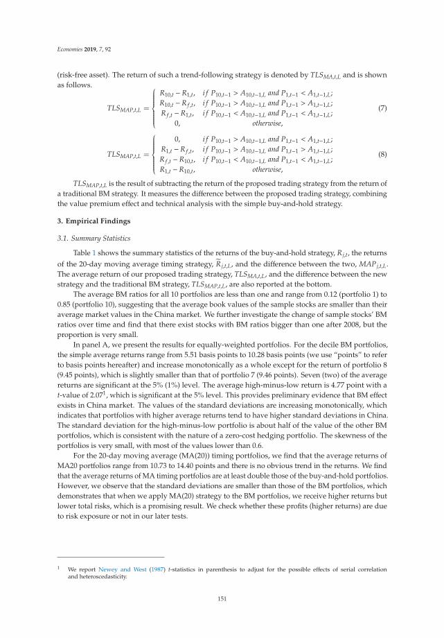
Economies 2019, 7, 92
(risk-free asset). The return of such a trend-following strategy is denoted by TLSMA,t,L and is shownas follows.
TLSMAP,t,L =
⎧⎪⎪⎪⎪⎪⎪⎨⎪⎪⎪⎪⎪⎪⎩R10,t −R1,t, i f P10,t−1 > A10,t−1,L and P1,t−1 < A1,t−1,L;R10,t −R f ,t, i f P10,t−1 > A10,t−1,L and P1,t−1 > A1,t−1,L;R f ,t −R1,t, i f P10,t−1 < A10,t−1,L and P1,t−1 < A1,t−1,L;
0, otherwise,
(7)
TLSMAP,t,L =
⎧⎪⎪⎪⎪⎪⎪⎨⎪⎪⎪⎪⎪⎪⎩0, i f P10,t−1 > A10,t−1,L and P1,t−1 < A1,t−1,L;
R1,t −R f ,t, i f P10,t−1 > A10,t−1,L and P1,t−1 > A1,t−1,L;R f ,t −R10,t, i f P10,t−1 < A10,t−1,L and P1,t−1 < A1,t−1,L;R1,t −R10,t, otherwise,
(8)
TLSMAP,t,L is the result of subtracting the return of the proposed trading strategy from the return ofa traditional BM strategy. It measures the difference between the proposed trading strategy, combiningthe value premium effect and technical analysis with the simple buy-and-hold strategy.
3. Empirical Findings
3.1. Summary Statistics
Table 1 shows the summary statistics of the returns of the buy-and-hold strategy, Rj,t, the returnsof the 20-day moving average timing strategy, Rj,t,L, and the difference between the two, MAPj,t,L.The average return of our proposed trading strategy, TLSMA,t,L, and the difference between the newstrategy and the traditional BM strategy, TLSMAP,t,L, are also reported at the bottom.
The average BM ratios for all 10 portfolios are less than one and range from 0.12 (portfolio 1) to0.85 (portfolio 10), suggesting that the average book values of the sample stocks are smaller than theiraverage market values in the China market. We further investigate the change of sample stocks’ BMratios over time and find that there exist stocks with BM ratios bigger than one after 2008, but theproportion is very small.
In panel A, we present the results for equally-weighted portfolios. For the decile BM portfolios,the simple average returns range from 5.51 basis points to 10.28 basis points (we use “points” to referto basis points hereafter) and increase monotonically as a whole except for the return of portfolio 8(9.45 points), which is slightly smaller than that of portfolio 7 (9.46 points). Seven (two) of the averagereturns are significant at the 5% (1%) level. The average high-minus-low return is 4.77 point with at-value of 2.071, which is significant at the 5% level. This provides preliminary evidence that BM effectexists in China market. The values of the standard deviations are increasing monotonically, whichindicates that portfolios with higher average returns tend to have higher standard deviations in China.The standard deviation for the high-minus-low portfolio is about half of the value of the other BMportfolios, which is consistent with the nature of a zero-cost hedging portfolio. The skewness of theportfolios is very small, with most of the values lower than 0.6.
For the 20-day moving average (MA(20)) timing portfolios, we find that the average returns ofMA20 portfolios range from 10.73 to 14.40 points and there is no obvious trend in the returns. We findthat the average returns of MA timing portfolios are at least double those of the buy-and-hold portfolios.However, we observe that the standard deviations are smaller than those of the BM portfolios, whichdemonstrates that when we apply MA(20) strategy to the BM portfolios, we receive higher returns butlower total risks, which is a promising result. We check whether these profits (higher returns) are dueto risk exposure or not in our later tests.
1 We report Newey and West (1987) t-statistics in parenthesis to adjust for the possible effects of serial correlationand heteroscedasticity.
151

Economies 2019, 7, 92
Ta
ble
1.
Des
crip
tive
stat
isti
csfo
rBM
,MA
(20)
,and
MA
Pra
nked
port
folio
s.
Ran
kB
MR
ati
oB
MD
eci
leP
ort
foli
os
MA
(20)
Tim
ing
Po
rtfo
lio
sM
AP
Av
eR
et
Std
Dev
Sk
ew
tA
ve
Ret
Std
Dev
Sk
ew
tA
ve
Ret
Std
Dev
Sk
ew
t
Pan
el
A:E
qu
all
y-w
eig
hte
dp
ort
foli
os
Lo
w0.
125.
5115
.97
0.55
1.54
11.8
812
.80
1.02
4.15
5.57
8.39
0.52
2.97
20.
205.
8815
.58
0.41
1.69
11.0
614
.68
0.09
3.37
4.28
8.50
1.74
2.25
30.
266.
7516
.05
0.61
1.88
10.7
313
.82
0.97
3.47
3.11
7.16
−0.0
21.
944
0.31
7.82
15.9
70.
622.
1913
.23
12.5
60.
554.
714.
448.
120.
752.
455
0.35
8.06
16.2
20.
332.
2212
.71
13.4
90.
394.
213.
648.
280.
241.
976
0.40
9.39
16.9
40.
412.
4813
.18
13.7
20.
944.
292.
846.
460.
291.
967
0.45
9.46
16.6
50.
402.
5413
.81
13.5
50.
614.
563.
368.
250.
311.
828
0.52
9.45
17.3
50.
422.
4314
.40
16.4
60.
903.
913.
898.
640.
262.
029
0.62
9.78
17.6
90.
432.
4713
.58
14.7
00.
764.
132.
855.
510.
042.
31H
igh
0.85
10.2
817
.78
0.77
2.59
13.0
315
.85
0.79
3.68
1.77
7.15
0.21
1.11
Hig
h–L
ow
4.77
8.32
1.22
2.56
0.86
9.12
2.10
0.42
−4.2
17.
220.
49−2
.61
(2.0
7)(0
.40)
(−2.
87)
TL
S16
.43
14.9
20.
284.
9211
.23
12.4
00.
994.
05(4
.85)
(4.1
2)P
an
el
B:V
alu
e-w
eig
hte
dp
ort
foli
os
Lo
w0.
125.
7816
.13
0.41
1.60
11.2
213
.12
1.02
3.82
4.62
8.88
0.40
2.33
20.
205.
4414
.80
0.52
1.64
10.3
614
.42
0.12
3.21
4.02
8.84
1.61
2.04
30.
265.
3416
.42
0.87
1.45
9.76
14.2
61.
143.
063.
497.
290.
242.
144
0.31
8.78
16.7
90.
632.
3412
.11
12.3
20.
464.
402.
267.
30−0
.05
1.38
50.
357.
2817
.78
0.58
1.83
11.8
614
.03
0.54
3.78
3.55
9.00
0.73
1.76
60.
407.
1318
.43
0.01
1.73
12.3
314
.06
0.78
3.92
4.19
6.85
0.76
2.73
70.
459.
4916
.60
0.41
2.56
13.2
113
.42
0.72
4.40
2.74
8.09
0.24
1.51
80.
528.
3117
.79
0.58
2.09
13.0
217
.48
1.02
3.33
3.61
8.81
0.44
1.83
90.
6210
.35
19.2
40.
842.
4113
.41
15.5
90.
953.
852.
126.
650.
111.
42H
igh
0.85
10.7
918
.43
0.85
2.62
13.0
317
.01
0.80
3.42
1.24
6.80
0.28
0.82
Hig
h–L
ow
4.78
8.46
0.58
2.53
1.39
10.3
21.
440.
60−3
.87
8.16
0.16
−2.1
2(2
.15)
(0.6
0)(−
2.12
)T
LS
15.3
415
.97
0.42
4.30
9.94
12.0
60.
873.
68(4
.50)
(3.9
5)
The
sam
ple
stoc
ksar
eso
rted
inas
cend
ing
orde
rby
thei
rBM
rati
osan
das
sign
edin
tode
cile
port
folio
sea
chye
ar.T
heeq
ually
-wei
ghte
dan
dva
lue-
wei
ghte
dpo
rtfo
lioda
ilyre
turn
sar
eth
enob
tain
ed,f
orw
hich
the
sum
mar
yst
atis
tics
are
repo
rted
inPa
nels
Aan
dB,
resp
ectiv
ely.
The
aver
age
retu
rns,
stan
dard
devi
atio
n,sk
ewne
ss,a
ndt-
test
stat
istic
sof
thes
epo
rtfo
lios
are
rep
orte
d.
MA
(20)
rep
rese
nts
the
tech
nica
lana
lysi
sw
ith
20-d
aym
ovin
gav
erag
eti
min
gsi
gnal
sim
pos
edon
the
BM
por
tfol
ios.
MA
Pre
pre
sent
sth
ed
iffer
ence
betw
een
the
MA
(20)
stra
tegy
and
the
buy-
and-
hold
stra
tegy
.Hig
h–Lo
wre
pres
ents
the
retu
rndiff
eren
cebe
twee
nth
ehi
ghes
tand
low
estB
Mpo
rtfo
lios,
the
high
estM
A(2
0)an
dlo
wes
tMA
(20)
port
folio
s,an
dth
ehi
ghes
tand
low
estM
AP,
resp
ecti
vely
.TLS
MA
repr
esen
tsth
epr
opos
edte
chni
cala
naly
sis
enha
nced
BMst
rate
gy.T
LSM
AP
repr
esen
tsth
ediff
eren
cebe
twee
nth
epr
osed
stra
tegy
and
the
buy-
and-
hold
stra
tegy
.Sim
ple
t-st
atis
tics
are
repo
rted
inco
lum
nta
ndN
ewey
and
Wes
t(19
87)t
-sta
tist
ics
are
repo
rted
inth
epa
rent
hese
s.
152

Economies 2019, 7, 92
The differences between MA(20) and BM portfolios, MAPs, are all positive and range from 1.77to 5.57 points. Interestingly, we observe the special pattern that the average MAPs are generallydecreasing as portfolio BM ratios increase, which indicates that the moving average technical analysisis more successful for portfolios with lower BM ratios.
For the proposed trading strategy, we can see that the average high-minus-low return of theMA(20) portfolios is very small (0.86 points) and insignificant (t = 0.40), much smaller than that ofthe BM portfolios (4.77 points). We conjecture that the small and insignificant result is caused by themisuse of the moving average timing signals. The high-minus-low return of MA(20) can be regardedas longing the highest MA(20) and shorting the lowest MA(20) portfolios. Shorting the lowest portfoliomeans that we will sell the assets when the last trading price Pj,t−1 is higher than the last 20-day movingaverage indicator Aj,t−1,L, whose signal indicates that the price will increase. In other words, we willsell the assets that we think will grow, which is logically wrong. Therefore, we conduct our tradingstrategy with the correct use of the moving average indicator for the lowest BM portfolio, which wediscussed in the methodology section. The TSLMA,t,L is 16.43 points, which is substantially higherthan that of the buy-and-hold strategy (4.77 points). The average significant difference between thetwo strategies (TSLMAP,t,L) is 11.23 points, which represents the additional profits from the new TLSstrategy, which is 2.36 times the buy-and-hold strategy.
In panel B, we present the performance of the value-weighted portfolios to check the size effecton the result. We find that the magnitude of the portfolio average returns is only slightly biggerthan the return of the corresponding equally-weighted portfolios. The simple average return of thebuy-and-hold strategy ranges from 5.34 to 10.79 points, with portfolio 10 (3) getting the highest (lowest)average return. In addition, all deciles with the MA(20) strategy have higher returns than the BMportfolios, ranging from 9.76 to 13.03 points. All of the MAP returns are positive and have lowerstandard deviations. The daily average return of the new trading strategy, TSLMA,t,L, is 15.34 points(t = 4.50), which is 221.13% higher than the high-minus-low return of the BM portfolio (4.78 points)but lower than the corresponding equally-weighted portfolios. The difference between MA(20) andbuy-and-hold strategies, TSLMAP,t,L, is 9.94 points (t = 3.95), which is also slightly lower than that ofthe corresponding equally-weighted portfolios.
Overall, Table 1 shows that the value premium effect exists in the China stock market and thatthe moving average technical analysis strategy is useful in producing positive and significant excessreturns. In addition, the proposed strategy, TSLMA,t,L, clearly outperforms the traditional buy-and-holdBM strategy.
3.2. Risk-Adjusted Performances
The MAP results show that the MA timing strategy outperforms the buy-and-hold strategy.However, we observe that generally, portfolios with higher returns have higher standard deviations,which suggests that their risk (or total risk) levels are different. Therefore, a natural research questionis whether the return differences are due to exposure to risks. In this sub-section, we concentrate onthe risk-adjusted profitability of MAP and TLS using three asset pricing models: the CAPM, FF3F,and LIQ4F models. We use MAP and TLSMAP,t,L as dependent variables and run time-series regressionsagainst the risk factors. The results are presented in Table 2.
If the portfolio average return, MAPj,t,L is not fully explained by the risk factors, we expect α j,L tobe significantly different from zero. Otherwise, it suggests that the positive additional return found inthe MA strategy is artificial after taking exposure to well-documented risk factors into consideration.
153

Economies 2019, 7, 92
Table 2. Time-series regressions with the CAPM and LIQ4F models.
RankCAPM LIQ4F Model
α βmkt Adj. R2 α βmkt βsmb βhml βliq Adj. R2
Low 8.18 −0.45 0.40 9.08 −0.46 −0.59 0.20 0.15 0.45(5.41) (−18.52) (6.26) (−18.38) (−9.45) (6.21) (4.13)
2 7.13 −0.49 0.42 8.10 −0.49 −0.53 0.15 0.17 0.46(4.73) (−18.38) (5.59) (−18.35) (−8.92) (5.03) (4.99)
3 5.77 −0.46 0.39 6.70 −0.47 −0.51 0.15 0.16 0.42(3.75) (−16.98) (4.48) (−16.78) (−7.97) (4.84) (4.36)
4 7.42 −0.52 0.43 8.53 −0.51 −0.43 0.07 0.19 0.46(4.76) (−18.50) (5.58) (−18.30) (−6.95) (2.24) (5.39)
5 6.69 −0.53 0.44 8.12 −0.52 −0.53 0.05 0.15 0.47(4.20) (−18.79) (5.33) (−18.59) (−8.19) (1.54) (4.21)
6 5.64 −0.49 0.40 7.12 −0.48 −0.44 −0.01 0.19 0.44(3.48) (−17.45) (4.60) (−17.56) (−7.33) (−0.28) (5.41)
7 5.64 −0.49 0.40 8.00 −0.49 −0.47 −0.04 0.18 0.45(3.48) (−17.45) (5.12) (−18.31) (−7.44) (−1.23) (5.14)
8 6.98 −0.54 0.41 8.98 −0.51 −0.43 −0.12 0.19 0.48(4.10) (−18.26) (5.61) (−18.34) (−6.82) (−3.20) (5.18)
9 5.63 −0.49 0.39 7.30 −0.47 −0.37 −0.09 0.18 0.43(3.45) (−17.32) (4.69) (−17.41) (−6.29) (−2.46) (5.36)
High 4.65 −0.50 0.40 6.57 −0.48 −0.40 −0.14 0.15 0.45(2.86) (−17.57) (4.25) (−17.92) (−6.57) (−3.56) (4.20)
High–Low−3.53 −0.05 0.01 −2.51 −0.02 0.19 −0.33 0.00 0.08
(−2.49) (−3.27) (−1.82) (−1.24) (3.71) (−8.34) (−0.08)
TLSMAP13.24 −0.09 0.01 15.14 −0.04 0.14 −0.46 0.12 0.06(5.24) (−1.88) (6.08) (−0.86) (1.39) (−7.99) (1.90)
The sample stocks are sorted in ascending order by their BM ratios and assigned into decile portfolios eachyear. The equally-weighted portfolio daily returns are then obtained. MAP is the difference between the MA(20)strategy and the buy-and-hold strategy. The regression models are MAPj,t,L = α j.L + β j,L,MKTRMKT,t + ε j,t,L andMAPj,t,L = α j.L + β j,L,MKTRMKT,t + β j,L,SMBRSMB,t + β j,L,HMLRHML,t + β j,L,LIQRLIQ,t + ε j,t,L, where RMKT,t is marketexcess returns; RSMB,t is the size factor; RHML,t is the book-to-market factor; RLIQ,t. is the liquidity risk factor proxiedby turnover ratio; ε j,t,L is an error term assumed to have a zero mean and to be uncorrelated with all other explanatoryvariables; and the factor sensitivities or loadings, β j,L,MKT , β j,L,SMB, β j,L,HML, and β j,L,LIQ, are the slope coefficients forthe factors, respectively. α j.L is the intercept of the regression. t-test statistics are presented in the parentheses.
Table 2 provides the results of the equally-weighted portfolios on the CAPM and LIQ4F models.Because the results of FF3F are similar to those from the LIQ4F model, we do not report them to savespace. All of the alphas of the 10 portfolios in the two models are significantly different from zero atthe 5% level, which suggests that the profits generated from the timing strategy are not fully capturedby these well-known risk factors. The alphas of the CAPM model range from 4.65 to 8.18 points, whilethe alphas of the LIQ4F model range from 6.57 to 9.08 points.
The betas of the market excess return and size factors are all negative and highly significant, whichcan partially explain why the alpha becomes larger than the unadjusted return of the MAPs. Half ofthe coefficients of the HML factor are positive and half are negative. The coefficients of the LIQ factorare all significantly positive.
The alphas of the TSLMAP in the CAPM and LIQ4F models are 13.24 and 15.14 points, respectively,which are larger than the unadjusted TSLMAP (11.23 points). Interestingly, while the adjusted R2 formost of the deciles in the two models are larger than 40%, the adjusted R2 for the TSLMAP is extremelylow. Overall, the low R2 and significant alphas indicate that the CAPM and LIQ4F models cannotexplain the excess profit from the new BM strategy.
3.3. Components of Strategies
We now establish that the moving average technical analysis can help us obtain better returnsthan the buy-and-hold strategy. We are curious about how exactly the excess returns are created.To answer this question, we consider the operation of the MA timing strategy. We know that we holdthe underlying portfolio when the signal Pj,t−1 > Aj,t−1,L appears and hold the risk-free asset otherwise.Comparing this with the buy-and-hold strategy, a difference appears only when Pj,t−1 < Aj,t−1,L.
154

Economies 2019, 7, 92
This difference is between the return generated from the underlying portfolio and the risk-free asset.Therefore, we can express the MAP return in another way:
MAPj,t,L =
{0, i f Pj,t−1 > Aj,t−1,L;
R f ,t −Rj,t, otherwise,(9)
To examine the difference, we separate the sample into two parts: when Pj,t−1 > Aj,t−1,L (buysignal) and when Pj,t−1 ≤ Aj,t−1,L (sell signal). We calculate the proportion of days when Rj is higher(or lower) than Rf for the buying and selling signal states. The results are shown in Table 3.
Table 3. Components of strategies.
Rank Condition Position Equally-Weighted Portfolio
Rp > Rf Rp ≤ Rf
Low Pi,t−1 > Ai,t−1,L BM portfolio 58.8 41.2Pi,t−1 ≤ Ai,t−1,L Risk-free asset 47.83 52.17
2 Pi,t−1 > Ai,t−1,L BM portfolio 56.71 43.29Pi,t−1 ≤ Ai,t−1,L Risk-free asset 49.35 50.65
3 Pi,t−1 > Ai,t−1,L BM portfolio 56.96 43.04Pi,t−1 ≤ Ai,t−1,L Risk-free asset 46.8 53.2
4 Pi,t−1 > Ai,t−1,L BM portfolio 59.29 40.71Pi,t−1 ≤ Ai,t−1,L Risk-free asset 48.82 51.18
5 Pi,t−1 > Ai,t−1,L BM portfolio 59.71 40.29Pi,t−1 ≤ Ai,t−1,L Risk-free asset 47.85 52.15
6 Pi,t−1 > Ai,t−1,L BM portfolio 59.85 40.15Pi,t−1 ≤ Ai,t−1,L Risk-free asset 46.03 53.97
7 Pi,t−1 > Ai,t−1,L BM portfolio 60.02 39.98Pi,t−1 ≤ Ai,t−1,L Risk-free asset 48.46 51.54
8 Pi,t−1 > Ai,t−1,L BM portfolio 59.66 40.34Pi,t−1 ≤ Ai,t−1,L Risk-free asset 49.38 50.62
9 Pi,t−1 > Ai,t−1,L BM portfolio 60.15 39.85Pi,t−1 ≤ Ai,t−1,L Risk-free asset 48.97 51.03
High Pi,t−1 > Ai,t−1,L BM portfolio 58.83 41.17Pi,t−1 ≤ Ai,t−1,L Risk-free asset 49.82 50.18
We separate the MA(20) portfolio sample into two parts. One is when Pj,t−1 > Aj,t−1,L which indicates a buy signaland the other is when Pj,t−1 ≤ Aj,t−1,L which suggests a sell signal. We then compare the return of the BM portfolioand the risk-free rate. We calculate the proportion of each situation for buying and selling signal states.
We find that the proportions of the state in which Rj,t > R f ,t are all bigger than 50%, rangingfrom 56.71% to 60.15%, when Pj,t−1 > Aj,t−1,L. However, this does not affect the MAP. In addition,the proportions of the state in which Rj,t < R f ,t are also all bigger than 50% when Pj,t−1 ≤ Aj,t−1,L.The highest is 53.97% in decile 6 and the lowest is 50.18% in decile 10. Although the successful rates arenot very high (mostly between 50% and 60%), all of them are bigger than 50%, which leads to betterperformance by MA strategy when a selling signal emerges. These results show that the MA signal isuseful in generating positive excess returns and help explain why the moving average can outperformthe buy-and-hold strategy.
3.4. Alternative Lag Lengths
In this sub-section, we investigate how the returns of the MAP and TLS change with the laglengths. We conduct the moving average timing strategy with 5-day, 10-day, 20-day, 50-day, 100-day,and 200-day timing signals. The results are illustrated in Figure 1.
155

Economies 2019, 7, 92
(a) (b)
-5
0
5
10
5 10 20 50 100 200
poin
ts
Lag length
Average MAP(L)
Raw return CAPM LIQ4F
0
5
10
15
20
5 10 20 50 100 200
poin
ts
Lag length
TLS(L)
Raw return CAPM LIQ4F
Figure 1. (a) For each BM portfolio, the moving average timing strategy is imposed with 5-day, 10-day,20-day, 50-day, 100-day, and 200-day timing signals. The MAP returns for the decile portfolios are thenaveraged cross-sectionally. The raw returns of the average MAP, risk-adjusted alphas of CAPM andLIQ4F models are plotted; (b) The proposed technical analysis enhanced BM strategy is imposed with5-day, 10-day, 20-day, 50-day, 100-day, and 200-day timing signals. The raw returns of the average TLSstrategy, risk-adjusted alphas of CAPM and LIQ4F models are plotted.
Figure 1a plots the average return of MAPs across the decile portfolios with different lag lengths.The 20-day average MAP return is the highest (in fact, although it is not plotted, the 20-day MAP is thehighest for each decile portfolio). The 5-day MAP and 10-day MAP are also significantly positive butare slightly smaller than that of the 20-day signals. The returns with signals that are longer than 20days start to decline and become progressively smaller, and the results of the 100-day lag even becomenegative. The CAPM and LIQ4F model-adjusted MAP alphas present similar patterns to that of theunadjusted returns.
The returns of the proposed trading strategy, TLS, are plotted in Figure 1b. Again, the 20-daylag strategy generates the highest raw and risk-adjusted profits. The MA(5) and MA(10) strategiesalso perform well, as their returns are close to that of MA(20). However, when lags longer than 50days are used, the strategy return drops sharply, almost reaching zero. We conjecture that this isbecause the Chinese stock market is highly volatile. A shorter moving average signal can capture thefluctuations in information more accurately than a longer moving average signal. The signals withlong lag length may miss important information changes, and so the abnormal return produced bythese signals becomes flat and small.
The results seem to suggest that a shorter moving average of up to 50 days can produce significantand meaningful positive returns. However, the 20-day lag signal provides the best result by capturingthe most information regarding past prices. To sum up, lag length can influence the performance ofthe moving average timing strategy, and we need to choose the best one for China’s stock market.
3.5. Transaction Operations
In the real market, the utilization of the moving average timing strategy would induce moretransaction operations, resulting in higher transaction costs. In this section, we examine the effect oftrading costs on the earlier results. Table 4 reports the statistics that address this issue.
The average holding days is the average number of days that we hold the portfolio. Longeraverage holding days suggest that the trading portfolio is more stable. From Table 4, we can tell thatthe average holding days becomes longer as the moving average lag length increases. The averageholding days of the 5-day MAP is around 4 days, while that of the 20-day MAP is around 10 days.Moreover, the average holding days for 200-day MAP ranges from 130.99 days to 183.08 days. We donot report those of the two zero-cost trading strategies because it is difficult to define the holdingperiod while investors hold two portfolios simultaneously.
156

Economies 2019, 7, 92
Ta
ble
4.
Tran
sact
ion
oper
atio
ns.
Ran
kM
AP
(5)
MA
P(1
0)
MA
P(2
0)
MA
P(5
0)
MA
P(1
00)
MA
P(2
00)
Ho
ldin
gF
req
BE
TC
Ho
ldin
gF
req
BE
TC
Ho
ldin
gF
req
BE
TC
Ho
ldin
gF
req
BE
TC
Ho
ldin
gF
req
BE
TC
Ho
ldin
gF
req
BE
TC
Lo
w3.
800.
2938
.77
5.56
0.20
41.2
09.
350.
1383
.35
19.3
70.
0781
.28
50.0
60.
04−7
.51
168.
650.
0287
.36
23.
810.
298.
505.
760.
2017
.49
10.3
40.
1364
.09
16.0
60.
09−8
.96
51.7
40.
0416
.88
150.
480.
0241
.78
33.
920.
2911
.84
6.34
0.19
15.1
69.
900.
1347
.22
25.5
70.
0724
.41
43.1
70.
05−4
1.89
130.
990.
0228
.16
43.
870.
2813
.58
6.14
0.19
23.7
510
.54
0.12
76.7
919
.94
0.08
8.84
50.8
10.
05−2
5.54
137.
260.
020.
305
3.95
0.28
8.28
6.16
0.19
18.4
89.
590.
1358
.54
21.5
10.
0733
.90
48.2
50.
04−2
.14
176.
570.
0212
1.70
64.
070.
283.
566.
260.
1910
.09
10.9
50.
1248
.74
25.3
10.
0745
.19
67.4
10.
04−1
0.50
183.
080.
0212
6.02
73.
920.
284.
666.
400.
1828
.86
11.4
50.
1161
.02
22.1
10.
0722
.78
46.5
00.
05−2
2.12
141.
550.
0265
.13
84.
070.
2716
.91
6.63
0.18
13.1
911
.04
0.11
69.3
827
.90
0.07
78.5
747
.64
0.05
−9.2
614
6.77
0.02
81.6
89
4.00
0.28
4.42
6.37
0.18
22.5
610
.80
0.12
48.9
220
.48
0.07
33.7
346
.56
0.05
−18.
2215
6.47
0.02
120.
17H
igh
4.01
0.28
−3.0
06.
720.
1810
.80
10.4
50.
1228
.91
21.2
20.
08−9
.39
48.8
60.
06−6
0.33
141.
450.
0252
.11
Hig
h–L
ow
0.45
0.32
0.22
0.13
0.09
0.03
TL
S0.
450.
320.
220.
130.
090.
03T
ran
sact
ion
Co
stfo
rT
LS
7.09
5.24
3.95
2.99
2.68
2.58
MA
Pfo
rT
LS
9.99
9.67
11.2
37.
083.
391.
51R
etu
rnaft
er
Tra
nsa
ctio
nC
ost
2.91
4.43
7.28
4.08
0.70
−1.0
8
We
calc
ulat
eth
eav
erag
eho
ldin
gd
ays,
trad
ing
freq
uenc
yof
MA
and
TL
Spo
rtfo
lios,
brea
k-ev
entr
ansa
ctio
nco
stan
daf
ter
tran
sact
ion
cost
retu
rns
ofT
LS.
The
aver
age
hold
ing
day
sre
pres
entt
heav
erag
enu
mbe
rof
days
duri
ngw
hich
the
port
folio
ishe
ldbe
fore
itis
sold
out.
The
trad
ing
freq
uenc
yof
the
port
folio
sis
the
frac
tion
ofth
enu
mbe
rof
trad
ing
days
toth
enu
mbe
rof
day
sin
the
who
lesa
mpl
epe
riod
.Bre
ak-e
ven
tran
sact
ion
cost
(BE
TC
)is
the
fee
whi
chis
requ
ired
inea
chro
und
-tri
ptr
ansa
ctio
nfo
rth
epo
rtfo
lios
ifth
efin
alpr
ofiti
sze
ro.
Tran
sact
ions
Cos
tfor
TLS
cons
ists
com
mis
sion
,tra
nsfe
rfe
e,st
amp
tax,
and
inte
rest
fee
for
stoc
kbo
rrow
.MA
Pfo
rTL
Sis
the
retu
rndiff
eren
cebe
twee
nth
epr
opos
edte
chni
cala
naly
sis
enha
nced
BMst
rate
gyan
dth
etr
adit
iona
lbuy
-and
-hol
dBM
stra
tegy
.
157

Economies 2019, 7, 92
Next, we calculate the trading frequency of the MAP and TLS portfolios, which is the fraction ofthe number of trading days of the number of days in the whole period. A shorter (longer) lag lengthstrategy implies that the portfolios will be traded more (less) and that the trading frequency should behigher (smaller). For the 20-day lag length, the trading frequency ranges from 0.11 to 0.13 for the 10deciles and is 0.22 for the High–Low and TLS strategies. The trading frequency for all of the decileswith lag lengths longer than 20 days is lower than 0.10. Apparently, the MA timing strategies incurhigher transaction fees if a shorter lag length is chosen for the MA indicator.
According to the China Securities Regulatory Commission, the Securities Association of Chinaand notices of securities companies, the cost for trading A-shares consists of a commission, transfer fee,and stamp tax. The commission fee should be lower than 30 basis points of the transaction amount andis determined by securities companies in the allowable interval. Because securities companies in Chinause low price strategies to attract customers, according to the Eastmoney Choice Database, the averagecommission fee for trading stocks in 2015 is just 5.1 basis points. The amounts of the other two kinds offees are fixed. The transfer fee for A-shares is 0.2 basis points of the transaction amount, and the stamptax is 10 basis points only on the sell side. To sum up, we need to pay 20.6 ((5.1 + 0.2)*2 + 10) basispoints on average for a round trip of transactions. Following Balduzzi and Lynch (1999), we assumethat we pay the transaction fee when we trade BM portfolios but not when we trade the risk-free asset.
Following Han et al. (2013) and Ko et al. (2014), we use break-even transaction costs (BETCs)to evaluate the profit versus cost for the MAP returns. BETC here is the fee that we can afford ineach round-trip transaction for the deciles if the final profit is zero. We report the results in Table 4,where we label BETCs with n.a. when the MAP return is negative, as BETCs are meaningless in sucha situation. Overall, the BETCs are mostly higher than 20.6 basis points. The MAP(5) and MAP(10)strategies in general have lower BETCs because transaction operations are too frequent, thus incurringhigher transaction fees. The BETCs of MAP(20) are higher than 20.6 for all deciles, indicating positiveafter-cost profitability. The BETCs start to decline after the MAP(20) strategy. This pattern is similar tothe results in Figure 1.
In our new proposed zero-cost trading strategy, TLS, we need to borrow stocks when receivingshort signals and pay interest for stock borrowing. In China, most interest rates for short-selling arelower than 9% annually, which is 2.4658 points daily (9%/365). To compute the after-cost returns of TLS,in addition to the normal transaction fee, we need to subtract the interest fee. We calculate the interestfee by multiplying the short-selling interest rate by the number of days that we borrow stocks. FromTable 4, we can see that transaction costs for TLS decrease monotonically from 7.09 to 2.58 points as thelag length increases. We obtain a positive final return for all of the portfolios except for the MAP(200)strategy. Again, the MAP(20) strategy generates the highest after-transaction-cost TLS returns, whichis consistent with the findings in Figure 1. Therefore, MA timing strategy with 20-day lag seems to bethe best choice both before and after transaction costs.2
4. Robustness Tests
This section presents the tests of the robustness of the MA and TLS trading strategies. First,we examine whether there is a difference in the trading results in the sub-periods before and after thenon-tradable stock reform in China. Second, we investigate whether business cycles affect returns.Third, we study the impact of market timing ability on the strategies. Lastly, we use an alternativesample that contains stocks for which short-selling is permitted in China’s market.
2 In an unablated wealth analysis test, the end wealth of an initial zero-cost investment (long $1 million in highest BM portfolioand short $1 million in lowest BM portfolio) using the TLS(20) strategy is $687 million, while the counterpart from thebuy-and-hold strategy is only $10.22 million.
158

Economies 2019, 7, 92
4.1. Sub-Period Analysis
Since China’s market underwent non-tradable stock reform in 2005, market conditions, suchas market regulations, rules, trading mechanisms, participants, and trading volume, have changeddrastically. To investigate the effect of the policy change on our strategy, we conduct tests on sub-periods,dividing our whole sample period at mid-2005 into two periods of nearly equal length. We repeatour analysis and obtain the daily average return data for the two sub-periods, 1 July 1995 to 30June 2005 and 1 July 2005 to 30 June 2015. To examine the difference between the two subsamples,we conduct a two-sample mean test. First, we check the normality of the two subsamples using theKolmogorov–Smirnov test, which is suitable for big data like ours. Panel A of Table 5 shows that all ofthe p-values for the sample differences are smaller than 0.01, which indicates that the samples do notfollow a normal distribution.
We then conduct the Wilcoxon rank-sum test to check the difference between the two sub-periodsafter determining that they do not follow a normal distribution. Panel B of Table 5 reports the testresults. Most of the p-values are smaller than 0.1, ranging from 0.0005 to 0.3607. The p-value of theTLS portfolio is 0.0118, which is very small and rejects the null hypothesis. The two sub-samples aresignificantly different from each other in the TLS strategy.
Next, we run regressions with the CAPM, FF3F, and LIQ4F models to check the robustness of therisk-adjusted returns. Because the results are similar, we only report the LIQ4F model alphas and betasin the sub-periods in Table 5 to save space.
Overall, we find that the two sub-periods’ results are similar to those for the whole period.All of the alphas of the deciles are positive, and almost all of them are significant (portfolio 10 ismarginally significant at 10%). As in the previous findings, the coefficients of market excess returnand SMB are negative. The TLS strategy alphas are large and highly significant for both sub-periods;however, the result for the latter sub-period is better than the former for both the deciles and the TLS.Specifically, the second sub-period alpha of the TLS is 19.32 points, while that of the former period is11.12. The results suggest that the MA and TLS strategies work better in the most recent period, whichhas undergone non-tradable share reform to push more non-tradable shares to become tradable sharesin the market. As many more shares are traded in the market, the market becomes more efficient, whichsuggests that technical analysis should become less profitable in the market. However, our resultsseem to contradict this inference. These results are interesting and need further investigation, which isbeyond the scope of our study.
159

Economies 2019, 7, 92
Ta
ble
5.
Sub-
peri
odan
alys
is.
Pa
ne
lA
:N
orm
ali
tyC
he
ck(K
olm
og
oro
v–
Sm
irn
ov
)P
an
el
B:
Wil
cox
on
Tw
o-S
am
ple
Te
st
Ra
nk
Fir
stS
ub
-Pe
rio
dS
eco
nd
Su
b-P
eri
od
Ra
nk
Sta
tist
icN
orm
al
Ap
pro
xim
ati
on
ZT
wo
-Sid
ed
Pr>|Z|
Sta
tist
icD
p-V
alu
eS
tati
stic
Dp-
Va
lue
Lo
w0.
2586
<0.
0100
0.32
58<
0.01
00L
ow
6021
507
3.50
0.00
052
0.28
84<
0.01
000.
3415
<0.
0100
259
0550
10.
910.
3607
30.
2925
<0.
0100
0.33
46<
0.01
003
5967
378
2.36
0.01
844
0.26
87<
0.01
000.
3349
<0.
0100
459
9264
52.
890.
0038
50.
2741
<0.
0100
0.32
03<
0.01
005
5956
286
2.06
0.03
996
0.29
17<
0.01
000.
3289
<0.
0100
659
9256
62.
930.
0034
70.
285
<0.
0100
0.33
41<
0.01
007
5942
272
1.76
0.07
818
0.28
57<
0.01
000.
3285
<0.
0100
859
5651
22.
080.
0375
90.
2863
<0.
0100
0.33
07<
0.01
009
5982
790
2.69
0.00
71H
igh
0.28
83<
0.01
000.
3223
<0.
0100
Hig
h59
2462
41.
350.
1766
Hig
h–
Lo
w0.
2286
<0.
0100
0.24
02<
0.01
00H
igh
–L
ow
5818
216
−1.0
30.
3020
TL
S0.
1373
<0.
0100
0.13
05<
0.01
00T
LS
5744
009
−2.5
20.
0118
Pa
ne
lC
:T
ime
-se
rie
sre
gre
ssio
ns
wit
hL
IQ4
Fm
od
el
Ra
nk
Fir
stS
ub
-Pe
rio
dS
eco
nd
Su
b-P
eri
od
αβ
mk
tβ
smb
βh
ml
βli
qA
dj.
R2
αβ
mk
tβ
smb
βh
ml
βli
qA
dj.
R2
Lo
w7.
24−0
.43
−0.5
60.
220.
140.
4410
.96
−0.4
8−0
.53
0.09
0.20
0.46
(4.0
1)(−
11.9
8)(−
6.95
)(5
.61)
(2.8
2)(4
.86)
(−14
.38)
(−6.
15)
(1.6
7)(3
.84)
23.
95−0
.49
−0.5
20.
150.
110.
4812
.07
−0.4
9−0
.43
0.08
0.28
0.45
(2.1
3)(−
11.9
9)(−
6.18
)(3
.94)
(2.3
5)(5
.47)
(−14
.29)
(−5.
23)
(1.3
5)(5
.37)
36.
07−0
.44
−0.5
40.
130.
080.
437.
16−0
.48
−0.3
80.
090.
300.
42(3
.43)
(−10
.85)
(−6.
56)
(3.6
7)(1
.69)
(2.9
7)(−
13.1
1)(−
4.16
)(1
.54)
(5.1
1)4
6.92
−0.4
9−0
.45
0.04
0.11
0.49
10.0
2−0
.52
−0.3
30.
040.
310.
45(3
.81)
(−12
.09)
(−5.
74)
(1.1
1)(2
.37)
(4.0
6)(−
14.0
1)(−
3.72
)(0
.69)
(5.4
9)5
6.45
−0.4
9−0
.44
0.02
0.06
0.47
9.86
−0.5
5−0
.44
−0.0
40.
320.
48(3
.41)
(−11
.56)
(−5.
42)
(0.6
5)(1
.19)
(4.1
9)(−
15.1
9)(−
4.77
)(−
0.71
)(5
.34)
160

Economies 2019, 7, 92
Ta
ble
5.
Con
t.
65.
75−0
.44
−0.3
9−0
.03
0.13
0.43
8.73
−0.5
1−0
.42
−0.0
30.
260.
44(3
.07)
(−11
.45)
(−4.
98)
(−0.
89)
(3.1
0)(3
.57)
(−13
.69)
(−4.
82)
(−0.
48)
(4.4
7)7
5.43
−0.4
4−0
.45
−0.0
70.
100.
4410
.83
−0.5
4−0
.41
−0.0
80.
290.
48(2
.88)
(−11
.79)
(−5.
91)
(−1.
77)
(2.4
8)(4
.43)
(−14
.70)
(−4.
43)
(−1.
30)
(4.9
4)8
7.63
−0.4
8−0
.40
−0.1
30.
170.
4910
.58
−0.5
5−0
.43
−0.1
50.
220.
48(3
.83)
(−11
.48)
(−4.
93)
(−2.
87)
(3.8
3)(4
.24)
(−14
.84)
(−4.
77)
(−2.
20)
(3.5
8)9
5.81
−0.4
4−0
.40
−0.1
00.
120.
438.
71−0
.49
−0.2
5−0
.17
0.29
0.44
(2.9
4)(−
11.5
7)(−
5.15
)(−
2.19
)(2
.85)
(3.6
4)(−
13.2
2)(−
2.98
)(−
2.77
)(5
.22)
Hig
h3.
83−0
.41
−0.3
3−0
.13
0.14
0.42
9.73
−0.5
4−0
.39
−0.2
10.
180.
48(1
.94)
(−10
.87)
(−4.
39)
(−2.
84)
(3.0
6)(4
.23)
(−15
.22)
(−4.
60)
(−3.
34)
(3.1
8)H
igh
–L
ow
−3.4
10.
020.
22−0
.35
0.00
0.12
−1.2
2−0
.05
0.14
−0.3
0−0
.02
0.04
(−1.
83)
(1.0
9)(3
.05)
(−7.
28)
(−0.
03)
(−0.
60)
(−2.
46)
(1.9
0)(−
6.23
)(−
0.45
)T
LS
11.1
20.
04−0
.05
−0.4
10.
190.
0919
.32
−0.1
10.
22−0
.52
0.06
0.05
(3.4
2)(0
.52)
(−0.
31)
(−5.
62)
(2.2
5)(5
.20)
(−1.
81)
(1.6
1)(−
5.35
)(0
.70)
The
two
sub-
peri
ods
are
befo
rean
daf
ter
the
non-
trad
able
stoc
kre
form
.The
first
sub-
peri
odis
from
1Ju
ly19
95to
30Ju
ne20
05an
dth
ese
cond
sub-
peri
odis
from
1Ju
ly20
05to
30Ju
ne20
15.P
anel
Apr
esen
tsth
ere
sults
ofth
eK
olm
ogor
ov–S
mir
nov
test
whi
chch
ecks
the
norm
ality
ofth
etw
osu
bsam
ples
.Pan
elB
pres
ents
the
resu
ltsof
the
Wilc
oxon
rank
-sum
test
whi
chch
ecks
the
diff
eren
cebe
twee
nth
etw
osa
mpl
epe
riod
saf
ter
know
ing
they
do
notf
ollo
wno
rmal
dis
trib
utio
ns.P
anel
Cpr
esen
tsre
sult
sof
the
tim
e-se
ries
regr
essi
ons
wit
hth
eL
IQ4F
mod
elfo
rth
etw
osu
b-pe
riod
s.t-
test
stat
isti
csar
epr
esen
ted
inth
epa
rent
hese
s.
161

Economies 2019, 7, 92
4.2. Business Cycles
We now come to the question of whether there is any relation between the moving average signalsand business cycles. Here, we use two methods to test the influence of business cycles. First, Liew andVassalou (2000) construct the following model, which uses the GDP growth rate as a proxy for goodand bad business states
MAPj,t,L = α j.L + β j,L,MKTRMKT,t + β j,L,SMBRSMB,t + β j,L,HMLRHML,t + β j,L,GoodDGDPGood,t+
β j,L,BadDGDPBad,t + ε j,t,L, j = 1, . . . , 10,
(10)
TLSt,L = αL + βL,MKTRMKT,t + βL,SMBRSMB,t + βL,HMLRHML,t + βL,GoodDGDPGood,t + βL,BadDGDP
Bad,t+
εt,L,(11)
In the model, DGDPGood,t and DGDP
Bad,t are the dummy variables for good and bad business states. When
the GDP growth rate in the quarter is in the top 25% of the whole sample period, DGDPGood,t will be
one, which indicates that business cycles are in a good period. DGDPBad,t indicates the bad state when
the quarterly GDP growth rate is in the bottom 25% of the overall sample. We can determine thecontribution of both expansionary (good business state) and recessionary (bad business state) periodsfrom their coefficients. If they are significantly positive, the predictability is strong, and the strategyworks in the state.
The other model from Cooper et al. (2004) uses a dummy variable for bad market performance.We follow them and perform the following regression using market return data:
MAPj,t,L = α j.L + β j,L,MKTRMKT,t + β j,L,SMBRSMB,t + β j,L,HMLRHML,t + β j,L,BadDMarketBad,t + ε j,t,L,
j = 1, . . . , 10,(12)
TLSt,L = αL + βL,MKTRMKT,t + βL,SMBRSMB,t + βL,HMLRHML,t + βL,BadDMarketBad,t + εt,L, (13)
DMarketBad,t is the dummy variable that denotes the bad state of the business cycle. We calculate the
market return of the past three years before every yearly holding period. If the result is negative,DMarket
Bad,t will be one, and zero otherwise. We can determine the effect of a bad market environment
on our excess return from its coefficients. If the coefficients on DMarketBad,t are significantly positive, our
strategy works in the bad market state.Panels A and B of Table 6 show the results of these two regressions. We find that the pattern of the
alphas in the two models changes only slightly from before. However, the coefficients on most of thedummy variables are insignificant. For the first model, 9 of the 10 portfolio coefficients are insignificantat the 10% level. For the second model, only two of the coefficients of the dummy variable DMarket
Bad,t aresignificant at either the 5% or 10% level. These results clearly show that business cycles have a veryweak influence on the average returns of MA strategy.3
3 From unablated robustness test results, we find that other famous cycle effects like the January effect and the Lunar cycle(Wong and McAleer 2009) also have weak influence over the MA and TLS strategies.
162

Economies 2019, 7, 92
Ta
ble
6.
Busi
ness
cycl
e.
Ran
kG
oo
dan
dB
ad
Sta
tes
Are
Iden
tifi
ed
by
GD
PG
row
th(P
ast
20
Years
)G
oo
dan
dB
ad
Sta
tes
Are
Iden
tifi
ed
by
Past
Th
ree-Y
ear
Mark
et
Retu
rns
αβ
mk
tβ
smb
βh
ml
βli
qβ
Go
od
βB
ad
Ad
j.R
2α
βm
kt
βsm
bβ
hm
lβ
liq
βB
ad
Ad
j.R
2
Lo
w9.
74−0
.46
−0.5
90.
200.
151.
91−4
.45
0.45
9.60
−0.4
6−0
.59
0.20
0.15
−1.2
90.
45(4
.93)
(−18
.36)
(−9.
43)
(6.1
6)(4
.13)
(0.5
0)(−
1.46
)(4
.88)
(−18
.38)
(−9.
46)
(6.2
1)(4
.13)
(−0.
47)
27.
55−0
.49
−0.5
20.
150.
176.
48−3
.94
0.46
8.68
−0.4
9−0
.53
0.15
0.17
−1.4
50.
46(3
.78)
(−18
.33)
(−8.
89)
(4.9
9)(4
.98)
(1.7
9)(−
1.21
)(4
.53)
(−18
.35)
(−8.
93)
(5.0
3)(4
.99)
(−0.
52)
37.
27−0
.47
−0.5
10.
150.
161.
69−3
.88
0.42
7.19
−0.4
7−0
.51
0.15
0.16
−1.2
20.
42(3
.61)
(−16
.77)
(−7.
93)
(4.8
1)(4
.36)
(0.4
4)(−
1.20
)(3
.48)
(−16
.79)
(−7.
96)
(4.8
4)(4
.37)
(−0.
44)
48.
77−0
.51
−0.4
30.
070.
192.
01−2
.85
0.46
10.3
3−0
.51
−0.4
30.
070.
19−4
.49
0.47
(4.2
9)(−
18.2
8)(−
6.92
)(2
.21)
(5.3
9)(0
.50)
(−0.
89)
(4.9
7)(−
18.3
0)(−
6.96
)(2
.24)
(5.4
0)(−
1.56
)5
8.49
−0.5
2−0
.53
0.05
0.15
2.00
−3.3
60.
479.
59−0
.52
−0.5
30.
050.
15−3
.65
0.47
(4.1
4)(−
18.5
8)(−
8.17
)(1
.52)
(4.2
1)(0
.51)
(−1.
03)
(4.5
7)(−
18.6
0)(−
8.21
)(1
.55)
(4.2
1)(−
1.28
)6
7.67
−0.4
8−0
.43
−0.0
10.
191.
29−3
.42
0.44
8.59
−0.4
8−0
.44
−0.0
10.
19−3
.66
0.44
(3.6
6)(−
17.5
5)(−
7.32
)(−
0.31
)(5
.42)
(0.3
2)(−
1.06
)(4
.00)
(−17
.56)
(−7.
35)
(−0.
28)
(5.4
2)(−
1.27
)7
8.31
−0.4
9−0
.47
−0.0
40.
185.
03−6
.01
0.45
9.56
−0.4
9−0
.48
−0.0
40.
18−3
.90
0.45
(3.9
9)(−
18.3
1)(−
7.42
)(−
1.29
)(5
.14)
(1.2
8)(−
1.75
)(4
.47)
(−18
.31)
(−7.
47)
(−1.
23)
(5.1
5)(−
1.33
)8
9.63
−0.5
1−0
.43
−0.1
20.
191.
65−4
.18
0.48
11.7
5−0
.51
−0.4
3−0
.12
0.19
−6.9
10.
48(4
.46)
(−18
.33)
(−6.
78)
(−3.
24)
(5.1
9)(0
.41)
(−1.
21)
(5.2
7)(−
18.3
5)(−
6.86
)(−
3.20
)(5
.19)
(−2.
33)
98.
26−0
.47
−0.3
7−0
.09
0.18
0.05
−3.8
90.
437.
94−0
.47
−0.3
7−0
.09
0.18
−1.6
00.
43(3
.95)
(−17
.39)
(−6.
25)
(−2.
49)
(5.3
6)(0
.01)
(−1.
18)
(3.6
3)(−
17.4
0)(−
6.29
)(−
2.46
)(5
.36)
(−0.
55)
Hig
h6.
04−0
.48
−0.3
9−0
.14
0.15
3.46
−1.1
50.
458.
74−0
.48
−0.4
0−0
.14
0.15
−5.4
10.
45(2
.90)
(−17
.92)
(−6.
57)
(−3.
57)
(4.2
0)(0
.84)
(−0.
37)
(3.9
8)(−
17.9
3)(−
6.60
)(−
3.56
)(4
.21)
(−1.
91)
Hig
h–L
ow
−3.7
0−0
.02
0.19
−0.3
30.
001.
553.
300.
08−0
.85
−0.0
20.
19−0
.33
0.00
−4.1
20.
08(−
1.95
)(−
1.25
)(3
.67)
(−8.
31)
(−0.
09)
(0.4
3)(1
.11)
(−0.
49)
(−1.
23)
(3.6
8)(−
8.35
)(−
0.08
)(−
1.50
)T
LS
14.8
4−0
.04
0.15
−0.4
60.
125.
53−4
.02
0.06
18.0
4−0
.04
0.14
−0.4
60.
12−7
.22
0.06
(4.3
0)(−
0.86
)(1
.42)
(−8.
01)
(1.9
0)(0
.84)
(−0.
77)
(5.0
5)(−
0.86
)(1
.37)
(−8.
00)
(1.9
1)(−
1.57
)
Two
mod
els
are
use
dto
test
the
infl
uen
ceof
busi
ness
cycl
e.O
neis
MA
Pj,t
,L=α
j.L+β
j,L,M
KT
RM
KT
,t+β
j,L,S
MB
RSM
B,t+β
j,L,H
MLR
HM
L,t+β
j,L,G
oodD
GD
PG
ood,
t+β
j,L,B
adD
GD
PBa
d,t+ε
j,t,L
.In
the
mod
el,D
GD
PG
ood,
tan
dD
GD
PBa
d,t
are
the
dum
my
vari
able
sfo
rgo
odan
dba
dbu
sine
ssst
ates
.Whe
nth
eG
DP
grow
thra
tein
the
quar
ter
isin
the
top
25%
ofth
ew
hole
sam
ple
peri
od,D
GD
PG
ood,
tw
ill
beon
e,w
hich
ind
icat
eth
ebu
sine
sscy
cle
isin
good
peri
od.O
nth
eot
her
hand
,DG
DP
Bad,
tin
dic
ates
the
bad
stat
ew
hen
the
quar
terl
yG
DP
grow
thra
teis
inth
ebo
ttom
25%
ofth
eov
eral
l
sam
ple.
The
othe
rm
odel
isM
AP
j,t,L=α
j.L+β
j,L,M
KT
RM
KT
,t+β
j,L,S
MB
RSM
B,t+β
j,L,H
MLR
HM
L,t+β
j,L,B
adD
Mar
ket
Bad,
t+ε
j,t,L
.We
use
DM
arke
tBa
d,t
asth
edu
mm
yva
riab
leto
deno
teth
eba
dst
ate
of
the
busi
ness
cycl
e.W
eca
lcul
ate
the
mar
ketr
etur
nof
past
thre
eye
ars
befo
reth
eye
arly
hold
ing
peri
od.I
fthe
resu
ltis
nega
tive,
DM
arke
tBa
d,t
will
beon
ean
dze
root
herw
ise.
t-te
stst
atis
tics
are
pres
ente
din
the
pare
nthe
ses.
163

Economies 2019, 7, 92
4.3. Market Timing Ability
To find out more about how the moving average and TLS strategies can outperform thebuy-and-hold strategy, we also investigate their timing ability, which may drive the performance.We take use approaches proposed by Treynor and Mazuy (1966) and Henriksson and Merton (1981) totest the market timing ability of the two strategies in our paper.
Treynor and Mazuy (1966)’s model is
MAPj,t,L = α j.L + β j,L,MKTRMKT,t + β j,L,MKT2R2MKT,t + ε j,t,L, j = 1, . . . , 10, (14)
TLSt,L = αL + βL,MKTRMKT,t + βL,MKT2R2MKT,t + εt,L, (15)
These is a quadratic model where R2MKT,t is the squared market excess return. If the coefficients
are significantly positive, it indicates that the strategies may have some market timing ability.Henriksson and Merton (1981) propose the following model to test market timing ability:
MAPj,t,L = α j.L + β j,L,MKTRMKT,t + γ j,L,MKTRMKT,tIrMKT,t>0 + ε j,t,L, j = 1, . . . , 10, (16)
TLSt,L = αL + βL,MKTRMKT,t + γL,MKTRMKT,tIrMKT,t>0 + εt,L, (17)
In these regressions, the value of the indicator function, IrMKT , will be one if the market excessreturn is positive and zero otherwise. If the parameter γL,MKT is significantly positive, it suggests thatthere is market timing ability.
The regression results of these two tests are shown in Table 7. Different from the results of Han etal. (2013) and Ko et al. (2014), most of the coefficients on β j,L,MKT2 and γ j,L,MKT in our regressions areinsignificant. In particular, both of the market timing coefficients for the TLS strategy are insignificant.In addition, the alpha values do not change substantially from our main findings. The overall resultssuggest that the profits generated by our strategy are not due to market timing ability.
Table 7. Market timing ability.
RankTM Regression HM Regression
α βmkt βmkt2 Adj. R2 α βmkt γmkt Adj. R2
Low 7.22 −0.45 0.30 0.40 3.39 −0.49 0.08 0.40(3.93) (−18.54) (0.50) (1.23) (−13.02) (1.41)
2 3.88 −0.49 1.03 0.43 −1.46 −0.56 0.14 0.43(2.01) (−18.82) (1.55) (−0.50) (−13.55) (2.40)
3 4.14 −0.46 0.52 0.39 0.21 −0.51 0.09 0.39(2.05) (−17.14) (0.73) (0.07) (−11.84) (1.48)
4 6.13 −0.51 0.41 0.43 1.51 −0.56 0.10 0.44(3.05) (−18.65) (0.57) (0.49) (−12.74) (1.53)
5 4.29 −0.53 0.76 0.44 −0.20 −0.58 0.11 0.44(2.18) (−19.11) (1.09) (−0.07) (−13.19) (1.82)
6 5.86 −0.49 −0.07 0.40 2.56 −0.51 0.05 0.40(3.14) (−17.54) (−0.10) (0.86) (−11.55) (0.81)
7 4.72 −0.51 0.49 0.41 −0.43 −0.56 0.11 0.41(2.44) (−18.15) (0.72) (−0.14) (−12.77) (1.76)
8 3.22 −0.53 1.20 0.43 −3.06 −0.61 0.16 0.43(1.61) (−18.61) (1.65) (−0.99) (−13.30) (2.51)
9 4.92 −0.49 0.23 0.39 0.93 −0.52 0.08 0.39(2.61) (−17.38) (0.33) (0.31) (−11.72) (1.21)
High 2.73 −0.50 0.61 0.40 −2.15 −0.55 0.11 0.40(1.45) (−17.70) (0.88) (−0.72) (−12.29) (1.74)
High–Low −4.49 −0.05 0.31 0.01 −5.53 −0.06 0.03 0.01(−3.61) (−3.22) (1.15) (−3.29) (−2.77) (0.94)
TLS 11.88 −0.09 0.43 0.01 7.52 −0.14 0.09 0.01(3.58) (−1.86) (0.35) (1.42) (−1.85) (0.86)
Two methods are used to test the market timing ability. One is MAPj,t,L = α j.L + β j,L,MKTRMKT,t + β j,L,MKT2 R2MKT,t +
ε j,t,L. These are quadratic models, where R2MKT,t the squared market excess return. The other model is MAPj,t,L =
α j.L + β j,L,MKTRMKT,t + γ j,L,MKTRMKT,tIrMKT,t>0 + ε j,t,L. In these regressions, we have IrMKT,t>0. The value of thisindicator function will be one if the market excess return is positive and will be zero otherwise. t-test statistics arepresented in the parentheses.
164

Economies 2019, 7, 92
4.4. Subsample of Short-Selling
As China’s stock market is very young, the government and stock exchanges have implemented anumber of regulations to stabilize investors’ trading behaviors and control risks. On 31 March 2010,China lifted the restriction on short-selling and allowed certain large cap stocks to be short-sold byqualified investors. The list quickly expanded in the following years, and short-selling activities inChina developed rapidly.
Because short-selling was not allowed before 2010, it may not be possible to implement the MAand TLS strategies for our whole sample period. To check whether the profits generated from ourstrategies are realistic, we re-ran our tests in the period after 2010, when short-selling was flexible.Because not all stocks can be short-sold, when we conduct the TLS strategy, some stocks in the low BMportfolio cannot be shorted in the real market. We exclude those stocks and perform a subsample testfrom 31 March 2010 to 30 June 2015. We repeat the method used in Section 4.1 to obtain the summarystatistics of the average returns of BM deciles, MA(20), and MAP(20) strategy.
From the summary statistics in Table 8, we find that the moving average strategy still outperformsthe tradition buy-and-hold strategy, with higher returns on all portfolios. Almost all of the MAPs arepositive. The result of the zero-cost trading strategy (TLS) for MA(20) is 10.50 points (t = 3.25), whichis much bigger than the result from the high-minus-low with buy-and-hold strategy. Obviously, themoving average indicator is useful, and the TLS strategy is profitable.
Table 8. Subsample of short-selling.
Rank
BM Decile PortfoliosMA(20) Timing
PortfoliosMAPs
AveRet
StdDev
Skew t Ave Ret Std Dev Skew t AveRet
StdDev
Skew t
Low −0.53 20.78 −0.45 −0.06 4.31 16.94 0.01 0.62 4.22 7.02 0.33 1.472 1.68 21.79 −0.30 0.19 10.07 10.94 1.74 2.25 7.57 13.07 1.74 1.423 2.10 26.75 −0.25 0.19 2.44 24.12 −0.58 0.25 −0.25 5.58 0.92 −0.114 2.41 25.37 −0.24 0.23 10.17 14.66 1.67 1.70 6.93 14.02 1.69 1.215 0.48 27.54 −0.62 0.04 7.44 13.93 0.47 1.31 6.01 14.94 1.45 0.996 1.80 28.38 −0.49 0.16 9.07 15.86 1.16 1.40 6.47 15.42 1.41 1.037 0.48 29.43 −0.45 0.04 4.70 16.32 0.08 0.71 3.39 13.41 0.92 0.628 0.52 30.35 −0.59 0.04 5.97 19.34 0.77 0.76 4.63 13.11 1.16 0.879 0.67 31.17 −0.57 0.05 7.78 19.22 1.03 0.99 6.17 13.88 1.80 1.09
High −0.81 32.97 −0.53 −0.06 6.77 16.41 1.63 1.01 6.84 19.27 1.99 0.87High–Low −0.94 12.81 −0.55 −0.18 1.76 7.90 −0.28 0.55 2.25 15.05 2.15 0.37
(−0.18) (0.99) (0.45)TLS 10.50 14.12 1.61 1.82 10.86 15.62 0.43 1.70
(3.25) (2.81)
Stocks that cannot be shorted are excluded from the lowest BM portfolio and a subsample test is performed for theperiod from 31 March 2010 to 30 June 2015. Summary statistics of average return of BM decile portfolios, MA(20)strategy and MAP returns. t-test statistics are presented in the parentheses.
In conclusion, excluding stocks that cannot be shorted in the lowest BM portfolio, the movingaverage technical analysis indicator and proposed TLS strategy work well and still contribute impressiveand significant excess returns. This subsample test provides further evidence for the validity andusefulness of our two trading strategies.
5. Conclusions
In this paper, we first use the buy-and-hold strategy to confirm the existence of value premium inChina’s stock market. We then use a technical analysis tool, the moving average indicator, to conducttrade on the decile BM portfolios. The results suggest that technical analysis is workable and hassuperior performance compared to the buy-and-hold strategy. Next we construct a zero-cost tradingstrategy by longing the high BM portfolio and shorting the low BM portfolio at the same time usingthe moving average indicator and find a much higher average excess return. Using the CAPM, FF3F,and LIQ4F models, the returns of our strategy are still positive and significant. In addition, the profits
165

Economies 2019, 7, 92
remain positive and significant after tests are conducted using different lag length moving averageindicators and considering transaction costs.
Robustness tests are essential in our study. We discover that non-tradable share reforms andbusiness cycles do not affect the predictability of technical analysis, and market-timing ability cannotexplain it either. Finally, we conduct tests in the period in which short-selling is allowed and find thatsignificant positive profits still exist in the subsample.
This study makes an initial attempt to unveil the profitability of combined trading strategies inChina’s stock market. Extensions of our combined strategies would include other technical analysis,such as candlestick analysis and relative strength index, and firm characteristics, such as size andliquidity. Another direct extension would be to identify more drivers of profitability by investigatingmore macroeconomic and risk factors, such as investment and profitability.
Author Contributions: K.S.K.L. contributed key research ideas, reviewed important literature in related areasand advised on revisions of this paper; L.D. designed data analysis and conducted writing of this paper, B.Y.collected the important data and performed data analysis.
Funding: This research was funded by the Research Committee of University of Macau grantnumber MYRG2018-00155-FBA.
Conflicts of Interest: The authors declare no conflict of interest.
References
Balduzzi, Pierluigi, and Anthony W. Lynch. 1999. Transaction costs and predictability: Some utility costcalculations. Journal of Financial Economics 52: 47–78. [CrossRef]
Bauman, W. Scott, Mitchell C. Conover, and Robert E. Miller. 1998. Growth versus value and large-cap versussmall-cap stocks in international markets. Financial Analysts Journal 54: 75–89. [CrossRef]
Brock, William, Josef Lakonishok, and Blake LeBaron. 1992. Simple technical trading rules and the stochasticproperties of stock returns. The Journal of Finance 47: 1731–64. [CrossRef]
Chen, Kong-Jun, and Xiaoming M. Li. 2006. Is technical analysis useful for stock traders in China? Evidence fromthe SZSE Component A-Share Index. Pacific Economic Review 11: 477–88. [CrossRef]
Cooper, Michael J., Roberto C. Gutierrez, and Allaudeen Hameed. 2004. Market states and momentum. The Journalof Finance 59: 1345–65. [CrossRef]
Daniel, Kent, and Sheridan Titman. 1997. Evidence on the characteristics of cross sectional variation in stockreturns. The Journal of Finance 52: 1–33. [CrossRef]
Datar, Vinay T., Narayan Y. Naik, and Robert Radcliffe. 1998. Liquidity and stock returns: An alternative test.Journal of Financial Markets 1: 203–19. [CrossRef]
Du, Jun, and Wing-Keung Wong. 2018. Predictability of Technical Analysis on Singapore Stock Market, beforeand after the Asian Financial Crisis. Available online: https://ssrn.com/abstract=3207078 (accessed on 9September 2019).
Fama, Eugene F., and Kenneth R. French. 1992. The cross-section of expected stock returns. The Journal of Finance47: 427–65. [CrossRef]
Fama, Eugene F., and Kenneth R. French. 1993. Common risk factors in the returns on stocks and bonds. Journal ofFinancial Economics 33: 3–56. [CrossRef]
Fama, Eugene F., and Kenneth R. French. 1996. Multifactor explanations of asset pricing anomalies. The Journal ofFinance 51: 55–84. [CrossRef]
Fama, Eugene F., and Kenneth R. French. 1998. Value versus growth: The international evidence. The Journal ofFinance 53: 1975–99. [CrossRef]
Han, Yufeng, Guofu Zhou, and Yingzi Zhu. 2016. A trend factor: Any economic gains from using informationover investment horizons? Journal of Financial Economics 122: 352–75. [CrossRef]
Han, Yufeng, Ke Yang, and Guofu Zhou. 2013. A new anomaly: The cross-sectional profitability of technicalanalysis. Journal of Financial and Quantitative Analysis 48: 1433–61. [CrossRef]
Henriksson, Roy D., and Robert C. Merton. 1981. On market timing and investment performance. II. Statisticalprocedures for evaluating forecasting skills. Journal of Business 54: 513–33. [CrossRef]
166

Economies 2019, 7, 92
Ko, Kuan-Cheng, Shinn-Juh Lin, Hsiang-Ju Su, and Hsing-Hua Chang. 2014. Value investing and technicalanalysis in Taiwan stock market. Pacific-Basin Finance Journal 26: 14–36. [CrossRef]
Lakonishok, Josef, Andrei Shleifer, and Robert W. Vishny. 1994. Contrarian investment, extrapolation, and risk.The Journal of Finance 49: 1541–78. [CrossRef]
Lam, Keith S., and Lewis H. Tam. 2011. Liquidity and asset pricing: Evidence from the Hong Kong stock market.Journal of Banking & Finance 35: 2217–30.
Liew, Jimmy, and Maria Vassalou. 2000. Can book-to-market, size and momentum be risk factors that predicteconomic growth? Journal of Financial Economics 57: 221–45. [CrossRef]
Lim, Kian-Ping, and Weiwei Luo. 2012. The weak-form efficiency of Asian stock markets: new evidence fromgeneralized spectral martingale test. Applied Economics Letters 19: 905–8. [CrossRef]
Lo, Andrew W., Harry Mamaysky, and Jiang Wang. 2000. Foundations of technical analysis: Computationalalgorithms, statistical inference, and empirical implementation. The Journal of Finance 55: 1705–70. [CrossRef]
Menkhoff, Lukas. 2010. The use of technical analysis by fund managers: International evidence. Journal of Banking& Finance 34: 2573–86.
Neely, Christopher J., David E. Rapach, Jun Tu, and Guofu Zhou. 2014. Forecasting the equity risk premium: therole of technical indicators. Management Science 60: 1772–91. [CrossRef]
Newey, Whitney K., and Kenneth D. West. 1987. A simple, positive semi-definite, heteroskedasticity andautocorrelation consistent covariance matrix. Econometrica 55: 703–8. [CrossRef]
Rosenberg, Barr, Kenneth Reid, and Ronald Lanstein. 1985. Persuasive evidence of market inefficiency. Journal ofPortfolio Management 11: 9–17. [CrossRef]
Shynkevich, Andrei. 2012. Performance of technical analysis in growth and small cap segments of the US equitymarket. Journal of Banking & Finance 36: 193–208.
Su, Cheng-jian, and Shun-juan Xu. 2006. Empirical study of the value premium in China stock markets. Mathematicsin Practice and Theory 36: 125–30.
Treynor, Jack, and K. Mazuy. 1966. Can mutual funds outguess the market? Harvard Business Review 44: 131–36.Wang, Jinbin. 2004. Value premium: An empirical study of China stock market (1994–2002). Journal of Financial
Research 3: 79–89.Wang, Zhigang, Yong Zeng, Heping Pan, and Ping Li. 2011. Predictability of moving average rules and nonlinear
properties of stock returns: Evidence from the China stock market. New Mathematics and Natural Computation7: 267–79. [CrossRef]
Wong, Wing-Keung, Jun Du, and Terence Tai-Leung Chong. 2005. Do the technical indicators reward chartists inGreater China stock exchanges? Review of Applied Economics 1: 183–205.
Wong, Wing-Keung, Manzur Meher, and Benjamin Si Hao Chew. 2003. How rewarding is technical analysis?Evidence from Singapore stock market. Applied Financial Economics 13: 543–51. [CrossRef]
Wong, Wing-Keung, and Michael McAleer. 2009. Mapping the Presidential Election Cycle in US stock markets.Mathematics and Computers in Simulation 11: 3267–77. [CrossRef]
Xie, Shiqing, and Qiuying Qu. 2016. The three-factor model and size and value premiums in China’s stock market.Emerging Markets Finance and Trade 52: 1092–105. [CrossRef]
Zhu, Hong, Zhi-Qiang Jiang, Sai-Ping Li, and Wei-Xing Zhou. 2015. Profitability of simple technical trading rulesof Chinese stock exchange indexes. Physica A: Statistical Mechanics and its Applications 439: 75–84. [CrossRef]
Zhu, Yingzi, and Guofu Zhou. 2009. Technical analysis: An asset allocation perspective on the use of movingaverages. Journal of Financial Economics 92: 519–44. [CrossRef]
© 2019 by the authors. Licensee MDPI, Basel, Switzerland. This article is an open accessarticle distributed under the terms and conditions of the Creative Commons Attribution(CC BY) license (http://creativecommons.org/licenses/by/4.0/).
167


economies
Review
Review on Efficiency and Anomalies in Stock Markets
Kai-Yin Woo 1, Chulin Mai 2, Michael McAleer 3,4,5,6,7 and Wing-Keung Wong 8,9,10,*
1 Department of Economics and Finance, Hong Kong Shue Yan University, Hong Kong 999077, China;[email protected]
2 Department of International Finance, Guangzhou College of Commerce, Guangzhou 511363, China;[email protected]
3 Department of Finance, Asia University, Taichung 41354, Taiwan; [email protected] Discipline of Business Analytics, University of Sydney Business School, Sydney, NSW 2006, Australia5 Econometric Institute, Erasmus School of Economics, Erasmus University Rotterdam, 3062 Rotterdam,
The Netherlands6 Department of Economic Analysis and ICAE, Complutense University of Madrid, 28040 Madrid, Spain7 Institute of Advanced Sciences, Yokohama National University, Yokohama 240-8501, Japan8 Department of Finance, Fintech Center, and Big Data Research Center, Asia University, Taichung 41354,
Taiwan9 Department of Medical Research, China Medical University Hospital, Taichung 40447, Taiwan10 Department of Economics and Finance, Hang Seng University of Hong Kong, Hong Kong 999077, China* Correspondence: [email protected]
Received: 22 December 2019; Accepted: 4 March 2020; Published: 12 March 2020
Abstract: The efficient-market hypothesis (EMH) is one of the most important economic and financialhypotheses that have been tested over the past century. Due to many abnormal phenomena andconflicting evidence, otherwise known as anomalies against EMH, some academics have questionedwhether EMH is valid, and pointed out that the financial literature has substantial evidence ofanomalies, so that many theories have been developed to explain some anomalies. To address theissue, this paper reviews the theory and literature on market efficiency and market anomalies. We givea brief review on market efficiency and clearly define the concept of market efficiency and the EMH.We discuss some efforts that challenge the EMH. We review different market anomalies and differenttheories of Behavioral Finance that could be used to explain such market anomalies. This review isuseful to academics for developing cutting-edge treatments of financial theory that EMH, anomalies,and Behavioral Finance underlie. The review is also beneficial to investors for making choices ofinvestment products and strategies that suit their risk preferences and behavioral traits predictedfrom behavioral models. Finally, when EMH, anomalies and Behavioral Finance are used to explainthe impacts of investor behavior on stock price movements, it is invaluable to policy makers, whenreviewing their policies, to avoid excessive fluctuations in stock markets.
Keywords: market efficiency; EMH; anomalies; Behavioral Finance; Winner–Loser Effect; MomentumEffect; calendar anomalies; BM effect; the size effect; Disposition Effect; Equity Premium Puzzle;herd effect; ostrich effect; bubbles; trading rules; technical analysis; overconfidence; utility;portfolio selection; portfolio optimization; stochastic dominance; risk measures; performancemeasures; indifference curves; two-moment decision models; dynamic models; diversification;behavioral models; unit root; cointegration; causality; nonlinearity; covariance; copulas; robustestimation; anchoring
JEL Classification: A10; G10; G14; O10; O16
Economies 2020, 8, 20; doi:10.3390/economies8010020 www.mdpi.com/journal/economies169

Economies 2020, 8, 20
1. Introduction
The efficient-market hypothesis (EMH) is one of the most important economic and financialhypotheses that have been tested over the past century. Traditional finance theory supporting EMH isbased on some important financial theories, including the arbitrage principle (Modigliani and Miller1959, 1963; Miller and Modigliani 1961), portfolio principle (Markowitz 1952a), Capital Asset PricingModel (Treynor 1961, 1962; Sharpe 1964; Lintner 1965; Mossin 1966), arbitrage pricing theory (Ross1976), and option pricing theory (Black and Scholes 1973). In addition, Adam Smith (Smith 1776)commented that the rational economic man will chase the maximum personal profit. When a rationaleconomic individual comes to stock markets, they become a rational economic investor who aims tomaximize their profits in stock markets.
However, an investor’s rationality requires some strict assumptions. When not every investor inthe stock market looks rational enough, the assumptions could be relaxed to include some “irrational”investors who could trade randomly and independently, resulting in offsetting the effects from eachother so that there is no impact on asset prices (Fama 1965a).
What if those “irrational” investors do not trade randomly and independently? In this situation,Fama (1965a) and others have commented that rational arbitrageurs will buy low and sell high toeliminate the effect on asset prices caused by “irrational” investors. Fama and French (2008) pointedout that the financial literature is full of evidence of anomalies. Another school (see, for example,Guo and Wong (2016) and the references therein for more information) believes that Behavioral Financeis not caused by “irrational” investors but is caused by the existence of many different types of investorsin the market.
In this paper, we review the theory and the literature on market efficiency and market anomalies.We give a brief review on market efficiency and define clearly the concept of market efficiency andthe efficient-market hypothesis (EMH). We discuss some efforts that challenge the EMH. For example,we document that investors may not carry out the dynamic optimization problems required bythe tenets of classical finance theory, or follow the Vulcan-like logic of the economic individual,but use rules of thumb (heuristic) to deal with a deluge of information and adopt psychologicaltraits to replace the rationality assumption, as suggested by Montier (2004). We then review differentmarket anomalies, including the Winner–Loser Effect, reversal effect; Momentum Effect; calendaranomalies that include January effect, weekend effect, and reverse weekend effect; book-to-marketeffect; value anomaly; size effect; Disposition Effect; Equity Premium Puzzle; herd effect and ostricheffect; bubbles; and different trading rules and technical analysis.
Thereafter, we review different theories of Behavioral Finance that might be used to explain marketanomalies. This review is useful to academics for developing cutting-edge treatments of financialtheory that EMH, anomalies, and Behavioral Finance underlie. The review is also beneficial to investorsfor making choices of investment products and strategies that suit their risk preferences and behavioraltraits predicted from behavioral models. Finally, when EMH, anomalies, and Behavioral Finance areused to explain the impacts of investor behavior on stock price movements, it is invaluable to policymakers in reviewing their policies to avoid excessive fluctuations in stock markets.
The plan of the remainder of the paper is as follows. In Section 2, we define the concept of marketefficiency clearly, review the literature on market efficiency, and discuss several models to explainmarket efficiency. We discuss some market anomalies in Section 3 and evaluate Behavioral Finance inSection 4. Section 5 gives some concluding remarks.
2. Market Efficiency
The concept of market efficiency is used to describe a market in which relevant information israpidly impounded into the asset prices so that investors cannot expect to earn superior profits fromtheir investment strategies. In this section, we define the concept of market efficiency clearly, reviewthe literature of market efficiency, and discuss several models to explain market efficiency.
170

Economies 2020, 8, 20
2.1. Definition of Market Efficiency
The definition of market efficiency was first anticipated in a book written by Gibson (1889), entitledThe Stock Markets of London, Paris and New York, in which he wrote that, when “shares become publiclyknown in an open market, the value which they acquire may be regarded as the judgment of the bestintelligence concerning them”.
In 1900, a French mathematician named Louis Bachelier published his PhD thesis, Théorie dela Spéculation (Theory of Speculation) (Bachelier 1900). He recognized that “past, present and evendiscounted future events are reflected in market price, but often show no apparent relation to pricechanges”. Hence, the market does not predict fluctuations of asset prices. Moreover, he deducedthat “The mathematical expectation of the speculator is zero”, which is a statement that is in line withSamuelson (1965), who explained efficient markets in terms of a martingale. The empirical implicationis that asset prices fluctuate randomly, and then their movements are unpredictable. Bachelier’scontribution to the origin of market efficiency was discovered when his work was published in Englishby Cootner (1964) and discussed in Fama (1965a, 1970).
2.2. Early Development in EMH
Pearson (1905) introduced the term random walk to describe the path taken by a drunk, who staggersin an unpredictable and random pattern. Kendall and Hill (1953) examined weekly data on stockprices and finds that they essentially move in a random-walk pattern with near-zero autocorrelation ofprice changes. Working (1934) and Roberts (1959) found that the movements of stock returns look likea random walk. Osborne (1959) showed that the logarithm of common stock prices follows Brownianmotion and finds evidence of the square root of time rule.
If prices follow a random walk, then it is difficult to predict the future path of asset prices. Cowles(1933, 1944) and Working (1949) documented that professional forecasters cannot successfully forecast,and professional investors cannot beat the market. Granger and Morgenstern (1963) found thatshort-run movements of the price series obey the random-walk hypothesis, using spectral analysis,but that long-run movements do not. There is evidence of serial correlation in stock prices (Cowlesand Jones 1937) which, however, could be induced by averaging (Working 1960, and Alexander 1961).Cowles (1960) reexamined the results in Cowles and Jones (1937) and still found mixed evidence ofserial correlation even after correcting an error caused by averaging.
2.3. Recent Developments in Market Efficiency
The 2013 Nobel laureate, Eugene Fama, provided influential contributions to theoretical andempirical investigation for the recent development of market efficiency. According to Fama (1965a),an efficient market is defined as a market in which there are many rational, profit-maximizing, activelycompeting traders who try to predict future asset values with current available information. In anefficient market, competition among many sophisticated traders leads to a situation where actual assetprices, at any point in time, reflect the effects of all available information, and therefore, they will begood estimates of their intrinsic values.
The intrinsic value of an asset depends upon the earnings prospects of the company under study,which is not known exactly in an uncertain world, so that its actual price is expected to be above orbelow its intrinsic value. If the number of the competing traders is large enough, their actions shouldcause the actual asset price to wander randomly about its intrinsic value through offsetting mechanismsin the markets, and then the resulting successive price changes will be independent. Independentsuccessive price changes are then consistent with the existence of an efficient market.
A market in which the prices of securities change independently of each other is defined as arandom-walk market (Fama 1965a). Fama (1965b) linked the random-walk theory to the empiricalstudy on market efficiency. The theory of random walk requires successive prices changes to beindependent and to follow some probability distribution.
171

Economies 2020, 8, 20
When the flow of news coming into the market is random and unpredictable, current price changeswill reflect only current news and will be independent of past price changes. Hence, independence ofsuccessive price changes implies that the history of an asset price cannot be used to predict its futureprices and increase expected profits. It is then consistent with the existence of an efficient market.Using serial correlation tests, run tests, and Alexander’s (1961) filter technique, Fama (1965b) concludedthat the independence of successive price changes cannot be rejected. Then, there are no mechanicaltrading rules based solely on the history of price changes that would make the expected profits of themarket traders higher than buy-and-hold.
The random-walk theory does not specify the shape of the probability distribution of pricechanges, which needs to be examined empirically. Fama (1965b) found that a Paretian distributionwith characteristic exponents less than 2 fit the stock market data better than the Gaussian distribution;this finding is in line with the findings of Mandelbrot (1963). Hence, the empirical distributions havemore relative frequency in their extreme tails than would be expected under a Gaussian distributionwhile the intrinsic values change by large amounts during a very short period of time.
2.4. EMH
A comprehensive review of the theory and evidence on market efficiency was first providedby Fama (1970). He defined a market in which asset prices at any time fully reflect all availableinformation as efficient and then further introduced three kinds of tests of EMH that are concernedwith different sets of relevant information. They are the weak-form tests based on the past history ofprices; the semi-strong tests based on all public information, including the past history of price; andfinally the strong-form tests based on all private, as well as public, information.
2.4.1. Weak-Form Tests
Weak-form tests are tests used to examine whether investors can earn abnormal profits fromthe past data on asset prices. If successive price changes are independent and then unpredictable,it is impossible for investors to earn more than buy-and-hold. In the literature, there is evidence ofrandom walk and independence in the successive price changes in support of weak-form marketefficiency (e.g., Alexander 1961; Fama 1965a, 1965b; Fama and Blume 1966). However, Fama (1970)documented some evidence of departures from random walk with non-zero serial correlations insuccessive price changes on stocks (e.g., Cootner 1964; Neiderhoffer and Osborne 1966). Nevertheless,Fama (1970) recognized that rejection of random-walk model does not imply market inefficiency.The independence assumption is too restrictive and not a necessary condition for EMH because marketefficiency only requires the martingale process of asset returns (Samuelson 1965) with zero expectedprofits to the investors.
2.4.2. Semi-Strong-Form Tests
Semi-strong-form tests involve an event study, which is used to test the adjustment speed of assetprices in response to an event announcement released to the public. An event study averages thecumulative abnormal return (CAR) of assets of interest over time, from a specified number of pre-eventtime periods to a specified number of post-event periods. Fama et al. (1969) provided evidence onthe reaction of share prices to stock split. The market seems to expect public information, and mostprice adjustments are made before the event is revealed to the market, with the rest quickly andaccurately adjusted after the news is released. Fama et al. (1969) concluded that their results supportthe EMH. Apart from stock split, other event studies on earnings announcements (Ball and Brown1968), announcements of discount rate changes (Waud 1970) and secondary offerings of common stocks(Scholes 1972) generally provide supportive evidence for the semi-strong form of market efficiency.
172

Economies 2020, 8, 20
2.4.3. Strong-Form Tests
Strong-form tests are used to assess whether professional investors have monopolistic access to allprivate, as well as public, information so that they can outperform the market. Jensen (1968) evaluatesthe performance of mutual funds over the nineteen-year period of 1945–1964, on a risk-adjusted basis.The findings indicate that the funds cannot beat the market in favor of the strong-form market efficiency,regardless of whether loading charges, management fees, and other transaction costs are ignored.
Table 1 briefly summarizes Fama’s (1970) taxonomy of EMH tests.
Table 1. Fama’s (1970) taxonomy of efficient-market-hypothesis (EMH) tests.
Kinds of Tests Relevant Information Sets Methodology Literatures
Weak form Past history of price Filter tests, run tests,random-walk tests
Alexander (1961); Fama(1965a, 1965b); Fama and
Blume (1966)
Semi-strong form Public information includingpast history of price Event study
Fama et al. (1969); Balland Brown (1968); Waud
(1970); Scholes (1972)
Strong form All private and publicinformation
Mutual fundperformance Jensen (1968)
2.5. Explaining Market Efficiency by Factor Models
Under the traditional framework of rational and frictionless agents, the price of a security equalsits “fundamental value”. This is the present value sum of expected future cash flows, where at the timeof forming the expectation, the investor handles all available information properly, and the discountrate is in line with the normal acceptable preference norm. In an efficient market, no investmentstrategy can obtain a risk-adjusted excess average return, or higher than the average return guaranteedby its risk, which means that there is no “free lunch” (Barberis and Thaler 2003). If EMH is appliedto understand the volatility of stock market prices, there should be enough evidence to justify pricechanges, by showing that real investment values change over time.
Taking the American stock market as an example, from 1871 to 1986, the change of the totalreal investment value of the stock market was measured by three factors: the change of dividend,the change of real interest rate, and the direct measure of the inter-period marginal substitution rate(Shiller 1987). In this section, we introduce some famous models, using different factors that helpexamine reasons behind price changes of securities or abnormal profits. Although there are abnormalprofits in the market, as long as methods are provided to predict or calculate the price that brings outthe abnormal returns, the abnormal profits will return to zero and make the market efficient again,with the help of rational arbitrageur’s buying low and selling high.
2.5.1. Fama–French Three-Factor Model
Merton (1973)’s ICAPM and Ross’s APT (1976), Fama and French (1993) first documented thata Three-Factor Model could be established to explain stock returns, which is more significant thanICAPM and APT. The model considers that the excess return of a portfolio (including a single stock) canbe explained by its exposure to three factors: market risk premium (RMRF), market value factor (SMB,Small market capitalization Minus Big market capitalization), book-to-market ratio factor (HML, Highbook-to-market ratio Minus Low book-to-market ratio). Based on monthly data of Pakistan financialand non-financial firms from 2002 to 2016, Ali et al. (2018) showed that the Pakistani stock market issatisfactorily explained by the Three-Factor Model, especially with the addition of SMB and HML.
173

Economies 2020, 8, 20
2.5.2. Carhart Four-Factor Model
There are limitations in the Fama–French Three-Factor Model, as factors like short-term reversal,medium-term momentum, volatility, skewness, gambling, and others are not considered or included.Based on the Fama–French Three-Factor Model, Carhart (1997) developed an extended version whichincludes a momentum factor for asset pricing in stock markets. The extra consideration is PR1YR,which is the return for the one-year momentum in stock returns. By applying this Four-FactorModel, Carhart (1997) claimed that it helps to explain a significant amount of variations in time series.Furthermore, the high average returns of SMB, HML, and PR1YR indicate that these three factors couldexplain the large cross-sectional variation of the average returns of stock portfolios.
2.5.3. Fama–French Five-Factor Asset-Pricing Model
Although Carhart’s Four-Factor Model helped develop the Fama–French Three-Factor Model,Fama and French (2015) figured out a new augmentation of the Three-Factor Model by consideringprofitability and investment factors, which is called the Five-Factor Asset-Pricing Model, to fix moreanomaly variables that cause problems to the Three-Factor Model. In addition, Fama and French (2015)concluded that the ability of the Five-Factor Model on capturing mean stock returns performs betterthan the Three-Factor Model.
However, the Five-Factor Model did have its drawbacks. For those low mean returns on smallstocks, just like returns of those firms invest heavily regardless of low profitability, it fails to seize, andit was tested in North America, Europe, and Asia-Pacific stock markets by Fama and French (2017).Furthermore, the performance of the model is insensitive to the way in which the factors are defined.With the increase of profitability and investment factors, the value factors of the Three-Factor Modelbecome superfluous for describing the mean return in the samples that Fama and French (2015) test.
2.5.4. Factor Models in Chinese Markets
Given the development of the factor model itself, Fama–French Three-Factor Model remains thebenchmark in US stock markets for many years. Yet many studies copying Fama–French three factorsin China’s A-share market, have not achieved very satisfactory results until Liu et al.’s (2019) Chineseversion Three-Factor Model. Given the strict IPO regulation rules in China’s A share market, whichconsists of the fact that most of the smallest listed firms are targeted as potential, and reflecting thevalue of, shells, in order to develop this model, Liu, Stambaugh and Yuan deleted 30% of stocks atthe bottom to avoid small listed firms whose values are contaminated by shell-values. Furthermore,they use EP (earning-to-price ratio) to replace BM (book-to-market ratio) due to the former capturingthe value effect more accurately in China in the sense that it is the most significant factor.
Using this Chinese version of the Three-Factor Model, most reported anomalies in China’s A-sharemarket are well explained, where profitability and volatility anomalies are included. Furthermore,Liu et al. (2019) add the turnover factor PMO (Pessimistic minus Optimistic) into the model to make ita Four-Factor Model and help explain reversal and turnover anomalies. Same on the studies of Chinastock markets, based on the Fama–French Five-Factor Model, Li et al. (2019) developed a Seven-FactorModel by adding trading volume and turnover rates factors.
When additional factors are included, the Chinese version of the Seven-Factor Model performswell in empirical testing of herding behavior in China’s A-share market, especially during three famousstock market crash periods.
Table 2 briefly summarizes factor models that explain market efficiency.
174

Economies 2020, 8, 20
Table 2. Explaining market efficiency by factor models.
Kinds of Models Factors in Models Literatures
Fama–French Three-FactorModel
RMRF, SMB, and HML Fama and French (1993)
Carhart Four-Factor Model RMRF, SMB, HML, and PR1YR Carhart (1997)
Fama–French Five-Factor AssetPricing Model
RMRF, SMB, HML, and profitability andinvestment factors Fama and French (2015)
Chinese version Three-FactorModel
RMRF, SMB, and EP Liu et al. (2019)
Chinese version Four-FactorModel
RMRF, SMB, EP, and PMO Liu et al. (2019)
Chinese version Seven-FactorModel
RMRF, SMB, HML, profitability factors,investment factors, trading volume, and
turnover rates factorsLi et al. (2019)
Apart from above models, there are methods measuring or explaining liquidity in stock markets.For low-frequency data, there are spread proxies, including Roll’s (1984) spread (ROLL), Hasbrouck’s(2009) Gibbs estimate (HASB), LOT measure provided by Lesmond et al.’s (1999) study, and others,while there are also price impact proxies, including the AMIHUD, a measure came up by Amihud(2002), the Amivest measure, or AMIVEST set up by Cooper et al. (1985), and the PASTOR estimate putup by Pástor and Stambaugh (2003). Ahn et al. (2018) studied tick data of 1183 stocks of 21 emergingmarkets and proved that LOT measure and AMIHUD are the best proxy among the three, respectively.
2.6. Explaining Market Efficiency in Subdividing Areas
There is substantial evidence to show that markets are inefficient (see, for example, Jensen 1978;Lehmann 1990; Fama 1998; Chordia et al. 2008). Loughran and Ritter (2000) suggested that multifactormodels and time-series regressions should not be used to test for market efficiency.
Market efficiency has withstood the challenge of the long-term return anomaly literature.Consistent with the assumption that anomalies in market efficiency are accidental outcomes, apparentoverreactions to information are as common as underreactions, and the after-event continuation ofabnormal returns before an event is as frequent as the reversal after an event. Most importantly,the obvious anomalies can be methodological, and most long-term outliers, tend to disappear astechnology makes sense, as market efficiency predicts (Fama 1998). Dimson and Mussavian (1998)recorded a large number of studies showing that abnormal behaviors seem inconsistent with marketefficiency at first glance.
The review and analysis of market efficiency above are not the whole stories due to continuousstudies are ongoing. There are supportive academics showing that EMH is significant in subdividingareas. Jena et al. (2019) proved that both volumes Put–Call Ratio and open interest Put–Call Ratiocould be sufficient predictor of market returns under certain conditions. Chang et al. (2019) pointedout that the use of financial constraints has a significant positive impact on the long-term performanceof companies after issuing convertible bonds.
Based on a Structure Equation Model (SEM), Li and Zhao (2019) claimed that the comprehensiveeffect of housing on stock investment is positive under the background of Chinese cities. Chiang (2019)studied monthly data from 15 stock markets, along with economic policy uncertainty (EPU) as a newsvariable, and found that news is able to predict stock market future returns. Ehigiamusoe and Lean(2019) pointed out that financial development has a long-term positive impact on economic growth,while the real exchange rate and its volatility weaken this impact. The development of the financialsector will not bring ideal economic benefits unless it is accompanied by the decline and stability of thereal exchange rate.
175

Economies 2020, 8, 20
Moreover, in some simulation cases, possibilities are found to help explain market efficiency.For example, in the experiment of Zhang and Li (2019), AR and TAR models with gamma randomerrors were tested on empirical volatility data of 30 stocks, with 33% of them being very suitable,indicating that the model may be a supplement to the current Gaussian random error model withappropriate adaptability. In addition, in some cases, scholars will examine and compare severalmethods on market efficiency explanation, before applicable practical prediction. Guo et al. (2017b)used first-order stochastic dominance and the Omega ratio in market efficiency examination andapplied the theory they put forward to test the relationship between the scale of assets and real-estateinvestment in Hong Kong.
It is possible that scholars will find conflicts again. When studying impacts of exchange rateson stock markets, Ferreira et al. (2019) found that the exchange rate has a significant impact onIndian stock market, while there is no significant impact on European stock market. In the researchof Lee and Baek (2018), although changes in oil prices do have a significant and positive impact onrenewable energy stock prices in an asymmetric manner, it is a short-term impact only. Although insome of the cases, the existing models could not be considered, or quantitative analysis and modelingare still in progress, it is reasonable to postulate that, if the abnormal returns underlying anomalies arewell explained, the market will become efficient with arbitrage.
Many scholars hypothesize that stock prices that are determined in efficient markets cannot becointegrated. Nonetheless, Dwyer and Wallace (1992) showed that market efficiency or the existenceof arbitrage opportunities are not related to cointegration. However, Guo et al. (2017b) developedstatistics that academics and practitioners can use to test whether the market is efficient, whether ornot there are any arbitrage opportunities, and whether there is any anomaly. Stein (2009) examinedwhether the market is efficient by both crowding and leverage factors for sophisticated investors.
Chen et al. (2011) applied cointegration and the error-correction method to obtain aninterdependence relationship between the Dollar/Euro exchange rate and economic fundamentals.They found that both price stickiness and secular growth affect the exchange rate path. Clark et al.(2011) applied stochastic dominance to get efficient portfolio from an inefficient market. By applying astochastic dominance test, Clark et al. (2016) examined the Taiwan stock and futures markets,
Lean et al. (2015) examined the oil spot and futures markets; Qiao and Wong (2015) examinedthe Hong Kong residential property market; and Hoang et al. (2015b) examined the Shanghai goldmarket. Each of these papers concluded that the markets are efficient. However, Tsang et al. (2016)examined the Hong Kong property market by using the rental yield, and concluded that the market isnot efficient and there exist arbitrage opportunities in the Hong Kong property market.
3. Market Anomalies
There are many market anomalies that are important areas of theoretical and practical interestin Behavioral Finance. As many market anomalies have been observed that EMH cannot explain,many academics have to think of a new theory to explain market anomalies found, and this make avery important new area in finance, Behavioral Finance, which can be used to explain many marketanomalies. We discuss some market anomalies in this section and discuss Behavioral Finance in thenext section.
3.1. Winner–Loser Effect/Reversal Effect
De Bondt and Thaler (1985, 1987) found that investors are too pessimistic about the past loserportfolio and too optimistic about the past winner portfolio, resulting in the stock price deviatingfrom its basic value. After a period of time, when the market is automatically correct, past losers arewinning positive excess returns, while past winners are having negative excess returns, which supportthe Winner–Loser Effect. In particular, stocks used in the experiment of De Bondt and Thaler (1985) arethose top 35 and those worst 35 in the long-term (five years period), then a return reversal happens in
176

Economies 2020, 8, 20
the next three years. Thus, a new method can be advanced to predict stock returns: using reversalstrategy to buy the loser portfolio in the past three to five years and sell the winner portfolio.
This strategy enables investors to obtain excess returns in the next three to five years. Further,Jegadeesh (1990) and Lehmann (1990), respectively, proved that return reversal also happens in theshort-term. The representative heuristic (Tversky and Kahneman 1974), for example, people tend torely too heavily on small samples and rely too little on large samples, inadequately discount for theregression phenomenon, and discount inadequately for selection bias in the generation or reporting ofevidence (Hirshleifer 2001), can be used to explain the Winner–Loser Effect.
Thus, due to the existence of representative heuristics, investors show excessive pessimism aboutthe past loser portfolio and excessive optimism about the past winner portfolio, that is, investorsoverreact to both good news and bad news. This will lead to the undervaluation of the loser portfolioprice and the overvaluation of the winner portfolio price, causing them to deviate from their basic values.
3.2. Momentum Effect
At the moment when more and more empirical evidences are gathered to testify Winner–LoserEffect, Jegadeesh and Titman (1993) found that stock returns are positively correlated in the periodof 3–12 months, i.e., the Momentum Effect. If stock returns are examined over a period of sixmonths, the average return of the “winner portfolio” is about 9% higher than that of the “loserportfolio”. Chan et al. (1996) enlarged Jegadeesh and Titman’s (1993) research samples and obtainedthe same results.
Research conducted by Rouwenhorst (1998) showed that the Momentum Effect also exists in otherdeveloped markets and some emerging stock markets. Moskowitz and Grinblatt (1999) studied theMomentum Effect of portfolio selected by industry, and they found that the industry portfolio hassignificant Momentum Effect in the US stock market, and the abnormal return is larger than that ofindividual portfolio.
Unlike other researchers in the literature, Asness et al. (2014) challenged the existence ofmomentum itself, instead of explaining it by claiming the limitation of momentum. They proved thatmomentum return is small in size, fragmentary, under the concern of disappearing, and only applicablein short position. In the second place, momentum itself is unstable to rely on, behind which there is notheory. Last but not least, momentum might not exist or be limited by taxes or transaction costs, and itprovides various results, depending on different momentum measures in a given period of time.
3.3. Calendar Anomalies—January Effect, Weekend Effect, and Reverse Weekend Effect
3.3.1. January Effect
The January Effect was first discovered by Wachtel (Wachtel). In a further research, Rozeffand Kinney (1976) found that the return of NYSE’s stock index in January from 1904 to 1974 wassignificantly higher than that of other 11 months. Gultekin and Gultekin (1983) studied the stockreturns of 17 countries from l959 to l979, and found that 13 of them had higher stock returns in Januarythan in other months. Lakonishok et al. (1998) found that, between l926 and l989, the smallest 10%of stock returns exceeded those of other stocks in January. Nippani and Arize (2008) found strongevidence of the January Effect in the study of three major US market indices: corporate bond index,industrial index, and public utility index from, 1982 to 2002. However, according to Riepe (1998),the January Effect is weakening.
The most important explanations for the January Effect are the Tax-Loss Selling Hypothesis(Gultekin and Gultekin 1983) and the Window Effect Hypothesis (Haugen and Lakonishok 1988):the Tax-Loss Selling Hypothesis holds that people will sell down stocks at the end of the year, therebyoffsetting the appreciation of other stocks in that year, in order to achieve the purpose of paying lesstax. After the end of the year, people buy back these stocks. This collective buying and selling leads toa year-end decline in the stock market and a January rise in the stock market the following year.
177

Economies 2020, 8, 20
The Window Effect Hypothesis holds that institutional investors want to sell losing stocks andbuy profitable stocks to decorate year-end statements. This kind of trading exerts positive pricepressure on profitable stocks at the end of the year, and negative pressure on losing stocks. Whenthe selling behavior of institutional investors stops at the end of the year, the losing stocks that weredepressed in the previous year will rebound tremendously in January, leading to a larger positive trendof income generation.
Sias and Starks (1997), Poterba and Weisbenner (2001), and Chen and Singal (2004) compared andanalyzed the explanatory effect of the Window Effect Hypothesis and Tax-Loss Selling Hypothesis onthe January Effect, and preferred the explanation of Tax-Loss Selling Hypothesis. Starks et al. (2006),based on the above research, through the study of closed-end funds of municipal bonds, further provedthat the Tax-Loss Selling Hypothesis is the real reason for the January Effect.
3.3.2. Weekend Effect and Reverse Weekend Effect
In distinguish or test between the Weekend Effect and Reverse Weekend Effect is easy. When onegets higher returns on Friday than on Monday, it is regarded as the Weekend Effect, and when one getshigher returns on Monday rather on Friday, it is called the Reverse Weekend Effect. Weekend effectshave been identified in the foreign-exchange and money markets, as well as in stock market returnsby many scholars. Based on daily data from 1990 to 2010, in the world, Europe, and other countries,Bampinas et al. (2015) investigated the weekend effect of the Securitization Real Estate Index andconcluded that the average return rate on Friday is significantly higher than that on other days of theweek. Chan and Woo (2012) found the evidence of reverse weekend effect when Monday exhibited thehighest returns for the H-shares index in Hong Kong from 3 January 2000 to 1 August 2008.
However, Olson et al. (2015) examined the US stock market with cointegration analysis andbreakpoint analysis and concluded that, after the discovery of the weekend effect in 1973, the weekendeffect tends to weaken and disappears in the long run. In the United States, although the effect appearsto be stronger in the 1970s than in earlier or later times, there already exist various explanations forstock market behavior on weekends. For example, the regular Weekend Effect has been attributed topayment and check-clearing settlement lags.
Kamstra et al. (2000) claimed that the importance of daylight-saving-time changes indicatedin their paper makes the issue something well worth sleeping on, and a matter that is as worthy offurther study as to other explanations of the weekend anomaly. When the Weekend Effect weakensand disappears, the Reverse Weekend Effect will appear. In the continuous studies of Brusa et al.(2000, 2003, 2005), the Reverse Weekend Effect was found: (1) The main stock indexes have the ReverseWeekend Effect. (2) The Weekend Effect tends to be related to small firms, while the Reverse WeekendEffect tends to be related to large firms. During the period in which Reverse Weekend Effect is observed,the Monday returns of large firms tend to follow the positive Friday returns of last Friday, but they donot follow the negative Friday returns. (3) After 1988, both the broad market index and the industryindex showed positive returns on Monday. Returns were regressed, with Monday as a dummy variable,in Brusa et al.’s (2011) research, and they emphasized that the Reverse Weekend Effect is widelydistributed in large companies, not just a few.
3.4. Book-to-Market Effect/Value Anomaly
Many studies have been undertaken on the Book-to-Market (BM) effect by scholars around theworld. Fama and French (1992) studied all stocks listed in NYSE, AMEX and NASDAQ from 1963to 1990 and found that the combination with the highest BM value (value portfolio) had a monthlyaverage return of 1.53% over the combination with the lowest BM value (charm portfolio). Wang andXu (2004) took A-share stocks in Shanghai and Shenzhen stock markets from June 1993 to June 2002 assamples, calculated the return data of holding one, two, and three years, and considered that the BMeffect exists. The same conclusion was drawn by Lam et al.’s (2019) study covering data from July 1995to June 2015 in Chinese stock markets.
178

Economies 2020, 8, 20
Black (1993) and MacKinlay (1995) argued that BM effect exists only in a specific sample during aspecific test period, and is the result of data mining, which is not the same as what Kothari et al. (1995)found: It is the selection bias in the formation of BM combination that causes the BM effect. However,Chan et al. (1991), Davis (1994), and Fama and French (1998) tested the stock market outside theUnited States or during the extended test period, and still found that the BM effect existed significantly,negating the argumentation of Black (1993) and MacKinlay (1995).
Fama and French (1992, 1993, 1996) asserted that BM represents a risk factor, i.e., financialdistress risk. Companies with high BM generally have poor performance in profitability, sales, andother fundamental aspects. Their financial situation is also more fragile, making their risk higherthan that of companies with low BM. What is also considered is that the high return obtained bycompanies with high BM is only the compensation for their own high risk, and is not the unexplainedanomaly. Furthermore, for the BM effect on the international level, Fama and French (1998) confirmedthat a Two-Factor Model with a relative distress risk factor added could explain it rather than aninternational CAPM.
De Bondt and Thaler (1987) and Lakonishok et al. (1994) agreed that the BM effect is causedby investors’ overreaction to company fundamentals. On the premise of confirming the positivecorrelation between BM and the company’s fundamentals, as investors are usually too pessimisticabout companies with poor fundamentals and too optimistic about companies with good fundamentals,when the overreaction is corrected, the profits of high BM companies will be higher than those of lowBM companies.
3.5. The Size Effect
Banz (1981) found that the stock market value decreased with the increase of company size.The phenomenon that small-cap stocks earn higher returns than those calculated by CAPM (Reinganum1981) and large-cap stocks (Siegel 1998) clearly contradicts EMH especially in January, as size of thefirm and arrival of January are regarded as public information. Lakonishok et al. (1994) found that,since the stock with high P/E ratio is riskier, if P/E ratio is presumed to be known information, then thisnegative relationship between P/E ratio and return rate provides a considerable prediction on the latter,bringing a serious challenge to EMH.
On the contrary, Daniel and Titman (1997) claimed that BM and size only represent the preferenceof investors, not the determinants of returns. Due to the poor fundamentals of high BM companiesand good fundamentals of low BM companies, while investors prefer to hold value stocks with goodfundamentals rather than those with poor fundamentals, the return rate of companies with high BMis higher.
3.6. Disposition Effect
Shefrin and Statman (1985) proposed that the Disposition Effect refers to two phenomena of thestock market: The first is that investors tend to have a strong psychology of holding loss-making stocksand are not willing to realize losses; and the second is that investors tend to avoid risks before profits,thereby willing to sell stocks in order to lock in profits. In these cases, two kinds of psychology are addedto describe investors where regret and embarrassment cause the first phenomenon, and arroganceleads to the second.
The Disposition Effect is one implication of extending Kahneman and Tversky’s prospect theory(1979) to investments. For example, suppose an investor purchases a stock that she believes to have anexpected return high enough to justify its risk. If the stock appreciates and she continues to use thepurchase price as a reference point, the stock price will then be in a more concave, risk-averse part of theinvestor’s value function. The stock’s expected return may continue to justify its risk, but if the investorlowers her expectation for the stock’s return somewhat, she will be likely to sell the stock. If instead ofappreciating, the stock declines, its price is in the convex, risk-seeking part of the value function.
179

Economies 2020, 8, 20
Consequently, the investor will continue to hold the stock even if its expected return falls lowerthan would have been necessary for her to justify its original purchase. Thus, the investor’s beliefabout expected return must fall further, to motivate the sale of a stock that has already declined ratherthan one that has appreciated. Similarly, suppose an investor holds two stocks. One is up, and theother is down. If he is facing a liquidity demand and has no new information about either stock, he ismore likely to sell the stock that is up (Barber and Odean 1999).
In addition, Kahneman and Tversky (1979) argued that investors are more concerned with regretthan arrogance, and therefore are more willing to take no action, which leads investors to be reluctantto lose or make a profit, while those who do not sell profitable shares worry that prices will continue torise. In other words, if one investor is not confident enough in trading stocks, he or she tends to followinvestment advisers’ decision or advice to buy or sell a stock, which, at least, no matter the selectedstock gains or losses, he or she is not the one to be blamed and thus reduces the feeling of regret.
Locke and Mann (2015) provided evidence that professional futures floor traders appear tobe subject to Disposition Effect. These traders as a group hold losing trades longer on averagethan gains. Their evidence also indicates that relative aversion to loss realization is related tocontemporaneous and future trader relative success. Though many factors can coordinate trading (e.g.,tax-loss selling, rebalancing, changing risk preference, or superior information), Barber et al. (2005)argued their empirical results are primarily driven by three behavioral factors: the representativenessheuristic, limited attention, and the disposition. When buying, similar beliefs about performancepersistence in individual stocks may lead investors to buy the same stocks—a manifestation of therepresentativeness heuristic.
Investors may also buy the same stocks simply because those stocks catch their attention.In contrast, when selling, the extrapolation of past performance and attention play a secondaryrole. Attention is less of an issue for selling, since most investors refrain from short selling and caneasily give attention to the few stocks they own. If investors solely extrapolated past performance,they would sell losers. However, they do not. This is because, when selling, there is a powerfulcountervailing factor—the Disposition Effect—a desire to avoid the regret associated with the sale of alosing investment. Thus, investors sell winners rather than losers.
Barber et al. (2008) analyzed all trades made on the Taiwan Stock Exchange between 1995 and1999 and provided strong evidence that, in aggregate and individually, investors have a DispositionEffect; that is, investors prefer to sell winners and hold losers. The Disposition Effect exists for bothlong and short position, for both men and women (to roughly the same degree), and tends to declinefollowing periods of market appreciation.
Odean (1998a, 1999) proposed an indicator to measure the degree of Disposition Effect andused this indicator to verify the strong selling, earning, and losing tendency of US stock investors.Meanwhile, Odean also found that US stock investors sold more loss-making shares in December,making the effect less pronounced because of tax avoidance. In the research on the DispositionEffect of the Chinese stock market, Zhao and Wang (2001) concluded that Chinese investors are moreinclined to sell profitable stocks and continue to hold loss-making stocks, which is more serious thanforeign investors.
3.7. Equity Premium Puzzle
The Equity Premium Puzzle, first proposed by Mehra and Prescott (1985), refers to the fact thatequity yields far exceed Treasury yields. Rubinstein (1976) and Lucas (1978) showed that the stockpremium could only be explained by a very high-risk aversion coefficient. Kandel and Stambaugh(1991) argued that risk aversion is actually higher than traditionally thought. However, this leadsto the risk-free interest rate puzzle of Weil (1989): In order to adapt to the low real interest rate,they observed, investors can only be assumed to give preference weights equal to or higher than theircurrent consumption in the future. This results in low or even a negative time preference rate ofinvestors where, in practice, negative time preferences are impossible.
180

Economies 2020, 8, 20
In order to solve the risk-free interest rate puzzle suggested by Weil (1989), Epstein and Zin (1991)further introduced the utility function of investors’ first-level risk aversion attitude, which is unrelatedto the risk-aversion coefficient and the cross-time substitution elasticity of consumers. With generalizedexpected utility proposed, this model solves the risk-free interest rate puzzle rather than the equitypremium. At the same time, more and more revised versions of the utility function occur: a utilityfunction containing the past consumer spending habits’ effect shows that equity premium is due toindividuals being more sensitive to the shrinking of short-term consumption (Constantinides 1990).
The consumption utility function, affected by the average consumption level of the society,is defined to explain the risk-free interest rate puzzle to a certain extent from the demand for bonds(Abel 1990). Studies that explain the Equity Premium Puzzle under certain economic conditions,apart from the catastrophic event with low probability, as studied by Rietz (1988), will increase thestock premium. In the research of Berkman et al. (2017), the expected market risk premium wassuccessfully explained by using a measure of global political instability as an indicator of disaster risk,a profit–price ratio, and a dividend–price ratio, respectively.
Campbell and Cochrane (1999), adding the probability of the recession which will lead to futureconsumption levels included in the utility function, concluded the following: The increase in theprobability, on the one hand, can lead to investor risk aversion increases, so they prefer a higher riskpremium; on the other hand, this will increase the investor demand to meet the motives of prevention,so that the risk-free interest rate will fall.
Cecchetti et al. (2000) proposed an irrational expectation method to explain the equity premium bycomparing it with the rational expectations of Campbell and Cochrane (1999). Chen (2017) explainedthat the Equity Premium Puzzle is due to habits formed during the life cycle of the economy, especiallyduring recessions; for example, households develop a habit of maintaining comfortable lifestyles,which leads to macroeconomic risks that are not reflected in asset-pricing models. Not until 2019, in amodel that uses age-dependent increased risk aversion but no other illogical levels of risk aversionassumptions, did DaSilva et al. (2019) obtain results consistent with US equity premium data.
In terms of the risk of labor income, which will produce losses, Heaton and Lucas (1996, 1997)claimed that investors require higher equity premium as compensations, so that they are willing tohold stocks, then generating equity premium. However, Constantinides and Duffie (1996) arguedthat the corresponding situation happens at a time of economic depression, when investors are morereluctant to hold stocks, for the fear of decline in the value of their equity assets; thus, higher equitypremium is necessary to attract investors.
Kogan et al. (2007) found out that equity premium could be achieved in an economy that imposesborrowing constraints, while Constantinides et al. (2002) noted that equity premium is determinedby middle-aged investors under the conditions of relaxed lending constraints. Bansal and Coleman(1996) claimed that negative liquidity premium of bonds reduces the risk-free interest rate and furtherexpands the gap with stock returns, causing the Equity Premium Puzzle.
De Long et al. (1990) claimed that dividend generation is a high-risk process that leads to a highequity premium. Lacina et al. (2018) got rid of the use of the way forecasts, proving a near-zerorisk premium. In addition, individual income tax rates (McGrattan and Prescott 2010), GDP growth(Faugere and Erlach 2006), and information (Gollier and Schlee 2011; Avdisa and Wachter 2017) andspatial dominance (Lee et al. 2015) are also used to explain the Equity Premium Puzzle.
With the rise of Behavioral Finance, some scholars began to use theories from Behavioral Financeto explain the Equity Premium Puzzle. Benartzi and Thaler (1995) proposed a causal relationshipbetween loss aversion and equity premium based on prospect theory: Precisely due to the fact thatinvestors are afraid of stock losses, equity premium is an important factor to attract investors to holdstock assets and maintain the proportion of stocks and bonds in their portfolios.
Furthermore, Barberis et al. (2001) emphasized in the BHS model they constructed that investors’loss aversion would constantly change, thus generating equity premium, while Ang et al. (2005),Xie et al. (2016), and others explained the Equity Premium Puzzle by introducing disappointment
181

Economies 2020, 8, 20
aversion of Behavioral Finance as an influence factor. Hamelin and Pfiffelmann (2015) used BehavioralFinance to explain why entrepreneurs who are aware of their high exposure still accept low returnsand show the cognitive traders the riddle of how to explain the private equity.
Mehra and Prescott (2003) analyzed 107 papers on the research of the Equity Premium Puzzle,and drew a conclusion that none has provided a plausible explanation. Given the above reviewin this paper, a conclusion can be drawn that, with the existing and unsolved anomalies in stockmarkets, efficiency in stock markets requires certain assumptions. In other words, on the way tosolve and explain anomalies, a large number of models will be set up, along with new assumptionsinside those models. Many long-standing puzzles can already be solved with different techniques(Ravi 2018), though extra efforts need to be paid on academic research as the world grows quicker withtechnological developments, making economics complicated.
3.8. Herd Effect and Ostrich Effect
Patel et al. (1991) introduced two behavioral hypotheses to help explain financial phenomena:Barn Door Closing for mutual fund purchases and Herd Migration Behavior for debt–equity ratio.Barn Door Closing, in the horse protection sense, refers to undertaking behavior today that wouldhave been profitable yesterday. Herd Migration in finance occurs when market conditions change,so that individual decision makers wish to alter their holdings substantially.
Their transition is slowed because they seek protection by traveling with the herd. Herd behavior(i.e., people will do what others are doing rather than what is optimal, given their own information)refers to behavior patterns that are correlated across individuals—but could also be caused by correlatedinformation arrival in independently acting investors.
Herding is closely linked to impact expectations, fickle changes without new information, bubbles,fads, and frenzies. Barber et al. (2003) compared the investment decisions of groups (stock clubs)and individuals. Both individuals and clubs are more likely to purchase stocks that are associatedwith good reasons (e.g., a company that is featured on a list of most-admired companies). However,stock clubs favor such stocks more than individuals, despite the fact that such reasons do not improveperformance. The mentioned Seven-Factor Model by Li et al. (2019) also indicates that herd behavior ofChinese A-share market is more prevalent in times of market turmoil, especially when the market falls.
Hon (2015b) found a significant correlation between the reason given by small investors forchanging their current security holdings, and the reason given for the sharp correction in the bankstock market. This empirical finding suggests that herding behavior occurred frequently among thesmall investors, and they tend to sell their stock during the sharp correction period. Hon (2013d)found that there was a change in the behavior of small investors during and immediately after thebuoyant stock market of January 2006 to October 2007, in Hong Kong. During the buoyant market,small investors were overconfident and bought stock. The small investors also exhibit herd behavior,and, once the sharp correction to the market began after October 2007, they sold the stock.
In Galai and Sade (2006)’s paper, it is recorded that government Treasury bonds provide highermaturity rates than non-current assets with the same risk level in Israel. Additional research showsthat liquidity is positively correlated with market information flows. As ostriches are thought to dealwith obvious risk situations by hopefully pretending that risk does not exist, so the ostrich effect isused to describe the above investors’ behavior. Karlsson et al. (2009) presented a decision theoreticalmodel in which information collection is linked to investor psychology.
For a wide range of plausible parameter values, the model predicts that the investor should collectadditional information conditional on favorable news, and avoid information following bad news.Empirical evidence collected from Scandinavian investors supports the existence of the ostrich effect infinancial markets.
182

Economies 2020, 8, 20
3.9. Bubbles
The first study to report bubbles in experimental asset markets was published by Smith et al.(1988). Bubbles feature large and rapid price increases which result in the rising of share prices tounrealistically high levels. Bubbles typically begin with a justifiable rise in stock prices. The justificationmay be a technological advance or a general rise in prosperity. The rise in share prices, if substantialand prolonged, leads to members of the public believing that prices will continue to rise.
People who do not normally invest begin to buy shares in the belief that prices will continueto rise. More and more people, typically those who have no knowledge of financial markets, buyshares. This pushes up prices even further. There is euphoria and manic buying. This causes furtherprice rises.
There is a self-fulfilling prophecy wherein the belief that prices will rise brings about the rise,since it leads to buying. People with no knowledge of investment often believe that if share prices haverisen recently, those prices will continue to rise in the future (Redhead 2003). A speculative bubblecan be described as a situation in which temporarily high prices are sustained largely by investors’enthusiasm rather than by consistent estimations of real value. The essence of a speculative bubble isa sort of feedback, from price increases to increased investor enthusiasm, to increased demand, andhence further price increases. According to the adaptive expectations’ version of the feedback theory,feedback takes place because past price increases generate expectations of further price increases.
According to an alternative version, feedback occurs as a consequence of increased investorconfidence in response to past price increases. A speculative bubble is not indefinitely sustainable.Prices cannot go up forever, and when price increases end, the increased demand that the priceincreases generated ends. A downward feedback may replace the upward feedback.
Shiller’s (2000) paper presents evidence on two types of investor attitudes that change in importantways through time, with important consequences for speculative markets. The paper explores changesin bubble expectations and investor confidence among institutional investors in the US stock market atsix-month intervals for the period 1989 to 1998 and for individual investors at the start and end ofthis period.
Since current owners believe that they can resell the asset at an even higher price in the future,bubbles refer to asset prices that exceed an asset’s fundamental value. There are four main strands ofmodels that identify conditions under which bubbles can exist.
The first class of models assumes that all investors have rational expectations and identicalinformation. These models generate the testable implication that bubbles have to follow an explosivepath. In the second category of models, investors are asymmetrically informed and bubbles can emergeunder more general conditions because their existence need not be commonly known.
A third strand of models focuses on the interaction between rational and behavioral traders.Bubbles can persist in these models since limits to arbitrage prevent rational investors from eradicatingthe price impact of behavioral traders.
In the final class of models, bubbles can emerge if investors hold heterogeneous beliefs, potentiallydue to psychological biases, and they agree to disagree about the fundamental value. Experiments areuseful to isolate, distinguish, and test the validity of different mechanisms that can lead to or rule outbubbles (Abreu and Brunnermeier 2003).
West (1987) suggested that the set of parameters needed to calculate the expected presentdiscounted value of a stream of dividend can be estimated in two ways. One may test for speculativebubbles, or fads, by testing whether the two estimates are the same. When the test is applied to someannual US stock market data, the data usually reject the null hypothesis of no bubbles. The test isgenerally interesting, since it may be applied to a wide class of linear rational expectations models.The seeming tendency for self-fulfilling rumors about potential stock price fluctuations to result inactual stock price movements has long been noted by economists.
For example, in a famous passage, Keynes describes the stock market as a certain type of beautycontest: speculators devote their “intelligence to anticipating what average opinion expects average
183

Economies 2020, 8, 20
opinion to be”. In recent rational expectations’ work, this possibility has been rigorously formalized,and the self-fulfilling rumors have been dubbed speculative bubbles.
Craine (1993) suggests that the fundamental value of a stock is the sum of the expected discounteddividend sequence. Bubbles are deviations in the stock’s price from the fundamental value. Rationalbubbles satisfy an equilibrium pricing restriction, implying that agents expect them to grow fast enoughto earn the expected rate of return. The explosive growth causes the stock’s price to diverge from itsfundamental value.
Whether the actual volatility of equity returns is due to time variation in the rational equityrisk premium or to bubbles, fads, and market inefficiencies is an open issue. Bubble tests require awell-specified model of equilibrium expected returns that have yet to be developed, and this makesinference about bubbles quite tenuous.
Chan and Woo (2008) employed a new test to detect the existence of stochastic explosive rootbubbles. If a speculative bubble exists, the residual process from the regression of stock prices ondividends will not be stationary. The data series include the monthly aggregate stock price indices,dividend yields and price indices for the stock markets of Taiwan, Malaysia, Indonesia, the Philippines,Thailand, and South Korea. The sample period spans from March 1991 to October 2005 for all markets.
The dividend series are estimated by multiplying the price indices by dividend yields. The stockprice indices and dividends are deflated by the producer price index for Malaysia, and by the consumerprice indices for the other markets. They found evidence of bubble in stock markets of Taiwan,Malaysia, Indonesia, the Philippines and Thailand, but no evidence of bubbles in South Korea overtheir sample period.
Homm and Breitung (2012) proposed several reasonable bubble-testing methods, which areapplied to NASDAQ index and other financial time series, to test their power properties, coveringchanges from random walk to explosion process. They concluded that a Chow-type break test providesthe highest power and performs well relative to the power envelope, and they also put forward aprogram to monitor speculative bubbles in real time.
In order to explore bubbles further, in the next section, we introduce several factors underlyingthe bubble that help explain bubbles.
3.9.1. The Internet
Investors, in general, and online investors, in particular, now make decisions in a very differentenvironment than investors in the past. They have access to far more data via the Internet. They oftenact without personal intermediaries. They can conduct extensive searches and comparisons on a widevariety of criteria. A critical and largely unexplored research question is how this different environmentaffects the decision-making of investors (Barber and Odean 2001b).
Barber and Odean (2002) analyzed 1607 investors who switched from phone-based to onlinetrading during the 1990s. Those who switched to online trading performed well prior to goingonline, beating the market by more than 2% annually. After going online, they traded more actively,more speculatively, and less profitably than before, lagging the market by more than 3% annually.
Reductions in market frictions (lower trading costs, improved execution speed, and greater easeof access) do not explain these findings. Overconfidence—augmented by self-attribution bias and theillusions of knowledge and control—can explain the increase in trading and reduction in performanceof online investors.
3.9.2. Derivatives
Hon (2013a) attempted to identify the ways that the Hong Kong companies in the Hang SengIndex Constituent Stocks manage their financial risk with derivatives. By analyzing the companies’annual reports and financial reviews, it was found that 82.6% of these companies used derivativesin 2010. Specifically, 58.7% of them used swaps to hedge interest rate risk, and 54.3% of them used
184

Economies 2020, 8, 20
forward contracts to hedge foreign-exchange risk. The results are largely consistent with the predictionthat companies use derivatives to manage their financial risk.
By investing in stocks, bonds, and other financial assets, people have been able to build up a bufferin case of being dismissed. Firms have tilted their compensation packages to management away fromfixed salaries toward participation and result-based compensations, such as stock options. With suchoptions, management has an incentive to do everything possible to boost share prices. They have anincentive to maintain an appearance of corporate success and a corporation working its way toward animpressive future with increasing profits. It seems as a strategy to boost the stock value and to refinethe company’s objectives and announcing that it was a part of the e-business society.
Heath et al. (1999) investigated stock-option-exercise decisions by over 50,000 employees at sevencorporations. Controlling for economic factors, psychological factors influence exercise. Consistentwith psychological models of beliefs, employee exercise in response to stock price trends—exerciseis positively related to stock returns during the preceding month and negatively related to returnsover longer horizons. Consistent with psychological models of values that include reference points,employee exercise activity roughly doubles when the stock price exceeds the maximum price attainedduring the previous year. Options have no purchase price to serve as a reference point.
Employees do not purchase options; they receive them at a strike price that is equal to the stockprice on the date of the grant. Because employees can only exercise their options when the stock priceexceeds the strike price, reference points, if they exist, will be dynamically determined by stock pricemovement after the grant.
CEO compensation has grown dramatically. Average CEO compensation as a multiple of averageworker compensation rose from 45 in 1980, to 96 in 1990, and to an astounding 458 in 2000. A largeportion of this compensation comes in the form of stock options. Economists fear that managers willbehave more conservatively than is in the best interests of shareholders because managers’ careers aretied to the firm. Executive stock options mitigate this problem by rewarding managers when the firm’sshare price goes up but not punishing them when it goes down. Such convex compensation contractsencourage managers to take risks.
Gervais et al. (2011) argued that executives are likely to be overconfident and optimistic, and thusbiased, when assessing projects, and that many shareholders are under-diversified and do care aboutspecific risk. A manager may further manipulate investor expectations by managing earnings throughdiscretionary accounting choices. Furthermore, research indicates that earnings manipulations canaffect prices.
Derivatives are a new segment of secondary market operations in India. Ganesan et al. (2004)found that a buoyant and supporting cash market is a must for a robust derivative market. Hon’s (2015a)found that the majority of respondents who invested in their derivative investments during January2013 to January 2014 in Hong Kong were relatively younger. More than 58.1% of the respondents hadtertiary education for their derivatives investments. Males preferred to invest in warrants more thanfemales did, while females preferred to invest in stock options more than males did.
Hon (2015c), based on the survey results, derived the ascending order of importance of referencegroup, return performance, and personal background (reference group is the least important andpersonal background is the most important) in the Hong Kong derivatives markets. The results ofHon’s paper (Hon 2013c) indicate that small investors mostly tend to trade Callable Bull/Bear Contacts(35% of total) and warrants (23% of total). Hon (2012) identified five factors that capture the behavior ofsmall investors in derivatives markets in Hong Kong. The factors are personal background, referencegroup, return performance, risk tolerance, and cognitive style.
3.9.3. Feedback Models
The essence of a speculative bubble is the familiar feedback pattern—from price increases toincreased investor enthusiasm to increased demand and, hence, to further price increase. The higher
185

Economies 2020, 8, 20
demand for the asset is generated by the public’s memory of high past returns and optimism the highreturns generate for the future (Shiller 2002).
When speculative prices go up, creating successes for some investors, this may attract publicattention, promote word-of-mouth enthusiasm, and heighten expectations for further price increases.The talk attracts attention that justifies the price increases. This process, in turn, increases investordemand and thus generates another round of price increases. If the feedback is not interrupted,it may produce after many rounds a speculative “bubble”, in which high expectations for further priceincreases support very high current prices. The high prices are ultimately not sustainable, since theyare high only because of expectations of further price increases, and so the bubble eventually bursts,and prices come falling down.
The feedback that propelled that bubble carries the seeds of its own destruction, and the endof the bubble may be unrelated to news stories about fundamentals. The same feedback mayalso produce a negative bubble, downward price movements propelling further downward pricemovements, promoting word-of-mouth pessimism, until the market reaches an unsustainably lowlevel (Shiller 2003).
3.9.4. Smart Money
The efficient markets theory, as it is commonly expressed, asserts that when irrational optimistsbuy a stock, smart money sells, and when irrational pessimists sell a stock, smart money buys, therebyeliminating the effect of the irrational traders on market price. From a theoretical point of view, it is farfrom clear that smart money has the power to drive market prices to fundamental values. For example,in one model with both feedback traders and smart money, the smart money tended to amplify, ratherthan diminish, the effect of feedback traders, by buying in ahead of the feedback traders in anticipationof price increases they would cause (Shiller 2003). In addition to search costs, investors might choosemutual funds with high expenses if high-expense funds provided better service than other funds.
Barber et al. (2005) asserted that different levels of service are unlikely to explain their results,since first-rate service and low expenses are not mutually exclusive. For example, Vanguard, which iswell-known for its low-cost mutual fund offerings, has won numerous service awards. Barber andOdean (2003) concluded that either models of optimal asset location are incomplete or a substantialfraction of investors are misallocating their assets. Though tax considerations leave clear footprints inthe data they analyzed, many households could improve their after-tax performance by fully exploitingthe tax-avoidance strategies available on equities.
3.9.5. The Media
Media may well have an important role in directing this public attention toward markets, whichmay consequently result in abnormal market behavior. Stock-market price increases generate newsstories, which generate further stories about new-era theories that explain the price increases, which,in turn, generate more news stories about the price increases (Shiller 2002). In the United Kingdom,Diacon (2004) found that lay investors perceive higher risks in investing in financial services productsthan do their financial advisers (coupled with an inherent optimism about likely benefits) has substantialramifications in the light of recent reports, such as the “Sandler Review”. This may have the effect ofencouraging consumers to deal directly with providers rather than via independent financial advisers.
Dispensing with the services of financial advisers is likely to lead consumers to make moreconservative investment choices: for example, by investing too little in equities and too much infixed-income assets when saving retirement. As a result, consumers may find themselves withsurprisingly inadequate levels of savings to meet future commitments such as a pension on retirement.Hon (2013b) studied the investment attitude and behavior of the small investors on derivatives marketsin Hong Kong. He found that the most decisive factor that could influence small investor’s decisionmaking is highly accessible and updated. In total, 37.8% and 25.8% of respondents considered theInternet and news/magazines/newspaper, respectively, as the decisive factor.
186

Economies 2020, 8, 20
3.9.6. Emotions and Sentiments
There are serious questions concerning whether the phenomenon on excess volatility exists in thefirst place and, and if it does, whether abandonment of assumptions of rational expectations in favor ofassumptions of mass psychology and fads as primary determinants of price changes is the best avenuefor current research (Kleidon 1986). Using common sense, one knows that the stock market couldrepeat the performance of recent years. That possibility seems quite real, just as real as the possibilityof a major correction in the market. The question is how the private investor feels when he fills out hischoice of mutual funds for his retirement scheme. How this person feels depends on his experiencesin investing.
If one has been out of the market without participating in earning money that other investors mayhave done, one may be feeling a sharp pain of regret. Regret has been found by psychologists to be oneof the strongest motivations to make a change in something. Envy is another dominant characteristic:To see other people having made more money in the stock market than oneself has made from work isa painful experience, especially since it diminishes one’s ego. In case the other people were smarter,one feels like a fool, and even if they were not any smarter, just lucky, it may not feel any better.
A common feeling in this situation is that if one can participate just one more year in rising stockmarket everything will be much better and mitigate the pain. One may also think that the potential losswill be much more diminishing to one’s ego than the failure to participate has already been. One mayalso realize that one takes the risk of entering the market just as it begins a downward turn. However,the psychological cost of such a potential future loss may not be so much greater relative to the veryreal regret of having been out of the market in the past.
Barberis et al. (1998) presented a parsimonious model of investor sentiment, or of how investorsform expectations of future earnings. The model they proposed was motivated by a variety ofpsychological evidence; in making forecasts, people pay too much attention to the strength of theevidence they are presented with and too little attention to its statistical weight. Loewenstein et al.(2001) proposed an alternative theoretical perspective, the risk-as-feelings hypothesis, which highlightsthe role of affect experienced at the precise moment of decision-making. Drawing on research fromclinical, physiological, and other subfield of psychology, they showed that emotional reactions to riskysituations often diverge from cognitive assessments of those risks. When such divergence occurs,emotional reactions often drive behavior. The risk-as-feelings hypothesis is shown to explain a widerange of phenomena that have resisted interpretation in cognitive–consequentialist terms.
If one participates in the market today for a while and ponders whether get out or not, he hasa fundamentally different emotional frame of mind. This person feels satisfaction and probablypride in his past successes, and he will certainly feel wealthier. One may feel as gamblers do afterthey have “hit big-time”, i.e., that one is gambling with the “house money”, and therefore hasnothing to lose emotionally by wagering again. The concept of gambling with the house money is atheory about people’s risk preferences and is related to mental accounting. Investors will generallybecome more risk-averse in the case of prior losses and less risk-averse in the case of prior gain(Barberis and Thaler 2003); they will also take greater risks as their profits grow.
This provides support for the notion that successful traders are more likely to be overconfident.The emotional state of investors when they decide on their investment is no doubt one of themost important factors causing bull market. From the neuroscience literature, Peterson (2002)demonstrated correlations between reward anticipation and the arousal of affect (feelings, emotions,moods, attitudes, and preferences). He briefly outlined an investment strategy for exploiting theevent-related security-price pattern described by the trading strategy “buy on the rumor and sell onthe news”.
In their research, Chow et al. (2015) conducted a survey to examine whether the theory developedin Lam et al. (2010, 2012) and Guo et al. (2017a) holds empirically, by studying the behavior of differenttypes of Hong Kong small investors in their investment, especially during financial crisis. They foundthat determinants of the Hong Kong small investors’ investment decision have uniform views as to the
187

Economies 2020, 8, 20
ascending order of importance of time horizon, sentiment, and risk tolerance. Time horizon is the leastimportant factor, and risk tolerance is the most important factor.
3.10. Volume and Volatility
Fong and Wong (2007) applied the volatility–volume regressions to the daily realized volatility ofcommon stocks to study sources of volatility predictability. They found that unexpected volume canexplain half of the variations in realized volatility and that the ARCH effect is robust in the presenceof volume.
Xiao et al. (2009) studied the relationship between volume and volatility in the entire AustralianStock Market for different firm size and trading volume. They found that daily trading volume hassignificant explanatory power on the variance of daily returns. Actively traded stocks having a largernumber of information arrivals per day will have a larger impact of volume on the variance of dailyreturns. Low trading volume and small firm lead to a higher persistence of GARCH effects, unlikethe elimination effect for the top most active stocks. In general, the elimination of both ARCH andGARCH effects by introducing the volume variable on all other stocks, on average, is not as much asthat for the top most active stocks. The elimination of both ARCH and GARCH effects by introducingthe volume variable is higher for stocks in the largest volume and/or the largest market capitalizationquartile group. Their empirical findings rejected the pure random-walk hypothesis for stock returns,and they concluded that the relationship between volume and volatility is not a statistical fluke. Unlikemost anomalies, the volume effect on volatility is not likely to be eliminated after its discovery.
3.11. Trading Rules and Technical Analysis
If investors could make significant profit when they use any tool in technical analysis, adopt anytrading rule, or employ any indicator in their investment, then we will consider this is an anomalybecause this shows that the market is not efficient so that investors could have opportunity to makeprofit. There are many studies in this area. We list a few here.
We first discuss the adaptation of indicators and trading rules. For instance, Wong et al. (2001)introduced a new stock market indicator by using both E/P ratios and bond yields, and developed twostatistics to test the following hypotheses:
Hypothesis 1 (H1). Using the proposed indicator could make significantly good profit from the markets.
Hypothesis 2 (H2). Using the proposed indicator could beat the buy-and-hold (BH) strategy.
In order to test the hypotheses, they examined the performance of their proposed indicator infive different stock markets, namely the UK, USA, Japan, Germany, and Singapore stock markets.Firstly, from their empirical study, they did not reject the hypothesis H1 in (i) and concluded that theirindicator could produce buy and sell signals that investors could escape from most, if not all, of themajor crashes, catch many of the bull markets, and generate significantly good profit.
Thereafter, they conducted an analysis to test the hypothesis H2 in (ii), and their analysis led themnot to reject the hypothesis in (ii) and to conclude that their proposed indicator performs better thanthe BH strategy, because using their proposed indicator enabled investors to make significant higherprofit then the BH strategy.
McAleer et al. (2016) developed some new indicators, or new trading rules, that can profiteerfrom any main financial crisis, and they examined the applicability of their proposed indicators/tradingrules on the 1997 Asian Financial Crisis (AFC), the 2000 dot-com crisis (DCC), and the 2007 GlobalFinancial Crisis (GFC). They examined the two hypotheses H1 and H2 in (i) and (ii) with theirproposed indicators.
The empirical study did not reject (i) and concluded that using the signals generated by theirproposed indicators/trading rules generate significantly good profit from the markets during AFC,
188

Economies 2020, 8, 20
DCC, and GFC. Their empirical study also did not reject (ii), and they concluded that their proposedindicators/trading rules beat the BH strategy, because by using their proposed indicators/trading rules,investors could make very huge profit from the markets during AFC, DCC, and GFC; nonetheless,by adopting the BH strategy, all the profits are eaten up by the downtrend of the crisis and investorsend up not having any profit or even bear big loss.
Chong et al. (2017) developed a new market sentiment index by using HIBOR, short-selling volume,money flow, the turnover ratio, the US and Japanese stock indices, and the Shanghai and ShenzhenComposite indices. Thereafter, they used the index as a threshold variable to determine different statesin the market and applied the threshold regression to generate buy-and-sell signals. They illustratedthe applicability of their proposed trading rules on the HSI or S&P/HKEx LargeCapIndex by testing thetwo hypotheses H1 and H2 in (i) and (ii), with the now-proposed indicator as their proposed approach.
Their empirical study did not reject (i), and they concluded that the use of their proposed approachgenerated significant profit from the Hong Kong market; the study did not reject (ii), and it concludedthat their proposed approaches beat the BH strategy when investors buy the stock indices when thesentiment index is smaller than the lower threshold value, and vice versa.
Using both intraday and daily data, Lam et al. (2007) examined both surges and plummets ofstock price and construct momentums and five trading rules of trading in stocks. They found that alltheir proposed trading rules cannot get any significant profit in both European and American stockmarkets but can get significant profit from the Asian stock markets. Their findings accept market forEuropean and American stock markets but reject efficiency in the Asian stock markets, implying thatthe Asian stock markets are not as efficient as American and European stock markets.
There are many trading rules. An easy one is the single lump-sum investment rule (LS) that oneinvests all the fund at the beginning. Another popular one is the dollar-cost averaging investmentrule (DCA) in which, regardless of ups and downs in the markets, one invests a fixed amount ofmoney periodically over a given time interval in equal installments. This approach could avoid riskand the devastating effect when the market crashes suddenly. The literature shows that the LS ruleoutperforms the DCA rule when the market is uptrend, and the DCA rule outperforms the LS rulewhen the market is downtrend or mean-reverted.
Does the LS rule really outperform the DCA rule when the market is uptrend? Lu et al. (2020)conjectured that the DCA rule could still outperform the LS rule when the market is uptrend. To showthat their conjecture could hold true, they applied both Sharpe Ratio (SR) and economic performancemeasure (EPM) and compared the performance of both LS and DCA rules in both accumulative anddisaccumulative situations. They showed that, when the trend is not too upward, the DCA ruleperforms better than the LS rule in almost all the situations. In addition, when the market is uptrend,the DCA rule could still outperforms the LS rule in many situations, especially when volatility is highand when longer investment horizon is chosen.
Thus, the authors concluded that their conjecture hold true that the DCA rule could outperformthe LS rule in many situations even in the situation the market is in the uptrend. Together with thefindings in the literature that the DCA rule outperforms the LS rule when the market is downtrend ormean-reverted, the authors recommended that investors not choose the LS rule but use the DCA rulein their investment.
We note that one could apply the rules in the above papers to make good profit in their studyingperiods. If this is the case, then we will consider this is an anomaly, because this shows that the marketis not efficient so that investors could have opportunity to make profit. However, there is a chance thatthe rules may not be able to make money after the rules released. If this is the case, then the market isstill efficient and the anomaly disappears. Now, we turn to discuss using technical analysis (TA) togenerate profit.
There are many studies that show that technical analysis can be used to generate profit.For example, to examine whether TA is profitable, Wong et al. (2003) used two popular technicaltools—moving average (MA) and relative strength index (RSI)—and introduced two statistics to test
189

Economies 2020, 8, 20
the two hypotheses, H1 and H2, in (i) and (ii), with the now-proposed indicators MA and RSI. Usingthe data from the Singapore stock market, they accepted both H1 and H2 and concluded that bothMA and RSI could be used to make significantly positive profit and both MA and RSI beat the BHstrategy significantly.
In addition, to examine whether TA is profitable, Wong et al. (2005) examined the performanceof different MAs in the Taiwan, Shanghai, and Hong Kong stock markets and tested the hypothesesH1 and H2 in (i) and (ii) with the now-proposed indicators, are MA rules from MA family, by usingthe Greater China data. Their empirical findings did not reject H1, and they concluded that, ingeneral, all MAs from the entire MA family can generate significantly positive profit and accept H2,and conclude that, in general, all MAs from the entire MA family generate significantly higher profitthan the BH strategy in the two subperiods before and after the 1997 AFC, and in the entire period, aswell as in all the bull, bear, and mixed markets.
Moreover, they conducted a wealth analysis and examined how much more wealth one can get byusing all the MA rules from the entire MA family and concluded that different MA rules could yielddifferent cumulative wealth, which could be as much as hundreds of times more than that obtainedby choosing the BH strategy, when transaction costs have been considered. Without consideringtransaction costs, the cumulative wealth is much higher. Their findings and observations imply thatthe MA family is useful in investment that can create significant higher wealth so that we can rejectmarket efficiency in the Greater China markets.
Like many other studies in TA rules, the above studies conclude that the TA rules are useful andcan generate higher profit so that we can consider this is an anomaly. Nonetheless, not all studiesmake the same conclusions. Some could conclude that TA rules are not useful or at least not usefulin some periods or in some markets. For example, to test the hypotheses H1 and H2 in (i) and (ii),Kung and Wong (2009a) made the following conjecture:
Conjecture 1. Using TA rules may not be able to generate significant profit recently and the anomaly isdisappearing.
In order to test whether their conjecture holds true, they applied three most commonly used MArules and tested whether using these three MAs rules could enable investors to make a significant profitin all the periods they studied in the Singapore stock market. From their empirical study, they didaccept H1 in (i) and concluded that using the three MAs did generate significantly higher profit in the1988–1996 period, but they reject H1 in (i), and they concluded that the three MAs did not generatesignificantly higher profit in the 1999–2007 periods.
In addition, their analysis led them to accept H2 in (ii) and conclude that using the three MAs didgenerate significantly higher profit than adopting the BH strategy in the 1988–1996 period, but theyrejected H2 in (ii) and concluded that the three MAs did not generate significantly higher profit thanadopting the BH strategy in the 1999–2007 periods. Based on their findings, market efficiency wasrejected before the 1997 AFC, but was rejected for the period after the 1997 AFC in the Singapore stockmarket. This could mean that the anomaly is disappearing after the trading rules being introduced.
In addition, to test the hypotheses H1 and H2 in (i) and (ii) and test whether Conjecture 1 holdstrue, Kung and Wong (2009b) conducted a similar analysis in the Taiwan market. From their analysis,H1 in (i) was strongly accepted, and they concluded that the two popular TA rules could be used togenerate significant profit in the 1983–1990 period. However, H1 in (i) was not so strongly accepted inthe 1991–1997 period, and they concluded that the two popular TA rules could be used to generateonly marginally significant profit in the 1991–1997 period.
Moreover, H1 in (i) was strongly rejected in the 1998–2005 period, and they concluded that the twopopular TA rules could not be used to generate any significant profit in the 1998–2005 period. Based ontheir findings, market efficiency was strongly rejected in the 1983–1990 period, weakly rejected in the1991–1997 period, and strongly accepted in the 1985–2005 period for the Taiwan stock market. Thus,the empirical findings from Kung and Wong (2009a, 2009b) support their conjecture that using TA
190

Economies 2020, 8, 20
rules could be useful in the past, but it may not be able to generate significant profit recently, and theanomaly is disappearing. Readers may refer to Chan et al. (2014) for further information.
4. Behavioral Finance
There are many different areas in Behavioral Finance, including the topics discussed in the nextsection. Readers may refer to Wagner and Wong (2019) and the references therein for more information.Here, we only discuss a few.
4.1. Behavioral Finance and Market Efficiency
Behavioral Finance is a new approach to financial markets that has emerged, at least in part,in response to the difficulties faced by the traditional paradigm. In broad terms, it argues that somefinancial phenomena can be better understood using models in which some agents are not fullyrational. More specifically, it analyzes what happens when we relax one, or both, of the two tenetsthat underlie individual rationality (Barberis and Thaler 2003). Behavioral Finance is the study ofthe influence of psychology on the behavior of financial practitioners and the subsequent effect onmarkets. In any situation that causes market inefficiency, as long as there exist sufficient explanationsthat can help to explain any of the anomalies or there is any way to maintain the relationship betweeninformation and stock price, it is the weak-form market efficiency, at least (Mullainathan et al. 2005).If Behavioral Finance makes it, then Behavioral Finance supports EMH. Since Behavioral Financestudies the behavior of investors and helps explain that market anomalies are caused by investors, itmeans that Behavioral Finance supports EMH when the below three assumptions of Fama (1965a)might not hold:
Assumption 1 (A1). Rational investor.
Assumption 2 (A2). Independent deviation from rationality.
Assumption 3 (A3). Arbitrage.
As Fama (1965a, 1970) claimed that any one of above three assumptions holds will make EMHeffective, and A1 is stricter that A2, and meanwhile A2 is stricter than A3, Behavioral Finance explainswhy A1 or A2 or A3 hold does not hold.
4.2. Overconfidence
The key behavioral factor and perhaps the most robust finding in the psychology of judgmentneeded to explain A1 or A2 or A3 is overconfidence. Overconfidence is sometimes reversed for veryeasy items. Overconfidence implies over-optimism about the individual’s ability to succeed in hisendeavors (Frank 1935). Such optimism has been found in a number of different settings. Men tendto be more overconfident than woman, though the size of difference depends on whether the taskis perceived to be masculine or feminine (Hirshleifer 2001). Economists have long asked whetherinvestors who misperceive asset returns can survive in a competitive asset market such as a stock or acurrency market.
De Long et al. (1991) concluded that there is, in fact, a presumption that overconfidentinvestors—even grossly overconfident investors—will tend to control a higher proportion of thewealth invested in securities markets as time passes. This presumption is based on the empiricalobservations that (a) most investors appears to be more risk-averse than log utility; and (b) idiosyncraticrisk is large relative to systematic risk. Under these conditions, investors who are mistaken about theprecision of their estimate of the returns expected from a particular stock will end up taking on moresystematic risk. Taken as a group, these investors will exhibit faster rates of wealth accumulation thanfully rational investors with risk aversion greater than given by log utility.
Kyle and Wang (1997) showed that overconfidence may strictly dominate rationality since anoverconfident trader may not only generate higher expected profit and utility than his rational opponent,
191

Economies 2020, 8, 20
but also higher if he is also rational. This occurs because overconfidence acts like a commitmentdevice in a standard Cournot duopoly. As a result, for some parameter values the Nash equilibriumof two-fund game is a Prisoner’s Dilemma in which both funds hire overconfident managers. Thus,overconfidence can persist and survive in the long run.
Daniel et al. (1998) developed a theory based on investor overconfidence and on changes inconfidence resulting from biased self-attribution of investment outcomes. The theory implies thatinvestors will overreact to private information signals and underreact to public information signals.Odean (1998b) finds that people are overconfident. His paper examines markets in which price-takingtraders, a strategic-trading insider, and risk-averse market-makers are overconfident. Overconfidenceincreases expected trading volume, increases market depth, and decreases the expected utility ofoverconfident traders.
Benos (1998) studied an extreme form of posterior overconfidence where some risk-neutralinvestors overestimate the precision of their private information. The participation of overconfidenttraders in the market leads to higher transaction volume, larger depth, and more volatile and moreinformation prices. An important anomaly in finance is the magnitude of volume in the market.For example, Odean (1999) noted that the annual turnover rate of shares on the New York Stockexchange is greater than 75 percent, and the daily trading volume of foreign-exchange transactions inall currencies (including forwards, swaps, and spot transactions) is equal to about one-quarter of thetotal annual world trade and investment flow. Odean (1999) then presented data on individual tradingbehavior, suggesting that extremely high volume may be driven, in part, by overconfidence on the partof investors.
Individual investors who hold common stocks directly pay a tremendous performance penalty foractive trading. Of 66,465 households with accounts at a large discount broker during 1991 to 1996, thosethat trade most earn an annual return of 11.4 percent, while the market returns 17.9 percent. The averagehousehold earns an annual return of 16.4 percent, tilts its common stock investment toward high-beta,small-value stocks, and turns over 75 percent of its portfolio annually. Overconfidence can explain hightrading levels and the resulting poor performance of individual investors (Barber and Odean 2000a).
Barber and Odean (2000b) reported their analysis, using account data from a large discountbrokerage firm, of the common stock investment performance of 166 investment clubs from February1991 through January 1997. The average club tilts its common stock investment toward high-beta,small-cap growth stocks and turns over 65 percent of its portfolio annually. The average club lags theperformance of a broad-based market index and the performance of investors. Moreover, 60 percent ofthe clubs underperform the index.
Gervais and Odean (2001) developed a multi-period market model describing both the processby which traders learn about their ability and how a bias in this learning can create overconfidenttraders. A trader’s expected level of overconfidence increases in the early stages of his career. Then,with more experience, he comes to better recognize his own ability. The patterns in trading volume,expected profits, price volatility, and expected prices resulting from this endogenous overconfidenceare analyzed. Theoretical models predict that overconfident investors trade excessively.
Barber and Odean (2001a) tested this prediction by partitioning investors on gender. Psychologicalresearch demonstrates that, in areas such as finance, men are more overconfident than women. Thus,theory predicts that men will trade more excessively than women. They documented that mentrade 45 percent more than women. Trading reduces men’s net return by 2.65 percentage pointsa year, as opposed to 1.72 percentage points for women. People (especially males) seem to tradetoo aggressively, incurring higher transactions costs, without higher return. From the view that thebehavior of overconfident investors is irrational, and the anomaly arises because investors are notrational, Behavioral Finance does not confront, but supports EMH. Once A1 or A2 or A3 is satisfied,the market is still efficient.
192

Economies 2020, 8, 20
4.2.1. Utility
One of the main reasons that EMH is rejected in many cases and there are many market anomaliesin the market is that different investors could have different types of utilities.
4.2.2. Investors with Different Shapes in Their Utility Functions
Many scholars, for example, Bernoulli (1954), believe that investors are risk averse; that is,their utility is increasing concave. Many financial models are developed based on the foundationalassumption that investors are risk averse or their utility is increasing concave. For example, Markowitz(1952a) developed the mean–variance (MV) portfolio optimization theory based on this assumption.
In reality, investors’ utility may not be increasingly concave. It could be increasingly convex (thatis, investors are risk-seeking) or S-shaped or reverse S-shaped. Tobin (1958), Hammond (1974), Stoyan(1983), Wong and Li (1999), Li and Wong (1999), Wong (2006, 2007), Wong and Ma (2008), Levy (2015),Bai et al. (2015), Guo and Wong (2016), and many others have built up their theories by assuming thatinvestors could be risk averse or risk seeking.
Kahneman and Tversky (1979) suggested investors’ utility1 could be concave for gains andconvex for losses, implying that investors have a S-shaped utility function. On the other hand, Thalerand Johnson (1990) observed that investors are more risk-seeking on gains and more risk-averse onlosses, inferring that investors have a reverse S-shaped utility function. Other academics, for example,Levy and Wiener (1998), Levy and Levy (2002, 2004), Wong and Chan (2008), and Bai et al. (2011b)developed their theories based on the assumption that investors possess S-shaped or reverse S-shapedutility function.
4.2.3. Other Utility Functions
Academics not only use the shape of utility functions to measure the behaviors of differentinvestors, but also use other forms of utility functions to measure their behaviors, for example,regret-aversion (Guo et al. 2015; Egozcue et al. 2015), disappointment-aversion (Guo et al. 2020),and many others. In addition, Guo et al. (2016) developed the exponential utility function with a2n-order and established an estimation approach to find the smallest possible n to provide a goodapproximation for any integer n.
Chan et al. (2019a) proposed using polynomial utility functions to measure the behavior ofrisk-averters and risk-seekers. Wong and Qiao (2019) proposed including both risk-averse andrisk-seeking components to measure the behavior of investors who could gamble and buy insurancetogether, or buy any less risky and more risky assets at the same time. Egozcue and Wong (2010a)propose a utility function for Segregation and Integration.
4.3. Portfolio Selection and Optimization
Portfolio optimization and portfolio selection are the founding theories of modern finance,and they are one of the major areas in Behavioral Finance. They are related to Behavioral Financebecause different investors with different utilities could make different selections and get differentoptimizations. The foundational portfolio optimization theory developed by Markowitz (1952a), tofind out how investors will choose their portfolios, requests assumption of risk-aversion on investors.
Nevertheless, the MV portfolio optimization theory developed by Markowitz (1952a) has beenfound to have serious problem in its (plug-in) estimation (Michaud 1989), while Bai et al. (2009a) notonly prove that the serious estimation problem is natural and it is overestimation, not underestimation.In addition, they find out the magnitude of the overestimation. Thus, one is not surprised they canapply the asymptotic properties of eigenmatrices for large sample covariance matrices (Bai et al. 2011c)
1 Kahneman and Tversky (1979) and others call it value function, while we call it utility function.
193

Economies 2020, 8, 20
to find out the estimation (they call it bootstrap-corrected estimation) that is consistent to the trueoptimal return.
Nonetheless, the problem of the bootstrap-corrected estimation is that it does not have a closed-form.To solve the problem, Leung et al. (2012) extended the theory by developing the estimation withclosed-form, and Bai et al. (2009b) extended the theory of portfolio optimization for the problem ofself-financing. In addition, Bai et al. (2016) further extended the model by employing the spectraldistribution of the sample covariance to develop the spectral-corrected estimation that performs betterthan both plug-in and bootstrap-corrected estimations.
The problem of all the above estimations developed by Markowitz (1952a), Bai et al. (2009a,2009b), Leung et al. (2012), and many others is that the estimations are the same for any investorwith risk-averse utility. Nonetheless, it is well-known that different investors could choose differentoptimal portfolios. In addition, Guo et al. (2019b) established some properties on efficient frontiers andboundaries of portfolios by including background risk in the model and by using several approaches,including MV, mean–VaR, and mean–CVaR approaches.
Many studies have explored how to get solutions for different investors. For example, Li et al.(2018) applied the Maslow portfolio selection model (MPSM) to develop a model that could take care ofthe need of investors with low financial sustainability who will first look into their lower-level (safety)need, and thereafter look into their higher-level (self-actualization) need, to obtain their optimal return.They illustrated their model by comparing the out-of-sample performance of the traditional model andtheir proposed model by using the real American stock data. They observed that their proposed modeloutperformed the traditional model to get the best out-of-sample performance.
We note that one can modify the model developed by Li et al. (2018) to find the optimal return forinvestors with high financial sustainability who prefer to looking into their higher-level need first, andthen satisfying their lower-level need. Though both investors with high and low financial sustainabilityare risk-averse, their choices are different in the portfolio selections.
There are many applications using the theory of portfolio optimization (for example,Abid et al. (2009, 2013, 2014), Hoang et al. (2015a, 2015b, 2018, 2019), Mroua et al. (2017), Bouri et al.(2018), and many others).
4.4. Stochastic Dominance
Stochastic dominance (SD) is one of the most important areas in Behavioral Finance, because SDcan be used to compare the performance of different assets, which is equivalent is the preferences ofinvestors with different utilities. We discuss some important SD papers in this section. Readers mayrefer to Levy (2015), Sriboonchitta et al. (2009), and the references therein for more information.
4.4.1. Stochastic Dominance for Risk-Averters and Risk-Seekers
SD is one of the most important selection rules for both risk-averters and risk-seekers. Quirkand Saposnik (1962), Fishburn (1964, 1974), Hadar and Russell (1969, 1971), Hanoch and Levy (1969),Whitmore (1970), Rothschild and Stiglitz (1970, 1971), Tesfatsion (1976), Meyer (1977), and othersdeveloped the SD rules for risk-averters. On the other hand, Hammond (1974), Meyer (1977), Hersheyand Schoemaker (1980), Stoyan (1983), Myagkov and Plott (1997), Wong and Li (1999), Li and Wong(1999), Anderson (2004), Post and Levy (2005), Wong (2006, 2007), Levy (2015), Guo and Wong (2016),and others developed the SD rules for risk-seekers.
4.4.2. Stochastic Dominance for Investors with (Reverse) S-Shaped Utility Functions
Friedman and Savage (1948) observed that many individuals buy insurance, as well as lotterytickets, and it is well-known that utility with strictly concavity or strictly convexity cannot explainthis phenomenon. To solve this problem, academics developed S-shaped and reverse S-shaped utilityfunctions, while Levy and Levy (2002, 2004) and others developed the SD theory for investors withS-shaped and reverse S-shaped utility functions. We call the SD theory for individual with S-shaped
194

Economies 2020, 8, 20
prospect SD (PSD) and the SD theory for individual with reverse S-shaped utility function MarkowitzSD (MSD).
Wong and Chan (2008) extended the PSD and MSD theory to the first three orders. They developedseveral important properties for MSD and PSD. For example, they showed that the dominance of assetsin terms of PSD (MSD) is equivalent to the expected utility preference of the assets for investors with(reverse) S-shaped utility function.
4.4.3. Almost Stochastic Dominance
The theory of almost stochastic dominance (ASD) was developed by Leshno and Levy (2002,LL) to measure a preference for “most” decision makers but not all decision makers. However,Tzeng et al. (2013, THS) found that expected-utility maximization does not hold in the second-degreeASD (ASSD) defined by LL. Thus, they suggested to use another definition of the ASSD definition thatpossesses the property. Nonetheless, Guo et al. (2013) proved that, though LL’s ASSD does not satisfythe expected-utility maximization, it possesses the hierarchy property, whereas though THS’s ASSDpossesses the expected-utility maximization, it does not possess the hierarchy property.
Guo et al. (2014) extended the ASD theory by developing the necessary conditions for the ASDrules. In addition, they established several important properties for ASD. Guo et al. (2016) furtherextended the theory of ASD theory by including the theory of ASD for risk-seekers. In addition, theyestablished some relationships between ASD for both risk-averters and risk-seekers. Tsetlin et al. (2015)established the theory of generalized ASD (GASD), and Guo et al. (2016) compared ASD and GASDand pointed out their advantages and disadvantages.
4.4.4. Stochastic Dominance Tests and Applications
There are many stochastic dominance tests that can be used in Behavioral Finance. The commonlyused SD tests include Davidson and Duclos (2000), Linton et al. (2005), Linton et al. (2010), Bai et al.(2011b, 2015), and Ng et al. (2017). We note that Lean et al. (2008) conducted simulations to comparethe performance of different SD tests and found that the SD test developed by Davidson and Duclos(2000) has decent size and power.
The SD tests developed by Bai et al. (2011b, 2015) are improvements of the SD test developed byDavidson and Duclos (2000). Thus, the SD tests developed by Bai et al. (2011b, 2015) also have decentsize and power. Ng et al. (2017) conducted simulations and found that their proposed SD test also haddecent size and power. Chan et al. (2019a) developed a third-order SD test.
There are many studies that have applied stochastic dominance tests to test for market efficiencyand check whether there is any anomaly in the market (for example, Fong et al. (2005, 2008), Wong etal. (2006, 2008, 2018a), Lean et al. (2007, 2010a, 2010b, 2013, 2015), Gasbarro et al. (2007, 2012), Wong(2007), Chiang et al. (2008), Abid et al. (2009, 2013, 2014), Qiao et al. (2010, 2012, 2013), Chan et al.(2012), Qiao and Wong (2015), Hoang et al. (2015a, 2015b, 2018, 2019), Tsang et al. (2016), Mroua et al.(2017), Bouri et al. (2018), and Valenzuela et al. (2019), among others).
4.5. Risk Measures and Performance Measures
The theory of risk measures and performance measures is one of the most important theories inBehavioral Finance because it can be used to measure the preferences of investors from different typesof utilities. We discuss some different risk measures in this section.
4.5.1. Mean Variance Rules
Markowitz (1952b) and Tobin (1958) first proposed the mean–variance (MV) selection rulesfor risk-averters, while Wong (2007) extended the theory by introducing the MV selection rules forrisk-seekers and established the relationship between SD and MV rules for both risk-averters andrisk-seekers. Chan et al. (2019b) further extended the theory by introducing the moment rules for bothrisk-averters and risk-seekers, and establishing the relationship between SD and the moment rules.
195

Economies 2020, 8, 20
4.5.2. Sharpe Ratio
The Sharpe ratio, developed by Sharpe (1966), is one of the most commonly used reward-to-riskmeasures, but it does not provide the testing of the ratio. To circumvent the limitation, Lo and othersdeveloped the testing statistics for the Sharpe ratio. Leung and Wong (2008a) extended the theoryfurther by establishing the testing statistic to multivariate settings and developing the asymptoticdistribution of the statistic and related properties. Chow et al. (2019b) showed the relationship betweenSD and the Sharpe ratio. Wong et al. (2012) introduced the mixed Sharpe ratio to the theory andshowed that the mixed Sharpe ratio changes over time.
4.5.3. Mean–Variance Ratio
It is well-known that the Sharpe ratio test is not uniformly most powerful unbiased (UMPU).To get a UMPU test, Bai et al. (2011d) established the mean–variance-ratio (MVR) statistic to testthe equality of mean–variance ratios for different assets. Bai et al. (2012) further improved the testby removing the background risk. They showed that their proposed MVR statistic is UMPU in anysample, no matter whether the sample is big or small.
4.5.4. Omega Ratio
The Omega ratio introduced by Keating and Shadwick (2002) is one of the most importantperformance measures by using the probability-weighted ratio of gains and losses for any thresholdreturn target. Guo et al. (2017b) developed the properties to study the relationships between the Omegaratio and (a) the first-order SD; (b) the second-order SD for risk-averters; and (c) the second-orderSD for risk-seekers. Chow et al. (2019b) further established the necessary conditions between theOmega ratio and SD for both risk-averters and risk-seekers, and demonstrated that the Omega ratiooutperforms the Sharpe ratio in many cases.
4.5.5. Economic Performance Measure
Homm and Pigorsch (2012) developed the economic performance measure (EPM), which isrelated to Behavioral Finance, because it is related to SD, which, in turn, is related Behavioral Finance.Thus, EPM is related to Behavioral Finance. To make the EPM become useful in the comparison ofdifferent assets, Niu et al. (2018) developed the theory of construction confidence intervals for EPMs,including one-sample and two-sample confidence intervals, and derived the asymptotic distributionsfor one-sample confidence interval and for two-sample confidence interval for samples that areindependent. The testing approach developed by Niu et al. (2018) is robust for many dependent cases.
4.5.6. Other Risk Measures and Performance Measures
Because variance gives the same weight in measuring downside risk as well as upside profit forany prospect, it is not a good measure to capture the downside risk. To circumvent the limitation,several risk measures and performance measures have been proposed, including Value-at-Risk (VaR,Jorion 2000; Guo et al. 2019b), conditional-VaR (C-VaR, Rockafellar and Uryasev 2000; Guo et al.2019b), Kappa ratio (Kaplan and Knowles 2004), Farinelli and Tibiletti (FT, Farinelli and Tibiletti 2008),economic performance measure (Homm and Pigorsch 2012), and others. In addition, Ma and Wong(2010) proved that VaR is related to first-order SD and C-VaR is related to second-order SD. Niu et al.(2017) proved that the Kappa ratio is related to SD, and Guo et al. (2019a) proved that the F–T ratio isrelated to SD for both risk-averse and risk-seeking investors under some conditions.
4.5.7. Applications of Risk Measures and Performance Measures
There are many applications of using risk measures and performance measures to test formarket efficiency, and check whether there is any anomaly in the market. Examples include Sharpe(1966), Keating and Shadwick (2002), Kaplan and Knowles (2004), Broll et al. (2006, 2011, 2015),
196

Economies 2020, 8, 20
Wong et al. (2008, 2018a), Leung and Wong (2008a), Fong et al. (2008), Abid et al. (2009, 2013, 2014),Qiao et al. (2010, 2012, 2013), Lean et al. (2010a, 2010b, 2013, 2015), Homm and Pigorsch (2012), Chanet al. (2012, 2019a, 2019b), Bai et al. (2013), Qiao and Wong (2015), Hoang et al. (2015a, 2015b, 2018,2019), Tsang et al. (2016), Guo et al. (2017b, 2019a), Mroua et al. (2017), Niu et al. (2017), Bouri et al.(2018), and Chow et al. (2019b), among others.
4.5.8. Indifference Curves
The indifference curve, which was first developed by Tobin (1958), is one of the important areasin Behavioral Finance, because it reveals the behavior of both risk-averters and risk-seekers in themean and variance diagram. Tobin (1958) proved that the indifference curve is increasingly convex forrisk-averters, decreasingly convex for risk-seekers, averse (seeking) investors, and is horizontal forrisk-neutral investors when assets follow the normal distribution. Meyer (1987) extended the theoryby relaxing the assumption of normality and including the location-scale (LS) family to the theory ofindifference curve.
Wong (2006, 2007) extended the theory to include the general conditions that were presented inMeyer (1987)Meyer Wong and Ma (2008) further extended the theory by introducing some generalnon-expected utility functions and the LS family with general n random seed sources, and establishedsome important properties of the theory of indifference curves. To date, the literature only discussesindifference curves for risk-averters and risk-seekers. Broll et al. (2010) extended the theory byexamining the behavior of indifference curves for investors with S-shaped utility functions.
4.6. Two-Moment Decision Models and Dynamic Models with Background Risk
The two-moment decision model is related to Behavioral Finance because it can be used to measurethe behaviors of both risk-averters and risk-seekers. Many works have been done in this area. Forinstance, Alghalith et al. (2017) showed that the change of the price of expected energy will affect thedemand for both energy and non-risky inputs, but the uncertain energy price only affects uncertainenergy price but not the demands for the non-risky inputs for any risk-averse firm.
Alghalith et al. (2017) showed that the variance of energy price affects the demands of bothnon-risky inputs and energy decrease when the variance is vulnerable, but does not affect the demandsof the non-risky inputs when there is only uncertain in energy price for any risk-averse firm. Guo et al.(2018a) contributed to the MV model with multiple additive risks by establishing some properties onthe marginal rate of substitution between mean and variance. They also illustrated the properties byusing the MV model with multiple additive risks to study banks’ risk-taking behaviors.
In addition, Alghalith et al. (2016) extended the theory of the stochastic factor model with anadditive background risk and the dynamic model with either additive or multiplicative backgroundrisks by including a general utility function in the models in which the risks are correlated with thefactors in the models.
4.7. Diversification
Diversification is one of the important areas in Behavioral Finance. It is related to BehavioralFinance because different investors will have different behaviors in diversification. In the theory ofportfolio selection developed by Markowitz (1952a), investors are assumed to be risk-averse, and thereis only one best optimal portfolio that investors should choose. Li et al. (2018) showed that eveninvestors are risk-averse, as they can choose different optimal portfolios if one looks into their safetyneed first, and thereafter, look into his/her self-actualization need while another one looks into his/herself-actualization need first, and then look into his/her safety need.
In addition, Li and Wong (1999) have shown that if all assets are independently and identicallydistributed, then it is true that risk-averters will choose the same optimal portfolio, which is thecompletely diversified portfolio. However, they found that investing in a single asset is the best choicefor risk-seekers. Wong (2007) extended the theory for the diversification behaviors of both risk-averters
197

Economies 2020, 8, 20
and risk-seekers to the gain, as well as to the loss, while Guo and Wong (2016) extended the theoryfurther, in order to study the diversification behaviors of both risk-averters and risk-seekers in themultivariate settings.
To date, Li and Wong (1999), Wong (2007), and Guo and Wong (2016) only developed thediversification theory to study the diversification behaviors of both risk-averters and risk-seekers,to compare any pair of asset/portfolio(s) among a single asset, partially diversified portfolios, andcompletely diversified portfolio, but they have not developed any result in the comparison betweenany two portfolios of partial diversification. To circumvent the limitation, Egozcue and Wong (2010b)established a diversification theory to compare any pair of partially diversified portfolios, includingcompletely diversified portfolios and individual asset.
Using the out-of-sample performance tool, DeMiguel et al. (2009) showed that the naive 1/Nportfolio outperforms the “optimal” portfolio from the 14 models in terms of several commonly usedmeasures in their study, and thus, they drew conclusion that the “optimal” portfolio is not optimal.Hoang et al. (2015b) found that risk-averters agree with Markowtiz to select the portfolios fromthe efficient frontier, while risk-seekers agree with De Miguel, Garlappi, and Uppal to select theequal-weighted portfolio. On the other hand, Bouri et al. (2018) found that risk-averters prefer theportfolios from the efficient frontier for low-risk with-wine portfolios but are indifferent between theportfolios from the efficient frontier and the naïve portfolio for any high-risk with-wine portfolios.
Statman (2004) showed that investors do not follow Markowtiz’s suggestion to invest in thecompletely diversified portfolio and do not buy only one stock but buy a few. This is the well-knowndiversification puzzle. To provide a possible solution to the puzzle, Lozza et al. (2018) showed thatinvestors’ choices on optimal assets are similar if their utility are not too different.
Egozcue et al. (2011a) bridged the gap in the literature to develop some properties for thediversification behaviors for investors with reverse S-shaped utility functions that have never studiedbefore. They found that the diversification preference for investors with reverse S-shaped utilityfunctions are complicated and depend on the sensitivities toward losses and gains.
4.8. Behavioral Models
In this section, we discuss several behavioral models for Behavioral Finance that relate to marketefficiency and anomalies in stock markets. So far, all the models discussed in Sections 4.1–4.7 arebehavioral models. Thus, in this section, we discuss the behavioral models that are not discussed inSections 4.1–4.7.
4.8.1. Behavioral Models for Some Financial Anomalies
By applying the concept of both conservatism and representativeness heuristics, Barberis et al.(1998) and others developed the Bayesian models, which can be used to explain investors’ behavioralbiases. Lam et al. (2010) extended their work by introducing a pseudo-Bayesian approach to reflectthe biases from investors’ behavior on each of each dividend being assigned (Thompson and Wong1991, 1996; Wong and Chan 2004). Their model can be used to explain excess volatility, long-runoverreaction, short-run underreaction, and their magnitude effect. Lam et al. (2012) improved thetheory by establishing some new properties by using the pseudo-Bayesian model to explain the marketanomalies and the investors’ behavioral biases.
Fung et al. (2011) further improved the theory by considering the impact of a financial crisis. Guoet al. (2017a) improved the theory by first relaxing the normality assumption to any exponential familydistribution for the earning shock of an asset that follows a random-walk model, with and withoutdrift. They established additional properties to explain excess volatility, long-term overreaction,short-term underreaction, and their magnitude effects during financial crises, as well as the period ofrecovery thereafter.
The theory developed by Guo et al. (2017a) and the references therein can only explain somemarket anomalies, like excess volatility, long-run overreaction, short-run underreaction, and their
198

Economies 2020, 8, 20
magnitude effect, but cannot be used to test it empirically. To circumvent the limitation, Fabozzi et al.(2013) developed several statistics that can be used to test whether there is any long-run overreactionand short-run underreaction, and their magnitude effect in the markets. They applied their statisticsempirically and concluded that long-run overreaction, short-run underreaction, and their magnitudeeffect did exist in the markets they studied.
In addition to conducting statistical analysis to real data of stock prices to test whether there isany market anomaly, scholars could also use questionnaires to conduct surveys to examine investors’attitude on the market anomaly. For example, Wong et al. (2018b) distributed their questionnaires tosmall investors in Hong Kong, to conduct a survey to examine the behavior of investor behavior onlong-term overreaction, short-term underreaction, and their magnitude effect. Their empirical findingssupport the theory developed by Guo et al. (2017a), and the references therein, that small investors inHong Kong have both conservative and representative heuristics and they do use momentum andcontrarian strategies in their investment.
4.8.2. Other Behavioral Models
The regret-aversion model is an important model for Behavioral Finance; for example, it can beused for investors to make decision in their portfolio investment (Barberis et al. 2006; Muermann et al.2006). It can be used in many other areas, as well, for example, options (Sarver 2008) and hedging(Egozcue et al. 2015; Guo et al. 2015; Guo and Wong 2019).
On the other hand, the disappointment-aversion model developed by Bell (1982) and Loomesand Sugden (1982) can also be used in Behavioral Finance. For example, it can be used to determinethe weights investors should hold stock and bond. Readers may refer to Guo et al. (2020) and thereference therein for more information.
Wan and Wong (2001) developed a behavioral model with incomplete information that can beused in refinancing during finance crisis. They found out the conditions to make financial crisis happenfrom one country to another one. In addition, Fry et al. (2010) and Fry-McKibbin and Hsiao (2018)developed statistics to test for contagion effect.
Given the studies in Sections 3.1 and 3.2, Fama (1998) claims that EMH survives in the abnormalreturns brought by the Winner–Loser Effect and Momentum Effect. In particular, Fama insists thatanomalies are chance results, which is consistent with the EMH, as it is obvious that overreaction toinformation is as common as underreaction to information. Moreover, the duration of abnormal returnsbefore and after events is similar to the frequency of reversal of past events. Most importantly, consistentwith market efficiency forecasts, the obvious anomalies may be due to different methodologies, as mostlong-term earnings anomalies tend to disappear as technology changes reasonably.
Some of the other literature has attempted to explain the above anomalies through theBehavioral Finance perspective, and the authors developed models. The first one is BSV model.Barberis et al. (1998) consider that there are two wrong paradigms when people make investmentdecisions: representative bias and conservative bias. The former refers to investors paying too muchattention to the change patterns of recent data, but not enough attention to the overall characteristicsof these data. The latter describes how investors cannot modify the increased forecasting model intime according to the changed situation. These two biases lead to underreaction and overreaction,separately. The BSV model explains how investors’ decision-making models lead to market pricechanges deviating from the EMH.
By importing investor overconfidence and biased self-attribution, another two well-knownpsychological biases, Daniel et al. (1998) set up the DHS model. In the DHS model, overconfidentinvestors are believed to overestimate their own prediction ability, underestimate their own predictionerrors, over-trust private information, and underestimate the value of public information, which makesthe weight of private signals in the eyes of overconfident investors higher than previous informationand causes overreaction. While noisy public information can partially correct price inefficiencies whenit arrives, overreacting prices tend to reverse when additional public information is available.
199

Economies 2020, 8, 20
The third model to fix momentum anomalies is the HS model. The HS model, also known asthe unified theoretical model, differs from the BSV model and DHS model in that it focuses on themechanism of different actors rather than the cognitive bias of the actors (Hong and Stein 1999).The model divides participants into two categories: observers and momentum traders. Observersare assumed to make predictions based on future value information, while momentum traders relyentirely on past price changes.
Under the above assumptions, the model unifies the underreaction and overreaction as the basis.The model argues that the tendency of observers to underreact to private information first leadsmomentum traders to try to exploit this by hedging strategies, which in turn leads to overreaction atthe other extreme.
4.9. Unit Root, Cointegration, Causality, and Nonlinearity
Unit root test, cointegration, and causality are important areas in Behavioral Finance becausethey can measure many different behaviors in Behavioral Finance. For example, Lam et al. (2006)developed three test statistics that can be used to test whether a series follows a random-walk or astationary general-mean-reversed (GMR) model. It is investors’ behavior to make stock prices followa stationary general-mean-reversed (GMR) model. If the market is efficient, the stock price shouldfollow a random-walk model. It is also because of investors’ behavior that some stocks are movingtogether (cointegration) or not moving together, or one stock price could cause (causality) another one.
The authors have developed some unit root (Tiku and Wong 1998), cointegration (Penm et al.2003; Wong et al. 2007), causality (Bai et al. 2010, 2011a, 2018), and nonlinearity (Hui et al. 2017) teststhat related to Behavioral Finance.
There are many applications of unit root, cointegration, causality, and nonlinearity tests in manydifferent areas of Behavioral Finance, including Manzur et al. (1999), Wong et al. (2004a, 2004b, 2007),Lam et al. (2006), Qiao et al. (2008a, 2008b, 2008c, 2009, 2011), Zheng et al. (2009), Chiang et al.(2009), Liew et al. (2010), Owyong et al. (2015), Vieito et al. (2015), Chow et al. (2018a, 2018b, 2019a),Batmunkh et al. (2018), Demirer et al. (2019), Gupta et al. (2019b), Zhu et al. (2019), Cheng et al. (2019),Lv et al. (2019), and many others.
4.10. Covariance and Copulas
Covariance and copulas are important areas in Behavioral Finance because they can measurethe time-varying covariances that are caused by investors’ different behavior over time; for example,Lam et al. (2010, 2012), Fung et al. (2011), Guo et al. (2017a), and many others showed that investorconservatism and representativeness heuristics cause excess volatility in financial markets.
We have developed some theories in covariance and copulas (see, for example, Egozcue et al.(2009, 2010, 2011a, 2011b, 2011c, 2012, 2013), Bai et al. (2009a, 2009b, 2011c), and Ly et al. (2019a,2019b)). We have also conducted some analysis by using covariance and copulas (Tang et al. 2014).
4.11. Robust Estimation and Other Econometric Models/Tests
Robust estimation and other econometric models/tests are an important area in BehavioralFinance because they can measure the models in Behavioral Finance better. For example, Wong andBian (2000) found that the robust Bayesian estimation introduced by Bian and Dickey (1996) couldlead to mean square error (MSE) being greater than one thousand times smaller than that of thetraditional least squares (LS) estimates when the error terms follow very heavy tails that are commonin Behavioral Finance.
We have developed some theories in robust estimation and other econometric models/tests (see,for example, Wong and Miller (1990); Matsumura et al. (1990); Tiku et al. (1999a, 1999b, 2000); Wongand Bian (2005); Wong et al. (2001); Leung and Wong (2008b); Bian et al. (2011); and many others).
We have also used robust estimation to conduct many applications (see, for example, Wong andBian (2000); Phang et al. (1996); Phang and Wong (1997); Wong et al. (2001); Fong and Wong (2006);
200

Economies 2020, 8, 20
Qiao et al. (2008c); Bian et al. (2011); Raza et al. (2016); Xu et al. (2017); Chan et al. (2018); Guo et al.(2018b); Tsendsuren et al. (2018); Gupta et al. (2019a); Pham et al. (2020); and many others).
Fong and Wong (2007) applied the volatility–volume regressions to the daily realized volatilityof common stocks to study sources of volatility predictability. They found that unexpected volumecan explain half of the variations in realized volatility and find that the ARCH effect is robust in thepresence of volume.
4.12. Anchoring and Adjustment
In many situations, people make estimates by starting from an initial value that is adjusted toyield the final answer. The initial value, or starting point, may be suggested by the formulation ofthe problem, or it may be the result of a partial computation. In either case, adjustments are typicallyinsufficient. That is, different starting points yield different estimates, which are biased toward theinitial values. We call this phenomenon anchoring (Tversky and Kahneman 1974).
Thus, anchoring refers to the decision-making process where quantitative assessments are requiredand where these assessments may be influenced by suggestions. People have in their minds somereference points (anchors), for example, in the study of Momentum Effect, anchors are previous stockprices. When they get new information, they adjust this past reference insufficiently (under-reaction)to new information acquired. Anchoring describes how individuals tend to focus on recent behaviorand give less weight to longer time trends.
Anchoring can cause investors to underreact to new information (Fuller 1998). Values in speculativemarkets, like the stock market, are inherently ambiguous. It is hard to tell what the value of theHang Seng Index should be. There is no agreed-upon economic theory that would provide an answerto this question. In the absence of any better information, past prices are likely to be importantdeterminants of prices today. Therefore, the anchor, being the most recently remembered prices, causesthe Momentum Effect.
5. Conclusions
Scholars could use data from stock markets all over the world to check whether the marketsare efficient, as well as find whether there is any market anomaly. When there is any anomaly beingdiscovered, scholars first confirm the existence of the market anomaly and thereafter look for anyexisting model to explain the anomaly. If scholars cannot estimate, evaluate, and forecast any model toexplain the anomaly, scholars will then explain the anomaly by using quantitative analysis, modeling,or even building up a new theory to explain the anomaly that built up the theory of Behavioral Finance.However, if there is any unexplained anomaly, one may grasp the methods to profiteer by using theanomaly. On the one hand, this is a good way to offer investors valuable investment advice. On theother hand, in the long run, these anomalies may disappear unconsciously.
Many studies, for example, Frankfurter and Mcgoun (2000), argue that numerous empiricalresearches are not consistent with the EMH, and they conclude that debate on Behavioral Finance isnot rigorous enough. In this paper, we revisited the issue on market efficiency and market anomalies.We first gave a brief review on market efficiency, including discussing some theories for marketefficiency and reviewing some important works in market efficiency. We then reviewed differentmarket anomalies, including Winner–Loser Effect, reversal effect, Momentum Effect, calendar anomaliesthat include January effect, weekend effect and reverse weekend effect, book-to-market effect, valueanomaly, size effect, Disposition Effect, Equity Premium Puzzle, herd effect and ostrich effect, bubbles,and different trading rules and technical analysis.
Thereafter, we reviewed different theories of Behavioral Finance that could be used to explainmarket anomalies. Although we have discussed many studies on market efficiency and anomalies,there are still many theoretical contributions in other areas that could also be useful to explain andinterpret market efficiency and anomalies. Readers may refer to Chang et al. (2016a, 2016b, 2016c,2017, 2018) for contributions in other cognate areas that might be useful in theory and practice that
201

Economies 2020, 8, 20
related to market efficiency and anomalies. Finally, we note that this review is useful to academics fortheir studies in EMH, anomalies, and Behavioral Finance; useful to investors for their decisions ontheir investment; and useful to policy makers in reviewing their policies in stock markets.
Author Contributions: Conceptualization, K.-Y.W., C.M., and W.-K.W.; writing—original draft preparation,K.-Y.W., C.M., and W.-K.W.; writing—review and editing, K.-Y.W., C.M., M.M., and W.-K.W.; supervision, K.-Y.W.,M.M., and W.-K.W.; project administration, K.-Y.W. and W.-K.W. All authors have read and agreed to the publishedversion of the manuscript.
Funding: This research received no external funding.
Acknowledgments: For financial support, the third author wishes to thank the Australian Research Counciland the National Science Council, Ministry of Science and Technology (MOST), Taiwan. The fourth authoracknowledges the Research Grants Council of Hong Kong (Project Number 12500915), Ministry of Science andTechnology, Taiwan (MOST, Project Numbers 106-2410-H-468-002 and 107-2410-H-468-002-MY3), Asia University,China Medical University Hospital, and Hang Seng Management College. The fourth author would also like tothank Robert B. Miller and Howard E. Thompson for their continuous guidance and encouragement.
Conflicts of Interest: The authors declare no conflict of interest.
References
Abel, Andrew B. 1990. Asset Prices under Habit Formation and Catching up With the Joneses. American EconomicReview 80: 38–42.
Abid, Fathi, Mourad Mroua, and Wing-Keung Wong. 2009. The Impact of Option Strategies in Financial PortfoliosPerformance: Mean-Variance and Stochastic Dominance Approaches. Finance India 23: 503–26. [CrossRef]
Abid, Fathi, Mourad Mroua, and Wing-Keung Wong. 2013. Should Americans Invest Internationally?The Mean-Variance Portfolios Optimization and stochastic dominance approaches. Risk and DecisionAnalysis 4: 89–102. [CrossRef]
Abid, Fathi, Pui-Lam Leung, Mourad Mroua, and Wing-Keung Wong. 2014. International diversification versusdomestic diversification: Mean-variance portfolio optimization and stochastic dominance approaches.Journal of Risk and Financial Management 7: 45–66. [CrossRef]
Abreu, Dilip, and Markus K. Brunnermeier. 2003. Bubbles and Crashes. Econometrica 71: 173–204. [CrossRef]Ahn, Hee-Joon, Jun Cai, and Cheol-Won Yang. 2018. Which Liquidity Proxy Measures Liquidity Best in Emerging
Markets? Economies 6: 67. [CrossRef]Alexander, Sidney S. 1961. Price Movements in Speculative Markets: Trends or Random Walks. Industrial
Management Review 2: 7–26.Alghalith, Moawia, Xu Guo, Wing-Keung Wong, and Lixing Zhu. 2016. A General Optimal Investment Model in
the Presence of Background Risk. Annals of Financial Economics 11: 1650001. [CrossRef]Alghalith, Moawia, Cuizhen Niu, and Wing-Keung Wong. 2017. The impacts of joint energy and output prices
uncertainties in a mean-variance framework. Theoretical Economics Letters 7: 1108–20. [CrossRef]Alghalith, Moawia, Xu Guo, Cuizhen Niu, and Wing-Keung Wong. 2017. Input Demand under Joint Energy and
Output Prices Uncertainties. Asia Pacific Journal of Operational Research 34: 1750018. [CrossRef]Ali, Fahad, RongRong He, and YueXiang Jiang. 2018. Size, Value and Business Cycle Variables. The Three-Factor
Model and Future Economic Growth: Evidence from an Emerging Market. Economies 6: 14. [CrossRef]Amihud, Yakov. 2002. Illiquidity and stock returns: Cross-section and time series effects. Journal of Financial
Markets 5: 31–56. [CrossRef]Anderson, Gordon. 2004. Toward an empirical analysis of polarization. Journal of Econometrics 122: 1–26.
[CrossRef]Ang, Andrew, Geert Bekaert, and Jun Liu. 2005. Why Stocks May Disappoint. Journal of Financial Economics 76:
471–508. [CrossRef]Asness, Clifford, Andrea Frazzini, Ronen Israel, and Tobias Moskowitz. 2014. Fact, Fiction, and Momentum
Investing. Journal of Portfolio Management 40: 75–92. [CrossRef]Avdisa, Efstathios, and Jessica A. Wachter. 2017. Maximum likelihood estimation of the equity premium. Journal
of Financial Economics 125: 589–609. [CrossRef]Bachelier, Louis. 1900. Theory of Speculation. Paris: Gauthier-Villars.
202

Economies 2020, 8, 20
Bai, Zhidong, Huixia Liu, and Wing-Keung Wong. 2009a. Enhancement of the applicability of Markowitz’sportfolio optimization by utilizing random matrix theory. Mathematical Finance 19: 639–67. [CrossRef]
Bai, Zhidong, Huixia Liu, and Wing-Keung Wong. 2009b. On the Markowitz mean-variance analysis ofself-financing portfolios. Risk and Decision Analysis 1: 35–42. [CrossRef]
Bai, Zhidong, Wing-Keung Wong, and Bingzhi Zhang. 2010. Multivariate Linear and Non-Linear Causality Tests.Mathematics and Computers in Simulation 81: 5–17. [CrossRef]
Bai, Zhidong, Heng Li, Wing-Keung Wong, and Bingzhi Zhang. 2011a. Multivariate Causality Tests withSimulation and Application. Statistics and Probability Letters 81: 1063–71. [CrossRef]
Bai, Zhidong, Hua Li, Huixia Liu, and Wing-Keung Wong. 2011b. Test statistics for prospect and Markowitzstochastic dominances with applications. Econometrics Journal 14: 278–303. [CrossRef]
Bai, Zhidong, Huixia Liu, and Wing-Keung Wong. 2011c. Asymptotic Properties of Eigenmatrices of a LargeSample Covariance Matrix. Annals of Applied Probability 21: 1994–2015. [CrossRef]
Bai, Zhidong, Keyan Wang, and Wing-Keung Wong. 2011d. Mean-variance ratio test, a complement to coefficientof variation test and Sharpe ratio test. Statistics and Probability Letters 81: 1078–85. [CrossRef]
Bai, Zhidong, Yongchang Hui, Wing-Keung Wong, and Ricardas Zitikis. 2012. Prospect performance evaluation:Making a case for a non-asymptotic UMPU test. Journal of Financial Econometrics 10: 703–32. [CrossRef]
Bai, Zhidong, Kok Fai Phoon, Keyan Wang, and Wing-Keung Wong. 2013. The performance of commodity tradingadvisors: A mean-variance-ratio test approach. North American Journal of Economics and Finance 25: 188–201.[CrossRef]
Bai, Zhidong, Hua Li, Michael McAleer, and Wing-Keung Wong. 2015. Stochastic dominance statistics for riskaverters and risk seekers: An analysis of stock preferences for USA and China. Quantitative Finance 15:889–900. [CrossRef]
Bai, Zhidong, Hua Li, Michael McAleer, and Wing-Keung Wong. 2016. Spectrally-Corrected Estimation forHigh-Dimensional Markowitz Mean-Variance Optimization. Tinbergen Institute Discussion Paper, TI 2016–025/III.Amsterdam and Rotterdam: Tinbergen Institute.
Bai, Zhidong, Yongchang Hui, Dandan Jiang, Zhihui Lv, Wing-Keung Wong, and Shurong Zheng. 2018. A NewTest of Multivariate Nonlinear Causality. PLoS ONE 13: e0185155. [CrossRef]
Ball, Ray, and Philip Brown. 1968. An Empirical Evaluation of Accounting Income Numbers. Journal of AccountingResearch 6: 159–78. [CrossRef]
Bampinas, Georgios, Stilianos Fountas, and Theodore Panagiotidis. 2015. The day-of-the-week effect is weak:Evidence from the European real estate sector. Journal of Economics and Finance 40: 549–67. [CrossRef]
Bansal, Ravi, and Wilbur John Coleman. 1996. A Monetary Explanation of the Equity Premium, Term Premium,and RiskFree Rate Puzzles. Journal of Political Economy 104: 1135–71. [CrossRef]
Banz, Rolf W. 1981. The Relationship Between Return and Market Value of Common Stocks. Journal of FinancialEconomics 9: 3–18. [CrossRef]
Barber, Brad M., and Terrance Odean. 1999. The courage of misguided convictions. Financial Analysts Journal 55:41–55. [CrossRef]
Barber, Brad M., and Terrance Odean. 2000a. Trading Is Hazardous to Your Wealth: The Common Stock InvestmentPerformance of Individual Investors. Journal of Finance 55: 773–806. [CrossRef]
Barber, Brad M., and Terrance Odean. 2000b. Too Many Cooks Spoil The Profits: Investment Club Performance.Financial Analysts Journal 56: 17–25. [CrossRef]
Barber, Brad M., and Terrrance Odean. 2001a. Boys Will Be Boys: Gender, Overconfidence, and Common StockInvestment. Quarterly Journal of Economics 116: 261–92. [CrossRef]
Barber, Brad M., and Terrance Odean. 2001b. The Internet and the Investor. Journal of Economics Perspectives 15:41–54. [CrossRef]
Barber, Brad M., and Terrance Odean. 2002. Online Investors: Do the Slow Die First? The Review of FinancialStudies 15: 455–88. [CrossRef]
Barber, Brad M., and Terrance Odean. 2003. Are Individual Investors Tax Savvy? Evidence from Retail andDiscount Brokerage Accounts. Journal of Public Economics 88: 419–22. [CrossRef]
Barber, Brad M., Chip Heath, and Terrance Odean. 2003. Good reason-based choice among group and individualinvestors in the stock market. Management Science 49: 1636–52. [CrossRef]
Barber, Brad M., Terrance Odean, and Lu Zheng. 2005. Out of Sight, Out of Mind: The Effects of Expenses onMutual Fund Flows. Journal of Business 78: 2095–120. [CrossRef]
203

Economies 2020, 8, 20
Barber, Brad M., Yi-Tsung Lee, Yu-Jane Liu, and Terrance Odean. 2008. Just How Much Do Individual InvestorsLose by Trading? Review of Financial Studies 22: 609–32. [CrossRef]
Barberis, Nicholas, and Richard Thaler. 2003. A Survey of Behavioral Finance. Handbook of the Economics of Finance18: 1053–128.
Barberis, Nicholas, Andrei Shleifer, and Robert W. Vishny. 1998. A Model of Investor Sentiment. Journal of FinancialEconomics 49: 307–43. [CrossRef]
Barberis, Nicholas, Ming Huang, and Tano Santos. 2001. Prospect Theory and Asset Prices. Quarterly Journal ofEconomics 116: 1–53. [CrossRef]
Barberis, Nicholas, Ming Huang, and Richard H. Thaler. 2006. Individual preferences, monetary gambles, andstock market participation: A case for narrow framing. American Economic Review 96: 1069–90. [CrossRef]
Batmunkh, Munkh-Ulzii, Michael McAleer, Massoud Moslehpour, and Wing-Keung Wong. 2018. Confucius andHerding Behaviour in the China and Taiwan Stock Markets. Sustainability 10: 4413. [CrossRef]
Bell, David E. 1982. Regret in decision making under uncertainty. Operations Research 30: 961–81. [CrossRef]Benartzi, Shlomo, and Richard Thaler. 1995. Myopic Loss Aversion and the Equity Premium Puzzle. Quarterly
Journal of Economics 110: 73–92. [CrossRef]Benos, Alexandros V. 1998. Aggressiveness and Survival of Overconfident Traders. Journal of Financial Markets 1:
353–83. [CrossRef]Berkman, Henk, Ben Jacobsen, and John B. Lee. 2017. Rare disaster risk and the expected equity risk premium.
Accounting and Finance 57: 351–72. [CrossRef]Bernoulli, Daniel. 1954. Exposition of a New Theory on the Measurement of Risk. Econometrica 22: 22–36.
Originally from 1738. First published 1954. Translated by Dr. Louise Sommer. [CrossRef]Bian, Guorui, and James M. Dickey. 1996. Properties of multivariate Cauchy and poly-Cauchy distributions with
Bayesian g-prior applications. In Bayesian Analysis in Statistics and Econometrics: Essay in Honor of ArnoldZellner. Edited by Donald A. Berry, Kathryn Chaloner, John Geweke and Arnold Zellner. New York: JohnWiley & Sons, pp. 299–310.
Bian, Guorui, Michael McAleer, and Wing-Keung Wong. 2011. A Trinomial Test for Paired Data When There areMany Ties. Mathematics and Computers in Simulation 81: 1153–60. [CrossRef]
Black, Fischer. 1993. Beta and Return. Journal of Portfolio Management 20: 8–18. [CrossRef]Black, Fischer, and Myron Scholes. 1973. The Pricing of Options and Corporate Liabilities. Journal of Political
Economy 81: 637–54. [CrossRef]Bouri, Elie, Rangan Gupta, Wing-Keung Wong, and Zhenzhen Zhu. 2018. Is Wine a Good Choice for Investment?
Pacific-Basin Finance Journal 51: 171–83. [CrossRef]Broll, Udo, Jack E. Wahl, and Wing-Keung Wong. 2006. Elasticity of risk aversion and international trade.
Economics Letters 91: 126–30. [CrossRef]Broll, Udo, Martín Egozcue, Wing-Keung Wong, and Ricardas Zitikis. 2010. Prospect theory, indifference curves,
and hedging risks. Applied Mathematics Research Express 2010: 142–53.Broll, Udo, Wing-Keung Wong, and Mojia Wu. 2011. Banking firm, risk of investment and derivatives. Technology
and Investment 2: 222–27. [CrossRef]Broll, Udo, Xu Guo, Peter Welzel, and Wing Keung Wong. 2015. The banking firm and risk taking in a two-moment
decision model. Economic Modelling 50: 275–80. [CrossRef]Brusa, Jorge, Pu Liu, and Craig T. Schulman. 2000. The Weekend Effect, ‘Reverse’ Weekend Effect, and Firm Size.
Journal of Business Finance & Accounting 27: 555–74.Brusa, Jorge, Pu Liu, and Craig T. Schulman. 2003. The Weekend and ‘Reverse’ Weekend Effects: An Analysis by
Month of the Year, Week of the Month, and Industry. Journal of Business Finance & Accounting 30: 863–90.Brusa, Jorge, Pu Liu, and Craig T. Schulman. 2005. Weekend Effect, “Reverse” Weekend Effect, and Investor
Trading Activities. Journal of Business Finance and Accounting 32: 1495–517. [CrossRef]Brusa, Jorge, Rodrigo Hernández, and Pu Liu. 2011. Reverse weekend effect, trading volume, and illiquidity.
Managerial Finance 37: 817–39. [CrossRef]Campbell, John Y., and John H. Cochrane. 1999. By Force of Habit: A Consumption-Based Explanation of
Aggregate Stock Market Behavior. Journal of Political Economy 107: 205–51. [CrossRef]Carhart, Mark M. 1997. On Persistence in Mutual Fund Performance. Journal of Finance 52: 57–82. [CrossRef]Cecchetti, Stephen G, Pok-Sang Lam, and Nelson C Mark. 2000. Asset Pricing With Distorted Beliefs: Are Equity
Returns Too Good to Be True? American Economic Review 90: 787–805. [CrossRef]
204

Economies 2020, 8, 20
Chan, Hing Lin, and Kai-Yin Woo. 2008. Testing for Stochastic Explosive Root Bubbles in Asian Emerging StockMarkets. Economics Letters 99: 185–88. [CrossRef]
Chan, Hing Lin, and Kai-Yin Woo. 2012. Day-of-the-week effect on the return and conditional variance of theH-shares index in Hong Kong. Applied Economics Letters 19: 243–49. [CrossRef]
Chan, Louis K. C., Yasushi Hamao, and Josef Lakonishok. 1991. Fundamentals and Stock Returns in Japan. Journalof Finance 46: 1739–64. [CrossRef]
Chan, Louis K. C., Narasimhan Jegadeesh, and Josef Lakonishok. 1996. Momentum Strategies. Journal of Finance51: 1681–713. [CrossRef]
Chan, Chia-Ying, Christian de Peretti, Zhuo Qiao, and Wing-Keung Wong. 2012. Empirical test of the efficiencyof the UK covered warrants market: Stochastic dominance and likelihood ratio test approach. Journal ofEmpirical Finance 19: 162–74. [CrossRef]
Chan, Raymond H., Spike Tsz Ho Lee, and Wing-Keung Wong. 2014. Technical Analysis and Financial AssetForecasting: From Simple Tools to Advanced Techniques. Singapore: World Scientific Publishing Company.
Chan, Raymond H., Teng Chen, Pui Lam Leung, and Wing-Keung Wong. 2018. A New Index to Measure theIncome Inequality for the Poor and the Rich with Application. Social Science Research Network WorkingPaper Series 3266360. Available online: http://ssrn.com/abstract=3266360 (accessed on 6 November 2018).
Chan, Raymond H., Ephraim Clark, Xu Guo, and Wing-Keung Wong. 2019a. New Development on the Third OrderStochastic Dominance for Risk-Averse and Risk-Seeking Investors with Application in Risk Management.Risk Management. [CrossRef]
Chan, Raymond H., Sheung-Chi Chow, Xu Guo, and Wing-Keung Wong. 2019b. Central Moments, StochasticDominance, Moment Rule, and Diversification. Social Science Research Network Working Paper Series3431903. Available online: https://ssrn.com/abstract=3431903 (accessed on 7 November 2019).
Chang, Chia-Lin, Michael McAleer, and Wing Keung Wong. 2016a. Behavioural, financial, and health & medicaleconomics: A connection. Journal of Health & Medical Economics 2: 1–4.
Chang, Chia-Lin, Michael McAleer, and Wing Keung Wong. 2016b. Informatics, data mining, econometrics andfinancial economics: A connection. Journal of Informatics and Data Mining 1: 1–5.
Chang, Chia-Lin, Michael McAleer, and Wing Keung Wong. 2016c. Management science, economics and finance:A connection. International Journal of Economics and Management Sciences 5: 1–19.
Chang, Chia-Lin, Michael McAleer, and Wing Keung Wong. 2017. Management information, decision sciences,and financial economics: A connection. Journal of Management Information and Decision Sciences 20. [CrossRef]
Chang, Chia-Lin, Michael McAleer, and Wing Keung Wong. 2018. Big Data, Computational Science, Economics,Finance, Marketing, Management, and Psychology: Connections. Journal of Risk and Financial Management 11:15. [CrossRef]
Chang, Chong-Chuo, Tai-Yung Kam, Chih-Chung Chien, and Wan Su. 2019. The Impact of Financial Constraintson the Convertible Bond Announcement Returns. Economies 7: 32. [CrossRef]
Chen, James Ming. 2017. The Equity Premium Puzzle. In Econophysics and Capital Asset Pricing. QuantitativePerspectives on Behavioral Economics and Finance. Cham: Palgrave Macmillan, pp. 139–73.
Chen, Honghui, and Vijay Singal. 2004. All Things Considered, Taxes Drive the January Effect. Journal of FinancialResearch 27: 351–72. [CrossRef]
Chen, Heng, Dietrich K. Fausten, and Wing-Keung Wong. 2011. Evolution of the Trans-Atlantic exchange ratebefore and after the birth of the Euro and policy implications. Applied Economics 43: 1965–77. [CrossRef]
Cheng, Andy Wui-Wing, Nikolai Sheung-Chi Chow, David Kam-Hung Chui, and Wing-Keung Wong. 2019. TheThree Musketeers relationships between Hong Kong, Shanghai and Shenzhen before and after Shanghai–HongKong Stock Connect. Sustainability 11: 3845. [CrossRef]
Chiang, Thomas C. 2019. Market Efficiency and News Dynamics: Evidence from International Equity Markets.Economies 7: 7. [CrossRef]
Chiang, Thomas C., Hooi Hooi Lean, and Wing-Keung Wong. 2008. Do REITs Outperform Stocks and Fixed-IncomeAssets? New Evidence from Mean-Variance and Stochastic Dominance Approaches. Journal of Risk andFinancial Management 1: 1–37. [CrossRef]
Chiang, Thomas C., Zhuo Qiao, and Wing-Keung Wong. 2009. New Evidence on the Relation between ReturnVolatility and Trading Volume. Journal of Forecasting 29: 502–15. [CrossRef]
Chong, Terence Tai-Leung, Bingqing Cao, and Wing Keung Wong. 2017. A Principal Component Approach toMeasuring Investor Sentiment in Hong Kong. Journal of Management Sciences 4: 237–47. [CrossRef]
205

Economies 2020, 8, 20
Chordia, Tarun, Richard Roll, and Avanidhar Subrahmanyam. 2008. Liquidity and market efficiency. Journal ofFinancial Economics 87: 249–68. [CrossRef]
Chow, Sheung-Chi, Tai-Yuen Hon, Wing-Keung Wong, and Kai-Yin Woo. 2015. Empirical Study on the Behaviorsof Different Types of Hong Kong Small Investors’ in Their Investment. Social Science Research NetworkWorking Paper Series 2565780. Available online: http://papers.ssrn.com/sol3/papers.cfm?abstract_id=2565780(accessed on 18 February 2015).
Chow, Sheung Chi, Juncal Cunado, Rangan Gupta, and Wing-Keung Wong. 2018a. Causal Relationships betweenEconomic Policy Uncertainty and Housing Market Returns in China and India: Evidence from Linear andNonlinear Panel and Time Series Models. Studies in Nonlinear Dynamics and Econometrics 22. [CrossRef]
Chow, Sheung Chi, João Paulo Vieito, and Wing-Keung Wong. 2018b. Do both demand-following andsupply-leading theories hold true in developing countries? Physica A: Statistical Mechanics and Its Applications513: 536–54. [CrossRef]
Chow, Sheung-Chi, Rangan Gupta, Tahir Suleman, and Wing-Keung Wong. 2019a. Long-Run Movement andPredictability of Bond Spread for BRICS and PIIGS: The Role of Economic, Financial and Political Risks.Journal of Reviews on Global Economics 8: 239–57. [CrossRef]
Chow, Sheung-Chi, Richard Lu, and Wing-Keung Wong. 2019b. Could Omega Ratio perform better thanSharpe Ratio? Social Science Research Network Working Paper Series 3431979. Available online: https://ssrn.com/abstract=3198033 (accessed on 26 September 2018).
Clark, Ephraim, Octave Jokung, and Konstantinos Kassimatis. 2011. Making inefficient market indices efficient.European Journal of Operational Research 209: 83–93. [CrossRef]
Clark, Ephraim, Zhuo Qiao, and Wing-Keung Wong. 2016. Theories of risk: Testing investor behaviour on theTaiwan stock and stock index futures markets. Economic Inquiry 54: 907–24. [CrossRef]
Constantinides, George M. 1990. Habit Formation: A Resolution of the Equity Premium Puzzle. Journal of PoliticalEconomy 98: 519–43. [CrossRef]
Constantinides, George M., and Darrell Duffie. 1996. Asset Pricing With Heterogeneous Consumers. Journal ofPolitical Economy 104: 219–40. [CrossRef]
Constantinides, George M., John B. Donaldson, and Rajnish Mehra. 2002. Junior Can’t Borrow: A New Perspectiveon the Equity Premium Puzzle. Quarterly Journal of Economics 117: 269–96. [CrossRef]
Cooper, S. Kerry, John C. Groth, and William E. Avera. 1985. Liquidity, exchange listing and common stockperformance. Journal of Economics and Business 37: 19–33. [CrossRef]
Cootner, Paul, ed. 1964. The Random Character of Stock Market Prices. Cambridge: The MIT Press, pp. 17–78.Cowles, Alfred. 1933. Can Stock Market Forecasters Forecast? Econometrica 1: 309–24. [CrossRef]Cowles, Alfred. 1944. Stock Market Forecasting. Econometrica 12: 206–14. [CrossRef]Cowles, Alfred. 1960. A Revision of Previous Conclusions regarding Stock Price Behavior. Econometrica 28: 909–15.
[CrossRef]Cowles, Alfred, and Herbert E. Jones. 1937. Some a Posteriori Probabilities in Stock Market Action. Econometrica 5:
280–94. [CrossRef]Craine, Roger. 1993. Rational Bubble: A Test. Journal of Economic Dynamics and Control 17: 829–46. [CrossRef]Daniel, Kent, and Sheridan Titman. 1997. Evidence on the Characteristics of Cross Sectional Variation in Stock
Returns. Journal of Finance 52: 1–33. [CrossRef]Daniel, Kent, David Hirshleifer, and Avanidhar Subrahmanyam. 1998. Investor Psychology and Security Market
Under- and Overreactions. Journal of Finance 53: 1839–85. [CrossRef]DaSilva, Amadeu, Mira Farka, and Christos Giannikos. 2019. Age-Dependent Increasing Risk Aversion and the
Equity Premium Puzzle. Financial Review 54: 377–412. [CrossRef]Davidson, Russell, and Jean-Yves Duclos. 2000. Statistical inference for stochastic dominance and for the
measurement of poverty and inequality. Econometrica 68: 1435–64. [CrossRef]Davis, James L. 1994. The Cross-Section of Realized Stock Returns: The Pre-COMPUSTAT Evidence. Journal of
Finance 49: 1579–93. [CrossRef]De Bondt, Werner F. M., and Richard H. Thaler. 1985. Does the Stock Market Overreact? The Journal of Finance 40:
793–805. [CrossRef]De Bondt, Werner F. M., and Richard H. Thaler. 1987. Further Evidence On Investor Overreaction and Stock
Market Seasonality. Journal of Finance 42: 557–81. [CrossRef]
206

Economies 2020, 8, 20
De Long, J. Bradford, Andrei Shleifer, Lawrence H. Summers, and Robert J. Waldmann. 1990. Noise Trader Risk inFinancial Markets. Journal of Political Economy 98: 703–38. [CrossRef]
De Long, J. Bradford, Andrei Shleifer, Lawrence H. Summers, and Robert J. Waldmann. 1991. The Survival ofNoise Traders in Financial Markets. Journal of Business 64: 1–19. [CrossRef]
DeMiguel, Victor, Lorenzo Garlappi, and Raman Uppal. 2009. Optimal versus naive diversification: Howinefficient is the 1/N portfolio strategy. Review of Financial Studies 22: 1915–53. [CrossRef]
Demirer, Riza, Rangan Gupta, Zhihui Lv, and Wing-Keung Wong. 2019. Equity Return Dispersion and StockMarket Volatility: Evidence from Multivariate Linear and Nonlinear Causality Tests. Sustainability 11: 351.[CrossRef]
Diacon, Stephen. 2004. Investment risk perceptions: Do consumers and advisers agree? International Journal ofBank Marketing 22: 180–99. [CrossRef]
Dimson, Elroy, and Massoud Mussavian. 1998. A Brief History of Market Efficiency. European Financial Management4: 91–103. [CrossRef]
Dwyer, Gerald P., Jr., and Myles S. Wallace. 1992. Cointegration and market efficiency. Journal of InternationalMoney and Finance 11: 318–27. [CrossRef]
Egozcue, Martín, and Wing-Keung Wong. 2010a. Segregation and Integration: A Study of the Behaviors ofInvestors with Extended Value Functions. Journal of Applied Mathematics and Decision Sciences, now Advancesin Decision Sciences 2010: 302895. [CrossRef]
Egozcue, Martín, and Wing-Keung Wong. 2010b. Gains from diversification: A majorization and stochasticdominance approach. European Journal of Operational Research 200: 893–900. [CrossRef]
Egozcue, Martín, Luis Fuentes García, and Wing-Keung Wong. 2009. On some Covariance Inequalities forMonotonic and Non-monotonic Functions. Journal of Inequalities in Pure and Applied Mathematics 10: 1–7.
Egozcue, Martín, Luis Fuentes García, Wing-Keung Wong, and Ricardas Zitikis. 2010. Grüss-Type Bounds for theCovariance of Transformed Random Variables. Journal of Inequalities and Applications 2010: 619423. [CrossRef]
Egozcue, Martín, Luis Fuentes García, Wing-Keung Wong, and Ricardas Zitikis. 2011a. Do investors like todiversify? A study of Markowitz preferences. European Journal of Operational Research 215: 188–93. [CrossRef]
Egozcue, Martín, Luis Fuentes García, Wing-Keung Wong, and Ricardas Zitikis. 2011b. Grüss-type bounds forcovariances and the notion of quadrant dependence in expectation. Central European Journal of Mathematics 9:1288–97. [CrossRef]
Egozcue, Martín, Luis Fuentes García, Wing-Keung Wong, and Ricardas Zitikis. 2011c. The covariance sign oftransformed random variables with applications to economics and finance. IMA Journal of ManagementMathematics 22: 291–300. [CrossRef]
Egozcue, Martín, Luis Fuentes García, Wing-Keung Wong, and Ricardas Zitikis. 2012. The smallest upper boundfor the pth absolute central moment of a class of random variables. Mathematical Scientist 37: 1–7.
Egozcue, Martín, Luis Fuentes García, Wing-Keung Wong, and Ricardas Zitikis. 2013. Convex combinations ofquadrant dependent copulas. Applied Mathematics Letters 26: 249–51. [CrossRef]
Egozcue, Martín, Xu Guo, and Wing-Keung Wong. 2015. Optimal Output for the Regret-Averse Competitive FirmUnder Price Uncertainty. Eurasian Economic Review 5: 279–95. [CrossRef]
Ehigiamusoe, Kizito Uyi, and Hooi Hooi Lean. 2019. Influence of Real Exchange Rate on the Finance-GrowthNexus in the West African Region. Economies 7: 23. [CrossRef]
Epstein, Larry G., and Stanley E. Zin. 1991. Substitution, Risk Aversion, and the Temporal Behavior of Consumptionand Asset Returns: An Empirical Analysis. Journal of Political Economy 99: 263–86. [CrossRef]
Fabozzi, Frank J., Chun-Yip Fung, Kin Lam, and Wing-Keung Wong. 2013. Market Overreaction and Underreaction:Tests of the Directional and Magnitude Effects. Applied Financial Economics 23: 1469–82. [CrossRef]
Fama, Eugene F. 1965a. Random Walks in Stock Market Prices. Financial Analysts Journal 21: 55–59. [CrossRef]Fama, Eugene F. 1965b. The Behavior of Stock-Market Prices. Journal of Business 38: 34–105. [CrossRef]Fama, Eugene F. 1970. Efficient Capital Markets: A Review of Theory and Empirical Work. Journal of Finance 25:
383–417. [CrossRef]Fama, Eugene F. 1998. Market Efficiency, Long-Term Returns, and Behavioral Finance. Journal of Financial Economics
49: 283–306. [CrossRef]Fama, Eugene F., and Marshall E. Blume. 1966. Filter Rules and Stock Market Trading Profits. Journal of Business
38: 34–105. [CrossRef]
207

Economies 2020, 8, 20
Fama, Eugene F., and Kenneth R. French. 1992. The Cross-Section of Expected Stock Returns. Journal of Finance 47:427–65. [CrossRef]
Fama, Eugene F., and Kenneth R. French. 1993. Common Risk Factors in the Returns on Stocks and Bonds. Journalof Financial Economics 33: 3–56. [CrossRef]
Fama, Eugene F., and Kenneth R. French. 1996. Multifactor Explanations of Asset Pricing Anomalies. Journal ofFinance 51: 55–84. [CrossRef]
Fama, Eugene F., and Kenneth R. French. 1998. Value Versus Growth: The International Evidence. Journal ofFinance 53: 1975–99. [CrossRef]
Fama, Eugene F., and Kenneth R. French. 2008. Dissecting Anomalies. Journal of Finance 63: 1653–78. [CrossRef]Fama, Eugene F., and Kenneth R. French. 2015. A Five-Factor Asset Pricing Model. Journal of Financial Economics
116: 1–22. [CrossRef]Fama, Eugene F., and Kenneth R. French. 2017. International Tests of a Five-Factor Asset Pricing Model. Journal of
Financial Economics 123: 441–63. [CrossRef]Fama, Eugene F., Lawrence Fisher, Michael C. Jensen, and Richard Roll. 1969. The Adjustment of Stock Prices to
New Information. International Economic Review 10: 1–21. [CrossRef]Farinelli, Simone, and Luisa Tibiletti. 2008. Sharpe thinking in asset ranking with one-sided measures. European
Journal of Operational Research 185: 1542–47. [CrossRef]Faugere, Christophe, and Julian Van Erlach. 2006. The Equity Premium: Explained by GDP Growth and Consistent
With Portfolio Insurance. Financial Review 41: 547–64. [CrossRef]Ferreira, Paulo, Marcus Fernandes da Silva, and Idaraí Santos de Santana. 2019. Detrended Correlation Coefficients
Between Exchange Rate (in Dollars) and Stock Markets in the World’s Largest Economies. Economies 7: 9.[CrossRef]
Fishburn, Peter C. 1964. Decision and Value Theory. New York: Wiley.Fishburn, Peter C. 1974. Convex Stochastic Dominance with Continuous Distribution Functions. Journal of
Economic Theory 7: 143–58. [CrossRef]Fong, Wai Mun, and Wing-Keung Wong. 2006. The Modified Mixture of Distributions Model: A Revisit. Annals of
Finance 2: 167–78. [CrossRef]Fong, Wai Mun, and Wing-Keung Wong. 2007. The Stochastic Component of Realized Volatility. Annals of Financial
Economics 2: 57–66. [CrossRef]Fong, Wai Mun, Wing-Keung Wong, and Hooi-Hooi Lean. 2005. International momentum strategies: A stochastic
dominance approach. Journal of Financial Markets 8: 89–109. [CrossRef]Fong, Wai Mun, Hooi Hooi Lean, and Wing-Keung Wong. 2008. Stochastic dominance and behavior towards risk:
The market for internet stocks. Journal of Economic Behavior and Organization 68: 194–208. [CrossRef]Frank, Jerome D. 1935. Some Psychological Determinants of the Level of Aspiration. American Journal of Psychology
47: 285–93. [CrossRef]Frankfurter, George M., and Elton G. Mcgoun. 2000. Market Efficiency or Behavioral Finance: The Nature of the
Debate. Journal of Behavioral Finance 1: 200–10. [CrossRef]Friedman, Milton, and Leonard J. Savage. 1948. The Utility Analysis of Choices Involving Risk. Journal of Political
Economy 56: 279–304. [CrossRef]Fry, Renee, Vance L. Martin, and Chrismin Tang. 2010. A New Class of Tests of Contagion with Applications.
Journal of Business & Economic Statistics 28: 423–37.Fry-McKibbin, Renee, and Cody Yu-Ling Hsiao. 2018. Extremal dependence tests for contagion. Econometric
Reviews 37: 626–49. [CrossRef]Fuller, Russell J. 1998. Behavioral Finance and the Sources of Alpha. Journal of Pension Plan Investing 2: 291–93.Fung, Eric S., Kin Lam, Tak-Kuen Siu, and Wing-Keung Wong. 2011. A New Pseudo Bayesian Model for Financial
Crisis. Journal of Risk and Financial Management 4: 42–72. [CrossRef]Galai, Dan, and Orly Sade. 2006. The “Ostrich Effect” and the Relationship between the Liquidity and the Yields
of Financial Assets*. Journal of Business 79: 2741–59. [CrossRef]Ganesan, P., K. T. Rengamani, and P. Kiruthiga. 2004. Perception of, And Influences on, Derivatives Investments:
A Study of Indian Investors. Derivatives Use, Trading & Regulation 9: 365–76.Gasbarro, Dominic, Wing-Keung Wong, and J. Kenton Zumwalt. 2007. Stochastic dominance analysis of iShares.
European Journal of Finance 13: 89–101. [CrossRef]
208

Economies 2020, 8, 20
Gasbarro, Dominic, Wing-Keung Wong, and J. Kenton Zumwalt. 2012. Stochastic dominance and behaviortowards risk: The market for iShares. Annals of Financial Economics 7: 1250005. [CrossRef]
Gervais, Simon, and Terrance Odean. 2001. Learning to Be Overconfident. Review of Financial Studies 14: 1–27.[CrossRef]
Gervais, Simon, James B. Heaton, and Terrance Odean. 2011. Overconfidence, Compensation Contracts,and Capital Budgeting. Journal of Finance 66: 1735–77. [CrossRef]
Gibson, George Rutledge. 1889. The Stock Markets of London, Paris and New York. New York: G.P. Putnam’s Sons.Gollier, Christian, and Edward E. Schlee. 2011. Information and the Equity Premium. Journal of the European
Economic Association 9: 871–902. [CrossRef]Granger, Clive W. J., and Oskar Morgenstern. 1963. Spectral Analysis of New York Stock Market Prices. Kyklos 16:
1–27. [CrossRef]Gultekin, Mustafa N., and N. Bulent Gultekin. 1983. Stock Market Seasonality: International Evidence. Journal of
Financial Economics 12: 469–81. [CrossRef]Guo, Xu, and Wing-Keung Wong. 2016. Multivariate stochastic dominance for risk averters and risk seekers.
RAIRO—Operations Research 50: 575–86. [CrossRef]Guo, Xu, and Wing-Keung Wong. 2019. Comparison of the production behaviour of regret-averse and purely
risk-averse firms. Estudios de Economía 46: 157–72. [CrossRef]Guo, Xu, Xuehu Zhu, Wing-Keung Wong, and Lixing Zhu. 2013. A note on almost stochastic dominance. Economics
Letters 121: 252–56. [CrossRef]Guo, Xu, Thierry Post, Wing-Keung Wong, and Lixing Zhu. 2014. Moment conditions for almost stochastic
dominance. Economics Letters 124: 163–67. [CrossRef]Guo, Xu, Wing-Keung Wong, Qunfang Xu, and Xuehu Zhu. 2015. Production and Hedging Decisions under
Regret Aversion. Economic Modelling 51: 153–58. [CrossRef]Guo, Xu, Donald Lien, and Wing-Keung Wong. 2016. Good Approximation of Exponential Utility Function for
Optimal Futures Hedging. Journal of Mathematical Finance 6: 457–63. [CrossRef]Guo, Xu, Wing-Keung Wong, and Lixing Zhu. 2016. Almost stochastic dominance for risk averters and risk
seekers. Finance Research Letters 19: 15–21. [CrossRef]Guo, Xu, Michael McAleer, Wing-Keung Wong, and Lixing Zhu. 2017a. A Bayesian approach to excess volatility,
short-term underreaction and long-term overreaction during financial crises. North American Journal ofEconomics and Finance 42: 346–58. [CrossRef]
Guo, Xu, Xuejun Jiang, and Wing-Keung Wong. 2017b. Stochastic Dominance and Omega Ratio: Measures toExamine Market Efficiency, Arbitrage Opportunity, and Anomaly. Economies 5: 38. [CrossRef]
Guo, Xu, Andreas Wagener, Wing-Keung Wong, and Lixing Zhu. 2018a. The Two-Moment Decision Model withAdditive Risks. Risk Management 20: 77–94. [CrossRef]
Guo, Xu, Gao-Rong Li, Michael McAleer, and Wing-Keung Wong. 2018b. Specification Testing of Production in aStochastic Frontier Model. Sustainability 10: 3082. [CrossRef]
Guo, Xu, Cuizhen Niu, and Wing-Keung Wong. 2019a. Farinelli and Tibiletti Ratio and Stochastic Dominance.Risk Management 21: 201–13. [CrossRef]
Guo, Xu, Raymond H. Chan, Wing-Keung Wong, and Lixing Zhu. 2019b. Mean-Variance, Mean-VaR, Mean-CvaRModels for Portfolio Selection with Background Risk. Risk Management 21: 73–98. [CrossRef]
Guo, Xu, Martín Egozcue, and Wing-Keung Wong. 2020. Production theory under price uncertainty for firms withdisappointment aversion. International Journal of Production Research. Forthcoming. [CrossRef]
Gupta, Rangan, Chi Keung Marco Lau, Vasilios Plakandaras, and Wing-Keung Wong. 2019a. The Role ofHousing Sentiment in Forecasting US Home Sales Growth: Evidence from a Bayesian Compressed VectorAutoregressive Model. Economic Research-Ekonomska Istraživanja 32: 2554–67. [CrossRef]
Gupta, Rangan, Zhihui Lv, and Wing-Keung Wong. 2019b. Macroeconomic Shocks and Changing Dynamics ofthe U.S. REITs Sector. Sustainability 11: 2776. [CrossRef]
Hadar, Josef, and William R. Russell. 1969. Rules for Ordering Uncertain Prospects. American Economic Review 59:25–34.
Hadar, Josef, and William R. Russell. 1971. Stochastic Dominance and Diversification. Journal of Economic Theory 3:288–305. [CrossRef]
Hamelin, Anaïs, and Marie Pfiffelmann. 2015. The private equity premium puzzle: A behavioral finance approach.International Journal of Entrepreneurship and Small Business 24: 335. [CrossRef]
209

Economies 2020, 8, 20
Hammond, John S. 1974. Simplifying the choice between uncertain prospects where preference is nonlinear.Management Science 20: 1047–72. [CrossRef]
Hanoch, Giora, and Haim Levy. 1969. The Efficiency Analysis of Choices Involving Risk. Review of Economicstudies 36: 335–46. [CrossRef]
Hasbrouck, Joel. 2009. Trading Costs and Returns for U.S. Equities: Estimating Effective Costs from Daily Data.Journal of Finance 64: 1445–77. [CrossRef]
Haugen, Robert A., and Josef Lakonishok. 1988. The Incredible January Effect: The Stock Market’s Unsolved Mystery.Homewood: Irwin Professional Publishing.
Heath, Chip, Steven Huddart, and Mark Lang. 1999. Psychological Factors and Stock Option Exercise. QuarterlyJournal of Economics 114: 601–27. [CrossRef]
Heaton, John, and Deborah J. Lucas. 1996. Evaluating the Effects of Incomplete Markets on Risk Sharing andAsset Pricing. Journal of Political Economy 104: 443–87. [CrossRef]
Heaton, John, and Deborah J. Lucas. 1997. Market frictions, savings behavior, and portfolio choice. MacroeconomicDynamics 1: 76–101. [CrossRef]
Hershey, John C., and Paul J. H. Schoemaker. 1980. Risk taking and problem context in the domain of losses:An expected utility analysis. Journal of Risk and Insurance 47: 111–32. [CrossRef]
Hirshleifer, David. 2001. Investor Psychology and Asset Pricing. Journal of Finance 56: 1533–97. [CrossRef]Hoang, Thi Hong Van, Hooi Hooi Lean, and Wing-Keung Wong. 2015a. Is gold good for portfolio diversification?
A stochastic dominance analysis of the Paris stock exchange. International Review of Financial Analysis 42:98–108. [CrossRef]
Hoang, Thi Hong Van, Wing-Keung Wong, and Zhenzhen Zhu. 2015b. Is gold different for risk-averse andrisk-seeking investors? An empirical analysis of the Shanghai Gold Exchange. Economic Modelling 50: 200–11.[CrossRef]
Hoang, Thi Hong Van, Zhenzhen Zhu, Bing Xiao, and Wing-Keung Wong. 2018. The seasonality of gold prices inChina: Does the risk-aversion level matter? Accounting and Finance. [CrossRef]
Hoang, Thi Hong Van, Zhenzhen Zhu, Abdelbari El Khamlichi, and Wing-Keung Wong. 2019. Does the Shari’ahScreening Impact the Gold-Stock Nexus? A Sectorial Analysis. Resources Policy 61: 617–26. [CrossRef]
Homm, Ulrich, and Jörg Breitung. 2012. Testing for Speculative Bubbles in Stock Markets: A Comparison ofAlternative Methods. Journal of Financial Econometrics 10: 198–231. [CrossRef]
Homm, Ulrich, and Christian Pigorsch. 2012. Beyond the Sharpe ratio: An application of the Aumann-Serranoindex to performance measurement. Journal of Banking & Finance 36: 2274–84.
Hon, Tai-Yuen. 2012. The behavior of small investors in the Hong Kong derivatives markets: A factor analysis.Journal of Risk and Financial Management 5: 59–77. [CrossRef]
Hon, Tai-Yuen. 2013a. Managing financial risk by using derivatives: A study of Hong Kong listed companies.ELK Asia Pacific Journal of Finance & Risk Management 4: 88–99.
Hon, Tai-Yuen. 2013b. The Investment Behavior of Small Investors in the Hong Kong Derivatives Markets:A Statistical Analysis. International Journal of Financial Management 3: 1–8.
Hon, Tai-Yuen. 2013c. The Investment Preferences and Behavior of Small Investors in Derivatives Markets:A Survey on Derivative Investments in Hong Kong. Journal of Emerging Issues in Economics, Finance andBanking 1: 341–61.
Hon, Tai-Yuen. 2013d. The Investment Behavior of Small Investors in Stock Market: A Survey in Hong Kong.International Journal of Financial Management 3: 8–25.
Hon, Tai-Yuen. 2015a. Cross Tabulation Analysis of Investment Behavior for Small Investors in the Hong KongDerivatives Markets. ELK Asia Pacific Journal of Finance and Risk Management 6: 27–43.
Hon, Tai-Yuen. 2015b. The Preferences and Investment Behavior of Small Investors in the Hong Kong Bank StockMarket. Journal of Economics Bibliography 2: 39–47.
Hon, Tai-Yuen. 2015c. Rank Correlation Analysis of Investment Decision for Small Investors in the Hong KongDerivatives Markets. Journal of Economics Bibliography 2: 39–49.
Hong, Harrison, and Jeremy C. Stein. 1999. A Unified Theory of Underreaction, Momentum Trading,and Overreaction in Asset Markets. Journal of Finance 54: 2143–84. [CrossRef]
Hui, Yongchang, Wing-Keung Wong, Zhidong Bai, and Zhen-Zhen Zhu. 2017. A New Nonlinearity Test toCircumvent the Limitation of Volterra Expansion with Application. Journal of the Korean Statistical Society 46:365–74. [CrossRef]
210

Economies 2020, 8, 20
Jegadeesh, Narasimhan. 1990. Evidence of Predictable Behavior of Security Returns. The Journal of Finance 45:881–98. [CrossRef]
Jegadeesh, Narasimhan, and Sheridan Titman. 1993. Returns to Buying Winners and Selling Losers: Implicationsfor Stock Market Efficiency. Journal of Finance 48: 65–91. [CrossRef]
Jena, Sangram Keshari, Aviral Kumar Tiwari, and Amarnath Mitra. 2019. Put-Call Ratio Volume Vs. Open Interestin Predicting Market Return: A Frequency Domain Rolling Causality Analysis. Economies 7: 24. [CrossRef]
Jensen, Michael C. 1968. The Performance of Mutual Funds in the Period 1945–64. Journal of Finance 23: 389–416.[CrossRef]
Jensen, Michael C. 1978. Some Anomalous Evidence Regarding Market Efficiency. Journal of Financial Economics 6:95–101. [CrossRef]
Jorion, Philippe. 2000. Value-at-Risk: The New Benchmark for Managing Financial Risk. New York: McGraw-Hill.Kahneman, Daniel, and Amos Tversky. 1979. Prospect Theory: An Analysis of Decision Under Risk. Econometrica
47: 263–92. [CrossRef]Kamstra, Mark J., Lisa A. Kramer, and Maurice D. Levi. 2000. Losing Sleep at the Market: The Daylight Saving
Anomaly. American Economic Review 90: 1005–11. [CrossRef]Kandel, Shmuel, and Robert F. Stambaugh. 1991. Asset Returns and Intertemporal Preferences. Journal of Monetary
Economics 27: 39–71. [CrossRef]Kaplan, Paul D., and James A. Knowles. 2004. Kappa: A generalized downside risk-adjusted performance
measure. Journal of Performance Measurement 8: 42–54.Karlsson, Nikias, George Loewenstein, and Duane Seppi. 2009. The ostrich effect: Selective attention to information.
Journal of Risk & Uncertainty 38: 95–115.Keating, Con, and William F. Shadwick. 2002. A Universal Performance Measure. Journal of Performance
Measurement 6: 59–84.Kendall, Maurice George, and A. Bradford Hill. 1953. The Analysis of Economic Time-Series-Part I: Prices. Journal
of the Royal Statistical Society. 116: 11–34. [CrossRef]Kleidon, Allan W. 1986. Anomalies in Financial Economics: Blueprint for Change? Journal of Business 59: 469–99.
[CrossRef]Kogan, Leonid, Igor Makarov, and Raman Uppal. 2007. The Equity Risk Premium and the Riskfree Rate in an
Economy with Borrowing Constraints. Mathematics and Financial Economics 1: 1–19. [CrossRef]Kothari, S. P., Jay Shanken, and Richard G. Sloan. 1995. Another Look at the Cross-Section of Expected Stock
Returns. Journal of Finance 50: 185–224. [CrossRef]Kung, James J., and Wing-Keung Wong. 2009a. Profitability of Technical Analysis in Singapore Stock Market:
Before and After the Asian Financial Crisis. Journal of Economic Integration 24: 133–50. [CrossRef]Kung, James J., and Wing-Keung Wong. 2009b. Efficiency of the Taiwan stock market. Japanese Economic Review 60:
389–94. [CrossRef]Kyle, Albert S., and F. Albert Wang. 1997. Speculation Duopoly with Agreement to Disagree: Can Overconfidence
Survive The Market Test? Journal of Finance 52: 2073–90. [CrossRef]Lacina, Michael J., Byung T. Ro, and Lin Yi. 2018. How Low is the Equity Risk Premium? Evidence from Imputed
Earnings Forecasts. Journal of Accounting and Finance 18: 23–47.Lakonishok, Josef, Andrei Shleifer, and Robert W. Vishny. 1994. Contrarian Investment, Extrapolation, and Risk.
Journal of Finance 49: 1541–78. [CrossRef]Lakonishok, Josef, Louis K. C. Chan, and Jason Karceski. 1998. The Risk and Return from Factors. Journal of
Financial and Quantitative Analysis 33: 159–88.Lam, Kin, May Chun Mei Wong, and Wing-Keung Wong. 2006. New variance ratio tests to identify random walk
from the general mean reversion model. Journal of Applied Mathematics and Decision Sciences, now Advances inDecision Sciences 2006: 1–21. [CrossRef]
Lam, Vincent Wing-Shing, Terence Tai-Leung Chong, and Wing-Keung Wong. 2007. Profitability of Intraday andInterday Momentum Strategies. Applied Economics Letters 14: 1103–8.
Lam, Kin, Taisheng Liu, and Wing-Keung Wong. 2010. A Pseudo-Bayesian Model in Financial Decision Makingwith Implications to Market Volatility, Under- And Overreaction. European Journal of Operational Research 203:166–75. [CrossRef]
Lam, Kin, Taisheng Liu, and Wing-Keung Wong. 2012. A New Pseudo Bayesian Model with Implications toFinancial Anomalies and Investors’ Behaviors. Journal of Behavioral Finance 13: 93–107. [CrossRef]
211

Economies 2020, 8, 20
Lam, Keith S. K., Liang Dong, and Bo Yu. 2019. Value Premium and Technical Analysis: Evidence from the ChinaStock Market. Economies 7: 92. [CrossRef]
Lean, Hooi Hooi, Russell Smyth, and Wing-Keung Wong. 2007. Revisiting calendar anomalies in Asian stockmarkets using a stochastic dominance approach. Journal of Multinational Financial Management 17: 125–41.[CrossRef]
Lean, Hooi-Hooi, Wing-Keung Wong, and Xibin Zhang. 2008. The sizes and powers of some stochastic dominancetests: A Monte Carlo study for correlated and heteroskedastic distributions. Mathematics and Computers inSimulation 79: 30–48. [CrossRef]
Lean, Hooi Hooi, Donald Lien, and Wing-Keung Wong. 2010a. Preferences of Futures or Stocks? A StochasticDominance Study in Malaysian Markets. Advances in Investment Analysis and Portfolio Management 4: 49–80.
Lean, Hooi Hooi, Michael McAleer, and Wing-Keung Wong. 2010b. Market efficiency of oil spot and futures:A mean-variance and stochastic dominance approach. Energy Economics 32: 979–86. [CrossRef]
Lean, Hooi Hooi, Kok Fai Phoon, and Wing-Keung Wong. 2013. Stochastic dominance analysis of CTA funds.Review of Quantitative Finance and Accounting 40: 155–70. [CrossRef]
Lean, Hooi Hooi, Michael McAleer, and Wing-Keung Wong. 2015. Preferences of risk-averse and risk-seekinginvestors for oil spot and futures before, during and after the Global Financial Crisis. International Review ofEconomics and Finance 40: 204–16. [CrossRef]
Lee, Donggyu, and Jungho Baek. 2018. Stock Prices of Renewable Energy Firms: Are There Asymmetric Responsesto Oil Price Changes? Economies 6: 59. [CrossRef]
Lee, Eunhee, Chang Sik Kim, and In-Moo Kim. 2015. Equity premium over different investment horizons.Empirical Economics 48: 1169–87. [CrossRef]
Lehmann, Bruce N. 1990. Fads, Martingales, and Market Efficiency. Quarterly Journal of Economics 105: 1–28.[CrossRef]
Leshno, Moshe, and Haim Levy. 2002. Preferred by “all” and preferred by “most” decision makers: Almoststochastic dominance. Management Science 48: 1074–85. [CrossRef]
Lesmond, David A., Joseph P. Ogden, and Charles A. Trzcinka. 1999. A New Estimate of Transaction Costs. Reviewof Financial Studies 12: 1113–41. [CrossRef]
Leung, Pui-Lam, and Wing-Keung Wong. 2008a. On testing the equality of the multiple Sharpe ratios,with application on the evaluation of Ishares. Journal of Risk 10: 1–16. [CrossRef]
Leung, Pui-Lam, and Wing-Keung Wong. 2008b. Three-factor Profile Analysis with GARCH Innovations.Mathematics and Computers in Simulation 77: 1–8. [CrossRef]
Leung, Pui-Lam, Hon-Yip Ng, and Wing-Keung Wong. 2012. An Improved Estimation to Make Markowitz’sPortfolio Optimization Theory Users Friendly and Estimation Accurate with Application on the US StockMarket Investment. European Journal of Operational Research 222: 85–95. [CrossRef]
Levy, Haim. 2015. Stochastic Dominance: Investment Decision Making under Uncertainty, 3rd ed. New York: Springer.Levy, Moshe, and Haim Levy. 2002. Prospect Theory: Much Ado About Nothing? Management Science 48: 1334–49.
[CrossRef]Levy, Haim, and Moshe Levy. 2004. Prospect Theory and Mean-Variance Analysis. Review of Financial Studies 17:
1015–41. [CrossRef]Levy, Haim, and Zvi Wiener. 1998. Stochastic Dominance and Prospect Dominance with Subjective Weighting
Functions. Journal of Risk and Uncertainty 16: 147–63. [CrossRef]Li, Chi-Kwong, and Wing-Keung Wong. 1999. Extension of stochastic dominance theory to random variables.
RAIRO—Operations Research 33: 509–24. [CrossRef]Li, Jiandong, and Jianmei Zhao. 2019. How Housing Affects Stock Investment—An SEM Analysis. Economies 7:
26. [CrossRef]Li, Zongxin, Xinge Li, Yongchang Hui, and Wing-Keung Wong. 2018. Maslow Portfolio Selection for Individuals
with Low Financial Sustainability. Sustainability 10: 1128. [CrossRef]Li, Chao, Zongyi Hu, and Liwei Tang. 2019. Re-examining the Chinese A-share herding behavior with a
Fama-French augmented seven-factor model. Applied Economics 51: 488–508. [CrossRef]Liew, Venus Khim-Sen, Zhuo Qiao, and Wing-Keung Wong. 2010. Linearity and stationarity of G7 government
bond returns. Economics Bulletin 30: 1–13.Lintner, John. 1965. The valuation of risk assets and the selection of risky investments in stock portfolios and
capital budgets. Review of Economics and Statistics 47: 13–37. [CrossRef]
212

Economies 2020, 8, 20
Linton, Oliver, Esfandiar Maasoumi, and Yoon-Jae Whang. 2005. Consistent testing for stochastic dominanceunder general sampling schemes. Review of Economic Studies 72: 735–65. [CrossRef]
Linton, Oliver, Kyungchul Song, and Yoon-Jae Whang. 2010. An improved bootstrap test of stochastic dominance.Journal of Econometrics 154: 186–202. [CrossRef]
Liu, Jianan, Robert F. Stambaugh, and Yu Yuan. 2019. Size and Value in China. Journal of Financial Economics 134:48–69. [CrossRef]
Locke, Peter R., and Steven C. Mann. 2015. Learning by aspiring professional traders: Learning to take risk.Journal of Behavioral and Experimental Finance 8: 54–63. [CrossRef]
Loewenstein, George F., Elke U. Weber, Christopher K. Hsee, and Ned Welch. 2001. Risk as Feelings. PsychologicalBulletin 127: 267–86. [CrossRef]
Loomes, Graham, and Robert Sugden. 1982. Regret theory and alternative theory of rational choice underuncertainty. Economic Journal 92: 805–24. [CrossRef]
Loughran, Tim, and Jay R. Ritter. 2000. Uniformly least powerful tests of market efficiency. Journal of FinancialEconomics 55: 361–89. [CrossRef]
Lozza, Sergio Ortobelli, Wing-Keung Wong, Frank J. Fabozzi, and Martín Egozcue. 2018. Diversification versusOptimal: Is There Really a Diversification Puzzle? Applied Economics 50: 4671–93. [CrossRef]
Lu, Richard, Vu Tran Hoang, and Wing-Keung Wong. 2020. Lump-Sum Investing Strategy Outperform Dollar-CostAveraging Strategy in Uptrend Markets? Studies in Economics and Finance. Forthcoming.
Lucas, Robert E. 1978. Asset Prices in an Exchange Economy. Econometrica 46: 1429–74. [CrossRef]Lv, Zhihui, Amanda M. Y. Chu, Michael McAleer, and Wing-Keung Wong. 2019. Modelling Economic Growth,
Carbon Emissions, and Fossil Fuel Consumption in China: Cointegration and Multivariate Causality.International Journal of Environmental Research and Public Health 16: 4176. [CrossRef]
Ly, Sel, Kim-Hung Pho, Sal Ly, and Wing-Keung Wong. 2019a. Determining Distribution for the Product ofRandom Variables by Using Copulas. Risks 7: 23. [CrossRef]
Ly, Sel, Kim-Hung Pho, Sal Ly, and Wing-Keung Wong. 2019b. Determining Distribution for the Quotients ofDependent and Independent Random Variables by Using Copulas. Journal of Risk and Financial Management12: 42. [CrossRef]
Ma, Chenghu, and Wing-Keung Wong. 2010. Stochastic dominance and risk measure: A decision-theoreticfoundation for VaR and C-VaR. European Journal of Operational Research 207: 927–35. [CrossRef]
MacKinlay, A. Craig. 1995. Multifactor Models Do Not Explain Deviations from the CAPM. Journal of FinancialEconomics 38: 3–28. [CrossRef]
Mandelbrot, Benoit. 1963. The Variation of Certain Speculative Prices. Journal of Business 36: 394–419. [CrossRef]Manzur, Meher, Wing-Keung Wong, and Inn-Chau Chee. 1999. Measuring international competitiveness:
Experience from East Asia. Applied Economics 31: 1383–91. [CrossRef]Markowitz, Harry M. 1952a. Portfolio selection. Journal of Finance 7: 77–91.Markowitz, Harry M. 1952b. The utility of wealth. Journal of Political Economy 60: 151–56. [CrossRef]Matsumura, Ella Mae, Kam-Wah Tsui, and Wing-Keung Wong. 1990. An Extended Multinomial-Dirichlet Model
for Error Bounds for Dollar-Unit Sampling. Contemporary Accounting Research 6: 485–500. [CrossRef]McAleer, Michael, John Suen, and Wing Keung Wong. 2016. Profiteering from the Dot-com Bubble, Subprime
Crisis and Asian Financial Crisis. Japanese Economic Review 67: 257–79. [CrossRef]McGrattan, Ellen R., and Edward C. Prescott. 2010. Taxes, Regulations, and the Value of U.S. and U.K. Corporations.
Review of Economic Studies 72: 767–96. [CrossRef]Mehra, Rajnish, and Edward Prescott. 1985. The Equity Premium: A Puzzle. Journal of Monetary Economics 15:
145–61. [CrossRef]Mehra, Rajnish, and Edward Prescott. 2003. The Equity Premium in Retrospect. Handbook of the Economics of
Finance 2: 889–938.Merton, Robert C. 1973. An Intertemporal Capital Asset Pricing Model. Econometrica 41: 867–87. [CrossRef]Meyer, Jack. 1977. Second Degree Stochastic Dominance with Respect to a Function. International Economic Review
18: 477–87. [CrossRef]Meyer, Jack. 1987. Two-moment decision models and expected utility maximization. American Economic Review 77:
421–30.Michaud, Richard O. 1989. The Markowitz Optimization Enigma: Is “Optimized” Optimal? Financial Analysts
Journal 45: 31–42. [CrossRef]
213

Economies 2020, 8, 20
Miller, Merton H., and Franco Modigliani. 1961. Dividend Policy, Growth, and the Valuation of Shares. Journal ofBusiness 34: 411–33. [CrossRef]
Modigliani, Franco, and Merton H. Miller. 1959. The Cost of Capital, Corporation Finance and The Theory ofInvestment. American Economic Review 48: 443–53.
Modigliani, Franco, and Merton H. Miller. 1963. Corporate Income Taxes and the Cost of Capital: A Correction.American Economic Review 53: 433–43.
Montier, James. 2004. Behavioral Finance Insights into Irrational Minds and Markets. Hoboken: Wiley Finance.Moskowitz, Tobias J., and Mark Grinblatt. 1999. Do Industries Explain Momentum? Journal of Finance 54: 1249–90.
[CrossRef]Mossin, Jan. 1966. Equilibrium in a Capital Asset Market. Econometrica 34: 768–83. [CrossRef]Mroua, Mourad, Fathi Abid, and Wing-Keung Wong. 2017. Optimal diversification, stochastic dominance, and
sampling error. American Journal of Business 32: 8–79. [CrossRef]Muermann, Alexander, Olivia S. Mitchell, and Jacqueline M. Volkman. 2006. Regret, portfolio choice and
guarantees in defined contribution schemes. Insurance: Mathematics and Economics 39: 219–29. [CrossRef]Mullainathan, Sendhil, Burton Malkiel, and Bruce Edward Stangle. 2005. Market Efficiency versus Behavioral
Finance. Journal of Applied Corporate Finance 17: 124–36.Myagkov, Mikhail, and Charles R. Plott. 1997. Exchange economies and loss exposure: Experiments exploring
prospect theory and competitive equilibria in market environments. American Economic Review 87: 801–28.Neiderhoffer, Victor, and Maury F. M. Osborne. 1966. Market Making and Reversal on the Stock Exchange. Journal
of the American Statistical Association 61: 897–916. [CrossRef]Ng, Pin, Wing-Keung Wong, and Zhijie Xiao. 2017. Stochastic dominance via quantile regression with applications
to investigate arbitrage opportunity and market efficiency. European Journal of Operational Research 261:666–78. [CrossRef]
Nippani, Srinivas, and Chuck Arize. 2008. U.S. corporate bond returns: A study of market anomalies based onbroad industry groups. Review of Financial Economics 17: 157–71. [CrossRef]
Niu, Cuizhen, Wing-Keung Wong, and Qunfang Xu. 2017. Kappa Ratios and (Higher-Order) Stochastic Dominance.Risk Management 19: 245–53. [CrossRef]
Niu, Cuizhen, Xu Guo, Michael McAleer, and Wing-Keung Wong. 2018. Theory and Application of an EconomicPerformance Measure of Risk. International Review of Economics & Finance 56: 383–96.
Odean, Terrance. 1998a. Volume, Volatility, Price, and Profit When All Traders Are Above Average. Journal ofFinance 53: 1887–934. [CrossRef]
Odean, Terrance. 1998b. Are Investors Reluctant to Realize Their Losses? Journal of Finance 53: 1775–98. [CrossRef]Odean, Terrance. 1999. Do Investors Trade Too Much? American Economic Review 89: 1279–98. [CrossRef]Olson, Dennis, Charles Mossman, and Nan-Ting Chou. 2015. The Evolution of the Weekend Effect in US Markets.
Quarterly Review of Economics and Finance 58: 56–63. [CrossRef]Osborne, Maury F. M. 1959. Brownian Motion in the Stock Market. Operational Research 7: 145–73. [CrossRef]Owyong, David, Wing-Keung Wong, and Ira Horowitz. 2015. Cointegration and Causality among the Onshore
and Offshore Markets for China’s Currency. Journal of Asian Economics 41: 20–38. [CrossRef]Pástor, L’uboš, and Robert F. Stambaugh. 2003. Liquidity risk and expected stock returns. Journal of Political
Economy 111: 642–85. [CrossRef]Patel, Jayendu, Richard Zeckhauser, and Darryll Hendricks. 1991. The Rationality Struggle: Illustrations from
Financial Markets. American Economic Review 81: 232–36.Pearson, Karl. 1905. The Problem of the Random Walk. Nature 72: 294. [CrossRef]Penm, Jack H. W., Richard Deane Terrell, and Wing-Keung Wong. 2003. Causality and Cointegration, Tests in the
Framework of A Single Zero-Non-Zero Vector Time Series Modelling. Journal of Applied Sciences 3: 247–55.Peterson, Richard L. 2002. “Buy on the Rumor:” Anticipatory Affect and Investor Behavior. Journal of Psychology
and Financial Markets 3: 218–26. [CrossRef]Pham, Van Kien, Wing-Keung Wong, Massoud Moslehpour, and Dennis Musyoki. 2020. Simultaneous Adaptation
of AHP and Fuzzy AHP to Evaluate Outsourcing Services in East and Southeast Asia. Journal of Testing andEvaluation 48: 1594–614. [CrossRef]
Phang, Sock Yong, and Wing-Keung Wong. 1997. Government policies and private housing prices in Singapore.Urban Studies 34: 1819–29. [CrossRef]
214

Economies 2020, 8, 20
Phang, Sock-Yong, Wing-Keung Wong, and Ngee-Choon Chia. 1996. Singapore’s experience with car quotas:Issues and policy processes. Transport Policy 3: 145–53. [CrossRef]
Post, Thierry, and Haim Levy. 2005. Does risk seeking drive stock prices? A stochastic dominance analysis ofaggregate investor preferences and beliefs. Review of Financial Studies 18: 925–53. [CrossRef]
Poterba, James, and Scott Weisbenner. 2001. Capital Gains Tax Rules, Tax Loss Trading and Turn-of-the-YearReturns. Journal of Finance 56: 353–68. [CrossRef]
Qiao, Zhuo, and Wing-Keung Wong. 2015. Which is a better investment choice in the Hong Kong residentialproperty market: A big or small property? Applied Economics 47: 1670–85. [CrossRef]
Qiao, Zhuo, Thomas C. Chiang, and Wing-Keung Wong. 2008a. Long-run equilibrium, short-term adjustment, andspillover effects across Chinese segmented stock markets. Journal of International Financial Markets, Institutions& Money 18: 425–37.
Qiao, Zhuo, Yuming Li, and Wing-Keung Wong. 2008b. Policy Change and Lead-Lag Relations among China’sSegmented Stock Markets. Journal of Multinational Financial Management 18: 276–89. [CrossRef]
Qiao, Zhuo, Russell Smyth, and Wing-Keung Wong. 2008c. Volatility Switching and Regime InterdependenceBetween Information Technology Stocks 1995–2005. Global Finance Journal 19: 139–56. [CrossRef]
Qiao, Zhuo, Michael McAleer, and Wing-Keung Wong. 2009. Linear and nonlinear causality between changes inconsumption and consumer attitudes. Economics Letters 102: 161–64. [CrossRef]
Qiao, Zhuo, Weiwei Qiao, and Wing-Keung Wong. 2010. Examining the Day-of-the-Week Effects in ChineseStock Markets: New Evidence from a Stochastic Dominance Approach. Global Economic Review 39: 225–46.[CrossRef]
Qiao, Zhuo, Yuming Li, and Wing-Keung Wong. 2011. Regime-dependent relationships among the stock marketsof the US, Australia, and New Zealand: A Markov-switching VAR approach. Applied Financial Economics 21:1831–41. [CrossRef]
Qiao, Zhuo, Ephraim Clark, and Wing-Keung Wong. 2012. Investors’ preference towards risk: Evidence from theTaiwan stock and stock index futures markets. Accounting Finance 54: 251–74. [CrossRef]
Qiao, Zhuo, Wing-Keung Wong, and Joseph K. W. Fung. 2013. Stochastic dominance relationships between stockand stock index futures markets: International evidence. Economic Modelling 33: 552–59. [CrossRef]
Quirk, James P., and Rubin Saposnik. 1962. Admissibility and Measurable Utility Functions. Review of EconomicStudies 29: 140–46. [CrossRef]
Ravi, Kashyap. 2018. Solving the Equity Risk Premium Puzzle and Inching Toward a Theory of Everything.Journal of Private Equity Spring 21: 45–63.
Raza, Syed Ali, Arshian Sharif, Wing-Keung Wong, and Mohd Zaini Abd Karim. 2016. Tourism Developmentand Environmental Degradation in United States: Evidence from Wavelet based Analysis. Current Issues inTourism 2016: 1–23. [CrossRef]
Redhead, Keith. 2003. Introducing Investments: A Personal Finance Approach. Upper Saddle River: Prentice Hall.Reinganum, Marc R. 1981. Misspecification of Capital Asset Pricing: Empirical Anomalies Based on earnings’
Yields and Market Values. Journal of Financial Economics 9: 19–46. [CrossRef]Riepe, Mark W. 1998. Is Publicity Killing the January Effect? Journal of Financial Planning 11: 64–70.Rietz, Thomas A. 1988. The Equity Risk Premium a Solution. Journal of Monetary Economics 22: 117–31. [CrossRef]Roberts, Harry V. 1959. Stock Market “Patterns” and Financial Analysis: Methodological Suggestions. Journal of
Finance 14: 1–10.Rockafellar, R. Tyrrell, and Stanislav Uryasev. 2000. Optimization of conditional Value-at-Risk. Journal of Risk 2:
21–42. [CrossRef]Roll, Richard. 1984. A Simple Implicit Measure of the Effective Bid-Ask Spread in an Efficient Market. Journal of
Finance 39: 1127–39. [CrossRef]Ross, Stephen A. 1976. The Arbitrage Theory of Capital Asset Pricing. Journal of Economic Theory 13: 341–60.
[CrossRef]Rothschild, Michael, and Joseph E. Stiglitz. 1970. Increasing risk: I. A definition. Journal of Economic Theory 2:
225–43. [CrossRef]Rothschild, Michael, and Joseph E. Stiglitz. 1971. Increasing risk: II. Its economic consequences. Journal of Economic
Theory 3: 66–84. [CrossRef]Rouwenhorst, K. Geert. 1998. International Momentum Strategies. Journal of Finance 53: 267–84. [CrossRef]
215

Economies 2020, 8, 20
Rozeff, Michael S., and William R. Kinney. 1976. Capital Market Seasonality: The Case of Stock Returns. Journal ofFinancial Economics 3: 379–402. [CrossRef]
Rubinstein, Mark. 1976. The Valuation of Uncertain Income Streams and the Pricing of Options. The Bell Journal ofEconomics 7: 407–25. [CrossRef]
Samuelson, Paul A. 1965. Proof that Properly Anticipated Prices Fluctuate Randomly. Industrial ManagementReview 6: 41–49.
Sarver, Todd. 2008. Anticipating Regret: Why Fewer Options May Be Better. Econometrica 76: 263–305. [CrossRef]Scholes, Myron S. 1972. The Market for Securities: Substitution versus Price Pressure and the Effects of Information
on Share Prices. Journal of Business 45: 179–211. [CrossRef]Sharpe, William F. 1964. Capital asset prices: A theory of market equilibrium under conditions of risk. Journal of
Finance 19: 425–42.Sharpe, William F. 1966. Mutual Funds Performance. Journal of Business 39: 119–38. [CrossRef]Shefrin, Hersh, and Meir Statman. 1985. The Disposition to Sell Winners Too Early and Ride Losers Too Long:
Theory and Evidence. Journal of Finance 40: 777–90. [CrossRef]Shiller, Robert J. 1987. The Volatility of Stock Market Prices. Science 235: 33–37. [CrossRef]Shiller, Robert J. 2000. Measuring Bubble Expectations and Investor Confidence. The Journal of Psychology and
Financial Market 1: 49–60. [CrossRef]Shiller, Robert J. 2002. Bubbles, Human Judgment and Expert Opinion. Financial Analysts Journal 58: 18–26.
[CrossRef]Shiller, Robert J. 2003. From Efficient Markets Theory to Behavior Finance. Journal of Economic Perspectives 7:
83–104. [CrossRef]Sias, Richard W., and Laura T. Starks. 1997. Institutions and Individuals at the Turn-of-the-Year. The Journal of
Finance 52: 1543–62. [CrossRef]Siegel, Barry. 1998. The Perfect Witness. New York: Ballantine Books.Smith, Adam. 1776. An Inquiry into the Nature and Causes of the Wealth of Nations, 1st ed. Mclean: Indypublish.com.Smith, Vernon L., Gerry L. Suchanek, and Arlington W. Williams. 1988. Bubbles, Crashes, and Endogenous
Expectations in Experimental Spot Asset Markets. Econometrica 56: 1119–51. [CrossRef]Sriboonchitta, Songsak, Wing-Keung Wong, Sompong Dhompongsa, and Hung T. Nguyen. 2009. Stochastic
Dominance and Applications to Finance, Risk and Economics. Boca Raton: Chapman and Hall/CRC, Singapore:Taylor and Francis.
Starks, Laura T., Li Yong, and Lu Zheng. 2006. Tax-Loss Selling and the January Effect: Evidence from MunicipalBond Closed-End Funds. Journal of Finance 61: 3049–67. [CrossRef]
Statman, Meir. 2004. The Diversification Puzzle. Financial Analysts Journal 60: 44–53. [CrossRef]Stein, Jeremy C. 2009. Presidential address: Sophisticated investors and market efficiency. Journal of Finance 64:
1517–48. [CrossRef]Stoyan, Dietrich. 1983. Comparison Methods for Queues and Other Stochastic Models. New York: Wiley.Tang, Jiechen, Songsak Sriboonchitta, Vicente Ramos, and Wing-Keung Wong. 2014. Modelling dependence
between tourism demand and exchange rate using copula-based GARCH model. Current Issues in Methodand Practice 19: 1–19. [CrossRef]
Tesfatsion, Leigh. 1976. Stochastic Dominance and Maximization of Expected Utility. Review of Economic Studies43: 301–15. [CrossRef]
Thaler, Richard H., and Eric J. Johnson. 1990. Gambling with the House Money and Trying to Break Even:The Effects of Prior Outcomes on Risky Choice. Management Science 36: 643–60. [CrossRef]
Thompson, Howard E., and Wing-Keung Wong. 1991. On the unavoidability of ‘unscientific’ judgement inestimating the cost of capital. Managerial and Decision Economics 12: 27–42. [CrossRef]
Thompson, Howard E., and Wing-Keung Wong. 1996. Revisiting ‘Dividend Yield Plus Growth’ and Its Applicability.Engineering Economist 41: 123–47. [CrossRef]
Tiku, Moti L., and Wing-Keung Wong. 1998. Testing for a unit root in an AR(1) model using three and fourmoment approximations. Communications in Statistics: Simulation and Computation 27: 185–98. [CrossRef]
Tiku, Moti L., Wing-Keung Wong, and Guorui Bian. 1999a. Time series models with asymmetric innovations.Communications in Statistics: Theory and Methods 28: 1331–60. [CrossRef]
216

Economies 2020, 8, 20
Tiku, Moti L., Wing-Keung Wong, and Guorui Bian. 1999b. Estimating Parameters in Autoregressive Models inNon-normal Situations: Symmetric Innovations. Communications in Statistics: Theory and Methods 28: 315–41.[CrossRef]
Tiku, Moti L., Wing-Keung Wong, David C. Vaughan, and Guorui Bian. 2000. Time series models in non-normalsituations: Symmetric innovations. Journal of Time Series Analysis 21: 571–96. [CrossRef]
Tobin, James. 1958. Liquidity Preference as Behavior towards Risk. Review of Economic Studies 25: 65–86. [CrossRef]Treynor, Jack L. 1961. Market Value, Time, and Risk. Unpublished manuscript.Treynor, Jack L. 1962. Toward a Theory of Market Value of Risky Assets. Unpublished manuscript. A final version
was published in 1999. In Asset Pricing and Portfolio Metrics. Edited by Robert A. Korajczyk. London: RiskBooks, pp. 15–22.
Tsang, Chun-Kei, Wing-Keung Wong, and Ira Horowitz. 2016. Arbitrage opportunities, efficiency, and the role ofrisk preferences in the Hong Kong property market. Studies in Economics and Finance 33: 735–54. [CrossRef]
Tsendsuren, Saruultuya, Chu-Shiu Li, Sheng-Chang Peng, and Wing-Keung Wong. 2018. The effects of healthstatus on life insurance holding in 16 European-countries. Sustainability 10: 3454. [CrossRef]
Tsetlin, Ilia, Robert L. Winkler, Rachel J. Huang, and Larry Y. Tzeng. 2015. Generalized almost stochasticdominance. Operations Research 62: 363–77. [CrossRef]
Tversky, Amos, and Daniel Kahneman. 1974. Judgment under Uncertainty: Heuristics and Biases. Science 185:1124–31. [CrossRef]
Tzeng, Larry Y., Rachel J. Huang, and Pai-Ta Shih. 2013. Revisiting almost second-degree stochastic dominance.Management Science 59: 1250–54. [CrossRef]
Valenzuela, Maria Rebecca, Wing-Keung Wong, and Zhen-Zhen Zhu. 2019. Sources of inequality in the Philippines:Insights from stochastic dominance tests for richness and poorness. World Economy. [CrossRef]
Vieito, João Paulo, Wing-Keung Wong, and Zhen-Zhen Zhu. 2015. Could The Global Financial Crisis Improve thePerformance of The G7 Stocks Markets? Applied Economics 48: 1066–80. [CrossRef]
Wachtel, Sidney B. 1942. Certain Observations on Seasonal Movements in Stock Prices. Journal of Business of theUniversity of Chicago 15: 184–93. [CrossRef]
Wagner, Niklas, and Wing-Keung Wong. 2019. Review on Behavioral Economics and Behavioral Finance. Studiesin Economics and Finance. Forthcoming.
Wan, Henry, Jr., and Wing-Keung Wong. 2001. Contagion or inductance? Crisis 1997 reconsidered. JapaneseEconomic Review 52: 372–80. [CrossRef]
Wang, Fenghua, and Yexiao Xu. 2004. What Determines Chinese Stock Returns? Financial Analysts Journal 60:65–77. [CrossRef]
Waud, Roger N. 1970. Public Interpretation of Discount Rate Changes: Evidence on the ‘Announcement Effect’.Econometrica 38: 231–50. [CrossRef]
Weil, Philippe. 1989. The Equity Premium Puzzle and the Risk-Free Rate Puzzle. Journal of Monetary Economics 24:401–21. [CrossRef]
West, Kenneth D. 1987. West, Kenneth D. 1987. A Specification Test for Speculative Bubbles. Quarterly Journal ofEconomics 102: 553–80. [CrossRef]
Whitmore, G. A. 1970. Third-degree Stochastic Dominance. American Economic Review 60: 457–59.Wong, Wing-Keung. 2006. Stochastic Dominance Theory for Location-Scale Family. Journal of Applied Mathematics
and Decision Sciences, now Advances in Decision Sciences 2006: 1–10. [CrossRef]Wong, Wing-Keung. 2007. Stochastic dominance and mean-variance measures of profit and loss for business
planning and investment. European Journal of Operational Research 182: 829–43. [CrossRef]Wong, Wing-Keung, and Guorui Bian. 2000. Robust Estimation in Capital Asset Pricing Estimation. Journal of
Applied Mathematics & Decision Sciences 4: 65–82.Wong, Wing-Keung, and Guorui Bian. 2005. Estimating Parameters in Autoregressive Models with asymmetric
innovations. Statistics and Probability Letters 71: 61–70. [CrossRef]Wong, Wing-Keung, and Raymond H. Chan. 2004. On the estimation of cost of capital and its reliability.
Quantitative Finance 4: 365–72. [CrossRef]Wong, Wing-Keung, and Raymond H. Chan. 2008. Prospect and Markowitz Stochastic Dominances. Annals of
Finance 4: 105–29. [CrossRef]
217

Economies 2020, 8, 20
Wong, Wing-Keung, and Chi-Kwong Li. 1999. A note on convex stochastic dominance theory. Economics Letters 62:293–300. [CrossRef]
Wong, Wing-Keung, and Chenghu Ma. 2008. Preferences over location-scale family. Economic Theory 37: 119–46.[CrossRef]
Wong, Wing-Keung, and Robert B. Miller. 1990. Analysis of ARIMA-Noise Models with Repeated Time Series.Journal of Business and Economic Statistics 8: 243–50.
Wong, Wing-Keung, and Zhuo Qiao. 2019. Why investors buy insurance and try their luck with lotteries as well?Paper presented at the 94th WEAI Annual Conference, San Francisco, CA, USA, June 28–July 2.
Wong, Wing-Keung, Boon-Kiat Chew, and Douglas Sikorski. 2001. Can P/E ratio and bond yield be used to beatstock markets? Multinational Finance Journal 5: 59–86. [CrossRef]
Wong, Wing-Keung, Meher Manzur, and Boon-Kiat Chew. 2003. How Rewarding is Technical Analysis? Evidencefrom Singapore Stock Market. Applied Financial Economics 13: 543–51. [CrossRef]
Wong, Wing-Keung, Aman Agarwal, and Jun Du. 2004a. Financial Integration for India Stock Market, a FractionalCointegration Approach. Finance India 18: 1581–604.
Wong, Wing-Keung, Jack H.W. Penm, R.D. Terrell, and Karen Yann Ching Lim. 2004b. The Relationship betweenStock Markets of Major Developed Countries and Asian Emerging Markets. Advances in Decision Sciences 8:201–18. [CrossRef]
Wong, Wing-Keung, Jun Du, and Terence Tai-Leung Chong. 2005. Do the technical indicators reward chartists inGreater China stock exchanges? Review of Applied Economics 1: 183–205.
Wong, Wing-Keung, Howard E. Thompson, Steven Wei, and Ying-Foon Chow. 2006. Do Winners perform betterthan Losers? A Stochastic Dominance Approach. Advances in Quantitative Analysis of Finance and Accounting4: 219–54.
Wong, Wing-Keung, Jack H.W. Penm, and David Service. 2007. Are Mortgage and Capital Markets Integrated inthe USA? A Study of Time-Varying Cointegration. International Journal of Service Technology and Management8: 403–20. [CrossRef]
Wong, Wing-Keung, Kok Fai Phoon, and Hooi Hooi Lean. 2008. Stochastic dominance analysis of Asian hedgefunds. Pacific-Basin Finance Journal 16: 204–23. [CrossRef]
Wong, Wing-Keung, John Alexander Wright, Sheng Chi Phillip Yam, and Sui Pang Yung. 2012. A mixed Sharperatio. Risk and Decision Analysis 3: 37–65. [CrossRef]
Wong, Wing-Keung, Hooi Hooi Lean, Michael McAleer, and Feng-Tse Tsai. 2018a. Why are Warrant MarketsSustained in Taiwan but not in China? Sustainability 10: 3748. [CrossRef]
Wong, Wing-Keung, Sheung-Chi Chow, Tai-Yuen Hon, and Kai-Yin Woo. 2018b. Empirical Study on Conservativeand Representative Heuristics of Hong Kong Small Investors Adopting Momentum and Contrarian TradingStrategies. International Journal of Revenue Management 10: 146–67. [CrossRef]
Working, Holbrook. 1934. A Random-Difference Series for use in the Analysis of Time Series. Journal of theAmerican Statistical Association 29: 11–24. [CrossRef]
Working, Holbrook. 1949. The Investigation of Economic Expectations. American Economic Review 39: 150–66.Working, Holbrook. 1960. Note on the Correlation of First Differences of Averages in a Random Chain. Econometrica
28: 916–18. [CrossRef]Xiao, Jingliang, Robert D Brooks, and Wing-Keung Wong. 2009. GARCH and Volume Effects in the Australian
Stock Markets. Annals of Financial Economics 5: 79–105. [CrossRef]Xie, Yuxin, Athanasios A. Pantelous, and Chris Florackis. 2016. Disappointment aversion and the equity premium
puzzle: New international evidence. The European Journal of Finance 22: 1189–203. [CrossRef]Xu, RongHua, Wing-Keung Wong, Guanrong Chen, and Shuo Huang. 2017. Topological Characteristics of the
Hong Kong Stock Market: A Test-based P-threshold Approach to Understanding Network Complexity.Scientific Reports 7: 41379. [CrossRef]
Zhang, Ziyi, and Wai Keung Li. 2019. An Experiment on Autoregressive and Threshold Autoregressive Modelswith Non-Gaussian Error with Application to Realized Volatility. Economies 7: 58. [CrossRef]
Zhao, Xuejun, and Yonghong Wang. 2001. The Empirical Study on Disposition Effect in China’s Stock Market.Journal of Financial Research 7: 92–97.
218

Economies 2020, 8, 20
Zheng, Yi, Heng Chen, and Wing-Keung Wong. 2009. China’s Stock Market Integration with a Leading Powerand a Close Neighbor. Journal of Risk and Financial Management 2: 38–74.
Zhu, Zhen-Zhen, Zhidong Bai, João Paulo Vieito, and Wing-Keung Wong. 2019. The Impact of the Global FinancialCrisis on the Efficiency of Latin American Stock Markets. Estudios de Economía 46: 5–30. [CrossRef]
© 2020 by the authors. Licensee MDPI, Basel, Switzerland. This article is an open accessarticle distributed under the terms and conditions of the Creative Commons Attribution(CC BY) license (http://creativecommons.org/licenses/by/4.0/).
219


MDPISt. Alban-Anlage 66
4052 BaselSwitzerland
Tel. +41 61 683 77 34Fax +41 61 302 89 18
www.mdpi.com
Economies Editorial OfficeE-mail: [email protected]
www.mdpi.com/journal/economies

MDPI
St. Alban-Anlage 66
4052 Basel
Switzerland
Tel: +41 61 683 77 34
Fax: +41 61 302 89 18
www.mdpi.com ISBN 978-3-0365-3081-9

Copyright © 2022 FDOKUMEN