Utilizing Artificial Neural Network Model to Predict Stock Markets

CARESS Working Paper #00-11

Utilizing Artificial Neural Network Model to Predict Stock Markets

September 2000

Yochanan Shachmurove* Department of Economics

The City College of the City University of New York and The University of Pennsylvania

Dorota Witkowska Department of Management Technical University of Lodz

Abstract

The objective of this paper is to examine the dynamic interrelations among major world stock markets through the use of artificial neural networks. The data was derived from daily stock market indices of the major world stock markets of Canada, France, Germany, Japan, United Kingdom (UK), the United States (US), and the world excluding US (World). Multilayer Perceptron models with logistic activation functions were better able to foresee the daily stock returns than the traditional forecasting models, in terms of lower mean squared errors. Furthermore, a multilayer perceptron with five units in the hidden layer seemed to predict more precisely the returns of stock indices than a neural network with two hidden elements. Hence, it is inferred that neural systems could be used as an alternative or supplemental method for predicting financial variables and thus justified the potential use of these model by practitioners. JEL: C3, C32, C45, C5, C63, F3, G15. Keywords: Neural Networks, Major Stock Markets, Dynamic Interrelations, Forecasting.

* Please send all correspondence to, Professor Yochanan Shachmurove, Department of Economics, The University of Pennsylvania, 3718 Locust Walk. Philadelphia, PA 19104-6297. Telephone numbers: 215-898-1090 (O), 610-645-9235 (H). Fax number: 215-573-2057. E-mail address: [email protected] . We would like to thank Lawrence Klein for many discussions and encouragement.

1

Utilizing Artificial Neural Network Model to Predict Stock Markets

1. INTRODUCTION

Neural networks are powerful forecasting tools that draw on the most recent developments in artificial

intelligence research. They are non-linear models that can be trained to map past and future values of

time series data and thereby extract hidden structures and relationships that govern the data. Neural

networks are applied in many fields such as computer science, engineering, medical and criminal

diagnostics, biological investigation, and economic research. They can be used for analysing relations

among economic and financial phenomena, forecasting, data filtration, generating time-series, and

optimization (Hawley, Johnson, and Raina, 1990; White, 1988; White 1996; Terna, 1997; Cogger,

Koch and Lander. 1997; Cheh, Weinberg, and Yook, 1999; Cooper, 1999; Hu and Tsoukalas, 1999;

Moshiri, Cameron, and Scuse, 1999; Shtub and Versano, 1999; Garcia and Gencay, 2000; and Hamm

and Brorsen, 2000).

This paper investigates the application of artificial neural networks to the dynamic interrelations

among major world stock markets. These stock market indices are: Canada, France, Germany, Japan,

United Kingdom (UK), the United States (US), and the world excluding US (World). Based on the

criteria of Root Mean Square Error (RMSE), Maximum Absolute Error (MAE), and the value of the

objective function the model is compared to other statistical methods such as Ordinary Least Squares

(OLS) and General Linear Regression Model (GLRM).

Neural networks have found ardent supporters among various avant-garde portfolio managers,

investment banks and trading firms. Most of the major investment banks, such as Goldman Sachs and

Morgan Stanley, have dedicated departments to the implementation of neural networks. Fidelity

Investments has set up a mutual fund whose portfolio allocation is based solely on recommendations

produced by an artificial neural network. The fact that major companies in the financial industry are

investing resources in neural networks indicates that artificial neural networks may serve as an important

method of forecasting.

Artificial neural networks are information processing systems whose structure and function are

motivated by the cognitive processes and organizational structure of neuro-biological systems (Stephen,

Luit and Sema, 1992). The basic components of the networks are highly interconnected processing

2

elements called neurons, which work independently in parallel (Consten and May, 1996). Synaptic

connections are used to carry messages from one neuron to another. The strength of these connections

varies. These neurons store information and learn meaningful patterns by strengthening their inter-

connections. When a neuron receives a certain number of stimuli, and when the sum of the received

stimuli exceeds a certain threshold value, it fires and transmits the stimulus to adjacent neurons (Sohl,

1995).

The power of neural computing comes from the threshold concept. It provides a way to

transform complex interrelationships into simple yes-no situations. When the combination of several

factors begins to become overly complex, the neuron model posits an intermediate yes-no node to

retain simplicity. As a given algorithm learns by synthesizing more training records, the weights between

its interconnected processing elements strengthen and weaken dynamically (Baets, 1994). The

computational structure of artificial neural networks has attractive characteristics such as graceful

degradation, robust recall with noisy and fragmented data, parallel distributed processing, generalization

to patterns outside of the training set, non-linear modelling, and learning (Tours, Rabelo, and Velasco,

1993; Ripley, 1993; Terna, 1997; Cogger, Koch and Lander. 1997; Cheh, Weinberg, and Yook,

1999; Cooper, 1999; Hu and Tsoukalas, 1999).

Multilayer networks are formed by cascading a group of single layers. In a three layer network,

for example, there is an input layer, an output layer, and a "hidden" layer. The nodes of different layers

are densely interconnected through direct links. At the input layers, the nodes receive the values of input

variables and multiply them through the network, layer by layer. The middle layer nodes are often

characterized as feature-detectors. The number of hidden layers and the number of nodes in each

hidden layer can be selected arbitrarily. The initial weights of the connections can be chosen randomly.

The computed output is compared to the known output. If the computed output is correct, then

nothing more is necessary. If the computed output is incorrect, then the weights are adjusted so as to

make the computed output closer to the known output. This process is continued for a large number of

cases, or time-series, until the net gives the correct output for a given input. The entire collection of

cases learned is called a "training sample" (Connor, Martin, and Atlas, 1994). In most real world

problems, the neural network is never 100% correct. Neural networks are programmed to learn up to

3

a given threshold of error. After the neural network learns up to the error threshold, the weight

adaptation mechanism is turned off and the net is tested on known cases it has not seen before. The

application of the neural network to unseen cases gives the true error rate (Baets, 1994).

Artificial neural networks present a number of advantages over conventional methods of

analysis. First, artificial neural networks make no assumptions about the nature of the distribution of the

data and are not therefore, biased in their analysis. Instead of making assumptions about the underlying

population, neural networks with at least one middle layer use the data to develop an internal

representation of the relationship between the variables (White, 1992).

Second, since time-series data are dynamic in nature, it is necessary to have non-linear tools in order to

discern relationships among time-series data. Neural networks are best at discovering non-linear

relationships (Wasserman, 1989; Hoptroff, 1993; Moshiri, Cameron, and Scuse, 1999; Shtub and

Versano, 1999; Garcia and Gencay, 2000; and Hamm and Brorsen, 2000). Third, neural networks

perform well with missing or incomplete data. Whereas traditional regression analysis is not adaptive,

typically processing all older data together with new data, neural networks adapt their weights as new

input data becomes available (Kuo and Reitch, 1994). Fourth, it is relatively easy to obtain a forecast in

a short period of time as compared with an econometric model.

However, there are some drawbacks connected with the use of artificial neural networks. No

estimation or prediction errors are calculated with an artificial neural network (Caporaletti, Dorsey,

Johnson, and Powell, 1994). Also, artificial neural networks are “black boxes,” for it is impossible to

figure out how relations in hidden layers are estimated (Li, 1994). In addition, a network may become a

bit overzealous and try to fit a curve to some data even when there is no relationship.

Another drawback is that a neural networks have long training times. Reducing training time is

crucial because building a neural network forecasting system is a process of trial and error. Therefore,

the more experiments a researcher can run in a finite period of time, the more confident he can be of the

result.

The remainder of the paper is organized in the following sections. Section two offers a brief

review of the current literature. Section three summarizes the neural network model. Section four

describes the data used in this study. Section five presents the empirical results for the major stock

4

market indices. Section six concludes.

2. LITERATURE REVIEW

There is a growing body of literature based on the comparison of neural network computing to

traditional statistical methods of analysis. Hertz, Krogh, and Palmer (1991) offer a comprehensive view

of neural networks and issues of their comparison to statistics. Hinton (1992) investigates the statistical

aspects of neural networks. Weiss and Kulikowski (1991) offer an account of the

classification methods of many different neural and statistical models.

The main focus for the artificial neural network technology, in application to the financial and

economic fields, has so far been data involving variables in non-linear relation. Many economists

advocate the application of neural networks to different fields in economics (Kuan and White, 1994;

Bierens, 1994; Lewbel, 1994). According to Granger (1991) non-linear relationships in financial and

economic data are more likely to occur than linear relationships. New tests based on neural network

systems therefore have increased in popularity among economists. Several authors have examined the

application of neural networks to financial markets, where the non-linear properties of financial data

provide many difficulties for traditional methods of analysis (Omerod, Taylor, and Walker, 1991;

Grudnitski and Osburn, 1993; Altman, Marco, and Varetto, 1994; Kaastra and Boyd, 1995;

Witkowska, 1995).

Yoon and Swales (1990) compare neural networks to discriminant analysis with respect to

prediction of stock price performance and find that the neural network is superior to discriminant

analysis in its predictions. Surkan and Singleton (1990) find that a neural network models perform

better than discriminant analysis in predicting future assignments of risk ratings to bonds.

Trippi and DeSieno (1992) apply a neural network system to model the trading of Standard and

Poor 500 index futures. They find that the neural network system outperforms passive investment in the

index. Based on the empirical results, they favor the implementation of neural network systems into the

mainstream of financial decision making.

3. THE NEURAL NETWORK MODEL1

5

A single artificial neuron is the basic element of the neural network. It comprises several inputs

(x1, x

2,..., x

m) and one output y that can be written as follows:

(1) y = f(xi, wi)

where, wi are the function parameter weights of the function f.

Equation (1) is called an activation function. It maps any real input into a usually bounded

range, often [0, 1] or [-1, 1]. This function may be linear or non-linear such as one of the following:

A. Hyperbolic tangent: f(x) = tanh(x) = 1 - 2

1 2+ exp( )x ,

B. Logistic f(x) = 1

1 + −exp( )x ,

C. Threshold f(x) = 0 if x < 0, 1 otherwise,

D. Gaussian f(x) = exp( )x 2

2.

If equation (1) transforms inputs into output linearly, then a single neuron is described by the

following:

(2) y x wii

m

i==∑

1

= wTx

where, w = [wi ], the vector of weights assigned for each input x

i,

x = [xi], (i = 1, 2,..., m).

The neuron layer can be constructed having several neurons with the same sets of inputs but

with different outputs. The layer of neurons is the simplest network. Assuming that the network

consists of only one layer, and the activation function is linear, the output vector y can be derived from

input data x as the weighted sum of the inputs, as follows:

(3) y = WTx

6

where,

y = [yj] - the vector consists of n outputs,

WT = [wij]T - transposed matrix [nxm] of weights,

x = [xi] - the vector comprises m inputs.

To solve a problem using neural networks, sample inputs and desired outputs must be given.

The network then learns by adjusting its weights.

The daily stock price indices, ly Lj ( ) , are transformed to daily rates of return as follows:

(4) ly Lj ( ) = log[ y Lj ( ) ] - log[ y Lj ( )− 1 ]; for j = 0, 1,...,6;

L = 1, 2, ..., 15

where,

j - is the index of each country: Canada, France, Germany,

Japan, UK, or USA or “world,” i. e., world excluding USA

L - is the lag index,

y Lj ( ) - is daily stock returns in the j-th country lagged by L periods.

Two stages of experiments can be distinguished: regression analysis and application of the

artificial neural networks. The regression analysis is designed to help identify the statistically significant

variables of the model. Then, in the second stage, the significant variables are inputted to the neural

network model. The regression model is:

(5) ly 0 1( ) = f[ ly L0 ( ) , ly Lj ( )− 1 , ly Lj ( ) ]; for j = 1,2,...,5; L = 2,..., 15.

is the aim of the first stage of the investigation.

When f is a linear function, equation (5) can be written as:

7

(6) ly a a ly LLL

010 0

2

1 501( ) ( )= +

=∑ + a ly LL

L

1

1

1 51

=∑ ( ) + a ly LL

L

2

1

1 52

=∑ ( ) + ... + a ly LL

L

5

1

1 55

=∑ ( )

where,

a 10 - the intercept,

a Lj - parameter estimates (j = 0, 1, ..., 5; L = 1, 2,..., 15).

Several models are considered in this paper. The models include different sets of daily stock

returns ly Lj ( ) as explanatory

variables. Model (6) can be written as:

(7) ly a a ly LLL

L M A X0

10 0

2

01( ) ( )= +=

∑ + a ly LLL L M I N

L M A X1 1

=∑ ( ) + a ly LL

L L M I N

L M A X2 2

=∑ ( ) + ... + a ly LL

L L M I N

L M A X5 5

=∑ ( )

where,

LMAX - the highest index L,

LMIN - the smallest index L.

4. DESCRIPTION OF THE DATA

The data base for this study consists of daily stock market indices of major stock markets.

These stock market indices are: Canada, France, Germany, Japan, the United States (US), United

Kingdom (UK), and the world excluding US (WORLD). The indices for the rest of the countries were

calculated by Morgan Stanley Capital International Perspective, Geneva (MSCIP). One of the main

advantages of the stock market indices compiled by the MSCIP is that these indices do not double-

count those stocks which are multiple-listed on other foreign stock exchanges. Thus, any observed

interdependence among stock markets cannot be attributed to the multiple listings (Eun and Shim, 1989;

Shachmurove, 1996; Friedman and Shachmurove, 1996; Friedman and Shachmurove, 1997). The

data base covers the period January 3, 1987, through November 28, 1994, with a total of 2,064

observations per stock market.

8

5. THE EMPIRICAL RESULTS

The empirical results are based on two stages. In stage one, a regression analysis is designed to

help identify the statistically significant variables of the model. In section two, the significant variables

are inputted to the neural network model.

5.1 Empirical Results Based on OLS

Five variants of the regression model denoted by A, B, C, D and E are constructed. The five

regression models differ by the maximum number of lags (LMAX) and the number of minimum lags

(LMIN) and thus result in a different number of parameters to be estimated. For all models, except

model B, LMIN = 1, otherwise LMIN = 2. The LMAX values are: 3 for model A, 5 for models B and

C, 7 for model D, and 15 for model E.

All variants of the regression model are described in Tables 1-7 by:

- The symbol of the model together with the numbers of minimum and maximum lags (LMIN,

LMAX) in the variables ly Lj ( ) ,

- Number of explanatory variables in the model,

- Adjusted determination coefficient, R2, and

- RMSE - Root Mean Squared Error.

All models are run with and without trend, denoted by T. In all models the trend variable is

found insignificant.2

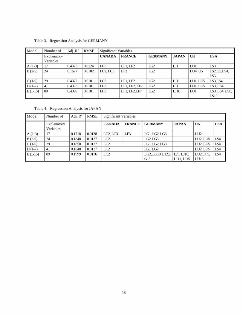
Tables 1-7 present the significant variables in all variants of the model for all investigated

countries. It is interesting to note that the Canadian stock exchange index influences all stocks in the

majority of countries and models except for the French index in models C and D. Except in model A,

France does not influence the Japanese financial market. France does not have auto-correlation except

for the seventh daily lag in models D and E. Except for Germany and the World, Japanese daily stock

returns are significant after 7 or even more days for the majority of models and countries. Germany

does not influence Canada, except for model B, but it strongly influences Japan.

9

Model E describes all explanatory variables the best since adjusted R2 is the highest and RMSE

is the smallest for this variant of the regression model. Though for other models, except for model B,

fitness statistics are similar. The lowest determination coefficients are found for Japan and World while

the percentage errors are the highest for Japan and Germany.

Based on the data presented in Tables 1 - 7 it can be ascertained that only some variables,

usually the same for all variants of the model, are significant and R2 does not essentially increase due to

the increase of the number of explanatory variables. In such situations, it is assumed that reducing (in

model E) the number of the explanatory variables to the ones that are significant will not essentially

affect the fitness statistics. Table 8 presents the comparison of the parameter estimates, t-statistics,

and RMSE for two linear models describing rates of daily stock returns for World. These models

contain, on one hand, all 89 variables and, on the other hand, the reduced number of explanatory

variables, i.e., only variables which are significant in the general model.

5.2 Empirical Results Based On Neural Network Models

Application of the artificial neural networks, constructed on the basis of model E, for further

analysis is the second stage of this investigation. Since it is impossible to introduce all 89 variables into

ANN experiments, the input layer contains only the significant, according to the regression analysis,

variables. Thus, the set of input variables is different for each country. Two types of ANN models are

constructed:

1. The simple neuron (1) with linear activation function GLRM,

(8) ly b b ly LLL

010 0 01

0

( ) ( )= +∈∑

β

+ b ly LLL

1 1

1∈∑

β

( ) + ... + b ly LLL

5 5

5∈∑

β

( )

where,

β β β0 1 5, , . . . , - are the sets of L indices defining significant variables,

b10 - the intercept (bias),

b Lj - are parameter estimates (j = 0, 1, ..., 5; L = 1, 2, ..., 15).

10

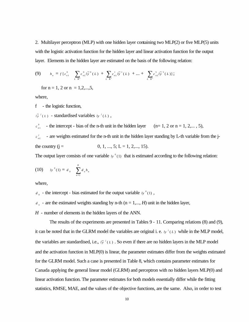
2. Multilayer perceptron (MLP) with one hidden layer containing two MLP(2) or five MLP(5) units

with the logistic activation function for the hidden layer and linear activation function for the output

layer. Elements in the hidden layer are estimated on the basis of the following relation:

(9) h f c c l y Ln n n LL

= +∈∑[ ~ ( )1

0 0 0

0β

+ c ly Ln LL

1 1

1∈∑

β

~ ( ) + ... + c l y Ln LL

5 5

5∈∑

β

~ ( )] ;

for n = 1, 2 or n = 1,2,...,5,

where,

f - the logistic function,

l y Lj~ ( ) - standardised variables ly Lj ( ) ,

c n 10 - the intercept - bias of the n-th unit in the hidden layer (n= 1, 2 or n = 1, 2,... , 5),

c n Lj - are weights estimated for the n-th unit in the hidden layer standing by L-th variable from the j-

the country (j = 0, 1, ..., 5; L = 1, 2,..., 15).

The output layer consists of one variable ly 0 1( ) that is estimated according to the following relation:

(10) ly 0 1( ) = d d hnn

H

n0

1

+=∑

where,

d 0 - the intercept - bias estimated for the output variable ly 0 1( ) ,

d n - are the estimated weights standing by n-th (n = 1,..., H) unit in the hidden layer,

H - number of elements in the hidden layers of the ANN.

The results of the experiments are presented in Tables 9 - 11. Comparing relations (8) and (9),

it can be noted that in the GLRM model the variables are original i. e. ly Lj ( ) while in the MLP model,

the variables are standardised, i.e., l y Lj~ ( ) . So even if there are no hidden layers in the MLP model

and the activation function in MLP(0) is linear, the parameter estimates differ from the weights estimated

for the GLRM model. Such a case is presented in Table 8, which contains parameter estimates for

Canada applying the general linear model (GLRM) and perceptron with no hidden layers MLP(0) and

linear activation function. The parameter estimates for both models essentially differ while the fitting

statistics, RMSE, MAE, and the values of the objective functions, are the same. Also, in order to test

11

the sensitivity of the results, the period of the analysis is broken into different sub-periods. The results

for the United States are detailed in Appendix 1.

Tables 10 and 11 present the RMSE, MAE, and objective function statistics based on the

regression model, GLRM, MLP(2) and MLP(5).

Comparing RMSE estimates for the regression model containing 89 explanatory variables to the one

obtained for the GLRM model that contains significant variables only, it can be noticed that both models

are not significantly different from one another. The variations of RMSE for the GLRM and MLP

models are visible, though the difference among these models are more visible if we compare MAE and

values of the objective function criteria. Thus, the multilayer perceptron models with logistic activation

functions predict daily stock returns better than traditional OLS and GLRM models.

Furthermore, the multilayer perceptron with five units in the hidden layer better predicts the

stock indices for USA, France, Germany, UK and World than the neural network with two hidden

elements. This can be seen by examining all the fitness statistics for MLP(5), which are smaller than

those for MLP(2). Only MAE estimated for Canada and Japan in the MLP(5) is higher than for

MLP(2).

6. Conclusion

This paper applies ordinary least squares, general linear regression, and artificial neural

network models, multi-layer perceptron models, in order to investigate the dynamic interrelations of

major world stock markets. The Multi-Layer Perceptron models contain one hidden layer with two

and five processing elements and logistic activation. The data base consists of daily stock market

indices of the following countries: Canada, France, Germany, Japan, United Kingdom, the United

States, and the world excluding US. Based on the criteria of Root Mean Square Error, Maximum

Absolute Error, and the value of the objective function, the models are compared to eachother.

It is found that the neural network consisting of multilayer perceptron models with logistic

activation functions predict daily stock returns better than the traditional ordinary least squares and

general linear regression models. Furthermore, it is found that a multilayer perceptron with five units in

12

the hidden layer better predicts the stock indices for USA, France, Germany, UK and World than a

neural network with two hidden elements.

This paper lends support in favour of using neural network models in the study of finance, in

particular in the area of international transmission of returns in stock markets. The returns for applying

neural network models are positive. Consequently, the results of this paper favor the increased use of

these model by practicioners like Goldman Sachs, Morgan Stanley, and Fidelity Investments as

alternative or additional tools for financial analysis.

Notes

1. Experimental Alpha releases SAS 6.09 and 6.11, 6.12 and 6.13 Systems are used. 2. For example, in the US model D* the parameter estimate for the trend variable equals 0.0000

and t-statistic equals 0.2587. The insignificance of the T variable (for the USA) can be noticed in Table 2.

References Altman, E.I., G. Marco, and F. Varetto, “Corporate Distress Diagnosis: Comparisons Using Linear Discriminant Analysis and Neural Networks (The Italian Experience),” Journal of Banking and Finance, 18(3), May 1994, 505-29. Baets, W., Venugopal V. "Neural Networks and Their Applications in Marketing Management." Cutting Edge, 16-20, 1994. Bierens, H.J., “Comment On Artificial Neural Networks: An Econometric Perspective,” Econometric Reviews, 13(1), 1994. Caporaletti, L.E., R.E. Dorsey, J.D. Johnson, and W.A. Powell, “A Decision Support System for In-Sample Simultaneous Equation System Forecasting Using Artificial Neural Systems,” Decision Support Systems, 11, 1994, 481-495. Cheh, John J; Weinberg, Randy S; Yook, Ken C. "An Application of an Artificial Neural Network Investment System to Predict Takeover Targets", Journal of Applied Business Research, Vol. 15 (4). p 33-45. Fall 1999.

13

Cogger, Kenneth O; Koch, Paul D; Lander, Diane M. "A Neural Network Approach to Forecasting Volatile International Equity Markets, Advances in financial economics. Volume 3. Hirschey, Mark Marr, M. Wayne, eds., Greenwich, Conn. and London: JAI Press. p 117-57, 1997. Connor, J.T., R.D. Martin, and L.E. Atlas, “Recurrent Neural Networks and Robust Time Series Prediction,” IEEE Transaction of Neural Networks, 2(2), 1994, 240-254. Consten, H. and C. May, “Artificial Neural Networks for Supporting Production Planning and Control,” Technovation, Feb. 1996. Cooper, John C B. "Artificial Neural Networks versus Multivariate Statistics: An Application from Economics", Journal of Applied Statistics, Vol. 26 (8). p 909-21, December 1999. Eun Cheol S. and Sangdal Shim, "International Transmission of Stock Market Movements," Journal of Financial and Quantitative Analysis, Vol. 24, No. 2, June 1989, 241-256. Friedman, J. and Y. Shachmurove, “Dynamic Linkages Among European Stock Markets” in Advances in International Stock Market Relationships and Interactions, J. Doukas ed., Greenwood Publishing, 1996, forthcoming. Friedman, J. and Y. Shachmurove, “Co-Movements of Major European Community Stock Markets: A Vector Autoregression Analysis,” Global Finance Journal, 7(2), forthcoming 1997. Garcia, Rene; Gencay, Ramazan. "Pricing and Hedging Derivative Securities with Neural Networks and a Homogeneity Hint", Journal of Econometrics, Vol. 94 (1-2). p 93-115. Jan.-Feb. 2000. Granger, C.W.J., “Developments in the Nonlinear Analysis of Economic Series,” Scandinavian Journal of Economics, 93(2), 1991, 263-76. Grudnitski, G. and L. Osburn, “Forecasting S&P and Gold Futures Prices: An Application of Neural Networks,” Journal of Futures Markets, 13(6), September 1993, 631-43. Hamm, Lonnie; Brorsen, B Wade. "Trading Futures Markets Based on Signals from a Neural Network", Applied Economics Letters, Vol. 7 (2). p 137-40, February 2000. Hawley, D.D., J.D. Johnson, and D. Raina, “Artificial Neural Systems: A New Tool for Financial Decision-Making,” Financial Analysis Journal, Nov/Dec, 1990, 63-72. Hertz, J., A. Krogh, R.G. Palmer, Introduction to the Theory of Neural Computation, Redwood City: Addison Wesley, 1991.

14

Hinton, G.E., “How Neural Networks Learn from Experience,” Scientific American, 267, September 1992, 144-151. Hoptroff, R.G., “The Principles and Practice of Time Series Forecasting and Business Modelling Using Neural Nets,” Neural Computing and Applications, 1, 1993, 59-66. Hu, Michael Y; Tsoukalas, Christos. "Combining Conditional Volatility Forecasts Using Neural Networks: An Application to the EMS Exchange Rates", Journal of International Financial Markets, Institutions & Money, Vol. 9 (4). p 407-22. August 1999. Kaastra, I. and M.S. Boyd, ”Forecasting Futures Trading Volume Using Neural Networks,” Journal of Futures Markets, 15(8), December 1995, 953-70. Kuan, C.M. and H. White, “Artificial Neural Networks: An Econometric Perspective,” Econometric Views, 13(1), 1994, 1-91. Kuo, C. and Reitsch, A., 1995-96, "Neural Networks vs. Conventional Methods of Forecasting." The Journal of Business Forecasting, Winter 1995-96, 17-22. Lewbel, A., “Comment On Artificial Neural Networks: An Econometric Perspective,” Econometric Reviews, 13(1), 1994. Li, E.Y., “Artificial Neural Networks and Their Business Applications,” Information and Management, Nov. 1994. Moshiri, Saeed; Cameron, Norman E; Scuse, David. "Static, Dynamic, and Hybrid Neural Networks in Forecasting Inflation", Computational Economics, Vol. 14 (3). p 219-35. December 1999. Ormerod, P., J.C. Taylor, and T. Walker, “Neural Networks in Economics,” Taylor, M.P., ed. Money and Financial Markets, Cambridge, Mass. and Oxford: Blackwell, 1991, 341-53. Ripley, B.D., “Statistical Aspects of Neural Networks,” in Barndorff-Nielsen, O.E., J.L. Jensen, and W.S. Kendall eds., Networks and Chaos: Statistical and Probabilistic Aspects, London: Chapman Hall, 1993. Rummelhart, D. and J. McClellend, Parallel Distributed Processing, MIT Press: Cambridge, 1986. Sarle, W.S., “Neural Networks and Statistical Models,” Proceedings of the Nineteenth Annula SAS Users Group International Conference, Cary, NC: SAS Institute, April 1994, 1538-1550. Shachmurove, Y., “Dynamic Linkages Among Latin American and Other Major World Stcok Markets,” in Research in International Business and Finance: Financial Issues in Emerging Capital

15

Markets, John Doukas and Larry Lang eds., JAI Press Inc., forthcoming 1996. Shtub, Avraham; Versano, Ronen. "Estimating the Cost of Steel Pipe Bending, a Comparison between Neural Networks and Regression Analysis", International Journal of Production Economics, Vol. 62 (3). p 201-07, September 1999. Sohl, Jeffrey E., Venkatachalam A.R. "A Neural Network Approach to Forecasting Model Selection", Information & Management, 29, 297-303, 1995. Terna, Pietro. "Neural Network for Economic and Financial Modelling: Summing Up Ideas Emerging from Agent Based Simulation and Introducing an Artificial Laboratory", Cognitive Economics, Viale, Riccardo, ed., LaSCoMES Series, vol. 1. Torino: La Rosa. p 271-309. 1997. Tours, S., L. Rabelo, and T. Velasco, “Artificial Neural Networks for Flexible Manufacturing System Scheduling,” Computer and Industrial Engineering, September 1993. Trippi, R.R.; D. DeSieno, “Trading Equity Index Futures with a Neural Network,” Journal of Portfolio Management, 19(1), Fall 1992, 27-33. Wasserman, P.D., Neural Computing: Theory and Practice, Van Nostrand Reinhold: New York, 1989. Weiss, S,M. and C.A. Kulikowski, Computer Systems that Learn, San Mateo: Morgan Kaufmann, 1991. White, H., “Economic Prediction Using Neural Networks: The Case of IBM Daily Stock Returns,” Proceedings of the IEEE International Conference of Neural Networks, July 1988, II451-II458. White, H., Artificial Neural Networks: Approximation and Learning Theory, Oxford: Blackwell, 1992. White, H., “Option Pricing in Modern Finance Theory and the Relevance of Artificial Neural Networks,” Discussion Paper, Econometrics Workshop, March 1996. Witkowska, D., “Neural Networks as a Forecasting Instrument for the Polish Stock Exchange,” International Advances in Economic Research, 1(3), August 1995, 232-241. Yoon, Y. and G. Swales, “Predicting Stock Price Performance,” Proceeding of the 24th Hawaii International Conference on System Sciences, 4, 156-162, 1997.

17

Table 1. Regression Analysis for CANADA

Model Number of Adj. R2 RMSE Significant Variables Explanatory

Variables CANADA FRANCE GERMANY JAPAN UK USA

A (1-3) 17 0.4545 0.0063 LC3 LF2 LU2 LS1, LS2, LS3 B (2-5) 24 0.1162 0.008 LC3, LC5 LG2 LS2, LS3,

LS4, LS5 C(1-5) 29 0.4593 0.0062 LC5 LF2 LU2, LU5 LS1, LS2,

LS3, LS5 D(1-7) 41 0.4601 0.0062 LC5 LF2, LF6 LU2 LS1, LS2,

LS3, LS4, LS5

E(1-15) 89 0.4975 0.006 LC2, LC5, LC14

LF2,LF6, LF8, LF10

LJ8, LJ9, LJ12,LJ13 LJ14,LJ15

LU2, LU8, LU10

LS1, LS2, LS3,LS4, LS5, LS8, LS10, LS14

Table 2. Regression Analysis for FRANCE



A(1-3) 17 0.4943 0.0086 LC3 LG1, LG2 LJ3 LU1 LS2, LS3 B (2-5) 24 0.1501 0.0111 LC2 LU5 LS2, LS3 C (1-5) 29 0.4958 0.0086 LG1, LG2 LU1 LS2, LS3 D (1-7) 41 0.4989 0.0085 LF7 LG1, LG2 LU1 LU7 LS2, LS3 E (1-15) 89 0.5138 0.0084 LC3, LC9,

LC11 LF7 LG1, LG2,

LG8 LJ11, LJ14 LU1, LU7 LS2, LS3,

LS9, LS10

18

Table 3. Regression Analysis for GERMANY



A (1-3) 17 0.4323 0.0124 LC3 LF1, LF2 LG2 LJ1 LU1 LS3 B (2-5) 24 0.1627 0.0102 LC2, LC3 LF2 LG2 LU4, U5 LS2, S3,LS4,

LS5 C (1-5) 29 0.4372 0.0101 LC3 LF1, LF2 LG2 LJ1 LU1, LU5 LS3,LS4 D (1-7) 41 0.4393 0.0101 LC3 LF1, LF2, LF7 LG2 LJ1 LU1, LU5 LS3, LS4 E (1-15) 89 0.4399 0.0101 LC3 LF1, LF2,LF7 LG2 LJ10 LU1 LS3, LS4, LS8,

LS10

Table 4. Regression Analysis for JAPAN

Model Number of Adj. R2 RMSE Significant Variables

Explanatory Variables

CANADA FRANCE GERMANY JAPAN UK USA

A (1-3) 17 0.1718 0.0138 LC2, LC3 LF3 LG1, LG2, LG3 LU2 B (2-5) 24 0.1848 0.0137 LC2 LG2, LG3 LU2, LU5 LS4 C (1-5) 29 0.1858 0.0137 LC2 LG1, LG2, LG3 LU2, LU5 LS4 D (1-7) 41 0.1848 0.0137 LC2 LG1, LG2 LU2, LU5 LS4 E (1-15) 89 0.1999 0.0136 LC2 LG2, LG10, L12,L

G15 LJ9, LJ10, LJ11, LJ15

LU2,LU5, LU13

LS4

19

Table 5. Regression Analysis for UK



A (1-3) 17 0.4171 0.0087 LC2, LC3 LF1, LF2, LF3

LG1 LJ2 LU2 LS2, LS3

B (2-5) 24 0.2354 0.0100 LC2, LC3 LF2, LF3 LU2 LS2, LS3, LS4

C (1-5) 29 0.4204 0.0087 LC2, LC3 LF1, LF2, LF3

LG1 LU2 LS2, LS3, LS4

D (1-7) 41 0.4239 0.0087 LC2, LC3 LF1, LF2, LF3

LG1 LU2, LU5 LS2, LS3, LS4

E (1-15) 89 0.4324 0.0086 LC2, LC3 LF1, LF2, LF3

LG1 LJ7, LJ8, LJ15

LU2, LU9 LS2, LS3, LS4,LS6

Table 6. Regression Analysis for USA



A (1-3) 17 0.4124 0.0079 LC1, LC2 LF2 LG3 LS2 B (2-5) 24 0.0288 0.0102 LC2, LC3,

LC4, LC5 LF2 LG2 LS2, LS3,

LS5 C (1-5) 29 0.4136 0.0079 LC1, LC2 LF2 LG5 LS2 D (1-7) 41 0.4140 0.0079 LC1, LC2,

LC6 LF2 LU7 LS2

D*(1-7) 42 0.4145 0.0079 LC1, LC2, LC6

LF2 LU7 LS2

E (1-15) 89 0.4482 0.0077 LC1, LC2 LF2 LG14 LJ8, LJ9, LJ12, LJ13, LJ14

LU7, LU8

20

Table 7. Regression Analysis for WORLD


Varariables CANADA FRANCE GERMANY JAPAN UK WORLD

A (1-3) 17 0.1886 0.0091 LC1, LC2, C3 LF1, LF3 LG2 LJ1, LJ3 LW3 B (2-5) 24 0.0490 0.0099 LC2, LC3 LF1 LJ4 --- C (1-5) 29 0.1883 0.0091 LC1, LC2, C3 LF1, LF3 LG2 LJ1, LJ4 LW3 D (1-7) 41 0.1896 0.0091 LC1, LC2, C3 LF1, LF3 LG2 LJ1 LW3 E (1-15) 89 0.2081 0.0090 LC1, LC2, C3 LF1, LF3 LG2, LG7 LJ1, LJ10, LJ12,

LJ13, LJ14 LU14 LW3

Table 8. Comparison of Parameter Estimates for Canada Obtained for the Model Defined as General Linear Model and

the Multilayer Perceptron with No Hidden Layers with Linear Activiation Function.

Name of Parameter Estimates Name of Parameter Estimates Variable GLRM MLP (0) Variable GLRM MLP (0) Intercerpt -0.0072 0.0092 LJ8 -2.9943 -0.0456 LC2 6.4658 0.0548 LJ9 2.2191 0.0338 LC5 12.7007 0.1077 LJ12 3.5066 0.0534 LC14 -7.0775 -0.0601 LJ13 -5.1498 -0.0784 LS1 50.4093 0.5233 LJ14 6.1927 0.0943 LS2 14.3979 0.1495 LJ15 -2.7559 -0.0420 LS3 -2.6777 -0.0278 LU1 -0.4169 -0.0048 LS4 5.4651 0.0567 LU2 3.6658 0.0420 LS5 -5.7831 -0.0600 LU3 1.1134 -0.0128 LS8 3.2992 0.0342 LU4 2.2438 0.0257 LS10 -3.5250 -0.0366 LU5 -0.6311 -0.0722 LS14 4.7867 0.0497 LU8 -3.7207 -0.0426 LF2 -4.3135 -0.0520 LU10 3.9289 0.0450 LF6 1.9017 0.0229 RMSE 0.6014 0.6014 LF8 4.6419 0.0560 MAE 5.9170 5.9170 LF10 -2.2179 0.0268 Objective func. 3.6510 3.6510 In Table 8 all parameters were multiplied by 100 since all parameters were very small.

21

Table 9. Comparison of the Regression Model (with 89 Explanatory Variables) to the General Linear Regression Model (GLRM) (with 14 Explanatory Variables) Regression Model GLRM Model

Variable Estimates t-Statistic Estimates T-Statistic Intercept 0.0001 0.4485 0.0001 0.62 LC1 0.4090 16.0784 0.4220 17.45 LC2 0.1254 4.4554 0.1307 5.12 LC3 -0.0773 -2.7422 -0.0813 -3.05 LW3 0.1373 2.5867 0.0917 2.13 LF1 0.1060 4.4077 0.1054 5.97 LF2 0.0569 2.3007 0.0370 2.19 LG2 -0.0474 -2.2434 -0.0483 -2.53 LG7 0.0458 2.1643 0.0213 1.43 LJ1 -0.0796 -3.0085 -0.0582 -2.46 LJ10 -0.0651 -2.4413 -0.0027 -0.21 LJ12 -0.0652 -2.4233 -0.0144 -1.08 LJ13 0.1231 -4.6346 -0.0629 -4.48 LJ14 0.0528 3.4979 0.0516 3.85 LU14 -0.0539 -2.0314 0.0088 0.47 RMSE 0.0090 0.0091

22

Table 10. Comparison of Fitness Statistics for the Linear Regression and General Linear Regression Models Regression model ANN – GLRM Country Num. of

Estimated Parameters

R2 Adj. R2 RMSE Num. of Estimated Parameters

RMSE MAE Obj. f.

USA 90 0.4722 0.4482 0.0077 12 0.0077 0.1205 0.061 Canada 90 0.5194 0.4975 0.0060 25 0.0060 0.0593 0.037 France 90 0.5350 0.5138 0.0084 16 0.0084 0.0447 0.072 Germany 90 0.4642 0.4399 0.0101 12 0.0101 0.0762 0.103 U. K. 90 0.4570 0.4324 0.0086 16 0.0087 0.0717 0.072 Japan 90 0.2347 0.1999 0.0136 14 0.0137 0.1656 0.191 World 90 0.2425 0.2081 0.0090 15 0.0091 0.0656 0.083

Table 11. Comparison of Fitness Statistics for Multilayer Perceptron Models with Two and Five Elements in the Hidden Layer. ANN – MLP (2) ANN - MLP (5) Country Num. of

est. par. RMSE MAE Obj. f. Num. of

est. par. RMSE MAE Obj. f.

USA 27 0.0069 0.0419 0.0478 66 0.0066 0.0407 0.044 Canada 53 0.0055 0.0281 0.0307 131 0.0054 0.0287 0.028 France 35 0.0082 0.0390 0.0674 86 0.0080 0.0361 0.063 Germany 27 0.0100 0.0681 0.1020 66 0.0093 0.0505 0.085 U. K. 35 0.0083 0.0578 0.0698 86 0.0081 0.0517 0.065 Japan 31 0.0133 0.1626 0.1796 76 0.0131 0.1758 0.169 World 33 0.0087 0.0655 0.0762 81 0.0085 0.066 0.072

23

Appendix 1

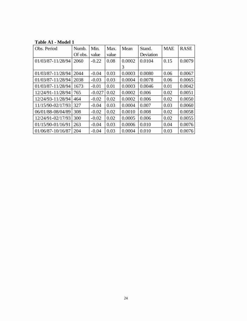
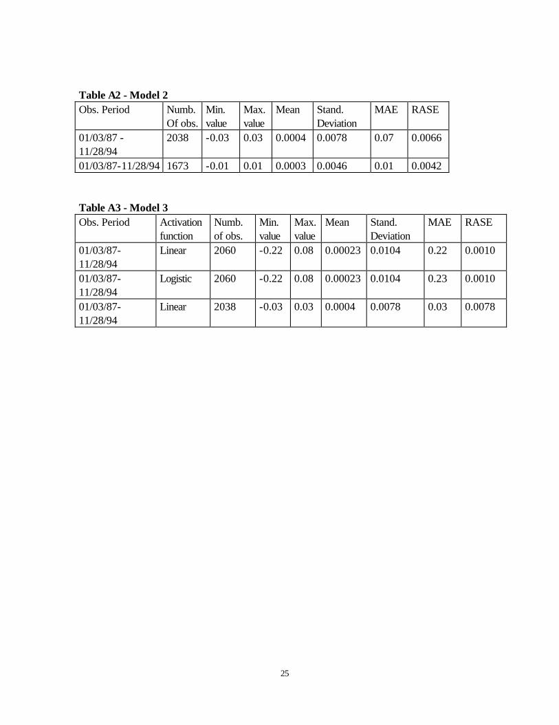
Based on plotting the data, a few sub-periods are considered. The three following models are tested for the sub-periods: Model 1. lusa(1)= f[lcan(1), lcan(2), lfra(1), lfra(2), lger(1), lger(2), ljap(1), ljap(2), luk(1), luk(2), In lusa(2), lusa(3)] where: f - linear, lusa(1)= ly Lj ( ) for the USA, L = 1 from relation (7) as follows: (7) ly Lj ( ) = log[ y Lj ( ) ] - log[ y Lj ( )− 1 ]; for j = 0, 1,...,6; L = 1, 2, 3 where: j - the index of each country (USA, Canada, France, Germany, UK or Japan) or “world” (i. e. world without USA), L - the lag index, y Lj ( ) - daily stock returns in j-th country lagged by L periods. Model 2 lusa(1)= f[lcan(1), lcan(2), lfra(1), lfra(2), lger(1), lger(2), ljap(1), ljap(2), luk(1), luk(2)] where f is linear activation. Model 3 lusa(1)= f[lcan(2), lcan(3), lfra(2), lfra(3), lger(2), lger(3), ljap(2), ljap(3), luk(2), luk(3), lusa(2), lusa(3)] where f is linear or logistic activation. The statistic MASE is not presented in Tables A1-A3 as it depends on the number of observations, which are different for each of the experiments. The Tables show that the errors are different for different periods. The highest RMSE is obtained for relatively short periods of time. Thus, although the errors are changed in different periods, the results are consistent with the ones reported in the paper. Tables A1-A3 correspond to Models 1-3, respectively, as follows:

24

Table A1 - Model 1 Obs. Period Numb.

Of obs. Min. value

Max. value

Mean Stand. Deviation

MAE RASE

01/03/87-11/28/94 2060 -0.22 0.08 0.00023

0.0104 0.15 0.0079

01/03/87-11/28/94 2044 -0.04 0.03 0.0003 0.0080 0.06 0.0067 01/03/87-11/28/94 2038 -0.03 0.03 0.0004 0.0078 0.06 0.0065 01/03/87-11/28/94 1673 -0.01 0.01 0.0003 0.0046 0.01 0.0042 12/24/91-11/28/94 765 -0.027 0.02 0.0002 0.006 0.02 0.0051 12/24/93-11/28/94 464 -0.02 0.02 0.0002 0.006 0.02 0.0050 11/15/90-02/17/93 327 -0.04 0.03 0.0004 0.007 0.03 0.0060 06/01/88-08/04/89 308 -0.02 0.02 0.0010 0.008 0.02 0.0058 12/24/91-02/17/93 300 -0.02 0.02 0.0005 0.006 0.02 0.0055 01/15/90-01/16/91 263 -0.04 0.03 0.0006 0.010 0.04 0.0076 01/06/87-10/16/87 204 -0.04 0.03 0.0004 0.010 0.03 0.0076

25

Table A2 - Model 2 Obs. Period Numb.

Of obs. Min. value

Max. value


MAE RASE

01/03/87 -11/28/94

2038 -0.03 0.03 0.0004 0.0078 0.07 0.0066

01/03/87-11/28/94 1673 -0.01 0.01 0.0003 0.0046 0.01 0.0042 Table A3 - Model 3 Obs. Period Activation

function Numb. of obs.

Min. value

Max. value


MAE RASE

01/03/87-11/28/94

Linear 2060 -0.22 0.08 0.00023 0.0104 0.22 0.0010

01/03/87-11/28/94

Logistic 2060 -0.22 0.08 0.00023 0.0104 0.23 0.0010

01/03/87-11/28/94

Linear 2038 -0.03 0.03 0.0004 0.0078 0.03 0.0078

Utilizing Artificial Neural Network Model to Predict Stock Markets

Documents

Transcript of Utilizing Artificial Neural Network Model to Predict Stock Markets