
Utilizing GPUs on Cluster Computers - CiteSeerX
116
U TILIZING GPU S ON C LUSTER C OMPUTERS P ROJECT WORK IN TDT4715 A LGORITHM CONSTRUCTION AND VISUALIZATION , DEPTH STUDY FALL 2006 L EIF C HRISTIAN L ARSEN MAIN SUPERVISOR :D R .A NNE C ATHRINE E LSTER C O - SUPERVISOR :TORE F EVANG ,S CHLUMBERGER LTD . Norwegian University of Science and Technology Faculty of Information Technology, Mathematics and Electrical Engineering Department of Computer and Information Science
-
Upload
khangminh22 -
Category
Documents
-
view
3 -
download
0
Transcript of Utilizing GPUs on Cluster Computers - CiteSeerX

UTILIZING GPUS ON CLUSTER COMPUTERS
PROJECT WORK IN TDT4715 ALGORITHM
CONSTRUCTION AND VISUALIZATION, DEPTH STUDY
FALL 2006
LEIF CHRISTIAN LARSEN
MAIN SUPERVISOR: DR. ANNE CATHRINE ELSTER
CO-SUPERVISOR: TORE FEVANG, SCHLUMBERGER LTD.
Norwegian University of Science and TechnologyFaculty of Information Technology, Mathematics and Electrical EngineeringDepartment of Computer and Information Science

ii

Abstract
iii

iv

Preface
This is the report for the project work done in the depth study course TDT4715 Algorithmconstruction, visualization and computational science at the Department of Computer andInformation Science (IDI) at the Norwegian University of Science and Technology (NTNU),Norway. The work was done over a period of four months, and was assigned by Schlum-berger Limited. The main supervisor for the project was Associate Professor Dr. AnneCathrine Elster of IDI-NTNU. The project was co-supervized by Tore Fevang of Schlum-berger Limited, Trondheim.
I am very grateful for the excellent support I have received from my supervisors during theproject. I would like to thank Dr. Elster for her excellent support, for hooking me up withSchlumberger and this project assignment, and for always taking the time to talk with meeven when she was busy preparing a 50 MNOK supercomputer.
A very special thanks goes to my co-supervisor Tore Fevang of Schlumberger Trondheim,who has been supportive and helpful at a level which far exceeded everything I could havehoped for. Mr. Fevang has been very helpful throughout the entire project, always had timefor questions, and always tried very hard answering all my questions.
I would also like to thank Schlumberger Limited and the manager at Schlumberger Trond-heim, Wolfgang Hochweller, for providing me with a great place to work and giving meaccess to very high-end hardware during the project. I would like to emphasize that with-out Schlumberger’s very significant support, the quality of this project work would be significantlydegraded.
I also want to thank everyone else at Schlumberger Trondheim for providing an excellentatmosphere to work in (even though I unfortunately did not manage to beat anyone at thetable football game).
Trondheim, December 21st, 2006
______________________Leif Christian Larsen
v

vi
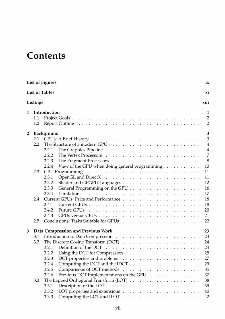
Contents
List of Figures ix
List of Tables xi
Listings xiii
1 Introduction 11.1 Project Goals . . . . . . . . . . . . . . . . . . . . . . . . . . . . . . . . . . . . . . 21.2 Report Outline . . . . . . . . . . . . . . . . . . . . . . . . . . . . . . . . . . . . . 2
2 Background 32.1 GPUs: A Brief History . . . . . . . . . . . . . . . . . . . . . . . . . . . . . . . . 32.2 The Structure of a modern GPU . . . . . . . . . . . . . . . . . . . . . . . . . . . 4
2.2.1 The Graphics Pipeline . . . . . . . . . . . . . . . . . . . . . . . . . . . . 42.2.2 The Vertex Processors . . . . . . . . . . . . . . . . . . . . . . . . . . . . 72.2.3 The Fragment Processors . . . . . . . . . . . . . . . . . . . . . . . . . . 82.2.4 View of the GPU when doing general programming . . . . . . . . . . . 10
2.3 GPU Programming . . . . . . . . . . . . . . . . . . . . . . . . . . . . . . . . . . 112.3.1 OpenGL and DirectX . . . . . . . . . . . . . . . . . . . . . . . . . . . . . 112.3.2 Shader and GPGPU Languages . . . . . . . . . . . . . . . . . . . . . . . 122.3.3 General Programming on the GPU . . . . . . . . . . . . . . . . . . . . . 162.3.4 Limitations . . . . . . . . . . . . . . . . . . . . . . . . . . . . . . . . . . 17
2.4 Current GPUs: Price and Performance . . . . . . . . . . . . . . . . . . . . . . . 182.4.1 Current GPUs . . . . . . . . . . . . . . . . . . . . . . . . . . . . . . . . . 182.4.2 Future GPUs . . . . . . . . . . . . . . . . . . . . . . . . . . . . . . . . . 202.4.3 GPUs versus CPUs . . . . . . . . . . . . . . . . . . . . . . . . . . . . . . 21
2.5 Conclusions: Tasks Suitable for GPUs . . . . . . . . . . . . . . . . . . . . . . . 22
3 Data Compression and Previous Work 233.1 Introduction to Data Compression . . . . . . . . . . . . . . . . . . . . . . . . . 233.2 The Discrete Cosine Transform (DCT) . . . . . . . . . . . . . . . . . . . . . . . 24
3.2.1 Definition of the DCT . . . . . . . . . . . . . . . . . . . . . . . . . . . . 243.2.2 Using the DCT for Compression . . . . . . . . . . . . . . . . . . . . . . 253.2.3 DCT properties and problems . . . . . . . . . . . . . . . . . . . . . . . . 273.2.4 Computing the DCT and the IDCT . . . . . . . . . . . . . . . . . . . . . 293.2.5 Comparisons of DCT methods . . . . . . . . . . . . . . . . . . . . . . . 353.2.6 Previous DCT Implementations on the GPU . . . . . . . . . . . . . . . 37
3.3 The Lapped Orthogonal Transform (LOT) . . . . . . . . . . . . . . . . . . . . . 383.3.1 Description of the LOT . . . . . . . . . . . . . . . . . . . . . . . . . . . . 393.3.2 LOT properties and extensions . . . . . . . . . . . . . . . . . . . . . . . 403.3.3 Computing the LOT and ILOT . . . . . . . . . . . . . . . . . . . . . . . 42
vii
CONTENTS viii
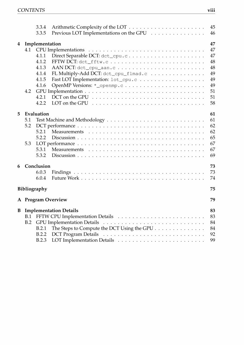
3.3.4 Arithmetic Complexity of the LOT . . . . . . . . . . . . . . . . . . . . . 453.3.5 Previous LOT Implementations on the GPU . . . . . . . . . . . . . . . 46
4 Implementation 474.1 CPU Implementations . . . . . . . . . . . . . . . . . . . . . . . . . . . . . . . . 47
4.1.1 Direct Separable DCT: dct_cpu.c . . . . . . . . . . . . . . . . . . . . . 474.1.2 FFTW DCT: dct_fftw.c . . . . . . . . . . . . . . . . . . . . . . . . . . 484.1.3 AAN DCT: dct_cpu_aan.c . . . . . . . . . . . . . . . . . . . . . . . . 484.1.4 FL Multiply-Add DCT: dct_cpu_flmad.c . . . . . . . . . . . . . . . 494.1.5 Fast LOT Implementation: lot_cpu.c . . . . . . . . . . . . . . . . . . 494.1.6 OpenMP Versions: *_openmp.c . . . . . . . . . . . . . . . . . . . . . . 49
4.2 GPU Implementation . . . . . . . . . . . . . . . . . . . . . . . . . . . . . . . . . 514.2.1 DCT on the GPU . . . . . . . . . . . . . . . . . . . . . . . . . . . . . . . 514.2.2 LOT on the GPU . . . . . . . . . . . . . . . . . . . . . . . . . . . . . . . 58
5 Evaluation 615.1 Test Machine and Methodology . . . . . . . . . . . . . . . . . . . . . . . . . . . 615.2 DCT performance . . . . . . . . . . . . . . . . . . . . . . . . . . . . . . . . . . . 62
5.2.1 Measurements . . . . . . . . . . . . . . . . . . . . . . . . . . . . . . . . 625.2.2 Discussion . . . . . . . . . . . . . . . . . . . . . . . . . . . . . . . . . . . 65
5.3 LOT performance . . . . . . . . . . . . . . . . . . . . . . . . . . . . . . . . . . . 675.3.1 Measurements . . . . . . . . . . . . . . . . . . . . . . . . . . . . . . . . 675.3.2 Discussion . . . . . . . . . . . . . . . . . . . . . . . . . . . . . . . . . . . 69
6 Conclusion 736.0.3 Findings . . . . . . . . . . . . . . . . . . . . . . . . . . . . . . . . . . . . 736.0.4 Future Work . . . . . . . . . . . . . . . . . . . . . . . . . . . . . . . . . . 74
Bibliography 75
A Program Overview 79
B Implementation Details 83B.1 FFTW CPU Implementation Details . . . . . . . . . . . . . . . . . . . . . . . . 83B.2 GPU Implementation Details . . . . . . . . . . . . . . . . . . . . . . . . . . . . 84
B.2.1 The Steps to Compute the DCT Using the GPU . . . . . . . . . . . . . . 84B.2.2 DCT Program Details . . . . . . . . . . . . . . . . . . . . . . . . . . . . 92B.2.3 LOT Implementation Details . . . . . . . . . . . . . . . . . . . . . . . . 99

List of Figures
2.1 Internal GPU structure . . . . . . . . . . . . . . . . . . . . . . . . . . . . . . . . 52.2 Internal vertex processor structure . . . . . . . . . . . . . . . . . . . . . . . . . 82.3 Internal fragment processor structure . . . . . . . . . . . . . . . . . . . . . . . 92.4 The fragment processor’s FP shader units . . . . . . . . . . . . . . . . . . . . . 92.5 The GPU viewed from the outside . . . . . . . . . . . . . . . . . . . . . . . . . 102.6 Data flow from a software application to the GPU . . . . . . . . . . . . . . . . 122.7 Passing shader programs to the GPU . . . . . . . . . . . . . . . . . . . . . . . . 14
3.1 Data compression and decompression using the DCT . . . . . . . . . . . . . . 253.2 Quantization with the DCT . . . . . . . . . . . . . . . . . . . . . . . . . . . . . 263.3 Original JPEG image, using almost no compression . . . . . . . . . . . . . . . 283.4 Image compressed with JPEG, quality 85 . . . . . . . . . . . . . . . . . . . . . 283.5 Image compressed with JPEG, quality 50 . . . . . . . . . . . . . . . . . . . . . 283.6 Image compressed with JPEG, quality 5 . . . . . . . . . . . . . . . . . . . . . . 283.7 Flowgraph for the AAN DCT algorithm . . . . . . . . . . . . . . . . . . . . . . 323.8 Flowgraph for the Feig-Linzer multiply-add DCT algorithm . . . . . . . . . . 343.9 Illustration of the DCT and LOT basis functions at block boundaries . . . . . 413.10 Flowgraph for the fast type-I LOT algorithm with blocksize 8 . . . . . . . . . 433.11 Flowgraph for the Z̃-matrix . . . . . . . . . . . . . . . . . . . . . . . . . . . . . 443.12 Flowgraph for the Y(θi)-matrix . . . . . . . . . . . . . . . . . . . . . . . . . . . 443.13 Computing the LOT for a data set . . . . . . . . . . . . . . . . . . . . . . . . . . 45
4.1 LOT boundary extension implementation . . . . . . . . . . . . . . . . . . . . . 504.2 OpenMP parallelization schemes when computing 2D transforms . . . . . . . 514.3 Computing transforms on the GPU . . . . . . . . . . . . . . . . . . . . . . . . . 524.4 Computing the DCT on the GPU . . . . . . . . . . . . . . . . . . . . . . . . . . 534.5 Row mapping between single- and multi-channel textures . . . . . . . . . . . 554.6 Column mapping between single- and multi-channel textures . . . . . . . . . 564.7 Fast LOT on the GPU . . . . . . . . . . . . . . . . . . . . . . . . . . . . . . . . . 58
5.1 32-bit DCT/IDCT performance . . . . . . . . . . . . . . . . . . . . . . . . . . . 635.2 32-bit DCT/IDCT CPU time usage . . . . . . . . . . . . . . . . . . . . . . . . . 655.3 Fast LOT/ILOT performance . . . . . . . . . . . . . . . . . . . . . . . . . . . . 685.4 32-bit 8× 8 LOT/ILOT CPU time usage for large data set sizes (user + system) 70
B.1 Using textures for computation . . . . . . . . . . . . . . . . . . . . . . . . . . . 88
ix

LIST OF FIGURES x
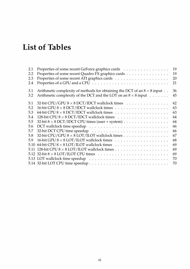
List of Tables
2.1 Properties of some recent GeForce graphics cards . . . . . . . . . . . . . . . . 192.2 Properties of some recent Quadro FX graphics cards . . . . . . . . . . . . . . . 192.3 Properties of some recent ATI graphics cards . . . . . . . . . . . . . . . . . . . 202.4 Properties of a GPU and a CPU . . . . . . . . . . . . . . . . . . . . . . . . . . . 21
3.1 Arithmetic complexity of methods for obtaining the DCT of an 8× 8 input . . 363.2 Arithmetic complexity of the DCT and the LOT on an 8× 8 input . . . . . . . 45
5.1 32-bit CPU/GPU 8× 8 DCT/IDCT wallclock times . . . . . . . . . . . . . . . 625.2 16-bit GPU 8× 8 DCT/IDCT wallclock times . . . . . . . . . . . . . . . . . . . 635.3 64-bit CPU 8× 8 DCT/IDCT wallclock times . . . . . . . . . . . . . . . . . . . 635.4 128-bit CPU 8× 8 DCT/IDCT wallclock times . . . . . . . . . . . . . . . . . . 645.5 32-bit 8× 8 DCT/IDCT CPU times (user + system) . . . . . . . . . . . . . . . . 645.6 DCT wallclock time speedup . . . . . . . . . . . . . . . . . . . . . . . . . . . . 665.7 32-bit DCT CPU time speedup . . . . . . . . . . . . . . . . . . . . . . . . . . . 665.8 32-bit CPU/GPU 8× 8 LOT/ILOT wallclock times . . . . . . . . . . . . . . . . 675.9 16-bit GPU 8× 8 LOT/ILOT wallclock times . . . . . . . . . . . . . . . . . . . 685.10 64-bit CPU 8× 8 LOT/ILOT wallclock times . . . . . . . . . . . . . . . . . . . 695.11 128-bit CPU 8× 8 LOT/ILOT wallclock times . . . . . . . . . . . . . . . . . . . 695.12 32-bit 8× 8 LOT/ILOT CPU times . . . . . . . . . . . . . . . . . . . . . . . . . 695.13 LOT wallclock time speedup . . . . . . . . . . . . . . . . . . . . . . . . . . . . 705.14 32-bit LOT CPU time speedup . . . . . . . . . . . . . . . . . . . . . . . . . . . . 70
xi

LIST OF TABLES xii

Listings
4.1 OpenMP-parallelized transform loop . . . . . . . . . . . . . . . . . . . . . . . . 504.2 32-bit Feig-Linzer multiply-add GPU implementation . . . . . . . . . . . . . . 564.3 GPU assembly code for the Feig-Linzer multiply-add DCT . . . . . . . . . . . 574.4 32-bit AAN GPU implementation . . . . . . . . . . . . . . . . . . . . . . . . . . 58B.1 OpenGL initialization . . . . . . . . . . . . . . . . . . . . . . . . . . . . . . . . . 84B.2 FBO and texture operations . . . . . . . . . . . . . . . . . . . . . . . . . . . . . 88B.3 Computation and Scattering . . . . . . . . . . . . . . . . . . . . . . . . . . . . . 90B.4 Vertex processor passthrough program . . . . . . . . . . . . . . . . . . . . . . . 92B.5 Row DCT on the GPU — Fragment program . . . . . . . . . . . . . . . . . . . 92B.6 Row scatter on the GPU — Fragment program . . . . . . . . . . . . . . . . . . 94B.7 Column DCT on the GPU — Vertex program . . . . . . . . . . . . . . . . . . . 96B.8 Column DCT on the GPU — Fragment program . . . . . . . . . . . . . . . . . 97B.9 Column scatter on the GPU — Vertex program . . . . . . . . . . . . . . . . . . 98B.10 Column scatter on the GPU — Fragment program . . . . . . . . . . . . . . . . 99B.11 The second butterflies and Z̃-block on the GPU — Fragment program . . . . . 99B.12 Row scatter for second butterflies and Z̃-block on the GPU — Fragment pro-
gram . . . . . . . . . . . . . . . . . . . . . . . . . . . . . . . . . . . . . . . . . . 101
xiii

LISTINGS xiv
Chapter 1
Introduction
A Graphics Processing Unit or GPU is a processor dedicated to manipulating and render-ing computer graphics. Since about 1995, GPUs capable of advanced 3D graphics process-ing have been developed, mainly driven by the ever-increasing requirements of computergames. Games are getting increasingly complex, and require large amounts of graphics pro-cessing to display advanced 3D scenes at high resolutions. Without the use of a GPU, suchgames would be practically impossible to make, since the GPU is up to several hundredtimes quicker than the central processing unit (CPU) for these compuations due to its spe-cialized and highly parallel design. Furthermore, since such advanced GPUs are fitted withpractically every new personal computer sold today, economies of scale make sure that theyare also very cheap. Accelerated 3D graphics processing systems were available prior to theintroduction of the GPU, but such systems were extremely expensive and not made for themass market.
In recent years, GPUs have evolved from being static processors, only capable of doinglimited 3D graphics rendering, to increasingly programmable processors. This evolutionstarted becoming a revolution in 2002, when the market-leading GPU vendor NVIDIA Cor-poration launched a new, specialized C-like programming language, Cg (an acronym forC for graphics), for programming the GPU. Prior to Cg, developers had to program GPUsthrough low-level assembly language. Since then, other, similar languages have been re-leased by other vendors. While Cg and other GPU programming languages (called shaderlanguages) were (and still are) primarily designed for offloading advanced graphics calcula-tions previously done by the CPU to the GPU, the low cost, high performance and increasingprogrammability of GPUs made it attractive to attempt to use the GPU for other computa-tionally intensive tasks unrelated to graphics processing. Since computational capability isparticularly important in computer clusters, which typically work on computationally in-tensive tasks, it is interesting to look at how GPUs can be utilized in applications running inclustered environments.
Recently, several tasks which traditionally have been executed on the CPU, such as proteinstructure prediction [1], linear algebra [2, 3], financial algorithms [4], flow simulation [5],fast Fourier transforms (FFTs) [6] and even sorting [7], have been implemented to run on theGPU and speedups of above 10 times over using the CPU have in some cases been obtained.Thus, the GPU is and will likely continue to be increasingly used as a general parallel vectorprocessor.
1
1.1. PROJECT GOALS 2
1.1 Project Goals
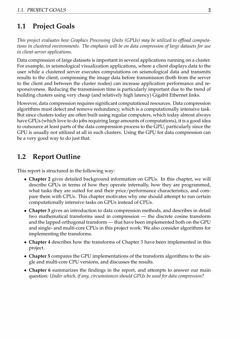
This project evaluates how Graphics Processing Units (GPUs) may be utilized to offload computa-tions in clustered environments. The emphasis will be on data compression of large datasets for usein client-server applications.
Data compression of large datasets is important in several applications running on a cluster.For example, in seismological visualization applications, where a client displays data to theuser while a clustered server executes computations on seismological data and transmitsresults to the client, compressing the image data before transmission (both from the serverto the client and between the cluster nodes) can increase application performance and re-sponsiveness. Reducing the transmission time is particularly important due to the trend ofbuilding clusters using very cheap (and relatively high latency) Gigabit Ethernet links.
However, data compression requires significant computational resources. Data compressionalgorithms must detect and remove redundancy, which is a computationally intensive task.But since clusters today are often built using regular computers, which today almost alwayshave GPUs (which love to do jobs requiring large amounts of computations), it is a good ideato outsource at least parts of the data compression process to the GPU, particularly since theGPU is usually not utilized at all in such clusters. Using the GPU for data compression canbe a very good way to do just that.
1.2 Report Outline
This report is structured in the following way:
• Chapter 2 gives detailed background information on GPUs. In this chapter, we willdescribe GPUs in terms of how they operate internally, how they are programmed,what tasks they are suited for and their price/performance characteristics, and com-pare them with CPUs. This chapter motivates why one should attempt to run certaincomputationally intensive tasks on GPUs instead of CPUs.
• Chapter 3 gives an introduction to data compression methods, and describes in detailtwo mathematical transforms used in compression — the discrete cosine transformand the lapped orthogonal transform — that have been implemented both on the GPUand single- and multi-core CPUs in this project work. We also consider algorithms forimplementing the transforms.
• Chapter 4 describes how the transforms of Chapter 3 have been implemented in thisproject.
• Chapter 5 compares the GPU implementations of the transform algorithms to the sin-gle and multi-core CPU versions, and discusses the results.
• Chapter 6 summarizes the findings in the report, and attempts to answer our mainquestion: Under which, if any, circumstances should GPUs be used for data compression?

Chapter 2
Background
The goal of this chapter is to give an understanding of how GPUs work, how they are pro-grammed, what they are good and bad at, and how they compare to CPUs.
In Section 2.1, we give a brief history of how GPUs have evolved. Then we describe thestructure and internals of current GPUs in Section 2.2, which is important in order to under-stand how they can be programmed. Next, we look at programming the GPU in Section 2.3.Then, we look at the price and performance characteristics of some of the currently availableGPUs compared to current CPUs in Section 2.4. Finally, which tasks GPUs are suitable orunsuitable for are discussed in Section 2.5.
2.1 GPUs: A Brief History
We now give a brief history of how GPUs have developed, to gain an understanding of howthey have evolved to where they are at today. For further information, see for example [8, 9].
In the late 1970s, and the beginning of the 1980s, most calculations concerning graphicsdrawing were done in software by the CPU. The first accelerated graphics operation camewith the introduction of a special bit block transfer or bitblt instruction on the Xerox Alto com-puter. This operation copies rectangular arrays of bitmap data from a source to a potentiallyoverlapping destination. This can, for instance, be used for animation of one image on topof a background image.
Through the 1980s, special graphics chips with an increasing number of features were devel-oped. A revolution came with the introduction of the Commodore Amiga machine, whichincorporated the first mass-market video accelerator able to draw and fill shapes and drawanimations (sprites) in hardware. The Amiga’s graphics subsystem comprised several chips.For instance, it had one chip dedicated exclusively to bit block transfers.
2D acceleration was further developed during the first half of the 1990s, when improve-ments in component manufacturing led to vendors integrating the features of several chipsinto single chips. Also, features to accelerate video playback were added. But in about 1995,3D games were becoming increasingly popular. This led to the release of dedicated chips— 3D GPUs — which were able to do 3D calculations. Later, these chips were integratedwith the 2D GPUs. 3D GPUs gradually went from only doing 3D rasterization (convertingsimple three-dimensional geometric primitives, such as lines, triangles and rectangles, totwo-dimensional screen pixels) and texture mapping (mapping a two-dimensional texture im-age on to a planar three-dimensional surface) from 1995–1998 to supporting more advancedcalculations like 3D translation, rotation and scaling, lighting and smoothing (1999–2000).
3
2.2. THE STRUCTURE OF A MODERN GPU 4
This is, however, not enough to produce all the effects a developer of a modern game wantsto implement. Although GPUs were becoming increasingly configurable towards year 2000,they were not programmable. For example, there was no way to modify how the GPUcalculated the lighting effects individually for each pixel drawn. This is a requirement in or-der to produce highly realistic 3D scenes. Developers wanting to create games employingsuch effects were therefore forced to compute the lighting effects for each pixel on the CPU,which is not a very good idea, such the CPU typically is only able to compute the lighting ofone or a few simultaneously, and has traditionally been much better at integer rather thanfloating-point operations. Since the GPUs were designed from the ground to process hun-dreds of pixels simultaneously and were optimized for floating-point computation, it wassoon evident that using the GPU for such computations was the only way realistic 3D scenescould be produced with acceptable frame rates. This lead to GPUs becoming increasinglyprogrammable, and such GPUs were introduced from 2001 and onwards.
In recent years, GPU programmability has gradually increased. GPUs can now execute asmall program which is run for each vertex passed to it (a vertex program), and a separateprogram for each pixel the GPU decides to draw (a fragment program). These programs en-able developers to create all types of advanced effects. For instance, the complicated calcu-lations of determining how smoke and fire moves in a 3D scene can be offloaded to the GPUusing such programs [10]. And, of course, the programmability of the GPU is increasinglybeing used for applications unrelated to graphics, examples of which were mentioned in theprevious chapter.
Initially, GPUs could only be programmed in low-level assembly language and the vertexand fragment programs were very limited in what operations they could execute. Today,high-level languages for GPU programming have been introduced, and with every newGPU generation, more programming limitations are removed. In the rest of this chapter,we take a look at how modern, programmable GPUs are structured and how they can beprogrammed.
2.2 The Structure of a modern GPU
Modern GPUs are structured around a graphics pipeline, which is a sequence of several stepsoperating in parallel and in a particular order to transform a set of geometric primitives andoperations to 2D projection of a 3D image appearing on the screen. We begin this sectionby describing the graphics pipeline and how it is implemented on the GPU. Then, we takea deeper look at the GPU’s vertex and fragment processors, which are the two currentlyprogrammable units within the GPU.
The following description is based on [11, 12]. Since we focus on the NVIDIA GeForce 6 and7 series, other GPUs might be structured in a slightly different manner.
2.2.1 The Graphics Pipeline
The graphics pipeline of the GPU is structured to transform a stream of vertices and com-mands from a software application to output an image which is displayed on screen. A(simplified!) block diagram of a typical modern GPU, adapted from [11] and [12], is shownin Figure 2.1 on the facing page.
Initially, the host CPU sends commands (such as setting up where the camera in the scene islocated, setting up colors and lighting, setting up whether squares, triangles or other figures

CHAPTER 2. BACKGROUND 5
Cull/clip/setup
Rasterization z-cull
Texture cache
DRAMpartition
DRAMpartition
DRAMpartition
DRAMpartition
processorsfragmentProgrammable
several processors)
z-compare
Programmablevertexprocessors
= Memory = Programmable unit = Non-programmable unit
(One block denotes
GPU frontend
and blendingunits
Figure 2.1: Block diagram of the internal structure of a GPU.
should be drawn), texture data (such as an image of a building being mapped to a largecube, to simulate a building), and vertex data (the coordinates of all the objects in the scene)to the GPU frontend via a bus such as PCI Express.
Next, commands, texture data and vertices are processed by the vertex processors or vertexshaders in the GPU. The vertex shaders run a vertex program for each vertex in the scene.The vertex programs can modify the vertex’s position, the color and the texture coordinateassociated with the vertex. The software application can upload the vertex program to theGPU in advance to transmitting rendering commands. On newer GPUs (from 2004 andonwards), vertex programs can access the texture memory of the GPU. An example of asituation where a vertex shader will be useful could be when rendering a mountain terrain.The software application running on the CPU would send a 2D grid of points along witha mountain terrain texture, where light colors in the texture indicate high elevations in theterrain and dark colors indicate lower elevations, to the GPU. The vertex program could readtexture memory and determine, based on the color of the texture at the vertex’s location,determine what elevation level the vertex should have, and thus generate a 3D terrain byoutputting a vertex at the correct elevation level. The alternative would be to do the samework on the CPU, which would likely be much slower, since the GPU is able to processseveral vertices simultaneously and has heavily optimized floating-point units which havebuilt-in instructions for dealing with small vectors.
2.2. THE STRUCTURE OF A MODERN GPU 6
After the vertex programs have been run, the vertex processors group vertices into geometricprimitives. For example, when drawing triangles, three vertices are grouped into a triangleprimitive. The vertex processors thus produce a stream of primitives, which are passed onto the cull/clip/setup block. This block uses efficient visibility clipping methods to removeprimitives which are not visible to the camera and calculates equations for the geometricprimitives to aid the rasterization block. (see [13] for information on visibility clipping meth-ods.)
Next, the rasterization block converts the geometric data produced by the cull/clip/setupblock into pixels, or points on the rendering target (e.g. the screen), by employing efficientalgorithms for converting mathematical descriptions of lines, circles and other geometricfigures to screen pixels (see [13] for an in-depth description of these algorithms). The raster-ization block also uses information from the z-cull block to determine if the current pixelsbeing processed are occluded by some previously processed pixels. If this is the case, thecurrent pixels can be discarded and are not processed by the later stages in the pipeline.However, it is not certain that all the points produced by the rasterization block will bedrawn. Some of them might end up being occluded by other objects (but this was not de-tected by the z-cull block at that time or the pixel is occluded by pixels processed after thecurrent pixel), and some pixels might have to be blended with other pixels — i.e. two pix-els are fused together into one pixel. Thus the rasterization block only produces candidatepixels, or fragments. Some fragments will end up as pixels, and some will not.
The rasterization block transfers fragments to the fragment processors or pixel processors, whichare programmable processors which do per-fragment processing. Just as the vertex proces-sors can run vertex programs, the fragment processors can run fragment programs, whichare invoked for each fragment. The fragment programs can write up to four 16 or 32-bitvalues to up to four fixed memory locations, and can read texture memory at any location.The fragment programs are called with the texture coordinates of the current pixel as an ar-gument (which is passed to it from the vertex processor). For example, a fragment programcould be used to calculate how each pixel should be lighted, using sophisticated lightingmodels based on real-world physics. Or, each pixel could represent a value in a numericalapproximation to the solution of a two-dimensional differential equation, and the fragmentprocessor could execute a program to calculate the Gauss-Seidel numerical method for com-puting solutions to systems of linear equations. The fragment processors operate on severalhundred pixels simultaneously, and, as the vertex processors, have optimized floating-pointhardware capable with built-in vector instructions.
The final stage in the rendering process is to do z-compares and blending (collectively re-ferred to as raster operations). The z-compare units determine whether each fragment is oc-cluded by some other fragment. This information is also sent to the z-cull block, so that newfragments can be discarded at an early stage (without going through the fragment proces-sors) if it is already known that some pixels will be drawn in front of them. Finally, pixels areblended (if necessary) and their final color is written to one of the GPU’s DRAM partitions.Having several DRAM partitions lets several pixels be written to memory simultaneously.The DRAM of the GPU stores textures and other input data to the rendering pipeline, andthe color values of the image being drawn to the screen. The GPU DRAM memory typicallyhas far more bandwidth than the normal DRAM of the CPU, but also has greater latency.
The GPU also employs several caches (which are not shown in Figure 2.1) and uses aggres-sive caching strategies . For instance, there is a vertex cache which checks whether a vertex ispassed to a vertex processor twice. If that is the case, the vertex program is run only once.Also, textures are heavily cached in a separate texture cache.
It should be evident from Figure 2.1 that the graphics pipeline is implemented as several

CHAPTER 2. BACKGROUND 7
functional units which operate serially. But it is also evident that even though the input toone functional unit is the output of some other functional unit, the units do not process theentire stream of vertices before outputing data to the next functional unit. For instance, thevertex processors typically only read three vertices before they assemble the vertices into atriangle and pass them on to the cull/clip/setup block, which also pass simple primitivesto the rasterizer. And the rasterizer passes large amounts of fragments to the fragment pro-cessors, which can process each fragment independently and in parallel. Hence if the vertexstream is very large — which is usually the case, since there typically will be hundredsof thousands of vertices and even more resulting pixels in a large scene — the functionalunits can operate in parallel. This enables so-called task-level parallelism since the individualblocks of the graphics pipeline can run in parallel. And since functional units which areconnected lie very close to each other on the chip, communication between them is veryfast. But instruction-level parallelism is also employed, since individual functional units pro-cess several elements at once. For example, there are many vertex and fragment processorswhich operate in parallel on several pixels simultaneously, and each individual vertex andfragment processor is capable of operating on a 4-value vector in parallel.
The fact that task-level and instruction-level parallelism is used, along with the fact thatthe individual blocks do not have complex dependencies between them, makes it possibleto design very efficient GPUs whose designs are tailored to push large amounts of verticesthrough the graphics pipeline. We will look closer at how the GPUs perform in comparisonto CPUs, which are structured in an entirely different and much more complicated manner,in Section 2.4. We now take a closer look at the vertex and fragment processors.
2.2.2 The Vertex Processors
The vertex processors run a vertex program for each vertex. A very simplified block diagramof the NVIDIA GeForce 6 and 7 vertex processors is shown in Figure 2.2 on the next page.
The vertex processor runs a program for each vertex passed to the GPU. Each processor con-sists of one scalar unit able to do floating-point operations, with at most 32 bits of precision.The vector unit operates on four values simultaneously, and is capable of doing a four-waySIMD (single instruction, multiple data) multiply-and-add (i.e. calculating W = X ∗ Y + Zwhere W, X, Y and Z are four-component vectors) instruction per clock cycle. In addition,the scalar unit can also in parallel to the vector unit be instructed to do a special scalar func-tion per clock cycle, such as exponential functions, calculating reciporals and trigonometricfunctions. It can therefore be regarded as a MIMD (multiple instructions, multiple data)processor since it can execute different instructions on different data at the same time.
The vertex processor also includes a simple branching unit. Programs on the vertex proces-sor may also access texture memory through the texture cache (since GeForce 6). Also, thereis a primitive assembly unit which groups vertices into primitives for subsequent graphicspipeline stages, and a viewport processing unit which can transform vertices into globalcoordinates if they have been passed to the GPU in a different reference coordinate system.
The vertex processor on the GeForce 6 series processors allows for programs of up to 512instructions and will run a maximum of 65,536 instructions per vertex. It also has 32 localregisters available to programs. The vertex processor has not changed much in GeForce7, except that vertex programs can have more complicated branching and can execute aninfinite amount of instructions per vertex.

2.2. THE STRUCTURE OF A MODERN GPU 8
Vertex processor
Texture fetch unit
Viewport processing
Branch unit
FP scalar unit FP vector unitTexture cache
Primitive assembly
Figure 2.2: Block diagram of the internal structure of a vertex processor, from GPU Gems 2[11].
2.2.3 The Fragment Processors
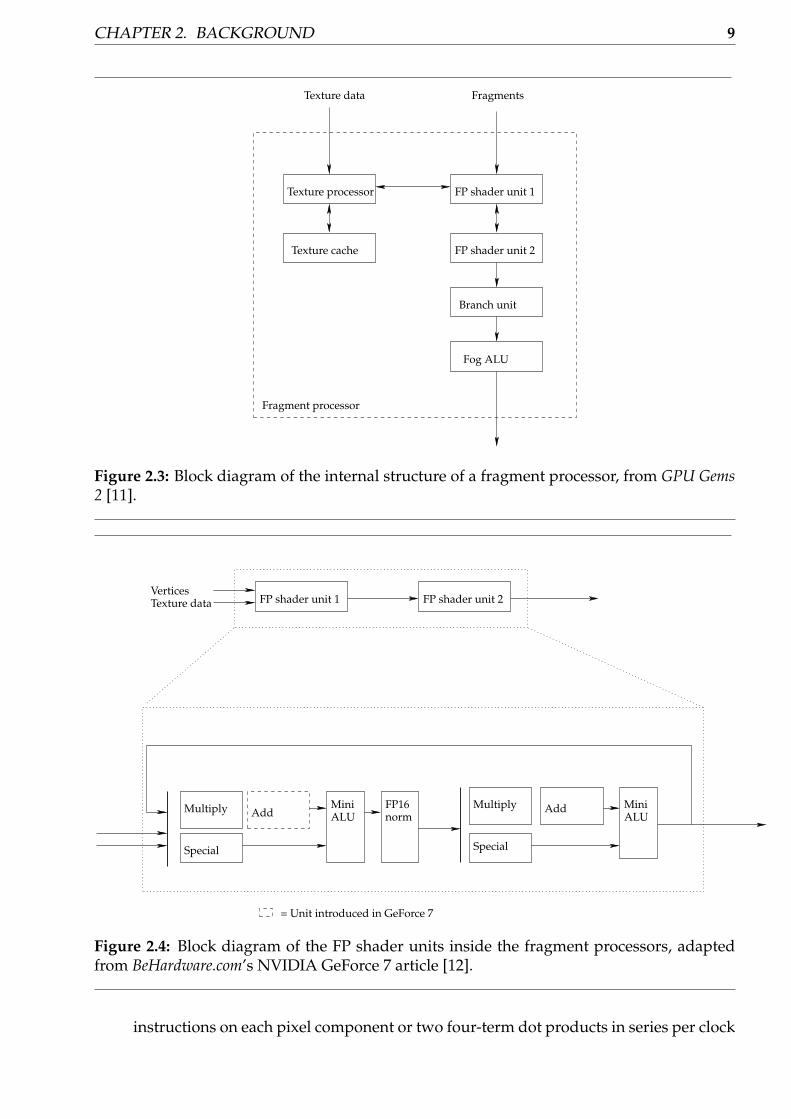
The fragment processors run a fragment program for each vertex. They are slightly differentthan the vertex processors. A simplified block diagram is shown in Figure 2.3 on the facingpage.
Fragment programs are run for each fragment passed from the rasterizer. On the NVIDIAGeForce 6 and 7 series, each fragment processor operates on four pixels at a time. A pixel isagain a vector of four scalar values: (R, G, B, A) where R is the red intensity, G is the greenintensity, B is the blue intensity and A is the alpha/transperancy value. Hence each pro-cessor operates on 16 values at a time, and there are usually many processors. The numberof fragment processors multiplied by the number of pipelines per fragment processors isreferred to as the number of pixel pipelines on the GPU; i.e. how many pixels the GPU can dooperations on simultaneously.
The two FP shader units, which do the actual work, are shown in Figure 2.4 on the nextpage.
On the GeForce 6 and 7 GPUs, the FP shader units, which each have 4 pipelines, are able to:
• Do one multiply-add (MADD) instruction on each component of a pixel or a four-termdot product and another multiplication in series per clock (GeForce 6), or two MADD
CHAPTER 2. BACKGROUND 9
Fragment processor
Texture processor
Texture cache
Texture data
FP shader unit 1
FP shader unit 2
Branch unit
Fog ALU
Fragments
Figure 2.3: Block diagram of the internal structure of a fragment processor, from GPU Gems2 [11].
Multiply Add
Special
Multiply
Special
Add
FP shader unit 2FP shader unit 1Texture dataVertices
MiniALU
FP16norm
MiniALU
= Unit introduced in GeForce 7
Figure 2.4: Block diagram of the FP shader units inside the fragment processors, adaptedfrom BeHardware.com’s NVIDIA GeForce 7 article [12].
instructions on each pixel component or two four-term dot products in series per clock
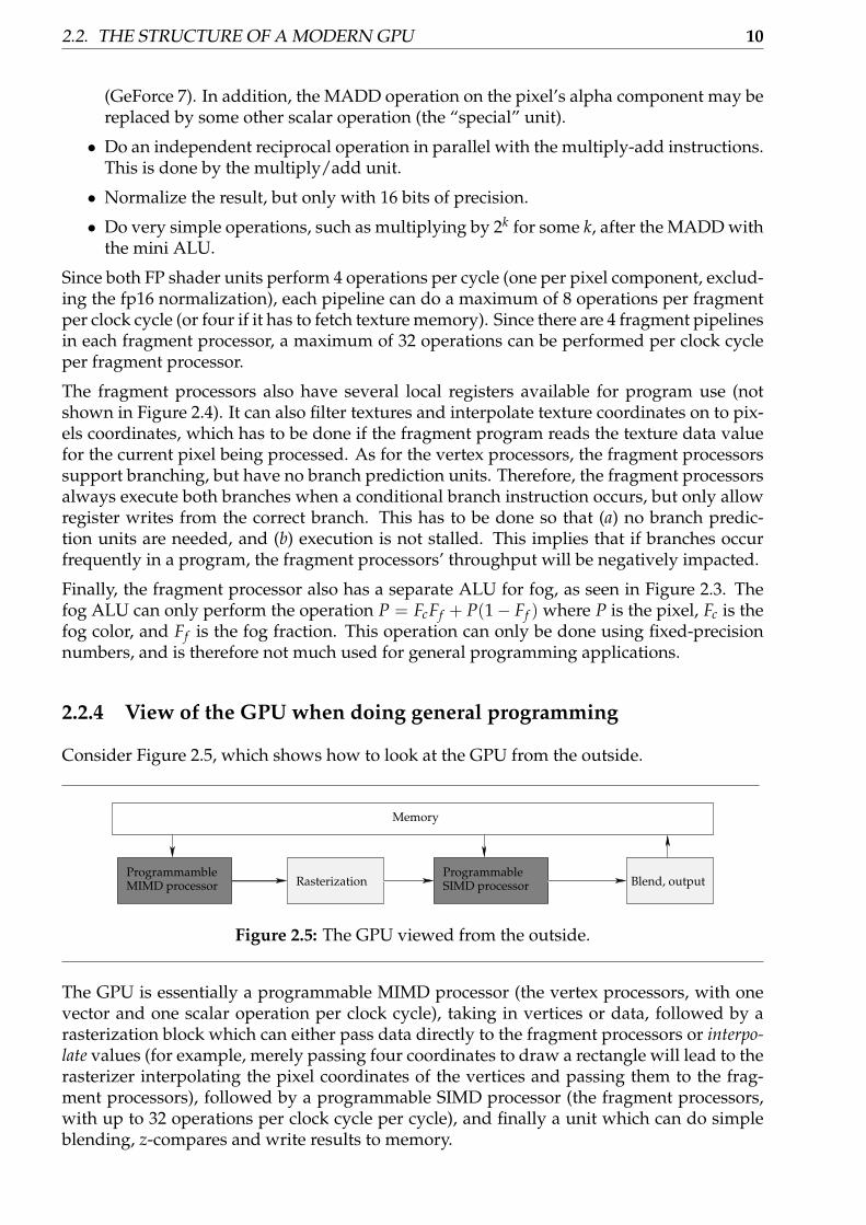
2.2. THE STRUCTURE OF A MODERN GPU 10
(GeForce 7). In addition, the MADD operation on the pixel’s alpha component may bereplaced by some other scalar operation (the “special” unit).
• Do an independent reciprocal operation in parallel with the multiply-add instructions.This is done by the multiply/add unit.
• Normalize the result, but only with 16 bits of precision.
• Do very simple operations, such as multiplying by 2k for some k, after the MADD withthe mini ALU.
Since both FP shader units perform 4 operations per cycle (one per pixel component, exclud-ing the fp16 normalization), each pipeline can do a maximum of 8 operations per fragmentper clock cycle (or four if it has to fetch texture memory). Since there are 4 fragment pipelinesin each fragment processor, a maximum of 32 operations can be performed per clock cycleper fragment processor.
The fragment processors also have several local registers available for program use (notshown in Figure 2.4). It can also filter textures and interpolate texture coordinates on to pix-els coordinates, which has to be done if the fragment program reads the texture data valuefor the current pixel being processed. As for the vertex processors, the fragment processorssupport branching, but have no branch prediction units. Therefore, the fragment processorsalways execute both branches when a conditional branch instruction occurs, but only allowregister writes from the correct branch. This has to be done so that (a) no branch predic-tion units are needed, and (b) execution is not stalled. This implies that if branches occurfrequently in a program, the fragment processors’ throughput will be negatively impacted.
Finally, the fragment processor also has a separate ALU for fog, as seen in Figure 2.3. Thefog ALU can only perform the operation P = FcFf + P(1− Ff ) where P is the pixel, Fc is thefog color, and Ff is the fog fraction. This operation can only be done using fixed-precisionnumbers, and is therefore not much used for general programming applications.
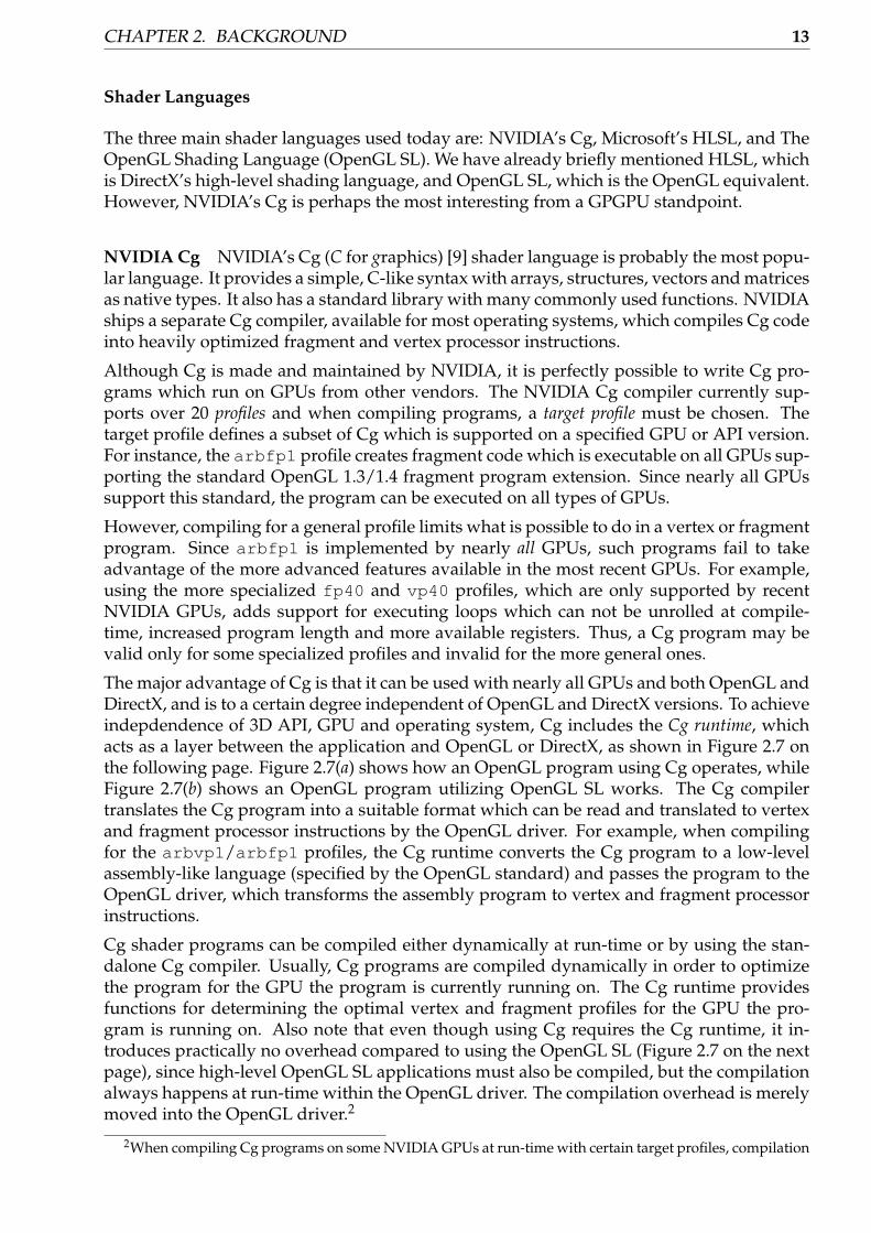
2.2.4 View of the GPU when doing general programming
Consider Figure 2.5, which shows how to look at the GPU from the outside.
ProgrammambleMIMD processor Rasterization
ProgrammableSIMD processor Blend, output
Memory
Figure 2.5: The GPU viewed from the outside.
The GPU is essentially a programmable MIMD processor (the vertex processors, with onevector and one scalar operation per clock cycle), taking in vertices or data, followed by arasterization block which can either pass data directly to the fragment processors or interpo-late values (for example, merely passing four coordinates to draw a rectangle will lead to therasterizer interpolating the pixel coordinates of the vertices and passing them to the frag-ment processors), followed by a programmable SIMD processor (the fragment processors,with up to 32 operations per clock cycle per cycle), and finally a unit which can do simpleblending, z-compares and write results to memory.

CHAPTER 2. BACKGROUND 11
The vertex processors can pass three types of values to the next stages of the pipeline: Acolor value associated with the vertex, a transformed vertex position, and several texturecoordinates, where each texture coordinate consists of two 16 or 32-bit floating-point values.The fragment processors can read the texture coordinates generated by the vertex proces-sors, which are linearly interpolated over pixels inside the region spanned by the vertices.The ability to pass values as texture coordinates has been exploited in the implementationsin this project, since it allows certain computations to be offloaded from the fragment to thevertex processors.
The fragment processors can output one four-component value, where each component is of32 or 16 bits of precision, to a maximum of four rendering targets. Thus, a single invocationof a fragment program can generate at most 16 floating-point values. These values must bewritten to the fragment’s position in the GPU’s memory (recall that a fragment is a candidatepixel, and thus, each fragment is associated with a specific position in the GPU’s texturememory). However, fragment programs can read from any position in texture memory.
It is apparent that the GPU architecture is quite different from CPU architecture, and there-fore uses very different programming models. We will now look closer at ways of program-ming the GPU and its performance characteristics in the next sections.
2.3 GPU Programming
We will now look at how programming can be done on the GPU. First, we begin with anintroduction to how traditional graphics applications use the GPU, before we look at howthe same methods and programming interfaces can be used for general GPU programming(GPGPU).
2.3.1 OpenGL and DirectX
The GPU drivers typically support the OpenGL [14] and Microsoft’s DirectX [15] applicationprogramming interfaces (APIs). We will mostly use OpenGL, as it is not bound to one par-ticular platform, which is the case with DirectX. With these APIs, a developer may easilydraw objects and apply color, lighting, shading and many advanced effects to a scene.
Typically, GPGPU applications use OpenGL or DirectX for passing commands, data and up-loading the vertex and fragment programs to the GPU. The typical data flow from a softwareapplication to the GPU is illustrated in Figure 2.6 on the next page. Note that the GPU partof the figure is a coarser view of Figure 2.1.

2.3. GPU PROGRAMMING 12
Softwareapplication
OpenGL/DirectXAPI calls
GPUFront-end
CPU
GPU
Commands and data
Vertexprocessor
Primitiveassembly
Rasterizer/interpolation
Fragmentprocessors
GPU drivers
Frame buffer(DRAM)
VerticesTransformedvertices
Primitives
Fragments
Transformedfragments PixelsRaster
operations
Figure 2.6: Data flow from a software application to the GPU, adapted from NVIDIA’s Cgbook [9]
2.3.2 Shader and GPGPU Languages
There are several specialized high-level languages for programming the vertex and frag-ment shaders.1 Prior to the introduction of the high-level shader programming languages,the only way to program the shaders was through a low-level assembly language. Withhigh-level languages, GPU vendors can do agressive optimization on the high-level code tooptimize for a particular GPU. Since far less is known about GPU internals than CPU in-ternals (mainly due to the highly proprietary nature of GPUs), using a high-level languageusually gives better results than attempting to hand-optimize a low-level assembly languageprogram.
But languages have also been created on top of high-level shader languages. These arecalled GPGPU languages and are created explicitly for doing more general programming onthe GPU. Typically, these languages use a compiler to translate from the GPGPU languageto a high-level shader language.
We now look at some of the high-level shader and GPGPU languages. Low-level shaderlanguages are practically never used anymore, since writing code in a high-level shaderlanguage usually yields better performing shader programs.
1Note that special-purpose shader languages for per-vertex and per-pixel processing is not something new.Rendering packages such as Pixar’s RenderMan, used to create several animated movies, have included suchspecial-purpose languages since the 1980s. However, RenderMan is not made for real-time rendering, and theshader programs execute on the CPU. It is therefore not used for speeding up rendering, but for creating moreadvanced effects.
CHAPTER 2. BACKGROUND 13
Shader Languages
The three main shader languages used today are: NVIDIA’s Cg, Microsoft’s HLSL, and TheOpenGL Shading Language (OpenGL SL). We have already briefly mentioned HLSL, whichis DirectX’s high-level shading language, and OpenGL SL, which is the OpenGL equivalent.However, NVIDIA’s Cg is perhaps the most interesting from a GPGPU standpoint.
NVIDIA Cg NVIDIA’s Cg (C for graphics) [9] shader language is probably the most popu-lar language. It provides a simple, C-like syntax with arrays, structures, vectors and matricesas native types. It also has a standard library with many commonly used functions. NVIDIAships a separate Cg compiler, available for most operating systems, which compiles Cg codeinto heavily optimized fragment and vertex processor instructions.
Although Cg is made and maintained by NVIDIA, it is perfectly possible to write Cg pro-grams which run on GPUs from other vendors. The NVIDIA Cg compiler currently sup-ports over 20 profiles and when compiling programs, a target profile must be chosen. Thetarget profile defines a subset of Cg which is supported on a specified GPU or API version.For instance, the arbfp1 profile creates fragment code which is executable on all GPUs sup-porting the standard OpenGL 1.3/1.4 fragment program extension. Since nearly all GPUssupport this standard, the program can be executed on all types of GPUs.
However, compiling for a general profile limits what is possible to do in a vertex or fragmentprogram. Since arbfp1 is implemented by nearly all GPUs, such programs fail to takeadvantage of the more advanced features available in the most recent GPUs. For example,using the more specialized fp40 and vp40 profiles, which are only supported by recentNVIDIA GPUs, adds support for executing loops which can not be unrolled at compile-time, increased program length and more available registers. Thus, a Cg program may bevalid only for some specialized profiles and invalid for the more general ones.
The major advantage of Cg is that it can be used with nearly all GPUs and both OpenGL andDirectX, and is to a certain degree independent of OpenGL and DirectX versions. To achieveindepdendence of 3D API, GPU and operating system, Cg includes the Cg runtime, whichacts as a layer between the application and OpenGL or DirectX, as shown in Figure 2.7 onthe following page. Figure 2.7(a) shows how an OpenGL program using Cg operates, whileFigure 2.7(b) shows an OpenGL program utilizing OpenGL SL works. The Cg compilertranslates the Cg program into a suitable format which can be read and translated to vertexand fragment processor instructions by the OpenGL driver. For example, when compilingfor the arbvp1/arbfp1 profiles, the Cg runtime converts the Cg program to a low-levelassembly-like language (specified by the OpenGL standard) and passes the program to theOpenGL driver, which transforms the assembly program to vertex and fragment processorinstructions.
Cg shader programs can be compiled either dynamically at run-time or by using the stan-dalone Cg compiler. Usually, Cg programs are compiled dynamically in order to optimizethe program for the GPU the program is currently running on. The Cg runtime providesfunctions for determining the optimal vertex and fragment profiles for the GPU the pro-gram is running on. Also note that even though using Cg requires the Cg runtime, it in-troduces practically no overhead compared to using the OpenGL SL (Figure 2.7 on the nextpage), since high-level OpenGL SL applications must also be compiled, but the compilationalways happens at run-time within the OpenGL driver. The compilation overhead is merelymoved into the OpenGL driver.2
2When compiling Cg programs on some NVIDIA GPUs at run-time with certain target profiles, compilation

2.3. GPU PROGRAMMING 14
Core Cgruntime
Cg program
GPU
OpenGL SLapplication
OpenGL SLprogram
OpenGL Cgruntime
Cg compiler
OpenGLdriver
OpenGLdriver
processor instructionsVertex/fragment
Cg program compiledto low-level target profile language
Vertex/fragmentprocessor instructions
Cgapplication
GPU
(a) (b)
Figure 2.7: (a) Passing Cg programs to the GPU — (b) Passing OpenGL SL programs to theGPU
Since some of the features in the profiles for newer GPUs can be very useful in GPGPU ap-plications, the GPGPU code in this project will be created for the most recent glslv/glslfprofiles. This ensures that we can use the most recent features and increases what we areallowed to express in our programs in addition to not tying our shaders to one particularvendor, since the code should be able to run on any OpenGL 2.0 compliant GPU.
Microsoft HLSL DirectX also has its own high-level shader language (briefly describedbelow), and also specifies the DirectX Shader Model, which specifies what types of shaderprograms GPUs implementing the Shader Model must support by describing a low-levelassembly-like language GPU drivers must be able to compile into shader instructions. Therehave been several versions of the Shader Model, with increasing requirements as to what theGPU must support. For instance, in Shader Model 2.0, branching instructions and precisionwere limited compared to the more recent Shader Model 3.0.
Microsoft’s HLSL (High Level Shader Language) is actually syntactically the same languageas Cg, but includes some additional support accessing DirectX via the shader programs. It isessentially Microsoft’s implementation of Cg, and is therefore bound to DirectX. For GPGPUapplications there is no advantage in using HLSL instead of Cg.
can also happen inside the OpenGL driver by the use of the GL_EXT_Cg_shader OpenGL extension imple-mented by the NVIDIA drivers, which allows passing Cg programs directly to OpenGL. Thus in this case,OpenGL SL and Cg programs are probably compiled using a common back-end compiler inside the driver,and the Cg runtime does not need to do any compilation. Developers can also, if using this extension, pass Cgprograms directly to OpenGL, at the cost of making programs less portable.
CHAPTER 2. BACKGROUND 15
The OpenGL Shading Language OpenGL version 2.0 specifies a way to write shader pro-grams by the means of a high-level C-like language that GPUs supporting the OpenGLstandard must be able to execute. In OpenGL version 1.5, this was an optional extension tothe OpenGL standard, but with OpenGL 2.0, support for shader programming was mademandatory and significantly improved. In OpenGL versions prior to 1.5, the only optionavailable for writing shader programs was to write shader programs in a special assemblylanguage. When programming shaders this way (using either the OpenGL SL or the low-level assembly language), the application passes a string containing the program sourcecode to the vendor-provided OpenGL driver, which dynamically compiles the program intoshader instructions and uploads it to the vertex and fragment processors.
The OpenGL shading language [16] is also similar to Cg and HLSL, and is a part of theOpenGL 2.0 standard. But Cg has so far been used more for GPGPU applications, andsince Cg (since version 1.5) has a glslv/glslf profile target, it can output OpenGL SLcompliant shader programs. OpenGL SL implementations were availble in late 2003, whileCg was released in 2002. Cg has, probably due to the head start, the massive support it hasreceived from NVIDIA and the fact that it has a standalone compiler (enabling developersto quickly check if a program is syntactially correct without actually attempting to run theprogram), become more popular than OpenGL SL for GPGPU applications. OpenGL SL alsolacks support for multidimensional arrays, non-square matrices, and some commonly usedoperators.
What language do we choose? All three shader languages are fairly similar — for a de-tailed comparison, see e.g. [17]. In this project, we have chosen to use NVIDIA’s Cg lan-guage. The reasons are:
1. Cg is relatively mature and has the most features of all the shader languages,
2. Cg provides (contrary to OpenGL SL) a standalone compiler which enables developingshader programs without actually running the application,
3. Cg is the most used language for GPGPU applications,
4. Cg enables development of shader programs which are not tied to a particular 3D API,operating system platform or GPU vendor.
One potential disadvantage of Cg is that it is fully controlled by NVIDIA. However, since Cgcan be used with GPUs from other vendors by compiling with non-NVIDIA specific profiles,this is of little importance.
Another big plus for Cg is that it is the only shader language which supports the SonyPlayStation 3, which will probably also be an interesting platform for GPGPU applications.3
GPGPU Languages
There are two main GPGPU languages: BrookGPU and Sh. These languages generate OpenGLSL or Cg code, which is again compiled to vertex and fragment processor instructions. Wehave chosen to not use these languages in this project, since they are relatively immatureand do not currently deliver as good performance as Cg, but will probably become muchmore interesting in the future.
3PlayStation 3 is fully compliant with the embedded version of the OpenGL 2.0 standard except that it usesCg instead of OpenGL SL.

2.3. GPU PROGRAMMING 16
BrookGPU BrookGPU [18] started as a research project at Stanford University’s GraphicsLab. It is specifically designed for GPGPU applications, and is higher-level than Cg, whichmakes it easier to write GPGPU applications. BrookGPU comes with a compiler which trans-lates BrookGPU code into Cg programs.
Sh Sh [19] is not really a programming language, but an integration of shader program-ming into C++. With Sh, shader programs are written directly in C++, and shaders can evenshare variables with a regular C++ application. Sh is intended for both graphics and GPGPUpurposes.
2.3.3 General Programming on the GPU
Programming GPUs consists of writing the procedures that do computations on the vertexand fragment streams. As we have seen, the GPU is structured around a stream compu-tation model, where data flows between individual kernels (vertex and fragment programs)which transform the stream. This stream computation model is the only model supportedby GPUs.
NVIDIA engineer Mark Harris suggests in [20] the following mapping of computationalconcepts of traditional stateful CPU programming to the GPU stream programming model:
• Rendering = Executing. To actually run a fragment or vertex shader program whichdoes computation, we simply pass drawing commands to the GPU. Passing drawingcommands will start the rendering process. Most GPGPU applications — includingthose developed in this project — will compute something over a 2D grid. Hence,we simply tell the GPU (via for example OpenGL) to render a 2D square to start thecalculations.
• GPU textures = CPU arrays. When we want to use an array, a texture can be used onthe GPU. GPU textures are natively two-dimensional, but three-dimensional textures(and thus 3D arrays) will also be natively supported by future GPUs.
• Fragment shader programs = Inner loops. A program on the fragment processor is exe-cuted for all the fragments, and writes values back to texture memory. A fragmentprogram can therefore be seen as the inner loop of computations. (The outer loops ona CPU would be a loop iterating over all the fragments. This loop is implicit whenprogramming GPUs, since the GPU will automatically execute the fragment programsfor all fragments.)
• Rendering to texture memory = Feedback. If a computation has several steps, we writethe results of each step to texture memory. The next step can then use the result as itsinput. When all the steps are done, we read texture memory to get the result back tothe CPU.
• Vertex coordinates = Computational range. The input vertices determine what pixels willbe rasterized and therefore what coordinates the fragment programs will write to. Ver-tex coordinates therefore determine the range of the computation.
• Texture coordinates = Computational domain. The computational domain can be repre-sented as a texture. Texture coordinates are passed along with each vertex. The GPUautomatically interpolates the vertex texture coordinates for the fragments which willbe rendered. GPGPU applications can take advantage of this, since it means that theinput domain will automatically be shrinked or magnified to cover the output domain.On a CPU, such shrinking and magnifying would have to be done manually.
CHAPTER 2. BACKGROUND 17
Although these mappings are fairly straightforward, special care must be taken when pro-gramming the GPU due to its specialized design.
2.3.4 Limitations
GPUs are able to execute calculations extremely quickly. But due to their specialized design,programming GPUs is more tricky than programming CPUs. When programming GPUs,the following must be considered [20]:
1. Branching is usually not a good idea. GPUs have absolutely no branch-prediction units,and since the SIMD fragment processor operates on several fragments at a time, if abranch is taken for some but not all fragments, both branches will be executed for allfragments. Furthermore, if-else instructions take up to six cycles. In six cycles, the frag-ment processor can do at least 4 × 4 × 6 = 96 floating-point multiply-add operations(since there are four pipelines, each of which operates on four values, per cycle), andtwice as much if we also take into account the second multiply-add unit which can doa multiply-add operation on the result of the first unit. Therefore, if an algorithm hasa large number of branches, it may not be suitable for GPUs — and if computation canreplace branching, it is almost always a good idea. In this project, we have replaced allbranches with computations.
2. GPU cache is different from CPU cache. GPU cache is optimized for fetching textures, notgeneral memory access. It is therefore small compared to the CPU cache. In addition,it is optimized for two-dimensional locality (i.e. for fetching 2D texture data), rather than1D locality, which is what the CPU cache is optimized for. Furthermore, the cache isread-only — the only way to write values to texture memory is through the fragmentprograms.
3. Random memory access is problematic. A fragment program can only write to up tofour fixed memory addresses in GPU texture memory on the GeForce GPUs, andeach memory location can contain four 16 or 32-bit values. The addresses to whichthe fragment program can write are determined before the fragment program is run.Therefore, it is not possible for one instance of a fragment program to scatter dataacross memory. Also, GPUs are optimized for sequential memory access. This makesGPUs worse at random memory accesses than CPUs. Since many algorithms dependon quick random memory access time, they might need to be heavily adjusted or re-designed to run on the GPU.
4. Floating-point precision. GPUs often perform best when working with only 16-bit pre-cision because it frees up more registers and allows more values to be processed perclock cycle, and increases the number of elements that are fetched from GPU mem-ory in each cycle. The fragment processor has a normalization unit which only op-erates on 16-bit values. Another potential problem is that some GPUs use shortcutswhen rounding floating-point values which gives slightly greater rounding error butquicker hardware. This might lead to slight differences between computation resultson the CPU and GPU.
5. No integers or booleans. GPUs deal with floating-point numbers, not integers. This canbe a problem, since there are some 32-bit integers which can not be exactly representedin 32-bit floating-point format. GPUs also do not currently provide any bitwise op-erators, but Cg has reserved symbols for such operators for the future, and integersupport has been announced in the NVIDIA G80 GPU (see Section 2.4.2).

2.4. CURRENT GPUS: PRICE AND PERFORMANCE 18
6. Data must be uploaded and downloaded. Computation results need to be uploaded anddownloaded to and from the GPU. The time it takes to upload and download the datamight be so large that we should rather use the CPU for computation. Thus the GPUis suitable only when very large amounts of operations are done on the data.
We will take a closer look at exactly what applications the GPU is suitable for towards theend of this chapter.
2.4 Current GPUs: Price and Performance
Let us now look at how GPUs actually stack up to CPUs. First, we look at some of thecurrent GPUs available. Then we look at how GPUs compare to CPUs. Finally, we discusswhat GPUs are suitable for GPGPU applications.
2.4.1 Current GPUs
The GPU market is dominated by two vendors: NVIDIA Corporation and ATI Technologies,which was recently acquired by the CPU maker AMD.
NVIDIA Corporation GPUs
NVIDIA’s GPUs have been favored by the GPGPU community, since NVIDIA has activelysupported GPGPU projects and provides the Cg programming language. NVIDIA has alsocontributed large amounts of research on GPGPU programming. NVIDIA produces twotypes of graphics cards — the GeForce and the Quadro — where the GeForce cards are in-tended for personal use and home entertainment and Quadro cards are intended for graph-ics professionals.
For GPGPU applications, the chips used in the GeForce 6 and Quadro FX 540, 1300, 1400,3400 and 4400 series (NV40 series) or the GeForce 7 and Quadro FX 3500, 4500 and 5500series (G70 series) are most suitable, since the vertex and fragment processors were dramat-ically improved from the previous GeForce chips. The G70 chip, which was launched in2005 and further developed in 2006, is based on the NV40 chip from 2004 and has not beenradically redesigned. New features include more fragment pipelines, more features in thefragment processors (the first FP shader unit is able to do an add after the multiply), andhigher memory and internal clock speeds. The G70 is also suspected (though unconfirmedby NVIDIA) to have a larger and improved cache.
G70 comes in various versions. The cheaper cards have a G70 chip with fewer vertex andfragment processors, less memory bandwidth and higher latency than the more expensivecards. Inferior cards have lower numbers. For instance, the GeForce 7600 is inferior to theGeForce 7800. The same applies to the Quadro FX cards.
Graphics cards based on G70 are currently the most attractive ones to use for GPGPU ap-plications. Information on some GeForce cards is shown in Table 2.1 on the facing page.Information on some Quadro FX cards is shown in Table 2.2 on the next page. For informa-tion on several other NVIDIA cards, see [21] and [22].
Although some of the Quadro cards seem inferior and overpriced in comparison to theGeForce cards, they have one distinct advantage: The ability to have more memory and

CHAPTER 2. BACKGROUND 19
Graphics card GF 6800 Ultra GF 7600 GT GF 7900 GS GF 7950 GTChip NV45 G73 G71 G71Transistors 222 million 177 million 278 million 278 millionCore clock speed 400 MHz 560 MHz 450 MHz 550 MHzMemory clock speed 1100 MHz 1400 MHz 1320 MHz 1400 MHzMemory bandwidth 33.6 GB/s 22.4 GB/s 42.2 GB/s 44.8 GB/sInterface PCI-E x16 PCI-E x16 PCI-E x16 PCI-E x16Pixel pipelines 16 12 20 24Vertex processors 6 5 7 8Released 2004 2006 2006 2006Retail price, NOK, Dec 2006 549 (256 MB) 949 (256 MB) 1,749 (256 MB) 2,495 (512 MB)
Table 2.1: Properties of some recent GeForce graphics cards
Graphics card Quadro FX 3500 Quadro FX 4500 Quadro FX 5500Chip G71 G70 G71Transistors 278 million 302 million 278 millionCore clock speed 470 MHz 470 MHz 700 MHzMemory clock speed 700 MHz 525 MHz 1000 MHzMemory bandwidth 42.2 GB/s 33.6 GB/s 33.6 GB/sInterface PCI-E x16 PCI-E x16 PCI-E x16Pixel pipelines 20 24 24Vertex processors 7 8 8Released 2006 2006 2006Retail price, NOK, Dec 2006 7,595 (256 MB) 13,582 (512 MB) 23,980 (1024 MB)
Table 2.2: Properties of some recent Quadro FX graphics cards
(slightly) faster readback (download) times. Quadro FX cards have up to 1 GB of mem-ory, while current GeForce cards have a maximum of 512 MB. This might be important forGPGPU applications. They are also advertised as having quicker download times, whichis very important for GPGPU applications. But the main difference and the reason for theenormous price gap lies in the Quadro cards supporting advanced stereoscopic vision, cer-tain high-quality video outputs and the ability to smooth (antialias) lines at a higher quality,which is useful for certain CAD applications. These features are irrelevant for GPGPU pro-grams. There is no difference between the GPU and memory bus of the Quadro FX andGeForce cards (in fact, some GeForce cards use a quicker memory bus!)
Any GeForce 6 or 7 series GPU card or Quadro 3500, 4500 or 5500 card with at least 256 MB ofRAM will probably be suitable for GPGPU usage. Performance will increase as the numberof pixel pipelines increase, since the number of pixel pipelines determines how many pixels(values) can be rendered (computed) in parallel.
ATI Technologies GPUs
ATI Technologies GPUs have been less popular within the GPGPU community, since NVIDIAhas been much more active supporting GPGPU programming. ATI’s chips are named Radeonand come in both regular and Pro versions.
For GPGPU applications, GPUs should be of at least the X1000 series (having an R500 GPU),introduced in 2005. Before the X1000 series, ATI chips were not very suited for GPGPUapplications. Since NVIDIA provides much better support for GPGPU applications than

2.4. CURRENT GPUS: PRICE AND PERFORMANCE 20
ATI, it is hard to recommend an ATI GPU for such applications currently. This will, however,probably change in the future. ATI has recently begun to broaden its GPGPU support.
Information on some recent ATI GPUs is shown in Table 2.3.
Graphics card X1600 Pro X1800 GTO X1950 XTChip R515 R520 R580Transistors 157 million 321 million 384 millionCore clock speed 500 MHz 500 MHz 625 MHzMemory clock speed 780 MHz 1500 MHz 1800 MHzMemory bandwidth 12.4 GB/s 48.0 GB/s 57.6 GB/sInterface PCI-E x16 PCI-E x16 PCI-E x16Pixel pipelines 12 16 164
Vertex processors 5 8 8Released 2006 2006 2006Retail price, NOK, Dec 2006 720 (256 MB) 1,749 (256 MB) 3,149 (256 MB)
Table 2.3: Properties of some recent ATI graphics cards
As seen from Table 2.3 and 2.1 on the preceding page, ATI and NVIDIA GPUs are fairlysimilar. The architecture is slightly different, with high-end NVIDIA GPUs having 24 pixelpipelines each capable of fetching texture data in parallel, while the ATI X1900 XT has 64pixel pipelines where only 16 may do texture fetches simultaneously. In practice, perfor-mance will be similar for both GPUs.
One problem with ATI GPUs, and the reason we have opted for NVIDIA GPUs throughoutthis project, is drivers. Their Linux drivers have traditionally been of lower quality thanNVIDIA’s Linux drivers, and no drivers exist for FreeBSD or Solaris, which are frequentlyused as cluster operating systems.
2.4.2 Future GPUs
GPUs are evolving quickly. Large developments have happened, even during the limitedtime period of this project. We therefore include this section to describe the latest develop-ments that have occured through this project.
In November 2006, NVIDIA launched the G80 GPU, which has over 600 million transistors.This GPU has a core 575 MHz clock speed, and a memory clock of 900 MHz. The memorybandwidth is up to 86.4 GB per second, representing a clear improvement compared to priorGPUs. The shader processors operate at 1350 MHz.
Next-generation GPUs, such as NVIDIA’s GeForce 8 (released one month before the end ofthis project), and ATI’s Radeon R800, feature programmable geometry shaders. These geome-try shaders can do operations on entire primitives, such as triangles and squares. Whetherthese can give any advantage to general programming on the GPU and exactly how theywill work is currently unknown.
These GPUs also integrate the vertex, geometry and fragment processors into a unified shader.Unified shaders solve two problems: First, the three processors will have similar capability(currently, fragment processors usually have more features than vertex processors) and sec-ond, applications can dynamically configure the unified shader according to the applicationneeds — for example, an application which loads the fragment processors heavily but does
CHAPTER 2. BACKGROUND 21
not use the vertex processors can configure all the unified shaders to act as fragment pro-cessors. This leads to better utilization of the GPUs resources. The NVIDIA G80 has 128such unified processors (which is about four times more processors than previous NVIDIAGPUs).
The GeForce 8 GPU has native support for integers, while prior GPUs can only emulateintegers. This feature was specifically aimed at GPGPU projects, and should increase thenumber of applications suitable for the GPU. It is currently unknown whether new integer-specific operators, such as bit manupulation operators, are supported.
NVIDIA has also launched (but not, at the time of writing, released) the CUDA library,which only supports the GeForce 8 GPU. This allows programmers to use the GPU’s com-puting power directly from the C programming language, and also permits for separatethreads to run on the GPU. CUDA will include a BLAS and FFT library, implemented onthe GPU, to allow developers to easily offload computations to the GPU. Debugging of GPUprograms is also improved, and upload and download times are also said to be shorter.CUDA will likely make GPGPU applications far much easier to write.
ATI has also launched a GPU specifically made for computation. The product, marketed asa “dedicated stream processor”, is essentially an R850 GPU with 1 GB of RAM.
All the recent developments indicate that GPUs will increasingly support general program-ming in the future.
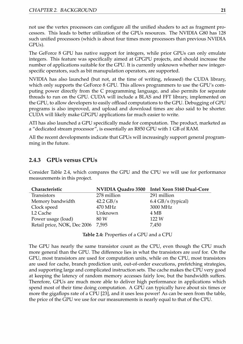
2.4.3 GPUs versus CPUs
Consider Table 2.4, which compares the GPU and the CPU we will use for performancemeasurements in this project.
Characteristic NVIDIA Quadro 3500 Intel Xeon 5160 Dual-CoreTransistors 278 million 291 millionMemory bandwidth 42.2 GB/s 6.4 GB/s (typical)Clock speed 470 MHz 3000 MHzL2 Cache Unknown 4 MBPower usage (load) 80 W 122 WRetail price, NOK, Dec 2006 7,595 7,450
Table 2.4: Properties of a GPU and a CPU
The GPU has nearly the same transistor count as the CPU, even though the CPU muchmore general than the GPU. The difference lies in what the transistors are used for. On theGPU, most transistors are used for computation units, while on the CPU, most transistorsare used for cache, branch prediction unit, out-of-order executions, prefetching strategies,and supporting large and complicated instruction sets. The cache makes the CPU very goodat keeping the latency of random memory accesses fairly low, but the bandwidth suffers.Therefore, GPUs are much more able to deliver high performance in applications whichspend most of their time doing computation. A GPU can typically have about six times ormore the gigaflops rate of a CPU [23], and it uses less power! As can be seen from the table,the price of the GPU we use for our measurements is nearly equal to that of the CPU.
2.5. CONCLUSIONS: TASKS SUITABLE FOR GPUS 22
2.5 Conclusions: Tasks Suitable for GPUs
We conclude, as [23], that the GPU is suitable for:
• Applications which have a high arithmetic intensity, i.e. has a large ratio of operationsper memory access.
• Applications where individual elements in the data stream are independent and arethus easily parallelizable.
The GPU is not suitable for:
• Applications having a random access pattern.
• Applications having a many complicated branches and inherent serial dependenciesbetween individual computation elements.
• Applications which are not easily parallelizable.
Examples of applications well suited for the GPU were mentioned in the previous chap-ter. Examples of applications that are not suitable for the GPU are recursive problems, suchas calculating the Fibonacci sequence through using the recursive formula Fn = Fn−1 +Fn−2 (F0 = F1 = 1) (because computing one element depends on computing two other el-ements), and a lexical analyzer or a compiler (which has to do several random memoryaccesses since it uses several data structures and complicated branching).
In sum, we can say that the GPU reflects the trend where computation is less expensive thancommunication. The GPU is designed for computation, and its programming model is sosimple that communication (random memory access) is kept to a minimum. The CPU, whichmust tolerate other, more complicated programming models and access patterns, must sac-rifice computation logic for communication logic.
It turns out that some mathematical transforms used in compression methods are suitablefor GPU implementation. We will look at the methods, which both are easily parallelizableand involve large amounts of floating-point computations, and their implementation on theGPU through the rest of this report.

Chapter 3
Data Compression and Previous Work
In this chapter, we will look at data compression methods and previous GPU implemen-tations of algorithms related to data compression. First, in Section 3.1, we will give somebackground material on general data compression. Next, in Sections 3.2 and 3.3, we willin greater detail look at two mathematical transforms commonly used for image data com-pression, describe and discuss specific algorithms — some of which have been implementedboth on the CPU and the GPU in this project — for calculating these transforms, and con-sider previous GPU implementations of the transforms.
3.1 Introduction to Data Compression
Data compression is the process of encoding data to a representation which uses less bitsthan the unencoded representation. This process is done by reducing or removing redun-dancy in the data. Redundancy reduction is, in turn, achieved by reducing correlation inthe data, since all data redundancy in general can be viewed as correlation. Several ways toreduce data correlation and thus compress data have been devised through large amountsof research in the field since the 1970s, and consequently, a pleathora of useful compressionmethods, which convert an unencoded input stream to a compressed output stream, exist.
In this project work, we focus on transform coding methods. Transform coding methods con-vert data into a representation (using a mathematical transform, such as the Discrete CosineTransform, which is a variant of the Discrete Fourier Transform, or other transforms) thatmakes it easier for the other methods to compress the data. Transform coding methods areparticularly interesting for image, audio and other signal compression, since they are usu-ally lossy, i.e. the methods lose some (hopefully unimportant) parts of the data in return forbetter compression ratios.1. In some cases, losing only 10% of the data can give 90% bettercompression ratios [24]. This fits signal data well, since signal data usually tolerate a slightloss of information without a significant loss in quality.
The GPU can best be used to assist computation in lossy transform coding methods, appliedto images, audio and other signals, due to the following reasons:
1. The GPU has far greater floating-point capability than the CPU, but currently has lim-ited support for integer operations. Signals are often represented using floating pointvalues values, and are not overly sensitive to rounding errors. A slight rounding error
1The compression ratio R is a metric by which compression algorithms can be evaluated. R is defined as thecompressed data size divided by the original data size.
23
3.2. THE DISCRETE COSINE TRANSFORM (DCT) 24
in an image or audio signal will, for example, not degrade quality as much as it willfor textual data.
2. Other compression methods use auxiliary, random-access data structures. For in-stance, text compression methods often use a hash table to store substrings. Imple-menting such a hash structure on the GPU would not be a good idea due to its verypoor random memory access performance. Lossy transform methods, however, re-quire little auxiliary data structures but in turn require more computations (which iswhat the GPU is good at). In short, the arithmetic intensity of lossy transform methodsis usually higher than that of the other methods.
3. The transforms used in transform coding methods can usually be computed in a data-parallel manner. Computation of the transformed value of an input stream element isindependent from the transformed value of other input stream elements at the samestep. Thus, these methods are well suited for the GPU’s data-parallel architecture.
We will now describe how some specific, commonly used transforms can be used to com-press data and their implementation on the GPU. Note that a mathematical transform initself does not compress data, but is usually the most computationally intensive part of theprocess. We will briefly describe how JPEG uses transform coding to compress images inthe next section to see how the transform fits into the entire transform coding process.
3.2 The Discrete Cosine Transform (DCT)
The discrete cosine transform or DCT [24, 25], which is a variant of the more well-knowndiscrete Fourier transform (DFT), is frequently used for compression. In this section, we willfirst define the DCT in Section 3.2.4, then describe how it can be used for data compressionand describe some of its properties in Sections 3.2.2 and 3.2.3, and look at efficient methodsfor DCT computation in Section 3.2.4. Finally, we discuss previous GPU implementations ofthe DCT in Section 3.2.6.
3.2.1 Definition of the DCT
The DCT is used as the core transform in the successful JPEG image format and also theMP3 and Ogg Vorbis audio formats. The success of these formats can largely be attributedto the properties of the DCT. There are four basic variants of the DCT, named DCT-I throughDCT-IV, where the DCT-II is the most frequently used and therefore is usually referred to as“the DCT”. Since DCT-III is actually the inverse transform of DCT-II, it is usually referred toas “the IDCT”.
There are many ways to define the DCT. The FFTW library [26] for calculating Fourier trans-forms (and DCTs) uses a DCT definition [27] which is different from what the JPEG standardand others use [24, 28]. One issue with the FFTW definition is that applying the inverseDCT to values transformed with the forward DCT will give the original values scaled bya factor of 2n, where n is the number of sample values. Thus, to get the original valuesback from the values obtained from the DCT, we need to scale the values from the IDCTby 1/2n. The JPEG DCT definition (and other definitions) incorporate the scaling factorsinto the transform equations. However, the FFTW definition of the DCT allows it to morestraightforwardly be computed as a DFT. In this report and our implementations, we willuse the JPEG definition of the DCT [28], since most DCT algorithms implement the JPEG

CHAPTER 3. DATA COMPRESSION AND PREVIOUS WORK 25
DCT. Furthermore, this definition is also used by IEEE Standard 1180 [29]. The definition isas follows:
Definition 1 Given n real numbers (sample values) xt for t = 0, . . . , n − 1, the (forward) dis-crete cosine transform of xt, Yf for f = 0, . . . , n − 1, is given by
Yf =
√2n
C f
n−1
∑t=0
xt cos[(2t + 1) f π
2n
](3.1)
Similarly, the inverse discrete cosine transform of Yf , xt (t = 0, . . . , n − 1) is given by
xt =
√2n
n−1
∑f =0
C f Yf cos[(2t + 1) f π
2n
](3.2)
C f is given by
C f ={
1/√
2 for f = 01 for f > 0
(3.3)
�
Note that Definition 1 easily generalizes to k dimensions as follows: To calculate the k-dimensional DCT of a set of real values, first calculate the DCT along the first dimension,then apply the DCT along the second dimension to the DCT values calculated along the firstdimension, and so on up to dimension k. Thus, the DCT is separable.
3.2.2 Using the DCT for Compression
Let us now look at how the DCT can be used to compress data. We shall primarily lookat two-dimensional digital images, but the concepts apply equally to other types of signaldata.
Consider Figure 3.1, which depicts how the DCT can be used for data compression. TheJPEG standard compresses images in a similar manner [24].
Data
Blockwiseinversetransform
Blockwisetransform
Transformeddata
Quantization
De-quantization
Compresseddata
Huffman/RLdecoding
Huffman/RL
encoding
Transformed,quantizeddata
Figure 3.1: Data compression and decompression using the DCT. Filled lines represent com-pression steps, while dashed lines represent decompression steps.
The first step is to do a two-dimensional blockwise transform on the data. Common blocksizes are 8 × 8, which is what JPEG uses, or 16 × 16. Large block sizes can give the decom-pressed image a more blocked appearence (i.e. block boundaries are more visible), but inturn can give better compression ratios. The JPEG 8 × 8 block size turns out to be a goodtradeoff between compression ratios and image quality.

3.2. THE DISCRETE COSINE TRANSFORM (DCT) 26
After the transform has been applied, the image is quantized. Quantization relies on thedirect link between the high-frequency DCT coefficients and details in the image, and sim-ilarly a link between the low-frequency DCT coefficients and the slowly-varying parts ofthe image. This is due to the following: Computing the DCT on a data set is equivalent tocomputing a representation of the data set in terms of a set of cosine basis functions. Thisis a frequency representation of the data set. The high-frequency components (high f -valuesin Definition 1) give the amount of quickly varying information in the data set, which is thesame as the details. Similarly, the low and middle-frequency components (low and middlef -values) give the amount of slowly and medium varying information in the data set. Forexample, in a picture of a black sky with small, bright stars, the high-frequency DCT coef-ficients will contain the information about the small, bright stars, while the low-frequencyDCT coefficients will contain mostly information about the black sky.
Quantization involves scaling each transformed value, usually scaling higher-frequencycomponents (located towards the lower right of the 8 × 8 2D DCT of the block) to num-bers equal or near zero, while retaining the lower frequency components (located towardsthe upper left of the 8× 8 2D DCT of the block). This ensures that very high-detail informa-tion is removed (since the quickly varying cosine basis functions are essentially left out ofthe representation), while the low- and mid-detail information is retained. See Figure 3.2.
Image
High column andHigh column,row frequencies.Removed/significantlyreduced duringquantization.
low row frequencies.Reduced during quantization.
Low row,low column frequencies.Retained during quantization. High row,
low columnfrequencies.Reduced duringquantization.
2D 8× 8 DCT
Figure 3.2: Quantization with the DCT
Removing very high-detail information in an image usually results in an insignificant lossof image quality, since in most images, most information is stored in the lower and middlefrequencies. Consider Figures 3.3 through 3.6 on page 28. The figures show an image, takenby a digital camera2, compressed at different JPEG quality levels. In Figure 3.4, a compres-sion ratio of 0.35 (compared to Figure 3.3) is obtained, but visually, the quality difference
2The image is c© Roger Midtstraum. Used with permission.

CHAPTER 3. DATA COMPRESSION AND PREVIOUS WORK 27
is unnoticable except for slight artifacts around certain edges (which are represented by thehigh-frequency coefficients). In Figures 3.5 and 3.6, we see, however, that as quantizationincreases (and as more high- and mid-frequency components are lost), details are lost. Forexample, the text on left building is not visible and the trees in the background are blurredin Figure 3.6.
There are various quantization schemes [24]. JPEG uses predefined quantization tableswhich are optimized for natural images. Another, simpler approach is to cut off all fre-quencies above a certain threshold.
In any event, the quantization process will produce blocks with smaller values and large rangesof values equal to zero — in fact, in JPEG, most of the block will consist of zero values. Twoimportant observations can now be exploited:
1. Element (0, 0) of the block, or the DC coefficient, is proportional to the average value ofthe entire block. This follows from Definition 1. In fact, we merely need to divide thiselement by 4n2 (n = 8 for 8 × 8 blocks) to get the average value of all the elements inthe block. But for most types of images, the average value and thus element (0, 0) isnot likely to change dramatically between consecutive blocks.
2. For the other coefficients (the AC coefficients), there will be a few nonzero values, butthey will likely have large ranges of zero-values in between. Furthermore, there willalmost always be only zero values towards the lower-right section of the block.
These observations can be exploited by encoding all the DC coefficients in the image in thefollowing way: Code only one DC coefficient and represent the other DC coefficients in theother blocks as differences. Since the differences are small, and since they are encoded alongwith the other coefficients which are also small compared to the DC coefficients, it is likelythat there will be long sequences of the same symbol in the encoded output. Huffman en-coding, which is a lossless compression method that works particularly well on sequenceswhere few symbols from a large input alphabet occur frequently, and run-length encoding(RLE), which is another lossless compression method which efficiently encodes long stringsof a single symbol, can be used in cojunction on the quantized transform values to obtaingood compression ratios. RLE will compress the sequences and Huffman encoding willwork well since there will be few different symbols. JPEG also uses some additional encod-ing tricks; see [24] for details.
To decompress the data, simply reverse the process: First do Huffman and RLE-decoding,then de-quantize, and finally apply the IDCT to each block. The result will, depending onthe quantization scheme used, have some detail loss, but in many cases this loss will be hardto see.
As mentioned, computing the transform — in this case the DCT — is the most time con-suming part of the compression process, and is also the part which is most suitable for GPUimplementation. We investigate the implementation of the DCT throughout the next sec-tions. First, we will look at some of the properties of the DCT.
3.2.3 DCT properties and problems
The DCT should be used for compression instead of the DFT or the DST (discrete sine trans-form — using sines instead of cosines in Defition 1). The DCT turns out to be superior to theDFT and DST for compression, since it is better at compacting energy at the low frequencies,while the DFT spreads the energy throughout a larger frequency spectrum. Thus, it is notefficient to merely cut off certain frequencies when using the DFT, since signal energy will

3.2. THE DISCRETE COSINE TRANSFORM (DCT) 28
Figure 3.3: Original JPEG image, us-ing almost no compression.
Figure 3.4: Image with JPEG quality85. Compression ratio: 0.35
Figure 3.5: Image with JPEG quality50. Compression ratio: 0.17
Figure 3.6: Image with JPEG quality5. Compression ratio: 0.02

CHAPTER 3. DATA COMPRESSION AND PREVIOUS WORK 29
be spread over all frequency coefficients. But this is precisely what makes efficient encodingpossible, since with the DCT method, there will be long runs of zeros and high-frequencyvalues will be small. It has also been proven (see [30]) that the DCT is closer to the theoreti-cally optimal Karhunen-Loève transform than the DFT. Therefore, the DCT is the preferredtransform method. The DCT is also a real transform, and only uses real numbers, which iseasier to encode than complex numbers. For further details on the DCT versus the DFT, see[31].
The DST is inferior to the DCT because it has no DC component. When we compute forf = 0 in Definition 1, all cosine terms will evaluate to 1 since cos(0) = 1. If we used sines,then since sin(0) = 0, the result would always be zero. Therefore, with the DCT, a constantsignal will be represented as a single DC component, while the DST will represent the signalusing a large number of AC coefficients. This is not good when, for instance, compressingan image consisting of large portions with similar color values — a property carried bymost natural images. In this case, the DCT will give less quality reduction for the samecompression ratio as the DFT or DST.
However, the DCT has certain problems, primarily related to the blocking effects. Since eachblock is transformed individually, the blocks’ boundaries can become visible and severelydegrade quality — particularly when using high quantization levels (i.e. small compressionratios). This is clearly seen in Figure 3.6. In addition, DCT methods usually emphasize lowfrequencies, while many types of data has most energy concentrated in the middle frequen-cies and carry almost no information in the low frequencies. We will these problems furtherin Section 3.3.
Also note that when we use a blocked DCT, it is not certain that we can get all the originaldata back even if we use no quantization. If we use k × k blocks on an N × N image wherek < N, there might exist spatial frequencies in the image which can not be represented bythe k2 cosine basis functions. However, with k = 8, this turns out to be insignificant for mostpractical purposes [28].
3.2.4 Computing the DCT and the IDCT
It is apparent that we need efficient ways of calculating the 2D DCT in order to use it forcompression. We will focus on doing a 2D, 8 × 8 DCT, which is the most frequently usedDCT in data compression. There are several approaches to calculating the DCT. In this sec-tion, we will describe some of them.
By generalizing Definition 1 to two dimensions (as described in Section 3.2.4), we obtain thefollowing expression for the 2D DCT Yij of an n × m data set pxy (x, i = 0, . . . , n − 1; y, j =0, . . . , m − 1):
Yij =2√nm
CiCj
n−1
∑x=0
m−1
∑y=0
pxy cos[(2y + 1)jπ
2m
]cos
[(2x + 1)iπ
2n
](3.4)
Similarly, we get the following expression for the IDCT:
pxy =2√nm
n−1
∑i=0
m−1
∑j=0
CiCjYij cos[(2y + 1)jπ
2m
]cos
[(2x + 1)iπ
2n
](3.5)

3.2. THE DISCRETE COSINE TRANSFORM (DCT) 30
We will now look at some ways of calculating these expressions for 8 × 8 blocks, and com-pare their efficiency.
Direct computation
The straightforward and naive method of computing Equations 3.4 and 3.5 is to implementthe formula directly, giving asymptotic running time Θ(n2m2) since there are Θ(nm) ele-ments which each take Θ(nm) time to compute. In general, the number of multiplicationsused will be n2m2 + nm (including final scalings by 2/
√nm), and the number of additions
will be nm(nm − 1) (since adding nm terms requires nm − 1 addition operations).
By exploiting the fact that the DCT, as the DFT, is separable, the number of operations usedcan be drastically reduced. In this case, we first compute a 1D DCT on each row of the dataset, followed by a 1D DCT on each column of the data set. This reduces the asymptoticrunning time to Θ(nm2 + n2m) = Θ(max(n, m)2 min(n, m)). The number of multiplicationswill be nm2 + n2m + nm, while the number of additions will be n(m − 1) + m(n − 1).
However, this is not quick enough. Even when using separability, a DCT of an 8 × 8 blockwill require 1200 additions and multiplications, which is too much, considering that imagesoften are of sizes above 1000× 1000. Fortunately, there are better methods.
Using the DFT/FFT or FFT-like methods
Large amounts of research has gone into calculating the discrete Fourier transform usingthe Fast Fourier Transform (FFT) algorithm; see for example [32, 33, 34]. The first FFT im-plementation was done by Cooley and Tukey in 1965 [35], and quickly afterwards, researchon the FFT algorithm surged [36]. The DCT can be calculated from the FFT in addition to aΘ(n) transformation on the input data [37]. Using this approach yields a time complexityof order Θ(N log2 N). The famous FFTW library [26] for uses this approach to calculate theDCT.
But even quicker DCT/IDCT computations can be obtained by using algorthms tailored tocompute the DCT. These algorithms are usually derived from the FFT. We now describe howthe three quickest known algorithms known for computing an 8× 8 DCT work.
The AAN Algorithm The AAN algorithm (named after the inventors Arai, Agui andNakajima) [38] computes a 1D 8-point DCT. It relies on the fact that we may obtain an N-point DCT may be obtained from a 2N-point DFT. In particular, consider the definition ofthe K-point Discrete Fourier Transform F(u) of an N-point sequence s(x) of real numbers inEquation 3.6 below.
F(u) =K−1
∑x=0
s(x)e−j2πux/K (3.6)
Next, extend s(x) symetrically about (2N − 1)/2; that is, let s(x) = s(2N − x − 1) for x =N, . . . , 2N − 1. With this extension, [39] proves that if F(u) is the 2N-point DFT of s(x), thenfor u = 0, . . . , N − 1 we have

CHAPTER 3. DATA COMPRESSION AND PREVIOUS WORK 31
<(F(u))2 cos
(πu2N
) =N−1
∑x=0
s(x) cos(
(2x + 1) uπ
2N
)(3.7)
The right side of Equation 3.7 is the (unnormalized) DCT coefficient of Definition 1, whilethe left side is the real part of the 2N-point DFT scaled by a constant. Thus this equationestablishes that we may obtain an N-point DCT by scaling the real part of the first N coeffi-cients of a 2N-point DFT.
This implies that in order to calculate an N-point DCT, we need a 2N-point DFT. An optimalform of a 16-point DFT has been given in [40]. But [38] noted that when computing the DCT,only the real parts of the coefficients are used, and the DFT will always be symmetrical,which implies that the final eight coefficients will be equal to the first eight coefficients.Due to this, parts of the computations in [40] can be avoided! This method of computingthe 8-point DCT is known as the AAN algorithm, and it is one of the quickest methods ofcalculating the DCT. It is used by the popular JPEG library made by the Inpdendent JPEGGroup3.
We now describe precisely how the AAN algorithm works. Consider the graph in Fig-ure 3.7 on the following page, which is a modified version of a similar flowgraph appearingin [28]. This flowgraph illustrates the AAN algorithm.
In Figure 3.7, the DCT is calculated by following the flowgraph from left to right. Nodesmerging two edges (black circles) indicate addition, boxes indicate multiplication by thefactor specified inside the box, and arrows indicate negation. As is evident by the figure, theAAN algorithm uses only 13 multiplications. Five of these — the ai multiplications — arenecessary to actually compute the DCT, while the other eight — the si multiplications — arejust present for scaling and normalizing the outputs. In data compression applications, thequantization step can be incorporated into the final eight multiplications, thus incorporatingthe quantization phase into the transform calculation.
From Figure 3.7, equations for calculating the DCT and IDCT, which is obtained by simplyfollowing the flowgraph in the opposite direction4, are easily derived. The ai scale factorsare5
a1 =√
22
(3.8)
a2 =√
2 cos(
3π
8
)(3.9)
a3 = a1 =√
22
(3.10)
a4 =√
2 cos(π
8
)(3.11)
a5 = cos(
3π
8
)(3.12)
3URL: http://www.jig.org4This is possible since the DCT is an orthogonal transform; i.e. the transform matrix is orthogonal. From
this property, it can easily be proven that reversing the direction in simple flowgraphs (using only addition,negation and multiplication) is equivalent to multiplying with the inverse transform matrix. Orthogonalityalso provides good numerical stability.
5See [38] for a derivation.

3.2. THE DISCRETE COSINE TRANSFORM (DCT) 32
s(0)
s(1)
s(2)
s(3)
s(4)
s(5)
s(6)
s(7)
a2
a3
a4
a5
a1
s0
s1
s2
s3
s4
s5
s6
s7
DCT[s(0)]
DCT[s(4)]
DCT[s(2)]
DCT[s(6)]
DCT[s(5)]
DCT[s(1)]
DCT[s(7)]
DCT[s(3)]
1 2 3 4 5 6 7
Figure 3.7: Flowgraph for the AAN DCT algorithm, based on Pennebaker and Mitchell’sbook [28] and Arai, Agui and Nakajima’s original article [38]
The si factors, which are required to convert the DFT coefficients to DCT coefficients and tonormalize the result, are derived as follows. By letting N = 8 and multiplying Equation 3.7with the normalization factor
√2/N from Definition 1 we obtain
√2<(F(0))
4=
12√
2
N−1
∑x=0
s(x) (u = 0) (3.13)
<(F(u))4 cos
(πu2N
) =12
N−1
∑x=0
s(x) cos(
(2x + 1) uπ
2N
)(u = 1, . . . , 7) (3.14)
The right sides of the two above equations are the DCT coefficients. Prior to the final scalingstage (i.e. subsequent to stage 7 in Figure 3.7), the calculated values are the real parts ofthe DFT coefficients; i.e. <(F(u)) in Equations 3.13 and 3.14. From this we conclude thats0 =
√2/4 and si = 1/ (4 cos(iπ/16)) for i = 1, . . . , 7. These scaling factors can be pre-
computed.
The AAN algorithm has been implemented both on the CPU (both single and multi-coreversions) and GPU in this project, and we will look closer at the implementation in thenext chapter. Note that in order to apply the AAN algorithm of an 8 × 8 block, we use theseparability property of the DCT discussed in Section 3.2.4.

CHAPTER 3. DATA COMPRESSION AND PREVIOUS WORK 33
The Feig-Linzer Algorithm for multiply-add architectures Feig and Linzer introduced analgorithm [41] for calculating the 1D DCT of 8 points, which is tailored to architectures hav-ing combined multiply-add (MADD) instructions (i.e. instructions calculating AB + C forinputs A, B and C), which should suit recent GPUs well. Recall from the previous chapter(see Figure 2.4 on page 9) that recent NVIDIA GeForce 7 GPUs can perform several vector-ized multiply-add instructions in parallel. The GPU is therefore a multiply-add architecture.This algorithm uses more multiplications than the AAN algorithm, but requires fewer ad-ditions. The total number of floating point operations required is therefore less than that ofthe AAN algorithm. This algorithm has been implemented both on the CPU and the GPUin this project.
We will briefly describe how this algorithm can be implemented; for further details, see [41].The Feig-Linzer multiply-add algorithm expresses the 8-point 1D DCT y = [y0 y1 · · · y7]T
of x = [x0 · · · x7]T as a set of linear equations
y = Cx (3.15)
where C is a 8× 8 matrix expressed in terms of the 8× 8 orthogonal matrices D, A3, A2, A1and A0:
C = DA3A2A1A0 (3.16)
A0 =
1 0 0 0 0 0 0 10 1 0 0 0 0 1 00 0 0 1 1 0 0 00 0 1 0 0 1 0 01 0 0 0 0 0 0 −10 1 0 0 0 0 −1 00 0 0 1 −1 0 0 00 0 −1 0 0 1 0 0
, A1 =
1 0 1 0 0 0 0 00 1 0 1 0 0 0 01 0 −1 0 0 0 0 00 1 0 −1 0 0 0 00 0 0 0 1 0 0 00 0 0 0 0 1 0 10 0 0 0 0 0 1 00 0 0 0 0 1 0 −1
,
A2 =
1 0 0 0 0 0 0 00 1 0 0 0 0 0 00 0 1 0 0 0 0 00 0 0 1 0 0 0 00 0 0 0 1 0 0 c40 0 0 0 0 c4 1 00 0 0 0 0 −c4 1 00 0 0 0 1 0 0 −c4
, A3 =
1 1 0 0 0 0 0 00 0 0 0 1 t1 0 00 0 1 t2 0 0 0 00 0 0 0 0 0 −1 t51 −1 0 0 0 0 0 00 0 0 0 0 0 t5 10 0 t2 −1 0 0 0 00 0 0 0 t1 −1 0 0
,
D =12
diag(c4, c1, c2, c5, c4, c5, c2, c1),
where cj = cos(jπ/16) and tj = tan(jπ/16). Multiplying a vector by A0, A1, A2, A3 andD can be, respectively, done with 8 additions, 6 additions, 4 multiply-add operations, 8multiply-add operations (of which two are only additions) and 8 multiplications. The mul-tiplication of A2 can be reduced to two multiplications and four additions, but as we shalldiscuss in the next chapter, this might not be a good idea. A flowgraph of the Feig-Linzer
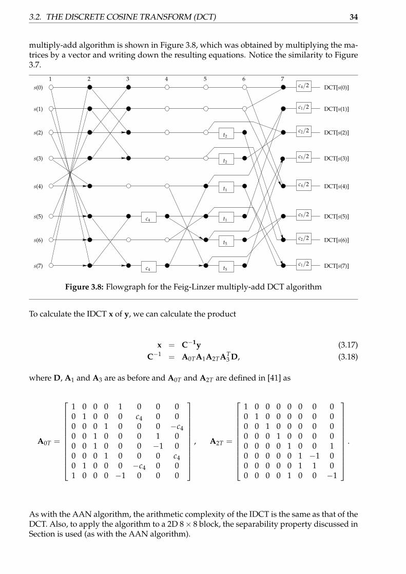
3.2. THE DISCRETE COSINE TRANSFORM (DCT) 34
multiply-add algorithm is shown in Figure 3.8, which was obtained by multiplying the ma-trices by a vector and writing down the resulting equations. Notice the similarity to Figure3.7.
s(0)
s(1)
s(2)
s(3)
s(4)
s(5)
s(6)
s(7)
DCT[s(0)]
1 2 3 4 5 6 7
c4
c4
DCT[s(1)]
DCT[s(2)]
DCT[s(3)]
DCT[s(4)]
DCT[s(5)]
DCT[s(6)]
DCT[s(7)]
t2
t2
t1
t1
t5
t5
c1/2
c2/2
c5/2
c4/2
c5/2
c2/2
c1/2
c4/2
Figure 3.8: Flowgraph for the Feig-Linzer multiply-add DCT algorithm
To calculate the IDCT x of y, we can calculate the product
x = C−1y (3.17)C−1 = A0TA1A2TAT
3 D, (3.18)
where D, A1 and A3 are as before and A0T and A2T are defined in [41] as
A0T =
1 0 0 0 1 0 0 00 1 0 0 0 c4 0 00 0 0 1 0 0 0 −c40 0 1 0 0 0 1 00 0 1 0 0 0 −1 00 0 0 1 0 0 0 c40 1 0 0 0 −c4 0 01 0 0 0 −1 0 0 0
, A2T =
1 0 0 0 0 0 0 00 1 0 0 0 0 0 00 0 1 0 0 0 0 00 0 0 1 0 0 0 00 0 0 0 1 0 0 10 0 0 0 0 1 −1 00 0 0 0 0 1 1 00 0 0 0 1 0 0 −1
.
As with the AAN algorithm, the arithmetic complexity of the IDCT is the same as that of theDCT. Also, to apply the algorithm to a 2D 8× 8 block, the separability property discussed inSection is used (as with the AAN algorithm).

CHAPTER 3. DATA COMPRESSION AND PREVIOUS WORK 35
This algorithm has been implemented on both the CPU and GPU in this project. We considerthe implementation in the next chapter.
The Optimal Feig-Linzer Algorithm The AAN and Feig-Linzer multiply-add algorithmare not the optimal methods for 2D 8× 8 DCTs in terms of arithmetic complexity. Since thesealgorithms only compute 1D 8-point DCTs, they must be implemented separably to calculatethe DCT of a two-dimensional data set. It turns out that approaches that are tailored to two-dimensional inputs reduce the total arithmetic complexity. The algorithm with the lowestarithmetic complexity for calculating a 2D 8 × 8 DCT is the optimal Feig-Linzer algorithm6
[42], which expresses the 2D transform as a series of tensor products. By manipulating theorder in which the tensor products are calculated, several multiplications and additions areeliminated. This leads to a reduction in arithmetic complexity compared to the AAN andFeig-Linzer multiply-add algorithms. This approach has proven to improve performance invideo compression applications employing the DCT [43].
But even though the optimal Feig-Linzer algorithm is the currently optimal algorithm interms of arithmetic complexity, it might not be the optimal algorithm in practice. We discussthe reasons for this in Section 3.2.5 below.
Integer methods
Algorithms have been developed to calculate the DCT using integer computation [44]. Suchalgorithms usually introduce rounding errors in the result, and there is certainly no advan-tage (rather, there is a disadvantage) to using integer instead of floating point computationon the GPU. Since it is more fair to compare GPU floating point performance to CPU float-ing point performance and not CPU integer performance, and since floating point versionsare most used in practice (e.g. in libraries for JPEG and MP3 encoding and decoding), wewill not consider such algorithms further in this report and focus on floating point DCTalgorithms.
3.2.5 Comparisons of DCT methods
Let us look at how the methods we discussed in the previous section compare. ConsiderTable 3.1 on the next page, which shows the approximate7 arithmetic complexity of each ofthe DCT/IDCT algorithms we have discussed when applied to an 8× 8 input data set. Thenumbers include any normalization operations. The table shows the total number of mul-tiplications and additions used (floating-point operations), and also how many multiplica-tions and additions may be fused together in one multiply-add instructions. These numbersare only theoretical; in practice, the compiler might decide not to use fused instructions forall multiplications followed by additions.
The FFTW library complexity was obtained by creating a plan for a 2D 8× 8 DCT and usingthe FFTW_MEASURE parameter, which executes all several FFTW algorithms and selects thequickest algorithm.8
6Note that this is a completely different algorithm than the Feig-Linzer multiply-add algorithm.7The real arithmetic complexity depends on the underlying architecture and compiler used.8This was done on both an Intel Core 2 Duo 2.13 GHz and an Intel Xeon 5160 3.0 GHz, running Linux and
FFTW 3.1.2.

3.2. THE DISCRETE COSINE TRANSFORM (DCT) 36
Algorithm Multipl. Additions Multiply-adds FL ops.Direct separable 976 0 112 1200FFTW library 224 320 96 736AAN separable 208 464 0 672FL multiply-add 64 256 160 640FL optimal 94 432 30 586
Table 3.1: Arithmetic complexity of methods for obtaining the DCT of an 8× 8 input. Num-bers for the optimal FL algorithm were obtained from [28].
Although, as the FFTW authors note in [34], arithmetic complexity might not be the mostimportant factor in choosing what algorithm to use, it is still of some importance. In termsof arithmetic complexity, the optimal Feig-Linzer 2D DCT algorithm is clearly the winner,since it uses the least floating point operations9. The AAN algorithm and the Feig-Linzermultiply-add algorithms have fairly similar arithmetic complexity. AAN uses less multipli-cations than FL multiply-add, but in turn uses more additions. The Feig-Linzer multiply-add algorithm will likely have an advantage on the GPU since, as mentioned earlier, mostmultiplications can be fused with additions, which suits GPU architecture much better thanperforming separate multiplications and additions. The FFTW library uses more multiplica-tions than AAN and FL multiply-add; this is probably due to FFTW using FFT subroutinesdirectly to calculate the DCT, which requires the input to be modified prior to computation.It is also necessary to normalize the output from the FFTW library in order to obtain the DCTwe defined in Definition 1. But even if we exclude the normalization operations from theFFTW library complexity in Table 3.1, the arithmetic complexity is still greater than the AANand Feig-Linzer multiply-add algorithms (even if normalization operations are not excludedfrom the arithmetic complexity of these algorithms).
Most of the algorithms discussed can be implemented on the GPU. The AAN and Feig-Linzer multiply-add algorithms have been implemented on the GPU in this project, andwe discuss the implementations in the next chapter. Although it would be interesting toimplement the optimal Feig-Linzer DCT, it is not very well suited for GPU implementation.The problem is that an efficient implementation of the optimal Feig-Linzer DCT algorithmwould have to consider the entire 8× 8 block at once, while only 8 elements are considererdat a time when doing the AAN and Feig-Linzer multiply-add algorithms. It is currently notpossible for a fragment processor to output 64 elements at one time, since each invocation ofa fragment program can only output one pixel value (4 floating point values) to maximum 4render targets, which gives a total of 16 values. Thus to implement the optimal Feig-LinzerDCT algorithm, blocks would have to be split up, and there would have to be branchinginstructions (or equivalent computations) in the fragment processor programs to determinewhat part of a block it is going to compute. This would destroy the algorithmical advantageof the optimal Feig-Linzer DCT algorithm.
The other algorithms only process 8 elements at a time, which makes branching unnecessary,since all 8 transform values can be written directly to GPU texture memory. In practice, theoptimal Feig-Linzer algorithm is not usually used, since the other algorithms are usually justas quick in practice. For instance, the Independent JPEG Group’s open source JPEG libraryuses the AAN algorithm. Finally, and most importantly, this algorithm is of no use whencomputing more advanced, superior transforms such as the LOT in the next section, sincecomputing the LOT requires computing 1D DCTs.
9Note that multiplications and additions usually take the same amount of time on both GPUs and modernCPUs.

CHAPTER 3. DATA COMPRESSION AND PREVIOUS WORK 37
For these reasons, we have implemented the AAN and the Feig-Linzer multiply-add algo-rithms on the GPU, but not the optimal Feig-Linzer algorithm.
3.2.6 Previous DCT Implementations on the GPU
There have been two previously known DCT implementations on the GPU.
NVIDIA AAN Implementation
NVIDIA Corporation has available a DCT/IDCT implementation using the AAN algorithm10.However, it is not optimal (which is also stated in the source code) in three aspects:
1. AAN implementation is not vectorized. The NVIDIA code does not use any vectorized op-erations. Using vector instructions is highly important when using the GPU, since theGPU fragment processors only operate on four-component vectors. The GPU versionof the AAN algorithm implemented in this project uses vector instructions to nearlythe maximum possible extent.
2. Does not use vertex processors. The NVIDIA code only loads the fragment processors,and does not utilize the power of the vertex processors at all. There are not many usesfor the vertex processors, since they deal with vertices instead of individual pixels,but the AAN version implemented in this project uses the vertex processors for a fewcalculations. Note that in the GeForce 8 series of GPUs, released when this report wasin preparation, uses a unified shader architecture which uses just one processor corefor both vertex, geometry and fragment processors. It is unclear whether using vertexprograms will still be advantageous on this GPU.
3. Does not use OpenGL Frame buffer objects (FBOs). Previously, to read data from the GPU,so-called pbuffers had to be used. Pbuffers were not originally designed for GPGPUusage, and are also very slow and not fully supported on platforms other than Win-dows. The code in this project uses the relatively recent frame-buffer objects OpenGLextension, which is a method of transferring data to and from the GPU, which wascreated with GPGPU applications in mind. This method is quicker and more portablethan pbuffers. (The reason the NVIDIA code uses pbuffers is likely because it is from2004).
In addition, the Feig-Linzer multiply-algorithm should be superior to AAN on the GPU.
Microsoft Research Asia / Zheijiang University Implementation
The second DCT/IDCT implementation on the GPU has been done by researchers at Mi-crosoft Research Asia and Zheijiang University in China, who in [45] argue that entirelynew DCT/IDCT algorithms must be developed for the GPU, because current algorithms areoptimized for the CPU’s cache. The paper presents GPU DCT implementations based onplain matrix multiplication, which is essentially the same algorithm as the naive separableDCT algorithm (see Table 3.1). Microsoft Corporation has a patent pending on this work inU.S. Patent Application number 2006020411911, where an elaboration on the choice of plainmatrix multiplication can be found:
10Available from http://download.developer.nvidia.com/developer/SDK/Individual_Samples/gpgpu_samples.html.
11Note that the work in this project in no way uses methods from the patent application. We use entirelydifferent methods, and have not considered implementing DCT (or the LOT) using plain matrix multiplication.

3.3. THE LAPPED ORTHOGONAL TRANSFORM (LOT) 38
[0041] It is desirable to use fast algorithms or techniques instead of direct matrix mul-tiplication for implementing a DCT/IDCT on a GPU. On the other hand, a GPU is gener-ally considered a stream processor and its internal processing engine is highly pipelined.As a result, the programming model of GPUs may be somewhat limited, mainly due tothe lack of random access writes. Moreover, each pixel (and correspondingly the internalgraphics engine) can have only up to four channels, for example, which implies at mostfour coefficients can be determined a time. With a GPU, the cost of addition, multipli-cation, multiplication and addition (MAD) and dot product of up to 4-element vectors(dp4) is the same. Moreover, the GPU is intrinsically a SIMD (single instruction, mul-tiple data) machine and the spatial data parallelism can be efficiently exploited. Based onthese factors, it is desirable to implement the DCT/IDCT by direct matrix multiplication.
The methods presented in the paper (and patent application) are unable to outperform theFFT-based SIMD-optimized methods on the single-core CPUs (see [45]). There is some roomfor improvements to their method. First, the naive separable DCT algorithm is slow, whilethe CPU algorithms which the paper compares the GPU algorithms with are FFT-methods.Although the 4-element dot product is used, which costs about the same as a multiply-add operation on the GPU, more instructions are still needed compared to the AAN or FLmultiply-add algorithms. Second, and probably more importantly: When plain matrix mul-tiplications are used, the fragment programs must in addition to input data also fetch matrixcoefficients from texture memory. The coefficients are stored as separate textures. This in-creases the number of texture memory accesses and could decrease the locality of the mem-ory accesses. This is unnecessary with the AAN or FL multiply-add methods implementedin this project. Thus, these methods should be able to outperform the methods in [45]. Thereis no reason why a naive DCT algorithm based on matrix multiplication should be quickerthan FFT-based methods on the GPU — in fact, it has been demonstrated in [6] that the FFT(which AAN and FL multiply-add are based on) perform very well on the GPU.
As we shall see, we have successfully managed to implement quicker DCT algorithms —where each fragment processor processes 8 coefficients at a time — and more advancedtransforms (the LOT) on the GPU while at the same time exploiting pipelining and the SIMDarchitecture of the GPU. However, note that our implementations are specialized for 8 × 8DCTs, while the Microsoft implementation generalizes to other block sizes more easily.
3.3 The Lapped Orthogonal Transform (LOT)
As we mentioned in the previous section, the DCT has certain disadvantages. We will inthis section describe the lapped orthogonal transform [46, 47, 30], or the LOT, which attemptsto solve the blocking-problem of the DCT. The LOT and an efficient algorithm for LOT com-putation was invented by Henrique S. Malvar in the 1980s. It has been shown that the LOTgives both objectively and subjectively better compression results than using the DCT byitself [30]. As we did for the DCT in the previous section, we will first give a description ofthe LOT transform in Section 3.3.1. Then, we will describe some properties of the transformand a fast algorithm for computing the transform in Sections 3.3.2 and 3.3.3, respectively.Finally, we look at the arithmetic complexity of the fast LOT algorithm in Section 3.3.4.

CHAPTER 3. DATA COMPRESSION AND PREVIOUS WORK 39
3.3.1 Description of the LOT
The lapped orthogonal transform12 is defined as follows [46, 30]. Consider M > 1 blocks ofN > 0 sample values, i.e. MN sample values x = [x0 · · · xMN−1]T. The transformed valuesy = [y0 · · · yMN−1]T may be written as a matrix-vector product
y = Tx (3.19)
T =
P1 0
P0. . .
0 P2
. (3.20)
T the MN × MN transform matrix containing the LOT basis functions (just as C is the trans-form matrix containing the DCT basis functions in Equation 3.15). P0 is an L × N matrixwith the LOT basis functions for each block. L is the number of sample values in each blockplus the number of overlapping sample values used, such that each block overlaps otherblocks with L− N sample values. P1 and P2 are matrices based on P0, but are adjusted sincethe first and last blocks only have one neighbouring block.
Now we choose L = 2N so that each block overlaps neighbouring blocks by 2N − N = Nsample values and P0 is of size 2N × N. One choice for P0 that works well is
P0 = PZ (3.21)
where
P =12
[De − Do De − Do
J(De − Do) J(Do − De)
]. (3.22)
(3.23)
Here, De and Do are, respectively, matrices of size N × N/2 containing the even and oddDCT basis functions for the current block. That is, if we write the transform in Definition 1as a matrix-vector product, but separate the even and odd DCT coefficients, we get the Deand Do. J is the N × N/2 counteridentity or anti-identity matrix, i.e. a matrix containing allzero values except values equal to 1 along its second diagonal (i.e. the diagonal going fromthe last row in the first column to the first row in the last column).
It can be shown [46] that a near-optimal Z matrix is given by
Z =[
I 00 Z̃
], (3.24)
12We are really describing one specific LOT. In general, it is possible to define other LOTs which are not basedon the DCT and do slightly more computations to further improve energy compaction properties. However,these are of limited practical interest since they have no quick algorithms and do not give any significantadvantages. The LOT we describe is near-optimal and has a fast algorithm.
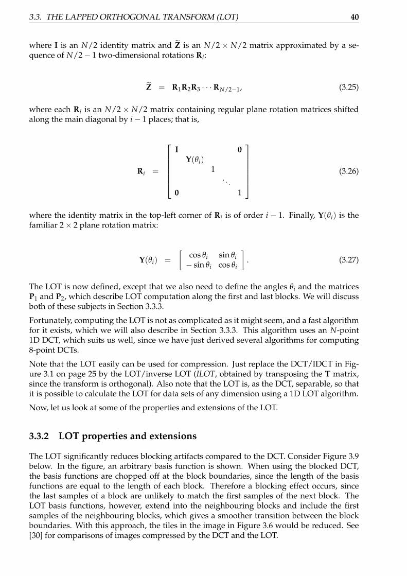
3.3. THE LAPPED ORTHOGONAL TRANSFORM (LOT) 40
where I is an N/2 identity matrix and Z̃ is an N/2 × N/2 matrix approximated by a se-quence of N/2− 1 two-dimensional rotations Ri:
Z̃ = R1R2R3 · · ·RN/2−1, (3.25)
where each Ri is an N/2 × N/2 matrix containing regular plane rotation matrices shiftedalong the main diagonal by i − 1 places; that is,
Ri =
I 0
Y(θi)1
. . .0 1
(3.26)
where the identity matrix in the top-left corner of Ri is of order i − 1. Finally, Y(θi) is thefamiliar 2× 2 plane rotation matrix:
Y(θi) =[
cos θi sin θi− sin θi cos θi
]. (3.27)
The LOT is now defined, except that we also need to define the angles θi and the matricesP1 and P2, which describe LOT computation along the first and last blocks. We will discussboth of these subjects in Section 3.3.3.
Fortunately, computing the LOT is not as complicated as it might seem, and a fast algorithmfor it exists, which we will also describe in Section 3.3.3. This algorithm uses an N-point1D DCT, which suits us well, since we have just derived several algorithms for computing8-point DCTs.
Note that the LOT easily can be used for compression. Just replace the DCT/IDCT in Fig-ure 3.1 on page 25 by the LOT/inverse LOT (ILOT, obtained by transposing the T matrix,since the transform is orthogonal). Also note that the LOT is, as the DCT, separable, so thatit is possible to calculate the LOT for data sets of any dimension using a 1D LOT algorithm.
Now, let us look at some of the properties and extensions of the LOT.
3.3.2 LOT properties and extensions
The LOT significantly reduces blocking artifacts compared to the DCT. Consider Figure 3.9below. In the figure, an arbitrary basis function is shown. When using the blocked DCT,the basis functions are chopped off at the block boundaries, since the length of the basisfunctions are equal to the length of each block. Therefore a blocking effect occurs, sincethe last samples of a block are unlikely to match the first samples of the next block. TheLOT basis functions, however, extend into the neighbouring blocks and include the firstsamples of the neighbouring blocks, which gives a smoother transition between the blockboundaries. With this approach, the tiles in the image in Figure 3.6 would be reduced. See[30] for comparisons of images compressed by the DCT and the LOT.

CHAPTER 3. DATA COMPRESSION AND PREVIOUS WORK 41
Block 1
Block 1
Block 2
Block 2
Overlapping region
DCT basis functions
LOT basis functions
Figure 3.9: Illustration of the DCT and LOT basis functions at block boundaries, adaptedfrom Malvar’s book on the LOT [30]
There have been other attempts at solving the blocking problem of the DCT. One approachis to apply a smoothing filter before or after DCT computation, another approach is to usethe infinite-length basis functions of the short-space Fourier transform (SSFT) [48]. Thesemethods, however, either decrease attainable compression ratios or introduce new artifactssuch as artificial rings in the image [30].
But there are several even more advanced methods based on the LOT, such as the gener-alized lapped orthogonal transform (GenLOT) [49] and generalized unequal-length lapped orthog-onal transform (GULLOT) [50], which reduce the number of artifacts even further. Theseare among the most superior transform coding methods for image compression currentlyknown. They are particularly well suited for seismological data [51, 52], which has greaterrequirements for accurate reconstruction than regular photographies. Applications runningon clusters and executing calculations on such seismological data, which is often very large,will benefit from compressing the data with LOT-based methods when communicating withinternal nodes and outside clients.
The GenLOT methods can be seen as a generalization of the LOT and the DCT. The DCTis the simplest GenLOT (an order-1 GenLOT), while the LOT is an order-2 GenLOT. Just asthe LOT adds a step after the DCT, as we shall see in the next section, GenLOT methodsof higher orders add several steps after computing the LOT to reduce artifacts occuringbetween a block and non-neighbouring blocks. Thus GenLOT corresponds to increasing thelength of the basis functions in Figure 3.9 even further.
The GULLOT method solves problems related to spread of quantization error to neighbour-ing blocks when using GenLOT [50]. GULLOT is a generalization of GenLOT in which thebasis functions may be on unequal length, as opposed to the GenLOT, LOT and DCT, wherebasis functions are always of fixed length. Thus GenLOT, LOT and DCT are all special casesof GULLOT. Thus, for instance, DCT may be viewed as a special case of an order-1 GULLOTwhere all the basis functions have the same length.
LOT-based methods are not the only solution to the blocking problem of the DCT. Usingthe discrete wavelet transform (DWT) reduces blocking problems and is used in the newJPEG-2000 standard. DWT-based methods have an advantage over DCT in that they notonly give what frequencies occur in the image, but also detect precisely where in the image

3.3. THE LAPPED ORTHOGONAL TRANSFORM (LOT) 42
the frequencies are “located”. This can be exploited so that high quantization levels are usedin areas with no high frequencies, and lower quantization levels are used in areas with manydetails, thus reducing the blocking effects. But DWT-based methods have certain problems.Significant artifacts can still occur — for example, artificial rings may be introduced in theimage. LOT-based methods have been proven to be superior for many types of images, bothobjectively (in terms of signal-to-noise ratio) and subjectively [53, 51].
Note that the theoretically optimal transform coding algorithm can be proven to be theKarhunen-Loève transform [30]. This transform, however, has no fast algorithm, and re-quires to be adjusted for the specific input sample values it is applied to. It has been shownthat the methods discussed in this section are good approximations to this transform. TheDCT is one good approximation, and the LOT is an even better approximation.
We will now look at an algorithm for computing the LOT using a block size of 8.
3.3.3 Computing the LOT and ILOT
Consider the flowgraph in Figure 3.10, which shows an implementation of the LOT de-scribed in Section 3.3.1 with N = 8. We will use the separability property of the LOT tocompute the 2D 8 × 8 LOT of an image. The following algorithm, by Malvar [46, 30], isknown as the Fast LOT algorithm, which computes a 1D LOT with a block size of 8. Thealgorithm described in this section is a type-I fast LOT. For larger block sizes (> 16), anotheralgorithm, known as type-II fast LOT can be used.
In the figure, we show type-I fast LOT computation for two blocks in the middle of somedata set s(k). The flowgraph corresponds to multiplying the input data set by one of theP0 matrices). To obtain the inverse type-I fast LOT, we simply traverse the flowgraph fromright to left instead of left to right — as with all other orthogonal transforms — and replacethe DCT by the IDCT.
It is easy to show that the first part of the flowgraph, consisting of computing the DCT,executing the first merge or butterfly on the resulting DCT coefficients, and then executingthe second butterfly and multiplying by 1/2 corresponds to multiplying the input values bythe P matrix of Section 3.3.1. Similarly, the final step is equivalent to multiplying by the Zmatrix, since half of the first coefficients are multiplied by the identity matrix and the otherhalf is multiplied by the Z̃ matrix. The flowgraph for multiplying by Z̃ — which is just acascade of multiplications by N/2 − 1 (in this case, 3) planar rotation matrices — is shownin Figure 3.11. A single planar rotation matrix is shown in Figure 3.12.
The Y(θi) rotation matrix in Figure 3.11 is shown as a flowgraph in Figure 3.12.
It can be proven [30] that approximate optimal angles for an 8-point LOT θ1, θ2, θ3 are givenby
[θ1 θ2 θ3] = [0.13π 0.16π 0.13π]. (3.28)
The final question is how to compute the LOT for the entire data segment, i.e. how to definethe P1 and P2 matrices of Section 3.3.1. There are several alternatives for extending the dataset at the boundaries.
We have used a simple boundary extension scheme in our implementations. This schemefirst extends the data set by N = 8 sample values both before the first and after the last

CHAPTER 3. DATA COMPRESSION AND PREVIOUS WORK 43
s(k + 10)
s(k)s(k + 1)
s(k + 2)
s(k + 3)
s(k + 4)
s(k + 5)s(k + 6)s(k + 7)
s(k + 8)s(k + 9)
s(k + 11)
s(k + 12)s(k + 13)
s(k + 14)s(k + 15)
1
2
3
4
567
0
01
2
3
45
67
02
4
6
1
357
02
6
57
13
4
...
.........
...
......
...
1/2
DCT
DCT
Multiplication by Z
Z̃
Multiplication by P
...
......
......
......
......
.........
...
...
...
...
LOT[0]
LOT[2]LOT[4]LOT[6]
LOT[1]LOT[3]
LOT[5]
LOT[7]
Figure 3.10: Flowgraph for the fast type-I LOT algorithm, with blocksize 8, adapted fromMalvar’s book on the LOT [30].
sample values. The new sample values are set to zero. When executing the transform,the DCT of the new first and last blocks will always evaluate to zero. Similarly, the firstbutterflies in Figure 3.10 for these blocks will also evaluate to zero. However, the secondbutterflies will introduce nonzero values in the, respectively, last and first halves of the newfirst and last blocks. These nonzero values are stored with the other transformed values,since not including them leads to artifacts along the boundaries. The image can then berestored without any artifacts by applying the inverse LOT transform.
Using this scheme implies that we need to store 8 additional values for each row and eachcolumn in an image in order to avoid artifacts around the image boundaries. For an imageof size 1024 × 1024, these extra values lead to 1.5% extra values having to be stored afterthe transform. Therefore, the compression ratio will slightly increase. But the advantage ofusing this scheme is that the same operation can be done on each block. In other words, wedo not need to treat the first and last blocks specially, as e.g. the scheme in [30] (implementedwith no modifications) would require. Doing the same operation on all blocks and avoidingspecial cases is very advantageous on the GPU, since special cases often requires branching,which is slow.
In any event, boundary extensions are best suited to be done on the CPU, and the LOTimplementations developed in this project can easily be used with certain more advancedschemes which would not require storing the extra values. For example, when using asymmetrical boundary extension, an application using our LOT implementation can extendthe data set symmetrically before calling the LOT routines, and discard unneccessary extravalues (which do not account for much of the total arithmetic complexity of the routine).In that way, storing the extra values is not necessary and only 8M values must be storedfor an M-block data set (instead of 8(M + 1) in our present implementation). Thus our

3.3. THE LAPPED ORTHOGONAL TRANSFORM (LOT) 44
Z̃
Y(θ2)
Y(θ3)
Y(θ1)
Figure 3.11: Flowgraph for the Z̃-block in Figure 3.10, based on a similar figure from Mal-var’s book and article [46, 30].
cos θi
sin θi
cos θi
sin θi
Figure 3.12: Flowgraph for the Y(θi)-matrix in Figure 3.11, based on a similar figure fromMalvar’s book and article [46, 30].
implementations can also be used with more advanced boundary extension schemes.
Figure 3.13 illustrates how the LOT is computed for an entire data set, along with our bound-ary extension scheme. Note that the section inside the dotted lines represents the operationin Figure 3.10. Also, notice that the first and last blocks are the extended blocks set to zero,and that the first and last halves of the first and last blocks, respectively, will always be

CHAPTER 3. DATA COMPRESSION AND PREVIOUS WORK 45
zero, but not the other halves, which must be stored in order to avoid artifacts. But it isevident from the figure that setting the extra blocks to zero enables us to do exactly the samecomputation on all the blocks, which makes the LOT easier to implement on the GPU.
Block 1
LOT block 1
DCTFirstbutterfliesBlock 2
......
......
...... ...
· · ·
Block M
· · ·
Zero-block
Zero-block DCTFirstbutterflies
DCTFirstbutterflies
DCTFirstbutterflies
DCTFirstbutterflies
E
O
E
O
E
O
O
E
E
O
LOT block M
LOT block M + 1
LOT block 2
(Always zero)
(Always zero)
Z̃
Z̃
Z̃
Z̃
Secondbutterflies
Secondbutterflies
Secondbutterflies
Secondbutterfliesand scaling
Figure 3.13: Computing the LOT for a data set, based on a similar figure in Malvar’s bookand article [30, 46]. The section inside dotted lines represent the steps of Figure 3.10. Notethat the figure is just a sequence of several such steps.
3.3.4 Arithmetic Complexity of the LOT
The LOT transform has not received the same popularity as the DCT, primarily due to theLOT requiring more computations. Consider Table 3.213 which shows the arithmetic com-plexity of the DCT and the LOT of an 8 × 8 block when the DCT part of the LOT is im-plemented with the 1D 8-point DCT algorithm of the lowest arithmetic complexity on newmachines (the Feig-Linzer multiply-add algorithm). The arithmetic complexity of the LOTfor a single 8-point block is 8 multiplications for the 1/2 scalings, 6 multiplications for theZ̃-block, 16 additions/subtractions for the two butterflies, and 6 multiply-adds for the Z̃-block, in addition to the arithmetic complexity of the Feig-Linzer multiply-add DCT for 8points.
Algorithm Multipl. Additions/ Multiply-adds FL ops.subtractions
FL multiply-add DCT 64 256 160 640Fast LOT using FL multiply-add DCT 288 512 256 1312
Table 3.2: Arithmetic complexity of the DCT and the LOT on an 8× 8 input
13A similar table for an 8-point 1D LOT occurs in [30]. However, that table assumes the AAN DCT algorithmis used, which is less optimal on machines where multiplications and additions take the same amount of time(which is true for all recent CPUs and GPUs). Also, the 1/2 scalings are not included.
3.3. THE LAPPED ORTHOGONAL TRANSFORM (LOT) 46
From the table, we see that the LOT requires more than twice as much operations as theFeig-Linzer multiply-add DCT. This suggests that a GPU implementation will give goodperformance, and that the LOT is actually better suited for the GPU than the DCT, due tothe higher arithmetic intensity than the DCT. Furthermore, all LOT steps except for the Z̃-block multiplication are suitable for vectorization (the first and second butterflies can beimplemented using one vector instruction) — which also fits the GPU well.
The LOT described in the past sections has been implemented on both the CPU (both singleand multi-core versions) and the GPU in this project. We look at the implementations in thenext chapter.
3.3.5 Previous LOT Implementations on the GPU
No previous publically known implementations of the LOT on the GPU are known.

Chapter 4
Implementation
This chapter describes how the DCT and LOT transforms have been implemented on theCPU and GPU in this project. Implementing these transforms on the GPU requires specialconsiderations, which we will discuss in this chapter. We look at CPU and GPU implemen-tations in Sections 4.1 and 4.2, respectively.
A program has been developed for benchmarking various DCT and LOT algorithms. Theprogram consists of about 16,000 lines of code, where 13000 lines are C code and 3000 linesare NVIDIA Cg code. An overview of the program is given in Appendix A.
The source code for the program developed can be found on the CD accompanying thisreport in the dct directory. We will show excerpts from the source code throughout thischapter and in the appendices.
4.1 CPU Implementations
The CPU implementations of the algorithms for the DCT/IDCT are in the files:
• dct_cpu.c: The direct separable DCT
• dct_fftw.c: The DCT through the FFTW library (both simple and advanced inter-face)
• dct_cpu_aan.c: The AAN algorithm
• dct_cpu_flmad.c: The FL multiply-add algorithm
• dct_cpu_aan_openmp.c: The AAN algorithm, OpenMP version
• dct_cpu_flmad_openmp.c: The FL multiply-add algorithm, OpenMP version
LOT/ILOT CPU implementations are in the files
• lot_cpu.c: Fast LOT
• lot_cpu_openmp.c: Fast LOT, OpenMP version
We will now briefly describe each implementation in turn.
4.1.1 Direct Separable DCT: dct_cpu.c
The direct separable DCT implementation is just an implementation of the equations in Def-inition 1 in the previous chapter. The algorithm first applies the equations to each row of
47

4.1. CPU IMPLEMENTATIONS 48
the input block, and then to each column. This is done for all the blocks in the input. Thisalgorithm is very slow, and is only included for completeness and checking the results ofthe other algorithms.
4.1.2 FFTW DCT: dct_fftw.c
The FFTW implementation is also quite simple, since the FFTW library does the actual com-putations.
FFTW uses plans to specify what computations are to be done, data set sizes, and whatbuffers should be used for input and output. There are two ways of using FFTW to computea blocked DCT. Either, the application can create a plan for an 8× 8 DCT, and split the inputset into separate 8 × 8 blocks and run the FFTW plan on each block. This is referred to the“simple” interface of FFTW, and requires that the application copies blocks into and out ofthe buffers specified when creating the plan. This can induce some overhead. Alternatively,we may use FFTW’s “advanced” interface, which allows for blocked transforms, to createan 8× 8 blocked DCT of the entire data set. In that case, a single plan execution is required.
The steps for computing the DCT using FFTW can be summarized as follows.
1. Create an FFTW plan for the computation using fftw_plan_r2r_2d (simple in-terface) or fftw_plan_many_r2r (advanced interface). The transform we use isFFTW_REDFT10 or FFTW_REDFT01, which is, respectively, the DCT or IDCT of theinput. The time the planning func tion takes is not included in any timings, since it canuse considerable amounts of time and does not actually compute any results. We alsouse the FFTW_MEASURE parameter, which executes several algorithms for calculatingthe specified transform and chooses the best one.
2. If executing the IDCT, scale inputs to FFTW according to Equations B.5 through B.8 inSection B.1 on page 83.
3. Execute the plan using fftw_execute. This does the actual computation.
4. If executing the forward DCT, scale outputs from FFTW according to Equations B.1through B.4 in Section B.1 on page 83.
5. If the simple interface is used, steps 2–4 are done for all blocks. If not, they are onlydone once.
The number of multiplications, additions and fused multiplications and additions is alsodisplayed. This number is not the same as the numbers in Table 3.1, since those numbersalso include input/output scalings.
Our FFTW implementation supports using FFTW with threads, and enables them automati-cally if linked to a FFTW library compiled to support threads. We have, however, not bench-marked FFTW with threads, since often, FFTW will choose not to use threads even if threadusage is requested.
4.1.3 AAN DCT: dct_cpu_aan.c
The implementation of the AAN algorithm is based on Figure 3.7 on page 32. For each blockin the input, we first apply the AAN to the rows and next to the columns. Explicit equationsfor the AAN DCT/IDCT are derived in [28], and our implementation is based directly onthose equations. DCT and IDCT has been implemented. See Section ?? on page ?? for sourcecode excerpts.

CHAPTER 4. IMPLEMENTATION 49
4.1.4 FL Multiply-Add DCT: dct_cpu_flmad.c
The implementation of the Feig-Linzer multiply-add algorithm is based on Figure 3.8 onpage 34 and the matrix equations for the algorithm in the previous chapter. As with the AANalgorithm, we first apply Feig-Linzer multiply-add to each row and then to each column ofall the blocks. Both DCT and IDCT has been implemented.
4.1.5 Fast LOT Implementation: lot_cpu.c
The fast LOT/ILOT implementations are based directly on Figures 3.10 on page 43 and 3.13 onpage 45. The LOT is, as the DCT, a separable transform [30], so in order to compute an 8× 82D LOT, we first compute the 8-point LOT in the x-direction and then the 8-point LOT inthe y-direction. Similarly, computing the 2D 8× 8 ILOT is done by computing a 1D ILOT ineach direction.
The fast LOT requires a 1D DCT algorithm. We have chosen to use the Feig-Linzer multiply-add algorithm for DCT and IDCT due to its low computational complexity.
We described the boundary extension scheme in Section 3.3.3 on page 42. This is imple-mented as follows: When computing the forward LOT, if the initial input data set size isN × N, the data set is extended to (N + 16)× (N + 16). The extra boundary values are ini-tially set to zero. From Figure 3.13 on page 45, it is evident that the first half of the firstextended block and the last half of the last extended block in each dimension will alwaysbe zero after the FLOT has been computed. The zero values are discarded after the forwardLOT computation is done, so that only (N + 8)× (N + 8) values are stored. See Figure 4.1 onthe following page.
Why do we allocate an (N + 16)× (N + 16) array when we only need an (N + 8)× (N + 8)array? The reason is that when executing the LOT on the GPU, letting the input data set bea set of full blocks (which it is not when we use an (N + 8) × (N + 8) array, since the firstfour values and the last four values will only be a “half” block), is advantageous. Allocatingthe extra blocks allows us to more easily apply exactly the same operation to all 8× 8 blocksof the data set, which is very important on the GPU, since it does not deal with special casesalong the boundaries very well.
While allocating an extra (N + 16)2 − (N + 8)2 = 16N + 192 values which will always bezero is not necessary on the CPU, the code that reads the input file is independent from thespecific algorithm used, so we allocate the extended array on the CPU as well. But both onthe CPU and GPU, we avoid doing the DCT and first butterfly on the first and last blocks ineach dimension.
When computing the inverse LOT, we read in (N + 8) × (N + 8) values from a file andextend the data set to (N + 16) × (N + 16) for the same reasons as for the forward LOT(simpler addressing on the GPU). We also avoid computing the obviously redundant inversefirst butterflies and IDCT on the first and last extended blocks. After computation, the extravalues are cut off and the original N × N data set is produced as output.
4.1.6 OpenMP Versions: *_openmp.c
OpenMP versions of the AAN, Feig-Linzer multiply-add and fast LOT algorithms have alsobeen developed1.
1It might seem strange to include separate OpenMP versions of the algorithms, since with number ofthreads set to 1, these algorithms do exactly the same as the non-OpenMP versions with very little or no over-

4.1. CPU IMPLEMENTATIONS 50
Original input data set
8 8 8 8
88
N
8
8
Extended blocks always equal to zero
Extended blocks not necessarily zero after forward LOT
N
Figure 4.1: LOT boundary extension implementation. All values except the first and last 8values of each dimension (white boxes) are stored.
There are several choices as to how to parallelize the loops of the AAN and FL multiply-addalgorithms. Consider Figure 4.2 below.
One way to use OpenMP, shown on the left side of Figure 4.2 is to compute each blocksequentially and divide the computations of the rows and columns between the threads.This corresponds to parallelizing the inner loop (which iterates over all the row/columns ina single block and executes an 8-point transform on each row/column). This is inefficient,because OpenMP will execute a fork and a join at each iteration of the outer loop, which turnsout to be more expensive than computing the entire 8× 8 DCT or LOT transform using onlyone thread! Therefore, gains from parallelization are lost when using this scheme.
A better scheme is shown on the right side of Figure 4.2. This corresponds to parallelizingthe outer loop (which iterates over all the blocks in the x-direction). This works more effi-ciently since OpenMP overhead is kept to a minimum. Listing 4.1 shows how this has beenimplemented in the OpenMP versions of the AAN, Feig-Linzer multiply-add and fast LOTalgorithms.
#pragma omp p a r a l l e l for p r i v a t e ( x _ s t a r t , y _ s t a r t , /∗ o t h e r per−t h r e a d v a r i a b l e sused in t h e t r a n s f o r m ∗ / )
head. However, annoying warnings may occur when compiling the OpenMP versions on certain compilersnot supporting OpenMP (about unrecognized #pragma directives). I have consequently provided implemen-tations not using OpenMP

CHAPTER 4. IMPLEMENTATION 51
Thread 1
Inefficient choice Efficient choice
Thread 2
Thread 3
Thread 1 Thread 28× 8 blocks
Thread 3
Figure 4.2: Different ways of using OpenMP when computing 2D transforms
for ( x _ s t a r t = 0 ; x _ s t a r t < x_blocks ; x _ s t a r t ++) {for ( y _ s t a r t = 0 ; y _ s t a r t < y_blocks ; y _ s t a r t ++) {
/∗ I n s e r t t r a n s f o r m o f a s i n g l e b l o c k s t a r t i n g a t∗ i n p u t [ y _ s t a r t ∗ l e n g t h ∗ 8 + x _ s t a r t ∗ 8 ] h e r e∗ /
}}
Listing 4.1: OpenMP-parallelized transform loop
Note that the LOT is implemented by a sequence of such loops, since certain steps of theLOT must be done sequentially.
4.2 GPU Implementation
The implementations of the GPU versions of the DCT algorithms are in the files:
• dct_gpu_aan.c and dct_gpu_aan.cg: The AAN algorithm, GPU version
• dct_gpu_flmad.c and dct_gpu_flmad.cg: The FL multiply-add algorithm, GPUversion
• lot_gpu.c and lot_gpu.cg: The AAN algorithm, GPU version
4.2.1 DCT on the GPU
We will now describe how the DCT has been implemented on the GPU. First, we will de-scribe how OpenGL and Cg are initialized and how computation on the GPU is done. Next,

4.2. GPU IMPLEMENTATION 52
we will describe the specific AAN and Feig-Linzer multiply-add implementations. The de-tails are quite complicated, so we will only give an overview. Very specific details can befound in the appendix in Section B.2 on page 84.
Executing Transforms on the GPU
A coarse overview of how our GPU transform implementation works is shown in Figure 4.3.
InitializeOpenGL
Initializeshaders
Uploadtextures
Executecomputation
Downloadresults
Needs to be doneonly once
Done
Figure 4.3: Computing transforms on the GPU
The steps in Figure 4.3 are detailed in Section B.2.1 on page 84. Summarized, they consist of:
1. OpenGL Initialization. This step involves creating an OpenGL coordinate system, de-scribing how coordinates should be interpreted, and a viewport, which describes whatpart of the coordinate system should be viewed from the screen. We set the coordinatesystem up so that there is a one-to-one mapping between texture coordinates, OpenGLgeometry coordinates, projection coordinates and viewport coordinates. This only hasto be done once.
2. Cg Initialization. Next, our GPU fragment and vertex programs are compiled by the Cgruntime. This also only needs to be done once.
3. Texture Upload/Initialization. Next, the input data set is uploaded to the GPU’s texturememory. For reasons described in Section B.2.1 on page 84, we use a single-channeltexture, i.e. a texture containing only “red” and not red, green, blue and alpha chan-nels, to represent the input data set. We also allocate two textures which are usedfor intermediate results. These textures are multi-channel, meaning that each textureelement has four channels. The two multi-channel textures are bound to an OpenGLframebuffer object (FBO 0), and the single-channel input texture is bound to another FBO(FBO 1). Using FBOs allow us to easily render to GPU memory instead of the screen.
4. Computation. After the input data set has been uploaded to the GPU and the texturesare initialized, computation starts. Starting the computation involves simply renderinga large square over the entire target texture. We do the computation in several steps(more on this below).
5. Download. After computation is done, we call OpenGL functions to read the texturefrom GPU memory to RAM.

CHAPTER 4. IMPLEMENTATION 53
The Computation Step
The actual GPU programs for both scattering and DCT/IDCT computation are located in thefiles dct_gpu_aan.cg (AAN algorithm) and dct_gpu_flmad.cg (Feig-Linzer multiply-add). Both 16-bit and 32-bit versions have been developed. Since the forward and inverseDCT are computed in a very similar manner, we will focus our description of forward DCTcomputation. The inverse DCT is simply a reversal of the steps, and is shown in the sourcecode in the appendix. The method of computation is precisely the same whether we useAAN or Feig-Linzer multiply-add, except for the core transform algorithm. The techniquespresented in this section are thus independent of the actual transform algorithm used, aslong as it computes a 1D 8-point transform.
The computation step involves a large amount of technicalities. Everything is thoroughlydocumented in Section ?? on page ??. Here, we only provide a summary of what happens.
Rowscatter
Columntransform
ColumnTo CPU
computation stage
re-used at each scatter stageand used for input/output from/tothe CPU
Rowtransform
FBO 1 single-channel texture
FBO 0 RGBA textures, re-used at each
from CPU/RAMData set
scatter
Figure 4.4: Computing the DCT on the GPU
Consider Figure 4.4. Computing the DCT on the GPU is done by both vertex and fragmentprograms. Recall from Chapter 2 that vertex programs can pass texture coordinates to thefragment programs, and the fragment programs can fetch textures, do computations andwrite the result to texture memory. Fragment programs do most of the job, but we havefound that the vertex processors can also be used for a few small computations.
From Figure 4.4, it is evident that the computation is done in four steps: The steps of com-puting the forward DCT are:

4.2. GPU IMPLEMENTATION 54
1. Row transform fragment program + passthrough vertex program. First, we compute the rowtransform. This program reads 8 elements from a single-channel texture and outputsthe first four transformed values in the first RGBA output texture, and the second fourtransformed values in the other RGBA texture. The vertex program does nothing; it istherefore a “passthrough” program.
2. Row scatter fragment program + passthrough vertex program. Next, we scatter the twoRGBA textures onto the single original input texture. A passthrough vertex programis also employed in this case.
3. Column transform fragment program + column vertex program. Now, a fragment programcomputing the column DCT is executed. Each execution of the program produces 8transform coefficients on two RGBA textures, similarly to the row transform fragmentprogram. A vertex program executes some per-vertex values that are useful whencomputing the address in the single-channel texture where the fragment program willfetch the input values.
4. Column scatter fragment program + column scatter vertex program. Finally, the transformedvalues on the two RGBA textures are scattered on to a single texture, which is down-loaded to the CPU. As with the transform program, a vertex program does some usefulcomputations on the texture coordinates.
We provide summaries of the steps below. For very technical details, see Section B.2.2 onpage 92.
Step 1. Row transform Recall from Chapter 2, where we claimed that fragment programscould only write to a single pre-determined texture memory location. However, each DCTprogram invocation computes eight transform values. This is precisely why we needed twoRBGA textures: Each RBGA texture contains four channels, and since there are two textures,we can write eight values.
However, one problem occurs. We need a mapping between the single-channel texture andthe RBGA texture. During the present step, one fragment program is invoked for each tex-ture location in the RGBA textures. This texture program needs to fetch correct input valuesfrom the single-channel texture. Details on how this is done is shown in Section B.2.2 onpage 92. The mapping between rows in the single-channel texture and the two RGBA tex-tures is shown in Figure 4.5 on the facing page.
Row transform is done by a single fragment program.
Step 2. Row scatter After step 1, we are left with two RGBA textures, and the computedvalues are spread over the two RGBA textures. However, if we are now going to do acolumn transform or download the results to the CPU, we will have a problem. Consider acolumn program doing a column transform on the first column. When the column transformprogram would fetch the first value of the first column from the RGBA textures (see Figure4.5 again), the program would automatically obtain three redundant values. This happenssince there is no way to fetch a single channel from an RGBA textures. Four values are alwaysfetched. In addition, the texture coordinate computations turns out to be complicated if acolumn transform is done over two RGBA textures — i.e. it is more difficult to find a columnof values in the two RGBA textures than in a large single-channel texture (where a columnis simply located along increasing y-coordinates).
This is why we use a scatter program. The row scatter program essentially computes theinverse mapping of the row transform program: The row transform program maps rows

CHAPTER 4. IMPLEMENTATION 55
������������
����������
������������
����������
����������������������������
����������������������
6543210
6543210
4 valuesin eachRGBA texture
Single 4-valuetexture elements
0 1 2 3 4 5 6 70 1 2 3 4 5 6 70 1 2 3 4 5 6 70 1 2 3 4 5 6 70 1 2 3 4 5 6 70 1 2 3 4 5 6 7
Single-channel textureis of size N× N with one channel per texture element,RGBA texture is of size N/4× N/2 with four channels perelement (N× N in total)
7
0 1 2 3 4 5 6 7 0 1 2 3 4 5 6 7
7
Input texture — One value per texture coordinate
RGBA texture 1 — Four values per texture coordinate
RGBA texture 2 — Four values per texture coordinate
Eight 1-valuetexture elements
Figure 4.5: Row mapping between eight texture elements in a single-channel texture andtwo multi-channel textures
from the single-channel texture to locations in the two RGBA textures, while the row scatterprogram maps locations from the two RGBA textures back into correct locations the single-channel texture. This makes the column transform simpler. The row scatter is done by asingle fragment program. As usual, we draw a large square over the target texture (in thiscase, the single-channel texture) to start computation.
Step 3. Column transform The column transform program is similar to the row transformprogram, but we now fetch values from columns instead of rows. Again, transformed valuesare written to the two RGBA textures. Figure 4.6 on the next page shows how the columntransform program map columns from the single-channel texture to the two RGBA-textures.
The column transform program uses a vertex program in addition to the fragment program,since some parts of the texture coordinate computations (computations for mapping coordi-nates of input values in the single-channel texture to the RGBA textures) can be done by thevertex program. See Section B.2.2 on page 92 for the details.
Step 4. Column scatter Finally, we execute a column scatter in order to prepare the trans-formed values for download to the CPU. Note that if we do not do this step, the transformedvalues will be spread out over the two RGBA textures. In order for the CPU to get the valuesin a standard array, we need to execute a column scatter.
The column scatter is similar to the row scatter, but operates on the mapping of Figure 4.6 onthe next page instead of Figure 4.5. See Section B.2.2 on page 92 for furhter information.

4.2. GPU IMPLEMENTATION 56
��������������
���������������������
�������
�����
�����
������������
������
����
������������
������
����
4 valuesin eachRGBA texture
Single 4-valuetexture elements
Single-channel textureis of size N× N with one channel per texture element,RGBA texture is of size N/4× N/2 with four channels perelement (N× N in total)
Input texture — One value per texture coordinate
Eight 1-valuetexture elements
8× 8 blocks
RGBA texture 2 — Four values per texture coordinate
RGBA texture 1 — Four values per texture coordinate
Figure 4.6: Column mapping between eight texture elements in a single-channel texture andtwo multi-channel textures
The Actual DCT Algorithms The row and column scattering is quite tedious. Now for thefun part. We have still not discussed the actual DCT algorithms. The forward Feig-LinzerDCT algorithms is shown in Listing 4.2 below. The AAN, inverse and 16-bit algorithms aresimilar, and can be found on the accompanying CD.
/ / Note t h a t FLMAD_T1 , FLMAD_T2 , e t c a r e p r e d e f i n e d c o n s t a n t svoid dct_gpu_fflmad ( inout f l o a t 4 in0_3 , inout f l o a t 4 in4_7 ){
f l o a t 4 vvec1 , vvec2 ;f l o a t 4 uvec1 , uvec2 ;
f l o a t 4 mvec ;
vvec1 = in0_3 . xywz + in4_7 . wzxy ;vvec2 = f l o a t 4 ( in0_3 . x , in0_3 . y , in0_3 .w, in4_7 . y ) − f l o a t 4 ( in4_7 .w, in4_7 . z ,
in4_7 . x , in0_3 . z ) ;
uvec1 = vvec1 . xyxy + f l o a t 4 ( vvec1 . z , vvec1 .w, − vvec1 . z , − vvec1 .w) ;uvec2 = vvec2 . xyzy + f l o a t 4 ( 0 . 0 , vvec2 .w, 0 . 0 , − vvec2 .w) ;
vvec1 = uvec1 ;vvec2 = FLMAD_C4 ∗ f l o a t 4 ( uvec2 .w, uvec2 . y , −uvec2 . y , −uvec2 .w) + vvec2 . xzzx ;
mvec = f l o a t 4 ( 1 . 0 , FLMAD_T1 , FLMAD_T2 , FLMAD_T5) ;
uvec1 = f l o a t 4 ( vvec1 . x , vvec2 . y , vvec1 .w, vvec2 .w) ∗ mvec + f l o a t 4 ( vvec1 . y ,vvec2 . x , vvec1 . z , − vvec2 . z ) ;
uvec2 = f l o a t 4 ( vvec1 . x , vvec2 . z , vvec1 . z , vvec2 . x ) ∗ mvec . xwzy − f l o a t 4 ( vvec1 .
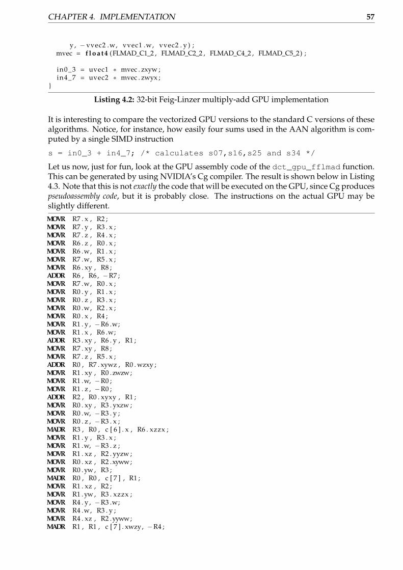
CHAPTER 4. IMPLEMENTATION 57
y , − vvec2 .w, vvec1 .w, vvec2 . y ) ;mvec = f l o a t 4 (FLMAD_C1_2 , FLMAD_C2_2 , FLMAD_C4_2 , FLMAD_C5_2) ;
in0_3 = uvec1 ∗ mvec . zxyw ;in4_7 = uvec2 ∗ mvec . zwyx ;
}
Listing 4.2: 32-bit Feig-Linzer multiply-add GPU implementation
It is interesting to compare the vectorized GPU versions to the standard C versions of thesealgorithms. Notice, for instance, how easily four sums used in the AAN algorithm is com-puted by a single SIMD instruction
s = in0_3 + in4_7; /* calculates s07,s16,s25 and s34 */
Let us now, just for fun, look at the GPU assembly code of the dct_gpu_fflmad function.This can be generated by using NVIDIA’s Cg compiler. The result is shown below in Listing4.3. Note that this is not exactly the code that will be executed on the GPU, since Cg producespseudoassembly code, but it is probably close. The instructions on the actual GPU may beslightly different.
MOVR R7 . x , R2 ;MOVR R7 . y , R3 . x ;MOVR R7 . z , R4 . x ;MOVR R6 . z , R0 . x ;MOVR R6 .w, R1 . x ;MOVR R7 .w, R5 . x ;MOVR R6 . xy , R8 ;ADDR R6 , R6, −R7 ;MOVR R7 .w, R0 . x ;MOVR R0 . y , R1 . x ;MOVR R0 . z , R3 . x ;MOVR R0 .w, R2 . x ;MOVR R0 . x , R4 ;MOVR R1 . y , −R6 .w;MOVR R1 . x , R6 .w;ADDR R3 . xy , R6 . y , R1 ;MOVR R7 . xy , R8 ;MOVR R7 . z , R5 . x ;ADDR R0 , R7 . xywz , R0 . wzxy ;MOVR R1 . xy , R0 .zwzw;MOVR R1 .w, −R0 ;MOVR R1 . z , −R0 ;ADDR R2 , R0 . xyxy , R1 ;MOVR R0 . xy , R3 . yxzw ;MOVR R0 .w, −R3 . y ;MOVR R0 . z , −R3 . x ;MADR R3 , R0 , c [ 6 ] . x , R6 . xzzx ;MOVR R1 . y , R3 . x ;MOVR R1 .w, −R3 . z ;MOVR R1 . xz , R2 . yyzw ;MOVR R0 . xz , R2 .xyww;MOVR R0 . yw , R3 ;MADR R0 , R0 , c [ 7 ] , R1 ;MOVR R1 . xz , R2 ;MOVR R1 . yw , R3 . xzzx ;MOVR R4 . y , −R3 .w;MOVR R4 .w, R3 . y ;MOVR R4 . xz , R2 .yyww;MADR R1 , R1 , c [ 7 ] . xwzy, −R4 ;

4.2. GPU IMPLEMENTATION 58
MULR oCol , R0 , c [ 8 ] ;MULR oCol1 , R1 , c [ 8 ] . xwzy ;
Listing 4.3: GPU assembly code for the Feig-Linzer multiply-add DCT
There are certainly many MOVR instructions, since we need to do several swizzles (reorders)and construction of vector values in the code. However, using swizzles and vector opera-tions should, according to NVIDIA and common sense, in general give better performancethan doing some computations serially [54].
Notice that the ADDR, MULR and MADR are all vectorized. It is particularly interesting to seethat multiply-add instructions (MADR) have been used three times. In the correspondingassembly output for the AAN algorithm, MADR is only used once, but it has many moreaddition (ADDR) instructions (8 vs. 4), and more multiply (MULR) instructions (8 vs. 4). Con-sequently, the Feig-Linzer multiply-add algorithm should, as we suspected in the previouschapter, be optimal for the GPU.
4.2.2 LOT on the GPU
That was DCT. Now let us look at the fast LOT implementation, which is an extension of theDCT implementation. We only describe forward LOT. The inverse LOT is just a reversal ofall the steps.
Figure 4.7 shows how the fast LOT of Section 3.3.3 on page 42 has been implemented. Forthe inverse LOT, follow the graph in the opposite direction. We will focus on the forwardLOT implementation in this section, since the inverse LOT is exactly the forward LOT done“backwards”. Source code for both the forward and inverse LOT, 32-bit versions, is providedin Section ?? on page ?? (16-bit versions are on the CD).
Row scatter2nd butterflies +Z̃-blockon rows
2nd butterflies +Z̃-blockon columns
DCT + 1stFLMADD
butterflies on rows
FLMADDDCT + 1stbutterflies on columns
row scatterModified
Column scatter column scatterModified
Figure 4.7: Fast LOT on the GPU
Consider Figure 3.10 on page 43. To compute the LOT on the GPU, we first compute therow DCT. We use the Feig-Linzer multiply-add algorithm, since, as we saw in the previoussection, it is probably better than AAN on the GPU. Now, it is easy to incorporate the firstbutterflies of the LOT inside the DCT. Just add one line to the end of dct_gpu_fflmadand change variables a bit so that the four even and odd transform variables are located inseparate variables, as in Listing 4.4 (see also Listing 4.2 on page 56):
void l o t _ g p u _ f f l m a d _ b u t t e r f l y ( inout f l o a t 4 in0_3 , inout f l o a t 4 in4_7 )
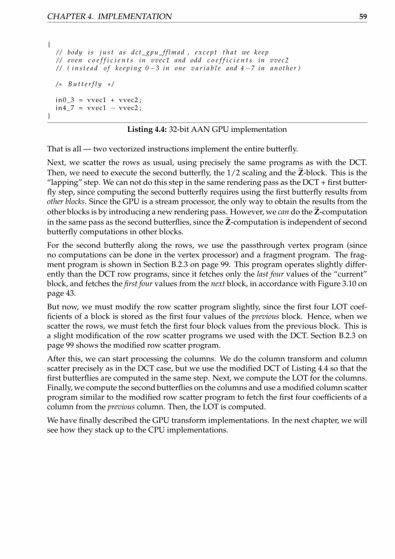
CHAPTER 4. IMPLEMENTATION 59
{/ / body i s j u s t a s d c t _ g p u _ f f l m a d , e x c e p t t h a t we k e e p/ / even c o e f f i c i e n t s in vvec1 and odd c o e f f i c i e n t s in vvec2/ / ( i n s t e a d o f k e e p i n g 0−3 in one v a r i a b l e and 4−7 in a n o t h e r )
/∗ B u t t e r f l y ∗ /
in0_3 = vvec1 + vvec2 ;in4_7 = vvec1 − vvec2 ;
}
Listing 4.4: 32-bit AAN GPU implementation
That is all — two vectorized instructions implement the entire butterfly.
Next, we scatter the rows as usual, using precisely the same programs as with the DCT.Then, we need to execute the second butterfly, the 1/2 scaling and the Z̃-block. This is the“lapping” step. We can not do this step in the same rendering pass as the DCT + first butter-fly step, since computing the second butterfly requires using the first butterfly results fromother blocks. Since the GPU is a stream processor, the only way to obtain the results from theother blocks is by introducing a new rendering pass. However, we can do the Z̃-computationin the same pass as the second butterflies, since the Z̃-computation is independent of secondbutterfly computations in other blocks.
For the second butterfly along the rows, we use the passthrough vertex program (sinceno computations can be done in the vertex processor) and a fragment program. The frag-ment program is shown in Section B.2.3 on page 99. This program operates slightly differ-ently than the DCT row programs, since it fetches only the last four values of the “current”block, and fetches the first four values from the next block, in accordance with Figure 3.10 onpage 43.
But now, we must modify the row scatter program slightly, since the first four LOT coef-ficients of a block is stored as the first four values of the previous block. Hence, when wescatter the rows, we must fetch the first four block values from the previous block. This isa slight modification of the row scatter programs we used with the DCT. Section B.2.3 onpage 99 shows the modified row scatter program.
After this, we can start processing the columns. We do the column transform and columnscatter precisely as in the DCT case, but we use the modified DCT of Listing 4.4 so that thefirst butterflies are computed in the same step. Next, we compute the LOT for the columns.Finally, we compute the second butterflies on the columns and use a modified column scatterprogram similar to the modified row scatter program to fetch the first four coefficients of acolumn from the previous column. Then, the LOT is computed.
We have finally described the GPU transform implementations. In the next chapter, we willsee how they stack up to the CPU implementations.

4.2. GPU IMPLEMENTATION 60
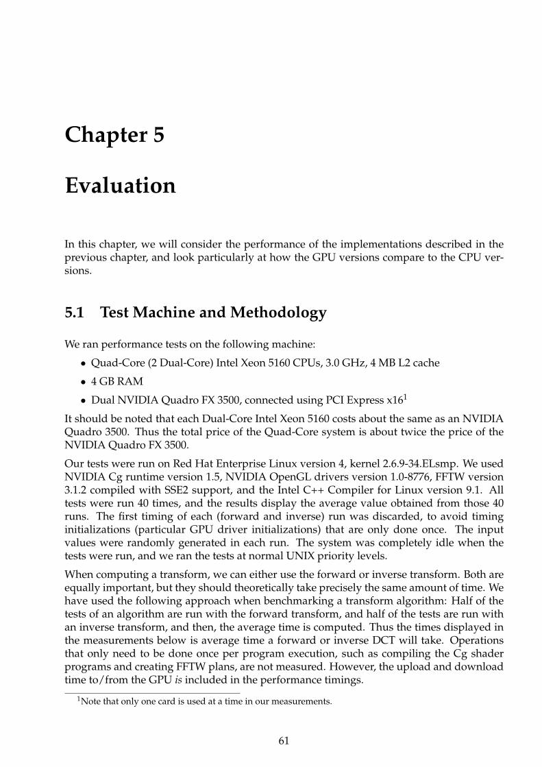
Chapter 5
Evaluation
In this chapter, we will consider the performance of the implementations described in theprevious chapter, and look particularly at how the GPU versions compare to the CPU ver-sions.
5.1 Test Machine and Methodology
We ran performance tests on the following machine:
• Quad-Core (2 Dual-Core) Intel Xeon 5160 CPUs, 3.0 GHz, 4 MB L2 cache
• 4 GB RAM
• Dual NVIDIA Quadro FX 3500, connected using PCI Express x161
It should be noted that each Dual-Core Intel Xeon 5160 costs about the same as an NVIDIAQuadro 3500. Thus the total price of the Quad-Core system is about twice the price of theNVIDIA Quadro FX 3500.
Our tests were run on Red Hat Enterprise Linux version 4, kernel 2.6.9-34.ELsmp. We usedNVIDIA Cg runtime version 1.5, NVIDIA OpenGL drivers version 1.0-8776, FFTW version3.1.2 compiled with SSE2 support, and the Intel C++ Compiler for Linux version 9.1. Alltests were run 40 times, and the results display the average value obtained from those 40runs. The first timing of each (forward and inverse) run was discarded, to avoid timinginitializations (particular GPU driver initializations) that are only done once. The inputvalues were randomly generated in each run. The system was completely idle when thetests were run, and we ran the tests at normal UNIX priority levels.
When computing a transform, we can either use the forward or inverse transform. Both areequally important, but they should theoretically take precisely the same amount of time. Wehave used the following approach when benchmarking a transform algorithm: Half of thetests of an algorithm are run with the forward transform, and half of the tests are run withan inverse transform, and then, the average time is computed. Thus the times displayed inthe measurements below is average time a forward or inverse DCT will take. Operationsthat only need to be done once per program execution, such as compiling the Cg shaderprograms and creating FFTW plans, are not measured. However, the upload and downloadtime to/from the GPU is included in the performance timings.
1Note that only one card is used at a time in our measurements.
61

5.2. DCT PERFORMANCE 62
N 64 128 256 512 1024 2048 4096Algorithmcpu-naive-32 0.0017 0.0067 0.0269 0.1073 0.4529 1.8165 7.2778cpu-fftw-simple-32 <0.0001 0.0002 0.0006 0.0028 0.0290 0.1274 0.5176cpu-fftw-advanced-32 <0.0001 0.0002 0.0008 0.0032 0.0306 0.2038 0.8298cpu-aan-32 <0.0001 0.0002 0.0007 0.0031 0.0310 0.1398 0.5842cpu-flmad-32 <0.0001 0.0001 0.0004 0.0019 0.0295 0.1285 0.5319cpu-aan-omp-2cpu-32 <0.0001 0.0001 0.0005 0.0021 0.0231 0.1065 0.4156cpu-flmad-omp-2cpu-32 <0.0001 0.0001 0.0004 0.0015 0.0232 0.1046 0.4059cpu-aan-omp-4cpu-32 <0.0001 <0.0001 0.0003 0.0013 0.0203 0.0789 0.2978cpu-flmad-omp-4cpu-32 <0.0001 <0.0001 0.0003 0.0011 0.0191 0.0741 0.3112gpu-aan-32 0.0106 0.0110 0.0123 0.0173 0.0381 0.1181 0.4371gpu-flmad-32 0.0101 0.0105 0.0121 0.0173 0.0378 0.1178 0.4372
Table 5.1: 32-bit 8× 8 DCT/IDCT wallclock times (seconds)
We focus on 32-bit computations, since 32 bits of precision is the only precision common tothe CPU and GPU. There is no support in Cg nor the GPU for more than 32 bits of precision,and the CPU does not support 16-bit natively. However, we include some benchmarks ofthe 16-bit GPU and 64- and 128-bit CPU algorithms to get an idea of the performance impactof increasing precision.
We only consider data set sizes up to 4096× 4096. The reason is that most GPUs, includingthe one we used for benchmarking, only support textures up to that size. Unfortunately,certain revisions of NVIDIA GeForce 6 and 7 GPUs have a hardware bug that makes thelast row and column of the 4096× 4096 texture unaccessable from fragment shader programs.We have tested the program on one such GPU, and the resulting transform values werecorrupted. Therefore, be careful when using the program with 4096 × 4096 textures. TheGPU in our benchmark machine did not have this problem.
5.2 DCT performance
In this section, we show benchmarks of and discuss the performance of the various DC-T/IDCT algorithms.
5.2.1 Measurements
We will now show the results of the performance measurements. We will consider wallclocktime, CPU time and download/upload time briefly.
Wallclock Time
Consider Table 5.1, which displays the wallclock time of the DCT/IDCT using 32 bits ofprecision. Boldfaced values indicate the quickest algorithm for a specific input set size. Theinteresting results are depicted graphically in Figures 5.1 on the next page.
For reference, we have also benchmarked 16-bit GPU versions and 64- and 128-bit CPUversions. The results are shown in Tables 5.2, 5.3 and 5.4, and illustrated in Figure ??.
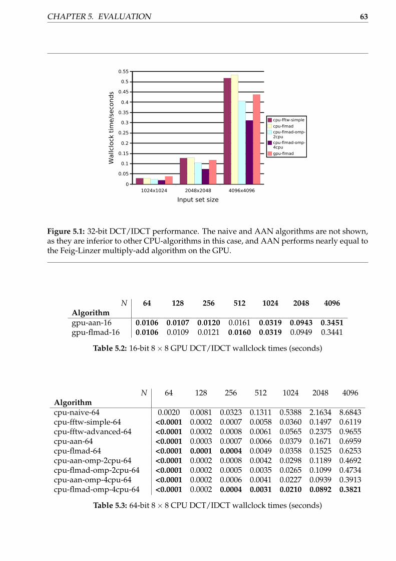
CHAPTER 5. EVALUATION 63
��������� ��������� ���������
�
��
��
��
��
��
��
��
��
��
�
�
� ���������� ��
� �������
� ���������� ��� �
� ���������� ��� �
� �������
�� �����������
�������!�����"�������
Figure 5.1: 32-bit DCT/IDCT performance. The naive and AAN algorithms are not shown,as they are inferior to other CPU-algorithms in this case, and AAN performs nearly equal tothe Feig-Linzer multiply-add algorithm on the GPU.
N 64 128 256 512 1024 2048 4096Algorithmgpu-aan-16 0.0106 0.0107 0.0120 0.0161 0.0319 0.0943 0.3451gpu-flmad-16 0.0106 0.0109 0.0121 0.0160 0.0319 0.0949 0.3441
Table 5.2: 16-bit 8× 8 GPU DCT/IDCT wallclock times (seconds)
N 64 128 256 512 1024 2048 4096Algorithmcpu-naive-64 0.0020 0.0081 0.0323 0.1311 0.5388 2.1634 8.6843cpu-fftw-simple-64 <0.0001 0.0002 0.0007 0.0058 0.0360 0.1497 0.6119cpu-fftw-advanced-64 <0.0001 0.0002 0.0008 0.0061 0.0565 0.2375 0.9655cpu-aan-64 <0.0001 0.0003 0.0007 0.0066 0.0379 0.1671 0.6959cpu-flmad-64 <0.0001 0.0001 0.0004 0.0049 0.0358 0.1525 0.6253cpu-aan-omp-2cpu-64 <0.0001 0.0002 0.0008 0.0042 0.0298 0.1189 0.4692cpu-flmad-omp-2cpu-64 <0.0001 0.0002 0.0005 0.0035 0.0265 0.1099 0.4734cpu-aan-omp-4cpu-64 <0.0001 0.0002 0.0006 0.0041 0.0227 0.0939 0.3913cpu-flmad-omp-4cpu-64 <0.0001 0.0002 0.0004 0.0031 0.0210 0.0892 0.3821
Table 5.3: 64-bit 8× 8 CPU DCT/IDCT wallclock times (seconds)

5.2. DCT PERFORMANCE 64
N 64 128 256 512 1024 2048 4096Algorithmcpu-naive-128 0.0071 0.0282 0.1128 0.4537 1.8265 7.3090 29.3542cpu-fftw-simple-128 0.0001 0.0003 0.0016 0.0109 0.0564 0.2394 1.0041cpu-fftw-advanced-128 0.0001 0.0004 0.0019 0.0149 0.0927 0.3886 1.6001cpu-aan-128 0.0001 0.0003 0.0017 0.0100 0.0481 0.1951 1.0308cpu-flmad-128 0.0001 0.0003 0.0016 0.0100 0.0489 0.2000 0.8452cpu-aan-omp-2cpu-128 0.0001 0.0003 0.0012 0.0058 0.0294 0.1305 0.6002cpu-flmad-omp-2cpu-128 <0.0001 0.0003 0.0009 0.0064 0.0299 0.1322 0.5656cpu-aan-omp-4cpu-128 0.0001 0.0003 0.0009 0.0065 0.0250 0.0970 0.3970cpu-flmad-omp-4cpu-128 <0.0001 0.0002 0.0009 0.0057 0.0267 0.1022 0.4103
Table 5.4: 128-bit 8× 8 CPU DCT/IDCT wallclock times (seconds)
N 64 128 256 512 1024 2048 4096Algorithmgpu-aan-32 0.0010 0.0013 0.0030 0.0068 0.0267 0.1062 0.4240gpu-flmad-32 0.0008 0.0015 0.0026 0.0069 0.0269 0.1071 0.4208cpu-fftw-simple-32 <0.0001 0.0002 0.0006 0.0028 0.0290 0.1274 0.5176cpu-flmad-32 <0.0001 0.0001 0.0004 0.0019 0.0294 0.1285 0.5319cpu-aan-32 <0.0001 0.0002 0.0007 0.0031 0.0310 0.1398 0.5842cpu-flmad-openmp-2cpu-32 <0.0001 0.0003 0.0008 0.0028 0.0460 0.2086 0.8104cpu-flmad-openmp-4cpu-32 0.0001 0.0003 0.0012 0.0044 0.0737 0.2911 1.2374
Table 5.5: 8× 8 DCT/IDCT CPU times (user + system)
CPU Time
Although the CPU seems to outperform the GPU when multiple cores are used in terms ofwallclock time, CPU time used will in many cases be more important. CPU time measuresCPU load, and using less CPU time on computing a transform means the ability to use CPUtime on something else.
For the single-core CPU algorithms, the CPU time was measured to (and should — if thesystem is idle) be almost the same as the wallclock time2. For multi-core CPU algorithms,the CPU time is equal to the wallclock time times the number of cores used. Most of the CPUtime used in the CPU algorithms is CPU user time. The CPU system time was measured topractically zero for all the CPU algorithms. This is natural, since the algorithms call nosystem calls while computing.
For the GPU, however, there is no simple connection between the CPU time and the wall-clock time, and more CPU system time is used since the operating system is heavily involvedin transferring commands and data to the GPU. The total CPU time for the 32-bit GPU DCTalgorithms is, along with the CPU time numbers for some of the CPU algorithms, shown inTable 5.5. Figure 5.2 on the next page provides a graphical illustration.
Impact of Upload and Download
The time used for uploading and downloading data to/from the GPU is a bottleneck. Thedata transfer speed is usually limited by the RAM bandwidth since data is transferred from
2The resolution of the CPU time timer is lower than that of the wallclock time. CPU time results thereforemay deviate slightly from the wallclock times.
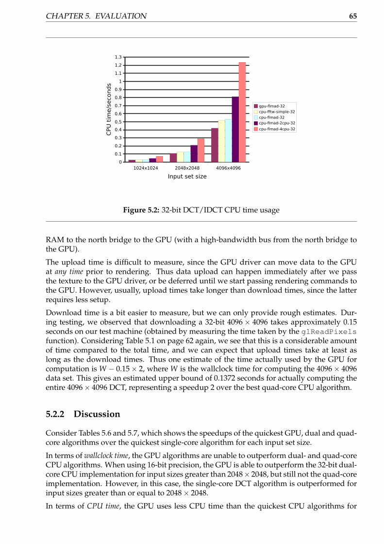
CHAPTER 5. EVALUATION 65
��������� ��������� ���������
�
��
��
�
��
��
��
��
��
��
�
��
��
�
����������
�����������������
�����������
����������������
����������������
��������������
!"�����#���$���
Figure 5.2: 32-bit DCT/IDCT CPU time usage
RAM to the north bridge to the GPU (with a high-bandwidth bus from the north bridge tothe GPU).
The upload time is difficult to measure, since the GPU driver can move data to the GPUat any time prior to rendering. Thus data upload can happen immediately after we passthe texture to the GPU driver, or be deferred until we start passing rendering commands tothe GPU. However, usually, upload times take longer than download times, since the latterrequires less setup.
Download time is a bit easier to measure, but we can only provide rough estimates. Dur-ing testing, we observed that downloading a 32-bit 4096 × 4096 takes approximately 0.15seconds on our test machine (obtained by measuring the time taken by the glReadPixelsfunction). Considering Table 5.1 on page 62 again, we see that this is a considerable amountof time compared to the total time, and we can expect that upload times take at least aslong as the download times. Thus one estimate of the time actually used by the GPU forcomputation is W − 0.15 × 2, where W is the wallclock time for computing the 4096 × 4096data set. This gives an estimated upper bound of 0.1372 seconds for actually computing theentire 4096× 4096 DCT, representing a speedup 2 over the best quad-core CPU algorithm.
5.2.2 Discussion
Consider Tables 5.6 and 5.7, which shows the speedups of the quickest GPU, dual and quad-core algorithms over the quickest single-core algorithm for each input set size.
In terms of wallclock time, the GPU algorithms are unable to outperform dual- and quad-coreCPU algorithms. When using 16-bit precision, the GPU is able to outperform the 32-bit dual-core CPU implementation for input sizes greater than 2048× 2048, but still not the quad-coreimplementation. However, in this case, the single-core DCT algorithm is outperformed forinput sizes greater than or equal to 2048× 2048.
In terms of CPU time, the GPU uses less CPU time than the quickest CPU algorithms for
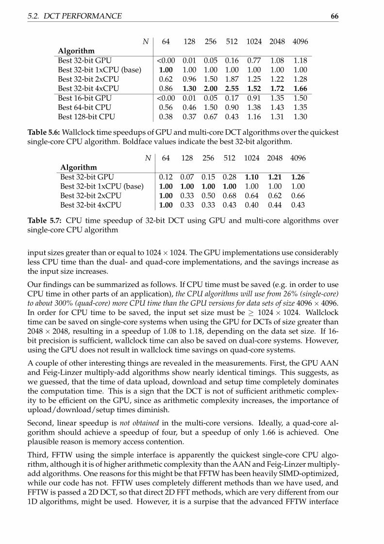
5.2. DCT PERFORMANCE 66
N 64 128 256 512 1024 2048 4096AlgorithmBest 32-bit GPU <0.00 0.01 0.05 0.16 0.77 1.08 1.18Best 32-bit 1xCPU (base) 1.00 1.00 1.00 1.00 1.00 1.00 1.00Best 32-bit 2xCPU 0.62 0.96 1.50 1.87 1.25 1.22 1.28Best 32-bit 4xCPU 0.86 1.30 2.00 2.55 1.52 1.72 1.66Best 16-bit GPU <0.00 0.01 0.05 0.17 0.91 1.35 1.50Best 64-bit CPU 0.56 0.46 1.50 0.90 1.38 1.43 1.35Best 128-bit CPU 0.38 0.37 0.67 0.43 1.16 1.31 1.30
Table 5.6: Wallclock time speedups of GPU and multi-core DCT algorithms over the quickestsingle-core CPU algorithm. Boldface values indicate the best 32-bit algorithm.
N 64 128 256 512 1024 2048 4096AlgorithmBest 32-bit GPU 0.12 0.07 0.15 0.28 1.10 1.21 1.26Best 32-bit 1xCPU (base) 1.00 1.00 1.00 1.00 1.00 1.00 1.00Best 32-bit 2xCPU 1.00 0.33 0.50 0.68 0.64 0.62 0.66Best 32-bit 4xCPU 1.00 0.33 0.33 0.43 0.40 0.44 0.43
Table 5.7: CPU time speedup of 32-bit DCT using GPU and multi-core algorithms oversingle-core CPU algorithm
input sizes greater than or equal to 1024× 1024. The GPU implementations use considerablyless CPU time than the dual- and quad-core implementations, and the savings increase asthe input size increases.
Our findings can be summarized as follows. If CPU time must be saved (e.g. in order to useCPU time in other parts of an application), the CPU algorithms will use from 26% (single-core)to about 300% (quad-core) more CPU time than the GPU versions for data sets of size 4096× 4096.In order for CPU time to be saved, the input set size must be ≥ 1024 × 1024. Wallclocktime can be saved on single-core systems when using the GPU for DCTs of size greater than2048 × 2048, resulting in a speedup of 1.08 to 1.18, depending on the data set size. If 16-bit precision is sufficient, wallclock time can also be saved on dual-core systems. However,using the GPU does not result in wallclock time savings on quad-core systems.
A couple of other interesting things are revealed in the measurements. First, the GPU AANand Feig-Linzer multiply-add algorithms show nearly identical timings. This suggests, aswe guessed, that the time of data upload, download and setup time completely dominatesthe computation time. This is a sign that the DCT is not of sufficient arithmetic complex-ity to be efficient on the GPU, since as arithmetic complexity increases, the importance ofupload/download/setup times diminish.
Second, linear speedup is not obtained in the multi-core versions. Ideally, a quad-core al-gorithm should achieve a speedup of four, but a speedup of only 1.66 is achieved. Oneplausible reason is memory access contention.
Third, FFTW using the simple interface is apparently the quickest single-core CPU algo-rithm, although it is of higher arithmetic complexity than the AAN and Feig-Linzer multiply-add algorithms. One reasons for this might be that FFTW has been heavily SIMD-optimized,while our code has not. FFTW uses completely different methods than we have used, andFFTW is passed a 2D DCT, so that direct 2D FFT methods, which are very different from our1D algorithms, might be used. However, it is a surpise that the advanced FFTW interface
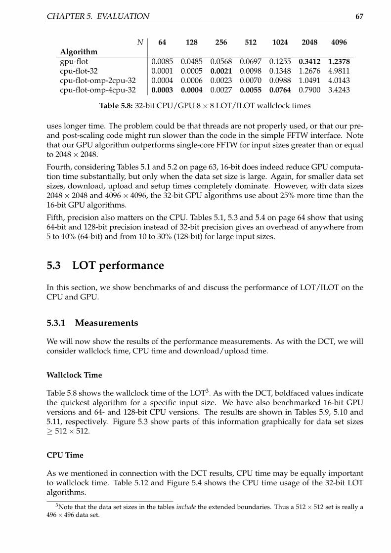
CHAPTER 5. EVALUATION 67
N 64 128 256 512 1024 2048 4096Algorithmgpu-flot 0.0085 0.0485 0.0568 0.0697 0.1255 0.3412 1.2378cpu-flot-32 0.0001 0.0005 0.0021 0.0098 0.1348 1.2676 4.9811cpu-flot-omp-2cpu-32 0.0004 0.0006 0.0023 0.0070 0.0988 1.0491 4.0143cpu-flot-omp-4cpu-32 0.0003 0.0004 0.0027 0.0055 0.0764 0.7900 3.4243
Table 5.8: 32-bit CPU/GPU 8× 8 LOT/ILOT wallclock times
uses longer time. The problem could be that threads are not properly used, or that our pre-and post-scaling code might run slower than the code in the simple FFTW interface. Notethat our GPU algorithm outperforms single-core FFTW for input sizes greater than or equalto 2048× 2048.
Fourth, considering Tables 5.1 and 5.2 on page 63, 16-bit does indeed reduce GPU computa-tion time substantially, but only when the data set size is large. Again, for smaller data setsizes, download, upload and setup times completely dominate. However, with data sizes2048 × 2048 and 4096 × 4096, the 32-bit GPU algorithms use about 25% more time than the16-bit GPU algorithms.
Fifth, precision also matters on the CPU. Tables 5.1, 5.3 and 5.4 on page 64 show that using64-bit and 128-bit precision instead of 32-bit precision gives an overhead of anywhere from5 to 10% (64-bit) and from 10 to 30% (128-bit) for large input sizes.
5.3 LOT performance
In this section, we show benchmarks of and discuss the performance of LOT/ILOT on theCPU and GPU.
5.3.1 Measurements
We will now show the results of the performance measurements. As with the DCT, we willconsider wallclock time, CPU time and download/upload time.
Wallclock Time
Table 5.8 shows the wallclock time of the LOT3. As with the DCT, boldfaced values indicatethe quickest algorithm for a specific input size. We have also benchmarked 16-bit GPUversions and 64- and 128-bit CPU versions. The results are shown in Tables 5.9, 5.10 and5.11, respectively. Figure 5.3 show parts of this information graphically for data set sizes≥ 512× 512.
CPU Time
As we mentioned in connection with the DCT results, CPU time may be equally importantto wallclock time. Table 5.12 and Figure 5.4 shows the CPU time usage of the 32-bit LOTalgorithms.
3Note that the data set sizes in the tables include the extended boundaries. Thus a 512 × 512 set is really a496× 496 data set.

5.3. LOT PERFORMANCE 68
��������� ��������� ���������
�
�
�
�
�
�
�
�
�
�
� ���������
� ���������
� ��������� ��� ����
� ��������� ��� ����
�� �����������
���
����
� �
����!�
Figure 5.3: Fast LOT/ILOT performance using Feig-Linzer multiply-add for the DCT step.16-, 32-, 64- and 128-bit algorithms are shown.
N 64 128 256 512 1024 2048 4096Algorithmgpu-flot-16 0.0928 0.0590 0.0574 0.0656 0.1039 0.2782 0.9226
Table 5.9: 16-bit 8× 8 GPU LOT/ILOT wallclock times (seconds)

CHAPTER 5. EVALUATION 69
N 64 128 256 512 1024 2048 4096Algorithmcpu-flot-64 0.0001 0.0005 0.0023 0.0182 0.2854 1.3138 5.6094cpu-flot-omp-2cpu-64 0.0004 0.0009 0.0028 0.0131 0.2554 0.9973 4.0171cpu-flot-omp-4cpu-64 0.0005 0.0008 0.0036 0.0362 0.2290 0.9635 3.6690
Table 5.10: 64-bit 8× 8 CPU LOT/ILOT wallclock times (seconds)
N 64 128 256 512 1024 2048 4096Algorithmcpu-flot-128 0.0002 0.0012 0.0059 0.0397 0.4256 1.8402 7.6342cpu-flot-omp-2cpu-128 0.0002 0.0006 0.0032 0.0381 0.3185 1.1834 4.8361cpu-flot-omp-4cpu-128 0.0008 0.0039 0.0136 0.0651 0.2848 1.0984 4.0254
Table 5.11: 128-bit 8× 8 CPU LOT/ILOT wallclock times (seconds)
Impact of Upload and Download
As for the DCT, we upload and download times take a large amount of the LOT computa-tion time. However, since the LOT is a more complex transform, the relative impact of thedownload and upload times should be less than that for the DCT. Using the same estimationmethod as we did for the DCT gives an estimated upper bound on the GPU LOT compu-tation time of a 4096× 4096 data set of about 1.2378− 0.15 · 2 = 0.9378, which is about 3.65times quicker than the quad-core CPU!
5.3.2 Discussion
Consider Tables 5.13 and 5.14 on the next page, which shows the speedup obtained by usingthe GPU and multi-core algorithms over using the single-core algorithm in terms of wall-clock and CPU time.
It seems that the GPU implementation finally outperforms the quad-core CPU. The GPULOT algorithm outperforms the 2 x dual-core CPUs, which are twice as expensive than the GPU weused, by a factor of 2.7 for a 4096 × 4096 data set. When only two cores are used, the speedupis 2.5, and when a single core is used, the speedup is above 4! And if 16-bit precision isused, The GPU outperforms all CPU algorithms in terms of wallclock time if the data set size is≥ 2048× 2048, and the speedup over the single-core version is 5.4!
In terms of CPU time, the results are even better. In this case, the GPU outperforms all CPUalgorithms if the input data set size is ≥ 1024 × 1024. For 4096 × 4096 data set sizes, thesingle- dual- and quad-core CPU algorithms use 4.2, 6.8 and 11.1 times more CPU time thanthe GPU algorithm, respectively.
N 64 128 256 512 1024 2048 4096Algorithmgpu-flot-32 0.0028 0.0035 0.0110 0.0229 0.0768 0.2985 1.1866cpu-flot-32 0.0001 0.0005 0.0022 0.0098 0.1348 1.2676 4.9811cpu-flot-omp-2cpu-32 0.0004 0.0011 0.0044 0.0132 0.1970 2.0956 8.0198cpu-flot-omp-4cpu-32 0.0017 0.0017 0.0112 0.0217 0.3025 3.0957 13.2131
Table 5.12: 32-bit 8× 8 LOT/ILOT CPU times (seconds)

5.3. LOT PERFORMANCE 70
��������� ���������
�
�
�
�
�
�
�
�
��
��
��
�
��
� ��������
� ��������
� ��������� ��� ���
� ��������� ��� ���
�� �����������
���
����
� �
����!�
Figure 5.4: 32-bit 8× 8 LOT/ILOT CPU time usage for large data set sizes (user + system)
N 64 128 256 512 1024 2048 4096Algorithmgpu-flot-32 0.01 0.01 0.04 0.14 1.07 3.71 4.02cpu-flot-32 (base) 1.00 1.00 1.00 1.00 1.00 1.00 1.00cpu-flot-omp-2cpu-32 0.25 0.83 0.91 1.40 1.36 1.21 1.24cpu-flot-omp-4cpu-32 0.33 1.25 0.78 1.78 1.76 1.60 1.45gpu-flot-16 0.01 0.01 0.04 0.15 1.29 4.55 5.40cpu-flot-omp-4cpu-64 0.20 0.63 0.58 0.27 0.59 1.32 1.36cpu-flot-omp-4cpu-128 0.01 0.13 0.15 0.15 0.47 1.15 1.24
Table 5.13: Wallclock time speedups of using GPU and multi-core LOT algorithms oversingle-core CPU algorithm. Boldface values indicate the best 32-bit algorithm.
N 64 128 256 512 1024 2048 4096Algorithmgpu-flot-32 0.04 0.14 0.20 0.43 1.76 4.24 4.20cpu-flot-32 (base) 1.00 1.00 1.00 1.00 1.00 1.00 1.00cpu-flot-omp-2cpu-32 0.25 0.45 0.50 0.74 0.68 0.60 0.62cpu-flot-omp-4cpu-32 0.06 0.29 0.20 0.45 0.45 0.41 0.38
Table 5.14: CPU time speedup of 32-bit LOT using GPU and multi-core algorithms oversingle-core CPU algorithm

CHAPTER 5. EVALUATION 71
We can summarize as follows. If the data set size is ≥ 2048× 2048 and wallclock time mustbe minimized, the GPU will give significant speedups over the single, dual or quad-coreCPUs. However, the data set size must be ≥ 2048 × 2048. However, if only a single-coreCPU is available, the GPU will still give a small speedup (1.07 32-bit, 1.29 16-bit) if the dataset size is 1024 × 1024. The GPU also gives significant CPU time speedups over all CPUalgorithms when the data set size is ≥ 1024× 1024, so if wallclock time is of less importance,the GPU can be used to reduce CPU user time when the data set size is 1024 × 1024 onquad-core CPUs.
Unfortunately, the GPU does not outperform the CPU for smaller data set sizes. The prob-lem is the same as with the DCT — namely, upload, download and setup times. However,contrary to the DCT, the GPU is able to outperform the quad-core CPU. This has one ex-planation: As arithmetic complexity increases, the bottleneck eventually becomes the actualcomputations, and not the upload, download and setup times. This is probably why theLOT, which has about twice the arithmetic complexity of the DCT, manages to outperformthe quad-core CPU in terms of wallclock time, while the DCT does not. This suggests thateven more complicated transforms, such as the GenLOT, will gain an even larger benefitfrom using the GPU.

5.3. LOT PERFORMANCE 72

Chapter 6
Conclusion
In this chapter, we summarize our findings and look at potential future work.
6.0.3 Findings
In this project, it was demonstrated that using the GPU for transform coding computationsis indeed not only possible, but the GPU will for large data set sizes and provides a speedupof 2.77 over a CPU costing twice as much when using the LOT transform. Let’s draw someconclusions.
Our first conclusion is that implementing algorithms on the GPU takes more time than itdoes on the CPU. On the GPU, few debugging tools exist, the programming model is lim-ited, many elements of standard CPU programming languages are simply not available (bit-shifting is one example) or must be emulated (integers and booleans as floating-point), andimplementing algorithms which need to write to several locations in memory can involvecomplicated calculations on texture coordinates. And worse, even if you do spend time im-plementing a GPU algorithm, it is not certain that any speedup will be obtained.
Our second conclusion is that upload and download of data to and from the GPU is the mainbottleneck, but as computations get large enough, the GPU wins. Our AAN and Feig-Linzermultiply-add implementations on the GPU run nearly at exactly the same time. The execu-tion time is (for relatively small data set sizes and for relatively simple computations) notbounded by whether or not fancy vectorized GPU code is used, but purely by upload anddownload times. However, and this is important, as the data set size or as the computationalcomplexity of an algorithm increases, computation time will eventually dominate. That is why ourLOT implementation outperformed the CPU implementation only for large data set sizes.Since the LOT does more computations than the DCT, more time is spent on computing, andthe floating-point power of the CPU becomes the bottleneck for large data set sizes.
The second conclusion leads us to our third conclusion, which is that even though GPUs mightbe slower than the CPU in terms of wallclock time in some cases, it still offloads the CPU.As we saw in the previous chapter, using the GPU in many cases lead to reduced CPU timeusage. This frees up the CPU to do other things, provided that the CPU program using theGPU for computations is multi-threaded.
We therefore conclude that the GPU should be considered for use for transform coding datacompression if:
• Large data set sizes are used.
73
74
• The transform used is of high arithmetic complexity — such as LOT, GenLOT or GUL-LOT.
• Other parts of the application would gain an advantage of having more CPU timeavailable.
• The application must reduce the wallclock time used on the transform coding algo-rithm to increase responsiveness.
This project has demonstrated that under these conditions, the GPU is very suitable fortransform coding computations, since for large data set sizes and transforms of high arith-metic complexity, the GPU saves both considerable amounts of CPU and wallclock time. But wehave also demonstrated that the GPU should not be used for transform coding data compres-sion if:
• Only relatively small data set sizes, such as 128× 128 and 256× 256, are used.
• The transform does very small amounts of computation.
• You are not prepared to spend more time on developing the GPU algorithm than theCPU algorithm.
• CPU and wallclock time are not of critical importance to the application. This is oftennot the case in clustered applications.
6.0.4 Future Work
The GPU adventure has just started. Projections [55] estimate that in 8 years, GPU comput-ing capability will increase by a factor of 40, GPU memory latency will be cut in half, andGPU memory bandwidth will increase by a factor of 8.
One of the most interesting things we found was that more complicated transforms benefit morefrom using the GPU. It would therefore be very interesting to implement transforms whichdo more computations than the LOT, for example GenLOT or GULLOT on the GPU. Thesetransforms will likely obtain even better speedups over corresponding CPU algorithms.
Bibliography
[1] P. Micikevicius. GPU Computing for Protein Structure Prediction. In M. Pharr andR. Fernando, editors, GPU Gems 2: Programming Techniques for High-Performance Graph-ics and General Purpose Computation, chapter 43, pages 695–702. Addison-Wesley, UpperSaddle River, NJ, USA, 1st edition, 2005.
[2] J. Bolz, I. Farmer, E. Grinspun and P. Schröder. Sparse matrix solvers on the GPU:conjugate gradients and multigrid. ACM Trans. Graph., 22(3):917–924, 2003.
[3] J. Krüger and R. Westermann. GPU Computing for Protein Structure Prediction.In M. Pharr and R. Fernando, editors, GPU Gems 2: Programming Techniques forHigh-Performance Graphics and General Purpose Computation, chapter 44, pages 703–718.Addison-Wesley, Upper Saddle River, NJ, USA, 1st edition, 2005.
[4] C. Kolb and M. Pharr. Options Pricing on the GPU. In M. Pharr and R. Fernando,editors, GPU Gems 2: Programming Techniques for High-Performance Graphics and GeneralPurpose Computation, chapter 45, pages 719–731. Addison-Wesley, Upper Saddle River,NJ, USA, 1st edition, 2005.
[5] X. Wei W. Li, Z. Fan and A. Kaufman. Flow Simulation with Complex Bound-aries. In M. Pharr and R. Fernando, editors, GPU Gems 2: Programming Techniques forHigh-Performance Graphics and General Purpose Computation, chapter 47, pages 747–764.Addison-Wesley, 1st edition, 2005.
[6] T. Sumanaweera and D. Liu. Medical Image Reconstruction with the FFT. In M. Pharrand R. Fernando, editors, GPU Gems 2: Programming Techniques for High-PerformanceGraphics and General Purpose Computation, chapter 48, pages 765–784. Addison-Wesley,1st edition, 2005.
[7] P. Kipfer and R. Westermann. Improved GPU Sorting. In M. Pharr and R. Fernando,editors, GPU Gems 2: Programming Techniques for High-Performance Graphics and GeneralPurpose Computation, chapter 46, pages 733–746. Addison-Wesley, 1st edition, 2005.
[8] Wikipedia. Graphics processing unit — Wikipedia, the free encyclopedia.http://en.wikipedia.org/w/index.php?title=Graphics_processing_unit&oldid=72792534, 2006. [Online; accessed 31-Aug-2006].
[9] R. Fernando and M. J. Kilgard. The Cg Tutorial. Addison-Wesley, 1st edition, 2003.
[10] J. Krüger and R. Westermann. GPU simulation and rendering of volumetric effects forcomputer games and virtual environments. Computer Graphics Forum, 24(3), 2005.
[11] E. Kilgariff and R. Fernando. The GeForce 6 Series GPU Architecture. In M. Pharrand R. Fernando, editors, GPU Gems 2: Programming Techniques for High-PerformanceGraphics and General Purpose Computation, chapter 30, pages 471–491. Addison-Wesley,1st edition, 2005.
75

BIBLIOGRAPHY 76
[12] BeHardware. NVIDIA GeForce 7800 GTX (page 1: Introduction). http://www.behardware.com/articles/574-1/nvidia-geforce-7800-gtx.html, 2005.[Online; accessed 03-Sep-2006].
[13] D. Hearn and M. P. Baker. Computer Graphics with OpenGL. Prentice Hall, 3rd edition,2004.
[14] M. Segal and K. Akeley. The OpenGL Graphics System: A Specification (Ver-sion 2.1). http://www.opengl.org/documentation/specs/version2.1/glspec21.pdf, July 2006. [Online; accessed 04-09-2006].
[15] Microsoft Corporation. DirectX Software Development Kit. http://msdn.microsoft.com/library/default.asp?url=/library/en-us/directx9_c/directx_sdk.asp, 2006. [Online; accessed 04-09-2006].
[16] J. Kessenich. The OpenGL Shading Language. http://www.opengl.org/registry/specs/ARB/GLSLangSpec.Full.1.20.6.pdf, July 2006. [Online, ac-cessed 04-09-2006].
[17] M. J. Kilgard. Cg and NVIDIA (Chapter 5 of SIGGRAPH 2006 course 3). http://www.csee.umbc.edu/~olano/s2006c03/ch05.pdf, 2006. [Online; accessed 26-September-2006].
[18] I. Buck et.al. BrookGPU. http://graphics.stanford.edu/projects/brookgpu, 2006. [Online, accessed 04-09-2006].
[19] RapidMind Inc. Sh: A high-level metaprogramming language for modern GPUs.http://libsh.org, 2006. [Online, accessed 04-09-2006].
[20] M. Harris. Mapping Computational Concepts to GPUs. In M. Pharr and R. Fernando,editors, GPU Gems 2: Programming Techniques for High-Performance Graphics and GeneralPurpose Computation, chapter 31, pages 493–508. Addison-Wesley, Upper Saddle River,NJ, USA, 1st edition, 2005.
[21] Wikipedia. Comparison of NVIDIA Graphics Processing Units — Wikipedia,The Free Encyclopedia. http://en.wikipedia.org/w/index.php?title=Comparison_of_NVIDIA_Graphics_Processing_Units&oldid=73077340,2006. [Online; accessed 4-September-2006].
[22] Wikipedia. NVIDIA Quadro — Wikipedia, The Free Encyclopedia. http://en.wikipedia.org/w/index.php?title=NVIDIA_Quadro&oldid=72555349,2006. [Online; accessed 4-September-2006].
[23] I. Buck. Taking the Plunge into GPU Computing. In M. Pharr and R. Fernando, editors,GPU Gems 2: Programming Techniques for High-Performance Graphics and General PurposeComputation, chapter 32, pages 509–519. Addison-Wesley, Upper Saddle River, NJ, USA,1st edition, 2005.
[24] D. Salomon. Data Compression: The Complete Reference. Springer, 3rd edition, 2004.
[25] Wikipedia. Discrete cosine transform — Wikipedia, The Free Encyclope-dia. http://en.wikipedia.org/w/index.php?title=Discrete_cosine_transform&oldid=81725562, 2006. [Online; accessed 22-October-2006].
[26] M. Frigo and S. G. Johnson. FFTW Home Page. http://www.fftw.org, 2006. [On-line; accessed 22-October-2006].
[27] M. Frigo and S. G. Johnson. 1d Real-even DFTs (DCTs) — FFTW 3.1.2. http://www.fftw.org/fftw3_doc/1d-Real_002deven-DFTs-_0028DCTs_0029.html,2006. [Online; accessed 22-October-2006].
BIBLIOGRAPHY 77
[28] W. B. Pennebaker and J. L. Mitchell. JPEG still image data compression standard. Springer,1st edition, 1993.
[29] IEEE Circuits and Systems Society. IEEE standard no. 1180 — specifications for imple-mentation of 8× 8 inverse discrete cosine transform. Technical report, 1991.
[30] H. S. Malvar. Signal Processing with Lapped Transforms. Artech House, 1st edition, 1992.
[31] G. Davis and A. Nosratinia. Wavelet-Based Image Coding: An Overview. Applied andComputational Control, Signals, and Circuits, 1(1), 1998.
[32] H. V. Sorenson, D.L. Jones, M. T. Heideman and C. S. Burrus. Real-valued fast Fouriertransform algorithms. IEEE Transactions on Acoustics, Speech, and Signal Processing,35(6):849–863, 1987.
[33] D. Takahashi. An extended split-radix FFT algorithm. IEEE Signal Processing Letters,8(5):145–147, 2001.
[34] M. Frigo and S. G. Johnson. FFTW: an adaptive software architecture for the FFT. Pro-ceedings of the 1998 IEEE International Conference on Acoustics, Speech, and Signal Process-ing. ICASSP ’98., 3:1381–1384, 1998.
[35] J. W. Cooley and J. W. Tukey. An algorithm for the machine calculation of complexFourier series. Mathematics of Compitation, 19:297–301, 1965.
[36] J. W. Cooley et al. The 1968 Arden House Workshop on Fast Fourier Transform Process-ing. IEEE Transactions on Audio and Electroacoustics: Special issue on Fast Fourier Transform,AU-17(2), 1969.
[37] J. Makhoul. A fast cosine transform in one and two dimensions. IEEE Transactions onAcoustics, Speech, and Signal Processing, 28(1):27–34, 1980.
[38] Y. Arai, T. Agui and M. Nakajima. A fast DCT-SQ scheme for images. Transactions ofthe Institute of Electronics, Information and Communication Engineers, E71(11):1095–1097,1988.
[39] B. D. Tseng and W. C. Miller. On Computing the Discrete Cosine Transform. IEEETransactions on Computers, C-27(10):966–968, 1978.
[40] S. Winograd. On Computing the Discrete Fourier Transform. Mathematics of Computa-tion, 23(141):175–199, 1978.
[41] E. Feig and E. Linzer. Scaled DCT Algorithms for JPEG and MPEG Implementations onfused multiply/add architectures. Proceedings of the SPIE Conference on Image ProcessingAlgorithms and Techniques; San Jose, CA; (USA); 25 Feb.-1 Mar. 1991, pages 458–467, 1991.
[42] E. Feig and E. Linzer. Discrete Cosine Transform Algorithms for Image Data Compres-sion. Electronic Imaging ’90 East Proceedings, pages 84–87, 1990.
[43] S.-L. Chang and T. Ogunfunmi. A fast DCT (Feig’s algorithm) implementation andapplication in MPEG1 video compression. Proceedings of the 38th Midwest Symposium onCircuits and Systems, 1995, 2:961–964, 1995.
[44] Y. Jeong and I. Lee. Fast discrete cosine transform structure suitable for implementationwith integer computation. Optical Engineering, 39(10):2672–2676, 2000.
[45] B. Fang, G. Shen, S. Li and H. Chen. Techniques for efficient DCT/IDCT implementa-tion on generic GPU. IEEE International Symposium on Circuits and Systems, ISCAS 2005,23.-26 May 2005, 2:1126–1129, 2005.
[46] H. S. Malvar and D. H. Staelin. The LOT: transform coding without blocking effects.IEEE Transactions on Acoustics, Speech, and Signal Processing, 37(4):553–559, 1989.

BIBLIOGRAPHY 78
[47] P.M. Cassereau, D.H. Staelin and G. de Jager. Encoding of images based on a lappedorthogonal transform. IEEE Transactions on Communications, 37(2):189–193, 1989.
[48] B. Hinman, J. Bernstein and D. Staelin. Short-space Fourier transform image pro-cessing. IEEE International Conference on Acoustics, Speech, and Signal Processing, 1984(ICASSP’84), 9:166–169, 1984.
[49] R.L. de Queiroz, T.Q. Nguyen and K.R. Rao. The GenLOT: generalized linear-phaselapped orthogonal transform. IEEE Transactions on Signal Processing, 44(3):497–507,1996.
[50] T. Nagai, M. Ikehara, M. Kaneko and A. Kurematsu. Generalized unequal lengthlapped orthogonal transform for subband image coding. IEEE Transactions on SignalProcessing, 48(12):3365–3378, 2000.
[51] L. C. Duval and T. Q. Nguyen. Seismic data compression: a comparative study betweenGenLOT and wavelet compression. Proceedings of SPIE conference on Wavelet Applicationsin Signal and Image Processing VII, 3813(1):802–810, 1999.
[52] L. C. Duval and T. Nagai. Seismic data compression using GULLOTS. Proceedings of2001 IEEE International Conference on Acoustics, Speech, and Signal Processing (ICASSP’01),3:1765–1768, 2001.
[53] S. Trautmann and T. Q. Nguyen. GenLOT — Design and Application for Transform-Based Image Coding. 1995 Conference Record of the Twenty-Ninth Asilomar Conference onSignals, Systems and Computers, 1:41–45, 1995.
[54] NVIDIA Corporation. Cg Toolkit: User’s Manual. A part of the Cg toolkit, availablefrom http://developer.nvidia.com/object/cg_toolkit.html, September2005. [Release 1.4].
[55] J. Owens. Streaming Architecture and Technology Trends. In M. Pharr and R. Fernando,editors, GPU Gems 2: Programming Techniques for High-Performance Graphics and GeneralPurpose Computation, chapter 44, pages 457–470. Addison-Wesley, Upper Saddle River,NJ, USA, 1st edition, 2005.

Appendix A
Program Overview
The dct program is a front-end program for all the algorithms (including LOT algorithms)implemented in this project. Using this program, benchmarking different algorithms can bedone very easily. The program reads an input file, applies a user-specified 8× 8 DCT/IDCTor LOT/ILOT algorithm to the (square) input, and writes the result to a file — which canbe /dev/stdout. The wallclock and CPU user and system time used for computing thetransform is also displayed.
To run and compile the code, the following is recommended:
• Linux with kernel version 2.6, running on an x86-64 CPU, with standard UNIX devel-opment tools such as make
• Intel C Compiler version 9.1 (preferably), or the GNU C Compiler version 4.2 or morerecent
• GNU C library version 2.4 or more recent
• A working X.org installation with NVIDIA GPU drivers version 1.0.8776 or more re-cent (available from http://www.nvidia.com). GLUT (GL Utility Toolkit) is alsorequired.
• NVIDIA Cg toolkit 1.5 or more recent (available from http://developer.nvidia.com)
• FFTW library version 3.1.2 or more recent (available from http://www.fftw.org).Note that single (fftwf), double (regular fftw) and long double (fftwl) precisionversions of FFTW must be installed. Also, threaded FFTW libraries should be installed.
All program code has been developed and tested on 64-bit x86 Linux kernel version 2.6.The code is developed for recent NVIDIA GPUs. Thus, in order to run the GPU programs,an NVIDIA NV40 or G70 GPU or more recent is required. Note that you must also useNVIDIA’s proprietary OpenGL drivers, as the open source drivers are currently very limitedand have no support for shader programs.
The program can be compiled using the make command, which produces an executable filenamed dct. For convenience, pre-compiled statically and dynamically linked binaries arealso provided on the CD as dct-static and dct-dynamic, but there is no guarantee thatthese will work on all systems.
The syntax for running the program is:
./dct <algorithm> <input file> <output file> <forward|inverse>[threads]
79

80
where algorithm is the DCT or LOT algorithm used, input/output file is the inputand output files, forward|inverse specifies whether the forward or inverse transformshould be computed, and threads specifies the number of threads to be used — this argu-ment is ignored for all algorithms except the OpenMP and FFTW algorithms, and defaultsto 1.
The following DCT algorithms are available:
• cpu-naive: Naive, direct separable DCT on CPU
• cpu-fftw-simple: FFTW library DCT algorithm on CPU, using the “simple” inter-face of FFTW
• cpu-fftw-advanced: FFTW library DCT algorithm on CPU, using the “advanced”interface of FFTW
• cpu-aan: AAN DCT algorithm on CPU
• cpu-flmad: Feig-Linzer multiply-add DCT algorithm on CPU
• cpu-aan-openmp: AAN DCT algorithm on CPU, OpenMP version
• cpu-flmad-openmp: Feig-Linzer multiply-add DCT algorithm on CPU, OpenMPversion
• gpu-aan: AAN DCT algorithm on GPU
• gpu-flmad: Feig-Linzer multiply-add DCT algorithm on GPU
The following algorithms are available for LOT computation:
• cpu-flot: Fast LOT on the CPU.
• cpu-flot-openmp: Fast LOT on the CPU, OpenMP version.
• gpu-flot: Fast LOT on the GPU
The program can use any of these algorithms to compute the forward or inverse DCT orLOT.
Input files which define 2D data sets must be passed to the program. Due to space re-strictions on the CD, only small files are included. To generate larger input sets, a simplegenerate program, located in the inputfiles subdirectory of the dct directory, can beused. To compile the generate program, type make in the inputfiles subdirectory. Thisprogram is run as
./generate <data file> <size> <precision> <count> <lot|dct>
where data file specifies the output file, size specifies the size of the square input dataset, and precision is the number of bits of precision (16, 32, 64 or 128 — but when using theGPU algorithms, 64 and 128-bit precision is not supported due to hardware limitations, andon the CPU, 16-bit is not supported — also due to hardware limitations). count specifiesthe number of data sets which should be written to the file (this is useful, for instance, if wewant to run an algorithm 10 times and obtain the average computation time), and lot|dctspecifies whether a LOT or DCT input data set must be generated1
The dct program will read the input files and write output files which can be read back bythe program. Thus, if a forward DCT on a data set is read from dct-in.txt and written todct-out.txt, the program can apply the IDCT to dct-out.txt (which would give thedata in dct-in.txt as result). This also applies to a forward/inverse LOT.
1We must separate LOT from DCT data sets because the program will extend boundaries on LOT inputsets. We will describe this more closely later in the chapter.

APPENDIX A. PROGRAM OVERVIEW 81
Data files are in plain text format, and several data sets can be defined in one file. A data setis specified in a data file as:
!<dct|lot>:<N>:<M>:<precision><element (0,0)> <element (0,1)> .. <element (0, M-1)>...<element (N-1,0)> <element (N-1,1)> .. <element (N-1, M-1)>
Thus, the data files start with a line with a signature (!dct or !lot), followed by the num-ber of rows and columns in the data set (<N> and <M> — but only square data sets aresupported), followed by how many bits of precision should be used in the calculation of theDCT of this data set2. Next, the actual data set is specified. Several data sets can be specifiedby including several such definitions to the same file.
2While the number of bits of precision be implemented as a command-line argument to the program, anadvantage of including it in the input files is that it specifies how precise the input numbers are, which is usefulif the numbers were previously calculated by the program.

82

Appendix B
Implementation Details
This chapter provides additional details on the implementations.
B.1 FFTW CPU Implementation Details
As we mentioned in Section 3.2.4, the FFTW computes a slightly different DCT than whatwe use. When FFTW computes the DCT, it does not include the C f factor nor the
√2/n
factor in Definition 1 in Section 3.2.4, but introduces a scale factor of 2 when computing theforward DCT. Consequently, inputs to or outputs from the FFTW DCT/IDCT routines mustbe scaled. When doing the forward transform, the following relations between the outputvalues at (i, j) from the FFTW DCT in a block B, FB,i,j, and the DCT values of Definition 1in that block, DB,i,j can easily be deduced from Definition 1 and the FFTW library’s DCTdefinition [27]:
DB,0,0 =4C2
064
FB,0,0 =1
32FB,0,0 (B.1)
DB,i,0 =C0/4
4FB,i,0 =
C0
16FB,i,0 (i = 1, . . . , 7) (B.2)
DB,0,j =C0/4
4FB,0,j =
C0
16FB,0,j (j = 1, . . . , 7) (B.3)
DB,i,j =1/4
4FB,i,j =
116
FB,i,j (i, j = 1, . . . , 7) (B.4)
(Note that C0 = 1/√
2 was defined in Definition 1.) Similarly, it follows from the FFTWlibrary’s IDCT definition that the following scalings must be applied to an FFTW IDCT inputblock B with values FB,i,j to obtain the values f ′B,i,j, prior to FFTW plan execution (providedwe did the scalings above when computing the forward DCT):
83

B.2. GPU IMPLEMENTATION DETAILS 84
f ′B,0,0 =64
4C20
FB,0,0 = 32FB,0,0 (B.5)
f ′B,i,0 =4
C0/4FB,i,0 =
16C0
FB,i,0 (i = 1, . . . , 7) (B.6)
f ′B,0,j =4
C0/4FB,0,j =
16C0
FB,0,j (j = 1, . . . , 7) (B.7)
f ′B,i,j =4
1/4FB,i,j = 16FB,i,j (i, j = 1, . . . , 7) (B.8)
Finally, IDCT values from FFTW must also be scaled (either prior to or after FFTW IDCTcomputation) by (2n)2 = 4n2 = 256 since FFTW scales the inverse values by 2n in eachdimension. After this step, our original input data set is obtained.
We do these scalings in our code such that all algorithms calculate the same DCT values,so that performance comparisons are fair (since several floating-point operations are savedwhen using FFTW’s definition of the DCT.)
By default, FFTW uses 64 bits of precision. When the input is 32 or 128 bits of precision,the code is the same, except for using, respectively, fftwf_ (which uses floats instead ofdoubles) or fftwl_ (long doubles) as a prefix to all FFTW functions and data structuresinstead of fftw_.
B.2 GPU Implementation Details
In this section, we provide further details on the GPU implementations.
B.2.1 The Steps to Compute the DCT Using the GPU
Step 1. OpenGL Initialization First, OpenGL is initialized. This involves creating anOpenGL coordinate system, describing how coordinates should be interpreted, and a view-port, which describes what part of the coordinate system should be viewed from the screen.Consider Listing B.1.
/∗ S e t up c o o r d i n a t e sys t em [ 0 , 0 ] x [W,H] , p a r a l l e l p r o j e c t i o n , c r e a t i n g∗ a 1 : 1 2D mapping be tween t h e " wor ld " and t h e p r o j e c t i o n s u r f a c e ( p i x e l s )∗ /
glMatrixMode (GL_PROJECTION) ;g lLoadIdent i ty ( ) ;glOrtho ( 0 . 0 , dataIN−>length_w , 0 . 0 , dataIN−>length_h , 0 . 0 , 1 . 0 ) ;
/∗ S e t up v i e w p o r t t o span a l l c o o r d i n a t e s , c r e a t i n g a 1 : 1 mapping∗ be tween p r o j e c t i o n and v i e w p o r t∗ /
glMatrixMode (GL_MODELVIEW) ;g lLoadIdent i ty ( ) ;glViewport ( 0 . 0 , 0 . 0 , dataIN−>length_w , dataIN−>length_h ) ;
Listing B.1: OpenGL initialization
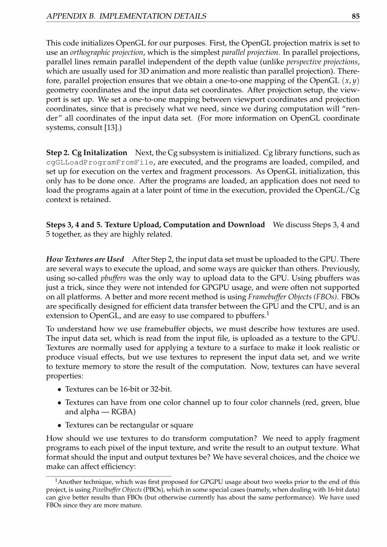
APPENDIX B. IMPLEMENTATION DETAILS 85
This code initializes OpenGL for our purposes. First, the OpenGL projection matrix is set touse an orthographic projection, which is the simplest parallel projection. In parallel projections,parallel lines remain parallel independent of the depth value (unlike perspective projections,which are usually used for 3D animation and more realistic than parallel projection). There-fore, parallel projection ensures that we obtain a one-to-one mapping of the OpenGL (x, y)geometry coordinates and the input data set coordinates. After projection setup, the view-port is set up. We set a one-to-one mapping between viewport coordinates and projectioncoordinates, since that is precisely what we need, since we during computation will “ren-der” all coordinates of the input data set. (For more information on OpenGL coordinatesystems, consult [13].)
Step 2. Cg Initalization Next, the Cg subsystem is initialized. Cg library functions, such ascgGLLoadProgramFromFile, are executed, and the programs are loaded, compiled, andset up for execution on the vertex and fragment processors. As OpenGL initialization, thisonly has to be done once. After the programs are loaded, an application does not need toload the programs again at a later point of time in the execution, provided the OpenGL/Cgcontext is retained.
Steps 3, 4 and 5. Texture Upload, Computation and Download We discuss Steps 3, 4 and5 together, as they are highly related.
How Textures are Used After Step 2, the input data set must be uploaded to the GPU. Thereare several ways to execute the upload, and some ways are quicker than others. Previously,using so-called pbuffers was the only way to upload data to the GPU. Using pbuffers wasjust a trick, since they were not intended for GPGPU usage, and were often not supportedon all platforms. A better and more recent method is using Framebuffer Objects (FBOs). FBOsare specifically designed for efficient data transfer between the GPU and the CPU, and is anextension to OpenGL, and are easy to use compared to pbuffers.1
To understand how we use framebuffer objects, we must describe how textures are used.The input data set, which is read from the input file, is uploaded as a texture to the GPU.Textures are normally used for applying a texture to a surface to make it look realistic orproduce visual effects, but we use textures to represent the input data set, and we writeto texture memory to store the result of the computation. Now, textures can have severalproperties:
• Textures can be 16-bit or 32-bit.
• Textures can have from one color channel up to four color channels (red, green, blueand alpha — RGBA)
• Textures can be rectangular or square
How should we use textures to do transform computation? We need to apply fragmentprograms to each pixel of the input texture, and write the result to an output texture. Whatformat should the input and output textures be? We have several choices, and the choice wemake can affect efficiency:
1Another technique, which was first proposed for GPGPU usage about two weeks prior to the end of thisproject, is using Pixelbuffer Objects (PBOs), which in some special cases (namely, when dealing with 16-bit data)can give better results than FBOs (but otherwise currently has about the same performance). We have usedFBOs since they are more mature.

B.2. GPU IMPLEMENTATION DETAILS 86
1. Input texture is single-channel, output texture is single-channel (single/single). In this case,the fragment program will be run once for each value in the output texture (since it isthe output texture we are rendering to — it can be considered as our screen). Therefore,each fragment program execution will compute a single transform coefficient. This isnot good, since we can not exploit SIMD parallelism at all! Fragment processors arecapable of processing four floating-point values simultaneously, but with this scheme,we only compute one transform coefficient per execution!2
2. Input texture is single-channel, output texture is multi-channel (single/multi). This schemeis better. Since the output texture is multi-channel (RGBA), each fragment programexecution can write four values to the output texture. This means that four coefficientscan be processed simultaneously by each fragment processor. But there is a problem:If we want to implement the fast LOT, Feig-Linzer multiply-add or AAN algorithms,we need to write eight values to the output texture, since these algorithms operate on8-point blocks, and computing only four coefficients can be problematic. Furthermore,the fragment processors must “detect” whether or not they are going to compute thefirst four or the last four transform values. Fortunately, there is a solution: We use twomulti-channel output textures! This technique is called multiple rendering targets, orMRT. Then, the fragment program writes the first four coefficients to the first texture,and the last four coefficients to the second texture.
3. Input texture is multi-channel, output texture is single-channel (multi/single). Unfortu-nately, the last method has a problem: Now, the transform coefficients are spreadon two multi-channel textures. For the transform values to be useful, they must bemerged into one large texture. Thus we need to develop code that scatters the values oftwo multi-channel textures into one large single-channel texture, which can be down-loaded to the CPU or used for other computations3. (But it would be unwise to usethis scheme when doing computation, for the same reasons as whith the single/singlescheme.)
4. Input texture is multi-channel, output texture is multi-channel (multi/multi). This schemeis better than the single/single scheme, but requires superfluous memory accessescompared to using the single/multi and multi/single schemes combined. Considerthe following case: Input values are stored along rows of the texture. The transform isapplied, and the output is written directly to the multi-channel output texture. Every-thing is OK so far. But if we now do a column transform, then one fragment processorcomputing the coefficients for the first column requires all the “red” values of the col-umn, while the fragment processor computing the coefficients for the second columnrequires all the “green” values, and so on. But when using multi-channel input tex-tures, there is no way to just read one color channel from that texture. Either, thefragment processor must fetch all the RGBA values, or nothing. This leads to a prob-lem: All the fragment programs will read 3 × 8 = 24 completely redundant valuesin each execution. Three fourths of the bandwidth used is not used for computation.Also, the column transform will be much slower than the row transform, since therow transform will only require one memory access per four values, while the columntransform requires reading four values for one value. To a certain degree, we get thesame problem with the multi/single scheme when we scatter, since single executionsof fragment programs must read all four color channels when only one channel is re-quired (but using the multi/single scheme must also be done at least once when using
2Using multiple rendering targets, this number would increase to four coefficients — but that is still notenough.
3The NVIDIA DCT implementation also uses scatters, but we use them in a slightly different way.

APPENDIX B. IMPLEMENTATION DETAILS 87
the multi/multi scheme in order compute a single, large texture at the end of compu-tation). Since the multi/multi scheme leads to column transforms having an entirelydifferent code than row transforms, and since they will likely be much slower thanthe row transforms, we have chosen to use the single/multi scheme combined withthe multi/single scheme, which does not have these problems. The code turns out tobe simpler since there is only one texture coordinate per input value when computingthe transform, and very little difference, performance and code-wise, between the rowand column transforms.
Summarizing our findings above, we have the following plan for executing the transform.
1. Upload the data set as a single-channel texture.
2. Execute fragment/vertex programs to do the computation. The results are written totwo multi-channel output textures. Two multi-channel output textures are requiredsince each fragment processor execution computs eight transform values simultane-ously.
3. Execute another set of fragment/vertex programs which as input takes the two outputtextures from the previous textures, scatters4 them, and writes the result back to theoriginal input texture (which is single-channel).
4. This texture can be read by the CPU, or used in successive computations. For instance,to compute a 2D DCT, we first do the above steps for the DCT along the rows. Then,we change the fragment/vertex programs to compute the DCT along the columns,and use the single-channel texture containing the row transform values as input, andrepeat the process (first a column transform is written to two RGBA textures, and aresubsequently merged into one texture — which can be downloaded to RAM.)
Figure B.1 on the following page illustrates.
Notice that we need to “swap” the textures’ role during the transform: Initially, the largesingle-channel texture is the input texture and the two RGBA textures are output textures.But at the scatter step, the two RGBA textures become input textures and the input texturebecomes the output textures. This brings us back to where we started: FBOs can be used toeasily “swap” the role of the textures, and also makes it easy to use MRT. Consider FigureB.1. We generate two FBOs. The first FBO is bound to the single-channel input textureof size N × N, and the second FBO is bound to two RGBA textures of size N/4 × N/2.Notice that the two RGBA textures can store N × N values, since each channel has fourchannels; thus we have 4 · 2 · (N/4× N/2) = N2. The reason we use N/4 values along thex-dimension is that the RGBA values are stored in the x-dimension, so each address valuein the x-direction corresponds to four values in the y-direction. That is, the four channels ofeach texture element is stored along the x-direction (see Figure B.1). This leads to that theRGBA textures are not square, since N/4 × 4 = N values are stored along the x-direction,but N/2 values are stored along the y-direction. Practically, this has no significance, becauseour scatter programs take care of the job of mapping the elements of the two RGBA texturesto the single-channel texture correctly.
Initializing FBOs Consider Listing B.2, extracted from the source code in Section ?? onpage ??, which shows how texture and FBO initialization, upload and download is done.As is evident from the listing, using FBOs makes doing this very simple.
4We use the term scatter since the program will scatter packed RGBA values on to several single-channelvalues.

B.2. GPU IMPLEMENTATION DETAILS 88
R R R
R R R
Step 1. Computation. RGBA RGBA RGBA
RGBA
RGBA RGBA RGBA
RGBA
programs doingcomputation
Step 2. Scatter
Fragment/vertexprograms forscattering
Download to CPU
Data from CPU/RAMor previous computationstep
Single-channeltextures
Multi-channeltextures
is bound to single-channeltexture
is bound totwo multi-channel
Fragment/vertex
FBO 0
or do anothercomputationon the GPU
FBO 1, color attachment 0
textures at twocolor attachments
Figure B.1: Using textures for computation
/∗ −−−− I n i t i a l i z e FBOs −−−− ∗ /s t a t i c GLuint fbs [ 2 ] ;
/∗ Each t e x t u r e a s s o c i a t e d with an FBO i s a s s o c i a t e d with a c o l o r a t t a c h m e n t .∗ In our c a s e , t h e i n p u t t e x t u r e i s mapped t o c o l o r a t t a c h m e n t 0 on FBO 0 ,∗ and t h e two RGBA t e x t u r e s a r e mapped t o c o l o r a t t a c h m e n t s 0 and 1 on FBO 1 .∗ /
GLenum drawbufs [ ] = { GL_COLOR_ATTACHMENT0_EXT, GL_COLOR_ATTACHMENT1_EXT } ;
/∗ G e n e r a t e f r a m e b u f f e r s ∗ /glGenFramebuffersEXT ( 2 , & fbs [ 0 ] ) ;
/∗ −−−− T e x t u r e u p l o ad −−−− ∗ //∗ G e n e r a t e t e x t u r e IDs ∗ /glGenTextures ( 1 , & i n o u t _ t e x t u r e ) ; /∗ Input t e x t u r e ∗ /glGenTextures ( 2 , o u t _ t e x t u r e s ) ; /∗ ( t emporary ) RGBA ou tp ut t e x t u r e s ∗ /
/∗ Upload i n p u t t e x t u r e t o f i r s t c o l o r a t t a c h m e n t on FBO 1 .glBindFrameBuf ferEXT i s r e q u i r e d so t h a t t h e g l F r a m e b u f f e r T e x t u r e 2 D c a l l
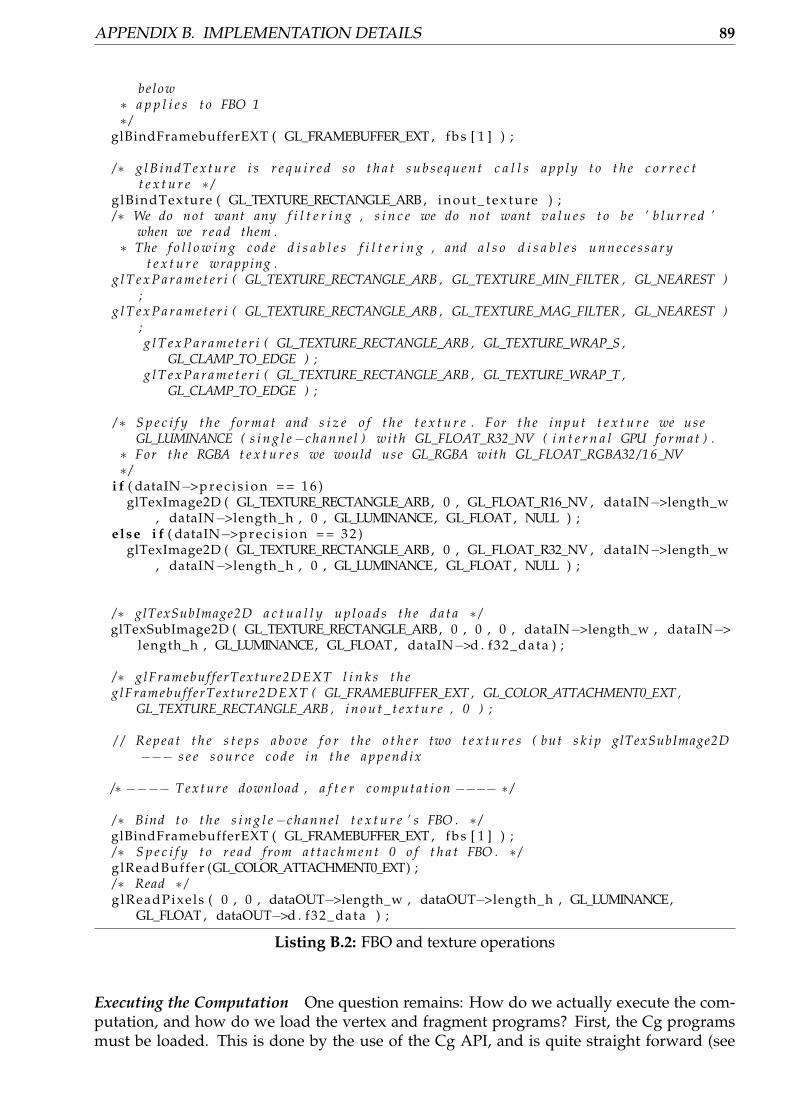
APPENDIX B. IMPLEMENTATION DETAILS 89
be low∗ a p p l i e s t o FBO 1∗ /
glBindFramebufferEXT ( GL_FRAMEBUFFER_EXT , fbs [ 1 ] ) ;
/∗ g l B i n d T e x t u r e i s r e q u i r e d so t h a t s u b s e q u e n t c a l l s a p p l y t o t h e c o r r e c tt e x t u r e ∗ /
glBindTexture ( GL_TEXTURE_RECTANGLE_ARB , i n o u t _ t e x t u r e ) ;/∗ We do not want any f i l t e r i n g , s i n c e we do not want v a l u e s t o be ’ b l u r r e d ’
when we r e a d them .∗ The f o l l o w i n g c o d e d i s a b l e s f i l t e r i n g , and a l s o d i s a b l e s u n n e c e s s a r y
t e x t u r e wrapping .g l T e x P a r a m e t e r i ( GL_TEXTURE_RECTANGLE_ARB , GL_TEXTURE_MIN_FILTER , GL_NEAREST )
;g l T e x P a r a m e t e r i ( GL_TEXTURE_RECTANGLE_ARB , GL_TEXTURE_MAG_FILTER , GL_NEAREST )
;g l T e x P a r a m e t e r i ( GL_TEXTURE_RECTANGLE_ARB , GL_TEXTURE_WRAP_S ,
GL_CLAMP_TO_EDGE ) ;g l T e x P a r a m e t e r i ( GL_TEXTURE_RECTANGLE_ARB , GL_TEXTURE_WRAP_T ,
GL_CLAMP_TO_EDGE ) ;
/ ∗ S p e c i f y t h e f o r m a t and s i z e o f t h e t e x t u r e . For t h e i n p u t t e x t u r e we useGL_LUMINANCE ( s i n g l e−c h a n n e l ) wi th GL_FLOAT_R32_NV ( i n t e r n a l GPU f o r m a t ) .
∗ For t h e RGBA t e x t u r e s we would use GL_RGBA with GL_FLOAT_RGBA32/ 1 6_NV∗ /
i f ( dataIN−>p r e c i s i o n = = 1 6 )glTexImage2D ( GL_TEXTURE_RECTANGLE_ARB, 0 , GL_FLOAT_R16_NV , dataIN−>length_w
, dataIN−>length_h , 0 , GL_LUMINANCE, GL_FLOAT , NULL ) ;e lse i f ( dataIN−>p r e c i s i o n = = 3 2 )
glTexImage2D ( GL_TEXTURE_RECTANGLE_ARB, 0 , GL_FLOAT_R32_NV , dataIN−>length_w, dataIN−>length_h , 0 , GL_LUMINANCE, GL_FLOAT , NULL ) ;
/∗ glTexSubImage2D a c t u a l l y u p l o a d s t h e d a t a ∗ /glTexSubImage2D ( GL_TEXTURE_RECTANGLE_ARB, 0 , 0 , 0 , dataIN−>length_w , dataIN−>
length_h , GL_LUMINANCE, GL_FLOAT , dataIN−>d . f32_data ) ;
/∗ glFramebuf f erTexture2DEXT l i n k s t h eg lFramebuf f erTexture2DEXT ( GL_FRAMEBUFFER_EXT , GL_COLOR_ATTACHMENT0_EXT ,
GL_TEXTURE_RECTANGLE_ARB , i n o u t _ t e x t u r e , 0 ) ;
/ / Re pe a t t h e s t e p s a b o v e f o r t h e o t h e r two t e x t u r e s ( but s k i p glTexSubImage2D−−− s e e s o u r c e c o d e in t h e a p p e n d ix
/∗ −−−− T e x t u r e download , a f t e r c o m p u t a t i o n −−−− ∗ /
/∗ Bind t o t h e s i n g l e−c h a n n e l t e x t u r e ’ s FBO . ∗ /glBindFramebufferEXT ( GL_FRAMEBUFFER_EXT , fbs [ 1 ] ) ;/∗ S p e c i f y t o r e a d from a t t a c h m e n t 0 o f t h a t FBO . ∗ /glReadBuffer (GL_COLOR_ATTACHMENT0_EXT) ;/∗ Read ∗ /glReadPixels ( 0 , 0 , dataOUT−>length_w , dataOUT−>length_h , GL_LUMINANCE,
GL_FLOAT , dataOUT−>d . f32_data ) ;
Listing B.2: FBO and texture operations
Executing the Computation One question remains: How do we actually execute the com-putation, and how do we load the vertex and fragment programs? First, the Cg programsmust be loaded. This is done by the use of the Cg API, and is quite straight forward (see

B.2. GPU IMPLEMENTATION DETAILS 90
the source code in Section ??). The parameters of the Cg programs must also be set up.Parameters can either be uniform, which are constants, or samplers, which are objects the pro-grams can fetch textures from. For example, when doing scattering, the size of the inputdata set is used to compute texture fetch coordinates. The size of the data set can be a uni-form parameter, which is set from the CPU code using the function cgGLSetParameter1f.Then, at each program execution, the uniform parameter is available. Also, we must linkthe OpenGL textures to the Cg programs. This is done in a similar manner: We use the CgAPI’s functions to link the OpenGL textures to input samplers of the Cg programs using thecgGLSetTextureParameter function.
Several Cg programs can be loaded, but only one program may be bound to the vertex andfragment processors at a time. To specify the current active program, we use thecgGLBindProgram call.
Finally, we also need to actually start execution! This is done by simply rendering a square.Because there is a one-to-one relation between our viewport, texture coordinates and projec-tion surface, we simply draw a large square covering the entire target texture. Thus whenrendering in the scatter step to the single-channel texture, our square will be of size N × N,and when rendering to the two RGBA textures during computation, our square will be ofsize N/4 × N/2. The fragment programs are executed for each pixel in the textures, andthe vertex programs are executed for each vertex in the square. To induce minimal over-head on the CPU when computing, we use display lists to store the textures. Display lists aresequences of OpenGL commands. We create one display list for generating a quadrilateralcovering the input target texture (to which the scatter programs render), and another onefor covering the RGBA textures (to which the computation programs render). Listing B.3shows an outline of the code for computing the DCT (again, for details, see the source codeor the appendix). Computing the LOT, as we will see, consists of more steps.
/∗ −−−− D i s p l a y l i s t i n i t i a l i z a t i o n ( done on ly once ) −−−− ∗ /
GLint q u a d l i s t s [ 2 ] ;/∗ We use d i s p l a y l i s t s t o draw t h e quads , i n s t e a d o f do ing t h e g l V e r t e x ( )
c a l l s when computing .∗ Thi s makes t h e CPU p a r t o f t h e program run q u i c k e r .∗ /
q u a d l i s t s [ 0 ] = glGenLis ts ( 2 ) ;q u a d l i s t s [ 1 ] = q u a d l i s t s [ 0 ] + 1 ;
/∗ Note t h a t t h e t e x t u r e c o o r d i n a t e s s p e c i f i e d a r e v i s i b l e t o t h e GPU s h a d e rprograms . ∗ /
glNewList ( q u a d l i s t s [ 0 ] , GL_COMPILE) ;glBegin (GL_QUADS) ;
glTexCoord2f ( 0 . 0 , 0 . 0 ) ;g l V e r t e x 2 f ( 0 . 0 , 0 . 0 ) ;glTexCoord2f ( dataIN−>length_w / 4 . 0 , 0 . 0 ) ;g l V e r t e x 2 f ( dataIN−>length_w / 4 . 0 , 0 . 0 ) ;glTexCoord2f ( dataIN−>length_w / 4 . 0 , dataIN−>length_h / 2 . 0 ) ;g l V e r t e x 2 f ( dataIN−>length_w / 4 . 0 , dataIN−>length_h / 2 . 0 ) ;glTexCoord2f ( 0 . 0 , dataIN−>length_h / 2 . 0 ) ;g l V e r t e x 2 f ( 0 . 0 , dataIN−>length_h / 2 . 0 ) ;
glEnd ( ) ;g lEndList ( ) ;
/∗ D i v i d i ng dataIN−>length_w by 4 w i l l become a p p a r e n t in s u b s e q u e n t s e c t i o n s

APPENDIX B. IMPLEMENTATION DETAILS 91
∗ /
glNewList ( q u a d l i s t s [ 1 ] , GL_COMPILE) ;glBegin (GL_QUADS) ;
glTexCoord2f ( 0 . 0 , 0 . 0 ) ;g l V e r t e x 2 f ( 0 . 0 , 0 . 0 ) ;glTexCoord2f ( dataIN−>length_w / 4 . 0 , 0 . 0 ) ;g l V e r t e x 2 f ( dataIN−>length_w , 0 . 0 ) ;glTexCoord2f ( dataIN−>length_w / 4 . 0 , dataIN−>length_h ) ;g l V e r t e x 2 f ( dataIN−>length_w , dataIN−>length_h ) ;glTexCoord2f ( 0 . 0 , dataIN−>length_h ) ;g l V e r t e x 2 f ( 0 . 0 , dataIN−>length_h ) ;
glEnd ( ) ;g lEndList ( ) ;
/∗ −−−− Actua l c o m p u t a t i o n o f t h e DCT−−−− ∗ /
GLenum drawbufs [ ] = { GL_COLOR_ATTACHMENT0_EXT, GL_COLOR_ATTACHMENT1_EXT } ;
/∗ Swapping i s done s imp l y by ( 1 ) swapping FBOs , and ( 2 ) s p e c i f y i n g t h edrawing b u f f e r s o f t h e new FBO . Doing t h i s g i v e s o f f −s c r e e n r e n d e r i n g t ot e x t u r e .
∗ /
/∗ Pass 1 : DCT on rows ∗ //∗ Loads a p a s s t h r o u g h v e r t e x program and DCT row program ∗ /cgGLBindProgram ( cgprog_passthrough_v ) ;cgGLBindProgram ( cgprog_row_f ) ;/∗ S e t up t o r e n d e r t o t h e two RGBA t e x t u r e s on FBO 0 ( c o l o r a t t a c h m e n t s 0
and 1 ) ∗ /glBindFramebufferEXT ( GL_FRAMEBUFFER_EXT , fbs [ 0 ] ) ;glDrawBuffers ( 2 , drawbufs ) ;/∗ A c t u a l l y draw t h e s q u a r e . ∗ /g l C a l l L i s t ( q u a d l i s t s [ 0 ] ) ;
/∗ Pass 2 : Conver t 2xRGBA −> 1xR ∗ /
cgGLBindProgram ( cgprog_passthrough_v ) ;cgGLBindProgram ( cgprog_rowscat ter_f ) ;/∗ S e t up t o r e n d e r t o t h e s i n g l e c h a n n e l t e x t u r e on FBO 1 ( c o l o r a t t a c h m e n t
0 ) ∗ /glBindFramebufferEXT ( GL_FRAMEBUFFER_EXT , fbs [ 1 ] ) ;glDrawBuffer ( GL_COLOR_ATTACHMENT0_EXT ) ;/∗ A c t u a l l y draw t h e s q u a r e c o v e r i n g t h e e n t i r e s i n g l e−c h a n n e l s q u a r e . ∗ /g l C a l l L i s t ( q u a d l i s t s [ 1 ] ) ;
/∗ Pass 3 : DCT on columns ∗ /
cgGLBindProgram ( cgprog_col_v ) ;cgGLBindProgram ( cgprog_col_f ) ;/∗ S e t up t o r e n d e r t o t h e two RGBA t e x t u r e s on FBO 0 ( c o l o r a t t a c h m e n t s 0
and 1 ) ∗ /glBindFramebufferEXT ( GL_FRAMEBUFFER_EXT , fbs [ 0 ] ) ;glDrawBuffers ( 2 , drawbufs ) ;/∗ A c t u a l l y draw t h e s q u a r e . ∗ /g l C a l l L i s t ( q u a d l i s t s [ 0 ] ) ;
/∗ Pass 4 : Conver t 2xRGBA −> 1xR ∗ /
cgGLBindProgram ( c g p r o g _ c o l s c a t t e r _ v ) ;

B.2. GPU IMPLEMENTATION DETAILS 92
cgGLBindProgram ( c g p r o g _ c o l s c a t t e r _ f ) ;/∗ S e t up t o r e n d e r t o t h e s i n g l e c h a n n e l t e x t u r e on FBO 1 ( c o l o r a t t a c h m e n t
0 ) ∗ /glBindFramebufferEXT ( GL_FRAMEBUFFER_EXT , fbs [ 1 ] ) ;glDrawBuffer ( GL_COLOR_ATTACHMENT0_EXT ) ;/∗ A c t u a l l y draw t h e s q u a r e . ∗ /g l C a l l L i s t ( q u a d l i s t s [ 1 ] ) ;
/∗ Download i s now r e a d y ! ∗ /
Listing B.3: Computation and Scattering
An illustration of how we use the textures was provided in Section 4.2.1.
B.2.2 DCT Program Details
Step 1. Row Transform The row transform on the GPU is done by the passthrough vertexprogram and the row transform fragment program. These programs are listed in ListingsB.4 and B.5, respectively.
void dct_gpu_flmad_passthrough_vertex ( in f l o a t 2 t c : TEXCOORD0,in f l o a t 4 pos : POSITION ,in f l o a t 4 c o l o r : COLOR,
out f l o a t 2 t c 0 : TEXCOORD0,out f l o a t 4 pos0 : POSITION ,out f l o a t 4 co lo r0 : COLOR,
uniform f l o a t 4 x 4 mvp){
t c 0 = t c ;pos0 = mul (mvp , pos ) ;co lo r0 = c o l o r ;
}
Listing B.4: Vertex processor passthrough program
Listing B.4 shows the vertex passthrough program. This is the simplest vertex program thatis possible to write. It passes on the texture coordinate position and the color (which actuallyis irrelevant, but must be passed on). However, the position must be modified. Since we areusing a vertex program, we must multiply the position by the model-view-projection (MVP)matrix, since if not, our viewpoint will not be located at the correct place (which is rightin front of the data set). Hence we use the operation mul(mvp,pos), which is a built-inCg function to perform a matrix-vector multiplication. The transformed position is passeddown to the rest of the pipeline.
Note that if we do not use vertex programs, the GPU will automatically multiply positionsby the MVP matrix. But when we use vertex programs, we have to do it in the vertex shaderprogram code.
Also notice that, unlike C, Cg has native vector (float2, float4) and matrix (float4x4)data types.void dct_gpu_fflmad_row_fragment (
in f l o a t 2 t c : TEXCOORD0,
out f l o a t 4 out0 : COLOR0,

APPENDIX B. IMPLEMENTATION DETAILS 93
out f l o a t 4 out1 : COLOR1,
uniform samplerRECT in0 ,uniform f l o a t xSize ,uniform half xSize_8 )
{f l o a t v0 , v1 , v2 , v3 , odd_row ;f l o a t 4 dctin0_3 , dct in4_7 ;
/∗ x S i z e _ 8 i s a uni form p a r a m e t e r s e t by t h e C c o d e e q u a l t o t h e h o r i z o n t a ll e n g t h d i v i d e d by 8 ,
∗ w h i l e x S i z e i s j u s t t h e h o r i z o n t a l i n p u t l e n g t h∗ /
t c = f l o o r ( t c ) ;odd_row = f l o o r ( t c . x/xSize_8 ) ;
t c ∗= f l o a t 2 ( 8 . 0 , 2 . 0 ) ;t c + = f l o a t 2 (−odd_row ∗ xSize , odd_row ) ;
/∗ Use v e c t o r i z e d a d d i t i o n t o c a l c u l a t e t e x t u r e c o o r d i n a t e s∗ Also , t h e o r d e r o f t h e c o m p u t a t i o n i s i m p o r t a n t : We c a l c u l a t e∗ t h e l a s t f o u r t e x t u r e c o o r d i n a t e s a f t e r t h e f1texRECTs have been i s s u e d∗ but b e f o r e we need t h e v a l u e s . Th i s min imize s was t e o f t ime .∗ /
dct in0_3 = t c . xxxx + half4 ( 0 . 0 , 1 . 0 , 2 . 0 , 3 . 0 ) ;
v0 = f1texRECT ( in0 , f l o a t 2 ( dct in0_3 . x , t c . y ) ) ;v1 = f1texRECT ( in0 , f l o a t 2 ( dct in0_3 . y , t c . y ) ) ;v2 = f1texRECT ( in0 , f l o a t 2 ( dct in0_3 . z , t c . y ) ) ;v3 = f1texRECT ( in0 , f l o a t 2 ( dct in0_3 .w, t c . y ) ) ;dct in4_7 = t c . xxxx + half4 ( 4 . 0 , 5 . 0 , 6 . 0 , 7 . 0 ) ;dct in0_3 = f l o a t 4 ( v0 , v1 , v2 , v3 ) ;v0 = f1texRECT ( in0 , f l o a t 2 ( dct in4_7 . x , t c . y ) ) ;v1 = f1texRECT ( in0 , f l o a t 2 ( dct in4_7 . y , t c . y ) ) ;v2 = f1texRECT ( in0 , f l o a t 2 ( dct in4_7 . z , t c . y ) ) ;v3 = f1texRECT ( in0 , f l o a t 2 ( dct in4_7 .w, t c . y ) ) ;dct in4_7 = f l o a t 4 ( v0 , v1 , v2 , v3 ) ;
/∗ Actua l FL MADD a l g o r i t h m ∗ /dct_gpu_fflmad ( dct in0_3 , dct in4_7 ) ;
/∗ Note t h a t d c t i n 0 _ 3 and d c t i n 4 _ 7 c o n t a i n t h e DCT c o e f f i c i e n t s a f t e r c a l l i n gd c t _ g p u _ f f l m a d .
∗ Cg s u p p o r t s c a l l by r e f e r e n c e .∗ /
out0 = dct in0_3 ;out1 = dct in4_7 ;
}
Listing B.5: Row DCT on the GPU — Fragment program
The fragment program in Listing B.5 executes the forward row transform on 8 points. Noticethat this fragment program first does some computations on the texture coordinates. Thisis necessary, since the texture coordinates passed to the fragment program is the location ofthe current pixel in the output texture, that is, the RGBA texture. However, we are fetchingdata from the single-channel texture. We hence need a function to map from our texturecoordinates (in the two RGBA textures) to eight input values in the single-channel texture.

B.2. GPU IMPLEMENTATION DETAILS 94
The texture computations in the code make sure that one coordinate position in the twoRGBA textures maps to eight distinct values on the same row in the input data set. Thisshould be apparent if you consider Figure 4.5 on page 55, which provides an illustration.
In the figure, the x texture coordinate of the texture element is shown inside the element.Note that one coordinate in the single-channel texture refers to exactly one value, while onecoordinate in the RGBA textures refers to four values. In the initial part of the code in ListingB.5, we map the RGBA texture coordinates to the single-channel texture coordinates. Thenwe fetch the corresponding row, compute the row DCT, and finally write out four values tothe first RGBA texture and four values to the second texture.
After computing the texture coordinates, the program uses the internal f1texRECTCg func-tion to fetch the row starting at those coordinates, and then, the DCT is computed, andfinally written to each RBGA texture. Note that nearly all operations are vectorized. In gen-eral, it pays off to vectorize Cg code as much as possible, as we will see later. We will alsoconsider the actual FL MADD algorithm (the dct_gpu_fflmad function) later. The AANimplementation is similar, but calls dct_gpu_faan instead. Computing the inverse rowtransform is done in precisely the same way, but we call dct_gpu_iflmad instead of theforward transform function.
Step 2. Row scatter Row scatter also uses the passthrough vertex program, since no com-putations it does can be done by the vertex processor (more on this later). The fragmentprogram simply computes a mapping from the single-channel texture coordinates to eachof the two RGBA textures, and fetches the correct value from the RBGA textures and putsthem into the single-channel texture at the correct location. Thus the program’s job is to pickthe right value from the two RGBA coordinates. The row scatter program is displayed inListing B.6.
void dct_gpu_flmad_rowscatter_fragment ( in f l o a t 2 t c : TEXCOORD0,out f l o a t out0 : COLOR0,uniform samplerRECT in0 ,uniform samplerRECT in1 ,uniform half xSize_8 )
{
half2 oddrowcol ;half4 componentselect ;f l o a t 4 v0 , v1 ;
/∗ x S i z e _ 8 i s t h e h o r i z o n t a l i n p u t s e t s i z e d i v i d e d by 8 . Th i s can be s t o r e d∗ in h a l f p r e c i s i o n s i n c e x S i z e _ 8 i s a lways < 2 0 4 8 .∗ /
componentselect = ( f r a c ( t c . x ) = = half4 ( 0 . 1 2 5 , 0 . 3 7 5 , 0 . 6 2 5 , 0 . 8 7 5 ) ) ;oddrowcol = f l o o r ( fmod ( tc , 2 ) ) ;t c = f l o o r ( t c − oddrowcol ) / 2 . 0 ;t c . x + = oddrowcol . y ∗ xSize_8 ;
v0 = f4texRECT ( in0 , t c ) ;v1 = f4texRECT ( in1 , t c ) ;
out0 = dot ( lerp ( v0 , v1 , oddrowcol . x ) , componentselect ) ;}
Listing B.6: Row scatter on the GPU — Fragment program

APPENDIX B. IMPLEMENTATION DETAILS 95
This program essentially does essentially the reverse of the previous program, in that theprevious program computed the mapping function from the two RGBA textures to thesingle-channel texture, while this program computes the mapping from the single-channeltexture to the two RGBA textures. This program illustrates a few important principles whenprogramming the GPU: Compute, don’t branch and Use internal Cg functions. The programfirst computes the mapping of the texture coordinates of the single-channel texture to thetexture coordinates of the two RGBA textures. But we have a problem. The first problemis that we do not know what RGBA texture contains our value (there are two — which onedo we choose?) And second, even if we knew which texture contained our value and theaddress of the element, the texture element at that address would have four components.How do we know what component we should pick?
Let us first look at the component selection problem — i.e. assume we have the addressof the texture element in the RGBA texture, but do not know which component (R, G, B orA) we are going to store. Recall from Listing B.3 on page 90 that we divided the x texturecoordinates by four. Normally, texture coordinates in the x-direction for the single channelsare passed as:
[ 0.5 1.5 2.5 3.5 4.5 ... ]
by the GPU. But dividing by four in the glTexCoord call gives us the sequence
[ 0.125 0.375 0.625 0.875 1.125 ... ]
This is why we divided the texture coordinate by four in Listing B.3, and this gives us the keyto choosing what component of the RGBA texture element we are interested in. Assume weknow the location of the RGBA texture element. Then, if the fraction value, that is x − bxc,of our texture coordinate is 0.125, we choose the R component. If it is 0.375, choose the Gcomponent. And so on. In fact, this can be expressed as a dot product! While we could dosomething like5
if(frac == 0.125) { out0 = textureElement.x; }else if(frac == 0.375) { out0 = textureElement.y; }else if(frac == 0.625) { out0 = textureElement.z; }else { out0 = textureElement.w; }
a dot product will be at least 12 times faster. I kid you not. Dot products take at most 1 cycle,while if-elseif-elseif-else takes at least 12 cycles.
Here is the idea, implemented in Listing B.6. We first do a vector comparison in the codeabove (we compare the fractional value of the x-coordinate to the four possible values in thecomponentselect variable). Then, if we have the four-component value in a variable x,the same effect as the above if-statements is obtained by simply computing the dot product
out0 = dot(textureElement, componentselect);
So that problem is certainly solved.
Let’s now look at how we can obtain the texture coordinates in the RBGA texture. ConsiderFigure 4.5 on page 55 again. Let us look at an example and do the computation step by step.Suppose we have 16 elements in the x-direction and just two elements in the y-direction.The texture coordinates in the x-direction passed to the row scatter programs are6
[0.125 0.375 0.625 0.875|1.125 1.375 1.625 1.875|2.125 2.375 2.625 2.875|3.125 3.375 3.625 3.875][0.125 0.375 0.625 0.875|1.125 1.375 1.625 1.875|2.125 2.375 2.625 2.875|3.125 3.375 3.625 3.875]
5Note that the RGBA components are accessed in Cg by suffixing the vector value with .x, .y, .z and .w,respectively.
6Note that only one coordinate is passed in each execution. This is done automatically by the GPU.

B.2. GPU IMPLEMENTATION DETAILS 96
Taking modulo 2 of these values and then computing the floor function gives us (this is theoddrowcol variable in the program)(*)[0.000 0.000 0.000 0.000|1.000 1.000 1.000 1.000|0.000 0.000 0.000 0.000|1.000 1.000 1.000 1.000][0.000 0.000 0.000 0.000|1.000 1.000 1.000 1.000|0.000 0.000 0.000 0.000|1.000 1.000 1.000 1.000]
for the x-components, and taking modulo 2 for the y-components (simply 0 for the first lineand 1 for the second) gives(**)[0.000 0.000 0.000 0.000|0.000 0.000 0.000 0.000|0.000 0.000 0.000 0.000|0.000 0.000 0.000 0.000][1.000 1.000 1.000 1.000|1.000 1.000 1.000 1.000|1.000 1.000 1.000 1.000|1.000 1.000 1.000 1.000]
for the y-components. Thus oddrowcol just says whether the row and column coordinatesare an odd number or not.
Now, subtracting the modulo 2 values from the original values, flooring and dividing by 2,componentwise, gives(***)[0.000 0.000 0.000 0.000|0.000 0.000 0.000 0.000|1.000 1.000 1.000 1.000|1.000 1.000 1.000 1.000][0.000 0.000 0.000 0.000|0.000 0.000 0.000 0.000|1.000 1.000 1.000 1.000|1.000 1.000 1.000 1.000]
for the x-components, and(****)[0.000 0.000 0.000 0.000|0.000 0.000 0.000 0.000|0.000 0.000 0.000 0.000|0.000 0.000 0.000 0.000][0.000 0.000 0.000 0.000|0.000 0.000 0.000 0.000|0.000 0.000 0.000 0.000|0.000 0.000 0.000 0.000]
for the y-components.
Finally, add the modulo 2 values for the y-component (**) multiplied by the input data setlength divided by eight (in this case, 2) to (***) (the x-component) above. Then we get,finally, the texture coordinates[0.000 0.000 0.000 0.000|0.000 0.000 0.000 0.000|2.000 2.000 2.000 2.000|2.000 2.000 2.000 2.000][1.000 1.000 1.000 1.000|1.000 1.000 1.000 1.000|3.000 3.000 3.000 3.000|3.000 3.000 3.000 3.000]
in the x-direction, and the texture coordinates in the y-direction are given by (****).
Wasn’t that an interesting pattern. It seems that we have obtained the texture coordinates in theRGBA texture! Just consider Figure 4.5 on page 55 again, and you will see that that is in factthe case. All we have to do now is to choose whether we are going to fetch from the firstor second RGBA texture. Assume that we have fetched the four-component value from thefirst texture in value v0 (using the f4texRECT Cg function) and the other in v0. Assumewe set oddrowcol.x to (*) and oddrowcol.y to (**). Then the correct output value issimply calculated by
out0 = dot( (1 - oddrowcol.x) * v0 + oddrowcol.x * v1), componentselect );
We may calculate the inner part by using the built-in Cg function lerp (linear interpolation),which gives us the last line in the fragment program in Listing B.6 on page 94.
Finding the correct mapping between the textures is quite tedious (and took quite a lot oftime during the project).
Step 3. Column transform The column transform fragment program is shown in ListingB.8 below. But we also use a vertex program for certain computations! This program is listedin Listing B.7 below.
void dct_gpu_flmad_col_vertex ( in f l o a t 2 t c : TEXCOORD0,in f l o a t 4 pos : POSITION ,in f l o a t 4 c o l o r : COLOR,
out f l o a t 2 t c 0 : TEXCOORD0,

APPENDIX B. IMPLEMENTATION DETAILS 97
out f l o a t 2 t c 1 : TEXCOORD1,out f l o a t 4 pos0 : POSITION ,out f l o a t 4 co lo r0 : COLOR,
uniform f l o a t 4 x 4 mvp,uniform half xSize_4 ,uniform half xSize_8 )
{/∗ x S i z e _ 4 and x S i z e _ 8 a r e t h e h o r i z o n t a l i n p u t s e t s i z e d i v i d e d by 4 and 8 ,
computed in CPU c o d e ∗ /t c 0 = t c ;pos0 = mul (mvp , pos ) ;co lo r0 = c o l o r ;t c 1 = f l o a t 2 ( t c . y / 4 . 0 , t c . y ∗ xSize_4 − xSize_8 ) ;
}
Listing B.7: Column DCT on the GPU — Vertex program
void dct_gpu_fflmad_col_fragment ( in f l o a t 2 t c : TEXCOORD0,in f l o a t 2 t c 1 : TEXCOORD1,
out f l o a t 4 out0 : COLOR0,out f l o a t 4 out1 : COLOR1,
uniform samplerRECT in0 ,uniform f l o a t xSize )
{/∗ x S i z e i s t h e h o r i z o n t a l l e n g t h o f t h e d a t a s e t ∗ /
f l o a t v0 , v1 , v2 , v3 , xaddr ;f l o a t 4 yaddr ;f l o a t 4 dctin0_3 , dct in4_7 ;
t c = f l o o r ( t c ) ;xaddr = t c . x + fmod ( t c 1 . y , xSize ) ;yaddr = f l o o r ( t c 1 . x ) ∗ 8 . 0 + half4 ( 0 . 0 , 1 . 0 , 2 . 0 , 3 . 0 ) ;
v0 = f1texRECT ( in0 , f l o a t 2 ( xaddr , yaddr . x ) ) ;v1 = f1texRECT ( in0 , f l o a t 2 ( xaddr , yaddr . y ) ) ;v2 = f1texRECT ( in0 , f l o a t 2 ( xaddr , yaddr . z ) ) ;v3 = f1texRECT ( in0 , f l o a t 2 ( xaddr , yaddr .w) ) ;yaddr + = 4 . 0 ;dct in0_3 = f l o a t 4 ( v0 , v1 , v2 , v3 ) ;v0 = f1texRECT ( in0 , f l o a t 2 ( xaddr , yaddr . x ) ) ;v1 = f1texRECT ( in0 , f l o a t 2 ( xaddr , yaddr . y ) ) ;v2 = f1texRECT ( in0 , f l o a t 2 ( xaddr , yaddr . z ) ) ;v3 = f1texRECT ( in0 , f l o a t 2 ( xaddr , yaddr .w) ) ;dct in4_7 = f l o a t 4 ( v0 , v1 , v2 , v3 ) ;
dct_gpu_fflmad ( dct in0_3 , dct in4_7 ) ;
out0 = dct in0_3 ;out1 = dct in4_7 ;
}
Listing B.8: Column DCT on the GPU — Fragment program
This is the first case in which we can use the vertex processor for something useful. Now, aswith the row transform, we need a mapping from one texture coordinate in the two RGBA

B.2. GPU IMPLEMENTATION DETAILS 98
textures to a column of eight values in the R texture. This is where the vertex processor cando some computation. For each texture coordinate, we need the values tc.y/4 and tc.y* xSize_4 - xSize_8. These are computed by the vertex program and passed to thefragment program in the texture coordinate parameter tc1.
One question immediately comes up. Can we move the other texture coordinate computa-tions to the vertex processor as well? The answer is no. We can, for example, not computethe floor or fmod functions in the vertex processor, since the vertex program is run onlyonce per vertex. So any texture coordinates it outputs is linearly interpolated over the entirequadrilateral. Thus non-linear functions such as will end up having a very wrong result.But we can move the scaling and addition computed prior to the nonlinear functions to thevertex processor, which saves us a few operations in the fragment processor.
Figure 4.6 on page 56 illustrates how columns in the single-channel texture map to the twoRGBA textures. Since the RGBA are along rows, we “transpose” the columns into the twoRGBA textures. The texture coordinate computations performed by the vertex and fragmentprograms compute the transformation from coordinates in the RGBA textures to columnsinthe single-channel texture, as can easily seen by an example similar to that in the lastsection. (Like the other mapping functions, this one also took some time to perfect.)
Subsequently to the the texture coordinate computation, the fragment program fetches theeight column values from the single-channel texture, computes the DCT, and outputs thefirst and last four transform values in the first and last RGBA texture, respectively. Notethat the DCT function called is the same function we used in the row transform. The AANimplementation is also exactly the same, but calls another DCT computation function. Thisis also the case when computing the inverse transform. Also, note that we are still usingSIMD operations.
Step 4. Column scatter The column scatter is for the column transform program as therow scatter is for the row transform program. Given a position inside the single-channeloutput texture, the column scatter program’s task is to store the correct value from one ofthe two RGBA textures at that location.
The column scatter fragment program is shown below, and is very similar to the row scatterprogram, except we now work on columns instead of rows. Also, we can use a vertexprogram for some computations. The column vertex and fragment programs are shownbelow in Listings B.9 and B.10.
void dct_gpu_f lmad_co lsca t ter_ver tex ( in f l o a t 2 t c : TEXCOORD0,in f l o a t 4 pos : POSITION ,in f l o a t 4 c o l o r : COLOR,
out f l o a t 2 t c 0 : TEXCOORD0,out f l o a t 2 t c 1 : TEXCOORD1,out f l o a t 2 t c 2 : TEXCOORD2,out f l o a t 4 pos0 : POSITION ,out f l o a t 4 co lo r0 : COLOR,
uniform f l o a t 4 x 4 mvp,uniform half xSize_4 )
{t c 0 = t c ;pos0 = mul (mvp , pos ) ;co lo r0 = c o l o r ;t c 1 = f l o a t 2 ( t c . x ∗ 4 . 0 / xSize_4 , t c . y / 4 . 0 ) ;

APPENDIX B. IMPLEMENTATION DETAILS 99
t c 2 = f l o a t 2 ( t c . x ∗ 4 . 0 , t c . y / 8 . 0 ) ;}
Listing B.9: Column scatter on the GPU — Vertex program
void dct_gpu_f lmad_colscat ter_fragment ( in f l o a t 2 t c : TEXCOORD0,in f l o a t 2 t c 1 : TEXCOORD1,in f l o a t 2 t c 2 : TEXCOORD2,out f l o a t out0 : COLOR0,uniform samplerRECT in0 ,uniform samplerRECT in1 ,uniform half xSize_4 )
{
half4 componentselect ;half oddblock ;
f l o a t 4 v0 , v1 ;
componentselect = ( f r a c ( t c 1 . y ) = = half4 ( 0 . 1 2 5 , 0 . 3 7 5 , 0 . 6 2 5 , 0 . 8 7 5 ) ) ;oddblock = fmod ( f l o o r ( t c 1 . y ) , 2 ) ; /∗ o d d b l o c k = 0 = > f e t c h from in0 , e l s e
f e t c h from in1 ∗ /
t c . y = f l o o r ( t c 1 . x ) + f l o o r ( t c 2 . y ) ∗ 4 . 0 ;t c . x = f l o o r ( fmod ( t c 2 . x , xSize_4 ) ) ;
v0 = f4texRECT ( in0 , t c ) ;v1 = f4texRECT ( in1 , t c ) ;
out0 = dot ( lerp ( v0 , v1 , oddblock ) , componentselect ) ;}
Listing B.10: Column scatter on the GPU — Fragment program
The texture coordinate computations in these programs are essentially the inverse of thecomputations in the column computation programs. In Figure 4.6 on page 56, instead ofmapping from the two RGBA textures to the single-channel texture, we now do the inversemapping. It is easy to verify from the above programs that they compute the correct texturecoordinates, just as we did when we dicussed the row scatter programs. Also note that weuse the same technique for component selection as we did in that program, but we nowwork in the y-direction.
B.2.3 LOT Implementation Details
The GPU row second butterfly/Z̃-program is shown in Listing B.11.
# def ine LOT_COS_THETA1 0.9177546256839811411456038575494851 /∗ c o s ( 0 . 1 3 ∗ Pi )∗ /
# def ine LOT_COS_THETA2 0.8763066800438635873081159039220626 /∗ c o s ( 0 . 1 6 ∗ Pi )∗ /
# def ine LOT_COS_THETA3 0.9177546256839811411456038575494851 /∗ c o s ( 0 . 1 3 ∗ Pi )∗ /
# def ine LOT_SIN_THETA1 0.3971478906347806137543773600194771 /∗ s i n ( 0 . 1 3 ∗ Pi )∗ /
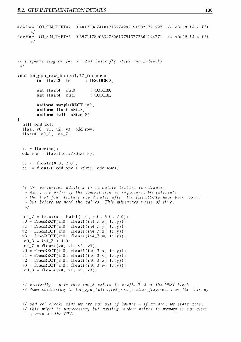
B.2. GPU IMPLEMENTATION DETAILS 100
# def ine LOT_SIN_THETA2 0.4817536741017152749871915028721297 /∗ s i n ( 0 . 1 6 ∗ Pi )∗ /
# def ine LOT_SIN_THETA3 0.3971478906347806137543773600194771 /∗ s i n ( 0 . 1 3 ∗ Pi )∗ /
/∗ Fragment program f o r row 2 nd b u t t e r f l y s t e p s and Z−b l o c k s∗ /
void lot_gpu_row_butterf ly2Z_fragment (in f l o a t 2 t c : TEXCOORD0,
out f l o a t 4 out0 : COLOR0,out f l o a t 4 out1 : COLOR1,
uniform samplerRECT in0 ,uniform f l o a t xSize ,uniform half xSize_8 )
{half odd_col ;f l o a t v0 , v1 , v2 , v3 , odd_row ;f l o a t 4 in0_3 , in4_7 ;
t c = f l o o r ( t c ) ;odd_row = f l o o r ( t c . x/xSize_8 ) ;
t c ∗= f l o a t 2 ( 8 . 0 , 2 . 0 ) ;t c + = f l o a t 2 (−odd_row ∗ xSize , odd_row ) ;
/∗ Use v e c t o r i z e d a d d i t i o n t o c a l c u l a t e t e x t u r e c o o r d i n a t e s∗ Also , t h e o r d e r o f t h e c o m p u t a t i o n i s i m p o r t a n t : We c a l c u l a t e∗ t h e l a s t f o u r t e x t u r e c o o r d i n a t e s a f t e r t h e f1texRECTs have been i s s u e d∗ but b e f o r e we need t h e v a l u e s . Th i s min imize s was t e o f t ime .∗ /
in4_7 = t c . xxxx + half4 ( 4 . 0 , 5 . 0 , 6 . 0 , 7 . 0 ) ;v0 = f1texRECT ( in0 , f l o a t 2 ( in4_7 . x , t c . y ) ) ;v1 = f1texRECT ( in0 , f l o a t 2 ( in4_7 . y , t c . y ) ) ;v2 = f1texRECT ( in0 , f l o a t 2 ( in4_7 . z , t c . y ) ) ;v3 = f1texRECT ( in0 , f l o a t 2 ( in4_7 .w, t c . y ) ) ;in0_3 = in4_7 + 4 . 0 ;in4_7 = f l o a t 4 ( v0 , v1 , v2 , v3 ) ;v0 = f1texRECT ( in0 , f l o a t 2 ( in0_3 . x , t c . y ) ) ;v1 = f1texRECT ( in0 , f l o a t 2 ( in0_3 . y , t c . y ) ) ;v2 = f1texRECT ( in0 , f l o a t 2 ( in0_3 . z , t c . y ) ) ;v3 = f1texRECT ( in0 , f l o a t 2 ( in0_3 .w, t c . y ) ) ;in0_3 = f l o a t 4 ( v0 , v1 , v2 , v3 ) ;
/ / B u t t e r f l y − n o t e t h a t in0_3 r e f e r s t o c o e f f s 0−3 o f t h e NEXT b l o c k/ / When s c a t t e r i n g in l o t _ g p u _ b u t t e r f l y 2 _ r o w _ s c a t t e r _ f r a g m e n t , we f i x t h i s up
/ / o d d _ c o l c h e c k s t h a t we a r e not out o f bounds − i f we are , we s t o r e z e r o ./ / t h i s might be u n n e c e s s a r y but w r i t i n g random v a l u e s t o memory i s not c l e a n
, even on t h e GPU!

APPENDIX B. IMPLEMENTATION DETAILS 101
odd_col = ( t c . x / 8 . 0 ! = xSize_8 − 1) ;
out0 = odd_col ∗ ( in4_7 − in0_3 ) ∗ 0 . 5 ;
/ / The f o l l o w i n g c o d e d o e s t h e Z−b l o c k s/ / U n f o r t u n a t e l y , computing t h e Z−b l o c k s i n v o l v e s some v e c t o r d e p e n d e n c i e s ,/ / but we can a t l e a s t c a l c u l a t e two v a l u e s in e a c h i n s t r u c t i o n/ / We use in0_3 as a t emporary v a r i a b l e
out1 . xy = LOT_COS_THETA1 ∗ out0 . xy + LOT_SIN_THETA1 ∗ f l o a t 2 (−out0 . y , out0 . x ) ;out1 . yz = LOT_COS_THETA2 ∗ f l o a t 2 ( out1 . y , out0 . z ) + LOT_SIN_THETA2 ∗ f l o a t 2 (−
out0 . z , out1 . y ) ;out1 . zw = LOT_COS_THETA3 ∗ f l o a t 2 ( out1 . z , out0 .w) + LOT_SIN_THETA3 ∗ f l o a t 2 (−
out0 .w, out1 . z ) ;
out0 = out1 ;out1 = odd_col ∗ ( in4_7 + in0_3 ) ∗ 0 . 5 ;
}
Listing B.11: The second butterflies and Z̃-block on the GPU — Fragment program
This program is similar to the fragment program for the row DCT, but there are a few differ-ences. The texture coordinate computation is precisely the same. However, notice that wenow fetch only the last four values (from the DCT + 1st butterfly) of our “current” block andthe first four values of the next block. This should be evident from Figure 3.10 on page 43.The Z̃-part of the block is stored in the first RGBA texture, while the part only having a sec-ond butterfly and the 1/2 scaling is stored in the second RGBA texture. Also notice that theZ̃-block computation is difficult to parallelize, which is evident from Figure 3.11 on page 44,but we can at least compute two values simultaneously.
The row scatter program, which fetches the first four block values from the previous block,is shown in Listing B.12 below.
void lo t_gpu_rowscat ter_but ter f ly2Z_fragment (in f l o a t 2 t c : TEXCOORD0,out f l o a t out0 : COLOR0,uniform samplerRECT in0 ,uniform samplerRECT in1 ,uniform half xSize_8 )
{
/ / F i r s t p a r t o m i t t e d − p r e c i s e l y e q u a l t o d c t _ g p u _ f l m a d _ r o w s c a t t e r _ f r a g m e n t
v1 = f4texRECT ( in1 , t c ) ;t c . x −= 1 . 0 ;v0 = f4texRECT ( in0 , t c ) ;
out0 = dot ( lerp ( v0 , v1 , oddrowcol . x ) , componentselect ) ;}
Listing B.12: Row scatter for second butterflies and Z̃-block on the GPU — Fragmentprogram
In order to avoid cramming this report with too much code, and since the column programsare very similar to what we have previously seen, the column second butterfly/Z̃ and mod-ified column scatter programs are not shown in the appendix, but is located on the CD. Theprogram function names are lot_gpu_col_butterfly2Z_fragment and

B.2. GPU IMPLEMENTATION DETAILS 102
lot_gpu_colscatter_butterfly2Z_fragment (the fragment programs) andlot_gpu_colscatter_butterfly2Z_vertex (the vertex program for the column scat-ter). These programs do exactly the same as the row programs, but operate on columns in-stead. The column second butterfly/Z̃ computation program uses the same vertex programas the DCT column transform (implemented in lot_gpu_col_vertex, and does almostexactly the same as the program in Listing B.11, but operates on columns. As in that pro-gram, the first four LOT values of a block are shifted by four positions. The column scattervertex and fragment programs are also simple modifications of the DCT column scatter pro-grams. The only difference, as with the row scatter, is that the first four values of a columnis fetched from the previous column (as was the case with the rows).
The C part of the GPU fast LOT is also similar to the C program for the GPU DCT C pro-grams. This program can be found in Section ?? on page ??.