�����������������

Citation: Song, C.; Zhang, P.; Wang,

C.; Chu, F. Piezomagnetic Anomalies

Associated with the 2021 MW 7.3

Maduo (China) Earthquake. Appl. Sci.

2022, 12, 1017. https://doi.org/

10.3390/app12031017

Academic Editor:

Giuseppe Lacidogna

Received: 13 December 2021

Accepted: 16 January 2022

Published: 19 January 2022

Publisher’s Note: MDPI stays neutral

with regard to jurisdictional claims in

published maps and institutional affil-

iations.

Copyright: © 2022 by the authors.

Licensee MDPI, Basel, Switzerland.

This article is an open access article

distributed under the terms and

conditions of the Creative Commons

Attribution (CC BY) license (https://

creativecommons.org/licenses/by/

4.0/).

applied sciences

Article

Piezomagnetic Anomalies Associated with the 2021 MW 7.3Maduo (China) EarthquakeChengke Song 1,*, Pengtao Zhang 2 , Can Wang 3 and Fei Chu 4

1 The First Monitoring and Application Center, China Earthquake Administration, Tianjin 300180, China2 Qinghai Earthquake Agency, Xining 810001, China; wsxsgzpt@163.com3 Institute of Geophysics, China Earthquake Administration, Beijing 100081, China; wangcan0312@cea-igp.ac.cn4 Anhui Earthquake Agency, Hefei 230031, China; chufei5201314@126.com* Correspondence: songchk@126.com

Abstract: Stress changes due to earthquake rupture can disturb geomagnetic fields significantly.In order to investigate the impact of the 2021 MW 7.3 Maduo earthquake on geomagnetic fields,a piezomagnetic model is constructed based on the coseismic slip to calculate the static coseismicpiezomagnetic anomalies (PMs). The PMs are considerable in near-field. However, the PMs arenegligible in regions tens of kilometers from the fault rupture. The PMs of our model are consistentwith those of other strike-slip earthquakes, indicating that our piezomagnetic model is reasonable. Theeast component of observed coseismic geomagnetic changes and calculated PMs on a geomagneticrepeat station located about 6 km from fault trace are +4.8 ± 2.2 nanotesla and +4.3 nanotesla,respectively. It seems that the piezomagnetic model can explain the observed data. The PMs areup to 10 nanotesla in the near-field with the initial magnetization of 3 A/m and stress sensitivity of2 × 10−3 MPa−1. Consequently, considerable coseismic geomagnetic changes that are above errorcould be observed along the fault, especially at locations with geometrical complexities.

Keywords: MW 7.3 Maduo earthquake; piezomagnetic anomalies; coseismic geomagnetic changes

1. Introduction

Seismomagnetic anomalies refer to magnetic disturbances associated with seismicactivities [1,2]. Seismomagnetic anomalies have been observed in recent decades by high-precision magnetometers in America [3–6], Japan [7–9], China [10,11], etc. Seismomagneticanomalies may provide valuable insights into stress accumulation in the crust [12] and themechanisms of earthquakes [10]. Many seismomagnetic anomalies are coseismic changesin the geomagnetic field [7,13,14]. Others are preseismic anomalies such as anomaliesobserved almost simultaneously with the minima of the variability of the order parameterof seismicity [15] two to three months before major earthquakes [16,17]. One mechanismof coseismic geomagnetic changes is the piezomagnetic effect caused by the static stresschanges due to earthquake rupture [18]. Many observed seismomagnetic anomalies havebeen explained by the piezomagnetic effect [19,20]. The piezomagnetic effect can also beused to explain the secular variation of geomagnetic fields in tectonic active zones, suchas subduction zones [21]. The piezomagnetic anomalies (PMs) associated with strongearthquakes in low strain rate regions are more important because coseismic PMs are muchlarger than those resulting from aseismic tectonic loading [22–24]. Thus, coseismic PMsmust be investigated and excluded before examining geomagnetic field variations due toaseismic tectonic loadings. The piezomagnetic effect can also contribute to understandingthe mechanisms of earthquakes as well as their rupture processes, since PMs are signifi-cantly dependent on fault geometry, slip, etc. [7,25]. New research into PMs has also beeninvolved in the early warning of earthquakes, because PMs may be observed earlier thanseismic waves [7,26].

Appl. Sci. 2022, 12, 1017. https://doi.org/10.3390/app12031017 https://www.mdpi.com/journal/applsci

Appl. Sci. 2022, 12, 1017 2 of 11

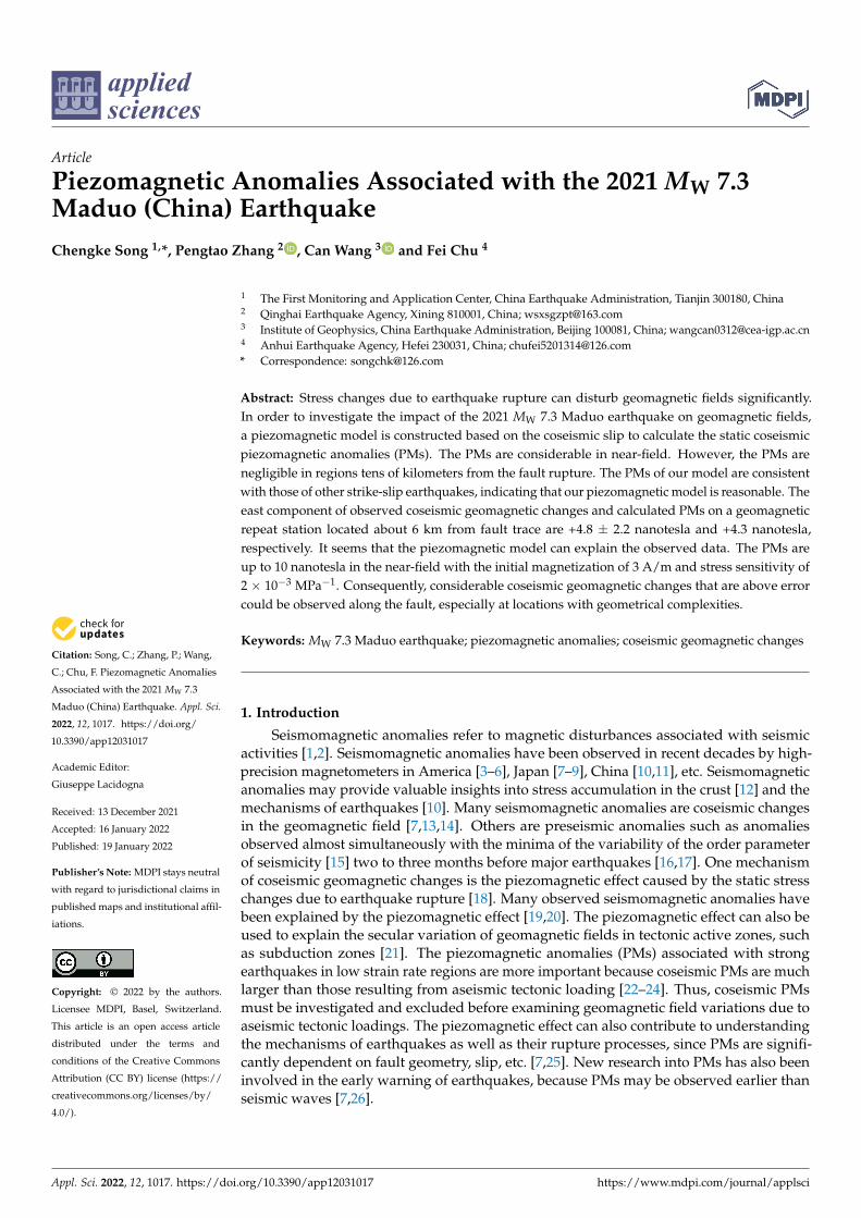
The Bayan Har block, involved in the eastward extrusion of the Tibetan Plateau [27],is a seismically active block [28]. Many strong earthquakes (MW > 6.5) in China occurredin this block and its border faults in past twenty years (Figure 1), including the 2001MW 7.9 Kokoxili earthquake, the 2008 MW 7.8 Wenchuan earthquake, the 2010 YushuMW 6.9 earthquake, the 2013 MW 6.6 Lushan earthquake, and the 2017 MW 6.5 Jiuzhaigouearthquake. In order to investigate geomagnetic anomalies before, during, and afterearthquakes, the China Earthquake Administration operates a geomagnetic network in-cluding geomagnetic observatories and geomagnetic repeat stations in the Tibetan Plateau.However, only a repeat station located 26 km from the epicenter of the MW 6.6 Lushanearthquake recorded PMs [29]. PMs can be neglected if the fault rupture is small [30],unless observations are conducted right on faults [3]. However, PMs must be investigatedcarefully for earthquakes with ruptures larger than 100 km for their huge energy releaseand strong impact on local and regional geomagnetic fields.

Appl. Sci. 2022, 12, x FOR PEER REVIEW 2 of 11

cesses, since PMs are significantly dependent on fault geometry, slip, etc. [7,25]. New re-search into PMs has also been involved in the early warning of earthquakes, because PMs may be observed earlier than seismic waves [7,26].

The Bayan Har block, involved in the eastward extrusion of the Tibetan Plateau [27], is a seismically active block [28]. Many strong earthquakes (MW > 6.5) in China occurred in this block and its border faults in past twenty years (Figure 1), including the 2001 MW 7.9 Kokoxili earthquake, the 2008 MW 7.8 Wenchuan earthquake, the 2010 Yushu MW 6.9 earthquake, the 2013 MW 6.6 Lushan earthquake, and the 2017 MW 6.5 Jiuzhaigou earth-quake. In order to investigate geomagnetic anomalies before, during, and after earth-quakes, the China Earthquake Administration operates a geomagnetic network including geomagnetic observatories and geomagnetic repeat stations in the Tibetan Plateau. How-ever, only a repeat station located 26 km from the epicenter of the MW 6.6 Lushan earth-quake recorded PMs [29]. PMs can be neglected if the fault rupture is small [30], unless observations are conducted right on faults [3]. However, PMs must be investigated care-fully for earthquakes with ruptures larger than 100 km for their huge energy release and strong impact on local and regional geomagnetic fields.

The MW 7.3 Maduo earthquake (herein referred to as Maduo earthquake) occurred at 18:04 UTC on 21 May 2021, with the epicenter located at 98.34° E and 34.59° N (http://www.csi.ac.cn/, accessed on 10 November, 2021). Maduo earthquake caused an about 160 km rupture (Figure 1) along the Maduo-Gande fault [31]; however, the tectonic deformation is significantly weak in the region [32]. How does the earthquake disturb geomagnetic fields in the Bayan Har block? Are the piezomagnetic fields localized? More importantly, how will the earthquake impact observations of piezomagnetic fields in the future? To address these questions, in this study, we construct a piezomagnetic model to calculate the static coseismic PMs based on a slip model of the Maduo earthquake. More-over, observed data of 2019 and 2021 on a repeat station are used to examine the PMs.

Figure 1. Tectonic setting. Black stars indicate the earthquakes with MW > 6.5 in the past twenty years. Black triangle is a geomagnetic repeat station. Benchballs indicate earthquake focal mecha-nism. Bold gray lines are block borders. Thin gray lines are faults. Black lines are fault ruptures of Maduo earthquake from Zhang et al. (2021). The lower inset is the location of target area.

Figure 1. Tectonic setting. Black stars indicate the earthquakes with MW > 6.5 in the past twentyyears. Black triangle is a geomagnetic repeat station. Benchballs indicate earthquake focal mechanism.Bold gray lines are block borders. Thin gray lines are faults. Black lines are fault ruptures of Maduoearthquake from Zhang et al. (2021). The lower inset is the location of target area.

The MW 7.3 Maduo earthquake (herein referred to as Maduo earthquake) occurred at18:04 UTC on 21 May 2021, with the epicenter located at 98.34◦ E and 34.59◦ N (http://www.csi.ac.cn/, accessed on 10 November 2021). Maduo earthquake caused an about 160 kmrupture (Figure 1) along the Maduo-Gande fault [31]; however, the tectonic deformation issignificantly weak in the region [32]. How does the earthquake disturb geomagnetic fieldsin the Bayan Har block? Are the piezomagnetic fields localized? More importantly, howwill the earthquake impact observations of piezomagnetic fields in the future? To addressthese questions, in this study, we construct a piezomagnetic model to calculate the staticcoseismic PMs based on a slip model of the Maduo earthquake. Moreover, observed dataof 2019 and 2021 on a repeat station are used to examine the PMs.

2. Data and Methods

There are two strategies to calculate the PMs due to earthquake rupture. One isStacey’s scheme, involving stress–magnetic calculation [2]. Another is Green’s function

Appl. Sci. 2022, 12, 1017 3 of 11

method, involving strain–magnetic calculation [33]. In this study, we prefer Stacey’s scheme,because the coseismic stress change is easily calculated nowadays. A piezomagnetic modelis constructed based on a slip model of Maduo earthquake to calculate the PMs.

2.1. Coseismic Slip Model

Zhao et al. determined the slip distribution of the coseismic rupture of Maduo earth-quake based on InSAR data (Figure 2) [32]. Their results show that the length of surfacerupture is about 160 km distributed on five sub-vertical segments with strikes of 89.5◦, 106◦,97.6◦, 117.5◦, and 83◦ and dips of 90◦, 75◦, 80◦, 90◦, and 90◦, respectively. The faulting styleis primarily left-lateral. The maximum strike slip and total slip (the sum of strike slip anddip slip) are about 6 m and 8 m at 6 km depth on segment 4, respectively. Most of them arereleased in the upper crust (0–15 km). There are three areas with significant coseismic slip(larger than 5 m), two areas in segment 2, and the other one is near the triple junction zonebetween segment 3, segment 4, and segment 5 (Figure 2).

Appl. Sci. 2022, 12, x FOR PEER REVIEW 3 of 11

2. Data and Methods There are two strategies to calculate the PMs due to earthquake rupture. One is

Stacey’s scheme, involving stress–magnetic calculation [2]. Another is Green’s function method, involving strain–magnetic calculation [33]. In this study, we prefer Stacey’s scheme, because the coseismic stress change is easily calculated nowadays. A piezomagnetic model is constructed based on a slip model of Maduo earthquake to calculate the PMs.

2.1. Coseismic Slip Model Zhao et al. determined the slip distribution of the coseismic rupture of Maduo earth-

quake based on InSAR data (Figure 2) [32]. Their results show that the length of surface rupture is about 160 km distributed on five sub-vertical segments with strikes of 89.5°, 106°, 97.6°, 117.5°, and 83° and dips of 90°, 75°, 80°, 90°, and 90°, respectively. The faulting style is primarily left-lateral. The maximum strike slip and total slip (the sum of strike slip and dip slip) are about 6 m and 8 m at 6 km depth on segment 4, respectively. Most of them are released in the upper crust (0–15 km). There are three areas with significant co-seismic slip (larger than 5 m), two areas in segment 2, and the other one is near the triple junction zone between segment 3, segment 4, and segment 5 (Figure 2).

Figure 2. Coseismic slip distribution of Maduo earthquake from Zhang et al. (2021).

2.2. Layer Elastic Model We adopt the PSGRN/PSCMP code to calculate the coseismic stress changes based

on an elastic crust model [34]. The crust model is based on the results of a previous study [35]. The detailed parameters of the model are listed in Table 1. The crust is discretized into 3864 sub-blocks with a dimension of 2 × 2 × 2 km.

Table 1. Parameters of the layer elastic model.

Layers Depth/km VP/km·s−1 VS/km·s−1 Density/kg·m−3 1 4 4.8 2.82 2600 2 10 5.9 3.47 2700 3 20 6.1 3.59 2850 4 48 6.5 3.82 3000 5 68 7.0 4.12 3100 6 100 8.1 4.76 3320

Figure 2. Coseismic slip distribution of Maduo earthquake from Zhang et al. (2021).

2.2. Layer Elastic Model

We adopt the PSGRN/PSCMP code to calculate the coseismic stress changes based onan elastic crust model [34]. The crust model is based on the results of a previous study [35].The detailed parameters of the model are listed in Table 1. The crust is discretized into3864 sub-blocks with a dimension of 2 × 2 × 2 km.

Table 1. Parameters of the layer elastic model.

Layers Depth/km VP/km·s−1 VS/km·s−1 Density/kg·m−3

1 4 4.8 2.82 2600

2 10 5.9 3.47 2700

3 20 6.1 3.59 2850

4 48 6.5 3.82 3000

5 68 7.0 4.12 3100

6 100 8.1 4.76 3320

Appl. Sci. 2022, 12, 1017 4 of 11

2.3. Piezomagnetic Model

The constitutive law of the stress and magnetization has been proposed as follows [36]:

∆J =32

βS·J (1)

where ∆J is the change of magnetization, S is the deviatoric stress tensor, J is the initialmagnetization, and β is the stress sensitivity.

The piezomagnetic potential dW at point P (x0, y0, z0) due to ∆J of a sub-block withcoordinates of (x, y, z) can be expressed as Equation (2) [36], and the PMs can be obtainedby differentiating the right-hand side of Equation (2).

dW =∆J·ρ

ρ3 dv = ∆J· l(x0 − x) + m(y0 − y) + n(z0 − z)ρ3 dxdydz (2)

where (l, m, n) are the direction cosines of J, and ρ is the distance between point P and thesub-block,

ρ =

√(x0 − x)2 + (y0 − y)2 + (z0 − z)2

The total PMs at point P are equal to the sum of the PMs derived from each sub-block,as follows:

∆X =∫ H

0

∫ +∞−∞

∫ +∞−∞

(∆JxU1 + ∆JyU4 + ∆JzU5

)dxdydz

∆Y =∫ H

0

∫ +∞−∞

∫ +∞−∞

(∆JxU4 + ∆JyU2 + ∆JzU6

)dxdydz

∆Z =∫ H

0

∫ +∞−∞

∫ +∞−∞

(∆JxU5 + ∆JyU6 + ∆JzU3

)dxdydz

(3)

where H is calculation depth,

U1 = 2(x0−x)2−(y0−y)2−(z0−z)2

ρ5

U2 = 2(y0−y)2−(x0−x)2−(z0−z)2

ρ5

U3 = 2(z0−z)2−(x0−x)2−(y0−y)2

ρ5

U4 = 3(x0−x)(y0−y)ρ5

U5 = 3(x0−x)(z0−z)ρ5

U6 = 3(y0−y)(z0−z)ρ5

The total intensity of PMs can be obtained through declination (D) and inclination (I)as follows [36]:

∆F = (∆X cos D + ∆Y sin D) cos I + ∆Z sin I (4)

The direction of initial magnetization is assumed to be consistent with the presentmagnetic fields, which have an inclination and a declination of 54◦ and −1◦ (westward),respectively. The magnetic anomalies are not strong in the Tibetan Plateau [37], whichindicates a weak heterogeneity in magnetization. Thus, a uniform initial magnetizationseems reasonable. Stress sensitivity of the order of 10−3 MPa−1 is considered in manystudies of seismomagnetic anomalies [3,7,13,19]. However, in some studies, the initialmagnetization of 1A/m and stress sensitivity of 1 × 10−3 MPa−1 are too small to explainthe observed data [21,25,29]. In our model, an average magnetization of 3 A/m and a stresssensitivity of 2 × 10−3 MPa−1 are assumed. A depth of 16 km was chosen because most ofthe stress associated with Maduo earthquake released in the upper crust (0–15 km).

3. Results

In order to eliminate the distortion of PMs resulting from stress concentration andsingularity on the fault plane, we do not consider the PMs in the project area of fault slipabout 2 km from the fault trace. The PMs are calculated at 1 m, where magnetometers

Appl. Sci. 2022, 12, 1017 5 of 11

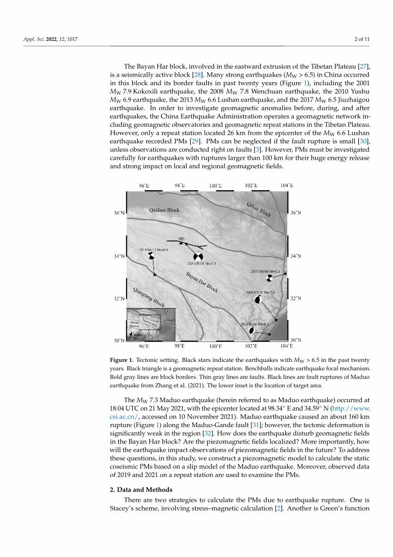
are usually installed. The total intensity (F) and east component (Y) of PMs are calculatedbecause Y is expected to be significantly changed under the east–west slip regime.

The spatial distribution of the PMs is shown in Figure 3. Our results show that thepattern of PMs is consistent with the left-lateral slip. For Y, negative changes appear in thecompressional area, whereas positive changes appear in the extensional area. This is theopposite for F, because F is primarily calculated from the north component (X) and thevertical component (Z) which are reverse variations with Y according to Equation (1).

Appl. Sci. 2022, 12, x FOR PEER REVIEW 5 of 11

The direction of initial magnetization is assumed to be consistent with the present magnetic fields, which have an inclination and a declination of 54° and −1° (westward), respectively. The magnetic anomalies are not strong in the Tibetan Plateau [37], which indicates a weak heterogeneity in magnetization. Thus, a uniform initial magnetization seems reasonable. Stress sensitivity of the order of 10−3 MPa−1 is considered in many stud-ies of seismomagnetic anomalies [3,7,13,19]. However, in some studies, the initial magnet-ization of 1A/m and stress sensitivity of 1 × 10−3 MPa−1 are too small to explain the observed data [21,25,29]. In our model, an average magnetization of 3 A/m and a stress sensitivity of 2 × 10−3 MPa−1 are assumed. A depth of 16 km was chosen because most of the stress associated with Maduo earthquake released in the upper crust (0–15 km).

3. Results In order to eliminate the distortion of PMs resulting from stress concentration and

singularity on the fault plane, we do not consider the PMs in the project area of fault slip about 2 km from the fault trace. The PMs are calculated at 1 m, where magnetometers are usually installed. The total intensity (F) and east component (Y) of PMs are calculated because Y is expected to be significantly changed under the east–west slip regime.

The spatial distribution of the PMs is shown in Figure 3. Our results show that the pattern of PMs is consistent with the left-lateral slip. For Y, negative changes appear in the compressional area, whereas positive changes appear in the extensional area. This is the opposite for F, because F is primarily calculated from the north component (X) and the vertical component (Z) which are reverse variations with Y according to Equation (1).

The large PMs occur in the near-field. The maximum amplitude of PMs is about 10 nanotelsa (nT) for F and 8 nT for Y. Additionally, three peaks are in the regions with much larger slip mentioned above. However, PMs are small at the epicenter area.

Figure 3. Contours of calculated (a) total intensity and (b) east component of PMs obtained from theMaduo earthquake. Contour interval is 1 nT. Focal spheres represent the epicenter. Gray lines are thesurface rupture. Dash lines are profiles.

The large PMs occur in the near-field. The maximum amplitude of PMs is about10 nanotelsa (nT) for F and 8 nT for Y. Additionally, three peaks are in the regions withmuch larger slip mentioned above. However, PMs are small at the epicenter area.

We also examine the Y changes on three profiles (Figure 4). Since the distributions ofthe F changes are opposite with the Y changes, we do not further analyze the F changes.The Y changes are more remarkable at the north side than that at the south side of faulttrace. The Y changes on profile 1 and profile 2 are about zero at 20 km and 30 km from thefault trace on the south side and north side, respectively. The Y changes on the profile 3 areabout 0.5 nT at 40 km away from the fault trace.

Appl. Sci. 2022, 12, 1017 6 of 11

Appl. Sci. 2022, 12, x FOR PEER REVIEW 6 of 11

Figure 3. Contours of calculated (a) total intensity and (b) east component of PMs obtained from the Maduo earthquake. Contour interval is 1 nT. Focal spheres represent the epicenter. Gray lines are the surface rupture. Dash lines are profiles.

We also examine the Y changes on three profiles (Figure 4). Since the distributions of the F changes are opposite with the Y changes, we do not further analyze the F changes. The Y changes are more remarkable at the north side than that at the south side of fault trace. The Y changes on profile 1 and profile 2 are about zero at 20 km and 30 km from the fault trace on the south side and north side, respectively. The Y changes on the profile 3 are about 0.5 nT at 40 km away from the fault trace.

Figure 4. East component of PMs on three profiles across fault trace. The dash lines represent fitted PMs instead of calculated ones as the PMs are neglected artificially in order to avoid singularity.

4. Discussion 4.1. Validation of Piezomagnetic Model

We compare the PMs of the Maduo earthquake with that of other major continental strike-slip earthquakes (M > 6), including the 1989 ML 7.1 Loma Prieta earthquake [19], the 1992 MW 7.3 Landers earthquake [20], and the 2004 M 6.0 Parkfield earthquake [4]. It should be noticed that the PMs strongly depend on parameters. Therefore, we focus on relative values of PMs here.

The PMs are proportional to initial magnetization and stress sensitivity according to Equation (1). We calculate the normalized PMs (NPMs) as follows:

NPMs = PMs/βJ (5)

The PMs exhibit a negative correlation with depth of slip (Hs) [38] and positive cor-relation with slip (S). The earthquake magnitude or moment considered by Mueller and Johnston [29] is substituted by the ratio of S and Hs in this paper. Because we cannot ob-tain the value of stress sensitivity for the Loma Prieta earthquake, 1 × 10−3 MPa−1 and 2 × 10−3 MPa−1 are assumed in the piezomagnetic model of Loma Prieta. Here, we choose the maximum PMs of these earthquakes to analyze. The correlation between maximum NPMs and S/Hs is shown in Figure 5. All values of these piezomagnetic models are shown in Table 2. Figure 5 shows that NPMs increase with S/Hs. In other words, given the same β and J, the larger S/Hs is, the larger the PMs are. As shown in Figure 5, NPMs of Maduo earthquake are consistent with those of other strike-slip earthquakes and the Loma Prieta earthquake with stress sensitivity of 2 × 10−3 MPa−1. It indicates that our piezomagnetic model is reasonable.

Figure 4. East component of PMs on three profiles across fault trace. The dash lines represent fittedPMs instead of calculated ones as the PMs are neglected artificially in order to avoid singularity.

4. Discussion4.1. Validation of Piezomagnetic Model

We compare the PMs of the Maduo earthquake with that of other major continentalstrike-slip earthquakes (M > 6), including the 1989 ML 7.1 Loma Prieta earthquake [19],the 1992 MW 7.3 Landers earthquake [20], and the 2004 M 6.0 Parkfield earthquake [4]. Itshould be noticed that the PMs strongly depend on parameters. Therefore, we focus onrelative values of PMs here.

The PMs are proportional to initial magnetization and stress sensitivity according toEquation (1). We calculate the normalized PMs (NPMs) as follows:

NPMs = PMs/βJ (5)

The PMs exhibit a negative correlation with depth of slip (Hs) [38] and positivecorrelation with slip (S). The earthquake magnitude or moment considered by Muellerand Johnston [29] is substituted by the ratio of S and Hs in this paper. Because we cannotobtain the value of stress sensitivity for the Loma Prieta earthquake, 1 × 10−3 MPa−1 and2 × 10−3 MPa−1 are assumed in the piezomagnetic model of Loma Prieta. Here, we choosethe maximum PMs of these earthquakes to analyze. The correlation between maximumNPMs and S/Hs is shown in Figure 5. All values of these piezomagnetic models are shownin Table 2. Figure 5 shows that NPMs increase with S/Hs. In other words, given the sameβ and J, the larger S/Hs is, the larger the PMs are. As shown in Figure 5, NPMs of Maduoearthquake are consistent with those of other strike-slip earthquakes and the Loma Prietaearthquake with stress sensitivity of 2 × 10−3 MPa−1. It indicates that our piezomagneticmodel is reasonable.

Table 2. Summary of piezomagnetic models of four earthquakes (M > 6).

Event Maximum PMs(nT)

Magnetization(A/m)

Stress Sensitivity(10−3 MPa−1)

S(m)

Hs(km)

Maduo ~10 3 2 8.1 6

Landers ~5 2 2 5 5

Loma Prieta ~1.5 1.5 1 or 2 2.3 6

Parkfield ~0.4 2 2 0.4 3

Appl. Sci. 2022, 12, 1017 7 of 11

Appl. Sci. 2022, 12, x FOR PEER REVIEW 7 of 11

Table 2. Summary of piezomagnetic models of four earthquakes (M > 6).

Event Maximum PMs (nT)

Magnetization (A/m)

Stress Sensitivity (10−3 MPa−1)

S (m)

Hs (km)

Maduo ~10 3 2 8.1 6 Landers ~5 2 2 5 5

Loma Prieta ~1.5 1.5 1 or 2 2.3 6 Parkfield ~0.4 2 2 0.4 3

Figure 5. Normalized PMs of four earthquakes. Square and star are NPMs of Loma Prieta earth-quake with stress sensitivity of 1 × 10−3 Mpa−1 and 2 × 10−3 Mpa−1. Dashed line is a fitting line of NPMs versus S/Hs for the four earthquakes.

4.2. Possible Values of Initial Magnetization and Stress Sensitivity Undoubtedly, we cannot obtain a completely correct estimation of PMs using uni-

form parameters in a piezomagnetic model [12]. The precise structure of magnetization is not easy to determine. Nevertheless, we still attempt to evaluate the initial magnetization and stress sensitivity assumed in our piezomagnetic model.

We examined the observed geomagnetic data on a geomagnetic repeat station (MD) located about 6 km from the fault trace, as shown in Figure 1. A non-magnetic plastic plate was set on the repeat station to ensure that the magnetometers were mounted on the same position every time. The preseismic observation was conducted at 06:09 to 06:41 UTC on 19 June 2019 to investigate the regional geomagnetic fields. The repeat observation was conducted at 06:05 to 06:31 UTC on 27 June 2021 to investigate the geomagnetic field changes associated with the Maduo earthquake. The Kp indices (the planetary 3-h-range Kp index was designed to measure solar particle radiation by its magnetic effects) were both 1 at two observations times, respectively, which suggests that there were no strong magnetic disturbances, solar flares, or solar storms. The geomagnetic vector data were obtained including declination (D), inclination (I), and total intensity (F). GSM-19T proton magnetometer with an accuracy of 0.2 nT was used to measure F. Flux-gate theodolite with an accuracy of 0.2 arcmin was used to measure D and I. Y was calculated according to D, I, and F, as Y = F cos I sin D. In order to calculate the geomagnetic field changes, we must eliminate the secular and diurnal variations, which are more than a few tens of nano-tesla [39]. The methods introduced by Wang et al. [40] including diurnal reduction and secular reduction are used to correct the raw data. The changes of F and Y between 2019 and 2021 are −0.55 nT and +4.8 nT, respectively, which seem to be large enough to be detected by magnetometers.

Here, we must investigate the error of repeat observation by analyzing the mounting error of magnetometers, diurnal reduction error, and secular reduction error. The maxi-mum magnetic gradient of MD is 0.2 nT/m. Thus, the mounting error resulting from po-sition deformation can be neglected. The larger RMS of diurnal reduction in 2019 and 2021

Figure 5. Normalized PMs of four earthquakes. Square and star are NPMs of Loma Prieta earthquakewith stress sensitivity of 1 × 10−3 Mpa−1 and 2 × 10−3 Mpa−1. Dashed line is a fitting line of NPMsversus S/Hs for the four earthquakes.

4.2. Possible Values of Initial Magnetization and Stress Sensitivity

Undoubtedly, we cannot obtain a completely correct estimation of PMs using uniformparameters in a piezomagnetic model [12]. The precise structure of magnetization is noteasy to determine. Nevertheless, we still attempt to evaluate the initial magnetization andstress sensitivity assumed in our piezomagnetic model.

We examined the observed geomagnetic data on a geomagnetic repeat station (MD)located about 6 km from the fault trace, as shown in Figure 1. A non-magnetic plasticplate was set on the repeat station to ensure that the magnetometers were mounted onthe same position every time. The preseismic observation was conducted at 06:09 to 06:41UTC on 19 June 2019 to investigate the regional geomagnetic fields. The repeat observationwas conducted at 06:05 to 06:31 UTC on 27 June 2021 to investigate the geomagnetic fieldchanges associated with the Maduo earthquake. The Kp indices (the planetary 3-h-rangeKp index was designed to measure solar particle radiation by its magnetic effects) wereboth 1 at two observations times, respectively, which suggests that there were no strongmagnetic disturbances, solar flares, or solar storms. The geomagnetic vector data wereobtained including declination (D), inclination (I), and total intensity (F). GSM-19T protonmagnetometer with an accuracy of 0.2 nT was used to measure F. Flux-gate theodolitewith an accuracy of 0.2 arcmin was used to measure D and I. Y was calculated accordingto D, I, and F, as Y = F cos I sin D. In order to calculate the geomagnetic field changes,we must eliminate the secular and diurnal variations, which are more than a few tens ofnanotesla [39]. The methods introduced by Wang et al. [40] including diurnal reductionand secular reduction are used to correct the raw data. The changes of F and Y between2019 and 2021 are −0.55 nT and +4.8 nT, respectively, which seem to be large enough to bedetected by magnetometers.

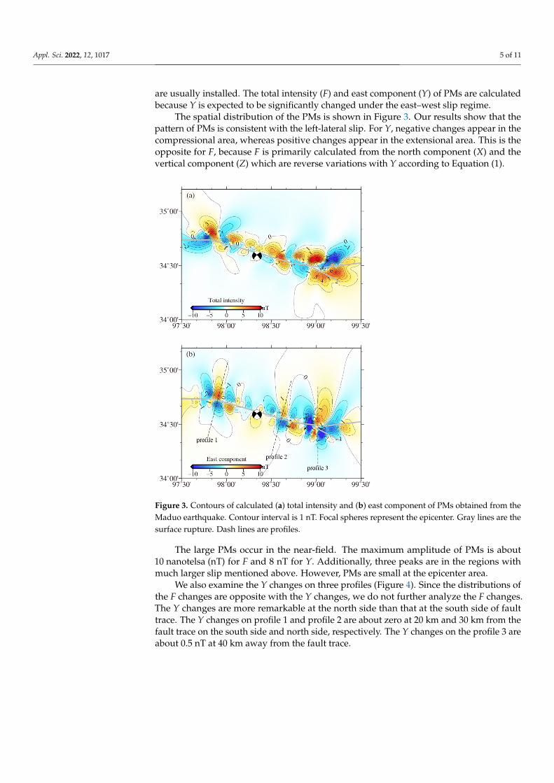
Here, we must investigate the error of repeat observation by analyzing the mountingerror of magnetometers, diurnal reduction error, and secular reduction error. The maximummagnetic gradient of MD is 0.2 nT/m. Thus, the mounting error resulting from positiondeformation can be neglected. The larger RMS of diurnal reduction in 2019 and 2021observed data are 0.11 arcmin, 0.03 arcmin, and 0.18 nT for D, I, and F, respectively, whichcan be regarded as the error of diurnal reduction. The sixth-order natural orthogonalcomponent (NOC) of the geomagnetic fields from June 2019 to July 2021 is used to correctthe secular variation. Figure 6 depicts the observed data in 72 quietest days and the valuesof NOC model from June 2019 to July 2021 on Jiayuguan geomagnetic observatory, which isone of the observatories used in the NOC model. The RMS of difference between observeddata and NOC model is 0.08 arcmin, 0.1 arcmin, and 0.75 nT for D, I, and F, respectively,which can be regarded as the error of secular reduction. The total error can be calculated bythe accuracy of instruments, diurnal reduction error, and secular reduction error, which

Appl. Sci. 2022, 12, 1017 8 of 11

are 0.24 arcmin, 0.22 arcmin, and 0.80 nT for D, I, and F, respectively. As Y is primarilydependent on D, the total error of Y can represent by the error of D, which is about 2.2 nTin MD for 0.24 arcmin.

Appl. Sci. 2022, 12, x FOR PEER REVIEW 8 of 11

observed data are 0.11 arcmin, 0.03 arcmin, and 0.18 nT for D, I, and F, respectively, which can be regarded as the error of diurnal reduction. The sixth-order natural orthogonal com-ponent (NOC) of the geomagnetic fields from June 2019 to July 2021 is used to correct the secular variation. Figure 6 depicts the observed data in 72 quietest days and the values of NOC model from June 2019 to July 2021 on Jiayuguan geomagnetic observatory, which is one of the observatories used in the NOC model. The RMS of difference between observed data and NOC model is 0.08 arcmin, 0.1 arcmin, and 0.75 nT for D, I, and F, respectively, which can be regarded as the error of secular reduction. The total error can be calculated by the accuracy of instruments, diurnal reduction error, and secular reduction error, which are 0.24 arcmin, 0.22 arcmin, and 0.80 nT for D, I, and F, respectively. As Y is pri-marily dependent on D, the total error of Y can represent by the error of D, which is about 2.2 nT in MD for 0.24 arcmin.

Since the observed F (−0.55 nT) is less than the error (0.80 nT), we do not compare it with calculated F changes. As the observed Y is about twice the error, we believe it was reasonable and authentic. The observed and predicted Y at MD are +4.8 ± 2.2 nT and +4.3 nT, respectively. We consider that our piezomagnetic model can explain the observed data. In other words, the observed geomagnetic changes before and after Maduo earth-quake at MD are caused by stress changes resulting from fault rupture. It also indicates that initial magnetization of 3 A/m and stress intensity of 2 × 10−3 MPa−1 assumed in piezo-magnetic model of Maduo earthquake are reasonable.

Figure 6. Observed data (red dot) and NOC model data from June 2019 to July 2021. (a): the varia-tion of declination. (b): the variation of inclination. (c) the variation of total intensity.

Figure 6. Observed data (red dot) and NOC model data from June 2019 to July 2021. (a): the variationof declination. (b): the variation of inclination. (c) the variation of total intensity.

Since the observed F (−0.55 nT) is less than the error (0.80 nT), we do not compareit with calculated F changes. As the observed Y is about twice the error, we believe itwas reasonable and authentic. The observed and predicted Y at MD are +4.8 ± 2.2 nTand +4.3 nT, respectively. We consider that our piezomagnetic model can explain theobserved data. In other words, the observed geomagnetic changes before and after Maduoearthquake at MD are caused by stress changes resulting from fault rupture. It also indicatesthat initial magnetization of 3 A/m and stress intensity of 2 × 10−3 MPa−1 assumed inpiezomagnetic model of Maduo earthquake are reasonable.

4.3. Potential Usefulness of Observations along Fault

Many magnetometers fail to record PMs during earthquakes. On one hand, they are faraway from fault rupture. As our piezomagnetic model shows, even for a MW 7.3 earthquakewith a rupture length of 160 km, the geomagnetic field changes that are above the mag-netometer accuracy are limited in areas 40 or 50 km from rupture. Considering the errorresulting from field observations and data processing, we consider that only magnetometersmounted at a region within 20 km from the fault rupture can observe useful seismomagneticsignals. On the other hand, it also could fail to record seismomagnetic signals even when

Appl. Sci. 2022, 12, 1017 9 of 11

the magnetometers are mounted in near-field. As our results show, the PMs are small inepicenter area. Thus, only stations that are ideally located can observe the PMs.

The near-field PMs show variations in the degree of localized strengthening alongrupture trace (Figure 3), especially at the triple junction of three fault segments. Indeed, thePMs are expected to be larger at ends of faults or locations with geometrical complexities,such as fault bend or branching [40]. Bifurcation of slip appears to be a common featureof some major continental strike-slip earthquakes [41,42]. It indicates that locations withgeometrical complexities are potential sites to observe the PMs.

5. Conclusions

The 2021 MW 7.3 Maduo earthquake is assumed to disturb local and regional geo-magnetic fields significantly. A piezomagnetic model is constructed to investigate thegeomagnetic fields changes due to stress changes resulted from earthquake rupture. Wevalidate the piezomagnetic model by comparing with piezomagnetic changes of otherstrike-slip earthquakes and observed data before and after earthquake on a geomagnetic re-peat station. The PMs of Maduo earthquake seem to appear in areas within 40 km from faulttrace. The PMs are larger at the location with bifurcation of slip. The observed geomagneticfield changes before and after Maduo earthquake can be explained by our piezomagneticmodel with initial magnetization of 3 A/m and stress sensitivity of 2 × 10−3 MPa−1. Thus,if there are more observations, we can constrain the detailed magnetic properties and theslip model.

Author Contributions: Conceptualization, F.C.; Data curation, P.Z.; Formal analysis, C.S. and C.W.;Funding acquisition, C.S.; Investigation, P.Z. and F.C.; Methodology, C.S. and C.W.; Validation, F.C.;Writing—original draft, C.S.; Writing—review and editing, C.S. and C.W. All authors have read andagreed to the published version of the manuscript.

Funding: This research was funded by the National Natural Science Foundation of China, grantnumber 41804091 and 42174125.

Institutional Review Board Statement: Not applicable.

Informed Consent Statement: Not applicable.

Data Availability Statement: The coseismic slip model used in this study is publicly available andcan be downloaded from https://doi.org/10.5281/zenodo.5324323, accessed on 15 November 2021.

Acknowledgments: Figures are drawn through the Generic Mapping Tools (GMT) software. Thecoseismic stresses are calculated through PSGRN/PSCMP program developed by Rongjiang Wang.The Kp indexes are obtained from WDC (http://wdc.kugi.kyoto-u.ac.jp/kp/index.html, accessed on16 November 2021).

Conflicts of Interest: The authors declare no conflict of interest.

References1. Stacey, F.D. Seismo-magnetic effect and the possibility of forecasting earthquakes. Nature 1963, 200, 1083–1085. [CrossRef]2. Stacey, F.D. The Seismomagnetic Effect. Pure Appl. Geophys. 1964, 58, 5–22. [CrossRef]3. Johnston, M.J.S.; Mueller, R.J. Seismomagnetic observation during the 8 July 1986 magnitude 5.9 North Palm Springs earthquake.

Science 1987, 237, 1201–1203. [CrossRef]4. Fraser-Smith, A.C.; Bernardi, A.; McGill, P.R.; Ladd, M.E.; Helliwell, R.A.; Villard, O.G. Low-frequency magnetic field measure-

ments near the epicenter of the Ms 7.1 Loma Prieta earthquake. Geophys. Res. Lett. 1990, 17, 1465–1468. [CrossRef]5. Hayakawa, M.; Kawate, R.; Molchanov, O.A.; Yumoto, K. Results of ultra-low-frequency magnetic field measurements during the

Guam earthquake of 8 August 1993. Geophys. Res. Lett. 1996, 23, 241–244. [CrossRef]6. Johnston, M.J.S.; Sasai, Y.; Egbert, G.D.; Mueller, R.J. Seismomagnetic effects from the long-awaited 28 September 2004 M 6.0

Parkfield earthquake. Bull. Seismol. Soc. Am. 2006, 96, S206–S220. [CrossRef]7. Okubo, K.; Takeuchi, N.; Utsugi, M.; Yumoto, K.; Sasai, Y. Direct magnetic signals from earthquake rupturing: Iwate-Miyagi

earthquake of M 7.2, Japan. Earth Planet. Sci. Lett. 2011, 305, 65–72. [CrossRef]8. Xu, G.; Han, P.; Huang, Q.; Hattori, K.; Febriani, F.; Yamaguchi, H. Anomalous behaviors of geomagnetic diurnal variations prior

to the 2011 off the Pacific coast of Tohoku earthquake (Mw9.0). J. Asian Earth Sci. 2013, 77, 59–65. [CrossRef]

Appl. Sci. 2022, 12, 1017 10 of 11

9. Han, P.; Hattori, K.; Hirokawa, M.; Zhuang, J.; Chen, C.; Febriani, F.; Yamaguchi, H.; Yoshino, C.; Liu, J.; Yoshida, S. Statisticalanalysis of ULF seismomagnetic phenomena at Kakioka, Japan, during 2001–2010. J. Geophys. Res. Space Phys. 2014, 119,4998–5011. [CrossRef]

10. Gao, Y.; Zhao, G.; Chong, J.; Klemperer, S.L.; Han, B.; Jiang, F.; Wen, J.; Chen, X.; Zhan, Y.; Tang, J.; et al. Coseismic electricand magnetic signals observed during 2017 Jiuzhaigou Mw6.5 earthquake and explained by electrokinetics and magnetometerrotation. Geophys. J. Int. 2020, 223, 1130–1143. [CrossRef]

11. Chen, C.H.; Lin, J.Y.; Gao, Y.; Lin, C.H.; Han, P.; Chen, C.R.; Lin, L.C.; Huang, R.; Liu, J.Y. Magnetic Pulsations Triggered byMicroseismic Ground Motion. J. Geophys. Res. Solid Earth. 2021, 126, e2020JB021416. [CrossRef]

12. Yamazaki, K. Calculation of the piezomagnetic field arising from uniform regional stress in inhomogeneously magnetized crust(II): Limitation in general cases. Earth Planets Space 2021, 63, 1217–1220. [CrossRef]

13. Utada, H.; Shimizu, H.; Ogawa, T.; Maeda, T.; Furumura, T.; Yamamoto, T.; Yamazaki, N.; Yoshitake, Y.; Nagamachi, S.Geomagnetic field changes in response to the 2011 off the Pacific Coast of Tohoku Earthquake and Tsunami. Earth Planet. Sci. Lett.2011, 311, 11–27. [CrossRef]

14. Gao, Y.; Harris, J.M.; Wen, J.; Huang, Y.; Twardzik, C.; Chen, X.; Hu, H. Modeling of the coseismic electromagnetic fields observedduring the 2004 Mw 6.0 Parkfield earthquake. Geophys. Res. Lett. 2016, 43, 620–627. [CrossRef]

15. Sarlis, N.V.; Skordas, E.S.; Varotsos, P.A. Order parameter fluctuations of seismicity in natural time before and after mainshocks.EPL (Europhys. Lett.) 2010, 91, 59001. [CrossRef]

16. Varotsos, P.A.; Sarlis, N.V.; Skordas, E.S. Study of the temporal correlations in the magnitude time series before major earthquakesin Japan. J. Geophys. Res. Space Phys. 2014, 119, 9192–9206. [CrossRef]

17. Sarlis, N.V.; Skordas, E.S.; Varotsos, P.A.; Nagao, T.; Kamogawa, M.; Uyeda, S. Spatiotemporal variations of seismicity beforemajor earthquakes in the Japanese area and their relation with the epicentral locations. Proc. Natl. Acad. Sci. USA 2015, 112,986–989. [CrossRef]

18. Stacey, F.D.; Johnston, M.J.S. Theory of the piezomagnetic effect in titanomagnetite-bearing rocks. Pure Appl. Geophys. 1972, 97,146–155. [CrossRef]

19. Mueller, R.J.; Johnston, M.J.S. Seismomagnetic effect generated by the October, 1989, ML, 7.1 Loma Prieta, California, Earthquake.Geophys. Res. Lett. 1990, 17, 1231–1234. [CrossRef]

20. Johnston, M.J.S.; Mueller, R.J.; Sasai, Y. Magnetic Field Observations in the Near-Field the 28 June 1992 Mw 7.3 Landers, California,Earthquake. Bull. Seismol. Soc. Am. 1994, 84, 792–798. [CrossRef]

21. Nishida, Y.; Sugisaki, Y.; Takahashi, K.; Utsugi, M.; Oshima, H. Tectonomagnetic study in the eastern part of Hokkaido, NE Japan:Discrepancy between observed and calculated results. Earth Planets Space 2004, 56, 1049–1058. [CrossRef]

22. Sasai, Y. A surface integral representation of the tectonomagnetic field based on the linear piezomagnetic effect. Bull. Earthq. Res.Inst. 1983, 58, 763–785.

23. Johnston, M.J.S. Local Magnetic Fields, Uplift, Gravity, and Dilational Strain Changes in Southern California. J. Geomagn. Geoelectr.1986, 38, 933–947. [CrossRef]

24. Rikitake, T. Magnetic and electric signals precursory to earthquake an analysis of Japanese data. J. Geomagn. Geoelectr. 1987, 39,47–61. [CrossRef]

25. Yamazaki, K. Improved models of the piezomagnetic field for the 2011 Mw 9.0 Tohoku-oki earthquake. Earth Planet. Sci. Lett.2013, 363, 9–15. [CrossRef]

26. Yamazaki, K. Temporal variations in magnetic signals generated by the piezomagnetic effect for dislocation sources in a uniformmedium. Geophys. J. Int. 2016, 206, 130–141. [CrossRef]

27. Tapponnier, P.; Peltzer, G.; Le Dain, A.Y.; Armijo, R.; Cobbold, P. Propagating extrusion tectonics in Asia: New insights fromsimple experiments with plasticine. Geology 1982, 10, 611–616. [CrossRef]

28. Deng, Q.; Cheng, S.; Ma, J.; Du, P. Seismic activities and earthquake potential in the Tibetan Plateau. Chin. J. Geophys. 2014, 57,2025–2042.

29. Song, C.; Zhang, H. Analysis of coseismic variations in magnetic field of the Lushan Ms7.0 earthquake in 2013. Seismol. Geol.2020, 42, 1301–1315.

30. Mueller, R.J.; Johnston, M.J.S. Review of magnetic field monitoring near active faults and volcanic calderas in California: 1974–1995.Phys. Earth Planet. Inter. 1998, 105, 131–144. [CrossRef]

31. Zhan, Y.; Liang, M.; Sun, X.; Huang, F.; Zhao, L.; Gong, Y.; Han, J.; Li, C.; Zhang, P.; Zhang, H. Deep structure and seismogenicpattern of the 2021.5.22 Madoi (Qinghai) MS7.4 earthquake. Chin. J. Geophys. 2021, 64, 2232–2252.

32. Zhao, D.; Qu, C.; Chen, H.; Shan, X.; Song, X.; Gong, W. Tectonic and Geometric Control on Fault Kinematics of the 2021 Mw7.3Maduo (China) Earthquake Inferred From Interseismic, Coseismic, and Postseismic InSAR Observations. Geophys. Res. Lett. 2021,48, e2021GL095417. [CrossRef]

33. Sasai, Y. Application of the Elasticity Theory of Dislocations to Tectonomagnetic Modelling. Bull. Earthq. Res. Inst. 1980, 55,387–447.

34. Wang, R.; Lorenzo-Martín, F.; Roth, F. PSGRN/PSCMP—A new code for calculating co- and post-seismic deformation, geoid andgravity changes based on the viscoelastic-gravitational dislocation theory. Comput. Geosci. 2006, 32, 527–541. [CrossRef]

35. Xiong, X.; Shan, B.; Zheng, Y.; Wang, R. Stress transfer and its implication for earthquake hazard on the Kunlun Fault, Tibet.Tectonophysics 2010, 482, 216–225. [CrossRef]

Appl. Sci. 2022, 12, 1017 11 of 11

36. Okubo, A.; Oshiman, N. Piezomagnetic field associated with a numerical solution of the Mogi model in a non-uniform elasticmedium. Geophys. J. Int. 2004, 159, 509–520. [CrossRef]

37. Kang, G.; Gao, G.M.; Bai, C.H.; Shao, D.; Feng, L.L. Characteristics of the crustal magnetic anomaly and regional tectonics in theQinghai-Tibet Plateau and the adjacent areas. Sci. China Earth Sci. 2011, 41, 1577–1585.

38. Utsugi, M.; Nishida, Y.; Sasai, Y. Piezomagnetic potentials due to an inclined rectangular fault in a semi-infinite medium. Geophys.J. Int. 2000, 140, 479–492. [CrossRef]

39. Wu, Y.; Liu, L.; Ren, Z. Equinoctial asymmetry in solar quiet field along the 120◦ E meridian chain. Appl. Sci. 2021, 11, 9150.[CrossRef]

40. Wang, Z.; Chen, B.; Yuan, J.; Yang, F.; Jia, L.; Wang, C. Localized geomagnetic field anomalies in an underground gas storage.Phys. Earth Planet. Inter. 2018, 283, 92–97. [CrossRef]

41. Jin, Z.; Fialko, Y. Coseismic and Early Postseismic Deformation Due to the 2021 M7.4 Maduo (China) Earthquake. Geophys. Res.Lett. 2021, 48, e2021GL095213. [CrossRef]

42. Klinger, Y.; Xu, X.; Tapponnier, P.; Van der Woerd, J.; Lasserre, C.; King, G. High-resolution satellite imagery mapping for thesurface rupture and slip distribution of the Mw ∼7.8, 14 November 2001 Kokoxili earthquake, Kunlun fault, northern Tibet,China. Bull. Seismol. Soc. Am. 2005, 95, 1970–1987. [CrossRef]