Hazard Checking of Timed Asynchronous Circuits Revisited

Frederic BealTokyo Institute of Technology

Tokyo, Japanfrederic@yt.cs.titech.ac.jp

Tomohiro YonedaNational Institute of Informatics

Tokyo, Japanyoneda@nii.ac.jp

Chris J. MyersUniversity of Utah

Salt Lake City, USAmyers@ece.utah.edu

Abstract

This paper proposes a new approach for the hazardchecking of timed asynchronous circuits. Previous papersproposed either exact algorithms, which suffer from state-space explosion, or efficient algorithms which use a (con-servative) approximation to avoid state-space explosion butcan result in the rejection of designs which are valid. Inparticular, [7] presents a timed extention of the work in [1]which is very efficient but is not able to handle circuits withinternal loops, which prevents its use in some cases. We pro-pose a new approach to the problem in order to overcomethe mentioned limitations, without sacrificing efficiency. Todo so, we first introduce a general framework targeted atthe conservative checking of safety failures. This frameworkis not restricted to the checking of timed asynchronous cir-cuits. Secondly, we propose a new (conservative) semanticsfor timed circuits, in order to use the proposed frameworkfor hazard checking of such circuits. Using this frameworkwith the proposed semantics yields an efficient algorithmthat addresses the limitations of the previous approaches.

1 Introduction

The main particularity of timed asynchronous circuits [6]is the presence of timing information, unlike the speed in-dependent approach [5]. While the additional informationmakes it possible to improve the quality of the generateddesigns [11, 12], by reducing the number of gates, and bymaking technology mapping easier, it can significantly in-crease the computational complexity of the synthesis andverification tools.

In the course of the synthesis of asynchronous circuits,extra care must be taken to avoid hazards. Hazards are con-ditions in which unexpected order of propagation of sig-nals causes incorrect behaviour in the design. This can hap-pen because of delays related to the operation of the gates.There are two approaches to the problem of hazard check-ing in timed asynchronous circuits. On the one hand, there

is the exact verification approach [10, 14, 8, 2, 15]. Though,this approach suffers from high cost, making it impracti-cal for large designs. Conservative methods for speed inde-pendent circuits are proposed in [1] which reduce the stateexplosion problem by restricting exploration to the specifi-cation state space. In [7], these methods are extended totimed circuits. These approaches, though, are restrictedto a subclass of circuits, as they cannot handle internalloops which appear frequently in the state variable inser-tion process during the automatic synthesis of circuits, andare somewhat overly-conservative, rejecting designs whichrespect the specification. Other approaches include [13],which applies a very general framework (abstract interpre-tation: [4]) to the problem of verification of asynchronouscircuits, and [3], which uses a more symbolic approach,trading execution speed for expressive power.

Section 2 presents a general framework for conservativerepresentation of designs. This framework is general andnot limited to the problem at hand (from this point of view,it is related to abstract interpretation, though it is less gen-eral than abstract interpretation itself and uses a more prac-tical approach). Then, general notions about timed asyn-chronous circuits are introduced, including a new represen-tation of the behaviour of circuits which is compact andprecise, though conservative, in order to apply the generalframework. In Section 4, the derived algorithm is presented.Its complexity is similar to the one of [7], and it overcomesthe limitations of the approach in [7]. Those limitationsinclude the impossibility to check circuits that have inter-nal loops and to detect that some hazards may not prop-agate to primary outputs. The proposed algorithm solvesthese limitations in a satisfactory manner. Finally, Section5 shows some experimental results to demonstrate the pro-posed method.

2 A new framework

Before describing the framework itself, a few definitionsare necessary.

2.1 Definitions

An alphabet is a finite set, the elements of which arecalled letters. A word is a finite sequence of letters. w · w′

denotes the concatenation of the words w and w′ ; ε is theempty word. If A and B are two set of words, then A + Brepresents the set A ∪ B, A · B represents the set of wordsw · w′ where w ∈ A and w′ ∈ B, A+ is the set of wordsw1 · ... · wn where wi ∈ A, and A? = A+ + ε. Theprojection of a word w on a set A (denoted ΠA(w)) is theword obtained by removing from w the letters that do notappear in A.

A state machine M is a 4-tuple M = (Φ, φ0, X, T )where Φ is a set of states, φ0 ∈ Φ is the initial state, Xis an alphabet and T ⊆ Φ ×X × Φ is a transition relation.Let States(M) and Trans(M) denote Φ and T , respec-tively. If (φ, x, φ′) ∈ T , the notation M : φ →x φ′ isused (or φ →x φ′ when there is no possible confusion).This notation is extended to φ →w φ′ for w ∈ X?. Astate machine M is said to be deterministic if and only iffor all φ, φ′, φ′′ ∈ States(M) and w ∈ X?, φ →w φ′ andφ →w φ′′ imply φ′ = φ′′.

For a word w, postw(q) is the set q′ | q →w q′. Sim-ilarly, for a set L of words, postL(q) is the set q′ | ∃w ∈L, q →w q′.

Let M and N be two state machines on the same alpha-bet. A relation R between states of M and N is a simula-tion relation, if and only if,

• R is not empty,

• if R(φ, q) and x ∈ X , with φ →x φ′, then there existsq′, such that q →x q′ and R(φ′, q′).

where φ and φ′ are states from M and q and q′ are statesfrom N .

Three distinct alphabets I, O and N are used (respec-tively input, output, and internal transitions 1). A specifica-tion state machine is a state machine on I + O. An imple-mentation state machine is a state machine on I + O + N .The specification and implementation states machines aredeterministic. In the rest of the section, S is a specificationstate machine and I is an implementation state machine.

The simulation relation is extended to the case where theleft item is a specification state machine and the right item isan implementation state machine, by projecting out internaltransitions on the implementation state machine, as follows:if q and q′ in States(I), x ∈ I + O, then q x q′ denotesthat there exists u, v ∈ N? with I : q →u·x·v q′. Then,a simulation relation R between the specification state ma-chine S and the implementation state machine I must sat-

1In general, a transition is a pair (wire, direction), often denoted byw+ or w−. However, in this section, transitions are represented by singleletters.

isfy: if R(φ, q), S : φ →x φ′ with x ∈ I + O, then thereexists q′, with I : q x q′ and R(φ′, q′).

It is supposed in the rest of this section that for the initialspecification state φ0 and the initial implementation stateq0, there exists R(φ0, q0). In other words, it is possible toemulate the execution of the specification in the implemen-tation state space.

2.2 Proposed framework

DI denotes 2States(I). DS = States(S) denotes thespecification domain. This definition is based on the factthat a set of implementation states corresponds to one givenspecification state.

Definition 1 The concretization (Figure 1) conc : DS →DI is defined as follows:

conc(φ) =

q | ∃w ∈ (I + O + N)?,φ0 →ΠI+O(w) φq0 →w q

φ0 φ1

φ2

DS DI

Specification domain Implementation domain

concconc

conc

conc

Figure 1. The concretization function.

The concretization of a specification state is the exactset of reachable implementation states corresponding to thisparticular specification state. An exact checking algorithmmust compute this function, but the complexity of this is ingeneral exponential or worse, so this should be avoided.

Using the specification in Figure 2 with the implementa-tion given in Figure 3, the following holds :

conc(φ0) = q0conc(φ1) = q1, q2, q3conc(φ2) = q4conc(φ3) = q5, q6

a

b

a

c

φ0 φ1

φ2φ3

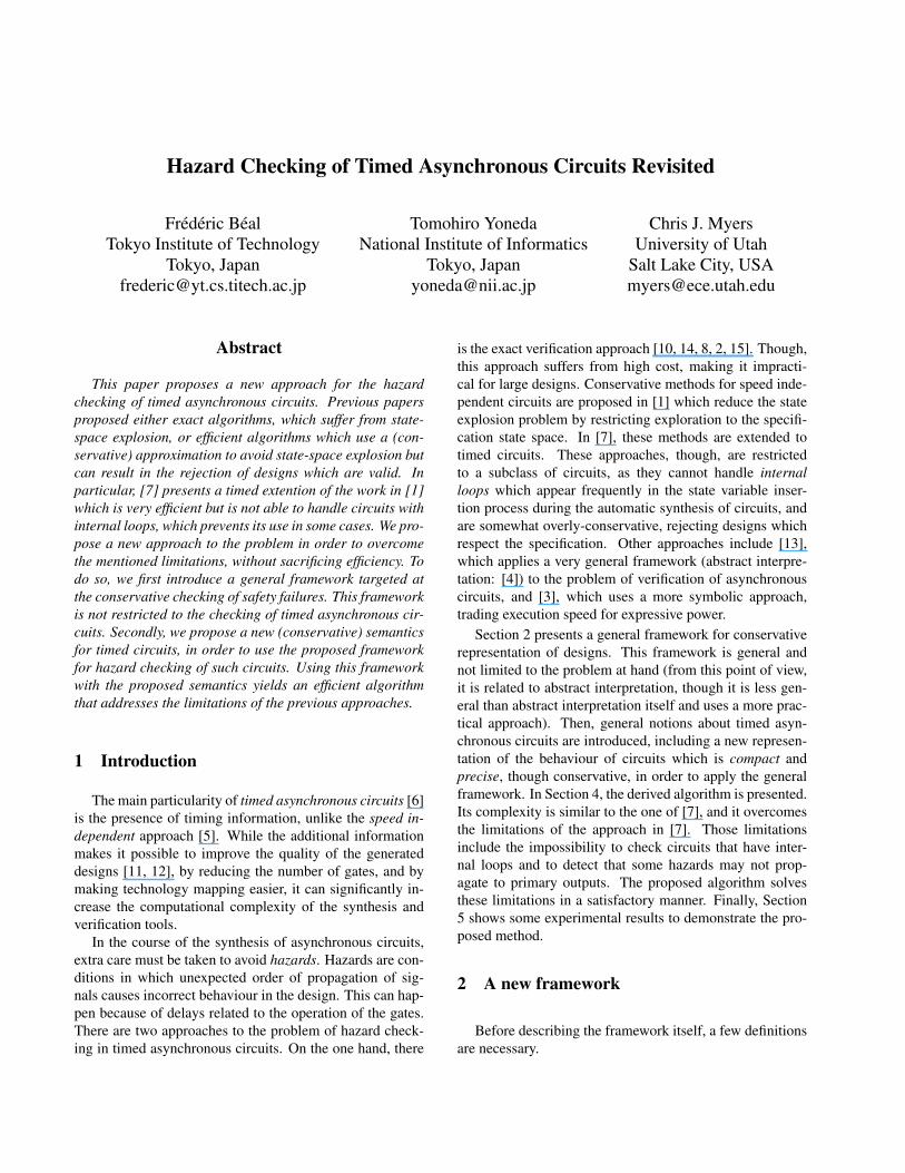
Figure 2. An example specification with I =a, O = b, c.

a

n1n2

b b

a

n3

c

q0 q1

q2 q3

q4q5

q6

Figure 3. An example implementation withI = a, O = b, c, N = n1, n2, n3.

Definition 2 The closure under internal transitions of theset X ∈ DI is the set

α(X) =⋃

q∈X

postN?

(q)

As an example, considering Figure 3, where a is an inputsignal, b, c are output signals and the nk are internal signals,α(q1) = q1, q2, q3.

A set X is closed under internal transitions if X =α(X). The collection of closed sets is denoted by DI′. In-tuitively,DI′ hides the internal transitions of the implemen-tation, hence is expected to be easier to handle.

In our example,

D′I =

q0, q1, q2, q3,q2, q3, q4, q5, q6, q6

.

Now, the definition of the transition relation on DI′ is asfollows: if X, Y ∈ DI′ and s ∈ I + O, then X ⇒s Ydenotes that Y = α(

⋃q∈X posts(q)).

As for the example, the following transitions on D′I :q0 ⇒a q1, q2, q3 ⇒b q4 ⇒a q5, q6 ⇒c q0

exist. The rest of the states in D′I are unreachable fromq0, so they are not interesting for our purpose. It can beremarked that the graph structure on the reachable states ofDI′ is isomorphic to the graph structure on DS .

It can be proven that the alternative representationDI′ isequivalent to DI in terms of computation of the reachableimplementation states. This also proves that the new tran-sition relation ⇒ is not easily computable. Hence, overap-proximation is needed. The purpose of the proposed frame-work is to introduce a methodology to create such overap-proximations, which is performed through the abstraction ofthe internal signals to have good performance (by limitingexploration to the specification state space).

For X ∈ DI′, it is possible to define the forward closureof X , denoted by

−→X , as follows:

−→X = w ∈ (O + N)? · (I + ε) | ∃q ∈ X, postw(q) 6= ∅

This forward closure includes any sequence of internaland outputs transitions, followed eventually by an inputtransition, that can occur from X .

Using the example,

−−→q0 = ε, a

−−−−−−−→q1, q2, q3 = ε, n1, n2, n1b, n2b, n1ba, n2ba, b, ba

−−→q4 = ε, a

−−−−−→q5, q6 = ε, n3, n3c, n3ca, c, ca

It is now possible to define the first object that is directlymanipulated by the framework.

A symbolic domain is any set D]I such that any subset

A ⊆ D]I has a least upper bound, denoted by tA, satisfy-

ing :∀a ∈ A, a ≺ tA (1)

(∀a ∈ A, a ≺ b) ⇒ tA ≺ b, (2)

where ≺ represents an ordering relation, which is definedlater. The alternative notations tx∈Xx = tX and a t b =ta, b are used in the rest of this paper. The elements ofD]I are called symbolic states.A symbolic representation is a pair (D]

I , base), wherebase is a function D]

I → DI . The symbolic represen-tation should be chosen so as to be easy to manipulate.The function trans : D]

I → 2(I+O+N)?

is defined as

trans(S) =−−−−−−−→α(base(S)). The set base(S) is called the base

state of S, and trans(S) represents the set of enabled tran-sitions of S.

The ordering relation ≺ between symbolic states is de-fined as :

S ≺ S′ ⇐⇒ base(S) ⊆ base(S′). (3)

The reason why the symbolic domain should have leastupper bounds is as follows. During full state exploration,when visiting a specification state that has already beenvisited (for example, through a different path), the corre-sponding set of implementation states becomes the union ofthe previously computed set and the newly computed one,and exploration is continued. In order to obtain similar be-haviour in the symbolic representation, the t operation isused. It follows from (3) that the least upper bound satis-fies the intuitive requirement that, if S′′ = S t S′, then anyimplementation state represented by S or S′ is also repre-sented by S′′.

Using the previous example, a particular symbolicrepresentation can be defined, of which the DI] isS0, S1, S2,Ω with base(S0) = q0, base(S1) =q1, q2, q3, q4, base(S2) = q5, q6 and base(Ω) =q0, q1, q2, q3, q4, q5, q6.

The symbolic representation is used to capture the be-haviour of the implementation state machine at every spec-ification state transition. Now, it is possible to define theoperations that can be performed on the symbolic states,that is, the forward implication and backward implicationfunctions, which are defined as follows:

Definition 3 A forward implication function is forw : I ×D]I → D]

I , safisfying the following property: for all S ∈D]I and x ∈ I , if S′ = forw(x, S) then for all q ∈ base(S)

and w = u · x ∈ trans(S) with u ∈ N?, postu·x(q) ⊆base(S′).

Using the previous example : for S = S0 and x = a,then trans(S) = ε, a, and the condition is that q1 mustbelong to base(S′). By definition, this gives S′ = S1 orS′ = Ω. Note that Ω is used to represent unknown be-haviour. That is why base(Ω) is the set of all implementa-tion states.

Definition 4 A backward implication function is back :O × D]

I → D]I , satisfying the following property: for all

S ∈ D]I and x ∈ O, if S′ = back(x, S), then if for some

q ∈ base(S), u · x · v ∈ trans(S) with u, v ∈ N? andq →u·x q′, then q′ ∈ base(S′).

Using the same example, for S = S1 and x = b, weobtain : q4 must belong to base(S′), hence S′ = S1 orS′ = Ω.

In other words, the role of the forward implication is topropagate an input transition. To do so, it must ensure thatany state that can be reached after the input transition underconsideration is computed, and the the set of enabling tran-sitions is updated in consequence. The role of the backwardimplication is to propagate an output transition. To do so, itmust ensure that any state that can be reached after the out-put transition under consideration is computed, and it may

remove from the set of enabled transitions the sequencesthat do not begin by the fired output transition. It is impor-tant to note that the definitions of the functions include thepossibility of any overapproximation: in other words, anyfunction that computes a bigger set than a given (forward,backward) implication is a (forward, backward) implicationitself.

Now, some notions must be introduced in order to provethe correctness of the method. It is possible first to define atransition relation on D]

I using the given forward and back-ward implication, as follows: if x is an input transition, thenX ⇒x

FB Y if and only if Y = forw(x, X). If x is an outputtransition, then X ⇒x

FB Y if and only if Y = back(x, X).It makes it possible to define the symbolic concretizationfunction, conc] : DS → D]

I , as

conc](φ) =⊔

∃w∈(I+O)?,φ0→wφ,S0⇒wF BS

S,

where S0 ∈ D]I satisfies α(q0) ⊆ base(S0). Then, the main

result about the correctness of the method is the followingresult:

Theorem 1 For all φ ∈ DS , base(conc](φ)) ⊇ conc(φ).

In other words, all reachable implementation states haveeffectively been collected, that is exact checking needs toexplore every implementation state that is reached throughthe execution of the system. The theorem states that, us-ing backward and forward implication, the algorithm vis-its symbolic states which represent sets of implementationstates that contain at least the exact set of reachable states.

In consequence, this framework can be used for conser-vative checking of safety properties. In other words, check-ing is performed on the computed conc](φ) states, and thetheorem states that these are actually larger than the realset of reachable states. Hence, if there is a safety failurein one of the reachable implementation states, it is success-fully found, but since the framework is overapproximate,false negatives can appear (that is, detect safety failures thatin fact do not occur), but no false positive (that is, if there isa safety failure, then it is detected).

In order to apply the proposed framework to a givenproblem, first, a symbolic representation should be defined,as well as a procedure to compute the least upper bound,and second, appropriate forward and backward implicationfunctions should be defined. Then, Algorithm 2.1 can beused. It computes a mapping conc] from DS to D]

I , whichis kept in K, and associates exactly one symbolic state toeach specification state.

Algorithm 2.1: procedure toplevel()

Output: K mapping φ ∈ DS to K[φ] ∈ D]I .

foreach φ ∈ DS doK[φ] := undef ;

endfchto visit := φ0;K[φ0] := compute initial sym. state;while to visit 6= ∅ do

cur := pop(to visit);foreach (x, dst) such that S : cur →x dst do

if x input transition thenS := forw(x,K[cur]);

elseS := back(x,K[cur]);

endifif K[dst] = undef then

K[dst] := S;push(dst, to visit);

elseS′ := S tK[dst];if S 6= S′ then

K[dst] := S′;push(dst, to visit);

endifendif

endfchendw

3 Behaviour of timed circuits

3.1 Definitions

3.1.1 Using timing information in state machines

This paragraph explains how to represent timing informa-tion in the proposed framework. A state machine has analphabet of transitions, and three particular sets are used :I , O, N . In the untimed case, such sets contain only tran-sitions (that is, a transition might be a+ to express a risingtransition on wire a). In the timed case, this is extendedwith a non-negative real number t ∈ R+ as, for exam-ple, (a+, 2.4) which is a timed event representing a risingtransition on wire a that occurs after 2.4 time units. Thetransition relation of a state machine is given as a set ofelements (φ, x, φ′); here x is (w∗, tl, th), where w is thename of a wire, ∗ is either + or − and tl, th are non-negative real numbers, th being possibly +∞. tl and thare the bounds for the firing time of the transition. That is,if at time t, the system has moved to state φ, and transitionT = (φ, (w∗, tl, th), φ′) is the transition to be followed,then the next state of the system is φ′, and the change oc-curs at time t′ where tl ≤ t′ − t ≤ th. Such timed state

machines are possibly infinite, but this paper restricts to thecase where it is possible to define, for the specification statemachine, a finite number of equivalence classes of timedstates. There is no such restriction for the implementationstate machine, since the proposed method does not need tohandle it directly.

3.1.2 Timed asynchronous circuits

A Timed Asynchronous Circuit is given as a tuple(WI ,WO,WN , G) where WI is the set of the primary in-puts, WO the primary outputs, WN the internal signals, andG : (WO + WN ) → R+ × R+ × F is the gate definitions,where F is the set of Boolean formulas over the variablesin WI + WO + WN , and R+ = R+ ∪ +∞.

If w ∈ WO + WN , then G(w) = (l, u, b) where l isthe lower bound of the gate, u the upper bound and b theBoolean formula. The semantics is as follows. When achange in the inputs of the gate at time t causes a change inthe evaluation of the Boolean function b, the actual value ofwire w changes at time t′, where l ≤ t′ − t ≤ u.

The implementation state machine of a timed asyn-chronous circuit is a timed state machine, as discussed in theprevious paragraph. Even though the actual computation ofthe implementation state machine from a given netlist is acomplex task, it does not need to do it explicitely, as allrelevant manipulations are done through the netlist.

For a signal w, fanin(w) denotes its fanin andfanout(w) its fanout in the current circuit.

3.1.3 Difference bound matrices

Let T be an infinite set of timers. Assume there is a spe-cial element κ ∈ T , called the current timer. A Differ-ence Bound Matrix (DBM) is a pair D = (B,M) whereB is a finite subset of T such that κ ∈ B and M is a two-dimensional vector M ∈ RB×B

. B is the set of timersof the DBM, and M is its underlying matrix, where R isR ∪ +∞, and R is the set of real numbers.

An assignment of a set B of timers is a vector in RB . Theset of solutions of D = (B,M) is the set of all assignmentsα of B, such that for all τ1, τ2 ∈ B, α(τ1) − α(τ2) 6M [τ1, τ2]. The set of solutions of D is denoted by ||D||.It is possible to consider the following ordering relation ona DBM: if D = (B,M) and D′ = (B′,M ′), then D 6D′ if and only if B = B′ and ∀τ, τ ′ ∈ B,M [τ, τ ′] 6M ′[τ, τ ′]. A DBM D is said to be canonical if and onlyif for all other DBM D′ such that ||D|| = ||D′||, D 6 D′.Canonicalization of a DBM is typically performed using theFloyd-Warshall algorithm.

3.2 Behaviour of the wires

This section gives a semantics to timed asynchronous cir-cuits that satisfies the following (qualitative) properties:

• it is conservative;

• it is algorithmically easy to handle.

To do so, we focus on the behaviour of one particular wirein one particular state of the system: what transitions it canmake, and what are the timing constraints associated withthe transitions. Timing constraints are represented usingDBMs.

3.2.1 Formalism

The set of directions is ∆ = (1,0, [↑], [↓]). 1 represents awire which stays high, 0 a wire which remains low, [↑] awire that makes a rising transition and [↓] a wire that makesa falling transition. We now demonstrate why additional el-ements in ∆ are not needed. In a given state, the behaviourof wire w is given as a triple (δ, τ, τh) with δ ∈ ∆, timersτ, τh ∈ T ∪ none. This is represented as w : δ τ

τh. δ is

the direction of the behaviour, τ is the standard timer andτh the hazard timer. τ is none if and only if δ is 1 or 0. τh

is none if and only if there is no hazard on the wire.τ is used to keep track of the timing constraints relative

to the firing of a rising or falling transition on wire w. Thatis, for a DBM D containing the current relations betweenthe timers in the system, if there exists α ∈ ||D|| with t =α(τ), and e.g. δ = [↑], then the rising transition on w cantake place at time t.

τh is used to keep track of the information concerningundefined behaviour on w. That is, if τh 6= none for someα ∈ ||D|| with t = α(τh), then the value of wire w at timet is undefined/unknown.

The set of behaviours is denoted by Bhv.

3.2.2 Computing the behaviours of gates

Using the proposed formalism, the behaviour of the outputof any gate can be determined (eventually in a conservativefashion) using only the behaviours of the inputs of this gate.In other words, a syntax directed algorithm can be used tocompute the behaviour of any wire in a circuit starting withthe (given) behaviours of its primary inputs.

This computation is separated into two (related) parts:the computation of the direction of the output wire w, andthe updating of the DBM in order to include the informationabout the timers of the behaviour of this wire. The first partis straightforward, using a table of operations: for example,if c = a∧b and a is 1, then c has the same direction as b; thepoint is that if a is [↑] and b is [↓], the result is ultimately 0but there is a transient period of time where the value of the

gate is undetermined. This is represented using the hazardtimer of the behaviour.

The second part is less straightforward, as four opera-tions must be introduced: the timer union, as well as thetimer minimum, maximum, and the global union. The timerunion, denoted by M ′ = M [τ ′′ := τ ∪ τ ′], updates theDBM M into M ′, by adding the new timer τ ′′ satisfy-ing the following condition: for all α ∈ ||M ||, there ex-ists α′, α′′ ∈ ||M ′|| such that α, α′ and α′′ take the samevalue everywhere except on τ ′′, and that α′(τ ′′) = α(τ),and α′′(τ ′′) = α(τ ′). In other words, admissible valuesfor τ ′′ are values admissible either for τ or τ ′. Since therequirement is only the existence of such α′, α′′, an imple-mentation is free to use any kind of overapproximation.

Similarly, for the minimum: M ′ = M [τ ′′ :=min(τ, τ ′)], M is updated to M ′, such that if α ∈ ||M ||,then there exists α′ ∈ ||M ′||, identical to α everywhere buton τ ′′, and α′(τ ′′) = min(α(τ), α(τ ′)). The maximum op-eration is defined similarly.

Finally, the global union of DBM M and M ′, denotedby M ∪M ′, is a matrix M ′′ satisfying ||M || ∪ ||M ′|| ⊆||M ∪M ′||.

Using these operations, it is possible to fully combinebehaviours into a new behaviour. Let us consider the exam-ple of a delay-less AND-gate c = AND(a, b). The rest ofthis paragraph shows two different examples:

• a : [↑] τa

τha

and b : [↑] τb

τhb

. Then c rises, and it does soas soon as the latest of a and b has done so. Thus,c : [↑] τc

τhc

, where the standard timer τc is obtained asthe maximum of τa and τb, and τh

c is the union ofthe timers τh

a and τhb , which is actually an approxima-

tion of the exact regroupment of behaviours. In otherwords, the updated DBM is

D′ := D[τc := max(τa, τb); τhc := τh

a ∪ τhb ]

• a : [↑] τa

none and b : [↓] τb

none . Then, depending on therelative orderings of τa and τb, either c : 0none

none (ifthe rising transition always take place after the fallingtransition), or c : 0none

τhc

(if it is possible for a to risebefore b has fallen). In the first case, no modificationto the DBM is necessary; in the latter case, the DBMis updated to reflect that a hazard is possible for τa ≤τhc ≤ τb.

3.2.3 Handling complex gates

It is well known that any complex gate can be representedusing only AND gates and NOT gates. In the case of timedcircuits, general timed gates can be represented by a delay-less complex gate, followed by a single timed buffer. The

only exception concerns memory elements, the representa-tion of which must be taken special care of. The manipu-lations refered to in this subsection only concern the delay-less part of the timed gates, thus they preserve the semanticsof the circuits.

Following the proposed methodology, it is only neededto define how to combine behaviours through these threekinds of gates in order to be able to handle any complexgate. The delay-less NOT gate is simple, as its only ef-fect is to inverse the direction of the behaviour, and thedelay-less AND gate has been described previously. Finally,the delayed buffer is simple, too, since its only effect is toadd some delay to the hazard timer and the standard timer,and that relation can be directly expressed using the DBM.Hence, the full problem of obtaining the behaviour of gatesin a circuit has been reduced to the problem of computingthe operation table of three different gates. Then, these threeoperation tables can be computed once and for all (typically,by hand; the process is tedious but simple) and an efficientway to compute the behaviour of internal and output wiresin a circuit is obtained, for any complex gate.

4 Hazard checking

Hazard checking is the analysis of the behaviour of agiven design with respect to a given specification, in or-der to verify that no improper sequence of operations dueto internal delays can cause a safety failure. In addition tobe a critical part of correctness, it is also a central problemduring technology mapping of asynchronous circuits. Moreformally, the input of a hazard checking algorithm is both aspecification (given as a timed state machine or a time petrinet) and an implementation (given as a timed asynchronouscircuit), and the output is a list of couples (w, φ) where gatew has a hazard in specification state φ.

The next subsection defines the symbolic representationfor this problem, and the three following subsections showthe relevant algorithms.

4.1 Applying the general framework

In order to apply the general framework to the problemat hand, the relevant data must be defined.DS is the set of states of the specification, given as a fi-

nite timed state machine. D]I is the set of all pairs (D, v)

where D is a DBM and v is a vector that maps a wire toa behaviour, that is, v ∈ BhvWI+WO+WN . D containsthe relative timer orderings and v contains the particular be-haviour of each wire.

From any symbolic state S = (D, v), it is possible toderive a set of sequences of transitions. For example, ifv(a) = [↑] τa

none and v(b) = [↓] τb

none , and D : 2 6 τb − κ 64, 1 6 τa − κ 6 3, then there is a solution α such that

α(τa) = 1, α(τb) = 2, and the corresponding sequence oftransitions would be: [(a+, 1) ; (b−, 1)]. If there are hazardtimers (that is, their value is not none), then they representthat the corresponding wire is able to make any transition atany time specificied by that hazard timer.

Hence, it is possible to define T as the set of sequencesof timed events that satisfy (D, v). base(S) is then the fol-lowing set:

base(S) = q ∈ DI , postT(q) 6= ∅

In this application, DI] is chosen with great care. Thus,the definition of base is straightforward. All algorithms inthis section are determined by this function. However, oncethe algorithms have been derived, it is not necessary to han-dle the base function directly anymore.

4.2 Least upper bound of behaviours

This subsection explains the algorithms for computingthe least upper bound using a simple example. Let us con-sider the following behaviours: S1 = (D1, v1) and S2 =(D2, v2) where D1 = 2 6 τ−κ 6 4, D2 = 3 6 τ−κ 6 5,v1[a] = [↑] τ

none , v2[a] = [↑] τnone . In this example, in S1,

a is enabled to rise after between 2 and 4 time units, andin S2, it is enabled to rise after between 3 and 5 time units.The least upper bound of S1 and S2 is computed as fol-lows. It must represent any sequence of transitions possiblefrom S1 and S2, and be minimal in this respect. Then, Smust be S = (D, v) where D = 2 6 τ − κ 6 5 andv[a] = [↑] τ

none , as a may rise after between 2 and 5 timesunits in either S1 or S2. Such D is computed by usingthe global union: D = D1∪D2. The reader may checkthat base(S) ⊇ base(S1) ∪ base(S2). In the general case,for each wire, depending on its direction in S1 and S2, itsdirection and timers are determined in the resulting sym-bolic state S using a table (as shown in Figure 4). The tableshows, for each pair of directions, what is the direction ofthe wire in the least upper bound. The computation of thestandard timer is split into 4 cases (a, b, c.1 and c.2).

• case a: the direction in S1 is equal to the direction inS2. As shown in the example at the beginning of thissubsection, the resulting direction is the same as thedirection in S1 and S2 and the resulting DBM is theglobal union of the DBMs of S1 and S2.

• case b: the direction in S1 and in S2 are opposite (0and 1, or [↑] and [↓]). Let us take the example wherethe direction in S1 is 0 and the direction in S2 is 1.Then, in the least upper bound of S1 and S2, at anytime, the value of the wire can be either 0 (since it islow in S1) or 1 (since it is high in S2). As a result,any possible behaviour of this wire is possible. This is

0 1 [↑] [↓]0 0 (a) X (b) 0 (c.1.) 0 (c.2.)1 X (b) 1 (a) 1 (c.2.) 1 (c.1.)[↑] 0 (c.1.) 1 (c.2.) [↑] (a) X (b)[↓] 0 (c.2.) 1 (c.1.) X (b) [↓] (a)

Figure 4. Least upper bound computation.

represented by setting the direction in S as any direc-tion, and the hazard timer as τh, a new timer with noconstraint (that is, at any moment, the value of the wireis undetermined). The case [↑], [↓] is treated similarly.Figure 4 uses an X to represent this behaviour.

• case c.1: for example, the direction in S1 is 0 and thedirection in S2 is [↑]. Then, before the rising transitionin S2 takes place, in both S1 and S2, the value of thewire is 0, and after the transition takes place, the valuebecomes undetermined (0 in S1 and 1 in S2). This isrepresented by setting the direction of the result to τh

a new timer, with the constraint 0 6 τh − τ2 6 +∞,where τ2 is the standard timer of the rising transitionin S2.

• case c.2: this situation is symetrical to the situation inc.1.

4.3 Forward implication in ⇒FB

The forward implication, as defined in Section 2, is de-fined as the operator that “reads” an input transition2 andupdates the state of the internal wires accordingly. Thisis exactly what the recomputation of the behaviours does:from a change of an input signal, behaviour combination(see Section 3.2.3) can be used to obtain the updated be-haviours of the internal signals. This is shown in Algorithm4.1.

First, a maximal number of visits, MAX , is chosen (typ-ically, 2 or 3). Then, the netlist is explored, from the mod-ified input, always visiting outputs of a gate after havingvisited this gate. For example, let us suppose the follow-ing definition: b = ¬a, c = b ∧ c. Then, if a is modified,b, c are visited, and then c again. When visiting a nodefor the first time, the current symbolic state is stored. Onthe next visit, the algorithm compares the newly computedsymbolic state with the stored one for this wire. If theyare equal, then the algorithm need not propagate from thisgate anymore, because a fixed point in the evaluation hasbeen reached. If not, then the algorithm continues explo-ration, replacing the current symbolic state by its least upperbound with the stored one, until this gate has been visited

2When there is feedback, output transitions are input transitions too.

Algorithm 4.1: procedure forw(w0, S)Input: w0 the primary input which value has changedOutput: the updated symbolic state of the system

foreach w wire dovisits[w] := 0;

endfch(D, v) := S;v[w0] :=the new behaviour of w0 w.r.t. S, updating D;to visit:= w0;while to visit 6= ∅ do

cur:=pop(to visit);if visits[cur] < MAX then

v[cur] :=the new behaviour of cur w.r.t.(D, v), updating D;if visits[cur] = 0 then

ss[cur] := (D, v);to visit := to visit ∪ fanout(cur);

else(D, v) := lub((D, v), ss[cur]);if (D, v) 6= ss[cur] then

to visit := to visit ∪ fanout(cur);ss[cur] := (D, v);

endifendif

elseremove constraints concerning the standardtimer and the hazard timer of v[cur] in D;report a possibly unstabilized wire;

endifvisits[cur]:= visits[cur]+1;

endwreturn (D, v);

at least MAX times. If no stabilization in the behaviour hasoccurred, the algorithm has detected that this gate is unsta-ble, and its behaviour is set to the fully unknown behaviour.Thus, an unconstrained hazard timer is used for this wire. IfMAX is set to a value of 2 or 3, then experimentally, conser-vativeness occurs only very rarely.

The algorithm is clearly terminating, as each wire isvisited at most MAX times. As DBM operations have acubic complexity, propagation itself has a complexity ofO((|I|+ |O|+ |N |)3× (|O|+ |N |)), that can be consideredas a biquadratic (n4) complexity in the number of wires ofthe implementation.

4.4 Backward implication in ⇒FB

Backward implication, shown in Algorithm 4.2, is calledwhen an output is fired. In this case, it only needs to check,for every timer τ such that, if D is the current DBM, thenD : τ 6 τ0 where τ0 is the standard timer of the output

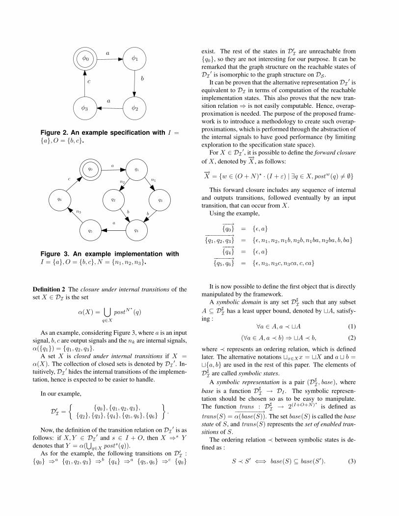
Algorithm 4.2: procedure back(S, w0)Input: w0 the primary output which has changedOutput: the updated symbolic state of the system

δ0τ0

none := v[w0];foreach w wire do

δ ττh

:= v[w];if D[τ, τ0] 6 0 then

REM: w is known to have fired;if δ = [↑] then

v[w] := 1noneτh

;else

REM: δ = [↓];v[w] := 0none

τh;

endifproject out τ from D;

endifif D[τh, τ0] 6 0 then

v[w] := δ τnone ;

project out τh from D;endif

endfchreturn (D, v);

transition that just fired and τ is the standard timer of somewire w : δ τ

τh. In this case, it is known that the transition on

w has fired, thus, δ is set to its stable value (1 for [↑], 0 for[↓]), and τ is projected out of the current DBM. If, for someτh, D : τh 6 τ0 where there is a wire w : δ τ

τh, then this

hazard transition has caused possible hazards in the past,but they have no direct effect on the future behaviour of thecircuit. Hence, the behaviour of w is set to δ τ

none and τh isprojected out.

The back procedure does not handle the case where thereis a hazard timer on wire w0. The reason is that, during themain procedure, when a hazard is detected on a primaryoutput such as w0, it is reported, then removed before thecall to the back procedure.

4.5 Detection of hazards

Failure states are symbolic states for which there existsat least one primary output with an existing hazard timer.Unlike previous approaches [1, 7], a hazard on an internalwire is not a case of failure when it can be proved to beabsorbed later. As shown in Algorithm 2.1, hazards are de-tected just after the call to forward, and the pair (x, cur) isadded to the list of hazards.

Table 1. Experimental results (timed)Example #G #h #d #at new atacs

alloc-outbound 11 0 0 0 0 0chu133 9 1 1 1 0 0ebergen 9 3 3 3 0 0

half 7 1 1 1 0 0sbuf-send-pkt2 13 0 0 1 0.13 0.05sbuf-ram-write 17 1 1 2 0.04 0.06

rpdft 8 1 1 3 0.035 0.029vme 12 1 1 – 0.05 –dff 6 2 2 – 0.08 –

trimos-send 24 5 5 5 2.43 1.7execution times are given in seconds#G is the number of gates, #h is the exact number of haz-ards, #d is the number of hazards detected by the proposedmethod, #at is the number of hazards detected by ATACS,new is the run time of the proposed method, ATACS is therun time of ATACS. 0 represents a run time inferior to 10ms.Entries labelled as – indicate that ATACS was unable tocheck the given circuit due to internal loops.

5 Experimental results

Experimental results shown in Table 1 were obtained ona Pentium IV 2GHz processor, with 3GB of RAM. The pro-posed approach has been compared to the implementationof [7] in the ATACS tool.

We also applied our framework to the checking of speed-independent circuits, using different adequate semantics forthe behaviour of wires, obtaining the results in Table 2, inwhich a comparison of the algorithm using our new frame-work to an implementation of [1] in ATACS is given, aswell as to versify [9], that uses a symbolic representation ofstates to reduce the cost of full exploration. The examplesused are hazard-free, and the three algorithms detect thiscorrectly.

The experimental results show that our algorithm has aspeed that compares well with [7], which is currently thefastest algorithm for the hazard checking of timed circuits,as both of them do not explore the full state space by usingdifferent representations for internal wires.

Furthermore, while the algorithm is conservative, falsenegatives have not been encountered, and it is possible togive the correct number of hazards for examples for which[7] could either not check because of the presence of inter-nal loops (as in examples vme and dff), or gave false neg-atives (as in examples sbuf-send-pkt2, sbuf-ram-write andrpdft).

6 Conclusion

This paper first presents a new general framework forthe conservative exploration of the state-space of an imple-mentation with respect to a given specification. In order toapply this framework to the problem of hazard-checking of

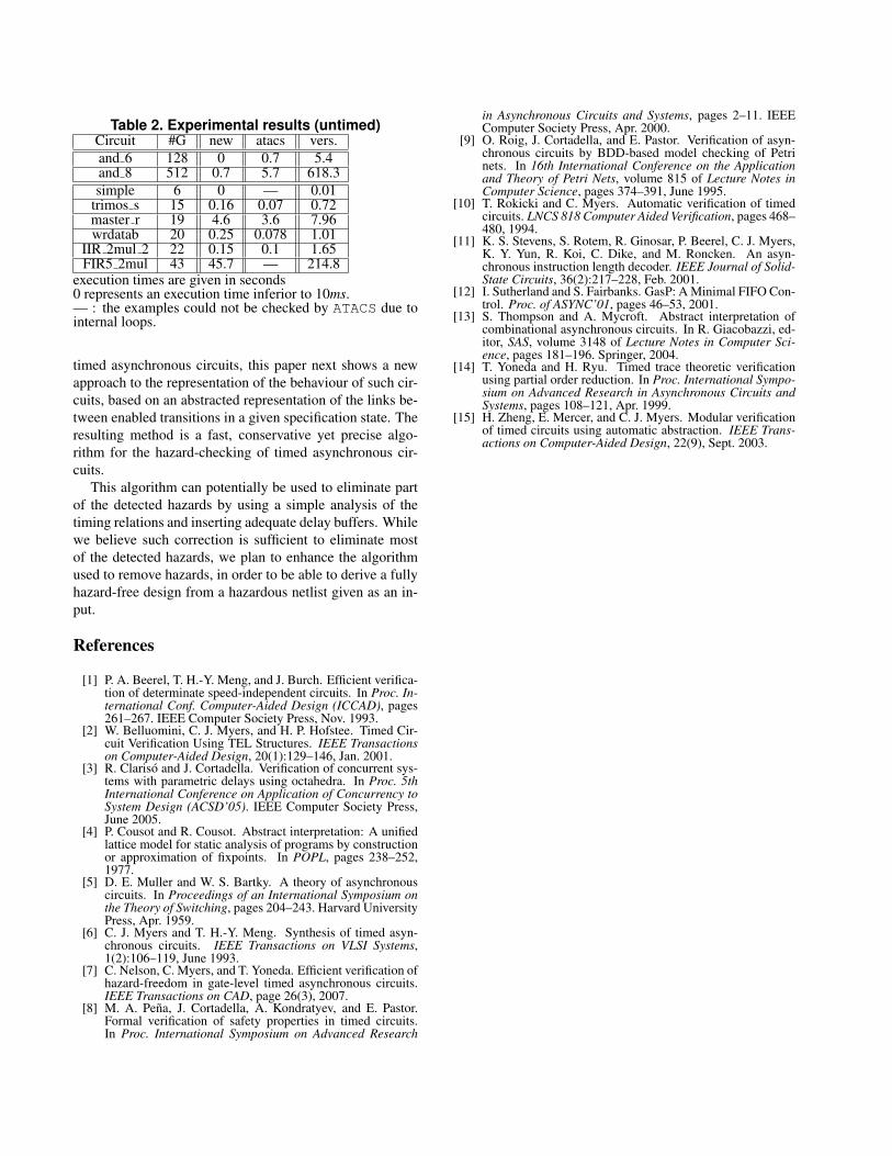
Table 2. Experimental results (untimed)Circuit #G new atacs vers.and 6 128 0 0.7 5.4and 8 512 0.7 5.7 618.3simple 6 0 — 0.01

trimos s 15 0.16 0.07 0.72master r 19 4.6 3.6 7.96wrdatab 20 0.25 0.078 1.01

IIR 2mul 2 22 0.15 0.1 1.65FIR5 2mul 43 45.7 — 214.8

execution times are given in seconds0 represents an execution time inferior to 10ms.— : the examples could not be checked by ATACS due tointernal loops.

timed asynchronous circuits, this paper next shows a newapproach to the representation of the behaviour of such cir-cuits, based on an abstracted representation of the links be-tween enabled transitions in a given specification state. Theresulting method is a fast, conservative yet precise algo-rithm for the hazard-checking of timed asynchronous cir-cuits.

This algorithm can potentially be used to eliminate partof the detected hazards by using a simple analysis of thetiming relations and inserting adequate delay buffers. Whilewe believe such correction is sufficient to eliminate mostof the detected hazards, we plan to enhance the algorithmused to remove hazards, in order to be able to derive a fullyhazard-free design from a hazardous netlist given as an in-put.

References

[1] P. A. Beerel, T. H.-Y. Meng, and J. Burch. Efficient verifica-tion of determinate speed-independent circuits. In Proc. In-ternational Conf. Computer-Aided Design (ICCAD), pages261–267. IEEE Computer Society Press, Nov. 1993.

[2] W. Belluomini, C. J. Myers, and H. P. Hofstee. Timed Cir-cuit Verification Using TEL Structures. IEEE Transactionson Computer-Aided Design, 20(1):129–146, Jan. 2001.

[3] R. Clariso and J. Cortadella. Verification of concurrent sys-tems with parametric delays using octahedra. In Proc. 5thInternational Conference on Application of Concurrency toSystem Design (ACSD’05). IEEE Computer Society Press,June 2005.

[4] P. Cousot and R. Cousot. Abstract interpretation: A unifiedlattice model for static analysis of programs by constructionor approximation of fixpoints. In POPL, pages 238–252,1977.

[5] D. E. Muller and W. S. Bartky. A theory of asynchronouscircuits. In Proceedings of an International Symposium onthe Theory of Switching, pages 204–243. Harvard UniversityPress, Apr. 1959.

[6] C. J. Myers and T. H.-Y. Meng. Synthesis of timed asyn-chronous circuits. IEEE Transactions on VLSI Systems,1(2):106–119, June 1993.

[7] C. Nelson, C. Myers, and T. Yoneda. Efficient verification ofhazard-freedom in gate-level timed asynchronous circuits.IEEE Transactions on CAD, page 26(3), 2007.

[8] M. A. Pena, J. Cortadella, A. Kondratyev, and E. Pastor.Formal verification of safety properties in timed circuits.In Proc. International Symposium on Advanced Research

in Asynchronous Circuits and Systems, pages 2–11. IEEEComputer Society Press, Apr. 2000.

[9] O. Roig, J. Cortadella, and E. Pastor. Verification of asyn-chronous circuits by BDD-based model checking of Petrinets. In 16th International Conference on the Applicationand Theory of Petri Nets, volume 815 of Lecture Notes inComputer Science, pages 374–391, June 1995.

[10] T. Rokicki and C. Myers. Automatic verification of timedcircuits. LNCS 818 Computer Aided Verification, pages 468–480, 1994.

[11] K. S. Stevens, S. Rotem, R. Ginosar, P. Beerel, C. J. Myers,K. Y. Yun, R. Koi, C. Dike, and M. Roncken. An asyn-chronous instruction length decoder. IEEE Journal of Solid-State Circuits, 36(2):217–228, Feb. 2001.

[12] I. Sutherland and S. Fairbanks. GasP: A Minimal FIFO Con-trol. Proc. of ASYNC’01, pages 46–53, 2001.

[13] S. Thompson and A. Mycroft. Abstract interpretation ofcombinational asynchronous circuits. In R. Giacobazzi, ed-itor, SAS, volume 3148 of Lecture Notes in Computer Sci-ence, pages 181–196. Springer, 2004.

[14] T. Yoneda and H. Ryu. Timed trace theoretic verificationusing partial order reduction. In Proc. International Sympo-sium on Advanced Research in Asynchronous Circuits andSystems, pages 108–121, Apr. 1999.

[15] H. Zheng, E. Mercer, and C. J. Myers. Modular verificationof timed circuits using automatic abstraction. IEEE Trans-actions on Computer-Aided Design, 22(9), Sept. 2003.