
ON ADAPTIVE FILTERING IN OVERSAMPLED SUBBANDS
239
-
Upload
khangminh22 -
Category
Documents
-
view
5 -
download
0
Transcript of ON ADAPTIVE FILTERING IN OVERSAMPLED SUBBANDS

ON ADAPTIVE FILTERING IN OVERSAMPLEDSUBBANDSa dissertationsubmitted to the signal processing division,department of electronic and electrical engineeringand the committee for postgraduate studiesof the University of Strathclydein partial fulfillment of the requirementsfor the degree ofdoctor of philosophy
ByStephan WeiMay 1998

The copyright of this thesis belongs to the author under the terms of theUnited Kingdom Copyright Acts as qualied by University of Strathclyde Regu-lation 3.49. Due acknowledgement must always be made of the use of any materialcontained in, or derived from, this thesis.c Copyright 1998
ii

DeclarationI declare that this Thesis embodies my own research work and that it is composedby myself. Where appropriate, I have made acknowledgement to the work ofothers. Stephan Wei
iii

Meinen lieben Eltern, Werner und Ursula Wei
iv

AbstractFor a number of applications like acoustic echo cancellation, adaptive lters arerequired to identify very long impulse responses. To reduce the computationalcost in implementations, adaptive ltering in subband is known to be benecial.Based on a review of popular fullband adaptive ltering algorithms and vari-ous subband approaches, this thesis investigates the implementation, design, andlimitations of oversampled subband adaptive lter systems based on modulatedcomplex and real valued lter banks.The main aim is to achieve a computationally ecient implementation foradaptive lter systems, for which fast methods of performing both the subbanddecomposition and the subband processing are researched. Therefore, a highlyecient polyphase implementation of a complex valued modulated generalizedDFT (GDFT) lter bank with a judicious selection of properties for non-integeroversampling ratios is introduced. By modication, a real valued single sidebandmodulated lter bank is derived. Non-integer oversampling ratios are particularlyimportant when addressing the eciency of the subband processing. Analysis ispresented to decide in which cases it is more advantageous to perform real orcomplex valued subband processing.Additionally, methods to adaptively adjust the lter lengths in subband adaptivelter (SAF) systems are discussed.Convergence limits for SAFs and the accuracy of the achievable equivalentfullband model based on aliasing and other distortions introduced by the em-ployed lter banks are explicitly derived. Both an approximation of the minimummean square error and the model accuracy can be directly linked to criteria inthe design of the prototype lter for the lter bank. Together with an iterativev

least-squares design algorithm, it is therefore possible to construct lter banksfor SAF applications with pre-dened performance limits.Simulation results are presented which demonstrate the validity and propertiesof the discussed SAF methods and their advantage over fullband and criticallysampled SAF systems.
vi

AcknowledgementsI wish to express my deepest gratitude to Dr Robert W. Stewart for his enthusi-asm, encouragement, dedication, and support, which he has shown over the pastyears for the work which I have performed under his supervision and of whicha part is compiled in this thesis. Particularly, I would like to thank Dr Stewartfor arranging to spend part of my PhD time at the Signal and Image ProcessingInstitute, University of Southern California. I would further like to thank ProfRichard Leahy of SIPI for his hospitality and the great experience of both stayingat SIPI and working with his functional brain imaging group.Thanks are also due to my colleague and friend Moritz Harteneck for in-spiring discussions and all the fun we had while working together. I am alsogreatly endebted to Dipl.-Ing. Alexander Stenger and Priv.-Doz. Dr.-Ing. habilRudolf Rabenstein from Telecommunications Institute I, University of Erlangen-Nurnberg, Germany, for many helpful discussions and collaboration. Part of thework presented here was performed in undergraduate projects, and I would par-ticularly like to mention Lutz Lampe and Dipl.-Ing. Uwe Sorgel for their valuableinput.This work would have been impossible without the generous support by astudentship from William Garven Research Bequest, which I gratefully acknowl-edge. I am also indebted to the Signal Processing Division and its members forproviding both the facilities and social background that enabled joyful working.Particular thanks to Dr Asoke Nandi for some valuable discussions, and excitingBadminton games.I would like to thank Dipl.-Phys. Dr. Ing. Ulrich Hoppe and Prof RichardLeahy, whos literary interest oered a great number of suggestions, which I havevii

devoured with appetite.Finally, I owe many thanks to my family at home, and my friends here andabroad for their support and encouragement. I could not have done without it.Stephan WeiGlasgow, April 1998
viii

ContentsDeclaration iiiAbstract vAcknowledgements viiContents viiiList of Figures xiiList of Tables xvMathematical Notations xviiAcronyms xxii1 Introduction 11.1 Context of Work . . . . . . . . . . . . . . . . . . . . . . . . . . . 11.2 Original Contribution . . . . . . . . . . . . . . . . . . . . . . . . . 51.3 Overview . . . . . . . . . . . . . . . . . . . . . . . . . . . . . . . . 72 Adaptive Filtering Algorithms 102.1 General Filtering Problem . . . . . . . . . . . . . . . . . . . . . . 102.2 Optimum Wiener Filter . . . . . . . . . . . . . . . . . . . . . . . 122.2.1 Mean Squared Error Formulation . . . . . . . . . . . . . . 122.2.2 Minimization and Wiener-Hopf Solution . . . . . . . . . . 132.2.3 Minimum Mean Squared Error . . . . . . . . . . . . . . . 15ix
2.3 Least Mean Square Algorithms . . . . . . . . . . . . . . . . . . . 162.3.1 Preliminaries | Gradient Descent Techniques . . . . . . . 162.3.2 One Sample Gradient Estimates . . . . . . . . . . . . . . . 162.3.3 Convergence Characteristics . . . . . . . . . . . . . . . . . 172.4 Least Squares Methods . . . . . . . . . . . . . . . . . . . . . . . . 212.4.1 Least Squares Formulation . . . . . . . . . . . . . . . . . . 222.4.2 Recursive Least Squares Algorithm . . . . . . . . . . . . . 222.4.3 Algorithm Complexity . . . . . . . . . . . . . . . . . . . . 242.5 Links Between LMS and RLS Algorithms . . . . . . . . . . . . . . 252.5.1 Normalized LMS Algorithm . . . . . . . . . . . . . . . . . 252.5.2 Ane Projection Algorithms . . . . . . . . . . . . . . . . . 292.6 Implementations and Complexity Issues . . . . . . . . . . . . . . . 322.6.1 Frequency Domain Implementation . . . . . . . . . . . . . 322.6.2 Subband Implementation . . . . . . . . . . . . . . . . . . . 342.7 Concluding Remarks . . . . . . . . . . . . . . . . . . . . . . . . . 363 Filter Banks and Subband Structures for Adaptive SubbandProcessing 373.1 Preliminaries on Multirate Systems . . . . . . . . . . . . . . . . . 383.1.1 Basic Multirate Operations . . . . . . . . . . . . . . . . . 383.1.2 Signal Bandwidth and Sampling . . . . . . . . . . . . . . . 403.2 Signal Decompositions . . . . . . . . . . . . . . . . . . . . . . . . 433.2.1 Orthogonal Decompositions . . . . . . . . . . . . . . . . . 443.2.2 Redundant Decompositions . . . . . . . . . . . . . . . . . 463.3 Filter Bank Analysis . . . . . . . . . . . . . . . . . . . . . . . . . 473.3.1 Modulation Description . . . . . . . . . . . . . . . . . . . 473.3.2 Polyphase Representation . . . . . . . . . . . . . . . . . . 483.3.3 Lossless Expansions . . . . . . . . . . . . . . . . . . . . . . 513.4 Dierent Approaches to Subband Adaptive Filtering . . . . . . . . 523.4.1 Aliasing in the Decimation Stage . . . . . . . . . . . . . . 523.4.2 Critically Decimated Filter Banks . . . . . . . . . . . . . . 533.4.3 Oversampled Filter Banks . . . . . . . . . . . . . . . . . . 623.5 Concluding Remarks . . . . . . . . . . . . . . . . . . . . . . . . . 69x

4 Oversampled GDFT Filter Banks 714.1 Complex Valued GDFT Filter Banks . . . . . . . . . . . . . . . . 714.1.1 GDFT Modulation . . . . . . . . . . . . . . . . . . . . . . 724.1.2 Polyphase Representation . . . . . . . . . . . . . . . . . . 774.1.3 Perfect Reconstruction and Gabor Frames . . . . . . . . . 784.2 Ecient Filter Bank Implementation . . . . . . . . . . . . . . . . 814.2.1 Polyphase Factorization . . . . . . . . . . . . . . . . . . . 814.2.2 Transform Implementation . . . . . . . . . . . . . . . . . . 874.2.3 Computational Complexity . . . . . . . . . . . . . . . . . . 884.3 SSB Modulated Real Valued Filter Banks . . . . . . . . . . . . . 904.3.1 SSB by Weaver Method and Modications . . . . . . . . . 904.3.2 SSB by GDFT Filter Bank Modication . . . . . . . . . . 924.4 Complex Vs Real Valued Subband Processing . . . . . . . . . . . 964.5 Filter Design . . . . . . . . . . . . . . . . . . . . . . . . . . . . . 994.5.1 Requirements . . . . . . . . . . . . . . . . . . . . . . . . . 994.5.2 Dyadically Iterated Halfband Filters . . . . . . . . . . . . 1024.5.3 Iterative Least Squares Design . . . . . . . . . . . . . . . . 1054.6 Concluding Remarks . . . . . . . . . . . . . . . . . . . . . . . . . 1125 Performance of Subband Adaptive Filter Systems 1155.1 General Performance Limiting In uences . . . . . . . . . . . . . . 1155.1.1 Performance Criteria . . . . . . . . . . . . . . . . . . . . . 1165.1.2 Performance Limitations . . . . . . . . . . . . . . . . . . . 1185.2 Minimum Mean Squared Error Limitations . . . . . . . . . . . . . 1215.2.1 Measuring Aliasing . . . . . . . . . . . . . . . . . . . . . . 1215.2.2 MMSE Approximations . . . . . . . . . . . . . . . . . . . 1265.3 Modelling Accuracy . . . . . . . . . . . . . . . . . . . . . . . . . . 1315.3.1 Equivalent Fullband Model Reconstruction . . . . . . . . . 1315.3.2 Maximally Achievable Model Accuracy . . . . . . . . . . . 1355.4 Simulations and Results . . . . . . . . . . . . . . . . . . . . . . . 1365.4.1 Subband Parameters . . . . . . . . . . . . . . . . . . . . . 1375.4.2 Performance Limits . . . . . . . . . . . . . . . . . . . . . . 1455.5 Concluding Remarks . . . . . . . . . . . . . . . . . . . . . . . . . 152xi

6 Variable Tap-Proles For Subband Adaptive Filters 1556.1 Idea and Background . . . . . . . . . . . . . . . . . . . . . . . . . 1556.1.1 Motivation . . . . . . . . . . . . . . . . . . . . . . . . . . . 1556.1.2 Approaches and Methods . . . . . . . . . . . . . . . . . . . 1576.2 Equivalent Fullband Model Length and Complexity . . . . . . . . 1596.2.1 Computational Complexity . . . . . . . . . . . . . . . . . . 1606.2.2 Equivalent Fullband Model Length . . . . . . . . . . . . . 1656.3 Tap-Prole Adaptation . . . . . . . . . . . . . . . . . . . . . . . . 1676.3.1 Optimum Tap-Prole . . . . . . . . . . . . . . . . . . . . . 1686.3.2 Tap-Distribution Mechanism . . . . . . . . . . . . . . . . . 1716.3.3 Distribution Criteria . . . . . . . . . . . . . . . . . . . . . 1726.4 Simulations . . . . . . . . . . . . . . . . . . . . . . . . . . . . . . 1746.4.1 Performance at Given Benchmark . . . . . . . . . . . . . . 1746.4.2 Bias of Tap-Prole Adaptation . . . . . . . . . . . . . . . 1806.5 Concluding Remarks . . . . . . . . . . . . . . . . . . . . . . . . . 1847 Conclusions 1867.1 Resume . . . . . . . . . . . . . . . . . . . . . . . . . . . . . . . . 1867.2 Core Results . . . . . . . . . . . . . . . . . . . . . . . . . . . . . . 1907.3 Outlook . . . . . . . . . . . . . . . . . . . . . . . . . . . . . . . . 1917.3.1 Extensions . . . . . . . . . . . . . . . . . . . . . . . . . . . 1917.3.2 Related Applications . . . . . . . . . . . . . . . . . . . . . 192Bibliography 194
xii

List of Figures1.1 Acoustic echo cancellation using an adaptive lter . . . . . . . . . 21.2 Adaptive lter in system identication set-up. . . . . . . . . . . . 31.3 Adaptive lter in adaptive noise cancellation set-up. . . . . . . . 31.4 Adaptive ltering in subbands. . . . . . . . . . . . . . . . . . . . 52.1 General lter problem. . . . . . . . . . . . . . . . . . . . . . . . . 112.2 Geometrical interpretation of the NLMS. . . . . . . . . . . . . . 272.3 NLMS convergence. . . . . . . . . . . . . . . . . . . . . . . . . . . 282.4 Comparison of convergence speed for NLMS, RLS, and APA. . . . 312.5 Geometrical interpretation of ane projection algorithms. . . . . 322.6 Generic diagram of adaptive ltering in subbands. . . . . . . . . 343.1 Filter banks with analysis and synthesis side. . . . . . . . . . . . . 373.2 Multirate operations for sampling rate alteration. . . . . . . . . . 383.3 Example for decimation and expansion by 2. . . . . . . . . . . . . 393.4 Spectrum of an analytic signal. . . . . . . . . . . . . . . . . . . . 423.5 Symmetric spectrum of a real valued signal. . . . . . . . . . . . . 423.6 Valid decimation rates for real valued bandpass sampling. . . . . . 433.7 Orthonormal projection and the scalar product. . . . . . . . . . . 453.8 Haar lter example for orthonormal decomposition. . . . . . . . . 463.9 Rearrangements based on the polyphase representation. . . . . . . 503.10 Example for \information leakage" in critically decimated banks. . 543.11 Adaptive identication in subbands. . . . . . . . . . . . . . . . . 553.12 2 channel critically decimated SAF system with cross-terms. . . . 583.13 Frequency response of a near perfectly reconstructing QMF pair. . 58xiii
3.14 Factorization of cross-terms. . . . . . . . . . . . . . . . . . . . . . 593.15 Power symmetric IIR lters with small alias level. . . . . . . . . . 603.16 Arrangement of bandpass lters for dierent lter bank types. . . 633.17 SSB demodulation for kth analysis lter branch. . . . . . . . . . . 663.18 SSB modulation for kth synthesis lter branch. . . . . . . . . . . 673.19 Explanation of SSB demodulation and modulation. . . . . . . . . 673.20 Example for a non-uniform oversampled real valued lter bank. . 694.1 Filter bank. . . . . . . . . . . . . . . . . . . . . . . . . . . . . . . 724.2 GDFT modulation example of real valued prototype lter. . . . . 734.3 Complex GDFT modulation of a lter and linear phase property. 754.4 Subband PSD after decimation and expansion. . . . . . . . . . . . 764.5 Exploiting periodicities in the GDFT modulation. . . . . . . . . . 824.6 Computational scheme for factorized polyphase representation. . . 864.7 Weaver SSB by complex quadrature modulation. . . . . . . . . . . 914.8 Real valued oversampled SSB modied GDFT lter bank. . . . . 934.9 SSB modication for kth subband of a GDFT lter bank. . . . . . 944.10 Example for re-alignment of subband PSDs in the SSB modication. 954.11 Required frequency response of a real valued prototype lter. . . . 1004.12 Flow graph for prototype design by dyadically iterated lters. . . 1034.13 Frequency responses of dyadically iterated halfband prototypes. . 1044.14 Frequency responses of iterative LS design prototype lters. . . . 1104.15 Bifrequency transfer function for complex GDFT lter bank. . . . 1124.16 Bifrequency transfer function for SSB modied GDFT lter bank. 1135.1 Decimation of a white noise excited source model. . . . . . . . . . 1225.2 Block diagram of kth lter bank branch with source model. . . . . 1235.3 Idealized frequency response of prototype lter. . . . . . . . . . . 1295.4 Subband adaptive lter system in system identication set-up. . . 1345.5 Equivalent fullband model of an SAF system. . . . . . . . . . . . 1345.6 Frequency response of prototype lters for dierent OSRs. . . . . 1385.7 Measured subband PSDs and eigenspectra. . . . . . . . . . . . . . 1395.8 ERLE for identication with white noise in complex subbands. . . 140xiv

5.9 ERLE for identication with white noise in real subbands. . . . . 1415.10 PSD of coloured input signal. . . . . . . . . . . . . . . . . . . . . 1415.11 ERLE for identication with coloured noise in complex subbands. 1425.12 ERLE for identication with coloured noise in real subbands. . . . 1435.13 ERLE for identication with white noise and various subbands. . 1445.14 ERLE for identication with coloured noise and various subbands. 1455.15 Pole-zero plot of the unknown system used for system identication.1465.16 Impulse and magnitude response of unknown system. . . . . . . . 1475.17 Reconstructed fullband MSE. . . . . . . . . . . . . . . . . . . . . 1475.18 PSD of error signal before and after adaptation. . . . . . . . . . . 1485.19 PSD of error after almost complete adaptation. . . . . . . . . . . 1485.20 Predicted and true residual error PSDs. . . . . . . . . . . . . . . . 1495.21 PSD of error signal before and after adaptation. . . . . . . . . . . 1505.22 Comparison between the predicted and measured PSD. . . . . . . 1516.1 Uniform and optimized tap-prole for SAF system. . . . . . . . . 1566.2 SAF system with adaptive adjustment of the tap-prole. . . . . . 1586.3 Relative computational cost for complex oversampled subbands. . 1636.4 Relative computational cost for real valued oversampled subbands. 1646.5 Relative computational cost for critically sampled subbands. . . . 1646.6 Relative fullband model length for complex oversampled SAF. . . 1666.7 Relative fullband model length for real valued oversampled SAF. . 1666.8 Relative fullband model length for critically sampled SAF. . . . . 1676.9 Identiable and unidentiable part of a system. . . . . . . . . . . 1686.10 Impulse response of the unknown system. . . . . . . . . . . . . . . 1756.11 Critically sampled SAF with variable tap-prole. . . . . . . . . . . 1776.12 Real valued oversampled SAF with variable tap-prole. . . . . . . 1786.13 Complex valued oversampled SAF with variable tap-prole. . . . . 1796.14 Final fullband model error with dierent SAF system structures. . 1816.15 Comparison of dierent tap-assignment algorithms. . . . . . . . . 1827.1 Transmultiplexer. . . . . . . . . . . . . . . . . . . . . . . . . . . . 193xv

List of Tables2.1 Equations for lter update by LMS adaptive algorithm. . . . . . 172.2 Equations for lter update by RLS adaptive algorithm. . . . . . 242.3 Equations for lter update by NLMS adaptive algorithm. . . . . 262.4 Equations for lter update by APA adaptive algorithm. . . . . . 304.1 Comparison of complexity for real and complex algorithms. . . . . 994.2 Filter bank properties for dyadically iterated halfband design. . . 1054.3 Characteristics of four dierent iterative LS designs. . . . . . . . . 1095.1 Prototype characteristics for iterative LS design with various OSRs.1375.2 Predicted fullband model error and nal MSE, and simulation results.1526.1 Comparison of fullband and SAF systems for system identication. 1756.2 Angles and radii of poles of unknown system. . . . . . . . . . . . 1756.3 Noise reduction with dierent tap-prole adaptation algorithms. . 183
xvi

Mathematical NotationsGeneral Notationsh scalar quantityh vector quantityH matrix quantityh(t) function of a continuous variable th[n] function of a discrete variable nhn short hand form for h[n] for dense notationH(ej) periodic Fourier spectrum of a discrete function h[n]H(z) z-transform of a discrete function h[n]Relations and Operators!= must equal| transform pair, e.g. h[n] | H(ej) or h[n] | H(z)() complex conjugate()H Hermitian (conjugate transpose)~H(z) parahermitian, ~H(z) = HH(z1)()T transpose convolution operatorEfg expectation operatorr gradient operator (vector valued)lmc(; ) least common multipleamodb modulo operator: remainder of a=bP() probability of xvii

de ceiling operator (round up)bc oor operator (round o)Sets and SpacesC set of complex numbersCMN set of M N matrices with complex entriesCMN(z) set of M N matrices with complex polynomial entries in zl2(Z) space of square integrable (i.e. nite energy) discrete time signalsN set of integer numbers 0R set of real numbersRMN set of M N matrices with real entriesRMN(z) set of M N matrices with real polynomial entries in zZ set of integer numbersSymbols and Variables energy bias RLS forgetting factor weighting in iterative LS lter design[n] Kronecker function, [n] = 1 for n = 0, [n] = 0 for n 6= 0 relaxation factor for APA LMS adaptive algorithm step size~ NLMS normalized step size[n], [n] basis functions, anglesLS least squares cost functionMSE mean square error cost functionMMSE minimum mean square error! (angular) frequency normalized (angular) frequency = !Ts, with sampling periodTsA gain xviii

Ap, As passband and stopband gainB bandwidthd[n] desired signaldk[n] desired signal in kth subbandD1;D2 factorial (diagonal) matrices of the GDFT transform matrixFx(ej) transfer path, with decimated white noise input and output signalx[n]F (A)x (ej) transfer path Fx(ej) for aliased signal components onlyF (S)x (ej) transfer path Fx(ej) for signal of interest onlyFx(ej) transfer path, with decimated white noise input and output signalx[n]gk[n] kth lter of the synthesis lter bankGnjk(z) n of N polyphase components of the kth synthesis lterGk(ej) frequency response of kth lter of synthesis lterG(z) vector of synthesis ltersG(z) polyphase matrix of the synthesis lter bankGm(z) modulation description of the synthesis lter bankhk[n] kth lter of the analysis lter bankHkjn(z) n of N polyphase components of the kth analysis lterHk(ej) frequency response of kth analysis lterH(z) polyphase matrix of the analysis lter bankHr(z) reduced polyphase matrix of the analysis lter bankHm(z) modulation description of the analysis lter bankIK K K identity matrixJK K K reverse identity matrixK (channel number) | K=2 subbands covering the frequency inter-val = [0; ] for both real and complex lter banks (see page64)La lter length of adaptive FIR lterLf lter length of FIR lterLp lter length of prototype lterLs length of impulse response of unknown system in system identi-cation xix

N decimation factor; for modulated lter banks, N is dened basedon the bandwidth (including transition bands) of the prototypelterO complexity orderp APA projection order; norm for adaptive tap-assignment criterionp[n] prototype lterP (2K)k (z) kth of 2K polyphase components of P (z)p cross-correlation vectorP(z) polyphase matrix of prototype lterPn solution hyperplane in ane projection algorithmqT (t t0) rectangular window with qT (t t0) = 1 for t 2 [t0; t0 + T ]Q update period for adaptive tap-prole algorithmsQ modal matrix containing eigenvectors of auto-correlation matrixRrxx() auto-correlation function of a stochastic process xrxy() cross-correlation function between two stochastic processes x andyR window length for estimation of tap-assignment criterionR auto-correlation matrixs[n] impulse response of unknown system (plant)in system identica-tionSm(z) modulation description of the unknown system projected into sub-bandsS1;S2 permutation matricesSxx(ej) power spectral density of the discrete time random process xSxy(ej) cross power spectral density between discrete time random pro-cesses x and yt[n] impulse response of distortion function, t[n] | T (z)tk;n transform coecientsT (z) distortion function of lter bankT transform matrixTDCT discrete cosine transform matrixTDFT discrete Fourier transform matrixTGDFT generalized discrete Fourier transform matrixxx
u[n] white noise excitation signal of source model L(ejw coecient vector of a lterwopt optimum coecient vector (Wiener lter)Wm(zK) adaptive lter matrixx[n] input signal to adaptive lter / lter bankX(z) polyphase vector of input signalXm(z) modulation description of the decimated input signalxk[n] decimated input signal in kth subbandx0k[n] decimated and expanded input signal in kth subbandxk[n] kth subband signal after passing through synthesis lterx[n] reconstructed fullband signal, summed over all xk[n]xn input vector to adaptive lterXn collection of current and past input vectors to adaptive ltery[n] output signal of adaptive lterz z-transform variablez[n] observation noisezk[n] observation noise in kth subband
xxi

AcronymsAEC acoustic echo cancellationAPA ane projection algorithmDCT discrete cosine transformDFT discrete Fourier transformDSP digital signal processorDWT discrete wavelet transformFDAF frequency domain adaptive lterFIR nite impulse responseFFT fast Fourier transformGDFT generalized discrete Fourier transformIIR innite impulse responseLMS least mean squares (algorithm)LPTV linear periodically time-varyingLTI linear time-invariantLS least squaresMMSE minimum mean squared errorMSE mean squared errorNLMS normalized least mean square (algorithm)OSR oversampling ratioPC power complementaryPR perfect reconstructionPSD power spectral densityQMF quadrature mirror lterRE reconstruction error xxii

RLS recursive least squares (algorithm)SAF subband adaptive lterSAR signal-to-aliasing ratioSNR signal-to-noise ratioSSB single sideband (modulation)TDAF transform domain adaptive lter
xxiii

Contents
xxiv

List of Tables
xxv

List of Figures
xxvi

Chapter 1Introduction1.1 Context of WorkDespite the constant growth in processing power, many digital signal processingalgorithms are still too complex to be implemented in real time. In the eld ofadaptive ltering the technological advances have recently enabled long-conceptedapplications such as active noise control to be realized [37]. However almost con-tinually new application ideas emerge that are yet more demanding in complexity.Thus, in parallel with the increasing hardware optimization to realize faster andmore powerful DSPs, a second track of optimization is dedicated to reduce thecomputational complexity of implemented DSP algorithms.A key example is acoustic echo cancellation (AEC) for hands-free telephonyand teleconferencing as shown in Fig. 1.1, which is often claimed to be one ofthe currently most computationally complex DSP applications [61, 62, 63]. In ahands-free telephone environment, the signal x[n] of the far end speaker is out-put to a loudspeaker. Over a free standing microphone, the near end speakercommunicates back to the far end. Unfortunately, the microphone signal d[n] notonly consists of the near end speaker's speech, but has superimposed on it thefeedback of the far end speaker signal x[n] ltered by the impulse response of asystem composed of loudspeaker, acoustic room transfer function, and the mi-crophone (LEMS | loudspeakerenclosuremicrophone system). This feedbackis perceived by the far end speaker as an echo of his/her own voice, which can1

CHAPTER 1. INTRODUCTION 2from
to
room
room
model
near-end
speaker
speaker
far-end
far-end
speaker
x[n]
e[n] d[n]
y[n]
Figure 1.1: Acoustic echo cancellation using an adaptive lter to identify a replicaof the room impulse response.create considerable disturbance and, at worst, make communication impossible.The acoustic echo cancellation approach is to incorporate a model of theLEMS into the communication system, which lters the far end speaker signalx[n] to produce a close replica y[n] of the echo contained in the near end signald[n]. Thus, the echo can be subtracted out to yield a signal e[n] containing thenear end speaker only. Since the room acoustics are likely to be time-varying dueto the changing presence, absence and mobility of conferees, the room model hasto be adjusted on-line to track changes; hence adaptive solutions are required.Acoustic echo cancellation by adaptive means may be interpreted as the hybridform of two fundamental adaptive ltering set-ups, adaptive noise cancellationand system identication.Adaptive System Identication. For the adaptive identication of some un-known system, a digital lter with variable coecients is set up in parallel to thesystem to be identied, as seen in Fig. 1.2. The adaptive lter will then try toproduce an output signal y[n] such that when subtracted from the desired signal

CHAPTER 1. INTRODUCTION 3y[n]
d[n]
unknown
system
adaptive
filterx[n] e[n]Figure 1.2: Adaptive lter in system identication set-up.y[n]adaptive
filter e[n]
d[n]
x[n]‘‘history of signals’’
s[n]
x[n]
z[n]
x’[n]
Figure 1.3: Adaptive lter in adaptive noise cancellation set-up.d[n], the resulting error signal e[n] will be minimized in an appropriate sense. Ifthe error tends towards zero, the unknown system and the adaptive lter havethe same input/output behaviour. Thus, if the exciting signal x[n] has beenbroadband, a complete parameterization of the unknown system is achieved.Adaptive Noise Cancellation. The application of adaptive ltering to noisecancellation [174] is shown in Fig. 1.3. The desired signal d[n] consists of a signalof interest z[n], which is corrupted by some unwanted noise (in case of AEC theecho). If a noise probe x[n] is available, which is correlated with the corruptingnoise x0[n], an adaptive lter can be employed to suppress the corrupting noiseas best as possible, such that the error signal e[n] contains the signal of interestonly. Considering the history of the signals x[n] and d[n], the similarity to asystem identication set-up as given in Fig. 1.2 becomes apparent: the correlationbetween the noise probe x[n] and the signal d[n] can be described by a lter s[n],which the adaptive lter will try to identify, if the input signal x[n] is broadband.

CHAPTER 1. INTRODUCTION 4In case of system identication, the signal z[n] is termed observation noise.The LEMS is to be identied over the spectral range of the human voice,and has therefore some avour of both system identication and active noisecancellation. While the coloured speech input is a problem on its own since itwill considerably slow the convergence speed of many adaptive algorithms, themain problem stems from the algorithmic complexity required for AEC, as thelength of the room impulse response in the LEMS usually spans several hundredmilliseconds. If the sampling rate is set to 16kHz, adaptive nite impulse responselters of several thousand coecients length would be required. Similar problemsarise when the classical system identication set-up is attempted to determineroom impulse responses and parameterize acoustics [46, 124].One method for reducing the complexity of adaptive systems is given by thesubband approach, whereby the signals involved are split into a number of fre-quency bands, which can be operated at a lower sampling rate. As shown forthe system identication set-up in Fig. 1.4, adaptive ltering is then performedin the subbands at the decimated sampling rate and with shorter lter lengths,which can yield a considerable reduction in computational complexity. Althoughthe original idea introduced by Kellermann [84, 85] and Gilloire [52] is now morethan a decade old, the research eort in this particular area has been probablyhigher than ever in the last years, driven by the promise of the high commercialrelevance of acoustic echo cancellers.To perform subband adaptive ltering (SAF) as shown in Fig. 1.4 a wide vari-ety of approaches exist, including critically decimated and oversampled systems,and ranging from perfectly reconstructing systems to some that introduce spec-tral loss or even distortion. However, the case of critical decimation, where thedecimation ratio equals the number of uniform subbands, requires either cross-terms at least between adjacent frequency bands [54], which compensates theinformation loss due to aliasing distortion, or gap lter banks [176, 148], whichintroduces spectral loss that may not be acceptable. Oversampled lter bankscan resolve this problem by introducing spectral redundancy, whereby oversam-pling in this context means that the subband signals are decimated by a factorsmaller than the critical one. While complex analytic subband signals can be

CHAPTER 1. INTRODUCTION 5analysis
filter
bank
bank
filter
analysis
bank
filter
unknown system
s[n]
d[n]
desired signal
inputsignal
x[n] e[n]
errorsignal
0
1
K/2-1
0
1
K/2-1
0
K/2-1
1
w
0w
1
wK/2-1
synthesis
d [n]
d [n]
d [n]
x [n]
x [n]
x [n]
e [n]
e [n]
e [n]Figure 1.4: Adaptive ltering in subbands.decimated at any integer factor above the critical one, for the real valued casebandpass signals are problematic to decimate, and oversampling requires eithernon-uniform lter banks [71, 69] or single side band (SSB) modulation [27, 167].1.2 Original ContributionThe research presented in this thesis has been mostly dedicated to a particulartype of oversampled complex valued lter bank, where the lters are derived bya generalized DFT (GDFT) transform from a real valued prototype lter. Theeciency when incorporated in an SAF system is given by two facts.Firstly, despite the requirement of complex arithmetic, the complex subbandapproach will be shown to be surprisingly ecient compared to the processing inreal valued oversampled subbands. This is particularly true if the computationalorder of the algorithm to be implemented in subbands is greater than linear in thelength of the adaptive lter. It will also outperform critically sampled systems,if the oversampling ratio is close to one.Secondly, we will introduce a highly ecient way of implementing our GDFTmodulated lter bank based on a polyphase factorization for non-integer over-sampling ratios, such that the lter bank can be operated close at the criticalrate. This will prove a common \subband" misconception wrong, which has led

CHAPTER 1. INTRODUCTION 6many researchers to use either less ecient integer oversampling ratios for SAFsystems, or to use other, less ecient implementations for the lter banks.Another key point in this thesis is the analysis of nal convergence limits forsubband adaptive lters based on aliasing and other distortions introduced by theemployed lter banks. We will derive explicit limits, and approximations thereof,which can be directly linked to the prototype lter on which the modulatedlter banks are based. Together with an iterative least-squares design algorithm,it will be possible to construct lter banks for SAF systems with pre-denedperformance limits.The following ideas, derivations, and experiments summarise original contri-butions of this work: a highly ecient implementation of GDFT banks based on a polyphaserepresentation, for K channel banks with arbitrary integer decimation ratio(i.e. including non-integer oversampling); a real-valued single sideband modulated lter bank based on a modiedGDFT lter bank in polyphase implementation; a discussion of the computational complexity for complex and real valuedsubband adaptive lter (or general subband processing) implementations; a description of aliasing in the subbands and its inhibition of adaptation; adescription of this phenomenon as information leakage in the time domain; the derivation of limits for the minimum error PSD, and the minimummeansquare error (MMSE) of an SAF system based on aliasing in the subbands; a derivation of the limit for the accuracy of the fullband equivalent modelidentied by the SAF system; approximations linking the performance limitations to design specicationsof the prototype lter of a modulated lter bank; a fast prototype lter design using an iterated least squares algorithm;
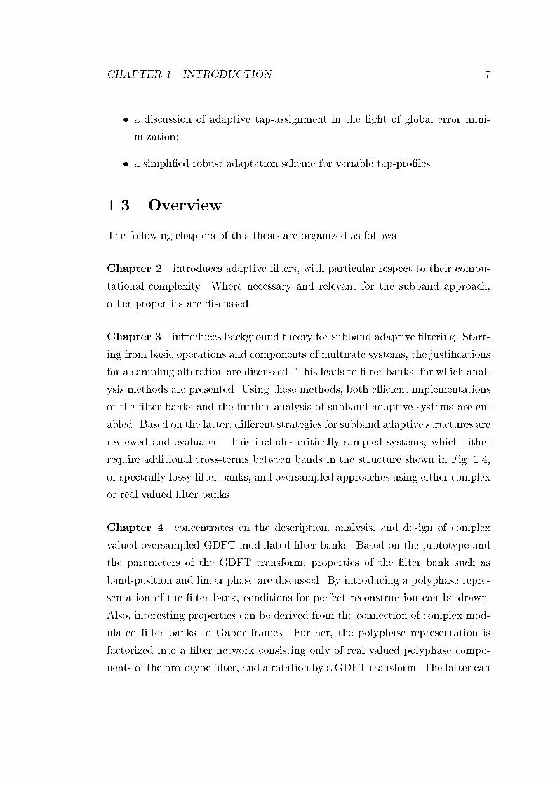
CHAPTER 1. INTRODUCTION 7 a discussion of adaptive tap-assignment in the light of global error mini-mization; a simplied robust adaptation scheme for variable tap-proles.1.3 OverviewThe following chapters of this thesis are organized as follows.Chapter 2 introduces adaptive lters, with particular respect to their compu-tational complexity. Where necessary and relevant for the subband approach,other properties are discussed.Chapter 3 introduces background theory for subband adaptive ltering. Start-ing from basic operations and components of multirate systems, the justicationsfor a sampling alteration are discussed. This leads to lter banks, for which anal-ysis methods are presented. Using these methods, both ecient implementationsof the lter banks and the further analysis of subband adaptive systems are en-abled. Based on the latter, dierent strategies for subband adaptive structures arereviewed and evaluated. This includes critically sampled systems, which eitherrequire additional cross-terms between bands in the structure shown in Fig. 1.4,or spectrally lossy lter banks, and oversampled approaches using either complexor real valued lter banks.Chapter 4 concentrates on the description, analysis, and design of complexvalued oversampled GDFT modulated lter banks. Based on the prototype andthe parameters of the GDFT transform, properties of the lter bank such asband-position and linear phase are discussed. By introducing a polyphase repre-sentation of the lter bank, conditions for perfect reconstruction can be drawn.Also, interesting properties can be derived from the connection of complex mod-ulated lter banks to Gabor frames. Further, the polyphase representation isfactorized into a lter network consisting only of real valued polyphase compo-nents of the prototype lter, and a rotation by a GDFT transform. The latter can

CHAPTER 1. INTRODUCTION 8be further factorized such that the transform matrix can be mainly implementedusing a standard FFT. This fast ecient implementation can also be used forreal valued subband processing by modication of the subband signals such thateectively a single sideband modulated lter bank is performed.This motivates to investigate which | real or complex valued subband pro-cessing | can be considered more ecient when implementing a specic subbandadaptive lter; this can be answered by separately evaluating the costs for thelter bank operations and for the algorithms operating in the subbands.Finally, two design methods for GDFT and SSB modied GDFT lter banksare introduced. The rst is an iterated halfband method producing power-of-twochannel lter banks from tabled halfband lters; the second yields a prototypelter using a least squares design to achieve both near perfect reconstruction andhigh stopband attenuation.Chapter 5 evaluates the performance of subband adaptive lters. This includesa review of general aspects of performance, such as convergence speed and nalerror behaviour. First, we identify aliasing in the subbands as an inhibition toadaptation. Based on a source model of the subband signals, it is possible tocalculate the power spectral density of the nal error signal due to aliasing. Anapproximation for the MMSE is derived, which is solely based on the stopbandproperties of the prototype lter. Second, we show how the fullband model canbe reconstructed from the nal adapted weights of the SAFs. This then allowsus to establish a lower model accuracy of the equivalent fullband system as givenby the distortion function of the employed lter banks.The experimentational part of this chapter demonstrates the in uence of theoversampling ratio and the number of subbands on the convergence speed of anSAF system using the NLMS algorithm, for both white and coloured input noise,and compares a number of dierent SAF structures, amongst themselves andto a fullband implementation. Another part of experiments presents simulationexamples to validate our prediction of nal error PSD, nal MMSE and the modelaccuracy of the reconstructed fullband equivalent model of the SAF system.
CHAPTER 1. INTRODUCTION 9Chapter 6 discusses and reviews the idea of a variable tap-prole for the SAFsystem, whereby each subband may have a dierent number of lter coecients inits adaptive lter. We motivate this approach by evaluating the potential benetsdue to either decreased system complexity, or increased length of the equivalentreconstructed fullband model of the SAF system. This also yields comparisonsfor the computational eciency of dierent subband structures, namely the over-sampled complex and real valued subband approaches compared to a criticallydecimated SAF structure with cross-terms.Finally, based on an adaptive algorithm controlling the distribution of com-putational power over dierent subbands, two dierent performance criteria arederived using a global error minimization approach. Simulations are presented togive an idea of the benets oered by variable tap-prole algorithms, and someinsight into their convergence behaviour.Chapter 7 summarizes the main results of this thesis, and puts forward ideasfor continued and future investigation.

Chapter 2Adaptive Filtering AlgorithmsThe lter problem, characterized in Sec. 2.1, is under stationary conditions opti-mally addressed in the linear least squares sense by the open loop Wiener ltersolution described in Sec. 2.2. Closed loop adaptive lters which converge to-wards this optimal solution become attractive due to their reduced complexityand tracking performance where non-stationary situations arise. Two dierenttypes of adaptive lters, based on mean squared and least squares error min-imization, are discussed in Secs. 2.3 and 2.4, respectively. Sec. 2.5 establisheslinks and similarities between both algorithmic approaches. Finally, Sec. 2.6 re-views methods to implement adaptive lters with reduced computational cost, ofwhich subband implementations of adaptive lters will be further researched inChap. 3. For generality, all algorithms will be presented in complex notation.2.1 General Filtering ProblemThe general application of lters within this thesis can be described as modellingthe relation (or more precisely correlation) between two signals: an input signalx[n] to the lter, and a desired signal d[n] to which the lter output is compared.This situation is illustrated in Fig. 2.1. The task is to minimize the error sig-nal e[n] in some sense by selecting appropriate lter parameters. A number ofmethods will be discussed in the following sections.In terms of possible lters, the scope within this thesis is restricted to linear10

CHAPTER 2. ADAPTIVE FILTERING ALGORITHMS 11x n[ ]
d n[ ]
y n[ ]
e n[ ]w n[ ]Figure 2.1: General lter problem with input x[n], lter impulse response w[n],output signal y[n], desired signal d[n], and residual error signal e[n].lters with nite impulse response (FIR). Particularly in the context of AEC,acoustics are perfectly linear; non-linear distortions usually only arise from low-cost audio equipment [74], and often can be compensated by some non-linearstructures in series with the linear processing [138]. The restriction to FIR ltershas two reasons. Firstly, innite impulse response (IIR) lters include a feedbackwhich can cause some stability problems when adaptive solutions are sought.Secondly, many researchers suggest that the nature of acoustic impulse responsesfavours FIR lter over IIR [59, 60, 118, 64]. More generally, if the system beingmodelled is not recursive then there is no advantage in using IIR.For the derivations, we are interested in the lter output, calculated by adiscrete convolution denoted as '',y[n] = w[n] x[n] = La1X=0 w[] x[n] = wHxn (2.1)between the coecients or weights w[n] of a lter of length La and the inputsignal x[n]. This convolution can be conveniently expressed in vector notation,whereby we dene a coecient vector w and a state vector xn,w = w0; w1; : : : wLa1T (2.2)xn = [x[n]; x[n 1]; : : : x[nLa1]]T : (2.3)Note, that for later convenience the coecient vector w contains complex conju-gate coecients wi . Finally, the error is given bye[n] = d[n] y[n] = d[n]wHxn : (2.4)

CHAPTER 2. ADAPTIVE FILTERING ALGORITHMS 122.2 Optimum Wiener FilterThis section presents a mean squared optimum lter, given by the Wiener-Hopfsolution, for the general ltering problem introduced in Sec. 2.1. The derivation isperformed by optimization of a quadratic error cost function derived in Sec. 2.2.1.2.2.1 Mean Squared Error FormulationMinimization of the mean squared error (MSE) is common practice and widelyused for optimization problems due to the relative mathematical ease with whichthe derivation can be performed. However, the MSE may be unsuitable forstochastic signals with heavy-tail distributions [108] where norms other than l2are more applicable. Also, perceptual error criteria may dier for some audio[15] or video applications [55] from the MSE. However, for most applicationsGaussianity of the signals may generally be assumed.The mean squared error (MSE) criterion MSE is given by the statistical ex-pectation of the squared error signal,MSE = Efe[n]e[n]g = E(dn wHxn)(dn xHnw) (2.5)= Efdndng EwHxndn EdnxHn w+ EwHxnxHnw (2.6)= dd wHEfxndng wTEfdnxng+wHExnxHn w (2.7)= dd wHpwTp +wHRw; (2.8)where substitutions with the cross-correlation vector p and the auto-correlationmatrix (covariance matrix for zero-mean processes) R have taken place. Thecross-correlation vector p is thus dened byp = Efxndng = [Efxndng ; Efxn1dng ; : : : EfxnLa+1dng]T (2.9)= rxd[0]; rxd[1]; : : : rxd[La+1]T (2.10)where rxd[ ] is the cross-correlation function between x[n] and d[n] [57, 149],rxd[ ] := Efx[n + ]d[n]g = rdx[ ]; (2.11)where both x[n] and d[n] are assumed wide-sense stationary (wss) and indepen-dent. The \classic" assumption of statistical independence of w and xn was also

CHAPTER 2. ADAPTIVE FILTERING ALGORITHMS 13assumed. The entries of the auto-correlation matrix R 2 C LaLaR = ExnxHn = E8>>>>><>>>>>:2666664 xnxn xnxn1 : : : xnxnLa+1xn1xn xn1xn1 : : : xn1xnLa+1... ... . . . ...xnLa+1xn xnLa+1xn1 : : : xnLa+1xnLa+1
37777759>>>>>=>>>>>;= 2666664 rxx[0] rxx[1] : : : rxx[La + 1]rxx[1] rxx[0] : : : rxx[La + 2]... ... . . . ...rxx[La + 1] rxx[La + 2] : : : rxx[0]3777775 (2.12)are samples of the auto-correlation function rxx[ ] dened analogously to (2.11).R is Toplitz, i.e. has a band structure with identical elements on all diagonalsand is Hermitian, i.e. RH = R. Furthermore, R is positive semi-denite and hasreal valued eigenvalues, by sole virtue of these structural properties [72, 58].The cost function MSE is apparently quadratic in the lter coecients, anddue to the positive semi-deniteness of R, (2.8) has a minimum, which is uniquefor a positive denite (full rank) auto-correlation matrix R. The cost functiontherefore forms an upright hyperparabola over the La-dimensional hyperplanedening all possible coecient sets wn.2.2.2 Minimization and Wiener-Hopf SolutionFor the form of (2.8) and the properties of R mentioned in the last section,optimization of the cost function can be yielded by determining a coecientvector, for which the rst derivative of MSE with respect to the coecients iszero.Wirtinger Calculus. For a general function f(w) of the complex valued vari-able w = wr + jwi 2 C , where wr is the real part and wi the imaginary part of wwith the complex number j = p1, Wirtinger calculus [43] gives derivatives@f(w)@w = 12 @f(w)@wr @f(w)@wi (2.13)@f(w)@w = 12 @f(w)@wr + @f(w)@wi : (2.14)

CHAPTER 2. ADAPTIVE FILTERING ALGORITHMS 14Using these equations, the two statements@w@w = 1 ; @w@w = 0 (2.15)can easily be veried. To optimize for multiple parameters in the lter coecientvector w, a gradient operator rr = @@w = 2666664 @@w0@@w1...@@wLa1
3777775 (2.16)is required. The asterix indicates complex conjugation in accordance with thedenition of the weight vector in (2.3). By applying (2.15), the important deriva-tives @wT@w = 2666664 @w0@w0 @w1@w0 : : : @wLa1@w0@w0@w1 @w1@w1 : : : @wLa1@w1... ... . . . ...@w0@wLa1 @w1@wLa1 : : : @wLa1@wLa13777775 = I 2 RLaLa (2.17)and @wH@w = 0 2 RLaLa (2.18)can be denoted.For optimization of a convex functional of complex parameters, according to(2.14) the functional has to be derived with respect to its complex conjugatecoecients MSE(w) != min ! rMSE = @MSE@w != 0; (2.19)to obtain the correct gradient. Therefore, to minimize the MSE performancefunction with respect to the coecients requires@MSE@w = p + @@wwHRw != 0: (2.20)

CHAPTER 2. ADAPTIVE FILTERING ALGORITHMS 15With transposing the scalar quantity (wHRw)T = wTRTw, the product rulecan be applied to solve the derivative for the second summand in (2.20),@@wwHRw = @@wwHRw + @@wwTRTw: (2.21)Thus, with (2.17) and (2.18), (2.20) yields with RT = R@MSE@w = p +Rw != 0: (2.22)If the auto-correlation matrix R is regular, by inversion of R (2.22) can be solvedfor the optimum coecient set wopt = R1p; (2.23)which is well-known as Wiener-Hopf solution.If R has not full rank, (2.23) cannot be computed. Due to the non-uniquenessof the minimum, an innite number of optimal solutions exists. If R has reducedrank r, the solution for w with the smallest l2-norm is given by the pseudo-inverseof a matrix consisting of r linearly independent rows of R and the accordingentries in the cross-correlation vector p.2.2.3 Minimum Mean Squared ErrorIf the desired signal d[n] is assumed to be a superposition of a signal correlatedwith the input signal x[n], and uncorrelated noise z[n],dn = wHoptxn + zn; (2.24)where wopt is responsible for the correlation between x[n] and d[n], the residualerror signal en will possess non-zero variance. The actual residual MSE at theoptimum solution, i.e. w = wopt, is called Minimum MSE (MMSE) and can becalculated by inserting the expansion (2.24) for d[n] into (2.5),MMSE = Efeneng w=wopt = Efznzng = 2zz (2.25)which is the variance of the observation noise, z[n]. Any mismatches in the modelw, e.g. as a result of impulse response truncation due to a too short model, canbe included into the observation noise and will represent an oset from zero forthe MSE cost function.

CHAPTER 2. ADAPTIVE FILTERING ALGORITHMS 162.3 Least Mean Square Algorithms2.3.1 Preliminaries | Gradient Descent TechniquesThe quadratic form of the cost function MSE derived in Sec. 2.2.2 allows foriterative solutions to nd the minimum. For minimization of convex functionalsthe general rule is to step-by-step follow the negative gradient of the cost function,which will eventually lead to the unique global minimum. Mathematically, thiscan be phrased as w[n+1] = w[n] rMSE[n]; (2.26)where w[n] marks the current weight vector at time n, from where a step is takenin direction of the negative gradient r[n] of the cost function to yield a newimproved coecient vector w[n+1]. The notation rMSE[n] is to indicate thatthe gradient is applied to the MSE cost function yielded by the coecient vectorwn at time n. The parameter is referred to as step-size, loosely dening thelength of a step by relaxation of the modulus of the gradient.The explicit term for the gradient has been derived with (2.22),rMSE[n] = @MSE@wn = p+Rwn ; (2.27)and insertion into (2.26) leads to the update equation known as the steepest de-scent algorithm [174, 72]. Apparently, no more inversion of the auto-correlationmatrix is required, but both auto-correlation matrix R and cross-correlation vec-tor p have to be reliably estimated. This can involve very long data windows,however recursive estimates can be performed as discussed later in Sec. 2.4.2.Furthermore, the multiplication with R creates a computational cost of orderO(L2a).2.3.2 One Sample Gradient EstimatesTo lower the computational complexity and statistical record of the involvedsignals, in a next step the true gradient is replaced by an estimate based only on

CHAPTER 2. ADAPTIVE FILTERING ALGORITHMS 17LMS Algorithm1: yn = wHn xn2: en = dn yn3: wn+1 = wn + xnenTable 2.1: Equations for lter update by LMS adaptive algorithm.the previous samples of x[n] and d[n],p = xndn (2.28)R = xnxHn (2.29)which is equivalent to minimizing the instantaneous squared error, enen, ratherthan the MSE. Inserting these estimates into (2.27)rn = p + Rwn = xn(dn xHnwn) = xnen (2.30)gives a gradient estimate, which together with (2.26) forms the basis for the leastmean squares (LMS) algorithm [173, 174, 72]wn+1 = wn + xnen : (2.31)The complete LMS equations are listed in Tab. 2.1, and are compared to previ-ous adaptive algorithms only of order O(La). Some of the LMS' properties arediscussed below.2.3.3 Convergence CharacteristicsFor a full proof of convergence, the reader is referred to standard text books [174,72, 73, 132, 93]. To prove that the LMS algorithm converges to the Wiener-Hopfsolution, two steps are required: (i) convergence in the mean to show that theLMS solution is bias-free, (ii) convergence in the mean square to prove consistency.Although (ii) presents a much stronger proof of convergence, (i) is easier to deriveand motivates some insight into the behaviour of the LMS algorithm. Therefore,in the following, the presentation is restricted to (i).

CHAPTER 2. ADAPTIVE FILTERING ALGORITHMS 182.3.3.1 Convergence LimitsTo prove convergence in the mean, the LMS update equation | the one samplegradient estimate (2.30) inserted into (2.26) | is modied by taking expectations:Efwn+1g = Efwng+ Efxneng : (2.32)We insert dn = wHoptxn + zn, i.e. the output of the unknown system at time n,superposed by observation noise, into the error equationen = dn xHnwn = xHn (wopt wn) + zn (2.33)and substitute this error term into (2.32) to yieldEfwn+1g = Efwng+ ExnxHn (wopt wn) + xnzn : (2.34)Assuming that the observation noise zn is uncorrelated with the input signal xn,i.e. Efxnzng = 0 leads toEfwn+1g = Efwng+ ExnxHn (wopt Efwng) (2.35)By expanding with a summand wopt on either side, a substitution withvn = Efwng wopt (2.36)translates the average weight vector Efwng such that the resulting coecientvector vn fullls vn ! 0 for n !1 (2.37)if the algorithm converges. The expected update equation in terms of vn nowcan be written as vn+1 = vn R vn = (I R)vn : (2.38)Now conider the eigenvalue decomposition of the auto-correlation matrix R,R = QQH (2.39)

CHAPTER 2. ADAPTIVE FILTERING ALGORITHMS 19where = diagf0; 1; La1g holds the eigenvalues i 0 and Q the eigen-vectors of R. In particular, the modal matrix Q is unitary, i.e. possessing theproperty Q1 = QH , and therefore QQH = I 2 RLaLa. Using the modal matrixQ, a rotation un = Qvn; (2.40)is introduced to substitute vn = QHun for un,un+1 = Q(I R)QHun = (I )un: (2.41)Therefore, by taking expectations in (2.32), translation (2.36), and rotation(2.40), the LMS weight update arrives at a form which exhibits coecients ina decoupled representation. Eqn. (2.41) also allows to trace adaptation back tothe initial coecient vector u0,un = (I )nu0 ; u0 arbitrary: (2.42)The evolution of each decoupled weight is described by a geometric seriesui;n = (1 i)nui;0 for i = 0(1)La1 (2.43)for arbitrary start values ui;0, which converges ij1 ij < 1 () 0 < < 2i for i = 0(1)La1 (2.44)holds for each of the La modes. Therefore, the general requirement on demandslimits 0 < < 2max : (2.45)In practice, the upper convergence limit on can be safely approximated bymax La1Xi=0 i = trfRg = La 2xx; (2.46)where the positive semi-deniteness of R insures the approximation by the tracetrfg of the auto-correlation matrixR, which according to (2.12) can be expressedby the power or variance 2xx = rxx[0] of the input signal x[n] and the lter lengthLa, yielding 0 < < 2La2xx (2.47)as practically calculable convergence limits for .
CHAPTER 2. ADAPTIVE FILTERING ALGORITHMS 202.3.3.2 Convergence SpeedIn the mean, the LMS exhibits an exponential convergence, which can be seenfrom the decoupled evolution of the algorithm in (2.43). A measure for theconvergence speed in form of a time constant T can be derived by tting anexponential en=T to the geometric series in (2.43),(1 i)n = enln(1i) =) Ti = 1ln(1 i) for i = 0(1)La1:(2.48)A simplication for the Ti is possible by exploiting the series expansion [18]ln(1 ) = 22 33 nn 8 1 < 1 (2.49) 8 jj 1 : (2.50)Thus for = i, (2.48) yieldsTi 1i 8jij 1: (2.51)Although the validity of this approximation is based on restrictions on , twostatements can be made: the overall convergence is governed by the slowest converging mode belong-ing to the smallest eigenvalue min of R; the maximum speed of convergence has to be set according to (2.45) toaccommodate for the largest eigenvalue max of R.Therefore, if the eigenvalues of R dier greatly, the convergence of the adaptivesystem is slowed down. This in uence of the auto-correlation sequence of theinput signal on the convergence speed of the adaptive system can be expressedby the condition number of R [141, 58], also often referred to as eigenvalue spread[72] = minmax min Sxx(ej)max Sxx(ej) : (2.52)This ratio between the minimum and maximum eigenvalue can be shown to relateto the extrema of the power spectral density (PSD) of the input signal x[n],Sxx(ej) [72] as indicated on the right hand side of (2.52).

CHAPTER 2. ADAPTIVE FILTERING ALGORITHMS 212.3.3.3 Bias and ConsistencyThe analysis of convergence of the LMS algorithm in the mean in Sec. 2.3.3.1has shown that the coecients approach the optimum if the step-size of theLMS algorithm is kept within its convergence bounds. Therefore, the adaptationis free of bias terms [72]. This holds as long as the system to be identied isstationary. If changes over time occur, or in the extreme case a dynamic systemhas to be tracked, a bias is produced by lagging behind the optimum solution byan amount proportional to the step size [93, 73, 165].Analysis of LMS convergence in the mean squared reveals that the nal errorvariance will dier from the MMSE value by an excess MSE, EX = MSE[n] MMSE with n!1, which can be derived as [72]EX = MMSE a1 a; with a = La1Xi=0 i2 i : (2.53)The in uence of is such that a trade-o is created between convergence speed(large for large ) and the size of the nal MSE, MSE[n] for n ! 1, which iskept small if a small parameter is selected.2.4 Least Squares MethodsInstead of trying to minimize the expectation of the squared error as done in thegradient descent and LMS techniques in Sec. 2.3, least squares (LS) algorithmsdirectly optimize the coecient set in terms of a sum of squared errors. Althoughtaking a dierent approach, in the limit this method will tend towards the Wiener-Hopf solution. Here, rst the general LS methodology is introduced. A recursiveestimation of required quantities then leads to the well-known recursive LS (RLS)algorithm. The last part of this section will then discuss complexity issues of theRLS.

CHAPTER 2. ADAPTIVE FILTERING ALGORITHMS 222.4.1 Least Squares FormulationThe performance criterion to be minimized in the least squares approach is a sumof squared errors over all previous samples up to the current time, nLS;n = nX=0 e[n ]e[n ]; (2.54)where 0 < 1 | often referred to as forgetting factor | is introduced tode-emphasize past error contributions by an exponential time window. Analogueto (2.19), the minimization of this error criterion requiresrLS;n = @LS;n@wn != 0: (2.55)The optimization procedure runs similar to the derivations in Sec. 2.2.2 [149, 72]and yields Rnwn = pn (2.56)with close similarity to the original Wiener-Hopf equation (2.23), whereby thequantities Rn and pn are dened asRn = nX=0 x[n ]xH [n ] (2.57)and pn = nX=0 d[n ]x[n ]; (2.58)thus implementing estimates of the auto-correlation matrix R and the cross-correlation vector p in the original derivation of the Wiener-Hopf solution. Inparticular with = 1 and for x[n] and d[n] being wide sense stationary (WSS)signals, in the limit case the estimates (2.57) and (2.58) tend towards the truestatistical quantities, e.g. limn!1Rn = R, apart from a normalization factor.2.4.2 Recursive Least Squares AlgorithmThe aim of RLS is to allow an updated vektor wn+1 to be produced from aknowledge of wn, Rn1, and pn1, i.e. without explicitly solving wn+1 = R1n pn.

CHAPTER 2. ADAPTIVE FILTERING ALGORITHMS 23This is based on recursively updating the estimates (2.57) and (2.58) byRn = Rn1 + xnxHn (2.59)and pn = pn1 + dnxn; (2.60)and solving (2.56) for each time index n. This equation involves an inversion ofRn, which can also be performed iteratively by applying the Matrix InversionLemma [174, 72](A+BCD)1 = A1 A1B(C1 +DA1B)1DA1 (2.61)to (2.59) and identifying A = Rn1, B = xn, C = 1, and D = xHn . By denotingthe recursive inverse of the estimated auto-correlation matrix by Sn = R1n , thisyields Sn = 1 Sn1 Sn1xnxHn Sn1 + xHn Sn1xn : (2.62)Note that the initial S0 is required to be regular; it is usually set equal to somesmall diagonal matrix. Dening a gain vectorgn = Sn1xn + xHn Sn1xn (2.63)and inserting (2.59) and (2.62) into wn+1 = Snpn, one nally arrives with somere-arrangements in the resulting equation [149] at the RLS weight updatewn+1 = wn + gnen: (2.64)Together with the lter equations, the update procedure is listed in Tab. 2.2 in anumerically ecient fashion.The initial setting S0 = I introduces a bias into the estimate of the inverseauto-correlation matrix. When analyzing the convergence [72], it can be shownthat the bias tends to zero and the MSE converges | dierent from the LMS |toward the MMSE without any excess MSE for n ! 1 under the assumptionof wss signals, a small observation noise level, and for a innite memory with a

CHAPTER 2. ADAPTIVE FILTERING ALGORITHMS 24RLS Algorithm1: yn = wHn xn2: en = dn yn3: r = xHn Sn14: = + rxn5: gn = Sn1xn=6: wn+1 = wn + gnen7: Sn = 1 (Sn1 gnr)Table 2.2: Equations for lter update by RLS adaptive algorithm.forgetting factor = 1. Generally, in stationary environments, the behaviour ofthe RLS is therefore far superior to the LMS, both in terms of convergence speedand nal misadjustment.Problems arise in non-stationary situations. There, a forgetting factor < 1has to be chosen to ensure that the algorithm \focuses" on the current statisticsand is not biased by its old memory. This has a serious in uence on the tracking ofdynamic systems which sometimes may arise in identication problems [165, 140],for which the LMS can actually in certain situations attain better performances[9, 92, 10, 94].2.4.3 Algorithm ComplexityThe computational complexity of the RLS algorithm as listed in the summary ofTab. 2.2 results in CRLS = 3La + 3L2a (2.65)multiplications, where La is the lter length. Note that a total of La divisionsper sampling period are required. Clearly, the RLS has a complexity which is anorder higher than the LMS with its O(La) complexity CLMS = 1+2La. Thereforein the past much eort has been dedicated to achieve fast versions of the RLSwith reduced complexity.

CHAPTER 2. ADAPTIVE FILTERING ALGORITHMS 252.5 Links Between LMS and RLS Algorithms2.5.1 Normalized LMS AlgorithmA couple of dierent approaches to derive the update equations of what is com-monly known as the normalized LMS (NLMS) algorithm will give some insightinto the links between LMS and RLS. Furthermore, this will lead over to aneprojection algorithms which are very popular for applications like acoustic echocancellation [111, 50, 51, 95] due to there fast convergence even for coloured inputsignals with high eigenvalue spread such as speech.2.5.1.1 Approaching from the LMS: Normalization of the Step SizeA simple description of the step size bounds for the LMS has been derived inSec. 2.3.3.1, with a dependence on the signal energy and the lter length. A xedchoice of generally has the drawback that in a non-stationary environment,where the variance of the input signal is changing, the convergence speed attimes of low variance may be insucient, as the algorithm still has to be stableat times of high signal power. Therefore, a step size normalization to exclude thein uence of the signal power appears desirable.If the variance of the input signal x[n] is estimated over a rectangular windowof length La, i.e. 2xx 1La La1X=0 jx[n ]j2 = 1LaxHn xn; (2.66)the step size parameter can be substituted by = ~xHn xn ; (2.67)resulting in the update equation for the NLMS algorithm in Tab. 2.3. The substi-tution introduced with (2.67) performs a normalization of the step size parameterby imposing new convergence limits0 < ~ < 2: (2.68)The selection of ~ sets a relative convergence speed independent of the varianceof the lter input signal x[n].

CHAPTER 2. ADAPTIVE FILTERING ALGORITHMS 26NLMS Algorithm1: yn = wHn xn2: en = dn yn3: wn+1 = wn + ~ xnenxHn xnTable 2.3: Equations for lter update by NLMS adaptive algorithm.The complexity of the NLMS has two additional multiplications over the LMSto compute the power estimate xHx, if a moving average (MA) is consideredwhereby the change over the previous power estimate is the inclusion of the newvalue xnxn and the exclusion of xnLaxnLa, values which have to be kept inthe tap-delay line anyway. The required division can be circumvented by a fastlook-up table or an approximation with a shift and add procedure.2.5.1.2 Least-Squares Approach to NLMS: Projection AlgorithmDierent from the normalization approach, the NLMS can also be seen as thesolution of the following optimization problem:Given the present weight vector wn, the state vector xn, and present value of thedesired signal dn, calculate a new coecient set wn+1 such thatkwn+1 wnk2 != min; (2.69)subject to the condition wHn+1xn != d[n]: (2.70)Haykin [72] explicitly shows how solving this problem analytically will yield theNLMS with ~ = 1. Instead, here a geometrical interpretation will be given toderive the NLMS solution from (2.69) and (2.70).The interpretation starts from the scalar product (2.70) between the vectorsxn and wn+1, both of dimension La, by introducing a normalization with 1=kxnk2on either side, wHn+1 xnkxnk2 != dnkxnk2 : (2.71)

CHAPTER 2. ADAPTIVE FILTERING ALGORITHMS 27
dn
Zn
Zn
⁄
Yn
Yn 1+
3n 1+
yn
en
∆Yn
Figure 2.2: Geometrical interpretation of the NLMS.It follows from Fig. 2.2, that possible solutions forwn+1 orthogonally project ontothe unit length vector xn=kxnk2 such that the resulting projection has lengthdn=kxnk2. The solution space for wn+1 has dimension La1 and forms a hyper-plane Pn+1 dened by its normal xn=kxnk2.Eqn. (2.70) demands that from the hyperplane Pn+1 we select the solutionwith minimum distance from the previous solution wn. Again, minimum dis-tance in the l2 sense means the orthogonal projection from wn onto Pn+1, whichis marked as the innovation wn in Fig. 2.2. For this innovation vector, thedirection and length can be obtained by inspection: as the projection is orthogonal, the direction is given by the normal of Pn+1,the normalized state vector xn=kxnk2; the length of the projection wn can be stated as en=kx2k2.Together, this yields for the innovationwn+1 = wn +wn = wn + enkxnk2| z length xnkxnk2| z direction : (2.72)By introducing a relaxation ~ into the update, i.e. at each iteration the innovationgets scaled by ~, wn+1 = wn + ~xn enxHn xn ; (2.73)

CHAPTER 2. ADAPTIVE FILTERING ALGORITHMS 28
0 5 10 15 20 250
0.1
0.2
0.3
0.4
0.5
0.6
0.7
0.8
0.9
1NLMS coefficient convergence
iteration steps
coeffic
ient valu
e
mu = 0.2; over−damped mu = 1.8; under−damped mu = 1.0; critically damped
Figure 2.3: NLMS with dierent convergence parameters, resulting in dierentforms of adaptation.nally the NLMS update equation is reached.It can be noted that for the fastest convergence parameter, the NLMS canbe viewed as a best t solution in the least squares sense of the lter outputto the desired signal regardless of correlations [130]. However dierent from theRLS method discussed in Sec. 2.4.1 minimizing sums of squared errors, this least-squares t only refers to one single time step. This clearly forms a disadvantage inthe presence of noise, as the lter will try to suppress any desired signal regardlessof underlying statistics [140].For the noise-free case, depending on the size of the relaxation factor, conver-gence may be classied into three cases as shown in Fig. 2.3 for a single-coecientlter. Apart from fastest convergence for ~ = 1, slower convergence can eithermean sliding down the performance surface (~ < 1) or jumping from side to sideresulting in an alternating asymptotic behaviour (~ > 1).
CHAPTER 2. ADAPTIVE FILTERING ALGORITHMS 292.5.2 Ane Projection AlgorithmsAne projection algorithms (APA) are a class of popular algorithms within theacoustic echo cancellation community [111, 50, 51, 95], and are therefore believedto be important in this context. Furthermore, the APA forms a cohesive linkbetween NLMS and RLS, as will be shown in the following.2.5.2.1 FormulationSimilar to the NLMS, the APA demands a change in the coecientskwn+1 wnk2 != min; (2.74)which is minimum in the sense of the l2 norm. However, besides the t to thepresent data, the new coecient set wn+1 also has to best t p 1 past inputvectors to the according desired signalsxHn wn+1 != dn (2.75)xHn1wn+1 != dn1 (2.76)... (2.77)xHnP+1wn+1 != dnP+1; (2.78)where p denes the order of the APA. The above system of equations can beconveniently expressed in matrix notationXHnwn+1 != dn: (2.79)Dening the coecient innovation in (2.74) as wn+1 = wn+1 wn, we haveXHnwn+1 != en ; (2.80)where en = dn XHnwn. The minimum norm solution for wn+1 as demandedin (2.74) is given by the pseudo-inverse of XHn [22, 58]. Depending on whetherthe system of equations (2.80) is underdetermined (P < La) or overdetermined(P La), either the left or right pseudo-inverse has to be used. Here, we onlyconsider the underdetermined case P < La which involves the left pseudo-inverse(XHn )y = Xn(XHnXn)1, yielding the APA update [111, 89]wn+1 = wn +Xn(XHnXn)1en : (2.81)

CHAPTER 2. ADAPTIVE FILTERING ALGORITHMS 30pth order APA Algorithm1: update Xn and dn2: en = dn XTnwn3: R1n = (XHnXn + I)14: wn+1 = wn + XnR1n enTable 2.4: Equations for lter update by APA adaptive algorithm.Introducing a relaxation factor into (2.81), one yields the update equation forthe pth order ane projection algorithm:wn+1 = wn + Xn(XHnXn)1en : (2.82)A numerically ecient implementation of this algorithm is listed in Tab. 2.4,where a weighted identity matrix is included in the matrix inversion of step (3)for regularization purposes.The convergence of APA is surveyed in e.g. [111, 100], and its speed is for risingprojection order p less dependent on the eigenvalue spread, i.e. the colouredness ofthe input signal. A noise-free simulation for dierent projection orders is shownin Fig. 2.4, where a system identication is attempted using a coloured inputsignal. Also shown are the learning curves of NLMS and RLS, which representboth extremes of the projection order. The APA for p = 1 yields an NLMS,while for p = n, the function to be minimized is equal to an RLS with = 1. Forp = La, the APA can be linked to a block version of the RLS [100].Following the implementation steps in Tab. 2.4, the computational complexityof the APA can be recorded asCAPA = (p2 +O(p3)) + 2pLa ; (2.83)where La is the length of the adaptive lter and p the projection order. Theterm O(p3) indicates the complexity of the matrix inverse calculated in step (3:)of Tab. 2.4. Fast implementations of APA (FAPA) claim to reduce this cost toCFAPA = 2La + 20p [51, 145].

CHAPTER 2. ADAPTIVE FILTERING ALGORITHMS 31
0 100 200 300 400 500 600 700 800 900 1000
−300
−250
−200
−150
−100
−50
0
NLMS (APA, P=1)
APA, P=2
APA, P=3
APA, P=4APA, P=8RLS
iterations, n
en
se
mb
le M
SE
/ [
dB
]
Figure 2.4: Comparison of convergence speed for dierent algorithms withcoloured input signal; the curves represent the ensemble MSE averaged over 40runs with NLMS (identical to rst order APA), APAs of orders 2,3,4, and 8, andan RLS adaptive lter.2.5.2.2 Geometrical InterpretationSimilar to the geometrical consideration arising from the NLMS update, the APAcan be interpreted as a generalization of Fig. 2.2. If the hyperplane Pni+1denes the solution space of the ith equation of the system of equations (2.75) (2.78), successive projections from the current coecient vector wn onto thehyperplanes Pnp+2; Pnp+3; Pn+1 will solve (2.79) if it is consistent, i.e. allhyperplanes Pni+1 cross at least in one point [50], which is equivalent to demandXn to have full column rank. Through observation noise in the measurementsdn or model mismatch (e.g. insucient lter length La) this system can becomeinconsistent [50] causing a noisy coecient vector being projected around theoptimum solution, and thus an excess mean squared error is procduced.Various versions of this algorithm have been introduced in dierent technicalareas. Depending on the application, they are known as e.g. row action projec-tion (RAP) algorithms [78, 50] based on its geometrical interpretation, algebraicreconstruction technique (ART) in tomographic applications [78], or simply \new

CHAPTER 2. ADAPTIVE FILTERING ALGORITHMS 32
3n 1–
3n
3n 1+
3n 2–
Yn 1+
Yn
Yopt
Figure 2.5: Geometrical interpretation of ane projection algorithms; the exam-ple shown uses a 4th order APA with 4 successive orthogonal projections ontodierent solution hyperplanes marked by the system of equations (2.75) (2.78).algorithm" [100].2.6 Implementations and Complexity IssuesA number of approaches exist to lower the computational complexity of adaptivealgorithms, like for RLS or APA. Often these are based on exploiting redundanciesin the processing, or on approximations. One technique to reduce the computa-tional complexity of the general adaptive ltering problem is the application offrequency domain methods, where convolutions can be simply expressed as prod-ucts. Similarly, subband implementation, whereby the appeal lies in processingltering tasks more eciently at a reduced sampling rate, can also be used toeciently implement adaptive lters.2.6.1 Frequency Domain ImplementationThe implementation of lters in the frequency domain is essentially based onperforming adaptive ltering in the time domain on blocks of data, rather thanfor every sample of incoming data [23]. This requires that the input x[n] and theerror signal e[n] are buered over a block length Lb. Once the data is collected,

CHAPTER 2. ADAPTIVE FILTERING ALGORITHMS 33in case of the LMS a convolution is performed between input and coecients,and a correlation for the weight update is calculated over the block of data. Bothcorrelation and convolution operations can be reduced to simple multiplicationsof signals when transformed into the frequency domain [24, 42, 128]. Howeverdrawbacks arise, as convergence speed and tracking ability of the algorithm arelikely to be reduced, since the maximum allowable step size is scaled down by theblock length Lb. Furthermore, block processing introduces an overall delay intothe system which is equivalent to the block length [128].The transformation of the blocked time domain data into the frequency do-main is performed by DFT algorithms, which can be eciently implemented usingthe FFT for appropriate block lengths [20]. Problems arise, as the DFT/FFT im-plements a circular convolution, i.e. introduces a periodization of the time domaindata block. In the implementation, this will lead to inaccuracies and distortions[8, 114]. To obtain linear convolution / correlation, modications are necessary,which can be implemented using either overlap-add or overlap-save strategies[27, 24, 128].Of the two methods for insuring a linear convolution, overlap-save performsa DFT of twice the block length on the new data block, appended at the previ-ous data block. After transformation, multiplication with the DFT of the ltercoecients, and inverse transform, the correct block of data is selected, the restdiscarded. Overlap-add [24] works similarly, but adds the old, shifted data inthe frequency domain to the transformation of the current, zero-padded block.In both cases, DFTs/FFTs of twice the block length are required to satisfy thelinearity of the convolution. Usually, the DFT/FFT length will match the lengthof the lter, La [128].The computational complexity of this approach results in 2 FFTs for trans-forming input and error signal, an inverse FFT for the output signal y[n], 2Lacomplex multiplications for both computing convolution and correlation in thefrequency domain. Additionally, the weight vector usually has to be constraintin the time domain requiring another forward and inverse FFT of length 2La,resulting inCFDAF = 1La (40La log2(2La) + 16La) = 40 log2(2La) + 16 (2.84)

CHAPTER 2. ADAPTIVE FILTERING ALGORITHMS 34analysis
filter
bank
analysis
filter
bank
synthesis
filter
bank
input
signal
desired
signal
error
signal
subband signals
adaptive filtersFigure 2.6: Generic diagram of adaptive ltering in subbands.real multiplications per sampling period for a frequency domain adaptive lter(FDAF) implementation of the LMS [128]. The division by La is justied, asthe complete procedure is only performed once per block, i.e. every La samples.Thus, savings can become substantial for large block sizes, although restrictionsmay apply due to the also growing system delay.If long lters are required to be implemented as found in e.g. acoustic appli-cations like AEC, the overall system delay can be cut shorter by partitioning intosmaller blocks and applying shorter transforms [35, 39]. This however will alsodrastically reduce the possible saving in computational complexity, such that rel-ative complexities vary in the range of 20-30% [110] of the original time domainmethod for typical AEC.Although mainly applied to LMS-type FIR lters, frequency domain meth-ods can also potentially be used for other algorithms like APA where the scalarproducts (2.75) (2.78) become a ltering operation in a block implementation[49, 100], and thus motivate a possible frequency domain approach.2.6.2 Subband ImplementationThe idea behind subband implementations is to decompose a fullband signal intoa number of channels | usually with restricted bandwidth | which are allowedto be sampled at a lower rate. Such a system is depicted in Fig. 2.6, wherebyboth input and desired signals are split into subbands by analysis lter banks.
CHAPTER 2. ADAPTIVE FILTERING ALGORITHMS 35Adaptive ltering can then be performed on the subband signals, and the erroror output signal, depending on the application, be reconstructed by a synthesislter bank. The components of the system in Fig. 2.6 will be subject of Chap. 3and discussed in greater detail therein.The advantages generally associated with subband structures include [52, 86,53, 54]:complexity reduction due to the reduced sampling rate, lters require fewertaps to cover the same time interval as in the fullband, and are updated ata lower rate;parallelization the parallel structure of the subbands can be exploited to dis-tribute tasks over dierent DSPs for systems of high computational com-plexity;spectral whitening occurs for the decomposition of coloured input signals, asthe lter banks divide the original fullband spectrum in smaller intervalswith reduced magnitude range and a greater likelihood of inband whiteness.The motivational force here is the use of subband structures to reduce the compu-tational complexity of implemented adaptive lter systems. While parallelizationis an obvious feature, spectral whitening has its pitfalls. The appeal of spectralwhitening lies in the dependency of algorithms like the LMS onto the eigenvaluespread, linking the spectral characteristics by (2.52) to the convergence speed ofthe algorithm, which then could be increased. However, as will be seen in thefollowing chapters, the lters in the lter banks themselves colour the subbandsignals signicantly and reduce or even compensate the advantage of separationinto spectral intervals.Depending on the length of the lters used in the lter banks, a delay isimposed on the overall system. The length of the lters depends on a numberof factors, like the number of subbands, the rate at which subband signals aresampled, and the quality requirements of the lter bank, which can be linked tothe performance of the subband adaptive system [172]. Given a certain criticaldelay which must not be surpassed, trade-os can be applied to keep the lterlength within limits.

CHAPTER 2. ADAPTIVE FILTERING ALGORITHMS 36Dierent from frequency domain methods, this approach is modular not onlyin its parallelization of processing tasks, but also independent of the specicalgorithm used in the subband structure. Once the lter banks are set up, almostany kind of adaptive lter can be placed there. This contrasts the in exibilityof the frequency domain implementation, where individual solutions for dierentalgorithmic approaches have to be sought.2.7 Concluding RemarksThis chapter has introduced adaptive ltering algorithms. Based on the opti-mal Wiener lter for stationary problems, two classes of algorithms, least-meansquares (LMS) and recursive least squares (RLS), have been derived along withsome important properties. As adaptive ltering in this thesis is targetted towardsthe identication of systems with very long impulse responses, the computationalcomplexity of the adaptive algorithm is of high importance, and implementationalschemes to lower this complexity are in demand. Here, we have basically lookedat frequency domain and subband approaches to lower complexity. From these,the subband approach is particularly valuable due its convenient modularizationof the processing task, the generality to apply just any algorithm to the subbands,and its low computational complexity, which has not been demonstrated but willbe the main aspects of the following chapters.In terms of adaptive algorithm performance, the LMS algorithm has beenshown to be dependent on the eigenvalue spread of the auto-correlation matrixof the input signal, while this does not aect convergence of the RLS. Aneprojection algorithms (APA) as a generalization of the normalized LMS havebeen introduced, which, depending on the projection order, show a convergencebehaviour linking LMS and RLS type algorithms. This aspect is important, asfor coloured input signals, as e.g. found with speech in the AEC environment, theconvergence rate of an algorithm can be seriously aected under this dependency.The sensitivity to the eigenvalue spread will also be important, as the lter banksto be constructed in Chap. 4 will impose a colouring on the input signal.

Chapter 3Filter Banks and SubbandStructures for Adaptive SubbandProcessingThis chapter discusses all components required for building and analysing sub-band structures for subband adaptive ltering. We start by introducing basicmultirate operations in Sec. 3.1. These constitute the elements of lter banks, asseen in Fig. 3.1, which perform signal decompositions to be addressed in Sec. 3.2.The following Sec. 3.3 is dedicated to analysis methods for lter banks, whichwill help to review prevalent subband structures for adaptive ltering discussedin Sec. 3.4, as well as lay the foundations for fast lter bank implementationsthat will be derived in Chap. 4.N
N
N
N
N
N
x[n] x[n]
analysis bank
H (z)
H (z)
G (z)
G (z)
synthesis bank
0
1
K-1 G (z)K-1
0
1
H (z)Figure 3.1: Analysis and synthesis branch of a K-channel lter bank with sub-bands decimated by N . 37

CHAPTER 3. FILTER BANKS AND SUBBAND STRUCTURES : : : 38-?N -x[n] y[n](a) -6N -x[n] y[n](b)Figure 3.2: Basic multirate operations for sampling rate alteration: (a) decima-tion; (b) expansion of signal x[n] by a factor of N .3.1 Preliminaries on Multirate SystemsA multirate system comprises of components running at dierent sampling fre-quencies. A typical example is the lter bank in Fig. 3.1, where each of theK subband signals between analysis and synthesis bank is sampled slower by afactor of N compared to the input or output fullband signal. This section willintroduce the basic operations and building blocks of a multirate system, and givedenitions and insight into the alteration of sampling rates for subband signals.Before discussing another approach in Sec. 3.2 based on signal expansions, thelegitimation for sampling rate reductions will rst be drawn from a review of thesampling theorem.3.1.1 Basic Multirate OperationsThe sampling rate alterations motivating the term multirate system are per-formed by two main operations, decimation and expansion, which are shown inFig. 3.2.Decimation. If a signal is fed through a decimator in Fig. 3.2(a), only everyNth sample is retained in the output signal y[n],y[n] = x[Nn]; (3.1)where N 2 N is assumed 1. An example is given in Fig. 3.3(b). Fractional valuesN are possible and lead to non-uniform sampling [26], which is not consideredhere, although it has been employed in the context of adaptive ltering [129]. In1Throughout this thesis, this action is termed decimation or downsampling, performed bydecimators or downsamplers. Note that no prior anti-alias ltering is involved.

CHAPTER 3. FILTER BANKS AND SUBBAND STRUCTURES : : : 39
Ω
0 2π−2π 4π−4π
jΩ|Y(e )|
π
Ω
0−π −π/2 /2 π
Ωj|Y(e )|
|X(e )|Ωj
π
Ω
0−2π 2π−π(e) (f)(d)
n
0
32
x[2n]
1
n
0
x[n/2]
2 4 6
n
0 1 2 3
x[n]
(b) (c)(a)
Figure 3.3: Example for decimation and expansion by 2: (a) original time domainsignal; (b) decimated signal; (c) expanded signal; (d) frequency domain of acomplex signal; (e) frequency domain of decimated signal; (f) frequency domainof expanded signal.

CHAPTER 3. FILTER BANKS AND SUBBAND STRUCTURES : : : 40the frequency domain, relation (3.1) can be expressed by [151]Y (z) = 1N N1Xn=0 X(z1=NW nN) ; (3.2)where WN = ej2=N . Thus, the spectrum Y (ej) is assembled by superimposingX(ej) stretched by a factor of N with N 1 versions shifted by multiples of2, as illustrated by an example in Fig. 3.3(e). This superposition leads to spec-tral overlap (\aliasing"), if x[n] is not a suitably band-limited signal. Problemsassociated with aliasing in a subband adaptive lter system will be discussed inSec. 3.4.1.Expansion. The expander in Fig. 3.2(b) is described byy[n] = n x[ nN ] n = N0 n 6= N ; 2 Z; (3.3)inserting N 1 zeros between every original sample 2. An example for N = 2 isdepicted in Fig. 3.3(c). In the frequency domain, expansion can be expressed byY (z) = X(zN ); (3.4)which for the spectrum Y (ej) means a rescaling of the frequency axis withrespect to X(ej) by a factor of N . An illustration is given in Fig. 3.3(f).3.1.2 Signal Bandwidth and SamplingFor an analogue signal x(t) which is band-limited in the frequency domain to thebaseband interval [!g;!g], Shannon's sampling theorem [126, 127] states thatTheorem 1 (Sampling Theorem) if x(t) is sampled at an angular frequency!s > 2!g, the analogue signal x(t) can be perfectly recovered by an ideal lowpasslter with an angular cuto frequency !s=2 (cited from [83]).2This operation will be termed expansion or upsampling, and the according device namedupsampler or expander, which does not include interpolation ltering.

CHAPTER 3. FILTER BANKS AND SUBBAND STRUCTURES : : : 41Therefore, if a discrete baseband signal has signal components such that thebandwidth is [!b;!b], where !b < !s=2, its sampling rate may be lowered inadherence with the above theorem.However for bandpass signals, the sampling theorem has to be amended. First,the term bandwidth has to be dened by the followingDenition 1 (Bandwidth) The bandwidth B is the total length of frequencyintervals, on which the discrete time function x[n] has non-zero contributionswithin the normalized angular frequency interval [; ].Using this denition, we look into the validity of the sampling theorem for bothanalytic and real valued functions, both of which are key elements within thisthesis.3.1.2.1 Analytic SignalsAn analytic signal is a complex valued signal x(a)[n],x(a)[n] = Rex(a)[n] + jImx(a)[n] ; (3.5)where real and imaginary part are related by the Hilbert transform, Imx(a)[n] =HfRex(a)[n]g. The Fourier domain of an analytic bandpass signal X(a)(ej) ischaracterized by the absence of a negative frequency spectrum,X(a)(ej) = 8>><>>: X(ej) 2]0; ]12X(1) = 00 2] ; 0[ ; (3.6)with an example shown in Fig. 3.4. Although X(a)(ej) has only been denedon the interval ] ; ], it is in fact periodic with 2. Therefore, an analyticbandpass signal of bandwidth B can be decimated by a factorN = 2B (3.7)without causing spectral overlaps due to the aliasing present in (3.2).It can be easily veried that the decimation according to (3.7) is also appli-cable to general complex signals not fullling (3.6), as long as their bandwidth Bconsists of one coherent interval.
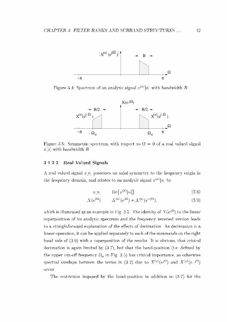
CHAPTER 3. FILTER BANKS AND SUBBAND STRUCTURES : : : 42(a)
X (e )jΩ
Ω
π−π
B
Figure 3.4: Spectrum of an analytic signal x(a)[n] with bandwidth B.Ω
π−π
(a)
B/2 B/2
X(e )j Ω
ΩΩ- u u
-j ΩX (e )
(a)X (e )
j Ω
Figure 3.5: Symmetric spectrum with respect to = 0 of a real valued signalx[n] with bandwidth B.3.1.2.2 Real Valued SignalsA real valued signal x[n] possesses an axial symmetry to the frequency origin inthe frequency domain, and relates to an analytic signal x(a)[n] byx[n] = Rex(a)[n] (3.8)X(ej) = X(a)(ej) +X(a)(ej); (3.9)which is illustrated as an example in Fig. 3.5. The identity of X(ej) to the linearsuperposition of its analytic spectrum and the frequency reversed version leadsto a straightforward explanation of the eects of decimation. As decimation is alinear operation, it can be applied separately to each of the summands on the righthand side of (3.9) with a superposition of the results. It is obvious, that criticaldecimation is again limited by (3.7), but that the band-position (i.e. dened bythe upper cut-o frequency u in Fig. 3.5) has critical importance, as otherwisespectral overlaps between the terms in (3.2) due to X(a)(ej) and X(a)(ej)occur.The restriction imposed by the band-position in addition to (3.7) for the

CHAPTER 3. FILTER BANKS AND SUBBAND STRUCTURES : : : 43
Ω /B2 u
4
3
2
1
0
1 2 3 4 5 6 7
2 /NBπ
m=1 m=2
m=3
Figure 3.6: Valid decimation rates N for real valued bandpass signals in depen-dency on the bandwidth B and the upper bound of the passband u; allowedcombinations lie within the shaded areas.selection of a valid decimation ratio N is given by [153, 19]km 2N B k 1m 1 ; k = 2uB m; m 2 N ; (3.10)where the sampling frequency is normalized to 2, u is the upper bound of thepassband and B the bandwidth as in Fig. 3.5, and N the decimation factor bywhich the sampling frequency may be lowered. Eqn. (3.10) has to be satised forany integer m. Possible choices are illustrated in Fig. 3.6 [153, 26, 81].3.2 Signal DecompositionsThe band-limited nature of a signal as a motivation to reduce its sampling rateis based on stringent frequency domain considerations. In the following, a timedomain approach by orthogonal signal decompositions is reviewed, which justiesa lowering of the sampling rate by other means. Finally, this is generalized tonon-orthogonal, redundant signal expansions.

CHAPTER 3. FILTER BANKS AND SUBBAND STRUCTURES : : : 443.2.1 Orthogonal DecompositionsConsider a signal expansion, which develops a discrete time input signal x[n] aftera set of functions hk[n], k 2 f0;K1gyk[n] = X hk[nK] x[] (3.11)where the yk[n] are the coecients of the expansion. Interpreted in terms of theanalysis lter bank in Fig. 3.1, the kernel functions hk[n] can be associated withthe bandpass lters producing the K frequency bands. Note that the convolutionin (3.11) already performs an implicit decimation byK. Using the vector notationdenitions hk = [hk[0] hk[1] hk[Lh1]]T ; (3.12)x = [x[] x[1] x[Lh+1]]T ; (3.13)where Lh is the length of the functions hk[n], the convolution in (3.11) can nowbe written as an iterated evaluation of scalar productsyk[n] = hHk xnK : (3.14)For each new calculation of the scalar product, the function hk[n] is shifted Ksamples along the time axis n.If additionally khkk2 = 1 is fullled, then (3.11) performs an orthonormalprojection, which can be geometrically interpreted as in Fig. 3.7. Therefore, thescalar product performs a best approximation of xnN by y[n]hk in a least squaressense. Note that the scalar product in the convolution 3.11 is only evaluated forshifts of K, implicitly performing a critical decimation.Orthonormal basis for l2(Z). If a set of functions hk[n] form an orthonormalbasis for the space l2(Z) of square integrable discrete signals, (3.11) performs arotation of the coordinate system of the vector space. While the original basis ofx[n] is a comb of Kronecker functions < [n] >, the coecients yk[n] express thissignal in terms of the new basis < hk[n] >. For the hk[n] to form an orthonormalbasis of the signal space l2(Z), two conditions have to be satised:
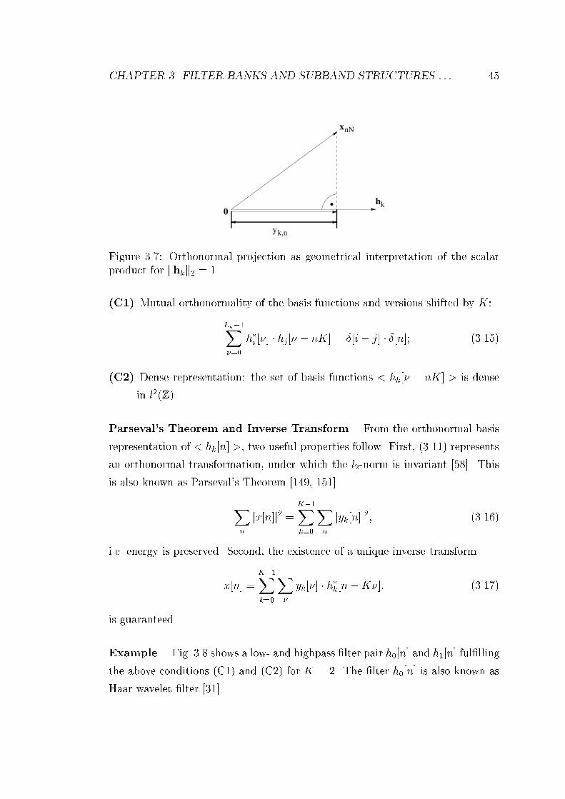
CHAPTER 3. FILTER BANKS AND SUBBAND STRUCTURES : : : 45
yk,n
hk
xnN
0Figure 3.7: Orthonormal projection as geometrical interpretation of the scalarproduct for khkk2 = 1.(C1) Mutual orthonormality of the basis functions and versions shifted by K:Lh1X=0 hi [] hj[ nK] = [i j] [n]; (3.15)(C2) Dense representation: the set of basis functions < hk[ nK] > is densein l2(Z).Parseval's Theorem and Inverse Transform. From the orthonormal basisrepresentation of < hk[n] >, two useful properties follow. First, (3.11) representsan orthonormal transformation, under which the l2-norm is invariant [58]. Thisis also known as Parseval's Theorem [149, 151]Xn jx[n]j2 = K1Xk=0Xn jyk[n]j2; (3.16)i.e. energy is preserved. Second, the existence of a unique inverse transformx[n] = K1Xk=0X yk[] hk[nK]: (3.17)is guaranteed.Example. Fig. 3.8 shows a low- and highpass lter pair h0[n] and h1[n] fulllingthe above conditions (C1) and (C2) for K = 2. The lter h0[n] is also known asHaar wavelet lter [31].

CHAPTER 3. FILTER BANKS AND SUBBAND STRUCTURES : : : 46−4 −2 0 2 4
−0.8
−0.6
−0.4
−0.2
0
0.2
0.4
0.6
(a) Haar − lowpass filter
time n −>
h0[n
]
−1 −0.5 0 0.5 10
0.5
1
1.5(b) frequency response − lowpass
normalized frequency Ω / pi
magnitude |H
0(e
jΩ)|
−4 −2 0 2 4−0.8
−0.6
−0.4
−0.2
0
0.2
0.4
0.6
(c) Haar − highpass filter
time n −>
h1[n
]
−1 −0.5 0 0.5 10
0.5
1
1.5(d) frequency response − highpass
normalized frequency Ω / pi
magnitude |H
1(e
jΩ)|
(a) (b) (c) (d)Figure 3.8: Example for lters performing an orthonormal decomposition: (a)lowpass lter h0[n]; (b) frequency response H0(ej); (c) highpass lter h1[n]; (d)frequency response H1(ej).Note that the decomposition in (3.11) implicitly performs a decimation byK between x[n] and yk[n]. The transform is therefore free of redundancy andthere is an equal number of samples in the coecient sets fx[n]g and fyk[n]g.Returning to the decimation problem, the coecients yk[n] form the samplesof K subband signals decimated by K, without reference to the bandwidth orspectral characteristic of the lters hk[n] and solely based on the properties of anorthonormal decomposition.3.2.2 Redundant DecompositionsIf the decomposition of a signal x[n] into K subbands is described byyk[n] =X hk[nN ] x[]; k 2 [0; K 1]; N K (3.18)(3.15) is no longer valid since the implicit decimation is performed by some factorN < K. The set of functions < hk[n] > now is linearly dependent, and constitutesa frame when dense in l2(Z) [142, 113]. For frames there exists an energy relationbetween the samples of the original signal and the transform coecients in thesubbands similar to Parseval's theorem,A Xn jx[n]j2 K1Xk=0 Xn jyk[n]j2 B Xn jx[n]j2; (3.19)valid for every x[n] 2 l2(Z). The constants A and B are called frame bounds, andhave the interesting property A K=N B. If A = B, i.e. there is a xed energy

CHAPTER 3. FILTER BANKS AND SUBBAND STRUCTURES : : : 47relation, the frame < hk[n] > is called tight. Through its linear dependency,expanding a signal x[n] in a frame obviously is a redundant representation.3.3 Filter Bank AnalysisThe signal decompositions discussed in Sec. 3.2 are usually performed by lterbanks as shown in Fig. 3.1, i.e. a tree of lters of dierent spectral characteristics.In the following, lter banks are analysed in the z-domain using the notation byVaidyanathan [151] with an extension to arbitrary integer decimation [88].3.3.1 Modulation DescriptionAs described in Fig. 3.1, an input signal x[n] is split into K subband signalsdecimated by factors N K. For N = K, the lter bank is called criticallysampled, and oversampled for N < K. If the K decimated subband signals arereferred to as V0(z); V1(Z); VK1(z) in the z-domain, we can write accordingto (3.2)V (z) = [V0(z) V1(z) VK1(z)]T = 1NHm(z1=N )Xm(z1=N ) (3.20)where the subscript ()m refers to the use of the modulation representation3[155, 131, 119] also known as alias component (AC) notation [151] of vectorsand matricesHm(z) = 2666664 H0(z) H0(zWN ) : : : H0(zWN1N )H1(z) H1(zWN ) : : : H1(zWN1N )... ... . . . ...HK1(z) HK1(zWN ) : : : HK1(zWN1N )3777775 (3.21)Xm(z) = X(z) X(zWN ) X(zWN1N )T ; (3.22)where Hk(z) | hk[n] is the z-transform of the kth lter of the analysis bank,and X(z) | x[n] the input signal. The matrix Hm(z) is termed modulationmatrix of the synthesis lter bank.3The modulation description expresses the aliasing introduced by decimation as a sum ofscaled and modulated terms, as dened in (3.2).

CHAPTER 3. FILTER BANKS AND SUBBAND STRUCTURES : : : 48Let the output of the expanders be denoted by U0(z); U1(z); UK1(z), whichare given by U(z) = V (zN ) = 1NHm(z)Xm(z): (3.23)With the synthesis ltersG(z) = [G0(z) G1(z) GK1(z)]T ; (3.24)the lter bank output on the synthesis side can be written asX(z) = GT (z)U(z) = 1NGT (z)Hm(z)Xm(z): (3.25)Therefore, (3.25) describes the input-output relationship of the lter bank inFig. 3.1. Conditions for perfect reconstruction, i.e. X(z) = czX(z), c 2 C =f0g,will be discussed in Sec. 3.3.3 based on a polyphase representation to be intro-duced next.3.3.2 Polyphase RepresentationThe polyphase representation [152, 7, 150, 151, 119] is an alternative form toanalyse multirate systems and has the advantage of leading to computationallyecient implementations of lter banks. The term polyphase refers to the deci-mation of a signal | if it is appropriately bandlimited and can be decimated bya factor N , N possibilities exist which set of samples to keep; in fact, one is asgood as any, as in the Fourier domain they only dier by their phase, but not bytheir magnitude.Transfer functions Hk(z) and Gk(z) can be expressed in the formsHk(z) = N1Xn=0 znHkjn(zN ) (Type 1 polyphase) (3.26)and Gk(z) = N1Xn=0 z(N1n)Gnjk(zN ) (Type 2 polyphase) (3.27)

CHAPTER 3. FILTER BANKS AND SUBBAND STRUCTURES : : : 49respectively, whereHkjn(z) = 1Xk=1hk(Nk + n)zk (3.28)Gnjk(z) = 1Xk=1 gk(Nk+N1n)zk : (3.29)The terms Hkjn(z), n = 0(1)N 1, are the N Type 1 polyphase componentsof Hk(z), which arise from decimation of dierently phase shifted analysis ltershk[n] and subsequent z-transformation. Correspondingly, Gnjk(z), n = 0(1)N1,represent the N Type 2 polyphase components of Gk(z). Note that the specialcase Gk(z) = Hk(z) gives Gnjk(z) = HkjN1n(z).Application of (3.26) yieldsH(z) = H(zN ) [1 z1 : : : z(N1)]T ; (3.30)where H(z) = 2666664 H0j0(z) H0j1(z) : : : H0jN1(z)H1j0(z) H1j1(z) : : : H1jN1(z)... ... . . . ...HK1j0(z) HK1j1(z) : : : HK1jN1(z)3777775 : (3.31)Correspondingly, (3.27) leads toGT (z) = [z(N1) z(N2) : : : 1] G(zN ); (3.32)where G(z) = 2666664 G0j0(z) G0j1(z) : : : G0jK1(z)G1j0(z) G1j1(z) : : : G1jK1(z)... ... . . . ...GN1j0(z) GN1j1(z) : : : GN1jK1(z)3777775 : (3.33)The matrices H(z) and G(z) are called the polyphase matrices of the lter bank.Using (3.30) and (3.32) in the lter bank in Fig. 3.1 yields an equivalent repre-sentation shown in Fig. 3.9(a). With respect to subsampling and upsampling,

CHAPTER 3. FILTER BANKS AND SUBBAND STRUCTURES : : : 50..
z-1
z-1...
.. ..
z-1
z-1
z-1
z-1
z-1
z-1...
.
.
.
.
.
.
z-1
z-1 ...
(a) .
.
z-1..
.
.
.
.
(b) .
.
z-1
0
1
0
1
N-1 K-1
0
1
0
1
0
1
0
1
0
1
0
1
K-1 N-1
N-1 K-1 K-1 N-1
N
N
N
N
N
N
N
N
N
N
N
N
x[n]
x[n]
x[n]
x[n]
N N (z )
(z) (z)
(z )H
H G
G
Figure 3.9: (a) Polyphase representation of a K-channel lter bank decimated bya factor N ; (b) re-arrangement using noble identities.the following identities hold [151, 142]H(z)(# N) = (# N)H(zN ) First Noble Identity (3.34)(" N)G(z) = G(zN )(" N) Second Noble Identity; (3.35)where (# N) denotes N -fold decimation, and (" N) N -fold expansion. By usingnoble identities, the lter bank can be modied and the equivalent form shownin Fig. 3.9(b) obtained. This structure has the advantage that the ltering isperformed at the subsampled rate.In terms of analysis, the ow chart in Fig. 3.9(b) has separated the lter bankinto two system types. Time multiplexers, which perform the separation into orinterleaving of K channels decimated by N , are linear periodically time-varying(LPTV) systems with period N . In contrast, the polyphase matrices H(z) andG(z) dene multiple-input multiple output (MIMO) systems, which are lineartime-invariant (LTI) and therefore convenient to analyze.

CHAPTER 3. FILTER BANKS AND SUBBAND STRUCTURES : : : 513.3.3 Lossless ExpansionsIn its most general form, the lter bank system can be shown to have perfectreconstruction property if and only if the product G(z)H(z) fullls [151]G(z)H(z) = cz " 0 INrz1Ir 0 # ; r 2 Z; 0 r N 1; 2 N ; c 2 C =f0g: (3.36)If this condition is satised, the reconstructed signal is only a scaled and delayedversion of the lter bank input x[n] = cx[n ], where = K + r + K 1constitutes the delay.A sucient even though not necessary condition to ensure (3.36) is the parau-nitary property of H(z). A matrix H(z) 2 C KN(z) of transfer functions is calledparaunitary if ~H(z)H(z) = cIN ; c 2 C =f0g; (3.37)where the matrix ~H(z) is called the parahermitian ofH(z), i.e. is transposed withits polyphase entries complex conjugated and time reversed [151, 29]. With H(z)being paraunitary it is easy to recognize that simply choosingG(z) = czl ~H(z); c 6= 0; (3.38)satises the perfect reconstruction condition. If its polyphase matrix H(z) isparaunitary and N equals K, the lter bank is also denoted orthogonal [142].As a consequence of (3.38) the synthesis lters can be easily found from theanalysis lters bygk[n] = c ~hk[nl] = c hk[ln] time domain (3.39)Gk(z) = c zl ~Hk(z) z-domain; (3.40)where k = 0(1)K1, l = N1+N. For critical decimation by a factor K, thisis the only choice for the synthesis lters by assumption of a paraunitary H(z)to achieve perfect reconstruction (PR).Note that the derived results in the z-domain correspond to time domain ex-pressions in Sec. 3.2. Later, the property of paraunitarity for polyphase matriceswill be explicitly linked to both orthogonal and redundant frame decompositions,which are implemented by such PR lter banks [156, 14].

CHAPTER 3. FILTER BANKS AND SUBBAND STRUCTURES : : : 523.4 Dierent Approaches to Subband AdaptiveFilteringBased on the subband decompositions introduced in the above section in thecontext of lter bank theory, the application of subband schemes to adaptiveltering is reviewed. The idea to perform adaptive ltering in frequency bandsgoes back to a number of researchers in the 1980s like Kellermann [84, 85, 86, 134],Furukawa and Yasukawa [48, 181], and Gilloire et al. [52, 53, 54], who mainlytargeted the echo problem in telecommunication lines caused by hybrids [134], orthe acoustic feedback problem in hands-free telephony [48, 84, 85].The main obstacle in subband adaptive ltering is the fact that although lterbanks may be perfectly reconstructing (i.e. aliasing is cancelled at the output ofa synthesis bank), aliasing present in the subband signals constitutes a ratherserious problem for adaptive lters. The origin of the problem and suggestedsolutions around it are the subject of this section.3.4.1 Aliasing in the Decimation StageSec. 3.1 has introduced two concepts that motivate the decimation of subbandsignals: the band-limited nature of signals, and an orthogonal basis or redundantframe decomposition of signals, where aliasing may be permitted in the subbanddomain but is subsequently cancelled in the signal reconstruction of the synthesisbank. However, a problem with perfect reconstruction does arise when decimatedsubbands of dierent fullband signals have to be compared.Filter banks are linear, but periodically time-varying systems due to up- anddownsampling. The alias terms introduced in the decimation stage in (3.2) man-ifests as a deviation from the linear time-invariant (LTI) system behaviour andcan be interpreted as a distortion [117]. An exact analysis of this phenomenon inthe z-domain will be performed in Sec. 3.4.2 following the explanations by Gilloireand Vetterli [54].Information Leakage. An example of the eect caused by the cyclic time-varying nature of a critical decimation stage is shown in Fig. 3.10 [135, 19].

CHAPTER 3. FILTER BANKS AND SUBBAND STRUCTURES : : : 53There, a near PR lter pair < h0; h1 > has been used for a decomposition, with ahalfband lowpass h0[n] tabulated as lter 32C in [27] and h1[n] = h0[n] cos(n)the according QMF highpass lter modulated by . If this lter pair is excitedby the lowpass lter itself, the subband signals arex0[n] = h0[n] h0[n] lowpass subband (3.41)x1[n] = h1[n] h0[n] highpass subband; (3.42)as shown in Fig. 3.10(a) and (d), respectively. Depending on whether even orodd samples are dropped in the decimation, two dierent patterns arise for eachsignal x0[n] and x1[n].An awkward situation results when the dierently decimated signals are cor-related. Cross-correlation between the two highpass bands in Fig. 3.10(e) and (f)yields zero, while for the correlation between (b) and (c) signal components aremissing that have leaked into the decimated highpass band in (e). In an adaptivesystem identication of an odd-numbered delay, where an adaptive lter wouldbe expected to try and identify these cross-correlations, minimization of the errorwould completely fail at least in the highpass band, thus yielding an insucientsolution.Note that an interesting case of non-causality can occur in this identicationproblem when the even-indexed x0[2n] in Fig. 3.10(c) forms the input signal toan adaptive lter, and the lter is supposed to provide a close t solution to adesired signal consisting of the odd-indexed x0[2n+1] in (b). This non-causalitywill be further discussed in Sec. 3.4.2.3.4.2 Critically Decimated Filter BanksAdaptive system identication in critically decimated subbands, i.e. the deci-mation ratio matches the number of subbands, N = K, was rst analysed byGilloire [52] and Gilloire and Vetterli [53, 54], leading to a modied subbandstructure with cross-terms between adjacent bands. A review of their approachis given below.The following denitions describe subband signals associated with adaptive

CHAPTER 3. FILTER BANKS AND SUBBAND STRUCTURES : : : 54
0 20 40 60
−0.2
0
0.2
0.4
0.6
0.8
1
(a) lowpass responsex
0[n
]
0 20 40 60
−0.2
0
0.2
0.4
0.6
0.8
1
(d) highpass response
x1[n
]
0 10 20 30
−0.2
0
0.2
0.4
0.6
0.8
1
(b) even samples decimated
x0[2
n+
1]
0 10 20 30
−0.2
0
0.2
0.4
0.6
0.8
1
(e) even samples decimated
x1[2
n+
1]
0 10 20 30
−0.2
0
0.2
0.4
0.6
0.8
1
(c) odd samples decimated
x0[2
n]
discrete time n −>0 10 20 30
−0.2
0
0.2
0.4
0.6
0.8
1
(f) odd samples decimated
x1[2
n]
discrete time n −>Figure 3.10: Example for \leakage" eect in the time-domain of subband sig-nals due to the phase-variant nature of the decimation process, when excitationmatches the lowpass lter 32C [27] of a 2-channel bank; (a) lowpass band x0[n]with (b) even and (c) odd decimation; (d) highpass band x1[n] with (e) even and(f) odd decimation.
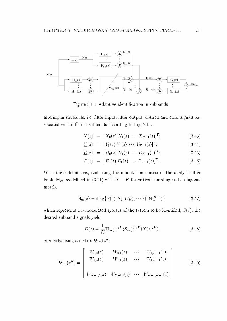
CHAPTER 3. FILTER BANKS AND SUBBAND STRUCTURES : : : 55K
K
K
K
0 0
S(z)
X(z)
D(z)
0D (z)
D (z)
Y (z)
Y (z)
E (z)
E (z)
K-1
K-1 K-1
H (z)
K-1
K-1
0H (z)
0H (z) K
K
0G (z)
G (z)K-1
E(z)
m (z)H (z)
WFigure 3.11: Adaptive identication in subbands.ltering in subbands, i.e. lter input, lter output, desired and error signals as-sociated with dierent subbands according to Fig. 3.11:X(z) = [X0(z) X1(z) XK1(z)]T ; (3.43)Y (z) = [Y0(z) Y1(z) YK1(z)]T ; (3.44)D(z) = [D0(z) D1(z) DK1(z)]T ; (3.45)E(z) = [E0(z) E1(z) EK1(z)]T : (3.46)With these denitions, and using the modulation matrix of the analysis lterbank, Hm, as dened in (3.21) with N = K for critical sampling and a diagonalmatrix Sm(z) = diagS(z); S(zWK); S(zWK1K ) (3.47)which represents the modulated spectra of the system to be identied, S(z), thedesired subband signals yieldD(z) = 1KHm(z1=K)Sm(z1=K)X(z1=K): (3.48)Similarly, using a matrix Wm(zK)Wm(zK) = 2666664 W0;0(z) W0;1(z) W0;K1(z)W1;0(z) W1;1(z) W1;K1(z)... ... . . . ...WK1;0(z) WK1;1(z) WK1;K1(z)3777775 (3.49)

CHAPTER 3. FILTER BANKS AND SUBBAND STRUCTURES : : : 56of polynomial entries for the adaptive lters, the output signals of the adaptivelters can be written asY (z) = 1KWm(z)Hm(z1=K)X(z1=K): (3.50)Therefore, the subband error signals are obtained fromE(z) = 1K Hm(z1=K)Sm(z1=K)Wm(z)Hm(z1=K) X(z1=K); (3.51)yielding a fullband error E(z) by reconstruction with the synthesis bank ltersG(z) described in (3.24),E(z) = GT (z)E(zK) (3.52)= 1K GT (z) Hm(z)Sm(z)Wm(zK)Hm(z) X(z): (3.53)To ensure E(z) ! 0, several sets of solutions exist [86]. The strictest conditionto force E(z) toward zero is given byWm(zK)Hm(z) = Hm(z)Sm(z) : (3.54)3.4.2.1 Filter Banks with Perfect Reconstruction PropertyThe further analysis of the critically decimated subband adaptive lter systemin [54] assumes that both analysis and synthesis lter bank are derived from acommon prototype lter, and that this employed lter bank has near perfectreconstruction property. Therefore,Hm(z) Gm(z) zLh+1Ik (3.55)holds [155], where the modulation matrix Gm(z) of the synthesis lters is denedanalogous to Hm(z) in (3.21). Eqn. (3.54) then yieldsWm(zK) zLh1Hm(z)Sm(z)GTm(z): (3.56)The matrix Wm(zK), as dened in (3.49), is not of diagonal form, but has o-diagonal polynomial entries Wi;j(z), which under the above mention assumptionscan be derived asWi;j(z) zLh1 K1Xk=0 Hl(zW kK) Gj(zW kK) S(zW kK): (3.57)
CHAPTER 3. FILTER BANKS AND SUBBAND STRUCTURES : : : 57It is important to note, that this solution is potentially non-causal due to thefactor zLh1. Therefore, an appropriate delay has to be placed in the path of thedesired signal. If in case of acoustic echo cancellation this delay is met by theacoustic transfer delay of the direct path between loudspeaker and microphone,no additional actions are required. Further, from (3.57) it can be easily seen, thatthe length La of the adaptive terms has to be [54, 135, 88]La = 2 Lh + LsK ; (3.58)where Ls is the length of the impulse response of the system to be identied, inorder to achieve satisfactory adaptation without truncation of the adapted model.The extreme example given in Fig. 3.10 of Sec. 3.4.1 underlines this case whentrying to adaptively identify a unit delay in the lowpass band, where the inputsignal is even indexed (c) and the desired signal odd-indexed (b), also highlightingthe non-causality inherently arising from the decimated setup and the transientsof the analysis lters.If the analysis lters are of good quality and reasonably selective, then onlyadjacent lters will overlap in the frequency domain, and the adaptive lter matrixW(z) in (3.49) can be well approximated by a tridiagonal form. In the actualimplementation of the subband adaptive lter, this therefore requires adaptivecross-terms between adjacent subbands in addition to the main adaptive terms,as shown in Fig. 3.12.The cross-terms Wi;j(z); i 6= j; can be factorized into a xed and an adaptivepart as shown in Fig. 3.14, where the xed part is the convolution of adjacentanalysis and synthesis lters decimated by a factor K [135, 53, 54]. The xedpart W (xed)i;j (z) forms a narrow bandpass covering the transition band betweenthe synthesis lter of the source band and the analysis lter of the target band[170, 135]. Therefore, adjustment of the adaptive termW (adapt)i;j (a) is restricted tothis spectral interval, yielding improved convergence [54] over the unconstrainedunfactorized case. With regard to the leakage interpretation of the criticallydecimated PR case introduced in Sec. 3.4.1, the cross-terms can be interpreted asa means to supply the subbands with information of the transition region whichhad leaked into adjacent frequency bands.

CHAPTER 3. FILTER BANKS AND SUBBAND STRUCTURES : : : 582
1H (z)
H (z)0
H (z)0
2
2
2
W (z)1,1
W (z)1,0
W (z)0,1
W (z)0,02
2 G (z)1
G (z)0
E (z)1
0E (z)
H (z)1
X(z)
S(z)
∆
∆
E(z)
--
-
-Figure 3.12: Two channel critically decimated lter bank with adaptive cross-terms between adjacent bands according to [54] and delays in the desired pathsto correct for potential non-causality in (3.57) .
0 0.1 0.2 0.3 0.4 0.5 0.6 0.7 0.8 0.9 1−80
−70
−60
−50
−40
−30
−20
−10
0
normalized frequency Ω / pi
magnitude / [dB
]
lowpass H0
highpass H1
Figure 3.13: Frequency response of a near perfectly reconstructing QMF lterpair derived from the prototype 32C in [27].
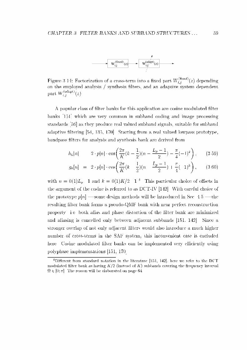
CHAPTER 3. FILTER BANKS AND SUBBAND STRUCTURES : : : 59i,j i,j(fixed)
W (z)(adapt)
W (z)Figure 3.14: Factorization of a cross-term into a xed part W (xed)i;j (z) dependingon the employed analysis / synthesis lters, and an adaptive system dependentpart W (adapt)i;j (z).A popular class of lter banks for this application are cosine modulated lterbanks [151] which are very common in subband coding and image processingstandards [56] as they produce real valued subband signals, suitable for subbandadaptive ltering [54, 135, 170]. Starting from a real valued lowpass prototype,bandpass lters for analysis and synthesis bank are derived fromhk[n] = 2 p[n] cos2K (k + 12)(n Lp 12 ) 4 (1)k ; (3.59)gk[n] = 2 p[n] cos2K (k + 12)(n Lp 12 ) + 4 (1)k ; (3.60)with n = 0(1)Lp1 and k = 0(1)K=21 4. This particular choice of osets inthe argument of the cosine is referred to as DCT-IV [142]. With careful choice ofthe prototype p[n] | some design methods will be introduced in Sec. 4.5 | theresulting lter bank forms a pseudo-QMF bank with near perfect reconstructionproperty. i.e. both alias and phase distortion of the lter bank are minimizedand aliasing is cancelled only between adjacent subbands [151, 142]. Since astronger overlap of not only adjacent lters would also introduce a much highernumber of cross-terms in the SAF system, this inconvenient case is excludedhere. Cosine modulated lter banks can be implemented very eciently usingpolyphase implementations [151, 170].4Dierent from standard notation in the literature [151, 142], here we refer to the DCTmodulated lter bank as having K=2 (instead of K) subbands covering the frequency interval 2 [0;]. The reason will be elaborated on page 64.
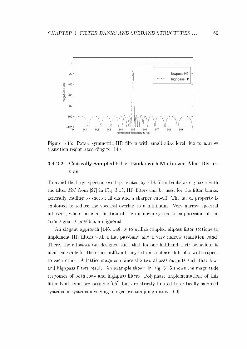
CHAPTER 3. FILTER BANKS AND SUBBAND STRUCTURES : : : 60
0 0.1 0.2 0.3 0.4 0.5 0.6 0.7 0.8 0.9 1−120
−100
−80
−60
−40
−20
0
normalized frequency Ω / pi
magnitude / [dB
]
lowpass H0
highpass H1
Figure 3.15: Power symmetric IIR lters with small alias level due to narrowtransition region according to [148].3.4.2.2 Critically Sampled Filter Banks with Minimized Alias Distor-tionTo avoid the large spectral overlap created by FIR lter banks as e.g. seen withthe lter 32C from [27] in Fig. 3.13, IIR lters can be used for the lter banks,generally leading to shorter lters and a sharper cut-o. The latter property isexploited to reduce the spectral overlap to a minimum. Very narrow spectralintervals, where no identication of the unknown system or suppression of theerror signal is possible, are ignored.An elegant approach [146, 148] is to utilize coupled allpass lter sections toimplement IIR lters with a at passband and a very narrow transition band.There, the allpasses are designed such that for one halfband their behaviour isidentical while for the other halfband they exhibit a phase shift of with respectto each other. A lattice stage combines the two allpass outputs such that low-and highpass lters result. An example shown in Fig. 3.15 shows the magnituderesponses of both low- and highpass lters. Polyphase implementations of thislter bank type are possible [65], but are strictly limited to critically sampledsystems or systems involving integer oversampling ratios [160].

CHAPTER 3. FILTER BANKS AND SUBBAND STRUCTURES : : : 61Although the low- and highpass lters arising from the allpass / lattice con-catenation are power symmetric [146], the phase is considerably distorted at theband edges, which may not be too disruptive for speech signals which are relativelyinsensitive to phase distortions, but could not be accepted for data communica-tions.3.4.2.3 Filter Banks with Spectral Loss / DistortionIn [147, 148], the power symmetric IIR lter bank approach with small spectraloverlap at band edges is further rened by inserting notch lters prior to per-forming the analysis lter bank operations. The notch lters are designed toremove the spectral intervals around the band edges which would otherwise beinsuciently adapted due to aliasing. This can signicantly reduce the residualerror power and positively in uence the overall convergence by the thus loweredMMSE. However, clearly the resulting lter bank system is now lossy, as spectralgaps occur due to the additional notch lters.The same result can be achieved by employing lossy lter banks with spectralgaps at the band edges in rst place. Explicit descriptions of how these gap lterbanks are constructed to comply with subband adaptive ltering can be foundin [181, 179, 180, 178]. Subband adaptive ltering in combination with IIR lterbanks is described in e.g. [176].Two comments should be made here. Firstly, the introduction of spectralgaps, although they may be kept to a minimum by using IIR lters with sharptransition bands, may reduce the perceived quality for speech applications and caneven be unacceptable for e.g. data communication system applications. Secondly,the lter design task of non-overlapping transition bands does not imply that theresulting lter banks will be completely alias free. There always is a residual aliaslevel due to the nite stop-band attenuation of lters, which sets limits to theachievable MSE in the adaptation [172]; this will be described in more detail inSec. 5.2.
CHAPTER 3. FILTER BANKS AND SUBBAND STRUCTURES : : : 623.4.3 Oversampled Filter BanksDistinct from critically sampled subband structures a non-critical decimationof the subband signals can avoid the aliasing problem, which gave rise to ei-ther complicated inclusion of cross-terms or gap-lter banks with spectral loss inSec. 3.4.2. In terms of the information leakage interpretation of the decimationstage in Sec. 3.4.1, the redundancy introduced by non-critical decimation will belocated around the band-edges, such that in every band enough information isavailable to succeed in adaptation. In the following, we want to brie y discusssubband adaptive lter structures based on oversampled near PR lter banks.From the introduction of the sampling theorem for bandpass signals in Sec. 3.1.2,we distinguish between complex and real valued lter banks. More detail on someunderlying techniques will be highlighted in Chap. 4.3.4.3.1 Complex Valued Filter BanksIf the bandpass lters in Fig. 3.1 are analytic, and the input signal real valued,the output of the lters will also be analytic. Therefore, decimation of the sub-band signals can usually be applied down to any rate above the critical samplingfrequency 5. This means a decimation factor N < K is employed, whereby Kis the number of subbands covering the interval 2 [0; 2]. Usually some ofthese subbands will be complex conjugate and will not need to be processed asthey carry redundant information, depending on how the bandpass lters in theanalysis and synthesis lter bank are arranged. While other designs are possible,in the following we will concentrate on uniform, modulated lter banks, as theyoer particularly ecient methods of implementation.DFT Modulated Filter Banks. A simple organization of bandpass ltershk[n] is given by DFT modulation of a lowpass lter by [27, 151, 29]hk[n] = p[n] ej 2K kn ; n = 0(1)Lp1 and k = 0(1)K1; (3.61)where Lp is the length of a prototype lowpass lter p[n] with a passband widthB = 2=K. For an even number K, there result K=2 + 1 frequency bands to5This also holds for complex valued lters and signals in the sense of Sec. 3.1.2.1.

CHAPTER 3. FILTER BANKS AND SUBBAND STRUCTURES : : : 63Ω
kjΩ
π 2π
(a)
H (e )
0 1 2 3 4 5 6 7 07
kjΩ
π 2π
(b)
π/8
H (e )
0 1 2 3 4 5 6
Ω
07 7
kjΩ
π 2ππ/8
10 2 30 3 2 1 0 0
Ω
(c)
H (e )
Figure 3.16: Arrangement of bandpass lters for K = 8 for (a) DFT modulatedlter bank and (b) GDFT modulated lter bank with k0 = 1=2 ; (c) DCT modu-lated lter bank; shaded spectra are redundant and are not required to process.be processed. An example for K = 8 is sketched in Fig. 3.16(a). Obviously, thelowest and highest band are only real valued, and decimation can be performedfor all subbands by a factor of N K. If N is chosen suciently small, nospectral overlap of image spectra as stated in (3.2) will occur, and the adaptivelter matrix of the SAF system shown in Fig. 3.11 takes on a diagonal form[86, 50, 3].GDFT Modulated Filter Banks. A generalized DFT (GDFT) transform[27] can also be employed to modulate a prototype lter p[n],hk[n] = p[n] ej( 2K (k+k0)(n+n0)+k) ; n = 0(1)Lp1 and k = 0(1)K1;(3.62)

CHAPTER 3. FILTER BANKS AND SUBBAND STRUCTURES : : : 64where osets k0 and n0 for frequency and time indices, respectively, and a phaseoset k are introduced. For even K, the frequency interval 2 [0; ] will becovered by exactlyK=2 subband signals, while the rest is complex conjugate as de-scribed by an example in Fig. 3.16(b). The case k0 = 12 is also sometimes referredto as \odd-stacked" DFT [12], in contrast to an \even-stacked" DFT in (3.61).Further note that insertion of a suitable parameter set fk0= 12 ;n0=Lp12 ; k=4 (1)kg (3.62) represents the analytic expansion of a DCT-IV pseudo-QMF mod-ulated lter bank for critical sampling as described in (3.59) [166]. Vice versa, areal valued DCT modulated lter bank can be derived from a GDFT lter bankby adding complex conjugate pairs of lters, i.e.hk[n] + hK1k[n] = hk[n] + hk[n] = 2 Refhk[n]g ; (3.63)and the result agrees with (3.59).Here a comment on the use of the number K associated with the number ofchannels in a lter bank seems appropriate since its use is dierent from commonnotation. As the lter banks discussed in this thesis are modulated, we dene Kbased on the passband width B = 2K of the prototype lter P (ej). Similarly, Nis dened as the total bandwidth of P (ej), i.e. including the transition bands.It follows that for complex valued lter banks as in Fig. 3.16(a) and (b) the interval 2[0; 2] is covered by K subbands which can be decimated by N . For realinput, some bands are redundant. In case of the GDFT lter bank inFig. 3.16(b), only K=2 subbands need to be processed. For real valued lter banks as in Fig. 3.16(c), there are K=2 subbands,which can be decimated by N=2 6.For the following discussions, it is easiest to realize that for any lter bank, real orcomplex, the number K=2 refers to the number of subbands completely coveringthe frequency interval 2 [0; ].6Decimation usually cannot be directly applied as otherwise bandpass sampling will lead tospectral overlap. Intermediate steps, like modulation of the subbands into the baseband priorto decimation, may be required.
CHAPTER 3. FILTER BANKS AND SUBBAND STRUCTURES : : : 65With respect to implementation, complex modulated oversampled lter bankscan be eciently calculated either by frequency domain implementation of thebandpass lters [1, 90] using the overlap-add method [27] as discussed in Sec. 2.6.1or via a polyphase representation. A somehow common misconception is thatpolyphase implementations are restricted to integer oversampling ratios KN 2 N[27, 90]. Therefore, for polyphase implementations integer oversampling ratiosare employed (e.g. K=N = 2) [3, 106, 38], which is less ecient and has poorerproperties in terms of whitening the subband signals than choosing N closer toK, potentially resulting in reduced convergence rate as will be demonstrated inChaps. 4, 5 and 6. If the main task is to eciently process subband signals, thedecimation ratio N has to chosen close to K, and preferred method in the litera-ture are frequency domain approaches rather than polyphase implementations ofthe lter banks [1, 90, 38].In a number of publications non-integer oversampling ratios are used [86, 129,87, 32, 33], where the focus is fully concentrated on ecient subband processingor convergence speed issues and but no statements are made regarding the actuallter bank implementation.3.4.3.2 Real Valued Filter BanksFor real valued signals, sampling of bandpass signals is restricted by the band-width and band position according to Fig. 3.6. It can be veried, that decimationby a factor of 1 < N < K will produce spectral overlap of images in at least oneof the subband signals. Even for integer oversampling ratios, although sometimesapplied, aliasing occurs at some of the band edges, as the sampling points inFig. 3.6 will partly fall onto the margins of \acceptable" areas. In the following,two approaches of real valued oversampled subband structures for adaptive lter-ing are reviewed, the rst one based on a modulation of each frequency band intothe baseband prior to decimation, the second one using non-uniform lter banks,whereby band-position and bandwidth of the single lters are chosen such as tocomply with Fig. 3.6.

CHAPTER 3. FILTER BANKS AND SUBBAND STRUCTURES : : : 66x[n] --@@
@@6?
sin(2kK n)cos(2kK n)
-- h[n]h[n] --@@@@6?
sin( Nn)cos( Nn) m+6? -#N2 -xk[n]
Figure 3.17: (a) Using SSB demodulation by means of quadrature modulationfor the kth branch of an analysis lter bank [27, 159].Single Sideband Modulation Single sideband modulation (SSB) by meansof quadrature modulation, also know as Weaver method [88], can be employedto construct oversampled real-valued lter banks. The analysis side is performedas SSB demodulation as depicted in Fig. 3.17 by modulating dierent spectralintervals into the baseband, where a lowpass lter is applied to lter out higherfrequency components above = =K for the kth subband signal prior to dec-imation [27, 159]. Similarly, the branches of the synthesis lter bank can beconstructed from an SSB modulation shown in Fig. 3.18. If the decimation factoris chosen such that the images of the downsampled subband signals according to(3.2) do not overlap, these lter bank implementations can be used to performsubband adaptive ltering free of cross-terms [21, 95, 19, 88]. Note that in accor-dance with the comments on page 64, the decimation factor is here referred to asN=2.A simple explanation of how the Weaver method works can be given wheninterpreting the normal and quadrature components (i.e. the two branches inFigs. 3.17 and 3.18) as real and imaginary part of a complex signal. Then, asshown in Fig. 3.19(a)(c), the analysis consists of a complex modulation of theband of interest into the baseband, where it is ltered out by H(ej) | h[n]from the remaining signal components. The second modulation lifts the signalup in frequency by =N . By a real operation, the spectrum is symmetrized with

CHAPTER 3. FILTER BANKS AND SUBBAND STRUCTURES : : : 67yk[n] -"N2 --@@
@@6?
sin( Nn)cos( Nn)
-- g[n]g[n] --@@@@6?
sin(2kK n)cos(2kK n) m+6? -y[n]
Figure 3.18: (a) Using SSB modulation by means of quadrature modulation forthe kth branch of a synthesis lter bank [27, 159].
/Nπ
2 k/Kπ π
π
π
−π
−π
−π
Ω
Ω
Ω
(b)
(a)
(c)
Ωj
Ωj
Ωj|X (e )|
|X (e )|k
k
|X (e )|
/Nπ
2 k/Kπ
j
−π
Ω
Ωj
(d)
π−π
Ω
Ωj
π
π−π
Ω
(e)
(f)
|Y (e )|
|Y (e )|
k
k
kΩ
|X (e )|
Figure 3.19: (a) (c) SSB demodulation as analysis lter of the kth subband; (d) (f) SSB modulation as kth synthesis lter operation in a lter bank.

CHAPTER 3. FILTER BANKS AND SUBBAND STRUCTURES : : : 68respect to = 0, and a real valued baseband signal of bandwidth B = 4=Nis obtained, which may now be decimated by a factor N=2. The SSB synthesisby Weaver can be performed by inverting the analysis process as illustrated inFig. 3.19(d)(f). After modulating the spectrum of interest into the basebandin Fig. 3.19(e), all image spectra introduced in the expander are removed by thelowpass lter G(ej) | g[n]. Finally, complex modulation by ej2k=K and areal operation to restore a symmetric spectrum yield the original spectrum in thekth frequency band of Fig. 3.19(a).Real valued oversampled subband signals based on an SSB modulation conceptcan be eciently implemented by a modication of DFT/GDFT lter banks [27,159, 167], which will be further discussed in the context of ecient factorizationsof oversampled GDFT polyphase lter banks in Sec. 4.3.As all ltering is either performed with or derived by modulation from asingle prototype lowpass lter p[n] of bandwidth 2=N , the resulting lter bankimplementation is uniform.Non-Uniform Filter Banks Dropping the restriction of uniform lter banks,band-position, bandwidth, and decimation factor of the corresponding subbandcan be selected independently for every bandpass lter in analysis and synthesisbank to comply with the criteria imposed by Fig. 3.6 and (3.10) [67, 71]. Anexample is given in Fig. 3.20, where dierent from Fig. 3.13, the PSD of thesubband signals produced by lowpass H0(ej) and highpass lter H1(ej) do notoverlap when decimated by factor 2, while the resulting gap is lled by a thirdband, which can be downsampled by a factor 3 with no spectral overlap occurring.A similar approach is described in [133], where the additional auxiliary band isnot decimated and therefore computational eciency of subband processing isnot fully exploited. The subband approach introduced by [71] can be extendedto any number of channels, whereby some implementational eciency can bereached by constructing the lter bank from a number of modulated prototypelters [70]. However when used for subband adaptive lter applications [68, 70]on a DSP, the presence of dierent sampling rates and a number of prototypelters can result in inconvenient implementations, which are costlier than fully

CHAPTER 3. FILTER BANKS AND SUBBAND STRUCTURES : : : 69
0 0.1 0.2 0.3 0.4 0.5 0.6 0.7 0.8 0.9 1−80
−70
−60
−50
−40
−30
−20
−10
0
10
normalized frequency Ω / pi
ma
gn
itu
de
/ [
dB
]H0, N=2
H1, N=3
H2, N=2
Figure 3.20: Example for a non-uniform oversampled real valued lter bank ac-cording to [67, 71]; the subband signals produced by the three lters Hk(ej) areeach decimated by dierent factors N .modulated lter banks [160].Both SSB modulated and non-uniform lter banks can be designed to be nearPR. An elegant link between non-uniform lter banks as mention above and frametheory is made in [70] and allows the of design lter banks with dierent lters inanalysis and synthesis bank. For the SSB case, we will return to the PR properyin Sec. 4.5.3.5 Concluding RemarksThis chapter has introduced lter banks, their description and analysis methods,and reviewed their application to subband adaptive lter structures. Of all thedierent types of subband adaptive lter system discussed, three properties arebelieved to be of key importance:Perfect Reconstruction. Generally, lter banks for subband adaptive lteringshould posses PR or near PR property, as otherwise applications are limitedto areas insensitive to distortion, spectral loss, or inadequate modelling.Aliasing. Aliasing in the subband signals has to be suppressed as far as possiblein order to guarantee satisfactory performance of the adaptive system.

CHAPTER 3. FILTER BANKS AND SUBBAND STRUCTURES : : : 70Ecient Implementation. Subband processing is performed to save compu-tations. Therefore, rstly subband signals should be sampled as close aspossible at the critical rate, N ! K. Secondly, analysis and synthesis lterbank operations should be performed with as few computations as possible.This is the more important, since the computational complexity of the orig-inal processing task usually decreases with the number of subbands, whilethe cost involved in performing analysis and synthesis operations increases.Although the demand for near PR property of the employed lter banks mayseem harsh for some applications, it is useful to have, and as will be seen laterin Chap. 5 can be relaxed and traded o against other properties of the subbandadaptive system such as the overall delay imposed on signals.In the following two chapters, we will introduce and analyse a very ecientimplementation of complex oversampled GDFT lter banks based on a gener-alization of the polyphase concept introduced in Sec. 3.3.2, and apply them forsubband adaptive lter structures. In terms of eciency, the relation and trade-o between critical and oversampled non-critical implementations, and lter bankand subband calculations using complex and real valued arithmetic will be of par-ticular interest and closely researched.

Chapter 4Oversampled GDFT Filter BanksThis chapter concentrates on the implementation and design of oversampled gen-eralized DFT (GDFT) lter banks, beginning with a view of their general prop-erties in Sec. 4.1. In Sec. 4.2 an extension and factorization of the polyphasedescription will then produce a highly ecient implementation of this type oflter bank producing complex valued subband signals. A restructuring of theWeaver method for SSB modulated real valued lter banks then leads to a mod-ied GDFT lter bank described in Sec. 4.3. Sec. 4.4 discusses real and complexvalued subband systems in terms of computational complexity of both lter banksand subband processing. Finally, Sec. 4.5 introduces design methods for complexoversampled GDFT lter banks which comply with the intended application tosubband adaptive ltering.4.1 Complex Valued GDFT Filter BanksIn Sec. 3.4.3.1 GDFT lter banks were brie y addressed. Here, a more detailedaccount of the modulation of a prototype lter and the properties of the resultinglter bank will be given.71

CHAPTER 4. OVERSAMPLED GDFT FILTER BANKS 72N
N
N
N
N
N
x[n] x[n]
analysis bank
H (z)
H (z)
G (z)
G (z)
synthesis bank
0
1
K-1 G (z)K-1
0
1
H (z)Figure 4.1: Analysis and synthesis branch of a K-channel lter bank with sub-bands decimated by N .4.1.1 GDFT ModulationThe general structure of a lter bank is shown in Fig. 4.1, consisting of an analysisand a synthesis bank. The analysis bank decomposes a signal x[n] into K sub-bands, each produced by a branch Hk(z) of the analysis bank. After decimationand expansion by a factor N , the fullband signal is reconstructed from the sub-bands in the synthesis bank by ltering with lters Gk(z) followed by summation.For modulated lter banks, both analysis and synthesis lters, hk[n] and gk[n],can be derived from a prototype lter by modulation. In the case of GDFT lterbanks, the lter components of the lter bank are derived from a real valued FIRprototype lowpass lter p[n] of even length Lp by modulation with a generalizeddiscrete Fourier transform (GDFT)hk[n] = tk;n p[n] ; tk;n = ej 2K (k+k0)(n+n0); k; n 2 N : (4.1)The term generalized DFT [27] stems from osets k0 and n0 applied to frequencyand time indices, which are responsible for important properties of the modulatedlter bank such as the band-position of the subbands and linear phase of themodulated lters.4.1.1.1 BandpositionsThe frequency oset k0 is responsible for the positioning of the modulated band-pass lters hk[n] along the frequency axis. In Sec. 3.4.3.1 and Fig. 3.16 the eectof this parameter has been demonstrated, while for a full review the reader is

CHAPTER 4. OVERSAMPLED GDFT FILTER BANKS 73
−1 −0.8 −0.6 −0.4 −0.2 0 0.2 0.4 0.6 0.8 1−100
−80
−60
−40
−20
0(a)
normalized frequency Ω/π
magnitude | P
(ejΩ
) | / d
B
−1 −0.8 −0.6 −0.4 −0.2 0 0.2 0.4 0.6 0.8 1−100
−80
−60
−40
−20
0(b)
normalized frequency Ω/π
magnitude | H
k(e
jΩ)
| / d
B
Figure 4.2: (a) Real valued prototype lowpass lter P (ej) with bandwidth B =2=16; (b) reduced modulated GDFT lter bank derived from the prototypelowpass lter P (ej) with K=2 = 8 lters covering the frequency range = [0; ].referred to [27]. With the choice of k0 = 1=2 for even K, a convenient situationarises, as for real input signals x[n] only K=2 subbands need to be processed,since the remaining subbands are complex conjugate versions of these. On thesynthesis side, the K=2 unprocessed subbands can be restored by a real operationRefg. However, other constellations are possible and in use [50].An example for the spectral coverage of the described reduced GDFT modula-tion is shown in Fig. 4.2. A lowpass lter with bandwidth B = 2=16 depicted inFig. 4.2(a) is modulated according to (4.1) with k0 = 12 , K = 16, with the resultgiven in Fig. 4.2(b). This reduced lter bank with only K=2 subbands has signi-cant bearing on the computational eciency of processing complex subbands, aswill be further highlighted in Sec. 4.4.

CHAPTER 4. OVERSAMPLED GDFT FILTER BANKS 744.1.1.2 Linear PhaseLinear phase (or constant group delay) as a property of a lter ensures that thelter output is not dispersed. Although any non-linear phase lter in the analysisbank could be compensated in the synthesis by ltering with the time reversedlter, linear phase is usually required for the lters hk[n] [31, 157].In the time domain linear phase corresponds to a symmetry of the impulseresponse for real valued FIR lters. In the z-domain a linear phase lter possessesonly zeros on the unit circle, jij = 1, or pairs of zeros (j;1; j;2) with the samephase but reciprocal magnitudes, i.e. j;1 = 1=j;2:P (z) = A Yi (1 ej i|zi z1)Yj (1 jz1)(1 1j z1): (4.2)Clearly for real valued p[n], all complex valued zeros have to be complementedby complex conjugate zeros.A modulation with a general complex exponential h[n] = ej(n+) p[n] resultsin H(z) = AejYi (1 iejz1)Yj (1 jejz1)(1 1j ejz1); (4.3)and therefore only rotates the zero locations by an angle , but does not changethe linear phase condition of the overall lter. However, with the choicen0 = Lp 12 (4.4)and starting from a real valued linear phase prototype p[n], both the real andimaginary part of hk[n] will separately satisfy linear phase conditions, solelythrough the linear phase of p[n] and the symmetry of the modulation sequencetk[n] to the lter delay (Lp 1)=2.Example. Fig. 4.3 shows the impulse response and zero-plot of a real valuedlinear phase lowpass lter p[n] with bandwidth B = tabulated as 32C in [27]with length Lp = 32. An example for a modulation by 32 and a time oset n0according to (4.4) results in a modulated lter h[n], which is characterized interms of its zero-plot in Fig. 4.3(b) and real and imaginary parts of its impulse,Refh[n]g and Imfh[n]g in Fig. 4.3(d) and (e).

CHAPTER 4. OVERSAMPLED GDFT FILTER BANKS 75
−2 −1 0 1 2−2
−1
0
1
2
Re(z) →
Im(z
) →
(a)
z−plane P(z)
−2 −1 0 1 2−2
−1
0
1
2
Re(z) →
Im(z
) →
(b)
z−plane H(z)
0 10 20 30
0
0.2
0.4 (c)
p[n
] →
0 10 20 30
−0.1
0
0.1
0.2
(d)
Re
h[n
] →
0 10 20 30−0.5
0
0.5
(e)
Imh
[n]
→
discrete time n →Figure 4.3: Complex GDFT modulation of a real valued linear phase lter p[n](32C from [27]) with oset n0 according to (4.4): (a) zeros of P (z); (b) zeros ofH(z); (c) axial symmetric impulse response of p[n]; (d) axial symmetric impulseresponse Refh[n]g; (e) point symmetric impulse response Imfh[n]g.

CHAPTER 4. OVERSAMPLED GDFT FILTER BANKS 76
−1 −0.5 0 0.5 1−60
−50
−40
−30
−20
−10
0
10(a)
normalized frequency Ω/π
ma
gn
itu
de
| H
2(e
jΩ)
| /
dB
−1 −0.5 0 0.5 1−60
−50
−40
−30
−20
−10
0
10(b)
normalized frequency Ω/π
ma
gn
itu
de
| S
xx,2
(ejΩ
) | /
dB
−1 −0.5 0 0.5 1−60
−50
−40
−30
−20
−10
0
10 (c)G
2(e
jΩ)
normalized frequency Ω/π
ma
gn
itu
de
| S
xx,2
(ejΩ
) | /
dB
Figure 4.4: Example for spectra after decimation and expansion: (a) 3rd bandpassanalysis lter H2(ej) from Fig. 4.2(b); (b) PSD of decimated subband signal asreaction to white noise excitation; (c) PSD of expanded subband signals with therelevant spectral part ltered out by 3rd synthesis lter G2(ej).4.1.1.3 Decimation of Subband SignalsAssume that the prototype lter P (ej) | p[n] has a total bandwidth includingthe transition bands of 2=N . The complex bandpass lters in the lter bankobtained by modulation will posses the same bandwidth. Therefore according toSec. 3.1.2.1 the subband signals can be decimated by a factor N K. Fig. 4.4(a)shows the third bandpass of the GDFT modulation example in Fig. 4.2(b), andthe resulting power spectral density (PSD) of the subband signals for white noiseinput after decimation by a factor N = 14 in Fig. 4.4(b). Clearly, there is nospectral overlap occurring. After expansion in the synthesis bank, Fig. 4.4(c)indicates that the relevant spectral signal part can be recovered by a synthesis

CHAPTER 4. OVERSAMPLED GDFT FILTER BANKS 77lter with characteristics similar to Hk(ej). How the synthesis lter can bechosen to allow for perfect reconstruction will be discussed in Sec. 4.1.3 based onconditions of the polyphase description of the analysis lter bank.4.1.2 Polyphase RepresentationWith the kth analysis lter written in the z-domain in terms of its N polyphasecomponents Hkjj(z), j = 0(1)N 1,Hk(z) = N1Xj=0 zjHkjj(zN ) (4.5)where the Hk;n(z) refer to the type-1 polyphase components described in (3.26),a matrixH(z) with polynomial entries can be created for the analysis lter bank:H(z) = 2666664 H0j0(z) H0j1(z) H0jN1(z)H1j0(z) H1j1(z) H1jN1(z)... . . . ...HK1j0(z) HK1j1(z) HK1jN1(z)3777775 : (4.6)Together with a polyphase decomposition X(z) =PN1j=0 zjXj(zN ) of the inputsignal X(z) | x[n] analogue to (4.5),X(z) = 2666664 X0(z)X1(z)...XN1(z)
3777775 ; Xi(z) | xi[n] = x[nN + i]; i = 0(1)N 1:(4.7)the analysis bank operation can be expressed asY (z) = H(z) X(z) ; (4.8)where Y (z) 2 C K1(z) contains the K subband signals.The lters in the synthesis bank can be represented by the type-2 polyphasedescription (3.27), Gk(z) = N1Xj=0 zN+1+jGjjk(zN ) (4.9)

CHAPTER 4. OVERSAMPLED GDFT FILTER BANKS 78to form a polyphase matrixG(z) = 2666664 G0j0(z) G0j1(z) G0jK1(z)G1j0(z) G1j1(z) G1jK1(z)... . . . ...GN1j0(z) GN1j1(z) GN1jK1(z)3777775 : (4.10)Thus, the synthesis lter bank operation can now be expressed asX = G(z)Y (z) = G(z)H(z)X (4.11)with X(z) = 2666664 X0(z)X1(z)...XN1(z)
3777775 ; (4.12)such that the reconstructed signal X(z) can be retrieved by interleaving itspolyphase components contained in X,X(z) = N1Xj=0 zN+1+jXj(z): (4.13)Conditions under which X(z) is only a delayed version of the input signal havebeen subject of Sec. 3.3.3 and will be further reviewed in the following section.4.1.3 Perfect Reconstruction and Gabor FramesFor perfect reconstruction (PR) such that the reconstructed signal X(z) is iden-tical to X(z) apart from a delay, Sec. 3.3.3 introduced a general condition on theanalysis and synthesis polyphase matricesH(z) and G(z). Allowing for synthesismatrices with stable but not necessarily causal entries, the existence of a matrixG(z) fullling G(z)H(z) = cI ; c 2 C ; (4.14)

CHAPTER 4. OVERSAMPLED GDFT FILTER BANKS 79ensures that the lter bank implements a frame operator [30], which is identicalto the PR requirement in (3.36). Of particular interest is the special case whereH(z) is paraunitary, i.e. ~H(z)H(z) = cI ; c 2 C ; (4.15)as the corresponding frame expansion is tight [29, 30]. As explained in Sec. 3.2.2,a tight frame guarantees an a priori known, xed energy translation between thefullband and its subband samples similar to Parseval's theorem for orthonormaltransforms and signal decompositions. This property has importance for thederivation of performance limitations of subband adaptive lters with respect tothe employed lter banks in Sec. 5.3 and tap-assignment strategies discussed inChap. 6.4.1.3.1 Gabor Frames and PropertiesGabor frames perform an expansion of a signal by expressing it in terms of win-dowed complex exponentials [13, 41], oering a uniform resolution in the timefrequency plane. In the discrete case [103] kernels of this expansion are thereforeidentical to the denition of the lters in the presented GDFT lter bank in (4.1).Generally, due to their redundancy frames posses superior robustness againstnoise interference in the expansion domain (quantization noise, channel interfer-ence) over basis representations of signals [28, 11], which can be exploited forcoding or data analysis.Ecient schemes for computing Gabor frame expansions are reported in [47,104, 12], however only for integer OSRs K=N 2 N. Therefore, fast schemesfor computing GDFT lter banks, which will be developed below in Sec. 4.2,could also be employed for fast computational schemes to compute certain Gaborexpansions.4.1.3.2 Selection of Synthesis FiltersFor oversampled lter banks, usually an innite number of polyphase synthesismatrices G(z) exists fullling (4.14). One of these solutions is the pseudo-inverse

CHAPTER 4. OVERSAMPLED GDFT FILTER BANKS 80of H(z) [29] G(z) = ~H(z)H(z)1 ~H(z) (4.16)which is particularly interesting since the resulting synthesis lters have minimuml2 norm. Therefore generally lowest sensitivity to noise interference in the subbanddomain is achieved. If the analysis prototype lter is designed such that theanalysis polyphase matrix H(z) is paraunitary, the minimum norm solution isthe synthesis polyphase matrix being identical to the parahermitian of H(z),G(z) = ~H(z). Thus, the synthesis lters will be time-reversed, complex conjugatecopies of the corresponding analysis lters,gk[n] = ~hk[n] = hk[Lp1n]: (4.17)If the GDFT transform is selected with a time o-set n0 according to (4.4), thesymmetries of the real and imaginary parts of hk[n] as discussed in Sec. 4.1.1.2result in gk[n] hk[n]: (4.18)This simple choice has two favourable advantages. First, the lter bank systemrepresents a tight frame operator. Secondly, the implementation on a DSP be-comes less memory demanding, since only one prototype lter needs to be stored,from which all lters in both analysis and synthesis bank are derived.4.1.3.3 Reduced Filter Bank for Real Valued InputFor real input signals x[n], an ecient GDFT lter bank implementation omitsK=2 subbands. Instead, missing subbands can be substituted on the synthesisside by a real operation Refg,X(z) = Ren ~Hr(z) Y r(z)o = Ren ~Hr(z) Hr(z) X(z)o : (4.19)

CHAPTER 4. OVERSAMPLED GDFT FILTER BANKS 81The subscript r refers to a reduced matrix representation including only the upperK=2 rows of the analysis polyphase matrix H(z),H(z) = 8>>>><>>>>:" Hr(z)JKHr(z) # ; for Lp even;" Hr(z)JKHr(z) # ; for Lp odd: (4.20)where JK is a reverse identity matrix ipping the rows of Hr(z) upside down.Since JKJK = IK it is easy to conrm the validity of (4.19).4.2 Ecient Filter Bank ImplementationTo eciently implement oversampled GDFT lter banks with real valued inputsignals, two steps have already been taken with the omission of K=2 redundantcomplex conjugate subbands and the polyphase representation, which avoids com-puting lter bank output samples that will be decimated afterwards. In thissection, we will further elaborate on the polyphase matrix H(z) to suppress cal-culations common to dierent branches of the lter bank by factorization ofH(z)into a real valued polyphase network containing only components of the proto-type lowpass lter and a transform matrix, which can be eciently calculatedusing FFT algorithms.4.2.1 Polyphase FactorizationSince all lters in the analysis and synthesis lter bank are derived by modulationfrom one single prototype lter p[n], the task in this section is to exploit anycalculations common to dierent branches of the lter bank.The way the coecients of the analysis lters emerge by modulation fromthe coecients of the prototype is illustrated in Fig. 4.5. The coecients hk[n],k = 0(1)K1, in the nth column are all derived from the same coecient p[n]by multiplication with the nth column vector tn = [t0;n; t1;n; tK=21;n]T of aGDFT matrix. Instead of multiplying each coecient of p[n] with a transformvector tn, the periodicity of the GDFT transform of 2K can be exploited to create

CHAPTER 4. OVERSAMPLED GDFT FILTER BANKS 82h h h h h h h h
h h h h h h h h
h h h h h h h
0,N-1 0,N 0,M-1 0,M0,0 0,1
1,0 1,1 1,N-1 1,N 1,M-1 1,M
k,1 k,Mk,M-1k,N-1 k,Nhk,0
0,2K-1
1,2K-1
k,2K-1
0,2K
1,2K
k,2K
. . .
. . .
. . .
. . .
. . .
. . .
. . .
. . .
. . .
. . .
. . .
. . .
. . .
. . .
. . .
. . .
. . .
. . .
. . .
. . .
. . .
. . .
p p p p p p p p0 1 N-1 N M-1 M2K-1 2K. . . . . . . . . . . .
GDFT transform. . . . . .
Figure 4.5: Factorization of the polyphase matrix: circles mark the coecientsbelonging to the rst polyphase components of the analysis lters; shaded areasindicate the periodicity of the GDFT transform, i.e. all coecients in this areaemerge from the prototype lter multiplied by the same transform coecientvector.sets of coecients of p[n] which will be multiplied by identical transform vectors.These coecient sets are the 2K polyphase components of p[n]. In Fig. 4.5, theperiodicity of the transform is indicated by under-laid shaded areas, where thecoecients fp[0]; p[2K]; p[4K]; g all are multiplied by the same vector t0 tocreate the rst of 2K polyphase coecients of the analysis lters hk[n].However, for the polyphase representation in Sec. 4.1.2, the lters hk[n] needto be expressed in terms of their N polyphase components. In the criticallysampled case N = K, this periodicity matches nicely with the arrangement ofthe polyphase components of the analysis polyphase matrixH(z), such thatH(z)can be expressed as a matrix product between a polyphase network consistingof the polyphase components of the prototype lter p[n] and a transform matrixperforming a complex rotation on the output of the polyphase network [27, 160,151].For the general oversampled case N < K, we need to have the correctpolyphase representation of the hk[n] and exploit the transform periodicity. Itis therefore necessary to divide p[n] into M polyphase components, where M is

CHAPTER 4. OVERSAMPLED GDFT FILTER BANKS 83the least common multiple (lcm) of the decimation ratio N and the transformperiodicity 2K, M = lcm(2K;N) 2 N : (4.21)Further, we dene M = J 2K = L N; J; L 2 Z. In the following, it will rstbe attempted to express the polyphase matrix H(z) from (4.5) in terms of Mpolyphase components, which will then enable the exploitation of the transformperiodicity.The polyphase entries of H(z) can be written in terms of the M polyphasecomponents of the analysis lters Hk(z), whereby the superscript indicates thenumber of polyphase components in the referring representationH(N)kjn (z) = L1Xl=0 zlH(M)kjlN+n(zL) = L1Xl=0 zl tk;lN+n PlN+n(zL) ; (4.22)and the polyphase components H(M)kjlN+n(zL) have been written in terms of theirmodulation from the M polyphase components of the prototype lter P (z),P (z) = M1Xm=0 zmPm(zM ) : (4.23)Using the expansion in (4.22), the kth component of the vector equation (4.8)describing the analysis lter bank can be reformulated asYk(z) = N1Xn=0 H(N)kjn (z) Xn(z) = N1Xn=0 L1Xl=0 zlH(M)kjlN+n(zL) Xn(z) (4.24)= N1Xn=0 L1Xl=0 tk;lN+n zlP (M)lN+n(zL) Xn(z) : (4.25)Now the analysis lter bank, decimated by a factor N , is fully expressed in termsof the polyphase components of the prototype lter and the transform coecientsemployed for modulation. Rearranging the M = LN products in (4.25) to orderthem in terms of the M prototype lter polyphase components yieldsYk(z) = M1Xm=0 tk;m P (M)m (zL) zbm=NcXmmod(N)(z) ; (4.26)

CHAPTER 4. OVERSAMPLED GDFT FILTER BANKS 84which can also be veried by inspection of Fig. 4.5. Considering all K=2 subbandsignals in (4.8), (4.26) can be written in matrix notationY (z) = T0GDFT;r P0(zL) X 0(z) ; (4.27)where T0GDFT;r 2 C K=2M is a GDFT transform matrix, P0(zL) a diagonal matrixcontaining the M polyphase components of the prototype lter,P0(zL) = diagP0(zL); P1(zL); : : : PM1(zL) ; (4.28)and X 0(z) is an assembly of delayed input polyphase vectors,X 0(z) = 2666664 X(z)z1X(z)...zL+1X(z)3777775 = 2666664 INz1IN...zL+1IN
3777775X(z) : (4.29)Thus, with (4.27) a factorization into a network of prototype polyphase ltersand a GDFT modulation matrix has been established.It remains to cut any redundancy in the transform matrix T0GDFT;r, whichcontains J repetitions of the fundamental transform period, by writingT0GDFT;r = T00GDFT;r ; : : : T00GDFT;r = T00GDFT;r [I2K I2K ] ; (4.30)where the matrix T00GDFT;r 2 C K=22K denes the upper half of a GDFT matrix,T00GDFT;r = 2666664 t0;0 t0;1 : : : t0;2K1t1;0 t1;1 : : : t1;2K1... ... . . . ...tK=21;0 tK=21;1 : : : tK=21;2K13777775 ; (4.31)containing in its rows the fundamental and harmonics of the complex exponentialused in the modulation of the lter bank. The structure of the transform matrixis such that the right half of the matrix is identical to the left half apart from asign change, and the possibility of writingT00GDFT;r = TGDFT;r [IK IK] (4.32)
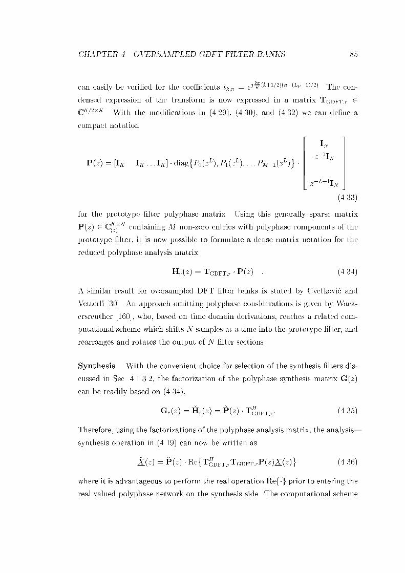
CHAPTER 4. OVERSAMPLED GDFT FILTER BANKS 85can easily be veried for the coecients tk;n = ej 2K (k+1=2)(n(Lp1)=2). The con-densed expression of the transform is now expressed in a matrix TGDFT;r 2C K=2K . With the modications in (4.29), (4.30), and (4.32) we can dene acompact notationP(z) = [IK IK : : : IK] diagP0(zL); P1(zL); : : : PM1(zL) 2666664 INz1IN...zL+1IN3777775(4.33)for the prototype lter polyphase matrix. Using this generally sparse matrixP(z) 2 C KN(z) containing M non-zero entries with polyphase components of theprototype lter, it is now possible to formulate a dense matrix notation for thereduced polyphase analysis matrixHr(z) = TGDFT;r P(z) : (4.34)A similar result for oversampled DFT lter banks is stated by Cvetkovic andVetterli [30]. An approach omitting polyphase considerations is given by Wack-ersreuther [160], who, based on time domain derivations, reaches a related com-putational scheme which shifts N samples at a time into the prototype lter, andrearranges and rotates the output of N lter sections.Synthesis. With the convenient choice for selection of the synthesis lters dis-cussed in Sec. 4.1.3.2, the factorization of the polyphase synthesis matrix G(z)can be readily based on (4.34),Gr(z) = ~Hr(z) = ~P(z) THGDFT;r: (4.35)Therefore, using the factorizations of the polyphase analysis matrix, the analysissynthesis operation in (4.19) can now be written asX(z) = ~P(z) ReTHGDFT;rTGDFT;rP(z)X(z) (4.36)where it is advantageous to perform the real operation Refg prior to entering thereal valued polyphase network on the synthesis side. The computational scheme

CHAPTER 4. OVERSAMPLED GDFT FILTER BANKS 86X(z) = ~P(z) TH discard T = Tr discard P(z) X(z)
real complex realsynthesis analysis
Figure 4.6: Computational scheme for analysissynthesis operation with factor-ized polyphase matrices; discarded matrix parts refer to omitted subbands inaccordance with Sec. 4.1.3.3.is illustrated in Fig. 4.6. One particular appeal of the factorized representationlies in the ability to perform the lter operations in the polyphase network usingentirely real valued arithmetic, while complex valued calculations are restrictedto the GDFT transforms only.Modied Prototype. Based on a decomposition of the prototype lter P (z)into 2K polyphase componentsP (z) = 2K1Xk=0 zkP (2K)k (z2K) ; (4.37)whereby the superscript (2K) implies the number of polyphases, a modied pro-totype lter p[n] | P (ej) can be denedP (z) = K1Xk=0 zkP (2K)k (z2K) zK K1Xk=0 zkP (2K)k+K (z2K) : (4.38)This modication divides the impulse response of the prototype lter into blocksof K samples, and inverts the sign in every second block. The motivation forthis action is that if analysis and synthesis lters, hk[n] and gk[n], are GDFTmodulated versions of the modied prototype p[n], the transform periodicity hasbeen cut to K, which can be veried by inspection of Fig. 4.5. By the virtualreduction of the transform periodicity, the least common multiple dened in (4.21)

CHAPTER 4. OVERSAMPLED GDFT FILTER BANKS 87can now be set to M = lcm(K;N); (4.39)which may potentially be smaller than M by a factor of two, and thus may resultin less indexing and book-keeping, sinceP(z) = [IK : : : IK] diagn P0(z L); P1(z L); : : : P M1(z L)o 2666664 INz1IN...zL+1IN3777775 (4.40)with L = M=N is identical to (4.33) but carries M polyphase components of p[n]instead of M M components of p[n].4.2.2 Transform ImplementationIn addition to the factorization of the polyphase analysis and synthesis matricesand the resulting computational savings, this sections derives a further factoriza-tion of the GDFT transform matrix TGDFT;r to make use of ecient numericaltools like the fast Fourier transform (FFT).GDFT Matrix. For ease of presentation and later reference, rst a factoriza-tion of an unreduced GDFT matrix TGDFT 2 C K2K , holding elementstk;n = ej 2K (k+k0)(n+n0) = ej 1K kn0 ej 2K kn| z DFT ej 2K k0(n+n0)with k = 0(1)K 1 ; n = 0(1)2K 1 ; (4.41)is demonstrated. One way to implement this in matrix notations is given byTGDFT = D1 T D2 (4.42)whereby D1 and D2 are diagonal matricesD1 = ej 2K kn0IK (4.43)D02 = diagnej 2K k0(n+n0)o 2 C 2K2K ; n = 0(1)2K 1 (4.44)
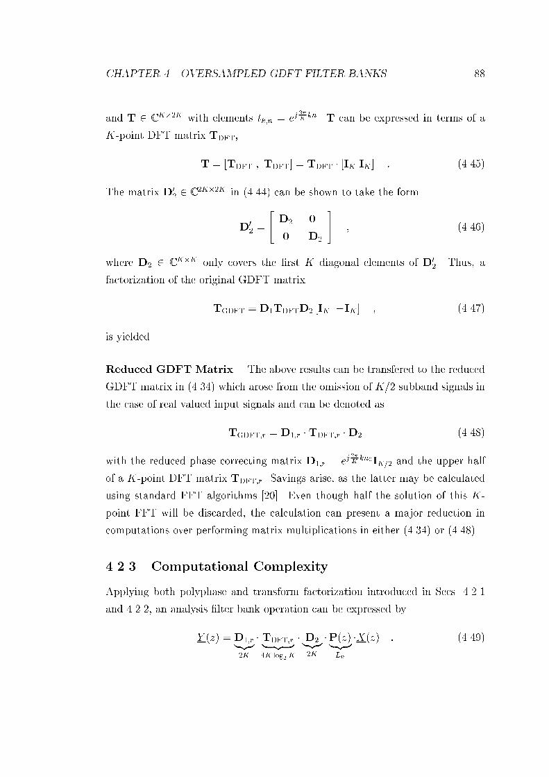
CHAPTER 4. OVERSAMPLED GDFT FILTER BANKS 88and T 2 C K2K with elements tk;n = ej 2K kn. T can be expressed in terms of aK-point DFT matrix TDFT,T = [TDFT ; TDFT] = TDFT [IK IK] : (4.45)The matrix D02 2 C 2K2K in (4.44) can be shown to take the formD02 = " D2 00 D2 # ; (4.46)where D2 2 C KK only covers the rst K diagonal elements of D02. Thus, afactorization of the original GDFT matrixTGDFT = D1TDFTD2 [IK IK] ; (4.47)is yielded.Reduced GDFT Matrix. The above results can be transfered to the reducedGDFT matrix in (4.34) which arose from the omission of K=2 subband signals inthe case of real valued input signals and can be denoted asTGDFT;r = D1;r TDFT;r D2 (4.48)with the reduced phase correcting matrix D1;r = ej 2K kn0IK=2 and the upper halfof a K-point DFT matrix TDFT;r. Savings arise, as the latter may be calculatedusing standard FFT algorithms [20]. Even though half the solution of this K-point FFT will be discarded, the calculation can present a major reduction incomputations over performing matrix multiplications in either (4.34) or (4.48).4.2.3 Computational ComplexityApplying both polyphase and transform factorization introduced in Secs. 4.2.1and 4.2.2, an analysis lter bank operation can be expressed byY (z) = D1;r|z2K TDFT;r| z 4K log2K D2|z2K P(z)|zLp X(z) : (4.49)

CHAPTER 4. OVERSAMPLED GDFT FILTER BANKS 89We now record the necessary real valued multiplications 1 when evaluating (4.49)from right to left for N fullband sampling periods:Polyphase Network. The scalar products between the polyphase componentsof the input signal and theM polyphase components of length Lp=M in thematrix P(z) result in Lp multiplications.Frequency Oset. The matrix multiplication with D2 can be mainly managedby book-keeping operations, andK multiplications of the real valued outputof the polyphase network with both real and imaginary part of the diagonalelements of D2, resulting in 2K real valued multiplications.DFT Matrix. If K is a power of two, an FFT requires 4K log2K real multipli-cations for complex data. Unless K is prime, mixed-radix algorithms canbe found attaining a similar eciency than a popular radix-2 FFT [20].Phase Correction. The multiplication withD1;r requires K=2 complex, i.e. 2Kreal valued multiplies with the diagonal elements.Therefore, in total the computational complexity per fullband sample results inCbank = 1N (4K log2K + 4K + Lp) (4.50)real multiplications for the analysis lter bank operation.For a synthesis operation, the same number of multiplications has to be com-puted, if the parahermitian of the ecient factorization in (4.49) is applied:X(z) = ~P(z)|zLp D2|z2K THDFT;r| z 4K log2K D1|z2K Y (z) : (4.51)Note, that the multiplication withD2 again only requires 2K real multiplications,since the imaginary result does not need to be processed for the input to thepolyphase network ~P(z).1The multiplication of two complex numbers x1 = x(r)1 + jx(i)1 and x2 = x(r)2 + jx(i)2 ,x1 x2 = x(r)1 x(r)2 x(i)1 x(i)2 + j(x(r)1 x(i)2 + x(r)2 x(i)1 ) ;requires 4 multiplications and two additions. Alternatively by re-shuing, this can be per-formed in 3 multiplications and 5 additions in a structure somewhat harder to implement [115].Therefore, one full complex multiplication will be accounted by 4 real valued multiplications.

CHAPTER 4. OVERSAMPLED GDFT FILTER BANKS 904.3 SSB Modulated Real Valued Filter BanksThis section will discuss a method for obtaining alias free, real valued subbandsignals of uniform bandwidth by single sideband (SSB) modulation. We start ofrom the Weaver method introduced in Sec. 3.4.3.2, which with the help of anequivalent complex modulation can be factorized into a complex modulated lterbank and a modication term. Including the computationally ecient scheme forimplementing GDFT modulated lter banks derived in the previous section, anSSB method with very low computational complexity will be obtained.4.3.1 SSB by Weaver Method and ModicationsSingle sideband modulation was introduced in Chap. 3 for oversampled real valuedlter bank techniques. The problem with decimating real valued bandpass signalswithout spectral overlap in any of the subband signals was solved by modulatingthe subbands into the baseband prior to decimation. In the Weaver methodbased on quadrature modulation shown in Figs. 3.17 and 3.18, one branch ofthe analysis lter bank can be compactly expressed by modulating the frequencyband of interest into the baseband, cut it out by a suitable lowpass lter h[n], andnally modulate it up by half of the channel bandwidth. The orthogonality ofsine and cosine in the modulation procedure ensures that spectral overlaps in thesignals are cancelled at the summation of the normal and quadrature componentin Fig. 3.17.To analyse the Weaver modulation, we employ an equivalent form to thestructures shown in Figs. 3.17 and 3.18 using complex notation and modulation,which is illustrated in Fig. 4.7 [27]. For a reason to become apparent in Sec. 4.3.2in order to compare to complex lter banks and with reference to the commentson page 64, the decimation factor is here denoted as N=2. For the analysis ofthe SSB demodulation applied as kth branch of the analysis lter bank, we can

CHAPTER 4. OVERSAMPLED GDFT FILTER BANKS 91(a) x[n] -@@?ej 2K kn - h[n] -@@?ej N n -Refg -#N2 -xk[n](b) yk[n] -"N2 -y(f)k [n]@@?ej N n - g[n] -@@?ej 2kK n -Refg -x[n]Figure 4.7: Complex quadrature modulation equivalent to the Weaver method forSSB in Figs. 3.17 and 3.18: (a) demodulation and for analysis and (b) modulationfor synthesis lter branches.describe the decimated subband signal at the output in Fig. 4.7(a) asxk[n] = Reej N nN=2 Lp1X=0 x[nN=2 ] ej 2K k(nN=2) h[] (4.52)= Renej( N 2kK )nN=2 Lp1X=0 x[nN=2 ] ej 2K kh[]| z hk[] o: (4.53)Obviously, the quadrature demodulation can be interpreted as ltering by a com-plex DFT modulated bandpass lter hk[n], followed by a displacement in fre-quency by the modulation term ej( N 2K k)n. It is therefore possible to performSSB analysis using a DFT lter bank followed by a modication which imposesthe frequency shift.The SSB quadrature modulation shown in Fig. 4.7(b) results in an outputxk[n] for the kth branch of the synthesis lter bank, which will form the recon-structed signal x[n] when summed up together with the remaining K 1 (orK=2 1 for real valued input x[n]) branch outputs. In terms of the upsampledkth subband signal y(f)k [n], where the superscript (f) refers to sampling at thefullband rate, the output xk[n] is given byxk[n] = Reej 2K nk Lp1X=0 y(f)k [n ]ej N (n) g[] : (4.54)
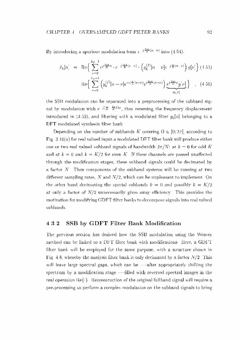
CHAPTER 4. OVERSAMPLED GDFT FILTER BANKS 92By introducing a spurious modulation term ej 2kK (nn) into (4.54),xk[n] = Ren Lp1X=0 ej 2kK n ej 2kK () y(f)k [n ]ej N (n) g[]o (4.55)= Ren Lp1X=0 y(f)k [n ]ej N (n)ej 2kK (n) ej 2kK g[]| z gk[] o ; (4.56)the SSB modulation can be separated into a preprocessing of the subband sig-nal by modulation with ej( N 2K k)n, thus reversing the frequency displacementintroduced in (4.53), and ltering with a modulated lter gk[n] belonging to aDFT modulated synthesis lter bank.Depending on the number of subbands K covering 2 [0; 2], according toFig. 3.16(a) for real valued input a modulated DFT lter bank will produce eitherone or two real valued subband signals of bandwidth 2=N : at k = 0 for odd Kand at k = 0 and k = K=2 for even K. If these channels are passed unaectedthrough the modication stages, these subband signals could be decimated bya factor N . Then components of the subband systems will be running at twodierent sampling rates, N and N=2, which can be unpleasant to implement. Onthe other hand decimating the special subbands k = 0 and possibly k = K=2at only a factor of N=2 unnecessarily gives away eciency. This provides themotivation for modifying GDFT lter banks to decompose signals into real valuedsubbands.4.3.2 SSB by GDFT Filter Bank ModicationThe previous section has derived how the SSB modulation using the Weavermethod can be linked to a DFT lter bank with modications. Here, a GDFTlter bank will be employed for the same purpose, with a structure shown inFig. 4.8, whereby the analysis lter bank is only decimated by a factor N=2. Thiswill leave large spectral gaps, which can be | after appropriately shifting thespectrum by a modication stage | lled with reversed spectral images in thereal operation Refg. Reconstruction of the original fullband signal will require apre-processing to perform a complex modulation on the subband signals to bring

CHAPTER 4. OVERSAMPLED GDFT FILTER BANKS 93x[n] - GDFTpolyphaseanalysislter bank - @@? -Refg - q - @@? -
- @@? -Refg - q - @@? -- @@? -Refg - q - @@? -ejK21n ejK21nej0n ej0nej1n ej1n GDFTpolyphasesynthesislter bank -x[n]
Figure 4.8: Complex valued oversampled GDFT analysis and synthesis lterbanks with modications stages to achieve real valued subband signals.the correct spectral part into place to be retained by the synthesis lter bank. Inthe following, the correct modications of the subband signals will be established.The kth lter hk[n] of a GDFT analysis lter bank as described in (4.1) coversa channel of bandwidth 2=K with a center angular frequency atc = 2(k + k0)K : (4.57)This also describes the position of the passband characteristic in the PSD of thekth undecimated subband signal, x(f)k [n]. If x(f)k [n] is decimated by a factor N=2,the frequency axis is re-scaled by a factorN=2, andN=21 image spectra are lledin equidistantly between the originals. Although other solutions are possible, it iseasiest to locate the original band-position and to perform a complex modulationfrom = N2 c down to = =2, as indicated in Fig. 4.9. Thus, the modulationfrequencies for the analysis lter bank outputs can be chosen ask = 2(k + 12)K N N2 = N(k + 12)K 2 : (4.58)to align the original images in the decimated subband signals in the spectral in-terval 2 [0; ]. The interval = [; 0] is initially unoccupied and is lled witha reversed image spectrum, since the real operation Refg enforces symmetry tothe frequency origin. Fig. 4.10 gives an example of what the PSDs of the subband

CHAPTER 4. OVERSAMPLED GDFT FILTER BANKS 94/Ν
2kπ
K
2(k+.5) π
K
2(k+1)π
K
π
π 2 /K
Ω
N/2
N
2π
complexmodulation
x x kk
S (e )Ωj
Figure 4.9: Power spectral density of the kth undecimated subband signal toexplain the complex modulation procedure to align the passband in the region 2 [0; ] analytically.signals on the analysis side look like prior to and after modulation with (4.58)for white noise excitation. Here, the prototype lter shown in Fig. 4.2 is used forK=2 = 8 subbands and decimation by N=2 = 7. Clearly, after modication thespectra are aligned in the positive half of the baseband, and real operation willnot destroy the signal and preserve narrow spectral gaps between adjacent imagespectra similar to Fig. 4.4(b) for complex subband signals.To describe the reconstruction properties of the modied GDFT lter bank,we rst look at the transfer from the kth output xk[n] of the GDFT analysislter bank to the kth synthesis lter input signal yk[n]. By representing xk[n] =x(r)k [n]+jx(i)k [n] in terms of its real and imaginary part, indicated by superscripts,the applied modications according to Fig. 4.8 by the modulation on analysis andsynthesis side are given byyk[n] = Ren(x(r)k [n] + jx(i)k [n])ejkno ejkn (4.59)= nx(r)k [n] cos(kn) x(i)k [n] sin(kn)o ejkn ; (4.60)where Euler's formula ej = cos() + j sin() has been exploited. Further usingthe equalities cos() = 12 ej + jej (4.61)sin() = 12j ej jej (4.62)

CHAPTER 4. OVERSAMPLED GDFT FILTER BANKS 95−1 −0.5 0 0.5 1
−60
−40
−20
0
k=0
PS
D /
[d
B]
(a) GDFT filter bank output (K/2=8,N/2=7)
−1 −0.5 0 0.5 1
−60
−40
−20
0
k=1
PS
D /
[d
B]
−1 −0.5 0 0.5 1
−60
−40
−20
0
k=2
PS
D /
[d
B]
−1 −0.5 0 0.5 1
−60
−40
−20
0
k=3
PS
D /
[d
B]
−1 −0.5 0 0.5 1
−60
−40
−20
0
k=4
PS
D /
[d
B]
−1 −0.5 0 0.5 1
−60
−40
−20
0
k=5
PS
D /
[d
B]
−1 −0.5 0 0.5 1
−60
−40
−20
0
k=6
PS
D /
[d
B]
−1 −0.5 0 0.5 1
−60
−40
−20
0
k=7
PS
D /
[d
B]
normalized frequency Ω / π
−1 −0.5 0 0.5 1
−60
−40
−20
0
k=0
PS
D /
[d
B]
(b) output of modification stage
−1 −0.5 0 0.5 1
−60
−40
−20
0
k=1
PS
D /
[d
B]
−1 −0.5 0 0.5 1
−60
−40
−20
0
k=2
PS
D /
[d
B]
−1 −0.5 0 0.5 1
−60
−40
−20
0
k=3
PS
D /
[d
B]
−1 −0.5 0 0.5 1
−60
−40
−20
0
k=4
PS
D /
[d
B]
−1 −0.5 0 0.5 1
−60
−40
−20
0
k=5
PS
D /
[d
B]
−1 −0.5 0 0.5 1
−60
−40
−20
0
k=6
PS
D /
[d
B]
−1 −0.5 0 0.5 1
−60
−40
−20
0
k=7
PS
D /
[d
B]
normalized frequency Ω / πFigure 4.10: Power spectral density of all K=2 subband signals in a modiedGDFT lter bank with K=2 = 8 channels and decimation by N=2 = 7 (a) priorto and (b) after modulation for correcting the frequency alignment of the subbandspectra to the region 2 [0; ].

CHAPTER 4. OVERSAMPLED GDFT FILTER BANKS 96we proceed toyk[n] = 12 nx(r)k [n] 1 + jej2kn+ x(i)k [n] j + ej2kno (4.63)= xk[n] + xk[n] ej(2kn+2 ) (4.64)where besides the original signal xk[n] a modulated version has appeared. Themodulation frequency 2k = 2N(k + 1=2)=K can be shown to shift withits rst summand onto a spectral repetition of X(ej), and nally by into aprevious unoccupied spectral gap. As for the original signal spectrum shown inFig. 4.9 the modications are transparent according to (4.64), the synthesis lterswill pass it, while suppressing the added reversed spectra with their stopbands.Complexity. Obtaining real valued subband signals is connected with someadditional costs in performing the lter bank calculations stated for the complexGDFT lter banks in (4.50). The additional overhead for performing the post-and preprocessing of GDFT analysis and synthesis lter bank is given by K=2complex valued multiplications. In case of the analysis bank, only the real outputof the modulation has to be computed, yielding K real multiplications. Similarly,the synthesis side multiplies real valued subband samples with complex quantities,yielding for both analysis and synthesisCbank = 2N (4K log2K + 5K + Lp) (4.65)multiplications per fullband period. Note, that compared to the cost for complexGDFT banks in (4.50) the computational eort for the SSB is approximatelydoubled. For real valued input, both lter banks produce K=2 subband signals.While however the complex GDFT subband signals can be decimated by N , thisfactor is halved in the SSB case.4.4 Complex Vs Real Valued Subband Process-ingThe original incentive for subband adaptive ltering has been the reduction ofcomputational complexity. While the previous sections were focused on the

CHAPTER 4. OVERSAMPLED GDFT FILTER BANKS 97derivation and implementation of oversampled lter banks with particular re-spect to eciency, no considerations have yet been made on the computationalcomplexity of the overall system, consisting of both subband processing task andcalculation of the lter bank operations. Therefore, this section will look into thecomplexity of processing in subbands, and in particular address which preferencesshould be made regarding the possibilities of real and complex valued subbandprocessing.To judge subband processing for real and complex subbands on an equal basis,we assume that the subbands are produced by lter banks derived from the sameprototype lowpass lter p[n] with bandwidth B = 2=K. This ensures that forboth signal decompositions, aliasing in the subbands and reconstruction error areapproximately identical, as will be demonstrated in Sec. 4.5. Further, we can ndan N = b2=Bc, where B is the bandwidth covering both passband and transitionbands of the prototype lter. Therefore generally the following statements canbe made:1. the decimation rate N for complex subband signals can be twice as high asfor real valued signals, which are only allowed to be downsampled by N=2;2. if for convenience integer decimation is employed (although possible [129],fractional sampling is awkward), the complex approach oers twice thenumber of possibilities of decimation ratios over a ner range to choose.Point (1) will be exploited to compare the complexity of implemented subbandprocessing in real and complex arithmetic.Let us assume some processing task is performed on La samples in a realvalued subband implementation, e.g. by an adaptive lter of length La. If thecomputational complexity of performing the operations associated with this pro-cessing is of order O(LIa), the number of multiplications can be written in formof a polynomial in La with coecients crealiCrealproc(La) = IXi=0 creali Lia = IXi=0 ; Crealproc;i (4.66)where Crealproc;i = creali Lia. As an example from Chap. 2, the computational com-plexity of the RLS can is given as CRLS = 3L2a + 3La + x. For complex valued
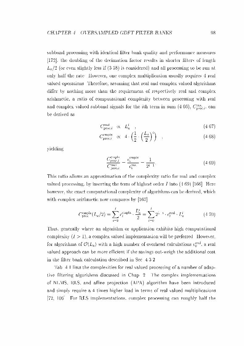
CHAPTER 4. OVERSAMPLED GDFT FILTER BANKS 98subband processing with identical lter bank quality and performance measures[172], the doubling of the decimation factor results in shorter lters of lengthLa=2 (or even slightly less if (3.58) is considered) and all processing to be run atonly half the rate. However, one complex multiplication usually requires 4 realvalued operations. Therefore, assuming that real and complex valued algorithmsdier by nothing more than the requirement of respectively real and complexarithmetic, a ratio of computational complexity between processing with realand complex valued subband signals for the ith term in sum (4.66), Crealproc;i, canbe derived as Crealproc;i / Lia ; (4.67)Ccmplxproc;i / 4 12 La2 i ; (4.68)yielding Ccmplxproc;iCrealproc;i = ccmplxicreali = 12i1 : (4.69)This ratio allows an approximation of the complexity ratio for real and complexvalued processing, by inserting the term of highest order I into (4.69) [166]. Herehowever, the exact computational complexity of algorithms can be derived, whichwith complex arithmetic now compares by [167]Ccmplxproc (La=2) = IXi=0 ccmplxi Lia2 = IXi=0 21i creali Lia (4.70)Thus, generally where an algorithm or application exhibits high computationalcomplexity (I > 1), a complex valued implementation will be preferred. However,for algorithms of O(La) with a high number of overhead calculations creal0 , a realvalued approach can be more ecient if the savings out-weigh the additional costin the lter bank calculation described in Sec. 4.3.2.Tab. 4.1 lists the complexities for real valued processing of a number of adap-tive ltering algorithms discussed in Chap. 2. The complex implementationsof NLMS, RLS, and ane projection (APA) algorithm have been introducedand simply require a 4 times higher load in terms of real valued multiplications[72, 106]. For RLS implementations, complex processing can roughly half the

CHAPTER 4. OVERSAMPLED GDFT FILTER BANKS 99Computational ComplexityAlgorithm Crealproc(La) Ccmplxproc (La=2)Normalized LMS 3 + 2La 6 + 2LaFast APA, order p 20p + 2La 40p + 2LaRecurs. Least Squares 3La + 3L2a 3La + 1:5L2aTable 4.1: Number of real multiplications of dierent algorithms in dependenceof the lter length La for real valued implementation.processing load over real valued calculations, while for LMS-type algorithms,processing is approximately equal in both real or complex subbands. However,for the latter, the lower processing gain for the lter bank calculation wouldfavour an implementation in complex subbands; a more detailed survey of thiscase will be presented in Chap. 6. For the APA, the load independent of the lterlength can be large enough for high projection orders p to prefer a real valuedimplementation.4.5 Filter DesignThe previous sections have dealt with modulated lter banks, where all lters inanalysis and synthesis bank are derived from one single prototype lowpass lter.This section will discuss some properties that these prototype lters have to fulll.Furthermore we will give two methods of how to obtain appropriate prototypelters. The rst one uses an iteration method to construct prototype lters forpower-of-2 channel lter banks, the second directly constructs prototype ltersfor an arbitrary number of bands K.4.5.1 RequirementsThis section discusses two requirements of the lter bank design | good stop-band attenuation for the suppression of aliasing in the subbands, and perfectreconstruction.

CHAPTER 4. OVERSAMPLED GDFT FILTER BANKS 100jP(e )Ω| |
0
freq
uen
cy r
esp
on
se /
[d
B]
/Kπ π/N
Ω
πFigure 4.11: Required frequency response of a real valued prototype lter p[n] fora K channel oversampled modulated GDFT lter bank with decimation by N .4.5.1.1 Filter Bandwidth and Cut-OThe frequency response of a prototype lter p[n] for aK-channel GDFT bank withdecimation by N is shown in Fig. 4.11. Therefore, the cut-o of the real valuedprototype lter p[n] is required to be at =K, with a transition band reaching upto =N . Every frequency component of an input signal in the interval [=N ; ] willbe aliased into the baseband after ltering and decimation, and cause a distortionof the subband signal, which can be modelled as additive noise, motivating anSNR-like measure for white Gaussian input signals [172]:SAR = R =N0 jP (ej)j2dR =N jP (ej)j2d ; (4.71)where SAR means signal-to-alias ratio. The denominator of (4.71) forms a mea-sure of the stopband energy, which a lter design would have to minimize. Aformulation in terms of the coecients of p[n] will be sought in Sec. 4.5.3.4.5.1.2 Power Complementary ConditionIf aliasing is suciently suppressed, approximate time-invariance of the input-output behaviour of the lter bank system in Fig. 3.1 is ensured and the near PRcondition reduces to the requirement of power complementarity [69, 151],XK1k=0 Hk(z1) Hk(z) = ~H(z)H(z) != 1 ; (4.72)

CHAPTER 4. OVERSAMPLED GDFT FILTER BANKS 101whereH(z) = [H0(z)H1(z) HK1(z)]T is a vector holding theK analysis lters.Exploiting the modulation of the bandpass lters Hk(z), H(z) can be expressedby H(z) = TGDFT diag1; z1; z2K+1| z z P (z) (4.73)where TGDFT 2 C K2K is a full GDFT matrix as given in (4.47) and P (z) avector holding 2K polyphase components of P (z),P (z) = hP (2K)0 (z2K) ; P (2K)1 (z2K) ; P (2K)2K1(z2K)i : (4.74)For the product on the left hand side of (4.72), one yields~H(z)H(z) = ~P (z)~z " IKIK #D2THDFTD1D1TDFTD2| z KIK [IK IK] zP (z) (4.75)= K ~P (z)~z " IK IKIK IK #zP (z) != 1 ; (4.76)with z as dened in (4.73. With the denition of a modied prototype lterin (4.38), the requirement of power complementarity condition in (4.72) for thelter bank can now be identied to be equivalent to demandingXK1k=0 Pk(zK) Pk(zK) != 1K ; (4.77)where Pk(z) are the K polyphase components of the modied prototype lterP (z). By looking at an arbitrary summand k on the left hand side,zkP (2K)k (z2K) z(k+K)P (2K)k+K (z2K) zkP (2K)k (z2K) z(k+K)P (2K)k+K (z2K) ;(4.78)it is clear that the auto-terms are non-zero only on a 2K grid, while the non-zerocomponents of mixed terms all lie exactly in between. Since this holds for allk 2 f0;K 1g, the requirement of (4.77) can be expressed directly in terms ofthe K polyphase components of the unmodied prototype lter,XK1k=0 Pk(zK) Pk(zK) != 1K : (4.79)

CHAPTER 4. OVERSAMPLED GDFT FILTER BANKS 102This is an important result, since (4.79) is fullled if and only if ~P (z)P (z) is aKth-band lter [151], also often referred to as Nyquist(K) lter in the communi-cations avoured literature [44, 83, 88]. In the time domain, the property (4.79)corresponds to a Kth-band lter having zero coecients at multiples of K apartfrom the center sample at time n = 0,rpp[n] = ~p[n] p[n] is a Kth-band lter (4.80)() rpp[nK] = [n] ; (4.81)where rpp[n] is the auto-correlation sequence of p[n]. The construction of K-th band lters can be achieved by a variety of methods including constraintoptimization using e.g. linear algebraic [151, 142] or windowing techniques [159,160]. Once theKth-band lter rpp[n] is designed, a diculty arises from necessaryfactorization of Rpp(z) | rpp[n] to extract analysis and synthesis lters [160,88]. The design, for example, in [159] fails to provide linear phase lters.4.5.2 Dyadically Iterated Halfband FiltersIt is possible to create | with some restrictions | lters fullling the Kth-band property with their auto-correlation function in good approximation froma lter p0[n] with a halfband auto-correlation sequence, which are widely tabledin literature [27, 31, 45] or can be constructed [99, 44]. In the following, we willsketch an iterative method based on the close connection between lter banksand the discrete wavelet transform [96, 136]. A similar approach is known in theliterature as interpolated FIR (IFIR) lters [107, 46].The idea is to dyadically scale down the impulse response of a lter p0[n] ,where p0[n] p0[n] has halfband property, i.e. stretch it to twice its support onthe time axis. This will also scale down the auto-correlation of p0[n] by a factorof two, and zeros-crossings previously at periodicity 2 for the halfband lter, willnow appear spaced at 4 samples, thus fullling the denition of a quarter-bandlter [170]. Further scaling will nally provide lters p[n] creating Kth-bandlters for higher channel numbers.Dyadic down-scaling can be achieved through expansion by 2 and a suitable

CHAPTER 4. OVERSAMPLED GDFT FILTER BANKS 103[n] - p0[n] -?p0[n]"2 - p0[n] -?p1[n]"2 - p0[n] -?p2[n]"2 - p0[n] -?p3[n] Figure 4.12: Flow graph for dyadic iteration of a prototype lter p0[n] to yieldpi[n], where K = 2i+1, whose auto-correlations satisfy Kth-band conditions, ifthe auto-correlation of p0[n] has halfband property.interpolation, for which here the original lter p0[n] is employed,pi[n] = pi1[n2 ] h[n]; i 2 N=f0g (4.82)with p0[n] p0[n] halfband lter ;which is shown as a ow graph in Fig. 4.12 for the rst four iterations. Withi!1, (4.82) will tend to a continuous scaling function belonging to the discretewavelet transform implemented by a dyadic, binary tree lter bank created fromthe lowpass lter p0[n] and its dual highpass lter [45, 161]. If the iteration(4.82) converges, the lters pi[n] represent discrete sampled versions of the scalingfunction. Finally, this connection ensures that scaling as described in the previousparagraph will work.Example. For the 32-tap lter 32C from [27], measures of power complemen-tarity of dyadically iterated K-channel prototype lters according to (4.82) arepresented in Tab. 4.2 and prove the validity of the proposed method. In thefrequency domain, scaling an impulse response results in the scaling of the fre-quency axis, as shown in Fig. 4.13. Expansion of the time domain signal withzeros introduces a highpass image spectrum with center frequency c = , whichis subsequently ltered out by interpolation with the original lter p0[n], as illus-trated by the frequency responses of the lter 32C and its rst three iterations inFig. 4.13(a)(d).Besides its advantageous simplicity, the dyadic iteration has several draw-backs. Firstly only lter banks can be constructed which have a power-of-two

CHAPTER 4. OVERSAMPLED GDFT FILTER BANKS 104
−1 −0.8 −0.6 −0.4 −0.2 0 0.2 0.4 0.6 0.8 1−100
−80
−60
−40
−20
0(a)
|P0(e
jΩ)|
/ [dB
]
−1 −0.8 −0.6 −0.4 −0.2 0 0.2 0.4 0.6 0.8 1−100
−80
−60
−40
−20
0(b)
|P1(e
jΩ)|
/ [dB
]
−1 −0.8 −0.6 −0.4 −0.2 0 0.2 0.4 0.6 0.8 1−100
−80
−60
−40
−20
0
|P2(e
jΩ)|
/ [dB
]
(c)
−1 −0.8 −0.6 −0.4 −0.2 0 0.2 0.4 0.6 0.8 1−100
−80
−60
−40
−20
0
|P3(e
jΩ)|
/ [dB
]
(d)
normalized frequency Ω/πFigure 4.13: (a) Frequency response of original halfband QMF lter 32C [27] andthree iteration (b)(d) yielding lters whos auto-correlation satisfy quarter-band,1=8th-band, and 1=16th-band lter conditions.

CHAPTER 4. OVERSAMPLED GDFT FILTER BANKS 105iteration no. i 0 1 2 3 4 5channel no. K 2 4 8 16 32 64lter length Lp 32 94 218 466 962 1954error 10 log10 e2 -64.96 -64.02 -63.42 -63.10 -63.26 -63.36Table 4.2: Dyadic iteration of halfband lter 32C [27], with resulting channelnumber K, prototype lter length Lp, and measure of power complementarity,e = k1PK1k=0 Pk(zK)Pk(zK)k2, at the ith iteration.number of channels K. Furthermore, the choice of possible decimation rates islimited, and the stopband attenuation, responsible for aliasing in the subbandsignals invariably xed. It is also clear from inspection of Fig. 4.13 that deepgaps in the stopband appear in course of the interpolation, which costs lterlength and therefore unnecessary computations and lter bank delay.4.5.3 Iterative Least Squares DesignThis section presents a least-squares design of suitable prototype lowpass lters,which directly minimizes both stopband energy and power complementarity asdiscussed in Sec. 4.5.1 where both criteria have been expressed in terms of theprototype lter. Here, rst measures for stopband energy and power complemen-tarity will be derived in terms of the lter coecients, which are then used in aleast-squares formulation for iterative minimization [163, 164].4.5.3.1 Stopband EnergyA common method to determine a measure for the stopband energyEs = 1 Z =N jP (ej)j2d (4.83)introduced as a lter design criterion in Sec. 4.5.1.1 is given by the eigenltermethod for linear phase lters [151, 142, 71], whereby the real part of the fre-quency response is evaluated for a set of discrete frequencies collected in a vector

CHAPTER 4. OVERSAMPLED GDFT FILTER BANKS 106 = [0; 1 I1]T , i 2 [=N ; ], i = 0(1)I 1ReP (eji) = TDCT p : (4.84)Note that the left hand side represents a vector quantity. The vector p 2 RLp1contains the coecients of the prototype lter,p = p[0]; p[1]; p[Lp 1]T ; (4.85)while TDCT 2 RMLp is a DCT transform holding cosine terms at the discretefrequencies i,TDCT = 2666664 1 cos(0) cos(20) : : : cos((Lp 1)0)1 cos(1) cos(21) : : : cos((Lp 1)1)... ... ... . . . ...1 cos(I1) cos(2I1) : : : cos((Lp 1)I1)3777775 : (4.86)An approximation of the stopband energy in 4.83 is now given byEs 1kTDCT pk22 : (4.87)Symmetry and therefore linear phase of the prototype lter p[n] is enforced byintroducing a matrix ST1 = ILp=2;JLp=2 such that p is mapped onto a vectorb 2 RLp=2 holding only the rst Lp=2 coecients of the prototype,b = 12ST1 p : (4.88)It is easily veried that this mapping can be reversed by p = S1 b.4.5.3.2 Power Complementary ConditionIn Sec. 4.5.1.2 the near perfect reconstruction condition for the lter bank hadbeen traced back to a power complementary condition of the prototype lter underthe assumption that the stopband energy of the lter was suciently small. Tocreate an expression in terms of the lter coecients which can be minimized,the power complementary condition (4.79) needs to be formulated in the timedomain.

CHAPTER 4. OVERSAMPLED GDFT FILTER BANKS 107For a convenient matrix formulation of the time domain operations, a vectorpk 2 RLp=K is dened to hold the kth polyphase component of p[n], i.e.pk = p[k]; p[K+k]; p[rK+k]T ; r = bLpK c; (4.89)where for convenience Lp is assumed to be an integer multiple of the channelnumber K. Further, we dene a convolutional matrix Pk 2 R(2Lp=K1)(Lp=K),Pk = 2666664 pk 0pk . . .0 pk3777775 : (4.90)Using the denitions (4.89) and (4.90), the power complementary condition (4.79)manifests itself in the time domain asK1Xk=0 Pk JK pk != 2664 01=K0 3775| z d (4.91)
where the reverse identity matrix JK has been used to convert a convolutioninto the required correlation operation, and d denes a delay with suitable zerovectors 0 of length Lp=K1. The sum on the left hand side of (4.91) can befurther condensed to matrix notation by dening a matrix V and an auxiliaryvector v,K1Xk=0 Pk JK pk = [P0JK; P1JK; PK1JK; ]| z V 2666664 p0p1...pK13777775| z v = VS2 p: (4.92)
The matrix S2 is a suitable Lp Lp permutation matrix such that ST2 performsa mapping from the synchronously ordered prototype coecients in p onto thesequence of polyphase vectors in v = ST2 p. The formulationVS2S1 b != d (4.93)

CHAPTER 4. OVERSAMPLED GDFT FILTER BANKS 108nally denes the power complementary condition including the symmetry con-straint for the prototype lter.4.5.3.3 Least Squares FormulationTo minimize stopband energy in (4.87) and achieve approximate power comple-mentarity as dened by (4.93), a least squares (LS) problemb = argminb " V(b)S2 S1 TDCTS1 #| z A b " d0 # 22 (4.94)has to be solved, where allows a weighting between both design criteria. Thenotation V(b) is given to indicate the dependency of the system matrix A 2R(2Lp=K+I1)Lp=2 upon the lter coecients. Thus, unfortunately (4.94) is nota quadratic problem and may exhibit local minima. However, analysis in [66]suggests for a similarly posed problem that the cost function in b possesses 3minima, of which two are symmetric with opposite sign and a third one denesa saddle point in between for b = 0.The minimization can be performed iteratively [122, 121, 71], solving at eachiteration j bj = argminbj " V(bj1)S2 S1 ! TDCTS1 #bj " d0 # 22 ; (4.95)where a previous solution bj1 is substituted to achieve a quadratic approximationof (4.94). A similar approach is reported in [82], where e.g. alternately analysisand synthesis lters are kept constant while the other one is optimized to achievea solvable quadratic expression.The resulting quadratic LS problem (4.95) can be easily solved using stan-dard linear algebraic tools [58]. As stopping criterion, the optimization may beregarded as sucient when the change from bj1 to bj falls below a certainthreshold [66].An additional weighting matrix ! in (4.95) can help to improve the stopbandattenuation towards the band edge. Furthermore, a relaxation can be introducedto solve for an a priori solution b0k at iteration step j, from which the a posteriori
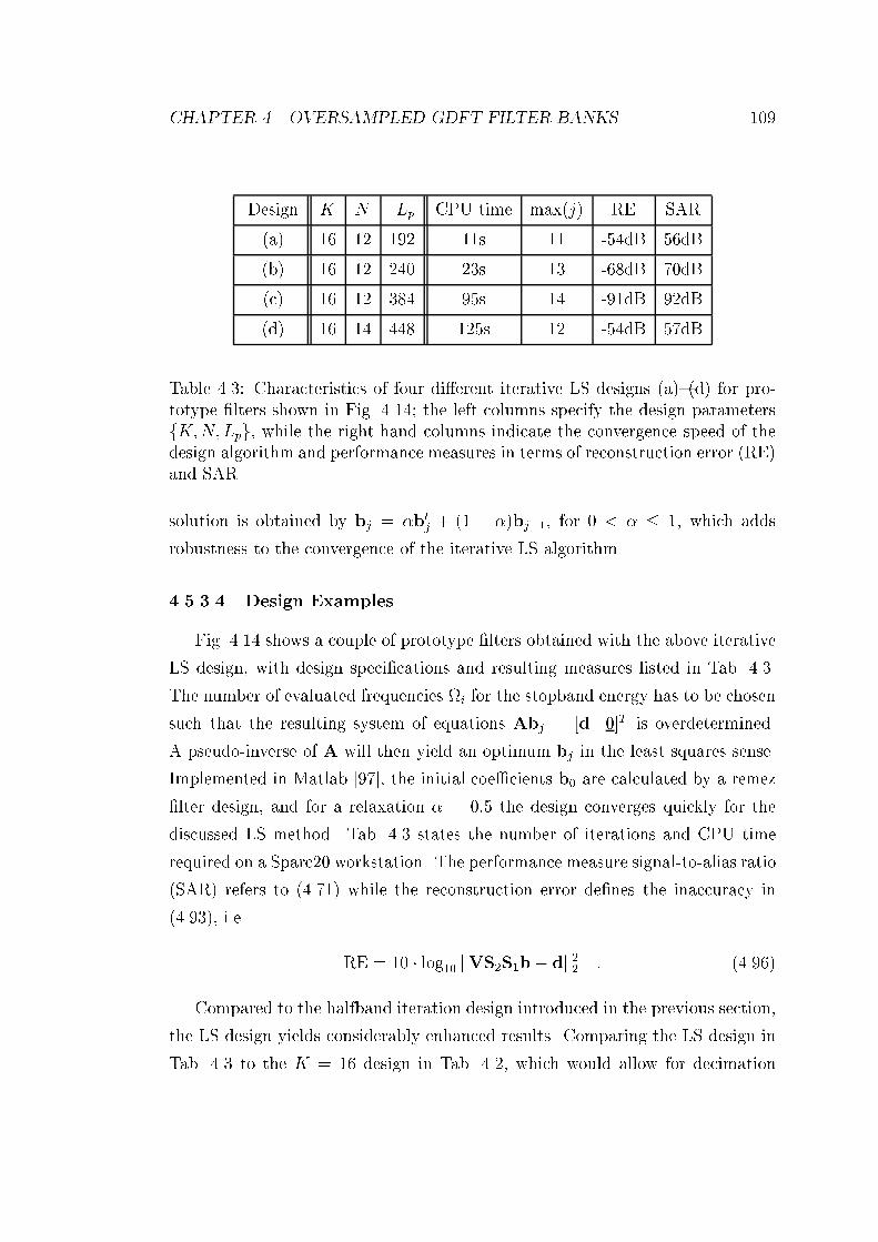
CHAPTER 4. OVERSAMPLED GDFT FILTER BANKS 109Design K N Lp CPU time max(j) RE SAR(a) 16 12 192 11s 11 -54dB 56dB(b) 16 12 240 23s 13 -68dB 70dB(c) 16 12 384 95s 14 -91dB 92dB(d) 16 14 448 125s 12 -54dB 57dBTable 4.3: Characteristics of four dierent iterative LS designs (a)(d) for pro-totype lters shown in Fig. 4.14; the left columns specify the design parametersfK;N; Lpg, while the right hand columns indicate the convergence speed of thedesign algorithm and performance measures in terms of reconstruction error (RE)and SAR.solution is obtained by bj = b0j + (1 )bj1, for 0 < 1, which addsrobustness to the convergence of the iterative LS algorithm.4.5.3.4 Design ExamplesFig. 4.14 shows a couple of prototype lters obtained with the above iterativeLS design, with design specications and resulting measures listed in Tab. 4.3.The number of evaluated frequencies i for the stopband energy has to be chosensuch that the resulting system of equations Abj = [d 0]T is overdetermined.A pseudo-inverse of A will then yield an optimum bj in the least squares sense.Implemented in Matlab [97], the initial coecients b0 are calculated by a remezlter design, and for a relaxation = 0:5 the design converges quickly for thediscussed LS method. Tab. 4.3 states the number of iterations and CPU timerequired on a Sparc20 workstation. The performance measure signal-to-alias ratio(SAR) refers to (4.71) while the reconstruction error denes the inaccuracy in(4.93), i.e. RE = 10 log10 kVS2S1b dk22 : (4.96)Compared to the halfband iteration design introduced in the previous section,the LS design yields considerably enhanced results. Comparing the LS design inTab. 4.3 to the K = 16 design in Tab. 4.2, which would allow for decimation

CHAPTER 4. OVERSAMPLED GDFT FILTER BANKS 110
−1 −0.8 −0.6 −0.4 −0.2 0 0.2 0.4 0.6 0.8 1
−120
−100
−80
−60
−40
−20
0
|Pa(e
jΩ)|
/ [dB
]
normalized frequency Ω/pi
(c)
−1 −0.8 −0.6 −0.4 −0.2 0 0.2 0.4 0.6 0.8 1
−120
−100
−80
−60
−40
−20
0
|Pb(e
jΩ)|
/ [dB
]
normalized frequency Ω/pi
(b)
−1 −0.8 −0.6 −0.4 −0.2 0 0.2 0.4 0.6 0.8 1
−120
−100
−80
−60
−40
−20
0
|Pc(e
jΩ)|
/ [dB
]
normalized frequency Ω/pi
(a)
−1 −0.8 −0.6 −0.4 −0.2 0 0.2 0.4 0.6 0.8 1
−120
−100
−80
−60
−40
−20
0
|Pd(e
jΩ)|
/ [dB
]
normalized frequency Ω/pi
(d)
Figure 4.14: Frequency responses of prototype lters constructed using an itera-tive LS design for K = 16 channel lter bank with possible decimation by N 12for (a)(c) and N 14 for (d); performance measures are given in Tab. 4.3.

CHAPTER 4. OVERSAMPLED GDFT FILTER BANKS 111by N = 12 with about 59dB and for N = 13 with 52dB SAR, clearly the lterlength can approximately be halved at almost identical performance for designs(a) and (b), or reach a sharper transition band and higher possible decimationrate at equal cost and quality measures with design (d), thus allowing for moreecient subband processing.Bifrequency Transfer Function. Aliasing distortion and imaging introducedby decimators and expanders in multirate systems can be completely describedby bifrequency transfer functions [27]. The sampling rate conversion causes | ifaliasing is not suciently suppressed | the multirate system to be linear periodi-cally time-varying (LPTV) with a period equivalent to the least common multipleof all sampling rate changes occurring within the system. The overall impulseresponse of such a system, h[n1; n2], therefore depends on the time of observationn2 and the time of excitation n1 [76]. Based on h[n1; n2], the bifrequency transferfunction is given byHej2; ej1 = 12 +1Xn1=1 +1Xn2=1h[n2; n1] ej(1n12n2) ; (4.97)which relates a frequency 1 at the input to each frequency 2 at the systemoutput.Using the measurement method by Reng and Heinle [120, 75], Fig. 4.15 showsthe bifrequency transfer function of a GDFT modulated lter bank consisting ofanalysis and synthesis as shown in Fig. 4.1 with a reduced number of K=2 = 8subbands and decimation by N = 14, based on the prototype lter listed inTab. 4.3 as design (d). The main diagonal in Fig. 4.15 indicates that the signalcomponents are passed without noticeable amplitude distortion, i.e. the overalllter bank is power complementary. The o-diagonals represent the alias levelcreating a noise oor at about -60 dB below. Note that for an LPTV system,aliasing occurs only along so called Dirac lines [27, 76], i.e. discrete o-diagonals.Further note that the lines for 2 1 = are missing, since for this case themodulated lters fulll the quadrature mirror lter (QMF) condition, resultingin alias cancellation in the synthesis bank.Fig. 4.16 shows the measurement of the bifrequency transfer function of an

CHAPTER 4. OVERSAMPLED GDFT FILTER BANKS 112
00.2
0.40.6
0.81
1.21.4
1.61.8
2
0
0.2
0.4
0.6
0.8
1
1.2
1.4
1.6
1.8
2
-140
-120
-100
-80
-60
-40
-20
0
1= 2=
jH(ej1; ej2)j=[dB]
Figure 4.15: Measurement of the bifrequency transfer function for a GDFT lterbank with K=2 = 8 complex channels and decimation by N = 14, using theprototype lter p[n] shown in Fig. 4.2(a).SSB modied GDFT modulated lter bank with K=2 = 8 real valued subbandsignals decimated byN=2 = 7. This lter bank is derived from the same prototypelter as the GDFT lter bank shown in Fig. 4.15. Since this system is decimatedat only half the rate of the previous complex lter bank, aliasing is restricted toN=2 1 Dirac lines on either side of the main diagonal.4.6 Concluding RemarksIn this chapter oversampled GDFT lter banks have been introduced. Someparticular conditions arising from the oset values for time and frequency in themodulating complex exponential have been highlighted, notably the organizationof the passbands of the lter bank lters, and their linear phase property. Anecient implementation of this type of lter bank has been suggested for arbitraryinteger decimationN K. It is based on a factorization of the polyphase analysismatrix into a real valued polyphase network and a GDFT transform, which canbe further factorized for fast implementations using FFT algorithms.

CHAPTER 4. OVERSAMPLED GDFT FILTER BANKS 113
00.2
0.40.6
0.81
1.21.4
1.61.8
2
0
0.2
0.4
0.6
0.8
1
1.2
1.4
1.6
1.8
2
-140
-120
-100
-80
-60
-40
-20
0
1= 2=
jH(ej1; ej2)j=[dB]
Figure 4.16: Measurement of the bifrequency transfer function for a modiedGDFT lter bank to perform an SSB with K=2 = 8 real channels and decimationby N=2 = 7, using the prototype lter p[n] shown in Fig. 4.2(b).Modications have been established for the GDFT lter bank to implementan SSB modulated lter bank with real valued subbands. Again, the factorizationof the GDFT lter banks involved allows for a highly ecient implementation.Based on the same prototype and therefore implementing approximately identicalperformance characteristics, the SSB modied GDFT lter bank produces realvalued subbands at twice the rate of a complex GDFT subband implementation.A comparison between real and complex subband processing has been made,which takes into account both the computational complexity of the lter bankimplementation and the subband processing e.g. performed by adaptive lters.This has yielded the initially surprising fact, that complex subband processingis despite its complex arithmetic generally at level with real valued subbandsfor O(La) algorithms and outperforms for orders O(L2a) algorithms and greater,which is mainly due to the higher possible sampling rate for the complex system.However, exceptions exist e.g. for the APA and potentially other algorithms, forwhich a real valued implementation may be considered advantageous.

CHAPTER 4. OVERSAMPLED GDFT FILTER BANKS 114Finally, design methods have been presented which allow to construct proto-type lowpass lters for oversampled GDFT lter banks with low aliasing level inthe subband signals, based on a dyadic iteration of tabulated lters and by aniterative LS design. In Chap. 5, the performance of subband adaptive systemswill be closely linked to the optimization criteria in the latter design algorithm,enabling to create application specic lter banks for subband adaptive systemswith predened performance limits.

Chapter 5Performance of SubbandAdaptive Filter SystemsThis chapter discusses the performance and limitations in performance of subbandadaptive ltering (SAF) in oversampled subbands. Sec. 5.1 will rst introduceand review dierent general aspects of the performance of SAF systems. Inparticular, aliasing in the subbands which may limit the MMSE performancewill be addressed in Sec. 5.2, and Sec. 5.3 will link inaccuracies in the adaptedequivalent fullband model to the employed analysis and synthesis lter banks.Based on the use of GDFT lter banks as introduced in the previous chapter, someproperties of the resulting subband adaptive structures are derived in these twosections, which can be directly linked to quality measures of the lter bank design.Finally, Sec. 5.4 will demonstrate the impact of dierent set-up parameters on thesubband adaptive system by simulation and validate the performance measuresgiven in Secs. 5.2 and 5.3.5.1 General Performance Limiting In uencesFirst, we will concentrate on general performance limiting in uences for subbandadaptive lter systems. Sec. 5.1.1 will dene dierent aspects and measures ofSAF performance, e.g. nal MSE, accuracy of the adapted SAF, and convergencespeed. A discussion of how they are aected by dierent parameters of the set-up115

CHAPTER 5. PERFORMANCE OF SAF SYSTEMS 116will follow in Sec. 5.1.2.5.1.1 Performance Criteria5.1.1.1 Final MSEThe quality of adaptation can be judged from the nal achievable mean squarederror value, which ideally represents an ensemble average and can therefore betime-varying. For stationary situations the MSE level for n ! 1 gives an in-dication for the quality of adaptation. Since the nal MSE level is an absolutequantity, sometimes it is more interesting to measure by how much an initial,i.e. uncancelled, error level can be reduced through the application of the sub-band adaptive lter system. This gives rise to the denition of noise reduction,which represents an SNR-like measurenoise reduction = 10 log10 Efd2[n]gEfe2[n]g jn!1 : (5.1)Note that noise reduction is dened in terms of the fullband desired signal d[n]and the reconstructed fullband error signal e[n]. It is also possible to dene anoise reduction measure based on the subband desired and error signals, whichwill be revisited in Sec. 5.2.2. Both measures for fullband and subbands can bedirectly linked if the employed lter banks perform frame expansions, since axed energy relation between subband and fullband signals exists.5.1.1.2 Modelling ErrorBesides measuring the MSE of the error signal, it is also possible to assess thestate or quality of adaptation in terms of the nal weight values of the subbandadaptive lter impulse responses and their distance from the optimal solution.This implies, that either the Wiener Solution for the subband lters is known, orthat a reconstruction of the fullband equivalent model to be derived in Sec. 5.3.1can be compared to the \unknown" system that the SAF set-up is supposed toidentify. The latter clearly cannot give any indication for system performancein the case of a band-limited input signal, since the optimally achievable model
CHAPTER 5. PERFORMANCE OF SAF SYSTEMS 117is only dened at the excited frequencies, and has an arbitrary since undenedfrequency response otherwise [86].5.1.1.3 Convergence SpeedFor most adaptive lter applications, it is desirable to nd and reach optimalor almost optimal performance as fast as possible. For algorithms like the LMSdiscussed in Sec. 2.3, a measure for the convergence speed is given by a timeconstant associated with its exponential convergence. For more complex set-upslike subband adaptive ltering, where the adaptive algorithm is embedded in asubband architecture, the behaviour is often dicult to condense into a singlemeasure. However, in practical applications, convergence speed can be judged byobserving the time required for the error of the SAF system to reach a stationaryvalue, i.e. the nal MSE as introduced in Sec. 5.1.1.1.5.1.1.4 Robustness towards Observation NoiseThe presence of observation noise on the desired signal d[n], which is assumedto be uncorrelated with the input signal x[n], has a number of implications onthe adaptive system. The MMSE is not equal to zero, and the residual errorsignal injects noise into the adaptation of the adaptive lter coecients. Thiscan (for example in the LMS' case) cause inaccuracy of the identied model andan additional variance term in the error signal, which in Sec. 2.3.3.3 was referredto as excess MSE. If the level of observation noise is very high, i.e. the desiredsignal has low SNR, the adaptive lters may not converge.Another aspect of robustness is how well the algorithm preserves the obser-vation noise contained in the desired signal. Although labelled noise, in manyapplications like AEC or noise cancellation the observation noise is a speech sig-nal or similar signal of interest, which is to be recovered. However, many fastconverging algorithms like NLMS or APA can show a rather aggressive behaviourtowards the observation noise, as for short lter lengths and large step size, abest LS t of the input signal to the current desired signal value is attempted[130, 140], as indicated in Sec. 2.5.1.2. Thus, often a measure called echo returnloss enhancement (ERLE) similar to (5.1) is preferred, whereby the observation

CHAPTER 5. PERFORMANCE OF SAF SYSTEMS 118noise s[n] is subtracted from both the desired and error,ERLE = 10 log10 Ef(d[n] s[n])2gEf(e[n] s[n])2g jn!1 ; (5.2)therefore only judging the reduction of the signal of interest and considering anychanges made to the observation noise. The name ERLE refers to its originalapplication of assessing the performance of echo cancellers in the presence of nearend speech.The literature provides an amazing number of suggestions how to improvethe robustness of adaptive algorithms [171], mostly by introducing a variablestep-size parameter [n], which is to be adjusted such that optimal adaptationis secured despite the (temporary) presence of observation noise, e.g. in the formof a near end speaker in AEC. Approaches in [125, 98] steer the step-size basedon the estimated correlation between error and input signal. More sophisticatedmethods in AEC attempt to detect double talk situations where the near endspeaker is active and adaptation of the SAF system has to be frozen [77, 17, 16].However, clearly robustness is a mostly algorithmic related issue, and not specicto subband adaptive systems.5.1.2 Performance LimitationsDierent parameters in the set-up of an SAF system are important in determin-ing its performance. In the following, we will partly review the literature andthereafter collect and discuss facts that have been striven for in Chapters 3 and4.5.1.2.1 Model TruncationThe question of how to choose the length of the subband adaptive lters is im-portant in the sense that a too short model will | for the case of white noiseexcitation | only be able to converge to a truncated response and thus noisyversion of what the optimal impulse response should be.For the critically sampled case, Sec. 3.4.2 presented equations from [53, 54]describing the optimal Wiener solution for the subband adaptive lters in (3.57),

CHAPTER 5. PERFORMANCE OF SAF SYSTEMS 119which allowed us to derive the required lter length (3.58) dependent on the orderof the unknown system to be identied, and the length of analysis and synthesislters. The latter cause an increase in lter length which can be justied by thetransients introduced by the lter banks. Due to the decimation, these transientsare likely to dier in the kth subband between desired and input signal, andhence have to be appropriately modelled by the subband adaptive lters. It isworthwhile to note that the transients caused by the analysis lter bank generallyrequire the subband adaptive lters to operate non-causally, which can be easilypictured by inspecting the example in Fig. 3.10. Therefore, the desired signalusually needs to be delayed for correct adaptation, unless the plant to be identiedis known to possess a sucient delay.Analysis in one of the pioneering papers by Kellermann [86] and more recentlyin [175] argues on the basis of (3.54), by assuming ideal analysis lters with arectangular frequency response and hence innite support in the time domain.Their results for the optimum subband lters are decaying but innite solutions.Based on the analysis in Sec. 3.4.2 and on practical results in [135, 88, 66],it usually appears reasonable for worst case scenarios to choose the length of theadaptive lter, La, as La = 2Lp + LsN ; (5.3)where Lp and Ls are the lengths of lter bank prototype lter p[n] and theunknown system s[n], respectively, and N the decimation ratio. This formulacan be derived analogous to (3.58) assuming a paraunitary relationship betweenanalysis and synthesis lter bank for the oversampled case. Similarly, in worstcase scenarios delaying the desired signal by Lp=N samples in the subbands hasbeen shown to be more than sucient in practice.If a truncated model should occur, the unknown system can be imagined asa superposition of an identiable and an unidentiable part, where the output ofthe latter contributes to the observation noise in the system, since the correlationit imposes on the desired signal is inaccessible to the SAF structure. This causesan additional term on the MMSE and will create an inaccurate, and in the caseof LMS-type algorithms noisy model. However, even if innitely long subband

CHAPTER 5. PERFORMANCE OF SAF SYSTEMS 120adaptive lters were required for optimum performance and adaptation withoutmodel truncation [175], other limiting factors to be introduced in Sec. 5.2 willdominate the lower error bound.5.1.2.2 Spectral Separation and Eigenvalue SpreadSpectral Separation. By dividing the spectrum of the input signal into in-tervals, lter banks are often viewed as to \whiten" the spectra of the subbandsignals with respect to the fullband signal. However, instead of whitening we hererather refer to this phenomenon as spectral separation, since the lter banks alsohave an adverse eect on the whiteness of the subband signals by introduceingnotches due to non-perfect lter banks and OSRs > 1, as seen in Fig. 4.4. Theconvergence speed of mainly LMS-type adaptive lters depends on the eigenvaluespread of the input signal as introduced in Sec. 2.3, which can be approximated bythe ratio between minimum and maximum value of its PSD as in (2.52). Clearlyfor a strongly coloured input signal a separation into smaller spectral intervalsas performed by the analysis lter bank can help to form more balanced ratios,i.e. a smaller eigenvalue spread, and thus increase the convergence speed. Thiswill be demonstrated in Sec. 5.4.Eigenvalue Spread. As mentioned before, the increase in convergence speeddue to spectral separation can be degraded by the colouring (notches) introducedby the lter banks. As input frequencies in the transition band of analysis ltersare considerably attenuated, the input to the adaptive algorithm carries onlyweak spectral information on this part of the signal and thus indirectly of theunknown system, and the SAFs can adapt these spectral parts only very slowly[101]. With narrower transition bands as required for lter banks operating closeto critical decimation, a better overall convergence behaviour of the SAF systemseems achievable. On the other hand, broader transition bands that allow onlya lower decimation ratio to be implemented will result in a faster update rate ofthe adaptive algorithm, which again enhances convergence. Sec. 5.4 will discussthe resulting dierences in performance.

CHAPTER 5. PERFORMANCE OF SAF SYSTEMS 1215.2 Minimum Mean Squared Error LimitationsIn Sec. 3.4.1 the problem caused by aliasing in the subbands was introduced.Here, novel limits will be derived for the PSD of the minimum residual errorsignal due to aliasing in the subbands, and the resulting minimum mean squarederror (MMSE). Also, an easy-to-apply measure will be created, that can directlylink the stopband attenuation of the prototype lter design in Sec. 4.5 to thenoise reduction achievable by an SAF.5.2.1 Measuring AliasingSec. 4.5 introduced an SNR-type measure for the aliasing in the subbands causedby decimation and non-perfect stopband attenuation of the prototype lter forwhite Gaussian input. For a further discussion of the adaptation error, we areinterested in a power spectral density description of the minimum error of theWiener solution, to be compared to the adaptively achievable power spectraldensities of both the subband and reconstructed fullband nal error signals.While the SAR measure in Sec. 4.5 has ignored colouredness of the inputsignal to solely judge the quality of the lter bank, now the spectral character-istics of the input signal have to be taken into account. This poses a problem,as the power spectral density of the input signal is a quadratic quantity, and asimple superposition of spectral parts to describe aliasing would give an incom-plete solution, lacking the cross-terms in the PSD as spectral de-correlation ofthe input signal cannot generally be assumed. Therefore, the approach takenhere assumes the knowledge of a white iid noise excited source model, L(ej), asshown in Fig. 5.1, which together with the lters Hk(z) of the analysis bank isused to calculate aliasing terms from the systems' spectra, while the excitationnoise remains white iid in the decimation stage. With these two steps, nally thepower spectral densities due to aliasing can be derived.5.2.1.1 MethodSec. 3.1.1 introduced the formulation for the frequency domain eect of dec-imation. Assume we want to decimate the signal x[n] in Fig. 5.1(a) and would
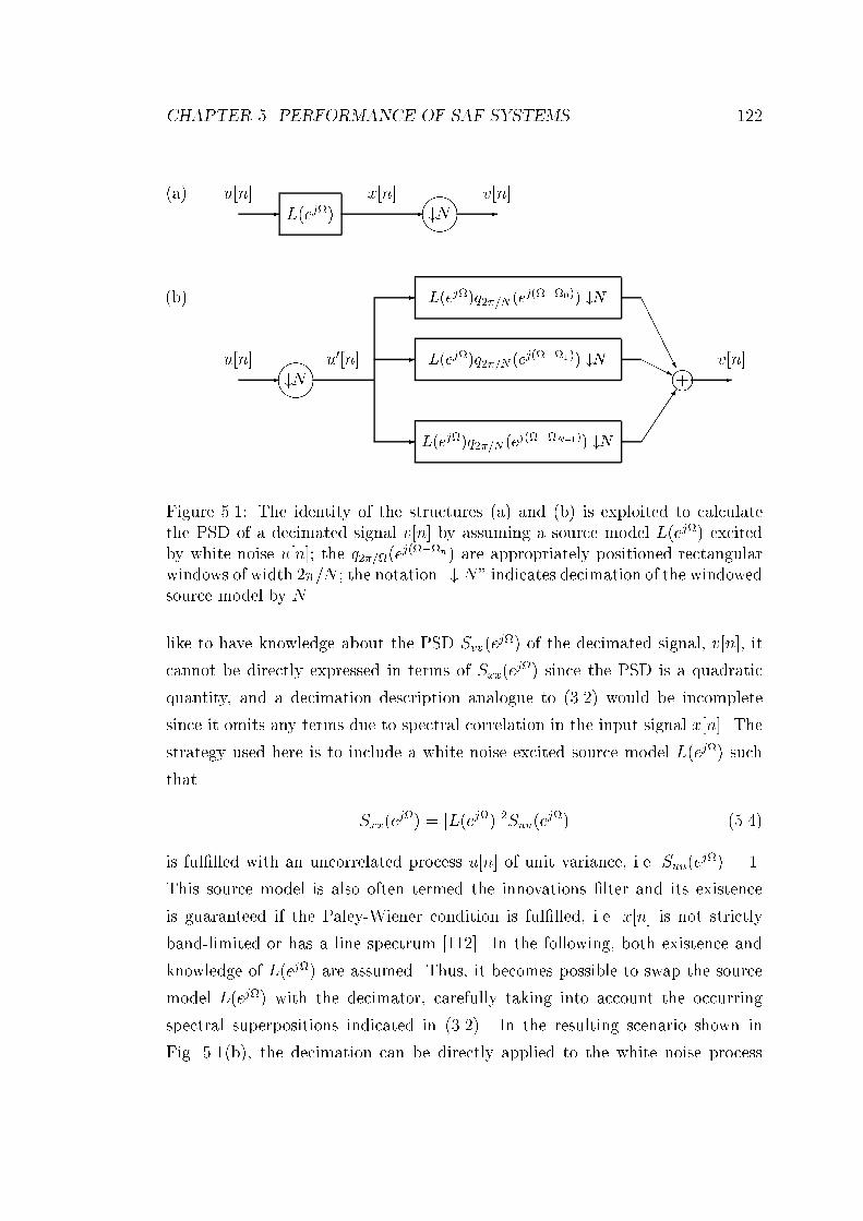
CHAPTER 5. PERFORMANCE OF SAF SYSTEMS 122(a) -u[n] L(ej) -x[n] #N -v[n](b) u[n] -#N u0[n] --
-L(ej)q2=N (ej(N1)) #N...L(ej)q2=N (ej(1)) #NL(ej)q2=N (ej(0)) #N
HHHjAAAAAU m+ -v[n]Figure 5.1: The identity of the structures (a) and (b) is exploited to calculatethe PSD of a decimated signal v[n] by assuming a source model L(ej) excitedby white noise u[n]; the q2=(ej(n) are appropriately positioned rectangularwindows of width 2=N ; the notation \# N" indicates decimation of the windowedsource model by N .like to have knowledge about the PSD Svv(ej) of the decimated signal, v[n], itcannot be directly expressed in terms of Sxx(ej) since the PSD is a quadraticquantity, and a decimation description analogue to (3.2) would be incompletesince it omits any terms due to spectral correlation in the input signal x[n]. Thestrategy used here is to include a white noise excited source model L(ej) suchthat Sxx(ej) = jL(ej)j2Suu(ej) (5.4)is fullled with an uncorrelated process u[n] of unit variance, i.e. Suu(ej) = 1.This source model is also often termed the innovations lter and its existenceis guaranteed if the Paley-Wiener condition is fullled, i.e. x[n] is not strictlyband-limited or has a line spectrum [112]. In the following, both existence andknowledge of L(ej) are assumed. Thus, it becomes possible to swap the sourcemodel L(ej) with the decimator, carefully taking into account the occurringspectral superpositions indicated in (3.2). In the resulting scenario shown inFig. 5.1(b), the decimation can be directly applied to the white noise process

CHAPTER 5. PERFORMANCE OF SAF SYSTEMS 123-u[n] L(ej)sourcemodel -x[n] Hk(ej)analysislter -decimation &expansion#N -xk[n]"N -x0k[n] Gk(ej)synthesislter -xk[n]
Figure 5.2: Block diagram for analysis of aliasing due to decimation by N in thekth subbandsexciting the source model L(ej). After decimation by N , obviously this noise isstill white with identical variance, i.e. Su0u0(ej) = 1.For the following analysis, for a branch of the analysis / synthesis lter bankthe model in Fig. 5.2 is used. There, the kth branch of the analysis lter bank,characterized by the lter Hk(ej), is excited by a signal x[n], which we assumeto be a non-deterministic signal arising from a white noise excited source modelL(ej) as discussed previously. After decimation and expansion by N , on thesynthesis side the signal is ltered by the kth synthesis lter Gk(ej). By de-nition of our GDFT lter bank, we have Gk(ej) = Hk(ej) according to (4.18).5.2.1.2 Power Spectral Density Description for Decimated and Ex-panded SubbandsDecimation and expansion of a signal by a factor ofN causes the original spectrumto be superimposed by N 1 shifted copies of itself. Following the thoughts inSec. 5.2.1.1, we only apply this superposition to a combined system consisting ofthe source model L(ej) and the kth analysis lter Hk(ej)Fx0k(j) = 1N N1Xn=0 Lej( 2nN ) Hk ej( 2nN ) q2=N (k) ; (5.5)where q2=N (k) is a rectangular frequency domain window,q2=N (k) = ( 1 for 2 k; k + 2N 0 for 62 k; k + 2N ; (5.6)and a frequency oset k = (2k + 1)K N (5.7)

CHAPTER 5. PERFORMANCE OF SAF SYSTEMS 124is chosen such that according to Fig. 4.9 the passband dened for the kth analysislter including its transitions bands is always contained in the term n = 0 withinthe sum (5.5). All other terms n 2 [1;N 1] dene aliased spectral parts. Notethat the superposed lter spectrum Fx0k(j) is only non-zero for a small windowdened by (5.6). It is periodized byFx0k(ej) = 1Xi=1 Fx0k j 2iN (5.8)which represents the sum over all parallel branches in Fig. 5.2(b) with the addi-tional inclusion of the kth analysis lter. Now the PSD of x0k[n] is given bySx0kx0k(ej) = Fx0k(ej)2 Su0u0(ej) = Fx0k(ej)2 : (5.9)From this PSD description of x0[n], it is easy to obtain both PSD of decimatedsubband signal and reconstructed fullband signal. The rst arises from rescalingthe frequency axis in (5.9), yieldingSxkxk(ej) = Sx0kx0k(ej=N) = Fx0k(ej=N )2 : (5.10)For the PSD of the reconstructed fullband signal, the synthesis lters Gk(ej) =Hk(ej) are included into the transfer function model,Fx(ej) = K1Xk=0 Fx0k(ej) Hk(ej) ; (5.11)and the PSD is similarly given bySxx(ej) = Fx(ej)2 = K1Xk=0 Fx0k(ej) Hk(ej)2 : (5.12)5.2.1.3 Power Spectral Densities of Minimum Error TermsThe formulations of PSDs for MMSE terms is based on a partitioning of theintermediate spectrum in (5.5) of the transfer from the decimated source modelinput to the upsampled subband signal x0k[n] intoFx0k(j) = F (S)x0k (j) + F (A)x0k (j) ; (5.13)

CHAPTER 5. PERFORMANCE OF SAF SYSTEMS 125where the superscripts (S) and (A) refer to signal of interest and aliased parts,respectively, dened asF (S)x0k (j) = 1NF (ej)Hk(ej) q2=N (k) ; and (5.14)F (A)x0k (j) = 1N N1Xn=1 F (ej( 2nN ))H(ej( 2nN )) q2=N (k): (5.15)By periodization analogous to (5.8) formulations for decimated and expandedsystems F (S)x0k (ej) and F (A)x0k (ej) can be derived from these intermediate spectra.With these two quantities, the PSD of the kth expanded subband signal in (5.9)can be split into four terms,Sx0kx0k(ej) = S(S)x0kx0k(ej) + S(S;A)x0kx0k (ej) + S(A;S)x0kx0k (ej) + S(A)x0kx0k(ej); (5.16)where two auto-termsS(S)x0kx0k(ej) = F (S)x0k (ej)2 and (5.17)S(A)x0kx0k(ej) = F (A)x0k (ej)2 ; (5.18)and two cross-terms between signal of interest and aliased partsS(S;A)x0kx0k (ej) = F (S)x0k (ej) F (A)x0k (ej) and (5.19)S(A;S)x0kx0k (ej) = F (S)x0k (ej) F (A)x0k (ej) = S(S;A)x0kx0k (ej) (5.20)dene the dierent contributions from signal of interest and alias signal compo-nents to the overall power spectral density.Assuming that an optimal lter removes all un-aliased signal components, thePSD of the minimum mean square error (MMSE) signal will only consist of theauto-term of aliased signal parts in (5.16),SMMSExkxk (ej) = S(A)x0kx0k(ej=N) = F (A)x0k (ej=N)2 ; (5.21)which has already been rescaled in terms of its frequency index by a factor ofN to correctly re ect the minimum error PSD of the kth decimated subbandsignal xk[n]. The superscript MMSE indicates that (5.21) gives the PSD of theerror signal provided the adaptive lter has achieved optimum adaptation and

CHAPTER 5. PERFORMANCE OF SAF SYSTEMS 126the error signal is minimum. The above PSD can be related to the MMSE valueby evaluating the inverse Wiener-Khintchine transform [123] for zero time shift,MMSE;k = 12 2Z0 SMMSExkxk (ej)d : (5.22)Similarly, the PSD of the reconstructed minimum error signal is derived from(5.12) by splitting Fx0k(ej) into true and aliased components, and assuming thatall true signal parts have been removed by the optimally adjusted adaptive lter.This yields for the PSDSMMSEx;x (ej) = K1Xk=0 F (A)xk (ej)2 = K1Xk=0 F (A)x0k (ej) ~Hk(ej)2 : (5.23)Analogous to the subband case, the minimum mean squared reconstructed errorvalue due to aliasing is given byMMSE = 12 2Z0 K1Xk=0 F (A)x0k (ej) ~Hk(ej)2 d: (5.24)The MMSE value of the fullband reconstructed error signal can also be accessed byexploiting the xed energy | and therefore power | relation between subbandsand fullband given by a tight frame condition in (3.19) such as satised by theemployed GDFT lter bank when constructed according to Sec. 4.5.5.2.2 MMSE ApproximationsIn the following, approximations to estimate the MMSE will be derived, whichare more workable than the limits stated in Sec. 5.2.1.3 since they can be calcu-lated directly from the frequency response of the prototype lters. The involvedapproximations will be justied by considering the two extrema of white noiseand narrowband (sinusoidal) input in Sec. 5.2.2.3, and underpined by simulationsin Sec. 5.4.5.2.2.1 Subband MMSEIn a rst approximation step, spectral correlation between dierent signal partssuperposed in the decimation stage is neglected. Thus, the PSD of the subband

CHAPTER 5. PERFORMANCE OF SAF SYSTEMS 127signals can be directly related to the PSD of the input signal. Instead of cal-culating the absolute levels of aliasing in the subbands, we can now also createan SNR-like ratio between the signal levels of true signal of interest and aliasedsignal parts, which is referred to here as signal-to-aliasing ratio (SAR)SARk = P (S)kP (A)k = Rp;k jHk(ej)j2Sxx(ej)dRs;k jHk(ej)j2Sxx(ej)d : (5.25)The quantity Sxx(ej) is the PSD of the input signal to a lter bank with ltersHk(ej), and p;k and s;k are the passband and stopband frequency intervalsof the kth analysis lter Hk(ej). In a second approximation, Sxx(ej) if furtherassumed to be white, i.e. Sxx(ej) = 2xx, yieldingSARk = =NR0 jP (ej)j2dR=N jP (ej)j2d ; (5.26)which only depends on the characteristics of the prototype lter p[n]. This di-rectly corresponds with (4.71) and the design criterion demanding good stopbandattenuation in Sec. 4.5.5.2.2.2 Fullband MMSEFor uniform modulated lter banks implementing tight frames, all subband sig-nals contribute with the same proportion to the reconstructed fullband signal.This fact is exploited by looking for the maximum true signal and aliased signallevels amongst all subbands, which will hence reconstruct to determine the maxi-mum levels of true signal of interest and aliased components in the fullband. Themaximum power level for the signal of interest amongst the K=2 subbands maybe dened as P (S)max = maxk 8><>: 12 Zp;k jHk(ej)j2Sxx(ej)d9>=>; ; (5.27)

CHAPTER 5. PERFORMANCE OF SAF SYSTEMS 128while P (A)max = maxk 8><>: 12 Zs;k jHk(ej)j2Sxx(ej)d9>=>; (5.28)determines the maximum level of aliasing found in the subbands. p;k and s;kdene the frequency range of passband (p) and stopband (s) of the k analysislter Hk(ej). Thus, in the reconstructed signal, the SAR is given bySAR = P (S)maxP (A)max : (5.29)For uncorrelated Gaussian input, Sxx(ej) = 2xx, (5.27) now takes the formP (S)max = 12 Zp;k jHk(ej)j22xxd; 8 k 2 f0;K1g (5.30)= 2xx =NZ0 jP (ej)j2d ; (5.31)where p[n] | P (ej) is the prototype lowpass lter, from which the complexpassband lters Hk(ej) emerge by modulation. A similar gure can be estab-lished for the aliased contributions, and nally the SAR of the reconstructedfullband signal can be expressed asSAR = =NR0 jP (ej)j2dR=N jP (ej)j2d (5.32)entirely in terms of the prototype lter's characteristics.5.2.2.3 Considerations for Narrowband InputThe above approximations were assumed to be white noise input signals. In thefollowing we want to look at the opposite extreme by considering narrowband(i.e. sinusoidal input) to demonstrate the validity of the above SAR approxima-tions also for other input signal types. The presented analysis will be based on the

CHAPTER 5. PERFORMANCE OF SAF SYSTEMS 129A p
P(e )Ωj
π/Νπ/Κ
ΩA s
0 πFigure 5.3: Idealized frequency response of prototype lter P (ej) with constantgain Ap and As in passband and stopband to analyse SAR for narrowband input.idealized frequency response of a prototype lter P (ej) in Fig. 5.3 with constantgain in both passband and stopband,P (ej) = 8>><>>: Ap ; 2 [0; =K]A; Ap>A>As ; 2 (=K; =N)As ; 2 [=N ; ] : (5.33)Note that here P (ej) has only been dened on the frequency interval [0; ], butis in fact symmetric to = 0 and periodic with 2.With a sinusoid of frequency sin 2 [0; ] as the input signal, X(ej) =P (sin+2), for one bandpass lter Hi(ej); i 2 [0;K1] the sinusoidwill lie exactly within its passband covering a frequency interval p;i, and themaximum signal level is given byP (S)max = 12 Zp;i Hi(ej) (sin)2 d ; sin 2 p;i (5.34)= A2p2 Zp;i (sin) d = A2p2 : (5.35)Thus, the SAR in the ith subbands tends towards SARi ! +1. Similarly, fora number of frequency bands, the sinusoidal frequency will lie in the stopbandcausing an aliased signal energy P (A) = A2s=(2). Since no signal of interest ispresent, for these subbands we have SARk ! 1. Finally, remaining frequencybands will contain the sinusoid in one of their transition bands and posses inniteSAR.

CHAPTER 5. PERFORMANCE OF SAF SYSTEMS 130To evaluate the SAR of the reconstructed signal without knowledge of howmany bands exactly will have SAR! +1 or 1, we look at one single analysislter | without loss of generality we choose P (ej) | and assume that the sinu-soidal frequency sin is a random variable uniformly distributed on the interval[0; ]. The probabilities for sin to fall into either passband, transition band, orstopband respectively are given bypp = P(0 sin K ) = 1K (5.36)pt = P( K < sin < N ) = 1N 1K (5.37)ps = P( N sin ) = N 1N : (5.38)Omitting the unspecied contribution(s) from any transition bands, the SAR onthe synthesis side is approximately given bySAR A2p ppA2s ps = A2pA2s 1K(N1)N = =KR0 A2pdR=N A2pd (5.39)= =KR0 jP (ej)j2dR=N jP (ej)j2d =NR0 jP (ej)j2dR=N jP (ej)j2d ; (5.40)where an ideal frequency response P (ej) as shown in Fig. 5.3 has been assumedand the approximation is based on the negligible contribution of the transitionband energy to the whole passband energy. This approximation is very accuratefor small oversampling ratio OSR = K=N . Thus, the original approximation forwhite Gaussian input in (5.32) has been reached, and validated for a wider rangeof input signals.The main advantages of the approximation with the SAR measure over theMMSE introduced in the previous section lies in the sole dependence on charac-teristics of the prototype lter. By considering a power ratio between the signalof interest and alias components, all signal dependent quantities dropped usingsimplications which seem to be justied, and which will be further justied

CHAPTER 5. PERFORMANCE OF SAF SYSTEMS 131by experiments in Sec. 5.4. In the interpretation of the MMSE and SAR, theMMSE dened the absolute lower limit for the adaptation error, while SAR willgive the dierence in error power between the unadapted state and optimal lteradjustment, i.e. a relative quantity.5.3 Modelling AccuracyApart from the residual error variance, another criterion for the state of adap-tation is the Euclidean distance between the optimum weights and the Wienersolution. In the subband adaptive lter case, a distinction has to be made be-tween the Wiener solution for the subband adaptive lter, and the question, howthe subband adaptive lter system as a whole can represent the unknown sys-tem. While the rst question has been addressed in e.g. [53, 54, 66], here weare interested in how the choice of the analysis and synthesis lter banks aectsthe accuracy of a representation of the unknown system. This is achieved byreconstructing an \equivalent fullband model" from the subband adaptive lterresponses, which in the following will be assumed to be optimally adapted.5.3.1 Equivalent Fullband Model ReconstructionThe reconstruction of an equivalent fullband model will rst be performed an-alytically by a 2-band example using PR or near PR critically decimated lterbanks, based on expressions for the optimal subband adaptive lter responses in[53, 54]. In a second part, a general reconstruction method will be based on amodication of the graphical ow graph of the subband adaptive lter system.5.3.1.1 Analytical Two-Band ExampleFor the case of critically sampled lter banks with cross-terms as discussed inSec. 3.4.2.1, the optimal subband responses are given by the lter matrix (3.56),

CHAPTER 5. PERFORMANCE OF SAF SYSTEMS 132which for the case of two subband channels can be brought into the form [53, 54]W(z) = 1A !24 H2(z 12 )S(z 12 )H2(z 12 )S(z 12 ) H(z 12 )H(z 12 )S(z 12 )S(z 12 )H(z 12 )H(z 12 )S(z 12 )S(z 12 ) H2(z 12 )S(z 12 )H2(z 12 )S(z 12 ) 35(5.41)where A = H2(z) H2(z) is approximated in [53, 54] by a delay. Also, forease of representation, the original analysis and synthesis lters in [54] have beenreplaced by selecting a QMF lter pair in analysis and synthesis lter bank, andchoosing the synthesis lters as reversed copies of the analysis lters,H0(z) = H(z) (5.42)H1(z) = H0(z) = H(z) (5.43)G0(z) = H1(z) = H(z) (5.44)G1(z) = H0(z) = H(z) ; (5.45)where H(z) is a suitable symmetric prototype lowpass lter.If the unknown system S(z) is projected into subbands using the analysis lterbank, the formulationsS0(z) = 12 nH0(z 12 )S(z 12 ) +H0(z 12 )S(z 12 )o = (5.46)= 12 nH(z 12 )S(z 12 ) +H(z 12 )S(z 12 )o (5.47)S1(z) = 12 nH1(z 12 )S(z 12 ) +H1(z 12 )S(z 12 )o = (5.48)= 12 nH(z 12 )S(z 12 ) +H(z 12 )S(z 12 )o (5.49)arise. A reconstruction of the subband projections S0(z) and S1(z) from thesubbands nally yieldsS(z) = S0(z2)G0(z) + S1(z2)G1(z) = (5.50)= 12 H2(z)H2(z) S(z) ; (5.51)where the term H2(z)H2(z) according to the selection (5.42)(5.42) obviouslycan be expressed asH2(z)H2(z) = H0(z)G0(z) +H1(z)G1(z) ; (5.52)
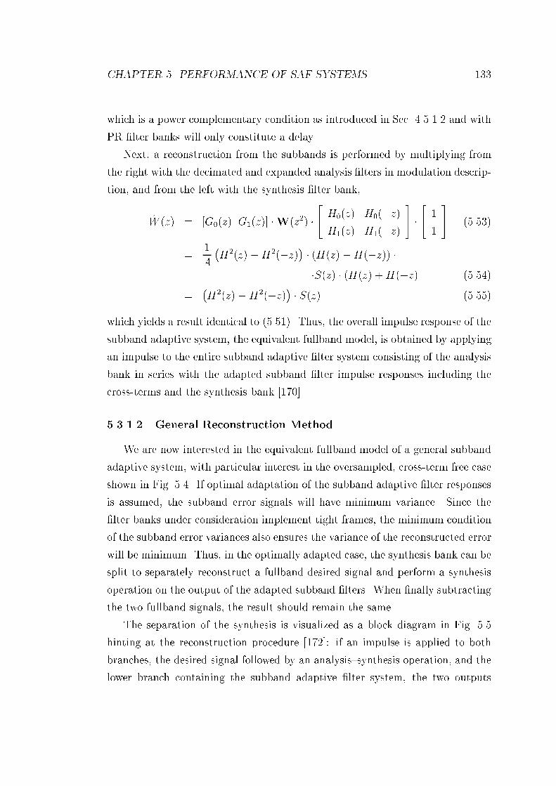
CHAPTER 5. PERFORMANCE OF SAF SYSTEMS 133which is a power complementary condition as introduced in Sec. 4.5.1.2 and withPR lter banks will only constitute a delay.Next, a reconstruction from the subbands is performed by multiplying fromthe right with the decimated and expanded analysis lters in modulation descrip-tion, and from the left with the synthesis lter bank,W (z) = [G0(z) G1(z)] W(z2) " H0(z) H0(z)H1(z) H1(z) # " 11 # (5.53)= 1A H2(z)H2(z) (H(z)H(z)) S(z) (H(z) +H(z) (5.54)= H2(z)H2(z) S(z) (5.55)which yields a result identical to (5.51). Thus, the overall impulse response of thesubband adaptive system, the equivalent fullband model, is obtained by applyingan impulse to the entire subband adaptive lter system consisting of the analysisbank in series with the adapted subband lter impulse responses including thecross-terms and the synthesis bank [170].5.3.1.2 General Reconstruction MethodWe are now interested in the equivalent fullband model of a general subbandadaptive system, with particular interest in the oversampled, cross-term free caseshown in Fig. 5.4. If optimal adaptation of the subband adaptive lter responsesis assumed, the subband error signals will have minimum variance. Since thelter banks under consideration implement tight frames, the minimum conditionof the subband error variances also ensures the variance of the reconstructed errorwill be minimum. Thus, in the optimally adapted case, the synthesis bank can besplit to separately reconstruct a fullband desired signal and perform a synthesisoperation on the output of the adapted subband lters. When nally subtractingthe two fullband signals, the result should remain the same.The separation of the synthesis is visualized as a block diagram in Fig. 5.5hinting at the reconstruction procedure [172]: if an impulse is applied to bothbranches, the desired signal followed by an analysissynthesis operation, and thelower branch containing the subband adaptive lter system, the two outputs

CHAPTER 5. PERFORMANCE OF SAF SYSTEMS 134analysis
filter
bank
bank
filter
analysis
bank
filter
unknown system
s[n]
d[n]
desired signal
inputsignal
x[n] e[n]
errorsignal
0
1
K/2-1
0
1
K/2-1
0
K/2-1
1
w
0w
1
wK/2-1
synthesis
d [n]
d [n]
d [n]
x [n]
x [n]
x [n]
e [n]
e [n]
e [n]Figure 5.4: Cross-term free subband adaptive lter system in a system identi-cation setup with an unknown system s[n].
equivalent fullband model[n] -
-analysisbankunknownsystems[n] -
--aaaa-- adaptedltersanalysisbank
--aaaa----aaaa-- synthesisbank
synthesisbank--w[n]s[n] t[n]
Figure 5.5: Separation of system identication structure for reconstruction offullband equivalent model.
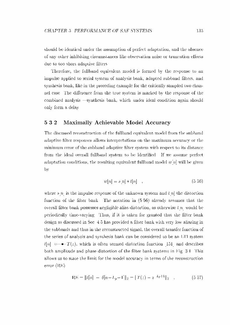
CHAPTER 5. PERFORMANCE OF SAF SYSTEMS 135should be identical under the assumption of perfect adaptation, and the absenceof any other inhibiting circumstances like observation noise or truncation eectsdue to too short adaptive lters.Therefore, the fullband equivalent model is formed by the response to animpulse applied to serial system of analysis bank, adapted subband lters, andsynthesis bank, like in the preceding example for the critically sampled two chan-nel case. The dierence from the true system is marked by the response of thecombined analysis synthesis bank, which under ideal condition again shouldonly form a delay.5.3.2 Maximally Achievable Model AccuracyThe discussed reconstruction of the fullband equivalent model from the subbandadaptive lter responses allows interpretations on the maximum accuracy or theminimum error of the subband adaptive lter system with respect to its distancefrom the ideal overall fullband system to be identied. If we assume perfectadaptation conditions, the resulting equivalent fullband model w[n] will be givenby w[n] = s[n] t[n] ; (5.56)where s[n] is the impulse response of the unknown system and t[n] the distortionfunction of the lter bank. The notation in (5.56) already assumes that theoverall lter bank possesses negligible alias distortion, as otherwise t[n] would beperiodically time-varying. Thus, if it is taken for granted that the lter bankdesign as discussed in Sec. 4.5 has provided a lter bank with very low aliasing inthe subbands and thus in the reconstructed signal, the overall transfer function ofthe series of analysis and synthesis bank can be considered to be an LTI systemt[n] | T (z), which is often termed distortion function [151] and describesboth amplitude and phase distortion of the lter bank systems in Fig. 3.1. Thisallows us to state the limit for the model accuracy in terms of the reconstructionerror (RE) RE = kt[n] [nLp+1]k2 = kT (z) zLp+1k2 ; (5.57)

CHAPTER 5. PERFORMANCE OF SAF SYSTEMS 136where k k2 indicates the l2 norm. Since T (z) is given by [151]T (z) = K1Xk=0 Hk(z) Gk(z) ; (5.58)the error measure (5.57) for model accuracy is equivalent to the deviation frompower complementarity in Sec. 4.5.1.2. If designing a prototype lter using theiterated LS method of Sec. 4.5.3, the power complementarity requirement is de-scribed by (4.93), and can therefore be used to a priori state the model accuracyas RE = kVS1S2 b dk2 : (5.59)This also describes the distortion imposed on any signal fed through the SAFsystem.The analysis presented here assumed that aliasing is suciently suppressed.Is this a reasonable and valid assumption? Sec. 5.2.1 has indicated that theminimum achievable error within the subbands is limited by the SAR, which hasbeen linked to the stopband attenuation of the employed prototype lter. Theresidual noise again causes an excess MSE, which for example with LMS typealgorithms is proportional to the MMSE and prohibits an accurate adjustmentof the subband adaptive lters. Therefore, if the error in perfect reconstructionwas considerably lower than the SAR, the error limit would still be linked to thesubband SAR. It is therefore vital to design the prototype lter such that itsstopband energy is at least as small as its deviation from perfect reconstruction.With this balance between stopband attenuation and perfect reconstruction, itis justied to swap the requirements of perfect reconstruction (PR) with powercomplementarity (PC).5.4 Simulations and ResultsSimulations presented within this section will evaluate the in uence of variousparameters in an SAF system using GDFT lter banks. Furthermore, examplesare given to underline the validity of the performance limitations calculated inSecs. 5.2 and 5.3.

CHAPTER 5. PERFORMANCE OF SAF SYSTEMS 137K=N Lp RE/[dB] SAR/[dB] p1[n] 32=28 896 -55 57 2:7 102p2[n] 32=24 960 -114 109 4:5 104p3[n] 32=20 960 -175 170 5:6 106p4[n] 32=16 896 -193 180 8:5 108Table 5.1: Filter design using the iterative LS method of Sec. 4.5.3 for K=2 = 16subbands and various decimation ratios N = 16(4)28.5.4.1 Subband ParametersThis section will evaluate how the choice of the channel number K and the dec-imation ratio N of the SAF will aect convergence. Sec. 5.4.1.1 investigates theadaptation for a xed number of subbands and a variable decimation ratio, whilein Sec. 5.4.1.2, the impact of the number of subbands will be surveyed by varyingK at a xed oversampling ratio (OSR) K=N .5.4.1.1 Oversampling RatioFilter Banks. Tab. 5.1 lists 4 prototype lters, which are designed for K=2 =16 subbands and a number of dierent decimation ratios. With these proto-type lters, subband adaptive systems operating at dierent oversampling ratios(OSR) OSR = KN 1 (5.60)can be created. For convenience, the lengths of the prototype lters have beenchosen such that polyphase implementation of the lter banks can be kept simplewith Lp being an integer multiple of lcm(K;N). Fig. 5.6 shows the resultingfrequency responses of the four prototype lters. Note that the 3 dB crossingpoint jPi(ej=16)j =p1=2, i = 1(1)4 is given through the required power comple-mentarity of the lters.

CHAPTER 5. PERFORMANCE OF SAF SYSTEMS 138
0 0.005 0.01 0.015 0.02 0.025 0.03 0.035 0.04 0.045 0.050
0.1
0.2
0.3
0.4
0.5
0.6
0.7
0.8
0.9
1
normalized frequency Ω/π
ma
gn
itu
de
|P
N(e
jΩ)|
N = 28N = 24N = 20N = 16
Figure 5.6: Frequency response of prototype lters pi[n], i = 1(1)4, for K = 32and various decimation ratios N = 16(4)28, belonging to the prototype designlisted in Tab. 5.1.Eigenvalue Spread. To analytically estimate the eigenvalue spread of the sub-band signals, the input signal to the analysis lter bank will be assumed to benormally distributed and white. Since all bandpass lters in the lter bank aremodulated versions, only a representative subband signal produced by the proto-type lter will be evaluated. An approximation of the PSD for the subband signalsomitting any spectral correlations between aliased components in the decimationstage similar to the proceeding in Sec. 5.2.2 is given by the squared magnitude ofthe prototype lter decimated by N ,Sxx(ej) Pl(ej)P l (ej) (5.61)jrxx[n] pl[n] pl[n] ; (5.62)where pl[n], l = 0(1)N1, is the lth of N polyphase components of the proto-type lter. A result of the approximation is that it does not matter which ofthe N polyphase components is picked to calculate (5.62). If N is chosen suchthat no aliasing in the subbands will occur, all N polyphase components will

CHAPTER 5. PERFORMANCE OF SAF SYSTEMS 1390 0.1 0.2 0.3 0.4 0.5 0.6 0.7 0.8 0.9 1
0
0.2
0.4
0.6
0.8
1
normalized frequency Ω/π
ma
gn
itu
de
Sxx(e
jΩ) (a)
N = 28N = 24N = 20N = 16
0 2 4 6 8 10 12 14 16 18 200
0.2
0.4
0.6
0.8
1
ranked order
eig
en
va
lue
s o
f R
xx
(b)
N = 28N = 24N = 20N = 16Figure 5.7: (a) subband PSD for lter bank with K = 32 and various decima-tion ratios N = 16(4)28; (b) eigenspectra of a 20 20 auto-correlation matrixbelonging to the curves in (a).have an identical magnitude response, but dier in their phase. However, in theauto-correlation operation, any phase information is lost, and thus all N com-ponents will yield identical results in (5.62). Fig. 5.7 shows the approximatedPSDs of a subband produced by the lowpass prototype lters in Tab. 5.1 deci-mated by the according factor N , as well as the eigenspectra, which are composedof ordered eigenvalues of a 20 20 1 auto-correlation matrix Rxx based on theauto-correlation sequence rxx[n] in (5.62), closely corresponding with the subbandPSDs.Simulations. The following simulations consist of the identication of a delayof 1000 taps using an NLMS algorithm with normalized step size ~ = 0:4. Asimple delay has been shown to be dicult to adapt to, since a delay passes allfrequencies equally and the slow convergence at the band-edges will have a main1The dimension of Rxx is likely to in uence the eigenvalue spread. Here, it has been selectedarbitarily, we are only interested in the relative dierence between dierent subband realizations.

CHAPTER 5. PERFORMANCE OF SAF SYSTEMS 140
0 1 2 3 4 5 6 7 8 9 10
x 104
−5
0
5
10
15
20
25
30
35
40
45
50
time n
ensem
ble
ER
LE
/ [dB
]
fullband N=28
N=16
Figure 5.8: ERLE curves for identication of a delay with white input signal inboth fullband and K=2 = 16 subbands produced by a complex valued GDFTmodulated lter banks with dierent decimation ratios N = f16; 20; 24; 28g.in uence on the overall adaptation behaviour [101, 88]. To enforce equal condi-tions on the subband adaptive lters despite the various aliasing levels producedby dierent lter banks in Tab. 5.1, observation noise at an SNR of 45dB is addedto the desired signal.Simulations for white Gaussian input x[n] are shown in Fig. 5.8 for a complexvalued GDFT lter banks with K=2 = 16 subbands and decimation ratios N of28, 24, 20, and 16. For comparison, the convergence curve of a fullband NLMSalgorithm for same system specications has been added. Identical simulationsusing an SSB modied GDFT lter bank for adaptation in real valued subbandsignals are shown in Fig. 5.9 for decimation ratios of N=2 = 14, 12, 10, and 8.Apparently, for both SAF systems using complex valued GDFT and real valuedSSB subband signals, the decimation ratio has no really strong eect on theconvergence, and they converge with approximately equal speed at the dierentOSRs. Compared to the fullband performance, apparently the SAFs exhibit afteran initially equally fast adaptation a slower convergence to the nal MSE, and

CHAPTER 5. PERFORMANCE OF SAF SYSTEMS 141
0 1 2 3 4 5 6 7 8 9 10
x 104
−5
0
5
10
15
20
25
30
35
40
45
50
time n
ensem
ble
ER
LE
/ [dB
]fullband N/2=14
N/2=8
Figure 5.9: ERLE curves for identication of a delay with a white input signal inreal valued subbands produced by SSB modied GDFT lter banks for decimationratios N=2 = f8; 10; 12; 14g.
0 0.1 0.2 0.3 0.4 0.5 0.6 0.7 0.8 0.9 1−50
−40
−30
−20
−10
0
10
normalized frequency Ω/π
PS
D S
xx(e
jΩ)
/ [d
B]
Figure 5.10: PSD of input signal for simulations with coloured noise.

CHAPTER 5. PERFORMANCE OF SAF SYSTEMS 142
0 1 2 3 4 5 6 7 8 9 10
x 104
−5
0
5
10
15
20
25
30
35
40
45
50
time n
ensem
ble
ER
LE
/ [dB
]
fullband
N=28
N=16
Figure 5.11: ERLE curves for identication of a delay with coloured input signalin both fullband and K=2 = 16 subbands produced by a complex valued GDFTmodulated lter banks with dierent decimation ratios N = f16; 20; 24; 28g.are still far from being completely adapted after 0:1 106 iterations. This is due tothe very high eigenvalue spread of the decomposed input signal for the SAFs,which is listed in the last column of Tab. 5.1 for the prototype lters employedfor the dierent OSRs. Also interestingly, the SSB modied GDFT system hasa considerably poorer convergence towards the nal MSE, since the PSDs ofthe subband signals posses two notches compared to one in the complex valuedsubband signals, as can be easily pictured from Fig. 4.10. No explanation has yetbeen found for the \bumps" of slow convergence appearing in the learning curveswith increasing OSR.The same simulations are repeated using a coloured input signal with aPSD shown in Fig. 5.10. Simulation results for SAF systems using GDFT andSSB modied GDFT lter banks with dierent oversampling ratios are given inFigs. 5.11 and 5.12. Remarkably, while the fullband NLMS algorithm is nowseverly slowed down, the convergence characteristics for SAF have hardly changedcompared to the white noise excitation in Figs. 5.8 and 5.9, since the spectrum

CHAPTER 5. PERFORMANCE OF SAF SYSTEMS 143
0 1 2 3 4 5 6 7 8 9 10
x 104
−5
0
5
10
15
20
25
30
35
40
45
50
time n
ensem
ble
ER
LE
/ [dB
]
fullband
N/2=14
N/2=8
Figure 5.12: ERLE curves for identication of a delay with coloured input sig-nal in real valued subbands produced by SSB modied GDFT lter banks fordecimation ratios N=2 = f8; 10; 12; 14g. = [0; ] is divided into 16 intervals, thus reducing the relative dierence betweenextrema of the PSD in each band.Concluding, the subband approach appears reasonably competitive for thewhite noise excitation case, where it maintains speed through shorter adaptivelters in the subbands, and gives great benet for adaptation for coloured noiseinput. The relative insensitivity of the SAF to the OSR suggests that lowerlter order at low OSR is traded o against longer lters, higher update rates,and higher eigenvalue spread at higher OSR, with a very slight convergence speedadvantage for decimation ratios close to the critical rate. This allows us to choosethe OSR of an SAF based on the criterion of computational complexity, as lowOSRs will allow for more ecient implementations.5.4.1.2 Number of SubbandsIn the previous section, the decimation ratio was varied for a xed number ofsubbands. Now the interest in on how the number of subbands K=2 in uences

CHAPTER 5. PERFORMANCE OF SAF SYSTEMS 144
0 1 2 3 4 5 6 7 8 9 10
x 104
−5
0
5
10
15
20
25
30
35
40
45
50
time n
ensem
ble
ER
LE
/ [dB
]
fullband
K/2=4,8 K/2=16
Figure 5.13: ERLE curves for identication of a delay with white input signal insubbands produced by complex valued GDFT lter banks for dierent numberof subbands K=2 = f4; 8; 16gconvergence, which will be performed at a xed OSR K=N = 8=7 for dierentvalues of K. Simulations for the identication of a delay of 1000 samples by SAFsusing complex GDFT lter banks are given for white input signal in Fig. 5.13and for coloured input in Fig. 5.14 with a PSD drawn in Fig. 5.10, in comparisonwith a fullband adaptive NLMS algorithm.For the broadband noise simulation in Fig. 5.13, the SAF learning curvesmigrate towards the fullband behaviour as the number of subbands is lowered.The subbands of the dierent systems will have similar eigenvalue spread sincethe OSR is constant, however the reduced adaptive lter length for the highernumber of subbands seems not to completely compensate for the slower algorith-mic convergence due to the lower update rate. With coloured noise excitation inFig. 5.14, the SAF systems with K=2 = 8 and 16 subbands perform almost identi-cal to the case of white noise excitation in Fig. 5.13, since they seem to provide asucient separation of the coloured input spectrum to balance convergence. Theopposite appears to be true for the case K=2 = 4 which now falls back behind
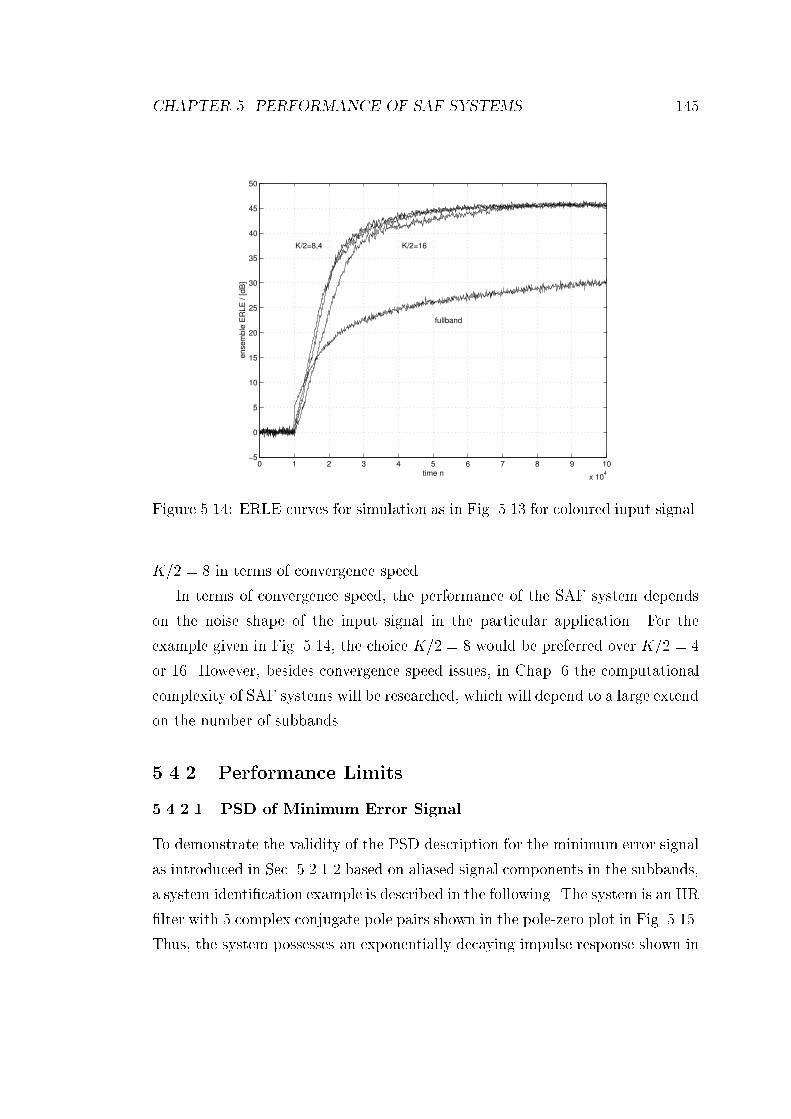
CHAPTER 5. PERFORMANCE OF SAF SYSTEMS 145
0 1 2 3 4 5 6 7 8 9 10
x 104
−5
0
5
10
15
20
25
30
35
40
45
50
time n
ensem
ble
ER
LE
/ [dB
]
fullband
K/2=8,4 K/2=16
Figure 5.14: ERLE curves for simulation as in Fig. 5.13 for coloured input signal.K=2 = 8 in terms of convergence speed.In terms of convergence speed, the performance of the SAF system dependson the noise shape of the input signal in the particular application. For theexample given in Fig. 5.14, the choice K=2 = 8 would be preferred over K=2 = 4or 16. However, besides convergence speed issues, in Chap. 6 the computationalcomplexity of SAF systems will be researched, which will depend to a large extendon the number of subbands.5.4.2 Performance Limits5.4.2.1 PSD of Minimum Error SignalTo demonstrate the validity of the PSD description for the minimum error signalas introduced in Sec. 5.2.1.2 based on aliased signal components in the subbands,a system identication example is described in the following. The system is an IIRlter with 5 complex conjugate pole pairs shown in the pole-zero plot in Fig. 5.15.Thus, the system possesses an exponentially decaying impulse response shown in

CHAPTER 5. PERFORMANCE OF SAF SYSTEMS 146
−1 −0.5 0 0.5 1
−1
−0.5
0
0.5
1
z−plane
Rez
Imz
Figure 5.15: Pole-zero plot of the unknown system used for system identication;poles are marked by \".Fig. 5.16, which slowly drops in power at a rate of approximately 40dB / 1000samples. This slow decay is due to two pole pairs sitting in close proximity of theunit circle. To exclude other error sources, correct lter lengths for the subbandadaptive lter was ensured, and no observation noise was added.Example 1. For identication, a decomposition into K=2 = 8 subbands deci-mated by N = 14 is used to perform subband adaptive ltering using an NLMSalgorithm with step size ~ = 0:8. Since one of the poles lies exactly at a bandedge, the convergence exhibits a very slow mode [101] and only after half a millioniterations, the algorithm appears to be almost completely adapted, as the MSEcurve in Fig. 5.17 illustrates. A number of PSDs of the error signal have beencalculated in Fig. 5.18 over time intervals in which the error was assumed station-ary. The solid upper line marks the PSD of the error signal before adaptation isswitched on at time n = 10000, which also represents the magnitude response ofthe unknown system, since it is excited by white noise of unit variance. More PSDsamples of the measured error signal have been evaluated over a time window of40 103 samples at n = 0:2 106, n = 0:3 106, and n = 0:5 106. Clearly, while theerror's energy at the band edges (marked in Fig. 5.18 by dashed vertical lines) isfurther reduced with each PSD sample, some spectral peaks remain unaected.Fig. 5.19 give a comparison between the PSD of the reconstructed fullbanderror signal of the SAF and a prediction of the residual error PSD based on

CHAPTER 5. PERFORMANCE OF SAF SYSTEMS 147
0 100 200 300 400 500 600 700 800 900 1000−0.2
−0.1
0
0.1
0.2
time n
impuls
e r
esponse s
[n]
(a)
0 0.1 0.2 0.3 0.4 0.5 0.6 0.7 0.8 0.9 1−40
−30
−20
−10
0
10
20
normalized frequency Ω/π
magnitude |S
(ejΩ
)| / [dB
]
(b)
Figure 5.16: (a) Impulse response and (b) magnitude response of the unknownsystem.
0 0.5 1 1.5 2 2.5 3 3.5 4 4.5 5
x 105
−60
−50
−40
−30
−20
−10
0
10
time n
ensem
ble
MS
E / [dB
]
Figure 5.17: Reconstructed fullband MSE of an SAF identifying the unknownsystem characterized in Figs. 5.15 and 5.16.
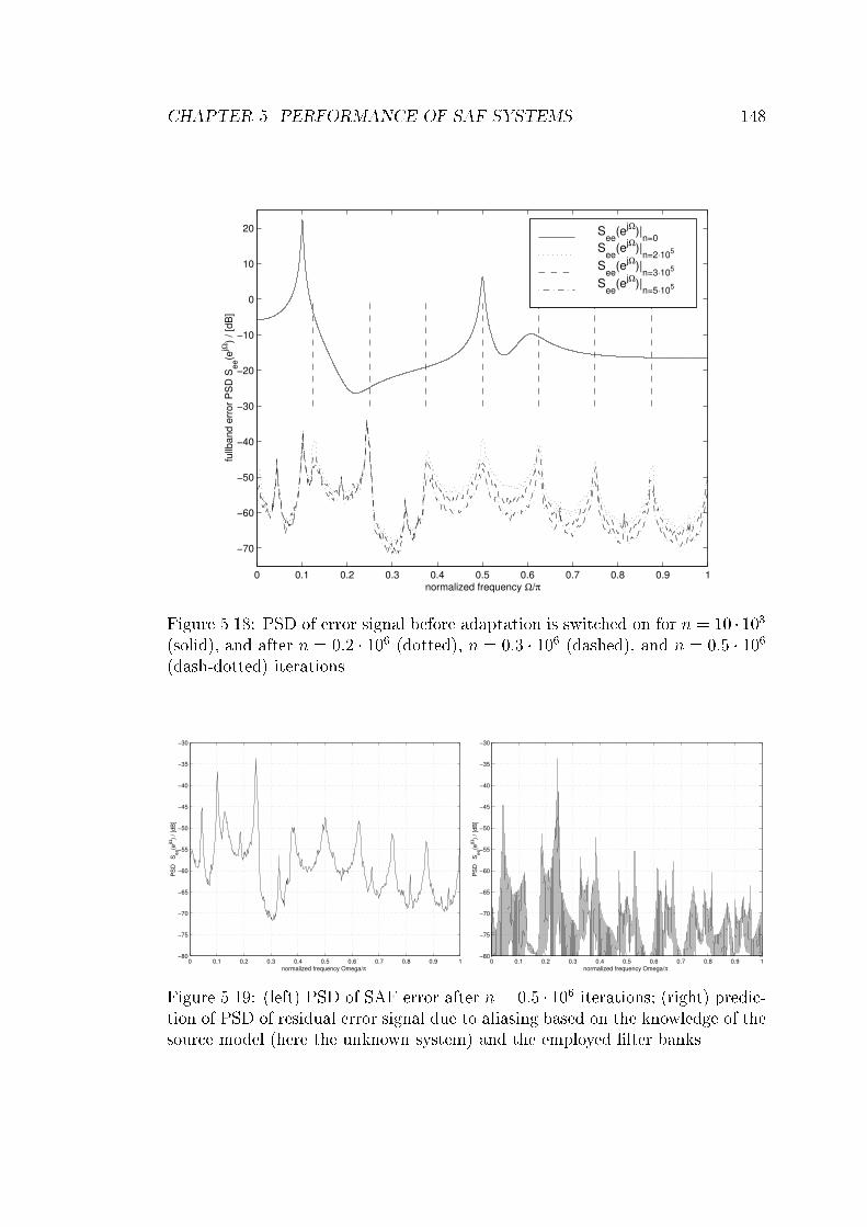
CHAPTER 5. PERFORMANCE OF SAF SYSTEMS 148
0 0.1 0.2 0.3 0.4 0.5 0.6 0.7 0.8 0.9 1
−70
−60
−50
−40
−30
−20
−10
0
10
20
normalized frequency Ω/π
fullb
an
d e
rro
r P
SD
See(e
jΩ)
/ [d
B]
See
(ejΩ
)|n=0
See
(ejΩ
)|n=2⋅10
5
See
(ejΩ
)|n=3⋅10
5
See
(ejΩ
)|n=5⋅10
5
Figure 5.18: PSD of error signal before adaptation is switched on for n = 10 103(solid), and after n = 0:2 106 (dotted), n = 0:3 106 (dashed), and n = 0:5 106(dash-dotted) iterations.
0 0.1 0.2 0.3 0.4 0.5 0.6 0.7 0.8 0.9 1−80
−75
−70
−65
−60
−55
−50
−45
−40
−35
−30
normalized frequency Omega/π
PS
D
Se
e(e
jΩ)
/ [d
B]
0 0.1 0.2 0.3 0.4 0.5 0.6 0.7 0.8 0.9 1−80
−75
−70
−65
−60
−55
−50
−45
−40
−35
−30
normalized frequency Omega/π
PS
D
Se
e(e
jΩ)
/ [d
B]
Figure 5.19: (left) PSD of SAF error after n = 0:5 106 iterations; (right) predic-tion of PSD of residual error signal due to aliasing based on the knowledge of thesource model (here the unknown system) and the employed lter banks.

CHAPTER 5. PERFORMANCE OF SAF SYSTEMS 149
0 0.1 0.2 0.3 0.4 0.5 0.6 0.7 0.8 0.9 1−80
−75
−70
−65
−60
−55
−50
−45
−40
−35
−30
normalized frequency Omega/π
PS
D
Se
e(e
jΩ)
/ [d
B]
Figure 5.20: Predicted residual error PSD (solid) overlaid with the true errorPSD measured after n = 0:5 106 iterations.aliased components in the subband signals. This prediction has been calcu-lated by approximating the equations presented in Sec. 5.2.1.3 with DFTs of thesource model, analysis and synthesis lters. The peaks in this spectrum representaliased components of the input signal caused by the resonances at = 0:1 and = 0:5. Fig. 5.20 shows both curves overlaid, and it can be appreciated thatthe measured PSD forms an envelope of the predicted lower error PSD boundover large spectral intervals. Deviations occur at the band edges, and for thefrequencies = 0:1 and = 0:5, where the original peaks of the uncancellederror signal resided. This insucient adaptation of the error can be justied bythe slow convergence properties at band edges [101] and by the fact that the errorpower is dominated by the aliased peak at = 0:1+ 2N 0:24, and minimizingthe rest of the spectrum will not greatly contribute to a lowering of the MSE.Example 2. A second example demonstrates the prediction of the residual errorPSD for a system identication set-up with coloured input signals as shown inFig. 5.10. The system to be identied is identical to the one used in the previousexample, apart from the strong pole originally at the band-edge = 0:5 now

CHAPTER 5. PERFORMANCE OF SAF SYSTEMS 150
0 0.1 0.2 0.3 0.4 0.5 0.6 0.7 0.8 0.9 1−100
−80
−60
−40
−20
0
20
normalized frequency Ω/π
PS
Ds
Se
e(e
jΩ),
Sd
d(e
jΩ)
/ [
dB
]
PSD of desired signalPSD of final error signal
Figure 5.21: PSD of error signal before and after adaptation, using an unknownsystem with 5 poles and coloured input signal.sitting at an angle of = 0:45. Again, the SAF set-up uses a modulated GDFTlter bank withK=2 = 8 subbands, decimation by N = 14, and NLMS algorithmswith ~ = 0:8 operating in the subbands. Fig. 5.21 shows the measured PSDs ofthe error signal before and after adaptation (n = 0:2 106). The prediction of theresidual error PSD used a source model consisting of the unknown system andthe noise shaping lter producing the PSD of the input signal as in Fig. 5.10.The result is overlaid with the measured PSD in Fig. 5.22, and obviously tsvery well as a lower bound. As one pole has been moved from the band edgeto the center position of the 3rd subband, the adaptation is more accurate aftershorter time than in the previous example, and the error signal contains lessuncancelled energy at the band edges and the strong original peaks at = 0:1and = 0:45.5.4.2.2 Performance MeasuresPerformance limitations of SAF systems closely related to the lter design param-eters of power complementarity and stopband attenuation have been derived in

CHAPTER 5. PERFORMANCE OF SAF SYSTEMS 151
0 0.1 0.2 0.3 0.4 0.5 0.6 0.7 0.8 0.9 1−100
−90
−80
−70
−60
−50
−40
normalized frequency Ω/π
PS
D
Se
e(e
jΩ)
/ [d
B]
predicted PSD of residual error measured error PSD after adaptation
Figure 5.22: Comparison between the predicted PSD of the minimum error andthe measured error PSD for coloured input signal.Secs. 5.2.2 and 5.3.2. To test for validity, a number of prototype lters have beendesigned using the iterative LS design of Sec. 4.5.3 for the application in SAF sys-tems with K=2 = 8 subbands and decimation by N = 12, but dierent weighting between the conditions of power complementarity and stopband attenuation.The resulting measures of perfect reconstruction (RE) and signal-to-alias ratio(SAR) according to (4.71) and (4.96) three dierent -designs with a lter lengthof Lp = 192 taps are shown in Tab. 5.2.The unknown system was set to be a simple delay, and identication with awhite Gaussian input signal used an RLS algorithm for adaptation of the SAFwith a forgetting factor = 0:9995. The RLS was here preferred over LMS-type algorithms to avoid slow convergence due to the coloured nature of thesubband signals introduced by the analysis lter bank. Tab. 5.2 displays in itstwo right columns the noise reduction, i.e. the dierence between the variancesof the uncancelled and adapted error signal, and the error of the reconstructedequivalent fullband model with respect to the delay to be identied. Apparentlyfor all three designs, both quantities match very closely with the measures derivedfrom the prototype lter, and can therefore be well used for predicting the MMSE

CHAPTER 5. PERFORMANCE OF SAF SYSTEMS 152Prototype Design Simulation Results10 log10( ) RE/dB SAR/dB 10 log10(kwsk22) 10 log10(2dd=2ee)0 -54.0821 55.6 -54.0153 54.030 -34.6191 65.2 -34.6143 66.260 -18.0016 77.8 -18.0010 78.5Table 5.2: Predicted fullband model error and nal MSE compared to simulationresults (all quantities in [dB]).performance of the implemented SAF system.For the more complex simulations presented in Sec. 5.4.2.1, the noise reductionvalues attained by the SAF systems were measured to be -53.93dB for example1 as shown in Fig. 5.17, and -56.73dB for example 2, for which the PSDs ofuncancelled and cancelled error signal are given in Fig. 5.21. The characteristicsof the prototype lter p[n] used for the decomposition into K=2 = 8 subbandsand decimation by N = 14 | contained in Tab. 4.3 as design (d) | exhibit anSAR value -57.01dB calculated according to (4.71). This very closely agrees withthe measured noise reduction for the system identication in example 2, whichused a very long impulse response as the unknown system and a coloured inputsignal. For example 1, the discrepancy between the SAR value of the prototypelter and the noise reduction of -53.93dB can be explained by the SAF not beingcompletely adapted after 0:5 106 iterations, which is indicated in Fig. 5.18 bythe remaining energy in the PSD at the band edges.5.5 Concluding RemarksA number of performance characteristics of subband adaptive lter systems havebeen addressed in this chapter. The main aspects were focused on the convergencebehaviour of the SAF set-up, and the performance limitations in the MMSEbehaviour.For the minimum error performance of SAF, the analysis of aliased signal

CHAPTER 5. PERFORMANCE OF SAF SYSTEMS 153components has been used to calculate the limits for the power spectral densityof the minimum error signal, based on the knowledge of a source model and thecharacteristics of the analysis and synthesis lter bank. Approximations havebeen derived for the MMSE in both subbands and fullband, which have beenlinked to the stopband attenuation of the prototype lter of the lter bank. Theequivalent fullband model, i.e. the impulse response of the overall SAF systemconsisting of analysis lter bank, subband adaptive lters, and synthesis lterbank, has been shown to be limited in its accuracy by the reconstruction error ofthe employed lter banks.The calculated or estimated performance limitation on MMSE and fullbandequivalent model have been veried by simulation, which agree well with the twodesign criteria of the prototype lter, stopband attenuation and reconstructionerror. Although these measures have specically addressed GDFT modulatedlter banks, similar derivation can be made for other lter bank types. Theappeal lies in the fact that these measures provide convenient tools to design lterbanks for SAF systems fullling pre-specied performance limits [172]. Thus, forapplications like acoustic echo control, where the adaptation error is the mostimportant issue, the banks can be designed to be just good (and short) enoughto satisfy relaxed constraints on the model error.Concerning convergence speed, several in uencing factors have been addres-sed, including the lter length of the adaptive lter, the update rate, and theeigenvalue spread of the subband decomposition of the input signal. The eectof varying the oversampling ratio and the number of subbands was highlighted ina number of simulations. Results from these simulations suggest that the OSRhas a minor in uence on the convergence speed, while the number of subbandsis governed by an optimal trade-o between the spectral separation for colouredPSD of the input signal, and the reduced update rate and SAF lter lengthprevalent with higher channel numbers K for constant OSR. Generally comparedto a fullband adaptive solution, the convergence speed slowed down particularlywhen approaching the MMSE, but was considerably enhanced for coloured inputsignals.As lowering the OSR has hardly any in uence | and if at all, it appears to

CHAPTER 5. PERFORMANCE OF SAF SYSTEMS 154be a positive one | on the convergence speed, but does greatly reduce the com-putational complexity of the implemented system due to the reduced adaptivelter length and lower update rate of all involved lters, it appears sensible torun the SAF system at the lowest possible rate, i.e. using an oversampling ratioclose to one. Since the demand for an ecient implementation also includes themaximum exploitation of computational saving in the lter bank implementa-tion, we nally come back to the GDFT lter banks presented in Chap. 4 whenassessing the complexity of the overall SAF system and comparing it to otherimplementations in the following chapter.

Chapter 6Variable Tap-Proles ForSubband Adaptive FiltersThe subband adaptive ltering approach allows a selection of a dierent set ofalgorithmic parameters for each subband. While in the past section this hasbeen exploited to choose dierent convergence parameters to increase the overallconvergence speed, here we will discuss methods to vary the lter lengths of thedierent adaptive lters in an SAF system. We rst introduce the underlying ideaand review related work in Sec. 6.1. Sec. 6.2 analyses the potential benets andalso gives an insight and comparison into the computational savings achievablewith dierent subband approaches. Two algorithms for variable lter tap-proleare presented in Sec. 6.3. Finally, Sec. 6.4 discusses some simulations and results.6.1 Idea and Background6.1.1 MotivationFor the identication of long impulse responses, such as found in acoustic echocontrol problems, the achievable model is often a truncated representation dueto the computational limitation of the digital signal processor (DSP) on whichan adaptive system is implemented. As a solution to reduce the computationalcomplexity, the subband adaptive approach has been discussed in Chap. 3. Amethod to further enhance the ecient use of computational resources on a DSP155

CHAPTER 6. Variable Tap-Proles for SAF 1567
6
5
4
3
2
1
0
subban
ds
k
time n
-50dB -60dB-40dBnorm
aliz
ed f
requen
cyΩ
π
0
7
6
5
4
3
2
1
0
subban
ds
k
time n
-60dBnorm
aliz
ed f
requen
cyΩ
π
0
-50dB-40dB(a) (b)Figure 6.1: (a) uniform and (b) optimized tap-prole for an SAF with K=2 = 8subbands, with decay levels for the power of the unknown system; the under-laidshaded areas represent the equivalent lengths of the subband lters with respectto the fullband.is by introducing a variable tap-prole subband adaptive system, whereby com-putational resources can be dynamically allocated to subbands where they arerequired. If the unknown system to be identied is spectrally unbalanced or theinvolved signals are coloured, this approach can be advantageous.Fig. 6.1 shows three decay levels of the spectral power belonging to the spec-trogram of some unknown system. In many applications, this decay is spectrallyunbalanced, as for example in room acoustics low frequencies generally reverber-ate longer due to frequency dependent absorption by the walls. If such a spectrallyunbalanced system is to be identied by an SAF system, and each subband hasan adaptive lter of equal length (as indicated in Fig. 6.1(a)), the resulting full-band model error will be dominated by the subband whose lter length is shortestcompared to the unknown system's decay time in that frequency band. As anexample, in Fig. 6.1(a)), the band k = 0 would be mainly responsible for themagnitude of the nal modelling error after adaptation. Fig. 6.1(b) shows anoptimization of the tap-prole | i.e. the lengths of the dierent SAFs | suchthat with the same overall number of coecients the SAF system will actuallyhave improved performance, since the remaining truncation errors in the dierentsubbands are approximately equalized.The optimization of the tap-prole of an SAF system can therefore by viewedas the task to exploit the resources of a DSP with a given computational bench-mark to achieve an enhanced overall performance. The author's idea was based

CHAPTER 6. Variable Tap-Proles for SAF 157on subband ADPCM, where signals are decomposed and dierently quantized ineach frequency band. From a xed pool of bits, each band is allocated a dier-ent bit resolution depending on the relative signal energy within that band, thusincreasing the signal quality at a xed bit rate of transmission. Transfered tothe SAF problem, more computations and thus longer lters can be dedicated tosubbands with a high error power, while coecients are withdrawn from thosewith low power. Thus, balancing the dierent subband errors can help to achievea minimization of a global (fullband) error, as will be derived in Sec. 6.3.6.1.2 Approaches and MethodsThe idea of tap-prole optimization is not new. Dierent approaches can be foundin the literature and will be discussed in the following, whereby we rst look intoschemes calculating an approximate optimum prole prior to start running theSAF system. Finally, adaptive solutions will be reviewed.6.1.2.1 A Priori OptimizationThe approach illustrated in Fig. 6.1 is performed in [1], which describes theimplementation of a commercial AEC system. Based on the measured energydecay of an impulse in two representative rooms, the lter lengths of the SAFsare set to a pre-specied tap-prole [1, 2]. Work presented in [34] not only takesspectrally unbalanced room impulse responses into account, but also considersthe spectral shape of speech and the characteristics of the human ear to derivean LS solution for a xed optimum tap-prole.6.1.2.2 Adaptive SchemesTo achieve and maintain approximate optimality of the SAF system duringoperation in order to track changes and to be able to take set-ups in dierentenvironments into account, the tap-prole can be varied adaptively. The originalSAF system is then ammended by a second adjustment algorithm as shown inFig.6.2, which will try to balance the subband errors. This idea was rst presentedin [91] and referred to as automatic tap-assignment. The exchange of coecients

CHAPTER 6. Variable Tap-Proles for SAF 158
analysis
filter
bank
bank
filter
analysis
unknown system
s[n]
d[n]
desired signal
inputsignal
x[n]
0
1
0
K/2-1
1
w
0w
1
wK/2-1
d [n]
d [n]
d [n]
x [n]
x [n]
signalerror
e[n]
synthesis
filter
bank
e [n]0
e [n]1
e [n]K/2-1
x [n]K/2-1
tap profile adaptationFigure 6.2: Subband adaptive lter system with adaptive adjustment of the tap-prole.

CHAPTER 6. Variable Tap-Proles for SAF 159between two lters in undecimated subbands was performed based on a criteriondependent on the subband error signals only. Modications of this tap-assignmentalgorithm are presented in [143, 144], which perform a tap-allocation based ona mixed criterion of the input signal and the trailing coecients of the impulseresponses of the SAFs. A general theory on both the methods by [91] and [143,144] will be developed in Sec 6.3. The work in [158] extends the ideas in [91, 143]by the inclusion of perceptual criteria based on the human ear similar to the apriori optimization by [34].The benet of yielding a lower model truncation error with tap-prole adapta-tion over standard subband or fullband adaptive ltering is demonstrated in [170],which also describes a simplied criterion over [143]. The experimentation usescritically decimated lter banks with cross-terms according to [54], but with asuboptimal lter bank implementation. A generalization of the global error mini-mization presented in [170] is performed in [162] to include tap-prole adaptationin oversampled non-uniform subbands [71, 69] as depicted in Fig. 3.20. Both ap-proaches in [170] and [162] are somewhat tedious, the rst through the necessaryinclusion of cross-terms, the latter through various subsampling ratios in dierentsubbands and the resulting subband-dependent computational cost and fullbandtime-representation of coecients, which requires inconvenient exchange rates1for shifting lter taps between subbands.6.2 Equivalent Fullband Model Length andComplexityIn the following, we will motivate the variable tap-prole approach by comparinga fullband adaptive lter with a number of dierent SAF systems based on thecritically decimated [54], and the oversampled GDFT and SSB modied GDFTlter banks [167] presented in Chap. 4. First, the resulting complexities basedon constant equivalent fullband model length will be evaluated in Sec. 6.2.1. InSec. 6.2.2, the problem will reversed, and we ask for the fullband model length1in ECU | equal complexity units [162]

CHAPTER 6. Variable Tap-Proles for SAF 160based on an implementation with a xed number of computations, as, for exam-ple, given when implementing SAF systems on a DSP.6.2.1 Complexity Based on Constant Equivalent FullbandModel LengthAlthough generally any adaptive ltering algorithm can be employed, for thefollowing analysis and examples, the complexity of the NLMS algorithm will beused. The linear order of complexity creates an interesting case since real andcomplex subband processing costs are approximately the same, as derived inSec. 4.4.6.2.1.1 Computational CostFor a general SAF system as depicted in Fig. 6.2, the computational cost consistsof three lter bank operations and the ltering and update procedures in thesubbands. Concerning the subband adaptive lters, we want to look at twoextrema for the tap-prole: uniform tap-prole, where all subband lters have equal length2; concentrated tap-prole, where all computations are dedicated to one singlesubband.Let us rst consider the uniform case. A practical relation between the length ofthe equivalent fullband model L(f)a and the length of the SAF length La has beenderived in Sec. 5.3.1, where the superscript (f) refers to the fullband samplingrate. Therefore, the length of the subband adaptive lters can be calculatedaccording to (5.3) as La = L(f)a + 2LpN ; (6.1)which accounts for the transients in the subband domain caused by the lterbanks. Including the lter bank operation, the total computational costs for SAF2The restriction to uniform lter banks ensures that the fullband time representation of eachlter is equal. For similar considerations for SAF in non-uniform subbands with a number ofdierent decimation ratios, please see [162].

CHAPTER 6. Variable Tap-Proles for SAF 161systems with real input can be stated for oversampled GDFT modulated complexlter banks asCGDFTtot = 1N (3 (4K log2K + 4K + Lp) + 4K2 2L(f)a + 2LpN + 3!) (6.2)real multiplication per fullband period, where the lter bank cost is given by(4.50), K=2 is the number of subbands decimated by N , and Lp the length of theprototype lter. For an SAF employing SSB modied GDFT lter banks, whosecomputational complexity is given by (4.65), processing in real valued subbandsamounts to a total cost ofCSSBtot = 2N (3 (4K log2K + 5K + Lp) + K2 2L(f)a + 2LpN=2 + 3!) (6.3)real valued multiplications.For comparison, the total computational cost for an NLMS subband adaptivelter operating in critically decimated subbands produced by DCT modulatedlter banks, which requires using the structure suggested in [53, 54], is given byCDCTtot = 2K(3 (4K log2K + 4K + Lp| z Cbank ) + K2 2L(f)a + 2LpK=2 + 3| z adaptive main terms ++ (K 2)23 L(f)a + 2LpK=2 + 3| z adaptive cross terms + (K 2)2Lp 1K=2 | z xed cross terms ): (6.4)This assumes that cosine modulated lter banks have been used, and have beencalculated using an ecient polyphase structure almost identical to the one foroversampled SSB modied GDFT lter banks discussed in Chap. 4. It is easy torealize that the additional modulation for the SSB modication is not required,since the subband spectra are already aligned. The subband dependent phaseshift =4 can be incorporated into the phase correcting matrix D1 in (4.43).Thus only a real operation is performed (at no cost) on the output of a GDFTlter bank with decimation by K=2. The cost for the SAF consists of threecontributions in (6.4): the adaptive main terms in each of the K=2 subbands,and K2 cross-terms, which can be split into a xed and an adaptive part as

CHAPTER 6. Variable Tap-Proles for SAF 162discussed in Sec. 3.4.2.1 (Fig. 3.14). The adaptive cross-terms are set to one thirdof the length of the main adaptive subband lters3, as hinted in [54]To obtain the total cost for a concentrated tap-prole, i.e. SAF is only per-formed within one single subband, the factor K=2 in the adaptive terms of (6.2)(6.4) is omitted.6.2.1.2 Example and ComparisonFig. 6.3 shows the total cost CGDFTtot derived in (6.2) for an SAF system usingoversampled GDFT lter banks relative to the cost of a fullband implementationof the NLMS, yielding C(f) = 2L(f)a +3. For four dierent lengths of the fullbandequivalent model L(f)a , the graphs indicate the cost ratio as a function of thenumber of subbands, K=2, of the specic subband implementation with a constantOSR = 8=7 1:14. As a rule of thumb, the length Lp of the prototype lter wasset to Lp(K) = 16 K, a realistic value for real-time AEC applications [137],which yields an approximately constant lter quality for variable K and constantOSR when using the iterative LS design introduced in Sec. 4.5.3.The cost ratios plotted in Fig. 6.3 illustrate how the computational savingsinitially rise with the number of subbands K=2, until for large K=2 most of thecomputations are used for the required lter bank operations, and the cost reduc-tion levels out and would even recede for very large numbers of subbands. Fora exible tap-prole as indicated in Fig. 6.1, the pair of curves for uniform andconcentrated tap distribution form the margins in between which the true costreduction with a variable tap-prole will lie. As an example, using an implemen-tation withK=2 = 32 subbands, the computational cost is reduced to 5% (10%) ofthe fullband implementation for the given response lengths of 16000(2000) taps,assuming a uniform tap-prole. For a concentrated tap-prole, this cost ratiowould be down to 1%(7%) of the cost for a fullband implementation.For an SAF system employing SSB modied oversampled GDFT lter banksfor real valued subband processing, Fig. 6.4 shows cost curves according to (6.3)for identical conditions to the previous complex subband processing example in3Experiments in [88] show that system identication problems, where the unknown systemshave poles at band-edges, 1=3 of the adaptive main term's length is not sucient. Thus, for ahigh performance system, the cost may be higher than shown here.

CHAPTER 6. Variable Tap-Proles for SAF 163
100
101
102
10−2
10−1
100
number of subbands K/2
red
uctio
n in
co
mp
lexity c
om
pa
red
to
fu
llba
nd
L = 2000L = 4000L = 8000L = 16000
Figure 6.3: Relative cost CGDFTtot =C(f) as a function of the number of subbandsK=2 for various given lengths L(f)a of the equivalent fullband model and uniform() and concentrated () tap-proles.Fig. 6.3. As discussed in Sec. 4.4, the cost for the actual subband processingis identical, however the lter bank operation requires approximately twice thenumber of multiplications. Therefore, the curves behave similarly to Fig. 6.3whenever the cost for lter bank operations is small relative to the computationalcost of the subband processing, i.e. for small channel numbers K=2 and very longresponse lengths L(f)a . Otherwise, SAF systems using GDFT lter banks andcomplex arithmetic are clearly advantageous.Fig. 6.5 displays the cost ratios achievable when critically sampled lter banksare used, yielding the computational complexity derived in (6.4). Compared tothe previous SSB example, the higher decimation ratio of K=2 clearly cannotcompensate for the cost introduced by the required cross-terms, and the costperformance is generally worse than for the SSB case in Fig. 6.4, and far behindthe cost reduction achieved for the GDFT case in Fig. 6.3.

CHAPTER 6. Variable Tap-Proles for SAF 164
100
101
102
10−2
10−1
100
number of subbands K/2
red
uctio
n in
co
mp
lexity c
om
pa
red
to
fu
llba
nd
L = 2000L = 4000L = 8000L = 16000
Figure 6.4: Relative cost CSSBtot =C(f) as a function of the number of subbands K=2for various given lengths L(f)a of the equivalent fullband model and uniform ()and concentrated () tap-proles.
100
101
102
10−2
10−1
100
number of subbands K/2
red
uctio
n in
co
mp
lexity c
om
pa
red
to
fu
llba
nd
L = 2000L = 4000L = 8000L = 16000
Figure 6.5: Relative cost CDCTtot =C(f) as a function of the number of subbandsK=2 for various given lengths L(f)a of the equivalent fullband model and uniform() and concentrated () tap-proles.

CHAPTER 6. Variable Tap-Proles for SAF 1656.2.2 Equivalent Fullband Model Length Based on Con-stant ComplexityAn interesting case arises when (6.2) (6.4) are solved for the equivalent fullbandmodel length L(f)a in dependency of the overall computational cost. Thus, for axed number of computations, which are for example given by the benchmarkperformance of a specic DSP chip, it is possible to predict which model length theoverall SAF system is capable to provide for dierent subband implementations(oversampled GDFT, oversampled SSB modied GDFT, and critically sampledcosine modulated lter bank) and a variable number of subbands K=2.For SAF systems with complex subbands produced by GDFT lter banks,the fullband equivalent model length in dependency of the available number ofcomputations Ctot can be derived from (6.2) by rearrangement. In Fig. 6.6,these equivalent fullband lengths are depicted relative to the length of an NLMSimplementation in the fullband with L = (Ctot 3)=2. As in Sec. 6.2.1, it isdistinguished between the two cases of \uniform" and \concentrated" tap-prole.Thus, for a given benchmark performance Ctot and a variable tap-prole, the trueincrease in the fullband model length will lie between these two marginal casesindicated in Fig. 6.6.Fig. 6.7 shows the same curves for a real valued SAF system using SSB modi-ed GDFT lter banks. Clearly noticeable, the groups of curves are wider spreadand the increase in model length for low benchmarks Ctot is not as good comparedto Fig. 6.6. This is again due to the doubled cost of the lter bank operation,which has a stronger in uence if the complexity for the subband processing israther low.The relative increase in model length for a real valued SAF system based oncritically decimated cosine modulated subbands is illustrated in Fig. 6.8. Dueto the number of computations required for the cross-terms, the resulting gainin lter length is not only further spread for the dierent given computationalcomplexities Ctot, but also drops for a high number of subbands K=2. The ex-planation is that the lter bank operations become so costly for high K=2, thatthere is hardly any computational power left to perform the subband processing.A similar behaviour could be demonstrated for the curves depicted in in Fig. 6.6

CHAPTER 6. Variable Tap-Proles for SAF 166
100
101
102
100
101
102
103
104
number of subbands K/2
rela
tive
le
ng
th o
f e
qu
iva
len
t fu
llba
nd
mo
de
l
C = 800C = 1000C = 1500C = 5000
Figure 6.6: Relative equivalent fullband model length L(f)a =L of an SAF systemwith GDFT modulated lter banks as a function of the given total complexityCtot and the number of subbands K=2 for () and concentrated () tap-proles.
100
101
102
100
101
102
103
104
number of subbands K/2
rela
tive length
of equiv
ale
nt fu
llband m
odel
C = 800C = 1000C = 1500C = 5000
Figure 6.7: Relative equivalent fullband model length L(f)a =L of an SAF systemwith SSB modied GDFT modulated lter banks as a function of the given totalcomplexity Ctot and the number of subbands K=2 for () and concentrated ()tap-proles.

CHAPTER 6. Variable Tap-Proles for SAF 167
100
101
102
100
101
102
103
104
number of subbands K/2
rela
tive length
of equiv
ale
nt fu
llband m
odel
C = 800C = 1000C = 1500C = 5000
Figure 6.8: Relative equivalent fullband model length L(f)a =L of an SAF systemwith critically sampled cosine modulated lter banks as a function of the giventotal complexity Ctot and the number of subbands K=2 for () and concentrated() tap-proles.and in Fig. 6.7, if only the K=2 was selected to be high enough.The examples given here used an NLMS algorithm, which exhibits an orderof complexity that is linear in the adaptive lter's length. For other algorithmsas introduced in Chap. 2, similar curves can be determined by inserting theappropriate complexity as discussed in Sec. 4.4 into (6.2) (6.4). This enablesus to judge the eciency of a certain lter bank operation in combination withthe desired algorithm and thus helps to derive the required numbers of subbandsfor an SAF system to be acceptable for a specic application.6.3 Tap-Prole AdaptationMotivated by the likely increase in eciency when adopting non-uniform SAFlengths, we now look into schemes of how to determine the optimum tap-prolebelow. For adaptive methods, we proceed with a description for a tap re-distribu-tion mechanism, which can be driven by a selection of criteria brie y introduced.

CHAPTER 6. Variable Tap-Proles for SAF 168--wopt;k[n] La;k nvk[n] La;k n 6?m+ -[n] sk[n]
Figure 6.9: Separation of the optimum lter wopt,k[n] into an identiable part,w[n], and an unidentiable component, vk[n] due to model truncation at n = La;k.6.3.1 Optimum Tap-Prole6.3.1.1 Minimum Subband MSEThe minimum mean squared error (MSE) in the kth subband is given byEnek[n]2o = En(dk[n] yk[n]) (dk[n] yk[n])Ho (6.5)with signals dened as in Fig. 6.2. In particular, the desired signal dk[n] can beexpressed in terms of a system sk[n] representing the unconstrained (in terms oflter length) Wiener solution for the subband adaptive lter, and an observationnoise term zk[n] including true observation noise and artifacts like aliased signalcomponents, dk[n] = sHk xk;n + zk[n] : (6.6)The output of a lter of length La;k which is optimal in the MSE sense is givenby yk[n] = wHopt;kxk;n : (6.7)By dening the mismatch between the unconstraint optimum solution, sk[n],and the constraint optimum solution, wopt;k, as vk = sk wopt;k as illustrated inFig. 6.9, the minimum MSE (MMSE) in the kth band, MMSE;k, is denoted asMMSE;k = Enek[n]2o min (6.8)= EnvHk xk;n + zk[n] vHk xk;n + zk[n]Ho : (6.9)

CHAPTER 6. Variable Tap-Proles for SAF 169Under the assumption that the observation noise zk[n] has zero mean and isuncorrelated with the input signal xk[n], and both zk[n] and xk[n] are wide sensestationary, the subband MMSE yieldsMMSE;k = EvHk xk;nxHk;nvk + Efzk[n]zk[n]g (6.10)= vHk Exk;nxHk;nvk + 2zkzk : (6.11)Let us further assume that the analysis lter bank is ideal and performs a su-ciently ne decomposition such that the input signal in the kth subband, xk[n], isapproximately decorrelated. Therefore the auto-correlation matrix R of the kthsubband input signal can be approximated asRxkxk = Exk;nxHk;n 2xkxk I : (6.12)Using this assumption, the MMSE in (6.11) can be written asMMSE;k = 2xkxkvHk vk + 2zkzk : (6.13)If the mismatch vector vk is expanded,MMSE;k = 2xkxk 1Xn=La;k sk[n]2 + 2zkzk ; (6.14)it becomes clear that the approximated MMSE depends on the energy of the resid-ual impulse response of the unknown system after model truncation, weighted bythe variance of the input signal and biased by the noise variance 2zkzk .6.3.1.2 Minimization of Global MSEConsidering that the lter banks employed in an SAF system, as for exampleshown in Fig. 6.2, implement tight frame decompositions, (3.19) guarantees axed energy transfer between the fullband and the dierent subband signals ofthe decomposition. If we further assume that the SAFs operate in steady-state,the frame equation can be written for the error signals asN2Xn=N1 e2[n] = 1A K1Xk=0 N2=NXn=N1=N ek[n]ek[n] (6.15)= 2A K=21Xk=0 N2=NXn=N1=N ek[n]ek[n] ; (6.16)
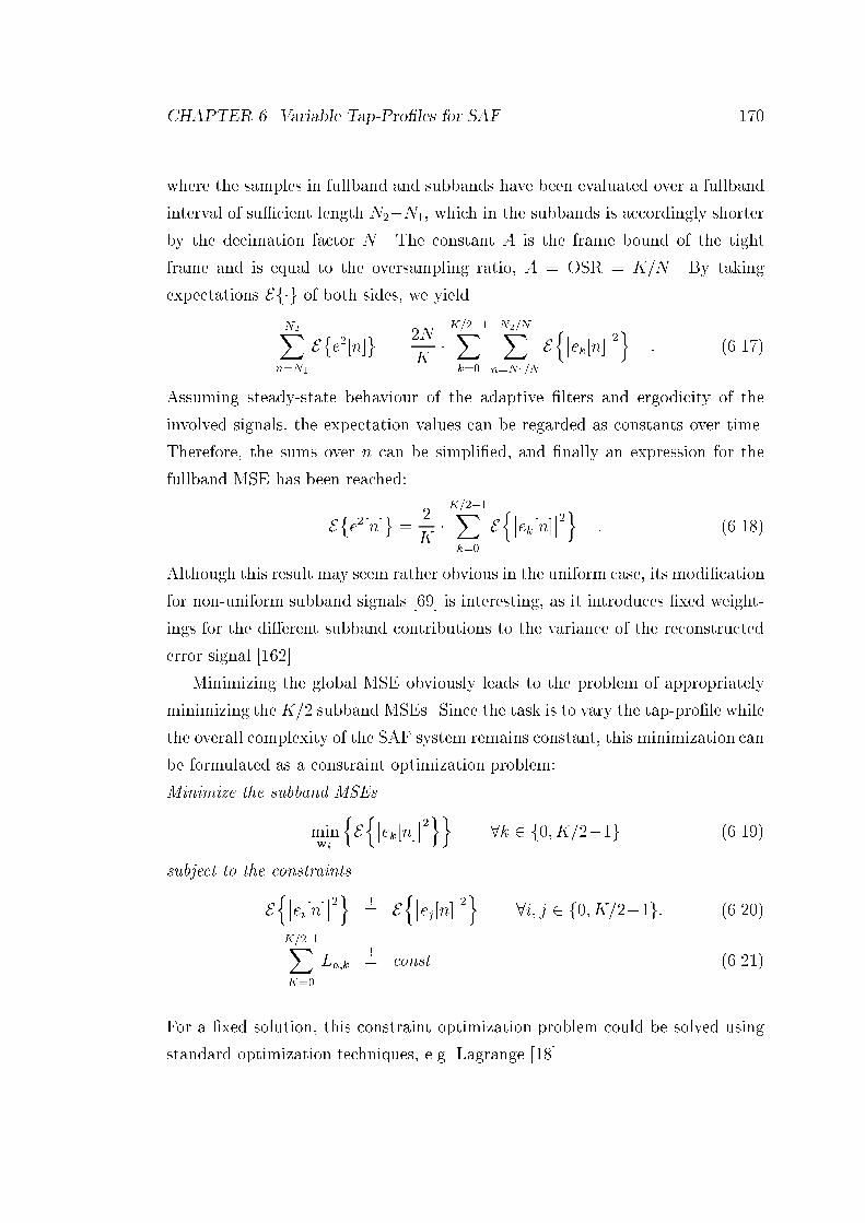
CHAPTER 6. Variable Tap-Proles for SAF 170where the samples in fullband and subbands have been evaluated over a fullbandinterval of sucient length N2N1, which in the subbands is accordingly shorterby the decimation factor N . The constant A is the frame bound of the tightframe and is equal to the oversampling ratio, A = OSR = K=N . By takingexpectations Efg of both sides, we yieldN2Xn=N1 Ee2[n] = 2NK K=21Xk=0 N2=NXn=N1=N Enek[n]2o : (6.17)Assuming steady-state behaviour of the adaptive lters and ergodicity of theinvolved signals, the expectation values can be regarded as constants over time.Therefore, the sums over n can be simplied, and nally an expression for thefullband MSE has been reached:Ee2[n] = 2K K=21Xk=0 Enek[n]2o : (6.18)Although this result may seem rather obvious in the uniform case, its modicationfor non-uniform subband signals [69] is interesting, as it introduces xed weight-ings for the dierent subband contributions to the variance of the reconstructederror signal [162].Minimizing the global MSE obviously leads to the problem of appropriatelyminimizing the K=2 subband MSEs. Since the task is to vary the tap-prole whilethe overall complexity of the SAF system remains constant, this minimization canbe formulated as a constraint optimization problem:Minimize the subband MSEsminwk nEnek[n]2oo 8k 2 f0; K=21g (6.19)subject to the constraintsEnei[n]2o != Enej[n]2o 8i; j 2 f0; K=21g; (6.20)K=21XK=0 La;k != const. (6.21)For a xed solution, this constraint optimization problem could be solved usingstandard optimization techniques, e.g. Lagrange [18].
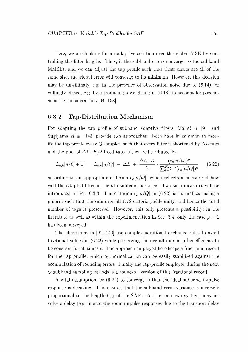
CHAPTER 6. Variable Tap-Proles for SAF 171Here, we are looking for an adaptive solution over the global MSE by con-trolling the lter lengths. Thus, if the subband errors converge to the subbandMMSEs, and we can adjust the tap prole such that these errors are all of thesame size, the global error will converge to its minimum. However, this decisionmay be unwillingly, e.g. in the presence of observation noise due to (6.14), orwillingly biased, e.g. by introducing a weighting in (6.18) to account for psycho-acoustic considerations [34, 158].6.3.2 Tap-Distribution MechanismFor adapting the tap prole of subband adaptive lters, Ma et al. [91] andSugiyama et al. [143] provide two approaches. Both have in common to mod-ify the tap prole every Q samples, such that every lter is shortened by L tapsand the pool of L K=2 freed taps is then redistributed byLa;k[n=Q+ 1] = La;k[n=Q] L + L K2 (ck[n=Q])pPK=21k=0 (ck[n=Q])p (6.22)according to an appropriate criterion ck[n=Q], which re ects a measure of howwell the adapted lter in the kth subband performs. Two such measures will beintroduced in Sec. 6.3.3. The criterion ck[n=Q] in (6.22) is normalized using ap-norm such that the sum over all K=2 criteria yields unity, and hence the totalnumber of taps is preserved. However, this only presents a possibility; in theliterature as well as within the experimentation in Sec. 6.4, only the case p = 1has been surveyed.The algorithms in [91, 143] use complex additional exchange rules to avoidfractional values in (6.22) while preserving the overall number of coecients tobe constant for all times n. The approach employed here keeps a fractional recordfor the tap-prole, which by normalization can be easily stabilized against theaccumulation of rounding errors. Finally the tap-prole employed during the nextQ subband sampling periods is a round-o version of this fractional record.A vital assumption for (6.22) to converge is that the ideal subband impulseresponse is decaying. This ensures that the subband error variance is inverselyproportional to the length La;k of the SAFs. As the unknown systems may in-volve a delay (e.g. in acoustic room impulse responses due to the transport delay
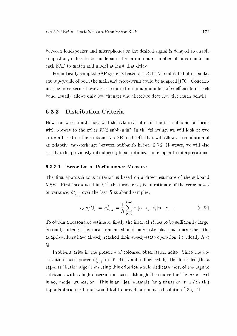
CHAPTER 6. Variable Tap-Proles for SAF 172between loudspeaker and microphone) or the desired signal is delayed to enableadaptation, it has to be made sure that a minimum number of taps remain ineach SAF to match and model at least that delay.For critically sampled SAF systems based on DCT-IV modulated lter banks,the tap-prole of both the main and cross-terms could be adapted [170]. Concern-ing the cross-terms however, a required minimum number of coecients in eachband usually allows only few changes and therefore does not give much benet.6.3.3 Distribution CriteriaHow can we estimate how well the adaptive lter in the kth subband performswith respect to the other K=2 subbands? In the following, we will look at twocriteria based on the subband MMSE in (6.14), that will allow a formulation ofan adaptive tap exchange between subbands in Sec. 6.3.2. However, we will alsosee that the previously introduced global optimization is open to interpretations.6.3.3.1 Error-based Performance Measure.The rst approach to a criterion is based on a direct estimate of the subbandMSEs. First introduced in [91], the measure ck is an estimate of the error poweror variance, 2ekek over the last R subband samples,ck[n=Q] = 2ekek = 1R P1Xr=0 ek[nr] ek[nr] : (6.23)To obtain a reasonable estimate, rstly the interval R has to be suciently large.Secondly, ideally this measurement should only take place at times when theadaptive lters have already reached their steady-state operation, i.e. ideally R <Q. Problems arise in the presence of coloured observation noise. Since the ob-servation noise power 2zkzk in (6.14) is not in uenced by the lter length, atap-distribution algorithm using this criterion would dedicate most of the taps tosubbands with a high observation noise, although the source for the error levelis not model truncation. This is an ideal example for a situation in which thistap-adaptation criterion would fail to provide an unbiased solution [135, 170].

CHAPTER 6. Variable Tap-Proles for SAF 1736.3.3.2 Reduced CriterionEqn. (6.14) has been exploited to create a criterion similar to [143], whereby thepower of the last S taps of an adaptive lter is taken to estimate the truncationerror, weighted by a measurement of the input signal power over a window of Rsamples,ck[n=Q] = 1R R1Xr=0 xk(nr)xk(nr)| z estimate of signal power 1S S1Xs=0 wk [La;k[n]s]wk [La;k[n]s]| z estimate of truncation error :(6.24)Although clearly the in uence of observation noise has been suppressed, this cri-terion introduces a twofold bias in the MSE estimate for (6.14). Firstly, bandswith shorter decay will be favoured since their last S untruncated coecientswill be more powerful than those of a longer decay, if decays are approximatelyexponential. Secondly, a colouring of input signal power will somewhat deviatethe result from what has previously been assumed as \optimum" for the iden-tication of an unknown system. The motivation for a variable tap-prole hasoriginally been to balance the lter lengths of the SAFs according to the decayof the unknown system in dierent frequency bands. If the specic applicationis less targeted on the identication of an unknown system, but the cancellationof some unwanted signal, as e.g. the far end speaker's echo in AEC, then mini-mization of (6.24) across all SAFs will be \optimum" in the sense of a minimumvariance of the fullband reconstructed error signal, not necessarily a \best-t" forthe unknown system as indicated in Fig. 6.1.Compared to the error-based criterion (6.23), the reduced criterion can becomputed with a minimum overhead over the regular update procedure of theSAFs. While the criterion in Sec. 6.3.3.1 requires to keep track of R past val-ues of the error signal (which otherwise does not need to be memorized), theevaluation of (6.24) only performs an estimate of the input power, which is sim-ilarly required in the normalization step of the NLMS algorithms. Finally, theweights wk are readily accessible for the approximation of the truncation error.While the criterion in [143] is a computationally intensive average of the righthand side of (6.24) over the last P iterations, the approach presented above only

CHAPTER 6. Variable Tap-Proles for SAF 174introduces a very low additional computational overhead of (S + 3)=NR multi-plications and K=(2NR) divisions per fullband sampling period for a complexsubband implementation.6.4 SimulationsThis section will give some examples and insight into the benet and behaviourof variable tap-proles for SAF systems. First, a system identication problemwill be discussed, whereby for a realistic result, a xed computational benchmarkis used to demonstrate the eciency of subband adaptive ltering, and how avariable tap-prole can further enhance its performance. A brief comparison ofthe two tap-assignment criteria presented in Sec. 6.3.3 will conclude this section.6.4.1 Performance at Given BenchmarkTo obtain a realistic benchmark gure, we assume a Motorola DSP56002 processor[105], capable of 20 million multiply accumulate (MAC) operations per second.Supposing that about 50% of the instruction cycles are required for overheadslike data transfer with ADC/DAC devices, interrupt handling, and indexing, at asampling rate of 16kHz there will be approximately Ctot = 1250 MACs availableper sampling period.Re-arranging equations (6.2) (6.4), the total number of available lter coe-cients in the SAFs, Ltot, can be determined for SAF systems based on oversampledGDFT, oversampled SSB modied GDFT, and critically sampled DCT-IV mod-ulated lter banks. The according value for each SAF system type are stated inTab. 6.1. For the DCT-IV modulation based SAF system, only the total numberof coecients in the main terms is given.The unknown system S(z) to be identied by the dierent adaptive architec-tures is an all-pole modelS(z) = A I1Xi=0 11 2i cos(i)z1 + 2i z2 (6.25)where for this specic case the 5 poles described in Tab. 6.2 have been selected.The gain factor A was chosen such that the impulse response s[n] | S(z)
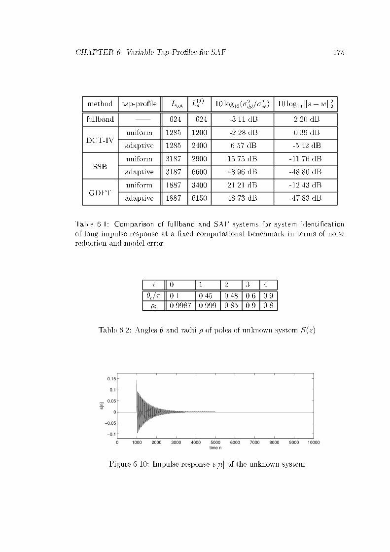
CHAPTER 6. Variable Tap-Proles for SAF 175method tap-prole Ltot L(f)a 10 log10(2dd=2ee) 10 log10 ks wk22fullband | 624 624 -3.11 dB 2.20 dBuniform 1285 1200 -2.28 dB 0.39 dBDCT-IV adaptive 1285 2400 6.57 dB -5.42 dBuniform 3187 2900 15.75 dB -11.76 dBSSB adaptive 3187 6600 48.96 dB -48.80 dBuniform 1887 3400 21.21 dB -12.43 dBGDFT adaptive 1887 6150 48.73 dB -47.83 dBTable 6.1: Comparison of fullband and SAF systems for system identicationof long impulse response at a xed computational benchmark in terms of noisereduction and model error.
i 0 1 2 3 4i= 0.1 0.45 0.48 0.6 0.9i 0.9987 0.999 0.85 0.9 0.8Table 6.2: Angles and radii of poles of unknown system S(z).
0 1000 2000 3000 4000 5000 6000 7000 8000 9000 10000
−0.1
−0.05
0
0.05
0.1
0.15
time n
s[n
]
Figure 6.10: Impulse response s[n] of the unknown system.

CHAPTER 6. Variable Tap-Proles for SAF 176(shown in Fig. 6.10) satises ks[n]k2 = 1, i.e. possesses unit energy. For thedierent SAF systems, the unknown system was given an additional delay of 1000taps to avoid non-causality of the subband responses to be identied. No delaywas set for the system identication using the fullband NLMS adaptive lter. Forall simulations, the normalized step size of the NLMS was set to ~ = 0:9.Critically Sampled SAF System. The simulation results for adaptive sys-tem identication in critically sampled DCT-IV modulated subbands is shown inFig. 6.11. The prototype lter used here is an iterated halfband design listed inTab. 4.2 for K = 16. The learning curves in Fig. 6.11(a) are given for the twocases of xed uniform and adaptive tap-prole using the error criterion in (6.23).For both cases, the resulting fullband equivalent model length L(f)a is suppliedin Tab. 6.1. Clearly for uniform tap-distribution, this model length is not longenough to allow the SAF system to properly adapt, since the observation noiselevel caused by the truncation is too high. For a similar reason, the fullband iden-tication completely fails. With a variable tap-prole, the algorithm manages toreduce the error variance by a small amount, since the tap-prole is adapted to amore suitable form for this problem, as indicated in Fig. 6.11(c). The PSD of thenal MSE in Fig. 6.11(b) clearly shows how the error spectrum is further reducedwith an adaptive prole in the two bands k = 0 and k = 3 dominating the overallerror. Note that band edges are marked by vertical dashed lines.Real Valued Oversampled SAF System. Fig. 6.12 presents the SAF sys-tem identication results using SSB modied GDFT lter banks with K=2 = 8subbands and decimation by N=2 = 7, and the prototype design of Tab. 4.3(d).In general, the results are far superior to the DCT case in Fig. 6.11, since thecross-terms required in the DCT based SAF systems are as costly as the com-plete lter bank operation, and not enough calculations remain to allow sucientSAF lengths. As in the SSB modied GDFT based system no cross-terms arerequired, the system can dedicate a much higher number of computations toadaptive ltering.Note in particular how in the SSB case the error PSD in Fig. 6.12(b) is bal-anced when the tap-prole adaptation is introduced. While the error spectrum

CHAPTER 6. Variable Tap-Proles for SAF 177
(b) (c)0 0.1 0.2 0.3 0.4 0.5 0.6 0.7 0.8 0.9 1−60
−50
−40
−30
−20
−10
0
10
20
30
normalized frequency Ω/π
PS
D
Se
e(e
jΩ)
/
[dB
]
0 1 2 3 4 5 6 70
100
200
300
subbands k
co
eff
icie
nts
0 0.2 0.4 0.6 0.8 1 1.2 1.4 1.6 1.8 2
x 105
−20
−15
−10
−5
0
5
10
15
time n
MS
E / [dB
]
uniform tap−profile
adaptive tap−profile(a)
Figure 6.11: K=2 = 8 subband SAF system with critically sampled DCT-IVmodulated lter banks: (a) locally averaged squared reconstructed fullband error;(b) PSD of desired signal (dotted) and of nal error for uniform (solid) andadaptive (dashed) tap-prole; (c) uniform (straight line) and adapted (bar plot)tap-prole.
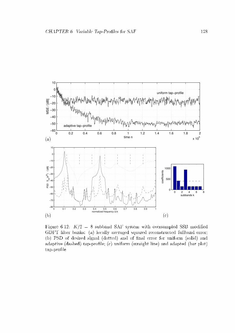
CHAPTER 6. Variable Tap-Proles for SAF 178
(b) (c)0 0.1 0.2 0.3 0.4 0.5 0.6 0.7 0.8 0.9 1−80
−70
−60
−50
−40
−30
−20
−10
0
10
normalized frequency Ω/π
PS
D
Se
e(e
jΩ)
/
[dB
]
0 2 4 6 80
500
1000
subbands k
coeffic
ients
0 0.2 0.4 0.6 0.8 1 1.2 1.4 1.6 1.8 2
x 105
−60
−50
−40
−30
−20
−10
0
10
time n
MS
E / [dB
]
uniform tap−profile
adaptive tap−profile(a)
Figure 6.12: K=2 = 8 subband SAF system with oversampled SSB modiedGDFT lter banks: (a) locally averaged squared reconstructed fullband error;(b) PSD of desired signal (dotted) and of nal error for uniform (solid) andadaptive (dashed) tap-prole; (c) uniform (straight line) and adapted (bar plot)tap-prole.

CHAPTER 6. Variable Tap-Proles for SAF 179
(b) (c)0 0.1 0.2 0.3 0.4 0.5 0.6 0.7 0.8 0.9 1−80
−70
−60
−50
−40
−30
−20
−10
0
10
normalized frequency Ω/π
PS
D
Se
e(e
jΩ)
/
[dB
]
0 1 2 3 4 5 6 70
500
1000
subbands k
coeffic
ients
0 0.2 0.4 0.6 0.8 1 1.2 1.4 1.6 1.8 2
x 105
−60
−50
−40
−30
−20
−10
0
10
time n
MS
E / [dB
]
uniform tap−profile
adaptive tap−profile(a)
Figure 6.13: K=2 = 8 subband SAF system with oversampled GDFT lter banks:(a) locally averaged squared reconstructed fullband error; (b) PSD of desiredsignal (dotted) and of nal error for uniform (solid) and adaptive (dashed) tap-prole; (c) uniform (straight line) and adapted (bar plot) tap-prole.is slightly increased in unimportant bands due to the withdrawal of coecientsthere, the error in the dominating bands can be more eectively suppressed, thusyielding a considerably enhanced noise reduction and a better accuracy for theidentied fullband equivalent model, for which measures are stated in Tab. 6.1.Complex Valued Oversampled SAF System. Results for a complex valuedSAF system using a GDFT modulated lter bank, which are based on the sameprototype as the SSB modied GDFT bank system discussed above, are given inFig. 6.13. Although the overall number of coecients is smaller than in the SSBcase, the GDFT system is running at only half the sampling rate, and therefore

CHAPTER 6. Variable Tap-Proles for SAF 180manages to achieve a better performance than the SSB for a uniform tap-prole.Again, the introduction of a variable tap-prole allows the balancing of the varioussubband errors as indicated in Fig. 6.13(b) and hence further reduces the fullbandnal MSE.Truncation Error. To demonstrate that the main hindrance in the adaptationof the above SAF systems was in fact the model truncation due to the very longimpulse response s[n] of the unknown system, the errors of the equivalent recon-structed fullband model, w[n], are plotted in Fig. 6.14. The fullband models havebeen calculated from the adapted subband responses (for the critically sampledsystem including the cross-terms) according to Sec. 5.3.1. Shown are the resultsfor the three dierent SAF systems, each for uniform and adaptive tap-prole.The approximate lengths of the reconstructed fullband models L(f)a are listed inTab. 6.1. It is easy to appreciate that truncation is the main source of error, asno observation noise has been injected, and the SAR values for the prototypes areapproximately 57 dB for all lter banks used. Since the truncation contributesto the MMSE, also the identiable part of the impulse response will be noisecorrupted due to the excess MSE yielded when using LMS-type algorithms.6.4.2 Bias of Tap-Prole AdaptationTo give an example of the tap assignment algorithms' behaviour, we try toidentify a slowly decaying system similar to previous examples, with a frequencyresponse as shown in Fig. 6.15(a), using both the error based and reduced criteriondiscussed in Sec. 6.3.3. For identication, we employ an NLMS subband adaptivesystem operating in 8 critically decimated subbands, which are produced by DCT-IV modulated lter banks based on the prototype lowpass lter from Tab. 4.2for K = 16. Factorized cross-terms have been included according to [53, 54] andFig. 3.4.2.1, where the lengths of the adaptive cross-terms are set to one third ofthe initial uniform SAF length of the main terms.Fig. 6.15(b) and (c) show the learning curves of the tap-prole evolving overtime for a white noise (unit variance) excited system identication set-up with noadded observation noise. Numbers at the right margin of each gure indicate the
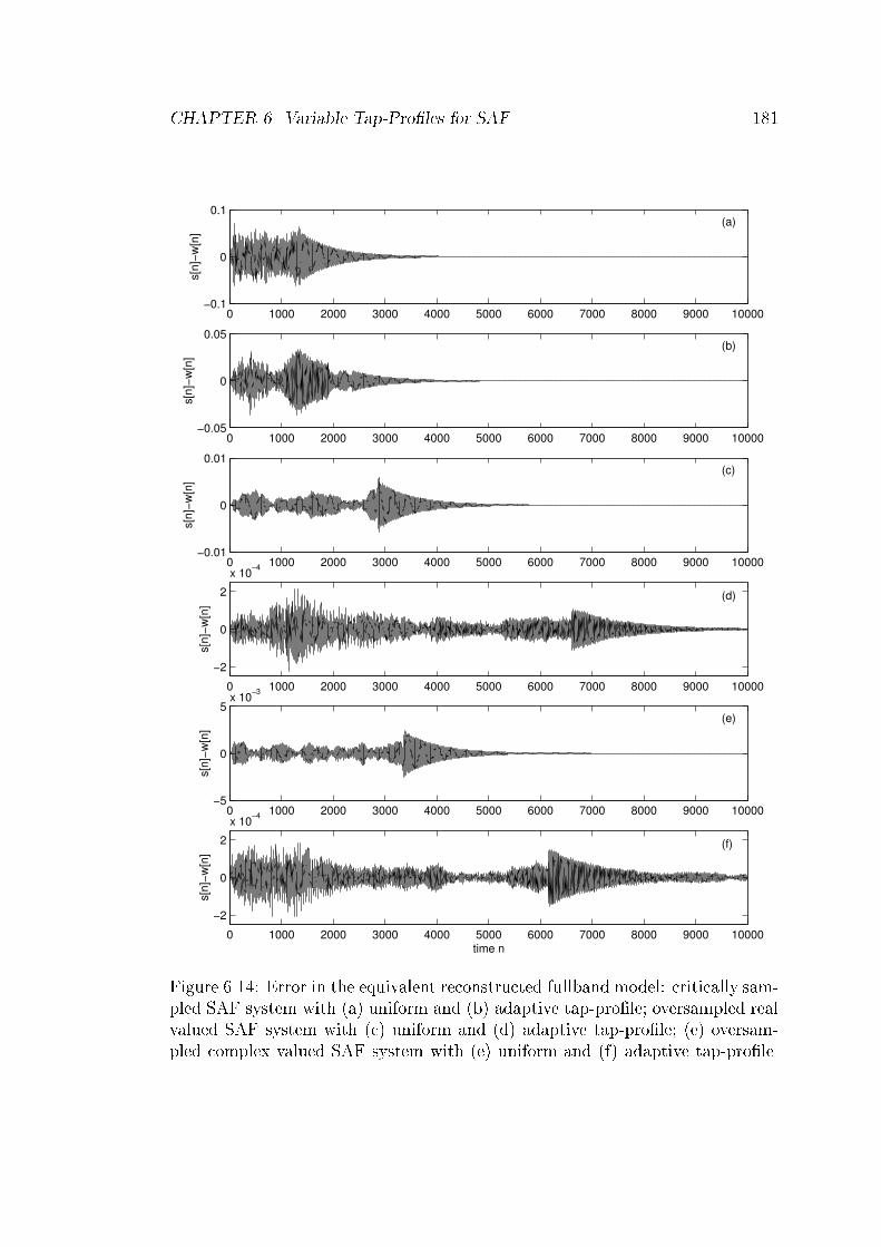
CHAPTER 6. Variable Tap-Proles for SAF 1810 1000 2000 3000 4000 5000 6000 7000 8000 9000 10000
−0.1
0
0.1
s[n
]−w
[n]
(a)
0 1000 2000 3000 4000 5000 6000 7000 8000 9000 10000−0.05
0
0.05
s[n
]−w
[n]
(b)
0 1000 2000 3000 4000 5000 6000 7000 8000 9000 10000−0.01
0
0.01
s[n
]−w
[n]
(c)
0 1000 2000 3000 4000 5000 6000 7000 8000 9000 10000
−2
0
2
x 10−4
s[n
]−w
[n]
(d)
0 1000 2000 3000 4000 5000 6000 7000 8000 9000 10000−5
0
5x 10
−3
s[n
]−w
[n]
(e)
0 1000 2000 3000 4000 5000 6000 7000 8000 9000 10000
−2
0
2
x 10−4
time n
s[n
]−w
[n]
(f)
Figure 6.14: Error in the equivalent reconstructed fullband model: critically sam-pled SAF system with (a) uniform and (b) adaptive tap-prole; oversampled realvalued SAF system with (c) uniform and (d) adaptive tap-prole; (e) oversam-pled complex valued SAF system with (e) uniform and (f) adaptive tap-prole.

CHAPTER 6. Variable Tap-Proles for SAF 182
0 0.1 0.2 0.3 0.4 0.5 0.6 0.7 0.8 0.9 1−50
−40
−30
−20
−10
0
10m
agnitude /[d
B]
normalized frequency Ω / π
(a) frequency response of system and noise spectrum
0 5 10 15
x 104
40
60
80
100
120
1404
3
7
6
0−2,5
tap p
rofile
(b) error criterion
0 5 10 15
x 104
40
60
80
100
120
140
4
3
7
6
0−2,5
(c) reduced criterion
0 5 10 15
x 104
50
100
150
2001
0
7342
5+6
time n
tap p
rofile
(d) error criterion, with noise
0 5 10 15
x 104
40
60
80
100
120
140
3
4
7
6
0−2,5
time n
(e) reduced criterion with noise
Figure 6.15: (a) Frequency response of unknown system to be identied (solid)and the PSD of the observation noise (dashed); band edges are plotted as verticaldotted lines; tap-prole trajectories for noiseless (b,c) and noisy (d,e) case forerror and reduced criterion based tap distribution algorithms (taken from [170]).

CHAPTER 6. Variable Tap-Proles for SAF 183criterion error (6.23) reduced (6.24)noise free 50.7 dB 43.5 dBnoisy 15.0 dB 17.4 dBTable 6.3: Noise reduction measures, 10 log10(2dd=2ee), for the noise-free and noisy(SNR -18.5 dB) system identication examples given in Fig. 6.15 using adaptivetap-distribution based on two dierent criteria.subband number k for each line, corresponding successively to the 8 frequencyintervals specied in Fig. 6.15(a) by vertical dashed lines. Obviously, the noise freesimulation behaves as expected, and with either criterion most taps are dedicatedto the subbands for k = 7 containing one strong pole of the unknown system,and to k = 3 and 4, which share a strong pole sitting at the band edge = =2.The same system identication simulations are repeated with coloured obser-vation noise added at -18 dB SNR to the desired signal; the PSD of the noise isplotted in Fig. 6.15(a) as a dashed line. The resulting trajectories of the 8 SAFlengths are depicted in Fig. 6.15(e) and (f). While the assignment behaviour ofthe reduced criterion of (6.24) is hardly in uenced, the error based criterion [91]is completely biased by the observation noise. For the latter case, the tap distri-bution algorithm dedicates most adaptive lter coecients to the bands k = 0and 1, where the observation noise is spectrally strongest, although an increasein lter length cannot help to further reduce the error power.The nal reduction in error power achieved by the four dierent system iden-tication simulations described above is given in Tab. 6.3. From these values, itbecomes obvious that for the noise free case, the error based criterion outperformsthe reduced criterion, which is likely to yield a bias as discussed in Sec. 6.3.3.2.With observation noise added, the reduced criterion however performs more ro-bustly as seen in Fig. 6.15(f) and yields a higher noise reduction than the stronglybiased error criterion.

CHAPTER 6. Variable Tap-Proles for SAF 1846.5 Concluding RemarksThis chapter has been concerned with the ecient use of system resources byexploiting spectral properties of the unknown system or the input signal. Insuch an environment of spectrally unbalanced signals, the largest subband errordominates the accuracy and performance of the overall SAF system. This hasmotivated the idea of adopting a non-uniform tap-prole which is able to balancetruncation errors occurring e.g. due to the spectrally dierent decay of the un-known system to be identied. A number of approaches found in the literaturefor both xed and adaptive adjustment of the tap-prole have been reviewed.Two extrema for distributing computations over the subbands have been anal-ysed. The rst extreme case is a uniform tap-prole, where each subband has thesame time representation, which for uniform subband decompositions is equiva-lent for the SAFs to posses identical lter lengths and same number of computa-tions per subband. The other extremum is formed by a concentrated tap-prole,where all computations are dedicated to one single subband. These extremadened the performance margins for variable tap-proles.For the NLMS algorithm, the total cost of an SAF system based on dierentsubband decompositions (oversampled GDFT, oversampled SSB modied GDFT,and critically sampled DCT-IV modulated lter banks) has been derived. Basedon this, the performance margins have been calculated for two scenarios, where(i) the cost reduction for a xed time representation of the SAF system and (ii)the time representation at xed cost (e.g. given by the benchmark performanceof a DSP) are of interest. For required cost reduction or increase in time repre-sentation, it is therefore possible to select an SAF system suitable for a particularapplication, specied by its parameters (lter bank type, number of subbands,decimation rate).For an adaptive adjustment of the tap-prole, we have adopted a tap-distribu-tion mechanism driven by a criterion for the performances of the dierent SAFsin the system. We have based our derivation for a suitable SAF performance mea-sure on the minimization of the global error, which creates a background theoryfor distribution criteria reported in the literature. This has yielded a subbanderror based criterion, and a reduced criterion suppressing the bias introduced

CHAPTER 6. Variable Tap-Proles for SAF 185by coloured observation noise. Their properties when employed to adjust thetap-prole of SAF systems have been demonstrated and veried by simulation.The benet of the subband approach and a possible further enhancement bytap-prole adaptation for adaptive ltering has been demonstrated in a series ofexamples, where a xed computational benchmark was given for the identicationof a very long impulse response. As a side eect, this has also highlighted thesuperior properties of oversampled subband approaches in terms of computationalsystem complexity over the critically sampled case.

Chapter 7Conclusions7.1 ResumeMotivated by the identication of long impulse responses, this thesis has dis-cussed and compared subband adaptive lter structures based on complex andreal valued oversampled modulated lter banks, their components, implementa-tions, limitations, and design.Adaptive Filter Algorithms. Adaptive ltering has been reviewed, with a fo-cus on popular algorithms such as LMS, RLS, and ane projection. Some insighthas been given into the derivation of these algorithms and their similarities, withthe main emphasis on their computational complexity, and their convergence andtracking properties. In particular, the convergence speed of LMS-type algorithmswas strongly aected by coloured input signals. Regarding the computationalcomplexity, the only dierence between real and complex valued implementa-tions for the presented algorithms was the use of complex arithmetic, which interms of real valued multiplications is simply an increase by a factor of four.Background and Review of Adaptive Filtering in Subbands. Moving to-wards subband implementations, rst basic multirate operations were introduced.The reason for reducing the sampling rate was based on two facts. Firstly, forband-limited signals the sampling rate could be lowered in accordance with thebandpass sampling theorem, where dierences arose for the decimation of real186
CHAPTER 7. CONCLUSIONS 187valued and complex valued signals. While for analytic or complex bandpass sig-nals, decimation of a signal based on its bandwidth is unproblematic, for realvalued signals bandpass sampling is bound by strict rules. Secondly, another le-gitimation for decimation was given based on orthonormal decompositions of asignal into a number of decimated subbands, which was extended to redundantdecompositions representing frame expansions. This naturally led to lter banksimplementing such signal expansions.To analyse lter banks, we introduced two analysis methods: modulationdescription and polyphase representation. From the latter, ecient implementa-tions of lter banks and the conditions for perfect reconstruction were derived.The modulation description approach was used to analyse subband adaptive l-ter (SAF) systems based on critically decimated perfect reconstruct (PR) lterbanks, which resulted in the requirement of cross-terms at least between adjacentsubbands due to aliasing. An example illustrating the corresponding time domaineect of \information leakage" was given.To avoid cross-terms in the SAF structure, a number of dierent approacheswere reviewed, including critically sampled systems based on non-PR lter bankswith spectral loss or other distortions, and oversampled approaches. The lattercovered complex valued and real valued lter banks. For real valued oversampledlter banks, two strategies where discussed to circumvent problems encounteredwith bandpass sampling: lter banks with non-uniform bandwidths and band-positions of the frequency bands, and a single-sideband modulation approach,whereby subbands are modulated into the baseband prior to decimation.GDFT Filter Banks. Aiming for near PR lter banks only, we investigated acertain type of complex valued modulated lter bank based on a generalized DFT(GDFT) modulation. The generalization of the DFT modulation consisted of theinclusion of osets in time and frequency indices to obtain a linear phase propertyand an odd-stacked positioning of the analysis lters' passbands. For real valuedinput signals, this allowed us to retain only half the number of complex valuedsubbands, based on redundancy considerations. For the synthesis lter bank, an

CHAPTER 7. CONCLUSIONS 188innite number of solutions existed in the oversampled case. Here, the minimum-norm solution, i.e. the parahermitian or left pseudo-inverse of the analysis bankhas been chosen. Backed by frame theory, this selection bore useful numericalproperties such as improved robustness towards noise in the subband domain anda xed energy relation between fullband and subbands, and practical advantages,as the synthesis prototype lter is identical to the one for the analysis bank.Regarding implementation, starting from the polyphase representation forgeneral non-integer oversampling, we derived a factorization into a real valuedpolyphase network, that only depended on the polyphase components of the pro-totype lter, and followed by a GDFT transform applying a complex rotation tothe outputs of the polyphase network. This transform could be further factor-ized, such that it mainly reduced to the computation of a DFT, which could berealized by an FFT for fast evaluation. Thus, a highly ecient implementationwas obtained.The presented GDFT lter bank has been modied such that an SSB modu-lated real valued lter bank was implemented, circumventing the Weaver method.Due to the low complexity of the GDFT implementation, we thus obtained a fastWeaver-like SSB decomposition. For the same number of subbands, this lterbank required about twice the number of computations of the standard GDFTlter bank, and produced real valued subband samples at twice the rate.To judge the overall computational complexity of implemented SAF systems,a comparison for the cost ratio between real and complex valued processing hasbeen derived. While for example for linear algorithmic orders of subband pro-cessing (like LMS), both methods were shown to be equally costly, the compleximplementation turned out to be more ecient by about a factor of two for aquadratic order of complexity (e.g. RLS).Two methods have been introduced to obtain suitable prototype lters forGDFT and SSB modied GDFT lter banks. The rst would construct prototypelters for lter banks with higher channel numbers (restricted to powers of two)by appropriate scaling of a halfband lter, which was accomplished by iterativeexpansion and interpolation. Secondly, criteria for perfect reconstruction andlow aliasing level in the subband signals were derived in terms of the prototype
CHAPTER 7. CONCLUSIONS 189lter which enabled a fast converging iterative least squares optimization. Aweighting between the two criteria allowed us to trade power complementarityagainst stopband attenuation.Subband Adaptive Filter Performance. Novel limits for the power spectraldensity (PSD) of the error signal at the Wiener solution have been derived, basedon the aliasing created in the lter banks, and a knowledge of the source modelsof the decomposed signals. This allowed us to state the minimum mean squarederror (MMSE), which has approximated by an easy-to-apply measure (SAR |signal-to-aliasing ratio) describing the lower limit for the MSE solely based on theprototype lter of the lter bank. The equivalent fullband model of the overallSAF system has been derived from the adapted weights of the SAFs, and has beenshown to be limited in its accuracy by the distortion function (i.e. the deviationfrom power complementarity) of the lter bank. Thus, the two main limits ofnal error performance could be directly linked to the design of the prototypelter.A number of simulations were performed to verify the derived limits, for whichthe results matched remarkably well with the predicted quantities. Further exper-iments aimed to evaluate the convergence speed showed that SAF systems usingan NLMS algorithm were almost insensitive to coloured input signals. While forwhite noise excitation, fullband algorithms gave a clear, but narrow advantage,for coloured input signals subband approaches considerably outperformed thefullband algorithm. Remarkably, the oversampling ratio was shown to have noneor only little in uence on the convergence speed of SAF systems. For the numberof subbands, it turned out that, with regard to convergence speed, an optimumexisted, given by a trade-o between the spectral separation of the coloured inputsignal, the spectral notches introduced by the analysis lters, and the dierentupdate rates and subband adaptive lter lengths.Tap-Prole Adaptation. Finally, we have discussed the possibility of vari-able tap-proles for subband adaptive lters. This enabled the application ofmore lter coecients to subbands where they are required to identify an oth-erwise truncated model. Based on a global error minimization approach two

CHAPTER 7. CONCLUSIONS 190dierent distribution criteria were derived, of which the rst attempted a directminimization of the error. A second, reduced criterion for unbiased performancein the presence of coloured observation noise was introduced which presented asimplied algorithm compared to a similar method in the literature.The performance of SAF systems with variable tap-prole was illustrated bynoise-free and noisy simulations, which gave an account of the sensitivity andbias of the discussed algorithms. For system identication experiments with aspectrally balanced unknown system with a long impulse response, the benet ofvariable tap-prole approach was clearly demonstrated. Also comparison for theeciency of dierent SAF systems was performed, which was exercised using theNLMS algorithms as an example. This gave a clear indication of the advantage ofoversampled SAF systems with low OSR over critically decimated systems withcross-terms.7.2 Core ResultsThe main aim throughout this thesis was to achieve an ecient implementationfor adaptive lter systems, for which we have chosen the subband approach.Therefore, the clear task was to nd methods to ensure that both the subbanddecomposition and processing algorithms were as computationally ecient aspossible.Since subband processing is most ecient at low OSR, thus avoiding cross-terms but still operating close to the critical rate, this has to be accommodatedby the lter banks. This has been enabled by deriving a highly ecient polyphaseimplementation of a complex valued modulated GDFT lter bank with a judi-cious selection of properties for non-integer OSRs. A real valued lter bank usingan SSB modied GDFT bank allowed a highly ecient implementation of sub-band decompositions for real valued subband processing. The choice whether toperform real or complex subband processing is specic to the particular adaptivealgorithm to be used, and can be answered based on its computational complexity.The high performance advantage of complex valued systems has been surprisingin this context.

CHAPTER 7. CONCLUSIONS 191Final convergence limits for subband adaptive lters and the accuracy of theachievable equivalent fullband model based on aliasing and other distortions in-troduced by the employed lter banks were explicitly derived, and agreed verywell with simulation results. Both an approximation of the MMSE and the modelaccuracy were linked to conditions on the prototype lter of the lter bank, whichare directly related to criteria in the prototype lter design. Together with a pre-sented iterative least-squares design algorithm, it is therefore possible to constructlter banks for SAF applications with pre-dened performance limits. The ap-peal is that for applications like acoustic echo cancellation, where the adaptationerror is the most important issue, the lter banks can be designed to be just good(and short) enough to satisfy relaxed constraints on the model error.7.3 OutlookThis thesis concludes with suggestion for further work, either to improve andelaborate, or to transfer some of the presented ideas to other applications.7.3.1 ExtensionsIn Chap. 6, the tap-distribution mechanism was introduced implicitly using thep-norm for normalization of the criterion used, although only p = 1 was employed.In fact, dierent values for p could be tried, which would yield possibly interestingcases of convergence. For the case p > 1, it is expected that the band with thelargest error will be assigned coecients more quickly, while for 0 < p < 1, thetap withdrawal from bands with smallest error would be enforced.Although the subband approach has been shown to improve convergence inthe presence of coloured input, a number of other methods could be evaluated fortheir additional benet in particular to combat slow convergence at band-edges[101] e.g. as encountered in Fig.5.18. Fast converging algorithmic approachesinclude transform-domain adaptive ltering [128, 5], where the lter input is pre-processed by a sliding unitary transform. This approximately decorrelates theinput values in the tap-delay line of the lter. A complete decorrelation is givenby the Karhunen-Loeve transform [72], but other transforms like DFT or DCT can

CHAPTER 7. CONCLUSIONS 192already provide a considerable whitening [4]. An evaluation of a transform of thelength of the adaptive lter is required to be calculated at every sampling period.Although elegant methods exist to reduce complexities of some of the transformsto linear order in the lter length [6], it appears promising for inclusion intothe subband approach, since the computational load would be considerably lowerthan for a fullband transform-domain implementation.A second approach to increase convergence speed at the band-edges is given by aselection of lter banks such that the analysis lters are wider than the synthesislters [32, 79, 40, 106]. Thus, the SAFs are supplied with enough signal energy atthe band-edges, while super uous slow converging modes are ltered out on thesynthesis side. Particularly, it should be interesting to survey which conditionshave to be fullled by the lter banks to guarantee the PR property, and developan appropriate prototype design.Finally, the iterative least-squares design presented in Chap. 4 exhibited anuneven stopband attenuation. To yield a atter stopband response as obtainedwith minimax lter designs, a re-weighting during the iterative design steps couldbe attempted.7.3.2 Related ApplicationsA dual application to lter banks for subband decompositions are transmulti-plexers as shown in Fig. 7.1, which stack several users for transmission over oneline [154]. There, a synthesis lter bank performs the multiplexing of data atthe sender, while an analysis bank acting as demultiplexer retrieves the userson the receiving side. An oversampled approach (or rather undersampled withrespect to the lter banks) could lead to an increased robustness against channelinterference.Since fast implementations of the Gabor expansion have so far only beenreported for integer oversampling ratios [104, 47, 11], the fast polyphase imple-mentation of the GDFT lter bank presented in Chap. 4 can be transfered andapplied.Wavelet-based applications like detection [171, 80] or noise reduction [168, 169]suer from the phase-sensitivity of the orthogonal DWT and therefore currently

CHAPTER 7. CONCLUSIONS 1930
1x [n]
multiplexer (synthesis filter bank)
1
N
N
N G (z)K-1
1
0G (z)
G (z)
x [n]
channel1
00
K-1
z[n]interference
demultiplexer (analysis filter bank)
N
N
N
H (z)
H (z)
H (z)K-1
K-1x [n]
y [n]
y [n]
y [n]Figure 7.1: Transmission of K users over one channel by a transmultiplexer usinglter banks; note that N K.require \translation-invariant" DWT transforms implemented by undecimatedlter banks [25]. Although oversampled Gabor expansions are not \translation-invariant" in the true sense, signal energy is guaranteed to be found within aspecic subband independent of the fullband signal's phase, if the expansionproduces a low level of subband aliasing. Hence, oversampled Gabor transformsappear as a useful alternative to wavelet techniques [41], while a low OSR canmaintain a low level of additional computational complexity.Apart from the system identication / noise cancellation set-up targetedwithin this thesis, other applications like adaptive equalization [116] or line en-hancement are possible [177]. For adaptive equalization (or inverse system iden-tication [174]), very long impulse responses can occur when the channel to beinverted is considerably distorting. Also coloured channel output may motivatean SAF system to be applied. Although the delay of the lter banks inhibits di-rect use for delay sensitive applications like active noise control (ANC [36, 139]),a possibility is given by so called delay-less structures [102, 38, 109] where adap-tation is performed in the subband domain but ltering is done in the fullband.In each decimated period the updated subband weights are transformed back intothe time domain. This calculation is based on frequency domain methods andassumes a uniform tap-prole. For a general case, applying the reconstructionmethod in Sec. 5.3.1 could be employed.

Bibliography[1] P. Abbott. Acoustic Echo Cancelling in Video Telephony and Conferenc-ing on a Single DSP. In Proceedings of DSP UK II, volume 2, London,December 1994.[2] P. Abbott. Personal Communication. Signals and Software, Ltd, Harrow,England, April 1996.[3] F. Amano and H. Perez. \A New Subband Echo Canceler Structure".In Proc. IEEE International Conference on Acoustics, Speech, and SignalProcessing, volume 5, pages 35853588, Toronto, Canada, May 1991.[4] F. Beaufays. \Orthogonalizing Adaptive Algorithms: RLS, DFT/LMS,and DCT/LMS". In B. Widrow and E. Walach, editors, Adaptive InverseControl. Prentice Hall, Englewood Clis, NJ, 1995.[5] F. Beaufays. \Transform-Domain Adaptive Filters | An Analytical Ap-proach". IEEE Transactions on Signal Processing, Vol.43(No.2):pp.422431, February 1995.[6] F. Beaufays. \Two-Layer Linear Structures for Fast Adaptive Filtering".PhD thesis, Systems Laboratory, Department of Electrical Engineering,Stanford University, June 1995.[7] M. G. Bellanger. Adaptive Digital Filters and Signal Analysis. MarcelDekker Inc., New York, 1987.[8] N. J. Bershad and P. L. Feintuch. \Analysis of the Frequency DomainAdaptive Filter". Proceedings of the IEEE, Vol.67(No.12):pp.16581659,Dec. 1979. 194
BIBLIOGRAPHY 195[9] N. J. Bershad and O. M. Macchi. \Comparison of RLS and LMS Algorithmsfor Tracking A Chirped Signal". In Proc. IEEE International Conference onAcoustics, Speech, and Signal Processing, volume 2, pages 896899, Glas-gow, Scotland, May 1989.[10] N. J. Bershad and O. M. Macchi. \Adaptive Recovery of a Chirped Sinusoidin Noise, Part 1: Performance of the RLS Algorithm". IEEE Transactionon Signal Processing, Vol.39(No.3):pp.583594, March 1991.[11] H. Bolcskei and F. Hlawatsch. \Oversampled Filter Banks: Optimal NoiseShaping, Design Freedom, and Noise Analysis". In Proc. IEEE Interna-tional Conference on Acoustics, Speech, and Signal Processing, volume IV,pages 24532456, Munich, Germany, April 1997.[12] H. Bolcskei and F. Hlawatsch. \Oversampled Modulated Filter Banks". InH. G. Feichtinger and T. Strohmer, editors, Gabor Analysis and Algorithms| Theory and Applications, chapter 9. Birkhauser, 1997.[13] H. Bolcskei, F. Hlawatsch, and H. G. Feichtinger. \On the Equivalence ofDFT Filter Banks and the Gabor Expansion". In SPIE Proc. WaveletApplications in Signal and Image Processing III, volume 2569, pages 128139, San Diego, CA, 1995.[14] H. Bolcskei, F. Hlawatsch, and H. G. Feichtinger. \Oversampled FIR andIIR Filter Banks and Weyl-Heisenberg Frames". In Proc. IEEE Interna-tional Conference on Acoustics, Speech, and Signal Processing, volume III,pages 13511354, Atlanta, GA, May 1996.[15] K. Brandenburg and T. Sporer. \NMR and Masking Flag: Evaluation ofQuality Using Perceptual Criteria". In Proc. International Conference ofthe Audio Engineering Society, pages 169179, Portland, Oregon, 1992.[16] C. Breining. \Applying a Neural Network for Stepsize Control in Echo Can-cellation". In Proc. International Workshop on Acoustic Echo and NoiseControl, pages 4144, Imperial College, London, September 1997.

BIBLIOGRAPHY 196[17] C. Breining and P. Dreiseitel. \Zustandsabhangige Steuerung einer Freis-precheinrichtung mit Gerauschreduktion". In Proc. 9. Aachener KolloquiumSignaltheorie, Aachen, Germany, 1997.[18] I. Bronstein and K. Semendjajew. Taschenbuch der Mathematik. VerlagHarri Deutsch, Thun und Frankfurt/Main, 23rd edition, 1987.[19] M. Budde. Adaptive Filtering in Subbands Using Critical Decimated andOversampled Filter Banks. Technical report, Signal Processing Division,University of Strathclyde, Glasgow, U.K., July 1996.[20] C. S. Burrus and T. W. Parks. DFT/FFT and Convolution Algorithms:Theory and Implementation. Wiley, NJ, 1985.[21] P. L. Chu. \Weaver SSB Subband Acoustic Echo Canceller". In IEEEWorkshop on Applications of Signal Processing to Audio and Acoustics,1993.[22] A. Cichocki and R. Unbehauen. Neural Networks for Optimization andSignal Processing. John Wiley & Sons Ltd., Chichester, 1993.[23] G. A. Clark, S. K. Mitra, and S. R. Parker. \Block Implementation ofAdaptive Digital Filters". IEEE Transactions on Circuits and Systems |II: Analog and Digital Signal Processing, Vol. CAS-28(No.6):pp.584592,June 1981.[24] G. A. Clark, S. R. Parker, and S. K. Mitra. \A Unied Approach toTime- and Frequency-Domain Realization of FIR Adaptive Digital Filters".IEEE Transactions on Acoustics, Speech, and Signal Processing, Vol. ASSP-31(No.5):pp.10731083, Oct. 1983.[25] R. R. Coifman and D. L. Donoho. \Translation-Invariant De-Noising". InA. Antoniadis, editor, Wavelets and Statistics. Springer Verlag, 1995.[26] A. J. Coulson. \A Generalization of Nonuniform Bandpass Sampling".IEEE Transactions on Signal Processing, Vol.43(No.3):pp.694704, March1995.
BIBLIOGRAPHY 197[27] R. E. Crochiere and L. R. Rabiner. Multirate Digital Signal Processing.Prentice Hall, Englewood Clis, NJ, 1983.[28] Z. Cvetkovic and M. Vetterli. \Overcomplete Expansions and Robustness".In Proc. IEEE International Symposium on Time-Frequency and Time-Scale Analysis, pages 325328, Paris, June 1996.[29] Z. Cvetkovic and M. Vetterli. \Oversampled Filter Banks". IEEE Trans-actions on Signal Processing, Vol.46(No.5):pp.12451255, May 1998.[30] Z. Cvetkovic and M. Vetterli. \Tight Weyl-Heisenberg Frames in l2(Z)".IEEE Transactions on Signal Processing, Vol.46(No.5):pp.12561259, May1998.[31] I. Daubechies. Ten Lectures on Wavelets. SIAM, Philadelphia, 1992.[32] P. L. de Leon II and D. M. Etter. \Experimental Results with IncreasedBandwidth Analysis Filters in Oversampled Subband Acoustic Echo Can-celers". IEEE Signal Processing Letters, Vol.2(No.1):pp.13, January 1995.[33] P. L. de Leon II and D. M. Etter. \Experimental Results of SubbandAcoustic Echo Cancelers under Sperically Invariant Random Processors".In Proc. IEEE International Conference on Acoustics, Speech, and SignalProcessing, volume 2, pages 961964, Atlanta, GA, May 1996.[34] E. Diethorn. \Perceptually Optimum Adaptive Filter Tap Proles for Sub-band Acoustic Echo Cancellers". In Proc. International Conference onSignal Processing and Technology, pages 290293, Boston, MA, 1995.[35] G. P. M. Egelmeers. Real Time Realization Concepts of Large AdaptiveFilters. PhD thesis, Technical University Eindhoven, 1995.[36] S. Elliott and P. Nelson. Active Control of Sound. Academic Press, London,1992.[37] S. Elliott and P. Nelson. \Active Noise Control". IEEE Signal ProcessingMagazine, Vol.10(No.4):pp. 12 35, October 1993.
BIBLIOGRAPHY 198[38] P. Eneroth and T. Gansler. \A Modied Open-Loop Delayless SubbandAdaptive Echo Canceller". In Proc. International Workshop on AcousticEcho and Noise Control, pages 156159, Imperial College, London, Septem-ber 1997.[39] P. Estermann. Adaptive Filter im Frequenzbereich: Analyse und Entwurf-sstrategie. PhD thesis, Eidgenossische Technische Hochschule Zurich, 1996.[40] B. Farhang-Boroujeny and Z. Wang. \Adaptive Filtering in Subbands:Design Issues and Experimental Results for Acoustic Echo Cancellation".Signal Processing, Vol.61(No.3):pp.213223, 1997.[41] H. G. Feichtinger and T. Strohmer, editors. Gabor Analysis and Algorithms| Theory and Applications. Birkhauser, Boston, MA, October 1997.[42] E. R. Ferrara. \Frequency-Domain Adaptive Filtering". In C. F. N. Cowanand P. M. Grant, editors, Adaptive Filters, chapter 6, pages 145179. Pren-tice Hall, Englewood Clis, NJ, 1985.[43] W. Fischer and I. Lieb. Funktionentheorie. Vieweg Verlag, Braunschweig,Germany, 1983.[44] N. J. Fliege. \Half-Band Bandpass Filters and Filter Banks with AlmostPerfect Reconstruction". IEEE Transactions on Acoustics, Speech, andSignal Processing, Vol.35(No.1):pp.5966, January 1987.[45] N. J. Fliege. Multiraten-Signalverarbeitung. B.G.Teubner, Stuttgart, 1993.[46] N. J. Fliege. Multirate Digital Signal Processing: Multirate Systems, FilterBanks, Wavelets. John Wiley & Sons, Chichester, 1994.[47] B. Friedlander and A. Zeira. \Oversampled Gabor Representationfor Transient Signals". IEEE Transactions on Signal Processing,Vol.43(No.9):pp.20882094, Sept. 1995.[48] I. Furukawa. \A Design of Canceller of Broad Band Acoustic Echo". InInt. Teleconference Symposium, pages 1/88/8, Tokyo, 1984.

BIBLIOGRAPHY 199[49] T. Furukawa, H. Kubota, and S. Tsujii. \The Orthogonal Projection Algo-rithm for Block Adaptive Signal Processing". In Proc. IEEE InternationalConference on Acoustics, Speech, and Signal Processing, volume II, pages10591062, Glasgow, Scotland, UK, May 1989.[50] S. L. Gay and R. J. Mammone. \Fast Converging Subband Acoustic EchoCancellation Using Rap on the WE DSP16A". In Proc. IEEE InternationalConference on Acoustics, Speech, and Signal Processing, volume 2, pages11411144, Albuquerque, NM, April 1990.[51] S. L. Gay and S. Tavathia. \The Fast Ane Projection Algorithm". In Proc.IEEE International Conference on Acoustics, Speech, and Signal Process-ing, volume V, pages 30233026, Detroit, Michigan, 1995.[52] A. Gilloire. \Experiments with Subband Acoustic Echo Cancelers forTeleconferencing". In Proc. IEEE International Conference on Acoustics,Speech, and Signal Processing, pages 21412144, Dallas, April 1987.[53] A. Gilloire and M. Vetterli. \Adaptive Filtering in Subbands". In Proc.IEEE International Conference on Acoustics, Speech, and Signal Process-ing, pages 15721575, New York, April 1988.[54] A. Gilloire and M. Vetterli. \Adaptive Filtering in Subbands withCritical Sampling: Analysis, Experiments and Applications to AcousticEcho Cancelation". IEEE Transactions on Signal Processing, Vol.SP-40(No.8):pp.18621875, Aug. 1992.[55] B. Girod. \What's Wrong With Mean Squared Error?". In A. Watson,editor, Visual Factors of Electronic Image Communications. MIT Press,1993.[56] B. Girod, F. Hartung, and U. Horn. \Subband Image Coding". In M. J. T.Smith and A. N. Akansu, editors, Subband and Wavelet Transforms: Designand Applications, chapter 7. Kluwer Academic Publishers, Boston, October1995.

BIBLIOGRAPHY 200[57] B. Girod, R. Rabenstein, and A. Stenger. Einfuhrung in die Systemtheorie.B. G. Teubner Verlag, Stuttgart, 1997.[58] G. H. Golub and C. F. Van Loan. Matrix Computations. Johns HopkinsUniversity Press, Baltimore, Maryland, 3rd edition, 1996.[59] S. Gudvangen and S. J. Flockton. \Comparison of Pole-Zero and All-Zero Modeling of Acoustic Transfer Functions". IEE Electronics Letters,Vol.28(No.21):pp.19761978, 1992.[60] S. Gudvangen and S. J. Flockton. \Modeling of Acoustic Transfer-Functions for Echo-Cancelers". IEE-Proc Vision Image and Signal Pro-cessing, Vol.142(No.1):pp.4751, 1995.[61] E. Haensler. \The Hands-Free Telephone Problem: an Annoted Bibliogra-phy". Signal Processing, Vol.27(No.3):pp.259271, June 1992.[62] E. Hansler. \The Hands-Free Telephone Problem: an Annoted Bibliog-raphy Update". Annales des Telecommunications, Vol.49(No.7-8):pp.360367, Juli/August 1994.[63] E. Hansler. \The Hands-Free Telephone Problem: A Second AnnotatedBibliography Update". In Proc. International Workshop on Acoustic Echoand Noise Control, Rros, Norway, 1995.[64] E. Hansler. \From Algorithms to Systems | It's a Rocky Road". In Proc.International Workshop on Acoustic Echo and Noise Control, pages K1K4,London, September 1997.[65] J. E. Hart, P. A. Naylor, and O. Tanrikulu. \Polyphase All-Pass IIR Struc-tures for Subband Acoustic Echo Cancellation". In Proc. EUROSPEECH,pages 18131816, Berlin, Germany, Sept. 1993.[66] M. Harteneck. Real Valued Filter Banks for Subband Adaptive Filtering.PhD thesis, Signal Processing Division, University of Strathclyde, 1998.[67] M. Harteneck, J. Paez-Borallo, and R. W. Stewart. \A Filterbank Designfor Oversampled Filter Banks without Aliasing in the Subbands". In 2nd

BIBLIOGRAPHY 201IEEE UK Symposium on Applications of Time-Frequency and Time-ScaleMethods, Coventry, UK, August 1997.[68] M. Harteneck, J. Paez-Borallo, and R. W. Stewart. \An OversampledSubband Adaptive Filter Without Cross Adaptive Filters". In InternationalWorkshop on Acoustic Echo and Noise Control, pages 136139, London,UK, September 1997.[69] M. Harteneck, J. M. Paez-Borrallo, and R. W. Stewart. \An OversampledSubband Adaptive Filter Without Cross Adaptive Filters". Signal Process-ing, Vol.64(No.1):pp.93101, January 1998.[70] M. Harteneck and R. W. Stewart. \An Oversampled Subband AdaptiveFilter Without Cross Adaptive Filters". In Asilomar Conference on Signals,Systems, and Computers, Monterey, CA, November 1997.[71] M. Harteneck and R. W. Stewart. \Filterbank Design for OversampledFilter Banks Without Aliasing in the Subbands". IEE Electronics Letters,Vol.38(No.18):pp.15381539, August 1997.[72] S. Haykin. Adaptive Filter Theory. Prentice Hall, Englewood Clis, 2ndedition, 1991.[73] S. Haykin. Adaptive Filter Theory. Prentice Hall, Englewood Clis, 3rdedition, 1996.[74] F. Heinle, R. Rabenstein, and A. Stenger. \A Measurement Method forthe Linear and Nonlinear Properties of Electro-Acoustic Transmission Sys-tems". Signal Processing, Vol.64(No.1):pp.4960, January 1998.[75] F. A. Heinle. \A New Approach to the Compensation of Aliasing in Trans-form and Subband Coders". In Proc. IEEE International Conference onAcoustics, Speech, and Signal Processing, pages 24572460, Munich, Ger-many, April 1997.

BIBLIOGRAPHY 202[76] F. A. Heinle and H. W. Schuler. \An Enhanced Method for Measuringthe Performance of Multirate Systems". In Proc. International Conferenceon Digital Signal Processing, pages 182187, Limassol, Cyprus, June 1995.[77] P. Heitkamper. \An Adaptation Control for Acoustic Echo Cancellers".IEEE Signal Processing Letters, Vol.4(No.6):pp.170172, June 1997.[78] G. T. Herman. Image Reconstruction From Projections: The Fundamentalsof Computerized Tomography. Academic Press, New York, 1980.[79] Y. Higa, H. Ochi, and S. Kinjo. \A Subband Adaptive Filter with a VariableAnalysis Filter Bank". In Proc. IEEE International Conference on Acous-tics, Speech, and Signal Processing, volume 2, pages 17271730, Atlanta,GA, May 1996.[80] U. Hoppe, U. Eysholdt, and S. Wei. \A Sequential Detection Method forLate Auditory Evoked Potentials". In International Conference of the IEEEEngineering in Medicine and Biology Society, Amsterdam, The Nether-lands, November 1996.[81] H. P. Hsu. \Sampling". In J. Gibson, editor, The Mobile CommunicationsHandbook, chapter 2, pages 1322. CRC Press, Boca Raton, Florida, 1996.[82] V. K. Jain and R. E. Crochiere. \A Novel Approach to the Design ofAnalysis/Synthesis Filter Banks". In Proc. IEEE International Conferenceon Acoustics, Speech, and Signal Processing, 1983.[83] K. D. Kammeyer. Nachrichtenubertragung. (Serie Informationstechnik).B.G.Teubner, Stuttgart, 1992.[84] W. Kellermann. \Kompensation akustischer Echos in Frequenzteilban-dern". In Aachener Kolloquium, pages 322325, Aachen, Germany, 1984.[85] W. Kellermann. \Kompensation akustischer Echos in Frequenzteilban-dern". Frequenz, Vol.39(No.7/8):pp.209215, July 1985.[86] W. Kellermann. \Analysis and Design of Multirate Systems for Cancel-lation of Acoustical Echoes". In Proc. IEEE International Conference on

BIBLIOGRAPHY 203Acoustics, Speech, and Signal Processing, volume 5, pages 25702573, NewYork, 1988.[87] H. Kiya, H. Yamazaki, and K. Ashihara. \An Oversampling Subband Adap-tive Digital Filter with Rational Decimation Ratios". Electronics and Com-munication in Japan, Part 3, Vol.78(No.1):pp.8997, January 1995.[88] L. Lampe. Adaptive ltering in oversampled subbands. Studienarbeit,University of Strathclyde, Glasgow, UK, August 1997.[89] D. Linebarger, B. Raghothaman, D. Begusic, and R. DeGroat. \Low RankTransform Domain Adaptive Filtering". In Asilomar Conference on Signals,Systems, and Computers, volume 1, pages 123127, Pacic Grove, CA,November 1997.[90] Q.-G. Liu and B. Champagne. \Simple Design of Filter Banks for SubbandAdaptive Filtering". In Proc. International Workshop on Acoustic Echoand Noise Control, pages 132135, Imperial College, London, September1997.[91] Z. Ma, K. Nakayama, and A. Sugiyama. \Automatic Tap Assignmentin Sub-Band Adaptive Filter". IEICE Transactions on Communications,Vol.E76-B(No.7):pp.751754, July 1993.[92] O. M. Macchi. \A General Methodology for Comparison of Adaptive Filter-ing Algorithms in a Nonstationary Context". In European Signal ProcessingConference, volume 1, pages 189192, Barcelona, Spain, September 1990.[93] O. M. Macchi. Adaptive Processing: The LMS Approach with Applicationsin Transmission. Wiley, New York, 1995.[94] O. M. Macchi and N. J. Bershad. \Adaptive Recovery of a Chirped Sinusoidin Noise, Part 2: Performance of the LMS Algorithm". IEEE Transactionon Signal Processing, Vol.39(No.3):pp.595602, March 1991.

BIBLIOGRAPHY 204[95] S. Makino, J. Noebauer, Y. Haneda, and A. Nakagawa. \SSB Subband EchoCanceller Using Low-Order Projection Algorithm". In Proc. IEEE Inter-national Conference on Acoustics, Speech, and Signal Processing, volume 2,pages 945948, Atlanta, GA, May 1996.[96] S. G. Mallat. \A Theory for Multiresolution Signal Decomposition: TheWavelet Representation". IEEE Transactions on Pattern Analysis and Ma-chine Intelligence, Vol.11(No.7):pp.674692, July 1989.[97] The MathWorks, Inc., Natick, MA. Matlab 5.0, December 1996.[98] K. Mayyas and T. Aboulnasr. \A Robust Variable Step Size LMS-TypeAlgorithm: Analysis and Simulations". In Proc. IEEE International Con-ference on Acoustics, Speech, and Signal Processing, pages 14081411, 1995.[99] F. Mintzer. \On half-band, third-band and Nth band FIR lters and theirdesign". IEEE Transactions on Acoustics, Speech, and Signal Processing,Vol.ASSP-30(No.10):pp.734738, October 1982.[100] M. Montazeri and P. Duhamel. \A Set of Algorithms Linking NLMSand Block RLS Algorithms". IEEE Transactions on Signal Processing,Vol.43(No.2):pp.444453, Feb. 1995.[101] D. R. Morgan. \Slow Asymptotic Convergence of LMS AcousticEcho Cancellers". IEEE Transactions on Speech and Audio Processing,Vol.2(No.3):pp.126136, March 1995.[102] D. R. Morgan and J. C. Thi. \A Delayless Subband Adaptive Filter Archi-tecture". IEEE Transactions on Signal Processing, Vol.43(No.8):pp.18191830, August 1995.[103] J. M. Morris and Y. H. Lu. \Discrete Gabor Expansion of Disrete-Time Sig-nals in l2(Z) Via Frame-Theory". Signal Processing, Vol.40(No.2-3):pp.155181, 1994.[104] J. M. Morris and H. Xie. \Fast Algorithms for Generalized Discrete GaborExpansion". Signal Processing, Vol.39(No.3):pp.317331, 1994.

BIBLIOGRAPHY 205[105] Motorola Inc. \DSP56002 Digital Signal Processor User's manual", 1993.[106] A. Nakagawa, Y. Haneda, and S. Makino. \Subband Acoustic Echo Can-celler Using Two Dierent Analysis Filters and 8th Order Projection Al-gorithm". In Proc. International Workshop on Acoustic Echo and NoiseControl, pages 140143, Imperial College, London, September 1997.[107] Y. Neuvo, D. Cheng-Yu, and S. K. Mitra. \Interpolated Finite ImpulseResponse Filters". IEEE Transactions on Acoustics, Speech, and SignalProcessing, Vol.32(No.6):pp.563570, June 1984.[108] C. L. Nikias and M. Shao. Signal Procseeing with Alpha-Stable Distributionsand Applications. John Wiley & Sons, 1995.[109] K. Nishikawa and H. Kiya. \Conditions for convergence of a delayless sub-band adaptive lter and its ecient implementation". IEEE Transactionson Signal Processing, Vol.46(No.4):pp.11581167, April 1998.[110] B. Nitsch. \The Partitioned Exact Frequency Domain Block NLMS Al-gorithm". In Proc. International Workshop on Acoustic Echo and NoiseControl, pages 4548, Imperial College, London, Sept. 1997.[111] K. Ozeki and T. Umeda. \An Adaptive Filtering Algorithm Using an Or-thogonal Projection to an Ane Subspace and Its Properties". Electronicsand Communications in Japan, Vol.67-A(No.5):pp.1927, February 1984.[112] A. Papoulis. Probability, Random Variables, and Stochastic Processes.McGraw-Hill, New York, 3rd edition, 1991.[113] S.-C. Pei and M.-H. Yeh. \An Introduction to Discrete Finite Frames |Methods for Describing Vector Behavior for Signal Representation". IEEESignal Processing Magazine, Vol.14(No.6):pp.8496, November 1997.[114] L. Pelkowitz. \Frequency Domain Analysis of Wrap-Around Error in FastConvolution Algorithms". IEEE Transactions on Acoustics, Speech, andSignal Processing, Vol. ASSP-29(No.3):pp.413422, June 1981.

BIBLIOGRAPHY 206[115] W. H. Press, S. A. Teukolsky, W. T. Vetterling, and B. P. Flannery. Nu-merical Recipes in C. Cambridge University Press, Cambridge, 2. edition,1992.[116] J. G. Proakis. \Channel Equalization". In J. D. Gibson, editor, The MobileCommunications Handbook, chapter 6, pages 5680. CRC Press / IEEEPress, 1996.[117] R. Rabenstein. Private communications, October 1997.[118] P. Regalia and A. Liavas. \Performance Assessments of FIR versus IIRModels in Acoustic Echo Cancellation". In Proc. International Workshopon Acoustic Echo and Noise Control, pages 58, Imperial College, London,UK, September 1997.[119] R. L. Reng. \Polyphase and Modulation Descriptions of Multirate Systems| A Systematic Approach". In Proc. International Conference on DigitalSignal Processing, pages 212217, Limassol, Cyprus, June 1995.[120] R. L. Reng and H. W. Schuler. \Measurement of Aliasing Distortion andQuantization Noise in Multirate Systems". In Proc. IEEE InternationalSymposium on Circuits and Systems, pages 23282331, SanDiego, CA, 1992.[121] M. Rossi, J.-Y. Zhang, and W. Steenaart. \A New Algorithm for Design-ing Prototype Filters for M-Band Pseudo QMF Banks". In European Sig-nal Processing Conference, volume II, pages 11951198, Trieste, September1996.[122] M. Rossi, J.-Y. Zhang, and W. Steenaart. \Iterative Least Squares Designof Perfect Reconstruction QMF Banks". In Proc. Canadian Conference onElectrical and Computer Engineering, May 1996.[123] H. Schlitt. Systemtheorie fur stochastische Prozesse. Springer Verlag,Berlin, 1992.

BIBLIOGRAPHY 207[124] M. Schonle, N. J. Fliege, and U. Zolzer. \Parametric Approximation ofRoom Impulse Responses by Multirate Systems". In Proc. IEEE Interna-tional Conference on Acoustics, Speech, and Signal Processing, volume I,pages 153156, Minneapolis, May 1993.[125] T. J. Shan and T. Kailath. \Adaptive Algorithms with an Automatic GainControl Feature". IEEE Transactions on Circuits and Systems, Vol.CAS-35(No.1):pp.120127, January 1988.[126] C. E. Shannon. \A Mathematical Theory of Communications (Part I)".Bell Syst. Technic. Journal, Vol.27:pp.379423, 1948.[127] C. E. Shannon. \A Mathematical Theory of Communications (Part II)".Bell Syst. Technic. Journal, Vol.27:pp.623656, 1948.[128] J. J. Shynk. \Frequency-Domain and Multirate Adaptive Filtering". IEEESignal Processing Magazine, Vol.9:pp.1437, Jan. 1992.[129] D. T. M. Slock. \Fractionally-Spaced Subband and Multiresolution Adap-tive Filters". In IEEE International Conference on Acoustics, Speech andSignal Processing, volume 5, pages 36933696, 1991.[130] D. T. M. Slock. \On the Convergence Behaviour of the LMS and theNormalized LMS Algorithms". IEEE Transactions on Signal Processing,Vol.41(No.9):pp.28112825, September 1993.[131] M. J. T. Smith and T. P. Barnwell III. \A New Filter Banks Theoryfor Time-Frequency Representations". IEEE Transactions on Acoustics,Speech, and Signal Processing, Vol.35(No.3):pp.314327, March 1987.[132] V. Solo and X. Kong. Adaptive Signal Processing Algorithms | Stabilityand Performance. Prentice Hall, Englewood Clis, NJ, 1995.[133] V. Somayazulu, S. Mitra, and J. Shynk. \Adaptive Line EnhancementUsing Multirate Techniques". In Proc. IEEE International Conference onAcoustics, Speech, and Signal Processing, volume 2, pages 928931, Glas-gow, Scotland, UK, May 1989.

BIBLIOGRAPHY 208[134] M. M. Sondhi and W. Kellermann. \Adaptive Echo Cancellation for SpeechSignals". In S. Furui and M. M. Sondhi, editors, Advances in Speech SignalProcessing, chapter 11, pages 327356. Marcel Dekker, New York, 1989?[135] U. Sorgel. Adaptive Filtering in Subbands Using Critical Sampling andTap Assignement. Technical report, Signal Processing Division, Universityof Strathclyde, Glasgow, U.K., April 1996.[136] P. Steen, P. N. Heller, R. A. Gopinath, and C. S. Burrus. \Theory ofRegularM -Band Wavelet Bases". IEEE Transactions on Signal Processing,Vol. SP-41(No.12):pp.34973511, 1993.[137] A. Stenger. Private communications, August 1997.[138] A. Stenger and R. Rabenstein. \An Acoustic Echo Canceller with Com-pensation of Nonlinearities". In European Signal Processing Conference,Rodos, Greece, September 1998.[139] R. W. Stewart, R. J. Duncan, and S. Weiss. \Multichannel Adaptive ActiveNoise Cancellation Using the DSP56001". In Proc. IEEE InternationalConference on Acoustics, Speech, and Signal Processing, volume 1, pages185188, Minneapolis, May 1993.[140] R. W. Stewart, S. Weiss, and D. H. Crawford. \Convergence Behaviourof LMS-Type Algorithms for Adaptive Noise Control in Noisy DopplerEnvironments". In International Symposium on Methods and Models inAutomation and Robotics, volume I, pages 6976, Miedzyzdroje, Poland,September 1996.[141] G. Strang. Linear Algebra and Its Applications. Academic Press, New York,2nd edition, 1980.[142] G. Strang and T. Nguyen. Wavelets and Filter Banks. WellesleyCambridgePress, Wellesley, MA, 1996.[143] A. Sugiyama and A. Hirano. \A Subband Adaptive Filtering Algorithmwith Adaptive Intersubband Tap-Assignment". IEICE Transactions on

BIBLIOGRAPHY 209Fundamentals of Electronics, Communications, and Computer Science,Vol.E77-A(No.9):pp.14321438, October 1994.[144] A. Sugiyama and F. Landais. \A New Adaptive Intersubband Tap-Assignment Algorithm for Subband Adaptive Filters". In Proc. IEEE Inter-national Conference on Acoustics, Speech, and Signal Processing, volume V,pages 30513054, Detroit, Michigan, 1995.[145] M. Takana, Y. Kaneda, S. Makino, and J. Kojima. \A Fast Projec-tion Algorithm for Adaptive Filtering". IEICE Transactions on Funda-mentals of Electronics, Communications, and Computer Sciences, Vol.E87-A(No.10):pp.13551361, October 1995.[146] O. Tanrikulu, B. Baykal, and A. G. Constantinides. \The Fast Ane Pro-jection Algorithm". In Proc. IEEE International Conference on Acoustics,Speech, and Signal Processing, volume V, pages 30233026, Detroit, Michi-gan, 1995.[147] O. Tanrikulu, B. Baykal, A. G. Constantinides, and J. Chambers. \Resid-ual Signal in Sub-Band Acoustic Echo Cancellers". In European SignalProcessing Conference, volume 1, pages 2124, Trieste, Italy, September1996.[148] O. Tanrikulu, B. Baykal, A. G. Constantinides, and J. Chambers. \ResidualEcho Signal in Critically Sampled Subband Acoustic Echo Cancellers Basedon IIR and FIR Filter Banks". IEEE Transactions on Signal Processing,Vol.45(No.4):pp.901912, 1997.[149] R. Unbehauen. Systemtheorie. R.Oldenbourg Verlag, Munchen, Wien, 5.edition, 1990.[150] P. P. Vaidyanathan. \Multirate Digital Filters, Filter Banks, PolyphaseNetworks, and Applications: A Tutorial". Proceedings of the IEEE,Vol.78(No.1):pp.5693, January 1990.[151] P. P. Vaidyanathan. Multirate Systems and Filter Banks. Prentice Hall,Englewood Clis, 1993.
BIBLIOGRAPHY 210[152] P. Vary. \On the Design of Digital Filter Banks Based on a ModiedPrinciple of Polyphase". Archiv Elektrische Ubertragung, Vol.33:pp.293300, 1979.[153] R. G. Vaughan, N. L. Scott, and D. R. White. \The Theoryof Bandpass Sampling". IEEE Transactions on Signal Processing,Vol.39(No.9):pp.19731984, September 1991.[154] M. Vetterli. \Perfect Transmultiplexers". In Proc. IEEE InternationalConference on Acoustics, Speech, and Signal Processing, volume V, pages25672570, Tokyo, Japan, April 1986.[155] M. Vetterli. \A Theory of Multirate Filter Banks". IEEE Transactions onAcoustics, Speech, and Signal Processing, Vol.35(No.3):pp.356372, March1987.[156] M. Vetterli and Z. Cvetkovic. \Oversampled FIR FIlter Banks and Framesin l2(Z)". In Proc. IEEE International Conference on Acoustics, Speech,and Signal Processing, volume 2, pages 15301533, Atlanta, GA, May 1996.[157] M. Vetterli and C. Herley. \Wavelets and Filter Banks: Theory and De-sign". IEEE Transactions on Signal Processing, Vol.40(No.9):pp:22072232,September 1992.[158] M. Vukadinovic and T. Aboulnasr. \A Study of Adaptive IntersubbandTap Assignment Algorithms from a Psychoacoustic Point of View". InProc. IEEE International Symposium on Circuits and Systems, volume 2,pages 6568, Atlanta, May 1996.[159] G. Wackersreuther. \Some New Aspects of Filters for Filter Banks".IEEE Transactions on Acoustics, Speech, and Signal Processing, Vol. ASSP-34(No.10):pp.11821200, October 1986.[160] G. Wackersreuther. Ein Beitrag zum Entwurf digitaler Filter Banke.PhD thesis, Insitut fur Nachrichtentechnik, Universitat Erlangen-Nurnberg,1987.

BIBLIOGRAPHY 211[161] S. Wei. Rekonstruktion Akustisch Evozierter Potentiale. Technical re-port, Univ.-HNO-Klinik Erlangen / Lehrstuhl fur Technische Elektronik,Universitat Erlangen-Nurnberg, Germany, Dec. 1994.[162] S. Wei, M. Harteneck, and R. W. Stewart. \Adaptive System Identi-cation with Tap-Assignment in Oversampled and Critically Sampled Sub-bands". In Proc. International Workshop on Acoustic Echo and Noise Con-trol, pages 148151, Imperial College, London, September 1997.[163] S. Wei, M. Harteneck, and R. W. Stewart. \Ecient Design and Imple-mentation of an Oversampled GDFT Modulated Filter Bank for SubbandProcessing". In Digest IEE Colloquium on Digital Filters: an EnablingTechnology, pages 12/112/8, London, April 1998.[164] S. Wei, M. Harteneck, and R.W. Stewart. \On Implementation and Designof Filter Banks for Subband Adaptive Systems". In IEEE Workshop onSignal Processing Systems (SiPS'98), Cambridge, MA, October 1998.[165] S. Wei and U. Hoppe. \Recognition and Reconstruction of Late AuditoryEvoked Potentials Using Wavelet Analysis". In Proc. IEEE InternationalSymposium on Time-Frequency and Time-Scale Analysis, pages 473476,Paris, June 1996.[166] S. Wei, L. Lampe, and R. W. Stewart. \Ecient Subband Adaptive Fil-tering with Oversampled GDFT Filter Banks". In Digest IEE Colloquiumon Adaptive Signal Processing for Mobile Communication Systems, pages4.14.9, London, England, October 1997.[167] S. Wei, L. Lampe, and R. W. Stewart. \Ecient Implementations of Com-plex and Real Valued Filter Banks for Comparative Subband Processingwith an Application to Adaptive Filtering.". In Proc. International Sym-posium on Communication Systems and Digital Signal Processing, pages3235, Sheeld, UK, April 1998.[168] S. Wei, R. M. Leahy, J. C. Mosher, and R. W. Stewart. \Ensemble De-noising of Spatio-Temporal EEG and MEG Data". In Proc. 2nd IEEE UK

BIBLIOGRAPHY 212Symposium on Applications of Time-Frequency and Time-Scale Methods,pages 3336, University of Warwick, England, August 1997.[169] S. Wei, R. M. Leahy, J. C. Mosher, and R. W. Stewart. \An EnsembleDe-Noising Method for Spatio-Temporal EEG and MEG Data". AppliedSignal Processing, 1998. (Invited paper, to appear).[170] S. Wei, U. Sorgel, and R.W. Stewart. \Computationally Ecient AdaptiveSystem Identication in Subbands with Intersubband Tap Assignment forUndermodelled Problems". In Asilomar Conference on Signals, Systems,and Computers, pages 818822, Monterey,CA, November 1996.[171] S. Wei, R. W. Stewart, and D. Crawford. Adaptive Noise SuppressionTechniques for Emergency Roadside Telephones | Part II: Simulationson Real Data. Technical report, Signal Processing Division, University ofStrathclyde, Glasgow, Scotland, January 1996.[172] S. Wei, R. W. Stewart, A. Stenger, and R. Rabenstein. \PerformanceLimitations of Subband Adaptive Filters". In European Signal ProcessingConference, Rodos, Greece, September 1998.[173] B. Widrow, J. McCool, and M. Ball. \The Complex LMS Algorithm".Proceedings of the IEEE, Vol.63:pp.719720, August 1975.[174] B. Widrow and S. Stearns. Adaptive Signal Processing. Prentice Hall,Englewood Clis, New York, 1985.[175] R. J. Wilson, P. A. Naylor, and D. Brookes. \Performance Limitations ofSubband Acoustic Echo Controllers". In Proc. International Workshop onAcoustic Echo and Noise Control, pages 176179, Imperial College, London,UK, September 1997.[176] Y. Yamada, H. Ochi, and H. Kiya. \A Subband Adaptive Filter AllowingMaximally Decimation". IEEE Journal on Selected Areas in Communica-tions, Vol.12(No.9):pp.15481552, September 1994.

BIBLIOGRAPHY 213[177] G. Y. Yang, N. I. Cho, and S. U. Lee. \On the performance analysisand applications of the subband adaptive digital lter". Signal Processing,Vol.41(No.3):pp.295307, February 1995.[178] H. Yasukawa. \Performance Degradation of a Subband Adaptive Dig-ital Filter with Critical Sampling". IEICE Transactions on Fun-damentals of Electronics, Communications, and Computer Science,Vol.E77A(No.9):pp.14971501, September 1994.[179] H. Yasukawa, I. Furukawa, and Y. Ishiyama. \Characteristics of AcousticEcho Cancellers Using Sub-Band Sampling and Decorrelation Methods".IEE Electronics Letters, Vol.24:pp.10391040, 1988.[180] H. Yasukawa and S. Shimada. \An Acoustic Echo Canceller Using Sub-band Sampling and Decorrelation Methods". IEEE Transactions on SignalProcessing, Vol.41(No.2):pp.926930, February 1993.[181] H. Yasukawa, S. Shimada, and I. Furukawa. \Acoustic Echo Canceller withHigh Speech Quality". In Proc. IEEE International Conference on Acous-tics, Speech, and Signal Processing, volume IV, pages 21252128, Dallas,April 1987.