Denoising preterm EEG by signal decomposition and adaptive

filtering: A comparative study

X. Navarro1,2,3, F. Poree1,2, A. Beuchee1,2,4, G. Carrault1,2,5

1INSERM, U1099, Rennes, F-35000, France;2Universite de Rennes 1, Laboratoire Traitement du Signal et de l’Image, Rennes, F-35000, France;3Sorbonne Universites, UPMC Univ Paris 06, INSERM, UMRS 1158, Neurophysiologie Respiratoire

Experimentale et Clinique, Paris, F-75005, France4CHU Rennes, Pole Medico-Chirurgical de Pediatrie et de Genetique Clinique, Rennes, F-35000, France

5INSERM, CIC 1414, Rennes, F-35000, France

Abstract

Electroencephalography (EEG) from preterm infants’ monitoring systems is usually contam-inated by several sources of noise that have to be removed in order to correctly interpret signalsand perform automated analysis reliably. Band-pass and adaptive filters (AF) continue to besystematically applied, but their efficacy may be decreased facing preterm EEG patterns suchas the trace alternant and slow delta-waves. In this paper, we propose the combination of EEGdecomposition with AF to improve the overall denoising process. Using artificially contaminatedsignals from real EEGs, we compared the quality of filtered signals applying different decom-position techniques: the discrete wavelet transform, the empirical mode decomposition (EMD)and a recent improved version, the complete ensemble EMD with adaptive noise. Simulationsdemonstrate that introducing EMD-based techniques prior to AF can reduce up to 30% the rootmean squared errors in denoised EEGs.

Keywords: Electroencephalography; Empirical mode decomposition; Mode mixing; Adaptivefilter; Preterm infants

1 Introduction

Brain monitoring, based on a simplified electroencephalographic (EEG) montage, adds complemen-tary and crucial information to the cardio-respiratory monitoring in the Neonatal Intensive CareUnit (NICU). Composed by one (two electrodes) or two channels (four electrodes), this EEG set-up provides simplicity, reasonable cost and direct information about the neurological status of theinfant and is usually time-compressed and visualized as amplitude-integrated EEG [1]. As multiplesources of noise contaminate the EEG and a clean signal is mandatory for clinical interpretation[2], the design of a strategy to remove correctly the artifacts becomes challenging.

∗Address for correspondence: Neurophysiologie Respiratoire Experimentale et Clinique, Hopital de la PitieSalpetriere, 91 Boulevard de l’Hopital, 75013 Paris.B: xavier.navarro@upmc.com

1

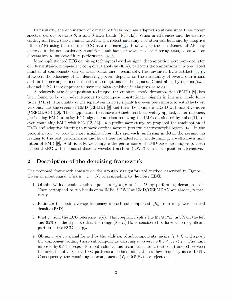
Particularly, the elimination of cardiac artifacts requires adapted solutions since their powerspectral density overlaps θ, α and β EEG bands (4-30 Hz). When interferences and the electro-cardiogram (ECG) have similar waveforms, a robust and simple solution can be found by adaptivefilters (AF) using the recorded ECG as a reference [3]. However, as the effectiveness of AF maydecrease under non-stationary conditions, sub-band or wavelet-based filtering emerged as well asalternatives to improve filters performance [4, 5].

More sophisticated EEG denoising techniques based on signal decomposition were proposed lateron. For instance, independent component analysis (ICA), performs decompositions in a prescribednumber of components, one of them containing, presumably, the unwanted ECG artifact [6, 7].However, the efficiency of the denoising process depends on the availability of several derivationsand on the accomplishment of certain assumptions on the signals. Constrained by our one/two-channel EEG, these approaches have not been exploited in the present work.

A relatively new decomposition technique, the empirical mode decomposition (EMD) [8], hasbeen found to be very advantageous to decompose nonstationary signals in intrinsic mode func-tions (IMFs). The quality of the separation in noisy signals has even been improved with the latestversions, first the ensemble EMD (EEMD) [9] and then the complete EEMD with adaptive noise(CEEMDAN) [10]. Their application to remove artifacts has been widely applied, as for instance,performing EMD on noisy ECG signals and then removing the IMFs dominated by noise [11], oreven combining EMD with ICA [12, 13]. In a preliminary study, we proposed the combination ofEMD and adaptive filtering to remove cardiac noise in preterm electroencephalogram [14]. In thepresent paper, we provide more insights about this approach, analyzing in detail the parametersleading to the best performances and how these are affected by mode mixing, a well-known limi-tation of EMD [9]. Additionally, we compare the performance of EMD-based techniques to cleanneonatal EEG with the use of discrete wavelet transform (DWT) as a decomposition alternative.

2 Description of the denoising framework

The proposed framework consists on the six-step straightforward method described in Figure 1.Given an input signal, x(n), n = 1 . . . N , corresponding to the noisy EEG:

1. Obtain M independent subcomponents xk(n), k = 1 . . .M by performing decomposition.They correspond to sub-bands or to IMFs if DWT or EMD/CEEMDAN are chosen, respec-tively.

2. Estimate the main average frequency of each subcomponent (fk) from its power spectraldensity (PSD).

3. Find fe from the ECG reference, z(n). This frequency splits the ECG PSD in 5% on the leftand 95% on the right, so that the range [0 - fe] Hz is considered to have a non significantportion of the ECG energy.

4. Obtain xH(n), a signal formed by the addition of subcomponents having fk ≥ fe and xL(n),the component adding those subcomponents carrying δ-waves, i.e 0.5 ≤ fk < fe. The limitimposed by 0.5 Hz responds to both clinical and technical criteria, that is, a trade-off betweenthe inclusion of very slow EEG patterns and the minimization of low-frequency noise (LFN).Consequently, the remaining subcomponents (fk < 0.5 Hz) are rejected.

2

xk(n)

x(n)

xH(n)

Decomposition(DWT, EMD or CEEMDAN)

Recomposition

ECG cancellation

(AF)

xL(n)

z(n)

+

fk < 0.5 Hz

xH(n)

xLFN(n) fk ≥ fe0.5 Hz ≤ fk < fe

Frequency estimation

M

x(n)

fk , fe

Figure 1: Block diagram of the proposed methodology with different options to decompose the EEG.

5. Remove ECG noise in xH(n) using the recorded ECG as a reference and obtain the cleanedcomponent, xH(n). To this end, adaptive filtering can be performed because the cardiacartifacts appearing in newborns’ EEG are similar to the ECG originated in the chest [15].

6. Reconstruct the clean EEG, x(n), by the addition of xL(n) and xH(n).

3 Methods

3.1 EEG decomposition by the discrete wavelet transform

The wavelet transform is a very useful and popular analysis tool for time-scale representation anddecomposition of non-stationary signals (for a complete survey about the theory of wavelets, theinterested reader can refer to [16]). By means of the DWT, the decomposition can be performed sothat the frequencies are in a power of two scale, a procedure also known as multi resolution analysis(MRA).

3.2 EEG decomposition by empirical mode decomposition

The application of empirical mode decomposition yields the so-called intrinsic modal functions [8],a number of subcomponents that must satisfy two conditions: 1) the number of extrema and zero-crossing must be equal or differ at most by one, and 2) the mean value of the upper and lowerenvelopes must be zero. Then, the unmixing process, also called sifting, can be performed:

1. Find local minima and maxima of the input signal, x(n).

2. Form upper, eu(n), and lower, el(n), envelopes by cubic splines interpolation.

3

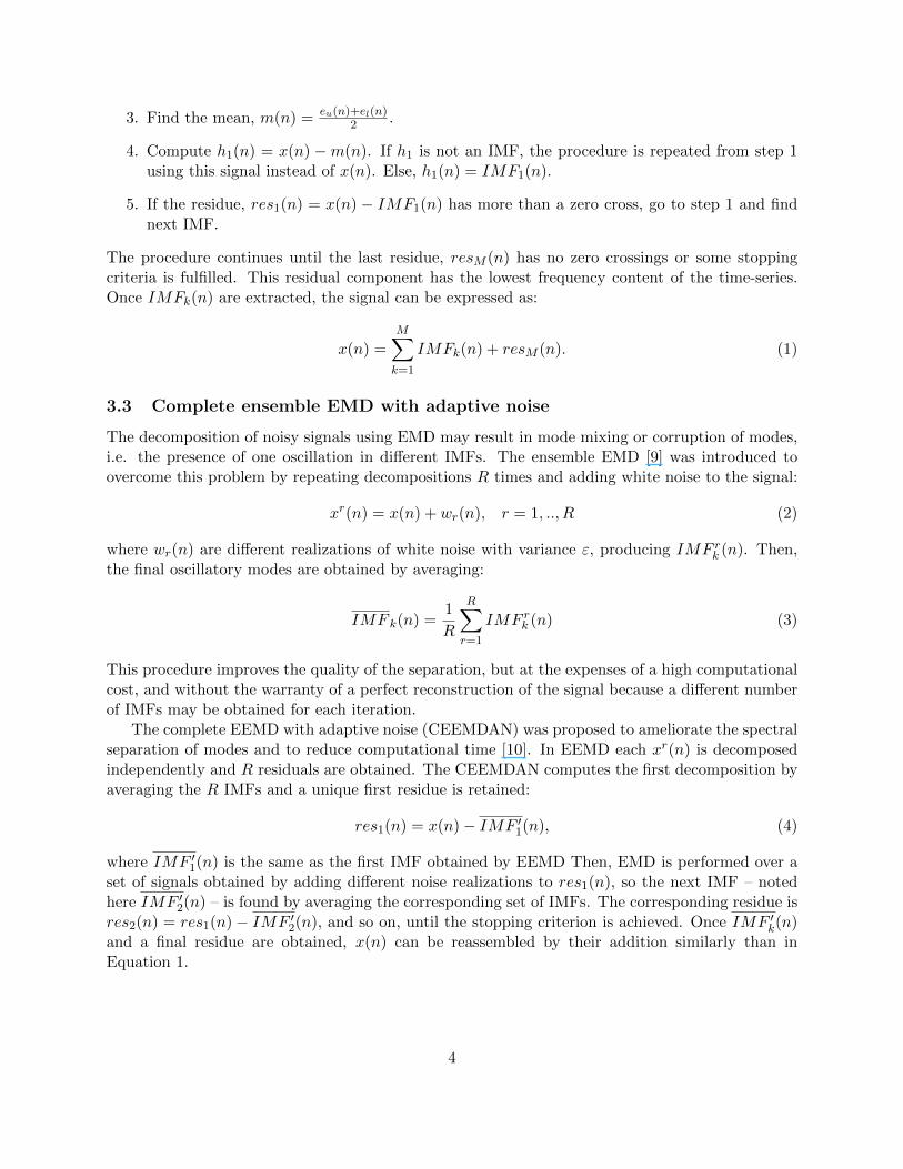
3. Find the mean, m(n) = eu(n)+el(n)2 .

4. Compute h1(n) = x(n) −m(n). If h1 is not an IMF, the procedure is repeated from step 1using this signal instead of x(n). Else, h1(n) = IMF1(n).

5. If the residue, res1(n) = x(n) − IMF1(n) has more than a zero cross, go to step 1 and findnext IMF.

The procedure continues until the last residue, resM (n) has no zero crossings or some stoppingcriteria is fulfilled. This residual component has the lowest frequency content of the time-series.Once IMFk(n) are extracted, the signal can be expressed as:

x(n) =M∑k=1

IMFk(n) + resM (n). (1)

3.3 Complete ensemble EMD with adaptive noise

The decomposition of noisy signals using EMD may result in mode mixing or corruption of modes,i.e. the presence of one oscillation in different IMFs. The ensemble EMD [9] was introduced toovercome this problem by repeating decompositions R times and adding white noise to the signal:

xr(n) = x(n) + wr(n), r = 1, .., R (2)

where wr(n) are different realizations of white noise with variance ε, producing IMF rk (n). Then,the final oscillatory modes are obtained by averaging:

IMF k(n) =1

R

R∑r=1

IMF rk (n) (3)

This procedure improves the quality of the separation, but at the expenses of a high computationalcost, and without the warranty of a perfect reconstruction of the signal because a different numberof IMFs may be obtained for each iteration.

The complete EEMD with adaptive noise (CEEMDAN) was proposed to ameliorate the spectralseparation of modes and to reduce computational time [10]. In EEMD each xr(n) is decomposedindependently and R residuals are obtained. The CEEMDAN computes the first decomposition byaveraging the R IMFs and a unique first residue is retained:

res1(n) = x(n)− IMF ′1(n), (4)

where IMF ′1(n) is the same as the first IMF obtained by EEMD Then, EMD is performed over aset of signals obtained by adding different noise realizations to res1(n), so the next IMF – notedhere IMF ′2(n) – is found by averaging the corresponding set of IMFs. The corresponding residue isres2(n) = res1(n)− IMF ′2(n), and so on, until the stopping criterion is achieved. Once IMF ′k(n)and a final residue are obtained, x(n) can be reassembled by their addition similarly than inEquation 1.

4

3.4 Adaptive filtering

Adaptive filtering has been extensively applied to cancel cardiac artifacts in biomedical signals usingthe recorded ECG as a reference [21]. In our denoising framework, we implemented the recursiveleast square algorithm (RLS) as it provides faster convergences than the classic least mean squares[22].

4 Validation strategy

To validate the efficacy of the different denoising options, contaminated signals were generated fromreal recordings. Data came from 30 preterm infants (36 to 39 weeks post-menstrual age) born atthe University Hospital of Rennes (France). ECG and double-channel EEG (Fp1-T3, Fp2-T4) wereacquired originally at 512 Hz sampling frequency, low-pass filtered (40 Hz cut-off) and subsampledto 128 Hz.

Since EEG signals acquired NICUs can also be contaminated with low frequency noise, weconstructed two groups to simulate realistic conditions:

1. Group 1: Thirty EEG excerpts with added ECG noise (filtering recorded EEG by a 21th-order FIR filter with random coefficients) with signal-to-noise ratios (SNRs) ranging from -5to 10 dB in steps of 5.

2. Group 2: Thirty EEG excerpts with added ECG at 5dB SNR plus LFN at variable SNR. Toemulate breathing and other slow movements, that may appear spontaneously and discontin-uously, LFN noise consisted in one cycle of a sinusoidal wave, very close to the limit of thedelta band, fixed randomly between 0.3 and 0.5 Hz. The power of the wave was set to obtainSNRs (relative to the original signal) ranging from -10 to 10 dB in steps of 5 dB.

Excerpts were selected by an experienced clinician, ensuring the absence of artifacts and includingdifferent EEG neonatal patterns. The amplitude of the noisy components was properly modifiedto obtain SNRs according to the following equation:

SNR = 10 logPEEGPnoise

(5)

where PEEG and Pnoise are the power of an original EEG excerpt and the power of the addedartifacts, respectively. Some examples of artificially contaminated EEG signals are shown in Figure2.

After processing separately each noisy EEG excerpt, x(n), by the denoising framework, thequality of the different decomposition options described in Figure 1 is measured in terms of rootmean squared error (RMSE):

RMSE =

√√√√ 1

N

N∑n=1

[xo(n)− x(n)]2 (6)

where xo(n) is the original, uncorrupted EEG, x(n) is the cleaned signal and N is the number ofsamples in each excerpt.

5

0 1 2 3 4 5 6 7 8 9 10-100

0

100Clean EEG excerpt

0 1 2 3 4 5 6 7 8 9 10-100

0

100EEG contaminated with ECG (SNR = 10 dB)

0 1 2 3 4 5 6 7 8 9 10-100

0

100EEG contaminated with ECG (SNR = 5 dB)

0 1 2 3 4 5 6 7 8 9 10-100

0

100EEG contaminated with ECG (SNR =5 dB) and LFN (SNR = 0 dB)

0 0.2 0.4 0.6 0.8 1 1.2 1.4 1.6 1.8 2-600

-100

400

Time (s)

Detail of original and filtered ECG

Original Filtered

Figure 2: Example of the generation of artificially contaminated EEGs by the filtered ECG and LFN. Using thefirst signal (clean EEG), two examples of Group 1 (second and third signals) have been formed. The fourth signal (aGroup 2 example) is formed by the addition of the third signal and LFN at 0 dB. The lower plot shows the originallyrecorded ECG, z(n), and the ECG noise obtained by applying the 21st-order FIR filter.

5 Tuning of parameters

5.1 Filtering and decomposition

To find the appropriate parameters for the different techniques, some preliminary tests were carriedout. Firstly, we found the appropriate order and algorithm of the adaptive filter in our particularsignals. A filter order L=16 and a forgetting factor λ = 1 − 1

10L (as suggested by Eleftheriou andFalconer [22]) yielded the best results.

The DWT was performed using 6th order Daubechies wavelet [17], a choice with satisfactoryresults in these signals [18]. The MRA framework was configured to obtain seven levels of successivedetails and the approximation interval, yielding eight subcomponents with their frequency intervalsbetween 32-64, 16-32, 8-16, 4-8, 2-4, 1-2, 0.5-1 and <0.5 Hz, that corresponded to LFN.

The EMD was computed by an efficient algorithm [19] that introduces two thresholds (θ1 andθ2) in the second criterion to consider an IMF, and a tolerance factor, α ∈ [0, 1]. They aim at guar-anteeing globally small fluctuations in the mean while taking into account locally large excursions.Finally, the CEEMDAN was performed by a recent algorithm improvement that optimizes speedand enhances quality with respect to its previous version [20].

5.2 Study of mode mixing

As mentioned before, subcomponents obtained by EMD-based techniques can suffer mode mixing,however, this phenomenon is not a major concern as far as it mixes frequencies from only one side

6

of the separation determined by fe. In this case, the sum of the IMFs yielding xL(n) and xH(n)should be the same as in the absence of mode mixing. More attention needs to be paid to thoseIMFs having frequency tones on both sides of the fe boundary, in particular:

1. Modes with fk ≥ fe –summed in xH(n)– containing oscillations below fe. Since xH(n) isprocessed by the AF, these low frequencies may lead to underperform the ECG cancellation.

2. Modes with 0.5 ≤ fk < fe containing frequencies above fe. The ECG noise could be partiallyinstalled in xL(n) so it would be unprocessed by the AF and incompletely removed in thefinal reassembled signal.

These two cases will be subsequently referred as to critical mixing I and II, respectively. Figure 3shows frequencies contained in IMFs performing EMD in a real EEG. The two first IMFs clearlyexhibit mode mixing, but since it occurs beyond the limit of fe, it has no consequences on thedenoising process. The energies carried by frequencies in the lower whiskers of IMF1, IMF2 andIMF3 crossing the horizontal dashed line constitute critical mixing I. Likewise, the energies in thefrequencies crossing fe in IMF4 determine critical mixing II.

10−1

100

101

1 2 3 4 5 6 7 8 9 10IMF number

Freq

uenc

y (H

z)

fe

Figure 3: Frequencies contained in all IMFs performing EMD in a real EEG. IMF1 and IMF2 contain almostidentical frequencies, evidencing mode mixing. The small frequency portions below fe of IMF1, IMF2 and IMF3

can be considered as critical mixing I, and conversely, the portion of IMF4 exceeding fe can be accounted as criticalmixing II.

To quantify critical mixing we took advantage of the IMFs to characterize the frequency andamplitude of the components. To illustrate this idea, let us consider an IMF with a single zero-crossing. Since the oscillation of this signal completes an entire period, its frequency can be obtainedby simply computing the inverse of the cycle time. Even if decompositions of experimental signalsdo not yield pure tones, this operation can approximate the frequencies describing cycles within anIMF.

Therefore, if a k-th IMF is composed by Ck cycles, with frequencies f lk (l = 1 . . . Ck), the totalenergy of the cycles into the critical mixing I region, CMI , can be expressed as:

CMI =∑k

fk≥fe

Ck∑l=1f lk≥fe

∥∥∥IMF lk(n)∥∥∥2 (7)

7

Table 1: Decomposition parameters for EMD (θ1, α) and CEEMDAN ( ε) minimizing critical mixing in ten examplesfrom Group 1 (G1) and Group 2 (G2). The average number of IMFs (M) is also shown.

SNRs for EMD θ1 α M CMI (%) CMII (%)G1 (-5 dB) 0.03 0.03 9.80 ± 0.42 1.62 ± 0.56 0.63 ± 0.24G1 (5 dB) 0.02 0.01 10.3 ± 0.48 1.44 ± 1.18 1.57 ± 1.12G2 (-5 dB) 0.03 0.02 10.1 ± 0.31 0.63 ± 0.52 0.64 ± 0.51G2 (5 dB) 0.03 0.02 10.3 ± 0.58 0.97 ± 0.62 0.32 ± 0.03

SNRs for CEEMDAN εG1 (-5 dB) 0.25 9.62 ± 0.52 0.94 ± 0.60 0.06 ± 0.02G1 (5 dB) 0.90 10.1 ± 0.55 1.46 ± 1.68 0.03 ± 0.02G2 (-5 dB) 0.35 10.2 ± 0.05 0.24 ± 0.11 0.01 ± 0.01G2 (5 dB) 0.95 9.80 ± 0.44 0.67 ± 0.57 0.04 ± 0.02

where the first summation includes those IMFs having their main frequency below fe and∥∥IMF lk(n)

∥∥is the norm of the l-th cycle in the k-th IMF. Equivalently, for critical mixing II:

CMII =∑k

0.5≤fk<fe

Ck∑l=1f lk<fe

∥∥∥IMF lk(n)∥∥∥2 (8)

CMI and CMII were then divided by the sum the energies contained in all IMFs to obtain therelative portion of critical mixing in each signal.

Several simulations were performed to find the decomposition parameters minimizing criticalmixing at different noise levels. In a first test, ten randomly selected signals from Group 1 werecontaminated with -5 dB and 5 dB SNR of cardiac noise and decomposed by both types of EMD.This test was then repeated using ten signals from Group 2, but contaminated with -5 dB and 5 dBSNR LFN. In order to prevent the sifting process from over-iteration and avoid over-decompositionof the signal, it is suggested by Rilling et al. [19] to use the default values θ1 = 0.05, θ2 = 10θ1 andα = 0.05. We therefore modified θ1 and α from 0.01 to 0.1 in steps of 0.005 to evaluate their effecton critical mixing.

In CEEMDAN, ε was modified from 0.05 to 1 in steps of 0.05 and R was fixed to 50, a choiceproviding an optimal computational time with negligible reconstruction error [20].

The values of the parameters leading to minimal ratios of critical mixing have been depictedin Table 1. From these tests, it can be stated that CEEMDAN reduces significantly CMII , thusmore effective to remove cardiac artifacts. We stated as well that the decomposition parameters(especially ε [9]) depend on the noise levels of contaminated signals and, hence, they should beadjusted increasingly as the EEG signals become more noisy to reduce critical mixing.

6 Results and discussion

6.1 ECG removal

The results of denoising Group 1 are summarized in Table 2. Indeed, the application of signaldecomposition techniques before the adaptive filter resulted in a general decrease of the RMSEscompared to denoising without EEG decomposition. However, this gain of quality was unequally

8

distributed and statistically significant only for certain SNRs. CEEMDAN provided in average a30% reduction of RMSEs whereas EMD and DWT resulted in 7.3% and 3.4% respective reductions.

It is noteworthy to mention that high SNR levels are then more favorable to perform EEGsignal decomposition, probably due to smaller distortion introduced to the final reconstructedsignal when only the noisy part of the EEG is processed by the AF. On the contrary, in low SNRsthe denoising performances of all methods converge because useful information is masked by noiseand decomposition become less effective.

6.2 ECG and low frequency noise removal

The scenario in which signals also contain low frequency noise has been evaluated using data fromGroup 2. To compare the improvements of introducing EEG decompositions, we processed theraw signals using a finite impulsional response (FIR) filter with a cutoff frequency of 0.5 Hz beforeapplying the cancellation of ECG noise. This high-pass filter (HPF) can prevent phase distortion,but employing a high order (382) that introduced delay (>1.5 s).

As it can be stated in Table 2, to remove simultaneously LFN and ECG noise only EMD-baseddecompositions are advantageous in all noise levels, with a 6.7% average RMSE reduction for EMDand 13% for CEEMDAN.

6.3 Denoising real signals

Finally, we performed some tests on real signals, contaminated both with ECG and LFN. Toevaluate quantitatively the noise elimination, we employed the artifact rejection ratio (ARR),defined as the ratio of the power of the removed artifacts to the cleaned EEG [23]:

ARR =

N∑n=1

[x(n)− x(n)]2

N∑n=1

x2(n)

(9)

where x(n) and x(n) are the real EEG before and after the denoising process, respectively.Since ARR gives information of the whole denoising process (comprising low frequency and

cardiac noise), we computed this ratio in small windows surrounding the QRS-peak instants (50ms) on the noisy excerpt and on the cleaned one. This parameter, ARRqrs, is conceived to give aquantitative idea of how attenuated are the heartbeat artifacts.

The metrics ARR and ARRqrs were computed on the selected excerpts (see Table 2), contami-nated with ECG artifacts and low frequency noise. As it can be noticed, the overall noise removalgiven by ARR and ARRqrs is greater using CEEMDAN. Of note, decomposition techniques arenot always advantageous to suppress QRS artifacts, as is the case of DWT and EMD. They pro-vided the lowest ARRqrs values probably for an incomplete separation of xH(n) before the ECGcancellation takes place.

7 Conclusion

The results presented in this paper show that, in general, EMD-based techniques performed bet-ter than DWT decomposition in the EEG signals studied here. This is probably due to the use

9

Table 2: Results from denoising simulated and real signals. For simulated EEG (both G1 and G2), the efficacy ofthe different denoising options is expressed as RMSEs (mean ± std. dev.). Best values (lower RMSEs) are in bold. Inbrackets, the improvement percentages compared to the simple usage of the adaptive filter (”NO DEC” columns) oradaptive filter plus high-pass filter (”NO DEC + HPF”). A Wilcoxon signed rank test compared ”NO DEC (+HPF)”with the three decomposition solutions ( * denote statistically significant differences at p <0.05). The last two rowsshow the noise removal estimation by the ARR metrics. Best values (greatest ARR) are highlighted in bold.

G1 simulated signals (SNRs) NO DEC DWT EMD CEEMDAN-5 dB 18.8 ± 6.06 18.5 ± 6.06 (1.6%) 18.4 ± 6.00 (2.1%) 17.2 ± 5.78 (8.6%)0 dB 10.7 ± 3.41 10.4 ± 3.36 (2.8%) 10.3 ± 3.35 (3.7%) 8.12 ± 3.13∗(25%)5 dB 6.23 ± 1.95 6.01 ± 1.93 (3.5%) 5.80 ± 1.86 (6.9%) 3.94 ± 1.74∗(36%)10 dB 3.86 ± 1.17 3.64 ± 1.16 (5.7%) 3.22 ± 1.02∗(16%) 1.93 ± 0.96∗(49%)

Mean improvement 3.4% 7.3% 30%

G2 simulated signals (SNRs) NO DEC + HPF-5 dB 19.8 ± 6.36 21.2 ± 7.55 (-7%) 17.5 ± 6.63 (12%) 16.5 ± 5.16∗(16%)0 dB 12.7 ± 3.99 13.1 ± 4.56 (-3.1%) 12.1 ± 4.83 (4.7%) 10.8 ± 3.31∗(15%)5 dB 9.08 ± 2.88 9.23 ± 3.08 (-1.6%) 8.64 ± 2.90 (4.8%) 7.92 ± 3.12 (13%)10 dB 7.67 ± 2.44 7.54 ± 2.47 (1.7%) 7.27 ± 2.69 (5.2%) 7.03 ± 2.39 (8.3%)

Mean improvement -2.5% 6.7% 13%

Real signals (noise elimination)ARR 1.94±2.20 2.77±2.98 2.38±2.72 4.54±6.33∗

ARRqrs 8.66±10.2 8.17±6.71 7.60±8.51 9.37±7.60

of power of two in the scale factors in DWT, an imposition that yields only four subcomponentsbetween 0.5 and 8 Hz. But as the energy distribution within this range of frequencies is variable,an optimal separation of the EEG bands may require a different number of subcomponents. Theadaptive manner of decomposing signals by the EMD and CEEMDAN is, therefore, more conve-nient to separate and reassemble the subcomponents as a function of fe, the frequency containingthe ECG artifacts. Other wavelet-based methods not explored here, such as the wavelet packettransform, could be employed alternatively to obtain more subcomponents in the aforementionedrange. However, finding the optimal basis in this solution is not straightforward.

The major issue of EMD, mode mixing, has not been found to be a major concern in theapplication presented herewith. The main problem was rather to have IMFs with oscillationscrossing the threshold established by fe, critical mixing, a fact that is not necessarily related tomode mixing. By quantifying critical mixing, we corroborated that the CEEMDAN, thanks to itssuperior performance, reduces this effect and provides the best denoising results.

However, the use of decomposition techniques introduce some limitations that should be takeninto account. Firstly, distortion in low frequency bands cannot be completely avoided since therejection of subcomponents below 0.5 Hz implies the removal of certain content over this frequency.Although this limitation is partially solved by the enhanced spectral separation of CEEMDAN,the degree of rejected true slow-delta waves needs to be studied in future works because not onlytechnical, but also physiological and maturational considerations appear on the scene [24]. But wealso would like to note that in less noisy environments the low frequency limit could be decreasedbelow 0.5 Hz to include the slowest delta content. Secondly, the choice of CEEMDAN implies anincreased computational cost, but even if a recent algorithm has reduced its complexity, it is stillmay be considered a drawback for current real-time systems. In the near future, the applicationof the family of EMD methods to denoise EEG is more plausible for the NICU as the algorithmcontinues to be improved in terms of speed and bedside equipment is becoming more powerful.

10

Conflict of interest

There are no known conflicts of interest associated with this publication and there has been nosignificant financial support for this work that could have influenced its outcome. The databaseinvolved in this study received the ethic approval by the Regional Ethics Committee (Comite deProtection des Personnes, CPP Ouest 6-598).

Acknowledgements

The research for this paper was financially supported by the project INTEM between RennesUniversity Hospital and the LTSI-INSERM U1099. X. Navarro is currently funded by Air LiquideMedical Systems France through the COVEM Project.

References

[1] D. Maynard, P. F. Prior and D. F. Scott. Device for continuous monitoring of cerebral activity inresuscitated patients. British Medical Journal, 4(5682): 545–546, 1969.

[2] C. F. Hagmann, N. J. Robertson and D. Azzopardi. Artifacts on Electroencephalograms May Influencethe Amplitude-Integrated EEG Classification: A Qualitative Analysis in Neonatal Encephalopathy.Pediatrics, 118(6):2552–4, 2006.

[3] P. Celka, B. Boashash, and P. Colditz. Preprocessing and time-frequency analysis of newborn EEGseizures. IEEE Engineering in Medicine and Biology Magazine, 20(5):30–39, 2001.

[4] N. Erdol and F. Basbug. Wavelet transform based adaptive filters: analysis and new results. IEEETransactions on Signal Processing, 44(9):2163–2171, 1996.

[5] S. Hosur and A.H. Tewfik. Wavelet transform domain adaptive FIR filtering. IEEE Transactions onSignal Processing, 45(3):617–630, 1997.

[6] T. P. Jung, S. Makeig, C. Humphries, T. W. Lee, M. J. McKeown, V. Iragui, and T. J. Sejnowski.Removing electroencephalographic artifacts by blind source separation. Psychophysiology, 37(2):163–178, 2000.

[7] F. Poree, A. Kachenoura, H. Gauvrit, C. Morvan, G. Carrault, and L. Senhadji. Blind source sepa-ration for ambulatory sleep recording. IEEE Transactions on Information Technology in Biomedicine,10(2):293–301, 2006.

[8] N. E. Huang, Z. Shen, S. R. Long, M. C. Wu, H. H. Shih, Q. Zheng, N-C. Yen, C. C. Tung, and H. H.Liu. The empirical mode decomposition and the hilbert spectrum for nonlinear and non-stationarytime series analysis. Proceedings of the Royal Society of London. Series A: Mathematical, Physical andEngineering Sciences, 454(1971):903–995, 1998.

[9] Z. Wu and N. E. Huang. Ensemble Empirical Mode Decomposition: A noise-assisted data analysismethod. Advances in Adaptive Data Analysis, 01(01):1, 2009.

[10] M. E. Torres, M. A. Colominas, G. Schlotthauer, and P. Flandrin. A complete ensemble empirical modedecomposition with adaptive noise. In 2011 IEEE International Conference on Acoustics, Speech andSignal Processing (ICASSP), pages 4144–4147. IEEE, 2011.

11

[11] S. Pal and M. Mitra. Empirical mode decomposition based ECG enhancement and QRS detection.Computers in Biology and Medicine, 42(1):83–92, 2012.

[12] J. P. Lindsen and J. Bhattacharya. Correction of blink artifacts using independent component analysisand empirical mode decomposition. Psychophysiology, 47(5):955–960, 2010.

[13] B. Mijovic, M. De Vos, I. Gligorijevic, J. Taelman and S. Van Huffel. Source Separation From Single-Channel Recordings by Combining Empirical-Mode Decomposition and Independent Component Anal-ysis IEEE Transactions on Biomedical Engineering, 57(9):2188–2196, 2010.

[14] X. Navarro, F. Poree, and G. Carrault. ECG removal in preterm EEG combining empirical modedecomposition and adaptive filtering. In 2012 IEEE International Conference on Acoustics, Speech andSignal Processing (ICASSP), pages 661–664, 2012.

[15] J. M. Stern. Atlas of EEG Patterns. Lippincott Williams & Wilkins, 2005.

[16] S. Mallat. A wavelet tour of signal processing Academic press, 1999.

[17] I. Daubechies. Ten Lectures on Wavelets. SIAM: Society for Industrial and Applied Mathematics, 1edition, 1992.

[18] J.P Turnbull, K.A Loparo, M.W Johnson, and M.S Scher. Automated detection of trace alternantduring sleep in healthy full-term neonates using discrete wavelet transform. Clinical Neurophysiology,112(10):1893–1900, 2001.

[19] G. Rilling, P. Flandrin, and P. Goncalves. On empirical mode decomposition and its algorithms. InProceedings of the 6th IEEE/EURASIP Workshop on Nonlinear Signal and Image Processing (NSIP’03), Grado, Italy, 2003.

[20] M. A. Colominas, G. Schlotthauer and M. E. Torres Improved complete ensemble EMD: A suitabletool for biomedical signal processing Biomedical Signal Processing and Control, 14: 19–29, 2014

[21] S. Haykin. Adaptive Filter Theory. Pearson Education, 4 edition, 2002.

[22] E. Eleftheriou and D.D. Falconer. Tracking properties and steady-state performance of RLS adaptivefilter algorithms. IEEE Transactions on Acoustics, Speech and Signal Processing, 34(5):1097–1110,1986.

[23] S. Puthusserypady and T. Ratnarajah. Robust adaptive techniques for minimization of EOG artefactsfrom EEG signals. Signal Processing, 86(9):2351–2363, 2006.

[24] M.D Lamblin, M. Andre, M.J Challamel, L. Curzi-Dascalova, A.M. d’Allest, E. De Giovanni, F.Moussalli-Salefranque, Y. Navelet, P. Plouin, M.F Radvanyi-Bouvet, D. Samson-Dollfus and M.F.Vecchierini-Blineau. Electroencephalography of the premature and term newborn. Maturational as-pects and glossary. Neurophysiol Clin., 29(2):123–219, 1999.

12