Adaptive deformable mirror : based on electromagneticactuatorsCitation for published version (APA):Hamelinck, R. F. M. M. (2010). Adaptive deformable mirror : based on electromagnetic actuators. [Phd Thesis 1(Research TU/e / Graduation TU/e), Mechanical Engineering]. Technische Universiteit Eindhoven.https://doi.org/10.6100/IR675512

DOI:10.6100/IR675512

Document status and date:Published: 01/01/2010

Document Version:Publisher’s PDF, also known as Version of Record (includes final page, issue and volume numbers)

Please check the document version of this publication:

• A submitted manuscript is the version of the article upon submission and before peer-review. There can beimportant differences between the submitted version and the official published version of record. Peopleinterested in the research are advised to contact the author for the final version of the publication, or visit theDOI to the publisher's website.• The final author version and the galley proof are versions of the publication after peer review.• The final published version features the final layout of the paper including the volume, issue and pagenumbers.Link to publication

General rightsCopyright and moral rights for the publications made accessible in the public portal are retained by the authors and/or other copyright ownersand it is a condition of accessing publications that users recognise and abide by the legal requirements associated with these rights.

• Users may download and print one copy of any publication from the public portal for the purpose of private study or research. • You may not further distribute the material or use it for any profit-making activity or commercial gain • You may freely distribute the URL identifying the publication in the public portal.

If the publication is distributed under the terms of Article 25fa of the Dutch Copyright Act, indicated by the “Taverne” license above, pleasefollow below link for the End User Agreement:www.tue.nl/taverne

Take down policyIf you believe that this document breaches copyright please contact us at:openaccess@tue.nlproviding details and we will investigate your claim.

Download date: 21. Sep. 2022

ADAPTIVE DEFORMABLE MIRROR

BASED ON ELECTROMAGNETIC ACTUATORS

ROGER HAMELINCK

Adaptive deformable mirrorbased on ele tromagneti a tuators

This research was partially funded by TNO Science and Industry and the IOP Precision Technologyprogram of the Dutch Ministry of Economic Affairs.

A catalogue record is available from the Eindhoven University of Technology Library

Adaptive deformable mirror, based on electromagnetic actuators / by Roger Hamelinck –Eindhoven : Technische Universiteit Eindhoven, 2010, ProefschriftISBN 978-90-386-2278-1Copyright c© 2010 by R.F.M.M. Hamelinck.

This thesis was prepared with the LATEX 2ε documentation system.Reproduction by ORO Grafisch Project Management, Koekange,The Netherlands.Cover design by Hans Timmer, Oosterhout, The Netherlands.

Adaptive deformable mirrorbased on ele tromagneti a tuatorsProefontwerp

ter verkrijging van de graad van doctoraan de Technische Universiteit Eindhoven,

op gezag van de rector magnificus, prof.dr.ir. C.J. van Duijn,voor een commissie aangewezen door het College voor Promoties

in het openbaar te verdedigenop dinsdag 22 juni 2010 om 16.00 uur

door

Roger Francisus Mattheus Maria Hamelinck

geboren te Dongen

iv

De documentatie van het proefontwerp is goedgekeurd door depromotor:

prof.dr.ir. M. Steinbuch

Copromotor:dr.ir. P.C.J.N. Rosielle

ContentsSummary ix

Nomenclature xi

Acronyms xix

1 Introduction 11.1 Imaging through atmospheric turbulence . . . . . . . . . . . . .. . . . . . 21.2 The adaptive optics system . . . . . . . . . . . . . . . . . . . . . . . . .. 4

1.2.1 Atmospheric turbulence . . . . . . . . . . . . . . . . . . . . . . . 41.2.2 Wavefront sensing . . . . . . . . . . . . . . . . . . . . . . . . . . 51.2.3 Wavefront correction . . . . . . . . . . . . . . . . . . . . . . . . . 51.2.4 Wavefront control . . . . . . . . . . . . . . . . . . . . . . . . . . . 9

1.3 Challenges . . . . . . . . . . . . . . . . . . . . . . . . . . . . . . . . . . . 101.3.1 Challenges for the wavefront corrector . . . . . . . . . . . .. . . . 111.3.2 Challenges for the control system . . . . . . . . . . . . . . . . .. 12

1.4 Problem formulation and outline . . . . . . . . . . . . . . . . . . . .. . . 13

2 Design requirements and design concept 152.1 Requirements . . . . . . . . . . . . . . . . . . . . . . . . . . . . . . . . . 16

2.1.1 Atmospheric turbulence . . . . . . . . . . . . . . . . . . . . . . . 162.1.2 The Kolmogorov turbulence model . . . . . . . . . . . . . . . . . 16

2.2 Error budget . . . . . . . . . . . . . . . . . . . . . . . . . . . . . . . . . . 202.2.1 The fitting error . . . . . . . . . . . . . . . . . . . . . . . . . . . . 212.2.2 The temporal error . . . . . . . . . . . . . . . . . . . . . . . . . . 212.2.3 Error budget division . . . . . . . . . . . . . . . . . . . . . . . . . 22

2.3 Actuator requirements . . . . . . . . . . . . . . . . . . . . . . . . . . . .232.4 Control system and electronics requirements . . . . . . . . .. . . . . . . . 252.5 The design concept . . . . . . . . . . . . . . . . . . . . . . . . . . . . . . 27

2.5.1 The mirror facesheet . . . . . . . . . . . . . . . . . . . . . . . . . 282.5.2 The actuator modules . . . . . . . . . . . . . . . . . . . . . . . . . 292.5.3 The control system and electronics . . . . . . . . . . . . . . . .. . 302.5.4 The base frame . . . . . . . . . . . . . . . . . . . . . . . . . . . . 30

3 The mirror facesheet 313.1 Overview of thin mirrors . . . . . . . . . . . . . . . . . . . . . . . . . . .32

3.1.1 Thin and ultra thin glass mirrors . . . . . . . . . . . . . . . . . .. 323.1.2 Beryllium X-ray windows . . . . . . . . . . . . . . . . . . . . . . 343.1.3 Existing membrane deformable mirrors . . . . . . . . . . . . .. . 35

v

vi Contents

3.1.4 Thin and ultra thin wafers . . . . . . . . . . . . . . . . . . . . . . 363.1.5 Thin Carbon Fiber Reinforced Plastic (CFRP) mirrors .. . . . . . 373.1.6 Nanolaminate deformable mirrors . . . . . . . . . . . . . . . . .. 373.1.7 Epoxy Replicated Aluminum Foil (ERAF) . . . . . . . . . . . . .383.1.8 Space membrane mirror technologies . . . . . . . . . . . . . . .. 38

3.2 Design of the mirror facesheet . . . . . . . . . . . . . . . . . . . . . .. . 403.2.1 The facesheet thickness . . . . . . . . . . . . . . . . . . . . . . . . 403.2.2 Actuator forces for mirror deformation . . . . . . . . . . . .. . . 423.2.3 Power dissipation . . . . . . . . . . . . . . . . . . . . . . . . . . . 423.2.4 Mirror facesheet material comparison . . . . . . . . . . . . .. . . 45

3.3 Constraining the mirror facesheet . . . . . . . . . . . . . . . . . .. . . . . 473.3.1 The facesheet’s out-of-plane Degrees Of Freedoms (DOFs) . . . . . 473.3.2 The mirror’s in-plane DOF . . . . . . . . . . . . . . . . . . . . . . 503.3.3 Wrinkling and pretension in the membrane . . . . . . . . . . .. . 52

3.4 The influence function . . . . . . . . . . . . . . . . . . . . . . . . . . . . 543.5 The connection struts . . . . . . . . . . . . . . . . . . . . . . . . . . . . .553.6 Assembly of the connection struts . . . . . . . . . . . . . . . . . . .. . . 573.7 Results . . . . . . . . . . . . . . . . . . . . . . . . . . . . . . . . . . . . . 703.8 Conclusions and recommendations . . . . . . . . . . . . . . . . . . .. . . 71

4 Modular actuator grid 734.1 Actuator requirements . . . . . . . . . . . . . . . . . . . . . . . . . . . .74

4.1.1 The actuator force . . . . . . . . . . . . . . . . . . . . . . . . . . 754.2 Electromagnetic actuators . . . . . . . . . . . . . . . . . . . . . . . .. . . 75

4.2.1 The Lorentz actuator . . . . . . . . . . . . . . . . . . . . . . . . . 754.2.2 Reluctance actuators . . . . . . . . . . . . . . . . . . . . . . . . . 76

4.3 The variable reluctance actuator . . . . . . . . . . . . . . . . . . .. . . . 804.3.1 The actuator membrane suspension . . . . . . . . . . . . . . . . .824.3.2 The electromagnetic force . . . . . . . . . . . . . . . . . . . . . . 854.3.3 A static actuator model . . . . . . . . . . . . . . . . . . . . . . . . 894.3.4 A dynamic actuator model . . . . . . . . . . . . . . . . . . . . . . 924.3.5 Measurements and validation . . . . . . . . . . . . . . . . . . . . 974.3.6 Sensitivity analysis . . . . . . . . . . . . . . . . . . . . . . . . . . 1004.3.7 Lessons learned . . . . . . . . . . . . . . . . . . . . . . . . . . . . 104

4.4 The actuator module . . . . . . . . . . . . . . . . . . . . . . . . . . . . . 1064.4.1 Actuator grid design . . . . . . . . . . . . . . . . . . . . . . . . . 1064.4.2 Actuator grid assembly . . . . . . . . . . . . . . . . . . . . . . . . 1094.4.3 Measurement results . . . . . . . . . . . . . . . . . . . . . . . . . 1134.4.4 Power dissipation . . . . . . . . . . . . . . . . . . . . . . . . . . . 115

4.5 Conclusions . . . . . . . . . . . . . . . . . . . . . . . . . . . . . . . . . . 1164.6 Recommendations . . . . . . . . . . . . . . . . . . . . . . . . . . . . . . . 117

vii

5 Electronics 1195.1 Introduction . . . . . . . . . . . . . . . . . . . . . . . . . . . . . . . . . . 1205.2 Driver electronics . . . . . . . . . . . . . . . . . . . . . . . . . . . . . . .120

5.2.1 Requirements . . . . . . . . . . . . . . . . . . . . . . . . . . . . . 1205.2.2 Concepts . . . . . . . . . . . . . . . . . . . . . . . . . . . . . . . 121

5.3 Communication electronics . . . . . . . . . . . . . . . . . . . . . . . .. . 1245.4 Implementation and realization . . . . . . . . . . . . . . . . . . . .. . . . 125

5.4.1 Pulse Width Modulation (PWM) implementation . . . . . . .. . . 1255.4.2 Field Programmable Gate Array (FPGA) implementation. . . . . . 1285.4.3 The ethernet to Low Voltage Differential Signalling (LVDS) bridge 130

5.5 Modeling . . . . . . . . . . . . . . . . . . . . . . . . . . . . . . . . . . . 1305.6 Testing and validation . . . . . . . . . . . . . . . . . . . . . . . . . . . .. 133

5.6.1 Communications tests . . . . . . . . . . . . . . . . . . . . . . . . 1335.6.2 Parasitic resistance measurements . . . . . . . . . . . . . . .. . . 1345.6.3 Actuator system validation . . . . . . . . . . . . . . . . . . . . . .1345.6.4 Nonlinear behavior . . . . . . . . . . . . . . . . . . . . . . . . . . 139

5.7 Power dissipation . . . . . . . . . . . . . . . . . . . . . . . . . . . . . . . 1405.7.1 Optimizing the FPGA power efficiency . . . . . . . . . . . . . . .1415.7.2 Cooling . . . . . . . . . . . . . . . . . . . . . . . . . . . . . . . . 143

5.8 Conclusions . . . . . . . . . . . . . . . . . . . . . . . . . . . . . . . . . . 144

6 System modeling and characterization 1476.1 Introduction . . . . . . . . . . . . . . . . . . . . . . . . . . . . . . . . . . 1486.2 Deformable Mirror (DM) integration . . . . . . . . . . . . . . . . .. . . . 149

6.2.1 Integration of the 61 actuator mirror . . . . . . . . . . . . . .. . . 1496.2.2 Integration of the 427 actuator mirror . . . . . . . . . . . . .. . . 150

6.3 Static system validation . . . . . . . . . . . . . . . . . . . . . . . . . .. . 1536.3.1 Modeling . . . . . . . . . . . . . . . . . . . . . . . . . . . . . . . 1546.3.2 Measurements and results . . . . . . . . . . . . . . . . . . . . . . 1576.3.3 Power dissipation . . . . . . . . . . . . . . . . . . . . . . . . . . . 166

6.4 Dynamic system validation . . . . . . . . . . . . . . . . . . . . . . . . .. 1696.4.1 Dynamic modeling . . . . . . . . . . . . . . . . . . . . . . . . . . 1696.4.2 System identification . . . . . . . . . . . . . . . . . . . . . . . . . 1736.4.3 Modal analysis . . . . . . . . . . . . . . . . . . . . . . . . . . . . 175

6.5 Conclusions . . . . . . . . . . . . . . . . . . . . . . . . . . . . . . . . . . 179

7 Conclusions 1817.1 Conclusions . . . . . . . . . . . . . . . . . . . . . . . . . . . . . . . . . . 1827.2 Recommendations . . . . . . . . . . . . . . . . . . . . . . . . . . . . . . . 186

Appendices 187A Measurement of the magnetic properties of Permanent Magnets (PMs) . . . 189B Setup to measure the nonlinear stiffness of the membrane suspensions . . . 193C Fourier series of a PWM signal . . . . . . . . . . . . . . . . . . . . . . . . 197D The LVDS protocol . . . . . . . . . . . . . . . . . . . . . . . . . . . . . . 199E The UDP protocol . . . . . . . . . . . . . . . . . . . . . . . . . . . . . . . 203

viii Contents

F Spatial variation of actuator properties . . . . . . . . . . . . . .. . . . . . 205G Quantization . . . . . . . . . . . . . . . . . . . . . . . . . . . . . . . . . . 207

Bibliography 209

Samenvatting 223

Dankwoord 225

Curriculum Vitae 227

SummaryAdaptive deformable mirror based on electromagnetic actuatorsRefractive index variations in the earth’s atmosphere cause wavefront aberrations and limitthereby the resolution in ground-based telescopes. With Adaptive Optics (AO) the tempo-rally and spatially varying wavefront distortions can be corrected in real time. Most imple-mentations in a ground based telescope include a WaveFront Sensor, a Deformable Mirrorand a real time wavefront control system. The largest optical telescopes built today havea ≈10m primary mirror. Telescopes with more collecting area and higher resolution aredesired. ELTs are currently designed with apertures up to 42m. For these telescopes seriouschallenges for all parts of the AO system exist. This thesis addresses the challenges for theDM. An 8m class telescope on a representative astronomical site is the starting point.The atmosphere is characterized by the spatial and temporalspectra of Kolmogorov tur-bulence and the frozen flow assumption. The wavefront fittingerror, caused by a limitednumber of actuators and the temporal error, caused by a limited control bandwidth, are themost important for the DM design. It is shown that≈5000 actuators and 200Hz closedloop bandwidth form a balanced choice between the errors andcorrect an 8m wavefront inthe visible to nearly diffraction limited. An actuator stroke of≈5.6µm and≈0.36µm interactuator stroke is thereby needed. Together with the nm’s resolution, low power dissipation,no hysteresis and drift, these form the main DM requirements.The design, realization and tests of a new DM that meets theserequirements and is extend-able and scalable in mechanics, electronics and control to suit further ELTs is presented.In the DM a few layers are distinguished: a continuous mirrorfacesheet, the actuator gridand the base frame. Below the facesheet, in the actuator grid, the low voltage electromag-netic push-pull actuators are located. Identical actuatormodules, each with 61 actuators,hexagonally arranged on a 6mm pitch can be placed adjacent toform large grids. The baseframe provides a stable and stiff reference.A thin facesheet is needed for low actuator forces and power dissipation, whereby its lowerlimit is set by the facesheets inter actuator deflection determined by gravity or wind pressure.For both scaling laws for force and dissipation are derived.Minimum power dissipation isachieved when beryllium is used for the mirror facesheet. Pyrex facesheets with 100µmthickness are chosen as a good practical, alternative in theprototype development. Struts(∅0.1×8mm) connect the facesheet to the actuators and ensure a smooth surface over theimposed heights and allow relative lateral movement of the facesheet and the actuator grid.Measurements show 3nm RMS surface unflattness from the gluedattachment.The stiffness of the actuators form the out-of-plane constraints for the mirror facesheet anddetermine the mirrors first resonance frequency. The stiffness is chosen such that the res-onance frequency is high enough to allow the high control bandwidth but not higher thatneeded to avoid excessive power dissipation and fix points inthe surface in case of failure.

ix

x Summary

The electromagnetic variable reluctance actuators designed, are efficient, have low movingmass and have suitable stiffness. Other advantages are the low costs, low driving voltagesand negligible hysteresis and drift. The actuators consistof a closed magnetic circuit inwhich a PM provides static magnetic force on a ferromagneticcore that is suspended in amembrane. This attraction force is increased of decreased by a current through a coil. Theactuators are free from mechanical hysteresis, friction and play and therefore have a highpositioning resolution with high reproducibility. The actuator modules are build in layers toreduces the number of parts and the complexity of assembly and to improve the uniformityin properties.Dedicated communication and driver electronics are designed. FPGA implemented PWMbased voltage drivers are chosen because of their high efficiency and capability to be im-plemented in large numbers with only a few electronic components. A multidrop LVDSbased serial communication is chosen for its low power consumption, high bandwidth andconsequently low latency, low communication overhead and extensive possibilities for cus-tomization. A flat-cable connects up to 32 electronics modules, each suited to drive 61actuators in an actuator module, to a custom communicationsbridge, which translates theEthernet packages from the control PC into LVDS.Two DMs prototypes were successfully assembled: a∅50mm DM with 61 actuators anda ∅150mm DM with 427 actuators. In the second prototype modularity is shown by theassembly of seven identical grids on a common base. The dynamic performance of eachactuator is measured, including its dedicated driver and communication. All actuators werefound to be functional, indicating that the manufacturing and assembly process is reliable.A nonlinear mathematical model of the actuator was derived describing both its static anddynamic behavior based on equations from the magnetic, mechanic and electric domains.The actuator model was linearized, leading to expressions for the actuator transfer functionand properties such as motor constant, coil inductance, actuator stiffness and resonance fre-quency. From frequency response function measurements these properties showed slightdeviations from the values derived from the model, but the statistical spread for the prop-erties was small, stressing the reliability of the manufacturing and assembly process. Themean actuator stiffness and resonance frequency were 0.47kN/m and 1.8kHz respectively,which is close to their design values of 500N/m and 1.9kHz. The time domain response ofan actuator to a 4Hz sine voltage was used to determine hysteresis and semi-static nonlinearresponse of the actuator. This showed the first to be negligible and the second to remainbelow 5% for±10µm stroke. Measurements showed that in the expected operating range,the total power dissipation is dominated by indirect lossesin FPGAs.The static DM performance is validated using interferometric measurements. The measuredinfluence matrix is used to shape the mirror facesheet into the first 28 Zernike modes, whichincludes the piston term that represents the best flat mirror. The total RMS error is≈25nmfor all modes. The dynamic behavior of the DM is validated by measurements. A laservibrometer is used to measure the displacement of the mirrorfacesheet, while the actuatorsare driven by zero-mean, bandlimited, white noise voltage sequence. Using the MOESPsystem identification algorithm, high-order black-box models are identified with VAF val-ues around 95%. The first resonance frequency identified is 725Hz, and lower than the974Hz expected from the analytical model. This is attributed to the variations in actuatorproperties, such as actuator stiffness. The power dissipation in each actuator of the∅50mmmirror to correct a typical Von Karmann turbulence spectrumis≈1.5mW.

Nomen latureSymbols

Symbol Description Unit0 vector or matrix whose elements are all zero1 vector or matrix whose elements are all unityAga cross section of the axial airgap [m2]Agr cross section of the radial airgap [m2]Am cross section of the actuator membrane suspension [m2]Aw cross section of the coil winding [m2]B magnetic field density [T]Bs magnetic saturation [T]Bρ influence matrix that links the PWM voltages to the facesheet

deflection at the actuator locations[m/V]

Bf,w influence matrix that links the PWM voltages to the facesheetdeflection on the measurement grid of the Wyko interferometer

[m/V]

Bf,w measured, zero piston, influence matrix that links the PWMvoltages to the facesheet deflection on the measurement gridof the Wyko interferometer

[m/V]

Bf influence matrix that links the PWM voltages to the facesheetdeflections at an arbitrary grid of points on the facesheet

[m/V]

C(s) continuous time controllerC(z) discrete time controllerC1 linear stiffness coefficient [-]C2 nonlinear stiffness coefficient [-]Ca diagonal matrix whoseith diagonal element is the stiffnessca

of actuatori[N/m]

Caf stiffness matrix comprehending both the facesheet and actuatorstiffnesses

[N/m]

CFPGA capacitance of the FPGA [F]Cl capacitance used in the analog low pass filter [F]

C2N Atmospheric turbulence strength [m

−23 ]

D diameter [m]Df flexural rigidity [Nm]Dn index of refraction structure function [-]Ds diameter of the connection struts [m]Dt diameter of the telescopes primary mirror [m]DDM diameter of the DM [m]Dφ phase structure function [-]E Young’s modulus or elastic modulus [N/m2]

xi

xii Nomenclature

Symbol Description UnitEf Young’s modulus of the mirror facesheet [N/m2]Eg Young’s modulus of the glue [N/m2]Em Young’s modulus of the actuator membrane suspension [N/m2]Es Young’s modulus of the connection strut [N/m2]Fa actuator force [N]Fa vector of actuator forces [N]Fρ net force acting on the facesheet at the actuator location [N]Fb buckling force [N]FL Lorentz force [N]Fm magnetic force [N]Fres actuator force resolution [N]Fs spring force [N]Fρ vector of net forces acting on the facesheet at the actuator loca-

tions[N]

Fi magnetomotive force in the flux path with indexi [A]H(s) transfer function from voltage to position [m/V]

HI(s) transfer function from current to position [m/A]Hm(s) transfer function from force to position [m/N]H∗

p,Ts(z, θ) discretized transfer function from voltage to position [m/V]H∗

v,Ts(z, θ) discretized transfer function from voltage to speed [m/sV]Hp,Ts(z, θ) estimated transfer function from voltage to position [m/V]Hv,Ts(z, θ) estimated transfer function from voltage to speed [m/sV]H∗

p,Ts(z, θ) estimated and discretized transfer function from voltage to po-sition

[m/V]

H∗

v,Ts(z, θ) estimated and discretized transfer function from voltage tospeed

[m/sV]

Hτc Transfer function for the communication latency [-]HZOH(s) Transfer function of the zero order hold operation [-]Hbc magnetic field intensity in the coil core [A/m]Hcm coercivity of the PM [A/m]Hga magnetic field intensity in the axial airgap [A/m]Hgr magnetic field intensity in the radial airgap [A/m]Hm magnetic field intensity in the PM [A/m]Hr magnetic field intensity in the core and baseplate [A/m]I current [A]I identity matrixIs second moment of inertia of the connection strut [m4]Ia current through the actuator coil [A]ICl

current through the capacitanceCl [A]If current through the fictitious winding [A]IRl

current through the resistanceRl [A]J1(·) Bessel function of the first kind [-]Ja current density in the actuator coil [A/m2]Jθ moment of inertia around the z-axis [kgm2]Ka motor constant [N/A]Ka diagonal matrix, whose ith diagonal element is the motor con-

stantka of actuator i[N/A]

Km facesheet stiffness matrix [N/m]L length [m]

xiii

Symbol Description UnitL0 atmospheric outer scale [m]L11, L22 self inductance [H]L12, L21 mutual inductance [H]La actuator inductance [H]Ll inductance of the low pass filter [H]Ls length of the connection strut [m]Lw length of coil wire [m]M moment [Nm]Maf diagonal matrix whose ith diagonal element is the sum of the

moving actuator mass and the lumped facesheet mass at its lo-cation

[kg]

magnetization [A/m]Mϕ moment around the x-axis [Nm]N number of windings [-]Na number of actuators [-]Nav number of actuators [-]Nb number of counter bits [-]Nd demagnetization factor [-]Nf number of fictitious windings [-]Nm number of actuator modules [-]Ns number of WaveFront Sensor (WFS) lenselets [-]Nw number of pixels used in the Wyko interferometer [-]P plant to be controlledP pressure [N/m2]

temporal power spectrum [J/Hz]Power dissipation [W]

P projection matrix to remove the ’piston’ term [-]P0 light intensity [lm/m2]Pa power dissipation in the actuator [W]Pdyn(fclk) dynamic power dissipation in an FPGA as function of the clock

frequency[W]

Pe electrical power dissipation [W]Pload power dissipation due to the load [W]Psc short circuit power dissipation [W]Ptot total power dissipation [W]Qn Hadamard matrix of sizenxn [-]Ra electrical resistance of the actuator coil [Ω]Rc electrical resistance applied for the fine PWM signal [Ω]Rl electrical resistance of the analog low pass filter [Ω]ℜbc magnetic reluctance of the part of the baseplate that forms the

core of the actuator coil[1/H]

ℜc magnetic reluctance of the actuator moving core [1/H]ℜflc magnetic reluctance of leakage flux path of the coil [1/H]ℜflm magnetic reluctance of leakage flux path of the PM [1/H]ℜga magnetic reluctance of the actuator axial airgap [1/H]ℜgr magnetic reluctance of the actuator radial airgap [1/H]ℜm magnetic reluctance of the PM [1/H]S Strehl ratio [-]S(s) transfer function from disturbance to residual error [-]

xiv Nomenclature

Symbol Description UnitT temperature [K]Te control loop delay [s]Ts sampling time [s]TPWM time periode for the PWM base frequency [s]Ur three-column matrix containing piston, tip and tilt modes eval-

uated on an arbitrary grid[-]

Uρ three-column matrix containing piston, tip and tilt modes eval-uated on the actuator grid

[-]

V voltage [V]V matrix of actuator command voltage vectors for identification [V]Va voltage over the actuator coil [V]Vcc supply voltage [V]VCl

voltage over the capacitorCl [V]vi actuator command voltage vector with indexi for identification [V]Vm volume of the PM [m3]Vw coil volume [m3]VRa voltage over the resistanceRa [V]W magnetic coenergy [J]

ba mechanical damping in the actuator [Ns/m]c speed of light in vacuum [m/s]cD compression factor (=Dt/DDM ) [-]ca actuator stiffness [N/m]cf out-of-plane stiffness of the mirror facesheet [N/m]cs axial stiffness of the connection strut [N/m]cx,y,z stiffness in direction x, y and z [N/m]d inter actuator spacing [m]dt inter actuator spacing projected on the telescope aperture [m]f frequency of light [Hz]fc control bandwidth [Hz]fclk FPGA clock frequency [Hz]fex,y,z resonance frequency in x, y and z [Hz]fes resonance frequency of the actuator strut [Hz]fe undamped mechanical actuator resonance frequency [Hz]fFPGA FPGA clock frequency [Hz]fG Greenwood frequency [Hz]fPWM PWM base frequency [Hz]fN Nyquist frequency [Hz]fs sampling frequency [Hz]g gravitation acceleration [m/s2]h distance between the core in the undeflected membrane suspen-

sion core and the PM[m]

h height [m]hn heat transfer coefficient [W/m2]kφ,ϕ,θ rotational stiffness around the x, y and z axis [Nm/rad]kH Helmholtz coil constant [m]l0 atmospheric inner scale [m]lb magnetic flux path length through the baseplate [m]lc magnetic flux path length through the moving core [m]

xv

Symbol Description Unitlga magnetic flux path length through the axial air gap [m]lgr magnetic flux path length through the radial air gap [m]lm magnetic flux path length through the PM [m]m mass [kg]mac mass of the moving core in the actuator [kg]maf

mass of the mirror facesheet per actuator [kg]mf mass of the mirror facesheet [kg]ms mass of the actuator strut [kg]mz magnetic dipole moment [m2A]n white noise vectorn index of refraction [-]nair index of refraction of air [-]pw wind pressure [N/m2]r spatial coordinate [m]r0 Fried parameter [m]ri normalized spatial coordinate with indexi in the complex plane [-]r vector of normalized coordinates in the complex plane [-]rf mirror facesheet radius [m]rm actuator membrane suspension radius [m]s Laplacian variable (s = jω) [rad/s]

the number of block-rows used in the Multivariable Output-Error State-sPace (MOESP) algorithm

[-]

t time [s]t thickness [m]tm actuator membrane suspension thickness [m]tf mirror facesheet thickness [m]v(h) wind speed at altitudeh [m/s]v speed of light [m/s]vw wind speed [m/s]wx rigid body rotation around the x-axis (tip) [m]wp rigid body displacement in z-direction (piston) [m]wy rigid body rotation around the y-axis (tilt) [m]za actuator displacement [m]za actuator velocity [m/s]za actuator acceleration [m/s2]zf facesheet deflection [m]zf,0 unactuated facesheet deflection [m]zf measured facesheet deflection [m]zia inter actuator stroke [m]z0 initial axial air gap height [m]zs suspension membrane deflection [m]

α linear coefficient of expansion [m/m/K]switching activity in an FPGA [-]integrator gain [-]

β Catalan Beta function [-]γ contact angle [rad]γw command vector scaling constant [m]Γv diagonal scaling matrix on command voltages [-]

xvi Nomenclature

Symbol Description UnitΓz diagonal scaling matrix on measured displacements [-]ζ Riemann Zeta functionζ telescope angle w.r.t. Zenith []η actuator coupling [-]η actuator efficiency [-]θ rotation around the z-axis [rad]θ angular coordinate [-]θa angular distance between object and reference star [rad]Θ angle of the chief ray w.r.t. the optical axis [rad]κ spatial frequency [1/m]κx spatial frequency in x direction [1/m]κy spatial frequency in y direction [1/m]κz spatial frequency in z direction [1/m]κf fitting error coefficient [-]λ wavelength of light [m]

thermal conductivity [W/mK]flux linkage [Wb]

Λ diagonal scaling matrix on command voltages [-]µ0 magnetic permeability of vacuum [N/A2]µr relative magnetic permeability [-]µrm relative magnetic permeability of the PM [-]µrb

relative magnetic permeability of the baseplate [-]ν Poisson ratio [-]νm Poisson ratio of the actuator membrane suspension material [-]νf Poisson ratio of the mirror facesheet material [-]ρ material density [kg/m3]ρm density of the actuator membrane suspension material [kg/m3]ρa density of air [kg/m3]ρf density of the mirror facesheet material [kg/m3]ρi complex coordinate with indexi [m]+j[m]ρs density of the connection strut material [kg/m3]σ11 principle stress [N/m2]σ22 principle stress [N/m2]σ2angle wavefront variance due to off axis observation angle [nm2]σ2cal wavefront variance due to calibration errors [nm2]σ2ctrl wavefront variance due to a control error [nm2]σ2delay wavefront variance due to a delay [nm2]σ2fit wavefront variance due to limited number of actuators [nm2]σg gravitational sag [m]σ2meas wavefront variance due to measurement errors [nm2]σ2n wavefront variance due to measurement noise [nm2]σ2temp wavefront variance due to limited bandwidth [nm2]σ2total total wavefront variance [nm2]σ(v, i) expected Root Mean Square (RMS) actuator voltage based on a

Von Karmann spatial power spectrum[V]

σw deflection by wind [m]σ2wf wavefront variance [nm2]τ delay [s]τe Sensor integration time [s]

xvii

Symbol Description Unitτc communication latency [s]τUDP delay caused by the User Datagram Protocol (UDP) packet

transfer[s]

τLVDS delay caused by the LVDS packet transfer [s]φ optical phase [rad]

rotation around the x-axis [rad]φi magnetic flux in a circuit with indexi [Wb]Φ spatial PSD [rad2]

magnetic flux [Vs]ψ rotation around the y-axis [rad]Ωρρ facesheet compliance matrix w.r.t. the actuator grid [m/N]Ωrρ facesheet compliance matrix mapping forces at the actuatorlo-

cationsρ to displacements at an arbitrary gridr[m/N]

Operators and sets

Symbol Description∇ Laplacian operator (partial derivative)Tr(·) Trace of the dotted matrix〈·〉 expected value of the dotted expressionNn(m,C) set of ergodic white noise signalss(t) ∈ R

n with meanm and covariance(matrix)C

‖ · ‖F Frobenius norm of the dotted expression

.

A ronymsADC Analog to Digital ConvertorAFRL Air Force Research LaboratoryAO Adaptive OpticsASIC Application-Specific Integrated

CircuitASM Adaptive Secondary MirrorCAN Controller Area NetworkCCD Charge Coupled DeviceCFHT Canada France HawaiiTelescopeCFRP Carbon Fiber ReinforcedPlasticCPU Central Processing UnitCME Coefficient of MoistureExpansionCMOS Complementary Metal OxideSemiconductorCNC Computer Numerical ControlCS Curvature SensorCTE Coefficient of ThermalExpansionDAC Digital to Analog ConvertorDM Deformable MirrorDOF Degrees Of FreedomDC Direct CurrentEDM Electrical Discharge MachiningE-ELT European Extremely LargeTelescopeELT Extremely Large TelescopeERAF Epoxy Replicated AluminumFoilERA Eigensystem RealizationAlgorithmFEM Finite Element ModelFET Field Effect TransistorFOV Field Of ViewFPD Flat Panel Display

FPGA Field Programmable GateArrayFRF Frequency Response FunctionFWHM Full Width Half MaximumGMT Giant Magellan TelescopeHST Hubble Space TelescopeIC Integrated CircuitIP Internet ProtocolIR Infra RedJWST James Webb Space TelescopeLBT Large Binocular TelescopeLLNL Lawrence Livermore NationalLaboratoryCAD Computer Aided DesignLTI Linear Time-InvariantLVDS Low Voltage DifferentialSignallingLSB Least Significant BitMAC Media Access ControlMOESP Multivariable Output-ErrorState-sPaceMEMS Micro-Electro-MechanicalSystemsMIMO Multi-Input Multi-OutputMIT Massachusetts Institute ofTechnologyMMT Multiple Mirror TelescopeMTBF Mean Time Before FailureMSB Most Significant BitNCPA Non Common Path AberrationNGST Next Generation SpaceTelescopesNMSD NGST Mirror SystemDemonstratorOPD Optical Path DifferenceOWL Overwhelmingly LargeTelescope

xix

xx AcronymsPBSID Predictor Based SubspaceIDentificationPCB Printed Circuit BoardPHY PHYsical layer (ethernet)PMN Lead Manganese NiobatePM Permanent MagnetPSD Power Spectral DensityPSF Point Spread FunctionPS Pyramid SensorPTV Peak To ValleyPWM Pulse Width ModulationRAM Random Access MemoryRMS Root Mean SquareSCIDAR SCIntillation Detection andRangingSHS Shack Hartmann sensorSISO Single-Input Single-OutputSVD Singular Value Decomposition

TCP Transmission Control ProtocolTF Transfer FunctionTMT Thirty Meter TelescopeUDP User Datagram ProtocolULE Ultra Low ExpansionUSB Universal Serial BusUV Ultra VioletVAF Variance Accounted ForVLT Very Large TelescopeWFS WaveFront SensorWHT William Herschel TelescopeZOH Zero Order HoldNASA National Aeronautics andSpace AdministrationSMEC Stretched Membrane withElectrostatic CurvatureXUP Xylinx University Program

Chapter oneIntrodu tionAtmospheric turbulence is introduced as the cause of wavefront aberrations.This limits the resolution in ground-based telescope systems. The image qual-ity can be improved with an Adaptive Optics system. In an AO system thewavefront aberration is measured with a wavefront sensor and in realtime cor-rected by a wavefront corrector and control system. The wavefront correctoris usually a Deformable Mirror, where the reflective surfacetakes the oppositeshape of the disturbed wavefront. An overview is given of current availablewavefront correctors and the main challenges for the wavefront corrector andcontrol system for future AO systems are addressed. A problem formulationand outline of this thesis is given at the end of this chapter.

1

2 1 Introduction

Higher than average refractive index

Lower than average refractive index

t0

t0+t

Average refractive index

Flat, undistorted wavefront

Distorted wavefront

e.g. higher than average temperature

e.g. lower than average temperature

Figure 1.1: The atmosphere, represented by a set of air bubbles with higher- and lower-than-averagerefractive index. The refractive index variations change the wavelength of the wavefrontand the speed by which the light travels through the atmosphere such that the initially flatwavefront distorts.

1.1 Imaging through atmospheric turbulence

After the invention of the telescope in 1608 astronomers realized that for higher resolutionof the observed images larger telescope apertures are required. This does not bring a fullsolution. Christian Huygens proposed around 1656 that the atmosphere was to blame.Light emitted by a distant star is undistorted as it enters the earth’s atmosphere. The atmo-sphere can be seen as a set of air bubbles with slightly different physical properties, e.g.temperature and pressure. The initially flat wavefront distorts when passing through theseair bubbles due to refractive index variations caused by thetemperature, pressure, humidityand CO2-concentration variations [57].The index of refraction is defined as the ratio between the speed of light in vacuum (c) andthe speed of light in the medium (v): n = c

v [100]. With the variation of the refractive index,the speed of light at which the wavefront travels through theatmosphere will vary. Since thefrequency of the light (f ) does not change, the change of speed of light will lead to a changeof its wavelength:λ = v

f [100]. In Chapter 2, Equation (2.1), it will be shown that parts ofthe atmosphere that are hotter-than-average have a lower-than-average refractive index andvice versa. Parts of the wavefront that pass through air withlower-than-average refractiveindex are advanced and parts that pass through air with higher refractive index are retarded.As a result, the initially flat wavefront is distorted. This is shown schematically in Figure1.1. Optical distortions caused by the earth’s atmosphere are always present. Even Newtondid not see a solution. In his ’Opticks’ in 1730 he stated thatit was impossible to overcomethe optical degradation caused by the earth’s atmosphere [139]:

"If the Theory of making Telescopes could at length be fully brought into Prac-tice, yet there would be certain Bounds beyond which Telescopes could notperform. For the Air Through which we look upon the Stars, is in perpetualTremor; as may be seen by the tremulous Motion of Shadows castfrom highTowers, and by the twinkling of the fix’d Stars. But these Stars do not twinkle

1.1 Imaging through atmospheric turbulence 3

when viewed through Telescopes which have large apertures.For the Rays ofLight which pass through divers parts of the aperture, tremble each of themapart, and by means of their various and sometimes contrary Tremors, fall atone and the same time upon different points in the bottom of the Eye, and theirtrembling Motions are too quick and confused to be perceivedseverally. Andall these illuminated Points constitute one broad lucid Point, composed of thosemany trembling Points confusedly and insensibly mixed withone another byvery short and swift Tremors, and thereby cause Star to appear broader than itis, and without any trembling brighter and larger than shortones can do, butthey cannot be so formed as to take away that confusion of the Rays whicharises from the Tremors of the Atmosphere. The only Remedy isa most sereneand quiet Air, such as may perhaps be found on the tops of the highest Moun-tains above the grosser Clouds."

With an ideal telescope and without the presence of the atmosphere a point source is shapedby diffraction and is described by the Airy function [100]:

P0(~θ) =πD2

t

4λ2

2J1

(πDt|~θ|λ

)

(πDt|~θ|λ

)

2

(1.1)

whereP0 is the light intensity as function of the angular coordinate~θ, λ the wavelength,Dt

the telescope diameter andJ1 the Bessel function. The first dark ring (Figure 1.3) is at anangular distance of 1.22λDt

and is called the resolution of the ideal telescope. An astronom-ical object can be seen as an number of point sources. Each point spreads according to theAiry function. The convolution of these functions forms theobject’s image. This forms theimage with the least degradation possible and is called diffraction limited.In practice the image quality is not diffraction limited, but further degraded. Imperfectoptical components and misalignment and atmospheric turbulence are a few causes. Thefunction Equation (1.1) is then referred to as the Point Spread Function (PSF). From this,multiple measures of the optical quality are defined:

Figure 1.2: The diffraction limited Airy functionof a point source.

Figure 1.3: Top view of the Airy function.

4 1 Introduction

• Strehl ratio (S) =P0(~θ)

P (~θ). This is the theoretical central peak intensity (P0(~θ)) compared

to the central peak intensity of the Point Spread Function (PSF) (P (~θ)).

• The Full Width Half Maximum (FWHM) of the PSF.

• Encircled energy. This is a measure for the energy concentration in the optical image.It gives the distribution of energy in the PSF. The PSF integral over the disc of radiusr is called the encircled energy.

For long time no solution to the natural degradation of the optical quality was seen. Thischanged in 1953 when Horace Babcock proposed to use a deformable optical element and awavefront sensor to compensate for the ’Tremors of the Atmosphere’ [8]. This is regardedas the start of the field of adaptive optics as defined today [187]. Adaptive optics is a tech-nique for removing temporally and spatially varying optical wavefront aberrations in realtime. Its applications are broad and include optics, lasersand medicine, but one of the mostchallenging is correcting blurred images in large ground-based astronomical telescopes.In the next section the standard implementation of the adaptive optics system and its com-ponents in ground based telescopes is described.

1.2 The adaptive optics system

An Adaptive Optics system for astronomy consists of a WaveFront Sensor, a wavefront cor-rector and a real time wavefront control system. A schematicof the AO system is shown inFigure 1.4. After a few reflections in the telescope, the wavefront reflects on the wavefrontcorrector, usually a Deformable Mirror, after which a dichroic beamsplitter splits the wave-front: partially to the WaveFront Sensor and partially to the science camera. The controllercalculates the new actuator signals for the DM based on information from the WFS. In thenext sections atmospheric turbulence and the main components of the AO system will bediscussed.

1.2.1 Atmospheric turbulence

The atmosphere is often represented as a set of different size air bubbles, each with theirown physical properties as temperature, pressure and humidity, and therefore with their ownrefractive indexn. The wind carries these air bubbles over the telescope aperture withoutsignificant change in properties. The latter is called the frozen flow assumption or Taylorhypothesis. At most telescope sites a large part of the turbulence is at the lower altitude,where a temperature gradient between air and ground exists [186].In 1941 Kolmogorov laid the foundation for the currently used atmospheric turbulence mod-els [117]. Kolmogorov concluded that in a turbulent flow the kinetic energy decreases withthe −5

3 power of the spatial frequency. From this, Tatarski [182] and Fried [65] developedthe standard model for astronomical seeing. In Chapter 2 a more detailed description ofatmospheric turbulence and its consequences on the deformable mirror design is given.

1.2 The adaptive optics system 5

Object

Deformable mirror

Control

Atmosphericturbulence

Telescope

CCDcamera

sensorWavefront

system

Figure 1.4: The adaptiveoptics system for groundbased telescopes shownschematically.

1.2.2 Wavefront sensing

For the correction, measurement of the wavefront is needed.Direct phase measurement isdifficult and often replaced by slope measurements with a Shack Hartmann sensor (SHS)[169]. This sensor is shown schematically in Figure 1.5. Thewavefront is focused througha lensslet array on a Charge Coupled Device (CCD) camera. Local slopes result in a trans-lation of the foci on the CCD, which is a measure of slope. The wavefront shape can bereconstructed by the integration of these slopes. Besides the widely used SHS other sensorssuch as the Curvature Sensor (CS) [155] and the Pyramid Sensor (PS) [150] exist. As inthe SHS, the CS uses an array of lenses to focus the wavefront,but a sensor measures theintensity before and after the focal plane. If there’s a local curvature in the wavefront, theposition of the focal spot is changed. By measuring the different relative spot intensities thecurvature can be deduced. In the PS the wavefront falls on thetop of many small pyramids.The facets of each pyramid split the light into a number of beams, which then are imagedonto a detector. If the wavefront is flat the result is an equalamount of light in all beams. Ifwavefront aberrations are present this distribution changes. By additional movement of thepyramids extra resolution is gained [150].

1.2.3 Wavefront correction

The wavefront corrector performs the physical correction of the wavefront. A wide varietyof wavefront correctors exists. Not all types will be covered in this section. The objectivehere is to display the diversity and to point out the main properties of the different correc-

6 1 Introduction

Figure 1.5: Wavefront sensing with the Shack-Hartmann sensor

CCDdetector

displacement

focal length

plane

aberratedwavefront

wavefront

tors.Probably the oldest wavefront corrector is the segmented mirror. This mirror is made upfrom a number of small closely packed mirror segments that can move in one or three De-grees Of Freedom. In the first case the individual mirror elements can only move up anddown (piston) along the optical axis, in the second case eachmirror segment can rotate overtwo orthogonal axes of tilt as well. Piezoelectric actuators and strain gauges are most com-monly used to move the segments and to provide position feedback. One example is thesegmented mirror from ThermoTrex Corporation used on the 4.2 meter William HerschelTelescope (WHT) [138, 210]. This mirror has 76 mirror segments, each of which havetip/tilt and piston actuation giving a total of 228 DOFs. Other examples can be found in[45], [108], [97] and [75]. By having separated segments there is no cross coupling andmirror parts can be relatively easily replaced, this at the cost of having small gaps that actas a grating and cause diffraction.Another type of wavefront corrector is the Deformable Mirror. Most DMs have continuousfacesheets and have a stack of piezoelectric actuators placed under the reflective surface.They are placed perpendicular to the mirror surface and impose out-of-plane displacementson the facesheet. This type of DM is under development since 1974 and was first built forhigh energy laser systems [187]. At the end of the ’70s these mirrors were developed forinfrared systems [54, 55]. Current development on this typeof mirror is driven by minia-turization [171], increasing actuator linearity, stroke [161] and position accuracy and de-creasing operating voltages, drift [33, 161] and hysteresis [172]. Piezo stacked deformablemirrors are made by e.g. Xinetics, CILAS and OKO Technologies. A large AO-system witha piezo stacked mirror is on the 10-meter Keck telescope. Here a 349-channel piezoelectricmirror from Xinetics is implemented [203]. Besides piezoelectric materials also Lead Man-ganese Niobate (PMN) or magnetostrictive actuators are used. Recently a 3368 channel,PMN DM from Xinetics on a 66×66 grid with 1.8mm pitch, with≈1.2µm actuator stroke,is developed for the 5.1 meter Hale Telescope at Palomar Observatory as a high-order up-grade to the Palomar Adaptive Optics System [16]. The high voltage drivers dissipate about4kW and need liquid cooling since cable constraints force the drivers to be placed near theCassegrain focus. The system is planned to operate in 2011.A separate class of continuous facesheet DMs are the bimorphmirrors. Unlike the DMswith stacked piezo actuators, bimorph mirrors have actuators placed parallel to the reflec-

1.2 The adaptive optics system 7

tive surface. A bimorph mirror usually consists of a glass ormetal facesheet that is bondedto a sheet of piezoelectric ceramic. There is a conductive electrode in the bond betweenthe piezoelectric material and the facesheet. On the backside of the ceramic a series ofelectrodes is attached. When a voltage is applied between the front and back electrode thedimensions of the piezoelectric material change and a localradius of curvature is forced intothe mirror. Bimorph mirror were first used in astronomy in thebeginning of the ’90s on theCanada France Hawaii Telescope (CFHT) [156]. One of the largest bimorph mirrors is a188-element bimorph mirror, developed by CILAS, and currently used in the AO-system forthe 8.2-meter SUBARU telescope. This mirror is∅130mm, but only the inner∅90mm isilluminated [179]. The remaining 40 electrodes outside this diameter are needed to enforcethe proper boundary conditions [143].In bimorph mirrors the local curvature is proportional withthe voltage and the coefficient ofthe dielectric tensor and inversely proportional with the square of the thickness. The maxi-mum voltage is given by the breakdown voltage. This also determines the gap between theelectrodes and thereby sets a limit for the actuator density. Since the mechanical resonancefrequency is mainly determined by the diameter-thickness ratio it is clear that a trade-offbetween mirror size, resonance frequency and stroke (curvature) is to be made. Critical inthe design are the bonds between the different layers. Bimorph mirrors suitable for highpower lasers with integrated cooling have also been developed [6, 164, 197]. Bimorph mir-rors are used in combination with a CS because the reconstruction step can then be avoided([118, 187]).Besides piezo stacked and bimorph mirrors a few implementations exist with actuators thatimpart bending moments at the edge of the mirror [69].To reduce the background emissivity from surfaces added by the AO system the numberof reflective surfaces in astronomical telescopes should bekept to a minimum. This isespecially the case for Infra Red (IR) observations. From this thought the idea for an Adap-tive Secondary Mirror (ASM) was born in the ’90s [162]. In contrast with the previouslydiscussed correctors, secondary mirrors in a telescope areusually strongly curved, givingadditional challenges in making them adaptive. The first ASMis build for the 6.5m MultipleMirror Telescope (MMT) in Arizona in the mid ’90s and has 336 actuators [123]. The staticsecondary mirror is replaced by a thin deformable zerodur shell with a radius of curvatureof 1795mm. The shell is 1.9mm thick and 640mm in diameter [129]. In the center of theshell a membrane suppresses the lateral DOFs. A number of 336small radially magne-tized permanent magnets are glued at the backside of the zerodur shell and form togetherwith the voice coils that are fixed in a reference plate the actuators that push and pull at theshell. Capacitive sensors are placed concentric with the actuators in between the Ultra LowExpansion (ULE) glass reference structure and the backsideof the thin shell. They pro-vide distance measurements for the local feedback loops. A 30mm thick aluminium platewith cooling channels is used to remove the heat produced [18, 20, 105, 189, 190]. Theschematic of the ASM unit and photo can be seen in Figure 1.6 and Figure 1.7. After theconversion at the MMT two ASMs were made for the Large Binocular Telescope (LBT).Both the ASMs have a radius of curvature of 1974.2mm and measure 911mm across. Toreduce the deformation forces and resulting power dissipation, a 1.6mm thick zerodur shellis chosen. Each of the shells have 672 electromagnetic actuators [70]. One of the VeryLarge Telescopes (VLTs) will be equipped with an ASM as well.First light is foreseen in2015. This one has a radius of curvature of 4553mm and is 1120mm across and equipped

8 1 Introduction

Figure 1.6: The ASM unit at the MMT shown inschematic. Figure taken from [200]

Figure 1.7: Photo of the adaptive secondarymirror unit at the MMT. Photo taken from [200].

with 1170 actuators [7].The ASMs exhibit a few drawbacks. One of them is the high complexity. Due to the lackof mechanical stiffness in the thin shell, literary hundreds of eigenmodes need to be sup-pressed by the control system. To be able to control the mirror each actuator is equippedwith a capacitive sensor and associated conditioning electronics and needs a significantamount of computational power for closed-loop control [199]. Research on controlling thisthin shell is still ongoing [159]. Since the power consumption is high (MMT:2kW [123] ,LBT:2.665kW [12], VLT:1.47kW [7]), active fluidic cooling is needed. Leakage is knownto occur in such systems [70]. Furthermore it is difficult to keep the dust out of the 50µmthin gap between the shell and reference structure [70]. Theassembly has a high mass(MMT:130kg, LBT:250kg, VLT:180kg) which results in low mechanical resonances: theassembly hub starts to resonate in its metering structure. At the MMT, the wind causes thehub to rotate both perpendicular as well as along its opticalaxis. The resonance frequenciesare 14 and 19 Hz respectively. Extra measures have been takento reduce the optical degra-dation mentioned [174].The last type of continuous facesheet deformable mirror discussed here is the membranemirror. A very thin membrane (<1µm) usually not bigger than 15mm across is deformedby electrostatic forces. The membrane is usually stretchedand placed in a silicon housing.Electrodes exist at the backside of the membrane and the housing. By applying a voltage tothe electrostatic electrode actuators it is possible to deform the membrane. In most cases abias voltage is applied to all the electrodes, to make the membrane initially spherical. In thisway the membrane can be moved in both directions. Probably the most wide spread exam-ple is the 37 actuator electrostatic deformable mirror fromOKO Technologies [125, 188].

1.2 The adaptive optics system 9

Due to the thickness of the membrane the mirrors are very fragile. Critical in the designis to avoid possible snap down and avoid dust in the very narrow gaps. Another actuationmethod on membrane mirrors can be found in [46, 47]. Here a small magnet is suspendedto the membrane and coils are used to deform the membrane. Since no mechanical stiffnessexists, scaling to large diameters is not possible while retaining inter actuator stroke anddensity as well as dynamic properties.Other small DMss are the Micro-Electro-Mechanical Systems(MEMS) devices. With thepotential to be fabricated in large quantities and with large numbers of actuators this seemsa promising technique. Most MEMS suffer from limited (inter)actuator stroke and poor sur-face quality. MEMS DMs are manufactured by Boston Micromachines [149] and Iris AO[102].Not all wavefront correctors are based on reflection, high-order transmission based correc-tors are also available [124]. Most of them are based on liquid crystals and are limited instroke and dynamic behavior.It is clear that, since the first wavefront corrector, many different types have been developed.Constant development of the DM has led to large, meter scale mirrors with≈ 1000 actuatorswith several tens of Hz control bandwidth and smaller DMs with several hundred actuators.Mirrors with more actuators and a higher control bandwidth are needed for existing largeand future European Extremely Large Telescopes (E-ELTs) telescopes. Section 1.3.1 willaddress the main challenges for these wavefront correctors. Issues as extendability, scala-bility, low power dissipation, low failure probability, and a low price per channel still needsto be solved.

1.2.4 Wavefront control

The goal of the control system is to compensate the atmospheric wavefront distortion. Thequality of this compensation can be measured using the Strehl ratio. According to theMaréchal approximation [187], this ratio is inversely related to the variance of the wave-front aberration. Therefore, the goal for the control system reflected in the mathematicalformulae is to minimize this variance.Based on mathematical formulae, e.g. the control law, the control system processes Wave-Front Sensor measurement data in realtime to determine setpoints for the actuators. In mostcases this involves post-processing of the WFS measurements as they come from CCDdetectors to the desired quantities and by the use of spatialand temporal models of thewavefront corrector and atmospheric turbulence.For large AO systems the control laws are implemented on dedicated FPGA boards that canperform many calculations in parallel. These processors obtain the measurements via a fast,usually digital communication link to the sensor and outputthe commands via Digital toAnalog Convertors (DACs) to the actuators.AO systems can be configured in both open loop (Figure 1.9) as well as closed loop (Figure1.8). Both configurations have their advantages and both areused in practice. In the openloop configuration the measurements are not influenced by theshape of the corrector andprovide direct information on the wavefront distortion. However in case of strong turbulencethe wavefront distortion may exceed the range of the WFS, leading to poor performance.Further, the effect of the control actions is not observed bythe control system, which has

10 1 Introduction

corrector

RTC

beamsplitter

incoming

light

WFS

sciencecamera

WFS

sciencecorrector

RTC

beam

incoming

light

camera

splitter

Figure 1.8: Schematic of an AO system config-ured in closed loop.

Figure 1.9: Schematic of an AO system config-ures in open loop.

to rely on a model that accurately describes the behavior of the wavefront corrector. Forobvious reasons, this model cannot be calibrated in this configuration. On the other hand,an inaccurate model cannot lead to instabilities as long as the open loop controller itself isstable. This in contrast to the closed loop case, which – if not properly tuned – can becomeunstable. But this seems a reasonable price to pay for solving all previously mentioned is-sues of the open loop configuration. Therefore, throughout this thesis a closed loop controlsystem will be considered.

1.3 Challenges

The largest optical telescopes built today have a 10m primary mirror. Examples are theVLTs, the LBT, the Keck telescopes and the SUBARU telescope.To explore the universefurther and further, telescopes with more collecting area and higher resolution are desired.Both can be achieved by enlarging the telescopes primary mirror diameter. Telescopes arecurrently being designed with these extremely large aperture diameters (Extremely LargeTelescopes (ELTs)). A consortium in the USA has conceived the Thirty Meter Telescope(TMT) with an aperture diameter of 30m [178]. Another recentAmerican initiative is theGiant Magellan Telescope (GMT) [113]. The primary mirror ofthis 22-meter telescopeis made out of 7, 8-meter class, segments. The European project called OverwhelminglyLarge Telescope (OWL) started as a 100m telescope [52], but is recently downsized to a42m telescope called the E-ELT [74]. Another initiative by the Swedish Lund Universitycalled the EURO-50, is now superseded by the E-ELT.It does not make sense to design and build such large telescopes without the use of adaptiveoptics. One would only gain by the collecting area and able toobserve fainter objects, butwithout increased resolution. The design of AO systems for such large telescopes involvesserious challenges for all parts of the AO system. For the scope of this thesis only thechallenges for the wavefront corrector and the control system will be addressed.

1.3 Challenges 11

1.3.1 Challenges for the wavefront corrector

The number of controllable degrees of freedom of DMs for suchlarge telescopes must be inthe order of ten of thousands, because - as discussed in the next chapter - the actuator densityremains constant for a given optical quality. The highest number of actuators currentlyavailable for DMs is≈1000 and the costs are around 1ke per actuator. It is not trivial toextend current designs to larger actuator numbers. A few reasons can be identified.

• Extendability. Straightforward extension of many currentDM designs leads to anincrease in mass that cannot be matched by stiffness and thusleads to a severe reduc-tion of the resonance frequencies. Low resonance frequencies reduce the achievablecontrol bandwidth and thus the achievable wavefront correction performance. Ex-tendability is not only needed in its mechanics but also for the control system andelectronics involved.

• Scalability. DMs are needed with a wide range of actuator pitch. The first generationAO systems for the E-ELT will have 30mm actuator pitch and around 8000 actuators[107]. Later generations will have an actuator pitch down to1mm with over a 100.000actuators. No current design is available that matches these requirements. DMs areneeded with a wide range of actuator pitch.

• Power dissipation. Most DM designs involve substantial power dissipation. As aconsequence e.g. the temperature of the DM surface with respect to its environmentwill rise with detrimental air flow in the path of light as a result. So active coolingis required. Active cooling systems add complexity to the system and have the riskof leakage. The fluid flow will introduce vibrations on the nm level that affect thewavefront correction performance as well.

• Failure probability. As the number of actuators increases,the probability of defectactuators also increases. When an actuator has high stiffness it fixes the displacementin the facesheet at one point, a so-called hard point and thiswill affect a large fractionof the mirror area and thus its performance. So besides developing actuators witha high Mean Time Before Failure (MTBF), actuators should notcause a significantdecrease in the optical surface quality after failing.

• The price per channel. The budget for a whole ELT is 500Me. With current cost perchannel a full size AO system for these telescopes will not beaffordable.

In this thesis a design will be proposed that is driven by above-mentioned reasons. Ex-tendable and scalable mirror design is needed, in mechanics, electronics and control withlightweight construction with high resonance frequencies, low power dissipation and softand cheap actuators. As a starting point for further requirements an 8m class telescope on arepresentative astronomical site is chosen.

12 1 Introduction

Figure 1.10: The computa-tional load for different con-trol algorithms as function ofthe number of DOFs to be con-trolled

101

102

103

104

105

106

108

1010

1012

1014

1016

Number of actuators

Com

puta

tions

per

sec

ond

Classic integratorOptimal controlDistributed control

0.4 0.6 1 2 4 6 10 20 40

100

102

104

106

Primary mirror diameter [m]

Num

ber

of p

roce

ssor

s

1.3.2 Challenges for the control system

Already since the first AO system, the speed at which the control system has to operate hasformed a serious challenge. At that time, a shearing interferometer was used to measurethe wavefront. Similar to the SHS described above, this sensor also does not providedirect information on the wavefront phase, but via a spatialtransformation. Inversionof this transformation and subsequent calculation of suitable actuator command signalsare computationally costly operations, which would have taken more than a day on acontemporary computer [98]. Instead, an analog electroniccircuit was designed in whichmeasurements were introduced as controlled currents, yielding the actuator commands asmeasurable voltages. Although this controller structure was very inflexible, it allowed forupdate rates of around 1kHz, which is respectable even for today’s standards.Currently, SHSs are the most widely used and digital controlsystems have become suffi-ciently fast to do the required computations. For the futurelarge telescopes, this will notbe trivial to maintain. Digital processors may continue to increase in computational power,but this may not be sufficient. Without efficient algorithms,the required computationalpower increases approximately with the square of the numberof actuators and thus to thefourth power in the telescope aperture. This is plotted in Figure 1.10 and based on a desiredStrehl ratio of 0.87. It shows that without efficient numerical algorithms an AO system forthe 42m E-ELT with over 100.000 actuators would require almost 10.000 processors eachcapable of 10 giga-flops. It requires a careful design for both hard- and software to achievean efficient parallel computer system. In [59, 73, 195] control algorithms are shown with acomputational complexity ofO(N

3/2a ). But even these would require many processors to

compute the setpoints for the 100.000 actuators at a rate of 1kHz.Besides computational problems, increasing the number of actuators yields many practicalproblems. Usually the actuation has at least two connectionwires. In case of 100.000actuators, this leads to 200.000 wires and thus a large probability of defects, disturbances,etc. To keep the lengths of these wires to a minimum and obtaina straightforwardmulti-processor hardware architecture, a modular, distributed control system is proposed:

1.4 Problem formulation and outline 13

each actuator or small group of actuators is driven by a separate hardware module that hasdirect communication links to only a few neighboring modules. Each module receivesa small fraction of the wavefront sensor measurements and all modules are identical inhardware. This allows cost efficient production of the modules, enables the straightforwardconstruction of a control system for a new, larger AO system and quick replacement ofdefective modules.By assigning computational power per actuator, the total computational power increasesonly linearly with the number of actuators, which is less than is required by current efficientalgorithms. In [183] is shown that these algorithms are not suitable for the distributedarchitecture and research into new algorithms, whose primedesign driver is the distributedstructure, is needed. The performance achieved by the use ofthese algorithms is subjectedto the choice for specific properties of the structure, but should approximate that oftraditional, centralized architectures. These properties are what neighbors the modules cancommunicate with, what information they exchange and whichmeasurements they receive.A suitable choice for these properties requires insight into how they affect the AO system’sperformance. More details on these issues can be found in thePhD thesis of RogierEllenbroek [183]. The temporal part of the traditional controller is an integrator structurethat despite its limited tuning freedom usually yields sufficient performance. Firstlybecause the frequency content of the wavefront disturbancecan be well approximated by afirst order low-pass characteristic. Secondly because the high gain of an integrator at lowfrequencies provides the means to compensate mismatches between the real DM and themodel used.

1.4 Problem formulation and outline

Existing large and future even larger telescopes can only beutilized to the full extend, whenthey are equipped with AO systems that enhance the telescopes resolution to the diffractionlimit. The development of new DM technology that meets theserequirements is thereforessential. This thesis will focus on the design, realization and testing of a new DM that isextendable and scalable in mechanics, electronics and control. Since this thesis is a result ofa joint research project there is an accompanied thesis, by Rogier Ellenbroek, on the devel-opment of a distributed control framework. In Chapter 2 the requirements will be deducedbased on typical atmospheric turbulence conditions. The requirements are made quantita-tive and the design concept is presented. Chapter 3 will focus on the deformable element,the facesheet. The design, realization and testing of the actuators and dedicated driver elec-tronics is presented in Chapter 4 and Chapter 5. In Chapter 6 results of a 61 actuators anda 427 actuators prototype will be presented and validated ondeveloped models. Finally inChapter 7 conclusions and recommendations will be given.

Chapter twoDesign requirements and design on eptThe main requirements for the adaptive deformable mirror and control sys-tem are derived for typical atmospheric conditions. The spatial and temporalproperties of the atmosphere are covered by the spatial and temporal spectraof the Kolmogorov turbulence model and the frozen flow assumption. Themain sources for the residual wavefront aberrations are identified. The fittingerror, caused by a limited number of actuators and the temporal error, causedby a limited control bandwidth, are considered to be the mostimportant for themirror design. A balanced choice for the number of actuatorsand the controlbandwidth is made for a desired optical quality after correction. Then the actu-ator requirements are defined, such as the pitch, total stroke and inter-actuatorstroke, resolution and power dissipation. Requirements are derived for the con-trol system and the electronics. Finally, the full DM systemdesign concept ispresented, consisting of the thin mirror facesheet, the mirror-actuator connec-tion, the actuators, the control system, the electronics and the base frame.

Sections 2.1 and 2.2 and Section 2.4 are joint work with Rogier Ellenbroek

15

16 2 Design requirements and design concept

2.1 Requirements

The goal is to make a DM that can correct a wavefront of an 8-meter telescope in visiblelight, which is aberrated by atmospheric turbulence to the diffraction limit. The mirror’smain requirements will be derived from the spatial and temporal properties of typical atmo-spheric conditions as they exist on astronomical sites suchas Cerro Paranal in Chile. Theseconditions will be shown to determine the number of actuators, the (inter) actuator strokeand the control bandwidth. Further, the mirror should have low roughness and high reflec-tion for the wavelengths utilized and be functional in a temperature range between−10 Cand30 C [87].The mirror surface may not heat up more than 1K relative to theenvironment to prevent thedeformable mirror itself to become a significant heat source. Finally, the number of sensorsand actuators in the AO system will be of such order of magnitude that efficient controlalgorithms are required to prevent problems in the realization of suitable computation hard-ware. Known efficient control algorithms such as proposed in[59, 73, 130, 196] exploit thestructure present in a system to obtain efficient implementations. For AO applications, suchalgorithms exploit sparsity or spatial invariance of the DMs influence matrix and generallycomprehend its temporal dynamics only in terms of a number ofsamples delay. The DM tobe designed should behave accordingly up to a sampling time scale defined in Section 2.4.

2.1.1 Atmospheric turbulence

In Section 1.1 it is explained that refractive index variations of the atmosphere cause wave-front aberrations. Based on the work of Edlén [57] several contributions have been madeto describe the dependence of the refractive indexnair on temperature, pressure, humidityand CO2-concentration [13, 39, 114, 142, 148]. Many different formulations exist, whichare often aimed at specific wavelength of interest. Because of the weak dependence on therelative humidity (for vertical propagation through the atmosphere) and CO2-concentration,these are often neglected [98]. The dependence of the refraction index on pressure andtemperature is given by [44]:

nair = 1 + 7.76 · 10−5P

T

(

1 +7.52 · 10−3

λ2

)

(2.1)

WhereP is the pressure in millibars,T the temperature inK andλ the wavelength inmicrons. As a result of the change in the refractive index some parts of the initially flatwavefront are advanced and some parts of the wavefront are retarded.

2.1.2 The Kolmogorov turbulence model

The work of Kolmogorov in 1941 [117] formed the basis for currently used atmosphericturbulence models . Kolmogorov concluded that in a turbulent flow the kinetic energy is fedinto the system at the outer scaleL0 and decreases till it is dissipated in heat at the smallest,inner scalel0. The outer scale corresponds to the radius of the largest airbubbles and theinner scale to that of the smallest. Outside the outer scale the isotropic behavior of the

2.1 Requirements 17

outer scale

inner scale

Solar energy

Wind shear

convection

Figure 2.1: Schematic of Kolmogorov turbu-lence. Energy is fed into the system at the outerscale and cascades till dissipated in heat at theinner scale.

Figure 2.2: A typical profile measured witha SCIDAR instrument at Mt. Graham (profiletaken from S.E.Egner [58]).

atmosphere is violated and inside the inner scale viscous effects are dominant and kineticenergy is dissipated in heat. This is schematically shown inFigure 2.1.

Spatial model of atmospheric turbulence

Kolmogorov described the random movement of the wind with statistical quantities bymeans of structure functions. Structure functions describe the mean squared difference be-tween two randomly fluctuating values. With the assumption that the atmosphere is locallyhomogeneous, isotropic and incompressible he concluded from a dimensional analysis thatthe kinetic energy decreases with the spatial frequency to the power− 5

3 . Tatarski [182] re-lated Kolmogorov’s velocity structure function to the index of refraction structure functionDn(h, r) given by:

Dn(h, r) = 〈|n(h, r′) − n(h, r′ + r)|2〉= C2

N (h)r23 , for l0 ≪ r ≪ L0

where〈〉 denotes the variance of the enclosed expression at heighth and distancer. C2N (h)

is used to take into account the atmospheric turbulence contributions from all altitudes abovethe telescope. Figure 2.2 gives a typicalC2

N (h) profile. From this refractive index structurefunction profile it becomes clear that the ground layer and the high wind speed at the jetstream at about 10 km height strongly contribute to the wavefront aberrations.To quantify the effect of variations in index of refractionsin terms of wavefront phase,another structure function is used: the phase structure functionDφ(r). For the values of thephaseφ at any two points in the wavefront that are separated by a distancer this structurefunction is given by [98]:

Dφ(r) = 〈|φ(r′, t) − φ(r′ + r, t)|2〉,

18 2 Design requirements and design concept

= 2.91

(2π

λ

)21

cos(ζ)r

53

∫ ∞

0

C2N (h)dh,

= 6.88

(r

r0

) 53

(2.2)

whereζ is the angle with zenith andr0 is the Fried parameter defined as:

r0 =

[

0.423

(2π

λ

)21

cos(ζ)

∫ ∞

0

C2N (h)dh

]− 35

.

The Fried parameterr0 is the characteristic spatial scale, which forλ=550nm typicallyranges between 5 and 20cm [98]. The Fried parameter corresponds to the aperture diameterDt of a telescope for which the varianceσ2

wf of the wavefront aberrations is roughly 1 rad2.This variance can be expressed as [141]:

σ2wf = 1.03

(Dt

r0

) 53

(2.3)

Other important statistics are described by the spatial Power Spectral Density (PSD),which is a measure for the relative contribution of aberrations with spatial frequency

κ =√

κ2x + κ2

y + κ2z to the total wavefront distortion. For the Kolmogorov turbulence

model this is given by [141]:

Φ(κ, h) = 0.033C2N(h)κ−

113 ,

Φ(κ) = 0.023r− 5

30 κ−

113 (assuming isotropy). (2.4)

This spatial PSD is often truncated at the outer and inner scale of the turbulence in whichthe Kolmogorov model is valid. This is mostly done using the Von Karmann model:

Φ(κ) =0.023r

− 53

0

(κ2 + κ2o)

116

exp−(κ

κi

)2

(2.5)

whereκo = 2π/L0 corresponds to the boundary set by the outer scaleL0 andκi = 5.92/l0corresponding to the lower boundary set by the inner scalel0. The outer boundary is inthe order of tens of meters [42] and the inner scale is in the order of tens of millimeters[56, 122]. The outer scale constrains the lower order wavefront distortions. Since theseare dominant, the outer scale also determines the total stroke requirements for the actuatorsin adaptive mirrors. Knowledge of the outer scale at a certain telescope location for ELTsis therefore of great importance. For intensity variations(scintillation) the inner scale ismore relevant. In Figure 2.3 the Kolmogorov PSD defined by Equation (2.4) and the VonKarmann PSD defined by Equation (2.5) is shown.

Temporal model of atmospheric turbulence

In analogy with the refractive index structure function a temporal structure functionDφ(δt)can be defined between two wavefront phase values separated in time byδt:

Dφ(δt) = 〈|φ(r, t) − φ(r, t+ δt)|2〉,

2.1 Requirements 19

10−2

10−1

100

101

102

103

10−11

10−9

10−7

10−5

10−3

10−1

101

103

Outer scale Inner scale

Spatial frequency [m−1]

Φ [m

−3 ]

Kolmogorov Power Spectral DensityVon Karmann Power Spectral Density Figure 2.3: The spatial PSDs of

the wavefront aberrations for the Kol-mogorov and Von Karmann turbulencemodels.

where〈·〉 denotes the variance of the enclosed expression over space (r) and time (t). Underthe assumption that the wavefront aberrations are fixed and turbulence layers at altitudehare moving with a wind speedv(h) over the telescope aperture – the frozen flow assumption– the temporal structure function can be expressed in the spatial frequencyκ as [41]:

Dφ(v, κ) ∝∫ ∞

0

1

v(h)

(κ

v(h)

)− 83

C2N (h)dh.

This function integrates the effect of all turbulence layers. When this integration is per-formed for a single turbulent layer at altitudeh of thicknessδh traveling with a wind speedvw, the temporal power spectrumP of the phase valueφ observed at a certain point in spacecan be expressed in terms of the temporal frequencyf as:

P (f, h) ∝ C2N (h)

δh

vw

(f

vw

)−8/3

.

This −8/3 power law is often used in the context of controller design for AO [98, 187],where integrator structures approximate the−8/3 power law by -2.In the previous paragraph, the characteristic spatial scale r0 was introduced to quantifythe spatial variance of atmospheric turbulence. A similar value exists that describes thecharacteristic timescale for changes in wavefront aberrations [160]: the coherence timeτ0.Various definitions exist [27, 187], but let it here be definedas the time for wind to carryfrozen flow turbulence over an aperture of sizer0. Based on the mentioned assumptions,this would imply that the wind speed is indicative of the coherence timeτ0. This is in factthe case, even though the validity of the frozen flow assumption is questionable: it is e.g.shown in [48, 160] that the so-called boiling effect plays a major role in the evolution ofphase errors on the timescales of practical interest. Let the coherence timeτ0 be expressedthrough its inverse, the Greenwood frequencyfG [78]:

fG =1

τ0= 2.31λ−

65

[1

cos(ζ)

∫ ∞

0

C2N (h)v

53 (h)dh

] 35

.

For a single turbulence layer with constant wind speedvw the Greenwood frequency can beapproximated as:

fG = 0.43vwr0.

For representative values of the wind velocityvw = 10m/s and the Fried parameterr0 =0.166m the Greenwood frequency is approximately 25Hz. Since the Greenwood frequency

20 2 Design requirements and design concept

is a measure for the rate of change of the wavefront distortion, it is related to the requiredcontrol bandwidth of an AO system.

2.2 Error budget

The atmospheric conditions and the desired optical qualityafter correction are the maindesign drivers for the AO system. They determine the number of actuators and the controlbandwidth. The optical quality is often expressed by a Strehl-ratio S. This ratio can berelated to the varianceσ2 of the wavefront measured in radians using the extended Maréchalapproximation [15, 98, 187]:

S ≈ e−σ2

This approximation is valid up toσ = 2rad [98]. For the design of the DM the practicallimit to the diffraction limited level is set at a Strehl ratio of 0.85. This leads to a total errorbudget ofσ ≈ 2π

16 rad, which forλ=550nm corresponds to550/16 ≈ 34nm. Assuming thatall error sources are independent, the total variance can beapproximated as the sum of thevariances corresponding to the main contributing sources:

σ2 = σ2fit + σ2

temp + σ2meas + σ2

delay︸ ︷︷ ︸

σ2ctrl

+σ2angle + σ2

cal. (2.6)

The fitting errorσfit arises from the limited number DOF of the DM and thus the limitednumber of spatial frequencies that it can correct. The temporal errorσtemp is due to thelimited control bandwidth of the AO-system.If the light source used for wavefront sensing (i.e. the reference star), is not the same as theobject for which the correction is used (the science object), a so called anisoplanatic erroris made. The variance of this error is related to the angleθa by which the two objects areseparated asσ2

angle ∝ θ5/3a . Further,σ2

meas covers all the measurement errors (e.g. mea-surement noise in the wavefront sensor) andσ2

delay the errors due to delays in the wavefrontsensor and the controller. As will be discussed in Section 2.4, a closed loop controller in-fluences not only the temporal, but also the measurement and delay related errors, hencein Equation (2.6) the combination of these sources is related to the controller and denotedσ2ctrl. Finally,σ2

cal consists of all calibration errors. Calibration is needed for the correctionof static aberrations that are not seen by the wavefront sensor and are called Non CommonPath Aberrations (NCPAs) [166]. A good review of the main errors in an AO system canbe found in [98]. Since a large part of the total error budget is consumed byσ2

fit andσ2temp

which both can be influenced by the DM and controller design, the other error sources willfurther be neglected. The fitting and temporal errors will beconsidered in the next twoparagraphs to derive requirements for inter-actuator stroke and control bandwidth.

2.2 Error budget 21

2.2.1 The fitting error

The variance of the fitting error can be approximated by [98]:

σ2fit = κf

(dtr0

) 53

, (2.7)

wheredt is the inter actuator distance projected onto the primary aperture andr0 the Friedparameter. The fitting error coefficientκf depends on the type of mirror that is used:

κf =

1.26 for segmented mirrors with only piston correction,

0.18 for segmented mirrors with tip, tilt and piston correction,

0.28 for membrane mirrors.

In [125] it is shown that for piston, continuous face-sheet and membrane mirrors for anequal number of actuator the correction quality does not significantly depend on the actu-ator geometry as long as the actuator distribution is fairlyhomogenous. This means thatEquation (2.7) gives an estimate for the fitting error variance to be expected for a specificDM on a telescope with known diameter at a site with a certainr0. Althoughκf given aboveis the smallest for segmented mirrors with tip, tilt and piston correction, this type of mirrorhas three actuators per segment whereas the inter actuator distancedt is assumed to be thesegment size. For a more fair comparison, let the fitting error be expressed in terms of thetotal number of actuatorsNa, which can be achieved by writing the inter actuator spacingdtas a function ofNa. For piston and membrane type mirrors, the inter actuator spacing can beapproximated asdt ≈ Dt/2

√

π/Na, whereas for segmented mirrors with piston, tip and tiltcorrection the number of actuators must be scaled by three, yielding dt ≈ Dt/2

√

3π/Na.After substitution into Equation (2.7),σ2

fit can thus alternatively be expressed as:

σ2fit = κf,Na

Dt

(√

π/Nar0

)5/3

,

where

κf,Na=

0.63 for segmented mirrors with only piston correction,

0.23 for segmented mirrors with tip, tilt and piston correction,

0.14 for membrane mirrors.

This implies that for the same number of actuators, the fitting error is the smallest for amembrane type mirror.

2.2.2 The temporal error

Although in practice the temporal error depends on all components of the AO system aswell as on actual atmospheric conditions, Greenwood [78] showed that the variance of thetemporal error can be related to the Greenwood frequencyfG as:

σ2temp = k

(fGfc

) 53

, (2.8)

22 2 Design requirements and design concept

wherefc is the control bandwidth andk a scaling constant. For the ideal – though unrealistic– case that the controller fully suppresses the wavefront disturbance up to the bandwidthfcand does not affect higher frequencies, the scaling constant k is equal to 0.191. For a morerealistic integrator type controller it is equal to 1, whichmeans that Equation (2.8) givesan estimate for the temporal error to be expected for a given type of controller and a giventemporal behavior of the wavefront disturbance.However, the derivation of this relation is based on many assumptions. Starting point is awavefront disturbance with a Kolmogorov spectrum and a frozen flow behavior, which iscorrected by a DM system that is able to track a command signalup to the bandwidthfc.The temporal error is then defined as the servo tracking errorof the DM with respect to theassumed type of wavefront disturbance. This means that the estimate of the temporal errorvariance in Equation (2.8) does not take into account the ability of a (closed loop) controllaw to reduce the detrimental effects of measurement noise or DM dynamics. It does notconsider the dynamics of the wavefront sensor or delays in the disturbance signal to track.In AO literature, the latter is considered as a separate effect on the eventual performanceand is quantified as the varianceσ2

delay between wavefronts measuredτ seconds apart [66]:

σ2delay = 28.44 (fGτ)

53 .

By considering control system delays as a separate source oferrors, it is not taken into ac-count that the control system can exploit spatio-temporal correlations of the wavefront dis-tortion to make accurate short term predictions to compensate delays [104]. However, as thelatter strongly depends on the atmospheric turbulence conditions, Equation (2.8) will fur-ther be used for the estimation of the expected error. Since the wavefront sensor is regardedas a given part of the AO system and delays in a controller affect its already consideredbandwidth, the effect of delays will further be neglected asa separate source of errors.

2.2.3 Error budget division

If the main atmospheric parameters (r0 andfG) are known for a specific telescope locationand only the fitting and temporal errors are considered, the actuator spacingdt and controlbandwidthfc can be related to a desired Strehl ratio (Figure 2.4). When also the diameterDt of a telescope is known, the number of actuatorsNa can be calculated in approximationasNa = π

4 (Dt/dt)2. For an 8-meter telescope (Dt = 8m), Figure 2.5 shows the Strehl

ratios for the number of actuatorsNa and control bandwidthfc based onfG = 25Hzand r0 = 0.166m (λ=550nm). Observe from Figures 2.4 and 2.5 that the same Strehlratio can be achieved by different combinations of control bandwidthfc and number ofactuatorsNa. According to Figure 2.5 the effect of increasing the numberof actuators islimited when this it not matched by an increase in control bandwidth and vice versa. Acombination of actuator count and control bandwidth shouldbe chosen for which the fittingand temporal errors are approximately equal. For a desired Strehl ratio of0.85 this leadsto a combination of 5000 actuators and 200Hz control bandwidth, which is marked by awhite star in Figures 2.4 and 2.5. The corresponding RMS fitting and temporal errors areσfit =

√0.28(Dt/

√

4Na/π/r0)5/6 = 0.34rad andσtemp =√

fG/fc = 0.17rad, whichfor λ =550nm corresponds to 30nm and 15nm respectively.

2.3 Actuator requirements 23

Figure 2.4: The Strehl ratio as function of therelative actuator densitydt/r0 and control band-widthfG/fc.

Figure 2.5: The Strehl ratio as function of thenumber of actuatorsNa and control bandwidthfc based onDt = 8m, r0 = 0.166m andfG =

25Hz.

2.3 Actuator requirements

Before stating the requirements for the actuators, it should be noted that the Optical PathDifference (OPD) of the light is the double of the facesheet displacement. This is explainedin Figure 2.6 and implies that the magnitude of the mirror deflection required to correcta wavefront needs to be half the magnitude of the wavefront unflatness. For the nearlydiffraction limited correction of an 8 meter telescope in the visible part of the light spectrumthe main requirements for the actuators are as follows:

• Mirror diameter and actuator spacingGiven a number of actuatorsNa, the actuator spacing depends on the diameter ofthe DM. The location of a DM is not restricted to a single position in the opticalpath of a telescope system. Because of the dynamic requirements and the ease ofmanufacturing, usually a flat surface with a smaller diameter is chosen. The lowerlimit is set by the Smith-Lagrange invariant. This optical invariant is explained inFigure 2.7 and states that at all cross-sections in the optical path the productDΘ isconstant. Herein isD the illuminated diameter or the envelope of all rays andΘ the

Outgoing corrected wavefront

Incoming distorted wavefront

Mirror shape

Figure 2.6: The magnitude of the mirror deflec-tion required to correct a wavefront needs onlybe half the magnitude of the wavefront unflatnessbecause the deflection distance of the mirror istraveled twice. The summed lengths of all pairsof black and grey arrows are equal.

24 2 Design requirements and design concept

focusΘ Θ′

Dt

D′ = Dt/10

ΘDt = Θ′D′ → Θ′ = ΘDt/D′ = 10Θ

Figure 2.7: The optical Smith-Lagrange invariant, which states that atall cross-sectionsin the optical path the productDΘ is constant.D is herein the illuminateddiameter, the envelope of all rays andΘ the angle between the optical axis andthe chief (outer) ray. WhenD increases,Θ must decrease and vice versa.

angle between the optical axis and the chief (outer) ray of the beam. At the primarymirror of this telescope the invariant is equal toDtΘ, whereΘ equals the Field OfView (FOV) and at apertures further along the optical path the angleΘ′ will becomeΘ′ = ΘDt/D

′. To keepΘ′ within realizable values for e.g. the 8m VLT with a halfdegree FOV and the 42m E-ELT with 10 degree FOV, a realistic lower bound for theDM diameter lies in the order of 500mm. This will be chosen as astarting point inthe design. With the 5000 actuators this defines a500 · 10−3/

√

4 · 5000/π ≈ 6mmactuator spacing.

• Total actuator strokeThe total actuator stroke can be derived using Equation (2.3) describing the RMSunflatness of the wavefront. WithDt = 8m andr0 = 0.166m (λ=550nm) this givesσ2stroke = σ2

wf = 1.03(Dt/r0)5/3 = 657rad2. The square root of this variance

relates to the RMS actuator position, whereas in fact the Peak To Valley (PTV) valueis sought that forms the total actuator stroke. For AO applications the RMS andPTV values are often related via a scaling factor 5, yieldinga total actuator stroke of5 ·√

657 = 128rad. Considering the reflection doubling the OPD (Figure 2.6) for λ =550nm, this corresponds to a required actuator stroke ofλ/2π · 128/2 = ±5.6µm. Inaddition to this stroke a fewµm are added to be able to deal with misalignment of theDM in the optical system.

• Inter actuator strokeThe inter actuator stroke can be calculated using the structure function in Equation(2.2) describing the mean square difference between two wavefront phase values sep-arated by a distancer. Substitution ofr = dt and usingr0 = 0.166m (λ=550nm)then yields the required mean square inter-actuator strokeasσ2

ia = 6.88(dt/r0)5/3 =

2.8 · 10−2rad2. Using the factor 5 between the RMS and PTV strokes, the latter be-comes5 ·

√2.8 = 8.3rad. Due to the reflection doubling the OPD (Figure 2.6) for

λ = 550nm this corresponds to a required inter-actuator stroke of±0.36µm.

2.4 Control system and electronics requirements 25

• Actuator resolutionThe actuator resolution should be well below the error budget as derived in Section2.2 of 2π

16 rad (forλ = 550nm this is 34nm RMS). The design value for the actuatordisplacement resolution is therefore set significantly smaller at 5nm.

• Power dissipationTo avoid the need of active cooling, all energy dissipated inheat should be convectedfrom the mirror surface by natural convection. The temperature difference betweenthe mirror surface and the surrounding air of 1K is usually allowed. A typical valuefor the heat transfer coefficienthn is 1 < hn < 40W/m2 [10]. Usinghn = 12W/m2

and 5000 actuators on the∅500mm DM, this allows for≈ 0.5mW per actuator.Assuming that only half of the heat dissipated in the actuators is transferred to themirror surface, the maximum heat dissipation per actuator is set to≈ 1mW.

Dependence on telescope diameterDt

Observe that according to Equation (2.7) and Equation (2.8)an increase of the telescopediameterDt only affects the fitting error varianceσ2

fit and not the temporal error varianceσ2temp. To maintain the desired Strehl ratio, the actuator spacingdt must therefore remain

constant and the number of actuatorsNa must increase withD2t . For the E-ELT this would

result in52 · 5000 = 625000 actuators.However, Equation (2.7) and Equation (2.8) do not consider any beneficial effects that ascale increase may have on the achievable controller errorσctrl. For instance, a largernumber of correlated sensor inputs may lead to better short term predictions and a lowersensitivity to measurement noise. It is therefore likely that the actual number of actuatorsrequired at the E-ELT for the same Strehl ratio is smaller.

2.4 Control system and electronics requirements

The goal of the control system is to calculate suitable actuator commands based on wave-front sensor measurements. The AO system performance ultimately depends on the accu-racy with which the control system can match the mirror shapeto half that of the actualwavefront disturbance. In Section 2.2.3 a desired control bandwidth of 200Hz was speci-fied. As a rule of thumb this requires a sampling frequencyfs at least five times higher, i.e.fs ≈1kHz. This rule of thumb is based on classical control theoryof a Single-Input Single-Output (SISO) system, where it is assumed that the loop gain has a first order roll-off andthus -90 phase lag around the bandwidth. The sampling (Zero Order Hold (ZOH) plus de-lay) at 1kHz adds another 72 at the bandwidth of 200Hz, leaving an 18 phase margin. Al-though this reasoning does not directly apply to general Multi-Input Multi-Output (MIMO)systems, it is used for AO systems under the assumption that the loop gain is diagonalized– i.e. decoupled into SISO systems – by the inverse DM influence matrix.However, the sampling frequency cannot exceed the frame rate of the CCDs camera inthe wavefront sensor. For current state-of-the-art devices 1kHz is a realistic rate, but asthis leads to very short exposure times, measurement noise becomes more significant. The

26 2 Design requirements and design concept

Figure 2.8: Influence of sampling timeTs and exposuretimeTe. The black line represents|S(2πf)|2 and the greyline the disturbance spectrumP (f) that has a horizontalasymptote on the measurement noise levelσn.

Frequency [Hz]

Mag

nitu

de2

[-]

Te

Ts

1

−83

fc

σ2n

|S|2

P

varianceσ2n of the measurement noise of a SHS consists of several components that are

related to the exposure timeTe in various ways. For instance, photon noise is attenuatedby increasingTe, whereas dark current and read-out noise are attenuated by decreasing it[109, 110, 140]. When measurement noise becomes significantfor Te ≤ Ts and its varianceis added to the temporal error variance in Equation (2.8), this sum may not strictly decreasewith the sampling frequencyfs. This can be illustrated using Figure 2.8, which sketches thedisturbance spectrumP (f), white measurement noise with varianceσ2

n and a disturbancerejection characteristic of sensitivity function|S(2πjf)|2 of the control system. Assumingthe AO system to be Linear Time-Invariant (LTI), the disturbance suppression characteris-tic S(2πjf) is the transfer function between disturbance and residual error. The externaldisturbance acting on the control loop does not only includethe wavefront disturbance withtemporal spectrumP (f), but also the measurement noise with varianceσ2

n. In contrast tothe servo tracking point of view that forms the basis for the temporal error variance dis-cussed in Section 2.2.2, a realistic disturbance suppression characteristic|S(2πjf)| is hereused that includes the effect of loop delays and obeys the Bode-sensitivity integral. Thisintegral states that the disturbance rejection at low frequencies must be matched by amplifi-cation at higher frequencies.When the filterS(2πjf) is applied to a disturbance signal with temporal spectrumP (f) +σ2n, the output (i.e. the residual error) spectrum can be expressed as|S(2πjf)|2(P (f)+σ2

n).Using Parseval’s theorem, the control error varianceσ2

ctrl introduced in Equation (2.6) onpage 20 can then be expressed as:

σ2ctrl =

∞∫

0

|S(2πjf)|2(P (f) + σ2

n

)df.

Now let this be applied to Figure 2.8. Accordingly, a decrease of the sampling timeTs maylead to an increased bandwidthfc, but also to an increased disturbance amplification at highfrequencies and since0 < Te ≤ Ts also to higher measurement noiseσn. As a result, theerror varianceσctrl may not diminish by a decrease ofTs. The same error may be achievedusing various choices forTs andTe.In fact, theTe andTs form control loop delays, as do communication delays and com-putation time. In contrast to the exposure time, a reductionof the communication delaysor computation time will always be beneficial to performance. However, communicationspeeds have limits and more computational power will resultin limited performance gain atsignificant costs. A detailed specification ofTe andTs is complicated by the fact that the

2.5 The design concept 27

measurement noiseσn and read-out time are highly device specific, whereas the WFS is notincluded in the AO system to be designed. Moreover, model based controller designs areable to predict (to some extent) future wavefront disturbances and so compensate for loopdelays. In an optimal controller design the effects of measurement noise are also minimizedwith respect to some – usually a quadratic – cost function. The noise residual then becomesdependent also on the DM dynamics and the accuracies of the models used.Due to these a priori unknowns, the temporal error variance in Equation (2.8) will furtherbe used to express the worst case error. An indicative sampling time ofTs = 1ms willbe assumed, equal to the exposure timeTe and communication and computation delays areassumed to be small compared toTs. This leads to a total loop delay of 1 sample or 1ms.As discussed in [67, 68], the best performance is obtained when the number of measure-ment positions of the wavefront sensor is proportional to the number of actuators. In thesupplied references the location of the actuators with respect to the wavefront sensors is notexplicitly analyzed, whereas it is known from control theory that performance may degradewhen actuators and sensors are not collocated. On the other hand, the gradient measure-ment concept of a SHS versus the deflection based DM actuationalready clouds the notionof collocation.Nevertheless, for a SHS with two measurements per lenselet,it will be assumed that thenumber of measurementsNs is approximately equal to twice the number of actuatorsNa.The total processing power of the control system must then besufficient to evaluate thecommand update equations from∼ 10000 measurements to 5000 command signals withina fraction of the sampling timeTs of 1ms. This also involves the processing of the CCD ofthe SHS image to obtain the actual gradient measurements [110, 184]. A detailed discussioncan be found in [183].The displacement of each actuator is changed by a current through the actuator coil. Thiscurrent will be generated by dedicated electronics with sufficient accuracy to meet the spec-ified 5nm actuator position accuracy. Further, the dynamicsintroduced by these driver elec-tronics should not affect the lowest eigenfrequency or risetime of the system that may leadto a lower achievable control bandwidth.

2.5 The design concept

The design concept for the adaptive deformable mirror that meets the requirements, as listedin the previous sections, is schematically given in Figure 2.9. The design concept is basedon [83]. In the design a few layers are distinguished, which will be discussed in more detail:

• the mirror facesheet,• the actuator grid,• the base frame.

The first layer consists of the thin reflective facesheet, which is the deformable element. Thefacesheet is continuous and stretches out over the whole mirror. In the underlying layer - theactuator grid - low voltage electro-magnetic push-pull actuators are located. The actuatorgrid consists of a number of identical actuator modules. Each actuator is connected via

28 2 Design requirements and design concept

Deformable facesheetActuatorgrid with actuator modules

Base frame

Deformable facesheetmirror - actuator connection

Actuator grid

Actuator grid - base frame connection

Base frame

Figure 2.9: Schematic of the adaptive deformable mirror design.

a strut to the mirror facesheet. The mirror facesheet, the mirror-actuator connection andthe actuator modules form a thin structure with low out-of-plane stiffness so a third layeris added, the base frame, to provide a stable and stiff reference plane for the actuators.This base frame is a mechanically stable and thermally decoupled structure. Besides thesedistinguished layers a control system and electronics is present which is also describedbriefly.

2.5.1 The mirror facesheet

A membrane-type mirror is chosen because of its low moving mass and low out-of-planestiffness. This results in low actuator forces and the best wavefront correction for a givennumber of actuators (Section 2.2.1). Because of the low out-of-plane stiffness of the thinfacesheet, the inter-actuator coupling and the width of theinfluence functions can be keptsmall. This is desirable for currently available efficient control algorithms [59, 73, 196]and facilitates the implementation of a distributed control system [183]. Finally, the limitedthickness leads to a short thermal time constant that allowsfor quick adaptation to changingenvironmental temperatures.

The mirror-actuator connection

The connection between the actuators and the mirror facesheet is made by struts. Via thesestruts, the actuators impose the out-of-plane displacements on the facesheet. The strutsconstrain one DOF since their bending stiffness is significantly lower than the local bendingstiffness of the facesheet. Because the struts leave theφ andϕ rotation free, the bendingstiffness of the facesheet can form a smooth surface throughthe imposed z-positions, asis shown schematically in Figure 2.11. The piston-effect, shown schematically in Figure

2.5 The design concept 29

2.10 is thereby avoided. As a result no higher order aberrations are introduced into thewavefront.The struts neither constrain the x- and y-positions of the mirror facesheet. Differencesin the thermal expansion coefficient of the facesheet material and the actuators and/or atemperature difference between them is therefore possiblewithout unwanted deformationof the mirror surface. The struts are glued with small droplets to both the mirror facesheetas the actuators.

The mirror facesheet and mirror-actuator connection is discussed in detail in [84–87]and in Chapter 3 of this thesis.

2.5.2 The actuator modules

Because a large number of actuators is needed it is attractive to produce actuator arrayswith a layer based construction instead of single actuators, where each of them is positionedwith respect to its neighbors. Therefore, a standard actuator module with 61 low voltageelectromagnetic actuators in hexagonal arrangement is designed. More than 80 of suchactuator modules are needed for a DM with 5000 actuators. Figure 2.12 shows the mirrorfacesheet with the mirror-actuator connections and the working principle of the actuatorsin schematic. The actuators are of the variable reluctance type and consist of a closedmagnetic circuit in which a PM provides static magnetic force on a ferromagnetic core thatis suspended in a membrane. This attraction force is influenced by a current through acoil, which is situated around the PM to provide movement of the core. Figure 2.12 showsthat with the direction of the current the attractive force of the PM is either increased ordecreased, allowing movement in both directions.The efficient actuators are free from mechanical hysteresis, friction and play and thereforehave a high positioning resolution with high reproducibility. The stiffness of the actuatoris determined by the membrane suspension and the magnetic circuit. There exists a largedesign freedom for both. The stiffness of the actuators is chosen such that, if one shouldfail, no hard point will form in the mirror surface.The coil wires are soldered to a flex foil. This flex foil is connected to a Printed CircuitBoard (PCB) with dedicated electronics for 61 actuators. Each actuator module is connected

Actuator side

Actuator- facesheet connections with high bending stiffness

Actuator side

Actuator- facesheet connections with low bending stiffness

Figure 2.10: A connection, between the actua-tors and the facesheet, with high bending stiff-ness constrains the localφ- andϕ-rotation in themirror surface, causing local flattening.

Figure 2.11: A connection, between the actua-tors and the facesheet, with low bending stiffnessresults in a smooth surface and allows lateral ex-pansion between the facesheet and the actuators.

30 2 Design requirements and design concept

to the base frame via three A-frames . The actuator grid is scalable, so the actuator pitchcan be chosen freely and extendable since many modules can form large grids of actuators.The actuator module design is described in [90–93] and in Chapter 4 of this theses.

2.5.3 The control system and electronics

To make the control system and the electronics of the AO system extendable without a fullredesign, a modular structure is foreseen for these components. Each grid of 61 actuatorsis given a dedicated electronics module to supply each actuator with its current. Thesemodules include 61 PWM drivers implemented using FPGAs and 61 2nd order analog low-pass filters. For the DM prototypes, the FPGAs receive their setpoint updates from a PC viaa custom designed, multi-drop LVDS communication link (Chapter 5). A distributed controlsystem is to be implemented in the FPGAs of the electronics modules [183]. These modulescommunicate with a limited number of neighboring modules instead of the complete set,corresponding to a centralized controller.This architecture has consequences for the controller design, which is discussed in detail in[183].

2.5.4 The base frame

To support the 80 actuator modules, a light and stiff and thermally stable base frame hasbeen designed. The diameter of this support structure is 500mm, its height 150mm andits mass 5kg with a first mechanical resonance frequency of 1kHz. This base frame is awelded hexagonal box with ribs made of 2mm thick aluminium plates. The cover of the boxis a 25mm thick aluminium honeycomb plate, which supports the actuator modules. Alu-minium is chosen because of its good thermal properties. Since the box is well ventilated,it will adapt quickly to changes in the ambient temperature and hereby expand and contracthomogeneously. Finally, the box can contain the electronics for the mirror modules.

NS

NS

NS

permanent magnet

strut

coil

reflective deformable facesheet

ferromagnetic core

undeformed

deformed

membrane suspension

base plate

PM PM - Coil PM + CoilFigure 2.12: Three actuators shown in schematic.

Chapter threeThe mirror fa esheetAn overview of materials and fabrication techniques for thin, large scale, rigid,active and adaptive mirrors is given. The thickness of the mirror facesheet isshown to be very relevant to minimize actuator forcesFa and actuator powerdissipationPa. The scaling laws forFa andPa are derived, depending on thesize op the uncompressed wavefrontDt, the compression factorcD = Dt

DDM,

the number of actuatorsNa, the thickness of the mirrortf and Kolmogorovturbulence. To reduce power dissipation, beryllium is shown to be the favor-able material for mirror facesheets. For the prototype developments, Pyrexfacesheets with 100µm thickness are used as a best, practical, alternative.Three folded leafsprings constrain the in-plane DOFs of themirror facesheetand the actuators form the out-of-plane constraints. The influence of the ac-tuator stiffnessca on the mirror’s first resonance frequencyfe is shown. Asmooth influence function is achieved by the use of connection struts betweenthe actuators and the mirror facesheet. Tooling is developed to assemble gridsof struts to the facesheet and actuators, for mirrors up to∅200mm.

31

32 3 The mirror facesheet

3.1 Overview of thin mirrors

In this section an overview is given of developments in thin,large scale mirrors. Thisoverview is not intended to be complete, but meant to presentcurrent technologies, availableand applicable for a wide range of mirror types. Static, active and adaptive, thin plate andmembrane mirrors are included in this listing. Their application and main characteristicsand potential usage is discussed. This section serves as a starting point in the design bycreating insight in the difficulties and trivial aspects on thin, large mirrors.

3.1.1 Thin and ultra thin glass mirrors

Since the invention of the telescopes in the beginning of the17th century, glass is usedfor mirrors. First used as a material for transmissive and later, with a coating applied,for reflective optics. Some of the latest developments in thin, flat and curved, static andadaptive, mirrors are summarized below.

Adaptive Secondary Mirrors

Adaptive Secondary Mirrors were briefly discussed in Section 1.2.3. ASMs are built sincethe ’90s and today present in several telescopes. The first ASM was built for the MultipleMirror Telescope, which is located on Mount Hopkins, Arizona and is followed by twoASMs for the Large Binocular Telescope. A fourth one is currently under development andis aimed to replace one of the four solid secondaries at the Very Large Telescope. All theASMs have a convex glass mirror shell with a thickness of 1.5-2mm.Production of the shell is done at the Steward Observatory Mirror Lab. Each shell starts asa thick zerodur block, that is ground to a thick meniscus. Theconcave side of this meniscusis then attached to a more rigid convex blocking body with a 100µm thick layer of pitch,for example Gugolz 73. Blocked on this body it is made thinnerby grinding and finallypolishing. The bond with pitch provides a stiff support for the polishing forces but allowsthe glass to relax under internal stress that may change as material is removed during thethinning process. The pitch is a visco-elastic material with a Young’s modulus of≈5GPaand very high viscosity at room temperature (≈1GPa·s). A 30cm stressed lap and smallpassive tools are used to polish the aspheric surfaces. The glass shell is released from itsrigid support by heating and melting of the pitch. This is done in a slowly heated bath ofoil.The surface accuracy achieved is better than 19nm RMS [129].For the large shells with∅>1m, the support and handling requires additional tooling.The smaller one, for the MMT,could still be held at the edge by a single person.The production of an ASM is expensive and time consuming. Further thickness reduction isdifficult with the increased risk on breakage. The production technique allows for stronglycurved, aspheric shapes and is thereby usable to replace many existing rigid secondarymirrors.

3.1 Overview of thin mirrors 33

NGST Mirror System Demonstrators

The desire for large collecting area and higher resolution is, as in ground-based telescopes,also present for space telescopes. The successor of the Hubble Space Telescope (HST),with its 2.4m monolithic primary mirror, is the James Webb Space Telescope (JWST) witha segmented primary mirror of 6.5m. The primary mirror assembly of the HST weighed1860kg, with an areal density of 410kg/m2 and its primary mirror weighed 830kg with anareal density of 180kg/m2. By comparison, the entire JWST optical telescope assemblyisrequired to weigh less than 1300kg and the primary mirror assembly has an areal densityof < 30kg/m2 [173]. This has driven the development of Next Generation Space Telescopes(NGST) Mirror System Demonstrators with low areal density.A few of these designs makeuse of a thin glass facesheet (t≈2mm), which is supported by a grid of support points, thatconnect the thin glass sheet to a stiff and lightweighted, non-glass structure.At the Steward Observatory Mirror Lab a 53cm demonstrator with a 2mm zerodur shell ismade. This NGST Mirror System Demonstrator (NMSD) is a concave spherical mirror with1.5m radius of curvature, which results in a sagittal depth of 25mm. The mirror is supportedby 36 actuators and connected to a carbon fiber composite support structure. The total arealdensity is 20kg/m2. The shell started as a 7cm thick zerodur block. This block isground andpolished using conventional methods while it was blocked toan 8cm thick zerodur blockingbody [21].After the 53cm prototype, a demonstrator that consists of a 2m hexagonal segment is madewith an areal density of 12kg/m2. In this demonstrator, the shell is 2mm thick and fabricatedout of a 50mm thick piece of Borosilicate. This block is squeezed on a 0.75mm layer of pitchon a blocking body. After the facesheet is released it is cut with diamond in a hexagonal.Whiffle tree supports connect the face sheet to the compositesupport structure. Furtherrefinement of the NMSD design would result in an areal densityof 5kg/m2 [23].A third mirror is developed based on the previous 53cm and 2m mirror. It has an aluminum-coated reflective glass facesheet of 1mm and is supported by 31 actuators. It was fabricatedout of a 6" thick zerodur block. First the optical surface waspolished and glued to a graniteblock of the desired curvature using pitch. Then it was reduced in thickness and as a laststep loadspreaders were attached to the facesheet while it was still supported on the graniteblock.Even thinner, 0.4mm thick, glass membranes were produced for adaptive mirrors [22].Since the production process of the described NMSD is comparable to that of the ASMs,the same disadvantages are present. Because most NMSDs are not strongly curved thefacesheets can be made thinner than for the ASMs.

Slumped glass membranes

Thermal shaping of glass, also referred to as ’glass slumping’, brings an alternative togrinding a thin shell from a much thicker piece, which is timeconsuming, costly and notwithout risk.With its application in the Flat Panel Display (FPD) industry, high quality, thin glass(<1mm) is available for example by Schott under the tradenames D-263 and AF-45.With the planned 10th generation FPDs the maximum size of a single glass sheet is

34 3 The mirror facesheet

2850mm×3050mm. The glass is smooth for length scales up to the size ofa single displayand has sub nm surface roughness. Thickness variation, particulary present in the directionof production, is in the order of 10% of the total thickness. Furthermore a 200µm thickglass sheet has a typical 200µm warpage over an area of 100x100mm2. This makes thefacesheets not directly applicable in high precision optics. Due to the amorphous structureof glass the low-spatial frequency figure and waviness can be improved through thermalshaping [135].Glass slumping is used for the fabrication of precision conical mirrors for hard X-ray optics[82, 101] and in the preshaping of strongly curved, gas bonded, glass honeycomb mirrorsby the Hextek corporation.In the slumping process the glass sheet is placed on top of a mandrel and heated in a oven.Gravity causes the glass sheet to slump over the mandrel. Forthe mandrel several materialsare used, for example fused silica, pure silicon [135] and special zerodur [53]. For goodresults, temperature uniformity and a prescribed thermal profile is required.There are a few difficulties with slumping. The flatness closeto the edges is usually worsethan in the central part. With the use of a slightly larger sheet and cutting the edges off afterslumping, is dealt with this problem. The second problem is that the glass sheets sticks tothe mandrel. If heated and in close contact with the mandrel Van der Waals forces makethe glass stick to the mandrels surface. Additional TiO2 coating with increased surfaceroughness reduces this problem [135]. The third issue is related to dust particles. If trappedbetween the glass and the mandrel they will cause a bump of typically 5µm high and 5mmacross. More thorough cleaning will usually not entirely solve this problem and has thenegative side effect that sticking is increased. One solution is found in a silicon chuckwith a grid of pins of 25µm x 25µm each, on a orthogonal grid with 0.25mm pitch. Theunderlying idea is that dust particles fall into the space between the pins that is deep enoughfor the dust particles. The chance that a dust particle is trapped between a pin and thefacesheet is reduced with respect to a conventional mandrel.The unflatness of FPD glass can, with slumping, be reduced by afactor 100 [135]. Theshape quality comes hereby in theµm regime. To obtain a better surface shape specialpolishing techniques have been developed. Besides this shape correction, techniques likeEpoxy Replicated Aluminum Foil (ERAF) can be used as well.Slumping is considered as an alternative for the previouslydescribed ASM manufacturing[7].

3.1.2 Beryllium X-ray windows

Beryllium has a high specific stiffness (E/ρ) and good thermal properties, as a low Co-efficient of Thermal Expansion (CTE) and high thermal conductivity λ. This makes it asuperior material compared to widely used mirror materialslike glass and aluminium.However, beryllium processing is also known to be toxic. Small particles that come into con-tact with oxygen can cause berylliosis, a lung decease, wheninhaled. Special precautionsneed to be taken when beryllium is manufactured, which results in only a few companies inthe world that are properly equipped.Examples of high precision optics made from beryllium are the lightweighted primary mir-

3.1 Overview of thin mirrors 35

ror segments for the JWST and the secondary mirrors for the VLTs.Besides good mechanical and thermal properties, berylliumhas a low mass absorption co-efficient, which means that it is highly transmissive to X-rays. Therefor beryllium is usedin X-ray equipment as a window. A thin beryllium sheet or foilis used between the X-raysource in vacuum or inert gas and atmospheric conditions. Beryllium windows are mostlyused in medical and industrial equipment, such as computed tomographic (CT) scanning,mammography and in X-ray tubes for baggage inspection.Several grades of beryllium exist. Beryllium windows can bemade by extruding, slicingand/or hot rolling ingots or hot-pressed blocks. Berylliumwindows of 100µm thickness upto 140mm diameter are available. Specials with a diameter of16cm and 127µm are alsoreported [99, 121]. Smaller beryllium foils with 25mm diameter with high optical qualityare available in 50µm thickness. Beryllium coatings and structural elements can also beproduced by means of plasma spraying [31]. With additional coatings, beryllium, can beused as a mirror material.

3.1.3 Existing membrane deformable mirrors

Membrane DMs were first reported in 1977. A titanium membrane∅50mm and 1.4µmthick was proposed by [81]. Underneath the membrane 53 hexagonally arranged electro-static electrodes are located. A next milestone was set in 1991 by [32] who proposed a biasvoltage to create a static parabolic shape. Several membrane adaptive mirror have been de-veloped afterwards. Although the list below is by no means complete, the list should bringsome insight in what current continuous facesheet deformable membrane mirrors exist.

OKO Technologies

OKO Technologies makes micro machined membrane DMs since the mid ’90s with a clearaperture of 10 to 50mm. The membranes are 0.5µm thick and etched from bulk siliconnitride and coated with 0.2µm aluminium. The membranes are mounted with a 20 to 100µmgap between the membrane and the electrodes that actuate themembrane [188].

ALPAO

As a spin-off company from the Université Joseph Fourier in Grenoble and supported bythe Laboratoire d’Astrophysique of Grenoble, ALPAO makes silicon membrane deformablemirrors with voice coil actuators. They have several DMs ranging from∅15-40mm and 52to 241 actuators. The inter actuator stroke is≈1µm.

Polymer membrane mirror from the Laboratoire d’Electrotec hnique de Grenoble

The mirror has a polymer membrane with 2-5µm thickness. At the back small SmCo5 PMof ∅0.85×0.25mm are glued. An array of planar micro coils that interact with the PMs arepositioned underneath.

36 3 The mirror facesheet

The polymer membranes are developed at the Institut d’Electronique et Micro Electroniquedu Nord [163]. The membrane is produced by spinning of a liquid polymer (Ultradel 3112Coating) onto a polished 50mm GaAs substrate. The liquid filmis solidified in an oven andthen released by wet-etching of the central part of the GaAs substrate. The roughness of themembrane is copied from the GaAs surface and≈10nm. The membrane is finally coatedwith a thin layer of aluminium.

∅100mm aluminized nitrocellulose membrane mirror

The reflective membrane in the mirror assembly presented in [25] is a 2.5µm thick,∅100mm aluminized nitrocellulose membrane. This is similarto beamsplitter pellicles.Such a pellicle is a very thin, optical-grade nitrocellulose membrane stretched over a lappedaluminum ring and bonded in place. These pellicles are desirable in interferometric ap-plications since they don’t produce ghost images and optical path length change and nochromatic aberrations when converging beams are used. Pellicles have a typical thicknessuniformity of 2λ per 25mm.The nitrocellulose membrane used for the electrostatic DM has a tension applied of≈50N/m. It is shown by [180] than hereby good optical membranes are realized. Fromthe ∅100mm mirror only the inner∅42mm can be used for correction. Approximately400µm under the membrane a∅56mm concentric array of 31 electrodes is present. Thelarge, very thin membrane is sensitive for air-coupled vibration, therefor an additional en-trance window is used [25].A few limitations to these membrane deformable mirrors exist. Firstly, the scaling tolarge mirror diameters is limited. The deformable mirrors have a first resonance frequency

∝ 1rf

√Qρf tf

, whereQ is the membrane tension,ρf the membrane material density,rf the

mirror radius andtf the mirror thickness. Without additional measures, a high resonancefrequency cannot be achieved easily for large mirror diameters. A low mechanical reso-nance frequency can be dealt with by the use of a complex control system, where localsensors exist and local feedback is realized, as with the ASMs. More on this subject can befound in Section 3.3.1. Secondly cleaning of the mirrors is hardly possible since they arevery fragile. The mirrors are sensitive for air-coupled vibration as well.

3.1.4 Thin and ultra thin wafers

A wide variety of wafer materials and sizes exist that have the potential to be used -withadditional coating- as a continuous facesheet for a deformable mirror. Silicon and Pyrex arethe most obvious ones. Standard silicon wafers are available up to 12" and usually≈600µmthick. ∅200mm Silicon wafers can be ground and polished down to 20µm [147, 165]. A∅300mm silicon wafer with 5µm thickness is reported by [1]. Wafer scale silicon adaptivemirrors have been reported in [208]. Besides silicon, Pyrexwafers with large diameters arealso available. Thinning≈600µm thick 6" wafers down to 100µm is well possible on acommercial scale.

3.1 Overview of thin mirrors 37

3.1.5 Thin CFRP mirrors

With the same drivers that initiated the NMSD projects, the use of Carbon Fiber ReinforcedPlastic in large, thin (deformable) mirrors is initiated. Fiber reinforced plastics are strong,low density materials, vacuum compatible and stable at cryogenic temperature. The carbonfiber reinforcements allow the CTE to be controlled since theCTE of the fiber is-1µm/m/K.Although other fiber materials as aramid (kevlar), aluminium and glass, exist, carbon isoften chosen for its superior stiffness. The individual fibers are usually between 5 and10µm thick.Mirrors made from CFRP are made by replication. A mandrel is needed on which severallayers of carbon fibre material and cyanite ester resin are stacked. When cured, the mirroris released from its mandrel. With replication a high volumeat low costs is achievable.Several mirrors, with optical quality have been reported inliterature ([157], [106], [204]).For example, a 0.9m flat mirror, with areal density of 6kg/m2 is made [157]. The figureaccuracy isλ/20 RMS, at 632.8nm and roughness <10nm RMS is reported. AdditionalSiC and Al/MgF2 coatings for high Ultra Violet (UV) reflectivity can be added. Anotherexample is a 0.5m flat mirror with 0.5mm thickness with a replication accuracy of a fewµms [106].One of the main issues with CFRP is the fibre print through, caused by a difference inresin and fiber cure shrinkage, CTE and Coefficient of Moisture Expansion (CME). Severalsolutions to this have been found. A thicker, resin-rich, outer layer is used to damp thismismatch in properties. Another solution involves additional coating over the replicatedsurface with a harder material which can be polished. The harder material damps out theresin/fiber mismatch errors more effectively than the extrathick resin-rich layer. Anothersolution is to apply a layer of nano-fiber reinforced polymercomposite between the maincomposite fibers. The smaller diameter fibers will cause a print-through effect of smallermagnitude. These nano carbon fibres can be as thin as∅50nm and have a Young’s modulusof 600GPa.Even the replication figure can be improvement by polishing an additional layer of SiO2[204].Although CFRP is often cited as a material with exceptionally high specific stiffness thisneeds additional attention. The ratio of mass density, 1800kg/m3 and stiffness, 190GPa, ofcarbon fibre itself is high, but cannot be obtained in CFRP constructions. All stiffness in aCFRP comes from the high Young’s modulus of the carbon fibre, but with a typical fill factorof 0.6, the effective stiffness is already reduced. Secondly since stiffness is needed in morethan one direction, not all fibers will contribute significantly. If, for example, in a 8 layerstack, only the outer layers are ’well’ oriented, the in plane stiffness, will further decreaseby a factor of 4. It is clear that the theoretical specific stiffness is therefor easily a factor 10lower than initially expected and its advantage over other materials, even aluminium, is notpresent in planar applications.

3.1.6 Nanolaminate deformable mirrors

Nanolaminates are foils, up to a few hundredµm thick, produced by sputtering layers ofalternating materials, where each layer is only a few nm thick. As with the CFRP, slumping

38 3 The mirror facesheet

and ERAF, shapes are replicated from mandrels. First the mandrel is coated with a separa-tion layer, than the reflective coating and nanolaminate is sputtered. The foils can have highultimate tensile strength and toughness due to its very small grains, which size is limited bythe individual layer thickness.The Lawrence Livermore National Laboratory (LLNL) has developed nanolaminate foil foradaptive deformable mirror facesheets [103, 144–146]. Oneof their nanolaminates is madeout of alternating layers of copper, with 60nm thickness andthinner layers of an amorphouscopper-zirconium alloy, with 8nm thickness. The latter hasan approximate compositionof Cu3Zr [103]. From a 25µm thick foil of this nanolaminate mechanical properties aremeasured. The Young’s modulus is 100GPa and the CTE is 13µm/m·K. The LLNL hasdeveloped a series of 0.25m and 0.5m spherical nanolaminatemirrors that have less than0.5kg/m2 areal density. Actuators, comparable with the electrostatic MEMS actuators fromBoston Micromachines can be added to make a large adaptive deformable mirror. This isalready shown on small scale [146].Other nanolaminate materials developed are Pt/Cr and 304 stainless steel/Zr laminates.

3.1.7 Epoxy Replicated Aluminum Foil (ERAF)

Epoxy Replicated Aluminum Foil is a foil made by replicationwith its main applicationin X-ray optic fabrication. An aluminium foil (≈ 400µm) is rolled or stress-relieved on amandrel to obtain its figure. The foil is then pressed onto an Au-coated mandrel with a thin(≈ 40µm) layer of epoxy to smooth out the surface ripple in the foil.This is done in vacuumto avoid air to be trapped. With this replication technique very good reflecting surfaces withlow X-ray scatter can be obtained at low cost.

3.1.8 Space membrane mirror technologies

Interest in membrane mirrors for space has grown in the recent years. Research on radioand radar antennae, optical telescopes, and solar power andpropulsion applications is car-ried out [80]. Initiatives have been taken by National Aeronautics and Space Administration(NASA) [11], the Air Force Research Laboratory (AFRL) [29, 38, 127, 128, 201], the Opti-cal Sciences Center and Steward Observatory from the University of Arizona [24, 175] andthe Massachusetts Institute of Technology (MIT) Space Systems Laboratory [49, 50].A good overview of membrane technology for space is given in [30, 111, 158, 198].At the University of Arizona research on future space telescopes designs with 50-500mapertures is conducted. As in ground-based ELTs these designs use a primary reflectormade from flat or near flat membrane segments. The secondary reflector and subsequentoptics would fly in formation with the primary reflector [175].Polyimide plastic and nickel are already being used for reflectors in space. Solar reflectorsand multilayered insulation are made from polyimide. Electroformed nickel has been usedfor X-ray telescopes such as the XMM satellite. Both materials can be formed using glassas a mandrel. Surface roughness and waviness is hereby copied.Up to two meter wide films from polyimide are available from Dupont and SRS Technolo-gies with thicknesses of 10-20µm and thickness variations≈1µm. Any thickness variation

3.1 Overview of thin mirrors 39

Figure 3.1: The assembly of a Stretched Membrane with Electrostatic Curvature mirror is shown inschematic. The central part of the membrane is made wrinkle free by the pretensioncaused by the weight of the ring

will cause an equivalent wavefront error and should therefor be further reduced [24]. Be-sides this, the plastics exhibit creep [175].Membranes have no stiffness, so tension is required to make them flat. The simplest methodof controlling the surface of the membrane is to constrain the entire boundary, similar to apellicle. The perimeter defines the plane for the membrane. Via positive tension in themembrane buckling and wrinkling is avoided. Discrete attachment points are sufficient totension the material. Results of useable flat area as a function of the number of attachmentpoints is given in [175]. Besides flat mirrors, mirrors with asmall curvature have been cre-ated by the use of an electrostatic force between the membrane and an electrode behind it.The electrostatic shaping of membranes was already described by [134] in 1980. An elec-trostatic attractive force distributed over the area is balanced with the membrane tensionto create a concave optical surface [5, 60]. These StretchedMembrane with ElectrostaticCurvature (SMEC) mirrors are reported in [5, 60]. The SMEC mirror consists of a thinmembrane film attached to a ring. The membrane is a 10µm thick CP1-1 polyimide ma-terial developed by SRS Technologies. The 6" ring is an aluminum ring with a 8 degreebevel along the top surface. Two grooves were machined in thering to prevent the gluefrom entering the landing area and thereby affecting the membranes shape. Piezo actuatorsare able to deform the ring and electrostatic electrodes placed 1.5mm behind the membraneare able to force the membrane in a 32m radius of curvature with 1200V applied.It is essential to ensure uniform tension in the membrane. Toachieve this a much larger,12" membrane, is stretched by means of 12 discrete attachment points. Once the membraneis uniformly stretched, the 6" ring is placed on top of the membrane. Weight from the ringprovides adequate tension to pull out wrinkles in the central part of the membrane. This isshown in schematic in Figure 3.1. A two component viscous glue is then flowed into thegap between the bevel and the membrane. The measured surfacequality over the central 4"was better thanλ/20 RMS.At the AFRL the feasibility of a membrane as a primary mirror surface is considered[38, 127, 128, 201]. [29] shows precise surface measurementof a∅28cm diameter, 125µm

40 3 The mirror facesheet

thick polyimide membrane mirror that is shaped by pressure to form a concave mirror with4.47m radius of curvature. The circular membrane is therebymounted to an optically-polished ring and then figured using gas pressure and axisymmetric tension. The high shapequality of the ring greatly reduces shape errors that propagate towards the mirror center. Theerror between the achieved shape and the desired paraboloidis shown to be in the hundredsof wavelengths.At MIT research is done to predict the static behavior of axisymmetric, doubly-curvedmem-branes accurately by [49, 50].Membranes are also considered for transmission and reception (T/R) antennas. T/Rantennas made from Dupont’s copper-clad all-Polyimide flexible circuit material,PyraluxrAPTM and 50µm thick with 9µm copper layers. These antennas are describedin [137]. Tension springs connected between the edges of theantenna’s catenary-shapedboundary and a metal frame keep the antenna taut and flat. Other membrane antenna arrays,also with catenary systems, up to 8m with 2.5µm membranes, are presented in [61].Most polymeric membranes are formed by spin casting on a solid or liquid mandrel or theyare cast on a mandrel with high optical quality. Spin castingon a liquid mandrel allowsscalability, but a limited number of materials can be used. Spin casting on a solid concavemandrel increases the cost significantly though the mandreldoes not need to be of opticalquality to form a surface with high optical quality. The backside of the mirror will takeon the shape of the mandrel while the front of the membrane will form the parabolic figuredictated by the spin rate. By casting or depositing the film ona non spinning mandrel alarger number of membrane materials is available since thismethod does not rely on theflowability of the material [28].

3.2 Design of the mirror facesheet

From the overview in the previous section it can be concludedthat for large thin mirrorsdifferent fabrication techniques and materials are available. In this section the consequencesof the material choice are discussed. The effects of material parameters as Young’s modulusEf and densityρf and actuator spacingd on the mirrors inter actuator gravitational sagσgand deflection caused by windσw is shown. Consequences of the facesheet thicknesstf forthe actuator stiffnessca, forceFa, power dissipationPa and mirror resonancefe, will beexplained.

3.2.1 The facesheet thickness

The shape that the mirror must take is given by the wavefront distortions caused by atmo-spheric turbulence and is often represented by the Kolmogorov spatial spectrum (Equation(2.4) and Equation (2.5)). This and the out-of-plane stiffness of the facesheet determinethe forces that the actuators have to generate for the mirrordeformation (see Section 3.2.2).With the efficiency of the actuators these forces will resultin energy dissipated in heat.The out-of-plane stiffness of a plate is∝ Ef t

3f . This stiffness should be kept to a minimum,

but with the mirror only supported by an actuators grid with pitch, the inter actuator deflec-tion caused by gravity or wind pressure should be limited as well. This maximum allowable

3.2 Design of the mirror facesheet 41

inter actuator deflection will set the lower limit on the mirror thickness.The gravitational sag is maximal when the mirror is placed horizontally and can be ne-glected when placed vertically as in most breadboard setups. The deflection, when placedhorizontally, should not be significant in comparison with the residual wavefront error. Thelimit for the RMS deflectionσg is 1nm. Under the assumptions of a infinitely extended, thinmirror, actuated by orthogonally arranged point forces, the analytic formula for the RMSgravitational sagσg is given by [18]:

σg =12(

1 − ν2f

)

Ef t2fρfg

(d

2π

)4√

4ζ (4)β (4) (3.1)

whereEf , νf andρf are respectively the Young’s modulus, the Poisson-ratio and the densityof the facesheet material.tf Is the mirror thickness,d the actuator pitch,g the gravitationalacceleration,ζ the Riemann Zeta function andβ de Catalan Beta function:ξ(4)β(4) ≃1.07. From Equation (3.1) the minimum mirror thickness, for a given orthogonal actuatorgrid, mirror material and maximal RMS gravitational deflection is:

tfmin=

(d

2π

)2

√√√√

12(

1 − ν2f

)

gρf√

4ξ(4)β(4)

σgEf(3.2)

Wind pressurepw, if present, will cause additional deflection. The wind pressure on themirror surface can be modeled by [18]:

pw = 2 sin(θ)

√

1 + sin(θ)

2ρav

2

whereθ the angle between the wind direction and the mirror surface,ρa the air density andv the average windspeed. If the average windspeedv is > 1m/s the wind loading becomesdominant over the gravitational sag and Equation (3.1) can be approximated with

σw ≈12(

1 − ν2f

)

Ef t3f(pw)

(d

2π

)4√

4ζ (4)β (4)

The minimal mirror facesheet thickness is then calculated by:

tfmin≈

3

√√√√(d

2π

)4 12(

1 − ν2f

)

pw√

4ξ(4)β(4)

Efσw(3.3)

Since the mirror is not intended to have any optical power, itis most likely placed further inthe optical path, without any significant wind pressure. Forthe dimensioning of the mirrorfacesheet thickness only gravitational sag is taken into account. Since the mirror might beplaced as a folding mirror (e.g. the folding mirror needed ina Nasmyth telescope design)calculations are made with a worst case gravitational deflection.

42 3 The mirror facesheet

3.2.2 Actuator forces for mirror deformation

The RMS actuator forceFarmsneeded to deform the mirror surface for the Kolmogorov

spatial spectrum is given by [18]:

Farms≃

√10.9

Ef t3f

12(

1 − ν2f

)λ

(r0cD

)−56

d−76 (3.4)

Herein isλ the wavelength to correct for andcD the compression factor between the primarymirror aperture and the DM diameter.Farms

addresses only the forces needed to deform themirror surface. Other actuator forces, that are needed for the actuator stiffness or dynamicforces are not included. This actuator stiffness is also related to the facesheet thickness,since that determines the mass per actuator and for a given resonance frequency, the actuatorstiffness.For Kolmogorov turbulence, 83% of the total actuator strokeis needed for the correctionof the tip/tilt component of the wavefront aberration [141]. For this correction no mirrordeformation is needed. Only the mirrors mass and the stiffness of the actuator is felt. Witha high actuator stiffness this can become dominant. For a detailed analysis of the actuatorstiffness one is referred to Section 3.3.1.

3.2.3 Power dissipation

This section will show the dependence of the total actuator forceF needed to deform themirror and power dissipationP on:

• the size of the uncompressed wavefront, determined by the telescopes primary aper-ture diameterDt,

• the compression factorcD, which is the ratio betweenDt and the diameter of the DMDDM ,

• the number of actuators or DOFs that need to be correctedNa,

• the thickness of the mirrortf ,

• the atmospheric conditionsr0 with its corresponding wavelengthλ.

Two cases will be considered. In the first case the mirror facesheet thickness is determinedby the maximum inter actuator deflection caused by gravity (Equation (3.2)). In this case,the mirror is placed in a environment with wind speeds <1m/s.In the second case the mirror facesheet thickness is determined by the maximum inter actu-ator deflection caused by wind pressure (Equation (3.3)). Inthis case, the mirror is placedin a environment where the inter actuator deflection inducedby wind pressure is dominantover the gravitational sag.In both cases the RMS actuator forces needed to deform the DM are related to the Kol-mogorov wavefront statistics according to Equation (3.4).For all cases the power dissipation is assumed to depend onF 2, which is valid for Lorentzactuators (Section 4.2.1).

3.2 Design of the mirror facesheet 43

Case 1: scaling laws forF and P when gravity determines the facesheet thickness

The minimum mirror facesheet thickness is determined by a maximum inter actuator de-flection caused by gravity as in Equation (3.2). From this equation the facesheet thicknessas function of the actuator pitchd and material propertiesρf andEf can be written. Theactuator pitchd on the DM can also, more general, be expressed by the primary aperture di-ameterDt, the diameter ratio with the DMcD and the number of actuators in the orthogonalgridNa. The sum of all the actuator forcesF and dissipationP is then expressed as:

d ∝ Dt

cD√Na

tf ∝ d2

√ρfEf

∝(Dt

cD

)21

Na

√ρfEf

F ∝ Na ·Ef t

3f

d2∝(Dt

cD

)41

Naρf

√ρfEf

P ∝ F 2 ∝(Dt

cD

)81

N2a

ρ3f

Ef(3.5)

In the force and power dissipation three different contributions are noted.In the first contribution, the telescope size and design is addressed. If the DM diameterDDM (=Dt/cD), is smaller, the total force and total power dissipation will reduce dramati-cally.The second contribution relates to the number of DOFs orNa corrected in the wavefront.More DOFs result in a smaller actuator pitch, which will, forthe same gravity induced de-flection, result in a decreased mirror facesheet thickness.This thickness reduction will resultin a lower out-of-plane stiffness and therefor lower actuator forces and power dissipation.The last contribution is related to the material propertiesρf andEf of the mirror facesheetmaterial. A low mass density and high elastic modulus are favorable material propertiesfor mirror materials. A comparison of material properties and its consequences is shown inTable 3.1.If, in Equation (3.5), the Kolmogorov wavefront statistics, similar to 3.4, are included thescaling laws become:

F = Na · Farms∝ NaEf t

3fλ

(r0cD

)−56

d−76

F ∝ D296t c−4

D N−1712a ρ

32

f E−12

f λr−56

0

P ∝ F 2 ∝ D293t c−8

D N−176

a ρ3fE

−1f λ2r

−53

0

Note thatP is also proportional to the actuator efficiency. For this efficiency one is referredto Chapter 4.

44 3 The mirror facesheet

Case 2: Scaling laws forF and P when wind pressure determines the facesheet thick-ness

Here the minimum mirror facesheet thickness is assumed not to be determined by the grav-itational sag but by a more relevant wind pressurepw and is calculated with Equation (3.3).In analogue with Equation (3.5) the scaling forF andP can be written as:

d ∝ Dt

cD√Na

tf ∝ 3

√

d4pwEf

∝3

√√√√

(Dt

cD

)4pw

N2a

Ef

F ∝ Na ·Ef t

3f

d2∝(Dt

cD

)2

pw

P ∝ F 2 ∝(Dt

cD

)4

p2w (3.6)

Unlike Equation (3.5), only the DM diameter and wind pressure pw are relevant. The totalactuator force does not depend of the number of actuators andnot on the mirror material. Acertain out-of-plane stiffness is required to match the wind pressure. For the total actuatorforce or power dissipation it does not matter whether this isachieved by a material with ahigh elastic modulus and low facesheet thickness of vice versa. For the total actuator forcean actuator number increase, with a decreased facesheet stiffness, is matched by the actuatornumber increase. So there is no dependance on the number of DOFsNa as well.If, in Equation (3.6), the Kolmogorov wavefront statisticsare included, the scaling lawsbecome:

F = Na · Farms∝ NaEf t

3fλ

(r0cD

)−56

d−76

F ∝ D176t c−2

D N−512a pwλr

−56

0

P ∝ F 2 ∝ D173t c−4

D N−56a p2

wλ2r

−53

0

Compared with Equation (3.6), a small dependance ofNa and a more significant depen-dence onDt is found.

3.2 Design of the mirror facesheet 45

3.2.4 Mirror facesheet material comparison

The materials used in the technologies as described in Section 3.1 and other common ma-terials are listed in Table 3.1. For these potential facesheet materials the densityρf , theYoung’s modulusEf , the Poisson ratioνf , the CTE and the thermal conductivityλ is listed.In addition the specific stiffnessEf/ρf and the ratioEf/ρ3

f is listed. The latter is relevantfor Equation (3.5). Equation (3.2) and Table 3.1 are used to calculate the minimum mirrorfacesheet thickness. The results are listed in Table 3.2 andare calculated for an orthogonalgrid with 6mm pitch and an allowed inter actuator deflection caused by gravity of 1nm RMS.Besides the minimum facesheet thickness, the relative actuator force and power dissipatedis calculated based on Equation (3.4). The values are relative to the values of beryllium. InTable 3.2 it is shown that large differences exist in thickness, force and power dissipation.The choice of facesheet material is clearly of importance. As much as a factor of 200 is to begained or lost. When low forces and power dissipation are required, the application of e.g.Cu/Zr nano laminate, stainless 316 or nickel is not favorable when compared to beryllium,CFRP, silicon or Pyrex. Beryllium is superior, but with the thickness of 35µm extremelythin and will be an expensive piece to make with significant lead time. CFRP is, due to itslow density, close to beryllium. When the thickness of a single carbon fibre is considered,an isotropic facesheet without print through with a thickness of 53µm will however be hardto make. Silicon and Pyrex serve as an good practical alternative.For DMs where wind pressure determines the facesheet thickness no difference exist inforce and power dissipation for different materials.In the mirror facesheet selection many aspects should be taken into account. Material prop-ertiesEf andρf and the consequence for the mirror thickness, force and power dissipationare discussed in Section 3.2.4. Besides the drive for low out-of-plane stiffness, low actua-tor forces and power dissipation other aspects, such as manufacturability and availability asdescribed in Section 3.1 are also relevant. For the mirror itis furthermore relevant that themirror is flat on length scales corresponding to the inter actuator pitch, since the actuatorcan not correct for this unflattness. Unflattness corresponding to the lowest spatial frequen-cies is allowed since very little force is needed since its corresponding stiffness is low. Itwill be clear from Section 3.6 how is dealt with unflattness that is present. The roughnesshowever should be in the order of nm and depending on the wavelength spectrum of interestthe mirror should have a coating with suitable reflectivity.Beryllium with a coating is superior when low forces and dissipation is required, but in thisresearch several tests and prototypes with many facesheetsare needed so this is not cho-sen at this stage. Form Table 3.2 silicon and Pyrex both are alternatives and form a goodcompromise between low actuator forces and power dissipation and obtainability, combinedwith short lead times and low costs.Since for Pyrex a larger thickness is allowed, this materialis chosen. In this thesis calcula-tions will be made for both the Pyrex and the beryllium facesheet.

46 3 The mirror facesheet

Table 3.1: Mechanical properties for different mirror facesheets materials.

Materiala ρf Ef νf α λEf

ρf

Ef

ρ3f

[kgm3

] [Nm2

]

[−][

mm·K

] [W

m·K

] [Nmkg

] [

Nm7

kg3

]

·109 ·10−6 ·106 ·1018

Berylliumb 1850 303 0.1 11.4 216 163 47.9Aluminium 6061 2700 68 0.3 25 237 25 3.5Titanium 4430 110 0.3 9.5 17 25 1.3Nickel 8900 207 0.3 13 60 23 0.3Stainless 316 8000 193 0.3 16 16 24 0.4Pyrexc 2230 64 0.2 3.2 1 29 5.8Silicond 2300 130 0.2 2.6 150 56 10.7CFRPe 1600 103 0.34 0.2 14 64 25.1Nano laminatef 8000 100 13 12.5 0.2CP1 Polyimideg 1430 2.1 51 1.5 0.7

a All properties are at 298 K.b O-30 grade from Brush Wellmann.c Borosilicate from Corning, in composition equal to Schott’s ’Duran’ glass or glass 8830.d Single crystal silicon in the <110> orientation, data takenfrom [202].e EX1515/M55J from Bryte Technologies Inc. 0 45 90 135 woven laminate.f Cu/Zr nanolaminate, values taken from LLNL [103].g Space grade polyimide by SRS Technology.

Table 3.2: Mirror facesheet thickness comparison

Material tf tfrelFarel

Prel

[µm] [-] [-] [-]

Beryllium 35 1 1 1Aluminium 6061 86 2.4 3.6 12.7Titanium 86 2.5 5.9 34.8Nickel 89 2.5 12.2 149.8Stainless 316 87 2.5 10.8 116.7Pyrex 82 2.4 2.8 8.0Silicon 59 1.7 2.1 4.3CFRP 53 1.5 1.3 1.7Nano laminate 122 3.5 15.0 225.2CP1 Polyimide 355 10.1 7.8 61.3

3.3 Constraining the mirror facesheet 47

3.3 Constraining the mirror facesheet

This section will describe how the mirror facesheet is constrained. The out-of-plane DOFsconstraints by the actuators and the constraints for the in-plane DOFs will be discussed.

3.3.1 The facesheet’s out-of-plane DOFs

The mirror facesheet is supported by a grid of actuators. Each actuator adds stiffnessca tothe mirror facesheet. This stiffness, as will be shown below, will determine the resonancefrequencies of the mirror facesheet. Besides an increase inresonance frequency, a higherstiffness will give rise to higher actuator forces.These forces contribute to the previously mentioned actuator forces needed to deform thefacesheet, which were mentioned in Section 3.2.2. The deformation of the mirror facesheetis small compared to the total actuator stroke, which is±10µm as derived in Section 2.3and largely needed for the tip/tilt correction of the aberrated wavefront.The influence of the actuator stiffness on the mirrors first resonance frequency is calculatedwith a Finite Element Model (FEM) and is shown in Figure 3.3. Four different mirrorfacesheets have been analyzed. Two mirror facesheets are∅50mm and two are∅150mm.For each diameter, one facesheet is made of beryllium and 35µm thick and one is made fromPyrex and 100µm thick. Figure 3.2 shows the FEM model of the∅50mm mirror facesheet.

On a hexagonal grid with 6mm pitch, the actuator stiffnessca is added to the mirrorfacesheet. 61 Actuators are added under the∅50mm facesheet and 516 actuators for the∅150mm facesheet. The in-plane DOFs are fixed by constrainingx and y at the edge themirror facesheet. Figure 3.3 is discussed and explained on the basis of the actuator stiffness.

• Zero actuator stiffnessWhenca = 0 the first resonance frequency is determined by the bending stiffness ofthe facesheet. This frequency is low and its mode shape is shown in seen in Figure 3.3on the left. It is a global bending mode of the facesheet. For acircular plate, simplysupported at the edge, this first resonance frequency can be calculated with [14]:

fe =4.977tf2πr2f

√

Ef12ρf(1 − ν2

f )(3.7)

Whererf is the mirror radius,tf the thickness andEf andρf the Young’s mod-ulus and density of the mirror facesheet material. The FEM results: 212, 150, 26and 20Hz for respectively∅50mm Pyrex,∅50mm beryllium,∅150mm Pyrex and∅150mm beryllium are close to the analytical results form Equation (3.7): 205, 167,23 and 18 Hz. Withca = 0 the actuators are pure force actuators. Since the firstmechanical resonance is low, additional control stiffnesswill be needed to control themany internal modes of the mirror facesheet. The local sensors and a control loopincrease the overall complexity significantly.

48 3 The mirror facesheet

Figure 3.2: The FEM model to calculate the resonance frequencies in a∅50mm mirror facesheet.The model is made of 2D plate elements that represent the mirror facesheet and 1D linearelements that represent the actuator stiffness. The in-plane DOFs are fixed by constrain-ing x and y at the edge. Furthermore the edge is constrained inz to make it a simplysupported circular plate. On the actuator positions, arranged in a hexagonal grid with6mm pitch, the linear elements constrain z with the actuatorstiffnessca.

• Actuator stiffness:0 < ca < 5e3 N/mWhen any actuator stiffness is added to the facesheet stiffness this soon becomessignificant over the bending stiffness of the mirror membrane. Since the mass of the35µm beryllium facesheet is less then the 100µm Pyrex, the resonance frequencyincrease is larger. For all facesheets the resonance frequency in this regime can beapproximated withfe = 1

2π

√ca

maf

, wheremafis the total mass of the facesheet

divided by the number of actuators carrying the facesheet. This approximation isplotted in Figure 3.3 for the Pyrex and beryllium facesheets. There exist no differencein the first resonance frequency between the∅50mm and∅150mm facesheets. Witha diameter increase, the added facesheet mass is matched with more support pointswith actuator stiffness. For the Pyrex facesheets the first mode shape remains a globalbending untilca ≈ 104 N/m and for the beryllium facesheet untilca ≈ 3 · 103 N/m.The actuator can still be considered soft. Limited force is needed to overcome theactuator stiffness.

• Actuator stiffness:5e3 < ca < 1e5 N/mWhen 5e3 <ca < 1e5 N/m there is a transition between the global, previously de-scribed modes and the more local modes as described below. The stiffness of theactuators is of the same order of magnitude as the facesheet between the actuators.The modes shapes are not global as before, but local bending of the facesheet is vis-ible. An example of such a mode shape is visible in Figure 3.3.The force needed tomove the actuators is significant.

3.3 Constraining the mirror facesheet 49

Figure 3.3: The first resonance frequencyfe as function of the actuator stiffnessca for a ∅50mmand∅150mm mirror facesheet made from Pyrex and beryllium. The Pyrex facesheets are100µm thick and the beryllium facesheets are 35µm thick.

• Actuator stiffness > 1e5 N/mWhen the actuator stiffness is significantly higher than thefacesheet between the ac-tuators, the facesheet starts to resonate first. The facesheet can be considered fixed onthe actuator positions. Adding even more stiffness to the actuators will not increasethe first resonance. This resonance is higher for the 100µm Pyrex facesheet as for35µm beryllium. The bending of the facesheet is local as can be seen in Figure 3.3.The actuator is an stiff actuator and actuator forces will behigh. There will be a hardpoint in the mirror facesheet if one fails.

With 200Hz control bandwidth as a goal, the first mechanical resonance frequency of theassembled mirror is aimed at 1kHz. With the moving mass of theactuators still to be addedto the previously discussed calculations, an actuator stiffness of 500N/m will be needed.This is sufficient for both a 35µm beryllium and and 100µm Pyrex facesheet. With thisthere will be no additional local control loop needed and theactuator stiffness is not higherthan needed thereby avoiding excessive power dissipation.In Chapter 4 the actuator and theactuator stiffness design is shown.

50 3 The mirror facesheet

A

A’

x

yθ

x

yθ

A-A’

Figure 3.4: On the left, three tangentially placed struts constrain thex and y translation andθ-rotation. On the right, the three tangential rods are replaced by three folded leafsprings.

3.3.2 The mirror’s in-plane DOF

Each actuator will only constrain one DOF in the mirror facesheet. The actuators togetherwill constrain all the out-of-plane DOFs. The facesheet canbe considered stiff in-plane,therefor only three additional constraints for the in-plane DOFs of the facesheet are needed:x, y andθ. Figure 3.4 will show two implementations. On the left threetangentially placedrods constrain the x and y translation andθ-rotation. The thermal center coincides with theoptical axis, but thermal expansion will lead to a small rotation θ of the mirror facesheet.When folded leafsprings replace the tangential rods as shown on the right in Figure 3.4, thisis avoided. Each folded leafspring will constrain one DOF: along its fold line. Becauselateral expansion is possible without rotation the folded leafsprings are implemented. Thenext section will describe the detailed design.

The folded leafspring

The required stiffness in the direction of the fold linecf is determined. For the translationsx and y and theθ-rotation of the mirror facesheet, the first mechanical resonancefex,y

andfeθ

should be >1 kHz. The minimum stiffnesscf needed to constrain a∅150mm Pyrexmirror facesheet with 0.1mm thickness is:

fex,y=

1

2π

√

3cfx,y

2mf=

1

2πrf

√

3cfx,y

2πtfρf> 1kHz, → cfx,y

> 1.1 · 105 Nm

feθ=

1

2π

√

kθJθ, Jθ =

1

2mfr

2f , kθ = 3cfθ

r2f

feθ=

1

2πrf

√

6cfθ

πtfρf> 1kHz,→ kθ > 4.5 · 102 Nm

rad,→ cfθ

> 2.7 · 104 Nm

(3.8)

3.3 Constraining the mirror facesheet 51

Figure 3.5: The dimensions of the folded leafsprings as used to constrain the in-plane DOFs

wheremf is the mirror facesheet mass andJθ is the moment of inertia of the mirrorfacesheet aroundz. Equation (3.8) shows that the minimum stiffnesscf is determinedby the resonance frequency in x and y direction. The stiffness should therefor be1.1 · 105

N/m. Figure 3.5 shows the folded leafspring with its dimensions. The folded leafspringis made out of two parts. An aluminium part forms the short, vertical part of the foldedleafspring. This leafspring is made with wire Electrical Discharge Machining (EDM). Thesecond part is a 15-5 PH steel foil. The steel foil is glued to the thickened end of the alu-minium leafspring. The steel foil is glued with two spots to the back of the mirror facesheet.

Figure 3.6: The first four resonance frequenciesin the folded leafspring at 1517, 2093, 2218 and3504 Hz.

Figure 3.7: Photo of five folded leafspringsplaced on a carrier.

52 3 The mirror facesheet

The aluminium part is provided with end stops that avoid excessive bending and provideprotection. FEM analysis shows a stiffness of4.8 · 105 N/m in the direction of the fold line.The steel foil should be less stiff in bending then the mirrorfacesheet. Since the bendingstiffness scales∼ Et3/L3 a 20µm thick steel foil with 9mm bending length will have twoorders of magnitude lower stiffness than the 0.1mm thick Pyrex facesheet on a 6mm actua-tor pitch.Besides the stiffness properties, the first resonance frequency of the folded leafspring shouldbe >1kHz as well. Figure 3.6 shows the results of a FEM analysis of the first four resonancefrequencies and corresponding mode shapes. For this model the aluminium leafspring isfixed at the base and the holes for the glue are fully constrained. The FEM analysis showsa sufficiently high resonance. Figure 3.7 shows five folded leafsprings placed on an alu-minium carrier.

Alternatives

Besides the mirror facesheet suspension, where the out-of-plane DOFs are constrained bythe actuators and x,y, andθ by the folded leafsprings, a few alternatives will be discussed.Instead of a free edge, the mirror facesheet could also be simply supported of even clampedat the edge. One possible way is to clamp the edge with a ring, similar to Figure 3.1, thepellicle beamsplitter and a membrane in drums. The rigid ring can be adjusted in z,ϕandψ and aligned with respect to the actuator grid. The facesheetcan be fixed to the ringwith glue or allowed lateral expansion over the edge while kept taut by pretension. Withthis pretension wrinkling is avoided and the facesheets resonance frequency is increased.In the next section different ways to pretension the facesheet will be shown. Under whatconditions wrinkling will happen and how this can be avoidedis discussed as well.

3.3.3 Wrinkling and pretension in the membrane

With pretension wrinkling of the facesheet can be avoided. If not properly done however,this pretension will induce wrinkling. The wrinkling phenomenon is a subject of researchfor many years. [112, 154] and [71] give an extensive overview on various aspects of wrin-kling. To avoid wrinkling it is necessary to know under what conditions wrinkling willexist. A common way to approach this question is by the use of the principal stress crite-rion. When the principle stresses in the membrane are considered, the state of the membranecan be predicted:

σ11 > 0, σ22 > 0, taut

σ11 > 0, σ22 ≤ 0, wrinkled

σ11 ≤ 0, σ22 ≤ 0, slack

In other words, if a membrane is not taut, it is regularly wrinkled if one principal stress ispositive. A membrane is slack if it is neither taut nor regularly wrinkled.If a wrinkled region is found, the wrinkle frequency and amplitude can be determined ana-lytically by methods described in [205, 206].For the design of a wrinkle free facesheet, isotropic positive stress should be in the facesheet

3.3 Constraining the mirror facesheet 53

Figure 3.8: Soft springs at the circumference pretension the mirror facesheet (Left). This can becombined by a ring whereby the central part of the mirror willbe kept wrinkle free (Right).

under all conditions. When a facesheet is pre-tensioned by pulling at discrete points atthe circumference, small wrinkles will occur, but they die out over a short range [5]. Theleft of Figure 3.8 shows how this pretension can be brought into the facesheet, similar to atrampoline. The soft springs can pull under a small angle when combined with a ring at theedge of the aperture as shown on the right in Figure 3.8. The central part within this ringwill be wrinkle free. To reduce the radial dimensions, the soft springs at the circumferencecan also be placed 90 rotated, parallel to the optical axis. Still local regions with wrinkles,outside the ring, will exist.For isotropic stress over the full aperture an alternative is found in the use of a catenary[79]. By pulling a catenary or tension cord, attached to the edge of the mirror facesheet,the full aperture is pretensioned. Depending on the cord shape different loads are appliedon the facesheet [79]. When the edges of the facesheet are perfectly circular shaped thiswill result in a uniform load locally perpendicular to the cord and will result in a uniformisotropic stress. This is shown in Figure 3.9. The number andsize of the arcs may differ aslong as they are all perfectly circular. To work properly thecord and mirror facesheet shouldhave equal stiffness. It is thereby avoided that any shear istransferred between the cord andmirror facesheet. The required cross section stiffness(EA)cord for a support arc radiusRiis: (EA)cord =

EfRitf(1−νf ) whereEf andνf are the mirror facesheet Young’s modulus and

Poisson ratio. If the material of the cord and the facesheet are equal no additional thermalproblems will rise. Another possibility is to apply a shear compliant transition between the

σ1 = σ2 = σf

ǫ1 = ǫ1 = σ(1−νf )Ef

Ri

Fi = Riσftf

Figure 3.9: At the perimeter of the facesheet atension cord, or catenary, is attached that in per-fect circular shapes brings uniform isotropic ten-sion in the mirror facesheet.

54 3 The mirror facesheet

cord and the mirror facesheet. For polyamide membranes by SRS this is done by perforatingslots to create a series of ’struts’ [181].

3.4 The influence function

In Section 3.3.1 the effect of different actuator stiffnessca on the first resonance frequencyof the mirror facesheet is shown. The actuator stiffness is also relevant for the mechanicalcoupling between actuators and thereby for the shape op the influence function. The influ-ence function for an actuator describes the shape the mirrorfacesheet takes when only thisactuator is actuated. The mirror shape is made by a linear superposition of all the influencefunctions.When the actuator stiffness is low, there will be a large coupling between adjacent actuatorsand the influence function will be wide. With a high actuator stiffness the coupling will below and the influence function will be narrow.Figure 3.10 shows a model of the mirror facesheet with the attached actuators. In this modelza,1 is the position of the central actuator andza,2 are the positions ofN adjacent actuators.The positions are linked by the actuators stiffnessca, the connection struts stiffnesscs andthe mirror facesheet stiffnesscf . Sincecs ≫ cf , ca, the axial compliance of the connectionstrut can be ignored and the model further simplified.The actuator couplingη can then be written as:

η =za,2za,1

=cf

cf +N · cacf is calculated with FEM and found to be 1200N/m for a 35µm beryllium facesheet and6300N/m for a 100µm Pyrex facesheet with a 6mm hexagonal actuator pitch.For a hexagonal grid with 6mm pitch the coupling is calculated for different actuator stiff-ness for both the 35µm thick beryllium and 100µm thick Pyrex mirror facesheet. The results

cf

N · cs

N · ca

cs

ca

za,1

za,2

103

104

0

0.1

0.2

0.3

0.4

0.5

Actuator stiffness ca [N/m]

Cou

plin

g η

Beryllium, t=35µmPyrex, t=100µm

Figure 3.10: Model of the mirror facesheetwith attached actuators to determine the actua-tor coupling.

Figure 3.11: The actuator coupling in a hexag-onal actuator grid with 6mm pitch for the 35µmberyllium and 100µm Pyrex facesheet as func-tion of the actuator stiffness.

3.5 The connection struts 55

are shown in Figure 3.11. Withca=500N/m as described in Section 3.3.1 this would giveηBe=0.28 andηPyrex=0.65. This is an appropriate value for the beryllium facesheet butrather large for the Pyrex. In the prototypes Pyrex is used, but beryllium is considered moreideal and a realistic material for further developments. Therefor the actuators will be de-signed for 500N/m.Besides the width of the influence function, its shape is alsorelevant. The shape should besmooth to prevent higher order aberrations to be introducedin the wavefront. With the useof struts between the actuators and the facesheet, the bending stiffness of the facesheet willbe able to form this smooth shape. More details on the influence function can be found inChapter 6.

3.5 The connection struts

As explained in Section 2.5 struts couple the actuators to the mirror facesheet. This sectionwill govern the dimensioning of the struts. Four aspects arehereby considered. First thestruts should be less stiff in bending than the mirror facesheet, secondly the struts should bestiff enough axially to impose the axial position of the actuator on the mirror facesheet. Thethird aspect will govern the struts own first resonance frequency. As last, the struts shouldnot buckle under load. All these aspects will have their consequences for the lengthLsand diameterDs combinations of the struts. Goal is to make a suitable choicetaking theseaspects into account.

The bending stiffness of the strut

The bending stiffnesskϕs,ψsof the strut needs to be significantly lower than that of the

mirror facesheet to prevent the pistons as in Figure 2.10. Atthe actuator side, the strutis considered to be fixed inϕ andψ. This is schematically shown in Figure 3.12. The

Mϕϕ

Figure 3.12: The mirror facesheet imposes a mo-mentMϕ and since its bending stiffness is low,the mirror will imposeϕ andψ to the connectionstrut (onlyϕ is shown).

Figure 3.13: A cut through shows the deformedmirror facesheet due to an applied momentMϕ

(made with FEM). From the deformation, the lo-cal rotation is found and the mirror rotationalstiffnesskϕf ,ψf

is calculated.

56 3 The mirror facesheet

bending stiffnesskϕf ,ψfof the mirror facesheet is determined by FEM analysis. In the

FEM analysis a∅50mm Pyrex facesheet of 100µm is fixed inz on the hexagonal actuatorgrid with 6mm pitch. On the central actuator position a momentMϕ is applied. Figure 3.13shows a cut through of the deformation that results. From this analysis the bending stiffnesskϕf ,ψf

=0.05 Nm/rad is found. The design goal is to make the connection strut 20 timesmore flexible. With this the requiredLs andDs of the strut from Figure 3.12 is determined:

kϕ,ψ =4EsIsLs

, Is =πD4

s

64, → kϕ,ψ =

πEsD4s

16LsD4s

Ls=

16kϕs,ψs

πEs, kϕs,ψs

<kϕf ,ψf

20

WhereEs is the Young’s modulus of the strut material andIs is the second moment ofinertia of a strut with round cross section.

The axial stiffness of the strut

The frequencyfezwhere the mass of the mirror facesheet carried by an actuatormaf

startsto resonate on the axial stiffness of connection strutscs needs to be significantly higher thanthe first resonance of the mirror facesheet and is set on 5kHz.From this theLs

Dsrequirements

can be determined:

fez=

1

2π

√csmaf

, cs =EsA

Ls=πEsD

2s

4Ls, maf

≈ πd2tfρf4

fez=

Ds

2πd

√

EstfρfLs

,D2s

Ls>

4π2f2ezρf tfd

2

Es

Whered is the actuator pitch,tf the mirror facesheet thickness andρf the mirror facesheetmaterial.

The first resonance frequency of the strut itself

When the struts become more slender, the struts first resonancefescan become undesirably

low. The strut is designed such that this bending mode not occurs under 2kHz. For the strutin Figure 3.12fes

is calculated with [14]:

fes=

25π

32L2s

√EsIsms

, ms =ρsπD

2s

4

Ds

L2s

=128fes

25π

√ρsEs

3.6 Assembly of the connection struts 57

0 1 2 3 4 5 6 7 8 9 100

20

40

60

80

100

120

140

160

180

200

Length of the strut [mm]

Dia

met

er o

f the

str

ut [µ

m]

Maximum thickness for kφ,ψ

Minimum thickness for fe

z

Minimum thickness for fe

s

Minimum thickness for Fb

Figure 3.14: Combinations of lengthLs and diameterDs for the connec-tion struts to satisfy the design criteriafrom Section 3.5. The design choice ismarked with an asterisk: *.

Buckling of the strut

Buckling of the struts needs to be prevented. The buckling forceFb for the strut in Figure3.12 and suitableLs

Dsrequirements are calculated by:

Fb =2π2EsIsL2s

=π3EsD

4s

32L2s

D4s

L2s

≥ 32Fbπ3Es

With the actuator forces in the order of mN’s, the 50mN is a safe value for the bucklingforce.For all the previously mentioned aspects the differentLs

Dsratios are plotted in Figure 3.14.

The figure is made for stainless steel struts andfes=3kHz,fez

=5kHz,Fb=50mN andkϕ,ψis 20 times less stiff than the facesheet. From Figure 3.14 the dimensions∅0.1×8mm ischosen. Straight wires of∅0.1×200mm made of AISI 302 are obtained and cut to length(in bundles), by wire EDM.

3.6 Assembly of the connection struts

Glue is considered for the attachment of the strut to the mirror facesheet and actuators. In theglued connection tolerances, such as strut length and axialactuator position, are taken careof. The most basic idea to join the struts is seen in Figure 3.15. The strut is first glued witha small droplet at the back of the mirror facesheet. Any length variation is handled at theactuator side where the droplet is bigger. The axial gap between the tip of the strut and theactuator is filled with glue and can vary from strut to strut. Axial shrinkage differences willresult in mirror facesheet unflattness. Figure 3.16 shows a more complex version of Figure3.15. Here the strut is made out of two parts. Both parts are first joint to the facesheet andactuators. A small tube will act as the stiffened central part of the strut and has a joint wherelength tolerances can be handled. Any radial shrinkage is this joint will not result in mirrorfacesheet unflattness. Since this is a more complex version,first the basic version is tested.

58 3 The mirror facesheet

The joint at the mirror facesheet side should not result in significant facesheet deformation.Deformation is the result of shape of the droplet and the glueshrinkage and Young’s mod-ulus. Since a stiff connection in z-direction is needed and the glue area is limited a gluewith relative high Young’s modulus is needed. With a stronger glue, the surface area onthe facesheet and the cylindrical face of the struts can be reduced. Therefor a strong, lowshrinkage and stiff glue is wanted.From a practical point of view the glue should have a relatively long pot life (≈1 hour) andshould be suitable for use with dispensing needles. A glue with low viscosity is therebyfavorable. The assembly can not easily be baked in an oven, therefor room temperaturehardening is desired. Glue that cures with UV can not be used,since the joint will be diffi-cult to illuminate.Epoxies based on two components are considered. Many epoxies exist. In Table 3.3 threecommon industrial epoxies with relevant properties are shown. Araldite 2011 is a toughepoxy with a long pot life and a good resistance to dynamic loading. The glue is suitable forbonding a wide variety of materials, e.g. metals, ceramics,glass, rubber and rigid plastics.Araldite 2020 has an extremely low viscosity, which makes iteasy to use. It is colorlessand with a refractive index close to glass, especially designed for glass bonding. The glueis suitable for bonding metals, ceramics, rubbers and rigidplastics. DP460 from 3M isa high strength epoxy. All epoxies cure relatively slowly atroom temperature. Araldite2020 reaches half shear strength at 24 hours. All others are fully cured by that time. Dur-ing curing, the epoxies will shrink. All manufactures claima shrinkage <1%. All epoxiesare amine-cured epoxies. If polymerized in conditions of low ambient temperature or highhumidity, amine-cured epoxy resins can develop a surface oiliness or exudate, commonly

mirror facesheet

droplet of glue

droplet of glue

actuator side

Basic connection strut

tolerance

mirror facesheet

droplet of glue

droplet of glue

actuator side

Stiffened connection strut

radial joint

tolerance

Figure 3.15: The most simplified version of thestrut joint. The strut is first glued with a smalldroplet at the back of the mirror facesheet. Anylength variation is handled at the actuator side,where the droplet can be bigger. The axial gapbetween at the tip of the strut can vary from strutto strut, resulting in shrinkage differences andmirror facesheet unflattness.

Figure 3.16: An alternative to Figure 3.15. Herethe strut is made out of two parts. Both parts arefirst joint to the facesheet and actuators. A smalltube will act as the stiffened central part of thestrut and has a joint where length tolerances canbe handled. Any radial shrinkage is this joint willnot result in mirror facesheet unflattness.

3.6 Assembly of the connection struts 59

θ

h

γSV

γLV

γSL

Vapor

Liquid

Solid

Figure 3.17: The shape of a gluedroplet.

referred to as ’amine-blush’ or ’sweating’. The amine component reacts with moisture andatmospheric carbon dioxide to form ammonium bicarbonate and/or ammonium carbamate[26]. Araldite 2020 proved to be sensitive to the environmental conditions. In several teststhe small droplets did not harden although properly mixed. This is attributed to the amineblushing, since the small droplets have a relatively large exposed surface area with respectto its volume. Because of its high strength and the lack of amine blushing, DP460 is finallychosen.When a droplet of glue is placed on the mirror facesheet, the droplet can spread out com-pletely or form an almost perfect sphere like a water dropleton a waxed surface. In thefirst case the droplet fully wets the surface and in the secondcase there is no wetting at all.Figure 3.17 gives a generalized shape of a droplet on a flat solid surface. The contact angleθ represents the wettability and is related to the interfacial tensions of the system. FromFigure 3.17 the contact angle in the thermodynamic equilibrium is given by the Young’sequation [209]:

γLV · cos θ = γSV − γSL

WhereγSL, γSV , andγLV are the solid-liquid, solid-vapor and liquid-vapor interfa-cial tensions. These tensions are a measure of the free energy per unit area. Since thedroplets are small, gravity forces can be ignored. Ifθ = 0, there is complete wetting, when0 < θ < 90 the surface is partially wet, whenθ > 90 the surfaces is non-wetting and

Table 3.3: Epoxy glue properties.

Epoxy Eg LSSa Viscosityb Shrinkage Mix ratioc Pot lifed[

GNm2

] [N

mm2

]

[Pa· s] [min]

Araldite 2020 2.5 17 150·10−3 <1% 100:30 40-50Araldite 2011 1.9 19 30-45 <1% 100:80 90DP460 from 3M 1 31 80 <1% 100:48 60

a Lap Shear Strength at 23. Typical value for a lap joint of 170 x 25 x 1.5mm aluminiumstrips.The joint area is thereby 12.5 x 25mm2.b Values at 25.c In weight %.d For 100g at 25.

60 3 The mirror facesheet

whenθ = 180 the surface is completely non-wetting. The droplet should partially wet thesurface. When fully wetted the droplet heighth is small and there is a good chance that thetip of the strut will not be in the glue. No meniscus will be formed. The timescale on whichthe droplet will take its equilibrium shape is determined bythe viscosity of the glue. Whenthe viscosity is very high, the equilibrium shape may not be reached by the time hardeningof the epoxy has already started.Figure 3.36 and Figure 3.37 show the results of struts placedin small droplets of DP460. Bypulling at the struts in axial direction, the strength of theconnection is tested. The forces thatcould be applied before breakage are >500mN. When the joint is broken, the glue dropletremains at the back of the mirror surface and the strut is pulled out of the droplet.The optical effect of the attachment is tested. The goal is tomeasure the mirror facesheet’sdeformation caused by the glued connection. Figure 3.18 shows an interferogram of theprint through. The interferogram shows the central hexagonof a ∅50mm mirror. Under-neath this hexagon 7 connection struts are glued on a 6mm pitch. One central and 6 on theouter edges of the hexagon. The surface unflatness is 25nm PTVand 3nm RMS. The de-formation is considered small enough. The deformation willbe proportional to the bendingstiffness of the mirror facesheet.

Assembly procedure

Assembly of the thin, flexible and fragile mirror facesheet,the connection struts and thesoft actuators is a challenge. This section describes all assembly steps and additional tool-ing needed. To see whether the assembly procedure will do andto gain experience, first a∅150mm Pyrex facesheet is connected with connection struts to a rigid dummy instead ofa more expensive actuator array. In Chapter 6 assembly to theactuator array will be shown.From Chapter 4 it will be clear that the actuators are arranged in hexagonal actuator mod-ules containing 61 actuators each. Under a∅150mm facesheet, 7 of these modules willbe placed. That arrangement with 427 actuators is used in this assembly procedure. Thetooling developed is identical for the dummy and for the actuator arrays. With small mod-ifications, other actuator arrangements and pitches are possible. Furthermore the toolingallows mirrors with diameters up to 200mm to be assembled.Goal of the assembly is to end up with an initially flat mirror facesheet. This means that themirror unflattness should be±1µm and the actuator forces needed to flatten the mirror willbe≈ 10% of the total available force. To make the assembly possible, the mirror facesheetis attached to a reference flat. This reference flat is provided by the porous graphite airbearing. A vacuum pump connected to the air bearing will ensure the mirror facesheet tocopy the shape of the air bearing.With the mirror facesheet attached to the air bearing, the struts are first attached to the mir-ror facesheet and in a second step the struts are attached at the actuator side. Finally the airbearing can be removed.All individual steps are shown and discussed in detail below.

3.6 Assembly of the connection struts 61

Figure 3.18: An interferogram of a centralhexagon of∅50mm, 100µm thick, Pyrex mirror.At the back of this hexagon, 7 struts are glued onthe 6mm pitch. A central one and 6 on the edges.The total unflatness is 25nm PTV and 3nm RMS.

1 Placement of the mirror facesheet on the porous graphite air bearing.

With the use of a porous graphite air bearing and a vacuum pompit is possible to ’suck’the mirror facesheet to the air bearing’s reference surface. Since the air bearings in normalapplication are used with air gaps of≈5µm the air bearing’s flatness is expected to be good.The flatness of the air bearing is measured with an interferometer and shown in Figure3.19. For the∅200mm air bearing 12 interferograms were stitched together. Figure 3.19shows the air bearing to be≈4µm concave. Superimposed on this global concave shape,concentric grooves with 150nm PTV are present. This is probably print through caused bythe glue, which joints the slice of graphite to the aluminiumhousing. The shape of the airbearing when the focus term is removed is shown on the right inFigure 3.19. From the

Figure 3.19: The flattness of the central∅150mm of a∅200mm NewWayr air bearing. On the leftthe stitched interferogram. On the right the measurement with the focus term removed.

62 3 The mirror facesheet

Figure 3.20: Vacuum pressure clamps the mirrorfacesheet to the upper air bearing. The upperair bearing is lowered to a few tenths of a mmabove the reference air bearing. When the vac-uum is removed the mirror facesheet will ’fall’down. Vacuum pressure connected to the lowerair bearing will hold the mirror facesheet.

0.2mm150mm

200mm

Porous graphite air bearing

Porous graphite air bearing

interferograms it is clear that the air bearing will only copy low spatial frequencies withsignificant amplitude into the mirror facesheet. These frequencies correspond with a lowfacesheet stiffness and will therefor, when corrected, result in low actuator forces. The airbearing therefor serves as a suitable reference for the mirror facesheet.The Pyrex facesheet is manufactured by LightMachinery in Ottawa, Canada and providedwith a single sided protected aluminium coating. This∅150mm facesheet is only 0.1mmthick and therefor vulnerable and should be handled with care. Handling and placement onthe reference air bearing is done in a clean room. Goal is to avoid dust to be trapped betweenthe air bearing reference surface and the mirror facesheet.This is done with the followingsteps.

• The Pyrex mirror is placed with the non-coated side facing upwards. This side of thefacesheet is cleaned with Whatman Grade 105 lens cleaning tissues and isopropanol.

• A second, in this case∅150mm porous graphite air bearing is cleaned with iso-propanol. With the vacuum pump connected to this air bearing, the mirror facesheetis sucked onto this air bearing.

• Supported by the air bearing the coated side of the mirror facesheet can now becleaned. After cleaning, the mirror and air bearing are suspended with the mirrorfacing down.

• The∅200mm air bearing is cleaned. This air bearing is, with the reference surfaceupwards, placed under the air bearing holding the mirror facesheet. The latter islowered to a few tenths of a mm above the∅200mm reference air bearing. Whenproperly cleaned, no dust particles are present between themirror facesheet and thereference air bearing.

• The vacuum pump is turned off and the mirror facesheet will ’fall’ on the referenceair bearing. This is schematically shown in Figure 3.20. A small overpressure can beused to release the facesheet from the top air bearing. In case air is trapped under thefallen facesheet, a few pieces of scotch tape at the circumference prevent the mirrorfacesheet from sliding off. In Figure 3.21 a photo of the∅150mm Pyrex facesheetplaced on the∅200mm air bearing is shown.

An alternative for isopropanol and lens cleaning tissues isCO2 snow cleaning. In thissurface cleaning method a combination of high velocity small dry ice particles and carbon

3.6 Assembly of the connection struts 63

Figure 3.21: Photo of the aluminium coated,∅150mm Pyrex mirror facesheet placed on the∅200mm air bearing. The filter of the air flowcabin is visible in reflection.

dioxide gas streams are directed towards the mirror facesheet. The interactions betweenthe solid and gaseous CO2 and the surface particles and hydrocarbon contamination lead tosurface cleaning [135]. Cleaning with CO2 snow leads to removal of micron and submicronsized particles.But even in a clean room environment it is difficult not to trapany dust particles. A typicaldust particle will cause a bump of a few micron high and a few mmacross. Besides thoroughcleaning, a possible solution is to make grooves in the graphite surface where particlescan be embedded. The grooves should be small to avoid significant quilting of the mirrorfacesheet under the vacuum pressure.The porous graphite can be machined well by fly cutting and lapping. The possibility tomake a flatter reference surface with additional grooves is therefor considered realistic.

2 Attachment of the connection struts to the mirror facesheet.

A few possible ways to attach the connection struts to the back of the mirror facesheet exist.A first option is to dip the tips of the struts in glue. When the struts are pulled out of theglue a residue is left on the tip of the struts, similar to the phosphor tip of a match. The struttips are then placed on the backside of the mirror facesheet.This step could be done forall struts simultaneously. The struts need therefor be pre assembled in a holder with all thestrut tips at equal height. An advantage is that the alignment between droplet and strut tipis guaranteed and a short lead time is present, independent of the number of struts. Practicewith Aralditer 2020 showed that the droplet will not stay at the tip, like thephosphor tipin a match, but move over the struts cylindrical face. Therefor a meniscus is not formedbetween the strut and the mirror facesheet.Alternatively the droplet is placed on the mirror facesheetfirst and the strut is pushedthrough the surface tension of the droplet. A good meniscus is thereby formed, but ad-ditional alignment between the droplet and strut should be provided. When the strut isnot placed concentrically with the droplet, the surface tension of the droplet will force thedroplet towards a more rotationally symmetric meniscus. When the droplets are placed se-quentially, the lead time increases with every strut added.With large numbers, significantepoxy curing may be present. When the struts are placed directly after each droplet or whena screen printing technique is used, no significant curing will be present. Still alignment

64 3 The mirror facesheet

Figure 3.22: Overview of the aluminium hous-ing, which contains the air bearing and thealignment ring.

Figure 3.23: Photo of the droplets placed by adispensing needle, which is mounted in the ma-chines z-axis.

between droplet and struts is needed.In the prototype development, the number of actuators does not exceed 427, therefor se-quential placement of the glue droplets is still possible in5-10 minutes without significantcuring.

2a The air bearing with the mirror facesheet is placed in a housing and aligned.

The air bearing with the mirror facesheet is placed in an aluminium housing. Figure 3.22shows this housing with the reference air bearing and mirrorfacesheet. Figure 3.24 showsthe exploded view. The drawings show that the airbearing with the mirror facesheet isassembled from the back. A cover and a rubber ring will press the air bearing to ensureproper clamping of the reference side to the aluminium housing. An alignment ring isconnected to the aluminium housing by three folded leafsprings. These folded leafspringsconstrain, similar to Figure 3.4, x, y andθ. Three micro spindles are placed orthogonally tothe alignment ring and allow adjustment with respect to the housing in z,ϕ andψ. The roundspindle tips make contact with tungsten carbide plates, which are glued in the aluminiumalignment ring. Springs ensure contact. In the ring three V-grooves are also present, placedunder 120. The V-grooves are made from tungsten carbide plates, whichare glued to thealignment ring. On the machine, which places the glue droplets, the mirror facesheet isaligned with the machines x- and y-axis. By measuring the position of the three V-grooves,theθ-rotation is adjusted. A groove at the circumference of the aluminium housing enablesclamping on the Computer Numerical Control (CNC) machine bed.When the housing is aligned and fixed, the droplets are placedon the mirror facesheet.

3.6 Assembly of the connection struts 65

mirror facesheet

micro spindle (3x)

air bearing

rubber ring

clamping plate

folded leafspring (3x)

V-groove (3x)

ball (3x)

alignment ring

Figure 3.24: Exploded view of the assembly in Figure 3.22.

66 3 The mirror facesheet

Figure 3.25: Drawing of the strut holder. Figure 3.26: The strut holder connected to thealignment ring.

2b Droplets of glue are placed on the mirror facesheet.

A CNC program moves the needle from actuator position to the next. On each positionthe needle is lowered. With an EFD Pressure Dispenser a positive pressure is applied fora short time period. The glue is forced through the gauge 30 needle. This needle has a0.15mm inner diameter. The positive pressure is followed bya short time period with underpressure that prevents excessive glue from flowing out. Whenthe droplet is placed, theneedle retracts and moves to the next actuator position. Figure 3.23 shows a photo of thesyringe in its holder, mounted to the machine z-axis and the droplets placed on the∅150mmPyrex mirror facesheet.

2c The holder with struts is placed.

To place all struts orthogonally to the mirror facesheet they are placed in a holder. Thisholder consists of a plate that contains 427 tubes, made fromneedles. The needle tubesare used because it is hard to drill a hole with∅0.1mm with sufficient length to guide thestruts. Even with the∅0.3mm thick needle tubes a hole over several mm is costly. Thereforthe plate is assembled from three layers. The 0.5mm thick aluminium outer layers holdthe pattern with∅0.3mm holes and are glued on a 3mm thick aluminium core with largerholes. This pattern is modified when a different actuator grid is needed. The needle tubesare threaded through the sandwich plate and glued. Figure 3.25 shows the drawing of theholder filled with connection struts. Additional slots are made, which make it possible toobserve the glued connection.At the corners of the holder, three balls are glued in cups foralignment of the holder withrespect to the alignment ring. Each ball contains a hole for abolt. A spring is added toensure contact between the ball of the holder and groove in the alignment ring.Figure 3.26 shows the holder connected to the alignment ringby the three balls and V-grooves. Each tube is filled with a connection strut before the gluing starts. A thin plate

3.6 Assembly of the connection struts 67

Figure 3.27: Photo of the strut holder in place. Figure 3.28: Photo of a few struts guided by theneedle tubes while placed in the glue droplets.

underneath prevents the struts from falling through. When placed above the droplets thisplate is laterally retracted. A rubber layer and a weight is placed on the struts to press thetips into the glue droplets.

Figure 3.27 shows a photo of the holder with the struts in place. Figure 3.28 shows a photoof a detail where a few struts can be seen, guided by the needletubes and placed in thedroplets.

2d The glue is hardened and the strut holder is removed.

When the glue is hardened the strut holder is removed. By rotation of the spindles, thealignment ring with the strut holder is moved in z until the needle tubes are above thestruts. Then the holder can be removed manually. The grid with struts, glued to the mirrorfacesheet, remains. Figure 3.29 shows all the 427 struts placed on the back of the mirrorfacesheet after removal of the strut holder. In Figure 3.30 adetail of the grid with struts is

Figure 3.29: With the strut holder removed thegrid of struts becomes visible.

Figure 3.30: Detail of the struts placed indroplets of glue.

68 3 The mirror facesheet

Figure 3.31: The droplets of glue are placed onthe dummy with a syringe.

Figure 3.32: The droplets of glue after place-ment on the dummy.

shown. The mirror facesheet with struts is now ready to be attached to the actuator side.

3 Attachment of the struts to the actuator side.

To gain practice a first mirror facesheet with connection struts will be attached to an actuatordummy. In analogue to step 2, the dummy is placed on an aluminium base that is aligned tothe CNC machine. Figure 3.32 shows the dummy placed on this base. The aluminium baseholds three V-grooves. These V-grooves are made from tungsten carbide and glued to thebase. Alignment on the machine is carried out with respect tothese V-grooves. The dummy,which consists of a∅165×25mm stainless steel disc is placed on a thick aluminium spacer

Figure 3.33: The assembly in the last step. Theupper part contains the air bearing, which holdsthe mirror facesheet and connection struts. Thelower part contains the actuator dummy. Threeballs in the upper part fit in three radially placedV-grooves in the lower part. The upper part islowered until the strut tips are in the droplets ofglue placed on the actuator dummy.

3.6 Assembly of the connection struts 69

Figure 3.34: The∅150mm, 0.1mm Pyrex mirrorfacesheet successfully connected with 427 strutsto an actuator dummy.

Figure 3.35: The assembled prototype placedvertically in front of the Wyko 400 interferome-ter.

and clamped on the base. When the base with the dummy is aligned, the base is clamped tothe machine. The droplets can be placed. This is done in a way similar to the droplets on themirror facesheet side. Figure 3.31 and Figure 3.32 show photos of the droplets being placedand the finished grid. When the droplets have been placed, theassembly, which consists ofthe aluminium housing with reference air bearing, mirror facesheet, connection struts andalignment ring, is placed above the droplets. The three balls in the alignment ring connecthereby to the three V-grooves in the base. When placed, contact is ensured by springs,which pretension the contact. The three spindles attached in the housing, align the mirrorfacesheet and struts in z,ϕ andψ with respect to the dummy’s front surface. The tips of thestruts are hereby placed in equal distance to the surface andlowered into the droplets.

When the strut tips break through the surface tension and enter the droplets, it is difficult tosee how close they are to the front surface of the dummy. Lowering the struts is therefor firstdone without the droplets present. The tips of the struts areobserved through a binocularmicroscope that is placed at the circumference of the housing. The spindle’s micro scale

Figure 3.36: Photo of the connection strutsplaced in rows on a 6mm pitch. Each connectionstrut is∅0.1×8mm.

Figure 3.37: Photo of a detail of the 427 connec-tions struts between the mirror facesheet and theactuator dummy. The meniscus at the facesheetand actuator side are visible.

70 3 The mirror facesheet

is read when the struts are 0.1mm above the front surface. Theassembly is then takenoff, droplets are placed, and the spindles lower the struts to the previously found spindlesettings. To prevent the upper assembly from tipping over, an extra strut is placed. The strutwill not support the alignment ring, but only serve as a safety stop. Figure 3.33 shows thefinal assembly with the safety strut in front.

4. Removal of the reference air bearing and its housing.

When the glue is hardened, the top assembly with the air bearing reference is removed.First the vacuum pump is disconnected. The upper assembly isslowly moved upwardsby the spindles. This is done very slowly because air should be given time to flow in thenarrow gap between the mirror facesheet and the air bearing.When sufficiently separatedthe upper assembly can be removed entirely. The mirror assembly becomes visible. Figure3.34 shows the mirror facesheet with 427 struts successfully attached to a stainless steelactuator dummy. Figure 3.36 and Figure 3.37 show details of the connection struts glued tothe mirror facesheet and the actuator dummy.

3.7 Results

The assembled prototype is placed vertically in front of a Wyko 400 interferometer withIntelliwave wavefront reconstruction software. The assembly placed in the measurementmount is shown in Figure 3.35. Since the maximum diameter that can be measured with theinterferometer is 4", a full interferogram is realized through stitching. The stitched result ofthe measurement is shown in Figure 3.38 on the left. Since the427 actuators do not supportthe whole∅150mm facesheet, the unsupported edges are removed from theinterferogram.In the interferogram the actuator locations are plotted as black dots.The result is a facesheet with a PTV unflattness similar to thereference air bearing, al-though no direct relation is visible with Figure 3.19. The actuator dummy is rigid and as aconsequence all axial shrinkage will result in displacement of the mirror facesheet. With therigid dummy replaced by the actuator stiffness this effect will be reduced since the actuatorstiffness is significantly lower than the facesheet out-of-plane stiffness.When the initial facesheet shape is theoretically corrected with the actuators influence func-tions a best flat is made. This flattening procedure is described in detail in Section 6.3.2.Here only the results are shown. After the flattening only thehigh spatial frequencies thatcan not be corrected by the actuators remain. The residue shown in Figure 3.38 on theright shows an unflatness of 20nm RMS. In Section 6.21 the actuator forces needed for thisflattening are shown to be 0.4mN RMS.

3.8 Conclusions and recommendations 71

3.8 Conclusions and recommendations

Materials and fabrication techniques for thin, large scale, rigid, active and adaptive mir-rors have been summarized. Thin and ultra thin glass mirrorsconventionally machined forASMs and NMSDs and slumped glass mirrors from FPD substratesare discussed. Thinnedsilicon and Pyrex wafers up to∅300mm are well suited for membrane deformable mirrors.Also high specific stiffness materials as beryllium, used for X-ray windows and CFRP areconsidered. Newly developed nanolaminates, ERAF replication and space membrane tech-nologies conclude the list.The DM design is driven by minimizing the power dissipationP . A thin mirror facesheet isneeded for low actuator forcesFa and power dissipation. The facesheet thicknesstf lowerlimit is set by the inter actuator deflectionσ. This deflection is determined by gravity orwhen wind speeds >1m/s are present, by wind pressure. For both situations the scaling lawsfor F andP are derived, depending on the size of the uncompressed wavefrontDt, thecompression factorcD, which is Dt

DDM, the number of actuatorsNa and the thickness of the

mirror. For gravity induced deflection the total actuator force isF ∝ 1Na

(Dt

cD

)4

ρf√

ρf

Ef.

With the telescope’s optical design and desired optical quality fixed, the power dissipationis minimized by selecting a facesheet material with highEf

ρ3f

. When significant wind pres-

sure is present, the total actuator force isF ∝(Dt

cD

)2

pw. F andP are independent of the

facesheet material properties and the number of actuators.For this deformable mirror, only gravity induced deflectionis taken into account. Minimumpower dissipation is achieved when beryllium is used for themirror facesheet. With 35µmfacesheet thickness and an actuator grid with 6mm pitch 1nm RMS inter actuator deflectionis present. Since thin beryllium facesheets are expensive and several are needed for the pro-totype developments, Pyrex facesheets with 100µm thickness are chosen as a best practical,alternative.The actuators are the out-of-plane constraints for the mirror facesheet and determine themirror’s first resonance frequencyfe. When the actuator stiffnessca is smaller than themirrors bending stiffness of the facesheet between two actuators,fe is well approximatedwith = 1

2π

√ca

maf

, wheremafis the total mass of the facesheet divided by the number of

actuators carrying the facesheet. The first resonance is independent of the mirror diameterand the mode shape is a global bending of the mirror. Whenca is further increased, localmodes appear and more stiffness will not increase the resonance. The actuator is now a stiffactuator and there will be a hard point in the mirror facesheet.The design goal for the actuator stiffness isca = 500N/m. Hereby the first resonance is>1kHz, which is needed for the 200Hz closed loop bandwidth, but not higher than the nec-essary to avoid excessive actuator forces and dissipation.The in-plane DOFs of the mirror facesheet are constrained with three tangentially placedfolded leafsprings. With the actuator stiffness, the actuator coupling is 0.65 for the thickerPyrex mirror and 0.28 for the beryllium facesheet.A smooth influence function is achieved with the connection struts between the actuatorsand the mirror facesheet. The connection struts allow the mirror facesheet to form a smoothsurface over the imposed heights. When the bending stiffness, axial stiffness, resonance fre-

72 3 The mirror facesheet

Figure 3.38: The stitched interferogram on the left shows the shape of themirror facesheet of theassembly shown in Figure 3.34. The edge of the facesheet is not supported by the strutsis removed. The strut positions are plotted as black dots. Onthe right the residue isshown after a theoretical flattening with 427 actuators.

quency and buckling load of the strut are considered, the diameter and length of the strutsare determined. A round stainless steel strut with∅0.1×8mm is chosen.The struts are glued, with DP460 epoxy, to the backside of themirror facesheet and actu-ators. Interferometric measurements show a 3nm RMS surfaceunflattness caused by theglued attachment. Tooling is developed to assemble the struts to the mirror facesheet andthe actuators for mirrors up to∅200mm. A dummy prototype is made with a∅150mmPyrex facesheet, connected with 427 struts to an actuator dummy. The goal is an initiallyflat mirror facesheet. Therefor the facesheet is supported by a porous graphite air bearingduring the assembly. The 427 struts are placed in a holder andplaced in small glue dropletsat the backside of the mirror facesheet. With the glue hardened and the holder removed, thefacesheet with struts is placed in droplets of glue placed atthe actuator side. The flatness ofthe assembly is measured to be 4µm PTV, which is in the same order of the unflattness ofthe air bearing reference. The assembly tooling and procedure is also suited to assemble thestruts to the actuator grids.One of the most difficult steps is to place the mirror facesheet on the reference air bearingwithout dust being trapped. By adding grooves in the air bearing, the chance that a dustparticle causes a bump in the mirror surface, is reduced.

Chapter fourModular a tuator gridThis chapter describes the low voltage electromagnetic variable reluctance ac-tuators, which are used in the adaptive Deformable Mirror. The actuators arearranged hexagonally in a module of 61 actuators on a 6mm pitch. The actua-tors have a stroke of±10µm, nm resolution and high efficiency. Each actuatorconsists of a Permanent Magnet surrounded by a coil, a ferromagnetic movingcore in a membrane suspensionand a baseplate. The magnetic force from thePM attracts the ferromagnetic core, which causes the membrane suspension todeflect. A current through the coil will, depending on its direction, decreaseor increase the electromagnetic force and thereby cause a translation of thecore. In the design there is force equilibrium between the mechanical springand the electromagnetic force. The positive stiffness of the membrane suspen-sion together with the negative stiffness of the magnetic circuit determine theactuator stiffness. Static and dynamic electromagnetic models of the actuatorare derived. These models include leakage flux. For 7 actuator modules, eachindividual actuator is measured in an automated set-up. Themeasurementsof the motor constant, actuator stiffness and resonance frequency show reason-ably good agreement with the analytical models. The sensitivity of parameters,such as dimensions and material properties, for variation of the motor constant,actuator stiffness and resonance frequency is analyzed anddifferences betweenthe model and measurements are explained.

Section 4.3 and Section 4.4.3 is a joint work with Rogier Ellenbroek

73

74 4 Modular actuator grid

4.1 Actuator requirements

In Section 2.2, the actuator requirements that result from the atmospheric conditions, tele-scope aperture and desired optical quality are derived. Foran 8-meter wavefront in the visi-ble (380< λ <750nm) the aim is to reduce the wavefront error in medium seeing conditions(r0=0.166m atλ=550nm) to λ

16 . The main requirements for the actuators are enumerated.

• The number of actuatorsNa.To reduce the fitting error≈5000 actuators are needed.

• Actuator pitchd and arrangement.The diameter goal of the DM is 500mm. For 5000 actuators this results in a≈6mmpitch. A hexagonal arrangement is chosen, because this results in the most actuatorsper unit area and the most rotationally symmetric influence function.

• The actuator stroke.For the atmospheric disturbance correction±5.6µm mechanical stroke is needed. Afew micron is added to prevent saturation when alignment errors are present. Thetotal actuator stroke needed is therefor±10µm.

• The inter actuator stroke.The inter actuator stroke is determined by the atmospheric conditions and the actuatorpitch and is±0.4µm.

• The actuator resolution.The resolution should be a fraction of the wavelength and is set on 5nm.

• The first resonance frequency and actuator stiffness.In Section 3.3.1 is shown that an actuator stiffnessca= 500N/m is needed. Withthis stiffness the first resonance frequency of the mirror facesheet is≈1kHz and willthereby enable 200Hz control bandwidth. The actuator stiffness is significantly lowerthan the out-of-plane stiffness of the mirror facesheet between two actuators. Theactuator is therefor called a soft actuator.

Besides these requirements, the actuators should be free ofdrift and hysteresis. If not, thiscan lead to a significant complexity increase for the mirror control system. Local positionsensors would be needed.When a large number of actuators is needed, the MTBF and the consequences of an actuatorfailure become relevant. A simple and robust actuator, which is preferably replaceable, isideal. Since the actuators are soft, the optical degradation is case of an actuator failure islimited: the facesheet will take the mean position of the adjacent actuators.The actuators design should be suited for large numbers. Therefor it is chosen not to makeindividual actuators and positions each with respect to each other, but to manufacture theactuators in modules of several actuators. With these modules, the actuator grid can beextended without much effort.

4.2 Electromagnetic actuators 75

ziaza

optical axis

ca

Actuator pitch

Figure 4.1: The actuator force is determined by the actuator stiffnessca, the facesheet stiffnesscf ,the actuator strokeza and the inter actuator strokezia.

4.1.1 The actuator force

The inertial and damping forces are at least one order of magnitude smaller than the stiff-ness forces. The actuator force requirements are thereforeonly determined by stiffness andstroke. Figure 4.1 shows that the actuator forceFa can be approximated by:

Fa = caza + cfzia (4.1)

whereca andcf are the actuator and mirror facesheet stiffness andzia andza are the interactuator and actuator stroke. Typical values areca = 500N/m andcf = 6000N/m. Theactuator force is calculated with andz = ±5.6µm andzia = ±400nm. This results inFa ≈ ±5mN, the RMS force is thereby estimated to be 1mN.

4.2 Electromagnetic actuators

Electromagnetic actuators are considered an alternative to the stiff, widely used, piezo elec-tric actuators. Electromagnetic actuators can be producedat very low cost. A widely knownexample is found in a CD or DVD player.Two types of electromagnetic actuators will be discussed here. First, the voice coil orLorentz actuator and second the (variable) reluctance actuator.

4.2.1 The Lorentz actuator

The Lorentz forceFL is the force on an electrical current in a carrier in the presence ofa magnetic field. The force on a coil, with currentIa, and resulting Ohmic lossPa iscalculated with:

FL = B × IaLw, Ja =IaAw

, Va = AwLw

FL = B × JaVw , Ra =ρeLwAw

76 4 Modular actuator grid

Pa = I2aRa = J2

aVwρe =F 2Lρe

B2Vw

whereB is the magnetic field density,Ia the current through the actuator coil,Lw the lengthof the coil wire in the magnetic field,Ja the current density in the coil windings,Aw thecross section of the winding,Vw the coil volume andRa the electrical resistance of theactuator coil. In most designs the magnetic field is made by a PM. For the coil, the fillfactor has to be taken into account. The fill factor depends onthe method of winding, thecoil wire’s cross section and size and the isolation layer onthe wire. The fill factor willreduce the effective coil density.When the current densityJa is under 10 A/mm2 usually no thermal problems exist and along lifetime is guaranteed.The efficiencyη of the voice coil actuator is expressed by:

η =FL√Pa

= B

√

Vwρe

An efficient actuator is achieved with a high flux density, a large coil volume and coil wiresmade of material with a low electrical resistance, such as copper, aluminium or silver.The coil or the PM can be the moving part in the voice coil actuator. Since the mass of thecoil is much smaller this is often preferred. A linear current to force relation can be obtainedwhen the product ofB andIa is equal in all coil positions. This can be realized with anuniform magnetic field throughout the total stroke, or with asmaller magnetic field in whicha constant number of windings pass. Of course the latter is less efficient.With an elastic suspension for the moving part, the actuatoris free from friction, mechanicalhysteresis and play and its resolution is mostly determinedby the driver electronics and/ormeasurements system.The actuator has no stiffness, except for the stiffness of the suspension. In for example theASMs [18–20] such actuators are used. The PM moves with the mirror facesheet and theactuators have no mechanical stiffness. In the ASMs additional control stiffness is added bylocal position feedback and a complex control system [159].With the low stiffness desired, a disadvantage of a moving coil is the parasitic force thatthe connection wires exert. A second disadvantage is the limited heat transfer from the coil.The heat developed has to cross the air gap before it is removed by conduction. This resultsin a higher coil temperature.An alternative to the voice coil actuator is the reluctance actuator. In this actuator the ad-vantages of a low moving mass and a fixed actuator coil are combined with a high actuatorefficiency.

4.2.2 Reluctance actuators

In the reluctance actuator, ferromagnetic material is attracted by a magnetic force. It is oftencalled a hybrid actuator, when - besides coils -, a PM is present for magnetic preloading. Themain advantage of a reluctance actuator is the lower power dissipation. Figure 4.2 shows theinitial reluctance actuator design. A similar actuator design can be found in [152]. In the ac-tuator, a PM attracts a ferromagnetic membrane. This causesthe ferromagnetic membrane

4.2 Electromagnetic actuators 77

z

ns

Φ

magnetic permeable membrane

coil

PM

mirror facesheet

connection strut

air gap

baseplate

Figure 4.2: Schematic of the variable reluctanceactuator. A PM attracts a ferromagnetic mem-brane. The magnetic flux crosses the axial airgap, passes radially through the ferromagneticmembrane and returns to the PM via the base-plate. The magnetic force provides a positionbias to the ferromagnetic membrane. A currentthrough the coil can, depending on its direction,decrease or increase the electromagnetic forceand can thereby provide movement in both direc-tions. This movement is transferred by the con-nection strut to the mirror facesheet.

to deflect. The magnetic flux crosses the axial air gap, passesradially through the ferro-magnetic membrane and returns to the PM via the baseplate. The ferromagnetic membraneacts as a flux carrier and by its mechanical stiffness it determines, together with the nega-tive stiffness from the magnetic circuit, the total actuator stiffness. A current through thecoil can, depending on its direction, decrease or increase the electromagnetic force and canthereby provide movement in both directions. The coil is fixed and any heat is directly con-ducted through the baseplate. Movement of the central part of the ferromagnetic membraneis transferred by the connection strut to the mirror facesheet.

Force equilibrium and actuator stiffness

In the actuator there is a force equilibrium between the electromagnetic attraction forceFmand the ferromagnetic membrane’s restoring forceFs. A good value for the initial air gap,when the current through the coil is 0, is between 50 and 100µm. Small enough for highefficiency and large enough to allow for sufficient actuator stroke. The airgap should also belarge enough to allow particles, like dust, to be present in the airgap without malfunction ofthe actuator. In the equilibrium position there should be a positive stiffnessca in the orderof 500 N/m (See Section 3.3.1). This stiffness is the sum of the positive stiffness of themembrane suspension and a negative stiffness from the electromagnetic circuit:

Fs + Fm = 0

∂Fs∂z

+∂Fm∂z

= ca

On the design as shown in Figure 4.2 two remarks need to be madeconcerning the mem-brane thickness profile and the occurrence of magnetic saturation.

1. The thickness profile of the ferromagnetic membrane.To achieve the low actuator stiffness of 500N/m, the out-of-plane stiffness of the ferro-magnetic membrane should be limited. The thicknesstm should be kept small, sincethe bending stiffness scales witht3m. For the design in Figure 4.2 all magnetic fluxpasses through the membrane. If saturation occurs, this will first occur at the centralpart of the membrane. To avoid saturation and to maintain lowout-of-plane stiffness,

78 4 Modular actuator grid

0 10 20 30 40 500

10

20

30

40

50

60

70

80

90

100

Deflection z [µm]

For

ce [m

N]

Thickness 25µm

0 2 4 6 8 100

10

20

30

40

50

60

70

80

90

100

Deflection z [µm]

For

ce [m

N]

Thickness 75µm

Uniform thickness

Two stepped membrane

Continous thickness decrease

Figure 4.3: Nonlinear FEM analysis shows the deflection of a∅5mm, clamped, 25µm and 75µmthick, centrally loaded, ferromagnetic membrane. A uniform thick, a two stepped mem-brane and a membrane designed for uniform flux density are analyzed.

the thickness of the membrane in inward radial direction canbe increased. This isshown in the schematic design in Figure 4.2. The thicknesstm(r) of the membrane ischosen such that the areaA for the flux to cross is kept constant:A = 2πr·tm(r). Theinfluence on the out-of-plane stiffness is, for these non-uniformly thick membranes,shown in Figure 4.3. The deflection of a 25µm and 75µm non-uniformly thick mem-brane is compared with the deflection of a uniform thick membrane. Furthermore asa crude but easy to manufacture approximation of the membrane with constant fluxdensity, a two stepped membrane, is added. The results from anonlinear analysiswith Algorr, are shown for a∅5mm membrane, clamped at the edge and loadedwith a central force. Figure 4.3 shows that the out-of-planestiffness can be reducedby a factor of two without decreased flux carrying capabilitycompared to the uniformthick membrane.Besides the higher stiffness, the stiffness of the 75µm thick membrane is more linear.The linear bending stiffness is dominant over the nonlinearstiffness which is a resultof the in-plane stretching of the membrane. More on this nonlinear stiffness can befound in Section 4.3.1.

2. Magnetic saturation.Magnetic saturation should be avoided. The example below shows that this satura-tion occurs quickly without the use of materials with a high saturation limit such asCoNiFe withBs=1.8T [151] or Vacoflux withBs=2.2T [3].The magnetic flux density in the membrane can be estimated when the thickness andrequired force and corresponding flux are known. An estimateof the thicknesstmfollows from the actuator stiffness requirement. A first estimate is made, with onlythe bending stiffness taken into account. The bending stiffness of a constant thickness

4.2 Electromagnetic actuators 79

z

ns

Φ2

magnetic permeable membranecoil

PM

mirror facesheet

connection strut

airgap

baseplate

ns

Φ1

PMairgap

Figure 4.4: Schematic of the balanced reluc-tance actuator based on [153]. The actuatorconsist of two magnetic circuits, each with itsown PM. Both PMs are magnetized in the samedirection. From each PM flux travels throughan axial air gap through the central membraneand back via the baseplate. Only the differenceof the magnetic fluxes travels through the cen-tral membrane. Planar coils surround the PMsand are driven such that the produced magneticfluxes are in opposite direction. This causes a de-creased flux across one air gap and an increasedflux across the other. In the upper PM a hole ismade for the strut which connects the movementof the membrane to the mirror facesheet.

membrane, centrally loaded and clamped at the edge, is givenby [185]:

cm =4πEmt

3m

3r2m(1 − ν2m)

Wherecm is the out-of-plane bending stiffness of the thin plate,Em andνm are theYoung’s modulus and Poisson ratio of the suspension material andrm andtm are themaximum radius and thickness of the membrane. As shown above, the out-of-planestiffness roughly doubles when a membrane with non-uniformthickness, designedfor constant flux density is used, due to the thickened central part. Since this will beneeded to avoid saturation the out-of-plane stiffness aimed for in this calculation withthe constant thickness membrane is therefor 250N/m. WithEm=2e11N/m2, νm=0.3and rm=2.5mm, a membrane thicknesstm=12µm is found at the edge. With thedimensions of membrane known, an estimate of the maximum magnetic flux densityis made when the maximum force is applied on the membrane. Therelations betweenmagnetic forceFm, flux Φ and flux densityB is given by:

Fm = − Φ2

2µ0Aga

B =Φ

Am=

Φ

2πrmtm

Whereµ0 the permeability of vacuum andAgathe cross-sectional area of the axial

air gap for the flux to cross andAm is the cross-sectional area for the flux to cross inthe actuator membrane suspension.Fm is the bias force by the PM and the electro-magnetic force created by the coil. The bias force is taken a factor 10 larger than theelectromagnetic force needed for the wavefront correction(Section 4.1.1). The forceFm is therefor -55mN. With the membrane dimensions this would require membranematerials withBs=1.8T.

From these design considerations it becomes clear that thin(≈12µm) membranes areneeded to achieveca=500N/m and membrane materials with high saturation limit are re-

80 4 Modular actuator grid

Figure 4.5: Schematic of the variable reluctanceactuator used in the adaptive DM. In contrast toFigure 4.2, the membrane suspension will onlyserve as a mechanical spring on which the fer-romagnetic core is suspended. The magnetic fluxfrom the PM passes through the axial air gap,the ferromagnetic moving core and a radial airgap to the three pole shoes (one shown) locatedin the baseplate and finally back to the PM.

z

ns

Φ

ferromagnetic moving core

coil

PM

mirror facesheet

connection strut

axial airgap

baseplate

radial airgap membrane suspension

pole shoe

quired. Magnetic materials with high saturation limit haveusually a low stress level allowed,typically 250N/mm2 [3], and will therefor result in vulnerable actuators. A variant of theinitial reluctance actuator, where saturation can be avoided, is shown in Figure 4.4. Thisis the balanced variable reluctance actuator, similar to the design proposed in [153]. Theactuator consist of two PMs, which are magnetized in the samedirection. From each PMflux travels through an axial air gap through the membrane back via the baseplate. Only thedifference of the magnetic fluxes travels through the membrane itself. Planar coils surroundthe PMs and are driven such that the produced magnetic fluxes are in opposite direction.This causes a decreased flux across one air gap and an increased flux across the other. Forthis actuator the electromagnetic forceFm becomes [153]:

Fm =Φ2

2 − Φ21

2µ0Am

Φ1 andΦ2 are the magnetic flux across air gap 1 and 2,µ0 is the permeability of vacuumandAm is the cross-sectional area of the air gap.Fm results from the difference of the mag-netic fluxes across the two air gaps and is 0 for equal fluxes. The additional force generatedby the coils is constant for a constant coil current and independent of the position of themembrane [153].Disadvantages of the design are the number of parts and increased complexity. For ex-ample, a hole is needed in the upper PM for the strut that connects the movement of themembrane to the mirror facesheet. This makes assembly more difficult. Furthermore, whenthe membrane is very thin and some negative stiffness is present due to internal stresses, itsuse around the central position is not advisable.To avoid both the thin vulnerable membrane with high flux densities from the initial designand the complexity of the balanced reluctance actuator, yetanother alternative is proposedin the next section.

4.3 The variable reluctance actuator

Figure 4.5 shows the schematic of the variable reluctance actuator which is used in the adap-tive DM. In this actuator design the membrane suspension is no longer part of the magneticcircuit. The membrane suspension will only serve as a mechanical spring by which the fer-romagnetic core is suspended. The position of the moving core is coupled by a connectionstrut to the mirror facesheet. The magnetic flux from the PM passes through the axial air

4.3 The variable reluctance actuator 81

gap, the ferromagnetic moving core and a radial air gap to oneof the three pole shoes lo-cated in the baseplate and finally back to the PM. In contrast to the design in Figures 4.2 and4.4 it is possible to select a high strength material for the membrane suspension and highmagnetic permeable materials for the moving core. Figure 4.6 shows the CAD drawing ofthe actuator and Figure 4.9 shows a photo of a single actuator. An insert which contains thePM, the coil and part of the iron circuit is shown on the left ofthe photo. As in the actuatorsfrom Figures 4.2 and 4.4, a match is made between a positive stiffness from a mechanicalspring and a negative stiffness from the magnetic circuit. At the cost of an extra radial airgap and increased complexity, design freedom is obtained where the membrane suspensiondesign is separated from the magnetic flux circuit design.In the remainder of this chapter, first the relevant actuatorparts are discussed and mathe-matical equations for their behavior derived. This leads tononlinear models describing boththe static and dynamic behavior of the actuator. A series of measurements is performedon a single actuator prototype, whose results are used to validate the derived model. Thesensitivity of the actuator behavior is then analyzed w.r.t. geometric, magnetic and elec-tric properties, which is used to improve the actuator design before manufacturing them inmodules. Finally, measurement results will be shown for theactuator module prototypes

Figure 4.6: CAD drawing of the variable reluctance actuator. The membrane suspension, with threeleafsprings and the ferromagnetic core is shown. The magnetic flux from the PM passesthrough the axial air gap, through the ferromagnetic movingcore and through a radialair gap the three pole shoes located in the baseplate, back tothe PM.

82 4 Modular actuator grid

Figure 4.7: Dimensions in mm of the tested membrane designs.

and conclusions and recommendations will be formulated.

4.3.1 The actuator membrane suspension

The stiffness of the membrane, in which the moving core is suspended, largely determinesthe actuator’s resonance frequencies and thereby the resonance frequencies of the adaptivedeformable mirror Chapter 3. The magnetic force generated by the PM and the coil actson the moving core and pre-tensions the membrane suspension. According to [185], thenonlinear relation between spring forceFs and membrane deflectionzs can be approximatedby:

Fs(zs) = −C1Emt

3m

r2mzs − C2

Emtmr2m

z3s (4.2)

−150 −100 −50 0 50 100 150

−200

−150

−100

−50

0

50

100

150

200

Displacement [µm]

For

ce [m

N]

MeasurementFEM data

−150 −100 −50 0 50 100 150

−200

−150

−100

−50

0

50

100

150

200

Displacement [µm]

For

ce [m

N]

Measurement

FEM data

Figure 4.8: Comparison of the nonlinear spring characteristic of the suspension designs as shown inFigure 4.7, as calculated with FEM and as measured. The measurements were performedusing the test setup described in Appendix B.

4.3 The variable reluctance actuator 83

Figure 4.9: Photo of a single actuator. On theleft, the insert is shown that contains the PM andthe coil.

where tm and rm are the suspension membrane thickness and radius andEm is themembrane material’s Young’s modulus. The coefficientsC1 andC2 depend on the designand boundary conditions and will be estimated from FEM results and measurements.The membrane deflectionzs follows the sign definition as indicated in Figure 4.12 and isalways negative due to the PM pretension. Since the resulting deflection is larger than themembrane thickness, a linear approximation of the stiffness is no longer valid: not only thebending stiffness

(Emt

3m/r

2m

), but also the nonlinear stiffness due to in-plane stretching

becomes relevant.

Figure 4.7 shows on the left a design with springs placed radially towards a central disc.Results from both FEM analysis and measurements depicted inFigure 4.8 show that theradially placed springs cause the suspension to stiffen quickly. This nonlinear effect isundesirable as this will complicate the design of a control system for the DM and reducethe achievable optical correction quality. One way to reduce the nonlinearity is to use arelatively thick membrane as was already noticed from Figure 4.3. Another way to reducethe nonlinearity is to allow rotation of the central part to reduce the tensional forces. Thisleads to the design shown on the right in Figure 4.7. Here the springs are placed tangentially.Due to the out-of-plane displacement, bending in the leaf springs occurs and the centralpart will rotate with typically 2 per Newton [4]. Since the glued connection strut has alow rotational stiffness (Figure 2.12 on page 30), this rotation will not lead to an actuatormalfunction after assembly of the DM.

Stiffness measurements

To verify the FEM analysis a test set-up was designed to measure the nonlinear stiffnessfor different membrane suspensions. This measurement setup is described in [126] and inAppendix B. In the setup the displacement is measured optically with a Philtec D21 sensorwith sub-µm resolution. The force required to enforce the displacement is measured witha Kistler 9203 piezo sensor, with mN resolution. The membrane suspensions are placed incontainers (∅25x8mm) to be able to handle them and place them in the measurement setup.In the containers the membranes are clamped at the outer edge. In the setup the suspensions

84 4 Modular actuator grid

are subjected to an out-of-plane displacement of±100-150µm. For the suspensions shownin Figure 4.7 the results of the nonlinear FEM analyses are compared with the measurementsand shown in Figure 4.8. A few remarks on the measurements aregiven below:

• FEM prediction of the stress in the membrane is needed prior to the measurement toavoid plastic deformation during measurement.

• Around the central position a negative stiffness is observed. This can be explained,partly from the stress present in the material due to the production of the foil, which isrolled, and partly from the clamping forces in the container. However, the membranesuspension will not be used in this position as the PM pre-tensions the membranesuspension. To deal with the negative stiffness, the membrane is placed a little higherabove the magnet than originally designed. The spring forcemodel in Equation (4.2)is well able to describe a negative stiffness aroundzs = 0 and only the coefficientC1

needs to be adapted. By using a single rolled sheet for all actuators, the variation inmembrane material stresses between the actuators is minimized.

• The measurements are made using slow back and forward motion. A small differencebetween the two directions is observed, which is attributedpartly to hysteresis in theclamp and partly to charge leakage in the piezo based sensor.

The suspension membranes of the first actuators (e.g. Figure4.9) were made with tita-nium rolled sheets. The titanium sheets had limited yield strength (250N/mm2) and yieldedvulnerable actuators. In later designs, sheets of Havarr, a non-magnetic, cobalt based,high-strength alloy, were used. Its yield strength is 1860N/mm2 and its Young’s modulus200GPa [2]. The available choice in sheet thickness is limited. The design on the right inFigure 4.8 was made with a 25µm Havarr rolled sheet. The constantsC1 andC2 wereestimated using a least squares fit as:

C1 = -0.12, C2 = 0.02.

The ’bowleg’ membrane suspension

A further improvement to the membrane design on the right in Figure 4.8 is the ’bowleg’-design [4] shown in Figure 4.10. This suspension design has amore linear stiffness, has lessparasitic rotation of the central part and has a more uniformstress distribution in the leafsprings. The curved legs allow bending and avoid high stresses and stiffening. Each leg canbe represented by two beams and three rotation points. Rotation of the central part of themembrane can now be minimized since both beams will rotate.

Figure 4.10: The ’bowleg’ membrane suspension proposed by [4]. Thenonlinear stiffness and the parasitic rotation of the central part is de-creased and a more uniform stress distribution in the leaf springs is ob-tained.

4.3 The variable reluctance actuator 85

ℜga(za)

ℜm

ℜgr

ℜb

NIa

-Hcmlm

NS

φ1

ℜc

Va

za

φ1

φ2

φ3

φ5

φ4

ℜflm

ℜflc

1

2

3ℜbc

φ2

φ3

Figure 4.11: Left: a schematic representation of the variable reluctance actuator from Figure 4.6.Right: the electrical equivalent circuit including two leakage flux paths.

4.3.2 The electromagnetic force

The axial magnetic force acting on the ferromagnetic core will be modeled as a function ofthe actuator deflectionza (Figure 4.12) and the actuator currentIa. First the magnetic fluxdensity in the axial air gap is determined, followed by a force derivation based on magneticcoenergy.The magnetic circuit of the actuator from Figure 4.6 is shownschematically in Figure 4.11.The model includes leakage flux paths: one that short-circuits the coil and one that short-circuits the PM. As will be shown later, the first one mainly affects the actuator coil in-ductance, whereas the latter affects many properties such as motor constant and actuatorstiffness. The indicated flux paths contain two sources – thePM and the coil – and eightreluctances: the reluctanceℜm of the PM itself,ℜga

(za) of the axial air gap,ℜc of theferromagnetic core,ℜgr

of the radial air gap,ℜb of the baseplate,ℜbc of the part of thebaseplate that forms the core of the coil andℜflc andℜflm of the leakage flux paths thatshort-circuit the coil and PM respectively. Based on first principles, the reluctances of thePM, the axial and radial air gaps and the coil core are expressed as:

ℜm =lm

µ0µrmAm

,ℜga(za) =

z0 + zaµ0Aga

,ℜgr=

lgr

µ0Agr

,ℜbc =lc

µ0µrbAm

, (4.3)

whereµ0 is the permeability of vacuum andµrmandµrb

are the relative permeabilities ofthe PM and the baseplate material respectively.Since the thickness of the pole shoe is larger than the thickness of the ferromagnetic coreplus the displacement range, the reluctanceℜgr

of the radial air gap is considered to beindependent of the displacementza. Am andAgr

are the cross sectional areas of the fluxpaths through the PM and the radial air gap respectively and(z0 + za), lgr

andlc are theaxial air gap height and the lengths of the flux paths through the radial air gap and coil corerespectively. A schematic of the actuator with the definitions of za andz0 is depicted inFigure 4.12. The effective lengths and areas of the flux pathsthrough the base plate and theferromagnetic core are estimated from the actuator geometry, leading to the reluctancesℜbandℜc as listed in Table 4.1. Their values lie two orders of magnitude below the reluctances

86 4 Modular actuator grid

of the air gaps and the PM and will be combined into a single reluctanceℜr = ℜc + ℜbwith a characteristic path lengthlr.

Figure 4.11 indicates five different magnetic fluxesφ1 . . . φ5 with positive directions.Since the sum of the fluxes towards each node must be equal to zero, these fluxes are relatedas:

φ1 − φ2 + φ3 = 0,

φ2 − φ3 − φ4 + φ5 = 0,

φ4 − φ5 − φ1 = 0.

(4.4)

The PM is represented as a source with an internal reluctanceand the coil as a source ofmagnetomotive force. According to Ampère’s law, the magnetomotive forcesF1 . . .F3 canbe derived for the three different flux paths indicated in thefigure as:

F1 =∮

1

Hdl = NIa = Hmlm +Hga(za + z0) +Hrlr +Hgr

lgr+Hbclbc,

F2 =∮

2

Hdl = 0 = Hmlm +Hflmlflm,

F3 =∮

3

Hdl = NIa = Hflclflc +Hbclbc,

whereHm, Hga, Hgr

, Hr andHbc are the magnetic field intensity in the PM, the axial airgap, the radial air gap, the combined baseplate and moving core and the coil core respec-tively.Assuming that all flux conductors represent linear magneticmaterials, their flux densitiesBare related to their magnetic field intensityH via the material’s magnetic permeabilityµ asB = µH . For the PM, this relation includes an offset:

Bm = µ0µrm(Hm −Hcm

), (4.5)

whereHcmis the coercivity of the PM. According to Gauss’s law, fluxφ is the integral of

the flux densityB over an areaA:

φ =

∫

A

B · dA = BA, (4.6)

where the latter equality assumes that the flux density is constant over the cross-sectionalareaA.

When substituted into Equation (4.5), this allows the magnetic field intensity of the PM tobe expressed as:

Hm =Bmµ0µrm

+Hcm=

φ4

µ0µrmAm

+Hcm. (4.7)

Figure 4.12: Definition of the axial air gapheight through the initial gapz0 and the dis-placementza. The heighth is the axial airgap when the suspension membrane is not de-flected, i.e. zs = 0. The membrane deflectionzs is related to the actuator displacementza aszs = za + z0 − h, and is negative for downwardmembrane deflection.

h z0

za-zs

4.3 The variable reluctance actuator 87

Substitution of Equation (4.7), Gauss’s law from Equation (4.6), the definitions of the reluc-tances from Equation (4.3) and the linear relations betweenflux density and magnetic fieldintensity into the expressions forF1 . . .F3 then yields:

F1 = NIa = ℜmφ4 +Hcmlm + (ℜga

(za) + ℜr + ℜgr)φ1 + ℜbcφ2,

F2 = 0 = ℜmφ4 +Hcmlm + ℜflmφ5,

F3 = NIa = ℜflcφ3 + ℜbcφ2.

From these three relations and the three flux relations in Equation (4.4), five uncoupledexpressions can be solved for the fluxesφ1 . . . φ5 as:

φ1(Ia, za) =NIaℜflcℜ2 −Hcm

lmℜflmℜ3

ℜ(za)(4.8a)

φ2(Ia, za) =NIaℜ(za) −Hcm

lmℜflcℜflmℜ(za)

(4.8b)

φ3(Ia, za) =NIa (ℜflmℜm + ℜ1(za)ℜ2) +Hcm

lmℜbcℜflmℜ(za)

(4.8c)

φ4(Ia, za) =NIaℜflcℜflm −Hcm

lmℜ(za)

ℜ(za)(4.8d)

φ5(Ia, za) =NIaℜflcℜm −Hcm

lm (ℜbcℜflc + ℜ3ℜ1(za))

ℜ(za)(4.8e)

where

ℜ1(za) = ℜga(za) + ℜr + ℜgr

,

ℜ2 = ℜm + ℜflm,ℜ3 = ℜbc + ℜflc,

ℜ(za) = (ℜflc + ℜ1(za))ℜ2 + ℜflmℜm,ℜ(za) = (ℜflm + ℜ1(za))ℜ3 + ℜbcℜflc,ℜ(za) = (ℜflmℜm + ℜ2ℜ1(za))ℜ3 + ℜbcℜflcℜ2.

Note that the fluxφ4(Ia, za) through the PM will be zero when the winding currentIa isequal toIacc

= −(Hcmlmℜ(za)/(Nℜflmℜflc) or in absence of leakage flux toIacc

=−Hcm

lm/N . For this current, the coil’s magnetic field fully cancels that of the PM. Forthe values in Table 4.1 and in the absence of leakage flux, thiscorresponds to a currentIa =324mA. For the coil’s∅50µm copper wire this corresponds to an unrealistic currentdensity of 165A/mm2.From the derived expressions for the fluxes, the operating point of the PM on its B-H curveis obtained. This operating point indicates how efficientlythe volume of the PM is usedto generate a desired flux density. Substitution of the fluxφ4(Ia, za) from Equation (4.8d)into the expression for the magnetic field intensity of the PMin Equation (4.7) provides themagnetic field intensityHm of the PM as:

Hm = Hcm− NIaℜflmℜflc +Hcm

lmℜ(za)

µ0µrmAmℜ(za)

. (4.9)

88 4 Modular actuator grid

In the unactuated state (i.e.Ia = 0, za = 0), with the use of the values from Table 4.1,this yieldsHm =-313kA/m. Subsequent substitution into Equation (4.5) then leads toBm =0.33T. The product of flux densityBm and magnetic field intensityHm indicatesthe available PM energy per unit volume. Using Equation (4.5), the maximum of this prod-uct is found as:

|BmHm|max =∣∣∣µ0µrm

(Hm −Hcm)Hm

∣∣∣max

= µ0µrmH2cm/4 = 106kJ/m3.

The value derived for the actuator is|HmBm| =104kJ/m3, which is very close to theoptimum. In fact, this optimum corresponds to the situationwhenHm = −Hcm

/2 and thus– when considering Equation (4.9) forIa = 0 – to:

ℜ(za)

ℜ(za)=

1

2ℜm.

In absence of leakage flux (i.e.ℜflc,ℜflm → ∞) this reduces toℜm = ℜbc + ℜ1 =ℜbc + ℜgr

+ ℜr + ℜga(za), which implies that the highest volume efficiency of the PM is

obtained when the internal reluctanceℜm of the PM is exactly equal to the external reluc-tance felt by the PM.The magnetic force on the ferromagnetic core is calculated via flux linkage and magneticcoenergy [62]. In this procedure the PM is modeled as a fictitious winding with the equiva-lent magnetomotive force. This means thatHcm

lm is replaced by−NfIf , whereNf is thenumber of turns of the fictitious winding andIf the fictitious current through it. The fluxlinkagesλ of the coil andλf of the fictitious winding are given by [62]:

λ(Ia, za) = Nφ2(Ia, za) = L11(za)Ia + L12(za)If , (4.10)

λf (Ia, za) = Nfφ4(Ia, za) = L21(za)Ia + L22(za)If ,

whereL11(za) andL22(za) are the self inductances of the coil and the PM andL12(za) andL21(za) the corresponding mutual inductances:

L11(za) =N2ℜ(za)

ℜ(za), L12(za) =

NNfℜflcℜflmℜ(za)

,

L21(za) =NNfℜflcℜflm

ℜ(za), L22(za) =

N2fℜ(za)

ℜ(za).

(4.11)

As expected, the two mutual inductancesL12(za) andL21(za) are equal. The magneticcoenergy can be expressed in terms of these (mutual) inductances as [62]:

W (Ia, za) =1

2L11(za)I

2a + L12(za)IaIf +

1

2L22(za)I

2f , (4.12)

=1

2L11(za)I

2a +

L12(za)

NfIaHcm

lm +L22(za)

2N2f

H2cml2m,

=1

2ℜ(za)

(N2I2

aℜ(za) − 2NIaHcmlmℜflmℜflc +H2

cml2mℜ(za)

).

Note that in the second step the magnetomotive forceNfIf of the fictitious winding is againreplaced by the−Hcm

lm of the PM. After substitution of the inductances from Equation

4.3 The variable reluctance actuator 89

(4.11) in the final step, the expression forW (Ia, za) becomes independent ofNf andIf .The electromagnetic forceFm(Ia, za) is equal to the partial derivative of the coenergy withrespect to the displacementza and can be expressed as:

Fm(Ia, za) =∂W (Ia, za)

∂za=

−1

2Agaµ0

(NIaℜflcℜ2 −Hcm

lmℜflmℜ3

ℜ(za)

)2

(4.13)

4.3.3 A static actuator model

Together, the derived equations for the electromagnetic forceFm(Ia, za) in Equation (4.13)and the mechanical spring force in Equation (4.2) provide static relations for the behavior ofthe actuator. This provides insight in the nonlinear actuator stiffness, the required actuatorcurrent and voltage, its motor constant and power dissipation. However, the derived rela-tions do not provide insight into dynamic properties such asresonance frequency, damping,inductance, etc. that affect the achievable controller performance and thus the correctionquality of the AO system. Therefore, in Section 4.3.4 these equations are extended to alsoinclude dynamic behavior.The static force equilibrium can be expressed as:

Fs(zs) + Fm(Ia, za) = 0. (4.14)

Let the nominal operating point of the actuator be defined as the unactuated equilibriumpoint, where the air gapz0 is such that the electromagnetic forceFm(Ia = 0, za = 0)equals the membrane suspension spring forceFs(zs). The deflectionzs of the suspensionmembrane can be expressed in terms of theza, z0 andh as defined in Figure 4.12 by:

zs = za + z0 − h.

Using this definition withza = 0, the initial gapz0 can be solved from the force equilibriumin Equation (4.14) through substitution of Equation (4.13)and Equation (4.2):

− 1

2µ0Aga

(Hcm

lmℜflmℜ3

ℜ(za)

)2

− C1Emt

3m

r2(z0 − h) − C2

Emtmr2m

(z0 − h)3 = 0, (4.15)

This leads to a fifth order equation inz0 with five solutions. The solution that correspondsto practise is real-valued. Moreover, it forms a stable equilibrium – i.e. the derivative ofthe sum of forces with respect toz0 at the solution forz0 is negative – and finally has avalue within the range0 < z0 < h. This solution is found numerically after substitutionof the parameters from Table 4.1. Note that the values for some parameters in this table aredetermined from measurements as described in Section 4.3.5. The initial gapz0 found isz0 =109µm. The spring and electromagnetic forces of Equation (4.15)are plotted in Figure4.13 as a function ofz0.

90 4 Modular actuator grid

Table 4.1: Electromagnetic and mechanical parameters of the variablereluctance actuator.

Parameter Value Unit Parameter Value UnitHcm

-540a kA/m C1 -0.12c -lm 0.30 mm C2 0.02c -Aga

0.79 mm2 Em 200 GPaAgr

0.48 mm2 tm 25 µmAm 0.79 mm2 rm 2.5 mm

ℜga(0) 111 1/µH mac

3.6 mgℜm 262 1/µH Ra 39.0 Ωℜr 512 1/µH h 230d µmℜgr

248 1/µH z0 109e µmℜbc 1 1/µH ba 0.4f mNs/mℜflc 100b 1/µH ca 583e N/mℜflm 600b 1/µH

a Estimated from PM measurements (Appendix A)b Value estimated from measurements on actuator prototypesc Fitted on nonlinear FEM model with typical value for negative stiffness includedd Design parametere Derived valuef Estimated from actuator measurements

0 50 100 150 200−0.05

0

0.05

0.1

0.15

0.2

Air gap z0 [µm]

For

ce [N

]

Spring force Fs

Magnet force Fm

Residual force

Equilibrium

−10 −5 0 5 100

100

200

300

400

500

600

700

800

Displacement z [µm]

Stif

fnes

s [N

/m]

SpringMagnetResidual

Figure 4.13: Forces exerted by the membranesuspension and the PM respectively as a functionof the axial air gap.

Figure 4.14: The stiffness of the suspensionmembrane and PM as a function of the actuateddisplacementza around the equilibriumz0.

The relation between currentIa and displacementza is found by solving the force equilib-rium equation in Equation (4.14) for the actuator currentIa, yielding:

Ia(za) =

Hcmlmℜflmℜ3 ±

√

−2Agaµ0ℜ2(za)

(C1Emt3sr2m

zs + C2Emtmr2m

z3s

)

Nℜflcℜ2(4.16)

wherezs is used for brevity of the expression. Since Equation (4.13)and thus Equation

4.3 The variable reluctance actuator 91

(4.14) is quadratic in the current, there are two solutionsIa(za) – as indicated by the± sign– of which only the solution with a plus sign is valid. Since a current yields a displacementza around thez0 for which Ia = 0, both positive and negative currents lead to realisticdisplacements. The solution forIa(za) with a minus sign could never lead to a positivecurrent because the first term(Hcm

lmℜflmℜ3) is always negative (Hcmis negative) and

for realistic displacements the square root term is always positive. The viable relation forIa(za) is plotted in Figure 4.15 for the physical properties in Table 4.1. Note that despitethe nonlinearity of the equations, the relation between current and deflection is highly linearwithin the intended operating range of−10µm< za < 10µm.The mechanical stiffnessca of the actuator can be derived by taking the partial derivative ofthe sum of forces in Equation (4.14) with respect to the deflection za. Although this remainsa function of bothIa andza, these quantities are statically coupled through Equation(4.16).The dependence onIa can therefore be replaced by an implicit constantIaz

= Ia(za) thatdenotes the static current required to reach the displacement za = z′a. The mechanicalstiffnessca(za) can thus be derived as:

ca(Iaz, za) = − ∂

∂za(Fs (za) + Fm (Ia = Iaz

, za))

= − ∂

∂za

(

−C1Emt

3m

r2mzs − C2

Emtmr2m

z3s −

(NIazℜflcℜ2 −Hcm

lmℜflmℜ3)2

2µ0Agaℜ2(za)

)

= C1Emt

3m

r2m+ 3C2

Emtmr2

(za + z0 − h)2

− ℜ2ℜ3 (NIazℜflcℜ2 −Hcm

lmℜflmℜ3)2

µ20A

2gaℜ3(za)

.

By substituting the relation between currentIazand displacementza from Equation (4.16),

an expression for the actuator stiffness in terms of onlyza is found:

ca(za) = − C2Emtm

r2mµ0Agaℜ(za)

z3s +

3C2Emtmr2m

z2s −

C1Emt3m

r2mµ0Agaℜ(za)

zs +C1Emt

3m

r2m, (4.17)

wherezs was resubstituted for brevity of the expression. Note that this expression is afunction of the initial air gapz0, such that it does not fully reflect the effect of parametersaffectingz0. Moreover, the stiffness is a third order polynomial in the deflectionza, whereaswithout the PM this was second order. Based on the numerical solution forz0 and the otherproperties shown in Table 4.1, the actuator stiffness has been plotted in Figure 4.14 fordisplacementsza within the intended operating range. The stiffness decreases for positiveza and increases for negativeza and varies approximately 16.5% over the full intendedoperating range. At the equilibriumza = 0 andzs = z0 − h, the actuator stiffness is foundasca(0) =583N/m.

Figure 4.15 also shows the dissipated powerPa(za) calculated via Ohm’s law:

Pa(za) = I2a(za)Ra,

whereRa is the resistance of the actuator coil that can be expressed in terms of geometry

92 4 Modular actuator grid

−10 −5 0 5 10

−30

−20

−10

0

10

20

30

40

Cur

rent

Ia [m

A],

Pow

er P

a [mW

]

Displacement z [µm]

CurrentPower

−30 −20 −10 0 10 20 30−8

−6

−4

−2

0

2

4

6

8

Current ∆I [mA]

Act

uato

r fo

rce

Fa [m

N]

Force at z = −10µmForce at z = 0µmForce at z = 10µm

Figure 4.15: The actuator currentIa and cor-responding power dissipation required for a dis-placementza.

Figure 4.16: The force that can be exerted by theactuator on the DM facesheet as a function of thecurrentIa at three deflectionsza.

and material properties as:

Ra =2πNrca

ρeAw

,

wherercais the average coil radius,ρe the specific resistance of the coil’s material andAw

the cross-sectional area of the coil’s wire. For the∅50µm copper wire used this leads to thevalueRa ≈39.0Ω found in Table 4.1.In Figure 4.16 the generated actuator forceFa is plotted. This is the external force requiredto keep the actuator at a fixed operating pointza = z′a as a function of a supplied currentoffset∆Ia = Ia − Ia(z

′a). It is calculated by augmenting the static force equilibrium with

an additional termFa(∆Ia, z′a) and solving for it:

Fa(∆Ia, z′a) = Fm (Ia (z′a) + ∆Ia, z

′a) + Fs (z0 + z′a − h) . (4.18)

The common relation between force and current in linear systems is through the motorconstant defined in Newtons per Ampère, whereas Equation (4.18) expresses this relation forthe derived nonlinear system. Figure 4.16 shows that the relation between the current offset∆Ia and forceFa(∆Ia, z′a) is highly linear within the intended operating range. Accordingto this figure, the generated force due to a change in current is only marginally differentat the intended extreme operating points. In fact, when nonlinearities are neglected, it canbe observed from Figure 4.16 that the force per current unit –i.e. the motor constant – isapproximately 0.2N/A.

4.3.4 A dynamic actuator model

The derived equations that describe the electromagnetic part of the actuator will be extendedwith the mechanical equations of motion to a (nonlinear) dynamic model. This model islinearized to obtain Bode plots of the actuator and linear electromechanical properties suchas motor constant and coil inductance.

4.3 The variable reluctance actuator 93

The terminal voltageVa(t) over the actuator coil can be expressed as a function of timetusing the flux linkage termλ(Ia, za) corresponding to the actuator coil as [62]:

Va(t) = Ia(t)R+∂λ(Ia, za)

∂t(4.19)

In the expression for the flux linkage in Equation (4.10), themagnetomotive force of thePM is expressed by that of a fictitious winding asNfIf . The latter can again be replaced by−Hcm

lm of the PM, leading to:

λ(Ia, za) =N

ℜ(za)

(NIaℜ −Hcm

lmℜflcℜflm). (4.20)

Since this expression forλ(Ia, za) is a function of both currentIa and positionza, the partialderivative in Equation (4.19) w.r.t. timet expands via the chain rule into:

Va = IaRa +∂λ

∂Ia

∂Ia∂t

+∂λ

∂za

∂za∂t

= IaR+∂λ

∂IaIa +

∂λ

∂zaza (4.21)

where the dependence ont has been omitted for brevity. The first partial derivative repre-sents the self-inductance voltage term, whereas the secondoccurs in product with the actua-tor velocityza and is called the speed voltage. The latter is common to all electromechanicalenergy-conversion systems and is responsible for energy transfer between the mechanicalsystem and the electrical system.Substitution of the flux linkageλ(Ia, za) of Equation (4.20) into Equation (4.21) then leadsto:

Va = IaRa +N2ℜℜ(za)

Ia +Nℜflc

Agaµ0ℜ2ℜ2(za)

(Hcmlmℜflmℜ3 −NIaℜflcℜ2) za (4.22)

This equation describes the electromagnetic part of the system that generates the forceFm(za, Ia) in Equation (4.13) on the suspended mass. The equation of motion of thismass-spring-damper system can be expressed as:

macza + baza = Fm(za, Ia) + Fs(za + z0 − h), (4.23)

whereba is the mechanical viscous damping,m the mass of the ferromagnetic movingcore,Fm(Ia, za) is defined in Equation (4.13) andFs(zs) in Equation (4.2). Together withEquation (4.22) this equation forms a nonlinear dynamic actuator model. When assuming astate vectorx = [Ia za za]

T , the time derivative of this state vector can be expressed as:

Iazaza

=

ℜ(za)(Va−RaIa)

N2ℜ(za)− ℜflc

Agaµ0Nℜ2ℜ(za)ℜ(za)(Hcm

lmℜflmℜ3 −NIaℜflcℜ2) za

za1

mac(−Fm(za, Ia) − baza − Fs(za + z0 − h))

(4.24)whereIa was solved from Equation (4.22) andza from Equation (4.23) after substitution ofEquation (4.13) and Equation (4.2). All state derivatives exceptza are nonlinear equations

94 4 Modular actuator grid

in terms of the state variables. However, if the effect of thenonlinearities on the actuatorbehavior is small, the nonlinear equations will only complicate the design of a controller.Therefore, this effect will be investigated in the next subsection through linearization of thenonlinear equations. This will also provide insight into (linear) dynamic properties such asinductance, resonance frequency and damping.

Linearization of the dynamic model

Linearization is a widely used technique that enables the application of linear, frequencydomain tools on nonlinear systems. However, it can only provide useful insight when thenonlinearities play a negligible role around a certain operation point or state. To verify thisfor the nonlinear system in Equation (4.24), linearizations at several displacementsza = z′aaround the initial air gapz0 will be derived and their frequency response functions plotted.The coil terminal voltageVa serves as the system input and is assumed to be supplied by avoltage source. The system output is the displacementza, where no notational difference ismade between the original and linearized system description as this is always clear from thecontext. The linearized system with statexl = [Ia za za]

T can thus be expressed as [72]:

xl(t) =∂x

∂ xT

∣∣∣∣∣x=xz′

a,Va=Ia

z′aRa

xl(t) +∂x

∂ Va

∣∣∣∣∣x=xz′

a

Va(t),

where the operating pointxz′a is chosen as[Iaz′az′a 0]T whereIaz′

a= Ia(z

′a) and the current

required for the actuator displacementza = z′a as plotted in Figure 4.15. In the operatingpoint used for linearization the velocityza is assumed to be zero. The output of this systemcan then be chosen as displacementza, velocityza and/or currentIa. After taking the partialderivatives, substitutingx = xz′a andVa = IaRa and omitting dependence ont for brevitythis leads to:

xl =

−Ra/La(z′a) 0 −Ka(z′a)/La(z

′a)

0 0 1Ka(z

′a)/mac

−ca(z′a)/mac−ba/mac

︸ ︷︷ ︸

Al

xl +

1/La(z′a)

00

︸ ︷︷ ︸

Bl

Va, (4.25)

whereca(z′a) was defined in Equation (4.17) and the elementsIa, za and za of the statexl now form small signal variations around the operating pointxz′a . Further,Ka(z

′a) and

La(z′a) are the motor constant and inductance at the operating pointza = z′a respectively

and can be expressed as:

Ka(z′a) =

Nℜflcℜ2 (NIaℜflcℜ2 −Hcmlmℜflmℜ3)

µ0Agaℜ2(z′a)

,

La(z′a) =

N2 (ℜ1ℜ2 + ℜflcℜ2 + ℜflmℜm)

ℜ(z′a)(4.26)

Figure 4.22 shows the values of the motor constant and the coil inductance as function ofthe operation pointza = z′a. Both the motor constant and the inductance decrease as the air

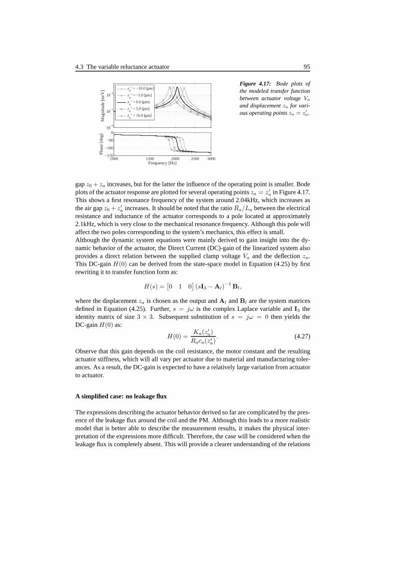
4.3 The variable reluctance actuator 95

1000 1500 2000 2500 3000−270

−180

−90

0

Frequency [Hz]

Pha

se [d

eg]

10−6

10−5

10−4

Mag

nitu

de [m

/V]

za’ = −10.0 [µm]

za’ = −5.0 [µm]

za’ = 0.0 [µm]

za’ = 5.0 [µm]

za’ = 10.0 [µm]

Figure 4.17: Bode plots ofthe modeled transfer functionbetween actuator voltageVaand displacementza for vari-ous operating pointsza = z′a.

gapz0 + za increases, but for the latter the influence of the operating point is smaller. Bodeplots of the actuator response are plotted for several operating pointsza = z′a in Figure 4.17.This shows a first resonance frequency of the system around 2.04kHz, which increases asthe air gapz0 + z′a increases. It should be noted that the ratioRa/La between the electricalresistance and inductance of the actuator corresponds to a pole located at approximately2.1kHz, which is very close to the mechanical resonance frequency. Although this pole willaffect the two poles corresponding to the system’s mechanics, this effect is small.Although the dynamic system equations were mainly derived to gain insight into the dy-namic behavior of the actuator, the Direct Current (DC)-gain of the linearized system alsoprovides a direct relation between the supplied clamp voltage Va and the deflectionza.This DC-gainH(0) can be derived from the state-space model in Equation (4.25)by firstrewriting it to transfer function form as:

H(s) =[0 1 0

](sI3 − Al)

−1Bl,

where the displacementza is chosen as the output andAl andBl are the system matricesdefined in Equation (4.25). Further,s = jω is the complex Laplace variable andI3 theidentity matrix of size3 × 3. Subsequent substitution ofs = jω = 0 then yields theDC-gainH(0) as:

H(0) =Ka(z

′a)

Raca(z′a). (4.27)

Observe that this gain depends on the coil resistance, the motor constant and the resultingactuator stiffness, which will all vary per actuator due to material and manufacturing toler-ances. As a result, the DC-gain is expected to have a relatively large variation from actuatorto actuator.

A simplified case: no leakage flux

The expressions describing the actuator behavior derived so far are complicated by the pres-ence of the leakage flux around the coil and the PM. Although this leads to a more realisticmodel that is better able to describe the measurement results, it makes the physical inter-pretation of the expressions more difficult. Therefore, thecase will be considered when theleakage flux is completely absent. This will provide a clearer understanding of the relations

96 4 Modular actuator grid

between quantities such as geometric dimensions, number ofcoil turns and inductance, mo-tor constant, etc.The absence of leakage flux corresponds to the limit of all above electromagnetic equationsfor ℜflm,ℜflc → ∞. For the fluxesφ2(Ia, za) andφ4(Ia, za) through the coil and the PMrespectively, this leads to:

φ′2(Ia, za) = limℜflm,ℜflc→∞

φ2(Ia, za) =NIa −Hcm

lmµ0Aga

ℜ′1(za)

,

φ′4(Ia, za) = limℜflm,ℜflc→∞

φ4(Ia, za) =NIa −Hcm

lmµ0Aga

ℜ′1(za)

,

whereℜ′1(za) denotes the sum of all remaining reluctances:

ℜ′1(za) = ℜga

(za) + ℜr + ℜbc + ℜgr+ ℜm.

Note that since there is only a single flux path left, fluxesφ2 andφ4 are equal.Similarly, for ℜflm,ℜflc → ∞ the expression for the magnetic coenergyW (Ia, za) inEquation (4.12) reduces to:

W ′(Ia, za) = limℜflm,ℜflc→∞

W (Ia, za) =(NIa −Hcm

lm)2

2µ0Agaℜ′

1(za)

and that for the magnetic force in Equation (4.13) to:

F ′m(Ia, za) = lim

ℜflm,ℜflc→∞Fm(Ia, za) =

− (NIa −Hcmlm)

2

2µ0Aga(ℜ′

1(za))2

=−1

2µ0Aga

(φ′2(Ia, za))2.

The fluxes, the coenergy and the magnetic force are all proportional to the total magne-tomotive force in the system and inversely proportional to the total, position dependentreluctanceℜ′

1(za). In fact, the fluxes are linearly proportional to the total magnetomotiveforce, whereas the coenergy and force are both quadratically proportional to this. The re-sulting cross product between the magnetomotive forceNIa of the coil and theHcm

lm ofthe PM amplifies the effect of the coil on the electromagneticforce, which is an advantageof using a PM to pre-load the spring.Comparison of the derived limit equations for flux, magneticcoenergy and electromagneticforce with the original equations in Equation (4.8d), Equation (4.12) and Equation (4.13)shows that leakage flux leads to additional weights on the magnetomotive forces of the coiland the PM as well as on their cross products.For the static actuator model, the absence of leakage flux leads to a simplified relation be-tween currentIa and displacementza:

I ′a(za) = limℜflm→∞ℜflc→∞

Ia(za) =Hcm

lmN

+1

N

√

−2 (ℜ′1(za))

2

(

C1Emt3mr2m

zs + C2Emtmr2m

z3s

)

,

4.3 The variable reluctance actuator 97

actuator

Laser-vibrometerSiglab Current

amplifiervelocity

excitation

Figure 4.18: Experimentalsetup to measure the behav-ior of a single actuator usinga SiglabTMsystem, a currentsource and a laser vibrometer.

wherezs is again used for brevity of notation. The relation between actuator stiffnessca(za)and displacementza becomes:

c′a(za) = limℜflm,ℜflc→∞

ca(za),

= − 2C2Emtmr2mµ0Aga

ℜ′1

z3s +

3C2Emtmr2m

z2s +

2C1Emt3m

r2µ0Agaℜ′

1

zs +C1Emt

3m

r2m, (4.28)

where the dependence ofℜ′1 on the actuator deflectionza has been omitted for brevity. Ob-

serve that the actuator stiffness remains a third order polynomial in the membrane deflectionzs, where only the first and third order terms depend on the magnetic circuit and are scaledby the total path reluctanceℜ′

1(za).When the leakage flux is neglected for the equations describing the dynamic actuator be-havior in Equation (4.24), the expression forIa becomes:

I ′a(za) = limℜflm,ℜflc→∞

Ia(za) =−ℜ′

1(za)

N2

(

RaIa − Va +N (Hcm

lm −NIa)

Agaµ0ℜ′

1(za)za

)

.

The expression for the linearized system in Equation (4.25)is unaffected, but the actuatorstiffnessca(z′a) is given byc′a(z

′a) in Equation (4.28) and the motor constantKa(z

′a) and

inductanceLa(z′a) becomeK ′a(z

′a) andL′

a(z′a) respectively, where:

K ′a(z

′a) =

−N (NIa −Hcmlm)

(ℜ′1(z

′a))

2 , L′a(z

′a) =

N2

ℜ′1(z

′a).

Both the motor constant and the inductance are thus inversely proportional to the total re-luctanceℜ′

1(z′a). Since the motor constant is inversely proportional to the square of this

reluctance, a modest reduction in reluctance will lead to a significant improvement of themotor constant.

4.3.5 Measurements and validation

Several prototypes of single variable reluctance actuators have been manufactured and mea-surements have been performed to determine their (dynamic)behavior. The quasi-staticbehavior of the actuator is governed by the force-displacement characteristic as derived inEquation (4.16), whereas its dynamics will be analyzed in terms of the parameters of thelinearized system in Equation (4.25) and its mechanical resonance frequency. The mea-surements were performed using the test setup as depicted inFigure 4.18, consisting of aSiglabTM[43] system and a Polytec laser vibrometer. The Siglab system was used to gener-ate an excitation signal that was fed to a current amplifier and also measured back at one of

98 4 Modular actuator grid

1000 1500 2000 2500 3000−90

0

90

Frequency [Hz]

Pha

se [d

eg]

100

101

102

103

Mag

nitu

de [m

/s/A

]

∆ Ia = −14mA

∆ Ia = −7mA

∆ Ia = 0mA

∆ Ia = 7mA

∆ Ia = 14mA

1000 1500 2000 2500 3000−90

0

90

Frequency [Hz]

Pha

se [d

eg]

100

101

102

103

Mag

nitu

de [m

/s/A

]

∆ Ia = −14mA

∆ Ia = −7mA

∆ Ia = 0mA

∆ Ia = 7mA

∆ Ia = 14mA

Figure 4.19: Measured frequency response func-tions of a single actuator for various current off-sets∆Ia.

Figure 4.20: Bode plots of the modeled transferfunctions of a single actuator for various currentoffsets∆Ia.

the Siglab inputs. The laser vibrometer was used to measure the velocityza of the movingcore and its output – an analog voltage – was also fed to a Siglab input. The sensitivity ofthe laser vibrometer was set to 25mm/s/V with an output range of-10. . .10V.To measure Frequency Response Functions (FRFs), a wide band, white noise excitation sig-nal was used with an RMS level of≈1.5mA and DC offsets∆Ia varying between -15 and15mA. The FRFs are estimated using the Siglab software with aHanning window of 8192samples and 50 averages without overlap. The results are shown in Figure 4.19. Observethat the resonance frequency of the actuator lies around 2.1kHz and varies approximately2Hz per mA current offset.From the measured FRFs it is also possible to estimate the viscous damping, actuator stiff-ness and motor constant. This step requires the linearized model expressed in Equation(4.25) to be adapted from voltage to current input, as used inthe test setup. When the cur-rentIa is prescribed, the first state (Ia) of the system vanishes and the system is determinedby the equations for the accelerationza and the velocityza. This yields the following,second order state-space system:

[zaza

]

=

[0 1

−ca(z′a)/mac−ba/mac

] [zaza

]

+

[0

Ka(z′a)/mac

]

Ia(t),

whereza is chosen as the system output corresponding to the type of laser vibrometer mea-surement used. This system can be rewritten into transfer function form as:

HI(s, z′a) =

Ka(z′a)s

macs2 + bs+ ca(z′a)

(4.29)

and has an undamped mechanical resonance frequencyfe that depends on the operatingpointz′a:

fe(z′a) =

1

2π

√

ca(z′a)

mac

.

To obtain estimates forKa(z′a), ba andca(z′a), first a parametric identification on the FRF

will be performed using Matlab’sinvfreqs function. However, to be able to derive the

4.3 The variable reluctance actuator 99

−15 −10 −5 0 5 10 1510

−1

100

101

DC current offset ∆Ia [mA]

Resonance frequency [kHz]Actuator stiffness [N/mm]Motor constant [N/A]Damping [mNs/m]

−15 −10 −5 0 5 10 1510

−1

100

101

DC current offset ∆Ia [mA]

Resonance frequency [kHz]Actuator stiffness [N/mm]Motor constant [N/A]

Figure 4.21: The viscous dampingba, resultingactuator stiffnessca, motor constantKa and un-damped mechanical resonance frequencyfe as afunction of the DC current offsetI ′a as identifiedfrom measurement data.

Figure 4.22: The modeled actuator stiffnessca,motor constantKa and resonance frequencyfeas a function of the DC current offsetI ′a.

desired properties from the estimated coefficients, two modifications must be made to theabove transfer function. Firstly, note that the lowest termof the numerator polynomialis zero. To prevent the need for a constraint in the parametric identification procedure, thenumerator is divided bys. This corresponds to time domain integration that must be appliedto the measured velocity signal prior to parametric identification. The second change is dueto the fact that of the four coefficients only three can be uniquely identified and a fourthmust be given. Since the value ofmac

is well defined by manufacturing tolerances, this isfurther assumed to be known as listed in Table 4.1. The transfer function whose coefficientswill be estimated can thus be expressed as:

HI(s, z′a) =

Ka(z′a)/mac

s2 + (ba/mac)s+ ca(z′a)/mac

. (4.30)

The Matlab functioninvfreqs is then used to estimate the three unknown coefficients fromwhichKa(z

′a), ba andca(z′a) are determined. The obtained values are plotted together with

the damped resonance frequency corresponding to the poles of Equation (4.30) in Figure4.21.The following observations can be made by comparing the values obtained from the modelin Figure 4.22 and from the measurements in Figure 4.21:

• the measured resonance frequency is higher than modeled andsince the moving massis known, this implies that the actuator stiffness must be higher,

• the stiffness and resonance frequency decrease with an increased axial air gap,• the measured motor constant is higher than modeled,• the measured viscous damping depends on the position of the core.

To explain the differences found, a sensitivity analysis ofthe variable reluctance actuator isperformed.

100 4 Modular actuator grid

180 200 220 240 260 280 30010

−2

10−1

100

Height h [µm]

La [mH]

fe [kHz]

ca [kN/m]

Ka [N/A]

z0 [mm]

−0.1 0 0.1Stiffness coëficient C

1 [−]

0.005 0.01 0.015 0.02 0.025Nonlinear stiffness coëficient C

2 [−]

Figure 4.23: Sensitivity of the resonance frequencyfe, resulting stiffnessca, motor constantKa andinductanceLa of the actuator w.r.t. the heighth and the stiffness constantsC1 andC2.The thick, dashed vertical line represents the nominal value of the parameter, as listedin Table 4.1.

4.3.6 Sensitivity analysis

Figure 4.23 shows the sensitivity of the resonance frequency fe, actuator stiffnessca, motorconstantKa and inductanceLa of the actuator w.r.t. the heighth and the stiffness coeffi-cientsC1 andC2. This figure is obtained by evaluating the expressions forfe, Ka, ca andLa derived in the previous subsections while varying a single actuator property and keepingall others at their nominal values as listed in Table 4.1. These values are marked by thethick, dashed vertical lines. The results include the effect of the parameters on the initial airgapz0 on which all expressions implicitly depend. From Figure 4.23 the following remarksare made:

The heighth.An increase of the heighth causes an increase of the initial air gap and a workingpoint with less stiffness and lower motor constant.

The stiffness coefficientC1.A change in the linear stiffness coefficientC1 of the membrane suspension will resultin a change in initial air gapz0. The magnetic force depends on the reluctance of

4.3 The variable reluctance actuator 101

the magnetic circuit and therefore on the position of the moving core. In the equi-librium position, the spring force is equal to this magneticforce. The spring force isproportional to the deflection and the linear and nonlinear stiffness of the membranesuspension. If the linear stiffness coefficient decreases,the initial air gapz0 will de-crease and the contribution of the nonlinear stiffness on the actuator stiffness willincrease. This effect is attenuated by the stiffness due to the magnetic circuit whichalso increases for smaller air gaps. However, this effect islinear with the decrease airgap whereas the effect on the mechanical spring stiffness isquadratic. The net effectis an increase in actuator stiffness and resonance frequency.For a smaller air gap the magnetic reluctance drops, causingthe magnetic flux, hencethe forceFm and the motor constantKa to increase.

The stiffness coefficientC2.A decrease in the nonlinear stiffness coefficientC2 of the membrane suspension willalso result in a smaller initial air gap. In analogy with the linear stiffness coefficientC1 this leads to a larger deflection to maintain force equilibrium, but this deflectionincrease is accompanied by a lower spring stiffness and willtherefore – in contradic-tion to the stiffness coefficientC1 – result in a lower overall stiffness.Again with the smaller air gap the magnetic reluctance dropsand the motor constantincreases.

Figure 4.24 shows the sensitivity of the resonance frequency fe, actuator stiffnessca, motorconstantKa and inductanceLa w.r.t. the leakage flux reluctancesℜflc andℜflm of the coiland the PM respectively and the radial air gap reluctanceℜga

. The figure was obtained thesame way as Figure 4.23 and the thick, dashed vertical lines represent the parameter valueslisted in Table 4.1. From Figure 4.24 the following is observed:

The coil leakage flux reluctanceℜflc.The leakage flux reluctance of the coil has no significant effect on the initial air gapz0, actuator stiffnessca or resonance frequencyfe. As the reluctanceℜflc of the coilleakage flux decreases to the order of the reluctanceℜbc of the coil core, the motorconstant becomes affected. The major part of the flux generated by the coil will thenflow into the leakage flux path.The coil inductanceLa decreases for increasingℜflc, since this inductance is propor-tional toN2/ℜ(za) andℜ(za) is proportional toℜflc.

The PM leakage flux reluctanceℜflm.If the reluctanceℜflm of the PM leakage flux is decreased, the attraction force on theferromagnetic core decreases and the initial air gap will belarger. As illustrated byFigure 4.13, a lower equilibrium force will result in a lowerstiffness of the membranesuspension and resonance frequency. The motor constantKa decreases whenℜflmdecreases since the equilibrium force decreases and the airgap increases. As long asℜflm does not significantly affect the total reluctance experienced by the coil, thereis little change in coil inductance.

The radial air gap reluctanceRga.

The reluctance of the radial air gap forms a significant part of the total reluctance

102 4 Modular actuator grid

107

108

109

10−2

10−1

100

Coil leak flux reluctance Rflc

[1/H]

La [mH]

fe [kHz]

ca [kN/m]

Ka [N/A]

z0 [mm]

107

108

109

Magnet leak flux reluctance Rflm

[1/H]10

710

810

9

Radial air gap reluctance Rga

[1/H]

Figure 4.24: Sensitivity of the resonance frequencyfe, resulting stiffnessca, motor constantKa andinductanceLa of the actuator w.r.t. the leakage flux reluctances of the coil ℜflc andthe PMℜflm and the radial air gap reluctanceℜga . The thick, dashed vertical linerepresents the parameter value listed in Table 4.1.

in the flux path through the axial air gap (φ1). This explains its significant effect ofmotor constant and initial air gapz0. When the total reluctance decreases, the flux, theforce and the motor constant increase. The decrease of the axial air gapz0 explainsthe increase in actuator stiffness and resonance frequency.

Figure 4.25 shows the sensitivity of the resonance frequency fe, actuator stiffnessca, motorconstantKa and inductanceLa of the actuator w.r.t. the axial air gap areaAga

, the coercivityof the PMHcm

and the PM thicknesslm. The figure was obtained the same way as Figure4.23 and the thick, dashed vertical lines represent the parameter values listed in Table 4.1.From Figure 4.25 the following is observed:

The axial air gap areaAga.

Observe that the areaAgais present in the expression for the magnetic forceFm in

Equation (4.13) and thus directly influences the initial airgapz0. However,Agaalso

affects the actuator properties indirectly via the reluctanceℜga. This reluctance enters

quadratically in Equation (4.13) and becomes the dominant term for small values ofAga

. This leads to an increased magnetic force and a reduction ofthe nominal air gap

4.3 The variable reluctance actuator 103

0.5 1 1.510

−2

10−1

100

Axial air gap area Aga

[mm2]

La [mH]

fe [kHz]

ca [kN/m]

Ka [N/A]

z0 [mm]

−650 −600 −550 −500 −450PM coercive force H

cm [kA/m]

250 300 350

PM thickness lm [µm]

Figure 4.25: Sensitivity of the resonance frequencyfe, resulting stiffnessca, motor constantKa andinductanceLa of the actuator w.r.t. the axial air gap radiusrga , and the coercivity ofthe PMHcm and thicknesslm of the PM. The thick, dashed vertical line represents theparameter value listed in Table 4.1.

width that explains the minimum in the graph forz0. The initial air gap also affectsthe motor constant, leading to a maximum in the graph forKa that corresponds tothe minimum for the air gapz0. The actuator stiffness decreases asz0 increases forsmall values ofAga

. For larger values ofAga, the stiffnessca is dominated by the

nonlinear mechanical spring stiffness that decreases as the air gapz0 increases. Thedecreased negative magnetic stiffness will not compensatefor the mechanical springstiffness reduction and an overall decrease in stiffness results.

The magnetic field intensityHcmof the PM.

If the coercive force of the PM is increased the magnetic force increases. This in-crease leads to a smaller air gap with a higher actuator stiffness, resonance and motorconstant.

The thicknesslm of the PM.A thickness increase of the PM has the same effect as a coercive force increase.

Besides sensitivity of the actuator propertiesfe, ca, Ka andLa on the parametersh, C1,C2, ℜflc, ℜflm, ℜga

, Aga, Hcm

and lm, it is relevant to know what causes the possible

104 4 Modular actuator grid

differences in these parameters and how to minimize them. First of all, the predictability ofthe actuator properties is increased by the measurements performed to identify the coercivityHcm

of the PMs and the stiffness coefficientsC1 andC2 of the membrane suspension.Besides this, the manufacturing tolerances and assembly tolerances play an important role:

Manufacturing tolerances.All dimensions of the actuator are subject to manufacturingtolerances. Manufactur-ing tolerances are typically in the order of tens ofµm. These dimensions directlydetermine all modeled magnetic reluctances, the mechanical stiffness coefficientsC1

andC2 and the moving massmac. Besides dimensions, the magnetic permeability

of the ARMCO can be influenced by stresses caused by the manufacturing process.This is likely to play a role for the reluctances of the baseplate, the moving core andthe radial air gap. As a result, all actuator properties willbe affected and vary fromactuator to actuator.

Assembly tolerances.In addition to tolerances on the manufactured parts themselves, the design dimensionsare affected by the assembly process. For instance, the thickness of the glue layers be-tween (1) the PM and the coil insert and (2) between the baseplate and the membranesuspension and (3) between the moving core and the suspension membrane lead toa variation of the heighth. Another example is the reluctance of the radial air gap,which is affected by the in-plane alignment of the moving core w.r.t. the pole shoes.Tolerances on the assembly process used are expected to be typically in the order oftenµm. In Section 4.4 it will be shown how – by design and assembly –the effect ofmanufacturing and assembly tolerances on the actuator behavior is minimized.

In the next section, the results from the modeled actuator (Figure 4.22) and the measuredactuator (Figure 4.21) will be compared and analyzed based on insights of the sensitivityanalysis.

4.3.7 Lessons learned

Actuator stiffness ca and resonance frequencyfeThe actuator stiffnessca is directly coupled to the mechanical resonance frequencyfe via the massmac

. The stiffness values derived from the measurements are higherthan expected from the model. With the use of Figures 4.23 and4.24 it is shown thatthe stiffnessca varies significantly for all considered parameters except for the coilleakage flux reluctance. This is caused mainly by its dependence on the initial airgapz0, which is affected by all parameters. Note from Figure 4.14 that in general thestiffness increases asz0 decreases. Variation of parameters that lead to an increaseinz0 will therefore lead to a decrease inca.The same effect is observed in the variation w.r.t. the operating point. In accordanceto the model, the stiffness is found to change with the deflectionza (orIa): it increasesfor negativeza and decreases for positiveza.

4.3 The variable reluctance actuator 105

Motor constant Ka

The measured value (≈ 0.28N/A) for the motor constantKa is higher than the origi-nal design value of≈0.2N/A. As can be observed in Figures 4.23 and 4.24, the motorconstant shows considerable variation w.r.t. all analyzedparameters except the coilleakage flux reluctanceℜflc. Most noticeable is the strong dependence of the radialair gap reluctanceℜga

. A higher motor constant can therefore be partially attributedto a lower reluctance of the radial air gap.Finally, note from Figure 4.25 that there exists a value for the axial air gap areaAga

where the motor constant has a maximum. This may be exploitedin future designs toobtain a higher power efficiency.

InductanceLaAs can be observed in Equation (4.26), the inductanceLa of the actuator is a functionof the number of turnsN in the coil and the reluctances in the magnetic circuit.Consequently, only parameters that have a significant effect on the total reluctancewill cause a significant change inLa. The dominant reluctances areℜga

(za) of theaxial air gap andℜgr

of the radial air gap andℜm of the PM.

Damping baIn the model, the damping is considered a constant, but the measurement results inFigure 4.21 indicate that the damping varies with the deflection of the moving core.A possible explanation for this effect is that a so-called squeeze film exists betweenthe PM and the moving core. When the core moves, air is either expelled from orcompressed between the two objects. Viscosity hampers the flow of air, which leadsto both spring and damper behavior that depends on the distance between the twoobjects and the relevant time scale (i.e. frequency of motion) [119].

Although differences between the model and measurements exist and the analysis resultsindicate that improvement of the motor constant in particular is well possible, the results aregood enough to proceed with design and integration of actuators in grids.The design and realization of these actuator modules will beintroduced in the next sec-tion. Measurement results, including the variation and spread in actuator properties, on allactuators of seven prototype grids will be presented in Section 4.4.3.

106 4 Modular actuator grid

Figure 4.26: The standard actuator module with61 actuators seen from the front.

Figure 4.27: The standard actuator module with61 actuators seen from the back.

4.4 The actuator module

In the transformation of the single actuator design into a grid actuator module, the philoso-phy is to design in layers that extend over many actuators andnot to make many individualactuators that need to be placed and aligned individually. This reduces the number of partsand the complexity of assembly and improves the uniformity of the actuator properties.A hexagonal actuator layout is chosen since this gives the highest actuator areal density.The grids are also given a hexagonal shape to accommodate theassembly of large DMsfrom many actuator grids. The grid layout consists of a central actuator surrounded by anumber of hexagonal ’rings’ of actuators. This approach results in a total of 7, 19, 37, 61,91 or 127 actuators for 1, 2, 3, 4, 5 or 6 rings respectively. For the prototype grids realized,four rings, corresponding to 61 actuators, are chosen. In this choice, several practical issueswere taken into account, such as the size of the baseplate andits corresponding resonancefrequency. A larger grid would require more thickness, or additional support points to avoidinternal resonances. Further, the actuator coils are connected through flex foils. These willbecome more difficult to manufacture as the number of actuators per grid increases. Whenthe line pattern is made on a single layer there is not enough area for more connections.Finally, the number 61 is close to a division factor of26 = 64, which is likely to be used indigital electronics for drivers and communication.

4.4.1 Actuator grid design

The actuator grid is shown in Figures 4.26 and 4.27. Figure 4.28 shows the exploded viewof the actuator grid. The main parts shown in the exploded view are summarized and willbe discussed in detail:

The baseplateThe baseplate serves a the flux carrier for the magnetic circuits for 61 actuators andis made from from ARMCOr. The baseplates are cut from bar and their front and

4.4 The actuator module 107

M1x6 (3x)

Membrane suspension

Moving cores (61x)

Baseplate

Coils (61x)

SmCo Magnets (61x)

Inserts (61x)

Flex foil

A-frames (3x)

Strain relief and clamps (3x)

Figure 4.28: An exploded view of the actuator grid shown in Figures 4.26 and 4.27.

108 4 Modular actuator grid

back surfaces are made plan parallel. The serrated circumference is made such thatthe actuator grids can be placed adjacent with a 0.3mm gap. The holes in the backsideare made by milling, the circumference and pole shoe contours are made with wireEDM.

The membrane suspension with moving coresThe membrane suspension is made by laser cutting. The same sheet of rolled Havarr

material is used for all actuator grids in the same orientation to obtain uniformity forthe spring characteristic. The moving cores are laser cut and made from a 0.3mmthick ARMCOr sheet.

Inserts with the SmCo5 PMs and coilsThe inserts complete the magnetic circuit. The inserts are produced on a CNC lathe.After measurement and selection of the PMs described in Appendix A, the PMs areglued on the inserts with Araldite 2020. The coils, made of 50µm copper wire with500 turns, are fabricated separately from the insert and have pre-leaded ends. Theelectrical resistance of each coil is measured before placement. The inner radius ofthe coil is made slightly larger than the insert core to avoiddamage to the electricalisolation when placed. The bottom of the inserts contains a hole and a slot to providean axial feed through for the coil wires.

The flex foilA flex foil is designed to connect the coil wires to the driver PCB. This flex foildesign is shown in Figure 4.43. Each of the three branches of the flex foil connectsto a double row, 0.3mm pitch, connector. The central hexagonal part of the flex foilholds∅2.5mm holes through which the coil wires emerge. At the circumference ofthe holes, the two wires of that coil are soldered each on a copper pad. After soldering,a droplet of silicon glue is placed to encapsulate the fragile coil wires. A strain relief(Figure 4.27) is added to avoid damage to the soldered connections.

The actuator grid supportsThe actuator grid is connected with three A-frames to its support structure. EachA-frames is connected with one point to the baseplate and with two points to thesupport structure to avoid moments enforced on the baseplate. The A-frames areconnected with M1 bolts. When the actuator grid is placed facedown on the table,with the membrane suspensions facing down, the bolt heads support the actuator gridand avoid damage to the suspension systems.

The next subsection will describe the assembly of an actuator grid.

4.4 The actuator module 109

Figure 4.29: Top view of the laser cut membranesuspension made from 25µm thick Havarr.

Figure 4.30: A mould placed on top of the mem-brane suspension to position the ferromagneticmoving cores. The struts to align the mouldand thereby the moving cores with respect to themembrane suspension are visible.

4.4.2 Actuator grid assembly

The assembly of the actuator grids is done in four steps.

1. The ferromagnetic cores are glued to the membrane suspension.

2. The membrane suspension with the ferromagnetic cores is assembled to the baseplate.

3. The PMs and coils are glued to the inserts and the inserts placed in the baseplate.

Figure 4.31: Struts are pressed to the cores toensure a thin layer of glue between the cores andthe membrane suspension. An elastomer foamand a weight is added on top of the struts (notshown).

Figure 4.32: The cores glued on the membranesuspension visible after removal of the mould.The Havarr foil is seen to be slightly curved dueto internal stress as a result of the foil rollingprocess.

110 4 Modular actuator grid

Figure 4.33: Front side of the baseplate. Figure 4.34: Back side of the baseplate.

4. The flex foil is placed and the coil wires are soldered to theflex foil. Three A-framesand a strain relief are bolted to the actuator grid. The actuator grid is fully assembledand can be placed on the support structure.

Each assembly step is described in more detail and clarified by photo’s.

Step 1: Assembly of the cores and the membrane suspension

Figure 4.29 shows the laser cut membrane suspension made from a 25µm Havarr rolledfoil. For assembly this foil is placed on a flat base and laterally constrained by three metalstruts. These struts can move up and down in the base. A 2.5mm thick mould, that contains61 holes to position the cores, is placed on top of the foil. The struts align the mould andholes to the membrane suspension. Figure 4.30 shows the basewith the mould placed on topof the membrane suspension. 61 Droplets of glue (Araldite 2020) are manually placed in

Figure 4.35: The baseplate is placed on themembrane suspension.

Figure 4.36: The baseplate is supported by thestruts and lowered on the membrane suspension.

4.4 The actuator module 111

Figure 4.37: The baseplate placed on the mem-brane suspension. The cores are visible betweenthe pole shoes.

Figure 4.38: A detailed view off one of the actua-tor suspensions with moving core and pole shoesin the baseplate. The air gap between the coreand pole shoes is 0.1mm.

the holes of the mould followed by an iron core. Figure 4.31 shows 61 struts that are pressedto the cores to ensure a thin layer of glue between the cores and membrane suspension. Anelastomer foam and a weight is added on top of the struts to ensure equal pressure. Whenthe glue is hardened the struts and mould are removed. The result is shown in Figure 4.32.

Step 2: Assembly of the membrane suspension and baseplate

Figure 4.33 and Figure 4.34 show the front and back side of thebaseplate. Droplets of glueare placed on the membrane suspension at the end of each leafspring of the suspension.

Figure 4.39: Top view of the baseplate withmembrane suspension and cores.

Figure 4.40: The assembled inserts with PM andcoil placed in a container. Note the droplets ofglue on the wires to avoid damage to the insula-tion.

112 4 Modular actuator grid

Figure 4.41: Assembling the inserts in the base-plate.

Figure 4.42: All inserts placed in the base-plate. The coil wires extend over 8mm and aretin plated.

The baseplate is placed on the thinned ends of the struts and lowered on the membranesuspension. This is shown in Figures 4.35, 4.36 and 4.37. Figure 4.38 shows a detail of thebaseplate. The pole shoes, membrane suspension and core areshown for a single actuator.The air gap between the core and the pole shoes is 0.1mm. Figure 4.39 shows the top viewof the baseplate with membrane suspension and cores as removed from the assembly base.All air gaps are checked before proceeding.

Step 3: Assembly of the inserts

On the iron inserts, a PM and coil is placed. All magnets are placed with their magnetizationin the same direction. In the bottom part of the insert, a holeand slot has been prepared for

Figure 4.43: The flex foil that provides twoelectrical connections per actuator between thedriver electronics PCB and the actuators.

Figure 4.44: The coil wires pass through theholes in the flex foil.

4.4 The actuator module 113

Figure 4.45: The flex foil connected to the actu-ator grid.

Figure 4.46: Detail view of the actuator grid.

the coil wires. Figure 4.40 shows a photo of the inserts prepared awaiting assembly in acontainer. Figure 4.41 and Figure 4.42 show the inserts being placed in the baseplate.

Step 4: Flex foil assembly

The flex foil is shown in Figure 4.43. Figure 4.44 shows the flexfoil lowered over the coilwires. The two wires of each coil pass through a hole in the flexfoil and are soldered ontoa copper pad at the circumference of the holes. Silicone glueis added to protect the wiresand soldered connection from damage. The A-frames are bolted on the baseplate and thestrain relief is added. The flex foil is folded and clamped on the frame. The result is shownin Figures 4.26 and 4.27. The grid is then bolted on the three A-frames. Figure 4.46 showsa detail of the actuator grid.

4.4.3 Measurement results

A batch of seven grids was realized using the above procedure. The only difference in nom-inal dimensions with respect to the single actuator is an additional 25µm for the heighth.Although this is known to have a negative effect on the motor constant, actuator stiffness andresonance frequency, more margin is hereby built in for manufacturing errors and the riskon ferromagnetic cores to snap down on the PMs is avoided. Thereduced motor constant,actuator stiffness and resonance frequency are estimated from Figure 4.23 asKa=0.17 N/A,ca=550N/m andfe=1980 Hz.For each grid all actuators are measured with the same experimental setup as shown in Fig-ure 4.18. Figure 4.47 shows a typical transfer function witha parametric model fit of oneof the actuators in the grid. As a reference, the figure also shows the nominal transfer func-tion derived from the analytical model depicted previouslyin Figure 4.20. Besides the firstresonance frequency around 2kHz, a second resonance is visible at approximately 5kHz.This is the tip/tilt mode of the ferromagnetic core in its membrane suspension that can only

114 4 Modular actuator grid

Figure 4.47: Bode plot ofthe measured transfer functionH(za) from a single actuatorin a grid, together with thefitted model and the analyticmodel. The measured transferfunction of the single actuatoras shown in Figure 4.19 is alsoplotted for comparison.

10−2

10−1

100

101

102

103

Mag

nitu

de [m

/s/A

]

Grid actuator measurementFitted modelOriginal modelSingle actuator measurement

101

102

103

104

−180

−90

0

90

180

Pha

se [d

eg]

Frequency [Hz]

be observed when the laser vibrometer is not perfectly aligned to the center of the movingcore.Estimates for the actuator stiffnessca, resonance frequencyfe, motor constantKa andviscous dampingba are obtained from the measurement data using the same procedure asdescribed in Section 4.3.5. The average and standard deviation values are listed in Table4.2 and more detailed results are shown in Figures 4.48, 4.49, 4.50 and 4.51. The values inthe figures are sorted to provide insight into the statistical spread and differences in medianvalues between grids. The mean actuator stiffness and resonance frequency are 471N/mand 1.83kHz respectively, which is lower than expected. In Figure 4.48 it is shown that thespread in stiffness values within a grid is similar for all grids, but that the mean differs fromgrid to grid. This can be caused by manufacturing and assembly variations that directly

10 20 30 40 50 60300

350

400

450

500

550

600

650

Actuator number [−]

Act

uato

r st

iffne

ss ca [N

/m]

Module 1Module 2Module 3Module 4Module 5Module 6Module 7

10 20 30 40 50 601500

1600

1700

1800

1900

2000

2100

Actuator number [−]

Res

onan

ce fr

eque

ncy F

e [Hz]

Module 1Module 2Module 3Module 4Module 5Module 6Module 7

Figure 4.48: The identified actuator stiffnessca,for mac =3.6mg sorted for each measured ac-tuator grid separately.

Figure 4.49: The identified actuator resonancefe, for mac =3.6mg sorted for each measuredactuator grid separately.

4.4 The actuator module 115

10 20 30 40 50 600.06

0.08

0.1

0.12

0.14

0.16

0.18

0.2

Actuator number [−]

Mot

or c

onst

ant K

a [N/A

]

Module 1Module 2Module 3Module 4Module 5Module 6Module 7

10 20 30 40 50 600.1

0.2

0.3

0.4

0.5

0.6

0.7

0.8

0.9

Actuator number [−]

Vis

cous

dam

ping

ba [m

Ns/

m]

Module 1Module 2Module 3Module 4Module 5Module 6Module 7

Figure 4.50: The fitted motor constantsKa, formac =3.6mg sorted for each measured actuatorgrid separately.

Figure 4.51: The fitted dampingba, formac =3.6mg sorted for each measured actua-tor grid separately.

Table 4.2: Average values and standard deviations of the actuator properties measured over all gridactuators.

Property Ka ca ba feAverage 0.12N/A 471N/m 0.36mNs/m 1.83kHzStd.dev. 0.02N/A 48N/m 0.10mNs/m 95Hz

affect all actuators in a module, such as baseplate or suspension membrane thickness varia-tions.Figure 4.50 shows the values of the motor constants, which are lower than expected. Theanalytic model predictedKa=0.17N/A, whereas 0.12N/Ais measured. A possible explana-tion for the measurement results is that the leakage flux reluctances for the PM and coil aresmaller in the actuator module baseplate than for the singleactuator. The few high valuesfor damping are explained by rests of glue in between the moving core and baseplate.

4.4.4 Power dissipation

To analyze the expected power dissipation of the actuator, only its static response is con-sidered and assumed to be linear. The validation measurements have shown this to be anaccurate approximation at least up to approximately 1600Hz, where effects such as viscousdamping and eddy currents play a negligible role.The power dissipated by the currentIa through the actuator coil with resistanceRa can beexpressed as:

Pa = I2aRa =

(FaKa

)2

Ra,

where for the second step the linearized caseFa = KaIa was used. In Chapter 2 theexpected RMS actuator force was derived as 1mN, which was based on an actuator stiffness

116 4 Modular actuator grid

ca of 500N/m. Since the stiffness of the realized actuator was found to be very close to thisvalue, the 1mN RMS force remains a valid basis to evaluate power dissipation. For 1mNRMS actuator force and a measured average motor constantKa of 0.12N/A this yields anRMS actuator currentIa of approximately 8mA. Via the coil resistanceRa ≈ 39Ω, thiscorresponds to a power dissipation of approximately 3mW peractuator. This means that therealized actuators meet the specification in Chapter 2 that the power dissipation must be inthe order of mW’s.

4.5 Conclusions

The application of electromagnetic actuators for adaptivedeformable mirrors has severaladvantages. Electromagnetic actuators can be designed with a limited stiffness, such thatfailure of an actuator will cause no hard point in the reflective surface and thus a small op-tical degradation compared to e.g. stiff piezo-electric elements. Other advantages over thelatter type of actuators at the relatively low cost, low driving voltages and negligible hys-teresis and drift.Variable reluctance type actuators were primarily chosen because of their high efficiencyand low moving mass. A nonlinear mathematical model of the actuator was derived describ-ing both its static and dynamic behavior based on equations from the magnetic, mechanicand electric domains. The nonlinear spring force characteristic of the membrane suspensionwas modeled and verified via measurements in a dedicated measurement setup (AppendixB). This indicated that FEM analysis can predict the nonlinear behavior well, but could notpredict the effect of internal stresses resulting from the production of the rolled Havarr foil.The model was linearized, leading to expressions for the actuator transfer function and lin-ear electromechanical properties such as motor constant, coil inductance, actuator stiffnessand resonance frequency.Single actuator prototypes were realized and transfer functions were estimated from mea-surement data, based on white noise current excitation. This was done for various operatingpoints by adding static current offsets to the excitation signal, which showed that the ef-fect of the nonlinearities is indeed small. The resonance frequency and the DC-gain of thetransfer functions showed only marginal variation with respect to the operating point. Thismeans that a control system will be able to use an LTI control law without sacrificing perfor-mance. The measured nominal resonance frequency is higher than modeled: 2.1kHz insteadof 2kHz, corresponding to an actuator stiffness of≈680N/m. The measured motor constantis also higher than modeled 0.27N/A instead of 0.2N/A.Due to the satisfactory measurement results, the design forsingle actuators was applied withlittle modification to the design of standard hexagonal modules with 61 actuators. Only thenominal heighth of the moving core above the PM was increased by 25µm to limit the riskof the ferromagnetic cores snapping down onto the PM. Based on the results of a sensitivityanalysis, this modification was expected to reduce the motorconstant, actuator stiffness andresonance frequency toKa=0.17N/A,ca=550N/m andfe=1980Hz respectively.In this sensitivity analysis the effect was determined of variation in a number of model pa-rameters on several actuator properties (i.e. stiffness, resonance frequency, motor constantand inductance) as derived from the mathematical model. In particular, this indicated a

4.6 Recommendations 117

strong influence of the radial air gap reluctance on the motorconstant and actuator stiffness,which can explain the deviation between the modeled and measured properties.Seven actuator module prototypes were made of which all actuators were measured withthe same setup as the single actuator prototypes. All actuators were found to be functional,indicating that the manufacturing and assembly process is reliable. From transfer functionmeasurements, the motor constant, actuator stiffness and resonance frequency were iden-tified. These properties showed slight deviations from the values derived from the model,but the statistical spread for the properties was small, stressing the reliability of the manu-facturing and assembly process. The mean actuator stiffness and resonance frequency were471N/m and 1.83kHz respectively, which are very close to their design values of 500N/mand 1885Hz. The value derived from the model for the motor constantKa was 0.17N/A,whereas on average only 0.12N/A was measured. This may be theresult of leakage fluxreluctances in the baseplate being lower – and thus the leakage flux being larger – than forthe single actuator.Despite the motor constants of the actuators realized beinglower than expected, the RMSpower dissipation of the actuators is still low during operation and expected to be≈ 3mW.

4.6 Recommendations

In a redesign, the large influence of the radial air gap reluctance can be used to increasethe motor constant and reduce power dissipation. A factor oftwo reluctance reduction willincrease the motor constant to 0.37N/A and increase the actuator stiffness to 750N/m. Thiscan be realized by a smaller gap width or by a larger gap area.A reduction of the axial air gap area will lead to a further increase in motor constant. Withthese changes, an improvement by a factor four is feasible. Since power dissipation isinversely proportional to the squared motor constant, a power dissipation reduction by afactor 16 is achieved. A convenient side effect is the increased electronic damping of themechanical resonance frequency. This is illustrated in Figure 4.52. The magnitude peakof the two systems is almost equal, whereas the DC-gain of theimproved system is fourtimes higher. This implies that the resonance mode is much better damped and will be lesslimiting for the controller performance.

102

103

−270

−180

−90

0

Frequency [Hz]

Pha

se [d

eg]

Ka = 0.19N/A

Ka = 0.76N/A

10−6

10−5

10−4

Mag

nitu

de [m

/V] Figure 4.52: Bode plot of the voltage to position

actuator model with the currently measured andfour times higher motor constant. Note the in-creased relative damping of the resonance mode.

Chapter veEle troni sThis chapter describes the design and realization of the actuator driver elec-tronics and communication system. PWM based voltage drivers are selectedand implemented in three FPGAs for 61 actuators (one actuator module). Ahigh base frequency of 61kHz and an additional analog2nd order low-passfilter is used to reduce the actuator position response ripple due to harmonicsof the PWM signal to less than a quarter of the Least Significant Bit (LSB)of the setpoint. The driver electronics of each actuator module are containedon a single PCB, which is placed behind the actuator module topreserve themodular concept. The FPGAs receive the voltage setpoints via an LVDS com-munication link from the control system. As no commercial LVDS interfaceboard was available for a standard PC, an ethernet-to-LVDS communicationsbridge is developed that translates ethernet packages intoLVDS packages andvice versa. A single flat-cable connects up to 32 driver PCBs to this communi-cations bridge.The actuator model from Chapter 4 is extended with models forthe communi-cation and driver electronics. The communication is modeled as a pure delayand the driver electronics as an ideal voltage source with a linear, analog2nd

order low-pass filter. The dynamic model is validated using white noise iden-tification measurements on the actuator system. The system is evaluated oncontrol aspects, showing the dependance of achievable bandwidth on the sam-pling frequency. Finally, the power dissipation of the FPGAs is evaluated andfound to exceed the power dissipation in the actuator coils.Concepts are pro-posed and analyzed to reduce power dissipation in the digital electronics.

Joint work with Rogier Ellenbroek

119

120 5 Electronics

5.1 Introduction

In this chapter, the design and realization of the electronics required to generate the currentsthrough the coils of the actuators is described. The actuators were described in Chapter 4The electronics consist of two parts: a communication system and driver electronics. Thecommunication system transmits the current value calculated by the control system to thedriver electronics, which generate the actual currents. The main difficulty of the driver elec-tronics is the required number of channels combined with thedesired high power efficiency.After the realization of these electronics, the behavior ofthe full actuator system is analyzedby comparing it to a first principles model. This model is obtained by extending the modelfrom Chapter 4 to include the components of the electronics systems.In the next two sections design concepts for the driver and communication electronics willbe presented, followed by their implementation and realization in Section 5.4. The first prin-ciples model is derived in Section 5.5 and compared to measurement results in Section 5.6.Since the driver electronics and the actuators are located close to the DMs reflective surface,power dissipation is an important design driver. Therefore, in Section 5.7 the power dissipa-tion of the prototype actuator system is analyzed and compared to the design requirements.Finally, the main conclusions will be formulated.

5.2 Driver electronics

The driver electronics provide currents through the coils of the variable reluctance actuators.In the actuator, the current converts into forces that deform the mirror facesheet. In thissection the requirements, design concepts and implementation of the driver electronics willbe discussed.

5.2.1 Requirements

In Section 2.3 the required actuator positioning resolution is derived as 5nm. From thisvalue, the worst-case required range and resolution will bederived of the currents and volt-ages that must be provided by the driver electronics. Since the resolution requirement is interms of displacement, the mechanical stiffness, motor constant and circuit resistance mustbe considered. The mechanical stiffness depends on the resulting deformation of the re-flective surface. The minimal stiffness is used to determinethe required resolutions and themaximal stiffness is used to determine the required ranges.Inertia forces and other dynamiceffects are neglected. The stiffness is minimal when all actuators have the same displace-ment and the reflective membrane does not deform. The worst case force resolution for theactuator stiffnessca =583N/m can thus be derived asFres = 2.9µN. Via a motor constantKa of 0.19N/A (Figure 4.16) and an actuator coil resistanceRa of 39.0Ω (Table 4.1), thisleads to required current and voltage resolutions of 15µA and 0.60mV respectively.The required current and voltage range follows from the maximum actuator force, motorconstant and coil resistance. The actuator force is calculated with Equation (4.1), wherecfis ≈6kN/m (Section 3.4),za = 10µm andzia = 0.36µm as derived in Chapter 2. This

5.2 Driver electronics 121

results in a range of the required force of±8mN. Via the motor constant and actuator coilresistance previously used, this leads to the required current and voltage range of±42mAand±1.6V respectively.This implies that the dynamic range (the total range dividedby the resolution) of the driverelectronics must be at least2 · 8 · 10−3/(2.9 · 10−6) ≈ 5.5 · 103. For a digital driver system,this would require at least 13 bits of accuracy. This is a minimum and does not provide anymargin for a stiffer facesheet, initial flattening and alignment of the mirror and variationin motor constant between actuators. To account for this andacknowledge that the digitalimplementation in 16 bits is likely to be more efficient, thisis the starting point in the de-sign. The consequences for the driver electronics from thisrequirement will be elaboratedin Section 5.2.2.The DM actuators are designed to have a high efficiency. In combination with the low ac-tuator force requirement, this minimizes power dissipation. As a result no active cooling isneeded and vibrations introduced by such systems are avoided. Through natural convection,heat is convected without adding significantly to the wavefront disturbances that are to becorrected. By placing the driver electronics near the electromagnetic actuators the numberof wires to the DM can be limited and spacious connectors avoided. With the short lengthof the wires, sensitivity to environmental loads (e.g. leadbreakage, magnetic fields fromnearby power sources, etc.) is reduced. However, it also means that the power dissipationof the driver electronics must be in the order of mW’s, similar to the actuators.Finally, the electronics should be compact in size, have lowcost/actuator and preferablyreplaceable. Since the actuator grid is made extendable by means of the standard modulesthat hold 61 actuators each, the same should hold for the electronics. All drivers for a singleactuator module should therefore be placed on a single PCB.

5.2.2 Concepts

For the driver electronics concept, two categories are distinguished: current and voltagesources. A current driver converts the digital setpoint from the control computer into a con-trolled current through the electromagnetic actuator. A voltage driver converts this setpointinto a voltage over the actuator clamps, upon which the circuit resistance determines thecurrent. The current may therefore vary due to dynamics or time variance in the electroniccircuit. TheLa/Ra time constant is approximately 2.93mH/39.0Ω ≈ 75µs (Section 4.3.5),which is small compared to the intended sampling time of 1ms.Therefore, an applied volt-age will result in a current without significant delay.The DC-gain of the actuator system including driver electronics depends on the actuator’smotor constantKa, stiffnessca and – in the case of a voltage source – the resistanceR ofthe actuator circuit. All three properties vary from actuator to actuator and vary with tem-perature, causing slow gain variations. A current source will compensate for variations inthe resistanceRa, but variations ofKa andca must still be compensated by the AO controlsystem. Therefore, the conceptual advantage of a current driver over a voltage driver issmall, but concrete designs of both driver types will be discussed before a choice is made.

122 5 Electronics

b16

!b16

!b16

b16

I15actuator

I1

b15b1

Iref

Iout

Vout

Load

Figure 5.1: A design based on current sources that can be ef-ficiently implemented in an ASIC using current mirrors. The"!" denotes a logicalnot. Figure 5.2: Schematic of a single

current mirror. The reference cur-rent Iref – here determined by a re-sistor – is mirrored to the output cur-rent Iout.

Current mirrors

In practice, a current source regulates its voltage output based on measurement of the actualcurrent. This feedback can be done with a linear amplifier circuit, but for this applica-tion this approach has several drawbacks. Firstly, the circuit needs two supply voltages togenerate positive and negative currents. Secondly, the required number of components isrelatively high since no standard ASICs are available that compactly house a large numberof accurate, efficient and low power linear amplifiers. Finally, the amplifier obtains its set-point current from an analog voltage input that must be generated from the digital value ofthe control system by an additional component such as a DAC.

These drawbacks can be circumvented using a design based on current mirrors, which isschematically represented in Figure 5.1. This design holds15 current mirrors and can beefficiently implemented in CMOS technology. A single current mirror (Figure 5.2) consistsof two parts: in the first part a reference current is generated that is mirrored with a certainratio to the second part that includes the load. The reference currents of the current mirrorswill be permanently flowing, whereas the mirrored load currents can be switched accordingto the setpoint bits. The physical dimensions of the currentmirror’s two transistors deter-mine the ratios between the reference and load currents. These ratios can be designed tominimize the permanently flowing reference currents and thus optimize power efficiency.The total current can be constructed with 15 fixed current mirrors and a sign-switch cor-responding to the Most Significant Bit (MSB) of the setpoint.The sign-switch is obtainedusing the full bridge configuration as depicted in Figure 5.1, where the four switches aredriven by the MSB of the setpoint and its inverse. This designis relatively simple, has alinear setpoint to current characteristic and many of thesecircuits can be implemented ina single Integrated Circuit (IC). However, it requires an ASIC, which is expensive to de-sign and manufacture. Its power efficiency is comparable to that of linear amplifiers anddependent on the ratio between the RMS and PTV currents: the crest factor. The currentsources regulate their output voltage, leading to internalvoltage drops and thus dissipation.When neglecting internal current paths of the current sources, the total power consumptionPtot can be expressed in terms of the supply voltageVcc and the desired actuator currentI

5.2 Driver electronics 123

asPtot = VccI. The powerPload dissipated in the load with resistanceRload is equal toPload = I2Rload and can be expressed relative toPtot as:

PloadPtot

= IRloadVcc

=I

Imax.

This means that for low currents, almost all power is dissipated by the current source andfor the maximum currentImax = Vcc/Rload all power is consumed by the load.For the RMS current of 8mA (Section 4.4.4), a load resistanceof 39.0Ω and a supply voltageof 1.6V, this yields a power efficiency of approximately 20%.This low efficiency could beimproved by adapting the supply voltageVcc in accordance with the desired actuator currentby dividing the output range over a number of supply voltages. However, as this leads toan even more complex design that can only be realized in an ASIC, a PWM voltage driverwith a higher power efficiency is considered as an alternative in the next section.

Pulse Width Modulation

The absence of a feedback path to regulate a current simplifies the design in comparisonwith linear amplifiers although this advantage is limited when compared to the current mir-ror design. A regulated voltage source that generates an analog voltage for the actuator fromthe digital setpoint value is essentially a DAC. There existmany types of DACs, but the highaccuracy and low power consumption required for this application limit the options. For in-stance, the low accuracy of the resistors of the common resistor ladder network DAC limitsthe useful accuracy of this type of converter to 8 bits or less.For high accuracy applications the PWM principle is often used, in which a digital outputis modulated between high and low states to yield a desired average DC value of the outputvoltage. The desired output voltage is translated into a duty cyclerPWM, which is the timefraction that the digital output is high during a certain time periodTPWM. This time periodforms the base frequencyfPWM = 1/TPWM of the PWM.The advantage of a PWM based voltage source over the proposedmirror concept is twofold.Firstly the PWM generators can be implemented in FPGAs, which reduces the number ofcomponents and does not require the expensive and complex design and realization of anASIC. Moreover, its power efficiency is superior to the current mirror driver because ithas no internal voltage drop that leads to dissipation. Dissipation is limited to switchinglosses and indirect losses of the PWM signal generator and does not significantly dependon the desired output voltage. Finally, PWM design and implementation is well under-stood, which limits development risks. A drawback of PWM is that it outputs a signalwith high-frequency components, which causes a corresponding ripple on the system out-put. Using the Fourier series expansion shown in Appendix C,for a constant duty cyclerPWM ∈ [0 . . . 1] the PWM output voltageVPWM that modulates between 0 (low) andVcc(high) can be expressed as the following infinite sum of cosines:

VPWM(t) = Vcc

rPWM +

∞∑

n=1

sin(nπrPWM)

nπcos (2πnfPWMt)

, (5.1)

whereVcc is the switched supply voltage. The spectrum of this PWM signal thus onlycontains power at frequencies2πnfPWM for n = 1, 2, . . .∞. These harmonic frequencies

124 5 Electronics

Table 5.1: Properties of industrial communication standards as derived from data sheets of availabledriver ICs.

Standard Bandwidth Multi-drop Predefined protocolUSB2 480Mb/s no yes, high overheadFireWire 800 800Mb/s no yes, high overheadCAN 1Mb/s yes yesGigabit Ethernet 1Gb/s no yes, high overheadRS-485 (Profibus) 40Mb/s yes noLVDS 655Mb/sa yes no

a According to LVDS standard as defined inANSI/TIA/EIA-644-A

must be sufficiently attenuated by the dynamics of the drivensystem, such that the remainingripple on the system’s output is within the accuracy margin of a quarter of the LSB. Toachieve this, not only the base frequencyfPWM can be suitably chosen, but also the system’sresponse to the PWM signal harmonics can be tailored using additional filters.As this drawback can thus well be handled, the driver electronics for the DM actuators willbe based on PWM.

5.3 Communication electronics

The communication electronics send the actuator setpointsfrom the control computer to thedriver electronics. The communication link should have lowlatency to allow a high controlbandwidth (e.g. low phase lag) and a high reliability and bandwidth to allow a large num-ber of actuators to be quickly updated. In addition, the power dissipation, flexibility andcosts are relevant. If for example, the number of actuators,the bandwidth or the number ofsetpoint bits changes, the communication link and protocolshould allow adaptation. Fur-thermore a protocol that can be chosen freely and with low overhead is preferred. To limitdevelopment costs, the choice is limited to industrial standards, such as RS-485 (Profibus),USB2, ethernet, LVDS, CAN and FireWire. A few relevant properties of these standardsare listed in Table 5.1. When an update rate of 1kHz and 16 bit setpoint values are assumed,the minimum bandwidth for 5000 actuators is:1000 · 5000 · 16 = 80Mb/s. With a pro-tocol overhead of 10% and latency limited to one quarter of the sampling time (250µs), aminimum bandwidth of(5000 · 1000 · 16 · 1.1/0.250) ≈350Mb/s is obtained. For the pro-totypes developed with actuator numbers up to 427 actuators, approximately 30Mb/s wouldalready suffice, but with future, larger, systems the CAN busand RS-485 are no option.Since the driver electronics will be placed on modules and located close to the DM thepower consumption of the transceivers must be as small as possible and for practical rea-sons the number of wires leading to the modules should be small. Both arguments suggestthe use of a multi-drop topology in which one transmitter communicates to many receiverson the same bus. The modules are given a unique identificationcode to allow messagesto be passed to specific modules. For such topologies the modules do not require a power

5.4 Implementation and realization 125

Vpwm

Ve

Cl Ra

La

RlLl

VpwmB

Rc

Low-pass filter coil

Act

uato

r

Figure 5.3: The analog elec-tronic circuit, consisting of acoarse and a fine PWM gener-ator, an analog low-pass filterand the actuator.

dissipating termination resistor and the number of communication wires is independent ofthe number of receiving modules. However, the power efficiency and speed of the com-munication link are not only determined by its hardware alone. If the method requires aspecific protocol with a high overhead, both speed and power efficiency are reduced andflexibility for future upgrades limited. Both arguments favor the development of a customprotocol. Development costs of such a protocol will be limited, as a master-slave structurewith a small command set will suffice and throughput is more important than guaranteedtransmission.The LVDS standard was chosen for the serial communication. In contrast to USB, thisallows for a high bandwidth multi-drop topology for which low-power transceiver ICs arecommercially available. Each transceiver dissipates only15mW and requires no termina-tion resistor. A custom communication protocol can be designed that has a small overheadcompared to e.g. the USB, FireWire or ethernet protocols. Two LVDS wire pairs can beused to keep the protocol as simple as possible: one command line and one return line.

5.4 Implementation and realization

In this section the implementation of the chosen design concepts for the driver and commu-nication electronics will be discussed.

5.4.1 PWM implementation

For several reasons the PWM voltage drivers will be implemented in an FPGA. Firstly,because this leads to a compact design with few components because the FPGA can housemany PWM generators. Moreover, no expensive ASIC has to be designed and realized andit allows modifications to the implementation through a software update.

As derived in Section 5.2.1, the driver electronics requirea dynamic range of 16 bits. ThePWM driver electronics will be designed such that the ripplemagnitude due to the harmoniccomponent in the PWM signal at the frequencyfPWM is less than a quarter of the system’sresponse to the least significant bit for any duty cyclerPWM. LetH(s) denote the transferfunction between the PWM voltageVPWM and the positionza of a single actuator. Observefrom Equation (5.1) that the worst case magnitude of the firstharmonic (n = 1) occurs for

126 5 Electronics

Figure 5.4: H-bridge con-struction to allow the PWMvoltage VPWM of the coarsePWM to be both positive andnegative.

a

b

c

dVcc

VPWM

rPWM = 0.5 and is equal toVcc/π. The design condition can thus be formulated as:

Vccπ

|H(2πjfPWM)| < 1

4

Vcc216

|H(0)|

and thus:|H(2πjfPWM)| < π

218|H(0)|. (5.2)

In Section 4.3.4, the frequency response functionH(jω) has been derived for the case thatthe PWM output is directly connected to the actuator coil. A Bode plot ofH(jω) is plottedin Figure 5.9, which shows that thefPWM for which Equation (5.2) is satisfied lies above100kHz.When implemented in an FPGA, the PWM generator will consist of a 16 bit counter and acomparator. The counter value is increased by one at every FPGA clock cycle and resetsto zero at the beginning of each PWM time period. The comparator compares the countervalue to a value corresponding to the setpoint. The PWM output is high if the counter ishigher than this value and low otherwise. The counting and thus clock frequency of theFPGA can be expressed as:

fFPGA = fPWM2Nb (5.3)

whereNb is the number of bits of the counter. The clock frequency of currently availableFPGAs is limited to approximately 200MHz, which implies that for Nb = 16 the base fre-quencyfPWM is limited to approximately 3kHz. The dynamic power dissipation of digitalelectronics is for most designs linearly correlated with the clock frequency, which is an im-portant drive to keep the base frequency as low as possible.To keepfFPGA below 200MHz while implementing 16bit PWM generators, two modifi-cations are made. Firstly, an analog2nd order low-pass filter is added to reduce the systemresponse magnitude at high frequencies and secondly the PWMis split into a fine part con-sisting of 5 bits and a course part of 11 bits. For 11 bits, the PWM base frequency can beincreased to approximately 95kHz.The analog low-pass filter consists of the inductor with inductanceLl and a capacitor withcapacitanceCl (Figure 5.3). It is given a bandwidth of 5kHz that is high enough to havea negligible influence on the behavior of the system up to the mechanical resonance, butlow enough to reduce the required PWM base frequencyfPWM to less than 95kHz. Assumethat above the resonance at 2kHz the magnitude response of the actuator between drivingvoltage and position decays a factor 1000 per decade. Further, the response of the analoglow-pass filter decays a factor 100 per decade above 5kHz. Theminimum PWM frequency

5.4 Implementation and realization 127

AB

Vpwm time

〈Vpwm〉 = 0

time

〈Vpwm〉 > 0

0

Vcc

−Vcc

0

0

1

1

AB

Vpwm

0

Vcc

−Vcc

0

0

1

1

Figure 5.5: Comparison of the traditional and BD modulation schemes. The latter is represented bythe black, solid lines and the first by the gray, dashed lines that are shifted slightly to thetop-right for clarity.

fPWM that satisfies Equation (5.2) is then solved from:

(fPWM

2000

)3

·(fPWM

5000

)2

= 218

yielding fPWM ≈ 35kHz. Without the low-pass filter this would be 128kHz, such that thisfilter reduces the required PWM base frequency almost a factor 4.However, this reduced base frequency is only achievable forcurrently available FPGAswhen the number of bits is less or equal to 12. Therefore, the PWM has been split intotwo parts: the 11-bit course PWM providesVPWM whereas the 5-bit fine PWM providesVPWMB . The latter can re-use the lowest 5 bits of the course PWMs counter and is con-nected through an appropriately chosen resistor Rc to one of the actuator clamps (Figure5.3). Evaluating Equation (5.3) forNb = 11 bits, the required FPGA clock frequency be-comes approximately 125MHz. The number of bits of the PWM is split into unequal partson purpose, as the resistance of Rc is in practise inaccurate and causes an output bias thatincreases with the magnitude of the fine PWMs highest bit.To send positive and negative currents through the actuatorcoil, the PWM must providepositive and negative voltages. This is achieved with an H-bridge construction as shownin Figure 5.4. This construction has only been applied for the coarse PWM. Due to thelimited range of the fine PWM, the added value of a sign change does not make up for theextra FPGA pins and PCB connections. The PWM signals controlthe switchesa, b, c, andd such that current flows either viaa andd or via b andc. Care must be taken that botha andb as well asc andd are never closed at the same time as this forms a short-circuit.By defining the PWM output ’low’ as the closing ofa andd and the PWM output ’high’as the closing ofb andc, the effective voltage over the actuator coil can be varied between−Vcc andVcc. However, in practise the mean actuator voltage will be approximately zero,which for this approach corresponds to a duty cycle of 50% (Figure 5.5). This means thatthe voltages over the coils of the actuator and the low-pass filter will continuously vary,resulting in small, but significant dissipative currents. These can be prevented by the use of

128 5 Electronics

a BD modulation scheme.For the BD modulation scheme, thea − d andb − c switches are driven by two different,but related PWM signals A and B, whereas otherwise these would be complementary (i.e.A=not B). For a zero effective voltage, both signals have a duty cycle of 50% and are fullyin-phase (Figure 5.5). In this situation neither thea − d path nor theb − c path will everconduct and cause dissipation. If a positive voltage is desired then the period of PWM signalA is increased whereas that of B is decreased and for a negative voltage vice versa. For bothmodulation methods, the signals A and B drive the switches according toa = A, b = not A,c = B andd = not B. Therefore, switchesb andd have always the opposite state ofa andcrespectively to prevent short-circuits.A second advantage of the BD modulation method is that the output voltage swing is onlyVcc, whereas for the traditional modulation this is2Vcc (Figure 5.5). Consequently, the mag-nitudes of the harmonics in the frequency spectrum of the traditionally modulated signal aretwice as high as suggested in Equation (5.1).

5.4.2 FPGA implementation

In Section 5.2.1 it is explained that for modularity of the DMsystem, the driver electron-ics should be made in PCB modules containing 61 driver circuits and connect to a singleactuator module. To implement the 61 PWM generators and the LVDS communicationprotocol, three Altera Cyclone II (EP2C8) FPGAs are presenton each electronics module.One master FPGA handles the LVDS protocol and two identical slaves implement 32 PWMgenerators each. The functionality is not realized in a single FPGA to limit the risk of thenumber of available logic cells or electrical connections being insufficient to implement therequired functionality. Due to the two-level PWM solution discussed in Section 5.2.2, eachactuator requires FPGA connections for each of the four H-bridge switches and one for thefine PWM signal. This results in 5 connections in total per actuator and thus 305 connec-tions for 61 actuators.The master FPGA decodes the LVDS signal using 5-times over-sampling (200MHz) andinterprets the commands. If required, information is sent to or requested from the slavesvia a 16-bit parallel data bus. The slaves each have one counter that is increased with thefrequency of an externally supplied 125MHz clock. There the11-bit counter signal is fedto 32 comparator circuits that generate the PWM signals. These circuits are divided intofour blocks of eight circuits to prevent a large fan-out of connection wires that bring thecounter to the comparators. Such fan-out limits the switching speed and leads to undesireddissipation.Nevertheless, as will be discussed at the end of this chapter, the dissipation of the threeFPGAs is dominant over the RMS dissipation in the actuator coils. In Section 5.7.1 severaldesign concepts will be proposed to reduce this.

Figure 5.7 shows the double-sided PCB with 61 drivers and thePCB with the masterFPGA, the DC/DC convertors and the LVDS drivers. The connector board that connectsto the three flex foil flaps on one side and the analog electronics PCB on the other side isshown in the lower right photo in Figure 6.2.

5.4 Implementation and realization 129

Master

Slave 1

LVDSconverters

H-bridges

Actuator controller

Actuators 1-31

. . .

LVDS

Slave 2

. . .

125 MHz clockdata-bus

address-buscontrol lines

H-bridges

Actuators 32-61

...

...

Clock

200 MHz125 MHz

Figure 5.6: Actuator controller architecture.

Figure 5.7: PCB (top and bottom) containing the analog filter electronics for 61 actuators. (left) PCB(top and bottom) containing the master FPGA, DC-DC convertors and LVDS drivers.(right)

130 5 Electronics

Figure 5.8: Top-view of the encased LVDS communica-tions bridge.

5.4.3 The ethernet to LVDS bridge

At the time of design, no general purpose PC expansion card was available to provide anoff-the-shelf PC with two LVDS connections and a fully customized communication proto-col. Therefore, a communications bridge was conceived thatbridges the 100Mb/s ethernetconnection of a PC with the custom LVDS connection. The LVDS bridge must relay mes-sages received over the ethernet connection to the LVDS on the other side and vice versa.The bridge should be reliable and add little latency – i.e. the delay between reception andtransmission of the first bit of a data package – to the delay ofthe two-step communicationchain. To limit development time, the LVDS bridge is based onan Altera NIOS-II FPGAdevelopment board (Figure 5.8). This board is extended withan ethernet PHY that imple-ments the MAC layer of the ethernet protocol in hardware to limit latency. A second plug-inPCB contains the LVDS driver ICs. The NIOS FPGA implements a processor that executesan open source Internet Protocol (IP) stack that has been optimized for latency. As with anycommunication type, transmission errors may occur for which detection methods are usu-ally implemented. However, for real-time application it ismore important to limit latencythan to detect or recover rarely occurring errors. Therefore, the UDP protocol has been cho-sen (Appendix E) for the ethernet communication, whose checksums to detect faulty datahave been disabled or are ignored.

5.5 Modeling

The actuator and its electronic circuit are modeled to determine a suitable base frequencyfor the PWM signals and to check whether both the actuator andthe electronics behave asdesigned. Furthermore it allows validation of the full DM system including its reflectivefacesheet (Chapter 6) and serves as input for a controller synthesis procedure.Recall the analog electronic circuit depicted in Figure 5.3. Let the circuit be driven by thePWM voltageVPWM. The effect of the fine PWM signal that connects to the system at adifferent location – leading to different dynamics – will further be neglected. The actuatorhas been modeled in Section 4.3.4, leading to the linearizedsystem in Equation (4.25) onpage 94. The2nd order analog low-pass filter consists of coilLl with internal resistanceRlin series with capacitorCl that is connected in parallel with the actuator. From Kirchoff’slaws it follows that:

VPWM = VLl+ VRl

+ Va, and IRl= ICl

+ Ia,

5.5 Modeling 131

Table 5.2: Properties of the components of the2nd order analog low-pass filter.

Parameter Value Unit Parameter Value UnitLl 220 µH Cl 4.7 µFRl 2.7 Ω Rc 16.2 kΩR′l 2.4 Ω R′

a 3 Ω

whereVRlandVLl

denote the potentials overRl andLl andIClandIRl

the currents throughCl andRl respectively. They are defined through the following constitutional equations:

VRl= RlIRl

, VLl= LlIRl

, ICl= ClVa.

The mechatronic system will be modeled in the state-update form,

x = Ax + BVPWM, (5.4)

with state vectorx(t) = [Ia(t) za(t) za(t) Va(t) IRl(t)]T . The time derivatives of the state

elements can be derived from the constitutional equations together with the two Kirchhoffequations, leading to:

IRl= (VPWM −RlIRl

− Va) /Ll,

Va = (IRl− Ia) /Cl.

These two equations can be combined with the previously derived actuator system equationin Equation (4.25) and expressed in the state update form of Equation (5.4) as:

IazazaVaIRl

=

−Ra/La 0 −Ka(z′a)/La 1/La 0

0 0 1 0 0Ka(z

′a)/mac

−ca/mac−ba/mac

0 0−1/Cl 0 0 0 1/Cl

0 0 0 −1/Ll −Rl/Ll

IazazaVaIRl

+

0000

1/Ll

VPWM.

(5.5)The output signals that will be used for analysis and testingare the actuator displacementza(t) = [0 1 0 0 0]x(t) and the voltageVa(t) = [0 0 0 1 0]x(t) that can be measuredover actuator coil. Let the transfer function between the PWM voltageVPWM(t) and theactuator positionza(t) be denotedH(s). For properties of the actuator and the electronicsas in Table 5.2, Figure 5.9 shows the Bode plots of the resulting transfer functions. Figure5.9 also shows the transfer function when only the current-controlled mechanical systemis considered. The static relationIa = Va/Ra is used to scale the corresponding transferfunction in Equation (4.29) on page 98 and allow comparison with the full mechatronicsystem. When omitting the nominal operating pointz′a, this yields the transfer function:

Hm(s) = HI(s)/Ra =Ka

macRas2 + baRas+ caRa

. (5.6)

Observe in the Bode plot that the electronics provide a smallamount of additional dampingof the mechanical resonance, but have negligible influence on the low-frequent actuatorbehavior.

132 5 Electronics

The PWM base frequency

In Section 5.2.2 it was discussed that an 18-bit attenuation of the PWM ripple is desirable.To achieve this with an FPGA based implementation, an additional2nd order low-pass filterwas added to the design.The effect of this filter is illustrated in Figure 5.9, which contains Bode plots of the actuatorsystem with and without the filter as described by Equations (5.5) and (4.25) respectively.The 18-bit ripple attenuation is shown in the magnitude plotof Figure 5.9 as the dash-dotted line. Observe that the application of the low-pass filter reduces the PWM frequencyrequirement from approximately 128kHz to approximately 35kHz.Although higher than necessary for DMs with Pyrex facesheets, the base frequencyfPWM

is set at 61kHz. This is done because in future developments the replacement of the Pyrexmirror facesheet by beryllium is foreseen, demanding a higher base frequency. The specificstiffness of beryllium is more than five times higher (Chapter 3), which allows for thinnerfacesheets and thus less mass per actuator. With the same actuator stiffness this increasesthe system’s eigenfrequency and decreases the attenuationof the PWM ripple.For the foreseen update rate of 1kHz the base frequency of 61kHz provides 61 times over-sampling of the setpoint signal. This means that cross-harmonics in the PWM output voltageVPWM resulting from non-constant setpoint signals can be neglected.

Serial communication

The serial communication via both ethernet (UDP) and LVDS will introduce a certain delayτc of the control output. This delay should be as small as possible and its variation (jitter)should be restricted to a negligibly small fraction of the delay itself. The communicationlatency is in the Laplace domain modeled asHτc

(s) = e−τcs. Due to the definition of thecommunication protocol (Appendix E) and its serial nature,the latencyτc will be differentfor each 61-actuator module.

Figure 5.9: Bode diagram of three transfer func-tions: Hm(s) from Equation(5.6) (only the me-chanics),Hmv(s) from Equation (4.27) (me-chanics including the actuator coil) andH(s)

defined in Section 5.5 (mechanics with actuatorcoil and low-pass filter).

10−10

10−8

10−6

10−4

Mag

nitu

de [m

/V]

Hmech

(s)

Hv(s)

H(s)

18 bit suppression

103

104

105

−450−360−270−180−90

0

Pha

se [d

eg]

Frequency [Hz]

5.6 Testing and validation 133

Figure 5.10: Seven PCBs con-nected to the LVDS bridge viathe multi-drop flat-cable. Thebridge is connected to the lap-top via ethernet.

5.6 Testing and validation

The electronics and the actuator grids were tested. The dynamic response of the actuatorswas first measured using a controlled current source. These results were shown in Section4.4.3. In this section, first the test results of the communication between a PC and the LVDSbridge and between the PC and the driver modules are shown (Figure 5.10) followed by afull system test. Here the dynamic response of the actuatorsis measured. At the end of thesection the power dissipation of the electronics will be discussed.

5.6.1 Communications tests

To measure the latency of the communications bridge, two of its debug lines were con-nected to a logic analyzer. The first line is high while a UDP packet is being received andthe second while an LVDS packet is being transmitted. A second computer was used tosend burst packets (Appendix E). These are the most relevantin practise and contain 16-bitsetpoint updates for all 61 actuators corresponding to 1024bits in total. To minimize ether-net protocol overhead, each UDP burst packet can contain up to eight LVDS burst packets(Appendixs D and E).Measurements taken by the logic analyzer show that the transmission time of a UDP burstpacket can be expressed as:

τudp ≈ 4.7 · 10−6 + 10.24 · 10−6Nm

whereNm is the number of actuator modules within the packet. The constant part is dueto ethernet protocol overhead and the approximately 10µs per module corresponds to 1024bits at a rate of 100Mb/s.Further, the measurements show a time delay of approximately 85µs with a variation (jit-ter) of less than 10µs after reception of the UDP packet, before transmission of an LVDSpacket. During this time the bridge processes the packet, splits it into LVDS packets andcopies it to the transmit buffer. Since calculation of the UDP checksum takes a significanttime – approximately(10Nm)µs – this checksum is sacrificed for speed and ignored in thecurrent implementation. Transmission of the 1024 functional bits over the 40Mb/s LVDSconnection with 16-bit data words separated by 18 pause bits, one start-bit and one stop-bit

134 5 Electronics

should takeτlvds ≈ 28.8 · 10−6Nm, which is confirmed by the measurements.The total communication latencyτc can thus be expressed as:

τc = τudp + 85 · 10−6 + τlvds = 89.7 · 10−6 + 39 · 10−6Nm

Since the communication chain consists of two sequential, buffered links, the maximumupdate rate is determined by the slowest link, in this case the LVDS line. This rate equals1/28.8 · 10−6/Nm, which forNm = 1 andNm = 7 is approximately 35 and 5kHz re-spectively. However, since the LVDS bridge may drop incoming packets during its 85µsprocessing time, in practise this latency adds directly to the ethernet latency. For the casethatNm = 1, this makes the ethernet latency dominant and reduces the maximum updaterate to approximately10kHz.

5.6.2 Parasitic resistance measurements

Before the full actuator systems will be tested, first several properties of the electronicsare measured. Deviations of the expected values measured inthe next section can then beproperly attributed to either the electronics or the mechanics.In practise – due to wiring – the resistancesRl andRa are assumed to increase byR′

l andR′a respectively. Resistance measurements of the actuator coils show on average the design

value of 39.0Ω, but the average resistance measured over the capacitorCl is found to be42Ω, indicating thatR′

a ≈ 3Ω. The resistanceR′l will be estimated from a few additional

measurements. Firstly, the PWM setpoints are set such that the measured voltage overthe capacitorCl is VCl

=1.001V. After reconnecting the actuators this yielded an averagevoltage drop over the capacitor ofV =0.903V. Using the fact that the current throughRl,R′

l,Ra andR′

a is equal and the sum of the voltage drops is equal to the PWM voltage of 1.001V,the resistanceR′

l is estimated asR′l = 2.4Ω. A 1Ω part of the latter can be attributed to

a safety resistor present in the design for short-circuit protection, whereas the rest must beattributed to wiring and connector resistance.Although the supply voltage variations will not have an effect for power dissipation – thiswill be compensated by a controller – the power dissipation increases linearly with theresistance of the current path. The total parasitic resistance ofR′

a + R′l = 3 + 2.4 =

5.4Ω will therefore lead to an undesired increase in power dissipation on the driver PCB of(R′

a +R′l)/(Ra +Rl) · 100% = 5.4/(39.0+2.7) · 100% ≈ 13%.

5.6.3 Actuator system validation

Whereas dynamic measurements were performed on the single actuator prototypes using aSiglab system, the setup depicted in Figure 5.11 will be usedfor testing and model validationof the grid actuators. A MatlabTM xPC-target computer is used to generate a white noisesequence and send it in UDP burst packets (Appendix E) over anethernet connection. Thesequence is logged internally to be used for analysis later.The ethernet connection goesvia a switch to allow both the xPC target and the dedicated electronics to be controlled andconfigured by a host computer. Although this doubles the ethernet latency, this is not criticalfor the open loop validation measurements.

5.6 Testing and validation 135

actuator

Laser-vibrometerxPC Ethernet

switchvelocity

excitation LVDSbridgeUDP

ElectronicsmoduleUDP LVDS

position

Figure 5.11: Setup used to perform the actuator response measurements using the custom built elec-tronics.

The LVDS bridge then converts the packets into LVDS packets to be sent to the electronicsmodule corresponding to the targeted actuator. Both the position and velocity response ofthe actuator are measured using a polytec laser vibrometer.This outputs the measurementsas analog voltages that are fed back to the xPC target using a National Instruments Analogto Digital Convertor (ADC) card (NI-6025E) that does not contain any anti-aliasing filters.The measurements are performed for update rates of 1, 3, 5 and10kHz to be able to evaluatethe effects of sampling and aliasing.

Let the discrete time frequency response function between the PWM voltage outputand the actuator positionza that includes the effects of sampling and digital communicationbe denotedH∗

p,Ts(za, θ, τc), where the subscriptTs indicates the corresponding sampling

time and the vectorθ contains the physical parametersmac, ba, ca, La,Ra,Ka, Ll,Rl and

Cl. Similarly,H∗v,Ts

(za, θ, τc) denotes the transfer function to the actuator velocityza. Theeffect of the sampling performed by the NI ADC card can be modeled by assuming a zero

10−6

10−4

Mag

nitu

de [m

/V]

MeasurementsFitted modelsOriginal model

101

102

103

−720−540−360−180

0

Pha

se [d

eg]

Frequency [Hz]

Fs = 1kHz

Fs = 3kHz

Fs = 10kHz

10−4

10−3

10−2

10−1

100

Mag

nitu

de [m

/Vs]

101

102

103

−720−540−360−180

0180

Pha

se [d

eg]

Frequency [Hz]

Fs = 1kHz F

s = 3kHz

Fs = 10kHz

Figure 5.12: Bode plot of empirical frequencyresponse function estimatesH∗

p,Ts(f) together

with the parametric fitH∗

p,Ts(za, θ) and the

nominal modelH∗

p,Ts(za, θ0) at 1, 3 and 10kHz

sampling frequencies.

Figure 5.13: Bode plot of empirical frequencyresponse function estimatesHv,Ts(f) togetherwith the parametric fitH∗

v,Ts(za, θ) and the

nominal modelH∗

v,Ts(za, θ0) at 1, 3 and 10kHz

sampling frequencies.

136 5 Electronics

10 20 30 40 50 60300

350

400

450

500

550

600

650

Actuator number [−]

Act

uato

r st

iffne

ss ca [N

/m]

Module 1Module 2Module 3Module 4Module 5Module 6Module 7

10 20 30 40 50 601500

1600

1700

1800

1900

2000

2100

Actuator number [−]

Res

onan

ce fr

eque

ncy f e [H

z]

Module 1Module 2Module 3Module 4Module 5Module 6Module 7

Figure 5.14: Identified actuator stiffnesscawhen assumingmac =3.6mg sorted on valuefor each measured actuator grid separately. Thevalue predicted by the original model is 583N/m.

Figure 5.15: Resonance frequenciesfe when as-sumingmac =3.6mg sorted on value for eachmeasured actuator grid separately.

order hold on the excitation signal and applying thez-transform , yielding:

H∗p,Ts

(z, θ, τc) = ZTs

(1 − eTss

sH(s, θ)e−τcs

)

= (1 − z−1)ZTs

(H(s)e−τcs/s

),

H∗v,Ts

(z, θ, τc) = ZTs

(1 − eTss

ssH(s, θ)e−τcs

)

= (1 − z−1)ZTs

(H(s)e−τcs

),

whereH(s, θ) denotes the transfer functionH(s) based on the physical parametersin the vectorθ. Let the empirical transfer function estimates ofH∗

p,Ts(za, θ, τc) and

H∗v,Ts

(za, θ, τc) be denotedH∗p,Ts

(f) and H∗v,Ts

(f) respectively, wheref is the fre-

10 20 30 40 50 600.06

0.08

0.1

0.12

0.14

0.16

0.18

0.2

Actuator number [−]

Mot

or c

onst

ant K

a [N/A

]

Module 1Module 2Module 3Module 4Module 5Module 6Module 7

10 20 30 40 50 600

0.2

0.4

0.6

0.8

1

Actuator number [−]

Vis

cous

dam

ping

ba [m

Ns/

m]

Module 1Module 2Module 3Module 4Module 5Module 6Module 7

Figure 5.16: The motor constantsKa when as-sumingmac =3.6mg sorted on value for eachmeasured actuator grid separately. The valuepredicted by the original model is 0.19N/A.

Figure 5.17: The viscous dampingba when as-sumingmac =3.6mg sorted on value for eachmeasured actuator grid separately.

5.6 Testing and validation 137

10 20 30 40 50 602

2.2

2.4

2.6

2.8

3

3.2

3.4

3.6

Actuator number [−]

Indu

ctan

ce L

a [mV

s/A

]

Module 1Module 2Module 3Module 4Module 5Module 6Module 7

10 20 30 40 50 60155

160

165

170

Actuator number [−]

Late

ncy

τ c [µs

]

Module 1Module 2Module 3Module 4Module 5Module 6Module 7

Figure 5.18: Identified actuator coil inductanceLa when assumingmac =3.6mg sorted on valuefor each measured actuator grid separately. Thevalue used for the original model is 2.93mH.

Figure 5.19: The communication latencyτcsorted on value for each measured actuator gridseparately.

Table 5.3: Average values and standard deviations of the actuator system properties measured overall grid actuators using the setup depicted in Figure 5.11.

Property Ka ca ba fe LaAverage 0.11N/A 473N/m 0.30mNs/m 1.83kHz 3.0mHStd.dev. 0.02N/A 46N/m 0.11mNs/m 91Hz 0.2mH

quency. These estimates together with the corresponding coherence functionsCp,Ts(f)

andCv,Ts(f) were obtained from 10s of input-output data logged by the xPC target using

Welch’s averaged periodogram method with a block size of 2048 samples with 70% overlapand a Hanning window. A typical set of estimates is shown in Figures 5.12 and 5.13 foractuator 10 of grid 1.

The model parametersca/mac,Ka/mac

, ba/mac,La and the latencyτc will be identified

from the empirical transfer function estimates. The other model parametersRl, Ll andClare assumed to be accurately known. A single set of parameters is fit against eight measure-ments series: four different sampling frequencies times two measurement outputs (positionand velocity). The optimization is performed w.r.t. the cost functionJp + Jv, in which:

Jp =∑

Ts∈Ts

∑

f∈Fm(Ts)

Cp,Ts

(f)∣∣∣Hp,Ts

(f)∣∣∣

∣∣∣H∗

p,Ts(e2πjf ) − Hp,Ts

(f)∣∣∣

2

,

Jv =∑

Ts∈Ts

∑

f∈Fm(Ts)

Cv,Ts

(f)∣∣∣Hv,Ts

(f)∣∣∣

∣∣∣H∗

v,Ts(e2πjf ) − Hv,Ts

(f)∣∣∣

2

.

The setTs consists of the sampling times corresponding to 1, 3, 5 and 10kHz update ratesand the setsFm(Ts) contain the frequencies at which the transfer functions were estimated

138 5 Electronics

for the sampling timeTs. The values of the coherence functionsCp,Ts(f) andCv,Ts

(f) areused as weights to include the reliability of the transfer function estimates in the parametricoptimization problem. To remove the bias introduced by the system magnitude response,the inverse of this response is applied as a second weight. Inthe optimization the propertiesof the electric components that form the analog low-pass filter are taken from Table 5.2 andinclude the parasitic resistancesR′

l andR′a. The z-transform is implemented using Matlab’sC2D function, which also accounts for the latencyτc. Since this cost function is non-linear

w.r.t. the parameters to be estimated, the optimization is performed using Matlab’s nonlin-ear least squares solverlsqnonlin.Examples of the estimation result for an arbitrary actuatorare depicted as the gray dashedlines in Figures 5.12 and 5.13, showing only very slight deviations between the model andthe measurements. Moreover, it should be noted that both figures are based on the sameset of parameter estimates. The average values and standarddeviations of the estimates forKa, ca, ba andLa when assumingmac

=3.6mg are listed in Table 5.3. These values agreewell with the results obtained using the current source in the previous chapter as listed inTable 4.2 on page 115, which indicates the robustness of the measurement and identificationprocess. Further, all estimates are plotted in Figures 5.16, 5.14, 5.17 and 5.18. For theseplots the values are sorted per actuator module for better insight into their statistical spreadand correspond well to the values estimated using the current source setup in Section 4.4.3depicted in Figures 4.50, 4.48 and 4.51 on page 115. Each module has a few actuators withsignificantly different properties, but only a single actuator is malfunctioning. Moreover,the variation between actuators is not linked to the location of the actuator in the grid. Thisis illustrated for the resonance frequency and motor constant in the figures in Appendix F.These show the corresponding values for all actuator grids in relation to the location of theactuator in the module.Although the resistance in the current path of an actuator affect this system’s DC-gain, itcannot be separately estimated. The parasitic resistancesR′

a andR′l are only practically

measurable for a few actuators per module. Measurements forapproximately 20 actuatorsprovided the average value used for the estimation of the actuator parameters. The severalpercent resistance variation affects the parameter estimates, which together with estimationerrors explains the differences with the values obtained from current source measurementsshown in Section 4.4.3.In addition to the results shown in Section 4.4.3, the voltage excitation allows to estimate theactuator inductanceLa. Observe from Figure 5.18 that also the average of the inductancediffers significantly per actuator module, which is most significant for module 5. This mod-ule also has a relatively low average motor constant (Figure5.16). Based on the sensitivityanalysis performed on the actuator design in Section 4.3.6,such variation can for instancebe attributed to an increased radial air gap reluctanceℜgr

. This reluctance depends stronglyon the radial air gap width, which is e.g. equally affected for all actuators of a module bythe radius of the mill used in the baseplate milling process.Finally, the estimated latency varies between approximately 160 and170µs, of which89.7+39 = 128.7µs can be attributed to the serial communication (Section 5.6.1). Another8µs can be attributed to communication between the master and slave FPGAs and also 8µsto the implemented PWM update method that yields an average latency of half a period ofthe PWM base frequency. The remaining20µs are likely caused by overhead in the XPCtarget computer, in which ethernet communication is performed by a background process

5.6 Testing and validation 139

−3 −2 −1 0 1 2 3−40

−30

−20

−10

0

10

20

30

Voltage setpoint [V]

Dis

plac

emen

t [µm

]

Response measurementLinear approximationLinearity error

−4

−3

−2

−1

0

1

2

3

Err

or [µ

m]

Figure 5.20: Non linearity and hys-teresis measurements performed on asingle actuator excited by a 4Hz sineexcitation voltage with 3.3V ampli-tude. The response is plotted againstthe excitation for single (thick solidline) and the deviation from a linearresponse (dashed line) is plotted asthe thin solid line on the right verticalaxis.

and not strictly real-time.

5.6.4 Nonlinear behavior

So far only the linear system dynamics were considered, whereas it was shown in Sec-tion 4.3.3 that both the mechanical and magnetic stiffnesses of the actuator are nonlinearfunctions of current and deflection. This is particularly true for large deflections, when thedifference with the operating point used for linearizationbecomes significant. However,measurement results show that no significant (i.e. measurable) hysteresis is present (Figure5.20).

Measurements were performed to quantify both effects for the single actuator system.The previously described setup depicted in Figure 5.11 was used to excite the system witha low frequent sine signal and measure its deflection response. Differential measurementcapabilities of the laser vibrometer were used to limit drift due to e.g. air motion and reduceexternal disturbances such as floor vibrations. The excitation frequency is chosen at 4Hzsuch that only the system’s static behavior (stiffness) plays a role and not its resonances.An amplitude of 3.3V corresponding to the maximum availableinput voltage is used. Thesampling frequency of the measurements is chosen as 10kHz tominimize effects of aliasingand the results depicted in Figure 5.20 have been compensated for the discussed latenciesthat yield a spurious hysteresis loop. The figure shows that hysteresis is negligible and ofsimilar order of magnitude as the drift of the laser vibrometer. A linear function is fit to theresponse and shown as the dashed line. The difference with the actual response is plot asthe dash-dotted line against the right y-axis. Although forlarge deflections the nonlinearactuator stiffness becomes visible, for the intended±10µm deflection, the actuator linearityerror is less than 5%.

140 5 Electronics

5.7 Power dissipation

As stressed in Chapter 2, power dissipation forms a design driver for the DM system. Inthis section, the power dissipation measured will be discussed.For the analysis only the static response of the system is considered, which is assumed tobe linear w.r.t. the PWM voltage setpoint. The validation measurements have shown this tobe an accurate approximation at least up to approximately 1600Hz. Non-static dissipativeeffects such as viscous damping and eddy currents play a negligible role in this frequencyrange. The remaining power dissipation of the single actuator system consists of severalparts. Firstly, there is the power dissipated as a direct consequence to the actuator current.This flows through the actuator coil with a resistanceRa+R

′a and the coil of the analog low-

pass filter with resistanceRl +R′l. For the static case, the corresponding power dissipation

can be expressed as:

Pa = I2a(Ra +R′

a +Rl +R′l) =

(FaKa

)2

(Ra +R′a +Rl +R′

l),

where for the second step the system was assumed to be linear such thatFa = KaIa.For the expected RMS actuator force of 1mN, a measured average motor constantKa ≈0.12N/A andRa+R′

a+Rl+R′l ≈ 39+3+2.7+2.2 ≈ 46.9Ω, this corresponds to3.2mW

per actuator. For the design values in Tables 4.1 and 5.2 thispower dissipation would be1.4mW, which means that the actual dissipation will be approximately2.3 times higher thanexpected.Besides direct dissipation of the electronics, there is also indirect dissipation. This consistsof the power dissipated by the FPGAs to generate the PWM signals and handle the com-munication and dissipation of the Field Effect Transistor (FET) switches of the H-bridges,LVDS drivers and voltage converters. These contributions have been quantified by mea-suring the supply current to a single electronics module forvarious configurations using aFluke digital multi-meter.The static power dissipation of the three FPGAs is provided by the manufacturer as approx-imately 40mW. The summed power dissipated by the master FPGA, the voltage converterand the LVDS driver has been obtained by measuring the supplycurrent with only the masterprint connected. The power dissipated by the slave FPGAs that generate the PWM signalshas been obtained by measuring the supply current with the resulting PWM outputs dis-abled. Losses in the analog part of the electronics and due tothe switching of the H-bridgewere obtained by measuring the supply current for various actuator setpoints, but withoutthe actuators being connected. This prevents DC currents from flowing and allows the mea-suring of parasitic effects only. Further, the difference in supply current to the case thatthe actuators are connected can be attributed to actuator currents and resulting dissipation.Finally, for all measurements the DC-DC convertor was assumed to have an efficiency of85%, leading to the results plotted in Figure 5.21.For an output voltage of 0V the dissipation consists only of the mentioned indirect losses,whereas for non-zero voltages the dissipation is proportional to the square of the voltagesetpoint divided by the total resistance. The results in thefigure confirm this resistanceto be around 40Ω. The RMS voltage setpoint expected in practise is derived from the ex-pected RMS actuator force of 1mN derived in Chapter 2 by division by the motor constant

5.7 Power dissipation 141

PWM voltage Vpwm

[V]

Pow

er p

er a

ctua

tor

[mW

]

−0.8 −0.6 −0.4 −0.2 0 0.2 0.4 0.6 0.80

5

10

15

20

25

30

35DCDC−convertorActuatorsAnalog electronicsSlave initializationSlavesMaster

Figure 5.21: Measuredpower dissipation of thesingle actuator system in-cluding driver and commu-nication electronics. Re-sults are split into the con-tributions of several com-ponents.

Ka ≈ 0.12N/A and multiplication by the total resistanceRa+R′a+Rl+R

′l ≈ 46.9Ω, yield-

ing 0.39V. Observe in Figure 5.21 that for this voltage setpoint value the power dissipatedin the FPGAs dominates the power dissipated in the actuator to generate force. A reduc-tion of the total power consumption will thus be most effectively achieved by a reductionof the power consumption of the FPGAs. The FPGA implementation has been analyzed indetail by William de Bruijn, who also proposed design modifications to improve the powerefficiency. His work has been documented in detail in [51], but only the main findings anddesign proposals will be summarized.

5.7.1 Optimizing the FPGA power efficiency

The driver electronics developed for the DM system use threeFPGAs to implement 61PWM signal generators and the LVDS communication with a control computer. The powerdissipated by an FPGA can be divided into static and dynamic dissipation. The first isdissipated regardless of the program loaded or configuration, but depends highly on thespecific IC. For each of the Altera ICs this dissipation is approximately 40mW. The dynamicdissipation depends on the program loaded and can be approximated as:

Pdyn = Psc(fclk) + αCV 2ccfclk, (5.7)

wherePsc is the short-circuit power dissipation that is linearly proportional to the clockfrequencyfclk. Further,α denotes the switching activity (the average number of 0 to 1transitions per clock cycle),Vcc the supply voltage andC the total capacitance. The latteris a measure for the amount of hardware (transistors, interconnection wires, etc.) in use.The static power dissipation and the supply voltageVcc are determined by the choice fora particular FPGAs. Both are likely to decrease for future models due to technologicalprogress. A reduction of the dynamic power dissipation can be achieved by reducing the

142 5 Electronics

0 10 20 30 40 50 60 70 80 90 100

Master

Slaves

Fraction of total power dissipation [%]

ClocksRAMLVDS receiverPWM counterComparatorsOther

Figure 5.22: The power usage of the master and slave FPGAs subdivided intoseveral functionalcategories.

capacitanceC and the total number of state switches per second expressed by the productαfclk. Such a reduction requires more insight into the distribution of the dissipation overspecific parts of the current FPGA program.To determine the contribution of code parts, the existing FPGA programs were first ported toa Xylinx University Program (XUP) development board. This development board containsa single Xylinx chip instead of the three Altera’s, but measurements confirmed that the dy-namic FPGA power dissipation is of the same order of magnitude: approximately 550mWinstead of 673mW. The latter is derived from Figure 5.21 by summing the contributions ofthe master, the slaves and the initialization thereof atVPWM = 0. These measurements wereused as a benchmark to compare with the output of the XPower simulation tool [207] byXylinx that uses the post-place and routing net-lists of theModelSim PE simulator [133].Since the simulation results corresponded well to the measurements [51], the more detailedresults of the XPower tool were trusted to provide an accurate subdivision of the total dissi-pation. This is shown graphically in Figure 5.22 for the master and slave FPGAs. Observethat the dissipation of the master FPGA can be mainly attributed to a RAM module and thatthe dissipation of both FPGA types is for over 50% attributable to clock signals. This meansthat power dissipation is reduced by:

1. Removing the Random Access Memory (RAM) module.2. Reducing the clock frequencyfclk.3. Reducing the amount of clocked hardware.

The RAM module is currently used to buffer the incoming LVDS messages, which is notnecessary. According to Equation (5.7) the dynamic dissipation is linearly proportional tothe clock frequencyfclk. A reduction is not possible for all functionality of the FPGA,since this is linked to the PWM base frequency (Section 5.2.2), but for some parts it is.The dissipation due to clock signals can be significantly reduced using an asynchronousdesign in which logic cells are synchronized using local handshakes instead ofglobalclocksignals. Such an asynchronous design can be efficiently written in a parallel language suchas Tangram or HASTE [95], but the achievable reduction in dissipation depends highly

5.7 Power dissipation 143

on the software tools used for mapping this code onto a specific FPGA. For maximumeffect the design should be mapped to an ASIC instead of an FPGA. Nevertheless, threenew designs were proposed that have been conceptually analyzed and evaluated using bothsimulations and implementations on the XUP development board. This has lead to thefollowing observations:

• The master functionality can be efficiently expressed in an asynchronous language.After implementation without RAM module, a reduction in thepower dissipation ofthe master FPGA of 40% was measured.

• Although asynchronous designs have a high potential for power reduction, this cannotbe fully exploited by implementation on FPGAs, because these devices are inherentlysynchronous and must in fact simulate asynchronous programs.

• The slave functionality was most efficiently implemented using a recursive PWMdriver designs. This design has no central counter, but usesa counter for each channel.A power reduction is achieved via a recursive counter designin which the bits areclocked at their rate of change (lower bits have a higher clock frequency).

• A combination of a recursive counter implementation for each PWM driver and theasynchronous master lead to a reduction in overall power dissipation of approximately29%. This reduction is significantly larger when the design is mapped to an ASIC.

5.7.2 Cooling

The improvements proposed in Section 5.7.1 are not yet implemented. The power dissipa-tion in the FPGAs will therefor still exceed the power dissipation of the coils by far. Toavoid this heat to be transferred to the ambient air with detrimental air flow in the path oflight as a result, a possibility for active cooling is added.This cooling system consists of analuminium fin which is placed between the master and two slaveFPGAs. The aluminiumfan is connected with a the aluminium block, which holds the cooling channels. The coolingliquid cools the block and thereby the aluminium fan. In caseof, for example, an electronic

Figure 5.23: The cooling system seen from theback.

Figure 5.24: The cooling system seen from thefront.

144 5 Electronics

failure, the PCB together with the aluminium fin can be disconnected from the coolingsystem without disconnection of the fluid system. The flow is regulated by a commercialCentral Processing Unit (CPU) cooling system. The aluminium block is suspended in a thinplate to allow dimensional change of the PCB as well as tolerances on the PCB size. InFigures 5.24 and 5.23 the active cooling system for the FPGAsis shown.

5.8 Conclusions

The electronics for the prototype DMs consist of two parts: the communication electronicsthat supply the setpoints as computed by the control system and the driver electronics thatgenerate the corresponding actuator voltages. The requirements for both part are derived.Both current and voltage drivers are considered. Current mirrors were not implemented be-cause of their complexity to produce them and the lower efficiency, especially with the largedynamic range required. Since theLa/Ra time of the actuator is short: 75µs, the advantageof current control over voltage control is limited. The motor constantKa, stiffnessca and –in the case of a voltage source – the resistanceR of the actuator circuit, will vary from ac-tuator to actuator and vary with temperature, causing slow gain variations. A current sourcewill compensate for variations in the resistanceR, but variations ofKa andca must stillbe compensated by the AO control system. PWM based voltage drivers are chosen becauseof their high efficiency and capability to be implemented in large numbers with only a fewelectronic components.A LVDS based serial communication bus was chosen for its low power consumption(15mW/transceiver), high bandwidth (up to 655Mb/s) and consequently low latency, lowcommunication overhead and extensive possibilities for customization. The driver elec-tronics for 61 actuators are located on a single, multi-layer PCB and consist of FPGAs togenerate the PWM signals, FETs for the H-bridge switches anda coil/capacitor pairs thatform 2nd order low-pass filters. The FPGAs that generate the PWM signals also controltwo LVDS communication connections – one up- and one downlink – to receive setpointupdates and to report status information. A 16-wire flat-cable connects up to 32 electronicsmodules to a custom designed communications bridge, which translates ethernet packagesinto LVDS packages and vice versa. The ethernet side of the communications bridge isconnected to the control computer at a speed of 100Mbit/s anduses the UDP protocol tominimize overhead and latency.The actuator model from Chapter 4 was extended with models for the communication anddriver electronics. The communication is modeled as a pure delay and the driver elec-tronics as a voltage source with an analog2nd order low-pass filter. The model is usedto select a suitable PWM base frequency for which the position response from the volt-age ripple due to higher harmonics of the PWM signal is less than a quarter of the LSBof the setpoint. This frequency should be higher than 40kHz for the DMs with Pyrexfacesheets, but is set at 61kHz to be suited for the replacement of these facesheets byberyllium. The actuator model including its communicationand electronics was vali-dated by measurements. The measurements include communication tests, static and dy-namic response measurements and power dissipation measurements. It is shown that thecommunication latency is well represented byτc = 89.7 · 10−6 + 39 · 10−6Nm, where

5.8 Conclusions 145

Nm is the number of the actuator grid. With the actuator response measurements, ac-tuator properties as stiffness (ca =473±46N/m), motor constant (Ka =0.11±0.02N/A),damping (ba =0.30±0.11mNs/m), inductance(La =3.0±0.2mH) and resonance frequency(fe =1.83±91Hz) are verified. These properties showed some variation between actuators,but this could not be attributed to the location of the actuator in the grid (Appendix F).The time domain response of an actuator to a 4Hz sine voltage was used to determine hys-teresis and semi-static nonlinear response of the actuator. This showed the first to be negli-gible and the second to remain below 5% for the intended±10µm stroke.Finally, power dissipation was measured. Unintended resistances in the paths between thevoltage source and the actuator, combined with the lower motor constant showed to leadto 2.3 times higher power consumptions of the actuators: 3.2mW instead of 1.4mW. Mea-surements also showed that in the expected operating range,the total power dissipation isdominated by indirect losses in the FPGAs. An alternative FPGA implementation is inves-tigated. A reduction of 40% in the master FPGA and 29% in the slave FPGAs is therebyachieved.

Chapter sixSystem modeling and hara terizationThe developed actuator modules and electronics will be integrated with thereflective facesheet to form a complete DM system. The staticand dynamicsystem behavior is modeled and compared to measurement results. The re-flective deformable facesheet, which couples all actuators, is modeled with abiharmonic plate equation and an analytic solution for the surface shape undera regular actuator grid is found. The model is used to derive the actuator influ-ence functions. The static model is extended with lumped masses to include thedynamic behavior. From the model, the transfer functions, impulse responsefunctions and mode shapes are derived. The verification of the static behaviorof the DM system is done using an interferometer setup. The dynamic systemidentification is performed using white noise excitation onthe actuators anddisplacement and velocity measurement of the mirror facesheet with a laservibrometer. With these measurements the model modal analysis is comparedwith the measurements.

Sections 6.3 and 6.4 are joint work with Rogier Ellenbroek

147

148 6 System modeling and characterization

6.1 Introduction

In this chapter the developed actuator modules (Chapter 4) and electronics (Chapter 5) willbe combined with a reflective facesheet (Chapter 3) into a complete prototype DM system.First, the integration of these parts is described, after which the behavior of the DM systemwill be analyzed. An analytical model for the reflective facesheet is derived that – combinedwith the DC-gain of the single actuator system provides a static model for the DM system.This model describes the actuator influence functions that will be compared with measure-ments on the DM system. Further, measurement results are presented that show the initialflatness of the DM and its ability to form Zernike mode shapes.Finally, the DC model isused to determine the expected average power dissipation ofthe DM when correcting Kol-mogorov type wavefront disturbances.An analytical dynamic model for the system is then derived based on the available modelfor a single actuator system from Chapter 5. From this model the expected resonance fre-quencies and modal shapes are derived that will be compared to measurement results onthe DM system. Finally, the dynamic behavior of the DM systemwill be evaluated w.r.t.discrete time control aspects.

Figure 6.1: The DM prototype with 61 actuators shown during final assembly. The upperleft figure shows 61 struts attaching the mirror facesheet tothe actuator mod-ule. The module is connected to the (black) base with three A-frames. Theflex foil is fed through a central hole in the base. On the right, the foldedleafsprings that constrain the facesheet’s in-plane DOFs are shown prior toassembly. In the lower left, one of the folded leafsprings islocated a little be-low the mirror facesheet, before it is translated to make theglued connectionwith the facesheet.

6.2 DM integration 149

6.2 DM integration

A single actuator grid with 61 actuators is integrated with a100µm thick ∅50mm Pyrexfacesheet and a single PCB to form the first prototype. In a second, larger prototype, 7actuator modules are placed on a reference base and connected to a single,∅150mm Pyrexfacesheet.

6.2.1 Integration of the 61 actuator mirror

In Figure 6.1 the integration the first DM prototype is shown at different stages. Similar tothe procedure described in Section 3.6, the actuator strutsare first connected to the back ofthe mirror facesheet and then connected to the actuator grid. With the struts attached, onlythe out-of-plane DOFs of the facesheet are constrained. The in-plane DOFs are still free andwill be constrained by the three folded leafsprings described in Section 3.3.2 and shown inFigure 3.7. The folded leafsprings are placed in their aluminium mount and glued to the

Figure 6.2: The 61 actuator DM. The protective cover is not shown, to see the inner parts. Theconnector board, described in Section 5.4.2 is shown in the lower right photo.

150 6 System modeling and characterization

Figure 6.3: The 61 actuator DM in-cluding its electronics.

backside of the facesheet. Figure 6.2 shows the DM with the folded leafsprings in place andFigure 6.3 shows the 61 prototype DM including its electronics and protective cover.

6.2.2 Integration of the 427 actuator mirror

The second DM prototype with 427 actuators is assembled similar to the single actuatorgrid DM. First the 7 actuator grids are placed on a reference base (Figures 6.4 and 6.5).The corrugated edges of the actuator grids are separated by 0.3mm. The base is made froma 40mm thick aluminium block, perforated with 7 large holes (∅30mm) and a pattern ofsmall holes to accommodate the M2-bolts to attach the A-frames that connect to the actu-ator grids. These bolts are mounted from the back. The base itself is placed vertically andsupported by three larger A-frames.The PCBs with the driver electronics are placed in one box (Figure 6.6). The PCBs aremounted similar to Figures 5.24 and 5.23. Via the slits in thefront plate, the flex foils con-nect to the connector boards and PCBs. Figure 6.7 shows the electronic box connected to

Figure 6.4: Seven actuator modules placed onthe reference base. The actuator grids are sepa-rated by 0.3mm.

Figure 6.5: The backside of the reference basewith the 7 actuator modules mounted. The flexfoils are visible through the larger holes.

6.2 DM integration 151

Figure 6.6: The 7 PCBs with driver electronics assembled in the electronics box. The cooling, similarto Figure 5.24 is visible. Via the slits in the front plate, the flex foils connect to theconnector boards and PCBs.

the actuator grids.The electronic box is decoupled before the mirror facesheetis connected to the actuator

grids by means of the actuator struts and small droplets of glue. The procedure, describedin Section 3.6 to mount the facesheet is again followed. First the connection struts are gluedto the backside of the mirror facesheet, during which the mirror facesheet is supported by a

Figure 6.7: The DM ready for testing. Each actuator is tested individually (Section 5.6.3). Aftertesting the facesheet is assembled.

152 6 System modeling and characterization

Figure 6.8: CNC placement of the glue dropletson the actuator grids.

Figure 6.9: The mirror facesheet with connec-tion struts is lowered on the actuator grids, whileclamped on the air bearing.

porous air bearing. Figures 6.8 to 6.15 show pictures taken during this procedure. Figure6.8 shows the CNC controlled placement of the droplets at theactuator side. The refer-ence base with actuator grids is aligned on the machine bed prior to the droplet placement.When all droplets are placed, the mirror facesheet and the connection struts are lowered onthe actuator grids. The tooling needed to align the connection struts with the droplets ofglue is described in Section 3.6. Three V-grooves and balls are used to dock both parts ofthe assembly, whereas three micro spindles are used to lowerthe struts carefully into thedroplets and to adjust for small angular alignment mismatches inϕ andψ. After curing ofthe glue, the vacuum is removed from the air bearing. The air bearing and its housing cannow be removed. Figure 6.11 shows the mirror facesheet mounted on 427 struts on the ac-tuator grids.Finally, the folded leafsprings needed to constrain the in-plane DOFs are placed

Figure 6.10: Placement of the mirror facesheetwith struts suspended by the reference air bear-ing (upper part) on the reference base with theactuator grids.

Figure 6.11: After removal of the air bearingand its aluminium housing, the mirror facesheetbecomes visible, placed on the actuator grid.

6.3 Static system validation 153

Figure 6.12: Detail of one of the three foldedleafsprings that constrain the in-plane DOFs.

Figure 6.13: The assembled DM with 427 actu-ators.

(Figure 6.12) and the flex foils are connected to the electronics (Figure 6.13). The mirroris now fully assembled, except for the protective cover ring. Unfortunately, while placingthe cover ring the mirror got damaged before any measurements could be obtained from thecompleted DM system. The results presented in the sequel of this thesis originate from thesingle actuator module prototype shown in Figure 6.3.

6.3 Static system validation

In this section, the static behavior of the DM is modeled, providing a description for theactuator influence functions. This involves modeling of themirror facesheet and combin-ing this with the static model of the actuator system from Chapter 5. The actual influence

Figure 6.14: The author of this thesis and DaveBax, the instrument maker who manufacturedand assembled most of the DMs.

Figure 6.15: The broken DM.

154 6 System modeling and characterization

functions of the DM system are measured using a Wyko interferometer to which the mod-eled influence functions are compared. This was done for all 61 actuators in the∅50mmDM. Further, the influence matrix derived from the measurements is used to form the mirrorfacesheet into the first 28 Zernike mode-shapes including the piston term that represents thebest flattened mirror [88, 89]. The measured shapes are compared to the perfect Zernikemodes and to the least square fit based on the DC model derived.No measurement results could be obtained from the∅150mm DM since it was broken.Only a best theoretical flatness for the∅150mm Pyrex dummy mirror, used in the glue ex-periment in Section 3.7, is computed using the static model.This results in actuator forces,stroke and power dissipation needed to obtain the best flat mirror.

6.3.1 Modeling

First a model for the reflective facesheet is derived, leading to an expression for the influ-ence function matrix. Finally, this matrix is used in an algorithm to calculate the actuatorcommands that provide a facesheet that best approximates a certain Zernike shape in a leastsquares or absolute-error sense.

Facesheet modeling

The mirror facesheet is modeled as a circular plate with freeedges, subjected to point forces.Although the facesheet has a large diameter to thickness ratio, the facesheet is still a platewith significant bending stiffness, particularly on the spatial scale of the actuator pitch. Incontrast to a true membrane, there is no pre-tension from which it derives its stiffness andresonance frequency. Since the connection struts are only 100µm thick – which is smallin comparison to the pitch – the forces exerted on the reflective facesheet are consideredto be point-forces. The in-plane stiffness is provided at the circumference by three foldedleaf springs at 120 intervals. The out-of-plane stiffness that these springs contribute isnegligible in comparison to the facesheet and can thereforebe neglected (Section 3.3.2).The edge of the facesheet is thus considered to be free.Let r(i) andρ(j) for i = 1 . . .Nr andj = 1 . . .Na be complex values corresponding tocoordinates in the complex plane. The deflectionzf(r(i)) at coordinater(i) of a circular,thin plate of Hookean material, with radiusrf and free edge conditions due to a point forceF(j) located atρ(j) can be derived from the biharmonic plate equation [185] in terms of theLaplacian operator∇2 and the plate’s flexural rigidityDf as:

∇4zf (r) =F(j)r

2f

Df,

where ∇2(r) =δ2

δRe2(r)+

δ2

δIm 2(r), and Df =

Ef t3f

12(1 − ν2f ).

Further,Re(r) andIm (r) denote the real and imaginary parts ofr respectively,Ef is theplate material’s Young’s modulus,νf its Poisson ratio andtf its thickness. The deflection

6.3 Static system validation 155

Table 6.1: Dimensions and material properties of the reflective facesheets of the 61 and 427 actuatorDM prototypes.

Parameter Value Unitrf for the 61 actuator DM 25.4 mmrf for the 427 actuator DM 76.2 mm

Ef 64 GPaρf 2230 kg/m3

tf 100 µmνf 0.2 -

Z(r(i)) can be expressed analytically in terms ofF(j) as [125]:

Z(r(i)) =F(j)r

2f

16πDfW (r(i), ρ(j)) + wp + wxRe(r(i)) + wyIm(r(i)),

wherewp,wx andwy denote the rigid body motions in the out-of-plane directionand aroundthex- andy axes respectively. The functionW (r(i), ρ(j)) is defined as:

W (r(i), ρ(j)) = (i,j)∗(i,j)

ln((i,j))+ ln(∗(i,j))+1–νf3+νf

[ln(1–r(i)ρ

∗(j))+ ln(1–r∗(i)ρ(j))

]

+(1–νf )2

(1+νf )(3+νf )r(i)r

∗(i)ρ(j)ρ

∗(j)+

8(1+νf )(1–νf )(3+νf )

(1–r(i)ρ∗(j)) ln(1–r(i)ρ

∗(j))

+k(r(i)ρ∗(j))+(1–r∗(i)ρ(j)) ln(1–r∗(i)ρ(j))+k(r

∗(i)ρ(j))

,

where the superscript∗ denotes the complex conjugate and

(i,j) = r(i) − ρ(j) and k(x) =

x∫

0

ln(1 − ς)

ςdς = −dilog(1 − x).

This analytic expression allows the spatial grids to be discretized without loss of accuracy.The values of the geometric and material parameters for the 61 and 427 actuator DM proto-types can be found in Table 6.1.

Influence function modeling

The shape of the influence functions depend on the stiffness of the facesheet and actuatorsand the lay-out of the actuator grid. Linearity is assumed toallow linear superposition ofmultiple point forces. For convenience, matrix-vector notation is used, where matrices areset in a bold typeface.Let zf,(i) = Z(r(i)), za,(i) = Z(ρ(i)) andFρ,(j) = F(j) be elements of the vectorszf , zaandFρ respectively. Similarly, the coordinatesr(i) andρ(j) form theith andjth elementsof the vectorsr andρ andΩrρ,(i,j) = w(r(i), ρ(j)) the elements of the matrixΩrρ. The

156 6 System modeling and characterization

facesheet deflectionzf can then be expressed as:

zf = ΩrρFρ + Urwpxy, (6.1)

whereUr = [1Nr×1 Re(r) Im (r)] andwpxy = [wp wx wy]T . The reflective facesheet is

supported by actuators with effective mechanical stiffnesses that exert forces denoted by thevectorFa. Since these stiffnesses can be considered linear (Section5.6.4 on page 139), thefollowing force equilibrium must be satisfied at the actuator locations in the vectorρ:

Fa − Caza − Fρ = 0, (6.2)

whereCa is a diagonal matrix whoseith diagonal element is the stiffnessca of actuatori and it is assumed that the facesheet deflection at the actuator locations is equal to theactuator deflectionza.Since the rigid body modes are not constrained by the free edge condition of the plate, themoments due to the net plate forcesFρ around the x and y axes and the net force in the out-of-plane direction should be zero. This leads to the extra conditionUT

ρ Fρ = 0, whereUρ

is defined similar toUr asUρ = [1Nr×1 Re(ρ) Im(ρ)]. When Equation (6.1) is evaluatedonly on the actuator grid – i.e.r = ρ – it can be expressed asza = ΩρρFρ + Uρwpxy,whereΩρρ = Ωrρ|r=ρ. Together with the rigid body constraint this can be writteninmatrix form as: [

za0

]

=

[Ωρρ Uρ

UTρ 0

] [Fρ

wpxy

]

,

which can be inverted to:[

Fρwpxy

]

=

[Ωρρ Uρ

UTρ 0

]−1 [za0

]

=

[Km

Kz

]

za, (6.3)

in which the matricesKm andKz are implicitly defined. Substitution of this result forFρinto the force equilibrium in Equation (6.2) then yields:

Fa − Caza − Kmza = 0

and thus the facesheet deflectionza at the actuator positions is related to the actuator forcesFa as

za = (Km + Ca)−1

Fa, (6.4)

The static forceFa of a certain actuator due to a supplied PWM voltageVPWM can beexpressed as the quotient of the motor constantKa and the total electric resistance:Fa =Ka/(Ra +R′

a +Rl +R′l)VPWM. This can be written in vector notation for all actuators as:

Fa = Ka(Ra + R′a + Rl + R′

l)−1VPWM, (6.5)

where theith diagonal elements of the diagonal matricesKa, Ra, R′a, Rl andR′

l are thevalues of the corresponding (regularly typefaced) symbolsfor all actuatorsi = 1 . . . Na.Further, the vectorVPWM stacks the PWM voltagesVPWM of all actuators. Substitution ofEquation (6.5) into Equation (6.4) then leads to:

za = (Km + Ca)−1

Ka(Ra + R′a + Rl + R′

l)−1

︸ ︷︷ ︸

Bρ

VPWM, (6.6)

6.3 Static system validation 157

DM

Wyko 400interferometer

PCEthernetswitch

setpoint

bridge UDP

Driverelectronics

UDP

LVDS

IntelliwaveTM

software

EthernetLVDS

Figure 6.16: The measurement setup which is used to measure the influence functions of the DM.

whereBρ is the influence matrix that links PWM voltages to facesheet deflection at theactuator locations. The plate deflections due to point forces at positionsρ can also be eval-uated over the arbitrary grid with complex coordinate vector r. The results from Equation(6.3) can be substituted into the plate equation in Equation(6.1) together with Equation(6.4), yielding:

zf = (ΩrρKm + UrKz)Fa

= (ΩrρKm + UrKz)Bρ︸ ︷︷ ︸

Bf

VPWM, (6.7)

whereBf is the influence matrix that links PWM voltages to deflectionsat an arbitrary gridof points on the facesheet.

6.3.2 Measurements and results

This section describes the setup and procedure used to measure the mirrors influence func-tions and low order Zernike modes.

Interferometric measurement setup

The verification of the static behavior of the DM system is done using an interferometersetup. A Wyko 400 interferometer available at TNO Science and Industry measures thesurface shape of the DM. IntelliwaveTM software is used to perform the reconstruction ofthe actual wavefront from the measured fringe patterns. Figure 6.16 shows the schematicof the measurement setup, where a PC sends desired setpoint commandsVPWM via theethernet/LVDS communication link to the DM. All shapes and measurements in the comingsections are considered w.r.t. an arbitrary grid as determined by the interferometer’s CCDcamera. Since the interferometer cannot observe the pistonmode corresponding to a non-zero average deflection, it is assumed that all measurementsz are piston-free. When consid-ering the zero-mean, white measurement noisen, this allows the measurementszf ∈ R

Nw

158 6 System modeling and characterization

to be expressed as:zf = Pzf + Pn, (6.8)

where the rank deficient matrixP = I − ppT projects out the piston term denoted by thevectorp whose elements are all equal to1/

√Nw s.t.pTp = 1.

Assuming the static response of the DM to be linear, let the shapezf of the DM facesheetbe expressed as:

zf = Bf,wVPWM + zf,0,

wherezf,(0) is the initial unactuated shape of the DM facesheet and the matrix Bf,w is theinfluence matrixBf w.r.t. the measurement grid of the Wyko interferometer. Substitutionof this expression forzf into Equation (6.8) then yields the measurement corresponding toa certain actuator commandVPWM as:

zf = PBf,wVPWM + Pzf,0 + Pn (6.9)

This measurement equation will be used in the following two subsections to estimate theinfluence function matrixBf,w and fit the DM facesheet to a desired set of shapes.

Influence function measurements

As described in Section 6.3.1, the influence functions are the static responses of the DM toactuator commands. Analytically they are expressed over the actuator grid by the matrixBρ in Equation (6.6) and over an arbitrary grid asBf in Equation (6.7). In this section themethod is described that is used to measure the influence functions of the DM prototypes.The most obvious method to determine the influence functionsis to individually poke eachactuator, measure the response and then compute the influence function. Multiple measure-ments must be used per actuator to reduce the measurement noise and at least two differentcommand values are required to determine the influence function as a linear relation be-tween command and deflection. More command values and measurements can be used todistinguish any nonlinear behavior. Each Wyko measurementtakes approximately 8 sec-onds including data processing. When several commands are used for each actuator andthe number of actuators is large (e.g. 427) the measurementswould take several hours tocomplete. And even then, each influence function has to be estimated from only a few mea-surements, still leading to a high sensitivity to measurement noise. Better and more efficientmethods can be used. For instance, in [94, 115] columns of scaled Hadamard matrices [17]are used as the actuator command vectors. This setpoint choice will minimize the meanstandard deviation of the estimation error of the influence matrix due to measurement noiseand thus requires fewer measurements.All elements of a Hadamard matrixQn ∈ R

n×n are either 1 or -1 and the matrix is orthog-onal s.t.QnQ

Tn = nI. Although it is yet unknown whether Hadamard matrices existfor all

n ∈ N+, algorithms are available for specific dimensions. When an algorithm is unavailable

for n = Na, it is argued in [115] that virtual actuators can be added that do not influencethe DM shape, but allow the use of a larger Hadamard matrix of sizeNav > Na thatdoesexist at the cost of additional measurements.Accordingly, for the 61 actuator DM prototype a64 × 64 Hadamard matrix is used thatis generated by Matlab’shadamard function. For the 427 actuator DM, the428 × 428

6.3 Static system validation 159

Figure 6.17: The 61 influence functions of the DM prototype shown in Figure6.3. Each influencefunction is downsized and placed on the location of the corresponding actuator in thegrid.

Hadamard matrix derived in [116] can be used. In the procedure described below, the in-fluence matrixBr is estimated that includes influence functions of both the real and virtualactuators. After estimation, the columns corresponding tothe virtual actuators are ignored.By individual scaling of the rows of the Hadamard command matrix it is possible to com-pensate for the lower stiffness at the edges of the DM that would lead to a larger deflectionthan at the center. This is done for optimal use of the measurement range of the interferom-

160 6 System modeling and characterization

eter and avoid large deflections that would exceed the measurement range.Let measurements be expressed as in Equation (6.9) using actuator setpointsVPWM takenas the columns of the matrixV that consist of the vectorsv(i) s.t.

V = [v(0) v(1) . . . v(Nav)] ∈ RNav×Nav+1.

Herev(0) = 0 is a zero voltage command vector that is included to allow direct estimation ofthe unactuated shapez(0). Further,v(i) = Λq(i) for i = 1 . . .Nav are the command vectorsbased on the Hadamard matrixQNav

, whereQNav= [q(1) . . .q(Nav)]. The diagonal matrix

Λ scales the rows of the Hadamard matrixQNavand provides the mentioned individual

setpoint gains for all actuators. This matrix will be derived from the DM system model.For the influence functions identification, Equation (6.9) becomes:

zf,(i) = Pzf,(0) + Bf,wv(i) + Pn(i),

whereBf,w = PBf,w. Before stating the estimation problem, let all measurements beexpressed in matrix form as:

Zf = Bf,wV + Pzf,(0)1T + N =

[

Bf,w Pzf,(0)]

︸ ︷︷ ︸

X

[0 ΛQNav

1 1T

]

︸ ︷︷ ︸

Υ

+N,

where Zf = [zf,(0) z1 . . . zNav],

N = P[n(0) n(1) . . . n(Nav)],

and all elements of the column vectors1 and0 are equal to 1 and 0 respectively.The matrixX of unknowns is estimated as:

X = argminX

Tr((

Zf − XΥ)(

ZTf − ΥTXT))

,

= ZfΥT(

ΥΥT)−1

,

= Zf

[

− 1Nav

1TQTNav

Λ−1 11

NavQTNav

Λ−1 0

]

,

where the second step follows from a completion of squares argument and the last followsfrom the orthogonality of the Hadamard matrixQNav

. The sought estimate of the influencematrix forms the firstNa columns ofX and that of the unactuated shapePzf,(0) the lastcolumn.Although the Hadamard matrix approach has minimal sensitivity to measurement noise, itassumes linearity of the DM system and does not lead to an overdetermined set of equationsfrom which to estimate the influence matrix. As a result, neither the quality of the estimatenor the linearity of the DM can be verified using criteria suchas the Variance AccountedFor (VAF). Such information can be obtained by extending theset of measurements, e.g.by repeating the measurements using scaled versions of the actuator setpoints.Finally, it should be noted that the same procedure can be used to determine the influencefunctions from measurements of a Shack-Hartmann sensor.

6.3 Static system validation 161

Influence function results

The above described procedure is used on the 61 actuator DM prototype, where the com-mand vector scaling matrixΛ was obtained as:

Λ =

[γwdiag(Bρ)

−1 0

0 I

]

,

Here, the bottom-right identity matrix corresponds to the three virtual actuators and is ofsize3 × 3. The scalarγw determines the range of the facesheet deflections and thus themeasurement range of the interferometer. A valueγw = 2µm has been used. The matrixBρ was computed for this DM from Equation (6.6) by substitutionof the relevant parametervalues in Tables 4.1, 5.2 and 6.1. Further, diag(·) denotes the diagonal operator that sets allelements of the matrix between brackets to zero except for the diagonal entries.The estimated influence functions are shown in Figures 6.17,6.18 and 6.19. Figure 6.17shows the 61 influence functions downsized and placed on the location of the correspondingactuator. The facesheet deflection due to a unit voltage increases for actuators near the edgeof the facesheet, which is the result of the decreased stiffness due to the facesheet boundaryand the smaller number of surrounding actuators. As can be expected from a hexagonalactuator layout, a 60 symmetry is observed.Figures 6.18 and 6.19 show the cross sections over two indicated axes of the measuredand modeled influence functions. From the right figure the actuator couplingη can bewell observed as the ratio between the the deflection value ata radius of 6mm (a singleactuator spacing) from the maximum and the maximum deflection value. For the centralactuator this leads toη ≈ 0.52, whereas for the edge actuators this reduces toη ≈ 0.3 dueto the reduced facesheet stiffness at the edge. The in Section 3.4 estimated value for theactuator coupling was 0.65, which is slightly higher than was measured. This is attributedto the fact that only the six surrounding actuators were considered in the former analysis,

−20 −10 0 10 20

0

0.5

1

1.5

2

2.5

Radius [mm]

Dis

plac

emen

t [µm

]

MeasurementsModel

−20 −10 0 10 20

0

0.5

1

1.5

2

2.5

Radius [mm]

Dis

plac

emen

t [µm

]

MeasurementsModel

Figure 6.18: The cross-section of the five influ-ence functions of Figure 6.17 along the x-axis.The thick lines represent the functions as derivedwith the model.

Figure 6.19: The cross-section of nine influ-ence functions in Figure 6.17 along the axis ro-tated 30-degree counter-clockwise. The thicklines represent the functions as derived with themodel.

162 6 System modeling and characterization

which is an underestimation of the stiffness present and thus leads to an over-estimation ofthe couplingη. Although the influence function measured for the center actuator matchesalmost perfectly to the one derived from the model, the errors vary per actuator. This isattributed to the measured variation between actuators in properties that determine its DC-gain, i.e. motor constantKa, stiffnessca and the total electrical resistanceRa+R′

a+Rl+R′l.

Zernike mode measurements and results

With superposition of the influence functions, the DM facesheet can be fit to a desired shape.This shape may be entirely flat, in which case the actuators must compensate for the initialunflatness of the DM. Here it is only possible to correct for spatial frequencies up to theNyquist frequency, which is determined by the actuator spacing. Higher order deformations,e.g. caused by the shrinkage of the glue that connects the actuator struts to the reflectivefacesheet, or initial waviness in the polished facesheet, cannot be corrected.The flat surface shape corresponds to the first Zernike mode: piston. With the influencefunction superposition also higher order Zernike modes arefit. The shape errors can beminimized for both the PTV and RMS norms, corresponding to theℓ1 andℓ2 norms respec-tively.Let a shape measurement be denoted by the vectorzf as defined in Equation (6.9) andsubject to white measurement noise. Let the command vectorVℓ for which the differencebetween the measured facesheet shapezf and the desired shapezd is minimized w.r.t. anarbitrary normℓ:

Vℓ = arg minVPWM

‖zf − zd‖ℓ= arg min

VPWM

∥∥PBfVPWM + Pzf,(0) + Pn − zd

∥∥ℓ.

In practise the PWM voltage is limited toVmax = 3.3V , leading to the constrained opti-mization problem:

Vℓ = arg minVPWM

∥∥PBfVPWM + Pzf,(0) + Pn − zd

∥∥ℓ

subject to − Vmax ≤ VPWM ≤ Vmax.

The effects of the measurement noisen can be reduced by takingzf,(0) as the averageof several measurements. Since the actual influence matrixBf is not known, the productPBf shall be replaced by the piston removed estimateBf .

6.3 Static system validation 163

Figure 6.20: The first 28 Zernike modes made with the DM from Figure 6.3. Theinset showsthe RMS fitting errors w.r.t. the desired shape for the model and the measure-ments.

164 6 System modeling and characterization

For theℓ1 norm (i.e. minimization of the PTV value), the optimizationproblem becomes alinear programming problem:

Vℓ1 = arg minVPWM,γ

γ subject to

−γ ≤ (BfVPWM + Pzf,(0) + Pn − zd) ≤ γ and − Vmax ≤ VPWM ≤ Vmax.

For theℓ2 norm, the optimization problem becomes a quadratic programming problem:

Vℓ2 = arg minVPWM

∥∥∥BfVPWM + Pzf,(0) + Pn − zd

∥∥∥ℓ2

subject to − Vmax ≤ VPWM ≤ Vmax.

However, due to e.g measurement noisen and nonlinear behavior of the DM prototypes, theDM model in Equation (6.9) withPBf replaced byBf will not be correct. The estimatedcommand vectorsVℓ1 andVℓ2 will thus neither minimize‖PBfVPWM+Pzf,(0) −zd‖ℓ fortheℓ1 norm, nor for theℓ2 norm. Therefore, an iterative process with iteration indexm isused to derive the vectorV(m)

ℓ :

V(m+1)ℓ = V

(m)ℓ + arg min

∆VPWM

∥∥∥Bf∆VPWM + z

(m)f − zd

∥∥∥ℓ,

where the minimization is subject to−Vmax − V(m)ℓ ≤ ∆VPWM ≤ Vmax − V

(m)ℓ .

Each new setpoint yields the measurement:

z(m)f = PBf V

(m)ℓ + Pzf,(0) + Pn(m).

Here again the effect of measurement noise can be reduced by taking z(m)f as the average

of several measurements.

The above procedure has been applied for the 61 actuator DM prototype, using an∅44mmcircular aperture area that corresponds the inscribed circle of the hexagonal actuator grid.The results for the first 28 Zernike modes with an RMS amplitude of 400nm are shown inFigure 6.20. Since the DM has only a limited number of regularly spaced actuators, therewill be a fitting error. The inset in Figure 6.20 shows the RMS errors w.r.t. a perfect Zernikemode together with the numerically evaluated fitting error of the derived static model.

Since the latter is not subject to measurement noise, nonlinearities or initial unflatness, thisforms the error contribution only due the limited number of actuators. From the piston,tip and tilt mode it becomes clear that the higher order unflatness is≈25nm RMS. Thisunflattness can not be compensated by the (limited) number ofactuators. For the higherorder Zernike modes this unflattness can result in better or in worse fitting.

Flattening of the ∅150mm dummy mirror

Since the 427 actuator DM prototype was broken during the last assembly step, it was notpossible to measure its initial unflatness, static or dynamic behavior. Also the effect of

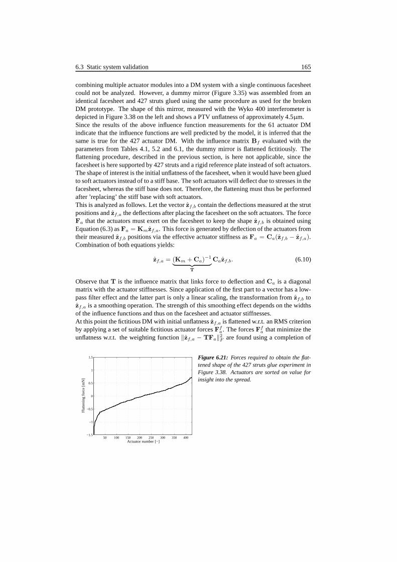
6.3 Static system validation 165

combining multiple actuator modules into a DM system with a single continuous facesheetcould not be analyzed. However, a dummy mirror (Figure 3.35)was assembled from anidentical facesheet and 427 struts glued using the same procedure as used for the brokenDM prototype. The shape of this mirror, measured with the Wyko 400 interferometer isdepicted in Figure 3.38 on the left and shows a PTV unflatness of approximately 4.5µm.Since the results of the above influence function measurements for the 61 actuator DMindicate that the influence functions are well predicted by the model, it is inferred that thesame is true for the 427 actuator DM. With the influence matrixBf evaluated with theparameters from Tables 4.1, 5.2 and 6.1, the dummy mirror is flattened fictitiously. Theflattening procedure, described in the previous section, ishere not applicable, since thefacesheet is here supported by 427 struts and a rigid reference plate instead of soft actuators.The shape of interest is the initial unflatness of the facesheet, when it would have been gluedto soft actuators instead of to a stiff base. The soft actuators will deflect due to stresses in thefacesheet, whereas the stiff base does not. Therefore, the flattening must thus be performedafter ’replacing’ the stiff base with soft actuators.This is analyzed as follows. Let the vectorzf,b contain the deflections measured at the strutpositions andzf,a the deflections after placing the facesheet on the soft actuators. The forceFa that the actuators must exert on the facesheet to keep the shape zf,b is obtained usingEquation (6.3) asFa = Kmzf,a. This force is generated by deflection of the actuators fromtheir measuredzf,b positions via the effective actuator stiffness asFa = Ca(zf,b − zf,a).Combination of both equations yields:

zf,a = (Km + Ca)−1

︸ ︷︷ ︸

T

Cazf,b. (6.10)

Observe thatT is the influence matrix that links force to deflection andCa is a diagonalmatrix with the actuator stiffnesses. Since application ofthe first part to a vector has a low-pass filter effect and the latter part is only a linear scaling, the transformation fromzf,b tozf,a is a smoothing operation. The strength of this smoothing effect depends on the widthsof the influence functions and thus on the facesheet and actuator stiffnesses.At this point the fictitious DM with initial unflatnesszf,a is flattened w.r.t. an RMS criterionby applying a set of suitable fictitious actuator forcesFfa . The forcesFfa that minimize theunflatness w.r.t. the weighting function‖zf,a − TFa‖2

F are found using a completion of

50 100 150 200 250 300 350 400−1.5

−1

−0.5

0

0.5

1

1.5

Actuator number [−]

Fla

tteni

ng fo

rce

[mN

]

Figure 6.21: Forces required to obtain the flat-tened shape of the 427 struts glue experiment inFigure 3.38. Actuators are sorted on value forinsight into the spread.

166 6 System modeling and characterization

squares argument as:Ffa = (TTT)−1TT zf,a = Cazf,b,

where the second step uses the definition ofT in Equation (6.10). The resulting forcesFfaare plotted in Figure 6.21. Note that these forces are independent of the influence functionsand just overcome the actuator spring forces correspondingto the deflectionzf,b. Figure3.38 shows the hypothetical unflatness that remains when fictitious, soft actuators exert theforceFfa . For this dummy mirror the residual RMS unflatness is approximately 20nm, re-quiring an RMS actuator force of 0.4mN. With the average values of the actuator propertiesKa, Ra, Rl as measured in the previous chapter, the latter correspondsto an RMS actuatorvoltage of 0.17V which is approximately 5% of the available maximum voltage. In Section3.6 this fraction was budgetted smaller then 10%.

6.3.3 Power dissipation

Based on the measured influence functions and flattening commands, the expected averagepower dissipation to correct atmospheric wavefront distortions, is estimated. For realisticresults, a trade-off is made between power dissipation and performance in terms of fittingerror. The RMS powerPa, dissipated by the actuators, can be expressed in terms of theactuator voltage setpoint and the total resistanceRa+R′

a+Rl +R′l estimated in Sections

5.6.2 and 5.6.3 as:

Pa = (Ra + R′a + Rl + R′

l)−1 ⟨

V2PWM(t)

⟩, (6.11)

where(·)2 denotes the element-wise square andt the time. The actuator voltages con-sists of the static voltagesVf required for the initial flattening of the DM and the dy-namic voltagesVd(t) required to correct atmospheric wavefront disturbances. The value⟨V2

PWM(t)⟩

in Equation (6.11) can be expressed accordingly as⟨(Vd(t) + Vf )

2⟩. This

reduces to⟨V2d(t)

⟩+V2

f when the atmospheric wavefront distortion and thusVd is a zero-mean signal that is therefore not correlated with the constant signalVf . Application ofthese simplifications to Equation (6.11) yields:

Pa = (Ra + R′a + Rl + R′

l)−1 (⟨

V2d(t)

⟩+ V2

f

). (6.12)

An estimate for the vectorVf with flattening voltages is obtained from the measurementsdescribed above. To quantify

⟨V2d(t)

⟩, consider the atmospheric wavefront disturbance

to have a Von Karmann spatial spectrum (Section 2.1.2) with covariance matrixCφ =⟨

φ(t)φT (t)⟩

. Here the vectorφ(t) denotes the wavefront distortion over a fine grid over

the telescope aperture in radians. The matrixCφ is numerically approximated using theapproach described in [96] with the modification that the Kolmogorov structure functionhas been replaced by the Von Karmann structure function [98]corresponding to the powerspectrum given in Equation (2.5) on page 18:

Dvkφ (r) = 6.88

(r

r0

) 53

[

1 − 1.485

(r

L0

)1/3

+ 5.383

(r

L0

)2

− 6.381

(r

L0

)7/3]

.

The resulting covariance matrix is an approximation, sincethe continuous spatial integralsare replaced by numerical sums over a discrete grid of pointswithin the telescope aperture.

6.3 Static system validation 167

The incoming wavefront is corrected by reflection on the DM. Let the DM shapezf (t)be expressed by Equation (6.6), based on the estimated influence matrixBf . Althoughinertial forces are neglected, the static model accuratelydescribes the DM facesheet deflec-tions, since its first resonance frequency lies far above thecontrol bandwidth. A fine grid isused to model the wavefront distortions and the DM influence functions. Hereby a realis-tic estimate of the fitting error and power dissipation is made. When considering the openloop controlled case, let the actuator voltages be chosen asthe minimizing argument of aquadratic cost function that weights both fitting error and control effort. Let the fitting error,in meters, be expressed as:

efit(t) = λ2πφ(t) − BfVPWM(t)

whereλ is the wavelength of the incoming light. The optimal actuator command vectorVd(t) is chosen as:

Vd(t) = arg minVPWM(t)

⟨∥∥efit(t)

T efit(t)∥∥

2

F

⟩

+ γ‖⟨‖VT

d (t)‖2F

⟩

= λ2π B+

f φ(t), (6.13)

whereB+f = (BT

f Bf + γ2I)BTf is a regularized pseudo inverse ofBf andγ is a weighting

factor for the control effort. For this command vector the fitting errorefit(t) becomes:

efit = (I − Bf B+f )

︸ ︷︷ ︸

B−

f

φ(t) (6.14)

and the command signal covariance matrixCVdcan be expressed as:

CVd=⟨Vd(t)V

Td (t)

⟩=(λ2π

)2B+f Cφ

(

B+f

)T

,

where the second step follows after substitution of Equation (6.13). The diagonal elementsof the covariance matrixCVd

now form the vector⟨V2d

⟩. Similarly, using Equation (6.14)

the fitting error covariance matrixCfit can be expressed as:

Cfit =⟨efit(t)e

Tfit(t)

⟩=(λ2π

)2B−f Cφ

(

B−f

)T

,

from which the RMS fitting errorσfit,d can be derived as:

σfit,d =

√

Tr(Cfit)

nf,

wherenf is the number of grid points used. To provide insight in the power dissipation,based on measurements on a 61 actuator prototype, several parameters must be scaled.Firstly, in Chapter 2 the number of actuators for an 8 meter telescope is 5000, whichimplies that for the same actuator density, the 61 actuator DM prototype should be usedon a 0.9m telescope. Secondly, a continuous facesheet type DM can only prescribe theslope of the facesheet at the aperture edge if there is at least one ring of actuators outside

168 6 System modeling and characterization

10−8

10−7

10−6

10−6

10−5

10−4

10−3

10−2

Pow

er [W

]

RMS fitting error [nm]

Illuminated areaEdgeUncorrected error

10−8

10−7

10−6

10−6

10−5

10−4

10−3

10−2

Pow

er [W

]

RMS fitting error [m]

Illuminated areaEdgeUncorrected error

Figure 6.22: Relation between the fitting errorσfit,d and the average power dissipation per ac-tuator based on the measured influence matrix ofthe 61 actuator DM prototype. Power dissipationis differentiated between actuators in- and out-side the∅32mm illuminated area (λ=550nm).

Figure 6.23: Relation between the fitting errorσfit,d and the average power dissipation per ac-tuator based on the modeled influence matrix ofa 427 actuator DM. Power dissipation is differ-entiated between actuators in- and outside the∅102mm illuminated area (λ=550nm).

Table 6.2: The expected average power dissipation in mW per actuator based on the influence functionmeasurements for a 0.9m telescope using a∅32mm illuminated area on the DM and aVon Karmann spectrum with a Fried parameterr0=0.16m (λ=550nm) and an outer scaleL0=100m.

Atmospheric Flattening Totalturbulence

Edge 1.5 23.8 25.3Illuminated area 1.4 5.5 6.9Full area average 1.4 14.5 15.9

the illuminated aperture. Therefore, an illuminated diameter of 32mm will be consideredover which the Von Karmann spectrum is to be corrected. Actuators outside this areaare only used for flattening and for prescribing the boundaryconditions. By varying thecontrol effort weighting factorγ and assuming a wavelengthλ = 550nm, evaluationof Equation (6.12) yields the relation between fitting errorand power dissipation shownin Figure 6.22. When a fitting error of 35nm is taken, which is 2.5% above the bestachievable value, the corresponding average power dissipation of the actuators is listed inTable 6.2. A distinction is made between actuators in the illuminated area and those at theedges. Also the two causes for the dissipation – i.e. the correction of wavefront errorsdue to atmospheric turbulence and the correction of the initial DM unflatness – are statedseparately. The dissipation for actuators in the illuminated area required for atmosphericwavefront correction is approximately 1.4mW. Although this is less than the 3.2mWestimated in Section 5.7, it depends on the chosen regularization factorγ. Further, thedissipation required for flattening is larger than the functional dissipation, due to significant

6.4 Dynamic system validation 169

Table 6.3: The expected average power dissipation in mW per actuator based on the influence functionmeasurements for a 2.3m telescope using a∅102mm illuminated area on the DM and aVon Karmann spectrum with a Fried parameterr0=0.16m (λ=550nm) and an outer scaleL0=100m.

Atmospheric Flattening Totalturbulence

Edge 0.2 0.4 0.6Illuminated area 0.6 0.2 0.8Full area average 0.4 0.2 0.6

initial unflatness of the DM, especially at the edge of the DM.

For the∅150mm dummy DM a similar table is derived based on an illuminated area of∅102mm. This corresponds to the largest diameter, which is fully filled with actuators, ascan be observed in Figure 6.26. With the same actuator density as the 5000 actuator DMproposed for an 8m class telescope, this DM is suitable for a 2.3m wavefront. The forces asderived in Section 6.3.2 are assumed to be indicative of the forces required to compensatethe initial unflatness of the∅150mm facesheet. Figure 6.23 shows the trade-off betweenperformance and effort for this DM and Table 6.3 shows the estimated power dissipation forthe same fitting errorσfit,d of 35nm as used for the 61 actuator DM. The table shows thatboth the power dissipated to correct the initial unflatness as well as the power dissipated tocorrect the atmospheric wavefront distortions with a Von Karman spectrum is smaller thanfor the 61 actuator DM. However, this only holds true for the regularization factor chosen.

6.4 Dynamic system validation

In Section 6.3 the static behavior of the DM system was validated. In this section thedynamic behavior will be added to the DM facesheet model and combined with the actuatormodels. The resonance frequencies, mode shapes, modal damping and transfer functionsfrom this model will then be compared to a black-box model, identified from measurementdata, using the PO-MOESP subspace identification algorithm.

6.4.1 Dynamic modeling

There is no known analytic solution available for the biharmonic plate equation for a cir-cular plate including inertia and viscous damping terms subjected to multiple point forces.The dynamic behavior can be modeled using a FEM approach, buthere it will be done bycombining the derived models for the actuators and the facesheet and extending this withlumped masses and dampers.Let the force equilibrium in Equation (6.2) be extended accordingly to:

Fa − Fρ − Caza − Baza − Maf za = 0, (6.15)

170 6 System modeling and characterization

where each(i, i) element of the diagonal matricesBa andMaf are the viscous actuatordampingba and the sum of the lumped facesheet mass and the moving actuator mass at co-ordinateρi respectively. Note that for simplicity it is assumed that the actuator and lumpedmass/damper locations coincide, but this can be generalized by using an arbitrary grid andappropriately attributing mass, stiffness and damping values. The mass distribution chosenleads to adequate approximations of the mode shapes with spatial frequencies significantlybelow the Nyquist frequency of the actuator grid, which corresponds to the lower eigenfre-quencies. These are the most relevant for the achievable correction quality, since they posethe tightest limit on the achievable control bandwidth. Moreover, the stiffness matrix usedcorresponds to the solution of the biharmonic plate equation under the assumption of purebending. For high spatial frequencies, shear forces becomedominant and this assumptionloses its validity.When the result in Equation (6.3) forFρ is substituted into Equation (6.15) and transformedto the Laplace domain this yields the dynamic system:

(Caf + Bas+ Mafs

2)za = Fa, (6.16)

whereCaf = Km + Ca. The undamped mechanical eigenfrequenciesfe,(i) and modeshapesx(i) for i = 1 . . .Na can be obtained by solving the generalized eigenvalue problem:

(Caf − λ(i)Maf

)x(i) = 0,

wherefe,(i) =√λ(i)/2/π.

This procedure has been performed for two different cases. Firstly for a DM with regularlyplaced actuators with 6mm pitch in a hexagonal pattern. Equal lumped masses were addedat all actuator grid points and all actuator and facesheet properties were used as given inTables 4.1, 5.2 and 6.1. The first 100 resonance frequencies for this model are plotted ascircles in Figure 6.24 and the first twelve resonance modes are shown in Figure 6.25. FromFigure 6.24 it is clear that the first resonance modes occur ina small frequency band andfrom Figure 6.25 it is clear that the modal shapes correspondvery well to the Zernike poly-nomials [141]. Traditionally, these polynomials are used to describe both the aberrations inthe optical domain as well as the dynamic modes of the wavefront corrector in the mechan-ical domain.However, the resonance frequencies and corresponding modal shapes are influenced by theedge conditions of the reflective facesheet. When considering the 427 actuator DM proto-type that consists of seven hexagonal actuator modules, observe that the gaps between thehexagons at the outside have no actuators that support the mirror facesheet. In the dynamicmodel in Equation (6.16) leads to ’zero’ elements on the diagonals of the matricesCa andBa and to lower values of the corresponding diagonal elements in Maf due to the absenceof moving actuator masses. The lack of support stiffness in the edge areas leads to lowerresonance frequencies with local mode shapes. To properly attribute lumped mass fractionsof the facesheet to grid points in edge areas, its mass is distributed based on the Voronoidiagram of the grid points (Figure 6.26). The Voronoi diagram is the dual of the Delaunaygrid triangulation [131, 168] that is frequently used to draw a surface defined at arbitrarygrid of points. The Voronoi diagram creates a polygon area around each grid point in whichall points are closest to that particular grid point. For most grid points this yields a closedpolygon, but for edge points this is open towards the edge. The polygon area determines the

6.4 Dynamic system validation 171

20 40 60 80 100200

400

600

800

1000

1200

1400

1600

1800

Mode number [−]

Fre

quen

cy [H

z]

427 actuators in seven grids of 61559 actuators in a full hexagonal array

Figure 6.24: The lowest 100 undamped mechan-ical resonance frequencies.

Figure 6.25: The lowest 12 undamped mechan-ical resonance modes corresponding to the fre-quencies plotted as circles in Figure 6.24.

lumped fraction of the facesheet mass and can for closed polygons be computed using Mat-lab’spolyarea function [131]. The open edge polygons are first extended with two pointson the circular facesheet edge by which the polygon is closed. The total area is then the sumof the area of the artificially closed polygon and the area between these two points and thecircle, which follows from the distance between the two additional edge points. Since allareas can be calculated analytically, no approximations are made and the summed area forall grid points exactly equalsπr2f . For the 427 actuator DM prototype the result is plottedin Figure 6.26.The lowest 100 eigenfrequencies for this case are plotted inFigure 6.24 as the solid dots.The first resonance frequencies are lower than in the homogenously supported case andthe corresponding modal shapes are local bending modes of the unsupported edge areas.Clearly, the actuator layout of future DMs should be chosen such that the facesheet edgesare uniformly supported.

Figure 6.26: Voronoi diagram for the hexago-nally arranged grid points marked with a smalldot. The actuator grid of the 427 actuator DMprototype is marked with ”o”.

172 6 System modeling and characterization

10−10

10−5

Mag

nitu

de (

abs)

Central actuatorTo first neighborTo second neighborTo third neighbor

101

102

103

−540

−360

−180

0

180

Pha

se (

deg)

Frequency [Hz]0 10 20 30 40 50

−0.5

0

0.5

1

1.5

2

2.5

Time [ms]

Dis

plac

emen

t [µm

]

Central actuatorTo first neighborTo second neighborTo third neighbor

Figure 6.27: Bode plots from the PWM voltageof the central actuator to the position of itself andthree neighbors.

Figure 6.28: Step response from the PWM volt-age of the central actuator to the position of itselfand three neighbors.

Although the mechanics largely determine the behavior of the DM in terms of resonancefrequencies, the electronics influence the damping, response time, gain, etc. Therefore, thestate-space description for the single actuator behavior in Equation (5.4) on page 131 isextended to describe the behavior of multiple actuators andcombined with the mechanicalequations of motion in Equation (6.15). The scalar statesIRl

, Ia, VCl, za and za become

the vectorsIRl, Ia, VCl

, za and za whoseith elements contain the corresponding statesof the ith actuator. Similarly, the scalar parametersKa, Ra, Rl, La, Ll andCl for eachactuatori become the(i, i) diagonal elements of the square diagonal matricesKa, Ra, Rl,La, Ll andCl respectively. Further, instead of the mechanical equationof motion for thesingle, uncoupled actuator in Equation (4.25), the dynamicequation in Equation (6.16) willbe used, leading to:

Iazfzf

Va

IRl

=

−L−1a Ra 0 −L−1

a Ka L−1a 0

0 0 I 0 0

M−1af Ka−M−1

af Caf−M−1af Ba 0 0

−C−1l 0 0 0 C−1

l

0 0 0 −L−1l −L−1

l Rl

︸ ︷︷ ︸

Afm

IazfzfVa

IRl

+

0

0

0

0

L−1l

︸ ︷︷ ︸

Bfm

VPWM

(6.17)The transfer matrixH(s) between the PWM voltageVPWM and the facesheet deflectionzfcan be expressed accordingly as:

H(s) =[0 I 0 0 0

](sI− Afm)−1

BTfm.

The DC-gain of this transfer matrix is equal to Equation (6.6) and can be derived by evalu-atingH(s) for s = 0:

H(0) = −[0 I 0 0 0

]A−1fmBT

fm = C−1af Kt(Ra + Rl)

−1 = Bρ, (6.18)

6.4 Dynamic system validation 173

whereAfm andBfm are defined in Equation (6.17) and the final expression follows fromthe definition ofBρ in Equation (6.6).The model in Equation (6.17) has been generated numericallyfor a ∅150mm reflectivefacesheet that is regularly supported by 6mm spaced actuators over its entire area. The ac-tuator, electronics and facesheet properties used are given in Tables 4.1, 5.2 and 6.1. InFigure 6.27 Bode plots are shown of the entries of the transfer matrix corresponding to thePWM voltage of the central actuator and the position of itself and three neighbors at 6, 12and 18mm distance. It shows that the static DC response to neighboring actuator positionsindeed decays rapidly with the spatial distance, but that the global shapes of the lightlydamped, lowest dynamic modes (Figure 6.25) lead to a strong coupling between the actua-tors at high frequencies. To illustrate this low damping, Figure 6.28 shows the step responseof the same actuators due to a step input at the PWM voltage of the central actuator. Inpractise the damping will be higher due to the presence of airabove the facesheet, intrinsicdamping of the facesheet and strut materials, deformation of the glue between the struts andthe facesheet, etc. To quantify this effect, the relative damping of the resonant modes of thismodel will be compared to the damping derived from a modal analysis in Section 6.4.3. .

6.4.2 System identification

Modal (or structural) analysis is frequently performed using the Eigensystem Real-ization Algorithms (ERAs) [9, 63] and its variants [120]. The ERAs are a subspacebased identification methods that estimate a state space by taking the Singular ValueDecomposition (SVD) of a Hankel matrix of the system’s impulse response function.This impulse response function is either measured directlyfrom impulse excitation orestimated from more generic input-output data. For open loop measurement data of MIMOsystems the MOESP algorithm [191] and its variants [194] arevery suitable. For closedloop identifications the Predictor Based Subspace IDentification (PBSID) identificationalgorithm [35, 37] can be used, which has been applied for theidentification of a DM with60 actuators and 104 sensors of the MAD (Multi-conjugate Adaptive-optics Demonstrator)system in [36]. However, the DM can here be identified in open loop, making the addedcomplexity of the PBSID algorithm superfluous. Besides subspace based identificationalgorithms that use state-space parameterizations, otheralgorithms can be used for MIMOsystem identifications with other parameterizations. For instance, in [177] a MIMOTransfer Function (TF) parametrization is shown to be very efficient in both the number ofparameters and the required computational effort, when compared to subspace algorithms.The identification algorithm used for modal analysis of the DM prototype is chosen basedon several requirements. It must be able to deal with 61 simultaneous inputs and at leastas many outputs. Since the sampling frequency of the setup used is limited to 10kHz, thedynamics of the electronics that become dominant above 5kHzwill not be well observablefrom the measurement data. Although the DM facesheet dynamics are of infinite order,the low frequent resonance modes can be adequately described using a limited number oflumped masses. This means that the system order required foridentification is at least twicethe number of lumped masses, which in this case is in the orderof hundreds. It also meansthat the model parametrization used must allow the large number of poles and zeros to beindependent to properly describe the numerous resonance modes of the DM facesheet. The

174 6 System modeling and characterization

poles will be used after the identification step to compute the resonance frequencies, theirrelative damping and the modal shapes.Since for identification of a state-space model a high state dimension and large numbers ofin- and outputs are required, the identification algorithm used must be efficient w.r.t. bothmemory and computation steps. Moreover, the method must be suitable for the availablemeasurement setup, which is the same as used previously to identify the behavior of singleactuators and depicted in Figure 5.11. In this setup, the deflection of the DM facesheet canbe measured only at a single point at a time with a Polytec laservibrometer. The obtainedmeasurement data is thus expected to be significantly corrupted both by measurementand process noise, since the measurements are performed in anoisy environment withoutvibration isolation facilities. The identification algorithm must be robust for these types ofnoise. On the other hand, since all quantization is performed in the control PC in an openloop setting there is no quantization noise.

Identification using the MOESP algorithm

The MOESP algorithm is a subspace identification algorithm that uses a QR decomposition[76] of the input-output data matrix to compress the data andthus improve the computationalefficiency. The algorithm and its variants are found in literature [192–194] and Matlab im-plementations are readily available. Since the identification is subject to both measurementand process noise, the PO-MOESP algorithm will be used, which uses past inputs and out-puts as instrumental variables to provide unbiased estimates w.r.t. measurement and processnoise. Since in literature this variant of the algorithm is generally intended when referringto MOESP, the prefix PO- will here also be neglected.Details on the theory and implementation of the MOESP identification method used on thisDM are found in [183].The quality of the obtained system is evaluated by applying the estimated system realizationto a validation data sequence and computing the VAF, defined as:

VAF =

1 −

⟨

(zf (t) − zf (t))T

(zf (t) − zm(t))⟩N

t0⟨

zTf (t)zf (t)⟩N

t0

· 100%,

wherezf (t) is obtained by simulating the identified model for the known excitation signalVPWM (t) andzf (t) is the vector of facesheet deflections measured by the laser vibrometer.The VAF represents the fraction of the signal variance that is accounted for by the modeland should be close to 100%.

6.4 Dynamic system validation 175

6.4.3 Modal analysis

The modal analysis of the identified system begins with a modal decomposition of itsA-matrix. This decomposition is such thatΛA = MA, where the diagonal matrixΛ containsthe (complex) eigenvalues ofA and the columns ofM contain the (complex) eigenvectors.The matrixM forms a state transform matrix that diagonalizes the systemand yields astate-space description with statex(t) whose state transition matrix is equal toΛ:

x(t+ 1) = Λx(t) + M−1Bu(t),

zf (t) = CMx(t),

where the influence of process and measurement noise is neglected. For the discrete timesystem, each eigenvalueλ(i) on the diagonal ofΛ is related to the resonance frequencyωn,(i) and relative dampingζ(i) of modei as [64]:

λ(i) = eTs

(

−ζ(i)ωn,(i)±jωn,(i)

√

1−ζ2(i)

)

= |λ(i)| · ∠λ(i),

whereTs is the sampling frequency and

|λ| = e−Tsζ(i)ωn,(i) , ∠λ = e±Tsjωn,(i)

√

1−ζ2(i) .

Inversely, the resonance frequenciesωn,(i) and damping ratio’sζ(i) can be computed as:

ωn,(i) =ln∠λ− ln|λ|

Tsand ζ(i) = − ln|λ|

ln|λ| − ln∠λ.

Further, the vectors of the matrixCM form the facesheet shapes corresponding to thesystem’s eigenfrequencies. Since complex poles occur in conjugate pairs(a, b) with thesame modal frequencyωn,a = ωn,b, the matrix’s complex part and columns correspondingto complex conjugate eigenvalues will for the modal analysis be ignored.

Results

For the 61 actuator DM prototype, the facesheet response is measured on the 79 pointsshown in Figure 6.29. These are the 61 actuator locations and18 points on the facesheetalong its edge. The signal acquisition and DM setpoint update rate is chosen as high aspossible to minimize the effects of sampling and aliasing. The 10kHz sampling frequencyused, is close to the upper limit of the serial communicationchain but still significantly lowerthan the PWM actuator voltage base frequency. The laser vibrometer is pointed at eachgrid location for 10 seconds, producing 100.000 measurements. A zero-mean, bandlimited,white noise sequenceVPWM (t) ∈ N (0, σ2

eI) is generated withσe = 0.13V and t =0 . . .10s and applied on each location. Except for small variations in initial conditions andtiming (i.e. jitter), the obtained data is equal to the data that would have been obtained whenthe response of all points is measured simultaneously.The obtained measurement data set is split into an identification set of 85.000 samples and

176 6 System modeling and characterization

Figure 6.29: The grid of points at which theresponse of the 61 actuator DM prototype wasmeasured. Points 1. . .61 correspond to the actu-ator locations.

12

34

5

67

89

10

1112

1314

15

1617

1819

20

21

22

23

24

25

26

27

28

29

30

31

32

33

34

35

36

37

38

39

40

41

4243

4445

46

4748

4950

51

5253

5455

56

5758

5960

61

62

63

646566

67

68

69

70

71

72

7374 75

76

77

78

79

a validation set of 15.000. The MOESP system identification method is applied to thefirst part of this input-output data and the VAF value is computed after simulation on thesecond part. The VAF found is 95%. Figures 6.30 and 6.31 show the first 12resonance frequencies and the corresponding modal shapes derived from the analytic modelin Equation (6.17) and the black-box model identified with the MOESP algorithm. Forthe modal analysis of the analytic model, the average measured actuator properties listedin Table 5.3 are used. When all actuators have equal properties, the modal shapes showa high degree of symmetry (Figure 6.30). In practice the actuator properties vary, leadingto the asymmetric mode shapes in Figure 6.31. The lowest resonance mode of the systemlies at∼725Hz and corresponds to a motion of the lower-left edge areaof the facesheet.

Figure 6.30: The first 12 modal shapes derivedfrom the analytic model in Equation(6.17)usingthe average actuator properties listed in Table5.3 and the facesheet properties listed in Table6.1.

Figure 6.31: The first 12 modal shapes derivedwith the MOESP system identification method .

6.4 Dynamic system validation 177

500 1000 150010

−3

10−2

10−1

100

Frequency [Hz]

Rel

ativ

e da

mpi

ng [−

]

MOESPAnalytical model

10−8

10−6

Mag

nitu

de [m

/V]

101

102

103

−360

−180

0

Frequency [Hz]

Pha

se [d

eg]

Poked actuatorTo first neighborTo second neighborTo third neighbor

Figure 6.32: Relative dampingζ correspondingto the eigenfrequencies of the models identifiedwith the MOESP algorithm and of the analyticalmodel from Equation(6.17).

Figure 6.33: Bode plot of the model identifiedwith the MOESP algorithm between the com-mand voltage at actuator 2 and its first, secondand third neighboring actuators 41, 42 and 47respectively.

This frequency is lower than expected. Since the edges are supported by a few actuators,the low resonance may be caused by a lower stiffnessca of only a few actuators. Therelative dampingζ identified with the MOESP algorithm and in the analytical model fromEquation (6.17), based on the average actuator properties listed in Table 5.3, are shownin Figure 6.32. The relative damping in the analytical modelis significantly lower thanin the black-box model, which means that the damping observed in the DM system is notentirely due to the actuators. This suggests the presence ofother dissipative processes suchas material damping, damping in the glue used or damping due to the movement of airabove the facesheet. The latter is a likely explanation, since the facesheet vibrations due tothe noise excitations used were clearly audible.

A Bode plot of the identified model is shown in Figure 6.33 for the transfer functions

Figure 6.34: The influence function of actuator 2 (Figure 6.29) as derivedfrom the analytical model(left), from the Wyko measurements of Section 6.3.2 (middle) and from the model identi-fied using MOESP (right).

178 6 System modeling and characterization

0 10 20 30 40 50−0.2

0

0.2

0.4

0.6

0.8

1

1.2

Time [ms]

Dis

plac

emen

t [µm

]

Central actuatorFirst neighborSecond neighborThird neighbor

0 10 20 30 40 50−0.5

0

0.5

1

1.5

2

Time [ms]

Dis

plac

emen

t [µm

]

Central actuatorFirst neighborSecond neighborThird neighbor

Figure 6.35: Step response of the central actua-tor in the model identified with the MOESP algo-rithm . The response is shown of four locations:the central actuator and three actuators at 1, 2and 3 actuator spacings distance.

Figure 6.36: Step response of the central actu-ator of the analytical model in Equation(6.17),using the average actuator parameters listed inTable 5.3. The response is shown of four loca-tions: the central actuator and three actuators at1, 2 and 3 actuator spacings distance.

from the actuator voltage at actuator 2 to the displacement at its first, second and thirdneighboring actuators 41, 42 and 47. This shows the high peaks in the magnitude responseas a result of the low relative damping. However, where the magnitude of the peaks doesnot decrease with frequency in the Bode plot of the analytical model in Figure 6.27, they doin the model as identified, which suggests the presence of additional dissipative processesat high frequencies.Further, the influence functions have been derived from the model identified by computingthe DC gain matrix of the system according to Equation (6.18)asC(I − A)−1B whosecolumns contain the influence functions. The influence function of actuator 2 is shownin Figure 6.34 together with the influence functions of the same actuator derived from theanalytic model and the Wyko measurements of Section 6.3.2. The shape and magnitudematch qualitatively, but some quantitative error can be observed.

This is partly due to the poor alignment accuracy of the laservibrometer spot.Finally, the step response functions derived from the modelfrom the central actuator voltagesetpoint to the displacement of four points on the reflectivesurface are shown in Figure 6.35.The four points are the location of the actuator itself and that of three neighbors with 1, 2and 3 actuator spacings distance. In Figure 6.36, the corresponding step response derivedfrom the analytical model is shown for the same actuators. A comparison with Figure 6.35confirms that in the analytical model of the 61 actuator DM damping is underestimated.

6.5 Conclusions 179

6.5 Conclusions

The assembly of two DMs prototypes is shown: a∅50mm DM with 61 actuators and a∅150mm DM with 427 actuators. In the first prototype a single actuator grid is used,whereas for the second prototype modularity is shown by the assembly of seven identi-cal grids on a common base. The seven actuator grids, with accompanying dedicated driverboards, are attached to a single, continuous, facesheet.The actuator model derived in the Chapter 5 is extended with alinear model of the con-tinuous facesheet, based on an analytic solution of the biharmonic plate equation and pointforces. Lumped masses are added to obtain the dynamic behavior. Both static and dynamicperformance is validated on the∅50mm DM using measurements. Scaled Hadamard matri-ces for the actuator voltage command vectors are used to measure the 61 influence functionsin front of a Wyko interferometer. This approach minimizes the variance estimation errorsof the influence matrix due to measurement noise.The measured actuator coupling of the central actuators is 52% and close to the 65% fromthe estimate in Section 3.4 and the predicted value from the static model in Section 6.3.2.In the estimate, only the six surrounding actuators were included, thereby neglecting thestiffness contribution of other actuators and leading to anover-estimation of the coupling.In the static model from Section 6.3.2 these were included and the prediction close to themeasurements.The measured shape and amplitude of the influence functions agree with the prediction withthe static model (Figures 6.18 and 6.19). This includes the increased static gain (m/V) ofthe actuators at the edge of the DM due to the reduced facesheet stiffness from the mirror’sfree-edge boundary condition. The variation in the static gain is observed and attributed tovariation in motor constant, actuator stiffness and electrical resistance and driver circuits.The influence matrix derived from the measurements is used toshape the mirror facesheetinto the first 28 Zernike modes, which includes the piston term that represents the best flatmirror. The interferometrically measured shapes are compared to the perfect Zernike modesand to the Zernike modes as made with the limited number of regularly spaced actuators inthe actuator grid. The total RMS error is≈25nm for all modes, whereas the inevitable fit-ting error varies between 0 and 23nm depending on the mode.The power dissipation in each actuator of the∅50mm mirror to correct the Von Karmanturbulence spectrum (D/r0 = 5.4, L0 = 100m) is estimated. Actuators outside the illumi-nated area are distinguished from those inside this area. Furthermore, the estimated powerdissipation is split into turbulence correction and mirrorflattening. For the turbulence cor-rection, 1.5mW for the outer and 1.4mW for the inner actuators, is dissipated. For staticflattening these values are 23.8mW and 5.5mW respectively.The 427 actuator DM prototype was broken during placement ofits protective cover, there-for it was not possible to measure its unflatness, static or dynamic behavior. A dummymirror (Figure 3.35) with similar facesheet specifications, which was used to test the as-sembly procedure of the 427 connection struts, was interferometrically measured instead.This mirror showed≈4.5µm PTV unflatness. This mirror was fictitiously flattened, withthe use of the modeled influence matrix and requires 0.17V RMSactuator voltage, whichcorresponds to 5% of the available output voltage range and apower dissipation of 0.2mWper actuator.

180 6 System modeling and characterization

The predicted dynamic behavior of the DM is validated by measurements. A laser vibrom-eter is used to measure the displacement of the mirror facesheet, while the actuators aredriven by zero-mean, bandlimited, white noise voltage sequence. Using the MOESP sys-tem identification algorithm, high-order black-box modelsare identified with VAF valuesaround 95%. This identified model is compared with the derived analytical model. Thelatter uses the average actuator properties as measured in Chapter 5. The first resonance fre-quency identified is 725Hz, and lower than the 974Hz expectedfrom the analytical model.This is attributed to the variations in actuator properties, such as actuator stiffness.The relative modal damping of the model identified is an orderof magnitude higher than thedamping in the analytical model, where only actuator damping is considered. The differenceis attributed to the presence air damping and damping in the glue used for the connectionstruts.

Chapter sevenCon lusionsIn the previous chapters the design, realization and test ofthe adaptive de-formable mirror based on electromagnetic actuators is shown. This chapterwill summarize the main conclusions from these chapters andoutline the sub-jects of future work.

181

182 7 Conclusions

7.1 Conclusions

Refractive index variations in the earth’s atmosphere limit the resolution in ground basedtelescopes. Existing large and future even larger telescopes can only be utilized fully, whenthey are equipped with AO systems that enhance optical resolution. The development ofDM technology that meets the requirements for these future AO systems is essential.The requirements for the adaptive deformable mirror and control system are derived fromtypical atmospheric conditions (r0=0.166 (λ=550nm) andfG=25Hz). The spatial and tem-poral properties of the atmosphere are hereby covered by thespatial and temporal spectraof Kolmogorov turbulence and the frozen flow assumption. Thefitting error, caused by alimited number of actuators and the temporal error, caused by a limited control bandwidth,are the most important for the DM design.≈5000 actuators and 200Hz bandwidth forma balanced choice for the number of actuators and the controlbandwidth and can correctan 8m wavefront in the visible to nearly diffraction limited. An actuator stroke of≈5.6µmand≈0.36µm inter actuator stroke is needed. Together with the nm’s resolution, low powerdissipation, no hysteresis and drift, form these the main actuator requirements.The design, realization and tests of a new DM that meets theserequirements and is extend-able and scalable in mechanics, electronics and control is presented.

The DM design

In the DM design a few layers are distinguished: the mirror facesheet, the actuator gridand the base frame. The first layer is the thin reflective facesheet, which is the deformableelement. The facesheet is continuous and stretches over thefull aperture. In the underlyinglayer - the actuator grid - low voltage electro-magnetic push-pull actuators are located. Theactuator grid consists of a number of identical actuator modules, each with 61 actuators.Each actuator is connected via a strut to the mirror facesheet. The mirror facesheet, themirror-actuator connection and the actuator modules form athin structure with low out-of-plane stiffness, so a third layer is added, the base frame, to provide a stable and stiffreference plane for the actuators.

The mirror facesheet

A thin facesheet is needed for low actuator forces and power dissipation, whereby its lowerlimit is set by the inter actuator deflection. This deflectionis determined by gravity or, ifpresent, by wind pressure. For both situations the scaling laws for the total actuator forceFand power dissipationP are derived, depending on the size of the uncompressed wavefrontDt, the compression factorcD, which is the ratio between the uncompressed wavefrontand the DM that performs the correction, the number of actuators and the thickness of thefacesheet. If no significant wind pressure is present (v<1m/s), and the telescope’s opticaldesign and desired optical quality is fixed, the power dissipation is minimized by selectinga facesheet material with highEf

ρ3f

. When significant wind pressurepw is present, the total

actuator force isF ∝(Dt

cD

)2

pw. F andP are then independent of the facesheet material

7.1 Conclusions 183

properties and the number of actuators.Here only gravity induced deflection is taken into account. Minimum power dissipation isachieved when beryllium is used for the mirror facesheet. With 35µm facesheet thicknessand an actuator grid with 6mm pitch, 1nm RMS inter actuator deflection is present. Sincethin beryllium facesheets are expensive and several are needed for the prototype develop-ments, Pyrex facesheets with 100µm thickness are chosen as a best practical, alternative.Struts connect the facesheet to the actuators. The connection struts allow the mirrorfacesheet to form a smooth surface over the imposed heights.The diameter and length of thestruts are determined by taken into account its bending stiffness, axial stiffness, resonancefrequency and buckling load. A round stainless steel strut with ∅0.1×8mm is selected.During assembly, the facesheet is supported by a porous graphite air bearing. First the strutsare glued to the facesheet, hereby supported by a tool. In thesecond step, the facesheetwith struts is placed in droplets of glue at the actuator side. The flatness of a∅150mmfacesheet with 427 struts attached, is measured and 4µm PTV, which is in the same orderof the unflattness of the air bearing reference surface. Interferometric measurements showa local 3nm RMS surface unflattness around the glued attachment.The stiffnesses of the actuators form the out-of-plane constraints for the mirror facesheetand determine the mirrors first resonance frequencyfe. When the actuator stiffnessca issmaller than the bending stiffness of the facesheet betweentwo actuators,fe is well ap-proximated with= 1

2π

√ca

maf

, wheremafis the total mass of the facesheet divided by the

number of actuators carrying the facesheet. The first resonance is then independent of themirror diameter and the mode shape is a global bending of the mirror. Whenca is furtherincreased, local modes appear and higher stiffness will notincrease the resonance frequency.

Actuators

The application of electromagnetic actuators for adaptivedeformable mirrors has severaladvantages. Electromagnetic actuators can be designed with a limited stiffness, such thatfailure of an actuator will not cause a hard point in the reflective surface and thus a smalloptical degradation compared to e.g. stiff piezo-electricelements exists. Other advantagesare the low costs, low driving voltages and negligible hysteresis and drift. Reluctance typeactuators are chosen because of their high efficiency and lowmoving mass. The actuatorsconsist of a closed magnetic circuit in which a PM provides static magnetic force on a fer-romagnetic core, which is suspended in a membrane. This attraction force is influencedby a current through a coil, which is situated around the PM toprovide movement of thecore. With the direction of the current the attractive forceof the PM is either increased ordecreased, allowing movement in both directions. The actuators are free from mechanicalhysteresis, friction and play and therefore have a high positioning resolution with high re-producibility. The stiffness of the actuator is determinedby the membrane suspension andthe magnetic circuit. There exists a large design freedom for both. Actuators are realizedin modules of 61 actuators, hexagonally arranged with 6mm pitch. The hexagonal actuatorlayout is chosen since this gives the highest actuator arealdensity. The grids are design inlayers. This reduces the number of parts and the complexity of assembly and improves theuniformity of the actuator properties. The grids are given ahexagonal contour to accommo-date the assembly of large DMs from many actuator modules.

184 7 Conclusions

Electronics

The electronics consist of two parts: the communication electronics that supply the setpointsas computed by the control system and the driver electronicsthat generate the correspondingactuator voltages. Since theLa/Ra time of the actuator is short: 75µs, the advantage ofcurrent control over voltage control is limited. The motor constantKa, stiffnessca and – inthe case of a voltage source – the resistanceR of the actuator circuit, will vary from actuatorto actuator and vary with temperature, causing slow gain variations. A current source willcompensate for variations in the resistanceR, but variations ofKa and ca must still becompensated by the AO control system. PWM based voltage drivers are chosen becauseof their high efficiency and capability to be implemented in large numbers with only a fewelectronic components. A LVDS based serial communication is chosen for its low powerconsumption (15mW/transceiver), high bandwidth (up to 655Mb/s) and consequently lowlatency, low communication overhead and extensive possibilities for customization. Thedriver electronics for 61 actuators are located on a single,multi-layer PCB and consistof FPGAs to generate the PWM signals, FETs for the H-bridge switches and coil/capacitorpairs that form2nd order low-pass filters. A flat-cable connects up to 32 electronics modulesto a custom designed communications bridge, which translates ethernet packages into LVDSpackages and vice versa. The ethernet side of the communications bridge is connected to thecontrol computer at a speed of 100Mbit/s and uses the UDP protocol to minimize overheadand latency.

Results

Two DMs prototypes were successfully assembled: a∅50mm DM with 61 actuators anda ∅150mm DM with 427 actuators. In the first prototype a single actuator grid is used,whereas for the second prototype modularity is shown by the assembly of seven identicalmodules on a common base. All actuators are attached to a single, continuous, facesheet.

Actuator and electronics performance

The dynamic performance of each actuator is measured, including its dedicated driver andcommunication electronics. All actuators were found to be functional, indicating that themanufacturing and assembly process is reliable. A nonlinear model of the actuator wasderived describing both its static and dynamic behavior based on equations from the mag-netic, mechanic and electric domains. The nonlinear springforce characteristic of the mem-brane suspension was modeled and verified via measurements in a dedicated measurementsetup. The communication is modeled as a pure delay and the driver electronics as a volt-age source with an analog2nd order low-pass filter. The actuator model was linearized,leading to expressions for the actuator transfer function and linear electromechanical prop-erties such as motor constant, coil inductance, actuator stiffness and resonance frequency.The actuator model including its communication and driver electronics was validated bymeasurements. The measurements include communication tests, static and dynamic re-sponse measurements and power dissipation measurements. It is shown that the commu-

7.1 Conclusions 185

nication latency is well represented byτc = 89.7 · 10−6 + 39 · 10−6Nm, whereNmis the number of the actuator module. With the frequency response measurements, ac-tuator properties as stiffness (ca =473±46N/m), motor constant (Ka =0.11±0.02N/A),damping (ba =0.30±0.11mNs/m), inductance(La =3.0±0.2mH) and resonance frequency(fe =1.83±91Hz) are verified. These properties showed some variation between actuators,but this could not be attributed to the location of the actuator in the grid.The time domain response of an actuator to a 4Hz sine voltage was used to determine hys-teresis and semi-static nonlinear response of the actuator. This showed the first to be negli-gible and the second to remain below 5% for the intended±10µm stroke.Measurements also showed that in the expected operating range, the total power dissipationis dominated by indirect losses in the FPGAs. An alternativeFPGA implementation is in-vestigated. A reduction of 40% in the master FPGA and 29% in the slave FPGAs is therebyachieved.

Static DM performance

The actuator model is extended with a linear model of the continuous facesheet, based on ananalytic solution of the biharmonic plate equation and point forces. The static performanceis validated on the∅50mm DM using interferometric measurements. Scaled Hadamardmatrices for the actuator voltage command vectors are used to measure the 61 influencefunctions. This approach minimizes the variance estimation errors of the influence matrixdue to measurement noise. The measured shape and amplitude of the influence functionsagree with the prediction from the static model. This includes the increased static gain(m/V) of the actuators at the edge of the DM due to the reduced facesheet stiffness from themirror’s free-edge boundary condition. Other small variation in the static gain is observedand attributed to variation in motor constant, actuator stiffness, electrical resistance anddriver circuits. The measured actuator coupling of the central actuators is 52% and close tothe predicted value from the static model.The influence matrix, derived from the measurements, is usedto shape the mirror facesheetinto the first 28 Zernike modes, which includes the piston term that represents the best flatmirror. The interferometrically measured shapes are compared to the perfect Zernike modesand to the Zernike modes as made with the limited number of regularly spaced actuators inthe actuator module. The total RMS error is≈25nm for all modes, whereas the inevitablefitting error varies between 0 and 23nm depending on the mode.

Dynamic DM performance

Lumped masses are added to the model to obtain the dynamic behavior. The predicted dy-namic behavior of the DM is validated by measurements. A laser vibrometer is used tomeasure the displacement of the mirror facesheet, while theactuators are driven by a zero-mean, bandlimited, white noise voltage sequence. Using theMOESP system identificationalgorithm, high-order black-box models are identified withVAF values around 95%. Thisidentified model is compared with the derived analytical model. The latter uses the aver-age actuator properties as measured. The first resonance frequency identified is 725Hz, andlower than the 974Hz expected from the analytical model. This is attributed to the varia-

186 7 Conclusions

tions in actuator properties, such as actuator stiffness. The relative modal damping of themodel identified is an order of magnitude higher than the damping in the analytical model,where only actuator damping is considered. The difference is attributed to the presence ofair damping and damping in the glue used to attach the connection struts.The power dissipation in each actuator of the∅50mm mirror to correct the Von Karmannturbulence spectrum (D/r0 = 5.4, L0 = 100m) is estimated. Actuators outside the illumi-nated area are distinguished from those inside this area. Furthermore, the estimated powerdissipation is split into turbulence correction and mirrorflattening. For the turbulence cor-rection,≈1.5mW for the outer and≈1.4mW for the inner actuators, is dissipated. For staticflattening these values are≈23.8mW and≈5.5mW respectively.

7.2 Recommendations

Recoatability

One of the drawbacks in the DM design as presented, is the limited possibility to recoat thefacesheet. This is due to the fact that the facesheet with connection struts and actuators formone glued assembly. The (cheap) facesheet can not be replaced without replacement of thewhole actuator grid. A possible solution would be to make an additional separation layer. Inthe current design, the connection struts are glued to the membrane suspension and movingcore. This suspension is currently glued to the actuator baseplate. In future designs, thisbaseplate could be separated in two layers, where the upper part forms an assembly withthe suspension and the moving core and the lower part forms the assembly with the PMsand coils. For recoating the upper part could be separated from the lower part and replacedtogether with the facesheet.

Actuator performance

To further improve the actuator properties it is recommended to lower the reluctance of theradial airgap. In a sensitivity analysis of the actuator model, this showed to be of strong in-fluence on the motor constant and actuator stiffness. A factor of two in reluctance reductionwill increase the motor constant to 0.37N/A and increase theactuator stiffness to 750N/m.This can be realized by a smaller gap width or by a larger gap area. Besides the higher mo-tor constant, increased electronic damping of the mechanical resonance frequency is thenobserved and will become less limiting for the controller performance without adding com-plexity to the actuator or electronics design.

Assembly

Dust, trapped between the facesheet and the porous airbearing, proved difficult to avoid andmade the placement of the facesheet onto the air bearing one of the most difficult steps inthe assembly. This could be simplified by the addition of small grooves in the air bearing.The chance that a dust particle causes a bump in the mirror surface, is thereby reduced.

Appendix AMeasurement of the magneti properties of PMsA Helmholtz test setup is realized to measure the magnetic properties of the PMs. Thepurpose of the setup is to verify the magnetic properties, especially the 2nd quadrant of theB-H curve, as provided by the PM manufacturer and to select a subset of PMs for whichthe magnetic properties show only small variations to obtain uniformity in the resultingelectromagnetic actuators characteristics.

The Helmholtz coil set

A Helmholtz coil test setup is chosen because it is made relatively easy at low costs, mea-surements can be made in a short time and the PMs are not exposed to external magneticfields that could affect its magnetization. Figure A.1 showsa Helmholtz coil in schematic.The Helmholtz coil consists of a pair of identical circular coils on a common axis. If thecoils are connected in series and current flows through the coils in the same direction, auniform magnetic field is produced at the center. With the Biot-Savart law, the magneticfield produced by a current loop can be calculated. The magnetic field from the two coilsof the Helmholtz coil arrangement can be obtained by superimposing the two constituentfields. The primary component of the uniform magnetic field isparallel to the axes of thetwo coils. The uniform field is the result of the addition of the two field components parallelto the axes of the two coils and the difference between the components perpendicular to theaxes. For a given coil radius, the optimal coil separation can be calculated needed for thelargest uniform central field. This separation is equal to the radius of the coils. Furthermore,

rL

W

r

0.93r

0.6r

Figure A.1: Schematic of a Helmholtz coil. The regionwithin the dashed lines holds an uniform magnetic fieldwhen a current is applied through both coils.

189

190 7 Conclusions

to get a homogeneous field for coils with finite dimensions, the coil’s cross-section shouldbe according to [132]:

W

L=

√

31

36

The resulting area with a uniform field (<1% variation) is also shown in Figure A.1 andexpressed as fraction of the coil mean radius. A Helmholtz coil can not only be used toproduce a uniform magnetic field, but also, if coupled to an integrating volt meter or fluxmeter, to measure the magnetic dipole moment of a PM placed inthat region [40].With a Helmholtz coil, the magnetic dipole moment at the actual operating point of thePM is measured. The measured magnetic dipole moment dependson the magnet volume,shape and its relative permeability. The magnetic moment represents the product of the polestrength and magnetic length of the sample. The pole strength is a measure of total fluxat the pole. The magnetic length is not the same as physical length of the PM and variesfrom 0.7 times the physical length in long and/or low coercivity PMs to nearly the physicallength in short and/or high coercivity PMs and varies with the level of magnetization [176].By reciprocity, the coil flux caused by the dipole will not depend on the position in the areaof uniform field as described above. If the PM is placed closerto one coil, that coil is cutby more flux and the other coil by less, but the total flux seen bythe two coils remainsconstant. By Faraday’s law it follows that the voltage generated is proportional with the rateof the change of the flux in the loop. Magnetic flux is hereby defined as the product of themagnitude of the magnetic field and the area of the loop. By inserting or extracting a PM,the voltage induced can be integrated as a measure for the dipole moment. If the insertedPM is rotated over 180 degrees over an axis perpendicular to the coil axis, the magneticdipole moment as measured is doubled. A turn at the center of the cross section of eachof the two coils will enclose a specific flux when a magnetic dipole, withmz as a dipolemoment is inserted in the center of the coil. This flux is givenby [40]:

φ =µ0mzN

r

2

5

√

4

5

For a coil withN turns and a finite cross section the coupled flux is [40]:

φ =µ0mzN

r

2

5

√

4

5

(

1 − 1

60

(w

r

)2)

= kHmz

The constantkH is linked to the Helmholtz coil geometry.

Reconstructing the 2nd quadrant of the B-H curve

Because the PMs used in the actuators can be stacked, it is possible to reconstruct a signifi-cant part of the B-H curve with the Helmholtz coil test setup [40].The 2nd quadrant of the B-H curve can for linear permanent magnetic materials be describedby:

B = µ0H + µ0M(H)

= µ0µrH +Br (A.1)

Appendix A Measurement of the magnetic properties of PMs 191

WhereB is the magnetic induction in T,Br is the magnetic remanence in T,µ0 is thepermeability in vacuum, equivalent to 4π·10−7 Tm/A, µr is the relative permeability andH is the magnetic field intensity in A/m andM(H) is the average magnetization in A/m.The average magnetizationM(H) per unit volume of the measured (stack) PMs can becalculated by:

M(H) =mz(H)

Vm

whereVm is the volume of the PMs. The measured value is lower than the value ofM0

becauseM(H) is dependent on the internal field in the PM:

M =M0

µ0− µr − 1

µ0µrB

The average value ofB inside the PM in air depends only on the PM shape. The internalB-value increases with the relative length in the magnetization direction. To obtain the valueof B in Equation (A.1) the value forH andM(H) is needed. It is possible to obtain thevalue ofB by the introduction of the demagnetization factorNd.

H = −NdM (A.2)

The value ofNd is between 0 and 1 and depends only on the shape of the PM [34].The process to get from the measurements with the Helmholtz coil to a reconstructed B-Hcurve is:

1. Measuring the magnetic dipole momentmz of stacks of the PMs (e.g. 1,2,3,..., 16PMs).

2. Calculate the average value ofM(H) per unit volume.

3. Determining the demagnetization factor for each of the stacks, depending on the di-ameter and height.

4. Calculate the value of the magnetic field intensityH with Equation (A.2).

5. Calculate the average value of the flux densityB from Equation (A.1).

The found values forB andH are plotted to form the linear part of the 2nd quadrant of theB-H curve.

Measurements with the Helmholtz coil test setup

A dedicated Helmholtz coil test setup is fabricated to measure the small PMs used in theactuators (∅1.0×0.3mm). The mean diameter of the coils is 15mm. Each coil has 580windings with 50µm copper wire. The coil constant for the conversion between measuredflux and magnetization is 6.87e-2. The Helmholtz coil setup has a rotation table into whichthe PMs can be inserted and two stops to rotate the table over 180 degrees, see FigureA.2. The setup can be connected to a commercially available flux meter. The realized test

192 7 Conclusions

Figure A.2: Photo of the realized Helmholtz testsetup

Figure A.3: The rotation table within the∅15mm coils with its end stops is visible.

setup is shown in Figure A.2 and Figure A.3. A set of 200 SmCo5 PMs with dimensions∅1.0×0.3mm were measured. The histogram of the flux measurements with the designedHelmholtz coil and commercial flux meter is given in Figure A.4. The figure shows thatone of the PMs is probably not well magnetized. All other PMs show small differences: themean value for the integrated voltage is 9.6Vs and the variance is 0.05 V2s2.A set of PMs with the mean measured value is taken for the reconstruction of the 2nd

quadrant of the B-H curve. The steps as described in Section A to get from the flux mea-surements with the Helmholtz coil to a reconstructed B-H curve are taken. The result isshown in Figure A.5 together with the data from the PM supplier: Hcm

=676±40 kA/m andBr=1.05±0.05T are plotted. Differences might be caused by the size ofthe PMs. In thesmall PMs the surface area is rather large in comparison to its volume. Damage of the sur-face caused by grinding has a relatively big influence. An increase of the magnet thicknesswill compensate for lower measured dipole moment. The reluctance in the actuator willhereby also increase.

8 8.5 9 9.5 10 10.5 110

5

10

15

20

25

30

35

40

Integrated voltage [µVs]

# m

agne

ts

−7 −6 −5 −4 −3 −2 −1 0

x 105

0

0.2

0.4

0.6

0.8

1

H [A/m]

B [T

]

Max B−H curve (supplier data)Min B−H curve (supplier data)Measurement dataData fit

Figure A.4: Histogram of the flux measurements Figure A.5: Reconstruction of the 2nd quadrantof the B-H curve of the PM material.

Appendix BSetup to measure the nonlinearstiness of the membranesuspensionsA measurement setup is designed and built to measure both thenonlinear stiffness of mem-brane suspensions as used in the different actuator designs(Section 4.3) and the dynamicbehavior of single actuators [126].

Measurements of the nonlinear stiffness of the membrane suspension

Figure B.1 shows the schematic lay-out of the measurement device. In the set up the out-of-plane displacement of the membrane suspension is coupled tothe force exerted. In the setup, the force is measured piezo-electrically and the displacement optically, by a Philtec D21sensor. Each of the sensors is placed in a separate, monolithic block on an elastic parallelguiding mechanism, driven via a lever by a micro spindle.The spindle, which is connected to the force sensor’s parallel guiding mechanism is used to

Displacement sensorForce sensor

membrane suspension

Figure B.1: Schematic of the measurement setup to measure the nonlinearstiffness of a membranesuspension.

193

194 7 Conclusions

Philtec D21

Lever ratio 2:1

Kistler 9203

Lever ratio 2,5:1

MicrometerContainer with membrane

Force sensor Strut Fiberoptic displacement sensor

77

55

148.5 30

Figure B.2: The CAD drawing of the cross section of the setup to test the nonlinear stiffness of themembrane suspension in the variable reluctance actuator.

enforce a displacement in the membrane suspension. The force sensor is connected to themembrane suspension by means of a strut to decouples all DOFs, except the axial displace-ment.The optical sensor is placed co-axial with the force sensor and brought into range by meansof its micro spindle, lever and guiding mechanism. The suspension is placed in a container(∅25x8mm) to be more handy and placed between the two blocks. Force can thus be mea-sured as function of the displacement.Figure Figure B.2 shows a cross section of the setup in detail, including its main dimen-sions. The test setup as realized is shown in Figure B.3. The containers with the differentmembranes are shown in Figure B.4 and Figure B.5.

Figure B.3: Photo of the manufactured test setup.

Appendix B Setup to measure the nonlinear stiffness of the membrane suspensions 195

Figure B.4: Photo of the container withmembrane suspension.

Figure B.5: The strut that connects themembrane suspension to the force sensor isclearly visible.

Dynamic measurements of single actuators

With the same optical sensor and the use of a SiglabTM[43] system, the dynamic characteris-tic of single actuators can be measured. The block with the force sensor is thereby replacedby a block that holds the container with a fully assembled actuator. This is shown in FigureB.6 and Figure B.7. The SiglabTMsystem can be used to generate an excitation signal whichcan be fed to a current amplifier and to the coil wires. By measurement of the Siglab’sgenerated signal and the displacement of the optical sensorFRFs are constructed.

Figure B.6: The actuator placed in thecontainer

Figure B.7: The block with the fully assembled actua-tor connected to the block that holds the optical displace-ments sensor.

Appendix CFourier series of a PWM signalA PWM signal is a periodic signal with periodTPWM that switches between a high valueand a low value depending on a duty cyclerPWM ∈ 0, 1. For the BD modulation princi-ple used in Section 5.2.2, the high value is equal to the clampvoltageVcc and the low valueequal to zero. Let the PWM signaly(t) be defined as a function of timet as:

y(t) =

Vcc, for − TPWMrPWM/2 + kTPWM ≤ t ≤ TPWMrPWM/2 + kTPWM ,

0, otherwise,(C.1)

wherek ∈ Z.According to Fourier theory, any periodic signal can be written as a sum of sines and cosines.Since this signal is symmetric int = 0, it can be expressed in cosines only as:

y(t) = a0 +

∞∑

n=1

an cos(2πnfPWM t), (C.2)

wherefPWM = 1/TPWM . The Fourier coefficientsan for n ≥ 1 can be determined byintegrating the product ofy(t) with a single cosine over one full period. Let this integralInbe defined as:

In =

TPW M/2∫

−TPW M/2

y(t) cos(2πfPWMnt)dt,

=

TPW M/2∫

−TPMW /2

[

a0 +∞∑

m=1

am cos(2πmfPWM t)

]

cos(2πfPWMnt)dt,

where the second step follows from substitution of Equation(C.2). This can be furthersimplified toIn = anTPWM/2 for n ≥ 1 and toI0 = a0TPWM for n = 0 using thefollowing goniometric identities:

TPW M/2∫

−TPW M/2

cos(2πfmt) cos(2πfnt) =

0 for n 6= m,

TPWM for n = m = 0,

TPWM/2 for n = m ≥ 1.

197

198 7 Conclusions

Conversely, the coefficientsan for n ≥ 1 can be calculated as:

an =2In

TPWM

=2

TPWM

TPW M/2∫

−TPW M/2

y(t) cos(2πfPWMnt)dt,

=2

TPWM

τ/2∫

−τ/2

Vcc cos(2πfPWMnt)dt, (C.3)

=2Vcc sin(2πfPWMnt)

2πfPWMnTPWM

]τ/2

−τ/2

,

= Vccsin(πfPWMnτ)

πn,

= Vccsin(πnrPWM )

πn. (C.4)

whereτ = TPWMrPWM . In Equation (C.3), the signaly(t) from Equation (C.1) is substi-tuted and the remaining steps useTPWMfPWM = 1 and other common algebra identitiesto simplify the result.The derived result is not valid forn = 0, buta0 can be obtained directly asa0 = I0/TPWM ,which reduces to:

a0 =1

TPWM

TPW M/2∫

−TP WM/2

y(t)dt =Vcct

TPWM

]τ/2

−τ/2

= VccrPWM .

Summarizing, the PWM signaly(t) as defined in Equation (C.1) can be expressed as aninfinite series of cosines by substituting thisa0 andan from Equation (C.4) into Equation(C.2), yielding:

y(t) = Vcc

(

rPWM +

∞∑

n=1

sin(πnrPWM )

πncos(2πnfPWM t)

)

.

Appendix DThe LVDS proto olThe electronics modules communicate with the communication bridge over an LVDS con-nection. This communication method uses a current source totransmit information insteadof a voltage source, which makes it much less sensitive to thecable length or resistance.The sign of the current defines the binaryhighandlow values.The LVDS connection does not use a clock signal to synchronize the communication. Eachmessage is preceded by 18pause bitson which a message pointer can be synchronized andonestart and onestopbit on which the 16-bit data words can be synchronized. A start bitis high and the pause and stop bits are low. Noparity bitsare used.Each message consists of four parts: 18 pause bits, a header,the data and a checksum. Theheader consists of one 16-bit word of which the lower eight bits are formed by the moduleidentifier and the upper eight by the message identifier:

byte index number of bits description0 8 module identifier1 8 message identifier2 depends on message typecommand data? 16 checksum

The sum of all data words – including the checksum itself – equals zero, which makesthe checksum the 2’s complement of the sum of the preceding words. The data structuredepends on the message identifier, which can be one of the following.

Burst write (1)

A burst-write message contains setpoints for all 61 actuators on the specified module. Themessage identifier for this message is 1 and the command data field is defined as:

byte index number of bits description0 16 setpoint for actuator 12 16 setpoint for actuator 2...

......

120 16 setpoint for actuator 61

199

200 7 Conclusions

Register write (2)

A register writemessage can be used to modify a specific register on one of the modules.The message identifier for this message is 2 and the command data field is defined as:

byte index number of bits description0 16 register number2 16 new register value

Register read (3)

A register readmessage can be used to read back a specific register on one of the modules.The message identifier for this message is 3 and the command data field consists only of a16-bit register number.The module will respond with a message with the format of aregister writeand the moduleand message identifiers set to the values used in the requesting register readmessage.

Registers

Each module contains the following registers:

index description0x00. . . 0x1e PWM setpoints for actuators 1. . . 310x1f not used0x20. . . 0x21 Enable PWM A bits for actuators 1. . . 310x22. . . 0x23 Enable PWM B bits for actuators 1. . . 310x24. . . 0x25 Enable PWM C bits for actuators 1. . . 310x26. . . 0x27 Coil integrity control bits for actuators 1. . . 31 (read-only)0x28 Global settings register for actuators 1. . . 310x29. . . 0x3f not used0x40. . . 0x5d PWM setpoints for actuators 32. . . 610x5e. . . 0x5f not used0x60. . . 0x61 Enable PWM A bits for actuators 32. . . 610x62. . . 0x63 Enable PWM B bits for actuators 32. . . 610x64. . . 0x65 Enable PWM C bits for actuators 32. . . 610x66. . . 0x67 Coil integrity control bits for actuators 32. . . 61 (read-only)0x68 Global settings register for actuators 32. . . 610x69. . . 0x7f not used0x80. . . 0xff reserved

Global settings registers

Each slave FPGA has a global, 16-bit settings register with which its global behavior can becontrolled. Its bits have the following meaning:

Appendix D The LVDS protocol 201

Bit index Description0. . . 3 Dead-time in 8ns steps (default = ’0111’)4. . . 6 Not used7 Set global PWM B to high (used forcoil integrity check)8 Global PWM C enable9 Global PWM B enable10 Global PWM A enable11 Testmode (used forcoil integrity check)12:15 Revision number (= ’0001’)

Coil integrity check

The FPGA slaves can be put into test-mode to perform the so-called coil integrity check.This can be used to determine whether the actuator coil conducts electricity or not.First, the fine PWM C signal that is directly provided by the FPGA is set to high (figure 5.4)and the course PWM signals are disabled. If the actuator coildoes not conduct (e.g. becauseof a broken wire), this will charge capacitorCl (figure 5.3) and build up a capacitor voltage.Otherwise, the actuator coil will prevent this build-up andthe voltage will quickly drop tozero when PWM C is disabled. This behavior can be checked by reversing the directionalityof the FPGA pin corresponding to the PWM C signal and using it to measure the capacitorvoltage. If the voltage is zero, the actuator coil is fine and if it’s high, it does not conductelectricity.These operations are controlled via specific bits of the global settings registers. The coilintegrity check procedure should be as follows:

1. Enable bits 7 and 11 of the global settings registers. Thisenables the test mode forwhich the course PWM signals are disabled and the fine PWM signal is permanentlyhigh.

2. Wait at least four times the time constantRaCl of the system to allow charging of thecapacitor.

3. Set bits 7 of the global settings registers to zero, causing the FPGA pins correspondingto PWM’s C to go into tri-state and allowing them to measure the capacitor voltages.

4. Disable the test-mode by setting bits 11 of the global settings registers to zero. Theresults of the voltage measurements can now be found in thecoil integrity controlreg-isters. These should be zero for conducting actuator coils and one for malfunctioningones.

Appendix EThe UDP proto olUDP is a very lean communication protocol, since no feedbackis given whether the messageis properly received. Each message is a stand-alone message and not part of a stream suchas a Transmission Control Protocol (TCP)/IP message. Besides the required IP header, themessage contains a small UDP header that contains thesourceanddestinationports, themessagelengthand achecksum:

byte index number of bits description0 16 source port2 16 destination port4 16 message length6 16 checksum8 ?? UDP data

The checksum value is ignored by the LVDS communications bridge to improve latency.The data of the UDP message comes after the checksum field and has a substructure thatconsists of the following parts: a module identifier (8 bits), a message identifier (8 bits) andthe command data:

byte index number of bits description0 8 module identifier1 8 message identifier2 ?? command data

The module identifier byte specifies the module for which the message is intended and themessage identifier specifies the type of message that follows. The command data specifica-tion depends on the type of message used. The message type canbe one of the following.

Burst write

A burst-write message contains setpoints for all 61 actuators on the specified module. Themessage identifier for this message is 1 and the command data field is defined as:

203

204 7 Conclusions

byte index number of bits description0 16 setpoint for actuator 12 16 setpoint for actuator 2...

......

120 16 setpoint for actuator 61122 16 Reserved124 16 Sequence number (for diagnostics)

Together with the module and message identifier bytes, a burst write message is thus exactly128 bytes in length. It is possible to include up to eight of such burst messages in one singleUDP message. Since the UDP-to-LVDS communication bridge has a processing time of85µs per message, this significantly reduces the latency in caseof many modules.The communications bridge will recognize a combined UDP message by its size and splitsit into multiple LVDS messages before transmitting them sequentially over the LVDS con-nection. The limit of eight burst messages per UDP message isdue to the protocol limit ofthe UDP message size.

Register write

A register writemessage can be used to modify a specific register on one of the modules.The message identifier for this message is 2 and the command data field is defined as:

byte index number of bits description0 16 register number2 16 new register value

Register read

A register readmessage can be used to read back a specific register on one of the modules.The message identifier for this message is 3 and the command data field consists only of a16-bit register number.The module will respond over the LVDS connection in the form specified in appendix D.This is wrapped into the standard UDP form by the communication bridge. The module andmessage identifiers will be identical to those bytes of the request message and the commanddata field is identical to that of a register write message.

Diagnostic messages

Finally, the communications bridge counts the number of burst messages that it has properlyreceived since start-up. This 16-bit number can be read backby reading register 255 ofmodule 255. This counter can also be set by writing to this same register.

Appendix FSpatial variation of a tuatorpropertiesThe two figures below illustrate that there is no obvious correlation between the values ofthe resonance frequency and motor constant of the actuatorsmeasured and their location inthe grid.

Figure F.1: The value of the resonance frequen-cies, represented proportionally by the size of thedots for the modules 1. . .7 from left to right andthen top to bottom.

Figure F.2: The value for the motor constants,represented proportionally by the size of the dotsfor the modules 1. . .7 from left to right and thentop to bottom.

205

Appendix GQuantizationIn Chapter 5 a choice was made to use a 16 bit PWM voltage signalgenerator to drive theactuators, leading to sufficiently small quantization errors. At that point, the considerationwas based on general design parameters of the system, which is here performed in moredetail to validate the choice.The RMS wavefront errorσquant due to quantization errors has been specified in Chapter 2as at most 5nm. Due to quantization, the actual command vector VPWM will be the sum ofthe intended actuator voltageVPWM and quantization noisen. Since wavefront correctionis only possible for frequencies below the control bandwidth, which is generally below thefirst system resonance, the static DM system model from Equation (6.7) on page 157 withinfluence matrixBf will here be used:

zf = BfVPWM = Bf (VPWM + n),

wherezf denotes the actual facesheet deflection in contrast to the facesheet deflection forthe intended commandVPWM. According to the design requirements, the varianceσ2

quant

of the quantization noisen should be such thatσquant = 〈‖Bfn‖F 〉 ≤ 5nm, where

σ2quant =

1

NaTr(Bf

⟨nnT

⟩BTf

). (G.1)

To derive the covariance matrix⟨nnT

⟩, let the elementsni of n be uncorrelated stochastic

values with a square probability density functionPn(ni):

Pn(ni) =

q−1 for |ni| ≤ q/2,

0 otherwise,

whereq is the command quantization step size in Volt. Each diagonalelement of⟨nnT

⟩

can thus be expressed as [136]:

⟨n2i

⟩=

∞∫

−∞

n2iPn(ni)dni =

q/2∫

−q/2

n2i

qdni =

q2

12

hence⟨nnT

⟩= q

12I. Using Equation (G.1) theq for whichσquant is smaller than 5nm can

207

208 7 Conclusions

now be derived as:

1

NaTr

(q2

12BfB

Tf

)

≤ (5 · 10−9)2,

q2

12Tr(BfB

Tf ) ≤ (5 · 10−9)2Na,

q ≤√

12(5 · 10−9)2NaTr(BfB

Tf )

.

Using the influence matrix identified in Section 6.3.2 for the61 actuator DM system thisyieldsq ≈ 190µV, which is only slightly more than the 100µV accuracy provided by therealized 16 bit PWM voltage source with a supply voltage of 3.3V. The quantization valueof the driver electronics was thus properly chosen.Finally, note that incorporation of noise shaping techniques [77, 167, 170] into the con-troller design may enlarge the required quantization step.Such techniques could push thequantization effects to (high) temporal frequencies for which the wavefront disturbance hasa low magnitude, so reducing the effect on the optical performance.

Bibliography[1] www.disco.co.jp/eg/solution/library/thin.html.[2] www.goodfellow.com.[3] www.vacuumschmelze.de.[4] C. A. Aerts. Optimizing and implementing leaf springs for the reluctance motor.

Technical Report DCT 2005.94, Technische Universiteit Eindhoven, 2005.[5] R. Angel, J. Burge, K. Hege, M. Kenworthy, and N. Woolf. Stretched membrane

with electrostatic curvature (SMEC): A new technology for ultra-lightweight spacetelescopes. In J. B. Breckinridge and P. Jakobsen, editors,Proceedings of SPIE: UV,Optical, and IR Space Telescopes and Instruments, volume 4013, Munich, 2000.

[6] V. Apollonov, V. Borodin, A. Brynskikh, G. Vdovin, and S.Murav. Cooled adap-tive mirror with magnetostrictive spring-type actuators.Soviet Journal of QuantumElectronics, 20(11):1403–1406, 1990.

[7] R. Arsenault, R. Biasi, D. Gallieni, A. Riccardi, P. Lazzarini, N. Hubin, E. Fedrigo,R. Donaldson, S. Oberti, S. Stroebele, R. Conzelmann, and M.Duchateau. A de-formable secondary mirror for the VLT. InProceedings of SPIE, volume 6272, 2006.

[8] H. Babcock. The possibility of compensating astronomical seeing.Publications ofthe Astronomical Society of the Pacific, 65(386):229–236, October 1953.

[9] F. Bazán. Eigensystem realization algorithm (ERA): reformulation and system poleperturbation analysis.Journal of Sound and Vibration, 274:433–444, 2004.

[10] A. Bejan.Heat transfer. John Wiley and Sons Ltd, 1990.[11] W. Belvin, H. Edighoffer, and C. Herstrom. Quasistaticshape adjustment of a 15-

meter-diameter space antenna.Journal of Spacecraft and Rockets, 26:129–136, May1989.

[12] R. Biasi, M. Andrighettoni, D. Veronese, V. Biliotti, L. Fini, A. Riccardi, P. Man-tegazza, and D. Gallieni. LBT adaptive secondary electronics. In P. L. Wizinowichand D. Bonaccini, editors,Proceedings of SPIE: Astronomical Telescopes and In-strumentation, volume 4839, pages 772–782, Waikoloa, Hawaii, USA, August2002.

[13] K. Birch and M. Downs. Correction to the updated Edlen equation for the refractiveindex of air.Metrologia, 31(4):315–316, 1994.

[14] R. Blevins. Formulas for natural frequency and mode shape. Krieger PublishingCompany, 1979.

[15] M. Born and E. Wolf.Principles of Optics: Electromagnetic Theory of Propagation,Interference, and Diffraction of Light. Cambridge University Press,7th edition, 1999.

[16] A. H. Bouchez, R. G. Dekany, J. R. Angione, C. Barane, K. Bui, R. S. Burruss,J. R. Crepp, E. E. Croner, J. L. Cromer, S. R. Guiwits, D. D. Hale, J. R. Henning,D. Palmer, J. E. Roberts, M. Troy, T. N. Truong, and J. Zolkower. Status of thePALM-3000 high-order adaptive optics system. In N. Hubin, C. E. Max, and P. L.

209

210 Bibliography

Wizinowich, editors,Proceedings of SPIE: Adaptive Optics Systems, volume 7015,2008.

[17] J. Brenner and L. Cummings. The hadamard maximum determinant problem.Amer-ican Mathematics Montly, 79(6):626–630, 1972.

[18] G. Brusa, A. Riccardi, M. Accardo, V. Biliotti, M. Carbillet, C. del Vecchio, S. Es-posito, B. Femenía, O. Feeney, L. Fini, S. Gennari, L. Miglietta, P. Salinari, andP. Stefanini. From adaptive secondary mirrors to extra-thin extra-large adaptive pri-mairy mirrors. InESO Conference Proceedings, 1999.

[19] G. Brusa, A. Riccardi, V. Biliotti, C. D. Vecchio, P. Salinari, P. Stefanini, P. Man-tegazza, R. Biasi, M. Andrighettoni, C. Franchini, and D. Gallieni. Adaptive sec-ondary mirror for the 6.5m conversion of the Multiple MirrorTelescope: first labora-tory testing results. In R. K. Tyson and R. Q. Fugate, editors, Proceedings of SPIE:Adaptive Optics Systems and Technology, volume 3762, September 1999.

[20] G. Brusa-Zappellini, A. Riccardi, S. D. Ragland, S. Esposito, C. D. Vecchio, L. Fini,P. Stefanini, V. Biliotti, P. Ranfagni, P. Salinari, D. Gallieni, R. Biasi, P. Mantegazza,G. Sciocco, G. Noviello, and S. Invernizzi. Adaptive secondary P30 prototype: labo-ratory results. In D. Bonaccini and R. K. Tyson, editors,Proceedings of SPIE: Adap-tive Optical System Technologies, volume 3353, pages 764–775, September 1998.

[21] J. Burge, J. Angel, B. Cuerden, H. Martin, S. Miller, andD. Sandler. Lightweightmirror technology using a thin facesheet with active rigid support. In P. Y. Bely andJ. B. Breckinridge, editors,Proceedings of SPIE: Space Telescopes and InstrumentsV, volume 3356, pages 690–701, 1998.

[22] J. Burge, J. Angel, B. Cuerden, and N. Woolf. Glass Membrane Mirrors beyondNGST. InConference proceedings of SPIE: Ultra Lightweight Space Optics Chal-lenge Workshop, Napa, CA, March 1999.

[23] J. Burge, S. DeRigne, R. Angel, B. Cuerden, S. Clapp, G. Rivlis, P. Woida,P. Gohman, S. Bell, and R. Kingston. NGST Mirror System Demonstrator from theUniversity of Arizona. InProceedings of SPIE: Imaging Technology and Telescopes,volume 4451, pages 105–113, 2001.

[24] J. Burge, E. Sabatke, J. Angel, and N. Woolf. Optical Design of Giant Telescopes forSpace. In J. M. Sasian, editor,Proceedings of SPIE: Novel Optical Systems Designand Optimization III, volume 4092, pages 82–93, 2000.

[25] G. S. Burley, J. R. Stilburn, and G. A. H. Walker. Membrane mirror and bias elec-tronics.Applied Optics, 37(21):4649–4655, 1998.

[26] B. L. Burton. Amine-Blushing problems? No Sweat! InEpoxy Resin FormulatorsMeeting of The Society of the Plastics Industry., 2001.

[27] D. Buscher. A Thousand and One Nights of Seeing on Mt. Wilson. In J. B. Breck-inridge, editor,Proceedings of SPIE: Amplitude and Intensity Spatial InterferometryII , volume 2200, pages 260–271, 1994.

[28] O. Carlin. Lightweight mirror systems for spacecraft -an overview of materials andmanufacturing needs. InIEEE Aerospace Conference Proceedings, volume 4, pages169–182, 2000.

[29] R. A. Carreras, D. K. Marker, and J. M. Wilkes. Membrane mirror characteristicsfor used with real time holography. In J. D. Gonglewski and M.A. Vorontsov, edi-tors,Proceedings of SPIE: Artificial Turbulence for Imaging and Wave Propagation,volume 3432, pages 120–128, 1999.

211

[30] C. Cassapakis and M. Thomas. Inflatable Structures Technology DevelopmentOverview.American Institute of Aeronautics and Astronautics, 1995.

[31] R. G. Castro, L. A. Jacobson, and P. W. Stanek. Berylliumprocessing technologyreview for applications in plasma-facing components. Technical Report LA–12545-MS, Los Alamos National Laboratory, July 1993.

[32] R. Centamore and A. Wirth. High bias membrane mirror. InM. A. Ealey, editor,Proceedings of SPIE: Active and Adaptive Optical Components, volume 1543, pages128–132, 1991.

[33] R. Changhai and S. Lining. Hysteresis and creep compensation for piezoelectricactuator in open-loop operation.Sensors and Actuators A, 122:124–130, 2005.

[34] D.-X. Chen, J. A. Brug, and R. Goldfarb. Demagnetizing Factors for Cylinders.IEEETransactions on magnetics, 27:3601–3619, 1991.

[35] A. Chiuso. The role of vector autoregressive modeling in predictor-based subspaceidentification.Automatica, 43:1034–1048, 2007.

[36] A. Chiuso, R. Muradore, and E. Marchetti. Dynamic calibration of adaptive opticssystems: a system identification approach. InProceedings of the Conference onDecision and Control, 2008.

[37] A. Chiuso and G. Picci. Consistency analysis of some closed loop subspace identifi-cation methods.Automatica, 41(3):377–391, 2005.

[38] S. Chodimella, J. D. Moore, B. G. Patrick, B. DeBlonk, and D. K. Marker. Design,fabrication, and validation of an ultra-lightweight membrane mirror. InProceedingsof SPIE: Advanced wavefront control, volume 5894, 2005.

[39] P. Ciddor. Refractive index of air: new equations for the visible and near infrared.Applied Optics, 35:1566–1573, 1996.

[40] J. Compter and L. van der Veen. Magnetic analysis with a Helmholz coil set.IEEProceedings - Science, Measurement and Technology, 150:177–182, 2003.

[41] J.-M. Conan, G. Rousset, and P.-Y. Madec. Wavefront temporal spectra in high-resolution imaging through turbulence.Journal of the Optical Society of America A,12:1559–1570, July 1995.

[42] R. Conan, R. Avila, and L. Sanchez. Wavefront outer scale and seeing measurementsat San Pedro Martir Observatory.Astronomy and Astrophysics, 396:723–730, 2002.

[43] D. T. Corporation. SigLab Users Guide, 1994.[44] A. Cox, editor.AllenŠs Astrophysical Quantities. AIP Press., 2000.[45] L. Cuellar, P. Johnson, and D. Sandlar. Performance tests of a 1500 degree-of-

freedom adaptive optics system for atmspheric compensation. In Proceedings ofSPIE: Active and adaptive optical systems, volume 1542, pages 468–476, 1991.

[46] O. Cugat, S. Basrour, C. Divoux, P. Mounaix, and G. Reyne. Deformable magneticmirror for adaptive optics: technological aspects.Sensors and Actuators A: Physical,89:1–9, 2001.

[47] O. Cugat, P. Mounaix, S. Basrour, C. Divoux, and G. Reyne. Deformable magneticmirror for adaptive optics: first results. InThe13th Annual International Conferenceon Micro Electro Mechanical Systems, 2000.

[48] J. Dainty, D. Hennings, and K. O’Donnel. Space-time correlation of stellar specklepatterns.Journal of the Optical Society of America, 71:490–492, April 1981.

212 Bibliography

[49] B. J. de Blonk.Optical-Level Structural Modelling of Membrane Mirrors for Space-borne Telescopes. PhD thesis, Massachusetts Institute of Technology, 2003.

[50] B. J. de Blonk and D. W. Millery. Narrowing the design space of a large membranemirror. In Ultra Lightweight Space Optics Challenge Workshop, 1999.

[51] W. de Bruijn. Low power deformable mirror actuator controller. Master’s thesis,Technische Universiteit Eindhoven (TU/e), Den Dolech 2, 5600MB, Eindhoven, TheNetherlands, 2009.

[52] P. Dierickx and R. Gilmozzi. Progress of the OWL 100-m Telescope ConceptualDesign. In T. A. Sebring and T. Andersen, editors,Proceedings of SPIE: TelescopeStructures, Enclosures, Controls, Assembly/Integration/Validation, and Commission-ing, volume 4004, pages 290–299, Munich, March 2000.

[53] T. Döhring, R. Jedamzik, P. Hartmann, H. Esemann, and C.Kunisch. Forming man-drels for X-ray telescopes made of modified Zerodur. In O. Citterio and S. L. O’Dell,editors,Prococeedings of SPIE: Optics for EUV, X-Ray, and Gamma-RayAstronomy,volume 5168, pages 148–156, 2003.

[54] M. Ealey. Deformable mirrors at Litton/Itek: A historical persepective. In D. Vuko-bratovich, editor,Proceedings of SPIE: Precision Engineering and Optomechanics,volume 1167, November 1989.

[55] M. Ealey and J. Washeba. Continous facesheet low voltage deformable mirrors.Op-tical Engineering, 29:1191–1198, October 1990.

[56] F. Eaton and G. Nastrom. Preliminary estimates of the vertical profiles of inner andouter scales from White Sands Missile Range.Radio Science, 33:895–903, 1998.

[57] Edlén. The refractive index of Air.Metroligia, 2:71–80, 1966.[58] S. E. Egner.Multi-Conjugate Adaptive Optics for LINC-NIRVANA. PhD thesis, Max

Planck Institute for Astronomy, University of Heidelberg,2006.[59] B. Ellerbroek. Efficient computation of minimum-variance wave-front reconstructors

with sparse matrix techniques.Journal of the Optical Society of America A, 19:1803–1816, September 2002.

[60] S. Errico, R. Angel, B. Stamper, J. Burge, and T. Connors. Stretched Membrane withElectrostatic Curvature (SMEC) Mirrors: A new technology for large lightweightspace telescopes. InProceedings of SPIE: Highly Innovative Space Telescope Con-cepts, volume 4849, pages 356–364, December 2002.

[61] H. Fang, U. Quijano, K. Knarr, J. Huang, and R. Lovick. Experimental and AnalyticalStudies of a Large In-Space Deployable Dual-Band Membrane Reflectarray Antenna.Technical report, Jet Propulsion Laboratory, California Institute of Technology, 2007.

[62] A. E. Fitzgerald, C. K. Jr., and S. D. Umans.Electric Machinery. McGraw-Hill, 6thedition, 2003.

[63] A. Florakis and S. Fassois. MIMO LMS-ARMAX identification of vibrating struc-tures - part II: a critical assessment.Mechanical systems and signal processing, 15,2001.

[64] G. F. Franklin, J. Powell, and A. Emami-Naeini.Feedback control of dynamic sys-tems. Addison-Wesley, 3rd edition, 1994.

[65] D. Fried. Statistics of a Geometric Representation of Wavefront Distortion.Journalof the Optical Society of America, 55:1427–1435, November 1965.

213

[66] D. Fried. Time delay induced mean square error in adaptive optics. Journal of theOptical Society of America A, 7(7):1224–1225, 1990.

[67] M. E. Furber and D. Jordan. Optimal design of wavefront sensors for adaptive opti-cal systems: part 1, controllability and observability analysis. Optical Engineering,36:1843–1855, July 1997.

[68] M. E. Furber and D. Jordan. Optimal design of wavefront sensors for adaptive opticalsystems: part 2, optimization of sensor subaperture locations. Optical Engineering,36:1856–1871, July 1997.

[69] A. Fuschetto. Three-actuator deformable water-cooled mirror. Journal of OpticalEngineering, 20(2):310–315, March/April 1981.

[70] D. Gallieni, E. Anaclerio, P. Lazzarini, A. Ripamonti,R. Spairani, C. DelVecchio,P. Salinari, A. Riccardi, P. Stefanini, and R. Biasi. LBT adaptive secondary units finaldesign and construction. In P. L. Wizinowich and D. Bonaccini, editors,Proceedingsof SPIE: Adaptive Optical System Technologies II, volume 4839, pages 765–771,2003.

[71] C. Garner and M. Leipold. Developments and Activities in Solar Sail Propulsion.American Institute of Aeronautics and Astronautics, 2003.

[72] A. Gelb. Applied optimal estimation. The MIT press, 15th edition, 1999.[73] L. Gilles. Order-N sparse minimum-variance open-loopreconstructor for extreme

adaptiveoptics.Optics Letters, 28(20):1927–1929, October 2003.[74] R. Gilmozzi and J. Spyromilio. The European Extremely Large Telescope. The

Messenger (Telescopes and Instrumentation) 127, EuropeanSouthern Observatory,March 2007.

[75] A. Glecker, D. Markason, and G. Ames. PAMELA; Control ofa segmented mirrorvia wavefront tilt and segment piston sensing. In M. A. Ealey, editor,Proceedingsop SPIE: Active and Adaptive Optical Components, volume 1543, pages 176–189,January 1991.

[76] G. H. Golub and C. F. V. Loan.Matrix computations. Johns Hopkins UniversityPress, Baltimore, MD, USA, 3rd edition, 1996.

[77] G. Goodwin, D. Quevedo, and D. McGrath. Moving-horizonoptimal quantizer foraudio signals.Journal of the Audio Engineering Society, 51(3):138–149, 2003.

[78] D. Greenwood. Bandwidth specification for adaptive optics systems.Journal of theOptical Society of America, 67:390, 1977.

[79] G. Greschik, C. V. White, and M. A. Salama. On the precisely uniform and uniaxialtensioning of a film sheet via integrated catenary. In44th AIAA/ASME/ASCE/AHSStructures, Structural Dynamics, and Materials Conference, 2003.

[80] G. Grossman and G. Williams. Inflatable concentrators for solar propulsion and dy-namic space power.Journal of Solar Energy Engineering, 112:229–236, November1990.

[81] R. Grosso and M. Yellin. The membrane mirror as an adaptive optical element.Journal of the Optical Society of America, 67:399–406, 1977.

[82] C. J. Hailey, S. Abdali, F. E. Christensen, W. W. Craig, T. R. Decker, F. A. Harrison,and M. A. Jimenez-Garate. Investigation of substrates and mounting techniques forthe High Energy Focusing Telescope (HEFT). In R. B. Hoover and A. B. Walker,editors,Proceedings of SPIE: EUV, X-ray and Gamma-ray instrumentation for As-tronomy VIII, volume 3114, 1997.

214 Bibliography

[83] R. Hamelinck. Ontwerp van een adaptieve deformeerbarespiegel voor het corrigerenvan atmosferische turbulentie. Master’s thesis, Technische Universiteit Eindhoven,Den Dolech 2, 5600MB, Eindhoven, The Netherlands, 2003.

[84] R. Hamelinck, R. Ellenbroek, N. Rosielle, M. Steinbuch, M. Verhaegen, and N. Doel-man. Validation of a new adaptive deformable mirror concept. In N. Hubin, C. E.Max, and P. L. Wizinowich, editors,Proceedings of SPIE: Astronomical telescopesand instrumentation, volume 7015, Marseille, France, June 2008.

[85] R. Hamelinck, N. Rosielle, and N. Doelman. Large adaptive deformable membranemirror with high actuator density: design and first actuatortests. InProceedings ofthe5th Workshop on Adaptive Optics for Industry and Medicine, August 2005.

[86] R. Hamelinck, N. Rosielle, and N. Doelman. Large adaptive deformable mirror:design and first prototypes. In M. T. Gruneisen, J. D. Gonglewski, and M. K. Giles,editors,Proceedings of SPIE: Advanced Wavefront Control: Methods,Devices, andApplications III, volume 5894, San Diego, August 2005.

[87] R. Hamelinck, N. Rosielle, J. Kappelhof, B. Snijders, and M. Steinbuch. Large adap-tive deformable membrane mirror with high actuator density. In D. B. Calia, B. L.Ellerbroek, and R. Ragazzoni, editors,Proceedings of the SPIE: Astronomical Tele-scopes and Instrumentation, volume 5490, pages 1482–1492, Glasgow, UK, June2004.

[88] R. Hamelinck, N. Rosielle, and M. Steinbuch. Modular adaptive deformable mirrortechnology based on electromagnetic actuators. In8th International Workshop onAdaptive Optics for Industry and Medicine, Shatura, Russia, 2009.

[89] R. Hamelinck, N. Rosielle, M. Steinbuch, and N. Doelman. Electromagnetic dmtechnology meets future ao demands. InAO4ELT, Paris, France, 2009.

[90] R. Hamelinck, N. Rosielle, M. Steinbuch, N. Doelman, R.Ellenbroek, and M. Ver-haegen. Actuator grid design for an adaptive deformable mirror. In Proceedings ofthe 7th EUSPEN International Conference, Bremen, Germany, May 2007.

[91] R. Hamelinck, N. Rosielle, M. Steinbuch, R. Ellenbroek, M. Verhaegen, and N. Doel-man. Actuator tests for a large deformable membrane mirror.In B. L. Ellerbroek andD. C. B. Calia, editors,Proceedings of SPIE: Astronomical telescopes and instru-mentation - Advances in Adaptive Optics, volume 6272, May 2006.

[92] R. Hamelinck, N. Rosielle, M. Steinbuch, R. Ellenbroek, M. Verhaegen, and N. Doel-man. Deformable membrane mirror with high actuator densityand distributed con-trol. In 6th International Workshop on Adaptive Optics for Industry andMedicine,Galway, Ireland, June 2007.

[93] R. Hamelinck, N. Rosielle, M. Steinbuch, R. Ellenbroek, M. Verhaegen, and N. Doel-man. Test results of an adaptive deformable mirror for future large telescopes. InProceedings of the 8th EUSPEN International Conference, 2008.

[94] P. J. Hampton, R. Conan, O. Keskin, C. Bradley, and P. Agathoklis. Self-characterization of linear and nonlinear adaptive optics systems. Applied Optics,47(2):126–134, Januari 2008.

[95] Handshake Solutions.Haste-Programming Language Manual, 2007.[96] C. M. Harding, R. A. Johnston, and R. G. Lane. Fast simulation of a Kolmogorov

phase screen.Applied Optics, 38(11):2161–2170, April 1999.

215

[97] J. Hardy. Instrumental limitations in adaptive opticsfor astronomy. InProceedingsof SPIE: Active telescope systems, volume 1114, pages 2–13, November 1989.

[98] J. Hardy. Adaptive optics for Astronomical Telescopes. Oxford University Press,New York, 1998.

[99] N. Hartman, D. Li, and J. Corlett. Thin Beryllium Windows - Analysis and DesignStatus. Technical Report 180, 2002.

[100] Hecht, editor.Optics. Addison Wesley, 2002.[101] R. Heilmann, G. Monnelly, O. Mongrard, N. Butler, C. Chen, L. Cohen, C. Cook,

L. Goldman, P. Konkola, M. McGuirk, G. Ricker, and M. Schattenburg. Novelmethods for shaping thin-foil optics for x-ray astronomy. In R. B. Hoover andA. B. Walker, editors,Proceedings of SPIE: X-ray Optics, Instruments, and Missions,2001.

[102] M. Helmbrecht, M. He, and C. Kempf. Scaling of the Iris AO segmented MEMS DMto larger arrays. In S. S. Olivier, T. G. Bifano, and J. A. Kubby, editors,Proceedingsof SPIE: MEMS Adaptive Optics III, volume 7209, February 2009.

[103] G. Hickey, S. Lih, and T. Barbee. Development of nanolaminate thin shell mirrors.In H. A. MacEwen, editor,Conferences of SPIE: Highly Innovative Space TelescopeConcepts, volume 4849, pages 63–76, August 2002.

[104] K. J. Hinnen.Data-Driven Optimal Control for Adaptive Optics. Phd dissertation,Delft University of Technology, January 2007. ISBN 978-90-9021188-6.

[105] P. Hinz, M. Kenworthy, D. Miller, V. Vaitheeswaran, G.Brusa, and G. Zappellini.Riding the hub: characterization of the MMT adaptive secondary performance. InB. L. Ellerbroek and D. C. B. Calia, editors,Proceedings of SPIE: Astronomicaltelescopes and instrumentation, volume 6272, 2006.

[106] W. F. Hoffmann, P. M. Woida, J. H. Burge, and B. Catanzaro. Active CompositeMembrane Mirrors. InUltra Lightweight Space Optics Challenge Workshop, 1999.

[107] N. Hubin. Technical specification for the Conceptual Design, Prototyping, Prelimi-nary Design of the M4 adaptive unit for the E-ELT. Technical Report E-ESO-SPE-106-0037 1.0, European Southern Observatory, 2007.

[108] B. Hulburd and D. Sandler. Segmented mirrors for atmospheric compensation.Op-tical Engineering, 29(10):1186, 1990.

[109] R. Irwan.Wavefront estimation in astronomical imaging. PhD thesis, Department ofelectrical engineering, University of Canterbury, March 1999.

[110] R. Irwan and R. G. Lane. Analysis of optimal centroid estimation applied to Shack-Hartmann sensing.Applied Optics, 38:6737–6743, November 1999.

[111] C. Jenkins. Gossamer Spacecraft: Membrane and Inflatable Structures Technologyfor Space Applications.American Institute of Aeronautics and Astronautics, 191,2001.

[112] C. Jenkins, R. Freeland, J. Bishop, and W. Sadeh. An up-to-date review of inflatablesstructures technology for space-based applications. In R.Galloway and S. Lokaj, edi-tors,Proceedings of the 6th International Conference and Exposition of Engineering,Construction, and Operations in Space, pages 66–73, 1998.

[113] M. Johns, R. Angel, S. Shectman, R. Bernstein, D. Fabricant, P. McCarthy, andM. Phillips. Status of the Giant Magellan Telescope (GMT) Project. In Proceed-ings of SPIE, volume 4007, 2000.

216 Bibliography

[114] F. Jones. The refractivity of air.Journal of Research of the National Bureau ofStandards, 86:27–32, 1981.

[115] M. Kasper, E. Fedrigo, D. P. Looze, H. Bonnet, L. Ivanescu, and S. Oberti. Fastcalibration of high-order adaptive optics systems.Journal of the Optical Society ofAmerica A, 2:1004–1008, 2004.

[116] H. Kharaghani and B. Tayfeh-Rezaie. A hadamard matrixof order 428.Journal ofCombinatorial Designs, 13:435–440, 2005.

[117] A. Kolmogorov. Dissipation of energy in a locally isotropic turbulence, volume 3of Turbulence, Classic Papers on Statistical Theory. Wiley-Interscience, New York,October 1961.

[118] M. Langlois, R. Angel, M. Lloyd-Hart, F. W. G. Love, andA. Naumov. High OrderReconstructor-Free Adaptive Optics for 6-8 meter class Telescopes. InESO Confer-ence & Workshop Proceedings, Beyond Conventional AdaptiveOptics, volume 58,pages 113–120, Venice, Italy, 2001.

[119] W. Langlois. Isothermal squeeze films.Quarterly applied mathematics, XX:131–150, 1962.

[120] J.-S. Lew, J.-N. Juang, and R. Longman. Comparison of several system identificationmethods for flexible structures.Journal of Sound and Vibration, 167(3):461–480,November 1993.

[121] D. Li, A. Ladran, D. Lozano, and R. Rimmer. Mechanical and thermal analysis ofberyllium windows for RF cavities in a muon cooling channel.Technical ReportDE2002-799628, 2002.

[122] P. M. Livingston. Proposed method for inner scale measurements in a turbulent at-mosphere.Applied Optics, 11(3):684–687, 1972.

[123] M. Lloyd-Hart, F. Wildi, H. Martin, P. McGuire, M. Kenworthy, R. Johnson, B. Fitz-Patrick, G. Angeli, S. Miller, and R. Angel. Adaptive opticsfor the 6.5m MMT. InP. L. Wizinowich, editor,Proceedings of SPIE: Adaptive Optical Systems Technology,volume 4007, pages 167–174, 2000.

[124] M. Loktev.Modal wavefront correctors based on nematic liquid crystals. PhD thesis,Delft University of Technology, 2005.

[125] M. Loktev, D. W. D. L. Monteiro, and G. Vdovin. Comparison study of the per-formance of piston, thin plate and membrane mirrors for correction of turbulence-induced phase distortions.Optics Communications, 192:91–99, May 2001.

[126] E. Manders. Design of a device to measure the out-of-plane, nonlinear stiffness ofcircular membranes. Technical report, Technische Universiteit Eindhoven, 2004.

[127] D. Marker and R. Carreras. On the system identificationfor an optical quality mem-brane mirrors. InIEEE International Conference on Systems, Man and Cybernetics,volume 3, pages 2899–2904, 2005.

[128] D. K. Marker and C. H. Jenkins. Surface precision of optical membranes with curva-ture. Optics Express, 1(11), 1997.

[129] H. Martin, J. Burge, C. D. Vecchio, L. Dettmann, S. Miller, B. Smith, and F. Wildi.Optical fabrication of the MMT adaptive secondary mirror. In P. L. Wizinowich,editor, Proceedings of SPIE: Adaptive Optical Systems Technology, volume 4007,pages 502–507, 2000.

217

[130] P. Massioni and M. Verhaegen. Distributed Control forIdentical Dynamically Cou-pled Systems: a Decomposition Approach. Submitted paper.

[131] T. Mathworks. Scientific computing software, 2009. http://www.mathworks.com.[132] J. Maxwell. A treatise on electricity & magnetism, volume 2. Dover Publications,

3rd edition, 1954.[133] Mentor Graphics Corporation.ModelSim User’s Manual, 2007.[134] D. Mihora and P. Redmond. Electrostatically formed antennas.Journal of Spacecraft

and Rockets, 17(5):465–473, September 1980.[135] O. Mongrard. High-Accuracy Foil Optics for X-ray Astronomy. Master’s thesis,

Massachusetts Institute of Technology, 2001.[136] D. C. Montgomery and G. C. Runger.Applied statistics and probability for engineers.

John Wiley and Sons, Inc., New York,2nd edition, 1999.[137] A. Moussessian, L. D. Castillo, J. Huang, G. Sadowy, J.Hoffman, P. Smith,

T. Hatake, C. Derksen, and B. Lopez. Membrane Array Using T/RMembranes.In Earth Science Technology Conference, 2005.

[138] R. M. Myers, A. J. Longmore, C. R. Benn, D. F. Buscher, P.Clark, N. A. Dipper,N. Doble, A. P. Doel, C. N. Dunlop, X. Gao, T. Gregory, R. A. Humphreys, D. Ives,R. Østensen, P. Peacocke, R. G.M.Rutten, C. J. Tierney, A. J.Vik, M. R. Wells, R. W.Wilson, S. P. Worswick, and A. Zadrozny. The NAOMI Adaptive Optics System forthe 4.2m William Herschel Telescope. In P. L. Wizinowich andD. Bonaccini, editors,Proceedings of SPIE: Adaptive Optical System TechnologiesII , volume 4839, pages647–658, 2003.

[139] I. Newton.Opticks. based on 4th edition, 1979 (1730).[140] M. Nicolle, T. Fusco, G. Rousset, and V. Michau. Improvement of Shack-

Hartmann wave-front sensor measurement for extreme adaptive optics. Optics Let-ters, 29(23):2743–2745, 2004.

[141] R. Noll. Zernike polynomials and atmospheric turbulence. Journal of the OpticalSociety of America, 66:207–211, March 1976.

[142] J. Owens. Optical refractive index of air: dependenceon pressure, temperature andcomposition.Applied Optics, 6:51–59, 1967.

[143] S. Oya, A. Bouvier, O. Guyon, M. Watanabe, Y. Hayano, H.Takami, M. Iye, M. Hat-tori, Y. Saito, M. Itoh, S. Colley, M. Dinkins, M. Eldred, andT. Golota. Performanceof deformable mirror for Subaru LGSAO system. In B. L. Ellerbroek and D. C. B.Calia, editors,Proceedings of SPIE: Astronomical telescopes and instrumentation -Advances in Adaptive Optics, volume 6272, 2006.

[144] A. Papavasiliou, S. Olivier, T. Barbee, R. Miles, and K. Chang. Large-ScaleNanolaminate Deformable Mirror. In S. S. Olivier, S. A. Tadigadapa, and A. K.Henning, editors,Proceedings of SPIE: MEMS/MOEMS Components and Their Ap-plications III, volume 6113, pages 200–209, 2006.

[145] A. Papavasiliou, S. Olivier, T. Barbee, R. Miles, C. Walton, M. Cohn, and K. Chang.Nanolaminate Deformable Mirrors. InIEEE/LEOS International Conference on Op-tical MEMS and Their Applications, pages 158–159, 2006.

[146] A. Papavasiliou, S. Olivier, T. Barbee, C. Walton, andM. Cohn. MEMS ActuatedDeformable Mirror. In S. S. Olivier, S. A. Tadigadapa, and A.K. Henning, editors,Proceedings of SPIE: MEMS/MOEMS Components and Their Applications III, vol-ume 6113, pages 190–199, 2006.

218 Bibliography

[147] I. Paul, B. Majeed, K. M. Razeeb, and J. Barton. Characterizing stress in ultrathinsilicon wafers.Applied Physics Letters, 89, 2006.

[148] E. Peck and K. Reeder. Dispersion of air.Journal of the Optical Society of America,62:958–962, 1972.

[149] J. Perreault, P. Bierden, M. Horenstein, and T. Bifano. Manufacturing of an optical-quality mirror system for adaptive optics. In J. Gonglewski, M. Vorontsov, andM. Gruneisen, editors,Proceedings of SPIE: X-ray Optics, Instruments, and Mis-sions, volume 4493, pages 13–20, February 2002.

[150] R. Ragazzoni. Pupil plane wavefront sensing with an oscillating prism. Journal ofModern Optics, 43(2):289–293, 1996.

[151] F. Rasmussen, J. Ravnkilde, P. Tang, O. Hansen, and S. Bouwstra. Electroplatingand characterization of CoNiFe and NiFe for magnetic microsystems applications.In Eurosensors XIV, pages 505–508, 2000.

[152] J. Rehder, L. H. Andersen, P. Rombach, and O. Hansen. Magnetic reluctance changeactuator for loudspeaker application. InProceedings of Eurosensors XVI, 2002.

[153] J. Rehder, P. Rombach, and O. Hansen. Balanced membrane micromachined loud-speaker for hearing instrument application.Journal of Micromechanics and Micro-engineering, 11:334–338, 2001.

[154] J. M. Renno.Dynamics and Control of Membrane Mirrors for Adaptive OpticAppli-cations. PhD thesis, Virginia Polytechnic Institute and State University, 2008.

[155] F. Roddier. Curvature sensing and compensation: a newconcept in adaptive optics.Applied Optics, 27(7):1223–1225, 1988.

[156] F. Roddier.Adaptive optics in astronomy. Cambridge University Press, 1999.[157] R. C. Romeo and P. C. Chen. Ultra Lightweight CompositeReplica Mirror Technol-

ogy. InUltra Lightweight Space Optics Challenge Workshop, 1999.[158] E. J. Ruggiero.Modeling and Control of SPIDER Satellite Components. PhD thesis,

Virginia Polytechnic Institute and State University, 2005.[159] T. Ruppel, M. Lloyd-Hart, D. Zanotti, and O. Sawodny. Modal Trajectory Genera-

tion for Adaptive Secondary Mirrors in Astronomical Adaptive Optics. IEEE Inter-national Conference on Automation Science and Engineering, pages 430–435, 2007.

[160] D. Saint-Jacques and J. E. Baldwin. Taylor’s hypothesis: good for nuts. In P. J.Lena and A. Quirrenbach, editors,Proceedings of SPIE: Interferometry in OpticalAstronomy, volume 4006, pages 951–962, 2000.

[161] T. Sakai and H. Kawamoto. Improvement in Time-Dependent Displacement Degra-dation of Piezoelectrc Ceramics by Manganese/Indium Addition 1427. Journal ofthe American Ceramic Society, 83:1423–1427, 2000.

[162] P. Salinari, C. D. Vecchio, and V. Biliotti. A study of an adaptive secondary mirror. InF. Merkle, editor,ICO-16 Satellite conference on Active and Adaptive Optics, 1993.

[163] P. Salzenstein, O. Dupuis, M. Helal, E. Lheurette, O. Vanbésien, P. Mounaix, andD. Lippens. Coplanar waveguides on dielectric membranes micromachined on aGaSa substrate.Electronics Letters, 32(9):821–822, September 1996.

[164] V. Samarkin, A. Aleksandrov, and V. Dubikovsky. Water-cooled wavefront correc-tors. Advanced Optoelectronics and Lasers, 1:119, 2005.

219

[165] J. Sass, K. Mazur, B. Surma, F. Eichhorn, D. Litwin, J. Galas, and S. Sitarek. X-ray studies of ultra-thin si wafers for mirror application.Nuclear instruments &methods in physics research. Section B, Beam interactions with materials and atoms,253:236–240, 2006.

[166] J. Sauvage, T. Fusco, G. Rousset, and C. Petit. Calibration and precompensationof noncommon path aberrations for extreme adaptive optics.Journal of the OpticalSociety of America A, 24:2334–2346, 2007.

[167] R. Schreier and G. Temes.Delta-Sigma data converters: theory, design and simula-tion. IEEE Press, 1997.

[168] T. N. Science and T. R. C. for Computation and Visualization of Geometric Struc-tures. Qhull software, 2009. http://www.qhull.org.

[169] R. V. Shack and B. C. Platt. Production and use of a lenticular hartmann screen.Journal of the Optical Society of America, 61:656, 1971.

[170] E. Silva, G. Goodwin, D. Quevedo, and M. Derpich. Optimal Noise Shaping forNetworked Control Systems. InProceedings of the European Control Conference,Kos, Greece, 2007.

[171] J. Sinquin, J. Lurçon, and C. Guillemard. Deformable mirrors technologies for as-tronomy at CILAS. In N. Hubin, C. E. Max, and P. L. Wizinowich,editors,Proceed-ings of SPIE: Adaptive Optics Systems, volume 7015, 2008.

[172] H. Song, R. Fraanje, M. Verhaegen, and G. Vdovin. Hysteresis compensation forpiezo deformable mirror. InProceedings of the6th International Workshop on Adap-tive Optics for Industry and Medicine, 2007.

[173] H. P. Stahl. Ares V Launch Capability Enables Future Space Telescopes. In H. A.MacEwen and J. B. Breckinridge, editors,Proceedings of SPIE: UV/Optical/IRSpace Telescopes: Innovative Technologies and Concepts III, volume 6687, 2007.

[174] T. Stalcup and K. Powell. Image motion correction using accelerometers at the MMTobservatory,. InProceedings of SPIE, volume 7018, 2008.

[175] B. Stamper, R. Angel, J. Burge, , and N. Woolf. Flat Membrane Mirrors for SpaceTelescopes. In J. W. Bilbro, J. B. Breckinridge, R. A. Carreras, S. R. Czyzak, M. J.Eckart, R. D. Fiete, and P. S. Idell, editors,Proceedings of SPIE: Imaging Technologyand Telescopes, volume 4091, pages 126–136, 2001.

[176] R. E. Stelter. Low Cost Method For Magnet Testing. Brochure, June 1993.[177] P. Stoica and M. Jansson. MIMO system identification: state-space and subspace ap-

proximations versus transfer function and instrumental variables.IEEE Transactionson Signal Processing, 48:3087–3099, 2000.

[178] K. Szeto, S. Roberts, S. Sun, L. Stepp, J. Nelson, M. Gedig, N. Loewen, andD. Tsang. TMT telescope structure system - design and development. In L. M.Stepp, editor,Proceedings of SPIE: Ground-based and airborne telescopes, volume6267, May 2006.

[179] H. Takami, S. Colley, M. Dinkins, M. Eldred, O. Guyon, T. Golot, M. Hattori,Y. Hayano, M. Ito, M. Iye, S. Oya, Y. Saito, and M. Watanabe. Status of Sub-aru Laser Guide Star AO System. In B. L. Ellerbroek and D. C. B.Calia, editors,Proceedings of SPIE: Astronomical telescopes and instrumentation - Advances inAdaptive Optics, volume 6272, 2006.

220 Bibliography

[180] H. Takami and M. Iye. Membrane deformable mirror for SUBARU adaptive optics.In M. A. Ealey and F. Merkle, editors,Proceedings of SPIE: Adaptive Optics inAstronomy, volume 2201, page 762U767, 1994.

[181] C. Talley, W. Clayton, P. Gierow, J. McGee, and J. Moore. Advanced membranematerials for inmproved solar sail capabilities.American Institute of Aeronauticsand Astronautics, 2002.

[182] V. Tatarski.Wavefront Propagation in a Turbulent Medium. McGraw-Hill, 1961.[183] R.M.L. Ellenbroek.Adaptive deformable mirror feasibility of modularly distributed

control. PhD thesis, Delft university of technology, 2010. ISBN 123-456-789-0.[184] S. Thomas. Optimized centroid computing in a Shack-Hartmann sensor. In D. B.

Calia, B. L. Ellerbroek, and R. Ragazzoni, editors,Proceedings of SPIE: Advance-ments in Adaptive Optics., volume 5490, pages 1238–1246, 2004.

[185] S. Timoshenko and S. Woinowsky-Krieger.Theory of plates and shells. McGraw-Hill, Auckland, second edition edition, 1989.

[186] A. A. Tokovinin, B. Gregory, H. E. Schwarz, V. Terebizh, and S. Thomas. A visible-light AO system for the 4.2-m SOAR telescope. In P. L. Wizinowich and D. Bonac-cini, editors,Proceedings of SPIE: Adaptive Optical System TechnologiesII , volume4839, pages 673–680, 2003.

[187] R. K. Tyson.Principles of adaptive optics. Academic Press, 1998.[188] G. Vdovin and P. Sarro. Flexible mirror micro-machined in silicon. Applied Optics,

34(16):2968–2972, 1995.[189] C. D. Vecchio. Aluminium reference plate, heat sink, and actuator design for an

adaptive secondary mirror. In D. Bonaccini and R. K. Tyson, editors,Proceedings ofSPIE: Adaptive Optical System Technologies, volume 3353, pages 839–849, 1998.

[190] C. D. Vecchio, W. Gallieni, P. Salinari, and P. Gray. Preliminary mechanical designof an adaptive secondary unit for the MMT-conversion telescope. In M. Cullum,editor,Proceedings of ESO, volume 54, page 243, 1996.

[191] M. Verhaegen. Subspace model identification part 3. analysis of the ordinary output-error state-space model identification algorithm.International Journal of Control,56:555–586, 1993.

[192] M. Verhaegen. Identification of the deterministic part of state-space models in inno-vations form from input-output data.Automatica, 30(1):61–74, 1994.

[193] M. Verhaegen and P. Dewilde. Subspace model identification part I - The output-error state-space model identification class of algorithms. International Journal ofControl, 56(5):1187–1210, 1992.

[194] M. Verhaegen and V. Verdult.Filtering and system identification. Cambridge univer-sity press, New York, 1st edition, 2007.

[195] C. Vogel. Sparse matrix methods for wavefront reconstruction revisited. In B. L.Ellerbroek and R. Ragazzoni, editors,Proceedings of SPIE: Advancements in Adap-tive Optics, volume 5490, pages 1327–1335, 2004.

[196] C. R. Vogel and Q. Yang. Fast optimal wavefront reconstruction for multi-conjugateadaptive optics using the fourier domain preconditioned conjugate gradient algo-rithm. Optics Express, 14:7487–7498, 2006.

221

[197] M. Vorontsov, G. Izakson, A. Kudryashov, G. Kosheleva, S. Nazarkin, Y. F. Suslov,and V. I. Shmalgauzen. Adaptive cooled mirror for the resonator of an industriallaser.Soviet Journal of Quantum Electronics, 15(7):888, 1985.

[198] B. Wada and M. Lou. Pre-flight validation of gossamer structures.American Instituteof Aeronautics and Astronautics, 2002.

[199] F. Wildi, G. Brusa, A. Riccardi, R. Allen, M. Lloyd-Hart, D. Miller, B. Martin, R. Bi-asi, and D. Gallieni. Progress of the MMT adaptive optics program. In R. K. Tyson,D. Bonaccini, and M. C. Roggemann, editors,Proceedings of SPIE, volume 4494,pages 11–18, 2001.

[200] F. Wildi, G. Brusa, A. Riccardi, M. Lloyd-Hart, M. Martin, and L. Close. Towards 1stlight of the 6.5m MMT adaptive optics system with deformablesecondary mirror. InP. L. Wizinowich and D. Bonaccini, editors,Proceedings of SPIE: Adaptive OpticalSystem Technologies II, volume 4839, pages 155–163, 2002.

[201] J. M. Wilkes and D. K. Marker. A review of membrane optics research. TechnicalReport A924634z, Air Force Research Laboratory, 2005.

[202] C. Wilson and P. Beck. Fracture testing of bulk siliconmicrocantilever beams sub-jected to a side load.Journal of microelectromechanical Systems, 5:142–150, 1996.

[203] P. Wizinowich. Adaptive optics at the keck oservatory. IEEE Instrumentation andmeasurement magazine, 2005.

[204] P. Woida and W. Hoffmann. Enhancing CFRP panels with silicon monoxide to im-prove as-replicated figure accuracy. In R. B. Hoover and A. B.C. Walker, editors,Proceedings of SPIE: Grazing Incidence and Multilayer X-Ray Optical Systems, vol-ume 3113, pages 494–499, 1997.

[205] Y. Wong and S. Pellegrino.Textile Composites and inflateble structures, volume 3,chapter Amplitude of wrinkles in thin membranes, pages 109–122. Springer Nether-lands, 2003.

[206] Y. Wong, S. Pellegrino, and K. Park. Prediction of Wrinkle Amplitudes in SquareSolar Sails.American Institute of Aeronautics and Astronautics, 2003.

[207] Xilinx Inc. Xilinx ISE 9.1i Software Manuals and Help.[208] E.-H. Yang and D. V. Wiberg. A Wafer-Scale Membrane Transfer Process for the

Fabrication of Optical Quality, Large Continuous Membranes. Journal of Micro-ElectroMechanical Systems, 12(6):804 – 815, 2003.

[209] T. Young. An Essay on the Cohesion of Fluids.Philosophical Transactions of theRoyal Society, 95:65–87, 1805.

[210] A. Zadrozny, M. Chang, D. Buscher, R. Myers, A. Doel, C.Dunlop, R. Sharples, andR. Arnold. First Atmospheric Compensation With a Linearised High Order AdaptiveMirror -ELECTRA. In E. D. Bonaccini, editor,ESO Conference Workshop Proceed-ings, number 56, pages 459–468. ESO, 1999.

SamenvattingBrekingsindex variaties in de atmosfeer veroorzaken golffrontverstoringen en limiterendaarmee de resolutie in aardse telescopen. Met adaptieve optiek kunnen de golffrontver-storingen in realtime worden gecorrigeerd. Meestal bestaat een adaptief systeem uit eengolffrontsensor, een deformeerbare spiegel en een regeling.De huidige grootste telescopen hebben een 10m primaire spiegel. Voor de toekomst zijntelescopen met een grotere apertuur en een betere resolutiegewenst. Op dit moment wordenELTs ontworpen met diameters tot 42m. AO systemen voor deze telescopen zijn een groteuitdaging. Dit proefschrift richt zich op de uitdagingen voor de deformeerbare spiegel.Een 8 meter telescoop, op een representatieve locatie, dient hierbij als startpunt. Deatmosfeer wordt daarbij voorgesteld met Kolmogorov turbulentie en frozen flow wordtaangenomen. De golffrontfitfout, veroorzaakt door een beperkt aantal actuatoren en detemporele fout, veroorzaakt door een beperkte regelbandbreedte, vormen de belangrijk-ste opwerpparameters voor de deformeerbare spiegel. Voor een 8 meter telescoop vormtde combinatie van 5000 actuatoren en 200Hz bandbreedte een goede balans tussen beidefoutenbronnen en levert bijna diffractiebegrensde kwaliteit voor zichtbaar licht. Een actua-torslag van≈5.6µm en≈0.36µm interactuatorslag zijn nodig. Vrij van hysterese en drift,met nm resolutie en de lage warmteontwikkeling vormen daarbij de belangrijkste eisen.In dit proefschrift worden het ontwerp, de realisatie en de testresultaten van een deformeer-bare spiegel die hieraan voldoet gepresenteerd. Het ontwerp is uitbreidbaar in mechanica,elektronica en regeltechniek en daarmee ook geschikt voor de toekomstige grotere tele-scopen. Het spiegelontwerp is opgebouwd uit lagen: de facesheet, de actuatorgrid en desteunstructuur. Onder de facesheet bevinden zich de elektromagnetische actuatoren diezowel kunnen duwen als trekken aan de facesheet. Identieke actuatormodules met in elk61 actuatoren, in een hexagonale lay-out op een 6mm steek, kunnen worden samengevoegdtot grote grids. De steunstructuur dient hierbij als stijveen stabiele referentie.Om de actuatorkrachten en warmteontwikkeling laag te houden is een dunne facesheetvereist. De ondergrens wordt daarbij bepaald door de doorbuiging van de facesheet tussende actuatoren onder invloed van zwaartekracht of winddruk.Voor beide situaties zijn deschaalwetten voor actuatorkracht en warmteontwikkeling afgeleid. Deze warmteontwikke-ling is minimaal door gebruik te maken van beryllium als facesheet materiaal. Vanuitpraktisch oogpunt worden echter voor de prototypes goed verkrijgbare 100µm dikke Pyrexfacesheets gebruikt. Door de toepassing van sprieten (∅0.1×8mm) als verbinding tussen defacesheet en de actuatoren wordt een glooiend spiegeloppervlak verkregen en is laterale be-weging tussen de facesheet en de actuatoren mogelijk. Metingen tonen aan dat de lokale on-vlakheid veroorzaakt door de gebruikte lijmverbinding 3nmRMS is. De actuatoren leggende vrijheidsgraden uit het vlak van de facesheet vast en bepalen daarmee de eerste eigen-frequentie van de spiegel. De actuatorstijfheid is zo ontworpen dat de eigenfrequentie hoog

223

224 Samenvatting

genoeg is voor de beoogde regelbandbreedte, maar niet hogerdan noodzakelijk om daarmeeoverbodige warmte ontwikkeling in de actuatoren te voorkomen. Tevens wordt hiermeevoorkomen dat een kapotte actuator een punt in het spiegeloppervlak fixeert. De elektro-magnetische variabele reluctantie actuatoren zijn efficiënt en hebben een lage bewegendemassa. Andere voordelen zijn de prijs, de lage aanstuurspanning en de verwaarloosbarehysterese en drift. De actuatoren bestaan uit een magneetcircuit, waarin een permanentemagneet een ferromagnetische kern voorspant in zijn membraanophanging. Deze krachtwordt met een spoel vergroot of verkleind. De actuatoren bewegen daarbij wrijvingsloos,zonder mechanische hysterese en vrij van speling. De actuatormodules zijn opgebouwd uitlagen om het aantal onderdelen te verminderen, de assemblage te vereenvoudigen en tevensuniforme actuator eigenschappen te verkrijgen.Communicatie- en besturingselektronica is ontwikkeld. InFPGAs geïmplementeerde,PWMs spanningversterkers zijn toegepast vanwege de hoge efficiëntie en mogelijkheid dezein grote aantallen te realiseren met een beperkt aantal componenten. Een multidrop LVDSseriëële communicatie is gekozen vanwege de hoge bandbreedte en lage latency en lageoverhead. Aan de flat cable kunnen maximaal 32 elektronica modules wordt verbonden,ieder goed voor de aansturing van 1 actuatorgrid met 61 actuatoren. De flatcable is verbon-den met een communicatie box die Ethernet pakketten van de control PC vertaald in LVDS.Twee deformeerbare spiegels zijn succesvol geassembleerd. Een∅50mm deformeerbarespiegel met 61 actuatoren en een∅150mm spiegel met 427 actuatoren. Met het laatsteprototype is de modulariteit aangetoond door het gebruik van 7 identieke grids die zijngeplaatst op een gemeenschappelijk basis. De dynamische eigenschappen van iedere actua-tor, inclusief de communicatie en aansturingelektronica,zijn gemeten. Alle actuatoren zijnfunctioneel, hetgeen betrouwbaarheid van het productie enassemblage proces aantoont.Een niet lineair model van de actuator is afgeleid, dat zowelde statische als dynamischeeigenschappen in het magnetische, mechanische en elektrische domein beschrijft. Met lin-earisatie is de overdrachtsfunctievan de spanning naar actuatorpositie en zijn eigenschappenzoals motorcontante, spoelinductie, actuatorstijfheid en eigenfrequentie afgeleid. Frequen-tie responsie metingen tonen kleine afwijkingen in deze eigenschappen ten opzichte vanhet model en tevens dat de spreiding over alle actuatoren gering is. De gemiddelde actu-atorstijfheid en eigenfrequentie is respectievelijk 0.47kN/m en 1.8kHz en ligt dicht bij deontwerpwaarde van 0.5kN/m en 1.9kHz. Met een 4Hz sinusvormige spanning is de hys-terese en de semi-statische non-lineaire responsie van de actuator gemeten. De hystereseblijkt verwaarloosbaar en de niet lineariteit minder dan 5%over de±10µm slag. Metingentonen dat de warmteontwikkeling wordt gedomineerd door verliezen in de FPGAs.De statische performance is gevalideerd voor een interferometer. De gemeten influencematix is gebruikt om 28 Zernike modes in de spiegel te maken, inclusief de piston term, diede best mogelijke vlakke spiegel voorstelt. De fout ten opzichte van de perfecte Zernikemode is≈25nm voor alle modes. Het dynamische gedrag is gevalideerd door metingenmet een laser vibrometer. Hiermee is de verplaatsing van hetspiegeloppervlak gekoppeldaan een witte ruis input spanningssignaal. Identificatie van de spiegel is uitgevoerd met hetMOESP systeem identificatie algoritme. The VAF waarden zijnhierbij≈95%. De gemeteneerste eigenfrequentie is 725Hz en lager dan de verwachtte 974Hz. Dit te wijten aan vari-aties in de actuator eigenschappen, zoals actuatorstijfheid. De energie dissipatie in warmtein een actuator in de∅50mm spiegel tijdens de correctie van een typisch Von Karmannturbulentie spectrum is≈1.5mW.

DankwoordHet is even geleden dat er hardware binnen deze promotie gereed kwam. Hier isnu het laatste stuk; de gedrukte letters. De promotie was voor mij een prachtkans omeen eigen idee van papier om te zetten in werkende hardware... en vervolgens weer in papier.

Tijdens mijn promotie heb ik veel kunnen leren, waarvoor ik dankbaar ben. Eenaantal mensen is hierbij onmisbaar geweest en wil ik hier bedanken.

Beste Nick, vanaf september 2001 heb ik in het lab tijdens mijn stage, afstuderen enpromotie plezier gevonden in dit vak. Jouw kennis, inzicht en creativiteit hebben mijgeïnspireerd, keer op keer. Ik heb veel van je mogen leren. Het plezier daarvan ervaar ikdagelijks. Dank voor alles en ik wens in de toekomst nog veel met je samen te werken.

Beste Maarten, ondanks je vele studenten, promovendi en andere werkzaamhedenheb je altijd wel even ergens tijd. Ook nog tussen het maandelijkse overleg door. Ik wil jebedanken voor het luisterend oor, de ruimte die je biedt voorontwikkeling, het aanstekelijkeenthousiasme en de hulp waar nodig. De mogelijkheden die je bood om naar conferentieste gaan om daar te presenteren en andere vakgenoten te ontmoeten waren ongekend.

Beste Rogier, je was al een goede vriend voordat we aan onze promotie begonnen.Dat is gedurende deze jaren alleen maar versterkt. Je kwaliteit, inzet en betrouwbaarheidwaardeer ik enorm. Het was prettig samenwerken! Niet alleendoordeweeks, maar ook inde weekenden. Nog even en jouw promotie zit er ook op!

Beste Dave, je bent een goede instrumentmaker en daarbij ookprettig om mee samente werken. Zonder jouw toewijding en constante kwaliteit was het niet mogelijk zoveelonderdelen betrouwbaar te realiseren en te assembleren. Inbelangrijke mate heb jij hetsucces van deze promotie mede mogelijk gemaakt. Bedankt!

Beste Pieter en Jacob Jan, vanaf het begin zijn jullie vanuithet toenmalig TNO TPDbij dit onderwerp betrokken. Tijdens mijn afstuderen en alsmede-initiatiefnemers van hetIOP project. Hartelijk dank voor jullie inzet en de mogelijkheden die jullie mij gebodenhebben.

Erik, Corné en William wil ik bedanken voor hun stage- en afstudeerbijdragen. Ikheb met plezier met jullie samengewerkt. Jullie bijdrage was waardevol en jullie begeleid-ing voor mij een leerzame ervaring.

225

226 Dankwoord

Een bedankje is op zijn plaats voor de mensen bij het toenmalige TNO TPD en lat-ere TNO Industrie en Techniek voor de samenwerking en ondersteuning en in het bijzonderPaul Keijzer voor zijn bijdrage aan de elektronica. Daarnaast is er nog de expertise vande mensen van de Sterrewacht Leiden met Rudolf in het bijzonder. Jouw enthousiasmegecombineerd met kennis van zaken werkt aanstekelijk!

Dit project was niet mogelijk geweest zonder het IOP Precisie Technologie. Lou,Eddy en Casper wil ik hiervoor bedanken, evenals het projectteam en de leden van debegeleidingscommissie. De halfjaarlijkse bijeenkomstenmet de feedback gaven een frisseblik van buitenaf en een stimulans om door te gaan.

A special thanks to prof.dr. Andreas Quirrenbach (Universität Heidelberg), prof.ir.Rob Munnig Schmidt (TU Delft) and prof.dr. Elena Lomonova (TU/e) for their effort toread my thesis and their useful comments.

Verder was mijn verblijf aan de TU/e lang niet zo plezierig geweest zonder de labgenotenen collega’s bij DCT. In het bijzonder wil ik daarvoor Rens enChris bedanken. Het was ergprettig om met jullie vele jaren te delen!Verder wil ik ook mijn ’oude’ vrienden bedanken voor alle ontspanning die jullie al jarenbieden.

Beste pa en ma, dankzij de ruimte en mogelijkheden die jullieme boden heb ik mekunnen ontwikkelen. Kon ik worden wie ik nu ben en kan ik met plezier en een goed gevoelterugkijken. Bedankt voor alles!Ook wil ik Ranko bedanken. Ik kan me geen betere broer wensen.

Niet op de minste plaats ben ik veel dank verschuldigd aan Annemarie. Voor deruimte die je me geeft en het begrip dat je hebt opgebracht voor al die avonden enweekenden die ik achter mijn laptop doorbracht.Bedankt dat je me laat zien dat er veel meer is dan werk en promotie alleen!

RogerBreda, mei 2010

Curri ulum VitaeRoger Hamelinck was born on May 6, 1979 in Dongen, the Netherlands. After finishingAtheneum in 1997 at the ’Cambreurcollege’ in Dongen, he studied Mechanical Engineeringat the Technische Universiteit Eindhoven. In 2003 he graduated within the Constructions& Mechanisms Group on the design of an adaptive deformable mirror, carried out at TNOTPD in Delft. This work was granted with a KIVI-award for best Mechanical Engineeringmaster thesis of the year at the Technical University of Eindhoven. From 2004 to 2009 hecontinued the design and realization of the deformable mirror in a PhD project, of whichthe results are presented in this thesis. Since October 2007he is employed by the PrecisionMotion Systems department of TNO Science and Industry.

227