Morphological Appearance Manifolds in Computational Anatomy:Groupwise Registration and Morphological Analysis

Sajjad Baloch and Christos DavatzikosUniversity of Pennsylvania, Philadelphia, PASajjad Baloch: sajjad.baloch@gmail.com; Christos Davatzikos: christos@rad.upenn.edu

AbstractExisting approaches to computational anatomy assume that a perfectly conforming diffeomorphismapplied to an anatomy of interest captures its morphological characteristics relative to a template.However, the amount of biological variability in a groupwise analysis renders this task practicallyimpossible, due to the nonexistence of a single template that matches all anatomies in an ensemble,even if such a template is constructed by group averaging procedures. Consequently, anatomicalcharacteristics not captured by the transformation, and which are left out in the residual image, arelost permanently from subsequent analysis, if only properties of the transformation are examined.

This paper extends our recent work [37] on characterizing subtle morphological variations via alossless morphological descriptor that takes the residual into account along with the transformation.Since there are infinitely many [transformation, residual] pairs that reconstruct a given anatomy, wetreat them as members of an Anatomical Equivalence Class (AEC), thereby forming a manifoldembedded in the space spanned by [transformation,residual]. This paper develops a unique andoptimal representation of each anatomy that is estimated from the corresponding AECs by solvinga global optimization problem. This effectively determines the optimal template and transformationparameters for each individual anatomy, and eliminates respective confounding variation in the data.It, therefore, constitutes the second novelty, in that it represents a group-wise optimal registrationstrategy that individually adjusts the template and the smoothness of the transformation accordingto each anatomy. Experimental results support the superiority of our morphological analysisframework over conventional analysis, and demonstrate better diagnostic accuracy.

KeywordsComputational anatomy; groupwise registration; deformation based morphometry; voxel-basedmorphometry; morphological appearance manifolds

1. IntroductionComputational anatomy typically characterizes anatomical differences between a subject S anda template T by mapping the template space ΩT to the subject space ΩS through a diffeomorphicshape transformation h : ΩT → ΩS, x ↦ h(x). The resulting transformation h carriesinformation about morphological differences between a subject and a template. Variousdescriptors may then be derived from h for quantifying these morphological characteristics[22,3,2,47,21,19,16,34].

Correspondence to: Sajjad Baloch, sajjad.baloch@gmail.com.

NIH Public AccessAuthor ManuscriptNeuroimage. Author manuscript; available in PMC 2010 May 17.

Published in final edited form as:Neuroimage. 2009 March ; 45(1 Suppl): S73–S85. doi:10.1016/j.neuroimage.2008.10.048.

NIH

-PA Author Manuscript

NIH

-PA Author Manuscript

NIH

-PA Author Manuscript

Such approaches date back to D’Arcy Thompson [46], who, in 1917, studied differences amongspecies by measuring deformations of the coordinate grids from images of one species to thoseof another. [27] later capitalized on this idea to propose the deformable template basedmorphometrics, which were further extended by the landmark-based approach [12]. Later work[17,38] provided a foundation for numerous approaches [28,40,39,26,36] based on thediffeomorphic transformations.

Deformation based morphometry (DBM), for instance, establishes group differences based onthe local deformation, and displacement, [3,25,30,20,15], or the divergence of the displacementof various anatomical structures [45]. A feature of particular interest in this case is the Jacobiandeterminant (JD), which identifies regional volumetric changes [22,1,19]. Tensor basedmorphometry (TBM) [47,34,43] utilizes the tensor information for capturing localdisplacement. Variants of TBM include voxel compression mapping [24], which describestissue loss rates over time.

Another class of methods known as voxel-based morphometry (VBM) [2,21,6,13,16] factorsout global differences via a relatively low dimensional transformation, before analyzing themfor anatomical differences. VBM is, therefore, considered as complementary to DBM or TBM,since the former utilizes the information not represented by the transformation. RAVENS maps[21] addressed some of the limitations of both approaches, in a mass preserving framework,by combining the corresponding complimentary features. An important characteristic of theresulting maps was their ability to retain the total amount of a tissue under a shapetransformation in any arbitrary region by accordingly increasing or decreasing the tissuedensity.

Irrespective of the features employed in various types of analyses, their accuracy largelydepends on the ability of finding a spatial transformation that allows perfect warping ofanatomical structures. Such transformations are typically driven by image similarity measures,in the so-called intensity-driven methods [17,55,54,1], either by directly employing intensitydifferences or via mutual information. Topological relationships among anatomical structuresare maintained by imposing smoothness constraints either via physical models [17,8] ordirectly on the deformation field. Although these methods have provided remarkable results,their ability to establish anatomically meaningful correspondences is not always certain, sinceimage similarity does not necessarily imply anatomical correspondence. Alternative methods[48,53] are based on feature identification and matching. Hybrid methods, such as [42],incorporate geometrically significant features to identify anatomically more consistenttransformations.

Despite remarkable success of the above methods, their fundamental shortcomings result frominherent complexity of the problem. First, anatomical correspondence may not be uniquelydetermined from intensity-based image attributes, which drive these algorithms. Second, exactanatomical correspondence may not exist at all due to anatomical variability across subjects.For instance, it may not be possible to perfectly warp a single-folded cingulate sulcus to adouble-folded cingulate sulcus through a biologically meaningful transformation. As a result,the choice of a template plays an important role in the accuracy of the analysis. Anatomiescloser to the template are well represented by a diffeomorphism. However, large differencesbetween an individual and the template lead to the residual information that the transformationdoes not capture. In other words, a priori fixing a single template for all subjects biases theanalysis [13,11]; this has been a fundamental assumption in computational anatomy. Althoughone may argue that this residual may be eliminated by a very aggressive registration, this maycreate biologically implausible correspondences, as illustrated in Fig. 1. Aggressive warpingmay also lead to noisy deformation fields that are unsuitable for subsequent statistical analysis.To avoid these situations, typically some level of regularity is always desirable in the

Baloch and Davatzikos Page 2

Neuroimage. Author manuscript; available in PMC 2010 May 17.

NIH

-PA Author Manuscript

NIH

-PA Author Manuscript

NIH

-PA Author Manuscript

transformation. Both parameters, i.e., the choice of a template as well as the level of regularity,are often arbitrarily or empirically chosen. More importantly, they are not optimized for eachanatomy; individually this leads to unwanted confounding variation in the morphologicalmeasurements, which may reduce our ability to detect subtle abnormalities.

Fig. 2 shows a characteristic example of residuals that persist after registration of brain images.MRI scans of 31 human brains were spatially normalized to the template given in Fig. 2(a)using deformable registration of [42], with the smoothness parameter adjusted to avoid thecreation of biologically incorrect warpings. The average of spatially normalized brains is givenin Fig. 2(b), whose clarity indicates relatively good registration. A typical subject (Fig. 2(c)),on the other hand, when warped to the template (Fig. 2(d)) still exhibits significant residual asshown in Fig. 2(e). Depending on the template, this residual may be large enough to offsetdisease specific atrophy in a brain, and may easily confound subtle anatomical variations. Thequestion under consideration is, therefore, how to carry out accurate statistical analysis in suchsituations.

Some approaches have recently been proposed that utilize the mean brain as a template [23,4]. In most practical cases, considerable differences still persist between some samples and themean brain, and consequently, the residual is never negligible. A very promising approach inthis situation is the groupwise registration [9,50,10], which solves the problem to a certainextent, in the sense that instead of minimizing individual dissimilarity measures it minimizescombined cost. Bhatia et al. [9], for instance, implicitly find a common coordinate system byconstraining the sum of all deformations from itself to each subject to be zero. Joshi et al.[31] compute the most representative template image through a combined cost functional, bydefining a metric on the diffeomorphism group of spatial deformations. Such groupwiseregistration based representations are, therefore, more consistent across the samples, eventhough they still fail to eliminate residual.

A very elegant approach that addresses residual image differences after a diffeomorphism isthe so-called metamorphosis [49], which constructs paths that simultaneously spatiallytransform and change the intensity of the template, so that it matches a target. In this paper,we restrict our attention to a specific subset of such paths, i.e., those which reconstruct a givenanatomy, and we attempt to learn the respective submanifold by varying parameters of thetransformation and the template. We start with a framework that constructs a completemorphological descriptor1 (CMD) of the form [Transformation, Residual] for a givenanatomy. Instead of fixing registration parameters arbitrarily or in some ad hoc manner, webuild an entire class of such anatomically equivalent CMDs by varying templates andregularization levels, which we refer to as Anatomical Equivalence Class (AEC). This leadsto a manifold representation of each anatomy that reflects variations due to the choice of thetemplate and parameters. In other words, a given anatomy is not represented by a singlemeasurement, but by infinitely many different, yet in some sense equivalent, representations.We find an optimal morphological signature (OMS) for each individual anatomy by allowingeach anatomy to traverse its own manifold; the optimal positions on their respective manifoldsare determined from all anatomies simultaneously, by optimizing certain criteria. Since thisoptimization is applied jointly to all images in the group, it effectively defines a group-wiseregistration procedure. Our results indicate that this morphological representation providesgenerally better and more robust detection of group morphological differences than thetransformation alone. Moreover, it is largely invariant to template selection, and the amountof regularization in the transformation, thus avoiding their arbitrary selection.

1The term “complete” is used, since this morphological descriptor does not discard any image information via consideration of theresidual.

Baloch and Davatzikos Page 3

Neuroimage. Author manuscript; available in PMC 2010 May 17.

NIH

-PA Author Manuscript

NIH

-PA Author Manuscript

NIH

-PA Author Manuscript

The idea of residual based analysis was first proposed in [37], where individual anatomies weremapped to a global PCA subspace, and projections on the orthogonal subspace were used toremove confounding variations that result merely from varying the transformation parameters.A major limitation of this approach was its inability to construct a manifold from eachindividual, by jointly fitting a single hyperplane to all individuals together. The current paperbuilds on the work presented in [5], where we approximate each individual AEC by ahyperplane. In addition, [37] considered only the regularization parameter, whereas similar to[5] in this paper, we combine all confounding factors, including the effect of the choice of thetemplate in a general framework that leads to optimal representation for morphologicalanalysis.

The concept of an appearance manifold has gained a great deal of attention in the past 5 yearsin the computer vision community [33,18,41,35], albeit in a different context. In particular,object recognition depends largely on lighting and pose, which are variable and are consideredconfounding parameters. Image appearance manifolds are often constructed by varying thelighting and pose parameters, and learning the resulting image variations. Morphologicalappearance manifolds herein are constructed in an analogous way: parameters such asregularization constants and templates are varied for each anatomy, thereby allowing us toconstruct an appearance manifold of that anatomy, and to factor out variations that do not reflectunderlying biological characteristics.

The paper is organized as follows. We start with problem formulation and morphometricanalysis framework given next. Proposed optimal descriptor will be presented in the later partof Section 2. Section 3 presents and discusses the experimental results on synthetic 2D andreal 3D volumetric datasets with simulated atrophy. We conclude in Section 4 with a discussionof results and future directions.

2. Morphological Descriptor Framework2.1. Motivation

The fundamental principle of computation anatomy is that differences between variousindividuals, Si, i = 1,…,L are characterized relative to a template T. This requires mapping thetemplate space ΩT to individual subject space ΩSi through a diffeomorphism hi ∈ ℋSi : ΩT →ΩSi, x ↦ h(x), where ℋSi is the set of all optimal diffeomorphic transformations that maximizesome similarity criterion between T and normalized subject . The resulting transformationshi, i = 1,…,L then carry morphological information of different individuals relative to thetemplate [22,38,3,30,2,47,21,19,16,34]. Ideally, the warped subject and the template should beidentical, i.e., T(x) − Si(hi(x)) = 0, ∀x ∈ ΩT. More importantly, hi must define anatomicalcorrespondences for all individuals in the ensemble. Simultaneously achieving both goals isusually not possible, and residual error follows:

(1)

We, therefore, view transformation jointly with the residual for a complete representation,

, which we refer to as CMD. Note that the subscript of ℳ denotes thetransformation with superscript representing the individual. As a result, no information is lost,even if the transformation fails to capture some shape characteristics of the subject.

2.2. Anatomical Equivalence Class Framework

The CMD, , depends not only on the underlying anatomy S but also on transformationparameters, which collectively are denoted by a vector θ. An entire family of CMDs may be

Baloch and Davatzikos Page 4

Neuroimage. Author manuscript; available in PMC 2010 May 17.

NIH

-PA Author Manuscript

NIH

-PA Author Manuscript

NIH

-PA Author Manuscript

generated by varying θ ∈ Dθ, where Dθ represents the domain of θ, thereby, defining aparametric manifold, should θ be a continuous variable. In short, is generated by combiningvectorial forms of h and Rh.

Definition 1—Two CMDs (hp, Rhp) and (hq, Rhq) ∈ X are anatomically equivalent (~) if fora given template T, they reconstruct the same anatomy S:

(2)

where X is the space spanned by all such CMDs, and y ∈ ΩS.

This non-uniqueness of representation will be removed in Sections 2.3 and 2.4. We will discussabout specific examples of θ later; first we develop the framework in a general setting.

Assumption 1—For a given anatomy S, the class of anatomically equivalent CMDs, referredto as anatomically equivalent class (AEC), is generated by varying transformation parametersθ ∈ Dθ:

(3)

forms a smooth manifold QS embedded in the subspace X ⊆ ℝn spanned by CMDs, n beingtwice the cardinality of discretized ΩT.

Note that all CMDs, each represented as a set of discretized components in Eq.(3), satisfy the constraint S(hθ(x)) = T(x) − Rhθ(x), ∀x ∈ ΩT, which according to Definition 1makes them anatomically equivalent. It is known that image appearance manifolds constructedby varying such parameters are continuous but not differentiable, if the images contain edges[52]. They can, however, be approximated by smooth manifolds, either by fitting parameterizedmanifolds to them, or by smoothing the images from which they are constructed [51]. Herein,we take the former approach, by approximating the manifold by a hyperplane within which it

is contained. Since the dependence of on diffeomorphism h is through the transformationparameters θ, in the rest of the text we drop the subscript to represent CMDs as ℳS(θ).

2.3. Anatomical Comparisons based on AEC ManifoldsAlthough the resulting AEC represents the entire range of variability in Rhθ, it is not alwaysclear what θ should be selected for analysis. For instance, a small residual does not necessarilycorrespond to the best CMD, as we will experimentally show later, although minimizingresiduals is a common target in most of deformable registration algorithms. It is, therefore,imperative to find an appropriate θ for each individual that is optimized to the underlyinganatomy according to a certain criterion J, leading to optimal parameters Θ = (θ1,…,θL), whereL is the number of subjects.

In order to define our criterion for optimality of Θ, we first consider the simplest case of twosubjects. To find the distance between two anatomies represented by their respective manifolds,one may define J as the minimum separation between their corresponding manifolds.Physically this amounts to inter-orbital distance and is computed by moving along themanifolds such that the distance between corresponding points is minimized.

Baloch and Davatzikos Page 5

Neuroimage. Author manuscript; available in PMC 2010 May 17.

NIH

-PA Author Manuscript

NIH

-PA Author Manuscript

NIH

-PA Author Manuscript

(4)

where d represents Euclidean distance defined on X, and ℱSA and ℱSB respectively denote thespaces of diffeomorphisms for anatomies A and B. While this works for two anatomies,comparing more than two anatomies becomes problematic as shown in Fig. 3, where theoptimal representations for comparison between SA and SB differ from those for comparisonbetween SB and SC.

To generalize the cost functional, we notice that for two subjects, optimization allows slidingalong the respective manifolds to find two representations that yield minimum distance. Theserepresentations best highlight differences between these anatomies, since together theyeliminate confounding effects of θ. For L anatomies, we allow their representations to slidealong respective AECs to minimize the sum of pairwise squared distances of all individuals.The objective functional, therefore, becomes:

(5)

and the optimization is constrained to respective manifolds such that we in effect find optimalparameters as:

(6)

where ℳi(θi) is the CMD of subject i for Θ = (θ1,…,θL). Θ* represents the optimal selectionof parameters, whose values provide the optimal θ for each individual, which differs, in general,across individuals.

It is trivial to show that the criterion of Eq. (6) minimizes the variance of morphologicaldescriptors over entire ensemble with respect to confounding factors, leading to:

(7)

where:

represents the mean descriptor. The resulting OMS, , corresponding to optimalparameters, , for each individual, and, therefore, removes arbitrariness due to theseparameters, as illustrated schematically in Fig. 4.

Baloch and Davatzikos Page 6

Neuroimage. Author manuscript; available in PMC 2010 May 17.

NIH

-PA Author Manuscript

NIH

-PA Author Manuscript

NIH

-PA Author Manuscript

2.4. Optimal Morphological SignatureFor simplicity and tractability, we approximate AEC manifolds with hyperplanes to solve theoptimization problem of Eq. (7), as illustrated in Fig. 5.

Each manifold is first independently represented in terms of its principal directions, computed

through principal component analysis (PCA). If represent principal directionsof subspace Xi in which the manifold QSi of subject Si is embedded, and ℳ̂i denotescorresponding subject mean, then the linear hyperplane approximating the corresponding AECmanifold is given by:

(8)

where capture transformation dependent variability originallyrepresented by θi. Basically, αij identifies the component of a complete descriptor ℳi(θ) along

direction , and by varying it in the interval , we allow sliding along the manifold.

The bounds , and define the extents of the manifold, and may be computed fromcorresponding principal modes. In the experiments of this paper, these bounds were selectedso as to allow moving twice the standard deviation along each principal direction.

The objective function of Eq. (7), therefore, becomes:

(9)

where

is the mean CMD across subjects for current correspondence αi = (αi1,…,αin).

Solution to this constrained problem is an algorithm that allows moving along individualhyperplanes, to minimize the objective function. As shown in Fig. 5, at each optimizationiteration, an update of ℳi(αi) is computed, which yields the current floating mean ℳ̄(A). Theprocedure is repeated until the minimum of Eq. (9) is attained. Analytically it leads to thefollowing solution subject to constraints given above:

(10)

When combined with Eq. (8), optimal yields OMS, ℳi*, which is then used for subsequentanalysis. It provides optimal combination of transformation and residual by finding optimalselection of transformation parameters θ.

Baloch and Davatzikos Page 7

Neuroimage. Author manuscript; available in PMC 2010 May 17.

NIH

-PA Author Manuscript

NIH

-PA Author Manuscript

NIH

-PA Author Manuscript

2.5. Robustness to Template and Regularization ParametersIn this section, we particularize the above formulation to the problem at hand, by noting thatthe residual is mainly a consequence of two parameters, namely the template and theregularization of the diffeomorphism, as mentioned in Section 1. The AEC of a given anatomy,S, is generated by varying these two parameters λ ∈ ∝+ and τ ∈ T with T representing the setof all possible templates. Since analysis eventually has to be carried out in a common space,we ultimately bring all warped anatomies to a common template space ΩT, as illustrated in Fig.6. However, variations caused by the selection of different templates have already beenrepresented by the intermediate templates τ (Fig. 6).

Suppose that for a given τ, ℱSτ represents the set of all diffeomorphisms that warp2 S to τ toyield Sτ whereas GSτT denotes the set of diffeomorphisms that warp Sτ to T:

Then, the set of transformations that take S to T is given by:

(11)

Each element of ℱSτ, GSτT, or ℰS, is a diffeomorphism that minimizes, in a standard deformableregistration, an energy functional of the form [Data term] + λ [Smoothness term]. The regularityparameter λ, therefore, controls the level of flexibility of the transformation. For viscous fluid,for instance, it corresponds to the viscosity, whereas in elastic registration, it might representYoung’s modulus. For consistency, we reparameterize λ, such that small values correspond tomore aggressive transformations, and, therefore, small residuals, in which case moreinformation is carried by the transformation. Large λs, on the other hand, fuse more informationin the residual at the cost of relatively smooth transformation.

The second parameter, τ provides a milestone between S and T to guide the registrationalgorithm. For a given λ, individual anatomies are first normalized to a stepping-stone templateτ ∈ T through fλ,τ ∈ ℱSτ as shown in Fig. 6. Intermediate results are then warped to T throughgλ,τ ∈ GSτT, which brings all anatomies to a single reference space, ΩT. We have found thatappropriate selection of τ typically facilitates registration, and anatomies, which are otherwisenot well represented by T, are captured effectively through ℰS. This is illustrated in Fig. 7,where indirect warping performs better than direct warping.

2Warp after the convergence of the registration algorithm. Note that for different λs, the algorithm will converge to differenttransformations.

Baloch and Davatzikos Page 8

Neuroimage. Author manuscript; available in PMC 2010 May 17.

NIH

-PA Author Manuscript

NIH

-PA Author Manuscript

NIH

-PA Author Manuscript

2.6. Feature ExtractionThe previously discussed framework was derived in a very general setting, with its applicabilitygoing beyond medical image analysis. In this paper, we leave out discussion on the applicationof this approach to other areas of computer vision, and instead focus on how to formulatefeatures for application to biomedical image analysis.

So far we have used a general notation ℳh for CMDs, which is suitable for groupwiseregistration. However, several avenues open if one concentrates on the problem at hand. Forinstance, if one is interested in characterizing volumetric deficits for diagnosis of Alzheimer’sdisease, Jacobian determinant (JD), Jh, of the transformation h is a feature of interest. Formodeling brain development patterns, one may utilize some measure of diffusivity, such asfractional anisotropy [7]. For consistent labeling, intensity values provide a good feature ofinterest.

We are primarily interested in the amount of growth/shinakage of the brain tissue. The formeris typically due to brain development and the latter to various neurodegenerative pathologiesthat cause tissue death. A natural feature of interest in this case is based on JD with the CMD

Baloch and Davatzikos Page 9

Neuroimage. Author manuscript; available in PMC 2010 May 17.

NIH

-PA Author Manuscript

NIH

-PA Author Manuscript

NIH

-PA Author Manuscript

defined as ℳh := (Jh, Rh). Combining Jh and Rh features in one descriptor is problematic sinceboth represent different physical quantities. We propose two approaches to solve this problem.

2.6.1. Weighted Combination of Features—One may readily suggest weightingindividual features with their z-scores. In this paper, we adopt a more natural combination thattakes into account physical nature of the two quantities. It first involves the segmentation ofwarped anatomy, S(h(x)), into c tissues. For example, skull-stripped brain MR images are oftensegmented with c = 3 into grey matter (GM), white matter (WM), and cerebrospinal fluid (CSF).Pre-processed cardiac MR images are also typically segmented with c = 3 into muscle, blood,and fat. Based on segmented images one may readily extract tissues of interest. Suppose Ik(h(x)) and Kk(x) respectively denote indicator functions for k = 1,…,c tissues in the individualimage S and the template T. Then corresponding residuals are defined as:

(12)

Since JD represents the degree of growth or atrophy, a similar quantity is derived by weightingtissue based residuals to have values of { −1, 0, +1}. With such weighting +1 indicates unitincrease in volume, and −1 represents a unit decrease. Total tissue loss or gain as reflected bythe residual may be computed by integrating the residual over the region of interest, which istantamount to counting up or down the number of non-zero voxels (assuming that a voxel hasa unit positive or negative volume), where the sign indicates volumetric growth or deficit. Asa result, if the Jh shows an atrophy at x ∈ ΩT, actual volumetric deficit at x may be lower orhigher depending on the corresponding .

2.6.2. Tissue Density Maps—h and Rh may also be combined to form a morphometricdescriptor based on residual and shape-based features, referred to as tissue density map (TDM)(RAVENS maps in [21]) that relates to the spatial distribution of anatomical tissues in thetarget anatomy:

Definition 2: A tissue density map (TDM), Dk : ΩT → ΩT, for k = 1,…,c tissues is defined as:

(13)

TDMs may be computed in a mass-preserving framework of [21] by warranting that the amountof tissues in S are preserved exactly under the transformation.

Theorem 1: TDM defined by Eq. (13) is a mass preserving map [37].

Proof: For any region R ⊂ ΩT defined in the template space,

As a consequence of this theorem, regions that contract under h−1 demonstrate an increase indensity. Since a relatively larger anatomical region contracts to a smaller one, its densityincreases if the tissue mass is to be preserved, as illustrated in Fig. 8.

Baloch and Davatzikos Page 10

Neuroimage. Author manuscript; available in PMC 2010 May 17.

NIH

-PA Author Manuscript

NIH

-PA Author Manuscript

NIH

-PA Author Manuscript

In further discussion, CMDs derived from these two types of features will be discussed.

3. ExperimentsIn this section, we present extensive experimental results to support the hypothesis that residualcarries significant amount of information for identifying group differences and that OMS yieldssuperior performance by maintaining group separation between normal and pathologicanatomies in a voxel-wise statistical comparison framework.

For comparison, we perform two types of tests on CMDs in addition to OMSs: (1) t-tests onindividual log Jhλ,τ and Rhλ,τ components, and (2) T2 test on (log Jhλ,τ, Rhλ,τ) descriptor, tocompute p values. This assigns a level of significance to each feature in terms of differencesbetween healthy and pathologic anatomies. For CMDs, we randomly selected intermediatetemplates for each subject before conducting tests for all smoothness levels λ. Note that residualwas smoothed with a Gaussian filter with various selections of smoothness parameter σ priorto statistical tests mainly due to two reasons. First, it ensures the Gaussianity of the smoothedresidual. Second, since the residuals appear only on tissue boundaries, even if tissue atrophyis in the interior of the structure, smoothing produces a more spatially uniform residual. JD,on the other hand, was not smoothed for the T2 test due to its inherent smoothness.

Three datasets are considered comprising 2D toy data and 3D simulated cross-sectional andlongitudinal MRI data.

It should also be mentioned that the proposed approach does not depend on the choice of theregistration algorithm. We, therefore, utilized viscous fluid based registration for 2D dataset,whereas HAMMER for the 3D case. As discussed later, both algorithms yielded consistentresults. In order to simulate the effect of variation in the regularization λ in transformation(shown in Fig. 6), we first registered all individuals with “maximal” flexibility (lowest λ) tomultiple templates. These highly aggressive diffeomorphisms were then gradually smoothedto generate transformations hλ,τ with various levels of regularity. In addition, we smoothresidual slightly (a Gaussian kernel of standard deviation of 0.5) before optimization in orderto ensure regularity of the AEC manifolds.

3.1. 2D Synthetic DatasetA 2D dataset of 60 shapes was generated by introducing random variability in 12 manuallycreated templates given in Fig. 9. First, the shape of each template is represented by a numberof control points, which are then randomly perturbed to simulate the variability across subjectsresembling anatomical differences encountered in the gray matter folds of the human brain.Thinning was introduced (5%) in center one-third of the fold of 30 subjects to simulate atrophy(patient data). All subjects were spatially normalized to T12 via T1,…,T11, for smoothness levelsof λ = 0,…,42 to construct individual AECs.

Effect of transformation parameters on registration accuracy is illustrated in Figs. 10 and 11.Note how registration accuracy deteriorates with inappropriate selection of λ and T. Anatomiesthat are topologically similar to the template are represented well, whereas others require anintermediate level of regularity to avoid the creation of biologically incorrect structures.

3.1.1. Voxel-wise Statistical Tests—First we compare the level of significance of groupdifferences based on CMDs and OMSs by computing p-value maps for various values of σ(and λ for tests on CMDs). Minimum of p-value maps is plotted in Fig. 12 as a function of σto indicate the best achievable performance for the two descriptors.

Baloch and Davatzikos Page 11

Neuroimage. Author manuscript; available in PMC 2010 May 17.

NIH

-PA Author Manuscript

NIH

-PA Author Manuscript

NIH

-PA Author Manuscript

It may be observed from results based on CMDs that residual achieves considerably lower pvalues as compared to JD. The significance of both log JD (LJD) and the residual increaseswith σ and λ up to a point after which it starts degrading. Similarly, T2 test also shows bestperformance for intermediate values of λ (Fig. 13(a)), which means that an overly aggressivetransformation tends to contaminate statistical analysis. This agrees with [14], which arguedthe need of moderate regularization in the transformation. These observations are also inaccordance with our hypothesis that the residual carries anatomical information that iscomplementary to, and perhaps is more important than, the transformation. After optimization,the absolute minimum p value improves from 10−9 at λ = 23 for CMD to 10−10 for OMS(corresponding to σ = 13) as shown in Fig. 13(a).

It should be noted that the minimum p value plots given in Figs. 12 and 13(a) do not completelyrepresent spatial distribution. For classification, it is essential to use a descriptor that leads tosmall p-values in the entire ROI. For OMS, p values were consistently found to be small in theentire ROI, whereas for CMDs, it is typically an isolated voxel that yields low p-value. Acomparison of mean p values in regions with p ≤ 10−2 is given in Fig. 13(b), which demonstratesthat OMS (p = 10−4.5) slightly outperforms the best possible CMD (p = 10−4, λ = 39). It may,however, be immediately inferred from the figure that the OMS significantly outperforms theCMDs in general, i.e., over the entire range of λ values.

p-significant ROIs (p = 10−2) were computed for OMS and CMD corresponding to theparameter selection that yielded best performance (λ = 23 for CMD and σ = 13) as shown inFig. 14. Note how OMS helps in precisely localizing atrophy, which is in accordance with theobjective function of Eq. (9). On the other hand, CMDs fail to accurately localize atrophy, witha considerably large number of false positives.

3.1.2. Invariance to Template Selection—In order to evaluate the robustness of OMS-based statistical analysis, we vary the template T to which all anatomies are finally warped (seeFig. 6). Three different choices of T were considered (T1, T2, T3) to set up three optimizationproblems. For each Ti, Hotelling’s T2 test was conducted on optimized as well as unoptimized(log10 Jhλ,τ, Rhλ,τ) descriptors. We specifically considered the best parametric selections forCMDs and OMS, which correspond to σ = 13 and λ = 23 as indicated by Fig. 13(b). p-valuemaps thus computed after appropriate thresholding (p = 10−4) are given in Fig. 15. Figs. 15(a)-(c) indicate that statistical test on CMDs lead to somewhat different regions of significantdifferences for different template selections. On the other hand, statistical analysis based onOMS is robust to variations in the choice of the template, and better agrees with the trueunderlying atrophy. In addition, OMS results in low p-values throughout the region of atrophy(p = 10−9 ~ 10−10), whereas those for CMDs are mostly in the range p = 10−5 ~ 10−7.

3.1.3. Classification—In this section, we further test the performance of the CMD and OMSthrough pattern classification. For comparison, both OMS and CMD were consideredcorresponding to their best parameter selections. As indicated by the p-value maps of Figs. 14and 19, not all voxels in morphological descriptors are discriminating. We, therefore, employHotelling’s T2 test to rank all features according to their associated p-values, and then select asubset of features with p < 10−2. Note that the resulting feature vectors, in general, form a lowdimensional embedding in a high dimensional space. It is, therefore, necessary to find theembedding or to carry out dimension reduction to avoid the curse of dimensionality [29]. Sinceour proposed method is distance based, we used isomap [44] to find the embedding therebypreserving the distance structure. The neighborhood parameter was varied from 4 to 15 (onefourth of the dataset), and the dimensionality of the embedding was consistently found to be3 as indicated by the elbow of the residual variance curve. Consequently, a support vectormachine based classifier is learned to partition the embedding through corresponding lowdimensional feature vectors.

Baloch and Davatzikos Page 12

Neuroimage. Author manuscript; available in PMC 2010 May 17.

NIH

-PA Author Manuscript

NIH

-PA Author Manuscript

NIH

-PA Author Manuscript

In order to account for nonlinearity of the class boundary, we utilized a radial basis function(RBF) kernel. SVM classifier was trained and tested for both CMD and OMS through 5-foldcross validation, where classification rates were found to increase from 73% for CMD to 91%for OMS. This improvement clearly demonstrates the superiority of the proposed method overtraditional approaches.

3.2. 3D MRI Sectional Data with Simulated AtrophyThe second dataset consisted of real MRI scans of 31 subjects. To simulate patient data, 10%atrophy was introduced in 15 randomly selected subjects in a spherical region as shown in Fig.16 using the simulator of [32]. Five intermediate templates were selected for spatialnormalization to generate AECs for all subjects with smoothing levels of λ = 0,…,7.

Minimum of p-value maps were computed for all values of σ (and λ for tests on CMDs).Minimum log10 p plots given in Fig. 17 show that residual achieves considerably lower p valuesas compared to LJD, again indicating the significance of residual for capturing groupdifferences. Best performance is achieved at high λ (λ = 7). The dependence of (Jhλ,τ, Rhλ,τ) onλ is eliminated through optimization as indicated in Fig. 18 by OMSs. However, noimprovement in minimum p value was achieved through optimization. In this particularexample, CMDs perform slightly better (p = 10−9.75) than OMSs (p = 10−10.5). However, OMSappears superior to CMD due to its relative insensitivity to σ. The variation in p-values forOMS is in the range σ = 2−6 is 10−0.75, whereas that for CMDs is 103.5, which highlights thatCMDs are much more affected by σ. Small variations in σ, therefore, may considerably degradeCMD-based analysis. OMS is, hence, not only more robust due to better dynamic range, butit also maintains the separation between the two groups as indicated by very low p-values.Importantly, the OMS is clearly better than the CMD if one considers the range of λ, and notthe best value of λ. This is important since in practice we do not know the best value of λ andif we were to select the λ that yields the lowest p-values, we would introduce significantmultiple comparison problems.

When p was thresholded to find regions with values 10−2, CMDs resulted in false negatives asshown in Fig. 19(a). On the other hand, OMS helped in precisely localizing atrophy Fig. 19(b), which is in accordance with the objective function of Eq. (9).

3.3. 3D MRI Simulated Longitudinal Data (Serial Scans)The third set of experiments evaluated the concept of building AECs from a differentperspective, by generating simulated longitudinal aging profile in an individual MRI scan. 50%atrophy was introduced in three different regions of the brain: (1) posterior cingulate; (2)hippocampus; and (3) superior temporal gyrus over 12 time points (simulating a period of 12years). Such datasets are quite common in practical studies for modeling normal decay of GMversus disease specific atrophy. The reason for performing this experiment can be appreciated,if one considers Fig. 4, where each of the manifolds now correspond to the same anatomymeasured at different time points. The true longitudinal change may then be better estimatedif we measure distances across manifolds, rather than distances of individual measurements,which can artificially appear larger than true longitudinal variation.

GM TDM were computed by warping these 12 images to a common template via multiple(five) “intermediate” templates to construct anatomical manifolds. Each manifold, thus,accounted for the morphological description of a particular time point, simulating the situationwhere an anatomy evolves through a series of manifolds as an individual progresses in age.Factorization of variability along these manifolds is, therefore, necessary to find optimaldescriptors that retain only temporal variation.

Baloch and Davatzikos Page 13

Neuroimage. Author manuscript; available in PMC 2010 May 17.

NIH

-PA Author Manuscript

NIH

-PA Author Manuscript

NIH

-PA Author Manuscript

We compare the proposed approach with traditional TDM based analysis (most aggressiveregistration with direct warping), by evaluating mean temporal profiles of TDMs in regionswith atrophy (Fig. 20) as well as regions without atrophy (Fig. 21). Results highlight thelimitations of traditional analysis, which suffers from random fluctuations in TDMs resultingfrom arbitrariness due to transformation parameters. Consequently, they fail to correctlycharacterize temporal profiles. For instance, in Fig. 21, a linear regression model highlightsatrophy, where in reality no atrophy was present. OMS, on the other hand, helps in minimizingthis arbitrariness, to accurately account for underlying atrophy.

In order to understand the effect of optimization, regression maps were computed. For instance,that for traditional descriptor (Fig. 22(a)) indicates local tissue growth in the highlighted area,which is in fact a side effect of registration errors. It should be noted that a local growth in suchcases contaminates the amount of atrophy modeled by traditional descriptors, as observed inFigs. 20 and 21.

These effects were minimized by OMS based analysis, as indicated by Fig. 22(b), whichcorrectly highlights atrophy in GM.

4. ConclusionsIn this paper, we proposed a fundamentally novel framework for morphological analysis withthree major contributions. First, the transformation, normalizing an anatomy to a commontemplate space, was combined with the residual for a complete representation of the anatomy.Second, each anatomy was represented through an AEC manifold, reflecting variability due todifferent templates and regularization parameters. Third, an unsupervised approach wasconsequently developed for factoring out this unwanted variation due to these parameters,thereby measuring the true inter-subject differences. Such an approach ensures that optimaldescriptors do not depend on group associations. Moreover, it yields similar morphologicaldescriptors if the underlying anatomies are similar, irrespective of their group membership.

In the experiments presented in the paper, we focussed on atrophy based analysis, and validatedthe proposed approach with 2D synthetic and 3D real datasets with simulated cross-sectionalas well as longitudinal atrophy. Two features were, therefore, considered, namely (LJD,residual), and TDM. Several improvements on traditional descriptors were readily observed.Residual was consistently found to be highly significant for characterizing group differences,as indicated by considerably low p values. T2 tests on CMDs confirmed our hypothesis thatbest performance is achieved for not so aggressive registration. Decreasing the level ofregularity from very aggressive registration improves performance up to a certain extent afterwhich it starts deteriorating. This suggests the importance of optimal selection oftransformation parameters, which actually depends on the individual anatomy.

Optimization was found to introduce several improvements in the performance. First, it resultedin significantly low p-values indicating its ability to detect significant group differences.Second, the p-values were found to be consistently low in the entire ROI of the true atrophy,whereas the CMD results in very low p-values for only a few of the voxels. Consequently, theCMDs were found less discriminating for classification purposes. This was confirmed by theclassification of morphological descriptors into healthy and pathologic anatomies throughnonlinear support vector machines. As a consequence of optimization, classification rate wasfound to improve by 18%.

One of the most important aspects of optimization is its ability to precisely highlight the regionsof significant differences. The CMD, however, resulted in relatively poorer localization of suchregions, with considerable false positives and false negatives, thus lowering the specificity andsensitivity of the analysis. Invariance to the choice of the template was also readily observed

Baloch and Davatzikos Page 14

Neuroimage. Author manuscript; available in PMC 2010 May 17.

NIH

-PA Author Manuscript

NIH

-PA Author Manuscript

NIH

-PA Author Manuscript

for the OMS, in contrast to the unoptimized representation. It should be noted that the bestperformance of the CMD in terms of the lowest p-value requires intermediate values of λ,which are not exactly known a priori. On could potentially choose the λ that yields the mostsignificant group differences. However, such an approach by construction amplifies themultiple comparison problem, which is prevalent in voxel-based statistical analysis of medicalimages. In addition, p-values were found to be less sensitive to σ after optimization, yieldinga better dynamic range.

For the longitudinal dataset, the proposed approach was able to detect group differences wheretraditional analysis failed. Optimization helped in minimizing random fluctuations in thetemporal profiles for more accurate characterization. Application of this approach formeasuring longitudinal changes in serial scans is particularly interesting and encouraging. Theproblem of “jittery” measurements from serial scans is very important when evaluating subtlechanges due to disease progression or response to treatment. These random variations that areunrelated to the true underlying morphological changes significantly reduce sensitivity andspecificity of these measurements. Our approach effectively removed the confoundingvariations that are due to the template and smoothness parameter selection, and allowed us toobtain considerably more stable estimates of longitudinal change.

Future work includes application to real datasets for computer aided diagnosis as well asnonlinear modeling of AEC manifolds.

References1. Ashburner J, Friston K. Nonlinear spatial normalization using basis functions. Human Brain Mapping

1999;7(4):254–266. [PubMed: 10408769]2. Ashburner J, Friston KJ. Voxel-based morphometry – the methods. NeuroImage 2000;11(6):805–821.

[PubMed: 10860804]3. Ashburner J, Hutton C, Frackowiak R, Johnsrude I, Price C, Friston K. Identifying global anatomical

differences: deformation-based morphometry. Human Brain Mapping 1998;6(6):348–357. [PubMed:9788071]

4. Avants BB, Epstein CL, Gee JC. Geodesic image normalization and temporal parameterization in thespace of diffeomorphisms. MIAR 2006:9–16.

5. Baloch S, Verma R, Davatzikos C. An anatomical equivalence class based joint transformation-residualdescriptor for morphological analysis. IPMI 2007:594–606.

6. Baron J, Chetelat G, et al. In vivo mapping of gray matter loss with voxel-based morphometry in mildAlzheimer’s disease. Neuroimage 2001;14(2):298–309. [PubMed: 11467904]

7. Basser P, Pierpaoli C. Microstructural and physiological features of tissues elucidated by quantitative-diffusion-tensor MRI. Journal of Magnetic Resonance, Series B 1996;111:209–219. [PubMed:8661285]

8. Beg MF, Miller MI, Trouvé A, Younes L. Computing large deformation metric mappings via geodesicflows of diffeomorphisms. Int J Comput Vision 2005;61(2):139–157.

9. Bhatia K, Hajnal J, Puri B, Edwards A, Rueckert D. Consistent groupwise non-rigid registration foratlas construction. ISBI’04 2004:908–911.

10. Bhatia KK, Aljabar P, Boardman JP, Srinivasan L, Murgasova M, Counsell SJ, Rutherford MA,Hajnal JV, Edwards AD, Rueckert D. Groupwise combined segmentation and registration for atlasconstruction. MICCAI (1) 2007:532–540.

11. Blezek, DJ.; Miller, JV. Atlas stratification. In: Larsen, R.; Nielsen, M.; Sporring, J., editors. MICCAI(1). Vol. 4190 of Lecture Notes in Computer Science. Springer; 2006. p. 712-719.

12. Bookstein F. Principal warps: Thin-plate splines and the decomposition of deformations. IEEE Transon Pattern Analysis and Machine Intelligence 1989;11(6):567–585.

13. Bookstein F. Voxel-based morphometry should not be used with imperfectly registered images.Neuroimage 2001;14(6):1454–1462. [PubMed: 11707101]

Baloch and Davatzikos Page 15

Neuroimage. Author manuscript; available in PMC 2010 May 17.

NIH

-PA Author Manuscript

NIH

-PA Author Manuscript

NIH

-PA Author Manuscript

14. Cachier, P. MICCAI ‘01: Proceedings of the 4th International Conference on Medical ImageComputing and Computer-Assisted Intervention. Springer-Verlag; London, UK: 2001. How to tradeoff between regularization and image similarity in non-rigid registration?; p. 1285-1286.

15. Cao J, Worsley K. The geometry of the Hotelling’s T2 random field with applications to the detectionof shape changes. Annals of Statistics 1999;27(3):925–942.

16. Chetelat G, Desgranges B, et al. Mapping gray matter loss with voxel-based morphometry in mildcognitive impairment. Neuroreport 2002;13(15):1939–1943. [PubMed: 12395096]

17. Christensen, G.; Rabbit, R.; Miller, M. Proc Conference on Information Sciences and Systems. JohnsHopkins University; 1993. A deformable neuroanatomy textbook based on viscous fluid mechanics;p. 211-216.

18. Christoudias CM, Morency L-P, Darrell T. Light field appearance manifolds. ECCV 2004:481–493.19. Chung M, Worsley K, Paus T, Cherif C, Collins D, Giedd J, Rapoport J, Evans A. A unified statistical

approach to deformation-based morphometry. NeuroImage 2001;14(3):595–600. [PubMed:11506533]

20. Collins D, Paus T, Zijdenbos A, Worsley K, Blumenthal J, Giedd J, Rapoport J, Evans A. Age relatedchanges in the shape of temporal and frontal lobes: an MRI study of children and adolescents. SocNeurosci Abstr 1998;24

21. Davatzikos C, Genc A, Xu D, Resnick S. Voxel-based morphometry using RAVENS maps: methodsand validation using simulated longitudinal atrophy. Neuroimage 2001;14:1361–1369. [PubMed:11707092]

22. Davatzikos C, Vaillant M, Resnick S, Prince J, Letovsky S, Bryan R. A computerized approach formorphological analysis of the corpus callosum. Journal of Comp Assisted Tomography 1996;20(1):88–97.

23. Davis B, Lorenzen P, Joshi S. Large deformation minimum mean squared error template estimationfor computational anatomy. ISBI’04 2004:173–176.

24. Fox N, Crum W, Scahill R, Stevens J, Janssen J, Rossor M. Imaging of onset and progression ofAlzheimers disease with voxel compression mapping of serial magnetic resonance images. Lancet2001;358:201–205. [PubMed: 11476837]

25. Gaser C, Volz H, Kiebel S, Riehemann S, Sauer H. Detecting structural changes in whole brain basedon nonlinear deformationsapplication to schizophrenia research. Neuroimage 1999;10(2):107–113.[PubMed: 10417245]

26. Geng X, Kumar D, Christensen GE. Transitive inverse-consistent manifold registration. IPMI2005:468–479.

27. Grenander, U. Tech rep. Brown University; 1983. Tutorial in pattern theory: a technical report.28. Grenander U, Miller MI. Computational anatomy: An emerging discipline. Quarterly of Applied

Mathematics 1998;56:617–694.29. Hastie, T.; Tibshirani, R.; Friedman, JH. The Elements of Statistical Learning. Springer; 2001.30. Joshi, S. Ph.D. thesis. Washington University; St Louis: 1998. Large deformation diffeomorphisms

and gaussian random fields for statistical characterization of brain sub-manifolds.31. Joshi S, Davis B, Jomier M, Gerig G. Unbiased diffeomorphic atlas construction for computational

anatomy. NeuroImage Jan;2004 23(Suppl 1):S151–60. [PubMed: 15501084]32. Karachali B, Davatzikos C. Simulation of tissue atrophy using a topology preserving transformation

model. IEEE Trans on Medial Imaging 2006;25(5):649–652.33. Lee K, Ho J, Yang M, Kriegman D. Video-based face recognition using probabilistic appearance

manifolds. IEEE Conference on Computer Vision and Pattern Recognition 2003:I, 313–320.34. Leow A, Klunder A, Jack C, Toga A, Dale A, Bernstein M, Britson P, Gunter J, Ward C, Whitwell

J, Borowski B, Fleisher A, Fox N, Harvey D, Kornak J, Schuff N, Studholme C, Alexander G, WeinerM, Thompson P. Longitudinal stability of MRI for mapping brain change using tensor-basedmorphometry. Neuroimage 2006;31(2):627–640. [PubMed: 16480900]

35. Lina, TAKAHASHI T, IDE I, MURASE H. Construction of appearance manifold with embeddedview-dependent covariance matrix for 3D object recognition. IEICE TRANSACTIONS onInformation and Systems 2008;E91-D(4):1091–1100.

Baloch and Davatzikos Page 16

Neuroimage. Author manuscript; available in PMC 2010 May 17.

NIH

-PA Author Manuscript

NIH

-PA Author Manuscript

NIH

-PA Author Manuscript

36. Lorenzen P, Prastawa M, Davis B, Gerig G, Bullitt E, Joshi S. Multi-modal image set registrationand atlas formation. Medical Image Analysis 2006;10(3):440–451. [PubMed: 15919231]

37. Makrogiannis S, Verma R, Davatzikos C. Anatomical equivalence class: A computational anatomyframework using a lossless shape descriptor. IEEE Trans on Biomedical Imaging 2007;26(4):619–631.

38. Miller M, Banerjee A, Christensen G, Joshi S, et al. Statistical methods in computational anatomy.Statistical Methods in Medical Research 1997;6:267–299. [PubMed: 9339500]

39. Miller M, Trouvé A, Younes L. On the metrics and Euler-Lagrange equations of computationalanatomy. Annual Review of Biomedical Engineering 2002;4:375–405.

40. Miller M, Younes L. Group actions, homeomorphisms, and matching: a general framework.International Journal of Computer Vision 2001;41(1):61–84.

41. Shan C, Gong S, McOwan P. Appearance manifold of facial expression. ECCV Workshop onComputer Vision in Human-Computer Interaction 2005:221.

42. Shen D, Davatzikos C. HAMMER: Hierarchical attribute matching mechanism for elastic registration.IEEE Transactions on Medical Imaging 2002;21(11):1421–1439. [PubMed: 12575879]

43. Studholme C, Cardenas V. Population based analysis of directional information in serial deformationtensor morphometry. MICCAI (2) 2007:311–318.

44. Tenenbaum J, de Silva V, Langford J. A global geometric framework for nonlinear dimensionalityreduction. Science 2000;290:2319–2323. [PubMed: 11125149]

45. Thirion J, Calmon G. Deformation analysis to detect quantify active lesions in 3D medical imagesequences. IEEE Trans Med Imag 1999;18:429–441.

46. Thompson, D. On growth and form. Cambridge University Press; 1917.47. Thompson P, Giedd J, Woods R, MacDonald D, Evans A, Toga A. Growth patterns in the developing

human brain detected using continuum-mechanical tensor mapping. Nature 2000;404(6774):190–193. [PubMed: 10724172]

48. Thompson P, Toga A. A surface-based technique for warping three-dimensional images of the brain.IEEE Trans on Med Imaging 1996;15:402–417.

49. Trouvé A, Younes L. Metamorphoses through lie group action. Foundations of ComputationalMathematics 2005;5(2):173–198.

50. Twining C, Cootes T, Marsland S, Petrovic V, Schestowitz R, Taylor C. A unified information-theoretic approach to groupwise non-rigid registration and model building. IPMI’05 2005:1–14.

51. Wakin, MB. Ph.D. thesis. Rice University; Houston: 2007. The geometry of low-dimensional signalmodels.

52. Wakin MB, Donoho DL, Choi H, Baraniuk RG. High-resolution navigation on non-differentiableimage manifolds. ICASSP’05 2005;5:1073–1076.

53. Wang Y, Peterson B, Staib L. 3D brain surface matching based on geodesics and local geometry.Computer Vision and Image Understanding 2003;89:252–271.

54. Woods R, Dapretto M, Sicotte N, Toga A, Mazziotta J. Creation and use of a Talairach-compatibleatlas for accurate, automated, nonlinear intersubject registration, and analysis of functional imagingdata. Hum Brain Mapp 1999;8(23):73–79. [PubMed: 10524595]

55. Woods R, Mazziotta J, Cherry S. MRI-PET registration with automated algorithm. J Comput AssistTomogr 1993;17:536–546. [PubMed: 8331222]

Baloch and Davatzikos Page 17

Neuroimage. Author manuscript; available in PMC 2010 May 17.

NIH

-PA Author Manuscript

NIH

-PA Author Manuscript

NIH

-PA Author Manuscript

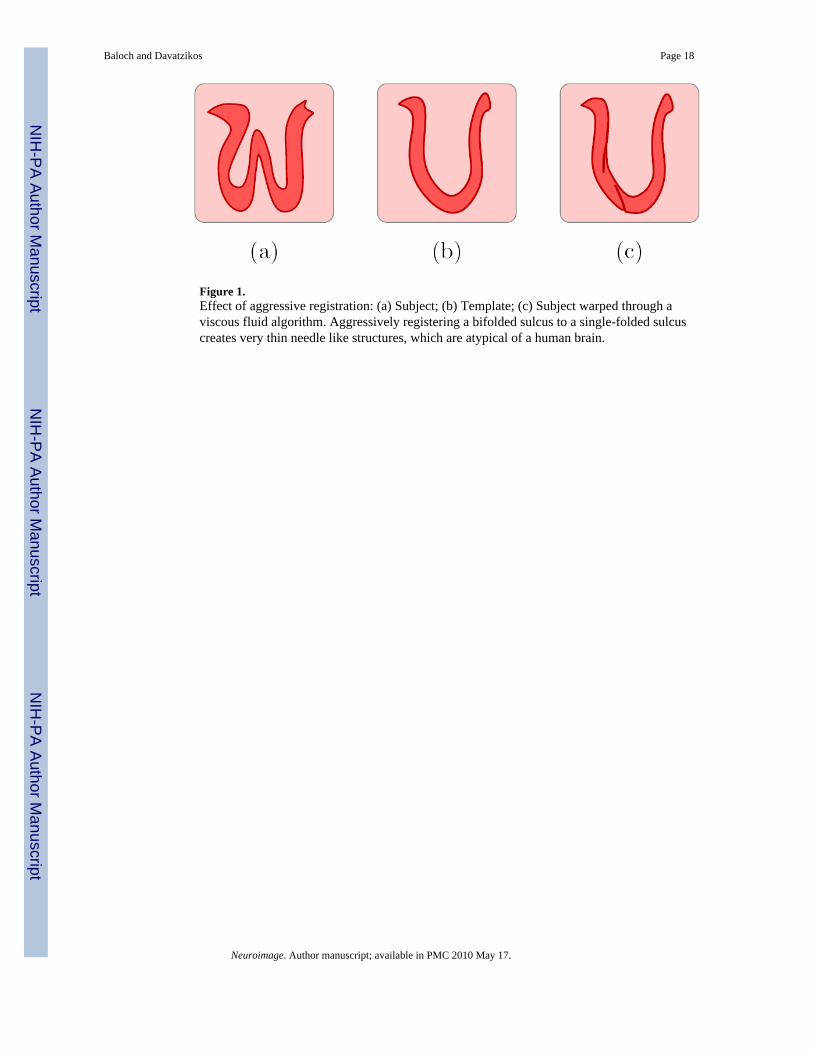
Figure 1.Effect of aggressive registration: (a) Subject; (b) Template; (c) Subject warped through aviscous fluid algorithm. Aggressively registering a bifolded sulcus to a single-folded sulcuscreates very thin needle like structures, which are atypical of a human brain.

Baloch and Davatzikos Page 18

Neuroimage. Author manuscript; available in PMC 2010 May 17.

NIH

-PA Author Manuscript

NIH

-PA Author Manuscript

NIH

-PA Author Manuscript

Figure 2.(a) Template; (b) Mean of 31 spatially normalized brains; (c) A representative subject; (d)Spatial normalization of (b) using HAMMER; (e) Corresponding residual. While crispness ofthe mean brain indicates reasonably good anatomical correspondence, there are still significantanatomical differences, which may be large enough to offset disease specific atrophy in a brain.

Baloch and Davatzikos Page 19

Neuroimage. Author manuscript; available in PMC 2010 May 17.

NIH

-PA Author Manuscript

NIH

-PA Author Manuscript

NIH

-PA Author Manuscript

Figure 3.Manifold structure and intersubject comparisons based on Euclidean distance.

Baloch and Davatzikos Page 20

Neuroimage. Author manuscript; available in PMC 2010 May 17.

NIH

-PA Author Manuscript

NIH

-PA Author Manuscript

NIH

-PA Author Manuscript

Figure 4.OMS versus CMD: (a) Randomly selecting CMDs (random parameter selection) reduces inter-group separation. Dots marked with arrows represent group means; (b) OMS results in optimalseparation between the two groups.

Baloch and Davatzikos Page 21

Neuroimage. Author manuscript; available in PMC 2010 May 17.

NIH

-PA Author Manuscript

NIH

-PA Author Manuscript

NIH

-PA Author Manuscript

Figure 5.Approximation of AEC manifolds with hyperplanes. τ and λ may be two of the confoundingfactors invariance to which is sought, as explained later in Section 2.5.

Baloch and Davatzikos Page 22

Neuroimage. Author manuscript; available in PMC 2010 May 17.

NIH

-PA Author Manuscript

NIH

-PA Author Manuscript

NIH

-PA Author Manuscript

Figure 6.Constructing AECs: Each subjects is normalized to ΩT via intermediate templates at differentsmoothness levels of the warping transformations.

Baloch and Davatzikos Page 23

Neuroimage. Author manuscript; available in PMC 2010 May 17.

NIH

-PA Author Manuscript

NIH

-PA Author Manuscript

NIH

-PA Author Manuscript

Figure 7.Intermediate templates aid registration: (a) Template of Fig 2(a); (b) Direct warping of Fig. 2(c); (c) Warping via an intermediate template.

Baloch and Davatzikos Page 24

Neuroimage. Author manuscript; available in PMC 2010 May 17.

NIH

-PA Author Manuscript

NIH

-PA Author Manuscript

NIH

-PA Author Manuscript

Figure 8.Schematic illustration of tissue density maps (TDMs). Left column shows subjects of varyingsizes, which are warped to the template given in middle column. When expansion takes placeduring warping of an individual shape to the template, the tissue density values are smaller(darker intensity), while in contraction the tissue density increases (brighter).

Baloch and Davatzikos Page 25

Neuroimage. Author manuscript; available in PMC 2010 May 17.

NIH

-PA Author Manuscript

NIH

-PA Author Manuscript

NIH

-PA Author Manuscript

Figure 9.2D synthetic dataset – Templates T1,…,T12 simulating gray matter folds.

Baloch and Davatzikos Page 26

Neuroimage. Author manuscript; available in PMC 2010 May 17.

NIH

-PA Author Manuscript

NIH

-PA Author Manuscript

NIH

-PA Author Manuscript

Figure 10.2D synthetic dataset – Dependence of residual on regularization λ: : See how registrationdeteriorates by changing the λ. (a) Subject; (b) Template; (c) Subject warped with the mostaggressive transformation (small λ); (d) Subject warped with intermediate level aggression(intermediate λ); (e) Subject warped with very mild transformation (small λ).

Baloch and Davatzikos Page 27

Neuroimage. Author manuscript; available in PMC 2010 May 17.

NIH

-PA Author Manuscript

NIH

-PA Author Manuscript

NIH

-PA Author Manuscript

Figure 11.2D synthetic dataset – Dependence of residual on template T: See how registration deterioratesby changing the template. (a) Subject; (b) Template T12; (c) Subject warped to T12; (d) TemplateT1; (e) Subject warped to T1.

Baloch and Davatzikos Page 28

Neuroimage. Author manuscript; available in PMC 2010 May 17.

NIH

-PA Author Manuscript

NIH

-PA Author Manuscript

NIH

-PA Author Manuscript

Figure 12.2D synthetic dataset – The effect of regularization parameter λ and smoothing σ on theperformance of morphological descriptors without optimization, as depicted by minimum p-value plots based on the t-test for capturing significant group differences: (a) min log10 p forLJD; (b) min log10 p for Residual. For LJD, best performance is achieved for low regularization(λ = 3), whereas residual performs the best with intermediate regularization (λ = 27). Eithercases correspond to large smoothing (σ = 13).

Baloch and Davatzikos Page 29

Neuroimage. Author manuscript; available in PMC 2010 May 17.

NIH

-PA Author Manuscript

NIH

-PA Author Manuscript

NIH

-PA Author Manuscript

Figure 13.2D synthetic dataset – OMS versus CMDs for capturing significant group differences basedon Hotelling’s T2-tests: (a) Minimum p values; (b) Mean of p-values after thresholding themto 10−2. Optimization yields better performance with about an order of magnitude improvementin the p-values.

Baloch and Davatzikos Page 30

Neuroimage. Author manuscript; available in PMC 2010 May 17.

NIH

-PA Author Manuscript

NIH

-PA Author Manuscript

NIH

-PA Author Manuscript

Figure 14.2D synthetic dataset – T2-test based log10 p-value maps for 2D simulated data at σ = 13thresholded to p ≤ 10−2: (a) CMD λ = 23; (b) OMS.

Baloch and Davatzikos Page 31

Neuroimage. Author manuscript; available in PMC 2010 May 17.

NIH

-PA Author Manuscript

NIH

-PA Author Manuscript

NIH

-PA Author Manuscript

Figure 15.2D synthetic dataset – Hotelling’s T2 test on CMD and OMS corresponding to the best case ofFig. 13, i.e., σ = 13, and λ = 23. Note that p-value maps are thresholded to p ≤ 10−4. Resultsare shown on a log10-scale: (a) CMD with T1; (b) CMD with T2; (c) CMD with T3; (d) OMSwith T1; (e) OMS with T2; (f) OMS with T3.

Baloch and Davatzikos Page 32

Neuroimage. Author manuscript; available in PMC 2010 May 17.

NIH

-PA Author Manuscript

NIH

-PA Author Manuscript

NIH

-PA Author Manuscript

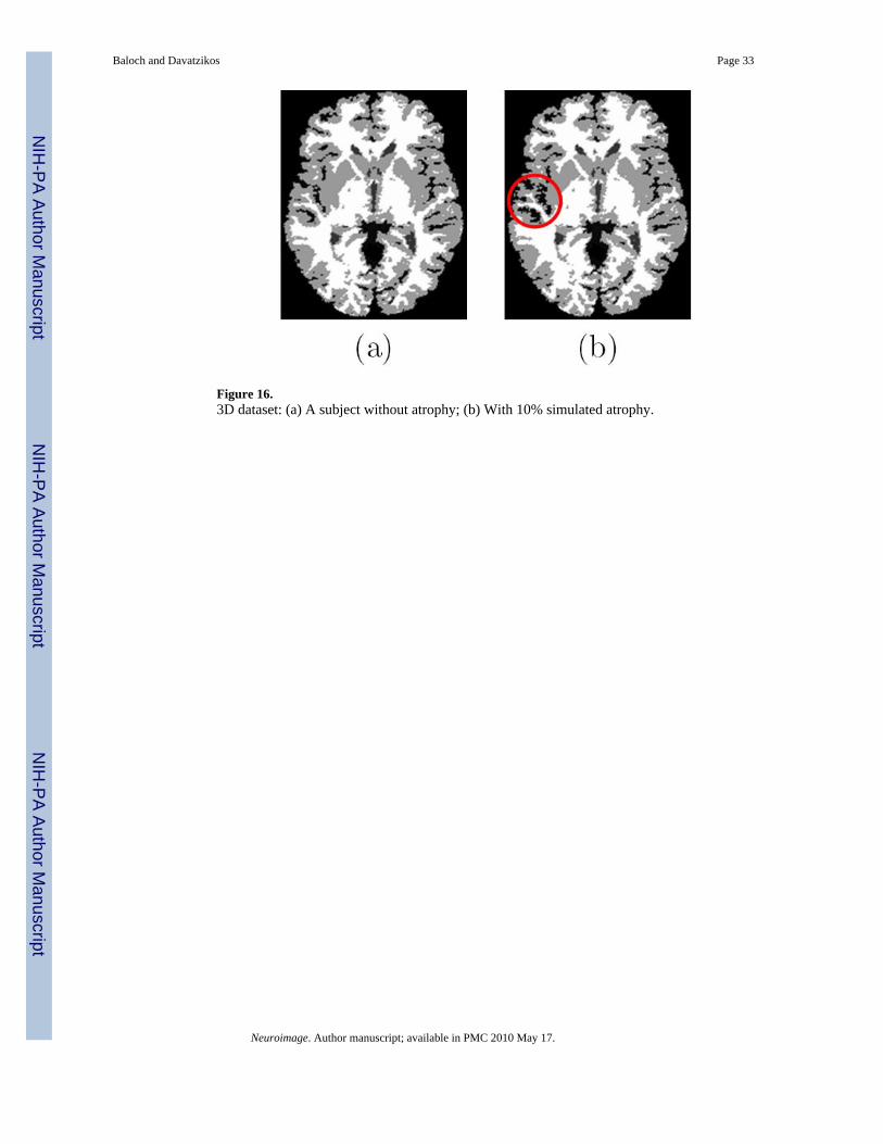
Figure 16.3D dataset: (a) A subject without atrophy; (b) With 10% simulated atrophy.

Baloch and Davatzikos Page 33

Neuroimage. Author manuscript; available in PMC 2010 May 17.

NIH

-PA Author Manuscript

NIH

-PA Author Manuscript

NIH

-PA Author Manuscript

Figure 17.3D dataset – The effect of regularization parameter λ and smoothing σ on the performance ofmorphological descriptors without optimization, as depicted by minimum p-value plots basedon the t-test for capturing significant group differences: (a) log Jhλ,τ; (b) Rhλ,τ. For log Jhλ,τ,best performance is achieved for low regularization (λ = 0), whereas Rhλ,τ performs the bestfor high regularization (λ = 7).

Baloch and Davatzikos Page 34

Neuroimage. Author manuscript; available in PMC 2010 May 17.

NIH

-PA Author Manuscript

NIH

-PA Author Manuscript

NIH

-PA Author Manuscript

Figure 18.3D dataset – Hotelling’s T2-test based minimum p-value plots for CMDs and OMS. Theperformance of CMDs is highly dependent on λ. Optimization, on the other hand, removes thisdependency as evident from the largely stable curve for OMS, which is also less sensitive toσ.

Baloch and Davatzikos Page 35

Neuroimage. Author manuscript; available in PMC 2010 May 17.

NIH

-PA Author Manuscript

NIH

-PA Author Manuscript

NIH

-PA Author Manuscript

Figure 19.Atrophy maps as captured by CMD and OMS for the 3D dataset – T2 test based p-value mapscorresponding to the best results for each descriptor thresholded to p ≤ 10−5: (a) CMD λ = 7,σ = 4; (b) OMS with σ = 5.

Baloch and Davatzikos Page 36

Neuroimage. Author manuscript; available in PMC 2010 May 17.

NIH

-PA Author Manuscript

NIH

-PA Author Manuscript

NIH

-PA Author Manuscript

Figure 20.Longitudinal dataset – Comparison between most conforming CMD (traditional approach) andOMS in terms of mean GM TDM in the ROI in the presence of atrophy: (a) Posterior Cingulate;(b) Hippocampus; (c) Superior temporal gyrus. Dotted lines represent the corresponding linearregression fits.

Baloch and Davatzikos Page 37

Neuroimage. Author manuscript; available in PMC 2010 May 17.

NIH

-PA Author Manuscript

NIH

-PA Author Manuscript

NIH

-PA Author Manuscript

Figure 21.Longitudinal dataset – Comparison between CMD and OMS in terms of mean TDM in theROI when no atrophy is present. Note that random fluctuations in traditional approach maycontribute to incorrect estimation of the temporal profile. Dotted lines represent thecorresponding linear regression fits.

Baloch and Davatzikos Page 38

Neuroimage. Author manuscript; available in PMC 2010 May 17.

NIH

-PA Author Manuscript

NIH

-PA Author Manuscript

NIH

-PA Author Manuscript

Figure 22.Longitudinal dataset – Comparison between CMD (traditional approach) and OMS in termsof rate of atrophy: (a) CMD based regression map for TDM; (b) OMS based regression mapfor TDM. Note how OMS was able to eliminate growth falsely picked up by the traditionalanalysis, resulting in more accurate analysis.

Baloch and Davatzikos Page 39

Neuroimage. Author manuscript; available in PMC 2010 May 17.

NIH

-PA Author Manuscript

NIH

-PA Author Manuscript

NIH

-PA Author Manuscript

NIH

-PA Author Manuscript

NIH

-PA Author Manuscript

NIH

-PA Author Manuscript

Baloch and Davatzikos Page 40

Table 1

List of abbreviations introduced in the paper

DBM Deformation based Morphometry

TBM Tensor based Morphometry

VBM Voxel based Morphometry

AEC Anatomical Equivalence Class

CMD Complete Morphological Descriptor

OMS Optimal Morphological signature

LJD Log Jacobian Determinant

TDM Tissue Density Map

Neuroimage. Author manuscript; available in PMC 2010 May 17.