Resource-Constrained Multi-Project Scheduling: Priority Rule Performance Revisited

Tyson R. Browning* Ali A. Yassine Neeley School of Business Texas Christian University

TCU Box 298530 Fort Worth, TX 76129

t.browning@tcu.edu

Department of Industrial & Enterprise Systems Engineering (IESE)

University of Illinois at Urbana-Champaign Urbana, IL 61801 yassine@uiuc.edu

This Version: March 15, 2010

Final Version Later Published as: Browning, Tyson R. and Ali A. Yassine (2010) "Resource-Constrained Multi-Project Scheduling: Priority Rule Performance Revisited," International Journal of

Production Economics, 126(2): 212-228.

*Corresponding author The authors are grateful to two anonymous reviewers and Sönke Hartmann for helpful comments on the paper, Ibrahim Kurtulus for discussions on multi-project scheduling, and Terry Dielman for additional statistical expertise. Any errors in this paper are our own. The first author is grateful for support from the Neeley Summer Research Award Program from the Neeley School of Business at Texas Christian University.

Resource-Constrained Multi-Project Scheduling: Priority Rule Performance Revisited

Abstract

Managers of multiple projects with overly constrained resources face difficult decisions in how to allocate

resources to minimize the average delay per project or the time to complete the whole set of projects. We

address the static resource-constrained multi-project scheduling problem (RCMPSP) with two lateness

objectives, project lateness and portfolio lateness. In this context, past research has reported conflicting results

on the performance of activity priority rule heuristics and does not provide managers with clear guidance on

which rule to use in various situations. Using recently improved measures for RCMPSP characteristics, we

conducted a comprehensive analysis of 20 priority rules on 12,320 test problems generated to the specifications

of project-, activity-, and resource-related characteristics—including network complexity and resource

distribution and contention. We found several situations in which widely-advocated priority rules perform

poorly. We also confirmed that portfolio managers and project managers will prefer different priority rules

depending on their local or global objectives. We summarize our results in two decision tables, the practical use

of which requires managers to do only a rough, qualitative characterization of their projects in terms of

complexity, degree of resource contention, and resource distribution.

Keywords: Project Management; Multi-Project Scheduling; Resource Constraints; Priority Rules

1

1. Introduction

As projects have become ever-more-common structures for organizing work in contemporary enterprises,

issues involving the simultaneous management of multiple projects (or a portfolio of projects) have become

more pervasive and acute. For example, studies have shown that managers typically deal with up to four projects

at once (Liberatore and Pollack-Johnson 2003; Maroto et al. 1999). In this paper, we address the case of a

portfolio of concurrent projects with identical start times. Each project consists of an activity network that draws

from common pools of multiple types of resources which are typically not large enough for all of the activities

to work concurrently. The goal is to prioritize activities so as to optimize an objective function such as

minimizing the delay to each project or the overall portfolio. Such is the basic resource-constrained multi-

project scheduling problem (RCMPSP). According to Payne (1995), up to 90% of the value of all projects

accrues in a multi-project context, so the impact of even a small improvement in their management could

provide an enormous benefit.

Most research on resource-constrained project scheduling has dealt with single projects—the resource-

constrained project scheduling problem (RCPSP). When dealing with multiple projects, two approaches have

been used: (1) a single-project approach, using dummy activities and precedence arcs to combine the projects

into a single mega-project, thereby reducing the RCMPSP to a RCPSP with a single critical path, or (2) a multi-

project (MP) approach, maintaining the RCMPSP and a separate critical path per project (Kurtulus and Davis

1982). In this paper, we take the second approach, because (1) it is more realistic, (2) it has received less

attention in past research, (3) it presents a greater opportunity for improvement (Herroelen 2005), and, critically,

(4) the existing decision guidance for managers is inconclusive.

Both the RCPSP and the RCMPSP are strongly NP-hard, meaning there are no known algorithms for find-

ing optimal solutions in polynomial time (Lenstra and Kan 1978). Hence, most research has sought efficient

heuristics and meta-heuristics. Priority rule (PR) heuristics are crucial for several reasons: (1) meta-heuristics’

improved performance comes at greater computational expense, meaning that PRs are necessary for very large

problems (Kolisch 1996a); (2) PRs are a component of other (local search-based and sampling) heuristics

(Kolisch 1996b) and “are indispensible” for constructing initial solutions for meta-heuristics (Hartmann and

Kolisch 2000); and (3) PRs are used extensively by commercial project scheduling software due to their speed

and simplicity (Herroelen 2005). However, perhaps the most important argument for PRs is that they are very

important in practice. For a variety of reasons, most project managers do not (or cannot) actually build the

2

formal activity network models which are prerequisites to the application of meta-heuristics. That is, it does not

matter how large an activity network that a modern computer can process optimally or with meta-heuristics if a

project cannot or does not invest in the effort to construct such a network! When faced with a resource

allocation decision, project managers will often make a quick call based on intuition or simple rules of thumb.

Therefore, the question of which PR to use is discussed in many contemporary project management textbooks

(e.g., Meredith and Mantel 2009), but without conclusive guidance for project managers. This is because few

comprehensive, systematic studies have been reported in the literature (Herroelen 2005), and these few studies

have dealt with relatively small subsets of the common PRs. Moreover, these studies have presented conflicting

results on PR performance, because this varies based on portfolio, project, resource, and activity characteristics.

Thus, a more comprehensive study of a larger set of PRs and RCMPSP characteristics—that will give

managerial decision makers firmer guidance—is of great value and much needed.

In this paper, we address the static RCMPSP with two lateness objectives. Based on the salient

characteristics of the RCMPSP in terms of its constituent projects, activities, and resources, we use five recent

measures of RCMPSP characteristics to define a multi-dimensional problem space. Then, using a full factorial

experiment with 12,320 randomly generated problem instances, we demonstrate the superiority of the new

measures and analyze the performance of 20 PRs. We find significant differences in the performance of the

PRs—implying that the choice of PR does indeed matter—and that several widely-advocated PRs generally do

not perform well. Finally, we organize these results for managers, distinguishing the project and portfolio

management perspectives.

The rest of the paper is organized as follows. After stating the mathematical formulation of the basic

RCMPSP (Section 2) and reviewing related literature (§3), in §4 we discuss characteristics of the RCMPSP,

including objective functions, network characteristics, and resource characteristics. §5 presents our study, and

§6 distills its implications for managers. §7 concludes the paper.

2. Basic Problem Statement

The static RCMPSP can be stated as follows. A set of l = 2,…, L projects are to be performed. Each project

consists of i = 1,…,Nl activities with deterministic, non-preemptable duration dil. The activities are interrelated

by predecessor and resource constraints. Predecessor constraints keep activity i from starting until all of its

predecessors have finished. Each activity requires rik units of resource type k ∈ K during every period of its

3

duration. Resource k has a renewable capacity of Rk. At any time, if the set of eligible (precedence

unconstrained) activities requires more than Rk for any k, then some activities will be delayed. The RCMPSP

entails finding a schedule for the activities (i.e., determining the start or finish times) that optimizes a

performance measure, such as minimizing the average delay in all projects. Each project is associated with a due

date, set by its resource-unconstrained duration, which is used to measure delays. Let Fil represent the finish

time of activity i in project l, such that a schedule can be represented by a vector of finish times (F1l, ..., Fil, ...,

lNlF ). Let At be the set of activities in work at time instant t. Pil is the set of all immediate predecessors of

activity i in project l. i∈ Pil. With these definitions, the problem can be formally stated as:

Optimize: Performance Measure (∀i ∈ Nl, l ∈ L: F1l, ..., Fil, ..., lNlF ) (1)

Subject to: ∀i ∈ Nl, i∈ Pil, l ∈ L: liF ≤ Fil – dil (2)

∀i, l ∈ At: ∑∈

≤)(, tAli

kilk Rr k ∈ K; t ≥ 0 (3)

∀i ∈ Nl, l ∈ L: Fil ≥ 0 (4)

The objective function (1) seeks to optimize a pre-specified performance measure. Constraints (2) impose the

precedence relations between activities; constraints (3) limit the resource demand imposed by the activities

being processed at time t to the capacity available; and constraints (4) force the finish times to be non-negative.

The basic (static) problem can be expanded in several ways. New projects might arrive at various rates (the

dynamic problem).1 Project interdependencies (beyond common resources) might exist. Activities could be

performed in various modes, each requiring different types and/or amount of resources (e.g., Tseng 2004).

Activity preemption might be allowed, perhaps implying switching or restart costs (e.g., Ash 2002). Activity

durations could be stochastic. Resource transfer times could be non-zero (Krüger and Scholl 2008; Krüger and

Scholl 2009), and resources might be non-renewable. To maximize our insights from the basic RCMPSP, we do

not address these additional features in this paper, although our approach could be extended to do so.

3. Literature Review

This paper addresses the static RCMPSP and maintains the distinction between projects (the MP approach

mentioned in §1). While an abundant amount of literature addresses the (single-project) RCPSP (several reviews

are available: e.g., Brucker et al. 1999; Hartmann and Briskorn 2009; Herroelen 2005; Kolisch and Hartmann

1 In a static RCMPSP environment (e.g., Lawrence and Morton 1993; Lova and Tormos 2001; Pritsker et al. 1969), all projects within the portfolio and their associated activities are known prior to scheduling, unlike in the dynamic case (e.g., Bock and Patterson 1990; Dumond and Mabert 1988; Kim and Leachman 1993; Yang and Sum 1993; Yang and Sum 1997).

4

2005), the single-project approach to solving RCMPSPs has several drawbacks (Chiu and Tsai 1993). First, it is

less realistic, as it implicitly assumes equal delay penalties for all projects (Kurtulus 1985). Second, independent

project analysis becomes difficult when all projects are bound together—e.g., it is hard to reveal the degree of

concurrency among different projects and to maintain the distinction in their critical paths. In many realistic

situations, each project has its own manager who is interested in the individual project’s performance

characteristics. Third, aggregating multiple projects yields very large problems.

Using the MP approach, two general approaches are exact methods and heuristic procedures. Exact

methods (e.g., Chen 1994; Deckro et al. 1991; Pritsker et al. 1969; Vercellis 1994) are limited to solving small

problem instances and impractical for solving large RCMPSPs (Herroelen 2005; Özdamar and Ulusoy 1995).

On the other hand, heuristic procedures can be divided into four groups: PR-based X-pass heuristics, classical

meta-heuristics, non-standard meta-heuristics, and miscellaneous heuristics (Kolisch and Hartmann 1999;

Kolisch and Hartmann 2005). Classical meta-heuristics include simulated annealing (e.g., Bouleimen and

Lecocq 2000), genetic algorithms (GAs) (e.g., Gonçalves et al. 2008; Kim et al. 2005; Kumanan et al. 2006),

and swarm optimization (e.g., Linyi and Yan 2007). Non-standard meta-heuristics include agent-based and non-

GA population-based approaches (e.g., Confessore et al. 2007; Homberger 2007). Miscellaneous heuristics

include forward-backward improvement and others (e.g., Lova and Tormos 2002).

PR-based heuristics, also known as X-pass methods, include single- and multi-pass methods (Hartmann and

Kolisch 2000). Single-pass PRs prioritize the activity that optimizes a particular value. Multi-pass methods

include multi-priority rules, which employ more than one PR in succession (e.g., Lova and Tormos 2001), and

sampling methods, which generally make use of a single PR along with some degree of randomness (Hartmann

and Kolisch 2000).

PRs can also be classified by the information they use: (a) activity-related, (b) project-related, or (c)

resource-related (Kolisch 1996a).2 Activity-related PRs assign high priority to an activity based on a parameter

or characteristic of the activity itself, such as its duration (e.g., shortest operation first—SOF) or slack (e.g.,

minimum slack first—MINSLK). Project-related PRs promote activities based on the project they belong to or

characteristics of that project (e.g., shortest activity from shortest project first—SASP). Resource-related PRs

assign priority in terms of an activity and/or project’s resource demands, scarcity of resources used, or some

2 These classes are neither exclusive nor exhaustive, and this taxonomy is one of many possible. For instance, considering whether a PR returns the same value regardless of the stage it is performed in, we may characterize it as static, compared to a dynamic PR that changes value depending on the stage (Kolisch 1996a).

5

combination. High priorities are usually assigned to potential bottleneck activities. An example is the maximum

total work content (MAXTWK) PR. Some PRs combine elements of information about the activity, the project,

and/or the resources (Hartmann and Kolisch 2000). For each PR addressed in our study, we note its “Basis”

according to this classification in Tables 1 and 5.

Davis and Patterson (1975) noted that successful PRs generally incorporate some measure of time or

resource usage, and they also isolated three important characteristics in the RCPSP: an activity’s resource

utilization, the ratio of average slack per activity to the critical path length, and project complexity. Interestingly,

project size (number of activities) has not been found to be a significant determinant of PR performance (e.g.,

Pascoe 1966). Ulusoy and Özdamar (1989) suggested the following measures for distinguishing successful PRs:

percentage of critical activities, network complexity and resource measures, obstruction value, and utilization

factor.

While many studies have been conducted on the performance of a myriad of PRs for the RCPSP, only a

relative handful of rules have been developed for and studied in a MP environment (Herroelen 2005). It is

important to note that the single- and MP approaches often produce different schedules with the same PR

(Kurtulus 1978; Lova and Tormos 2001), especially if the rule depends on the critical path—e.g., the MINSLK

rule. While the single-project approach is more efficient for minimizing a single project’s duration, PRs based

on the MP approach perform better when minimizing the average delay in several projects (Kurtulus and Davis

1982). RCMPSP studies have disagreed about which PR performs best and under which conditions, although

MINSLK has generally performed well (Cohen et al. 2004; Davis and Patterson 1975; Fendley 1968). Kurtulus

and Davis (1982) developed six PRs for the MP environment, and along with three single-project PRs (see the

list in Table 1), analyzed these with the objective of minimizing total project delay, finding that SASP was best

under most conditions. Kurtulus (1985) and Kurtulus and Narula (1985) provided further results. In summary,

while various studies have identified potentially important characteristics of the RCMPSP and proposed various

PRs, the variety of results and their disagreements have left project managers lacking clear guidance on which

PR to use in a particular situation.

4. RCMPSP Characteristics and Measures

Four important characteristics of the RCMPSP—objective function, network complexity, resource

distribution, and resource contention—have been identified that distinguish problem and project situations. Each

6

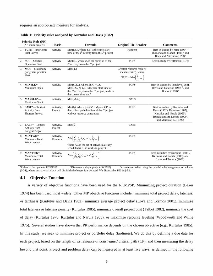
requires an appropriate measure for analysis. Table 1: Priority rules analyzed by Kurtulus and Davis (1982)

Priority Rule (PR) (* = multi-project) Basis Formula Original Tie-Breaker Comments

1. FCFS—First Come First Served

Activity Min(ESil), where ESil is the early start time of the ith activity from the lth project

Random Best in studies by Mize (1964) Dumond and Mabert (1988)a and

Bock and Patterson (1990)a

2. SOF—Shortest Operation First

Activity Min(dil), where dil is the duration of the ith activity from the lth project

FCFS Best in study by Patterson (1973)

3. MOF—Maximum (longest) Operation First

Activity Max(dil) Greatest resource require-ments (GRES), where

= ∑

=

K

kilkrGRES

1Max

4. MINSLK*—Minimum Slack

Activity Min(SLKil), where SLKil = LSil – Max(ESil, t), LSil is the late start time of the ith activity from the lth project, and t is the current time stepc

FCFS Best in studies by Fendley (1968), Davis and Patterson (1975)b, and

Boctor (1990)b

5. MAXSLK*—Maximum Slack

Activity Max(SLKil) GRES

6. SASP*—Shortest Activity from Shortest Project

Activity, Project

Min(fil), where fil = CPl + dil and CPl is the critical path duration of the lth project without resource constraints

FCFS Best in studies by Kurtulus and Davis (1982), Kurtulus (1985),

Kurtulus and Narula (1985), Tsubakitani and Deckro (1990),

and Maroto et al. (1999)

7. LALP*—Longest Activity from Longest Project

Activity, Project

Max(fil) GRES

8. MINTWK*—Minimum Total Work content

Activity, Resource ,Min

11

+ ∑∑ ∑

== ∈

K

kilk

K

kil

ASiilkil rdrd

l

where ASl is the set of activities already scheduled (i.e., in work) in project l

FCFS

9. MAXTWK*—Maximum Total Work content

Activity, Resource

+ ∑∑ ∑

== ∈

K

kilk

K

kil

ASiilkil rdrd

l 11Max FCFS Best in studies by Kurtulus (1985),

Kurtulus and Narula (1985), and Lova and Tormos (2001)

aRefers to the dynamic RCMPSP bDiscusses a single project (RCPSP) ct is relevant when using the parallel schedule generation scheme (SGS), where an activity’s slack will diminish the longer it is delayed. We discuss the SGS in §5.1.

4.1 Objective Function

A variety of objective functions have been used for the RCMPSP. Minimizing project duration (Baker

1974) has been used most widely. Other MP objective functions include: minimize total project delay, lateness,

or tardiness (Kurtulus and Davis 1982), minimize average project delay (Lova and Tormos 2001), minimize

total lateness or lateness penalty (Kurtulus 1985), minimize overall project cost (Talbot 1982), minimize the cost

of delay (Kurtulus 1978; Kurtulus and Narula 1985), or maximize resource leveling (Woodworth and Willie

1975). Several studies have shown that PR performance depends on the chosen objective (e.g., Kurtulus 1985).

In this study, we seek to minimize project or portfolio delay (tardiness). We do this by defining a due date for

each project, based on the length of its resource-unconstrained critical path (CP), and then measuring the delay

beyond that point. Project and problem delay can be measured in at least five ways, as defined in the following

7

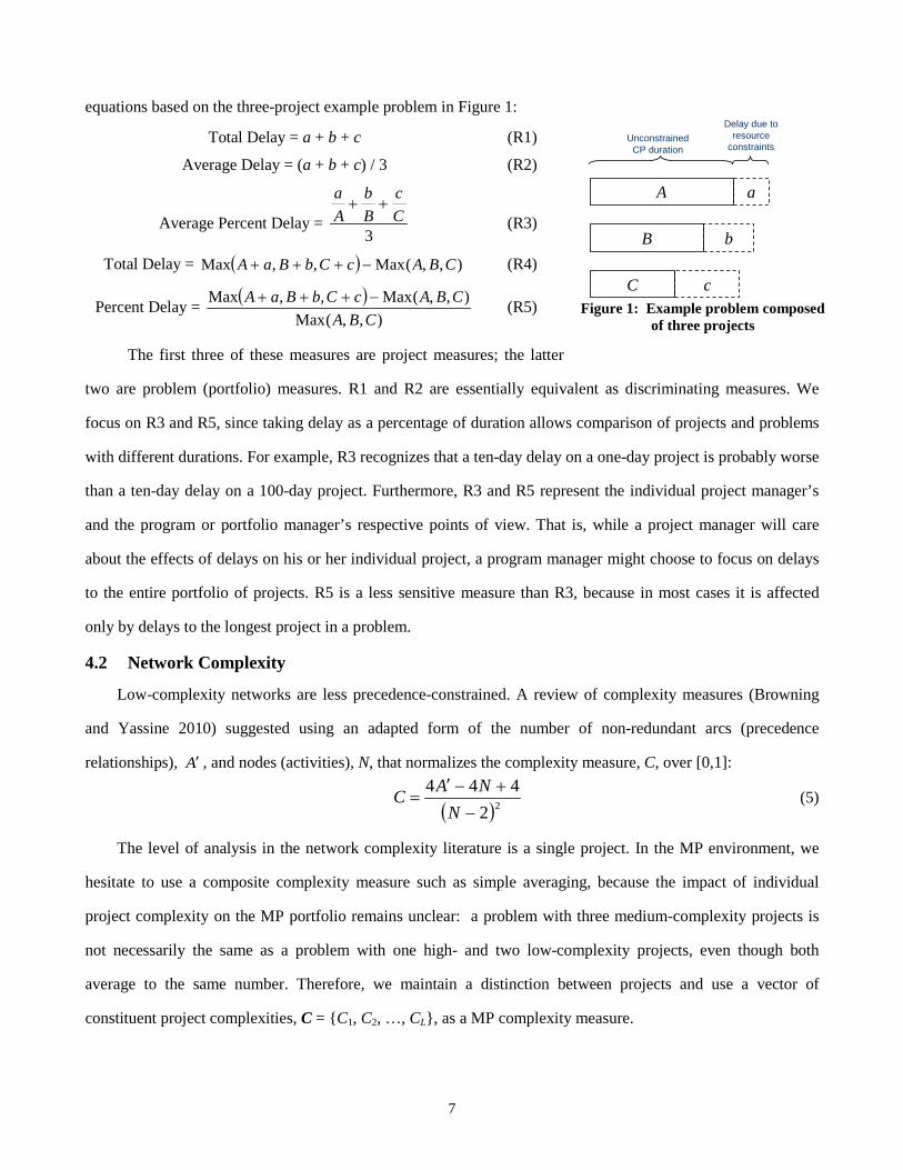
equations based on the three-project example problem in Figure 1:

Total Delay = a + b + c (R1)

Average Delay = (a + b + c) / 3 (R2)

Average Percent Delay = 3

Cc

Bb

Aa

++ (R3)

Total Delay = ( ) ),,(Max,,Max CBAcCbBaA −+++ (R4)

Percent Delay = ( )),,(Max

),,(Max,,MaxCBA

CBAcCbBaA −+++ (R5)

The first three of these measures are project measures; the latter

two are problem (portfolio) measures. R1 and R2 are essentially equivalent as discriminating measures. We

focus on R3 and R5, since taking delay as a percentage of duration allows comparison of projects and problems

with different durations. For example, R3 recognizes that a ten-day delay on a one-day project is probably worse

than a ten-day delay on a 100-day project. Furthermore, R3 and R5 represent the individual project manager’s

and the program or portfolio manager’s respective points of view. That is, while a project manager will care

about the effects of delays on his or her individual project, a program manager might choose to focus on delays

to the entire portfolio of projects. R5 is a less sensitive measure than R3, because in most cases it is affected

only by delays to the longest project in a problem.

4.2 Network Complexity

Low-complexity networks are less precedence-constrained. A review of complexity measures (Browning

and Yassine 2010) suggested using an adapted form of the number of non-redundant arcs (precedence

relationships), A′ , and nodes (activities), N, that normalizes the complexity measure, C, over [0,1]:

( )22

444−

+−′=

NNAC (5)

The level of analysis in the network complexity literature is a single project. In the MP environment, we

hesitate to use a composite complexity measure such as simple averaging, because the impact of individual

project complexity on the MP portfolio remains unclear: a problem with three medium-complexity projects is

not necessarily the same as a problem with one high- and two low-complexity projects, even though both

average to the same number. Therefore, we maintain a distinction between projects and use a vector of

constituent project complexities, C = {C1, C2, …, CL}, as a MP complexity measure.

A

B

C

a

b

c

Unconstrained CP duration

Delay due to resource

constraints

Figure 1: Example problem composed of three projects

8

4.3 Resource Distribution

Several measures of the availability and distribution of project resources have been developed for the

RCPSP. Two early ones are the resource factor, RF, which indicates the average number of resources used by an

activity (Cooper 1976; Kolisch et al. 1995; Pascoe 1966), and the resource strength, RS, which expresses the

relationship between resource requirements and resource availability (Cooper 1976; Kolisch et al. 1995).

However, Kurtulus and Davis (1982) noted that these measures are not as useful in a MP environment and

proposed an alternative measure for the RCMPSP, the average resource loading factor, ARLF, which identifies

whether the bulk of a project’s total resource requirements are in the front or back half of its (resource

unconstrained) critical path (CP) duration3 and the relative size of the disparity. For project l, it is defined as:

∑∑∑= = =

=

l il lCP

t

K

k

N

i il

ilkiltilt

ll K

rXZ

CPARLF

1 1 1

1 (6)

where

>≤−

=2121

l

lilt CPt

CPtZ ,

=otherwise0

at time active is project of activity if1 tliX ilt , ZiltXilt ∈ {-1, 0, 1}, Nl is the

number of activities in project l, Kil is the number of types of resources required by an activity i in project l, and

rilk is the amount of resource type k required by task i in project l.4 Projects with ARLF < 0 are “front-loaded” in

their resource requirements, while projects with ARLF > 0 are “back-loaded.”

However, the ARLF measure has several problems. First, it can fall victim to the “flaw of averages” and

fail to distinguish significantly different cases. For example, Figure 2 illustrates some stylized resource

distributions and their ARLFs. In the first row, both distributions are front-loaded (relative to the mid-point of

the project’s critical path duration, indicated

by the dashed, vertical line) and have negative

ARLF. Despite their different shapes, they

could have the same ARLF value. Similarly,

both distributions in the second row might

have the same, positive ARLF value. More

problematically, both distributions in the

bottom row have ARLF ≈ 0.

Observation 1: Projects with ARLFl ≈ 0 can have dramatically different shapes. 3 Based on scheduling each activity at its early start time (the “all EST” schedule) 4 The original definition of Znlt in (K&D, 1982) and (Kurtulus 1978, p. 59) assumes activities are indexed from 0 to Nl – 1 and therefore puts the equal sign in the second case rather than the first—i.e., t ≥ CPl / 2. However, it seems more intuitive to index activities from 1 to Nl. For example, in a 10-day project, with days numbered 1-10, we assign activities on day 5 (10 / 2 = 5) to the first half of the project.

Project Resource Distributions

ARLF Start Mid-Point End Start Mid-Point End

Negative

Positive

Near-zero

Figure 2: Example resource distributions over project time

9

Second, despite its use in the MP context, ARLF pertains to a single project. Kurtulus and Davis (1982)

define the ARLF for a problem as the average of its constituent projects’ ARLFs:

∑=

=L

llARLF

LARLF

1

1 (7)

Again, averaging sacrifices important information. Consider the following two observations.

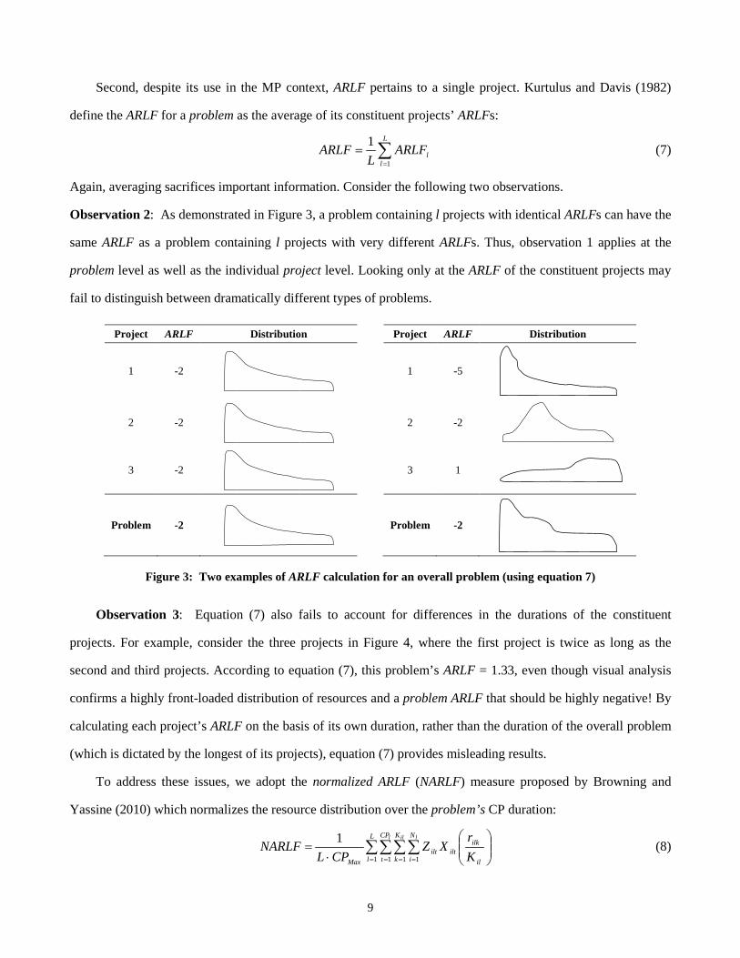
Observation 2: As demonstrated in Figure 3, a problem containing l projects with identical ARLFs can have the

same ARLF as a problem containing l projects with very different ARLFs. Thus, observation 1 applies at the

problem level as well as the individual project level. Looking only at the ARLF of the constituent projects may

fail to distinguish between dramatically different types of problems.

Project ARLF Distribution Project ARLF Distribution

1 -2

1 -5

2 -2

2 -2

3 -2

3 1

Problem -2

Problem -2

Figure 3: Two examples of ARLF calculation for an overall problem (using equation 7)

Observation 3: Equation (7) also fails to account for differences in the durations of the constituent

projects. For example, consider the three projects in Figure 4, where the first project is twice as long as the

second and third projects. According to equation (7), this problem’s ARLF = 1.33, even though visual analysis

confirms a highly front-loaded distribution of resources and a problem ARLF that should be highly negative! By

calculating each project’s ARLF on the basis of its own duration, rather than the duration of the overall problem

(which is dictated by the longest of its projects), equation (7) provides misleading results.

To address these issues, we adopt the normalized ARLF (NARLF) measure proposed by Browning and

Yassine (2010) which normalizes the resource distribution over the problem’s CP duration:

∑∑∑∑= = = =

⋅

=L

l

CP

t

K

k

N

i il

ilkiltilt

Max

l il l

Kr

XZCPL

NARLF1 1 1 1

1 (8)

10

where CPmax = Max(CP1, …, CPL).5 We also explored an additional measure proposed by Browning and

Yassine (2010), the variance of a problem’s constituent ARLFs from its NARLF:

( )∑=

−=L

llARLF NARLFARLF

L 1

22 1σ (9)

Project ARLF Distribution

1 -2

2 3

3 3

Problem 1.33

4.4 Resource Contention

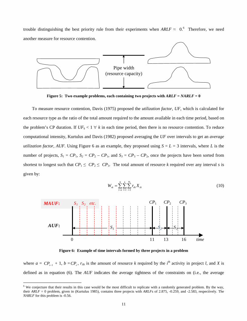
As a further complication with both ARLF and NARLF as effective measures of resource distribution, refer

to the last row in Figure 2, about which we make the following observation.

Observation 4: As |ARLF| and |NARLF| 0, they become less effective measures of the size of a resource

distribution. That is, since ARLF (NARLF) provides a relative comparison of the resource load in the front half

of a project (problem) with the resource load in the back half, this comparative value diminishes as the load

moves towards the mid-point of the project (problem).

This observation has important implications for the RCMPSP. Consider the four projects with ARLF =

NARLF = 0 in Figure 5. Using the metaphor of a pipe to represent the resource constraints, a problem containing

the two projects whose resource distributions are shown on the left (the upper one of which has been flipped

vertically to emphasize its complementarity with its lower counterpart) is much easier to fit through the pipe

without delaying some of its activities than a problem containing the two projects on the right. Neither ARLF

nor NARLF captures this important difference in these problems. Interestingly, Kurtulus and Davis (1982) had

5 Since ARLF and NARLF assume fungible resources, they are sensitive to disparities in the number of types, K. For example, in a three-project problem, if one of the projects uses four types of resources and the other two projects use only one of those types, then K = 4. If all three projects use four types of resources, then K = 4 also. For this reason, we use a constant K for all projects in our experiments.

Figure 4: Example ARLF calculation for a problem using equation (7)

11

trouble distinguishing the best priority rule from their experiments when ARLF ≈ 0.6 Therefore, we need

another measure for resource contention.

Figure 5: Two example problems, each containing two projects with ARLF = NARLF = 0

To measure resource contention, Davis (1975) proposed the utilization factor, UF, which is calculated for

each resource type as the ratio of the total amount required to the amount available in each time period, based on

the problem’s CP duration. If UFk < 1 ∀ k in each time period, then there is no resource contention. To reduce

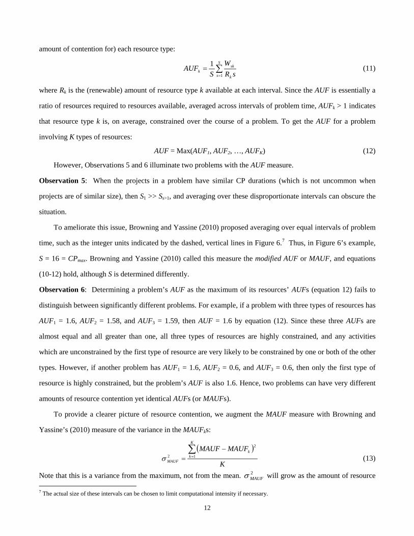
computational intensity, Kurtulus and Davis (1982) proposed averaging the UF over intervals to get an average

utilization factor, AUF. Using Figure 6 as an example, they proposed using S = L = 3 intervals, where L is the

number of projects, S1 = CP1, S2 = CP2 – CP1, and S3 = CP3 – CP2, once the projects have been sorted from

shortest to longest such that CP1 ≤ CP2 ≤ CP3. The total amount of resource k required over any interval s is

given by:

∑∑∑= = =

=b

at

L

l

N

iiltilksk

l

XrW1 1

(10)

Figure 6: Example of time intervals formed by three projects in a problem

where a = 1−sCP + 1, b = sCP , rilk is the amount of resource k required by the ith activity in project l, and X is

defined as in equation (6). The AUF indicates the average tightness of the constraints on (i.e., the average

6 We conjecture that their results in this case would be the most difficult to replicate with a randomly generated problem. By the way, their ARLF = 0 problem, given in (Kurtulus 1985), contains three projects with ARLFs of 2.875, -0.259, and -2.583, respectively. The NARLF for this problem is -0.56.

Pipe width(resource capacity)

time0

CP1 CP2 CP3

S1 S2 S3AUF:

11 13 16

MAUF: S1 S2 etc.

12

amount of contention for) each resource type:

∑=

=S

s k

skk sR

WS

AUF1

1 (11)

where Rk is the (renewable) amount of resource type k available at each interval. Since the AUF is essentially a

ratio of resources required to resources available, averaged across intervals of problem time, AUFk > 1 indicates

that resource type k is, on average, constrained over the course of a problem. To get the AUF for a problem

involving K types of resources:

AUF = Max(AUF1, AUF2, …, AUFK) (12)

However, Observations 5 and 6 illuminate two problems with the AUF measure.

Observation 5: When the projects in a problem have similar CP durations (which is not uncommon when

projects are of similar size), then S1 >> Ss>1, and averaging over these disproportionate intervals can obscure the

situation.

To ameliorate this issue, Browning and Yassine (2010) proposed averaging over equal intervals of problem

time, such as the integer units indicated by the dashed, vertical lines in Figure 6.7 Thus, in Figure 6’s example,

S = 16 = CPmax. Browning and Yassine (2010) called this measure the modified AUF or MAUF, and equations

(10-12) hold, although S is determined differently.

Observation 6: Determining a problem’s AUF as the maximum of its resources’ AUFs (equation 12) fails to

distinguish between significantly different problems. For example, if a problem with three types of resources has

AUF1 = 1.6, AUF2 = 1.58, and AUF3 = 1.59, then AUF = 1.6 by equation (12). Since these three AUFs are

almost equal and all greater than one, all three types of resources are highly constrained, and any activities

which are unconstrained by the first type of resource are very likely to be constrained by one or both of the other

types. However, if another problem has AUF1 = 1.6, AUF2 = 0.6, and AUF3 = 0.6, then only the first type of

resource is highly constrained, but the problem’s AUF is also 1.6. Hence, two problems can have very different

amounts of resource contention yet identical AUFs (or MAUFs).

To provide a clearer picture of resource contention, we augment the MAUF measure with Browning and

Yassine’s (2010) measure of the variance in the MAUFks:

( )

K

MAUFMAUFK

kk

MAUF

∑=

−= 1

2

2σ (13)

Note that this is a variance from the maximum, not from the mean. 2MAUFσ will grow as the amount of resource

7 The actual size of these intervals can be chosen to limit computational intensity if necessary.

13

contention in the non-max resource types deviates from the maximum. Therefore, all else being equal, higher 2MAUFσ should correlate with reduced problem delay.

5. Our Study 5.1 Scheduling Algorithm

All PR-based heuristics require a schedule generation scheme (SGS). Boctor (1990) distinguished between

“serial” and “parallel” schemes: in the serial SGS, each activity’s priority is calculated once at beginning of the

SGS algorithm, whereas in the parallel SGS an activity’s priority is dynamically re-determined (as necessary) at

each time step. We adopt the parallel SGS, which seems to have been most widely used in MP studies.

The parallel SGS proceeds as follows. First, the overall problem duration is broken down into time steps.

At each, the algorithm separates the activities into four disjoint sets: the completed set, C (finished activities),

the active set, A (ongoing, “already scheduled” activities), the decision set, D (un-started activities that depend

only on activities in C), and the ineligible set, I (activities with predecessors in A or D). Since preemption is not

allowed, the SGS automatically assigns resources to activities in A. If the remaining resources are sufficient to

perform the activities in D, then the algorithm adds these to A. If not, then it uses a PR to rank the activities in

D. The highest-ranking activities are added to A as resources allow. The time step ends when the first activity

(or activities) in A finishes. Finished activities are moved to C, and activities in I are checked for potential

transfer to D. The schedule is complete (i.e., the project durations are known) when all activities are in C.

5.2 Set-Up

We compiled a set of 20 popular PRs from the literature (Tables 1 and 4), some of which were developed

specifically for the RCMPSP and others which have been successful in a single-project environment. To

increase their comparability, we standardized the tie-breaker for all PRs to be FCFS.

We designed a full factorial experiment to test the influence of the factors listed in Table 3. To maximize

the insights from varying the last four factors, we held the first three constant.8 The choices for NARLF and

MAUF levels follow K&D (1982). We designated two levels of project complexity, “high” (C = 0.69) and “low”

(C = 0.14).9 We used these to form four variations in problem complexity: all high-complexity projects

(“HHH”), all low-complexity projects (“LLL”), and two intermediate combinations. Furthermore, we wanted

some problems where all of the individual resources’ MAUFs were equal (i.e., where 2,desMAUFσ = 0) and others

8 No specific relationship has been reported between portfolio size or project size and the solution quality obtained by the various PRs (Hartmann and Kolisch 2000; Kurtulus and Davis 1982; Lova and Tormos 2001). Meanwhile, since K is used to determine NARLF (equation (8)), its variation would be confounded with NARLF. 9 By equation (5), C = 0.69 implies 75 non-redundant arcs among 20 activities and C = 0.14 implies 30.

14

where one resource’s MAUF determined the overall problem’s MAUFdes while the other three types of resources

had a significantly different MAUF. Thus, we needed 7 × 11 × 4 × 2 = 616 test problems for this experiment.

Standard problem generators and test sets such as ProGen/PSPLIB (Kolisch et al. 1995) cannot create MP

problems to these specifications, so we used a test problem generator recently developed by Browning and

Yassine (2010). To enable the identification of random effects, we used 20 replications for each setting, thus

generating 12,320 problems (36,960 networks). We solved each problem with 20 PRs, thus producing 246,400

experimental outcomes. We specified each outcome in terms of the five objective functions in §4.1, thereby

yielding 1,232,000 data points. Table 2: Additional priority rules analyzed in this study

Priority Rule (PR) (* = multi-project) Basis Formula Comments

10. RAN—Random Activities selected randomly Best in study by Akpan (2000)a but used by others mainly as a

benchmark (e.g., Davis and Patterson 1975)a

11. EDDF—Earliest Due Date First

Activity Min(LSil)

12. LCFS—Last Come First Served

Activity Max(ESil)

13. MAXSP—Maximum Schedule Pressure

Activity ,

−

ilil

il

WdLFt

Max where Wil is the percentage of the activity remaining

to be done at time t

Also known as “critical ratio” (e.g., Chase et al. 2006)a

14. MINLFT—Minimum Late Finish time

Activity Min(LFil) Best in study by Mohanty and Siddiq (1989); equivalent to

MINSLK in serial scheduling case (Kolisch 1996a)a

15. MINWCS—Minimum Worst Case Slack

Activity, Resource

Min(LSi – Max[E(i,j) | (i,j) ∈ APt]), where E(i,j) is the earliest time to schedule activity j if activity i is started at time t, and APt is the set of all feasible pairs of eligible, un-started activities at time t

Best in study by (Kolisch 1996a)a; without resource

constraints, reduces to MINSLK

16. WACRU—Weighted Activity Criticality & Resource Utilization

Activity, Resource ( ) ( ) ,11

1 1 ,

−++∑ ∑

= =

−iN

q

K

k kMax

ikiq R

rwSLKwMax α where Ni is the number of

immediate successors of the ith activity, w is the weight associated with Ni (0 ≤ w ≤ 1), SLKiq is the slack in the qth immediate successor of the ith activity, and α is a weight parameter

Best in study by (Thomas and Salhi 1997)a

We use w = 0.5 and α = 0.5

17. TWK-LST*—MAXTWK & earliest Late Start time (2-phase rule)

Activity, Resource

Prioritize first by MAXTWK (without FCFS tie-breaker) and then by Min(LSil)

(Lova and Tormos 2001); min. late start time (MINLST) was best in study by (Davis and

Patterson 1975)a

18. TWK-EST*—MAXTWK & earliest Early Start time (2-phase rule)

Activity, Resource

Prioritize first by MAXTWK (without FCFS tie-breaker) and then by Min(ESil)

(Lova and Tormos 2001)

19. MS—Maximum Total Successors

Activity Max(TSil), where TSil is the total number of successors of the ith activity in the lth project

Best in study by (Kolisch 1996a)a

20. MCS—Maximum Critical Successors

Activity Max(CSil), where CSil is the number of critical successors of the ith activity in the lth project; CSil ∈ TSil

aDiscusses a single project (RCPSP)

15

Table 3: Experimental design Constant Factors Setting

Main Factors Levels

L 3 projects per problem NARLF 7 levels: -3, -2, -1, 0, 1, 2, 3

N 20 activities per project MAUF 11 levels: 0.6 - 1.6 in increments of 0.1 K 4 types of resources per activity C 4 levels: HHH, HHL, HLL, and LLL

2MAUFσ 2 levels: 0 (no variance) and 0.25 (“high” variance)a

aThe basis for selecting the “high” variance setting is explained in (Browning and Yassine 2010).

5.3 Superiority of the NARLF and MAUF Measures

We used an analysis of variance (ANOVA) to compare two linear models, the first with the five factors

NARLF, MAUF, C, 2MAUFσ , and PR, and the second with ARLF and AUF instead of NARLF and MAUF. The

results are shown in an online supplement. For objective R3, the respective R2 measures for the two models were

82% and 65%. For objective R5, the R2 measures were 92% and 65%. We take these results as a tentative

confirmation of the superiority of the NARLF and MAUF measures to ARLF and AUF, as supposed in §4. Also,

as the third ANOVA model in the supplement shows, the five original factors and their interactions has an R2 of

85% for R3 and 94% for R5. Thus, we also infer that the selected measures do a reasonable job of explaining

performance variances. We discuss the individual factors and interactions in the next sub-sections.

5.4 Results for R3: Average Percent (Project) Delay

Although we analyzed the results for all five objectives, we present the results for R3 and R5 (for the

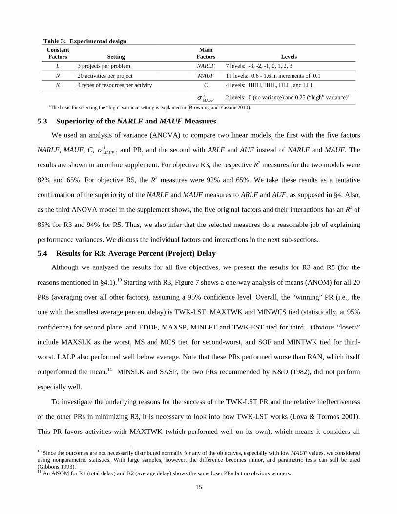
reasons mentioned in §4.1).10 Starting with R3, Figure 7 shows a one-way analysis of means (ANOM) for all 20

PRs (averaging over all other factors), assuming a 95% confidence level. Overall, the “winning” PR (i.e., the

one with the smallest average percent delay) is TWK-LST. MAXTWK and MINWCS tied (statistically, at 95%

confidence) for second place, and EDDF, MAXSP, MINLFT and TWK-EST tied for third. Obvious “losers”

include MAXSLK as the worst, MS and MCS tied for second-worst, and SOF and MINTWK tied for third-

worst. LALP also performed well below average. Note that these PRs performed worse than RAN, which itself

outperformed the mean.11 MINSLK and SASP, the two PRs recommended by K&D (1982), did not perform

especially well.

To investigate the underlying reasons for the success of the TWK-LST PR and the relative ineffectiveness

of the other PRs in minimizing R3, it is necessary to look into how TWK-LST works (Lova & Tormos 2001).

This PR favors activities with MAXTWK (which performed well on its own), which means it considers all

10 Since the outcomes are not necessarily distributed normally for any of the objectives, especially with low MAUF values, we considered using nonparametric statistics. With large samples, however, the difference becomes minor, and parametric tests can still be used (Gibbons 1993). 11 An ANOM for R1 (total delay) and R2 (average delay) shows the same loser PRs but no obvious winners.

16

(three) projects simultaneously. Meanwhile, the other less effective PRs favor either the shortest (or longest)

project, or focus on the number of successors within a single project. PRs that consider all three projects (such

as MAXTWK, MINWCS, and TWK-EST) generally perform well on R3.

Figure 7: One-way analysis of means (ANOM) for R3 (α = 0.05)

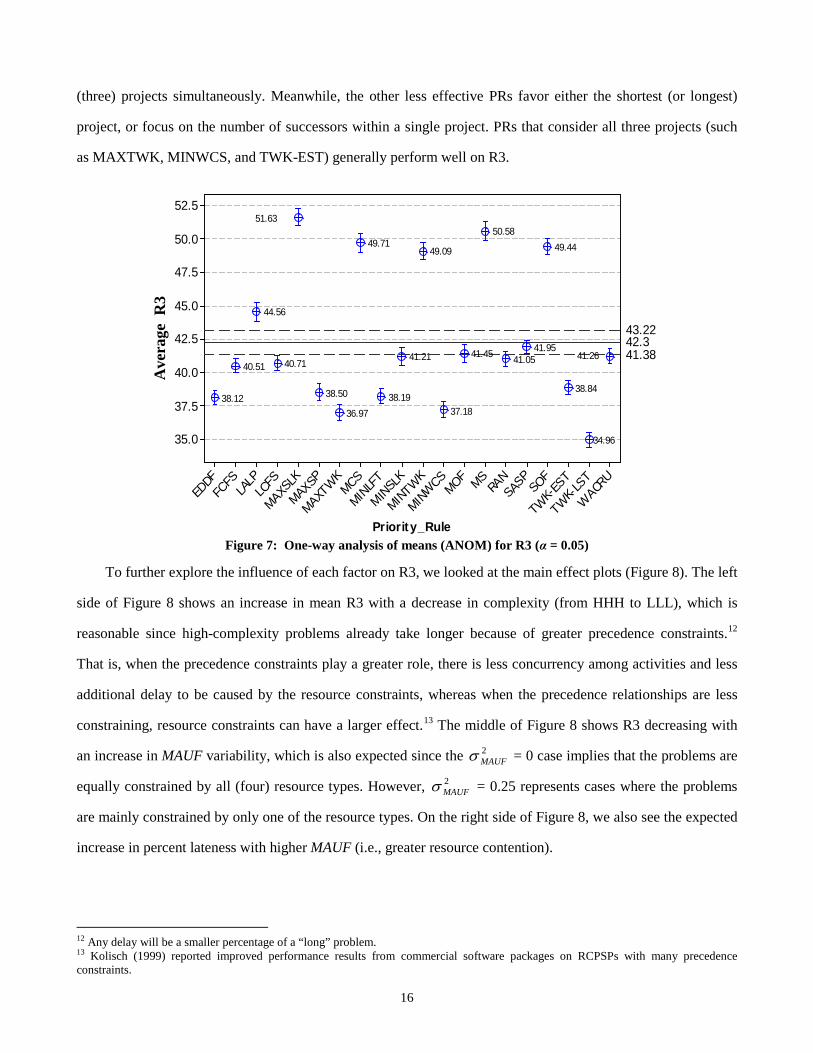
To further explore the influence of each factor on R3, we looked at the main effect plots (Figure 8). The left

side of Figure 8 shows an increase in mean R3 with a decrease in complexity (from HHH to LLL), which is

reasonable since high-complexity problems already take longer because of greater precedence constraints.12

That is, when the precedence constraints play a greater role, there is less concurrency among activities and less

additional delay to be caused by the resource constraints, whereas when the precedence relationships are less

constraining, resource constraints can have a larger effect.13 The middle of Figure 8 shows R3 decreasing with

an increase in MAUF variability, which is also expected since the 2MAUFσ = 0 case implies that the problems are

equally constrained by all (four) resource types. However, 2MAUFσ = 0.25 represents cases where the problems

are mainly constrained by only one of the resource types. On the right side of Figure 8, we also see the expected

increase in percent lateness with higher MAUF (i.e., greater resource contention).

12 Any delay will be a smaller percentage of a “long” problem. 13 Kolisch (1999) reported improved performance results from commercial software packages on RCPSPs with many precedence constraints.

Priority_Rule

R3

_A

vg

_%

_La

te

WAC

RU

TWK-

LST

TWK-

EST

SOF

SASPRA

NMSMOF

MINW

CS

MINTW

K

MINSL

K

MINLF

TMCS

MAXTW

K

MAXSP

MAXSL

KLC

FSLA

LPFC

FSED

DF

52.5

50.0

47.5

45.0

42.5

40.0

37.5

35.0

43.2242.341.3841.26

34.96

38.84

49.44

41.9541.05

50.58

41.45

37.18

49.09

41.21

38.19

49.71

36.97

38.50

51.63

40.71

44.56

40.51

38.12

Ave

rage

R3

17

Figure 8: Main effect plots for R3

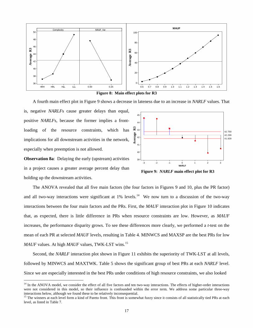
A fourth main effect plot in Figure 9 shows a decrease in lateness due to an increase in NARLF values. That

is, negative NARLFs cause greater delays than equal,

positive NARLFs, because the former implies a front-

loading of the resource constraints, which has

implications for all downstream activities in the network,

especially when preemption is not allowed.

Observation 8a: Delaying the early (upstream) activities

in a project causes a greater average percent delay than

holding up the downstream activities.

The ANOVA revealed that all five main factors (the four factors in Figures 9 and 10, plus the PR factor)

and all two-way interactions were significant at 1% levels.14 We now turn to a discussion of the two-way

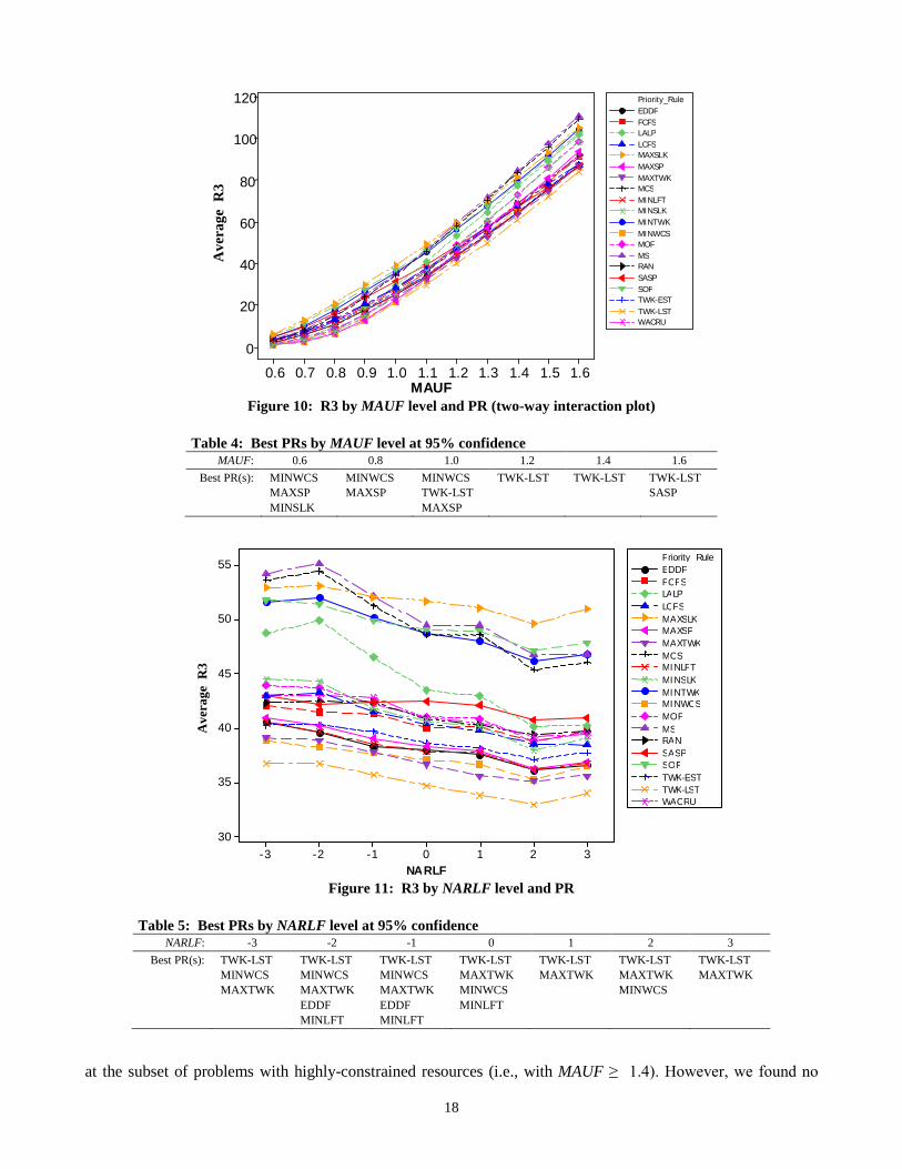
interactions between the four main factors and the PRs. First, the MAUF interaction plot in Figure 10 indicates

that, as expected, there is little difference in PRs when resource constraints are low. However, as MAUF

increases, the performance disparity grows. To see these differences more clearly, we performed a t-test on the

mean of each PR at selected MAUF levels, resulting in Table 4. MINWCS and MAXSP are the best PRs for low

MAUF values. At high MAUF values, TWK-LST wins.15

Second, the NARLF interaction plot shown in Figure 11 exhibits the superiority of TWK-LST at all levels,

followed by MINWCS and MAXTWK. Table 5 shows the significant group of best PRs at each NARLF level.

Since we are especially interested in the best PRs under conditions of high resource constraints, we also looked 14 In the ANOVA model, we consider the effect of all five factors and ten two-way interactions. The effects of higher-order interactions were not considered in this model, so their influence is confounded within the error term. We address some particular three-way interactions below, although we found these to be relatively inconsequential. 15 The winners at each level form a kind of Pareto front. This front is somewhat fuzzy since it consists of all statistically tied PRs at each level, as listed in Table 7.

Mea

n of

R3_

Avg

_%_L

ate

LLLHLLHHLHHH

50

48

46

44

42

40

38

360.250.00

Complexity MAUF_Var

Mea

n of

R3_

Avg

_%_L

ate

1.61.51.41.31.21.11.00.90.80.70.6

100

80

60

40

20

0

MAUFA

vera

ge R

3

Ave

rage

R3

Figure 9: NARLF main effect plot for R3

NARLF

Mea

n

3210-1-2-3

45

44

43

42

41

40

39

41.839

42.759

42.299

Ave

rage

R3

18

Figure 10: R3 by MAUF level and PR (two-way interaction plot)

Table 4: Best PRs by MAUF level at 95% confidence

MAUF: 0.6 0.8 1.0 1.2 1.4 1.6 Best PR(s): MINWCS

MAXSP MINSLK

MINWCS MAXSP

MINWCS TWK-LST MAXSP

TWK-LST TWK-LST TWK-LST SASP

Figure 11: R3 by NARLF level and PR

Table 5: Best PRs by NARLF level at 95% confidence

NARLF: -3 -2 -1 0 1 2 3 Best PR(s): TWK-LST

MINWCS MAXTWK

TWK-LST MINWCS MAXTWK EDDF MINLFT

TWK-LST MINWCS MAXTWK EDDF MINLFT

TWK-LST MAXTWK MINWCS MINLFT

TWK-LST MAXTWK

TWK-LST MAXTWK MINWCS

TWK-LST MAXTWK

at the subset of problems with highly-constrained resources (i.e., with MAUF ≥ 1.4). However, we found no

MAUF

R3

1.6 1.5 1.4 1.3 1.2 1.1 1.0 0.9 0.8 0.7 0.6

120

100

80

60

40

20

0

MINSLK MINTWK MINWCS MOF MS RAN SASP SOF TWK-EST TWK-LST

EDDF

WACRU

FCFS LALP LCFS MAXSLK MAXSP MAXTWK MCS MINLFT

Priority_Rule

N A R L F 3 2 1 0 - 1 - 2 - 3

5 5

5 0

4 5

4 0

3 5

3 0

M I N S L K M I N T W K M I N W C S M O F M S R A N S A S P S O F T W K - E S T T W K - L S T

E D D F

W A C R U

F C F S L A L P L C F S M A X S L K M A X S P M A X T W K M C S M I N L F T

P r i o r i t y _ R u l e

Ave

rage

R3

Ave

rage

R3

19

significant change in the winning PRs in the case of this three-way interaction.

Third, we looked at varied complexity levels (Figure 12 and Table 6). TWK-LST outperforms the other

PRs at high complexity. At low complexity, SASP is best but statistically ties with TWK-LST, MINLFT and

EDDF. The behavior of SASP is especially interesting. In contrast to the other PRs, SASP seems to be robust to

changes in complexity: it is the only PR whose performance improves as C decreases. As complexity decreases,

the number of precedence constraints in each project’s network decreases. However, SASP does not consider

the number of precedence constraints when making the prioritization decision, so its robustness to complexity

makes sense. Finally, we again looked at the subset of problems with MAUF ≥ 1.4 (three-way interactions); the

results were similar.

Figure 12: R3 by complexity level and PR

Table 6: Best PRs by complexity level at 95% confidence

C: HHH HHL HLL LLL Best PR(s): TWK-LST

MAXTWK TWK-LST MAXTWK

TWK-LST MINWCS EDDF MAXTWK

SASP TWK-LST MINLFT EDDF TWK-EST

Fourth, regarding 2MAUFσ , TWK-LST was the best PR at zero variance, while it statistically tied with

MINWCS at 0.25 variance, as shown in Figure 13(a). As expected, all PRs perform better as a problem’s

resources are constrained by fewer of its resource types. However, this did not change the ranking of most PRs.

Considering only the problems with highly-constrained resources (i.e. MAUF ≥ 1.4) did not much alter the

picture. We also looked at 2NARLFσ levels (Figure 13(b)), where TWK-LST was the best PR regardless. Again,

the ranking of the PRs did not change much with this factor, although as 2NARLFσ increases, it becomes easier to

C o m p l e x i t y

R3

L L L H L L H H L H H H

6 0

5 5

5 0

4 5

4 0

3 5

3 0

M I N S L K M I N T W K M I N W C S M O F M S R A N S A S P S O F T W K - E S T T W K - L S T

E D D F

W A C R U

F C F S L A L P L C F S M A X S L K M A X S P M A X T W K M C S M I N L F T

P r i o r i t y _ R u l e

Ave

rage

R3

20

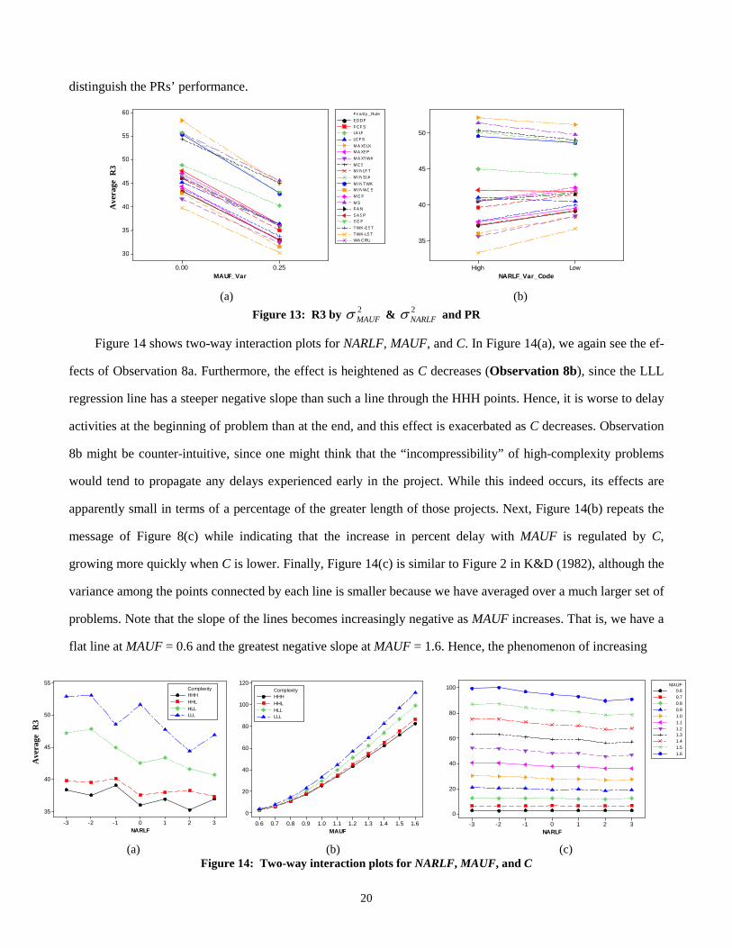
distinguish the PRs’ performance.

(a) (b)

Figure 13: R3 by 2MAUFσ & 2

NARLFσ and PR

Figure 14 shows two-way interaction plots for NARLF, MAUF, and C. In Figure 14(a), we again see the ef-

fects of Observation 8a. Furthermore, the effect is heightened as C decreases (Observation 8b), since the LLL

regression line has a steeper negative slope than such a line through the HHH points. Hence, it is worse to delay

activities at the beginning of problem than at the end, and this effect is exacerbated as C decreases. Observation

8b might be counter-intuitive, since one might think that the “incompressibility” of high-complexity problems

would tend to propagate any delays experienced early in the project. While this indeed occurs, its effects are

apparently small in terms of a percentage of the greater length of those projects. Next, Figure 14(b) repeats the

message of Figure 8(c) while indicating that the increase in percent delay with MAUF is regulated by C,

growing more quickly when C is lower. Finally, Figure 14(c) is similar to Figure 2 in K&D (1982), although the

variance among the points connected by each line is smaller because we have averaged over a much larger set of

problems. Note that the slope of the lines becomes increasingly negative as MAUF increases. That is, we have a

flat line at MAUF = 0.6 and the greatest negative slope at MAUF = 1.6. Hence, the phenomenon of increasing

(a) (b) (c)

Figure 14: Two-way interaction plots for NARLF, MAUF, and C

M A U F _ V a r

R3

0 . 2 5 0 . 0 0

6 0

5 5

5 0

4 5

4 0

3 5

3 0

M I N S L K M I N T W K M I N W C S M O F M S R A N S A S P S O F T W K - E S T T W K - L S T

E D D F

W A C R U

F C F S L A L P L C F S M A X S L K M A X S P M A X T W K M C S M I N L F T

P r i o r i t y _ R u l e

NARLF_Var_CodeLowHigh

50

45

40

35

NARLF

Mea

n

3210-1-2-3

55

50

45

40

35

MAUF1.61.51.41.31.21.11.00.90.80.70.6

120

100

80

60

40

20

0

NARLF3210-1-2-3

100

80

60

40

20

0

1.51.6

0.60.70.80.91.01.11.21.31.4

MAUF

HHHHHLHLLLLL

ComplexityHHHHHLHLLLLL

Complexity

Ave

rage

R3

Ave

rage

R3

21

delays with lower NARLF is exacerbated by higher MAUF (Observation 8c), just as it was by decreased C.

5.5 Results for R5: Percent (Problem) Delay

We repeated the above set of analyses for R5, although we will report only on the key differences from the

R3 results. While R3 attends to the effects of delay on the projects individually, R5 only accounts for delays that

lengthen the overall portfolio of projects. While individual project managers would care more about R3,

program or portfolio managers would have reason to focus on R5. However, since R5 is driven by the single

longest project in a problem, it is a less sensitive measure than R3.

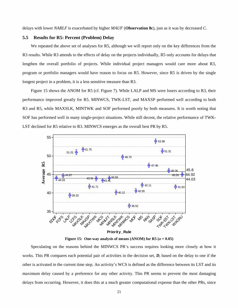
Figure 15 shows the ANOM for R5 (cf. Figure 7). While LALP and MS were losers according to R3, their

performance improved greatly for R5. MINWCS, TWK-LST, and MAXSP performed well according to both

R3 and R5, while MAXSLK, MINTWK and SOF performed poorly by both measures. It is worth noting that

SOF has performed well in many single-project situations. While still decent, the relative performance of TWK-

LST declined for R5 relative to R3. MINWCS emerges as the overall best PR by R5.

Figure 15: One-way analysis of means (ANOM) for R5 (α = 0.05)

Speculating on the reasons behind the MINWCS PR’s success requires looking more closely at how it

works. This PR compares each potential pair of activities in the decision set, D, based on the delay to one if the

other is activated in the current time step. An activity’s WCS is defined as the difference between its LST and its

maximum delay caused by a preference for any other activity. This PR seems to prevent the most damaging

delays from occurring. However, it does this at a much greater computational expense than the other PRs, since

Priority_Rule

R5_

%_D

elay

WAC

RU

TWK-L

ST

TWK-E

STSOF

SASPRA

NMSMOF

MINWCS

MINTW

K

MINSL

K

MINLF

TMCS

MAXTW

K

MAXSP

MAXSL

KLC

FSLA

LPFC

FSED

DF

55

50

45

40

35

45.844.9244.03

45.03

41.63

46.06

51.31

53.98

47.46

42.11

40.55

36.52

49.70

40.12

44.0443.41

43.91

41.71

51.7551.01

39.33

44.67

44.03

Ave

rage

R5

22

it must “look ahead” for the potential downstream delays in terms of each possible pair of activities in D. Note

that this PR also performs well for R3 (except for high MAUF cases).

Finally, while SASP performed well by R3 in several situations, it was the worst PR by R5. Taking the

shortest activity from the shortest project is good for minimizing the average percent delay to all projects, but

the duration of a problem is governed by the duration of its longest project, which is given lowest priority by

SASP. Thus, SASP performs very poorly with R5, while LALP performs well.16

The ANOVA based on R5 also revealed that all five main factors and two-way interactions are significant

at the 1% level. The overall trends in the two-way interaction plots are mostly similar to those of R3, although

the performance of various PRs differs. Figure 16(a) (cf. Figure 10) shows the expected reduction in

performance as MAUF increases. MINWCS emerges as the best PR for MAUF ≥ 1.0. SASP performs poorly at

all MAUF levels. While also showing the clear superiority of MINWCS and the inferiority of SASP, Figure

16(b) does not show improved performance with higher NARLF values, as seen in Figure 11 (for R3). This

would seem to be because the delays early in the projects (which occur due to the front-loading of the resource

demands) are largely absorbed by the two shorter projects, whose delays do not usually show up in R5. Thus,

Observation 8 does not apply to R5 (which we also confirmed by examining other two-way interactions).

Figure 16(c) indicates the trend towards diminished performance with lower complexity levels, as per

Figure 12, although SASP no longer bucks the trend. Instead, several other PRs now prevail against the general

trend by performing poorly under situations of high C. In particular, MS and MCS perform better as C

decreases. Perhaps this is because, as C decreases, the number of precedence constraints in each project’s

network decreases. This dearth of precedence constraints makes problems “harder,” because D is larger, and

thus there are more potential bad decisions that a PR can make. In these situations, PRs that happen to focus on

the factors that are important for a particular objective (versus on generally important ones) perform better. PRs

that do well on R5 tend to prioritize the longest project. The longest project will often have the longest chain of

activities, and therefore its activities will tend to have more successors than the shorter projects’ activities. As C

decreases, the number of successors becomes a more discriminating feature of a network. (In high C cases, all of

the activities have a lot of successors.) The MS and MCS PRs favor the longest project in a problem, the

minimization of which implies good results for R5, and this becomes more prominent as complexity decreases.

Finally, since the 2MAUFσ interaction plot for R5 did not show any unusual trends, we omit it here.

16 Although we did not study it, we suspect that a “shortest activity from the longest project” (SALP) rule might perform well for R5.

23

(a)

(b) (c)

Figure 16: R5 interaction plots between PRs and MAUF, NARLF, and C

6. Implications for Managers In the previous section, we identified, confirmed, and discussed several important factors that contribute to

project and portfolio delay. To distill these results for managers, we developed two decision tables (Tables 10

and 11) to aid in selecting the best PR for a particular situation. Here we clearly see the different results for R3

and R5. From an individual project manager’s point of view, R3 is a more appropriate objective, whereas R5

aligns more with an executive’s or portfolio manager’s point of view. The different results obtained by these two

objectives may relate to the friction that occurs between managers at different organizational levels.

We observe several patterns in these tables. First, the number of winning (statistically tied) PRs decreases

with greater MAUF and C in both tables. Also, for both R3 and R5, the results seem to be fairly robust to

MINSLKMINTWKMINWC SMO FMSRA NSA SPSO FTWK-ESTTWK-LST

EDDF

WA C RU

FC FSLA LPLC FSMA XSLKMA XSPMA XTWKMC SMINLFT

Priority _Rule

MAUF

Mea

n1.61.51.41.31.21.11.00.90.80.70.6

120

100

80

60

40

20

0

NARLF

Mea

n

3210-1-2-3

55

50

45

40

35

Complexity

Mea

n

LLLHLLHHLHHH

60

55

50

45

40

35

30

Ave

rage

R5

Ave

rage

R5

Ave

rage

R5

24

NARLF. That is, while NARLF affects the amount of delay for R3 (Observation 8), it does not much affect

which PR wins. For R3, under tight resource constraints (high MAUF), TWK-LST performs well under high C,

while SASP performs well under low C. For R5, under high MAUF, MINWCS performs well regardless of C.

Table 7: Summary of results for R3 (α = 0.05)* Resource Distribution Front-loaded

NARLF = -3 & -2 Not front- or back-loaded

NARLF = -1 & 0 & 1 Back-loaded

NARLF = 2 & 3

Res

ourc

e C

onte

ntio

n

Low (MAUF = 0.6-0.8)

C HHH LLL

MINWCS MAXSP MINSLK MOF TWK-LST MAXTWK LALP

MINWCS MAXSP TWK-LST MINSLK MINLFT EDDF MAXTWK MOF

C HHH LLL

MAXSP MINWCS MINSLK MOF LALP TWK-LST MAXTWK

MINWCS MAXSP MINSLK TWK-LST MOF

C HHH LLL

MINWCS MINSLK MAXSP MOF LALP TWK-LST MAXTWK

MINWCS MAXSP MINSLK TWK-LST MINLFT

Medium (MAUF =

1-1.2)

C HHH LLL

TWK-LST MAXTWK

SASP TWK-LST MINWCS EDDF MINLFT MAXTWK TWK-EST MAXSP FCFS

C HHH LLL

TWK-LST MAXTWK

TWK-LST SASP EDDF MINLFT MINWCS MAXTWK TWK-EST FCFS LCFS

C HHH LLL

TWK-LST TWK-LST EDDF MINLFT SASP MINWCS MAXSP MAXTWK TWK-EST LCFS

High (MAUF = 1.4-1.6)

C HHH LLL

TWK-LST MAXTWK FCFS TWK-EST

SASP MINLFT

C HHH LLL

TWK-LST SASP TWK-LST

C HHH LLL

TWK-LST LCFS MAXTWK TWK-EST

SASP LCFS

*Multiple entries in each cell are listed in order of increasing means (i.e., the best PR is listed first).

Table 8: Summary of results for R5 (α = 0.05)* Resource Distribution Front-loaded

NARLF = -3 & -2 Not front- or back-loaded

NARLF = -1 & 0 & 1 Back-loaded

NARLF = 2 & 3

Res

ourc

e C

onte

ntio

n

Low (MAUF = 0.6-0.8)

C HHH LLL

LALP MINSLK MINWCS MAXSP MOF

LALP MS MCS MINSLK MINWCS

C HHH LLL

LALP MINSLK MINWCS MOF MAXSP

LALP MINWCS MINSLK MAXSP

C HHH LLL

LALP MOF MINSLK MAXSP MINWCS

LALP MINWCS MINSLK MAXSP

Medium (MAUF =

1-1.2)

C HHH LLL

MINWCS LALP MOF MINSLK

MS MINWCS MCS

C HHH LLL

MINWCS LALP MINSLK MOF

MINWCS MS MCS

C HHH LLL

MINWCS MOF LALP

MINWCS MS MCS

High (MAUF = 1.4-1.6)

C HHH LLL

MINWCS LALP MOF MINSLK

MS MCS MINWCS

C HHH LLL

MINWCS MS MCS MINWCS

C HHH LLL

MINWCS MOF

MINWCS MS MCS EDDF MINLFT FCFS

*Multiple entries in each cell are listed in order of increasing means (i.e., the best PR is listed first).

25

Thus, if a manager wants to do well with R5, MINWCS is our overall recommendation for a robust rule in

a variety of situations where resources are moderately- to highly-constrained. For R3, we recommend TWK-

LST, except for cases where MAUF is high and C is low, where we recommend SASP. These recommendations

differ from ones in the previous literature. First, MINSLK is conspicuously absent. Second, the previous studies

that have recommended TWK-LST, MINWCS, or SASP have not qualified their recommendations by objective

or situation.

To benefit from our results and recommendations as summarized in Tables 10 and 11, managers must be

able to characterize their projects in terms of complexity (C), amount of resource contention (MAUF), and

resource distribution (NARLF). Thankfully, our results remain beneficial even when managers are unable to do

this exactly. First, regarding C, managers can qualitatively estimate whether they are dealing with a high-C

situation or a low-C one without having to precisely obtain a numerical estimate. A qualitative measure of

portfolio complexity may be obtained by simply asking whether a large portion of the constituent projects are

highly sequential or parallel. In a parallel project, many activities can be performed concurrently, while in a

sequential project fewer activities can be performed concurrently. Similarly, high-C projects contain a much

greater number of dependencies (precedence constraints). Thus, several indicators can help a manager rate C as

qualitatively “high” or “low.” Second, the general distribution of resources (front- or back-loading) can be

ascertained without too much effort. Third, the rough amount of resource contention can be qualitatively

estimated to be “low,” “medium,” or “high.” Hence, these results are readily applicable to practical issues

facing project and portfolio managers.

The relative robustness of certain PRs across appreciable ranges of NARLF, MAUF, and C is a cause for

optimism. Since the effort to build a comprehensive activity network model for a new project can be daunting or

prohibitive, and since such a model, if built, would include what could be highly questionable assumptions

about the project’s activity content and precedence relationships,17 it is difficult to experiment with various PRs

or apply meta-heuristics. However, if a manager can do some rough characterization of a few key project and

problem attributes, some helpful guidance on activity prioritization is now available nonetheless.

7. Summary & Conclusion Multi-project management is becoming ever-more important in contemporary practice. Decisions about

17 Since a project is doing something new for the first time, and especially in the case of projects such as new product development, there is a large amount of ambiguity in the work to be done and its relationships to other work. Thus, in such a project it can be dangerous to put too much stock in any particular activity network model.

26

which activities to do when (based on resource allocations) have a tremendous effect on project completion

times. Yet, many project managers, who often do not have an activity network model to which they might apply

more advanced techniques, make resource allocation decisions based on “rules of thumb” such as MINSLK.

In the context of the static RCMPSP, this paper uses relatively new measures in the most comprehensive

study of PRs to date, making a number of observations, some of which are relatively intuitive and others which

are less so. While many additional PRs could also be studied, we cover the most popular ones, and a much

larger group than other published studies in this area. For the study, we generated 12,320 project portfolios (each

consisting of three projects) according to a full factorial experiment that included four factors at various levels.

Our analysis provides much-needed guidance on the use of certain PRs in varied project situations and

objectives. Finally, the paper explicitly distinguishes the perspectives of project and portfolio managers.

From an individual project manager’s perspective (R3), TWK-LST performs well under high network

complexity, while SASP performs well under low complexity. From a portfolio manager’s perspective (R5),

MINWCS performs well regardless of complexity. While exhibiting a significant effect, the MAUF and NARLF

variances do not change the choice of the best PR. Accordingly, we developed a decision table to guide

managers in choosing among best PRs based on MAUF, NARLF, and C, which constitutes a significant

extension to the results reported by K&D (1982) and related studies. These results show how different

objectives for individual project managers and portfolio managers can lead to preferences for different decision

rules and thus organizational tensions.

Importantly, our analysis shows that previously published results are not generally accurate, since widely-

advocated rules such as MINSLK, SASP, and MAXTWK did not perform well except under limited conditions.

On the other hand, our study confirms the superiority of MINWCS (Kolisch 1996a) and TWK-LST (Lova and

Tormos 2001). Since we did not invent new PRs for this study, it was inevitable that we would confirm certain

PRs as superior and others as inferior, agreeing with some prior studies while disagreeing with others. However,

even the prior studies with which our results agree did not caveat their recommendations by problem

characteristics, nor did they compare them with many other PRs. Therefore, beyond mere confirmation, we

provide much greater generalization and specification of some particular results from prior studies.

While project scheduling, PRs, and related topics have been studied for at least fifty years, resulting in a

myriad of papers, it is in some ways astounding that no firmer guidance has appeared for decision makers in a

MP context with limited resources, the most realistic situation in contemporary practice. Thus, explaining the

27

conditions under which certain PRs perform well (or poorly) is an important contribution that allows managers

to sift through the conflicting results in the literature. Distinguishing the project and portfolio manager

perspectives is also important in practice. In short, these results should be immediately applicable in practical

situations. While we looked at a static (rather than a dynamic) case of identical project start times, our approach

could also be applied on a rolling-horizon basis in a dynamic environment.

Future research could expand our study to include additional PRs, compare results with the serial SGS,

explore other RCMPSP formulations (such as with preemption, stochastic activity durations, or dynamic project

arrivals) in a similarly comprehensive study, or explore the performance gaps between PRs and more advanced

heuristics. The results reported in this study can also be used for the development of improved PRs that take

advantage of the superiority of certain PRs under specific conditions. For instance, one might develop an

adaptive PR that shifts between simpler PRs as a project or portfolio progresses and its circumstances change.

References Akpan, E.O.P. 2000. Priority Rules in Project Scheduling: A Case for Random Activity Selection. Production Planning &

Control, 11(2) 165-170.

Ash, R. 2002. Serial and Multi-Project Scheduling with and without Preemption. Proceedings of the Annual Meeting of the

Decision Sciences Institute, San Diego, CA, November.

Baker, K. 1974. Introduction to Sequencing and Scheduling. Wiley, New York.

Bock, D., J. Patterson. 1990. A Comparison of Due Date Setting, Resource Assignment, and Job Preemption Heuristics for

the Multi-Project Scheduling Problem. Decision Sciences, 21(3) 387-402.

Boctor, F.F. 1990. Some Efficient Multi-heuristic Procedures for Resource-constrained Project Scheduling. European

Journal of Operational Research, 49(1) 3-13.

Bouleimen, K., H. Lecocq. 2000. Multi-Objective Simulated Annealing for the Resource-Constrained Multi-Project

Scheduling Problem. Proceedings of the 7th International Workshop on Project Management and Scheduling (PMS

2000), Osnabrück, Germany, Apr 17-19.

Browning, T.R., A.A. Yassine. 2010. A Random Generator of Resource-Constrained Multi-Project Network Problems.

Journal of Scheduling, 13(2) 143-161.

Brucker, P., A. Drexl, R. Möhring, K. Neumann, E. Pesch. 1999. Resource-Constrained Project Scheduling: Notation,

Classification, Models, and Methods. European Journal of Operational Research, 112(1) 3-41.

Chase, R.B., F.R. Jacobs, N.J. Aquilano. 2006. Operations Management for Competitive Advantage. 11th Edition, McGraw-

Hill/Irwin, New York.

Chen, V.Y.X. 1994. A 0-1 Programming Model for Scheduling Multiple Maintenance Projects at a Copper Mine. European

Journal of Operational Research, 76(1) 176-191.

Chiu, H.N., D.M. Tsai. 1993. A Comparison of Single-project and Multi-project Approaches in Resource Constrained

Multi-project Scheduling Problems. Journal of the Chinese Institute of Industrial Engineers, 10, 171-179.

28

Cohen, I., A. Mandelbaum, A. Shtub. 2004. Multi-Project Scheduling and Control: A Process-Based Comparative Study of

the Critical Chain Methodology and Some Alternatives. Project Management Journal, 35(2) 39-50.

Confessore, G., S. Giordani, S. Rismondo. 2007. A Market-based Multi-Agent System Model for Decentralized Multi-

Project Scheduling. Annals of Operations Research, 150(1) 115-135.

Cooper, D.F. 1976. Heuristics for Scheduling Resource-Constrained Projects: An Experimental Investigation. Management

Science, 22(11) 1186-1194.

Davis, E.W. 1975. Project Network Summary Measures and Constrained Resource Scheduling. IIE Trans, 7(2) 132-142.

Davis, E.W., J.H. Patterson. 1975. A Comparison of Heuristic and Optimum Solutions in Resource-Constrained Project

Scheduling. Management Science, 21(8) 944-955.

Deckro, R.F., E.P. Winkofsky, J.E. Hebert, R. Gagnon. 1991. A Decomposition Approach to Multi-project Scheduling.

European Journal of Operational Research, 51(1) 110-118.

Dumond, J., V.A. Mabert. 1988. Evaluating Project Scheduling and Due Date Assignment Procedures: An Experimental

Analysis. Management Science, 34(1) 101-118.

Fendley, L.G. 1968. Towards the Development of a Complete Multiproject Scheduling System. Journal of Industrial

Engineering, 19(10) 505-515.

Gibbons, J.D. 1993. Nonparametric Statistics. Sage Publications, Newbury Park, CA.

Gonçalves, J.F., J.J.d.M. Mendes, M.G.C. Resende. 2008. A Genetic Algorithm for the Resource Constrained Multi-Project

Scheduling Problem. European Journal of Operational Research, 189(3) 1171-1190.

Hartmann, S., D. Briskorn. 2009. A Survey of Variants and Extensions of the Resource-constrained Project Scheduling

Problem. European Journal of Operational Research, forthcoming.

Hartmann, S., R. Kolisch. 2000. Experimental Evaluation of State-of-the-Art Heuristics for the Resource-Constrained

Project Scheduling Problem. European Journal of Operational Research, 127(2) 394-407.

Herroelen, W.S. 2005. Project Scheduling - Theory and Practice. Production and Operations Management, 14(4) 413-432.

Homberger, J. 2007. A Multi-agent System for the Decentralized Resource-constrained Multi-project Scheduling Problem.

International Transactions in Operational Research, 14(6) 565-589.

Kim, K.W., Y.S. Yun, J.M. Yoon, M. Gen, G. Yamazaki. 2005. Hybrid Genetic Algorithm with Adaptive Abilities for

Resource-constrained Multiple Project Scheduling. Computers in Industry, 56(2) 143-160.

Kim, S.-Y., R.C. Leachman. 1993. Multi-Project Scheduling with Explicit Lateness Costs. IIE Transactions, 25(2) 34-44.

Kolisch, R. 1996a. Efficient Priority Rules for the Resource-Constrained Project Scheduling Problem. Journal of

Operations Management, 14(3) 179-192.

Kolisch, R. 1996b. Serial and Parallel Resource-Constrained Project Scheduling Methods Revisited: Theory and

Computation. European Journal of Operational Research, 90(2) 320-333.

Kolisch, R. 1999. Resource Allocation Capabilities of Commercial Project Management Software Packages. Interfaces,

29(4) 19-31.

Kolisch, R., S. Hartmann. 1999. Heuristic Algorithms for Solving the Resource-Constrained Project Scheduling Problem:

Classification and Computational Analysis. in Weglarz, J., Ed., Project scheduling: Recent Models, Algorithms and

Applications, Kluwer Academic Publishers, Boston, 147-178.

Kolisch, R., S. Hartmann. 2005. Experimental Investigation of Heuristics for Resource-Constrained Project Scheduling: An

Update. European Journal of Operational Research, 174(1) 23-37.

29

Kolisch, R., A. Sprecher, A. Drexl. 1995. Characterization and Generation of a General Class of Resource-Constrained

Project Scheduling Problems. Management Science, 41(10) 1693-1703.

Krüger, D., A. Scholl. 2008. Managing and Modelling General Resource Transfers in (Multi-)Project Scheduling. OR

Spectrum(forthcoming).

Krüger, D., A. Scholl. 2009. A Heuristic Solution Framework for the Resource Constrained (Multi-)Project Scheduling

Problem with Sequence-Dependent Transfer Times. European Journal of Operational Research, 197, 492-508.

Kumanan, S., G.J. Jose, K. Raja. 2006. Multi-project Scheduling using an Heuristic and a Genetic Algorithm. International

Journal of Manufacturing Technology, 31(3-4) 360-366.

Kurtulus, I. 1978. An Analysis of Scheduling Rules for Multi-Project Scheduling. Ph.D. Thesis (Business), University of

North Carolina at Chapel Hill, Chapel Hill.

Kurtulus, I. 1985. Multiproject Scheduling: Analysis of Scheduling Strategies under Unequal Delay Penalties. Journal of

Operations Management, 5(3) 291-307.

Kurtulus, I., E.W. Davis. 1982. Multi-Project Scheduling: Categorization of Heuristic Rules Performance. Management

Science, 28(2) 161-172.

Kurtulus, I.S., S.C. Narula. 1985. Multi-Project Scheduling: Analysis of Project Performance. IIE Trans, 17(1) 58-65.

Lawrence, S.R., T.E. Morton. 1993. Resource-Constrained Multi-Project Scheduling with Tardy Costs: Comparing

Myopic, Bottleneck, and Resource Pricing Heuristics. European Journal of Operational Research, 64(2) 168-187.

Lenstra, J.K., A.H.G.R. Kan. 1978. Complexity of Scheduling under Precedence Constraints. Operations Res, 26(1) 22-35.

Liberatore, M.J., B. Pollack-Johnson. 2003. Factors Influencing the Usage and Selection of Project Management Software.

IEEE Transactions on Engineering Management, 50(2) 164-174.

Linyi, D., L. Yan. 2007. A Particle Swarm Optimization for Resource-Constrained Multi-Project Scheduling Problem. Proc

of the International Conference on Computational Intelligence and Security, Harbin, China, Dec 15-19, 1010-1014.

Lova, A., P. Tormos. 2001. Analysis of Scheduling Schemes and Heuristic Rules Performance in Resource-Constrained

Multi-Project Scheduling. Annals of Operations Research, 102(1-4) 263-286.

Lova, A., P. Tormos. 2002. Combining Random Sampling and Backward-Forward Heuristics for Resource-Constrained

Multi-Project Scheduling. Proc of the 8th Int Workshop on Proj Mgmt and Sched, Valencia, Spain, Apr. 3-5, 244-248.

Maroto, C., P. Tormos, A. Lova. 1999. The Evolution of Software Quality in Project Scheduling. in Weglarz, J., Ed.,

Project Scheduling, Kluwer Academic Publishers, Boston, 239-259.

Meredith, J.R., S.J. Mantel. 2009. Project Management. 7th Edition, Wiley, New York.

Mize, J.H. 1964. A Heuristic Scheduling Model for Multi-Project Organizations. Ph.D. Thesis Purdue University, .

Mohanty, R.P., M.K. Siddiq. 1989. Multiple Projects - Multiple Resources-Constrained Scheduling: Some Studies.

International Journal of Production Research, 27(2) 261-280.

Özdamar, L., G. Ulusoy. 1995. A Survey on the Resource-constrained Project Scheduling Problem. lIE Transactions, 27(5)

574-586.

Pascoe, T.L. 1966. Allocation of Resources - CPM. Revue Française de Recherche Opérationelle, 38, 31-38.

Patterson, J.H. 1973. Alternative Methods of Project Scheduling with Limited Resources. Naval Research Logistics

Quarterly, 20(4) 767-784.

Payne, J.H. 1995. Management of Multiple Simultaneous Projects: A State-of-the-Art Review. International Journal of

Project Management, 13(3) 163-168.

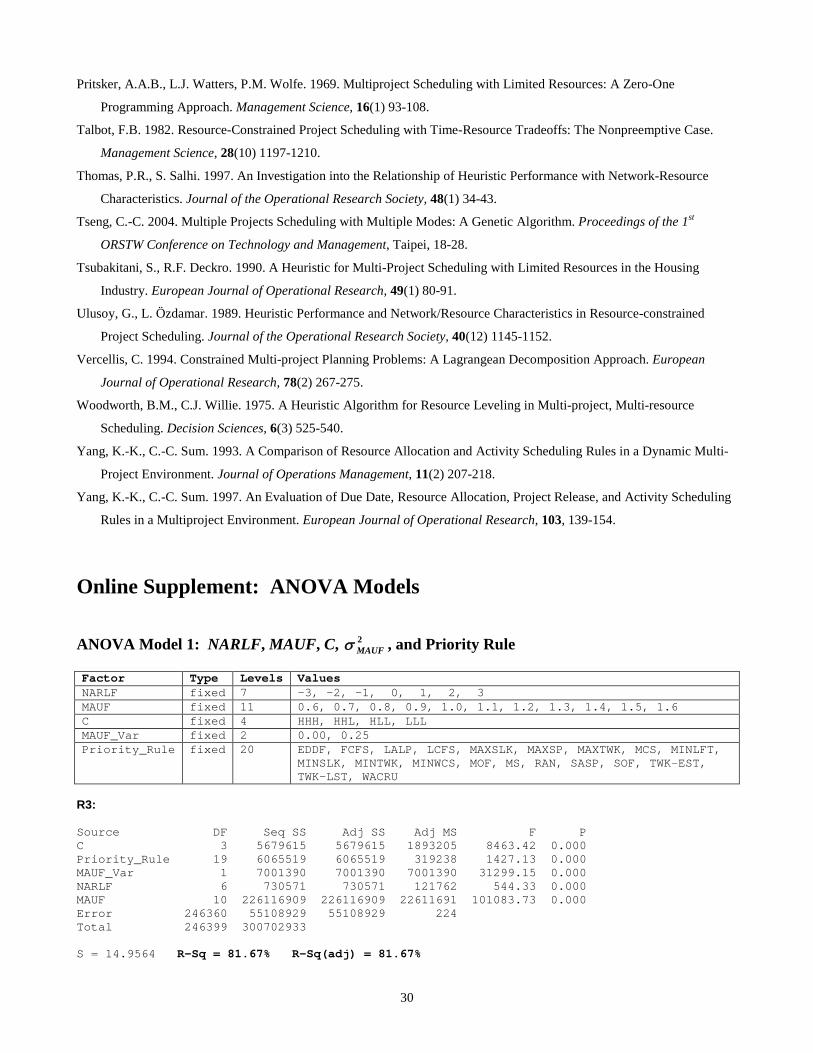
30

Pritsker, A.A.B., L.J. Watters, P.M. Wolfe. 1969. Multiproject Scheduling with Limited Resources: A Zero-One

Programming Approach. Management Science, 16(1) 93-108.

Talbot, F.B. 1982. Resource-Constrained Project Scheduling with Time-Resource Tradeoffs: The Nonpreemptive Case.

Management Science, 28(10) 1197-1210.

Thomas, P.R., S. Salhi. 1997. An Investigation into the Relationship of Heuristic Performance with Network-Resource

Characteristics. Journal of the Operational Research Society, 48(1) 34-43.

Tseng, C.-C. 2004. Multiple Projects Scheduling with Multiple Modes: A Genetic Algorithm. Proceedings of the 1st

ORSTW Conference on Technology and Management, Taipei, 18-28.

Tsubakitani, S., R.F. Deckro. 1990. A Heuristic for Multi-Project Scheduling with Limited Resources in the Housing

Industry. European Journal of Operational Research, 49(1) 80-91.

Ulusoy, G., L. Özdamar. 1989. Heuristic Performance and Network/Resource Characteristics in Resource-constrained

Project Scheduling. Journal of the Operational Research Society, 40(12) 1145-1152.

Vercellis, C. 1994. Constrained Multi-project Planning Problems: A Lagrangean Decomposition Approach. European

Journal of Operational Research, 78(2) 267-275.

Woodworth, B.M., C.J. Willie. 1975. A Heuristic Algorithm for Resource Leveling in Multi-project, Multi-resource

Scheduling. Decision Sciences, 6(3) 525-540.

Yang, K.-K., C.-C. Sum. 1993. A Comparison of Resource Allocation and Activity Scheduling Rules in a Dynamic Multi-

Project Environment. Journal of Operations Management, 11(2) 207-218.

Yang, K.-K., C.-C. Sum. 1997. An Evaluation of Due Date, Resource Allocation, Project Release, and Activity Scheduling

Rules in a Multiproject Environment. European Journal of Operational Research, 103, 139-154.

Online Supplement: ANOVA Models

ANOVA Model 1: NARLF, MAUF, C, 2MAUFσ , and Priority Rule

Factor Type Levels Values NARLF fixed 7 -3, -2, -1, 0, 1, 2, 3 MAUF fixed 11 0.6, 0.7, 0.8, 0.9, 1.0, 1.1, 1.2, 1.3, 1.4, 1.5, 1.6 C fixed 4 HHH, HHL, HLL, LLL MAUF_Var fixed 2 0.00, 0.25 Priority_Rule fixed 20 EDDF, FCFS, LALP, LCFS, MAXSLK, MAXSP, MAXTWK, MCS, MINLFT,

MINSLK, MINTWK, MINWCS, MOF, MS, RAN, SASP, SOF, TWK-EST, TWK-LST, WACRU

R3: Source DF Seq SS Adj SS Adj MS F P C 3 5679615 5679615 1893205 8463.42 0.000 Priority_Rule 19 6065519 6065519 319238 1427.13 0.000 MAUF_Var 1 7001390 7001390 7001390 31299.15 0.000 NARLF 6 730571 730571 121762 544.33 0.000 MAUF 10 226116909 226116909 22611691 101083.73 0.000 Error 246360 55108929 55108929 224 Total 246399 300702933 S = 14.9564 R-Sq = 81.67% R-Sq(adj) = 81.67%

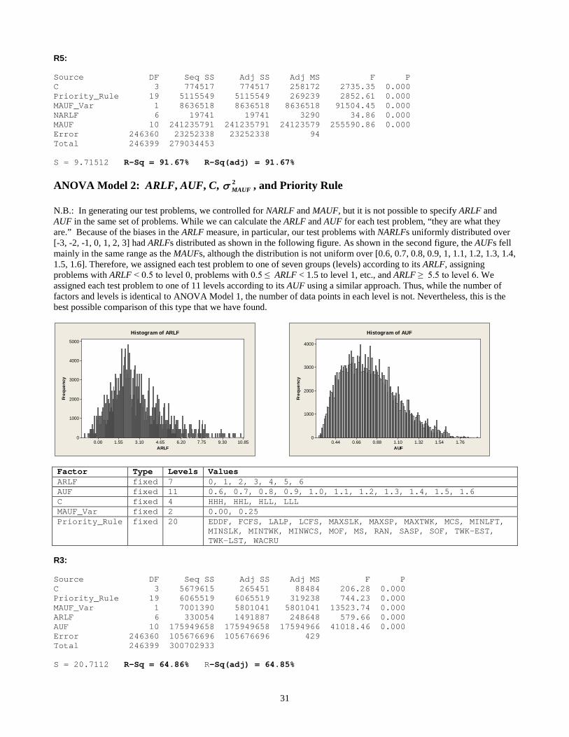
31

R5: Source DF Seq SS Adj SS Adj MS F P C 3 774517 774517 258172 2735.35 0.000 Priority_Rule 19 5115549 5115549 269239 2852.61 0.000 MAUF_Var 1 8636518 8636518 8636518 91504.45 0.000 NARLF 6 19741 19741 3290 34.86 0.000 MAUF 10 241235791 241235791 24123579 255590.86 0.000 Error 246360 23252338 23252338 94 Total 246399 279034453 S = 9.71512 R-Sq = 91.67% R-Sq(adj) = 91.67%

ANOVA Model 2: ARLF, AUF, C, 2MAUFσ , and Priority Rule

N.B.: In generating our test problems, we controlled for NARLF and MAUF, but it is not possible to specify ARLF and AUF in the same set of problems. While we can calculate the ARLF and AUF for each test problem, “they are what they are.” Because of the biases in the ARLF measure, in particular, our test problems with NARLFs uniformly distributed over [-3, -2, -1, 0, 1, 2, 3] had ARLFs distributed as shown in the following figure. As shown in the second figure, the AUFs fell mainly in the same range as the MAUFs, although the distribution is not uniform over [0.6, 0.7, 0.8, 0.9, 1, 1.1, 1.2, 1.3, 1.4, 1.5, 1.6]. Therefore, we assigned each test problem to one of seven groups (levels) according to its ARLF, assigning problems with ARLF < 0.5 to level 0, problems with 0.5 ≤ ARLF < 1.5 to level 1, etc., and ARLF ≥ 5.5 to level 6. We assigned each test problem to one of 11 levels according to its AUF using a similar approach. Thus, while the number of factors and levels is identical to ANOVA Model 1, the number of data points in each level is not. Nevertheless, this is the best possible comparison of this type that we have found.

Factor Type Levels Values ARLF fixed 7 0, 1, 2, 3, 4, 5, 6 AUF fixed 11 0.6, 0.7, 0.8, 0.9, 1.0, 1.1, 1.2, 1.3, 1.4, 1.5, 1.6 C fixed 4 HHH, HHL, HLL, LLL MAUF_Var fixed 2 0.00, 0.25 Priority_Rule fixed 20 EDDF, FCFS, LALP, LCFS, MAXSLK, MAXSP, MAXTWK, MCS, MINLFT,

MINSLK, MINTWK, MINWCS, MOF, MS, RAN, SASP, SOF, TWK-EST, TWK-LST, WACRU

R3: Source DF Seq SS Adj SS Adj MS F P C 3 5679615 265451 88484 206.28 0.000 Priority_Rule 19 6065519 6065519 319238 744.23 0.000 MAUF_Var 1 7001390 5801041 5801041 13523.74 0.000 ARLF 6 330054 1491887 248648 579.66 0.000 AUF 10 175949658 175949658 17594966 41018.46 0.000 Error 246360 105676696 105676696 429 Total 246399 300702933 S = 20.7112 R-Sq = 64.86% R-Sq(adj) = 64.85%

ARLF

Freq

uenc

y

10.859.307.756.204.653.101.550.00

5000

4000

3000

2000

1000

0

Histogram of ARLF

AUF

Freq

uenc

y

1.761.541.321.100.880.660.44

4000

3000

2000

1000

0

Histogram of AUF

32

R5: Source DF Seq SS Adj SS Adj MS F P C 3 774517 2859828 953276 2409.75 0.000 Priority_Rule 19 5115549 5115549 269239 680.60 0.000 MAUF_Var 1 8636518 7337229 7337229 18547.50 0.000 ARLF 6 18126 1194117 199019 503.09 0.000 AUF 10 167031888 167031888 16703189 42223.35 0.000 Error 246360 97457856 97457856 396 Total 246399 279034453 S = 19.8895 R-Sq = 65.07% R-Sq(adj) = 65.07% ANOVA Model 3: Full Model with Interactions (no ARLF or AUF) Factor Type Levels Values NARLF fixed 7 -3, -2, -1, 0, 1, 2, 3 MAUF fixed 11 0.6, 0.7, 0.8, 0.9, 1.0, 1.1, 1.2, 1.3, 1.4, 1.5, 1.6 C fixed 4 HHH, HHL, HLL, LLL MAUF_Var fixed 2 0.00, 0.25 Priority_Rule fixed 20 EDDF, FCFS, LALP, LCFS, MAXSLK, MAXSP, MAXTWK, MCS, MINLFT,

MINSLK, MINTWK, MINWCS, MOF, MS, RAN, SASP, SOF, TWK-EST, TWK-LST, WACRU

R3: Source DF SS MS F P Complexity 3 5676637 1892212 10172.87 0.000 NARLF 6 730977 121829 654.98 0.000 MAUF 10 226106220 22610622 121558.76 0.000 MAUF_Var 1 7001496 7001496 37641.30 0.000 Priority_Rule 19 6065896 319258 1716.39 0.000 Complexity*NARLF 18 405170 22509 121.01 0.000 Complexity*MAUF 30 3076039 102535 551.24 0.000 Complexity*MAUF_Var 3 31672 10557 56.76 0.000 Complexity*Priority_Rule 57 1031467 18096 97.29 0.000 NARLF*MAUF 60 438699 7312 39.31 0.000 NARLF*MAUF_Var 6 35560 5927 31.86 0.000 NARLF*Priority_Rule 114 166361 1459 7.85 0.000 MAUF*MAUF_Var 10 2143448 214345 1152.36 0.000 MAUF*Priority_Rule 190 1960751 10320 55.48 0.000 MAUF_Var*Priority_Rule 19 95391 5021 26.99 0.000 Error 245853 45730060 186 Total 246399 300695843 S = 13.6384 R-Sq = 84.79% R-Sq(adj) = 84.76% R5: Source DF SS MS F P Complexity 3 774555 258185 3607.00 0.000 NARLF 6 19749 3291 45.98 0.000 MAUF 10 241218951 24121895 336997.70 0.000 MAUF_Var 1 8634599 8634599 120630.65 0.000 Priority_Rule 19 5115274 269225 3761.24 0.000 Complexity*NARLF 18 103962 5776 80.69 0.000 Complexity*MAUF 30 1159921 38664 540.16 0.000 Complexity*MAUF_Var 3 138260 46087 643.86 0.000 Complexity*Priority_Rule 57 826638 14502 202.61 0.000 NARLF*MAUF 60 39960 666 9.30 0.000 NARLF*MAUF_Var 6 47134 7856 109.75 0.000 NARLF*Priority_Rule 114 41161 361 5.04 0.000 MAUF*MAUF_Var 10 2607946 260795 3643.46 0.000 MAUF*Priority_Rule 190 666202 3506 48.99 0.000

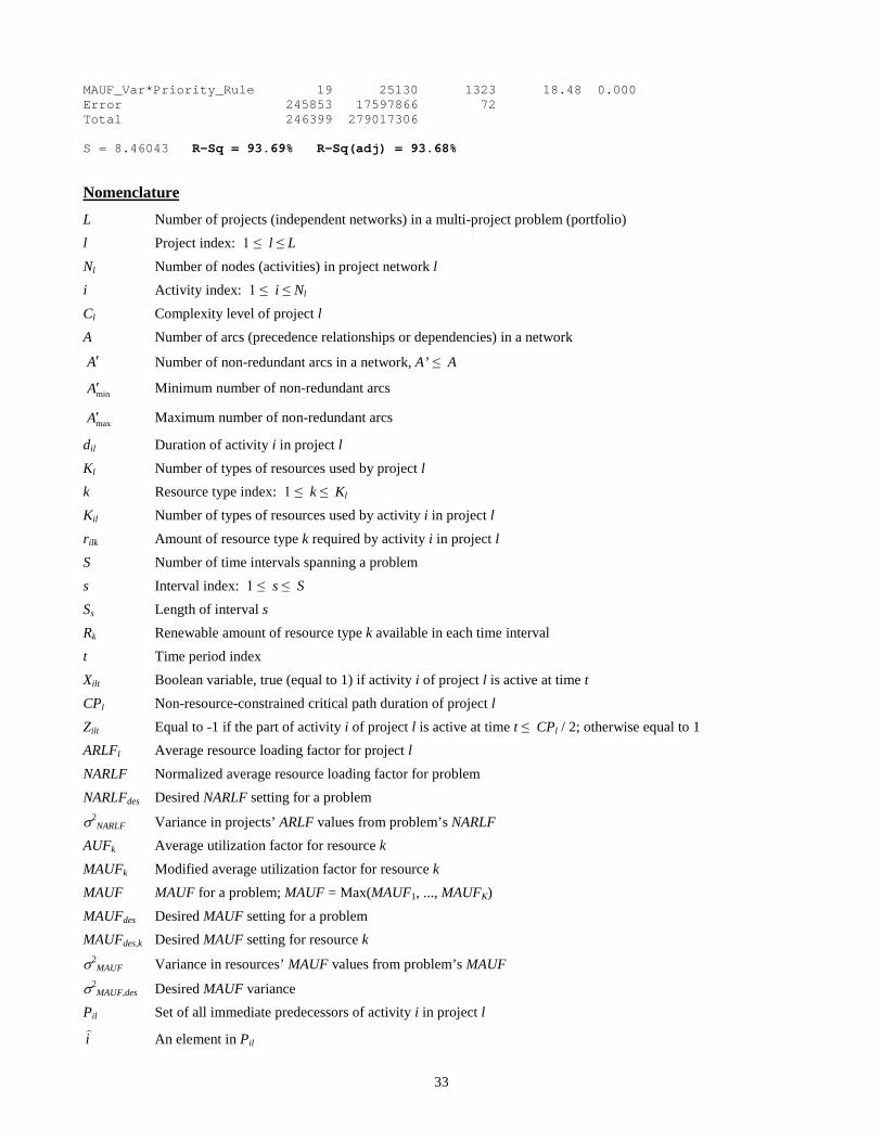
33

MAUF_Var*Priority_Rule 19 25130 1323 18.48 0.000 Error 245853 17597866 72 Total 246399 279017306 S = 8.46043 R-Sq = 93.69% R-Sq(adj) = 93.68%

Nomenclature

L Number of projects (independent networks) in a multi-project problem (portfolio) l Project index: 1 ≤ l ≤ L Nl Number of nodes (activities) in project network l i Activity index: 1 ≤ i ≤ Nl Cl Complexity level of project l A Number of arcs (precedence relationships or dependencies) in a network

A′ Number of non-redundant arcs in a network, A’ ≤ A

minA′ Minimum number of non-redundant arcs

maxA′ Maximum number of non-redundant arcs

dil Duration of activity i in project l Kl Number of types of resources used by project l k Resource type index: 1 ≤ k ≤ Kl Kil Number of types of resources used by activity i in project l rilk Amount of resource type k required by activity i in project l S Number of time intervals spanning a problem s Interval index: 1 ≤ s ≤ S Ss Length of interval s Rk Renewable amount of resource type k available in each time interval t Time period index Xilt Boolean variable, true (equal to 1) if activity i of project l is active at time t CPl Non-resource-constrained critical path duration of project l Zilt Equal to -1 if the part of activity i of project l is active at time t ≤ CPl / 2; otherwise equal to 1 ARLFl Average resource loading factor for project l NARLF Normalized average resource loading factor for problem NARLFdes Desired NARLF setting for a problem

σ2NARLF Variance in projects’ ARLF values from problem’s NARLF

AUFk Average utilization factor for resource k MAUFk Modified average utilization factor for resource k MAUF MAUF for a problem; MAUF = Max(MAUF1, ..., MAUFK) MAUFdes Desired MAUF setting for a problem MAUFdes,k Desired MAUF setting for resource k

σ2MAUF Variance in resources’ MAUF values from problem’s MAUF

σ2MAUF,des Desired MAUF variance

Pil Set of all immediate predecessors of activity i in project l

i

An element in Pil