A unified framework for deterministic time constrained vehicle routing and crew scheduling problems

1 A UNIFIED FRAMEWORK FOR

DETERMINISTIC TIME CONSTRAINED VEHICLE

ROUTING AND CREW SCHEDULING PROBLEMS

Guy Desaulniers1;5, Jacques Desrosiers2;5, Irina Ioachim3;5

Marius M. Solomon4;5, Francois Soumis1;5, and Daniel Villeneuve1;5

1�Ecole Polytechnique, P.O. Box 6079

Station \Centre-Ville", Montr�eal, Canada, H3C 3A72�Ecole des Hautes �Etudes Commerciales

3000 Chemin de la Cote-Ste-Catherine, Montr�eal, Canada, H3T 2A73Universit�e Laval, Qu�ebec, Canada, G1K 7P4

4Northeastern University Boston, U.S.A., 021155GERAD

Abstract: The need for an integrating framework for vehicle routing and crew scheduling

problems has been apparent for some time. While several attempts have been made in this

direction, they have stopped short of formally modeling several important practical complex-

ities.

This paper presents a more general model than previously considered which integrates all

the di�erent time constrained vehicle routing and crew scheduling problem types examined

so far in the literature. This enables the reader to understand the common structure of these

problems. It also allows to perceive the relations between the various problems, the di�erent

forms of the model used previously in the literature, and assorted applications across a uni�ed

formulation.

To solve the multi-commodity problems in this class, the paper presents a branch-and-

bound framework where the lower bounds are derived by using a decomposition approach.

We focus on an extension of the Dantzig-Wolfe decomposition principle and establish that

this is valid even for nonlinear objective functions and constraints. We also illustrate that

it embeds the column generation-based methods previously suggested in the literature as

special cases. The branching module used to obtain integer solutions compatible with column

generation is more general, but yet simpler than other prior strategies. Finally, we examine the

constrained Shortest Path Problems that appear at the subproblem level of the decomposition.

The paper permits to see the variety of specialized dynamic programming algorithms that

have been developed to solve these and more general single commodity problems and the

aspects which have not yet received attention.

1

2

1.1 INTRODUCTION

Time constrained routing and scheduling is of signi�cant importance across land, air and

water transportation. These problems are also encountered in a variety of manufacturing,

warehousing and service sector environments. Their mathematical complexity and the mag-

nitude of the potential cost savings to be achieved by utilizing O.R. methodologies have

attracted researchers since the early days of the �eld. Witness to this are the pioneering

e�orts of Dantzig and Fulkerson (1954), Ford and Fulkerson (1962), Appelgren (1969, 1971),

Levin (1971), Madsen (1976) and Orlo� (1976). Much of the methodology developed has

made extensive use of network models and algorithms.

The eighties mark a turning point in this �eld, as important new developments have lead

to the solution of more general and realistic problems. These advances were captured in a

number of extensive and insightful surveys. Beginning with Magnanti (1981), several authors

including Bodin et al. (1983), Carraresi and Gallo (1984), Solomon and Desrosiers (1988),

Desrochers et al. (1988), Laporte (1992) and Fisher (1995) have provided timely reviews

of the �eld. Two areas that have greatly bene�ted from these developments are urban

mass transit and the airline industry. The proceedings of the workshops on computer-aided

transit scheduling (see, for example, Desrochers and Rousseau 1992 and Daduna, Branco and

Paix~ao 1995), those of the AGIFORS meetings, and the surveys conducted by Etschmaier

and Mathaisel (1984, 1985) highlight the spectacular progress made in these contexts.

These achievements have fueled an even stronger interest in vehicle eet planning and

crew scheduling problems in the nineties. This has been re ected by a large number of

articles dedicated to the subject. While most of them have been covered in the recent

comprehensive survey conducted by Desrosiers et al. (1995), several notable advances have

since been reported in the airline context. These concern eet applications - Hane et al.

(1995), Desaulniers et al. (1997b) and Gu et al. (1994); crew applications - Barnhart, Hatay

and Johnson (1995), Barnhart et al. (1994a), Ho�man and Padberg (1993), Graves et al.

(1993), Wedelin (1995) and Desaulniers et al. (1997a); rostering applications - Gamache

and Soumis (1997), Gamache et al. (1997a), Gamache et al. (1997b) and Ryan (1992); and

day-to-day operations - Stojkovi�c, Soumis and Desrosiers (1997). Additional very recent

developments will be presented in later sections.

The need for an integrating framework for vehicle routing and crew scheduling prob-

lems has been apparent for some time. Several attempts have been made in this direction.

The �rst descriptive taxonomy has been proposed by Bodin and Golden (1981). Later,

Desrochers, Lenstra and Savelsbergh (1990) have suggested a formal classi�cation scheme.

Recently, Desrosiers et al. (1995) have introduced the �rst general model for vehicle routing

and crew scheduling problems. While it encompasses a variety of real-world environments,

it stops short of modeling several important practical complexities.

This paper provides important contributions on both the modeling and algorithmic di-

mensions. On the modeling level, it presents a more general model than Desrosiers et al.

(1995) which integrates all the di�erent time constrained vehicle routing and crew schedul-

ing problem types examined so far. In particular, it includes all the deterministic problems

classi�ed by Desrochers, Lenstra and Savelsbergh (1990). The model extends well-known

generic formulations to allow the modeling of all real-world circumstances encountered to

date in this environment. In addition, it enables the reader to understand the common

structure of time constrained problems. It also allows to perceive the relations between

the various problems, the di�erent forms of the model used previously in the literature,

and assorted applications across a uni�ed formulation. This �nally permits the reader to

remark the diversity of specialized algorithms which have been designed to solve these, and

especially to comprehend the di�culties inherent in certain modeling aspects.

A UNIFIED FRAMEWORK... 3

At the algorithmic level, the paper presents a branch-and-bound framework to solve the

nonlinear multi-commodity network ow models in this class. It shows that a variety of

strategies and algorithms can be utilized for the computation of lower bounds and for devis-

ing branching schemes. The lower bounds are derived by using a decomposition approach.

We focus on an extension of the Dantzig-Wolfe decomposition principle and establish that

this is valid even for nonlinear objective functions and constraints. We also illustrate that

it embeds, as special cases, the column generation-based methods using Set Partitioning

formulations previously suggested in the literature. The branching module used to obtain

integer solutions compatible with column generation is more general, but yet simpler than

other prior strategies. Finally, we examine the constrained Shortest Path Problems that

appear at the subproblem level of the decomposition. The paper permits to see the variety

of specialized dynamic programming algorithms that have been developed to solve these

and more general single commodity problems and some of the aspects which have not yet

received attention.

1.2 RELATIONS BETWEEN TIME CONSTRAINED PROBLEMS

The formulations presented in this section model various types of vehicle routing and crew

scheduling problems. They all have an underlying time-space network structure. The tasks

to be covered are associated with nodes, which in turn represent customers to service, sites

to visit or activities to perform (e.g., ight legs). The arcs represent inter-task activities such

as traveling and deadheading. Starting from the Shortest Path Problem with time windows,

we gradually add practically important constraints to model more complex problems such

as the Vehicle Routing Problem with Time Windows (VRPTW) and its extensions involv-

ing pickup and delivery requests, precedence constraints and nonlinear objective functions.

This hierarchical model construction establishes clear relations among the various time con-

strained routing and scheduling problems. It also leads to a uni�ed formulation given in

Section 1.3.

1.2.1 The VRPTW and Related Problems

Let G = (V;A) be a directed graph, where V is the node set and A is the arc set. A time

window [ai; bi], i 2 V is associated with each node. Each arc (i; j) 2 A is characterized by a

real cost cijand a positive duration t

ij, and it satis�es the feasibility condition a

i+ t

ij� b

j.

We assume that the service time at node i is included in the time value tijand that waiting

is allowed before the start of a time window. The set of nodes V is composed of N [ fo; dg,where N consists of nodes that can be visited on paths originating at the source node o and�nishing at the sink node d.

Shortest Path Problems with Time Windows: They constitute the backbone of the

problem structures to be discussed as they are embedded in all time window constrained

routing and scheduling problems. We begin by providing a nonlinear formulation for the El-

ementary Shortest Path Problem with Time Windows (ESPTW). Recall that an elementary

path is a path without cycles. This problem involves binary ow variables Xij, (i; j) 2 A

which are equal to 1 for the arcs in the solution path and 0 otherwise, and time variables

Ti, i 2 V which represent the start of service at node i. Formally, ESPTW seeks to

MinimizeX

(i;j)2A

cijXij

(1)

4

subject to:Xj:(o;j)2A

Xoj=X

i:(i;d)2A

Xid= 1 ; (2)

Xj:(i;j)2A

Xij�X

j:(j;i)2A

Xji= 0 ; 8 i 2 N (3)

Xij(Ti+ t

ij� T

j) � 0 ; 8 (i; j) 2 A (4)

ai� T

i� b

i; 8 i 2 V (5)

Xijbinary; 8 (i; j) 2 A : (6)

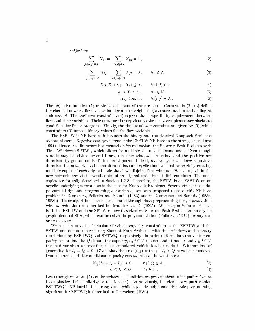
The objective function (1) minimizes the sum of the arc costs. Constraints (2){(3) de�ne

the classical network ow constraints for a path originating at source node o and ending at

sink node d. The nonlinear constraints (4) express the compatibility requirements between

ow and time variables. Their structure is very close to the usual complementary slackness

conditions for linear programs. Finally, the time window constraints are given by (5), while

constraints (6) impose binary values for the ow variables.

The ESPTW is NP-hard as it includes the binary and the classical Knapsack Problems

as special cases. Negative cost cycles render the ESPTW NP-hard in the strong sense (Dror

1994). Hence, the literature has focused on its relaxation, the Shortest Path Problem with

Time Windows (SPTW), which allows for multiple visits at the same node. Even though

a node may be visited several times, the time window constraints and the positive arc

durations tij

guarantee the �niteness of paths. Indeed, as any cycle will have a positive

duration, the network can be transformed into an acyclic time-oriented network by creating

multiple copies of each original node that have disjoint time windows. Hence, a path in the

new network may visit several copies of an original node, but at di�erent times. The node

copies are formally described in Section 1.2.2. Therefore, the SPTW is an ESPTW on an

acyclic underlying network, as is the case for Knapsack Problems. Several e�cient pseudo-

polynomial dynamic programming algorithms have been proposed to solve this NP-hard

problem in Desrosiers, Pelletier and Soumis (1983) and in Desrochers and Soumis (1988a,

1988b). These algorithms can be accelerated through data preprocessing (i.e., a priori time

window reduction) as described in Desrosiers et al. (1995). When ai= b

ifor all i 2 V ,

both the ESPTW and the SPTW reduce to a classical Shortest Path Problem on an acyclic

graph, denoted SPA, which can be solved in polynomial time (Fulkerson 1972) for any real

arc cost values.

We consider next the inclusion of vehicle capacity constraints in the ESPTW and the

SPTW and denote the resulting Shortest Path Problems with time windows and capacity

restrictions by ESPTWQ and SPTWQ, respectively. In order to formulate the vehicle ca-

pacity constraints, let Q denote the capacity, li, i 2 V the demand at node i and L

i, i 2 V

the load variables representing the accumulated vehicle load at node i. Without loss of

generality, let lo= l

d= 0. Given that the arcs (i; j) with l

i+ l

j> Q have been removed

from the arc set A, the additional capacity constraints can be written as:

Xij(L

i+ l

j� L

j) � 0 ; 8 (i; j) 2 A ; (7)

li� L

i� Q ; 8 i 2 V : (8)

Even though relations (7) can be written as equalities, we present them in inequality format

to emphasize their similarity to relations (4). As previously, the elementary path version

ESPTWQ is NP-hard in the strong sense, while a pseudo-polynomial dynamic programming

algorithm for SPTWQ is described in Desrochers (1986).


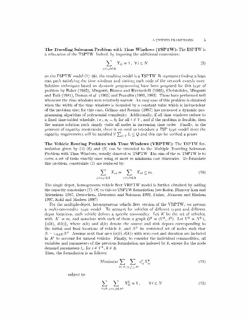
The Traveling Salesman Problem with Time Windows (TSPTW): The ESPTW is

a relaxation of the TSPTW. Indeed, by imposing the additional constraints:

Xj:(i;j)2A

Xij= 1 ; 8 i 2 N (9)

on the ESPTW model (1){(6), the resulting model is a TSPTW. It represents �nding a least

cost path satisfying the time windows and visiting each node of the network exactly once.

Solution techniques based on dynamic programming have been proposed for this type of

problem by Baker (1983), Mingozzi, Bianco and Ricciardelli (1993), Christo�des, Mingozzi

and Toth (1981), Dumas et al. (1995) and Psaraftis (1980, 1983). These have performed well

whenever the time windows were relatively narrow. An easy case of this problem is obtained

when the width of the time windows is bounded by a constant value which is independent

of the problem size; for this case, G�elinas and Soumis (1997) has proposed a dynamic pro-

gramming algorithm of polynomial complexity. Additionally, if all time windows reduce to

a �xed time-tabled schedule, i.e., ai= b

ifor all i 2 V , and if the problem is feasible, then

the unique solution path simply visits all nodes in increasing time order. Finally, in the

presence of capacity constraints, there is no need to introduce a TSP type model since the

capacity requirements will be satis�ed ifP

i2Vli� Q and this can be veri�ed a priori.

The Vehicle Routing Problem with Time Windows (VRPTW): The TSPTW for-

mulation given by (1){(6) and (9) can be extended to the Multiple Traveling Salesman

Problem with Time Windows, usually denoted m-TSPTW. The aim of the m-TSPTW is to

cover a set of tasks exactly once using at most m minimum cost itineraries. To formulate

this problem, constraints (2) are replaced by:

Xj:(o;j)2A

Xoj=X

i:(i;d)2A

Xid� m : (10)

The single depot, homogeneous vehicle eet VRPTW model is further obtained by adding

the capacity constraints (7){(8) to thism-TSPTW formulation (see Kolen, Rinnooy Kan and

Trienekens 1987, Desrochers, Desrosiers and Solomon 1992, Fisher, J�ornsten and Madsen

1997, Kohl and Madsen 1997).

For the multiple-depot, heterogeneous vehicle eet version of the VRPTW, we present

a multi-commodity type model. To account for vehicles of di�erent types and di�erent

depot locations, each vehicle de�nes a speci�c commodity. Let K be the set of vehicles,

with jKj = m, and associate with each of them a graph Gk = (V k; Ak). Let V k = Nk [

fo(k), d(k)g, where o(k) and d(k) denote the source and sink depots corresponding to

the initial and �nal locations of vehicle k, and Nk its restricted set of nodes such that

N = [k2KN

k. Assume next that arcs (o(k); d(k)) with zero cost and duration are included

in Ak to account for unused vehicles. Finally, to consider the individual commodities, all

variables and parameters of the previous formulation are indexed by k, except for the nodedemand parameters l

i, for i 2 V k, k 2 K.

Then, the formulation is as follows:

MinimizeXk2K

X(i;j)2Ak

ckijXk

ij(11)

subject to:

Xk2K

Xj:(i;j)2Ak

Xk

ij= 1 ; 8 i 2 N (12)

6

Xj:(o(k);j)2Ak

Xk

o(k);j =X

i:(i;d(k))2Ak

Xk

i;d(k) = 1 ; 8 k 2 K (13)

Xj:(i;j)2Ak

Xk

ij�

Xj:(j;i)2Ak

Xk

ji= 0 ; 8 k 2 K; 8 i 2 Nk (14)

Xk

ij(T ki+ tk

ij� T k

j) � 0 ; 8 k 2 K; 8 (i; j) 2 Ak (15)

aki� T k

i� bk

i; 8 k 2 K; 8 i 2 V k (16)

Xk

ij(Lk

i+ l

j� Lk

j) � 0 ; 8 k 2 K; 8 (i; j) 2 Ak (17)

li� Lk

i� Qk ; 8 k 2 K; 8 i 2 V k (18)

Xk

ijbinary; 8 k 2 K; 8 (i; j) 2 Ak : (19)

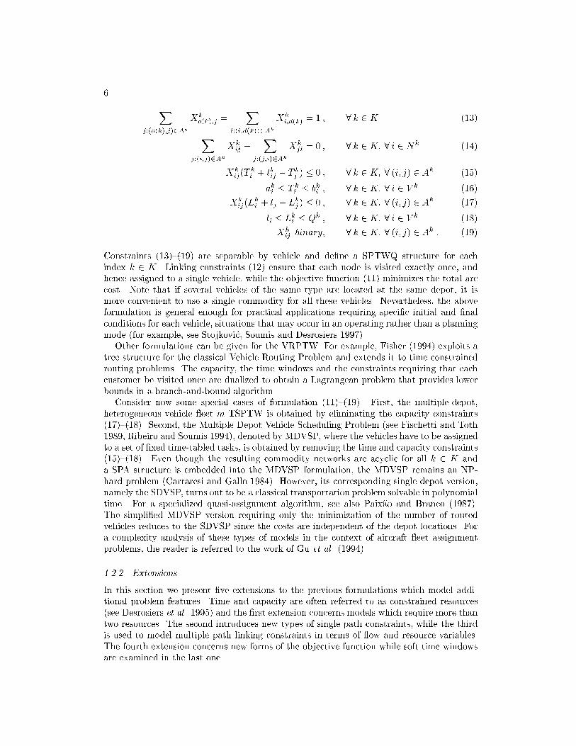
Constraints (13){(19) are separable by vehicle and de�ne a SPTWQ structure for each

index k 2 K. Linking constraints (12) ensure that each node is visited exactly once, and

hence assigned to a single vehicle, while the objective function (11) minimizes the total arc

cost. Note that if several vehicles of the same type are located at the same depot, it is

more convenient to use a single commodity for all these vehicles. Nevertheless, the above

formulation is general enough for practical applications requiring speci�c initial and �nal

conditions for each vehicle, situations that may occur in an operating rather than a planning

mode (for example, see Stojkovi�c, Soumis and Desrosiers 1997).

Other formulations can be given for the VRPTW. For example, Fisher (1994) exploits a

tree structure for the classical Vehicle Routing Problem and extends it to time constrained

routing problems. The capacity, the time windows and the constraints requiring that each

customer be visited once are dualized to obtain a Lagrangean problem that provides lower

bounds in a branch-and-bound algorithm.

Consider now some special cases of formulation (11){(19). First, the multiple-depot,

heterogeneous vehicle eet m-TSPTW is obtained by eliminating the capacity constraints

(17){(18). Second, the Multiple Depot Vehicle Scheduling Problem (see Fischetti and Toth

1989, Ribeiro and Soumis 1994), denoted by MDVSP, where the vehicles have to be assigned

to a set of �xed time-tabled tasks, is obtained by removing the time and capacity constraints

(15){(18). Even though the resulting commodity networks are acyclic for all k 2 K and

a SPA structure is embedded into the MDVSP formulation, the MDVSP remains an NP-

hard problem (Carraresi and Gallo 1984). However, its corresponding single depot version,

namely the SDVSP, turns out to be a classical transportation problem solvable in polynomial

time. For a specialized quasi-assignment algorithm, see also Paix~ao and Branco (1987).

The simpli�ed MDVSP version requiring only the minimization of the number of routed

vehicles reduces to the SDVSP since the costs are independent of the depot locations. For

a complexity analysis of these types of models in the context of aircraft eet assignment

problems, the reader is referred to the work of Gu et al. (1994).

1.2.2 Extensions

In this section we present �ve extensions to the previous formulations which model addi-

tional problem features. Time and capacity are often referred to as constrained resources

(see Desrosiers et al. 1995) and the �rst extension concerns models which require more than

two resources. The second introduces new types of single path constraints, while the third

is used to model multiple path linking constraints in terms of ow and resource variables.

The fourth extension concerns new forms of the objective function while soft time windows

are examined in the last one.


Multiple Resource Problems: Several resources, other than time and capacity, may be

speci�ed for a given problem. For example, crew scheduling problems in urban transit, rail

or airline contexts involve many other resource restrictions stemming from the respective

collective agreement speci�cations. Let Rk represent the resource set for commodity k,k 2 K. Several parameters and problem variables are resource dependent. Thus, let T kr

i2

[akri; bkri] denote the resource variable specifying the value of resource r 2 Rk accumulated

at node i 2 V k on commodity network k and let tkrij

be the consumption of that resource on

the arc (i; j) 2 Ak. When replacing the time and capacity constraints (15){(18) by the set

of resource constraints:

Xk

ij(T kri

+ tkrij� T kr

j) � 0 ; 8 k 2 K; 8 r 2 Rk; 8 (i; j) 2 Ak (20)

akri� T kr

i� bkr

i; 8 k 2 K; 8 r 2 Rk; 8 i 2 V k; (21)

we obtain a formulation of the Multiple Traveling Salesman Problem with Resource Con-

straints (m-TSPR). For m = 1, one can easily derive the Traveling Salesman Problem

with Resource Constraints (TSPR). Similarly, the resource constrained Shortest Path Prob-

lems ESPR and SPR can be obtained as extensions of the ESPTWQ and SPTWQ. The

SPR is NP-hard and the pseudo-polynomial dynamic programming algorithm described in

Desrochers (1986) can be used for its solution. Note that in most crew scheduling appli-

cations, the underlying networks Gk are acyclic, since the schedules are requested for �xed

time-tabled tasks. In such cases, the ESPR and SPR are equivalent as the solution of the

latter problem directly provides an elementary path.

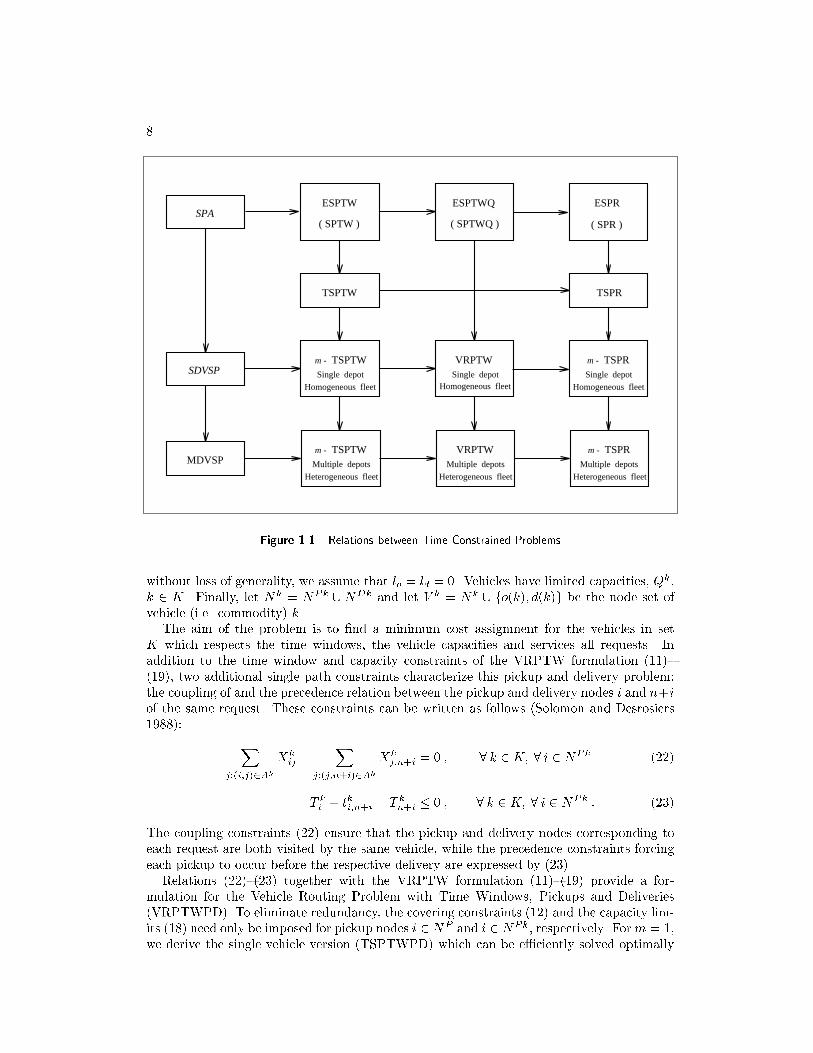
The relations between all previous problem types are illustrated in Figure 1.1. The �rst

row depicts time constrained Shortest Path Problems. The second row contains only two

single-vehicle TSP type problems. Finally, the last two rows illustrate multi-vehicle traveling

salesman problems with side constraints involving single/multiple depots and a homoge-

neous/

heterogeneous vehicle eet. Acronyms in italics denote problems solvable in polynomial time

(the SPA and SDVSP), while the problems ESPTW, ESPTWQ, ESPR, TSPTW, TSPR,

MDVSP, m-TSPTW, VRPTW and m-TSPR are NP-hard in the strong sense. Pseudo-

polynomial algorithms have been developed for three NP-hard time constrained Shortest

Path Problems on acyclic graphs, namely the SPTW, SPTWQ and SPR, which are written

in parenthesis in Figure 1.1. Arrows from left to right and from top to bottom portray an

increasing set of constraints.

Single Path Constraints: The resource constraints (20){(21) are called single path con-

straints because they are related to the feasibility of a single path, i.e., to a single commodity

k 2 K. Other types of single path constraints have been utilized in the literature and we

chose two important examples to discuss next. The �rst arises in pickup and delivery prob-

lems. The second is introduced to partially, or completely, eliminate cycles in non-elementary

shortest path problems. Finally, drawing from these examples, we propose a general form

of such single path constraints.

Consider the following pickup and delivery problem for which a set of transportation

requests has been speci�ed in advance. Each transportation request has two associated

nodes, one for the pickup and the other for the delivery. Without loss of generality, we

can assume that pickup and delivery nodes are di�erent from the depot nodes. Let N =

NP [ ND, where NP denotes the set of pickup nodes and ND denotes the set of delivery

nodes, with jNP j = jNDj = n. Next, for i 2 NP , let n + i 2 ND denote the associated

delivery node. Time windows and demands are speci�ed for all the nodes. Pickup nodes

have positive demands li, delivery nodes have negative demands l

n+i = �li, i 2 NP and,

8

SPAESPTWQ

( SPTWQ )

SDVSP

Homogeneous fleet

VRPTWSingle depot

VRPTWMultiple depots

Heterogeneous fleet

MDVSP

ESPTW

( SPTW )

TSPTW

ESPR

( SPR )

TSPR

Homogeneous fleet

Multiple depots

Heterogeneous fleet

Homogeneous fleet

Single depot

Multiple depots

Heterogeneous fleet

Single depot

m - TSPTW

m - TSPTW

m - TSPR

m - TSPR

Figure 1.1 Relations between Time Constrained Problems

without loss of generality, we assume that lo= l

d= 0. Vehicles have limited capacities, Qk,

k 2 K. Finally, let Nk = NPk [ NDk and let V k = Nk [ fo(k); d(k)g be the node set of

vehicle (i.e. commodity) k.The aim of the problem is to �nd a minimum cost assignment for the vehicles in set

K which respects the time windows, the vehicle capacities and services all requests. In

addition to the time window and capacity constraints of the VRPTW formulation (11){

(19), two additional single path constraints characterize this pickup and delivery problem:

the coupling of and the precedence relation between the pickup and delivery nodes i and n+iof the same request. These constraints can be written as follows (Solomon and Desrosiers

1988):

Xj:(i;j)2Ak

Xk

ij�

Xj:(j;n+i)2Ak

Xk

j;n+i = 0 ; 8 k 2 K; 8 i 2 NPk (22)

T ki+ tk

i;n+i � T kn+i � 0 ; 8 k 2 K; 8 i 2 NPk : (23)

The coupling constraints (22) ensure that the pickup and delivery nodes corresponding to

each request are both visited by the same vehicle, while the precedence constraints forcing

each pickup to occur before the respective delivery are expressed by (23).

Relations (22){(23) together with the VRPTW formulation (11){(19) provide a for-

mulation for the Vehicle Routing Problem with Time Windows, Pickups and Deliveries

(VRPTWPD). To eliminate redundancy, the covering constraints (12) and the capacity lim-

its (18) need only be imposed for pickup nodes i 2 NP and i 2 NPk, respectively. Form = 1,

we derive the single vehicle version (TSPTWPD) which can be e�ciently solved optimally


by dynamic programming whenever the time or capacity windows are relatively narrow

(Desrosiers, Dumas and Soumis 1986). Obviously, the Shortest Path Problems ESPTWPD

and SPTWPD can be similarly obtained as extensions of the ESPTWQ and SPTWQ, re-

spectively. An optimal dynamic programming algorithm for the SPTWPD is provided in

Dumas, Desrosiers and Soumis (1991).

The second example of additional single path constraints are the cycle elimination con-

straints. When negative cost cycles are present in the network, several copies of a task node

can be created in order to eliminate the cycles. These copies have disjoint time windows

obtained by partitioning the original time windows. Let now w 2 N represent a task to be

covered, and COPY k(w) denote the set of copy nodes of task w in Gk. There are at most

bkw� ak

w+ 1 such copies if the time related problem data is integer. To eliminate 2-cycles,

that is, path segments of the form i1 ! j ! i2 with i1; i2 2 COPY k(w), we must add the

following constraints to the path structure (13){(19):

Xi2COPY k(w)

(Xk

ij+Xk

ji) � 1 ; 8 k 2 K; 8 w; j 2 Nk : (24)

Appending these constraints to a resource constrained shortest path problem formulation

will help reduce the gap between the solution of the respective Shortest Path Problem and the

corresponding elementary Shortest Path Problem. Several papers report on algorithms and

results obtained by using this type of relations, such as Kolen, Rinnooy Kan and Trienekens

(1987), Desrochers, Desrosiers and Solomon (1992) and Kohl and Madsen (1997) for the

SPTWQ and Houck et al. (1980) for the classical Traveling Salesman Problem.

To achieve complete cycle elimination and to provide a formulation for the ESPTW on

the augmented network, created by adding all necessary node copies, the following stronger

constraint set must be satis�ed:Xi2COPY k(w)

Xj:(i;j)2Ak

Xk

ij� 1 ; 8 k 2 K; 8w 2 Nk : (25)

The use of the augmented network forces other constraints to be modi�ed accordingly. For

example, for the task covering constraints, relations (12) must be replaced by bundle type

constraints over the copies of an original task-node:

Xk2K

Xi2COPY k(w)

Xj:(i;j)2Ak

Xk

ij= 1 ; 8 w 2 N : (26)

Note that due to the computational burden involved, no e�cient algorithms using this type

of cycle elimination constraints have been developed to date.

From the above examples we can develop a general form of these single path constraints

that we give next. Let Lk, indexed by l, denote the set of single path constraints other than

the resource constraints (20){(21) and the usual ow conservation equations (13){(14). Let

dkrli

and dkl;ij

denote the coe�cients of the resource and ow variables, respectively, and dl

the right hand side value. General single path constraints can then be expressed as:

X(i;j)2Ak

dkl;ij

Xk

ij+Xi2V k

Xr2Rk

dkrliT kri

� dl; 8 k 2 K; 8 l 2 Lk : (27)

The ow variables permit these constraints to embed the cycle elimination constraints (24),

(25) and the coupling constraints (22), while the time variables allow constraints (27) to con-

tain the precedence constraints (23) as a special case. Other types of precedence relations

such as those required in Mingozzi, Bianco and Ricciardelli (1993) for TSP type problems

10

can be modelled using these general single path constraints. Finally, note that constraints of

the same form as (27) were obtained by several authors when linearizing the compatibility

constraints between the ow and resource variables (20).

Multiple Path Linking Constraints: The third extension focuses on constraints involv-

ing several commodities k 2 K, called linking constraints. Let H , indexed by h, denote theset of these additional constraints other than the usual covering constraints (12). Further

letting bkh;ij

denote the coe�cient of variable Xk

ijin constraint h and b

hits right hand side

value, a special case of these constraints can be formulated as:

Xk2K

X(i;j)2Ak

bkh;ij

Xk

ij� b

h; 8 h 2 H : (28)

This type of constraint is needed to model multiple path ow requirements. For example, if

cycle elimination constraints (24) or (25) are not imposed in the path structure corresponding

to each commodity k, then the classical subtour elimination constraints:

Xk2K

Xi2N 0

Xj2NnN 0

Xk

ij� 1 ; 8N 0

� N; 2 � jN 0j � jN j � 1 (29)

can be used. Such constraints have been used by Langevin et al. (1993) for the TSPTW

and by Fisher (1994) and Kohl et al. (1997) for the VRPTW. Additionally, such multiple

path constraints are used to restrict the eet size (see Desrosiers et al. 1995) or the eet

composition in vehicle routing problems, and as base constraints related to the number of

available crews in the airline context.

A more general form of constraints (28) links together the ow and resource variables.

Given that bkrhi

denotes the coe�cient of variable T kri

in constraint h, these constraints canbe written as:

Xk2K

X(i;j)2Ak

bkh;ij

Xk

ij+Xk2K

Xi2V k

Xr2Rk

bkrhiT kri

� bh; 8 h 2 H : (30)

Such constraints are useful in periodic aircraft routing and scheduling with time windows

(Desaulniers et al. 1997b), in airline schedule synchronization (Ioachim et al. 1994) and in

applications with sliding time windows (Ferland and Fortin 1989). The use of constraints

(30) forces the resource window restrictions (21) to be replaced by relations:

akri� T kr

i� bkr

i; 8k 2 K;8r 2 Rk;8i 2 fo(k); d(k)g (31)

akri(X

j:(i;j)2Ak

Xk

ij) � T kr

i� bkr

i(X

j:(i;j)2Ak

Xk

ij) ; 8k 2 K;8r 2 Rk;8i 2 Nk : (32)

For a given k, constraints (32) impose that T kri

= 0, 8 r 2 Rk wheneverP

j:(i;j)2Ak Xk

ij= 0,

k 2 K and i 2 Nk, that is, only the nodes within a single solution path in Gk contribute to

resource coe�cients in the constraint set (30).

Objective Functions: More general objective functions have been reported in the lit-

erature, especially for Shortest Path Problems. Several examples include (33){(36) given

below. Xr2Rk

X(i;j)2Ak

g(T kri)ckijXk

ij; (33)


where ckijare real parameters, g is a positive non-decreasing function and T kr

iare resource

variables; for example, g(Lki) denotes a function of the total load transported in a vehicle k

when it leaves node i in a VRPTWPD model (Dumas, Desrosiers and Soumis 1991).

X(i;j)2Ak

ckijXk

ij+Xi2V k

Xr2Rk

ckriT kri; (34)

where ckijand ckr

iare real parameters and T kr

iare resource variables. Such an objective func-

tion may be encountered when linking constraints (30) together with (12) are Lagrangean

relaxed. See Desaulniers et al. (1997b) for applications in periodic aircraft routing and

scheduling problems with time windows. When a single resource is used, namely time, an

optimal dynamic programming algorithm for the Shortest Path Problem with Time Win-

dows and Time Costs has been proposed in Ioachim et al. (1997). For the special case of

this problem where the path is �xed, several polynomial algorithms have been suggested to

�nd the optimal schedule by Sexton and Bodin (1985), Sexton and Choi (1986) and Dumas,

Desrosiers and Soumis (1990). Finally, using this type of objective function for the TSPTW,

G�elinas (1997) presents an application to job-shop scheduling.

X(i;j)2Ak

ckijXk

ij+ g(T k1

d(k); : : : ; TkjR

kj

d(k)); (35)

where ckijare real parameters and g is a non-decreasing function of the resource variables

T krd(k)

, r 2 Rk, at the sink node d(k). The cost of a crew duty in bus driver scheduling

problems falls in this category (Desrochers et al. 1992).

X(i;j)2Ak

ckijXk

ij+Xi2V k

Xr2Rk

gkri(T kri)X

j:(i;j)2Ak

Xk

ij; (36)

where ckijare real parameters, gkr

iare non-decreasing functions and T kr

iare resource vari-

ables. An example is provided by cost functions in airline crew pairing problems. Since a

pairing involves several duty periods, the cost may depend on resource values at the end of

each duty period, in addition to depending on resource values at the end of the pairing.

Soft Time Windows: Several papers (Koskosidis, Powell and Solomon 1992, Sexton and

Choi 1986) have considered soft time windows to derive feasible solutions to problems where

hard time windows are too restrictive. In such cases the �xed interval for a given resource

variable T kri

is replaced by a penalty function gkri

which determines the penalty to be

incurred whenever the resource variable is not within a target value range at node i 2 Nk.

For shortest path type problems, if the penalty functions are piecewise linear, an optimal

solution can be found using the algorithm presented in Ioachim et al. (1997). Nondecreasing

functions on nodes and arcs constitute another simple case since the solution is given by the

smallest feasible resource values at each node on a path (see Section 1.4.2). Hence, for an

arbitrary nonlinear penalty function, only the intervals where the function is decreasing pose

a problem. If they are reasonably narrow, these can be approximated by linear functions or

discretized for optimal solutions.

1.3 A UNIFIED FORMULATION

In the previous section, starting from simple scheduling problems we gradually introduced

additional constraints to model more complex situations. In this section we present a for-

mulation which encompasses all these constraints. To describe this model we consider a

12

di�erent type of time-space network where the tasks to be covered are positioned on the

arcs. An arc may represent a single activity or a series of activities. Furthermore, the

same task can appear on several arcs. As examples, consider network representations of

crew pairing problems appearing in airline and urban transit contexts where a task ( ight

leg/trip leg) can be found on several duty arcs (Lavoie, Minoux and Odier 1988, Desrochers

et al. 1992, Desaulniers et al. 1997a). The nodes represent sites at di�erent moments in

time such as the beginning and the end of any activity. The task-on-node problem formula-

tions introduced in Section 1.2 can be transformed into task-on-arc formulations by simply

associating a given task with all the arcs entering the respective task node.

On the one hand, the more general task-on-arc formulation presented next permits to

include in the network model some constraints on the path structure required by an appli-

cation. To do so, it is su�cient to include in the network all the arcs corresponding to the

task sequences satisfying these constraints and to exclude all other arcs covering these same

tasks. On the other hand, in some cases, a large subnetwork derived from path enumeration

can be replaced by an aggregated subnetwork of smaller size which uses less activities by arc

and less intermediate nodes. Examples are provided by the time-line networks used for crew

pairing and aircraft routing applications where the number of arcs becomes linear in terms

of the number of tasks to cover (Levin 1971, Soumis, Ferland and Rousseau 1980, Barnhart

et al. 1994a, and Desrosiers et al. 1995). For each application, the trade o� between path

enumeration and network aggregation is the determining factor for the computational e�-

ciency of the solution algorithms.

Notation and Formulation: Let N , indexed by w, represent the set of tasks to cover andnwthe number of times that task w must be covered. Applications where a task has to be

covered more than once are encountered, for example, in rostering, bidline and locomotive

assignment contexts (see Gamache et al. 1997a, Ziarati et al. 1997). Let again K represent

the set of commodities and Gk = (V k; Ak) be an acyclic network associated with k 2 K,

where V k = Nk [ fo(k); d(k)g is the node set and Ak is the arc set. Note that with the

task-on-arc network representation, nodes in Nk no longer represent tasks to cover, but only

time-space sites. Let further Rk be the set of resources speci�c to commodity k. Using thepreviously introduced ow and resource variables, let Xk = (Xk

ijj (i; j) 2 Ak) denote the

ow variable array, and T k

i= (T kr

ij r 2 Rk), i 2 V k the resource variable arrays. Next, let

akw;ij

designate the binary coe�cient of the ow variable Xk

ij, 1 if arc (i; j) 2 Ak covers task

w and 0 otherwise, for k 2 K. Finally, let S denote a set of additional variables Ystaking

values in [as; bs], for s 2 S. In addition to the notation used in the previous section, new

de�nitions are needed to model the more general constraints of the uni�ed model: T k0d(k)

is

the cost function for commodity k evaluated by using a resource indexed r = 0 in network

Gk, k 2 K; aws, b

hsare the coe�cients of the variable Y

s, s 2 S in the task covering

constraint w 2 N and in the linking constraint h 2 H , respectively; fkrij

is a function used

for the resource extension from node i to node j, (i; j) 2 Ak for resource r 2 Rk and ow of

type k 2 K. The importance and utilization of this type of function is given below.

With this notation, the uni�ed model can be presented as a nonlinear mixed-integer

program:

MinimizeXk2K

T k0d(k) +

Xs2S

csYs

(37)

subject to:

Xk2K

X(i;j)2Ak

akw;ij

Xk

ij+Xs2S

awsYs= n

w; 8 w 2 N (38)


Xk2K

X(i;j)2Ak

bkh;ij

Xk

ij+Xk2K

Xi2V k

Xr2Rk

bkrhiT kri+Xs2S

bhsYs= b

h; 8 h 2 H (39)

as� Y

s� b

s; 8s 2 S (40)X

j:(o(k);j)2Ak

Xk

o(k);j = 1; 8 k 2 K (41)

Xj:(i;j)2Ak

Xk

ij�

Xj:(j;i)2Ak

Xk

ji= 0; 8 k 2 K; 8 i 2 Nk (42)

Xj:(j;d(k))2Ak

Xk

j;d(k) = 1; 8 k 2 K (43)

Xk

ij(fkrij(T k

i;T k

j)� T kr

j) � 0; 8 k 2 K; 8 r 2 Rk; 8 (i; j) 2 Ak (44)

akri� T kr

i� bkr

i; 8 k 2 K; 8 r 2 Rk; 8 i 2 fo(k); d(k)g (45)

akri(X

j:(i;j)2Ak

Xk

ij) � T kr

i� bkr

i(X

j:(i;j)2Ak

Xk

ij); 8 k 2 K; 8 r 2 Rk; 8 i 2 Nk (46)

X(i;j)2Ak

dkl;ij

Xk

ij+Xi2V k

Xr2Rk

dkrliT kri

� dl; 8 k 2 K; 8 l 2 L (47)

Xk

ijbinary; 8 k 2 K; 8 (i; j) 2 Ak : (48)

The analysis of this formulation focuses on three new aspects: the objective function,

the new variables and the resource extension functions. The objective function (37) seeks

to minimize the total cost incurred. Examples of both linear and nonlinear functions have

been presented in Section 1.2.2. Given the above de�nition of the cost function, its value is

completely computed at the sink node d(k). Therefore, all nonlinearities are moved into the

subproblem structure and are now part of the resource extension functions fk0ij. Additional

aspects of the cost function are discussed in Section 1.4.2.

Several applications use the additional variables Ys, s 2 S, appearing in constraints

(38){(40). In constraint set (38), these may represent slack variables used for task under

or over covering (Barnhart et al. 1994a, Graves et al. 1993, Desaulniers et al. 1997a,

Ziarati et al. 1997) and associated penalty costs may be speci�ed in the objective function.

Constraints of type (39) are a more general version of constraints (28) and (30) which also

involve the additional variables Ys. Consider an example where constraints (28) are used

to control the eet size; one additional variable Yscan be used to represent the number

of vehicles required in a solution. Thus, this variable Yscan be used during the solution

process to impose lower and upper integer bounds on the eet size. As another example,

constraints linking time variables and additional variables Yswere introduced for a weekly

eet assignment problem with ight synchronization constraints in Ioachim et al. (1994).

These variables were used to model special time restrictions stating that each occurrence

of a given origin-destination ight leg had to start at the same time, within a certain time

window, each day of the week. Note that constraints (39) are a more general form of the

covering constraints (38) and, depending on the application, only one of these two sets may

be needed. Finally, constraints (40) give the set of admissible values for the additional

variables for which integrality requirements may also be imposed.

The resource extension function introduced in this formulation leads to a new expression

(44) of the previous resource constraints (20). This function, fkrij(T k

i;T k

j), may be linear

or nonlinear and it may depend of several resources. The particular case involving a single

14

resource variable, that is, fkrij(T kri) = T kr

i+ tkr

ijfor all r 2 Rk, has been discussed in Section

1.2.2. An example of a nonlinear resource extension function is presented next. Other than

(44), the remainder of the constraints were discussed in Section 1.2.

The VRPTW with Simultaneous Pickups and Deliveries: We consider the simulta-

neous pickup and delivery problem (Min 1989) to describe a nonlinear form of a resource

extension function fkrij

dependent of resource vector T k

i. In this problem, vehicles starting

with an unknown load at the source depot must visit nodes having both pickup and delivery

requests. We focus our analysis on the capacity constraints. For this, we de�ne non-negative

load values lPifor pickups and lD

ifor deliveries, for all nodes i 2 N . Two types of resource

variables can be associated with the capacity constraints (see G�elinas 1990 and Halse 1992):

Lki, which denotes the usual load accumulated at the visited pickup nodes from the source

node o(k) up to node i, and MaxLki, which denotes the maximum load carried at some

point by the vehicle since its departure from the source depot up to node i, for all k 2 Kand i 2 Nk. These variables have the following bounds:

lPi� Lk

i� Qk ; 8k 2 K; 8 i 2 Nk (49)

max(lPi; lDi) �MaxLk

i� Qk ; 8 k 2 K; 8 i 2 Nk : (50)

Let fk1ij

and fk2ij

denote the resource extension functions, for the two resources, respec-

tively. The load accumulated in the vehicle at node j is computed using solely the �rst

resource variable:

fk1ij(Lk

i;MaxLk

i) = fk1

ij(Lk

i) = Lk

i+ lP

j; 8 k 2 K ; 8 (i; j) 2 Ak : (51)

However, the maximal load ever accumulated in the vehicle must also account for deliveries.

Hence its resource extension function must depend on both capacity resource variables:

fk2ij(Lk

i;MaxLk

i) = max fLk

i+ lP

j;MaxLk

i+ lD

jg; 8 k 2 K ; 8 (i; j) 2 Ak : (52)

A special case of this problem is the VRPTW with backhauls. Its associated resource

extension function can be easily derived from (51){(52) since the nodes are either pickups

or deliveries. In addition, for simple backhauling where a vehicle �rst performs all the

deliveries before starting to visit the pickup nodes, only one capacity variable is required as

the problem can be modeled as a VRPTW (G�elinas et al. 1995).

For simplicity, we have used the simultaneous pickup and delivery problem to illustrate

the use of resource extension functions dependent of multiple resource variables. However,

these are often encountered for crew scheduling problems arising in airline, urban and rail

transit situations where the cost function depends on several resources. In such cases, the

cost itself can be de�ned as a resource and the incurred cost of a path is evaluated using

resource extension functions.

The above uni�ed model is general enough to include all the deterministic problem types

presented in the classi�cation scheme of Desrochers, Lenstra and Savelsbergh (1990) as spe-

cial cases. It also includes problems for which the solution can be represented as a set of

paths on a graph of all possible states of the commodities. Therefore, applications involving

a Knapsack Problem structure can be modelled by using this uni�ed formulation. Such ap-

plications include the Bin Packing Problem, i.e., the binary Cutting-Stock Problem (Vance

et al. 1994), the Generalized Assignment Problem (Savelsbergh 1993), graph coloring prob-

lems (Mehrorta and Trick 1993), and even the classical Cutting-Stock Problem (Gilmore

and Gomory 1961). This last problem can also be formulated as a Vehicle Routing Problem

in which the vehicles and their capacities correspond to the large rolls to be cut into smaller


rolls (called items) and their widths, respectively; the customers and their demands corre-

spond to the items and their widths, respectively; and the vehicle routes are the cutting

patterns. These patterns are obtained by solving a Knapsack Problem which is formulated

as a constrained Shortest Path Problem on an acyclic graph with a capacity window on the

sink node. As a further illustration, we next show how a formulation for the VRPTW with

split deliveries can be derived from our model.

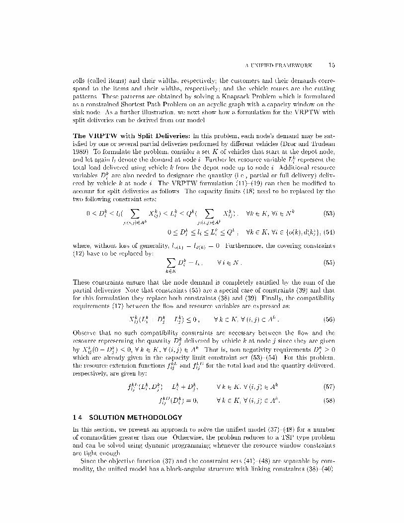
The VRPTW with Split Deliveries: In this problem, each node's demand may be sat-

is�ed by one or several partial deliveries performed by di�erent vehicles (Dror and Trudeau

1989). To formulate the problem, consider a set K of vehicles that start at the depot node,

and let again lidenote the demand at node i. Further let resource variable Lk

irepresent the

total load delivered using vehicle k from the depot node up to node i. Additional resourcevariables Dk

iare also needed to designate the quantity (i.e., partial or full delivery) deliv-

ered by vehicle k at node i. The VRPTW formulation (11){(19) can then be modi�ed to

account for split deliveries as follows. The capacity limits (18) need to be replaced by the

two following constraint sets:

0 � Dk

i� l

i(X

j:(i;j)2Ak

Xk

ij) � Lk

i� Qk(

Xj:(i;j)2Ak

Xk

ij) ; 8k 2 K; 8i 2 Nk (53)

0 � Dk

i� l

i� Lk

i� Qk ; 8k 2 K; 8i 2 fo(k); d(k)g; (54)

where, without loss of generality, lo(k) = l

d(k) = 0. Furthermore, the covering constraints

(12) have to be replaced by: Xk2K

Dk

i= l

i; 8 i 2 N : (55)

These constraints ensure that the node demand is completely satis�ed by the sum of the

partial deliveries. Note that constraints (55) are a special case of constraints (39) and that

for this formulation they replace both constraints (38) and (39). Finally, the compatibility

requirements (17) between the ow and resource variables are expressed as:

Xk

ij(Lk

i+Dk

j� Lk

j) � 0 ; 8 k 2 K; 8 (i; j) 2 Ak : (56)

Observe that no such compatibility constraints are necessary between the ow and the

resource representing the quantity Dk

jdelivered by vehicle k at node j since they are given

by Xk

ij(0 �Dk

j) � 0, 8 k 2 K, 8 (i; j) 2 Ak . That is, non-negativity requirements Dk

j� 0

which are already given in the capacity limit constraint set (53){(54). For this problem,

the resource extension functions fkLij

and fkDij

for the total load and the quantity delivered,

respectively, are given by:

fkLij

(Lki; Dk

j) = Lk

i+Dk

j; 8 k 2 K; 8 (i; j) 2 Ak (57)

fkDij

(Dk

i) = 0; 8 k 2 K; 8 (i; j) 2 Ak: (58)

1.4 SOLUTION METHODOLOGY

In this section, we present an approach to solve the uni�ed model (37){(48) for a number

of commodities greater than one. Otherwise, the problem reduces to a TSP type problem

and can be solved using dynamic programming whenever the resource window constraints

are tight enough.

Since the objective function (37) and the constraint sets (41){(48) are separable by com-

modity, the uni�ed model has a block-angular structure with linking constraints (38){(40).

16

Therefore a natural way to solve it is to use a decomposition approach such as Dantzig-Wolfe

decomposition (Dantzig and Wolfe 1960) or Lagrangean Relaxation (see Geo�rion 1974) to

obtain lower bounds to be used within a branch-and-bound framework. Even though these

are equivalent primal and dual decomposition approaches, we have chosen to present an

extension of the former. This is because this column generation type approach is the most

widely encountered methodology in the time constrained vehicle routing and scheduling

literature.

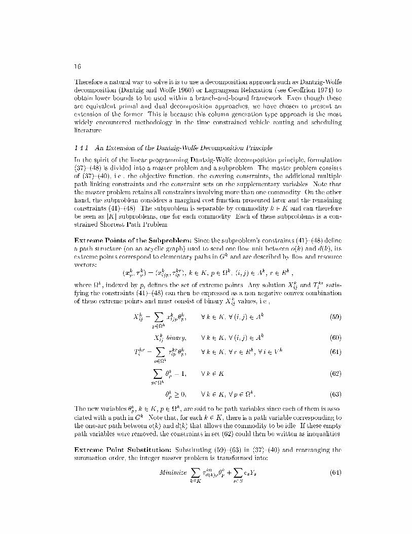
1.4.1 An Extension of the Dantzig-Wolfe Decomposition Principle

In the spirit of the linear programming Dantzig-Wolfe decomposition principle, formulation

(37){(48) is divided into a master problem and a subproblem. The master problem consists

of (37){(40), i.e., the objective function, the covering constraints, the additional multiple

path linking constraints and the constraint sets on the supplementary variables. Note that

the master problem retains all constraints involving more than one commodity. On the other

hand, the subproblem considers a marginal cost function presented later and the remaining

constraints (41){(48). The subproblem is separable by commodity k 2 K and can therefore

be seen as jKj subproblems, one for each commodity. Each of these subproblems is a con-

strained Shortest Path Problem.

Extreme Points of the Subproblem: Since the subproblem's constraints (41){(48) de�ne

a path structure (on an acyclic graph) used to send one ow unit between o(k) and d(k), itsextreme points correspond to elementary paths in Gk and are described by ow and resource

vectors:

(xkp; � k

p) = (xk

ijp; �krip); k 2 K; p 2 k; (i; j) 2 Ak; r 2 Rk ;

where k, indexed by p, de�nes the set of extreme points. Any solution Xk

ijand T kr

isatis-

fying the constraints (41){(48) can then be expressed as a non-negative convex combination

of these extreme points and must consist of binary Xk

ijvalues, i.e.,

Xk

ij=Xp2k

xkijp�kp; 8 k 2 K; 8 (i; j) 2 Ak (59)

Xk

ijbinary; 8 k 2 K; 8 (i; j) 2 Ak (60)

T kri

=Xp2k

�krip�kp; 8 k 2 K; 8 r 2 Rk; 8 i 2 V k (61)

Xp2k

�kp= 1; 8 k 2 K (62)

�kp� 0; 8 k 2 K; 8 p 2 k: (63)

The new variables �kp, k 2 K, p 2 k, are said to be path variables since each of them is asso-

ciated with a path in Gk . Note that, for each k 2 K, there is a path variable corresponding to

the one-arc path between o(k) and d(k) that allows the commodity to be idle. If these emptypath variables were removed, the constraints in set (62) could then be written as inequalities.

Extreme Point Substitution: Substituting (59){(63) in (37){(40) and rearranging the

summation order, the integer master problem is transformed into:

MinimizeXk2K

�k0d(k)p�

k

p+Xs2S

csYs

(64)


subject to:Xk2K

Xp2k

(X

(i;j)2Ak

akw;ij

xkijp)�kp+Xs2S

awsYs= n

w; 8 w 2 N (65)

Xk2K

Xp2k

(X

(i;j)2Ak

bkh;ij

xkijp+Xi2V k

Xr2Rk

bkrhi�krip)�kp+Xs2S

bhsYs= b

h; 8 h 2 H (66)

as� Y

s� b

s; 8s 2 S (67)X

p2k

�kp= 1; 8 k 2 K (68)

�kp� 0; 8 k 2 K; 8 p 2 k (69)

Xk

ij=Xp2k

xkijp�kp; 8 k 2 K; 8 (i; j) 2 Ak (70)

Xk

ijbinary; 8 k 2 K; 8 (i; j) 2 Ak: (71)

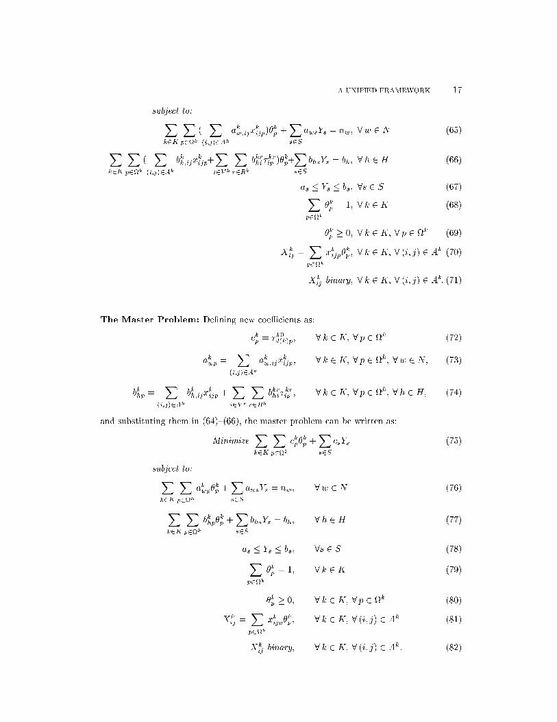
The Master Problem: De�ning new coe�cients as:

ckp= �k0

d(k)p; 8 k 2 K; 8 p 2 k (72)

akwp

=X

(i;j)2Ak

akw;ij

xkijp; 8 k 2 K; 8 p 2 k; 8w 2 N; (73)

bkhp

=X

(i;j)2Ak

bkh;ij

xkijp

+Xi2V k

Xr2Rk

bkrhi�krip; 8 k 2 K; 8 p 2 k; 8 h 2 H; (74)

and substituting them in (64){(66), the master problem can be written as:

MinimizeXk2K

Xp2k

ckp�kp+Xs2S

csYs

(75)

subject to:Xk2K

Xp2k

akwp�kp+Xs2S

awsYs= n

w; 8 w 2 N (76)

Xk2K

Xp2k

bkhp�kp+Xs2S

bhsYs= b

h; 8 h 2 H (77)

as� Y

s� b

s; 8s 2 S (78)

Xp2k

�kp= 1; 8 k 2 K (79)

�kp� 0; 8 k 2 K; 8 p 2 k (80)

Xk

ij=Xp2k

xkijp�kp; 8 k 2 K; 8 (i; j) 2 Ak (81)

Xk

ijbinary; 8 k 2 K; 8 (i; j) 2 Ak: (82)

18

In general, it is not true that binary restrictions on the Xk

ijarc variables can be replaced

by binary restrictions on the �kppath variables. However this statement holds when the coe�-

cients bkhp

are expressed solely in terms of the arc variable values, i.e., bkhp

=P

(i;j)2Ak

bkh;ij

xkijp.

In this case, since the de�nition of the original master problem solution space (37){(40) in-

volves only arc variables, binary requirements on these variables are equivalent to binary

requirements on path variables. Constraints (81) and (82) can therefore be removed.

In the general case, that is, when some coe�cients bkrhi

in (74) are di�erent from zero, the

solution part associated with commodity k may actually be fractional in terms of the path

variables while it corresponds to the same path with di�erent resource values. Hence, the arc

variables take binary values equal to 1 for all arcs in the selected path and 0 otherwise, and

no branching decisions are necessary. The optimal solution in terms of the resource variables

can therefore be computed as a non binary convex combination of the path variables using

relations (61).

An example of this situation is presented in Ioachim et al. (1994) for an aircraft rout-

ing problem that considers the synchronization of ight departures within their respective

time window. The branch-and-bound process is stopped as soon as the arc variables take

binary values even though there still remain fractional-valued path variables. Time variable

optimal values are then derived from (61). It appears that the optimal solutions for some

commodities cannot be obtained as subproblem extreme points.

Objective Function of the Subproblem: To describe the objective function of subprob-

lem k 2 K, let � = f�wj w 2 Ng, � = f�

hj h 2 Hg and = f k j k 2 Kg, be the vectors

of the dual variables associated with constraint sets (76), (77) and (79), respectively. The

reduced cost �ckp(�;�; ) of any path variable �k

pin function of vectors �, � and is given

by:

�ckp(�; �; ) = ck

p�Xw2N

akwp�w�Xh2H

bkhp�h� k

= �k0d(k)p �

X(i;j)2Ak

(Xw2N

akw;ij

�w+Xh2H

bkh;ij

�h)xkijp

�Xi2V k

Xr2Rk

(Xh2H

bkrhi�h)�krip� k:

This relation can then be used to write the objective function of subproblem k in terms

of the original ow and resource variables satisfying (41){(48):

Minimize T k0d(k) �

X(i;j)2Ak

(Xw2N

akw;ij

�w+Xh2H

bkh;ij

�h)Xk

ij�Xi2V k

Xr2Rk

(Xh2H

bkrh;i�h)T kri� k:

(83)

1.4.2 Algorithmic Issues

As described above, the uni�ed model (37){(48) can be transformed into the master problem

(75){(82) and the subproblem (41){(48) and (83). This transformation permits instead of

directly solving the former model, to solve the latter using a branch-and-bound algorithm.

The two key elements in the master problem solution process are the computation of lower

bounds and the selection of branching strategies. Regarding the subproblem solution, we

address special structures for the cost and resource extension functions. Finally, commodity

aggregation for identical subproblems is examined.


Master Problem Lower Bounds: At each branching node, a lower bound can be found

by solving the linear relaxation (75){(80) of the master problem (75){(82) using a column

generation technique. This consists of alternately solving a restricted linear master problem

and the subproblems until the solution of the latter proves that optimality has been reached

for the former. The role of the restricted linear master problem is to �nd the best solution

to the master problem while considering a relatively small number of variables. Hence, path

variables to be introduced in the restricted master problem are generated as needed. The

dual variables corresponding to this solution are then transferred to the subproblems. The

role of the subproblems is to �nd new path variables with negative reduced costs taking into

account the dual variables provided by the restricted linear master problem. If these exist,

the coe�cient columns associated with a subset of them are generated and transferred to

the restricted linear master problem that will be solved again. If no such path variables

exist, the solution process stops.

The restricted linear master problem is often degenerate in some applications and the

dual simplex method could be used in place of the primal simplex algorithm to accelerate

the solution process. Alternatively, a right hand side perturbation and other anti-cycling

techniques can be used to avoid degeneracy di�culties (see Wolfe 1963, Desrosiers, Soumis

and Desrochers 1984, and Falkner and Ryan 1988). Recent stabilization techniques involving

both perturbation and penalization strategies are described in du Merle et al. (1997) and

Hansen et al. (1997). Interior point methods can also be used to solve the restricted

linear master problem. The analytic center cutting plane method developed by (Go�n and

Vial 1996, Go�n et al.) is compatible with column generation approaches in the sense

that a warm start is possible when new variables are added. This method provides more

stable dual variables than the simplex algorithm (see also du Merle 1995). These methods

have a tendency to provide more stable dual variables. Since the master problem has a

block-angular structure, it can also be solved using specialized solution procedures such as

the generalized upper bounding procedure of Dantzig and Van Slyke (1967). This method

performs all the iterations of the simplex method on a working basis of reduced size. A

detailed description of it, in the context of multi-commodity ow models, is given in Barnhart

et al. (1991).

A lower bound can also be found using Lagrangean Relaxation. In this context, the

Lagrangean relaxed problem corresponds to the subproblem, while the Lagrangean Dual

problem has the same role as the restricted linear master problem in the Dantzig-Wolfe

decomposition. Their essential purpose is to provide dual multipliers for the subproblems. In

a Lagrangean Relaxation approach, the Lagrangean dual can be solved by either subgradient

optimization or by a bundle method. See LeMar�echal (1989) for a general description of the

method, and Kohl and Madsen (1997) for an application of it to the VRPTW. In the latter

case the dual variables are adjusted by quadratic programming. When they are solved to

optimality, these two dual methods produce the same lower bound on the master problem

as the Dantzig-Wolfe decomposition scheme. However, in practice, these dual methods are

stopped early to avoid expensive tailing-o� behavior.

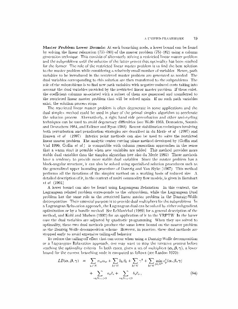
To reduce the tailing-o� e�ect that can occur when using a Dantzig-Wolfe decomposition

or a Lagrangean Relaxation approach, one may want to stop the iterative process before

reaching the optimality criteria. In both cases, given a set of multipliers (�; �; ), a lower

bound for the current branching node is computed as follows (see Lasdon 1970):

LB(�;�; ) =Xw2N

nw�w+Xh2H

bh�h+Xk2K

k +Xk2K

minp2k

�ckp(�; �; )

+X

s2S:�cs>0

as�cs+

Xs2S:�cs<0

bs�cs; (84)

20

where �csdenotes the reduced cost of supplementary variable Y

s. The last two components

of (84) account for the contribution of the supplementary variables to the lower bound. The

reader can also observe that the sum of the �rst two components is equal to the value of

the objective function for the current restricted master problem. Note that this is the usual

lower bound computed in a Lagrangean Relaxation approach since the multipliers will

cancel out between the third and fourth components of (84). At a given branching node,

the best lower bound is computed as the maximum over all the lower bounds obtained at

this node.

When the objective function consists solely in minimizing the number of commodities

used and no supplementary variables are involved in the formulation, the expression of the

lower bound takes a very simple form. Let n be the number of commodities used, zLP

the

objective value of the current restricted master problem and �cmin

the minimum path reduced

cost. Therefore, relation n � zLP

+ jKj�cmin

can be favorably replaced by n � zLP

+ n�cmin

to yield a better valid lower bound:

n � dzLP

=(1� �cmin

)e : (85)

This bounding procedure has been used successfully by Farley (1990) and Vance et al. (1994)

for various cutting stock problems.

A result on the quality of the master problem lower bound has been obtained when the

model reduces to a Set Partitioning Problem. In this case, Bramel and Simchi-Levi (1997)

showed that the relative gap between fractional and integer solutions becomes arbitrarily

small as the number of tasks to cover increases. This could make the branch-and-bound

process more e�cient.

Finally, we emphasize that the solution of a relaxed version of a constrained Shortest Path

Problem does not invalidate the solution process. For example, using the SPTW instead of

the ESPTW as a subproblem (or equivalently, using an expanded acyclic graph) only results

in a deterioration of the master problem lower bound. Columns which contain several copies

of the same tasks may appear in the master problem structure, but the branch-and-bound

decisions and the cutting strategies must eliminate them, as they cannot be part of any

optimal solution.

Branching and Cutting Strategies: Several papers report on the use of column genera-

tion techniques to optimally solve integer programs. Methods �nding k-best solutions wereproposed by Sweeney and Murphy (1979), Hansen, Minoux and Labb�e (1987), Hansen, Jau-

mard and Poggi de Arag~ao (1991, 1992) and Maculan, Michelon and Plateau (1992). The

paper of Holm and Tind (1988) looks in another direction and generalizes the Dantzig-Wolfe

decomposition principle to linear integer programs by means of concave, polyhedral price

functions. This method however requires to solve an integer restricted master program at

each main iteration.

Branch-and-bound, cuts and column generation have been combined several times in

various vehicle routing applications: Desrosiers, Soumis and Desrochers (1984) for the m-

TSPTW, Dumas, Desrosiers and Soumis (1991) for the VRPTWPD, Desrochers, Desrosiers

and Solomon (1992) for the VRPTW, and G�elinas et al. (1995) for the simple backhauling

problem with time windows. Other applications include bus drivers assignment (Desrochers

and Soumis 1989), frame decomposition for telecommunication by satellite (Ribeiro, Minoux

and Penna 1989), urban bus assignment (Ribeiro and Soumis 1994). Recent papers are those

on the binary cutting-stock problems (Vance et al. 1994), the generalized assignment prob-

lem (Savelsbergh 1993), graph coloring problems (Mehrorta and Trick 1993), the airline

crew pairing problem (Desaulniers et al. 1997a), the aircraft routing problem (Desaulniers

et al. 1997b) and the locomotive assignment problem (Ziarati et al. 1997). Vanderbeck and


Wolsey (1996) presents a general framework which extends a branching scheme proposed by

Ryan and Foster (1981) for the Set Partitioning Problem and additional results reported in

Barnhart et al. (1994b). In this paper, Vanderbeck and Wolsey develop a combined branch-

ing and subproblem modi�cation scheme: branching decisions are taken on the variables of

the column generation master problem while the subproblem necessitates the addition of

new variables and constraints to account for these decisions.

We propose a general and yet simple branching and cutting framework based on ow,

resource or supplementary variables, or on any weighted sum of these variables. When the

uni�ed model (37){(48) is solved by Lagrangean Relaxation (a dual approach), branching

decisions are naturally taken on ow Xk

ij, and when integrality is required, on resource T kr

i

or on supplementary Ysvariables. Flow-based branching decisions occur, for example, in

Fisher (1994) for the classical Vehicle Routing Problem and in Kohl and Madsen (1997) for

the VRPTW. When a Dantzig-Wolfe decomposition approach is applied, i.e., an equivalent

primal approach, the same branching and cutting strategies can be utilized. Furthermore,

designing branching decisions and cutting planes which are based on the original problem

variables becomes crucially important when general integer problems are solved using a

Dantzig-Wolfe decomposition scheme. As shown in Desrosiers et al. (1994), imposing in-

tegrality requirements on the master problem variables does not always result in a valid

formulation.

In our uni�ed model, general strategies based on the original variables are as follows.

On the one hand, if a decision involves more than one commodity, then this multiple path

decision can be written in the form of the linking constraints (39). As previously described,

such a constraint is transferred to constraint set (77) of the master problem, using substi-

tution equations (59) and (61). Through relation (77), the multiplier associated with this

constraint is adequately transferred to the arcs and nodes of the relevant subproblem net-

works as coe�cient for the ow and resource variables. On the other hand, if a decision

involves a single commodity, then it is a single path decision. Such a decision can be re-

stricted to a single subproblem. However, if it modi�es the subproblem structure, a new

specialized algorithm has to be used for solving it. This new algorithm may be one of the

several algorithms presented in Section 1.2 or may yet have to be designed. Alternatively,

any cumbersome single path constraint in set (47) may be left at the master problem level

since it is a special case of a constraint in set (39).

Next, we present several examples of branching and cutting decisions compatible with

the column generation approach proposed to solve the uni�ed model. We �rst present some

special multiple path linking decisions that can be treated at the subproblem level. We then

provide examples of branching decisions and cutting planes to be inserted at the master

problem level. We also give an example of a very strong cutting plane that acts locally at

the subproblem level. Finally, decisions involving resource and supplementary variables are

discussed.

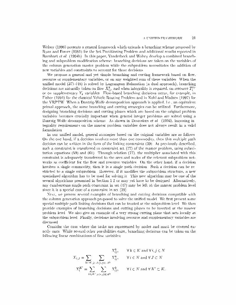
Consider the case where the tasks are represented by nodes and must be covered ex-

actly once. While several other possibilities exist, branching decisions can be taken on the

following linear combinations of ow variables:

Xk

ij; 8 k 2 K and 8 i; j 2 N

Xi;J

=Xk2K

Xj2J:(i;j)2Ak

Xk

ij; 8 i 2 N and 8 J � N

XK

0

i=Xk2K0

Xj:(i;j)2Ak

Xk

ij; 8 i 2 N and 8K 0

� K:

22

Variables Xk

ijand the linear combinations X

i;Jand XK

0

imust take binary values at opti-

mality since the tasks must be covered exactly once. Therefore, any such fractional-valued

binary variable can be set to 0 on one branch and to 1 on the other branch. Fixing Xk

ijat 1

corresponds to consecutively assigning tasks i and j to commodity k. Setting Xi;J

to 1 spec-

i�es that a task of subset J must be performed immediately after task i without identifyingthe commodity. In particular, if J contains a single task, then this task must immediately

follow task i. Finally, �xing XK

0

iat 1 implies that task i must be covered by a commodity of

subset K 0. In particular, if K 0 contains a single commodity, then this commodity must carry

out task i. Branching decisions on these multiple path linking constraints can be taken into

account in the subproblems without changing their mathematical structure. For example,

if variable Xi;fjg is �xed at 1, arcs (i; j0) 2 Ak, such as j0 6= j and (i0; j) 2 Ak such as i0 6= i

are removed from network Gk, 8k 2 K. If variable Xi;fjg is �xed at 0, the arc (i; j) 2 Ak is

removed from network Gk, 8k 2 K.

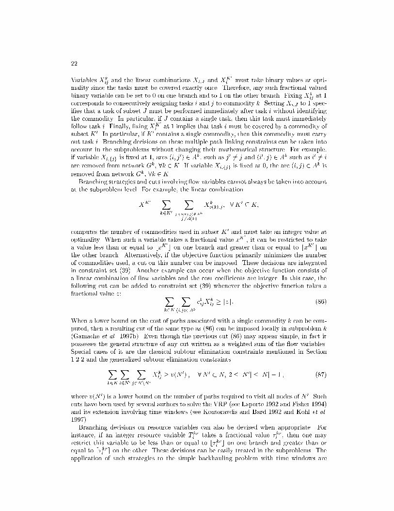
Branching strategies and cuts involving ow variables cannot always be taken into account

at the subproblem level. For example, the linear combination

XK

0

=Xk2K0

Xj:(o(k);j)2Ak

j 6=d(k)

Xk

o(k);j ; 8K 0� K;

computes the number of commodities used in subset K 0 and must take an integer value at

optimality. When such a variable takes a fractional value xK0

, it can be restricted to take

a value less than or equal to bxK0

c on one branch and greater than or equal to dxK0

e on

the other branch. Alternatively, if the objective function primarily minimizes the number

of commodities used, a cut on this number can be imposed. These decisions are integrated

in constraint set (39). Another example can occur when the objective function consists of

a linear combination of ow variables and the cost coe�cients are integer. In this case, the

following cut can be added to constraint set (39) whenever the objective function takes a

fractional value z: Xk2K

X(i;j)2Ak

ckijXk

ij� dze: (86)

When a lower bound on the cost of paths associated with a single commodity k can be com-puted, then a resulting cut of the same type as (86) can be imposed locally in subproblem k(Gamache et al. 1997b). Even though the previous cut (86) may appear simple, in fact it

possesses the general structure of any cut written as a weighted sum of the ow variables.

Special cases of it are the classical subtour elimination constraints mentioned in Section

1.2.2 and the generalized subtour elimination constraints

Xk2K

Xi2N 0

Xj2NnN 0

Xk

ij� v(N 0) ; 8N 0 � N; 2 � jN 0j � jN j � 1 ; (87)

where v(N 0) is a lower bound on the number of paths required to visit all nodes of N 0. Such

cuts have been used by several authors to solve the VRP (see Laporte 1992 and Fisher 1994)

and its extension involving time windows (see Kontoravdis and Bard 1992 and Kohl et al.

1997).

Branching decisions on resource variables can also be devised when appropriate. For

instance, if an integer resource variable T kri

takes a fractional value �kri, then one may

restrict this variable to be less than or equal to b�kric on one branch and greater than or

equal to d�krie on the other. These decisions can be easily treated in the subproblems. The

application of such strategies to the simple backhauling problem with time windows are


presented in G�elinas et al. (1995). A stronger type of resource branching decision is derived

for the aircraft schedule synchronization problem described in Ioachim et al. (1994). In this

case, supplementary variables are de�ned as Y r

i=Pk2K

T kri

and when such a variable Y r

i

takes a fractional value yri, then two branches are created as above using byr

ic and dyr

ie.

Since variable Y r

iis linked with a speci�c resource variable r, these decisions are locally

transferred at the subproblem level to all the corresponding T kri

variables, i.e., T kri

� byric

on one branch and T kri

� dyrie on the other. Moreover, this type of decision also applies

for an integer value of Y r

iif yr

iis obtained as a convex combination of several columns with

di�erent �krip

values: the two branches are then given by Y r

i� yr

i� 1 and Y r

i� yr

i.

Branching decisions involving resource variables which cannot be taken into account in the

subproblems can also be devised, since these decisions have the general form of constraints

(39). However, if the objective function of the subproblem did not contain any resource

variable before the addition of this type of constraint, the subproblem structure will be

modi�ed since its objective function will now contain resource variables (see Subproblem

Solution below).

In the uni�ed model (37){(48) where the tasks are represented by arcs on time-space

networks, most of the branching decisions and cuts described above are directly applicable

or need simple adaptations. Taking into account the speci�cs of each application, one can

devise other e�cient branching rules and cuts.

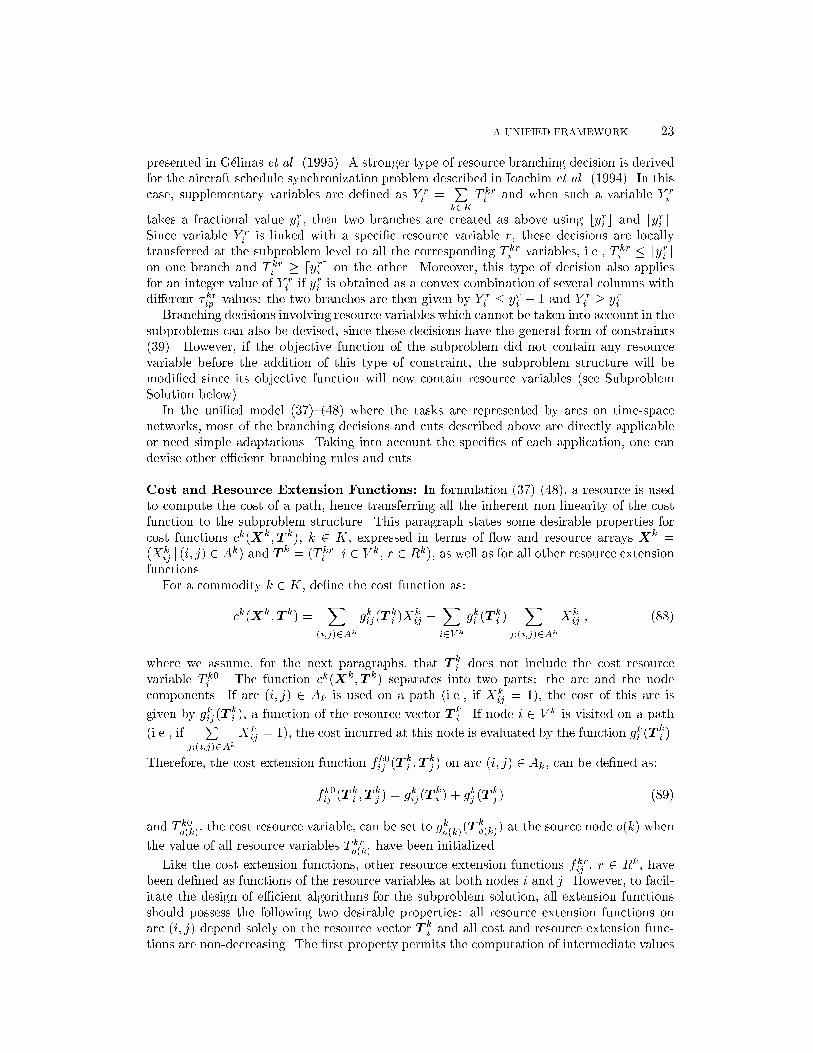
Cost and Resource Extension Functions: In formulation (37)-(48), a resource is used

to compute the cost of a path, hence transferring all the inherent non linearity of the cost

function to the subproblem structure. This paragraph states some desirable properties for

cost functions ck(Xk;T k), k 2 K, expressed in terms of ow and resource arrays Xk =

(Xk

ijj (i; j) 2 Ak) and T k = (T kr

ij i 2 V k; r 2 Rk), as well as for all other resource extension

functions.

For a commodity k 2 K, de�ne the cost function as:

ck(Xk;T k) =X

(i;j)2Ak

gkij(T k

i)Xk

ij+Xi2V k

gki(T k

i)X

j:(i;j)2Ak

Xk

ij; (88)

where we assume, for the next paragraphs, that T k

idoes not include the cost resource

variable T k0i. The function ck(Xk;T k) separates into two parts: the arc and the node

components. If arc (i; j) 2 Akis used on a path (i.e., if Xk

ij= 1), the cost of this arc is

given by gkij(T k

i), a function of the resource vector T k

i. If node i 2 V k is visited on a path

(i.e., ifP

j:(i;j)2Ak

Xk

ij= 1), the cost incurred at this node is evaluated by the function gk

i(T k

i).

Therefore, the cost extension function fk0ij(T k

i;T k

j) on arc (i; j) 2 A

k, can be de�ned as:

fk0ij(T k

i;T k

j) = gk

ij(T k

i) + gk

j(T k

j) (89)

and T k0o(k)

, the cost resource variable, can be set to gko(k)

(T k

o(k)) at the source node o(k) when

the value of all resource variables T kro(k)

have been initialized.

Like the cost extension functions, other resource extension functions fkrij, r 2 Rk, have

been de�ned as functions of the resource variables at both nodes i and j. However, to facil-itate the design of e�cient algorithms for the subproblem solution, all extension functions

should possess the following two desirable properties: all resource extension functions on

arc (i; j) depend solely on the resource vector T k

iand all cost and resource extension func-

tions are non-decreasing. The �rst property permits the computation of intermediate values

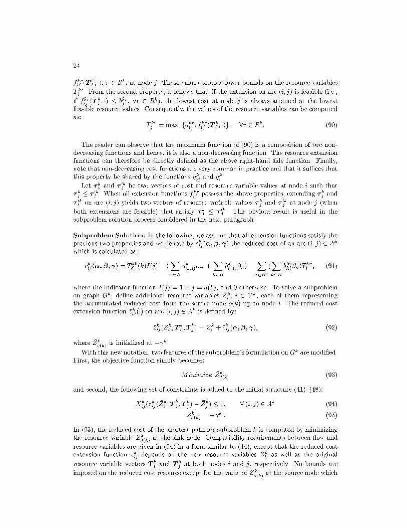
24

fkrij(T k

i; �), r 2 Rk, at node j. These values provide lower bounds on the resource variables

T krj. From the second property, it follows that, if the extension on arc (i; j) is feasible (i.e.,

if fkrij(T k

i; �) � bkr

j, 8r 2 Rk), the lowest cost at node j is always attained at the lowest

feasible resource values. Consequently, the values of the resource variables can be computed

as:

T krj

= max fakrij; fkrij(T k

i; �)g; 8r 2 Rk: (90)

The reader can observe that the maximum function of (90) is a composition of two non-

decreasing functions and hence, it is also a non-decreasing function. The resource extension

functions can therefore be directly de�ned as the above right-hand side function. Finally,

note that non-decreasing cost functions are very common in practice and that it su�ces that

this property be shared by the functions gkijand gk

i.

Let � kiand � 0k

ibe two vectors of cost and resource variable values at node i such that

� ki� � 0k

i. When all extension functions fkr

ijpossess the above properties, extending � k

iand

� 0kion arc (i; j) yields two vectors of resource variable values � k

jand � 0k

jat node j (when

both extensions are feasible) that satisfy � kj� � 0k

j. This obvious result is useful in the

subproblem solution process considered in the next paragraph.

Subproblem Solution: In the following, we assume that all extension functions satisfy the

previous two properties and we denote by �ckij(�;�; ) the reduced cost of an arc (i; j) 2 Ak

which is calculated as:

�ckij(�; �; ) = T k0

d(k)I(j) � (

Xw2N

akw;ij

�w+Xh2H

bkh;ij

�h)�Xr2Rk

(Xh2H

bkrhi�h)T kri; (91)

where the indicator function I(j) = 1 if j = d(k), and 0 otherwise. To solve a subproblem

on graph Gk, de�ne additional resource variables �Zki, i 2 V k, each of them representing

the accumulated reduced cost from the source node o(k) up to node i. The reduced cost

extension function �zkij(�) on arc (i; j) 2 Ak is de�ned by:

�zkij( �Zk

i;T k

i;T k

j) = �Zk

i+ �ck

ij(�;�; ); (92)

where �Zko(k)

is initialized at � k.

With this new notation, two features of the subproblem's formulation on Gk are modi�ed.

First, the objective function simply becomes:

Minimize �Zkd(k) (93)

and second, the following set of constraints is added to the initial structure (41){(48):

Xk

ij(zkij( �Zk

i;T k

i;T k

j)� �Zk

j) � 0; 8 (i; j) 2 Ak (94)

�Zko(k) = � k : (95)

In (93), the reduced cost of the shortest path for subproblem k is computed by minimizing

the resource variable �Zkd(k)

at the sink node. Compatibility requirements between ow and

resource variables are given in (94) in a form similar to (44), except that the reduced cost

extension function �zkij

depends on the new resource variables �Zkias well as the original

resource variable vectors T k

iand T k

jat both nodes i and j, respectively. No bounds are

imposed on the reduced cost resource except for the value of �Zko(k)

at the source node which


is given by (95). Note however that an upper bound of zero can be imposed on �Zkd(k)

since

the subproblem searches for negative reduced cost paths.

Even though the original cost function T kd(k)

and the subproblem objective function �Zkd(k)

are obviously non-decreasing, the reduced cost extension functions �zkijare not necessarily

non-decreasing. Indeed, it depends on the sign of the coe�cients (�Ph2H

bkrhi�h) of the

resource variables appearing in the last term de�ning the reduced cost of an arc (91). If

these coe�cients are all non negative, then the reduced cost extension functions are also non-

decreasing. This condition is satis�ed when no resource variables appear in the multiple path

constraints (39), i.e., bkrhi

= 0, 8 k 2 K; 8 i 2 V k; 8 r 2 Rk and 8 h 2 H .

When labelling algorithms are used to solve resource constrained problems, the labels

require the reduced cost component and an additional component for each resource. Hence,

the SPTW and the TSPTW use two-dimensional labels involving the reduced cost and the

time, while the SPTWQ involves three-dimensional labels. Starting at the sink node, these

algorithms iteratively construct paths in Gk which are stored as labels. Thus, each label

corresponds to a partial path from the origin node o(k) to the current node. It is representedby a vector containing a reduced cost component and jRkj components for the resources.

Let Ek

i= (��k

i; � k

i) denote such a (reduced cost, resource vector)-label corresponding to a

partial path ending at node i. Unlike classical labelling algorithms for unconstrained short-

est path problems, the resource constrained algorithms require to keep at each node all

multi-dimensional labels that are not dominated according to the following de�nition.

De�nition. Label Eidominates label E0

i, denoted E

i� E0

i, if and only if E

i� E0

i.

Under the three above conditions, the label dominance de�nition permits the elimination

of those labels that cannot be present in any optimal shortest path solution.

Proposition. Let Ek

iand E0k

ibe the labels associated with two partial paths from o(k) up

to node i in Gk. Let also Ek

jand E0k

jbe two feasible labels obtained from Ek

iand E0k

i,

respectively, by adding arc (i; j) 2 Ak. If all extension functions fkrij

are non-decreasing and

depend solely on the resource vector T k

i, and all coe�cients bkr

hi

= 0, then Ek

i� E0k

iyields

Ek

j� E0k

j.

Proof: On the one hand, the relation � ki� � 0k

iimplies that:

fkrij(� k

i; �) � fkr

ij(� 0k

i; �) (96)

and

�krj

= max(akrj; fkrij(� k

i; �)) � max(akr

j; fkrij(� 0k

i; �)) = �kr

j; 8 r 2 Rk: (97)

Hence, � kj� � 0k

j. On the other hand, the relation ��k

i� �� 0k

iimplies that:

��kj= �zk

ij(��ki; � k

i; � k

j) � �zk

ij(�� 0ki; � 0k

i; � 0k

j) = �� 0k

j: (98)

Relations (96) and (98) are direct consequences of the non-decreasing property of functions

fkrij, 8 r 2 Rk and �zk

ij, respectively. The second relation (97) also follows from the fact

that all of the reduced cost functions are non-decreasing: therefore, the lowest cost value is

attained for the smallest feasible resource values, i.e., either akrj

or the value computed by

using fkrij(�). Hence, (��k

j; � k

j) � (�� 0k

j; � 0k

j) and the result follows from the label dominance

de�nition.

For decreasing subproblem cost functions such as the ones encountered in applications

involving soft time windows (Koskosidis, Powell and Solomon 1992), ight departure syn-

chronization (Ioachim et al. 1994) or combined inventory and ship routing (Christiansen

26

1996), the label elimination process is more complex. As opposed to the previous case where

a label at node i is extended to at most one label at a successor node j (the new label may

be infeasible), several non-comparable new labels may need to be created when the cost ex-

tension function is decreasing in terms of (increasing) resource values. Ioachim et al. (1997)

provides an optimal algorithm when the �gki, i 2 V k, k 2 K are linear functions. As an

example of a relatively di�cult objective function in (37), consider the minimization of the

total duration (makespan) of all solution pathsXk2K

(T kd(k) � T k

o(k)) : (99)

For each subproblem k 2 K, the cost function involves a decreasing component in terms of

variable T ko(k) within the interval [ak

o(k); bk

o(k)]. However, this objective function is increasing

if the starting time T ko(k) is restricted to be equal to a single time-tabled value ak

o(k) = bko(k).

Alternatively to the method presented in Ioachim et al. (1997) for the case ako(k) 6= bk

o(k),

one can modify the initial network by discretizing the time window at node o(k). Hence,

the decreasing cost component is removed by creating several copies of the source node and

by assigning the resulting �xed cost directly to the new nodes.

Commodity Aggregation: When several commodities are identical, the variables corre-

sponding to these commodities can be aggregated to reduce the number of subproblems as

well as the number of variables and constraints in the master problem. To illustrate this

aggregation process, consider the linear relaxation (75){(80) of the master problem (75){

(82) and assume that all commodities are identical (otherwise, the aggregation process can

be performed separately on the various subsets of identical commodities). In this case, all

networks Gk, k 2 K, are identical and so are all sets of subproblem's extreme points k,

k 2 K. Denote this common set of extreme points by and the column coe�cients by cp

and awp

(i.e., = k, cp= ck

pand a

wp= ak

wp, 8 k 2 K). De�ne also new variables as:

�p=Xk2K

�kp; 8 p 2 :

Since the variables �kpare non-negative, the variables �

pcan only take non-negative values.

Furthermore, summing the constraints in set (79), we have:Xk2K

Xp2

�kp=Xk2K

1,Xp2

Xk2K

�kp= jKj ,

Xp2

�p= jKj : (100)

The linear relaxation (75){(80) is therefore equivalent to:

MinimizeXp2

cp�p+Xs2S

csYs

(101)

subject to:Xp2

awp�p+Xs2S

awsYs= n

w; 8 w 2 N (102)

Xp2

bhp�p+Xs2S

bhsYs= b

h; 8 h 2 H (103)

as� Y

s� b

s; 8s 2 S (104)

�p� 0; 8 p 2 (105)


�p=Xk2K

�kp; 8 p 2 (106)

Xp2

�kp= 1; 8 k 2 K (107)

�kp� 0; 8 k 2 K; 8 p 2 : (108)

For a solution to (101){(105) fractional in �p, there exists a solution in �k

pthat satis�es

(106){(108). Indeed, assume that �p, p 2 , is a solution to (101){(105) and assign to �k

p,

k 2 K, p 2 , the values:

�kp=

�p

jKj; 8 k 2 K; 8 p 2 :

By using (100), it is then easy to verify that this solution also satis�es (106){(108). Since

any solution consisting of the aggregated variables �p, p 2

p, can be converted into a

solution in terms of the disaggregated variables �kp, k 2 K, p 2 , the problem (101){(105)

can be used as the linear master problem. This aggregated linear master problem contains

jKj times less variables and has fewer constraints than the original one.

In the case where the solution of the aggregated linear master problem is integer, it is

possible to convert it to a binary solution in terms of the variables �kp. Indeed, assume

that �p, p 2 , is an integer solution to (101){(105). By (100), at most jKj variables �

p

are positive. Let �p1; �p2; : : : ; �

pnbe these variables. Next, assign path p1 to the �rst �

p1

commodities, path p2 to the next �p2, ..., and path p

nto the last �

pncommodities. These

assignments translate into the following mathematical expressions:

�kp1

=

�1 if 1 � k � �

p1

0 otherwise,

�kp2

=

�1 if �

p1+ 1 � k � �

p1+ �

p2

0 otherwise,

...

�kpn

=

8<:

1 ifn�1Pi=1

�pi+ 1 � k � jKj

0 otherwise,

�kp

= 0 if p 62 fp1; p2; : : : ; png and 1 � k � jKj.

One can verify that this solution also satis�es (106){(108). Finally, if the aggregated solution

is mixed integer, both of the above conversion processes need to be applied accordingly.

1.5 CONCLUSION

This paper has developed a much needed integrating framework for deterministic time con-

strained vehicle routing and crew scheduling problems. It consists of a more general model

than previously considered which encompasses all the important practical complexities ex-

amined to date in the literature. Each distinct type of problem explored so far in this

environment can be cast as a special instance of this uni�ed formulation. A number of prior

research e�orts have involved the direct application of di�erent forms of this model to solve

speci�c problem types in this class. Furthermore, approaches that have been based on a

Set Partitioning/Covering formulation and additional constraints customizing each unique

application represent indirect uses of the uni�ed model. In addition to consolidating the

most widely utilized time constrained vehicle routing and crew scheduling problem models,

28

this framework extends beyond this environment. Any problem for which the solution can

be expressed as a set of paths in a deterministic state-space graph can be formulated as a

special case of the proposed uni�ed model. As an example, this formulation can be used

to model one of the earliest application of column generation, namely the Cutting-Stock

Problem.

To solve the multi-commodity problems in this class, we have proposed a branch-and-

bound framework. The lower bounds are obtained by using a decomposition approach. This

exploits the special structure of these problems involving an objective function and many of

the constraints separable by commodity. While the framework leads to a number of algo-

rithmic choices for each module, we have concentrated on an extension of the Dantzig-Wolfe

decomposition principle. We have proved that it remains valid even when nonlinear objec-

tive functions and constraints are present. We have also shown that it is more general than

the prior column generation-based methods as is the compatible branching module used.

Finally, we have scanned the dynamic programming algorithms designed for the di�erent

constrained shortest path subproblems or the more general single commodity problems and

determined some needs for future research.

We believe that the framework proposed in this paper has uni�ed much of the previ-

ous research directed at deterministic time constrained vehicle routing and crew scheduling

problems. It is our hope that it will also constitute the basis for future approaches directed

at problems of larger size and at new application areas.

Acknowledgments

This research was supported by the Quebec Government (Programme Synergie du Fonds de D�evelop-

pement Technologique) and by the Natural Sciences and Engineering Council of Canada. Marius

M. Solomon was partially supported by the Patrick F. and Helen C. Walsh Research Professorship.

We would also like to thank Andreas N�ou from the Royal Institute of Technology, Stockholm, for

fruitful discussions regarding the paper.

References

Appelgren, L.H. A Column Generation Algorithm for a Ship Scheduling Problem. Trans-

portation Science, 3:53{98, 1969.

Appelgren, L.H. Integer Programming Methods for a Vessel Scheduling Problem. Trans-

portation Science, 5:64{78, 1971.

Baker, E. An Exact Algorithm for the Time Constrained Traveling Salesman Problem.

Operations Research, 31:938{945, 1983.

Barnhart, C., C.A. Hane, E.L. Johnson, and G. Sigismondi. An Alternative Formulation

and Solution Strategy for Multi-Commodity Network Flow Problems. Report COC-9102,

Georgia Institute of Technology, Atlanta, Georgia, 1991.

Barnhart, C., L. Hatay, and E.L. Johnson. Deadhead Selection for the Long-Haul Crew

Pairing Problem. Operations Research, 43:491{499, 1995.

Barnhart, C., E.L. Johnson, R. Anbil, and L. Hatay. A Column Generation Technique for the

Long-Haul Crew Assignment Problem. In T.A. Ciriani and R. Leachman (eds.), Mathe-

matical Programming and Modeling Techniques in Practice, Optimization in Industry 2.

John Wiley and Sons, New-York, 7{22, 1994a.

Barnhart, C., E.L. Johnson, G.L. Nemhauser and, M.W.P. Savelsbergh. Branch and Price:

Column Generation for Solving Huge Integer Programs. Computational Optimization

Center, COC{94{03, Georgia Institute of Technology, Atlanta, 1994b.

Bodin, L. and B. Golden. Classi�cation in Vehicle Routing and Scheduling. Networks, 11:97{

108, 1981.


Bodin, L., B. Golden, A. Assad, and M. Ball. Routing and Scheduling of Vehicles and Crews:

The State of the Art. Computers and Operations Research, 10:62{212, 1983.

Bramel, J. and D. Simchi-Levi. On the E�ectiveness of Set Coveringing Formulations for the

Vehicle Routing Problem with Time Windows. Operations Research, 45:295{301, 1997.

Carraresi, P. and G. Gallo. Network Models for Vehicle and Crew Scheduling. European

Journal of Operations Research, 16:139{151, 1984.

Christiansen, M. Inventory and Time Constrained Ship Routing - A Mathematical Approach.

Ph.D. Dissertation, Norvegian University of Science and Technology, Trondheim, Norway,

1996.

Christo�des, N., A. Mingozzi, and P. Toth. Space-State Relaxation Procedures for the Com-

putation of Bounds to Routing Problems. Networks, 11:145{164, 1981.

Daduna, J.R., I. Branco, and J. Paix~ao. (eds.) Computer-Aided Transit Scheduling. Lecture

Notes in Economics and Mathematical Systems 430. Springer Verlag, Berlin, 1995.

Dantzig, G. and D. Fulkerson. Minimizing the Numbers of Tankers to Meet a Fixed Schedule.

Naval Research Logistics Quarterly, 1:217{222, 1954.

Dantzig, G.B. and R.M. Van Slyke. Generalized Upper Bounding Techniques. Journal of

Computer and System Sciences, 1:213{226, 1967.

Dantzig, G.B. and P. Wolfe. Decomposition Principle for Linear Programs. Operations Re-

search, 8:101{111, 1960.

Desaulniers, G., J. Desrosiers, Y. Dumas, S. Marc, B. Rioux, M.M. Solomon, and F. Soumis.

Crew Pairing at Air France. European Journal of Operational Research, 97:245{259,

1997a.

Desaulniers, G., J. Desrosiers, M.M. Solomon, and F. Soumis. Daily Aircraft Routing and

Scheduling. Management Science, 43:841{855, 1997b.

Desrochers, M. 1986. La Fabrication d'Horaires de Travail pour les Conducteurs d'Autobus

par une M�ethode de G�en�eration de Colonnes. Universit�e de Montr�eal, Centre de recherche

sur les Transports, Publication #470. CP 6128, Succursale A, Montr�eal, Qu�ebec, H3C

3J7. (In French)

Desrochers, M., J. Desrosiers, and M. Solomon. A New Optimization Algorithm for the

Vehicle Routing Problem with Time Windows. Operations Research, 40:342{354, 1992.

Desrochers, M., J. Gilbert, M. Sauv�e, and F. Soumis. CREW-OPT: Subproblem Modeling in

a Column Generation Approach to Urban Crew Scheduling. In M. Desrochers and J.-M.

Rousseau, (eds.), Computer-Aided Transit Scheduling, Lecture Notes in Economics and

Mathematical Systems 386. Springer Verlag, Berlin, 395{406, 1992.

Desrochers, M., J.K. Lenstra, and M.W.P. Savelsbergh. Classi�cation of Vehicle Routing

and Scheduling Problems. European Journal of Operational Research, 46:322{332, 1990.

Desrochers, M., J.K. Lenstra, M.W.P. Savelsbergh, and F. Soumis. Vehicle Routing with

Time Windows: Optimization and Approximation. In B. Golden and A.A. Assad (eds.),

Vehicle Routing: Methods and Studies. North-Holland, Amsterdam, 65{84, 1988.

Desrochers, M. and J.-M. Rousseau (eds.). Computer-Aided Transit Scheduling. Lecture

Notes in Economics and Mathematical Systems 386. Springer Verlag, Berlin, 1992.

Desrochers, M. and F. Soumis. A Generalized Permanent Labeling Algorithm for the Short-

est Path Problem with Time Windows. INFOR, 26:191{212, 1988a.

Desrochers, M. and F. Soumis. A Reoptimization Algorithm for the Shortest Path Problem

with Time Windows. European Journal of Operational Research, 35:242{254, 1988b.

Desrochers, M. and F. Soumis. A Column Generation Approach to the Urban Transit Crew

Scheduling Problem. Transportation Science, 23:1{13, 1989.

Desrosiers, J., Y. Dumas, M.M. Solomon, and F. Soumis. Time Constrained Routing and

Scheduling. In M.O. Ball et al. (eds.), Network Routing, Handbooks in Operations Re-

search and Management Science 8. Elsevier Science, Amsterdam, 35{139, 1995.

30

Desrosiers, J., Y. Dumas and F. Soumis. A Dynamic Programming Solution of the Large-

Scale Single-Vehicle Dial-a-Ride Problem with Time Windows. The American Journal of

Mathematical and Management Sciences, 6:301{325, 1986.

Desrosiers, J., P. Hansen, B. Jaumard, F. Soumis, and D. Villeneuve. Dantzig-Wolfe Decom-

position and Column Generation for Linear and Nonlinear Integer Programs. Working

paper. GERAD, �Ecole des HEC, Montr�eal, Canada, H3T 2A7, 1994.

Desrosiers, J., P. Pelletier, and F. Soumis. Plus Court Chemin avec Contraintes d'Horaires,

RAIRO, 17:357{377, (in French) 1983.

Desrosiers, J., F. Soumis, and M. Desrochers. Routing with Time Windows by Column

Generation. Networks, 14:545{565, 1984.

Dror, M. Note on the Complexity of the Shortest Path Models for Column Generation in

VRPTW. Operations Research, 42:977{978, 1994.

Dror, M. and P. Trudeau. Savings by Split Delivery Routing. Transportation Science, 23:141{

145, 1989.

Dumas, Y., J. Desrosiers, E. G�elinas, and M.M. Solomon. An Optimal Algorithm for the

Traveling Salesman Problem with Time Windows. Operations Research, 43:367{371, 1995.

Dumas, Y., J. Desrosiers, and F. Soumis. Optimizing the Schedule for a Fixed Vehicle Path

with Convex Inconvenience Costs. Transportation Science, 24:145{151, 1990.

Dumas, Y., J. Desrosiers and F. Soumis. The Pickup and Delivery Problem with Time

Windows. European Journal of Operational Research, 54:7{22, 1991.

Du Merle, O. Points Int�erieurs et Plans Coupants: Mise en Oeuvre et D�eveloppement

d'une M�ethode pour l'Optimisation Convexe et la Programmation Lin�eaire Structur�ee

de Grande Taille. Ph.D. Dissertation, Universit�e de Gen�eve, Switzerland, (in French)

1995.

Du Merle, O., D. Villeneuve, J. Desrosiers, and P. Hansen. Stabilisation dans le Cadre de la

G�en�eration de Colonnes. Les Cahiers du GERAD, G{97{08, �Ecole des HEC, Montr�eal,

Canada, H3T 2A7, (in French) 1997.

Etschmaier, M.M. and D.F.X. Mathaisel. Aircraft Scheduling: The State of the Art. AGI-

FORS Proceedings XXIV, 181{225, 1984.

Etschmaier, M.M. and D.F.X. Mathaisel. Airline Scheduling: an Overview. Transportation

Science, 19:127{138, 1985.

Falkner, J.C. and D.M. Ryan. Aspects of Bus Crew Scheduling Using a Set Partitioning

Model. In J.R. Daduna and A. Wren (eds.), Computer-Aided Transit Scheduling, Lecture

Notes in Economics and Mathematical Systems 308. Springer-Verlag, Berlin, 91{103,

1988.

Farley, A.A. A Note on Bounding a Class of Linear Programming Problems, including Cut-

ting Stock Problems. Operations Research, 38:922{923, 1990.

Ferland, J.A. and L. Fortin. Vehicle Routing with Sliding Time-Windows. European Journal

of Operational Research, 38:359{378, 1989.

Fischetti, M. and P. Toth. An Additive Bounding Procedure for Combinatorial Optimization

Problems. Operations Research 37:319{328, 1989.

Fisher, M.L. Optimal Solution of Vehicle Routing Problems Using Minimum

k-Trees. Operations Research, 42:626{642, 1994.Fisher, M.L. Vehicle Routing. In M.O. Ball et al. (eds.), Network Routing, Handbooks in

Operations Research and Management Science 8. Elsevier Science, Amsterdam, 1{33,

1995.

Fisher, M.L., K.O. J�ornsten, and O.B.G. Madsen. Vehicle Routing with Time Windows {

Two Optimization Algorithms. Operations Research, 45:488{498, 1997.

Ford, L. and D.R. Fulkerson. Flows in Networks. Princeton University Press, Princeton,

N.J., 1962.


Fulkerson, D.R. Flow Networks and Combinatorial Operations Research. In A.M. Geo�rion

(ed.), Perspectives on Optimization. Addison-Wesley, Reading, Mass., 139{171, 1972.

Gamache, M. and F. Soumis. A Method for Optimally Solving the Rostering Problem.

Operations Research in Airline Industry, 1997. Forthcoming.

Gamache, M., F. Soumis, G. Marquis, and J. Desrosiers. A Column Generation Approach

for Large Scale Aircrew Rostering Problem. Operations Research, 1997a. Forthcoming.

Gamache, M., F. Soumis, D. Villeneuve, J. Desrosiers, and E. G�elinas. The Preferential

Bidding System at Air Canada. Transportation Science, 1997b. Forthcoming.

G�elinas, S. Fabrication de Tourn�ees avec Rechargement. Master Thesis, �Ecole Polytechnique

de Montr�eal, Canada, (in French) 1990.

G�elinas, S. Probl�emes d'ordonnancement. Ph.D. Dissertation, �Ecole Polytechnique de Montr�eal,

Canada, (in French) 1997. In preparation.

G�elinas, S., M. Desrochers, J. Desrosiers, and M.M. Solomon. A New Branching Strategy

for Time Constrained Routing Problems with Application to Backhauling. Annals of

Operations Research, 61:91{109, 1995.

G�elinas, S. and F. Soumis. A Dynamic Programming Algorithm for Single Machine Schedul-

ing with Ready Times and Deadlines to Minimize Total Weighted Completion. MIS Col-

lection in The Annals of Operations Research, 1997. Forthcoming.

Geo�rion, A.M. Lagrangian Relaxation and its Uses in Linear Programming. Mathematical

Programming Study, 2:82{112, 1974.

Gilmore, P.C. and R.E. Gomory. A Linear Programming Approach to the Cutting-Stock

Problem. Operations Research, 9:849{859, 1961.

Go�n, J.-L., J. Gondzio, K. Sarkissian, and J.-P. Vial. Solving Nonlinear Multicommodity

Flow Problems by the Analytic Center Cutting Plane Method. Mathematical Program-

ming, 76:131{154, 1997.

Go�n, J.-L. and J.-P. Vial. Shallow, Deep and Very Deep Cuts in the Analytic Center

Cutting Plane Method. Les Cahiers de GERAD, G{96{20, �Ecole des HEC, Montr�eal,

Canada, H3T 2A7, 1996.

Graves, G.W., R.D. McBride, I.Gershko�, D.Anderson, and D. Mahidhara. Flight Crew

Scheduling. Management Science, 39:736{745, 1993.

Gu, Z., E.L. Johnson, G.L. Nemhauser, and Y. Wang. Some Properties of the Fleet Assign-

ment Problem. Operations Research Letters, 15:59{71, 1994.

Halse, K. Modeling and Solving Complex Vehicle Routing Problems. Ph.D. Dissertation no.

60, IMSOR, Technical University of Denmark, Lyngby, 1992.

Hane, C., C. Barnhart, E.L. Johnson, R. Marsten, G.L. Nemhauser, and G. Sigismondi.

The Fleet Assignment Problem: Solving a Large-Scale Integer Program. Mathematical

Programming, 70:211{232, 1995.

Hansen, P., B. Jaumard, S. Krau, and O. du Merle. An l1-norm Bundle Method for the

Multisource Weber Problem. Les Cahiers de GERAD, �Ecole des Hautes �Etudes Commer-

ciales, Montr�eal, Canada, H3T 2A7, 1997. Forthcoming.

Hansen, P., B. Jaumard and M. Poggi de Arag~ao. Un Algorithme Primal de Programmation

Lin�eaire G�en�eralis�ee pour les Programmes Mixtes. Comptes Rendus de l'Acad�emie des

Sciences de Paris, 313:557{560, 1991. In French.

Hansen, P., B. Jaumard and M. Poggi de Arrag~ao. Mixed Integer Column Generation and the

Probabilistic Maximum Satis�ability Problem. Proceedings of IPCO2, Carnegie-Mellon

University, Pittsburgh, 165{180, 1992.

Ho�man, K.L. and M. Padberg. Solving Airline Crew Scheduling Problems by Branch-and-

Cut. Management Science, 39:657{682, 1993.

Holm, S. and J. Tind. A Uni�ed Approach for Price Directive Decomposition Procedures in

Integer Programming. Discrete Applied Mathematics, 20:205{219, 1988.

32

Houck Jr., D.J., J-C. Picard, M. Queyranne, and R.R. Vemuganti. The Traveling Salesman

Problem as a Constrained Shortest Path Problem: Theory and Computational Experi-

ence. Opsearch, 17:93{109, 1980.

Ioachim, I., J. Desrosiers, F. Soumis, and N. B�elanger. Fleet Routing with Schedule Syn-

chronization Constraints. Les Cahiers du GERAD, G{94{48, �Ecole des HEC, Montr�eal,

Canada, H3T 2A7, 1994.

Ioachim, I., S. G�elinas, J. Desrosiers, and F. Soumis. A Dynamic Programming Algorithm

for the Shortest Path Problem with Time Windows and Linear Node Costs. Networks,

1997. Forthcoming.

Kohl, N. and O.B.G. Madsen. An Optimization Algorithm for the Vehicle Routing Problem

with Time Windows Based on Lagrangean Relaxation. Operations Research, 45:395{406.

1997.

Kohl, N., J. Desrosiers, O.B.G. Madsen, M.M. Solomon, and F. Soumis. 2-Path Cuts for the

Vehicle Routing Problem with Time Windows. Transportation Science, 1997. Forthcom-

ing.

Kolen, A.W.J., A.H.G. Rinnooy Kan, and H.W.J.M. Trienekens. Vehicle Routing with Time

Windows. Operations Research, 35:266{273, 1987.

Kontoravdis, G. and J.F. Bard. Improved Heuristics for the Vehicle Routing Problem with

Time Windows. Working paper. Department of Mechanical Engineering, The University

of Texas, Austin, TX 78712{1063, 1992.

Koskosidis, Y.A., W.B. Powell, and M.M. Solomon. An Optimization Based Heuristic for

Vehicle Routing and Scheduling with Soft Time Window Constraints. Transportation

Science, 26:69{85, 1992.

Langevin, A., M. Desrochers, J. Desrosiers, and F. Soumis. A Two-Commodity Flow Formu-

lation for the Traveling Salesman and Makespan Problems with Time Windows. Networks,

23:631{640, 1993.

Laporte, G. The Vehicle Routing Problem: An Overview of Exact and Approximate Algo-

rithms. European Journal of Operational Research, 59:345{358, 1992.

Lasdon, L.S. Optimization Theory for Large Systems. Collier-MacMillan, New-York, 1970.

Lavoie, S., M. Minoux, and E. Odier. A New Approach of Crew Pairing Problems by Column

Generation and Application to Air Transport. European Journal of Operational Research

35, 45{58, 1988.

LeMar�echal, C.. Non Di�erentiable Optimization. In G.L. Nemhauser, A.G.H. Rinnooy Kan

and M.J. Todol (eds.), Optimization, Handbooks in Operations Research and Manage-

ment Science 1. Elsevier Science, Amsterdam, 529{572, 1989.

Levin, A. Scheduling and Fleet Routing Models for Transportations Systems. Transportation

Science, 5:232{255, 1971.

Maculan, N., P. Michelon, and G. Plateau. Column-Generation in Linear Programming with

Bounding Variable Constraints and its Application in Integer Programming. Working

Paper ES{268/92, Federal University of Rio de Janeiro, P.O. Box 68511, 21945 Rio de

Janeiro, Brazil, 1992.

Madsen, O.B.G. Optimal Scheduling of Trucks | A Routing Problem with Tight Due Times

for Delivery. In H. Strobel, R. Genser and M. Etschmaier (eds.), Optimization Applied

to Transportation Systems. International Institute for Applied System Analysis (IIASA),

CP{77{7, Laxenburgh, Austria, 126{136, 1976.

Magnanti, T. Combinatorial Optimization and Vehicle Fleet Planning: Perspectives and

Prospects. Networks, 11:179{214, 1981.

Mehrorta, A. and M.A. Trick. A Column Generation Approach to Graph Coloring. Graduate

School of Industrial Administration, Carnegie Mellon University, Pittsburgh, 1993.


Min, H. The Multiple Vehicle Routing Problem with Simultaneous Delivery and Pickup

Points. Transportation Research, 23A:377{386, 1989.

Mingozzi, A., L. Bianco, and S. Ricciardelli. Dynamic Programming Strategies for the Trav-

eling Salesman Problem with Time Window and Precedence Constraints. Operations Re-

search, 45:365{377. 1997.

Orlo�, C. Route Constrained Fleet Scheduling. Transportation Science, 10:149{168, 1976.

Paix~ao, J. and I.M. Branco. A Quasi-Assignment Algorithm for Bus Scheduling. Networks

17:249{270, 1987.

Psaraftis, H. A Dynamic Programming Solution to the Single-Vehicle, Many-to-Many, Im-

mediate Request Dial-a-ride Problem. Transportation Science, 14:130{154, 1980.

Psaraftis, H. An Exact Algorithm for the Single-Vehicle Many-to-Many Dial-a-ride Problem

with Time Windows. Transportation Science, 17:351{357, 1983.

Ribeiro, C., M. Minoux, and C. Penna. An Optimal Column-Generation-with-Ranking Al-

gorithm for Very Large Scale Set Partitioning Problems in Tra�c Assignment. European

Journal of Operational Research, 41:232{239, 1989.

Ribeiro, C. and F. Soumis. A Column Generation Approach to the Multiple Depot Vehicle

Scheduling Problem. Operations Research, 42:41{52, 1994.

Ryan, D.M. and B.A. Forster. An Integer Programming Approach to Scheduling. In A.

Wren (ed.), Computer Scheduling of Public Transport Urban Passenger Vehicle and Crew

Scheduling. North-Holland, Amsterdam, 269{280, 1981.

Ryan, D.M. The Solution of Massive Generalized Set Partitioning Problems in Air Crew

Rostering. Journal of the Operational Research Society, 43:459{467, 1992.

Savelsbergh, M.W.P. A Branch-and-Price Algorithm for the Generalized Assignment Prob-

lem. Computational Optimization Center COC{93{03, Georgia Institute of Technology,

Atlanta, Georgia, 1993.

Sexton, T. and L. Bodin. Optimizing Single Vehicle Many-to-Many Operations with Desired

Delivery Times: I. Scheduling. Transportation Science, 19:378{410, 1985.

Sexton, T. and Y. Choi. Pickup and Delivery of Partial Loads with TimeWindows. American

Journal of Mathematical and Management Sciences, 6:369{398, 1986.

Solomon M.M. and J. Desrosiers. Time Window Constrained Routing and Scheduling Prob-

lems. Transportation Science, 22:1{13, 1988.

Soumis, F., J. Ferland, and J.-M. Rousseau. A Large Scale Model for Airline Fleet Planning

and Scheduling Problem. Transportation Research, 14B:191{201, 1980.

Stojkovi�c, M., F. Soumis, and J. Desrosiers. The Operational Airline Crew Scheduling Prob-

lem. Les Cahiers du GERAD, G{97{15, �Ecole des HEC, Montr�eal, Canada, H3T 2A7,

1997.

Sweeney, D.J. and R.A. Murphy. A Method of Decomposition for Integer Programs. Oper-

ations Research, 27:1128{1141, 1979.

Vance, P.H., C. Barnhart, E.L. Johnson, and G.L. Nemhauser. Solving Binary Cutting Stock

Problems by Column Generation and Branch-and-Bound. Computational Optimization

and Applications, 3:111{130, 1994.

Vanderbeck, F. and L.A. Wolsey. An Exact Algorithm for IP Column Generation.Operations

Research Letters, 19:151{159, 1996.

Wedelin, D. An Algorithm for Large Scale 0-1 Integer Programming with Applications to

Airline Crew Scheduling. Annals of Operations Research, 57:283{301, 1995.

Wolfe, P. A Technique for Resolving Degeneracy in Linear Programming. Journal of the

Society for Industrial and Applied Mathematics, 11:205{211, 1963.

Ziarati, K., F. Soumis, J. Desrosiers, S. G�elinas, and A. Saintonge. Locomotive Assignment

with Heterogeneous Consists at CN North America. European Journal of Operational

Research, 97:281{292, 1997.

A unified framework for deterministic time constrained vehicle routing and crew scheduling problems

Documents

Transcript of A unified framework for deterministic time constrained vehicle routing and crew scheduling problems