An Approximate Solution for Boundary Value Problems in Structural Engineering and Fluid Mechanics
13
Hindawi Publishing Corporation Mathematical Problems in Engineering Volume 2008, Article ID 394103, 13 pages doi:10.1155/2008/394103 Research Article An Approximate Solution for Boundary Value Problems in Structural Engineering and Fluid Mechanics A. Barari, 1 M. Omidvar, 2 D. D. Ganji, 1 and Abbas Tahmasebi Poor 1 1 Departments of Civil Engineering and Mechanical Engineering, Mazandaran University of Technology, P.O. Box 484, Babol, Iran 2 Technical and Engineering Faculty, Gorgan University of Agricultural Sciences and Natural Resources, Gorgan, Iran Correspondence should be addressed to A. Barari, [email protected] Received 10 January 2008; Accepted 19 May 2008 Recommended by David Chelidze Variational iteration method VIM is applied to solve linear and nonlinear boundary value problems with particular significance in structural engineering and fluid mechanics. These problems are used as mathematical models in viscoelastic and inelastic flows, deformation of beams, and plate deflection theory. Comparison is made between the exact solutions and the results of the variational iteration method VIM. The results reveal that this method is very effective and simple, and that it yields the exact solutions. It was shown that this method can be used effectively for solving linear and nonlinear boundary value problems. Copyright q 2008 A. Barari et al. This is an open access article distributed under the Creative Commons Attribution License, which permits unrestricted use, distribution, and reproduction in any medium, provided the original work is properly cited. 1. Introduction This paper discusses the analytical approximate solution for fourth-order equations with nonlinear boundary conditions involving third-order derivatives. The general form of the equation for a fixed positive integer n, n ≥ 2, is a differential equation of order 2n: y 2n f x, y 0 1.1 subject to the boundary conditions y 2j a A 2j , y 2j b B 2j , j 01n − 1, 1.2 where −∞ <a ≤ x ≤ b< ∞ ,A 2j ,B 2j ,j 01n − 1 are finite constants.
-
Upload
independent -
Category
Documents
-
view
0 -
download
0
Transcript of An Approximate Solution for Boundary Value Problems in Structural Engineering and Fluid Mechanics

Hindawi Publishing CorporationMathematical Problems in EngineeringVolume 2008, Article ID 394103, 13 pagesdoi:10.1155/2008/394103
Research ArticleAn Approximate Solution for BoundaryValue Problems in Structural Engineeringand Fluid Mechanics
A. Barari,1 M. Omidvar,2 D. D. Ganji,1 and Abbas Tahmasebi Poor1
1Departments of Civil Engineering andMechanical Engineering, Mazandaran University of Technology,P.O. Box 484, Babol, Iran
2 Technical and Engineering Faculty, Gorgan University of Agricultural Sciences and Natural Resources,Gorgan, Iran
Correspondence should be addressed to A. Barari, [email protected]
Received 10 January 2008; Accepted 19 May 2008
Recommended by David Chelidze
Variational iteration method (VIM) is applied to solve linear and nonlinear boundary valueproblems with particular significance in structural engineering and fluid mechanics. Theseproblems are used as mathematical models in viscoelastic and inelastic flows, deformation of beams,and plate deflection theory. Comparison is made between the exact solutions and the results of thevariational iteration method (VIM). The results reveal that this method is very effective and simple,and that it yields the exact solutions. It was shown that this method can be used effectively forsolving linear and nonlinear boundary value problems.
Copyright q 2008 A. Barari et al. This is an open access article distributed under the CreativeCommons Attribution License, which permits unrestricted use, distribution, and reproduction inany medium, provided the original work is properly cited.
1. Introduction
This paper discusses the analytical approximate solution for fourth-order equations withnonlinear boundary conditions involving third-order derivatives. The general form of theequation for a fixed positive integer n, n ≥ 2, is a differential equation of order 2n:
y(2n) + f(x, y) = 0 (1.1)
subject to the boundary conditions
y(2j)(a) = A2j , y(2j)(b) = B2j , j = 0(1)n − 1, (1.2)
where −∞ < a ≤ x ≤ b <∞ , A2j , B2j , j = 0(1)n − 1 are finite constants.
2 Mathematical Problems in Engineering
0 1
f(x)
Bearing g
Figure 1: Beam on elastic bearing.
It is assumed that y is sufficiently differentiable and that a unique solution of (1.1)exists. Problems of this kind are commonly encountered in plate-deflection theory and in fluidmechanics for modeling viscoelastic and inelastic flows [1–3]. Usmani [1, 2] discussed sixthorder methods for the linear differential equation y(4) + P(x)y = q(x) subject to the boundaryconditions y(a) = A0, y′′(A) = A2, y(b) = B0 , y
′′(b) = B2. The method described in [1] leads tofive diagonal linear systems and involves p′, p′′, q′, q′′ at a and b, while the method describedin [2] leads to nine diagonal linear systems.
Ma and Silva [4] adopted iterative solutions for (1.1) representing beams on elasticfoundations. Referring to the classical beam theory, they stated that if u = u(x) denotes theconfiguration of the deformed beam, then the bending moment satisfies the relation M =−EIu//, where E is the Young modulus of elasticity and I is the inertial moment. Consideringthe deformation caused by a load f = f(x), they deduced, from a free-body diagram, thatf = −v/ and v = M/ = −EIu///, where v denotes the shear force. For u representing an elasticbeam of length L = 1, which is clamped at its left side x = 0, and resting on an elastic bearingat its right side x =1, and adding a load f along its length to cause deformations (Figure 1), Maand Silva [4] arrived at the following boundary value problem assuming an EI = 1:
u(iv)(x) = f(x, u(x)
), 0 < x < 1, (1.3)
the boundary conditions were taken as
u(0) = u/(0) = 0, (1.4)
u//(1) = 0, u///(1) = g(u(1)
), (1.5)
where f ∈ C([0, 1] × R) and g ∈ C(R) are real functions. The physical interpretation of theboundary conditions is that u///(1) is the shear force at x = 1, and the second condition in (1.5)means that the vertical force is equal to g(u(1)), which denotes a relation, possibly nonlinear,between the vertical force and the displacement u(1). Furthermore, since u//(1) = 0 indicatesthat there is no bending moment at x = 1, the beam is resting on the bearing g.
Solving (1.3) by means of iterative procedures, Ma and Silva [4] obtained solutions andargued that the accuracy of results depends highly upon the integration method used in theiterative process.
With the rapid development of nonlinear science, many different methods wereproposed to solve differential equations, including boundary value problems (BVPS). Thesetwo methods are the homotopy perturbation method (HPM) [5–7] and the variational iterationmethod (VIM) [8–17]. In this paper, it is aimed to apply the variational iteration methodproposed by He [14] to different forms of (1.1) subject to boundary conditions of physicalsignificance.

A. Barari et al. 3
2. Basic idea of He’s variational iteration method
To clarify the basic ideas of He’s VIM, the following differential equation is considered:
L[u(t)
]+N
[u(t)
]= g(t), (2.1)
where L is a linear operator, N is a nonlinear operator, and g(t) is an inhomogeneous term.According to VIM, a correction functional could be written as follows:
un+1(t) = un(t) +∫ t
0λ(τ)
(Lun(τ) +Nun(τ) − g(τ)
)dτ, (2.2)
where λ is a general Lagrange multiplier which can be identified optimally via the variationaltheory. The subscript n indicates the nth approximation and un is considered as a restrictedvariation, that is, δun = 0.
For fourth-order boundary value problem with suitable boundary conditions,Lagrangian multiplier can be identified by substituting the problem into (2.2), upon making itstationary leads to the following:
d4
dτ4λ = 0,
−λ′′′ + 1|τ=x = 0,
λ′′|τ=x = 0.
(2.3)
Solving the system of (2.3) yields
λ =16(τ − x)3 (2.4)
and the variational iteration formula is obtained in the form
un+1(x) = un(x) +∫ x
0
16(τ − x)3(u(4)n (τ) + f
(τ, un, u
′n, u
′′n, u
′′′n
))dτ. (2.5)
3. The applications of VIM method
In this section, the VIM is applied to different forms of the fourth-order boundary valueproblem introduced in through (1.1).
Example 3.1. Consider the following linear boundary value problem:
u(4)(x) = 4ex + u(x), 0 < x < 1, (3.1)
subject to the boundary conditions
u(0) = 1, u′(0) = 2, u(1) = 2e, u′(1) = 3e. (3.2)

4 Mathematical Problems in Engineering
The exact solution for this problem is
u(x) = (1 + x)ex. (3.3)
According to (2.5), the following iteration formulation is achieved:
un+1(x) = un(x) +∫ x
0
16(τ − x)3(u(4)n (τ) − un(τ) − 4eτ
)dτ. (3.4)
Now it is assumed that an initial approximation has the form
u0(x) = ax3 + bx2 + cx + d, (3.5)
where a, b, c, and d are unknown constants to be further determined.By the iteration formula (3.4), the following first-order approximation may be written:
u1(x) = u0(x) +∫ x
0
16(τ − x)3(u(4)0 (τ) − u0(τ) − 4eτ
)dτ
= ax3 + bx2 + cx + d +∫ x
0
16(τ − x)3( − aτ3 − bτ2 − cτ − d − 4eτ
)dτ
=1
840ax7 +
1360
bx6 +1
120cx5+
124dx4 +
(− 2
3+ a
)x3 + (b − 2)x2 + (c − 4)x + 4ex + d − 4.
(3.6)
Incorporating the boundary conditions (3.2), into u1(x), the following coefficients can beobtained:
a = −2289756301681
+916440301681
e, b =4575063301681
− 1516680301681
e, c = 2, d = 1. (3.7)
Therefore, the following first-order approximate solution is derived:
u1(x) =(− 27259
3016810+
1091301681
e
)x7 +
(1525021
36201720− 4213
301681e
)x6
+1
60x5+
124x4+
(− 7472630
905043+
916440301681
e
)x3+
(3971701301681
− 1516680301681
e
)x2− 2x− 3+ 4ex.
(3.8)
Comparison of the first-order approximate solution with exact solution is tabulated in Table 1,showing a remarkable agreement.
Similarly, the following second-order approximation is obtained:
u2(x) = u1(x) +∫ x
0
16(τ − x)3(u(4)1 (τ) − u1(τ) − 4eτ
)dτ
=1
6652800ax11 +
11814400
bx10 +1
362880cx9 +
140320
dx8 +(
1840
a − 11260
)x7
+(
1360
b − 1180
)x6 +
(− 1
30+
1120
c
)x5 +
(− 1
6+
124d
)x4
+(− 4
3+ a
)x3 + (b − 4)x2 + (c − 8)x − 8 + 8ex + d,
a = −12706529114180681628862391
+8553568161600012042109902241
e, c = 2,
b =8416302814865227209620797
− 15745272661440012042109902241
e, d = 1.
(3.9)

A. Barari et al. 5
Table 1: Comparison of the first-order approximate solution with exact solution.
x UE U1 Error0 1.000000000 1.000000000 0.0000E + 0000.1 1.215688010 1.215681524 6.4860E − 0060.2 1.465683310 1.465660890 2.2420E − 0050.3 1.754816450 1.754773923 4.2527E − 0050.4 2.088554577 2.088492979 6.1598E − 0050.5 2.473081906 2.473007265 7.4641E − 0050.6 2.915390080 2.915312734 7.7346E − 0050.7 3.423379602 3.423312592 6.7010E − 0050.8 4.005973670 4.005929404 4.4266E − 0050.9 4.673245911 4.673229891 1.6020E − 0051.0 2e 2e 0.0000E + 000
Table 2: Comparison of the second-order approximate solution with exact solution.
x UE U2 Error0 1.000000000 1.000000000 0.0E + 0000.1 1.215688010 1.215688008 2.0E − 0090.2 1.465683310 1.465683305 5.0E − 0090.3 1.754816450 1.754816444 6.0E − 0090.4 2.088554577 2.088554566 1.1E − 0080.5 2.473081906 2.473081902 4.0E − 0090.6 2.915390080 2.915390064 1.6E − 0080.7 3.423379602 3.423379600 2.0E − 0090.8 4.005973670 4.005973650 2.0E − 0080.9 4.673245911 4.673245930 1.9E − 0081.0 2e 2e 0.0E + 000
Therefore, the second-order approximate solution may be written as
u2(x) =(− 57756950519
20612456798703840+
1285709512042109902241
e
)x11
+(
168326056297382449827194815360
− 8677950112042109902241
e
)x10 +
1181440
x9
+1
40320x8 +
(− 731163797543
31809346911580+
10182819240012042109902241
e
)x7
+(
796188357327181795463486920
− 43736868504012042109902241
e
)x6 − 1
60x5
− 18x4 +
(− 13615367597368
681628862391+
8553568161600012042109902241
e
)x3
+(
7507464331677227209620797
− 15745272661440012042109902241
e
)x2 − 6x − 7 + 8ex.
(3.10)
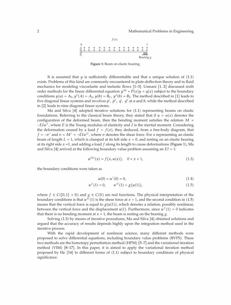
Again, the obtained solution is of distinguishing accuracy, as indicated in Table 2 and Figure 2.
6 Mathematical Problems in Engineering
5.5
5
4.5
4
3.5
3
2.5
2
1.5
10 0.2 0.4 0.6 0.8 1
u(x)
x
Exact solutionVariational iteration method
Figure 2: Comparison between different solutions.
Example 3.2. Consider the following linear boundary value problem:
u(4)(x) = u(x) + u′′(x) + ex(x − 3), 0 < x < 1, (3.11)
subject to the boundary conditions
u(0) = 1, u′(0) = 0, u(1) = 0, u′(1) = −e. (3.12)
The exact solution for this problem is
u(x) = (1 − x)ex. (3.13)
According to (2.5), the iteration formulation may be written as
un+1(x) = un(x) +∫ x
0
16(τ − x)3
(u(4)n (τ) − un(τ) − u′′u(τ) − eτ(τ − 3)
)dτ. (3.14)
Now it is assumed that an initial approximation has the form
u0(x) = ax3 + bx2 + cx + d. (3.15)
Where a, b, c, and d are unknown constants to be further determined.By the iteration formula (3.14), the following first-order approximation is developed:
u1(x) = u0(x) +∫ x
0
16(τ − x)3
(u(4)0 (τ) − u0(τ) − u′′0(τ) − eτ(τ − 3)
)dτ
= ax3 + bx2 + cx + d +∫ x
0
16(τ − x)3( − aτ3 − bτ2 − (6a + c)τ − 2b − d − eτ(τ − 3)
)dτ
=1
840ax7+
1360
bx6 +(
120a +
1120
c
)x5 +
(1
12b +
124d
)x4 +
(23+ a
)x3 +
(b +
52
)x2
+(ex + 6 + c
)x − 7ex + 7 + d.
(3.16)
A. Barari et al. 7
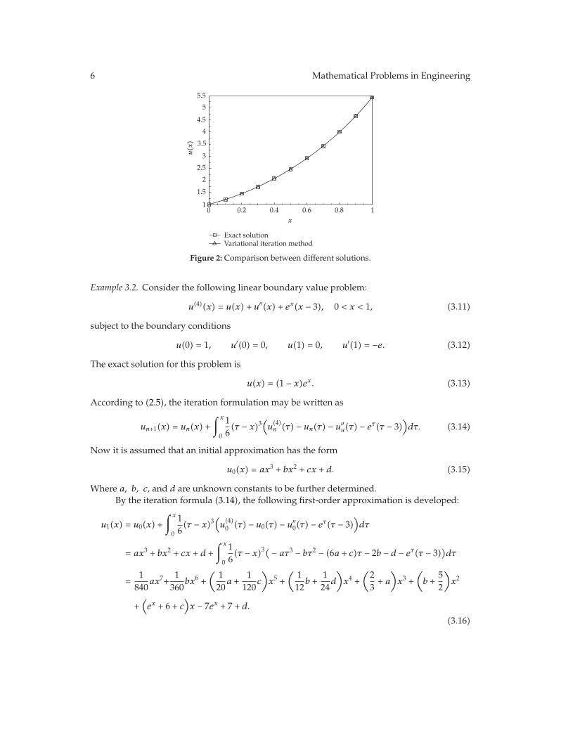
Table 3: Comparison of the first-order approximate solution with exact solution.
x UE U1 Error0 1.0000000000 1.0000000000 0.0000000E + 0000.1 0.9946538262 0.9947931547 1.3932850E − 0040.2 0.9771222064 0.9775949040 4.7269760E − 0040.3 0.9449011656 0.9457776230 8.7645740E − 0040.4 0.8950948188 0.8963297250 1.2349062E − 0030.5 0.8243606355 0.8258087440 1.4481085E − 0030.6 0.7288475200 0.7302919280 1.4444080E − 0030.7 0.6041258121 0.6053240800 1.1982679E − 0030.8 0.4451081856 0.4458625400 7.5435440E − 0040.9 0.2459603111 0.2462193000 2.5898890E − 0041.0 0.0000000000 0.0000000000 0.0000000E + 000
Incorporating the boundary conditions (3.12), into u1(x), it can be written as
a =7904470323149
− 2950080323149
e, b = −12770295323149
+4640400323149
e, c = 0, d = 1. (3.17)
Therefore, the following first-order approximate solution is obtained:
u1(x) =(
1129213877788
− 3512323149
e
)x7 +
(− 851353
7755576+
12890323149
e
)x6
+(
790447646298
− 147504323149
e
)x5 +
(− 25217441
7755576+
386700323149
e
)x4
+(
24359708969447
− 2950080323149
e
)x3 +
(− 23924845
646298+
4640400323149
e
)x2
+(6 + ex
)x + 8 − 7ex.
(3.18)
Comparison of the first-order approximate solution with exact solution is tabulated in Table 3,again showing a clear agreement. Even higher accurate solutions could be obtained withoutany difficulty.
Similarly, the following second-order approximation can be written as
u2(x) = u1(x) +∫ x
0
16(τ − x)3(u(4)1 (τ) − u1(τ) − u′′1(τ) − eτ(τ − 3)
)dτ
=1
6652800ax11 +
11814400
bx10 +(
1362880
c +1
30240a
)x9 +
(1
10080b +
140320
d
)x8
+(
15040
c +1
420a +
11260
)x7 +
(1
720d +
1144
+1
180b
)x6 +
(112
+1
20a +
1120
c
)x5
+(
12+
124d +
112b
)x4 + (3 + a)x3 +
(b +
212
)x2 +
(24 + 3ex + c
)x + 27 − 27ex + d.
(3.19)

8 Mathematical Problems in Engineering
Incorporating the boundary conditions, (3.12), into u2(x), yields
a =381804789300110
4289712004667− 140985028800000
4289712004667e, c = 0,
b = −6294953010820654289712004667
+230790037363200
4289712004667e, d = 1.
(3.20)
The following second-order approximate solution is then achieved in the following form:
u2(x) =(
3470952630001259441782042260160
− 6357550012869136014001
e
)x11
+(− 41966353405471
518883564084520320+
38159728412869136014001
e
)x10
+(
3818047893001112972089102113008
− 1398661000012869136014001
e
)x9
+(− 2513691492323593
172961188028173440+
228958370404289712004667
e
)x8
+(
11497040799049975405037125880420
− 3356786400004289712004667
e
)x7
+(− 415373822050043
514765440560040+
12821668742404289712004667
e
)x6
+(
23337258558473351476544056004
− 70492514400004289712004667
e
)x5
+(− 1203224346103459
102953088112008+
192325031136004289712004667
e
)x4
+(
3946739253141114289712004667
− 1409850288000004289712004667
e
)x3
+(− 1168906650066123
8579424009334+
2307900373632004289712004667
e
)x2
+(3ex + 24
)x + 28 − 27ex.
(3.21)
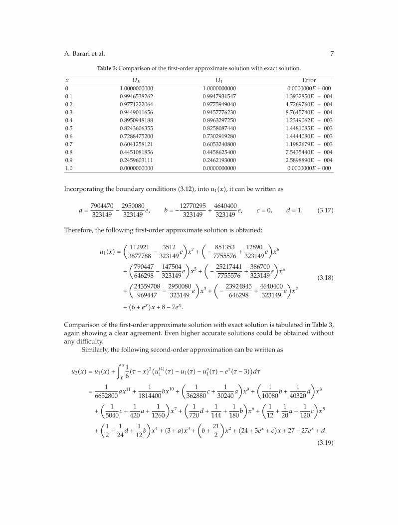
The obtained solution is of evident accuracy, as shown in Table 4 and Figure 3.
Example 3.3. Consider the following nonlinear boundary value problem:
u(4)(x) = u2(x) + g(x), 0 < x < 1, (3.22)
subject to the boundary conditions
u(0) = 0, u′(0) = 0, u(1) = 1, u′(1) = 1, (3.23)
where
g(x) = −x10 + 4x9 − 4x8 − 4x7 + 8x6 − 4x4 + 120x − 48. (3.24)

A. Barari et al. 9
00.1
0.2
0.3
0.40.5
0.6
0.70.8
0.9
1
u(x)
0 0.25 0.5 0.75 1x
Exact solutionVariational iteration method
Figure 3: Comparison between different solutions.
Table 4: Comparison of the second-order approximate solution with exact solution.
x UE U2 Error0 1.0000000000 1.0000000000 0.00000E + 0000.1 0.9946538262 0.9946577580 3.93180E − 0060.2 0.9771222064 0.9771357780 1.35716E − 0050.3 0.9449011656 0.9449268900 2.57244E − 0050.4 0.8950948188 0.8951321100 3.72912E − 0050.5 0.8243606355 0.8244058800 4.52445E − 0050.6 0.7288475200 0.7288945300 4.70100E − 0050.7 0.6041258121 0.6041666500 4.08379E − 0050.8 0.4451081856 0.4451352800 2.70944E − 0050.9 0.2459603111 0.2459701300 9.81890E − 0061.0 0.0000000000 0.0000000000 0.00000E + 000
The exact solution for this problem is
u(x) = x5 − 2x4 + 2x2. (3.25)
According to (2.5), the iteration formulation is written as follows:
un+1(x) = un(x) +∫ x
0
16(τ − x)3(u(4)n (τ) − u2
n(τ) − g(τ))dτ. (3.26)
Now it is assumed that an initial approximation has the form
u0(x) = ax3 + bx2 + cx + d, (3.27)
where a, b, c, and d are unknown constants to be further determined.

10 Mathematical Problems in Engineering
Table 5: Comparison of the first-order approximate solution with exact solution.
x UE U1 Error0 0.0000000000 0.0000000000 0.0000000E + 0000.1 0.0198100000 0.0198624243 5.2424300E − 0050.2 0.0771200000 0.0773022107 1.8221070E − 0040.3 0.1662300000 0.1665781379 3.4813790E − 0040.4 0.2790400000 0.2795490972 5.0909720E − 0040.5 0.4062500000 0.4068747265 6.2472650E − 0040.6 0.5385600000 0.5392178270 6.5782700E − 0040.7 0.6678700000 0.6684511385 5.8113850E − 0040.8 0.7884800000 0.7888727023 3.9270230E − 0040.9 0.8982900000 0.8984356964 1.4569640E − 0041.0 1.0000000000 1.0000000000 0.0000000E + 000
By the iteration formula (3.26), the following first-order approximation is obtained:
u1(x) = u0(x) +∫ x
0
16(τ − x)3(u(4)0 (τ) − u2
0(τ) + τ10 − 4τ9 + 4τ8 + 4τ7 − 8τ6 + 4τ4 − 120τ + 48
)dτ
= − 124024
x14 +1
4290x13 − 1
2970x12 − 1
1980x11 +
(1
5040a2 +
1630
)x10
+1
1512abx9 +
(− 1
420+
11680
b2 +1
840ac
)x8 +
(1
420bc +
1420
ad
)x7
+(
1180
bd +1
360c2)x6 +
(1 +
160cd
)x5 +
(124d2 − 2
)x4 + ax3 + bx2 + cx + d.
(3.28)
Incorporating the boundary conditions (3.23), into u1(x), results in the following values:
a = −0.006871650809; b = 2.005929593; c = 0, d = 0. (3.29)
The following first-order approximate solution is then achieved:
u1(x) = −4.162504162 × 10−5x14 + 2.331002331 × 10−4x13
− 3.367003367 × 10−4x12 − 5.050505050 × 10−4x11
+ 1.587310956 × 10−3x10 − 9.116433669 × 10−6x9
+1.4139007 × 10−5x8 + x5−2x4 − 6.871650809 × 10−3x3
+2.005929593x2.
(3.30)
Comparison of the first-order approximate solution with exact solution is tabulated in Table 5,which once again shows an excellent agreement.
Similarly, the following second-order approximation may be written:
u2(x) = u1(x) +∫ x
0
16(τ − x)3(u(4)1 (τ) − u2
1(τ)+τ10 − 4τ9 + 4τ8 + 4τ7 − 8τ6 + 4τ4 − 120τ + 48
)dτ.
(3.31)
A. Barari et al. 11
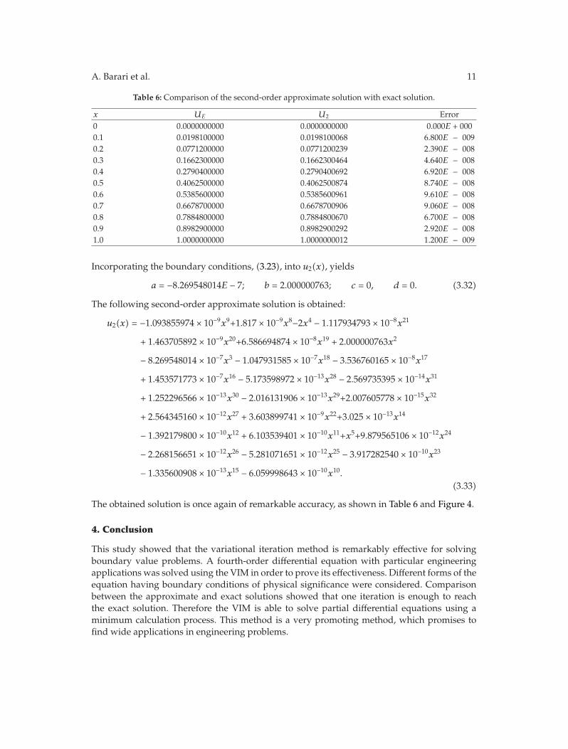
Table 6: Comparison of the second-order approximate solution with exact solution.
x UE U2 Error0 0.0000000000 0.0000000000 0.000E + 0000.1 0.0198100000 0.0198100068 6.800E − 0090.2 0.0771200000 0.0771200239 2.390E − 0080.3 0.1662300000 0.1662300464 4.640E − 0080.4 0.2790400000 0.2790400692 6.920E − 0080.5 0.4062500000 0.4062500874 8.740E − 0080.6 0.5385600000 0.5385600961 9.610E − 0080.7 0.6678700000 0.6678700906 9.060E − 0080.8 0.7884800000 0.7884800670 6.700E − 0080.9 0.8982900000 0.8982900292 2.920E − 0081.0 1.0000000000 1.0000000012 1.200E − 009
Incorporating the boundary conditions, (3.23), into u2(x), yields
a = −8.269548014E − 7; b = 2.000000763; c = 0, d = 0. (3.32)
The following second-order approximate solution is obtained:
u2(x) = −1.093855974 × 10−9x9+1.817 × 10−9x8−2x4 − 1.117934793 × 10−8x21
+ 1.463705892 × 10−9x20+6.586694874 × 10−8x19 + 2.000000763x2
− 8.269548014 × 10−7x3 − 1.047931585 × 10−7x18 − 3.536760165 × 10−8x17
+ 1.453571773 × 10−7x16 − 5.173598972 × 10−13x28 − 2.569735395 × 10−14x31
+ 1.252296566 × 10−13x30 − 2.016131906 × 10−13x29+2.007605778 × 10−15x32
+ 2.564345160 × 10−12x27 + 3.603899741 × 10−9x22+3.025 × 10−13x14
− 1.392179800 × 10−10x12 + 6.103539401 × 10−10x11+x5+9.879565106 × 10−12x24
− 2.268156651 × 10−12x26 − 5.281071651 × 10−12x25 − 3.917282540 × 10−10x23
− 1.335600908 × 10−13x15 − 6.059998643 × 10−10x10.
(3.33)
The obtained solution is once again of remarkable accuracy, as shown in Table 6 and Figure 4.
4. Conclusion
This study showed that the variational iteration method is remarkably effective for solvingboundary value problems. A fourth-order differential equation with particular engineeringapplications was solved using the VIM in order to prove its effectiveness. Different forms of theequation having boundary conditions of physical significance were considered. Comparisonbetween the approximate and exact solutions showed that one iteration is enough to reachthe exact solution. Therefore the VIM is able to solve partial differential equations using aminimum calculation process. This method is a very promoting method, which promises tofind wide applications in engineering problems.

12 Mathematical Problems in Engineering
00.1
0.2
0.3
0.40.5
0.6
0.70.8
0.91
u(x)
0 0.25 0.5 0.75 1x
Exact solutionVariational iteration method
Figure 4: Comparison between different solutions.
References
[1] R. A. Usmani, “On the numerical integration of a boundary value problem involving a fourth orderlinear differential equation,” BIT, vol. 17, no. 2, pp. 227–234, 1977.
[2] R. A. Usmani, “An O(h6) finite difference analogue for the solution of some differential equationsoccurring in plate deflection theory,” Journal of the Institute of Mathematics and Its Applications, vol. 20,no. 3, pp. 331–333, 1977.
[3] S. M. Momani, Some problems in non-Newtonian fluid mechanics, Ph.D. thesis, Wales University, Wales,UK, 1991.
[4] T. F. Ma and J. da Silva, “Iterative solutions for a beam equation with nonlinear boundary conditionsof third order,” Applied Mathematics and Computation, vol. 159, no. 1, pp. 11–18, 2004.
[5] J.-H. He, “New interpretation of homotopy perturbation method,” International Journal of ModernPhysics B, vol. 20, no. 18, pp. 2561–2568, 2006.
[6] D. D. Ganji and A. Sadighi, “Application of He’s homotopy-perturbation method to nonlinear coupledsystems of reaction-diffusion equations,” International Journal of Nonlinear Sciences and NumericalSimulation, vol. 7, no. 4, pp. 411–418, 2006.
[7] M. Rafei and D. D. Ganji, “Explicit solutions of Helmholtz equation and fifth-order Kdv equationusing homotopy-perturbation method,” International Journal of Nonlinear Sciences and NumericalSimulation, vol. 7, no. 3, pp. 321–328, 2006.
[8] N. H. Sweilam and M. M. Khader, “Variational iteration method for one dimensional nonlinearthermoelasticity,” Chaos, Solitons & Fractals, vol. 32, no. 1, pp. 145–149, 2007.
[9] S. M. Momani and Z. Odibat, “Numerical comparison of methods for solving linear differentialequations of fractional order,” Chaos, Solitons & Fractals, vol. 31, no. 5, pp. 1248–1255, 2007.
[10] S. M. Momani and S. Abuasad, “Application of He’s variational iteration method to Helmholtzequation,” Chaos, Solitons & Fractals, vol. 27, no. 5, pp. 1119–1123, 2006.
[11] N. Bildik and A. Konuralp, “The use of variational iteration method, differential transform methodand adomian decomposition method for solving different types of nonlinear partial differentialequations,” International Journal of Nonlinear Sciences and Numerical Simulation, vol. 7, no. 1, pp. 65–70, 2006.
[12] A. Barari, M. Omidvar, S. Gholitabar, and D. D. Ganji, “Variational iteration method and homotopy-perturbation method for solving second-order nonlinear wave equation,” in Proceedings of theInternational Conference of Numerical Analysis and Applied Mathematics (ICNAAM ’07), vol. 936, pp. 81–85, Corfu, Greece, September 2007.
[13] D. D. Ganji, M. Jannatabadi, and E. Mohseni, “Application of He’s variational iteration method tononlinear Jaulent-Miodek equations and comparing it with ADM,” Journal of Computational and AppliedMathematics, vol. 207, no. 1, pp. 35–45, 2007.

A. Barari et al. 13
[14] J.-H. He, “Variational iteration method—a kind of nonlinear analytical technique: some examples,”International Journal of Non-Linear Mechanics, vol. 34, no. 4, pp. 699–708, 1999.
[15] Z. Odibat and S. Momani, “Application of variational iteration method to nonlinear differentialequations of fractional order,” International Journal of Nonlinear Sciences and Numerical Simulation, vol.7, no. 1, pp. 27–34, 2006.
[16] H. Tari, D. D. Ganji, and M. Rostamian, “Approximate solutions of K (2.2), KdV and modified KdVequations by variational iteration method, homotopy perturbation method and homotopy analysismethod,” International Journal of Nonlinear Sciences and Numerical Simulation, vol. 8, no. 2, pp. 203–210,2007.
[17] E. Yusufoglu, “Variational iteration method for construction of some compact and non-compactstructures of Klein-Gordon equations,” International Journal of Nonlinear Sciences and NumericalSimulation, vol. 8, no. 2, pp. 152–158, 2007.