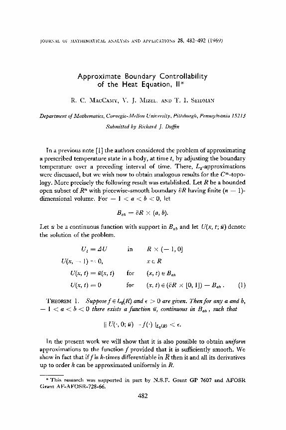
JOURKXL 01; 1L\THEhLITICXL ISALYSLS .AND XPPLiC.tTtONS 28, 452492 (lY6Y)

Approximate Boundary Controllability of the Heat Equation, II*

R. C. IGcCAnw, Y. J. MIZEL. AND T. I. SEIDMAN

Department of Mathematics, Cnmegie-Mellon L.‘niversity, Pittsburgh, Pennsylvania 15213

Submitted by Richard J. Dufin

In a previous note [I] the authors considered the problem of approximating a prescribed temperature state in a body, at time t, by adjusting the boundary temperature over a preceding interval of time. There, &-approximations were discussed, but we wish now to obtain analogous results for the P-topo- logy. More precisely the following result was established. Let R be a bounded open subset of R” with piecewise-smooth boundary aR having finite (n - l)- dimensional volume. For - 1 < a < b < 0, let

B,, = aR N (a, b).

Let Al be a continuous function with support in B,, and let U(x, t; ii) denote the solution of the problem.

U, = AC in R x (- l,O]

U(x, - 1) = 0, XER

U(x, t) = qx, t) for (x, t) E Bat,

U(x, t) = 0 for (x, t) E (aR x [0, 11) - B,, . (1)

THEOREM 1. Suppose f E L,(R) and E > 0 are given. Then for any a and b, - 1 < a < b < 0 there exists a function C, continuous in Bab , such that

II v.9 0; 4 -f(.) lIL*(R) < l .

In the present work we will show that it is also possible to obtain uniform approximations to the function f provided that it is sufficiently smooth. We show in fact that if f is k-times differentiable in R then it and all its derivatives up to order k can be approximated uniformly in R.

* This research was supported in part by N.S.F. Grant GP 7607 and AFOSR Grant AF-AFOSR-728-66.

482

APPROXIMATE BOUNDARY CONTROLLABILITY 483

In the present application we will have to discuss derivatives of functions up to and including the boundary. Hence it is necessary to put some smooth- ness conditions on aR. In order not to have to concern ourselves with precise conditions in various situations we make the following hypothesis:

aR is a Cm surface. (A.11

Next we point out that if a function f is to be uniformly approximated by functions of the form U(x, t; U) it is necessary that it satisfy certain compatibil- ity conditions on aR. Note first that any function of the form U(X, t; U) is identically zero for x E aR and t near zero. Hence we must have

$ U(x, t; Zc) = 0 for x E aR, t=1, K=O,1,2 )....

But then it follows from the first of Eqs. (1) that

A”U(x, t; u) = 0 for x E aR, t = 1, k = 0, 1, 2 ,... . (2)

Suppose now that f E CM(R)* and that f together with all derivatives up to order M can be uniformly approximated on R by functions of the form U(x, t; ti). Then it follows from (2) that f must satisfy the conditions,

Ajf=O for xEaR, j = 0, l,... F . I 1 64.2)

Our main result is that all functions f which satisfy conditions (A.2) can be uniformly approximated in the sense desired.

THEOREM 2. Let R be a domain in Rn satisfying (A.l). Let f E CM(R)

and suppose that f satisfies (A.2). Let E > 0 be given. Then for any a and b, - 1 < a < b < 0, there exists a function ii continuous in B,, such that

If - ujM= sug / D”f-DW <E. (3) bl<M

Here we use the standard notation in which 01 is a vector (CQ ,..., LX,) with nonnegative integer entries,

1 a 1 = 011 + ... + an and Dm = (&,“’ . . . (&,““,

* That isfe CM(R) and the derivatives off up to order M are all uniformly con- tinuous in R.

We shall prove Theorem 2 presently. First, however, we wish to point out that we can modify our result so that it gives uniform approximations to general K-times differentiable functions. To accomplish this we must, of course, give up the requirement that the boundary functions ii should vanish near t = 0. For - 1 < c < 0 let us denote by B, the set

B, = aR x (c, 01.

Now define U(x, t; a) as in (1) but with B, replacing B,, . Then we have the following result.

THEOREM 3. Let R be a domain satisfying (A.l). Let f E CM(R). Then for

any c, - 1 < c < 0, there exists a @ continuous in B, such that ;f f(x) = f (x) - U(x, 0; U) then f~ CM(R) andf satisfies (A.2).

Once we have Theorems 2 and 3 we can approximate an arbitrary f E CM(R) by an expression of the form U(x, t; U; + GJ where ir, has support in B,, and iis has support in B, , a, b, c arbitrary.

The proof of Theorem 3 is easy and we give it here. Suppose that for the given function f we have,

djf = vj for x EaR, iti!

j = 0, l,... y . [ I

Let u be a function defined on B, such that

lim ajq.y, t) fT0 atj

= q2j(X) .E^ E R, j = 0, l,... ; , [ 1 (4)

and consider the function U(X, t; u). We have then

hence by (4)

U(x, t; u) = qx, t) (x, t) E B, ,

lim ai+, t; 21) tTO ati = 44 XEaR, j = 0, I,... g . [ 1 (5)

On the other hand, U(.r, t; G) is a solution of the heat equation; hence,

aj djfJ(x, 0; u) = atj U(x, 0; U) = c&(x), XER, j = 0, I,... ; , [ 1

by (5).

PROOF OF THEOREM 2. For each integer m, let Hs, denote the Hilbert space composed of functions on R having 2m strong derivatives, in L”(R),

APPROXIMATE BOUNDARY CONTROLLABILITY 485

and let A,,, denote the closed subspace of Hzm which is generated by those functions in C”“(R) satisfying,

Ajf=O for xEaR and j<m---1. (6)

[That is, A,,, is generated by functions all of whose normal derivatives of even order < 2m - 2 are zero]. Now on A,,,., the bilinear form (e, .)m,d defined by

(u, v),,,~ = j”, A”% A”v dx (7)

defines a norm ]I I(m,d which is equivalent to the Ham-norm defined by

That is, one has the following result.

LEMMA 1. There exists a constant K depending only on m and R such that for any u E LA ,

II u IL G K II u llm.~ .

PROOF. To see that II llm,d is a norm, notice that if f E Cans(R) satisfies (6) and in addition 11 f Ijm,d = 0 then, in particular, we have

A*f = A(A+lf) = 0 in R, Anl-lf = 0 for x E aR.

Thus it follows that AnL-lf = 0 in R. Proceeding successively we deduce from (6) that f = 0 in R. Moreover, for any f E CT(R) which satisfies f = 0 for x E aR one has ([2], p. 195)

Ilf IL < c II Af h-2 3 (8)

where C depends only on R and r. Hence beginning with r = 2m and pro- ceeding successively, we deduce that for all f E Czm(R) which satisfy (6) one has

Ilf ILm d C II Af IL--e G C’ II W,m-, < .** G Kll Amf Ilo = Kllf Ilm.~ > (9

where K depends only on m and R. This concludes the argument. Now recall that, according to Sobolev’s Lemma, if 2m > M + (n/2) then

the following inequality holds for all functions in Hz,,, ,

If IluG Cllfllzm. (10)

where the norm on the left is the CM-norm defined in (3) and where C depends only on M, m, and R. Thus Lemma 1 yields the following result.

COROLLARY. If u E Id,,,,L( md 2m :- JI + (n/2) thea

(11)

where C depends onb on AI, m and R.

The proof of Theorem 2 now rests on the following two lemmas.

LEMMA 2. For any a and b the functions U(x, 0; ii), for u continuous in B ab , are dense in -IrnSd .

LEMMA 3. Let 119 be given and let m be any integer with m > M + [n/2]. Let f E CM(a) and satisfy (A.2) and let E > 0 be given. Then there exists an fi E Pm(R) which satisfies (6) and is such that 1 f - fi lM < E.

1f:ith these two lemmas in hand the proof of Theorem 2 is immediate. Given f E CM(R) and the numbers a, b, and E > 0, Lemma 3 states that we can find, for any m > M -+ [n/2], an fi E P”‘(R) satisfying (6) and such that / f - fi !.hl < 42. Then by Lemma 2 we can find a function u continuous in B,, such that

llfd.) - v.3 0; a) Ilm.A c &.

Since fi and U( *, ., U) are both in CYmi(R) and satisfy (6) it follows then by (11) that

hence

Ifi - q., 0; q I&f < ; ;

If (*) - U(., 0; q IM < E.

PROOF OF LEMMA 2. Let us now outline the proof of Lemma 2. This closely parallels that of [l] and proceeds as follows. The functions U(X, t; E) at t = 0 can be written in the form,

uk, 0; U> = jr,,, iZ(r, T) G&, y, - T) dr. (12)

Here G(x, y, t - T) is the Green’s function for the heat equation in R and G, denotes the normal derivative with respect to the variabley. For (y, 7) E B,, it is easy to see that G,(*, y, - T), considered as a function of X, belongs to C2n@) and satisfies (6), for any m. In [l] we exploited the fact that these functions spanned L,(R). The key here is that they also span A,n,d .

APPROXIMATE BOUNDARY CONTROLLABILITY 487

LEMMA 4. The functions {GY(*, y, - T)> for (y, T) E B,, span the space -4 ?,,,A .

We assume the validity of Lemma 4 for the moment and complete the proof of Lemma 2. The f of Lemma 2 belongs to Am,A . Hence given any E we can find points (yr , or) ,... (yn , 7,) in B,, and numbers cr ,..., c, such that,

ciG,.(., yi , 4 I << - .

6,i.A ;

Now the function G,(x, y, - T) has d erivatives of all orders which are continuous in y and 7. Hence, given any C’ > 0, we can find 6 such that

1 k’~G,,(.r, y, - T) - d”G,(x, yi , - Q) I < E’ (14) ..-

for s E R and 1 y - yi 1 < 6, 1 7 - 7i j < 6. Let us choose functions Bi(y, T) with supports in I y - yi 1 < 6, 1 7 - 7i / < 6, respectively, such that

0 *

SJ BjdYdT = 1 (15)

-1 c?R

and consider the function

We have by (14) and (15)

I Cj / .

1

(16)

If we choose E’ according to the inequality,

E’ < i I ci I ( 1

-1

1

A-W + ,

where A denotes the n-volume of R, then it follows from (15), (16) and Schwarz’s inequality that,

I,f (.) - u (., 0; t CA] lam d < 6.

Thus the proof of Lemma 2 is reduced to that of Lemma 4.

488 MACCAMY, MIZEL, AND SEIDMAN

In order to prove Lemma 4 we need to make use of the eigenfunctions of the Laplacian for R. These are functions uk satisfying the conditions,

Au, = -.- &.a, , ak == 0 on >R, ,; 06 IIL.JRI ~= 1. (17)

The ak’s form an orthonormal basis for L,(R). The {XJ are positive and if we let {& be the distinct &-values, ordered by increasing magnitude, then {pLi/ja} is bounded away from 0 and co.

LEMMA 5. The functions {,\~“a,} form an orthonormal basis for An,,d .

PROOF. It follows from (A.l) that the uk are infinitely differentiable in R (see [2] pp. 190, 201). By (17) we see that Aja, = 0 on aR for any j. Hence h;“a, E C*“(E) n A,,,, . We have, by (17),

= 1 akal dx = 6,, . R

Hence the set {&“ak} is orthonormal. Suppose q~ E Cam(R) n d,,,, is ortho- gonal to hima, for all K. Then

0 = (him a/; 9 e)nt.d = s X;fnA’n~k4’ncp dx R

= I& I, akdmp, dx

Since the (CZ~} span L,(R), it follows that A’%p = 0 in R and this together with A$ = 0 on 3R, j = 0, l,... m - 1, implies that y = 0.

We can now complete the proof of Lemma 4. Suppose the span of

A = Pd., Y, - 4 : (Y, 4 E B,,)

were not dense in A,,., . We could then find a nonzero v E J&I; that is a function v E A,., such that

0 = (~9 GA., Y, - 4)n,,~ for each (y, T) E Bal, . (18)

We can expand q~ in the form

Hence (18) becomes

0 = c Pkrk(Y, 4 k

(19)

APPROXIMATE BOUNDARY CONTROLLABILITY 489

where r,(y, T) denotes the kth Fourier coefficient of G,(*, y, - 7) with respect to {h;muk}. Now G(x, y, - T) has the expansion

It follows that

A ‘%(x, Y,

where

Hence we have

G(x, y, - T) = c a&c) uk(y) t+‘. k

T) = $ drn%(4 b(Y) eAk7 = ; (- A,)” a,&) b,(y) eAk7

h(Y) = 2 (Y)*

rk(y, T) = (- l>,, hEmb,(y) eAk’

and Eq. (19) becomes,

Now the series (20) converges absolutely and uniformly for (y, 7) E B,, . To see this note that the inequalities Zk2 < A, < LP imply the existence of a constant J such that XEmeAkT < Je Akb’z. Thus (20) is majorized by the series x I t% 1 1 b(Y) 1 eAkbiz for (Y, 7) E 8, . This converges uniformly in y since bk(y) eAkbi* are the Fourier coefficients of G,(*, y, - b/4) for the set {ak} and the functions G,(., y, - b/4) are uniformly bounded in L,(R), thus ensuring that / bk(y) 1 e k A bf* < CeAkb;3 for some fixed C. This provides a convergent series dominating (20) since the pk are the coefficients of cp in the set {Xinak}.

The remainder of the proof is exactly as in [l]. We collect terms in (20) in which the eigenvalues are the same. Thus, if {pi} are the distinct eigen- values, (20) yields

0 = 1 yje”i7a < T < b < 0 (21)

where

(22)

Here Kj = {K : A, = pj} (note that each Ki is finite). From (21) we obtain

(see i21) 0 = 2 &b,(y) for year.

keKj

But then &z, ,5$&y) has both Dirichlet and Neumann data zero. Hence it is identically zero (see [l]) and by the independence of {ak} it follows that the fin’s are all zero.

PROOF OF LEarnTA 3. Finally we give a proof of Lemma 3. LetfE C”(n) and satisfy Ojf = 0 on %R for; = 0, I,... [M,‘Z]. Now we can find a function @ satisfying the conditions

af@ pf -=~YI; on

iW %R for k odd and k :* M, (25)

where Y denotes the normal to i?R. conditions (24) and (25) constitute a part of the Dirichlet data for equation (23). The remaining part is a set of values of normal derivatives for @ of orders greater than or equal to M and less than or equal to 2m. These latter can be specified arbitrarily as Cm functions and @ thus determined as a function in Pm(R) C P(R).

Let F = f - @. Then FE CM(R) and moreover we have

A~F = 0 on aR M j< - , [ 1 2

SF -= iW

0 on 6R for k odd and k <. M.

From these conditions it is easy to see that FE CoM(R); that is, F and all its derivatives up to order M vanish on 3R. Hence if we write f = CD + F we see that Lemma 3 will be proved if we can show that it is possible to approximate functions in Ca”(li) by functions in C”“(R) which satisfy (6). We establish, in fact, the stronger result that the set C,,“O(R) (Cm functions of compact support) is dense in Ca”.

LEMMA 6. Corn(R) is a dense subset of COM(R).

PROOF. The smoothness assumption on aR implies that for each x E 3R there exists a ball N” containing x which is such that

(a) the center z, of IV” lies in R. (b) none of the segments z,y, y E IV” r\ i?R, is tangent to (i.e., supports)

t3R at y,

Hence, bY compactness of aR there exists a finite collection {Pi i = I,..., p> covering aR and there is some 8, E (0, n/2) such that the segments

%J’ (y E A% n t3D, i = l,...,p)

APPROXIMATE BOUNDARY CONTROLLABILITY 491

all make an angle with aR at y exceeding B0 . Moreover, for some E > 0 the set UT N”i contains the closed E-neighborhood 6?& of aR. Let R, = R - QE . Then the sets

R EP W’ll<i<, (26)

form an open covering for R. Let {pjj$,< jcl, denote a corresponding Cm partition of unity for R:

SUPP ~0 C R , supp yj c AT”‘, i = I,..., p, (27)

s E R. (28)

Given an f E CoM(R) (extended as zero outside R) let 6 > 0 be prescribed and examine the functions fj delined by

fj = fJ2j j = O,...,p. (29)

Now f. is in P(E) and has its support in R, , hence inside R. It follows ([3], p. 1642) that f. can be approximated arbitrarily closely in the norm 1 lM by functions belonging to Corn(R). Select j0 satisfying

Ifo-hf<;, h E Corn(R). (30)

Next we observe that by (27)

fi E COM(W n I?) i = 1,...,p.

Define the family of functions ( fif}, t E (1, CO), by

fi”(X) = f&x + (1 - t) z,J for tE(1, co). (31)

It follows by our construction of the {Pj} that the functions {fit} satisfy

fi” E CO‘yR) for t E (1, co). (32)

Moreover it is easily verified that

If? -fi I.h-fO as t-+ 1, i = I,..., p. (33)

Hence there exist numbers ti E (1, co) such that

If+filM<& i = l,..., p. (34)

492 MACCARIT, MIZEL, AND SEIDMAN

In addition, for t E (1, oz)fi” has its support inside R and hence as above eachfit can be approximated arbitrarily closely in the norm / iM by functions belonging to C,m(R). Select {~.},rI iCy such that

By construction, the function f defined by

f& j=O

(35)

(36)

belongs to Corn(R) and by Eqs. (33)-(36) we have

Since 8 > 0 was chosen arbitrarily, this concludes the argument.

.kXNOwLEDChlENT

This research was supported in part by the National Science Foundation under Grant GP 7607 and by the Air Force Office of Scientific Research under Grant AF-AFOSR-728-66.

1. R. C. MACCA~IY, V. J. MIZEL, AND T. I. SEIDILIAN. Approximate Boundary Con- trollability for the Heat Equation. 1. Math. Anal. Appl. 23, (1968), 699-703.

2. L. BERS AND SCHECHTER. “Partial Differential Equations.” Interscience, New York (1964).

3. N. DUNFORD AND J. T. SCHWARTZ. “Linear Operators Part II.” Interscience, New York (1963).