Observation and prediction for the heat equation. IV: Patch observability and controllability

JOURNAL OF DIFFERENTIAL EQUATIONS 20, 18-27 (1976)

Observation and Prediction for the Heat Equation, III

THOMAS I. SEIDMAN

University of Maryland, Baltimore, Maryland 21228

Received June 25, 1974

1. INTRODUCTION

The standard “well-posed problems” for the heat equation

ut = Au for0 <t < T > XESZCZP (1)

are initial-boundary value problems. Classical study of this equation shows that “arbitrary” specification of the initial state u0 = ~(0, .) together with either Dirichlet data

@, 4 = v,(t, x) forO<t<T,xEaQ (2)

or Neumann data

w aw, 4 = 4(t, 4 for0 <t < T,xEaQ (3)

(au/&) denotes the derivative outwardly normal to aQ) suffices to determine the evolution of the heat diffusion process; in particular, the terminal state u T= u( T, *) is determined by either of the pairs (u,, , ‘p) or (uO , 4).

If the internal initial state u0 is not given, we ask whether knowledge of both Dirichlet and Neumann data suffices. The pair (p), 9) cannot be specified arbitrarily, but we adopt the viewpoint that, in observation of an ongoing process, any consistency conditions are automatically satisfied; thus, we may assume that the observed pair (p), #) lies in the admissible manifold& and the existence of a solution to the triple (l)-(3), is not at issue. We are concerned here with the well-posedness of the observation/prediction problem; i.e., to show that the map: (v, $) t+ uT is well defined and continuous, using L, topologies for domain and range.

This well-posedness, in the restricted case 4 z 0, has already been demon- strated in certain special geometries in [5, 61. The argument in [5] for J2 a one-dimensional interval reduced the problem to one of Dirichlet series approximation; this has since been generalized in [II] to cover one-dimensional diffusion equations with variable (but t-independent) coefficients.

18 Copyright 0 1976 by Academic Press, Inc. All rights of reproduction in any form reserved.

PREDICTION FOR THE HEAT EQUATION 19

For Sz a cylinder or ball in W”, the arguments in [5, 61 depended on separa- bility of the Laplacian. (For further discussion, see also [lo].) The principal result of this paper is to show that the result does not depend on any particular geometry, that the observation/prediction problem is well posed for the heat equation in a general domain JJ in P.

2. PRELIMINARIES

We begin by introducing some notation. Assume throughout that we are given a bounded, connected, open set G in W” with “sufficiently smooth” boundary as2 and a fixed T > 0. Set Q = (0, T) x $2 and Z = (0, T) x %Q. For smooth enough functions defined on Q, we define Etu for 0 < t < T to be the trace of u on a, = {t) x Sz; i.e.,

[E,ul(x) = 4,~) for xe:sZ

(extended by continuity for t = 0, T). Similarly, define the boundary operators Ba , B, by letting B,u be the trace of u on Z and B,u the derivative (outwardly) normal to aa; thus, conditions (2) and (3) may be written as

Bou = Y, B,u = +.

Let @a be the closure of the set of smooth solutions of the heat equation (1) in the Hilbert space

W. = {w E H'sO(Q): wt E H-1*0(Q) = dual of IPa(Q

let %r be the closure of the set of smooth solutions in VI = !IPJ/~(Q) and let %a be its closure in wa = ZPl”*s’*(Q). Let so = H1/2*1/4(Z) and FI = H-1/2*-1/4(Z) = Fo*. For a discussion of these Sobolev spaces, see [3], from which we also take some relevant results on the initial-boundary value problems.

THEOREM 1. The mapping a0 : (u. , ‘p) = (E,u, B,u) H u is initiah’y well de$ned for smooth solutions of (1) and extends by continuity to an isomorphism of L,(Q) x So onto e. .

THEOREM 2. For each (u. , #) cL2(Q) x SI , there is a unique (weak) soZution u of (l), (3) in WI (hence, in +YJ and the mapping: a, : (u. , 4) = (E,u, Bru) I+ u so defined is continuous from L,(Q) x 9rI + S1 . Further, for each u. E H’/“(Q) and each 4 E L,(Z), there is a unique u E ‘I92 with E,u = u. , B,u = I& the mapping a2 : P/$(Q) x L,(Z) -+ 4)1, so defined is continuolrs.

20 THOMAS I. SEIDhUiV

Both of these theorems are immediate consequences of results in [3, Chap. 4, Section 151. Theorem 1 follows from (15.38) on restriction to the heat equation, for which m = 1. The two parts of Theorem 2 similarly follow from (15.1) with m,, = 1 and with 0 = Q and ;P, respectively; as required by (14.5), these are greater than y = (4 - trn - m&m) = -$. 1

Remark 1. Observe that, for t > 0 and ua EL&~), E,rrr(tl, , 0) is well defined in L,(9). If 71 = ol(r+, , 0), one has the expansion

v(t, .) = .Zkck exp[h,t] uk

where {(& , uk)) are the eigenpairs for the Neumann problem for the Laplacian and (ck) E I,(% = Zkcku,) so (ck exp[&t]) E Es since each X, < 0. (Indeed, formally,

AV(t, -) = 2Tkck(h,” exp[h,t]) ffk ,

which converges in L,(Q) since {X,m exp[h,t]) is bounded for each m, so that, by the Sobolev embedding theorem, it follows that et(t, *) E C-(G) for t > 0.) Observe also that, for u, E&(SZ) and tfi EL,(Z) C F1 , one has

so that E,or(u* , $) is well defined: for or(ua , 0) as above and for ~~(0, #) = u&O, $q E a‘2 c wt = Hs /z,3/*(~) by the usual trace argument, (e.g., [3]).

Remark 2. We note that %., C GY,, . To see this, suppose u were a smooth solution of (1) and ZI E H1so(Q); then

s, zqo = s, (A+ = -s, Vu . Vu,

from which it follows that the N-l~O(Q)-norm of ut is dominated by the PO(Q)-norm of u. Thus, the closure of the set of smooth solutions of (1) in the IGO(norm is contained in e0 and, a fortiori, a1 C e0 with a continuous (indeed, compact) injection map.

We now adapt a somewhat asymmetric attitude toward the conditions (2), (3) in viewing (l)-(3) as an observation/control problem in which $ is a control and ‘p an observation: ‘Someone” is applying the Neumann control 4 to some (unobservable by us) initial state u. , and we can observe the resulting Dirichlet data p, as well as the control 4. Assuming tit, is to be in L,(sZ), we see that for $ E&(Z) C Fr , Theorem 2 asserts u = oi(r~~ , 4) E %r C 4l;b (as noted above), whence, by Theorem 1, we have


~JI = B,u E PO CL,(Z). It is entirely reasonable, therefore, to topologize the manifold of admissible data.

as a subspace of [L,(Z)]2. The formulation of the state identification problem most frequently used

in (finite dimensional) linear system theory would require the determination of the initial state u. from knowledge of the observed pair (v, #) E A. It is easily seen (e.g., by considering the one-dimensional case) that one might reasonably expect the map (v, 4) ++ u. to be well defined (u, unique) but not continuous from M to L,(Q), since the diffusion process has such strong smoothing properties for increasing t. These same properties suggest the appropriateness of attempting, instead, prediction of the terminal state ur , i.e., considering the observation/prediction map.

=(F,#)bu r : d4f c [L,(z)]2 -+ L,(Q).

The earlier work in [5], [6] considered the restricted map

?T,:g,~u,:~o-+L2(L?)

with

do = CP: (9h 0) E -4 CJ52(4

and showed continuity of x0 for certain choices of Q. The results in [5] were actually a bit stronger than that, since observation of v was restricted to a proper subset of Z, a point to which we shall return in Section 4.

3. RESULTS

We begin by relating the adjoint of the map no to a control problem [4, 2, 81. At this point it is not assumed that the domains 9(x0) C J%~ or .9(x0*) CL,(Q) are all of do or L,(Q).

LEMMA 1. For (u. , #) gL2(S2) x L,(Z), we have

with

where 1,8 is giwen by &t, CC) = $(T - t, x) for (t, x) E Z.

(4)

22 THOMAS I. SEIDMAN

Proof. Given (u,, , (G) EL#~) x L,(Z), set u = ul(uo , #) and define zi, $ from u, $J by substituting (T - t) for t. By Remark 1 above E&2 EL,(Q) for 0 < t < T and, clearly,

d, = -A& Blfi = $, E,Ei = ETu, ETii = u,, . (5)

For any 9 E 52(x0), there exists v0 E&(Q) such that Bow = rp for a = Q~(w,, , 0) and ~F,,QI = Erw, (again, Etw EL@), by Remark 1). Thus, so tiw It = SD (E&(E,w) is well defined for each t and

= f

o [(-Azi)w + zi Aw]

as Blw = 0. Thus,

bo*uol~ = ja uo(xod = jn (WET4

If ETu = 0, then (4) holds and the continuous dependence of its left-hand side on y shows that [p, ++ l u,(x,~] EJY~* so I(~ E 9(no*). Conversely, (4) implies J-(ET u w0 = 0 for each w. obtained as above from a q E 9(lr0). ) But for any w. EL,(Q), there exists w = crl(wo , 0) E %I C ‘SYo and so a suitable 7 = Bow E F. CL,(Z). Thus, (4) holds if and only if ETu = 0. 1

From a system theoretic viewpoint, we might call a state u0 E&(G) Neumann null-controllable, if there exists a Neumann control 4 taking u. to 0 in time T, i.e., if there exists I# EL,(Z) for which E,u,(u, , 4) = 0. The lemma asserts that u. is Neumann null-controllable if and only if it is in .9(5co*), in which case any 4 satisfying (4) is a suitable Neumann control. In particular, as x0 is a Hilbert space, it follows from the Riesz representation theorem that there is such a control (a representation of the linear functional xo*lc in do*) in A0 itself; this is unique and will be the null-control having minimal L,(Z)-norm.


COROLLARY. The map q, : A, + L,(Q) is continuous if and only if every uO E L,(Q) is Neumann null-controllable.

Proof. Consider the set of pairs (us, #) E L,(Q) x .,#a for which Eror(~a , t,L) = 0. By the discussion above, there is at most one such $ E ~?a for any u0 E Lz(J2), so this set is the graph of an operator. Since or is continuous on L,(Q) x gr (hence, a fortiori, on L,(Q) x Jo) by Theorem 2 and since ET is certainly continuous (with an appropriately topologized codomain), the set of pairs, being the nullspace of Eror , is closed. Thus, the control map, u,, H 4 is a closed linear operator which we may view as x,,*: L,(Q) t-+ A0 . If x0* is known to be defined on all of L,(Q), its continuity follows from the Closed Graph Theorem; conversely, if x,, * is continuous, its domain is all of L,(Q). The corollary now follows from the lemma and the observation that x0* is continuous if and only if 7c,, is. 1

Observe that this shows that “universal” Neumann null-controllability for this system implies the existence of a constant C( = 11 n,,* 11 = /I x,, 11) such that the Neumann control $ taking u0 to 0 may be chosen so that 119 II < C 11 u,, I/. It is interesting to compare this corollary with [l, Theorem 131, which asserts that n,, is well defined (~a unique, given v) if and only if there exists, for each u,, and E > 0, a control & such that II b-~&, , h)ll -=c E; see also [4].

LEMMA 2. The map x: A? w L,(G) is continuous if (and, of course, only if) the restricted map x0 is continuous.

Proof. Given (p,, 4) E A, let 2, E @!z be the solution, as in Theorem 2, of (l), E,e, = 0, B,v = I,L Now 9, is clearly continuously embedded in a,, , which is isomorphic, by Theorem 1, with L,(Q) x so ; thus, B,v E go CL,(Z) is well defined and continuously dependent on o. Similarly, since e2 C ZiW2m3/4(Q), we have the trace ET continuous from e2 to L,(Q); see, for example, [3, Chap. 11. If u satisfies (1) with B,u = o, and B,u = #, then w = (U - V) satisfies (1) with B,w = [v - Ban] and B,w = 0, so E,w = x,,[~ - B,u]. Thus, we have the identity

Since v E 4, depends continuously on # by Theorem 2 and, except possibly for 57a , all the other maps are continuous, the proof is complete. i

THEOREM 3. The observation/prediction problem (for any bounded domain Q in 9” with smooth boundary aQn> is well posed; i.e., the map x: .A? -+ L,(Q) is continuous.

24 THOMAS I. SEIDhfAN

Proof. Given any u, EL&~), let v = csi(uo , 0) and set V, = v(e. m), which is in L,(Q) by Remark 1. Now choose any ball G, in 8” containing D in its interior and extend (as is always possible since o, , Z%2 are smooth) V~ to & E H1i2(fz,). Since the restricted observation/prediction problem is known to be well posed for 0, by [6, Theorem 21, it follows from the Corollary to Lemma 1 that $e is null-controllable. Thus, there exists 6 satisfying (I) in 8% = (E, 7’) x fz, with +(c, *) = vu, , (%/a~) EL&Z*)(Z* = (E, T) x X+.J, and 8(T, .) = 0. Applying the second part of Theorem 2 to Q* , it follows that 8 E H3/z*3~*(Q.+), whence, by a standard trace theorem, we may define $ as the derivative of fl normal to Z: = (E, T) x XJ and have I,$ ELM. Now define u, + on Q, Z respectively, by

u(t, x) = v(t, x) for0 < t <e,xES1),

= qt, -4 fore < t < T,xEQ,

w, 4 = 0 forO<t<e,xEa52,

= $f$, x) fore <t < T,xE%~,

and observe that u satisfies (1) in Q with E,,u = E,v = U, and E&u = 8(T, .) /o = 0. This shows that u0 is null-controllable by a Neumann control 4 EL,(Z). It follows by the Corollary to Lemma I that x0 is continuous and the theorem then follows by Lemma 2. 1

4. REMARKS

In attempting to extend the result of Theorem 3 (this has been done in [ll] for the t-independent, one-dimensional case) to more genera1 diffusion equations,

Ut =Lu:=V*pVu-qu (6)

(p > 0, q 2 0), and to consideration of observation restricted to a proper subset of the boundary, note that suitable generalizations of Lemma I and its Corollary and Lemma 2 are easily obtained. We now let ??JO , 6, , syt, denote appropriate spaces of solutions of (6) with the maps (I,, , ui , a2 correspondingly defined; assuming p, 4 are smooth, Theorems I and 2 continue to hold. Given a subset Z” of .Z, d is now defined as

where we take L,(F) to mean {v E.&(Z): cp = 0 on zl\Z’}; A,, is now a


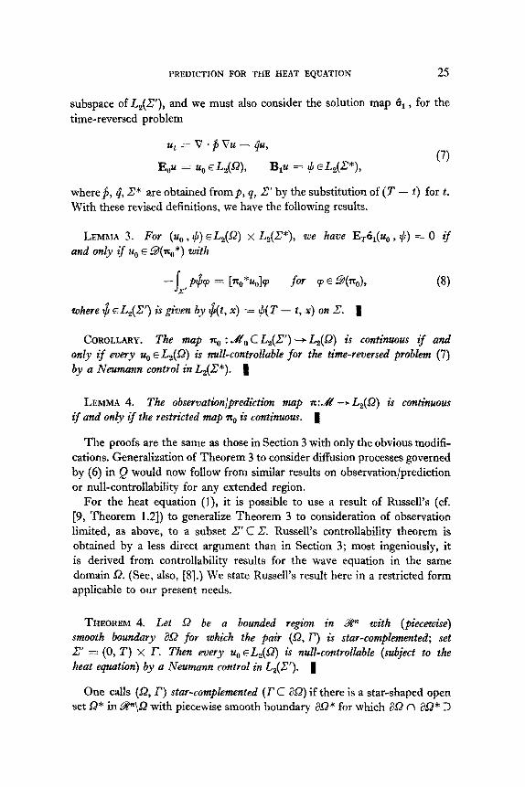
subspace of L,(z”), and we must also consider the solution map 6, , for the time-reversed problem

ut = V -$Qu - t$it

E,u = u0 EL@), B,u = I,I “L&Z*),

where $, g,Z* are obtained from p, Q, .Z’ by the substitution of (T - t) for t. With these revised definitions, we have the following results.

LEMMA 3. Far (u, , $J) ELM x L,(.Z*), we have Erij&~g, Z/J) = 0 if and on& if u. E 53(tFg*) with

where $ EL&??) is g&n by $(t, x) = #(T - t, x) on Z. 1

COROLLARY I The map TC~ : A’, C L&Y’) + L&2) is continuous if and 5nly if eveYy U@ EL,(Q) is uull-~ont~ollable for the time-y~~sed ~oblem (7) by a Neumann control in L,(zI*). 8

LEMMA 4. The observation/prediction map x:&I -3 L&2) is continuous if and only if the resty~~ted map z. is ~~t~~~us. 4

The proofs are the same as those in Section 3 with only the obvious modifi- cations. Generalization of Theorem 3 to consider diffusion processes governed by (6) in Q would now follow from similar results on obse~ation~prediction or null-controllability for any extended region.

For the heat equation (l), it is possible to use a result of Russell’s (cf. [9, Theorem 1.21) to generalize Theorem 3 to consideration of observation limited, as above, to a subset L” C Z: Russell’s controllabili~ theorem is obtained by a less direct argument than in Section 3; most ingeniously, it is derived from controllability results for the wave equation in the same domain G. (See, also, [8].) We state Russell’s result here in a restricted form applicable to our present needs.

THEOREM 4. Let Q be a bounded region in S@ with (piece&e) smooth bou~a7y XI for which the pair (f2, I’) is stay-~~pl~te~ set 27 = (0, T) x r, Then every u,, EL,(G) is null-controllable (subject to the heat equation) by a Neumann control in L,(C’). 1

One calls (fz, r) t s ~-comple~ted (I’ C &Z) if there is a star-shaped open set 9* in W”\52 with piecewise smooth boundary asZ* for which 852 n XI* 3

26 THOMAS I. SEIDMAN

(Xi\r). Roughly, then, (0, r) is star-complemented if there is a neighborhood in .9P\s2 from which one can “see” all of as2\r.

From Theorem 4, Lemma 4, and the corollary to Lemma 3, one immediately has the well-posedness of the relevant observation/prediction problem.

THEOREM 5. Let (l2, r) be star-complemented and set

Z’=(O,T) x rcz=(o,T) x ac2.

Then for u satisjying the heat equation (1) in Q = (0, T) x a, observation of z+4 = au/& ELM and F = u jz, EL,(Z) suffices for unique and continuous prediction of uT = u(T, .) EL,(Q). I

It seems likely that Theorem 4 can be extended to apply to more general diffusion equations as (6) but, since Russell’s argument relating this controllability to that for the corresponding wave equation makes essential use of a space/time separation of variables, such an extension is clear only for autonomous equations.

Another generalization of this discussion would be to unbounded regions in 9” with the governing equation (1) supplemented by the usual conditions at infinity. It is possible to obtain such results from the treatment above simply by inverting 5%“’ with respect to a sphere centered in the complement of 0

A word is in order relating the observation/prediction problem considered here to a similar problem in systems theory: state identification. The relevant state identification problem may be posed as follows (cf. [7], in particular).

Let ‘p, # be (inexact) observations over (0, T) of the Dirichlet and Neumann data of a solution u of (1) in Q; suppose F, I/ EL,(Z). Determine a “best prediction” of ur EL,(G), using v, 1/, and relevant information as to the inexactitude of the observations.

Thus, if a bound E were given on the L,(Z)-errors in observing q, $, one would be trying to find a prediction ur* which minimized the error II&---ur*/~overallzir = zi(T, .) for zi satisfying (1) with I$? = B,zZ, 6 = B,& satisfying 1) @ - IJI !I, /I r,8 - 4 jl < E. Th e existence of such a “best prediction” ur* (given E > 0) is, of course, a quite different question than the observation/ prediction problem which, effectively, asks whether ur* converges appropriately as e - 0. Similarly, state identification is considered with the observation errors assumed statistical, e.g., Gaussian in some sense with mean 0, and a “maximum likelihood” prediction sought. Theorem 3 is then relevant to the question of convergence of this estimated ur as the variance goes to 0.


ACKNOWLEDGMENTS

I should like to express my thanks and appreciation for a variety of reasons, to Ivo BabuBka, Roger Brockett, Fritz John, Victor Mizel, and David Russell.

REFERENCES

1. M. C. DELFOUR AND S. K. MITTER, Controllability and observability for infinite- dimensional systems, in “Recent Developments in Control Theory,” (N. P. Bhatia, Ed.), pp. 109-113, SIAM, Philadelphia, Pa., 1972 (also, SIAM 1. Control 10 (1972)).

2. H. 0. FATTORINI AND D. L. RUSSELL, Exact controllability theorems for linear parabolic equations in one space dimension, Arch. Rational Me&. Anal. 43 (1971). 272-292.

3. J. L. LIONS AND E. MAGENES, “Non-Homogeneous Boundary Value Problems and Applications,” Vols. 1, 2, Springer, New York, 1972.

4. R. C. MACCAMY, V. J. MIZEL, AND T. I. SEIDMAN, Approximate boundary controllability for the heat equation, I and II, 1. Math. Anal. AppZ. 23 (1968), 699-703; 28 (1969), 482-492.

5. V. J. MIZEL AND T. I. SEIDMAN, Observation and prediction for the heat equation, J. Math. Anal. AppZ. 28 (1969), 303-312.

6. V. J. MIZEL AND T. I. SEIDMAN, Observation and prediction for the heat equation, II, j. Math. Anal. AppZ. 38 (1972), 149-166.

7. G. A. PHILLIPSON, “Identification of Distributed Systems,” American Elsevier, New York, 1971.

8. D. L. RUSSELL, A unified boundary controllability theory for hyperbolic and parabolic partial differential equations, Stud. ApPZ. Math., Lll (1973). 189-211.

9. D. L. RUSSELL, Exact boundary value controllability theorems for wave and heat processes in star-complemented regions, to appear.

10. T. I. SEIDMAN, The ‘observation and prediction’ problem, Proc. Eleventh Annual Allerton Conference on Circuit and System Theory, 1973.

11. T. I. SEIDMAN, Observation and prediction for one-dimensional diffusion processes, J. Math. Anal. Appl., 51 (1975), 165-175.

Observation and prediction for the heat equation. IV: Patch observability and controllability

Documents

Transcript of Observation and prediction for the heat equation. IV: Patch observability and controllability