Addendum to “Concentration and lack of

observability of waves in highly

heterogeneous media”, [1]

C. Castro, E. Zuazua ?

Abstract

In [1] we introduced a class of 1−d wave equations with rapidly oscillat-ing Holder continuous coefficients for which the classical boundary observ-ability property fails. We also established that these examples could be usedto contradict Strichartz-type inequalities for the wave equation with low reg-ularity coefficients. The object of this Note is to further analyze this issue.As we will see, the argument in [1] only provides sharp counterexamples tothe Strichartz estimates when the coefficient ρ belongs to L∞. We carefullyanalyze this counterexamples for Holder continuous coefficients. We alsogive a new application of our construction showing that some eigenfunctionestimates for elliptic operators due to Sogge can fail when coefficients arenot smooth enough.

1. Introduction

In [1] we introduced a counterexample to the boundary observabilityproperty of the wave equation with a density ρ ∈ C0,s for all 0 < s < 1.Moreover, we observed that this construction could be adapted to obtaincounterexamples to the Strichartz estimates for the wave equation withHolder continuous coefficients. However, the proof in [1] is only valid whenρ ∈ L∞.

The aim of this addendum is twofold. In section 2 we present a completeand rigorous statement on this matter complementing [1] and, in section 3,we give a new application of our construction that allows obtaining sharplimits to the Sogge’s estimates for the eigenfunctions of second order ellipticoperators.

? Partially Supported by Grant BFM 2002-03345 of MCYT (Spain) and GrantHPRN-CT-2002-00284 of the European program New materials, adaptive systemsand their nonlinearities: modelling, control and numerical simulation

2 C. Castro, E. Zuazua

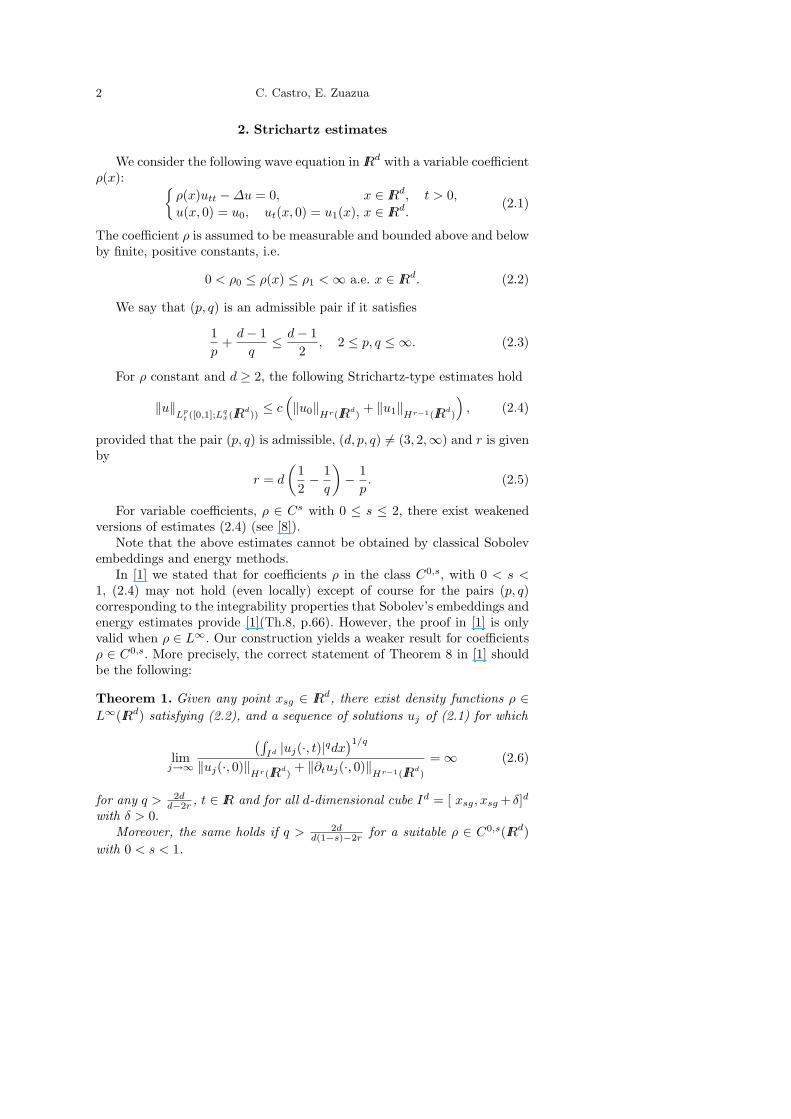
2. Strichartz estimates

We consider the following wave equation in IRd with a variable coefficientρ(x): {

ρ(x)utt −∆u = 0, x ∈ IRd, t > 0,u(x, 0) = u0, ut(x, 0) = u1(x), x ∈ IRd.

(2.1)

The coefficient ρ is assumed to be measurable and bounded above and belowby finite, positive constants, i.e.

0 < ρ0 ≤ ρ(x) ≤ ρ1 <∞ a.e. x ∈ IRd. (2.2)

We say that (p, q) is an admissible pair if it satisfies

1p

+d− 1q

≤ d− 12

, 2 ≤ p, q ≤ ∞. (2.3)

For ρ constant and d ≥ 2, the following Strichartz-type estimates hold

‖u‖Lp

t ([0,1];Lqx(IRd

))≤ c

(‖u0‖Hr(IRd

)+ ‖u1‖Hr−1(IRd

)

), (2.4)

provided that the pair (p, q) is admissible, (d, p, q) 6= (3, 2,∞) and r is givenby

r = d

(12− 1q

)− 1p. (2.5)

For variable coefficients, ρ ∈ Cs with 0 ≤ s ≤ 2, there exist weakenedversions of estimates (2.4) (see [8]).

Note that the above estimates cannot be obtained by classical Sobolevembeddings and energy methods.

In [1] we stated that for coefficients ρ in the class C0,s, with 0 < s <1, (2.4) may not hold (even locally) except of course for the pairs (p, q)corresponding to the integrability properties that Sobolev’s embeddings andenergy estimates provide [1](Th.8, p.66). However, the proof in [1] is onlyvalid when ρ ∈ L∞. Our construction yields a weaker result for coefficientsρ ∈ C0,s. More precisely, the correct statement of Theorem 8 in [1] shouldbe the following:

Theorem 1. Given any point xsg ∈ IRd, there exist density functions ρ ∈L∞(IRd) satisfying (2.2), and a sequence of solutions uj of (2.1) for which

limj→∞

(∫Id |uj(·, t)|qdx

)1/q

‖uj(·, 0)‖Hr(IRd

)+ ‖∂tuj(·, 0)‖

Hr−1(IRd)

= ∞ (2.6)

for any q > 2dd−2r , t ∈ IR and for all d-dimensional cube Id = [ xsg, xsg + δ]d

with δ > 0.Moreover, the same holds if q > 2d

d(1−s)−2r for a suitable ρ ∈ C0,s(IRd)with 0 < s < 1.

Title Suppressed Due to Excessive Length 3

Theorem 1 establishes that when ρ ∈ L∞ one cannot guarantee anyfurther integrability property of the solution, other than that implied byenergy estimates and Sobolev embeddings. In the class of coefficients ρ ∈C0,s(IRd) we also show that inequality (2.4) may fail for admissible pairs(p, q) with q > 2d/[d(1− s)− 2r]. According to this, we have the following:

Corollary 1. Assume that for any ρ ∈ L∞ there exists a constant c > 0such that (2.4) holds. Then

r ≥ d

(12− 1q

) (or, equivalently, q ≤ 2d

d− 2r

). (2.7)

Moreover, if (2.4) is assumed to hold in the class of densities ρ ∈ C0,s,0 < s < 1, then

r ≥ d

(12− 1q

)− ds

2. (2.8)

Remark 1. 1. The bound for r in (2.8) is greater than the value in (2.5) if s <2/(pd). This shows in particular that one may not guarantee the Strichartzestimate (2.4) for all coefficients ρ in the class C0,s unless s ≥ 2/(pd).

2. The results in [8] show that if ρ ∈ Cs with 0 ≤ s ≤ 2 (L∞ if s = 0,Cs = C0,s if 0 < s < 1, Lipschitz if s = 1 and Cs = C1,s−1 if 1 < s < 2)then the estimates (2.4) hold, with a constant c depending only on the Cs

norm of ρ, when

r = d

(12− 1q

)+σ − 1p

, σ =2− s

2 + s. (2.9)

Moreover, in [7] it is proved that this result is sharp in the sense that if theinequalities (2.4) hold with a constant c > 0 depending only on the Cs-normof the coefficients then r must be greater or equal than the value in (2.9).

When s = 0 the value of r in (2.9) coincides with the bound (2.7) andthen the result of Corollary 1 is sharp. Note also that, in this case, theresult in Corollary 1 is somehow stronger than the one in [7]. Indeed, in [7]it is proved that the constant c > 0 in (2.4) can not be chosen dependingonly on the L∞−norm of ρ, while Corollary 1 shows that, in fact, there areparticular coefficients ρ ∈ L∞ for which the constant c in (2.4) does noteven exist.

If s > 0, the optimal value of r in (2.9) is strictly greater than the boundwe get in (2.8). Therefore Corollary 1 is not sharp in this case.

The counterexamples in [7] are based on a construction of a sequence ofcoefficients, bounded in the Cs−norm, for which there are solutions concen-trated along characteristics. Then, the constant in (2.4) becomes unboundedunless r satisfies (2.9). Our examples are of different nature. We constructparticular coefficients ρ ∈ C0,s for which there exists a sequence of solu-tions, arbitrarily concentrated near a given point (instead of a characteristiccurve), for all time. Since our construction is based on eigenfunctions for the

4 C. Castro, E. Zuazua

elliptic problem in the whole space it is also useful to analyze Strichartz-likeestimates for other models too as, for example, for the Schrodinger equation.

Proof of Theorem 1: For completeness we sketch the proof given in[1] paying special attention to computing the regularity s of the coefficientmaking the Strichartz estimate (2.4) fail. We first consider the case ρ ∈ C0,s

with s > 0. The case ρ ∈ L∞ will be treated separately at the end of theproof.

Assume, without loss of generality, that xsg = 0 and K = [0, 1]. In [1](formula (6.6)) we constructed a positive density function ρ ∈ L∞(Kd) forwhich there exists a sequence of eigenpairs (h2

j , ϕj) satisfying

∆ϕj + h2jρ(x)ϕj = 0, x ∈ Kd, (2.10)

withhj →∞, (2.11)

and such that ϕj is strongly concentrated around xsg = 0.Note that no boundary conditions are imposed on (2.10). Actually, the

sequence ϕj is constituted by local eigenfunctions whose main propertyis the concentration around xsg = 0. The growth of the sequence hj , theregularity of the coefficient ρ and the degree of concentration of the sequenceϕj are intimately related. In order to get the bounds stated in the Theorem,we need to further analyze the properties of hj , ρ and ϕj .

The density ρ is constructed in separated variables. Thus, the key pointis the understanding of its behavior in one space dimension. It is a positivefunction that oscillates more and more rapidly along a sequence Ij of disjointintervals of K. Roughly, hj is the frequency of the oscillation of ρ over Ij .The intervals Ij are of length lj → 0 and their centers mj converge to thesingular point xsg = 0.

We now give a more precise description.According to (3.11) and (6.13) in [1] the density ρ and the eigenpairs

(h2j , ϕj) may be built so that

|ρ|C0,s(Kd) ≤M supjεjh

sj , (2.12)

for a suitable M > 0, εj → 0 and 0 < s < 1.Furthermore, for suitable constants C and Cp > 0:∫

(I−j

)d

|ϕj(x)|2dx ≥ Ch−3dj , (2.13)

|ϕj(x)|2 + |∇ϕj(x)|2 ≤ Cph−pj , ∀p > 0, x ∈ Kd\(I−j )d, (2.14)

where

I−j = (mj −lj2,mj +

lj2

], mj =lj2

+∞∑

k=j+1

rk. (2.15)

Title Suppressed Due to Excessive Length 5

This may be done provided that the sequences lj , hj and εj satisfy thefollowing conditions

∞∑j=1

lj = 1,hj lj2

is an integer,

εk ≤1

2M, 4M

k−1∑j=1

εjhjrj ≤ εkhkrk, 2M∞∑

j=k+1

εjrj ≤ εkrk,

hpje−εjhj lj → 0 as j →∞ for all p > 0. (2.16)

The following choice guarantees that all these conditions are fulfilled:

lj = 2−j , hj = 22Nj

, εj = h−sj , (2.17)

for a sufficiently large integer fixed N . Note that with this choice, we haveρ ∈ C0,s, in view of (2.12).

Remark 2. In [1] we assumed εj = h−1j (log hj)2 instead of εj = h−s

j in(2.17). This allowed us to prove that the coefficient ρ belongs to C0,s forall 0 < s < 1. But the construction above is better adapted to deal withcoefficients in a specific class C0,s.

As mentioned above, the functions ϕj(x) and ρ(x) are defined in sepa-rated variables over Kd (see (6.6) and (6.8) in [1]). In fact, we have

ϕj(x) = ϕj(x1)...ϕj(xd),ρ(x) = ρ(x1) + ...+ ρ(xd), (2.18)

where ρ ∈ C(K) is a positive function which takes the value 4π2 on theboundary of K and ϕj solves

(ϕj)′′(y) + h2j ρ(y)ϕj(y) = 0, for y ∈ K. (2.19)

In particular, over each I−j we have

ϕj(x) = ϕj(x1)...ϕj(xd) = wεj(hj(x1 −m−

j ))...wεj(hj(xd −m−

j )), (2.20)

where wε is of the form,

wε(x) = pε(x)e−ε|x| (2.21)

for some function pε(x) 1−periodic on x > 0 and x < 0 (see (2.5) in [1]),and satisfying

|wε|+ |w′ε|+ |w′′ε | ≤ C,

∫ 1

0

|wε(x)|2dx ≥ γ, (2.22)

for some C, γ > 0, independent of ε (see Lemma 1 in [1], p. 42).

6 C. Castro, E. Zuazua

In fact, we take as wεjthe explicit example given in [1] (pag. 44) for

which the following bound holds for the derivatives of any order r:

|wr)ε (x)| ≤ Cr, ∀x ∈ IR, ∀ε > 0. (2.23)

Once the eigenpair (hj , ϕj) is built we construct the solutions of thewave equation by separation of variables:

uj(x, t) = eihjtϕj(x). (2.24)

This constitutes a sequence of solutions of (2.1) over Kd × [0, T ] that weextend to solutions of (2.1) over IRd× [0, T ]. To this end we first extend thecoefficient ρ from Kd to IRd. This extension is defined in separated variables,as in (2.18), by extending ρ from K to IR by the constant value 4π2. Theexponent in the Holder continuous regularity property of ρ in IRd is thesame as the one of ρ in Kd since ρ = 4π2 on the boundary of K. Then, weextend ϕj in separated variables, as in (2.18), by extending ϕj in such away that it satisfies (2.19) in IR (with ρ extended as before). This is done bysolving the ODE in the exterior domain IR\K with the Cauchy data givenby ϕj(y) and ϕ′j(y) at the extremes of K.

In this way, uj , defined by (2.24), is extended to a solution of (2.1) inIRd× [0, T ]. To simplify the notation we denote the extension simply by uj .Note however that we can not guarantee that uj(0) = ϕj ∈ Hr(IRd) sinceour extension of ϕj does not decay as x → ∞, since it solves a constantcoefficients second order differential equation away of K.

To avoid this difficulty we rather define the extension of uj as the so-lution of (2.1) with truncated initial data. More precisely, (u(0), ut(0)) =(ϕj(x)χ(x), ihjϕj(x)χ(x)), where χ(x) is a cut-off function that satisfies

χ(x) ∈ C∞(IRd), |χ| ≤ 1,χ(x) = 1, if |x| < R and χ(x) = 0, if |x| > R+ 1,

and R is a sufficiently large number that we chose in order to guaranteethat the solutions of (2.1) with the above truncated initial data coincidewith (2.24) over Kd× [0, 1]. Note that, by the finite velocity of propagation,this holds if R is sufficiently large. Due to the estimates (2.14) and thefact that ϕj in IR\K is a linear combination of sinusoidal functions whichoscillate with frequency hj we get

‖(uj(x, 0), ∂tuj(x, 0))‖Hr(IRd

)×Hr−1(IRd)= ‖(χϕj , ihjχϕj)‖Hr(IRd

)×Hr−1(IRd)

= ‖(ϕj , ihjϕj)‖Hr(Kd)×Hr−1(Kd) +O(h−pj ). (2.25)

Observe that |uj(·, t)| = |ϕj(·)| for all t and x ∈ Kd. Therefore, taking(2.25) into account, the limit in (2.6) coincides with

limj→∞

(∫Id |ϕj(x)|qdx

)1/q

‖ϕj‖Hr(Kd) + hj ‖ϕj‖Hr−1(Kd) +O(h−pj )

. (2.26)

Title Suppressed Due to Excessive Length 7

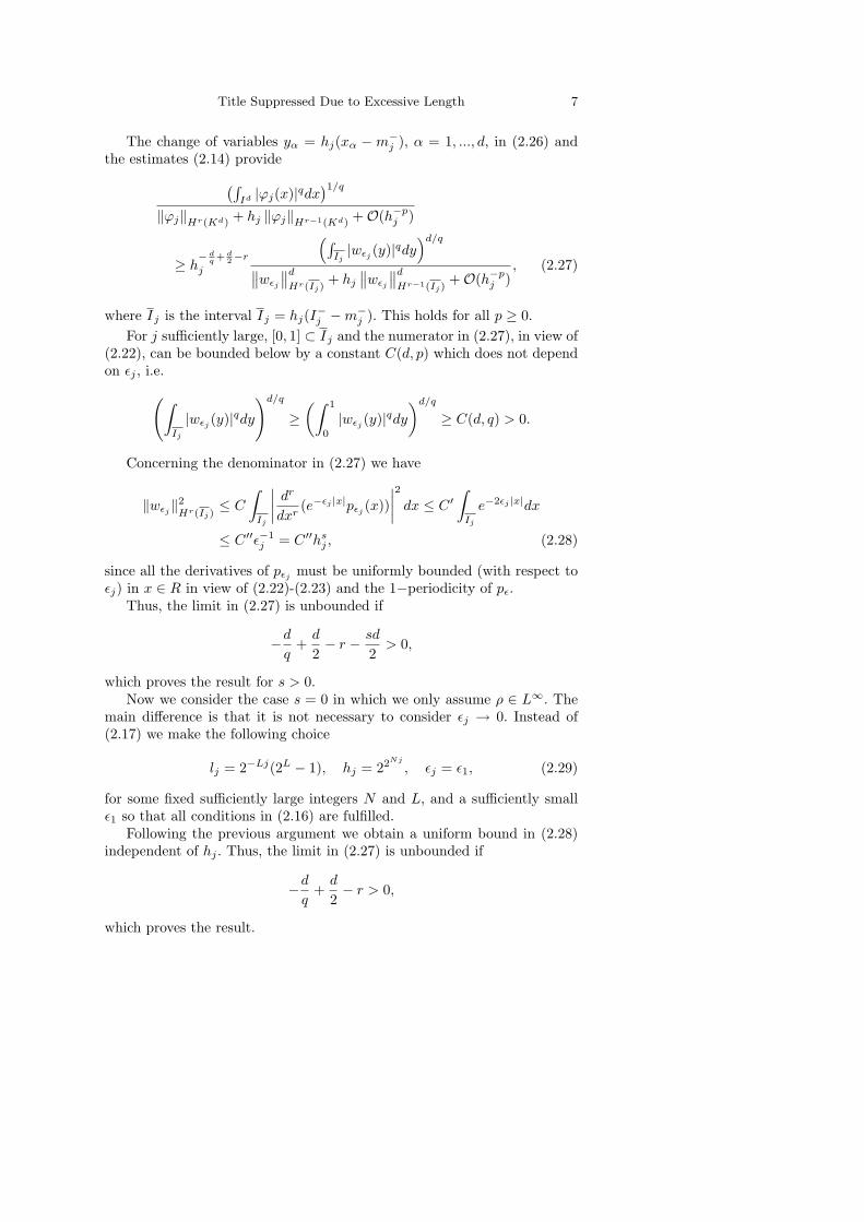
The change of variables yα = hj(xα −m−j ), α = 1, ..., d, in (2.26) and

the estimates (2.14) provide(∫Id |ϕj(x)|qdx

)1/q

‖ϕj‖Hr(Kd) + hj ‖ϕj‖Hr−1(Kd) +O(h−pj )

≥ h− d

q + d2−r

j

(∫Ij|wεj

(y)|qdy)d/q

∥∥wεj

∥∥d

Hr(Ij)+ hj

∥∥wεj

∥∥d

Hr−1(Ij)+O(h−p

j ), (2.27)

where Ij is the interval Ij = hj(I−j −m−j ). This holds for all p ≥ 0.

For j sufficiently large, [0, 1] ⊂ Ij and the numerator in (2.27), in view of(2.22), can be bounded below by a constant C(d, p) which does not dependon εj , i.e.(∫

Ij

|wεj(y)|qdy

)d/q

≥(∫ 1

0

|wεj(y)|qdy

)d/q

≥ C(d, q) > 0.

Concerning the denominator in (2.27) we have

‖wεj‖2Hr(Ij)≤ C

∫Ij

∣∣∣∣ dr

dxr(e−εj |x|pεj (x))

∣∣∣∣2 dx ≤ C ′∫

Ij

e−2εj |x|dx

≤ C ′′ε−1j = C ′′hs

j , (2.28)

since all the derivatives of pεj must be uniformly bounded (with respect toεj) in x ∈ R in view of (2.22)-(2.23) and the 1−periodicity of pε.

Thus, the limit in (2.27) is unbounded if

−dq

+d

2− r − sd

2> 0,

which proves the result for s > 0.Now we consider the case s = 0 in which we only assume ρ ∈ L∞. The

main difference is that it is not necessary to consider εj → 0. Instead of(2.17) we make the following choice

lj = 2−Lj(2L − 1), hj = 22Nj

, εj = ε1, (2.29)

for some fixed sufficiently large integers N and L, and a sufficiently smallε1 so that all conditions in (2.16) are fulfilled.

Following the previous argument we obtain a uniform bound in (2.28)independent of hj . Thus, the limit in (2.27) is unbounded if

−dq

+d

2− r > 0,

which proves the result.

8 C. Castro, E. Zuazua

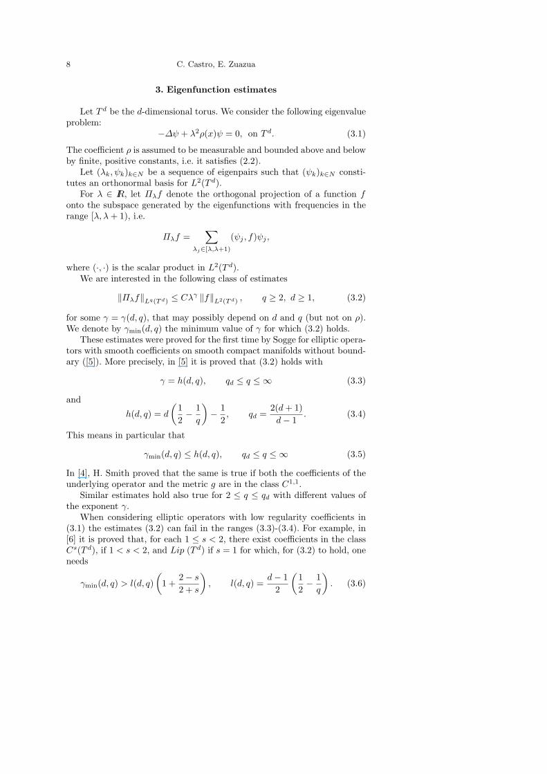
3. Eigenfunction estimates

Let T d be the d-dimensional torus. We consider the following eigenvalueproblem:

−∆ψ + λ2ρ(x)ψ = 0, on T d. (3.1)

The coefficient ρ is assumed to be measurable and bounded above and belowby finite, positive constants, i.e. it satisfies (2.2).

Let (λk, ψk)k∈N be a sequence of eigenpairs such that (ψk)k∈N consti-tutes an orthonormal basis for L2(T d).

For λ ∈ IR, let Πλf denote the orthogonal projection of a function fonto the subspace generated by the eigenfunctions with frequencies in therange [λ, λ+ 1), i.e.

Πλf =∑

λj∈[λ,λ+1)

(ψj , f)ψj ,

where (·, ·) is the scalar product in L2(T d).We are interested in the following class of estimates

‖Πλf‖Lq(T d) ≤ Cλγ ‖f‖L2(T d) , q ≥ 2, d ≥ 1, (3.2)

for some γ = γ(d, q), that may possibly depend on d and q (but not on ρ).We denote by γmin(d, q) the minimum value of γ for which (3.2) holds.

These estimates were proved for the first time by Sogge for elliptic opera-tors with smooth coefficients on smooth compact manifolds without bound-ary ([5]). More precisely, in [5] it is proved that (3.2) holds with

γ = h(d, q), qd ≤ q ≤ ∞ (3.3)

and

h(d, q) = d

(12− 1q

)− 1

2, qd =

2(d+ 1)d− 1

. (3.4)

This means in particular that

γmin(d, q) ≤ h(d, q), qd ≤ q ≤ ∞ (3.5)

In [4], H. Smith proved that the same is true if both the coefficients of theunderlying operator and the metric g are in the class C1,1.

Similar estimates hold also true for 2 ≤ q ≤ qd with different values ofthe exponent γ.

When considering elliptic operators with low regularity coefficients in(3.1) the estimates (3.2) can fail in the ranges (3.3)-(3.4). For example, in[6] it is proved that, for each 1 ≤ s < 2, there exist coefficients in the classCs(T d), if 1 < s < 2, and Lip (T d) if s = 1 for which, for (3.2) to hold, oneneeds

γmin(d, q) > l(d, q)(

1 +2− s

2 + s

), l(d, q) =

d− 12

(12− 1q

). (3.6)

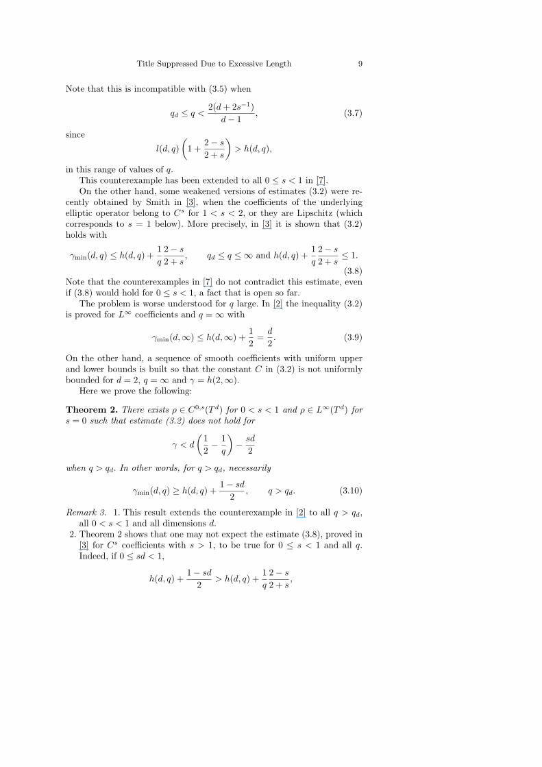
Title Suppressed Due to Excessive Length 9

Note that this is incompatible with (3.5) when

qd ≤ q <2(d+ 2s−1)

d− 1, (3.7)

since

l(d, q)(

1 +2− s

2 + s

)> h(d, q),

in this range of values of q.This counterexample has been extended to all 0 ≤ s < 1 in [7].On the other hand, some weakened versions of estimates (3.2) were re-

cently obtained by Smith in [3], when the coefficients of the underlyingelliptic operator belong to Cs for 1 < s < 2, or they are Lipschitz (whichcorresponds to s = 1 below). More precisely, in [3] it is shown that (3.2)holds with

γmin(d, q) ≤ h(d, q) +1q

2− s

2 + s, qd ≤ q ≤ ∞ and h(d, q) +

1q

2− s

2 + s≤ 1.

(3.8)Note that the counterexamples in [7] do not contradict this estimate, evenif (3.8) would hold for 0 ≤ s < 1, a fact that is open so far.

The problem is worse understood for q large. In [2] the inequality (3.2)is proved for L∞ coefficients and q = ∞ with

γmin(d,∞) ≤ h(d,∞) +12

=d

2. (3.9)

On the other hand, a sequence of smooth coefficients with uniform upperand lower bounds is built so that the constant C in (3.2) is not uniformlybounded for d = 2, q = ∞ and γ = h(2,∞).

Here we prove the following:

Theorem 2. There exists ρ ∈ C0,s(T d) for 0 < s < 1 and ρ ∈ L∞(T d) fors = 0 such that estimate (3.2) does not hold for

γ < d

(12− 1q

)− sd

2

when q > qd. In other words, for q > qd, necessarily

γmin(d, q) ≥ h(d, q) +1− sd

2, q > qd. (3.10)

Remark 3. 1. This result extends the counterexample in [2] to all q > qd,all 0 < s < 1 and all dimensions d.

2. Theorem 2 shows that one may not expect the estimate (3.8), proved in[3] for Cs coefficients with s > 1, to be true for 0 ≤ s < 1 and all q.Indeed, if 0 ≤ sd < 1,

h(d, q) +1− sd

2> h(d, q) +

1q

2− s

2 + s,

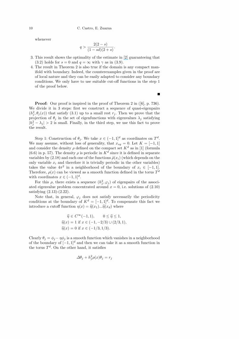
10 C. Castro, E. Zuazua

whenever

q >2(2− s)

(1− sd)(2 + s).

3. This result shows the optimality of the estimate in [2] guaranteeing that(3.2) holds for s = 0 and q = ∞ with γ as in (3.9).

4. The result in Theorem 2 is also true if the domain is any compact man-ifold with boundary. Indeed, the counterexamples given in the proof areof local nature and they can be easily adapted to consider any boundaryconditions. We only have to use suitable cut-off functions in the step 1of the proof below.

Proof: Our proof is inspired in the proof of Theorem 2 in ([6], p. 736).We divide it in 3 steps: first we construct a sequence of quasi-eigenpairs(h2

j , θj(x)) that satisfy (3.1) up to a small rest rj . Then we prove that theprojection of θj in the set of eigenfunctions with eigenvalues λj satisfying|h2

j − λj | > 2 is small. Finally, in the third step, we use this fact to provethe result.

Step 1: Construction of θj . We take x ∈ (−1, 1]d as coordinates on T d.We may assume, without loss of generality, that xsg = 0. Let K = [−1, 1]and consider the density ρ defined on the compact set Kd as in [1] (formula(6.6) in p. 57). The density ρ is periodic in Kd since it is defined in separatevariables by (2.18) and each one of the functions ρ(xi) (which depends on theonly variable xi and therefore it is trivially periodic in the other variables)takes the value 4π2 in a neighborhood of the boundary of xi ∈ [−1, 1].Therefore, ρ(x) can be viewed as a smooth function defined in the torus T d

with coordinates x ∈ (−1, 1]d.For this ρ, there exists a sequence (h2

j , ϕj) of eigenpairs of the associ-ated eigenvalue problem concentrated around x = 0, i.e. solutions of (2.10)satisfying (2.13)-(2.22).

Note that, in general, ϕj does not satisfy necessarily the periodicityconditions at the boundary of Kd = [−1, 1]d. To compensate this fact weintroduce a cutoff function η(x) = η(x1)...η(xd) where

η ∈ C∞(−1, 1), 0 ≤ η ≤ 1,η(x) = 1 if x ∈ (−1,−2/3) ∪ (2/3, 1),η(x) = 0 if x ∈ (−1/3, 1/3).

Clearly θj = φj− ηφj is a smooth function which vanishes in a neighborhoodof the boundary of [−1, 1]d and then we can take it as a smooth function inthe torus T d. On the other hand, it satisfies

∆θj + h2jρ(x)θj = rj

Title Suppressed Due to Excessive Length 11

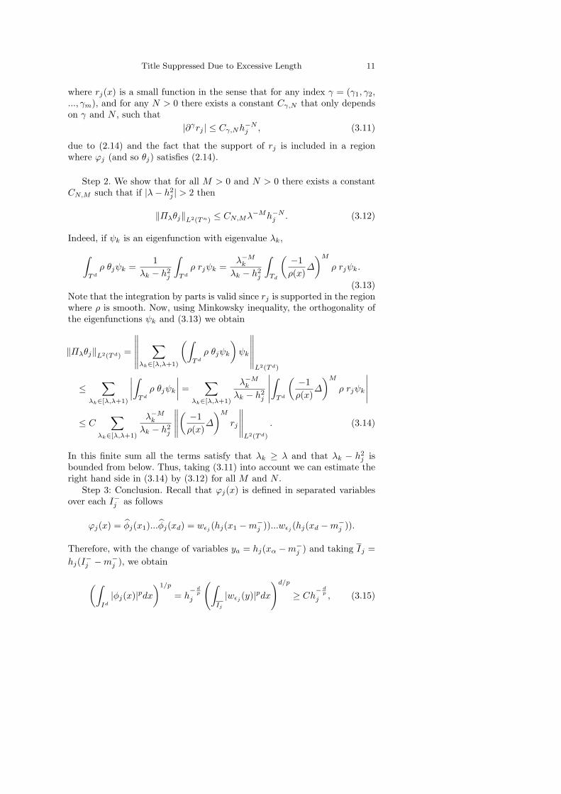
where rj(x) is a small function in the sense that for any index γ = (γ1, γ2,..., γm), and for any N > 0 there exists a constant Cγ,N that only dependson γ and N , such that

|∂γrj | ≤ Cγ,Nh−Nj , (3.11)

due to (2.14) and the fact that the support of rj is included in a regionwhere ϕj (and so θj) satisfies (2.14).

Step 2. We show that for all M > 0 and N > 0 there exists a constantCN,M such that if |λ− h2

j | > 2 then

‖Πλθj‖L2(T n) ≤ CN,Mλ−Mh−Nj . (3.12)

Indeed, if ψk is an eigenfunction with eigenvalue λk,∫T d

ρ θjψk =1

λk − h2j

∫T d

ρ rjψk =λ−M

k

λk − h2j

∫Td

(−1ρ(x)

∆

)M

ρ rjψk.

(3.13)Note that the integration by parts is valid since rj is supported in the regionwhere ρ is smooth. Now, using Minkowsky inequality, the orthogonality ofthe eigenfunctions ψk and (3.13) we obtain

‖Πλθj‖L2(T d) =

∥∥∥∥∥∥∑

λk∈[λ,λ+1)

(∫T d

ρ θjψk

)ψk

∥∥∥∥∥∥L2(T d)

≤∑

λk∈[λ,λ+1)

∣∣∣∣∫T d

ρ θjψk

∣∣∣∣ = ∑λk∈[λ,λ+1)

λ−Mk

λk − h2j

∣∣∣∣∣∫

T d

(−1ρ(x)

∆

)M

ρ rjψk

∣∣∣∣∣≤ C

∑λk∈[λ,λ+1)

λ−Mk

λk − h2j

∥∥∥∥∥(−1ρ(x)

∆

)M

rj

∥∥∥∥∥L2(T d)

. (3.14)

In this finite sum all the terms satisfy that λk ≥ λ and that λk − h2j is

bounded from below. Thus, taking (3.11) into account we can estimate theright hand side in (3.14) by (3.12) for all M and N .

Step 3: Conclusion. Recall that ϕj(x) is defined in separated variablesover each I−j as follows

ϕj(x) = φj(x1)...φj(xd) = wεj(hj(x1 −m−

j ))...wεj(hj(xd −m−

j )).

Therefore, with the change of variables ya = hj(xα −m−j ) and taking Ij =

hj(I−j −m−j ), we obtain

(∫Id

|φj(x)|pdx)1/p

= h− d

p

j

(∫Ij

|wεj(y)|pdx

)d/p

≥ Ch− d

p

j , (3.15)

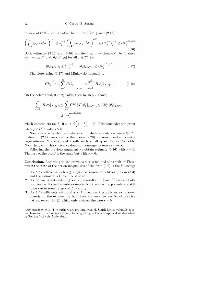
12 C. Castro, E. Zuazua

in view of (2.22). On the other hand, from (2.21), and (2.17)(∫T d

|φj(x)|2dx)1/2

≤ h− d

2j

(∫IR|wεj

(y)|2dx)d/2

≤ Ch− d

2j ε

− d2

j ≤ Ch− d(1−s)

2j .

(3.16)Both estimates (3.15) and (3.16) are also true if we change φj by θj sinceφj = θj on Id and |θj | ≤ |φj | for all x ∈ T d, i.e.

‖θj‖Lp(Id) ≤ Ch− d

p

j , ‖θj‖L2(T d) ≤ Ch− d(1−s)

2j . (3.17)

Therefore, using (3.17) and Minkowsky inequality,

Ch− d

q

j ≤

∥∥∥∥∥∞∑

k=1

Πkθj

∥∥∥∥∥Lq(Id)

≤∞∑

k=1

‖Πkθj‖Lq(Id) . (3.18)

On the other hand, if (3.2) holds, then by step 2 above,

∞∑k=1

‖Πkθj‖Lq(Id) ≤∞∑

k=1

Ckα ‖Πkθj‖L2(T d) ≤ Chαj ‖θj‖L2(T d)

≤ Chα− d(1−s)

2j

which contradicts (3.18) if α < d(

12 −

1q

)− sd

2 . This concludes the proof

when ρ ∈ C0,s with s > 0.Now we consider the particular case in which we only assume ρ ∈ L∞.

Instead of (2.17) we consider the choice (2.29) for some fixed sufficientlylarge integers N and L, and a sufficiently small ε1 so that (2.16) holds.Note that, with this choice, εj does not converge to zero as j →∞.

Following the previous argument we obtain estimate (3.16) with s = 0.The rest of the proof is the same but with s = 0.

Conclusion. According to the previous discussion and the result of Theo-rem 2 the state of the art on inequalities of the form (3.2) is the following:

1. For Cs coefficients with s ≥ 2, (3.2) is known to hold for γ as in (3.3)and the estimate is known to be sharp.

2. For Cs coefficients with 1 ≤ s < 2 the results in [3] and [6] provide bothpositive results and counterexamples but the sharp exponents are stillunknown in some ranges of d, s and q.

3. For Cs coefficients with 0 ≤ s < 1 Theorem 2 establishes some lowerbounds on the exponent γ but there are very few results of positivenature, except for [2] which only address the case s = 0.

Acknowledgements. The authors are grateful with H. Smith for his valuable com-ments on our previous work [1] and for suggesting us the new application describedin Section 3 of this Addendum.

Title Suppressed Due to Excessive Length 13

References

1. C. Castro and E. Zuazua, Concentration and lack of observability of waves inhighly heterogeneous media, Arch. Rational Mech. Anal., 164 (2002), 39-72.

2. E.B. Davies, Spectral proerties of compact manifolds and changes of metrics,Amer. J. Math. 112, (1990) 15-39.

3. H.F. Smith, Sharp L2 − Lq bounds on spectral projectors for low regularitymetrics, preprint.

4. H.F. Smith, Spectral cluster estimates for C1,1 metrics, preprint.5. C.D. Sogge, Concerning the Lp norm of spectral clusters for second order el-

liptic operators on compact manifolds, J. Funct. Analysis 5, (1988) 123-134.6. H.F. Smith and C.D. Sogge, On Strichartz and eigenfunctions estimates for

low regularity metrics, Math. Res. Let. 1, (1994) 729-737.7. H.F. Smith and D. Tataru, Sharp counterexamples for Strichartz estimates for

low frequency metrics, Math. Res. Let. 9, (2002) 199-204.8. D. Tataru, Strichartz estimates for second order hyperbolic operators with non-

smooth coefficients II, Amer. J. Math. 123, (2001) 385-423.

Departamento de Matematica e InformaticaETSI Caminos, Canales y Puertos

Univ. Politecnica de Madrid28040 Madrid, Spain.

ccastro@caminos.upm.es

and

Departamento de MatematicasUniversidad Autnoma28049 Madrid, Spain.

enrique.zuazua@uam.es