Article

Spectral fiber photometry

derives hemoglobinconcentration changes for accuratemeasurement offluorescent sensor activity

Graphical abstract

Highlights

d Hemoglobin absorbs light and creates artifacts in fiber

photometry recordings in vivo

d A method to derive hemoglobin concentration changes from

spectral photometry

d Correction of this artifact provides accuratemeasurements of

fluorescent sensor signals

d Quantification of regional differences in neurovascular

transfer function

Zhang et al., 2022, Cell Reports Methods 2, 100243July 18, 2022 ª 2022 The Authors.https://doi.org/10.1016/j.crmeth.2022.100243

Authors

Wei-Ting Zhang, Tzu-Hao Harry Chao,

Yue Yang, ..., Hongtu Zhu, Guohong Cui,

Yen-Yu Ian Shih

Correspondencecuig@mail.nih.gov (G.C.),shihy@unc.edu (Y.-Y.I.S.)

In brief

Changes in hemoglobin concentration

affect the accuracy of fiber photometry

measurements in vivo, even flipping the

measured signal polarity under certain

conditions. Zhang et al. develop an

approach to derive oxy- and deoxy-

hemoglobin concentration changes from

spectral fiber photometry data and a

pipeline to correct for these artifacts in

fluorescent sensor measurements.

ll

OPEN ACCESS

ll

Article

Spectral fiber photometry derives hemoglobinconcentration changes for accuratemeasurement of fluorescent sensor activityWei-Ting Zhang,1,2,3,9 Tzu-Hao Harry Chao,1,2,3,9 Yue Yang,1,2,3,4 Tzu-Wen Wang,1,2 Sung-Ho Lee,1,2,3

Esteban A. Oyarzabal,1,2,3 Jingheng Zhou,5 Randy Nonneman,1,2,3 Nicolas C. Pegard,6,7 Hongtu Zhu,2,4,8 Guohong Cui,5,*and Yen-Yu Ian Shih1,2,3,7,10,*1Center for Animal MRI, University of North Carolina at Chapel Hill, Chapel Hill, NC 27599, USA2Biomedical Research Imaging Center, University of North Carolina at Chapel Hill, Chapel Hill, NC 27599, USA3Department of Neurology, University of North Carolina at Chapel Hill, Chapel Hill, NC 27599, USA4Department of Biostatistics, University of North Carolina at Chapel Hill, Chapel Hill, NC 27599, USA5In Vivo Neurobiology Group, Neurobiology Laboratory, National Institute of Environmental Health Sciences, National Institutes of Health,

Durham, NC 27709, USA6Department of Applied Physical Sciences, UNCNeuroscience Center, University of North Carolina at Chapel Hill, Chapel Hill, NC 27599, USA7Department of Biomedical Engineering, University of North Carolina at Chapel Hill, Chapel Hill, NC 27599, USA8Department of Computer Science, University of North Carolina at Chapel Hill, Chapel Hill, NC 27599, USA9These authors contributed equally10Lead contact

*Correspondence: cuig@mail.nih.gov (G.C.), shihy@unc.edu (Y.-Y.I.S.)

https://doi.org/10.1016/j.crmeth.2022.100243

MOTIVATION Hemoglobin (Hb) in blood vessels is known to absorb light and affect the accuracy of opticalmeasurements. In fiber photometry, where photons are collectively sampled from a volume of the brain tis-sue, changes in Hb concentration could have a significant effect on its readout. It is therefore important toquantify Hb concentration fluctuations to ensure accurate photometry-based fluorescent sensor activitymeasurements. Here we describe a measurement platform and analytical methods that allowquantificationof oxy- and deoxy-Hb concentration changes and correction of Hb absorption artifacts in fiber photometrydata. We also demonstrate the added benefit of our methods to compute hemodynamic response functionusing the derived Hb concentration information.

SUMMARY

Fiber photometry is an emerging technique for recording fluorescent sensor activity in the brain. However,significant hemoglobin absorption artifacts in fiber photometry data may bemisinterpreted as sensor activitychanges. Because hemoglobin exists widely in the brain, and its concentration varies temporally, such arti-facts could impede the accuracy of photometry recordings. Here we present use of spectral photometry andcomputational methods to quantify photon absorption effects by using activity-independent fluorescencesignals, which can be used to derive oxy- and deoxy-hemoglobin concentration changes. Although thesechanges are often temporally delayed compared with the fast-responding fluorescence spikes, we foundthat erroneous interpretation may occur when examining pharmacology-induced sustained changes andthat sometimes hemoglobin absorption could flip the GCaMP signal polarity. We provide hemoglobin-basedcorrection methods to restore fluorescence signals and compare our results with other commonly used ap-proaches.We also demonstrated the utility of spectral fiber photometry for delineating regional differences inhemodynamic response functions.

INTRODUCTION

Fiber photometry relies on an implanted optical fiber to excite

and detect fluorescence signals and is best known for its ability

tomeasure ensemble neuronal or neurochemical activity in small

CelThis is an open access article under the CC BY-N

volumes of brain tissue in animal models. The simplicity and cost

effectiveness of the optical system make the technique highly

accessible (Meng et al., 2018), and lightweight, miniature fiber

opticsmake photometry compatible with awide variety of exper-

imental settings, such as freely moving behavioral assessment

l Reports Methods 2, 100243, July 18, 2022 ª 2022 The Authors. 1C-ND license (http://creativecommons.org/licenses/by-nc-nd/4.0/).

Articlell

OPEN ACCESS

(Kim et al., 2016; Meng et al., 2018) or head-fixed brain-wide im-

aging (Chen et al., 2019; Pais-Roldan et al., 2020; Figure 1A).

Several genetically encoded fluorescent sensors of cellular ac-

tivity and neurotransmitters have become widely available

(Chen et al., 2013; Dana et al., 2016; Marvin et al., 2013, 2019;

Patriarchi et al., 2018; Sun et al., 2018; Tian et al., 2009; Wang

et al., 2018a, 2018b), expanding the range of applications for fi-

ber photometry. The tunable spectral specificity has also

enabled new parallel sensing capabilities with wavelength multi-

plexing. Given its rapidly increasing usage in neuroscience (Cui

et al., 2013; Luchsinger et al., 2021; Pisano et al., 2019; Sych

et al., 2019), understanding the inherent confounding factors in

fiber photometry data is of paramount significance.

One of the most notable confounders affecting fluorescence

measurements is light absorption by hemoglobin (Hb) in blood

vessels (Ma et al., 2016; Prahl, 1999). Hb absorption artifacts

have been studied extensively in wide-field imaging with reflec-

tive or backscattered lights (Ma et al., 2016; Valley et al., 2020)

and recently in two-photon lifetime microscopy (2PLM)

measuring the partial pressure of O2 (Machler et al., 2021). Hb

absorption artifacts should be present in most photometry

data because the intervascular distance of capillaries is known

to be less than 60 mm in nearly every location in the brain (Smith

et al., 2019) and commonly used photometry targeted volumes

are 105–106 mm3 (Pisanello et al., 2019). This absorption occurs

in two phases: along the excitation path, by absorbing photons

that travel from the fiber tip to the targeted fluorescent proteins,

and along the emission path, by absorbing photons emitted by

the fluorescent proteins as they travel back toward the optical fi-

ber (Figure 1B). Both absorption effects add up and result in a

substantial photon count reduction. Importantly, Hb absorption

is nonlinear and wavelength dependent and varies as a function

of dynamic oxy-Hb (HbO) and deoxy-Hb (HbR) concentration

changes in vivo (DCHbO and DCHbR, respectively) (Meng and

Alayash, 2017; Prahl, 1999; Figures S1A and S1B; derived from

Prahl, 1999). Because the power spectra of hemodynamic sig-

nals overlap significantly with most fluorescent sensors (Fig-

ure S1C), Hb absorption artifacts cannot be removed from fiber

photometry data by notch filtering or regressing cerebral blood

flow or cerebral blood volume (CBV) signals. To the best of our

knowledge, the influence of Hb absorption on fiber photom-

etry-derived fluorescent sensor activity has never been studied.

The ability to quantify Hb concentration fluctuations in photom-

etry data would not only enable more accurate fluorescent

sensor activity measurements but also provide concurrent he-

modynamic metrics, which is the foundation of several brain

mapping techniques, including functional magnetic resonance

imaging (fMRI) (Schulz et al., 2012), intrinsic optics (Hillman,

2007), and functional ultrasound (Rungta et al., 2017).

In this study, we propose use of spectrally resolved fiber

photometry and computational methods that can independently

derive HbO and HbR concentration changes from activity-inde-

pendent fluorescent reporter signals. We present use of this

technique to remove Hb absorption artifacts from calcium activ-

ity recording and demonstrate the added benefit to compute the

transfer function between neuronal and vascular activity, which

is crucial for interpreting hemodynamics-based neuroimaging

data such as fMRI, functional ultrasound, and intrinsic optics.

2 Cell Reports Methods 2, 100243, July 18, 2022

A step-by-step protocol of this method could be found in Zhang

et al. (2022).

RESULTS

Theoretical Hb absorption effect on photometryrecordingsWe solved the following equation using the generalized method

of moments (GMM) (Hansen, 1982) with spectrometer outputs,

which provides quantifiable photon counts across spectra:

Fðt; lEmÞFðt0; lEmÞ = e� ½Dmaðt;lExÞXðlExÞ+Dmaðt;lEmÞXðlEmÞ�$

CðtÞCðt0Þ (Equation 1)

where Dmaðt; lExÞ and Dmaðt; lEmÞ represent the absorption coef-

ficient changes at excitation wavelength lEx and emission wave-

length lEm , respectively, at time point t compared with a refer-

ence time point t0. Dmaðt; lExÞ and Dmaðt; lEmÞ are affected by

DCHbO and DCHbR (STAR Methods, Equation 16). XðlExÞ and

XðlEmÞ represent the photon traveling path lengths (see STAR

Methods for details) at the excitation and emission wavelengths,

respectively. To solve Equation 1, we first performed a Monte

Carlo simulation using the pipeline shown in Figure S2A to obtain

XðlExÞ and XðlEmÞ. We determined the average photon traveling

path lengths for emission wavelengths from 488–700 nm in the

simulated brain tissue from a total of 29 simulations (2–2.5 3

104 photons each; Figure 1C, detailed numbers tabulated in

Table S1). These results are expected to be generalizable and

can be used across labs. As an example, we illustrated spatial

probability and luminance-distance profiles for the commonly

used 488-nm excitation, 515-nm emission and 580-nm emission

in Figures S2B–S2D (see also Video S1). These results allowed

calculating the simulated effects of Hb absorption on fluores-

cence signal measurements, for which we observed significant

nonlinear, wavelength-dependent effects (Figure 1D).

Ex vivo quantification of Hb absorption effects onphotometry recordingsWe first performed ex vivomeasurements and showed that add-

ing 1 mL of fresh venous mouse blood into a 10-mL mixture of

Alexa 488 and 568 fluorescent dye solution significantly reduced

both fluorescence signals measured by fiber photometry.

Compared with adding the blood, adding 1 mL vehicle (0.9% sa-

line) induced significantly less reduction in Alexa 488 and 568

signals (Figures S3A–S3C). Subsequently, we saturated the

mixture with 100% oxygen to increase the HbO-HbR ratio and

observed marked increases in the Alexa 568 signals but de-

creases in Alexa 488 signals. We did not observe significant

signal changes when infusing oxygen into the solution with

1 mL saline added (Figures S3B and S3D).

In vivo quantification of Hb absorption effects onphotometry recordingsWe performed an in vivo experiment to measure the Hb absorp-

tion of activity-independent fluorescence signals in fiber photom-

etry. We selected a commonly used fluorophore, enhanced

yellow fluorescent protein (EYFP), whose fluorescence signal is

Figure 1. Spectrally resolved fiber photometry sys-

tem and Hb absorption effects

(A) Schematic of a spectrally resolved fiber photometry sys-

tem used for recording fluorescence signals.

(B) Hb in red blood cells absorbs light in two phases: exci-

tation light from the optical fiber (left) and emission light to be

recorded by the optical fiber (right). The color density of ar-

rowheads indicates light intensity. An increase in Hb is ex-

pected to decrease the number of photons in both phases.

(C) Simulated average excitation and emission photon trav-

eling path lengths across 488- 700-nm emission wavelengths

from our database of paired excitation/emission light paths.

(D) Effect of HbO and HbR concentration on DF/F. Shown are

simulated effects of HbO and HbR concentration changes on

measurement of fluorescence signals. DCHb0 and DCHbR

ranging from �90 to +90 mM were used to simulate fluores-

cence signal changes (DF/F) between 500 and 700 nm using

the molar extinction coefficients of HbO and HbR (Figure S1)

and simulated light paths (Figure 1C). Graphs shaded in blue

indicate an overall decrease in total Hb (HbT), and graphs

shaded in red indicate an overall increase in HbT.

See also Figures S1, S2, Video S1, and Table S1.

Cell Reports Methods 2, 100243, July 18, 2022 3

Articlell

OPEN ACCESS

Figure 2. In vivo quantification of HbO and HbR changes using EYFP emission in fiber photometry and correction of EYFP signals for Hb

absorption

(A) Preparation for fiber photometry measurement of EYFP signals in S1FL.

(B) Confocal image showing EYFP expression.

(C) Simultaneous dual spectral photometry recording of EYFP signals and hemodynamic responses (CBV) was achieved by intravenously injecting a long-

circulating red fluorescent dye, Rhodamine B.

(D–J) Peri-stimulus heatmaps showing repeated trials and average response time courses of the changes in measured rhoCBV, measured EYFP, derived HbO,

derived HbR, corrected rhoCBV, corrected EYFP, and derived HbT, respectively. The gray-shaded segment indicates the forepaw stimulation period. Hb ab-

sorption induces pseudo-negative changes in measured EYFP signals during stimulation.

(K and L) Correction of the contaminated EYFP and rhoCBV signals, respectively, in 5 hemispheres and 30 trials (***p < 0.001, paired t test). Measured and

corrected EYFP signals are compared. Measured rhoCBV was normalized to 0 to show the difference before and after correction.

All color bars use the same unit as the y axis of the time course. Error bars represent standard deviation.

See also Figures S3–S5.

Articlell

OPEN ACCESS

activity independent and has an emission spectrum peaking at

526 nm. We virally expressed EYFP using an adeno-associated

virus (AAV) in the primary somatosensory cortex of the forelimb

region (S1FL) under the Ca2+/calmodulin-dependent protein

kinase IIa (CaMKIIa) promoter and then implanted an optical fiber

into this target area (Figures2Aand2B).On thedayof photometry

recording, we intravenously administered Rhodamine B, a long-

circulating red fluorescent dye, to enable steady-state CBVmea-

surements (Unekawa et al., 2015; Figure 2C) and cross-validate

our proposed method for calculating total Hb concentration

changes. The resulting EYFP and Rhodamine B spectra overlap-

ped significantlywith theHbabsorption spectra (FiguresS1Aand

S1B), suggesting a significant effect of Hb absorption on the data

from these fluorescence signals. Upon electrical stimulation of

the contralateral forepaw (9 Hz, 3 mA, 0.5-ms pulse width for

10 s), we observed robust positive Rhodamine-derived CBV

4 Cell Reports Methods 2, 100243, July 18, 2022

(rhoCBV) changes, as expected (Figure 2D). Intriguingly, the

EYFP signal concurrently recorded from the same fiber showed

robust negative changes (Figure 2E), which indicated significant

Hb absorption of the EYFP signal in vivo. Although a pH-depen-

dent effect on the EYFP signal cannot be completely excluded,

a previous study has shown that, at pH 6.5–9, where typical pH

homeostasis of a hippocampal neuron (�7.03–7.46) is located

(Ruffin et al., 2014), EYFP excited by 470 nmwas not significantly

affected by the pH changes (Nakabayashi et al., 2012). Using

well-documented molar extinction coefficients (Figures S1A

and S1B), photon-traveling path lengths derived from a Monte

Carlo simulation (Figure 1C) and spectral fiber photometry

datapoints across 502- to 544-nm wavelengths over time (see

Equations 17, 18, 19, 20, and 21 in STAR Methods), we derived

DCHbOðtÞ and DCHbRðtÞ using GMM. This is feasible and robust

because we have access to a range of spectral datapoints for

Articlell

OPEN ACCESS

every single time point and therefore could use numerous empir-

ical data to solve two unknowns (DCHbO and DCHbR; see also

Figures S4A and S4B for the effect of input spectral datapoints).

The derived concentration changes (Figures 2F and 2G) were

within physiological ranges and comparable with those reported

in the literature (Ma et al., 2016), and the summation of the two

(i.e., total Hb concentration changes, termed DCHbTðtÞ ) informs

CBV changes (Ma et al., 2016; Figure 2J). The calculated

DCHbTðtÞ highly resembled the rhoCBV changes measured from

a distinct and less affected red spectrum (Figures S4C–S4E).

With DCHbOðtÞ and DCHbRðtÞ obtained, we then calculated

Dmaðt; lExÞ and Dmaðt; lEmÞ and entered these parameters into

Equation 1 to correct the rhoCBV changes (Figure 2H) and

EYFP signals (Figure 2I). Figure 2I shows a flattened EYFP trace

after the proposed correction, demonstrating the validity of our

approach. Although the influence of Hb absorption on EYFP sig-

nals varied by trials, our proposed method accurately corrected

EYFP signals in all trials (Figure 2K). Despite the smaller influence

on the rhoCBV signal measured from the red spectrum, the ab-

sorption effect remained statistically significant (Figure 2L). In

addition to the fluorescence signal changes induced by forepaw

sensory stimulations, we also replicated these findings using a

5% CO2 hypercapnic challenge paradigm and successfully

restored the contaminated EYFP signal changes (Figure S5).

Effect of Hb absorption on acute GCaMP signal mea-surements using fiber photometryWe virally expressed GCaMP6f (hereafter called GCaMP), one of

the most widely used genetically encoded calcium indicators

(Chen et al., 2013), using an AAV under the CaMKIIa promoter

in the S1FL. We also expressed tandem dimer tomato (tdTo-

mato), an activity-independent red fluorescent protein, under

the CAG promoter (Figures 3A and 3B) and then implanted an

optical fiber into this target area. Our rationale for choosing tdTo-

mato was similar to that for EYFP (Figure 2): it does not encode

activity changes, and, thus, its photon counts can be used to

derive DCHbO and DCHbR. Unlike in the experiment described in

Figure 2, Rhodamine B could no longer be used for CBV

cross-validation because the red spectrum was occupied by

tdTomato (Figure 3C). Instead, we performed this GCaMP-

tdTomato experiment in an MRI scanner, where CBV changes

could be measured by intravenously administering an iron oxide

contrast agent, Feraheme23 (Figure 3D). This allowed CBV to be

validated using an established and completely independent mo-

dality. After a short, 1-s electrical stimulation of the contralateral

forepaw (9 Hz, 3 mA, 0.5-ms pulse width), we observed a

rapid increase in GCaMP signal followed by an undershoot

(Figures 3E–3Q). Such an undershoot is absent in cultured neu-

rons where Hb is not present and rarely observed in two-photon

imaging data, where neurons and blood vessels are mostly

segregated in space (Chen et al., 2013; Mittmann et al., 2011).

The tdTomato signal decreased significantly upon forepaw stim-

ulation and showed a much longer delay in its kinetics, but its

peak temporally matched that of the GCaMP undershoot (Fig-

ure 3F). Using methods similar to that described in Figure 2,

but with spectral photometry datapoints across 575- 699-nm

wavelengths over time, we derived DCHbO (t) and DCHbR (t)

(Figures 3G and 3H). Interestingly, the derived DCHbR data ex-

hibited a rapid initial increase (Figure 3H) before a more pro-

longed reduction, a phenomenon well documented in the optical

literature (Devor et al., 2003) and termed ‘‘initial dip’’ in blood-ox-

ygen-level-dependent fMRI (Hu and Yacoub, 2012). This initial

increase in HbR was not detectable in the raw tdTomato data,

indicating that our method is capable of deriving parameters

with temporal kinetics distinct from the detected raw fluores-

cence activity. Figure 3J shows the corrected GCaMP signals,

where the after-stimulus undershoot no longer exists. Accord-

ingly, Figure 3K shows a flattened tdTomato trace after the

correction. The derived DCHbT(t) (Figure 3I) highly resembled

the CBV changes measured by fMRI (Figure 3L), and these two

time-courses correlated significantly (Figure 3M). The derived

DCHbT showed higher sensitivity than MRI-CBV (Figure 3N).

We observed no significant time lag between the DCHbT and

CBV-fMRI time courses (Figures 3O and 3P).

Figures 3Q and 3R demonstrate the corrections of pseudo-

undershoot artifacts in GCaMP time courses of short (1 s)

and long (10 s) stimulations, respectively. These artifacts after

short bursts of activation were also apparent when optogenetic

stimulation was applied in the brain (Figures S6A–S6D). We

also observed a significant correction effect on GCaMP

response amplitudes (Figure S6E). Without proper correction

of Hb absorption artifacts, the accuracy of quantified fluores-

cence signals is compromised, leading to misinterpretation of

fiber photometry data. This problem could become exacer-

bated in the absence of time-locked stimulations because the

desired activity could be superimposed on physiological hemo-

dynamic signal changes.

Effect of Hb absorption on sustained GCaMP signalmeasurement using fiber photometryTo demonstrate the effect of Hb absorption on GCaMP signals

over an extended period of time, we leveraged an acute ethanol

challenge protocol (Broadwater et al., 2018; Vaagenes et al.,

2015) that has been shown to decrease neuronal activity

(Lotfullina and Khazipov, 2018) as well as cerebral perfusion

(Broadwater et al., 2018; Kelly et al., 1997; Sano et al., 1993).

We virally expressed GCaMP using an AAV under the

CaMKIIa promoter and tdTomato under the CAG promoter in

the prelimbic cortex (PrL) (Figure 4A) and then implanted an op-

tical fiber in this target area. On the day of the experiment,

ethanol (2 g/kg, 20% [v/v], intraperitoneally [i.p.]) was given

5 min after onset of fiber photometry recording. After ethanol

administration, we observed robust increases in the raw,

measured tdTomato (Figure 4B) and GCaMP (Figure 4C) sig-

nals. These changes were ethanol specific because we did

not observe any changes in a separate session where the

same group of subjects received a vehicle injection (an equal

volume of 0.9% saline, i.p.) (Figures 4B and 4C). Next, we

derived DCHbOðtÞ, DCHbRðtÞ, and DCHbT ðtÞ (Figure 4D) from

the ethanol data using correction methods identical to that

described in Figure 3 and found robust decreases in

DCHbOðtÞ and DCHbT ðtÞ, in agreement with studies showing

reduced Hb affinity for oxygen (Van De Borne et al., 1997)

and vasoconstriction (Kudo et al., 2015) following acute alcohol

administration. Following our proposed correction, the tdTo-

mato trace flattened as expected (Figures 4B and 4E).

Cell Reports Methods 2, 100243, July 18, 2022 5

Figure 3. In vivo quantification of HbO and HbR changes using tdTomato emission in fiber photometry and correction of GCaMP signals for

Hb absorption

(A) Preparation for fiber photometry measurement of GCaMP and tdTomato signals in S1FL.

(B) Confocal images showing GCaMP and tdTomato expression.

(C) GCaMP and tdTomato emission spectra from 488-nm excitation.

(D) Concurrent CBVmeasurement was achieved byMRI and intravenous injection of long-circulating iron oxide nanoparticles (Feraheme). The inset shows amap

of group-level fMRI activation induced by forepaw stimulation (corrected p < 0.05, n = 5 hemispheres).

(E–L) Peri-stimulus heatmaps showing repeated trials and average response time courses of the changes in measured GCaMP, measured tdTomato, derived

HbO, derived HbR, derived HbT, corrected GCaMP, corrected tdTomato, and measured MRI-CBV, respectively. The gray-shaded segment indicates the fore-

paw stimulation period. All color bars use the same unit as the y axis of the time course.

(M) Two-dimensional histogram summarizing the changes in HbT and MRI-CBV in 5 hemispheres and 27 trials. The color bar indicates counts on the log scale.

(N) HbT derived from photometry exhibited higher sensitivity than MRI-CBV (***p < 0.001, paired t-test).

(O) Cross-correlation at the trial level between the Z scores of the derived HbT and the Z scores of the MRI-CBV over the 10-s peri-stimulus period.

(P) Scatterplots showing the cross-correlation coefficients (left) and time lag (right) of all trials.

(Q andR) Correction of pseudo-undershoot artifacts inGCaMP time courses of (Q) short (1 s), and (R) long (10 s) stimulations, respectively (***p < 0.001, paired t-test).

All error bars represent standard deviation.

See also Figures S6, S9, and S10.

Articlell

OPEN ACCESS

Importantly, the trend of the GCaMP signal shifted from unex-

pected positive changes to the expected negative changes

(Lotfullina and Khazipov, 2018; Figures 4C and 4F). In another

two proof-of-concept experiments, we also noted the influence

of Hb absorption on anesthetics- and pharmacology-induced

fluorescence signal changes (Figure S7). These data highlight

the importance of correcting for Hb absorption in fiber photom-

etry studies because misinterpretation may otherwise occur.

6 Cell Reports Methods 2, 100243, July 18, 2022

Correction of Hb absorption artifacts in other fiberphotometry settingsTo expand the utility of our method, we modeled and compared

the Hb absorption correction techniques among three settings.

The first method involves using a spectrometer with a sequence

that interleaves between 405 and 488 nmexcitation. TheGCaMP

isosbestic point is around 405 nm (Tian et al., 2009; Dana et al.,

2019), where excitation light delivered at this range would

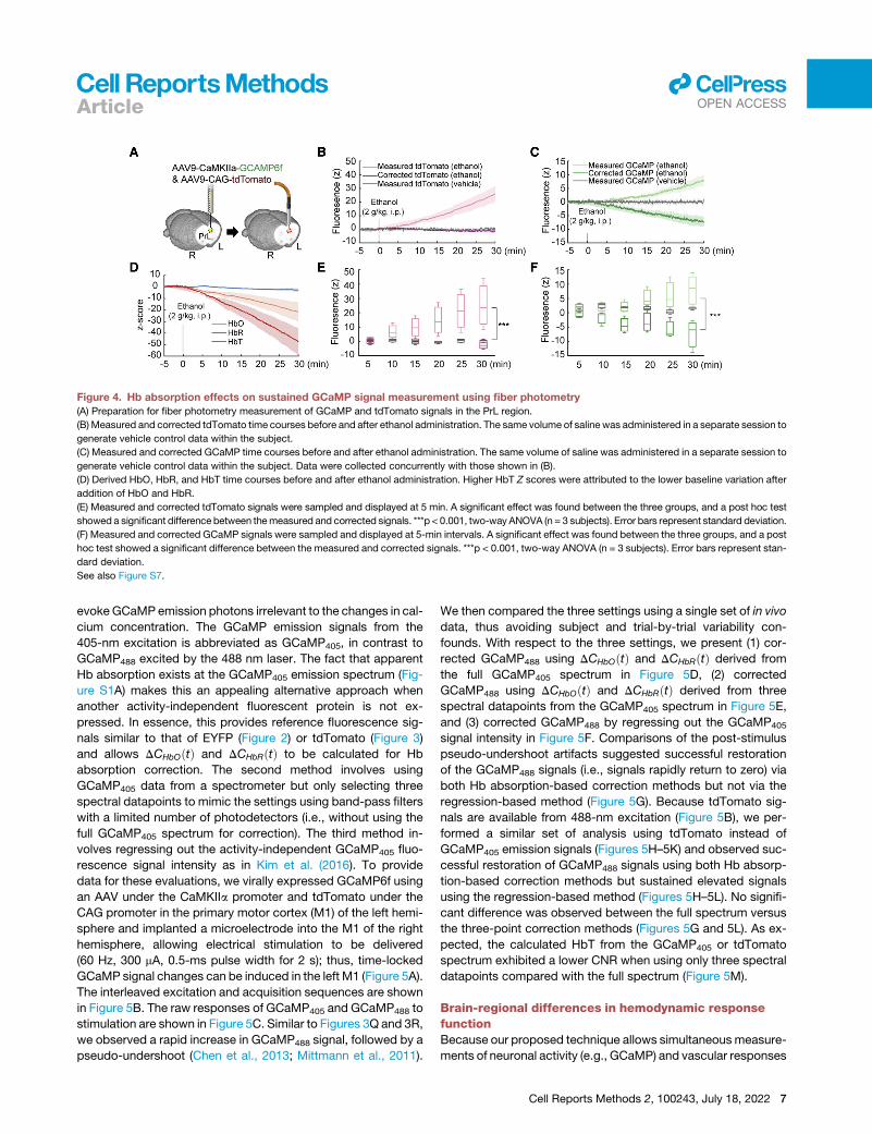
Figure 4. Hb absorption effects on sustained GCaMP signal measurement using fiber photometry

(A) Preparation for fiber photometry measurement of GCaMP and tdTomato signals in the PrL region.

(B) Measured and corrected tdTomato time courses before and after ethanol administration. The same volume of saline was administered in a separate session to

generate vehicle control data within the subject.

(C) Measured and corrected GCaMP time courses before and after ethanol administration. The same volume of saline was administered in a separate session to

generate vehicle control data within the subject. Data were collected concurrently with those shown in (B).

(D) Derived HbO, HbR, and HbT time courses before and after ethanol administration. Higher HbT Z scores were attributed to the lower baseline variation after

addition of HbO and HbR.

(E) Measured and corrected tdTomato signals were sampled and displayed at 5 min. A significant effect was found between the three groups, and a post hoc test

showed a significant difference between themeasured and corrected signals. ***p < 0.001, two-way ANOVA (n = 3 subjects). Error bars represent standard deviation.

(F) Measured and corrected GCaMP signals were sampled and displayed at 5-min intervals. A significant effect was found between the three groups, and a post

hoc test showed a significant difference between the measured and corrected signals. ***p < 0.001, two-way ANOVA (n = 3 subjects). Error bars represent stan-

dard deviation.

See also Figure S7.

Articlell

OPEN ACCESS

evoke GCaMP emission photons irrelevant to the changes in cal-

cium concentration. The GCaMP emission signals from the

405-nm excitation is abbreviated as GCaMP405, in contrast to

GCaMP488 excited by the 488 nm laser. The fact that apparent

Hb absorption exists at the GCaMP405 emission spectrum (Fig-

ure S1A) makes this an appealing alternative approach when

another activity-independent fluorescent protein is not ex-

pressed. In essence, this provides reference fluorescence sig-

nals similar to that of EYFP (Figure 2) or tdTomato (Figure 3)

and allows DCHbOðtÞ and DCHbRðtÞ to be calculated for Hb

absorption correction. The second method involves using

GCaMP405 data from a spectrometer but only selecting three

spectral datapoints to mimic the settings using band-pass filters

with a limited number of photodetectors (i.e., without using the

full GCaMP405 spectrum for correction). The third method in-

volves regressing out the activity-independent GCaMP405 fluo-

rescence signal intensity as in Kim et al. (2016). To provide

data for these evaluations, we virally expressed GCaMP6f using

an AAV under the CaMKIIa promoter and tdTomato under the

CAG promoter in the primary motor cortex (M1) of the left hemi-

sphere and implanted a microelectrode into the M1 of the right

hemisphere, allowing electrical stimulation to be delivered

(60 Hz, 300 mA, 0.5-ms pulse width for 2 s); thus, time-locked

GCaMP signal changes can be induced in the left M1 (Figure 5A).

The interleaved excitation and acquisition sequences are shown

in Figure 5B. The raw responses of GCaMP405 and GCaMP488 to

stimulation are shown in Figure 5C. Similar to Figures 3Q and 3R,

we observed a rapid increase in GCaMP488 signal, followed by a

pseudo-undershoot (Chen et al., 2013; Mittmann et al., 2011).

We then compared the three settings using a single set of in vivo

data, thus avoiding subject and trial-by-trial variability con-

founds. With respect to the three settings, we present (1) cor-

rected GCaMP488 using DCHbOðtÞ and DCHbRðtÞ derived from

the full GCaMP405 spectrum in Figure 5D, (2) corrected

GCaMP488 using DCHbOðtÞ and DCHbRðtÞ derived from three

spectral datapoints from the GCaMP405 spectrum in Figure 5E,

and (3) corrected GCaMP488 by regressing out the GCaMP405

signal intensity in Figure 5F. Comparisons of the post-stimulus

pseudo-undershoot artifacts suggested successful restoration

of the GCaMP488 signals (i.e., signals rapidly return to zero) via

both Hb absorption-based correction methods but not via the

regression-based method (Figure 5G). Because tdTomato sig-

nals are available from 488-nm excitation (Figure 5B), we per-

formed a similar set of analysis using tdTomato instead of

GCaMP405 emission signals (Figures 5H–5K) and observed suc-

cessful restoration of GCaMP488 signals using both Hb absorp-

tion-based correction methods but sustained elevated signals

using the regression-based method (Figures 5H–5L). No signifi-

cant difference was observed between the full spectrum versus

the three-point correction methods (Figures 5G and 5L). As ex-

pected, the calculated HbT from the GCaMP405 or tdTomato

spectrum exhibited a lower CNR when using only three spectral

datapoints compared with the full spectrum (Figure 5M).

Brain-regional differences in hemodynamic responsefunctionBecause our proposed technique allows simultaneous measure-

ments of neuronal activity (e.g., GCaMP) and vascular responses

Cell Reports Methods 2, 100243, July 18, 2022 7

Figure 5. Correction of Hb absorption artifacts in other fiber photometry settings

(A) Preparation for fiber photometry measurement of GCaMP and tdTomato signals in the left M1, with the right M1 receiving local micro-electrical stimulation.

(B) Interleaved acquisition paradigm with 405- and 488-nm excitation lasers. Ca2+-independent GCaMP signals (GCaMP405) were excited by a 405-nm laser,

whereas Ca2+-dependent GCaMP signals (GCaMP488) and tdTomato signals were excited by a 488-nm laser. This interleaved paradigm was used because

GCaMP405 and GCaMP488 share nearly identical emission spectra and cannot be spectrally unmixed. Data were acquired at 50% duty cycle every 50 ms using a

box paradigm to avoid spectrometer frame loss during trigger mode. The final sampling rate is 10 Hz for all signals.

(C) Measured GCaMP488 and GCaMP405 signals without any correction.

(D) Corrected GCaMP488 using HbO and HbR dynamics derived from the full GCaMP405 spectrum.

(E) Corrected GCaMP488 using HbO and HbR dynamics from 3 datapoints in the GCaMP405 spectrum (at 502, 523, and 544 nm).

(F) Corrected GCaMP488 by regressing out the GCaMP405 signal dynamics.

(legend continued on next page)

8 Cell Reports Methods 2, 100243, July 18, 2022

Articlell

OPEN ACCESS

Articlell

OPEN ACCESS

(e.g., DCHbT ) with minimized Hb absorption artifacts, it offers a

significant added benefit for studying the relationship between

the two. This relationship, often termed the hemodynamic

response function (HRF), governs data interpretation of many

noninvasive neuroimaging technologies such as fMRI, intrinsic

optics, and functional ultrasound (Taylor et al., 2018). Although

use of a canonical HRF to model activity throughout the brain re-

mains the most common practice in the field, accumulating evi-

dence shows that HRF is region dependent (Devonshire et al.,

2012; Taylor et al., 2018) and that a thorough understanding of

HRF affected by regional cell types, neurochemicals, and sub-

ject conditions is crucial to accurately interpret most neuroimag-

ing data (Lecrux and Hamel, 2016). To demonstrate the utility of

our proposed technique for computing region- and sensor-

dependent HRFs (Chao et al., 2022), we first described the

method to compute HRF (Figure S8A), similar to that in Chao

et al. (2022), and then validated the results on a dataset not

used in HRF computation (Figure S8B). Next, we virally ex-

pressed GCaMP6f using an AAV under the CaMKIIa promoter

and tdTomato under theCAGpromoter in theM1 of the left hemi-

sphere and the caudate putamen (CPu; also known as the dorsal

striatum) of the right hemisphere (Figures 6A and 6B). We im-

planted a microelectrode into the M1 of the right hemisphere

(Figure 6A) so that transcallosal and corticostriatal stimulation

could be achieved simultaneously. Upon electrical stimulation

(60 Hz, 300 mA, 0.5-ms pulse width for 2 s), we observed robust

GCaMP changes in the left M1 and right CPu (Figures 6C and

6D), which are both monosynaptically connected to the stimula-

tion target. After calculation of Hb concentration changes, Hb

absorption correction, and computation of HRFs, we observed

that the M1 and CPu exhibited distinct HRF profiles

(Figures 6C and 6D). Interestingly, we also observed distinct

HbR polarities between these two regions.

DISCUSSION

Techniquesmeasuring fluorescence signals in vivo, such as fiber

photometry (Liang et al., 2017; Schlegel et al., 2018; Chao et al.,

2022), one-photon microscopy (Bollimunta et al., 2021), two-

photon microscopy (Baraghis et al., 2011), or macroscopic im-

aging through a thinned skull or implanted window (Cramer

et al., 2021), may suffer from Hb absorption. Unlike many imag-

ing techniques that provide spatial information, fiber photometry

does not resolve fluorescence signals emitted from individual

cells, and its analysis cannot spatially circumvent the blood ves-

sels. Instead, fiber photometry uses an optical fiber to collect all

photons from the targeted volume (Figures S2B–S2D). With the

(G) Comparisons of the post-stimulus undershoot artifacts among uncorrected

shown, respectively, in (D)–(F). ***p < 0.001, paired t-test (4 subjects, 31 trials).

(H) Measured GCaMP488 and tdTomato signals without any correction.

(I) Corrected GCaMP488 using HbO and HbR dynamics derived from full the tdTo

(J) Corrected GCaMP488 using HbO and HbR dynamics from 3 datapoints in the

(K) Corrected GCaMP488 by regressing out the tdTomato signal dynamics.

(L) Comparisons of the post-stimulus undershoot artifacts among uncorrected

shown, respectively, in (I)–(K). ***p < 0.001, paired t-test (4 subjects, 31 trials).

(M) Sensitivity of HbO, HbR, and HbT derived from full or 3-point emission spectr

GCaMP405 and tdTomato signals. ***p < 0.001, paired t-test (4 subjects, 31 trials

All error bars represent standard deviation.

conventional fiber photometry setting, the targeted volume has

been reported to be 105–106 mm3with a recording depth approx-

imately 200 mm from the fiber tip (Pisanello et al., 2019). Our

simulated detection volume is well within this range (Figure S9A).

With the average blood volume fraction in the brain and the Hb

concentration documented in the literature (van Zijl et al.,

1998), about 9,860 mM Hb would appear in the photometry-

detectable brain volume and affect the accuracy of fluorescent

sensor measurement by absorbing excitation and emission pho-

tons. Under normal physiological conditions, CHbO, CHbR, and

CHbT could change up to 40 mM (Hillman, 2014), and CBV could

change up to �20% (Uluda�g and Blinder, 2018; Hua et al., 2019)

in response to neuronal activity, making such correction a time

dependent problem. Our derived changes in DCHbO, DCHbR,

and DCHbT (Figures 2F, 2G, 2J, and 3G–3I) and measured

rhoCBV (Figure 2H) and MRI-CBV (Figure 3L) confirm that the

amplitudes of those changes are possible in vivo. Our data indi-

cated that roughly 20% of the CBV increase would contribute to

a 4.08% decrease in green fluorescence signal changes (Fig-

ure S9B; 95% confidence interval [CI], 1.33%–6.83%) and

2.20%decrease in red fluorescence signal changes (Figure S9C;

95% CI, 0.57%–3.84%). This level of fluorescence signal

changes (DF/F) on green and red sensors is commonly reported

in the photometry literature (Chen et al., 2013; Sun et al., 2018)

and could be interpreted as changes in specific sensor activity

when caution was not exercised. Conventionally, in brain regions

where CBV increases after local neuronal activation, pseudo-

negative fluorescent sensor activity would be expected. Howev-

er, in cases where CBV decreases with neuronal inhibition (e.g.,

Figure 4), or on occasion with activation (Shih et al., 2009, 2011,

2014; Schridde et al., 2008; Mishra et al., 2011), a pseudo-pos-

itive fluorescence signal would occur. Although several tech-

niques are readily available to measure CBV (Kwong et al.,

1992; Mintun et al., 1984; Sakai et al., 1985; Siegel et al., 2003;

Figures 2D–2H and 3L), correction of Hb absorption cannot be

achieved simply by regressing the CBV signal measured concur-

rently (Figures S9D and S9E). This is mainly due to the fact that

HbO and HbR absorption are wavelength dependent, and their

respective concentrations change over time (Meng and Alayash,

2017; Prahl, 1999; Figures S1A and S1B). Our simulation sug-

gested that the accuracy of the fluorescence signal could be

compromised even without a net change in CBV (see Figure 1D

for plots without a shaded background). This makes it crucial to

quantify DCHbO and DCHbR so that the true changes in the fluo-

rescence signal can be restored.

At present, two major fluorescence-measurement strategies

are used in fiber photometry. One is non-spectrally resolved

GCaMP488 and corrected GCaMP488 signals from three different settings, as

mato spectrum.

tdTomato spectrum (at 578, 594, and 610 nm).

GCaMP488 and corrected GCaMP488 signals from three different settings, as

a. A comparison was made between these two conditions and between use of

); ###p < 0.001, two-way ANOVA (4 subjects, 31 trials).

Cell Reports Methods 2, 100243, July 18, 2022 9

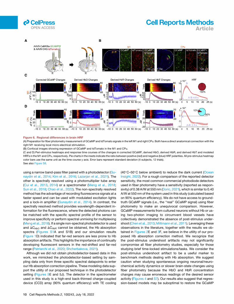
Figure 6. Regional differences in brain HRF

(A) Preparation for fiber photometrymeasurement of GCaMPand tdTomato signals in the left M1 and right CPu. Both have a direct anatomical connection with the

right M1 receiving local micro-electrical stimulation.

(B) Confocal images showing expression of GCaMP and tdTomato in the M1 and CPu.

(C and D) Peri-stimulus heatmaps and response time courses of the changes in corrected GCaMP, derived HbO, derived HbR, and derived HbT and modeled

HRFs in theM1 andCPu, respectively. Pie charts in the insets indicate the ratio between positive (red) and negative (blue) HRF polarities. All pre-stimulus heatmap

color bars use the same unit as the time course y axis. Error bars represent standard deviation (4 subjects, 12 trials).

See also Figure S8.

Articlell

OPEN ACCESS

using a narrow band-pass filter paired with a photodetector (Gu-

naydin et al., 2014; Kim et al., 2016; Lazarjan et al., 2021). The

other is spectrally resolved using a photomultiplier tube array

(Cui et al., 2013, 2014) or a spectrometer (Meng et al., 2018;

Sun et al., 2018; Chao et al., 2022). The non-spectrally resolved

method has the advantage of recording fluorescence signals at a

faster speed and can be used with modulated excitation lights

and a lock-in amplifier (Gunaydin et al., 2014). In contrast, the

spectrally resolved method provides wavelength-dependent in-

formation for the fluorescence, where the detected photons can

be matched with the specific spectral profile of the sensor to

improve specificity or perform spectral unmixing for multiplexing

(Meng et al., 2018). If a single non-spectral photodetector is used

and DCHbO and DCHbR cannot be obtained, the Hb absorption

spectra (Figures S1A and S1B) and our simulation results

(Figure 1D) indicated that far-red sensors are less prone to Hb

absorption artifacts. This highlights the importance of continually

developing fluorescent sensors in the red-shifted and far-red

range (Patriarchi et al., 2020; Shcherbakova, 2021).

Although we did not obtain photodetector-based data in this

work, we mimicked the photodetector-based setting by sam-

pling data only from three specific spectral datapoints to enter

our Hb absorption correction pipeline. Thesemodeling data sup-

port the utility of our proposed technique in the photodetector

setting (Figures 5E and 5J). The detector in the spectrometer

used in this study is a high-end back-thinned charge-coupled

device (CCD) array (90% quantum efficiency) with TE cooling

10 Cell Reports Methods 2, 100243, July 18, 2022

(40�C–50�C below ambient) to reduce the dark current (Ocean

Insight, 2022). For a rough comparison of the reported detector

sensitivity, the most common commercial photodiode detectors

used in fiber photometry have a sensitivity (reported as respon-

sivity) of 0.38 A/Wat 550 nm (Doric, 2021), which is similar to 0.40

A/W at 550 nm of the system used in this study (calculated based

on 90% quantum efficiency). We do not have access to ground-

truth GCaMP signals (i.e., the ‘‘real’’ GCaMP signal) using fiber

photometry to make an unequivocal comparison. However,

GCaMPmeasurements from cultured neurons without Hb or us-

ing two-photon imaging to circumvent blood vessels have

collectively demonstrated the absence of post-stimulus under-

shoot (Chen et al., 2013; Mittmann et al., 2011). Leveraging these

observations in the literature, together with the results we ob-

tained in Figures 2E and 3F, we believe in the utility of our pro-

posed Hb absorption correction method. We recognize that

the post-stimulus undershoot artifacts may not significantly

compromise all fiber photometry studies, especially for those

studying brief time-locked stimulations/tasks. We consider the

post-stimulus undershoot artifact to be a useful marker to

benchmark methods dealing with Hb absorption. We suggest

caution when studying spontaneous ongoing neuronal/neuro-

chemical activity dynamics or slower brain-state changes using

fiber photometry because the HbO and HbR concentration

changes may cause erroneous readings of the desired sensor

activity (Figures 4 and S7). Our results also suggest that regres-

sion-based models may be suboptimal to restore the GCaMP

Articlell

OPEN ACCESS

signal changes in fiber photometry (Figures 5F–5K) and high-

lighted the benefits of CNR when using a spectrometer system

to derive HbO and HbR changes (Figure 5M).

Fluorescence signals generated from GCaMP isosbestic

excitation can be used as the activity-independent fluorescent

reference signal in the analytical method proposed in this study

and derive DCHbO and DCHbR to restore the functional GCaMP

signals (Figure 5). Potential limitations of this approach are (1)

trade-off in temporal resolution because interleaved excitation

is required, (2) relatively low CNR (Figure 5M; approximately

one-tenth of the emission signal was obtained compared with

488-nm excitation), (3) higher susceptibility to pH-related con-

founding factors (Shaner et al., 2005; Barnett et al., 2017), and

(4) although GCaMP has an isosbestic point at an amenable

wavelength for this method, other functional fluorescent sensors

may perform optimally at a different wavelength (Akerboom

et al., 2012; Sun et al., 2020).

The opportunity to examine the interactions between cell

types and/or neurotransmitters has become increasingly popu-

lar in fiber photometry. When the green and the red spectrum

are used to encode fluorescent sensor activities, it may be

possible to use the interleaved sequence, as shown in Figure 5,

or spectral signals from the unmixing residuals (i.e., the remain-

ing autofluorescence) to achieve hemodynamic correction (Fig-

ure S10). In our hands, the residual method suffers significantly

from CNR issues because of very low residual photon counts.

However, this approach may demonstrate its utility with the

advent of a more sensitive spectrometer system or an improved

unmixing algorithm. Considering the increasing need for multi-

plexing, a valuable next step should consider establishing an

experimental pipeline to achieve motion and Hb absorption arti-

fact-free measurement of green and a red fluorescent sensor

(e.g., GCaMP and jRGECO) in freely moving animals. This may

be achieved by incorporating a far-red activity-independent

fluorescent sensor for motion correction first (because Hb

absorption is negligible in this range; Figure S1), followed by

Hb absorption correction using data from isosbestic GCaMP

excitation, as shown in Figure 5.

Given the irreplaceable roles of noninvasive hemodynamics-

based neuroimaging techniques (such as fMRI, near-infrared,

intrinsic optics, functional ultrasound, positron emission

tomography, etc.) for studying brain function, identifying brain

region-dependent HRF is crucial for accurate interpretation of

hemodynamics-based neuroimaging data. Current standard

fMRI analysis uses one HRF shape throughout the brain.

Increasingly, literature has pointed to potential problems with

this analysis pipeline because HRF is brain region dependent

(Devonshire et al., 2012; Ekstrom, 2021; Jin et al., 2020; Sloan

et al., 2010). The current study and other pioneering studies (Alb-

ers et al., 2017; He et al., 2018; Liang et al., 2017; Schlegel et al.,

2018; Schmid et al., 2016; Schulz et al., 2012; Schwalm et al.,

2017; Wang et al., 2018a, 2018b; Zhang et al., 2022; Chao

et al., 2022) have demonstrated that fiber photometry could be

seamlessly coupled with fMRI and provide ground-truth cellular

activity to help unravel the relationship between neuronal and

hemodynamic responses. These studies have bridged a crucial

knowledge gap in interpretation of fMRI data. The method pro-

posed in this study expands the scope of this research area

because it generates hemodynamic signals ‘‘free of charge’’

with better sensitivity than fMRI (Figure 3N), and the results

can be readily compared with the concurrently recorded fluores-

cent sensor activity. With spectral photometry recording

becoming increasingly popular, the proposed method opens

up a unique opportunity to compute HRF in a cell-type-depen-

dent, stimulation-circuit-dependent, and neurotransmission-

dependent manner. We expect that this information can be

obtained by performing a meta-analysis on fiber photometry

data shared through an open-science platform and contribute

significantly to a more accurate interpretation of hemody-

namics-based neuroimaging results.

We demonstrated that significant Hb absorption artifacts in fi-

ber photometry data may cause inaccurate measurements and,

therefore, erroneous interpretation. We proposed a method that

addresses this issue by quantifying dynamic HbO and HbR ab-

sorption changes using activity-independent fluorescence

spectra and demonstrated that these additional quantitative

measurements were efficient in correcting the artifact and

retrieve the desired, unperturbed fluorescence signals in fiber

photometry. This approach simultaneously measures HbO,

HbR, and the activity of a selected fluorescent sensor, providing

an additional experimental capability to investigate the influence

of neuronal or neurochemical activity on cerebral hemody-

namics. Through a proof-of-principle study, we provide direct

evidence that HRF is brain region dependent, suggesting that

analysis of hemodynamics-based neuroimaging data should

not apply a single HRF across all brain regions.

Limitations of the studyLack of access to ground-truth GCaMP signals is a limitation

whenmaking unequivocal comparisonsbetween the ‘‘corrected’’

GCaMP and the ‘‘real’’ GCaMP signals. Second, post-stimulus

undershoot may not be significant in all fiber photometry studies.

Finally,we recognize that applying thismethod in a non-spectrally

resolved fiber photometry system might be challenging because

multiple band-pass filters, each combined with a photodetector,

are required.

STAR+METHODS

Detailed methods are provided in the online version of this paper

and include the following:

d KEY RESOURCES TABLE

d RESOURCE AVAILABILITY

B Lead contact

B Materials availability

B Data and code availability

d EXPERIMENTAL MODELS AND SUBJECT DETAILS

d METHOD DETAILS

B Monte Carlo simulation for photon transport in fiber-

photometry recording

B Correction of Hb-absorption

B Stereotactic surgery

B Experimental setup

B Animal subject preparation and physiology manage-

ment

Cell Reports Methods 2, 100243, July 18, 2022 11

Articlell

OPEN ACCESS

B Concurrent fMRI scan with fiber-photometry recording

B CBV fMRI data processing and statistical analyses

B Fiber-photometry spectral unmixing

B Modeling the hemodynamic response function

B Histology

d QUANTIFICATION AND STATISTICAL ANALYSIS

SUPPLEMENTAL INFORMATION

Supplemental information can be found online at https://doi.org/10.1016/j.

crmeth.2022.100243.

ACKNOWLEDGMENTS

We thank Drs. Elizabeth Hillman, Anna Devor, Lindsay Walton, Dom Cerri, and

UNC CAMRI members for their helpful discussions and critiques. This work is

supported in part by NIH grants (RF1MH117053, RF1NS086085, R01

MH126518, R01MH111429, R01NS091236, P60AA011605, U01AA020023,

P50HD103573, S10MH124745, and S10OD026796 to Y.Y.I.S.), the Intramural

Research Program of the NIH/NIEHS (1ZIAES103310 to G.C.), the Burroughs

Wellcome Fund (CASI 5113244 to N.C.P.), and the Arnold and Mabel Beckman

Foundation (2021BYI to N.C.P.).

AUTHOR CONTRIBUTIONS

W.-T.Z., T.-H.H.C., G.C., and Y.-Y.I.S. conceived the project and designed the

experiments. W.-T.Z., T.-H.H.C., T.-W.W., E.A.O., J.Z., and R.N. implemented

the methods. W.-T.Z., T.-H.H.C., Y.Y., S.-H.L., and N.C.P. analyzed data.

W.-T.Z., T.-H.H.C., and Y.-Y.I.S. wrote the manuscript with input from all au-

thors. H.Z., G.C., and Y.-Y.I.S. supervised the study and provided funding

support.

DECLARATION OF INTERESTS

The authors declare no competing interests.

Received: October 14, 2021

Revised: April 8, 2022

Accepted: June 8, 2022

Published: June 29, 2022

SUPPORTING CITATIONS

The following references appear in the supplemental information: Bekar et al.

(2012).

REFERENCES

Akerboom, J., Chen, T.-W., Wardill, T.J., Tian, L., Marvin, J.S., Mutlu, S., Cal-

deron, N.C., Esposti, F., Borghuis, B.G., Sun, X.R., et al. (2012). Optimization of

a GCaMP calcium indicator for neural activity imaging. J. Neurosci. 32, 13819–

13840. https://doi.org/10.1523/jneurosci.2601-12.2012.

Albers, F., Wachsmuth, L., van Alst, T.M., and Faber, C. (2017). Multimodal

functional neuroimaging by simultaneous BOLD fMRI and fiber-optic calcium

recordings and optogenetic control. Mol. Imaging Biol., 171–182. https://doi.

org/10.1007/s11307-017-1130-6.

Baraghis, E., Devor, A., Fang, Q., Srinivasan, V.J., Wu, W., Lesage, F., Ayata,

C., Kasischke, K.A., Boas, D.A., and Sakadzic, S. (2011). Two-photon micro-

scopy of cortical NADH fluorescence intensity changes: correcting contamina-

tion from the hemodynamic response. J. Biomed. Opt. 16, 106003. https://doi.

org/10.1117/1.3633339.

Barnett, L.M., Hughes, T.E., and Drobizhev, M. (2017). Deciphering the molec-

ular mechanism responsible for GCaMP6m’s Ca2+-dependent change in fluo-

rescence. PLoS One 12, e0170934. https://doi.org/10.1371/journal.pone.

0170934.

12 Cell Reports Methods 2, 100243, July 18, 2022

Bekar, L.K., Wei, H.S., and Nedergaard, M. (2012). The locus coeruleus-

norepinephrine network optimizes coupling of cerebral blood volume with ox-

ygen demand. J. Cereb. Blood FlowMetab. 32, 2135–2145. https://doi.org/10.

1038/jcbfm.2012.115.

Bollimunta, A., Santacruz, S.R., Eaton, R.W., Xu, P.S., Morrison, J.H., Moxon,

K.A., Carmena, J.M., and Nassi, J.J. (2021). Head-mounted microendoscopic

calcium imaging in dorsal premotor cortex of behaving rhesus macaque. Cell

Rep. 35, 109239. https://doi.org/10.1016/j.celrep.2021.109239.

Broadwater, M.A., Lee, S.-H., Yu, Y., Zhu, H., Crews, F.T., Robinson, D.L., and

Shih, Y.-Y.I. (2018). Adolescent alcohol exposure decreases frontostriatal

resting-state functional connectivity in adulthood. Addict. Biol. 23, 810–823.

https://doi.org/10.1111/adb.12530.

Chao, T.-H.H., Chen, J.-H., and Yen, C.-T. (2018). Plasticity changes in fore-

brain activity and functional connectivity during neuropathic pain development

in rats with sciatic spared nerve injury. Mol. Brain 11, 55. https://doi.org/10.

1186/s13041-018-0398-z.

Chao, T.-H.H., Zhang, W.-T., Hsu, L.-M., Cerri, D.H., Wang, T.W.W., and Shih,

Y.-Y.I. (2022). Computing hemodynamic response functions from concurrent

spectral fiber-photometry and fMRI data. Neurophotonics 9, 032205. https://

doi.org/10.1117/1.nph.9.3.032205.

Chen, T.W., Wardill, T.J., Sun, Y., Pulver, S.R., Renninger, S.L., Baohan, A.,

Schreiter, E.R., Kerr, R.A., Orger, M.B., Jayaraman, V., et al. (2013). Ultrasen-

sitive fluorescent proteins for imaging neuronal activity. Nature 499, 295–300.

https://doi.org/10.1038/nature12354.

Chen, X., Sobczak, F., Chen, Y., Jiang, Y., Qian, C., Lu, Z., Ayata, C., Logothe-

tis, N.K., and Yu, X. (2019). Mapping optogenetically-driven single-vessel fMRI

with concurrent neuronal calcium recordings in the rat hippocampus. Nat.

Commun. 10, 5239. https://doi.org/10.1038/s41467-019-12850-x.

Cox, R.W. (1996). AFNI: software for analysis and visualization of functional

magnetic resonance neuroimages. Comput. Biomed. Res. Int. J. 29,

162–173. https://doi.org/10.1006/cbmr.1996.0014.

Cramer, S.W., Carter, R.E., Aronson, J.D., Kodandaramaiah, S.B., Ebner, T.J.,

and Chen, C.C. (2021). Through the looking glass: a review of cranial window

technology for optical access to the brain. J. Neurosci. Methods 354, 109100.

https://doi.org/10.1016/j.jneumeth.2021.109100.

Cui, G., Jun, S.B., Jin, X., Luo, G., Pham,M.D., Lovinger, D.M., Vogel, S.S., and

Costa, R.M. (2014). Deep brain optical measurements of cell type-specific

neural activity in behaving mice. Nat. Protoc. 9, 1213–1228. https://doi.org/

10.1038/nprot.2014.080.

Cui, G., Jun, S.B., Jin, X., Pham, M.D., Vogel, S.S., Lovinger, D.M., and Costa,

R.M. (2013). Concurrent activation of striatal direct and indirect pathways dur-

ing action initiation. Nature 494, 238–242. https://doi.org/10.1038/na-

ture11846.

Dana, H., Mohar, B., Sun, Y., Narayan, S., Gordus, A., Hasseman, J.P., Tse-

gaye, G., Holt, G.T., Hu, A., Walpita, D., et al. (2016). Sensitive red protein cal-

cium indicators for imaging neural activity. Elife 5, e12727. https://doi.org/10.

7554/eLife.12727.

Dana, H., Sun, Y., Mohar, B., Hulse, B.K., Kerlin, A.M., Hasseman, J.P.,

Tsegaye, G., Tsang, A., Wong, A., Patel, R., et al. (2019). High-performance

calcium sensors for imaging activity in neuronal populations and microcom-

partments. Nat. Methods 16, 649–657. https://doi.org/10.1038/s41592-019-

0435-6.

Decot, H.K., Namboodiri, V.M.K., Gao, W., McHenry, J.A., Jennings, J.H., Lee,

S.-H., Kantak, P.A., Jill Kao, Y.-C., Das, M., Witten, I.B., et al. (2017). Coordi-

nation of brain-wide activity dynamics by dopaminergic neurons. Neuropsy-

chopharmacology 42, 615–627. https://doi.org/10.1038/npp.2016.151.

Devonshire, I.M., Papadakis, N.G., Port, M., Berwick, J., Kennerley, A.J.,

Mayhew, J.E., and Overton, P.G. (2012). Neurovascular coupling is brain re-

gion-dependent. Neuroimage 59, 1997–2006. https://doi.org/10.1016/j.neuro-

image.2011.09.050.

Devor, A., Dunn, A.K., Andermann, M.L., Ulbert, I., Boas, D.A., and Dale, A.M.

(2003). Coupling of total hemoglobin concentration, oxygenation, and neural

Articlell

OPEN ACCESS

activity in rat somatosensory cortex. Neuron 39, 353–359. https://doi.org/10.

1016/s0896-6273(03)00403-3.

Doric. (2021). Integrated FluorescenceMini Cubes (Gen2) User Manual (Doric).

Ekstrom, A.D. (2021). Regional variation in neurovascular coupling and whywe

still lack a Rosetta Stone. Philos. Trans. R. Soc. Lond. B Biol. Sci. 376,

20190634. https://doi.org/10.1098/rstb.2019.0634.

Gunaydin, L.A., Grosenick, L., Finkelstein, J.C., Kauvar, I.V., Fenno, L.E., Ad-

hikari, A., Lammel, S., Mirzabekov, J.J., Airan, R.D., Zalocusky, K.A., et al.

(2014). Natural neural projection dynamics underlying social behavior. Cell

157, 1535–1551. https://doi.org/10.1016/j.cell.2014.05.017.

Hansen, L.P. (1982). Large sample properties of generalized method of mo-

ments estimators. Econometrica 50, 1029. https://doi.org/10.2307/1912775.

He, Y., Wang, M., Chen, X., Pohmann, R., Polimeni, J.R., Scheffler, K., Rosen,

B.R., Kleinfeld, D., and Yu, X. (2018). Ultra-slow single-vessel BOLD and CBV-

based fMRI spatiotemporal dynamics and their correlation with neuronal intra-

cellular calcium signals. Neuron 97, 925–939.e5. https://doi.org/10.1016/j.

neuron.2018.01.025.

Henyey, L.C., and Greenstein, J.L. (1941). Diffuse radiation in the galaxy. As-

trophys. J. 93, 70. https://doi.org/10.1086/144246.

Hillman, E.M. (2014). Coupling mechanism and significance of the BOLD

signal: a status report. Annu. Rev. Neurosci. 37, 161–181. https://doi.org/10.

1146/annurev-neuro-071013-014111.

Hillman, E.M.C. (2007). Optical brain imaging in vivo: techniques and applica-

tions from animal toman. J. Biomed. Opt. 12, 051402. https://doi.org/10.1117/

1.2789693.

Hu, X., and Yacoub, E. (2012). The story of the initial dip in fMRI. Neuroimage

62, 1103–1108. https://doi.org/10.1016/j.neuroimage.2012.03.005.

Hua, J., Liu, P., Kim, T., Donahue, M., Rane, S., Chen, J.J., Qin, Q., and Kim,

S.-G. (2019). MRI techniques to measure arterial and venous cerebral blood

volume. Neuroimage 187, 17–31. https://doi.org/10.1016/j.neuroimage.2018.

02.027.

Jin, M., Wang, L., Wang, H., Han, X., Diao, Z., Guo, W., Yang, Z., Ding, H.,

Wang, Z., Zhang, P., et al. (2020). Disturbed neurovascular coupling in hemo-

dialysis patients. PeerJ 8, e8989. https://doi.org/10.7717/peerj.8989.

Jones-Tabah, J., Mohammad, H., Clarke, P.B.S., and Hebert, T.E. (2021).

In vivo detection of GPCR-dependent signaling using fiber photometry and

FRET-based biosensors. Methods, 422–430. https://doi.org/10.1016/j.

ymeth.2021.05.002.

Kelly, D.F., Lee, S.M., Pinanong, P.A., and Hovda, D.A. (1997). Paradoxical ef-

fects of acute ethanolism in experimental brain injury. J. Neurosurg. 86,

876–882. https://doi.org/10.3171/jns.1997.86.5.0876.

Kim, C.K., Yang, S.J., Pichamoorthy, N., Young, N.P., Kauvar, I., Jennings,

J.H., Lerner, T.N., Berndt, A., Lee, S.Y., Ramakrishnan, C., et al. (2016). Simul-

taneous fast measurement of circuit dynamics at multiple sites across the

mammalian brain. Nat. Methods 13, 325–328. https://doi.org/10.1038/

nmeth.3770.

Kudo, R., Yuui, K., Kasuda, S., and Hatake, K. (2015). [Effect of alcohol on

vascular function]. Nihon Arukoru Yakubutsu Igakkai Zasshi 50, 123–134.

Kwong, K.K., Belliveau, J.W., Chesler, D.A., Goldberg, I.E., Weisskoff, R.M.,

Poncelet, B.P., Kennedy, D.N., Hoppel, B.E., Cohen, M.S., Turner, R., et al.

(1992). Dynamic magnetic resonance imaging of human brain activity during

primary sensory stimulation. Proc. Natl. Acad. Sci. U S A. 89, 5675–5679.

https://doi.org/10.1073/pnas.89.12.5675.

Lazarjan, V.K., Gashti, A.B., Feshki, M., Garnier, A., and Gosselin, B. (2021).

Miniature fiber-spectrophotometer for real-time biomarkers detection. IEEE

Sens. J. 21, 14822–14837. https://doi.org/10.1109/JSEN.2021.3072578.

Lecrux, C., and Hamel, E. (2016). Neuronal networks and mediators of cortical

neurovascular coupling responses in normal and altered brain states. Philos.

Trans. R. Soc. Lond. B Biol. Sci. 371, 20150350. https://doi.org/10.1098/

rstb.2015.0350.

Liang, Z., Ma, Y., Watson, G.D.R., and Zhang, N. (2017). Simultaneous

GCaMP6-based fiber photometry and fMRI in rats. J. Neurosci. Methods

289, 31–38. https://doi.org/10.1016/j.jneumeth.2017.07.002.

Lotfullina, N., and Khazipov, R. (2018). Ethanol and the developing brain: inhi-

bition of neuronal activity and neuroapoptosis. Neuroscientist 24, 130–141.

https://doi.org/10.1177/1073858417712667.

Luchsinger, J.R., Fetterly, T.L., Williford, K.M., Salimando, G.J., Doyle, M.A.,

Maldonado, J., Simerly, R.B., Winder, D.G., and Centanni, S.W. (2021). Delin-

eation of an insula-BNST circuit engaged by struggling behavior that regulates

avoidance in mice. Nat. Commun. 12, 3561. https://doi.org/10.1038/s41467-

021-23674-z.

Ma, Y., Shaik, M.A., Kim, S.H., Kozberg, M.G., Thibodeaux, D.N., Zhao, H.T.,

Yu, H., and Hillman, E.M.C. (2016). Wide-field optical mapping of neural activ-

ity and brain haemodynamics: considerations and novel approaches. Philos.

Trans. R. Soc. Lond. B Biol. Sci. 371, 20150360. https://doi.org/10.1098/

rstb.2015.0360.

Machler, P., Fomin-Thunemann, N., Thunemann, M., Sætra, M.J., Desjardins,

M., Kılıc, K., Sxencan, I., Li, B., Saisan, P., Cheng, Q., et al. (2021). Microscopic

quantification of oxygen consumption across cortical layers. Preprint at bio-

Rxiv. https://doi.org/10.1101/2021.10.13.464176.

Marvin, J.S., Borghuis, B.G., Tian, L., Cichon, J., Harnett, M.T., Akerboom, J.,

Gordus, A., Renninger, S.L., Chen, T.-W., Bargmann, C.I., et al. (2013). An opti-

mized fluorescent probe for visualizing glutamate neurotransmission. Nat.

Methods 10, 162–170. https://doi.org/10.1038/nmeth.2333.

Marvin, J.S., Shimoda, Y., Magloire, V., Leite, M., Kawashima, T., Jensen, T.P.,

Kolb, I., Knott, E.L., Novak, O., Podgorski, K., et al. (2019). A genetically en-

coded fluorescent sensor for in vivo imaging of GABA. Nat. Methods 16,

763–770. https://doi.org/10.1038/s41592-019-0471-2.

Meng, C., Zhou, J., Papaneri, A., Peddada, T., Xu, K., and Cui, G. (2018). Spec-

trally resolved fiber photometry for multi-component analysis of brain circuits.

Neuron 98, 707–717.e4. https://doi.org/10.1016/j.neuron.2018.04.012.

Meng, F., and Alayash, A.I. (2017). Determination of extinction coefficients of

human hemoglobin in various redox states. Anal. Biochem. 521, 11–19.

https://doi.org/10.1016/j.ab.2017.01.002.

Mintun,M.A., Raichle,M.E.,Martin,W.R., andHerscovitch, P. (1984). Brain ox-

ygen utilization measured with O-15 radiotracers and positron emission to-

mography. J. Nucl. Med. 25, 177–187.

Mishra, A.M., Ellens, D.J., Schridde, U.,Motelow, J.E., Purcaro,M.J., DeSalvo,

M.N., Enev, M., Sanganahalli, B.G., Hyder, F., and Blumenfeld, H. (2011).

Where fMRI and electrophysiology agree to disagree: corticothalamic and

striatal activity patterns in the WAG/Rij rat. J. Neurosci. 31, 15053–15064.

https://doi.org/10.1523/jneurosci.0101-11.2011.

Mittmann, W., Wallace, D.J., Czubayko, U., Herb, J.T., Schaefer, A.T., Looger,

L.L., Denk, W., and Kerr, J.N.D. (2011). Two-photon calcium imaging of

evoked activity from L5 somatosensory neurons in vivo. Nat. Neurosci. 14,

1089–1093. https://doi.org/10.1038/nn.2879.

Nakabayashi, T., Oshita, S., Sumikawa, R., Sun, F., Kinjo, M., and Ohta, N.

(2012). pH dependence of the fluorescence lifetime of enhanced yellow fluo-

rescent protein in solution and cells. J. Photochem. Photobiol. Chem. 235,

65–71. https://doi.org/10.1016/j.jphotochem.2012.02.016.

Ocean Insight (2022). QE Pro-FL Product Details (Ocean Insight). https://www.

oceaninsight.com/products/spectrometers/high-sensitivity/qepro-fl/?qty=1.

Pais-Roldan, P., Takahashi, K., Sobczak, F., Chen, Y., Zhao, X., Zeng, H.,

Jiang, Y., and Yu, X. (2020). Indexing brain state-dependent pupil dynamics

with simultaneous fMRI and optical fiber calcium recording. Proc. Natl.

Acad. Sci. U S A 117, 6875–6882. https://doi.org/10.1073/pnas.1909937117.

Patriarchi, T., Cho, J.R., Merten, K., Howe, M.W., Marley, A., Xiong, W.-H.,

Folk, R.W., Broussard, G.J., Liang, R., Jang, M.J., et al. (2018). Ultrafast

neuronal imaging of dopamine dynamics with designed genetically encoded

sensors. Science 360, eaat4422. https://doi.org/10.1126/science.aat4422.

Patriarchi, T., Mohebi, A., Sun, J., Marley, A., Liang, R., Dong, C., Puhger, K.,

Mizuno, G.O., Davis, C.M., Wiltgen, B., et al. (2020). An expanded palette of

dopamine sensors for multiplex imaging in vivo. Nat. Methods 17, 1147–

1155. https://doi.org/10.1038/s41592-020-0936-3.

Pisanello, M., Pisano, F., Hyun, M., Maglie, E., Balena, A., De Vittorio, M., Sa-

batini, B.L., and Pisanello, F. (2019). The three-dimensional signal collection

Cell Reports Methods 2, 100243, July 18, 2022 13

Articlell

OPEN ACCESS

field for fiber photometry in brain tissue. Front. Neurosci. 13, 82. https://doi.

org/10.3389/fnins.2019.00082.

Pisano, F., Pisanello, M., Lee, S.J., Lee, J., Maglie, E., Balena, A., Sileo, L.,

Spagnolo, B., Bianco, M., Hyun, M., et al. (2019). Depth-resolved fiber

photometry with a single tapered optical fiber implant. Nat. Methods 16,

1185–1192. https://doi.org/10.1038/s41592-019-0581-x.

Prahl, S. (1999). Optical absorption of hemoglobin. http://omlc.org/spectra/

hemoglobin.

Ruffin, V.A., Salameh, A.I., Boron, W.F., and Parker, M.D. (2014). Intracellular

pH regulation by acid-base transporters in mammalian neurons. Front. Phys-

iol. 5, 43. https://doi.org/10.3389/fphys.2014.00043.

Rungta, R.L., Osmanski, B.-F., Boido, D., Tanter, M., and Charpak, S. (2017).

Light controls cerebral blood flow in naive animals. Nat. Commun. 8, 14191.

https://doi.org/10.1038/ncomms14191.

Sakai, F., Nakazawa, K., Tazaki, Y., Ishii, K., Hino, H., Igarashi, H., and Kanda,

T. (1985). Regional cerebral blood volume and hematocrit measured in normal

human volunteers by single-photon emission computed tomography.

J. Cereb. Blood Flow Metab. 5, 207–213. https://doi.org/10.1038/jcbfm.

1985.27.

Sano, M., Wendt, P.E., Wirsen, A., Stenberg, G., Risberg, J., Ingvar, D.H., and

Wirsen, A. (1993). Acute effects of alcohol on regional cerebral blood flow in

man. J. Stud. Alcohol 54, 369–376. https://doi.org/10.15288/jsa.1993.54.369.

Schlegel, F., Sych, Y., Schroeter, A., Stobart, J., Weber, B., Helmchen, F., and

Rudin, M. (2018). Fiber-optic implant for simultaneous fluorescence-based

calcium recordings and BOLD fMRI in mice. Nat. Protoc. 13, 840–855.

https://doi.org/10.1038/nprot.2018.003.

Schmid, F., Wachsmuth, L., Schwalm, M., Prouvot, P.H., Jubal, E.R., Fois, C.,

Pramanik, G., Zimmer, C., Faber, C., and Stroh, A. (2016). Assessing sensory

versus optogenetic network activation by combining (o)fMRI with optical Ca2+

recordings. J. Cereb. Blood Flow Metab. 36, 1885–1900. https://doi.org/10.

1177/0271678x15619428.

Schridde, U., Khubchandani, M., Motelow, J.E., Sanganahalli, B.G., Hyder, F.,

and Blumenfeld, H. (2008). Negative BOLDwith large increases in neuronal ac-

tivity. Cereb. Cortex 18, 1814–1827. https://doi.org/10.1093/cercor/bhm208.

Schulz, K., Sydekum, E., Krueppel, R., Engelbrecht, C.J., Schlegel, F.,

Schroter, A., Rudin, M., and Helmchen, F. (2012). Simultaneous BOLD fMRI

and fiber-optic calcium recording in rat neocortex. Nat. Methods 9,

597–602. https://doi.org/10.1038/nmeth.2013.

Schwalm, M., Schmid, F., Wachsmuth, L., Backhaus, H., Kronfeld, A., Aedo

Jury, F., Prouvot, P.H., Fois, C., Albers, F., van Alst, T., et al. (2017). Cortex-

wide BOLD fMRI activity reflects locally-recorded slow oscillation-associated

calcium waves. Elife 6, e27602. https://doi.org/10.7554/eLife.27602.

Shaner, N.C., Steinbach, P.A., and Tsien, R.Y. (2005). A guide to choosing fluo-

rescent proteins. Nat. Methods 2, 905–909. https://doi.org/10.1038/

nmeth819.

Shcherbakova, D.M. (2021). Near-infrared and far-red genetically encoded in-

dicators of neuronal activity. J. Neurosci. Methods 362, 109314. https://doi.

org/10.1016/j.jneumeth.2021.109314.

Shih, Y.Y.I., Chen, C.C.V., Shyu, B.C., Lin, Z.J., Chiang, Y.C., Jaw, F.S., Chen,

Y.Y., and Chang, C. (2009). A new scenario for negative functional magnetic

resonance imaging signals: endogenous neurotransmission. J. Neurosci. 29,

3036–3044. https://doi.org/10.1523/JNEUROSCI.3447-08.2009.

Shih, Y.Y.I., Li, G., Muir, E.R., De La Garza, B.H., Kiel, J.W., and Duong, T.Q.

(2012). Pharmacological MRI of the choroid and retina: blood flow and

BOLD responses during nitroprusside infusion. Magn. Reson. Med. 68,

1273–1278. https://doi.org/10.1002/mrm.24112.

Shih, Y.-Y.I., Huang, S., Chen, Y.-Y., Lai, H.-Y., Kao, Y.-C.J., Du, F., Hui, E.S.,

and Duong, T.Q. (2014). Imaging neurovascular function and functional recov-

ery after stroke in the rat striatum using forepaw stimulation. J. Cereb. Blood

Flow Metab. 34, 1483–1492. https://doi.org/10.1038/jcbfm.2014.103.

Shih, Y.-Y.I., Wang, L., De La Garza, B.H., Li, G., Cull, G., Kiel, J.W., and Du-

ong, T.Q. (2013). Quantitative retinal and choroidal blood flow during light, dark

14 Cell Reports Methods 2, 100243, July 18, 2022

adaptation and flicker light stimulation in rats using fluorescent microspheres.

Curr. Eye Res. 38, 292–298. https://doi.org/10.3109/02713683.2012.756526.

Shih, Y.-Y.I., Wey, H.-Y., De La Garza, B.H., and Duong, T.Q. (2011). Striatal

and cortical BOLD, blood flow, blood volume, oxygen consumption, and

glucose consumption changes in noxious forepaw electrical stimulation.

J. Cereb. Blood Flow Metab. 31, 832–841. https://doi.org/10.1038/jcbfm.

2010.173.

Siegel, A.M., Culver, J.P., Mandeville, J.B., and Boas, D.A. (2003). Temporal

comparison of functional brain imaging with diffuse optical tomography and

fMRI during rat forepaw stimulation. Phys. Med. Biol. 48, 1391–1403.

https://doi.org/10.1088/0031-9155/48/10/311.

Sloan, H.L., Austin, V.C., Blamire, A.M., Schnupp, J.W.H., Lowe, A.S., Allers,

K.A., Matthews, P.M., and Sibson, N.R. (2010). Regional differences in neuro-

vascular coupling in rat brain as determined by fMRI and electrophysiology.

Neuroimage 53, 399–411. https://doi.org/10.1016/j.neuroimage.2010.07.014.

Smith, A.F., Doyeux, V., Berg, M., Peyrounette, M., Haft-Javaherian,M., Larue,

A.-E., Slater, J.H., Lauwers, F., Blinder, P., Tsai, P., et al. (2019). Brain capillary

networks across species: a few simple organizational requirements are suffi-

cient to reproduce both structure and function. Front. Physiol. 10, 233.

https://doi.org/10.3389/fphys.2019.00233.

Sun, F., Zeng, J., Jing, M., Zhou, J., Feng, J., Owen, S.F., Luo, Y., Li, F., Wang,

H., Yamaguchi, T., et al. (2018). A genetically encoded fluorescent sensor en-

ables rapid and specific detection of dopamine in flies, fish, andmice. Cell 174,

481–496.e19. https://doi.org/10.1016/j.cell.2018.06.042.

Sun, F., Zhou, J., Dai, B., Qian, T., Zeng, J., Li, X., Zhuo, Y., Zhang, Y., Wang,

Y., Qian, C., et al. (2020). Next-generation GRAB sensors for monitoring dopa-

minergic activity in vivo. Nat. Methods 17, 1156–1166. https://doi.org/10.

1038/s41592-020-00981-9.

Sych, Y., Chernysheva, M., Sumanovski, L.T., and Helmchen, F. (2019). High-

density multi-fiber photometry for studying large-scale brain circuit dynamics.

Nat. Methods 16, 553–560. https://doi.org/10.1038/s41592-019-0400-4.

Taylor, A.J., Kim, J.H., and Ress, D. (2018). Characterization of the hemody-

namic response function across the majority of human cerebral cortex. Neuro-

image 173, 322–331. https://doi.org/10.1016/j.neuroimage.2018.02.061.

Tian, L., Hires, S.A., Mao, T., Huber, D., Chiappe, M.E., Chalasani, S.H., Pet-

reanu, L., Akerboom, J., McKinney, S.A., Schreiter, E.R., et al. (2009). Imaging

neural activity in worms, flies and mice with improved GCaMP calcium indica-

tors. Nat. Methods 6, 875–881. https://doi.org/10.1038/nmeth.1398.

Uluda�g, K., and Blinder, P. (2018). Linking brain vascular physiology to hemo-

dynamic response in ultra-high field MRI. Neuroimage 168, 279–295. https://

doi.org/10.1016/j.neuroimage.2017.02.063.

Unekawa, M., Tomita, Y., Toriumi, H., Osada, T., Masamoto, K., Kawaguchi,

H., Itoh, Y., Kanno, I., and Suzuki, N. (2015). Hyperperfusion counteracted

by transient rapid vasoconstriction followed by long-lasting oligemia induced

by cortical spreading depression in anesthetized mice. J. Cereb. Blood Flow

Metab. 35, 689–698. https://doi.org/10.1038/jcbfm.2014.250.

Vaagenes, I.C., Tsai, S.-Y., Ton, S.T., Husak, V.A., McGuire, S.O., O’Brien,

T.E., and Kartje, G.L. (2015). Binge ethanol prior to traumatic brain injury

worsens sensorimotor functional recovery in rats. PLoS One 10, e0120356.

https://doi.org/10.1371/journal.pone.0120356.

Valdes-Hernandez, P.A., Sumiyoshi, A., Nonaka, H., Haga, R., Aubert-Vas-

quez, E., Ogawa, T., Iturria-Medina, Y., Riera, J.J., and Kawashima, R.

(2011). An in vivo MRI template set for morphometry, tissue segmentation,

and fMRI localization in rats. Front. Neuroinf. 5, 26. https://doi.org/10.3389/

fninf.2011.00026.

Valley, M.T., Moore, M.G., Zhuang, J., Mesa, N., Castelli, D., Sullivan, D., Re-

imers, M., and Waters, J. (2020). Separation of hemodynamic signals from

GCaMP fluorescence measured with wide-field imaging. J. Neurophysiol.

123, 356–366.

Van De Borne, P., Mark, A.L., Montano, N., Mion, D., and Somers, V.K. (1997).

Effects of alcohol on sympathetic activity, hemodynamics, and chemoreflex

sensitivity. Hypertension 29, 1278–1283. https://doi.org/10.1161/01.hyp.29.

6.1278.

Articlell

OPEN ACCESS

van Zijl, P.C., Eleff, S.M., Ulatowski, J.A., Oja, J.M., Uluǧ, A.M., Traystman,

R.J., and Kauppinen, R.A. (1998). Quantitative assessment of blood flow,

blood volume and blood oxygenation effects in functional magnetic resonance

imaging. Nat. Med. 4, 159–167. https://doi.org/10.1038/nm0298-159.

Wang, H., Jing, M., and Li, Y. (2018a). Lighting up the brain: genetically

encoded fluorescent sensors for imaging neurotransmitters and neuromodula-

tors. Curr. Opin. Neurobiol. 50, 171–178. https://doi.org/10.1016/j.conb.2018.

03.010.

Wang, M., He, Y., Sejnowski, T.J., and Yu, X. (2018b). Brain-state dependent

astrocytic Ca(2+) signals are coupled to both positive and negative BOLD-

fMRI signals. Proc. Natl. Acad. Sci. U S A 115, E1647–E1656. https://doi.

org/10.1073/pnas.1711692115.

Worsley, K.J., and Friston, K.J. (1995). Analysis of fMRI time-series revisited–

again. Neuroimage 2, 173–181. https://doi.org/10.1006/nimg.1995.1023.

Zhang, W.-T., Chao, T.-H.H., Cui, G., and Shih, Y.-Y.I. (2022). Simultaneous

recordingofneuronalandvascularactivity in the rodentbrainusingfiber-photom-

etry. STAR Protoc 3, 101497. https://doi.org/10.1016/j.xpro.2022.101497.

Zhang, Q., Cramer, S.R., Ma, Z., Turner, K.L., Gheres, K.W., Liu, Y., Drew, P.J.,

and Zhang, N. (2022). Brain-wide ongoing activity is responsible for significant

cross-trial BOLD variability. Cereb. Cortex.

Zhang, Y.-F., Vargas Cifuentes, L., Wright, K.N., Bhattarai, J.P., Mohrhardt, J.,

Fleck, D., Janke, E., Jiang, C., Cranfill, S.L., Goldstein, N., et al. (2021). Ventral

striatal islands of Calleja neurons control grooming in mice. Nat. Neurosci. 24,

1699–1710. https://doi.org/10.1038/s41593-021-00952-z.

Cell Reports Methods 2, 100243, July 18, 2022 15

Articlell

OPEN ACCESS

STAR+METHODS

KEY RESOURCES TABLE

REAGENT or RESOURCE SOURCE IDENTIFIER

Bacterial and virus strains

AAV5-CaMKIIa-EYFP UNC Vector Core N/A

AAV9-CaMKIIa-GCaMP6f-WPRE-SV40 U.Penn Vector Core AV-9-PV3435

AAV9-CAG-tdTomato UNC Vector Core N/A

AAV9-CaMKIIa-ChR2-EYFP UNC Vector Core N/A

Chemicals, peptides, and recombinant proteins

Rhodamine B, 70,000 MW, Neutral Fisher scientific D1841

Phosphate Buffered Saline (10 x) Sigma-Aldrich P4417

Lidocaine HCl jelly (2%, 5mL) UNC SSC Pharmacy N/A

Meloxicam oral suspension Henry Schein N/A

Software and algorithms

MATLAB Mathworks R2019b

RStudio RStudio Inc. Version 1.0.136

Oceanview Ocean Insight N/A

Correction for Hb-absorption artifact in fiber-photometry In this paper https://github.com/CAMRIatUNC/HemoCorrection

(https://doi.org/10.5281/zenodo.6599234)

Computation of hemodynamic response function Chao et al., 2022 https://github.com/CAMRIatUNC/Photometry-tools

(https://doi.org/10.5281/zenodo.6599442)

Other

488 nm laser and remote Coherent OBIS 488 LS (60 mW)

561 nm laser and remote Coherent OBIS 561 LS (50 mW)

Spectrometer Ocean Insight QEPro-FL

Optic patch cable Thorlabs FT200EMT (200 mm, 0.39 NA)

Uncleaved fiber optic cannula Thorlabs CFMC12U-20 (200 mm, 0.39 NA)

Bipolar Tungsten electrode P1 Technologies MS303T/2C-B/SP ELEC .008/.2MM

TW TUNGSTEN (MRI)

Dual-edge dichroic mirror Chroma ZT488/561rpc

Dual-band emission filter Chroma ZET488/561m

Smart control panel Med Associate inc. DIG-716P2

RESOURCE AVAILABILITY

Lead contactFurther information and requests for data and resources should be directed to andwill be fulfilled by the lead contact, Yen-Yu Ian Shih

(shihy@unc.edu).

Materials availabilityThis study did not generate new materials or new reagents.

Data and code availabilityAll original code has been deposited at Github and is publicly available as of the date of publication. DOIs are listed in the Key

Resources Table.

Data reported in this paper will be shared by the lead contact upon request.

Any additional information required to reanalyze the data reported in this paper is available from the lead contact upon

request.

e1 Cell Reports Methods 2, 100243, July 18, 2022

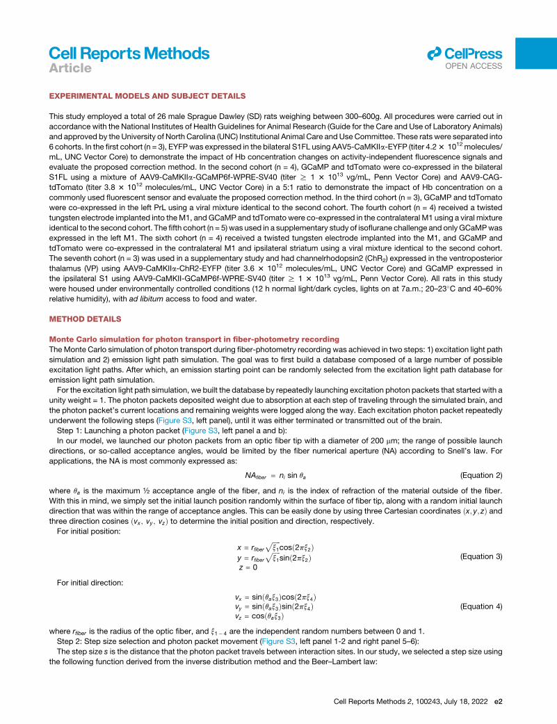
Articlell

OPEN ACCESS

EXPERIMENTAL MODELS AND SUBJECT DETAILS

This study employed a total of 26 male Sprague Dawley (SD) rats weighing between 300–600g. All procedures were carried out in

accordance with the National Institutes of Health Guidelines for Animal Research (Guide for the Care and Use of Laboratory Animals)

and approved by the University of North Carolina (UNC) Institutional Animal Care andUse Committee. These rats were separated into

6 cohorts. In the first cohort (n = 3), EYFPwas expressed in the bilateral S1FL using AAV5-CaMKIIa-EYFP (titer 4.23 1012molecules/

mL, UNC Vector Core) to demonstrate the impact of Hb concentration changes on activity-independent fluorescence signals and

evaluate the proposed correction method. In the second cohort (n = 4), GCaMP and tdTomato were co-expressed in the bilateral

S1FL using a mixture of AAV9-CaMKIIa-GCaMP6f-WPRE-SV40 (titer R 1 3 1013 vg/mL, Penn Vector Core) and AAV9-CAG-

tdTomato (titer 3.8 3 1012 molecules/mL, UNC Vector Core) in a 5:1 ratio to demonstrate the impact of Hb concentration on a

commonly used fluorescent sensor and evaluate the proposed correction method. In the third cohort (n = 3), GCaMP and tdTomato

were co-expressed in the left PrL using a viral mixture identical to the second cohort. The fourth cohort (n = 4) received a twisted

tungsten electrode implanted into theM1, and GCaMP and tdTomato were co-expressed in the contralateral M1 using a viral mixture

identical to the second cohort. The fifth cohort (n = 5) was used in a supplementary study of isoflurane challenge and onlyGCaMPwas

expressed in the left M1. The sixth cohort (n = 4) received a twisted tungsten electrode implanted into the M1, and GCaMP and

tdTomato were co-expressed in the contralateral M1 and ipsilateral striatum using a viral mixture identical to the second cohort.

The seventh cohort (n = 3) was used in a supplementary study and had channelrhodopsin2 (ChR2) expressed in the ventroposterior

thalamus (VP) using AAV9-CaMKIIa-ChR2-EYFP (titer 3.6 3 1012 molecules/mL, UNC Vector Core) and GCaMP expressed in

the ipsilateral S1 using AAV9-CaMKII-GCaMP6f-WPRE-SV40 (titer R 1 3 1013 vg/mL, Penn Vector Core). All rats in this study

were housed under environmentally controlled conditions (12 h normal light/dark cycles, lights on at 7a.m.; 20–23�C and 40–60%

relative humidity), with ad libitum access to food and water.

METHOD DETAILS

Monte Carlo simulation for photon transport in fiber-photometry recordingTheMonte Carlo simulation of photon transport during fiber-photometry recording was achieved in two steps: 1) excitation light path

simulation and 2) emission light path simulation. The goal was to first build a database composed of a large number of possible

excitation light paths. After which, an emission starting point can be randomly selected from the excitation light path database for

emission light path simulation.

For the excitation light path simulation, we built the database by repeatedly launching excitation photon packets that started with a

unity weight = 1. The photon packets deposited weight due to absorption at each step of traveling through the simulated brain, and

the photon packet’s current locations and remaining weights were logged along the way. Each excitation photon packet repeatedly

underwent the following steps (Figure S3, left panel), until it was either terminated or transmitted out of the brain.

Step 1: Launching a photon packet (Figure S3, left panel a and b):

In our model, we launched our photon packets from an optic fiber tip with a diameter of 200 mm; the range of possible launch

directions, or so-called acceptance angles, would be limited by the fiber numerical aperture (NA) according to Snell’s law. For

applications, the NA is most commonly expressed as:

NAfiber = ni sin qa (Equation 2)

where qa is the maximum ½ acceptance angle of the fiber, and ni is the index of refraction of the material outside of the fiber.

With this in mind, we simply set the initial launch position randomly within the surface of fiber tip, along with a random initial launch

direction that was within the range of acceptance angles. This can be easily done by using three Cartesian coordinates ðx; y; zÞ andthree direction cosines ðvx; vy; vzÞ to determine the initial position and direction, respectively.

For initial position:

x = rfiberffiffiffiffiffix1

pcosð2px2Þ

y = rfiberffiffiffiffiffix1

psinð2px2Þ

z = 0

(Equation 3)

For initial direction:

vx = sinðqax3Þcosð2px4Þvy = sinðqax3Þsinð2px4Þvz = cosðqax3Þ

(Equation 4)

where rfiber is the radius of the optic fiber, and x1� 4 are the independent random numbers between 0 and 1.

Step 2: Step size selection and photon packet movement (Figure S3, left panel 1-2 and right panel 5–6):

The step size s is the distance that the photon packet travels between interaction sites. In our study, we selected a step size using

the following function derived from the inverse distribution method and the Beer–Lambert law:

Cell Reports Methods 2, 100243, July 18, 2022 e2

Articlell

OPEN ACCESS

s = � ln x

mt

(Equation 5)

where x is a random number between 0 and 1, and mt is the total interaction coefficient (the sum of the absorption coefficient (ma) and

scattering coefficient (ms) of brain tissue). The ma and ms for distinct wavelengths of a traveling photon were derived from the optical

absorption and scattering properties provided by an online database from Oregon Medical Laser Center, Oregon Health & Science

University (https://omlc.org/software/mc/mcxyz/index.html). We assumed 3% blood with 75% average oxygen saturation in our

simulated brain.

Once the step size was selected, the photon packet traveled for distance s in the direction defined by direction cosines, and the

coordinates were updated as follows:

x)x + vxsy)y + vysz)z+ vzs

(Equation 6)

Step 3: Absorption and scattering (Figure S3, left panel 3–4 and right panel 7–8):

At each interaction site, photon weight was partially absorbed by brain tissue, and the decreased fraction of the weight Dw can be

defined as:

Dw = wð1 � e�masÞ (Equation 7)

The weight of the photon packet was then updated as follows:

w)w � Dw (Equation 8)

Following absorption, the photon packet was scattered. The scattering direction was defined by both scattering angle q and polar

angle 4. The scattering angle was determined using the Henyey-Greenstein phase function (Henyey and Greenstein, 1941):

cos q =

8><>:

1

2g

"1+ g2 �

�1 � g2

1 � g+ 2gx

�2#

jif gs0

1 � 2x jif g = 0

(Equation 9)

where g refers to scattering anisotropy, which has a value between�1 and 1. When g is 0, it generally indicates that the scattering is

isotropic. As g approaches 1 or -1, the scattering is confined to forwards and backwards, respectively.

The polar angle was assumed to be uniformly distributed between 0 and 2p, as below:

4 = 2px (Equation 10)

With these angles and the original direction cosines, we were able to calculate the new set of propagation direction cosines, which

can be represented in the global coordinate system as follows:

v0x =

8>><>>:

sin q�vxvz cos 4 � vy sin 4

�ffiffiffiffiffiffiffiffiffiffiffiffiffiffiffi1 � v2z

q +mx cos q if jvzs1Xmzs � 1

sin q cos 4 if jvz = 1Wmz = � 1

v0y =

8>>>>>>><>>>>>>>:

sin q�vyvz cos 4 � vx sin 4

�ffiffiffiffiffiffiffiffiffiffiffiffiffiffiffi1 � v2z

q +my cos q if vzs1Xmzs � 1

sin q sin 4 if jvz = 1

� sin q sin 4 if jvz = � 1

v0z =

8>>>><>>>>:

�ffiffiffiffiffiffiffiffiffiffiffiffiffiffiffi1 � v2z

qsin q cos 4+ vz cos q

cos q

� cos q

if vzs1Xmzs � 1

if jvz = 1

if jvz = � 1

(Equation 11)

Step 4: Photon termination

Steps 2 and 3 were repeated until the weight of the photon packet reached 10�4 or less, then the simulation for this particular

photon packet was terminated. The excitation light path and weight of each step were saved to the database, after which a new

photon packet simulation was started from step 1.

The emission light path simulation was similar to the excitation light path simulation. Specifically, we need to first determine the

initial position, the initial direction, and the initial weight before launching an emission photon packet (Figure S3, right panel C-D).

e3 Cell Reports Methods 2, 100243, July 18, 2022

Articlell

OPEN ACCESS

The initial coordinates of each emission photon packet were randomly selected from the excitation light path database. All coordi-

nates in the database had an equal probability to be selected regardless of excitation light path. If the selected coordinates were

within an area containing fluorophore, its initial coordinates were determined first, and then the corresponding excitation light

path history (from the start to the point where the emission occurred) was recorded. In this study, we assumed the fluorophore existed

equally within a 1 mm diameter sphere of viral expression area centered 0.3 mm below the fiber tip.

The initial direction of an emission photon was assumed to have isotropic probability in all directions; therefore, the direction co-

sines can be derived using the following:

vx = sinðpx1Þcosð2px2Þvy = sinðpx1Þsinð2px2Þvz = cosðpx1Þ

(Equation 12)

Lastly, the initial weights were inherited from the remaining weights of the excitation photon packet at the initial coordinates.

Steps 2 and 3 were repeated until the weight of the photon packet reached 10�4 or less, and then the simulation of this photon

packet was terminated (step 4). In emission step 4, only when the photon packet reached the fiber tip at smaller than ½ acceptance

angle and a weight beyond 10�4, the paired excitation/emission light path and the weight of each step were saved to the database. In

order to improve signal-to-noise ratio, we collected 2–2.5 3 104 pairs of excitation and emission light paths.

The final weight (Wfinal) when the emission photon reaching the optical fiber tip represents the survival rate of the current combined

excitation/emission light path. Therefore, the total average pathlength of excitation and emission lights are then calculated by sum-

ming each survived photon’s Wfinal multiplied by its paired excitation and emission pathlength respectively:

XexðlemÞ =XNn = 1

XexðnÞ $ e�maðlexÞ,XexðnÞ $ e�maðlemÞ,XemðnÞ =XNn = 1

XexðnÞ $Wfinal

XemðlemÞ =XNn = 1

XemðnÞ $ e�maðlexÞ,XexðnÞ $ e�maðlemÞ,XemðnÞ =XNn = 1

XemðnÞ $Wfinal

(Equation 13)

Since the Wfinal is affected during both excitation and emission phase, the emission measured at different wavelengths have not

only distinct average emission pathlength (XemðlemÞÞ, but also distinct average excitation pathlength (XexðlemÞ) even when these

emission wavelengths are excited by the same excitation wavelength. In this study, only the 488 nm excitation wavelength was

used and simulated.

To plot the 488 nm excitation light illuminating distribution (Figures S3A S3B), all excitation light paths’ coordinates generated from

the excitation light path simulation, regardless to the emission light detection, were first compressed into 2D coordinates, and then

used for the 2D histogram. To plot the 515 or 580 nm emission light receptive probability map (Figures S3B-S3C), the initial emission

3D coordinate of each successfully detected 515 or 580 emission photons were compressed into 2D coordinates and shown in a 2D

histogram.

Correction of Hb-absorptionGiven the different absorption of HbO and HbR (Figure S1), their dynamic concentration changesmust be quantified in order to prop-

erly correct fluorescent sensor signals. To address this, we proposed the following methods to derive changes in the HbO and HbR

concentration (DCHbO and DCHbR) using spectral datapoints.

In a simple, non-absorbing and non-scattering medium, the measured fluorescence signal F at any time t is linearly related to the

fluorescent protein concentration CðtÞ:FðtÞFðt0Þ =

CðtÞCðt0Þ (Equation 14)

where Fðt0Þ and Cðt0Þ represent the fluorescence signal and the fluorescent protein concentration at the reference time point 0,

respectively. When the absorption of the medium is considered, and F is measured at multiple wavelengths lEm, Equation (14)

can be further modified according to an established model (Ma et al., 2016):

Fðt; lEmÞFðt0; lEmÞ = e� ½Dmaðt;lExÞXðlExÞ+Dmaðt;lEmÞXðlEmÞ� $

CðtÞCðt0Þ

Then after natural logarithmic transformation:

ln

�Fðt; lEmÞFðt0; lEmÞ

�= � ½Dmaðt; lExÞXðlExÞ + Dmaðt; lEmÞXðlEmÞ�+ ln

CðtÞCðt0Þ (Equation 15)

where Dmaðt; lExÞ represents the change of the absorption coefficient ma at excitation wavelength lEx at the time point t compared to

the time point 0; Dmaðt; lEmÞ represents the change of the absorption coefficient ma at emission wavelength lEm at the time point t

compared to the time point 0; XðlExÞ and XðlEmÞ represent the photon traveling pathlengths at the given wavelength, respectively.

Next, HbO and HbR concentration changes (DCHbO and DCHbR) as a function of time need to be incorporated. When using

Cell Reports Methods 2, 100243, July 18, 2022 e4

Articlell

OPEN ACCESS

488 nm excitation, the absorption term in Equation (15) that contains Dma could be expressed as:

Dmaðt; lExÞXðlExÞ+Dmaðt; lEmÞXðlEmÞ= Dmaðt;488nmÞXð488nmÞ+Dmaðt; lEmÞXðlEmÞz½xHbOð488 nmÞDCHbOðtÞ+ xHbRð488 nmÞDCHbRðtÞ�Xð488 nmÞ+ ½xHbOðlEmÞDCHbOðtÞ+ xHbRðlEmÞDCHbRðtÞ�XðlEmÞ= DCHbOðtÞ½xHbOð488 nmÞXð488 nmÞ+ xHbOðlEmÞXðlEmÞ�+DCHbRðtÞ½xHbRð488 nmÞXð488 nmÞ+ xHbRðlEmÞXðlEmÞ�

(Equation 16)

where xHbO and xHbR are well-established molar extinction coefficients at different wavelengths of HbO and HbR, respectively (Prahl,

1999).

At the time point t, the measured fluorescence ratio after natural logarithmic transformation, ranged from lEm1to lEmn

could be put

together in a vector form MðtÞ:

MðtÞ =

2666666664

ln

F�t; lEm1

�F�0; lEm1

�!

«

«

ln

�Fðt; lEmn ÞFð0; lEmn Þ

�

3777777775

(Equation 17)

Additionally, two vectors A and B could be used to represent the following:

A = xHbOð488 nmÞ,Xð488 nmÞ+

2664xHbO

�lEm1

�,X�lEm1

�««

xHbOðlEmnÞ,XðlEmn Þ

3775 (Equation 18)

B = xHbRð488 nmÞ,Xð488 nmÞ+

2664xHbR

�lEm1

�,X�lEm1

�««

xHbRðlEmn Þ,XðlEmn Þ

3775 (Equation 19)

With any activity-independent fluorescence signals, the last component ln CðtÞCðt0Þ should be 0. Practically, we designate an error value

s. Taken together, Equation (15) could then be simplified and reorganized as Equation (20). To solve DCHbOðtÞ and DCHbRðtÞ at anytime point t, we used generalized method of moment (GMM) (Hansen, 1982) to minimize L in Equation (21). By performing the GMM

computation for each time point, we can obtain time-courses of DCHbOðtÞ, DCHbRðtÞ and s.

MðtÞ + DCHbOðtÞ,A+DCHbRðtÞ,B � s = 0 (Equation 20)

L =Xni = 1

�MðtÞi +DCHbOðtÞ,Ai +DCHbRðtÞ,Bi � s

�2(Equation 21)

In this case, we have numerous spectral datapoints that can be used to resolve two unknowns that are of interest – DCHbOðtÞ andDCHbRðtÞ. After which,Dmaðt; lExÞ andDmaðt; lEmÞ can be calculated using Equation (16) and Fðt; lEmÞ can be subsequently calculated

using Equation (15) to correct for HbO and HbR absorptions.

Stereotactic surgeryFor all surgical procedures, rats were initially anesthetizedwith 5% isoflurane, andmaintainedwith a constant flow of 2–3% isoflurane

mixed with medical air. Rectal temperature was continuously monitored and maintained within 37 ± 0.5�C using a feedback-

controlled heating pad (Harvard Apparatus, Model 557,020, Holliston, MA). Rats were head-fixed to a stereotactic frame (Kopf In-

struments, Model 962, Tujunga, CA). The skin was opened to expose the skull surface, and burr holes were prepared according

to experimental coordinates. All coordinates used for microinjection are listed as follows. S1: AP = +0.5 mm and ML = +3.7 mm,

DV = 1.3 mm, M1: AP = +1.8 mm and ML = �2.5 mm, DV = 2.0 mm, Striatum: AP = 0.5 mm and ML = 4.0 mm, DV = 5.2 mm, VP:

AP =�2.8 mm and ML = +2.5 mm, DV = 6.5 mm, PrL: AP = 2.2 mm and ML = 0.9 mm, DV = 4.1 mm. Microinjections were performed

at a flow rate of 0.1 mL/min for 1 mL, and an additional 10 min was given for virus diffusion prior to slow retraction of the microsyringe

needle. The burr holes were then sealed with bone wax (Fisher Scientific, Pittsburgh, PA), and the wound was sutured. A month after

virus microinjection, the skin was reopened to expose the skull, then bone wax was removed and optical fibers (200 mm in diameter;

NA: 0.39) were chronically implanted to the coordinates 0.2–0.5 mm above the virus injection sites. Four MR-compatible miniature

brass screws (Item #94070A031, McMaster Carr, Atlanta, GA) were anchored to the skull, then the surface of the skull was covered

with dental cement to seal implanted components and the wound was sutured to further protect the surgical site.

e5 Cell Reports Methods 2, 100243, July 18, 2022

Articlell

OPEN ACCESS

At the end of each surgical procedure, lidocaine jelly (#866096, Henry Schein Inc., Melville, NY) was applied around the surgical

wound to relieve pain and prevent the rat from scratching the wound. Meloxicam (#6451720670, Henry Schein Inc., Melville, NY)

was also given by oral administration for further pain relief. Rats were allowed at least 1 week to recover from surgical procedures

before any further experiments.

Experimental setupThe spectrally resolved fiber-photometry system in this study replicates an established system described previously (Meng et al.,

2018). Laser beams from a 488 nm 60 mW continuous wave (CW) laser (OBIS 488 LS-60, Coherent, Santa Clara, CA) and a

561 nm 50 mW CW laser (OBIS 561 LS-50, Coherent, Inc.) are aligned and combined by broadband dielectric mirrors (BB1-E02,

Thorlabs, newton, NJ) and a long-pass dichroic mirror (ZT488rdc, Chroma Technology Corp), then launched into a fluorescence

cube (DFM1, Thorlabs, newton, NJ). Extra neutral density filters (NEK01, Thorlabs, newton, NJ) are placed between the combined

laser beam and the fluorescence cube to adjust the final laser power. The fluorescence cube contains a dichroic mirror (ZT488/

561rpc, Chroma Technology Corp) to reflect and launch the combined laser beam through an achromatic fiber port (PAFA-X-4-A,

Thorlabs, newton, NJ) into the core of a 105/125 mm core/cladding multi-mode optical fiber patch cable (FG105UCA, Thorlabs,

newton, NJ). The distal end of the patch cable is connected to an implantable optical fiber probe for both excitation laser delivery

and emission fluorescence collection. The emission fluorescence collected from the fiber travels back along the patch cable into

the fluorescence cube, passes through the dichroic mirror and an emission filter (ZET488/561 m, Chroma Technology Corp, Bellows

Falls, VT), then launches through an aspheric fiber port (PAF-SMA-11-A, Thorlabs, newton, NJ) into the core of an AR-coated 200/

230mmcore/claddingmulti-mode patch cable (M200L02S-A, Thorlabs, newton, NJ). The AR-coatedmulti-mode patch cable is con-

nected to a spectrometer (QE Pro-FL, Ocean Optics, Largo, FL) for spectral data acquisition, which can be operated by a UI software

OceanView (Ocean Optics, Largo, FL). In order to achieve concurrent recording during fMRI, trigger mode is used in OceanView,

where the photometry system is synchronized with MRI using an Arduino micro-controller board.

The stimulation system uses a DAQ board (1208Hs-2AO, Measurement Computing Corp., Norton, MA) to send out stimulus trig-

gers according to the stimulus paradigm set in a homemade software program. During fMRI experiments, the DAQ synchronizes

stimulation pulses via triggers from the MRI system. The stimulation pulses were driven by a constant current stimulus isolator

(A385RC, World Precision Instruments, Sarasota, FL) for forepaw and micro-electrical stimulation experiments; and by a 473 nm

blue diode laser (Shang Laser and Optics Century, BL473T8-200FC + ADR-800A, Shanghai, China) for optogenetic experiments.

Animal subject preparation and physiology managementThe rats were initially anesthetized with 4% isoflurane (Vaporizer #911103, VetEquip Inc., Livermore, CA, USA) mixed with medical air

and endotracheally intubated using a 14G x 2"(>400 g) or 16G x 2"(<400 g) i.v. catheter (Surflash Polyurethane Catheter, TERUMO,

Somerset, NJ, USA). Respiration was maintained by a ventilator (SAR-830 or MRI-1, CWE Inc, Ardmore, PA, USA) set at 60 breaths/

min and an inspiration time ratio of 40%. A rectal probe was used to monitor core body temperature (OAKTON Temp9500, Cole-

Parmer, Vernon Hills, IL, USA) and a capnometer was used to monitor heart rate, peripheral blood oxygen saturation, and end-tidal

CO2 (SURGIVET V90041LF, Smith Medical, Dublin, OH, USA). Body temperature was maintained at 37 ± 0.5 �C using a circulating

water blanket connected to a temperature adjustable water bath (Haake S13, Thermo Fisher Scientific, Waltham, MA, USA). Venti-

lation tidal volume was adjusted to keep the heart rate at 300 ± 50 beats per minute, peripheral blood oxygen saturation above 90%,

and end-tidal CO2 between 2.8 and 3.2%. End-tidal CO2 values from this capnometer system were previously calibrated against

invasive sampling of arterial blood gas, reflecting a partial pressure of carbon dioxide (pCO2) level of 30–40 mm Hg (Shih et al.,

2012, 2013). For studies using Rhodamine B for CBV measurements, a bolus dose of 40 mg/kg (Sigma–Aldrich, St. Louis, MO)

was injected via tail vein.

Concurrent fMRI scan with fiber-photometry recordingAll fMRI data in this study were collected on a Bruker BioSpec 9.4-Tesla, 30 cm bore system with 6.0.1 on an AVANCE II console

(Bruker BioSpin Corp., Billerica, MA). An RRI BFG 150/90 gradient insert (Resonance Research, Inc, Billerica, MA) paired with a Cop-

ley C700 gradient amplifier (Copley Controls Corp., Canton, MA) was used. A homemade single-loop surface coil with an internal

diameter of 1.6 cm was used as a radio-frequency transceiver. Isoflurane concentrations were adjusted to 2% and animals were

secured in to a custom-built, MR-compatible rat cradle. Animal physiology was monitored and maintained as described in the pre-

vious paragraph.

Upon stabilizing the animals, a pair of needle electrodes was inserted under the skin of forepaw for stimulation, or electrode/optical

fiber patch cables were connected according to experimental design. Before connecting the fiber-photometry patch cable, all light

in the room was turned off, the final output power of the 488 nm laser and 561 nm laser were 51.3 ± 18.6 mW (mean ± SD, n = 26),

which were adjusted to balance spectral amplitudes (Meng et al., 2018). The 100 mWpower is the maximum we suggested when the

virus expression is less robust. This power range is consistent with published fiber-photometry studies (Gunaydin et al., 2014;

Jones-Tabah et al., 2021, p.; Liang et al., 2017; Zhang et al., 2021). A background spectrumwasmeasured as a reference by pointing

the fiber tip to a nonreflective background in the dark room. This background spectrum was then automatically subtracted by

OceanView during photometry recording.

Cell Reports Methods 2, 100243, July 18, 2022 e6

Articlell

OPEN ACCESS

Following setup processes, the cradle was pushed into MRI bore, and a bolus of dexmedetomidine (0.025 mg/kg; Dexdormitor,

Orion, Espoo, Finland) cocktailed with paralytic agent rocuronium bromide (4.5 mg/kg; Sigma–Aldrich, St. Louis, MO) was injected

into the tail vein (Chao et al., 2018). Fifteen minutes after bolus injection, a continuous intravenous infusion of dexmedetomidine

(0.05 mg/kg/h) and rocuronium bromide (9 mg/kg/h) cocktail was initiated and the isoflurane concentration was adjusted to

0.5–1% for the entire scanning period.

Magnetic field homogeneity was optimized first by global shim and followed by local first- and second-order shims according to B0

map. Anatomical images for referencing were acquired using a rapid acquisition with relaxation enhancement (RARE) sequence (12

coronal slices, thickness = 1 mm, repetition time (TR) = 2500 ms, echo time (TE) = 33 ms, matrix size = 256 3 256, field-of-view

(FOV) = 25.63 25.6mm2, in plane resolution 0.13 0.1mm, average = 8, RARE factor = 8). The center of the fifth slice from the anterior

direction was aligned with the anterior commissure. Cerebral blood volume (CBV) fMRI scans were acquired using a multi-slice sin-

gle-shot gradient echo echo-planar imaging sequence (GE-EPI) (slice thickness = 1 mm, TR = 1000 ms, TE = 8.1 ms, matrix size =

80 3 80, FOV = 25.6 3 25.6 mm2, in plane resolution 0.32 3 0.32 mm, bandwidth = 250 kHz), with the same image slice geometry

imported from the previously acquired T2-weighted anatomical image. A session of GE-EPI scans with 300 repetitions was taken,

and at about the 100th scan, Feraheme (30 mg Fe/kg, i.v.) was administered for CBV percentage change calculations.

CBV fMRI data processing and statistical analysesAll fMRI data were analyzed using the Analysis of Functional Neuroimages (AFNI) (Cox, 1996) general linear model (GLM) framework

(Worsley and Friston, 1995). All EPI images were skull-stripped, and slice-timing was corrected. Then automatic co-registration was

applied to realign time-courses within subjects to correct subtle drift of EPI images. Finally all EPI images were aligned to a T2-

weighted rat brain template (Valdes-Hernandez et al., 2011) to generate normalized fMRI images to allow for group-level compari-

sons. Gaussian smooth (FWHM = 0.5 mm) was performed before feeding into the GLM fitting. To test the significant consistency of

the stimulus-evoked responses at the group-level, we employed a parametric one-sample t test implemented in AFNI. The false dis-

covery rate correction was used to adjust for multiple comparisons of fMRI maps (p < 0.05). A 3x3 voxel region of interest (ROI) was

placed at the fiber tip in the S1 to extract fMRI time-course data. To account for Feraheme kinetics during the course of the exper-

iments, the following equations were used to calculate the DR�2ðbaselineÞ, DR�

2ðstimÞ , and DCBV (Decot et al., 2017).

DR�2ðbaselineÞ = � 1

TEln

�Sprestim

S0

�(Equation 22)

DR�2ðstimÞ = � 1

TEln

�Sstim

Sprestim

�(Equation 23)

DCBV =DR�

2ðstimÞDR�

2ðbaselineÞ(Equation 24)

where Sprestim and S0 represents MR signal intensity after and before Feraheme injection, respectively, and Sstim are the MR signal

intensities during the stimulation.

Fiber-photometry spectral unmixingMixed spectra acquired by fiber-photometry were analyzed using a spectral linear unmixing algorithm (Meng et al., 2018). Briefly, at

any time point n, the mixed spectrum YðnÞ was modeled as:

YðnÞ = Coeff1ðnÞ3S1 +Coeff2ðnÞ3S2 +C+ εðnÞ (Equation 25)

where S1 and S2 are the normalized reference emission spectra of the two fluorescence signal sources. Coeff1 and Coeff2 are the

unknown regression coefficients corresponding to the S1 and S2 respectively. C is the unknown constant, and εðnÞ is random error.

Coeff1ðnÞ, Coeff2ðnÞ, and εðnÞ at each time point were estimated using the lm() function in the RStudio package (RStudio Inc.

V1.0.136, Boston, MA).

Modeling the hemodynamic response functionThe relationship between neuronal activity and hemodynamic response can be expressed as:

HbTðTÞ = NðTÞ€A HRFðtÞ+ c+ dðTÞ (Equation 26)

where the HbTðTÞ represents hemoglobin fluctuation time-course, the NðTÞ represents neuronal activity time-course, the HRFðtÞrepresents an impulse hemodynamic response function with t sampling points, c is a constant for baseline offset and dðTÞ is for lineardrift over time. Assuming T = f0; 1; 2;.;mg; t = f0; 1; 2; .; ng ,this equation can be expressed as:

e7 Cell Reports Methods 2, 100243, July 18, 2022

Articlell

OPEN ACCESS

2666666666666664

HbTð0ÞHbTð1ÞHbTð2Þ

«

HbTðmÞ

3777777777777775

=

2666666666666664

Nð0Þ 0 0

Nð1Þ Nð0Þ 0

Nð2Þ Nð1Þ Nð0Þ/

0

0

0

1

1

1

0

1

m

2

m

« 1 «

NðmÞ Nðm � 1Þ Nðm � 2Þ / Nðm � nÞ 1 1

3777777777777775

3

2666666666666664

HRFð0ÞHRFð1ÞHRFð2Þ«

HRFðnÞc

D

3777777777777775

(Equation 27)

Therefore, the HRFðtÞ, c and D (slope of dðTÞ) can be solved using Ordinary Least Squares solution with known HbTðTÞ and NðTÞ.To avoid physiological noise contamination, HbTðTÞ were low-pass filtered with a cutoff frequency at 0.5 Hz before the HRF

estimation.

HistologyAt the end of the experiments, the rats were euthanized with a mixture of 1–2 mL of sodium pentobarbital and phenytoin sodium (Eu-

thasol, Virbac AH, Inc., Westlake, TX), and transcardially perfused with saline followed by 10% formalin. The brains were removed

and stored in 10% formalin overnight, then transferred to a 30% sucrose solution (in 0.1 M phosphate buffer) for 2 to 3 days, until the

brains sunk to the bottom of storage bottles. These brains were cut into serial coronal sections (40 mm) using a cryotome (#HM450,

Thermo Fisher Scientific, Waltham, MA) and mounted on glass slides. The Fluoro-Gel II Mounting Medium (#17985-50, Electron Mi-

croscopy Sciences, Hatfield, PA) was covered on the brain slides to provide DAPI stain and for fluorescence imaging. The slides were

imaged using a Zeiss LSM780 confocal microscope.

QUANTIFICATION AND STATISTICAL ANALYSIS

The fiber-photometry data a nalysis was carried out using customized codes in MATLAB (Mathworks, R2019b). A customized pro-

gramwas written in R to fit Hb changes and called byMATLAB internally. Linear regression (in Figure 5), two-way ANOVA, and paired

t test were carried out using MATLAB (Mathworks, R2019b). Statistical data including means, sample numbers n, what n represents

and significance values were indicated in the main body or figure legends. One hemisphere in cohort 1 and three hemispheres in

cohort 2 were excluded due to the lack of response to forepaw stimulation. All error bars in the figures are SD.

Cell Reports Methods 2, 100243, July 18, 2022 e8

Cell Reports Methods, Volume 2

Supplemental information

Spectral fiber photometry derives hemoglobin

concentration changes for accurate

measurement of fluorescent sensor activity

Wei-Ting Zhang, Tzu-Hao Harry Chao, Yue Yang, Tzu-Wen Wang, Sung-Ho Lee, EstebanA. Oyarzabal, Jingheng Zhou, Randy Nonneman, Nicolas C. Pegard, Hongtu Zhu, GuohongCui, and Yen-Yu Ian Shih

Figure S1. Molar extinction coefficients of HbO and HbR and power spectral distribution of several

commonly used fluorescent sensors, related to Figure 1

(A) Broad-band presentation of Molar extinction coefficients of HbO and HbR as a function of

wavelength.

(B) Zoomed from (A) in the range commonly used to measure fluorescent sensor activity.

(C) Power spectral distribution. Note that CBV was measured by intravenously injecting a long-

circulating red fluorescent dye, Rhodamine B (rhoCBV). Data were acquired continuously to generate

time-courses and then converted to power spectra density using Fourier transform.

Figure S2. Monte Carlo simulation of the light path and results, related to Figure 1

(A) Flow diagram of the light path simulation.

(B) Illuminating distribution of the excitation 488 nm light. Left showing the spatial probability map, and

middle and right showing normalized luminance-distance profiles in x and z directions.

(C) Receptive probability of the 515 nm emission light. Left showing the spatial probability map, and

middle and right showing normalized luminance-distance profiles in x and z directions.

(D) Receptive probability of the 580 nm emission light. Left showing the spatial probability map, and

middle and right showing normalized luminance-distance profiles in x and z directions.

Color bars indicate probability from 0 to 1.

Figure S3. Ex vivo quantification of Hb-absorption effects on photometry recordings, related to Figure

2

(A) DF/F changes before and after adding 1 mL of fresh mouse venous blood or 1 mL vehicle (0.9%

saline) to a 10 mL saline solution containing 10 µL of Alexa 488 and 10 µL of Alexa 568 fluorescent dyes.

Adding saline decreased the concentrations of Alexa 488 and 568, which caused the slight but significant

reduction in signal intensity. Error bars represent standard deviation. *** p < 0.001, t-test (n = 100 time

points). ### p < 0.001, two-way ANOVA (n = 100).

(B) DF/F changes before and after 100% oxygen infusion into the solution containing blood or vehicle

and fluorescent dye mixture. Error bars represent standard deviation. *** p < 0.001, t-test (n = 100 time

points). ### p < 0.001, two-way ANOVA (n = 100).

(C) Normalized intensity spectra of the fluorescent solution mixture before and after adding blood or

vehicle.

(D) Normalized intensity spectra of the blood-fluorescent solution mixture, or vehicle-fluorescent

solution mixture, before and after oxygen infusion.

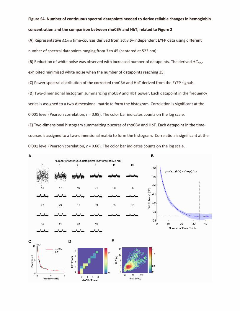
Figure S4. Number of continuous spectral datapoints needed to derive reliable changes in hemoglobin

concentration and the comparison between rhoCBV and HbT, related to Figure 2

(A) Representative DCHbO time-courses derived from activity-independent EYFP data using different

number of spectral datapoints ranging from 3 to 45 (centered at 523 nm).

(B) Reduction of white noise was observed with increased number of datapoints. The derived DCHbO

exhibited minimized white noise when the number of datapoints reaching 35.

(C) Power spectral distribution of the corrected rhoCBV and HbT derived from the EYFP signals.

(D) Two-dimensional histogram summarizing rhoCBV and HbT power. Each datapoint in the frequency

series is assigned to a two-dimensional matrix to form the histogram. Correlation is significant at the

0.001 level (Pearson correlation, r = 0.98). The color bar indicates counts on the log scale.

(E) Two-dimensional histogram summarizing z-scores of rhoCBV and HbT. Each datapoint in the time-

courses is assigned to a two-dimensional matrix to form the histogram. Correlation is significant at the

0.001 level (Pearson correlation, r = 0.66). The color bar indicates counts on the log scale.

Figure S5. Fiber-photometry in S1 with EYFP during hypercapnia (5% CO2), related to Figure 2

(A-G) Peri-event heatmaps showing repeated trials and average response time-courses of the changes in

measured rhoCBV, measured EYFP, derived HbO, derived HbR, derived HbT, corrected rhoCBV, and

corrected EYFP, respectively. The gray-shaded segment indicates infusion of 5% CO2. All color bars use

the same unit as the Y axis of the time-course. Error bars represent standard deviation.

(H, I) Correction of the contaminated rhoCBV and EYFP signals, respectively, across all subjects and all

trials (n=5, total trials =18; *** indicates p < 0.001, paired t-test).

(J) Power spectral distribution.

(K) Two-dimensional histogram summarizing rhoCBV and HbT power. Each datapoint in the frequency

series is assigned to a two-dimensional matrix to form the histogram. Correlation is significant at the

0.001 level (Pearson correlation, r = 0.98). The color bar indicates counts on the log scale.

(L) rhoCBV exhibited a higher sensitivity than derived HbT. Error bars represent standard deviation. ***

indicates p < 0.001 (paired t-test).

(M) Two-dimensional histogram summarizing rhoCBV and HbT z-scores. Each datapoint in the time-

courses is assigned to a two-dimensional matrix to form the histogram. Correlation is significant at the

0.001 level (Pearson correlation, r = 0.50). The color bar indicates counts on the log scale.

Figure S6. Simultaneous optogenetic-evoked CBV-fMRI and fiber-photometry recording and

comparison of the peak GCaMP responses before and after Hb-absorption correction, related to

Figure 3

(A) GCaMP and channelrhodopsin-2 (ChR2) were virally expressed using AAV under the CaMKIIa

promoter in the S1 and ventroposterior (VP) thalamus, respectively. Rhodamine B was injected

intravenously to achieve CBV measurement.

(B) Confocal images showing GCaMP expression.

(C) MRI-CBV activation maps in response to optogenetic stimulation of VP.

(D) Uncorrected time-courses for GCaMP, rhoCBV, and MRI-CBV (n = 3, total trials =33 trials). After a

short optogenetic stimulation of VP (60Hz, 10mW power, 0.5 ms pulse width for 1 s), uncorrected

GCaMP signal exhibited a strong undershoot with signal pattern mirrored the rhoCBV and MRI-CBV data,

indicative of significant Hb absorption in vivo.

(E) The peak amplitude of the GCaMP responses is significantly higher in the corrected GCaMP

compared to the uncorrected GCaMP. (*** indicates p<0.001, paired t-test, n=27)

Figure S7. Hb-absorption effects on fiber-photometry measurement during 5% isoflurane challenges

and pharmacological studies, related to Figure 4

(A) Preparation for fiber-photometry measurement of GCaMP and Rhodamine B signals in left M1. Ca2+-

independent GCaMP signal (GCaMP405) was excited by a 405 nm laser and used for hemodynamic

correction. rhoCBV signals were measured as described in Figure 2.

(B) Measured and corrected GCaMP405 time-courses before, during, and after 2-min 5% isoflurane

challenges (baseline = 0.5% isoflurane). The gray-shaded segment indicates the isoflurane period. Error

bars represent standard deviation.

(C) Scatter plots of measured and corrected GCaMP405 signals at 1, 2, 3, 4, 5, 6, and 7 min after the onset

of isoflurane challenge (n = 5, p < 0.001, two-way ANOVA).

(D) Derived HbO, HbR, and HbT time-courses before, during, and after isoflurane challenge.

(E) Measured and corrected rhoCBV time-courses before and after the isoflurane challenge. Rhodamine

B readout could be misinterpreted without hemodynamic correction.

(F) Scatter plots of measured and corrected rhoCBV signals at 1, 2, 3, 4, 5, 6, and 7 min after the onset of

isoflurane challenge (n = 5, p < 0.001, two-way ANOVA).

(G) Fiber-photometry measurement of GCaMP and tdTomato signals in left M1.

(H) Measured and corrected tdTomato time-courses before and after administering an a2 adrenergic

antagonist Atipamezole (1 mg/kg, s.c., Zoetis, Parsipanny, NJ).

(I) Scatter plots of measured and corrected tdTomato signals at 2, 4, 6, 8, and 10 min after atipamezole

administration (n = 3, p < 0.001, two-way ANOVA).

(J) Derived HbO, HbR, and HbT time-courses before and after atipamezole administration. Increased CBV

could be the result of redistribution of blood supply to active brain regions (Bekar et al., 2012).

(K) Measured and corrected GCaMP time-courses before and after atipamezole administration. the

increased GCaMP activity in the cortex would have been otherwise unchanged without hemodynamic

correction.

(L) Scatter plots of measured and corrected GCaMP signals at 2, 4, 6, 8, and 10 min after atipamezole

administration (n = 3, p < 0.05, two-way ANOVA).

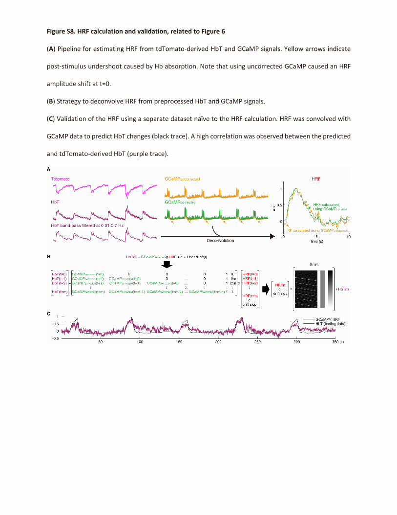
Figure S8. HRF calculation and validation, related to Figure 6

(A) Pipeline for estimating HRF from tdTomato-derived HbT and GCaMP signals. Yellow arrows indicate

post-stimulus undershoot caused by Hb absorption. Note that using uncorrected GCaMP caused an HRF

amplitude shift at t=0.

(B) Strategy to deconvolve HRF from preprocessed HbT and GCaMP signals.

(C) Validation of the HRF using a separate dataset naïve to the HRF calculation. HRF was convolved with

GCaMP data to predict HbT changes (black trace). A high correlation was observed between the predicted

and tdTomato-derived HbT (purple trace).

Figure S9. Simulated detection volume, correlation of signals drops with CBV changes, and using

regression to correct GCaMP signals, related to Figure 3

(A) Simulated detection volume of fiber-photometry and its projected probability.

(B) Two-dimensional histogram summarizing % changes of corrected rhoCBV and measured EYFP signal.

Each datapoint in the time-courses is assigned into a two-dimensional matrix to make the histogram.

Correlation is significant at the 0.001 level (Pearson correlation, r = -0.62). Color bars indicate datapoint

counts. Linear fit (red line) and 95% confidence interval (pink lines) are also shown.

(C) Two-dimensional histogram summarizing % changes of MRI-CBV and measured tdTomato signal.

Each datapoint in the time-courses is assigned into a two-dimensional matrix to make the histogram.

Correlation is significant at the 0.001 level (Pearson correlation, r = -0.33). Color bars indicate datapoint

counts. Linear fit (red line) and 95% confidence interval (pink lines) are also shown.

(D) Correcting GCaMP signals by regressing out the HbT with short (1 s) stimulation

(E) Correcting GCaMP signals by regressing out the HbT with long (10 s) stimulation.

Figure S10. Quantification of Hb-absorption effects using residue signals of fiber-photometry, related

to Figure 3

(A) Preparation for fiber-photometry measurement of the GCaMP signal in S1 of the forelimb region.

(B) Confocal images showing GCaMP expression.

(C) Simultaneous dual-spectral photometry recording of GCaMP and rhoCBV.

(D-I) Peri-stimulus heatmaps showing repeated trials and average response time-courses of the changes

in uncorrected GCaMP, measured rhoCBV, derived HbO, derived HbR, corrected GCaMP, and derived

HbT, respectively. The gray-shaded segment indicates forepaw-stimulation period. All color bars use the

same unit as the Y axis of the time-course. Error bars represent standard deviation.

(J) Correction of the post-stimulus dip of the GCaMP signals (n = 2, total trials = 6; ** indicates p < 0.01,

paired t-test).

(K) Two-dimensional histogram summarizing rhoCBV and HbT z-scores. Each datapoint in the time-

courses is assigned into a two-dimensional matrix to make the histogram. Correlation is significant at the

0.001 level (Pearson correlation, r = 0.28). Colorbar indicates the number of datapoints. Linear fit (red

line) and 95% confidence interval (pink lines) are also shown.