1

Observability Analysis and Keyframe-BasedFiltering for Visual Inertial Odometry with Full

Self-CalibrationJianzhu Huai1, Member, IEEE, Yukai Lin2, Yuan Zhuang1†, Member, IEEE

Charles Toth3, Senior Member, IEEE, and Dong Chen1, Member, IEEE

Abstract—Camera-IMU (Inertial Measurement Unit) sensorfusion has been extensively studied in recent decades. Numerousobservability analysis and fusion schemes for motion estimationwith self-calibration have been presented. However, it has beenuncertain whether both camera and IMU intrinsic parametersare observable under general motion. To answer this question,we first prove that for a global shutter camera-IMU system,all intrinsic and extrinsic parameters are observable with anunknown landmark. Given this, time offset and readout timeof a rolling shutter (RS) camera also prove to be observable.Next, to validate this analysis and to solve the drift issue of astructureless filter during standstills, we develop a Keyframe-based Sliding Window Filter (KSWF) for odometry and self-calibration, which works with a monocular RS camera or stereoRS cameras. Though the keyframe concept is widely used invision-based sensor fusion, to our knowledge, KSWF is the first ofits kind to support self-calibration. Our simulation and real datatests validated that it is possible to fully calibrate the camera-IMU system using observations of opportunistic landmarks underdiverse motion. Real data tests confirmed previous allusions thatkeeping landmarks in the state vector can remedy the drift instandstill, and showed that the keyframe-based scheme is analternative cure.

Index Terms—keyframe-based sliding window filter, observ-ability analysis, rolling shutter, visual inertial odometry, self-calibration

I. INTRODUCTION

V ISUAL Inertial Odometry (VIO) estimates the motionof an agent using data captured by the rigidly mounted

cameras and Inertial Measurement Units (IMUs). With greatpotential for augmented reality and robotics, many VIO meth-ods have been developed and deployed on smartphones [1],unmanned aerial vehicles [2], floor-cleaning robots [3], anddelivery robots [4]. However, these methods still have manyweaknesses related to dynamic scenes [5], unstable initializa-tion [6], coarse sensor calibration [7], and degenerate motion[8], to name a few. In an effort to build low-cost and robustVIO systems, this paper looks into the last two problems.

For most VIO methods, proper camera-IMU system cali-bration is ineluctable in achieving accurate motion estimation

1J. Huai, Y. Zhuang, D. Chen are with the State Key Laboratory ofInformation Engineering in Surveying, Mapping, and Remote Sensing (LIES-MARS), Wuhan University, 129 Luoyu Road, Wuhan, Hubei, 430079, China.Homepage of J. Huai: https://www.jianzhuhuai.com/.

2Y. Lin is with Huawei, Shanghai, China.3Charles Toth is with the Department of Civil, Environmental, and Geodetic

Engineering, The Ohio State University, Columbus, OH 43210, USA.†Corresponding author, yuan.zhuang@whu.edu.cn.

[7] and stable initialization [6]. But millions of consumerproducts, e.g., smartphones, often have low-cost sensors thatare inaccurately calibrated. For such sensor systems, real-time self-calibration along with motion estimation has becomea viable option, motivated by the ensuing benefits. First,additional computation for self-calibration is marginal andusually improves motion estimation [9], [10]. Second, thiscapability can be disabled online to save power if need be.Third, self-calibration also comes in handy when dealing withlegacy data captured without premeditated calibration. Thus,current VIO methods usually have some ability to calibratethe sensor system, especially the IMU biases and cameraextrinsic parameters, e.g., [11], [12]. One question underlyingself-calibration is whether the calibration parameters are ob-servable. Several works have analyzed observability of cameraextrinsics [13], camera intrinsics [14], and IMU intrinsics [15].There is empirical evidence [9], [16] that the camera-relatedparameters and IMU intrinsic parameters could be jointlyestimated in VIO, but there lacks a formal proof for this fullself-calibration.

Ideally, a VIO method should exhibit little drift whenthe system goes though degenerate motion, e.g., standstill.Although filtering-based VIO systems have been taking thelead in research and commercial products [1], [17] becauseof its efficiency among the existing geometrical approaches,quite a few of them suffer from drift during degenerate motion[18]. One influential strand of filters stems from the multi-stateconstraint Kalman filter (MSCKF) [19]. In contrast to the EKFstyle filters which keep the latest motion variables and a setof landmarks in the state, e.g., [20], [12], MSCKFs [21], [10]keep in the state vector a sliding window of motion variablesassociated with images but not landmarks (hence structure-less or memoryless). Despite the efficency brought about bythe disposal of landmarks, existing structureless filters formonocular VIO are prone to dramatic drift under degeneratemotion, e.g. hovering or standstill [18]. Several attempts havebeen made to address this issue. A state management strategybased on the last-in-first-out rule was presented in [8], butit requires detecting hovering. OpenVINS [10] deals withstandstills by using zero velocity update (ZUPT) which againrequires motion detection heuristics.

This paper tries to address the above two challenges toVIO, inaccurate sensor calibration and degenerate motion.First, we advocate calibrating the visual inertial system byfully accounting for relevant sensor parameters, and support

arX

iv:2

201.

0498

9v1

[cs

.RO

] 1

3 Ja

n 20

22

2

its feasibility by a thorough observability analysis. Second, wepropose a Keyframe-based Sliding Window Filter (KSWF),leveraging keyframes to handle degenerate motion.

Specifically, first, we develop the observability analysis of aVIO system that self-calibrates camera intrinsic and extrinsicparameters and IMU intrinsics in an unknown environment,with the Observability Rank Condition (ORC) [22], [23] ofLie derivatives. Under general motion, these parameters proveto be observable. Conditioned on this, we further prove thatthe camera time offset and rolling shutter (RS) readout timeare also able to be estimated. To our knowledge, observabilityanalysis for the full calibration has not been done before.

Then, the KSWF with self-calibration is presented for setupsconsisting of an IMU and one or two cameras. Its frontendtakes as input from the camera rig a sequence of framesor roughly synced frame pairs (called frame bundles forgenerality), associates keypoints between frames, and selectskeyframe bundles based on view overlaps. The backend filterkeeps in the state vector a sliding window of motion statevariables which will be opportunely marginalized depend-ing on whether they are associated with keyframe bundles,and opportunistic landmarks. As keyframes typically do notchange when the platform goes through degenerate motion, thekeyframe-based scheme is resilient to standstill and hovering.Granted that KSWF has similarities with recent VIO methods,it is unique in several ways. For example, compared tothe original MSCKF [19], KSWF is equipped with supportfor RS effect and stereo camera setups, full self-calibration,keyframe-based feature matching, and keyframe-based statemanagement.

Lastly, in simulation and real world tests with KSWF, wevalidate that the camera and IMU calibration parameters areobservable and self-calibration improves motion estimationunder general motion, and that the drift of existing monocularstructureless filters in degenerate motion can be mitigated bythe keyframe-based scheme.

The next section reviews recent developments on VIO fromthe aspects of observability analysis and real-time motionestimation with degenerate motion and distinguishes our studyfrom related ones. Section III describes the proposed KSWFincluding measurement models, state vector, keyframe-basedfrontend and backend. Its observability analysis is presentedin Section IV. Simulation study on sensor parameter observ-ability is reported in Section V. Section VI evaluates motionestimation and self-calibration on public benchmarks. SectionVII summarizes the work and points out future directions.

II. RELATED WORK

Regarding observability analysis that underlies on-the-flysensor calibration and real-time VIO methods that deals withdegenerate motion, we briefly review investigations aboutcamera-IMU-based sensor fusion.

A. Observability Analysis and Self-Calibration

As the camera-IMU systems are widely adopted, the neces-sity of calibration motivates the observability property analysiswhich has been explored from various aspects, usually with the

ORC of an observability matrix [24] constructed from eitherJacobians of the linearized system (e.g., [25], [26]) or gradientsof Lie derivatives of the original nonlinear system (e.g., [27],[13], [20], [15], [28]). Both types of ORC have revealed thatthe camera-IMU-based odometry in general has four unob-servable directions, i.e., the absolute translation and rotationabout gravity [25], [29]. Free of approximation, the latter ORCapproach lends itself to automated symbolic computation, thuscapable of dealing with more complex systems.

Much effort has been devoted to the observability of sen-sor parameters which is the theoretical foundation for self-calibration. The camera extrinsic parameters are found in[27] to be observable when a calibration target is available.With natural features, the extrinsic parameters prove to beobservable when at least two axes of the accelerometer andtwo axes of the gyroscope are excited (nonzero) [13]. Yanget al. [26] showed that the spatiotemporal parameters areobservable with general motion by analyzing the linearizedcamera-IMU-based odometry system. They further presentedthat the IMU intrinsic parameters are observable when allaxes of the IMU are excited [30]. The same conclusion wasdrawn in [15] for a stereo camera-IMU system by usingLie derivatives. The camera intrinsic parameters (excludingdistortion) are shown to be observable in [14] under generalmotion. Though studies have shown that online calibration ofthe camera intrinsic, extrinsic, and IMU intrinsic parametersin combination is possible and beneficial to motion estimation[9], [16], a formal analysis of whether these parameters areobservable is unavailable.

For the camera time offset to the IMU, it is asserted in[26] that it is only unobservable when the IMU experiencesconstant angular rate and linear acceleration. This assertion canalso be interpreted from deductions in [31]. To our knowledge,the observability of temporal parameters in a VIO system hasonly been analyzed with a linearized system in [26] where themotion state variables are at variable times that depend on thetime offset. Despite being conceptually simpler, the approachbased on Lie derivatives has not been used to analyze temporalobservability.

Regarding the above gaps, we conduct observability analysisof the VIO system with full self-calibration by using the Liederivatives, revealing the observables in monocular camera-IMU and stereo camera-IMU setups.

B. Motion Estimation in Degenerate Motion

Two types of geometrical approaches for VIO are preva-lent, those based on optimization, and filters. As some mea-surements arrive, an optimization-based approach conductsrepeated linearizations and updates to refine the motion andstructure variables. Example optimization-based VIO systemsare OKVIS [11], VINS-Mono [32], and [33]. By contrast,a filter linearizes these measurements and updates the statevariables and their covariance once, thereby saving muchcomputation while supplying the covariance at no additionalcost, especially suitable for low-cost systems [1].

The early VIO systems are often formulated as filters, e.g.[34], [35]. In the evolution of filters for VIO, the MSCKF

3

TABLE IDIFFERENCES AND SIMILARITIES OF OUR WORK TO RELATED STUDIES.

RS: ROLLING SHUTTER. PROP.: PROPAGATION.

Methods Ours [11] [9] [32] [10]Supportedsetup

monostereo

monostereo mono mono ≥ 1

camerasKeyframe-basedfrontend

X X × × ×

Keyframe-basedbackend

X X × X ×

Standstillin monosetup

Work Work Fail Work Fail

Calibratedparams

camera-IMUparams

cameraextrinsics

camera-IMUparams

cameraextrinsics,delay

cameraextrinsics,intrinsics

Deal withRS effect

IMUprop. N/A IMU

prop.optic flowcorrection

interpol.by posesin state

proposed in [19] had been a milestone, enabling real-timemotion estimation with a monocular camera-IMU setup. It hadsome bearing on many subsequent filtering approaches, e.g.,[36], [37], [12]. Among them, these methods [21], [20], [38],[39], [10] can be viewed as derivatives of MSCKF, enhancingit to be consistent and to deal with multiple cameras.

However, structureless filters that update motion estimateswith every arrived image, e.g., variants of MSCKF, are proneto drift during hovering or stationary periods. This issue wasmitigated by switching to a last-in-first-out state managementstrategy in [8]. Later, ZUPT was adopted in [10]. Theseapproaches require heuristics for motion detection which oftenare not portable. For instance, ZUPT may not work well withhovering.

To bridle drift of a structureless filter in degenerate motion,we leverage the concept of keyframes in both the featureassociation frontend and the state estimation backend.

Though keyframes have been widely adopted inoptimization-based visual SLAM methods [40], e.g., [11],[32], where the keyframe schemes help reduce computationin optimizing local maps, very few filters incorporatethe keyframe concept perhaps because of efficiency inthemselves. The VIO filters in [41], [39] used keyframe-basedstate management in the backend similar to VINS-Mono [32].In [1], a preprocessing module selects a subset of frames askeyframes and poses of only keyframes are estimated in thebackend inverse SWF. To deal with stationary periods, theEKF proposed in [42] keeps a cloned state variable for thelatest keyframe in order to use for update epipolar constraintsdue to points observed in that keyframe and the currentframe. Overall, our proposed KSWF shares features with [9],[11], [32], [10] to which the differences are summarized inTable I. In view of these studies, we believe that the proposedKSWF is the first keyframe-based filter that supports fullself-calibration.

III. KEYFRAME-BASED SLIDING WINDOW FILTER WITHSELF-CALIBRATION

From two aspects, self-calibration and resilience to degen-eration motion, this work studies the VIO problem, whichis to track the pose (position and orientation) and optionallycalibrate the sensor parameters of a platform consisting ofan IMU and at least one camera using inertial readings andimage observations of opportunistic landmarks with unknownpositions. Considering both aspects, we propose the KSWFwith self-calibration. It has two keyframe-based components:the feature association frontend which extracts feature matchesfrom images, and the estimation backend which fuses featurematches and inertial measurements to estimate motion andoptional parameters. Next, we present in turn notation conven-tions, IMU and camera measurement models, state variables,the frontend, and the backend filter.

A. Notation and Coordinate Frames

The Euclidean transformation from reference frame {B} to{A} is represented by a transformation matrix TAB whichconsists of a 3× 3 rotation matrix RAB and a 3D translationvector pAAB which is coordinates of {B}’s origin in {A}, i.e.,

TAB =

[RAB pAAB

0T 1

], For brevity, we will write pAAB as pAB

or pA when its meaning is clear.This work uses several right-handed coordinate frames,

camera frames {Ck}, k = 0, 1, body frame {B}, and worldframe {W}. The right-down-forward frame {Ck} is affixedto the lens optical center of a camera k. Without loss ofgenerality, we assign index 0 to the left camera of a stereo rigand refer to it as the main camera. {B} is the frame affixedto the platform which estimated poses by a VIO methodrefer to. It is defined to have origin at the intersection of theaccelerometer x and y input axes, and a known orientationRBC0

to the main camera. For easy result comparison, RBC0

is set to be the nominal orientation between the IMU andmain camera. Moreover, a quasi-inertial world frame {W} isinstantiated at the start with accelerometer measurements suchthat its z-axis is along negative gravity.

B. IMU Measurements

To consider systematic and random errors in the three-axisgyroscope and accelerometer, we use an IMU model as in [9]which accounts for random biases and noises, and systematicerrors (also known as IMU intrinsic parameters) includingscale factor errors, misalignment, relative orientations, and g-sensitivity. This model is chosen to simplify the subsequentobservability analysis.

The accelerometer measures the specific force applied tothe IMU in {B}, aBs . The measurement am is affected bysystematic errors encoded in a 3×3 matrix Ta, accelerometerbias ba and noise process νa,

aBs = RTWB · (vWB −

[0 0 −g

]T)

am = TaaBs + ba + νa

ba = νba,

(1)

4

where vWB is platform velocity in {W}, g is gravity magni-tude and ba is assumed to be driven by Gaussian white noiseprocess νba. Nine entries of Ta represent 3-DOF (degree-of-freedom) scale factor errors, 3-DOF misalignment, and 3-DOForientation between accelerometer input axes and {B}.

The gyroscope measures angular rate of the platform in{B}, ωBWB . The measurement ωm is affected by systematicerrors encoded in a 3 × 3 matrix Tg , g-sensitivity effectencoded in a 3 × 3 matrix Ts, gyroscope bias bg , and noiseprocess νg ,

ωm = TgωBWB + TsaBs + bg + νg

bg = νbg.(2)

where bg is assumed to be driven by Gaussian white noiseprocess νbg . Nine entries of Tg represent 3-DOF scale factorerrors, 3-DOF misalignment, and 3-DOF orientation betweengyroscope input axes and {B}. Here, Ta and Tg are fullypopulated for generality, but they may be simplified to be lowertriangular given an alternative {B} or extra knowledge of theIMU.

The power spectral densities of νa, νg , νba, and νbg ,are usually assumed to be σ2

aI3, σ2gI3, σ2

baI3, and σ2bgI3,

respectively, but they may have disparate diagonal values, andnonzero off-diagonal entries, e.g., for a 2-DOF gyro.

To predict pose and velocity and their covariance, propa-gation with IMU data by the trapezoidal rule is carried outas described in [16, Appendix A], [43]. We also extend thepropagation to support integration backward in time so as topredict camera poses for features in images captured by a RScamera. The propagation step uses the gravity norm providedby the user (1).

C. Camera Measurements

The proposed method supports image streams from onecamera or two roughly synchronized cameras. In the stereosetup, two frames of the two cameras are grouped into a framebundle when they have close timestamps per the camera clock.In a frame bundle of index j, we denote the original time ofan image k, k = 0, 1, stamped by the camera clock, by tCk

j .Camera k’s clock has an offset tkd relative to the IMU clock.Then, the timestamp by the IMU clock for the central row ofimage k, tkj , is given by

tkj = tCkj + tkd. (3)

In the filter, state variables will be stamped by the estimatedIMU time for the main camera’s images. Suppose that thelatest time offset estimate of the main camera as frame bundlej arrives is t0d,j , then the time for state variables associatedwith bundle j is set to a constant value tj given by

tj = tC0j + t0d,j . (4)

With mid-exposure time of an image, we can compute theobservation time per the IMU clock of any row in an image.Denote the frame readout time for camera k by tkr . Suppose

that a landmark i has an observation at row v in image k, thenits timestamp tki,j is computed by

tki,j = tkj + (v

h− 1

2)tkr (5)

where h is the height of image k. Using the central row ofthe RS image as the reference epoch instead of its first rowreduces the average prediction horizon and hence computationwhen predicting camera poses with IMU data for landmarkobservations.

We use the conventional reprojection model for landmarkobservations in images. Consider a landmark Li observed inimage k, k = 0, 1, of frame bundle j at zki,j = [u, v]T, anddenote the reprojection function of camera k by hk(·) whichfactors in all camera parameters, xkC , including the cameraextrinsic and intrinsic parameters, camera time offset tkd , andframe readout time tkr .

The reprojection model varies slightly depending on howthe landmark is parameterized. If the landmark is expressedin {W}, pWi = [xi, yi, zi, 1]T, the model is given by

zki,j = hk(T−1BCkT−1WB(tki,j)

pWi ) + wc (6)

where B(tki,j) denotes the body frame at feature time tki,j , andwe assume that an image observation is affected by Gaussiannoise wc ∼ N(0, σ2

c I2). This reprojection model is used forobservability analysis in Section IV for simplicity.

If landmark Li is anchored in image b, b ∈ {0, 1}, offrame bundle a, and represented with its inverse depth, thereprojection model will involve the body frame at bundle a’sassigned epoch ta (4), {B(ta)}. Now Li is expressed in thecamera frame at ta of image b, {Cb(ta)}, i.e., pCb(ta)

i =1ρi

[αi, βi, 1, ρi]T, with inverse depth ρi and observation direc-

tion [αi, βi, 1], the observation model is given by

zki,j = hk(T−1BCkT−1WB(tki,j)

TWB(ta)TBCb· pCb(ta)i ) + wc. (7)

This model is used in our experiments because anchoredlandmark representation does not cause inconsistency [44].

For the camera observation, the estimator will need mea-surement Jacobians of zki,j . Among them, one key componentis Jacobians of the pose at feature time tki,j , TWB(tki,j)

, relativeto the pose and velocity at state time tj , TWB(tj) and vWB(tj),respectively. Both are computed along with IMU propagationfrom tj to tki,j . Jacobians relative to time parameters, e.g., tkd ,k = 0, 1, are computed with the propagated velocity vWB(tki,j)and fitted angular rate ωBWB(tki,j). Jacobians relative to IMUparameters are ignored as in [45] because their entries areusually small (with first order terms up to O(tr)).

Our estimation framework supports multiple camera mod-els. When the camera intrinsic parameters are to be calibrated,we recommend using the pinhole radial tangential 8-parametermodel [46] or the Kannala Brandt 6-parameter model [47]as the observability analysis in Section IV shows that theirparameters are observable. Without loss of generality, weassume the pinhole radial tangential 8-parameter model (14)is used in the following unless otherwise stated.

5

TABLE IISTATE VARIABLES ESTIMATED BY KSWF FOR A STEREO CAMERA-IMU

SETUP. NOTE THAT RC0B IS KNOWN AND THE PINHOLE RADIALTANGENTIAL MODEL IS ASSUMED.

State variables Time-varying Time-invariant

Motion TWB(t), vWB(t){TWB(tj)

, vWB(tj)}

j = 0, 1, · · · , Nkf +Ntf − 1

IMU bg , ba Tg ,Ts,Ta

Camera Time-invariant

Extrinsics pC0B , TBC1

Intrinsics {fkx , fky , ckx, cky , kk1 , kk2 , pk1 , pk2}, k = 0, 1

Time offset tkr , k = 0, 1Readout time tkd , k = 0, 1

D. State Variables in the Filter

The state vector of the KSWF at time t, x(t), consists ofcurrent navigation state variable π(t), IMU parameters xS ,parameters of N cameras xC , and a sliding window of pastnavigation state variables xW at known epochs {tj} where jenumerates Nkf keyframe bundles and Ntf recent temporalframe bundles, and landmarks xL. That is,

x(t) = {π(t), xS , xC , xW , xL} (8)π(t) = {pWB(t),RWB(t), vWB(t)} (9)

xS ={

bg(t) ba(t) ~Tg ~Ts ~Ta}

(10)

xC = {xkC |k = 0, 1} (11)xW = {π(tj)|j = 0, 1, · · ·Nkf +Ntf − 1} (12)xL = {Li|i = 0, 1, · · · } (13)

where ~(·) concatenates rows of a matrix into a vector.The extrinsic parameters of the main camera, TC0B , has

a preset known rotation RBC0, therefore, for a monocular

camera-IMU setup, the camera parameters suitable for cali-bration are

xC = {pC0B , f0x , f

0y , c

0x, c

0y, k

01, k

02, p

01, p

02, t

0d, t

0r} (14)

For the second camera, its extrinsic variable is parameterizedby TBC1

. Parameters that can be estimated by the filter for astereo camera-IMU setup are listed in Table II.

Each navigation state in the sliding window π(tj) associatedwith frame bundle j is at a known epoch tj (4). Tyingnavigation state variables to known epochs is conceptuallysimpler than tying them to true epochs which are uncertainas in [10], [45]. The past navigation variables also includevelocity so that the RS camera pose for a landmark observationcan be propagated from the relevant navigation state variablewith IMU measurements.

Camera parameters xC and IMU intrinsic parameters areassumed to be unknown constants as in [9], [10], as theychange little in the timespan of the sliding window. However,if a sensor parameter is in fact not constant, noise can be addedto account for its drift over time as done for IMU biases.

The error δx for a state variable x in a vector space isdefined to be x = x + δx, where x is its estimate. For the

rotation matrices on a Lie group, the error state is definedby the Lie algebra. For example, RWB’s error state δθWB

is defined by RWB = exp(δθ×WB)RWB ≈ (I + δθ×WB)RWB ,where (·)× obtains the skew-symmetric matrix of a 3D vector.

E. Feature Association Frontend

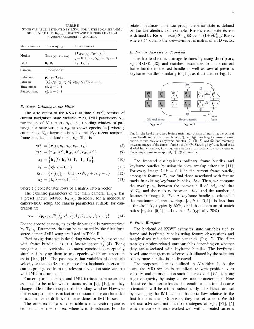
The frontend extracts image features by using descriptors,e.g., BRISK [48], and matches descriptors from the currentframe bundle to the last bundle as well as several previouskeyframe bundles, similarly to [11], as illustrated in Fig. 1.

New frameOld keyframes Recent frames

3

2

1

4

5

6

7

Fig. 1. The keyframe-based feature matching consists of matching the currentframe bundle to the last frame bundle, 1© and 4©, matching the current framebundle to two previous keyframe bundles, 2©, 3©, 5©, and 6©, and matchingbetween images of the current frame bundle, 7©. Showing keyframe bundles asshaded frame bundles, this diagram assumes a platform with stereo cameras.For a single camera setup, only 1©- 3© are needed.

The frontend distinguishes ordinary frame bundles andkeyframe bundles by using the view overlap criteria in [11].For every image k, k = 0, 1, in the current frame bundle,among its features Fk, we find those associated with featuretracks in existing keyframe bundles, Mk. Then, we computethe overlap ok between the convex hull of Mk and thatof Fk, and the ratio rk between |Mk| and the number offeatures in image k, |Fk|. A keyframe bundle is selected ifthe maximum of area overlaps {ok|k ∈ [0, 1]} is less thana threshold To (typically 60%) or if the maximum of matchratios {rk|k ∈ [0, 1]} is less than Tr (typically 20%).

F. Filter Workflow

The backend of KSWF estimates state variables tied toframe and keyframe bundles using feature observations andmarginalizes redundant state variables (Fig. 2). The filtermanages motion-related state variables depending on whetherthey are associated with keyframe bundles. The keyframe-based state management scheme is facilitated by the selectionof keyframe bundles in the frontend.

The proposed filter is outlined in Algorithm 1. At thestart, the VIO system is initialized to zero position, zerovelocity, and an orientation such that z-axis of {W} is alongnegative gravity by using a few accelerometer data. Notethat since the filter enforces this condition, the initial coarseorientation will be refined subsequently. The biases are setby averaging the IMU data if the optic flow relative to thefirst frame is small. Otherwise, they are set to zero. We didnot use advanced initialization strategies of e.g., [32], [6]which in our experience worked well with calibrated cameras

6

Cameraframes

①Extract features

IMU data

②Match features based on keyframes

③Propagate state

④Clonenavigation

SVs

⑤Add landmark SVs, update state

⑥Marginalize based on

keyframes

Feature tracks

⑦State and covariance

Image epochs

Keyframe-based sliding window filter

Fig. 2. Flowchart of the keyframe-based sliding window filter. SV: statevariable. 1©- 2© are touched on in III-E. 3©- 6© are presented in III-F. 7© isdescribed in III-D.

Fig. 3. Schematic drawing of a landmark i’s observation Jacobians relative tothe state vector whose nonzero entries are shaded. For clarity, the landmark isassumed not in the state. In accordance with Fig. 1, as a new frame bundle jarrives, this landmark completes its feature track at frame bundle j−1 whichserves as its anchor frame bundle (7). After the navigation state variable forframe bundle j has been cloned as πj := π(tj), the computed Jacobiansfor i are stacked as shown and ready for canceling out the Jacobian for i’sparameters (Section III-F).

but poorly with inaccurate calibration. Remaining IMU andcamera parameters are initialized to values from datasheetsor experience. The standard deviations of state variables areinitialized to sensible values (see Table IV for simulation).

As a frame bundle j arrives, the navigation state π(t) andthe covariance matrix are propagated with IMU data to thestate epoch tj (Box 3© of Fig. 2). Then, π(t) is clonedand appended to the state vector and the covariance matrixis also expanded for the cloned π(tj) (Line 3, Box 4© ofFig. 2). As π(tj) is at a known epoch tj , unlike [10] or [45,(30)], we need not to account for uncertainty in its time whenaugmenting covariance for π(tj). Instead, we need to computethe measurement Jacobian relative to camera time offsets inthe update step (Line 12).

In parallel, feature descriptors are extracted from images ofbundle j and matched to those of the last bundle j − 1 andseveral recent keyframe bundles (e.g., bundle j − 2 and j2 inFig. 1). After that, three types of feature tracks will be usedfor update: tracks that disappear in bundle j, observations oflandmarks in the state vector, and tracks that can triangulatea new landmark to the state. They differ in how to preparefor the update. For disappeared tracks, Jacobians relativeto landmark parameters need to be canceled out by matrixnullspace projection [19]. For the third type, triangulated newlandmarks will be augmented to the state and covariance. Forall three observation types, the update is carried out identicalto the classic EKF [43], [16]. It is possible to use an iteratedupdate scheme for disappeared features. However, empirically,

despite additional computation, its improvement on accuracyacross datasets was marginal [12].

For a landmark i, stacked Jacobians of its observationsrelative to the state vector are visualized in Fig. 3. For alandmark with large depth, the observation Jacobian relativeto its parameters (i.e., the landmark Jacobian) can be rank-deficient, and the fact should be considered in cancelingout the landmark Jacobian and in performing the followingMahalanobis gating test.

To bound computation, redundant frame bundles are se-lected and marginalized from the filter (Lines 25-27, Box 6©of Fig. 2), once the number of navigation state variables in thesliding window exceeds Nkf +Ntf . In a marginalization oper-ation, at least Nr redundant bundles (Nr is 3 for a monocularsetup, 2 for a stereo setup) are chosen (Line 25) since tworeprojection measurements for an unknown landmark is unin-formative [39]. To meet this requirement, redundant bundlesare chosen first among the recent non-keyframe bundles whileexcluding the most recent Ntf bundles and secondly amongthe oldest keyframe bundles. For the case of Fig. 1, Nkf = 2and Ntf = 3, the redundant bundles for the latest bundle jare keyframe bundle j1 and frame bundle j − 3.

With these redundant bundles, we update the filter withobservations of landmarks each observed more than twice inthese bundles (Line 26). For such a landmark, if it can betriangulated with its entire observation history, its observationsin the redundant bundles are used for EKF update. Otherobservations in the redundant bundles are discarded. After theupdate, state variables and entries in the covariance matrix forthese redundant bundles are removed (Line 27).

To ensure filter consistency, for IMU propagation andcamera measurements, Jacobians are evaluated at propagatedvalues of position and velocity, i.e., first estimates [21], andat the latest estimates of other variables, e.g., IMU biases,landmarks expressed by anchored inverse depth, since they donot affect the unobservable directions [44].

IV. OBSERVABILITY ANALYSIS

By using the ORC of Lie derivatives, this section showsthat the VIO system with self-calibration is weakly observableunder general motion while excluding the four immanentunobservable dimensions. We first review the basics of ob-servability analysis with Lie derivatives. Then, this methodis applied to the monocular global shutter (GS) camera-IMU-based odometry with self-calibration while ignoring timevariables. Discussions on extensions are also given. Lastly, weconsider observability of time offset and RS readout time.

A. Observability Analysis Fundamentals

According to [28], a state at time t0, x(t0), is weaklyobservable if there is a neighborhood in which all its neighborscan be distinguished from itself by the knowledge of outputsand user-chosen inputs in a time interval I = [t0, t0 + T ].For a noise-free system that is affine in the control inputs ui,i = 1, 2, · · · , p,

x = f0(x) +

p∑i=1

fi(x)ui, y = h(x) (15)

7

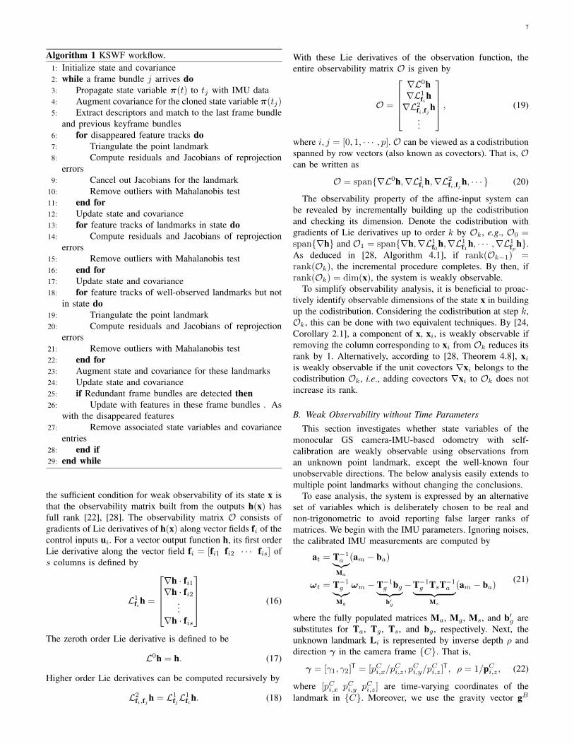
Algorithm 1 KSWF workflow.1: Initialize state and covariance2: while a frame bundle j arrives do3: Propagate state variable π(t) to tj with IMU data4: Augment covariance for the cloned state variable π(tj)5: Extract descriptors and match to the last frame bundle

and previous keyframe bundles6: for disappeared feature tracks do7: Triangulate the point landmark8: Compute residuals and Jacobians of reprojection

errors9: Cancel out Jacobians for the landmark

10: Remove outliers with Mahalanobis test11: end for12: Update state and covariance13: for feature tracks of landmarks in state do14: Compute residuals and Jacobians of reprojection

errors15: Remove outliers with Mahalanobis test16: end for17: Update state and covariance18: for feature tracks of well-observed landmarks but not

in state do19: Triangulate the point landmark20: Compute residuals and Jacobians of reprojection

errors21: Remove outliers with Mahalanobis test22: end for23: Augment state and covariance for these landmarks24: Update state and covariance25: if Redundant frame bundles are detected then26: Update with features in these frame bundles . As

with the disappeared features27: Remove associated state variables and covariance

entries28: end if29: end while

the sufficient condition for weak observability of its state x isthat the observability matrix built from the outputs h(x) hasfull rank [22], [28]. The observability matrix O consists ofgradients of Lie derivatives of h(x) along vector fields fi of thecontrol inputs ui. For a vector output function h, its first orderLie derivative along the vector field fi = [fi1 fi2 · · · fis] ofs columns is defined by

L1fih =

∇h · fi1∇h · fi2

...∇h · fis

(16)

The zeroth order Lie derivative is defined to be

L0h = h. (17)

Higher order Lie derivatives can be computed recursively by

L2fi,fj h = L1

fjL1fih. (18)

With these Lie derivatives of the observation function, theentire observability matrix O is given by

O =

∇L0h∇L1

fih∇L2

fi,fj h...

, (19)

where i, j = [0, 1, · · · , p]. O can be viewed as a codistributionspanned by row vectors (also known as covectors). That is, Ocan be written as

O = span{∇L0h,∇L1fih,∇L

2fi,fj h, · · · } (20)

The observability property of the affine-input system canbe revealed by incrementally building up the codistributionand checking its dimension. Denote the codistribution withgradients of Lie derivatives up to order k by Ok, e.g., O0 =span{∇h} and O1 = span{∇h,∇L1

f0h,∇L1f1h, · · · ,∇L1

fph}.As deduced in [28, Algorithm 4.1], if rank(Ok−1) =rank(Ok), the incremental procedure completes. By then, ifrank(Ok) = dim(x), the system is weakly observable.

To simplify observability analysis, it is beneficial to proac-tively identify observable dimensions of the state x in buildingup the codistribution. Considering the codistribution at step k,Ok, this can be done with two equivalent techniques. By [24,Corollary 2.1], a component of x, xi, is weakly observable ifremoving the column corresponding to xi from Ok reduces itsrank by 1. Alternatively, according to [28, Theorem 4.8], xiis weakly observable if the unit covectors ∇xi belongs to thecodistribution Ok, i.e., adding covectors ∇xi to Ok does notincrease its rank.

B. Weak Observability without Time Parameters

This section investigates whether state variables of themonocular GS camera-IMU-based odometry with self-calibration are weakly observable using observations froman unknown point landmark, except the well-known fourunobservable directions. The below analysis easily extends tomultiple point landmarks without changing the conclusions.

To ease analysis, the system is expressed by an alternativeset of variables which is deliberately chosen to be real andnon-trigonometric to avoid reporting false larger ranks ofmatrices. We begin with the IMU parameters. Ignoring noises,the calibrated IMU measurements are computed by

at = T−1a︸︷︷︸Ma

(am − ba)

ωt = T−1g︸︷︷︸Mg

ωm − T−1g bg︸ ︷︷ ︸b′g

−T−1g TsT−1a︸ ︷︷ ︸Ms

(am − ba)(21)

where the fully populated matrices Ma, Mg , Ms, and b′g aresubstitutes for Ta, Tg , Ts, and bg , respectively. Next, theunknown landmark Li is represented by inverse depth ρ anddirection γ in the camera frame {C}. That is,

γ = [γ1, γ2]T = [pCi,x/pCi,z, p

Ci,y/p

Ci,z]

T, ρ = 1/pCi,z, (22)

where [pCi,x pCi,y pCi,z] are time-varying coordinates of thelandmark in {C}. Moreover, we use the gravity vector gB

8

expressed in {B} to encode gravity magnitude, and roll andpitch of the camera-IMU system. Overall, the system state is

x = {γ, ρ, vB , gB ,b′g,ba, ~Mg, ~Ms, ~Ma, xC} (23)

where xC = {pCB , fx, fy, cx, cy, k1, k2, p1, p2}, excludingtemporal parameters t0d and t0r and dropping the camera index0 from superscripts for brevity. Comparing to (8), we see thatthe alternative system state covers all variables in the originalmonocular VIO system except t0d, t0r , pWB , and yaw. The statedimension is dim(x) = 53.

Assuming that biases are constant in a short timespan, withbasic derivations, the system model is found to be

γρ

vBgB

=

Cγρ[(RCBωt)× (ρpCB − γ)−

RCBρvB ]vB × ωt + at + gB

gB × ωt

= f0 + f1am + f2ωm

b′g = ba = 03×1Mg = Ms = Ma = 03×3, xC = 011×1

(24)

where the shorthand notations are

γ = [γT 1]T, Cγρ =

[I2 −γ

01×2 −ρ

]. (25)

To save space, the coefficient vector fields fi, i = 0, 1, 2 arenot expanded. The known RCB is expressed by [qx, qy, qz, 1]T.

There are two types of observations to the system, pointobservation h1, and gravity magnitude h2,

h1 =

fx[γ1(1 + k1r

2 + k2r4) + 2p1γ1γ2+

p2(r2 + 2γ21)] + cxfy[γ2(1 + k1r

2 + k2r4) + p1(r2 + 2γ22)+

2p2γ1γ2] + cy

(26)

h2 = (gB)TgB (27)

where r2 = γTγ.We analyze the system of (24), (26), and (27) by in-

crementally constructing codistributions. With first order Liederivatives, we find rank(O1) = 17. With second order Liederivatives, rank(O2) = 46. By using the two deductiontechniques, we identify that eight parameters of the pinholeradial tangential model, Mg , and Ms, are weakly observable.The same procedure shows that the FOV 5-parameter model[49], the extended unified camera 6-parameter model [50],and the Kannala Brandt 6-parameter model [47] are weaklyobservable with the second order codistribution O2.

As a result, we can replace h1 with h′1 = γ and removecamera intrinsic parameters from x, giving a shorter statevector x′, greatly simplifying the arduous analysis. For thenew system, the third order codistribution has full rank,rank(O3) = 45 = dim(x′), implying that the system is weaklyobservable. One set of covectors spanning O3 is given by

O3 = span{∇L0h1,∇L0h2,∇L1f0h1,∇L1

f1h1,

∇L1f2h1,∇L2

f0,f0h1,∇L2f1,f0h1,∇L2

f2,f0h11,

∇L2f0,f11h1,∇L2

f11,f11h11,∇L2f0,f12h1,

∇L2f0,f13h1,∇L2

f0,f21h1,∇L2f0,f22h11,

∇L3f0,f0,f0h1,∇L3

f11,f0,f0h11,∇L3f0,f11,f0h11,

∇L3f0,f12,f0h11,∇L

3f0,f13,f0h11,∇L

3f0,f0,f11h11}

(28)

where h1 , [h11, h12]T. The 45-row spanning set involves Liederivatives computed along vector fields of all control inputs,am and ωm, implying that weak observability of the systemrequires that all six axes of the IMU are excited at some timeof the interval I.

C. Discussions on Extensions

It is worth noting that the known gravity magnitude isneeded for calibrating scale factors of the accelerometer. Ifh2 is unavailable, the system of (24) and (26) is identifiableup to a metric scale with the unobservable direction

N =[0T2 −ρ vBT gBT 0T24 ~MT

a pTCB 0T8]T

(29)

which satisfies OkN = 0.Also, if we assume one component of RCB is unknown, say

qx, then in the system of h′ and x′, the number of unknownsbecomes 46, but rank(O3) = rank(O4) = 45, meaning thatthe 3-DOF RCB is unobservable.

For the case of stereo cameras, if the IMU is unavailable,it is easy to show that the intrinsic and extrinsic parametersof the stereo camera rig (of dimension 22) are observablegiven 4D observations of 21 landmarks and the baseline length.Otherwise, for the stereo camera-IMU system, following theabove analysis based on Lie derivatives, it can be shownthat the intrinsic and extrinsic parameters of both camerasand the IMU intrinsic parameters as listed in Table II areobservable given 4D observations of an unknown landmarkand the gravity magnitude or the baseline length. Intuitively,one of the two latter constraints resolves the scale ambiguity.

When the system is standstill, whether at the beginning ormiddle of estimation, all state variables turn into unknownconstants. None of them can be resolved given the set ofobservation equations because the Jacobian of these equationsis rank deficient, unless some parameters are assumed wellestimated. For instance, the IMU biases can be estimatedif Tg , Ts, Ta, and gW are roughly known. Moreover, thesystem pose can be obtained given sufficient observations oflandmarks of roughly known positions along with the cameraintrinsic parameters.

D. Observability of Time Parameters

Next, we deduce that in general the camera time offset of theVIO system can be estimated, that is, h(x(t+ td)) 6= h(x(t)).To this end, we identify the conditions under which h(x(t +td)) = h(x(t)), and show that they are unlikely to occur.

By expanding the Taylor series for h(x(t + td)) in termsof x(t) and ui(t) (Appendix A), we identify the followingcondition that leads to unobservable time offset,

O · x = 0, am = const, ωm = const. (30)

This condition means that time offset becomes unobservableunder constant inputs and when some other state variablesare unobservable, i.e., O is rank deficient. For instance, whenthe platform rotates about direction of the only feature withconstant rate, and both the constant applied force and gravityare along the feature direction. Both [31] and [26] have

9

also found that time offset may become unobservable underconstant inputs. These situations are unlikely to occur inpractice.

Finally, we remark that the frame readout time can be ob-tained as long as the other sensor parameters can be estimated.We can choose an observation zki,j of landmark Li, given theimage k’s timestamp, the frame readout time can be solvedfor by a Newton-Raphson method.

In summary, the state in the VIO system (24), cameratime offset, and readout time can be estimated under generalmotion. These variables correspond to the state variables of themonocular KSWF (8) except global translation and rotationabout gravity, meaning that KSWF with self-calibration isfeasible in theory.

V. SIMULATION STUDY

By simulation, this section shows that the presented sensorparameters can be estimated with observations of opportunisticpoint landmarks, and that the proposed KSWF can accuratelyestimate platform motion with inaccurately calibrated sensors.

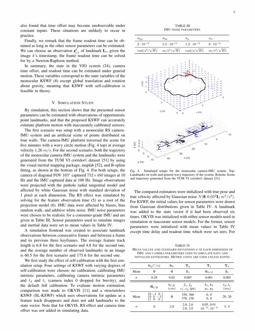
The first scenario was setup with a monocular RS camera-IMU system and an artificial scene of points distributed onfour walls. The camera-IMU platform traversed the scene forfive minutes with a wavy circle motion (Fig. 4 top) at averagevelocity 1.26 m/s. For the second scenario, both the trajectoryof the monocular camera-IMU system and the landmarks weregenerated from the TUM VI corridor1 dataset [51] by usingthe visual inertial mapping package, maplab [52], and B-splinefitting, as shown at the bottom of Fig. 4. For both setups, thecamera of diagonal FOV 103◦ captured 752×480 images at 10Hz and the IMU captured data at 100 Hz. Image observationswere projected with the pinhole radial tangential model andaffected by white Gaussian noise with standard deviation of1 pixel at each dimension. The RS effect was simulated bysolving for the feature observation time (5) as a root of theprojection model (6). IMU data were affected by biases, biasrandom walk, and additive white noise. IMU noise parameterswere chosen to be realistic for a consumer-grade IMU and aregiven in Table III. Sensor parameters used to simulate imagesand inertial data were set to mean values in Table IV.

A simulation frontend was created to associate landmarkobservations between consecutive frames and between a frameand its previous three keyframes. The average feature tracklength is 6.8 for the first scenario and 4.8 for the second one,and the average number of observed landmarks in an imageis 60.5 for the first scenario and 175.6 for the second one.

We first study the effect of self-calibration with the first sim-ulation setup. Four settings of KSWF with varying degrees ofself-calibration were chosen: no calibration, calibrating IMUintrinsic parameters, calibrating camera intrinsic parametersand td and tr (camera index 0 dropped for brevity), andthe default full calibration. To evaluate motion estimation,comparison was made to OKVIS [11] and a structurelessKSWF (SL-KSWF) which uses observations for update as afeature track disappears and does not add landmarks to thestate vector. Note that for OKVIS, RS effect and camera timeoffset was not added in simulating data.

TABLE IIIIMU NOISE PARAMETERS.

σbg σba σg σa

2 · 10−5 5.5 · 10−5 1.2 · 10−3 8 · 10−3

rad/s2/√Hz m/s3/

√Hz rad/s/

√Hz m/s2/

√Hz

-1

5

0

z (

m)

1

5

y (m)

0

x (m)

0

-5 -5

10

0

-10

x (m)

-20

-20

2

5

z (

m)

0 -30

y (m)

-5-40

-10

Fig. 4. Simulated setups for the monocular camera-IMU system. Top:Landmarks on walls and general wavy trajectory of the system. Bottom: Sceneand trajectory generated from the TUM VI corridor1 dataset [51].

The compared estimators were initialized with true pose andtrue velocity affected by Gaussian noise N(0, 0.052I3m2/s4).For KSWF, the initial values for sensor parameters were drawnfrom Gaussian distributions given in Table IV. A landmarkwas added to the state vector if it had been observed sixtimes. OKVIS was initialized with either sensor models used insimulation or inaccurate sensor models. For the former, sensorparameters were initialized with mean values in Table IVexcept time delay and readout time which were set zero. For

TABLE IVMEAN VALUES AND STANDARD DEVIATIONS σ AT EACH DIMENSION OF

IMU AND CAMERA PARAMETERS USED TO SIMULATE DATA ANDINITIALIZE ESTIMATORS. METRIC UNITS ARE USED UNLESS NOTED.

bg(◦/s) ba Tg Ts Ta

Mean 0 0 I3 03×3 I3

σ 0.29 0.02 0.005 0.001 0.005

RCBtCB

(cm)fx, fy

cx, cy (px)k1, k2p1, p2

td, tr(ms)

Mean[0−1 00 0 −11 0 0

]0

350, 360378, 238

0, 00, 0 20, 20

σ 0 2.0 2.0, 2.02.0, 2.0

0.05, 0.0110−3, 10−3 5, 5

10

TABLE VRMSE AT THE END OF 5-MINUTE WAVY MOTION FOR OKVIS, SL-KSWF,

AND KSWF WITH VARYING LEVELS OF SELF-CALIBRATION, COMPUTEDOVER SUCCESSFUL RUNS OF 100 ATTEMPTS WHICH WERE DEEMED

SUCCESSFUL IF THE POSITION ERROR AT THE END IS <100 M.

Method RMSE SuccessrunspWB (m) RWB (◦)

OKVIS 0.49 6.82 100

OKVIS inaccurate calib 13.94 39.79 85

KSWF calib off 38.32 40.42 60

KSWF calib camera 2.00 18.18 100

KSWF calib IMU 30.73 40.55 69

KSWF full calib 0.23 1.22 100

SL-KSWF full calib 0.61 5.60 100

0 50 100 150 200 250 300

time (sec)

0

10

20

30

40

50

60

Pose N

EE

S (

1)

Wavy circle KSWF full calib

Wavy circle SL-KSWF full calib

Reference

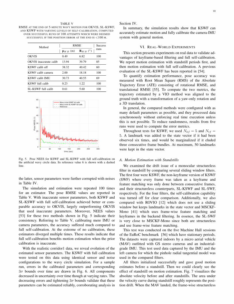
Fig. 5. Pose NEES for KSWF and SL-KSWF with full self-calibration onthe artificial wavy circle data. Its reference value 6 is shown with a dashedline.

the latter, sensor parameters were further corrupted with noisesin Table IV.

The simulation and estimation were repeated 100 timesfor an estimator. The pose RMSE values are reported inTable V. With inaccurate sensor parameters, both KSWF andSL-KSWF with full self-calibration achieved better or com-parable accuracy to OKVIS, largely outperforming OKVISthat used inaccurate parameters. Moreover, NEES values[53] for these two methods shown in Fig. 5 indicate theirconsistency. Referring to Table V, calibrating mere IMU orcamera parameters, the accuracy suffered much compared tofull self-calibration. At the extreme of no calibration, theseestimators diverged multiple times. These results indicate thatfull self-calibration benefits motion estimation when the priorcalibration is inaccurate.

With the realistic corridor1 data, we reveal evolution of theestimated sensor parameters. The KSWF with full calibrationwere tested on this data using identical sensor and noiseconfigurations to the wavy circle simulation. For a samplerun, errors in the calibrated parameters and corresponding3σ bounds over time are drawn in Fig. 6. All componentsdecreased in uncertainty over time though at varying rates. Thedecreasing errors and tightening 3σ bounds validate that theseparameters can be estimated reliably, corroborating analysis in

Section IV.In summary, the simulation results show that KSWF can

accurately estimate motion and fully calibrate the camera-IMUsystem with general motion.

VI. REAL-WORLD EXPERIMENTS

This section presents experiments on real data to validate ad-vantages of keyframe-based filtering and full self-calibration.We report motion estimation with standstill periods first, andthen motion estimation with full self-calibration. A previousevaluation of the SL-KSWF has been reported in [54].

To quantify estimation performance, pose accuracy wasmeasured with Root Mean Square (RMS) of the AbsoluteTrajectory Error (ATE) consisting of rotational RMSE, andtranslational RMSE [55]. To compute the two metrics, thetrajectory estimated by a VIO method was aligned to theground truth with a transformation of a yaw-only rotation anda 3D translation.

In general, the compared methods were configured with asmany default parameters as possible, and they processed datasynchronously without enforcing real time execution unlessthis is not possible. To reduce randomness, results from fiveruns were used to compute the error metrics.

Throughout tests for KSWF, we used Nkf = 5 and Ntf =5. A landmark was added to the state vector if it had beenobserved six times, and would be marginalized if it eludedthree consecutive frame bundles. At maximum, 50 landmarkswere kept in the state vector.

A. Motion Estimation with Standstills

We examined the drift issue of a monocular structurelessfilter in standstill by comparing several sliding window filters.The first four were KSWF, the non-keyframe version of KSWF(SWF) where every frame was taken as a keyframe andfeature matching was only done between consecutive frames,and their structureless counterparts, SL-KSWF and SL-SWF,respectively. For the four filters, the self-calibration capabilitywas turned off for clear comparison. Additionally, we alsocompared with ROVIO [12] which does not use a slidingwindow but keeps landmarks in the state vector and MSCKF-Mono [41] which uses frame-wise feature matching andkeyframes in the backend filtering. In essence, the SL-SWFis very close to MSCKF-Mono since both are structurelessand use frame-wise feature matching.

This test was conducted on the five Machine Hall sessionsof the EuRoC benchmark [56] which have stationary periods.The datasets were captured indoors by a micro aerial vehicle(MAV) outfitted with GS stereo cameras and an industrial-grade IMU. This test used data captured by the IMU and theleft camera for which the pinhole radial tangential model wasused in the compared filters.

All filters initialized successfully and gave good motionestimates before a standstill. Then we could clearly see theeffect of standstill on motion estimation. Fig. 7 visualizes theabsolute velocity before and after standstills. The area underthe velocity curve during standstill roughly represents the posi-tion drift. When the MAV landed, the frame-wise structureless

11

0 50 100 150 200 250 300

-20

0

20

40

0 50 100 150 200 250 300

-20

0

20

0 50 100 150 200 250 300

-20

0

20

0 50 100 150 200 250 300

-2

0

2

0 50 100 150 200 250 300

-2

0

2

0 50 100 150 200 250 300

-2

0

2

0 50 100 150 200 250 300

-20

0

20

0 50 100 150 200 250 300

-20

0

20

0 50 100 150 200 250 300

-20

0

20

0 50 100 150 200 250 300

-5

0

5

0 50 100 150 200 250 300

-5

0

5

0 50 100 150 200 250 300

-10

0

10

0 50 100 150 200 250 300

-10

0

10

20

0 50 100 150 200 250 300

-10

-5

0

5

10

0 50 100 150 200 250 300

-5

0

5

0 20 40 60 80 100

-2

0

2

0 20 40 60 80 100

-2

0

2

0 20 40 60 80 100

-20

0

20

0 20 40 60 80 100

-20

0

20

0 20 40 60 80 100

-20

0

20

0 20 40 60 80 100

-20

0

20

Fig. 6. Errors (solid lines) and 3σ bounds (dashed lines) of estimated camera-IMU system parameters in a sample run of KSWF on the data simulated fromTUM VI corridor1 data. The x axis represents time in seconds. For brevity, only three off-diagonal elements of Tg , Ts, Ta are shown.

filters, both MSCKF-Mono and SL-SWF, suffered positiondrifts, although MSCKF-Mono organizes state variables interms of keyframes in the backend. Interestingly, both filtersmanaged to estimate the velocity more or less accurately afterthe stationary periods. We think that the drift of MSCKF-Monoand SL-SWF is caused by frame-wise feature matching whichprovides many low disparity matches during standstills.

By contrast, filters that keep landmarks in the state, ROVIO,KSWF, and SWF, and filters that use keyframe-based match-ing, SL-KSWF and KSWF, reported almost zero velocity instandstill. On one hand, landmarks in the state vector serve asmemory, constraining the filter during degenerate motion. Onthe other hand, feature matching relative to previous keyframeswhich do not depend on time retrieves matches of largedisparity even during stationary periods.

This comparative test illustrates that keyframe-based featurematching helps structureless filters deal with degenerate mo-tion, e.g., standstill, and keeping landmarks in the state vectoralso resolves this issue.

B. Motion Estimation with Self-Calibration

To show the feasibility and benefits of self-calibration,tests were conducted on raw room sequences of the TUM

VI benchmark [51]. These sequences were captured by ahandheld device with stereo GS cameras of fisheye lenses ofdiagonal FOV 195◦ and a consumer-grade IMU. Ground truthmotion was recorded by a motion capture system, servingwell to evaluate VIO methods. The authors have providedraw sequences, calibration data for the sensor setup, andcalibrated sequences where the IMU data were corrected withthe estimated IMU intrinsic parameters. For this test, we chosethe six room sequences because they have diverse motion. Thecamera-IMU calibration results provided in the benchmark canserve as reference to validate the full self-calibration.

To prepare the raw sequences, images were down-scaled to512 × 512 as in [51], and timestamps of camera and IMUmessages were shifted by a constant duration to be alignedwith the ground truth for the sake of evaluation.

Then, these sequences were processed by several recent VIOmethods. Five KSWF variants were used including KSWF, SL-KSWF, KSWF without self-calibration, KSWF that calibratesonly IMU intrinsics, and KSWF that calibrates only cameraextrinsics, intrinsics, tid, and tir, i = 0, 1. For comparison,OKVIS [11] with extrinsic calibration, VINS-Mono [32] withextrinsic calibration, and OpenVINS [10] with camera intrinsicand spatiotemporal calibration were also used. Note that the

12

0 10 20 30 40 50 60

time (sec)

0

1

2

3

4

5

6

Standstill

KSWF

SL-KSWF

SL-SWF

SWF

MSCKF-mono

ROVIO mono

0 10 20 30 40 50 60

time (sec)

0

0.5

1

1.5

2

Standstill

0 10 20 30 40 50 60

time (sec)

0

0.5

1

1.5

2

2.5

Standstill

0 10 20 30 40 50 60

time (sec)

0

1

2

3

Standstill

0 10 20 30 40 50 60

time (sec)

0

1

2

3

Standstill

Fig. 7. Velocity estimated by KSWF, SL-KSWF, SWF, SL-SWF, MSCKF-mono, and ROVIO for EuRoC MH 1-5 sequences. All methods ran inmonocular mode using the left camera images. SL-SWF and MSCKF-monohave nonzero velocity during standstills in contrast to other methods.

last variant of KSWF is similar to OpenVINS [10] in config-uration. VINS-Mono only processed the left camera imagesand IMU data. Features of these methods are summarized inTable VI.

These methods were mostly configured using parametersprovided by their authors, e.g., OpenVINS and VINS-Mono.For OKVIS, the configuration file provided by the TUM VIbenchmark was used as a starting point. Then, for all esti-mators, sensor parameters were initialized to nominal values.If a parameter was not to be calibrated, it was locked to theinitial value. Initial values for IMU intrinsics are Tg = I,Ts = 0, and Ta = I. The camera extrinsic parameters wereset zero in translation and a nominal rotation in orientation.The Kannala Brandt 6-parameter model [47] were used for

TABLE VIFEATURES OF THE COMPARED ODOMETRY METHODS.

Method OKVIS VINS-Mono OpenVINS KSWF

RS camera model X X

Calibratecameras

Extrinsics X X X X

Intrinsics X X

td X X X

tr X

CalibrateIMU

Intrinsics X

Biases X X X X

the stereo cameras with initial values f ix = f iy = 190 (px),cix = 256 (px), ciy = 256 (px), ki1 = 0, and ki2 = 0 fori = 0, 1. The temporal parameters had initial values tid = 0 sand tir = 0.02 s for i = 0, 1. Because the raw sequences havelarge IMU errors, for all estimators, the IMU noise parameterswere inflated from values provided by authors with a simplegrid search.

For these estimators starting from inaccurate parameters,the error metrics of estimated motion versus the number ofruns on the raw room sequences are drawn in Fig 8. Methodswith very limited self-calibration, e.g., OKVIS and VINS-Mono, suffered significantly in motion estimation accuracyand often diverged. This contrasts with their performance onthe calibrated room sequences with accurate sensor param-eters, for which all compared estimators estimated motionaccurately without obvious drift, achieving <0.2% relativetranslation error [55]. Comparing the variants of KSWF, asthe level of self-calibration increased, the motion estimationbecame less brittle and more accurate. This is particularly truewhen the IMU intrinsics were calibrated, likely because theconsumer-grade IMU is notoriously affected by scale factorerrors and misalignment. Interestingly, OpenVINS and KSWFthat calibrated camera parameters had similar performance asboth calibrated almost the same set of parameters.

To examine observability of parameters in full self-calibration, we compared their values estimated by KSWFand OpenVINS, and values provided by the benchmark. Forreference, the benchmark’s authors have estimated the IMUintrinsic and camera extrinsic parameters with their calibrationdata. For comparison, these values were converted to ournotation. On the other hand, reference camera intrinsics wereobtained with a program Basalt [57] using the calibration data.Besides the estimated parameters from the 27 convergent runsof KSWF in the previous test, we also calibrated camera-related parameters by running OpenVINS on the six calibratedroom sequences. These estimated parameters with 3σ boundsand their references, relative to initial values, are visualized inFig. 9. Since OpenVINS gives identical results for five runson the same sequence, only one estimate of a parameter isdrawn for each sequence.

For parameters estimated by KSWF, we see that: (1) bg ,ba, Tg , Ts, tid, tir with i = 0, 1 were estimated consistentlywith small variances; (2) camera intrinsics f i, cix, ciy , ki1,i = 0, 1, and some dimensions of Ta, had some estimates that

13

0 5 10 15 200

5

10

15

20

25

30

KSWF

SL-KSWF

KSWF cal cam

KSWF cal IMU

KSWF no cal

OpenVINS

OKVIS

VINS-mono

0 5 10 15 20 25 30 35 40

0

5

10

15

20

25

30

Fig. 8. Translation and rotation RMSE of odometry methods, KSWF withdefault full calibration, SL-KSWF with default full calibration, KSWF thatcalibrates only camera-related parameters, KSWF that calibrates only IMUparameters, KSWF without calibration, OKVIS, OpenVINS, VINS-mono, onthe TUM VI six raw stereo room sequences. Each method ran five times ona sequence.

deviated much from the reference; and (3) the camera extrin-sics pC0B , pBC1 , and RBC1 had dispersed estimates in somecomponents. Observations (2-3) indicate that some parametersof the camera-IMU system are more challenging to calibrate.Considering that all parameters were estimated mostly closeto their references starting from the initial inaccurate values,this largely confirmed that these parameters are observable.

For OpenVINS, since the IMU intrinsic errors had beenmostly corrected and only camera parameters were calibrated,we expect it to estimate parameters closer to the referencesand to have smaller variances than KSWF. Strangely, we seethat ki2, i = 0, 1, had unusual large uncertainty, and someparameters consistently deviated from reference values, e.g.,k01 , and pBC1

(3).To evaluate the efficiency of KSWF, we timed its three com-

ponents, feature extraction, feature matching, and estimationincluding filter update and marginalization, with the EuRoCbenchmark [56], on a Dell Insipiron 7590 laptop with 16 GBRAM and a 2.60 GHz 6-core Intel Core i7-9750H processorrunning Ubuntu 18.04. The time costs of components of SL-

TABLE VIITIME COST OF MAJOR FUNCTIONS OF SL-KSWF IN PROCESSING EUROC

SEQUENCES IN MILLISECONDS. VALUES IN BOLD IDENTITY ROUTINESTHAT DETERMINE AVERAGE TIME TO PROCESS A FRAME BUNDLE.

Function Mono Stereomean σ mean σ

Feature extraction 0 3.0 0.3 5.1 1.5Feature extraction 1 0 0 5.1 1.6Match to keyframes 1.3 0.2 2.9 0.7Match to last frame 0.7 0.1 1.8 0.5Match left to right 0 0 0.5 0.1Filter update 4.5 1.4 13.4 3.6Marginalization 1.5 0.8 5.1 1.9Time per frame 8.0 N/A 23.7 N/A

KSWF with full self-calibration and synchronous processingare presented in Table VII. The time costs of KSWF areslightly larger than SL-KSWF in filter update and marginal-ization, varying with the allowed number of landmarks in thestate vector. As feature extraction is done in parallel, averageprocessing time for a frame bundle amounts to the time costsfor feature matching and estimation, thereby, 8 ms (125 Hz)in the monocular mode, and 23.7 ms (42.2 Hz) in the stereomode, meaning that the proposed method has good efficiency.

VII. CONCLUSION AND FUTURE WORK

Regarding VIO with self-calibration, this paper solves twoexisting problems: whether the full set of calibration pa-rameters are observable, and the drift issue in conventionalstructureless monocular filters under degenerate motion.

For the former, using Lie derivatives, we prove that cameraintrinsics, extrinsics, time offset, and IMU intrinsics of thecamera-IMU system are observable under general motionusing observations of opportunistic landmarks. Given thiscondition, the frame readout time can be estimated. Theseobservability assertions were confirmed with simulation andreal data tests. We foresee that this type of symbolic compu-tation can greatly simplify observability analysis of a slew ofparameter estimation problems compared to manual derivation.

For the latter, we introduce the keyframe concept to boththe feature matching frontend and sliding window filteringbackend. Together with the self-calibration capability, thisbrings about the KSWF framework. Real world tests validatedthe strength of keyframe-based filtering, revealing that eitherkeyframe-based matching or keeping landmarks in the statevector helps remedy the drift issue of structureless monocularfilters in standstill. Moreover, on datasets captured by inaccu-rate sensors, KSWF with self-calibration largely outperformedrecent VIO methods of minimal calibration, indicating thevalue of self-calibration for low-cost sensors.

Besides motion estimation, an interesting application of ourmethod is to inspect the setup of legacy data. For example,by running KSWF on the TUM rolling shutter datasets [58],it is found that they were captured with the left camera in GSmode and the right camera in RS mode.

We are aware that full self-calibration will encounter unob-servable dimensions when the camera-IMU system is confinedin motion, e.g., on a ground vehicle. In such situations, it is

14

x y z

0

2

b g (

/s)

x y z

1

0

b a (m

/s2 )

1, 1 1, 2 1, 3 2, 1 2, 2 2, 3 3, 1 3, 2 3, 3

50

0

50

T g (0

.001

)

1, 1 1, 2 1, 3 2, 1 2, 2 2, 3 3, 1 3, 2 3, 3

2.5

0.0

2.5

T s (0

.001

rad/

sm

/s2)

1, 1 1, 2 1, 3 2, 1 2, 2 2, 3 3, 1 3, 2 3, 340200

204060

T a (0

.001

)

pC0B(1) pC0B(2) pC0B(3) pBC1(1) pBC1(2) pBC1(3)

5

0

5

(cm

)f0 c0

x c0y f1 c1

x c1y

10

5

0

5

(px)

k01 k0

2 k11 k1

2

10

5

0

5

(0.0

01)

roll pitch yaw3

2

1

0

R BC1

()

t0d t0

r t1d t1

r

20

15

10

5

0

(ms)

KSWFOpenVINSTUM VI Ref.

Fig. 9. Parameter estimates relative to initial values and 3σ bounds by KSWF on the six TUM VI raw room sequences and by OpenVINS on the six calibratedroom sequences. Blue bars are for 27 successful runs of KSWF (five attempts for each sequence). Orange bars are for OpenVINS (one run for each sequence).Red crosses show reference values from the benchmark. Note that frame readout times were initialized to 20 ms.

advisable to lock up those unobservable parameters. To thisend, identifying unobservable directions with Lie derivativesis one of the worthwhile directions to look into. A relatedproblem is VIO initialization in the case of coarse calibration.

APPENDIXWHEN TIME OFFSET IS UNOBSERVABLE

This section identifies the condition when the time offsetin outputs of an affine-input system is indistinguishable. Forsimple deduction, we rewrite the affine-input system (15) withscalar inputs ui, i = 1, 2, · · · ,m,

x = f0(x) +

m∑i=1

fi(x)ui, y = h(x) (31)

We try to find when h(x(t+ td)) = h(x(t)) holds. The Taylorexpansion for h(x(t+ td)) regarding td is

h(x(t+ td)) = h(x(t)) + tdh(x) +t2d2

h(x)+

t3d6

...h(x) + · · · .

(32)

The first three derivatives are given by

h(x(t)) = ∇h · x = L1f0h +

m∑i=1

L1fihui (33)

h(x) = ∇(L1f0h +

m∑i=1

L1fihui)x +

m∑i=1

L1fihui

= L2f0,f0h +

m∑i=1

L2f0,fihui +

m∑i=1

L2fi,f0hui+

m∑j=1

m∑i=1

L2fi,fj huiuj +

m∑i=1

L1fihui

(34)

...h(x) = ∇(L2

f0,f0h +

m∑i=1

L2f0,fihui +

m∑i=1

L2fi,f0hui+

m∑j=1

m∑i=1

L2fi,fj huiuj +

m∑i=1

L1fihui)x+

m∑i=1

L2f0,fihui +

m∑i=1

L2fi,f0hui +

m∑i=1

L1fihui+

m∑j=1

m∑i=1

L2fi,fj huiuj +

m∑j=1

m∑i=1

L2fi,fj huiuj

(35)

15

The above expressions show that in general dkhdtk

is a linearcombination of covectors (e.g., ∇L2

f0,fi ) with coefficients x,and time derivatives of inputs (e.g., L2

fi,fj huiuj). The conditionto make td unobservable is that

dkhdtk

(x, ui, ui, · · · ) = 0, k = 1, 2, · · · , i = 1, 2, · · · ,m(36)

As with the observability analysis, we are free to choose ui.By setting ui, i = 1, 2, · · · ,m, to constants in the time intervalI, (36) is satisfied when x meets the below constraints,

O · x = 0 (37)

Otherwise, when ui, i = 1, 2, · · · ,m, are time varying andhave non-vanishing time derivatives up to order k, there willbe much fewer points in the space M of x satisfying (36).Intuitively, the reason is that under the set of constraints (36)on x and ui, i = 1, 2, · · · ,m, the freedom of x shrinks whenthe inputs ui are allowed more freedom.

ACKNOWLEDGMENT

We would like to thank Agostino Martinelli for guidanceon Lie derivatives. We are grateful to the Editor who awardedus four extensions. Moreover, we appreciate the inspiringcomments from anonymous reviewers who exhorted us tonovelty and contribution.

REFERENCES

[1] A. Flint, O. Naroditsky, C. P. Broaddus, A. Grygorenko, S. Roume-liotis, and O. Bergig, “Visual-based inertial navigation,” US PatentUS9 424 647B2, Aug., 2016. 1, 2, 3

[2] S. R. McClure, B. S. Thompson, A. Bry, A. Bachrach, and M. Don-ahoe, “Perimeter structure for unmanned aerial vehicle,” US PatentUS20 170 341 776A1, Nov., 2017. 1

[3] R. T. Pack, S. R. Lenser, J. H. Kearns, and O. Taka, “Simultaneouslocalization and mapping for a mobile robot,” US Patent US9 037 396B2,May, 2015. 1

[4] J. Huai, Y. Qin, F. Pang, and Z. Chen, “Segway DRIVE benchmark:Place recognition and SLAM data collected by a fleet of delivery robots,”Segway Robotics, Beijing, China, Tech. Rep., Jul. 2019. 1

[5] B. Bescos, C. Campos, J. D. Tardos, and J. Neira, “DynaSLAM II:Tightly-Coupled Multi-Object Tracking and SLAM,” IEEE Robotics andAutomation Letters, vol. 6, no. 3, pp. 5191–5198, Jul. 2021. 1

[6] D. Zuniga-Noel, F.-A. Moreno, and J. Gonzalez-Jimenez, “An analyticalsolution to the IMU initialization problem for visual-inertial systems,”arXiv:2103.03389 [cs], Mar. 2021. 1, 5

[7] T. Schneider, M. Li, C. Cadena, J. Nieto, and R. Siegwart,“Observability-aware self-calibration of visual and inertial sensors forego-motion estimation,” IEEE Sensors Journal, vol. 19, no. 10, pp.3846–3860, May 2019. 1

[8] C. Guo, D. Kottas, R. DuToit, A. Ahmed, R. Li, and S. Roumeliotis,“Efficient visual-inertial navigation using a rolling-shutter camera withinaccurate timestamps,” in Robotics: Science and Systems (RSS), Berke-ley, USA, Jul. 2014. 1, 3

[9] M. Li, H. Yu, X. Zheng, and A. I. Mourikis, “High-fidelity sensormodeling and self-calibration in vision-aided inertial navigation,” inIEEE Intl. Conf. on Robotics and Automation (ICRA), Hong Kong,China, May 2014, pp. 409–416. 1, 2, 3, 5

[10] P. Geneva, K. Eckenhoff, W. Lee, Y. Yang, and G. Huang, “Open-VINS: A research platform for visual-inertial estimation,” in Workshopon Visual-Inertial Navigation: Challenges and Applications at IROS,Macau, China, Nov. 2019. 1, 3, 5, 6, 11, 12

[11] S. Leutenegger, S. Lynen, M. Bosse, R. Siegwart, and P. Furgale,“Keyframe-based visual-inertial odometry using nonlinear optimization,”The International Journal of Robotics Research, vol. 34, no. 3, pp. 314–334, Mar. 2015. 1, 2, 3, 5, 9, 11

[12] M. Bloesch, M. Burri, S. Omari, M. Hutter, and R. Siegwart, “Iteratedextended Kalman filter based visual-inertial odometry using directphotometric feedback,” The International Journal of Robotics Research,vol. 36, no. 10, pp. 1053–1072, Sep. 2017. 1, 3, 6, 10

[13] J. Kelly and G. S. Sukhatme, “Visual-inertial sensor fusion: Localiza-tion, mapping and sensor-to-sensor self-calibration,” The InternationalJournal of Robotics Research, vol. 30, no. 1, pp. 56–79, 2011. 1, 2

[14] S.-H. Tsao and S.-S. Jan, “Observability analysis and performanceevaluation of EKF-based visual-inertial odometry with online intrinsiccamera parameter calibration,” IEEE Sensors Journal, vol. 19, no. 7, pp.2695–2703, Apr. 2019. 1, 2

[15] J. H. Jung, S. Heo, and C. G. Park, “Observability analysis of IMU in-trinsic parameters in stereo visual–inertial odometry,” IEEE Transactionson Instrumentation and Measurement, vol. 69, no. 10, pp. 7530–7541,Oct. 2020. 1, 2

[16] J. Huai, “Collaborative SLAM with crowdsourced data,” Ph.D. disser-tation, The Ohio State University, Columbus OH, May 2017. 1, 2, 4,6

[17] S. I. Roumeliotis and A. I. Mourikis, “Vision-aided inertial navigation,”US Patent US9 766 074B2, Sep., 2017. 1

[18] D. G. Kottas, K. J. Wu, and S. I. Roumeliotis, “Detecting and dealingwith hovering maneuvers in vision-aided inertial navigation systems,”in 2013 IEEE/RSJ International Conference on Intelligent Robots andSystems. Tokyo: IEEE, Nov. 2013, pp. 3172–3179. 1

[19] A. I. Mourikis and S. I. Roumeliotis, “A multi-state constraint Kalmanfilter for vision-aided inertial navigation,” in IEEE Intl. Conf. onRobotics and Automation (ICRA), Rome, Italy, Apr. 2007, pp. 3565–3572. 1, 2, 3, 6

[20] J. A. Hesch, D. G. Kottas, S. L. Bowman, and S. I. Roumeliotis,“Camera-IMU-based localization: Observability analysis and consis-tency improvement,” The International Journal of Robotics Research,vol. 33, no. 1, pp. 182–201, Jan. 2014. 1, 2, 3

[21] M. Li and A. I. Mourikis, “High-precision, consistent EKF-based visual-inertial odometry,” The International Journal of Robotics Research,vol. 32, no. 6, pp. 690–711, May 2013. 1, 3, 6

[22] R. Hermann and A. Krener, “Nonlinear controllability and observability,”IEEE Transactions on Automatic Control, vol. 22, no. 5, pp. 728–740,Oct. 1977. 2, 7

[23] A. Martinelli, “Visual-inertial structure from motion: Observability andresolvability,” in 2013 IEEE/RSJ International Conference on IntelligentRobots and Systems (IROS). Tokyo, Japan: IEEE, Nov. 2013, pp. 4235–4242. 2

[24] K. Maes, M. N. Chatzis, and G. Lombaert, “Observability of nonlinearsystems with unmeasured inputs,” Mechanical Systems and SignalProcessing, vol. 130, pp. 378–394, 2019. 2, 7

[25] J. A. Hesch, D. G. Kottas, S. L. Bowman, and S. I. Roumeliotis, “Con-sistency analysis and improvement of vision-aided inertial navigation,”IEEE Transactions on Robotics, vol. 30, no. 1, pp. 158–176, Feb. 2014.2

[26] Y. Yang, P. Geneva, K. Eckenhoff, and G. Huang, “Degenerate motionanalysis for aided INS with online spatial and temporal sensor calibra-tion,” IEEE Robotics and Automation Letters, vol. 4, no. 2, pp. 2070–2077, Apr. 2019. 2, 8

[27] F. M. Mirzaei and S. I. Roumeliotis, “A Kalman filter-based algorithmfor IMU-camera calibration: Observability analysis and performanceevaluation,” IEEE Transactions on Robotics, vol. 24, no. 5, pp. 1143–1156, Oct. 2008. 2

[28] A. Martinelli, Observability: A new theory based on the group ofinvariance, ser. Advances in Design and Control. Society for Industrialand Applied Mathematics, Jan. 2020. 2, 6, 7

[29] ——, “Vision and IMU data fusion: Closed-form solutions for attitude,speed, absolute scale, and bias determination,” IEEE Transactions onRobotics, vol. 28, no. 1, pp. 44–60, Feb. 2012. 2

[30] Y. Yang, P. Geneva, X. Zuo, and G. Huang, “Online IMU intrinsiccalibration: Is it necessary?” in Robotics: Science and Systems (RSS),Corvallis, Oregon, Jul. 2020, pp. 716–725. 2

[31] M. Li and A. I. Mourikis, “Online temporal calibration for camera–IMUsystems: Theory and algorithms,” The International Journal of RoboticsResearch, vol. 33, no. 7, pp. 947–964, 2014. 2, 8

[32] T. Qin, P. Li, and S. Shen, “VINS-Mono: A robust and versatile monoc-ular visual-inertial state estimator,” IEEE Transactions on Robotics,vol. 34, no. 4, pp. 1004–1020, Aug. 2018. 2, 3, 5, 11

[33] V. Usenko, N. Demmel, D. Schubert, J. Stuckler, and D. Cremers,“Visual-inertial mapping with non-linear factor recovery,” IEEE Roboticsand Automation Letters, vol. 5, no. 2, pp. 422–429, Apr. 2020. 2

16

[34] D. Strelow and S. Singh, “Motion estimation from image and inertialmeasurements,” The International Journal of Robotics Research, vol. 23,no. 12, pp. 1157–1195, Dec. 2004. 2

[35] M. J. Veth, “Fusion of imaging and inertial sensors for navigation,”Ph.D. dissertation, Airforce Institute of Technology, Dayton, OH, Sep.2006. 2

[36] E. S. Jones and S. Soatto, “Visual-inertial navigation, mapping andlocalization: A scalable real-time causal approach,” The InternationalJournal of Robotics Research, vol. 30, no. 4, pp. 407–430, Jan. 2011. 3

[37] S. Weiss, M. W. Achtelik, S. Lynen, M. Chli, and R. Siegwart, “Real-time onboard visual-inertial state estimation and self-calibration ofMAVs in unknown environments,” in IEEE Intl. Conf. on Robotics andAutomation (ICRA), St Paul, MN, USA, May 2012, pp. 957–964. 3

[38] K. Wu, A. Ahmed, G. Georgiou, and S. Roumeliotis, “A square rootinverse filter for efficient vision-aided inertial navigation on mobiledevices,” in Robotics: Science and Systems XI. Robotics: Science andSystems Foundation, Jul. 2015. 3

[39] K. Sun, K. Mohta, B. Pfrommer, M. Watterson, S. Liu, Y. Mulgaonkar,C. J. Taylor, and V. Kumar, “Robust stereo visual inertial odometry forfast autonomous flight,” IEEE Robotics and Automation Letters, vol. 3,no. 2, pp. 965–972, Apr. 2018. 3, 6

[40] G. Younes, D. Asmar, E. Shammas, and J. Zelek, “Keyframe-basedmonocular SLAM: Design, survey, and future directions,” Robotics andAutonomous Systems, vol. 98, pp. 67–88, 2017. 3

[41] A. Z. Zhu, N. Atanasov, and K. Daniilidis, “Event-based visual inertialodometry,” in 2017 IEEE Conference on Computer Vision and PatternRecognition (CVPR), Jul. 2017, pp. 5816–5824. 3, 10

[42] D. Abeywardena, S. Huang, B. Barnes, G. Dissanayake, andS. Kodagoda, “Fast, on-board, model-aided visual-inertial odometrysystem for quadrotor micro aerial vehicles,” in 2016 IEEE InternationalConference on Robotics and Automation (ICRA), May 2016, pp. 1530–1537. 3

[43] C. Jekeli, Inertial Navigation Systems with Geodetic Applications.Berlin, Germany: de Gruyter, Jan. 2001. 4, 6

[44] J. Huai, Y. Lin, Y. Zhuang, and M. Shi, “Consistent right-invariant fixed-lag smoother with application to visual inertial SLAM,” in 35th AAAIConference on Artificial Intelligence, Feb. 2021. 4, 6

[45] M. Li and A. I. Mourikis, “Vision-aided inertial navigation with rolling-shutter cameras,” The International Journal of Robotics Research,vol. 33, no. 11, pp. 1490–1507, 2014. 4, 5, 6

[46] G. R. Bradski and A. Kaehler, Learning OpenCV: Computer vision withthe OpenCV library, 1st ed. Sebastopol, CA, USA: O’Reilly Media,Inc., 2008. 4

[47] J. Kannala and S. S. Brandt, “A generic camera model and calibrationmethod for conventional, wide-angle, and fish-eye lenses,” IEEE Trans-actions on Pattern Analysis and Machine Intelligence, vol. 28, no. 8,pp. 1335–1340, Aug. 2006. 4, 8, 12

[48] S. Leutenegger, M. Chli, and R. Y. Siegwart, “BRISK: Binary robustinvariant scalable keypoints,” in Intl. Conf. on Computer Vision (ICCV),Barcelona, Spain, Nov. 2011, pp. 2548–2555. 5

[49] F. Devernay and O. Faugeras, “Straight lines have to be straight,”Machine Vision and Applications, vol. 13, no. 1, pp. 14–24, Aug. 2001.8

[50] B. Khomutenko, G. Garcia, and P. Martinet, “An enhanced unifiedcamera model,” IEEE Robotics and Automation Letters, vol. 1, no. 1,pp. 137–144, Jan. 2016. 8

[51] D. Schubert, T. Goll, N. Demmel, V. Usenko, J. Stuckler, and D. Cre-mers, “The TUM VI benchmark for evaluating visual-inertial odometry,”in IEEE/RSJ Intl. Conf. on Intelligent Robots and Systems (IROS),Madrid, Spain, Oct. 2018. 9, 11

[52] T. Schneider, M. Dymczyk, M. Fehr, K. Egger, S. Lynen, I. Gilitschen-ski, and R. Siegwart, “Maplab: An open framework for research invisual-inertial mapping and localization,” IEEE Robotics and Automa-tion Letters, vol. 3, no. 3, pp. 1418–1425, 2018. 9

[53] Y. Bar-Shalom, X. Li, and T. Kirubarajan, Estimation with applicationsto tracking and navigation: Theory algorithms and software. JohnWiley & Sons, 2004. 10

[54] J. Huai, Y. Lin, C. Toth, Y. Zhuang, and D. Chen, “A versatile keyframe-based structureless filter for visual inertial odometry,” Wuhan University,Hubei, China, Tech. Rep., Dec. 2020. 10

[55] Z. Zhang and D. Scaramuzza, “A tutorial on quantitative trajectoryevaluation for visual(-inertial) odometry,” in IEEE/RSJ Intl. Conf. onIntelligent Robots and Systems (IROS), Madrid, Spain, Oct. 2018, pp.7244–7251. 10, 12

[56] M. Burri, J. Nikolic, P. Gohl, T. Schneider, J. Rehder, S. Omari, M. W.Achtelik, and R. Siegwart, “The EuRoC micro aerial vehicle datasets,”

The International Journal of Robotics Research, vol. 35, no. 10, pp.1157–1163, 2016. 10, 13

[57] V. Usenko, N. Demmel, and D. Cremers, “The double sphere cameramodel,” in 2018 International Conference on 3D Vision (3DV). Verona,Italy: IEEE, Sep. 2018, pp. 552–560. 12

[58] D. Schubert, N. Demmel, L. von Stumberg, V. Usenko, and D. Cremers,“Rolling-shutter modelling for direct visual-inertial odometry,” TechnicalUniversity of Munich, Germany, Tech. Rep., Nov. 2019. 13