Observability-Based Guidance and Sensor Placement

Brian T. Hinson

A dissertationsubmitted in partial fulfillment of the

requirements for the degree of

Doctor of Philosophy

University of Washington

2014

Reading Committee:

Kristi Morgansen Hill, Chair

Juris Vagners

Maryam Fazel Sarjoui

Brian C. Fabien

Program Authorized to Offer Degree:Aeronautics and Astronautics

c©Copyright 2014

Brian T. Hinson

University of Washington

Abstract

Observability-Based Guidance and Sensor Placement

Brian T. Hinson

Chair of the Supervisory Committee:Associate Professor Kristi Morgansen Hill

Aeronautics and Astronautics

Control system performance is highly dependent on the quality of sensor informa-

tion available. In a growing number of applications, however, the control task must

be accomplished with limited sensing capabilities. This thesis addresses these types

of problems from a control-theoretic point-of-view, leveraging system nonlinearities

to improve sensing performance. Using measures of observability as an information

quality metric, guidance trajectories and sensor distributions are designed to improve

the quality of sensor information. An observability-based sensor placement algorithm

is developed to compute optimal sensor configurations for a general nonlinear sys-

tem. The algorithm utilizes a simulation of the nonlinear system as the source of

input data, and convex optimization provides a scalable solution method. The sensor

placement algorithm is applied to a study of gyroscopic sensing in insect wings. The

sensor placement algorithm reveals information-rich areas on flexible insect wings,

and a comparison to biological data suggests that insect wings are capable of acting

as gyroscopic sensors. An observability-based guidance framework is developed for

robotic navigation with limited inertial sensing. Guidance trajectories and algorithms

are developed for range-only and bearing-only navigation that improve navigation ac-

curacy. Simulations and experiments with an underwater vehicle demonstrate that

the observability measure allows tuning of the navigation uncertainty.

TABLE OF CONTENTS

Page

List of Figures . . . . . . . . . . . . . . . . . . . . . . . . . . . . . . . . . . . iii

List of Tables . . . . . . . . . . . . . . . . . . . . . . . . . . . . . . . . . . . . v

Chapter 1: Introduction . . . . . . . . . . . . . . . . . . . . . . . . . . . . 1

1.1 Literature Review . . . . . . . . . . . . . . . . . . . . . . . . . . . . . 3

1.2 Contributions of this Thesis . . . . . . . . . . . . . . . . . . . . . . . 10

1.3 Organization of the Report . . . . . . . . . . . . . . . . . . . . . . . . 11

Chapter 2: Observability Measures . . . . . . . . . . . . . . . . . . . . . . 12

2.1 Nonlinear Observability . . . . . . . . . . . . . . . . . . . . . . . . . 12

2.2 Observability Gramian . . . . . . . . . . . . . . . . . . . . . . . . . . 19

Chapter 3: Observability-Based Sensor Placement . . . . . . . . . . . . . . 26

3.1 Problem Statement . . . . . . . . . . . . . . . . . . . . . . . . . . . . 26

3.2 Solution Methods . . . . . . . . . . . . . . . . . . . . . . . . . . . . . 27

3.3 Sensor Data Compression . . . . . . . . . . . . . . . . . . . . . . . . 35

Chapter 4: Sensor Placement Application: Gyroscopic Sensing in Insect Wings 38

4.1 Background . . . . . . . . . . . . . . . . . . . . . . . . . . . . . . . . 38

4.2 Flexible Wing Flapping Dynamics . . . . . . . . . . . . . . . . . . . . 40

4.3 Simulation Methods . . . . . . . . . . . . . . . . . . . . . . . . . . . . 53

4.4 Sensor Placement Results . . . . . . . . . . . . . . . . . . . . . . . . 61

4.5 Discussion . . . . . . . . . . . . . . . . . . . . . . . . . . . . . . . . . 73

Chapter 5: Robotic Navigation with Limited Sensors: Observability-BasedGuidance Trajectories . . . . . . . . . . . . . . . . . . . . . . . 77

5.1 Problem Statement . . . . . . . . . . . . . . . . . . . . . . . . . . . . 77

i

5.2 Uniform Flow Field Identification . . . . . . . . . . . . . . . . . . . . 80

5.3 Range-only Localization . . . . . . . . . . . . . . . . . . . . . . . . . 87

5.4 Bearing-only Localization . . . . . . . . . . . . . . . . . . . . . . . . 90

5.5 Generalization to Higher-Dimensional Nonholonomic Systems . . . . 94

5.6 Simulation Results . . . . . . . . . . . . . . . . . . . . . . . . . . . . 101

Chapter 6: Robotic Navigation with Limited Sensors: Observability-BasedGuidance Algorithms . . . . . . . . . . . . . . . . . . . . . . . . 108

6.1 System Analysis . . . . . . . . . . . . . . . . . . . . . . . . . . . . . . 108

6.2 Observability-Based Guidance for Single Landmark Navigation . . . . 112

6.3 Simulation Results . . . . . . . . . . . . . . . . . . . . . . . . . . . . 121

6.4 Experimental Results . . . . . . . . . . . . . . . . . . . . . . . . . . . 127

Chapter 7: Conclusion . . . . . . . . . . . . . . . . . . . . . . . . . . . . . 134

Bibliography . . . . . . . . . . . . . . . . . . . . . . . . . . . . . . . . . . . . 138

ii

LIST OF FIGURES

Figure Number Page

2.1 Observability radius as the region of attraction for Newton’s method 19

2.2 Output energy level sets for different observability condition numbers. 24

3.1 Example of piecewise linear interpolation . . . . . . . . . . . . . . . . 30

4.1 Free body diagram of a thin plate . . . . . . . . . . . . . . . . . . . . 40

4.2 Wing coordinate system . . . . . . . . . . . . . . . . . . . . . . . . . 45

4.3 Deformed wing element . . . . . . . . . . . . . . . . . . . . . . . . . . 49

4.4 Aerodynamic coefficient variation with angle-of-attack . . . . . . . . . 50

4.5 Wing stroke angles . . . . . . . . . . . . . . . . . . . . . . . . . . . . 55

4.6 Wing mode shapes . . . . . . . . . . . . . . . . . . . . . . . . . . . . 56

4.7 Wing flapping model comparison to experimental data . . . . . . . . 58

4.8 Nominal wing stroke sequence . . . . . . . . . . . . . . . . . . . . . . 59

4.9 Lift force for rigid and flexible wings . . . . . . . . . . . . . . . . . . 60

4.10 Comparison of aerodynamic and inertial loads . . . . . . . . . . . . . 61

4.11 Angular acceleration is required for wing rotation observability . . . . 66

4.12 Angular acceleration during the nominal wing stroke sequence . . . . 66

4.13 Wing rotation observability using shear and bending strain . . . . . . 67

4.14 Body axis system for the wing flapping simulation . . . . . . . . . . . 69

4.15 Observability eigenvalues for body rotation rates . . . . . . . . . . . . 70

4.16 Shear strain pattern during body rotations . . . . . . . . . . . . . . . 71

4.17 Optimal sensor placement results . . . . . . . . . . . . . . . . . . . . 73

4.18 Optimal sensor type selection results . . . . . . . . . . . . . . . . . . 74

5.1 Wind vector triangulation . . . . . . . . . . . . . . . . . . . . . . . . 79

5.2 Optimal uniform flow identification trajectory . . . . . . . . . . . . . 86

5.3 Beacon position dynamics . . . . . . . . . . . . . . . . . . . . . . . . 87

5.4 Symmetry of the range-only navigation problem . . . . . . . . . . . . 89

iii

5.5 Observability-optimal trajectory for the nonholonomic integrator . . . 101

5.6 Uniform flow estimation results . . . . . . . . . . . . . . . . . . . . . 103

5.7 Range-only navigation results . . . . . . . . . . . . . . . . . . . . . . 104

5.8 Bearing-only navigation results . . . . . . . . . . . . . . . . . . . . . 105

5.9 Navigation symmetry parameterization . . . . . . . . . . . . . . . . . 105

5.10 Estimation performance variation with symmetry . . . . . . . . . . . 106

5.11 Estimation performance for nonholonomic integrator . . . . . . . . . 106

6.1 Relative position dynamics of a static landmark. . . . . . . . . . . . . 109

6.2 Vehicle path planning relative to a static landmark . . . . . . . . . . 113

6.3 Geometry of landmark positions relative to waypoints. . . . . . . . . 119

6.4 Comparison of the quasi-convex objective and relaxed convex objective 120

6.5 Pareto optimality for range-only and bearing-only guidance . . . . . . 124

6.6 Range-only and bearing-only trajectories used to generate Pareto curve 125

6.7 Impact of landmark location on range-only estimation error . . . . . . 126

6.8 Impact of landmark location on bearing-only estimation error . . . . 127

6.9 Robotic fish testbed . . . . . . . . . . . . . . . . . . . . . . . . . . . . 128

6.10 Bearing-only navigation experiment results . . . . . . . . . . . . . . . 130

6.11 Range-only navigation experiment trajectories . . . . . . . . . . . . . 132

6.12 Pareto optimality for range-only navigation experiments . . . . . . . 132

iv

LIST OF TABLES

Table Number Page

2.1 Singular value measures of the nonlinear observability matrix . . . . . 17

2.2 Eigenvalue measures of the observability Gramian . . . . . . . . . . . 24

v

ACKNOWLEDGMENTS

This thesis represents four years of research that was influenced by countless indi-

viduals. I would like to acknowledge the guidance of my advisor, Kristi Morgansen,

who shaped my ideas while allowing me freedom in my research endeavors. My su-

pervisory committee provided useful comments throughout the research process that

sparked new ideas and refined my results. In particular, Tom Daniel was an invaluable

reference, as were his students Annika Eberle and Brad Dickerson.

I appreciate the camaraderie of my fellow labmates in the Nonlinear Dynamics

and Controls Lab, who made my PhD an enjoyable and memorable learning experi-

ence. In particular, I want to thank Nathan Powel, Caleb Woodruff, Atiye Alaeddini,

Jake Quenzer, Laszlo Techy, Natalie Brace, Josue Calderon, Cody Deacon, and Jared

Becker for their numerous insightful conversations.

I also would like to acknowledge the National Science Foundation for the invest-

ment that they have made in my education.

I want to thank my parents, who instilled in me the drive to succeed and supported

me in all my endeavors. Finally, I am indebted to my wife, Kimber, who supported

me in uncountably many ways. Her love and support made this possible.

vi

DEDICATION

to my wife, Kimberly Ann

vii

1

Chapter 1

INTRODUCTION

The crux of many guidance, navigation, and control problems is the ability to esti-

mate the state of the system (e.g., position and velocity) from a time history of sensor

measurements (e.g., from a localization solution such as GPS). Observability analy-

sis provides engineers with a tool to determine if the system states can be identified

and to what degree each state can be observed. For linear systems, the observability

analysis results are independent of the actuation provided to the system, thus if the

system has poor observability characteristics, the only avenues for improvement are to

modify the outputs (i.e., add more sensors) or modify the dynamics (i.e., redesign the

system). For nonlinear systems, however, the sensing and actuation may be coupled,

therefore the choice of input can directly impact the ability to observe system states.

This coupling can be exploited in many cases to actively control the system to shape

the observability characteristics.

One large area of research that utilizes this coupling is in the control of under-

sensed systems — systems with insufficient sensors to directly measure the state

of the system, but where active control can be used to recover additional sensory

information. Simultaneous localization and mapping (SLAM), for example, requires

active vehicle motion to track and observe landmarks [1, 2], and motion planning can

be used to improve navigation quality [3, 4]. Underwater vehicle localization using a

single ranging beacon also requires careful path planning to ensure observability [5, 6].

Mobile sensor networks and parameter identification fall into this category as well.

Solutions to these problems all require vehicle motion to observe all system states, a

process known as active sensing.

2

Active sensing appears not only in engineering problems, but is also found in

the natural motions of many biological systems. One example of active sensing in

biology is the halteres in flies [7]. The halteres are a pair of small organs evolved from

hindwings. Similar to the forewings, the halteres beat during flight, which makes

them sensitive to Coriolis forces and allow them to actively measure inertial rotations.

These measurements would not be possible without the active beating. Active sensing

is also observed in the vibrissa system (whiskers) in rodents [8, 9]. Rodents actively

move their whiskers to detect objects in their environment through tactile sensing.

The morphology of the rat vibrissa system allows for multiple spatial frequencies to

be scanned in one motion, thus improving the resolution of sensing available through

active motion. Yet another use of active sensing by biological systems is the active

head motion in insects, birds, and mammals [10, 11]. Head saccades in birds and other

animals have been shown to provide depth perception in animals without appreciable

stereoscopic vision (i.e., little or no overlap in the field of view of the eyes). These head

motions are used solely to provide this extra sensory information. In fact, pigeons

walking on treadmills have been observed to not use the head bobbing motion [12].

Active sensing can also be considered on a larger scale, where the path of the animal

is chosen to achieve a sensory goal. Mosquitoes and other insects have been observed

utilizing a “surge-and-cast” type maneuver to track plumes of carbon dioxide and

odors [13]. This maneuver consists of surging upwind when a concentration of the

gas or odor is detected, followed by casting back-and-forth crosswind to relocate the

plume when the odor is lost. This problem is strongly related to the adaptive sampling

problem in engineering, and heuristics based on the surge-and-cast behavior have been

analyzed for engineered systems [14].

These four examples of active sensing in biology encompass problems where the

sensory goals are independent of the control objectives. That is, the actuation utilized

for improved sensing does not affect the locomotion of the animal (consider the pigeon

on the treadmill, for example). Another interesting problem is when active sensing

3

is combined with the motion of the system. An example of this phenomenon is the

abdomen in the hawkmoth Manduca sexta. The abdomen has been shown to support

flight control as a pitch control mechanism [15], and strain sensing on the abdomen

has been hypothesized to be used to estimate body rotations during periodic motions

of the abdomen through Coriolis forces [16]. Therefore, the actuation used for sensing

is also the actuation used to stabilize and control the pitch attitude of the animal.

This inseparable coexistence of sensing and control is motivation for studying the

coupling of sensing and control inherit in nonlinear systems. This thesis aims to

answer questions about active sensing from an engineering perspective. How can

active sensing motions be designed for engineered systems? How does the spatial

distribution of sensors impact the ability to observe system behavior, as measured by

the ability to accurately reconstruct the system state?

1.1 Literature Review

The active sensing observed in nature manifests itself in a wide range of engineering

applications — from power grid monitoring to robotic navigation. These sensing

problems are solved by fusing ideas from information theory, optimal control, systems

theory, and combinatorial optimization. The array of applications can be classified

into two problem types: static sensor placement and mobile sensor planning. In this

section, the current state-of-the-art in these areas is discussed, and the open research

problems are enumerated.

1.1.1 Static sensor placement

The static sensor placement problem considers where to place sensors to optimally

observe a static or dynamic process. Applications are numerous in civil structure

health monitoring [17, 18, 19], power grid monitoring [20, 21], environmental moni-

toring [22, 23], and robotic navigation [24, 25, 26]. The diversity of applications has

driven solution approaches from several different angles.

4

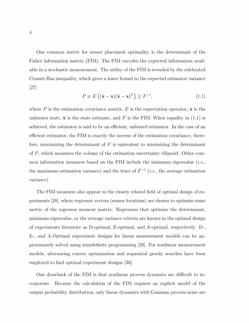
One common metric for sensor placement optimality is the determinant of the

Fisher information matrix (FIM). The FIM encodes the expected information avail-

able in a stochastic measurement. The utility of the FIM is revealed by the celebrated

Cramer-Rao inequality, which gives a lower bound to the expected estimator variance

[27]

P ≡ E

(x− x)(x− x)T≥ F−1, (1.1)

where P is the estimation covariance matrix, E is the expectation operator, x is the

unknown state, x is the state estimate, and F is the FIM. When equality in (1.1) is

achieved, the estimator is said to be an efficient, unbiased estimator. In the case of an

efficient estimator, the FIM is exactly the inverse of the estimation covariance, there-

fore, maximizing the determinant of F is equivalent to minimizing the determinant

of P , which measures the volume of the estimation uncertainty ellipsoid. Other com-

mon information measures based on the FIM include the minimum eigenvalue (i.e.,

the maximum estimation variance) and the trace of F−1 (i.e., the average estimation

variance).

The FIM measures also appear in the closely related field of optimal design of ex-

periments [28], where regressor vectors (sensor locations) are chosen to optimize some

metric of the regressor moment matrix. Regressors that optimize the determinant,

minimum eigenvalue, or the average variance criteria are known in the optimal design

of experiments literature as D-optimal, E-optimal, and A-optimal, respectively. D-,

E-, and A-Optimal experiment designs for linear measurement models can be ap-

proximately solved using semidefinite programming [29]. For nonlinear measurement

models, alternating convex optimization and sequential greedy searches have been

employed to find optimal experiment designs [30].

One drawback of the FIM is that nonlinear process dynamics are difficult to in-

corporate. Because the calculation of the FIM requires an explicit model of the

output probability distribution, only linear dynamics with Gaussian process noise are

5

amenable to the FIM framework. For this reason, many researchers have utilized the

observability Gramian to measure sensor fitness. The observability Gramian is the de-

terministic analog to the FIM, measuring the relative observability of system modes.

Early work on observability-based sensor placement used the observability Gramian

for systems with linear dynamics [31, 32]. Nonlinear dynamics were incorporated

into the sensor placement problem using the transient observability function (i.e., the

output energy) [31], and later, using the independence of measurement functions via

the Gram determinant [33] as measures of observability. The advent of the empirical

observability Gramian allowed numerical computation of the observability Gramian

about a nominal trajectory of the nonlinear system [34, 35]. The empirical observ-

ability Gramian was first developed for balancing and model reduction in nonlinear

systems [34, 35] and later adapted for observability analysis [36], measuring sensor

fitness [37], and computing optimal sensor placement [38, 39].

One of the difficulties of the sensor placement problem is the combinatorial nature

of the problem. In its most general form, the sensor placement problem can be written

as a mixed integer nonlinear optimization problem, which consists of a nonlinear cost

function (typically convex) in continuous and integer variables. The presence of the

integer variables causes the problem to scale poorly to higher-dimensional problems

(e.g., large number of states or sensors). Several approaches have been taken to

mediate the “curse of dimensionality” and allow solution of reasonably-sized problems.

For small numbers of sensors, the optimal solution may be found by brute force by

sampling each combination of sensors [33, 38, 40]. For more general problems, branch-

and-bound techniques have been used with Lagrangian relaxation to prune portions

of the search space that do not lead to an optimal solution [31]. Other approaches

to carry out global optimization include successive linearization and relaxation of

the mixed integer nonlinear program [39] or an iterative solution with exponential

smoothing [24].

In all cases, the goal of the optimization procedure is to find the optimal (or

6

near-optimal) sensor set with reasonable computation time. Current state-of-the-art

mixed integer programming solvers (such as CPLEX) can solve linear sensor place-

ment problems with on the order of 10,000 sensor nodes in less than an hour [41].

However, “robust” sensor placement problems — maximizing the worst-case sensor

performance or minimizing the covariance of sensor performance — require consid-

erably more computational effort. Simulations in [42] demonstrated that the robust

sensor placement problem could be solved for a system with about 400 sensor nodes in

reasonable time (less than 10 minutes), but a system with approximately 3,000 sensor

nodes could not be solved in less than a 24 hours. Conversely, a convex optimization

approach developed in [43] can find near-optimal sensor sets for systems with on the

order of 1,000 sensor nodes in a few seconds.

The current state-of-the art in sensor placement techniques requires improvement

in three main areas. First, the most general observability-based sensor placement

methods consider sensors that directly measure individual states [38, 39]. In many

interesting applications, however, the measurement function may be some nonlinear

function of the states. Second, problems involving heterogeneous sensor sets are not

adequately addressed in the literature. Finally, more solution methods are needed to

allow the sensor placement problem to scale to large systems.

1.1.2 Mobile sensor planning

The mobile sensor planning problem encompasses the largest area of research in op-

timal sensing. These problems can be thought of as an extension of the static sensor

problem, where the sensors are allowed to move dynamically in time to optimally

observe a spatially (and possibly temporally) varying process. A classic problem in

this class is the target tracking problem, where a vehicle with either range or bear-

ing measurements to a moving target is controlled to obtain an optimal estimate of

the target’s location and velocity. This problem has been studied with single [44]

and multiple sensors [45, 46], as well as with varying fidelities of target motion mod-

7

els [47]. Similar to the static sensor scenario, most formulations of optimal target

tracking utilize the FIM in the cost functional.

One subclass of mobile sensor problems that has received much attention is adap-

tive sampling using sensor networks. Adaptive sampling is a data-driven method that

utilizes past measurements to actively decide where to sample next. One common

problem formulation is the gradient climb (descent) problem, where vehicles detect

the gradient of a scalar field and adaptively change heading to climb (descend) along

the gradient to find a local maximum (minimum) [48]. For a single vehicle, estimating

the local gradient requires some form of control excitation [49]. Other methods include

minimizing uncertainty of a statistical model of the scalar field [50], minimizing the

covariance of a particular estimation scheme [51], or maximizing the measurements of

areas with high uncertainty [52]. Adaptive sampling has seen success in application

to autonomous underwater vehicle (AUV) motion planning, where the AUV’s mis-

sion is to actively sample the ocean environment. However, as is evidenced by the

variety of approaches listed here, the appropriate metric for sampling is still an open

question, and issues related to navigation and compensation for currents are yet to

be effectively solved [50].

Information-based algorithmic approaches to the mobile sensor planning problem

have recently grown in usage. These algorithms, under the name of information gath-

ering, consider the spatial distribution of the quality of information as a scalar field

that the vehicle must traverse to collect the most information under limited path

length budget, where the measure of information is typically derived from the FIM.

Generic, sampling-based algorithms have been successfully applied to the informa-

tion gathering problem using rapidly-exploring random trees (RRT) [53, 54]. These

algorithms can handle nonholonomic vehicle motion constraints and non-convex do-

main constraints using branch-and-bound techniques on trajectories generated from

the RRT algorithm.

Another class of mobile sensor planning problems is planning sensor motion for

8

optimal online parameter estimation. Here, there is a fixed set of sensors, and the

goal is to find control inputs that optimize the ability of the sensors to measure

unknown parameters. This problem is often found in the literature of system iden-

tification, where “exciting” trajectories are desired to facilitate structured parameter

identification [55]. The controls are chosen to minimize the condition number of the

linear regressor matrix, which then optimally conditions a least-squares estimation

of system parameters. This solution method has been successful in identification of

robotic base parameters [55, 56], where the high-order (but linear in the parameters)

dynamics demand specific trajectories to extract the desired parameters.

1.1.3 Robotic navigation

In all of the classes of mobile sensor planning problems listed here, the trajectory

planning problem is solved to optimize a single objective — maximize a measure of

information obtained by the mobile sensor. Thus, only sensory goals are considered.

In the case of mobile robot motion planning, however, higher-level mission goals will

likely need to be balanced with information quality. One particularly interesting

example is motion planning for vehicles with limited navigation information (e.g.,

range-only or bearing-only navigation), where vehicle motion is used not only to

improve navigation information, but also to achieve higher-level mission objectives.

Therefore, an algorithm is required that can balance the sensory goals with higher-

level control objectives.

The range-only and bearing-only navigation problems have been studied in the

literature from an observability perspective to derive informative trajectories — tra-

jectories that improve navigation accuracy or uncertainty. In the context of single

range-aided navigation, observability measures have been implemented to measure

and improve estimation performance. An observability metric based upon the mini-

mum singular value and condition number of the observability matrix were introduced

in [57] to measure the relative observability of vehicle trajectories. Experimental re-

9

sults indicated that trajectory segments passing closer to the ranging beacon reduce

estimation error. Another observability metric based upon linearization about a tra-

jectory was presented by the author of this thesis in [58], and an optimization strategy

showed that circular trajectories centered at the ranging beacon maximize vehicle po-

sition observability. This metric was then used in [59] to plan trajectories for a mobile

navigation aid to maximize observability of an underwater vehicle using range-only

localization. A numerical trajectory optimization technique was employed in [46] to

coordinate multiple mobile sensors to track a single target using range measurements.

The optimal heading to minimize covariance of an extended Kalman filter was found

to be perpendicular to the bearing to the target.

Observability-based trajectory planning has also been applied to bearing-only nav-

igation. In [44], the FIM was used in a cost function to derive observer maneuvers to

optimally track a moving target. The first-order necessary conditions for a minimum

to the proposed optimal control problem required the vehicle heading to be perpen-

dicular to the target at the end of the optimization time horizon. The optimization

problem was solved using direct numerical optimization to arrive at vehicle trajecto-

ries that minimize range uncertainty under bearing-only tracking. An observability

measure based upon the determinant of the observability matrix was used in [60]

to plan trajectories that optimize observability of time-to-contact with static obsta-

cles in the environment. Simulation results showed that the observability-based path

planning improved obstacle estimation and allowed the vehicle to navigate through

obstacle fields.

Although observability-based path planning has been used to improve range-only

and bearing-only navigation, some additional work is needed to make these guidance

strategies viable for autonomous vehicle operation. The most in-depth analysis of

these navigation problems comes from the target tracking community, where the only

goal is to accurately track the target. However, in autonomous vehicle navigation,

a framework is needed that can plan paths such that the vehicle can accomplish

10

some mission (e.g., sensor coverage, search pattern, waypoint following) while main-

taining sufficient navigation system performance. Sampling-based solution methods

have shown promise for solving information-based path planning problems when non-

convex path and environment constraints are imposed. In this work, however, a path

planning solution is desired that can be implemented using a convex optimization

framework with minimal computational requirements. By implementing a problem-

specific path planner, better performance can be achieved compared to the more

general sampling-based approaches.

1.2 Contributions of this Thesis

This thesis addresses the open problems discussed above and improves the state-of-the

art in optimal active sensing through the following contributions:

• Development of an observability-based sensor placement procedure that incor-

porates nonlinear dynamics, nonlinear measurement models, and heterogeneous

sensors.

• Convex optimization solution methods for the sensor placement problem that

are scalable to large systems.

• Extension of the sensor placement problem to an observability-based sensor data

compression algorithm.

• Application of the sensor placement procedure to discover sensor configurations

for gyroscopic sensing in insect wings, with comparison to biological data.

• Observability-based optimal trajectory generation procedure for robotic navi-

gation with limited sensors.

11

• Observability-based guidance algorithm for range-only and bearing-only navi-

gation that allows balancing of sensing objectives and higher-level mission ob-

jectives.

• Experimental validation of the observability-based guidance algorithm.

1.3 Organization of the Report

The remainder of the report is organized as follows. Methods for observability anal-

ysis and measures of observability for nonlinear systems are discussed in Chapter 2.

Formulation of the observability-based sensor placement problem and solution meth-

ods are provided in Chapter 3. In Chapter 4, the sensor placement procedure is

applied to an example system representing the dynamics of flexible, flapping insect

wings. The wing flapping dynamics are derived and the observability-based optimal

sensor configuration is compared to biological data. observability-based guidance for

robotic navigation with limited sensors is described in Chapters 5 and 6. In Chap-

ter 5, analytical solutions to the observability-based guidance problem are derived

for range-only navigation, bearing-only navigation, and navigation in currents. An

observability-based guidance algorithm for range-only and bearing-only navigation

is developed in Chapter 6 with experimental results demonstrating its effectiveness.

Finally, a discussion of the results and directions for future work are described in

Chapter 7.

12

Chapter 2

OBSERVABILITY MEASURES

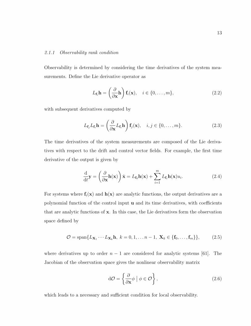
In this chapter, a review of nonlinear observability is provided using differen-

tial geometric methods. Quantitative measures of observability are introduced that

utilize the nonlinear observability matrix and the observability Gramian for linear

time-varying systems. A connection between the nonlinear observability matrix, the

observability Gramian, and estimation uncertainty is established, which motivates the

use of observability as a measure of estimation performance.

2.1 Nonlinear Observability

Observability of nonlinear systems is analyzed following the work of Anguelova [61],

which builds upon foundational works by Hermann and Krener [62] and Sontag and

Wang [63], among others. The standard control-affine class of nonlinear systems is

considered, which represents a wide array of physical systems. Specifically,

x = f0(x) +m∑i=1

fi(x)ui

y = h(x),

(2.1)

where x ∈ Rn are the states, u ∈ Rm are the controls, y ∈ Rp are the measurements,

f0(x) ∈ Rn is the drift vector field, and fi(x) ∈ Rn i ∈ 1, . . . ,m are the control

vector fields.

13

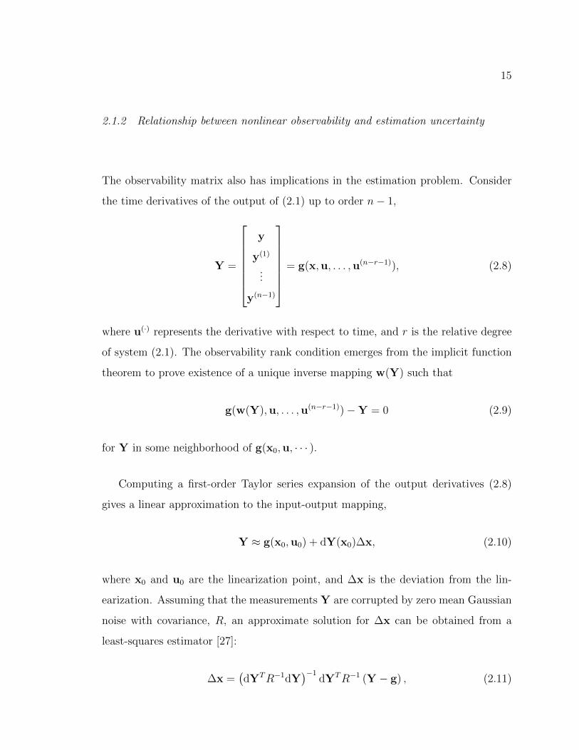
2.1.1 Observability rank condition

Observability is determined by considering the time derivatives of the system mea-

surements. Define the Lie derivative operator as

Lfih =

(∂

∂xh

)fi(x), i ∈ 0, . . . ,m, (2.2)

with subsequent derivatives computed by

LfjLfih =

(∂

∂xLfih

)fj(x), i, j ∈ 0, . . . ,m. (2.3)

The time derivatives of the system measurements are composed of the Lie deriva-

tives with respect to the drift and control vector fields. For example, the first time

derivative of the output is given by

d

dty =

(∂

∂xh(x)

)x = Lf0h(x) +

m∑i=1

Lfih(x)ui. (2.4)

For systems where fi(x) and h(x) are analytic functions, the output derivatives are a

polynomial function of the control input u and its time derivatives, with coefficients

that are analytic functions of x. In this case, the Lie derivatives form the observation

space defined by

O = spanLX1 · · ·LXkh, k = 0, 1, . . . n− 1, Xk ∈ f0, . . . , fm, (2.5)

where derivatives up to order n − 1 are considered for analytic systems [61]. The

Jacobian of the observation space gives the nonlinear observability matrix

dO =

∂

∂xφ∣∣ φ ∈ O , (2.6)

which leads to a necessary and sufficient condition for local observability.

14

Definition 1 (Observability rank condition [62]). The control affine system (2.1) is

locally weakly observable if and only if it satisfies the observability rank condition

rank(dO(x)) = n. (2.7)

The observability rank condition states that dO(x) must contain n independent

covector fields. Because the system is analytic, the rank of dO is constant, except at

singular points where the matrix drops rank [61]. The observability rank condition

considers the generic rank of the matrix dO(x), which is the maximal rank over the

manifold of admissible states. Therefore, if dO is full rank everywhere except at

isolated singular points, the system is locally weakly observable.

The presence of the control vector fields in the observability space is counter-

intuitive to what is known from observability of linear systems, where studying the

uncontrolled system is sufficient to establish observability. In nonlinear systems, how-

ever, the sensing and actuation may be coupled, and the choice of control input can af-

fect the system observability. If the observability matrix dO is full rank, but loses rank

when the Lie derivatives with respect to the control vector field fi(x) i ∈ 1, . . . ,m

are removed, then actuation in the control input ui is required for system observabil-

ity. Therefore, in some cases excitation via control input may be necessary to observe

all system states. The benefit of the observability rank condition is that it explicitly

accounts for this coupling and provides information about what, if any, control actu-

ation is required to obtain system observability. The drawback, however, is that the

observability rank condition gives only a binary answer to the observability question,

not a continuous measure of observability.

15

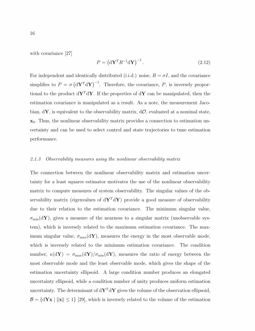
2.1.2 Relationship between nonlinear observability and estimation uncertainty

The observability matrix also has implications in the estimation problem. Consider

the time derivatives of the output of (2.1) up to order n− 1,

Y =

y

y(1)

...

y(n−1)

= g(x,u, . . . ,u(n−r−1)), (2.8)

where u(·) represents the derivative with respect to time, and r is the relative degree

of system (2.1). The observability rank condition emerges from the implicit function

theorem to prove existence of a unique inverse mapping w(Y) such that

g(w(Y),u, . . . ,u(n−r−1))−Y = 0 (2.9)

for Y in some neighborhood of g(x0,u, · · · ).

Computing a first-order Taylor series expansion of the output derivatives (2.8)

gives a linear approximation to the input-output mapping,

Y ≈ g(x0,u0) + dY(x0)∆x, (2.10)

where x0 and u0 are the linearization point, and ∆x is the deviation from the lin-

earization. Assuming that the measurements Y are corrupted by zero mean Gaussian

noise with covariance, R, an approximate solution for ∆x can be obtained from a

least-squares estimator [27]:

∆x =(dYTR−1dY

)−1dYTR−1 (Y − g) , (2.11)

16

with covariance [27]

P =(dYTR−1dY

)−1. (2.12)

For independent and identically distributed (i.i.d.) noise, R = σI, and the covariance

simplifies to P = σ(dYTdY

)−1. Therefore, the covariance, P , is inversely propor-

tional to the product dYTdY. If the properties of dY can be manipulated, then the

estimation covariance is manipulated as a result. As a note, the measurement Jaco-

bian, dY, is equivalent to the observability matrix, dO, evaluated at a nominal state,

x0. Thus, the nonlinear observability matrix provides a connection to estimation un-

certainty and can be used to select control and state trajectories to tune estimation

performance.

2.1.3 Observability measures using the nonlinear observability matrix

The connection between the nonlinear observability matrix and estimation uncer-

tainty for a least squares estimator motivates the use of the nonlinear observability

matrix to compute measures of system observability. The singular values of the ob-

servability matrix (eigenvalues of dYTdY) provide a good measure of observability

due to their relation to the estimation covariance. The minimum singular value,

σmin(dY), gives a measure of the nearness to a singular matrix (unobservable sys-

tem), which is inversely related to the maximum estimation covariance. The max-

imum singular value, σmax(dY), measures the energy in the most observable mode,

which is inversely related to the minimum estimation covariance. The condition

number, κ(dY) = σmax(dY)/σmin(dY), measures the ratio of energy between the

most observable mode and the least observable mode, which gives the shape of the

estimation uncertainty ellipsoid. A large condition number produces an elongated

uncertainty ellipsoid, while a condition number of unity produces uniform estimation

uncertainty. The determinant of dYTdY gives the volume of the observation ellipsoid,

B = dYx | ‖x‖ ≤ 1 [29], which is inversely related to the volume of the estimation

17

Table 2.1: Singular value measures of the nonlinear observability matrix

measure significance

σ−1min(dY) maximum estimation uncertaintyσ−1

max(dY) minimum estimation uncertaintyκ(dY) shape of estimation uncertainty ellipsoid

det[(dYTdY)−1

]volume of estimation uncertainty ellipsoid

Tr[(dYTdY)−1

]average estimation uncertainty

uncertainty ellipsoid. A summary of the singular value measures of observability is

provided in Table 2.1.

2.1.4 Observability radius

Although the least squares estimate provides a nice connection between estimation

uncertainty and the nonlinear observability matrix, the relationship considers a single

step of a linearized estimator. In practice, an iterative or dynamic estimator (e.g.,

nonlinear least squares) will provide a better estimate of the unknown state x, but

general relationships between observability and estimation uncertainty are difficult to

establish for most iterative estimators. One interesting connection that can be drawn

is the relationship between the observability matrix and the region of convergence of

Newton’s method. Using Kantorovitch’s theorem and the inverse function theorem,

a lower bound to the radius of the region of attraction of Newton’s method can be

computed using the methods of [64]. The radius of the region of attraction is denoted

here as the observability radius, which is described in the following theorem.

Theorem 1 (Observability Radius). Let dYn(x) be a set of n independent rows of

dY(x) with corresponding continuously differentiable mapping gn : Rn → Rn that

maps states to the n independent elements of Y, denoted by Yn. Let Bx ⊂ Rn

be a ball of radius 2R‖dY−1n (x0)‖F centered at state x0 with corresponding output

18

Y0 = gn(x0). If the matrix dYn(x) satisfies the Lipschitz condition

‖dYn(u)− dYn(v)‖F ≤M‖u− v‖2 ∀ u,v ∈ Bx (2.13)

with Lipschitz constant M , then there exists a ball By ⊂ Rn centered at Y0 with radius

R =1

2M‖dY−1n (x0)‖2

F

(2.14)

and a unique, continuously differentiable inverse mapping

wn : By → Bx (2.15)

such that

gn(wn(Yn)) = Yn and dwn(Yn) = dgn(wn(Yn))−1. (2.16)

Proof. The proof follows directly from the inverse function theorem [64, Theorem

2.9.4].

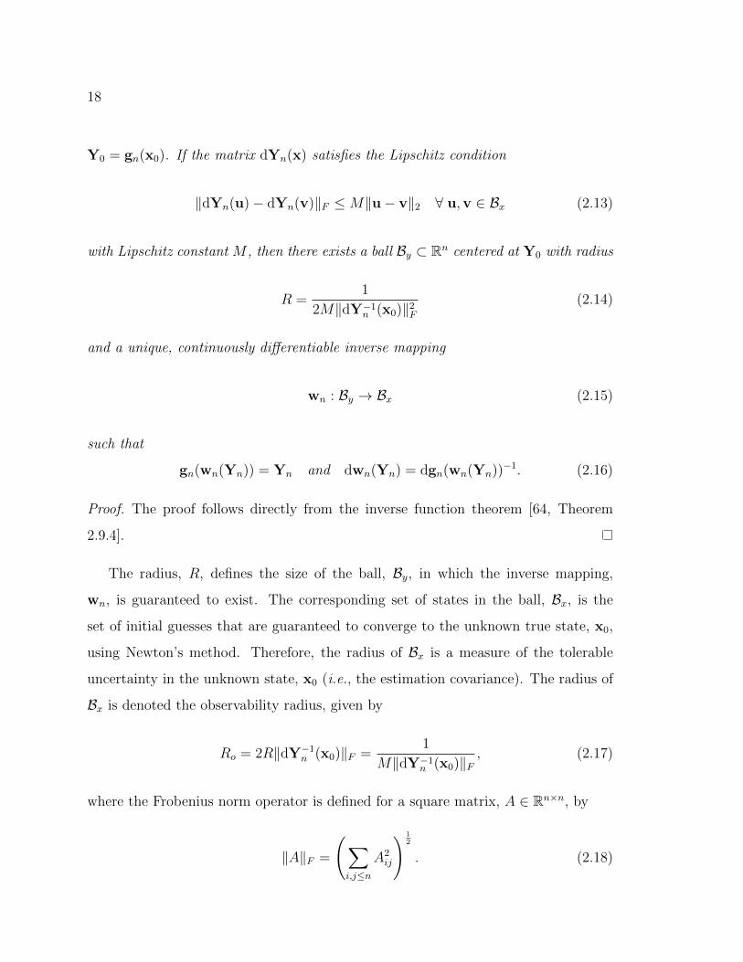
The radius, R, defines the size of the ball, By, in which the inverse mapping,

wn, is guaranteed to exist. The corresponding set of states in the ball, Bx, is the

set of initial guesses that are guaranteed to converge to the unknown true state, x0,

using Newton’s method. Therefore, the radius of Bx is a measure of the tolerable

uncertainty in the unknown state, x0 (i.e., the estimation covariance). The radius of

Bx is denoted the observability radius, given by

Ro = 2R‖dY−1n (x0)‖F =

1

M‖dY−1n (x0)‖F

, (2.17)

where the Frobenius norm operator is defined for a square matrix, A ∈ Rn×n, by

‖A‖F =

(∑i,j≤n

A2ij

) 12

. (2.18)

19

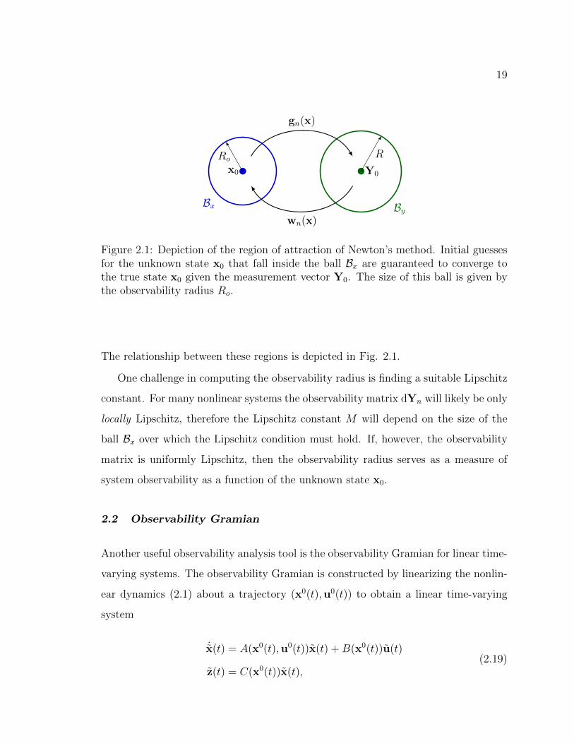
x0

Bx

Ro

By

Y0

R

gn(x)

wn(x)

Figure 2.1: Depiction of the region of attraction of Newton’s method. Initial guessesfor the unknown state x0 that fall inside the ball Bx are guaranteed to converge tothe true state x0 given the measurement vector Y0. The size of this ball is given bythe observability radius Ro.

The relationship between these regions is depicted in Fig. 2.1.

One challenge in computing the observability radius is finding a suitable Lipschitz

constant. For many nonlinear systems the observability matrix dYn will likely be only

locally Lipschitz, therefore the Lipschitz constant M will depend on the size of the

ball Bx over which the Lipschitz condition must hold. If, however, the observability

matrix is uniformly Lipschitz, then the observability radius serves as a measure of

system observability as a function of the unknown state x0.

2.2 Observability Gramian

Another useful observability analysis tool is the observability Gramian for linear time-

varying systems. The observability Gramian is constructed by linearizing the nonlin-

ear dynamics (2.1) about a trajectory (x0(t),u0(t)) to obtain a linear time-varying

system

˙x(t) = A(x0(t),u0(t))x(t) +B(x0(t))u(t)

z(t) = C(x0(t))x(t),(2.19)

20

where x(t) = x(t)−x0(t) and u(t) = u(t)−u0(t) are the deviations from the nominal

trajectory and z(t) is the measurement deviation. The linearized dynamics matrices

are computed using the Jacobian of the nonlinear dynamics,

A(x0(t),u0(t)) =∂

∂x

[f0(x) +

m∑i=1

fi(x)ui

]∣∣∣∣∣x=x0,u=u0

B(x0(t)) =∂

∂u

[f0(x) +

m∑i=1

fi(x)ui

]∣∣∣∣∣x=x0

C(x0(t)) =∂

∂xh(x)

∣∣∣∣x=x0

,

(2.20)

where it should be noted that for control affine systems, the input matrix, B, is not a

function of the nominal control, u0(t), because the dynamics are linear in the control

variables. The input matrix is, however, an explicit function of the nominal state

trajectory.

The observability of a linear time varying system is measured by the observability

Gramian [65, ch. 6]:

W (t0, tf ) =

tf∫t0

ΦT (t, t0)CT (x0(t))C(x0(t))Φ(t, t0)dt, (2.21)

where Φ(t, t0) ∈ Rn×n is the state transition matrix defined by

Φ(t, t0) = A(x0(t),u0(t))Φ(t, t0). (2.22)

If W (t0, tf ) is rank n for some tf , then the linear time-varying system (2.19) is ob-

servable. Interestingly, the observability Gramian also provides information about the

observability of the original nonlinear system (2.1). If the linear time-varying system

is observable, then the nonlinear system (2.1) is locally observable about the nominal

trajectory (x0(t),u0(t)) [37].

21

The observability Gramian thus provides an alternative to the nonlinear observ-

ability tools discussed in Section 2.1. Although the linear time-varying observability

analysis considers the unactuated system (i.e., the control deviation u is zero), the

coupling between sensing and actuation is still explicitly considered through the choice

of the linearization trajectory (x0(t),u0(t)). When choosing a nominal trajectory for

analysis, care must be taken to utilize the control inputs that are required to excite

the system dynamics. Insight gleaned from nonlinear observability analysis of the

system provides these necessary control inputs (if any are required).

One disadvantage to the linearization approach is that the Gramian is difficult to

compute analytically for a given nonlinear system and trajectory. Only for particu-

larly simple nonlinear systems can the Gramian be computed in closed-form for an

arbitrary linearization trajectory. For this reason, the Gramian is frequently com-

puted numerically, which can be achieved using the empirical observability Gramian.

2.2.1 Empirical observability Gramian

The empirical observability Gramian provides a numerical procedure for approximat-

ing the linear time-varying observability Gramian (2.21) by simulating the nonlinear

dynamics (2.1). The procedure for computing the Gramian from simulation output

follows the development of [37]. The Gramian is computed by simulating the nonlin-

ear system dynamics with perturbed initial conditions in each state and comparing

the output time history for each perturbation. Each state initial condition is inde-

pendently perturbed by ±ε and simulated using the nominal input sequence u0(t).

Let y+i be the simulation output with a positive perturbation in the initial condition

for state xi, and y−i be the output with a negative perturbation in the initial condi-

tion for state xi. Define the change in output ∆yi = y+i − y−i, then the empirical

22

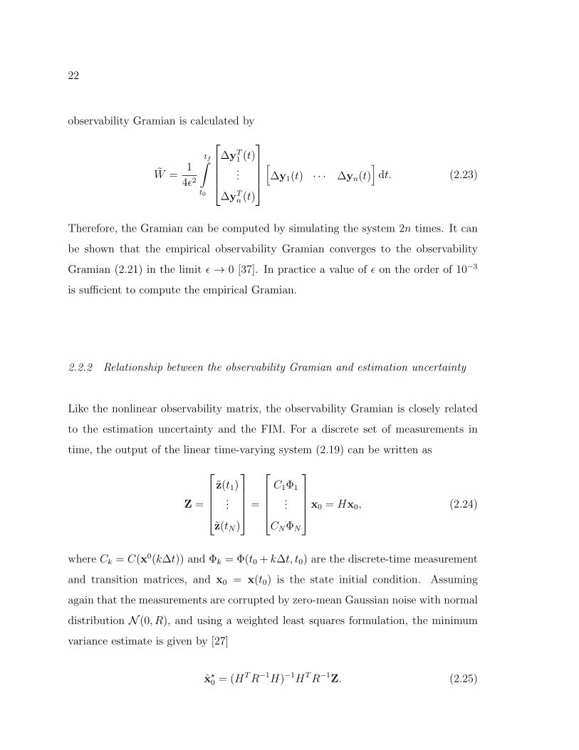
observability Gramian is calculated by

W =1

4ε2

tf∫t0

∆yT1 (t)

...

∆yTn (t)

[∆y1(t) · · · ∆yn(t)]

dt. (2.23)

Therefore, the Gramian can be computed by simulating the system 2n times. It can

be shown that the empirical observability Gramian converges to the observability

Gramian (2.21) in the limit ε → 0 [37]. In practice a value of ε on the order of 10−3

is sufficient to compute the empirical Gramian.

2.2.2 Relationship between the observability Gramian and estimation uncertainty

Like the nonlinear observability matrix, the observability Gramian is closely related

to the estimation uncertainty and the FIM. For a discrete set of measurements in

time, the output of the linear time-varying system (2.19) can be written as

Z =

z(t1)

...

z(tN)

=

C1Φ1

...

CNΦN

x0 = Hx0, (2.24)

where Ck = C(x0(k∆t)) and Φk = Φ(t0 + k∆t, t0) are the discrete-time measurement

and transition matrices, and x0 = x(t0) is the state initial condition. Assuming

again that the measurements are corrupted by zero-mean Gaussian noise with normal

distribution N (0, R), and using a weighted least squares formulation, the minimum

variance estimate is given by [27]

x?0 = (HTR−1H)−1HTR−1Z. (2.25)

23

Computing the estimate covariance gives

P = E

(x?0 − x0)(x?0 − x0)T

=(HTR−1H

)−1. (2.26)

The least squares estimator is known to be efficient (i.e., the Cramer-Rao lower bound

is achieved) [27], therefore the FIM is exactly the inverse of the estimation covariance,

F = HTR−1H. If the measurement noise variables are i.i.d., then R = σI, where

σ is the variance of each measurement, and the FIM simplifies to F = σ−1HTH.

Expanding the FIM gives

HTH =N∑k=1

ΦTkC

Tk CkΦk = Wd(1, N), (2.27)

which is the discrete-time observability Gramian. Therefore, the observability Gramian

is proportional to the FIM in the case of i.i.d. measurements and inversely propor-

tional to the estimate covariance. If the observability Gramian eigenvalues are ma-

nipulated (or even specified), then the estimation covariance is directly manipulated

as a result.

2.2.3 Observability measures using the observability Gramian

Because the observability Gramian is closely related to the estimation uncertainty

and the FIM, the eigenvalues of the observability Gramian directly control the Fisher

information and inversely control the estimation covariance. The eigenvalues of the

observability Gramian represent the relative observability of each system mode. The

minimum eigenvalue, λmin(W ), is a measure of the output energy for the least ob-

servable mode, while the maximum eigenvalue is the measure of the output energy

for the most observable mode,

λmin(W )‖x(0)‖ ≤∫ tf

t0

zT zdt ≤ λmax(W )‖x(0)‖. (2.28)

24

x1

x2

ν2

ν1

x1

x2

ν2

ν1

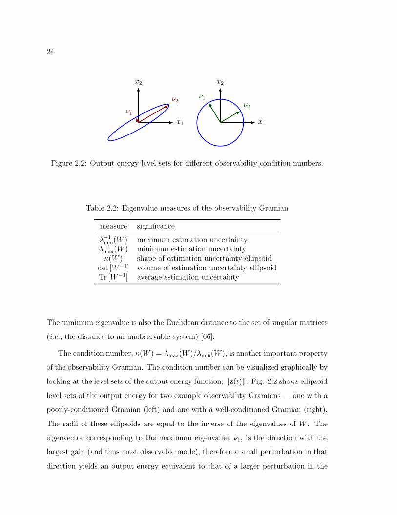
Figure 2.2: Output energy level sets for different observability condition numbers.

Table 2.2: Eigenvalue measures of the observability Gramian

measure significance

λ−1min(W ) maximum estimation uncertainty

λ−1max(W ) minimum estimation uncertaintyκ(W ) shape of estimation uncertainty ellipsoid

det [W−1] volume of estimation uncertainty ellipsoidTr [W−1] average estimation uncertainty

The minimum eigenvalue is also the Euclidean distance to the set of singular matrices

(i.e., the distance to an unobservable system) [66].

The condition number, κ(W ) = λmax(W )/λmin(W ), is another important property

of the observability Gramian. The condition number can be visualized graphically by

looking at the level sets of the output energy function, ‖z(t)‖. Fig. 2.2 shows ellipsoid

level sets of the output energy for two example observability Gramians — one with a

poorly-conditioned Gramian (left) and one with a well-conditioned Gramian (right).

The radii of these ellipsoids are equal to the inverse of the eigenvalues of W . The

eigenvector corresponding to the maximum eigenvalue, ν1, is the direction with the

largest gain (and thus most observable mode), therefore a small perturbation in that

direction yields an output energy equivalent to that of a larger perturbation in the

25

direction of the eigenvector corresponding to the minimum eigenvalue, ν2 (direction

of the least observable mode). Because the condition number measures the ratio of

maximum eigenvalue to minimum eigenvalue, an observability Gramian with a large

condition number indicates that the output energy is dominated by some modes,

while others are difficult to observe. A summary of the observability measures for the

observability Gramian is provided in Table 2.2.

26

Chapter 3

OBSERVABILITY-BASED SENSOR PLACEMENT

Using the measures of observability introduced in Chapter 2, the first main con-

tribution of this thesis is presented in this chapter — an observability-based sensor

placement procedure. First, the sensor placement problem is formally defined in

Section 3.1. Next, solution methods are proposed using convex optimization and

mixed-integer programming in Section 3.2. Finally, the sensor compression problem

is described as an extension to the sensor placement problem in Section 3.3.

3.1 Problem Statement

The observability-based sensor placement problem considers a nonlinear control affine

system

x = f0(x) +m∑i=1

fi(x)ui

yi = hi(x, si) i = 1, · · · , p,

(3.1)

where si is the sensor location for sensor i with measurement model hi(x, si). The

sensor location si is constrained to a known finite set of feasible sensor locations

si ∈ S. Similarly, the sensor model is constrained to a known set of models, hi ∈ H,

where H may contain a single element for homogeneous sensor placement, or multiple

for heterogeneous sensors.

The goal of the sensor placement procedure is to choose sensor locations si to op-

timize a measure of observability (c.f., Chapter 2). Because observability in nonlinear

systems is inherently a local concept, observability-based sensor placement optimizes

27

system observability locally about a trajectory. Therefore, the nominal trajectory

(x0(t),u0(t)) is assumed to be known, and the sensors are placed to optimize ob-

servability about the nominal trajectory. In terms of the observability Gramian, the

observability-based sensor placement problem can be formally written as

mins,h

J [W (s,h)]

subject to si ∈ S

hi ∈ H

(3.2)

where J [·] is a convex scalar measure of the observability Gramian (e.g., condition

number). The solution to the observability-based optimal sensor placement problem

is a set of p sensor locations, s, and sensor types, h, that optimize system observ-

ability about the nominal trajectory. Because the observability measures are closely

related to estimation uncertainty, optimally placed sensors will improved estimator

performance.

3.2 Solution Methods

The observability-based sensor placement problem is developed in this section as a

tractable optimization problem to solve for sensor locations and types. First, the

nonlinear dynamics (3.1) are linearized about the nominal trajectory (x0(t),u0(t))

and converted to discrete time with N time steps of length ∆t to obtain

A(k) = Φ(k∆t, 0)

Cji (k) = Cj

i (x0(k∆t)) =

∂

∂xhj(x, si)

∣∣∣∣x=x0(k∆t)

.(3.3)

The observability Gramian is constructed by noting that each sensor is additive

to the Gramian (i.e., the total Gramian is the sum of the Gramians for each sensor).

Let the dimension of S be ns > p and the dimension of H be nh ≥ 1. Define the

28

sensor activation function βji ∈ 0, 1, where βji = 1 indicates that a sensor of type

hj is located at sensor location si. Then the observability Gramian is written as

W (β) =∑

i≤ns,j≤nh

βji

N∑k=1

A(k)TCji (k)TCj

i (k)A(k) =∑

i≤ns,j≤nh

βjiWji . (3.4)

Alternatively, the observability Gramian for each sensor location/type combination,

W ji , can be computed using the empirical observability Gramian, W j

i . Therefore, the

input data to the optimal sensor placement problem consist of the set of possible

sensor locations S, the set of sensor types H, and a simulation that can be used to

compute the empirical observability Gramian.

3.2.1 Mixed integer programming

The observability-based sensor placement problem can be posed as a mixed inte-

ger/convex optimization problem, which consists of convex objective and constraints,

with integer constraints on a subset of the variables. All of the observability measures

listed in Table 2.2 can be written as convex functions of W (concave measures such

as λmin are simply negated). Because composition with affine mappings preserves

convexity, each measure is also a convex function of the sensor activation variable βji

[29]. Thus, the sensor placement problem can be written as a mixed-integer/convex

problem

minβ

J [W (β)]

subject to

nh∑j=1

βji ≤ 1

ns∑i=1

nh∑j=1

βji = p

βji ∈ 0, 1

(3.5)

29

where the sum over j enforces that each sensor may only assume one type, and the

sum over i and j enforces that p sensor locations must be selected.

Because mixed-integer programs scale exponentially in the number of binary vari-

ables, minimizing the number of binary variables in the problem formulation is of

paramount importance. For ns possible sensor locations and nh sensor types, the

number of binary variables is equal to nsnh. For most problems, nh will be small.

However, ns may be large due to a large number of possible sensor locations. To reduce

the number of sensor locations, a coarser discretization can be used while allowing

the sensor location to be continuous and approximating the observability Gramian

at any sensor location through linear interpolation between the discrete sensor nodes.

In the case of homogeneous sensors (i.e., nh = 1), this piecewise linear approximation

procedure is achieved through the use of special ordered sets of type two (SOS2, see

[67, p. 177 - 182] and [52] for details). SOS2 are tools from mixed-integer program-

ming that allow a vector of continuous variables to contain only two adjacent nonzero

entries, with all other entries identically zero.

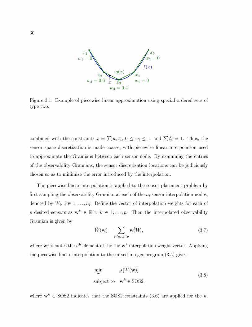
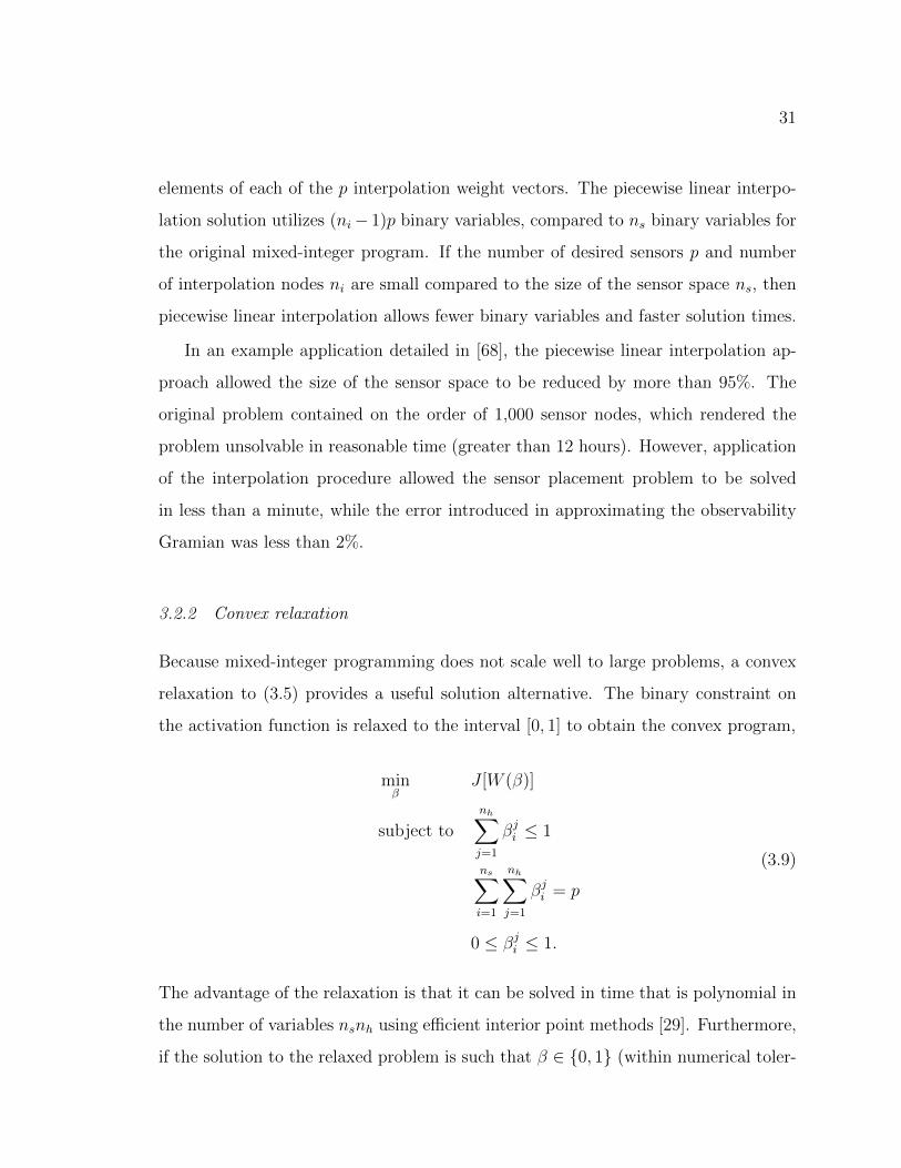
To illustrate how these tools can be used for piecewise linear approximation,

consider approximating the function f(x) = x2 with a piecewise linear function

g(x) =∑wi(x)f(xi) as depicted in Fig. 3.1. Here, wi are interpolation weights,

which must contain only two adjacent nonzero entries for g(x) to lie on the piece-

wise linear approximation to f(x). Introducing n − 1 binary variables δi, the SOS2

constraint is written as a series of linear inequalities

w1 − δ1 ≤ 0

w2 − δ1 − δ2 ≤ 0

...

wn−1 − δn−2 − δn−1 ≤ 0

wn − δn−1 ≤ 0,

(3.6)

30

f(x)g(x)

x1

w1 = 0

x2

w2 = 0.6 x3

w3 = 0.4

x4

w4 = 0

x5

w5 = 0

x

Figure 3.1: Example of piecewise linear approximation using special ordered sets oftype two.

combined with the constraints x =∑wixi, 0 ≤ wi ≤ 1, and

∑δi = 1. Thus, the

sensor space discretization is made coarse, with piecewise linear interpolation used

to approximate the Gramians between each sensor node. By examining the entries

of the observability Gramians, the sensor discretization locations can be judiciously

chosen so as to minimize the error introduced by the interpolation.

The piecewise linear interpolation is applied to the sensor placement problem by

first sampling the observability Gramian at each of the ni sensor interpolation nodes,

denoted by Wi, i ∈ 1, . . . , ni. Define the vector of interpolation weights for each of

p desired sensors as wk ∈ Rni , k ∈ 1, . . . , p. Then the interpolated observability

Gramian is given by

W (w) =∑

i≤ni,k≤p

wkiWi, (3.7)

where wki denotes the ith element of the the wk interpolation weight vector. Applying

the piecewise linear interpolation to the mixed-integer program (3.5) gives

minw

J [W (w)]

subject to wk ∈ SOS2,

(3.8)

where wk ∈ SOS2 indicates that the SOS2 constraints (3.6) are applied for the ni

31

elements of each of the p interpolation weight vectors. The piecewise linear interpo-

lation solution utilizes (ni− 1)p binary variables, compared to ns binary variables for

the original mixed-integer program. If the number of desired sensors p and number

of interpolation nodes ni are small compared to the size of the sensor space ns, then

piecewise linear interpolation allows fewer binary variables and faster solution times.

In an example application detailed in [68], the piecewise linear interpolation ap-

proach allowed the size of the sensor space to be reduced by more than 95%. The

original problem contained on the order of 1,000 sensor nodes, which rendered the

problem unsolvable in reasonable time (greater than 12 hours). However, application

of the interpolation procedure allowed the sensor placement problem to be solved

in less than a minute, while the error introduced in approximating the observability

Gramian was less than 2%.

3.2.2 Convex relaxation

Because mixed-integer programming does not scale well to large problems, a convex

relaxation to (3.5) provides a useful solution alternative. The binary constraint on

the activation function is relaxed to the interval [0, 1] to obtain the convex program,

minβ

J [W (β)]

subject to

nh∑j=1

βji ≤ 1

ns∑i=1

nh∑j=1

βji = p

0 ≤ βji ≤ 1.

(3.9)

The advantage of the relaxation is that it can be solved in time that is polynomial in

the number of variables nsnh using efficient interior point methods [29]. Furthermore,

if the solution to the relaxed problem is such that β ∈ 0, 1 (within numerical toler-

32

ance), then the original mixed-integer problem has been solved. The relaxation serves

two roles — an approximate (suboptimal) solution to the mixed-integer problem, and,

in some cases, a fast optimal solution to the mixed-integer problem. In simulation

studies, the convex relaxation could solve much larger problems (on the order of 1,000

sensor nodes) than the mixed integer programming approach [68].

3.2.3 `1-regularization

In both the mixed-integer problem (3.5) and the convex relaxation (3.9), the desired

number of sensors was explicitly constrained to p. Another approach is to allow

the number of sensors to be a free variable. In the sensor placement problem, a

sparse solution is desired, where only a few of the sensor activation functions βji

are one, while the rest are zero. This solution property permits the construction of

a convex relaxation of problem (3.5) that promotes a sparse solution using the `1

regularization technique (see, e.g., [29, p. 304]). This approach is common in sparse

sensing problems, where the binary constraint on β is relaxed to linear inequality

constraints and a penalty on the `1-norm of β is added to the cost function to promote

a sparse solution vector. Applying this relaxation to problem (3.5) yields a convex

problem with `1 penalty,

minβ

J [W (β)] + c‖β‖1

subject to

nh∑j=1

βji ≤ 1

0 ≤ βji ≤ 1.

(3.10)

where the constant c ≥ 0 is the weighting on the `1-norm penalty. By varying the

weight c, the number of sensors in the solution set will change to balance the sparsity

penalty with the observability measure, tracing the Pareto tradeoff curve between

sparsity and observability. The `1-regularization provides insight into how few sensors

33

can be used to achieve a particular level of observability.

Interestingly, the `1-regularization method frequently selects sensor locations very

near the global optimal solution found by the mixed integer program. In simulation

studies detailed in [68], the `1-regularization approach selected sensor locations near

the optimal (within 1% of the length scale in the problem), but with less than a third

of the required solution time. Similar to the convex relaxation, the `1-regularization

problem can be solved in a few seconds for sensor spaces with on the order of 1,000

sensor nodes.

3.2.4 Exploiting submodularity in the sensor placement problem

Although the sensor placement problem is combinatorial in nature, some sensor place-

ment objectives are submodular functions, which admit a simple greedy algorithm to

find sensor sets that achieve suboptimality within a guaranteed bound. Submodu-

lar functions exhibit a diminishing returns feature that enable the success of greedy

approximations, which is described in the following definition.

Definition 2 (Submodularity). Given a set Ω, a function f : 2Ω → R, is submodular

if and only if

f(X ∪ x)− f(X) ≥ f(Y ∪ x)− f(Y )

for all subsets X ⊆ Y ⊆ Ω and x ∈ Ω \ Y .

In essence, the submodular function increases more from the addition of a new

set member when the current size of the set is smaller. In the context of the sensor

placement problem, the set members are the sensor locations and types. The sen-

sor placement problem can be placed in a set function framework as the following

34

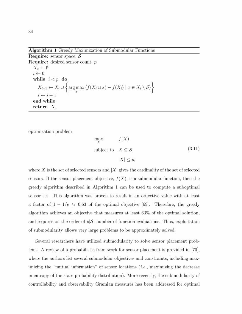
Algorithm 1 Greedy Maximization of Submodular Functions

Require: sensor space, SRequire: desired sensor count, pX0 ← ∅i← 0while i < p do

Xi+1 ← Xi ∪

arg maxx

(f(Xi ∪ x)− f(Xi) | x ∈ Xi \ S)

i← i+ 1

end whilereturn Xp

optimization problem

maxX

f(X)

subject to X ⊆ S

|X| ≤ p,

(3.11)

where X is the set of selected sensors and |X| gives the cardinality of the set of selected

sensors. If the sensor placement objective, f(X), is a submodular function, then the

greedy algorithm described in Algorithm 1 can be used to compute a suboptimal

sensor set. This algorithm was proven to result in an objective value with at least

a factor of 1 − 1/e ≈ 0.63 of the optimal objective [69]. Therefore, the greedy

algorithm achieves an objective that measures at least 63% of the optimal solution,

and requires on the order of p|S| number of function evaluations. Thus, exploitation

of submodularity allows very large problems to be approximately solved.

Several researchers have utilized submodularity to solve sensor placement prob-

lems. A review of a probabilistic framework for sensor placement is provided in [70],

where the authors list several submodular objectives and constraints, including max-

imizing the “mutual information” of sensor locations (i.e., maximizing the decrease

in entropy of the state probability distribution). More recently, the submodularity of

controllability and observability Gramian measures has been addressed for optimal

35

actuator and sensor placement [71]. The authors demonstrated that for a Gramian

matrix, the functions −tr(W−1), logdet(W ), and rank(W ) are submodular functions.

The authors also proved by counter example that the minimum eigenvalue, λmin(W ),

is not a submodular function. Therefore, if the observability-based sensor placement

objective is to maximize J(W ) = −tr(W−1) (i.e., minimize the average estimation

uncertainty), or J(W ) = logdet(W ) (i.e., minimize the estimation uncertainty vol-

ume), or J(W ) = rank(W ) (i.e., maximize the number of observable states), then the

greedy heuristic can be used to approximately solve the problem within a factor of

63% of optimal.

3.3 Sensor Data Compression

Frequently, the sensor placement problem is solved to find a sparse set of sensors that

will provide the most information about a temporally and spatially varying process.

In this sense, the goal of the sensor placement is to find a sensor configuration that

provides the highest information density — the most information with the fewest

sensors. The sensor placement procedure developed in Section 3.2 provides a solution

for the spatial configuration of sensors that produces the highest information density,

yielding the spatial positions where the most informative measurements can be made.

The concept of information density is extended in this section to the temporal filtering

of sensors.

The goal of temporal filtering is to optimally design a time-weighting of the sensor

output yi(t), thus revealing the temporal distribution of information in the sensor

signal. The mechanics of the observability-based sensor placement procedure are

easily adapted to solve for the sensor compression function. Consider the output of a

sensor with known location and type, filtered by a scalar sensor compression function

ξ(t) ≥ 0

yi(t) = ξi(t)h(x). (3.12)

36

Linearizing the measurement about the nominal trajectory (x0(t),u0(t)) and convert-

ing to discrete time gives the linear output matrix weighted by the sensor compression

function

Ci(k) = ξi(k∆t)∂

∂xh(x)

∣∣∣∣x=x0(k∆t)

. (3.13)

Therefore, the discrete time observability Gramian over the length of the trajectory

is given by

W (ξ) =

p∑i=1

N∑k=1

ξ2i (k)A(k)TCi(k)TCi(k)A(k), (3.14)

which is a linear function of ξ2i . Alternatively, the output of the empirical observability

Gramian can be used to compute the weighted Gramian via

W (ξ) =1

4ε2

p∑i=1

N∑k=1

ξ2i (k)

∆yT1 (k∆t)

...

∆yTn (k∆t)

[∆y1(k∆t) · · · ∆yn(k∆t)]

∆t. (3.15)

Similar to the sensor placement problem, the sensor compression problem can be

written as a convex optimization problem.

minξ

J[W(ξ1/2)]

subject to ‖ξi‖1 ≤ δ

ξi ≥ 0,

(3.16)

where ξi = ξ2i and J [·] is any convex observability measure. As a note, W (ξ1/2) is

a linear function of ξ, which makes J [W (ξ1/2)] a convex function of ξ. The non-

negativity constraint on ξ ensures that a feasible reconstruction of ξ = ξ1/2 can be

performed after the problem is solved. The norm constraint on ξ limits the energy that

can be added to the sensor signal to prevent an unbounded solution. The bound δ on

37

the norm is arbitrary and does not affect the shape of the solution for the compression

function.

In the context of distributed sensing applications, the sensor compression function

ξ(t) represents sensor processing performed before the sensor data are sent back to a

central location to be fused with data from other sensors. In many cases, the solution

for the compression function will be sparse, thus minimizing the amount of data that

is sent back to and processed by the central server. The solution provides not only

a means for compressing the sensor data, but also insight into when and where the

most informative bits of information occur in the process. In the context of biological

systems, the sensor compression function represents neural filtering performed by

individual sensors, which reduces the amount of information that must be processed by

a central unit. Using only a simulation of a nonlinear system, the sensor compression

function can be computed using the empirical observability Gramian as input data

to the optimization problem (3.16).

38

Chapter 4

SENSOR PLACEMENT APPLICATION: GYROSCOPICSENSING IN INSECT WINGS

The sensor placement procedure detailed in Chapter 3 can be applied to a wide

range of engineering problems due to its generality — from positioning of navigation

aids for planetary landing [72] to health monitoring of civil structures [17]. In this

chapter, the optimal sensor placement procedure is used to characterize the gyroscopic

sensing capabilities of the wings of the hawkmoth Manduca sexta. This application

is relevant not only to the biological community, but also has important engineering

implications. Because the hawkmoth demonstrates flight agility above the capabilities

of modern engineered flight systems, insight gleaned from the hawkmoth sensory

systems may be used to develop new design principles for biologically-inspired flight

vehicles. This chapter begins with background information about the hawkmoth in

Section 4.1. A low-order model of wing flapping dynamics is developed in Section 4.2,

and details of the wing flapping simulation are provided in Section 4.3. The results of

the observability-based sensor placement procedure are presented in Section 4.4 and

a discussion of the results is provided in Section 4.5.

4.1 Background

The wings of hawkmoths contain mechanoreceptors, campaniform sensilla, that pro-

vide sensory information about wing deformation during flight [73]. Wing deformation

arises from both aerodynamic loads and a variety of inertial forces, with the latter

dominating [74]. An intriguing property of these sensory structures lies in their sim-

ilarity to those found in halteres, the gyroscopic organ of flies. Halteres are known

39

to respond to Coriolis forces and are critically involved in flight control. They con-

tain patches of campaniform sensilla that respond with incredible sensitivity to subtle

loads and deflections. Importantly, halteres are evolutionarily derived from the insect

wings, suggesting that wings themselves may serve a similar control function. Indeed,

recent experimental results [73, 75] indicate that the campaniform sensilla embedded

in the hawkmoth wing serve to detect inertial rotations. Like the halteres, the wings

are actuated, flexible structures, and they deform in response to inertial rotations due

to Coriolis forces. The deformations induce a spatial and temporal strain pattern on

the wing that encodes the rotation rates. Thus, as suggested previously, the strain-

sensitive campaniform sensilla may allow the wings to serve as gyroscopic organs in

addition to their roles as actuators. Because the wing deforms in response to several

stimuli — inertial-elastic loads due to normal flapping motion, aerodynamic loads,

and other exogenous forces — the strain sensing must disambiguate these various

influences to effectively act as a gyroscopic sensor. However, the ability to isolate

strain patterns due to body rotations during typical flapping and aerodynamic loads

has yet to be demonstrated.

Additionally, the role of sensillum strain directional sensitivity in detecting in-

ertial rotations is not well-understood in wings. Experimental evidence has shown

that the campaniform sensilla in Drosophila wings developed into two classes: one

set tuned for slower excitation and another for faster excitation [76], which suggests

that the sensitivity of campaniform sensilla may be heterogeneously distributed. Ex-

periments on locust wings indicate that campaniform sensillum sensitivity to shear

strain is important for detecting wing supination [77], though the details of how shear

strain is locally encoded remains unclear. Early studies on campaniform sensilla on

the legs of cockroaches demonstrated that the campaniform geometry may predict

strain directional sensitivity. Oval-shaped campaniform sensilla were found in groups

with aligned major axes [78], with the maximum sensory response corresponding to

compression along the short axis of the oval [79]. To complement physiological char-

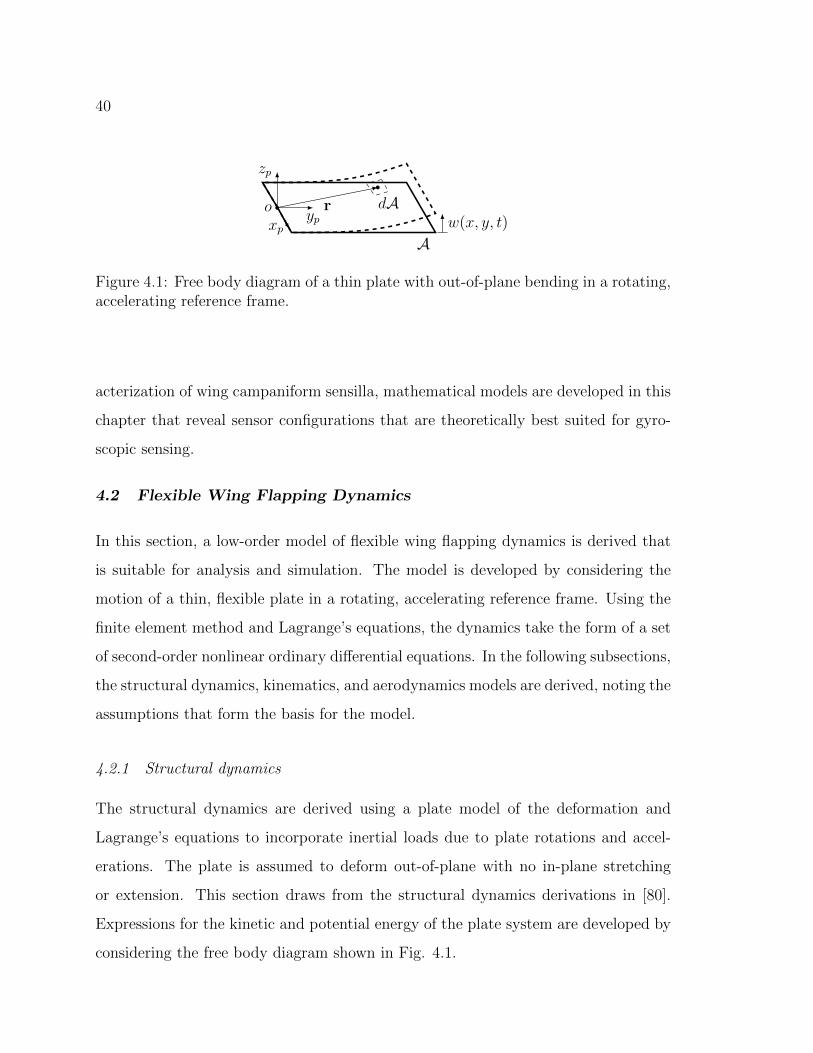
40

yp

zp

xp

ow(x, y, t)

A

r dA

Figure 4.1: Free body diagram of a thin plate with out-of-plane bending in a rotating,accelerating reference frame.

acterization of wing campaniform sensilla, mathematical models are developed in this

chapter that reveal sensor configurations that are theoretically best suited for gyro-

scopic sensing.

4.2 Flexible Wing Flapping Dynamics

In this section, a low-order model of flexible wing flapping dynamics is derived that

is suitable for analysis and simulation. The model is developed by considering the

motion of a thin, flexible plate in a rotating, accelerating reference frame. Using the

finite element method and Lagrange’s equations, the dynamics take the form of a set

of second-order nonlinear ordinary differential equations. In the following subsections,

the structural dynamics, kinematics, and aerodynamics models are derived, noting the

assumptions that form the basis for the model.

4.2.1 Structural dynamics

The structural dynamics are derived using a plate model of the deformation and

Lagrange’s equations to incorporate inertial loads due to plate rotations and accel-

erations. The plate is assumed to deform out-of-plane with no in-plane stretching

or extension. This section draws from the structural dynamics derivations in [80].

Expressions for the kinetic and potential energy of the plate system are developed by

considering the free body diagram shown in Fig. 4.1.

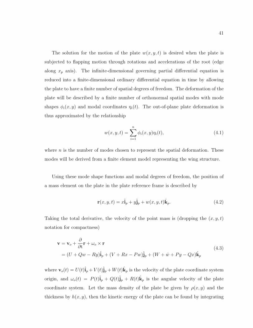
41

The solution for the motion of the plate w(x, y, t) is desired when the plate is

subjected to flapping motion through rotations and accelerations of the root (edge

along xp axis). The infinite-dimensional governing partial differential equation is

reduced into a finite-dimensional ordinary differential equation in time by allowing

the plate to have a finite number of spatial degrees of freedom. The deformation of the

plate will be described by a finite number of orthonormal spatial modes with mode

shapes φi(x, y) and modal coordinates ηi(t). The out-of-plane plate deformation is

thus approximated by the relationship

w(x, y, t) =n∑i=1

φi(x, y)ηi(t), (4.1)

where n is the number of modes chosen to represent the spatial deformation. These

modes will be derived from a finite element model representing the wing structure.

Using these mode shape functions and modal degrees of freedom, the position of

a mass element on the plate in the plate reference frame is described by

r(x, y, t) = xip + yjp + w(x, y, t)kp. (4.2)

Taking the total derivative, the velocity of the point mass is (dropping the (x, y, t)

notation for compactness)

v = vo +∂

∂tr + ωo × r

= (U +Qw −Ry)ip + (V +Rx− Pw)jp + (W + w + Py −Qx)kp

(4.3)

where vo(t) = U(t)ip +V (t)jp +W (t)kp is the velocity of the plate coordinate system

origin, and ωo(t) = P (t)ip + Q(t)jp + R(t)kp is the angular velocity of the plate

coordinate system. Let the mass density of the plate be given by ρ(x, y) and the

thickness by h(x, y), then the kinetic energy of the plate can be found by integrating

42

over the area of the plate A,

Te(t) =1

2

∫A

ρ(x, y)h(x, y)v(x, y, t) · v(x, y, t)dA. (4.4)

To compute the potential energy of the plate, define the strain vector as

χ =

∂2w/∂x2

∂2w/∂y2

2∂2w/∂x∂y

, (4.5)

and the matrix of material constants, D, which gives the potential energy ([80] p. 35)

Ue(t) =1

2

∫A

h(x, y)3

12χ(x, y, t)TDχ(x, y, t)dA. (4.6)

The generalized coordinates describing the structural configuration are the modal

coordinates η. Lagrange’s equations are applied to the expressions for kinetic and

potential energy via

d

dt

(∂Te∂ηi

)− ∂Te∂ηi

+∂Ue∂ηi

= Qi, i = 1, . . . , n, (4.7)

where Qi are the exogenous non-conservative generalized forces.

Substituting the assumed modal form of the displacement w (4.1) into the expres-

sions for kinetic energy Te (4.4), the first term of Lagrange’s equations is

d

dt

(∂Te∂ηi

)=

d

dt

∫A

ρhφi

(W + Py −Qx+

n∑j=1

φj ηj

)dA

=

∫A

ρhφi

(W + P y − Qx+

n∑j=1

φj ηj

)dA.

(4.8)

Because the mode shapes are assumed to be orthonormal, the integral of the product

43

of two modes, φi(x, y)φj(x, y), is unity for i = j and zero otherwise. The remaining

terms can be organized into a mass matrix multiplying the applied accelerations:

d

dt

(∂Te∂η

)= η +Ma

W

P

Q

, (4.9)

where the ith row of the applied acceleration mass matrix Ma is

Mai =

∫A

[ρhφi ρhφiy −ρhφix

]dA. (4.10)

The second term of Lagrange’s equations includes centripetal and Coriolis terms:

∂Te∂ηi

=

∫A

ρhφi

[Q (U −Ry)− P (V +Rx) +

(Q2 + P 2

) n∑j=1

φjηj

]dA

⇒ ∂Te∂η

= (Q2 + P 2)η +MaCa(vo, ωo),

(4.11)

where the Coriolis force Ca is

Ca(vo, ωo) =

QU − PV

−QR

PR

. (4.12)

The final term in Lagrange’s equations is the stiffness term due to strain energy.

This final term can be computed by assembling the expression for χ in terms of the

generalized coordinates

χ =n∑j=1

(∂2φj/∂x

2)

(∂2φj/∂y2)

(∂2φj/∂x∂y)

ηj. (4.13)

Substituting χ into the expression for potential energy Ue (4.6) yields the third term

44

in Lagrange’s equations,

∂Ue∂ηi

=

∫A

h3

12(∂χ/∂ηi)

TDχdA. (4.14)

By definition, the orthonormal free-vibration modes satisfy the homogeneous differ-

ential equation

η + Ωη = 0, (4.15)

where Ω is the diagonal modal frequency matrix with entries defined by

Ωij =

∫A

h3

12

∂2φi/∂x

2

∂2φi/∂y2

∂2φi/∂x∂y

T

D

∂2φj/∂x

2

∂2φj/∂y2

∂2φj/∂x∂y

dA, (4.16)

with Ωij = ω2i for i = j and Ωij = 0 for i 6= j. Thus, the final term in Lagrange’s equa-

tions reduces to a diagonal mode frequency matrix multiplying the modal generalized

coordinates,∂Ue∂η

= Ωη. (4.17)

Finally, assembling the equations of motion for the flexible plate in a rotating,

accelerating reference frame yields

η + (Ω− (Q2 + P 2)︸ ︷︷ ︸centripetal

)η +Ma

W

P

Q

−Ca(vo, ωo)

︸ ︷︷ ︸

acceleration + Coriolis

= Q. (4.18)

These equations of motion contain terms familiar to structural dynamics problems

with some additional terms due to the inertial loads. The effective stiffness is reduced

by the centripetal forces acting on the rotating plate. This behavior is intuitive

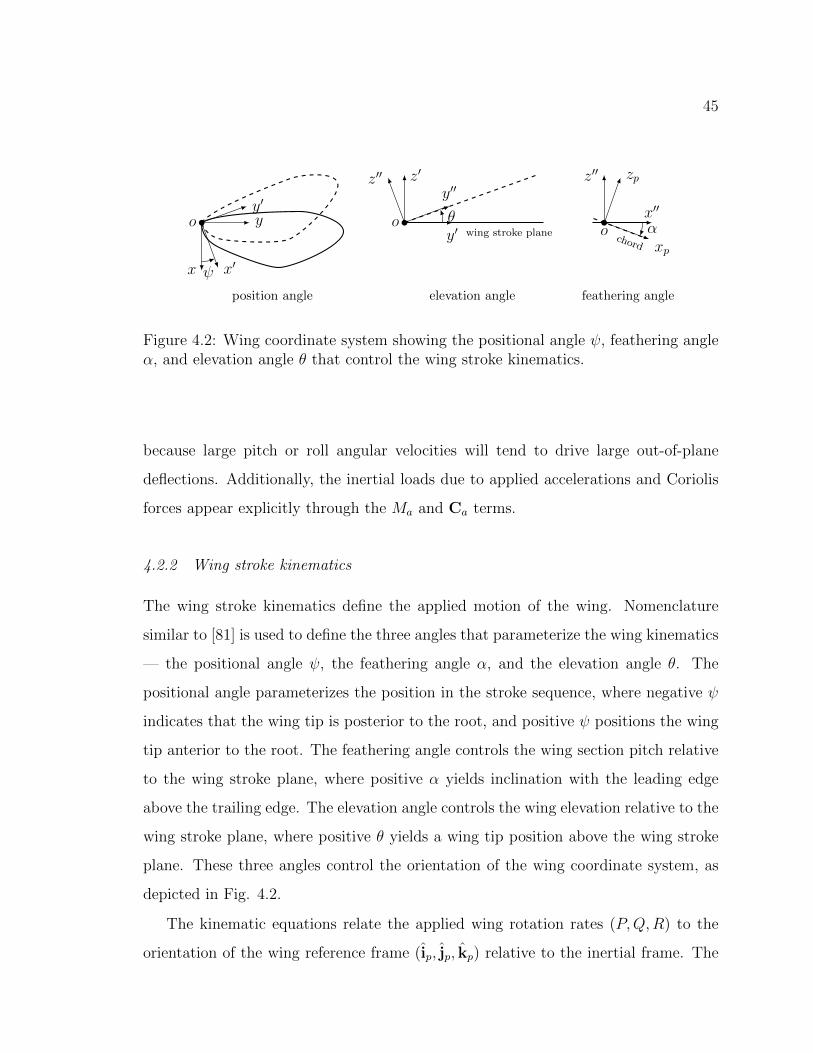
45

y

x

oy′

x′ψ

y′

z′

owing stroke plane

y′′z′′

θ x′′

z′′

oxp

zp

chord

α

position angle elevation angle feathering angle

Figure 4.2: Wing coordinate system showing the positional angle ψ, feathering angleα, and elevation angle θ that control the wing stroke kinematics.

because large pitch or roll angular velocities will tend to drive large out-of-plane

deflections. Additionally, the inertial loads due to applied accelerations and Coriolis

forces appear explicitly through the Ma and Ca terms.

4.2.2 Wing stroke kinematics

The wing stroke kinematics define the applied motion of the wing. Nomenclature

similar to [81] is used to define the three angles that parameterize the wing kinematics

— the positional angle ψ, the feathering angle α, and the elevation angle θ. The

positional angle parameterizes the position in the stroke sequence, where negative ψ

indicates that the wing tip is posterior to the root, and positive ψ positions the wing

tip anterior to the root. The feathering angle controls the wing section pitch relative

to the wing stroke plane, where positive α yields inclination with the leading edge

above the trailing edge. The elevation angle controls the wing elevation relative to the

wing stroke plane, where positive θ yields a wing tip position above the wing stroke

plane. These three angles control the orientation of the wing coordinate system, as

depicted in Fig. 4.2.

The kinematic equations relate the applied wing rotation rates (P,Q,R) to the

orientation of the wing reference frame (ip, jp, kp) relative to the inertial frame. The

46

orientation of the wing reference frame is represented via the three Euler angles (ψ,

θ, and α) and a 3-1-2 rotation sequence (i.e., rotate about the 3-axis, then the 2-axis,

then the 1-axis [82]). First, the inertial frame is rotated about the 3-axis by the

positional angle ψ

R3(φ) =

cosψ sinψ 0

− sinψ cosψ 0

0 0 1

. (4.19)

Next, the resulting frame is rotated about the 1-axis by the elevation angle θ

R1(θ) =

1 0 0

0 cos θ sin θ

0 − sin θ cos θ

. (4.20)

Finally, the resulting frame is rotated about the 2-axis by the feathering angle α

R2(α) =

cosα 0 − sinα

0 1 0

sinα 0 cosα

. (4.21)

Combining all the rotations yields the rotation matrix from inertial frame to wing

frame

R(ψ, θ, α) = R2(α)R1(θ)R3(ψ). (4.22)

The kinematic equations that relate the Euler angle rates to the wing-fixed angular

velocities are derived by successively rotating the Euler angle rates into the wing-fixed

axis system. Let the Euler angles be represented by a vector u =[θ α ψ

]T, let

the wing axis angular rates be represented by ωo =[P Q R

]T. Defining the unit

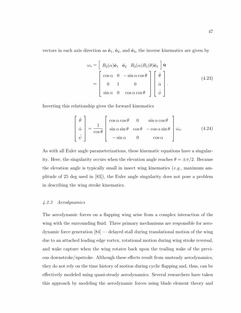
47

vectors in each axis direction as e1, e2, and e3, the inverse kinematics are given by

ωo =[R2(α)e1 e2 R2(α)R1(θ)e3

]u

=

cosα 0 − sinα cos θ

0 1 0

sinα 0 cosα cos θ

θ

α

φ

. (4.23)

Inverting this relationship gives the forward kinematicsθ

α

ψ

=1

cos θ

cosα cos θ 0 sinα cos θ

sinα sin θ cos θ − cosα sin θ

− sinα 0 cosα

ωo. (4.24)

As with all Euler angle parameterizations, these kinematic equations have a singular-

ity. Here, the singularity occurs when the elevation angle reaches θ = ±π/2. Because

the elevation angle is typically small in insect wing kinematics (e.g., maximum am-

plitude of 25 deg used in [83]), the Euler angle singularity does not pose a problem

in describing the wing stroke kinematics.

4.2.3 Aerodynamics

The aerodynamic forces on a flapping wing arise from a complex interaction of the

wing with the surrounding fluid. Three primary mechanisms are responsible for aero-

dynamic force generation [84] — delayed stall during translational motion of the wing

due to an attached leading edge vortex, rotational motion during wing stroke reversal,

and wake capture when the wing rotates back upon the trailing wake of the previ-

ous downstroke/upstroke. Although these effects result from unsteady aerodynamics,

they do not rely on the time history of motion during cyclic flapping and, thus, can be

effectively modeled using quasi-steady aerodynamics. Several researchers have taken

this approach by modeling the aerodynamic forces using blade element theory and

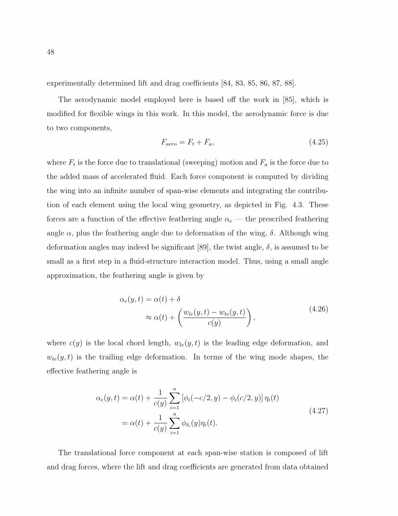
48

experimentally determined lift and drag coefficients [84, 83, 85, 86, 87, 88].

The aerodynamic model employed here is based off the work in [85], which is

modified for flexible wings in this work. In this model, the aerodynamic force is due

to two components,

Faero = Ft + Fa, (4.25)

where Ft is the force due to translational (sweeping) motion and Fa is the force due to

the added mass of accelerated fluid. Each force component is computed by dividing

the wing into an infinite number of span-wise elements and integrating the contribu-

tion of each element using the local wing geometry, as depicted in Fig. 4.3. These

forces are a function of the effective feathering angle αe — the prescribed feathering

angle α, plus the feathering angle due to deformation of the wing, δ. Although wing

deformation angles may indeed be significant [89], the twist angle, δ, is assumed to be

small as a first step in a fluid-structure interaction model. Thus, using a small angle

approximation, the feathering angle is given by

αe(y, t) = α(t) + δ

≈ α(t) +

(wle(y, t)− wte(y, t)

c(y)

),

(4.26)

where c(y) is the local chord length, wle(y, t) is the leading edge deformation, and

wte(y, t) is the trailing edge deformation. In terms of the wing mode shapes, the

effective feathering angle is

αe(y, t) = α(t) +1

c(y)

n∑i=1

[φi(−c/2, y)− φi(c/2, y)] ηi(t)

= α(t) +1

c(y)

n∑i=1

φδi(y)ηi(t).

(4.27)

The translational force component at each span-wise station is composed of lift

and drag forces, where the lift and drag coefficients are generated from data obtained

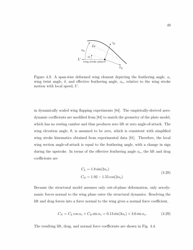
49

xp

zp

o

δαe

wing stroke planeU

α

Figure 4.3: A span-wise deformed wing element depicting the feathering angle, α,wing twist angle, δ, and effective feathering angle, αe, relative to the wing strokemotion with local speed, U .

in dynamically scaled wing flapping experiments [84]. The empirically-derived aero-

dynamic coefficients are modified from [84] to match the geometry of the plate model,

which has no resting camber and thus produces zero lift at zero angle-of-attack. The

wing elevation angle, θ, is assumed to be zero, which is consistent with simplified

wing stroke kinematics obtained from experimental data [81]. Therefore, the local

wing section angle-of-attack is equal to the feathering angle, with a change in sign

during the upstroke. In terms of the effective feathering angle αe, the lift and drag

coefficients are

CL = 1.8 sin(2αe)

CD = 1.92− 1.55 cos(2αe).(4.28)

Because the structural model assumes only out-of-plane deformation, only aerody-

namic forces normal to the wing plane enter the structural dynamics. Resolving the

lift and drag forces into a force normal to the wing gives a normal force coefficient,

CN = CL cosαe + CD sinαe = 0.13 sin(3αe) + 3.6 sinαe. (4.29)

The resulting lift, drag, and normal force coefficients are shown in Fig. 4.4.

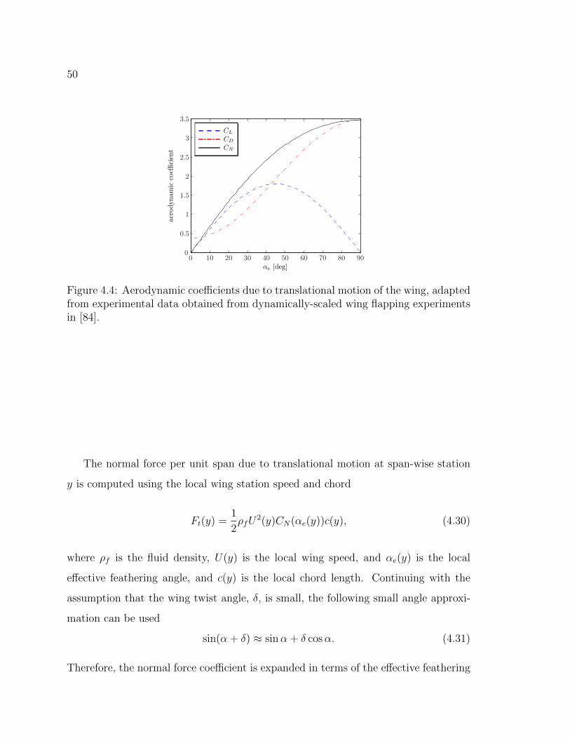
50

Figure 4.4: Aerodynamic coefficients due to translational motion of the wing, adaptedfrom experimental data obtained from dynamically-scaled wing flapping experimentsin [84].

The normal force per unit span due to translational motion at span-wise station

y is computed using the local wing station speed and chord

Ft(y) =1

2ρfU

2(y)CN(αe(y))c(y), (4.30)

where ρf is the fluid density, U(y) is the local wing speed, and αe(y) is the local

effective feathering angle, and c(y) is the local chord length. Continuing with the

assumption that the wing twist angle, δ, is small, the following small angle approxi-

mation can be used

sin(α + δ) ≈ sinα + δ cosα. (4.31)

Therefore, the normal force coefficient is expanded in terms of the effective feathering

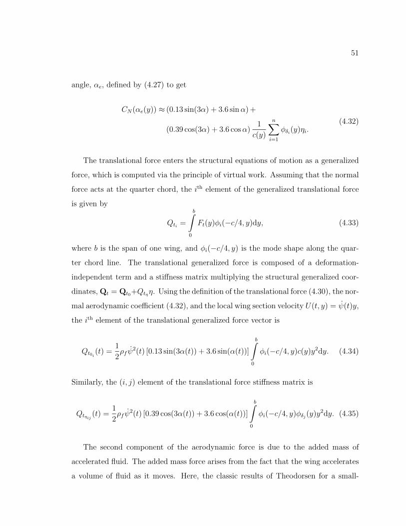
51

angle, αe, defined by (4.27) to get

CN(αe(y)) ≈ (0.13 sin(3α) + 3.6 sinα) +

(0.39 cos(3α) + 3.6 cosα)1

c(y)

n∑i=1

φδi(y)ηi.(4.32)

The translational force enters the structural equations of motion as a generalized

force, which is computed via the principle of virtual work. Assuming that the normal

force acts at the quarter chord, the ith element of the generalized translational force

is given by

Qti =

b∫0

Ft(y)φi(−c/4, y)dy, (4.33)

where b is the span of one wing, and φi(−c/4, y) is the mode shape along the quar-

ter chord line. The translational generalized force is composed of a deformation-

independent term and a stiffness matrix multiplying the structural generalized coor-

dinates, Qt = Qt0+Qtηη. Using the definition of the translational force (4.30), the nor-

mal aerodynamic coefficient (4.32), and the local wing section velocity U(t, y) = ψ(t)y,

the ith element of the translational generalized force vector is

Qt0i(t) =

1

2ρf ψ

2(t) [0.13 sin(3α(t)) + 3.6 sin(α(t))]

b∫0

φi(−c/4, y)c(y)y2dy. (4.34)

Similarly, the (i, j) element of the translational force stiffness matrix is

Qtηij(t) =

1

2ρf ψ

2(t) [0.39 cos(3α(t)) + 3.6 cos(α(t))]

b∫0

φi(−c/4, y)φδj(y)y2dy. (4.35)

The second component of the aerodynamic force is due to the added mass of

accelerated fluid. The added mass force arises from the fact that the wing accelerates

a volume of fluid as it moves. Here, the classic results of Theodorsen for a small-

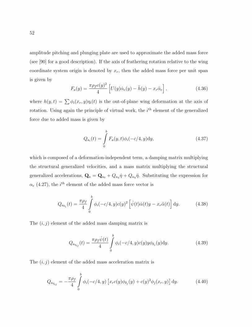
52

amplitude pitching and plunging plate are used to approximate the added mass force

(see [90] for a good description). If the axis of feathering rotation relative to the wing

coordinate system origin is denoted by xr, then the added mass force per unit span

is given by

Fa(y) =πρfc(y)2

4

[U(y)αe(y)− h(y)− xrαe

], (4.36)

where h(y, t) =∑φi(xr, y)ηi(t) is the out-of-plane wing deformation at the axis of

rotation. Using again the principle of virtual work, the ith element of the generalized

force due to added mass is given by

Qai(t) =

b∫0

Fa(y, t)φi(−c/4, y)dy, (4.37)

which is composed of a deformation-independent term, a damping matrix multiplying

the structural generalized velocities, and a mass matrix multiplying the structural

generalized accelerations, Qa = Qa0 + Qaη η + Qaη η. Substituting the expression for

αe (4.27), the ith element of the added mass force vector is

Qa0i(t) =

πρf4

b∫0

φi(−c/4, y)c(y)2[ψ(t)α(t)y − xrα(t)

]dy. (4.38)

The (i, j) element of the added mass damping matrix is

Qaηij(t) =

πρf ψ(t)

4

b∫0

φi(−c/4, y)c(y)yφδj(y)dy. (4.39)

The (i, j) element of the added mass acceleration matrix is

Qaηij= −πρf

4

b∫0

φi(−c/4, y)[xrc(y)φδj(y) + c(y)2φj(xr, y)

]dy. (4.40)

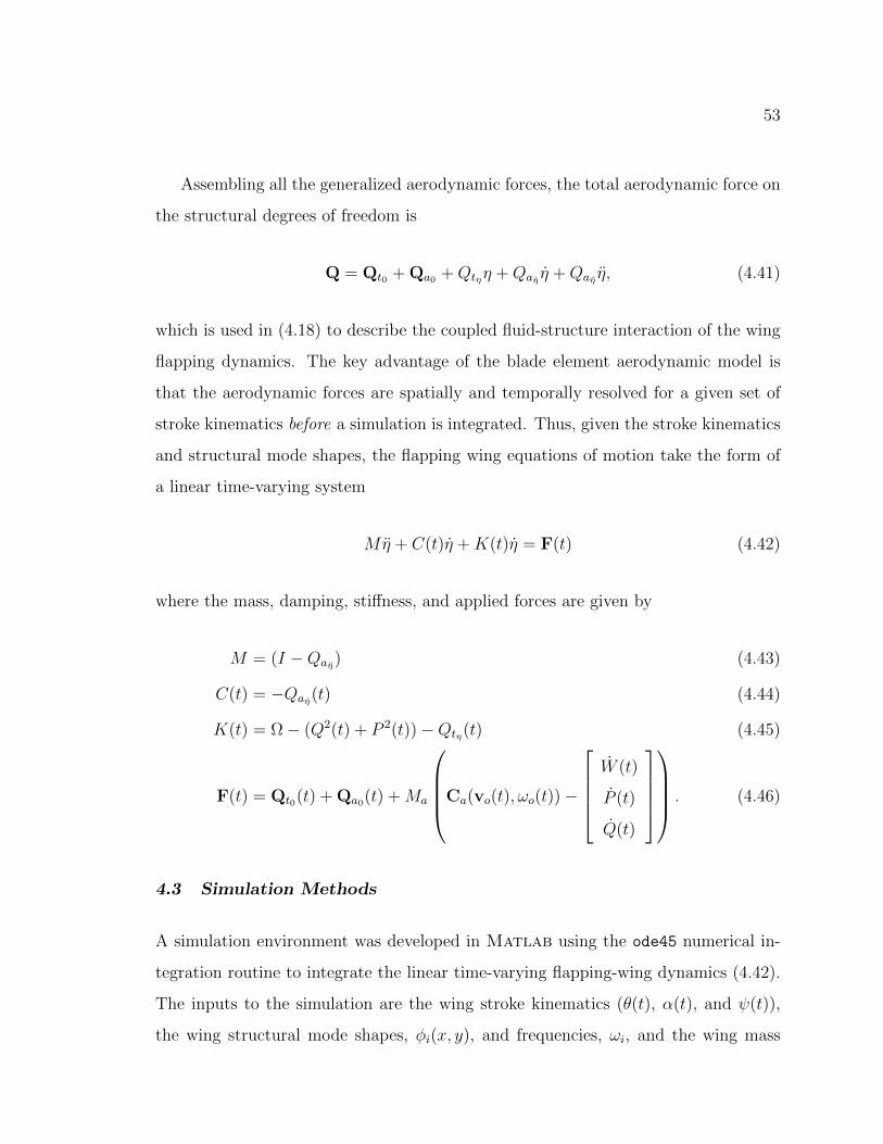
53

Assembling all the generalized aerodynamic forces, the total aerodynamic force on

the structural degrees of freedom is

Q = Qt0 + Qa0 +Qtηη +Qaη η +Qaη η, (4.41)

which is used in (4.18) to describe the coupled fluid-structure interaction of the wing

flapping dynamics. The key advantage of the blade element aerodynamic model is

that the aerodynamic forces are spatially and temporally resolved for a given set of

stroke kinematics before a simulation is integrated. Thus, given the stroke kinematics

and structural mode shapes, the flapping wing equations of motion take the form of

a linear time-varying system

Mη + C(t)η +K(t)η = F(t) (4.42)

where the mass, damping, stiffness, and applied forces are given by

M = (I −Qaη) (4.43)

C(t) = −Qaη(t) (4.44)

K(t) = Ω− (Q2(t) + P 2(t))−Qtη(t) (4.45)

F(t) = Qt0(t) + Qa0(t) +Ma

Ca(vo(t), ωo(t))−

W (t)

P (t)

Q(t)

. (4.46)

4.3 Simulation Methods

A simulation environment was developed in Matlab using the ode45 numerical in-

tegration routine to integrate the linear time-varying flapping-wing dynamics (4.42).

The inputs to the simulation are the wing stroke kinematics (θ(t), α(t), and ψ(t)),

the wing structural mode shapes, φi(x, y), and frequencies, ωi, and the wing mass

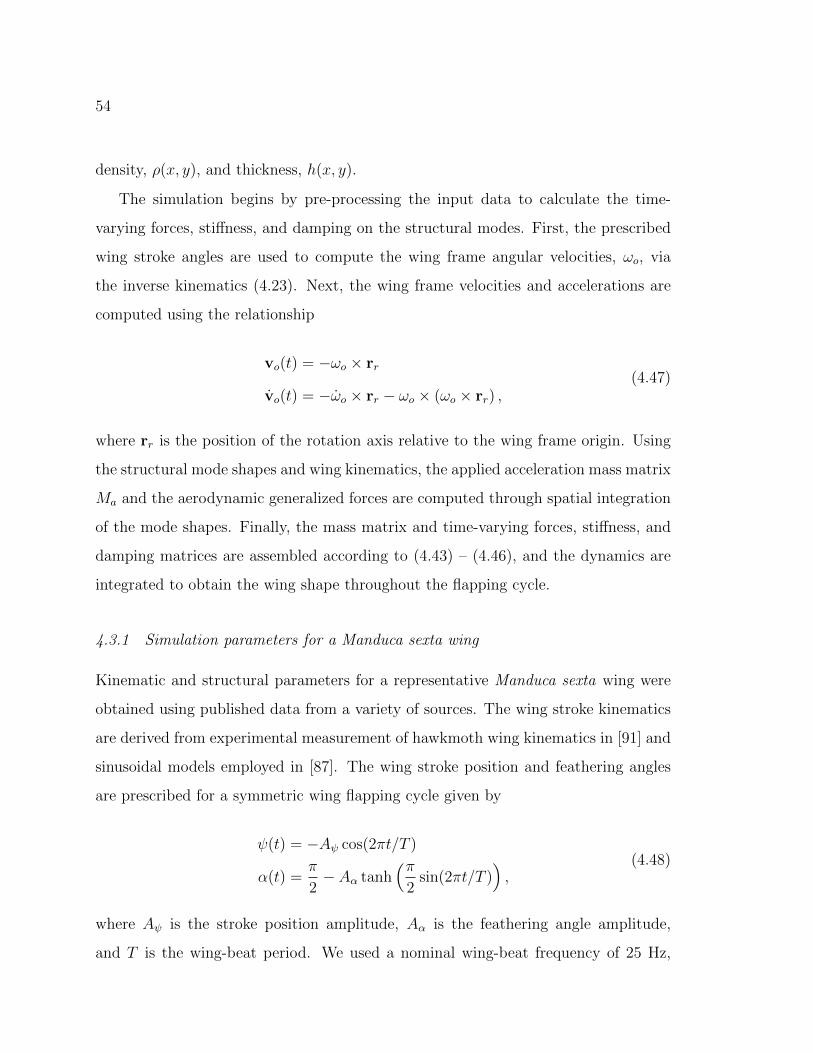
54

density, ρ(x, y), and thickness, h(x, y).

The simulation begins by pre-processing the input data to calculate the time-

varying forces, stiffness, and damping on the structural modes. First, the prescribed

wing stroke angles are used to compute the wing frame angular velocities, ωo, via

the inverse kinematics (4.23). Next, the wing frame velocities and accelerations are

computed using the relationship

vo(t) = −ωo × rr

vo(t) = −ωo × rr − ωo × (ωo × rr) ,(4.47)

where rr is the position of the rotation axis relative to the wing frame origin. Using

the structural mode shapes and wing kinematics, the applied acceleration mass matrix

Ma and the aerodynamic generalized forces are computed through spatial integration

of the mode shapes. Finally, the mass matrix and time-varying forces, stiffness, and

damping matrices are assembled according to (4.43) – (4.46), and the dynamics are

integrated to obtain the wing shape throughout the flapping cycle.

4.3.1 Simulation parameters for a Manduca sexta wing

Kinematic and structural parameters for a representative Manduca sexta wing were

obtained using published data from a variety of sources. The wing stroke kinematics

are derived from experimental measurement of hawkmoth wing kinematics in [91] and

sinusoidal models employed in [87]. The wing stroke position and feathering angles

are prescribed for a symmetric wing flapping cycle given by

ψ(t) = −Aψ cos(2πt/T )

α(t) =π

2− Aα tanh

(π2

sin(2πt/T )),

(4.48)

where Aψ is the stroke position amplitude, Aα is the feathering angle amplitude,

and T is the wing-beat period. We used a nominal wing-beat frequency of 25 Hz,

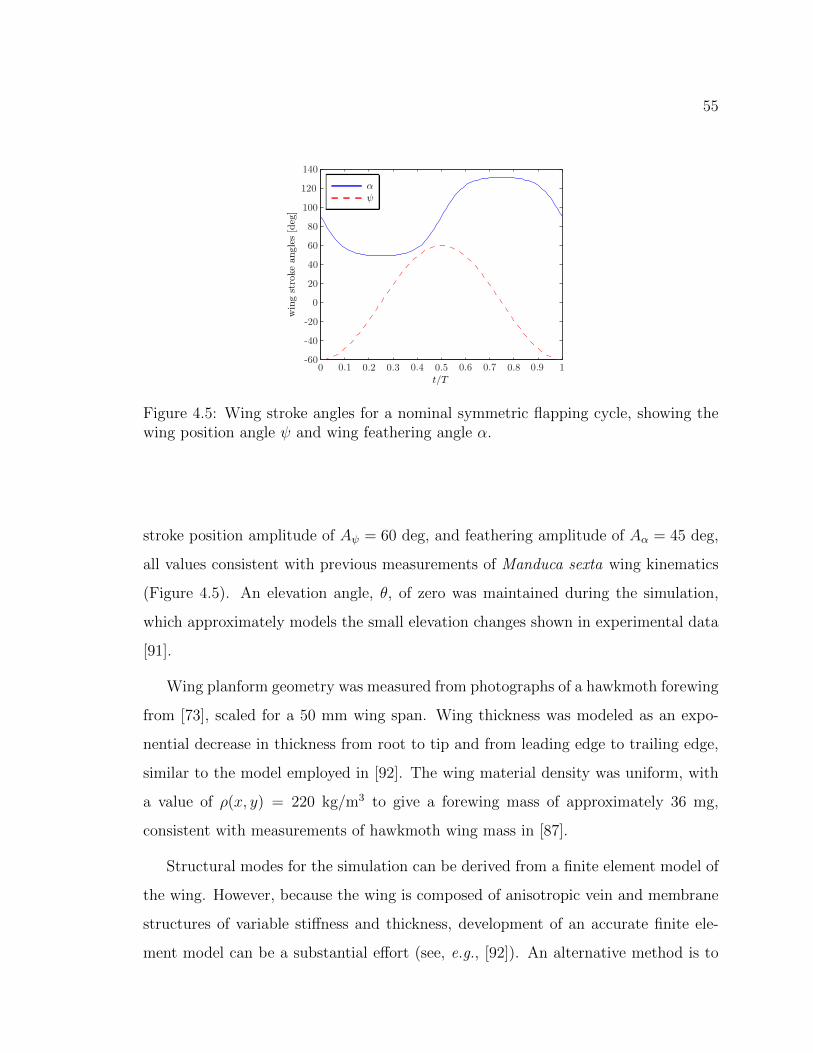
55

Figure 4.5: Wing stroke angles for a nominal symmetric flapping cycle, showing thewing position angle ψ and wing feathering angle α.

stroke position amplitude of Aψ = 60 deg, and feathering amplitude of Aα = 45 deg,

all values consistent with previous measurements of Manduca sexta wing kinematics

(Figure 4.5). An elevation angle, θ, of zero was maintained during the simulation,

which approximately models the small elevation changes shown in experimental data

[91].

Wing planform geometry was measured from photographs of a hawkmoth forewing

from [73], scaled for a 50 mm wing span. Wing thickness was modeled as an expo-

nential decrease in thickness from root to tip and from leading edge to trailing edge,

similar to the model employed in [92]. The wing material density was uniform, with

a value of ρ(x, y) = 220 kg/m3 to give a forewing mass of approximately 36 mg,

consistent with measurements of hawkmoth wing mass in [87].

Structural modes for the simulation can be derived from a finite element model of

the wing. However, because the wing is composed of anisotropic vein and membrane

structures of variable stiffness and thickness, development of an accurate finite ele-

ment model can be a substantial effort (see, e.g., [92]). An alternative method is to

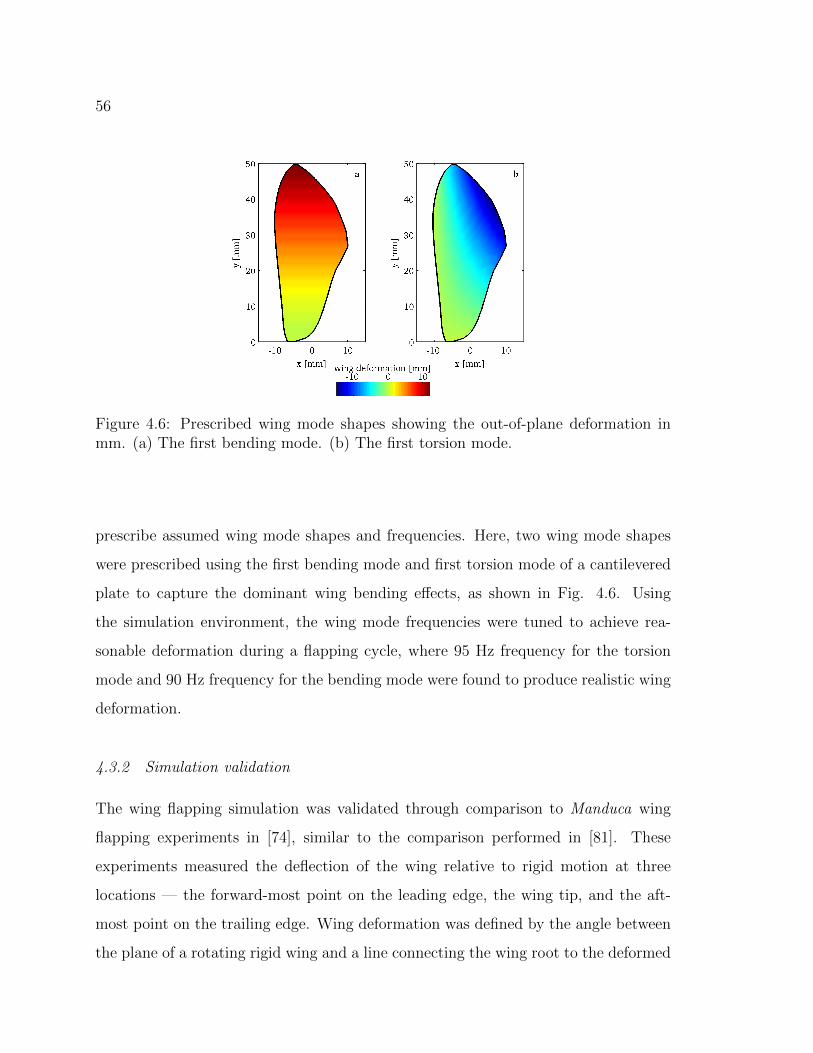
56

Figure 4.6: Prescribed wing mode shapes showing the out-of-plane deformation inmm. (a) The first bending mode. (b) The first torsion mode.

prescribe assumed wing mode shapes and frequencies. Here, two wing mode shapes

were prescribed using the first bending mode and first torsion mode of a cantilevered

plate to capture the dominant wing bending effects, as shown in Fig. 4.6. Using

the simulation environment, the wing mode frequencies were tuned to achieve rea-

sonable deformation during a flapping cycle, where 95 Hz frequency for the torsion

mode and 90 Hz frequency for the bending mode were found to produce realistic wing

deformation.

4.3.2 Simulation validation

The wing flapping simulation was validated through comparison to Manduca wing

flapping experiments in [74], similar to the comparison performed in [81]. These

experiments measured the deflection of the wing relative to rigid motion at three

locations — the forward-most point on the leading edge, the wing tip, and the aft-

most point on the trailing edge. Wing deformation was defined by the angle between

the plane of a rotating rigid wing and a line connecting the wing root to the deformed

57

point (see Fig. 1 in [74]).

The conditions for these experiments were simulated using a wing stroke amplitude

of Aφ = 54 deg at a frequency of 26 Hz (adjusted from 25 Hz in order to match the

experiment), with a constant wing feathering angle of α = 90 deg. The structural

generalized coordinates, η, and velocities, η, were initialized to zero and the dynamics

were integrated for four wing stroke cycles. The structural dynamics settled into a

limit cycle after the second wing stroke cycle, and the fourth wing stroke cycle was

used to compute wing deformation at the trailing edge and wing tip for comparison

to experimental data collected in [74]. One wing stroke cycle was sampled from the

data presented in [74] for the wing tip and trailing edge positions. The simulated

results that were obtained are compared to the sampled data, along with second-

order Fourier fits of the experimental and simulation data using the first two Fourier

coefficients (26 Hz and 72 Hz), shown in Fig. 4.7. Despite the fact that the simulation

only integrates four state variables (two modal coordinates and two modal velocities),

the simulation captures the overall wing motion well, as evidenced by the similarity

between the second-order Fourier fits of each data set (shown in dashed curves). The

root mean square (RMS) error between the second-order Fourier fits of the simulation

and experiment were computed as 2.5 deg for the wing tip deformation and 2.0 deg

for the trailing edge deformation, confirming that the simulation captures the wing

motion up to second-order harmonics.

4.3.3 Nominal flapping trajectory

The nominal flapping trajectory defined by the stroke kinematics shown in Fig. 4.5

was simulated to analyze wing deformation during a flapping cycle. The structural

generalized coordinates and velocities were initialized to zero, and the dynamics were

integrated for four flapping cycles. The wing shape for the deformed wing was com-

pared to the rigid motion of the wing (i.e., the wing position and feathering angles

defined by the kinematics). The stroke sequence for the deformed wing shape and

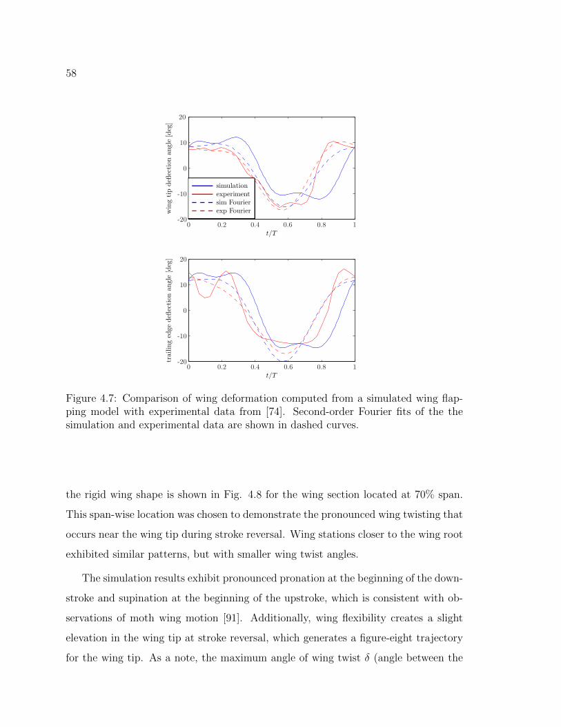
58

Figure 4.7: Comparison of wing deformation computed from a simulated wing flap-ping model with experimental data from [74]. Second-order Fourier fits of the thesimulation and experimental data are shown in dashed curves.

the rigid wing shape is shown in Fig. 4.8 for the wing section located at 70% span.

This span-wise location was chosen to demonstrate the pronounced wing twisting that

occurs near the wing tip during stroke reversal. Wing stations closer to the wing root

exhibited similar patterns, but with smaller wing twist angles.

The simulation results exhibit pronounced pronation at the beginning of the down-

stroke and supination at the beginning of the upstroke, which is consistent with ob-

servations of moth wing motion [91]. Additionally, wing flexibility creates a slight

elevation in the wing tip at stroke reversal, which generates a figure-eight trajectory

for the wing tip. As a note, the maximum angle of wing twist δ (angle between the

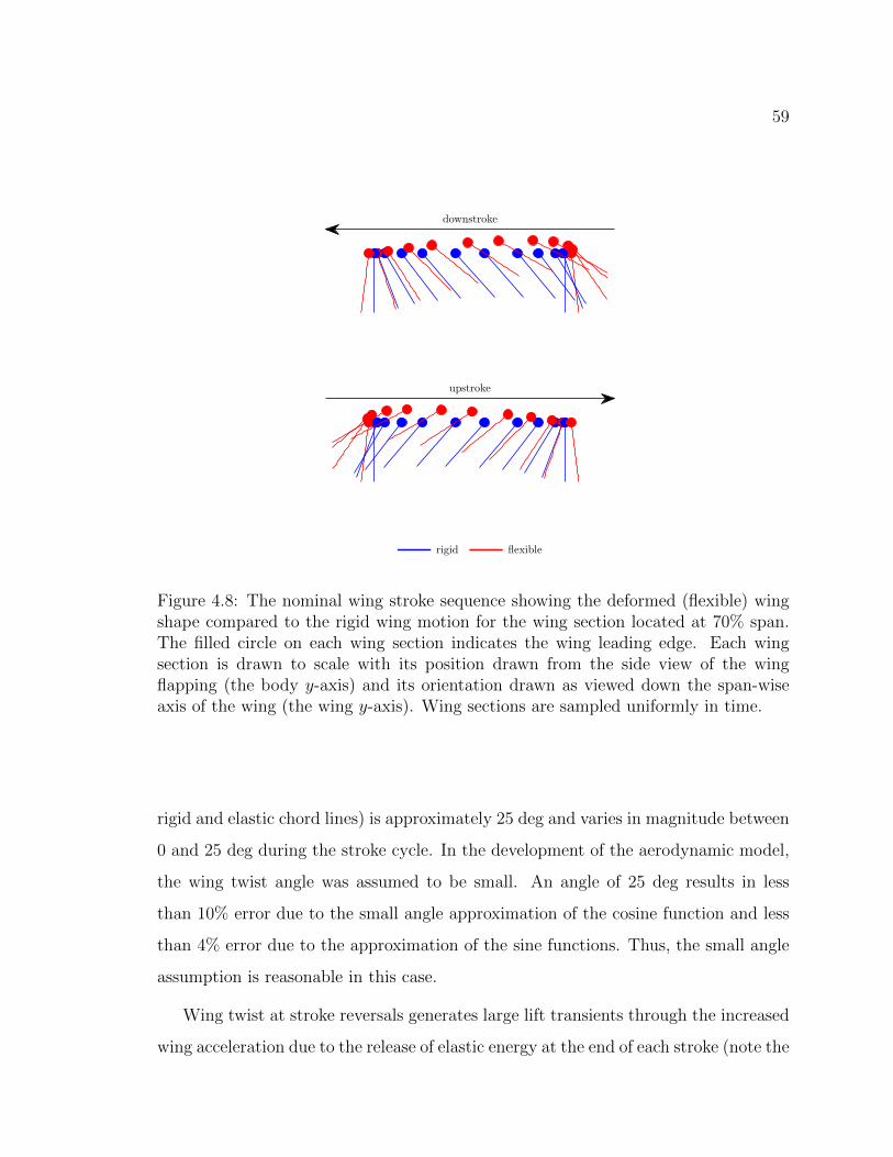
59

Figure 4.8: The nominal wing stroke sequence showing the deformed (flexible) wingshape compared to the rigid wing motion for the wing section located at 70% span.The filled circle on each wing section indicates the wing leading edge. Each wingsection is drawn to scale with its position drawn from the side view of the wingflapping (the body y-axis) and its orientation drawn as viewed down the span-wiseaxis of the wing (the wing y-axis). Wing sections are sampled uniformly in time.

rigid and elastic chord lines) is approximately 25 deg and varies in magnitude between

0 and 25 deg during the stroke cycle. In the development of the aerodynamic model,

the wing twist angle was assumed to be small. An angle of 25 deg results in less

than 10% error due to the small angle approximation of the cosine function and less

than 4% error due to the approximation of the sine functions. Thus, the small angle

assumption is reasonable in this case.

Wing twist at stroke reversals generates large lift transients through the increased

wing acceleration due to the release of elastic energy at the end of each stroke (note the

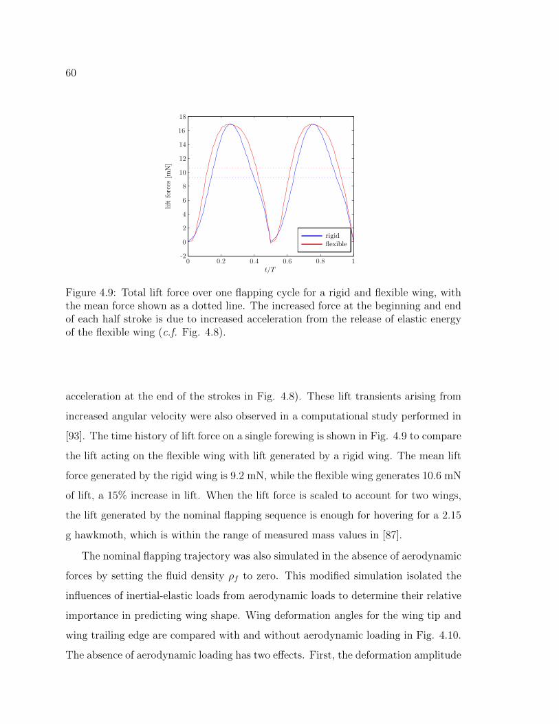
60

Figure 4.9: Total lift force over one flapping cycle for a rigid and flexible wing, withthe mean force shown as a dotted line. The increased force at the beginning and endof each half stroke is due to increased acceleration from the release of elastic energyof the flexible wing (c.f. Fig. 4.8).

acceleration at the end of the strokes in Fig. 4.8). These lift transients arising from

increased angular velocity were also observed in a computational study performed in

[93]. The time history of lift force on a single forewing is shown in Fig. 4.9 to compare

the lift acting on the flexible wing with lift generated by a rigid wing. The mean lift

force generated by the rigid wing is 9.2 mN, while the flexible wing generates 10.6 mN

of lift, a 15% increase in lift. When the lift force is scaled to account for two wings,

the lift generated by the nominal flapping sequence is enough for hovering for a 2.15

g hawkmoth, which is within the range of measured mass values in [87].

The nominal flapping trajectory was also simulated in the absence of aerodynamic

forces by setting the fluid density ρf to zero. This modified simulation isolated the

influences of inertial-elastic loads from aerodynamic loads to determine their relative

importance in predicting wing shape. Wing deformation angles for the wing tip and

wing trailing edge are compared with and without aerodynamic loading in Fig. 4.10.

The absence of aerodynamic loading has two effects. First, the deformation amplitude

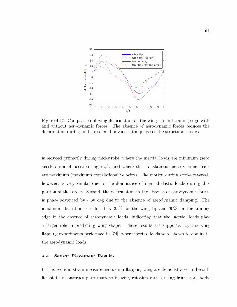
61

Figure 4.10: Comparison of wing deformation at the wing tip and trailing edge withand without aerodynamic forces. The absence of aerodynamic forces reduces thedeformation during mid-stroke and advances the phase of the structural modes.

is reduced primarily during mid-stroke, where the inertial loads are minimum (zero

acceleration of position angle ψ), and where the translational aerodynamic loads

are maximum (maximum translational velocity). The motion during stroke reversal,

however, is very similar due to the dominance of inertial-elastic loads during this

portion of the stroke. Second, the deformation in the absence of aerodynamic forces

is phase advanced by ∼30 deg due to the absence of aerodynamic damping. The

maximum deflection is reduced by 35% for the wing tip and 30% for the trailing

edge in the absence of aerodynamic loads, indicating that the inertial loads play

a larger role in predicting wing shape. These results are supported by the wing

flapping experiments performed in [74], where inertial loads were shown to dominate

the aerodynamic loads.

4.4 Sensor Placement Results

In this section, strain measurements on a flapping wing are demonstrated to be suf-

ficient to reconstruct perturbations in wing rotation rates arising from, e.g., body

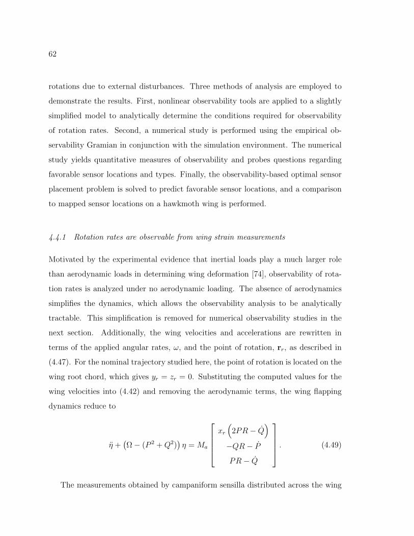
62

rotations due to external disturbances. Three methods of analysis are employed to

demonstrate the results. First, nonlinear observability tools are applied to a slightly

simplified model to analytically determine the conditions required for observability

of rotation rates. Second, a numerical study is performed using the empirical ob-

servability Gramian in conjunction with the simulation environment. The numerical

study yields quantitative measures of observability and probes questions regarding

favorable sensor locations and types. Finally, the observability-based optimal sensor

placement problem is solved to predict favorable sensor locations, and a comparison

to mapped sensor locations on a hawkmoth wing is performed.

4.4.1 Rotation rates are observable from wing strain measurements

Motivated by the experimental evidence that inertial loads play a much larger role

than aerodynamic loads in determining wing deformation [74], observability of rota-

tion rates is analyzed under no aerodynamic loading. The absence of aerodynamics

simplifies the dynamics, which allows the observability analysis to be analytically

tractable. This simplification is removed for numerical observability studies in the

next section. Additionally, the wing velocities and accelerations are rewritten in

terms of the applied angular rates, ω, and the point of rotation, rr, as described in

(4.47). For the nominal trajectory studied here, the point of rotation is located on the

wing root chord, which gives yr = zr = 0. Substituting the computed values for the

wing velocities into (4.42) and removing the aerodynamic terms, the wing flapping

dynamics reduce to

η +(Ω− (P 2 +Q2)

)η = Ma

xr

(2PR− Q

)−QR− P

PR− Q

. (4.49)

The measurements obtained by campaniform sensilla distributed across the wing

63

are modeled using the local wing strain. Experimental evidence has suggested that

these mechanoreceptors can measure both tension and compression [94], therefore the

sensor information is modeled using the wing strain at the sensor location. Linear

elastic theory states that strain measurements are proportional to the local curva-

ture of the wing. For a strain sensor located at rs = xsip + ysjp + zskp, the strain

measurement vector is given in by [80]

ε = −zs

∂2w(xs, ys)/∂x

2

∂2w(xs, ys)/∂y2

2∂2w(xs, ys)/∂x∂y

, (4.50)

which gives the chord-wise bending strain, span-wise bending strain, and shear strain.

In terms of the modal coordinates, the strain measurement is

ε = −n∑i=1

zs

∂2φi(xs, ys)/∂x

2

∂2φi(xs, ys)/∂y2

2∂2φi(xs, ys)/∂x∂y

ηi. (4.51)

In this analysis, the strain sensors are assumed to report a scalar value as a linear

combination of the strain vector components (e.g., only bending or shear strain or

some combination). Therefore, the measurement model is a linear combination of the

modal coordinates:

y = Hη, (4.52)

where H is a function of the sensor locations, which (for now) are assumed to be

known.

The observability rank condition is applied to the wing flapping dynamics to

test if wing rotation rates (P,Q,R) are observable using strain measurements on

the wing. The wing flapping system is modeled with the control input variable

u =[P Q R

]T(i.e., the wing rotational accelerations are known inputs), and

64

state vector x =[ηT ηT P Q R

]T. Rewriting the dynamics (4.49) in control-

affine form gives

x =

η

K(ωo)η + (2M1xr + M3)PR−M2QR

0

0

0

+

0 0 0

−M2 −M1xr −M3 0

1 0 0

0 1 0

0 0 1

u

y = Hη,

(4.53)

where K(ωo) = P 2 +Q2−Ω is the stiffness matrix, and Mj denotes the jth column of

the Ma matrix. We consider the case of r structural modes, with r linearly indepen-

dent strain measurements (i.e., H ∈ Rr×r is full rank). Because H is full rank, we can

equivalently consider the output y = η. Using this output, the Lie derivatives with

respect to the drift vector field, fo(x), are considered. Computing the Lie derivatives,

the rank of the matrix

dO =∂

∂x

h

Lfoh

L2fo

h

L3fo

h

(4.54)

is found to be deficient by one, and the fourth-order Lie derivative L4fo

h is linearly

dependent on the lower-order derivatives. Thus, the system is unobservable without

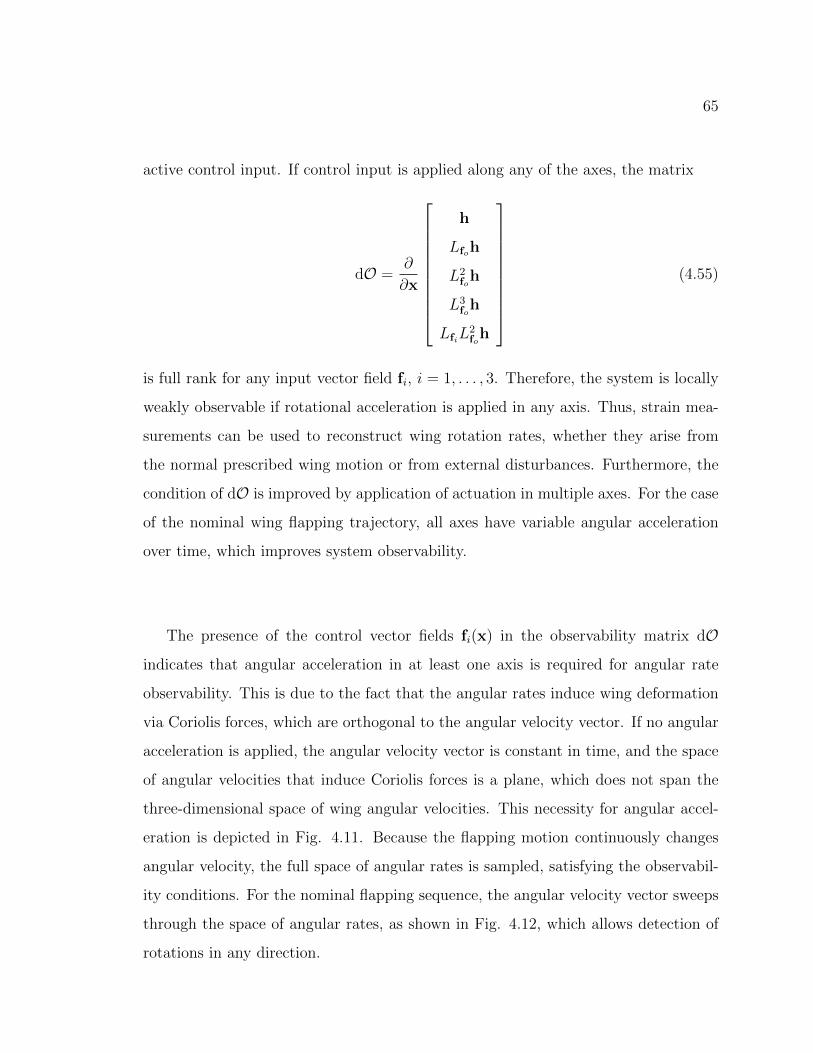
65

active control input. If control input is applied along any of the axes, the matrix

dO =∂

∂x

h

Lfoh

L2fo

h

L3fo

h

LfiL2fo

h

(4.55)

is full rank for any input vector field fi, i = 1, . . . , 3. Therefore, the system is locally

weakly observable if rotational acceleration is applied in any axis. Thus, strain mea-

surements can be used to reconstruct wing rotation rates, whether they arise from

the normal prescribed wing motion or from external disturbances. Furthermore, the

condition of dO is improved by application of actuation in multiple axes. For the case

of the nominal wing flapping trajectory, all axes have variable angular acceleration

over time, which improves system observability.

The presence of the control vector fields fi(x) in the observability matrix dO

indicates that angular acceleration in at least one axis is required for angular rate

observability. This is due to the fact that the angular rates induce wing deformation

via Coriolis forces, which are orthogonal to the angular velocity vector. If no angular

acceleration is applied, the angular velocity vector is constant in time, and the space

of angular velocities that induce Coriolis forces is a plane, which does not span the

three-dimensional space of wing angular velocities. This necessity for angular accel-

eration is depicted in Fig. 4.11. Because the flapping motion continuously changes

angular velocity, the full space of angular rates is sampled, satisfying the observabil-

ity conditions. For the nominal flapping sequence, the angular velocity vector sweeps

through the space of angular rates, as shown in Fig. 4.12, which allows detection of

rotations in any direction.

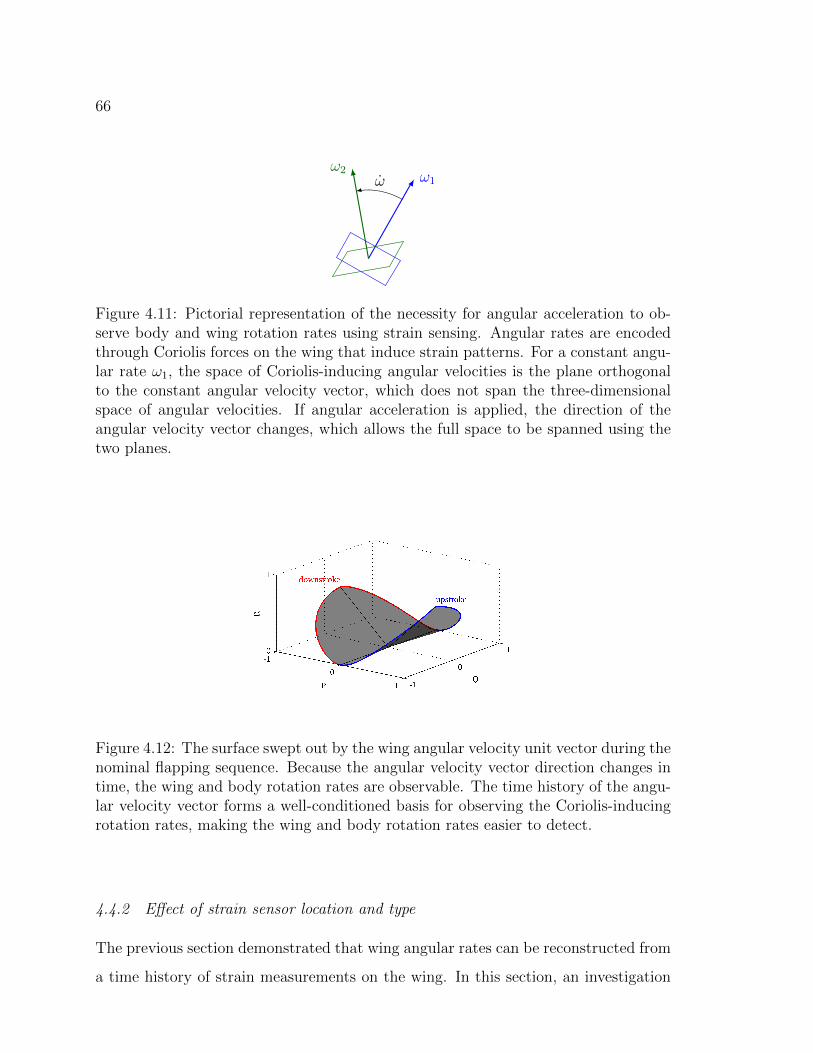
66

ω1

ω2ω

Figure 4.11: Pictorial representation of the necessity for angular acceleration to ob-serve body and wing rotation rates using strain sensing. Angular rates are encodedthrough Coriolis forces on the wing that induce strain patterns. For a constant angu-lar rate ω1, the space of Coriolis-inducing angular velocities is the plane orthogonalto the constant angular velocity vector, which does not span the three-dimensionalspace of angular velocities. If angular acceleration is applied, the direction of theangular velocity vector changes, which allows the full space to be spanned using thetwo planes.

Figure 4.12: The surface swept out by the wing angular velocity unit vector during thenominal flapping sequence. Because the angular velocity vector direction changes intime, the wing and body rotation rates are observable. The time history of the angu-lar velocity vector forms a well-conditioned basis for observing the Coriolis-inducingrotation rates, making the wing and body rotation rates easier to detect.

4.4.2 Effect of strain sensor location and type

The previous section demonstrated that wing angular rates can be reconstructed from

a time history of strain measurements on the wing. In this section, an investigation

67

Figure 4.13: Observability indices for varying sensor location and type, normalizedby the maximum index. (a) The observability index for sensors measuring shearstrain, which is maximum at the wing tip where wing twist is maximum. (b) Theobservability index for sensors measuring span-wise bending strain, which is maximumat the wing root.

is performed to discover the role of sensor location and type (bending or shear strain)

in wing rotation sensing. Sensor fitness is measured by the empirical observability

Gramian (see Chapter 2), which gives a quantitative measure of system observability

for a given sensor configuration.

The empirical observability Gramian was computed over the nominal flapping

cycle for varying sensor location and type by perturbing the angular rate initial con-

ditions in each of the three wing axes, simulating a disturbance to the wing kinematics.

Strain measurements were sampled in a grid of 51 span-wise stations, with 21 chord-

wise samples per station, resulting in a minimum grid spacing of 1mm. The empirical

observability Gramian was computed for each sensor location for sensors measuring

bending strain, εyy, and shear strain, εxy (note that the assumed structural modes

used here do not have chord-wise bending, so εxx is identically zero).

68

The observability index for each sensor location and type is shown in Fig. 4.13.

The observability indices indicate that the angular rates are encoded primarily through

shear strain (left side of Fig. 4.13), with the maximum information gained at the wing

tip, where wing twist is dominant during pronation and supination. Bending strain

(right side of Fig. 4.13) is largest at the wing root and encodes more information

about wing rotation rates than shear strain near the wing root. These results provide

hypotheses regarding favorable sensor type as a function of location on the wing —

sensors near the wing tip provide more information when sensitive to shear strain,

while sensors near the wing root provide more information when sensitive to bending

strain.

A second set of Gramian computations were performed to assess the relative ob-

servability of angular rate perturbations to the body axis system, which is fixed to the

moth body with x axis pointing aft along the wing stroke plane, y right in the wing

stroke plane, and z normal to the wing stroke plane, as shown in Fig. 4.14. Angular

rate perturbations were applied in each of the three axis directions: roll (x), pitch

(y), and yaw (z). Because the nominal wing stroke is symmetric between the left and

right wing, only the right wing was simulated to compute the empirical observability

Gramians. The Gramian for the left wing is computed from the Gramian for the right

wing by noting that the perturbations in the x and z axes are opposite for the left

wing,

Wl =

Wr(1, 1) −Wr(1, 2) Wr(1, 3)

−Wr(2, 1) Wr(2, 2) −Wr(2, 3)

Wr(3, 1) −Wr(3, 2) Wr(3, 3)

, (4.56)

where Wr(i, j) is the (i, j) element of the empirical observability Gramian computed

from the simulation of the right wing. This complementary nature of the information

encoded by sensors on the two wings improves the observability index when summed

together. Thus, information fused between sensors on both wings provides a better

estimate of the body rotation rates.

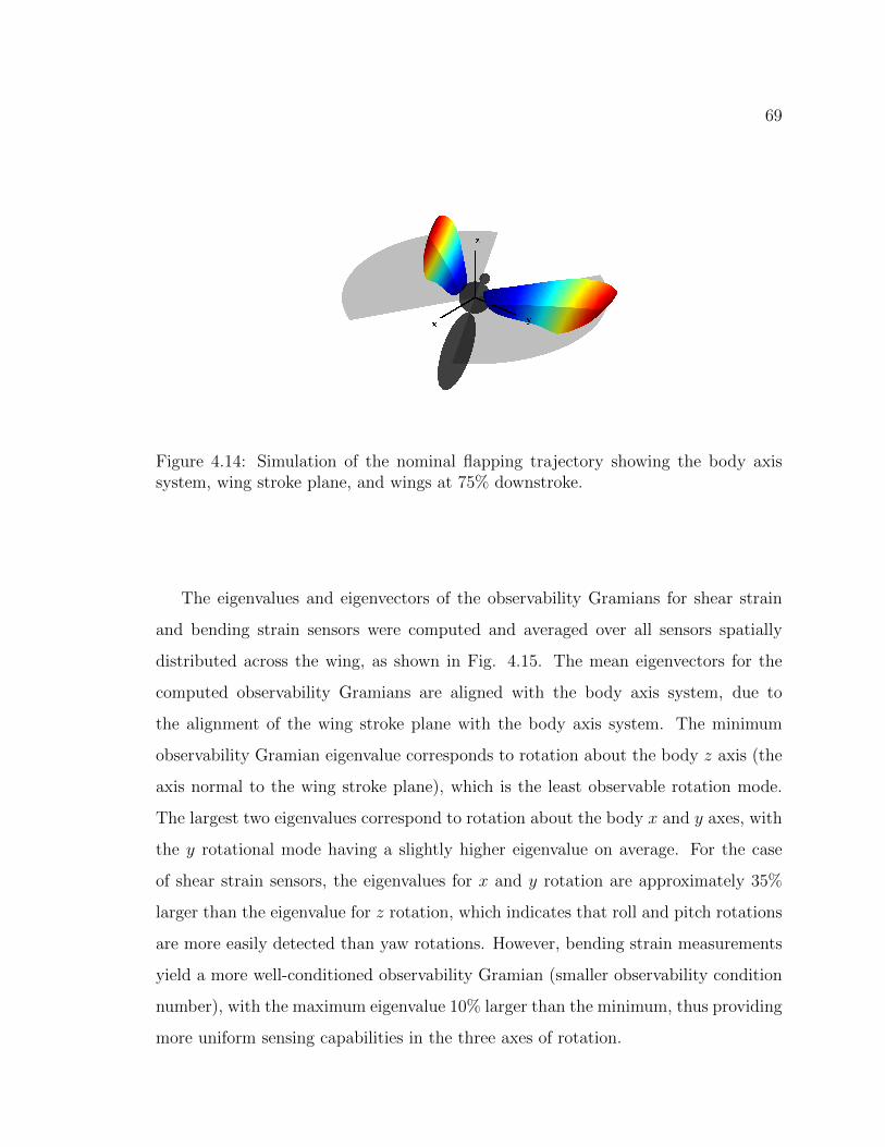
69

Figure 4.14: Simulation of the nominal flapping trajectory showing the body axissystem, wing stroke plane, and wings at 75% downstroke.

The eigenvalues and eigenvectors of the observability Gramians for shear strain

and bending strain sensors were computed and averaged over all sensors spatially

distributed across the wing, as shown in Fig. 4.15. The mean eigenvectors for the

computed observability Gramians are aligned with the body axis system, due to

the alignment of the wing stroke plane with the body axis system. The minimum

observability Gramian eigenvalue corresponds to rotation about the body z axis (the

axis normal to the wing stroke plane), which is the least observable rotation mode.

The largest two eigenvalues correspond to rotation about the body x and y axes, with

the y rotational mode having a slightly higher eigenvalue on average. For the case

of shear strain sensors, the eigenvalues for x and y rotation are approximately 35%

larger than the eigenvalue for z rotation, which indicates that roll and pitch rotations

are more easily detected than yaw rotations. However, bending strain measurements

yield a more well-conditioned observability Gramian (smaller observability condition

number), with the maximum eigenvalue 10% larger than the minimum, thus providing

more uniform sensing capabilities in the three axes of rotation.

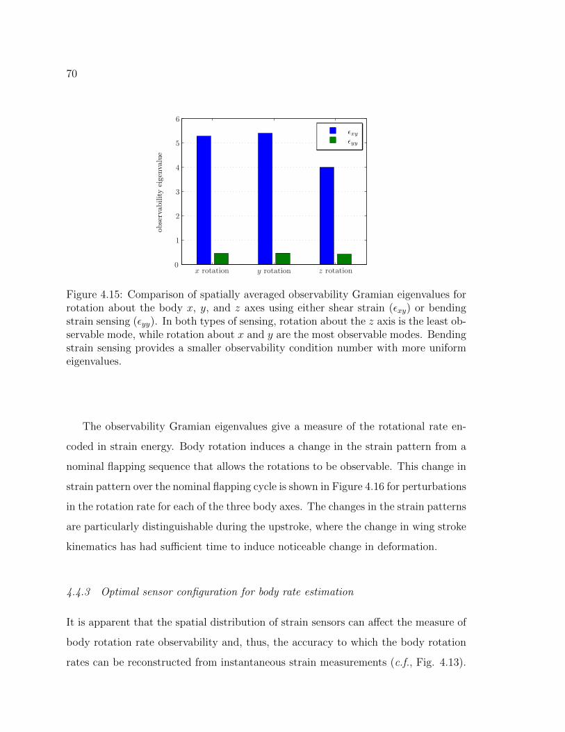
70

Figure 4.15: Comparison of spatially averaged observability Gramian eigenvalues forrotation about the body x, y, and z axes using either shear strain (εxy) or bendingstrain sensing (εyy). In both types of sensing, rotation about the z axis is the least ob-servable mode, while rotation about x and y are the most observable modes. Bendingstrain sensing provides a smaller observability condition number with more uniformeigenvalues.

The observability Gramian eigenvalues give a measure of the rotational rate en-

coded in strain energy. Body rotation induces a change in the strain pattern from a

nominal flapping sequence that allows the rotations to be observable. This change in

strain pattern over the nominal flapping cycle is shown in Figure 4.16 for perturbations

in the rotation rate for each of the three body axes. The changes in the strain patterns

are particularly distinguishable during the upstroke, where the change in wing stroke

kinematics has had sufficient time to induce noticeable change in deformation.

4.4.3 Optimal sensor configuration for body rate estimation

It is apparent that the spatial distribution of strain sensors can affect the measure of

body rotation rate observability and, thus, the accuracy to which the body rotation

rates can be reconstructed from instantaneous strain measurements (c.f., Fig. 4.13).

71

Figure 4.16: Change in the mean shear strain over one flapping cycle due to rotationsin each of the three body axes.

In this section, the sensor locations and types (shear or bending strain) that optimize

observability of body rotation rates are computed based upon the empirical observ-

ability Gramian. The optimal sensor sets are compared to locations of campaniform

sensilla found on Hawkmoth wings [73], and hypotheses for sensor type distribution

are developed for the known campaniform locations.

The optimal sensor placement problem (3.9) is formed to compute the optimal

sensor configuration for rotation rate observability. In the interest of finding a sensor

set that provides both a large observability index and a small observability condition

number, the cost function is formed as a weighted sum of the condition number and

the inverse of the observability index (the unobservability index), both of which are

convex functions of the Gramian, W [29]. Defining the condition number as κ(W ), the

inverse of the minimum eigenvalue as ν(W ), and the weight wν ≥ 0, the observability-

based sensor placement cost function is

J [W ] = κ(W ) + wνν(W ). (4.57)

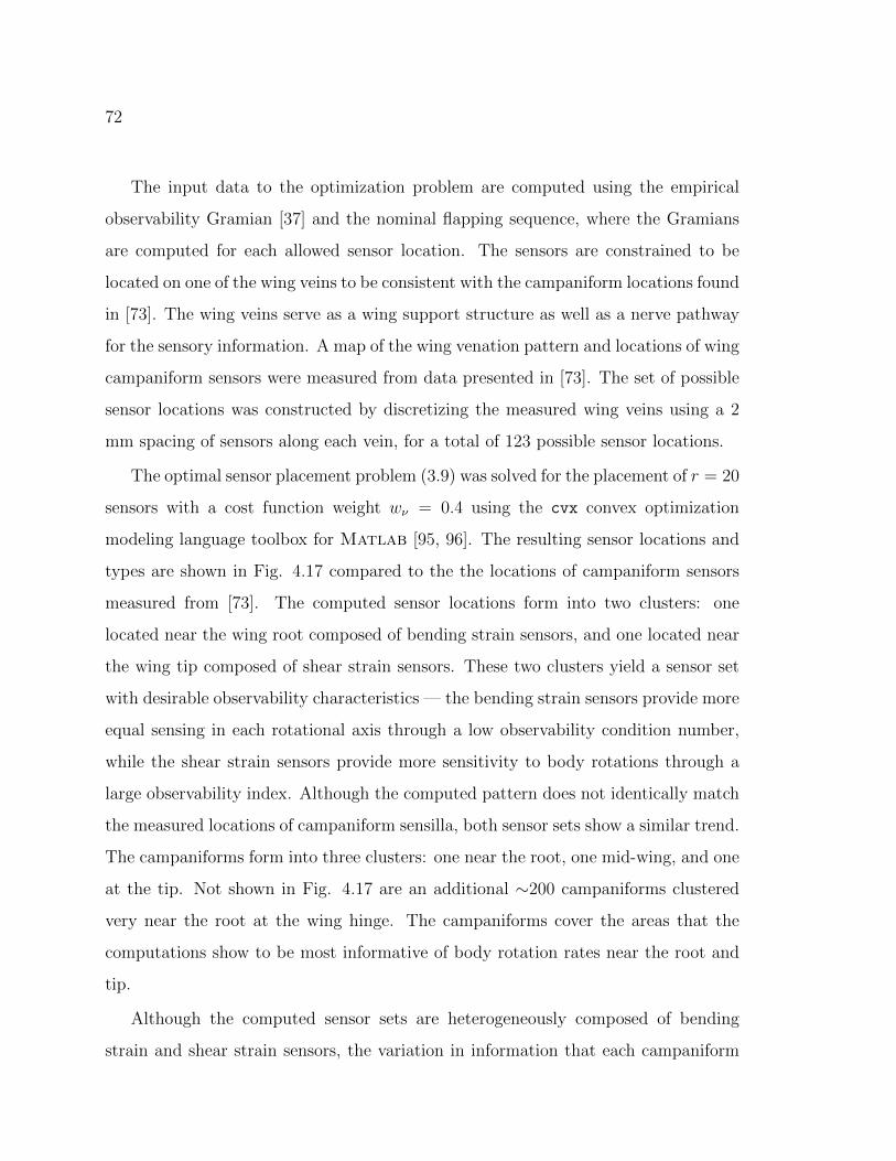
72

The input data to the optimization problem are computed using the empirical

observability Gramian [37] and the nominal flapping sequence, where the Gramians

are computed for each allowed sensor location. The sensors are constrained to be

located on one of the wing veins to be consistent with the campaniform locations found

in [73]. The wing veins serve as a wing support structure as well as a nerve pathway

for the sensory information. A map of the wing venation pattern and locations of wing

campaniform sensors were measured from data presented in [73]. The set of possible

sensor locations was constructed by discretizing the measured wing veins using a 2

mm spacing of sensors along each vein, for a total of 123 possible sensor locations.

The optimal sensor placement problem (3.9) was solved for the placement of r = 20

sensors with a cost function weight wν = 0.4 using the cvx convex optimization

modeling language toolbox for Matlab [95, 96]. The resulting sensor locations and

types are shown in Fig. 4.17 compared to the the locations of campaniform sensors

measured from [73]. The computed sensor locations form into two clusters: one

located near the wing root composed of bending strain sensors, and one located near

the wing tip composed of shear strain sensors. These two clusters yield a sensor set

with desirable observability characteristics — the bending strain sensors provide more

equal sensing in each rotational axis through a low observability condition number,

while the shear strain sensors provide more sensitivity to body rotations through a

large observability index. Although the computed pattern does not identically match

the measured locations of campaniform sensilla, both sensor sets show a similar trend.

The campaniforms form into three clusters: one near the root, one mid-wing, and one

at the tip. Not shown in Fig. 4.17 are an additional ∼200 campaniforms clustered

very near the root at the wing hinge. The campaniforms cover the areas that the

computations show to be most informative of body rotation rates near the root and

tip.

Although the computed sensor sets are heterogeneously composed of bending

strain and shear strain sensors, the variation in information that each campaniform

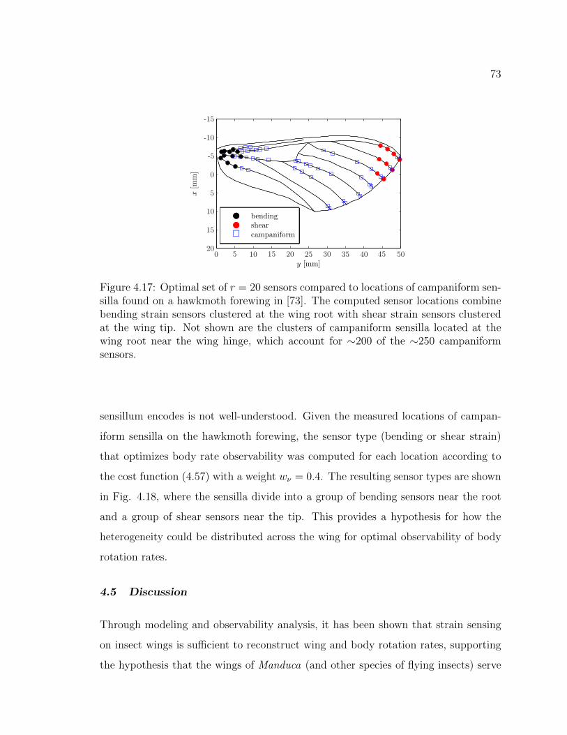
73

Figure 4.17: Optimal set of r = 20 sensors compared to locations of campaniform sen-silla found on a hawkmoth forewing in [73]. The computed sensor locations combinebending strain sensors clustered at the wing root with shear strain sensors clusteredat the wing tip. Not shown are the clusters of campaniform sensilla located at thewing root near the wing hinge, which account for ∼200 of the ∼250 campaniformsensors.

sensillum encodes is not well-understood. Given the measured locations of campan-

iform sensilla on the hawkmoth forewing, the sensor type (bending or shear strain)

that optimizes body rate observability was computed for each location according to

the cost function (4.57) with a weight wν = 0.4. The resulting sensor types are shown

in Fig. 4.18, where the sensilla divide into a group of bending sensors near the root

and a group of shear sensors near the tip. This provides a hypothesis for how the

heterogeneity could be distributed across the wing for optimal observability of body

rotation rates.

4.5 Discussion

Through modeling and observability analysis, it has been shown that strain sensing

on insect wings is sufficient to reconstruct wing and body rotation rates, supporting

the hypothesis that the wings of Manduca (and other species of flying insects) serve

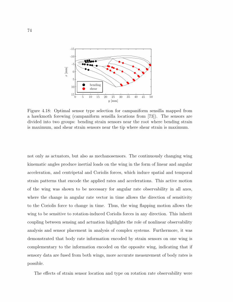
74

Figure 4.18: Optimal sensor type selection for campaniform sensilla mapped froma hawkmoth forewing (campaniform sensilla locations from [73]). The sensors aredivided into two groups: bending strain sensors near the root where bending strainis maximum, and shear strain sensors near the tip where shear strain is maximum.

not only as actuators, but also as mechanosensors. The continuously changing wing

kinematic angles produce inertial loads on the wing in the form of linear and angular

acceleration, and centripetal and Coriolis forces, which induce spatial and temporal

strain patterns that encode the applied rates and accelerations. This active motion

of the wing was shown to be necessary for angular rate observability in all axes,

where the change in angular rate vector in time allows the direction of sensitivity

to the Coriolis force to change in time. Thus, the wing flapping motion allows the

wing to be sensitive to rotation-induced Coriolis forces in any direction. This inherit

coupling between sensing and actuation highlights the role of nonlinear observability

analysis and sensor placement in analysis of complex systems. Furthermore, it was

demonstrated that body rate information encoded by strain sensors on one wing is

complementary to the information encoded on the opposite wing, indicating that if

sensory data are fused from both wings, more accurate measurement of body rates is

possible.

The effects of strain sensor location and type on rotation rate observability were

75

analyzed via the empirical observability Gramian. The most information about body

rotation rates was found to be encoded as shear strain due to wing twisting, and

sensors near the wing tip were found to be best positioned to measure the shear

strain. The shear strain energy is dominant due to the pronounced twisting during

wing pronation and supination. The timing and magnitude of the wing twist are

perturbed by body rotation disturbances, which allows these disturbances to be easily

detected from a time history of shear strain. Although wing bending strain provides

less information about body rotation rates, these sensors are more equally sensitive

to rotations in each of the three body axes. A well-balanced combination of shear

strain and bending strain sensors provides large amounts of information about body

rotation rates that is not directionally sensitive.

The observability-based optimal sensor placement problem was solved for strain

sensor locations and types along the Manduca forewing. The optimal sensor set

consisted of two clusters of sensors — one cluster of shear strain sensors near the wing

tip and one cluster of bending strain sensors near the wing root. The campaniform

sensilla mapped from a hawkmoth forewing also contain a large cluster of sensors

near the wing root, and pairs of sensors on each wing vein at the wing tip, suggesting

that these sensor sets could be used for measuring body rotation rates. The fact that

the true campaniform locations are not predicted by the observability-based sensor

placement is not surprising due to the fact that strain measurements likely serve

multiple sensory roles. Here, sensor location and type were optimized for observing

rotation rates, but the same strain information is useful for proprioceptive sensing

for, e.g., wing-beat timing [77, 97]. Nevertheless, the campaniform sensilla on the

hawkmoth forewing cover the areas with the most information about body rotation

rates and, thus, are well-placed for the wings to serve as gyroscopic sensors. The

relative composition of shear and bending sensors is dependent on the weighting

in the observability-based cost function. A high weighting on the unobservability

index results in larger portion of shear strain sensors due to more body rotation rate

76

information encoded through wing twisting. A low weight results in a more bending

strain sensors that more evenly measure rotation rates in each axis.

The directional sensitivity of strain sensors is an interesting component to the sen-

sor placement results. The campaniform sensilla found on insect wings and halteres

have two levels of signal filtering — a biomechanical filter due to the geometry and

material makeup of the campaniform structure, and neural filtering on the strain-

induced signals [98]. The observability tools utilized in this work may be a useful

complement to a neural study to hypothesize campaniform directional sensitivity and

interpret sensing capabilities for discovered campaniform biomechanical and neural

properties. Properties of the neural filtering may be discovered by the sensor com-

pression problem detailed in Chapter 3, which is an interesting avenue for future

work.

77

Chapter 5

ROBOTIC NAVIGATION WITH LIMITED SENSORS:OBSERVABILITY-BASED GUIDANCE TRAJECTORIES

It is apparent from the observability measures detailed in Chapter 2 that the

system nominal trajectory (x0(t),u0(t)) has an impact on the observability measure

and, thus, the estimation performance. In some cases, the proper choice of trajectory

changes the system from unobservable to observable (e.g., when control actuation is

required due to the presence of Lfih in the observation space O). In this chapter, the

observability measures are used to develop guidance trajectories for robot navigation.

In particular, the focus is centered on robotic navigation with limited inertial sensors,

where active vehicle motion is used to improve navigation capabilities. First, the

observability-based guidance problem is formally stated in Section 5.1. Analytical so-

lutions to the observability-based guidance problem for four different robot navigation

scenarios are presented. Trajectories for uniform flow field identification are devel-

oped in Section 5.2, followed by range-only and bearing-only guidance trajectories in

Sections 5.3 and 5.4. The guidance trajectories are generalized to higher-dimensional

nonholonomic models of robot motion in Section 5.5. Finally, the optimal trajectories

are demonstrated in simulation to improve estimation performance in Section 5.6.

5.1 Problem Statement

Many vehicles are forced to operate with limited inertial sensing due to environmental

restrictions or economic infeasibility. In the underwater environment, for example, a

common form of navigation is through the use of a single ranging beacon. Vehicles

operating in GPS-denied or GPS-degraded environments, such as indoors, urban ar-

78

eas, or in the presence of GPS jamming must resort to other sensors for localization

such as vision-based bearing measurements. In all of these cases, complete inertial

position and orientation data are unavailable and must be reconstructed using an es-

timator. Because the vehicle path affects the quality of information collected by the

limited set of sensors, an observability-based guidance scheme can be used to improve

navigation capabilities. In this section, the observability-based guidance problem is

formally stated for vehicles navigating with limited inertial sensors.

5.1.1 Motivating example

The observability-based guidance problem was inspired by the first unmanned flight

across the Atlantic by the Aerosonde [99]. The Aerosonde was able to cross the

Atlantic with limited sensor information and no communication with a ground station

for the majority of the flight. An on-board GPS unit was used to measure inertial

position and velocity during the flight and a pitot probe measured airspeed, however,

no compass was installed due to payload restrictions. The standard method of wind

calculation through vector subtraction, Vw = Vg − Va, was therefore not possible

due to unknown heading information. The Aerosonde instead used ingenuitive flight

path planning to sample the wind at different headings. The aircraft made 90-degree

turns in flight to obtain ground speed measurements at different headings, which

allowed the wind vector to be triangulated as depicted in Fig. 5.1. Note that if

the planned trajectory is a straight, constant speed path, then the measured ground

velocity vectors will be identical at every point, therefore the wind velocity vector

cannot be determined using straight flight paths.

The Aerosonde problem demonstrates the inherit coupling between sensing and

actuation in nonlinear systems — the system observability is dependent upon the

choice of trajectory. Observability-based guidance considers the question: what is

the most informative way to move the vehicle? This problem can be formally stated

using the observability measures developed in Chapter 2.

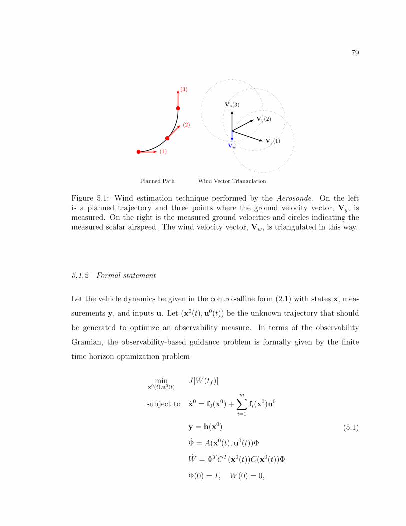
79

Figure 5.1: Wind estimation technique performed by the Aerosonde. On the leftis a planned trajectory and three points where the ground velocity vector, Vg, ismeasured. On the right is the measured ground velocities and circles indicating themeasured scalar airspeed. The wind velocity vector, Vw, is triangulated in this way.

5.1.2 Formal statement

Let the vehicle dynamics be given in the control-affine form (2.1) with states x, mea-

surements y, and inputs u. Let (x0(t),u0(t)) be the unknown trajectory that should

be generated to optimize an observability measure. In terms of the observability

Gramian, the observability-based guidance problem is formally given by the finite

time horizon optimization problem

minx0(t),u0(t)

J [W (tf )]

subject to x0 = f0(x0) +m∑i=1

fi(x0)u0

y = h(x0)

Φ = A(x0(t),u0(t))Φ

W = ΦTCT (x0(t))C(x0(t))Φ

Φ(0) = I, W (0) = 0,

(5.1)

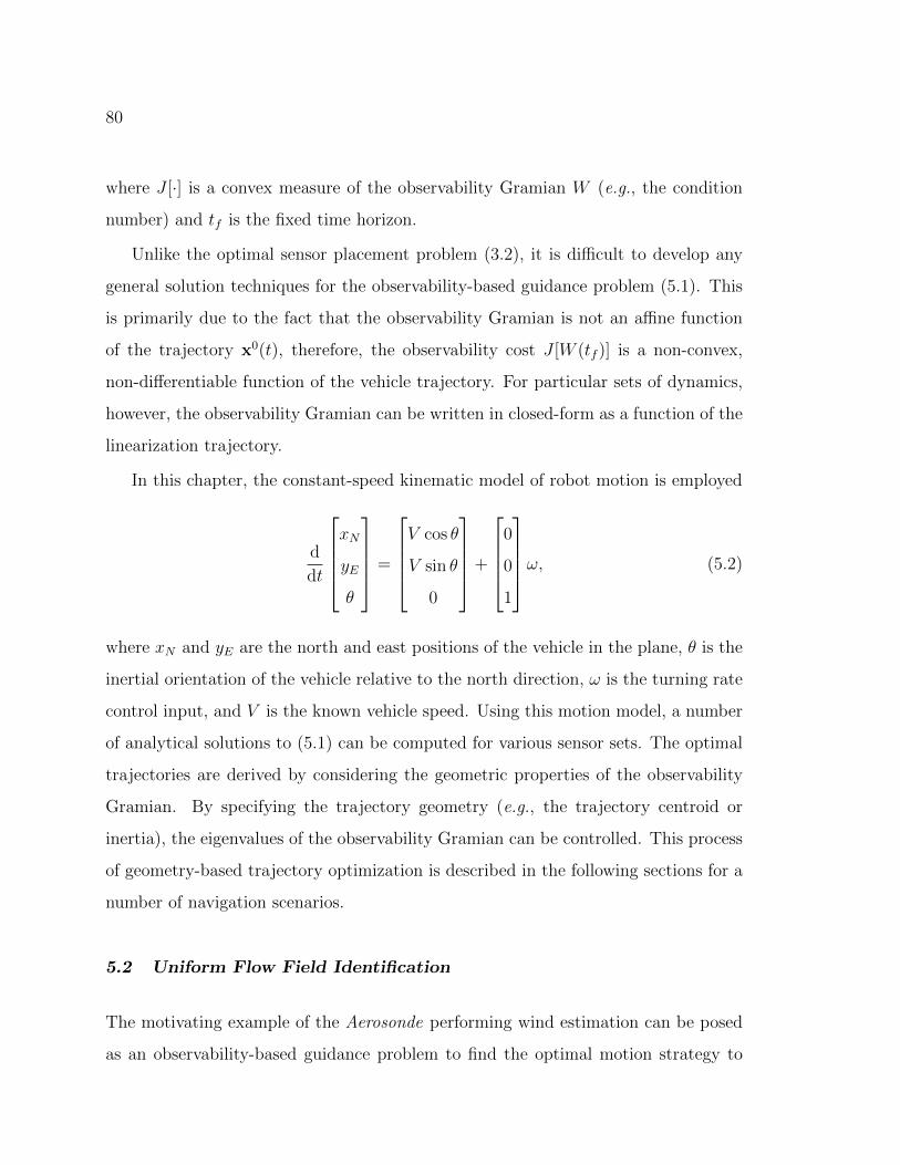
80

where J [·] is a convex measure of the observability Gramian W (e.g., the condition

number) and tf is the fixed time horizon.

Unlike the optimal sensor placement problem (3.2), it is difficult to develop any

general solution techniques for the observability-based guidance problem (5.1). This

is primarily due to the fact that the observability Gramian is not an affine function

of the trajectory x0(t), therefore, the observability cost J [W (tf )] is a non-convex,

non-differentiable function of the vehicle trajectory. For particular sets of dynamics,

however, the observability Gramian can be written in closed-form as a function of the

linearization trajectory.

In this chapter, the constant-speed kinematic model of robot motion is employed

d

dt

xN

yE

θ

=

V cos θ

V sin θ

0

+

0

0

1

ω, (5.2)

where xN and yE are the north and east positions of the vehicle in the plane, θ is the

inertial orientation of the vehicle relative to the north direction, ω is the turning rate

control input, and V is the known vehicle speed. Using this motion model, a number

of analytical solutions to (5.1) can be computed for various sensor sets. The optimal

trajectories are derived by considering the geometric properties of the observability

Gramian. By specifying the trajectory geometry (e.g., the trajectory centroid or

inertia), the eigenvalues of the observability Gramian can be controlled. This process

of geometry-based trajectory optimization is described in the following sections for a

number of navigation scenarios.

5.2 Uniform Flow Field Identification

The motivating example of the Aerosonde performing wind estimation can be posed

as an observability-based guidance problem to find the optimal motion strategy to

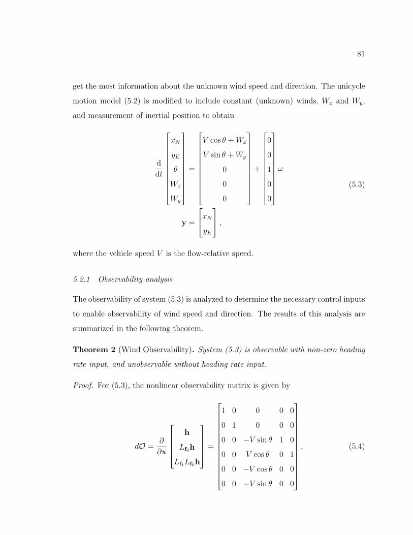
81

get the most information about the unknown wind speed and direction. The unicycle

motion model (5.2) is modified to include constant (unknown) winds, Wx and Wy,

and measurement of inertial position to obtain

d

dt

xN

yE

θ

Wx

Wy

=

V cos θ +Wx

V sin θ +Wy

0

0

0

+

0

0

1

0

0

ω

y =

xNyE

,

(5.3)

where the vehicle speed V is the flow-relative speed.

5.2.1 Observability analysis

The observability of system (5.3) is analyzed to determine the necessary control inputs

to enable observability of wind speed and direction. The results of this analysis are

summarized in the following theorem.

Theorem 2 (Wind Observability). System (5.3) is observable with non-zero heading

rate input, and unobservable without heading rate input.

Proof. For (5.3), the nonlinear observability matrix is given by

dO =∂

∂x

h

Lf0h

Lf1Lf0h

=

1 0 0 0 0

0 1 0 0 0

0 0 −V sin θ 1 0

0 0 V cos θ 0 1

0 0 −V cos θ 0 0

0 0 −V sin θ 0 0

, (5.4)

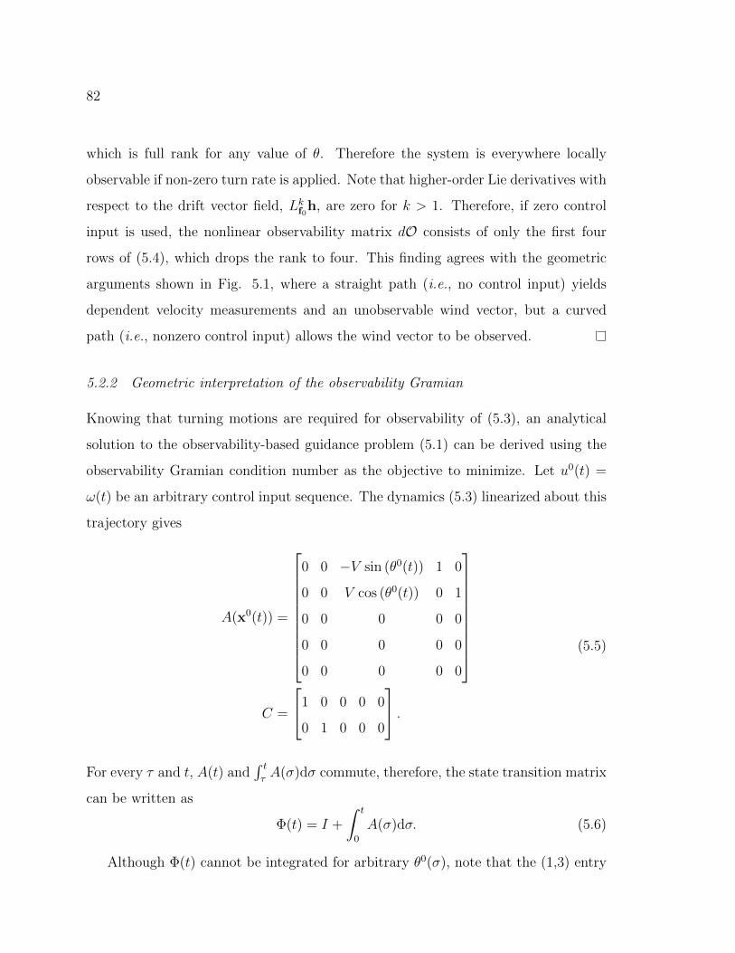
82

which is full rank for any value of θ. Therefore the system is everywhere locally

observable if non-zero turn rate is applied. Note that higher-order Lie derivatives with

respect to the drift vector field, Lkf0h, are zero for k > 1. Therefore, if zero control

input is used, the nonlinear observability matrix dO consists of only the first four

rows of (5.4), which drops the rank to four. This finding agrees with the geometric

arguments shown in Fig. 5.1, where a straight path (i.e., no control input) yields

dependent velocity measurements and an unobservable wind vector, but a curved

path (i.e., nonzero control input) allows the wind vector to be observed.

5.2.2 Geometric interpretation of the observability Gramian

Knowing that turning motions are required for observability of (5.3), an analytical

solution to the observability-based guidance problem (5.1) can be derived using the

observability Gramian condition number as the objective to minimize. Let u0(t) =

ω(t) be an arbitrary control input sequence. The dynamics (5.3) linearized about this

trajectory gives

A(x0(t)) =

0 0 −V sin (θ0(t)) 1 0

0 0 V cos (θ0(t)) 0 1

0 0 0 0 0

0 0 0 0 0

0 0 0 0 0

C =

1 0 0 0 0

0 1 0 0 0

.

(5.5)

For every τ and t, A(t) and∫ tτA(σ)dσ commute, therefore, the state transition matrix

can be written as

Φ(t) = I +

∫ t

0

A(σ)dσ. (5.6)

Although Φ(t) cannot be integrated for arbitrary θ0(σ), note that the (1,3) entry

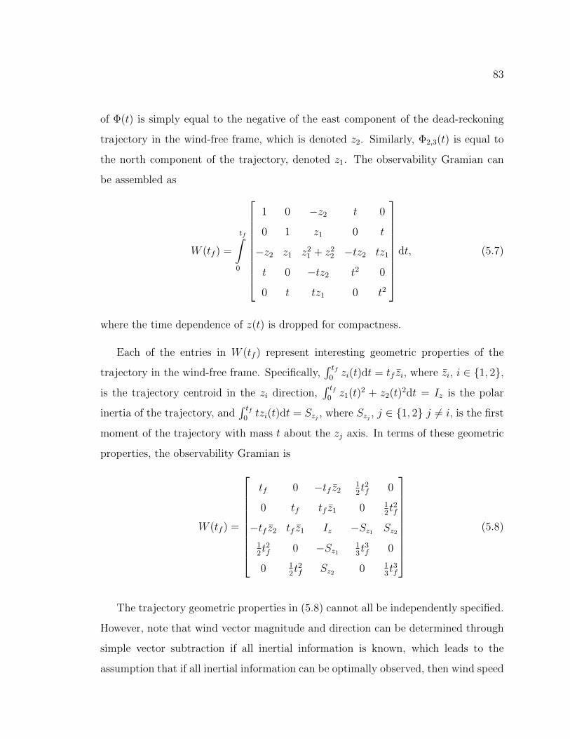
83

of Φ(t) is simply equal to the negative of the east component of the dead-reckoning

trajectory in the wind-free frame, which is denoted z2. Similarly, Φ2,3(t) is equal to

the north component of the trajectory, denoted z1. The observability Gramian can

be assembled as

W (tf ) =

tf∫0

1 0 −z2 t 0

0 1 z1 0 t

−z2 z1 z21 + z2

2 −tz2 tz1

t 0 −tz2 t2 0

0 t tz1 0 t2

dt, (5.7)

where the time dependence of z(t) is dropped for compactness.

Each of the entries in W (tf ) represent interesting geometric properties of the

trajectory in the wind-free frame. Specifically,∫ tf

0zi(t)dt = tf zi, where zi, i ∈ 1, 2,

is the trajectory centroid in the zi direction,∫ tf

0z1(t)2 + z2(t)2dt = Iz is the polar

inertia of the trajectory, and∫ tf

0tzi(t)dt = Szj , where Szj , j ∈ 1, 2 j 6= i, is the first

moment of the trajectory with mass t about the zj axis. In terms of these geometric

properties, the observability Gramian is

W (tf ) =

tf 0 −tf z212t2f 0

0 tf tf z1 0 12t2f

−tf z2 tf z1 Iz −Sz1 Sz212t2f 0 −Sz1 1

3t3f 0

0 12t2f Sz2 0 1

3t3f

(5.8)

The trajectory geometric properties in (5.8) cannot all be independently specified.

However, note that wind vector magnitude and direction can be determined through

simple vector subtraction if all inertial information is known, which leads to the

assumption that if all inertial information can be optimally observed, then wind speed

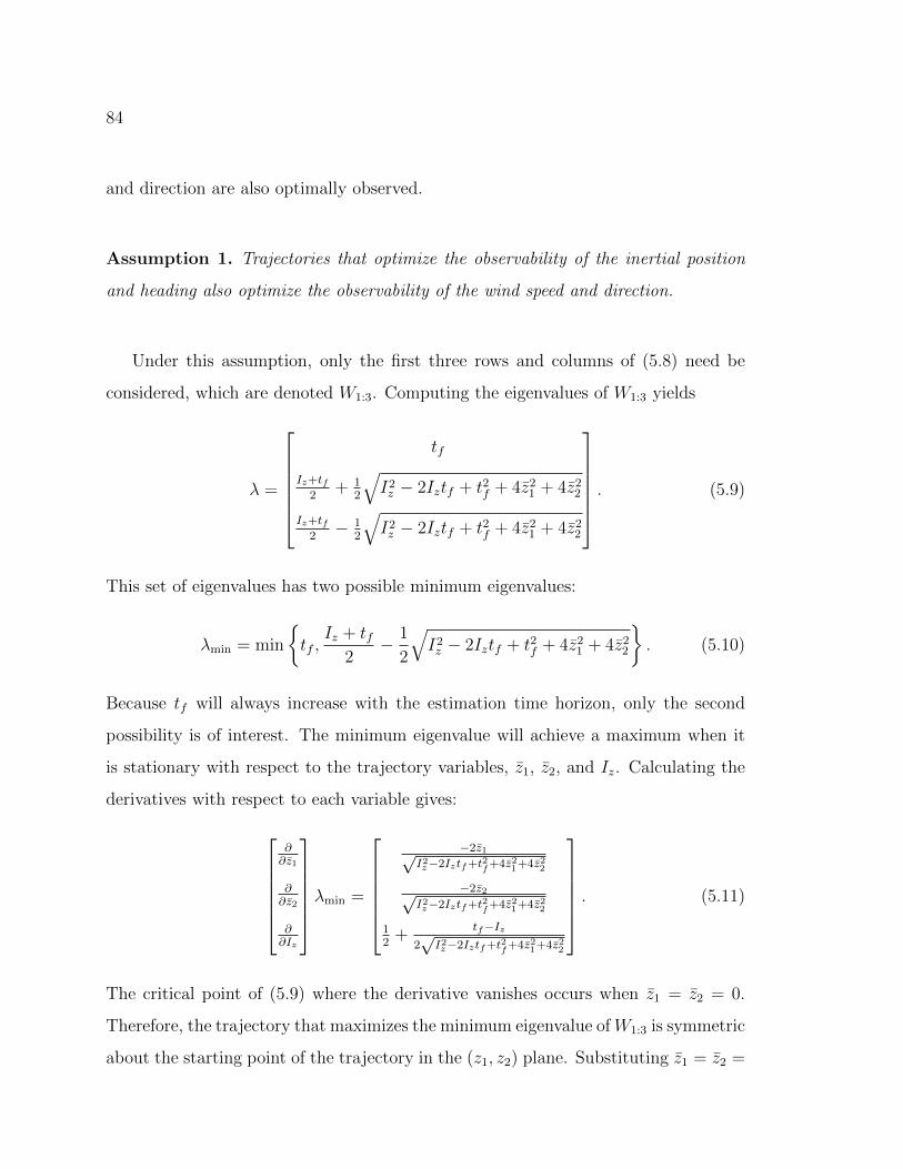
84

and direction are also optimally observed.

Assumption 1. Trajectories that optimize the observability of the inertial position

and heading also optimize the observability of the wind speed and direction.

Under this assumption, only the first three rows and columns of (5.8) need be

considered, which are denoted W1:3. Computing the eigenvalues of W1:3 yields

λ =

tf

Iz+tf2

+ 12

√I2z − 2Iztf + t2f + 4z2

1 + 4z22

Iz+tf2− 1

2

√I2z − 2Iztf + t2f + 4z2

1 + 4z22

. (5.9)

This set of eigenvalues has two possible minimum eigenvalues:

λmin = min

tf ,

Iz + tf2− 1

2

√I2z − 2Iztf + t2f + 4z2

1 + 4z22

. (5.10)

Because tf will always increase with the estimation time horizon, only the second

possibility is of interest. The minimum eigenvalue will achieve a maximum when it

is stationary with respect to the trajectory variables, z1, z2, and Iz. Calculating the

derivatives with respect to each variable gives:

∂∂z1

∂∂z2

∂∂Iz

λmin =

−2z1√

I2z−2Iztf+t2f+4z21+4z22

−2z2√I2z−2Iztf+t2f+4z21+4z22

12

+tf−Iz

2√I2z−2Iztf+t2f+4z21+4z22

. (5.11)

The critical point of (5.9) where the derivative vanishes occurs when z1 = z2 = 0.

Therefore, the trajectory that maximizes the minimum eigenvalue ofW1:3 is symmetric

about the starting point of the trajectory in the (z1, z2) plane. Substituting z1 = z2 =

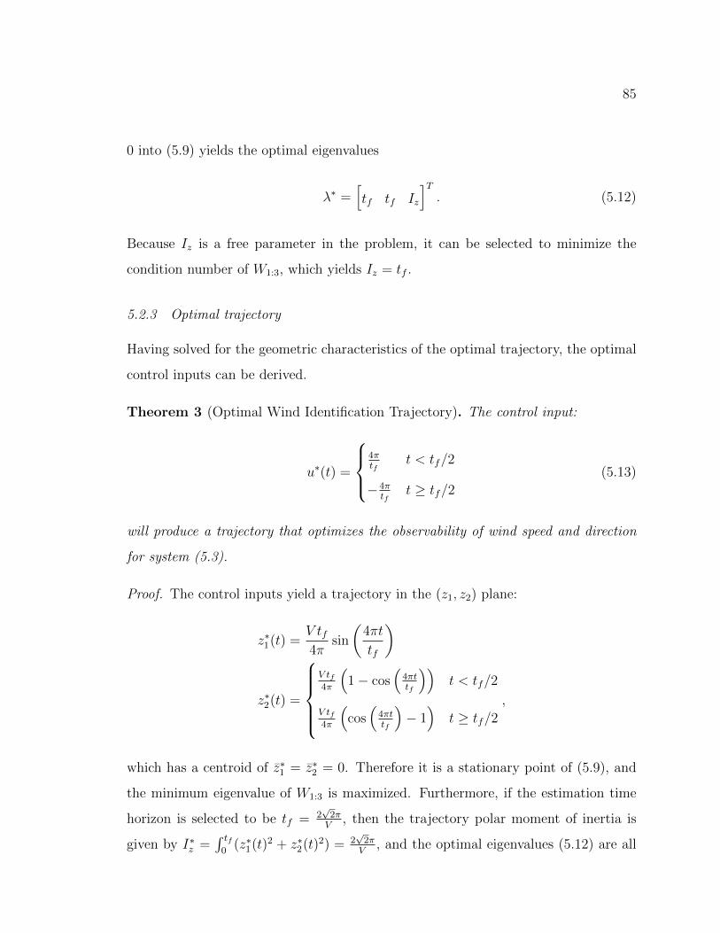
85

0 into (5.9) yields the optimal eigenvalues

λ∗ =[tf tf Iz

]T. (5.12)

Because Iz is a free parameter in the problem, it can be selected to minimize the

condition number of W1:3, which yields Iz = tf .

5.2.3 Optimal trajectory

Having solved for the geometric characteristics of the optimal trajectory, the optimal

control inputs can be derived.

Theorem 3 (Optimal Wind Identification Trajectory). The control input:

u∗(t) =

4πtf

t < tf/2

−4πtf

t ≥ tf/2

(5.13)

will produce a trajectory that optimizes the observability of wind speed and direction

for system (5.3).

Proof. The control inputs yield a trajectory in the (z1, z2) plane:

z∗1(t) =V tf4π

sin

(4πt

tf

)

z∗2(t) =

V tf4π

(1− cos

(4πttf

))t < tf/2

V tf4π

(cos(

4πttf

)− 1)

t ≥ tf/2

,

which has a centroid of z∗1 = z∗2 = 0. Therefore it is a stationary point of (5.9), and

the minimum eigenvalue of W1:3 is maximized. Furthermore, if the estimation time

horizon is selected to be tf = 2√

2πV

, then the trajectory polar moment of inertia is

given by I∗z =∫ tf

0(z∗1(t)2 + z∗2(t)2) = 2

√2πV

, and the optimal eigenvalues (5.12) are all

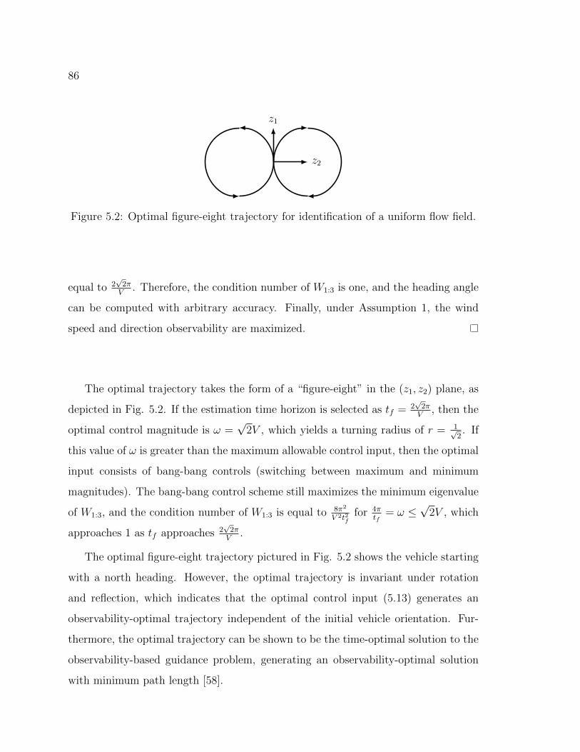
86

z1

z2

Figure 5.2: Optimal figure-eight trajectory for identification of a uniform flow field.

equal to 2√

2πV

. Therefore, the condition number of W1:3 is one, and the heading angle

can be computed with arbitrary accuracy. Finally, under Assumption 1, the wind

speed and direction observability are maximized.

The optimal trajectory takes the form of a “figure-eight” in the (z1, z2) plane, as

depicted in Fig. 5.2. If the estimation time horizon is selected as tf = 2√

2πV

, then the

optimal control magnitude is ω =√

2V , which yields a turning radius of r = 1√2. If

this value of ω is greater than the maximum allowable control input, then the optimal

input consists of bang-bang controls (switching between maximum and minimum

magnitudes). The bang-bang control scheme still maximizes the minimum eigenvalue

of W1:3, and the condition number of W1:3 is equal to 8π2

V 2t2ffor 4π

tf= ω ≤

√2V , which

approaches 1 as tf approaches 2√

2πV

.

The optimal figure-eight trajectory pictured in Fig. 5.2 shows the vehicle starting

with a north heading. However, the optimal trajectory is invariant under rotation

and reflection, which indicates that the optimal control input (5.13) generates an

observability-optimal trajectory independent of the initial vehicle orientation. Fur-

thermore, the optimal trajectory can be shown to be the time-optimal solution to the

observability-based guidance problem, generating an observability-optimal solution

with minimum path length [58].

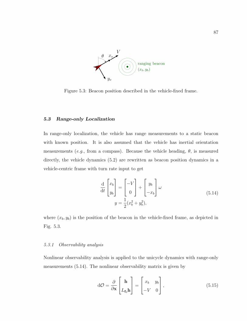
87

xv

yv

Vθ

ranging beacon

(xb, yb)

Figure 5.3: Beacon position described in the vehicle-fixed frame.

5.3 Range-only Localization

In range-only localization, the vehicle has range measurements to a static beacon

with known position. It is also assumed that the vehicle has inertial orientation

measurements (e.g., from a compass). Because the vehicle heading, θ, is measured

directly, the vehicle dynamics (5.2) are rewritten as beacon position dynamics in a

vehicle-centric frame with turn rate input to get

d

dt

xbyb

=

−V0

+

yb

−xb

ωy =

1

2(x2

b + y2b ),

(5.14)

where (xb, yb) is the position of the beacon in the vehicle-fixed frame, as depicted in

Fig. 5.3.

5.3.1 Observability analysis

Nonlinear observability analysis is applied to the unicycle dynamics with range-only

measurements (5.14). The nonlinear observability matrix is given by

dO =∂

∂x

h

Lf0h

=

xb yb

−V 0

, (5.15)

88

which is full rank as long as V yb 6= 0. As a note, the Lie derivative with respect to the

control vector field, Lf1h, is identically zero, therefore turning input does not alter

system observability. The observability matrix drops rank under two conditions: if

V 6= 0 (i.e the vehicle is not moving) or if yb = 0 (i.e., the vehicle heading is aligned

with the beacon). The first case (V = 0) causes the system to be unobservable because

a single range measurement does not uniquely localize the vehicle. The second case

(yb = 0) causes dO to drop rank because the system evolves on a lower-dimensional

manifold when the beacon is aligned with the vehicle heading. In this scenario, the

lower-dimensional dynamics are given by

xb = ±V

y =1

2x2b ,

(5.16)

where the sign of V is determined by the vehicle heading. These lower-dimensional

dynamics are still locally observable, therefore, system (5.14) is everywhere locally

observable if the vehicle is moving with non-zero speed.

Although the system is locally observable during straight-path motions, the ob-

servability matrix is poorly conditioned when the vehicle heading is nearly aligned

with the landmark due to the symmetry in the range-only navigation problem, as

depicted in Fig. 5.4. Straight paths are indistinguishable from a path mirrored about

the landmark, and the close proximity of two indistinguishable paths results in an

ill-conditioned estimation problem.

5.3.2 Optimal trajectory

Similar to the procedure employed for flow field identification in Section 5.2, the

observability Gramian for range-only localization can be computed in closed-form as

a function of the vehicle trajectory. Linearizing system (5.14) about an arbitrary

89

yE

xN

ranging landmark

line o

f sym

metry

Figure 5.4: The symmetry in the range-only navigation problem causes straight linepaths to be indistinguishable from their mirrored transformation about a parallel linethrough the landmark.

input u0(t) = ω(t) and state trajectory (x0b(t), y

0b (t)) results in the LTV system

d

dt

xbyb

=

0 u0(t)

−u0(t) 0

xbyb

y =

[x0b(t) y0

b (t)]xb

yb

.(5.17)

The corresponding state transition matrix is given by

Φ(t) =

cos θ0(t) sin θ0(t)

− sin θ0(t) cos θ0(t)

, (5.18)

where θ0(t) is the vehicle heading over the linearization trajectory. Computing the

observability Gramian as a function of the linearization trajectory gives

W (tf ) =

tf∫0

x2N(t) xN(t)yE(t)

xN(t)yE(t) y2E(t)

dt, (5.19)

90

where (xN(t), yE(t)) is the nominal trajectory of the vehicle relative to the beacon in

the inertial frame. Therefore, the observability Gramian is an explicit function of the

inertial vehicle trajectory, which can be computed to optimize the eigenvalues of the

observability Gramian.

Theorem 4 (Optimal Range-Only Localization Trajectory). A circular trajectory

centered at the beacon with radius ρxN(t)

yE(t)

=

ρ cos(2πt/tf )

ρ sin(2πt/tf )

t ∈[0 tf

]

will minimize the condition number of the observability Gramian for the range-only

localization system (5.14).

Proof. The trajectory gives the observability Gramian

W (tf ) =

tfρ2/(2π) 0

0 tfρ2/(2π)

which has a condition number of one, and maximizes the observability of the inertial

position given range measurements to a single beacon.

The optimal trajectory is a somewhat unintuitive result. A circular trajectory

centered at the ranging beacon will yield constant measurements, which would seem

to provide poor information about the vehicle position. However, with knowledge

of the circular trajectory, the vehicle position can be uniquely determined with the

radius of the circle (range measurement) and the vehicle heading.

5.4 Bearing-only Localization

Similar to the case of range-only localization presented in Section 5.3, the bearing-only

localization problem assumes bearing measurements to a static beacon and inertial

91

orientation measurements. Using the beacon dynamics in the vehicle-centric frame

(see Fig. 5.3), the bearing-only localization dynamics are given by

d

dt

xbyb

=

−V0

+

yb

−xb

ωy = tan−1(yb/xb),

(5.20)

where (xb, yb) is the position of the beacon in the vehicle-fixed frame, as depicted in

Fig. 5.3.

5.4.1 Observability analysis

Nonlinear observability analysis is applied to the unicycle dynamics with bearing-only

measurements (5.20). The nonlinear observability matrix is given by

dO =∂

∂x

h

Lf0h

=1

x2b + y2

b

−yb xb−V xbybx2b+y

2b

V (x2b−y2b )

x2b+y2b

, (5.21)

which has the determinant

det(dO) =V yb

(x2b + y2

b )2. (5.22)

Therefore, the observability matrix is full rank if V 6= 0 (i.e., the vehicle is moving)

and yb 6= 0 (i.e., the beacon is not aligned with the vehicle heading). As a note, the

Lie derivative with respect to the control vector field, Lf1h, is equal to −1, which

contains no state information and does not increase the span of O. Thus, turn rate

input does not alter the observability of system (5.20). Just as in the range-only

case, vehicle position is unobservable using bearing measurements if the vehicle is

not moving (V = 0). When the beacon position is aligned with the vehicle heading

92

(yb = 0), the vehicle dynamics evolve on a a lower-dimensional manifold given by

xb = ±V

y = 0,(5.23)

which are unobservable. Thus, inertial position is observable using bearing measure-

ments to a static beacon if the vehicle is moving with non-zero speed and the beacon

position is not aligned with the vehicle heading.

5.4.2 Optimal trajectory

The observability-optimal trajectory is derived by again considering the linearization

of the nonlinear dynamics (5.20) about an arbitrary trajectory (x0(t),u0(t)). Let

u0(t) = ω(t) and (x0b(t), y

0b (t)) be the linearization input and state trajectory, then

the linearized dynamics are given by (dropping the (·)0 nomenclature for clarity)

d

dt

xbyb

=

0 u(t)

−u(t) 0

xbyb

y =

1

x2b(t) + y2

b (t)

[−yb(t) xb(t)

]xbyb

.(5.24)

The corresponding state transition matrix is equivalent to the range measurement

case, given by

Φ(t) =

cos θ0(t) sin θ0(t)

− sin θ0(t) cos θ0(t)

, (5.25)

where θ0(t) is the vehicle heading over the linearization trajectory. Computing the

observability Gramian in terms of the linearization trajectory yields the expression

W (tf ) =

tf∫0

1

(x2N + y2

E)2

y2E(t) −xN(t)yE(t)

−xN(t)yE(t) x2N(t)

dt, (5.26)

93

where (xN(t), yE(t)) is the vehicle linearization trajectory relative to the beacon in

the inertial frame. The form of the observability Gramian for bearing measurements

is very similar to the form for range measurements (5.19). As a consequence, the

observability-optimal trajectory takes the form of a circle, which is proven in the

following theorem.

Theorem 5 (Optimal Bearing-Only Localization Trajectory). A circular trajectory

centered at the beacon with radius ρxN(t)

yE(t)

=

ρ cos(2πt/tf )

ρ sin(2πt/tf )

t ∈[0 tf

]

will minimize the condition number of the observability Gramian for the bearing-only

localization system (5.20).

Proof. The trajectory gives the observability Gramian

W (tf ) =

tf/(2πρ2) 0

0 tf/(2πρ2)

which has a condition number of one, and maximizes the observability of the inertial

position given bearing measurements to a single beacon.

Interestingly, the optimal trajectory is identical to the optimal range-only localiza-

tion trajectory provided in Theorem 4. Because the range and bearing measurements

are complementary, sampling one measurement along the circular trajectory enables

optimal observability of the other state. Although the trajectory produces observabil-

ity Gramians with unity condition number for both sensing modalities, the eigenvalues

of the two Gramians have different relationships with the radius ρ of the circular tra-

jectory. The eigenvalues of the observability Gramian for range-only localization are

proportional to ρ2, while the eigenvalues for bearing-only localization are inversely

94

proportional to ρ2. Thus, to increase the volume of the observation ellipsoid, larger

radius trajectories should be used in range-only localization, while smaller radius

trajectories should be used in bearing-only localization.

5.5 Generalization to Higher-Dimensional Nonholonomic Systems

The results of the previous sections considered the unicycle model for a nonholonomic

vehicle, using the geometry of the linearization trajectories to compute observability

measures. Interestingly, the observability-based trajectory generation generalizes to

higher-dimensional nonholonomic systems [100]. In this section, the unicycle model

of robotic motion (which is a first-order nonholonomic system with three states) is

generalized to more general first-order nonholonomic systems in canonical form,

x = u

zij = xiuj − xjui ∀ i, j ∈ 1, 2, . . . ,m, i > j,(5.27)

where x ∈ Rm (m ≥ 2) are the holonomic states, z ∈ Rm(m−1)/2 are the nonholonomic

states, and u ∈ Rm are the controls.

This type of system was studied in the context of geometric and optimal control

by Brockett [101] and later by Murray and Sastry [102]. This class of systems has

practical importance for several reasons. First, these systems exhibit fundamental

challenges due to the nonholonomic constraints which form the most basic, but inter-

esting nonlinearity. Second, many systems of engineering interest are diffeomorphic to

the nonholonomic integrator (e.g., the unicycle model just studied, or robotic grasp-

ing models). Finally, the properties of the nonholonomic integrator give insight into

systems with higher complexity.

95

5.5.1 Observability analysis

The class of systems described by (5.27) are first-order Lie bracket controllable, mean-

ing that the control Lie algebra constructed by the control vector fields and their

first-order Lie brackets is full rank. Because the Lie brackets are necessary to guaran-

tee full rank of the control Lie algebra, switching or area-generating controls must be

used to steer the system from an initial configuration to an arbitrary final configura-

tion. These systems also have interesting observability characteristics. Consider the

case when system (5.27) has an output function y = z. Taking Lie derivatives of the

output, we see that Lfizij = −xj and Lfjzij = xi, therefore xi and xj are observable

with measurements of zij and use of the controls ui and uj. This result leads to the

following theorems.

Theorem 6 (Canonical Form Observability). First-order nonholonomic systems in

canonical form (5.27) are observable if and only if measurements of the nonholonomic

states z are available.

Proof. If all nonholonomic states are measured, then the observability Lie algebra is

O = spanzij,−xj, xi ∀ i, j ∈ 1, 2, . . . ,m, i > j, and rank(dO) = m(m + 1)/2 =

dim(x) + dim(z), therefore the system is observable if all z states are measured and

control actuation is utilized. Now, assume that one nonholonomic state zkl is not

measured. Because zkl does not appear in the control vector fields, it will not be

observable, and rank(dO) ≤ m(m+1)/2−1, thus the system will be unobservable.

Theorem 7 (Actuation Required for Observability). System (5.27) with output y = z

is observable if and only if actuation in at least two control channels is utilized.

96

Proof. The Lie derivative of one output with respect to a control vector field is

Lfkzij =

−xj k = i

xi k = j

0 otherwise.

Because all outputs zij ∀ i, j ∈ 1, 2, . . . ,m, i > j are measured, the span of the

Lie derivative of all outputs with respect to a control vector field is spanLfiz =

spanxj ∀ j 6= i, which spans all x states except xi. Therefore, any two control

vector fields fk and fl, k 6= l, have Lie derivatives that span all x states, and the

system is observable with a minimum of two control inputs.

Corollary 1. If all z states are measured and one xi state is measured, then actuation

in ui will give an observable system.

5.5.2 Optimal trajectory

The first-order nonholonomic system in canonical form (5.27) can be rewritten as a bi-

linear system without loss of generality to facilitate the observability-based trajectory

optimization process:

x = u

z = F (u)x

y = z.

(5.28)

The matrix F (u) ∈ Rm(m−1)/2×m consists of m− 1 blocks,

F (u) =[F1(u)T F2(u)T . . . Fm−1(u)T

]T, (5.29)

97

where each block Fi(u) ∈ R(m−i)×m is given by

Fi(u) =

0(i−1) ui+1 −ui 0 . . . 0

0(i−1) ui+2 0 −ui . . . 0...

......

.... . .

...

0(i−1) um 0 0 . . . −ui

, (5.30)

and 0(i−1) is a row vector of zeros of length (i− 1). As an example, when the length

of u is three, F (u) is given by

F (u) =

u2 −u1 0

u3 0 −u1

0 u3 −u2

. (5.31)

Because the nonholonomic states z are directly measured, the goal of the trajectory

optimization is to optimize the observability Gramian associated with the holonomic

states x. Integrating to determine the output at time t gives

y(t) = z0 +

t∫0

F (u(τ))x(τ)dτ

= z0 +

t∫0

F (u(τ1))

x0 +

τ1∫0

u(τ2)dτ2

dτ1.

(5.32)

Now, collect the terms influenced by the unknown initial condition of the holonomic

states, and define a new output

η = y −

z0 +

t∫0

F (u(τ1))

τ1∫0

u(τ2)dτ2

dτ1

=

t∫0

F (u(τ1))dτ1x0 = F

t∫0

u(τ1)dτ1

x0.

(5.33)

98

For notational simplicity, define ξ(t) =∫ t

0u(τ1)dτ1. The output energy associated

with holonomic states is now

‖η(t)‖ = xT0

tf∫0

F (ξ(t))TF (ξ(t))dtx0

= xT0Wx(0, tf )x0,

(5.34)

where Wx(0, tf ) is the observability Gramian associated with the holonomic states.

Expanding the terms inside the integral gives

(F (ξ)TF (ξ)

)ij

=

−ξiξj i 6= j∑l 6=iξ2l i = j

. (5.35)

Based on the form of (5.35), the observability-optimal trajectory is computed using

the following theorem.

Theorem 8 (Optimal Nonholonomic Integrator Trajectory). Cyclic controls of the

form

u?j(t) =2πjAjtf

cos(2πjt/tf ),

and corresponding state trajectories

ξ?j (t) = Aj sin(2πjt/tf ) ∀ j ∈ 1, 2, . . . ,m

allow placement of the observability Gramian eigenvalues over the time horizon tf for

first order nonholonomic systems in canonical form (5.27) with output y = z.

Proof. First, note that∫ tf

0ξ?i (t)ξ

?j (t)dt = 0 and

∫ tf0ξ?i (t)

2dt = A2i tf/2. Substituting

99

the optimal trajectory into (5.34), the ij entry of the observability Gramian is

(Wx(0, tf ))ij =

0 i 6= j∑l 6=iA2l tf/2 i = j

.

Therefore, the observability Gramian is diagonalized, and the eigenvalues of Wx(0, tf )

can be placed using appropriate amplitudes Aj.

Remark 1. Note that the choice of integer j in the sinusoidal frequency is arbitrary.

The integer j is used as the integer frequency multiplier for state ξj for convenience

only, but any integer can be used such that no ξi and ξj have the same frequency.

The desired observability Gramian eigenvalues form a set of equations that can

be solved for the optimal state trajectory amplitudes. Extracting the diagonal of

Wx(0, tf ) yieldstf2

(11T − I

)A2 = λ, (5.36)

where 1 is a column vector of ones, A2 is a column vector of the amplitudes squared,

and λ is a column vector of desired observability Gramian eigenvalues with λi rep-

resenting the eigenvalue associated with the xi state. Showing that (11T − I) is a

full-rank matrix is straightforward, therefore the solution for A2 always exists and is

unique. Given a set of desired eigenvalues λ, the amplitudes A2 can be solved for

explicitly. Subtracting the first equation of (5.36) from the remaining equations yields

A2i = A2

1 +2

tf(λ1 − λi) ∀ i ∈ 2, 3, . . . ,m. (5.37)

Substituting these expressions back into the first equation and solving for A21 and A2

i

gives

A2i =

2

tf

(−λi +

1

(m− 1)

m∑j=1

λj

)∀ i. (5.38)

100

For this solution to be feasible the squared amplitudes must be positive, A2i ≥ 0, thus

0 < λi ≤1

(m− 2)

∑j 6=i

λj (5.39)

for a feasible solution. The constraint imposed by (5.39) essentially limits the spread

of the eigenvalues of Wx(0, tf ). The case when all λi are equivalent (i.e., a condition

number of κ(Wx(0, tf )) = 1) is always a feasible. The feasible set of eigenvalues is

the interior of a cone in the positive orthant with the vertex at the origin. When

m = 2, the constraint (5.39) does not limit the choice of λ, and the feasible set is

the entire positive orthant. When m > 2, the feasible space is enclosed by m hyper-

planes passing through the origin with equations −λi + 1/(m − 2)∑

j 6=i λj = 0. As

m increases, the cone becomes smaller, and in the limit m → ∞, the cone reduces

to the line of all λi equivalent. Practically speaking, the constraint (5.39) does not

impose undesirable limitations on the choice of λ because a condition number of one

is desirable and always feasible. Therefore, the observability Gramian eigenvalues can

be nearly arbitrarily placed to control the estimation uncertainty.

As an example, consider calculation of the optimal trajectory for the case when

m = 3. Suppose that observability Gramian eigenvalues of λ =[50 50 50

]Tare de-

sired over a time horizon of tf = 2. Then using (5.38), the state trajectory amplitudes

are

Ai =

√(−50 +

1

2(150)

)= 5, (5.40)

which results in an observability Gramian of Wx(0, 2) = diag[

50 50 50]

. Note

that the negative square root could also be chosen for the amplitude Ai (i.e., -5)

without loss of optimality. The resulting state trajectory would simply be mirrored

in the ith axis direction. The optimal trajectory traces a figure-eight in the state

space, as shown in Fig. 5.5. It is shown here with the origin of the trajectory at the

origin of the state space, but the optimal trajectory is translationally invariant, so

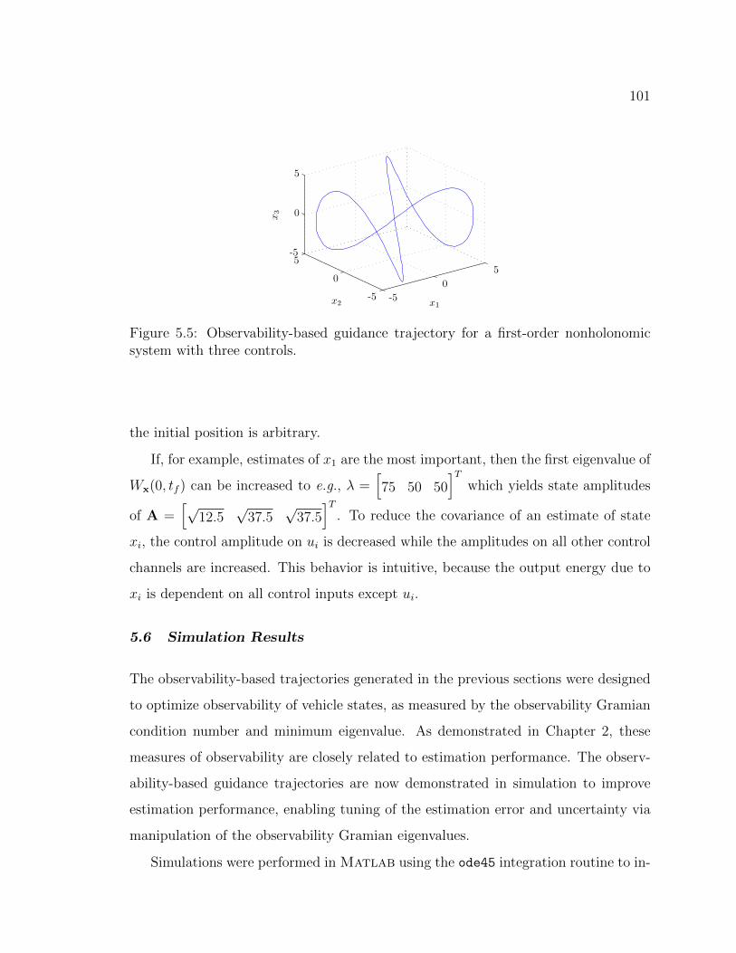
101

Figure 5.5: Observability-based guidance trajectory for a first-order nonholonomicsystem with three controls.

the initial position is arbitrary.

If, for example, estimates of x1 are the most important, then the first eigenvalue of

Wx(0, tf ) can be increased to e.g., λ =[75 50 50

]Twhich yields state amplitudes

of A =[√

12.5√

37.5√

37.5]T

. To reduce the covariance of an estimate of state

xi, the control amplitude on ui is decreased while the amplitudes on all other control

channels are increased. This behavior is intuitive, because the output energy due to

xi is dependent on all control inputs except ui.

5.6 Simulation Results

The observability-based trajectories generated in the previous sections were designed

to optimize observability of vehicle states, as measured by the observability Gramian

condition number and minimum eigenvalue. As demonstrated in Chapter 2, these

measures of observability are closely related to estimation performance. The observ-

ability-based guidance trajectories are now demonstrated in simulation to improve

estimation performance, enabling tuning of the estimation error and uncertainty via

manipulation of the observability Gramian eigenvalues.

Simulations were performed in Matlab using the ode45 integration routine to in-

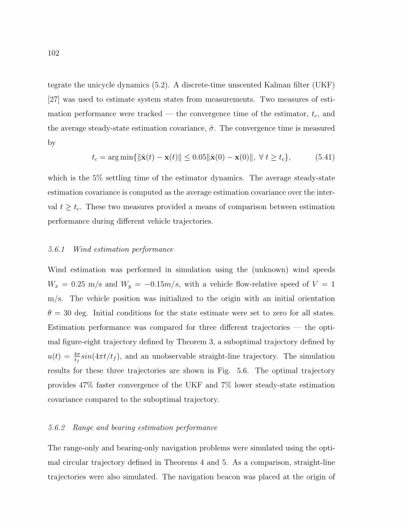
102

tegrate the unicycle dynamics (5.2). A discrete-time unscented Kalman filter (UKF)

[27] was used to estimate system states from measurements. Two measures of esti-

mation performance were tracked — the convergence time of the estimator, tc, and

the average steady-state estimation covariance, σ. The convergence time is measured

by

tc = arg min‖x(t)− x(t)‖ ≤ 0.05‖x(0)− x(0)‖, ∀ t ≥ tc, (5.41)

which is the 5% settling time of the estimator dynamics. The average steady-state

estimation covariance is computed as the average estimation covariance over the inter-

val t ≥ tc. These two measures provided a means of comparison between estimation

performance during different vehicle trajectories.

5.6.1 Wind estimation performance

Wind estimation was performed in simulation using the (unknown) wind speeds

Wx = 0.25 m/s and Wy = −0.15m/s, with a vehicle flow-relative speed of V = 1

m/s. The vehicle position was initialized to the origin with an initial orientation

θ = 30 deg. Initial conditions for the state estimate were set to zero for all states.

Estimation performance was compared for three different trajectories — the opti-

mal figure-eight trajectory defined by Theorem 3, a suboptimal trajectory defined by

u(t) = 4πtfsin(4πt/tf ), and an unobservable straight-line trajectory. The simulation

results for these three trajectories are shown in Fig. 5.6. The optimal trajectory

provides 47% faster convergence of the UKF and 7% lower steady-state estimation

covariance compared to the suboptimal trajectory.

5.6.2 Range and bearing estimation performance

The range-only and bearing-only navigation problems were simulated using the opti-

mal circular trajectory defined in Theorems 4 and 5. As a comparison, straight-line

trajectories were also simulated. The navigation beacon was placed at the origin of

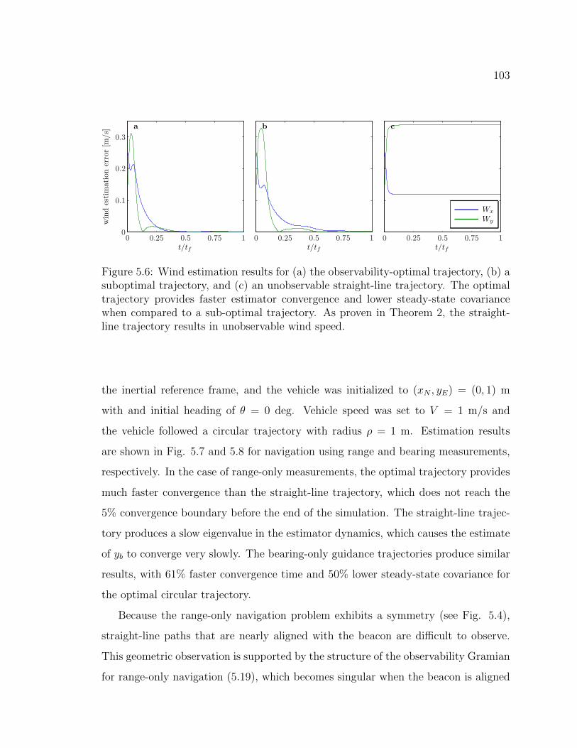
103

Figure 5.6: Wind estimation results for (a) the observability-optimal trajectory, (b) asuboptimal trajectory, and (c) an unobservable straight-line trajectory. The optimaltrajectory provides faster estimator convergence and lower steady-state covariancewhen compared to a sub-optimal trajectory. As proven in Theorem 2, the straight-line trajectory results in unobservable wind speed.

the inertial reference frame, and the vehicle was initialized to (xN , yE) = (0, 1) m

with and initial heading of θ = 0 deg. Vehicle speed was set to V = 1 m/s and

the vehicle followed a circular trajectory with radius ρ = 1 m. Estimation results

are shown in Fig. 5.7 and 5.8 for navigation using range and bearing measurements,

respectively. In the case of range-only measurements, the optimal trajectory provides

much faster convergence than the straight-line trajectory, which does not reach the

5% convergence boundary before the end of the simulation. The straight-line trajec-

tory produces a slow eigenvalue in the estimator dynamics, which causes the estimate

of yb to converge very slowly. The bearing-only guidance trajectories produce similar

results, with 61% faster convergence time and 50% lower steady-state covariance for

the optimal circular trajectory.

Because the range-only navigation problem exhibits a symmetry (see Fig. 5.4),

straight-line paths that are nearly aligned with the beacon are difficult to observe.

This geometric observation is supported by the structure of the observability Gramian

for range-only navigation (5.19), which becomes singular when the beacon is aligned

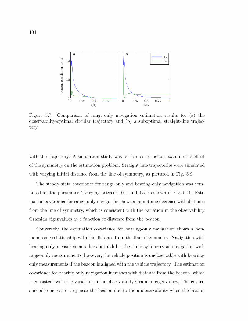
104

Figure 5.7: Comparison of range-only navigation estimation results for (a) theobservability-optimal circular trajectory and (b) a suboptimal straight-line trajec-tory.

with the trajectory. A simulation study was performed to better examine the effect

of the symmetry on the estimation problem. Straight-line trajectories were simulated

with varying initial distance from the line of symmetry, as pictured in Fig. 5.9.

The steady-state covariance for range-only and bearing-only navigation was com-

puted for the parameter δ varying between 0.01 and 0.5, as shown in Fig, 5.10. Esti-

mation covariance for range-only navigation shows a monotonic decrease with distance

from the line of symmetry, which is consistent with the variation in the observability

Gramian eigenvalues as a function of distance from the beacon.

Conversely, the estimation covariance for bearing-only navigation shows a non-

monotonic relationship with the distance from the line of symmetry. Navigation with

bearing-only measurements does not exhibit the same symmetry as navigation with

range-only measurements, however, the vehicle position is unobservable with bearing-

only measurements if the beacon is aligned with the vehicle trajectory. The estimation

covariance for bearing-only navigation increases with distance from the beacon, which

is consistent with the variation in the observability Gramian eigenvalues. The covari-

ance also increases very near the beacon due to the unobservability when the beacon

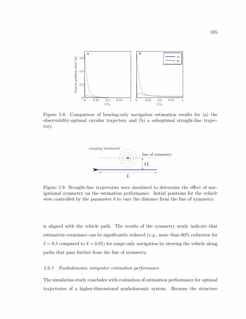
105

Figure 5.8: Comparison of bearing-only navigation estimation results for (a) theobservability-optimal circular trajectory and (b) a suboptimal straight-line trajec-tory.

ranging landmark

line of symmetry

L

δL

Figure 5.9: Straight-line trajectories were simulated to determine the effect of nav-igational symmetry on the estimation performance. Initial positions for the vehiclewere controlled by the parameter δ to vary the distance from the line of symmetry.

is aligned with the vehicle path. The results of the symmetry study indicate that

estimation covariance can be significantly reduced (e.g., more than 60% reduction for

δ = 0.5 compared to δ = 0.01) for range-only navigation by steering the vehicle along

paths that pass further from the line of symmetry.

5.6.3 Nonholonomic integrator estimation performance

The simulation study concludes with evaluation of estimation performance for optimal

trajectories of a higher-dimensional nonholonomic system. Because the structure

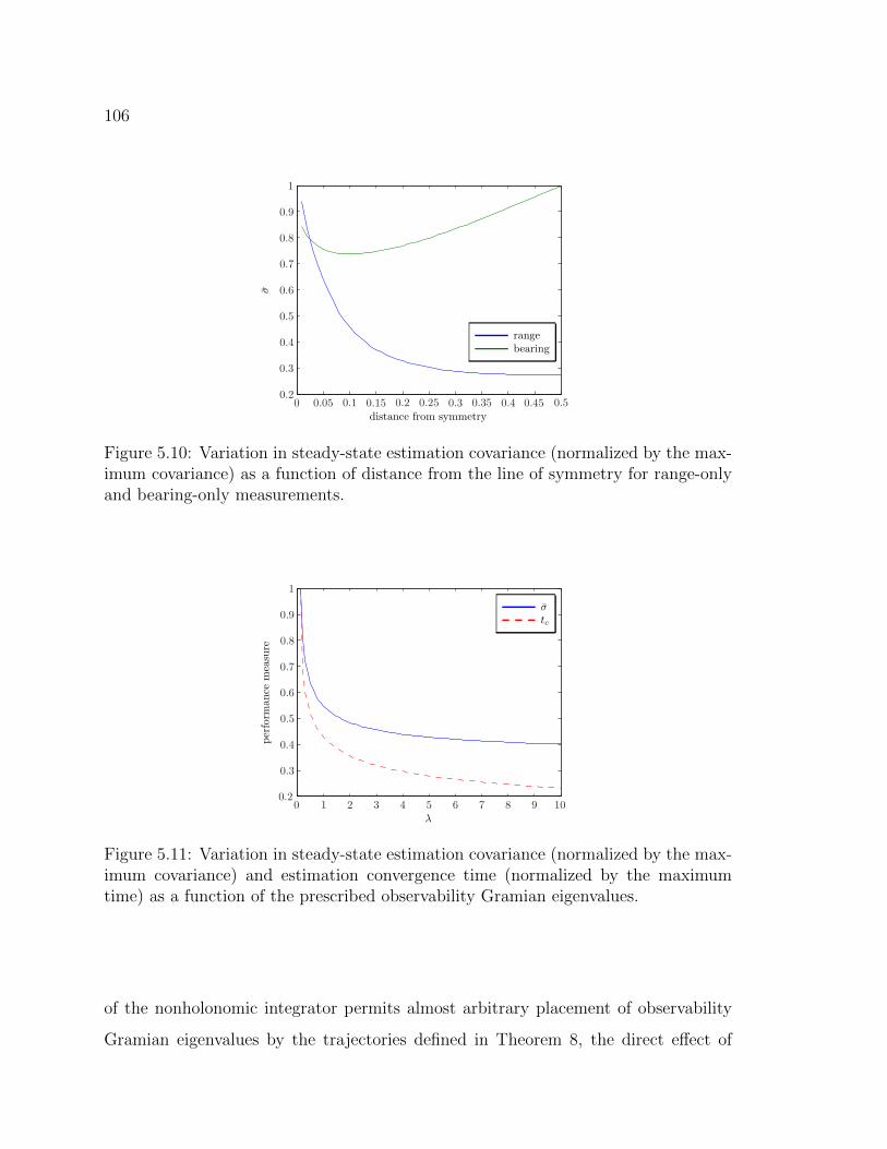
106

Figure 5.10: Variation in steady-state estimation covariance (normalized by the max-imum covariance) as a function of distance from the line of symmetry for range-onlyand bearing-only measurements.

Figure 5.11: Variation in steady-state estimation covariance (normalized by the max-imum covariance) and estimation convergence time (normalized by the maximumtime) as a function of the prescribed observability Gramian eigenvalues.

of the nonholonomic integrator permits almost arbitrary placement of observability

Gramian eigenvalues by the trajectories defined in Theorem 8, the direct effect of

107

observability Gramian eigenvalues on estimation performance could be determined.

The nonholonomic integrator dynamics (5.27) were integrated for m = 2 controls for

observability-optimal trajectories with different prescribed eigenvalues. The optimal

trajectories were computed according to Theorem 8 for eigenvalues prescribed to be

all equivalent (i.e., condition number of one) and magnitude ranging from 0.1 to

10. The resulting estimation covariances and estimator convergence times are shown

in Fig. 5.11. The results confirm that the estimation performance can be directly

controlled via manipulation of the observability Gramian eigenvalues.

108

Chapter 6

ROBOTIC NAVIGATION WITH LIMITED SENSORS:OBSERVABILITY-BASED GUIDANCE ALGORITHMS

In Chapter 5, trajectories were derived that optimize measures of observability

for robotic navigation with limited inertial sensors. These trajectories were shown

to improve estimator performance through simulation, allowing vehicle position and

orientation to be estimated more quickly and with lower uncertainty. Although the

observability-optimal trajectories provide superior localization accuracy, they are de-

signed with localization as the only objective and do not incorporate higher-level

mission objectives, such as waypoint following or sensor coverage.

In this chapter, observability-based guidance for range-only and bearing-only nav-

igation is extended to include waypoint following through initial and final constraints

on the vehicle position in the observability-based guidance problem. An observability-

based cost function is developed using the determinant of the inverse of the nonlinear

observability matrix, and a guidance framework is presented that enables path plan-

ning between waypoints using an explicit tradeoff between path observability and

path length. The algorithm development begins with system analysis in Section 6.1,

followed by presentation of the guidance algorithm in Section 6.2. The guidance al-

gorithm is evaluated in simulation in Section 6.3 and in experiment on an underwater

robotic testbed in Section 6.4.

6.1 System Analysis

In this section, the vehicle and landmark dynamics are developed, and the observ-

ability of landmarks is analyzed. A measure of landmark observability is developed

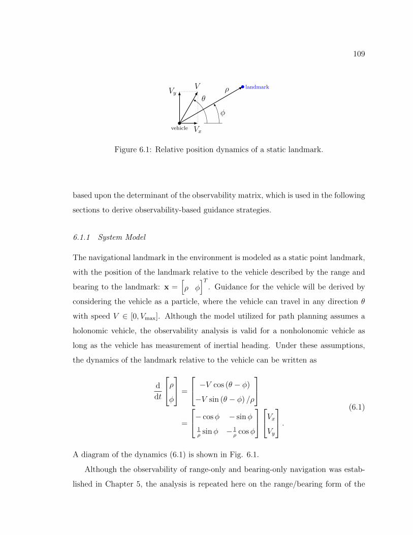
109

Vx

VyV

vehicle

landmarkρ

φ

θ

Figure 6.1: Relative position dynamics of a static landmark.

based upon the determinant of the observability matrix, which is used in the following

sections to derive observability-based guidance strategies.

6.1.1 System Model

The navigational landmark in the environment is modeled as a static point landmark,

with the position of the landmark relative to the vehicle described by the range and

bearing to the landmark: x =[ρ φ

]T. Guidance for the vehicle will be derived by

considering the vehicle as a particle, where the vehicle can travel in any direction θ

with speed V ∈ [0, Vmax]. Although the model utilized for path planning assumes a

holonomic vehicle, the observability analysis is valid for a nonholonomic vehicle as

long as the vehicle has measurement of inertial heading. Under these assumptions,

the dynamics of the landmark relative to the vehicle can be written as

d

dt

ρφ

=

−V cos (θ − φ)

−V sin (θ − φ) /ρ

=

− cosφ − sinφ

1ρ

sinφ −1ρ

cosφ

VxVy

.(6.1)

A diagram of the dynamics (6.1) is shown in Fig. 6.1.

Although the observability of range-only and bearing-only navigation was estab-

lished in Chapter 5, the analysis is repeated here on the range/bearing form of the

110

dynamics (6.1) to compute the nonlinear observability matrix that will be used in the

observability-based cost function.

6.1.2 Observability with Bearing-Only Measurements

Applying the observability test to the landmark dynamics (6.1) with bearing mea-

surement

y = φ (6.2)

yields the observability matrix

dYφ =

0 1

V sin(θ − φ)/ρ2 V cos(θ − φ)/ρ

, (6.3)

with corresponding determinant

|dYφ| = −V sin(θ − φ)/ρ2, (6.4)

which is nonzero for V 6= 0 and θ 6= φ+ kπ, k ∈ Z. Therefore, the range and bearing

to the landmark is locally observable if the vehicle is moving with nonzero speed and

the heading of the vehicle θ is not aligned with the bearing to the landmark φ (see

Fig. 6.1).

The determinant (6.4) can be maximized (or minimized) for a given state x by

moving the vehicle with heading θ? = φ± π/2 and speed V ? = Vmax. In the presence

of a static landmark, implementation of this greedy-optimal policy results in a circular

orbit about the landmark, which is equivalent to the optimal trajectory based on the

observability Gramian eigenvalues developed in Section 5.4. In the following sections,

this measure of observability will be used to derive guidance policies for waypoint

following using a single landmark for navigation.

111

6.1.3 Observability with Range-Only Measurements

Applying the nonlinear observability test to the landmark dynamics (6.1) with range

measurement

y = ρ (6.5)

yields the observability matrix

dYρ =

1 0

0 −V sin(θ − φ)

. (6.6)

Just as in the bearing case, the observability matrix drops rank when the vehicle

heading is aligned with the landmark. The rank drop results from the system dy-

namics evolving on a lower dimensional manifold when the vehicle heading is aligned

with (moving directly towards or away from) the landmark,

ρ = ±V

φ = 0,(6.7)

where the sign of V is determined by the heading of the vehicle. This lower-dimensional

system is still locally observable with range-only measurements (but not with bearing-

only measurements), therefore the landmark system is always locally observable with

range-only measurements.

Interestingly, the determinant of the observability matrix for range-only measure-

ments,

|dYρ| = −V sin(θ − φ), (6.8)

has a very similar form to the bearing-only case (6.4). The greedy-optimal strategy

to maximize the determinant again yields θ? = φ± π/2 and V ? = Vmax, which results

in a circular trajectory centered at the landmark. Again, this greedy-optimal tra-

jectory matches the optimal trajectory based upon the observability Gramian eigen-

112

values derived in Section 5.3. Using this similarity, a single framework for deriving

observability-based guidance policies is proposed for range-only and bearing-only nav-

igation.

6.2 Observability-Based Guidance for Single Landmark Navigation

The determinant of the observability matrices for bearing measurements (6.4) and

range measurements (6.8) are now used as guides to determine a waypoint guidance

policy while using a single landmark for navigation. The goal of the guidance policy

is to steer the vehicle from an initial point r0 to a final point rf while optimizing

landmark observability and maintaining the landmark in the field-of-view of a sensor.

Additionally, an algorithm is desired that allows balancing of observability objectives

and the trajectory length. Because the determinant is optimized when the vehicle

heading is perpendicular to the bearing to the landmark, a lateral facing sensor with

field-of-view α is assumed.

6.2.1 Observability Cost Function for Bearing Measurements

The guidance policy is derived by considering the vehicle path in the landmark-

centric frame, as shown in Fig. 6.2. The vehicle path is parameterized by the angle

γ ∈ [0, γf ], where γf is the interior angle between r0 and rf . The guidance trajectory

is designed by choosing ρ(γ) and β(γ) such that the observability-based cost function

is optimized. Let u = ρ tan β, then the vehicle path can be described by

dρ

dγ= u. (6.9)

Landmark observability is incorporated into the path planning problem by mini-

mizing the determinant of dY−1, which is chosen due to its relation to the volume of

the estimation uncertainty ellipsoid (see Chapter 2). For bearing-only measurements,

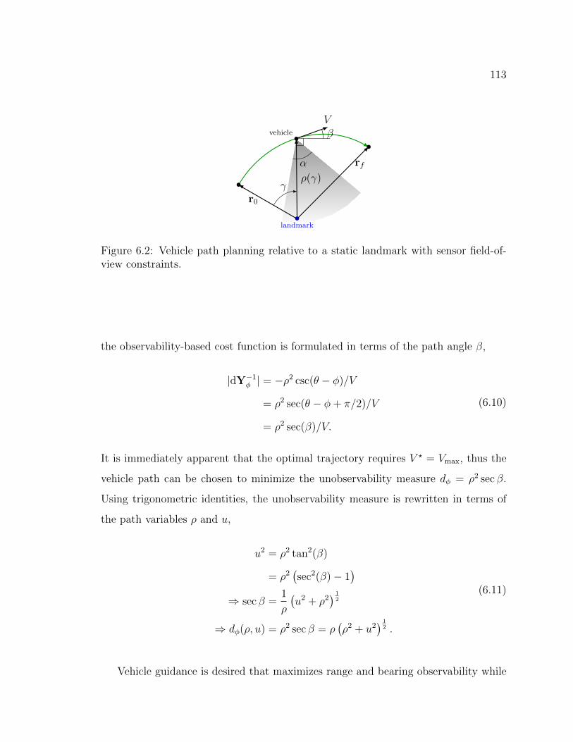
113

V

α

βvehicle

landmark

r0

rfρ(γ)

γ

Figure 6.2: Vehicle path planning relative to a static landmark with sensor field-of-view constraints.

the observability-based cost function is formulated in terms of the path angle β,

|dY−1φ | = −ρ

2 csc(θ − φ)/V

= ρ2 sec(θ − φ+ π/2)/V

= ρ2 sec(β)/V.

(6.10)

It is immediately apparent that the optimal trajectory requires V ? = Vmax, thus the

vehicle path can be chosen to minimize the unobservability measure dφ = ρ2 sec β.

Using trigonometric identities, the unobservability measure is rewritten in terms of

the path variables ρ and u,

u2 = ρ2 tan2(β)

= ρ2(sec2(β)− 1

)⇒ sec β =

1

ρ

(u2 + ρ2

) 12

⇒ dφ(ρ, u) = ρ2 sec β = ρ(ρ2 + u2

) 12 .

(6.11)

Vehicle guidance is desired that maximizes range and bearing observability while

114

minimizing path length, where path length in the landmark-centric frame is given by

L(ρ, u) =

γf∫0

(ρ2 + u2

) 12 dγ. (6.12)

This multi-objective problem is formed as a weighted optimization problem with the

objective

Jφ(ρ, u) =

γf∫0

(L(ρ, u) + wdφ(ρ, u)) dγ

=

γf∫0

(1 + wρ)(ρ2 + u2

) 12 dγ,

(6.13)

where w ≥ 0 is the tuning weight. The tuning weight can be interpreted as follows.

When w = 0, the objective is to minimize the path length without regard to path

observability. For w → ∞, the objective is to maximize range and bearing observ-

ability without regard to path length. The tuning weight can thus be used to make

a tradeoff between observability and path length.

Theorem 9. The bearing cost function (6.13) is a convex function of ρ and u for

path angle |β| < tan−1(√

2).

Proof. First note that L(ρ, u) is a convex function and a weighted sum of convex

functions is also convex. Therefore, it must be shown that dφ(ρ, u) is convex for

|β| < tan−1(√

2). Computing the Hessian of dφ yields

Hφ =

∂2

∂ρ2∂2

∂ρ∂u

∂2

∂u∂ρ∂2

∂u2

dφ(ρ, u)

=(ρ2 + u2

)− 32

2ρ3 + 3ρu2 u3

u3 ρ3

.(6.14)

115

Because ρ > 0, the first minor of Hφ is positive. The second minor is the determinant,

given by

|Hφ| =3ρ2

ρ2 + u2− 1, (6.15)

which is positive for

u2

ρ2< 2 ⇔ tan2(β) < 2 ⇔ |β| < tan−1(

√2). (6.16)

Therefore, if |β| < tan−1(√

2), then Hφ is positive definite, and dφ is a convex function

on the domain |u| <√

2ρ.

The restriction on the path angle is equivalent to a field-of-view constraint on

the sensor. For |β| < tan−1(√

2), the equivalent sensor field-of-view is α ≈ 109 deg.

Thus, if the sensor field-of-view is less than 109 deg, then the domain constraint is

already satisfied. If the sensor field-of-view is greater than 109 deg, then the domain

constraint limits the amount that the observability-based path can deviate from the

minimum length path. As it will be shown in the simulation results, however, the

larger path deviations have diminishing returns on the observability measure and the

domain constraint does not limit performance in practice. In exchange for a restricted

solution domain, we gain guaranteed convergence and optimality for the convex cost

function.

6.2.2 Observability Cost Function for Range Measurements

Observability using range measurements is incorporated into the path planning frame-

work using the same methods employed for bearing measurements. The unobserv-

ability measure for range measurements is given by

dρ(ρ, u) = sec β =1

ρ

(ρ2 + u2

) 12 . (6.17)

116

Theorem 10. The range unobservability measure dρ(ρ, u) is a quasi-convex function

of ρ and u for ρ > 0.

Proof. Quasi-convexity is proven by examining the second-order conditions for quasi-

convexity. The gradient of the expression is given by ∂∂ρ

∂∂u

f(ρ, u) =(ρ2 + u2

)− 12

−u2

ρ

u

, (6.18)

which is zero for u = 0 on the domain ρ > 0. Therefore, by the second-order conditions

for quasi-convexity [29], the Hessian must be positive semidefinite for u = 0, and must

have at least one positive eigenvalue when u 6= 0. The first-order minor of the Hessian

is given by∂2

∂ρ2f(ρ, u) =

u2 (3ρ2 + 2u2)

ρ3 (ρ2 + u2)32

≥ 0, (6.19)

and the determinant of the Hessian is

|Hρ| = −u2

ρ4(ρ2 + u2)≤ 0. (6.20)

Thus, the Hessian has one positive and one negative eigenvalue when u 6= 0. When

u = 0, the Hessian is

Hρ

∣∣u=0

=

0 0

0 1/ρ2

, (6.21)

which is positive semi-definite for ρ > 0. Therefore, the range unobservability mea-

sure, dρ(ρ, u) is quasi-convex in ρ and u for ρ > 0.

Although the quasi-convex guidance problem can be solved via sequential convex

optimization and a line search, we propose a convex relaxation to the range unob-

servability measure that allows an approximate solution to be more readily obtained.

117

Consider the relaxation of dρ(ρ, u) given by

dρ(u) = dρ(ρ, u) =

(1 +

u2

ρ2

) 12

, (6.22)

where ρ is the average of the initial and final conditions on the range, ρ = 12(ρ0 + ρf ).

If the variation in the range over the length of the trajectory is small, these two

objectives will result in similar optimal trajectories. In some scenarios, these two

objectives will produce equivalent trajectories.

Theorem 11. The solution to the observability-based guidance problem

minρ(γ),u(γ)

γf∫0

dρ(ρ, u)dγ

subject todρ

dγ= u

ρ(0) = ρ(γf ) = ρ0

(6.23)

is equivalent to the solution of the problem when the objective, dρ(ρ, u), is replaced by

the relaxed objective, dρ(u).

Proof. The proof is done by showing that the optimal trajectory, ρ?(γ) = ρ0 and

u?(γ) = 0 satisfy the first-order necessary conditions for a minimum of both problems

(see [103]). The Hamiltonians for each problem are given by

H(ρ, u) = dρ(ρ, u) + λu

H(u) = dρ(u) + λu.(6.24)

118

The stationarity conditions for the two problems are

∂

∂uH(ρ, u) =

u

ρ2

(1 +

u2

ρ2

)− 12

+ λ = 0

∂

∂uH(u) =

u

ρ2

(1 +

u2

ρ2

)− 12

+ λ = 0,

(6.25)

which are both satisfied by the optimal trajectory (ρ?, u?) and λ? = λ? = 0. The

costate dynamics are given by

dλ

dγ= − ∂

∂ρH(ρ, u) =

u2

ρ3

(1 +

u2

ρ2

)− 12

dλ

dγ= − ∂

∂ρH(u) = 0,

(6.26)

which are satisfied by the optimal trajectory (ρ?, u?) and λ? = λ? = 0. Therefore, the

two solutions are equivalent in the case when the initial and final ranges are equal.

The condition ρ0 = ρf implies that the landmark is on the separating hyperplane

between the two waypoints. The two objectives will not produce equivalent solutions

for every landmark position, but numerical studies have shown that the relaxed objec-

tive produces very similar trajectories over a large range of landmark positions. The

unobservability measure, dρ(ρ, u), was evaluated for optimal trajectories generated by

both the relaxed and quasi-convex optimization problems for varying landmark posi-

tion. Landmark position was varied using the parameters δ and ζ, as shown in Fig.

6.3. The percentage increase in observability measure due to the relaxed objective is

shown in Fig. 6.4, with the thick line indicating the 5% contour. The majority of

landmark positions result in minimal change in the unobservability measure, with the

exception of areas very near the waypoints.

These results motivate the use of the relaxed objective to reduce computational

requirements. Combining the unobservability measure with the path length measure

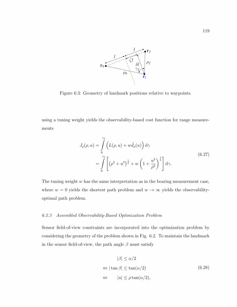
119

r0

rfl

l

rlρ0

ρfδlζl

γf

Figure 6.3: Geometry of landmark positions relative to waypoints.

using a tuning weight yields the observability-based cost function for range measure-

ments

Jρ(ρ, u) =

γf∫0

(L(ρ, u) + wdρ(u)

)dγ

=

γf∫0

[(ρ2 + u2

) 12 + w

(1 +

u2

ρ2

) 12

]dγ.

(6.27)

The tuning weight w has the same interpretation as in the bearing measurement case,

where w = 0 yields the shortest path problem and w → ∞ yields the observability-

optimal path problem.

6.2.3 Assembled Observability-Based Optimization Problem

Sensor field-of-view constraints are incorporated into the optimization problem by

considering the geometry of the problem shown in Fig. 6.2. To maintain the landmark

in the sensor field-of-view, the path angle β must satisfy

|β| ≤ α/2

⇔ | tan β| ≤ tan(α/2)

⇔ |u| ≤ ρ tan(α/2),

(6.28)

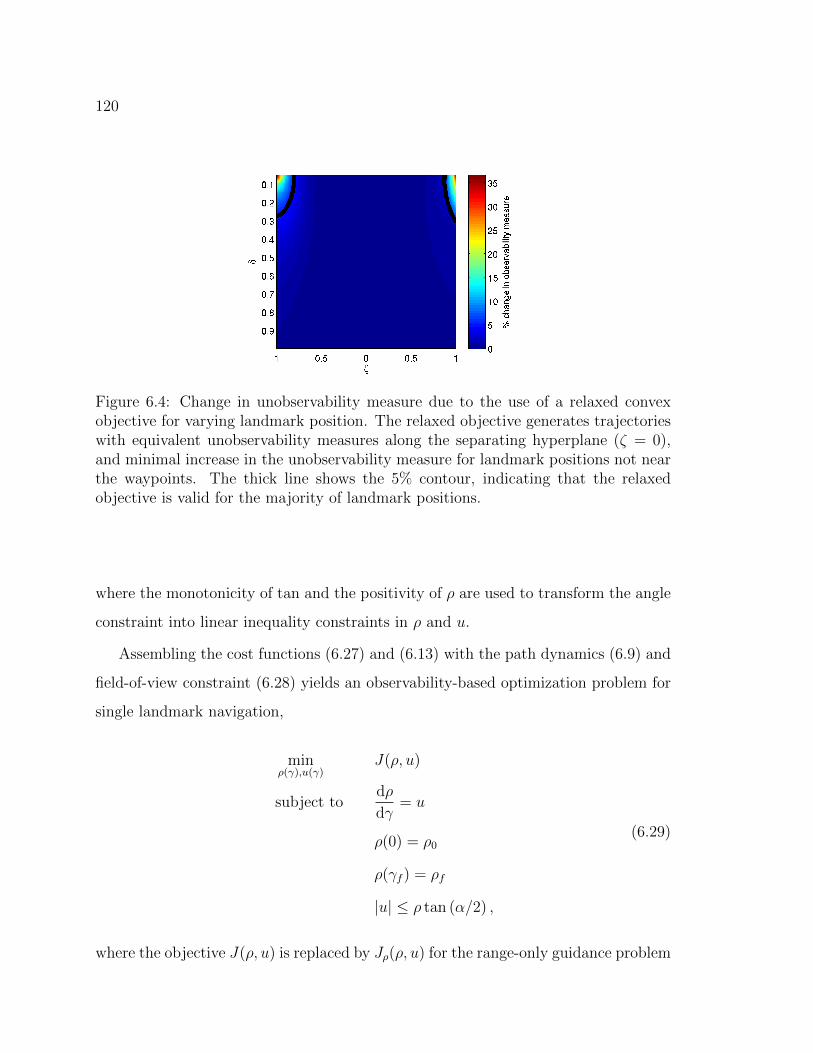
120

Figure 6.4: Change in unobservability measure due to the use of a relaxed convexobjective for varying landmark position. The relaxed objective generates trajectorieswith equivalent unobservability measures along the separating hyperplane (ζ = 0),and minimal increase in the unobservability measure for landmark positions not nearthe waypoints. The thick line shows the 5% contour, indicating that the relaxedobjective is valid for the majority of landmark positions.

where the monotonicity of tan and the positivity of ρ are used to transform the angle

constraint into linear inequality constraints in ρ and u.

Assembling the cost functions (6.27) and (6.13) with the path dynamics (6.9) and

field-of-view constraint (6.28) yields an observability-based optimization problem for

single landmark navigation,

minρ(γ),u(γ)

J(ρ, u)

subject todρ

dγ= u

ρ(0) = ρ0

ρ(γf ) = ρf

|u| ≤ ρ tan (α/2) ,

(6.29)

where the objective J(ρ, u) is replaced by Jρ(ρ, u) for the range-only guidance problem

121

and Jφ(ρ, u) for the bearing-only guidance problem. The optimization problem (6.29)

is a convex problem in the variables ρ and u and can be solved given problem data

ρ0, ρf , α, and w using angular discretization of γ and efficient interior-point methods

[29].

6.3 Simulation Results

Simulation studies were performed to evaluate the effectiveness of the observability-

based guidance. Performance was evaluated in simulation in matlab using the in-

terior point method of the optimization toolbox to solve the path planning problem

(6.29).

6.3.1 Trajectory Tracking Controller Design

A controller was designed to allow the vehicle to track the observability-based guid-

ance trajectories. A model predictive control (MPC) scheme is used to compute the

control input. The advantage of the MPC method is that it converts the solution of an

optimization problem into a feedback control law. The optimization problem (6.29)

is discretized into N equal angular segments of size ∆γ. At each step of the control

law, the estimated vehicle position is updated using the latest range or bearing mea-

surement. Then, the trajectory is re-planned by solving the discretized optimization

problem (6.29). Finally, the first control action in the trajectory is taken and the

vehicle moves towards the goal for one time step. This procedure is repeated until

the vehicle reaches the goal position as detailed in Algorithm 2.

The estimated range and bearing are obtained using an extended Kalman filter

(EKF) according to the continuous-discrete formulation presented in [27]. The con-

tinuous time dynamics model is given by (6.1) and time-discretized measurements of

the range ρ or bearing φ are used to update the filter. The dynamics linearization

performed at each step of the EKF is found by linearization of the nonlinear dynamics

122

Algorithm 2 Observability-Based MPC Guidance Law

Require: Landmark position, rlRequire: Estimated initial position, r0

Require: Desired final position, rfRequire: Sensor field of view angle, αRequire: Number of trajectory time discretizations, NRequire: Observability tuning weight, wρ← ‖rl − r0‖φ← ∠(rl − r0)ρf ← ‖rl − rf‖φf ← ∠(rl − rf )while N > 0 do

Propagate and update ρ and φγf ← φ− φfSolve problem (6.29) using ρ as an initial rangeθ ← tan−1(u(0)/ρ(0)) + φ+ π/2

V← Vmax

[cos θsin θ

]Apply control V for ∆t = (ρ(0)2 + u(0)2)

12 ∆γVmax

N ← N − 1end while

model (6.1),

F (x) =

0 −V sin(θ − φ)

Vρ2

sin(θ − φ) Vρ

cos(θ − φ)

. (6.30)

6.3.2 Pareto Optimality

The Pareto optimality curve was explored for the range-only and bearing-only guid-

ance policies. Each policy was simulated in closed-loop with an EKF providing range

and bearing estimates to the MPC Algorithm 2. The simulation used N = 20 time

steps, and the dynamics (6.1) were integrated at each time step using the ode45 solver.

The Pareto optimality curve was obtained by simulating the closed-loop system for

varying values of the weight w, which controls the tradeoff between path length and

the unobservability measure. Because it was hypothesized that decreasing the un-

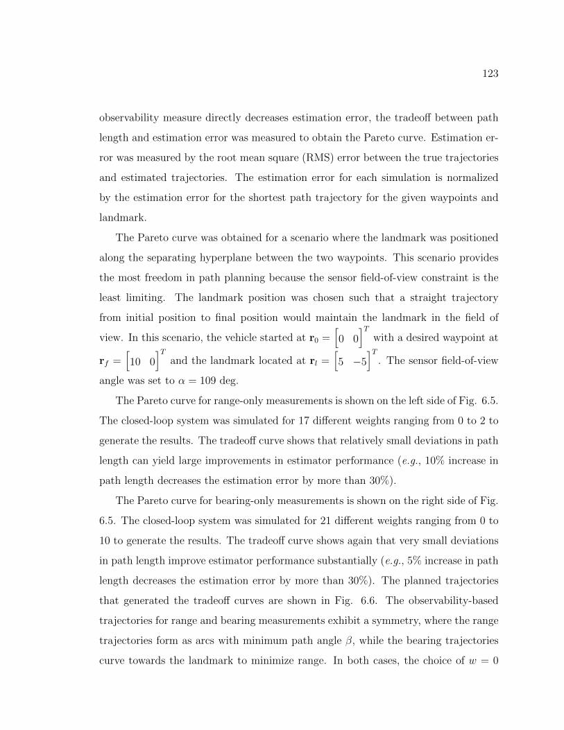
123

observability measure directly decreases estimation error, the tradeoff between path

length and estimation error was measured to obtain the Pareto curve. Estimation er-

ror was measured by the root mean square (RMS) error between the true trajectories

and estimated trajectories. The estimation error for each simulation is normalized

by the estimation error for the shortest path trajectory for the given waypoints and

landmark.

The Pareto curve was obtained for a scenario where the landmark was positioned

along the separating hyperplane between the two waypoints. This scenario provides

the most freedom in path planning because the sensor field-of-view constraint is the

least limiting. The landmark position was chosen such that a straight trajectory

from initial position to final position would maintain the landmark in the field of

view. In this scenario, the vehicle started at r0 =[0 0

]Twith a desired waypoint at

rf =[10 0

]Tand the landmark located at rl =

[5 −5

]T. The sensor field-of-view

angle was set to α = 109 deg.

The Pareto curve for range-only measurements is shown on the left side of Fig. 6.5.

The closed-loop system was simulated for 17 different weights ranging from 0 to 2 to

generate the results. The tradeoff curve shows that relatively small deviations in path

length can yield large improvements in estimator performance (e.g., 10% increase in

path length decreases the estimation error by more than 30%).

The Pareto curve for bearing-only measurements is shown on the right side of Fig.

6.5. The closed-loop system was simulated for 21 different weights ranging from 0 to

10 to generate the results. The tradeoff curve shows again that very small deviations

in path length improve estimator performance substantially (e.g., 5% increase in path

length decreases the estimation error by more than 30%). The planned trajectories

that generated the tradeoff curves are shown in Fig. 6.6. The observability-based

trajectories for range and bearing measurements exhibit a symmetry, where the range

trajectories form as arcs with minimum path angle β, while the bearing trajectories

curve towards the landmark to minimize range. In both cases, the choice of w = 0

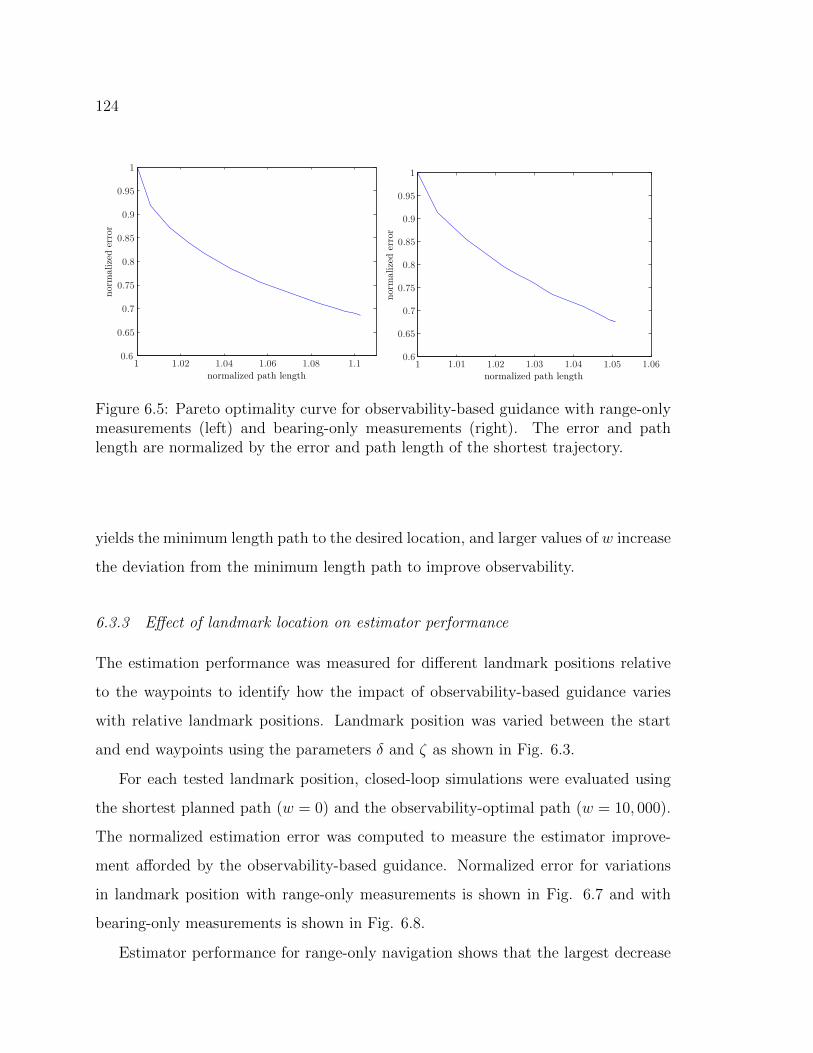
124

Figure 6.5: Pareto optimality curve for observability-based guidance with range-onlymeasurements (left) and bearing-only measurements (right). The error and pathlength are normalized by the error and path length of the shortest trajectory.

yields the minimum length path to the desired location, and larger values of w increase

the deviation from the minimum length path to improve observability.

6.3.3 Effect of landmark location on estimator performance

The estimation performance was measured for different landmark positions relative

to the waypoints to identify how the impact of observability-based guidance varies

with relative landmark positions. Landmark position was varied between the start

and end waypoints using the parameters δ and ζ as shown in Fig. 6.3.

For each tested landmark position, closed-loop simulations were evaluated using

the shortest planned path (w = 0) and the observability-optimal path (w = 10, 000).

The normalized estimation error was computed to measure the estimator improve-

ment afforded by the observability-based guidance. Normalized error for variations

in landmark position with range-only measurements is shown in Fig. 6.7 and with

bearing-only measurements is shown in Fig. 6.8.

Estimator performance for range-only navigation shows that the largest decrease

125

Figure 6.6: Observability-based guidance trajectories for bearing-only and range-only measurements that were used to generate the Pareto optimality curves. Theobservability-based trajectories for range-only measurements form into an arc, whilethe trajectories for bearing-only measurements curve towards the landmark.

in error compared to following the shortest path occurs when the landmark is located

near the starting waypoint (ζ < 0 and δ < 0.5). In this region, the estimation error

can be reduced by more than half by using the observability-based guidance scheme

proposed here. This performance increase is attributed to the fact that following

the shortest path results in large path angles β and, therefore, large values of the

unobservability index dρ. The observability-based guidance produces the minimum

unobservability index and, thus, gives a significant improvement in estimator perfor-

mance. The opposite effect is observed when the landmark is near the final waypoint

(ζ > 0 and δ < 0.2). In this region, the shortest path and the observability-optimal

path are very similar when they approach the final waypoint and, thus, have similar

unobservability indices and estimator performance. When the landmark is distant

(δ → ∞) the difference between the shortest path and the observability-optimal arc

path is minimal, resulting in little difference in estimator performance. From the re-

sults of Fig. 6.7, it is shown that for δ > 2, which is equivalent to a landmark position

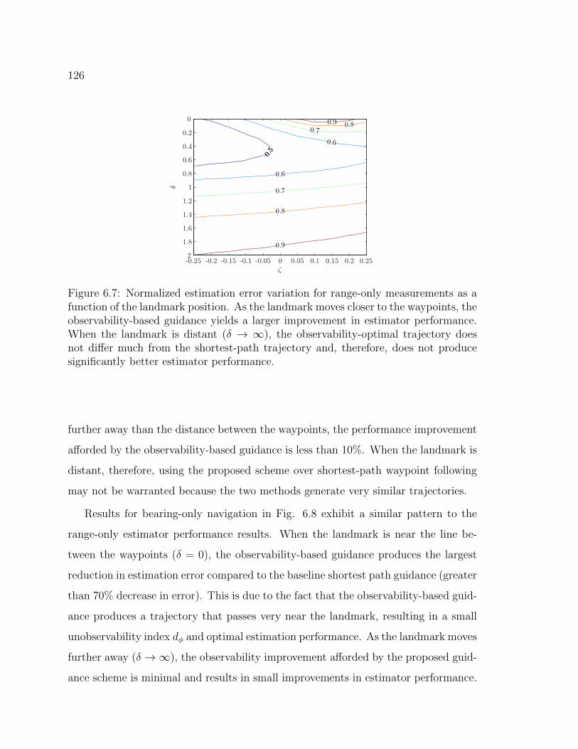
126

Figure 6.7: Normalized estimation error variation for range-only measurements as afunction of the landmark position. As the landmark moves closer to the waypoints, theobservability-based guidance yields a larger improvement in estimator performance.When the landmark is distant (δ → ∞), the observability-optimal trajectory doesnot differ much from the shortest-path trajectory and, therefore, does not producesignificantly better estimator performance.

further away than the distance between the waypoints, the performance improvement

afforded by the observability-based guidance is less than 10%. When the landmark is

distant, therefore, using the proposed scheme over shortest-path waypoint following

may not be warranted because the two methods generate very similar trajectories.

Results for bearing-only navigation in Fig. 6.8 exhibit a similar pattern to the

range-only estimator performance results. When the landmark is near the line be-

tween the waypoints (δ = 0), the observability-based guidance produces the largest

reduction in estimation error compared to the baseline shortest path guidance (greater

than 70% decrease in error). This is due to the fact that the observability-based guid-

ance produces a trajectory that passes very near the landmark, resulting in a small

unobservability index dφ and optimal estimation performance. As the landmark moves

further away (δ →∞), the observability improvement afforded by the proposed guid-

ance scheme is minimal and results in small improvements in estimator performance.

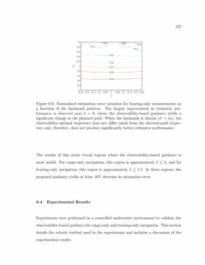
127

Figure 6.8: Normalized estimation error variation for bearing-only measurements asa function of the landmark position. The largest improvement in estimator per-formance is observed near δ = 0, where the observability-based guidance yields asignificant change in the planned path. When the landmark is distant (δ →∞), theobservability-optimal trajectory does not differ much from the shortest-path trajec-tory and, therefore, does not produce significantly better estimator performance.

The results of this study reveal regions where the observability-based guidance is

most useful. For range-only navigation, this region is approximately δ ≤ 2, and for

bearing-only navigation, this region is approximately δ ≤ 1.5. In these regions, the

proposed guidance yields at least 10% decrease in estimation error.

6.4 Experimental Results

Experiments were performed in a controlled underwater environment to validate the

observability-based guidance for range-only and bearing-only navigation. This section

details the robotic testbed used in the experiments and includes a discussion of the

experimental results.

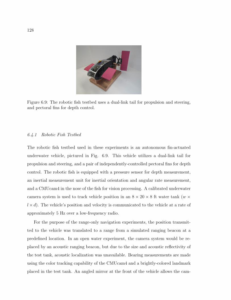
128

Figure 6.9: The robotic fish testbed uses a dual-link tail for propulsion and steering,and pectoral fins for depth control.

6.4.1 Robotic Fish Testbed

The robotic fish testbed used in these experiments is an autonomous fin-actuated

underwater vehicle, pictured in Fig. 6.9. This vehicle utilizes a dual-link tail for

propulsion and steering, and a pair of independently-controlled pectoral fins for depth

control. The robotic fish is equipped with a pressure sensor for depth measurement,

an inertial measurement unit for inertial orientation and angular rate measurement,

and a CMUcam4 in the nose of the fish for vision processing. A calibrated underwater

camera system is used to track vehicle position in an 8 × 20 × 8 ft water tank (w ×

l× d). The vehicle’s position and velocity is communicated to the vehicle at a rate of

approximately 5 Hz over a low-frequency radio.

For the purpose of the range-only navigation experiments, the position transmit-

ted to the vehicle was translated to a range from a simulated ranging beacon at a

predefined location. In an open water experiment, the camera system would be re-

placed by an acoustic ranging beacon, but due to the size and acoustic reflectivity of

the test tank, acoustic localization was unavailable. Bearing measurements are made

using the color tracking capability of the CMUcam4 and a brightly-colored landmark

placed in the test tank. An angled mirror at the front of the vehicle allows the cam-

129

era to obtain a lateral field-of-view, and a pinhole camera model transforms measured

color centroids to a bearing to the landmark.

The robotic fish houses a single board computer with 1.3 GHz processor running

Ubuntu Linux. Communication, guidance, control, and estimation applications are

written in C++ with the aid of the Robot Operating System (ROS) for inter-process

communication. The observability-based guidance is computed on-board using the C

API for the nonlinear programming feature of the mosek optimizer [104]. A typical

optimization solution with N = 12 waypoints is obtained in 40 ms on the single board

computer. Although the solution time is more than fast enough to run in real time,

the guidance trajectories were computed once at the beginning of each experiment,

rather than iteratively as in the MPC Algorithm 2. A proportional heading controller

was used to follow the waypoints generated from the guidance solution. The EKF

used for estimating range and bearing to the landmark utilized the armadillo linear

algebra library. Estimates from the EKF were propagated and updated at a rate of

5 Hz using a fourth-order Runge-Kutta integration.

6.4.2 Bearing-Only Navigation Results

Bearing-only navigation experiments were conducted to explore the effect that sensor

field-of-view has on the observability-based path planning. The camera on board the

robotic fish is the CMUcam4, which has a 50 degree field-of-view. Because the field-

of-view is fairly narrow, the freedom in path planning is limited and the difference

between shortest path guidance and observability-optimal guidance is minimal. The

path planning problem (6.29) constrains the path to allow the landmark to remain in

the sensor field-of-view at all times. This constraint was relaxed to allow the vehicle to

deviate further from the shortest path to obtain a better observing position relative

to the landmark, while sacrificing some measurements en route. The field-of-view

constraint was varied from the minimum, 50 deg, to the maximum, 109 deg, seeking

to answer the question: when it comes to landmark measurements, is quality better

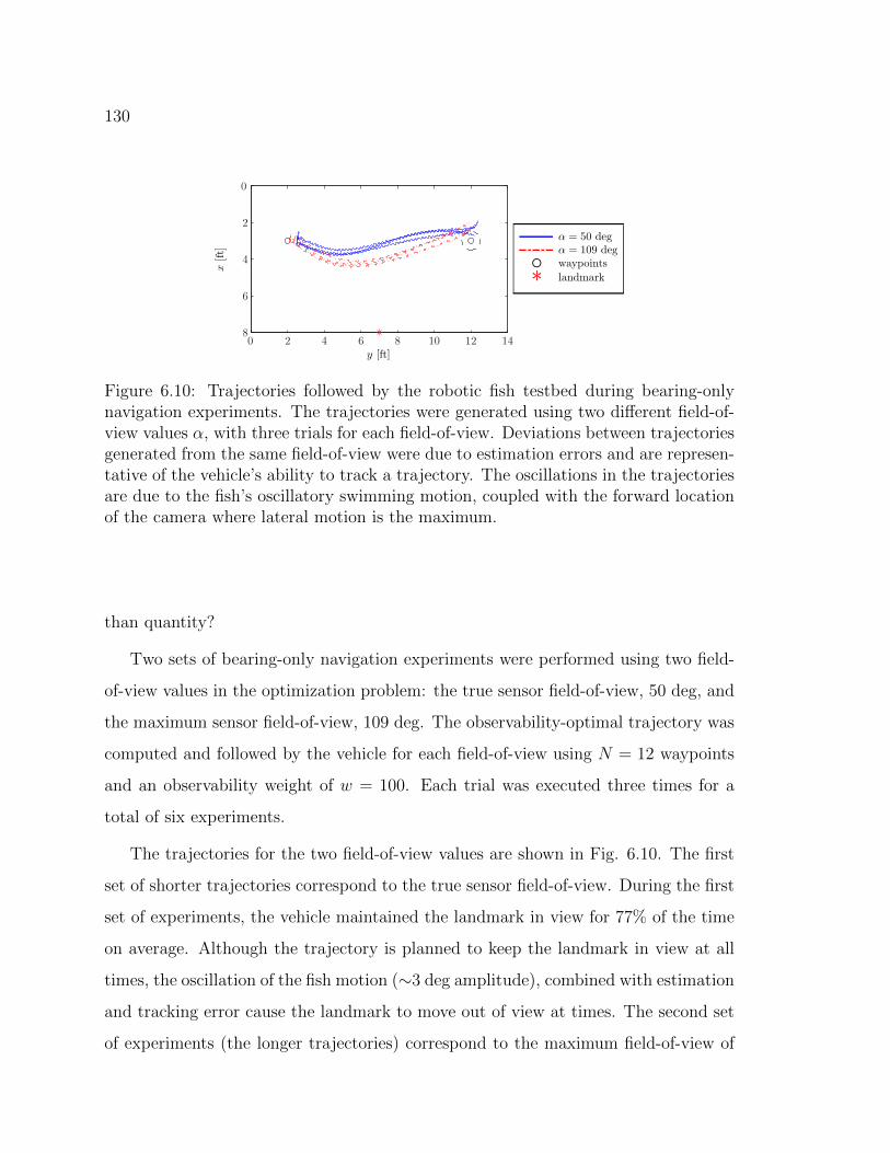
130

Figure 6.10: Trajectories followed by the robotic fish testbed during bearing-onlynavigation experiments. The trajectories were generated using two different field-of-view values α, with three trials for each field-of-view. Deviations between trajectoriesgenerated from the same field-of-view were due to estimation errors and are represen-tative of the vehicle’s ability to track a trajectory. The oscillations in the trajectoriesare due to the fish’s oscillatory swimming motion, coupled with the forward locationof the camera where lateral motion is the maximum.

than quantity?

Two sets of bearing-only navigation experiments were performed using two field-

of-view values in the optimization problem: the true sensor field-of-view, 50 deg, and

the maximum sensor field-of-view, 109 deg. The observability-optimal trajectory was

computed and followed by the vehicle for each field-of-view using N = 12 waypoints

and an observability weight of w = 100. Each trial was executed three times for a

total of six experiments.

The trajectories for the two field-of-view values are shown in Fig. 6.10. The first

set of shorter trajectories correspond to the true sensor field-of-view. During the first

set of experiments, the vehicle maintained the landmark in view for 77% of the time

on average. Although the trajectory is planned to keep the landmark in view at all

times, the oscillation of the fish motion (∼3 deg amplitude), combined with estimation

and tracking error cause the landmark to move out of view at times. The second set

of experiments (the longer trajectories) correspond to the maximum field-of-view of

131

109 deg. The relaxed field-of-view constraint allowed the vehicle to move closer to the

landmark for better observation. During these experiments, the landmark was in view

47% of the time on average. Despite fewer measurements being available, the relaxed

field-of-view constraint produced 8% lower RMS range and bearing estimation error

on average when compared to the baseline field-of-view of 50 deg.

6.4.3 Range-Only Navigation Results

Range-only navigation experiments were conducted to demonstrate the tradeoff be-

tween path observability and path length, similar to the Pareto-optimality simulation

studies detailed in Section 6.3. Initial and final waypoints were designed such that

the landmark was located on the mean plane between the waypoints (ζ = 0), and

the landmark was nearby (δ = 0.4). Observability-based guidance was used to com-

pute trajectories for six different weights w, ranging from 0 (shortest path) to 10

(observability-optimal), for N = 12 waypoints. Because the range sensing does not

have a field-of-view, field-of-view constraints in the optimization problem were omit-

ted (i.e., α = 180 deg). Each trial began with the vehicle placed at the starting

waypoint. The vehicle was commanded to perform the observability-based guidance,

at which point the optimal trajectory was computed and the vehicle began follow-

ing the trajectory using a proportional heading controller. The trial ended when the

vehicle reached a circular manifold around the final waypoint (radius 0.5 ft in these

trials). Each trial was performed three times.

The 18 trajectories generated by the vehicle are shown in Fig. 6.11, where the

six groups of trajectories delineate the six observability weights used in the trajec-

tory optimization. Qualitatively, the trajectories with higher observability weight

(the longer, more arc-like trajectories) are more repeatable and coalesce near the fi-

nal waypoint, indicating superior estimation performance and, thus, better trajectory

tracking. These observations are supported by the estimation error computed for

each trial. The RMS error between the EKF estimates of range and bearing and the

132

Figure 6.11: Trajectories followed by the robotic fish testbed during range-only nav-igation experiments. The trajectories were generated using six different observabilityweights w, with three trials for each weight. Deviations between trajectories gener-ated from the same weight were due to estimation errors and are representative of thevehicle’s ability to track a trajectory.

Figure 6.12: Normalized RMS error and unobservability measures for range-only nav-igation experiments as a function of path length. As the observability weight isincreased (increased path length), the RMS error is decreased. The RMS error showsa strong correlation to the unobservability measure.

range and bearing measured by the camera tracking system was computed for each

trial. The three trials for each observability weight were averaged and normalized by

133

the averaged RMS error for the shortest trajectories. The unobservability measure

for each trajectory was computed and averaged for the three trials. A comparison

of the RMS error and unobservability measures, normalized by the shortest path

error and unobservability measure, is shown in Fig. 6.12. The RMS error for the

observability-optimal path (w = 10) is 58% of the RMS error for the straight path,

which corresponds well to the simulation studies for a landmark placed at ζ = 0 and

δ = 0.4 (see Fig. 6.7). The RMS error shows a strong correlation to the unobservabil-

ity measure, validating the observability-based guidance as a method for controlling

estimation error.

134

Chapter 7

CONCLUSION

This dissertation developed an observability-based approach to the analysis and

design of motion planning and sensor placement for nonlinear systems. Several mea-

sures of observability were employed as metrics for trajectory or sensor fitness, of

which the observability Gramian proved to be particularly useful. Although the ob-

servability Gramian is a measure of observability for linear systems, simulations and

experiments demonstrated that the Gramian can provide valid and meaningful mea-

sures of observability for nonlinear systems about a nominal trajectory.

One of the main contributions of this thesis is a sensor placement algorithm that

incorporates nonlinear dynamics, nonlinear measurement models, and heterogeneous

sensor types. By leveraging methods from mixed integer programming and convex

optimization, solution methods were proposed that allow the algorithms to scale more

favorably to larger problems. In particular, the `1-regularization technique allowed

the sensor placement problem to be posed as a semidefinite program, which scales well

with system size (number of states) and number of sensors. Because the observability

Gramian can be approximated numerically using the empirical observability Gramian,

the sensor placement algorithm can be applied using only a simulation of a nonlinear

system as input data, with no analytical model required.

The sensor placement procedure was extended to a sensor data compression algo-

rithm, which finds a temporal filter that compresses sensor data such that the amount

of information in the filtered signal is maximized. The data compression problem was

posed as a convex optimization problem with an `1-bound on the compression fil-

ter, which promotes a sparse filter solution. By applying the sensor placement and

135

compression algorithms, the spatial and temporal distribution of information in a pro-

cess can be identified, and the most informative measurements can be selected. The

sensor compression algorithm has interesting implications for distributed sensing ap-

plications, where data compression can be used to minimize communication between

sensor nodes and minimize computation when sensor data are fused between multiple

nodes. Additionally, the data compression has an analogous role in neural filtering in

biological systems, where filtering on individual sensors reduces the amount of data

passed to a central processing unit.

The utility of the sensor placement and compression algorithms is their broad

applicability. Because these algorithms were designed for a nonlinear system defined

by a general, control-affine ordinary differential equation, they can be applied in

a wide variety of areas. One interesting application is in the study of biological

systems, where distributed sensing is prevalent. A detailed example application was

provided in a study of the gyroscopic sensing capabilities in insect wings. The sensor

placement strategy revealed how the heterogeneity of campaniform sensilla might

be distributed along the wing of the hawkmoth to optimally detect inertial rotation

rates. Comparison to biological data indicated that the algorithm predicted areas

where sensors are clustered on the wing, indicating that these clusters of sensors may

serve as good encoders of gyroscopic information.

The second main contribution of this thesis is an observability-based guidance

framework for vehicles navigating with limited inertial information. The observability-

based guidance problem was solved analytically for vehicles navigating with range-

only or bearing-only measurements to a static landmark, showing that a circular

trajectory centered at the landmark minimized the observability Gramian condition

number. The guidance problem was also solved analytically for navigation in cur-

rents and extended to higher-dimensional nonholonomic systems. These observability-

based trajectories provided superior estimation performance in simulation when com-

pared to suboptimal trajectories, indicating that the observability Gramian measure

136

captures the nonlinear dynamics. An example application of this guidance framework

is motion planning for single range-aided navigation of an underwater vehicle. In this

scenario, the vehicle can perform the optimal circle maneuver to obtain an accurate

localization, after which, the vehicle can perform its mission with reduced localization

uncertainty (e.g., follow a sensor coverage trajectory).

The observability-based guidance framework was extended to an algorithmic guid-

ance strategy for range-only and bearing-only navigation. These algorithms allow ve-

hicle path planning and observability to be considered simultaneously, therefore, tra-

jectories can be computed that explicitly tradeoff observability measures with mission

parameters (e.g., path length). The guidance algorithms were tested in simulation

to explore the effect of landmark location on estimation performance. Experiments

with a robotic fish testbed validated the usefulness of the algorithms, demonstrating

that the observability tuning weight can be used to directly control localization uncer-

tainty. Because the guidance is computed using convex optimization, the algorithm is

amenable to implementation on robotic platforms with limited processing power. In

the robotic experiments presented here, the typical guidance trajectory was computed

in approximately 40 ms, which is fast enough for implementation on many robotic

platforms.

The research presented in this thesis provides several interesting avenues for future

work. One intriguing research area is in the application of the sensor compression

algorithm to natural and engineered systems. Because biological systems often use

massively distributed sensing, the neural filtering component of the sensing provides

a sort of distributed computation that reduces the amount of computation required

by a central unit. By pairing the tools developed here with a neurological study, the

benefits of neural compression may be better characterized from a systems-theoretic

perspective. In the context of sensor networks, the sensor compression algorithm may

allow for the design of distributed estimation with limited communication, where only

the most important bits of information are exchanged between sensor nodes.

137

The observability-based guidance algorithms for range-only and bearing-only navi-

gation were developed for waypoint following, but can be extended to plan higher-level

trajectories such as search patterns. Given a radius of region to search, the vehicle

path can be planned in the landmark-centric frame with multiple revolutions about

the landmark (γf > 2π). Constraints on the search pattern parameters (e.g., pitch be-

tween consecutive passes) can easily be integrated into the optimization problem. For

range-only navigation, a spiral-like trajectory centered at the landmark will likely pro-

duce good observability characteristics while covering a circular search region. These

guidance algorithms will provide an integrated trajectory planner that simultaneously

accounts for high-level mission tasks and localization accuracy.

Another potential extension of the observability-based guidance is path planning

with multiple landmarks present. One simple solution to this scenario is to select a

single key landmark for navigation that provides the best observability characteristics

and use the existing framework to plan a trajectory relative to the single landmark.

The results of the landmark position study (see Figs. 6.7 and 6.8) can be used to

select a key landmark that provides good performance. When landmarks are sparsely

distributed, selecting a single landmark for navigation will likely be advantageous.

However, when landmarks are densely distributed, selecting a single landmark may

not provide optimal observability.

Finally, because the guidance algorithms can be used to replan the trajectory

as the mission progresses, the framework lends itself well to dynamically selecting

optimization parameters. For example, the observability tuning weight w could be

dynamically selecting based upon feedback of estimator performance, such as the

covariance matrix. When the covariance is high, a large weight should be chosen to

maneuver to improve observability and thus reduce the estimation uncertainty. When

the covariance is low, a smaller weight should be chosen to minimize path length.

138

BIBLIOGRAPHY

[1] B. J. Guerreiro, P. Batista, C. Silvestre, and P. Oliveira, “Sensor-based simulta-neous localization and mapping – part I: GAS robocentric filter,” in AmericanControl Conference, 2012.

[2] ——, “Sensor-based simultaneous localization and mapping – part II: Onlineinertial map and trajectory estimation,” in American Control Conference, 2012.

[3] M. Bryson and S. Sukkarieh, “An information-theoretic approach to au-tonomous navigation and guidance of an uninhabited aerial vehicle in unknownenvironments,” in Intelligent Robots and Systems, 2005.

[4] ——, “Observability analysis and active control for airborne SLAM,” IEEETransactions on Aerospace and Electronic Systems, vol. 44, no. 1, pp. 261–280,Jan 2008.

[5] A. Gadre, “Observability analysis in navigation systems with an underwater ve-hicle application,” Ph.D. dissertation, Virginia Polytechnic Institute and StateUniversity, 2007.

[6] P. Batista, C. Silvestre, and P. Oliveira, “Single range aided navigation andsource localization: Observability and filter design,” Systems & Control Letters,vol. 60, no. 8, pp. 665–673, Aug. 2011.

[7] W. P. Chan, F. Prete, and M. H. Dickinson, “Visual input to the efferent controlsystem of a fly’s “gyroscope”,” Science, vol. 280, pp. 289–292, 1998.

[8] D. Kleinfeld, E. Ahissar, and M. E. Diamond, “Active sensation: insights fromthe rodent vibrissa sensorimotor system,” Current Opinion in Neurobiology,vol. 16, no. 4, pp. 435–444, August 2006.

[9] R. B. Towal and M. J. Z. Hartmann, “Principles and applications of activetactile sensing strategies in the rat vibrissal system,” in IEEE SENSORS Con-ference, 2010.

[10] K. Kral, “Behaviouralanalytical studies of the role of head movements in depthperception in insects, birds and mammals,” Behavioural Processes, vol. 64, pp.1–12, 2003.

139

[11] R. Necker, “Head-bobbing of walking birds,” Journal of Comparative PhysiologyA, vol. 193, pp. 1177–1183, 2007.

[12] B. J. Frost, “The optokinetic basis of head-bobbing in the pigeon,” Journal ofExperimental Biology, vol. 74, pp. 187–195, 1978.

[13] T. Dekker and R. T. Carde, “Moment-to-moment flight manoeuvres of thefemale yellow fever mosquito (Aedes aegypti L.) in response to plumes of carbondioxide and human skin odour,” Journal of Experimental Biology, vol. 214, pp.3480–3494, October 2011.

[14] T. Lochmatter and A. Martinoli, “Theoretical analysis of three bio-inspiredplume tracking algorithms,” in International Conference on Robotics and Au-tomation, 2009.

[15] J. P. Dyhr, K. A. Morgansen, T. L. Daniel, and N. J. Cowan, “Flexible strategiesfor flight control: an active role for the abdomen,” Journal of ExperimentalBiology, vol. 216, pp. 1523–1536, 2013.

[16] B. T. Hinson, E. Rombokas, J. P. Dyhr, T. L. Daniel, and K. A. Morgansen,“Sensing from control: airframe deformation for simultaneous actuation andstate estimation,” in Conference on Decision and Control, 2013.

[17] G. W. van der Linden, A. Emami-Naeini, R. L. Kosut, H. Sedarat, and J. P.Lynch, “Optimal sensor placement for health monitoring of civil structures,” inAmerican Control Conference, 2011.

[18] M. Weickgenannt, S. Neuhaeuser, B. Henke, W. Sobek, and O. Sawodny, “Op-timal sensor placement for state estimation of flexible shell structures,” in In-ternational Conference on Fluid Power and Mechatronics, 2011.

[19] M. R. Safizadeh and I. Z. M. Darus, “Optimal location of sensor for activevibration control of flexible square plate,” in International Conference on In-formation Science, Signal Processing and Their Applications, 2010.

[20] K.-S. Cho, J.-R. Shin, and S. H. Hyun, “Optimal placement of phasor mea-surement units with gps receiver,” in IEEE Power Engineering Society WinterMeeting, 2001.

[21] D. Dua, S. Dambhare, R. K. Gajbhiye, and S. A. Soman, “Optimal multi-stage scheduling of PMU placement: An ILP approach,” IEEE Transactions onPower Delivery, vol. 23, no. 4, pp. 1812 – 1820, October 2008.

140

[22] A. Krause, A. Singh, and C. Guestrin, “Near-optimal sensor placements ingaussian process: Theory, efficient algorithms, and empirical studies,” Journalof Machine Learning Research, vol. 9, pp. 235–284, 2008.

[23] C. C. Castello, J. Fan, A. Davari, and R.-X. Chen, “Optimal sensor place-ment strategy for environmental monitoring using wireless sensor networks,” inSoutheastern Symposium on System Theory, 2010.

[24] J. Perez-Ramirez, D. K. Borah, and D. G. Voelz, “Optimal 3D landmark place-ments for vehicle localization using heterogeneous sensors,” IEEE Transactionson Vehicular Technology, vol. 62, no. 7, pp. 2987–2999, 2013.

[25] D. Moreno-Salinas, A. M. Pascoal, and J. Aranda, “Optimal sensor placementfor underwater positioning with uncertainty in the target location,” in Interna-tional Conference on Robotics and Automation, 2011.

[26] J. T. Isaacs, D. J. Klein, and J. P. Hespanha, “Optimal sensor placement fortime difference of arrival localization,” in Conference on Decision and Control,2009.

[27] J. L. Crassidis and J. L. Junkins, Optimal Estimation of Dynamic Systems.Chapman & Hall, 2004.

[28] F. Pukelsheim, Optimal Design of Experiments. John Wiley & Sons, 1993.

[29] S. Boyd and L. Vandenberghe, Convex Optimization. Cambridge UniversityPress, 2004.

[30] K. Yu, J. Bi, and V. Tresp, “Active learning via transductive experimentaldesign,” in International Conference on Machine Learning, 2006.

[31] D. Georges, “The use of observability and controllability gramians or functionsfor optimal sensor and actuator location in finite-dimensional systems,” in Con-ference on Decision and Control, 1995.

[32] F. W. J. van den Berg, H. C. J. Hoefsloot, H. F. M. Boelens, and A. K. Smilde,“Selection of optimal sensor position in a tubular reactor using robust degreeof observability criteria,” Chemical Engineering Science, vol. 55, pp. 827–837,2000.

[33] A. V. Wouwer, N. Point, S. Porteman, and M. Remy, “An approach to theselection of optimal sensor locations in distributed parameter systems,” Journalof Process Control, vol. 10, no. 4, pp. 291–300, August 2000.

141

[34] S. Lall and J. E. Marsden, “A subspace approach to balanced truncation formodel reduction of nonlinear control systems,” International Journal on Robustand Nonlinear Control, vol. 12, pp. 519–535, 2002.

[35] J. Hahn and T. F. Edgar, “An improced method for nonlinear model reductionusing balancing of empirical gramians,” Computers & Chemical Engineering,vol. 26, pp. 1379–1397, 2002.

[36] A. K. Singh and J. Hahn, “On the use of empirical gramians for controllabilityand observability analysis,” in American Control Conference, 2005.

[37] A. J. Krener and K. Ide, “Measures of unobservability,” in Conference on De-cision and Control, 2009.

[38] A. K. Singh and J. Hahn, “Determining optimal sensor locations for state andparameter estimation for stable nonlinear systems,” Industrial & EngineeringChemistry Research, vol. 44, no. 15, pp. 5645–5659, 2005.

[39] M. Serpas, G. Hackebeil, C. Laird, and J. Hahn, “Sensor location for nonlin-ear dynamic systems via observability analysis and MAX-DET optimization,”Computers & Chemical Engineering, vol. 48, pp. 105–112, 2013.

[40] L. DeVries and D. A. Paley, “Observability-based optimization for flow sens-ing and control of an underwater vehicle in a uniform flowfield,” in AmericanControl Conference, 2013.

[41] J. Berry, W. E. Hart, C. A. Phillips, J. G. Uber, and J.-P. Watson, “Sensorplacement in municipal water networks with temporal integer programmingmodels,” Journal of Water Resources Planning and Management, vol. 132, pp.218–224, 2006.

[42] J.-P. Watson, R. Murray, and W. E. Hart, “Formulation and optimization fordrinking water contamination warning systems,” Journal of Infrastructure Sys-tems, vol. 15, pp. 330–339, 2009.

[43] S. Joshi and S. Boyd, “Sensor selection via convex optimization,” IEEE Trans-actions on Signal Processing, vol. 57, pp. 451–462, 2009.

[44] J. M. Passerieux and D. V. Cappel, “Optimal observer maneuver for bearings-only tracking,” IEEE Transactions on Aerospace and Electronic Systems,vol. 34, pp. 777–788, 1998.

142

[45] S. Martınez and F. Bullo, “Optimal sensor placement and motion coordinationfor target tracking,” Automatica, vol. 42, no. 4, pp. 661–668, 2006.

[46] K. Zhou and S. I. Roumeliotis, “Optimal motion strategies for range-only con-strained multisensor target tracking,” IEEE Transactions on Robotics, vol. 24,no. 5, pp. 1168–1185, October 2008.

[47] T. L. Song, “Observability of target tracking with bearings-only measurements,”IEEE Transactions on Aerospace and Electronic Systems, vol. 32, no. 4, pp.1468–1472, October 1996.

[48] P. Ogren, E. Fiorelli, and N. E. Leonard, “Cooperative control of mobile sensornetworks,” IEEE Transactions on Automatic Control, vol. 49, no. 8, pp. 1292–1302, Aug. 2004.

[49] S. Liu and M. Krstic, “Stochastic source seeking for nonholonomic unicycle,”Automatica, vol. 46, pp. 1443–1453, 2010.

[50] N. E. Leonard, D. A. Paley, F. Lekien, R. Sepulchre, D. M. Fratantoni, and R. E.Davis, “Collective motion, sensor networks, and ocean sampling,” Proceedingsof the IEEE, vol. 95, pp. 48–74, 2007.

[51] D. O. Popa, A. C. Sanderson, V. Hombal, R. J. Komerska, S. S. Mupparapu,D. R. Blidberg, and S. G. Chappel, “Optimal sampling using singular valuedecomposition of the parameter variance space,” in Intelligent Robots and Sys-tems, 2005.

[52] N. K. Yilmaz, C. Evangelinos, P. F. J. Lermusiaux, and N. M. Patrikalakis,“Path planning of AUVs for adaptive sampling using MILP,” IEEE Journal ofOceanic Engineering, vol. 33, no. 4, pp. 522–537, Oct. 2008.

[53] D. S. Levine, “Inromation-rich path planning under general constraints usingrapidly-exploring random trees,” Master’s thesis, Massachusetts Institute ofTechnology, 2010.

[54] G. A. Hollinger and G. S. Sukhatme, “Sampling-based robotic information gath-ering algorithms,” International Journal of Robotics Research, vol. 33, pp. 1271–1287, 2014.

[55] M. Gautier and W. Khalil, “Exciting trajectories for the identification of baseinertial parameters of robots,” in Conference on Decision and Control, 1991.

143

[56] G. Venture, K. Ayusawa, and Y. Nakamura, “A numerical method for choosingmotions with optimal excitation properties for identification of biped dynam-ics - an application to human,” in International Conference on Robotics andAutomation, 2009.

[57] F. Arrichiello, G. Antonelli, A. P. Aguiar, and A. Pascoal, “Observability metricfor the relative localization of AUVs based on range and depth measurements:theory and experiments,” in IEEE/RSJ International Conference on IntelligentRobots and Systems, 2011.

[58] B. T. Hinson, M. K. Binder, and K. A. Morgansen, “Path planning to optimizeobservability in a planar uniform flow field,” in American Control Conference,2013.

[59] J. D. Quenzer, “Obserservability based path planning in range-only localiza-tion,” Master’s thesis, University of Washington, 2013.

[60] H. Yu, R. Sharma, R. W. Beard, and C. N. Taylor, “Observability-based localpath planning and collision avoidance for micro air vehicles using bearing-onlymeasurements,” in American Control Conference, 2011.

[61] M. Anguelova, “Nonlinear obserservability and identifiability: General theoryand a case study of a kinetic model for S. cerevisiae,” Ph.D. dissertation,Chalmers University of Technology and Goteborg University, 2004.

[62] R. Hermann and A. J. Krener, “Nonlinear controllability and observability,”IEEE Transactions on Automatic Control, vol. 22, no. 5, pp. 728–740, 1977.

[63] E. D. Sontag and Y. Wang, “I/O equations for nonlinear systems and observa-tion spaces,” in Conference on Decision and Control, 1991.

[64] J. H. Hubbard and B. B. Hubbard, Vector Calculus, Linear Algebra, and Dif-ferential Forms, A Unified Approach. Prentice Hall, 1999.

[65] C.-T. Chen, Linear System Theory and Design, 3rd ed. Oxford UniversityPress, 1999.

[66] G. H. Golub and C. F. V. Loan, Matrix Computations, 3rd ed. Baltimore: TheJohns Hopkins University Press, 1996.

[67] H. P. Williams, Model Building in Mathematical Programming. John Wiley &Sons, 2006.

144

[68] B. T. Hinson and K. A. Morgansen, “Observability-based optimal sensor place-ment for flapping airfoil wake estimation,” AIAA Journal of Guidance, Control,and Dynamics, vol. 37, no. 5, pp. 1477–1486, 2014.

[69] G. L. Nemhauser, L. A. Wolsey, and M. L. Fisher, “An analysis of approxima-tions for maximizing submodular set functions,” Mathematical Programming,vol. 14, pp. 265–294, 1978.

[70] A. Krause and C. Guestrin, “Near-optimal observation selection using submod-ular functions,” in National Conference on Artificial Intelligence, 2007.

[71] F. L. Cortesi, T. H. Summers, and J. Lygeros, “Submodularity of energy relatedcontrollability metrics,” in IEEE Conference on Decision and Control, 2014.

[72] Z. Yu, P. Cui, and S. Zhu, “Observability-based beacon configuration opti-mization for mars entry navigation,” AIAA Journal of Guidance, Control, andDynamics, 2014, AIAA Early Edition.

[73] B. H. Dickerson, Z. N. Aldworth, and T. L. Daniel, “Control of moth flight pos-ture is mediated by wing mechanosensory feedback,” Journal of ExperimentalBiology, 2014, in press.

[74] S. A. Combes and T. L. Daniel, “Into thin air: contributions of aerodynamicand inertial-elastic forces to wing bending in the hawkmoth Manduca sexta,”Journal of Experimental Biology, vol. 206, pp. 2999–3006, 2003.

[75] A. L. Eberle, B. H. Dickerson, P. G. Reinhall, and T. L. Daniel, “A new twiston gyroscopic sensing: body rotations lead to torsion in flapping, flexible insectwings,” Journal of the Royal Society Interface, 2014, in review.

[76] M. H. Dickinson and J. Palka, “Pysiological porperties, time of develop-ment, and central projection are correlated in the wing mechanoreceptors ofDrosphila,” Journal of Neuroscience, vol. 7, no. 12, pp. 4201–4208, 1987.

[77] R. C. Elson, “Flight motor neurone reflexes driven by strain-sensitive wingmechanoreceptors in the locust,” Journal of Comparative Physiology A, vol.161, no. 5, pp. 747–760, 1987.

[78] J. W. S. Pringle, “Proprioception in insects ii. the action of the campaniformsensilla on the legs,” Journal of Experimental Biology, vol. 15, pp. 114–131,1938.

145

[79] S. M. Spinola and K. M. Chapman, “Proprioceptive indentation of the campan-iform sensilla of cockroach legs,” Journal of Comparative Physiology A, vol. 96,no. 3, pp. 257–272, 1975.

[80] M. Petyt, Introduction to Finite Element Vibration Analysis. Cambridge Uni-versity Press, 1990.

[81] T. Nakata and H. Liu, “A fluid-structure interaction model of insect flight withflexible wings,” Journal of Computational Physics, vol. 231, pp. 1822–1847,2012.

[82] J. Diebel. (2006) Representing attitude: Euler angles, unit quaternions, androtation vectors.

[83] S. P. Sane and M. H. Dickinson, “The control of flight force by a flappingwing: lift and drag production,” Journal of Experimental Biology, vol. 204, pp.2607–2626, 2001.

[84] M. H. Dickinson, F.-O. Lehmann, and S. P. Sane, “Wing rotation and theaerodynamic basis of insect flight,” Science, vol. 284, no. 5422, pp. 1954–1960,1999.

[85] S. P. Sane and M. H. Dickinson, “The aerodynamic effects of wing rotationand a revised quasi-steady model of flapping flight,” Journal of ExperimentalBiology, vol. 205, pp. 1087–1096, 2002.

[86] S. P. Sane, “The aerodynamics of insect flight,” Journal of Experimental Biol-ogy, vol. 206, pp. 4191–4208, 2003.

[87] T. L. Hedrick and T. L. Daniel, “Flight control in the hawkmoth Manducasexta: the inverse problem of hovering,” Journal of Experimental Biology, vol.209, pp. 3114–3130, 2006.

[88] M. Porez, F. Boyer, and A. Belkhiri, “A hybrid dynamic model for bio-inspiredrobots with soft appendages - application to a bio-inspired flexible flapping-wingmicro air vehicle,” in International Conference on Robotics and Automation,2014.

[89] A. M. Mountcastle and T. L. Daniel, “Aerodynamic and functional consequencesof wing compliance,” Experiments in Fluids, vol. 46, no. 5, pp. 873–882, 2009.

146

[90] J. Katz and A. Plotkin, Low Speed Aerodynamics. Cambridge University Press,2001.

[91] A. P. Willmott and C. P. Ellington, “The mechanics of flight in the hawk-moth Manduca sexta: I. kinematics of hovering and forward flight,” Journal ofExperimental Biology, vol. 200, pp. 2705–2722, 1997.

[92] S. A. Combes and T. L. Daniel, “Flexural stiffness in insect wings i. scaling andthe influence of wing venation,” Journal of Experimental Biology, vol. 206, pp.2979–2987, 2003.

[93] T. Nakata and H. Liu, “Aerodynamic performance of a hovering hawkmoth withflexible wings: A computational approach,” Proceedings of the Royal Society B,vol. 279, pp. 722–731, 2012.

[94] M. H. Dickinson, “Directional sensitivity and mechanical coupling dynamics ofcampaniform sensilla during chordwise deformations of the fly wing,” Journalof Experimental Biology, vol. 169, pp. 221–233, 1992.

[95] M. Grant and S. Boyd, “Graph implementations for nonsmooth convex pro-grams,” in Recent Advances in Learning and Control, ser. Lecture Notes inControl and Information Sciences, V. Blondel, S. Boyd, and H. Kimura, Eds.Springer-Verlag Limited, 2008, pp. 95–110.

[96] ——, “CVX: Matlab software for disciplined convex programming, version 2.0beta,” http://cvxr.com/cvx, Sep. 2012.

[97] M. H. Dickinson, “Comparison of encoding properties of campaniform sensillaon the fly wing,” Journal of Experimental Biology, vol. 161, pp. 245–261, 1990.

[98] S. P. Sane and M. J. McHenry, “The biomechanics of sensory organs,” Integra-tive and Comparative Biology, vol. 49, no. 6, pp. 8–23, 2009.

[99] T. McGeer and J. Vagners, “Historic crossing: an unmanned aircraft’s Atlanticflight,” GPS World, vol. 10, no. 2, pp. 24–30, Feb. 1999.

[100] B. T. Hinson and K. A. Morgansen, “Observability optimization for the non-holonomic integrator,” in American Control Conference, 2013.

[101] R. W. Brockett, “Control theory and singular riemannian geometry,” in NewDirections in Applied Mathematics, P. J. Hilton and G. S. Young, Eds. Springer,1981, pp. 11–27.

147

[102] R. M. Murray and S. S. Sastry, “Nonholonomic motion planning: Steering usingsinusoids,” IEEE Transactions on Automatic Control, vol. 38, no. 5, pp. 700–716, May 1993.

[103] D. E. Kirk, Optimal Control Theory, An Introduction. Dover, 2004.

[104] E. D. Andersen and K. D. Andersen, “MOSEK: High performance softwarefor large-scale LP, QP, SOCP, SDP and MIP,” www.mosek.com, Mar. 2013,version 7.0.